Download Marxan Tutorial for the Coastal Douglas-Fir and

Marxan Tutorial for the Coastal Douglas-Fir
and Conservation Partnership Study Area
Produced for the Coastal Douglas -Fir and Associated Ecosystems Conservation
Partnership with funds provided via the FBRC Chair in Applied Conservation Biology,
Natural Sciences and Engineering Research Council of Canada, Real Estate Founda tion of
British Columbia and The Nature Trust of British Columbia.
http://arcese.forestry.ubc.ca/marxan-tool/
Morrell, N. R. Schuster & P. Arcese
Department of Forest and Conservation Science, University of British Columbia
Contents
1.
Background Information ....................................................................................................................... 2
1.0 The Coastal Douglas-Fir and Associated Ecosystems Conservation Partnership ................................ 2
1.1 Why Marxan? ...................................................................................................................................... 2
1.2 What actually is Marxan? .................................................................................................................... 3
1.2 How does Marxan work? .................................................................................................................... 4
1.2.1 In a nutshell .................................................................................................................................. 4
1.2.2 A little more about the scoring of planning units ........................................................................ 4
1.3 What information does Marxan use? ................................................................................................. 5
2.
Using the Interface................................................................................................................................ 6
2.1 Getting Started .................................................................................................................................... 6
2.2 Manipulating Key Variables ................................................................................................................ 7
2.2.1 Global Parameters ....................................................................................................................... 7
2.2.2 Property Exclusions ...................................................................................................................... 9
2.2.2 Protection Targets...................................................................................................................... 11
2.2.3 Species Penalty Factor ............................................................................................................... 12
2.2.4 Connectivity ............................................................................................................................... 13
2.2.5 Number of Iterations ................................................................................................................. 13
2.3 Running Marxan and Interpreting the Results .................................................................................. 14
2.3.1 Scenario name............................................................................................................................ 14
2.3.2 Summary Tables ......................................................................................................................... 14
2.3.3 Output plots ............................................................................................................................... 16
2.4 Downloading and Viewing MARXAN results in ArcMap ................................................................... 17
1
3.
References .......................................................................................................................................... 18
4.
Additional Resources .......................................................................................................................... 19
5.
Appendices .......................................................................................................................................... 20
Appendix A. Old Forest Community Occurrence Map ............................................................................ 20
Appendix B. Savannah Community Occurrence Map ............................................................................. 21
Appendix C. Wetland Community Occurrence Map ............................................................................... 22
Appendix D. Human Commensal Birds Community Occurrence Map.................................................... 23
Appendix E. Old Forest and Savannah Beta Diversity Map .................................................................... 24
Appendix F. Garry Oak Ecosystem Plant Native Species Richness Map ................................................. 25
Appendix G. Example Maps - Locking In vs. Not Locking In Parks ......................................................... 26
1. Background Information
1.0 The Coastal Douglas-Fir and Associated Ecosystems Conservation Partnership
This tutorial was produced as part of an integrative conservation strategy to protect and
steward the Coastal Douglas-fir biogeoclimatic zone and associated ecosystems in south-western British
Columbia. The Coastal Douglas-fir and Associated Ecosystems Conservation Partnership (CDFCP) is a
collaboration of agencies, organizations, academic institutions, and land managers working to balance
competing land uses through “sound science, shared information, supportive policies, and community
education”. For more information on the CDFCP goals and collaborators, refer to the latest version of
the Conservation Strategy at: http://www.cdfcp.ca/index.php/about-the-cdfcp/conservation-strategy
1.1 Why Marxan?
Marxan is a problem solving tool that is used to help inform decisions on landscape-scale
conservation planning. As part of a systematic planning process, Marxan contributes towards a
transparent, inclusive and defensible decision making process. Historically, conservation decisionmaking has often focused on evaluating land parcels opportunistically as they become available for
purchase, donation, or under threat. This was often done without a complete understanding of how
their acquisition might contribute to targets for biodiversity conservation or the degree to which they
are likely to maximize return on the investment of scarce conservation dollars and time.
Using Marxan to simulate alternative reserve designs should help you to prioritize conservation
actions at the landscape level, and allow you to specify the targets such as focal or indicator species
richness, ecosystem representation, complementarity and connectivity, and to also minimize the overall
costs of conservation acquisitions. This tutorial will show you how to use Maxan to identify existing gaps
in biodiversity protection, to identify candidate areas to include in a growing reserve system, and to
provide decision support based on a clear and repeatable set of conservation targets.
2
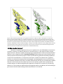
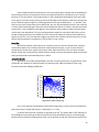
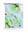
Figure 1. Maps of Salt Spring Island after running a Marxan simulation of 100 runs, with a 17% target for all conservation
features, boundary length modifier of 1, and species penalty factor of 3. The maps on the left indicates the frequency with
which particular parcels were selected (% of 100 runs), with dark blue indicating properties that were nearly or always part of
the solution, and yellow properties never selected. This output is often thought of as the portfolio of candidate reserves for
acquisition, stewardship or owner contact by managers. The figure on the right indicates the ‘reserve design’ Marxan returned
as the ‘best solution’ to the input goals and constraints. In this case, the conservation plan that achieved the highest overall
biodiversity score at the lowest overall cost (based here on 2014 BC Assessments).
1.2 What actually is Marxan?
Marxan is a computer application that runs an algorithm on a user-defined data set and returns
a solution in the form of a table of land parcels. These parcels form a ‘near optimal’ balance of input
targets and costs. Marxan is capable of analyzing large, complex datasets to find near-optimal solutions
because it uses an algorithm called “simulated annealing”(default setting, with others possible), which
selects properties that maximize progress towards your biodiversity goals while minimizing acquisition
or other user-controlled costs. It’s important to note that in its basic form, Marxan has no graphical
interface, it just does the computing. We have designed a web-based graphical user interface that lets
you set Marxan parameters and returns a spatially linked solution file that you can download to ArcMap
and view. In this tutorial, we will introduce you to our user interface, explain how to manipulate key
variables and gain an understanding about the application of output files in support of your planning
decisions. It is not essential to understand how the algorithm works to use Marxan, but those wishing to
gain a better technical understanding should consult Marxan’s User Manual.
3
1.2 How does Marxan work?
1.2.1 In a nutshell
After you specify your conservation targets and objectives (e.g., area to be conserved), Marxan
will start by assigning scores to planning unit configurations in the sample space. This score is based on
that particular configuration’s ability to meet the conservation objectives while minimizing the cost: the
lower the score, the better. Marxan will then compare a huge number of configurations (it would be
virtually impossible to compare them all) and find the one with the lowest overall score. This is your
solution. You can repeat the process as many times as you want: the more times you do, the more
confident you can be that you have found a near optimal solution.
1.2.2 A little more about the scoring of planning units
The score that Marxan assigns to each planning unit configuration is based on a mathematical
formula called the objective function. The complete formula is:
Score of the configuration being tested = (∑ 𝐶𝑜𝑠𝑡) +
+ (𝐵𝑜𝑢𝑛𝑑𝑎𝑟𝑦 𝐿𝑒𝑛𝑔𝑡ℎ 𝑀𝑜𝑑𝑖𝑓𝑖𝑒𝑟 × ∑ 𝐵𝑜𝑢𝑛𝑑𝑎𝑟𝑦 𝐿𝑒𝑛𝑔𝑡ℎ 𝑜𝑓 𝑡ℎ𝑒 𝑟𝑒𝑠𝑒𝑟𝑣𝑒 𝑠𝑦𝑠𝑡𝑒𝑚)
+ (∑ 𝑆𝑝𝑒𝑐𝑖𝑒𝑠 𝑃𝑒𝑛𝑎𝑙𝑡𝑦 𝐹𝑎𝑐𝑡𝑜𝑟 × 𝑃𝑒𝑛𝑎𝑙𝑡𝑦 𝑖𝑛𝑐𝑢𝑟𝑟𝑒𝑑 𝑓𝑜𝑟 𝑢𝑛𝑚𝑒𝑡 𝑡𝑎𝑟𝑔𝑒𝑡𝑠)
Cost
By costs, we are referring to the cost of including that particular set of planning units in a
configuration. Depending on the nature of your project, cost could be calculated as the area of planning
units, the costs of ongoing management, opportunity costs of displaced commercial activities, costs to
industry, tourism, and recreation from displaced activities, or acquisition cost. The lower the cost of a
unit, the lower the score will be and the more likely it is that the planning unit will be included in the
solution. Marxan then summarizes the cost of all of the selected planning units and this is incorporated
into the score.
Connectivity
The boundary length of the reserve system is way of quantifying the connectivity of a
configuration of planning units. It is a combination of the total length of the edges of the selected
planning units, and the weight that you choose to give to this value. This weighting is known as the
boundary length modifier (BLM). Essentially, If you choose to place importance on the boundary length
(i.e. you set the boundary length modifier to a value greater than 0), then configurations with many
small and isolated patches will have higher scores. Marxan works to find the solution with the lowest
score, so your reserve system will have a more clumped distribution. For this tutorial, it will be
important to understand the boundary length modifier and the consequences of constraining boundary
length on the “near optimal solution” that Marxan produces. Skip ahead to section 2.2.4 for instructions
on the practical use of the BLM. See section 2.5 for examples of this parameter in practice. Last, before
using a boundary modifier, consider existing levels of connectivity allowed via private land management
for forestry, agriculture, recreational or ecosystem values such as carbon storage, water purification or
pollination services. Keeping private land hospitable to native species has the potential to eliminate the
need to enforce connectivity via land acquisition.
4
Species Penalty Factor
The piece of the scoring formula is the penalty incurred for unmet targets. This is the sum of the
user-defined penalty for not meeting the target and the weight that you choose to give this value. This
weighting is known as the species penalty factor (SPF). As the user, you are in charge of setting how big
the penalty should be. When a planning unit configuration fails to meet a conservation target (e.g. it
does not contain a certain level of richness or a target species), then it will receive a penalty and this will
increase its score by a magnitude proportional to the size of the SPF. As a result, it is less likely to
represent the final solution. Skip ahead to section 2.2.3 for instructions on the practical use of the SPF.
See section 2.5 for examples of this parameter in practice.
1.3 What information does Marxan use?
In order to work, Marxan needs to know your project objectives and study area well, and this
input data needs to be organized into specific file types. The key information it requires is:
1. Your project area and a list of all of the planning units contained within it, as well as their
cost.
2. A list of target conservation features (species, habitats, soil types)
3. A clearly defined objective or series of objectives (ex. 30% of all grizzly bear habitat)
4. How much of each conservation feature is contained within each planning unit
The user interface we use in this tutorial already contains all of the important input information,
so it is not necessary to understand the specifics how the data is organized. However, it will be
important to understand how to organize your data into input files if you want to run Marxan manually.
Most of this information is found from external sources. Some of it, such as boundary length and the
conservation features contained within specific planning units, are determined using GIS software such
as ArcMap or QGis. For more information on the input file formats, you can refer to Qmarxan, an
excellent tool for assembling basic Marxan input files.
5
2. Using the Interface
2.1 Getting Started
The interface we use is linked to an external server that already contains all of the important
input layers for the Coastal Douglas Fir planning area. This includes the cadastral fabric, cost
information, existing parks, and numerous biodiversity indexes such as old forest birds, standing carbon,
TEM element occurrence, etc. To connect to the server, go to http://arcese.forestry.ubc.ca/marxan-tool/ in
your internet browser. The password is “BR2CR!”. You will be directed to the following index page.
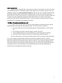
Each hyperlink directs you to a different subset of the total CDFCP dataset. To look for solutions
across the entire CDFCP area, follow the first “CDFCP wide” link.
Figure 2. Extent of coverage for the subsets available in the Marxan tool.
6
An important note about scale:
The spatial scale which you choose has the potential to greatly alter the solutions that Marxan produces.
A smaller planning area (ex. Salt Spring Island) has fewer land parcels to choose from, and as a result
Marxan may be forced to consider parcels with lower conservation value in order to meet its targets.
Expanding your planning area (ex. CRD) could increase the availability of high quality parcels, but this
may take the focus away from your area of interest. Consider running the same parameters at different
scales and comparing the results.
2.2 Manipulating Key Variables
Once you’ve chosen your data subset, you can begin manipulating the parameters that Marxan
uses to inform the objective function (See section 1.2.2). All manipulations are done within the grey
sidebar on the left hand side of the screen. Once you run Marxan, the results will be displayed on the
right. When you open the tool, the key variables will automatically be set to default settings according
to the recommendations contained in the Marxan Good Practices Guide (2010). You can choose to keep
them in this format, or manipulate them to better suit your study objectives. We’ll go through each
section of parameters and explain the options associated with each.
2.2.1 Global Parameters
This section provides Marxan with basic instructions on how it will run.
How to deal with protected areas
Specify if you want to force Marxan to include existing protected areas and parks in the final
solution. The two options on the dropdown menu are “Locked In” and “Available”. If you choose
“Locked In”, then every solution Marxan produces will have to include the planning units with a
protected status. This will be useful if you wish to identify areas to add to an existing reserve system
(e.g., If your objective is to increase parks from 6% to 17%). For most scenarios “Locked In” will be the
default. However, because existing parks may be located in areas of relatively low conservation value,
locking in protected areas can produce solutions with lower total scores than from an un-constrained 8
solution. Thus, when interested is identifying the highest priority parcels without respect to
management, choosing “Available” will allow Marxan to select only high-value parcels for the final
7
solution, regardless of protection status. We recommend all users employ this option when comparing
existing reserve systems to near-optimal designs based on user-defined targets (see Appendix G for
examples).
Include connectivity in the analysis
Specify if you want Marxan to include boundary length in the calculation for the objective
function (See section 1.2.2). If you select “No”, then the boundary length modifier will be set to 0 and
the boundary length of the configurations being tested will not be considered. This means that there will
be no consideration for the spatial clumping of planning units. If you do want to favour solutions with a
more clumped distribution, then select “Yes”. You can then select a range of boundary length modifiers
to test in the “Connectivity” section (see Section 2.2.4). You might wish to consider this option to
prevent Marxan from selecting isolated land parcels, but when doing so, keep in mind that this has the
potential to considerably increase the cost of the final solution. Users should also consider the
contribution of existing green space to facilitate dispersal in target species, because maintaining those
habitats represents a cost-effective approach to conservation planning.
Which cost metric should be used
Select the cost metric that best suits the goals of your project. Property size uses land area as a
proxy for cost and is useful if you are interested in protecting a certain percentage of the land base (ie.
50%), regardless of specific property costs. Assessed land value is generated using a combination of
cadastral data (Integrated Cadastral Information Society of BC) and 2014 land value assessments (BC
Assessment Agency). This metric is generally the most easily translated to acquisition cost and is useful
for projects with more constrained budgets. Human score is based on a weighting of expert scores for
urban and rural areas. As this metric identifies human impact rather than monetary value, only select it
if you wish to focus on biodiversity value and disregard acquisition cost. This is an ‘experimental’ metric
that represents species likely to thrive in human-dominated landscapes.
Number of repeats
Tell Marxan how many runs you would like it to complete, and as a result how many solutions it
will produce in the output. Because large, complex data sets will likely have many “near-optimal”
solutions, increasing the number of runs will increase the likelihood that you have found the best
possible configuration of land parcels (the one with the lowest score). However, this will also increase
the time it takes for Marxan to run, which can be a major constraint with large datasets and limited
time. We set the default to 100 runs, which in most cases will provide adequate repetition to assess
which parcels are selected most often in solutions, provide a good “best” solution, and minimize run
time.
8
Generate output for individual runs
Check this box if you want the option of looking at the solution table for individual runs. This can
be good idea in example runs, as it allows you to see the overall best run and summed solution
(selection frequency) outputs; but you may want to leave this box unchecked to improve processing
performance when exploring a range of scenarios
2.2.2 Property Exclusions
This section allows you be more specific about the types of land parcels you want included in
the solution. Leaving any of the sliders at 0 automatically removes these factors from Marxan analysis.
p(Old Forest Community)
Road density
Measured as kilometers of paved road per square kilometer and calculated for each land parcel
in the CDFCP using Terrain Resource Information Management (TRIM) data.
1.0
0.9
0.8
0.7
0.6
0.5
0.4
0.3
0.2
0.1
0
1
2
3
Roads (sqrt km/km-sq)
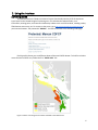
Figure 3. An empirical relationship of the effect of road density on the occurrence of the old-
forest bird community in forest stands ≥80 years of age (N= 1248 stands, r2 = -0.42).
9
Empirical data based from 700 locations across the CDFCP region indicate that the probability of
encountering old forest-associated bird communities begins declining at road densities over 1 km/km2,
but there is a lot of variation in these observations. In part, openings associated with some rural roads
act as gaps in the forest canopy that can promote the abundance and diversity of old-forest species that
rely on understory plants (Figure 3). Excluding properties with high road density (i.e., >1-3km/km2) may
help fine-tune your solution away from roaded areas, but may also dramatically constrain your solutions
in human-dominated landscapes. Note also that the deleterious effects of roads on native bird and plant
communities is also included to some degree in the predictive species maps we used to identify target
communities (see Appendices). Thus, by setting protection targets for native birds and plants, you are
already including constraints on road density to the extent they reduce the value of those biodiversity
targets (see Section 2.2.2). We therefore suggest you explore the usefulness of this function by running
Marxan with and without a road density to see its effect on your results.
Parcel Size
Marxan will consider all land parcels in a solution unless you chose to exclude them. However,
small habitats patches do not always represent viable acquisition targets, so you can also choose to
exclude parcels smaller than a given size using the slider. Many beta-users of this tool have excluded
parcels smaller than 2 hectares from CDFCP solutions, based on various assumptions about conservation
values and acquisition and stewardship costs in future.
p(Old Forest Community)
Agriculture density
Agriculture can include cultivated fields, orchards, vinyards, golf courses, or greenhouses, and is
measured in our database as square kilometers of agriculture per square kilometer of land, using
Terrestrial Ecosystem Mapping (TEM) data.
1.0
0.9
0.8
0.7
0.6
0.5
0.4
0.3
0.2
0.1
0 1 2 3 4 5 6
Agriculture (sqrt ha/km-sq)
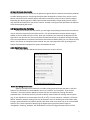
Figure 4. An empirical representation of the effect of agriculture on the occurrence of old-forest
bird communities in stands ≥80 years (N = 1248 stands, r2 = -0.42).
In parcels with more than 3 hectares of agriculture per km2, we expect about a 50% reduction in
the probability of encountering the old-forest bird community identified by experts as indicating high
quality old forest habitat. Excluding parcels with a lot of agricultural land may enhance the value of your
10
designs for forest bird species, but de-emphasize your focus on ‘savanna-woodland’ species, such as
chipping, savanna and white-crowned sparrows, and others. Overall, your final selection of parcel type
should be linked to your specific conservation goals.
2.2.2 Protection Targets
In this section, you specify your overall objectives or a series of objectives for the biodiversity
features contained in the CDFCP database. The tool defaults to a 17% global target for terrestrial
ecosystem conservation, as represented in the data set and adopted in the UN Convention on Biological
Diversity. This means that Marxan will try to include a minimum of 17% of each biodiversity feature in its
solutions. We suggest all users to consider carefully all protection targets in consultation with
stakeholders. With those targets identified, you can then check the “Set Individual Targets” box to
reveal a menu showing the biodiversity features currently mapped and available for the CDFCP area.
These features are listed briefly below.
Table 1. Current biodiversity feature layers in the CPFCP tool.
Old Forest Birds
A composite distribution map based on probability of occurrence of
birds typically associated with old forest habitat (Schuster and Arcese
2014). See Appendix A.
Savannah Birds
A composite distribution map based on probability of occurrence of
birds typically associated with savannah habitat (Schuster and Arcese
2014). See Appendix B.
Wetland Birds
A composite distribution map based on probability of occurrence of
birds typically associated with wetland and riparian habitats (Schuster
and Arcese, unpublished). See Appendix C.
Human Commensal Birds
A composite distribution map based on probability of occurrence of
birds typically associated with urban and rural human landscapes
(Schuster and Arcese, unpublished). See Appendix D.
Avoid Human Birds
A composite distribution map based on probability of occurrence of
birds that typically avoid urban and rural human landscapes
Bird Beta Diversity
Both savannah and old forest communities. Calculated using the
formula {β = (2+OF+SAV) / (OF + SAV)} (Schuster et al. 2014). See
Appendix E.
Standing Carbon
Total standing carbon per hectare (Seely 2012)
Carbon Sequestration
Potential
Predicted carbon sequestration per hectare in the next 20 years (Seely
2012)
11
TEM Element Occurrence
Terrestrial ecosystem map (TEM) of the Douglas-fir-Oregon-grape
community (a CDF variant) (BC Centre for Conservation Data 2014)
Garry Oak Plant Species
Predicted native species richness of Garry Oak and maritime meadow
plants (MacDougall et al. 2006, Bennett and Arcese 2013, Boag 2014).
See Appendix F.
SEI
Sensitive Ecosystem Inventory (Province of BC 2011)
Area
Total area target (i.e. Nature Needs Half). Note: Avoid setting this value
higher than the biodiversity targets, as Marxan will seek cheap
properties to fill the remaining area requirement, regardless of
biodiversity value.
2.2.3 Species Penalty Factor
This section is meant to help you understand the magnitude of penalty for unmet targets. For
example, if only 15% of biodiversity features are included in a configuration when your global target is
17%, the species penalty factor will determine how severe the penalty for this deficit. A higher SPF value
causes Marxan to place more importance on solutions that 13 meet targets, relative to cost or boundary
length. However, setting SPF too high can be restrictive by preventing Marxan from searching the
sample space efficiently. For more information on selecting an appropriate SPF, refer to the Marxan
User Manual.
For each of “Species Penalty Factor”, “Connectivity”, and “Iterations” below, there is a slider
called “Number of values”. By default this is set to 1, which means that only the value from “Minimum
value” will be taken for the Marxan run. In other words, the SPF used in the objective function will be
the minimum value used. However, you can also take advantage of this option to test a range of values
for tool calibration. Calibration is important if you are not yet familiar with running Marxan in your study
area or you have added new data layers. For example, by changing the “Number of values” slider to a
number greater than one, you are telling Marxan to test that many different SPF, connectivity or
iteration values. In each case, the values tested will increase in ``orders of magnitude`` of the minimum
value, as long as the box under the slider remains checked.
For example, if your minimum value for SPF is set to 1, and you set the “Number of values”
slider to 3, then Marxan will have to tests SPF values of 1, (1 * 101) and (1 * 102), or in other words 1, 10,
12
and 100. “Maximum value” will place a cap on how high those values can be. As you can probably
imagine, testing multiple values can increase the computational time substantially. However, doing so
may be necessary to explore the sensitivity of your outputs to the particular study area and variable
combinations chosen.
2.2.4 Connectivity
This section will only be relevant if you select “Yes” under “Include connectivity in the analysis”
in Global Parameters (See section 2.2.1). If so, then you can change the “Minimum value” for the
boundary length modifier (BLM). As with the Species Penalty Factor section (2.2.3) you can test a range
of values by setting the “Number of Values” slider to a number greater than one and keeping the box
beneath it checked.
2.2.5 Number of Iterations
This section specifies how many iterations Marxan will test per run. Because each iteration
returns a specific configuration of planning units, when more iterations are obtained the chance that
Marxan returns a configuration with a low objective function or ``near-optimal`` solution increases. The
Marxan Good Practices Guide suggests a minimum of 100,000 iterations to ensure a full exploration of
the sample space, which is why we recommend this as the default level. Increasing this value increases
computation time, but may allow Marxan to find a solution with a lower score. As with Species Penalty
13
Factor and Connectivity, you can test a number of values by setting the “Number of Values” slider to
greater than 1.
2.3 Running Marxan and Interpreting the Results
Once you’re satisfied that the settings for key variables meet your requirements, click the “Run
Marxan” button to generate a solution for each run and a best overall solution.
This computation can take anywhere from 30 seconds to 30 minutes or more, depending on
what you are asking Marxan to do. Since all calculations are done on an external, virtual server hosted
by the FRBC Chair in Applied Conservation Biolology at UBC (Arcese lab), you don’t have to worry about
your own computer’s computational capacity. When the calculations are complete, the results section
will be populated with plots and tables. We’ll now go through each of these components to provide a
basic explanation below. For additional information please consult the Marxan User Manual.
2.3.1 Scenario name
The tool automatically creates a run name for each set of runs with the same parameters, which
will look something like this:
S3_B1_I1e+05
S stands for species penalty factor, the number after that for its value.
B stands for boundary length modifier (the connectivity value), the number after that for its value.
I stands for number of iterations, the number after that for its value.
2.3.2 Summary Tables
The tool presents two key table types to summarize the results of the Marxan session, and these
can be viewed in the lower half of the results section. First, the overall summary table for the whole
session, which appears automatically under the “Summary” tab. This summary table provides you with
the average or count values for performance in cost, connectivity, and meeting targets across all runs
with the same parameters.
The second type of table summarizes the performance of the solution from each run. If you are
testing multiple values of SPF, BLM, or iterations, you will get one table for each set of parameters. This
table is in the same format as the summary table and can be viewed under the tab labelled with the run
name (ex. S3_B1_I1e+05). Note: If you don’t see a scroll bar, use the arrow keys to scroll left and right
on the table.
14
Table 2. Summary Table Headers and explanation
Runname
The name given to a set of runs with the same parameters
Score
The average objective function score across all solutions.
Cost
The average cost across all solutions. Measured in units of area, assessed value, or
human score (see section 2.2.1)
Pus
The average number of planning units (or land parcels) selected in solutions
B_length
The average total boundary length across all solutions
Penalty
The average penalty (determined as the sum of (SPF * the amount of each feature
that is missing from meeting the targets)) across all solutions
Shortfall
The average shortfall (The amount by which the target (s) have not been met in the
solution for a run) across all solutions
Missing_Values
The sum of runs with solutions that did not meet the targets
MPM
The sum of the “Minimum proportion met” value
Table 3. Run Solutions Table Headers and explanation
Run_Number
Which of the repeat runs the output refers to
Score
The overall objective function score for the solution for that run
Cost
The sum of the cost of each planning unit selected for the solution
PU’s
The number of planning units contained in the solution for that run
Connectivity
The sum of the planning boundaries that form the perimeter/edge of the solution for
that run.
Penalty
The sum of (SPF * the amount of each feature that is missing from meeting the
targets) for the solution for that run
Shortfall
The amount by which the target (s) have not been met in the solution for that run,
expressed as a proportion.
Missing_Values
Whether or not the solution has met the target (s)
MPM
The “minimum proportion met” value, or in other words, the proportion of the worst
achieving feature contained within a solution for a run.
15
2.3.3 Output plots
Cost (SPF)
This is the first plot you’ll see when Marxan finishes computing. It shows the cumulative number
of solutions with a cost greater than that of the best solution. In this case, the reference level for the
cost of the best solution is 100%, and every other solution will have a cost larger than this, adding up
until all 100 runs are accounted for. The shape of this curve can tell you how much variation in cost
there is between solutions, which can be important for calibrating SPF values. Calibration of the
appropriate SPF can be tricky, so users should consult the manual for guidance or accept the values
included in the tool, which are currently set to appropriate values.
Connectivity
16
The second tab in the results section will show you a plot comparing cost versus boundary
length for the BLM values. This will be important if you are testing a number of different BLM values
(See section 2.2.4). Depending on how you set your other parameters, it will look something like the
above figure, which results from setting Minimum Value to “1”, Maximum Value to “0”, Number of
Values to “3”, and keeping all other values at default levels.
Solution Score (#Iterations)
Like the cost plot, this plot shows the cumulative number of solutions that have a value greater
than that of the best solution. In this case, the value is the overall objective function score, expressed as
percentage larger than the best solution score. Again, the changing parameters can be seen to change
the shape of the curve.
2.4 Downloading and Viewing MARXAN results in ArcMap
The table that will be the most useful for visualizing your results is the “Summary Attribute
Table” located under the “Download” tab. This is an attribute table with the summed solutions and best
solution that you can join to the CDFCP shapefile. The column header with a “_B” after the run name is
the scenarios best overall solution, expressed as 0 or 1 depending on whether the planning unit was
chosen. The column header with no “_B” after the run name gives the selection frequencies of planning
units out of 100 runs (or however many runs were requested)
The other table is the “Individual Runs Attribute Table”. This is similar to the previous output,
but instead of including the selection frequency of parcels or the best run, the solutions for all 100 runs
of a scenario are included (_r001 - _r100) in the attribute table. This table will likely be less useful to you
but you can still choose to join it to the CDFCP shapefile in ArcMap for a more detailed look at the
solutions for individual runs.
To start, download the “Cadastral Fabric” (property parcel layer for the CDFCP). Also download
the “Summary attribute table”.
17
To display Marxan outputs correctly, you will have to load the cadastral fabric and then join the
results attribute table to that layer. This step can be a bit tricky, because you are joining a .csv file to the
cadastral shapefile. To do so, first create a 'File Geodatabase' in ArcCatalog or the Catalog tab of
ArcMap. You can do this by browsing to your desired folder location in the Catalog, right clicking and
selecting New  File Geodatabase. Next, browse to the downloaded Summary attribute table from the
online tool. Right click on that and select Export  To Geodatabase (single). A ‘Table to Table’ tool
interface will pop up. For the ‘Output Location’ select the recently created ‘File Geodatabase’.
Next, in ArcMap right click the cadastral fabric you added, select Joins and Relates  ‘Join…’. In
the first drop down menu, select ‘Join attributes from a table’. In the following list of numbered items
choose:
1. RS_ID
2. Browse to the Marxan output table in the Geodatabase
3. ID (or PUID if you are working with the individual runs table)
And finally in the ‘Join Options’ select ‘Keep only matching records’. Click OK and the Marxan results
will be joined to the cadastral fabric. To save this join right click the ‘cadastral fabric’ again and select
Data  ‘Export Data…’. Choose file name and location, press OK and after the export is finished select
to ‘Add layer…’.
On this new layer right click and select properties. In the ‘Symbology’ tab select ‘Quantities’. In the
Value drop down menu select the run name of your choice and set up a color ramp for display.
3. References
Bennett, J.R. 2013, Comparison of native and exotic distribution and richness models across scales
reveals essential conservation lessons. Ecography 36: 1-10.
Bennett, J.R., and P. Arcese. 2013. Human influence and classical biogeographic predictors of rare
species occurrence. Conservation Biology 0: 1-5.
Boag, A.E. 2014. Spatial models of plant species richness for British Columbia’s Garry oak meadow
ecosystem. Master’s thesis, University of British Columbia.
Heilman, G.E., J.R. Stritthold, N.C. Slosser, and D.A. Dellasala. 2002. Forest fragmentation of the
conterminous united states: assessing forest intactness through road density and spatial
characteristics. BioScience 52: 411-422.
MacDougall, A.S., J. Boucher, R. Turkington, and G.E. Bradfield. 2006. Patterns of plant invasion along an
environmental stress gradient. Journal of Vegetation Science 17: 47-56.
Schuster, R., and P. Arcese. 212. Using bird species community occurrence to prioritize forests for old
growth restoration. Ecography 35: 1-9.
Schuster, R., T.G. Martin, P. Arcese. 212. Bird community conservation and carbon offsets in Western
North America. PLOS ONE 9: 1-9.
Seely, B. 2012. Evaluation of carbon storage within forests in the Coastal Douglas Fir zone. 14 pages.
18
4. Additional Resources
Marxan User Manual:
Ball, I.R., and H.P. Possingham, 2000. MARXAN (V1.8.2): Marine Reserve Design Using Spatially
Explicit Annealing, a Manual.
Marxan Good Practices Handbook:
Ardron, J. H.P. Possingham and C.J. Klein (Eds.),Version 2, 2010. Marxan good practices
handbook. University of Queensland, St. Lucia, Queensland, Australia, and Pacific Marine
Analysis and Research Association, Vancouver, British Columbia, Canada.
Another great resource is the tutorial available on the Marxan website, which goes through much of the
same material in greater detail:
http://www.uq.edu.au/marxan/tutorial/toc.html
19
5. Appendices
Appendix A. Old Forest Community Occurrence Map
Composite distribution map based on probability of occurrence of birds typically associated with old
forest habitat (Schuster and Arcese 2014).
20
Appendix B. Savannah Community Occurrence Map
Composite distribution map based on probability of occurrence of birds typically associated with
savannah habitat (Schuster and Arcese 2014).
21
Appendix C. Wetland Community Occurrence Map
Composite distribution map based on probability of occurrence of birds typically associated with
wetland and riparian habitats (Schuster and Arcese, unpublished)
22
Appendix D. Human Commensal Birds Community Occurrence Map
Composite distribution map based on probability of occurrence of birds typically associated with urban
and rural human landscapes (Schuster and Arcese, unpublished).
23
Appendix E. Old Forest and Savannah Beta Diversity Map
Both savannah and old forest communities. Calculated using the formula {β = (2+OF+SAV) / (OF + SAV)}
(Schuster et al. 2014).
24
Appendix F. Garry Oak Ecosystem Plant Native Species Richness Map
Predicted species richness of native Garry Oak and maritime meadow plants (MacDougall et al. 2006,
Bennett and Arcese 2013, Boag 2014).
25
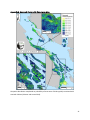
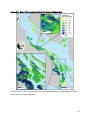
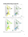
Appendix G. Example Maps - Locking In vs. Not Locking In Parks
Selection frequency map and best solution map for a Marxan simulation on the Capital Regional District with the
following specs: Parks Locked in – Yes; 100 Runs ; BLM set at 10; SPF set at 3; 100 000 iterations
Selection frequency map and best solution map for a Marxan simulation on the Capital Regional District with the
following specs: Parks Locked in – No; 100 Runs ; BLM set at 10; SPF set at 3; 100 000 iterations
26