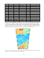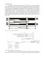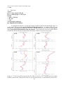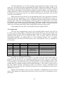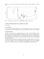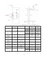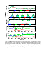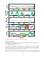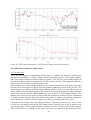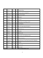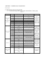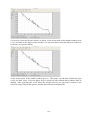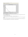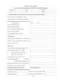
1
National Oceanography Centre Cruise Report No. 10 RRS James Clark Ross Cruises JR265 and JR254D 27 NOV – 24 DEC 2011 Part 1: The Drake Passage hydrographic repeat section SR1b Principal Scientist M J Yelland 2011 2 National Oceanography Centre, Southampton University of Southampton Waterfront Campus European Way Southampton Hants SO14 3ZH UK Tel: +44 (0)23 8059 6406 Email: [email protected] © National Oceanography Centre, 2011 DOCUMENT DATA SHEET AUTHOR Yelland, M.J. et al PUBLICATION DATE 2011 TITLE RRS James Clark Ross Cruises JR265 and JR254D, 27 Nov-24 Dec 2011. Part 1: The Drake Passage hydrographic repeat section SR1b. REFERENCE Southampton, UK: National Oceanography Centre, Southampton, 135pp. (National Oceanography Centre Cruise Report, No. 10) ABSTRACT This report describes the 17th complete occupation of the Drake Passage CTD section, established during the World Ocean Circulation Experiment as repeat section SR1b. It was first occupied by National Oceanography Centre (previously IOSDL and then SOC) in collaboration with the British Antarctic Survey in 1993, and has been re-occupied most years since then. Thirty two full depth stations were performed during JR265: two test stations, and all 30 of the nominal stations for the SR1b Drake Passage section. An initial result is that the estimated total transport measured across the section was 133 Sv which compares well to an average transport measured from the 16 previous UK cruises of 135 Sv (standard deviation of 7 Sv). In conjunction with the hydrographic cruise, a "Waves Aerosol and Gas Exchange Study" (WAGES) intensive observation cruise JR245D was also carried out. WAGES involves continuous measurement of the air-sea turbulent fluxes of CO2, sea spray aerosol, momentum and sensible and latent heat fluxes, plus directional sea-state and whitecap parameters using systems installed on the ship in May 2010. In addition to the continuous measurements, a number of intensive observation periods (IOPs) have been carried out by WAGES staff on board the ship. These involve deployments of a spar buoy to measure wave breaking and an aerial camera system to measure whitecap fraction. The activities of JR254D are summarised here, but are described in detail in a separate cruise report. Cruise JR264 was carried out by NOC-L staff at the same time as JR265 and JR254D. JR264 is also the subject of a separate cruise report. The CTD was an underwater SBE 9 plus unit equipped with the following sensors: dual temperature and conductivity sensors, a pressure sensor encased in the SBE underwater unit, a SBE-43 oxygen probe, an Aquatracka MKIII fluorometer, a transmissometer, an upwardlooking downwelling PAR sensor, and an altimeter. A downward-looking LADCP (RDI Workhorse Monitor 300 kHz) was deployed on all stations. Various underway measurements were obtained, including navigation, VM-ADCP, sea surface temperature and salinity, water depth and various meteorological parameters. A practical aim during this cruise was to update the detailed guides for each of the hydrographic data streams which were first written during JR195 in 2009. The hydrographic data analysis was performed using "MSTAR", a suite of Matlab programs developed at NOCS by Brian King and used on the JCR for the first time during JR195. KEYWORDS Acoustic Doppler Current Profiler, ADCP, air-sea flux, Antarctic Circumpolar Current, cruise 265 2011, CTD observations, Drake Passage, gas exchange, James Clark Ross, JR265, LADCP, lowered ADCP, sea-spray aerosol, SOLAS, Southern Ocean, SR1b, Valkyrie, vessel-mounted ADCP, WAGES, wave breaking, waves, whitecap, WOCE, World Ocean Circulation Experiment ISSUING ORGANISATION National Oceanography Centre University of Southampton Waterfront Campus European Way Southampton SO14 3ZH UK Tel: +44(0)23 80596116 Email: [email protected] A pdf of this report is available for download at: http://eprints.soton.ac.uk Page intentionally left blank CONTENTS SCIENTIFIC/TECHNICAL PERSONNEL ...............................................................................................9 SHIP'S PERSONNEL ...................................................................................................................................9 LIST OF TABLES .......................................................................................................................................11 LIST OF FIGURES .....................................................................................................................................11 ACKNOWLEDGEMENTS ........................................................................................................................12 1. OVERVIEW.............................................................................................................................................13 1.1 INTRODUCTION AND BACKGROUND. ....................................................................................................13 1.1.1 WAGES........................................................................................................................................13 1.1.2 Hydrographic Section. ...............................................................................................................13 1.2 SCIENTIFIC OBJECTIVES .......................................................................................................................15 1.2.1 JR265 Hydrographic section.......................................................................................................15 1.2.2 WAGES objectives for JR254D ...................................................................................................16 1.3 CRUISE NARRATIVE .............................................................................................................................16 1.3.1 Mobilisation period, 24th-27th November. ...................................................................................16 1.3.2 WAGES studies and Drake Passage section, 27th November - 5th December............................17 1.3.3 Antarctic Peninsular, 6th - 13th December...................................................................................18 1.3.4 Antarctic Peninsular to Stanley, 14th - 24th December................................................................19 2. CTD ...........................................................................................................................................................19 2.1 INTRODUCTION ....................................................................................................................................19 2.1.1 Problems and significant events during operations ....................................................................21 2.2 CONFIGURATION ..................................................................................................................................22 2.3 DEPLOYMENT .......................................................................................................................................23 2.4 DATA ACQUISITION ..............................................................................................................................23 2.4.1 Pre-cast procedure ......................................................................................................................23 2.4.2 Procedure for the cast .................................................................................................................24 2.4.3 Immediate post-cast operations. .................................................................................................25 2.5 SBE DATA PROCESSING .......................................................................................................................25 2.6 MSTAR DATA PROCESSING ................................................................................................................27 5 2.7 CALIBRATIONS .....................................................................................................................................28 2.7.1 Pressure.......................................................................................................................................28 2.7.2 Temperature ................................................................................................................................28 2.7.3 Salinity.........................................................................................................................................28 2.8 INITIAL RESULTS ..................................................................................................................................29 3. LOWERED ACOUSTIC DOPPLER CURRENT PROFILER (LADCP).........................................33 3.1 INTRODUCTION ....................................................................................................................................33 3.2 LADCP SET-UP ....................................................................................................................................34 3.3 PRE-DEPLOYMENT ...............................................................................................................................35 3.4 DEPLOYMENT .......................................................................................................................................36 3.5 RECOVERY ...........................................................................................................................................36 3.6 INITIAL DATA QUALITY CHECK ...........................................................................................................37 3.7 DATA PROCESSING ...............................................................................................................................39 3.7.1 UHDAS processing .....................................................................................................................40 3.7.2 LDEO processing ........................................................................................................................43 3.8 LADCP PROBLEMS ON JR265..............................................................................................................45 4. VESSEL-MOUNTED ACOUSTIC DOPPLER CURRENT PROFILER .........................................45 4.1 INTRODUCTION ....................................................................................................................................45 4.2 INSTRUMENTATION ..............................................................................................................................45 4.3 CONFIGURATION ..................................................................................................................................46 4.4 OUTPUTS ..............................................................................................................................................47 4.5 CODAS/HAWAII PROCESSING. ............................................................................................................47 5. SCS UNDERWAY DATA AQUISITION .............................................................................................52 5.1 UNDERWAY DATA ACQUISITION USING THE SCS SYSTEM ....................................................................52 6. NAVIGATION .........................................................................................................................................54 6.1 INSTRUMENTATION ..............................................................................................................................54 6.1.1 Seapath system ............................................................................................................................54 6.1.2 Ship’s Gyro..................................................................................................................................54 6.1.3 TSS Roll and Pitch.......................................................................................................................54 6.1.4 Ashtech ........................................................................................................................................54 6.1.5 Additional Data ...........................................................................................................................54 6.2. ROUTINE PROCESSING .........................................................................................................................54 6 6.2.1 SEAPATH ....................................................................................................................................54 6.2.2 GYRO ..........................................................................................................................................55 6.2.3 SEAPATH and GYRO..................................................................................................................55 6.2.4 ASHTECH ...................................................................................................................................56 6.3 GENERATING BESTNAV FILE................................................................................................................56 6.4 SUMMARY ............................................................................................................................................56 7. ECHO SOUNDER BATHYMETRY .....................................................................................................56 8. SURFACE METEOROLOGICAL SAMPLING SYSTEM................................................................58 8.1 INTRODUCTION ....................................................................................................................................58 8.2 INSTRUMENTATION ..............................................................................................................................58 8.3 ROUTINE PROCESSING ..........................................................................................................................60 8.4 SENSOR PERFORMANCE ........................................................................................................................62 9. UNDERWAY TEMPERATURE AND SALINITY .............................................................................64 9.1 INTRODUCTION ....................................................................................................................................64 9.3 CALIBRATION OF UNDERWAY SEA SURFACE TEMPERATURE ................................................................65 9.4 CALIBRATION OF UNDERWAY SALINITY DATA .....................................................................................66 9.4.1 Introduction .................................................................................................................................66 9.4.2 Calculating sample salinity .........................................................................................................67 9.4.3 Calibration of Underway salinity with bottle samples................................................................68 9.5 RESIDUALS ...........................................................................................................................................68 10. ARGO FLOAT DEPLOYMENT .........................................................................................................70 10.1 INTRODUCTION ..................................................................................................................................70 10.2 DEPLOYMENT PROCEDURE .................................................................................................................70 11. SALINOMETER....................................................................................................................................71 11.1 INTRODUCTION. .................................................................................................................................71 11.2 RUNNING THE SALINOMETER (AUTOSAL)..........................................................................................72 11.2.1 Initial setup of the Salinometer. ................................................................................................72 11.2.2 Initial standardisation ...............................................................................................................73 11.2.3 Taking bottle samples................................................................................................................73 11.3 ANALYSING A CRATE OF SAMPLES ONCE THE SALINOMETER IS SET UP. .............................................73 11.4 POTENTIAL PROBLEMS: ......................................................................................................................74 11.5 CALCULATION OF SALINITY IN EXCEL SPREADSHEETS.....................................................................75 7 12. DATA ARCHIVE OF NOSEA2 AND LABDATA.............................................................................75 13. ICT CRUISE REPORT.........................................................................................................................76 13.1 NETWARE SYSTEM .............................................................................................................................76 13.2 UNIX SYSTEMS ...................................................................................................................................76 13.3 LINUX SYSTEMS .................................................................................................................................76 13.4 SCS....................................................................................................................................................77 13.5 EM122 SWATH SYSTEM. ..................................................................................................................77 13.6 VSAT ..................................................................................................................................................77 14. SUMMARY AND RECOMMENDATIONS: .....................................................................................77 15. REFERENCES.......................................................................................................................................78 APPENDIX A. BRIDGE LOGS ................................................................................................................80 A.1 BRIDGE LOG OF SCIENTIFIC OPERATIONS.............................................................................................80 A.2 BRIDGE WEATHER LOG. ....................................................................................................................104 APPENDIX B – JR265 CTD INSTRUCTIONS .....................................................................................107 B.1 CTD DECK UNIT SETUP, PROCESSING AND DATA TRANSFER..............................................................107 B.2 BOTTLE FILE FORMATS ......................................................................................................................108 B.3 INSTRUMENT CALIBRATION CONSTANTS ...........................................................................................109 B.4 SEABIRD CTD CONFIGURATION FILE AS USED THROUGHOUT JR265.................................................110 B.5 DETAILS OF MSTAR PROCESSING.....................................................................................................114 APPENDIX C - UNDERWAY DATA PROCESSING ..........................................................................116 C.1 DAILY UNDERWAY DATA PROCESSING SCHEDULE.............................................................................116 C.2 MPLXYED EDITING OF DATA. .............................................................................................................118 APPENDIX D - LOG SHEETS ................................................................................................................122 APPENDIX E. VM-ADCP SETUP. .........................................................................................................130 8 SCIENTIFIC/TECHNICAL PERSONNEL JR265 Margaret Yelland (PSO) Mairi Fenton Vikki Frith (Naomi) Penny Holliday Helen Snaith NOC-S BAS, Rothera University of Reading NOC-S NOC-S, BODC JR254D Margaret Yelland (PSO) Sarah Norris Robin Pascal NOC-S University of Leeds NOC-S JR264 Miguel A M Maqueda (PSO) Geoff Hargreaves Stephen Mack NOC-L NOC-L NOC-L BAS technical support. Julian Klepacki Seth Thomas Johnnie Edmonston BAS (AME) BAS (AME) BAS (ITC) SHIP'S PERSONNEL Graham P Chapman Joanna L Cox Simon D Evans Ben P Thompson Charles A Waddicor Heather L Williams Harry Taylor John Roberts David J Cutting Glynn Collard James C Ditchfield Steven J Eadie Simon A Wright Nicholas J Dunbar "Hamish" James Gibson James Rudd George M Stewart Derek G Jenkins Clifford Mullaney John J McGowan Colin J Leggett John P O'Duffy Anthony J Estibeiro Mark A Robinshaw Master Chief Officer 2nd Officer 3rd Officer ETO (Comms) Cadet Cadet Cadet Chief Engineer 2nd Engineer 3rd Engineer 4th Engineer Deck Engineer ETO (Eng) Purser Doctor Bosun Bosun's Mate SG1 SG1 SG1 SG1 SG1 MG1 9 Matthew B Ashworth Keith A Walker Padraig G Molloy Kenneth Weston James Newall Derek W Lee Thomas Patterson MG1 Cook 2nd Cook Steward Steward Steward Steward 10 LIST OF TABLES Table 1.1: List of UK occupations of Drake Passage section. .........................................14 Table 2.1: Nominal station positions for Drake Passage CTD section ...........................20 Table 2.2: Actual CTD stations carried out during JR265.. ...........................................21 Table 3.1. Indication of a failing beam ..............................................................................45 Table 4.1. ADCP set up modes during JR265 .................................................................46 Table 4.2. Calibrations derived from the CODAS processing. ......................................48 Table 4.3 Mean calibration results for previous cruises.................................................48 Table 8.1 Meteorological instrument properties. .............................................................59 Table 9.1: Underway SST and salinity instrument details. .............................................65 Table 9.1: example TSG salinity calculation excel file.....................................................67 Table 10.1. JR265 ARGO Float Deployment details .......................................................70 Table 11.1. Standardisation history of the salinometer used on JR265. ........................72 Table A.1 Scientific events obtained from the bridge log.............................................104 Table A.2 Bridge weather observations .........................................................................106 LIST OF FIGURES Figure 1.1: The CTD section across Drake Passage.........................................................14 Figure 1.2. The JR265 and JR254D science team arriving at Rothera .........................16 Figure 2.1: Potential temperature across JR265 Drake Passage section. .....................30 Figure 2.2: Salinity (PSU) across JR265 Drake Passage section....................................30 Figure 2.3: Density across JR265 Drake Passage section. ..............................................31 Figure 2.4: Nominally calibrated dissolved oxygen concentration ................................31 Figure 2.5: Nominally calibrated chlorophyll fluorescence ...........................................32 Figure 2.6: T-S plot for Drake Passage section ...............................................................32 Figure 2.7: Geostrophic velocity on Drake Passage. ........................................................33 11 Figure 3.1. Star-Cable Connections...................................................................................34 Figure 3.2. Comms/Power cable connections....................................................................34 Figure 3.3. Deck-Test with weak Beam 3; Intensity offset with high counts. ................38 Figure 3.4. Data close to bottom showing Intensity offset and poor correlation...........38 Figure 3.5. Correctly functioning unit with Profiles ........................................................39 Figure 3.6. Close to bottom Profiles...................................................................................39 Figure 3.7. Velocity profiles generated by the UH processing ........................................42 Figure 3.8. Beam Stats figures for station 008 and station 009......................................44 Figure 3.9. Velocity profiles for station 008 and station 009. .........................................44 Figure 4.1. Calibrated surface currents. ...........................................................................52 Figure 7.1 Depth profile vs latitude. ..................................................................................58 Figure 8.1 Schematic of the sensor positions on the foremast.........................................59 Figure 8.2.a Meteorological data for days 331 to 336. .....................................................61 Figure 8.2.b Same plots as in figure 8.2.a, for days 336-340. ..........................................62 Figure 8.3 The difference between the humidity sensors ................................................63 Figure 8.4 Airtemp2 vs Airtemp1 (nighttime temperatures only)..................................63 Figure 8.5 Difference in night-time air temperatures against true wind speed.............64 Figure 9.1 TSG remote temperature vs CTD surface temperature measurements......66 Figure 9.2 Bottle and TSG Conductivity, with conductivity differences.. .....................68 Figure 9.3 Bottle and TSG Salinity (before and after conductivity calibration)...........69 Figure 9.4 The SBE45 salinity residuals after correcting the salinity data. ..................70 ACKNOWLEDGEMENTS I am indebted to the science team for their professionalism and enthusiasm, and to Graham Chapman, JCR Master, for a very successful and memorable cruise. The staff of the JCR are a real pleasure to sail with, and are always very efficient, friendly and helpful. Support from the BASE AME and IT staff on board was very much appreciated. Special thanks to the three members of the science team who were at sea for the first time: Mairi Fenton (BAS, Rothera) volunteered to help the science team and saved my sanity by taking my place on the night watch; Vikki Frith (Reading University) turned into a valuable hydrographer within hours of getting on board; Seth Thomas (BAS, AME) saved the WAGES scientific bacon by working all hours during mobilisation to build replacement circuit boards for the MotionPak interface. 12 1. OVERVIEW Margaret Yelland 1.1 Introduction and background. The research cruises JR265 and JR254D began from Mare Harbour, Falkland Islands, on the morning of the 27th November 2011 and finished at Stanley, Falkland Islands, on the 24th December 2011. The objective of JR265 was to perform a CTD section across Drake Passage (Figure 1.1), repeating the measurements made during previous research cruises for the purpose of long-term monitoring. The aim of JR254D was to deploy a wavebreaking buoy (Pascal et al., 2011) and an aerial whitecap camera system in a range of wind speed and sea state conditions. WAGES activities are summarised in this cruise report, but are described in detail in a separate report (Yelland, 2012a). A third cruise, JR264, was run by staff from NOC-Liverpool with the aim of recovering and deploying various Bottom Pressure Recorders which have been deployed across Drake Passage and elsewhere on the Antarctic Peninsular for more than 20 years. NOC-L also serviced various tide gauges in the Falkland Islands and along the Antarctic Peninsular. JR264 is described in detail in a separate cruise report (Morales Maqueda, in prep). 1.1.1 WAGES. JR254D was one of a series of Intensive Observation Periods (IOPs) for the Waves Aerosol and Gas Exchange Study (Yelland, 2012a). The aim was to deploy the novel spar buoy developed at NOC-S to measure wave breaking and whitecap fraction, along with an aerial camera system to capture the whitecap coverage across a wider spatial area. These deployments take place during cruises which are manned by members of the WAGES team. As part of WAGES the JCR was instrumented in the summer of 2010 with: the autonomous air-sea interaction system "AutoFlux" (Yelland et al., 2009b) to measure the air-sea fluxes of CO2, seaspray aerosol, momentum and sensible and latent heat; a WAVEX directional wave radar system; a webcam mounted on the bridge to capture whitecap fraction. These systems measure continuously. Previous IOPS and the continuous measurements are described in Yelland (2012b). WAGES activities during JR254D are summarised here and are described in detail in a separate cruise report (Yelland, 2012a) 1.1.2 Hydrographic Section. As described by Bacon and Cunningham (2005), the World Ocean Circulation Experiment established a repeat hydrographic section across Drake Passage and designated it SR1. This section was first occupied by the R/V Meteor in 1990 (Roether et al., 1993). Subsequently, the section was moved eastwards to lie on a satellite ground track with the northern end on the south side of Burdwood Bank, south of the Falkland Islands, and the southern end off Elephant Island at the tip of the Antarctic Peninsula. This revised section location was designated SR1b and was first occupied by the R/V Polarstern in 1992 (Gersonde, 1993). The first UK occupation of SR1b took place on RRS Discovery later the same year using SeaSoar (a profiler which undulates between the surface and ~400 m) (Turner, 1993; Read et al., 1993) only i.e. no CTD profiles. Between that time and the present there have been 16 UK (NOCS/BAS) complete occupations of SR1b at nearly one section per year, all with full-depth CTDs and, since 1996, with full depth LADCP also. See Table 1.1 for a list of cruises, dates and references. The scheduling of the cruises usually makes use of the BAS logistical requirement to re-supply the base at Rothera at the start of the austral summer, hence all bar two have taken place on the RRS James Clark Ross (JCR). 13 year 1992 1993 1994 1996 1997 1999 2000 2001 2002 2003 2004 2005 2006 2007 2008 2009 2009 2010 ** 2010 ** 2011 start date 11/11/1992 20/11/1993 13/11/1994 13/11/1996 17/12/1997 12/02/2000 21/11/2000 19/11/2001 18/12/2002 27/11/2003 01/12/2004 5/12/2005 7/12/2006 29/11/2007 Dec 2009 3/2/2009 18/11/2009 6/11/2010 9/4/2011 27/11/2011 end date 17/12/1992 18/12/1993 12/12/1994 07/12/1996 08/01/1998 16/02/2000 14/12/2000 17/12/2001 02/01/2003 17/12/2003 19/12/2004 12/12/2005 15/12/2006 8/12/2007 Dec 2009 3/3/2009 29/11/2009 10/12/1020 25/4/2011 25/12/2011 designator D198 - SeaSoar only JR0a or JR00_1 JR0b or JR00_2 JR16 JR27 JR47 JR55 JR67 JR81 JR94 JR115 JR139 JR163 JR193 JR194 JC031 JR195 JR240 JR276 JR265 LADCP N N N Y Y N Y Y Y Y Y Y Y Y Y Y Y Y Y Y cruise report Turner, 1993 Bacon and Cunningham 2005 Bacon and Cunningham 2005 Bacon and Cunningham 2005 Bacon and Cunningham 2005 Bacon and Cunningham 2005 Cunningham, 2001 Bacon et al., 2002 Bacon et al., 2003 Hawker et al., 2005 Sparrow et al., 2005 Stansfield et al., 2008 Williams et al., 2008 Hamersley and Quartly 2010a Hamersley and Quartly 2010b McDonagh et al., 2009 Yelland et al., 2009a Maksym, CTD 030-023, 007 Watson, CTD 020-007 This report, Yelland 2011 Table 1.1: List of UK occupations of Drake Passage section, WOCE designation SR1b (adapted from Bacon and Cunningham, 2005). Notes: “Year” is the year of the start of the relevant southern season. “LADCP” shows which cruises carried that instrument (JR115 experienced some technical difficulties with the LADCP). All occupations aimed to occupy the station positions (see Section 2) shown in Figure 1.1. D198 was occupied with an undulating profiling instrument, SeaSoar, with no full-depth CTDs. ** indicates the two partial occupations which took place in late 2010 and early 2011 to replace the cancelled 2010 JR242 cruise. Figure 1.1: The CTD section across Drake Passage. Red dots indicate the position of the CTD stations: for clarity, only some stations are numbered. 14 In 2010 the planned hydrographic section (JR242) was cancelled at short notice due to problems with the Dash-7 aircraft. The plan had been to fly the science team in to Rothera and perform the section northbound. The scientists on the preceding cruise JR240 (Maksym, in prep.) were due to fly out from Rothera on the same aircraft but had to stay on board the JCR back to Stanley: they performed the southernmost 9 CTD sections on their way north (stations 030 to 023 inclusive from Table 2.1 below, plus station 007 from the "standard" section list, see Yelland, 2009a). A subsequent cruise JR276 in April 2011 performed 14 CTD casts in the northern end of the section, from station 020 to about 007 (see Table 2.1), omitting the 6 most northerly stations due to lack of time (Watson, in prep). It should be noted that the northernmost 9 CTD stations carried out during JR265 followed a line directly north-south along 58° West, similar in position to those used by McDonagh (2009) and Watson (in prep), rather than the "standard" CTD location used in most of the previous occupations of the section (e.g. Yelland, 2009a). This report will describe each major hydrographic data stream in turn. Each data stream was the primary responsibility of one science team member: CTD, Vikki Frith; LADCP and VMADCP, Penny Holliday; underway data (meteorology, navigation, echosounder etc), Helen Snaith; salinometer operations, Margaret Yelland. A practical aim during this cruise was to update the detailed guides written during JR195 (Yelland, 2009a) for each data stream, including how to set the systems up, operations while on station or underway, initial examination of data to ensure that the systems are working correctly, through to data analysis to the level required for a cruise report. Much of the data analysis was performed using "MSTAR", a suite of Matlab programs developed at NOCS by Brian King and used on the JCR for the first time during JR195. Some of these detailed guides are included in the main body of the report, whereas others are included as appendices. Unless stated otherwise, times are given in GMT. Jday of 1.5 represents 1200 GMT on 1st January: the same date and time is given by a decimal day of 0.5. Jday is used in this report, but some data outputs include a decimal day time stamp. 1.2 Scientific Objectives 1.2.1 JR265 Hydrographic section Drake Passage is the narrowest passage through which the Antarctic Circumpolar Current (ACC) flows, and thus is a convenient location for making measurements across the entire ACC. The objective of this section is to look at changes on interannual to decadal scales. The key objectives for the JR265 CTD section across Drake Passage are:(i) to determine the interannual variability of the position, structure and transport of the Antarctic Circumpolar Current (ACC) in Drake Passage; (ii) to examine the fronts associated with the ACC, and to determine their positions and strengths; (iii) by comparing geostrophic velocities with those measured directly (by the lowered ADCP), to determine the size of ageostrophic motions, and to attempt to estimate the barotropic components; (iv) to examine the temperature and salinity structure of the water flowing through Drake Passage, and thus identify the significant water masses; (v) to calculate the total flux of water through Drake Passage by combining all available measurements. 15 1.2.2 WAGES objectives for JR254D The overall aim of WAGES is to improve the parameterisations of the air-sea fluxes and to understand their dependence on sea-state, wave breaking and whitecap fraction. The aim of the IOPs is to deploy the buoy and aerial camera systems in a wide range of wind speeds and sea states, and in both short fetch and open-ocean conditions. JR254D had 48 hours of dedicated ship time. In addition to this the aim was to deploy the buoy and balloon systems during the deeper CTD stations whenever conditions allowed. 1.3 Cruise Narrative 1.3.1 Mobilisation period, 24th-27th November. The JR265 and JR254D science teams (Figure 1.2) travelled south on the RAF flight from Brize Norton on the 20th November, and arrived at the Falkland Islands on the evening of the 21st November. The teams were met by BAS personnel and transferred to accommodation in Stanley. The arrival of the JCR was delayed by bad weather and the science team did not get access to the ship in Mare Harbour until the 24th November, leaving two full days to mobilise prior to sailing on the morning of the 27th, day 331. BAS AME mobilised the hydrographic equipment in good time to train the hydrographic team prior to the ship sailing. During the mobilisation period the WAGES team worked hard to ensure that as much as possible was ready before the ship sailed. A major problem was found with one of the fundamental WAGES sensors on arrival at the ship: the housing of the MotionPak sensor (which measures the shipinduced motion at the flux sensors on the foremast platform) had leaked and the sensor had stopped working a few days previously. Seth Thomas (BAS AME) worked flat out to build new interface circuit boards for this sensor in time for the ship departure from Mare Harbour. Figure 1.2. The JR265 and JR254D science team (aka "the Valkyries") arriving at Rothera. Left to right: Helen, Vikki, Robin, Sarah, Mairi, Mags, Penny. 16 1.3.2 WAGES studies and Drake Passage section, 27th November - 5th December. During the hydrographic team worked 12 hour watches (8 til 8 local time), with Snaith and Fenton taking the night shift and Holliday and Frith taking the day shift. This worked well, since the deck crew and winch drivers worked the same watches. The WAGES team and the NOC-L team worked as appropriate to fit the other science work around the CTD section. Below is a short day-by-day account of scientific operations and weather conditions. All times stated in this cruise report are GMT unless specified otherwise. Notes on wind speed, sea state and ice conditions are courtesy of the bridge scientific log (see Appendix A.1) and the bridge weather observations (Appendix A.2). Section 2 gives details of the nominal, and actual, positions and depths of the CTD stations. 27th November, jday 331. JCR departed Mare Harbour 0900 local, 1200 GMT, and headed eastwards to perform a 12 hour short fetch study for WAGES. Once on station did a shallow (50 m) test CTD at station 900 (with Pudsey the mascot on the frame) then a 12 hour WAGES buoy deployment 1 at short fetch from 1200 to 2400 local, including balloon deployment 1 during which the altimeter was lost. The VM-‐ADCP was set to bottom tracking mode during the fetch study. SWATH was turned on prior to the start of the CTD section proper. 28th November, jday 332. Deep test CTD to about 2300 m at CTD station 901. During this second text dip the CTD frame carried one of the NOC-‐L microcats for calibration prior to deployment with the NOC-‐L BPR. Three 15 min stops at 1500, 1000, and 500 m depths were made for this purpose. CTDs 001 and 002 were done: some time was spent locating the correct depths since the northern part of the CTD section was moved east to longitude 58° W 29th November, jday 333 CTDs 003 to 009 again involved some hunting for the correct depths. A short SWATH survey was done to find a good location for the 1100 m depth deployment of the northern NOCL BPR. Once located CTD 004 done prior to the BPR deployment and SWATH was turned off (0245 GMT) since it was thought that it may interfere with the VM-ADCP. 1st Argo float 4900 deployed after CTD 007. WAGES buoy deployment 2 was done during CTD 008. After CTD 008 the LADCP beam 3 was found to be weak. The LADCP model WHM300-i-ug306, S/N 14443 was swapped for WHM300-i-ug301, S/N 15060 in time for dip 009. WAGES buoy deployment 3 took place during CTD 009. The IRIDIUM unit on the buoy was not sealed properly so became flooded and never recovered. 30th November, jday 334 Pudsey went on strike for the day. The ship was in position for CTD 010 in the early hours but the wire came off the roller at the very start of the deployment and the CTD was brought back on deck. A strong current combined with large seas and a strong wind led to the decision to wait for conditions to improve: station 010 is the deepest of the section and was thought to be at or near the Sub-Antarctic Front and was therefore thought important to complete. The conditions did not improve overnight and the forecast was bad, so WAGES buoy deployment 4 was begun at about 1100 GMT. 1st December, jday 335 The WAGES buoy was recovered at around 1300 GMT. The large waves encountered while the buoy was being hauled in caused the 4 rods at the base to bend and the buoy to lie horizontally in the water. The top half of the buoy tore away and the IRIDIUM unit, flashing light and camera mounted on the upper part were lost, but the bottom half of the buoy along with the data logger and current meter were recovered successfully. Once the buoy was recovered the 17 JCR steamed back on station and CTD 010 was performed. Since the swell was still large the CTD was sent straight down from 13 m rather than brining it back to the surface before performing the cast. 2nd December, jday 336. CTDs 011 to 15. The 2nd ARGO float (S/N 4901) was deployed after CTD 011. During CTD 012 the altimeter became noisy and intermittent and a big transmissometer spike implied that the CTD may have touched the bottom although on recovery it was found to be completely undamaged and only a smudge of mud was found on the base of the frame. WAGES buoy deployment 5 took place during CTD 013 and the altimeter was swapped out after that station was completed. WAGES buoy deployment 6 and balloon deployment 2 were performed during CTD 014 and the 3rd ARGO float (4902) was deployed immediately afterwards. The JCR did about 30 minutes of circuits and bumps for engine testing on the way to CTD 015 during which WAGES buoy deployment 7 and balloon deployment 3 took place. 3rd December, jday 337. CTDs 016 - 020. The 4th ARGO float (4903) was deployed after CTD 017. WAGES buoy deployment 8 was done during CTD 020. The 5th ARGO float (4999) was deployed after CTD 020. 4th December, jday 338. CTDs 021 – 026. CTD 021 was accompanied by several whales (possibly humpbacks) in the distance, and a lone chinstrap penguin close to the ship. 6th ARGO float 4998 deployed after CTD 023. JCR spent about 30 minutes doing engine checks. WAGES buoy deployment 9 done during CTD 024, with Pudsey as passenger. At the start of CTD 025 the pumps were very slow switching on. They were tested after the cast and were OK. – pump was tested after the cast and seemed to be ok, so left on. WAGES buoy deployment 10 and balloon deployment 4 (with Pudsey) were done during CTD 025. CTD 026 had three 15 minutes stops at 1500 m, 1000 m and 500 m to allow calibration of the other NOC-L microcat. 5th December, jday 339. CTDs 027 – 030. NOC-L team deployed APEX float before start of CTD 027. With 1580 m of wire out and an EO600 depth of 1630 m the altimeter had still not kicked in (which it should at about 100 m off the bottom). The cast was stopped while Johnnie switched the EM122 on briefly to check the depth. This gave a reading of 1778 m, so the cast was continued: the altimeter detected the bottom when there was about 1640 m wire out and the cast stopped at a depth of 1729 m. Given the under-read on the EA600 on the previous cast, the EM122 was switched on briefly to check the depth before the start of CTD 028: depths agreed within 20 m so the EM122 was switched off and the cast was carried out as normal. NOC-L then deployed and recovered BPRs from the deep (2000 m) and shallow (1000 m) sites: they also deployed a FETCH mooring but this surfaced again unexpectedly and was recovered. The last two CTD stations were then done and all completed by about 1230 local time. 1.3.3 Antarctic Peninsular, 6th - 13th December. At the end of the CTD section it was decided to postpone both the attempted recovery of the NOCL-L MYRTLE system and the NOC-L visit to Vernadsky (to maintain the tide gauges there) until the JCR was on passage northbound. This decision was made in order to arrive on time in Rothera on the 8th December so that three of the JR265 and JR254D science teams could catch their scheduled flight northwards on the DASH-7. Unfortunately on the 6th December it was decided that the DASH had to leave on the 7th, a day early, due to unforeseen circumstance. The JCR continued down the west side of the peninsular and arrived at Rothera at 0700 local time on the 8th. Rothera relief was completed on time and the ship sailed on the 11th. Sea-ice prevented the ship landing any people at Vernadsky, but on the evening of the 13th the NOC-L 18 tide gauge equipment and instructions (in Russian) were landed on the shore with the aid of some skilful ship parking by the Master, a fishing rod wielded by Mark Robinshaw and two of the staff of Vernadsky hauling on a rope. 1.3.4 Antarctic Peninsular to Stanley, 14th - 24th December. On the way north from Vernadsky to King George Island WAGES buoy deployment 11 was done off the coast of Livingston Island in the early hours of the 15th December (jday 349). The forecast was for strong winds from the west or north so the deployment was done about 2 nm off the coastline that runs from SW to NE. In the event the winds proved to be rather light and variable. Collected two passengers from Jubany base King George Island. The JCR arrived at the NOC-‐L MYRTLE site in the early hours of the 16th. MYRTLE responded to pings but did not release, so triangulation and SWATH surveys were done to get an accurate position for any future recovery attempt. On the way from the MYRTLE site towards Signy the JCR stopped to recover the NOC-‐L APEX float that was deployed (free drifting) earlier on the 5th December. Once this was on board the NOC-‐L SONAR bell (a gel sphere designed to be a target) was deployed to 1500 m but failed to show up on the EA600. The JCR then continued towards Signy. The wind was from astern, i.e. a bad direction for flux measurements so the pump for the new Licor-‐7200 was turned off to get null ("shrouded") data. On arrival at Signy on the morning of the 18th it was too windy to transfer people ashore in the small boats, so WAGES buoy deployment 12 was done for about 7 hours (1100 to 1800 local time, with the LICOR pump turned back on) until the wind dropped enough to get people ashore. JCR headed to Cape Geddes overnight and arrived on the morning of the 18th. While people were transferred ashore the old LICOR 7500 was shrouded and the pump for the new LICOR turned off again, and the inlet taped over. The ship then headed back to Signy again, arriving around 16:30 local time the same day. The ship had to stay at Signy while technical staff worked on the new V-‐SAT system, so on the 19th the science teams had the chance of a walk to Gourlay Point to see Adelie and Chinstrap colonies. Ship sailed evening of the 19th and headed towards Bird Island via the Lewthwaite Strait. Arrived Bird Island around 1300 local on the 21st. No run ashore because of danger from fur seals and the need to make the visit a short one, so ship departed about 15:30 local and headed for Stanley. One short stop was made on the morning of the 22nd for another test of the NOC-‐L Sonar bell and a short CTD dip so that the BAS AME staff could test the software changes made at the end of the cruise that were necessary to implement the updated Seasave and SBE Data Processing software (version 7). JCR arrived in Stanley on the afternoon of the 24th. 2. CTD Vikki Frith 2.1 Introduction A Conductivity-Temperature-Depth (CTD) unit was used to record vertical profiles of the temperature and salinity of the water column. Two test stations, one shallow (900) and one deep (901) were carried out before starting the Drake Passage transect. They allowed us to test the equipment and sensors’ configuration. Thirty stations were occupied across the Drake Passage SR1b transect. The locations of the nominal stations across Drake Passage are listed in Table 2.1. The actual locations of the stations occupied during JR265, alongside the water depth and other information, are listed in Table 2.2. Bad weather led to a 45 hour break in science between stations 009 and 010. 19 Additional details are given in Appendix B: B.1 gives details on pre-sailing setup and mobilisation; B.2 the bottle file formats; B.3 SeaBird instrument calibration; B.4 calibration details contained in the SeaBird Configuration file; B.5 a detailed explanation of the MSTAR processing that is summarised in Section 2.6. Station Lat, °S Lat, min Lon, °W Lon, min 900 901 1 2 3 4 5 6 7 8 9 10 11 12 13 14 15 16 17 18 19 20 21 22 23 24 25 26 27 28 29 30 53 54 54 54 55 55 55 55 55 55 55 56 56 56 57 57 57 58 58 58 59 59 59 60 60 60 60 60 60 60 61 30.0 40.00 55.34 58.6 0.39 04.20 07.26 10.16 12.86 31.00 50.00 09.00 28.00 47.00 06.00 25.00 44.00 03.00 22.00 41.00 00.00 20.00 40.00 00.00 20.00 40.00 47.97 49.99 51.02 58.86 03.00 58 58 58 58 58 58 58 58 58 58 57 57 57 57 57 56 56 56 56 56 55 55 55 55 55 54 54 54 54 54 54 04.36 00.0 00.0 00.0 00.0 00.0 00.0 00.0 00.0 00.0 49.23 37.45 25.67 13.90 02.12 50.35 38.57 26.79 15.02 03.24 51.47 39.07 26.67 14.28 01.88 49.49 44.55 43.30 42.66 37.80 35.23 Depth, m 50 2300 250 600 1000 1500 2000 2500 3000 3700 4200 4800 3400 3800 3200 3700 3700 3400 3900 3800 3800 3800 3800 3600 3500 3400 3100 2500 1500 1000 600 400 est time on station (hh:mm) 0:30 2:30 0:30 0:30 0:50 1:10 1:30 1:40 2:00 2:30 2:50 3:00 2:20 2:30 2:00 2:30 2:30 2:00 2:30 2:30 2:20 2:20 2:20 2:10 2:10 2:00 2:00 1:30 1:00 0:50 0:30 0:30 distance to next station (nm) 10 70.2 15.4 3.3 1.6 12 3.1 2.9 2.7 18.2 20.2 20.2 20.1 20.1 20.1 20.1 20.1 20.1 20 20 20 21 21 21 21 21 8.4 2.1 1.1 8.2 4.3 4.6 est. time to next station (hh:mm) 1:00 6:06 1:20 0:17 0:10 1:00 0:15 0:15 0:14 1:34 1:45 1:45 1:45 1:45 1:45 1:45 1:45 1:45 1:44 1:44 1:44 1:50 1:50 1:50 1:50 1:50 0:44 0:11 0:05 0:43 0:22 0:24 Table 2.1: Nominal station positions for Drake Passage CTD section (the right hand three columns show the estimates of distance and times as used by the bridge). NOTE that stations 001 to 009 have been moved to lie along 58 W: the positions for these stations are approximate and needed to be adjusted to get the correct depth (see Table 2.2). Instructions given to the bridge stated that for the shelf edge stations, i.e. 1 - 8 and 25 - 30 inclusive, the station should be at a position where the depth is within 100 m of the nominal depth. For stations 9 - 24 inclusive, the position should be within 0.5 nm of the nominal position. 20 CTD stn Date 900 901* 1 2 3 4 5 6 7 8** 9** 10 11 12*** 13** 14** 15** 16 17 18 19 20** 21 22 23 24** 25** 26* 27 28 29 30 27/11/11 28/11/11 28/11/11 28/11/11 29/11/11 29/11/11 29/11/11 29/11/11 29/11/11 29/11/11 29/11/11 01/12/11 02/12/11 02/12/11 02/12/11 02/12/11 02/12/11 03/12/11 03/12/11 03/12/11 03/12/11 03/12/11 04/12/11 04/12/11 04/12/11 04/12/11 04/12/11 04/12/11 05/12/11 05/12/11 05/12/11 05/12/11 Time hh:mm GMT 15:42 13:14 22:01 23:32 01:59 03:59 05:48 11:50 14:43 17:45 22:49 20:11 02:10 06:52 11:43 16:28 21:47 02:18 07:02 11:44 16:21 21:01 01:41 06:10 10:37 15:25 19:48 22:44 02:34 04:01 14:23 15:35 Jday Lat. °S Lat. (min) Lon. °W Lon. (min) Wire out (m) 331.654 332.551 332.917 332.981 333.083 333.166 333.242 333.493 333.613 333.740 333.951 335.841 336.090 336.286 336.488 336.686 336.908 337.096 337.293 337.489 337.681 337.876 338.070 338.257 338.442 338.642 338.825 338.947 339.107 339.167 339.599 339.649 51 53 54 54 54 54 55 55 55 55 55 55 56 56 56 57 57 57 58 58 58 59 59 59 60 60 60 60 60 60 60 61 47.22 27.70 47.34 54.54 58.80 59.94 02.34 05.70 09.42 12.00 31.32 49.92 08.70 27.90 47.04 06.06 24.96 43.98 03.06 22.02 41.04 00.00 19.98 40.02 00.00 19.98 39.84 47.94 49.98 51.00 58.86 03.00 57 57 57 57 57 57 57 57 58 57 58 57 57 57 57 57 56 56 56 56 56 55 55 55 55 55 54 54 54 54 54 54 52.56 56.79 59.76 59.64 58.50 59.82 59.88 59.94 00.06 59.40 01.26 48.72 35.76 25.14 13.14 01.26 49.56 38.58 26.76 15.00 03.24 51.48 39.06 26.64 14.28 01.92 48.30 44.58 43.32 42.66 37.80 35.22 45 2350 250 608 1075 1490 2025 2450 3000 3550 4200 4720 3489 3663 3267 3870 3475 3459 3933 3876 3730 3752 3736 3654 3478 3420 3060 2530 1729 978 570 345 CTD max pressure (db) 46 2389 254 617 1090 1514 2061 2495 3060 3622 4295 4829 3556 3739 3325 3951 3546 3532 4022 3963 3811 3833 3813 3733 3552 3491 3115 2577 1758 993 578 350 True wind (m/s) 3.2 9.88 9.83 12.6 10.8 13.9 18.5 12.2 14.5 16.2 16.2 13.1 8.5 13.2 8.4 3.3 3.1 5.3 8.1 1.9 9.5 8.8 6.5 6.7 5.0 6.4 4.1 8.5 14.9 15.6 8.9 5.9 Table 2.2: Actual CTD stations carried out during JR265. The time (GMT) and positions given for each station correspond to the time and position of the ship when the CTD was at the bottom of each cast. * CTD carried NOC-L microcats for calibration prior to deployment with BPR. Calibration required three 15 minute stops at 1500, 1000 and 500 m wire-out during the ascent. ** WAGES buoy deployed during CTD. *** Altimeter noisy: CTD may have touched bottom. Altimeter swapped out after station 013. 2.1.1 Problems and significant events during operations • On stations 901 and 026 the CTD was stopped for three 15 minute periods at 1500 m, 1000 m and 500 m to allow the NOC-L microcat calibrations. • WAGES buoy deployments were carried out at several stations, shown in Table 2.2. At these stations the buoy was deployed before the CTD and brought in before the CTD finished coming up. • Bad weather stopped CTD deployments from 21:35 on 29/11 to 18:41 on 01/12. The first few deployments after were not brought back to the surface before descending. • The altimeter was changed after station 013 due to noisy readings. On station 012 the CTD may have touched the bottom. 21 2.2 Configuration A 24-bottle BAS CTD frame was used throughout the cruise. The CTD frame was equipped with a SBE 32 Carousel Water Sampler, configured with 24 12-litre Ocean Test Equipment ("Niskin") bottles, connected to an SBE 9 plus CTD, controlled and powered by an SBE 11 plus deck unit. The Niskin bottles (98.5 cm high) were mounted vertically 15 to 20 cm above the sensors. The distance measured between the pressure sensor and the top / bottom of the bottles was 114 cm / 15.5 cm. An SBE-35 high precision temperature sensor was attached vertically on one side bar of the frame approximately level with the water bottles. This provided independent 8-second average temperature measurements each time a bottle was fired. The underwater SBE 9 plus unit was equipped with the following sensors: dual temperature and conductivity sensors, a pressure sensor encased in the SBE underwater unit, a SBE-43 oxygen probe, an Aquatracka MKIII fluorometer, a transmissometer, an upward-looking downwelling PAR sensor, and an altimeter. The altimeter was changed after station 013 due to increasingly noisy readings. Table 2.3 gives details of sensors, serial number and calibration date. The mapping between sensors and voltage or frequency channels remained the same throughout. A report of the CON file settings used for JR265 is listed in Appendix B.1. For all stations a self-logging downward-looking LADCP was attached to the main CTD frame (see section 3 of this report for detail of LADCP operations). The frame was equipped with a fin to reduce rotation of the package underwater. Sensor Pressure Conductivity – primary Conductivity – secondary Temperature – primary Temperature – secondary Oxygen Fluorometer Transmissometer PAR sensor Altimeter (Station 900-013) Altimeter (Stations 014-030) High Precision Temperature Manufacturer SBE Model SBE-9+ Serial Number 0771 Calibration date 20/07/2010 SBE SBE-04 1912 25/06/2010 SBE SBE-04C 041912 25/06/2010 SBE SBE-03 4874 25/06/2010 SBE SBE-03 2191 23/06/2010 SBE Chelsea Technologies Group Ltd. SBE-43 0242 21/01/2009 Aquatracka MkIII 0088-3598C 09/11/2009 25cm pathlength C-Star CST-846DR 16/02/2011 WETLabs Biospherical Instruments Inc. System Technologies System Technologies QCD-905L4S 7274 23/03/2011 PA200/20-6K8 7742.163162 30/05/2007 PA200/20-6K8 2130.26993 03/12/2008 SBE SBE 03Plus 03P2191 23/06/10 Table 2.3: Details of the sensors model, serial numbers and calibration status. The mapping between sensors and voltage channels was found to be as follows: V0 ---------- PAR V1 ---------- empty V2 ---------- fluorometer V3 ---------- empty V4 ---------- transmissometer V5 ---------- empty V6 ---------- oxygen V7 ---------- altimeter 22 2.3 Deployment The CTD was deployed from the mid-ship’s gantry. The deck unit was turned on before the CTD was moved. The deployment procedure was to start data-logging on deck with the pressure noted on the log sheet. The CTD was deployed and lowered to 10 m of cable out. The pumps were automatically water activated and should come on 60 seconds after the CTD is in the water, on station 025 the pumps took around 5 minutes. After a 3 minute soak, the package was raised to just below the surface and then continuously lowered at a speed of about 60 m/min to a nominal 10 m above the seabed. Due to large swell on station 010 the CTD was taken straight down after the pumps activated. Three bottles were fired 30 seconds after reaching the bottom of the downcast, with a 10 second wait between each bottle firing to allow for power recharge of the firing mechanism and the 8-second reading from the SBE-35 temperature probe. Subsequent Niskin bottles were fired during the upcast, with identical waiting times. The detailed procedure for CTD casts used during this cruise is given in Section 2.4 below. Bottles were fired at 3 to 6 depths, with 2 bottles fired at each depth. Water was only sampled for salinity analysis to calibrate the conductivity sensors, so sampling depths were therefore selected according to the shape of the salinity profile, avoiding strong gradients. Data-logging was stopped when the CTD was back on deck, but the deck unit left on for the first stage of processing. Log sheets for CTD deployments and salt sampling operations are given in Appendix D. 2.4 Data acquisition The CTD data were logged via the deck unit to a 1.4 GHz P4 PC, running Seasave Win32 version 5.30b (Sea-Bird Electronics Inc.) for data acquisition. The software allows numerical data to be listed to the screen in real time, together with several graphs of various parameters. The file naming convention was adapted to match the filename structure expected by the MSTAR processing routines. Four files were created by the software module for each station: ctd_jr265_NNN.dat — a binary data file ctd_jr265_NNN.CON — an ASCII configuration file containing calibration information ctd_jr265_NNN.HDR — an ASCII header file containing the sensor information ctd_jr265_NNN.BL — a file containing the data cycles at which a bottle was closed on the rosette where NNN refers to the CTD cast number. These files were saved directly to the PC’s hard disk under D:\data\jr265. 2.4.1 Pre-cast procedure • In CTD annexe: o Set up CTD, ensuring bottles are ready for firing, all taps are closed (pulled out), all air valves closed. o Make sure salt crate and plastic bottle stoppers are ready. • In CTD operation / winch control room: o Fill in a CTD Cast log sheet (Appendix D) with lat, long, time, etc.; o Prepare the CTD salt sampling log sheet (Appendix D); 23 Setup of Seasave for data acquisition: • Start seasave.exe • Check water sampler configuration under Configure>Water Sampler Configuration; • Check instrument configuration under Configure>New Style Instrument Configuration> Select instrument configuration: select the correct con file under /data/jr265/config/jr265.CON; • Check depth of water from the main echosounder (EA600 on JR265; • Setup the display window by right click over plot, ‘setup’, ’modify display params’. Set-up full depth plots of primary temp, conductivity, salinity and oxygen; and 300 sec of primary temp minus secondary temp, primary conductivity minus secondary conductivity and altimeter. • Set depth range on plots; • Ensure other ranges (temp, cond etc.) are suitable for location; • Check the PC clock – adjust to GMT if required; • Switch on the SBE911plus Deck Unit (red button); • Click RealtimeData> Start Acquisition • Select correct CON file for the cruise and enter output data filename (e.g. ctd_jr265_NNN); • Start Acquisition with the CTD still on deck; • Check deck pressures in the real-time display window; • If station depth > 100 m, check that altimeter reading is about 100 m at surface. Altimeter readings start 100 m from bottom. 2.4.2 Procedure for the cast • The winch should be zeroed (by the winch operator) when the CTD is just in the water; • Lower CTD to 10 m for 3 minutes; • 60 s after immersion – check pumps are on (0010 changes to 0011 on Deck Unit). The pump comes on approximately 1 minute after the CTD enters the water. If conductivity frequency drops below 3500Hz, the pump will stop and delay will start again. • Bring CTD back to near surface; • Lower CTD at reasonably constant speed (e.g. 60 m/min) to 10 m above seabed; • Monitor SeaSave display for unusual features, with close attention to the ALTIMETER; • When altimeter height start decreasing, tell winch driver 90 m to go; • Check altimeter height and wire out reading: Wire_out + altimeter_reading = depth_to_go • Underwater Unit error may be indicated by alarm on Deck Unit – ok if occasional but if persistent then problem with the termination – call the technician; • When altimeter starts reading, call out distance from the bottom and stop at 10 m though higher depending on sea state and/or bottom slope; • At bottom, wait for 10-15 s for things to settle; • Go to View>Fire>Bottle Control to bring up the bottle firing window; 24 • Close the first bottle. Red light will come on briefly. Wait for a further 10 s for SBE35 to capture (if set to 8 sec) and bottle firing power to recharge; fire other 2 bottles as required and using the same waiting routine; • Fill in the Cast log sheet (Appendix D) with appropriate pressure, temp and sal values; • Up to next depth, fire 3 bottles (allows for 2 missing bottles), following the waiting times as above: 10-15 s after arriving at firing depth and 24 s after closing each bottle; • Continue up to surface firing bottles at chosen depths, and filling in Cast Logsheet; • Fire all remaining bottles at the surface; • Complete Cast Logsheet. • DO NOT SWITCH THE DECK UNIT OFF until the SBE35 data are downloaded (see next section). • Click RealtimeData> Stop Acquisition 2.4.3 Immediate post-cast operations. Niskin bottle sampling protocol: Go down to CTD bay with salt sampling log sheet (Appendix D) to sample salt; Do sampling without gloves. Before sampling, put just enough clean plastic inserts into a little cup or clean plastic bag. Use a clean piece of blue-roll and between use leave it on a clean, dry surface (eg the logsheet, not on a salty aluminium box or chair) 1. Empty sample bottle, giving it a good shake as you do so. 2. Open tap by pressing with fingers, not the sample bottle (you can chip or break the bottle on the metal pin) 3. Rinse the bottle 3 times: each time half-fill with water, give it a shake and empty completely. Use the last rinse to pour over the NISKIN tap to rinse it of surface water or drips from the frame. 4. Fill the bottle by holding in the water stream (not against the tap) 5. Fill to halfway up the shoulder of the bottle 6. Rinse the black cap in the water stream 7. Dry the outside of the bottle neck (NOT the inside) 8. Put clean plastic insert in neck. Do NOT rinse the insert. Make sure it is pressed all the way in – if it wont go in, use another one. 9. Dry the inside of the black lid, do it up and place the bottle the right way up in the crate (unused bottles should be upside down). 10. Write salinity bottle numbers in log sheet against CTD Niskin bottle numbers; 11. When the crate is full, place it in the Bio Lab (next to salinometer) and make a note of the date and time on the logsheet. 2.5 SBE Data processing SBE data processing was carried out in two phases. Immediately after the cast the data were processed using SeaBird Data Processing routines on the CTD logging PC; SeaTerm was used to save the bottle files. The data were then copied to the ship’s network drive and on to the 25 NOCS Linux Sun workstation NOSEA2 for further processing using the MSTAR processing routines. On the CTD logging computer: SBE Data Processing software version 7.21d was used for initial processing as soon as the cast was finished, by running the following: 1) Data Conversion to convert the raw frequency and voltage data to engineering units as appropriate by applying the manufacturer's calibrations stored in the CON file and save both downcast and upcast to an ASCII format file. Input File: ctd_jr265_NNN.dat Output File: ctd_jr265_NNN.cnv 2) Align CTD to align the oxygen sensor in time relative to pressure. To find the optimum setting for the oxygen measurement the deep test station 901 was used (see Appendix B.1). Input File: ctd_jr265_NNN.cnv Output File: ctd_jr265_NNN_a.cnv 3) Cell Thermal Mass to correct the pressure and conductivity . The SeaBird recommended settings of alpha = 0.03 and 1/beta = 7.0 were used on both primary and secondary conductivities. Input File: ctd_jr265_NNN_a.cnv Output File: ctd_jr265_NNN_actm.cnv SeaTerm version 1.59 was used to communicate with the SBE35 and save the bottle files. The deck unit must be switched on. 'Connect' allowed the CTD data from the deck unit to be accessed. 'Capture' allowed the data to be saved. Output File: jr265_NNN.cap Three command were used: dc to record calibration coefficients ds to record the time, date and status dd to record the data Click 'capture' to stop saving data. Before disconnecting from the SBE35 'samplenum=0' was used to clear the data. Check time on the SBE35 clock. Accurate time makes merging the data with CTD bottle data easier. To check/reset time do: ds - check clock is accurate compared to GPS time – if not reset by: ddmmyy=311109 hhmmss=123000 (for example) NOTE: both date and time must be set together. It is not possible to execute the time command only. After disconnecting the deck unit was switched off. BAS_SVP was used to copy the processed files from D:\data\jr265 to U:\data\jr265, the ship's network drive, inputting the cruise name and station number as prompted. 26 2.6 MSTAR Data Processing The CTD stations were processed using NOCS MatLab-based MSTAR processing routines (see Appendix B.5 for more details). • do_265copyctdfiles (/local/users/pstar/cruise/data/ctd) was used to copy the data from the ship's network drive to the NOCS Sun workstation NOSEA2. The station number in this file was altered for each station. • MatLab was opened and 'm_setup' used to setup the environment for mexec processing. The MSTAR processing was split into several phases. 'ctd_all_part1' included the following: • msam_01 creates an empty sam file sam_jr265_NNN.nc (make sure that the list of variable contains the expected channels); • mctd_01 reads in 24Hz CTD data into ctd_jr265_NNN_raw.nc; • mctd_02 renames SeaBird variable names and creates ctd_jr265_NNN_24hz; • mctd_03 averages data to 1Hz (output to ctd_jr265_NNN_1hz.nc) and calculates derived variables (output to ctd_jr265_NNN_psal.nc); • mdcs_01 creates empty dcs file which will store information about start, bottom and end of good data in CTD file; • mdcs_02 populates dcs file with data to identify bottom of cast. The second phase consisted of running 'mdcs_03' and manually input the scan number corresponding to the start of good downcast data and the end of good upcast data, therefore excluding any measurements taken in air. A list of scan number, pressure and salinity was produced allowing the scan number aligning with the start of downcast and end of upcast to be found. Phase 3 routines grouped under 'ctd_all_part2' ran the following: • mctd_04 extract downcast data from psal file using index information from dcs file; sort, interpolate gaps and average to 2db (output to ctd_jr265_NNN_2db.nc); file; • mdcs_04 merge positions of start, bottom and end cast from navigation file into dcs • mfir_01 read in information from SeaBird .bl file and create netCDF fir file; • mfir_02 merge time from ctd file onto fir file using scan number (output to fir_jr265_NNN_time.nc); • mfir_03 merge CTD upcast data onto fir file; • mfir_04 paste CTD fir data into sam file and output to sam_jr265_NNN.nc; • mwin_01 creates win file which will hold winch data and extracts times from start and end of 1Hz ctd file; • mwin_03 merge winch wire out data onto fir file; • mwin_04 paste winch fir data into sam file; • mdcs_05 apply position from dcs_*_pos file to set of files. 27 If ctd_all_part2.m was run before the processed navigation file was available then mdcs_04, mdcs_05 and mctd_04 were run again using one script (ctd_all_part3.m). This populates the position fields and recalculate depth from pressure. Phase 4 consisted of adding the bottle salinity data, first the bottle salts files were copied into the folder: ctd/BOTTLE_SALTS. Then the following were run: • convert_sal_ascii on all crates to produce sal_jr265_NNN.csv files; • msal_01_jr195 to read bottle salinities; • msal_02_original to paste salinities into sam file; • msam_02_jr195 to calculate residuals botpsal-upsal1 and botpsal-upsal2. The latter three scripts were used because more recent versions of msal_01, msal_02 and msam_02 were not compatible with the bottle salinity file format. The final files from the initial processing carried out on board were, for each station: • ctd_jr265_NNN_24hz.nc, a 24Hz time series for the full cast, all variables; • ctd_jr265_NNN_psal.nc, a 1 Hz time series for the full cast, all variables; • ctd_jr265_NNN_2db.nc, a 2 db file of the downcast with all variables; • sam_jr265_NNN.nc, a bottle sam file containing upcast data at bottle firing time and bottle salinity data; • jr265_cordep.txt, containing corrected water depth data extracted from the LADCP processed files for each cast. 2.7 Calibrations 2.7.1 Pressure Pressures on deck were logged at each start and end of cast. No correction was required. 2.7.2 Temperature Initial comparison was made between the primary and secondary sensors. The agreement between the two sensors was excellent, the mean difference and one standard deviation were T1-T2 = 0.000007 ± 0.000288 ºC 2.7.3 Salinity Initial comparisons were made between the conductivities, and derived salinities, from the primary and secondary conductivity sensors, the agreement was good. Mean differences and one standard deviation between the primary and secondary sensors were as follows: C1-C2 = 0.0071 ± 0.0022 mS/cm S1-S2 = 0.0088 ± 0.0008 PSU At the end of the cruise, when the salinity bottle samples had all been merged into the sample files and residuals calculated (see Phase 4 in section 2.6 above), the final salinity calibration was made (S1 and S2). First visually examine the differences between the bottle and CTD salinity, plotting the residuals against pressure and time to look for any trends and outliers. This is most easily done by appending all the residual files into one mstar file (mapend). Outliers are samples with large differences that can be caused by mistakes in files, or samples 28 from high salinity gradient regions (where the bottle may not be sampling the same water as the CTD), but are often due to contaminated samples. (A "large difference" might be greater than ± 1 standard deviation from the mean). You might typically find 2 to 4 outliers per 100 samples, and those can be excluded from the analysis. It is also common for there to be higher variability in the residuals in water shallower than 1000m where the salinity gradients tend to be higher. If the scatter is significant above 1000m it can be useful to use only the deeper samples to obtain a calibration, but it is better to pick shallow sampling depths where gradients are lowest, in order to make use of the full range of salinities measured. On JR265 a total of 153 samples were taken, of which up to 7 were considered outliers. Plots showed that there were no trends with pressure or time, just a simple offset for each conductivity cell. Prior to calibration the statistics were: S1: mean (botpsal – upsal1) ± SD = 0.0027 ± 0.0008 (150 of 153 samples) S2: mean (botpsal – upsal2) ± SD = -0.0060 ± 0.0012 (146 of 153 samples) Salinity calibrations are best carried out by actually calibrating conductivity, which has the added benefit of taking care of any pressure effects. To do this, the conductivity of the bottle samples need to be derived and the conductivity residuals calculated and examined. Again, no trends were found in the residuals, just a simple offset for each cell. The calculation of bottle sample conductivity and residuals was carried out in a matlab script do_stuff.m Prior to calibration the statistics were: C1: mean (botc – ucond1) ± SD = 0.00234 ± 0.00096 (150 of 153 samples) C2: mean (botc – ucond2) ± SD = -0.00500 ± 0.00133 (146 of 153 samples) therefore an offset of 0.0023 was applied to cond1, and -0.0050 applied to cond2 in the 24 Hz files (after saving the original as a back-up) and new PSAL1 and PSAL 2 calculated (do_morestuff.m). • Next re-run the following (grouped into ctd_all_part4): o mdcs_05 o mctd_03 o mctd_04 o mfir_03 o mfir_04 o msam_02 msam_02 re-creates the residual files for each station, so they can be appended into a new summary file and the statistics for the calibrated salinities calculated. If you have done the calibration correctly, the new means should be zero and the standard deviations similar to the pre-cal values. For JR265, after conductivities were calibrated and salinity recalculated, the statistics were: calibrated S1: mean (botpsal – upsal1) ± SD = 0.0000 ± 0.001 (150 of 153 samples) calibrated S2: mean (botpsal – upsal2) ± SD = 0.0002 ± 0.001 (147 of 153 samples) 2.8 Initial results The following figures show the data across the Drake Passage transect as a function of distance from CTD station 001 in the north to station 030 in the south. These are data prior to final quality control and calibrations. Preliminary calculations suggest that the geostrophic transport across the section was 133.0 Sv. 29 Figure 2.1: Potential temperature across JR265 Drake Passage section. Figure 2.2: Salinity (PSU) across JR265 Drake Passage section. 30 Figure 2.3: Density across JR265 Drake Passage section. Figure 2.4: Nominally calibrated dissolved oxygen concentration (μmol/kg) across JR265 Drake Passage section. 31 Figure 2.5: Nominally calibrated chlorophyll fluorescence (mg m-3) in top 100m across JR265 Drake Passage section. The distribution shows much patchiness. No chlorophyll sample was taken during the cruise to calibrate the fluorometer against extracted chlorophyll. Figure 2.6: T-S plot for Drake Passage section of JR265 using data from the 2db-binned CTD profiles. 32 Figure 2.7: Geostrophic velocity on Drake Passage (referenced to zero at seafloor). Geostrophic transport across the section was 133.0 Sv. 3. LOWERED ACOUSTIC DOPPLER CURRENT PROFILER (LADCP) Penny Holliday and Julian Klepacki 3.1 Introduction The LADCP setup installed by Julian Klepacki (BAS AME) was a single RDI Workhorse Monitor 300 kHz instrument, battery pack and logging PC. Julian was responsible for charging and venting the battery pack. A single LADCP was deployed in downward-looking mode, instead of a 2-LADCP upward/downward slave/master configuration. The LADCP was connected to the controlling laptop (located in the Chemistry Lab, just forward of the water bottle annex) while the CTD was on board. Pre-deployment, the LADCP was woken up and the appropriate configuration command file was sent to start the instrument pinging before disconnecting the comms cable and blanking off the free ends. Post-recovery, the comms cable was reconnected to download the data. The data was examined in WinADCP on the PC, then run through the initial stages of the UH processing and LDEO processing routines in order to diagnose any problems promptly. As with other NOCS cruises the LADCPs were configured to have standard 10x16m bins, with one water track and one bottom track ping in a two second ensemble. Full description of the deployment and recovery procedures are provided below. Several casts into the section we realised that the first LADCP unit, a brand new instrument from RDI Teledyne, was faulty, with a failed Beam 3 (WHM300-I-UG306, S/N 14443). The unit was replaced in the CTD frame after cast 008 (new unit WHM300-I-UG301, S/N 15060). 33 3.2 LADCP set-up Once ADCP(s) installed and battery charged use AME laptop to perform installation test(s) and confirm operation of unit(s). The built-in tests require the immersion of the transducer faces in water. If not, some of the tests may fail. Running the tests in air will not harm the ADCP. Read ADCP testing/BBTalk documentation (Monitor_Sentinel/RDITools Users Guide) for insight and better understanding of what follows. Any problems refer to the WorkHorse Technical Manual, Section 5, Troubleshooting. Figure 1 shows the cabling connections for LADCP star-cable. Figure 2 shows wiring pin-outs for the comms/power cable. The ADCP charger plugs into the power connector at the PC end of the comms lead. Battery voltage can be checked by turning on the charger and measuring the voltage via the two DVM leads. Due to a diode in the Star-Cable Patch-Lead, battery voltage cannot be checked directly due to reverse bias of diode. Figure 3.1. Star-Cable Connections Figure 3.2. Comms/Power cable connections The communications cable was passed through the cable duct from the bottle annex where the CTD is stored to the adjacent chemistry lab which housed the LADCP laptop and 34 power supply. To test the LADCPs with the comms cable connected to the star cable, we ran through the deployment and recovery routines in the BBTalk software (see below). The LADCP laptop was networked and had its time syncronised with the master clock. The configuration command file for the downward-looking LADCP used on JR265 contained the following commands: PS0 CR1 CF11101 EA00000 EB00000 ED00000 ES35 EX11111 EZ0011101 TE00:00:01.00 TP00:01.00 WM15 LD111100000 LF0500 LN016 LP00001 LS1000 LV250 LJ1 LW1 LZ30,220 SM1 SA001 SW05000 CK CS 3.3 Pre-Deployment The following steps were completed to test the LADCP and to set it pinging prior to deployment of the CTD at each station. The instructions below include notes to record items in the LADCP log sheets (Appendix D). LADCP should be started just prior to CTD deployment. Pre-deployment checks and deployment activation only takes 2 minutes or so. • Make sure k9NT Debug is running on the LADCP PC and the time is set correctly synchronised to CTD PC time with NO daylight savings. • Open BBTalk connection if not already connected. • Send a Break (<End>) via 'B' icon to establish comms, should return: [BREAK Wakeup A] WorkHorse Broadband ADCP Version ##.## Teledyne RD Instruments (c) YYYY-YYYY All Rights Reserved. > • Select test file: File → Send Script File → PreDeployTest.rds → O.K (File can be found in C:\ LADCP \ Scripts \) 35 • Once file selected and accepted, a dialog box for the LOG file appears. Create log file associated with respective ADCP being tested. i.e. C:\ LADCP \ JR??? \ Logs \ jr???_NNN$.log Where ??? is the cruise number, NNN is the station number and $ is either m (master), s (slave) or excluded if single LADCP. • On clicking OK the PredeployTest script will run and a series of tests will be performed. Some tests (Bandwidth(s), Transmit/Receive) may fail due to unit being in air, this is normal. Should see initial hardware tests pass and Pitch and Roll changing when displayed during tests. • Pay attention to Internal Moisture at the beginning of PT200 test section, values beginning 9###h or 8###h are good. Lower (<7) or decreasing values indicate increasing moisture and units are ingressing water and will eventually fail. This is most likely with numerous cold, deep casts due to failing transducer potting. Also under the PT200 test section is a list of "RSSI high gain" values for each beam: NOTE that if one beam has a value significantly higher than the others (e.g. a few 10s greater) then this may indicate a failing beam. • Last command of pre-deployment script sets the ADCP clock to that of the PC time synchronised to the NTP server. • Finally, note ADCP recorder space shown as the following line; RS = nnn,NNN ------------- REC SPACE USED (MB), FREE (MB) • On completion of PreDeployTest script, hit <return> to exit script. • Command prompt ’>’ will now be available. • Erase recorder if data storage space insufficient with: re ErAsE command. Otherwise leave as data backup. MAKE SURE ALL DATA BACKED UP BEFORE ERASE! On JR265 there was sufficient space for all data to be left on the hard disk. 3.4 Deployment • On BBTalk select configuration file: • File → Send Script File → WHMJR265.txt → O.K. Or press <F2> to select a configuration script file. Scripts found in; C: \ LADCP \ Scripts \ Do not close down BBTalk or anything before disconnecting ADCPs at CTD otherwise a character may be sent stopping ADCP acquisition. • • Check LADCP(s) is pinging: Due to location not easy to hear Master/Single ADCP pinging with much ambient noise; wind, rattling doors, gossiping etc. Often simply cannot be heard pinging prior to deployment. Sometimes the slave ADCP if used can be heard pinging easier (location), but not always. If cannot hear pinging and passed tests, have faith, deploy and all should be good. • Disconnect comms cable(s) from star-cable at CTD. Re-connect dummy plug(s), new grease, (sparingly) if necessary. CHECK BATTERY VENT PLUG IF CHARGING CARRIED OUT! Re-install if not fitted. Making sure its clean and using some new grease (sparingly). Lock in place pinching collar cap-screw. ADCP(s) now ready to deploy. 3.5 Recovery • • Send a Break, B in BBTalk to wake up ADCP. Type command cb811 to change baud rate to 115200 to minimise download time. 36 • • • • • • • Choose data file: File → Recover Recorder → Select File(s) → OK. Only either ALL or single file can be selected.Save in: C:\ LADCP \ JR??? \ Data \, where ??? is cruise number. To speed up data recovery, check the Disable Window Output box. Download times at 115200 baud are approximately 3 minutes per Mb with disabled output window. Once data recovery complete and successful. Go to data and change file names to: jr???_NNN$.000 where ??? is the cruise number, NNN is the station number and $ is either m (master), s (slave) or left out if single ADCP. Record default names and changes. At BBTalk command prompt type cb411 to reset baud rate to 9600. Type cz to power down ADCP. Copy the raw files and the log files to jrlb/legwork (mounted on PC as E:\jr265\LADCP\). 3.6 Initial Data Quality Check Standard pre-deployment test PA checks the major WorkHorse modules and signal paths. Additional tests are performed to be comprehensive prior to deployment. In some instances these are not effective because some tests fail in air even though the instrument performs fine in water. A new user may be primed to expect failures in Transmit/Receive and Bandwidth, but interpreting the other tests to spot a fault requires knowledge of subtleties within the results. Previously we had relied on diagnostic plots generated at the end of the data processing stages described below. However, with the usual busy period at the start of the cruise, it took several casts before we recognised there was a fault in the first LADCP unit. In order to avoid this making this mistake again we recommend that the user examines the data in WinADCP on the LADCP computer after every cast: Open WinADCP File Menu => Open => c:/LADCP/jr265/Data/jr265NNN.000 This opens a graphical display of the data (see Fig 3). Choose Option Menu => Chart Options => Profile In dialogue box, tick boxes to select Beam Intensity and Correlation for all 4 beams • The left hand plot shows beam intensity and beam correlation for the period of the data file that is indicated by a red-box on the top coloured contour panel (echo intensity). You can change the period by sliding the bar below the plot left or right - for example you can see how parameters change from in-air to in-water, and over the duration of the cast. • Check Beam Intensity i) in air: if one beam has much higher counts than the other three (>5) then it may be faulty. This is not a secure test though - even our good instrument showed one beam slightly higher than the other 3 in air (2-5 counts). ii) in water: if one beam has consistently higher counts than the others then it is faulty (JR265 Bm 3 was 10-20 counts higher, sometimes more, especially on lower part of these plots. • Check Beam Correlation i) In air: this is not a useful test because in our faulty unit, the correlations all matched in air. ii) In water: if correlations from one beam are consistently lower than the other 3 then it is faulty. In our faulty unit, the beam 3 correlations were 60-70 counts lower than the other 3. The beam correlations do vary though the duration of the cast, but if all four are consistently grouped together then there is not a problem. • • • Figure 3.3 shows a screen capture below of a failing unit. Beam 3 on the Intensity profile (bottom left) can be seen to have a considerable offset whilst out of water sitting on the deck. 37 Scrolling the time-line also shows this intensity offset, especially as depth increases. Also a poor correlation is maintained between beams. These offsets, high-counts and poor correlations are all indicative of a failing beam requiring manufacturer attention. Read the WinADCP user manual for better insight, but really only a rudimentary knowledge is required to see if things are working properly. It is worth checking data as often as possible in this simple quick manner to monitor unit performance and performance degradation is often experienced. Figure 3.3. Deck-Test with weak Beam 3; Intensity offset with high counts. Figure 3.4. Data close to bottom showing Intensity offset and poor correlation. 38 Figure 3.5. Correctly functioning unit with Profiles showing similar intensities and correlations. Figure 3.6. Close to bottom Profiles showing maintained close intensities and good correlations. 3.7 Data processing Data from the LADCP instruments was processed when possible between each station to allow early detection of any problems with the ADCP workhorse. Two sets of software were 39 utilized: University of Hawaii (uh) and Lamont Doherty Earth Observatory at Columbia University (ldeo) programs. Both were run to allow a full picture of the LADCP performance to be obtained. Instructions are given below for initial shipboard LADCP processing during JR265. 3.7.1 UHDAS processing Bold text denotes commands to enter at the X-window/terminal prompt. ‘>>’ preceding bold text indicates commands to be entered in the Matlab window. Notes are in italics. 1. Log on as pstar, password pstar. Note: You must be logged on to the jruh station to get access to the matlab licence - this should be set up when NOSEA2 is connected to the ship’s network, and not required at each subsequent log in. 2. Move raw LADCP files to appropriate place on the Unix system: copy files (in j265_NNNm.000 format) from jrlb/legwork (mounted on nosea2 as /mnt/current/work/jr265/LADCP/) to pstar/cruise/data/ladcp/uh/raw/jr1112/ladcp 3. setup matlab paths, at the prompt enter cd ladcp cd uh source LADall 4. change location to processing directory: cd proc (this is not a typo - although the ladcp directory does not contain a subdirectory proc, the path to proc is set in the LADall file) cd Rlad linkscript Check the raw ladcp data; there should be a raw file called jr265_NNNm.000. Linkscript will make a symbolic link from jNNN_02.000 to the real raw file. We use _02 for compatibility with other cruises when there is more than one LADCP. The convention adopted on CD139 was that 02 is a down looking workhorse (WH) and 03 is an upward looking WH. Hence until the instruments are changed, use 03 in the following XXs. For JR265, there is only the downward looking WH, so NN = 02. 5. scan data file: cd proc perl −S scan.prl NNN_02 This will output to screen, check that times and depth are sensible, i.e. Zmax is approximately the same as the expected depth, and Zmin and Zend should be < 50m for shallow casts, and < 200m for deep ones. 6. Update cruise navigation files: matlab & >> m_setup >> putpos(NNN,02) check syntax >> magvarsm(NNN.02) check syntax (ignore decimal year warning) >> exit 7. perl −S load.prl NNN_02 loads into database, correcting for magvar.tab. IT IS VERY IMPORTANT THAT THIS STEP IS ONLY DONE ONCE. If you need to do it again, for example if you discover an error in step 5, then you must delete the database files first (i.e. proc/casts/jNNN_02/scdb/*.blk) 40 8. perl −S domerge.prl −c0 NNN_02 merge single pings into long shear profiles 9. Grabs navigation for the LADCP profile cd Rnav matlab >> m_setup >> make_sm >> exit cd proc 10. first look at profile: matlab >> plist = NNN.02; (this is a decimal number in matlab) >> do_abs Check figure 1 for X-character in profiles indicative of ADCP failure. Check Figure 5 for good heading, i.e. CTD not rotating. >> exit Next print the useful figures, examine them and put into "First Look" folder. The "lpr" command for printing did not work on JR265, so you can ftp the figures to your laptop and print from there: Open a new Terminal window (or tab) At the prompt type: sftp pstar@nosea2 pwd: pstar cd /local/users/pstar/cruise/data/ladcp/uh/pro/jr1112/ladcp/proc/casts/jNNN_02/merge mget duNNN02h.ps File printout in the "JR265 LADCP first look" folder Stop UH processing here if CTD has not been processed as far as 1Hz and perform the LDEO processing in Section 3.7.2 11. If/when the CTD has been processed as far as a 1hz file cd proc cd Rctd matlab >> m_setup >> mk_ctdfile(NNN) makes ascii version of CTD 1hz file in preparation for ladcp use >> exit 12. cd proc/Pctd matlab >> ctd_in(NNN,02) incorporates CTD data to LADCP profiles, using CTD to calculate exact sound speed etc. >> exit 13. cd proc/Fitd matlab >> plist = NNN.02; >> fd 41 check vertical velocities from ctd and adcp agree >> exit 14. final steps: cd proc perl −S add_ctd.prl NNN_02 perl −S domerge.prl −c1 NNN_02 matlab >> plist = NNN.02; >> do_abs >> exit cd casts/jNNN_02/merge lpr -Php4550 duNNN02h.ps To simplify the process, a script was written on JR195 which will run through steps 3-9 in the initial UH processing (pstar/jr265/data/ladcp/uh/script3-9). A further script will run through the remaining processing steps once the CTD data has been processed to the appropriate stage (pstar/jr265/data/ladcp/uh/script-uh-withctd). These short-cuts were not used on JR265 because this user preferred to examine the information written to screen at every stage. Figure 3.7. Velocity profiles generated by the UH processing: a) to c) profiles from the faulty LADCP (stations 005, 006 and 007) and d) a good profile from the second LADCP (station 012). 42 One check of the LADCP performance was to compare the velocity profiles from the down- and upcasts at each station. This is the duNNN02.ps figure (Figure 3.7) which is printed to go in the processing file. Preferably the up and down cast velocities do NOT form an ‘X’, which indicates poor quality data and a possible fault. This is a tricky diagnostic test for a nonexpert however, because adjacent stations can have profiles with varying degrees of the 'X' characteristic. This is illustrated in Figure 3.7 where profiles from stations 005, 006 and 007 show X profiles that range from subtle to obvious (all from the faulty LADCP), and the profile from station 012 with the new and fully functional unit. 3.7.2 LDEO processing This is a easy check of LADCP beam strength, but it usefulness depends on timely processing which can be hard to achieve during the early stages of the section. It was done after the first running the UH processing which generates the required navigation files, but you don’t need to have done the 1Hz CTD processing first. In a terminal window, enter: cd pstar/data/ladcp/ldeo/jr1112 matlab >> sp input NNN when prompted, when asked for run letter enter ‘noctd’ or ‘withctd’ as appropriate >> warning off >> lp >> print_ldeo_fig_2_13 Save useful figures not automatically saved by ldeo processing. >> warning on Turn warnings off because lp often calls FINITE which still works, although Mathworks has replaced/will soon replace with ISFINITE. Beam strength and correlation figures should show good agreement between the four (five for the Bangor unit) beams. >> exit If processed without CTD data, the following figures were printed for the JCR LADCP FIRST LOOK file: jr265NNNnoctd.beam_stats.ps, jr265NNNnoctd.ps, jr265NNNnoctd.ensembles.ps Open a new Terminal window (or tab) At the prompt type: sftp pstar@nosea2 pwd: pstar cd /local/users/pstar/jr265/data/ladcp/ldeo/jr1112/jr265NNN mget *.ps As with the UH processing, there are c-shell scripts developed on JR195 to run the LDEO processing all the way through the processing with CTD data. (pstar/jr265/data/ladcp/uh/script-ldeo and script-ldeo-withctd), though they were not typically used. Examples of the useful beam stats figures are shown in Figure 3.8. The left panel shows that the LADCP had a faulty beam 3 on station 008, but the new unit used for station 009 onwards was fully functional. For station 008, the high echo amplitude and low correlation of Beam 3 matches with the information observed in the raw data in WinADCP (see section 3.6). 43 Figure 3.8. Beam Stats figures for station 008 (faulty LADCP) and station 009 (replacement unit). Figure 3.9. Velocity profiles for station 008 (faulty LADCP) and station 009 (replacement unit). Examples of the velocity profiles generated are shown in Figure 3.9, also from stations 008 and 009. Note the poor quality data at station 008 (left hand panel) with large difference 44 between up and down cast, large difference between water track and bottom track velocities, and high velocity error. 3.8 LADCP problems on JR265 The significant problem with the LADCP on JR265 was the faulty beam 3 on the first LADCP installed. The result of the faulty beam is that casts 001 to 008 of the section have poor quality LADCP velocity data. Once the problem had been identified the LADCP was replaced and the data from the new unit was examined after each cast: it performed satisfactorily for the remainder of the cruise. The early stations with the faulty unit had a high percentage of 3-beam solutions (Table 3.1), with higher values on deeper stations. Similarly, in the pre-deployment checks the PT200 test showed beam 3 to have significantly larger values for the High Gain RSSI. Good quality VM ADCP data exists for these stations and those data should be used in preference to the LADCP data. Cast No. 3-bm solution 901 001 002 003 004 005 006 007 008 009 36% 0% 31% 32% 32% 34% 35% 37% 40% 0% (new unit) High Gain RSSI value from pre-deployment PT200 test beam 1 beam2 beam3 beam4 73 76 100 76 74 77 101 77 75 79 101 78 75 7 99 78 74 78 101 79 76 77 102 79 75 75 101 79 76 76 100 78 75 76 99 78 36 40 42 38 Table 3.1. Indication of a failing beam; percent of 3-beam solutions and High Gain RSSI values. 4. VESSEL-MOUNTED ACOUSTIC DOPPLER CURRENT PROFILER Penny Holliday 4.1 Introduction A 75 kHz RD Instruments Ocean Surveyor (OS75, – model 71A-1029-00, SN 2088) ADCP was used during this cruise. This has also been used on JR139 (in Dec 2005, Chief Scientist Stansfield), JR161 (Oct-Dec 2006, Shreeve), JR165 (Feb 2007, Shoosmith), JR193 (Dec 2007, Quartly), JR177 (Jan 2008, Tarling), JR218 (Oct 2008, Woodward) and JR200 (Mar 2009, Korb), JR195 (Dec 2011, Yelland). The OS75 is capable of profiling to deeper levels in the water column than the previous 150 kHz ADCP and can also be configured to run in either narrowband or broadband modes. 4.2 Instrumentation The OS75 unit is sited in the transducer well in the hull of the JCR. This is flooded with a mixture of 90% de-ionised water and 10% monopropylene glycol. With the previous 150 kHz unit, the use of a mixture of water/antifreeze in the transducer chest required a post-processing correction to derived ADCP velocities. However, the new OS75 unit uses a phased array transducer that produces all four beams from a single aperture at specific angles. A consequence of the way the beams are formed is that horizontal velocities derived using this instrument are independent of the speed of sound (vertical velocities, on the other hand, are not), hence this correction is no longer required. 45 The OS75 transducer on the JCR is aligned at approximately 60 degrees relative to the centre line. This differs from the recommended 45 degrees. Shortly after sailing for JR139, the hull depth was measured by Robert Patterson (Chief Officer), and found to be 6.47m. Combined with a value for the distance of the transducer behind the seachest window of 100-200mm and a window thickness of 50mm, this implies a transducer depth of 6.3m. This is the value assumed for JR200, but note that the ship was very heavily laden during cruise JR139, and for other cruises it may be shallower. During the trials cruise (JR139), it was noted that the OS75 causes interference with most of the other acoustic instruments on JCR, including the EM120 swath bathymetry system. To circumvent this, the ADCP pinging can be synchronised with the other acoustic instruments using the SSU. This issue was investigated in detail on JR218. On JR265 there was a newly fitted EM122 swath, but this was not used during the CTD transect except when it was turned on to do a brief survey for the deployment of the northernmost NOC-L BPR. In shallow water the ADCP was set in bottom track mode with varying depths (and therefore ping rates). The heading feed to the OS75 is the heading from the Seapath GPS unit. 4.3 Configuration The OS75 was controlled using Version 1.42 of the RDI VmDas software. The OS75 ran in various modes during JR265: narrowband with bottom-tracking on and narrowband with bottom-tracking off, with different maximum depths (Table 4.1). While bottom tracking the maximum water depth was set to 800m (50 bins, each 16 metres). SSU was not used. Narrowband profiling was enabled with an 8 metre blanking distance. The ‘set modes’ configuration files, as described in JR195 report, were used during the cruise (see Appendix E for cue-cards). File 002 008 009 010-016 019 Start GMT 331 13:14 332 06:05 332 18:17 332 22:59 339 16:25 End GMT 332 05:54 332 18:17 332 22:59 339 16:21 339 20:42 020 348 01:08 348 20:38 021 351 13:31 352 11:14 Feature Short Fetch Study Deep water, test station Burdwood Bank SR1b deep water Shallow water Elephant Island Shallow water Livingston Island Shallow water Signy Command file 250m BT 8m bins NotSSU 800m WT 16m bins NotSSU 500m BT 16m bins NotSSU 800m WT 16m bins NotSSU 800m BT 16m bins NotSSU 500m BT 16m bins NotSSU 500m BT 16m bins NotSSU Table 4.1. ADCP set up modes during JR265 Reducing the maximum water depth to less than twice the actual water depth (as measured by the EA600) has two significant advantages (see JR218 report for full details). Firstly it speeds up the ping rate as the instrument spends less time waiting for echoes. The second advantage is that the instrument stops listening before it can hear double-bottom echoes (sounds that goes transducer-bottom-surface-bottom-transducer). This leads to cleaner plots of the water column velocities. Note however that if you choose a variety of maximum water depths, the files produced by the CODAS processing need a bit of tweaking before they can be appended (see step 11). Salinity at the transducer was set to zero, and Beam 3 misalignment was set to 60.08 degrees. Data logging was stopped and restarted once a day to keep files to a manageable size for processing. 46 4.4 Outputs The ADCP writes files to a network drive that is samba-mounted from the Unix system. The raw data (.ENR and .N1R) are also written to the local PC hard drive. For use in the matlab scripts the raw data saved to the PC would have to be run through the VMDas software again to create the .ENX files. When the Unix system is accessed (via samba) from a separate networked PC, this enables post-processing of the data without the need to move files. Output files are of the form JRNNN_XXX_YYYYYY.ZZZ, where XXX increments each time the logging is stopped and restarted, and YYYYYY increments each time the present filesize exceeds 10 Mb. ZZZ are the filename extensions, and are of the form:.N1R (NMEA telegram + ADCP timestamp; ASCII) .ENR (Beam co-ordinate single-ping data; binary). These two are the raw data, saved to both disks .VMO (VmDas configuration; ASCII) .NMS (Navigation and attitude; binary) .ENS (Beam co-ordinate single-ping data + NMEA data; binary) .LOG (Log of ADCP communication and VmDas error; ASCII) .ENX (Earth co-ordinate single-ping data; binary). This is read by matlab processing .STA (Earth co-ordinate short-term averaged data; binary) .LTA (Earth co-ordinate long-term averaged data; binary). .N1R and .ENR files are saved to the secondary file path and can be reprocessed by the software to create the above files. 4.5 CODAS/Hawaii processing. The data were processed using the CODAS software. The processing route can be summarised as copying the raw files, converting them into a working format, merging navigation data, deriving velocities, quality control, and conversion of data to matlab and netcdf files. Calibration information can be obtained after several water and bottom-track data files have been processed; calibration can be performed at any time during the cruise or left until the end. While the ship is steaming, the main signal that the ADCP instrument records is the ship speed. 12 knots (6 m/s) is 1-2 orders of magnitude greater than the water velocity. This velocity is removed using GPS derived ship velocities but there is clearly the potential for a significant error associated with this process as the output data is the small difference between two large numbers. To address this, the velocity of the bottom can be measured and compared directly to the GPS velocity of the ship. This should give the amplitude error for the ADCP and the misalignment with the ship heading. This only works in water where the bottom track ping can reach the sea bed – 800m or shallower. In deeper water the processing uses changes in the ship velocity to assess what proportion of the ship velocity is contaminating the calculated water velocity. This calculation necessarily invokes assumptions that the true water velocity is relatively constant in space (if slowing down) or time (if turning round) and is therefore considered less precise than bottom tracking. Similarly to JR177 and JR200 a large number of water track data were collected during JR265, from slowing down and speeding up from stations. Table 4.2 lists the calibrations obtained from bottom-tracking or water-tracking. They are similar to calibrations found during previous cruises (Table 4.3). Each daily file was approximately 24 hours long (note that ensemble count in *out cal files does not make sense, neither does the jday range, so the time and "ncols" information in the *.nc files is recorded below). The weighted-average of the median value of the bottom track calibrations was considered most useful and was close to the weighted mean of the water track calibrations. Calibrated surface currents during the cruise are shown in Figs 4.1 and 4.2. Water track mode average: amplitude = 1.0163 phase = -0.1674 Bottom track mode: amplitude = 1.0100 phase = -0.0218 47 File NNN BT/WT 002 002 008 009 009 010 011 013 014 015 016 019 BT WT WT WT BT WT WT WT WT WT WT BT Amplitude Median Mean 1.0079 1.0079 1.0080 1.0080 1.0035 1.0035 1.0115 1.0115 1.0106 1.0114 1.0060 1.0070 1.0160 1.0163 1.0200 1.0218 1.0225 1.0210 1.0205 1.0205 1.0255 1.0255 1.0174 1.0173 s.d. 0.0012 0.0000 0.0092 0.0049 0.0025 0.0105 0.0006 00068 0.009 0.0177 0.0007 0.0013 Median -0.0317 -0.2930 0.5995 -1.0435 0.0047 -0.0740 -0.1920 -0.3150 -0.5505 0.2355 0.4875 -0.0124 Phase Mean -0.0438 -0.2930 0.5595 -1.0435 0.0159 -0.1570 -0.1247 -0.1633 -0.3187 0.2355 0.4875 -0.0272 ncols Start Date s.d 0.0012 0.0000 0.9694 0.4971 0.0925 0.2635 0.4003 0.4262 0.6132 0.6088 1.8010 0.0765 199 199 146 56 56 169 347 605 270 282 52 51 331 13:14 331 13:14 332 06:05 332 18:17 332 18:17 332 22:59 333 13:06 335 11:29 336 13:54 338 12:28 339 11:59 339 16:25 End Date 332 05:54 332 05:54 332 18:17 332 22:59 332 22:59 333 13:06 334 18:04 336 13:54 338 12:28 339 11:59 339 16:21 339 20:42 Table 4.2. Calibrations derived from the CODAS processing. BT indicates bottom tracking mode, and WT indicates water tracking. cruise JR276 JR276 JR195 JR195 JR200 JR177 JR165 JR158 JR161 date April 2011 April 2011 Nov 2009 Nov 2009 Mar-Apr 2009 Jan 2008 Mar-Apr 2007 Feb 2007 Oct-Dec 2006 bottom/water water bottom water bottom water water water bottom mean amplitude 1.0179 1.0116 1.0155 1.0381 1.0150 1.0124 1.0127 1.0161 1.0127 mean angle -1.1023 -1.0564 -0.2060 +0.6080 -0.0876 -0.0559 -0.0078 +0.1245 -0.0481 notes CODAS processing CODAS processing CODAS processing CODAS processing Table 4.3 Mean calibration results for previous cruises. Note that this software sometimes outputs a decimal day, calculated from time in seconds since the start of the year. Decimal day is 0.5 for noon on the 1st January: this contrasts with a jday of 1.5 for noon on the 1st January. Below is a summary of the processing steps. [UH HTML documentation in /local/users/pstar/cruise/sw/uh_adcp/programs/adcp_doc/index.html]. 1) Created once at start of cruise ~/data/vmadcp/jr265_os75 ~/data/vmadcp/jr265_os75/rawdata 2) For dataset NNN (eg NNN = 002), copy raw data files (ENX, N1R, etc) from /mnt/data/cruise/jcr/current/adcp into /local/users/pstar/jr265/data/vmadcp/jrCCC_os75/rawdata file names like OS75_JR265NNN_000000.ENX NNN increments each time the ADCP logging is re-started. Data logging was stopped and started once every day. The 000000 increments each time a new file is started, when the previous one reaches 10 Mb. All raw files are automatically transferred to /mnt/data/cruise/jcr/current/adcp (i.e. on jrlb) 3) cd ~pstar/jr265/data/vmadcp/jr265_os75 48 cshell script in /local/users/pstar/cruise/data/exec vmadcp_movescript redistributes raw data from rawdata to rawdataNNN; rawdataNNN is created if necessary (may need to edit movescript so that it parses the file names correctly). 4) adcptree.py jrCCCNNNnbenx --datatype enx Note "nb" for narrowband ping, and that the -- datatype has two dash characters 5) cd jrCCCNNNnbenx copy in a q_py.cnt file. Generally, you only need to edit the dbname and datadir for each NNN. An example q_py.cnt file is # q_py.cnt is ## comments follow hash marks; this is a comment line --yearbase 2011 --dbname jr265001nnx --datadir /local/users/pstar/cruise/data/vmadcp/jr265_os75/rawdata001 #--datafile_glob "*.LTA" --datafile_glob *.ENX --instname os75 --instclass os --datatype enx --auto --rotate_angle 0.0 --pingtype nb --ducer_depth 5 #--verbose # end of q_py.cnt # end of q_py.cnt At the start of the cruise check yearbase, dbname, os75 or os150 and datatype enx (glob ENX). Dbname should be of form jrCCCNNNPTT where P is n for narrowband, b for broadband. The instrument should be operated in narrow unless there is a good reason to choose broad. TT is “nx” for ENX; “ns” for ENS; “nr” for ENR; “lt” for LTA; “st” for STA. Standard processing is to process ENX. As far as I can tell, dbname must not exceed 11 chars. So if we use 9 for jr195NNNn, there are only two left to identify ENX, ENS, LTA, STA 6) still in directory ~data/vmadcp/jr265_os75/jr265001nbenx quick_adcp.py --cntfile q_py.cnt ("killed matlab engine" is the normal message received). This takes a minute or two per 24 hours of ENX data. Note –cntfile has two dash characters 7) To see the BT (bottom track) or WT (water track) calibration, look at the ascii output of jr265001nbenx/cal/*/*out (note that a calibration is not always achieved, for example if the ship has made no manoeuvres while the ADCP is in water tracking mode, so there may be no *out file). Note also that additional calibration information maybe saved after flags applied after gautoedit process. 49 8) To access data in Matlab matlab & >> m_setup >> codaspaths 9) Can manually clean up data by applying flags to suspected bad data cycles (this can be done post-cruise, ie omitted, go straight to step 10). This step can also be a useful first look at the data. Note that the uncalibrated files may show a slight bias in u and/or v which will appear as stripes that coincide with periods of on-station and steaming. This effect will disappear when you correct for the amplitude and phase error (step 12). >> cd data/vmadcp/jr265_os75/jr265001nbenx/edit >> gautoedit Clean up data. Select day and step (typically 0.1 or 0.2 days) to view, then "show now". "show now" may have to be done twice to get the surface velocity plot. "show next" to step through the file. "Del bad times" sets "bad" flags for a section of time, or for a whole profile. "rzap" allows single bins to be flagged. Note that "list to disk" must be clicked each time for the flags to be saved. Applying edits identified in gautoedit, The gautoedit process in Matlab sets flags, but doesn’t change the data. To apply the flags and recalculate a calibration, quick_adcp.py –-cntfile q_pyedit.cnt (note two dashes before cntfile) where q_pyedit.cnt contains # q_pyedit.cnt is ## comments follow hash marks; this is a comment line --yearbase 2009 --steps2rerun apply_edit:navsteps:calib:matfiles --instname os75 --auto # end of q_pyrot.cnt 10) To get data into MSTAR: >> cd /local/users/pstar/cruise/data/vmadcp/jr265_os75/jr265NNNnbenx >> mcod_01 produces output file os75_jr265NNNnnx.nc which has a collection of vars of dimensions Nx1 1xM NxM >> mcod_02 will calculate water speed and ship speed and get all the vars onto an NxM grid. This step makes data available for comparison with LADCP data. 11) Append individual 48-hour files using 50 >>mcod_mapend This script will append individual files to create a single cruise file. It does seem to depend on the files having the same bin number and bin depths which was not the case on JR265. 12) cd /local/users/pstar/cruise/data/vmadcp/jr265_os75/jr265NNNnbenx In directory apply the final cal ONLY ONCE (adjustments are cumulative, so if this step is done twice, the cal is applied twice) when you have done the edits and applied the time-varying heading adjustment. After inspecting the cal out files, and deciding what the amplitude and phase of the calibration should be: quick_adcp.py –-cntfile q_pyrot.cnt q_pyrot.cnt contains: (note two dashes before cntfile), where # q_pyrot.cnt is ## comments follow hash marks; this is a comment line --yearbase 2011 --rotate_angle -1.0564 --rotate_amp 1.0116 --steps2rerun rotate:navsteps:calib --auto # end of q_pyrot.cnt Final calibration values used were those given by the JR265 Bottom Track data. 13) In each directory re-create Matlab files: >>cd /local/users/pstar/cruise/data/vmadcp/jr265_os75/jr265NNNnbenx >>mcod_01 >>mcod_02 Then remove and recreate the appended matlab file: >>cd /local/users/pstar/cruise/data/vmadcp/jr265_os75 >>!/bin/rm os75_jr265nnx_01.nc >>mcod_mapend 51 Figure 4.1. Calibrated surface currents from a) Drake Passage section, b) short fetch study (Falklands Is.) and c) Livingston Is. Note that the length of the sticks is not consistent from one plot to another. 5. SCS UNDERWAY DATA AQUISITION Helen Snaith 5.1 Underway data acquisition using the SCS system The underway data are logged in ascii SCS files located under: jr1b.jcr.nerc-bas.ac.uk:/san/datavol/data/cruise/jcr/current/scs/Compress/ which is a mounted on NOSEA2 (as /mnt/ 20111123), and linked as: /local/users/pstar/jr265/data/scs_raw/ The original SCS files in data/scs_raw have file extension ACO, and these files are not easily parsed as they are mixed characters with comma separation. The SCS files are cleaned up using sed scripts that run on nosea2. At the beginning of the cruise or if the sed scripts hang, type: unix> sedexec_stopall unix> sedexec_startall This will restart all the sed scripts and create the data/scs_sed/*.ACO files from scratch from the beginning of the cruise. It will take a while to ‘catch up’ if parsing a whole cruise of data, but sed is very quick. The files in data/scs_sed are versions of the ACO files with commas, colons, characters, etc removed, so they are plain numerical files that can be loaded into Matlab. To check that sed is running use: 52 unix> top and watch for sed entries appearing every 10 seconds or so. If no sed is present then stop and restart the sed scripts using the commands above. Occasionally, the sed scripts will not completely clean the data, and leave behind odd characters. The data/scs_sed and data/scs_raw .ACO files cannot be edited manually without stopping and restarting the SCS logging as they are open for writing. If there are errors in the data/scs_raw files not corrected by the sed scripts, SCS logging has to be stopped, the file edited to remove offending lines, and the logging restarted. In order to make loading subsets of files acceptably fast in Matlab, the scs_sed/*ACO files are converted to Matlab. The results are located in: /local/users/pstar/jr265/data/scs_mat/*.mat These files can be updated at any time in Matlab. Ensure m_setup has been run, then run: matlab>>update_allmat which will update all the mat files. It is not necessary to run this script before doing daily processing, as the scripts that access SCS files automatically run the Matlab update first. The Underway processing covered 4 main areas: 1) Navigation (see Section 6), held in /local/users/pstar/jr265/data/nav/seapos (data/nav/seapos) /local/users/pstar/jr265/data/nav/gyros (data/nav/gyros) /local/users/pstar/jr265/data/nav/ash (data/nav/ash) /local/users/pstar/jr265/data/nav/bestnav (data/nav/bestnav) /local/users/pstar/jr265/data/nav/tss (data/nav/tss) 2) Bathymetry (see Section 7) /local/users/pstar/jr265/data/sim/ (data/sim) 3) Underway Meteorological Sampling (see Section 8) local/users/pstar/jr265/data/met/surfmet/ (data/met/surfnmet) 4) Underway Temperature, Salinity, transmittance and Fluorensence (see Section 9) /local/users/pstar/jr265/data/ocl/ (data/ocl) The processing strategy was the same for all the underway data streams: 1) Convert SCS (.ACO) data stream to daily mstar format files [using mday_00(‘instr’,jday)] 2) Perform basic cleaning of the raw daily files, removing duplicate or backward timesteps, and data outside acceptable ranges [using m*_01(jday) scripts]. At the end of this step, optional manual data file editing could be carried out using mplxyed to remove further spikes (see Appendix C.2 for more details). 3) Merge (edited) daily files with other data streams, as necessary (eg merging navigation streams or adding navigation, using mmerge* scripts) 4) Appending merged daily files to generate single ‘best’ file for the entire cruise [using mday_02(‘dir’,’instr’,jday)] 5) Carrying out final processing of cruise files This scheme meant that the different streams could be easily scripted, either to run processing daily, or to re-run an entire stream. Eg, mday_00_get_all(jday) will run mday_00 for all instruments active on the ship and generate the daily raw files for day ‘jday’. Appendix C.1 details the daily processing schedule. 53 6. NAVIGATION Helen Snaith 6.1 Instrumentation 6.1.1 Seapath system The primary, accurate navigation system onboard the JCR is the Seapath 200, logged via the ‘seatex’ SCS data streams at 1Hz. In addition to position (seatex-gll.ACO files) the Seapath system outputs heading, in the seatex-htg file, and heave and roll via the seatex-psxn.ACO files. Unfortunately, there is no indication of which channels are which in the psxn files. Instead, the main system for measuring pitch and roll is the tsshrp system (see Section 6.1.3). The data from the Seapath system are contained in directory data/nav/seapos. Separate feeds from the Seapath system are used for the LADCP and VMADCP processing chains. 6.1.2 Ship’s Gyro The ships gyro on the bridge was logged via the SCS data stream as gyro.ACO at 1Hz. The gyro data were used to remove any large outliers in the Seapath system. The data from this system are contained in data/nav/gyros. 6.1.3 TSS Roll and Pitch The ship has a TSS pitch and roll sensor located in the grav room, together with the Seapath pitch and roll sensors. The data from this system are contained in data/nav/tss. Early in the cruise, it was found that the copy of the tsshrp.ACO file in the data/scs_sed directory had approximately 30 corrupted lines at the top of the file. These lines prevented the file being converted to matlab format successfully. It was decided that these data were not essential during the cruise, and that the disturbance to the other underway data outweighed the benefits of stopping the logging, editing the data/scs_raw/tsshrp.ACO file and restarting the logging and sed script. 6.1.4 Ashtech The Ashtech used to be the primary system for obtaining the most accurate measurement of the ship’s heading and has been replaced by the Seapath and tsshrp systems. Data from the Ashtech were collected for completeness. The Ashtech was very unreliable on this cruise, and the heading information was regularly missing, or very inconsistent compared with the ship gyro data and so no further processing was carried out. The data from this system are held in data/nav/ash. 6.1.5 Additional Data For completeness, the emlog data were converted to matlab, but no further processing was carried out. 6.2. Routine processing 6.2.1 SEAPATH Data were transferred daily from the SCS system using mday_00_get_all(JJJ) which includes calls to: >> mday_00(‘pos’,JJJ) >> mday_00(‘poshdg’,JJJ) 54 where JJJ is the three figure jday. This generated 2 files: pos_jr265_dJJJ_raw.nc and poshdg_jr265_dJJJ_raw.nc containing the data for the jday specified in data/nav/seapos. NB the mday_00_get_all script(JJJ) transfers the wind speed data, ocean logger, and bathymetry data as well as the navigation data streams. All these data streams are processed in a similar manner. A table showing the daily processing sequence is in Appendix C.1. The raw pos_ daily file contain time (seconds), lat (degrees), long(degrees), inst_time (HHMM.SS), status(Blank). The raw poshdg_ daily files contain time (seconds), heading (degrees). The data are then cleaned using the script mday_00_clean_all(JJJ) which calls: >> mpos_01(JJJ) >> mhdg_01(JJJ) The scripts remove duplicate or backward time-steps (using mcalc to generate a monotonic flag, and mdatpik to remove data where flag <0.5 or >1.5), and only retain data within valid ranges: 90˚<=lat<=90˚, -180˚<=long<=180˚ or 0˚<= heading<=360˚ (setting data out of range to default values with medita). The Seapath heading variable in the _raw file is renamed head_pos. Files called pos_jr265_dJJJ.nc and poshdg_jr265_dJJJ.nc are created, holding the cleaned data. These files are copied to versions with the suffix ‘_edit’, which can be used by mplxyed to manually remove any remaining spikes or dubious data, after inspection (see Appendix C.2). This was not deemed necessary for any of the jr265 files. If changed during editing, the pos_jr265_dJJJ_edit.nc and poshdg_jr265_d265_edit.nc files must be copied to pos_jr265_dJJJ.nc and pos_jr265_dJJJ.nc. e.g. >>copyfile(‘pos_jr265_d334_edit.nc’,’pos_jr265_d334.nc’,’f’) The _edit files can be retained as backups to resume later processing from. 6.2.2 GYRO Data are imported from the SCS using mday_00(‘gyr’,JJJ) (called from within mday_00_get_all(JJJ)), to produce files called gyr_jr265_dJJJ_raw.nc in data/nav/gyros. These data are then cleaned using an identical process to that used for the Seapath heading data, using mgyr_01(JJJ) (called by mday_00_clean_all(JJJ)) with the gyro heading variable renamed head_gyr. As for the Seapath data, an _edit version of the files is saved, for manual editing using mplxyed if necessary, to be copied to gyr_jr265_dJJJ.nc once editing is complete. 6.2.3 SEAPATH and GYRO The cleaned Seapath heading and gyro data are merged onto the Seapath position data and then the pos-gyro heading difference is constructed to allow further data cleaning using: >> mmerge_pos_gyr In this script, medita is used to set head_pos to a default value where the Seapath and gyro headings differed by more than 5˚. Only a very small number of points were removed in this process. To reduce noise, the data are averaged to 30 s prior to generating the pos-gyro difference. The merged data are generated in file pos_jr265_dJJJ.nc (overwriting previous file) and a copy held in pos_jr265_dJJJ_mrg.nc as a backup. 55 6.2.4 ASHTECH Once converted to mstar format ash_jr265_dJJJ_raw.nc files using mday_00(‘ash’,JJJ), called from mday_00_get_all(JJJ), the 1 Hz data were cleaned using mash_01(JJJ), called from mday_00_clean_all(JJJ), to give ash_jr265_dJJJ.nc files, copied to ash_jr265_dJJJ_edit.nc for manual cleaning with mplxyed. Within the script, the heading variable in the raw file was renamed as head_ash, backward and duplicate times were removed using mcalc and mdatpik, and the following ranges were used to set out of range values to default values (medita): Ash 0<heading<360 Pitch -5<pitch<5 Roll -7<roll<7 Measurement RMS error: 10-4 < mrms < 0.01, Baseline RMS error 10-4 < brms < 0.1 Consistent with the Seapath processing, the Ashtech data were merged with the cleaned daily ship’s gyro data, using mmerge_ash_gyr(JJJ). Within this script, all data were set to default if the absolute calculated difference between the Ashtech and Gyro headings was more than 5˚. As the cruise progressed, this accounted for large portions of the data, and processing was not taken any further. 6.3 Generating BestNav file Having generated a series of 1Hz daily cleaned and merged position files, a single ‘cruise long’ 1 Hz file was generated by appending all the daily pos_jr265_dJJJ.nc files using: >>mday_02(‘M_POS’,’pos’,JJJ) creating or updating file pos_jr265_01.nc. Using the scripts mbest_01, mbest_02, mbest_03 and mbest_04 (which can be run together using mbest_all) this file is processed to generate file bst_jr265_01.nc in directory nav/bestnav. >>mbest_01 – extracts the 30 second average positions from pos_jr265_01 -> pos_jr265_ave.nc >>mbest_02 – calculates the speed, course and distance run from the 30 s average positions -> pos_jr265_spd.nc >>mbest_03 – generates a 30 s heading file from the 1Hz gyro headings -> gyr_jr265_ave.nc >>mbest_04 – merges the averages headings onto the speed, course an distance run to generate the bestnav file -> bst_jr065_01.nc 6.4 Summary No problems were encountered with the Seapath or gyro Navigation systems during the cruise. The Ashtech data proved very unreliable, particularly in terms of heading, and were not processed beyond simple generation of raw and cleaned daily files. 7. ECHO SOUNDER BATHYMETRY Helen Snaith Bathymetry data are measured every 2 seconds by a Kongsberg EA600 single beam echo sounder and are processed daily using the basic procedure outline in Section 5.1. 56 Specifically, the data are transferred from the SCS system to MSTAR format using the MSTAR routine: >>mday_00(‘sim’,JJJ) run as part of the from mday_00_get_all(JJJ), where JJJ is the three figure jday, as part of the daily processing (see Appendix C.1). A file sim_jr265_dJJJ_raw.nc containing the data for the jday specified was created in sim. The raw daily file contains; time (seconds), depth (feet), depth (m) and depth (fathoms). These raw files are cleaned using: >>msim_01(JJJ) called from mday_clean_all(JJJ), which performs basic cleaning of the data. The script removes any data with duplicate times or backward timesteps (using mcalc to generate a monotonic flag and datpik to select valid flagged data). The script then sets depths outside the range of 5m to 100km to absent data using medita. A version of the de-spiked 2s values was saved as sim_jr265_dJJJ_despike.nc. As the data were often very noisy, the cleaning script then reduced the data to 30 s median values, and output file sim_jr265_dJJJ was copied to sim_jr265_dJJJ_smooth.nc for possible further editing using >>mplxyed Using mplxyed, the daily _smooth data file was plotted and any outliers were interactively selected and set to absent data values. This is described in detail in Appendix C.2. NOTE: only the depth in meters has been edited. During periods when the NOC-L team were deploying and recovering Bottom Pressure Recorders (BPR) the EA600 was put in passive mode. This is to prevent the EA600 interfering with the release signal set to the BPR. In passive mode the data logged by the SCS system uses the signal from the EM122 swath bathymetry, when it is active, and is obviously noisy and should be removed using mplxyed. After plotting/cleaning the sim_jr265_dJJJ_smooth.nc files must be copied to sim_jr265_dJJJ.nc. e.g. >>copyfile(‘sim_jr265_d334_smooth.nc’,’sims_jr265_d334.nc’,’f’) The daily position data from the Seapath system were merged on the bathymetry data and the corrected depths calculated from the carter tables using mmerge_sim_nav. This step must be done after the Seapath file has been cleaned. Refer to the daily processing table (Appendix C.1). >> mmerge_sim_nav The daily merged files are then appended using mday_02(‘M_SIM’,’sim’,JJJ), run as part of mday_02_run_all(JJJ). To reset all the files at a particular level, to rerun processing from a specific point, e.g. to use a new navigation file in mmerge_sim_nav, from the unix command type: unix>> foreach file (sim_jr265_d???.nc) > cp ${file:r}_smooth.nc $file >end similarly for resetting to the raw values, use cp ${file:r}_raw.nc $file. The depth vs latitude, with station locations, is shown in Figure 7.1. The EA600 was very noisy, and did not provide accurate depth readings for much of the cruise. The data were particularly noisy when underway, presumably as detection of the single beam is sensitive to ship movement. For much of the cruise, the EA600 was over-reading by up to 50 m, when compared to the altimeter readings during CTD cast, especially during the deeper casts. 57 However, on at least one occasion (station 027) the EA600 was under-reading by more than 100m. Figure 7.1 Depth profile vs latitude. Actual CTD station locations are marked. 8. SURFACE METEOROLOGICAL SAMPLING SYSTEM Helen Snaith 8.1 Introduction The surface meteorological conditions were measured throughout the cruise. A brief discussion of the performance of the meteorological sensors is given in this section. All times refer to GMT. 8.2 Instrumentation The RRS James Clark Ross was instrumented with a variety of meteorological sensors to measure; air temperature and humidity, atmospheric pressure, short wave radiation (TIR), photosyntheticly active radiation (PAR) and wind speed and direction. These are logged as part the ‘oceanlogger’ at 5 second intervals, and ‘met’ systems at 2 second intervals. The oceanlogger also recorded the underway salinity and sea surface temperature. These data will be discussed separately in Section 9. The meteorological instruments were mounted on the ship’s foremast (Figure 8.1) in order to obtain the best exposure. The estimated heights of the instruments above the foremast platform were: Sonic anemometer, 0.65 m; air temperature and humidity 0.25 m and the irradiance sensors 0.2 m. The barometers were located in the ocean logger display cabinet in the UIC. 58 Figure 8.1 Schematic of the sensor positions on the foremast: left - plan view; right - side view. Instrument Serial number on cal sheet Sensor position Rotronic HC2-S3 0060599556 foremast Rotronic HC2-S3 Kipp and Zonen SP PAR Lite (400 – 700nm) Kipp and Zonen SP PAR Lite (400 – 700nm) Kipp and Zonen SP Lite2 (335 to 2200nm) Kipp and Zonen SP Lite (335 to 2200nm) 0060599558 Parameter specified accuracy Last calibration Airtemp1 ±0.3°C 16/3/2011 Humidity1 ±1.0% 16/3/2011 Airtemp2 ±0.3°C 16/3/2011 Humidity2 ±1.0% 16/3/2011 foremast 110126 foremast port side Par1 ±2% 5/1/2011 110127 foremast port side Par2 ±2% 5/1/2011 004742 112992 foremast starboard side Tir1 ±0.14µV/W/m2 26/1/2011 004742 112993 foremast starboard side Tir2 ±0.14µV/W/m2 26/1/2011 baro1 ±0.01 Hpa 10/4/2000 baro2 ±0.01 Hpa 10/4/2000 Wind speed 1.5% N/A Direction 2 to 4° N/A Vaisala PTB210 V145002 Vaisala PTB210 V145003 Windmaste sonic anemometer No information UIC In ocean logger cabinet UIC In ocean logger cabinet Foremast Table 8.1 Meteorological instrument properties. 59 8.3 Routine processing The data were routinely processed according to the underway method outlined in Section 5 please refer to Appendix C.1 for the daily processing guide. The data were transferred from SCS to mstar files using matlab>>mday_00(‘met’,JJJ) called by mday_00_get_all(JJJ). The raw calibrated wind speed data files were located on NOSEA2 under: surfmet/met_jr265_dJJJ_raw.nc where JJJ represents the day number. The raw data were cleaned to remove backward and repeated timesteps (mcalc and mdatpik), using mmet_01(JJJ), called from mday_clean_all. The script also set all data outside the following ranges to absent (using medita): Air temperature: -50 to 50 ˚C Humidity: 0.1 to 110 % TIR: -50 to 1500 PAR: 0.0001 to 50 These values are set in the mmet_01.m script, found /local/users/pstar/cruise/data/mexec_processing_scripts, which can be edited using matlab>>edit mmet_01.m in The daily data files (met_jr265_dJJJ.nc) were also copied to met_jr265_dJJJ_edit.nc. The _edit files were interactively edited using mplxyed (see Appendix C.2) to remove outliers. The clean _edit files were then copied to use for further processing using. matlab>>copyfile(‘met_jc031_dJJJ_edit.nc’,’met_jc031_dJJJ.nc’,f) These files were then appended together using mday_02(‘M_MET’,’met’,JJJ), called from mday_02_run_all(JJJ), to generate a single cruise met file called met_jr265_01.nc NB Before further data processing, the daily navigation file pos_jr265_01.nc must exist and be up to date and the bestnav navigation file must be up to date and include all navigation data covering the time period of the met data (see Section 6). See Appendix C.1 for the daily processing schedule. Once the basic processing has been carried out, running: matlab>>mtruew_01 calculates the true wind speed and direction for 2 minutes averages over the cruise duration. The wind direction is defined as the direction the wind is going to, rather the meteorological convention of direction coming from. Figure 8.2 gives the time series of the 2 minute average meteorological data. Only the basic quality control criteria described above have been applied to these data. Each page contains five plots showing different variables over a four or five day period. 60 Figure 8.2.a Meteorological data for days 331 to 336. Top panel - air temperatures and sea surface temperature. Upper middle panel - downwelling radiation from the two shortwave TIR and PAR sensors. Central middle panel – Atmospheric humidity and atmospheric pressure (pressure offset). Lower middle panel – relative wind direction (reldd = 180 degrees for a wind onto the bow) and true wind direction. Note: the wind direction is degrees to, not the usual convention of degrees from. The ship’ s heading is also shown. Bottom panel – relative and true wind speeds in m/s from the anemometer. The ship’s speed over the ground is also shown in m/s. 61 Figure 8.2.b Same plots as in figure 8.2.a, for days 336-340. 8.4 Sensor performance Air temperature and humidity: Two air temperature and humidity sensors were located on the bird table at the top of the foremast platform. matlab>>ocl_jr265_diff will produce the differences between pairs of instruments. The script produces ocl_jr265_01_diff.nc and only selects night-time air temperatures in ocl_jr265_01_air_night.nc. Night time air temperatures are used to remove any heating effects of the ship from the comparison. Night time is defined as a TIR value <0 W/m2. Figure 8.3 shows that the difference between humidity sensors. The mean offset for humidity <70% is -0.15%, with a st. dev. of 0.34% (range -3.3 to 2.0%). For higher humidities the 62 difference between the two sensors becomes much more variable, with a total range of -11 to +15%, but the mean offset is still only -0.2%, with a st. dev. of 1.14% Figure 8.3 The difference between the humidity sensors Figure 8.4 Airtemp2 vs Airtemp1 (night-time temperatures only). Data for days 333 & 334, with slightly higher difference, are highlighted in red. 63 Figure 8.5 difference in night-time air temperatures against true wind speed. Data for days 333 & 334, with slightly higher difference, are highlighted in red. Throughout the cruise, airtemp2 measured consistently higher than airtemp1, with the mean night-time temp difference being -0.05˚C (airtemp1-airtemp2), and a st. dev. of 0.03˚C. During jday 333 and 334, the offset decreased to -0.008˚C, with an increase in the st. dev. to 0.05˚C. Figure 8.4 shows the relationship of night-time temperature from sensor 1 and sensor 2, with the jday 333/334 data highlighted in red. These data were collected during a period of higher wind speeds, as shown in Figure 8.5. Wind speed and direction: The windmaster sonic anemometer was located on the bird table. Only data from one anemometer was logged by the ship system so no comparisons with other anemometers were made. There were no obvious instrument problems during the cruise. A comparison with the AutoFlux anemometer mounted on the foremast platform will be made in the WAGES JR254D cruise report (Yelland, 2012a) TIR and PAR sensors: The ship carried two total irradiance sensors TIR1 and TIR2 on the bird table. These measure downwelling radiation in the wavelength ranges given in Table 8.1. The mean difference between the two sensors was 6.5 W/m2 (TIR2 higher than TIR1) with a st. dev. of almost 10 W/m2. During darkness, both the TIR sensors had a very small -0.5 W/m2 offset. In addition to the TIR sensors the ship carried two PAR sensors, which measured downwelling radiation. The mean difference between the two PAR sensors was 2.5 W/m2 (PAR1 higher than PAR2), std.dev.=7.5. 9. UNDERWAY TEMPERATURE AND SALINITY Helen Snaith 9.1 Introduction Near surface oceanographic parameters were measured by sensors located on the non-toxic supply. These included a Fluorometer which measures fluorescence and a SBE45 thermosalinograph (TSG) measuring conductivity and water temperature at the point it reaches the instrument. The TSG (S/N 0016) was replaced before the beginning of the cruise and the new unit (S/N 0130) had a replacement conductivity cell at its last calibration (23 July 2010). The salinity was calculated in real time using the SBE45 housing temperature and conductivity measurements. The sea surface temperature (SST) was measured by a PRT100 temperature sensor located close to the non-toxic supply intake on the hull at a depth of 6 m. See Table 9.1 for serial numbers etc. The SST and salinity are recorded in the oceanlogger file, see Appendix C.1 for routine processing. This section describes the calibration of the underway temperature 64 (Section 9.3) and salinity (Section 9.4) measurements using underway bottle measurements of salinity, and SST and salinity measurements from the near-surface CTD data (Section 9.2). Last Calibration Sensor position Parameter Pre-2008 Near intake Sea surface temperature pre-2000 prep lab Fluorescence 4538936-0130 23 July 2010 prep lab conductivity temperature 088249 27/08/2009 prep lab transmissivity 05/81r9 13/6/2011 prep lab flow rate Instrument Serial number Remote temperature SST 10-AU Fluorometer PRT100 RS 455-4056 No serial number visible SBE45 Micro TSG Wet Labs C-Star Transmissometer Flow Meter O5SPFA4O Table 9.1: Underway SST, salinity and other flow instrument details. 9.2 Selecting surface CTD data SST and salinity measurements were selected at 5 and 7 dbar from each of the 2db average CTD file. NB: for some stations carried out during heavy seas (10, 11 and 12), the CTD started down from 10 or 12m and there are no surface data. The surface data were accessed using the script: matlab>>mctd_05 Which generates files called ctd_jr265_NNN_surf.nc in directory data/ocl/ (where NNN is the station number). NB if you have a data from number of stations to read in, ctd_05 can be run in a loop e.g. matlab>>for stn=1:30, ctd_05; end Now we need to create one file of data so we append them together using: matlab>> (‘ctd_jr265_surf_01’, ‘ctd_jr265_surf’, 'f', 'ctd_surf_files', '/', '/') The output file is called ctd_jr265_surf_01, and a list of input files (in time order) was generated using: ls -1 ctd_jr265_9*_surf.nc > ctd_surf_files ls -1 ctd_jr265_0*_surf.nc >> ctd_surf_files Next we create a 2minute average file of the underway data using. >>mavrge(‘ocl_jr265_01’,’ocl_jr265_01_2minav’,'/','time','28512001 29375998 120','/') Where the start and end times are taken from the times in the ocl_jr265_01 file. Then merge the 2 minute averages onto the ctd_jr265_surf_01 file using >>mmerge(‘ocl_jr265_001_merge’, ‘ctd_jr265_surf_01’,'time press temp temp2 psal psal2','time', ’ocl_jr265_01_2minav’,'time','sstemp tstemp conductivity salinity','k'); This gives file ocl_jr265_001_merge.nc, containing all the coincident surface temperature, conductivity and salinity data from the CTD and the TSG. 9.3 Calibration of underway sea surface temperature The SST measurements were compared to the surface temperature measurements from the primary (temp) and secondary (temp1) sensors on the CTD frame. Figure 9.1 shows that the remote TSG temperature underestimates the CTD measurements by around 0.15 ˚C. The offset was represented by the following linear regression: offset = 0.144 - 3.455e-08 x time The calibration has not been applied to the data. 65 Figure 9.1 TSG remote temperature vs CTD surface temperature measurements 9.4 Calibration of underway salinity data 9.4.1 Introduction There are two sources of independent salinity data to calibrate the underway salinity data measured by the SBE45; 1) salinity samples collected from the non-toxic water supply outflow, and 2) the surface salinities measured from near surface CTD. We have used salinity samples to provide the primary calibration method for the TSG salinity, and the CTD comparison has been used to check the resultant corrected salinity values. Water samples were collected approximately every 4 hours during the section. Water was taken from the clear white non-toxic supply pipe that feeds the underway sensors in the prep lab. The sample bottles were filled to half-way up the shoulder and the necks were wiped dry to prevent salt crystallisation at the bottle opening. The bottles were closed using airtight single-use plastic inserts and secured with the original bottle caps, just as done for CTD salinity samples. The samples were stored in open crates and left beside the salinometer in the bio lab for a minimum of 24 hours before analysis. This allowed their temperature to adjust to the ambient temperature of the laboratory. A total of 38 TSG samples were taken over the duration of the cruise. Using the surface salinity values from the near surface CTD casts (see Section 9.2), we were able to carry out a secondary check on the TSG salinity values. In total 29 out of the 32 stations were used in the analysis. The uncorrected surface salinities from the CTD were used in this analysis. This is believed to be acceptable as the usual correction to be applied to the measured surface 66 CTD salinities will be of the order 0.01, whereas the correction for the SBE45 will be of the order 0.1. The merged underway salinity and the CTD values are contained in the file created in Section 9.2 (ocl_jr265_001_merge.nc). Prior to calibration with the sample data, the TSG salinity already has a small difference with the uncalibrated CTD salinity. For the two CTD conductivity cells, the regressions give: SalTSG = SalCTD1 - 0.005153 + 7.557e-09 x time SalTSG = SalCTD2 + 0.001938+ 1.097e-08 x time And the standard deviation of the residuals to the Primary CTD salinity is only 0.0021. 9.4.2 Calculating sample salinity The conductivity ratio of each sample was measured by the Autosal salinometer (Section 11). The conductivity ratios were recorded and salinity was calculated using a Microsoft Excel 95 spreadsheet, along with the date and time of collection. The measured salinities of the samples were transferred to text files using matlab script convert_tsg_ascii2 NB this script will not work with excel 98 format files, and looks for file names including ‘TSG’. The script expects the excel file to have 9 ‘header’ lines (for SSW measurements and offsets etc) followed by up to 24 rows corresponding to bottles, with salinity in column 4, the first column being a non-numeric bottle number (eg1-1, B1) and the jday in column 9 – see table 9.1 for an example file. If the ‘sample no’ column is entered as numeric values (eg 1, 2, 3) the script will need to be edited. Any unused bottles should have a blank value entered for Salinity. K15 label K15 * 2 SSW meas Scorr 0.99997 1.99994 1.99994 <Label Std <Label * 2 <Measured Std 0.00000 <Correction 0.0005 0.0162 stndby start 6091 -0.0056 -0.0066 stndby end 6090 zero start -0.0001 zero end 0.00015 lab tmp lab temp start 23 end 22 -0.0375 0.0636 0.0144 Rs = 5.7 Sample Data: Crate 1 Bath Samp No Temp 4-1 24 4-2 24 G Ratio 1.93486 1.93585 Salinity Rt Sal 1 Sal 2 33.7218 0.967430 33.7281 -0.0063 33.7412 0.967925 33.7474 -0.0062 CTD stn TSG TSG jday 336.5576389 336.76875 Table 9.1: example TSG salinity calculation excel file The output .csv file was then converted to MSTAR format, and the dates and times were converted into seconds since midnight on 1st January 2011, using >>mtsg_01_jr265 To give files called botsal_tsg_jr265_cNN.nc, where NN is a sequential file number. These files are the appended, using mapend to give a single botsal_tsg_jr265_01.nc file containing all the TSG sample values. 67 9.4.3 Calibration of Underway salinity with bottle samples The calibration of the TSG salinity is carried out via the conductivity. The difference between the underway bottles and the TSG values are calculated using: >>mtsg_02_jr265 which merges the 2min average files calculated in Section 9.2 (ocl_jr265_01_2minav.nc) with the botsal_tsg_jr265_01.nc file. The scripts then calculates the bottle conductivity at the temperature of the TSG sample, and calculates the difference between the TSG and bottle conductivities, only retaining values where the conductivity difference is less than .02 S/m. NB, only one point was rejected by this test, from the region of the strongest salinity gradient. matlab>> mtsg_03_jr265 can then be used to calculate the calibration required for the TSG conductivity. This was determined as: CondTSG = Condbottle + 0.008189 -2.896e-10 x time The conductivity calibration was then applied to the cruise TSG data (file ocl_jr265_01.nc) using: matlab>> mtsg_04 To give final, calibrated values in ocl_jr265_01_cal.nc, and 10 minute averaged values in ocl_jr265_01_cal_av.nc. 9.5 Residuals The initial bottle – TSG conductivity residuals had a std dev of 0.00018 S/m, reducing to 0.00017 after calibration. Figure 9.2 shows that the SBE45 conductivity and sample bottle conductivity, and conductivity residuals before and after calibration. Figure 9.2 Bottle and TSG Conductivity, with conductivity differences. Note y-axis on lower plot is 10-3. 68 In terms of salinity, the initial difference between the bottle and TSG salinity had a regression of: SalTSG = Salbottle + 0.1211 -4.266e-09 x time with an rms difference of 0.0022. After calibration of the conductivity, and recalculation of the salinity, the rms dropped marginally to 0.0019, but the regression of TSG salinity against bottle data is improved significantly to give: SalTSG = Salbottle + 0. 005197 -1.817e-10 x time Figure 9.3 shows the effect of the conductivity calibration on the salinity differences when compared to bottle salinity values. Figure 9.3 Bottle and TSG Salinity (before and after conductivity calibration), with salinity differences. Note y-axis on lower plot is 10-3. As an independent check on the calibration, the TSG salinities were also compared to the surface CTD salinities, as generated in Section 9.2 above. After the TSG salinity data were re-calculated from the calibrated conductivity values, they were merged onto the surface CTD data and onto the sample bottle data, and the residuals calculated. The results are shown in Figure 9.4. The difference between the uncalibrated salinity values for the two sensors on the CTD is seen to be greater than the difference between the surface CTD values and the TSG values. The rms of the residuals are: 0.004 (SalCTD1 – SalTSG), 0007 (SalCTD2 – SalTSG) and 0.006 (SalBOTTLE – SalTSG) 69 Figure 9.4 The SBE45 salinity residuals after correcting the salinity data. 10. ARGO FLOAT DEPLOYMENT Helen Snaith and Penny Holliday 10.1 Introduction Six U.K. Met Office floats were deployed during JR265 (Table 10.1). The floats were pre-programmed and simply needed to be activated before deployment. Full instructions, a magnet and transmission detector were supplied in one crate. All 6 floats were deployed successfully and their deployment reported to Brian King (NOC) and Jon Turton (Met Office). Argo Number ARG01 ARG02 ARG03 ARG04 ARG05 ARG06 Float Serial Number 4900 4901 4902 4903 4999 4998 Date Jday 29/11/11 02/12/11 02/12/11 03/12/11 03/12/11 04/12/11 333 336 336 337 337 338 Time Activated (GMT) 14:20 02:33 16:26 07:13 21:09 10:51 Time deployed (GMT) 15:54 03:35 17:56 08:35 22:24 11:55 CTD Station Number CTD 007 CTD 011 CTD 014 CTD 017 CTD 020 CTD 023 Table 10.1. JR265 ARGO Float Deployment details 10.2 Deployment procedure A. Prepare Float: • Get float crate on deck and opened a few hours before deployment • Leave float in crate until deployed, if possible 70 Lat ° S Lon ° W 55° 09.45' 56° 08.40' 57° 05.93' 58° 03.10' 59° 00.00' 59° 59.96' 058° 00.00' 057° 34.25' 057° 00.43' 056° 26.80' 055° 51.80' 055° 14.33' • Remove the plastic bag over the Keep grease / oil away from the sensors sensor and the 3 labeled plugs: B. Activate Float • Record the float serial number on the checklist • Place transmission detector between sensor and aerial (you can hang it over the aerial) • Hold the supplied magnet against the “RESET” location on the case for approx. 5s • After approx 10s you should hear 6 beeps, each of 3s, 8s apart • If you don’t hear the beeps – try the magnet again for a bit longer. Sometimes a stronger magnet is required (e.g. Bilge magnet supplied by Simon Wright). • Listen for hum, and feel for vibration as the air bladder inflates (can take up to 10 mins). If in doubt, you can take out the bung in the bottom of the float and feel the bladder inflating, but make sure you put the bung back (easier before fully inflated). Alternatively, the bottom of the float will bulge slightly when bladder is fully inflated. • Once bladder is inflated, float sends messages every 90 seconds, and transmission detector will pick them up as beeps. If you don’t hear the 90s beeps – DO NOT DEPLOY THE FLOAT. • Once 90s beeps are heard, place float in the sea within 1 hour (see step D) • IF IN DOUBT AS TO ACTIVATION – DO NOT DEPLOY C. Deploy Float • Do not drop – place in the water • Make sure no plastic bags, ropes etc are still attached before releasing • Record time, lat & long of deployment in comments section of checklist and make other obs for checklist If not deployed within 2 hours of activation put the float back in its crate until ready to deploy and start again from step B: hold the magnet against the "RESET" location for at least 10 minutes. 11. SALINOMETER Margaret Yelland 11.1 Introduction. An Autosal salinometer (S/N 68533, last serviced and aligned in February 2011) was set up in the Bio Lab by Julian and Seth (AME) during the pre-cruise mobilisation. During mobilisation, the salinometer was set up by adjusting the RS trim knob until the reading agreed with 2 * K15 value of the SSW. The Bio Lab is not a constant temperature lab, but is surrounded by other labs and is as far from external doors as possible. The salinometer bath temperature was set to 24 degrees and the lab temperature was kept at about 22 degrees. Unlike previous cruises, no problems were encountered in keeping the lab at roughly the correct temperature (but see Yelland (2009a) for problems on JR195 and their solutions). Standard seawater (SSW) batch P151 was used throughout the cruise: P151 has a K15 of 0.99997, i.e. 2*K15 = 1.99994. Table 11.1 contains the SSW readings obtained at the start and end of each crate of samples, plus the standby and zero values at the start and end. These latter values are an indication of electronic drift. The salinometer was very stable apart from a small shift that occurred in the measurements of the SSW and in the standby and zero values that occurred between the analysis run 71 before/after day 338/339 (shown in bold in the Table). The reason for this small shift is not known. The following sections describe: how to set up the salinometer at the start of a cruise (and how to re-standardise if the bath temperature is changed); the procedure for obtaining bottle samples and how they should be stored; obtaining a stable lab temperature; routine operation of the salinometer once it is set up; and potential problems which can be encountered during routine operation. jday 334 334 334 334 337 337 337 340 340 341 341 341 crate standardisation WAGES-TSGorange12 orange23-1 orange38 bluegreen10 BEEyellowblackTSG orange30 orange26 redyellowA orange23-2 blackyellowB green4-TSG end start SSW start 1.99995 SSW end n/a stndby start 6094 stndby end n/a zero start -0.0001 zero end n/a 0.00003 -0.00001 0.00001 0.00000 1.99995 1.99998 1.99997 1.99997 1.99998 1.99997 1.99998 1.99997 6094 6094 6094 6093 6094 6094 6094 6093 -0.0001 0.0001 0.0001 0 0.0001 0.0001 0.0001 0 0.00000 0.00001 0.00001 0.00000 0.00001 0.00000 0.00000 1.99997 1.99997 1.99992 1.99993 1.99993 1.99994 1.99994 1.99997 1.99998 1.99993 1.99993 1.99994 1.99994 1.99994 6093 6093 6090 6091 6090 6091 6091 6093 6094 6091 6091 6091 6091 6090 0 0 -0.0002 -0.0001 -0.0001 -0.0001 -0.0001 0 0 -0.0001 -0.0001 -0.0001 -0.0001 -0.0001 Table 11.1. Standardisation history of the salinometer used on JR265. Note that the 2*K15 value of P151 was 1.99994. Throughout the analysis SSW batch P151 was used. RS trim was 5.7 and bath temperature was 24° throughout. Bold indicates a small shift in standardisation values which was accompanied by a small shift in standby and zero values. 11.2 Running the Salinometer (Autosal) 11.2.1 Initial setup of the Salinometer. The salinometer should be set up on the bench in the "bio lab" at least 24 hours before use to allow time for the water bath to equilibrate to room temperature and to perform checks. Connect the deionised water supply (Millipore) to the tank fill/drain nozzle and run a tube from the tank overflow to the drain/sink - all pipes are push fit. Make sure the tank fill/drain valve is open and fill the chamber until water runs out of the overflow - tank is about 18 litres. Turn the cell drain knob on bottom left. Turn off the water supply. Close the tank drain/fill knob and remove the tubing from the nozzle. Making sure the standby/read/zero switch is set to standby, turn on the unit at the mains. Set the bath temperature to 2-3°C above the lab temperature (bath was set to 24°C in the bio lab on JR265). Both heating lamps in the water bath should come on until the water has come to the right temperature. Once up to temperature, one lamp stays on and the other flashes intermittently to maintain the bath temperature a few degrees above ambient. The check "check heater" lamp also flashes intermittently, but if it is ALWAYS on then there is a lamp problem. A short length of tubing should be connected to the cell drain valve. Ideally this should drain into an isolated bucket that it does not touch. The cell drain must not provide an electrical path to ground, nor must it be long enough to cause a siphoning effect out of the conductivity cell (meaning the cell does not fill fully after flushing). 72 When not in use, the conductivity cell should be filled with deionised water. Flush the cell by placing a finger over the flush hole, until completely drained and no significant flow is coming out of the cell drain tube. Refill. Repeat at least twice. When filled with deionised water, switch the function knob to read, and turn the suppression knob fully anticlockwise. The readout should be no higher than 0.0±0050. When finished with the reading, switch back to standby. Then switch off the pumps, leaving the chamber full. Note that the function knob should never be switched to read unless the cell is full. Doing otherwise can damage the cell, and lead to unstable readings. 11.2.2 Initial standardisation Use RS trim knob to set salinometer so that it reads the same as a standard sea water (with 2 or 3 places in the last digit). Suppression knob will need turning clockwise a long way until the display stops flashing and shows a positive reading. This should only be done once at the start of the cruise unless serious problems are encountered. Note that if the display on the salinometer is in ratio, this is twice the value of the standard seawater (marked "k" on the standards). Note SSW should be stored on bench near salinometer so the sample is at lab temp. 11.2.3 Taking bottle samples Procedure for sampling Niskin Bottles. - old sample bottles are upside down in the crate, newly filled ones right way up. Protect from contamination by rain/salt (e.g. only put a few stoppers out ready for use each time - use a new small plastic bag each time to prevent the stoppers becoming salty through exposure). Rinse bottles 3 times. Fill to just below neck of bottle - need room to mix the water but want to minimise evaporation into air space. Once a crate is full, move it in to the Bio Lab (where the salinometer lives). Put the log sheet (Appendix D) in with the crate and note on it the date and time it was put in the lab. Samples need to be in the lab at least 24 hrs before analysis so they come to lab temp. Getting the lab temp stable is a balance between the thermostat inside the lab, and an external thermostat in the bottle annex/CTD hanger. The external thermostat regulates temps in the chem lab, but the hot air duct runs through the bio lab and can cause the temp to rise in there uncontrollably. If turning the external thermostat down does not work, ask the engineers to adjust the A/C in that part of the accommodation. A fan in the Bio Lab would help mix the air since large temperature gradients seem to exist. Putting one of the three PRT temperature probes in or near the crates to be sampled will give a better indication of when they are up to temperature. 11.3 Analysing a crate of samples once the salinometer is set up. A standard seawater (SSW) sample is run at the start and end of each crate. If possible run 2 crates back-to-back, using a total of 3 SSW. NOTE that a new SSW bottle should be used each time. We are aiming for 0.001 PSU accuracy, i.e. conductivity display good to 5 in the last digit. Experience of an open SSW bottles showed that after being open for just 1 hour the salinity had increased by 0.01 PSU, i.e. an order of magnitude greater than the accuracy we need. Make sure that the second digit is noted properly - there were at least two occasions when this digit was wrong and the salinity value was way out. 73 1) Note bottle details, time/date and lab temperature. Get zero and standby value. Work out twice the conductivity "k" ratio shown on the SSW vial label and note on the log sheet (Appendix D). 2) Gently agitate the bottle to mix out any salinity gradients which can develop in the standards and samples. Don't shake it - this introduces small bubbles. 3) Check function knob is on STANDBY whenever flushing/filling. If cell is empty at any time when knob is on READ, turn to STANDBY, fill and leave for 1 hr to recover. 4) Turn the flow rate on the salinometer to full and leave it there. Switch on the external pump to its first setting and leave it there.* 5) Open the SSW vial and insert the sample intake tube using a tissue to hold the tube. The tube should be wiped before and after each sample. 6) Fill and flush the cell 3 times. 7) Allow the chamber to refill, make sure there are no bubbles in the cell, and switch the function knob to READ. 8) If the display is flashing adjust the suppression knob until it stops flashing and shows a positive reading (usually a suppression of 1.9 for seawater). 9) Wait for the reading to stabilise, and note the entire display. 10) Switch to ‘STANDBY' and flush and fill the chamber once before the next reading. 11) Repeat until 3 consecutive (near) identical readings are obtained. (± 2 or 3 in last digit) 12) Run a crate of samples. Make sure to prevent contamination by wiping the sample tube and try not to touch it with bare fingers. Turn external pump off when swapping samples. 13) Again agitate (turn over) the samples and follow steps 6 to 11 in the procedure above. 14) Note any and all problems. For example: stopper may be missing neck of bottle crusty with salt fluff/shrimps floating in the sample - do not use! anything else… 15) After analysing a sample, put bottle upside down in the crate. 16) Once the crate is done, run another SSW vial to standardise again,. 17) Fill and flush chamber 3 times with MilliQ de-ionised water. 18) Allow chamber to refill with MilliQ and switch pumps off. 19) Note zero and standby again (this is a sign of electrical drift, and should not change by more than ±5 in the last digit between standardisations). Note lab temp. * The advice re pump flow rates varies a great deal (see notes below). However, having the internal pump on full and the external pump on low has always worked reliably and simplifies the procedure. If very pushed for time the external pump rate can be increased to speed up fill/flush but the advantage is very marginal. 11.4 Potential problems: If difficulty is encountered obtaining a stable reading, the external pump can be turned off to prevent the sample running out. 74 When running the SSW, the salinometer display should be within ±20 in the last digits compared to 2*K15. If it is more than this the salinometer may need the RS trim knob adjusting but this should be avoided if at all possible - it is best to keep the same RS trim value throughout a cruise. If large offsets (0.1 PSU or more) are seen in the salinometer/CTD comparison this may be due to the second decimal place in the salinometer readout not being noted correctly. The 1st decimal is usually constant but the second sometimes changes un-noticed by the operator. Air in cell: The Autosal can be used without an external pump but in this case the internal pumps require an airtight seal to be made around the neck of the sample bottle at the sample intake tube. The external pump removes this requirement, and also allows quicker filling of the conductivity cell. However, a potential drawback is that the external pump requires a longer sample intake tube, and this can harbour bubbles which may significantly affect the conductivity reading. In the absence of an external pump, air can be prevented from entering the cell uptake tube by turning the internal pump to low when the tube was not submerged. The pump was turned to low rather than off completely to prevent water running back down the tube and contaminating the new sample. During JR265 the external pump was left at the low setting at all times. Occasionally small bubbles could be seen entering the cell from the left and entering the first of the 4 arms of the cell. In this case the cell was flushed and re-filled before a reading was taken. Even if bubbles are not noticed, an indication of their presence can be seen in an unusually low and/or wandering reading. 11.5 Calculation of salinity in EXCEL spreadsheets. NOTE that the results for each crate need to be entered into an excel spreadsheet that calculates the salinities from the conductivities and bath temperature. For the MSTAR scripts to work the spreadsheet must a) be in excel 1995 version, c) have a file name that includes the word "crate" or "TSG" as appropriate, c) the bottle number column must be text format for the TSG file and number format for the CTD bottle files. Note that the MSTAR scripts "convert_sal_ascii" (for the CTD files) and "convert_tsg_ascii" (for the TSG) that convert the spreadsheet to an ascii file can change in their demands from one version to another. If the format etc is not correct then the resulting ascii files cause problems with the subsequent calibration processing. 12. DATA ARCHIVE OF NOSEA2 AND LABDATA At the start of the cruise, a tar file of the initial sate of nosea2 was made on an external usb disk. To maintain an offline archive of the jr265 data on nosea2, and also the data held on the jr265 areas of jr1b.jcr.nerc-bas.ac.uk, a copy was taken daily, using rsync, onto an external usb disk mounted on one of the Apple macs. After each rsync, the usb disk contained complete copies of: nosea2:/users/pstar/jr265 nosea2:/mnt/20111123 NB: 20111123 was the mount point for jr265, but will change depending on the start date of the cruise. Within the pstar home directory, all links (current, scs_rawship, scs_raw) point to the /mnt/current directory, which will change to point to the actual mount point on a cruise by cruise basis. List the mnt directory (using ls –l) to see what the "current" link points at. After the rsync was complete, a tar file of each of the rsynced directories was generated, to give a complete tar file at each backup time, whilst only needing to transfer changed or new files to the usb disk. 75 The transfer was simplified by a script, held on the external usb drive, called backup_nosea, and also linked as backup_lbdata in the same directory. When called using backup_nosea, the files in nosea2:/users/pstar/jr265 are backed up and a dated tar file generated. When invoked using backup_lbdata the nosea2:/mnt/20111123 data are backup up and tarred. The script file reads: #!/bin/tcsh set vol = jr265_2 #name of external usb disk on mac set cruise = jr265 #name of cruise directory on nesea2 and external disk set lbdata = 20111123 # name of legdata directory under /mnt on nosea2 set where=`pwd` #find current directory set d=`date +%y%m%d_%H%M` # used to set tar and log file names if (${0:t} == 'backup_nosea') then echo "Backing up nosea2 $cruise directory" rsync -aSv -e ssh --delete pstar@nosea2:$cruise /Volumes/$vol/$cruise/nosea2_$cruise > /Volumes/$vol/$cruise/nosea2_rsync.$d cd /Volumes/$vol/$cruise/nosea2_$cruise tar cf /Volumes/$vol/$cruise/nosea2_$d.tar $cruise cd $where else if (${0:t} == 'backup_lb') then echo "Backing up lbdata folder for $cruise from nosea2 /mnt/$lbdata" rsync -aSv -e ssh --delete pstar@nosea2:/mnt/$lbdata /Volumes/$vol/$cruise/lbdata_$cruise > /Volumes/$vol/$cruise/lbdata_rsync.$d cd /Volumes/$vol/$cruise/lbdata_$cruise tar cf /Volumes/$vol/$cruise/lbdata_$d.tar $lbdata cd $where endif 13. ICT CRUISE REPORT Johnnie Edmonston 13.1 Netware system No problems were encountered with the netware systems. 13.2 Unix Systems All unix systems on board presented no problems during the cruise. Nosea2, on board for the purpose of the cruise, and administered by Brian King, had the cruise data area mounted for MSTAR processing. 13.3 Linux Systems Linux Systems, including AMS3, jrla, jrlb presented no problems during the cruise. AMS was syncing on schedule but from time to time individual users would wait several hours at a time as the system presumably struggled with large quantities of mail, and/or large attachments. 76 13.4 SCS On jday 327 2153 GMT continuous acquisition was started. Acquisition still running at the time of writing this report. Anticipate closing this leg down and starting a new leg on the 24th at the latest. All back end processes, scs to levc, raw2compress, and web displays presented no problems. Nav streams were provided to POL for their above deck equipment. 13.5 Em122 SWATH system. Kongsberg EM122 (installed July 2011 using the original transducer array installed 2007) running from Elephant Island North. No problems with it. SVP currently running at approx 1449 m/s. 13.6 Vsat On 16th Dec 0300 GMT it was reported that vsat was still out despite heading being ok. As the ship was doing a figure of eight for POL myrtle recovery I noticed that satellite tracking would attempt to track for a few seconds before reporting syncro gyro failure and return to its home position. Woke the RO, who found the problem in a blown fuse in the syncro gyro repeater box. Once the fuse was replaced the vsat gear returned to normal function. 14. SUMMARY AND RECOMMENDATIONS: The JR265 and JR254D cruises both went very well. Combining the hydrographic work with the WAGES air-sea interaction study worked to the benefit of all. For example, when conditions were too rough to deploy the CTD the time was used to deploy the WAGES wavebreaking buoy instead. This meant that a) the WAGES study obtained the high wind data required and b) there was no down-time when the ship was unable to do science. In addition, it was possible to deploy the WAGES buoy (and sometimes the balloon too) during the longer CTD stations, thus maximising the amount of data obtained for the WAGES study at no extra cost in terms of ship time. The success of both cruises was due to the very helpful and professional approach of the staff of the JCR. Many of the recommendations from the previous Drake Passage hydrographic cruise (JR195, Yelland 2009a) have already been addressed thanks to Julian Klepacki and his colleagues at BAS AME (e.g. replacement of the ship's meteorological sensors, upgrading the Seasave and SBE data processing software and the addition of air pressure to the Oceanlogger display). Minor recommendations from this cruise; • A fan in the Bio Lab would prevent large gradients in air temperature and would make monitoring and regulation of the lab temp easier when using the AutoSal salinometer. • A winch repeater in the CTD hanger / bottle annex would be useful to people working on that deck. 77 15. REFERENCES Bacon, S. and Cunningham, S.A. (eds.) (2005): Drake Passage summary report: Cruises on RRS "James Clark Ross", 1993-2000. Drake Passage repeat hydrography: WOCE Southern Repeat Section 1b - Elephant Island to Burdwood Bank. Southampton, UK, Southampton Oceanography Centre, 151pp. (Southampton Oceanography Centre Cruise Report, 44) Bacon, S. and et al, . (2002): RRS James Clark Ross Cruise 67, 19 Nov-17 Dec 2001. Drake Passage repeat hydrography: WOCE Southern Repeat Section 1b – Burdwood Bank to Elephant Island. Southampton, UK, Southampton Oceanography Centre, 118pp. (Southampton Oceanography Centre Cruise Report, 38) Bacon, S and et al, . (2003): RRS James Clark Ross Cruise 81, 18 Dec 2002-02 Jan 2003. Drake Passage repeat hydrography: WOCE Southern Repeat Section 1b – Elephant Island to Burdwood Bank. Southampton, UK, Southampton Oceanography Centre, 86pp. (Southampton Oceanography Centre Cruise Report, 43) Cunningham, S. A., (2001): RRS James Clark Ross Cruise JR55, 21 Nov – 14 Dec 2000. Drake Passage Repeat Hydrography: WOCE Southern Repeat Section 1b – Burdwood Bank to Elephant Island. Southampton Oceanography Centre Cruise Report, No. 35, 75 pp. Gersonde, R., (1993): The Expedition Antarktis X/5 of RV Polarstern in 1992. Berichte zur Polarforschung, 131, 167 pp. Hamersley, D. R. C. and G. D. Quartly (eds) (2010a): RRS James Clark Ross Cruise 193, 29 Nov - 8 Dec 2007. Drake Passage repeat hydrography: WOCE Southern Repeat Section 1b – Elephant Island to Burdwood Bank. Southampton, UK, National Oceanography Centre, 75 pp. (National Oceanography Centre Cruise Report, 26) Hamersley, D. R. C. and G. D. Quartly (eds) (2010b): RRS James Clark Ross Cruise 194, 12 23 Dec 2008. Drake Passage repeat hydrography: WOCE Southern Repeat Section 1b – Elephant Island to Burdwood Bank. Southampton, UK, National Oceanography Centre, 46 pp. (National Oceanography Centre Cruise Report, 54) Hargreaves, G. W., M.A.M. Maqueda and S. Mack, (2010): RRS James Clark Ross, Leg 1, October 27, 2009 – November 12, 2009, Leg 2, Cruise JR198, November 17, 2009 – November 28, 2009, Sea Level Measurements in the Drake Passage and Southern Ocean. Proudman Oceanographic Laboratory, Cruise Report, No xx, 15 pp Hawker, E.J., King, B.A., Sparrow, M. and et al, . (2005): RRS James Clark Ross Cruise 94, 01 Dec-15 Dec 2003. Drake Passage repeat hydrography: WOCE Southern Repeat Section 1b - Burdwood Bank to Elephant Island. Southampton, UK, Southampton Oceanography Centre, 56pp. (Southampton Oceanography Centre Cruise Report, 55) Maksysm, E.: JR240 cruise report. In prep. McDonagh, E.L. and et al, .Hamersley, D.R.C. and McDonagh, E.L. (eds.) (2009): RRS James Cook Cruise JC031, 03 Feb-03 Mar 2009. Hydrographic sections of Drake Passage. Southampton, UK, National Oceanography Centre Southampton, 170pp. (National Oceanography Centre Southampton Cruise Report, 39) (In Press) Morales Maqueda, M. A.: JR264 cruise report. In prep. Pascal R. W., M. J. Yelland, M. A. Srokosz, B. I. Moat, E. Waugh, D. Comben, A. Cansdale, M. Hartman, D. Coles, P. C. Huseh and T. G. Leighton (2011): A spar buoy for high frequency wave measurements and detection of wave breaking in the open ocean. Journal of Atmospheric and Ocean Technology. 28, 590-605 doi: 10.1175/2010JTECHO764.1 78 Read, J. F., J. T. Allen, P. Machin, G. W. J. Miller, A. I. Morrison, R. T. Pollard and P. G. Taylor, (1993): SeaSoar data collected on RRS Discovery Cruise 198 (Sterna) across Drake Passage and in the Bellingshausen Sea. Institute of Oceanographic Sciences Deacon Laboratory, Internal Document, No. 320, 59 pp. Roether, W., R. Schlitzer, A. Putzka, P. Beining, K. Bulsiewicz, G. Rohardt and F. A. Delahoyde,(1993): Chlorofluoromethane and hydrographic section across Drake Passage - deep-waterventilation and meridional property transport. J. Geophys. Res. 98 (C8): 14423-14435. Sparrow, M., Hawker, E.J. and et al, . (2005): RRS James Clark Ross Cruise 115, 01 Dec-19 Dec 2004. Drake Passage repeat hydrography: WOCE Southern Repeat Section 1b Burdwood Bank to Elephant Island. Southampton, UK, Southampton Oceanography Centre, 80pp. (Southampton Oceanography Centre Cruise Report, 56) Stansfield, K., Meredith, M. and et al, . (2008): RRS James Clark Ross Cruise 139, 05 Dec-12 Dec 2005. Drake Passage Repeat Hydrography: WOCE Southern Repeat Section 1b – Burdwood Bank to Elephant Island. Southampton, UK, National Oceanography Centre Southampton, 72pp. (National Oceanography Centre Southampton Cruise Report, 24) Turner, D. R., (1993): BOFS ‘Sterna 92’ Cruise Report, Discovery 198 11/11/92 – 17/12/92. Plymouth Marine Laboratory, Plymouth, UK, 85 pp. Watson, A.: JR276 cruise report. In prep. Williams, A., Hadfield, R.E. and Quartly G.D., (2008): RRS James Clark Ross Cruise 163, 07 Dec-15 Dec 2006. Drake Passage repeat hydrography: WOCE Southern Repeat Section 1b - Burdwood Bank to Elephant Island. Southampton, UK, Southampton Oceanography Centre, 80pp. (National Oceanography Centre Cruise Report, 25) Yelland, M. J., (2009a): RRS James Clark Ross Cruise 195, 18 Nov – 29 Nov 2009. Drake Passage repeat hydrography of WOCE section SR1b: a beginner's guide. Southampton, UK, National Oceanography Centre, 123 pp. (National Oceanography Centre Cruise Report, 45) Yelland, M. J., R. W. Pascal, P. K. Taylor, and B. I. Moat, B. I. (2009b): AutoFlux: an autonomous system for the direct measurement of the air-sea fluxes of CO2, heat and momentum. Journal of Operational Oceanography, 2, (1), 15-23 Yelland, M. J. (2012a): JR254D cruise report. In prep. Yelland, M. J. (2012b): WAGES 2010/11 season on JCR and JR254A, B, C cruise report. In prep. 79 APPENDIX A. BRIDGE LOGS A.1 Bridge log of scientific operations. GMT 27/11/2011 15:06 27/11/2011 15:10 27/11/2011 15:14 27/11/2011 15:21 27/11/2011 15:29 27/11/2011 15:31 27/11/2011 15:35 27/11/2011 15:37 27/11/2011 15:47 27/11/2011 15:49 27/11/2011 15:51 27/11/2011 15:59 27/11/2011 18:00 27/11/2011 Event Shallow Test (Wave Buoy 1) Shallow Test (Wave Buoy 1) Shallow Test (Wave Buoy 1) Lat -51.78724 -51.78711 -51.78653 Shallow Test CTD -51.78655 Shallow Test CTD -51.78656 Shallow Test CTD -51.78666 Shallow Test CTD -51.78678 Shallow Test CTD -51.78763 Shallow Test CTD -51.78773 Shallow Test CTD -51.78783 Shallow Test CTD Shallow Test (Wave Buoy 1) Shallow Test (Wave Buoy 1) Shallow Test (Wave -51.78827 -51.79412 -51.79309 -51.79477 Lon 57.87571 57.87575 57.87579 Comment Commence deploying W.Buoy Tethered buoy in the water. Tethered buoy fully deployed. Approx 200m of line. Vessel HDG 355deg. DP current 048deg X 0.5kts -57.8758 57.87579 57.87581 57.87585 Commence deployment CTD -57.8763 57.87636 57.87644 57.87671 57.87169 57.85044 - CTD at surface. CTD in the water and soaking. EA 600 depth 54m. CTD veering All stopped wire out 45m CTD commence hauling. CTD recovered on deck Gantry block and CTD secure Wind 345Deg 27Kts. DP Current 211Deg 0.8Kts V/L HDG 355Deg Commence altering heading to 180 degrees. Since deployment. vessel moved 291 degrees x 1.03nm Altered heading to 260 degrees. now altering back to 000 degrees 80 19:54 27/11/2011 20:23 27/11/2011 20:49 27/11/2011 20:50 27/11/2011 20:57 27/11/2011 21:03 27/11/2011 21:13 27/11/2011 21:37 28/11/2011 00:00 28/11/2011 01:15 28/11/2011 02:35 28/11/2011 03:06 28/11/2011 12:23 28/11/2011 12:28 28/11/2011 12:34 28/11/2011 13:13 28/11/2011 14:59 28/11/2011 21:48 Buoy 1) Shallow Test (Wave Buoy 1) Shallow Test (Balloon 1) Shallow Test (Balloon 1) Shallow Test (Balloon 1) Shallow Test (Balloon 1) Shallow Test (Wave Buoy 1) Shallow Test (Wave Buoy 1) Shallow Test (Wave Buoy 1) Shallow Test (Wave Buoy 1) Shallow Test (Wave Buoy 1) -51.79015 -51.79004 -51.78958 -51.78943 -51.78852 -51.78667 -51.76862 -51.76139 -51.75732 -51.75707 Deep Test -53.46154 Deep Test CTD -53.46157 Deep Test CTD -53.46157 Deep Test CTD -53.4616 Deep Test CTD -53.46155 1 (CTD 1) -54.78941 1 (CTD 1) -54.7894 57.84116 57.83607 57.83605 57.83483 57.83293 57.82975 57.82185 57.77539 57.76414 57.75761 -57.7573 57.94652 57.94652 57.94651 57.94652 57.94654 57.99588 57.99588 Heading stead on 325 degrees Commence balloon deployment Balloon deployed Commence recovery of balloon Balloon recovered to deck. Teather transfered to starboard side Change heading to 270 degrees Change heading to 230 degrees. V/L has moved 044 degrees x 0.6 NM since 0000 UTC Commence recovery of buoy Buoy recovered to deck. V/L moved 044 degrees x 0.4 NM since 0115 UTC V/L stopped on station on DP for CTD CTD deployed CTD soaked. veering to 2350 m CTD stopped @ 2350m CTD recovered to deck Vessel on DP for CTD deployment. water depth 265m CTD deployed 81 28/11/2011 21:52 28/11/2011 22:01 28/11/2011 22:22 28/11/2011 23:13 28/11/2011 23:16 28/11/2011 23:21 28/11/2011 23:32 28/11/2011 23:49 28/11/2011 23:55 29/11/2011 00:23 29/11/2011 01:07 29/11/2011 01:29 29/11/2011 01:35 29/11/2011 01:40 29/11/2011 01:59 29/11/2011 02:27 29/11/2011 02:41 29/11/2011 1 (CTD 1) -54.78942 1 (CTD 1) -54.7897 2 (CTD 2) -54.90944 2 (CTD 2) -54.90944 2 (CTD 2) -54.90943 2 (CTD 2) -54.90944 2 (CTD 2) -54.90939 2 (CTD 2) -54.90939 -54.97387 -55.00285 3 (CTD 3) -54.97974 3 (CTD 3) -54.97991 3 (CTD 3) -54.97989 3 (CTD 3) -54.98007 3 (CTD 3) -54.98003 4 (BPR 1) -54.98003 4 (BPR 1) 5 (CTD 4) -54.98015 -54.99908 57.99578 57.99417 57.99372 CTD at 250m CTD secure on deck V/L stopped on station for CTD 2 -57.9937 57.99372 57.99373 57.99371 57.99367 57.99483 57.94578 57.97507 57.97525 57.97526 57.97509 57.97511 CTD deployed for soak -57.9751 57.97513 - BPR released CTD veering to 600m CTD stopped @ 608m CTD recovered to deck V/L off DP proceeding to CTD 3 Commence swath survey Complete swath survey V/L on station for CTD 3 CTD deployed for soak CTD veering to 1100m CTD stopped @ 1075m CTD recovered to deck BPR on the seabed. Vessel off D.P Vessel all stoped on D.P. 82 03:05 29/11/2011 03:24 29/11/2011 03:25 29/11/2011 03:29 29/11/2011 03:34 29/11/2011 04:00 29/11/2011 04:33 29/11/2011 05:00 29/11/2011 05:05 29/11/2011 05:07 29/11/2011 05:11 29/11/2011 05:47 29/11/2011 06:31 29/11/2011 06:41 29/11/2011 08:02 29/11/2011 08:10 29/11/2011 08:18 29/11/2011 08:26 5 (CTD 4) -54.99908 5 (CTD 4) -54.99908 5 (CTD 4) -54.99908 5 (CTD 4) -54.99909 5 (CTD 4) -54.99909 5 (CTD 4) -54.9991 6 (CTD 5) -55.03924 6 (CTD 5) -55.03922 6 (CTD 5) -55.03924 6 (CTD 5) -55.03923 6 (CTD 5) -55.03928 6 (CTD 5) -55.03929 7 (BPR recovery) -54.94314 7 (BPR recovery) -54.94315 7 (BPR recovery) -54.94266 7 (BPR recovery) -54.94274 7 (BPR recovery) -54.94271 57.99723 57.99721 57.99721 57.99721 57.99723 57.99723 57.99723 57.99832 57.99833 57.99834 57.99837 57.99831 57.99832 -58.3397 58.33959 58.34903 58.34962 58.34954 Commence deploying CTD CTD in the water and soaking Veering CTD to near bottom. EA 600 depth 1517m Wire out 1490m. commence hauling CTD at surface. CTD recovered to deck Commence deployment CTD CTD in the water and soaking CTD Veering. EA600 depth 2051m Wire out 2025m. Commence hauling CTD at surface. CTD on deck V/L on DP 1000m due east of BPR for recovery Move to 500m due east All stopped 460m due east. sending release signal Release signal sent Buoy released 83 29/11/2011 08:31 29/11/2011 08:48 29/11/2011 08:59 29/11/2011 10:47 29/11/2011 10:57 29/11/2011 11:05 29/11/2011 11:46 29/11/2011 12:51 29/11/2011 13:36 29/11/2011 13:45 29/11/2011 13:50 29/11/2011 14:41 29/11/2011 15:44 29/11/2011 15:51 29/11/2011 15:56 29/11/2011 16:21 29/11/2011 16:24 29/11/2011 7 (BPR recovery) -54.94263 7 (BPR recovery) -54.9412 7 (BPR recovery) -54.94064 -55.0946 8 (CTD 6) -55.09457 8 (CTD 6) -55.09459 8 (CTD 6) -55.0946 -55.15751 9 (CTD 7) -55.15748 9 (CTD 7) -55.15754 9 (CTD 7) -55.15749 9 (CTD 7) -55.15752 9 (CTD 7) -55.15753 10 (Apex 1) -55.15757 11 (Wave Buoy 2) -55.20233 11 (Wave Buoy 2) -55.20292 11 (Wave Buoy 2) 11 (Wave Buoy 2) -55.20218 -55.20305 58.34749 58.34807 58.34781 Buoy on surface Buoy grapnelled Buoy recovered to deck -57.9992 57.99917 57.99921 57.99915 Vessel stopped ready for CTD deployment -58.0009 58.00092 58.00097 58.00093 V/L on station for CTD 7 -58.0009 58.00093 58.00099 57.99407 57.99464 57.99385 - CTD at surface. CTD deployed. veering to 2450m depth CTD stopped @ 2450m CTD recovered to deck CTD deployed for soak CTD veering to 3000m CTD stopped @ 3000m CTD on deck Commence deployment Apex Buoy V/L on D.P Commence deployment of Wave Buoy Buoy released. Paying out line. Wave Buoy fully deployed. tethered line approx 200m 84 16:26 29/11/2011 16:31 29/11/2011 16:38 29/11/2011 16:41 29/11/2011 16:43 29/11/2011 16:53 29/11/2011 17:44 29/11/2011 17:47 29/11/2011 18:17 29/11/2011 18:20 29/11/2011 18:26 29/11/2011 18:31 29/11/2011 18:58 29/11/2011 19:08 29/11/2011 21:09 29/11/2011 21:18 29/11/2011 21:19 29/11/2011 21:22 12 (CTD 8) -55.20295 12 (CTD 8) -55.20277 12 (CTD 8) -55.20268 11 (Wave Buoy 2) -55.20217 12 (CTD 8) -55.19975 12 (CTD 8) -55.19963 11 (Wave Bouy 2) -55.19873 11 (Wave Buoy 2) -55.19876 11 (Wave Buoy 2) -55.1985 11 (Wave Buoy 2) -55.19845 12 (CTD 8) -55.19845 12 (CTD 8) -55.19848 13 (Wave buoy 3) -55.51486 -55.51529 13 (Wave buoy 3) -55.5151 13 (Wave buoy 3) -55.51519 13 (CTD 9) -55.51527 57.99483 57.99468 57.99454 -57.9944 57.99412 57.99031 57.99001 57.98874 57.98856 57.98803 57.98798 57.98791 57.98794 58.01071 58.01651 58.01403 58.01569 58.01652 Commence CTD deployment CTD in the water and soaking CTD Veering. EA600 depth 3623m Tether switched to STBD side. D.P current 221deg x 1.8Kts. Wind 230deg x 19Kts. Ships HDG 235deg CTD all stopped. wire out 3550m Commence hauling CTD Sleet. Wind 239deg x 15Kts. D.P current 223deg x 1.8Kts Sleet passed now dry Commence W.Buoy recovery Wave buoy fully recovered. Vessel moved 040(T) x 0.37nm whilst wave buoy deployed CTD at surface. CTD on deck Commence deployment of Wave Buoy Vessel on DP Wave buoy deployed. leading off starboard quarter Transfered wave buoy to port quarter Commence deployment of CTD 85 29/11/2011 21:30 29/11/2011 21:36 29/11/2011 22:43 29/11/2011 22:49 29/11/2011 23:43 29/11/2011 23:53 30/11/2011 00:29 30/11/2011 02:28 30/11/2011 02:47 30/11/2011 02:57 30/11/2011 03:09 30/11/2011 04:30 30/11/2011 06:35 30/11/2011 08:13 30/11/2011 10:40 30/11/2011 11:22 30/11/2011 12:00 30/11/2011 13 (CTD 9) -55.51537 -55.52183 13 (CTD 9) -55.52219 13 (Wave buoy 3) -55.52497 13 (Wave buoy 3) -55.52494 13 (CTD 9) -55.52495 -55.8322 14 (CTD 10) -55.83283 14 (CTD 10) -55.83383 14 (CTD 10) -55.83384 -55.83389 -55.83009 -55.83002 -55.83797 15 (Wave buoy 4) -55.83803 15 (Wave buoy 4) -55.83868 15 (Wave buoy 4) 15 (Wave buoy 4) -55.83816 -55.83827 58.01671 58.02038 58.02053 58.02151 58.02154 58.02157 57.81839 57.81905 57.81359 57.81359 57.81331 57.82339 CTD deployed Alter vessels heading from 265 degrees to 280 degrees CTD stopped at depth 4200m Commence wave buoy recovery Wave Buoy recovered to deck. CTD recovered to deck V/L on station on DP CTD deployed. Wire jumped off sheave. CTD recovered to deck. Wire checked no damage. Gantry and CTD secure. Vessel W.O.W Vessel off D.P. W.O.W. Vessel on D.P assesing conditions -57.8209 57.82574 Decision made that conditions are not workable. vessel off DP heave too -57.8254 57.82134 57.81355 - Wave buoy deployed. leading off port quarter V/L on DP in preparation for wavex deployment V/L has moved 094 degrees x 0.19 NM since deployment. Weather - occassional light drizzle Alter vessels heading from 240 degrees to 230 degrees V/L has moved 085 degrees x 0.33 NM since 1200 UTC. Weather - occassional light drizzle/ very 86 12:49 30/11/2011 13:00 30/11/2011 14:00 30/11/2011 15:00 30/11/2011 15:23 30/11/2011 15:48 30/11/2011 16:00 30/11/2011 17:00 30/11/2011 17:16 30/11/2011 17:45 30/11/2011 18:00 30/11/2011 19:00 30/11/2011 19:32 30/11/2011 19:39 30/11/2011 20:00 30/11/2011 21:00 30/11/2011 21:31 30/11/2011 21:48 15 (Wave buoy 4) -55.83948 15 (Wave buoy 4) -55.84071 15 (Wave buoy 4) -55.84074 15 (Wave buoy 4) -55.84034 15 (Wave buoy 4) -55.84035 15 (Wave buoy 4) -55.8405 15 (Wave buoy 4) -55.84046 15 (Wave buoy 4) -55.84045 15 (Wave buoy 4) -55.84039 15 (Wave buoy 4) -55.83975 15 (Wave buoy 4) -55.83963 15 (Wave buoy 4) -55.83922 15 (Wave buoy 4) -55.83904 15 (Wave buoy 4) -55.83774 15 (Wave buoy 4) -55.83712 15 (Wave buoy 4) -55.83674 15 (Wave buoy 4) -55.83648 57.81178 57.79893 57.78472 57.77898 57.77277 57.76925 57.75679 57.75288 57.74603 57.74322 57.72761 slight snow flurries -57.7179 57.71562 57.70975 57.68916 57.67924 57.67351 57.66989 Change heading to 245 degrees V/L has moved 100 degrees x 0.46 NM since 1300 UTC. Weather - squally passing showers V/L has moved 099 degrees x 0.48 NM since 1400 UTC. Weather - squally passing showers Heading Changed 240Deg Heading changed to 230Deg V/L has moved 088 degrees x 0.51 NM since 1500 UTC. Hdg 230 C.O.G 091Deg x 0.43nm. light snow showers. Squally Heading changed 240Deg Changed Heading 235Deg Vessel has moved 090Deg x 0.46nm since 1600UTC V/L Hdg 235Deg Vessel has moved 086Deg x 0.53nm since 1700UTC V/L Hdg 235Deg Change heading to 240 degrees Vessel moved 086 degrees x 0.63nm in last hour Vessel moved 085 degrees x 0.67 nm in last hour Change heading to 230degrees Change heading 240 degrees Vessel moved 083 degrees x 0.67 nm in last hour 87 30/11/2011 22:00 30/11/2011 23:00 30/11/2011 23:03 30/11/2011 23:15 30/11/2011 23:18 01/12/2011 00:00 01/12/2011 00:15 01/12/2011 00:46 01/12/2011 01:00 01/12/2011 01:20 01/12/2011 01:38 01/12/2011 01:45 01/12/2011 01:54 01/12/2011 02:00 01/12/2011 02:22 01/12/2011 03:00 01/12/2011 03:33 01/12/2011 15 (Wave buoy 4) -55.83514 15 (Wave buoy 4) -55.83512 15 (Wave buoy 4) -55.83407 15 (Wave buoy 4) -55.83427 15 (Wave buoy 4) -55.83284 15 (Wave buoy 4) -55.83179 15 (Wave buoy 4) -55.82913 15 (Wave buoy 4) -55.82777 15 (Wave buoy 4) -55.82574 15 (Wave buoy 4) -55.82403 15 (Wave buoy 4) -55.82338 15 (Wave buoy 4) -55.8225 15 (Wave buoy 4) -55.82195 15 (Wave buoy 4) -55.81963 15 (Wave buoy 4) -55.81658 15 (Wave buoy 4) -55.81414 15 (Wave buoy 4) 15 (Wave buoy 4) -55.81318 -55.81062 57.65213 57.65117 57.64469 57.64713 57.63221 57.62645 57.61454 57.60914 57.60119 57.59255 57.58933 57.58518 57.58247 57.57356 57.56248 57.55313 57.54782 - Vessel moved 083 degrees x 0.60 nm in last hour Change heading 250 degrees Change heading 245 degrees Change heading 240 degrees V/L has moved 078 degrees x 0.66 NM since 2300 UTC. Weather - squally wintry showers Change heading to 230 degrees Change heading 240 degrees V/L has moved 069 degrees x 0.88 NM since 2400 UTC. Weather - squally wintry showers Change heading 245 degrees Change heading 250 degrees Change heading 245 degrees Change heading 240 degrees V/L has moved 069 degrees x 0.98 NM since 0100 UTC. Weather - squally wintry showers Change heading 245 degrees V/L has moved 064 degrees x 0.73 NM since 0200 UTC. Weather - squally wintry showers Change heading 240 degrees Vessel has moved 068(T) x 0.54nm since 0300UTC V/L Hdg 240Deg. Weather - squally wintry showers Change heading 250 degrees 88 04:00 01/12/2011 04:43 01/12/2011 04:50 01/12/2011 05:00 01/12/2011 06:00 01/12/2011 06:12 01/12/2011 07:00 01/12/2011 07:17 01/12/2011 08:00 01/12/2011 08:22 01/12/2011 09:00 01/12/2011 09:04 01/12/2011 09:38 01/12/2011 10:11 01/12/2011 10:21 01/12/2011 11:00 01/12/2011 12:00 01/12/2011 13:00 15 (Wave buoy 4) -55.81017 15 (Wave buoy 4) -55.80923 15 (Wave buoy 4) -55.80394 15 (Wave buoy 4) -55.80338 15 (Wave buoy 4) -55.79785 15 (Wave buoy 4) -55.79549 15 (Wave buoy 4) -55.79097 15 (Wave buoy 4) -55.7889 15 (Wave buoy 4) -55.78588 15 (Wave buoy 4) -55.78549 15 (Wave buoy 4) -55.78236 15 (Wave buoy 4) -55.77974 15 (Wave buoy 4) -55.77844 15 (Wave buoy 4) -55.77507 15 (Wave buoy 4) -55.76753 15 (Wave buoy 4) -55.75748 15 (Wave buoy 4) -55.7464 57.54154 57.54044 57.53813 57.52532 57.52224 57.50518 57.49798 57.48082 57.47153 57.45375 57.45187 57.43709 57.42343 57.41952 57.40342 57.37509 57.34463 57.31573 Change heading 245 degrees Vessel has moved 054(T) x 0.40nm since 0400UTC V/L Hdg 245Deg. Weather - squally wintry showers Vessel has moved 054(T) x 0.53nm since 0500UTC V/L Hdg 245Deg. Weather - squally wintry showers Changed Heading 255Deg V/L moved 062Deg x 0.77nm V/L HDG 255Deg Light rain Change heading to 250degrees Vessel moved 063 degrees x 0.94nm in last hour Teather transfered to starboard quarter Vessel moved 073 degrees x 0.97 nm in last hour Change heading to 260degrees Change heading to 250 degrees Change heading 260 degrees Change heading 255 degrees Vessel moved 068 degrees x 0.85 nm V/L has moved 063 degrees x 1.06 NM since 1100 UTC. Weather - showers seen not at station V/L has moved 060 degrees x 1.17 NM since 1200 UTC. Weather - passing moderate showers Commence recovery of wave buoy. V/L has moved 055 degrees x 1.24 NM since 1300 UTC 89 01/12/2011 13:58 01/12/2011 14:15 01/12/2011 14:31 01/12/2011 18:06 01/12/2011 18:11 01/12/2011 18:36 01/12/2011 18:41 01/12/2011 18:44 01/12/2011 20:09 01/12/2011 22:02 02/12/2011 00:51 02/12/2011 01:05 02/12/2011 01:09 02/12/2011 02:10 02/12/2011 03:18 02/12/2011 03:20 02/12/2011 03:27 02/12/2011 15 (Wave buoy 4) -55.74566 15 (Wave buoy 4) -55.74568 16 (CTD 10) -55.83452 16 (CTD 10) -55.8347 16 (CTD 10) -55.8348 16 (CTD 10) -55.83472 16 (CTD 10) -55.83413 16 (CTD 10) -55.83206 16 (CTD 10) -55.82886 -56.14969 17 (CTD 11) -56.14998 17 (CTD 11) -56.14972 17 (CTD 11) -56.14505 17 (CTD 11) -56.13989 17 (CTD 11) -56.13966 18 (APEX 2) -56.13938 18 (APEX 2) 19 (CTD 12) -56.19564 -56.46745 57.31495 57.31492 57.83101 57.82929 -57.8296 57.82911 57.82494 57.81231 57.79325 57.62291 57.62388 57.62241 57.59586 57.56989 57.56874 57.56729 57.50141 - Wave Buoy broken in two during recovery. bottom section recovered to deck. V/L off DP. Proceeding to CTD 10 to assess conditions Vessel on D.P assessing conditions Vessel on D.P assessing conditions Commence deployment of CTD CTD deployed and soaking CTD veering to 4700m EA600 depth 4739m CTD stopped at 4720m CTD recovered to deck V/L on DP CTD deployed Veering to approx. 3400m CTD stopped @ 3489m CTD at surface. CTD recovered to deck Commence deployment Apex Bouy Apex Buoy deployed Commence CTD deployment 90 05:40 02/12/2011 05:45 02/12/2011 05:48 02/12/2011 05:52 02/12/2011 06:54 02/12/2011 08:06 02/12/2011 10:13 02/12/2011 10:18 02/12/2011 10:22 02/12/2011 10:27 02/12/2011 10:38 02/12/2011 11:44 02/12/2011 12:25 02/12/2011 13:01 02/12/2011 14:57 02/12/2011 15:01 02/12/2011 15:03 02/12/2011 15:07 57.43384 19 (CTD 12) -56.46731 CTD Soaking -56.46362 -57.4333 57.43189 57.41873 57.40447 57.40447 19 (CTD 12) -56.46711 19 (CTD 12) -56.46534 19 (CTD 12) -56.46362 19 (CTD 12) 20 (wave buoy 5) -56.78289 -57.2293 Commence deployment of wavex buoy from stbd quarter 20 (wave buoy 5) -56.78306 Wave buoy in the water. leading off starboard quarter 20 (wave buoy 5) -56.78324 20 (CTD 13) -56.78341 20 (CTD 13) -56.7843 20 (wave buoy 5) -56.78456 20 (wave buoy 5) -56.78407 21 (CTD 14) -57.10119 22 (Wave Buoy 6) -57.10168 22 (Wave Buoy 6) -57.1017 22 (Wave Buoy 6) -57.10178 21 (CTD 14) -57.10184 -57.2303 57.23188 57.23025 57.21849 57.21185 57.20858 57.03603 57.03793 57.03839 57.03934 57.03935 Veering CTD to near bottom. EA 600 depth 3770m Wire out 3663m. Commence hauling CTD recovered to deck CTD secure on deck Wave buoy fully deployed and secure CTD deployed CTD stopped @ 3267m Commence recovery of wave buoy Wave buoy recovered to deck V/L on D.P site 14 Commence deployment of Wave Buoy Wave buoy deployed. leading off starboard quarter. Paying out line Wave Buoy fully deployed. tethered line approx 200m Commence CTD deployment 91 02/12/2011 15:13 02/12/2011 15:17 02/12/2011 15:20 02/12/2011 15:38 02/12/2011 15:43 02/12/2011 15:46 02/12/2011 15:47 02/12/2011 16:00 02/12/2011 16:28 02/12/2011 16:30 02/12/2011 16:40 02/12/2011 16:41 02/12/2011 17:00 02/12/2011 17:11 02/12/2011 17:21 02/12/2011 17:48 02/12/2011 17:51 02/12/2011 21 (CTD 14) -57.10182 21 (CTD 14) -57.10177 22 (Wave Buoy 6) -57.10149 23 (Balloon 2) -57.10144 23 (Balloon 2) -57.1014 23 (Balloon 2) -57.10141 22 (Wave Buoy 6) -57.10127 21 (CTD 14) -57.10067 23 (Balloon 2) -57.10062 23 (Balloon 2) -57.10031 23 (Balloon 2) -57.10027 22 (Wave Buoy 6) -57.09964 22 (Wave Buoy 6) -57.09946 22 (Wave Buoy 6) -57.0989 21 (CTD 14) -57.09888 21 (CTD 14) -57.09887 24 (APEX 3) -57.09887 -57.41549 57.03885 57.03791 57.03248 57.03106 57.03038 57.03017 57.02757 57.02086 57.02039 57.01796 57.01769 -57.0128 57.00938 57.00719 57.00722 57.00717 57.00734 - CTD deployed and Soaking CTD veering to near bottom. EA 600 depth 4237m Teather transfered to Port quarter Balloon deployed Camera attached Balloon fully deployed. 0.31nm x 087Deg since 1500UTC V/L on D.P Hdg 268Deg/ Wire out 3870m. Commence hauling. EA600 depth 3913m Commence balloon recovery Camera detached Balloon fully recovered Vessel moved 078(T) x 0.50nm. Hdg 268deg since 1600UTC Commence wave buoy recovery Wave buoy fully recovered. V/L move 075Deg x 0.19nm since 1700UTC. D.P Hdg 268Deg CTD at surface. CTD recovered to deck Apex Buoy deployed Vessel on DP commence deployment of wave buoy 92 18:00 02/12/2011 20:25 02/12/2011 20:29 02/12/2011 20:35 02/12/2011 20:43 02/12/2011 21:20 02/12/2011 21:47 02/12/2011 21:48 02/12/2011 21:59 02/12/2011 22:26 02/12/2011 22:36 03/12/2011 01:07 03/12/2011 01:15 03/12/2011 01:20 03/12/2011 02:18 03/12/2011 03:36 03/12/2011 05:44 03/12/2011 05:47 25 (Wave Buoy 7) -57.41582 25 (Wave Buoy 7) -57.41591 25 (CTD 15) -57.41595 25 (Balloon 3) -57.41614 25 (CTD 15) -57.41605 25 (Balloon 3) -57.41604 25 (Balloon 3) -57.41608 25 (Wave Buoy 7) -57.41647 25 (Wave Buoy 7) -57.41678 25 (CTD 15) -57.41673 26 (CTD 16) -57.73303 26 (CTD 16) -57.73305 26 (CTD 16) -57.73329 26 (CTD 16) -57.73333 26 (CTD 16) -57.73332 27 (CTD 17) -58.05115 27 (CTD 17) -58.05109 56.83109 56.83167 56.83375 56.83301 56.82901 56.82626 56.82618 56.82507 56.82241 56.82094 56.82094 56.64388 56.64383 56.64278 56.64281 56.64284 56.44594 56.44592 Wave buoy in the water Wave buoy deployed off port quarter CTD deployed Balloon deployed CTD stopped at 3475m Commence recovery of balloon Balloon recovered to deck. Commence wave buoy recovery Wave buoy recovered to deck CTD recovered on deck CTD deployed Veering to approx. 3500m CTD stopped @ 3459m CTD at surface. CTD on deck Commence deployment CTD CTD veering to 3900m. EA 600 depth 3985m 93 03/12/2011 05:50 03/12/2011 07:01 03/12/2011 08:22 03/12/2011 10:28 03/12/2011 10:34 03/12/2011 11:45 03/12/2011 15:08 03/12/2011 15:11 03/12/2011 15:13 03/12/2011 15:17 03/12/2011 17:19 03/12/2011 17:21 03/12/2011 17:33 03/12/2011 19:33 03/12/2011 19:35 03/12/2011 19:38 03/12/2011 19:44 03/12/2011 27 (CTD 17) -58.05092 27 (CTD 17) -58.05094 27 (Apex 4) -58.05095 28 (CTD 18) -58.36668 28 (CTD 18) -58.36667 28 (CTD 18) -58.36665 29 (CTD 19) -58.68376 29 (CTD 19) -58.68378 29 (CTD 19) -58.68378 29 (CTD 19) -58.68378 29 (CTD 19) 56.44599 56.44604 56.44623 56.24868 56.25026 CTD stopped at 3933m CTD recovered on deck Apex buoy deployed CTD deployed CTD stopped @ 3876m -56.2502 56.05403 CTD recovered to deck -56.054 56.05402 CTD deployed and soaking CTD stopped at 3730m -58.68376 -56.0541 56.05401 29 (CTD 19) -58.68374 -56.0541 CTD at surface. 29 (CTD 19) -58.68374 CTD recovered to deck 30 (wave buoy 8) -59.0004 30 (wave buoy 8) -59.0005 30 (wave buoy 8) -59.00082 30 (CTD 20) 30 (wave buoy 8) -59.00087 -59.00081 -56.0541 55.85178 55.85255 55.85488 55.85527 - Commence deploying CTD Veering CTD to near bottom. EA 600 depth 3786m Commence hauling CTD Commence deployment of wavex buoy from stbd quarter Buoy in water Wave buoy fully deployed and secure CTD deployed Ship moving 302 degrees at 0.1 knots. Ship heading 267 degrees. Buoy leading 060 degrees 94 19:55 03/12/2011 20:00 03/12/2011 21:00 03/12/2011 21:01 03/12/2011 21:47 03/12/2011 21:58 03/12/2011 22:18 04/12/2011 00:27 04/12/2011 00:33 04/12/2011 00:38 04/12/2011 01:41 04/12/2011 04:57 04/12/2011 05:00 04/12/2011 05:04 04/12/2011 05:07 04/12/2011 06:09 04/12/2011 07:33 04/12/2011 09:27 30 (wave buoy 8) -59.00004 30 (CTD 20) -59.00005 30 (wave buoy 8) -59.00004 30 (wave buoy 8) -58.99995 30 (CTD 20) -58.99997 30 (APEX 5) -59 31 (CTD 21) -59.33347 31 (CTD 21) -59.33343 31 (CTD 21) -59.33335 31 (CTD 21) -59.33332 32 (CTD 22) -59.66698 32 (CTD 22) -59.66693 32 (CTD 22) -59.66688 32 (CTD 22) -59.6667 32 (CTD 22) -59.66669 33 (CTD23) -59.99902 33 (CTD23) -59.99899 55.85548 55.85781 55.85779 55.85965 55.86049 55.86048 55.86207 55.65163 55.65165 55.65112 55.65114 55.44535 55.44517 55.44502 55.44438 55.44435 55.23601 55.23642 Ship stationary. Vessel heading 267 degrees. Wave buoy bearing 055 degrees CTD @ depth 3752m Commence recovery of wavex buoy Wavex buoy recovered to deck CTD`recovered to deck Apex float deployed CTD deployed CTD veering to approx. 3700m CTD stopped @ 3736m CTD recovered to deck Commence deploying CTD CTD deployed and soaking CTD veering to near bottom. EA600 depth 3714 m Wire out 3654m. Commence hauling CTD recovered to deck V/L on DP at site CTD 23 CTD deployed 95 04/12/2011 09:33 04/12/2011 10:36 04/12/2011 11:54 04/12/2011 11:55 04/12/2011 14:05 04/12/2011 14:09 04/12/2011 14:16 04/12/2011 14:24 04/12/2011 14:27 04/12/2011 15:00 04/12/2011 15:15 04/12/2011 15:24 04/12/2011 16:00 04/12/2011 16:32 04/12/2011 16:40 04/12/2011 18:32 04/12/2011 18:34 04/12/2011 33 (CTD23) -59.9996 33 (CTD23) -59.9996 33 (APEX 6) -59.99959 33 (APEX 6) -59.99944 34 (Wave buoy 9) -60.33505 34 (Wave buoy 9) -60.3334 35 (CTD 24) -60.3331 35 (CTD 24) -60.33311 34 (Wave buoy 9) -60.3331 34 (Wave buoy 9) -60.33307 35 (CTD 24) -60.3331 34 (Wave buoy 9) 55.23833 55.23834 55.23835 55.23871 CTD all stopped @ 3478m CTD recovered to deck Float released. drifting clear. V/L remaining on station for stern tube inspection Float upright -55.0306 55.03134 55.03158 55.03158 55.03159 Wave buoy deployed off stbd quarter. Leading 140 degrees true Teather transfered to Port quarter. Change heading to 320(T) -60.33309 -55.0316 55.03162 55.03159 35 (CTD 24) -60.33307 -55.0316 CTD at the surface 35 (CTD 24) -60.33307 -55.0316 54.82049 54.82156 54.82095 - CTD recovered on deck -60.66841 36 (Wave buoy 10) -60.66727 36 (Wave buoy 10) 36 (Wave buoy 10) -60.66684 -60.66623 Buoy fully deployed. Ships heading 330 degrees. CTD deployed CTD veering to approx 3440m HDG 330(T). Weather - dry. Buoy leading 150(T) Wire out 3420m. Commence hauling Commence recovering wave buoy. vessel heading 320(T). buoy brg 180(T). Dry Vessel on D.P at CTD site 25 Commence deploying wave buoy on the port quarter Wave buoy deployed. leading off port quarter. paying out line Wave buoy fully deployed 96 18:37 04/12/2011 18:42 04/12/2011 18:46 04/12/2011 18:50 04/12/2011 18:54 04/12/2011 18:57 04/12/2011 19:00 04/12/2011 19:04 04/12/2011 19:19 04/12/2011 19:27 04/12/2011 19:47 04/12/2011 20:00 04/12/2011 20:02 04/12/2011 20:14 04/12/2011 20:17 04/12/2011 20:29 04/12/2011 20:57 04/12/2011 21:50 37 (CTD 25) -60.66624 37 (CTD 25) -60.66623 36 (Wave buoy 10) -60.66619 37 (CTD 25) -60.6661 36 (Wave buoy 10) -60.66595 36 (Wave buoy 10) -60.66575 38 (Balloon 4 ) -60.66493 36 (Wave buoy 10) -60.66417 37 (CTD 25) -60.66369 36 (Wave buoy 10) -60.66353 38 (Balloon 4 ) -60.66347 38 (Balloon 4 ) -60.66318 36 (Wave buoy 10) -60.6631 36 (Wave buoy 10) -60.66309 37 (CTD 25) -60.66352 39 (CTD 26) -60.79939 39 (CTD 26) -60.79946 54.82133 54.82134 54.82134 54.82071 54.81975 54.81862 54.81708 54.81363 54.81116 Commence deploying CTD CTD deployed and soaking Teather transfered to starboard quarter Veering CTD to near bottom. EA 600 depth 3130m Vessel heading 280(T). Wave buoy 080(T). Dry Alter heading to 300 degrees Ballon deployed from port quarter Alter heading to 290 degrees -54.8054 54.80179 54.80122 54.79828 54.79761 54.79518 54.79267 CTD @ depth 3060m -54.7445 54.74379 V/L on DP for CTD 26 Vessel heading 290 degrees. moved in last hour 074 degrees x 0.55nm. buoy on bearing 080 degrees Commence recovery of balloon Balloon recovered to deck Commence recovery of wavex buoy Wavex buoy recovered to deck CTD recovered to deck CTD deployed 97 04/12/2011 21:59 04/12/2011 22:43 05/12/2011 00:21 05/12/2011 00:23 05/12/2011 00:49 05/12/2011 01:18 05/12/2011 01:29 05/12/2011 01:39 05/12/2011 01:44 05/12/2011 02:11 05/12/2011 02:33 05/12/2011 03:08 05/12/2011 03:12 05/12/2011 03:32 05/12/2011 03:34 05/12/2011 03:38 05/12/2011 03:43 05/12/2011 39 (CTD 26) -60.79947 39 (CTD 26) -60.79947 -60.79947 -60.83334 40 (POL APEX 1) -60.83484 40 (POL APEX 1) -60.83432 40 (CTD 27) -60.83334 40 (CTD 27) -60.83326 40 (CTD 27) -60.83323 40 (CTD 27) -60.83324 40 (CTD 27) -60.83324 40 (CTD 27) -60.83325 41 (CTD 28) -60.85025 41 (CTD 28) -60.85026 41 (CTD 28) -60.85034 41 (CTD 28) -60.85042 41 (CTD 28) 41 (CTD 28) -60.85043 -60.85042 54.74334 54.74335 54.74334 54.71703 54.72019 54.72068 54.72148 54.72158 54.72166 54.72166 54.72169 -54.7217 54.71174 54.71174 54.71149 54.71112 54.71111 - CTD @ 2530 metres CTD recovered to deck V/L off DP V/L on DP POL APEX deployed Communications with buoy tested - OK CTD deployed CTD veering to approx. 1600m CTD stopped at 1579m. Finding bottom on echosounder CTD stopped @ 1729m CTD at the surface CTD recovered to deck Vessel on DP at CTD site 28 Commence CTD deployment CTD deployed CTD veering. EA600 depth 975m Wire out 978m. Commence hauling CTD at surface 98 04:00 05/12/2011 04:24 05/12/2011 04:47 05/12/2011 04:59 05/12/2011 05:01 05/12/2011 05:04 05/12/2011 05:13 05/12/2011 05:29 05/12/2011 06:04 05/12/2011 06:20 05/12/2011 06:32 05/12/2011 06:34 05/12/2011 06:44 05/12/2011 07:10 05/12/2011 07:14 05/12/2011 07:40 05/12/2011 07:50 05/12/2011 08:01 43 (BPR 1) -60.82514 54.71112 54.71111 54.72154 54.72166 54.72195 54.72195 54.72201 54.72198 54.72183 43 (BPR 1) -60.82493 -54.7221 Commence deploying BPR1 43 (BPR 1) -60.82493 BPR released. EA600 depth 920m (ish) 43 (BPR 1) -60.82491 43 (BPR 1) -60.82492 43 (BPR 1) -60.82491 43 (BPR 1) -60.82333 43 (BPR 1) -60.82821 43 (BPR 1) -60.82847 43 (BPR 1) -60.82851 -54.7221 54.72207 54.72209 54.72209 54.72268 54.72317 54.72464 54.72496 41 (CTD 28) -60.85042 42 (Fetch) -60.83318 42 (Fetch) -60.83315 42 (Fetch) -60.83305 42 (Fetch) -60.83304 42 (Fetch) -60.83306 -60.83304 CTD on deck Commence Fetch deployment. EA600 depth is 1640m. vessel heading 306 degrees Fetch released Hydrophone deployed Fetch at a depth of 900m Fetch on seabed and hydrophone recovered Vessel off DP Vessel on D.P for BPR1 deployment BPR at depth 520m BPR on seabed V/L off D.P. commencing boxing in of BPR Finished boxing in of BPR V/L on D.P. talking to BPR BPR released FETCH sighted at surface 99 05/12/2011 08:51 05/12/2011 09:05 05/12/2011 09:06 05/12/2011 09:18 05/12/2011 09:28 05/12/2011 09:37 05/12/2011 10:03 05/12/2011 10:21 05/12/2011 10:49 05/12/2011 11:00 05/12/2011 11:11 05/12/2011 11:32 05/12/2011 11:45 05/12/2011 11:48 05/12/2011 12:17 05/12/2011 12:37 05/12/2011 12:40 05/12/2011 43 (BPR 1) -60.82798 43 (BPR 1) -60.82774 43 (BPR 1) -60.82039 43 (BPR 1) -60.81878 43 (BPR 1) -60.81724 44 (BPR 2) -60.85241 44 (BPR 2) -60.85288 44 (BPR 2) -60.84833 44 (BPR 2) -60.84682 44 (BPR 2) -60.85239 44 (BPR 2) -60.85341 44 (BPR 2) -60.84777 44 (BPR 2) -60.84767 44 (BPR 3) -60.84933 44 (BPR 2) -60.84932 44 (BPR 3) -60.84933 44 (BPR 3) 45 (CTD 29) -60.85094 -61.05111 54.72633 54.72665 54.73124 54.72873 54.72817 54.70429 54.70502 54.71593 54.71528 54.71058 FETCH grapeled FETCH buoy on deck BPR sighted BPR grapeled BPR recovered to deck V/L stopped on D.P. at BPR 2 site BPR released. E.T.A. to surface 20mins BPR sighted at surface BPR recovered to deck Signal to BPR sent -54.7095 54.71171 54.71151 BPR sighted at surface -54.7112 54.71125 54.71125 54.71148 - BPR released Buoy hooked BPR on deck Buoy on seabed Vessel off DP. Boxing in on BPR. Buoy boxed in. proceeding to CTD site 29 CTD deployed 100 13:58 05/12/2011 14:07 05/12/2011 14:11 05/12/2011 14:21 05/12/2011 15:19 05/12/2011 15:23 05/12/2011 15:26 05/12/2011 15:28 05/12/2011 15:35 05/12/2011 15:45 05/12/2011 15:47 14/12/2011 23:59 15/12/2011 00:07 15/12/2011 00:14 15/12/2011 01:00 15/12/2011 01:05 15/12/2011 02:00 15/12/2011 02:14 45 (CTD 29) -60.98145 45 (CTD 29) -60.98118 45 (CTD 29) -60.98113 46 (CTD 30) -61.05022 46 (CTD 30) -61.05011 46 (CTD 30) -61.05012 46 (CTD 30) -61.05012 46 (CTD 30) -61.05012 46 (CTD 30) -61.05012 46 (CTD 30) -61.05012 47 (Wave buoy 11) -62.67009 47 (Wave buoy 11) -62.67002 47 (Wave buoy 11) -62.67058 47 (Wave buoy 11) -62.66801 47 (Wave buoy 11) -62.66769 47 (Wave buoy 11) -62.66318 47 (Wave buoy 11) -62.66279 54.58701 54.62983 54.63001 54.63006 54.58776 54.58723 54.58726 54.58725 54.58725 54.58725 54.58728 -59.8341 59.83341 59.83441 59.82751 59.82653 59.81618 59.81299 CTD veering to approx depth 560m CTD stopped at 520m CTD recovered to deck Vessel on D.P at CTD site 30 Commence deploying CTD CTD deployed and soaking CTD veering to near bottom. EA600 depth 364 Wire out 345m. Commence hauling CTD at the surface CTD recovered on deck Stopped on station ready to deploy wave buoy Wave buoy deployed off starboard quarter Buoy tether fully deployed vessel stopped to drift with buoy V/L has moved 052 degrees x 0.25 NM since 2400 UTC. Weather - dry 3/8 cloud cover Change heading to 275 degrees V/L has moved 048 degrees x 0.46 NM since 0100 UTC. Weather - dry 1/8 cloud cover V/L steaming 270 degrees at 0.5 knots. towing the buoy at 1.0 knots through the water 101 15/12/2011 02:38 15/12/2011 03:00 15/12/2011 04:00 15/12/2011 04:07 15/12/2011 04:09 16/12/2011 03:37 16/12/2011 03:42 16/12/2011 05:06 16/12/2011 05:21 16/12/2011 05:27 16/12/2011 05:33 16/12/2011 08:40 16/12/2011 08:46 16/12/2011 09:31 16/12/2011 13:58 16/12/2011 13:59 16/12/2011 14:03 16/12/2011 47 (Wave buoy 11) -62.66281 47 (Wave buoy 11) -62.66199 47 (Wave buoy 11) -62.66093 47 (Wave buoy 11) -62.66092 47 (Wave buoy 11) -62.66094 48 (Myrtle recovery) -60.61865 48 (Myrtle recovery) -60.61862 48 (Myrtle recovery) -60.61878 48 (Myrtle recovery) -60.61928 48 (Myrtle recovery) -60.62039 48 (Myrtle recovery) -60.62037 48 (Myrtle recovery) -60.62035 48 (Myrtle recovery) -60.62042 48 (Myrtle recovery) -60.61818 49 (APEX Recovery) -60.62684 49 (APEX Recovery) -60.62636 49 (APEX Recovery) 49 (APEX Recovery) -60.62591 -60.63678 -59.8198 59.81827 59.80348 59.80085 59.80081 53.84551 53.84551 53.85119 53.83866 53.83987 53.83985 53.83987 53.83976 53.84381 51.98521 51.98484 51.98377 - V/L stopped. Change heading to 000 degrees V/L has moved 055 degrees x 0.19 NM since 0100 UTC. Weather - dry 1/8 cloud cover Commence recovering wave buoy vessel heading 000(T) wave buoy leading 090(T) since 0300 GMT vessel has moved 080(T) x 0.42nm Wave buoy clear of the water Wave Buoy recovered on deck. V/L stopped on D.P. V/L off D.P. carrying out figure of eight for Myrtle location Completed fix for Myrtle. Myrtle position 60 37.197'S 053 50.3459'W V/L on D.P. V/L stopped on D.P. For sending release command Release command sent. no confirmation Release failed. Decision taken to move off station Vessel off DP. heading East for swath survey End of swath survey. proceeding to recovery position for APEX whilst on passage to Signy V/L on DP PSN received by email V/L off DP. Proceeding to last received PSN V/L on DP. Searching for buoy 102 14:29 16/12/2011 14:56 16/12/2011 15:02 16/12/2011 15:40 16/12/2011 15:54 16/12/2011 15:57 16/12/2011 16:23 16/12/2011 16:31 16/12/2011 16:40 16/12/2011 16:43 16/12/2011 17:01 16/12/2011 17:03 16/12/2011 17:07 16/12/2011 17:13 16/12/2011 17:18 16/12/2011 17:20 17/12/2011 13:18 17/12/2011 13:50 49 (APEX Recovery) -60.63322 49 (APEX Recovery) -60.63144 49 (APEX Recovery) -60.62393 50 (Sonar Bell) -60.62348 50 (Sonar Bell) -60.62347 50 (Sonar Bell) -60.62304 50 (Sonar Bell) -60.6228 50 (Sonar Bell) -60.62254 50 (Sonar Bell) -60.62251 50 (Sonar Bell) -60.6221 50 (Sonar Bell) -60.62206 50 (Sonar Bell) -60.62198 50 (Sonar Bell) -60.62184 50 (Sonar Bell) -60.62177 50 (Sonar Bell) -60.62172 -60.69543 51 (Wave buoy 12) -60.69535 51.96164 51.95017 51.94695 51.92452 51.92344 51.92353 Buoy sighted. 7 points off stbd bow. Approx. 80m off Buoy alongside. Commence recovery. attempting to catch with net APEX buoy hooked and recovered onboard. V/L stopped on D.P. Commence deploying Sonar Bell Sonar Bell deployed. veering to 1000m -51.923 51.92277 51.92244 51.92242 51.92184 51.92176 51.92163 51.92139 All stopped at 1000m. EA600 depth 3665m -51.9212 51.92116 45.55697 45.56706 Sonar bell at surface Cable veering further 500m to total of 1500m stopped at 1500m commence hauling sonar bell Cable stopped at 500m Re-commence hauling to 250m Stopped hauling at 250m Re-commence hauling Sonar bell recovered to deck V/L on DP for deploying wave buoy Buoy deployed over STBD quarter 103 17/12/2011 13:58 17/12/2011 15:00 17/12/2011 16:00 17/12/2011 16:23 17/12/2011 17:00 17/12/2011 18:00 17/12/2011 18:17 17/12/2011 19:00 17/12/2011 20:00 17/12/2011 20:56 17/12/2011 21:10 51 (Wave buoy 12) -60.69535 51 (Wave buoy 12) -60.69424 51 (Wave buoy 12) -60.6924 51 (Wave buoy 12) -60.69149 51 (Wave buoy 12) -60.69017 51 (Wave buoy 12) -60.68865 51 (Wave buoy 12) -60.68827 51 (Wave buoy 12) -60.68932 51 (Wave buoy 12) -60.69066 51 (Wave buoy 12) -60.69118 51 (Wave buoy 12) -60.69116 45.56885 45.56282 45.55673 45.55494 -45.5516 45.54737 45.54599 45.54302 45.53652 45.53028 45.52769 Tether fully deployed. Weather - dry, 7/8 cloud cover V/L has moved 067 degrees x 0.18 NM since 1358 UTC. Weather - dry, 7/8 could cover Vessel moved 059(T) x 0.20nm. Dry. Hdg 270(T) since 1500UTC. Buoy brg 070(T) Changed Heading 295(T) Vessel has moved 050 x 0.20nm since 1600UTC V/L Hdg 295(T). Dry. Buoy brg 076(T) Vessel has moved 051 x 0.15nm since 1700UTC V/L Hdg 295(T). Dry. Buoy brg 080(T) Change heading 285(T) Vessel has moved 109(T)x 0.14nm since 1800UTC V/L Hdg 285(T). Dry. Buoy brg 090(T) Vessel heading 285 degrees. V/L COG 112 degrees x 0.2nm. Buoy Brg 070 degrees Commence recovery of wavex buoy Wavex buoy recovered to deck Table A.1 Scientific events obtained from the bridge log. A.2 Bridge weather log. date 27/11/2011 28/11/2011 time GMT 15:00 21:00 00:00 03:00 12:00 21:00 wind dir Nw NNW force 4 6 air temp 11.4 11.2 sea temp 8.5 8.6 SW 4 6.8 7.7 sea state slight slight NW 5 7.4 6.5 104 swell state slight low precip dry dry dry dry showers cloud overcast clouds forming clear overcast cloud developing 29/11/2011 30/11/2011 01/12/2011 02/12/2011 03/12/2011 00:00 06:00 09:00 15:00 18:00 00:00 03:00 09:00 12:00 18:00 00:00 03:00 06:00 12:00 18:00 21:00 00:00 03:00 06:00 12:00 15:00 21:00 00:00 06:00 09:00 12:00 18:00 21:00 SW SSW SW SSW SSW NW NW 296 232 231 SW SW 250 266 WS WSW WSW WSW 260 W W W W W 250 SW WNW WNW 6 6 6 6 4 6 6 8 to 7 6 8 8 7 7 7 7 to 8 7 7 6 4 4 5 4 5 4 2 2 2 3.6 3.8 4.1 4.1 3.7 5.3 5.1 6 5.5 4.1 4.5 3.7 4.9 4.3 5.7 5.7 6.5 5.7 3.4 3.3 3.2 2.4 2.2 2.3 2.8 0 -0.4 0.6 6.3 6.2 5.9 5.9 5.7 5.9 5.9 6.2 6.2 6.1 6.1 6 6 5.9 5.9 6 5.9 5.3 2.7 1.4 1.3 1.2 1.2 1.4 1.4 1.4 1.7 1.3 mod mod mod mod mod mod mod to high rough mod rough rough mod to high mod to rough rough mod rough rough mod slight slight mod slight slight slight slight slight 105 slight mod mod mod mod to high mod high rough high heavy mod to rough high mod rough high mod mod mod mod mod mod slight low mod slight dry rain at times dry dry sleet dry light rain wet snow snow showers showers rain showers dry light rain dry dry dry dry dry dry dry dry dry overcast overcast overcast overcast overcast overcast overcast overcast overcast overcast overcast overcast overcast overcast overcast overcast overcast overcast clear fog fog overcast overcast fog 04/12/2011 05/12/2011 15/12/2011 17/12/2011 18/12/2011 00:00 06:00 09:00 12:00 15:00 18:00 00:00 03:00 06:00 12:00 15:00 00:00 03:00 12:00 18:00 21:00 00:00 03:00 NNW NNW NW NNW NNW 330 NNW NNW NNW NW NNW W NW W WNW WNW WSW SW 3 4 4 to 5 5 4 ot 5 5 4 4 2 3 3 5 2 to 3 8 8 7 to 8 5 5 to 6 0.7 1.1 1.1. 1.6 1.6 1.4 0.9 1.3 4.3 1.6 0.7 2.6 3.9 1.2 1.5 1.8 1.5 1 1.1 1 1.2 1 1.1 0.7 1 1.1 0.9 1 1 1.1 1 0 0.3 0.2 0.4 0.1 slight slight slight slight slight slight slight slight slight slight slight slight slight mod slight slight slight slight slight slight slight slight low slight low slight slight low mod slight slight slight slight broken cloud dry showers dry rain showers dry dry light rain rain dry dry dry dry dry dry Table A.2 Bridge weather observations for the Drake Passage section and subsequent WAGES deployments. 106 fog fog fog fog overcast overcast cloud with fog later fog fog fog overcast sun clear 1 8th cloud cloud overcast APPENDIX B – JR265 CTD INSTRUCTIONS B.1 CTD deck unit setup, processing and data transfer. Pre-sail checks CTD unit configuration Make a list of the sensors (with serial numbers) deployed on the CTD frame. Cross check with list provided by BAS technician. Highlight any discrepancies. CON file checks 1- Once the configuration of the CTD package is known, the SeaBird configuration master file needs to be checked or written from new. For JR265, the CTD configuration had been used previously so the default CON file was used. Open SeaSave and under the Configure menu go to “New Instrument Configuration”. Click <Create new> or <Modify> depending on whether or not you already have a CON file to edit. If creating from existing config save the new configuration under a new name using <Save as>. In addition to the list of sensors deployed on the frame (and their serial numbers), you will need the sensors calibration sheets and the mapping between voltage ports (V0, V1, V2, … V7) and the ancillary sensors or, for conductivity and temperature, whether the sensor is used as primary or secondary sensor. Remove any unused sensor setup and ensure that all sensors on the CTD frame are represented in the CON file. Enter the new serial numbers, calibration date and calibration coefficients for each sensor. Save as you go along. 2- Print the CON file report and cross-check against calibration sheets again to catch any typing mistakes. 3- Save the final CON file under the JR265 cruise directory ready for use on the first station. SBE Data processing set-up Data Conversion settings · Process scans to end of file: selected · Scans to skip over = 0; · Output format = ASCII; · Convert data from: Upcast and downcast; · Create file types: both data and bottle files; · Source of scan range data: Scans marked with bottle confirm bit; · Scan range offset = 0; · Scan range duration = 2; · Merge separate header file selected; · Selected Output Variables: · Pressure in db; o Primary and secondary conductivity in mS/cm; 107 o o o o o o o o Primary and secondary temperature ITS-90 in deg C; Scan count; Pressure temperature in deg C; Altimeter, in m; Time elapsed in seconds; Oxygen SBE43 in umol/kg; PAR/irradiance; Beam transmission and beam attenuation (note that we used a calibration based on % transmission relative to water); o Fluorescence; o Oxygen Voltage, SBE43 o Voltage V4 (transmissometer voltage) AlignCTD settings To find the optimum setting for the oxygen measurement the deep test station 901 was used. The shallow test station 900 could not be used to determine the settings as oxygen gradients were not significant enough. Align CTD was run multiple times with the oxygen data advanced by 0, 2, 4, 6, 8 and 10 seconds. The profiles of oxygen concentration on both downcast and upcast were plotted. The downcast and upcast matched best using an advance of 8 seconds. The test was repeated using advances of 7, 7.5, 8, 8.5 and 9 seconds, again finding 8 seconds gave the best results. An advance of 8 seconds was applied to all stations. CellTM settings The SeaBird recommended settings of alpha = 0.03 and 1/beta = 7.0 were used on both primary and secondary conductivities. Data path directory setup · Check that there are at least 5 Gbytes free on hard drive; · Create new directory for cruise data path under D:/data/ : e.g. D:/data/jr265/; · Create sub-directory “config” under D:/data/cruise to store the master config file and SeaSave windows setup. B.2 Bottle file formats *BL files This file is output by the SeaBird data acquisition software SeaSave and should be located under: /local/users/pstar/jr195/data/ctd/BOTTLE_FILES/ file name format is : ctd_jr265_001.bl Pylon number, firing number, date, time, firing start scan number, firing end scan number. e.g. D:\data\jr194\data\jr194_020\jr194_020.BL RESET Dec 16 2008 15:37:33 1, 1, Dec 16 2008 16:49:16, 103197, 103233 2, 2, Dec 16 2008 16:55:17, 111862, 111897 3, 3, Dec 16 2008 17:01:03, 120159, 120194 108 4, 4, Dec 16 2008 17:11:09, 134704, 134739 5, 5, Dec 16 2008 17:20:47, 148582, 148617 6, 6, Dec 16 2008 17:30:20, 162331, 162366 7, 7, Dec 16 2008 17:39:48, 175970, 176005 8, 8, Dec 16 2008 17:49:08, 189407, 189442 9, 9, Dec 16 2008 17:58:40, 203130, 203165 10, 10, Dec 16 2008 18:02:27, 208577, 208612 11, 11, Dec 16 2008 18:05:01, 212280, 212315 12, 12, Dec 16 2008 18:07:08, 215319, 215354 13, 13, Dec 16 2008 18:09:12, 218316, 218351 14, 14, Dec 16 2008 18:11:14, 221245, 221280 15, 15, Dec 16 2008 18:12:56, 223689, 223724 16, 16, Dec 16 2008 18:14:27, 225878, 225913 17, 17, Dec 16 2008 18:15:59, 228075, 228110 18, 18, Dec 16 2008 18:17:34, 230366, 230401 19, 19, Dec 16 2008 18:18:24, 231547, 231582 B.3 Instrument calibration constants Numerical values for all of the constants can be found in Appendix B.4 which includes the configuration report for the cruise. The final ASCII output file is of the form ???ctdnn_ctm.cnv. This correction followed the algorithm: Corrected Conductivity = c + ctm , where, ctm = (-1.0 * b * previous ctm) + (a * dcdt * dt), dt = (temperature - previous temperature), dcdt = 0.1 * (1 + 0.006 * (temperature - 20), a = 2 * alpha / (sample interval * beta + 2) and b = 1 - (2 * a / alpha) with alpha = 0.03 and beta = 7.0 All processed files were saved to the //jrua/pstar drive, and the _ctm.cnv, .ros and .bl files also copied to ~/pstar/data/ctd/ASCII_FILES/. The pressure sensor was calibrated following: where P is the pressure, T is the pressure period in µS, U is the temperature in degrees Centigrade, D is given by D = D1 + D2U, C is given by C = C1 + C2U + C3U2, T0 is given by T0 = T1+ T2U + T3U2 + T4U3 + T5U4. The conductivity sensor was calibrated following: where p is pressure, t is temperature, and δ = CTcorr and ε = Cpcorr. The temperature sensor was calibrated following: 109 where f is the frequency output by the sensor. The oxygen sensor was calibrated following: where V is voltage output from SBE43, T temperature, S Salinity, Oxsat(T,S) is oxygen saturation and P pressure while Soc, Tcor, Pcor are the constants from calibration sheet characteristic to instrument. PAR/Irradiance sensor was calibrated following: where calibration constants M and B are dependent on sensor type, V is output voltage while multiplier, cal.const and offset are the constants from calibration sheet characteristic to instrument. Fluorometer was calibrated following: +offset where V is output voltage measured by CTD and VB, V1, Vacetone, SF, offset are the constants from calibration sheet characteristic to instrument. B.4 Seabird CTD configuration file as used throughout JR265. Date: 12/15/2011 Instrument configuration file: C:\Documents and Settings\ctd\Desktop\JR265\jr265config.xmlcon Configuration report for SBE 911plus/917plus CTD -----------------------------------------------Frequency channels suppressed : 0 Voltage words suppressed :0 Computer interface : RS-232C Deck unit : SBE11plus Firmware Version >= 5.0 Scans to average :1 NMEA position data added : No NMEA depth data added : No NMEA time added : No Surface PAR voltage added : No Scan time added : No 1) Frequency 0, Temperature Serial number : 4874 Calibrated on : 25/06/2010 G : 4.30432453e-003 H : 6.35938529e-004 I : 2.05234495e-005 110 J F0 Slope Offset : 1.72243973e-006 : 1000.000 : 1.00000000 : 0.0000 2) Frequency 1, Conductivity Serial number : 3248 Calibrated on : 25/06/2010 G : -1.01194759e+001 H : 1.52674111e+000 I : 4.22561427e-004 J : 4.58098975e-005 CTcor : 3.2500e-006 CPcor : -9.57000000e-008 Slope : 1.00000000 Offset : 0.00000 3) Frequency 2, Pressure, Digiquartz with TC Serial number : 0771 Calibrated on : 25/06/2010 C1 : -4.785925e+004 C2 : -3.416160e-001 C3 : 1.442400e-002 D1 : 3.781000e-002 D2 : 0.000000e+000 T1 : 3.011158e+001 T2 : -3.924450e-004 T3 : 4.201770e-006 T4 : 2.250320e-009 T5 : 0.000000e+000 Slope : 0.99992000 Offset : -0.89300 AD590M : 1.284610e-002 AD590B : -8.492760e+000 4) Frequency 3, Temperature, 2 Serial number : 2191 Calibrated on : 23/06/2010 G : 4.31985118e-003 H : 6.39204988e-004 I : 2.30432597e-005 J : 2.23447131e-006 F0 : 1000.000 Slope : 1.00000000 Offset : 0.0000 5) Frequency 4, Conductivity, 2 Serial number : 1912 Calibrated on : 25/06/2010 G : -4.16170047e+000 111 H I J CTcor CPcor Slope Offset : 5.36176393e-001 : -5.83630963e-004 : 5.65767279e-005 : 3.2500e-006 : -9.57000000e-008 : 1.00000000 : 0.00000 6) A/D voltage 0, PAR/Irradiance, Biospherical/Licor Serial number : 7235 Calibrated on : 12/07/2010 M : 1.00000000 B : 0.00000000 Calibration constant : 38610038610.04000100 Multiplier : 1.00000000 Offset : -0.03666484 7) A/D voltage 1, Free 8) A/D voltage 2, Fluorometer, Chelsea Aqua 3 Serial number : 088-249 Calibrated on : 13/11/2007 VB : 0.181700 V1 : 2.097600 Vacetone : 0.202800 Scale factor : 1.000000 Slope : 1.000000 Offset : 0.000000 9) A/D voltage 3, Free 10) A/D voltage 4, Transmissometer, WET Labs C-Star Serial number : CST-1279DR Calibrated on : 26/08/2009 M : 22.4505 B : -1.4144 Path length : 0.250 11) A/D voltage 5, Free 12) A/D voltage 6, Oxygen, SBE 43 Serial number : 0242 Calibrated on : 21/01/09 Equation : Sea-Bird Soc : 4.16500e-001 Offset : -4.97900e-001 A : -9.13570e-004 B : 1.62030e-004 C : -2.34710e-006 E : 3.60000e-002 112 Tau20 D1 D2 H1 H2 H3 : 1.20000e+000 : 1.92634e-004 : -4.64803e-002 : -3.30000e-002 : 5.00000e+003 : 1.45000e+003 13) A/D voltage 7, Altimeter Serial number : 2130.27001 Calibrated on : 10/11/2006 Scale factor : 15.000 Offset : 0.000 113 B.5 Details of MSTAR processing NB: The cnv file MUST contain the scan number and pressure temperature as one of the output variables 3 Feb 2009; updated 13 Oct 2009; updated for jr195 Nov 2009 (gmon+bim). NOT updated for JR265 - see section 2.6 for implementation during the 2011 Nov/Dec cruise. This table shows the sequence for ctd and bottle processing start processing CTD data on nosea2: cd jr195 cd data/ctd/ step script example infile(s) example otfiles comments 1 msam_01 none sam_di344_016.nc create empty sam file (eg list of vars is in sam_di344_varlist.csv) variable list file is kept in directory M_TEMPLATES 2 3 4 mctd_01 mctd_02 mctd_03 ctd_di344_016_ctm.cnv ctd_di344_016_24hz.nc ctd_di344_016_24hz.nc ctd_di344_016_raw.nc ctd_di344_016_24hz.nc ctd_di344_016_1hz.nc ctd_di344_016_psal.nc read in ctd data (may need to be edited for exact ctd file name) rename SBE variable names average to 1 hz and calculate psal, potemp 2 3 5 mdcs_01 none dcs_di344_016.nc - 6 7 mdcs_02 mdcs_03 dcs_di344_016.nc dcs_di344_016.nc 8 mdcs_04 9 mdcs_05 dcs_di344_016.nc pos_di344_01.nc dcs_di344_016_pos.nc dcs_di344_016.nc dcs_di344_016.nc ctd_di344_016_surf.nc dcs_di344_016_pos.nc create empty dcs file; this is used to store information about start, bottom and end of good data in ctd file populate dcs file with data to identify bottom of cast populate dcs file with data to identify start and end of cast dcs_di344_016_pos.nc ctd_di344_016_raw,nc ctd_di344_016_24hz.nc ctd_di344_016_1hz.nc 114 merge positions onto ctd start bottom end times (requires nav file) can be left until calibration stage apply positions to set of files. Any of this list have positions set if the file exists The list should be extended to include any other chemistry files, and requires previous step - 3,5 3,6 7 & nav 8 ctd_di344_016_psal.nc ctd_di344_016_surf.nc ctd_di344_016_2db.nc fir_di344_016_bl.nc fir_di344_016_time.nc fir_di344_016_winch.nc fir_di344_016_ctd.nc sal_di344_016.nc sam_di344_016.nc sam_di344_016_resid.nc dcs_di344_016.nc the winch file if it exists It can be used at any time, once step 8 is complete Can be left until calibration stage (see 8) 10 mctd_04 ctd_di344_016_psal.nc ctd_di344_016_2db.nc extract downcast data from psal file using index information in dcs file; sort, interpolate gaps and average to 2db. Plot t,s curves using 2bd file. 4,8 11 12 mfir_01 mfir_02 fir_di344_016_bl.nc fir_di344_016_time.nc read in .bl file and create fir file merge time from ctd onto fir file using scan number 4,11 13 mfir_03 fir_di344_016_ctd.nc merge ctd upcast data onto fir file 4,12 14 mfir_04 ctd_di344_016.bl fir_di344_016_bl.nc ctd_di344_016_1hz.nc fir_di344_016_time.nc ctd_di344_016_psal.nc fir_di344_016_ctd.nc sam_di344_016.nc paste ctd fir data into sam file 1,13 15a mwin_01 techsas_files win_di344_016.nc 4 15 mwin_03 fir_di344_016_winch.nc 12 & 15a 16 mwin_04 fir_di344_016_time win_di344_016.nc fir_di344_016_winch.nc sam_di344_016.nc times extracted from start and end of ctd 1hz file, plus 10 minutes at either end merge winch wireout onto fir file (only relevant if winch data available) paste win fir data into sam file 17 18 msal_01 msal_02 none sal_di344_016.nc sal_di344_016.nc sam_di344_016.nc read in the bottle salinities paste sal data into sam file 1,17 19 msam_02 sam_di344_016.nc sam_di344_016_resid.nc calculate residuals in sam file 14,18 115 1,15 APPENDIX C - UNDERWAY DATA PROCESSING Helen Snaith C.1 Daily underway data processing schedule. **** Note that these steps need to be done in the order listed here. Run m_setup first**** script mday_00_get_a ll(JJJ) runs mday_00(‘instr’ ,JJJ) for ‘instr’: mday_00_clean _all(JJJ) calls input file(s) pos scs_sed/seapos-gll.ACO poshdg scs_sed/seapos-hdt.ACO gyr scs_sed/gyro.ACO ash chf tss sim scs_sed/ashtech.ACO scs_sed/emlog-vhw.ACO scs_sed/tsshrp.ACO scs_sed/ea600.ACO met scs_sed/anemometer.ACO ocl mpos_01( JJJ) mhdg_01( JJJ) mgyr_01( JJJ) mash_01( JJJ) mchf_01( JJJ) msim_01( JJJ) mmet_01( JJJ) mocl_01( JJJ) scs_sed/oceanlogger.ACO nav/seapos/pos_jr265_dJJJ_ raw.nc nav/seapos/poshdg_jr265_d JJJ_raw.nc nav/gyros/gyr_jr265_dJJJ_r aw.nc nav/ash/ash_jr265_dJJJ_raw .nc pos gyr mplxyed ash sim met ocl underwaycheck plots output file(s) nav/seapos/pos_jr265_dJJJ_raw. nc nav/seapos/poshdg_jr265_dJJJ_r aw.nc nav/gyros/gyr_jr265_dJJJ_raw.n c nav/ash/ash_jr265_dJJJ_raw.nc chf/chf_jr265_dJJJ_raw.nc nav/tss/tss_jr265_dJJJ_raw.nc sim/sim_jr265_dJJJ_raw.nc met/surfmet/met_jr265_dJJJ_raw .nc ocl/ocl_jr265_dJJJ_raw.nc nav/seapos/pos_jr265_dJJJ.nc nav/seapos/poshdg_jr265_dJJJ.n c nav/gyros/gyr_jr265_dJJJ.nc nav/ash/ash_jr265_dJJJ.nc chf/chf_jr265_dJJJ_raw.nc chf/chf_jr265_dJJJ.nc sim/sim_jr265_dJJJ_raw.nc sim/sim_jr265_dJJJ.nc met/surfmet/met_jr265_dJJJ _raw.nc met/surfmet/met_jr265_dJJJ.nc ocl/ocl_jr265_dJJJ_raw.nc ocl/ocl_jr265_dJJJ.nc nav/seapos/pos_jr265_dJJJ_ edit.nc nav/gyros/gyr_jr265_dJJJ_e dit.nc nav/ash/ash_jr265_dJJJ_edit .nc sim/sim_jr265_dJJJ_smooth .nc met/surfmet/met_jr265_dJJJ _edit.nc ocl/ocl_jr265_dJJJ_edit.nc nav/seapos/pos_jr265_dJJJ_ edit.nc sim/sim_jr265_dJJJ_smooth .nc met/surfmet/met_jr265_dJJJ _edit.nc ocl/ocl_jr265_dJJJ_edit.nc Comments updates scs_mat/*.mat files for all streams, converted given streams to MSTAR format, as long as output directory exists This will discard data cycles with repeat or backwards time jumps, and data outside specified ranges are set default msim_01 generates 30s median average output files also copied as <file>_edit.nc ready for editing in next step nav/seapos/pos_jr265_dJJJ.nc nav/gyros/gyr_jr265_dJJJ.nc nav/ash/ash_jr265_dJJJ.nc sim/sim_jr265_dJJJ.nc met/surfmet/met_jr265_dJJJ.nc 116 _edit /_smooth files edited in place, then copied to replace original files. Can be used to restart processing ocl/ocl_jr265_dJJJ.nc plots variety of parameters to png files mmerge_pos_g yr(JJJ) nav/seapos/pos_jr265_dJJJ. nc nav/seapos/poshdg_jr265_d JJJ.nc nav/gyros/gyr_jr265_dJJJ.n c nav/seapos/pos_jr265_dJJJ.nc nav/seapos/pos_jr265_dJJJ_mgd. nc mmerge_ash_g yr(JJJ) nav/ash/ash_jr265_dJJJ.nc nav/gyros/gyr_jr265_dJJJ.n c nav/ash/pos_jr265_dJJJ.nc nav/ash/pos_jr265_dJJJ_mgd.nc mmerge_sim_n av(JJJ) sim/sim_jr265_dJJJ.nc nav/seapos/pos_jr265_dJJJ. nc sim/sim_jr265_dJJJ.nc sim/sim_jr265_dJJJ_merged.nc [sim/sim_jr265_dJJJ_merged_co r.nc] mmerge_ocl_na v(JJJ) mday_02_run_a ll(JJJ) runs mday_02(‘dir’,’ instr’,JJJ) for ‘dir’,’instr’: mbest_all mtruew_01 M_POS,p os M_GYS,g yr M_ASH,a sh M_SIM,si m M_MET, met ocl/ocl_jr265_dJJJ.nc nav/seapos/pos_jr265_dJJJ. nc nav/seapos/pos_jr265_dJJJ. nc nav/gyros/gyr_jr265_dJJJ.n c ocl/ocl_jr265_dJJJ.nc [ocl/ocl_jr265_dJJJ_merged].nc nav/seapos/pos_jr265_01.nc nav/gyros/gyr_jr265_01.nc nav/ash/ash_jr265_dJJJ.nc nav/ash/ash_jr265_01.nc sim/sim_jr265_dJJJ.nc sim/sim_jr265_01.nc met/surfmet/met_jr265_dJJJ .nc met/surfmet/met_jr265_01.nc M_OCL,o cl ocl/ocl_jr265_dJJJ.nc ocl/ocl_jr265_01.nc mbest_01 nav/seapos/pos_jr265_01.nc nav/seapos/pos_jr265_ave.nc mbest_02 nav/seapos/pos_jr265_ave.n c nav/seapos/pos_jr265_spd.nc mbest_03 nav/gyros/gyr_jr265_01.nc nav/gyros/gyr_jr265_ave.nc mbest_04 nav/gyros/gyr_jr265_01.nc nav/seapos/pos_jr265_spd.n c nav/seapos/pos_jr265_01.nc nav/bestnav/bst_jr265_01.nc nav/bestnav/bst_jr265_01.n c met/surfmet/met_jr265_01.n c 117 _mgd file has gyro & poshdg merged but not vector averaged _mgd file has gyro merged but not vector averaged Carter corrected depths, merged on pos_ lat & lon. _merged_cor file is copy of sim_jr265_dJJJ. nc _merged files is a copy Just appends current day to end of cruise file. If reprocess previous files, start again (rm *_jr265_01.nc) and run: for jday=day1:last_ day; mday_02_run_al l(jday); end 30 s averaged nav calculate speed course and distance run 30s vector averaged headings merge vectoraveraged heading onto average speed, course calculate true wind speed and direction make_plot_jr26 5.jnl ocl_jr265_01.nc met_jr265_01.nc met_jr265_316-318.ps ferret.jnl.~* ocl_diff_jr265 ocl_jr265_01.nc ocl_jr265_01_diff.nc ocl_jr265_01_diff_night.nc unix>>cd /local/users/pstar /jr265/data/ocl unix>>setup v6.2 ferret unix>>ferret yes? go make_plots_jr26 5.jnl start stop yes?quit e.g. go make_plots_jr26 5.jnl 316 318 would plot data between 316 and 318 Do not run daily. Calculates the difference between meteorological variables. Used to examine offsets between different sensors. Air temperature difference is selected for night time only. C.2 mplxyed editing of data. The mstar routine mplxyed is used to plot data and interactively set data cycles to absent. A description of how to use mplxyed is described here using the bathymetry data. A matlab session should be started and m_setup need to be entered at the matlab prompt. >>pwd ans= /local/users/pstar/jr265/data/sim >> mplxyed *** mplxyed *** Enter name of input disc file Type name of mstar file, e.g. sim_jr265_d335_smooth ********************************************************************* Data Name : sim_jr265_d316 <version> 11 <site> jr265_atsea Platform : ship | RRS James Clark Ross | Cruise 195 Instrument : dpthi -999.00 dpthw -999.00 Position (lat lon) : -999.00000 -999.00000 Position (lat lon) : -999 00.000 -999 00.000 Data time origin : 2009-01-01 00:00:00 Fields : 5 Dimension sets: set nrows ncols norecs 1: 1 37903 37903 ****************************************************************** *name *units *dims* min * max * nabs * absval * ********************************************************************* * 1*time *seconds * 1 * 27216000.000 * 27302397.000 * 0 * -99999.000 * * 2*depth_feet *feet * 1* 0.0 * 7170.660 * 0 * -99999.000 * * 3*depth *m * 1* 2.150 * 2185.620 * 21619 * -99999.000 * * 4*depth_fathoms *Fathoms * 1 * NaN * NaN * 37903 * -99999.000 * 118 * 5*deltat *seconds * 1 * 1.000 * 796.000 * 0 * -99999.000 * ********************************************************************************************* comment: This mstar file created from scs stream comment: ea600 comment: at 2009-11-14 11:31:25 comment: Time converted from matlab day number to seconds after mstar time origin File last updated : 2009-11-15 12:11:31 Type variable name or number of independent (x) variable: 1 Type variable names or numbers of dependent (y) variables: 3 Type the number of the variable you wish to edit from the list below 1 depth :1 which action ? s : select data cycles l : list selected data w : plot with selected data cycles removed o : plot with original data a : zoom but make 'auto' tick values z : zoom to exact area chosen with cursor f : replot with first pdf b : go back to previous pdf e : edit selected data to NaN r : refresh q : quit A window has appeared showing the change in depth with time. Using the actions above s through to q we can clean up the data. in the matlab window at the action prompt type a You are taken to the depth vs time window. Using the cross hares click a box around the early part of the time series were the data is noisy. 119 we can now select the obvious outliers as absent. At the action point in the matlab window press s. You are taken to the depth vs time window. Use the cross hares select the data you wish to set to absent (see cyan box below). At the action point in the matlab window press w. This shows you the data without the data cycles you have select. If you are happy press e which will edit selected data to absent (NaN in matlab). After repeating this a few times the window has lots of cyan boxes around so lets refresh it using r. Repeat this process and the data will look something like: 120 When you are happy use the action q to quit out of mplxyed. Now the IMPORTANT bit. Copy the sim_jr265_d316_smooth.nc file sim_jr265_d316.nc. We can do this in matlab by using: >>copyfile(‘sim_jr265_d316_smooth.nc’, ‘sim_jr265_d316.nc’, ‘f’) If the sim_jr265_d316.nc file is not present the sim_jr265_d316_raw.nc file will be appended instead. Retain the _edit copy of the file, so you can use it if you need to reprocess data for this point on at a later date (eg change the nav file and want to re-merge the data) 121 APPENDIX D - LOG SHEETS Margaret Yelland The following log sheets are appended below: • CTD deck sampling log - used by the operator of the CTD deck unit. • CTD salt sampling log sheet - partly filled in by the operator of the CTD deck unit, then passed to the people taking the salt samples from the Niskin bottles. • LADCP log sheet - completed by the person setting up the LADCP before and after each CTD cast. • TSG sampling log sheet - completed by the person performing the watchkeeping check when sampling the non-toxic supply. • Salinometer operations - completed by the person operating the Autosal salinometer. • Underway log sheet - completed by the person performing watchkeeping checks. 122 CTD Sampling Deck Log for JR265 (Drake Passage 2011) Station: Time in water: Date: Time start down: Julian Day: Time at bottom: Operator: Wire Out (m): Water depth (EA600): Pressure (db): Deck Pressure (db) Altimeter (m): Start: Time start up: End: Time inboard: Start Lat (ºS): End Lat (ºS): Start Lon (W): End Lon (ºW): Rosette Niskin Actual Pressure Temp Salinity Expected Actual wire (db) (ºC) Num. Bottle Niskin to Niskin out Num. (m) samlpe sampled 1 1 2 2 3 3 4 4 5 5 6 6 7 7 8 8 9 9 10 10 11 11 12 12 13 13 14 14 15 15 16 16 17 17 18 18 19 19 20 20 21 21 22 22 23 23 24 24 Salts sample crate number: Sea Ice obs: colour: 123 Comments (expected wire out pre-cast) JR265 - NISKIN sampling log sheet CRATE IDENTIFIER (colour code of bottles and/or number)________________ CTD operator to fill in columns 2 and 3 SAMPLER to fill in columns 1 and 4 Once crate is full, move to BIO LAB and NOTE DATE AND TIME. SAMPLE NUMBER CTD STATION NISKIN BOTTLE COMMENT (label on bottle) NUMBER NUMBER Niskin etc.) 124 (e.g. leaky 125 126 JR265 - TSG underway sampling log sheet CRATE IDENTIFIER (colour code of bottles and/or number)____________ NOTE JDAY (or date if unsure) and time the sample was taken. Samples to be taken at least every 4 hours. Once crate is full, move to BIO LAB and NOTE DATE AND TIME. SAMPLE NUMBER JDAY (label on bottle) (or date) TIME GMT (i.e. ship + 3 hours) 127 COMMENT SALINOMETER OPERATION LOG SHEET Ship: Analyst: SSW Batch: Standby Start: Stanby End: Sample number Cruise no.: JR265 (2011) Lab Temp Start: End: K15: 2*K15 Zero start: Zero End: Guildline Ratio measured 128 Day/date: Cell temp: Crate No, Colour: Rs set: File name: Comments, final value JR265. Watch keeping sheet. (complete every 4hours) JDAY Time (GMT) Ea600 Depth (m) SCS logging Wind spd ADCP NAV feed Ensemble number 129 Flow (l/min) AirT (˚C) Varying T,S, Chl TSG Time of sample Salinomet er Lab T (˚C) APPENDIX E. VM-ADCP SETUP. 130 131 132 133 134 135