Download JR097 Cruise Report - British Oceanographic Data Centre

JR097 Cruise Report
Autosub Under Ice Cruise
to the southern Weddell Sea
RRS James Clark Ross
3 February to 11 March 2005
Compiled by Keith Nicholls from contributions by:
Povl Abrahamsen, Jeff Benson, Brian Bett, Justin Buck, Paul Dodd, Colin Goldblatt, Nick Hughes,
Daniel Jones, Arthur Kaletsky, Gregory Lane-Serff, Stephen McPhail, Nick Millard,
Keith Nicholls, Kevin Oliver, James Perrett, Martin Price, Carol Pudsey, Kevin Saw,
Kate Stansfield, Martin Stott, Andrew Webb and Jeremy Wilkinson.
1
Table of Contents
Table of Contents ........................................................................................ 2
Introduction.................................................................................................. 7
Overview .........................................................................................................................................7
Cruise diary ..................................................................................................................................11
Scientific party and responsibilities............................................................................................14
Satellite Data .............................................................................................. 15
QuickSCAT...................................................................................................................................15
AMSR Ice Concentration ............................................................................................................16
Envisat GMM ...............................................................................................................................16
MODIS ..........................................................................................................................................16
Envisat WSM................................................................................................................................17
16 January (Pre-cruise Planning) .............................................................................................18
4 February..................................................................................................................................19
11 February................................................................................................................................19
17 February................................................................................................................................20
19 & 20 February ......................................................................................................................20
23 February................................................................................................................................21
2 March ......................................................................................................................................22
Autosub Missions...................................................................................... 23
Test Missions ................................................................................................................................23
Mission 378 ................................................................................................................................23
Mission 379 ................................................................................................................................23
Mission 380 ................................................................................................................................23
Mission 381 ................................................................................................................................23
Missions under Fimbul Ice sheet ................................................................................................24
Mission 382 ................................................................................................................................24
Mission 383 ................................................................................................................................25
Known Facts about Mission 383 .................................................................................................25
Acoustic position fix using emergency beacon ..........................................................................26
2
Autosub Scientific Sensors ...................................................................... 28
Sensor suite ...................................................................................................................................28
Sensor Synchronisation ...............................................................................................................28
Seabird 911 CTD system .............................................................................................................28
Edgetech FS-AU Sub-Bottom Profiler. ......................................................................................29
Kongsberg EM2000 Multibeam Swath System.........................................................................29
Results from the upward mounted EM2000 during mission 382 ............................................31
Introduction................................................................................................................................31
Removing Autosub-2’s attitude from the EM2000 data.............................................................31
Removing erroneous data points................................................................................................32
Autosub CTD................................................................................................................................36
General CTD description (by James Perrett) ............................................................................36
CTD configuration .....................................................................................................................36
Outline mission descriptions......................................................................................................38
Data processing .........................................................................................................................39
CT sensor performance..............................................................................................................40
General problems.......................................................................................................................41
Calibration Histories .................................................................................................................41
Example data..............................................................................................................................42
The Aqualab water sampler........................................................................................................43
Description of Aqualab ..............................................................................................................43
Aqualab performance on this cruise ..........................................................................................44
Autosub ADCP .............................................................................................................................45
ADCP-backscatter .....................................................................................................................49
Autosub: Mobilisation and Mechanical.................................................... 51
Mobilization..................................................................................................................................51
Ship fitting ..................................................................................................................................51
Vehicle configuration...................................................................................................................52
Operations.....................................................................................................................................54
3
Shipboard CTD System Operation ........................................................... 58
CTD Data Processing ................................................................................ 60
Overview .......................................................................................................................................60
Seabird data capture and initial processing ..............................................................................64
Initial Matlab processing.............................................................................................................65
Initial matlab processing for non-standard sections.................................................................66
Stations 27-28 ............................................................................................................................66
Stations 39-41 and 47-47 ...........................................................................................................66
Stations 72 and 82......................................................................................................................66
Temperature and salinity calibration ........................................................................................66
Tests of an Idronaut OceanSeven 320 CTD probe. ................................. 72
Description of the instrument .....................................................................................................72
Logging modes..............................................................................................................................72
Experiments..................................................................................................................................73
Conclusions ...................................................................................................................................77
Salinity Sample Collection and Analysis ................................................. 79
Lowered Acoustic Doppler Current Profiler (LADCP)............................. 80
General configuration..................................................................................................................80
JR97 LADCP configuration files ................................................................................................81
Instructions for LADCP deployment and recovery during JR97 ...........................................81
Deployment ................................................................................................................................82
Recovery.....................................................................................................................................82
LADCP processing during JR97 ................................................................................................85
Installing the UH software in the Suns ......................................................................................85
Processing..................................................................................................................................85
Plume stations LADCP data .......................................................................................................86
LADCP command files ................................................................................................................89
Configuration for all stations except 62-72 and 82. ..................................................................89
Stations 62-71 ............................................................................................................................89
Stations 72 and 82......................................................................................................................90
4
Underway data: navigation, bathymetry and ocean logger .................... 91
Introduction..................................................................................................................................91
Data download..............................................................................................................................91
Automated download..................................................................................................................91
Manual download ......................................................................................................................91
Data output ...................................................................................................................................91
Data processing ............................................................................................................................93
Plotting scripts..............................................................................................................................93
Data coverage ...............................................................................................................................94
Shipboard ADCP........................................................................................ 95
Introduction..................................................................................................................................95
ADCP Set-up ................................................................................................................................95
ADCP monitoring ........................................................................................................................97
Calibration....................................................................................................................................97
Scale ...........................................................................................................................................97
Direction ....................................................................................................................................98
Data processing 1: Pstar ..............................................................................................................99
Initial set-up ...............................................................................................................................99
Editing the processing execs ....................................................................................................100
Processing sequence explanation ............................................................................................100
Post-processing........................................................................................................................101
Processing sequence details.....................................................................................................101
Data processing 2: CTD stations and other special processing .............................................101
Standard CTD Stations ............................................................................................................101
Long period (yo-yo) deployments ............................................................................................102
Transects..................................................................................................................................103
Large area average velocities..................................................................................................103
Vessel Mounted ADCP Processing Crib Sheet v1.2a..............................................................104
CFC Sampling .......................................................................................... 108
Introduction................................................................................................................................108
Difficulties ...................................................................................................................................108
Mooring work on JR097/JR131 ............................................................... 116
5
EM120 and TOPAS................................................................................... 121
Calibration and velocity profiles ..............................................................................................121
Surveys and data processing .....................................................................................................121
Equipment performance............................................................................................................121
Sea Ice Physics........................................................................................ 125
Sea Ice log................................................................................................ 126
Introduction................................................................................................................................126
Ice Concentration.......................................................................................................................128
Part 1 – 10 February 2005 to 22 February 2005, Fimbul Ice Shelf........................................128
Part 2 – 22 February 2005 to 25 February 2005, Transit to Halley.......................................131
Part 3 – 25 February 2005 to 4 March 2005, South-East Weddell Sea ..................................132
Ice Log Video..............................................................................................................................135
Ice Log Report............................................................................................................................135
Buoy Deployments .................................................................................. 136
Buoy 1: Tilt meter buoy.............................................................................................................136
Deployment ..............................................................................................................................136
Buoy 2: Argos buoy....................................................................................................................137
Sensor sampling .......................................................................................................................137
Deployment ..............................................................................................................................137
Measurements of new ice formation ...................................................... 139
Frazil ice measurements ............................................................................................................139
Pancake ice measurements........................................................................................................140
Biological operations .............................................................................. 141
Objectives....................................................................................................................................141
WASP ..........................................................................................................................................141
Rock Dredge ...............................................................................................................................150
Material Retained ......................................................................................................................151
List of Biological Stations ..........................................................................................................152
6
Introduction
Keith Nicholls
Overview
JR097 was the third and final cruise associated with the NERC thematic programme: Autosub
Under Ice (AUI).
The rationale for the programme is given on the AUI website
(http://www.soc.soton.ac.uk/aui/aui.html), but, in brief, the programme’s aim is to study the marine
environment of floating ice shelves using a combination of Autosub missions and conventional
ship-based measurements. The first cruise (JR084) was to the Pine Island Bay region of Antarctica;
the second cruise was to study sea-ice conditions in Fram Strait (JR106N) and the marine
environment in Kangerdlugssuaq Fjord, Greenland (JR106S); and this, the final cruise, was to target
the Filchner-Ronne Ice Shelf in the southern Weddell Sea.
The science party represented four projects:
ISOTOPE: Ice Shelf Oceanography: Transports, Oxygen-18 and Physical Exchanges (PI:
Karen Heywood, UEA);
Oceanographic Conditions and Processes beneath Ronne Ice Shelf (PI: Keith Nicholls,
BAS);
Observations and modelling of coastal polynya and sea ice processes in the Arctic and
Antarctic (PI: Peter Wadhams, DAMTP, Cambridge);
Controls on benthic biodiversity and standing stock in ice covered environments (PI: Paul
Tyler, SOC).
The Heywood and Nicholls projects are physical oceanography studies, and rely on both ship-based
observations over the continental shelf seaward of the ice front, and on data and water samples
collected from within the sub-ice shelf cavity. The Wadhams project aimed to obtain data from the
sea-ice margin of a shorelead, primarily using Autosub-mounted upward-looking swath and
oceanographic sensors. Ideally, this would be during an episode active polynya development:
freezing conditions and offshore winds. The Tyler project was to obtain ship-based photographic
imagery of the sea floor, together with imagery from beneath the ice shelf using a camera mounted
on Autosub.
Difficult sea-ice conditions routinely make Filchner-Ronne Ice Front inaccessible to ships. A
secondary target ice shelf had therefore been identified: Fimbul Ice Shelf on the prime meridian. In
the absence of extensive fast ice, Fimbul Ice Front is generally accessible, and this ice shelf has the
advantage of having a sub-ice cavity whose topography is relatively well known. The principal
disadvantage with this work area was the absence of sea-ice conditions suited to the aims of the
Wadhams project.
Nick Hughes describes the evolution of the sea ice conditions during the 2004-05 summer season in
the Satellite Data section. In summary, although the conditions during the pre-cruise planning
meeting in mid-January suggested that Ronne Ice Front was inaccessible, Filchner Ice Front could
be accessed, as confirmed by over flights from Halley. The imagery also confirmed that the
secondary target of Fimbul Ice Front was entirely free of sea ice. These conditions lasted until we
were en route from Port Stanley to the Filchner Ice Front, when satellite imagery showed that
conditions north of Filchner Ice Front had worsened: even if the ship had been able to gain access to
the ice front, it would have been very difficult to operated Autosub. The decision was then taken to
divert to Fimbul Ice Shelf.
At this time heavy brash ice in the coastal current was bearing down on the Fimbul area from the
east. The Fimbul ice tongue, which overhangs the continental shelf break, created an effective
barrier for the sea ice, however, and the ship was able to operate in clear water on the western side
of the tongue. Autosub trials began, as did a swath survey of the open continental shelf west of the
7
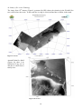
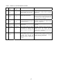
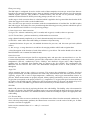
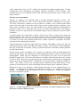
Figure 1. Plot of the track of RRS James Clark Ross during cruise JR097. The three boxes
(Fimbul west, Fimbul east, and Brunt area) are expanded in figures 2, 3 and 4.
ice tongue. About 11 days were spent in the vicinity of Fimbul Ice Shelf, yielding seven WASP
stations (benthic photographic surveys), comprehensive swath and CTD/LADCP surveys of the
western side of the ice tongue, several CTD/LADCP stations in challenging sea ice conditions east
of the ice tongue and a successful Autosub mission beneath Fimbul Ice Shelf. That period also saw
the unfortunate loss of Autosub beneath the ice shelf.
The ship then sailed for the Brunt Ice Shelf area. The aims here were to attempt to achieve at least
some of the objectives of the polynya/sea ice project, but also to conduct a study of the ice shelf
water-rich plume that flows down the continental slope north of Filchner Ice Shelf. A
CTD/LADCP section was occupied in support of the polynya work, two sea-ice buoys were
deployed, and pancake ice was sampled at various stages of its formation. The plume study
consisted of a CTD/LADCP section across the plume (down the slope), and two yo-yo-type
LADCP deployments.
While in the vicinity of Brunt Ice Shelf, two current meter moorings were recovered, and five
personnel were transferred from RRS Ernest Shackleton, in support of BAS logistics. While in the
vicinity of the sill at the continental shelf break north of Filchner Ice Shelf, a long term current
meter mooring was recovered, serviced, and then re-deployed.
8
1,
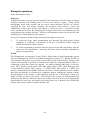
Figure 2. Ship track in work area west of the Fimbul ice tongue. The numbers indicate CTD
stations.
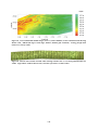
Figure 3. Ship track in work area east of Fimbul ice tongue. Numbers indicate CTD stations.
9
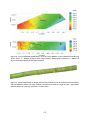
Figure 4. Ship track in work area near Brunt Ice Shelf. Numbers show locations of CTD
stations.
10
Cruise diary
3 Feb 2005
Set sail from Port Stanley for JR097. Deploy magnetometer and initiate swath
survey using the shipboard EM120. Swath and magnetometer surveys were
continued throughout the cruise whenever conditions allowed.
4 Feb 2005
Passage towards Scotia Sea.
Initiate shipboard ADCP and underway
instrumentation. Underway instrumentation was active and logged during the entire
cruise, except for instruments using the water inlet, which was closed when in sea
ice.
5 Feb 2005
Continue passage
6 Feb 2005
Continue passage
7 Feb 2005
Continue passage
8 Feb 2005
In the light of satellite imagery from the Filchner ice front region, the ship diverts
towards Fimbul Ice Shelf.
9 Feb 2005
Trial CTD deployment (Station 999) to check out CTD, LADCPs, the Idronaut 320
CTD, and the sampling rosette. Continue passage towards Fimbul Ice Shelf.
10 Feb 2005 Arrive at the west side of Fimbul Ice Tongue at 1400. Commence swath survey of
continental shelf area west of the tongue.
11 Feb 2005 Position at launch site for trial missions. This was in open water some kilometers
from the ice front. Trial missions 378, 379 and 380 were undertaken during the day
to test a number of different systems. CTD stations 001 to 007 along the ice front
were occupied overnight (see Figure 2).
12 Feb 2005 Deploy short-term current meter mooring at CTD station 007. Proceed to Autosub
trials launch site and launch trials mission 381. Recover Autosub. Continue CTD
profiling overnight, along western edge of ice tongue, to a depth of ~2200 m
(stations 008 to 014 – see Figure 2).
13 Feb 2005 Steam to launch site and launch sub-ice shelf Mission 382. Listen to 10-minute
transmissions from Autosub until vehicle turned to come back. Re-occupy CTD
Station 001 (Station 015) (Station 001 data compromised by frozen sensors). Steam
to Autosub pick-up point and recover vehicle. CTD profile at the recovery site
(Station 016 – Figure 2). Fill in CTD station 017 (between Stations 8 and 9), and
then extend the line of CTDs along the western side of the ice tongue (Station 018).
Difficult sea-ice conditions prevented extending further.
14 Feb 2005 Fill-in swath, and extend east-west ice front CTD section (stations 019 to 022 –
Figure 2). Begin cross-shelf CTD section north to the shelfbreak as far as Station 25.
Proceed to Autosub launch site for mission 383. On arrival at the launch site
increasing winds and an invasion of sea ice from the north resulted in the
postponement of Mission 383. Attempt a box core in the southern inlet in the ice
tongue, and then shelter from gale. Start yo-yo CTD (Station 026).
15 Feb 2005 Break from yo-yo to take water samples for salinity, and to inspect ice conditions
outside creek. Restart yo-yo at same site (Station 027). Stop yo-yo when fast ice
broken out from the head of the inlet is blown past the ship. Reposition ship outside
inlet, but still in the shelter of the ice tongue and recommence yo-yo (Station 028).
16 Feb 2005 Weather abated, so finish yo-yo and position at launch site for Mission 383. Launch
Mission 383. Steam to WASP site for two dredging runs. Listen for Autosub: clear
that Autosub aborted beneath ice shelf. Proceed to second inlet to complete swath
11
survey and occupy CTD stations 029 to 032. Ice and wind conditions prevent further
CTD profiling along the ice tongue, so proceed to eastern end of the Fimbul Ice Shelf
work area (see Figure 3).
17 Feb 2005 On passage to eastern end of work area. Sea-ice conditions too difficult to get to ice
front, so swath and take box core during the night.
18 Feb 2005 Break through pack to reach ice front pools. Occupy CTD stations 33 to 38,
breaking from one pool to the next. Break north out of ice. Steam west to eastern
edge of the Fimbul ice tongue.
19 Feb 2005 Break through heavy pack and occupy CTD Station 39, deploying the CTD over the
stern. This was as far south as it was possible to take the ship without risking
becoming trapped. Break north through pack to occupy CTD stations 40 to 43.
Make passage towards the western edge of the Fimbul ice tongue.
20 Feb 2005 Satellite imagery shows the inlets and western side of the ice tongue to be full of
pack ice. Proceed to western cross-shelf CTD section and continue the section,
starting from the northern end (stations 44 to 47 – see Figure 2), breaking ice as
necessary. Proceed northeast along continental shelfbreak towards one of the WASP
survey sites.
21 Feb 2005 Conduct five WASP surveys; listen to Autosub emergency beacon at three locations
in order to determine its position beneath the ice shelf; recover the current meter
mooring and obtain a CTD profile at that position (Station 48). Make passage to
Brunt Ice Shelf work area.
22 Feb 2005 Continue passage.
23 Feb 2005 Continue passage.
24 Feb 2005 Rendezvous with RRS Ernest Shackleton to pick up 5 pax. Steam to B1 mooring
site. Recover B1. Steam to B2 mooring site. No response either from the location
of mooring B2, or along the route an iceberg would be expected to drag it. Steam to
B3 mooring site. Recover B3. Proceed to the intersection of the sea ice edge with
the CTD section to be occupied in support of the polynyas project (Figure 4).
25 Feb 2005 Proceed along line into sea ice. Deploy tiltmeter ice buoy on thick floe. Drill for
thickness profile. Occupy CTD station 49. Break out of heavy pack ice, and then
return to CTD line to occupy Station 50. Continue CTD deployments along line
southeast towards coast, stopping for pancake sampling as required.
26 Feb 2005 Finish CTD section to coast (stations to 57). Return along CTD line towards sea ice
for further pancake sampling. Occupy fill-in CTD Station 58. Poor weather prevents
further CTD stations or pancake lifting.
27 Feb 2005 Proceed around pack ice to the location of mooring S2 (at CTD Station 59 – see
Figure 4). Sample pancakes where appropriate en route. Recover S2, occupy CTD
Station 59, and extend CTD section to west.
28 Feb 2005 Complete CTD line to west (up to Station 63). Proceed to occupy CTD section down
Filchner slope (stations 64 to 71 – Figure 4). Perform CTD/LADCP yo-yo through
plume (Station 72).
1 Mar 2005
Finish Station 72 yo-yo and steam to S2 to redeploy mooring and take a CTD profile
(Station 73). Continue CTD section eastward across the Filchner Sill from the
location of S2 (stations 75 to 78).
2 Mar 2005
Complete sill CTD section and then proceed into the pack ice (Figure 4) to find a
suitable floe to deploy the second sea-ice buoy. Deploy the buoy. Occupy trial CTD
12
station (Station 79) to test the conductivity sensors. Carry out additional pancake ice
sampling, and steam out and then around the pack ice to return to the slope area.
3 Mar 2005
Arrive at plume site. Profile with the Idronaut 320 CTD slung beneath the rosette
(Station 80), and then continue CTD/LADCP experiments through plume (stations
81 and 82).
4 Mar 2005
Box core at site on the slope, then make passage to Port Stanley.
5 to 10 Mar 2005
Continue passage. Arrive Port William 2150L.
11 Mar 2005 Berth at FIPASS, Port Stanley.
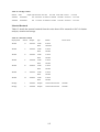
13
Scientific party and responsibilities
Project
Institute
Name
Autosub technical
SOC
Stephen McPhail
Autosub technical
SOC
Andrew Webb
Autosub technical
SOC
James Perrett
Autosub technical
SOC
Kevin Saw
Autosub technical
SOC
Nick Millard
Autosub team leader
Instrumentation
UKORS
Jeff Benson
Shipboard CTD&LADCP
ITS
BAS
Jeremy Robst
Ship fit IT
ETS
BAS
Mark Preston
Ship fit instrumentation
OPRIS
BAS
Keith Nicholls
PSO
OPRIS
BAS
Povl Abrahamsen
CFCs, moorings, 320, Autosub ADCPs
OPRIS
U of M
Gregory Lane-Serff
Ship ADCP
OPRIS
U of M
Justin Buck
CFCs
Swath
BAS
Carol Pudsey
EM120, TOPAS, box coring
AUI
SOC
Kate Stansfield
Autosub ADCP&CTD
ISOTOPE
UEA
Colin Goldblatt
Underway data
ISOTOPE
UEA
Paul Dodd
Salinometry
ISOTOPE
UEA
Kevin Oliver
LADCP data
ISOTOPE
UEA
Martin Price
Shipboard CTD
Benthic biodiversity
SOC
Brian Bett
WASP, dredge, trawl
Benthic biodiversity
SOC
Daniel Jones
Web diary
Polynyas and sea ice
U of M
Martin Stott
Polynyas and sea ice
DAMTP
Arthur Kaletsky
Polynyas and sea ice
SAMS
Jeremy Wilkinson
Sea ice sampling, ice buoys
Polynyas and sea ice
SAMS
Nick Hughes
Satellite imagery
SOC
BAS
SAMS
DAMTP
UEA
UKORS
U of M
Specific responsibility
Southampton Oceanography Centre
British Antarctic Survey
Scottish Association of Marine Sciences
Dept. of Applied Mathematics and Theoretical Physics, University of Cambridge
University of East Anglia
UK Ocean Research Service
University of Manchester
14
Satellite Data
Nick Hughes
Timely provision of satellite data on sea ice conditions in the Weddell Sea and around the Fimbul
Ice Shelf was essential for planning fieldwork operations. The main difference from the previous
Autosub Under Ice cruise to the Arctic last summer (JR106N) was that a full satellite internet link
had been installed on RRS James Clark Ross. This meant that, rather than waiting for data to be emailed to the ship and occasionally downloaded, it was possible to acquire data from the providers
directly as required.
There were three main sources of satellite data for JR97 fieldwork:
•
Daily AMSR, QuickSCAT and Envisat GMM data were provided by Leif Toudal of the
Danish Centre for Remote Sensing (DCRS) and downloaded from the http://www.seaice.dk/
website.
•
MODIS data was acquired from NASA’s Earth Observing System (EOS) Data Gateway at
http://edcimswww.cr.usgs.gov/pub/imswelcome/. Because each set of 250 and 500 metre
resolution files for each image is so large (~550Mb) these were uploaded to a SAMS
computer and processing carried out using an ssh terminal link to command-line processing
programs before the final result was downloaded onto the ship.
•
Acquisition of Envisat WSM data to cover the fieldwork was ordered by SAMS from ESA
prior to the cruise and arrangement made to access these through the ESA rolling archive
sites at ESRIN (http://pfd-ns-es.esrin.esa.int/es_pfd_web/) and Kiruna (http://pfd-ns-ks.esasalmi.irf.se/ks_pfd_web/). These covered large areas of the Weddell Sea and the Fimbul
area on 16 January, 4, 11, 17 and 23 February and 2 March. The internet link provision
allowed processing of the images by uploading them to a SAMS computer and generating
quicklooks using ESA’s BEST software. Compression of the full data scenes also allowed
them to be downloaded onto JCR during quiet periods overnight. As a backup, in the event
of the internet link not being available, processing of the data to derive quick look images
and e-mailing of these to the JCR was also carried out by Richard Hall of the Norwegian
Polar Institute (NPI).
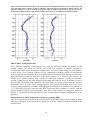
QuickSCAT
The algorithm for the QuickSCAT sensor on the
SeaWinds satellite is designed to detect the
presence of low concentrations of sea ice and
areas of open water. In the past this has been
found useful in determining areas where new ice
formation is taking place. The images are often
affected by areas of high wind speed causing
greater water surface roughness and appearing
as ice. QuickSCAT is also a fairly low
resolution (25 km) instrument and cannot
resolve areas of detail. This meant that although
it was useful in monitoring the situation in the
Weddell Sea the level of data was too coarse for
it to be useful in the Fimbul area. An example Figure 5. Example of QuikSCAT image
image from the Weddell Sea on 26 February is
shown in Figure 5. In this the edges of the main ice pack are clearly defined. Also visible is the
effect of a storm system, outside the main ice edge, and poor data quality around the coastlines.
15
AMSR Ice Concentration
Lower frequency channels provided by AMSR
provide good measurements of sea ice
concentration (percentage cover of sea ice within
an area) during autumn, winter and spring. During
summer AMSR, like the other passive microwave
SSM/I sensors and its predecessors SMMR and
ESMR, is affected by surface snow melt. Areas of
meltwater on a floe are seen by the satellite as
open water, even though there is ice beneath.
Summer ice concentration estimates tend therefore
to be less reliable and lower than those from
optical sensors. However, unlike in the Arctic last
summer, snow melt and pools were not observed
on any of the Antarctic sea ice encountered.
Figure 6. Example of passive microwave image
Therefore it would appear that passive microwave
sensor observations of Antarctic sea ice are more accurate than their Arctic counterparts. In the
example in Figure 6 the QuickSCAT ice limit is shown as a thin red line and is seen to be consistent
with the ice limit shown by AMSR.
Envisat GMM
The Global Monitoring Mode (GMM) of ESA’s
Envisat Advanced Synthetic Aperture Radar
(ASAR) sensor is used for wide area coverage
when the sensor is not tasked with specific data
acquisitions.
SAR or active microwave
produces a high resolution image of the surface
radar energy backscatter beneath the sensor. In
GMM image resolution is reduced to 1 km to
reduce data processing load and allow global
coverage. GMM shows up the boundaries of ice
and water areas as well as some large floes. The
example in Figure 7 is from 26 February and is
Figure 7. ASAR image of Weddell Sea
a mosaic produced by DCRS of the previous 3
day’s images. It covers the entire Weddell Sea. Open water with waves scattering radar energy
appear on the right side of the image. Open water with little or no wave activity does not reflect
radar energy so well and appears as the black areas in the image. Sea ice floes and open water
appear as the various levels of grey inbetween. Envisat GMM images are useful in supplementing
the WSM images received from Envisat.
The big advantage of SAR sensors like Envisat is that they can see, at high resolution, through the
cloud and darkness prevalent in polar regions. This makes them in invaluable tool for planning
fieldwork in these areas. A minor negative point is that interpretation cannot be automated and has
to be done by human eye. This makes the classification subject to debate especially where open
water generates a radar backscatter return similar to ice.
MODIS
The Moderate Resolution Imaging Spectroradiometer (MODIS) is a key instrument aboard NASA’s
Terra (EOS AM) and Aqua (EOS PM) satellites. Terra MODIS and Aqua MODIS view the entire
Earth's surface every 1 to 2 days, acquiring data in 36 spectral bands, or groups of wavelengths
covering visual and infrared. During JR97 use was made of a processing stream that had been set
up to generate quicklook images to monitor a buoy deployment on the fast ice off East Greenland
on JR106N. This takes 250 and 500 metre resolution MODIS data files ordered through the EOS
16
Data Gateway and uploaded to SAMS, takes out 3 channels used to generate a visual image, and
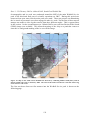
presents them in the form of a geo-located image as shown below. Quicklooks were designed to be
of the same map projection and grid as the AWI bathymetry chart used for planning fieldwork.
Figure 8. MODIS image of the southern Weddell Sea for 21st February 2005
As MODIS is an optical sensor it is affected by cloud and darkness. During JR97 this seemed to be
the prevalent state of the south-east Weddell Sea and the image in Figure 8 is one of the few where
the ice in this region can be clearly seen. However there is a solid blanket of cloud over the rest of
the Weddell Sea.
Envisat WSM
Envisat’s Wide Swath (WSM) mode provides the same width of coverage as GMM but with a
greater resolution of 150 metres. It was arranged that the position of JCR at the time of the satellite
overpass would be e-mailed to NPI to allow the position of the ship to be marked in the image and a
full resolution of an area around the ship to be produced.
17
16 January (Pre-cruise Planning)
The image from 16th January (Figure 9, generated by NPI) shows the situation in the Weddell Sea
two weeks before the cruise. In the south the ice edge is clearly defined but is diffuse in the north.
Figure 9. See text
Around Fimbul Ice Shelf
(Figure 10), there is no
indication of any sea ice
and the ice shelf front is
totally clear.
Figure 10. See text
18
4 February
There was a problem with delivery of images on 4 February. ESA failed to process the images until
8 February. As a result planning had to be done on the less detailed, and so subject to more debate,
uncorrected GMM images.
In the GMM image (Figure 11)
there is clear open water on the
eastern side of the Weddell
most of the way south to the
Filchner Ice Shelf along the
Coats
Land
coast.
Unfortunately in the critical
area the incidence angle of the
SAR and the increased water
backscatter mask out the ice.
11 February
The set of images delivered on
11 February for the south-east
Weddell Sea gave the first
clear indication of the ice
conditions in that area.
Figure 12 shows the image
with a division of the scene
into different ice regimes.
Figure 11. See text
In the Fimbul area (Figure 13) a stream of brash
ice can be seen being advected in from the east
by coastal currents.
Figure 13. See text
Figure 12. See text
19
Figure 14. See text
17 February
The 17 February image of the south-east Weddell Sea is shown in Figure 14. This image was used
for planning the sea ice work in the area. The green dotted lines represent proposed transects into
the ice. Also marked are the positions of the BAS moorings around the Brunt Ice Shelf and at the
Weddell Sill.
Figure 15. See text
19 & 20 February
As the Fimbul image from 17 February was unavailable (as a result of a delay in processing by
ESA) updates of the Fimbul for the 19th and 20th February were obtained as the RS Polarstern was
in the area. The most comprehensive of these, from 20 February, is shown in Figure 15, and covers
the entire coastline from 4°W to 6°E. This was used to generate a coastline vector for the
20
multibeam swath plots. A stream of sea ice can be seen being carried westward around the ice
tongue and filling the western creeks. A finger of ice shelf has also broken off in the 24 hours since
the last image and can be seen at 70°15’S 2°40’W.
23 February
Figure 16. See text
The next southern Weddell Sea image (Figure 16) just missed covering the open water area we were
interested in. However the ice edges remained stable, as confirmed by a transect into the ice on 26
February.
21
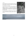
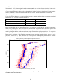
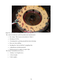
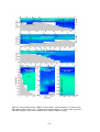
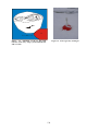
2 March
With final Envisat scene from the Weddell Sea (Figure 17)
being available on the JCR less than 3 hours after acquisition
by the satellite it was possible to undertake some validation
with recognisable sea ice features.
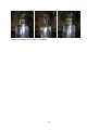
The transect into the ice started at a large, several miles wide,
tabular iceberg clearly visible in the satellite image (see
photograph in Figure 18). Comparison of this image with
GMM images from previous days showed that this iceberg
was drifting south in the Weddell Gyre. The satellite also
showed the existence of a gap in the ice pointing towards a
large unbroken floe.
The transit into the ice encountered the sea ice types and
concentrations indicated by the image, starting with sheets of
grease ice and following on through pancakes to broken 1st
year floes.
Figure 17. See text
Figure 18 See text
22
Autosub Missions
Test Missions
On 11th February, we arrived in the working area near the Fimbul ice shelf, and began some basic
shakedown of systems and sensors testing with Autosub.
Mission 378
As well as a basic systems and sensors test we planned to test high altitude control, and yo-yo
profiling. Unfortunately, due to a procedural mistake (a wrong version of the mission script was
compiled and downloaded), upon diving, the vehicle immediately head off in a northerly direction.
A timeout on the holding pattern prevented the Autosub getting into serious trouble, and it surfaced
1 hour later. The mission in practice ran at a constant 200 m altitude for 1 hour (6km).
Mission 379
Mission 379 was a re-run of the planned mission 378, with a test of the homing system at the end of
the run. It was completed without incident. The homing trails were partially successful. The
Autosub homed in when at range of 1000 m, but always lost the homing signal, when its range had
decreased to around 300. The reason for this, we surmise, is that with Autosub travelling at a
homing depth of 200 m, which is 100 m below the ship’s homing beacon, that the geometry for
signal reception becomes poor as the horizontal range to Autosub gets shorter. In future we must
ensure the homing depth is only a little deeper than the homing beacon.
The altitude control appeared to be quite unstable when at high altitude, with high pitch excursions.
Further analysis suggested that the algorithm which corrected the ADCP ranges for pitch was
ineffective. The software was changed so that the internal ADCP tilt sensors were used instead of
the INS systems.
Mission 380
This was a simple, short, out and back mission to test the altitude control. The altitude control,
although improved, still showed excessive oscillation in depth and pitch when at a high altitude.
The algorithm was changed again (this time to use the average of the four ADCP ranges, rather than
try to pitch correct the two forward beams). The mission was terminated by homing the vehicle into
towards the ship, then sending an acoustic end mission command.
Mission 381
This was another short mission to test altitude control at high altitude (450 m and 350 m ). The
results for altitude control were now acceptable.
23
Missions under Fimbul Ice sheet
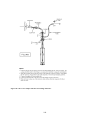
Mission 382
The planning for mission 382 was based upon previously carried out seismic soundings of the
Fimbul ice shelf. Figure 19 illustrates the mission profile.
WP4
WP1
WP3
WP2
Fimbul Ice shelf
180 m
220 m
450 m
300 m
150 m
400 m
820 m
0 km
12.5 km
25 km
Figure 19. Planned profile for mission 382
After a dive weight assisted dive, the Autosub circled waypoint 1 (WP1 in Figure 19) at an altitude
of 200 m while we checked via an acoustic telemetry link that all systems and sensors were
functioning correctly. We then sent a “Start” command (using the acoustic command system) and
Autosub proceeded under the Fimbul ice shelf.
The transit in was in constant altitude mode at 150 m off the seabed. At WP2, Autosub turned back
onto a reciprocal track, this time at an altitude of 400 m. At WP3 it descended to 300 m, and
continued until it reached the recovery waypoint, WP4, which was set further away from the ice
shelf, to allow for navigation errors. The reason for the change in altitude during the return, was an
attempt to maximize the amount of time that the Autosub would be able to survey the underside of
the ice shelf using the upward looking swath system.
During the mission we measured the range to Autosub (up to 18 km range), by listening for the
emergency beacon transmission, which Autosub transmits at 10 minutes intervals.
The mission proceeded without problems. When recovered, the Autosub Navigation estimate had
drifted 400m to the south west of the actual position. This drift, representing 0.8% of total distance
traveled, was worse than anticipated (0.2%). The most likely explanation for now is that the drift
was a result of the long-range bottom tracking during the return leg, giving larger errors than
normal. However more investigation is needed. A further problem noted was that the speed through
the water, as measured using the upward looking ADCP was about 1.6% faster than the speed
through the water measured suing the downward looking ADCP. The scale factor for the upwards
looking ADCP was adjusted to correct for this. Again we need to investigate this.
Waypoints:
WP_1 = S: 70:03.00, W:01:30.00
WP_2 = S: 70:09.70, W:00:49.60
WP_3 = S: 70:06.35, W:01:09.80
WP_4 = S: 70:02.50, W:01:33.00
Event Times (13th February 2005):
1223
Dived
1241
Acoustic Start (ending circling, beginning mission)
24
2317
On surface
2359
Recovered
Mission 383
The mission plan was to travel a similar distance under the ice shelf as Mission 382 (25 km). The
main difference was that the Mission was planned to yo-yo profile inwards (see Figure 20), then at
the turning point to travel out on the reciprocal line at 80 m under the ice shelf. The Mission Plane
is illustrated below. After circling the start waypoint, (waiting for an acoustic start command while
systems are checked out via telemetry), the Autosub headed into the ice cavity at a constant 100m
off the seabed. After progressing about 2 km into the ice cavity Autosub was to begin yo-yo
profiling between 80 m off the seabed and 80 m from the ice shelf. At the turning point (or if an
obstacle had been encountered), the Autosub would turn onto the reciprocal course and swath the
underside of the ice at an altitude of 80 m. The seismically measured ice drafts and water depths for
this run were similar to the first, although Mission 383 had a more southerly outbound course
compared to mission 382, 135 degrees rather than 100 degrees.
Six hours after the start of the mission the ship returned to the proximity of the launch site to
monitor the emergency beacon. It was heard to be transmitting every minute rather than its normal
10 minute interval. This was a sign that Autosub had aborted its mission and further monitoring of
the signal revealed that Autosub was stationary under the ice.
180 m
250 m
450 m
800m
0 km
12.5 km
25 km
Figure 20. Planned Autosub Mission 383, under the Fimbul ice shelf. Black traces are the inbound
run, profiling, red the outbound run, swathing the underside of the ice. The Ice draft was about 180 m
at the edge of the ice sheet, 250 m at the turn around point, 25 km in. The yellow ellipse marks the
supposed present position of the Autosub.
Known Facts about Mission 383
0733 16th February 2005.
•
Vehicle was launched and dived, using dive weight.
•
Position. S: 70 03.50, W 01 30.00.
The launch and start of Mission 383 was similar to Mission 382, and nothing abnormal was noted.
The launch used a dive weight, avoiding a surface run up (with can be hazardous in areas where ice
is present, because of the risk of damaging the propeller blades). Following launch the vehicle
circled around the start waypoint, at an altitude off the seabed of 200 m, waiting for an acoustic
command to start it on it's under ice mission.
25
Acoustic telemetry and emergency beacon times are listed in the JR97 Autosub log book. Extracts
are copied to this document.
0743
Acoustic telemetry (all angles in degrees, all distances in m). :
Depth: 214, Altitude: 280 , Heading: 046, Range to Go: 32, Speed: 1.03 m/s, Pitch: -14.0, Roll: 0.38, Fwd range sensor: 1000 (over range), Stern plane: 10.77, RPM:
350. Leak Voltage 1.65
(normal)., Battery Voltage 97.45 volts. , Battery Temperatures 23.7 C, 20.8 C.
The Stern plane reading seemed a little high, but within normal bounds. It was necessary to check
that it returned to a value of less than 5 degrees. The system was interrogated again. Stern plane
was now 4.29 degrees.
0744
Transmission from Emergency beacon received . Up Chirp 51.26 seconds , Down Chirp 51.85
seconds
0745 Acoustic telemetry: Depth: 263, Altitude: 205, Heading: 129, Range to go: 5,
Pitch: -2.16.
Speed: 1.25,
0748 The Telemetry seeming normal, the command start signal was sent acoustically from the ship.
Autosub acknowledged the signal, and proceed on its mission. No more acoustic telemetry was
received from the Autosub. This is normal, as when the Autosub turns away from the listening
position, the telemetry transducer on Autosub has an unfavorable path for telemetry.
The emergency beacon normally chirps every 10 minutes on Autosub, and until 0823, four more
emergency beacon chirps were received, confirming the Autosub increasing range. The acoustic
tracking system also showed the Autosub to be heading off in the correct direction and speed.
Tracking ceased at a range of 3000 m (this is normal range). At 0828 the emergency beacon
listening transducer was pulled inboard, freeing the ship for other science activities.
The launch point was 1 km from the ice front, hence the vehicle was 2 km under the ice shelf when
we ceased monitoring. All seemed normal. When we monitored the Emergency Beacon
transmission, 6 hours after the start of the mission 383, we found that it was transmitting at the 1
minute interval. The emergency beacon is a 4.5 kHz acoustic transmitter. When an abort event
occurs on the vehicle, the acoustic projector array is dropped on a 15 m cable under the Autosub,
and it begins to transmit at a 1 minute (rather than normal 10 minute) interval. This mode would
also be triggered if the projector array had been mechanically dropped for any other reason, as a
reed switch position sensor detects this event. The reasons for beacon drop and triggering without
the abort system are, electrical supply failure to the drop circuit or mechanical shock (quite
extreme).
Acoustic position fix using emergency beacon
Ranging and triangulation using three positions of the arrival time of the beacon transmission
indicated that the vehicle was at a distance of 17.5 km from the start position of S: 70 03.5, W: 01
30.0 and is a perpendicular distance of 194 m south west of the vehicle intended track (the turn
waypoint was S:70 13.04, W: 01 02.3). This would suggest that Autosub was following its intended
track when it aborted.
On 21st February, the ship returned to the ice shelf front, and we listened for Autosub again.
Triangulation placed Autosub less than 250 m from the original position. This displacement is
within the error bounds of the measurement, given that the clock on the beacon had drifted by 1.72
seconds. Hence we conclude that the Autosub had probably not moved in the past 6 days. We
received a strong signal from a range of 26 km.
26
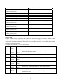
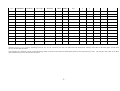
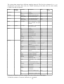
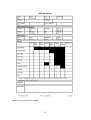
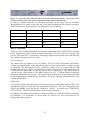
Table 1. Summary of Autosub Missions on JR97
#
Start
Time
End
Time
Description
Comments
378
11/2/2005
11/2/2005
11:47
13:12
Test of profiling between 30 alt,
and 30 m depth. Test of constant
altitude modes 350 m , 450 m .
Incorrect initial waypoint programmed in.
Surfaced after 1 hour. 200 m constant
altitude run
11/2/2005
11/2/2005
Instability in high altitude depth control.
15:24
21:14
Repeat of 378. Homing System
tested at the end of the run
11/2/2005
12/2/2005
22:10
00:40
Short out and back test mission
to test high altitude depth control
at 500m and 350 m.
Depth control improved, but still not
acceptable. Algorithm for ADCP range
correction changed again.
12/2/2005
12/2/2005
18:30
19:30
Rerun of mission 380, to test
depth control.
Depth control
acceptable.
13/2/2005
13/2/2005
12:23
23:18
Head Under Fimbul Ice Shelf.
150 m altitude in. 400m and 300
m altitudes out. Swathing the
under ice surface on the way out.
Successful completion. Drift of 400 m in
Navigation over the mission. Upward
ADCP velocity scale factor was an
unexplained 1.5 % different from downward
looking velocity scale factor.
16/2/2005
-
Plan to profile in between 80 m
off the seafloor to 80 m off the
ice shelf, then turn and run
reciprocal track, swathing the
underside of the ice shelf at 80
m range.
Autosub lost 14km under the ice shelf.
Presumed floating. Emergency beacon had
dropped, and was transmitting at 1 minute
interval, indicating "abort" state.
379
380
381
382
383
07:34
27
Homing system lost tracking when Autosub
was less than 300 m range. Presumably due
to bad geometry for sound path.
at
high
altitude
now
Autosub Scientific Sensors
Sensor suite
For JR106 the Autosub vehicle was fitted with the following scientific sensors:
•
RDI 150kHz ADCP looking downwards
•
RDI 300kHz ADCP looking upwards
•
Kongsberg EM2000 Multibeam swath system looking upwards.
•
Seabird 911 CTD system.
•
Edgetech FSAU sub-bottom profiler
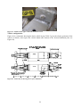
These instruments are described separately in the following sections. Figures 3, 4 and Table 1 in the
Autosub Mechanical section of this report shows the exact sensor locations. All the electronic
systems on the vehicle are connected to a single control network. The data from all sensors apart
from the multibeam system are recorded on the Autosub data logger. The Autosub logger uses a
proprietary data format but the data is translated into standard ASCII text files using the Logger File
Translator software running on a PC. This software also translates the CTD data into a standard
Seabird format file. The resultant ASCII file is then imported into the Axum processing software
and a standard script is run to produce the general post processed navigation file (.bnv file) and
various instrument specific files including a navigation file for the EM2000 multibeam system.
Sensor Synchronisation
The time synchronisation of the various on-board systems is important, especially where data from
different systems is likely to be merged at a later date (post processed navigation data for the
EM2000 is one example of this). Wherever possible the network time protocol (NTP) system is
used which allows for time comparisons with a resolution of better than 1millisecond. The primary
reference is a GPS receiver which sends an accurate pulse on each second boundary to the Autosub
shipboard data server. The Edgetech sub-bottom profiler acts as the primary Autosub vehicle time
server and uses the Autosub shipboard server as a reference whenever Autosub is in contact with
the ship. The Autosub logger can synchronise to the Edgetech on start up and the Kongsberg
EM2000 is synchronised to the logger. One problem is the poor quality of the logger clock which
can drift by 10 seconds in 12 hours. The data processing system can measure and compensate for
this drift so that the data output in the navigation files is correct. In the case of the EM2000, it was
realised towards the end of the cruise that the instrument continues to use its internal clock to
timestamp the data. The difference between the internal clock and Autosub time is recorded and any
post processing software must take this difference into account.
The same GPS referenced NTP system is also used to provide time information for the emergency
beacon receiver software.
The Autosub TimeSync monitoring software is run during each mission in order to monitor the
clock drift between underwater systems and various shipboard systems. The results are stored in the
TimeSync directory. The .txt file is the more verbose version while the .dit file contains the
differences in an ASCII table which can be read by most data processing software.
Seabird 911 CTD system
Autosub is fitted with a Seabird 911 CTD system, which includes two sets of conductivity and
temperature sensors. These are mounted in a ducted system with sea water pumped through them at
a precisely known rate. Depth is measured by a Digiquartz pressure sensor. In addition, a Seabird
SBE 43 oxygen sensor is fitted which is situated in the same duct as the secondary CT sensors. The
output from these sensors is recorded at a rate of 24Hz.
28
Sensor
Location
Serial Number
Primary Temperature
Port Side
2342
Primary Conductivity
Port Side
2760
Secondary Temperature
Starboard Side 2912
Secondary Conductivity Starboard Side 2730
Oxygen
Starboard Side 0259
Data from the system are continuously logged whenever Autosub is switched on but, in order to
prevent excessive wear on the pump, water is only pumped through the C/T sensors once a
predetermined pressure threshold has been exceeded. The data are stored on the Autosub logger in a
proprietary format but is normally translated into a Seabird format data file (.dat) at the end of each
mission. This data file, together with the necessary configuration file was then passed to the
scientific party for further processing. Sensor calibration data is stored in a separate file with the
.con extension. For the JR97 cruise the data was processed using the JR097new.con file which
contained calibration data from October 2004.
Edgetech FS-AU Sub-Bottom Profiler.
The Edgetech FS-AU is a sub-bottom profiler that transmits a swept frequency tone or ‘chirp’
containing frequencies between 4 and 12kHz and listens for the return. It can determine information
about the seabed and the layers just under the seabed from the characteristics of the return echoes.
On Autosub the instrument is triggered by a controller connected to the vehicle’s LONWorks
network. This controls the pulse rate and also allows the trigger pulse to be synchronised with other
systems in order to control interactions between instruments. The FS-AU has been shown to affect
acoustic communications with the vehicle and it is therefore disabled whenever these
communications are taking place.
For the JR97 cruise the instrument was set to ping on every fourth sync pulse which resulted in a
ping repetition period of approximately 6.5 seconds. Data was collected on all missions where
Autosub approached close enough to the seabed. A quick first look using the supplied J-Start
diagnostic software suggests that the data appears to be good but Autosub was flying too far from
the bottom for J-Star to give much information. This is due a range limitation of 190 metres with
the J-Star software.
Kongsberg EM2000 Multibeam Swath System.
The Kongsberg EM2000 is a multibeam swath bathymetry system which operates at a frequency of
200kHz and can give up to 111 beams of data with an angular coverage of up to +/-60 degrees
under favourable conditions.
On Autosub the instrument is triggered by a controller connected to the vehicle’s LONWorks
network. This controls the ping rate and also allows the trigger pulse to be synchronised with other
systems on the vehicle in order to control interactions between instruments. This controller also
sends time, range aiding and navigation information to the instrument. A second LONWorks
controller sends attitude and depth information to the instrument.
For JR106 this system was fitted with the transmit transducer mounted in the nose of the Autosub
vehicle and the receive transducer was mounted in the tail section facing upwards. The transducers
were mounted behind polythene windows in the vehicle’s fibreglass outer panels. (See table ? in the
Mechanical section of this report for exact sensor locations).
The initial instrument settings used were those that appeared to have given good results on the
JR106(N) cruise. The beam spacing was set to be equidistant and the maximum beam angles were
29
+/- 60 degrees. The sensor roll settings were set to zero, which meant that the system would place
the returns from the bottom of the ice shelf below Autosub rather than above it. Further post
processing would be necessary to compensate for this. This post processing software, which was
started on the JR106 cruise, is still unfinished at the time of writing.
When first tested on deck, the EM2000 did not respond at all. It was necessary to open the
instrument’s housing and connect a video monitor to diagnose the problem. When this was done it
was found that the flash memory that was used to boot the system had failed. The processor card
was replaced and the current version of software loaded which resulted in a working system.
Later in the cruise it was found that the EM2000 had again become unresponsive. This time it was
possible to connect to it via FTP for a few seconds after booting up. This problem had appeared
before and, as before, the solution was to delete the ‘runtime’ file and reload this file from a backup.
It is possible that this corruption is caused by a problem with an imperfect radio link between
Autosub and the EM2000 controller software, which updates the runtime file every time it is
started. This controller software has not been designed with AUV use in mind and must be used
with caution. The alternative EMControl software is available but this has not been developed
sufficiently to be user friendly.
It was also found that the transmit pulse timing jitter was higher than expected at around 200mS.
High levels of jitter had been seen on previous cruises and the triggering software in the controller
had previously been changed in order to improve this. It was decided to change the software further
and remove any little used parts of the code in order to improve the jitter performance.
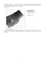
The only mission to give data from the EM2000 was Mission 382, which was run under the Fimbul
ice shelf. The return leg of this mission was run with a minimum overhead clearance setting of
100 m. This is greater than the optimum distance for the EM2000 but, given that the features of the
underside of the ice are unknown, it was felt that this was a safer distance whilst still giving the
opportunity of collecting a limited amount of data from the EM2000.
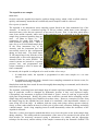
The picture in Figure 21 shows a typical section from the run out. The top left corner shows an area
where the underside of the ice shelf was out of range while the flatter sections show areas of good
returns. This section of data has not had the rotation applied to correct for the incorrect sensor
orientation but it gives an indication of data quality. There are obvious features present, which can
be analysed further once the post processing software has been completed.
Figure 21. Sample of Autosub EM2000 data from Mission 382.
30
Results from the upward mounted EM2000 during mission 382
Introduction
On the return leg of Mission 382, Autosub-2 was programmed to stay 300 m from the sea floor, and
maintain a distance of 100 m from the underside of Fimbul Ice Shelf (FIS). The route that Autosub2 took from under FIS meant that bedrock elevation decreased as it headed closer to the ice shelf
edge, and hence open water. This was due to Autosub-2 travelling out across the northwestern
slope of the large central cavity beneath FIS. At approximately 24 km from the ice shelf edge, the
water column thickness was less than 400 m, causing Autosub-2 to stay 100 m from the underside
of FIS as opposed to staying 300 m from the underlying bedrock. It was during this time that the
EM2000 started to be receive echoes from the underside of FIS. The following description
describes the processing procedure used to process to raw EM2000 data.
Removing Autosub-2’s attitude from the EM2000 data
The EM2000 collects waveforms from a few physical directional hydrophone transducers. It does
not output them externally at all. Instead it uses phased-array synthesis to synthesise up to 111
virtual beams and reports a number of data about what it considers to be the most distinct echo in
each virtual beam. The data is reported in a set of sequential files suffixed .all, one for approx 30
minutes of the mission. Each .all file consists of a sequence of datagrams, which are records of
various types. The datagram we primarily use is the raw range datagram which reports the distances
of the echoes in each beam, the beam angle, which varies from scan to scan, presumably in an
attempt to locate the clearest echo within an angular region and whether the echo was detected by
amplitude or phase shift. Amplitude-detected echoes are generally considered to be more reliable.
The .all files also contain attitude and position datagrams, but difficulties in decoding these
(which have since been apparently overcome) led us to use the navigation record file (with suffix
.bnv) for those data and correlate them to the .all data using time fields in each file.
Processing began by concatenating all the .all files of a mission into a single, time-ordered .all
file by using the Unix cat command. The C program dg_out was then run with the .all as
input producing 2 files: .out, which has space separated fields with the raw range for each beam,
reflectivity (intrinsic echo strength) for each beam, speed, time, calculated distance since mission
start, easting, northing, depth, pitch and roll. Note that at the time of processing, the position and
attitude data were unreliable. However, we considered it useful to do data cleaning on this file. Thus
plots of this file were produced (see Figure 22) and manual data cleaning was done on it. In
particular, manual removal of the cylindrical tunnel roof artefact first seen on JR106N was done at
this stage. In order to keep the fixed-column file format data points could not simply be removed.
We had to replace them by NaN (not-a-number) indicators.
The above .out and .bea file formats are designed to be suitable for Matlab input. The .out and
.bnv file were input into the Matlab function interp_mb2, which, after correcting for drift and
offset between the times in the two input files, interpolated position, speed, pitch, roll and yaw from
the .bnv into the appropriate fields of the .out file. The resulting file, of a format similar to that of
.out, has the suffix .cor .
The .cor and .bea files were then input to the Matlab function form_swath2.
This applies the relevant attitude (pitch, roll and yaw) to each beam individually and to produce a N
* 111 * 3 array. The first index is the scan number, the second the beam number. This selects a 3vector of the echo's [somewhat spherical] coordinates: longitude, latitude and negative depth. This
array is stored in a .pos file and can then be plotted and have other operations performed on it, e.g.
statistics.
31
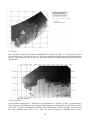
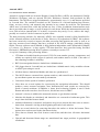
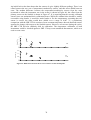
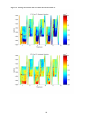
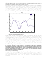
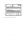
Removing erroneous data points
The EM2000 ice draft data from mission 382, after being corrected for Autosub-2’s attitude (section
above), is shown in Figure 22. At this stage the results are not presented in terms of distances,
rather in terms of the 9,133 pings that EM2000 sent out, with each ping being synthesised into 111
individual beams. To get an idea for length scales at this stage, pings were sent out typically every
4 m (though this is dependent of the speed of Autosub through the water), with the beams being
spaced roughly 2 m apart.
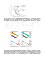
Notice in Figure 22 how the outermost beams (numbers 1-15 and 105-111) returned very little data.
The reason for this is the way that the upward mounted EM2000 onboard Autosub-2 was set up for
mission 382. It was set up so that the 111 beams were synthesised with a nominally fixed angle
between them. This fixed angle was calculated from either the maximum angle of the swath being
±60° from vertical, or the swath being no wider than ±120 m from the vertical.
For demonstration purposes, assume Autosub-2 was completely stable (i.e. pitch = yaw = roll = 0°)
and flying 100 m from the underside of a flat ice shelf, which was parallel to the horizontal. In this
case, an angle of
± arctan(120/100) ≈ ±50.13°
from the vertical would create a swath 240 m wide (±120 m from vertical). This suggests that the
second rule above would have decided the fixed angle between the 111 beams during mission 382.
In creating a swath of ±120 m from the vertical, however, the length of the two outermost beams
(usually numbers 1 and 111) to the underside of the ice shelf would be
(1002+1202)½ ≈ 156 m,
which exceeds the maximum range of the EM2000. This offers an explanation for the poor
percentage of returns from the outermost beams of EM2000 during mission 382. It is also evident
from Figure 22 that there were a high number of dropouts even in the centre beams of the EM2000.
Again, this is most likely to be due to the fact that the distance Autosub-2 was flying beneath the
FIS was close to the maximum range of its upward mounted EM2000.
32
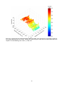
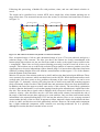
Figure 22. EM2000 ice draft data from Mission 382, after being corrected for Autosub's movement. The data
are presented in terms of the 111 individual beams (x-axis) from the 9,133 pings (y-axis) sent out by the EM2000.
The horizontal dashed lines indicate where the data were split into two run-sections.
There were approximately 1,500 pings from the start of the original data set that contained very
little data (Figure 22). Additionally, there is also a large section of the run, between pings 3,900
and 4,200, where a negligible amount of data were received by the EM2000. The data were
therefore split into run-sections 1 and 2, as shown in Figure 22.
Although not really visible in Figure 22, there is a notable portion of the ice draft data that did get
back to Autosub-2, which was obviously erroneous. The programming needed to remove these data
points automatically was considered too complex for now, so the decision was made to remove
these erroneous points manually. For this task, a MATLAB routine was created (Figure 23). This
routine took each of the two run-sections individually, displayed the 111 beams from 25
consecutive pings of the EM2000 in turn. To clean the data of erroneous data points, the routine
allowed a box to be drawn around a group of points, which would remove them. The axes would
then be rescaled automatically, enabling more accurate boxes to be drawn. Erroneous data points
were removed until the only points left from the 25 pings were those that were considered
“believable”. The next set of 25 pings was then displayed, and the process repeated until all pings
in both run-sections were cleaned.
33
Figure 23: A screenshot of the MATLAB routine used to clean the ice draft data from the upward mounted
EM2000 onboard Autosub. Shown are the 111 individual beams (x-axis) from pings 126-151 in run-section 1.
The y-axis is ice draft. Data points that are considered erroneous are removed by drawing boxes around them.
Boxes that were drawn for the 25 pings presented are shown in semi-transparent grey.
The two run-sections of ice draft data, after cleaning was completed, are shown in Figure 24.
Comparing this with Figure 22, it is evident that most of the erroneous data points existed in the
outermost beams. This is most visible for beams 1-15 of run-section 1 where almost no data are left
after cleaning.
For display purposes only, Figure 25 shows the ice draft data, in terms of distance parallel with, and
perpendicular to, Autosub-2’s track, for that part of the data that suffered the least dropouts. In
terms of pings from the EM2000, and the individual beams from each ping, this corresponds to
beams 19-91 from pings 600-2150 of run-section 1, as shown in Figure 24. It is stressed that the
horizontal axes in Figure 25 have very different scales.
Figure 24. EM2000 ice draft data left from (a) run-section 1, and (b) run-section 2 after cleaning (see text). The
horizontal dashed lines in (a) show the portion of run-section 1 presented in Figure 25.
34
Figure 25. A surface plot of ice draft beneath the Fimbul Ice Shelf. The region shown corresponds to beams 1991 of pings 600-2,150 from run-section 1 (Figure 24), and is the part of the total run which suffered the least
dropouts. Note the differing scale on the x-, y- and z-axis.
35
Autosub CTD
Kate Stansfield
General CTD description (by James Perrett)
Autosub is fitted with a SeaBird911 CTD system which includes two sets of conductivity and
temperature sensors. These are mounted in two separately ducted systems with sea water pumped
through them at a nominally known rate if the pumps are operating correctly. Depth is measured by
a Digiquartz pressure sensor. In addition, a SeaBirdSBE 43 oxygen sensor is fitted which is situated
in the same duct as the secondary CT sensors. The output from these sensors is recorded at a rate of
24Hz.
Data from the system is continuously logged whenever Autosub is switched on but, in order to
prevent excessive wear on the pump, water is only pumped through the C/T sensors once a
predetermined pressure threshold has been exceeded. The data is stored on the Autosub logger in a
proprietary format but is normally translated into a SeaBirdformat data file (.dat) at the end of each
mission. This data file, together with the necessary configuration file is then passed to the scientific
party for further processing. Sensor calibration data is stored in a separate file with the .con
extension. For the JR097 cruise the data was processed using the JR097new.con file which
contained the most recent calibration data prior to the start of the cruise.
CTD configuration
The CT sensor pairs are mounted on opposite sides of the Autosub nose cone (see Figure 26), the
primary sensor pair on the port side and the secondary sensor pair on the starboard side. Each pair
of sensors has a short inflow duct that protrudes through the front of the nose cone and is directly
connected to the intake of the temperature sensor and hence to the sensors own CT-duct. Similarly
each sensor pair also has a an outflow duct which also protrudes through the Autosub nose cone and
is located as near as is practically feasible to the intake duct to minimise any pressure head effects
across the ducted system (See Figures 26 and 27).
Internally, the CT sensor pairs are held against the inner surface of the nose-cone panel via the
plastic plate that houses the inflow and outflow ducts (see Figure 28). The sensors are then covered
by a moulded fibre glass cover (the black pen marks around the sensors in Figure 28 shows the
approximate dimensions of the cover) which in turn is insulated from the main payload cavity of the
nose cone using a flexible layer of foam (not shown). The space housing the CT sensors is flushed
directly with seawater by means of a series of holes through the nose cone panels fore and aft of the
sensor location (see Figure 28). These precautions are undertaken in an attempt to minimise any
thermal contamination of the data due to water being stored and/or warmed within Autosub’s nose
cone.
36
Inflow duct
Outflow duct
Figure 26. Nose cone of Autosub showing the location of the two CT-sensor pairs and the inflow/outflow ducts.
Inflow duct
Temperature sensor
TC duct
Conductivity cell
Outflow duct
Outline of fibreglass sensor cover
Rear sensor cavity flushing holes
Figure 27. Close up of the inflow and outflow ducts protruding through the Autosub nose cone. Also shown are
the forward holes in the nose-cone that allow the CT sensor cavity to flush with seawater.
Location of primary (port) CTD sensors
Location of secondary (starboard) CTD sensors.
Figure 28. Interior set-up of the CT sensors
Details of the individual instrument location, type/model, serial number and last calibration date are given in
Table 2.
37
Instrument
Type/Model Serial Number Calibration Date
Underwater Unit
SBE 9 plus
09P-?
N/A
Conductivity (primary – port CT cavity)
SBE 4
04C-2760
07-Oct-04
Temperature (primary – port CT cavity)
SBE 3 plus
03P-2342
09-Oct-04
Conductivity (secondary – starboard CT cavity) SBE 4
04C-2730
07-Oct-04
Temperature (secondary – starboard CT cavity) SBE 3 plus
03P-2912
29-Oct-04
Pressure
Digiquartz
90573
06-Sep-02
SBE 43
43-0259
01-May-02
SBE 5T
5T-3090
-
SBE 5T
5T-3609
-
(central payload cavity)
(central payload cavity)
Dissolved Oxygen
(central payload cavity)
Pump
(central payload cavity)
Pump
(central payload cavity)
Table 2. Instrument location, type/model number, serial number and last calibration date of the CTD sensors
used on JR097.
Output from the primary temperature and conductivity sensors was logged on frequency channels 0 and 1
respectively of the underwater unit, digiquartz pressure on frequency channel 2, secondary temperature and
conductivity on frequency channels 3 and 4 and oxygen on voltage channel 4. No other channels were used.
Outline mission descriptions
CTD data were collected on 5 successful missions.
Mission
#
Start
Time
End
378
11/2/2005
11:47
11/2/2005 Test of profiling between 30 alt, and 30 m depth. Test of constant
altitude modes 350 m , 450 m .
13:12
11/2/2005
11/2/2005 Repeat of 378. Homing System tested at the end of the run
15:24
21:14
11/2/2005
22:10
12/2/2005 Short out and back test mission to test high altitude depth control at
500m and 350 m.
00:40
12/2/2005
12/2/2005 Rerun of mission 380, to test depth control.
18:30
19:30
13/2/2005
12:23
13/2/2005 Head Under Fimbul Ice Shelf. 150 m altitude in. 400m and 300 m
altitudes out. Swathing the under ice surface on the way out.
23:18
16/2/2005
-
379
380
381
382
383
07:34
Description
Time
Plan to profile in between 80 m off the seafloor to 80 m off the ice shelf,
then turn and run reciprocal track, swathing the underside of the ice
shelf at 80 m range.
38
Data processing
The SBE 9plus is configured for twelve 24-bit words of data sampled at 24 scans per second. Raw data are
logged by the Autosub central data logger. Data are initially extracted from the mission (.log) file using the
Autosub wgetasc software. This produces a SeaBird format (.dat) file that can be processed using the
standard Sea-Bird SEASAVE-Win32 processing package (in this case v5.32a).
At this stage a clock correction factor is calculated which is applied to the log-sorted data based on the drifts
of the data logger clock relative to the SeaBird clock.
The (.dat) files were processed in accordance with the recommendations of Sea-Bird Inc. for SBE-911plus
data with oxygen. The binary files were passed through the following processing routines which form part of
the Sea-Bird SEASAVE-Win32 v5.32a processing package.
1) Data Conversion - data conversion
2) Align CTD - advance conductivity (0.073 seconds) and oxygen (6 seconds) relative to pressure.
4) Cell Thermal Mass - perform conductivity cell thermal mass correction
using a thermal anomaly amplitude (α) of 3 and a thermal anomaly time constant of 7. (1/β).
3) Wild Edit - mark a data value with badflag to eliminate wild points using
2 standard deviations for pass one, 20 standard deviations for pass two, and 100 scans per block (default
values).
5) Bin Average - average data into 2 second bins for merging with the ADCP and navigation data.
A brief description of the function of each of the utilities is given below. The reader should refer to the SeaBird SEASOFT win-32 manual for further details.
Data Conversion
Converts raw data from an input .dat file to engineering units, and stores the converted data in a .cnv file.
Converted data includes: scan number, pressure (db), temperature1 (ITS-90), conductivity1 (S/m), salinity1,
temperature2 (ITS-90), conductivity2 (S/m), salinity2, and dissolved oxygen (ml/l). Other diagnostic
variables may be appended. Scan number must be output as the first variable. The configuration file
JR097new.con was used for this cruise. The International Temperature Scale of 1990 (ITS-90) is used
throughout.
Align CTD
Aligns parameter data in time, relative to pressure. This ensures that calculations of salinity, dissolved
oxygen concentration, and other parameters are made using measurements from the same parcel of water.
Typically, Align CTD is used to align temperature, conductivity, and oxygen measurements relative to
pressure. When measurements are properly aligned, salinity spiking (and density) errors are minimized, and
oxygen data corresponds to the proper pressure (e.g., temperature vs. oxygen plots agree between down and
up profiles). For the SBE-911plus conductivity must be advanced relative to pressure, the default is by 0.073
seconds (1.75 scans). The SBE oxygen sensor data is advanced by 6 seconds relative to pressure.
Wild Edit
Marks wild points in the data by replacing the data value with badflag. The badflag value is documented in
the input .cnv header. The Wild Edit algorithm requires two passes through the data: the first pass obtains an
accurate estimate of the data’s true standard deviation, while the second pass replaces the appropriate data
with badflag.
Cell Thermal Mass
Uses a recursive filter to remove conductivity cell thermal mass effects from the measured conductivity. In
areas with steep temperature gradients, the thermal mass correction is on the order of 0.005 psu. In other
areas the correction is negligible.
In this case the standard values of α = and 1/β = were used.
Bin Average
39
Average data into desired time bins.
Following the SeaBird processing the files were converted into matlab format using the Matlab script
cnv2mat_asub. This allows merging with the Autosub ADCP data which is describe elsewhere in the cruise
report. cnv2mat_asub - converts the .cnv file to a .mat file containing seven variables, data, which is an nvals
x nvars dimensional matrix (where nvals is the number of variables and nvars is the number of scans) names,
sensors, ctdmatdate, and datstr. Variables other than data contain “header” information about the cast.
CT sensor performance
Using data below 100 metres, the relative offsets between the primary and secondary sensors were calculated
for mission 382. The results are shown in Table 3.
Quantity
Units
Mean
Std
CTD C2-C1
S/m
-0.00014
0.00067
CTD T2-T1
o
0.00006
0.0110
C
Table 3. Relative sensor differences on mission 382 based on 2-second data below 100 m
Initial investigations into the data collected on the test missions revealed that the secondary temperature
sensor was producing noisy data (see Figure 29). The secondary temperature sensor had been repaired and
re-calibrated by SeaBird in October of 2004 so it was surprising that the data should be so poor. A test was
made by changing the leads to the sensor but no improvement in data quality was achieved. The suspicion
(unconfirmed) is that the noise may be due to faulty circuitry within the main SeaBird under water unit.
Because of the noisiness of the secondary temperature sensor data, data from the primary sensors are to be
preferred. At this time no drift correction has been applied to either primary temperature or primary
conductivity based on calibration histories (see below).
Mission 378 Primary and Secondary temperature data segment
185
Depth (m)
190
195
200
−2
−1.99
−1.98
−1.97
−1.96
−1.95
−1.94
Temperature, Red secondary, Blue primary
−1.93
−1.92
Figure 29. CTD primary & secondary temperature data: example data segment from mission 378 showing noisy
secondary temperature sensor data.
40
General problems
The Autosub TimeSync monitoring software is run during each mission in order to monitor the
clock drift between underwater systems and various shipboard systems. The results are stored in the
TimeSync files. The .txt file is the more verbose version while the .dit file contains the differences
in an ASCII table which can be read by most data processing software.
The corrected time information for missions 379 and 380 should be ignored. There was an
interruption to the SeaBirdCTD data stream which is used to correct for the logger time drift. This
interruption was caused by updating the software on the EM2000 LONWorks node while the
system was running. The files in the logger directory with a b suffix have been reprocessed with an
estimated time correction. If it is necessary to relate logger time to real time then the information in
the TimeSync files should be treated as the most reliable.
Calibration Histories
As post cruise calibrations of the CT sensors are not possible I include what is known about the sensor
calibration histories. The primary temperature (03P-2342) and primary conductivity sensor (04C-2760) had
only been returned for one calibration since they were purchased. The pressure (90573) and oxygen sensor
(43-0259) calibrations are the originals, as they were never returned for calibration. The secondary
conductivity sensor (04C-2730) received a new conductivity cell in March of 2004, so the calibration history
before that date is of no use, as is the case with the secondary temperature sensor (03P-2912) which received
a new temperature probe in Oct 2004. Table 4 summarises the sensor drifts since last calibration (where
applicable).
Instrument
Serial
Number
Calibration
Date
Date of previous
calibration
Drift since last
calibration
Conductivity (primary – port)
04C-2760
07-Oct-04
10-Jul-02
-0.00050 psu/month
Temperature (primary – port)
03P-2342
09-Oct-04
25-Jul-03
-0.00044 deg C/year
Conductivity (secondary – stbd)
04C-2730
07-Oct-04
14-Mar-04
-0.00180 psu/month
Temperature (secondary – stbd)
03P-2912
29-Oct-04
None
N/A
Pressure
90573
06-Sep-02
None
N/A
Dissolved Oxygen
43-0259
01-May-02
None
N/A
Table 4. Summary of sensor drifts since last calibration.
41
Example data
Figure 30 Temperature, salinity and Oxygen data from below Fimbul ice shelf on Mission 382.
42
The Aqualab water sampler
Martin Price
On this cruise the Aqualab developed a problem during testing, which, while rectified relatively
quickly, unfortunately meant that no scientifically useful samples could be collected.
Description of Aqualab
The Aqualab is an autonomous water sampling system fitted in the front instrument bay of the
Autosub. It consists of a motorised syringe of 200 ml volume, which draws water through a
motorised rotary valve that can connect it to any one of 50 ports. Port 1 is the inlet, which draws
water from outside Autosub, while each of the remaining ports is connected to a 500 ml plastic
sample bag (perenteral nutrition bags are
used – see photo in Figure 31). The
connections are made with lengths of
small diameter flexible hose. There is
space for up to 50 full 500ml sample bags
in the front instrument bay of the
Autosub, and the instrument has been
successfully tested in this configuration
during on deck trials. The photo shows
25 full sample bags in the front bay of the
Autosub after a successful deployment on
Autosub Under Ice cruise JR106S. The
control systems are housed in a separate
pressure case, and programmed with
scripts containing a series of motor and
timer commands.
Figure 31. Arrangement of sample bags in nose cone.
In Autosub, the Aqualab is configured to be used in either of two ways:
1. In stand-alone mode, the Aqualab is programmed to take water samples at a set time
interval.
2. In sampling-on-command mode, Autosub issues sampling commands at chosen events, for
example on reaching a waypoint.
Stand-alone mode has been tested far more thoroughly than sampling-on-command, and is therefore
used wherever possible.
The Aqualab, connecting hoses and sample bags all contain rigid non-crushable parts. The sample
bags in particular would be damaged by hydrostatic pressure if they were deployed empty.
Consequently, the instrument is deployed with 40ml of ‘prime’ water in each bag to prevent the
rigid parts being damaged. Ideally, the prime water would be extracted before sampling, and the
sample bags and connecting hoses flushed at least three times. However, extraction of water from
the sample bags by the Aqualab has been found to be unreliable, with unpredictable volumes of
water being left in the bags. In addition, both the rotary and syringe motors operate relatively
slowly, so that it takes almost an hour for a full cycle of prime water extraction, flushing, and taking
a 400ml sample. Such a long sampling interval would dramatically reduce the usefulness of the
Aqualab in Autosub.
Therefore, we have developed a method that allows us to leave the prime water in the sample bags
during sampling. The salinity and the concentration of the tracer to be measured in the prime and
final mixture are accurately measured (using a salinometer for salinity and the appropriate
technique for the tracer), and the salinity of the sample is measured by the Autosub’s Seabird CTD
43
system. The latter is critical, so the instrument must be in good order and have been recently
calibrated. These measurements allow the ratio of prime water to sample to be calculated, and thus
the concentration of the tracer in the sample. Details of this method are set out in the JR106S cruise
report, but are omitted here because of the failure of the Aqualab during this cruise.
Aqualab performance on this cruise
On arrival the Aqualab was found to have erased the flash memory on which all the sampling
scripts had been stored. The system otherwise appeared in good order, so the scripts were all
uploaded again, and the problem did not recur. We do not know why or how the flash memory was
erased, but suggest that future users may wish to install recent firmware upgrades to the system in
case a firmware bug was to blame.
During on-deck testing the Aqualab initially appeared to be working well. However, a few of the
sample bags were found to contain less than the expected volume of water. With further testing,
including during Autosub trial missions 378 to 381, it became apparent that not only were the
sample volumes becoming more erratic, but the total volume of water was less than expected (i.e.
the errors were not explained by water being put into the wrong bags). Although in the past
problems with the Aqualab have been caused by the rotary valve becoming too stiff for the motor to
turn, these errors are not consistent with that problem, because with rotary valve problems the total
volume of water will usually be correct. The rotary valve was stripped and serviced, but found to
be in good order.
Further testing revealed that the linear syringe motor was operating intermittently and with very
little force – insufficient to power the syringe reliably. The problem was found by stripping the
linear motor down, as described in the Autosub Mechanical Report by Andy Webb and Kevin Saw
(see also the photographs in that section: figures 42 and 43). Seawater had been drawn through the
motor and had corroded the connections to at least two of the stepper motor’s windings. I am very
grateful for the help of Mark Preston, who was able to repair the windings, Andy Webb and Kevin
Saw who improved the oil seal on the motor housing and refinished the syringe shaft, and Paul
Dodd who helped with testing.
The motor seems to have been restored to good working order. Sadly, the repair was completed as
the news arrived that the Autosub had been lost under Fimbul Ice Shelf, so no under ice samples
were collected. The instrument has been rebuilt, however it is essential that the stepper motor is
replaced and the oil seal repair fully tested before the instrument is redeployed. For this reason, the
linear motor pressure housing has not yet been refilled with its pressure-balancing oil.
44
Autosub ADCP
Povl Abrahamsen & Kate Stansfield
Autosub is equipped with two Acoustic Doppler Current Profilers, ADCPs: one downward 150 kHz
Workhorse Navigator, and one upward 300 kHz Workhorse Sentinel, both produced by RD
Instruments. The ADCPs are triggered alternately, approximately every 1.6 s, and data are provided
in 2-second bins. The variables recorded are the velocities in a forward-starboard-up reference
frame, an error velocity, and returned ping intensity in raw counts for each bin. The downward
ADCP uses 24 8-meter bins, while the upward one uses 15 bins. In addition, bottom/surface-track
data is provided when in range, as well as ranges for each beam. While the instruments theoretically
cover 200 m below Autosub and 125 m above, in practice they rarely, if ever, achieve this range,
possibly as a result of a lack of scatterers in polar waters.
The data processing software for Autosub’s ADCPs was originally written by Kate Stansfield for
earlier Autosub missions in the Straits of Sicily. However, in preparation for JR097, this software
has been extensively revised to improve the data processing and optimize the code, as well as to
take into account several changes that have occurred in the ADCP settings, particularly during
JR106. The new software runs in Matlab, is fully platform-independent, and is optimized for Matlab
6.5 (release 13). However, it does require CTD data that have been processed using Sea-Bird
Electronics’ SBEDataProcessing-Win32 software, currently at version 5.32.
A very brief summary of the processing follows:
•
CTD data are loaded from the processed .CNV file (scan number, pressure, temperature, and
salinity are required, while oxygen is optional; scan number must be in field 1, the order of
the remaining variables is arbitrary)
•
BNV (best navigation data) are loaded into a Matlab matrix.
•
LS2 (logger data in 2-second bins) are loaded into a Matlab matrix. Only variables relevant
to ADCP-processing are saved.
•
All these data are loaded into Matlab, and times are synchronized.
•
The ADCP data are extracted into separate matrices, and rotated from a forward-starboardup coordinate system into east-north-up orientation.
•
Corrections for the speed of sound are performed.
•
Next, there are several options for reprocessing the navigation information. This should
produce a more accurate navigation, since bottom/surface track speeds are corrected for
speed of sound variations. In addition, a better dead reckoning solution is used if both
bottom and surface track are lost. However, this did not occur in JR097.
•
Autosub’s velocity is added to the measured currents, to get absolute currents.
•
Absolute bin depths are calculated, and intensities are converted to backscatter gains. This
step is later described in more detail.
•
Attitude information is extracted, and options are given to truncate the time series to remove
times when Autosub is circling at the beginning and end of each mission.
•
There are several choices for removing data above the surface or below the bottom. These
options have not been used in the data shown below.
•
Next, data are binned into fixed 8-meter vertical bins and then into 100-meter horizontal
bins.
•
Upward and downward beam ranges are transformed into target positions in geographical
coordinates.
45
Following this processing, a Matlab file with positions, times, and raw and binned velocities is
saved.
The result can be visualized as a section. M378 was a simple line, where bottom tracking was in
range all the time. The measured current across the section (in 100-metre horizontal bins) is shown
in Figure 32.
0
0
2
East-west component
4
6
8
0
0
North-south component
2
4
6
8
0.2
50
50
0.15
100
100
0.1
150
150
200
200
250
250
300
300
350
350
400
400
0.05
0
-0.05
-0.1
-0.15
-0.2
Figure 32. ADCP data from mission 378 plotted as a function of distance.
Here, an upward range of 100 m, and a downward range of up to 175 m was achieved, and gives a
coherent image of the currents. The bins just above the bottom are clearly contaminated with
bottom pings (this mission was just one line from south to north, so the signal is most visible in the
v component). These bins are easily removed during processing, but have been left in here as an
example. This mission was on a shelf with a relatively large number of scatterers, and the rest of the
signal appears to be quite independent of these bottom pings. It is known that reflections from beam
sidelobes pointing straight down will influence measurements within approx. 15% of the distance
from the bottom to the instrument.
Mission 382 was the first mission under an ice shelf, and here the data looked quite different. There
were extremely few scatterers, which wreaked havoc on the ADCPs. While the bottom/surface track
worked quite well, there seems to be a problem with many of the water velocities. As can be seen
from Figure 33, Autosub’s velocity (SE going into the ice shelf cavity and NW returning) appears
fairly consistently in the first bin of the upward data, and sometimes also in the first downward bin.
In addition, the outer bins appear to show some traces of this velocity. The most likely explanation
for this is that the backscatter is so low that ringing from the pulse transmission is significant in the
first bin. This means that a signal with no Doppler shift is detected, which is interpreted as zero
(relative) velocity. After this there may be a few bins with useful currents, but towards the end of
the range of detected currents there appear to be some artifacts. One area that could contain useful
information is the upward-looking data 35-55 km into the mission. Here we see a strong westward
current under the base of the ice shelf. It appears to follow Autosub’s depth, which follows the base
of the ice shelf, and this does not look particularly realistic. However, the north-south component
has a slight southward component, while Autosub was traveling northward. So it is possible,
although not certain, that these currents in fact are real.
46
0
0
10
East-west component
20
30
40
50
60 0
0
10
North-south component
20
30
40
50
60
0.2
100
100
0.15
200
200
0.1
300
300
400
400
500
500
600
600
700
700
800
800
0.05
0
-0.05
-0.1
-0.15
-0.2
Figure 33. Currents from mission 382.
The number of bins containing currents (regardless of how good or bad these currents may be) is
plotted in Figure 34. Regardless of the quality of the current data, it is interesting to see that the
number of bins returned drops off rapidly when Autosub enters the ice shelf cavity. There is a slight
difference between when Autosub enters and exists the cavity; this may be due to tides. The plots
do appear to be somewhat symmetric, indicating that there may be two bands of currents parallel to
the ice shelf front, containing a higher number of scatterers than in the rest of the cavity; this
increases coincides with the presence of ISW on the outward track. These currents appear to be in
the same location as two inverted depressions under the base of the ice shelf, and may be
topographically steered.
Figure 34. Number of bins containing current data for mission 382.
A mathematical attempt at investigating the quality of the Autosub ADCP data can be made by
looking at the correlation between the direction of the measured currents (after Autosub’s velocity
has been added), and the direction in which Autosub is traveling. If we do have a problem with the
bottom track velocities contaminating a certain bin, it would certainly come out here. This has been
plotted in Figure 35, for missions 365 and 380-382.
47
Figure 35. Correlations between measured current directions and the direction of travel.
The first conclusion is that we should disregard data more than 150 m below Autosub. These are
most probably bottom track pings that have not been properly masked out in the final stage of
processing (all data used for this plot have had bottom/surface track pings removed, but a few
points may have slipped through). Missions 365 and 382 appear to have quite different profiles than
test missions 380 and 381. Mission 365 has a large peak in downward-looking bin 4; this artifact,
probably due to timing issues between the two ADCPs, was clearly visible in all data from JR106. It
has apparently been eliminated with the new timing scheme used in JR097. However, upwardlooking bin 1 and, to a lesser extent, downward-looking bin 1 appear to have high correlations with
Autosub’s direction. This cannot be due to timing issues between the ADCPs, as it is not visible in
missions 380 and 381, but must be due to the small signal/noise ratio under the ice shelf. For future
under-ice shelf work, it may be a good idea to increase the blanking depth by at least 5 m,
particularly if bin 1 data are to be used for navigational purposes.
Figure 36. Detail of currents and CTD data from mission 382. The upper plotsshow east-west and north-south
velocities, bottom left is temperature, bottom right is salinity. Note that the color scale differs from Figure 33.
One bit of data that may actually contain useful information should also be highlighted. One of the
more surprising features in the CTD data was the existence of a very sharp temperature front around
25 km into the mission. The ADCP and CTD data for this section are plotted in Figure 36. Here a
shift in currents is noticeable: from a weak eastward current to a slightly stronger and clearer
48
southwestward current. In addition, there is a slight fall in the backscatter from downward bin 1
from around 22 km until the front is passed.
To summarize: the performance of Autosub’s ADCPs is disappointing under the ice shelf. Data are
very sparse, and of dubious quality. However, the lack of scatterers is an interesting result in itself,
and the backscatter and number of bins can, with some more work, be used as a proxy for the
number of scatterers. This may in turn offer some useful hints about the current structure and water
masses under the ice shelf.
ADCP-backscatter
The backscatter strength depends on the volume concentration, size, shape and density of the
scattering “particles”. The received intensity signal has to be corrected for sound absorption of clear
water, beam spreading, ADCP settings, varying transmit power, and varying receiver
efficiency/noise.
To calculate the absolute backscatter, Sv, the following processing was carried out:
1) Calculate the range as a function of bin.
R( n , L, Bk)
Bk ( n
1) .L
3.
4
L .
1
cos ( 30. deg )
Where:
R is the range (m).
L is the bin length. (4m or 8 m)
Bk is the blanking distance. (1.75 m for the 300kHz, 3.5 m for the 150 kHz).
n is the bin number. (2 for bin2)
Then the backscatter strength, Sv, is calculated from the sonar equation [Deines (1991), Eqn(2)]:
Sv( C, T , n , L, P , α , Kc , E, Er, Bk)
C
10. log ( T
273) . R( n , L, Bk)
2
10. log ( L)
P
2. α . R( n , L, Bk)
Kc . ( E
Er)
Where:
Sv is the backscatter strength (db)
C is an instrumental constant (-153.3 dB for the 150 kHz ADCP, -143 dB for the 300kHz
ADCP).
T is the temperature (Celsius).
L is the transmit pulse length (m)
P is the transmitted power (dB). 14.8 dB for the 300kHz, 15.4 dB for the 150 kHz.
α is the attenuation of sound in seawater. 0.044 db/m at 150 kHz, 0.066 dB/m at 150 kHz.
Kc is the constant converting instrument count to dB. (Taken as 0.45 dB , although this is
approximate.)
Er is the no signal intensity count. Lowest ever seen for the instrument is taken as the value.
40 for the 300 kHz, 42 for the 150 kHz.
The second term on the right hand side of the equation compensates for geometric beam spreading,
the fifth term corrects for the 2-way signal attenuation.
See Deines (1991) RDI Application note FSA-008 for further information.
On examining the data back at SOC, it was decided that data where the intensity count was less than
48 should be regarded as noise and set to NaN.
49
This results in the backscatter shown in Figure 37 for Mission 382.
Figure 37 Backscatter from Mission 382.
50
Autosub: Mobilisation and Mechanical
Andy Webb, Kevin Saw
Mobilization
Autosub, its launch and recover gantry, ancillary equipment and 7 sets of batteries were loaded into
3 x 20 foot containers for shipping from Southampton to the Falkland Islands on the 8th November
2004 and were awaiting the ships arrival in Stanley on 30th January 2004.
Mobilisation began on the 31st January and continued until the ship sailed on the morning of the 3rd
February. Two of the transportation containers had been modified to double as garage space and
workshop for Autosub, and were located on the aft deck, just forward of the launch and recovery
gantry on the port quarter. The third open top container used to ship the gantry and was unloaded
and left ashore. The fish containing the tracking and telemetry acoustics was loaded on to the PES
winch on the starboard side just forward of the bridge.
Ship fitting
Autosub and acoustic fish mobilisation was carried out in Stanley, F.I. on Sunday 30th and Monday
31st January. The layout on the aft deck was the same as the previous AUI campaign in 2004
(JR106). Figure 38 shows a plan view of the gantry and Autosub’s purpose made containers on the
aft deck of the James Clark Ross.
Figure 38. Plan layout of the containers on the aft deck
When unpacking the tail section it was noted that a structural weld had failed on the upper starboard
aluminium box section (A5803-00-040 issue C) causing the plate that fixes to the stainless steel
bulkhead ring to become detached (see Figure 38). This was satisfactorily repaired by a local
contractor in Stanley.
51
Figure 39. Failed weld on upper starboard tail frame section
Vehicle configuration
Figure 40 is a schematic showing the basic vehicle layout, Table 5 gives the relative positions of the
sensors on board, with respect the vehicle datum (the bottom of the forward bulkhead joint, see
Figure 40).
Figure 40. Vehicle layout showing sensor space and datum.
52
Figure 41. CTD arrangement.
Sensor
Longitudinal
centre of gravity
wrt vehicle
datum (m)
Vertical centre of
gravity wrt
vehicle datum
(m)
CTD (port and
starboard)
-1.1
0.45
Remarks
Ports side (primary)
Temp.1, Ser No. 03P2342.
(see figure 4)
Cond.1, Ser No. 042760
Starboard side (secondary)
Temp. 2, Ser No. 03P2912.
Cond. 2, Ser No. 042730
Oxygen sensor
-0.57
0.45
Plumbed in the starboard side
with Temp2 and Cond2
Digiquartz Depth
sensor
-0.5
0.65
EM 2000
-0.65
0.8
Position of transducer
looking upwards
head
EM 2000
3.87
0.7
Position of transducer
looking upwards
head
300kHz ADCP
3.33
0.85
Position of transducer
looking upwards
heads
150kHz ADCP
3.45
0.1
Position of transducer
looking downwards
heads
Forward looking
echo sounder
-0.14
0.45
Position of transducer
looking forwards
head
Camera
4.0
NA
Camera flash
-0.97
NA
Tilted to illuminate spot beneath
camera at XXm
Aqualab water
monitor
-0.69
0.55
Position of sampling ports (Not
fitted for mission 383)
Table 5 Positions of sensors relative to vehicle datum.
53
Operations
The ballast and trim of Autosub has to be carefully tailored for the local conditions to be 8 to 12kg
buoyant and neutral trim in order for it to both float and control without difficulty. Sea water
density and temperature measurements were made using sea water obtained from Stanley Harbour
and a floating hydrometer and thermometer. Density was recorded at 1024 kg.m-3 and temperature
at 12°C. The Autosub vehicle was floated in Stanley Harbour with lines attached to check for
adequate buoyancy. Although conditions were not ideal, being very windy with a significant chop
on the water, the buoyancy was estimated at 12kg. The water density and vehicle weight estimates
indicated a buoyancy of 8kg. The vehicle just floated (circa 2kg buoyancy) when floated with 10kg
of ballast taped on top, indicating the estimates were sufficiently accurate. Table 6 shows the
history of the density measurements and the changes made to the vehicles ballast and trim
throughout the cruise.
Autosub started the cruise with fresh batteries and no battery changes were carried out throughout
the science time. The battery packs were from Steatite Ltd, Redditch, (Fujitsu cells).
Mechanically, the vehicle performed well with few faults. The mechanical problems encountered
were:
•
Weld failure on tail frame as described above (failed during transit to F.I. not during
operation).
•
GPS antenna mount on top fin continually worked loose due to ineffective insert –
(permanent fix required for Autosub 3).
•
Sluggish performance of the launch and recovery gantry in icy conditions as experienced on
previous polar cruises.
•
Intermittent braking problems on the gantry rotary carriage drive were not apparent on this
cruise but gantry not operated in rough conditions.
•
Rotary carriage controls are reversed, i.e. clockwise control rotates carriage in a counter
clockwise direction and vice-versa.
•
Difficulty was encountered in connecting CTD inlet stub to stub-pipe mounted in nose panel
due to axial misalignment of the two.
•
The AquaLAB water sampler malfunctioned during mission 381. A subsequent strip-down
of the syringe drive housing revealed that seawater had entered the housing via the lip seal
(Figure 41) on the syringe drive shaft, exacerbated by poor quality of the shaft surface finish
(Figure 42). This was probably a gradual, long-term leak evidenced by fairly advanced
corrosion on the drive motor winding solder connections and rotor (Figure 43).
54
Figure 42a. Lip seal on syringe drive shaft
Figure 42b. Poor quality shaft surface finish
55
Figure 43. Corrosion on winding solder connections and rotor
The vehicle needed no repairs beyond normal maintenance:
•
Re-siting CTD sensors as described in Table 5.
•
Flushing of CTDs
•
Cleaning and re-greasing propulsion motor bearings
•
Recovery line stuffing
•
Packing the “Jack in the Box” grappling line
•
Adjustments to ballast and trim
•
Replacement of a number of spire clips.
The major consumables used were:•
1 battery set (28 packs/set).
•
1 Abort weight.
•
5 sink weights.
56
Date
Time
Location
Water
Density
(kg/m3)
Changes
made to
Autosub
ballast
Changes
made to
Autosub
trim
Remarks
03/02/05
1030h
Stanley
harbour
1024
(12C)
No change
No change
Judged to be 2kg buoyant with 10kg
lead ballast added
11/02/05
1135h
Mission
378 (trial)
1026.61
(-0.6C)
Nose: +2.2kg
lead at -0.84m,
0.8m.
No change
Density and temp from ship’s CTD.
1348h
11/02/05
1522h
2114h
off Fimbul
Ice Shelf
Spreadsheet indicated weight in
water as -13.6kg before change and
-9.3kg after.
Tail: +2.5kg
lead at 3.8m,
0.8m
Sub not recovered.
Mission
379 (trial)
off Fimbul
Ice Shelf
-
No change
No change
Sub not recovered.
11/02/05
2210h
Mission
380 (trial)
off Fimbul
Ice Shelf
-
No change
No change
Sub recovered at 0043h, 12/02/05.
12/02/05
1825h
Mission
381 (trial)
off Fimbul
Ice Shelf
-
No change
No change
Sub recovered at 1925h.
Mission
382 under
Fimbul
Ice Shelf
-
Mission
383 under
Fimbul
Ice Shelf
-
13/02/05
16/02/05
1217h
0748h
AquaLAB malfunctioned.
No change
No change
Sub recovered at 2240h.
AquaLAB
fitted
but
not
functioning. First mission under ice
shelf.
Nose: +17.1kg
lead at
-0.7m, 0.26m,
+4.5kg lead at
-0.6m, 0.26m
Table 6. History of trim and ballast changes
57
No change
AquaLAB removed and stripped
down for repair. Lead ballast added
to compensate.
Sub did not return.
Shipboard CTD System Operation
Jeff Benson
A total of 83 CTD casts were completed on the cruise, including 4 “yo-yo” stations, utilising a 24way frame arrangement with the following configuration:
•
Sea-Bird 9/11+ CTD
•
Sea-Bird 24 position Carousel
•
Chelsea Technologies Group fluorometer
•
Chelsea Technologies Group transmissometer
•
RD Instruments Workhorse LADCP (downward-looking)
•
RD Instruments Broadband LADCP (upward-looking)
•
WETLabs BBRTD Light Scattering Meter
•
Benthos altimeter/Tritech altimeter
•
Sonardyne High Frequency Marker beacon
•
SOC 10KHz beacon
•
SOC/Sea-Bird Breakout Box
•
24 by 10L Ocean Test Equipment water samplers
The configuration for the CTD was as follows, from cast 999 through cast 82:
•
Sea-Bird 9+ underwater unit, s/n 09P-31240-0720
•
Sea-Bird 3 Premium temperature sensor, s/n 03P-2919 (frequency=0)
•
Sea-Bird 4 conductivity sensor, s/n 04C-2407 (frequency=1)
•
Digiquartz temperature compensated pressure sensor, s/n 90573 (frequency=2)
•
Sea-Bird 3 Premium temperature sensor, s/n 03P-4116 (frequency=3)
•
Sea-Bird 4 conductivity sensor, s/n 04C-2450 (frequency=4)
•
Sea-Bird 5T submersible pump, s/n 05T-3090 (primary)
•
Sea-Bird 5T submersible pump, s/n 05T-3609 (secondary)
•
Sea-Bird 24 position Carousel, s/n 32-24680-0344
•
Sea-Bird 11+ deck unit, s/n 11P-24680-0589
The configuration for the A/D channels was as follows:
•
V0 = Sea-Bird 43 dissolved oxygen sensor, s/n 43-0612
•
V2 = Benthos PSA-916T altimeter, s/n 874/Tritech PA-200 altimeter
•
V3 = Chelsea Aquatracka MKIII fluorometer, s/n 088244
•
V6 = WETLabs BBRTD Scattering Meter, s/n BBRTD-115R
•
V7 = Chelsea Alphatracka MKII transmissometer, s/n 161050
The configuration for the remaining instruments was as below:
58
•
RD Instruments Workhorse Monitor 300 KHz, s/n 4908 (downward-looking/master)
•
RD Instruments Broadband Monitor 300 KHz, s/n 1855 (upward-looking/slave)
•
SOC LADCP aluminium battery pressure case, re-chargeable cells, s/n WH003
•
SOC/Sea-Bird Breakout Box, s/n BO19110
•
SOC 10KHz Beacon, s/n B1
•
Sonardyne HF Marker Beacon, s/n 213797-01 (4,000 metre)
3) The WETLabs Scattering Meter produced erratic data on several casts because of low-pressure
leakage of a connector on the Breakout Box. The cable was eventually mated securely and no
further problems were encountered.
4) During the CTD “yo-yo” stations, the Chelsea transmissometer shifted signal output on the
downcast, either to the decreased or increased output side, and did not correct the error until well
into the up cast. As the shift was only observed during repeat “yo-yo” casts, it is suspected the CTG
transmissometer is susceptible to electronic variations when continuously deployed over several
hours and subjected to the extremes of pressure/depth and cold temperatures. Discussions with the
manufacturer are ongoing and have not as of yet yielded an explanation. Subsequent casts have not
displayed any evidence of signal shift.
5) Prior to cast number 33, the BAS-owned Sea-Bird 35 Deep Ocean Standard Thermometer, s/n
0047, was added to the package to determine which of the primary or secondary Sea-Bird 3+
Premium Temperature sensors was the most accurate. The Sea-Bird 35 was removed after cast
number 48. The cause of the shift in temperature readings of the primary sensor was attributed to
sensor fouling, and after a number of casts the sensor resumed operating comparably to the
secondary sensor.
6) At cast number 45, the Benthos altimeter was exchanged for the BAS-owned and modified
Tritech PA-200 altimeter, s/n 2130.27001, for a comparison study. No changes were required in the
configuration or calibration files, and the original file remained unaltered.
7) Beginning with cast number 73, both Sea-Bird conductivity sensors shifted and began to read in
error compared to salinity samples taken. The cause is suspected to be ice damage from freezing
water left in the conductivity cells. A post-cruise evaluation of both sensors will be undertaken at
Sea-Bird.
8) During the “yo-yo” cast of CTD 82, the fluorometer signal failed. Upon investigation at the end
of the cast, the cable was found to have leaked, and was replaced.
59
CTD Data Processing
Martin Price and Colin Goldblatt
Overview
Eighty-two CTD stations were occupied during cruise JR97, 48 on the continental slope and shelf to
the north of the Fimbul Ice Shelf (figures 2 and 3), and the remaining 34 in the vicinity of the Brunt
Ice Shelf and Filchner Sill (Figure 4, see also the table of station positions at the end of this
section). These used a Seabird CTD and dissolved oxygen sensor, transmissometer, fluorometer,
altimeter and 24 x 20 litre bottle rosette. Instrument details are given in the previous section by Jeff
Benson.
Overall the performance of the Seabird CTD sensors has been good, however there have been a few
problems:
•
The primary temperature sensor was slightly unstable between stations 20-38, varying by up
to 0.002°C compared to the secondary temperature sensor. We were able to fit BASs SB35
Deep Ocean Standards Thermometer (serial number 0047, last calibrated 25th March 2004
and expected to be accurate to within 0.001°C), which takes a very accurate temperature
reading during bottle firings. This confirmed that the secondary temperature sensor was
stable and correct to within 0.0005°C. Therefore the primary temperature sensor was
calibrated by adding the median difference between it and the secondary sensor (the SB35
was not available for all casts).
•
The secondary conductivity sensor showed a fairly steady linear drift between stations 1 and
72 of around 0.0025 mS, equivalent to around 0.0025 in salinity. Bottle salinities confirmed
that between stations 1 and 72 the primary conductivity cell did not drift appreciably, and
was reading around 0.0018 mS low, while the secondary cell started the cruise reading only
around 0.0005 mS low but drifted to around 0.003 mS low by station 72.
•
Between stations 72 and 73 water is believed to have frozen in the sensors, with the result
that from station 73 onwards the conductivity offset is large – a median of 0.0169 mS in
conductivity for the primary cell (0.0129 in salinity), and 0.0271 mS in conductivity for the
secondary (0.0352 in salinity). These offsets have been applied and we believe them to have
successfully calibrated the salinities to an accuracy of close to 0.001 on average. As a
check, calibrated data from stations 70, 72, 81 and 82, which were all in the same place,
have been compared in a salinity-potential temperature diagram (See figure CTD1). Where
there are stable water masses all stations agree to within a range of 0.002 in salinity. This
adds confidence that the calibration has worked well. However, the sensor damage may
have introduced an offset that is a function of salinity, pressure, temperature or a
combination of all three. If so, then the error must be smaller than around 0.003 in salinity
at low pressure and salinity, but this will be investigated further on our return to the UK.
Bottle salinities have been of adequate quality for calibration to around 0.001 in salinity (these are
the values reported above). However, low pressure / high salinity gradient bottles have both a
larger scatter and a larger offset than the deeper bottles. At this stage we suspect this is caused by a
stratification dependent error in sampling i.e. the bottle contains water different from that seen by
the Seabird sensors and the problem is exacerbated where the stratification is high. If the offset
were caused by the bottle being higher in the water column than the sensors, the bottle salinity
would be lower than the CTD salinity. This is the opposite of what is seen, so is not the cause.
Checks have confirmed that salinity analysis is not introducing a significant systematic salinity
dependent error (see the section by Paul Dodd). Further investigation will follow after the cruise,
but we suspect the error is to do with the bottles taking a finite time (or distance through the water)
to flush. At this stage, salinity calibrations have been calculated from the deeper salinities only –
below around 600m the offset asymptotes to a constant value per station. However, this may be
60
Figure 44 Potential temperature-salinity diagrams for stations 70 (red), 72 (magenta),
80 (blue) and 82 (black). Primary and secondary sensor pairs shown by dot and cross
respectively.
revised later if the low pressure offsets turn out to be real. This is the reason why a pressure or
salinity dependent offset in stations 73-82 (see above) cannot be ruled out at this stage.
The data produced during the cruise are believed to have a systematic error in both temperature and
salinity of no more than 0.001°C / PSU for both sensor pairs, at least up to and including station 72
(see above). However, station by station errors may be slightly higher. A good deal of further work
and analysis will take place on our return home before a final calibrated data set will be produced.
This will include manual despiking and a more thorough analysis of the conductivity offsets. At
present, there is no strong reason to choose between the primary and secondary sensors. The
primary temperature and secondary conductivity both have small errors that have been calibrated
out. The secondaries may be slightly better, since the primary temperature error was slightly
unstable whereas the secondary conductivity drifted steadily. We don’t believe the difference to be
significant, however.
A station list is provided in Table 7. Most stations were standard, with the downcast used to
provide the best CTD data and the upcast used to fire bottles for calibration salinities, oxygen
isotope samples and CFC samples. However, some stations were unusual:
•
During station 1 the package was deployed with fresh water still in the sensors, and the CTD
data are poor. For the rest of the cruise, the CTD package was kept in a heated annex and
flushed with warm seawater before deployment. Station 15 was a repeat of station 1, so
station 1 is probably best discarded.
•
Stations 39-41 and 47-47 were deployed in heavy sea ice cover off the stern of the ship
(usually the CTD package is deployed over the starboard side). No useful data can be
recovered from approximately the top 20m of these casts, because the ship’s propeller was
61
run to create a hole in the ice for deployment and recovery, and will have stirred up the
upper water column.
•
Stations 26 to 28 were ‘yoyo’ stations, in which the package was raised and lowered
between near surface and near bottom without being recovered. Stations 26 and 27 were at
one location, station 28 at another nearby (we had to move because sea ice was making
operation at the first site difficult). Stations 26 and 27 contain respectively 18 and 13 casts,
and took a total of 12 hours and 40 minutes. Station 28 contains 27 casts and took 10 hours
and 20 minutes.
•
Stations 72 and 82 allowed the Lowered ADCPs (in a high vertical resolution configuration)
to hang at 90m off bottom and 180m off bottom to profile the currents in the ice shelf water
plume downstream of the Filchner Sill. The package was repeatedly allowed to hand at 90m
then 180m off bottom for 30 minutes each, with downcast CTD profiles between each
stationary period. Finally a normal upcast was completed, including bottle samples. Station
72 contained 3 such cycles and took 6 hours and 15 minutes, while station 82 contained 8
cycles and took 12 hours and 45 minutes.
Figure CTD2 (following page) shows a sample CTD section, from south to north to the west of the
Fimbul ice tongue. On the shelf, a pool of ice shelf water can be seen (θ < –1.9°C, S ≈ 34.3). Over
the slope, winter water (θ ≈ –1.6°C, S ≈ 34.3) can be seen between 200 db and 700 db, warm deep
water (θ ≈ 0.4°C, S ≈ 34.7) between 700 db and 1600 db and Antarctic bottom water (θ < 0°C, S ≈
34.7) between 1600 db and the sea bed.
Dissolved oxygen, beam transmission and fluorescence have been carried through all the processing
stages. We have no means of calibrating them, however, and so, while they may be useful in a
relative sense, they must be treated with caution.
62
Figure 45 Temperature and salinity sections along the west side of the Fimbul Ice Tongue.
63
Seabird data capture and initial processing
[The remainder of the CTD section of this report is based on the JR106S cruise report by Karen
Heywood.]
Seabird’s Seasave program was used to capture and save the output from the CTD. There are five
output files per cast, with extensions .DAT, .HDR, .BL, .CON and .NAV. The binary information
from the CTD is saved in the .DAT file, while the .HDR file contains header information including
a GPS NMEA start time and position. The .NAV file contains GPS NMEA position and time at the
start, bottom and end of each cast. The .CON files contain the most recent calibration coefficients
for each of the sensors, and are used during the first stage of processing. The .BL file contains
information on when bottles were fired during each cast.
Initial data processing was done using Seabird’s SBE Data Processing version 5.31b. The routines
we used were Data Conversion, Align CTD, Cell Thermal Mass, and Ascii Out. Data Conversion
takes the .DAT file and, using the calibration information in the .CON file, outputs a binary file in
Seabird’s .CNV format.
Align CTD applies a time shift to selected sensors to assign
measurements from the same parcel of water to the same scan number. In the setup used on JR97
the Seabird deck unit internally aligns temperature and conductivity, so the only post-processing
change was a 5 second delay to the dissolved oxygen sensor to allow for the relatively slow
response time of the sensor. The results were saved in files named *align.cnv. Cell Thermal Mass
makes corrections for the thermal mass of the conductivity cell (important in strong temperature
gradients). The constants used were those recommended by Seabird: alpha = 0.03 and 1/beta = 7.
The output was saved in files named *aligncelltm.cnv. Ascii Out then produces ascii files that can
easily be read into Matlab, where the remainder of our processing takes place.
For all CTD casts, the following variables are output at every stage:
1. Scan Count
2. Pressure, Digiquartz [db]
3. Temperature [ITS-90, deg C]
4. Temperature, 2 [ITS-90, deg C]
5. Conductivity [mS/cm]
6. Conductivity, 2 [mS/cm]
7. Altimeter [m]
8. Beam Transmission, Chelsea/Seatech/Wetlab CStar [%]
9. Fluorescence, Chelsea Aqua 3 Chl Con [µg/l]
10. Oxygen, SBE 43 [µg/kg]
11. Pump Status (on or off)
The remainder of the processing pathway was essentially the same as during JR40, JR80 and
JR106, and uses a series of Matlab scripts. Each cast has a numbered directory in the main ‘ctd’
directory, e.g 001, 002, 003. All the files for a given station can be found in this directory. A
README file was also maintained in each nnn directory and was updated manually every time any
modifications were made. In addition to data from all the sensors, the Matlab files for each station
carry through the cast start time (called gtime), and the station latitude and longitude from the GPS
NMEA stream (in lat and lon).
64
Initial Matlab processing
ctdcal.m
This reads in the CTD_nnn_aligncelltm.asc ascii data file and the CTD_nnn_aligncelltm.hdr header
file, using the functions cnv2mat.m and hdr2mat.m. They read the files, give useful names to all the
variables, save the data in a matlab file ctdnnn.cal.
offpress.m
This reads the ctdnnn.cal files, plots the data near the surface, and asks the user to choose a pressure
offset to apply. During JR97 these offsets were always small, typically less than 0.2 db. The script
also removes any data when the pumps variable is zero, indicating that the Seabird pumps were not
on. The resulting data are saved as ctdnnn.wat.
spike.m
This checks for, and sets to NaN, large single point spikes in conductivity, temperature,
fluorescence, transmittance and oxygen. It uses the despiking routine dspike.m. The resulting file is
ctdnnn.spk.
interpol.m
The programme finds any data set to NaN in any of the temperature, conductivity, fluorescence,
transmittance and oxygen variables, and interpolates across them to produce a continuous data set.
The output file is ctdnnn.int. At this point we have 24 Hz data for the up and down cast. We then
need the bottle salinity data to calibrate conductivity, however interim versions of the data were
always created so that we could look at the uncalibrated data quickly.
makebot.m
This uses the CTD_nnn.BL file to extract CTD data at the time of each bottle firing. The .BL file
contains ‘start’ and ‘end’ scan numbers that apply to each bottle firing, which are used to extract the
appropriate data from the ctdnnn.int file. Median values for each CTD variable are calculated for
each bottle firing. The standard deviations of the temperatures and conductivities are stored to
indicate the stability of the measurements during the bottle firing. A warning is given to the user if
large standard deviations are found. The median values and standard deviations are stored in the
output file, botnnn.sal. Makebot also creates variables for bottle salinity, botsal, initially set to
NaN, and a salinity bottle flag, salflag, initially set to 0. We do not use Seabird’s .ROS files for two
reasons. Firstly, our ctdnnn.int file has already been processed to remove spikes and bad data
(station by station manual despiking will be done at a later date, and will be inserted before the
ctdnnn.int stage of processing), so the resulting bottle data are of better quality. Secondly, the range
of scans selected is somewhat arbitrary (the start scan is usually when the bottle fire instruction was
sent, and the end scan is a user determined number of scans later), and our method allows us to
easily examine the effect of changing either the start or end times on the calibrations.
newvar.m
This calculates salinity from conductivity and temperature, and also derives potential temperature
and a selection of potential densities. The output is ctdnnn.var. This script exists simply to create an
interim version of the data before salinity calibrations are available.
splitcast.m
This splits the data from ctdnnn.var into an upcast and a downcast file, ctdnnn.var.dn and
ctdnnn.var.up. These are the final 24 Hz versions of the data.
65
ctd2db.m
This produces a convenient 2 decibar binned version of the 24Hz down cast, which is much smaller
and easier to handle and adequate for most purposes. A median filter is used which tends to
produce profiles of good quality even before manual despiking of the 24 Hz data.
Initial matlab processing for non-standard sections
Stations 27-28
For yo-yo sections the package did not resurface between casts so pressure offset could not be
determined for each cast. Minor alterations were made to the standard processing sequence and
pressure offset is taken from initial cast at each station. The processing stream used was controlled
from yoyomaster.m and consisted of yctdcal.m, yoffpress.m, yspike.m, yinterpol.m, ynewvar.m,
ysplitcast.m and yctd2db.m.
Stations 39-41 and 47-47
When the CTD was deployed from the stern it was not brought back to the surface after soaking.
Consequently, data from above the soaking depth, which was typically 15 – 20m, should be
regarded as bad. extrareject.m was used between offpress.m and spike.m to select the scan number
corresponding to the end of the soaking time and reject data from before then.
Stations 72 and 82
For the LADCP experiments, the CTD was repeatedly raised and lowered in the bottom of the water
column, meaning that the standard programs to split the cast and average could not be applied. In
place of splitcast.m, xsplit.m was used to split the cast into various sections and makes one second
averaged data. When run the first time, xsplit.m interactively determines the split; this information
is saved in splitlogxxx.mat and applied automatically subsequently. xsplit.m is appropriate for any
non-standard cast.
Temperature and salinity calibration
gestalts.m
This adds bottle sample salinity, botsal, to the botnnn.sal file. Bottle salinities are read from the
matlab ctd_salts.mat matlab file provided by Paul Dodd. The salinity flag, salflag, is set to 1 where
there are data, and 0 where data are absent. Salinity and conductivity offsets between the bottle and
CTD values are calculated and stored in the botnnn.sal file.
setsalflag.m
This checks the standard deviations of the CTD temperature and salinity data in botnnn.sal. If either
of these for the primary sensors exceeds a threshold of 0.001 (usually when the bottle in fired in the
halocline), the salflag for that bottle is set to 0. The output file is botnnn.flg.
salplot.m
This plots the bottle salinity and CTD salinity. It is used to identify bad data points in botsal, whose salflag is then set
manually to 0.
sb35read.m
The SB35 Deep Ocean Standards thermometer was available for stations 34-47. The output was
captured into a text file (extension .cap) using Seabird’s Seaterm program. sb35read.m reads this
output file and stores the SB35 data in a filed called botnnn.sb35.
sb35comp.m
This calculates the difference between the SB35 temperatures and CTD temperatures during bottle
firings and stores them as sb35t1 and sb35t2 in the file botnnn.sb35.
66
sb35diff.m
Plots the SB35 – CTD temperature offsets for all the stations for which the SB35 was fitted, and
calculates the median offset for both CTD temperature sensors. This confirms that the secondary
temperature sensor is stable and offset by around -0.0005°C, but that the primary sensor was
unstable before station 39. The median offsets are stored in the Matlab file calvalues.mat in the
root ctd directory.
sensdiff.m
Calculates the median difference between the primary and secondary CTD sensors on a station by
station basis, and stores the results in the Matlab file calvalues.mat in the root ctd directory.
calbottemp.m
Uses the calibrations calculated by sb35diff.m and sensdiff.m. The secondary temperature sensor
has the median offset calculated above applied, while the primary sensor is corrected by this plus
the station by station median difference between the secondary and primary sensors (because the
SB35 was only available for a handful of stations, not including the ones when primary temperature
was most inaccurate). Bottle conductivities are recalculated (they depend on temperature at the
CTD cells when the sample was taken), as well as CTD salinities during bottle firings and the
appropriate offsets. The output is stored in botnnn.caltemp.
salaanalyse.m
Plots the offsets of bottle salinity – CTD salinity (from the botnnn.caltemp files) for all bottle
firings against pressure, temperature, salinity and station number. The variable salflag is used to
ignore values with a high standard deviation. Also plots the conductivity offsets against the same
things. Station by station conductivity calibration values are stored in the Matlab file calvalues.mat
in the root ctd directory. The choice of median or linear fit offsets for each station is explained in
the overview.
calbotsal.m
Applies the conductivity calibrations calculated by salanalyse.m to the bottle firing CTD values,
and saves the result in botnnn.calsal. Bottle to CTD offsets are recalculated also. An optional input
to salanalyse.m and salplot.m allows the final calibrated bottle – CTD offsets to be inspected, to
make sure the calibrations have the desired effect.
salcalapp.m
Provided the results in the botnnn.calsal files are satisfactory (which they are), this applies the
temperature and conductivity calibrations to the CTD data from the ctdnnn.int file.
The CTD data are also calibrated and the derived variables calculated: salinities (sal1 and sal2),
potential temperatures (potemp1 and potemp2), and potential densities (sig0, sig2 and sig4, based
on the secondary cells). The output file ctdnnn.var replaces the uncalibrated interim file created by
newvar.m.
splitcast.m and ctd2db.m are then re-run on the calibrated ctdnnn.var file to produce the final
ctdnnn.var.dn, ctdnnn.var.up and ctdnnn.2db files.
67
Table 7. CTD station positions, maximum depth, and the number of each type of sample taken
Station
Time Upcast
Max.
Max. Min. Distance Salinity
O18
CFC
Barium
Number Date Started
Started
Latituede (N) Longitude (W) Pressure Depth
Off
Samples Samples Samples Samples
1
12/02/2005
03:00:38
-70 2.43
1 18.37
557
550.6
9.9
9
9
5
5
2
12/02/2005
04:36:37
-70 2.72
1 24.21
509
503.2
8.2
10
10
6
5
3
12/02/2005
06:18:04
-70 3.20
1 30.06
465
459.8
10.8
9
9
10
5
4
12/02/2005
08:06:25
-70 3.94
1 35.51
441
436.1
6.2
11
10
-
6
5
12/02/2005
09:27:47
-70 4.73
1 41.02
427
422.2
4
12
12
9
6
6
12/02/2005
11:18:27
-70 5.66
1 46.15
399
394.6
4.7
8
8
5
4
7
12/02/2005
12:47:57
-70 6.94
1 50.70
341
337.3
9.3
8
8
5
5
8
12/02/2005
21:45:49
-70 1.22
1 29.97
459
453.8
3.9
8
10
-
-
9
12/02/2005
23:47:58
-69 58.19
1 37.52
393
388.7
3.9
7
9
-
-
10
13/02/2005
01:20:55
-69 56.93
1 41.22
441
436.1
4
8
13
-
-
11
13/02/2005
02:48:05
-69 55.73
1 42.73
927
915.6
4.9
14
14
-
-
12
13/02/2005
04:36:01
-69 54.82
1 41.76
1401
1382.2
4.7
15
15
-
-
13
13/02/2005
06:41:06
-69 54.13
1 40.99
1783
1757.5
9.9
11
11
-
-
14
13/02/2005
09:01:51
-69 52.54
1 37.87
2207
2173.2
9.7
9
9
-
-
15
13/02/2005
18:33:54
-70 2.44
1 18.24
565
558.5
3.4
6
8
7
5
16
14/02/2005
01:02:56
-70 1.68
1 32.24
443
438
4.8
7
7
-
-
17
14/02/2005
02:14:53
-69 59.83
1 34.01
411
406.4
5.8
5
6
-
-
18
14/02/2005
04:39:21
-69 50.34
1 35.02
2363
2326
4.1
9
12
-
-
19
14/02/2005
10:39:22
-70 10.11
2 20.33
191
189
4.8
7
8
5
-
20
14/02/2005
12:10:26
-70 12.29
2 30.78
287
283.9
3.9
5
7
4
-
21
14/02/2005
13:35:55
-70 14.26
2 40.58
291
287.8
7.3
4
7
4
-
68
Comment
22
14/02/2005
15:12:13
-70 16.91
2 49.86
203
200.8
4
7
7
4
-
23
14/02/2005
16:42:17
-70 13.81
2 49.50
273
270.1
5.1
7
7
-
-
24
14/02/2005
18:27:51
-70 10.32
2 49.17
527
521
4.7
8
8
-
-
25
14/02/2005
19:37:05
-70 9.67
2 48.96
1023
1010.1
8.1
10
10
-
-
26*
15/02/2005
09:00:00
-70 2.42
1 26.11
491
485.5
6.9
2
2
-
2
Yoyo station
27*
15/02/2005
15:20:00
-70 2.43
1 26.13
495
489.4
4.5
3
3
-
-
Yoyo station
28*
15/02/2005
06:07:10
-70 0.17
1 31.14
441
436.1
6.1
4
4
-
4
Yoyo station
29
16/02/2005
20:50:09
-69 55.49
1 23.37
499
493.4
4.8
5
6
-
-
30
16/02/2005
22:25:31
-69 55.97
1 28.63
485
479.5
4.6
7
7
-
-
31
16/02/2005
23:33:12
-69 57.19
1 32.89
449
444
5.2
9
9
-
-
32
17/02/2005
01:32:29
-69 57.36
1 40.00
419
414.3
4.4
6
6
-
-
33
18/02/2005
12:19:17
-70 7.19
-4 8.12
331
327.4
6.8
7
7
6
7
34
18/02/2005
13:52:33
-70 5.39
-3 58.18
215
212.7
4.5
3
3
-
-
35
18/02/2005
15:37:34
-70 2.64
-3 39.49
293
289.8
4.7
5
5
4
-
36
18/02/2005
17:56:04
-70 4.07
-3 22.05
355
351.1
4.7
4
4
4
-
37
18/02/2005
20:03:31
-70 5.37
-2 59.40
389
384.7
4.9
8
8
6
8
38
18/02/2005
21:26:47
-70 7.50
-2 46.79
487
481.5
5.2
6
6
6
6
39
19/02/2005
13:27:12
-69 45.26
0 39.15
475
469.7
11
4
4
4
4
40
19/02/2005
15:14:12
-69 44.17
0 41.51
925
913.6
10.5
4
4
4
4
41
19/02/2005
16:39:14
-69 43.37
0 40.17
1295
1277.9
7.2
5
5
5
-
42
19/02/2005
18:58:13
-69 40.28
0 39.02
1717
1692.7
6.7
9
5
5
-
43
19/02/2005
21:20:58
-69 35.71
0 26.07
2049
2018.4
4.9
7
7
7
-
44
20/02/2005
10:13:10
-69 56.66
2 52.93
2565
2523.6
7.4
6
6
-
-
45
20/02/2005
13:11:06
-70 1.98
2 52.48
2173
2139.9
4.7
5
5
-
-
69
46
20/02/2005
16:28:44
-70 7.14
2 52.22
1883
1855.6
9.8
6
6
-
-
47
20/02/2005
18:39:44
-70 9.01
2 50.17
1477
1456.9
10.4
7
7
-
-
48
21/02/2005
14:40:00
-70 6.89
1 50.72
347
343.2
4.4
-
-
-
-
49
25/02/2005
18:29:49
-76 16.64
34 09.91
817
806.9
5.7
6
6
1
-
50
26/02/2005
03:21:58
-76 25.77
33 18.02
807
797
5.5
5
5
-
-
51
26/02/2005
06:05:57
-76 29.75
32 55.81
679
670.8
5.8
5
5
1
-
52
26/02/2005
07:40:03
-76 31.54
32 45.53
577
570.2
6.8
5
5
1
-
53
26/02/2005
09:18:59
-76 33.77
32 33.06
487
481.3
5.1
5
5
1
-
54
26/02/2005
10:41:35
-76 37.52
32 13.63
387
382.6
6.8
5
5
1
-
55
26/02/2005
12:00:15
-76 41.08
31 57.42
293
289.7
6
4
4
1
-
56
26/02/2005
13:33:14
-76 46.64
31 27.38
227
224.5
6.2
5
5
1
-
57
26/02/2005
14:53:54
-76 51.32
31 01.13
215
212.6
4.1
5
5
1
-
58
26/02/2005
17:38:16
-76 35.80
32 22.64
427
422.1
6.3
6
6
-
-
59
28/02/2005
00:27:01
-74 39.92
33 26.25
583
576.1
3.5
7
7
7
-
60
28/02/2005
02:17:36
-74 41.63
34 07.68
537
530.7
7.4
6
6
-
-
61
28/02/2005
05:16:08
-74 44.43
35 07.78
487
481.4
4.1
5
5
-
-
62
28/02/2005
07:04:35
-74 43.94
35 39.73
435
430
7
4
4
-
-
63
28/02/2005
08:56:32
-74 44.54
36 23.06
389
384.6
6.2
4
4
-
-
64
28/02/2005
11:34:53
-74 31.88
36 40.28
465
459.7
5.4
5
5
-
-
65
28/02/2005
12:55:16
-74 29.94
36 36.06
789
779.3
6.3
7
7
-
-
66
28/02/2005
14:32:17
-74 27.50
36 29.71
1041
1027.6
6.7
8
8
-
-
67
28/02/2005
16:51:16
-74 21.53
36 14.70
1425
1405.4
4.1
6
6
3
-
68
28/02/2005
19:15:29
-74 14.02
35 56.89
1825
1798.3
3.7
9
7
1
-
69
28/02/2005
21:52:05
-74 6.22
35 38.11
2129
2096.3
4.2
7
7
-
-
70
70
01/03/2005
01:04:30
-74 17.99
36 06.42
1649
1625.5
4.6
7
7
-
-
71
01/03/2005
04:10:32
-74 24.62
36 22.95
1227
1210.7
4.6
5
5
-
-
72†
01/03/2005
11:52:51
-74 18.04
36 06.36
1655
1631.4
2.7
6
6
-
-
73
01/03/2005
18:43:15
-74 39.45
33 29.18
585
578.1
3.5
6
6
-
-
74
01/03/2005
22:13:29
-74 38.38
32 31.87
599
591.9
3.7
8
8
-
-
75
02/03/2005
02:44:26
-74 36.85
31 16.33
549
542.6
5.3
4
4
-
-
76
02/03/2005
04:37:23
-74 40.88
30 49.69
497
491.3
5.5
6
4
-
-
77
02/03/2005
06:23:05
-74 43.89
30 29.00
451
445.8
6.2
11
3
-
-
78
02/03/2005
08:13:48
-74 49.60
29 49.75
399
394.5
5
5
5
-
-
79
02/03/2005
16:35:07
-75 26.52
32 41.93
647
639.3
8.4
4
-
-
-
80
03/03/2005
08:27:55
-74 18.01
36 06.61
1635
1611.8
20.5
4
4
-
-
81
03/03/2005
10:08:38
-74 17.99
36 06.44
1653
1629.4
3.3
17
17
14
-
82†
03/03/2005
02:17:05
-74 17.99
36 06.47
1651
1627.5
4.9
9
8
5
-
Plume expt.
Plume expt.
*Stations 26-28 are ‘yoyo’ stations, consisting of 18 (stn. 26), 13 (stn. 27) and 27 (stn. 28) casts within the same deployment. Samples were taken on the final upcast, and the time
given is the final time at bottom.
†The package was alternately raised, lowered and hung steady in and above the dense Ice Shelf Water plume for this experiment (see text). The samples were taken on the final
upcast and the time given is the final time at bottom.
71
Tests of an Idronaut OceanSeven 320 CTD probe.
Povl Abrahamsen
Description of the instrument
During JR097 a CTD probe from Idronaut, the OceanSeven 320, was mounted on the rosette to
compare the performance of this instrument with a Sea-Bird Electronics (SBE) 911+ CTD
system. The Idronaut CTD belongs to BAS, and has been used in the past for taking CTD casts
through holes drilled in the Ronne-Filchner Ice Shelf. It has a 7000 m pressure casing, a 4000
dbar pressure sensor, and dual temperature/conductivity sensors. In addition, a mechanical
bottom sensor switch and FSK telemetry circuitry are installed, although they were not used on
this cruise. There is also a magnetic on/off switch on the end of the instrument. Data were stored
in 1 MB of internal memory, as well as on a 128 MB memory expansion card. The probe was
running the newest available firmware, version 8.017, and had been returned to the factory in
November 2004 for recalibration following an upgrade of the conductivity preamplifier circuitry,
the design of which has been recently improved.
Data were downloaded in three ways: using Idronaut’s REDAS software, version 3.25, which is
primarily intended for real-time data acquisition, as well as with Idronaut’s terminal emulator
Iterm, which also has functions for downloading and saving data from the probe. In addition,
several Matlab scripts were written in order to download data directly from the probe using
REDAS 5 binary mode. It was verified that data downloaded in this way matched the data from
Iterm, albeit with more precision, while there were very small differences (rounding errors?)
between these data and the data from REDAS.
Logging modes
Several different logging modes were utilized on the cruise. When the instrument is connected to
a computer on an RS232 cable or through an FSK deck unit, it can transmit data at a rate near 20
Hz; the time stamps, which are added by the instrument to live data, have a mean time difference
of 51.5 ms. However, when the instrument logs internally, the options are somewhat more limited
and confusing.
Linear mode will supposedly log at full speed, taking a maximum of a certain number of samples
within a preset pressure interval. Only the downcast is recorded. The settings recommended by
Idronaut are 20 samples and a bin size of 0.2 dbar. We used this on some profiles, and on some
profiles we used 100 samples per bin. In practice, the timestamps in this mode are spaced very
irregularly, mostly oscillating between being 10 and 90 ms apart, but occasionally with large
jumps. For instance, in cast 3, a sequence of time stamps (in hundredths of seconds) is:
5170 5171 5180 5181 5190 5191 5290 5291 5292 5293 5294 5295 5296 5297 5298
5299 5300 5301 5302 5303 5304 5305 5306 5307 5308 5310 5320 5321 5330 5331
5340
These large jumps are few and far between, and the time stamps do appear to try to “catch up”,
but it seems unlikely that they correspond to the actual time of measurement. Instead, they may
be the time when data are written to memory. In linear mode, the mean time difference (during
an uninterrupted downcast) was found to be 57.5 ms.
In timed mode, a constantly spaced time series can be recorded. Here, the time stamps are quite
regularly spaced, but the highest sampling frequency available is 10 Hz. The time stamps are
usually 100 ms apart, but with bursts of four samples spaced 200, 10, and finally 90 ms apart;
occurring exactly every 11 seconds. This will average out to 100 ms. More worrying are longer
gaps, which occasionally occur, and where data simply are missing. These occur in several
stations, and appear to happen consistently within 1 s of timestamps 178890, 358890, and 539090
72
(i.e. half an hour apart), when there is a dropout of more than one second. An example (from
station 24) is:
178870 178880 178890 179010 179011 179020 179030 179040 179050 179060
Timed mode and linear mode can both be started using the magnetic switch, making them much
easier to use if the instrument is mounted on the rosette (without having to plug in a computer).
Finally, there is a fast acquisition mode, which cannot be started using the switch, but which is
supposed to log to memory at full speed. In this mode, the time stamp differences also appear to
oscillate between 90 and 10 ms, as in linear mode, and also exhibit the half-hourly data dropouts
seen in timed mode. However, the effective sampling rate still appears to be best in this mode,
with samples taken 50.5 ms apart on average.
Experiments
A summary of the casts taken is given in Table 8.
The instrument was in rosette position 5 except during station 80, when it was suspended by a
kevlar rope approximately 10 m below the rosette. When the probe was mounted in the rosette,
its pressure port was 48.5 cm above that of the SBE CTD. The SBE CTD was mounted
horizontally near the bottom of the rosette; the outflow from its pumps pointed slightly upwards,
possibly leading to a slight difference in flow rate between upcasts and downcasts.
Table 8. Summary of casts using the OS320 probe during JR097. Parameters are only indicated when they
were set, i.e. the magnetic switch was used between casts when “-” is indicated.
Station
Mode
Parameters
Station
Mode
Parameters
999 (test)
Linear
0.2 dbar, 20 samples
23
Timed
-
1
Linear
0.2 dbar, 100 samples
24
Timed
-
2
Linear
-
25
Timed
-
3
Linear
-
33
Timed
0.1 s, 1000000 samples
34
Timed
-
35
Timed
-
36
Timed
-
37
Timed
-
Sampling stopped
Batteries changed.
for
unknown
reason.
15
Timed
0.1 s, 1000000 samples
16
Timed
0.1 s, 1000000 samples
18
Timed
-
19
Timed
-
20
Timed
-
21
Timed
-
22
Timed
-
Batteries ran out. Changed.
79 (test)
Fast
n/a
80
Timed
0.1 s, 1000000 samples
Sampling stopped at 1600 dbar. See text.
The probe is powered by 2 packs containing 10 AA batteries each. The batteries only ran out
once, after Station 37. However, there are some gaps in the sampling. During stations 1-14 the
probe was in linear acquisition mode, and the probe was not connected to a computer between
stations. When the probe was connected to a computer after station 14, it did not enter logging
mode when the switch was turned, and only three casts had been stored. Apparently the probe
had somehow left linear logging mode, which is very disconcerting if the probe is to be used as a
“closed box” system by an untrained operator. The same thing may have happened during station
80. However, here the acquisition stopped in the middle of the profile, restarting briefly later in
the cast. It is possible that the connector between the endcap and the circuit board came loose
before or during this cast; the probe was not opened after Station 79, where it functioned
correctly.
73
An initial look at the data shows that the sensors do give slightly different readings. There is an
offset between the two sets of temperature/conductivity sensors, and this offset drifted between
casts. The median difference between the temperature/conductivity sensors from the casts
(truncated to when the instrument was in the water) is shown in Figure 46; the offset from the
primary sensor on the Seabird is shown in Figure 47. It is surprising that the recently calibrated
sensors have not maintained their calibrations better. While the conductivities should be readily
correctable using bottles, it would be much harder to fix the temperatures; assuming that one
sensor is correct, the other would have drifted over a range of 0.007 °C; a preliminary
comparison with the SBE CTD in sections of near-constant temperature showed that both sensors
appeared to change with respect to the Seabird sensors. However, at least once during the cruise,
the SBE CTD did also suddenly shift its calibration. The temperature calibration of both
instruments could be checked against a SBE 35 deep ocean standards thermometer, which was
used on some casts.
-3
Median(T1-T2)
8
x 10
6
4
2
0
09/02
12/02
15/02
18/02
21/02
24/02
27/02
02/03
12/02
15/02
18/02
21/02
24/02
27/02
02/03
Median(C1-C2)
0.015
0.01
0.005
0
09/02
Figure 46. .Differences between the two sets of sensors on the OS320 probe.
74
Temperature (deg C, IPTS-68)
Figure 47. Median offsets between the OS320 and SBE9+ measurements, relative to primary SBE C/T sensors,
for all stations where both instruments were run. Station 1 data from the second SBE sensor has been omitted
-3
2
x 10
0
-2
OS320 1
OS320 2
SBE 2
-4
-6
-8
-10
09/02
12/02
15/02
18/02
21/02
24/02
27/02
02/03
12/02
15/02
18/02
21/02
24/02
27/02
02/03
-3
Conductivity (mS/cm)
x 10
5
0
-5
-10
-15
-20
09/02
from the bottom plot, as it was filled with ice, and is far off the scale.
-1.1
-1.1
-1.2
-1.2
-1.3
-1.3
-1.4
-1.4
-1.5
-1.5
-1.6
-1.6
-1.7
-1.7
-1.8
-1.8
2.3
2.4
2.5
2.6
2.7
2.8
2.9
3
3.1
6.1
OS320 1
OS320 2
SBE 1
SBE 2
6.2
6.3
6.4
6.5
6.6
6.7
6.8
6.9
4
4
x 10
x 10
Figure 48. Detail of temperatures from the downcast and upcast from station 23.
Generally the OceanSeven 320 temperatures and conductivities appear to exhibit more variation
(noise/fine-scale structure?) than those of the SeaBird on the downcast. However, on the upcast
the opposite appears to be the case. There is a slight lag between the temperature and
conductivity sensors on the OS320 that does not appear to be present in the Seabird (presumably
as a result of its pumped system). This lag does vary with descent rate; the lag is particularly high
on station 80, where the descent rate was 0.5 m/s, and the mode of the lag is around 0.7 s.
Generally the lag is much smaller. Although no clear correlation was found with rate of change of
temperature, it is possible that the thermal mass of the conductivity cell is causing some of the
lag.
75
−0.6
OS320 1
OS320 2
SBE 1
SBE 2
−0.8
−1
−1.2
5.3
5.32
5.34
5.36
5.38
5.4
5.42
5.44
5.46
5
x 10
27.4
27.3
27.2
27.1
5.3
5.32
5.34
5.36
5.38
5.4
5.42
5.44
27
5.46
Conductivity (mS/cm)
Temperature (deg C, IPTS−68)
Figure 49. Temperature/conductivity lags for primary sensor pairs. Each point corresponds to the mode of the
cross-correlation of a 15-second window. All casts in table 1 are plotted here; station 80 is plotted in red.
5
x 10
Pressure (dbar)
60
40
20
0
5.3
5.32
5.34
5.36
5.38
5.4
5.42
5.44
5.46
5
x 10
Figure 50. A detail from the upcast of station 18. The domain covers approx. 3 minutes (ticks are 20 s apart).
76
−1.2
−1.25
8
8.02
8.04
8.06
8.08
8.1
8.12
8.14
8.16
8.18
8.2
8.22
4
x 10 27.85
27.8
27.75
8
8.02
8.04
8.06
8.08
8.1
8.12
8.14
8.16
8.18
8.2
8.22
Conductivity (mS/cm)
o
Temperature ( C, IPTS−68)
−1.15
4
x 10
OS320 1
OS320 2
SBE 1
SBE 2
8
8.02
8.04
8.06
8.08
8.1
8.12
8.14
8.16
8.18
8.2
8.22
4
x 10 34.5
34.48
34.46
Potential density σ0 (kg/m3)
34.44
8
8.02
8.04
8.06
8.08
8.1
8.12
8.14
8.16
8.18
8.2
Salinity (psu)
408
406
404
402
400
398
8.22
4
1027.76
x 10
1027.74
1027.72
1027.7
8
8.02
8.04
8.06
8.08
8.1
8.12
8.14
8.16
8.18
8.2
8.22
4
x 10
Figure 51. A detail from station 80. Temperature, conductivity, pressure, salinity, and potential density at 0
pressure have been plotted against time; each tick is 2 seconds apart. Note that the instruments were 10 m
apart, and the package was moving downwards at a near constant rate. Therefore the spacing of the features
may not be identical, although this is the same part of the water column.
Figure 51 shows a subsection of station 80; temperatures are increasing, as are conductivities
(and salinities). Although the OS320 temperatures appear smoother than those of the Seabird,
they are clearly not matched up properly against the conductivities, introducing salinity variations
of up to 0.04. In contrast, the Seabird, whose conductivity appears to vary approximately the
same amount as the Idronaut, but which has more variation in the temperature, produces a salinity
ignal that does not vary more than 0.004 from a straight line over the plotted range.
Conclusions
•
The OS320 cannot provide a regularly spaced time series at 20 Hz; for unattended
profiling this is a clear disadvantage compared with the constant 24 Hz logging rate of the
Seabird. However, it does have more complex logging options, which would be preferable
for other types of deployments. Perhaps a constant logging rate can be provided in future
firmware updates.
•
Data dropouts of 1 s length occur every half hour.
•
The recorded time stamps do not correspond to the time of measurement.
•
Unattended use of the OS320 did not prove reliable during the cruise; on two occasions
the instrument stopped logging, when it was supposed to be in an unattended mode.
•
The calibration of the two temperature sensors constantly changed over the cruise; this
difference is much greater than the stated accuracy. The Seabird sensors did also shift,
although this occurred only once (as a step), and was a much smaller shift, possibly due to
an electrical fault in the CTD.
•
The conductivities also shifted during the cruise; again, this difference is much larger than
the stated accuracies. This could be checked against water bottles.
•
The sensors on the OS320 exhibit slightly higher variability than on the Seabird on the
downcast; on the upcast the opposite is true.
77
•
There is a lag between the conductivity and temperature measurements, which is not
present on the Seabird (after conductivities have been advanced in the deck unit). The lag
is variable, and appears to be worse when profiling at 0.5 m/s compared with 1 m/s. In
addition, it is different between the upcasts and downcasts.
•
The lag introduces large errors in derived variables, which a simple smoothing would not
remove. Instead, it may be better to perform some more complex filtering to remove the
mismatch; more research into the time response of the sensors while profiling (not just in
a calibration tank) would probably be warranted. Perhaps the thermal mass of the
conductivity cell is responsible for some of the errors.
78
Salinity Sample Collection and Analysis
Paul Dodd
Salinity samples were collected from Niskin bottles fired at selected depths on every cast for the
purpose of calibrating CTD sensors, and every four hours from the ship’s uncontaminated
underway supply for calibration of the underway Oceanlogger system. Samples were stored in
200ml medicine flats, which were flushed with sample three times before filling to just below the
shoulder to allow space for thermal expansion. Bottle necks were wiped dry to prevent salt
crystallisation, before a single-use plastic insert and plastic screw cap were applied.
A Guildline 8400b Autosal salinometer (serial number SN60839) equipped with an Ocean
Scientific International Ltd. peristaltic pump was used to analyse samples. The salinometer was
sited in a constant temperature laboratory initially maintained at 21˚C but later at 24˚C as this
was more stable. The salinometer water bath temperature was maintained initially at 24˚C but at
27˚C when the laboratory temperature was increased. Salinity samples were stored in open wire
cages adjacent to the salinometer for 24 hours prior to analysis to allow them to reach laboratory
temperature.
On leaving port the salinometer was standardised at a salinity of 34.995 using IAPSO standard
seawater. The linearity of the salinometer’s response was determined by analysing IAPSO
standard seawater of salinity 30.005 immediately after the 34.995 standard. The standardizing
potentiometer was then fixed for the duration the cruise and conductivity ratio corrections were
applied in post processing. IAPSO standard seawater of salinity 34.995 was analysed before and
after each crate of 24 samples so that a moving offset calculated from the linear trend between
bracketing standards could be applied to each sample measurement. Additionally, a linear
function of the difference between the offset required to standardize the salinometer at 30.005
and 34.995 was applied to each sample measurement to account for the non-linearity of the
salinometer’s response away from a salinity of 34.995. All of the samples analysed during the
cruise had salinities between 30.005 and 34.995.
On 17 February 2005 algal growth became evident in the sample tube and at the extreme left
hand end of the conductivity cell. This was probably due to inadequate flushing of the
salinometer between sessions, but may indicate a leak between the conductivity cell and
surrounding water bath. Growth within the cell was stemmed by flushing the salinometer with a
solution of 80% methanol, 10% milliQ water and 10% detergent. The sample tube was also
replaced.
On 5 March 2005 the peristaltic pump failed following extensive corrosion to one of the solder
tabs on the unit’s on/off switch. This corrosion arose because sample leaking from a joint
between the pump outflow and the salinometer had accumulated within the pump housing. The
connection to the switch was cleaned and re-soldered and the leaking joint repaired.
During the cruise, several salinity samples from pairs of Niskin bottles fired together were
analysed to measure the repeatability of the combined sampling and salinometry procedure.
Replicate salinities were consistent to within +/- 0.0003.
79
Lowered Acoustic Doppler Current Profiler (LADCP)
Kevin Oliver and Justin Buck
[This section is based on LADCP reports from JR80 (by Alberto Naveira Garabato, Jon Wynar,
Ian Waddington and David Stevens) and JR106 (Louise Sime and Paul Dodd), with large sections
of text drawn directly from these reports.]
General configuration
The LADCP package used during JR97 consisted of a downward and an upward looking RDI
300 kHz Workhorse (WH) ADCP. The downward-looking WH (DWH; serial number 4908) was
mounted off-centre at the bottom of the frame, and the upward (UWH; serial number 1855) on
the outside of the frame. The details of their sampling configurations are described in section 2.
Between stations, each ADCP was usually connected to a controlling PC in the Underway
Instrument Control (UIC) room through a serial cable for delivery of pre-deployment instructions
and post-deployment data retrieval. When sea-ice necessitated lowering the package from the aft
of the ship, this was impossible due to insufficient length of cable, and the ADCPs were allowed
to continue pinging between stations. The battery package was recharged after each deployment,
by connection to a charging unit in the UIC room via a power lead.
Both instruments were deployed during every station except for station 79. At every other station
except the test station (station 999), where no data were obtained as a result of a minor error in
the command file for the master (DWH), they returned apparently reasonable raw data. The data
quality during downcasts/upcasts was poorer during station 62-72 and 82 when alternative
sampling configurations were used (see following section). For other stations, inspection
typically revealed better agreement with the shipboard ADCP for DWH downcasts than DWH
upcasts.
Processing of data from each workhorse was carried out independently using the University of
Hawaii (UH; Eric Firing’s group) software used on JR106 and JR80, detailed in the processing
section. Because problems were encountered, the data was also processed using software by
Lamont Doherty Earth Observatory (LDEO; Martin Visbeck’s group). Use of this software is not
detailed here. Because tables of the earth’s magnetic variation were not updated to 2005 in the
UH software, editing was necessary (see processing section). This provided magnetic field
information for the equivalent date in 2004. The error associated with this is likely to be smaller
than the precision of the ADCP compasses, and was not detectable from comparison with the
LDEO software output for the DWH. Further problems with UH processing for the UWH were
not resolved. There was good agreement between raw data from the DWH and the UWH. The
output from domerge.prl (see processing section) showed good agreement on spatial scales
greater than the range of the ADCPs but negative correlation on smaller spatial scales. On this
basis, it is suspected that the UH software was either treating the UWH as a DWH, or was
misinterpreting the bin distances from the UWH. Modification of the LDEO software has
provided processed UWH data that agrees well with DWH data, so we expect that the same is
eventually achievable with the UH software. An example of a processed station, using both
software packages, is plotted in Figure LADCP1, with ADCP data for comparison.
80
Figure 52 Eastward and northward velocity components from the DWH on Station 2, processed using the UH
(red) and LDEO (blue) software packages. Solid lines indicate downcasts; dashed lines indicate upcasts; the
light blue solid line is a mean of down- and upcasts using the LDEO shear based (as opposed to inverse)
method. The shipboard ADCP (with bottom tracking on this station), is included for comparison (black).
JR97 LADCP configuration files
Three different sampling configurations were used for different stations, depending on the
primary purpose for which the ADCPs were used. The majority of stations consisted of
conventional single down- and upcasts without pause except for bottle firing. For such stations,
as well as for “yoyo” stations (stations 26-28), consisting of multiple repeats of conventional
casts, the priority was obtaining the best possible current estimates despite package motion and a
short observation period for each part of the water column. As is usual for this purpose, the
ADCPs were operated with 16 large (10 m) bins and short ensembles (1 ping per ensemble;
average 1 ping/second). At some stations, the package was held for up to 30 minutes at one or
more depths (frequently with repetition), for observation of a dense plume from the Filchner
continental shelf. In such cases, package motion and limited observation time were lesser
concerns, and good quality ensembles with high spatial resolution were priorities. For stations 6271, 27 four metre bins were used for each WH. This is true also of stations 72 and 82, with the
further alteration that 300 ping ensembles were used. These stations are discussed further in
Section 5. Command files are provided for each of these three sampling configurations in the
appendix.
Instructions for LADCP deployment and recovery during JR97
This set of instructions is based on the LADCP section of the JR67 cruise report, written by Brian
King and colleagues. It can be used in conjunction with the LADCP log sheet included in the
present report.
81
Deployment
Connect the communication and battery leads for both instruments. The DWH should be
connected to the com1 port and the UWH to the com2 port.
Downward looking Workhorse (DWH) LADCP
1.
In the controlling PC, run BBTALK and open a window for COM1. Press <F3> to create
a log file in which all subsequent BB-related BBTALK output will be stored. Enter filename of
the form c:\ladcp\jr97\log_files\##m.txt (where ## is the station number). And the m refers to the
DWH master status.
2.
Press <END> to wake up the DWH. If the connection fails, check that the
communications lead is properly connected at the DWH end.
3.
Check the DWH clock against the scientific clock. The DWH clock does not keep good
time. Type TS? <ENTER> for a time in the form YYMMDDhhmmss. Reset the DWH clock to the
scientific clock time by typing TSYYMMDDhhmmss <ENTER>.
4.
Check the available memory of the DWH by typing RS? <ENTER>. If insufficient
memory is available, clear it by typing RE ErAsE <ENTER>. The memory should only be
cleared after all data has been transferred to the Suns and checked.
5.
Type PA <ENTER> to run diagnostic checks. Note that the Receive Path (PT3) and
Bandwidth (PT6) tests may fail if the WH is not in water. Other tests should pass.
6.
If the batteries have been recharged, switch off the battery charge unit and check battery
voltage. This step was generally carried out before the deployment procedure was started.
7.
Press F2 then select the DWH configuration file. See appendix 2 for the master
configuration file. The DWH is now ready for deployment.
8.
Press F3 to stop the log file.
Ensure that entries 1-4 have been filled in in the log sheet as the deployment is carried out. This
also helps ensure that no steps are omitted. The DWH should now be pinging.
Upward looking Workhorse (UWH) LADCP
Repeat steps 1-8 for the UWH. It is easiest if these are carried out in a separate adjacent window.
Alternatively, toggle to COM2. On JR97, repetition was carried out step by step (i.e. repeat step
1 for the UWH after step 1 for the DWH, not after step 8). Note the following minor differences:
1.
The UWH BBTALK log file should be named c:\ladcp\jr97\log_files\##s.txt, where the s
refers to the UWH slave status.
7.
Select the slave UWH configuration file - see appendix for details.
Finally, detach communication cables, and charger is necessary, for both instruments and fit
blanks to all cable ends.
Recovery
Remove blanks and attach the communication and charger cables, using fresh water and
absorbent paper to minimise their exposure to salt water.
1.
Run BBTALK. Select COM1 for the DWH (master) and press <END> to wake up the
LADCP. Use the adjacent COM2 window for the UWH and press <END> to wake up the
LADCP.
2.
Check battery voltage and switch on charger if necessary. Though this step can generally
be left to the end for the workhorse type ADCPs.
3.
Check the number of deployments by typing RA? <ENTER>. Then transfer the data to the
PC. Go to file, recover recorder. Select the c:\ladcp\jr97\master\ for the DWH and
82
c:\ladcp\jr97\slave as the destination for the UWH recovered files. This can take ten minutes or
more with large files. Once the data are transferred the WH should both be powered down by
typing CZ <ENTER>.
4.
Rename the default filenames to c:\ladcp\jr97\master\jr97##m.000 for the DWH and
c:\ladcp\jr97\slave\jr97##s.000 for the UWH.
5.
Note the file size down, and transfer the files by FTP or a zip disc to
/export/home/jr097\ladcp_raw on shagex. The program WINADCP on the LADCP PC can be
used to check the number of ensembles and whether the data recovered looks initially reasonable.
But this is not essential, since errors will come to like in the later processing.
The data are now ready for processing.
83
LADCP log sheet: – JR97
CTD CAST
Date:
JDAY
Lat:
Long:
Depth:
LADCP Deployment / Recovery Log Sheet
Pre-Deployment (Comms. and Charge leads should be in place)
In BBTALK:
MASTER
SLAVE
.txt
1. Log file name (F3)
2. Time check (TS?) and time correction if necessary
:
.txt
:
Mb
3. Memory unused (RS?) and erase if necessary (RE ErAsE)
:
:
Mb
4. Run tests (PA)
5. Battery Voltage
(max. 52V) measure across charger
V
Deployment
:
6. MASTER deployment time, from master clock
:
Recovery
In BBTALK
7. Time of stopping MASTER logging
:
8. Battery Voltage
V
Stop SLAVE
:
Measure on charger
Data Transfer
MASTER
In BBTALK
SLAVE
9. Number of deployments (RA?)
10. Default filename
-RDI-_
11. Renamed file
.000
-RDI-_
m.000
MASTER
Kb
In BBLIST
12. File size
13. Number of ensembles
16. Comments
84
.000
s.000
SLAVE
Kb
LADCP processing during JR97
Installing the UH software in the Suns
In the …jr097/ladcp directory, create a directory called uh . In that directory, download a tar’ed
copy of the complex UH directory structure with some example files (DEMO.LAD.tar) from a
CD provided by Brian King. A tar –xvf DEMO.LAD.tar in …jr097/ladcp/uh will set up the
directory structure that the UH software needs to run.
From uh.src.y2k in the CD, copy a directory called programs and all its contents to
…jr097/ladcp/uh .
In …jr097/ladcp/uh , configure the following environmental variables in the file LADall:
LADCP_PROCHOME and LADCP_PROGHOME should be set to …jr097/ladcp/uh ,
LADCP_CRUISEID to jr097 and LADCP_YEARBASE to 2005. Then type setup matlab and
source LADall.
Type cd proc . Edit the script makelinks and change the cruise identifier to jr097. Then execute
makelinks.
Processing
At the time of writing this report, processing has been carried out up to and including step 7 only.
Steps 1 to 6 allow the user to examine the quality of the data and to calculate relative velocity
profiles in the absence of CTD or navigational data. Navigation, but not CTD, data, is included
for step 7.
For yoyo stations or consecutive stations without recovery and redeployment, the raw (*.000)
files must first be sliced into separate files for each station/cast. This is possible using the
WINADCP PC software provided by RDI. After opening the file, adjust Options > Max
Ensembles to a large number (e.g. 9999). Then, for each cast right-click on the section plot, and
select the Subset ensembles for the given cast. This should be readily apparent from the
distribution of missing data, and from comparison of the ensemble times to the CTD log sheet.
Finally save by selecting File > Save Subset.
The raw (*.000) LADCP data should be placed in … jr097/ladcp/uh/raw/jr097/ladcp . We
followed the conventional nomenclature and renamed the files as at SOC (i.e. jsss_cc.000, where
sss is the 3-digit station number; cc is 02 for the master DWH and 03 for the slave UWH).
Exceptions were the yoyo stations (stations 26-28); here, cc was the cast number for the DWH,
and 50 plus the cast number for the UWH. For the yoyos, much of the below was automated,
providing greater efficiency at the expense of removing some of the human quality checks.
0.
Before each session of processing is carried out, source LADall needs to be run from the
…jr097/ladcp/uh directory.
1.
After typing cd proc , type perl –S scan.prl sss_cc to scan the raw data and create a
station-specific directory structure in the proc/casts directory. Check that the details of the cast
(depth, downcast / upcast times) agree approximately with those in the LADCP log sheet.
2.
Enter station position information using putpos sss cc latdeg latmin londeg lonmin (where
latdeg and londeg are lat and lon degrees, -ve if south or west; and latmin and lonmin are lat and
lon minutes, always +ve).
3.
Start matlab and type magvarsm(sss.cc). This will calculate a correction to the direction
of the LADCP velocities based on the local magnetic declination. It will append the declination
to mag_var.tab , and the date and position to stations.asc . On JR97, line 112 of geomag.m
(called by magvarsm.m, via mag_var.m) was altered by replacing “year(index)” with
“year(index)-1” so that this part of the software treated the data as if were collected on the
equivalent date in 2004.
85
4.
Exit matlab and type perl –S load.prl sss_cc . Reply ‘y’ at both prompts. This loads the
raw data to start processing. Sometimes the program does not execute because path names in
LADall are too long for the length of environmental variables predetermined in the UH software.
Use symbolic links if this happens.
5.
Type perl –S domerge.prl –c0 sss_cc to merge velocity shear profiles from individual
pings into a single downcast or upcast profile. The option –c0 states that we do not have CTD
data yet.
6.
In matlab, set the variable plist = sss.cc and run do_abs to calculate relative velocity
profiles. Check that there is a reasonable agreement between the downcast and upcast profiles,
and that the vertical velocity is of order 1 m s-1 and reverses sign between the downcast and
upcast.
Obtaining a final absolute velocity profile requires the incorporation of navigational and CTD
information into the processing.
7.
To incorporate navigational data, a file called sm.mat needs to be created in
…jr097/ladcp/uh/raw/jr097/gps . This file should contain the variable sm, which must have 3
columns in the following order: 1) time every 30 s; 2) GPS longitude; and 3) GPS latitude. Then
type cd proc , matlab and set have_sm=1 (to enforce the use of navigational information) and
plist=sss.cc . Run do_abs .
8.
The inclusion of CTD data permits a revision of the LADCP velocity profile according to
more accurate estimates of depth and sound velocity. A file containing 1 Hz CTD data (calibrated
and de-spiked) from both the downcast and upcast must be created for each station and LADCP
in …jr097/ladcp/uh/raw/jr097/ctd . This should contain the variable ctd, which must have 4
columns in the following order: 1) time (Julian day expressed in s); 2) pressure; 3) temperature;
and 4) salinity. In JR097, 24 Hz data from the Seabird CTD were binned to 1 Hz using the matlab
script readctd .
9.
Type cd Pctd and run ctd_in in matlab to read the 1Hz CTD data in. Still in matlab, type
cd Fitd , set plist=sss.cc and run fd to align the LADCP and CTD data sets in time. This can be
done in an automatic or an interactive mode.
10.
Type perl –S add_ctd.prl sss_cc to add CTD data to the *.blk LADCP files in the scdb
directory.
11.
Run perl –S domerge.prl –c1 sss_cc . The option –c1 states that we now have CTD data.
12.
Finally, in matlab, set have_sm =1 and plist = sss.cc and run do_abs to calculate final
absolute velocity profiles
In principle, combining the DWH and UWH data sets at the processing stage may be conducive
to more accurate velocities. However, this was not possible with the UH software on JR97,
because of the difficulties outlined above.
Plume stations LADCP data
The aim of stations 72 and 82 was to capture the plume of Ice Shelf Water (ISW) originating
from the Filchner Ice Shelf Cavity and flowing into the deep Weddell Sea. The CTD package
followed the cycle described in Table LADCP1. Along with the navigation being logged at each
stage the temperature and salinity were noted at each stage. Although the processing described in
Section 4 was carried out for these stations, as well as stations 62-71, this is of limited value. The
aim is to analyse the temporal variability of the plume. The reason for choosing to hold the
package at 90 m and 180 m above the bottom is so the LADCPs can get a profile for the whole
plume. An example plot of station 72 is shown in Figure 53.
86
Table 9 Description of cycle for Filchner ISW plume experiments.
Stage
cycle
in Description
1
CTD package lowered to 5m above sea bed
2
CTD raised to 90 m above bottom
3
CTD held at 90 m above for 30 minutes
4
CTD raised up and out of plume
5
CTD lowered to 5 m above sea bed
6
CTD raise to 180 m above sea bed
7
CTD held at 180 m above for 30 minutes
8
CTD raise up out of plume
9
Back to stage 1 and repeat cycle or bring CTD
package back to surface
87
Figure 53. Package movements and raw ADCP data from Station 72.
88
LADCP command files
Configuration for all stations except 62-72 and 82.
DWH – master, run on COM1
UWH – slave, run on COM2
PS0
CR1
CF11101
EA00000
EB00000
ED00000
ES35
EX11111
EZ0111111
TE00:00:01.00
TP00:01.00
LD111100000
LF0500
LN016
LP00001
LS1000
LV250
LJ1
LW1
LZ30,220
SM1
SA001
SW05000
CK
CS
PS0
CR1
CF11101
EA00000
EB00000
ED00000
ES35
EX11111
EZ0111111
TE00:00:01.00
TP00:01.00
LD111100000
LF0500
LN016
LP00001
LS1000
LV250
LJ1
LW1
LZ30,220
SM2
SA001
ST0
CK
CS
Stations 62-71
DWH – master, run on COM1
UWH – slave, run on COM2
CR1
CF11101
EA0
EB0
ED0
ES35
EX11111
EZ0111111
TE00:00:01.00
TP00:01.00
LD111100000
LF176
LN27
LP1
LS400
LV175
SM1
SA001
SW05000
LW1
CK
CS
CR1
CF11101
EA0
EB0
ED0
ES35
EX11111
EZ0111111
TE00:00:01.00
TP00:01.00
LD111100000
LF176
LN27
LP1
LS400
LV175
SM2
SA001
ST0
LW1
CK
CS
89
Stations 72 and 82
DWH – master, run on COM1
UWH – slave, run on COM2
CR1
CF11101
EA0
EB0
ED0
ES35
EX11111
EZ0111111
TE00:00:01.00
TP00:01.00
LD111100000
LF176
LN27
LP300
LS400
LV175
SM1
SA001
SW05000
LW1
CK
CS
CR1
CF11101
EA0
EB0
ED0
ES35
EX11111
EZ0111111
TE00:00:01.00
TP00:01.00
LD111100000
LF176
LN27
LP300
LS400
LV175
SM2
SA001
ST0
LW1
CK
CS
90
Underway data: navigation, bathymetry and ocean logger
Colin Goldblatt
Introduction
We set up a series of scripts to automate the daily download of navigation, bathymetry and ocean
logger data. The data were written to ASCII files, which can be read by matlab.
All work was done on the main server on board ‘jrua’, in the directory
/users/mlsd/pstar/jr097/underway/
For brevity, this is referred to as /underway below.
Data download
Automated download
Files to download data are contained in
/underway/auto_download/
There are three files used:
launch_get_data.sh
This is a shell script that sets up the environment variables needed by get_data.pl and then
calls get_data.pl.
data_list.mfmt
This contains a list of data that we want to download to setup the mutli command which
collects the data.
get_data.pl
This is the perl script which actually gets the data from the ship’s RVS data streams, using the
command mutli, formats it for matlab and puts it in the underway directory. The file written is
xxx.asc, where xxx is a three digit Julian day.
The automation of downloading needs to be set up at the start of the cruise; this is done with the
UNIX command crontab. In a terminal,
crontab -e
to edit the crontab file on jrua, paste the line of text from crontab_file.txt into this, then
exit.
More detailed instructions are given in /underway/auto_download/readme.txt.
The scripts used are based on scripts written by Duncan Mercer, given to us by
Jeremy Wilkinson (both of SAMS) and have been rewritten by Jeremy Robst (BAS ITS).
Manual download
get_data.pl can be called manually with arguments for start and end days and times. This should
be used when download needs to be re-run if the data list has been changed, or part of a day’s
data is wanted.
Instructions for use are given in
/underway/auto_download/readme.txt
Data output
Data are collected at 0005Z every day for the previous day and written to
/underway/xxx.asc
91
The various data streams have different sampling intervals. The first five columns of xxx.asc
describe time (year, jday, hour, min, sec). Further columns give the data value for each variable,
or NaN if no data is reported.
Stream
Interval
(seconds)
Variable
Description
Units
Col.
xxx.asc
Gps_nmea
1
Lat
Lon
Latitude
Longitude
deg
deg
6
7
Anemom
1
wind_dir
wind_speed
Measured wind direction
Measured wind speed
deg
knots
8
9
truewind
1
wind_dir
wind_speed
Corrected wind direction
Corrected wind speed
knots
knots
10
11
em120
Irregular*
Cendepth
Swath bathymetry, centrem
depth, corrected for speed
of sound
12
Sim500
Irregular*
Uncdepth
Navigational echosounderm
depth, uncorrected
13
bestnav
30
Lat
Lon
Vn
Ve
Cmg
Smg
Heading
dist_run
Latitude
Longitude
Velocity north
Velocity East
Course made good
Speed made good
Heading
Distance run
14
15
16
17
18
19
20
21
oceanlog
5
atemp1
hum1
par1
Air temperature
°C
Relative humidity
%
Photosynthetically
activeµmol/s.m2
radiation
Total incoming radiation Wm-2
Air temperature
°C
Relative humidity
%
Photosynthetically
activeµmol/s.m2
radiation
tir1
atemp2
hum2
par2
deg
deg
knots
knots
deg
knots
deg
km
Wm-2
tir2
Total incoming radiation
press1
press2
Saltemp
Barometric pressure
hPa
Barometric pressure
hPa
Temperature
of°C
conductivity cell
Conductivity of intakeS/m
water
Cond
22
23
24
25
26
27
28
29
30
31
32
33
Sal
Salinity of intake water
psu
34
Velocity
Derived speed of sound inm/s
intake water
35
Fluor
Fstemp
Fluorescence
Temperature
Fluorometer
36
37
Flow
Flow rate of intake water
Sst
Temperature of intake water °C
of°C
l/min
* Data are recorded every time a ping is received; which varies with depth.
To find the contents of a stream, with units, in a terminal:
92
38
39
in
vars -u stream
Data processing
Two high level functions are used to read xxx.asc into matlab, process the data and average it:
average(jday,int,filename)
Reads in data for the Julian days given in vector jdays, rejects bad data and averages over
interval int, in seconds. Saves to filename.mat if filename is specified, otherwise to default.
avappend(jday,int,partial,filein)
Appends a whole or partial days data to existing .mat file specified by filein.
Both of these call three lower level functions to do most of the real work:
checkint
Checks that the user supplied interval is reasonable.
averagingsheep
Median averages the data at the supplied interval. Additionally, checks whether the intake flow
rate of seawater drops below a threshold and sets all data which depend on flow rate to NaN
where flow is too low.
fmtdata
Formats the data output from averagingsheep and checks for any breaks. If any breaks are
found, a row of NaNs is inserted.
More information is given by
help function
at the matlab prompt. Refer to this before using average or avappend.
Plotting scripts
Two plotting scripts are provided:
plotoneday(day,int)
Plots most of the more interesting variables against time for one day. The rationale is to check
daily that everything is giving sensible results.
plottrack(filename)
This plots a pretty chart of the cruise track with a colour scale showing one variable.
More information is given by
help function
at the matlab prompt.
Figure 54 shows along track potential temperature and salinity for Julian days 35 – 64. Zonal
temperature structure can be seen clearly on the outward passage, across the Scotia Sea, and very
cold surface water, corresponding to regions of freezing, are seen in the Weddell Sea. Salinity
structure is more complex, suggesting a strong influence of eddies or meandering fronts.
93
Figure 54. Alongtrack surface temperature and salinity.
Data coverage
Data are recorded from Jday 34 to the end of the cruise. All data are stored in files xxx.asc and
can be read into matlab as desired.
When the ship travelled through ice, the ocean intake was blocked or turned off, so reported vales
of SST, salinity, conductivity, fluorescence and speed of sound in xxx.asc are meaningless.
These are set to NaN in matlab output.
94
Shipboard ADCP
Gregory Lane-Serff and Martin Price
Introduction
The shipboard ADCP was run continuously during the cruise, other than short breaks for
reconfiguring the settings. Throughout the cruise it was configured to run with 64, eight metre
bins. The centre of the first bin was effectively at a depth of 18 m, and thus the centre of the last
bin was at 522 m. In practice, good velocities were obtained down to about bin 40 to 50 (330 to
410 m), depending on conditions (the clearer waters near the ice shelf presumably having fewer
scatterers). When bottom tracking was enabled (as it generally was in shallow waters), good
bottom tracking velocities were obtained down to depths of 600 to 700 m.
Several different types of processing were carried out:
(i)
The usual processing based on pstar execs was carried out on all the shipboard ADCP
data on a daily basis.
(ii)
Data for periods when CTD stations were occupied were extracted and processed in a
different way, typically averaging over the period the station was occupied and
making use of bottom track information (where available) rather than using the
normal, navigation-based methods for removing ship movements. In fact, the ship
held position very steadily when on station (helped by the calm conditions at most
stations), so that the effective ship speed during a CTD station was generally less than
1 cm/s. The main exceptions to this are for deployments in ice, when the CTD was
deployed over the stern and the ship moved approximately with the ice with a bit of
forward movement to keep an ice-free patch astern.
(iii)
Some stations were occupied for prolonged periods of several hours, and for these
stations the ADCP data were averaged in hourly periods to give information about the
development of the flow with time.
(iv)
We conducted a short ADCP transect at the Fimbul Ice Shelf, steaming at a steady 5
knots along a course to give a section across the western part of the main channel into
the depression beneath the ice shelf.
(v)
Finally, a gross averaging and gridding of all ADCP data obtained in the region west
of the Fimbul Ice Shelf tongue gave mean velocity maps at three depth levels.
Initial calibrations were carried out based on bottom-tracked data obtained as we left the Falkland
Islands, and further calibrations were carried out in the Fimbul Ice Shelf area and in the Filchner
Depression. It is essential that at least the ADCP speeds (if not direction) are recalibrated when
moving into waters of different temperature.
The procedure for running and calibrating the ADCP, and the processing undertaken onboard, are
described in detail below. At the time of writing (March 2005), the ship’s ADCP is expected to
be replaced during the coming summer, so some of the following may not be applicable in future
years.
ADCP Set-up
The RRS James Clark Ross carries a hull-mounted RDI 153.6 kHz Acoustic Doppler Current
Profiler (ADCP), serial number 361. The ADCP is recessed into the hull behind a sea chest,
which contains 90% deionised water and 10% ethylene glycol. A 33 mm sheet of Low Density
PolyEthylene (LDPE) closes the underside of the chest. The effective depth of the transducer is 6
m.
The ADCP is run through a PC (Pentium II) in the UIC, using version 2.48 of the RDI Data
Acquisition Software (DAS) and version 17.07 of the firmware. The system is usually set up so
95
that it restarts if the PC is switched on or re-booted. If the software isn’t running, typing ADCP
<Enter> at the command prompt should start it (in directory C:\ADCP248). When operating,
accidental key-presses may pause the ADCP operation, so it is sensible to put the keyboard on the
stack of computers (rather than the desk), with the keyboard cover on. In the following, we will
refer to figures in the DAS user’s manual (Change 1 – 01 October 90), and these should be
referred to when setting up the ADCP.
Interrupt the program by pressing nearly any key (“a” works!); this should bring up the Interrupt
Menu (Figure 21-1). (If this is done accidentally, hitting <Enter> should restart the acquisition.)
Abort data collection (type A <Enter>) to go to the Main Menu (Figure 3-1). From here you can
access the other menus, usually by entering a two-letter code.
DG – Diagnostics menu. This allows you to check that the ADCP is connected, and the
software and firmware version numbers. (Figure 11-1).
AD – ADCP instrument set up menu. We set most of the parameters as in Figure 4-1, except
for: Sampling interval 120.00 (not 30.00), Blank beyond transmit 4.0 (not 2.0) and Profiler link to
Serial (not Parallel). Thus we had 64 bins of length 8 m (2^3), i.e. an overall depth of 512 m
(plus a bit more for the depth of the transducer, blanking length, etc – see below). If a different
number of bins are used, this will require some changes to the data processing procedure.
DP – Data processing/calculations menu. Changes from the values on Figure 4-2 are: Heading
compensation YES, Calculate sound velocity … YES, Use bottom tracking YES (to start with),
Use error velocity … YES, and Max error vel… 150.00 (not 100.00). The bottom tracking was
used initially, while we were still in shallow enough water for it to work (<600 m) to provide
information for calibration, but was turned off once we were in deeper water. Having bottom
tracking on reduces the number of water tracking pings, since the ADCP is spending half its time
doing bottom pings. The System scaling sub-menu is accessed from the DP menu, not the main
menu.
SS – System scaling /calibration menu. All as in Figure 4-3 except for Offset for heading set to
–45.00 (not 0.00). This is because the ADCP is mounted at approximately (minus) 45° to the
ship’s axis.
DR – Data recording menu. See Figure 4-4. The first four entries are all different: First
recording drive G:, Second recording drive D:, Recording on disk YES, Auto-ping on start up
YES. This ensures the Data are sent to the main system and the ADCP starts up after switching
on or rebooting. In the next batch of parameters, the only changes from Figure 4-4 are in the
second column: Record last raw AGC YES and Record Beam Statistics YES.
GC - Graphics control menu. Figure 13-1. Not really critical (except see warning below): you
want Display to be set to GRAPHICS, Graphics Mode to be ENHANCED and pick a suitable
velocity range (in cm/s). You could try playing with the items in the SG - select plotted variables
sub-menu, though we managed to crash the program by trying to get it to display velocity as
magnitude and direction instead of east and north components. The usual ones to display seem to
be north/south vel, east/west vel, vertical vel, vel error, average agc (a relative measure of
backscatter strength) and percent good (equal to percentage of good pings in our set up).
SR – Save/restore configuration menu. Enter ID to enter the cruise ID (e.g. JR097). Then use
SV, save configuration to default file. This will ensure that any changes you have made will
reload if the program restarts. You should do this again if, for example, you switch off bottom
tracking or make any other changes. Then X to exit back to the Main menu and from there P –
Ping Start Data Acquisition. (This entry also appears on some of the other menus.) After the
first two minute ensemble the graphical display should appear. Note that the time displayed with
the processed ensemble is NOT the time the data has been stamped with by the PC. The Data are
stamped with the PC time at the end of the ensemble (when it has finished the countdown
displayed on the screen) – unfortunately the time displayed on the screen is the PC time when the
data has been processed and sent to the screen – typically about 9 seconds later.
96
ADCP monitoring
Hourly check: The ADCP display was checked to ensure that it was still operating, and the
command ‘lookd’ used on one of the unix terminals to check the information was getting to the
main system (the ‘last updated’ entry for ‘adcp’ should be the time of the end of the last
ensemble). The most common reason for the ADCP to have paused is someone leaning on the
keyboard: <enter> should restart. If a restart is necessary, an extra time drift check should be
made, since the time difference may jump after a restart. The Ashtec heading was also checked:
sometimes this system hangs and needs restarting.
Four-hourly time drift check. Every four hours we logged the time shown by one of the digital
master clocks at the end of a two minute adcp ensemble (the countdown on the screen helps
here). Note this is the time on the digital clock as the countdown ends, don’t wait until the screen
displays. The PC time that the data has been stamped with can be found using the lookd adcp
entry at one of the terminals. It is also necessary to log the difference between the ship’s
computer system and the master clocks (e.g. by using the date command), though this only needs
to be done occasionally since the ship’s system clock is steady. A copy of the log sheet used is
appended to this summary, which also gives the calculations needed to find the difference
between the PC clock and the ship’s computer system clock – required for applying corrections
during the processing sequence.
Calibration
Calibration data can be acquired (and even processed) before getting the main processing suite
set up. Since bottom tracking data is particularly useful for calibration, and since this works in
shallower water (e.g. in the neighbourhood of the starting port) it is useful to start collecting this
data from the very beginning of the cruise. We ran the ADCP in bottom tracking mode from the
time we left port until the depth was too great for bottom tracking to work properly (about 600
m).
The ADCP data needs to be corrected for magnitude and direction. The corrections for
magnitude are more straightforward and should be done whenever possible, while those for
direction are more complicated and (if simply using the normal pstar processing suite) are less
likely to be necessary (since the effective orientation of the ADCP within the ship is unlikely to
change substantially). Calibrations can be calculated by running the usual pstar processing
sequence, but editing adpexec3 (which makes the calibration corrections) to have dummy
corrections of scale and direction of 1 and 0 respectively. By comparing the ship velocity (ve,
vn) with the calibrated bottom track velocity (ebotcal, nbotcal) as given in the final output files of
the form 097bot[jday]d.abs, one can find the necessary corrections to the magnitude and direction
(which should then be inserted into adpexec3).
Scale
Errors in the magnitude of the measured velocities are caused by variations in sound speed, made
more complicated by the ADCP being mounted in a sea chest filled with fluid at a different
temperature from the sea water. The changes in scale factor observed in this cruise were of the
order of 2%. This is unlikely to be important for measurements taken at stations, but for
underway measurements when moving at speeds of ~ 5 m/s (~ 10 knots) this will give an error in
the water velocity component in the direction the ship is moving of the order of 10 cm/s.
While the usual processing route will give the scale factors required, it is much simpler to directly
compare the speed over the ground calculated from the bottom track ADCP data with the speed
over the ground derived from the gps. Note that most of the main processing sequence is
designed to correct for direction errors, which is not necessary when comparing speeds. A
matlab calibration script (adcpcalg.m) was created in the directory ~jr097/adp/calibrate (more on
the directory structure below). First a pair of files containing the adcp and navigation data need
to be created using listit:
97
listit -s starttime -e endtime -i 60 adcp depth bottew bottns > adcp_start_bott
listit -s starttime -e endtime gps_ash lat lon > ash_start_bott
where starttime and endtime are in the usual pstar format YYDDDHHMM, e.g. 050341335 for
13:35 (GMT) on Julian day 034 (3rd Feb) 2005.
These instructions are repeated as comments in the matlab script. You should also edit
adcpcalg.m to select the lowest depth you want to use data for (we used mindepth = 50 m). Note
bad data are given a depth of –1, so this also acts as a useful filter. The script could easily be
modified to also discard data above a certain depth (on the grounds that the results are less
reliable at large depths). The script uses the file sw_dist.m (to find distances between points
given in lon, lat form) and a single estimate of the clock difference is also required. The array
‘scale’ then contains the necessary scaling needed for the calibration (see below): e.g. use mean
(or median) and std, perhaps after discarding further ‘bad’ points, to find the average scale factor.
The scale factor from the initial data near the Falkland Islands was 1.0265, and this value was
used for days 34 to 37 on the southward journey and days 66 onward on the return journey
(nominally “warm” waters). For the bulk of the cruise a value of 1.0409 was used, based on
measurements around the Fimbul Ice Shelf. This was checked periodically, including in
shallower waters around the Filchner Depression, and was not found to change significantly
(though the four decimal places in the value exaggerates the accuracy: changes of ±0.002 or so
over the course of a single day are not uncommon). The values used here are comparable with
the range of 1.021 to 1.0426 found by Gwyn Griffiths on a cruise in the Greenland area (JR106).
Direction
Ship
ADCP
The absolute water velocity is calculated by adding the ship’s
velocity calculated from the Ashtec gps system to the water
velocity calculated using the ADCP. When steaming at 10 knots,
small errors in the relative velocity directions would give
significant errors in the absolute water velocities
The ADCP is not perfectly aligned with the centre-line of the ship,
so that even if the ship’s heading were known perfectly, the
velocities returned by the ADCP need to be rotated to give the true velocities.
This offset can be calculated using the processed bottom track files of the form
097bot[jday]d.abs, as discussed earlier. We found an offset of phi = –1.78° (i.e. the ADCP
velocities need to be rotated by 1.78° anticlockwise). This is within 1/10° of the value found by
Gwyn Griffiths (-1.69°).
It is important to note that this offset is not the same as the offset returned by the matlab script
adcpcalg.m in the array coursediff. This latter offset is the difference between the course
calculated from the ADCP bottom track and the course calculated using the Ashtec gps positions.
To determine the ship’s heading, the ADCP uses the ship’s gyrocompass, not the Ashtec gps
heading.
ash
gyro
The difference between the Ashtec heading (generally taken to be
the true heading) and the gyro heading varies with time, affected by
the direction the ship is heading in, sharp turns, and a latitude
dependent error. The variation with latitude was particularly
noticeable on this cruise, with errors increasing at high latitudes.
The usual pstar processing sequence attempts to eliminate the gyro
error, and information on this error is returned in several of the
processed files as “a-ghdg” (Ashtec – gyro heading). Thus it is only the misalignment angle, phi,
that is needed in the final calibration of the ADCP velocities (script adpexec3 – see below).
These various offsets are not independent: the mean value of the difference between the Ashtec
98
and ADCP headings (returned as “coursediff”) is equal to the sum of the mean Ashtec – gyro
heading error (a-ghdg) plus the ADCP misalignment offset, phi.
For the processing at CTD stations the usual processing scripts were not used, so a correction
based on the difference between the Ashtec and ADCP headings was required. This was either
based on summing mean values of a-ghdg and phi, or by direct comparison of ADCP bottom
track and Ashtec position data (using the adcpcalg.m script). Errors here are less important, since
the ship’s speed is very small, and so we used a fixed offset value of –3.9° for all the stations in
the Fimbul Ice Shelf area and –5.2° for all the stations in the Filchner Depression area. The
difference is accounted for by an increase in the mean Ashtec-gyro error from approximately –
2.1° in the Fimbul area (latitude 70 S) to –3.4°
in the Filchner Depression (latitude 75 S).
While the information supplied by the Ashtec
system is generally good, it is prone to
occasional glitches, such as the example in
Figure 55. From this you can see that the
Ashtec data is usually smoother than the gyro
compass at short time scales, and the gyro
compass also has latitude and other errors, but
the Ashtec heading has periods where it is
significantly wrong. Ideally these should be
corrected during the processing, though no
attempt to do so was made during the cruise.
Figure 55. Ashtec vs gyro headings.
Data processing 1: Pstar
We begin with the processing based on pstar execs that were applied to all the Shipboard ADCP
data.
Initial set-up
In /nerc/packages/pexec/ the file pexec_setup needs to be edited so that the variables CRUISE
and YEAR are correct (in our case “097” and “050101” – this has to be first day of the current
year).
If logged on to the main system as user pstar, the base directory should be /users/mlsd/pstar, and
~ will be assumed to be this directory in what follows. The file ~/.cshrc needs to be edited so that
the right cruise directories (in our case …/jr097/…) appear in the variables PEXEC_HISTORY,
PATH and DAT. The following directories and contents are then required:
sub-directory (all ~/jr097/)
contains
pexec_history
[directory just needs to exist]
exec
[all the pstar execs, not necessary so long as all the
standard pstar execs are accessible somewhere]
nav/gyr
gyroexec0
nav/ash
ashexec0, ashexec1, ashexec2
nav/bsn
navexec0, navexec1
adp
adpexec0, adpexec1, adpexec2, adpexec3, adpexec4
[pstar2mat, pst2mat.m needed only for post-processing]
adp/calibrate
adcpcalg.m, sw_dist.m [needed only for calibration]
99
Editing the processing execs
The processing generally assumes that you have whole day data. This is not the case on some
days, especially the first day of the cruise. There is a similar part of each of the four “zero” files:
gyroexec0, ashexec0, navexec0 and adpexec0, that needs editing so that a start time just after
everything started running is used instead. These lines all look like:
if ( ${num} == 034 ) then
set start = 05034133500
endif
and need editing as appropriate (in our case we started at about 13:30 on day 34 of 2005, and
used a start time five minutes after this).
If you use different numbers or sizes of bins or blanking length, you need to edit adpexec0 further
so that nbins is the number of bins (64 for us) and delta is the amount you have to add to the bin
depths reported by the adcp to get the “real” depths. The total effective depth of the first bin is
transducer depth + blanking length + bin length (a whole bin length, because of the way the
averaging process works – this calculation is more complicated if the pulse length is longer than
the bin length). For us this total is 6 + 4 + 8 = 18 m, while the depth reported by the adcp for the
first bin is equal to half a bin length (at least it is if the pulse length is equal to bin length, but we
didn’t try anything else), so delta is given by 18 – 8/2 = 14 m.
The calibration is fixed in adpexec3, and thus this file needs editing so that both calA and calB
are equal to the mean scale factor (1.0265 or 1.0409 for us) and phi is the offset angle (-1.78).
Processing sequence explanation
gyroexec0 reads data from the ship’s gyrocompass, forcing headings to lie between 0 and 360
degrees and eliminating duplicate timestamps. A file 097gyr[jday]d.raw is produced, and
the data appended to a master file 097gyr01.
The ship’s gyro has various errors (see above), and so the heading data is corrected using the
ashexec0 reads in the Ashtec heading data, producing the file
Ashtec GPS.
097ash[jday]d.raw. ashexec1 combines the Ashtec and gyro data and calculates the
difference (a-ghdg) between them, forcing the result to lie between -180 and +180 degrees,
producing the file 097ash[jday].mrg. ashexec2 carries out quality control: discarding
outliers, including removing data when there was large pitch or roll; despiking and averaging the
a-ghdg data over two minute intervals, producing the two files 097ash[jday]d.edit and
097ash[jday]d.ave. The plot failure mentioned in the crib sheet happens at the end of the
script and can thus be ignored.
At this point the 097ash[jday]d.ave file is manually “papended” to the master file
097ash01.int – on the first day the file just needs copying, since there’s nothing to append it
to. Ideally at this point you should also manually edit the file to remove any glaring errors caused
by glitches in the Ashtec heading (see previous section).
navexec0 reads the Bestnav data, calculates ship velocities (ve and vn), distance run, etc, and
appends it to a master file abnv0971. navexec1 averages and filters this data, putting the result
in abnv0971.av.
Because the clock correction can push the adcp data into a later day, the next set of steps can only
be carried out a day behind the earlier steps. E.g. you have to carry out all the processing in the
nav subdirectories for days 038 and 039 before carrying out the adcp processing for day 038.
adpexec0 reads in the ADCP data, producing water track and bottom track files
097adp[jday]d and 097bot[jday]d, respectively. adpexec1 adjusts the timing of the
ADCP data to allow for the drift in the PC clock. It requires times (in terms of the PC clock) and
appropriate corrections to be added to this to give the ship’s computer time – the corrections must
cover the whole day and thus usually begin with the last correction from the previous day and end
100
with the first correction from the next day.
The corrected files produced are
097adp[jday]d.corr and 097bot[jday]d.corr, while information about the clock
drift is put in clock[jday]d. adpexec2 corrects for the errors in the gyro headings, making
use of the differences between the gyro and Ashtec headings (a-ghdg) calculated in the ashexec
sequence, producing the files 097adp[jday]d.true and 097bot[jday]d.true.
adpexec3 applies the calibration in scale and angle offset: this is contained within the script, not
input, so adpexec3 needs editing if you want to change the calibration; the files produced are
097adp[jday]d.cal and 097bot[jday]d.cal. Finally, adpexec4 subtracts the ship’s
velocity from the ADCP data to give absolute water velocities (absve, absvn), producing files
097adp[jday]d.abs and 097bot[jday]d.abs.
Post-processing
pstar2mat extracts the data from the 097adp[jday]d.abs files, which are still in Pstar
format, and produces an ascii file suitable for reading by matlab. The matlab script pst2mat.m
reads this into a suitable set of arrays for displaying, etc, using matlab.
E.g.
quiver(lon,lat,absve(4,:),absvn(4,:)) gives a good quick look at the data from bin 4 (approx 40 m
depth: Figure 56).
Processing sequence details
Day 55, bin 4
-73.5
-74
lon
-74.5
-75
-75.5
-76
-28
-27.5
-27
-26.5
lat
-26
-25.5
-25
Figure 56. Example of quiver plot; see text.
The crib sheet given at the end of this section was used, which details the steps needed to process
the data. A log sheet was produced with tick box spaces for all the execs, plus a column for the
before/after number of data cycles for the manual papend operation (step 2e). A log sheet was
also used for noting the clock drift. Both log sheets are also appended.
Data processing 2: CTD stations and other special processing
Standard CTD Stations
This processing was carried out in sub-directory ~/adp/station/. Many of the CTD stations
occupied during the cruise were at sufficiently shallow depths for the shipboard ADCP to be able
to use bottom-tracking mode. For most of the others, the ship’s dynamic positioning system was
101
sufficiently good that the water velocities relative to the ship, averaged over the period of
occupation of a station, are within 1 cm/s of the true velocities.
Some simple matlab scripts were devised first to check the ship’s position over time (poslook.m,
which uses the output of a simple listit command – details in the script) against a somewhat
arbitrary time co-ordinate. The time periods for station occupation were then based on times that
covered the CTD deployment, and often some time either side of this, where the ship could be
seen to hold a steady position. A further script (adcpstn.m, again requiring suitable listit output)
then made use of this time period to produce corrected mean velocities (corrve, corrvn) at the binCTD 8
15
east
north
10
cm/s
5
0
-5
-10
-15
0
50
100
150
200
depth (m)
250
300
350
400
Figure 57. ADCP profile from CTD station 8.
depths (bind), with the results output to matlab (v6) and ascii files of the form
ShipADCP_CTD[number].mat and .asc. For cases where there was no bottom tracking, a
script adcpnobot.m was used instead (or sometimes as well as adcpstn.m, if the bottom tracking
was uncertain), producing files of the form ShipADCPRel_CTD[number].mat and .asc.
Since no bottom-tracking information was used, greater care was taken in selecting periods of
steady ship position, but the ascii files contain warnings that the velocities have been calculated
relative to the ship. Both adcpstn.m and adcpnobot.m needed to be edited for the appropriate
scale (1.0409 for all stations) and angle correction (–3.9° for the Fimbul Ice Shelf area and –5.2°
for the Filchner Depression, as described earlier).
In a few cases, where the CTD was deployed in ice conditions, the ship moved significantly
during deployments when the depths were too great for bottom tracking. For these cases a period
of reasonably constant velocity was identified, and the script adcpnobot.m used, but the ascii files
have been edited to include an estimate of the ship’s velocity – for true velocities this should be
added to the relative velocities given in the files.
Long period (yo-yo) deployments
A number of sites at both the Fimbul Ice Shelf and the Filchner Depression were occupied for
several hours, typically with the CTD package yo-yoing between surface and bottom or between
other depths (and sometimes halted to use the LADCPs as effectively simple moored
instruments).
102
In addition to the whole station average, as just described, hourly-averaged data was also
compiled using the matlab script yoyoadcp.m or yoyonobot.m. (The hours are GMT hours, so
the first average for a deployment starting at, for example, 12:30, would actually cover the period
1230 to 1300, subsequent averages covering 13:00 to 14:00, 14:00 to 15:00, etc.). Similar
calibration details are required as for adcpstn.m. This processing was mostly intended for quick
looks during the cruise, but the data is recorded with the velocities in arrays (corrve, corrvn) in
matlab files: yoyo1.mat (CTD stations 26 and 27) and yoyo2.mat (CTD 28) from the
Fimbul area and plumeyoyo.mat from the Filchner Depression outflow.
Transects
By steaming at a steady five knots on a section covering the western side of the deep channel into
the cavity under the Fimbul Ice Shelf, good shipboard ADCP data were recovered which, with
minimal processing (using the usual adcpstn.m script and doing some further steps), gave a good
picture of the flow on this section. The corrected velocities along the transect are saved as arrays
(tranve, tranvn) in the matlab file transect.mat. Similar processing was applied to a few
other transects, though at higher ship speeds the results were less useful.
Large area average velocities
The region to the west of the Fimbul Ice Shelf was traversed and covered by numerous ship
tracks and CTD stations during the cruise. All of this data was compiled and averaged to produce
velocities on a regular spatial grid of 1 nm: i.e. 1 minute in latitude and 1/cos(70°) in longitude.
This was further averaged into upper (bins 1 to 12), middle (bins 13 to 24) and lower (bins 25 to
36) depth intervals. The processing scripts are in sub-directory ~/adp/station/bigsurvey/, while
the results are saved in the matlab file bigone.mat.
103
Vessel Mounted ADCP Processing Crib Sheet v1.2a
All our processing takes place in the jr097 subdirectory of the pstar home directory. Before
starting, log onto jrua and change to this directory. At various stages the programs ask for
yes/no (y/n) prompts before continuing – read the question and (usually) answer yes. When
asked for the Julian day you want to process, none of the scripts expect leading zeros (e.g. enter 1
not 001 and 35 not 035). However year should be entered as the last two digits of the year (e.g.
05).
1. a) start by entering the jr097/nav/gyr subdirectory.
b) run gyroexec0. When prompted enter the year (as 05) and Julian day.
2. a) change directory to the jr097/nav/ash subdirectory.
b) run ashexec0, entering the year and Julian day when prompted.
c) run ashexec1, entering the Julian day when prompted.
d) run ashexec2, entering the Julian day when prompted. The script tries to plot the results
but fails giving a warning. Ignore this.
e) run papend. When first asked for an input disc file give the name of the cumulative
ashtec file 097ash01.int. Check the number of data cycles the file contains, shown near
the top of the header information that is displayed, and note it on the log sheet as the
“before” entry.
When asked if you want to input filenames from a file enter n, then when asked for
another file name enter the name of the file you’ve just created which will be of the form
097ash{jday}d.ave, where {jday} will be the Julian day’s data you’re working on, in 3
digit format with leading zeros of necessary (e.g. 035 not 35). Then enter none to
indicate no more files to add. The new number of data cycles will be displayed – note this
on the log sheet as the “after” value. It should be 720 more than the number you noted
before.
3. a) change directory to jr907/nav/bsn
b) run navexec0, entering the year and Julian day when prompted, and whole day.
c) run navexec1, which doesn’t prompt for any input.
The remaining steps sometimes have to be run one jday behind steps 1-3 because the ADCP
clock correction can push the ADCP data into the next jday.
4. a) change to the jr097/adp directory.
b) run adpexec0, entering the year and Julian day when prompted. The script also asks if
you want to work on am/pm/whole day data – enter d for whole day (even on the first,
partial, day).
c) run adpexec1, entering the Julian day and d for whole day. You then have to enter the
sets of jday time offset (e.g. 35 225928 5) from the appropriate day’s ADCP clock log
sheet (where time is T3, the ‘lookd’ time, and offset is the ‘total offset’). The clock drifts
steadily, so omit any offset which are obviously out of place. Note that leading zeros are
not used. The times you enter must completely enclose the day you’re processing, so you
must include the last entry from the previous day and the first entry from the next day.
When you’ve entered them all, enter 0 to finish.
104
d) run adpexec2, entering the Julian day when prompted.
e) run adpexec3, entering the Julian day when prompted. This script does the
calibrations, which are written into the script. Values are displayed.
f) run adpexec4, entering the Julian day when prompted.
5. a) still in the jr097/adp directory, create a text output file by running pstar2mat, entering
the Julian day when prompted.
b) the output can be loaded into Matlab using pst2mat, entering the Julian day when
prompted.
105
Gyros
jday
of data
Ashtec
jday initials gyro0 ash0 ash1 ash2
Bestvan
papend cycles
nav0
nav1
before/after
/
/
/
/
/
/
/
/
/
/
/
/
/
/
/
/
/
/
/
/
/
/
106
ADCP
jday initials adp0
adp1
adp2
adp3
adp4
pstar2mat
JR97 ADCP Clock Correction
Jday
Master
Clock T1
ADCP
screen T2
‘lookd’ ADC
Difference
Total Offset
P time T3
D1=T1-T3
D1+D2
Computer system clock time TA (type ‘date’)
Master clock time TB
Difference D2 = TA – TB
107
Comments
CFC Sampling
Justin Buck and Povl Abrahamsen
Introduction
The time seawater was last exposed to the atmosphere, and thus, the flushing timescale of the
Fimbul and Ronne-Filchner Ice Shelves, is being considered by analyzing the CFC content of
the water at different levels. CFCs are manmade chemicals and were only introduced into the
atmosphere in the 20th century (industrial production began in the early 1930’s) and only
water masses that have been exposed to the atmosphere since this time, or have been mixed
with water that has, will contain CFCs; particularly CDW is known to have extremely low
CFC concentrations.
While there are past records of CFC concentrations in the southeastern Weddell Sea (see,
e.g., Mensch et al., 1996, Prog. Oceanog. 38, 377-415), the atmospheric concentrations are
changing, and thus any new measurements of the Weddell Sea water masses can be used to
constrain the timescales for circulation under the Ronne-Filchner. In addition, the surface
saturation of CFCs, partially in areas with ice cover, which limits the uptake of CFCs, is
relatively poorly known, and will become increasingly important as atmospheric CFC
concentrations fall. We took one section with just near-surface samples, on a line with
varying ice cover.
The sampling equipment was lent to us by Dr. Bill Smethie, of Lamont Doherty Earth
Observatory, Columbia University, Palisades, NY, and the water samples will be processed
there to determine the CFC content. The method for collection and sealing of samples is
shown in Figures 58 to 61 (courtesy of Bill Smethie), and photographs of the sealing of vials
are in Figure 62.
The locations and depths at which the samples were taken are shown in Figure 63. Only vials
that were successfully sealed are included in the figure. The vials were labelled with station
and bottle number.
Difficulties
The method used to sample water from Niskin bottles on the CTD was found to be time
consuming, with each sample taking around five minutes to collect. In very cold conditions
(air temperatures < -12°C) the tees occasionally froze so the sample had to be started again.
This was solved once the CTD annex was heated effectively.
The sealing of vials is a delicate and precise task requiring significant practice. Also, it is
difficult to consistently get good seals, especially initially. The production of a good seal is
dependent on the nitrogen flow (from 7-10 cm3 min-1) and flame settings (a hot narrow
oxygen-rich blue flame) being at exactly the right level. The nitrogen flow was found to vary
quite significantly between tees, with values drifting by up to 5 cm3 min-1, probably as a
result of the varying shapes of the tees. When the nitrogen flow was too high the nitrogen
back pressure would burst the seal once the glass was hot. If the vial was too full of water the
evaporation of water would cause the same problem. Because of this, many of the vials
collected at the start of the cruise were not sealed and samples were forfeited.
The seals obtained on the sample vials were not always as is shown as the correct seal in
Figure 61 and examples of the seal produced are shown in Figure 64. The seals on the vials
were tested after welding by shaking them vigorously once they were sufficiently cool.
108
Figure 58: CFC water sample collection and sealing methods 1.
109
Figure 59. CFC water sample collection and sealing methods 2.
110
Figure 60. CFC water sample collection and sealing methods 3.
111
Figure 61. CFC water sample collection and sealing methods 4.
112
Figure 62. Photographs of laboratory setup and the sealing of phials.
113
Figure 63. The locations of CFC samples on each transect. Station numbers are on the top axis
and sample numbers next to the x symbols at the depths samples were taken. Blue represents
cold water and green warm water, with the colour scales in each plot varying.
114
Figure 64. Examples of sealed CFC sample phials.
115
Mooring work on JR097/JR131
Povl Abrahamsen
During JR097 a mooring was deployed west of the ice tongue of the Fimbul Ice Shelf. In
addition, three days were allocated for a separate cruise, JR131, dedicated to recovering and
redeploying moorings around the Brunt Ice Shelf and the Filchner Sill.
These moorings were deployed from the RRS Ernest Shackleton in February 2003, and are
part of two different projects. Three moorings around the Brunt Ice Shelf form part of the
Lifetime of Halley project, and are intended to provide more information about melting rates
and water stress under the Brunt Ice Shelf. Two moorings were deployed south of the ice
shelf, and one on the north. In addition, one mooring was deployed on the Filchner Sill to
monitor the outflow of Ice Shelf Water from the Filchner depression. This mooring is part of
the BAS long-term monitoring program, and has been deployed in cooperation with the
Bjerknes Centre for Climate Research at the University of Bergen, Norway. The last
mooring was also re-deployed after servicing the current meters, and replacing and adding
more current meter.
All the current meters used are produced by Aanderaa Instruments, and have temperature
sensors; all but RCM7 #67 also have conductivity cells. In addition, RCM9 #195 and #630
have turbidity sensors, RCM9 #195 has dissolved oxygen, and RCM9 #195 and RCM7s
#8240, #11676, and #11677 have pressure sensors.
The Fimbul mooring was deployed on 12/2 at 14:06 UTC by streaming it out behind the ship,
and dropping the anchor last. During deployment, it is likely that the upper current meter
became tangled in the mooring line. The mooring was recovered nine days later, and
unfortunately both rotors were broken, one by a chain smashing into it, the other probably
after it had been recovered on deck. The latter rotor was repaired onboard, by putting an M4
bolt through the stem; this was definitely an improvement over the original design, where the
stem is glued onto the rotor itself. Accidentally RCM8S #5379 was in “momentary mode,”
where vector averaging is disabled, and all directions are instantaneous measurements. In
addition, this current meter’s vein was probably tangled in the mooring line, and all directions
measured after the mooring was in position are between 85° and 135° true. This would be
consistent with the compass being tilted more than a few degrees, which is what would
happen had the line been tangled around the vein, pulling it upwards. Sampling was done at
5-minute intervals, and both current meters logged throughout the deployment. RCM8S
#10067 did leak a bit of water, which was found to have entered through the cable connector
on the top. The cover was not screwed fully onto this connector, and there was some salt
residue inside the connector. The connector was cleaned out and sealed properly before the
current meter was redeployed. Initial plots of the data from the mooring are shown in
Figure 65.
After rendezvousing with the Shackleton on Feb. 24th, we proceeded to the B1 deployment
site. After several spurious ranges from the acoustic telemetry unit used to communicate
with the release on the mooring, the release was triggered at a range of approx. 2000 m, and
was sighted from the bridge when it arrived at the surface. All parts from this mooring were
recovered, and apart from a leak in an 11-inch plastic recovery float, all components were in
good condition. The pressure record on the upper current meter indicates a fall in pressure
for approx. two weeks, which may be due to the mooring being shifted around by icebergs. It
is highly probably that the mooring was moved from its original position by being dragged by
icebergs.
116
Following the recovery of B1, we proceeded to the B2 deployment site, but could not locate
the mooring, either by sonar or acoustic telemetry. A search pattern was initiated approx.
five miles SE along the ice shelf front, following the local iceberg track, as well as off the
slope. However, the mooring was not located.
Mooring B3 was located by acoustic ranging, as it had been moved from its deployment site.
Contact was achieved at a range of over 5 km, and by intersecting two ranges, the ship came
within 500 m of the mooring. After being released, the mooring was sighted from the bridge,
and was recovered. However, the top current meter and a 40-inch steel sphere were missing,
the mooring line having been severed below them. Several current meters had been
damaged, most likely by iceberg encounters, one had stopped logging after 1 year, but the
others were all in working condition electronically. No instruments had leaked.
RCM7 #11675, which now is the upper current meter, was severely distorted, probably from
being hit by an iceberg. The current record does indicate a few interesting features. For
almost 40 hours, starting on 23/2/2003, the current speeds increase to an average of over 30
cm/s, peaking at 43 cm/s on the 24th, towards SE. On 22/3/2003 the current regime appears
to change, with lower speeds and directions more towards SW, and lower speeds in all other
directions. Most probably, the mooring has already been moved at this point, and the rotor
shield has been bent, causing the fall in measured speeds. The mooring line was severed on
13/3/2004, and an iceberg probably hit the mooring again on 7/5/2004, since the compass
direction on the upper current meter changed again on this date.
On both B1 and B3, mooring components were covered in marine growth. This included
most of the rotors as well, although a few rotors were completely free of growth. This may
be due to a change in the composition of the anti-fouling paint used on rotors.
Mooring S2 was recovered at its deployment site, with no outside damage to the instruments.
Some components were slightly overgrown, but not nearly as seriously as on the Brunt
moorings. The upper current meter, RCM9 #195 was found to have leaked, and when it was
removed from its mooring frame, the pressure built up inside pressed the bottom out of the
pressure case. The data storage unit inside was not in working condition, and is probably
filled with seawater. However, it will be sent back to the manufacturer to see if any data can
be recovered. The current meter itself was heavily damaged, although some of the attached
sensors may be in working condition. The bottom current meter had run out of battery power
after 14 months, but the middle current meter was still logging at the time of recovery.
S2 was redeployed with a current meter added at 50 m, and a sediment trap added at 15 m.
The sediment trap is a BAS model, approximately 1 m high, with one bottle at the bottom.
There was one modification to the current meters after the Fimbul mooring: since the rotor
from RCM8S #10067 was irreparably broken and we had no replacements, the upper frame
was replaced with the rotor shield of a paddle-wheel type RCM8, and a paddle-wheel rotor
was attached. The redeployment was done anchor-first, due to the presence of sea ice.
During deployment, the bottle came off the sediment trap, but was reattached using vinyl
tape. In addition, the bottom rotor bearing came off the top current meter. It was hastily
repaired using super glue, and the rotor was reattached. The rotor appeared to spin freely
after the repair.
117
Table 10. Mooring deployment and recovery information
Mooring
Fimbul
Mooring
B1
B2
Deployment
time
Deployment
position
Recovery
time
Recovery
position
Water
12/2/2005
14:06
70°06.9’S
21/2/2005
Same position
355 m
001°50.6’W
13:40
7/2/2003
75°27.911’S
24/2/2005
75°28.1’S
17:22
026°50.477’W
14:58
027°55.7
6/2/2003
75°43.268’S
18:41
027°16.603’W
Instruments
depth
228 m
301 m
Height above bottom
RCM8S #10067 140 m
RCM8S #5379
20 m
RCM7 #11677
140 m
RCM8 #11216
40 m
Sediment trap #1
10 m
RCM7 #8240
225 m
RCM7 #6275
120 m
RCM8 #12297
40 m
Sediment trap
10 m
RCM7 #11676
255 m
RCM7 #11675
215 m
RCM7 #11657
135 m
RCM8 #12302
40 m
Sediment trap #2
10 m
Not recovered
B3
S2
6/2/2003
75°48.734’S
24/2/2005
75°52.24’S
17:11
026°51.953’W
21:20
026°46.02’W
10/2/2003
74°40.063’S
27/2/2005
74°40.02’S
19:12
033°26.649’W
22:39
033°26.71’W
329 m
596 m
RCM9 #195
150 m
RCM7 #67
100 m
RCM9 Mk2 #630 25 m
S2
1/3/2005
74°39.6’S
595 m
17:55
033°27.8’W
To be recovered in 2006/2007
RCM8S #5379
150 m
RCM8 #10067
100 m
RCM7 #67
50 m
RCM9 Mk2 #630 25 m
Sediment trap #2
15 m
Table 11. Current meter statistics
Mooring
Instrument
First
record
Last
record
U mean
U std.
V mean
V std.
T mean
T std.
Fimbul
10067
12/2/2005
21/2/2005
(4.52)1
(2.32) 1
(-2.20) 1
(1.89) 1
-1.96
0.13
5379
12/2/2005
21/2/2005
-1.71
5.86
4.16
3.76
-1.97
0.02
11677
7/2/2003
15/4/2003
-2.77
7.41
-0.40
6.82
-1.81
0.28
11216
7/2/2003
24/2/2005
-2.03
-1.91
0.02
-1.84
0.14
B1
B3
S2
8.55
1
-0.40
1
7.18
1
1
11675
6/2/2003
24/2/2005
(1.65)
11657
6/2/2003
24/2/2005
1.81
8.18
-4.23
6.03
-1.87
0.03
12302
6/2/2003
26/2/2004
1.38
8.43
-3.77
6.71
-1.86
0.05
67
10/2/2003
27/2/2005
-13.58
11.91
3.56
12.17
-1.83
0.28
630
10/2/2003
7/4/2004
-13.19
11.39
5.78
12.66
-1.89
0.10
(4.56)
1
(-2.06)
(3.38)
Current meters were not functioning properly, due to reasons described above. These values should be treated
with some suspicion, although the absolute speeds may be correct.
118
Temperature deg C
-1.2
Lower RCM
Upper RCM
-1.4
-1.6
-1.8
-2
12/02
13/02
14/02
15/02
16/02
17/02
18/02
19/02
20/02
21/02
22/02
13/02
14/02
15/02
16/02
17/02
18/02
19/02
20/02
21/02
22/02
13/02
14/02
15/02
16/02
17/02
18/02
19/02
20/02
21/02
22/02
Speed (cm/s)
30
20
10
0
12/02
Direction (deg true)
180
90
0
-90
-180
12/02
Figure 65. Preliminary plot of data from the Fimbul mooring.
119
Polypropylene recovery line
5 17-inch
Benthos/Vitrovex
spheres
on 3 m chain
“Eddygrip” 5x17-inch spheres
on 5 m rope
RCM8S #5379
DSU 2990E #10739
(temperature & conductivity)
RCM8S #10067
DSU 2990 #8825
Probably tilted
20 m kevlar
50 m kevlar
2 Benthos 17-inch spheres on 2
m ½-inch chain
50 m kevlar
RCM8 #10067
DSU 2990E #5739
(temperature & conductivity)
note: converted to paddle-wheel
50 m kevlar
2 Benthos 17-inch spheres on 2
m ½-inch chain
50 m kevlar
RCM7 #67
DSU 2990 #8825
(temperature only)
3 Benthos 17-inch
spheres on 2 m chain
“Eddygrip” 5x17-inch spheres
on 5 m rope
RCM8S #5379
DSU 2990 #6820
(temp. & cond.)
Not vector averaging
10 m kevlar
RCM9 Mk II #630
DSU 2990E #5853
(temp., cond., turbidity)
10 m kevlar
Sediment trap #ST2
Swivel
AR661 B2S-DDL #757
15 m chain
2 railway wheels (600 kg)
AR661 B2S-DDL #757
10 m chain
1 railway wheel (250 kg)
Figure 66a. Fimbul Ice Shelf mooring schematic
Figure 66b. S2 schematic
Note: Not to scale.
120
EM120 and TOPAS
Carol Pudsey
The EM120 swath bathymetry system and TOPAS sub-bottom profiler were run throughout
the cruise except while on station, during a few periods of bad weather or while working
particularly heavy ice. The data from the work areas were used as a background for
oceanographic studies and the passage data will be added to the regional BAS database.
Calibration and velocity profiles
A roll calibration was carried out on the abyssal plain in the southern Weddell Sea and an
offset of 0.6 degrees was applied to the system. Expendable bathythermographs (XBT’s;
Table 12) were launched once per day while on passage and the sound velocities from these
casts input to the EM120. Only T-7 probes were available so the parts of the profiles deeper
than 760 m had to be extrapolated. By experiment we found it best to edit the profile so that
the velocity-depth gradient from the lower half of the XBT profile continued to 4000-5000m,
rather than trying to fair it in to the “average ocean” gradient supplied with the Simrad sound
profile editor. This was especially necessary over the flat Weddell abyssal plain, where even
small errors in the sound profile result in an apparently curved seabed. The XBT cable failed
near the start of the cruise and was replaced. Fortunately the XBT probes were extremely
reliable; there were no complete failures and only one cast terminated at 200 m depth in
rough weather.
Within the oceanographic study areas, sound velocity profiles from CTD casts were used.
These were derived from the 2dB processed CTD data, using the standard sound velocity
calculation routine provided with the Matlab Seawater routines. Jeremy Robst wrote a
routine for uploading sound velocity data directly from the network (the XBT machine or the
pstar drive), which was a great improvement on previous methods. To enable XBT uploads,
go to the Applications menu (middle mouse button) and click on Start SVP Upload Interface.
A small window will appear in the MBES screen. Select the cruise and the XBT required,
click on Upload and proceed in the normal way.
Surveys and data processing
Ten surveys were completed (Figure 67a); the data were divided up in this way so that no
individual survey became too unwieldy or slow to plot. Ship speed was 10-12 knots and
beam angle was 60-65 degrees on the shelf and 52-58 degrees in deep water. The continental
shelf surveys east and west of the Fimbul ice tongue were cleaned using binstat (global rule =
remove data outside 2.0 or 2.5 standard deviations, plus manual editing). A 20 m grid was
used for continental shelf data and a 60 m or 80 m grid for the slope and rise.
Detailed surveys were carried out at four of the WASP stations (see Benthic Biodiversity
section), with an EM120 beam angle of 30 degrees and a ship speed of 7 knots. These data
were quite noisy and required manual editing one ping at a time. The cleaned data (5 or 10 m
grid) provide a link between the 20m grid of the initial survey and the metre-scale features
seen on the WASP video (see figures 92 and 93, for example).
Equipment performance
The main problem encountered was pack ice. The general noise effects of the ship moving
through ice are reasonably well known. They are unavoidable on TOPAS but can be
remedied to some extent on the EM120 by setting the spike filter strength to Strong and the
range gate to Small. It also helps to set a modest beam angle (45-50 degrees), to keep a small
gap between Max and Min Depths and to force the correct depth every few minutes. Even so
121
there were times in heavy pack ice when the EM120 lost the seabed completely and the echo
sounder had to be restarted.
After working particularly heavy pack on day 056 the starboard beams deteriorated badly
(Figure 67), an effect which lasted for several hours. A possible explanation is that fragments
of ice entered the EM120 transducer space through the sea vents, floated to the starboard side
as the ship heeled to port over the worst floe, and interfered with the acoustics until the ice
eventually melted.
The EM120 logging machine hung early on day 059 while changing surveys, and the
operator interface could only be restarted after a shutdown and restart of the system.
The Interference filter on the EM120 was found to be very effective at cutting out
interference from TOPAS, in deep water when TOPAS was running on a 4 second cycle.
However, this filter must be used with care because it also tends to wipe out areas of the
EM120 return on rough slopes (when TOPAS interference is less of a problem anyway).
The EPC chart recorder had an intermittent fault which caused it to advance approx 1 cm per
line intead of the setting of 1/75 inch. This could be cured by momentarily changing the lpi
setting to 100 and back to 75, but remains undiagnosed. On day 064 the end of the take-up
spindle came loose and had to be reassembled. Five-minute marks of time and EM120 centre
depth were printed on the EPC from a Toshiba T1850 laptop; this hung up every couple of
days and had to be rebooted.
At the start of the cruise the swath work area was reorganised by removing the sidescan
plotter and putting the EPC in its place at the aft end of the side bench; there is now bench
space for the watchkeeper to work at their own laptop, which is a big improvement.
1-page track chart with the swath surveys (a) to (j) in different colours, plus XBT stations
122
60°W
50°W
40°W
30°W
20°W
10°W
0°W
50°S
55°S
a
Scotia Sea
60°S
65°S
b
j
c
e
70°S
Weddell Sea
g
d,f
i
75°S
h
Figure 67. (a) Swath surveys. (b) Photograph of screen and section of data showing starboard beam
dropouts.
123
Table 12. XBT casts
No
EDF file no
Time/day
Latitude S
Longitude W Depth (m)
Cast length
01
T7_00002.EDF 2014/034
52 10.86’
56 25.78’
1041
760 m
03
T7_00005.EDF 2213/035
55 15.18’
48 54.70’
3670
760m 1
04B
T7_00007.EDF 2245/035
55 17.80’
48 48.0’
3720
760 m
05
T7_00009.EDF 1142/036
56 46.78’
44 55.38’
3517
760 m
06
T7_00011.EDF 1143/037
59 36.61’
37 07.74’
3580
760 m
07
T7_00017.EDF 0246/038
61 11.17’
32 29.27’
3201
220 m 2
08
T7_00017.EDF 1323/038
62 20.07’
29 36.42’
4576
760 m
09
T7_00019.EDF 1054/039
66 10.13’
25 57.88’
4900
760 m
10
T7_00020.EDF 1054/040
68 09.40’
14 45.50’
4888
760 m
11
T7_00021.EDF 0959/041
69 44.27’
03 39.02’
2433
760 m
12
T7_00022.EDF 2135/053
70 32.46’
12 33.92’
2135
760 m
13
T7_00023.EDF 0146/055
73 59.45’
25 56.68’
2959
760 m
14
T7_00024.EDF 2107/058
74 35.10’
32 47.29
638
760 m
15
T7_00025.EDF 1303/063
73 22.59’
34 23.50
3137
760 m
16
T7_00026.EDF 0033/064
71 13.47’
33 01.35
4122
760 m
17
T7_00027.EDF 1549/064
68 10.00’
35 03.28
4462
760 m
18
T7_00028.EDF 1211/065
63 58.13
37 42.30
4833
760 m
19
T7_00029.EDF 0149/066
61 27.22
39 40.82
3040
760 m
20
T7_00030.EDF 0112/069
54 41.87
51 07.31
4292
760 m
Notes
1. Problem with cable
2. Bad weather
124
Sea Ice Physics
Jeremy Wilkinson, Nick Hughes, Arthur Kaletzky and Martin Stott
The aim of the sea ice physics programme was to characterise the sea ice and oceanographic
properties within the lead or polynya (open water region) that is frequently observed in front
of the Filchner-Ronne ice shelf, through the use of ship and AUV based operations. Close
monitoring of the ice conditions from satellite images during the Austral summer revealed
that this open water region was indeed present. However, as we progressed towards the
southern Weddell Sea, it became apparent (again from remotely sensed data) that sea ice was
now filling the region to such an extent that the JCR and Autosub could not safely operate.
As a result the main priority of the cruise was changed from the Filchner-Ronne to the
Fimbul Ice Shelf. This was unfortunate as lead (and polynya) processes do not normally
occur in this region at this time of year, and it also meant that the possibility for sea ice work
was cut significantly. There was still the possibility of working near the Filchner-Ronne
towards the end of the cruise if the conditions improved. However, the combination of the
heavy ice conditions and time restrictions meant that attempting to reach the lead/polynya
remained impractical and therefore our ice work focused on the eastern ice margins of the
Weddell Sea.
A second blow to the sea ice campaign was the loss of the Autosub which meant that we had
to rethink our sampling strategy, as many of the measurements we wanted to perform could
only be achieved with the instrumentation onboard Autosub. Therefore sea ice work
concentrated on deploying the 2 drifting ice buoys, and the analysis and description of young
ice types that normally occur when a polynya is active.
The sea ice measurements obtained during the cruise can be broken down into the following
sections:
•
Ice log
•
Remote sensing (see Satellite Data section of report)
•
Buoy deployment
•
Ice sampling
o Sampling of biological material for CCAP
•
CTD transect (see CTD section of report)
•
Processing of multibeam data from Autosub mission 382
The remote sensing and CTD work are described elsewhere in the report. The remaining
elements are covered in the following pages.
125
Sea Ice log
Nick Hughes, Jeremy Wilkinson, Martin Stott and Arthur Kaletzky
Introduction
During JR97 hourly sea ice observations were conducted from the first encounter with pack
ice at 07:50 on 10 February 2005, until we left the ice at 10:00 on 4 March 2005. Due to the
diversion of the JCR to the Fimbul Ice Shelf less sea ice was encountered than was expected.
Observations were conducted using the Sea Ice Group (SIG) (as used at SPRI and later
SAMS/DAMTP) protocols for sea ice and the World Meteorological Organisation (WMO)
codes for weather as defined by ASPeCt. It was felt that the ASPeCt method of describing
sea ice, which is limited to primary, secondary and tertiary types, was too limited for a mixed
sea ice pack. The SIG method uses a matrix grid in which it possible to record all types of
sea ice and their characteristics should they occur together in the same hourly observation.
Not being familiar with the computer software used for processing ASPeCt observations an
SIG method of recording the data in an Microsoft Excel spreadsheet and mail-merging the
data output into an Microsoft Word document was designed for use with ice logs recorded on
RV Jan Mayen (CONV-0) in 2001 and RV Lance (CONV-3) in 2002 for the EC
CONVECTION project. The advantage of using a spreadsheet is that the data can be
tabulated in a form suitable for processing by other programs and an output form with any
layout can be created in the Word document.
The layout of the ice log sheet used to write down observations each hour is shown in
Figure 68. For JR97 the ASPeCt/WMO weather codes were printed on the reverse side of the
sheet. A pile of these was left on a table in the wheel house of JCR along with either a Fuji
FinePix A203 or a Fuji FinePix M603 digital camera. Digital photographs have proved to be
far superior and a more efficient means of delivering visual information into ice log reports
than the traditional black and white film used on RV Lance (CONV-1).
Processing the ice log data for JR97 is now underway with the aim of producing a separate
report. The data collected will also be tabulated in the spreadsheet to conform with the
ASPeCt protocol and the method compared with that of SIG to see if improvements can be
made to either method. Describing sea ice in this manner gives a survey of observed
conditions that are comparable to other methods of data collection for sea ice. A broad scale
is available in this region through satellite data but records of higher resolution and
intermediate to shorter distance scales remain sparse.
Maintenance of an hourly ice watch is difficult in sporadic ice conditions and when personnel
are also engaged with other duties. Reporting during JR97 was sometimes erratic. Quality of
observations between observers also varies and this will be the task of the ice log editor to
review. These issues do suggest that an automated, computerised ice watch system is
required. This would also have the advantage of being able to record observations more
frequently in rapidly changing ice conditions such as those found by a vessel operating in the
Marginal Ice Zone (MIZ). An automated sea ice/environmental data logging system is
available in the form of IceCam (Hughes, 2001) but funding pressures have meant that this
system has not been as widely deployed as desirable and a unit was not available for JR97.
126
Figure 68: Sea ice log sheet used on JR97.
127
Ice Concentration
The first iceberg was passed at 13:32 on 6 February in location 59°48’23”S 36°32’46”W.
After this icebergs became a regular feature, often being too numerous to record except by
referring to the radar screen in the wheelhouse. From the first sea ice log observation on 10
February JR97 can be viewed as being in three distinct parts:
Part 1 – 10 February 2005 to 22 February 2005, Fimbul Ice Shelf
During this period the JCR was operating around the margins of the Fimbul Ice Shelf
between longitudes 4°W and 4°E conducting CTD and seabed mapping in support of the
successful and terminal Autosub deployments. Data from both passive and active microwave
satellite sensors showed that a coastal band of broken up first-year ice floes and brash was
being advected around the ice tongue by a westward coastal current and winds. JCR had to
penetrate this barrier if it were to conduct CTD’s anywhere near the ice shelf front. This
band was narrow and forays in towards the ice shelf resulted in the ship entering the ice
between observations.
Figure 69. Map of the Fimbul Ice Shelf derived by combining GEBCO bathymetry and an Envisat WSM
scene from 20 February 2005. The track of the JCR is marked as a blue line and ice log observations as
red circles.
A typical two hours in the sea ice off the Fimbul Ice Shelf follows on the next two pages in
the form of ice log reports and photographs.
128
Date/Time:
18/02/05 08:00
Observation No.:
LXXVII
Latitude:
69°51.540’S
Longitude: 04°01.260’E
Observer:
NEH
Photographs:
Port:
077prt.jpg
Bow:
Concentrations:
Open Water
Total Ice
Ice Types:
Grease/Slush Ice
077bow.jpg
Starboard:
077str.jpg
Radar:
Narrative:
50
JCR is running parallel with the main ice pack to starboard.
50 Perpendicular to our course are bands of brash and grease ice.
Some very young pancake formation.
40
Pancake Ice:
Dark Nilas
Light Nilas
Grey/Grey-White Ice
1st Year Ice
Icebergs:
nd
2 Year Ice
6 visible, 5 of these in sea ice pack to starboard.
Multi Year Ice
Brash Ice
077rdr.jpg
10
129
Date/Time:
18/02/05 09:00
Observation No.:
LXXVIII
Latitude:
69°56.700’S
Longitude: 04°07.080’E
Observer:
NEH
Photographs:
Port:
078prt.jpg
Bow:
Concentrations:
Open Water
Total Ice
Ice Types:
Grease/Slush Ice
078bow.jpg
Starboard:
078str.jpg
Radar:
Narrative:
0
JCR is heading into the sea ice to get to the ice shelf front. Ice
100 pack consists of 1st Year floes less than 20 metres in diameter
(cakes) in a thick frazil/brash porridge. Swell waves are getting
through so whole ice field is slowly undulating.
10
Pancake Ice:
Dark Nilas
Light Nilas
Grey/Grey-White Ice
1st Year Ice
40
nd
2 Year Ice
Icebergs:
More than 12 visible with most these being tabular.
Multi Year Ice
Brash Ice
078rdr.jpg
50
130
Part 2 – 22 February 2005 to 25 February 2005, Transit to Halley
After leaving the Fimbul Ice Shelf area on 22 February the JCR steamed sou:th-west to pick
up passengers from RRS Ernest Shackleton off the Brunt Ice Shelf near the BAS research
station at Halley. No sea ice was encountered until the end of this period on 25 February
when broken up fast ice was encountered around the ice shelf. A decision was made to
maintain the ice watch but to concentrate on recording positions and morphology of icebergs.
The aim of this was to provide supporting data for the development of satellite algorithms to
detect and track icebergs. A typical report is shown below.
Date/Time:
23/02/05 08:55
Observation No.:
CLXXXIV
Latitude:
71°43.320’S
Longitude: 18°31.620’W
Observer:
NEH
Photographs:
Port:
Bow:
Concentrations:
Open Water
Total Ice
Starboard:
183str.jpg
Radar:
Narrative:
100
2 bergs - one close and one on starboard horizon. At 10:10 no
0 icebergs in range. By 12:05 no icebergs in range.
Ice Types:
Grease/Slush Ice
Pancake Ice:
Dark Nilas
Light Nilas
Grey/Grey-White Ice
1st Year Ice
Icebergs:
2nd Year Ice
Passed iceberg from previous hour on starboard side.
Multi Year Ice
Brash Ice
183rdr.jpg
0
131
Part 3 – 25 February 2005 to 4 March 2005, South-East Weddell Sea
Oceanographic and ice work was conducted around the MIZ of the main Weddell Sea ice
pack in the third and final part of scientific operations on JR97. During this period two
transects from open water into the main pack were made. These put pressure on maintaining
the ice watch as personnel were often engaged in other ice work. On the first of these runs an
attempt was made to video log the transect from three different angles. This is reported later
in this section. On the second transect on 2 March 2005 a near-real time Envisat Wide Swath
(WSM) image was available. This allowed targeting of the ship on a particular course to
enter the ice and ground truthing of the ice seen in the image.
Figure 70: Map of the south-eastern Weddell Sea derived by combining GEBCO bathymetry and an
Envisat WSM scene from 17 February 2005. The track of the JCR is marked as a blue line and ice log
observations as red circles.
The first two hours from our first transect into the Weddell Sea ice pack is shown on the
following page.
132
Date/Time:
25/02/05 10:00
Observation No.:
CCXVIII
Latitude:
76°22.560’S
Longitude: 32°06.000’W
Observer:
NEH
Photographs:
Port:
217prt.jpg
Bow:
Concentrations:
Open Water
217bow.jpg
Starboard:
217str.jpg
Radar:
217rdr.jpg
Narrative:
20
Grease/Slush Ice
Pancakes conglomerated into thin, translucent (nilas) sheets. The
80 majority are rafted. Some discolouration due to biological activity
(diatoms?). No evidence of frazil formation. Minute amounts of
grease ice between pancakes. Full iceblink from main pack
(beyond visual range) to starboard.
Pancake Ice:
80
Total Ice
Ice Types:
Dark Nilas
Light Nilas
Grey/Grey-White Ice
1st Year Ice
Icebergs:
nd
2 Year Ice
7 distant - mainly port side. Bergy bits amongst the pancakes.
Multi Year Ice
Brash Ice
0
133
25/02/05 11:00
Observation No.:
Latitude:
CCXIX
76°27.480’S
Longitude: 32°45.720’W
Observer:
NEH
Photographs:
Port:
218prt.jpg
Bow:
Concentrations:
Open Water
Total Ice
Ice Types:
Grease/Slush Ice
218bow.jpg
Starboard:
218str.jpg
1
Sheets of flat grey nilas with finger rafting. Pancakes in between
99 with scattered small 1st year floes. Some nilas sheets congealed
into proto-pancakes.
1
40
Dark Nilas
40
Light Nilas
10
Grey/Grey-White Ice
8
2nd Year Ice
Icebergs:
4 visual - radar cluttered with sea ice returns.
Multi Year Ice
Brash Ice
218rdr.jpg
Narrative:
Pancake Ice:
1st Year Ice
Radar:
0
134
Ice Log Video
On a run into the ice on the evening of 26 February 2005 an ice log video was recorded
simultaneous from 3 different cameras looking at the ice from different angles.
Camera 1 – Forward look from the wheelhouse.
Camera 2 – Downward look from the wheelhouse. A pink floatation ball was
suspended from a spar marked with 10 cm increments as a scale indicator.
Camera 3 – Sideways look from the UIC. This gave an oblique view of the ball and
spar and the same ice beneath.
The ship ran along a transect between open water and the main ice pack. The line included
grease and frazil ice being generated in the MIZ by a high wave state.
Ice Log Report
The full ice log report is being written up and will be released as a PDF file on the SAMS
web server in due course – see http://www.sams.ac.uk/seaice/projects/autosub/jr97.html.
The report will include a reworking of the data to provide the equivalent ASPeCt
measurements.
135
Buoy Deployments
As part of the polynya based sea ice work two buoys were to be released at the edge of the
polynya in order to track the ice motion. However, as explained earlier, we could not reach
the polynya in front of the Ronne-Filchner Ice shelf and therefore the buoys were deployed at
two different locations in the Weddell Sea. Each buoy recorded and transmitted different
parameters and at the time of writing both buoys were functioning well. The operation of
each buoy is explained below.
Buoy 1: Tilt meter buoy
As part of the European funded Greenland Arctic Shelf Ice Experiment (GreenIce) project a
new buoy was developed at SAMS to measure ice thickness using a new theory developed by
the Russian scientist Nagurny. This work allows area averaged ice thickness “measurements”
to be derived from the measurement of the wave spectra. The Nagurny method requires
observations of the periods of flexural waves passing through the sea ice cover. These waves
are generated by storms on the ice edge and then propagate through the ice cover. In the deep
pack these waves have peak-to-peak amplitudes of around 1mm and periods of about 30
seconds, though in summer these amplitudes are expected to be significantly larger due to the
reduced ice cover. The primary sensor of these buoys is a sensitive tiltmeter that has to be
able to resolve tilts in the surface ice cover on the order of microradians. In order to provide
these high resolution measurements, the buoy has an arrangement of stepper motors which
provide a self levelling capability which ensures that the sensor can be correctly levelled at
the start of each measurement cycle. Once deployed the buoy is not expected to be recovered
and it transmits it’s data across the Iridium satellite phone network.
Deployment
The area chosen for the buoy deployment was on a large, thick multiyear floe deep inside the
pack. This site was chosen as it should enable the buoy to survive any compaction of the
pack due to storm activity. The buoy was deployed on a ridge in the middle of the floe
(76.2700653 S, 34.1341476 W) at 15:58:00 on the 25 February and by the time we had
finished surveying the floe at 17:24:00 it had drifted in a south westerly direction to
76.2742538 S, 34.1510010 W. The floe and its drift are shown in figures 71 and 72.
50
0
distance (m)
-50
-100
-150
-200
-250
-300
-350
-400
-450
-450
-400
-350
-300
-250
-200
-150
-100
-50
0
50
distance (m)
Figure 72. The drift of the floe in metres.
Starting at the origin (0,0) the floe drifted in a
consistent south-westerly direction.
Figure 71. Picture of the floe taken from the
bow of the JCR.
136
Figure 73. Panoramic image taken from the buoy location and stitched together. The location of the
people in the image relate to the location of the drill holes for thickness measurements.
In order to ground truth the ice thickness predicted by the buoy five ice thickness
measurements were made on the floe, one at the buoy deployment site and the four others
10m from the site in a cross pattern. The thicknesses were as follows:
Name of hole
Total ice thickness
Freeboard
Snow thickness
Martin (at buoy)
5.90
Too deep to measure
0.10
Jeremy (1)
5.05
-0.05
0.90
Arthur (2)
3.10
0.10
1.10
Paul (3)
3.90
0.10
0.40
Nick (4)
4.30
-0.18
1.00
Buoy 2: Argos buoy
This buoy was a standard METOCEAN designed Lagrangian drifter (WOCE/SVP) designed
to the specifications of the WOCE scientific community. For our use the 15 m drogue was
cut off. The Argos PTT is activated by removing a magnet located on the side of the hull and
has a normal operating life of two years.
Sensor sampling
All sensor data are updated every 30 minutes. The sea surface temperature and battery
voltage are sampled at the Argos transmission interval of 90 seconds and a 7-sample average
is developed. The submergence sensor is sampled 4 times every 90 seconds and the total
number of times these sensors are underwater is summed over the 30-minute sampling period
to determine the percentage of time the surface unit is submerged. The buoy meets or
exceeds all the requirements of the DBCP Report #4, Rev 1, Global Drifter Programme
Barometer Drifter Design reference. The sensor data is formatted for Argos transmission and
reported information is updated every 30 minutes. The Argos message is transmitted every 90
seconds continuously.
Deployment
As with the tilt meter buoy this buoy was also deployed on a large, thick multiyear floe. The
photograph in Figure 71 shows the floe with the tilt meter buoy. The buoy was deployed on a
ridge in the middle of the floe on the 2 March at 14:53:25. It position was 75.4422760 S
32.7107582 W. This floe also drifted in a south-westerly direction.
In addition to the deployment of the buoy a hole was drilled to obtain the thickness of the floe
(ice thickness : 6.2; freeboard: 0.7; Snow depth: 0.7) and two ice cores were taken for ice
density and salinity analysis.
137
JCR
20m
Figure.75. SVP Argos buoy settling in.
Figure 74. Schematic of the ice floe with
location of the buoy, ridge system and drill hole
and core hole.
138
Measurements of new ice formation
Once the surface of the ocean is cooled to freezing, any additional heat loss produces a slight
supercooling of the water. Ice formation in the upper surface of the ocean can then occur
once it has been supercooled to below freezing. The first stage of ice formation is the creation
of small crystals, known as frazil ice. If the effects of both waves and wind are reduced, the
agitation of these ice crystals ceases and the surface layer of frazil can begin to consolidate.
This, in turn, enables the frazil to fuse together to form a continuous sheet of ice known as
nilas. Nilas is observed to be extremely plastic and can easily bend with the waves. Further
thickening of nilas will continue as a unidirectional process by which seawater freezes
directly to the underside as heat is conducted through the ice. This is known as congelation
growth. Nilas can also become thicker through rafting or ridging events.
If, however, wave action continues, pancake ice forms rather than nilas. The diameter of
primary pancakes depends on the high-frequency part of the wave spectrum. Around the
circumference of pancake ice is a raised ridge initially 1 or 2 cm higher than the surrounding
plane of the pancake. These ridges, which are generally uniform in height, are the first part
of the pancake to protrude above the water surface and are therefore the first indication that
pancake ice is forming. They are formed by the piling of frazil ice around the edges of the
pancakes by friction between them. This can be from general jostling and collisions between
pancakes and the cyclic pressure pulses of the wave field i.e. as pancakes are compressed
together at the trough of a wave frazil ice is pushed up on the sides of the pancake. The
edges appear grey at first, but as the seawater drains they become white in appearance.
Inside the raised rim the surface is usually quite smooth and moist. The watery nature of the
centre of a pancake is due to the greater salinity of mixed, separated brine and seawater.
Snow falling on the central area of the pancake will melt due to this salinity. Over time,
however, this will slowly reduce the salinity at the center of the pancake, enabling a full snow
cover to develop.
Immediately upon formation pancakes, like nilas, are very porous and have little strength as
the frazil bonds between the newly formed pancakes are very weak. When touched, for
example, newly formed pancakes will break into horizontally floating discoids and they will
also not sustain their own weight if removed from the ocean. As time passes, however, and
sub-freezing air temperatures continue, the interstitial water between frazil ice crystals
freezes, causing individual frazil ice crystals to grow and brine drainage to occur, all of which
strengthens the pancake.
Over the years we have studied brine rejection in both frazil, pancake and nilas ice in the
Arctic. This cruise gave us the opportunity to extend this study to the Antarctic.
Frazil ice measurements
Frazil ice concentration and thickness were measured by the use of a frazilometer from the
side of the ship. The frazilometer is a 0.3 m log cylindrical tube with the bottom covered
with 300 µm plankton netting. It was lowered, from the side of the vessel, directly through
the frazil layer to a depth of about 5 m, i.e. well below the frazil layer. The frazilometer was
then raised vertically through the water column and a frazil ice sample collected. Once
aboard, the seawater from the sample was allowed to drain and the frazil crystals were then
poured into a clean sample bottle. Several casts with the frazilometer were performed at most
stations where frazil was in the water column.
The samples were then melted so that their volume and conductivity could be measured with
the Hanna HI8733 conductivity meter. Conductivities were adjusted from the 25°C standard
139
of the conductivity meter to 15°C, which is the standard for salinity measurements. Finally,
conductivities were transformed to salinities using the UNESCO (1978) formula. The
conductivity meter was calibrated before and after the measurements with a 1288 µS/cm
buffer solution.
Pancake ice measurements
Pancake ice samples were obtained using a specially designed pancake ice lifter. The
dimensions of the lifter are 1.5m x 1.5m x 0.5m and it can lift over 1000 kg of ice at a time.
The lifter incorporates a number of novel features to enable a safe, efficient and reliable
process for recovering ice from the surface of the ocean, in almost pristine condition, to the
ship’s deck for analysis. This is the only feasible way to obtain analytical measurements of
pancake or nilas ice as it cannot be cored in-situ, as is done with larger floes. The lifting of
pancake or nilas ice onto the deck for detailed analysis can be performed in most weather
conditions.
A typical station can be described as follows. First the ice lifter is coupled to the crane and
lowered into the water. If the ice is closely packed, or there are large amounts of frazil ice
between pancakes, the lifter may take some time to sink. Once the lifter has sunk to a depth
of a metre or so the crane operator manoeuvres it under a pancake, or pancakes. The lifter
was then raised, capturing the pancakes.
Captured pancakes are then brought aboard for analysis. Depending on their size they are
either taken from the lifter to the dissection table or, if they are too big to be lifted manually,
the sides of the lifter are released, so they lay flat with the base of the lifter, and the pancakes
are slid onto the deck.
On this cruise, all the ice samples were of such a size that they could be transported to the
dissection table where their dimensions and distinguishing features could be measured and
photographed. When this was completed, a cross-section 0.1m wide was cut across the
pancake’s longest axis. This cross-sectional cut was further dissected into pieces 0.1 m long
by 0.05 m deep. Each piece was then placed into a clean bottle, melted, and its conductivity
measured (with the Hanna HI8733 conductivity meter) and salinity calculated (UNESCO,
1978). The salinity of the cross sectional pieces enabled the mean bulk salinity of the
pancake to be determined as well as identifying different salinity layers within the pancake.
During the cruise 19 ice samples of both pancake and nilas ice were obtained from 9 ice
stations. An additional ice station was performed to obtain an ice sample for biological
analysis. An example of the data obtained can be seen in Figure 76. A fuller description of
the data is available if needed.
Figure 76. (a) Retrieving pancake ice from station 4, (b) pancake ice sample awaiting analysis, and (c)
Distribution of salinity within the pancake.
140
Biological operations
Daniel Jones & Brian J. Bett
Objectives
A digital still camera system has been integrated into Autosub to aid in the study of benthic
biological diversity and standing stock in Arctic and Antarctic regions. Using seabed
photography (from both Autosub and the towed camera platform WASP, see below),
supported by trawl and dredge sampling, the biological study aimed to assess the
megabenthos in three types of polar environment: 1. open water areas, 2. seasonal ice areas,
and 3. permanent ice areas. By contrasting the ecology of these three environment types the
study addresses the primary question: "What are the dominant controls on the diversity and
standing stock of the benthos in polar regions?"
The specific objectives of the biological operations during the cruise were:
1.
To assess the larger fauna (megabenthos and demersal fish) and general seabed
conditions of contrasting environments in the area of Fimbul Ice Shelf using the
WASP and Autosub camera systems.
2.
To collect megabenthos specimen material (Agassiz trawl and rock dredge) from the
same areas for identification / taxonomy and other studies (nutrition, reproduction,
genetics) as appropriate.
WASP
The Southampton Oceanography Centre WASP (Wide-Angle Seabed Photography) system
was used throughout the cruise in its standard configuration (Figure 77). Briefly, WASP is a
self-contained, off-bottom, towed camera vehicle that provides still and video footage of the
seabed, and is capable of operation to 6,000m water depth on a simple mechanical cable (i.e.
conducting or fibre-optic cable not required). As deployed during RRS James Clark Ross
cruise JR97, WASP was fitted with: OSIL Mk7 (stills) camera, OSIL 1200J flash gun, SOC
OceanCam6000V (digital video) camera, 2 x 250W DSPL video lamps, 3 x DSPL 24V
batteries, Simrad Mesotech 200kHz altimeter, and a SOC acoustic telemetry system (10kHz).
Data from the altimeter is telemetered to a shipborne display enabling the operator to make
fine adjustments of the amount of cable deployed with the aim of keeping the vehicle at a
height of about 3 m above the seabed. The still and video cameras are both automatically
activated by the altimeter when the range to the seabed is less than 10 m. For all deployments
made during the cruise, the still camera was loaded with 30 m of Kodak Vision 250D film,
and the video camera with a 63-minute MiniDV tape.
141
Figure 77. The Southampton Oceanography Centre WASP vehicle, showing locations of A-altimeter, Cstill camera, L-video lamps, B-batteries, V-video camera, M-monitor (acoustic telemetry) and F-flashgun.
The acoustic telemetry from WASP was received through the ship’s hull-mounted
transducers and monitored with the BAS PES system. This system generally performed well,
though two simple improvements could be considered for future operations:
a) Depth marks (vertical lines) are shown on the waterfall display, which are apparently
produced in the waterfall software rather than the PES deck unit, these can complicate
interpretation of WASP telemetry. An alternative version of the waterfall software would
therefore be preferable. (Note also that the BAS waterfall software does not have a “clear
screen” function.)
b) When using the BAS PES system, “moving” the traces is achieved by quickly flicking the
sweep rate setting from 2 to 1 seconds. This is a hit and miss operation that would be much
improved by addition of a “slew” button or control via the repetition rate thumb wheels (i.e.
as per IOS versions).
Seven WASP deployments were undertaken during the course of the cruise (see Station List
below), with film and video run on all occasions (see Material Retained below). All
deployments had clear visibility and good quality video. The deployments spanned a
bathymetric range of between 250-550m and should enable a study of the differential impact
of iceberg disturbance of the seabed. The imagery appears to show evidence of seabed
disturbance (e.g. overturned sediment, seabed furrows etc.). This is evident in both the
seabed video and the ship-based swath bathymetry. There are variations in the fauna between
sites observed in the video but no characteristic dominant forms could be identified at this
stage. Echinoderms and cnidarians were the dominant phyla at all stations.
Table 13. WASP stations
Site station
date
depth (m) start time
lat start
long start end time
lat end
long end
A 56607#1 21/02/2005
245
22:44:39 -70.11441 -1.93774 23:16:00 -70.11635 -1.92682
B 56608#1 21/02/2005
300
23:55:27 -70.10296 -1.90329 00:30:00 -70.10611 -1.89266
C 56603#1 21/02/2005
340
09:34:00 -70.03831 -1.78531 10:05:30 -70.03941 -1.77648
D 56606#1 21/02/2005
388
20:44:57 -70.04029 -1.70476 21:19:30 -70.04136 -1.69207
E 56604#1 21/02/2005
425
11:58:22 -70.04979 -1.62752 12:34:00 -70.05016 -1.61341
F 56605#2 21/02/2005
465
18:50:51 -70.04991 -1.54183 19:22:00 -70.04977 -1.53052
G 56601#1 13/02/2005
510
20:26:36 -70.04991 -1.43414 21:30:00 -70.04878 -1.40901
142
Figure 78. Positions of WASP stations overlaid onto swath bathymetry of western Fimbul area.
Depth (m)
0
19
7
CTD station
6
-0.9
-0.9
-1.1
100
-1.5
5
4
3
-0.7
-0.9
2
15
-1.3
-1.1
-1.3
-1.3
-1.7
-1.9
200
-1.9
A
300
B
-1.9
C
400
D
E
500
600
F
G
0
5
10
15
20
25
30
35
40
Distance along track (km)
Figure 79. Cross section through WASP stations showing stations and seabed depths. Temperature
contours from CTD casts 15, 2, 3, 4, 5, 6, 7, 19 with cast position and number.
143
Figure 80. Processed EM120 shaded images of site A (station 56607#1) on the continental shelf showing
WASP track. EM120 (60 degree beam angle, 10knots, 20x20m grid resolution).
Figure 81. Mosaic of 60 seconds of WASP video showing seabed at site A. Note small cliff left of centre
and associated sediment types, feature probably owing to iceberg activity. Approximate width of mosaic
3m, each step represents 1 second of video.
144
Figure 82. Processed EM120 shaded images of site B (station 56608#1) on the continental shelf showing
WASP track. EM120 (60 degree beam angle, 10knots, 20x20m grid resolution).
Figure 83. Mosaic of 60 seconds of WASP video showing seabed at site B, note sediment striations and
rocky ridges, abundant cnidarian fauna on right of image. Approximate width of mosaic 3m, each step
represents 1 second of video.
145
Figure 84. Processed EM120 shaded images of site C (station 56603#1) on the continental shelf showing
WASP track. EM120 (60 degree beam angle, 10knots, 20x20m grid resolution). Iceberg plough mark
features are clearly visible.
Figure 85. Mosaic of 30 seconds of WASP video showing seabed at site C, several large holothurians are
visible. Approximate width of mosaic 2.5m, each line represents 1 second of video.
146
Figure 86. Processed EM120 shaded images of site D (station 56606#1) on the continental shelf showing
WASP track. A = EM120 (60 degree beam angle, 10knots, 20x20m grid resolution), B = EM120 (30
degree beam angle, 5knots, 10x10m grid resolution).
Figure 87. Mosaic of 60 seconds of WASP video showing seabed at site D, the transition between boulders
and soft sediment is shown, note large anemone and asteroid on cobble area right of centre. Approximate
width of mosaic 3m, each step represents 1 second of video.
147
Figure 88. Processed EM120 shaded images of site E (station 56604#1) on the continental shelf showing
WASP track. A = EM120 (60 degree beam angle, 10knots, 20x20m grid resolution), B = EM120 (30
degree beam angle, 5knots, 10x10m grid resolution).
Figure 89. Mosaic of 30 seconds of WASP video showing seabed at site E, the mid section has several
boulders with large white ophiuroids visible. Approximate width of mosaic 3m, each step represents 1
second
of
video.
148
Figure 90. Processed EM120 shaded images of site F (station 56605#2) on the continental shelf showing
WASP track. A = EM120 (60 degree beam angle, 10knots, 20x20m grid resolution), B = EM120 (30
degree beam angle, 5knots, 10x10m grid resolution).
Figure 91. Mosaic of 30 seconds of WASP video showing seabed at site F, the transition between boulders
and soft sediment is shown. Note large anemone at far right. Approximate width of mosaic 3m, each line
represents 1 second of video.
149
Figure 92. Processed EM120 shaded images of site G (station 56601#1) on the continental shelf showing
WASP track. EM120 (60 degree beam angle, 10knots, 20x20m grid resolution).
Figure 93. Mosaic of 60 seconds of WASP video of seabed at site G, showing transition between rocky
and sediment habitats associated with iceberg plough marks. Approximate width of mosaic 3m, each step
represents 1 second of video.
Rock Dredge
A rock dredge was supplied from the UK National Marine Equipment
Pool at Southampton Oceanography Centre. It was conventionally
rigged (i.e. with dredge bucket), as shown in Figure 94.
The two deployments of the rock dredge (56602#1 and 56602#2)
captured 1 x ophiuroid, 3 x holothurians (aff. Psolidium gaini), 1 x
echinoid, 1 x pennatulid and 1 x sabellid.
Figure 94. The UK National Marine Equipment Pool (SOC) rock dredge as
used during RRS James Clark Ross cruise JR97 conventionally rigged with
dredge bucket.
150
Table 14. Dredge stations
Station
Depth (m) Start time Lat start
Date
Lon start Time end Lat end
Lon end
56602#1
16/02/2005
497 09:29:00 -70.04913 -1.422604 10:40:00 -70.04133 -1.415330
56602#2
16/02/2005
501 11:59:00 -70.04036 -1.411987 13:01:00 -70.04737 -1.415541
Material Retained
Table 15 details the material retained from the cruise that will be returned to SOC for further
analysis, curation and storage.
Table 15. Material retained
Deployment
WASP
WASP
WASP
WASP
WASP
WASP
WASP
Station
Sample
type
Details
G
56601#1
Video
63 mins
Stills
14m film
Video
31 mins
Stills
7m film
Video
31 mins
Stills
7m film
Video
31 mins
Stills
7m film
Video
31 mins
Stills
7m film
Video
31 mins
Stills
7m film
Video
31 mins
Stills
7m film
C
E
F
D
A
B
56603#1
56604#1
56605#2
56606#1
56607#1
56608#1
Preservation
Dredge
1
56602#1
Sample
1 bucket mixed catch
formalin
Dredge
2
56602#2
Sample
1 bucket mixed catch
formalin
151
List of Biological Stations
Deployment details for operations undertaken during RRS James Clark Ross cruise JR97.
Station: “Discovery Collections” numbering system
Gear: Sampling equipment descriptor
Start / End: of sampling / observation period
Date / Time: of sampling / observation period in GMT
Lat: Latitude, decimal degrees (- indicates south)
Long: Longitude, decimal degrees (- indicates west)
Z (m): corrected depths of sampling / observation period (based on EM120 output)
Table 16. Biological stations occupied during JR097
Station
Gear
Date
Z (m) Time start Lat start Lon start Time end
Lat end Long end
56601#1 WASP 13/02/2005 510 20:26:36 -70.04991 -1.43414 21:30:00 -70.04878 -1.40901
56602#1 DREDGE 16/02/2005 497 09:29:00 -70.04913 -1.42260 10:40:00 -70.04133 -1.41533
56602#2 DREDGE 16/02/2005 501 11:59:00 -70.04036 -1.41198 13:01:00 -70.04737 -1.41554
56603#1 WASP 21/02/2005 340 09:34:00 -70.03831 -1.78531 10:05:30 -70.03941 -1.77648
56604#1 WASP 21/02/2005 425 11:58:22 -70.04979 -1.62752 12:34:00 -70.05016 -1.61341
56605#2 WASP 21/02/2005 465 18:50:51 -70.04991 -1.54183 19:22:00 -70.04977 -1.53052
56606#1 WASP 21/02/2005 388 20:44:57 -70.04029 -1.70476 21:19:30 -70.04136 -1.69207
56607#1 WASP 21/02/2005 245 22:44:39 -70.11441 -1.93774 23:16:00 -70.11635 -1.92682
56608#1 WASP 21/02/2005 300 23:55:27 -70.10296 -1.90329 00:30:00 -70.10611 -1.89266
152