Download Dynare: Reference Manual Version 4

Dynare Working Papers Series
http://www.dynare.org/wp/
Dynare: Reference Manual Version 4
Stéphane Adjemian
Houtan Bastani
Fréderic Karamé
Michel Juillard
Junior Maih
Ferhat Mihoubi
George Perendia
Johannes Pfeifer
Marco Ratto
Sébastien Villemot
Working Paper no. 1
Initial revision: April 2011
This revision: July 2014
142, rue du Chevaleret — 75013 Paris — France
http://www.cepremap.fr
Dynare
Reference Manual, version 4.4.3
Stéphane Adjemian
Houtan Bastani
Frédéric Karamé
Michel Juillard
Junior Maih
Ferhat Mihoubi
George Perendia
Johannes Pfeifer
Marco Ratto
Sébastien Villemot
c 1996-2014, Dynare Team.
Copyright Permission is granted to copy, distribute and/or modify this document under the terms
of the GNU Free Documentation License, Version 1.3 or any later version published by
the Free Software Foundation; with no Invariant Sections, no Front-Cover Texts, and
no Back-Cover Texts.
A copy of the license can be found at http://www.gnu.org/licenses/fdl.txt.
i
Table of Contents
1
Introduction . . . . . . . . . . . . . . . . . . . . . . . . . . . . . . . . . . . . . . . . . . . . . . . . . . . . . . 1
1.1
1.2
1.3
2
What is Dynare ? . . . . . . . . . . . . . . . . . . . . . . . . . . . . . . . . . . . . . . . . . . . . . . . . . . . . . . . . . . . . . . . . . . . . 1
Documentation sources . . . . . . . . . . . . . . . . . . . . . . . . . . . . . . . . . . . . . . . . . . . . . . . . . . . . . . . . . . . . . . . 2
Citing Dynare in your research . . . . . . . . . . . . . . . . . . . . . . . . . . . . . . . . . . . . . . . . . . . . . . . . . . . . . . . 2
Installation and configuration . . . . . . . . . . . . . . . . . . . . . . . . . . . . . . . . . . . 3
2.1
2.2
Software requirements . . . . . . . . . . . . . . . . . . . . . . . . . . . . . . . . . . . . . . . . . . . . . . . . . . . . . . . . . . . . . . . .
Installation of Dynare . . . . . . . . . . . . . . . . . . . . . . . . . . . . . . . . . . . . . . . . . . . . . . . . . . . . . . . . . . . . . . . .
2.2.1 On Windows . . . . . . . . . . . . . . . . . . . . . . . . . . . . . . . . . . . . . . . . . . . . . . . . . . . . . . . . . . . . . . . . . . . .
2.2.2 On Debian GNU/Linux and Ubuntu . . . . . . . . . . . . . . . . . . . . . . . . . . . . . . . . . . . . . . . . . . . . .
2.2.3 On Mac OS X . . . . . . . . . . . . . . . . . . . . . . . . . . . . . . . . . . . . . . . . . . . . . . . . . . . . . . . . . . . . . . . . . . .
2.2.4 For other systems. . . . . . . . . . . . . . . . . . . . . . . . . . . . . . . . . . . . . . . . . . . . . . . . . . . . . . . . . . . . . . . .
2.3 Configuration . . . . . . . . . . . . . . . . . . . . . . . . . . . . . . . . . . . . . . . . . . . . . . . . . . . . . . . . . . . . . . . . . . . . . . . .
2.3.1 For MATLAB . . . . . . . . . . . . . . . . . . . . . . . . . . . . . . . . . . . . . . . . . . . . . . . . . . . . . . . . . . . . . . . . . . .
2.3.2 For GNU Octave . . . . . . . . . . . . . . . . . . . . . . . . . . . . . . . . . . . . . . . . . . . . . . . . . . . . . . . . . . . . . . . .
2.3.3 Some words of warning . . . . . . . . . . . . . . . . . . . . . . . . . . . . . . . . . . . . . . . . . . . . . . . . . . . . . . . . . .
3
Running Dynare . . . . . . . . . . . . . . . . . . . . . . . . . . . . . . . . . . . . . . . . . . . . . . . . . 6
3.1
3.2
3.3
4
3
3
3
3
4
4
4
4
4
5
Dynare invocation . . . . . . . . . . . . . . . . . . . . . . . . . . . . . . . . . . . . . . . . . . . . . . . . . . . . . . . . . . . . . . . . . . . . 6
Dynare hooks . . . . . . . . . . . . . . . . . . . . . . . . . . . . . . . . . . . . . . . . . . . . . . . . . . . . . . . . . . . . . . . . . . . . . . . . 9
Understanding Preprocessor Error Messages . . . . . . . . . . . . . . . . . . . . . . . . . . . . . . . . . . . . . . . . . . 9
The Model file . . . . . . . . . . . . . . . . . . . . . . . . . . . . . . . . . . . . . . . . . . . . . . . . . . 10
4.1
4.2
4.3
Conventions . . . . . . . . . . . . . . . . . . . . . . . . . . . . . . . . . . . . . . . . . . . . . . . . . . . . . . . . . . . . . . . . . . . . . . . . .
Variable declarations . . . . . . . . . . . . . . . . . . . . . . . . . . . . . . . . . . . . . . . . . . . . . . . . . . . . . . . . . . . . . . . .
Expressions . . . . . . . . . . . . . . . . . . . . . . . . . . . . . . . . . . . . . . . . . . . . . . . . . . . . . . . . . . . . . . . . . . . . . . . . .
4.3.1 Parameters and variables . . . . . . . . . . . . . . . . . . . . . . . . . . . . . . . . . . . . . . . . . . . . . . . . . . . . . . .
4.3.1.1 Inside the model . . . . . . . . . . . . . . . . . . . . . . . . . . . . . . . . . . . . . . . . . . . . . . . . . . . . . . . . . . .
4.3.1.2 Outside the model . . . . . . . . . . . . . . . . . . . . . . . . . . . . . . . . . . . . . . . . . . . . . . . . . . . . . . . . .
4.3.2 Operators . . . . . . . . . . . . . . . . . . . . . . . . . . . . . . . . . . . . . . . . . . . . . . . . . . . . . . . . . . . . . . . . . . . . . .
4.3.3 Functions . . . . . . . . . . . . . . . . . . . . . . . . . . . . . . . . . . . . . . . . . . . . . . . . . . . . . . . . . . . . . . . . . . . . . .
4.3.3.1 Built-in Functions . . . . . . . . . . . . . . . . . . . . . . . . . . . . . . . . . . . . . . . . . . . . . . . . . . . . . . . . .
4.3.3.2 External Functions . . . . . . . . . . . . . . . . . . . . . . . . . . . . . . . . . . . . . . . . . . . . . . . . . . . . . . . .
4.3.4 A few words of warning in stochastic context. . . . . . . . . . . . . . . . . . . . . . . . . . . . . . . . . . . .
4.4 Parameter initialization . . . . . . . . . . . . . . . . . . . . . . . . . . . . . . . . . . . . . . . . . . . . . . . . . . . . . . . . . . . . .
4.5 Model declaration . . . . . . . . . . . . . . . . . . . . . . . . . . . . . . . . . . . . . . . . . . . . . . . . . . . . . . . . . . . . . . . . . . .
4.6 Auxiliary variables . . . . . . . . . . . . . . . . . . . . . . . . . . . . . . . . . . . . . . . . . . . . . . . . . . . . . . . . . . . . . . . . . .
4.7 Initial and terminal conditions . . . . . . . . . . . . . . . . . . . . . . . . . . . . . . . . . . . . . . . . . . . . . . . . . . . . . . .
4.8 Shocks on exogenous variables . . . . . . . . . . . . . . . . . . . . . . . . . . . . . . . . . . . . . . . . . . . . . . . . . . . . . . .
4.9 Other general declarations . . . . . . . . . . . . . . . . . . . . . . . . . . . . . . . . . . . . . . . . . . . . . . . . . . . . . . . . . . .
4.10 Steady state . . . . . . . . . . . . . . . . . . . . . . . . . . . . . . . . . . . . . . . . . . . . . . . . . . . . . . . . . . . . . . . . . . . . . . .
4.10.1 Finding the steady state with Dynare nonlinear solver . . . . . . . . . . . . . . . . . . . . . . . . .
4.10.2 Using a steady state file . . . . . . . . . . . . . . . . . . . . . . . . . . . . . . . . . . . . . . . . . . . . . . . . . . . . . . .
4.10.3 Replace some equations during steady state computations . . . . . . . . . . . . . . . . . . . . . .
4.11 Getting information about the model . . . . . . . . . . . . . . . . . . . . . . . . . . . . . . . . . . . . . . . . . . . . . . .
4.12 Deterministic simulation . . . . . . . . . . . . . . . . . . . . . . . . . . . . . . . . . . . . . . . . . . . . . . . . . . . . . . . . . . .
4.13 Stochastic solution and simulation . . . . . . . . . . . . . . . . . . . . . . . . . . . . . . . . . . . . . . . . . . . . . . . . . .
4.13.1 Computing the stochastic solution . . . . . . . . . . . . . . . . . . . . . . . . . . . . . . . . . . . . . . . . . . . . .
10
10
14
15
15
15
15
16
16
17
18
18
18
21
22
27
30
30
30
33
35
36
37
39
40
ii
4.13.2 Typology and ordering of variables . . . . . . . . . . . . . . . . . . . . . . . . . . . . . . . . . . . . . . . . . . . . 46
4.13.3 First order approximation . . . . . . . . . . . . . . . . . . . . . . . . . . . . . . . . . . . . . . . . . . . . . . . . . . . . . 47
4.13.4 Second order approximation . . . . . . . . . . . . . . . . . . . . . . . . . . . . . . . . . . . . . . . . . . . . . . . . . . . 47
4.13.5 Third order approximation . . . . . . . . . . . . . . . . . . . . . . . . . . . . . . . . . . . . . . . . . . . . . . . . . . . . 48
4.14 Estimation . . . . . . . . . . . . . . . . . . . . . . . . . . . . . . . . . . . . . . . . . . . . . . . . . . . . . . . . . . . . . . . . . . . . . . . . . 48
4.15 Forecasting . . . . . . . . . . . . . . . . . . . . . . . . . . . . . . . . . . . . . . . . . . . . . . . . . . . . . . . . . . . . . . . . . . . . . . . . 69
4.16 Optimal policy . . . . . . . . . . . . . . . . . . . . . . . . . . . . . . . . . . . . . . . . . . . . . . . . . . . . . . . . . . . . . . . . . . . . . 75
4.17 Sensitivity and identification analysis . . . . . . . . . . . . . . . . . . . . . . . . . . . . . . . . . . . . . . . . . . . . . . . 79
4.17.1 Sampling . . . . . . . . . . . . . . . . . . . . . . . . . . . . . . . . . . . . . . . . . . . . . . . . . . . . . . . . . . . . . . . . . . . . . . 79
4.17.2 Stability Mapping . . . . . . . . . . . . . . . . . . . . . . . . . . . . . . . . . . . . . . . . . . . . . . . . . . . . . . . . . . . . . 79
4.17.3 Reduced Form Mapping . . . . . . . . . . . . . . . . . . . . . . . . . . . . . . . . . . . . . . . . . . . . . . . . . . . . . . . 80
4.17.4 RMSE . . . . . . . . . . . . . . . . . . . . . . . . . . . . . . . . . . . . . . . . . . . . . . . . . . . . . . . . . . . . . . . . . . . . . . . . 80
4.17.5 Screening Analysis . . . . . . . . . . . . . . . . . . . . . . . . . . . . . . . . . . . . . . . . . . . . . . . . . . . . . . . . . . . . 82
4.17.6 Identification Analysis . . . . . . . . . . . . . . . . . . . . . . . . . . . . . . . . . . . . . . . . . . . . . . . . . . . . . . . . . 82
4.17.7 Performing Sensitivity and Identification Analysis . . . . . . . . . . . . . . . . . . . . . . . . . . . . . . 82
4.18 Markov-switching SBVAR . . . . . . . . . . . . . . . . . . . . . . . . . . . . . . . . . . . . . . . . . . . . . . . . . . . . . . . . . . 87
4.19 Displaying and saving results . . . . . . . . . . . . . . . . . . . . . . . . . . . . . . . . . . . . . . . . . . . . . . . . . . . . . . . 97
4.20 Macro-processing language . . . . . . . . . . . . . . . . . . . . . . . . . . . . . . . . . . . . . . . . . . . . . . . . . . . . . . . . . 98
4.20.1 Macro expressions . . . . . . . . . . . . . . . . . . . . . . . . . . . . . . . . . . . . . . . . . . . . . . . . . . . . . . . . . . . . . 98
4.20.2 Macro directives . . . . . . . . . . . . . . . . . . . . . . . . . . . . . . . . . . . . . . . . . . . . . . . . . . . . . . . . . . . . . . . 99
4.20.3 Typical usages . . . . . . . . . . . . . . . . . . . . . . . . . . . . . . . . . . . . . . . . . . . . . . . . . . . . . . . . . . . . . . . 101
4.20.3.1 Modularization . . . . . . . . . . . . . . . . . . . . . . . . . . . . . . . . . . . . . . . . . . . . . . . . . . . . . . . . . . 101
4.20.3.2 Indexed sums or products . . . . . . . . . . . . . . . . . . . . . . . . . . . . . . . . . . . . . . . . . . . . . . . 101
4.20.3.3 Multi-country models . . . . . . . . . . . . . . . . . . . . . . . . . . . . . . . . . . . . . . . . . . . . . . . . . . . . 102
4.20.3.4 Endogeneizing parameters . . . . . . . . . . . . . . . . . . . . . . . . . . . . . . . . . . . . . . . . . . . . . . . 102
4.20.4 MATLAB/Octave loops versus macro-processor loops . . . . . . . . . . . . . . . . . . . . . . . . . 103
4.21 Verbatim inclusion . . . . . . . . . . . . . . . . . . . . . . . . . . . . . . . . . . . . . . . . . . . . . . . . . . . . . . . . . . . . . . . . 104
4.22 Misc commands . . . . . . . . . . . . . . . . . . . . . . . . . . . . . . . . . . . . . . . . . . . . . . . . . . . . . . . . . . . . . . . . . . . 104
5
The Configuration File . . . . . . . . . . . . . . . . . . . . . . . . . . . . . . . . . . . . . . . . 106
5.1
5.2
6
Dynare Configuration . . . . . . . . . . . . . . . . . . . . . . . . . . . . . . . . . . . . . . . . . . . . . . . . . . . . . . . . . . . . . . 106
Parallel Configuration . . . . . . . . . . . . . . . . . . . . . . . . . . . . . . . . . . . . . . . . . . . . . . . . . . . . . . . . . . . . . . 107
Time Series . . . . . . . . . . . . . . . . . . . . . . . . . . . . . . . . . . . . . . . . . . . . . . . . . . . . 110
6.1
Dates . . . . . . . . . . . . . . . . . . . . . . . . . . . . . . . . . . . . . . . . . . . . . . . . . . . . . . . . . . . . . . . . . . . . . . . . . . . . . .
6.1.1 dates in a mod file . . . . . . . . . . . . . . . . . . . . . . . . . . . . . . . . . . . . . . . . . . . . . . . . . . . . . . . . . . . .
6.1.2 dates class . . . . . . . . . . . . . . . . . . . . . . . . . . . . . . . . . . . . . . . . . . . . . . . . . . . . . . . . . . . . . . . . . . . .
6.2 dseries class . . . . . . . . . . . . . . . . . . . . . . . . . . . . . . . . . . . . . . . . . . . . . . . . . . . . . . . . . . . . . . . . . . . . . . . .
110
110
111
120
7
Reporting . . . . . . . . . . . . . . . . . . . . . . . . . . . . . . . . . . . . . . . . . . . . . . . . . . . . . . 140
8
Examples. . . . . . . . . . . . . . . . . . . . . . . . . . . . . . . . . . . . . . . . . . . . . . . . . . . . . . . 147
9
Dynare misc commands. . . . . . . . . . . . . . . . . . . . . . . . . . . . . . . . . . . . . . . 148
10
Bibliography . . . . . . . . . . . . . . . . . . . . . . . . . . . . . . . . . . . . . . . . . . . . . . . . . . 150
Command and Function Index . . . . . . . . . . . . . . . . . . . . . . . . . . . . . . . . . . . 152
Variable Index . . . . . . . . . . . . . . . . . . . . . . . . . . . . . . . . . . . . . . . . . . . . . . . . . . . . . 155
Chapter 1: Introduction
1
1 Introduction
1.1 What is Dynare ?
Dynare is a software platform for handling a wide class of economic models, in particular dynamic
stochastic general equilibrium (DSGE) and overlapping generations (OLG) models. The models
solved by Dynare include those relying on the rational expectations hypothesis, wherein agents form
their expectations about the future in a way consistent with the model. But Dynare is also able
to handle models where expectations are formed differently: on one extreme, models where agents
perfectly anticipate the future; on the other extreme, models where agents have limited rationality
or imperfect knowledge of the state of the economy and, hence, form their expectations through a
learning process. In terms of types of agents, models solved by Dynare can incorporate consumers,
productive firms, governments, monetary authorities, investors and financial intermediaries. Some
degree of heterogeneity can be achieved by including several distinct classes of agents in each of
the aforementioned agent categories.
Dynare offers a user-friendly and intuitive way of describing these models. It is able to perform
simulations of the model given a calibration of the model parameters and is also able to estimate
these parameters given a dataset. In practice, the user will write a text file containing the list of
model variables, the dynamic equations linking these variables together, the computing tasks to be
performed and the desired graphical or numerical outputs.
A large panel of applied mathematics and computer science techniques are internally employed
by Dynare: multivariate nonlinear solving and optimization, matrix factorizations, local functional
approximation, Kalman filters and smoothers, MCMC techniques for Bayesian estimation, graph
algorithms, optimal control, . . .
Various public bodies (central banks, ministries of economy and finance, international organisations) and some private financial institutions use Dynare for performing policy analysis exercises
and as a support tool for forecasting exercises. In the academic world, Dynare is used for research
and teaching purposes in postgraduate macroeconomics courses.
Dynare is a free software, which means that it can be downloaded free of charge, that its source
code is freely available, and that it can be used for both non-profit and for-profit purposes. Most
of the source files are covered by the GNU General Public Licence (GPL) version 3 or later (there
are some exceptions to this, see the file license.txt in Dynare distribution). It is available for the
Windows, Mac and Linux platforms and is fully documented through a user guide and a reference
manual. Part of Dynare is programmed in C++, while the rest is written using the MATLAB programming language. The latter implies that commercially-available MATLAB software is required
in order to run Dynare. However, as an alternative to MATLAB, Dynare is also able to run on top
of GNU Octave (basically a free clone of MATLAB): this possibility is particularly interesting for
students or institutions who cannot afford, or do not want to pay for, MATLAB and are willing to
bear the concomitant performance loss.
The development of Dynare is mainly done at Cepremap by a core team of researchers who
devote part of their time to software development. Currently the development team of Dynare
is composed of Stéphane Adjemian (Université du Maine, Gains and Cepremap), Houtan Bastani
(Cepremap), Michel Juillard (Banque de France), Frédéric Karamé (Université du Maine, Gains and
Cepremap), Junior Maih (Norges Bank), Ferhat Mihoubi (Université Paris-Est Créteil, Epee and
Cepremap), George Perendia, Johannes Pfeifer (University of Mannheim), Marco Ratto (JRC) and
Sébastien Villemot (Cepremap). Increasingly, the developer base is expanding, as tools developed
by researchers outside of Cepremap are integrated into Dynare. Financial support is provided
by Cepremap, Banque de France and DSGE-net (an international research network for DSGE
modeling). The Dynare project also received funding through the Seventh Framework Programme
for Research (FP7) of the European Commission’s Socio-economic Sciences and Humanities (SSH)
Program from October 2008 to September 2011 under grant agreement SSH-CT-2009-225149.
Chapter 1: Introduction
2
Interaction between developers and users of Dynare is central to the project. A web forum is
available for users who have questions about the usage of Dynare or who want to report bugs.
Training sessions are given through the Dynare Summer School, which is organized every year and
is attended by about 40 people. Finally, priorities in terms of future developments and features to
be added are decided in cooperation with the institutions providing financial support.
1.2 Documentation sources
The present document is the reference manual for Dynare. It documents all commands and features
in a systematic fashion.
New users should rather begin with Dynare User Guide (Mancini (2007)), distributed with
Dynare and also available from the official Dynare web site.
Other useful sources of information include the Dynare wiki and the Dynare forums.
1.3 Citing Dynare in your research
If you would like to refer to Dynare in a research article, the recommended way is to cite the present
manual, as follows:
Stéphane Adjemian, Houtan Bastani, Michel Juillard, Frédéric Karamé, Ferhat Mihoubi, George Perendia, Johannes Pfeifer, Marco Ratto and Sébastien Villemot (2011),
“Dynare: Reference Manual, Version 4,” Dynare Working Papers, 1, CEPREMAP
Note that citing the Dynare Reference Manual in your research is a good way to help the Dynare
project.
If you want to give a URL, use the address of the Dynare website: http://www.dynare.org.
Chapter 2: Installation and configuration
3
2 Installation and configuration
2.1 Software requirements
Packaged versions of Dynare are available for Windows XP/Vista/7/8, Debian GNU/Linux, Ubuntu
and Mac OS X Leopard/Snow Leopard. Dynare should work on other systems, but some compilation steps are necessary in that case.
In order to run Dynare, you need one of the following:
• MATLAB version 7.3 (R2006b) or above;
• GNU Octave version 3.6 or above.
Packages of GNU Octave can be downloaded on the Dynare website.
The following optional extensions are also useful to benefit from extra features, but are in no
way required:
• If under MATLAB: the optimization toolbox, the statistics toolbox, the control system toolbox;
• If under GNU Octave, the following Octave-Forge packages: optim, io, java, statistics, control.
If you plan to use the use_dll option of the model command, you will need to install the
necessary requirements for compiling MEX files on your machine. If you are using MATLAB
under Windows, install a C++ compiler on your machine and configure it with MATLAB: see
instructions on the Dynare wiki. Users of Octave under Linux should install the package for MEX
file compilation (under Debian or Ubuntu, it is called liboctave-dev). If you are using Octave
or MATLAB under Mac OS X, you should install the latest version of XCode: see instructions on
the Dynare wiki. Mac OS X Octave users will also need to install gnuplot if they want graphing
capabilities. Users of MATLAB under Linux and Mac OS X, and users of Octave under Windows,
normally need to do nothing, since a working compilation environment is available by default.
2.2 Installation of Dynare
After installation, Dynare can be used in any directory on your computer. It is best practice to
keep your model files in directories different from the one containing the Dynare toolbox. That
way you can upgrade Dynare and discard the previous version without having to worry about your
own files.
2.2.1 On Windows
Execute the automated installer called dynare-4.x.y-win.exe (where 4.x.y is the version number),
and follow the instructions. The default installation directory is c:\dynare\4.x.y.
After installation, this directory will contain several sub-directories, among which are matlab,
mex and doc.
The installer will also add an entry in your Start Menu with a shortcut to the documentation
files and uninstaller.
Note that you can have several versions of Dynare coexisting (for example in c:\dynare), as
long as you correctly adjust your path settings (see Section 2.3.3 [Some words of warning], page 5).
2.2.2 On Debian GNU/Linux and Ubuntu
Please refer to the Dynare Wiki for detailed instructions.
Dynare will be installed under /usr/share/dynare and /usr/lib/dynare. Documentation will
be under /usr/share/doc/dynare.
Chapter 2: Installation and configuration
4
2.2.3 On Mac OS X
Execute the automated installer called dynare-4.x.y.pkg (where 4.x.y is the version number),
and follow the instructions. The default installation directory is /Applications/Dynare/4.x.y.
Please refer to the Dynare Wiki for detailed instructions.
After installation, this directory will contain several sub-directories, among which are matlab,
mex and doc.
Note that you can have several versions of Dynare coexisting (for example in
/Applications/Dynare), as long as you correctly adjust your path settings (see Section 2.3.3
[Some words of warning], page 5).
2.2.4 For other systems
You need to download Dynare source code from the Dynare website and unpack it somewhere.
Then you will need to recompile the pre-processor and the dynamic loadable libraries. Please
refer to README.md.
2.3 Configuration
2.3.1 For MATLAB
You need to add the matlab subdirectory of your Dynare installation to MATLAB path. You have
two options for doing that:
• Using the addpath command in the MATLAB command window:
Under Windows, assuming that you have installed Dynare in the standard location, and replacing 4.x.y with the correct version number, type:
addpath c:\dynare\4.x.y\matlab
Under Debian GNU/Linux or Ubuntu, type:
addpath /usr/share/dynare/matlab
Under Mac OS X, assuming that you have installed Dynare in the standard location, and
replacing 4.x.y with the correct version number, type:
addpath /Applications/Dynare/4.x.y/matlab
MATLAB will not remember this setting next time you run it, and you will have to do it again.
• Via the menu entries:
Select the “Set Path” entry in the “File” menu, then click on “Add Folder. . . ”, and select the
matlab subdirectory of your Dynare installation. Note that you should not use “Add with
Subfolders. . . ”. Apply the settings by clicking on “Save”. Note that MATLAB will remember
this setting next time you run it.
2.3.2 For GNU Octave
You need to add the matlab subdirectory of your Dynare installation to Octave path, using the
addpath at the Octave command prompt.
Under Windows, assuming that you have installed Dynare in the standard location, and replacing “4.x.y” with the correct version number, type:
addpath c:\dynare\4.x.y\matlab
Under Debian GNU/Linux or Ubuntu, there is no need to use the addpath command; the
packaging does it for you.
Under Mac OS X, assuming that you have installed Dynare in the standard location, and
replacing “4.x.y” with the correct version number, type:
Chapter 2: Installation and configuration
5
addpath /Applications/Dynare/4.x.y/matlab
If you don’t want to type this command every time you run Octave, you can put it in a file
called .octaverc in your home directory (under Windows this will generally be c:\Documents and
Settings\USERNAME\ while under Mac OS X it is /Users/USERNAME/). This file is run by Octave
at every startup.
2.3.3 Some words of warning
You should be very careful about the content of your MATLAB or Octave path. You can display
its content by simply typing path in the command window.
The path should normally contain system directories of MATLAB or Octave, and some subdirectories of your Dynare installation. You have to manually add the matlab subdirectory, and
Dynare will automatically add a few other subdirectories at runtime (depending on your configuration). You must verify that there is no directory coming from another version of Dynare than
the one you are planning to use.
You have to be aware that adding other directories to your path can potentially create problems
if any of your M-files have the same name as a Dynare file. Your file would then override the
Dynare file, making Dynare unusable.
Chapter 3: Running Dynare
6
3 Running Dynare
In order to give instructions to Dynare, the user has to write a model file whose filename extension
must be .mod. This file contains the description of the model and the computing tasks required by
the user. Its contents is described in Chapter 4 [The Model file], page 10.
3.1 Dynare invocation
Once the model file is written, Dynare is invoked using the dynare command at the MATLAB or
Octave prompt (with the filename of the .mod given as argument).
In practice, the handling of the model file is done in two steps: in the first one, the model
and the processing instructions written by the user in a model file are interpreted and the proper
MATLAB or GNU Octave instructions are generated; in the second step, the program actually
runs the computations. Both steps are triggered automatically by the dynare command.
dynare FILENAME[.mod] [OPTIONS . . . ]
[MATLAB/Octave command]
Description
This command launches Dynare and executes the instructions included in FILENAME.mod. This
user-supplied file contains the model and the processing instructions, as described in Chapter 4
[The Model file], page 10.
dynare begins by launching the preprocessor on the .mod file. By default (unless use_dll option
has been given to model), the preprocessor creates three intermediary files:
FILENAME.m
Contains variable declarations, and computing tasks
FILENAME_dynamic.m
Contains the dynamic model equations. Note that Dynare might introduce auxiliary equations and variables (see Section 4.6 [Auxiliary variables], page 21). Outputs
are the residuals of the dynamic model equations in the order the equations were
declared and the Jacobian of the dynamic model equations. For higher order approximations also the Hessian and the third-order derivatives are provided. When
computing the Jacobian of the dynamic model, the order of the endogenous variables in the columns is stored in M_.lead_lag_incidence. The rows of this matrix
represent time periods: the first row denotes a lagged (time t-1) variable, the second
row a contemporaneous (time t) variable, and the third row a leaded (time t+1) variable. The columns of the matrix represent the endogenous variables in their order
of declaration. A zero in the matrix means that this endogenous does not appear
in the model in this time period. The value in the M_.lead_lag_incidence matrix
corresponds to the column of that variable in the Jacobian of the dynamic model.
Example: Let the second declared variable be c and the (3,2) entry of M_.lead_
lag_incidence be 15. Then the 15th column of the Jacobian is the derivative with
respect to y(+1).
FILENAME_static.m
Contains the long run static model equations. Note that Dynare might introduce
auxiliary equations and variables (see Section 4.6 [Auxiliary variables], page 21).
Outputs are the residuals of the static model equations in the order the equations
were declared and the Jacobian of the static equations. Entry (i,j) of the Jacobian
represents the derivative of the ith static model equation with respect to the jth
model variable in declaration order.
These files may be looked at to understand errors reported at the simulation stage.
dynare will then run the computing tasks by executing FILENAME.m.
Chapter 3: Running Dynare
7
A few words of warning is warranted here: the filename of the .mod file should be chosen in
such a way that the generated .m files described above do not conflict with .m files provided
by MATLAB/Octave or by Dynare. Not respecting this rule could cause crashes or unexpected
behaviour. In particular, it means that the .mod file cannot be given the name of a MATLAB/Octave or Dynare command. Under Octave, it also means that the .mod file cannot be
named test.mod.
Options
noclearall
By default, dynare will issue a clear all command to MATLAB or Octave, thereby
deleting all workspace variables; this options instructs dynare not to clear the
workspace
debug
Instructs the preprocessor to write some debugging information about the scanning
and parsing of the .mod file
notmpterms
Instructs the preprocessor to omit temporary terms in the static and dynamic files;
this generally decreases performance, but is used for debugging purposes since it
makes the static and dynamic files more readable
savemacro[=FILENAME]
Instructs dynare to save the intermediary file which is obtained after macroprocessing (see Section 4.20 [Macro-processing language], page 98); the saved output
will go in the file specified, or if no file is specified in FILENAME-macroexp.mod
onlymacro
Instructs the preprocessor to only perform the macro-processing step, and stop
just after. Mainly useful for debugging purposes or for using the macro-processor
independently of the rest of Dynare toolbox.
nolinemacro
Instructs the macro-preprocessor to omit line numbering information in the intermediary .mod file created after the macro-processing step. Useful in conjunction
with savemacro when one wants that to reuse the intermediary .mod file, without
having it cluttered by line numbering directives.
nolog
Instructs Dynare to no create a logfile of this run in FILENAME.log. The default is
to create the logfile.
nowarn
Suppresses all warnings.
warn_uninit
Display a warning for each variable or parameter which is not initialized. See
Section 4.4 [Parameter initialization], page 18, or [load params and steady state],
page 105 for initialization of parameters. See Section 4.7 [Initial and terminal conditions], page 22, or [load params and steady state], page 105 for initialization of
endogenous and exogenous variables.
console
Activate console mode. In addition to the behavior of nodisplay, Dynare will not
use graphical waitbars for long computations.
nograph
Activate the nograph option (see [nograph], page 41), so that Dynare will not produce any graph
nointeractive
Instructs Dynare to not request user input
Chapter 3: Running Dynare
8
cygwin
Tells Dynare that your MATLAB is configured for compiling MEX files with Cygwin
(see Section 2.1 [Software requirements], page 3). This option is only available under
Windows, and is used in conjunction with use_dll.
msvc
Tells Dynare that your MATLAB is configured for compiling MEX files with Microsoft Visual C++ (see Section 2.1 [Software requirements], page 3). This option is
only available under Windows, and is used in conjunction with use_dll.
parallel[=CLUSTER_NAME]
Tells Dynare to perform computations in parallel. If CLUSTER NAME is passed,
Dynare will use the specified cluster to perform parallel computations. Otherwise,
Dynare will use the first cluster specified in the configuration file. See Chapter 5
[The Configuration File], page 106, for more information about the configuration
file.
conffile=FILENAME
Specifies the location of the configuration file if it differs from the default. See
Chapter 5 [The Configuration File], page 106, for more information about the configuration file and its default location.
parallel_slave_open_mode
Instructs Dynare to leave the connection to the slave node open after computation
is complete, closing this connection only when Dynare finishes processing.
parallel_test
Tests the parallel setup specified in the configuration file without executing the .mod
file. See Chapter 5 [The Configuration File], page 106, for more information about
the configuration file.
-DMACRO_VARIABLE=MACRO_EXPRESSION
Defines a macro-variable from the command line (the same effect as using the Macro
directive @#define in a model file, see Section 4.20 [Macro-processing language],
page 98).
nostrict
Allows Dynare to issue a warning and continue processing when
1. there are more endogenous variables than equations
2. an undeclared symbol is assigned in initval or endval
Output
Depending on the computing tasks requested in the .mod file, executing the dynare command
will leave variables containing results in the workspace available for further processing. More
details are given under the relevant computing tasks.
The M_, oo_, and options_ structures are saved in a file called FILENAME_results.mat. If they
exist, estim_params_, bayestopt_, dataset_, and estimation_info are saved in the same file.
Example
dynare ramst
dynare ramst.mod savemacro
The output of Dynare is left into three main variables in the MATLAB/Octave workspace:
[MATLAB/Octave variable]
M_
Structure containing various information about the model.
[MATLAB/Octave variable]
Structure contains the values of the various options used by Dynare during the computation.
options_
Chapter 3: Running Dynare
oo_
9
[MATLAB/Octave variable]
Structure containing the various results of the computations.
3.2 Dynare hooks
It is possible to call pre and post Dynare preprocessor hooks written as MATLAB scripts. The
script MODFILENAME/hooks/priorprocessing.m is executed before the call to Dynare’s preprocessor, and can be used to programmatically transform the mod file that will be read by the
preprocessor. The script MODFILENAME/hooks/postprocessing.m is executed just after the call
to Dynare’s preprocessor, and can be used to programmatically transform the files generated by
Dynare’s preprocessor before actual computations start. The pre and/or post dynare preprocessor
hooks are executed if and only if the aforementioned scripts are detected in the same folder as the
the model file, FILENAME.mod.
3.3 Understanding Preprocessor Error Messages
If the preprocessor runs into an error while processing your .mod file, it will issue an error. Due to
the way that a parser works, sometimes these errors can be misleading. Here, we aim to demystify
these error messages.
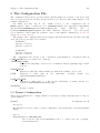
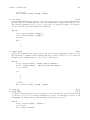
The preprocessor issues error messages of the form:
1. ERROR: <<file.mod>>: line A, col B: <<error message>>
2. ERROR: <<file.mod>>: line A, cols B-C: <<error message>>
3. ERROR: <<file.mod>>: line A, col B - line C, col D: <<error message>>
The first two errors occur on a single line, with error two spanning multiple columns. Error three
spans multiple rows.
Often, the line and column numbers are precise, leading you directly to the offending syntax.
Infrequently however, because of the way the parser works, this is not the case. The most common
example of misleading line and column numbers (and error message for that matter) is the case of
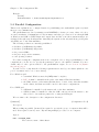
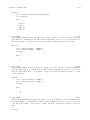
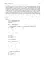
a missing semicolon, as seen in the following example:
varexo a, b
parameters c, ...;
In this case, the parser doesn’t know a semicolon is missing at the end of the varexo command
until it begins parsing the second line and bumps into the parameters command. This is because we allow commands to span multiple lines and, hence, the parser cannot know that the
second line will not have a semicolon on it until it gets there. Once the parser begins parsing the
second line, it realizes that it has encountered a keyword, parameters, which it did not expect.
Hence, it throws an error of the form: ERROR: <<file.mod>>: line 2, cols 0-9: syntax error,
unexpected PARAMETERS. In this case, you would simply place a semicolon at the end of line one
and the parser would continue processing.
Chapter 4: The Model file
10
4 The Model file
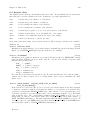
4.1 Conventions
A model file contains a list of commands and of blocks. Each command and each element of a
block is terminated by a semicolon (;). Blocks are terminated by end;.
Most Dynare commands have arguments and several accept options, indicated in parentheses
after the command keyword. Several options are separated by commas.
In the description of Dynare commands, the following conventions are observed:
•
•
•
•
•
•
•
•
•
•
•
•
•
•
optional arguments or options are indicated between square brackets: ‘[]’;
repreated arguments are indicated by ellipses: “. . . ”;
mutually exclusive arguments are separated by vertical bars: ‘|’;
INTEGER indicates an integer number;
DOUBLE indicates a double precision number. The following syntaxes are valid: 1.1e3,
1.1E3, 1.1d3, 1.1D3. In some places, infinite values Inf and -Inf are also allowed;
NUMERICAL VECTOR indicates a vector of numbers separated by spaces, enclosed by square
brackets;
EXPRESSION indicates a mathematical expression valid outside the model description (see
Section 4.3 [Expressions], page 14);
MODEL EXPRESSION indicates a mathematical expression valid in the model description
(see Section 4.3 [Expressions], page 14 and Section 4.5 [Model declaration], page 18);
MACRO EXPRESSION designates an expression of the macro-processor (see Section 4.20.1
[Macro expressions], page 98);
VARIABLE NAME indicates a variable name starting with an alphabetical character and
can’t contain: ‘()+-*/^=!;:@#.’ or accentuated characters;
PARAMETER NAME indicates a parameter name starting with an alphabetical character
and can’t contain: ‘()+-*/^=!;:@#.’ or accentuated characters;
LATEX NAME indicates a valid LATEX expression in math mode (not including the dollar
signs);
FUNCTION NAME indicates a valid MATLAB function name;
FILENAME indicates a filename valid in the underlying operating system; it is necessary to put
it between quotes when specifying the extension or if the filename contains a non-alphanumeric
character;
4.2 Variable declarations
Declarations of variables and parameters are made with the following commands:
var VARIABLE_NAME [$LATEX_NAME$] [(long name=QUOTED_STRING)] . . . ;
var (deflator = MODEL_EXPRESSION) VARIABLE_NAME [$LATEX_NAME$]
[(long name=QUOTED_STRING)] . . . ;
var (log deflator = MODEL_EXPRESSION) VARIABLE_NAME [$LATEX_NAME$]
[(long name=QUOTED_STRING)] . . . ;
[Command]
[Command]
[Command]
Description
This required command declares the endogenous variables in the model. See Section 4.1 [Conventions], page 10, for the syntax of VARIABLE NAME and MODEL EXPRESSION. Optionally
it is possible to give a LATEX name to the variable or, if it is nonstationary, provide information
regarding its deflator.
Chapter 4: The Model file
11
var commands can appear several times in the file and Dynare will concatenate them.
Options
If the model is nonstationary and is to be written as such in the model block, Dynare will need
the trend deflator for the appropriate endogenous variables in order to stationarize the model.
The trend deflator must be provided alongside the variables that follow this trend.
deflator = MODEL_EXPRESSION
The expression used to detrend an endogenous variable. All trend variables, endogenous variables and parameters referenced in MODEL EXPRESSION must already
have been declared by the trend_var, log_trend_var, var and parameters commands. The deflator is assumed to be multiplicative; for an additive deflator, use
log_deflator.
log_deflator = MODEL_EXPRESSION
Same as deflator, except that the deflator is assumed to be additive instead of
multiplicative (or, to put it otherwise, the declared variable is equal to the log of a
variable with a multiplicative trend).
long_name = QUOTED_STRING
This is the long version of the variable name. Its value is stored in M_.endo_names_
long. Default: VARIABLE NAME
Example
var c gnp q1 q2;
var(deflator=A) i b;
var c $C$ (long_name=‘Consumption’);
varexo VARIABLE_NAME [$LATEX_NAME$] [(long name=QUOTED_STRING)] . . . ;
[Command]
Description
This optional command declares the exogenous variables in the model. See Section 4.1 [Conventions], page 10, for the syntax of VARIABLE NAME. Optionally it is possible to give a LATEX
name to the variable.
Exogenous variables are required if the user wants to be able to apply shocks to her model.
varexo commands can appear several times in the file and Dynare will concatenate them.
Options
long_name = QUOTED_STRING
Like [long name], page 11 but value stored in M_.exo_names_long.
Example
varexo m gov;
varexo_det VARIABLE_NAME [$LATEX_NAME$]
[(long name=QUOTED_STRING)] . . . ;
[Command]
Description
This optional command declares exogenous deterministic variables in a stochastic model. See
Section 4.1 [Conventions], page 10, for the syntax of VARIABLE NAME. Optionally it is
possible to give a LATEX name to the variable.
Chapter 4: The Model file
12
It is possible to mix deterministic and stochastic shocks to build models where agents know
from the start of the simulation about future exogenous changes. In that case stoch_simul will
compute the rational expectation solution adding future information to the state space (nothing
is shown in the output of stoch_simul) and forecast will compute a simulation conditional
on initial conditions and future information.
varexo_det commands can appear several times in the file and Dynare will concatenate them.
Options
long_name = QUOTED_STRING
Like [long name], page 11 but value stored in M_.exo_det_names_long.
Example
varexo m gov;
varexo_det tau;
parameters PARAMETER_NAME [$LATEX_NAME$]
[(long name=QUOTED_STRING)] . . . ;
[Command]
Description
This command declares parameters used in the model, in variable initialization or in shocks
declarations. See Section 4.1 [Conventions], page 10, for the syntax of PARAMETER NAME.
Optionally it is possible to give a LATEX name to the parameter.
The parameters must subsequently be assigned values (see Section 4.4 [Parameter initialization],
page 18).
parameters commands can appear several times in the file and Dynare will concatenate them.
Options
long_name = QUOTED_STRING
Like [long name], page 11 but value stored in M_.param_names_long.
Example
parameters alpha, bet;
change_type (var | varexo | varexo det | parameters) VARIABLE_NAME |
PARAMETER_NAME . . . ;
[Command]
Description
Changes the types of the specified variables/parameters to another type: endogenous, exogenous,
exogenous deterministic or parameter.
It is important to understand that this command has a global effect on the .mod file: the type
change is effective after, but also before, the change_type command. This command is typically
used when flipping some variables for steady state calibration: typically a separate model file is
used for calibration, which includes the list of variable declarations with the macro-processor,
and flips some variable.
Example
Chapter 4: The Model file
13
var y, w;
parameters alpha, bet;
...
change_type(var) alpha, bet;
change_type(parameters) y, w;
Here, in the whole model file, alpha and beta will be endogenous and y and w will be parameters.
predetermined_variables VARIABLE_NAME . . . ;
[Command]
Description
In Dynare, the default convention is that the timing of a variable reflects when this variable
is decided. The typical example is for capital stock: since the capital stock used at current
period is actually decided at the previous period, then the capital stock entering the production
function is k(-1), and the law of motion of capital must be written:
k = i + (1-delta)*k(-1)
Put another way, for stock variables, the default in Dynare is to use a “stock at the end of the
period” concept, instead of a “stock at the beginning of the period” convention.
The predetermined_variables is used to change that convention. The endogenous variables
declared as predetermined variables are supposed to be decided one period ahead of all other
endogenous variables. For stock variables, they are supposed to follow a “stock at the beginning
of the period” convention.
Note that Dynare internally always uses the “stock at the end of the period” concept, even
when the model has been entered using the predetermined_variables-command. Thus, when
plotting, computing or simulating variables, Dynare will follow the convention to use variables
that are decided in the current period. For example, when generating impulse response functions
for capital, Dynare will plot k, which is the capital stock decided upon by investment today (and
which will be used in tomorrow’s production function). This is the reason that capital is shown
to be moving on impact, because it is k and not the predetermined k(-1) that is displayed. It
is important to remember that this also affects simulated time series and output from smoother
routines for predetermined variables. Compared to non-predetermined variables they might
otherwise appear to be falsely shifted to the future by one period.
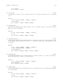
Example
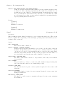
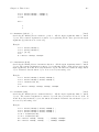
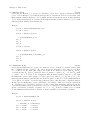
The following two program snippets are strictly equivalent.
Using default Dynare timing convention:
var y, k, i;
...
model;
y = k(-1)^alpha;
k = i + (1-delta)*k(-1);
...
end;
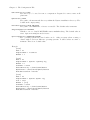
Using the alternative timing convention:
var y, k, i;
predetermined_variables k;
...
model;
y = k^alpha;
k(+1) = i + (1-delta)*k;
...
end;
Chapter 4: The Model file
trend_var (growth factor = MODEL_EXPRESSION) VARIABLE_NAME
[$LATEX_NAME$] . . . ;
14
[Command]
Description
This optional command declares the trend variables in the model. See Section 4.1 [Conventions],
page 10, for the syntax of MODEL EXPRESSION and VARIABLE NAME. Optionally it is
possible to give a LATEX name to the variable.
The variable is assumed to have a multiplicative growth trend. For an additive growth trend,
use log_trend_var instead.
Trend variables are required if the user wants to be able to write a nonstationary model in the
model block. The trend_var command must appear before the var command that references
the trend variable.
trend_var commands can appear several times in the file and Dynare will concatenate them.
If the model is nonstationary and is to be written as such in the model block, Dynare will
need the growth factor of every trend variable in order to stationarize the model. The growth
factor must be provided within the declaration of the trend variable, using the growth_factor
keyword. All endogenous variables and parameters referenced in MODEL EXPRESSION must
already have been declared by the var and parameters commands.
Example
trend_var (growth_factor=gA) A;
log_trend_var (log growth factor = MODEL_EXPRESSION) VARIABLE_NAME
[$LATEX_NAME$] . . . ;
[Command]
Description
Same as trend_var, except that the variable is supposed to have an additive trend (or, to put
it otherwise, to be equal to the log of a variable with a multiplicative trend).
4.3 Expressions
Dynare distinguishes between two types of mathematical expressions: those that are used to describe the model, and those that are used outside the model block (e.g. for initializing parameters or
variables, or as command options). In this manual, those two types of expressions are respectively
denoted by MODEL EXPRESSION and EXPRESSION.
Unlike MATLAB or Octave expressions, Dynare expressions are necessarily scalar ones: they
cannot contain matrices or evaluate to matrices1 .
Expressions can be constructed using integers (INTEGER), floating point numbers (DOUBLE),
parameter names (PARAMETER NAME), variable names (VARIABLE NAME), operators and
functions.
The following special constants are also accepted in some contexts:
inf
[Constant]
Represents infinity.
nan
[Constant]
“Not a number”: represents an undefined or unrepresentable value.
1
Note that arbitrary MATLAB or Octave expressions can be put in a .mod file, but those expressions have to
be on separate lines, generally at the end of the file for post-processing purposes. They are not interpreted by
Dynare, and are simply passed on unmodified to MATLAB or Octave. Those constructions are not addresses in
this section.
Chapter 4: The Model file
15
4.3.1 Parameters and variables
Parameters and variables can be introduced in expressions by simply typing their names. The
semantics of parameters and variables is quite different whether they are used inside or outside the
model block.
4.3.1.1 Inside the model
Parameters used inside the model refer to the value given through parameter initialization (see
Section 4.4 [Parameter initialization], page 18) or homotopy_setup when doing a simulation, or are
the estimated variables when doing an estimation.
Variables used in a MODEL EXPRESSION denote current period values when neither a lead
or a lag is given. A lead or a lag can be given by enclosing an integer between parenthesis just after
the variable name: a positive integer means a lead, a negative one means a lag. Leads or lags of
more than one period are allowed. For example, if c is an endogenous variable, then c(+1) is the
variable one period ahead, and c(-2) is the variable two periods before.
When specifying the leads and lags of endogenous variables, it is important to respect the
following convention: in Dynare, the timing of a variable reflects when that variable is decided. A
control variable — which by definition is decided in the current period — must have no lead. A
predetermined variable — which by definition has been decided in a previous period — must have
a lag. A consequence of this is that all stock variables must use the “stock at the end of the period”
convention. Please refer to Mancini-Griffoli (2007) for more details and concrete examples.
Leads and lags are primarily used for endogenous variables, but can be used for exogenous
variables. They have no effect on parameters and are forbidden for local model variables (see
Section 4.5 [Model declaration], page 18).
4.3.1.2 Outside the model
When used in an expression outside the model block, a parameter or a variable simply refers to
the last value given to that variable. More precisely, for a parameter it refers to the value given
in the corresponding parameter initialization (see Section 4.4 [Parameter initialization], page 18);
for an endogenous or exogenous variable, it refers to the value given in the most recent initval or
endval block.
4.3.2 Operators
The following operators are allowed in both MODEL EXPRESSION and EXPRESSION :
• binary arithmetic operators: +, -, *, /, ^
• unary arithmetic operators: +, • binary comparison operators (which evaluate to either 0 or 1): <, >, <=, >=, ==, !=
Note that these operators are differentiable everywhere except on a line of the 2-dimensional
real plane. However for facilitating convergence of Newton-type methods, Dynare assumes that,
at the points of non-differentiability, the partial derivatives of these operators with respect to
both arguments is equal to 0 (since this is the value of the partial derivatives everywhere else).
The following special operators are accepted in MODEL EXPRESSION (but not in EXPRESSION ):
STEADY_STATE (MODEL_EXPRESSION)
[Operator]
This operator is used to take the value of the enclosed expression at the steady state. A typical
usage is in the Taylor rule, where you may want to use the value of GDP at steady state to
compute the output gap.
EXPECTATION (INTEGER) (MODEL_EXPRESSION)
[Operator]
This operator is used to take the expectation of some expression using a different information
set than the information available at current period. For example, EXPECTATION(-1)(x(+1))
Chapter 4: The Model file
16
is equal to the expected value of variable x at next period, using the information set available
at the previous period. See Section 4.6 [Auxiliary variables], page 21, for an explanation of how
this operator is handled internally and how this affects the output.
4.3.3 Functions
4.3.3.1 Built-in Functions
The following standard functions are supported internally for both MODEL EXPRESSION and
EXPRESSION :
exp (x)
[Function]
Natural exponential.
log (x)
ln (x)
[Function]
[Function]
Natural logarithm.
log10 (x)
[Function]
Base 10 logarithm.
sqrt (x)
[Function]
Square root.
abs (x)
[Function]
Absolute value.
Note that this function is not differentiable at x = 0. However, for facilitating convergence of
Newton-type methods, Dynare assumes that the derivative at x = 0 is equal to 0 (this assumption
comes from the observation that the derivative of abs(x) is equal to sign(x) for x 6= 0 and from
the convention for the derivative of sign(x) at x = 0).
sign (x)
[Function]
Signum function.
Note that this function is not differentiable at x = 0. However, for facilitating convergence
of Newton-type methods, Dynare assumes that the derivative at x = 0 is equal to 0 (this
assumption comes from the observation that both the right- and left-derivatives at this point
exist and are equal to 0).
sin (x)
cos (x)
tan (x)
asin (x)
acos (x)
atan (x)
[Function]
[Function]
[Function]
[Function]
[Function]
[Function]
Trigonometric functions.
max (a, b)
min (a, b)
[Function]
[Function]
Maximum and minimum of two reals.
Note that these functions are differentiable everywhere except on a line of the 2-dimensional real
plane defined by a = b. However for facilitating convergence of Newton-type methods, Dynare
assumes that, at the points of non-differentiability, the partial derivative of these functions with
respect to the first (resp. the second) argument is equal to 1 (resp. to 0) (i.e. the derivatives at
the kink are equal to the derivatives observed on the half-plane where the function is equal to
its first argument).
Chapter 4: The Model file
17
normcdf (x)
normcdf (x, mu, sigma)
[Function]
[Function]
Gaussian cumulative density function, with mean mu and standard deviation sigma. Note that
normcdf(x) is equivalent to normcdf(x,0,1).
normpdf (x)
normpdf (x, mu, sigma)
[Function]
[Function]
Gaussian probability density function, with mean mu and standard deviation sigma. Note that
normpdf(x) is equivalent to normpdf(x,0,1).
erf (x)
[Function]
Gauss error function.
4.3.3.2 External Functions
Any other user-defined (or built-in) MATLAB or Octave function may be used in both a
MODEL EXPRESSION and an EXPRESSION, provided that this function has a scalar argument as a return value.
To use an external function in a MODEL EXPRESSION, one must declare the function using the external_function statement. This is not necessary for external functions used in an
EXPRESSION.
external_function (OPTIONS . . . );
[Command]
Description
This command declares the external functions used in the model block. It is required for every
unique function used in the model block.
external_function commands can appear several times in the file and must come before the
model block.
Options
name = NAME
The name of the function, which must also be the name of the M-/MEX file implementing it. This option is mandatory.
nargs = INTEGER
The number of arguments of the function. If this option is not provided, Dynare
assumes nargs = 1.
first_deriv_provided [= NAME]
If NAME is provided, this tells Dynare that the Jacobian is provided as the only
output of the M-/MEX file given as the option argument. If NAME is not provided,
this tells Dynare that the M-/MEX file specified by the argument passed to name
returns the Jacobian as its second output argument.
second_deriv_provided [= NAME]
If NAME is provided, this tells Dynare that the Hessian is provided as the only
output of the M-/MEX file given as the option argument. If NAME is not provided,
this tells Dynare that the M-/MEX file specified by the argument passed to name
returns the Hessian as its third output argument. NB: This option can only be
used if the first_deriv_provided option is used in the same external_function
command.
Example
Chapter 4: The Model file
18
external_function(name = funcname);
external_function(name = otherfuncname, nargs = 2,
first_deriv_provided, second_deriv_provided);
external_function(name = yetotherfuncname, nargs = 3,
first_deriv_provided = funcname_deriv);
4.3.4 A few words of warning in stochastic context
The use of the following functions and operators is strongly discouraged in a stochastic context:
max, min, abs, sign, <, >, <=, >=, ==, !=.
The reason is that the local approximation used by stoch_simul or estimation will by nature
ignore the non-linearities introduced by these functions if the steady state is away from the kink.
And, if the steady state is exactly at the kink, then the approximation will be bogus because the
derivative of these functions at the kink is bogus (as explained in the respective documentations of
these functions and operators).
Note that extended_path is not affected by this problem, because it does not rely on a local
approximation of the model.
4.4 Parameter initialization
When using Dynare for computing simulations, it is necessary to calibrate the parameters of the
model. This is done through parameter initialization.
The syntax is the following:
PARAMETER_NAME = EXPRESSION;
Here is an example of calibration:
parameters alpha, bet;
beta = 0.99;
alpha = 0.36;
A = 1-alpha*beta;
Internally, the parameter values are stored in M_.params:
[MATLAB/Octave variable]
Contains the values of model parameters. The parameters are in the order that was used in the
parameters command.
M_.params
4.5 Model declaration
The model is declared inside a model block:
model ;
model (OPTIONS . . . );
[Block]
[Block]
Description
The equations of the model are written in a block delimited by model and end keywords.
There must be as many equations as there are endogenous variables in the model, except when
computing the unconstrained optimal policy with ramsey_policy or discretionary_policy.
The syntax of equations must follow the conventions for MODEL EXPRESSION as described
in Section 4.3 [Expressions], page 14. Each equation must be terminated by a semicolon (‘;’).
A normal equation looks like:
MODEL_EXPRESSION = MODEL_EXPRESSION;
When the equations are written in homogenous form, it is possible to omit the ‘=0’ part and
write only the left hand side of the equation. A homogenous equation looks like:
Chapter 4: The Model file
19
MODEL_EXPRESSION;
Inside the model block, Dynare allows the creation of model-local variables, which constitute a
simple way to share a common expression between several equations. The syntax consists of a
pound sign (#) followed by the name of the new model local variable (which must not be declared
as in Section 4.2 [Variable declarations], page 10), an equal sign, and the expression for which
this new variable will stand. Later on, every time this variable appears in the model, Dynare
will substitute it by the expression assigned to the variable. Note that the scope of this variable
is restricted to the model block; it cannot be used outside. A model local variable declaration
looks like:
# VARIABLE_NAME = MODEL_EXPRESSION;
Options
linear
Declares the model as being linear. It spares oneself from having to declare initial
values for computing the steady state of a stationary linear model. This options
can’t be used with non-linear models, it will NOT trigger linearization of the model.
use_dll
Instructs the preprocessor to create dynamic loadable libraries (DLL) containing
the model equations and derivatives, instead of writing those in M-files. You need
a working compilation environment, i.e. a working mex command (see Section 2.1
[Software requirements], page 3 for more details). Using this option can result in
faster simulations or estimations, at the expense of some initial compilation time.2
block
Perform the block decomposition of the model, and exploit it in computations
(steady-state, deterministic simulation, stochastic simulation with first order approximation and estimation). See Dynare wiki for details on the algorithms used in
deterministic simulation and steady-state computation.
bytecode
Instead of M-files, use a bytecode representation of the model, i.e. a binary file
containing a compact representation of all the equations.
cutoff = DOUBLE
Threshold under which a jacobian element is considered as null during the model
normalization. Only available with option block. Default: 1e-15
mfs = INTEGER
Controls the handling of minimum feedback set of endogenous variables. Only available with option block. Possible values:
2
0
All the endogenous variables are considered as feedback variables (Default).
1
The endogenous variables assigned to equation naturally normalized
(i.e. of the form x = f (Y ) where x does not appear in Y ) are potentially
recursive variables. All the other variables are forced to belong to the
set of feedback variables.
2
In addition of variables with mfs = 1 the endogenous variables related
to linear equations which could be normalized are potential recursive
variables. All the other variables are forced to belong to the set of
feedback variables.
3
In addition of variables with mfs = 2 the endogenous variables related to
non-linear equations which could be normalized are potential recursive
variables. All the other variables are forced to belong to the set of
feedback variables.
In particular, for big models, the compilation step can be very time-consuming, and use of this option may be
counter-productive in those cases.
Chapter 4: The Model file
20
no_static
Don’t create the static model file. This can be useful for models which don’t have
a steady state.
differentiate_forward_vars
differentiate_forward_vars = ( VARIABLE_NAME [VARIABLE_NAME ...] )
Tells Dynare to create a new auxiliary variable for each endogenous variable that
appears with a lead, such that the new variable is the time differentiate of the
original one. More precisely, if the model contains x(+1), then a variable AUX_DIFF_
VAR will be created such that AUX_DIFF_VAR=x-x(-1), and x(+1) will be replaced
with x+AUX_DIFF_VAR(+1).
The transformation is applied to all endogenous variables with a lead if the option
is given without a list of variables. If there is a list, the transformation is restricted
to endogenous with a lead that also appear in the list.
This option can useful for some deterministic simulations where convergence is hard
to obtain. Bad values for terminal conditions in the case of very persistent dynamics
or permanent shocks can hinder correct solutions or any convergence. The new differentiated variables have obvious zero terminal conditions (if the terminal condition
is a steady state) and this in many cases helps convergence of simulations.
parallel_local_files = ( FILENAME [, FILENAME]... )
Declares a list of extra files that should be transferred to slave nodes when doing a
parallel computation (see Section 5.2 [Parallel Configuration], page 107).
Example 1: elementary RBC model
var c k;
varexo x;
parameters aa alph bet delt gam;
model;
c = - k + aa*x*k(-1)^alph + (1-delt)*k(-1);
c^(-gam) = (aa*alph*x(+1)*k^(alph-1) + 1 - delt)*c(+1)^(-gam)/(1+bet);
end;
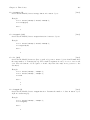
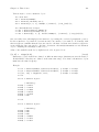
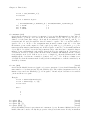
Example 2: use of model local variables
The following program:
model;
# gamma = 1 - 1/sigma;
u1 = c1^gamma/gamma;
u2 = c2^gamma/gamma;
end;
. . . is formally equivalent to:
model;
u1 = c1^(1-1/sigma)/(1-1/sigma);
u2 = c2^(1-1/sigma)/(1-1/sigma);
end;
Example 3: a linear model
model(linear);
x = a*x(-1)+b*y(+1)+e_x;
y = d*y(-1)+e_y;
end;
Chapter 4: The Model file
21
Dynare has the ability to output the list of model equations to a LATEX file, using the write_
latex_dynamic_model command. The static model can also be written with the write_latex_
static_model command.
write_latex_dynamic_model ;
[Command]
Description
This command creates a LATEX file containing the (dynamic) model.
If your .mod file is FILENAME.mod, then Dynare will create a file called FILENAME_dynamic.tex,
containing the list of all the dynamic model equations.
If LATEX names were given for variables and parameters (see Section 4.2 [Variable declarations],
page 10), then those will be used; otherwise, the plain text names will be used.
Time subscripts (t, t+1, t-1, . . . ) will be appended to the variable names, as LATEX subscripts.
Note that the model written in the TEX file will differ from the model declared by the user in
the following dimensions:
• the timing convention of predetermined variables (see [predetermined variables], page 13)
will have been changed to the default Dynare timing convention; in other words, variables
declared as predetermined will be lagged on period back,
• the expectation operators (see [expectation], page 15) will have been removed, replaced by
auxiliary variables and new equations as explained in the documentation of the operator,
• endogenous variables with leads or lags greater or equal than two will have been removed,
replaced by new auxiliary variables and equations,
• for a stochastic model, exogenous variables with leads or lags will also have been replaced
by new auxiliary variables and equations.
Compiling the TEX file requires the following LATEX packages: geometry, fullpage, breqn.
write_latex_static_model ;
[Command]
Description
This command creates a LATEX file containing the static model.
If your .mod file is FILENAME.mod, then Dynare will create a file called FILENAME_static.tex,
containing the list of all the equations of the steady state model.
If LATEX names were given for variables and parameters (see Section 4.2 [Variable declarations],
page 10), then those will be used; otherwise, the plain text names will be used.
Note that the model written in the TEX file will differ from the model declared by the user in
the some dimensions (see [write latex dynamic model], page 21 for details).
Also note that this command will not output the contents of the optional steady_state_model
block (see [steady state model], page 34); it will rather output a static version (i.e. without
leads and lags) of the dynamic model declared in the model block.
Compiling the TEX file requires the following LATEX packages: geometry, fullpage, breqn.
4.6 Auxiliary variables
The model which is solved internally by Dynare is not exactly the model declared by the user.
In some cases, Dynare will introduce auxiliary endogenous variables—along with corresponding
auxiliary equations—which will appear in the final output.
The main transformation concerns leads and lags. Dynare will perform a transformation of the
model so that there is only one lead and one lag on endogenous variables and, in the case of a
stochastic model, no leads/lags on exogenous variables.
Chapter 4: The Model file
22
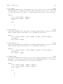
This transformation is achieved by the creation of auxiliary variables and corresponding equations. For example, if x(+2) exists in the model, Dynare will create one auxiliary variable AUX_
ENDO_LEAD = x(+1), and replace x(+2) by AUX_ENDO_LEAD(+1).
A similar transformation is done for lags greater than 2 on endogenous (auxiliary variables will
have a name beginning with AUX_ENDO_LAG), and for exogenous with leads and lags (auxiliary
variables will have a name beginning with AUX_EXO_LEAD or AUX_EXO_LAG respectively).
Another transformation is done for the EXPECTATION operator. For each occurrence of this operator, Dynare creates an auxiliary variable defined by a new equation, and replaces the expectation
operator by a reference to the new auxiliary variable. For example, the expression EXPECTATION(1)(x(+1)) is replaced by AUX_EXPECT_LAG_1(-1), and the new auxiliary variable is declared as
AUX_EXPECT_LAG_1 = x(+2).
Auxiliary variables are also introduced by the preprocessor for the ramsey_policy command.
In this case, they are used to represent the Lagrange multipliers when first order conditions of the
Ramsey problem are computed. The new variables take the form MULT_i, where i represents the
constraint with which the multiplier is associated (counted from the order of declaration in the
model block).
The last type of auxiliary variables is introduced by the differentiate_forward_vars option
of the model block. The new variables take the form AUX_DIFF_FWRD_i, and are equal to x-x(-1)
for some endogenous variable x.
Once created, all auxiliary variables are included in the set of endogenous variables. The output
of decision rules (see below) is such that auxiliary variable names are replaced by the original
variables they refer to.
The number of endogenous variables before the creation of auxiliary variables is stored in M_
.orig_endo_nbr, and the number of endogenous variables after the creation of auxiliary variables
is stored in M_.endo_nbr.
See Dynare Wiki for more technical details on auxiliary variables.
4.7 Initial and terminal conditions
For most simulation exercises, it is necessary to provide initial (and possibly terminal) conditions.
It is also necessary to provide initial guess values for non-linear solvers. This section describes the
statements used for those purposes.
In many contexts (deterministic or stochastic), it is necessary to compute the steady state of
a non-linear model: initval then specifies numerical initial values for the non-linear solver. The
command resid can be used to compute the equation residuals for the given initial values.
Used in perfect foresight mode, the types of forward-looking models for which Dynare was designed require both initial and terminal conditions. Most often these initial and terminal conditions
are static equilibria, but not necessarily.
One typical application is to consider an economy at the equilibrium, trigger a shock in first
period, and study the trajectory of return at the initial equilibrium. To do that, one needs initval
and shocks (see Section 4.8 [Shocks on exogenous variables], page 27.
Another one is to study, how an economy, starting from arbitrary initial conditions converges
toward equilibrium. To do that, one needs initval and endval.
For models with lags on more than one period, the command histval permits to specify different
historical initial values for periods before the beginning of the simulation.
initval ;
initval (OPTIONS . . . );
Description
[Block]
[Block]
Chapter 4: The Model file
23
The initval block serves two purposes: declaring the initial (and possibly terminal) conditions
in a simulation exercise, and providing guess values for non-linear solvers.
This block is terminated by end;, and contains lines of the form:
VARIABLE_NAME = EXPRESSION;
In a deterministic (i.e. perfect foresight) model
First, it provides the initial conditions for all the endogenous and exogenous variables at all the
periods preceeding the first simulation period (unless some of these initial values are modified
by histval).
Second, in the absence of an endval block, it sets the terminal conditions for all the periods
succeeding the last simulation period.
Third, in the absence of an endval block, it provides initial guess values at all simulation dates
for the non-linear solver implemented in simul.
For this last reason, it necessary to provide values for all the endogenous variables in an initval
block (even though, theoretically, initial conditions are only necessary for lagged variables). If
some variables, endogenous or exogenous, are not mentioned in the initval block, a zero value
is assumed.
Note that if the initval block is immediately followed by a steady command, its semantics is
changed. The steady command will compute the steady state of the model for all the endogenous
variables, assuming that exogenous variables are kept constant to the value declared in the
initval block, and using the values declared for the endogenous as initial guess values for the
non-linear solver. An initval block followed by steady is formally equivalent to an initval
block with the same values for the exogenous, and with the associated steady state values for
the endogenous.
In a stochastic model
The main purpose of initval is to provide initial guess values for the non-linear solver in
the steady state computation. Note that if the initval block is not followed by steady,
the steady state computation will still be triggered by subsequent commands (stoch_simul,
estimation. . . ).
It is not necessary to declare 0 as initial value for exogenous stochastic variables, since it is the
only possible value.
This steady state will be used as the initial condition at all the periods preceeding the first
simulation period for the two possible types of simulations in stochastic mode:
• in stoch_simul, if the periods options is specified
• in forecast (in this case, note that it is still possible to modify some of these initial values
with histval)
Options
all_values_required
Issues an error and stops processing the .mod file if there is at least one endogenous
or exogenous variable that has not been set in the initval block.
Example
initval;
c = 1.2;
k = 12;
x = 1;
Chapter 4: The Model file
24
end;
steady;
endval ;
endval (OPTIONS . . . );
[Block]
[Block]
Description
This block is terminated by end;, and contains lines of the form:
VARIABLE_NAME = EXPRESSION;
The endval block makes only sense in a deterministic model, and serves two purposes.
First, it sets the terminal conditions for all the periods succeeding the last simulation period.
Second, it provides initial guess values at all the simulation dates for the non-linear solver
implemented in simul.
For this last reason, it necessary to provide values for all the endogenous variables in an endval
block (even though, theoretically, terminal conditions are only necessary for forward variables).
If some variables, endogenous or exogenous, are not mentioned in the endval block, the value
assumed is that of the last initval block or steady command.
Note that if the endval block is immediately followed by a steady command, its semantics
is changed. The steady command will compute the steady state of the model for all the
endogenous variables, assuming that exogenous variables are kept constant to the value declared
in the endval block, and using the values declared for the endogenous as initial guess values for
the non-linear solver. An endval block followed by steady is formally equivalent to an endval
block with the same values for the exogenous, and with the associated steady state values for
the endogenous.
Options
all_values_required
See [all values required], page 23.
Example
var c k;
varexo x;
...
initval;
c = 1.2;
k = 12;
x = 1;
end;
steady;
endval;
c = 2;
k = 20;
x = 2;
end;
steady;
The initial equilibrium is computed by steady for x=1, and the terminal one, for x=2.
Chapter 4: The Model file
25
Example
var c k;
varexo x;
...
model;
c + k - aa*x*k(-1)^alph - (1-delt)*k(-1);
c^(-gam) - (1+bet)^(-1)*(aa*alph*x(+1)*k^(alph-1) + 1 - delt)*c(+1)^(-gam);
end;
initval;
c = 1.2;
k = 12;
x = 1;
end;
endval;
c = 2;
k = 20;
x = 1.1;
end;
simul(periods=200);
In this example, the problem is finding the optimal path for consumption and capital for the
periods t=1 to T=200, given the path of the exogenous technology level x. Setting x=1.1 in the
endval-block without a shocks-block implies that technology jumps to this new level in t=1
and stays there forever. Because the law of motion for capital is backward-looking, we also need
an initial condition for k at time 0, specified in the initval-block. Similarly, because the Euler
equation is forward-looking, we need a terminal condition for c at t=201, which is specified in
the endval-block. Specifying c in the initval-block and k in the endval-block has no impact
on the results: due to the optimization problem in the first period being to choose c,k at t=1
given predetermined capital stock k inherited from t=0 as well as the current and future values
for technology, the value for c at time t=0 plays no role. The same applies to the choice of
c,k at time t=200, which does not depend on k at t=201. As the Euler equation shows, that
choice only depends on current capital as well as future consumption c and technology x, but
not on future capital k. The intuitive reason is that those variables are the consequence of
optimization problems taking place in at periods t=0 and t=201, respectively, which are not
considered. Thus, when specifying those values in the initval and endval-blocks, Dynare
takes them as given and basically assumes that there were realizations of exogenous variables
and states (basically initial/terminal conditions at the unspecified time periods t<0 and t>201)
that make those choices equilibrium values.
This also suggest another way of looking at the use of steady after initval and endval. Instead
of saying that the implicit unspecified conditions before and after the simulation range have to
fit the initial/terminal conditions of the endogenous variables in those blocks, steady specifies
that those conditions at t<0 and t>201 are equal to being at the steady state given the exogenous
variables in the initval and endval-blocks and sets the endogenous variables at t=0 and t=201
to the corresponding steady state equilibrium values.
The fact that c at t=0 and k at t=201 specified in initval and endval are taken as given
has an important implication for plotting the simulated vector for the endogenous variables:
this vector will also contain the initial and terminal conditions and thus is 202 periods long
in the example. When you specify arbitrary values for the initial and terminal conditions for
forward- and backward-looking variables, respectively, these values can be very far away from
the endogenously determined values at t=1 and t=200. While the values at t=0 and t=201 are
Chapter 4: The Model file
26
unrelated to the dynamics for 0<t<201, they may result in strange-looking large jumps. In the
example above, consumption will display a large jump from t=0 to t=1 and capital will jump
from t=200 to t=201.
histval ;
[Block]
Description
In a deterministic perfect foresight context
In models with lags on more than one period, the histval block permits to specify different
historical initial values for different periods.
This block is terminated by end;, and contains lines of the form:
VARIABLE_NAME(INTEGER) = EXPRESSION;
EXPRESSION is any valid expression returning a numerical value and can contain already
initialized variable names.
By convention in Dynare, period 1 is the first period of the simulation. Going backward in time,
the first period before the start of the simulation is period 0, then period -1, and so on.
If your lagged variables are linked by identities, be careful to satisfy these identities when you
set historical initial values.
Variables not initialized in the histval block are assumed to have a value of zero at period 0
and before. Note that this behavior differs from the case where there is no histval block, where
all variables are initialized at their steady state value at period 0 and before (except when a
steady command doesn’t follow an initval block).
In a stochastic simulation context
In the context of stochastic simulations, histval allows setting the starting point of those simulations in the state space (it does not affect the starting point for impulse response functions).
As for the case of perfect foresight simulations, all not explicitly specified variables are set to
0. Moreover, as only states enter the recursive policy functions, all values specified for control
variables will be ignored.
Example
var x y;
varexo e;
model;
x = y(-1)^alpha*y(-2)^(1-alpha)+e;
...
end;
initval;
x = 1;
y = 1;
e = 0.5;
end;
steady;
histval;
y(0) = 1.1;
Chapter 4: The Model file
27
y(-1) = 0.9;
end;
resid ;
[Command]
This command will display the residuals of the static equations of the model, using the values
given for the endogenous in the last initval or endval block (or the steady state file if you
provided one, see Section 4.10 [Steady state], page 30).
initval_file (filename = FILENAME);
[Command]
Description
In a deterministic setup, this command is used to specify a path for all endogenous and exogenous
variables. The length of these paths must be equal to the number of simulation periods, plus the
number of leads and the number of lags of the model (for example, with 50 simulation periods,
in a model with 2 lags and 1 lead, the paths must have a length of 53). Note that these paths
cover two different things:
• the constraints of the problem, which are given by the path for exogenous and the initial
and terminal values for endogenous
• the initial guess for the non-linear solver, which is given by the path for endogenous variables
for the simulation periods (excluding initial and terminal conditions)
The command accepts three file formats:
• M-file (extension .m): for each endogenous and exogenous variable, the file must contain a
row vector of the same name.
• MAT-file (extension .mat): same as for M-files.
• Excel file (extension .xls or .xlsx): for each endogenous and exogenous, the file must
contain a column of the same name (supported under Octave if the io and java packages
from Octave-Forge are installed, along with a Java Runtime Environment).
Warning
The extension must be omitted in the command argument. Dynare will automatically figure
out the extension and select the appropriate file type.
4.8 Shocks on exogenous variables
In a deterministic context, when one wants to study the transition of one equilibrium position to
another, it is equivalent to analyze the consequences of a permanent shock and this in done in
Dynare through the proper use of initval and endval.
Another typical experiment is to study the effects of a temporary shock after which the system
goes back to the original equilibrium (if the model is stable. . . ). A temporary shock is a temporary
change of value of one or several exogenous variables in the model. Temporary shocks are specified
with the command shocks.
In a stochastic framework, the exogenous variables take random values in each period. In
Dynare, these random values follow a normal distribution with zero mean, but it belongs to the
user to specify the variability of these shocks. The non-zero elements of the matrix of variancecovariance of the shocks can be entered with the shocks command. Or, the entire matrix can be
directly entered with Sigma_e (this use is however deprecated).
If the variance of an exogenous variable is set to zero, this variable will appear in the report
on policy and transition functions, but isn’t used in the computation of moments and of Impulse
Response Functions. Setting a variance to zero is an easy way of removing an exogenous shock.
Chapter 4: The Model file
shocks ;
28
[Block]
In deterministic context
For deterministic simulations, the shocks block specifies temporary changes in the value of
exogenous variables. For permanent shocks, use an endval block.
The block should contain one or more occurrences of the following group of three lines:
var VARIABLE_NAME;
periods INTEGER[:INTEGER] [[,] INTEGER[:INTEGER]]...;
values DOUBLE | (EXPRESSION) [[,] DOUBLE | (EXPRESSION) ]...;
It is possible to specify shocks which last several periods and which can vary over time. The
periods keyword accepts a list of several dates or date ranges, which must be matched by as
many shock values in the values keyword. Note that a range in the periods keyword can be
matched by only one value in the values keyword. If values represents a scalar, the same value
applies to the whole range. If values represents a vector, it must have as many elements as
there are periods in the range.
Note that shock values are not restricted to numerical constants: arbitrary expressions are also
allowed, but you have to enclose them inside parentheses.
Here is an example:
shocks;
var e;
periods 1;
values 0.5;
var u;
periods 4:5;
values 0;
var v;
periods 4:5 6 7:9;
values 1 1.1 0.9;
var w;
periods 1 2;
values (1+p) (exp(z));
end;
A second example with a vector of values:
xx = [1.2; 1.3; 1];
shocks;
var e;
periods 1:3;
values (xx);
end;
In stochastic context
For stochastic simulations, the shocks block specifies the non zero elements of the covariance
matrix of the shocks of exogenous variables.
You can use the following types of entries in the block:
var VARIABLE_NAME; stderr EXPRESSION;
Specifies the standard error of a variable.
var VARIABLE_NAME = EXPRESSION;
Specifies the variance error of a variable.
Chapter 4: The Model file
29
var VARIABLE_NAME, VARIABLE_NAME = EXPRESSION;
Specifies the covariance of two variables.
corr VARIABLE_NAME, VARIABLE_NAME = EXPRESSION;
Specifies the correlation of two variables.
In an estimation context, it is also possible to specify variances and covariances on endogenous
variables: in that case, these values are interpreted as the calibration of the measurement errors
on these variables. This requires the var_obs-command to be specified before the shocks-block.
Here is an example:
shocks;
var e = 0.000081;
var u; stderr 0.009;
corr e, u = 0.8;
var v, w = 2;
end;
Mixing deterministic and stochastic shocks
It is possible to mix deterministic and stochastic shocks to build models where agents know
from the start of the simulation about future exogenous changes. In that case stoch_simul will
compute the rational expectation solution adding future information to the state space (nothing
is shown in the output of stoch_simul) and forecast will compute a simulation conditional
on initial conditions and future information.
Here is an example:
varexo_det tau;
varexo e;
...
shocks;
var e; stderr 0.01;
var tau;
periods 1:9;
values -0.15;
end;
stoch_simul(irf=0);
forecast;
mshocks ;
[Block]
The purpose of this block is similar to that of the shocks block for deterministic shocks, except
that the numeric values given will be interpreted in a multiplicative way. For example, if a value
of 1.05 is given as shock value for some exogenous at some date, it means 5% above its steady
state value (as given by the last initval or endval block).
The syntax is the same than shocks in a deterministic context.
This command is only meaningful in two situations:
• on exogenous variables with a non-zero steady state, in a deterministic setup,
• on deterministic exogenous variables with a non-zero steady state, in a stochastic setup.
Sigma_e
Warning
[Special variable]
Chapter 4: The Model file
30
The use of this special variable is deprecated and is strongly discouraged. You should use a
shocks block instead.
Description
This special variable specifies directly the covariance matrix of the stochastic shocks, as an upper
(or lower) triangular matrix. Dynare builds the corresponding symmetric matrix. Each row of
the triangular matrix, except the last one, must be terminated by a semi-colon ;. For a given
element, an arbitrary EXPRESSION is allowed (instead of a simple constant), but in that case
you need to enclose the expression in parentheses. The order of the covariances in the matrix is
the same as the one used in the varexo declaration.
Example
varexo u, e;
...
Sigma_e = [ 0.81 (phi*0.9*0.009);
0.000081];
This sets the variance of u to 0.81, the variance of e to 0.000081, and the correlation between e
and u to phi.
4.9 Other general declarations
dsample INTEGER [INTEGER];
[Command]
Reduces the number of periods considered in subsequent output commands.
periods INTEGER;
[Command]
Description
This command is now deprecated (but will still work for older model files). It is not necessary
when no simulation is performed and is replaced by an option periods in simul and stoch_
simul.
This command sets the number of periods in the simulation. The periods are numbered from 1
to INTEGER. In perfect foresight simulations, it is assumed that all future events are perfectly
known at the beginning of period 1.
Example
periods 100;
4.10 Steady state
There are two ways of computing the steady state (i.e. the static equilibrium) of a model. The first
way is to let Dynare compute the steady state using a nonlinear Newton-type solver; this should
work for most models, and is relatively simple to use. The second way is to give more guidance to
Dynare, using your knowledge of the model, by providing it with a “steady state file”.
4.10.1 Finding the steady state with Dynare nonlinear solver
steady ;
steady (OPTIONS . . . );
Description
[Command]
[Command]
Chapter 4: The Model file
31
This command computes the steady state of a model using a nonlinear Newton-type solver and
displays it. When a steady state file is used steady displays the steady state and checks that it
is a solution of the static model.
More precisely, it computes the equilibrium value of the endogenous variables for the value of
the exogenous variables specified in the previous initval or endval block.
steady uses an iterative procedure and takes as initial guess the value of the endogenous variables
set in the previous initval or endval block.
For complicated models, finding good numerical initial values for the endogenous variables is
the trickiest part of finding the equilibrium of that model. Often, it is better to start with a
smaller model and add new variables one by one.
Options
maxit = INTEGER
Determines the maximum number of iterations used in the non-linear solver. The
default value of maxit is 10. The maxit option is shared with the simul command.
So a change in maxit in a steady command will also be considered in the following
simul commands.
solve_algo = INTEGER
Determines the non-linear solver to use. Possible values for the option are:
0
Use fsolve (under MATLAB, only available if you have the Optimization Toolbox; always available under Octave)
1
Use Dynare’s own nonlinear equation solver (a Newton-like algorithm
with line-search)
2
Splits the model into recursive blocks and solves each block in turn using
the same solver as value 1
3
Use Chris Sims’ solver
4
Same as value 2, except that it does not try to adapt the search direction
when the Jacobian is nearly singular
5
Newton algorithm with a sparse Gaussian elimination (SPE) (requires
bytecode option, see Section 4.5 [Model declaration], page 18)
6
Newton algorithm with a sparse LU solver at each iteration (requires
bytecode and/or block option, see Section 4.5 [Model declaration],
page 18)
7
Newton algorithm with a Generalized Minimal Residual (GMRES)
solver at each iteration (requires bytecode and/or block option, see
Section 4.5 [Model declaration], page 18; not available under Octave)
8
Newton algorithm with a Stabilized Bi-Conjugate Gradient
(BICGSTAB) solver at each iteration (requires bytecode and/or
block option, see Section 4.5 [Model declaration], page 18)
Default value is 2.
homotopy_mode = INTEGER
Use a homotopy (or divide-and-conquer) technique to solve for the steady state. If
you use this option, you must specify a homotopy_setup block. This option can
take three possible values:
1
In this mode, all the parameters are changed simultaneously, and the
distance between the boundaries for each parameter is divided in as
Chapter 4: The Model file
32
many intervals as there are steps (as defined by homotopy_steps option); the problem is solves as many times as there are steps.
2
Same as mode 1, except that only one parameter is changed at a time;
the problem is solved as many times as steps times number of parameters.
3
Dynare tries first the most extreme values. If it fails to compute the
steady state, the interval between initial and desired values is divided by
two for all parameters. Every time that it is impossible to find a steady
state, the previous interval is divided by two. When it succeeds to find
a steady state, the previous interval is multiplied by two. In that last
case homotopy_steps contains the maximum number of computations
attempted before giving up.
homotopy_steps = INTEGER
Defines the number of steps when performing a homotopy. See homotopy_mode
option for more details.
homotopy_force_continue = INTEGER
This option controls what happens when homotopy fails.
0
steady fails with an error message
1
steady keeps the values of the last homotopy step that was successful
and continues. BE CAREFUL: parameters and/or exogenous variables
are NOT at the value expected by the user
Default is 0.
nocheck
Don’t check the steady state values when they are provided explicitly either by a
steady state file or a steady_state_model block. This is useful for models with
unit roots as, in this case, the steady state is not unique or doesn’t exist.
markowitz = DOUBLE
Value of the Markowitz criterion, used to select the pivot. Only used when solve_
algo = 5. Default: 0.5.
Example
See Section 4.7 [Initial and terminal conditions], page 22.
After computation, the steady state is available in the following variable:
oo_.steady_state
[MATLAB/Octave variable]
Contains the computed steady state.
Endogenous variables are ordered in order of declaration used in var command (which is also
the order used in M_.endo_names).
homotopy_setup ;
[Block]
Description
This block is used to declare initial and final values when using a homotopy method. It is used
in conjunction with the option homotopy_mode of the steady command.
The idea of homotopy (also called divide-and-conquer by some authors) is to subdivide the
problem of finding the steady state into smaller problems. It assumes that you know how to
compute the steady state for a given set of parameters, and it helps you finding the steady state
for another set of parameters, by incrementally moving from one to another set of parameters.
Chapter 4: The Model file
33
The purpose of the homotopy_setup block is to declare the final (and possibly also the initial)
values for the parameters or exogenous that will be changed during the homotopy. It should
contain lines of the form:
VARIABLE_NAME, EXPRESSION, EXPRESSION;
This syntax specifies the initial and final values of a given parameter/exogenous.
There is an alternative syntax:
VARIABLE_NAME, EXPRESSION;
Here only the final value is specified for a given parameter/exogenous; the initial value is taken
from the preceeding initval block.
A necessary condition for a successful homotopy is that Dynare must be able to solve the steady
state for the initial parameters/exogenous without additional help (using the guess values given
in the initval block).
If the homotopy fails, a possible solution is to increase the number of steps (given in homotopy_
steps option of steady).
Example
In the following example, Dynare will first compute the steady state for the initial values
(gam=0.5 and x=1), and then subdivide the problem into 50 smaller problems to find the steady
state for the final values (gam=2 and x=2).
var c k;
varexo x;
parameters alph gam delt bet aa;
alph=0.5;
delt=0.02;
aa=0.5;
bet=0.05;
model;
c + k - aa*x*k(-1)^alph - (1-delt)*k(-1);
c^(-gam) - (1+bet)^(-1)*(aa*alph*x(+1)*k^(alph-1) + 1 - delt)*c(+1)^(-gam);
end;
initval;
x = 1;
k = ((delt+bet)/(aa*x*alph))^(1/(alph-1));
c = aa*x*k^alph-delt*k;
end;
homotopy_setup;
gam, 0.5, 2;
x, 2;
end;
steady(homotopy_mode = 1, homotopy_steps = 50);
4.10.2 Using a steady state file
If you know how to compute the steady state for your model, you can provide a MATLAB/Octave
function doing the computation instead of using steady. Again, there are two options for doing
that:
Chapter 4: The Model file
34
• The easiest way is to write a steady_state_model block, which is described below in more
details. See also fs2000.mod in the examples directory for an example.
The steady state file generated by Dynare will be called FILENAME_steadystate2.m.
• You can write the corresponding MATLAB function by hand. If your MOD-file is called
FILENAME.mod, the steady state file must be called FILENAME_steadystate.m. See NK_
baseline_steadystate.m in the examples directory for an example. This option gives a
bit more flexibility, at the expense of a heavier programming burden and a lesser efficiency.
Note that both files allow to update parameters in each call of the function. This allows for
example to calibrate a model to a labor supply of 0.2 in steady state by setting the labor disutility
parameter to a corresponding value (see NK_baseline_steadystate.m in the examples directory).
They can also be used in estimation where some parameter may be a function of an estimated
parameter and needs to be updated for every parameter draw. For example, one might want to
set the capital utilization cost parameter as a function of the discount rate to ensure that capacity
utilization is 1 in steady state. Treating both parameters as independent or not updating one as a
function of the other would lead to wrong results. But this also means that care is required. Do
not accidentally overwrite your parameters with new values as it will lead to wrong results.
steady_state_model ;
[Block]
Description
When the analytical solution of the model is known, this command can be used to help Dynare
find the steady state in a more efficient and reliable way, especially during estimation where the
steady state has to be recomputed for every point in the parameter space.
Each line of this block consists of a variable (either an endogenous, a temporary variable or
a parameter) which is assigned an expression (which can contain parameters, exogenous at
the steady state, or any endogenous or temporary variable already declared above). Each line
therefore looks like:
VARIABLE_NAME = EXPRESSION;
Note that it is also possible to assign several variables at the same time, if the main function in
the right hand side is a MATLAB/Octave function returning several arguments:
[ VARIABLE_NAME, VARIABLE_NAME... ] = EXPRESSION;
Dynare will automatically generate a steady state file (of the form FILENAME_steadystate2.m)
using the information provided in this block.
Steady state file for deterministic models
steady_state_model block works also with deterministic models. An initval block and, when
necessary, an endval block, is used to set the value of the exogenous variables. Each initval
or endval block must be followed by steady to execute the function created by steady_state_
model and set the initial, respectively terminal, steady state.
Example
var m P c e W R k d n l gy_obs gp_obs y dA;
varexo e_a e_m;
parameters alp bet gam mst rho psi del;
...
// parameter calibration, (dynamic) model declaration, shock calibration...
...
Chapter 4: The Model file
35
steady_state_model;
dA = exp(gam);
gst = 1/dA; // A temporary variable
m = mst;
// Three other temporary variables
khst = ( (1-gst*bet*(1-del)) / (alp*gst^alp*bet) )^(1/(alp-1));
xist = ( ((khst*gst)^alp - (1-gst*(1-del))*khst)/mst )^(-1);
nust = psi*mst^2/( (1-alp)*(1-psi)*bet*gst^alp*khst^alp );
n
P
k
= xist/(nust+xist);
= xist + nust;
= khst*n;
l
c
d
y
R
=
=
=
=
=
psi*mst*n/( (1-psi)*(1-n) );
mst/P;
l - mst + 1;
k^alp*n^(1-alp)*gst^alp;
mst/bet;
// You can use MATLAB functions which return several arguments
[W, e] = my_function(l, n);
gp_obs = m/dA;
gy_obs = dA;
end;
steady;
4.10.3 Replace some equations during steady state computations
When there is no steady state file, Dynare computes the steady state by solving the static model,
i.e. the model from the .mod file from which leads and lags have been removed.
In some specific cases, one may want to have more control over the way this static model is
created. Dynare therefore offers the possibility to explicitly give the form of equations that should
be in the static model.
More precisely, if an equation is prepended by a [static] tag, then it will appear in the static
model used for steady state computation, but that equation will not be used for other computations.
For every equation tagged in this way, you must tag another equation with [dynamic]: that
equation will not be used for steady state computation, but will be used for other computations.
This functionality can be useful on models with a unit root, where there is an infinity of steady
states. An equation (tagged [dynamic]) would give the law of motion of the nonstationary variable
(like a random walk). To pin down one specific steady state, an equation tagged [static] would
affect a constant value to the nonstationary variable.
Example
This is a trivial example with two endogenous variables. The second equation takes a different
form in the static model.
var c k;
varexo x;
...
Chapter 4: The Model file
36
model;
c + k - aa*x*k(-1)^alph - (1-delt)*k(-1);
[dynamic] c^(-gam) - (1+bet)^(-1)*(aa*alph*x(+1)*k^(alph-1) + 1 - delt)*c(+1)^(-gam);
[static] k = ((delt+bet)/(x*aa*alph))^(1/(alph-1));
end;
4.11 Getting information about the model
check ;
check (solve algo = INTEGER) ;
[Command]
[Command]
Description
Computes the eigenvalues of the model linearized around the values specified by the last initval,
endval or steady statement. Generally, the eigenvalues are only meaningful if the linearization
is done around a steady state of the model. It is a device for local analysis in the neighborhood
of this steady state.
A necessary condition for the uniqueness of a stable equilibrium in the neighborhood of the
steady state is that there are as many eigenvalues larger than one in modulus as there are
forward looking variables in the system. An additional rank condition requires that the square
submatrix of the right Schur vectors corresponding to the forward looking variables (jumpers)
and to the explosive eigenvalues must have full rank.
Options
solve_algo = INTEGER
See [solve algo], page 31, for the possible values and their meaning.
qz_zero_threshold = DOUBLE
Value used to test if a generalized eigenvalue is 0/0 in the generalized Schur decomposition (in which case the model does not admit a unique solution). Default:
1e-6.
Output
check returns the eigenvalues in the global variable oo_.dr.eigval.
[MATLAB/Octave variable]
Contains the eigenvalues of the model, as computed by the check command.
oo_.dr.eigval
model_diagnostics ;
[Command]
This command performs various sanity checks on the model, and prints a message if a problem
is detected (missing variables at current period, invalid steady state, singular Jacobian of static
model).
model_info ;
model_info (OPTIONS . . . );
[Command]
[Command]
Description
This command provides information about:
• the normalization of the model: an endogenous variable is attributed to each equation of
the model;
• the block structure of the model: for each block model info indicates its type, the equations
number and endogenous variables belonging to this block.
Chapter 4: The Model file
37
This command can only be used in conjunction with the block option of the model block.
There are five different types of blocks depending on the simulation method used:
‘EVALUATE FORWARD’
In this case the block contains only equations where endogenous variable attributed
to the equation appears currently on the left hand side and where no forward looking
endogenous variables appear. The block has the form: yj,t = fj (yt , yt−1 , . . . , yt−k ).
‘EVALUATE BACKWARD’
The block contains only equations where endogenous variable attributed to the
equation appears currently on the left hand side and where no backward looking
endogenous variables appear. The block has the form: yj,t = fj (yt , yt+1 , . . . , yt+k ).
‘SOLVE FORWARD x’
The block contains only equations where endogenous variable attributed to the equation does not appear currently on the left hand side and where no forward looking
endogenous variables appear. The block has the form: gj (yj,t , yt , yt−1 , . . . , yt−k ) = 0.
x is equal to ‘SIMPLE’ if the block has only one equation. If several equation appears
in the block, x is equal to ‘COMPLETE’.
‘SOLVE FORWARD x’
The block contains only equations where endogenous variable attributed to the equation does not appear currently on the left hand side and where no backward looking
endogenous variables appear. The block has the form: gj (yj,t , yt , yt+1 , . . . , yt+k ) = 0.
x is equal to ‘SIMPLE’ if the block has only one equation. If several equation appears
in the block, x is equal to ‘COMPLETE’.
‘SOLVE TWO BOUNDARIES x’
The block contains equations depending on both forward and backward variables.
The block looks like: gj (yj,t , yt , yt−1 , . . . , yt−k , yt , yt+1 , . . . , yt+k ) = 0. x is equal to
‘SIMPLE’ if the block has only one equation. If several equation appears in the block,
x is equal to ‘COMPLETE’.
Options
’static’
Prints out the block decomposition of the static model. Without ’static’ option
model info displays the block decomposition of the dynamic model.
’incidence’
Displays the gross incidence matrix and the reordered incidence matrix of the block
decomposed model.
print_bytecode_dynamic_model ;
[Command]
Prints the equations and the Jacobian matrix of the dynamic model stored in the bytecode
binary format file. Can only be used in conjunction with the bytecode option of the model
block.
print_bytecode_static_model ;
[Command]
Prints the equations and the Jacobian matrix of the static model stored in the bytecode binary
format file. Can only be used in conjunction with the bytecode option of the model block.
4.12 Deterministic simulation
When the framework is deterministic, Dynare can be used for models with the assumption of perfect foresight. Typically, the system is supposed to be in a state of equilibrium before a period ‘1’
when the news of a contemporaneous or of a future shock is learned by the agents in the model.
The purpose of the simulation is to describe the reaction in anticipation of, then in reaction to
Chapter 4: The Model file
38
the shock, until the system returns to the old or to a new state of equilibrium. In most models,
this return to equilibrium is only an asymptotic phenomenon, which one must approximate by an
horizon of simulation far enough in the future. Another exercise for which Dynare is well suited is
to study the transition path to a new equilibrium following a permanent shock. For deterministic
simulations, the numerical problem consists of solving a nonlinar system of simultaneous equations
in n endogenous variables in T periods. Dynare offers several algorithms for solving this problem, which can be chosen via the stack_solve_algo-option. By default (stack_solve_algo=0),
Dynare uses a Newton-type method to solve the simultaneous equation system. Because the resulting Jacobian is in the order of n by T and hence will be very large for long simulations with many
variables, Dynare makes use of the sparse matrix capacities of MATLAB/Octave. A slower but
potentially less memory consuming alternative (stack_solve_algo=6) is based on a Newton-type
algorithm first proposed by Laffargue (1990) and Boucekkine (1995), which uses relaxation techniques. Thereby, the algorithm avoids ever storing the full Jacobian. The details of the algorithm
can be found in Juillard (1996). The third type of algorithms makes use of block decomposition
techniques (divide-and-conquer methods) that exploit the structure of the model. The principle is
to identify recursive and simultaneous blocks in the model structure and use this information to aid
the solution process. These solution algorithms can provide a significant speed-up on large models.
simul ;
simul (OPTIONS . . . );
[Command]
[Command]
Description
Triggers the computation of a deterministic simulation of the model for the number of periods
set in the option periods.
Options
periods = INTEGER
Number of periods of the simulation
maxit = INTEGER
Determines the maximum number of iterations used in the non-linear solver. The
default value of maxit is 10. The maxit option is shared with the steady command.
So a change in maxit in a simul command will also be considered in the following
steady commands.
stack_solve_algo = INTEGER
Algorithm used for computing the solution. Possible values are:
0
Newton method to solve simultaneously all the equations for every period, using sparse matrices (Default).
1
Use a Newton algorithm with a sparse LU solver at each iteration (requires bytecode and/or block option, see Section 4.5 [Model declaration], page 18).
2
Use a Newton algorithm with a Generalized Minimal Residual (GMRES) solver at each iteration (requires bytecode and/or block option,
see Section 4.5 [Model declaration], page 18; not available under Octave)
3
Use a Newton algorithm with a Stabilized Bi-Conjugate Gradient
(BICGSTAB) solver at each iteration (requires bytecode and/or block
option, see Section 4.5 [Model declaration], page 18).
4
Use a Newton algorithm with a optimal path length at each iteration
(requires bytecode and/or block option, see Section 4.5 [Model declaration], page 18).
Chapter 4: The Model file
39
5
Use a Newton algorithm with a sparse Gaussian elimination (SPE)
solver at each iteration (requires bytecode option, see Section 4.5
[Model declaration], page 18).
6
Use the historical algorithm proposed in Juillard (1996): it is slower
than stack_solve_algo=0, but may be less memory consuming on big
models (not available with bytecode and/or block options).
markowitz = DOUBLE
Value of the Markowitz criterion, used to select the pivot. Only used when stack_
solve_algo = 5. Default: 0.5.
minimal_solving_periods = INTEGER
Specify the minimal number of periods where the model has to be solved, before
using a constant set of operations for the remaining periods. Only used when stack_
solve_algo = 5. Default: 1.
datafile = FILENAME
If the variables of the model are not constant over time, their initial values, stored in
a text file, could be loaded, using that option, as initial values before a deterministic
simulation.
Output
The simulated endogenous variables are available in global matrix oo_.endo_simul.
[MATLAB/Octave variable]
This variable stores the result of a deterministic simulation (computed by simul) or of a stochastic simulation (computed by stoch_simul with the periods option or by extended_path).
oo_.endo_simul
The variables are arranged row by row, in order of declaration (as in M_.endo_names). Note
that this variable also contains initial and terminal conditions, so it has more columns than the
value of periods option.
[MATLAB/Octave variable]
This variable stores the path of exogenous variables during a simulation (computed by simul,
stoch_simul or extended_path).
oo_.exo_simul
The variables are arranged in columns, in order of declaration (as in M_.endo_names). Periods
are in rows. Note that this convention regarding columns and rows is the opposite of the
convention for oo_.endo_simul!
4.13 Stochastic solution and simulation
In a stochastic context, Dynare computes one or several simulations corresponding to a random
draw of the shocks.
The main algorithm for solving stochastic models relies on a Taylor approximation, up to third
order, of the expectation functions (see Judd (1996), Collard and Juillard (2001a), Collard and
Juillard (2001b), and Schmitt-Grohé and Urı́be (2004)). The details of the Dynare implementation
of the first order solution are given in Villemot (2011). Such a solution is computed using the
stoch_simul command.
As an alternative, it is possible to compute a simulation to a stochastic model using the extended
path method presented by Fair and Taylor (1983). This method is especially useful when there are
strong nonlinearities or binding constraints. Such a solution is computed using the extended_path
command.
Chapter 4: The Model file
40
4.13.1 Computing the stochastic solution
stoch_simul [VARIABLE_NAME . . . ];
stoch_simul (OPTIONS . . . ) [VARIABLE_NAME . . . ];
[Command]
[Command]
Description
stoch_simul solves a stochastic (i.e. rational expectations) model, using perturbation techniques.
More precisely, stoch_simul computes a Taylor approximation of the decision and transition
functions for the model. Using this, it computes impulse response functions and various descriptive statistics (moments, variance decomposition, correlation and autocorrelation coefficients).
For correlated shocks, the variance decomposition is computed as in the VAR literature through
a Cholesky decomposition of the covariance matrix of the exogenous variables. When the shocks
are correlated, the variance decomposition depends upon the order of the variables in the varexo
command.
The Taylor approximation is computed around the steady state (see Section 4.10 [Steady state],
page 30).
The IRFs are computed as the difference between the trajectory of a variable following a shock
at the beginning of period 1 and its steady state value. More details on the computation of IRFs
can be found on the DynareWiki.
Variance decomposition, correlation, autocorrelation are only displayed for variables with strictly
positive variance. Impulse response functions are only plotted for variables with response larger
than 10−10 .
Variance decomposition is computed relative to the sum of the contribution of each shock.
Normally, this is of course equal to aggregate variance, but if a model generates very large
variances, it may happen that, due to numerical error, the two differ by a significant amount.
Dynare issues a warning if the maximum relative difference between the sum of the contribution
of each shock and aggregate variance is larger than 0.01%.
The covariance matrix of the shocks is specified with the shocks command (see Section 4.8
[Shocks on exogenous variables], page 27).
When a list of VARIABLE NAME is specified, results are displayed only for these variables.
The stoch_simul command with a first order approximation can benefit from the block decomposition of the model (see [block], page 19).
Options
ar = INTEGER
Order of autocorrelation coefficients to compute and to print. Default: 5.
drop = INTEGER
Number of points (burnin) dropped at the beginning of simulation before computing
the summary statistics. Note that this option does not affect the simulated series
stored in oo .endo simul and the workspace. Here, no periods are dropped. Default:
100.
hp_filter = DOUBLE
Uses HP filter with λ = DOUBLE before computing moments. Default: no filter.
hp_ngrid = INTEGER
Number of points in the grid for the discrete Inverse Fast Fourier Transform used
in the HP filter computation. It may be necessary to increase it for highly autocorrelated processes. Default: 512.
Chapter 4: The Model file
41
irf = INTEGER
Number of periods on which to compute the IRFs. Setting irf=0, suppresses the
plotting of IRFs. Default: 40.
irf_shocks = ( VARIABLE_NAME [[,] VARIABLE_NAME ...] )
The exogenous variables for which to compute IRFs. Default: all.
relative_irf
Requests the computation of normalized IRFs in percentage of the standard error
of each shock.
irf_plot_threshold = DOUBLE
Threshold size for plotting IRFs. All IRFs for a particular variable with a maximum
absolute deviation from the steady state smaller than this value are not displayed.
Default: 1e-10.
nocorr
Don’t print the correlation matrix (printing them is the default).
nofunctions
Don’t print the coefficients of the approximated solution (printing them is the default).
nomoments
Don’t print moments of the endogenous variables (printing them is the default).
nograph
Do not create graphs (which implies that they are not saved to the disk nor displayed). If this option is not used, graphs will be saved to disk (to the format
specified by graph_format option, except if graph_format=none) and displayed to
screen (unless nodisplay option is used).
nodisplay
Do not display the graphs, but still save them to disk (unless nograph is used).
graph_format = FORMAT
graph_format = ( FORMAT, FORMAT... )
Specify the file format(s) for graphs saved to disk. Possible values are eps (the
default), pdf, fig and none (under Octave, only eps and none are available). If the
file format is set equal to none, the graphs are displayed but not saved to the disk.
noprint
Don’t print anything. Useful for loops.
print
Print results (opposite of noprint).
order = INTEGER
Order of Taylor approximation. Acceptable values are 1, 2 and 3. Note that for
third order, k_order_solver option is implied and only empirical moments are
available (you must provide a value for periods option). Default: 2 (except after an estimation command, in which case the default is the value used for the
estimation).
k_order_solver
Use a k-order solver (implemented in C++) instead of the default Dynare solver.
This option is not yet compatible with the bytecode option (see Section 4.5 [Model
declaration], page 18. Default: disabled for order 1 and 2, enabled otherwise
periods = INTEGER
If different from zero, empirical moments will be computed instead of theoretical
moments. The value of the option specifies the number of periods to use in the
simulations. Values of the initval block, possibly recomputed by steady, will be
used as starting point for the simulation. The simulated endogenous variables are
Chapter 4: The Model file
42
made available to the user in a vector for each variable and in the global matrix oo_
.endo_simul (see [oo .endo simul], page 39). The simulated exogenous variables
are made available in oo_.exo_simul (see [oo .exo simul], page 39). Default: 0.
qz_criterium = DOUBLE
Value used to split stable from unstable eigenvalues in reordering the Generalized
Schur decomposition used for solving 1^st order problems. Default: 1.000001 (except when estimating with lik_init option equal to 1: the default is 0.999999 in
that case; see Section 4.14 [Estimation], page 48).
qz_zero_threshold = DOUBLE
See [qz zero threshold], page 36.
replic = INTEGER
Number of simulated series used to compute the IRFs. Default: 1 if order=1, and
50 otherwise.
simul_replic = INTEGER
Number of series to simulate when empirical moments are requested (i.e. periods
> 0). Note that if this option is greater than 1, the additional series will not be used
for computing the empirical moments but will simply be saved in binary form to
the file FILENAME_simul. Default: 1.
solve_algo = INTEGER
See [solve algo], page 31, for the possible values and their meaning.
aim_solver
Use the Anderson-Moore Algorithm (AIM) to compute the decision rules, instead
of using Dynare’s default method based on a generalized Schur decomposition. This
option is only valid for first order approximation. See AIM website for more details
on the algorithm.
conditional_variance_decomposition = INTEGER
See below.
conditional_variance_decomposition = [INTEGER1:INTEGER2]
See below.
conditional_variance_decomposition = [INTEGER1 INTEGER2 ...]
Computes a conditional variance decomposition for the specified period(s). The
periods must be strictly positive. Conditional variances are given by var(yt+k |t).
For period 1, the conditional variance decomposition provides the decomposition
of the effects of shocks upon impact. The results are stored in oo_.conditional_
variance_decomposition (see [oo .conditional variance decomposition], page 45).
The variance decomposition is only conducted, if theoretical moments are requested,
i.e. using the periods=0-option. In case of order=2, Dynare provides a second-order
accurate approximation to the true second moments based on the linear terms of
the second-order solution (see Kim, Kim, Schaumburg and Sims (2008)). Note that
the unconditional variance decomposition (i.e. at horizon infinity) is automatically
conducted if theoretical moments are requested (see [oo .variance decomposition],
page 45)
pruning
Discard higher order terms when iteratively computing simulations of the solution.
At second order, Dynare uses the algorithm of Kim, Kim, Schaumburg and Sims
(2008), while at third order its generalization by Andreasen, Fernández-Villaverde
and Rubio-Ramı́rez (2013) is used.
partial_information
Computes the solution of the model under partial information, along the lines of
Pearlman, Currie and Levine (1986). Agents are supposed to observe only some
Chapter 4: The Model file
43
variables of the economy. The set of observed variables is declared using the varobs
command. Note that if varobs is not present or contains all endogenous variables,
then this is the full information case and this option has no effect. More references
can be found at http://www.dynare.org/DynareWiki/PartialInformation.
sylvester = OPTION
Determines the algorithm used to solve the Sylvester equation for block decomposed
model. Possible values for OPTION are:
default
Uses the default solver for Sylvester equations (gensylv) based on Ondra Kamenik’s algorithm (see the Dynare Website for more information).
fixed_point
Uses a fixed point algorithm to solve the Sylvester equation (gensylv_
fp). This method is faster than the default one for large scale models.
Default value is default
sylvester_fixed_point_tol = DOUBLE
It is the convergence criterion used in the fixed point Sylvester solver. Its default
value is 1e-12.
dr = OPTION
Determines the method used to compute the decision rule. Possible values for
OPTION are:
default
Uses the default method to compute the decision rule based on the
generalized Schur decomposition (see Villemot (2011) for more information).
cycle_reduction
Uses the cycle reduction algorithm to solve the polynomial equation for
retrieving the coefficients associated to the endogenous variables in the
decision rule. This method is faster than the default one for large scale
models.
logarithmic_reduction
Uses the logarithmic reduction algorithm to solve the polynomial equation for retrieving the coefficients associated to the endogenous variables
in the decision rule. This method is in general slower than the cycle_
reduction.
Default value is default
dr_cycle_reduction_tol = DOUBLE
The convergence criterion used in the cycle reduction algorithm. Its default value
is 1e-7.
dr_logarithmic_reduction_tol = DOUBLE
The convergence criterion used in the logarithmic reduction algorithm. Its default
value is 1e-12.
dr_logarithmic_reduction_maxiter = INTEGER
The maximum number of iterations used in the logarithmic reduction algorithm.
Its default value is 100.
loglinear
See [loglinear], page 53. Note that ALL variables are log-transformed by using the
Jacobian transformation, not only selected ones. Thus, you have to make sure that
your variables have strictly positive steady states. stoch_simul will display the
Chapter 4: The Model file
44
moments, decision rules, and impulse responses for the log-linearized variables. The
decision rules saved in oo_.dr and the simulated variables will also be the ones for
the log-linear variables.
Output
This command sets oo_.dr, oo_.mean, oo_.var and oo_.autocorr, which are described below.
If option periods is present, sets oo_.endo_simul (see [oo .endo simul], page 39), and also
saves the simulated variables in MATLAB/Octave vectors of the global workspace with the
same name as the endogenous variables.
If options irf is different from zero, sets oo_.irfs (see below) and also saves the IRFs in
MATLAB/Octave vectors of the global workspace (this latter way of accessing the IRFs is
deprecated and will disappear in a future version).
Example 1
shocks;
var e;
stderr 0.0348;
end;
stoch_simul;
Performs the simulation of the 2nd order approximation of a model with a single stochastic
shock e, with a standard error of 0.0348.
Example 2
stoch_simul(irf=60) y k;
Performs the simulation of a model and displays impulse response functions on 60 periods for
variables y and k.
[MATLAB/Octave variable]
After a run of stoch_simul, contains the mean of the endogenous variables. Contains theoretical
mean if the periods option is not present, and empirical mean otherwise. The variables are
arranged in declaration order.
oo_.mean
[MATLAB/Octave variable]
After a run of stoch_simul, contains the variance-covariance of the endogenous variables. Contains theoretical variance if the periods option is not present (or an approximation thereof for
order=2), and empirical variance otherwise. The variables are arranged in declaration order.
oo_.var
[MATLAB/Octave variable]
After a run of stoch_simul, contains a cell array of the autocorrelation matrices of the endogenous variables. The element number of the matrix in the cell array corresponds to the order
of autocorrelation. The option ar specifies the number of autocorrelation matrices available.
Contains theoretical autocorrelations if the periods option is not present (or an approximation thereof for order=2), and empirical autocorrelations otherwise. The field is only created if
stationary variables are present.
oo_.autocorr
l
The element oo_.autocorr{i}(k,l) is equal to the correlation between ytk and yt−i
, where y k
(resp. y l ) is the k-th (resp. l-th) endogenous variable in the declaration order.
Note that if theoretical moments have been requested, oo_.autocorr{i} is the same than oo_
.gamma_y{i+1}.
Chapter 4: The Model file
45
[MATLAB/Octave variable]
After a run of stoch_simul, if theoretical moments have been requested (i.e. if the periods
option is not present), this variable contains a cell array with the following values (where ar is
the value of the option of the same name):
oo_.gamma_y
oo_.gamma{1}
Variance/co-variance matrix.
oo_.gamma{i+1} (for i=1:ar)
Autocorrelation function. see [oo .autocorr], page 44 for more details. Beware, this
is the autocorrelation function, not the autocovariance function.
oo_.gamma{nar+2}
Unconditional variance decomposition see [oo .variance decomposition], page 45
oo_.gamma{nar+3}
If a second order approximation has been requested, contains the vector of the mean
correction terms.
In case of order=2, the theoretical second moments are a second order accurate approximation
of the true second moments, see conditional_variance_decomposition.
[MATLAB/Octave variable]
After a run of stoch_simul when requesting theoretical moments (periods=0), contains a
matrix with the result of the unconditional variance decomposition (i.e. at horizon infinity).
The first dimension corresponds to the endogenous variables (in the order of declaration) and
the second dimension corresponds to exogenous variables (in the order of declaration). Numbers
are in percent and sum up to 100 across columns.
oo_.variance_decomposition
[MATLAB/Octave variable]
After a run of stoch_simul with the conditional_variance_decomposition option, contains a
three-dimensional array with the result of the decomposition. The first dimension corresponds to
forecast horizons (as declared with the option), the second dimension corresponds to endogenous
variables (in the order of declaration), the third dimension corresponds to exogenous variables
(in the order of declaration).
oo_.conditional_variance_decomposition
[MATLAB/Octave variable]
After a run of stoch_simul with option irf different from zero, contains the impulse responses,
with the following naming convention: VARIABLE_NAME_SHOCK_NAME.
For example, oo_.irfs.gnp_ea contains the effect on gnp of a one standard deviation shock on
ea.
oo_.irfs
The approximated solution of a model takes the form of a set of decision rules or transition
equations expressing the current value of the endogenous variables of the model as function of the
previous state of the model and shocks observed at the beginning of the period. The decision rules
are stored in the structure oo_.dr which is described below.
extended_path ;
extended_path (OPTIONS . . . ) ;
[Command]
[Command]
Description
extended_path solves a stochastic (i.e. rational expectations) model, using the extended path
method presented by Fair and Taylor (1983). Time series for the endogenous variables are
generated by assuming that the agents believe that there will no more shocks in the following
periods.
This function first computes a random path for the exogenous variables (stored in oo_.exo_
simul, see [oo .exo simul], page 39) and then computes the corresponding path for endogenous
Chapter 4: The Model file
46
variables, taking the steady state as starting point. The result of the simulation is stored in
oo_.endo_simul (see [oo .endo simul], page 39). Note that this simulation approach does not
solve for the policy and transition equations but for paths for the endogenous variables.
Options
periods = INTEGER
The number of periods for which the simulation is to be computed. No default
value, mandatory option.
solver_periods = INTEGER
The number of periods used to compute the solution of the perfect foresight at every
iteration of the algorithm. Default: 200.
order = INTEGER
If order is greater than 0 Dynare uses a gaussian quadrature to take into account
the effects of future uncertainty. If order=S then the time series for the endogenous
variables are generated by assuming that the agents believe that there will no more
shocks after period t+S. This is an experimental feature and can be quite slow.
Default: 0.
hybrid
Use the constant of the second order perturbation reduced form to correct the paths
generated by the (stochastic) extended path algorithm.
4.13.2 Typology and ordering of variables
Dynare distinguishes four types of endogenous variables:
Purely backward (or purely predetermined) variables
Those that appear only at current and past period in the model, but not at future
period (i.e. at t and t − 1 but not t + 1). The number of such variables is equal to
M_.npred.
Purely forward variables
Those that appear only at current and future period in the model, but not at past
period (i.e. at t and t + 1 but not t − 1). The number of such variables is stored in
M_.nfwrd.
Mixed variables
Those that appear at current, past and future period in the model (i.e. at t, t + 1 and
t − 1). The number of such variables is stored in M_.nboth.
Static variables
Those that appear only at current, not past and future period in the model (i.e. only
at t, not at t + 1 or t − 1). The number of such variables is stored in M_.nstatic.
Note that all endogenous variables fall into one of these four categories, since after the creation
of auxiliary variables (see Section 4.6 [Auxiliary variables], page 21), all endogenous have at most
one lead and one lag. We therefore have the following identity:
M_.npred + M_.both + M_.nfwrd + M_.nstatic = M_.endo_nbr
Internally, Dynare uses two orderings of the endogenous variables: the order of declaration
(which is reflected in M_.endo_names), and an order based on the four types described above,
which we will call the DR-order (“DR” stands for decision rules). Most of the time, the declaration
order is used, but for elements of the decision rules, the DR-order is used.
The DR-order is the following: static variables appear first, then purely backward variables, then
mixed variables, and finally purely forward variables. Inside each category, variables are arranged
according to the declaration order.
Chapter 4: The Model file
47
Variable oo_.dr.order_var maps DR-order to declaration order, and variable oo_.dr.inv_
order_var contains the inverse map. In other words, the k-th variable in the DR-order corresponds
to the endogenous variable numbered oo_.dr_order_var(k) in declaration order. Conversely, k-th
declared variable is numbered oo_.dr.inv_order_var(k) in DR-order.
Finally, the state variables of the model are the purely backward variables and the mixed
variables. They are ordered in DR-order when they appear in decision rules elements. There
are M_.nspred = M_.npred + M_.nboth such variables. Similarly, one has M_.nsfwrd = M_.nfwrd
+ M_.nboth, and M_.ndynamic = M_.nfwrd+M_.nboth+M_.npred.
4.13.3 First order approximation
The approximation has the stylized form:
h
yt = y s + Ayt−1
+ But
where y s is the steady state value of y and yth = yt − y s .
The coefficients of the decision rules are stored as follows:
• y s is stored in oo_.dr.ys. The vector rows correspond to all endogenous in the declaration
order.
• A is stored in oo_.dr.ghx. The matrix rows correspond to all endogenous in DR-order. The
matrix columns correspond to state variables in DR-order.
• B is stored oo_.dr.ghu. The matrix rows correspond to all endogenous in DR-order. The
matrix columns correspond to exogenous variables in declaration order.
Of course, the shown form of the approximation is only stylized, because it neglects the required
different ordering in y s and yth . The precise form of the approximation that shows the way Dynare
deals with differences between declaration and DR-order, is
yt (oo .dr.order var)
=
y s (oo .dr.order var) + A · yt−1 (oo .dr.order var(k2)) −
y (oo .dr.order var(k2)) + B · ut
s
where k2 selects the state variables, yt and y s are in declaration order and the coefficient matrices
are in DR-order. Effectively, all variables on the right hand side are brought into DR order for
computations and then assigned to yt in declaration order.
4.13.4 Second order approximation
The approximation has the form:
h
h
h
h
+ But + 0.5C(yt−1
⊗ yt−1
) + 0.5D(ut ⊗ ut ) + E(yt−1
⊗ ut )
yt = y s + 0.5Δ2 + Ayt−1
where y s is the steady state value of y, yth = yt − y s , and Δ2 is the shift effect of the variance of
future shocks. For the reordering required due to differences in declaration and DR order, see the
first order approximation.
The coefficients of the decision rules are stored in the variables described for first order approximation, plus the following variables:
• Δ2 is stored in oo_.dr.ghs2. The vector rows correspond to all endogenous in DR-order.
• C is stored in oo_.dr.ghxx. The matrix rows correspond to all endogenous in DR-order.
The matrix columns correspond to the Kronecker product of the vector of state variables in
DR-order.
• D is stored in oo_.dr.ghuu. The matrix rows correspond to all endogenous in DR-order. The
matrix columns correspond to the Kronecker product of exogenous variables in declaration
order.
• E is stored in oo_.dr.ghxu. The matrix rows correspond to all endogenous in DR-order.
The matrix columns correspond to the Kronecker product of the vector of state variables (in
DR-order) by the vector of exogenous variables (in declaration order).
Chapter 4: The Model file
48
4.13.5 Third order approximation
The approximation has the form:
yt = y s + G0 + G1 zt + G2 (zt ⊗ zt ) + G3 (zt ⊗ zt ⊗ zt )
where y s is the steady state value of y, and zt is a vector consisting of the deviation from the
steady state of the state variables (in DR-order) at date t − 1 followed by the exogenous variables
at date t (in declaration order). The vector zt is therefore of size nz = M_.nspred + M_.exo_nbr.
The coefficients of the decision rules are stored as follows:
• y s is stored in oo_.dr.ys. The vector rows correspond to all endogenous in the declaration
order.
• G0 is stored in oo_.dr.g_0. The vector rows correspond to all endogenous in DR-order.
• G1 is stored in oo_.dr.g_1. The matrix rows correspond to all endogenous in DR-order. The
matrix columns correspond to state variables in DR-order, followed by exogenous in declaration
order.
• G2 is stored in oo_.dr.g_2. The matrix rows correspond to all endogenous in DR-order. The
matrix columns correspond to the Kronecker product of state variables (in DR-order), followed
by exogenous (in declaration order). Note that the Kronecker product is stored in a folded way,
i.e. symmetric elements are stored only once, which implies that the matrix has nz (nz + 1)/2
columns. More precisely, each column of this matrix corresponds to a pair (i1 , i2 ) where each
index represents an element of zt and is therefore between 1 and nz . Only non-decreasing
pairs are stored, i.e. those for which i1 ≤ i2 . The columns are arranged in the lexicographical
order of non-decreasing pairs. Also note that for those pairs where i1 6= i2 , since the element
is stored only once but appears two times in the unfolded G2 matrix, it must be multiplied by
2 when computing the decision rules.
• G3 is stored in oo_.dr.g_3. The matrix rows correspond to all endogenous in DR-order. The
matrix columns correspond to the third Kronecker power of state variables (in DR-order),
followed by exogenous (in declaration order). Note that the third Kronecker power is stored
in a folded way, i.e. symmetric elements are stored only once, which implies that the matrix
has nz (nz + 1)(nz + 2)/6 columns. More precisely, each column of this matrix corresponds to
a tuple (i1 , i2 , i3 ) where each index represents an element of zt and is therefore between 1 and
nz . Only non-decreasing tuples are stored, i.e. those for which i1 ≤ i2 ≤ i3 . The columns
are arranged in the lexicographical order of non-decreasing tuples. Also note that for tuples
that have three distinct indices (i.e. i1 6= i2 and i1 6= i3 and i2 6= i3 , since these elements are
stored only once but appears six times in the unfolded G3 matrix, they must be multiplied by
6 when computing the decision rules. Similarly, for those tuples that have two equal indices
(i.e. of the form (a, a, b) or (a, b, a) or (b, a, a)), since these elements are stored only once but
appears three times in the unfolded G3 matrix, they must be multiplied by 3 when computing
the decision rules.
4.14 Estimation
Provided that you have observations on some endogenous variables, it is possible to use Dynare to
estimate some or all parameters. Both maximum likelihood (as in Ireland (2004)) and Bayesian
techniques (as in Rabanal and Rubio-Ramirez (2003), Schorfheide (2000) or Smets and Wouters
(2003)) are available. Using Bayesian methods, it is possible to estimate DSGE models, VAR
models, or a combination of the two techniques called DSGE-VAR.
Note that in order to avoid stochastic singularity, you must have at least as many shocks or
measurement errors in your model as you have observed variables.
The estimation using a first order approximation can benefit from the block decomposition of
the model (see [block], page 19).
Chapter 4: The Model file
varobs VARIABLE_NAME . . . ;
49
[Command]
Description
This command lists the name of observed endogenous variables for the estimation procedure.
These variables must be available in the data file (see [estimation cmd], page 52).
Alternatively, this command is also used in conjunction with the partial_information option
of stoch_simul, for declaring the set of observed variables when solving the model under partial
information.
Only one instance of varobs is allowed in a model file. If one needs to declare observed variables
in a loop, the macro-processor can be used as shown in the second example below.
Simple example
varobs C y rr;
Example with a loop
varobs
@#for co in countries
GDP_@{co}
@#endfor
;
observation_trends ;
[Block]
Description
This block specifies linear trends for observed variables as functions of model parameters.
Each line inside of the block should be of the form:
VARIABLE_NAME(EXPRESSION);
In most cases, variables shouldn’t be centered when observation_trends is used.
Example
observation_trends;
Y (eta);
P (mu/eta);
end;
estimated_params ;
[Block]
Description
This block lists all parameters to be estimated and specifies bounds and priors as necessary.
Each line corresponds to an estimated parameter.
In a maximum likelihood estimation, each line follows this syntax:
stderr VARIABLE_NAME | corr VARIABLE_NAME_1, VARIABLE_NAME_2 | PARAMETER_NAME
, INITIAL_VALUE [, LOWER_BOUND, UPPER_BOUND ];
In a Bayesian estimation, each line follows this syntax:
stderr VARIABLE_NAME | corr VARIABLE_NAME_1, VARIABLE_NAME_2 |
PARAMETER_NAME | DSGE_PRIOR_WEIGHT
[, INITIAL_VALUE [, LOWER_BOUND, UPPER_BOUND]], PRIOR_SHAPE,
PRIOR_MEAN, PRIOR_STANDARD_ERROR [, PRIOR_3RD_PARAMETER [,
PRIOR_4TH_PARAMETER [, SCALE_PARAMETER ] ] ];
The first part of the line consists of one of the three following alternatives:
Chapter 4: The Model file
50
stderr VARIABLE_NAME
Indicates that the standard error of the exogenous variable VARIABLE NAME, or
of the observation error/measurement errors associated with endogenous observed
variable VARIABLE NAME, is to be estimated
corr VARIABLE_NAME1, VARIABLE_NAME2
Indicates that the correlation between the exogenous variables VARIABLE NAME1
and VARIABLE NAME2, or the correlation of the observation errors/measurement
errors associated with endogenous observed variables VARIABLE NAME1 and
VARIABLE NAME2, is to be estimated. Note that correlations set by previous
shocks-blocks or estimation-commands are kept at their value set prior to estimation if they are not estimated again subsequently. Thus, the treatment is the same
as in the case of deep parameters set during model calibration and not estimated.
PARAMETER_NAME
The name of a model parameter to be estimated
DSGE_PRIOR_WEIGHT
...
The rest of the line consists of the following fields, some of them being optional:
INITIAL_VALUE
Specifies a starting value for the posterior mode optimizer or the maximum likelihood
estimation. If unset, defaults to the prior mean.
LOWER_BOUND
Specifies a lower bound for the parameter value in maximum likelihood estimation
UPPER_BOUND
Specifies an upper bound for the parameter value in maximum likelihood estimation
PRIOR_SHAPE
A keyword specifying the shape of the prior density. The possible values are:
beta_pdf, gamma_pdf, normal_pdf, uniform_pdf, inv_gamma_pdf, inv_gamma1_
pdf, inv_gamma2_pdf. Note that inv_gamma_pdf is equivalent to inv_gamma1_pdf
PRIOR_MEAN
The mean of the prior distribution
PRIOR_STANDARD_ERROR
The standard error of the prior distribution
PRIOR_3RD_PARAMETER
A third parameter of the prior used for generalized beta distribution, generalized
gamma and for the uniform distribution. Default: 0
PRIOR_4TH_PARAMETER
A fourth parameter of the prior used for generalized beta distribution and for the
uniform distribution. Default: 1
SCALE_PARAMETER
A parameter specific scale parameter for the jumping distribution’s covariance matrix of the Metropolis-Hasting algorithm
Note that INITIAL VALUE, LOWER BOUND, UPPER BOUND, PRIOR MEAN,
PRIOR STANDARD ERROR, PRIOR 3RD PARAMETER, PRIOR 4TH PARAMETER
and SCALE PARAMETER can be any valid EXPRESSION. Some of them can be empty, in
which Dynare will select a default value depending on the context and the prior shape.
As one uses options more towards the end of the list, all previous options must be
filled: for example, if you want to specify SCALE PARAMETER, you must specify
Chapter 4: The Model file
PRIOR 3RD PARAMETER and PRIOR 4TH PARAMETER.
parameters don’t apply.
51
Use empty values, if these
Example
The following line:
corr eps_1, eps_2, 0.5, , , beta_pdf, 0, 0.3, -1, 1;
sets a generalized beta prior for the correlation between eps_1 and eps_2 with mean 0 and
variance 0.3. By setting PRIOR 3RD PARAMETER to -1 and PRIOR 4TH PARAMETER
to 1 the standard beta distribution with support [0,1] is changed to a generalized beta with
support [-1,1]. Note that LOWER BOUND and UPPER BOUND are left empty and thus
default to -1 and 1, respectively. The initial value is set to 0.5.
Similarly, the following line:
corr eps_1, eps_2, 0.5, -0.5, 1, beta_pdf, 0, 0.3, -1, 1;
sets the same generalized beta distribution as before, but now truncates this distribution to
[-0.5,1] through the use of LOWER BOUND and UPPER BOUND. Hence, the prior does not
integrate to 1 anymore.
Parameter transformation
Sometimes, it is desirable to estimate a transformation of a parameter appearing in the model,
rather than the parameter itself. It is of course possible to replace the original parameter by a
function of the estimated parameter everywhere is the model, but it is often unpractical.
In such a case, it is possible to declare the parameter to be estimated in the parameters
statement and to define the transformation, using a pound sign (#) expression (see Section 4.5
[Model declaration], page 18).
Example
parameters bet;
model;
# sig = 1/bet;
c = sig*c(+1)*mpk;
end;
estimated_params;
bet, normal_pdf, 1, 0.05;
end;
estimated_params_init ;
estimated_params_init (OPTIONS . . . );
[Block]
[Block]
This block declares numerical initial values for the optimizer when these ones are different from
the prior mean. It should be specified after the estimated_params-block as otherwise the
specified starting values are overwritten by the latter.
Each line has the following syntax:
stderr VARIABLE_NAME | corr VARIABLE_NAME_1, VARIABLE_NAME_2 | PARAMETER_NAME
, INITIAL_VALUE;
Options
use_calibration
For not specifically initialized parameters, use the deep parameters and the elements
of the covariance matrix specified in the shocks block from calibration as starting
Chapter 4: The Model file
52
values for estimation. For components of the shocks block that were not explicitly
specified during calibration or which violate the prior, the prior mean is used.
See [estimated params], page 49, for the meaning and syntax of the various components.
estimated_params_bounds ;
[Block]
This block declares lower and upper bounds for parameters in maximum likelihood estimation.
Each line has the following syntax:
stderr VARIABLE_NAME | corr VARIABLE_NAME_1, VARIABLE_NAME_2 | PARAMETER_NAME
, LOWER_BOUND, UPPER_BOUND;
See [estimated params], page 49, for the meaning and syntax of the various components.
estimation [VARIABLE_NAME . . . ];
estimation (OPTIONS . . . ) [VARIABLE_NAME . . . ];
[Command]
[Command]
Description
This command runs Bayesian or maximum likelihood estimation.
The following information will be displayed by the command:
• results from posterior optimization (also for maximum likelihood)
• marginal log data density
• posterior mean and highest posterior density interval (shortest credible set) from posterior
simulation
• Metropolis-Hastings convergence graphs that still need to be documented
• graphs with prior, posterior, and mode
• graphs of smoothed shocks, smoothed observation errors, smoothed and historical variables
Also, during the MCMC (Bayesian estimation with mh_replic>0) a (graphical or text) waiting
bar is displayed showing the progress of the Monte-Carlo and the current value of the acceptance
ratio. Note that if the load_mh_file option is used (see below) the reported acceptance ratio
does not take into account the draws from the previous MCMC. In the literature there is a
general agreement for saying that the acceptance ratio should be close to one third or one
quarter. If this not the case, you can stop the MCMC (Ctrl-C) and change the value of option
mh_jscale (see below).
Note that by default Dynare generates random numbers using the algorithm mt199937ar (ie
Mersenne Twister method) with a seed set equal to 0. Consequently the MCMCs in Dynare
are deterministic: one will get exactly the same results across different Dynare runs (ceteris
paribus). For instance, the posterior moments or posterior densities will be exactly the same.
This behaviour allows to easily identify the consequences of a change on the model, the priors or
the estimation options. But one may also want to check that across multiple runs, with different
sequences of proposals, the returned results are almost identical. This should be true if the
number of iterations (ie the value of mh_replic) is important enough to ensure the convergence
of the MCMC to its ergodic distribution. In this case the default behaviour of the random
number generators in not wanted, and the user should set the seed according to the system
clock before the estimation command using the following command:
set_dynare_seed(’clock’);
so that the sequence of proposals will be different across different runs.
Algorithms
The Monte Carlo Markov Chain (MCMC) diagnostics are generated by the estimation command
if [mh replic], page 54 is larger than 2000 and if option [nodiagnostic], page 59 is not used. If
[mh nblocks], page 54 is equal to one, the convergence diagnostics of Geweke (1992,1999) is
Chapter 4: The Model file
53
computed. It uses a chi square test to compare the means of the first and last draws specified
by [geweke interval], page 63 after discarding the burnin of [mh drop], page 54. The test is
computed using variance estimates under the assumption of no serial correlation as well as using
tapering windows specified in [taper steps], page 63. If [mh nblocks], page 54 is larger than 1, the
convergence diagnostics of Brooks and Gelman (1998) are used instead. As described in section
3 of Brooks and Gelman (1998) the univariate convergence diagnostics are based on comparing
pooled and within MCMC moments (Dynare displays the second and third order moments, and
the length of the Highest Probability Density interval covering 80% of the posterior distribution).
Due to computational reasons, the multivariate convergence diagnostic does not follow Brooks
and Gelman (1998) strictly, but rather applies their idea for univariate convergence diagnostics
to the range of the posterior likelihood function instead of the individual parameters. The
posterior kernel is used to aggregate the parameters into a scalar statistic whose convergence is
then checked using the Brooks and Gelman (1998) univariate convergence diagnostic.
Options
datafile = FILENAME
The datafile: a .m file, a .mat file, a .csv file, or a .xls/.xlsx file (under Octave,
the io from Octave-Forge is required for the .csv, .xls and .xlsx formats; in
addition, for the .xls and .xlsx formats, the java package is required, along with
a Java Runtime Environment)
xls_sheet = NAME
The name of the sheet with the data in an Excel file
xls_range = RANGE
The range with the data in an Excel file
nobs = INTEGER
The number of observations to be used. Default: all observations in the file
nobs = [INTEGER1:INTEGER2]
Runs a recursive estimation and forecast for samples of size ranging of INTEGER1
to INTEGER2. Option forecast must also be specified. The forecasts are stored
in the RecursiveForecast field of the results structure (see [RecursiveForecast],
page 66).
first_obs = INTEGER
The number of the first observation to be used. Default: 1
prefilter = INTEGER
A value of 1 means that the estimation procedure will demean each data series by
its empirical mean. Default: 0, i.e. no prefiltering
presample = INTEGER
The number of observations to be skipped before evaluating the likelihood. These
first observations are used as a training sample. Default: 0
loglinear
Computes a log-linear approximation of the model instead of a linear approximation.
As always in the context of estimation, the data must correspond to the definition of
the variables used in the model (see Pfeifer 2013 for more details on how to correctly
specify observation equations linking model variables and the data). If you specify
the loglinear option, Dynare will take the logarithm of both your model variables
and of your data as it assumes the data to correspond to the original non-logged
model variables. The displayed posterior results like impulse responses, smoothed
variables, and moments will be for the logged variables, not the original un-logged
ones. Default: computes a linear approximation
Chapter 4: The Model file
54
plot_priors = INTEGER
Control the plotting of priors:
0
No prior plot
1
Prior density for each estimated parameter is plotted. It is important
to check that the actual shape of prior densities matches what you have
in mind. Ill-chosen values for the prior standard density can result in
absurd prior densities.
Default value is 1.
nograph
See [nograph], page 41.
nodisplay
See [nodisplay], page 41.
graph_format = FORMAT
graph_format = ( FORMAT, FORMAT... )
See [graph format], page 41.
lik_init = INTEGER
Type of initialization of Kalman filter:
1
For stationary models, the initial matrix of variance of the error of
forecast is set equal to the unconditional variance of the state variables
2
For nonstationary models: a wide prior is used with an initial matrix of
variance of the error of forecast diagonal with 10 on the diagonal
3
For nonstationary models: use a diffuse filter (use rather the diffuse_
filter option)
4
The filter is initialized with the fixed point of the Riccati equation
Default value is 1. For advanced use only.
lik_algo = INTEGER
For internal use and testing only.
conf_sig = DOUBLE
Confidence interval used for classical forecasting after estimation. See See [conf sig],
page 69.
mh_conf_sig = DOUBLE
Confidence/HPD interval used for the computation of prior and posterior statistics
like: parameter distributions, prior/posterior moments, conditional variance decomposition, impulse response functions, Bayesian forecasting. Default: 0.9
mh_replic = INTEGER
Number of replications for Metropolis-Hastings algorithm. For the time being, mh_
replic should be larger than 1200. Default: 20000
sub_draws = INTEGER
number of draws from the Metropolis iterations that are used to compute posterior distribution of various objects (smoothed variable, smoothed shocks, forecast,
moments, IRF). sub_draws should be smaller than the total number of Metropolis
draws available. Default: min(1200,0.25*Total number of draws)
mh_nblocks = INTEGER
Number of parallel chains for Metropolis-Hastings algorithm. Default: 2
mh_drop = DOUBLE
The fraction of initially generated parameter vectors to be dropped as a burnin
before using posterior simulations. Default: 0.5
Chapter 4: The Model file
55
mh_jscale = DOUBLE
The scale parameter of the jumping distribution’s covariance matrix (MetropolisHastings algorithm). The default value is rarely satisfactory. This option must be
tuned to obtain, ideally, an acceptance ratio of 25%-33% in the Metropolis-Hastings
algorithm. Basically, the idea is to increase the variance of the jumping distribution
if the acceptance ratio is too high, and decrease the same variance if the acceptance
ratio is too low. In some situations in may help to consider parameter specific values
for this scale parameter, this can be done in the [estimated params], page 49 block.
Default: 0.2
mh_init_scale = DOUBLE
The scale to be used for drawing the initial value of the Metropolis-Hastings chain.
Default: 2*mh_scale
mh_recover
Attempts to recover a Metropolis-Hastings simulation that crashed prematurely.
Shouldn’t be used together with load_mh_file
mh_mode = INTEGER
...
mode_file = FILENAME
Name of the file containing previous value for the mode. When computing the mode,
Dynare stores the mode (xparam1) and the hessian (hh, only if cova_compute=1) in
a file called MODEL_FILENAME_mode.mat
mode_compute = INTEGER | FUNCTION_NAME
Specifies the optimizer for the mode computation:
0
The mode isn’t computed. When mode_file option is specified, the
mode is simply read from that file.
When mode_file option is not specified, Dynare reports the value of
the log posterior (log likelihood) evaluated at the initial value of the
parameters.
When mode_file option is not specified and there is no estimated_
params block, but the smoother option is used, it is a roundabout way to
compute the smoothed value of the variables of a model with calibrated
parameters.
1
Uses fmincon optimization routine (available under MATLAB if the
optimization toolbox is installed; not available under Octave)
2
Value no longer used
3
Uses fminunc optimization routine (available under MATLAB if the
optimization toolbox is installed; available under Octave if the optim
package from Octave-Forge is installed)
4
Uses Chris Sims’s csminwel
5
Uses Marco Ratto’s newrat. This value is not compatible with non
linear filters or DSGE-VAR models
6
Uses a Monte-Carlo based optimization routine (see Dynare wiki for
more details)
7
Uses fminsearch, a simplex based optimization routine (available under MATLAB if the optimization toolbox is installed; available under
Octave if the optim package from Octave-Forge is installed)
Chapter 4: The Model file
56
8
Uses Dynare implementation of the Nelder-Mead simplex based optimization routine (generally more efficient than the MATLAB or Octave
implementation available with mode_compute=7)
9
Uses the CMA-ES (Covariance Matrix Adaptation Evolution Strategy)
algorithm, an evolutionary algorithm for difficult non-linear non-convex
optimization
10
Uses the simpsa algorithm, based on the combination of the non-linear
simplex and simulated annealing algorithms and proposed by Cardoso,
Salcedo and Feyo de Azevedo (1996).
FUNCTION_NAME
It is also possible to give a FUNCTION NAME to this option, instead
of an INTEGER. In that case, Dynare takes the return value of that
function as the posterior mode.
Default value is 4.
mcmc_jumping_covariance = hessian|prior_variance|identity_matrix|FILENAME
Tells Dynare which covariance to use for the proposal density of the MCMC sampler.
mcmc_jumping_covariance can be one of the following:
hessian
Uses the Hessian matrix computed at the mode.
prior_variance
Uses the prior variances. No infinite prior variances are allowed in this
case.
identity_matrix
Uses an identity matrix.
FILENAME
Loads an arbitrary user-specified covariance matrix from FILENAME.mat.
The covariance matrix must be saved in a variable named jumping_
covariance, must be square, positive definite, and have the same dimension as the number of estimated parameters.
Note that the covariance matrices are still scaled with [mh jscale], page 55. Default
value is hessian.
mode_check
Tells Dynare to plot the posterior density for values around the computed mode for
each estimated parameter in turn. This is helpful to diagnose problems with the
optimizer
mode_check_neighbourhood_size = DOUBLE
Used in conjunction with option mode_check, gives the width of the window around
the posterior mode to be displayed on the diagnostic plots. This width is expressed
in percentage deviation. The Inf value is allowed, and will trigger a plot over the
entire domain (see also mode_check_symmetric_plots). Default: 0.5.
mode_check_symmetric_plots = INTEGER
Used in conjunction with option mode_check, if set to 1, tells Dynare to ensure
that the check plots are symmetric around the posterior mode. A value of 0 allows
to have asymmetric plots, which can be useful if the posterior mode is close to a
domain boundary, or in conjunction with mode_check_neighbourhood_size = Inf
when the domain in not the entire real line. Default: 1.
mode_check_number_of_points = INTEGER
Number of points around the posterior mode where the posterior kernel is evaluated
(for each parameter). Default is 20
Chapter 4: The Model file
57
prior_trunc = DOUBLE
Probability of extreme values of the prior density that is ignored when computing
bounds for the parameters. Default: 1e-32
load_mh_file
Tells Dynare to add to previous Metropolis-Hastings simulations instead of starting
from scratch. Shouldn’t be used together with mh_recover
optim = (NAME, VALUE, ...)
A list of NAME and VALUE pairs. Can be used to set options for the optimization
routines. The set of available options depends on the selected optimization routine
(ie on the value of option [mode compute], page 55):
1, 3, 7
Available options are given in the documentation of the MATLAB optimization toolbox or in Octave’s documentation.
4
Available options are:
’MaxIter’
Maximum number of iterations. Default: 1000
’NumgradAlgorithm’
Possible values are 2, 3 and 5 respectively corresponding
to the two, three and five points formula used to compute
the gradient of the objective function (see Abramowitz and
Stegun (1964)). Values 13 and 15 are more experimental.
If perturbations on the right and the left increase the value
of the objective function (we minimize this function) then
we force the corresponding element of the gradient to be
zero. The idea is to temporarily reduce the size of the optimization problem. Default: 2.
’NumgradEpsilon’
Size of the perturbation used to compute numerically the
gradient of the objective function. Default: 1e-6
’TolFun’
Stopping criteria. Default: 1e-7
’InitialInverseHessian’
Initial approximation for the inverse of the Hessian matrix
of the posterior kernel (or likelihood). Obviously this approximation has to be a square, positive definite and symmetric matrix. Default: ’1e-4*eye(nx)’, where nx is the
number of parameters to be estimated.
6
Available options are:
’NumberOfMh’
Number of MCMC run sequentially. Default: 3
’ncov-mh’
Number of iterations used for updating the covariance matrix of the jumping distribution. Default: 20000
’nscale-mh’
Maximum number of iterations used for adjusting the scale
parameter of the jumping distribution. 200000
’nclimb’
Number of iterations in the last MCMC (climbing mode).
Chapter 4: The Model file
58
’InitialCovarianceMatrix’
Initial covariance matrix of the jumping distribution. Default is ’previous’ if option mode_file is used, ’prior’
otherwise.
’AcceptanceRateTarget’
A real number between zero and one. The scale parameter of the jumping distribution is adjusted so that
the effective acceptance rate matches the value of option
’AcceptanceRateTarget’. Default: 1.0/3.0
8
Available options are:
’MaxIter’
Maximum number of iterations. Default: 5000
’MaxFunEvals’
Maximum number of objective function evaluations. No
default.
’MaxFunvEvalFactor’
Set MaxFunvEvals equal to MaxFunvEvalFactor times the
number of estimated parameters. Default: 500.
’TolFun’
Tolerance parameter (w.r.t the objective function). Default:
1e-4
’TolX’
Tolerance parameter (w.r.t the instruments). Default: 1e-4
’InitialSimplexSize’
Initial size of the simplex, expressed as percentage deviation
from the provided initial guess in each direction. Default:
.05
9
Available options are:
’MaxIter’
Maximum number of iterations.
’MaxFunEvals’
Maximum number of objective function evaluations. Default: Inf.
10
’TolFun’
Tolerance parameter (w.r.t the objective function). Default:
1e-7
’TolX’
Tolerance parameter (w.r.t the instruments). Default: 1e-7
Available options are:
’MaxIter’
Maximum number of iterations. Default: 5000
’MaxFunvEvals’
Maximum number of objective function evaluations. No
default.
’TolFun’
Tolerance parameter (w.r.t the objective function). Default:
1e-4
’TolX’
Tolerance parameter (w.r.t the instruments). Default: 1e-4
Chapter 4: The Model file
59
’EndTemperature’
Terminal condition w.r.t the temperature. When the temperature reaches EndTemperature, the temperature is set to
zero and the algorithm falls back into a standard simplex
algorithm. Default: .1
Example 1 To change the defaults of csminwel (mode_compute=4):
estimation(..., mode_compute=4, optim=(’NumgradAlgorithm’,3,’TolFun’,1e5), ...);
nodiagnostic
Does not compute the convergence diagnostics for Metropolis-Hastings. Default:
diagnostics are computed and displayed
bayesian_irf
Triggers the computation of the posterior distribution of IRFs.
The
length of the IRFs are controlled by the irf option. Results are stored in
oo_.PosteriorIRF.dsge (see below for a description of this variable)
dsge_var = DOUBLE
Triggers the estimation of a DSGE-VAR model, where the weight of the DSGE prior
of the VAR model is calibrated to the value passed (see Del Negro and Schorfheide
(2004)). It represents ratio of dummy over actual observations. To assure that the
prior is proper, the value must be bigger than (k + n)/T , where k is the number
of estimated parameters, n is the number of observables, and T is the number
of observations. NB: The previous method of declaring dsge_prior_weight as a
parameter and then calibrating it is now deprecated and will be removed in a future
release of Dynare.
dsge_var
Triggers the estimation of a DSGE-VAR model, where the weight of the DSGE prior
of the VAR model will be estimated (as in Adjemian et alii (2008)). The prior on the
weight of the DSGE prior, dsge_prior_weight, must be defined in the estimated_
params section. NB: The previous method of declaring dsge_prior_weight as a
parameter and then placing it in estimated_params is now deprecated and will be
removed in a future release of Dynare.
dsge_varlag = INTEGER
The number of lags used to estimate a DSGE-VAR model. Default: 4.
moments_varendo
Triggers the computation of the posterior distribution of the theoretical moments of the endogenous variables.
Results are stored in
oo_.PosteriorTheoreticalMoments (see [oo .PosteriorTheoreticalMoments],
page 65). The number of lags in the autocorrelation function is controlled by the
ar option.
conditional_variance_decomposition = INTEGER
See below.
conditional_variance_decomposition = [INTEGER1:INTEGER2]
See below.
conditional_variance_decomposition = [INTEGER1 INTEGER2 ...]
Computes the posterior distribution of the conditional variance decomposition for the specified period(s).
The periods must be strictly
positive.
Conditional variances are given by var(yt+k |t).
For period
1, the conditional variance decomposition provides the decomposition
Chapter 4: The Model file
60
of the effects of shocks upon impact.
The results are stored in oo_
.PosteriorTheoreticalMoments.dsge.ConditionalVarianceDecomposition,
but currently there is no displayed output. Note that this option requires the
option moments_varendo to be specified.
filtered_vars
Triggers the computation of the posterior distribution of filtered endogenous
variables/one-step ahead forecasts, i.e.
Et yt+1 .
Results are stored in
oo_.FilteredVariables (see below for a description of this variable)
smoother
Triggers the computation of the posterior distribution of smoothed endogenous
variables and shocks, i.e. the expected value of variables and shocks given
the information available in all observations up to the final date (ET yt ).
Results are stored in oo_.SmoothedVariables, oo_.SmoothedShocks and
oo_.SmoothedMeasurementErrors.
Also triggers the computation of oo_
.UpdatedVariables, which contains the estimation of the expected value of
variables given the information available at the current date (Et yt ). See below for
a description of all these variables.
forecast = INTEGER
Computes the posterior distribution of a forecast on INTEGER periods after the
end of the sample used in estimation. If no Metropolis-Hastings is computed, the
result is stored in variable oo_.forecast and corresponds to the forecast at the
posterior mode. If a Metropolis-Hastings is computed, the distribution of forecasts
is stored in variables oo_.PointForecast and oo_.MeanForecast. See Section 4.15
[Forecasting], page 69, for a description of these variables.
tex
Requests the printing of results and graphs in TEX tables and graphics that can be
later directly included in LATEX files (not yet implemented)
kalman_algo = INTEGER
0
Automatically use the Multivariate Kalman Filter for stationary models
and the Multivariate Diffuse Kalman Filter for non-stationary models
1
Use the Multivariate Kalman Filter
2
Use the Univariate Kalman Filter
3
Use the Multivariate Diffuse Kalman Filter
4
Use the Univariate Diffuse Kalman Filter
Default value is 0. In case of missing observations of single or all series, Dynare
treats those missing values as unobserved states and uses the Kalman filter to infer
their value (see e.g. Durbin and Koopman (2012), Ch. 4.10)
kalman_tol = DOUBLE
Numerical tolerance for determining the singularity of the covariance matrix of the
prediction errors during the Kalman filter (minimum allowed reciprocal of the matrix
condition number). Default value is 1e-10
filter_covariance
Saves the series of one step ahead error of forecast covariance matrices.
filter_step_ahead = [INTEGER1:INTEGER2]
See below.
filter_step_ahead = [INTEGER1 INTEGER2 ...]
Triggers the computation k-step ahead filtered values.
results
in
oo_.FilteredVariablesKStepAhead
and
.FilteredVariablesKStepAheadVariances.
Stores
oo_
Chapter 4: The Model file
61
filter_decomposition
Triggers the computation of the shock decomposition of the above k-step ahead
filtered values.
diffuse_filter
Uses the diffuse Kalman filter (as described in Durbin and Koopman (2012) and
Koopman and Durbin (2003)) to estimate models with non-stationary observed
variables.
When diffuse_filter is used the lik_init option of estimation has no effect.
When there are nonstationary exogenous variables in a model, there is no unique
deterministic steady state. For instance, if productivity is a pure random walk:
at = at−1 + et
any value of ā of a is a deterministic steady state for productivity. Consequently,
the model admits an infinity of steady states. In this situation, the user must
help Dynare in selecting one steady state, except if zero is a trivial model’s steady
state, which happens when the linear option is used in the model declaration.
The user can either provide the steady state to Dynare using a steady_state_
model block (or writing a steady state file) if a closed form solution is available, see
[steady state model], page 34, or specify some constraints on the steady state, see
[equation tag for conditional steady state], page 35, so that Dynare computes the
steady state conditionally on some predefined levels for the non stationary variables.
In both cases, the idea is to use dummy values for the steady state level of the
exogenous non stationary variables.
Note that the nonstationary variables in the model must be integrated processes
(their first difference or k-difference must be stationary).
selected_variables_only
Only run the smoother on the variables listed just after the estimation command.
Default: run the smoother on all the declared endogenous variables.
cova_compute = INTEGER
When 0, the covariance matrix of estimated parameters is not computed after the
computation of posterior mode (or maximum likelihood). This increases speed of
computation in large models during development, when this information is not always necessary. Of course, it will break all successive computations that would
require this covariance matrix. Otherwise, if this option is equal to 1, the covariance matrix is computed and stored in variable hh of MODEL_FILENAME_mode.mat.
Default is 1.
solve_algo = INTEGER
See [solve algo], page 31.
order = INTEGER
Order of approximation, either 1 or 2. When equal to 2, the likelihood is evaluated
with a particle filter based on a second order approximation of the model (see
Fernandez-Villaverde and Rubio-Ramirez (2005)). Default is 1, ie the likelihood of
the linearized model is evaluated using a standard Kalman filter.
irf = INTEGER
See [irf], page 41. Only used if [bayesian irf], page 59 is passed.
irf_shocks = ( VARIABLE_NAME [[,] VARIABLE_NAME ...] )
See [irf shocks], page 41. Only used if [bayesian irf], page 59 is passed. Cannot be
used with [dsge var], page 59.
irf_plot_threshold = DOUBLE
See [irf plot threshold], page 41. Only used if [bayesian irf], page 59 is passed.
Chapter 4: The Model file
62
aim_solver
See [aim solver], page 42.
sylvester = OPTION
See [sylvester], page 43.
sylvester_fixed_point_tol = DOUBLE
See [sylvester fixed point tol], page 43.
lyapunov = OPTION
Determines the algorithm used to solve the Lyapunov equation to initialized the
variance-covariance matrix of the Kalman filter using the steady-state value of state
variables. Possible values for OPTION are:
default
Uses the default solver for Lyapunov equations based on Bartels-Stewart
algorithm.
fixed_point
Uses a fixed point algorithm to solve the Lyapunov equation. This
method is faster than the default one for large scale models, but it
could require a large amount of iterations.
doubling
Uses a doubling algorithm to solve the Lyapunov equation (disclyap_
fast). This method is faster than the two previous one for large scale
models.
square_root_solver
Uses a square-root solver for Lyapunov equations (dlyapchol). This
method is fast for large scale models (available under MATLAB if the
control system toolbox is installed; available under Octave if the control
package from Octave-Forge is installed)
Default value is default
lyapunov_fixed_point_tol = DOUBLE
This is the convergence criterion used in the fixed point Lyapunov solver. Its default
value is 1e-10.
lyapunov_doubling_tol = DOUBLE
This is the convergence criterion used in the doubling algorithm to solve the Lyapunov equation. Its default value is 1e-16.
analytic_derivation
Triggers estimation with analytic gradient. The final hessian is also computed analytically. Only works for stationary models without missing observations.
ar = INTEGER
See [ar], page 40. Only useful in conjunction with option moments_varendo.
endogenous_prior
Use endogenous priors as in Christiano, Trabandt and Walentin (2011).
use_univariate_filters_if_singularity_is_detected = INTEGER
Decide whether Dynare should automatically switch to univariate filter if a singularity is encountered in the likelihood computation (this is the behaviour if the option
is equal to 1). Alternatively, if the option is equal to 0, Dynare will not automatically change the filter, but rather use a penalty value for the likelihood when such
a singularity is encountered. Default: 1.
qz_zero_threshold = DOUBLE
See [qz zero threshold], page 36.
Chapter 4: The Model file
63
taper_steps = [INTEGER1 INTEGER2 ...]
Percent tapering used for the spectral window in the Geweke (1992,1999) convergence diagnostics (requires [mh nblocks], page 54=1). The tapering is used to take
the serial correlation of the posterior draws into account. Default: [4 8 15].
geweke_interval = [DOUBLE DOUBLE]
Percentage of MCMC draws at the beginning and end of the MCMC chain taken
to compute the Geweke (1992,1999) convergence diagnostics (requires [mh nblocks],
page 54=1) after discarding the first [mh drop], page 54 percent of draws as a burnin.
Default: [0.2 0.5].
Note
If no mh_jscale parameter is used in estimated params, the procedure uses mh_jscale for all
parameters. If mh_jscale option isn’t set, the procedure uses 0.2 for all parameters.
Output
After running estimation, the parameters M_.params and the variance matrix M_.Sigma_e of
the shocks are set to the mode for maximum likelihood estimation or posterior mode computation
without Metropolis iterations.
After estimation with Metropolis iterations (option mh_replic > 0 or option load_mh_file
set) the parameters M_.params and the variance matrix M_.Sigma_e of the shocks are set to the
posterior mean.
Depending on the options, estimation stores results in various fields of the oo_ structure,
described below.
In the following variables, we will adopt the following shortcuts for specific field names:
MOMENT NAME
This field can take the following values:
HPDinf
Lower bound of a 90% HPD interval3
HPDsup
Upper bound of a 90% HPD interval
Mean
Mean of the posterior distribution
Median
Median of the posterior distribution
Std
Standard deviation of the posterior distribution
Variance
Variance of the posterior distribution
deciles
Deciles of the distribution.
density
Non parametric estimate of the posterior density. First and second columns
are respectively abscissa and ordinate coordinates.
ESTIMATED OBJECT
This field can take the following values:
measurement_errors_corr
Correlation between two measurement errors
measurement_errors_std
Standard deviation of measurement errors
parameters
Parameters
3
See option [conf sig], page 69 to change the size of the HPD interval
Chapter 4: The Model file
64
shocks_corr
Correlation between two structural shocks
shocks_std
Standard deviation of structural shocks
oo_.MarginalDensity.LaplaceApproximation
[MATLAB/Octave variable]
Variable set by the estimation command.
[MATLAB/Octave variable]
Variable set by the estimation command, if it is used with mh_replic > 0 or load_mh_file
option.
oo_.MarginalDensity.ModifiedHarmonicMean
[MATLAB/Octave variable]
Variable set by the estimation command, if it is used with the filtered_vars option.
After an estimation without Metropolis, fields are of the form:
oo_.FilteredVariables.VARIABLE_NAME
After an estimation with Metropolis, fields are of the form:
oo_.FilteredVariables.MOMENT_NAME.VARIABLE_NAME
oo_.FilteredVariables
[MATLAB/Octave variable]
Variable set by the estimation command, if it is used with the filter_step_ahead option.
The k-steps are stored along the rows while the columns indicate the respective variables. The
third dimension of the array provides the observation for which the forecast has been made. For
example, if filter_step_ahead=[1 2 4] and nobs=200, the element (3,5,204) stores the four
period ahead filtered value of variable 5 computed at time t=200 for time t=204. The periods
at the beginning and end of the sample for which no forecasts can be made, e.g. entries (1,5,1)
and (1,5,204) in the example, are set to zero.
oo_.FilteredVariablesKStepAhead
[MATLAB/Octave variable]
Variable set by the estimation command, if it is used with the filter_step_ahead option.
oo_.FilteredVariablesKStepAheadVariances
[MATLAB/Octave variable]
Variable set by the estimation command, if it is used with the filter_step_ahead option in
the context of Bayesian estimation. Fields are of the form:
oo_.Filtered_Variables_X_step_ahead.VARIABLE_NAME
The nth entry stores the k-step ahead filtered variable computed at time n for time n+k.
oo_.Filtered_Variables_X_step_ahead
[MATLAB/Octave variable]
Variable set by the estimation command, if it is used with the bayesian_irf option. Fields
are of the form:
oo_.PosteriorIRF.dsge.MOMENT_NAME.VARIABLE_NAME_SHOCK_NAME
oo_.PosteriorIRF.dsge
[MATLAB/Octave variable]
Variable set by the estimation command, if it is used with the smoother option. Fields are of
the form:
oo_.SmoothedMeasurementErrors.VARIABLE_NAME
oo_.SmoothedMeasurementErrors
[MATLAB/Octave variable]
Variable set by the estimation command (if used with the smoother option), or by the calib_
smoother command.
After an estimation without Metropolis, or if computed by calib_smoother, fields are of the
form:
oo_.SmoothedShocks.VARIABLE_NAME
After an estimation with Metropolis, fields are of the form:
oo_.SmoothedShocks.MOMENT_NAME.VARIABLE_NAME
oo_.SmoothedShocks
Chapter 4: The Model file
65
[MATLAB/Octave variable]
Variable set by the estimation command (if used with the smoother option), or by the calib_
smoother command.
After an estimation without Metropolis, or if computed by calib_smoother, fields are of the
form:
oo_.SmoothedVariables.VARIABLE_NAME
After an estimation with Metropolis, fields are of the form:
oo_.SmoothedVariables.MOMENT_NAME.VARIABLE_NAME
oo_.SmoothedVariables
[MATLAB/Octave variable]
Variable set by the estimation command (if used with the smoother option), or by the calib_
smoother command. Contains the estimation of the expected value of variables given the information available at the current date.
After an estimation without Metropolis, or if computed by calib_smoother, fields are of the
form:
oo_.UpdatedVariables.VARIABLE_NAME
After an estimation with Metropolis, fields are of the form:
oo_.UpdatedVariables.MOMENT_NAME.VARIABLE_NAME
oo_.UpdatedVariables
[MATLAB/Octave variable]
Variable set by the estimation command, if it is used with the moments_varendo option. Fields
are of the form:
oo_.PosteriorTheoreticalMoments.dsge.THEORETICAL_MOMENT.ESTIMATED_OBJECT.MOMENT_
NAME.VARIABLE_NAME
where THEORETICAL MOMENT is one of the following:
oo_.PosteriorTheoreticalMoments
covariance
Variance-covariance of endogenous variables
correlation
Auto- and cross-correlation of endogenous variables. Fields are vectors with correlations from 1 up to order options_.ar
VarianceDecomposition
Decomposition of variance (unconditional variance, i.e. at horizon infinity)4
ConditionalVarianceDecomposition
Only if the conditional_variance_decomposition option has been specified
[MATLAB/Octave variable]
Variable set by the estimation command, if it is used with mh_replic > 0 or load_mh_file
option. Fields are of the form:
oo_.posterior_density.PARAMETER_NAME
oo_.posterior_density
[MATLAB/Octave variable]
Variable set by the estimation command, if it is used with mh_replic > 0 or load_mh_file
option. Fields are of the form:
oo_.posterior_hpdinf.ESTIMATED_OBJECT.VARIABLE_NAME
oo_.posterior_hpdinf
[MATLAB/Octave variable]
Variable set by the estimation command, if it is used with mh_replic > 0 or load_mh_file
option. Fields are of the form:
oo_.posterior_hpdsup.ESTIMATED_OBJECT.VARIABLE_NAME
oo_.posterior_hpdsup
4
When the shocks are correlated, it is the decomposition of orthogonalized shocks via Cholesky decomposition
according to the order of declaration of shocks (see Section 4.2 [Variable declarations], page 10)
Chapter 4: The Model file
66
[MATLAB/Octave variable]
Variable set by the estimation command, if it is used with mh_replic > 0 or load_mh_file
option. Fields are of the form:
oo_.posterior_mean
oo_.posterior_mean.ESTIMATED_OBJECT.VARIABLE_NAME
[MATLAB/Octave variable]
Variable set by the estimation command, if it is used with mh_replic > 0 or load_mh_file
option. Fields are of the form:
oo_.posterior_mode
oo_.posterior_mode.ESTIMATED_OBJECT.VARIABLE_NAME
[MATLAB/Octave variable]
Variable set by the estimation command, if it is used with mh_replic > 0 or load_mh_file
option. Fields are of the form:
oo_.posterior_std
oo_.posterior_std.ESTIMATED_OBJECT.VARIABLE_NAME
Here are some examples of generated variables:
oo_.posterior_mode.parameters.alp
oo_.posterior_mean.shocks_std.ex
oo_.posterior_hpdsup.measurement_errors_corr.gdp_conso
[MATLAB/Octave variable]
Variable set by the forecast option of the estimation command when used with the nobs =
[INTEGER1:INTEGER2] option (see [nobs], page 53).
oo_.RecursiveForecast
Fields are of the form:
oo_.RecursiveForecast.FORECAST_OBJECT.VARIABLE_NAME
where FORECAST OBJECT is one of the following5 :
Mean
Mean of the posterior forecast distribution
HPDinf/HPDsup
Upper/lower bound of the 90% HPD interval taking into account only parameter
uncertainty
HPDTotalinf/HPDTotalsup
Upper/lower bound of the 90% HPD interval taking into account both parameter
and future shock uncertainty
VARIABLE NAME contains a matrix of the following size: number of time periods for which
forecasts are requested using the nobs = [INTEGER1:INTEGER2] option times the number of
forecast horizons requested by the forecast option. I.e., the row indicates the period at which
the forecast is performed and the column the respective k-step ahead forecast. The starting
periods are sorted in ascending order, not in declaration order.
[MATLAB/Octave variable]
Variable set by the convergence diagnostics of the estimation command when used with
[mh nblocks], page 54=1 option (see [mh nblocks], page 54).
oo_.convergence.geweke
Fields are of the form:
oo_.convergence.geweke.VARIABLE_NAME.DIAGNOSTIC_OBJECT
where DIAGNOSTIC OBJECT is one of the following:
posteriormean
Mean of the posterior parameter distribution
5
See [forecast], page 60 for more information
Chapter 4: The Model file
67
posteriorstd
Standard deviation of the posterior parameter distribution
nse_iid
Numerical standard error (NSE) under the assumption of iid draws
rne_iid
Relative numerical efficiency (RNE) under the assumption of iid draws
nse_x
Numerical standard error (NSE) when using an x% taper
rne_x
Relative numerical efficiency (RNE) when using an x% taper
pooled_mean
Mean of the parameter when pooling the beginning and end parts of the chain specified in [geweke interval], page 63 and weighting them with their relative precision.
It is a vector containing the results under the iid assumption followed by the ones
using the [taper steps], page 63 (see [taper steps], page 63).
pooled_nse
NSE of the parameter when pooling the beginning and end parts of the chain and
weighting them with their relative precision. See pooled_mean
prob_chi2_test
p-value of a chi squared test for equality of means in the beginning and the end
of the MCMC chain. See pooled_mean. A value above 0.05 indicates that the
null hypothesis of equal means and thus convergence cannot be rejected at the 5
percent level. Differing values along the [taper steps], page 63 signal the presence
of significant autocorrelation in draws. In this case, the estimates using a higher
tapering are usually more reliable.
model_comparison FILENAME[(DOUBLE)] . . . ;
model_comparison (marginal density = laplace | modifiedharmonicmean)
FILENAME[(DOUBLE)] . . . ;
[Command]
[Command]
Description
This command computes odds ratios and estimate a posterior density over a collection of models
(see e.g. Koop (2003), Ch. 1). The priors over models can be specified as the DOUBLE values,
otherwise a uniform prior over all models is assumed. In contrast to frequentist econometrics, the
models to be compared do not need to be nested. However, as the computation of posterior odds
ratios is a Bayesian technique, the comparison of models estimated with maximum likelihood is
not supported.
Example
model_comparison my_model(0.7) alt_model(0.3);
This example attributes a 70% prior over my_model and 30% prior over alt_model.
shock_decomposition [VARIABLE_NAME] . . . ;
shock_decomposition (OPTIONS . . . ) [VARIABLE_NAME] . . . ;
[Command]
[Command]
Description
This command computes and displays shock decomposition according to the model for a given
sample.
Note that this command must come after either estimation (in case of an estimated model) or
stoch_simul (in case of a calibrated model).
Options
Chapter 4: The Model file
68
parameter_set = PARAMETER_SET
Specify the parameter set to use for running the smoother. The PARAMETER SET can take one of the following five values: calibration, prior_
mode, prior_mean, posterior_mode, posterior_mean, posterior_median. Default value: posterior_mean if Metropolis has been run, else posterior_mode.
datafile = FILENAME
See [datafile], page 53. Useful when computing the shock decomposition on a calibrated model.
The results are stored in the field oo_.shock_decomposition, which is a three dimensional array.
The first dimension contains the endogenous variables for which the shock decomposition has
been requested. The second dimension stores in the first M_.exo_nbr columns the contribution
of the respective shocks. Column M_.exo_nbr+1 stores the contribution of the initial conditions,
while column M_.exo_nbr+2 stores the smoothed value of the respective endogenous variable.
The third dimension stores the time periods.
unit_root_vars VARIABLE_NAME . . . ;
[Command]
This command is deprecated. Use estimation option diffuse_filter instead for estimating a
model with non-stationary observed variables or steady option nocheck to prevent steady to
check the steady state returned by your steady state file.
Dynare also has the ability to estimate Bayesian VARs:
bvar_density ;
[Command]
Computes the marginal density of an estimated BVAR model, using Minnesota priors.
See bvar-a-la-sims.pdf, which comes with Dynare distribution, for more information on this
command.
Dynare can also run the smoother on a calibrated model:
calib_smoother [VARIABLE_NAME] . . . ;
calib_smoother (OPTIONS . . . ) [VARIABLE_NAME] . . . ;
[Command]
[Command]
Description
This command computes the smoothed variables (and possible the filtered variables) on a
calibrated model.
A datafile must be provided, and the observable variables declared with varobs. The smoother
is based on a first-order approximation of the model.
By default, the command computes the smoothed variables and shocks and stores the results in
oo_.SmoothedVariables and oo_.SmoothedShocks. It also fills oo_.UpdatedVariables.
Options
datafile = FILENAME
See [datafile], page 53.
filtered_vars
Triggers the computation of filtered variables. See [filtered vars], page 60, for more
details.
filter_step_ahead = [INTEGER1:INTEGER2]
See [filter step ahead], page 60.
Chapter 4: The Model file
69
4.15 Forecasting
On a calibrated model, forecasting is done using the forecast command. On an estimated model,
use the forecast option of estimation command.
It is also possible to compute forecasts on a calibrated or estimated model for a given constrained
path of the future endogenous variables. This is done, from the reduced form representation of the
DSGE model, by finding the structural shocks that are needed to match the restricted paths.
Use conditional_forecast, conditional_forecast_paths and plot_conditional_forecast
for that purpose.
Finally, it is possible to do forecasting with a Bayesian VAR using the bvar_forecast command.
forecast [VARIABLE_NAME . . . ];
forecast (OPTIONS . . . ) [VARIABLE_NAME . . . ];
[Command]
[Command]
Description
This command computes a simulation of a stochastic model from an arbitrary initial point.
When the model also contains deterministic exogenous shocks, the simulation is computed conditionally to the agents knowing the future values of the deterministic exogenous variables.
forecast must be called after stoch_simul.
forecast plots the trajectory of endogenous variables. When a list of variable names follows
the command, only those variables are plotted. A 90% confidence interval is plotted around the
mean trajectory. Use option conf_sig to change the level of the confidence interval.
Options
periods = INTEGER
Number of periods of the forecast. Default: 5.
conf_sig = DOUBLE
Level of significance for confidence interval. Default: 0.90
nograph
See [nograph], page 41.
nodisplay
See [nodisplay], page 41.
graph_format = FORMAT
graph_format = ( FORMAT, FORMAT... )
See [graph format], page 41.
Initial Values
forecast computes the forecast taking as initial values the values specified in histval (see
Section 4.7 [Initial and terminal conditions], page 22). When no histval block is present, the
initial values are the one stated in initval. When initval is followed by command steady,
the initial values are the steady state (see Section 4.10 [Steady state], page 30).
Output
The results are stored in oo_.forecast, which is described below.
Example
varexo_det tau;
varexo e;
Chapter 4: The Model file
70
...
shocks;
var e; stderr 0.01;
var tau;
periods 1:9;
values -0.15;
end;
stoch_simul(irf=0);
forecast;
[MATLAB/Octave variable]
Variable set by the forecast command, or by the estimation command if used with the
forecast option and if no Metropolis-Hastings has been computed (in that case, the forecast is
computed for the posterior mode). Fields are of the form:
oo_.forecast
oo_.forecast.FORECAST_MOMENT.VARIABLE_NAME
where FORECAST MOMENT is one of the following:
HPDinf
Lower bound of a 90% HPD interval6 of forecast due to parameter uncertainty
HPDsup
Lower bound of a 90% HPD interval due to parameter uncertainty
HPDTotalinf
Lower bound of a 90% HPD interval of forecast due to parameter uncertainty and
future shocks (only with the estimation command)
HPDTotalsup
Lower bound of a 90% HPD interval due to parameter uncertainty and future shocks
(only with the estimation command)
Mean
Mean of the posterior distribution of forecasts
Median
Median of the posterior distribution of forecasts
Std
Standard deviation of the posterior distribution of forecasts
[MATLAB/Octave variable]
Set by the estimation command, if it is used with the forecast option and if either mh_replic
> 0 or load_mh_file option is used.
oo_.PointForecast
Contains the distribution of forecasts taking into account the uncertainty about both parameters
and shocks.
Fields are of the form:
oo_.PointForecast.MOMENT_NAME.VARIABLE_NAME
[MATLAB/Octave variable]
Set by the estimation command, if it is used with the forecast option and if either mh_replic
> 0 or load_mh_file option is used.
oo_.MeanForecast
Contains the distribution of forecasts where the uncertainty about shocks is averaged out. The
distribution of forecasts therefore only represents the uncertainty about parameters.
Fields are of the form:
oo_.MeanForecast.MOMENT_NAME.VARIABLE_NAME
6
See option [conf sig], page 69 to change the size of the HPD interval
Chapter 4: The Model file
conditional_forecast (OPTIONS . . . ) [VARIABLE_NAME . . . ];
71
[Command]
Description
This command computes forecasts on an estimated or calibrated model for a given constrained
path of some future endogenous variables. This is done using the reduced form first order statespace representation of the DSGE model by finding the structural shocks that are needed to
match the restricted paths. Consider the an augmented state space representation that stacks
both predetermined and non-predetermined variables into a vector yt :
yt = T yt−1 + Rεt
Both yt and εt are split up into controlled and uncontrolled ones to get:
yt (contr vars) = T yt−1 (contr vars) + R(contr vars, uncontr shocks)εt (uncontr shocks) +
R(contr vars, contr shocks)εt (contr shocks)
which can be solved algebraically for εt (contr shocks).
Using these controlled shocks, the state-space representation can be used for forecasting. A
few things need to be noted. First, it is assumed that controlled exogenous variables are fully
under control of the policy maker for all forecast periods and not just for the periods where
the endogenous variables are controlled. For all uncontrolled periods, the controlled exogenous
variables are assumed to be 0. This implies that there is no forecast uncertainty arising from
these exogenous variables in uncontrolled periods. Second, by making use of the first order state
space solution, even if a higher-order approximation was performed, the conditional forecasts
will be based on a first order approximation. Third, although controlled exogenous variables
are taken as instruments perfectly under the control of the policy-maker, they are nevertheless
random and unforeseen shocks from the perspective of the households. That is, households
are in each period surprised by the realization of a shock that keeps the controlled endogenous
variables at their respective level. Fourth, keep in mind that if the structural innovations are
correlated, because the calibrated or estimated covariance matrix has non zero off diagonal
elements, the results of the conditional forecasts will depend on the ordering of the innovations
(as declared after varexo). As in VAR models, a Cholesky decomposition is used to factorize the
covariance matrix and identify orthogonal impulses. It is preferable to declare the correlations
in the model block (explicitly imposing the identification restrictions), unless you are satisfied
with the implicit identification restrictions implied by the Cholesky decomposition.
This command has to be called after estimation or stoch_simul.
Use conditional_forecast_paths block to give the list of constrained endogenous, and their
constrained future path. Option controlled_varexo is used to specify the structural shocks
which will be matched to generate the constrained path.
Use plot_conditional_forecast to graph the results.
Options
parameter_set = calibration | prior_mode | prior_mean | posterior_mode |
posterior_mean | posterior_median
Specify the parameter set to use for the forecasting. No default value, mandatory
option.
controlled_varexo = (VARIABLE_NAME...)
Specify the exogenous variables to use as control variables. No default value, mandatory option.
periods = INTEGER
Number of periods of the forecast. Default: 40. periods cannot be less than the
number of constrained periods.
Chapter 4: The Model file
72
replic = INTEGER
Number of simulations. Default: 5000.
conf_sig = DOUBLE
Level of significance for confidence interval. Default: 0.80
Output
The results are not stored in the oo_ structure but in a separate structure forecasts saved to
the harddisk into a file called conditional_forecasts.mat.
[MATLAB/Octave variable]
Variable set by the conditional_forecast command. It stores the conditional forecasts.
Fields are periods+1 by 1 vectors storing the steady state (time 0) and the subsequent
periods forecasts periods. Fields are of the form:
forecasts.cond.FORECAST_MOMENT.VARIABLE_NAME
where FORECAST MOMENT is one of the following:
forecasts.cond
Mean
Mean of the conditional forecast distribution.
ci
Confidence interval of the conditional forecast distribution. The size corresponds
to conf_sig.
[MATLAB/Octave variable]
Variable set by the conditional_forecast command. It stores the unconditional forecasts.
Fields are of the form:
forecasts.uncond.FORECAST_MOMENT.VARIABLE_NAME
forecasts.uncond
[MATLAB/Octave variable]
Variable set by the conditional_forecast command. Stores the names of the exogenous
instruments.
forecasts.instruments
[MATLAB/Octave variable]
Variable set by the conditional_forecast command. Stores the position of the constrained
endogenous variables in declaration order.
forecasts.controlled_variables
[MATLAB/Octave variable]
Variable set by the conditional_forecast command. Stores the information for generating
the conditional forecast plots.
forecasts.graphs
Example
var y a
varexo e u;
...
estimation(...);
conditional_forecast_paths;
var y;
periods 1:3, 4:5;
values 2, 5;
var a;
periods 1:5;
values 3;
Chapter 4: The Model file
73
end;
conditional_forecast(parameter_set = calibration, controlled_varexo = (e, u), replic =
plot_conditional_forecast(periods = 10) a y;
conditional_forecast_paths ;
[Block]
Describes the path of constrained endogenous, before calling conditional_forecast. The
syntax is similar to deterministic shocks in shocks, see conditional_forecast for an example.
The syntax of the block is the same than the deterministic shocks in the shocks blocks (see
Section 4.8 [Shocks on exogenous variables], page 27).
plot_conditional_forecast [VARIABLE_NAME . . . ];
plot_conditional_forecast (periods = INTEGER) [VARIABLE_NAME . . . ];
[Command]
[Command]
Description
Plots the conditional (plain lines) and unconditional (dashed lines) forecasts.
To be used after conditional_forecast.
Options
periods = INTEGER
Number of periods to be plotted. Default: equal to periods in conditional_
forecast. The number of periods declared in plot_conditional_forecast cannot
be greater than the one declared in conditional_forecast.
bvar_forecast ;
[Command]
This command computes (out-of-sample) forecasts for an estimated BVAR model, using Minnesota priors.
See bvar-a-la-sims.pdf, which comes with Dynare distribution, for more information on this
command.
If the model contains strong non-linearities or if some perfectly expected shocks are considered,
the forecasts and the conditional forecasts can be computed using an extended path method. The
forecast scenario describing the shocks and/or the constrained paths on some endogenous variables
should be build. The first step is the forecast scenario initialization using the function init_plan:
HANDLE = init_plan (DATES) ;
[MATLAB/Octave command]
Creates a new forecast scenario for a forecast period (indicated as a dates class, see [dates class
members], page 111). This function return a handle on the new forecast scenario.
The forecast scenario can contain some simple shocks on the exogenous variables. This shocks
are described using the function basic_plan:
HANDLE = basic_plan (HANDLE, ’VARIABLE NAME’,
[MATLAB/Octave command]
’SHOCK TYPE’, DATES, MATLAB VECTOR OF DOUBLE | [DOUBLE |
EXPRESSION [DOUBLE | | EXPRESSION] ] ) ;
Adds to the forecast scenario a shock on the exogenous variable indicated between quotes in the
second argument. The shock type has to be specified in the third argument between quotes:
’surprise’ in case of an unexpected shock or ’perfect foresight’ for a perfectly anticipated shock.
The fourth argument indicates the period of the shock using a dates class (see [dates class
members], page 111). The last argument is the shock path indicated as a Matlab vector of
double. This function return the handle of the updated forecast scenario.
Chapter 4: The Model file
74
The forecast scenario can also contain a constrained path on an endogenous variable. The values
of the related exogenous variable compatible with the constrained path are in this case computed.
In other words, a conditional forecast is performed. This kind of shock is described with the
function flip_plan:
HANDLE = flip_plan (HANDLE, ’VARIABLE NAME,
[MATLAB/Octave command]
’VARIABLE NAME’, ’SHOCK TYPE’, DATES, MATLAB VECTOR OF DOUBLE |
[DOUBLE | EXPRESSION [DOUBLE | | EXPRESSION] ] ) ;
Adds to the forecast scenario a constrained path on the endogenous variable specified between
quotes in the second argument. The associated exogenous variable provided in the third argument between quotes, is considered as an endogenous variable and its values compatible with the
constrained path on the endogenous variable will be computed. The nature of the expectation
on the constrained path has to be specified in the fourth argument between quotes: ’surprise’
in case of an unexpected path or ’perfect foresight’ for a perfectly anticipated path. The fifth
argument indicates the period where the path of the endogenous variable is constrained using a
dates class (see [dates class members], page 111). The last argument contains the constrained
path as a Matlab vector of double. This function return the handle of the updated forecast
scenario.
Once the forecast scenario if fully described, the forecast is computed with the command det_
cond_forecast:
DSERIES = det_cond_forecast (HANDLE[, DSERIES [,
DATES]]) ;
[MATLAB/Octave command]
Computes the forecast or the conditional forecast using an extended path method for the given
forecast scenario (first argument). The past values of the endogenous and exogenous variables
provided with a dseries class (see [dseries class members], page 120) can be indicated in the
second argument. By default, the past values of the variables are equal to their steady-state
values. The initial date of the forecast can be provided in the third argument. By default, the
forecast will start at the first date indicated in the init_plan command. This function returns
a dset containing the historical and forecast values for the endogenous and exogenous variables.
Example
/* conditional forecast using extended path method
with perfect foresight on r path*/
var y r
varexo e u;
...
smoothed = dseries(’smoothed_variables.csv’);
fplan = init_plan(2013Q4:2029Q4);
fplan = flip_plan(fplan, ’y’, ’u’, ’surprise’, 2013Q4:2014Q4,
[1 1.1 1.2 1.1 ]);
fplan = flip_plan(fplan, ’r’, ’e’, ’perfect_foresight’, 2013Q4:2014Q4,
dset_forecast = det_cond_forecast(fplan, smoothed);
plot(dset_forecast.{’y’,’u’});
plot(dset_forecast.{’r’,’e’});
[2 1.9 1.9 1.9 ]
Chapter 4: The Model file
75
4.16 Optimal policy
Dynare has tools to compute optimal policies for various types of objectives. You can either solve
for optimal policy under commitment with ramsey_policy, for optimal policy under discretion
with discretionary_policy or for optimal simple rule with osr.
osr [VARIABLE_NAME . . . ];
osr (OPTIONS . . . ) [VARIABLE_NAME . . . ];
[Command]
[Command]
Description
This command computes optimal simple policy rules for linear-quadratic problems of the form:
minγ E(yt0 W yt )
such that:
A1 Et yt+1 + A2 yt + A3 yt−1 + Cet = 0
where:
• E denotes the unconditional expectations operator;
• γ are parameters to be optimized. They must be elements of the matrices A1 , A2 , A3 , i.e.
be specified as parameters in the params-command and be entered in the model-block;
• y are the endogenous variables, specified in the var-command, whose (co)-variance enters
the loss function;
• e are the exogenous stochastic shocks, specified in the var_exo-command;
• W is the weighting matrix;
The linear quadratic problem consists of choosing a subset of model parameters to minimize the
weighted (co)-variance of a specified subset of endogenous variables, subject to a linear law of
motion implied by the first order conditions of the model. A few things are worth mentioning.
First, y denotes the selected endogenous variables’ deviations from their steady state, i.e. in case
they are not already mean 0 the variables entering the loss function are automatically demeaned
so that the centered second moments are minimized. Second, osr only solves linear quadratic
problems of the type resulting from combining the specified quadratic loss function with a first
order approximation to the model’s equilibrium conditions. The reason is that the first order
state-space representation is used to compute the unconditional (co)-variances. Hence, osr will
automatically select order=1. Third, because the objective involves minimizing a weighted sum
of unconditional second moments, those second moments must be finite. In particular, unit
roots in y are not allowed.
The subset of the model parameters over which the optimal simple rule is to be optimized, γ,
must be listed with osr_params.
The weighting matrix W used for the quadratic objective function is specified in the optim_
weights-block. By attaching weights to endogenous variables, the subset of endogenous variables
entering the objective function, y, is implicitly specified.
The linear quadratic problem is solved using the numerical optimizer csminwel of Chris Sims.
Options
The osr command will subsequently run stoch_simul and accepts the same options, including
restricting the endogenous variables by listing them after the command, as stoch_simul (see
Section 4.13.1 [Computing the stochastic solution], page 40) plus
maxit = INTEGER Determines the maximum number of iterations
used in the non-linear solver. Default: 1000
tolf = DOUBLE Convergence criterion for termination based on
the function value. Iteration will cease when it proves impossible to improve the
function value by more than tolf. Default: 1e-7
Chapter 4: The Model file
76
The value of the objective is stored in the variable oo_.osr.objective_function, which is
described below.
After running osr the parameters entering the simple rule will be set to their optimal value so
that subsequent runs of stoch_simul will be conducted at these values.
osr_params PARAMETER_NAME . . . ;
[Command]
This command declares parameters to be optimized by osr.
optim_weights ;
[Block]
This block specifies quadratic objectives for optimal policy problems
More precisely, this block specifies the nonzero elements of the weight matrix W used in the
quadratic form of the objective function in osr.
An element of the diagonal of the weight matrix is given by a line of the form:
VARIABLE_NAME EXPRESSION;
An off-the-diagonal element of the weight matrix is given by a line of the form:
VARIABLE_NAME,
VARIABLE_NAME EXPRESSION;
Example
var y inflation r;
varexo y_ inf_;
parameters delta sigma alpha kappa gammarr gammax0 gammac0 gamma_y_ gamma_inf_;
delta
kappa
alpha
sigma
= 0.44;
= 0.18;
= 0.48;
= -0.06;
gammarr = 0;
gammax0 = 0.2;
gammac0 = 1.5;
gamma_y_ = 8;
gamma_inf_ = 3;
model(linear);
y = delta * y(-1) + (1-delta)*y(+1)+sigma *(r - inflation(+1)) + y_;
inflation =
alpha * inflation(-1) + (1-alpha) * inflation(+1) + kappa*y + inf_;
r = gammax0*y(-1)+gammac0*inflation(-1)+gamma_y_*y_+gamma_inf_*inf_;
end;
shocks;
var y_; stderr 0.63;
var inf_; stderr 0.4;
end;
optim_weights;
inflation 1;
y 1;
y, inflation 0.5;
end;
Chapter 4: The Model file
77
osr_params gammax0 gammac0 gamma_y_ gamma_inf_;
osr y;
[MATLAB/Octave variable]
After an execution of the osr command, this variable contains the value of the objective under
optimal policy.
oo_.osr.objective_function
ramsey_model (OPTIONS . . . );
[Command]
Description
This command computes the First Order Conditions for maximizing the policy maker objective
function subject to the constraints provided by the equilibrium path of the economy.
The planner objective must be declared with the planner_objective command.
This command only creates the expanded model, it doesn’t perform any computations. It needs
to be followed by other instructions to actually perfrom desired computations. Note that it is
the only way to perform perfect foresight simulation of the Ramsey policy problem.
See Section 4.6 [Auxiliary variables], page 21, for an explanation of how Lagrange multipliers
are automatically created.
Options
This command accepts the following options:
planner_discount = EXPRESSION
Declares the discount factor of the central planner. Default: 1.0
instruments = (VARIABLE_NAME,...)
Declares instrument variables for the computation of the steady state under optimal
policy. Requires a steady_state_model block or a ..._steadystate.m file. See
below.
Steady state
Dynare takes advantage of the fact that the Lagrange multipliers appear linearly in the equations
of the steady state of the model under optimal policy. Nevertheless, it is in general very difficult
to compute the steady state with simply a numerical guess in initval for the endogenous
variables.
It greatly facilitates the computation, if the user provides an analytical solution for the steady
state (in steady_state_model block or in a ..._steadystate.m file). In this case, it is necessary
to provide a steady state solution CONDITIONAL on the value of the instruments in the optimal
policy problem and declared with option instruments. Note that choosing the instruments
is partly a matter of interpretation and you can choose instruments that are handy from a
mathematical point of view but different from the instruments you would refer to in the analysis
of the paper. A typical example is choosing inflation or nominal interest rate as an instrument.
ramsey_policy [VARIABLE_NAME . . . ];
ramsey_policy (OPTIONS . . . ) [VARIABLE_NAME . . . ];
[Command]
[Command]
Description
This command computes the first order approximation of the policy that maximizes the policy
maker objective function submitted to the constraints provided by the equilibrium path of the
economy.
The planner objective must be declared with the planner_objective command.
Chapter 4: The Model file
78
See Section 4.6 [Auxiliary variables], page 21, for an explanation of how this operator is handled
internally and how this affects the output.
Options
This command accepts all options of stoch_simul, plus:
planner_discount = EXPRESSION
Declares the discount factor of the central planner. Default: 1.0
instruments = (VARIABLE_NAME,...)
Declares instrument variables for the computation of the steady state under optimal
policy. Requires a steady_state_model block or a ..._steadystate.m file. See
below.
Note that only first order approximation is available (i.e. order=1 must be specified).
Output
This command generates all the output variables of stoch_simul.
In addition, it stores the value of planner objective function under Ramsey policy in oo_
.planner_objective_value.
Steady state
Dynare takes advantage of the fact that the Lagrange multipliers appear linearly in the equations
of the steady state of the model under optimal policy. Nevertheless, it is in general very difficult
to compute the steady state with simply a numerical guess in initval for the endogenous
variables.
It greatly facilitates the computation, if the user provides an analytical solution for the steady
state (in steady_state_model block or in a ..._steadystate.m file). In this case, it is necessary
to provide a steady state solution CONDITIONAL on the value of the instruments in the optimal
policy problem and declared with option instruments. Note that choosing the instruments
is partly a matter of interpretation and you can choose instruments that are handy from a
mathematical point of view but different from the instruments you would refer to in the analysis
of the paper. A typical example is choosing inflation or nominal interest rate as an instrument.
discretionary_policy [VARIABLE_NAME . . . ];
discretionary_policy (OPTIONS . . . ) [VARIABLE_NAME . . . ];
[Command]
[Command]
Description
This command computes an approximation of the optimal policy under discretion. The algorithm implemented is essentially an LQ solver, and is described by Dennis (2007).
You should ensure that your model is linear and your objective is quadratic. Also, you should
set the linear option of the model block.
Options
This command accepts the same options than ramsey_policy, plus:
discretionary_tol = NON-NEGATIVE DOUBLE
Sets the tolerance level used to assess convergence of the solution algorithm. Default:
1e-7.
maxit = INTEGER
Maximum number of iterations. Default: 3000.
Chapter 4: The Model file
79
planner_objective MODEL_EXPRESSION;
[Command]
This command declares the policy maker objective, for use with ramsey_policy or
discretionary_policy.
You need to give the one-period objective, not the discounted lifetime objective. The discount
factor is given by the planner_discount option of ramsey_policy and discretionary_policy.
The objective function can only contain current endogenous variables and no exogenous ones.
This limitation is easily circumvented by defining an appropriate auxiliary variable in the model.
With ramsey_policy, you are not limited to quadratic objectives: you can give any arbitrary
nonlinear expression.
With discretionary_policy, the objective function must be quadratic.
4.17 Sensitivity and identification analysis
Dynare provides an interface to the global sensitivity analysis (GSA) toolbox (developed by the
Joint Research Center (JRC) of the European Commission), which is now part of the official Dynare
distribution. The GSA toolbox can be used to answer the following questions:
1. What is the domain of structural coefficients assuring the stability and determinacy of a DSGE
model?
2. Which parameters mostly drive the fit of, e.g., GDP and which the fit of inflation? Is there
any conflict between the optimal fit of one observed series versus another?
3. How to represent in a direct, albeit approximated, form the relationship between structural
parameters and the reduced form of a rational expectations model?
The discussion of the methodologies and their application is described in Ratto (2008).
With respect to the previous version of the toolbox, in order to work properly, the GSA toolbox
no longer requires that the Dynare estimation environment is set up.
Sensitivity analysis results are saved locally in <mod_file>/GSA, where <mod_file>.mod is the
name of the DYNARE model file.
4.17.1 Sampling
The following binary files are produced:
• <mod_file>_prior.mat: this file stores information about the analyses performed sampling
from the prior ranges, i.e. pprior=1 and ppost=0;
• <mod_file>_mc.mat: this file stores information about the analyses performed sampling from
multivariate normal, i.e. pprior=0 and ppost=0;
• <mod_file>_post.mat: this file stores information about analyses performed using the
Metropolis posterior sample, i.e. ppost=1.
4.17.2 Stability Mapping
Figure files produced are of the form <mod_file>_prior_*.fig and store results for stability
mapping from prior Monte-Carlo samples:
• <mod_file>_prior_stab_SA_*.fig: plots of the Smirnov test analyses confronting the cdf of
the sample fulfilling Blanchard-Kahn conditions with the cdf of the rest of the sample;
• <mod_file>_prior_stab_indet_SA_*.fig: plots of the Smirnov test analyses confronting the
cdf of the sample producing indeterminacy with the cdf of the original prior sample;
• <mod_file>_prior_stab_unst_SA_*.fig: plots of the Smirnov test analyses confronting the
cdf of the sample producing unstable (explosive roots) behavior with the cdf of the original
prior sample;
• <mod_file>_prior_stable_corr_*.fig: plots of bivariate projections of the sample fulfilling
Blanchard-Kahn conditions;
Chapter 4: The Model file
80
• <mod_file>_prior_indeterm_corr_*.fig: plots of bivariate projections of the sample producing indeterminacy;
• <mod_file>_prior_unstable_corr_*.fig: plots of bivariate projections of the sample producing instability;
• <mod_file>_prior_unacceptable_corr_*.fig: plots of bivariate projections of the sample
producing unacceptable solutions, i.e. either instability or indeterminacy or the solution could
not be found (e.g. the steady state solution could not be found by the solver).
Similar conventions apply for <mod_file>_mc_*.fig files, obtained when samples from multivariate normal are used.
4.17.3 Reduced Form Mapping
The mapping of the reduced form solution forces the use of samples from prior ranges or prior
distributions, i.e.: pprior=1 and ppost=0. It uses 250 samples to optimize smoothing parameters
and 1000 samples to compute the fit. The rest of the sample is used for out-of-sample validation.
One can also load a previously estimated mapping with a new Monte-Carlo sample, to look at the
forecast for the new Monte-Carlo sample.
The following synthetic figures are produced:
• <mod_file>_redform_<endo name>_vs_lags_*.fig: shows bar charts of the sensitivity indices for the ten most important parameters driving the reduced form coefficients of the selected
endogenous variables (namendo) versus lagged endogenous variables (namlagendo); suffix log
indicates the results for log-transformed entries;
• <mod_file>_redform_<endo name>_vs_shocks_*.fig: shows bar charts of the sensitivity indices for the ten most important parameters driving the reduced form coefficients of the selected
endogenous variables (namendo) versus exogenous variables (namexo); suffix log indicates the
results for log-transformed entries;
• <mod_file>_redform_GSA(_log).fig: shows bar chart of all sensitivity indices for each parameter: this allows one to notice parameters that have a minor effect for any of the reduced
form coefficients.
Detailed results of the analyses are shown in the subfolder <mod_file>/GSA/redform_stab,
where the detailed results of the estimation of the single functional relationships between parameters
θ and reduced form coefficient are stored in separate directories named as:
• <namendo>_vs_<namlagendo>: for the entries of the transition matrix;
• <namendo>_vs_<namexo>: for entries of the matrix of the shocks.
Moreover, analyses for log-transformed entries are denoted with the following suffixes (y denotes
the generic reduced form coefficient):
• log: y ∗ = log(y);
• minuslog: y ∗ = log(−y);
• logsquared: y ∗ = log(y 2 ) for symmetric fat tails;
• logskew: y ∗ = log(|y + λ|) for asymmetric fat tails.
The optimal type of transformation is automatically selected without the need of user intervention.
4.17.4 RMSE
The RMSE analysis can be performed with different types of sampling options:
1. When pprior=1 and ppost=0, the toolbox analyzes the RMSEs for the Monte-Carlo sample
obtained by sampling parameters from their prior distributions (or prior ranges): this analysis
provides some hints about what parameter drives the fit of which observed series, prior to the
full estimation;
Chapter 4: The Model file
81
2. When pprior=0 and ppost=0, the toolbox analyzes the RMSEs for a multivariate normal
Monte-Carlo sample, with covariance matrix based on the inverse Hessian at the optimum: this
analysis is useful when maximum likelihood estimation is done (i.e. no Bayesian estimation);
3. When ppost=1 the toolbox analyzes the RMSEs for the posterior sample obtained by Dynare’s
Metropolis procedure.
The use of cases 2 and 3 requires an estimation step beforehand. To facilitate the sensitivity
analysis after estimation, the dynare_sensitivity command also allows you to indicate some
options of the estimation command. These are:
• datafile
• nobs
• first_obs
• prefilter
• presample
• nograph
• nodisplay
• graph_format
• conf_sig
• loglinear
• mode_file
Binary files produced my RMSE analysis are:
• <mod_file>_prior_*.mat: these files store the filtered and smoothed variables for the prior
Monte-Carlo sample, generated when doing RMSE analysis (pprior=1 and ppost=0);
• <mode_file>_mc_*.mat: these files store the filtered and smoothed variables for the multivariate normal Monte-Carlo sample, generated when doing RMSE analysis (pprior=0 and
ppost=0).
Figure files <mod_file>_rmse_*.fig store results for the RMSE analysis.
• <mod_file>_rmse_prior*.fig: save results for the analysis using prior Monte-Carlo samples;
• <mod_file>_rmse_mc*.fig: save results for the analysis using multivariate normal MonteCarlo samples;
• <mod_file>_rmse_post*.fig: save results for the analysis using Metropolis posterior samples.
The following types of figures are saved (we show prior sample to fix ideas, but the same
conventions are used for multivariate normal and posterior):
• <mod_file>_rmse_prior_*.fig: for each parameter, plots the cdfs corresponding to the best
10% RMSEs of each observed series;
• <mod_file>_rmse_prior_dens_*.fig: for each parameter, plots the pdfs corresponding to
the best 10% RMESs of each observed series;
• <mod_file>_rmse_prior_<name of observedseries>_corr_*.fig: for each observed series
plots the bi-dimensional projections of samples with the best 10% RMSEs, when the correlation
is significant;
• <mod_file>_rmse_prior_lnlik*.fig: for each observed series, plots in red the cdf of the
log-likelihood corresponding to the best 10% RMSEs, in green the cdf of the rest of the sample
and in blue the cdf of the full sample; this allows one to see the presence of some idiosyncratic
behavior;
• <mod_file>_rmse_prior_lnpost*.fig: for each observed series, plots in red the cdf of the
log-posterior corresponding to the best 10% RMSEs, in green the cdf of the rest of the sample
and in blue the cdf of the full sample; this allows one to see idiosyncratic behavior;
Chapter 4: The Model file
82
• <mod_file>_rmse_prior_lnprior*.fig: for each observed series, plots in red the cdf of the
log-prior corresponding to the best 10% RMSEs, in green the cdf of the rest of the sample and
in blue the cdf of the full sample; this allows one to see idiosyncratic behavior;
• <mod_file>_rmse_prior_lik_SA_*.fig: when lik_only=1, this shows the Smirnov tests for
the filtering of the best 10% log-likelihood values;
• <mod_file>_rmse_prior_post_SA_*.fig: when lik_only=1, this shows the Smirnov test for
the filtering of the best 10% log-posterior values.
4.17.5 Screening Analysis
Screening analysis does not require any additional options with respect to those listed in [Sampling
Options], page 83. The toolbox performs all the analyses required and displays results.
The results of the screening analysis with Morris sampling design are stored in the subfolder
<mod_file>/GSA/SCREEN. The data file <mod_file>_prior stores all the information of the analysis (Morris sample, reduced form coefficients, etc.).
Screening analysis merely concerns reduced form coefficients. Similar synthetic bar charts as for
the reduced form analysis with Monte-Carlo samples are saved:
• <mod_file>_redform_<endo name>_vs_lags_*.fig: shows bar charts of the elementary effect
tests for the ten most important parameters driving the reduced form coefficients of the selected
endogenous variables (namendo) versus lagged endogenous variables (namlagendo);
• <mod_file>_redform_<endo name>_vs_shocks_*.fig: shows bar charts of the elementary
effect tests for the ten most important parameters driving the reduced form coefficients of the
selected endogenous variables (namendo) versus exogenous variables (namexo);
• <mod_file>_redform_screen.fig: shows bar chart of all elementary effect tests for each
parameter: this allows one to identify parameters that have a minor effect for any of the
reduced form coefficients.
4.17.6 Identification Analysis
Setting the option identification=1, an identification analysis based on theoretical moments is
performed. Sensitivity plots are provided that allow to infer which parameters are most likely to
be less identifiable.
Prerequisite for properly running all the identification routines, is the keyword identification;
in the Dynare model file. This keyword triggers the computation of analytic derivatives of the
model with respect to estimated parameters and shocks. This is required for option morris=2,
which implements Iskrev (2010) identification analysis.
For example, the placing identification; dynare_sensitivity(identification=1,
morris=2); in the Dynare model file trigger identification analysis using analytic derivatives
Iskrev (2010), jointly with the mapping of the acceptable region.
The identification analysis with derivatives can also be triggered by the commands
identification; This does not do the mapping of acceptable regions for the model and uses
the standard random sampler of Dynare. It completely offsets any use of the sensitivity analysis
toolbox.
4.17.7 Performing Sensitivity and Identification Analysis
dynare_sensitivity ;
dynare_sensitivity (OPTIONS . . . );
Description
This command triggers sensitivity analysis on a DSGE model.
Options
[Command]
[Command]
Chapter 4: The Model file
83
Sampling Options
nsam = INTEGER
Size of the Monte-Carlo sample. Default: 2048
ilptau = INTEGER
If equal to 1, use LPτ quasi-Monte-Carlo. If equal to 0, use LHS Monte-Carlo.
Default: 1
pprior = INTEGER
If equal to 1, sample from the prior distributions. If equal to 0, sample from the
multivariate normal N (θ̄, Σ), where θ̄ is the posterior mode and Σ = H −1 , H is the
Hessian at the mode. Default: 1
prior_range = INTEGER
If equal to 1, sample uniformly from prior ranges. If equal to 0, sample from prior
distributions. Default: 1
morris = INTEGER
If equal to 0, ANOVA mapping (Type I error) If equal to 1, Screening analysis
(Type II error) If equal to 2, Analytic derivatives (similar to Type II error, only
valid when identification=1).Default: 1 when identification=1, 0 otherwise
morris_nliv = INTEGER
Number of levels in Morris design. Default: 6
morris_ntra = INTEGER
Number trajectories in Morris design. Default: 20
ppost = INTEGER
If equal to 1, use Metropolis posterior sample. If equal to 0, do not use Metropolis
posterior sample. NB: This overrides any other sampling option. Default: 0
neighborhood_width = DOUBLE
When pprior=0 and ppost=0, allows for the sampling
eters around the value specified in the mode_file, in
xparam1± |xparam1 × neighborhood_width|. Default: 0
of paramthe range
Stability Mapping Options
stab = INTEGER
If equal to 1, perform stability mapping. If equal to 0, do not perform stability
mapping. Default: 1
load_stab = INTEGER
If equal to 1, load a previously created sample. If equal to 0, generate a new sample.
Default: 0
alpha2_stab = DOUBLE
Critical value for correlations ρ in filtered samples: plot couples of parmaters with
|ρ| > alpha2_stab. Default: 0.3
ksstat = DOUBLE
Critical value for Smirnov statistics d: plot parameters with d > ksstat. Default:
0.1
pvalue_ks = DOUBLE
The threshold pvalue for significant Kolmogorov-Smirnov test (i.e. plot parameters
with pvalue < pvalue_ks). Default: 0.001
Chapter 4: The Model file
84
pvalue_corr = DOUBLE
The threshold pvalue for significant correlation in filtered samples (i.e. plot bivariate
samples when pvalue < pvalue_corr). Default: 0.001
Reduced Form Mapping Options
redform = INTEGER
If equal to 1, prepare Monte-Carlo sample of reduced form matrices. If equal to 0,
do not prepare Monte-Carlo sample of reduced form matrices. Default: 0
load_redform = INTEGER
If equal to 1, load previously estimated mapping. If equal to 0, estimate the mapping
of the reduced form model. Default: 0
logtrans_redform = INTEGER
If equal to 1, use log-transformed entries. If equal to 0, use raw entries. Default: 0
threshold_redform = [DOUBLE DOUBLE]
The range over which the filtered Monte-Carlo entries of the reduced form coefficients
should be analyzed. The first number is the lower bound and the second is the upper
bound. An empty vector indicates that these entries will not be filtered. Default:
empty
ksstat_redform = DOUBLE
Critical value for Smirnov statistics d when reduced form entries are filtered. Default: 0.1
alpha2_redform = DOUBLE
Critical value for correlations ρ when reduced form entries are filtered. Default: 0.3
namendo = (VARIABLE_NAME...)
List of endogenous variables. ‘:’ indicates all endogenous variables. Default: empty
namlagendo = (VARIABLE_NAME...)
List of lagged endogenous variables. ‘:’ indicates all lagged endogenous variables.
Analyze entries [namendo×namlagendo] Default: empty
namexo = (VARIABLE_NAME...)
List of exogenous variables. ‘:’ indicates all exogenous variables. Analyze entries
[namendo×namexo]. Default: empty
RMSE Options
rmse = INTEGER
If equal to 1, perform RMSE analysis. If equal to 0, do not perform RMSE analysis.
Default: 0
load_rmse = INTEGER
If equal to 1, load previous RMSE analysis. If equal to 0, make a new RMSE
analysis. Default: 0
lik_only = INTEGER
If equal to 1, compute only likelihood and posterior. If equal to 0, compute RMSE’s
for all observed series. Default: 0
var_rmse = (VARIABLE_NAME...)
List of observed series to be considered. ‘:’ indicates all observed variables. Default:
varobs
Chapter 4: The Model file
85
pfilt_rmse = DOUBLE
Filtering threshold for RMSE’s. Default: 0.1
istart_rmse = INTEGER
Value at which to start computing RMSE’s (use 2 to avoid big intitial error). Default: presample+1
alpha_rmse = DOUBLE
Critical value for Smirnov statistics d: plot parameters with d > alpha_rmse. Default: 0.002
alpha2_rmse = DOUBLE
Critical value for correlation ρ: plot couples of parmaters with |ρ| = alpha2_rmse.
Default: 1.0
datafile = FILENAME
See [datafile], page 53.
nobs = INTEGER
nobs = [INTEGER1:INTEGER2]
See [nobs], page 53.
first_obs = INTEGER
See [first obs], page 53.
prefilter = INTEGER
See [prefilter], page 53.
presample = INTEGER
See [presample], page 53.
nograph
See [nograph], page 41.
nodisplay
See [nodisplay], page 41.
graph_format = FORMAT
graph_format = ( FORMAT, FORMAT... )
See [graph format], page 41.
conf_sig = DOUBLE
See [conf sig], page 69.
loglinear
See [loglinear], page 53.
mode_file = FILENAME
See [mode file], page 55.
kalman_algo = INTEGER
See [kalman algo], page 60.
Identification Analysis Options
identification = INTEGER
If equal to 1, performs identification anlysis (forcing redform=0 and morris=1) If
equal to 0, no identification analysis. Default: 0
morris = INTEGER
See [morris], page 83.
morris_nliv = INTEGER
See [morris nliv], page 83.
Chapter 4: The Model file
86
morris_ntra = INTEGER
See [morris ntra], page 83.
load_ident_files = INTEGER
Loads previously performed identification analysis. Default: 0
useautocorr = INTEGER
Use autocorrelation matrices in place of autocovariance matrices in moments for
identification analysis. Default: 0
ar = INTEGER
Maximum number of lags for moments in identification analysis. Default: 1
lik_init = INTEGER
See [lik init], page 54.
identification ;
identification (OPTIONS . . . );
[Command]
[Command]
Description
This command triggers identification analysis.
Options
ar = INTEGER
Number of lags of computed autocorrelations (theoretical moments). Default: 1
useautocorr = INTEGER
If equal to 1, compute derivatives of autocorrelation. If equal to 0, compute derivatives of autocovariances. Default: 0
load_ident_files = INTEGER
If equal to 1, allow Dynare to load previously computed analyzes. Default: 0
prior_mc = INTEGER
Size of Monte-Carlo sample. Default: 1
prior_range = INTEGER
Triggers uniform sample within the range implied by the prior specifications (when
prior_mc>1). Default: 0
advanced = INTEGER
Shows a more detailed analysis, comprised of an analysis for the linearized rational
expectation model as well as the associated reduced form solution. Further performs
a brute force search of the groups of parameters best reproducing the behavior of
each single parameter. The maximum dimension of the group searched is triggered
by max_dim_cova_group. Default: 0
max_dim_cova_group = INTEGER
In the brute force search (performed when advanced=1) this option sets the maximum dimension of groups of parameters that best reproduce the behavior of each
single model parameter. Default: 2
periods = INTEGER
When the analytic Hessian is not available (i.e. with missing values or diffuse
Kalman filter or univariate Kalman filter), this triggers the length of stochastic
simulation to compute Simulated Moments Uncertainty. Default: 300
replic = INTEGER
When the analytic Hessian is not available, this triggers the number of replicas to
compute Simulated Moments Uncertainty. Default: 100
Chapter 4: The Model file
87
gsa_sample_file = INTEGER
If equal to 0, do not use sample file. If equal to 1, triggers gsa prior sample. If
equal to 2, triggers gsa Monte-Carlo sample (i.e. loads a sample corresponding to
pprior=0 and ppost=0 in the dynare_sensitivity options). Default: 0
gsa_sample_file = FILENAME
Uses the provided path to a specific user defined sample file. Default: 0
parameter_set = calibration | prior_mode | prior_mean | posterior_mode |
posterior_mean | posterior_median
Specify the parameter set to use. Default: prior_mean
lik_init = INTEGER
See [lik init], page 54.
kalman_algo = INTEGER
See [kalman algo], page 60.
nograph
See [nograph], page 41.
nodisplay
See [nodisplay], page 41.
graph_format = FORMAT
graph_format = ( FORMAT, FORMAT... )
See [graph format], page 41.
4.18 Markov-switching SBVAR
Given a list of variables, observed variables and a data file, Dynare can be used to solve a Markovswitching SBVAR model according to Sims, Waggoner and Zha (2008). Having done this, you can
create forecasts and compute the marginal data density, regime probabilities, IRFs, and variance
decomposition of the model.
The commands have been modularized, allowing for multiple calls to the same command within
a <mod_file>.mod file. The default is to use <mod_file> to tag the input (output) files used
(produced) by the program. Thus, to call any command more than once within a <mod_file>.mod
file, you must use the *_tag options described below.
markov_switching (OPTIONS . . . );
[Command]
Description
Declares the Markov state variable information of a Markov-switching SBVAR model.
Options
chain = INTEGER
The Markov chain. Default: none
state = INTEGER
This state has duration equal to duration. Exactly one of state and number_of_
states must be passed. Default: none
number_of_states = INTEGER
Total number of states. Implies that all states have the same duration. Exactly one
of state and number_of_states must be passed. Default: none
duration = DOUBLE | inf
The duration of the state or states. Default: none
Chapter 4: The Model file
88
svar (OPTIONS . . . );
[Command]
Description
Each Makov chain can control the switching of a set of parameters. We allow the parameters to
be divided equation by equation and by variance or slope and intercept.
Options
coefficients
Specifies that only the slope and intercept in the given equations are controlled by
the given chain. One, but not both, of coefficients or variances must appear.
Default: none
variances
Specifies that only variances in the given equations are controlled by the given chain.
One, but not both, of coefficients or variances must appear. Default: none
equations
Defines the equation controlled by the given chain. If not specified, then all equations
are controlled by chain. Default: none
chain = INTEGER
Specifies a Markov chain defined by [markov switching], page 87. Default: none
sbvar (OPTIONS . . . );
Description
To be documented.
SbvarOptions
[Command]
For now, see the wiki:
Options
datafile
freq
initial_year
initial_subperiod
final_year
final_subperiod
data
vlist
vlistlog
vlistper
restriction_fname
nlags
cross_restrictions
contemp_reduced_form
real_pseudo_forecast
no_bayesian_prior
dummy_obs
nstates
indxscalesstates
alpha
http: / / www . dynare . org / DynareWiki /
Chapter 4: The Model file
89
beta
gsig2_lmdm
q_diag
flat_prior
ncsk
nstd
ninv
indxparr
indxovr
aband
indxap
apband
indximf
indxfore
foreband
indxgforhat
indxgimfhat
indxestima
indxgdls
eq_ms
cms
ncms
eq_cms
tlindx
tlnumber
cnum
forecast
coefficients_prior_hyperparameters
svar_identification ;
[Block]
Description
This block is terminated by end;, and contains lines of the form:
UPPER_CHOLESKY;
LOWER_CHOLESKY;
EXCLUSION CONSTANTS;
EXCLUSION LAG INTEGER; VARIABLE_NAME [,VARIABLE_NAME...]
EXCLUSION LAG INTEGER; EQUATION INTEGER, VARIABLE_NAME [,VARIABLE_NAME...]
RESTRICTION EQUATION INTEGER, EXPRESSION = EXPRESSION;
To be documented. For now, see the wiki:
MarkovSwitchingInterface
http: / / www . dynare . org / DynareWiki /
Chapter 4: The Model file
90
ms_estimation (OPTIONS . . . );
[Command]
Description
Triggers the creation of an initialization file for, and the estimation of, a Markov-switching
SBVAR model. At the end of the run, the A0 , A+ , Q and ζ matrices are contained in the
oo_.ms structure.
Options
General Options
file_tag = FILENAME
The portion of the filename associated with this run. This will create the model
initialization file, init_<file_tag>.dat. Default: <mod_file>
output_file_tag = FILENAME
The portion of the output filename that will be assigned to this run. This will create, among other files, est_final_<output_file_tag>.out, est_intermediate_
<output_file_tag>.out. Default: <file_tag>
no_create_init
Do not create an initialization file for the model. Passing this option will cause
the Initialization Options to be ignored. Further, the model will be generated
from the output files associated with the previous estimation run (i.e. est_final_
<file_tag>.out, est_intermediate_<file_tag>.out or init_<file_tag>.dat,
searched for in sequential order). This functionality can be useful for continuing a
previous estimation run to ensure convergence was reached or for reusing an initialization file. NB: If this option is not passed, the files from the previous estimation
run will be overwritten. Default: off (i.e. create initialization file)
Initialization Options
coefficients_prior_hyperparameters = [DOUBLE1 DOUBLE2 DOUBLE3 DOUBLE4 DOUBLE5
DOUBLE6]
Sets the hyper parameters for the model. The six elements of the argument vector
have the following interpretations:
Position
Interpretation
1
Overall tightness for A0 and A+
2
Relative tightness for A+
3
Relative tightness for the constant term
4
Tightness on lag decay (range: 1.2 - 1.5); a faster decay produces better
inflation process
5
Weight on nvar sums of coeffs dummy observations (unit roots)
6
Weight on single dummy initial observation including constant
Default: [1.0 1.0 0.1 1.2 1.0 1.0]
freq = INTEGER | monthly | quarterly | yearly
Frequency of the data (e.g. monthly, 12). Default: 4
initial_year = INTEGER
The first year of data. Default: none
Chapter 4: The Model file
91
initial_subperiod = INTEGER
The first period of data (i.e. for quarterly data, an integer in [1,4]). Default: 1
final_year = INTEGER
The last year of data. Default: Set to encompass entire dataset.
final_subperiod = INTEGER
The final period of data (i.e. for monthly data, an integer in [1,12]. Default:
When final year is also missing, set to encompass entire dataset; when final year is
indicated, set to the maximum number of subperiods given the frequency (i.e. 4 for
quarterly data, 12 for monthly,...).
datafile = FILENAME
See [datafile], page 53.
xls_sheet = NAME
See [xls sheet], page 53.
xls_range = RANGE
See [xls range], page 53.
nlags = INTEGER
The number of lags in the model. Default: 1
cross_restrictions
Use cross A0 and A+ restrictions. Default: off
contemp_reduced_form
Use contemporaneous recursive reduced form. Default: off
no_bayesian_prior
Do not use Bayesian prior. Default: off (i.e. use Bayesian prior)
alpha = INTEGER
Alpha value for squared time-varying structural shock lambda. Default: 1
beta = INTEGER
Beta value for squared time-varying structural shock lambda. Default: 1
gsig2_lmdm = INTEGER
The variance for each independent λ parameter under SimsZha restrictions. Default:
50^2
specification = sims_zha | none
This controls how restrictions are imposed to reduce the number of parameters.
Default: Random Walk
Estimation Options
convergence_starting_value = DOUBLE
This is the tolerance criterion for convergence and refers to changes in the objective
function value. It should be rather loose since it will gradually be tightened during
estimation. Default: 1e-3
convergence_ending_value = DOUBLE
The convergence criterion ending value. Values much smaller than square root
machine epsilon are probably overkill. Default: 1e-6
convergence_increment_value = DOUBLE
Determines how quickly the convergence criterion moves from the starting value to
the ending value. Default: 0.1
Chapter 4: The Model file
92
max_iterations_starting_value = INTEGER
This is the maximum number of iterations allowed in the hill-climbing optimization routine and should be rather small since it will gradually be increased during
estimation. Default: 50
max_iterations_increment_value = DOUBLE
Determines how quickly the maximum number of iterations is increased. Default: 2
max_block_iterations = INTEGER
The parameters are divided into blocks and optimization proceeds over each block.
After a set of blockwise optimizations are performed, the convergence criterion is
checked and the blockwise optimizations are repeated if the criterion is violated.
This controls the maximum number of times the blockwise optimization can be
performed. Note that after the blockwise optimizations have converged, a single
optimization over all the parameters is performed before updating the convergence
value and maximum number of iterations. Default: 100
max_repeated_optimization_runs = INTEGER
The entire process described by [max block iterations], page 92 is repeated until
improvement has stopped. This is the maximum number of times the process is
allowed to repeat. Set this to 0 to not allow repetitions. Default: 10
function_convergence_criterion = DOUBLE
The convergence criterion for the objective function when max_repeated_
optimizations_runs is positive. Default: 0.1
parameter_convergence_criterion = DOUBLE
The convergence criterion for parameter
optimizations_runs is positive. Default: 0.1
values
when
max_repeated_
number_of_large_perturbations = INTEGER
The entire process described by [max block iterations], page 92 is repeated with
random starting values drawn from the posterior. This specifies the number of
random starting values used. Set this to 0 to not use random starting values. A
larger number should be specified to ensure that the entire parameter space has
been covered. Default: 5
number_of_small_perturbations = INTEGER
The number of small perturbations to make after the large perturbations have
stopped improving. Setting this number much above 10 is probably overkill. Default: 5
number_of_posterior_draws_after_perturbation = INTEGER
The number of consecutive posterior draws to make when producing a small perturbation. Because the posterior draws are serially correlated, a small number will
result in a small perturbation. Default: 1
max_number_of_stages = INTEGER
The small and large perturbation are repeated until improvement has stopped. This
specifics the maximum number of stages allowed. Default: 20
random_function_convergence_criterion = DOUBLE
The convergence criterion for the objective function when number_of_large_
perturbations is positive. Default: 0.1
random_parameter_convergence_criterion = DOUBLE
The convergence criterion for parameter values when number_of_large_
perturbations is positive. Default: 0.1
Chapter 4: The Model file
93
Example
ms_estimation(datafile=data, initial_year=1959, final_year=2005,
nlags=4, max_repeated_optimization_runs=1, max_number_of_stages=0);
ms_estimation(file_tag=second_run, datafile=data, initial_year=1959,
final_year=2005, nlags=4, max_repeated_optimization_runs=1,
max_number_of_stages=0);
ms_estimation(file_tag=second_run, output_file_tag=third_run,
no_create_init, max_repeated_optimization_runs=5,
number_of_large_perturbations=10);
ms_simulation ;
ms_simulation (OPTIONS . . . );
[Command]
[Command]
Description
Simulates a Markov-switching SBVAR model.
Options
file_tag = FILENAME
The portion of the filename associated with the ms_estimation run. Default: <mod_
file>
output_file_tag = FILENAME
The portion of the output filename that will be assigned to this run. Default:
<file_tag>
mh_replic = INTEGER
The number of draws to save. Default: 10,000
drop = INTEGER
The number of burn-in draws. Default: 0.1*mh_replic*thinning_factor
thinning_factor = INTEGER
The total number of draws is equal to thinning_factor*mh_replic+drop. Default:
1
adaptive_mh_draws = INTEGER
Tuning period for Metropolis-Hastings draws. Default: 30,000
save_draws
Save all elements of A0 , A+ , Q, and ζ, to a file named draws_<<file_tag>>.out
with each draw on a separate line. A file that describes how these matrices are
laid out is contained in draws_header_<<file_tag>>.out. A file called load_
flat_file.m is provided to simplify loading the saved files into the corresponding
variables A0, Aplus, Q, and Zeta in your MATLAB/Octave workspace. Default:
off
Example
ms_simulation(file_tag=second_run);
ms_simulation(file_tag=third_run, mh_replic=5000, thinning_factor=3);
Chapter 4: The Model file
94
ms_compute_mdd ;
ms_compute_mdd (OPTIONS . . . );
[Command]
[Command]
Description
Computes the marginal data density of a Markov-switching SBVAR model from the posterior
draws. At the end of the run, the Muller and Bridged log marginal densities are contained in
the oo_.ms structure.
Options
file_tag = FILENAME
See [file tag], page 93.
output_file_tag = FILENAME
See [output file tag], page 93.
simulation_file_tag = FILENAME
The portion of the filename associated with the simulation run. Default: <file_
tag>
proposal_type = INTEGER
The proposal type:
1
Gaussian
2
Power
3
Truncated Power
4
Step
5
Truncated Gaussian
Default: 3
proposal_lower_bound = DOUBLE
The lower cutoff in terms of probability. Not used for proposal_type in [1,2].
Required for all other proposal types. Default: 0.1
proposal_upper_bound = DOUBLE
The upper cutoff in terms of probability. Not used for proposal_type equal to 1.
Required for all other proposal types. Default: 0.9
mdd_proposal_draws = INTEGER
The number of proposal draws. Default: 100,000
mdd_use_mean_center
Use the posterior mean as center. Default: off
ms_compute_probabilities ;
ms_compute_probabilities (OPTIONS . . . );
[Command]
[Command]
Description
Computes smoothed regime probabilities of a Markov-switching SBVAR model. Output .eps
files are contained in <output_file_tag/Output/Probabilities>.
Options
file_tag = FILENAME
See [file tag], page 93.
Chapter 4: The Model file
95
output_file_tag = FILENAME
See [output file tag], page 93.
filtered_probabilities
Filtered probabilities are computed instead of smoothed. Default: off
real_time_smoothed
Smoothed probabilities are computed based on time t information for 0 ≤ t ≤ nobs.
Default: off
ms_irf ;
ms_irf (OPTIONS . . . );
[Command]
[Command]
Description
Computes impulse response functions for a Markov-switching SBVAR model. Output .eps files
are contained in <output_file_tag/Output/IRF>, while data files are contained in <output_
file_tag/IRF>.
Options
file_tag = FILENAME
See [file tag], page 93.
output_file_tag = FILENAME
See [output file tag], page 93.
simulation_file_tag = FILENAME
See [simulation file tag], page 94.
horizon = INTEGER
The forecast horizon. Default: 12
filtered_probabilities
Uses filtered probabilities at the end of the sample as initial conditions for regime
probabilities. Only one of filtered_probabilities, regime and regimes may be
passed. Default: off
error_band_percentiles = [DOUBLE1 ...]
The percentiles to compute. Default: [0.16 0.50 0.84]. If median is passed, the
default is [0.5]
shock_draws = INTEGER
The number of regime paths to draw. Default: 10,000
shocks_per_parameter = INTEGER
The number of regime paths to draw under parameter uncertainty. Default: 10
thinning_factor = INTEGER
Only 1/thinning_factor of the draws in posterior draws file are used. Default: 1
free_parameters = NUMERICAL_VECTOR
A vector of free parameters to initialize theta of the model. Default: use estimated
parameters
parameter_uncertainty
Calculate IRFs under parameter uncertainty. Requires that ms_simulation has
been run. Default: off
regime = INTEGER
Given the data and model parameters, what is the ergodic probability of being in
the specified regime. Only one of filtered_probabilities, regime and regimes
may be passed. Default: off
Chapter 4: The Model file
96
regimes
Describes the evolution of regimes. Only one of filtered_probabilities, regime
and regimes may be passed. Default: off
median
A shortcut to setting error_band_percentiles=[0.5]. Default: off
ms_forecast ;
ms_forecast (OPTIONS . . . );
[Command]
[Command]
Description
Generates forecasts for a Markov-switching SBVAR model. Output .eps files are contained
in <output_file_tag/Output/Forecast>, while data files are contained in <output_file_
tag/Forecast>.
Options
file_tag = FILENAME
See [file tag], page 93.
output_file_tag = FILENAME
See [output file tag], page 93.
simulation_file_tag = FILENAME
See [simulation file tag], page 94.
data_obs_nbr = INTEGER
The number of data points included in the output. Default: 0
error_band_percentiles = [DOUBLE1 ...]
See [error band percentiles], page 95.
shock_draws = INTEGER
See [shock draws], page 95.
shocks_per_parameter = INTEGER
See [shocks per parameter], page 95.
thinning_factor = INTEGER
See [thinning factor], page 95.
free_parameters = NUMERICAL_VECTOR
See [free parameters], page 95.
parameter_uncertainty
See [parameter uncertainty], page 95.
regime = INTEGER
See [regime], page 95.
regimes
See [regimes], page 96.
median
See [median], page 96.
ms_variance_decomposition ;
ms_variance_decomposition (OPTIONS . . . );
[Command]
[Command]
Description
Computes the variance decomposition for a Markov-switching SBVAR model. Output .eps files
are contained in <output_file_tag/Output/Variance_Decomposition>, while data files are
contained in <output_file_tag/Variance_Decomposition>.
Chapter 4: The Model file
97
Options
file_tag = FILENAME
See [file tag], page 93.
output_file_tag = FILENAME
See [output file tag], page 93.
simulation_file_tag = FILENAME
See [simulation file tag], page 94.
horizon = INTEGER
See [horizon], page 95.
filtered_probabilities
See [filtered probabilities], page 95.
no_error_bands
Do not output percentile error bands (i.e. compute mean). Default: off (i.e.
output error bands)
error_band_percentiles = [DOUBLE1 ...]
See [error band percentiles], page 95.
shock_draws = INTEGER
See [shock draws], page 95.
shocks_per_parameter = INTEGER
See [shocks per parameter], page 95.
thinning_factor = INTEGER
See [thinning factor], page 95.
free_parameters = NUMERICAL_VECTOR
See [free parameters], page 95.
parameter_uncertainty
See [parameter uncertainty], page 95.
regime = INTEGER
See [regime], page 95.
regimes
See [regimes], page 96.
4.19 Displaying and saving results
Dynare has comments to plot the results of a simulation and to save the results.
rplot VARIABLE_NAME . . . ;
[Command]
Plots the simulated path of one or several variables, as stored in oo .endo simul by either simul
(see Section 4.12 [Deterministic simulation], page 37) or stoch simul with option periods (see
Section 4.13.1 [Computing the stochastic solution], page 40). The variables are plotted in levels.
dynatype (FILENAME) [VARIABLE_NAME . . . ];
This command prints the listed variables in a text file named FILENAME.
ABLE NAME is listed, all endogenous variables are printed.
dynasave (FILENAME) [VARIABLE_NAME . . . ];
[Command]
If no VARI-
[Command]
This command saves the listed variables in a binary file named FILENAME. If no VARIABLE NAME are listed, all endogenous variables are saved.
In MATLAB or Octave, variables saved with the dynasave command can be retrieved by the
command:
load -mat FILENAME
Chapter 4: The Model file
98
4.20 Macro-processing language
It is possible to use “macro” commands in the .mod file for doing the following tasks: including
modular source files, replicating blocks of equations through loops, conditionally executing some
code, writing indexed sums or products inside equations. . .
The Dynare macro-language provides a new set of macro-commands which can be inserted inside
.mod files. It features:
• file inclusion
• loops (for structure)
• conditional inclusion (if/then/else structures)
• expression substitution
Technically, this macro language is totally independent of the basic Dynare language, and is
processed by a separate component of the Dynare pre-processor. The macro processor transforms
a .mod file with macros into a .mod file without macros (doing expansions/inclusions), and then
feeds it to the Dynare parser. The key point to understand is that the macro-processor only does
text substitution (like the C preprocessor or the PHP language). Note that it is possible to see
the output of the macro-processor by using the savemacro option of the dynare command (see
Section 3.1 [Dynare invocation], page 6).
The macro-processor is invoked by placing macro directives in the .mod file. Directives begin
with an at-sign followed by a pound sign (@#). They produce no output, but give instructions to
the macro-processor. In most cases, directives occupy exactly one line of text. In case of need, two
anti-slashes (\\) at the end of the line indicates that the directive is continued on the next line.
The main directives are:
• @#include, for file inclusion,
• @#define, for defining a macro-processor variable,
• @#if, @#ifdef, @#ifndef, @#else, @#endif for conditional statements,
• @#for, @#endfor for constructing loops.
The macro-processor maintains its own list of variables (distinct of model variables and of
MATLAB/Octave variables). These macro-variables are assigned using the @#define directive,
and can be of four types: integer, character string, array of integers, array of strings.
4.20.1 Macro expressions
It is possible to construct macro-expressions which can be assigned to macro-variables or used within
a macro-directive. The expressions are constructed using literals of the four basic types (integers,
strings, arrays of strings, arrays of integers), macro-variables names and standard operators.
String literals have to be enclosed between double quotes (like "name"). Arrays are enclosed
within brackets, and their elements are separated by commas (like [1,2,3] or ["US", "EA"]).
Note that there is no boolean type: false is represented by integer zero and true is any non-null
integer.
The following operators can be used on integers:
• arithmetic operators: +, -, *, /
• comparison operators: <, >, <=, >=, ==, !=
• logical operators: &&, ||, !
• integer ranges, using the following syntax: INTEGER1:INTEGER2 (for example, 1:4 is equivalent
to integer array [1,2,3,4])
The following operators can be used on strings:
• comparison operators: ==, !=
• concatenation of two strings: +
Chapter 4: The Model file
99
• extraction of substrings: if s is a string, then s[3] is a string containing only the third character
of s, and s[4:6] contains the characters from 4th to 6th
The following operators can be used on arrays:
• dereferencing: if v is an array, then v[2] is its 2nd element
• concatenation of two arrays: +
• difference -: returns the first operand from which the elements of the second operand have
been removed
• extraction of sub-arrays: e.g. v[4:6]
• testing membership of an array: in operator (for example: "b" in ["a", "b", "c"] returns
1)
• getting the length of an array: length operator (for example: length(["a", "b", "c"])
returns 3 and, hence, 1:length(["a", "b", "c"]) is equivalent to integer array [1,2,3])
Macro-expressions can be used at two places:
• inside macro directives, directly;
• in the body of the .mod file, between an at-sign and curly braces (like @{expr}): the macro
processor will substitute the expression with its value.
In the following, MACRO EXPRESSION designates an expression constructed as explained
above.
4.20.2 Macro directives
[Macro directive]
This directive simply includes the content of another file at the place where it is inserted. It is
exactly equivalent to a copy/paste of the content of the included file. Note that it is possible to
nest includes (i.e. to include a file from an included file).
@#include "FILENAME"
Example
@#include "modelcomponent.mod"
@#define MACRO_VARIABLE = MACRO_EXPRESSION
Defines a macro-variable.
Example 1
@#define
@#define
@#define
@#define
@#define
@#define
x
y
v
w
z
t
=
=
=
=
=
=
5
// Integer
"US"
// String
[ 1, 2, 4 ]
// Integer array
[ "US", "EA" ] // String array
3 + v[2]
// Equals 5
("US" in w)
// Equals 1 (true)
Example 2
@#define x = [ "B", "C" ]
@#define i = 2
model;
A = @{x[i]};
end;
is strictly equivalent to:
[Macro directive]
Chapter 4: The Model file
100
model;
A = C;
end;
[Macro directive]
[Macro directive]
[Macro directive]
[Macro directive]
[Macro directive]
Conditional inclusion of some part of the .mod file. The lines between @#if, @#ifdef or @#ifndef
and the next @#else or @#endif is executed only if the condition evaluates to a non-null integer.
The @#else branch is optional and, if present, is only evaluated if the condition evaluates to 0.
@#if MACRO_EXPRESSION
@#ifdef MACRO_VARIABLE
@#ifndef MACRO_VARIABLE
@#else
@#endif
Example
Choose between two alternative monetary policy rules using a macro-variable:
@#define linear_mon_pol = 0 // or 1
...
model;
@#if linear_mon_pol
i = w*i(-1) + (1-w)*i_ss + w2*(pie-piestar);
@#else
i = i(-1)^w * i_ss^(1-w) * (pie/piestar)^w2;
@#endif
...
end;
Example
Choose between two alternative monetary policy rules using a macro-variable. As linear_mon_
pol was not previously defined in this example, the second equation will be chosen:
model;
@#ifdef linear_mon_pol
i = w*i(-1) + (1-w)*i_ss + w2*(pie-piestar);
@#else
i = i(-1)^w * i_ss^(1-w) * (pie/piestar)^w2;
@#endif
...
end;
Choose between two alternative monetary policy rules using a macro-variable. As linear_mon_
pol was not previously defined in this example, the first equation will be chosen:
model;
@#ifndef linear_mon_pol
i = w*i(-1) + (1-w)*i_ss + w2*(pie-piestar);
@#else
i = i(-1)^w * i_ss^(1-w) * (pie/piestar)^w2;
@#endif
...
end;
@#for MACRO_VARIABLE in MACRO_EXPRESSION
@#endfor
[Macro directive]
[Macro directive]
Loop construction for replicating portions of the .mod file. Note that this construct can enclose
variable/parameters declaration, computational tasks, but not a model declaration.
Chapter 4: The Model file
101
Example
model;
@#for country in [ "home", "foreign" ]
GDP_@{country} = A * K_@{country}^a * L_@{country}^(1-a);
@#endfor
end;
is equivalent to:
model;
GDP_home = A * K_home^a * L_home^(1-a);
GDP_foreign = A * K_foreign^a * L_foreign^(1-a);
end;
[Macro directive]
Asks the preprocessor to display some message on standard output. The argument must evaluate
to a string.
@#echo MACRO_EXPRESSION
[Macro directive]
Asks the preprocessor to display some error message on standard output and to abort. The
argument must evaluate to a string.
@#error MACRO_EXPRESSION
4.20.3 Typical usages
4.20.3.1 Modularization
The @#include directive can be used to split .mod files into several modular components.
Example setup:
modeldesc.mod
Contains variable declarations, model equations and shocks declarations
simul.mod
Includes modeldesc.mod, calibrates parameters and runs stochastic simulations
estim.mod
Includes modeldesc.mod, declares priors on parameters and runs Bayesian estimation
Dynare can be called on simul.mod and estim.mod, but it makes no sense to run it on
modeldesc.mod.
The main advantage is that it is no longer needed to manually copy/paste the whole model (at
the beginning) or changes to the model (during development).
4.20.3.2 Indexed sums or products
The following example shows how to construct a moving average:
@#define window = 2
var x MA_x;
...
model;
...
MA_x = 1/@{2*window+1}*(
@#for i in -window:window
+x(@{i})
@#endfor
);
...
Chapter 4: The Model file
102
end;
After macro-processing, this is equivalent to:
var x MA_x;
...
model;
...
MA_x = 1/5*(
+x(-2)
+x(-1)
+x(0)
+x(1)
+x(2)
);
...
end;
4.20.3.3 Multi-country models
Here is a skeleton example for a multi-country model:
@#define countries = [ "US", "EA", "AS", "JP", "RC" ]
@#define nth_co = "US"
@#for co in countries
var Y_@{co} K_@{co} L_@{co} i_@{co} E_@{co} ...;
parameters a_@{co} ...;
varexo ...;
@#endfor
model;
@#for co in countries
Y_@{co} = K_@{co}^a_@{co} * L_@{co}^(1-a_@{co});
...
@# if co != nth_co
(1+i_@{co}) = (1+i_@{nth_co}) * E_@{co}(+1) / E_@{co}; // UIP relation
@# else
E_@{co} = 1;
@# endif
@#endfor
end;
4.20.3.4 Endogeneizing parameters
When doing the steady state calibration of the model, it may be useful to consider a parameter as
an endogenous (and vice-versa).
For example, suppose production is defined by a CES function:
ξ/(ξ−1)
y = α1/ξ `1−1/ξ + (1 − α)1/ξ k 1−1/ξ
The labor share in GDP is defined as:
lab_rat = (w`)/(py)
In the model, α is a (share) parameter, and lab_rat is an endogenous variable.
It is clear that calibrating α is not straightforward; but on the contrary, we have real world data
for lab_rat, and it is clear that these two variables are economically linked.
The solution is to use a method called variable flipping, which consist in changing the way of
computing the steady state. During this computation, α will be made an endogenous variable and
Chapter 4: The Model file
103
lab_rat will be made a parameter. An economically relevant value will be calibrated for lab_rat,
and the solution algorithm will deduce the implied value for α.
An implementation could consist of the following files:
modeqs.mod
This file contains variable declarations and model equations. The code for the declaration of α and lab_rat would look like:
@#if steady
var alpha;
parameter lab_rat;
@#else
parameter alpha;
var lab_rat;
@#endif
steady.mod
This file computes the steady state. It begins with:
@#define steady = 1
@#include "modeqs.mod"
Then it initializes parameters (including lab_rat, excluding α, computes the steady
state (using guess values for endogenous, including α, then saves values of parameters
and endogenous at steady state in a file, using the save_params_and_steady_state
command.
simul.mod
This file computes the simulation. It begins with:
@#define steady = 0
@#include "modeqs.mod"
Then it loads values of parameters and endogenous at steady state from file, using the
load_params_and_steady_state command, and computes the simulations.
4.20.4 MATLAB/Octave loops versus macro-processor loops
Suppose you have a model with a parameter ρ, and you want to make simulations for three values:
ρ = 0.8, 0.9, 1. There are several ways of doing this:
With a MATLAB/Octave loop
rhos = [ 0.8, 0.9, 1];
for i = 1:length(rhos)
rho = rhos(i);
stoch_simul(order=1);
end
Here the loop is not unrolled, MATLAB/Octave manages the iterations. This is interesting when there are a lot of iterations.
With a macro-processor loop (case 1)
rhos = [ 0.8, 0.9, 1];
@#for i in 1:3
rho = rhos(@{i});
stoch_simul(order=1);
@#endfor
This is very similar to previous example, except that the loop is unrolled. The macroprocessor manages the loop index but not the data array (rhos).
With a macro-processor loop (case 2)
@#for rho_val in [ "0.8", "0.9", "1"]
Chapter 4: The Model file
104
rho = @{rho_val};
stoch_simul(order=1);
@#endfor
The advantage of this method is that it uses a shorter syntax, since list of values
directly given in the loop construct. Note that values are given as character strings
(the macro-processor does not know floating point values. The inconvenient is that you
can not reuse an array stored in a MATLAB/Octave variable.
4.21 Verbatim inclusion
Pass everything contained within the verbatim block to the <mod_file>.m file.
verbatim ;
[Block]
Description
By default, whenever Dynare encounters code that is not understood by the parser, it is directly
passed to the preprocessor output.
In order to force this behavior you can use the verbatim block. This is useful when the code you
want passed to the <mod_file>.m file contains tokens recognized by the Dynare preprocessor.
Example
verbatim;
% Anything contained in this block will be passed
% directly to the <modfile>.m file, including comments
var = 1;
end;
4.22 Misc commands
(INTEGER)
[Command]
(’default’)
[Command]
(’clock’)
[Command]
(’reset’)
[Command]
(’ALGORITHM’, INTEGER)
[Command]
Sets the seed used for random number generation. It is possible to set a given integer value, to
use a default value, or to use the clock (by using the latter, one will therefore get different results
across different Dynare runs). The reset option serves to reset the seed to the value set by
the last set_dynare_seed command. On MATLAB 7.8 or above, it is also possible to choose a
specific algorithm for random number generation; accepted values are mcg16807, mlfg6331_64,
mrg32k3a, mt19937ar (the default), shr3cong and swb2712.
set_dynare_seed
set_dynare_seed
set_dynare_seed
set_dynare_seed
set_dynare_seed
save_params_and_steady_state (FILENAME);
[Command]
For all parameters, endogenous and exogenous variables, stores their value in a text file, using
a simple name/value associative table.
• for parameters, the value is taken from the last parameter initialization
• for exogenous, the value is taken from the last initval block
• for endogenous, the value is taken from the last steady state computation (or, if no steady
state has been computed, from the last initval block)
Note that no variable type is stored in the file, so that the values can be reloaded with load_
params_and_steady_state in a setup where the variable types are different.
Chapter 4: The Model file
105
The typical usage of this function is to compute the steady-state of a model by calibrating the
steady-state value of some endogenous variables (which implies that some parameters must be
endogeneized during the steady-state computation).
You would then write a first .mod file which computes the steady state and saves the result of
the computation at the end of the file, using save_params_and_steady_state.
In a second file designed to perform the actual simulations, you would use load_params_and_
steady_state just after your variable declarations, in order to load the steady state previously
computed (including the parameters which had been endogeneized during the steady state computation).
The need for two separate .mod files arises from the fact that the variable declarations differ
between the files for steady state calibration and for simulation (the set of endogenous and
parameters differ between the two); this leads to different var and parameters statements.
Also note that you can take advantage of the @#include directive to share the model equations
between the two files (see Section 4.20 [Macro-processing language], page 98).
load_params_and_steady_state (FILENAME);
[Command]
For all parameters, endogenous and exogenous variables, loads their value from a file created
with save_params_and_steady_state.
• for parameters, their value will be initialized as if they had been calibrated in the .mod file
• for endogenous and exogenous, their value will be initialized as they would have been from
an initval block
This function is used in conjunction with save_params_and_steady_state; see the documentation of that function for more information.
dynare_version ;
[MATLAB/Octave command]
Output the version of Dynare that is currently being used (i.e. the one that is highest on the
MATLAB/Octave path).
write_latex_definitions ;
[MATLAB/Octave command]
Writes the names,
EX names and long names of model variables to tables in a file named
<<M_.fname>>_latex_definitions.tex.
LAT
Chapter 5: The Configuration File
106
5 The Configuration File
The configuration file is used to provide Dynare with information not related to the model (and
hence not placed in the model file). At the moment, it is only used when using Dynare to run
parallel computations.
On Linux and Mac OS X, the default location of the configuration file is
$HOME/.dynare, while on Windows it is %APPDATA%\dynare.ini (typically C:\Documents
and Settings\USERNAME\Application Data\dynare.ini
under
Windows
XP,
or
C:\Users\USERNAME\AppData\dynare.ini under Windows Vista/7/8).
You can specify
a non standard location using the conffile option of the dynare command (see Section 3.1
[Dynare invocation], page 6).
The parsing of the configuration file is case-sensitive and it should take the following form, with
each option/choice pair placed on a newline:
[command0]
option0 = choice0
option1 = choice1
[command1]
option0 = choice0
option1 = choice1
The configuration file follows a few conventions (self-explanatory conventions such as
USER NAME have been excluded for concision):
COMPUTER NAME
Indicates the valid name of a server (e.g. localhost, server.cepremap.org) or an IP
address.
DRIVE NAME
Indicates a valid drive name in Windows, without the trailing colon (e.g. C).
PATH
Indicates a valid path in
/home/user/dynare/matlab/).
the
underlying
operating
system
(e.g.
PATH AND FILE
Indicates a valid path to a file in the underlying operating system (e.g.
/usr/local/MATLAB/R2010b/bin/matlab).
BOOLEAN
Is true or false.
5.1 Dynare Configuration
This section explains how to configure Dynare for general processing. Currently, there is only one
option available.
[hooks]
[Configuration block]
Description
The [hooks] block can be used to specify configuration options that will be used when running
Dynare.
Options
GlobalInitFile = PATH_AND_FILE
The location of the global initialization file to be run at the end of global_
initialization.m
Chapter 5: The Configuration File
107
Example
[hooks]
GlobalInitFile = /home/usern/dynare/myInitFile.m
5.2 Parallel Configuration
This section explains how to configure Dynare for parallelizing some tasks which require very little
inter-process communication.
The parallelization is done by running several MATLAB or Octave processes, either on local or
on remote machines. Communication between master and slave processes are done through SMB
on Windows and SSH on UNIX. Input and output data, and also some short status messages, are
exchanged through network filesystems. Currently the system works only with homogenous grids:
only Windows or only Unix machines.
The following routines are currently parallelized:
• the Metropolis-Hastings algorithm;
• the Metropolis-Hastings diagnostics;
• the posterior IRFs;
• the prior and posterior statistics;
• some plotting routines.
Note that creating the configuration file is not enough in order to trigger parallelization of the
computations: you also need to specify the parallel option to the dynare command. For more
details, and for other options related to the parallelization engine, see see Section 3.1 [Dynare
invocation], page 6.
You also need to verify that the following requirements are met by your cluster (which is composed of a master and of one or more slaves):
For a Windows grid
• a standard Windows network (SMB) must be in place;
• PsTools must be installed in the path of the master Windows machine;
• the Windows user on the master machine has to be user of any other slave machine
in the cluster, and that user will be used for the remote computations.
For a UNIX grid
• SSH must be installed on the master and on the slave machines;
• SSH keys must be installed so that the SSH connection from the master to the
slaves can be done without passwords, or using an SSH agent
We now turn to the description of the configuration directives:
[cluster]
[Configuration block]
Description
When working in parallel, [cluster] is required to specify the group of computers that will be
used. It is required even if you are only invoking multiple processes on one computer.
Options
Name = CLUSTER_NAME
The reference name of this cluster.
Chapter 5: The Configuration File
108
Members = NODE_NAME[(WEIGHT)] NODE_NAME[(WEIGHT)] ...
A list of nodes that comprise the cluster with an optional computing weight specified
for that node. The computing weight indicates how much more powerful one node
is with respect to the others (e.g. n1(2) n2(1) n3(3), means that n1 is two times
more powerful than n2 whereas n3 is three times more powerful than n2). Each
node is separated by at least one space and the weights are in parenthesis with no
spaces separating them from their node.
Example
[cluster]
Name = c1
Members = n1 n2 n3
[cluster]
Name = c2
Members = n1(4) n2 n3
[node]
[Configuration block]
Description
When working in parallel, [node] is required for every computer that will be used. The options
that are required differ, depending on the underlying operating system and whether you are
working locally or remotely.
Options
Name = NODE_NAME
The reference name of this node.
CPUnbr = INTEGER | [INTEGER:INTEGER]
If just one integer is passed, the number of processors to use. If a range of integers
is passed, the specific processors to use (processor counting is defined to begin at
one as opposed to zero). Note that using specific processors is only possible under
Windows; under Linux and Mac OS X, if a range is passed the same number of
processors will be used but the range will be adjusted to begin at one.
ComputerName = COMPUTER_NAME
The name or IP address of the node. If you want to run locally, use localhost
(case-sensitive).
Port = INTEGER
The port number to connect to on the node. The default is empty, meaning that
the connection will be made to the default SSH port (22).
UserName = USER_NAME
The username used to log into a remote system. Required for remote runs on all
platforms.
Password = PASSWORD
The password used to log into the remote system. Required for remote runs originating from Windows.
RemoteDrive = DRIVE_NAME
The drive to be used for remote computation. Required for remote runs originating
from Windows.
Chapter 5: The Configuration File
109
RemoteDirectory = PATH
The directory to be used for remote computation. Required for remote runs on all
platforms.
DynarePath = PATH
The path to the matlab subdirectory within the Dynare installation directory. The
default is the empty string.
MatlabOctavePath = PATH_AND_FILE
The path to the MATLAB or Octave executable. The default value is matlab.
SingleCompThread = BOOLEAN
Whether or not to disable MATLAB’s native multithreading. The default value is
true. Option meaningless under Octave.
OperatingSystem = OPERATING_SYSTEM
The operating system associated with a node. Only necessary when creating a
cluster with nodes from different operating systems. Possible values are unix or
windows. There is no default value.
Example
[node]
Name = n1
ComputerName = localhost
CPUnbr = 1
[node]
Name = n2
ComputerName = dynserv.cepremap.org
CPUnbr = 5
UserName = usern
RemoteDirectory = /home/usern/Remote
DynarePath = /home/usern/dynare/matlab
MatlabOctavePath = matlab
[node]
Name = n3
ComputerName = dynserv.dynare.org
Port = 3333
CPUnbr = [2:4]
UserName = usern
RemoteDirectory = /home/usern/Remote
DynarePath = /home/usern/dynare/matlab
MatlabOctavePath = matlab
Chapter 6: Time Series
110
6 Time Series
Dynare provides a Matlab/Octave class for handling time series data, which is based on a class for
handling dates. Dynare also provides a new type for dates, so that the basic user do not have to
worry about class and methods for dates. Below, you will first find the class and methods used for
creating and dealing with dates and then the class used for using time series.
6.1 Dates
6.1.1 dates in a mod file
Dynare understands dates in a mod file. Users can declare annual, quarterly, monthly or weekly
dates using the following syntax:
1990Y
1990Q3
1990M11
1990W49
Behind the scene, Dynare’s preprocessor translates these expressions into instantiations of the
Matlab/Octave’s class dates described below. Basic operations can be performed on dates:
plus binary operator (+)
An integer scalar, interpreted as a number of periods, can be added to a date. For
instance, if a = 1950Q1 then b = 1951Q2 and b = a + 5 are identical.
plus unary operator (+)
Increments a date by one period. +1950Q1 is identical to 1950Q2, ++++1950Q1 is identical to 1951Q1.
minus binary operator (-)
Has two functions: difference and subtraction. If the second argument is a date,
calculates the difference between the first date and the second date (e.g. 1951Q21950Q1 is equal to 5). If the second argument is an integer X, subtracts X periods from
the date (e.g. 1951Q2-2 is equal to 1950Q4).
minus unary operator (-)
Subtracts one period to a date. -1950Q1 is identical to 1949Q4. The unary minus
operator is the reciprocal of the unary plus operator, +-1950Q1 is identical to 1950Q1.
colon operator (:)
Can be used to create a range of dates. For instance, r = 1950Q1:1951Q1 creates a
dates object with five elements: 1950Q1, 1950Q2, 1950Q3, 1950Q4 and 1951Q1. By
default the increment between each element is one period. This default can be changed
using, for instance, the following instruction: 1950Q1:2:1951Q1 which will instantiate
a dates object with three elements: 1950Q1, 1950Q3 and 1951Q1.
horzcat operator ([,])
Concatenates dates objects without removing repetitions. For instance [1950Q1,
1950Q2] is a a dates object with two elements (1950Q1 and 1950Q2).
vertcat operator ([;])
Same as horzcat operator.
eq operator (equal, ==)
Tests if two dates objects are equal. +1950Q1==1950Q2 returns 1, 1950Q1==1950Q2
returns 0. If the compared objects have both n>1 elements, the eq operator returns a
column vector, n by 1, of zeros and ones.
Chapter 6: Time Series
111
ne operator (not equal, ~=)
Tests if two dates objects are not equal.
+1950Q1~=1950Q2 returns 0 while
1950Q1~=1950Q2 returns 1. If the compared objects both have n>1 elements, the ne
operator returns an n by 1 column vector of zeros and ones.
lt operator (less than, <)
Tests if a dates object preceeds another dates object. For instance, 1950Q1<1950Q3
returns 1. If the compared objects have both n>1 elements, the lt operator returns a
column vector, n by 1, of zeros and ones.
gt operator (greater than, >)
Tests if a dates object follows another dates object. For instance, 1950Q1>1950Q3
returns 0. If the compared objects have both n>1 elements, the gt operator returns a
column vector, n by 1, of zeros and ones.
le operator (less or equal, <=)
Tests if a dates object preceeds another dates object or is equal to this object. For
instance, 1950Q1<=1950Q3 returns 1. If the compared objects have both n>1 elements,
the le operator returns a column vector, n by 1, of zeros and ones.
ge operator (greater or equal, >=)
Tests if a dates object follows another dates object or is equal to this object. For
instance, 1950Q1>=1950Q3 returns 0. If the compared objects have both n>1 elements,
the ge operator returns a column vector, n by 1, of zeros and ones.
One can select an element, or some elements, in a dates object as he would extract some elements
from a vector in Matlab/Octave. Let a = 1950Q1:1951Q1 be a dates object, then a(1)==1950Q1
returns 1, a(end)==1951Q1 returns 1 and a(end-1:end) selects the two last elements of a (by
instantiating the dates object [1950Q4, 1951Q1]).
Remark Dynare substitutes any occurrence of dates in the mod file into an instantiation of
the dates class regardless of the context. For instance, d = 1950Q1; will be translated as d =
dates(’1950Q1’);. This automatic substitution can lead to a crash if a date is defined in a string.
Typically, if the user wants to display a date:
disp(’Initial period is 1950Q1’);
Dynare will translate this as:
disp(’Initial period is dates(’1950Q1’)’);
which will lead to a crash because this expression is illegal in Matlab. For this situation, Dynare
provides the $ escape parameter. The following expression:
disp(’Initial period is $1950Q1’);
will be translated as:
disp(’Initial period is 1950Q1’);
in the generated MATLAB script.
6.1.2 dates class
The dates class has three members:
freq
an integer equal to 1, 4, 12 or 52 (resp. for annual, quarterly, monthly or weekly dates).
ndat
an integer scalar, the number of declared dates in the object.
time
a ndat*2 array of integers, the years are stored in the first column, the subperiods (1
for annual dates, 1-4 for quarterly dates, 1-12 for monthly dates and 1-52 for weekly
dates) are stored in the second column.
Each member is private, one can display the content of a member but cannot change its value:
Chapter 6: Time Series
112
>> d = dates(’2009Q2’);
>> d.time
ans =
2009
2
>>
Note that it is not possible to mix frequencies in a dates object: all the elements must have
common frequency. The dates class has five constructors:
[dates]
[dates]
Returns an empty dates object with a given frequency (if the constructor is called with one
input argument). FREQ is a character equal to ’Y’ or ’A’ for annual dates, ’Q’ for quarterly
dates, ’M’ for monthly dates or ’W’ for weekly dates. Note that FREQ is not case sensitive, so
that, for instance, ’q’ is also allowed for quarterly dates. The frequency can also be set with an
integer scalar equal to 1 (annual), 4 (quarterly), 12 (monthly) or 52 (weekly). The instantiation
of empty objects can be used to rename the dates class. For instance, if one only works with
quarterly dates, he can create qq as:
dates ()
dates (FREQ)
qq = dates(’Q’)
and a dates object holding the date 2009Q2:
d0 = qq(2009,2);
which is much simpler if dates objects have to be defined programmatically.
[dates]
[dates]
Returns a dates object that represents a date as given by the string STRING. This string
has to be interpretable as a date (only strings of the following forms are admitted: ’1990Y’,
’1990A’, ’1990Q1’, ’1990M2’, ’1990W5’), the routine isdate can be used to test if a string
is interpretable as a date. If more than one argument is provided, they should all be dates
represented as strings, the resulting dates object contains as many elements as arguments to
the constructor.
dates (STRING)
dates (STRING, STRING, ...)
[dates]
[dates]
Returns a copy of the dates object DATES passed as input arguments. If more than one argument
is provided, they should all be dates objects. The number of elements in the instantiated dates
object is equal to the sum of the elements in the dates passed as arguments to the constructor.
dates (DATES)
dates (DATES, DATES, ...)
dates (FREQ, YEAR, SUBPERIOD)
[dates]
where FREQ is a single character (’Y’, ’A’, ’Q’, ’M’, ’W’) or integer (1, 4, 12 or 52) specifying
the frequency, YEAR and SUBPERIOD are n*1 vectors of integers. Returns a dates object with
n elements. If FREQ is equal to ’Y’, ’A’ or 1, the third argument is not needed (because
SUBPERIOD is necessarily a vector of ones in this case).
Examples
Chapter 6: Time Series
do1
do2
do3
do4
=
=
=
=
113
dates(’1950Q1’);
dates(’1950Q2’,’1950Q3’);
dates(do1,do2);
dates(’Q’,1950, 1);
A list of the available methods, by alphabetical order, is given below. Note that the Matlab/Octave
classes do not allow in place modifications: when a method is applied to an object a new object is
instantiated. For instance, to apply the method multiplybytwo to an object X we write:
Y = X.multiplybytwo()
or equivalently:
Y = multiplybytwo(X)
the object X is left unchanged, and the object Y is a modified copy of X.
append (A, B)
[dates]
Appends dates object B, or a string that can be interpreted as a date, to the dates object A.
If B is a dates object it is assumed that it has no more than one element.
C =
Example
>>
>>
>>
>>
>>
D = dates(’1950Q1’,’1950Q2’);
d = dates(’1950Q3’);
E = D.append(d);
F = D.append(’1950Q3’)
isequal(E,F)
ans =
1
>> F
F = <dates: 1950Q1, 1950Q2, 1950Q3>
[dates]
[dates]
Overloads the Matlab/Octave colon (:) operator. A and B are dates objects. The optional
increment i is a scalar integer (default value is i=1). This method returns a dates object and
can be used to create ranges of dates.
C =
C =
colon (A, B)
colon (A, i, B)
Example
>> A = dates(’1950Q1’);
>> B = dates(’1951Q2’);
>> C = A:B
C = <dates: 1950Q1, 1950Q2, 1950Q3, 1950Q4, 1951Q1>
>> D = A:2:B
D = <dates: 1950Q1, 1950Q3, 1951Q1>
double (A)
[dates]
Overloads the Matlab/Octave double function. A is a dates object. The method returns a
floating point representation of a dates object, the integer and fractional parts respectively
corresponding to the year and the subperiod. The fractional part is the subperiod number
minus one divided by the frequency (1, 4, 12 or 52).
B =
Chapter 6: Time Series
114
Example
>> a = dates(’1950Q1’):dates(’1950Q4’);
>> a.double()
ans =
1950.00
1950.25
1950.50
1950.75
C = eq (A, B)
[dates]
Overloads the Matlab/Octave eq (equal, ==) operator. dates objects A and B must have the
same number of elements (say, n). The returned argument is a n by 1 vector of zeros and ones.
The i-th element of C is equal to 1 if and only if the dates A(i) and B(i) are the same.
Example
>> A = dates(’1950Q1’,’1951Q2’);
>> B = dates(’1950Q1’,’1950Q2’);
>> A==B
ans =
1
0
C = ge (A, B)
[dates]
Overloads the Matlab/Octave ge (greater or equal, >=) operator. dates objects A and B must
have the same number of elements (say, n). The returned argument is a n by 1 vector of zeros
and ones. The i-th element of C is equal to 1 if and only if the date A(i) is posterior or equal
to the date B(i).
Example
>> A = dates(’1950Q1’,’1951Q2’);
>> B = dates(’1950Q1’,’1950Q2’);
>> A>=B
ans =
1
1
C = gt (A, B)
[dates]
Overloads the Matlab/Octave gt (greater than, >=) operator. dates objects A and B must have
the same number of elements (say, n). The returned argument is a n by 1 vector of zeros and
ones. The i-th element of C is equal to 1 if and only if the date A(i) is posterior to the date
B(i).
Example
Chapter 6: Time Series
115
>> A = dates(’1950Q1’,’1951Q2’);
>> B = dates(’1950Q1’,’1950Q2’);
>> A>B
ans =
0
1
D = horzcat (A, B, C, ...)
[dates]
Overloads the Matlab/Octave horzcat operator. All the input arguments must be dates
objects. The returned argument is a dates object gathering all the dates given in the input
arguments (repetitions are not removed).
Example
>> A = dates(’1950Q1’);
>> B = dates(’1950Q2’);
>> C = [A, B];
>> C
C = <dates: 1950Q1, 1950Q2>
C = intersect (A, B)
[dates]
Overloads the Matlab/Octave intersect function. All the input arguments must be dates
objects. The returned argument is a dates object gathering all the common dates given in the
input arguments. If A and B are disjoint dates objects, the function returns an empty dates
object. Returned dates in dates object C are sorted by increasing order.
Example
>> A = dates(’1950Q1’):dates(’1951Q4’);
>> B = dates(’1951Q1’):dates(’1951Q4’);
>> C = intersect(A, B);
>> C
C = <dates: 1951Q1, 1951Q2, 1951Q3, 1951Q4>
C = setdiff (A, B)
[dates]
Overloads the Matlab/Octave setdiff function. All the input arguments must be dates
objects. The returned argument is a dates object all dates present in A but not in B. If
A and B are disjoint dates objects, the function returns A. Returned dates in dates object C
are sorted by increasing order.
Example
>>
>>
>>
>>
>>
d1
d2
A = dates(’1950Q1’):dates(’1969Q4’) ;
B = dates(’1960Q1’):dates(’1969Q4’) ;
C = dates(’1970Q1’):dates(’1979Q4’) ;
d1 = setdiff(d1,d2);
d2 = setdiff(d1,d3);
= <dates: 1950Q1, 1950Q2, ..., 1959Q3, 1959Q4>
= <dates: 1950Q1, 1950Q2, ..., 1969Q3, 1969Q4>
Chapter 6: Time Series
B = isempty (A)
116
[dates]
Overloads the Matlab/Octave isempty function for dates object.
Example
>> A = dates(’1950Q1’):dates(’1951Q4’);
>> A.isempty()
ans =
0
C = isequal (A, B)
[dates]
Overloads the Matlab/Octave isequal function for dates objects.
Example
>> A = dates(’1950Q1’):dates(’1951Q4’);
>> isequal(A,A)
ans =
1
C = le (A, B)
[dates]
Overloads the Matlab/Octave le (less or equal, <=) operator. dates objects A and B must have
the same number of elements (say, n). The returned argument is a n by 1 vector of zeros and
ones. The i-th element of C is equal to 1 if and only if the date A(i) is not posterior to the
date B(i).
Example
>> A = dates(’1950Q1’,’1951Q2’);
>> B = dates(’1950Q1’,’1950Q2’);
>> A<=B
ans =
1
0
B = length (A)
[dates]
Overloads the Matlab/Octave length function. Returns the number of dates in dates object
A (B is a scalar integer).
Example
>> A = dates(’1950Q1’,’1951Q2’);
>> A.length()
ans =
2
Chapter 6: Time Series
117
C = lt (A, B)
[dates]
Overloads the Matlab/Octave lt (less than, <=) operator. dates objects A and B must have
the same number of elements (say, n). The returned argument is a n by 1 vector of zeros and
ones. The i-th element of C is equal to 1 if and only if the date A(i) preceeds the date B(i).
Example
>> A = dates(’1950Q1’,’1951Q2’);
>> B = dates(’1950Q1’,’1950Q2’);
>> A<B
ans =
0
0
D = max (A, B, C, ...)
[dates]
Overloads the Matlab/Octave max function. All input arguments must be dates objects. The
function returns a single element dates object containing the greatest date.
Example
>> A = {dates(’1950Q2’), dates(’1953Q4’,’1876Q2’), dates(’1794Q3’)};
>> max(A{:})
ans = <dates: 1953Q4>
D = min (A, B, C, ...)
[dates]
Overloads the Matlab/Octave min function. All input arguments must be dates objects. The
function returns a single element dates object containing the smallest date.
Example
>> A = {dates(’1950Q2’), dates(’1953Q4’,’1876Q2’), dates(’1794Q3’)};
>> min(A{:})
ans = <dates: 1794Q3>
C = minus (A, B)
[dates]
Overloads the Matlab/Octave minus operator (-). If both input arguments are dates objects,
then number of periods between A and B is returned (so that A+C=B). If B is a vector of integers,
the minus operator shifts the dates object by B periods backward.
Example
>> d1 = dates(’1950Q1’,’1950Q2’,’1960Q1’);
>> d2 = dates(’1950Q3’,’1950Q4’,’1960Q1’);
>> ee = d2-d1
ee =
2
2
0
Chapter 6: Time Series
118
>> d1-(-ee)
ans = <dates: 1950Q3, 1950Q4, 1960Q1>
C = ne (A, B)
[dates]
Overloads the Matlab/Octave ne (not equal, ~=) operator. dates objects A and B must have
the same number of elements (say, n) or one of the inputs must be a single element dates object.
The returned argument is a n by 1 vector of zeros and ones. The i-th element of C is equal to
1 if and only if the dates A(i) and B(i) are different.
Example
>> A = dates(’1950Q1’,’1951Q2’);
>> B = dates(’1950Q1’,’1950Q2’);
>> A~=B
ans =
0
1
C = plus (A, B)
[dates]
Overloads the Matlab/Octave plus operator (+). If both input arguments are dates objects,
then the method combines A and B without removing repetitions. If B is a vector of integers,
the plus operator shifts the dates object by B periods forward.
Example
>> d1 = dates(’1950Q1’,’1950Q2’)+dates(’1960Q1’);
>> d2 = (dates(’1950Q1’,’1950Q2’)+2)+dates(’1960Q1’);
>> ee = d2-d1;
ee =
2
2
0
>> d1+ee
ans = <dates: 1950Q3, 1950Q4, 1960Q1>
C = pop (A)
C = pop (A,B)
[dates]
[dates]
Pop method for dates class. If only one input is provided, the method removes the last element
of a dates object. If a second input argument is provided, a scalar integer between 1 and
A.length(), the method removes element number B from dates object A.
Example
>> d1 = dates(’1950Q1’,’1950Q2’);
>> d1.pop()
ans = <dates: 1950Q1>
Chapter 6: Time Series
119
>> d1.pop(1)
ans = <dates: 1950Q2>
B = sort (A)
[dates]
Sort method for dates objects. Returns a dates object with elements sorted by increasing
order.
Example
>> dd = dates(’1945Q3’,’1938Q4’,’1789Q3’);
>> dd.sort()
ans = <dates: 1789Q3, 1938Q4, 1945Q3>
B = uminus (A)
[dates]
Overloads the Matlab/Octave unary minus operator. Returns a dates object with elements
shifted one period backward.
Example
>> dd = dates(’1945Q3’,’1938Q4’,’1973Q1’);
>> -dd
ans = <dates: 1945Q2, 1938Q3, 1972Q4>
D = union (A, B, C, ...)
[dates]
Overloads the Matlab/Octave union function. Returns a dates object with elements sorted
by increasing order (repetitions are removed, to keep the repetitions use the horzcat or plus
operators).
Example
>> d1 = dates(’1945Q3’,’1973Q1’,’1938Q4’);
>> d2 = dates(’1973Q1’,’1976Q1’);
>> union(d1,d2)
ans = <dates: 1938Q4, 1945Q3, 1973Q1, 1976Q1>
B = unique (A)
[dates]
Overloads the Matlab/Octave unique function. Returns a dates object with repetitions removed (only the last occurence of a date is kept).
Example
>> d1 = dates(’1945Q3’,’1973Q1’,’1945Q3’);
>> d1.unique()
ans = <dates: 1973Q1, 1945Q3>
B = uplus (A)
[dates]
Overloads the Matlab/Octave unary plus operator. Returns a dates object with elements shifted
one period ahead.
Example
>> dd = dates(’1945Q3’,’1938Q4’,’1973Q1’);
>> +dd
ans = <dates: 1945Q4, 1939Q1, 1973Q2>
Chapter 6: Time Series
120
6.2 dseries class
The Matlab/Octave dseries class handles time series data. As any Matlab/Octave statements,
this class can be used in a Dynare’s mod file. A dseries object has eight members:
nobs
A scalar integer, the number of observations.
vobs
A scalar integer, the number of variables.
name
A cell of strings, the names of the variables.
tex
A cell of strings, the tex names of the variables.
freq
A scalar integer equal to 1, 4, 12 or 52, the frequency of the dataset.
init
A single element dates object, the initial date of the sample.
dates
A dates object with nobs element, the dates of the sample.
data
A nobs by vobs array of doubles, the data.
freq, nobs, vobs, data, name, tex are private members. The following constructors are available:
[dseries]
[dseries]
Instantiates an empty dseries object, with, if defined, an initial date given by the single element
dates object INITIAL DATE (the frequency is then set accordingly).
dseries ()
dseries (INITIAL_DATE)
[dseries]
Instantiates and populates a dseries object with a data file specified by FILENAME, a string
passed as input. Valid file types are .m file, .mat file, .csv file, and .xls file. A typical .m file
will have the following form:
INIT__ = ’1994Q3’;
NAMES__ = {’azert’;’yuiop’};
TEX__ = {’azert’;’yuiop’};
dseries (FILENAME)
azert = randn(100,1);
yuiop = randn(100,1);
If a .mat file is used instead, it should provide the same informations. Note that the INIT__
variable can be either a dates object or a string which could be used to instantiate the same
dates object.
dseries (DATA_MATRIX[, INITIAL_DATE[, LIST_OF_NAMES[,
LIST_OF_TEX_NAMES]]])
[dseries]
If the data is not read from a file, it can be provided via a T xN matrix as the first argument
to dseries’ constructor, with T representing the number of observations on N variables. The
optional second argument, INITIAL DATE, can be either a dates object representing the period
of the first observation or a string which would be used to instantiate a dates object. Its default
value is dates(’1Y’). The optional third argument, LIST OF NAMES, is a N by 1 cell of
strings with one entry for each variable name. The default name associated with column i of
DATA MATRIX is Variable_i. The final argument, LIST OF TEX NAMES, is a N by 1 cell
of strings composed of the LATEX names associated with the variables. The default LATEX name
associated with column i of DATA MATRIX is Variable\_i.
Examples
Chapter 6: Time Series
121
Various ways to create a dseries object:
In a mod file:
do1 = dseries(1999Q3);
do2 = dseries(’filename.csv’);
do3 = dseries([1; 2; 3], 1999Q3, {’var123’}, {’var_{123}’});
In
>>
>>
>>
a Matlab/Octave script:
do1 = dseries(dates(’1999Q3’));
do2 = dseries(’filename.csv’);
do3 = dseries([1; 2; 3], dates(’1999Q3’), {’var123’}, {’var_{123}’});
One can easily create subsamples from a dseries object using the overloaded parenthesis operator.
If ds is a dseries object with T observations and d is a dates object with S < T elements, such
that min(d) is not smaller than the date associated to the first observation in ds and max(d) is not
greater than the date associated to the last observation, then ds(d) instantiates a new dseries
object containing the subsample defined by d.
A list of the available methods, by alphabetical order, is given below.
[dseries]
If dseries objects A and B are defined on different time ranges, this function extends A and/or
B with NaNs so that they are defined on the same time range. Note that both dseries objects
must have the same frequency.
[A, B] =
align (A, B)
Example
>>
>>
>>
>>
ts0 = dseries(rand(5,1),dates(’2000Q1’)); % 2000Q1 -> 2001Q1
ts1 = dseries(rand(3,1),dates(’2000Q4’)); % 2000Q4 -> 2001Q2
[ts0, ts1] = align(ts0, ts1);
% 2000Q1 -> 2001Q2
ts0
ts0 is a dseries object:
2000Q1
2000Q2
2000Q3
2000Q4
2001Q1
2001Q2
|
|
|
|
|
|
|
Variable_1
0.81472
0.90579
0.12699
0.91338
0.63236
NaN
>> ts1
ts1 is a dseries object:
2000Q1
2000Q2
2000Q3
2000Q4
2001Q1
2001Q2
|
|
|
|
|
|
|
Variable_1
NaN
NaN
NaN
0.66653
0.17813
0.12801
Chapter 6: Time Series
122
[dseries]
Implementation of the Baxter and King (1999) band pass filter for dseries objects. This filter
isolates business cycle fluctuations with a period of length ranging between hf (high frequency)
to lf (low frequency) using a symmetric moving average smoother with 2K + 1 points, so that
K observations at the beginning and at the end of the sample are lost in the computation of the
filter. The default value for hf is 6, for lf is 32, and for K is 12.
B =
baxter_king_filter (A, hf, lf, K)
Example
% Simulate a component model (stochastic trend, deterministic trend, and a
% stationary autoregressive process).
e = .2*randn(200,1);
u = randn(200,1);
stochastic_trend = cumsum(e);
deterministic_trend = .1*transpose(1:200);
x = zeros(200,1);
for i=2:200
x(i) = .75*x(i-1) + e(i);
end
y = x + stochastic_trend + deterministic_trend;
% Instantiates time series objects.
ts0 = dseries(y,’1950Q1’);
ts1 = dseries(x,’1950Q1’); % stationary component.
% Apply the Baxter-King filter.
ts2 = ts0.baxter_king_filter();
% Plot the filtered time series.
plot(ts1(ts2.dates).data,’-k’); % Plot of the stationary component.
hold on
plot(ts2.data,’--r’);
% Plot of the filtered y.
hold off
axis tight
id = get(gca,’XTick’);
set(gca,’XTickLabel’,strings(ts.dates(id)));
Chapter 6: Time Series
123
The previous code should produce something like:
[dseries]
Sanity check of dseries object A. Returns 1 if there is an error, 0 otherwise. The second output
argument is a string giving brief informations about the error.
[error_flag, message ] =
check (A)
cumsum (A[, d[, v]])
[dseries]
Overloads the Matlab/Octave cumsum function for dseries objects. The cumulated sum cannot
be computed if the variables in dseries object A has NaNs. If a dates object d is provided as a
second argument, then the method computes the cumulated sum with the additional constraint
that the variables in the dseries object B are zero in period d. If a single observation dseries
object v is provided as a third argument, the cumulated sum in B is such that B(d) matches v
(dseries objects A and v must have the same number of variables).
B =
Example
>> ts1 = dseries(ones(10,1));
>> ts2 = ts1.cumsum();
>> ts2
ts2 is a dseries object:
1Y
2Y
3Y
4Y
5Y
6Y
7Y
8Y
9Y
10Y
|
|
|
|
|
|
|
|
|
|
|
cumsum(Variable_1)
1
2
3
4
5
6
7
8
9
10
>> ts3 = cumsum(dates(’3Y’));
>> ts3
Chapter 6: Time Series
124
ts3 is a dseries object:
|
1Y |
2Y |
3Y |
4Y |
5Y |
6Y |
7Y |
8Y |
9Y |
10Y |
cumsum(Variable_1)
-2
-1
0
1
2
3
4
5
6
7
>> ts4 = ts1.cumsum(dates(’3Y’),dseries(pi));
>> ts4
ts4 is a dseries object:
|
1Y |
2Y |
3Y |
4Y |
5Y |
6Y |
7Y |
8Y |
9Y |
10Y |
cumsum(Variable_1)
1.1416
2.1416
3.1416
4.1416
5.1416
6.1416
7.1416
8.1416
9.1416
10.1416
C = eq (A, B)
[dseries]
Overloads the Matlab/Octave eq (equal, ==) operator. dseries objects A and B must have the
same number of observations (say, T ) and variables (N ). The returned argument is a T by N
matrix of zeros and ones. Element (i, j) of C is equal to 1 if and only if observation i for variable
j in A and B are the same.
Example
>> ts0 = dseries(2*ones(3,1));
>> ts1 = dseries([2; 0; 2]);
>> ts0==ts1
ans =
1
0
1
B = exp (A)
Overloads the Matlab/Octave exp function for dseries objects.
[dseries]
Chapter 6: Time Series
125
Example
>> ts0 = dseries(rand(10,1));
>> ts1 = ts0.exp();
C = extract (A, B[, ...])
[dseries]
Extracts some variables from a dseries object A and returns a dseries object C. The input
arguments following A are strings representing the variables to be selected in the new dseries
object C. To simplify the creation of sub-objects, the dseries class overloads the curly braces
(D = extract (A, B, C) is equivalent to D = A{B,C}) and allows implicit loops (defined between
a pair of @ symbol, see examples below) or Matlab/Octave’s regular expressions (introduced by
square brackets).
Examples
The following selections are equivalent:
>> ts0 = dseries(ones(100,10));
>> ts1 = ts0{’Variable_1’,’Variable_2’,’Variable_3’};
>> ts2 = ts0{’Variable_@1,2,3@’}
>> ts3 = ts0{’Variable_[1-3]$’}
>> isequal(ts1,ts2) && isequal(ts1,ts3)
ans =
1
It is possible to use up to two implicit loops to select variables:
names = {’GDP_1’;’GDP_2’;’GDP_3’; ’GDP_4’; ’GDP_5’; ’GDP_6’; ’GDP_7’; ’GDP_8’; ...
’GDP_9’; ’GDP_10’; ’GDP_11’; ’GDP_12’; ...
’HICP_1’;’HICP_2’;’HICP_3’; ’HICP_4’; ’HICP_5’; ’HICP_6’; ’HICP_7’; ’HICP_8’; ..
’HICP_9’; ’HICP_10’; ’HICP_11’; ’HICP_12’};
ts0 = dseries(randn(4,24),dates(’1973Q1’),names);
ts0{’@GDP,HICP@_@1,3,5@’}
ans is a dseries object:
1973Q1
1973Q2
1973Q3
1973Q4
|
|
|
|
|
GDP_1
1.7906
2.1624
-0.81928
-0.03705
|
|
|
|
|
GDP_3
-1.6606
3.0125
1.5008
-0.35899
|
|
|
|
|
GDP_5
-0.57716
0.52563
1.152
0.85838
|
|
|
|
|
HICP_1
0.60963
0.70912
0.2798
-1.4675
|
|
|
|
|
HICP_3
-0.52335
-1.7158
0.88568
-2.1666
D = horzcat (A, B[, ...])
|
|
|
|
|
HICP_5
0.26172
1.7792
1.8927
-0.62032
[dseries]
Overloads the horzcat Matlab/Octave’s method for dseries objects. Returns a dseries object
D containing the variables in dseries objects passed as inputs: A, B, ... If the inputs are not
defined on the same time ranges, the method adds NaNs to the variables so that the variables
are redefined on the smallest common time range. Note that the names in the dseries objects
passed as inputs must be different and these objects must have common frequency.
Example
>> ts0 = dseries(rand(5,2),’1950Q1’,{’nifnif’;’noufnouf’});
>> ts1 = dseries(rand(7,1),’1950Q3’,{’nafnaf’});
Chapter 6: Time Series
126
>> ts2 = [ts0, ts1];
>> ts2
ts2 is a dseries object:
1950Q1
1950Q2
1950Q3
1950Q4
1951Q1
1951Q2
1951Q3
1951Q4
1952Q1
|
|
|
|
|
|
|
|
|
|
nifnif
0.17404
0.62741
0.84189
0.51008
0.16576
NaN
NaN
NaN
NaN
|
|
|
|
|
|
|
|
|
|
noufnouf
0.71431
0.90704
0.21854
0.87096
0.21184
NaN
NaN
NaN
NaN
|
|
|
|
|
|
|
|
|
|
nafnaf
NaN
NaN
0.83666
0.8593
0.52338
0.47736
0.88988
0.065076
0.50946
hpcycle (A[, lambda])
[dseries]
Extracts the cycle component from a dseries A object using Hodrick Prescott (1997) filter and
returns a dseries object, B. The default value for lambda, the smoothing parameter, is 1600.
B =
Example
% Simulate a component model (stochastic trend, deterministic trend, and a
% stationary autoregressive process).
e = .2*randn(200,1);
u = randn(200,1);
stochastic_trend = cumsum(e);
deterministic_trend = .1*transpose(1:200);
x = zeros(200,1);
for i=2:200
x(i) = .75*x(i-1) + e(i);
end
y = x + stochastic_trend + deterministic_trend;
% Instantiates time series objects.
ts0 = dseries(y,’1950Q1’);
ts1 = dseries(x,’1950Q1’); % stationary component.
% Apply the HP filter.
ts2 = ts0.hpcycle();
% Plot the filtered time series.
plot(ts1(ts2.dates).data,’-k’); % Plot of the stationary component.
hold on
plot(ts2.data,’--r’);
% Plot of the filtered y.
hold off
axis tight
id = get(gca,’XTick’);
set(gca,’XTickLabel’,strings(ts.dates(id)));
Chapter 6: Time Series
127
The previous code should produce something like:
hptrend (A[, lambda])
[dseries]
Extracts the trend component from a dseries A object using Hodrick Prescott (1997) filter and
returns a dseries object, B. Default value for lambda, the smoothing parameter, is 1600.
B =
ExampleUsing the same generating data process as in the previous example:
ts1 = dseries(stochastic_trend + deterministic_trend,’1950Q1’);
% Apply the HP filter.
ts2 = ts0.hptrend();
% Plot the filtered time series.
plot(ts1.data,’-k’); % Plot of the nonstationary components.
hold on
plot(ts2.data,’--r’);
% Plot of the estimated trend.
hold off
axis tight
id = get(gca,’XTick’);
set(gca,’XTickLabel’,strings(ts0.dates(id)));
Chapter 6: Time Series
128
The previous code should produce something like:
insert (A, B, I)
[dseries]
Inserts variables contained in dseries object B in dseries object A at positions specified by
integer scalars in vector I, returns augmented dseries object C. The integer scalars in I must
take values between 1 and A.length()+1 and refers to A’s column numbers. The dseries
objects A and B need not to be defined over the same time ranges, but it is assumed that they
have common frequency.
C =
Example
>> ts0 = dseries(ones(2,4),’1950Q1’,{’Sly’; ’Gobbo’; ’Sneaky’; ’Stealthy’});
>> ts1 = dseries(pi*ones(2,1),’1950Q1’,{’Noddy’});
>> ts2 = ts0.insert(ts1,3)
ts2 is a dseries object:
| Sly | Gobbo | Noddy | Sneaky | Stealthy
1950Q1 | 1
| 1
| 3.1416 | 1
| 1
1950Q2 | 1
| 1
| 3.1416 | 1
| 1
>> ts3 = dseries([pi*ones(2,1) sqrt(pi)*ones(2,1)],’1950Q1’,{’Noddy’;’Tessie Bear’});
>> ts4 = ts0.insert(ts1,[3, 4])
ts4 is a dseries object:
| Sly | Gobbo | Noddy | Sneaky | Tessie Bear | Stealthy
1950Q1 | 1
| 1
| 3.1416 | 1
| 1.7725
| 1
1950Q2 | 1
| 1
| 3.1416 | 1
| 1.7725
| 1
isempty (A)
[dseries]
Overloads the Matlab/octave’s isempty function. Returns 1 if dseries object A is empty, 0
otherwise.
B =
Chapter 6: Time Series
129
[dseries]
Overloads the Matlab/octave’s isequal function. Returns 1 if dseries objects A and B are
identical, 0 otherwise.
C =
isequal (A,B)
lag (A[, p])
Returns lagged time series. Default value of p, the number of lags, is 1.
B =
[dseries]
Examples
>> ts0 = dseries(transpose(1:4),’1950Q1’)
ts0 is a dseries object:
1950Q1
1950Q2
1950Q3
1950Q4
|
|
|
|
|
Variable_1
1
2
3
4
>> ts1 = ts0.lag()
ts1 is a dseries object:
1950Q1
1950Q2
1950Q3
1950Q4
|
|
|
|
|
lag(Variable_1,1)
NaN
1
2
3
>> ts2 = ts0.lag(2)
ts2 is a dseries object:
| lag(Variable_1,2)
1950Q1 | NaN
1950Q2 | NaN
1950Q3 | 1
1950Q4 | 2
dseries class overloads the parenthesis so that ts.lag(p) can be written more compactly as
ts(-p). For instance:
>> ts0.lag(1)
ans is a dseries object:
| lag(Variable_1,1)
1950Q1 | NaN
1950Q2 | 1
1950Q3 | 2
1950Q4 | 3
or alternatively:
>> ts0(-1)
Chapter 6: Time Series
130
ans is a dseries object:
1950Q1
1950Q2
1950Q3
1950Q4
|
|
|
|
|
lag(Variable_1,1)
NaN
1
2
3
lead (A[, p])
[dseries]
Returns leaded time series. Default value of p, the number of leads, is 1. As for the lag method,
the dseries class overloads the parenthesis so that ts.lead(p) is equivalent to ts(p).
B =
Example
>> ts0 = dseries(transpose(1:4),’1950Q1’);
>> ts1 = ts0.lead()
ts1 is a dseries object:
1950Q1
1950Q2
1950Q3
1950Q4
|
|
|
|
|
lead(Variable_1,1)
2
3
4
NaN
>> ts2 = ts0(2)
ts2 is a dseries object:
1950Q1
1950Q2
1950Q3
1950Q4
|
|
|
|
|
lead(Variable_1,2)
3
4
NaN
NaN
Remark
The overloading of the parenthesis for dseries objects, allows to easily create new dseries objects
by copying/pasting equations declared in the model block. For instance, if an Euler equation is
defined in the model block:
model;
...
1/C - beta/C(1)*(exp(A(1))*K^(alpha-1)+1-delta) ;
...
end;
and if variables C, A and K are defined as dseries objects, then by writting:
Residuals = 1/C - beta/C(1)*(exp(A(1))*K^(alpha-1)+1-delta) ;
outside of the model block, we create a new dseries object, called Residuals, for the residuals of
the Euler equation (the conditional expectation of the equation defined in the model block is zero,
but the residuals are non zero).
Chapter 6: Time Series
131
B = log (A)
[dseries]
Overloads the Matlab/Octave log function for dseries objects.
Example
>> ts0 = dseries(rand(10,1));
>> ts1 = ts0.log();
C = merge (A, B)
[dseries]
Merges two dseries objects A and B in dseries object C. Objects A and B need to have
common frequency but can be defined on different time ranges. If a variable, say x, is defined
both in dseries objects A and B, then the merge will select the variable x as defined in the
second input argument, B.
Example
>> ts0 = dseries(rand(3,2),’1950Q1’,{’A1’;’A2’})
ts0 is a dseries object:
| A1
1950Q1 | 0.42448
1950Q2 | 0.60726
1950Q3 | 0.070764
|
|
|
|
A2
0.92477
0.64208
0.1045
>> ts1 = dseries(rand(3,1),’1950Q2’,{’A1’})
ts1 is a dseries object:
| A1
1950Q2 | 0.70023
1950Q3 | 0.3958
1950Q4 | 0.084905
>> merge(ts0,ts1)
ans is a dseries object:
1950Q1
1950Q2
1950Q3
1950Q4
|
|
|
|
|
A1
NaN
0.70023
0.3958
0.084905
|
|
|
|
|
A2
0.92477
0.64208
0.1045
NaN
>> merge(ts1,ts0)
ans is a dseries object:
1950Q1
1950Q2
1950Q3
1950Q4
|
|
|
|
|
A1
0.42448
0.60726
0.070764
NaN
|
|
|
|
|
A2
0.92477
0.64208
0.1045
NaN
Chapter 6: Time Series
132
C = minus (A, B)
[dseries]
Overloads the minus (-) operator for dseries objects, element by element subtraction. If both
A and B are dseries objects, they do not need to be defined over the same time ranges. If A and
B are dseries objects with TA and TB observations and NA and NB variables, then NA must
be equal to NB or 1 and NB must be equal to NA or 1. If TA = TB , isequal(A.init,B.init)
returns 1 and NA = NB , then the minus operator will compute for each couple (t, n), with
1 ≤ t ≤ TA and 1 ≤ n ≤ NA , C.data(t,n)=A.data(t,n)-B.data(t,n). If NB is equal to 1
and NA > 1, the smaller dseries object (B) is “broadcast” across the larger dseries (A) so
that they have compatible shapes, the minus operator will subtract the variable defined in B
from each variable in A. If B is a double scalar, then the method minus will subtract B from all
the observations/variables in A. If B is a row vector of length NA , then the minus method will
subtract B(i) from all the observations of variable i, for i = 1, ..., NA . If B is a column vector
of length TA , then the minus method will subtract B from all the variables.
Example
>> ts0 = dseries(rand(3,2));
>> ts1 = ts0{’Variable_2’};
>> ts0-ts1
ans is a dseries object:
| minus(Variable_1,Variable_2)
1Y | -0.48853
2Y | -0.50535
3Y | -0.32063
>> ts1
ts1 is a dseries object:
| Variable_2
1Y | 0.703
2Y | 0.75415
3Y | 0.54729
>> ts1-ts1.data(1)
ans is a dseries object:
| minus(Variable_2,0.703)
1Y | 0
2Y | 0.051148
3Y | -0.15572
>> ts1.data(1)-ts1
ans is a dseries object:
|
1Y |
2Y |
3Y |
minus(0.703,Variable_2)
0
-0.051148
0.15572
|
|
|
|
minus(Variable_2,Variable_2)
0
0
0
Chapter 6: Time Series
133
C = mpower (A, B)
[dseries]
Overloads the mpower (^) operator for dseries objects and computes element-by-element
power. A is a dseries object with N variables and T observations. If B is a real scalar, then
mpower(A,B) returns a dseries object C with C.data(t,n)=A.data(t,n)^C. If B is a dseries
object with N variables and T observations then mpower(A,B) returns a dseries object C with
C.data(t,n)=A.data(t,n)^C.data(t,n).
Example
>> ts0 = dseries(transpose(1:3));
>> ts1 = ts0^2
ts1 is a dseries object:
| power(Variable_1,2)
1Y | 1
2Y | 4
3Y | 9
>> ts2 = ts0^ts0
ts2 is a dseries object:
| power(Variable_1,Variable_1)
1Y | 1
2Y | 4
3Y | 27
C = mrdivide (A, B)
[dseries]
Overloads the mrdivide (/) operator for dseries objects, element by element division (like
the ./ Matlab/Octave operator). If both A and B are dseries objects, they do not need
to be defined over the same time ranges. If A and B are dseries objects with TA and TB
observations and NA and NB variables, then NA must be equal to NB or 1 and NB must
be equal to NA or 1. If TA = TB , isequal(A.init,B.init) returns 1 and NA = NB , then
the mrdivide operator will compute for each couple (t, n), with 1 ≤ t ≤ TA and 1 ≤ n ≤ NA ,
C.data(t,n)=A.data(t,n)/B.data(t,n). If NB is equal to 1 and NA > 1, the smaller dseries
object (B) is “broadcast” across the larger dseries (A) so that they have compatible shapes.
In this case the mrdivides operator will divide each variable defined in A by the variable in
B, observation per observation. If B is a double scalar, then mrdivide will divide all the
observations/variables in A by B. If B is a row vector of length NA , then mrdivide will divide
all the observations of variable i by B(i), for i = 1, ..., NA . If B is a column vector of length
TA , then mrdivide will perform a division of all the variables by B, element by element.
Example
>> ts0 = dseries(rand(3,2))
ts0 is a dseries object:
|
1Y |
2Y |
3Y |
Variable_1
0.72918
0.93756
0.51725
|
|
|
|
Variable_2
0.90307
0.21819
0.87322
Chapter 6: Time Series
134
>> ts1 = ts0{’Variable_2’};
>> ts0/ts1
ans is a dseries object:
| divide(Variable_1,Variable_2)
1Y | 0.80745
2Y | 4.2969
3Y | 0.59235
|
|
|
|
divide(Variable_2,Variable_2)
1
1
1
C = mtimes (A, B)
[dseries]
Overloads the mtimes (*) operator for dseries objects and the Hadammard product (the .*
Matlab/Octave operator). If both A and B are dseries objects, they do not need to be
defined over the same time ranges. If A and B are dseries objects with TA and TB observations and NA and NB variables, then NA must be equal to NB or 1 and NB must be
equal to NA or 1. If TA = TB , isequal(A.init,B.init) returns 1 and NA = NB , then
the mtimes operator will compute for each couple (t, n), with 1 ≤ t ≤ TA and 1 ≤ n ≤ NA ,
C.data(t,n)=A.data(t,n)*B.data(t,n). If NB is equal to 1 and NA > 1, the smaller dseries
object (B) is “broadcast” across the larger dseries (A) so that they have compatible shapes,
mtimes operator will multiply each variable defined in A by the variable in B, observation per
observation. If B is a double scalar, then the method mtimes will multiply all the observations/variables in A by B. If B is a row vector of length NA , then the mtimes method will
multiply all the observations of variable i by B(i), for i = 1, ..., NA . If B is a column vector
of length TA , then the mtimes method will perform a multiplication of all the variables by B,
element by element.
C = ne (A, B)
[dseries]
Overloads the Matlab/Octave ne (equal, ~=) operator. dseries objects A and B must have the
same number of observations (say, T ) and variables (N ). The returned argument is a T by N
matrix of zeros and ones. Element (i, j) of C is equal to 1 if and only if observation i for variable
j in A and B are not equal.
Example
>> ts0 = dseries(2*ones(3,1));
>> ts1 = dseries([2; 0; 2]);
>> ts0~=ts1
ans =
0
1
0
h
h
h
h
(A)
[dseries]
(A, B)
[dseries]
(A[, ...])
[dseries]
(A, B[, ...])
[dseries]
Overloads Matlab/Octave’s plot function for dseries objects. Returns a Matlab/Octave plot
handle, that can be used to modify the properties of the plotted time series. If only one dseries
=
=
=
=
plot
plot
plot
plot
Chapter 6: Time Series
135
object, A, is passed as argument, then the plot function will put the associated dates on the xabscissa. If this dseries object contains only one variable, additional arguments can be passed
to modify the properties of the plot (as one would do with the Matlab/Octave’s version of the
plot function). If dseries object A contains more than one variable, it is not possible to pass
these additional arguments and the properties of the plotted time series must be modify using the
returned plot handle and the Matlab/Octave set function (see example below). If two dseries
objects, A and B, are passed as input arguments, the plot function will plot the variables in A
against the variables in B (the number of variables in each object must be the same otherwise
an error is issued). Again, if each object contains only one variable additional arguments can
be passed to modify the properties of the plotted time series, otherwise the Matlab/Octave set
command has to be used.
Examples
Define a dseries object with two variables (named by default Variable_1 and Variable_2):
>> ts = dseries(randn(100,2),’1950Q1’);
The following command will plot the first variable in ts
>> plot(ts{’Variable_1’},’-k’,’linewidth’,2);
The next command will draw all the variables in ts on the same figure:
>> h = plot(ts);
If one wants to modify the properties of the plotted time series (line style, colours, ...), the set
function can be used (see Matlab’s documentation):
>> set(h(1),’-k’,’linewidth’,2);
>> set(h(2),’--r’);
The follwing command will plot Variable_1 against exp(Variable_1):
>> plot(ts{’Variable_1’},ts{’Variable_1’}.exp(),’ok’);
Again, the properties can also be modified using the returned plot handle and the set function:
>> h = plot(ts, ts.exp());
>> set(h(1),’ok’);
>> set(h(2),’+r’);
C = plus (A, B)
[dseries]
Overloads the plus (+) operator for dseries objects, element by element addition. If both A and
B are dseries objects, they do not need to be defined over the same time ranges. If A and B are
dseries objects with TA and TB observations and NA and NB variables, then NA must be equal
to NB or 1 and NB must be equal to NA or 1. If TA = TB , isequal(A.init,B.init) returns
1 and NA = NB , then the plus operator will compute for each couple (t, n), with 1 ≤ t ≤ TA
and 1 ≤ n ≤ NA , C.data(t,n)=A.data(t,n)+B.data(t,n). If NB is equal to 1 and NA > 1,
the smaller dseries object (B) is “broadcast” across the larger dseries (A) so that they have
compatible shapes, the plus operator will add the variable defined in B to each variable in A.
If B is a double scalar, then the method plus will add B to all the observations/variables in A.
If B is a row vector of length NA , then the plus method will add B(i) to all the observations
of variable i, for i = 1, ..., NA . If B is a column vector of length TA , then the plus method will
add B to all the variables.
C = pop (A[, B])
[dseries]
Removes variable B from dseries object A. By default, if the second argument is not provided,
the last variable is removed.
Example
Chapter 6: Time Series
136
>> ts0 = dseries(ones(3,3));
>> ts1 = ts0.pop(’Variable_2’);
ts1 is a dseries object:
| Variable_1
1Y | 1
2Y | 1
3Y | 1
|
|
|
|
Variable_3
1
1
1
B = qdiff (A)
B = qgrowth (A)
[dseries]
[dseries]
Computes quarterly differences or growth rates.
Example
>> ts0 = dseries(transpose(1:4),’1950Q1’);
>> ts1 = ts0.qdiff()
ts1 is a dseries object:
1950Q1
1950Q2
1950Q3
1950Q4
|
|
|
|
|
qdiff(Variable_1)
NaN
1
1
1
>> ts0 = dseries(transpose(1:6),’1950M1’);
>> ts1 = ts0.qdiff()
ts1 is a dseries object:
1950M1
1950M2
1950M3
1950M4
1950M5
1950M6
|
|
|
|
|
|
|
qdiff(Variable_1)
NaN
NaN
NaN
3
3
3
B = rename (A,oldname,newname)
[dseries]
Rename variable oldname to newname in dseries object A. Returns a dseries object.
Example
>> ts0 = dseries(ones(2,2));
>> ts1 = ts0.rename(’Variable_1’,’Stinkly’)
ts1 is a dseries object:
| Stinkly | Variable_2
1Y | 1
| 1
2Y | 1
| 1
Chapter 6: Time Series
137
save (A, basename[, format])
[dseries]
Overloads the Matlab/Octave save function and saves dseries object A to disk. Possible
formats are csv (this is the default), m (Matlab/Octave script), and mat (Matlab binary data
file). The name of the file without extension is specified by basename.
Example
>> ts0 = dseries(ones(2,2));
>> ts0.save(’ts0’);
The last command will create a file ts0.csv with the following content:
,Variable_1,Variable_2
1Y,
1,
2Y,
1,
1
1
To create a Matlab/octave script, the following command:
>> ts0.save(’ts0’,’m’);
will produce a file ts0.m with the following content:
% File created on 14-Nov-2013 12:08:52.
FREQ__ = 1;
INIT__ = ’ 1Y’;
NAMES__ = {’Variable_1’; ’Variable_2’};
TEX__ = {’Variable_{1}’; ’Variable_{2}’};
Variable_1 = [
1
1];
Variable_2 = [
1
1];
The generated (csv, m, or mat) files can be loaded when instantiating a dseries object as
explained above.
B = set_names (A, s1, s2, ...)
[dseries]
Renames variables in dseries object A and returns a dseries object B with new names s1, s2,
s3, ... The number of input arguments after the first one (dseries object A) must be equal to
A.vobs (the number of variables in A). s1 will be the name of the first variable in B, s2 the
name of the second variable in B, and so on.
Example
>> ts0 = dseries(ones(1,3));
>> ts1 = ts0.set_names(’Barbibul’,[],’Barbouille’)
ts1 is a dseries object:
| Barbibul | Variable_2 | Barbouille
1Y | 1
| 1
| 1
Chapter 6: Time Series
138
[dseries]
Overloads the Matlab/Octave’s size function. Returns the number of observations in dseries
object A (ie A.nobs) and the number of variables (ie A.vobs). If a second input argument is
passed, the size function returns the number of observations if dim=1 or the number of variables
if dim=2 (for all other values of dim an error is issued).
[T, N ] =
size (A[, dim])
Example
>> ts0 = dseries(ones(1,3));
>> ts0.size()
ans =
1
3
B = tex_rename (A, name, newtexname)
[dseries]
Redefines the tex name of variable name to newtexname in dseries object A. Returns a
dseries object.
B = uminus (A)
[dseries]
Overloads uminus (-, unary minus) for dseries object.
Example
>> ts0 = dseries(1)
ts0 is a dseries object:
| Variable_1
1Y | 1
>> ts1 = -ts0
ts1 is a dseries object:
| -Variable_1
1Y | -1
D = vertcat (A, B[, ...])
[dseries]
Overloads the vertcat Matlab/Octave method for dseries objects. This method is used to
append more observations to a dseries object. Returns a dseries object D containing the
variables in dseries objects passed as inputs. All the input arguments must be dseries objects
with the same variables defined on different time ranges.
Example
>> ts0 = dseries(rand(2,2),’1950Q1’,{’nifnif’;’noufnouf’});
>> ts1 = dseries(rand(2,2),’1950Q3’,{’nifnif’;’noufnouf’});
>> ts2 = [ts0; ts1]
ts2 is a dseries object:
Chapter 6: Time Series
1950Q1
1950Q2
1950Q3
1950Q4
|
|
|
|
|
nifnif
0.82558
0.78996
0.089951
0.11171
139
|
|
|
|
|
noufnouf
0.31852
0.53406
0.13629
0.67865
B = ydiff (A)
B = ygrowth (A)
Computes yearly differences or growth rates.
[dseries]
[dseries]
Chapter 7: Reporting
140
7 Reporting
Dynare provides a simple interface for creating LATEX reports, comprised of LATEX tables and TikZ
graphs. You can use the report as created through Dynare or pick out the pieces you want for
inclusion in your own paper.
Reports are created and modified by calling methods on class objects. The objects are
hierarchical, with the following order (from highest to lowest): Report, Page, Section,
Graph/Table/Vspace, Series. For simplicity of syntax, we abstract away from these classes,
allowing you to operate directly on a Report object, while maintaining the names of these classes
in the Report Class methods you will use.
The report is created sequentially, command by command, hence the order of the commands
matters. When an object of a certain hierarchy is inserted, all methods will function on that object
until an object of equal or greater hierarchy is added. Hence, once you add a Page to the report,
every time you add a Section object, it will be added to this Page until another Page is added to
the report (via [addPage], page 141). This will become more clear with the example at the end of
the section.
Options to the methods are passed differently than those to Dynare commands. They take the
form of named options to Matlab functions where the arguments come in pairs (e.g. function_
name(’option_1_name’, ‘option_1_value’, ’option_2_name’, ’option_2_value’, ...),
where option_X_name is the name of the option while option_X_value is the value assigned to
that option). The ordering of the option pairs matters only in the unusual case when an option is
provided twice (probably erroneously). In this case, the last value passed is the one that is used.
Below, you will see a list of methods available for the Report class and a clarifying example.
report compiler, showDate, filename, margin, marginUnit, orientation,
[Method on Report]
paper, title
Instantiates a Report object.
Options
compiler, FILENAME
The full path to the LATEX compiler on your system. If this option is not provided,
Dynare will try to find the appropriate program to compile LATEX on your system.
Default is system dependent: Windows: the result of findtexmf --file-type=exe
pdflatex, Mac OS X and Linux: the result of which pdflatex
showDate, BOOLEAN
Display the date and time when the report was compiled. Default: true
filename, FILENAME
The filename to use when saving this report. Default: report.tex
margin, DOUBLE
The margin size. Default: 2.5
marginUnit, ‘cm’ | ‘in’
Units associated with the margin. Default: ‘cm’
orientation, ‘landscape’ | ‘portrait’
Paper orientation: Default: ‘portrait’
paper, ‘a4’ | ‘letter’
Paper size. Default: ‘a4’
title, STRING
Report Title. Default: none
Chapter 7: Reporting
addPage footnote, orientation, paper, title, titleFormat
141
[Method on Report]
Adds a Page to the Report.
Options
footnote, STRING
A footnote to be included at the bottom of this page. Default: none
orientation, ‘landscape’ | ‘portrait’
See [orientation], page 140.
paper, ‘a4’ | ‘letter’
See [paper], page 140.
title, STRING | CELL_ARRAY_STRINGS
With one entry (a STRING), the title of the page. With more than one entry (a
CELL_ARRAY_STRINGS), the title and subtitle(s) of the page. Default: none
titleFormat, STRING | CELL_ARRAY_STRINGS
A string representing the LATEX markup to use on the [title], page 141. The number
of cell array entries must be equal to that of the [title], page 141 option. Default:
none
addSection cols, height
[Method on Report]
Adds a Section to a Page.
Options
cols, INTEGER
The number of columns in the section. Default: 1
height, STRING
A string to be used with the \sectionheight LATEX command. Default: ‘!’
addGraph data, figname, figDirName, graphSize, showGrid, showLegend,
[Method on Report]
showLegendBox, legendLocation, legendOrientation, legendFontSize, seriesToUse,
shade, shadeColor, shadeOpacity, title, xlabel, ylabel, xrange, xTicks, xTickLabels,
yrange, showZeroline
Adds a Graph to a Section.
Options
data, dseries
The dseries that provides the data for the graph. Default: none
figname, STRING
The name to use when saving this figure. Default: [tempname ‘.tex’]
figDirName, STRING
The name of the folder in which to store this figure. Default: tmpFigDir
graphSize, NUMERICAL_VECTOR
The width and height to be passed to the third and fourth elements of the array
passed to the ‘Position’ option of Matlab’s figure command, passed as a vector
of size 2. Default: Matlab sets width and height
showGrid, BOOLEAN
Whether or not to display the minor grid on the graph. Default: true
showLegend, BOOLEAN
Whether or not to display the legend. Default: false
Chapter 7: Reporting
142
showLegendBox, BOOLEAN
Whether or not to display a box around the legend. Default: false
legendLocation, ‘North’ | ‘South’ | ‘East’ | ‘West’ | ‘NorthEast’ | ‘SouthEast’ |
‘NorthWest’ | ‘SouthWest’ | ‘NorthOutside’ | ‘SouthOutside’ | ‘EastOutside’ |
‘WestOutside’ | ‘NorthEastOutside’ | ‘SouthEastOutside’ | ‘NorthWestOutside’ |
‘SouthWestOutside’ | ‘Best’ | ‘BestOutside’
Where to place the legend in the graph. NB: some of these are not available under
Octave. Default: ‘SouthEast’
legendOrientation, ‘vertical’ | ‘horizontal’
Orientation of the legend. Default: ‘horizontal’
legendFontSize, DOUBLE
The font size for legend entries. Default: 8
seriesToUse, CELL_ARRAY_STRINGS
The names of the series contained in the dseries provided to the [data], page 141
option. If empty, use all series provided to [data], page 141 option. Default: empty
shade, dates
The date range showing the portion of the graph that should be shaded. Default:
none
shadeColor, MATLAB_COLOR_NAME
The color to use in the shaded portion of the graph. Default: ‘green’
shadeOpacity, DOUBLE
The opacity of the shaded area, must be in [0, 1]. Default: .2
title, STRING
Title for the graph. Default: none
xlabel, STRING
The x-axis label. Default: none
ylabel, STRING
The y-axis label. Default: none
xrange, dates
The boundary on the x-axis to display in the graph. Default: all
xTicks, NUMERICAL_VECTOR
Used only in conjunction with [xTickLabels], page 142, this option denotes the
numerical position of the label along the x-axis. The positions begin at 1. Default:
set by Matlab/Octave.
xTickLabels, CELL_ARRAY_STRINGS
The labels to be mapped to the ticks provided by [xTicks], page 142. Default: the
dates of the dseries
yrange, NUMERICAL_VECTOR
The boundary on the y-axis to display in the graph, represented as a NUMERICAL_
VECTOR of size 2, with the first entry less than the second entry. Default: all
showZeroline, BOOLEAN
Display a solid black line at y = 0. Default: false
addTable data, showHlines, precision, range, seriesToUse, title, titleSize,
vlineAfter, vlineAfterEndOfPeriod, showVlines
Adds a Table to a Section.
Options
[Method on Report]
Chapter 7: Reporting
143
data, dseries
See [data], page 141.
showHlines, BOOLEAN
Whether or not to show horizontal lines separating the rows. Default: false
precision, INTEGER
The number of decimal places to report in the table data. Default: 1
range, dates
The date range of the data to be displayed. Default: all
seriesToUse, CELL_ARRAY_STRINGS
See [seriesToUse], page 142.
title, STRING
Title for the table. Default: none
titleSize, STRING
LATEX string representing the size of the table title. Default: large
vlineAfter, dates | CELL_ARRAY_DATES
Show a vertical line after the specified date (or dates if a cell array of dates is
passed). Default: empty
vlineAfterEndOfPeriod, BOOLEAN
Show a vertical line after the end of every period (i.e. after every year, after the
fourth quarter, etc.). Default: false
showVlines, BOOLEAN
Whether or not to show vertical lines separating the columns. Default: false
addSeries data, graphLineColor, graphLineStyle, graphLineWidth,
[Method on Report]
graphMarker, graphMarkerEdgeColor, graphMarkerFaceColor, graphMarkerSize,
tableDataRhs, tableRowColor, tableShowMarkers, tableAlignRight, tableNegColor,
tablePosColor, tableSubSectionHeader, zerotol
Adds a Series to a Graph or a Table.
Options
data, dseries
See [data], page 141.
graphLineColor, MATLAB_COLOR
Color to use for the series in a graph. Default: ‘k’
graphLineStyle, ‘none’ | ‘-’ | ‘--’ | ‘:’ | ‘-.’
Line style for this series in a graph. Default: ’-’
graphLineWidth DOUBLE
Line width for this series in a graph. Default: 0.5
graphMarker, ‘+’ | ‘o’ | ‘*’ | ‘.’ | ‘x’ | ‘s’ | ‘square’ | ‘d’ | ‘diamond’ | ‘^’ |
‘v’ | ‘>’ | ‘<’ | ‘p’ | ‘pentagram’ | ‘h’ | ‘hexagram’ | ‘none’
The Marker to use on this series in a graph. Default: none
graphMarkerEdgeColor, MATLAB_COLOR
The edge color of the graph marker. Default: ‘auto’
graphMarkerFaceColor, MATLAB_COLOR
The face color of the graph marker. Default: ‘auto’
Chapter 7: Reporting
144
graphMarkerSize, DOUBLE
The size of the graph marker. Default: 6
tableDataRhs, dseries
A series to be added to the right of the current series. Usefull for displaying aggregate
data for a series. e.g if the series is quarterly tableDataRhs could point to the yearly
averages of the quarterly series. This would cause quarterly data to be displayed
followed by annual data. Default: empty
tableRowColor, STRING
The color that you want the row to be. Predefined values include LightCyan and
Gray. Default: white.
tableShowMarkers, BOOLEAN
In a Table, if true, surround each cell with brackets and color it according to
[tableNegColor], page 144 and [tablePosColor], page 144. No effect for graphs.
Default: false
tableAlignRight, BOOLEAN
Whether or not to align the series name to the right of the cell. Default: false
tableMarkerLimit, DOUBLE
For values less than −1 ∗ tableMarkerLimit, mark the cell with the color denoted
by [tableNegColor], page 144. For those greater than tableMarkerLimit, mark the
cell with the color denoted by [tablePosColor], page 144. Default: 1e-4
tableNegColor, LATEX_COLOR
The color to use when marking Table data that is less than zero. Default: ‘red’
tablePosColor, LATEX_COLOR
The color to use when marking Table data that is greater than zero. Default: ‘blue’
tableSubSectionHeader, STRING
A header for a subsection of the table. No data will be associated with it. It is
equivalent to adding an empty series with a name. Default: ’’
zerotol, DOUBLE
The zero tolerance. Anything smaller than zerotol and larger than -zerotol will
be set to zero before being graphed. Default: 1e − 6
addVspace hline, number
[Method on Report]
Adds a Vspace (vertical space) to a Section.
Options
hline, INTEGER
The number of horizontal lines to be inserted. Default: 0
number, INTEGER
The number of new lines to be inserted. Default: 1
[Method on Report]
Writes the LATEX representation of this Report, saving it to the file specified by [filename],
page 140.
write
compile compiler
[Method on Report]
Compiles the report written by [write], page 144 into a pdf file. If the report has not already
been written (determined by the existence of the file specified by [filename], page 140, [write],
page 144 is called. optionshead
Chapter 7: Reporting
145
compiler, FILENAME
Like [compiler], page 140, except will not overwrite the value of compiler contained
in the report object. Hence, passing the value here is useful for using different LATEX
compilers or just for passing the value at the last minute.
Example
The following code creates a one page report. The first part of the page contains two graphs
displayed across two columns and one row. The bottom of the page displays a centered table.
%% Create dseries
dsq = dseries(‘quarterly.csv’);
dsa = dseries(‘annual.csv’);
dsca = dseries(‘annual_control.csv’);
%% Report
rep = report();
%% Page 1
rep = rep.addPage(‘title’, ‘My Page Title’, ‘titleFormat’, ‘\large\bfseries’);
% Section 1
rep = rep.addSection(‘cols’, 2);
rep = rep.addGraph(‘title’, ‘Graph (1,1)’, ‘showLegend’, true, ...
‘xrange’, dates(‘2007q1’):dates(‘2013q4’), ...
‘shade’, dates(‘2012q2’):dates(‘2013q4’));
rep = rep.addSeries(‘data’, dsq{‘SERIES1’}, ‘color’, ‘b’, ...
‘graphLineWidth’, 1);
rep = rep.addSeries(‘data’, dsq{‘SERIES2’}, ‘color’, ‘g’, ...
‘graphLineStyle’, ’--’, ‘graphLineWidth’, 1.5);
rep = rep.addGraph(‘title’, ‘Graph (1,2)’, ‘showLegend’, true, ...
‘xrange’, dates(‘2007q1’):dates(‘2013q4’), ...
‘shade’, dates(‘2012q2’):dates(‘2013q4’));
rep = rep.addSeries(‘data’, dsq{‘SERIES3’}, ‘color’, ‘b’, ...
‘graphLineWidth’, 1);
rep = rep.addSeries(‘data’, dsq{‘SERIES4’}, ‘color’, ‘g’, ...
‘graphLineStyle’, ’--’, ‘graphLineWidth’, 1.5);
% Section 2
rep = rep.addSection();
rep = rep.addTable(‘title’, ‘Table 1’, ...
‘range’, dates(‘2012Y’):dates(‘2014Y’));
shortNames = {‘US’, ‘EU’};
longNames = {‘United States’, ‘Euro Area’};
for i=1:length(shortNames)
rep = rep.addSeries(‘data’, dsa{[‘GDP_’ shortNames{i}]});
delta = dsa{[‘GDP_’ shortNames{i}]}-dsca{[‘GDP_’ shortNames{i}]};
delta = delta.tex_rename(‘$\Delta$’);
rep = rep.addSeries(‘data’, delta, ...
‘tableShowMarkers’, true, ...
‘tableAlignRight’, true);
end
%% Write & Compile Report
Chapter 7: Reporting
rep.write();
rep.compile();
146
Chapter 8: Examples
147
8 Examples
Dynare comes with a database of example .mod files, which are designed to show a broad range
of Dynare features, and are taken from academic papers for most of them. You should have these
files in the examples subdirectory of your distribution.
Here is a short list of the examples included. For a more complete description, please refer to
the comments inside the files themselves.
ramst.mod
An elementary real business cycle (RBC) model, simulated in a deterministic setup.
example1.mod
example2.mod
Two examples of a small RBC model in a stochastic setup, presented in Collard (2001)
(see the file guide.pdf which comes with Dynare).
example3.mod
A small RBC model in a stochastic setup, presented in Collard (2001). The steady state
is solved analytically using the steady_state_model block (see [steady state model],
page 34).
fs2000.mod
A cash in advance model, estimated by Schorfheide (2000). The file shows how to use
Dynare for estimation.
fs2000_nonstationary.mod
The same model than fs2000.mod, but written in non-stationary form. Detrending of
the equations is done by Dynare.
bkk.mod
Multi-country RBC model with time to build, presented in Backus, Kehoe and Kydland
(1992). The file shows how to use Dynare’s macro-processor.
agtrend.mod
Small open economy RBC model with shocks to the growth trend, presented in Aguiar
and Gopinath (2004).
NK_baseline.mod
Baseline New Keynesian Model estimated in Fernández-Villaverde (2010). It demonstrates how to use an explicit steady state file to update parameters and call a numerical
solver.
Chapter 9: Dynare misc commands
148
9 Dynare misc commands
internals FLAG ROUTINENAME[.m]|MODFILENAME
[MATLAB/Octave command]
Depending on the value of FLAG, the internals command can be used to run unitary tests specific to a Matlab/Octave routine (if available), to display documentation about a Matlab/Octave
routine, or to extract some informations about the state of Dynare.
Flags
--test
Performs the unitary test associated to ROUTINENAME (if this routine exists and
if the matalab/octave m file has unitary test sections).
Example
>> internals --test ROUTINENAME
if routine.m is not in the current directory, the full path has to be given:
>> internals --test ../matlab/fr/ROUTINENAME
--info
Prints on screen the internal documentation of ROUTINENAME (if this routine
exists and if this routine has a texinfo internal documentation header). The path to
ROUTINENAME has to be provided, if the routine is not in the current directory.
Example
>> internals --doc ../matlab/fr/ROUTINENAME
At this time, will work properly for only a small number of routines. At the top of the
(available) Matlab/Octave routines a commented block for the internal documentation is written in the GNU texinfo documentation format. This block is processed
by calling texinfo from MATLAB. Consequently, texinfo has to be installed on your
machine.
--display-mh-history
Displays information about the previously saved MCMC draws generated by a mod
file named MODFILENAME. This file must be in the current directory.
Example
>> internals --display-mh-history MODFILENAME
--load-mh-history
Loads into the Matlab/Octave’s workspace informations about the previously saved
MCMC draws generated by a mod file named MODFILENAME.
Example
>> internals --load-mh-history MODFILENAME
This will create a structure called mcmc_informations (in the workspace) with the
following fields:
Nblck
The number of MCMC chains.
InitialParameters
A Nblck*n, where n is the number of estimated parameters, array of
doubles. Initial state of the MCMC.
LastParameters
A Nblck*n, where n is the number of estimated parameters, array of
doubles. Current state of the MCMC.
Chapter 9: Dynare misc commands
149
InitialLogPost
A Nblck*1 array of doubles. Initial value of the posterior kernel.
LastLogPost
A Nblck*1 array of doubles. Current value of the posterior kernel.
InitialSeeds
A 1*Nblck structure array. Initial state of the random number generator.
LastSeeds
A 1*Nblck structure array. Current state of the random number generator.
AcceptanceRatio
A 1*Nblck array of doubles. Current acceptance ratios.
Chapter 10: Bibliography
150
10 Bibliography
• Abramowitz, Milton and Irene A. Stegun (1964): “Handbook of Mathematical Functions”,
Courier Dover Publications
• Adjemian, Stéphane, Matthieu Darracq Parriès and Stéphane Moyen (2008): “Towards a
monetary policy evaluation framework”, European Central Bank Working Paper, 942
• Aguiar, Mark and Gopinath, Gita (2004): “Emerging Market Business Cycles: The Cycle is
the Trend,” NBER Working Paper, 10734
• Andreasen, Martin M., Jesús Fernández-Villaverde, and Juan Rubio-Ramı́rez (2013): “The
Pruned State-Space System for Non-Linear DSGE Models: Theory and Empirical Applications,” NBER Working Paper, 18983
• Backus, David K., Patrick J. Kehoe, and Finn E. Kydland (1992): “International Real Business
Cycles,” Journal of Political Economy, 100(4), 745–775
• Boucekkine, Raouf (1995): “An alternative methodology for solving nonlinear forward-looking
models,” Journal of Economic Dynamics and Control, 19, 711–734
• Brooks, Stephen P., and Andrew Gelman (1998): “General methods for monitoring convergence
of iterative simulations,” Journal of computational and graphical statistics, 7, pp. 434–455
• Cardoso, Margarida F., R. L. Salcedo and S. Feyo de Azevedo (1996): “The simplex simulated
annealing approach to continuous non-linear optimization,” Computers chem. Engng, 20(9),
1065-1080
• Collard, Fabrice (2001): “Stochastic simulations with Dynare: A practical guide”
• Collard, Fabrice and Michel Juillard (2001a): “Accuracy of stochastic perturbation methods:
The case of asset pricing models,” Journal of Economic Dynamics and Control, 25, 979–999
• Collard, Fabrice and Michel Juillard (2001b): “A Higher-Order Taylor Expansion Approach
to Simulation of Stochastic Forward-Looking Models with an Application to a Non-Linear
Phillips Curve,” Computational Economics, 17, 125–139
• Christiano, Lawrence J., Mathias Trabandt and Karl Walentin (2011): “Introducing financial
frictions and unemployment into a small open economy model,” Journal of Economic Dynamics
and Control, 35(12), 1999–2041
• Del Negro, Marco and Franck Schorfheide (2004): “Priors from General Equilibrium Models
for VARS”, International Economic Review, 45(2), 643–673
• Dennis, Richard (2007): “Optimal Policy In Rational Expectations Models: New Solution
Algorithms,” Macroeconomic Dynamics, 11(1), 31–55
• Durbin, J. and S. J. Koopman (2012), Time Series Analysis by State Space Methods, Second
Revised Edition, Oxford University Press
• Fair, Ray and John Taylor (1983): “Solution and Maximum Likelihood Estimation of Dynamic
Nonlinear Rational Expectation Models,” Econometrica, 51, 1169–1185
• Fernández-Villaverde, Jesús and Juan Rubio-Ramı́rez (2004): “Comparing Dynamic Equilibrium Economies to Data: A Bayesian Approach,” Journal of Econometrics, 123, 153–187
• Fernández-Villaverde, Jesús and Juan Rubio-Ramı́rez (2005): “Estimating Dynamic Equilibrium Economies: Linear versus Nonlinear Likelihood,” Journal of Applied Econometrics, 20,
891–910
• Fernández-Villaverde, Jesús (2010): “The econometrics of DSGE models,” SERIEs, 1, 3–49
• Geweke, John (1992): “Evaluating the accuracy of sampling-based approaches to the calculation of posterior moments,” in J.O. Berger, J.M. Bernardo, A.P. Dawid, and A.F.M. Smith
(eds.) Proceedings of the Fourth Valencia International Meeting on Bayesian Statistics, pp.
169–194, Oxford University Press
• Geweke, John (1999): “Using simulation methods for Bayesian econometric models: Inference,
development and communication,” Econometric Reviews, 18(1), 1–73
Chapter 10: Bibliography
151
• Ireland, Peter (2004): “A Method for Taking Models to the Data,” Journal of Economic
Dynamics and Control, 28, 1205–26
• Iskrev, Nikolay (2010): “Local identification in DSGE models,” Journal of Monetary Economics, 57(2), 189–202
• Judd, Kenneth (1996): “Approximation, Perturbation, and Projection Methods in Economic
Analysis”, in Handbook of Computational Economics, ed. by Hans Amman, David Kendrick,
and John Rust, North Holland Press, 511–585
• Juillard, Michel (1996): “Dynare: A program for the resolution and simulation of dynamic
models with forward variables through the use of a relaxation algorithm,” CEPREMAP, Couverture Orange, 9602
• Kim, Jinill, Sunghyun Kim, Ernst Schaumburg, and Christopher A. Sims (2008): “Calculating and using second-order accurate solutions of discrete time dynamic equilibrium models,”
Journal of Economic Dynamics and Control, 32(11), 3397–3414
• Koop, Gary (2003), Bayesian Econometrics, John Wiley & Sons
• Koopman, S. J. and J. Durbin (2003): “Filtering and Smoothing of State Vector for Diffuse
State Space Models,” Journal of Time Series Analysis, 24(1), 85–98
• Laffargue, Jean-Pierre (1990): “Résolution d’un modèle macroéconomique avec anticipations
rationnelles”, Annales d’Économie et Statistique, 17, 97–119
• Lubik, Thomas and Frank Schorfheide (2007): “Do Central Banks Respond to Exchange Rate
Movements? A Structural Investigation,” Journal of Monetary Economics, 54(4), 1069–1087
• Mancini-Griffoli, Tommaso (2007): “Dynare User Guide: An introduction to the solution and
estimation of DSGE models”
• Pearlman, Joseph, David Currie, and Paul Levine (1986): “Rational expectations models with
partial information,” Economic Modelling, 3(2), 90–105
• Pfeifer, Johannes (2013): “A Guide to Specifying Observation Equations for the Estimation
of DSGE Models”
• Rabanal, Pau and Juan Rubio-Ramirez (2003): “Comparing New Keynesian Models of the
Business Cycle: A Bayesian Approach,” Federal Reserve of Atlanta, Working Paper Series,
2003-30.
• Ratto, Marco (2008): “Analysing DSGE models with global sensitivity analysis”, Computational Economics, 31, 115–139
• Schorfheide, Frank (2000): “Loss Function-based evaluation of DSGE models,” Journal of
Applied Econometrics, 15(6), 645–670
• Schmitt-Grohé, Stephanie and Martin Urı́be (2004): “Solving Dynamic General Equilibrium
Models Using a Second-Order Approximation to the Policy Function,” Journal of Economic
Dynamics and Control, 28(4), 755–775
• Sims, Christopher A., Daniel F. Waggoner and Tao Zha (2008): “Methods for inference in
large multiple-equation Markov-switching models,” Journal of Econometrics, 146, 255–274
• Smets, Frank and Rafael Wouters (2003): “An Estimated Dynamic Stochastic General Equilibrium Model of the Euro Area,” Journal of the European Economic Association, 1(5), 1123–1175
• Villemot, Sébastien (2011): “Solving rational expectations models at first order: what Dynare
does,” Dynare Working Papers, 2, CEPREMAP
Command and Function Index
152
Command and Function Index
(
() . . . . . . . . . . . . . . . . . . . . . . . . . . . . . . . . . . . . . . . . . . . 112,
(A, . . . . . . . . . . . . . . . . . . . . . . . . . . . . . . . . . . . . . . . . . . . . . . .
(DATA_MATRIX[, . . . . . . . . . . . . . . . . . . . . . . . . . . . . . . . . . .
(DATES) . . . . . . . . . . . . . . . . . . . . . . . . . . . . . . . . . . . . . . . . . .
(DATES, . . . . . . . . . . . . . . . . . . . . . . . . . . . . . . . . . . . . . . . . . .
(FILENAME) . . . . . . . . . . . . . . . . . . . . . . . . . . . . . . . . . . . . . . .
(FREQ) . . . . . . . . . . . . . . . . . . . . . . . . . . . . . . . . . . . . . . . . . . .
(FREQ, . . . . . . . . . . . . . . . . . . . . . . . . . . . . . . . . . . . . . . . . . . .
(INITIAL_DATE) . . . . . . . . . . . . . . . . . . . . . . . . . . . . . . . . . .
(STRING) . . . . . . . . . . . . . . . . . . . . . . . . . . . . . . . . . . . . . . . . .
(STRING, . . . . . . . . . . . . . . . . . . . . . . . . . . . . . . . . . . . . . . . . .
120
137
120
112
112
120
112
112
120
112
112
@
@#define . . . . . . . . . . . . . . . . . . . . . . . . . . . . . . . . . . . . . . . . . . 99
@#echo . . . . . . . . . . . . . . . . . . . . . . . . . . . . . . . . . . . . . . . . . . . 101
@#else . . . . . . . . . . . . . . . . . . . . . . . . . . . . . . . . . . . . . . . . . . . 100
@#endfor . . . . . . . . . . . . . . . . . . . . . . . . . . . . . . . . . . . . . . . . . 100
@#endif . . . . . . . . . . . . . . . . . . . . . . . . . . . . . . . . . . . . . . . . . . 100
@#error . . . . . . . . . . . . . . . . . . . . . . . . . . . . . . . . . . . . . . . . . . 101
@#for . . . . . . . . . . . . . . . . . . . . . . . . . . . . . . . . . . . . . . . . . . . . 100
@#if. . . . . . . . . . . . . . . . . . . . . . . . . . . . . . . . . . . . . . . . . . . . . . 100
@#ifdef . . . . . . . . . . . . . . . . . . . . . . . . . . . . . . . . . . . . . . . . . . 100
@#ifndef . . . . . . . . . . . . . . . . . . . . . . . . . . . . . . . . . . . . . . . . . 100
@#include . . . . . . . . . . . . . . . . . . . . . . . . . . . . . . . . . . . . . . . . . 99
[
[cluster] . . . . . . . . . . . . . . . . . . . . . . . . . . . . . . . . . . . . . . . . 107
[hooks] . . . . . . . . . . . . . . . . . . . . . . . . . . . . . . . . . . . . . . . . . . 106
[node] . . . . . . . . . . . . . . . . . . . . . . . . . . . . . . . . . . . . . . . . . . . 108
A
abs . . . . . . . . . . . . . . . . . . . . . . . . . . . . . . . . . . . . . . . . . . . . . . . . 16
acos . . . . . . . . . . . . . . . . . . . . . . . . . . . . . . . . . . . . . . . . . . . . . . . 16
addGraph on Report . . . . . . . . . . . . . . . . . . . . . . . . . . . . . . 141
addPage on Report . . . . . . . . . . . . . . . . . . . . . . . . . . . . . . . 141
addSection on Report . . . . . . . . . . . . . . . . . . . . . . . . . . . . 141
addSeries on Report . . . . . . . . . . . . . . . . . . . . . . . . . . . . . 143
addTable on Report . . . . . . . . . . . . . . . . . . . . . . . . . . . . . . 142
addVspace on Report . . . . . . . . . . . . . . . . . . . . . . . . . . . . . 144
align . . . . . . . . . . . . . . . . . . . . . . . . . . . . . . . . . . . . . . . . . . . . 121
append . . . . . . . . . . . . . . . . . . . . . . . . . . . . . . . . . . . . . . . . . . . 113
asin . . . . . . . . . . . . . . . . . . . . . . . . . . . . . . . . . . . . . . . . . . . . . . . 16
atan . . . . . . . . . . . . . . . . . . . . . . . . . . . . . . . . . . . . . . . . . . . . . . . 16
B
basic_plan . . . . . . . . . . . . . . . . . . . . . . . . . . . . . . . . . . . . . . . . 73
baxter_king_filter . . . . . . . . . . . . . . . . . . . . . . . . . . . . . 122
bvar_density . . . . . . . . . . . . . . . . . . . . . . . . . . . . . . . . . . . . . 68
bvar_forecast . . . . . . . . . . . . . . . . . . . . . . . . . . . . . . . . . . . . 73
C
calib_smoother . . . . . . . . . . . . . . . . . . . . . . . . . . . . . . . . . . . 68
change_type . . . . . . . . . . . . . . . . . . . . . . . . . . . . . . . . . . . . . . . 12
check . . . . . . . . . . . . . . . . . . . . . . . . . . . . . . . . . . . . . . . . . 36, 123
colon . . . . . . . . . . . . . . . . . . . . . . . . . . . . . . . . . . . . . . . . . . . . 113
compile on Report . . . . . . . . . . . . . . . . . . . . . . . . . . . . . . . 144
conditional_forecast . . . . . . . . . . . . . . . . . . . . . . . . . . . . 71
conditional_forecast_paths . . . . . . . . . . . . . . . . . . . . . 73
cos . . . . . . . . . . . . . . . . . . . . . . . . . . . . . . . . . . . . . . . . . . . . . . . . 16
cumsum . . . . . . . . . . . . . . . . . . . . . . . . . . . . . . . . . . . . . . . . . . . 123
D
det_cond_forecast . . . . . . . . . . . . . . . . . . . . . . . . . . . . . . . . 74
discretionary_policy . . . . . . . . . . . . . . . . . . . . . . . . . . . . 78
double . . . . . . . . . . . . . . . . . . . . . . . . . . . . . . . . . . . . . . . . . . . 113
dsample . . . . . . . . . . . . . . . . . . . . . . . . . . . . . . . . . . . . . . . . . . . 30
dynare . . . . . . . . . . . . . . . . . . . . . . . . . . . . . . . . . . . . . . . . . . . . . 6
dynare_sensitivity. . . . . . . . . . . . . . . . . . . . . . . . . . . . . . . 82
dynare_version . . . . . . . . . . . . . . . . . . . . . . . . . . . . . . . . . . 105
dynasave . . . . . . . . . . . . . . . . . . . . . . . . . . . . . . . . . . . . . . . . . . 97
dynatype . . . . . . . . . . . . . . . . . . . . . . . . . . . . . . . . . . . . . . . . . . 97
E
endval . . . . . . . . . . . . . . . . . . . . . . . . . . . . . . . . . . . . . . . . . . . . 24
eq . . . . . . . . . . . . . . . . . . . . . . . . . . . . . . . . . . . . . . . . . . . 114, 124
erf . . . . . . . . . . . . . . . . . . . . . . . . . . . . . . . . . . . . . . . . . . . . . . . . 17
estimated_params . . . . . . . . . . . . . . . . . . . . . . . . . . . . . . . . . 49
estimated_params_bounds . . . . . . . . . . . . . . . . . . . . . . . . . 52
estimated_params_init . . . . . . . . . . . . . . . . . . . . . . . . . . . 51
estimation . . . . . . . . . . . . . . . . . . . . . . . . . . . . . . . . . . . . . . . . 52
exp . . . . . . . . . . . . . . . . . . . . . . . . . . . . . . . . . . . . . . . . . . . 16, 124
EXPECTATION . . . . . . . . . . . . . . . . . . . . . . . . . . . . . . . . . . . . . . . 15
extended_path . . . . . . . . . . . . . . . . . . . . . . . . . . . . . . . . . . . . 45
external_function . . . . . . . . . . . . . . . . . . . . . . . . . . . . . . . . 17
extract . . . . . . . . . . . . . . . . . . . . . . . . . . . . . . . . . . . . . . . . . . 125
F
flip_plan . . . . . . . . . . . . . . . . . . . . . . . . . . . . . . . . . . . . . . . . . 74
forecast . . . . . . . . . . . . . . . . . . . . . . . . . . . . . . . . . . . . . . . . . . 69
G
ge . . . . . . . . . . . . . . . . . . . . . . . . . . . . . . . . . . . . . . . . . . . . . . . . 114
gt . . . . . . . . . . . . . . . . . . . . . . . . . . . . . . . . . . . . . . . . . . . . . . . . 114
H
histval . . . . . . . . . . . . . . . . . . . . . . . . . . . . . . . . . . . . . . . . . . . 26
homotopy_setup . . . . . . . . . . . . . . . . . . . . . . . . . . . . . . . . . . . 32
horzcat . . . . . . . . . . . . . . . . . . . . . . . . . . . . . . . . . . . . . 115, 125
hpcycle . . . . . . . . . . . . . . . . . . . . . . . . . . . . . . . . . . . . . . . . . . 126
hptrend . . . . . . . . . . . . . . . . . . . . . . . . . . . . . . . . . . . . . . . . . . 127
I
identification . . . . . . . . . . . . . . . . . . . . . . . . . . . . . . . . . . . 86
inf . . . . . . . . . . . . . . . . . . . . . . . . . . . . . . . . . . . . . . . . . . . . . . . . 14
init_plan . . . . . . . . . . . . . . . . . . . . . . . . . . . . . . . . . . . . . . . . . 73
initval . . . . . . . . . . . . . . . . . . . . . . . . . . . . . . . . . . . . . . . . . . . 22
initval_file . . . . . . . . . . . . . . . . . . . . . . . . . . . . . . . . . . . . . 27
insert . . . . . . . . . . . . . . . . . . . . . . . . . . . . . . . . . . . . . . . . . . . 128
internals . . . . . . . . . . . . . . . . . . . . . . . . . . . . . . . . . . . . . . . . 148
intersect . . . . . . . . . . . . . . . . . . . . . . . . . . . . . . . . . . . . . . . . 115
isempty . . . . . . . . . . . . . . . . . . . . . . . . . . . . . . . . . . . . . 116, 128
Command and Function Index
153
isequal . . . . . . . . . . . . . . . . . . . . . . . . . . . . . . . . . . . . . 116, 129
Q
qdiff . . . . . . . . . . . . . . . . . . . . . . . . . . . . . . . . . . . . . . . . . . . . 136
qgrowth . . . . . . . . . . . . . . . . . . . . . . . . . . . . . . . . . . . . . . . . . . 136
L
lag . . . . . . . . . . . . . . . . . . . . . . . . . . . . . . . . . . . . . . . . . . . . . . . 129
le . . . . . . . . . . . . . . . . . . . . . . . . . . . . . . . . . . . . . . . . . . . . . . . . 116
lead. . . . . . . . . . . . . . . . . . . . . . . . . . . . . . . . . . . . . . . . . . . . . . 130
length . . . . . . . . . . . . . . . . . . . . . . . . . . . . . . . . . . . . . . . . . . . 116
ln . . . . . . . . . . . . . . . . . . . . . . . . . . . . . . . . . . . . . . . . . . . . . . . . . 16
load_params_and_steady_state . . . . . . . . . . . . . . . . . . 105
log . . . . . . . . . . . . . . . . . . . . . . . . . . . . . . . . . . . . . . . . . . . 16, 131
log_trend_var . . . . . . . . . . . . . . . . . . . . . . . . . . . . . . . . . . . . 14
log10 . . . . . . . . . . . . . . . . . . . . . . . . . . . . . . . . . . . . . . . . . . . . . 16
lt . . . . . . . . . . . . . . . . . . . . . . . . . . . . . . . . . . . . . . . . . . . . . . . . 117
R
ramsey_model . . . . . . . . . . . . . . . . . . . . . . . . . . . . . . . . . . . . . 77
ramsey_policy . . . . . . . . . . . . . . . . . . . . . . . . . . . . . . . . . . . . 77
rename . . . . . . . . . . . . . . . . . . . . . . . . . . . . . . . . . . . . . . . . . . . 136
report on Report . . . . . . . . . . . . . . . . . . . . . . . . . . . . . . . . 140
resid . . . . . . . . . . . . . . . . . . . . . . . . . . . . . . . . . . . . . . . . . . . . . 27
rplot . . . . . . . . . . . . . . . . . . . . . . . . . . . . . . . . . . . . . . . . . . . . . 97
S
M
markov_switching . . . . . . . . . . . . . . . . . . . . . . . . . . . . . . . . . 87
max . . . . . . . . . . . . . . . . . . . . . . . . . . . . . . . . . . . . . . . . . . . 16, 117
merge . . . . . . . . . . . . . . . . . . . . . . . . . . . . . . . . . . . . . . . . . . . . 131
min . . . . . . . . . . . . . . . . . . . . . . . . . . . . . . . . . . . . . . . . . . . 16, 117
minus . . . . . . . . . . . . . . . . . . . . . . . . . . . . . . . . . . . . . . . . 117, 132
model . . . . . . . . . . . . . . . . . . . . . . . . . . . . . . . . . . . . . . . . . . . . . 18
model_comparison . . . . . . . . . . . . . . . . . . . . . . . . . . . . . . . . . 67
model_diagnostics . . . . . . . . . . . . . . . . . . . . . . . . . . . . . . . . 36
model_info . . . . . . . . . . . . . . . . . . . . . . . . . . . . . . . . . . . . . . . . 36
mpower . . . . . . . . . . . . . . . . . . . . . . . . . . . . . . . . . . . . . . . . . . . 133
mrdivide . . . . . . . . . . . . . . . . . . . . . . . . . . . . . . . . . . . . . . . . . 133
ms_compute_mdd . . . . . . . . . . . . . . . . . . . . . . . . . . . . . . . . . . . 94
ms_compute_probabilities . . . . . . . . . . . . . . . . . . . . . . . . 94
ms_estimation . . . . . . . . . . . . . . . . . . . . . . . . . . . . . . . . . . . . 90
ms_forecast . . . . . . . . . . . . . . . . . . . . . . . . . . . . . . . . . . . . . . . 96
ms_irf . . . . . . . . . . . . . . . . . . . . . . . . . . . . . . . . . . . . . . . . . . . . 95
ms_simulation . . . . . . . . . . . . . . . . . . . . . . . . . . . . . . . . . . . . 93
ms_variance_decomposition . . . . . . . . . . . . . . . . . . . . . . 96
mshocks . . . . . . . . . . . . . . . . . . . . . . . . . . . . . . . . . . . . . . . . . . . 29
mtimes . . . . . . . . . . . . . . . . . . . . . . . . . . . . . . . . . . . . . . . . . . . 134
N
nan . . . . . . . . . . . . . . . . . . . . . . . . . . . . . . . . . . . . . . . . . . . . . . . . 14
ne . . . . . . . . . . . . . . . . . . . . . . . . . . . . . . . . . . . . . . . . . . . 118, 134
normcdf . . . . . . . . . . . . . . . . . . . . . . . . . . . . . . . . . . . . . . . . . . . 17
normpdf . . . . . . . . . . . . . . . . . . . . . . . . . . . . . . . . . . . . . . . . . . . 17
O
observation_trends. . . . . . . . . . . . . . . . . . . . . . . . . . . . . . .
optim_weights . . . . . . . . . . . . . . . . . . . . . . . . . . . . . . . . . . . .
osr . . . . . . . . . . . . . . . . . . . . . . . . . . . . . . . . . . . . . . . . . . . . . . . .
osr_params . . . . . . . . . . . . . . . . . . . . . . . . . . . . . . . . . . . . . . . .
49
76
75
76
P
parameters . . . . . . . . . . . . . . . . . . . . . . . . . . . . . . . . . . . . . . . . 12
periods . . . . . . . . . . . . . . . . . . . . . . . . . . . . . . . . . . . . . . . . . . . 30
planner_objective . . . . . . . . . . . . . . . . . . . . . . . . . . . . . . . . 79
plot. . . . . . . . . . . . . . . . . . . . . . . . . . . . . . . . . . . . . . . . . . . . . . 134
plot_conditional_forecast . . . . . . . . . . . . . . . . . . . . . . 73
plus . . . . . . . . . . . . . . . . . . . . . . . . . . . . . . . . . . . . . . . . . 118, 135
pop . . . . . . . . . . . . . . . . . . . . . . . . . . . . . . . . . . . . . . . . . . 118, 135
predetermined_variables . . . . . . . . . . . . . . . . . . . . . . . . . 13
print_bytecode_dynamic_model . . . . . . . . . . . . . . . . . . . 37
print_bytecode_static_model . . . . . . . . . . . . . . . . . . . . 37
save_params_and_steady_state . . . . . . . . . . . . . . . . . . 104
sbvar . . . . . . . . . . . . . . . . . . . . . . . . . . . . . . . . . . . . . . . . . . . . . 88
set_dynare_seed . . . . . . . . . . . . . . . . . . . . . . . . . . . . . . . . . 104
set_names . . . . . . . . . . . . . . . . . . . . . . . . . . . . . . . . . . . . . . . . 137
setdiff . . . . . . . . . . . . . . . . . . . . . . . . . . . . . . . . . . . . . . . . . . 115
shock_decomposition . . . . . . . . . . . . . . . . . . . . . . . . . . . . . 67
shocks . . . . . . . . . . . . . . . . . . . . . . . . . . . . . . . . . . . . . . . . . . . . 28
sign . . . . . . . . . . . . . . . . . . . . . . . . . . . . . . . . . . . . . . . . . . . . . . . 16
simul . . . . . . . . . . . . . . . . . . . . . . . . . . . . . . . . . . . . . . . . . . . . . 38
sin . . . . . . . . . . . . . . . . . . . . . . . . . . . . . . . . . . . . . . . . . . . . . . . . 16
size. . . . . . . . . . . . . . . . . . . . . . . . . . . . . . . . . . . . . . . . . . . . . . 138
sort. . . . . . . . . . . . . . . . . . . . . . . . . . . . . . . . . . . . . . . . . . . . . . 119
sqrt . . . . . . . . . . . . . . . . . . . . . . . . . . . . . . . . . . . . . . . . . . . . . . . 16
steady . . . . . . . . . . . . . . . . . . . . . . . . . . . . . . . . . . . . . . . . . . . . 30
STEADY_STATE . . . . . . . . . . . . . . . . . . . . . . . . . . . . . . . . . . . . . 15
steady_state_model. . . . . . . . . . . . . . . . . . . . . . . . . . . . . . . 34
stoch_simul . . . . . . . . . . . . . . . . . . . . . . . . . . . . . . . . . . . . . . . 40
svar . . . . . . . . . . . . . . . . . . . . . . . . . . . . . . . . . . . . . . . . . . . . . . . 88
svar_identification . . . . . . . . . . . . . . . . . . . . . . . . . . . . . 89
T
tan . . . . . . . . . . . . . . . . . . . . . . . . . . . . . . . . . . . . . . . . . . . . . . . . 16
tex_rename . . . . . . . . . . . . . . . . . . . . . . . . . . . . . . . . . . . . . . . 138
trend_var . . . . . . . . . . . . . . . . . . . . . . . . . . . . . . . . . . . . . . . . . 14
U
uminus . . . . . . . . . . . . . . . . . . . . . . . . . . . . . . . . . . . . . . 119, 138
union . . . . . . . . . . . . . . . . . . . . . . . . . . . . . . . . . . . . . . . . . . . . 119
unique . . . . . . . . . . . . . . . . . . . . . . . . . . . . . . . . . . . . . . . . . . . 119
unit_root_vars . . . . . . . . . . . . . . . . . . . . . . . . . . . . . . . . . . . 68
uplus . . . . . . . . . . . . . . . . . . . . . . . . . . . . . . . . . . . . . . . . . . . . 119
V
var . . . . . . . . . . . . . . . . . . . . . . . . . . . . . . . . . . . . . . . . . . . . . . . . 10
varexo . . . . . . . . . . . . . . . . . . . . . . . . . . . . . . . . . . . . . . . . . . . . 11
varexo_det . . . . . . . . . . . . . . . . . . . . . . . . . . . . . . . . . . . . . . . . 11
varobs . . . . . . . . . . . . . . . . . . . . . . . . . . . . . . . . . . . . . . . . . . . . 49
verbatim . . . . . . . . . . . . . . . . . . . . . . . . . . . . . . . . . . . . . . . . . 104
vertcat . . . . . . . . . . . . . . . . . . . . . . . . . . . . . . . . . . . . . . . . . . 138
W
write on Report . . . . . . . . . . . . . . . . . . . . . . . . . . . . . . . . . . 144
write_latex_definitions . . . . . . . . . . . . . . . . . . . . . . . . 105
write_latex_dynamic_model . . . . . . . . . . . . . . . . . . . . . . 21
write_latex_static_model . . . . . . . . . . . . . . . . . . . . . . . . 21
Command and Function Index
Y
ydiff . . . . . . . . . . . . . . . . . . . . . . . . . . . . . . . . . . . . . . . . . . . . 139
154
ygrowth . . . . . . . . . . . . . . . . . . . . . . . . . . . . . . . . . . . . . . . . . . 139
Variable Index
155
Variable Index
F
forecasts.cond . . . . . . . . . . . . . . . . . . . . . . . . . . . . . . . . . . .
forecasts.controlled_variables . . . . . . . . . . . . . . . . .
forecasts.graphs . . . . . . . . . . . . . . . . . . . . . . . . . . . . . . . . .
forecasts.instruments . . . . . . . . . . . . . . . . . . . . . . . . . . .
forecasts.uncond . . . . . . . . . . . . . . . . . . . . . . . . . . . . . . . . .
72
72
72
72
72
M
M_ . . . . . . . . . . . . . . . . . . . . . . . . . . . . . . . . . . . . . . . . . . . . . . . . . . 8
M_.endo_nbr . . . . . . . . . . . . . . . . . . . . . . . . . . . . . . . . . . . . . . . 22
M_.lead_lag_incidence . . . . . . . . . . . . . . . . . . . . . . . . . . . . 6
M_.nboth . . . . . . . . . . . . . . . . . . . . . . . . . . . . . . . . . . . . . . . . . . 46
M_.ndynamic . . . . . . . . . . . . . . . . . . . . . . . . . . . . . . . . . . . . . . . 47
M_.nfwrd . . . . . . . . . . . . . . . . . . . . . . . . . . . . . . . . . . . . . . . . . . 46
M_.npred . . . . . . . . . . . . . . . . . . . . . . . . . . . . . . . . . . . . . . . . . . 46
M_.nsfwrd . . . . . . . . . . . . . . . . . . . . . . . . . . . . . . . . . . . . . . . . . 47
M_.nspred . . . . . . . . . . . . . . . . . . . . . . . . . . . . . . . . . . . . . . . . . 47
M_.nstatic . . . . . . . . . . . . . . . . . . . . . . . . . . . . . . . . . . . . . . . . 46
M_.orig_endo_nbr . . . . . . . . . . . . . . . . . . . . . . . . . . . . . . . . . 22
M_.params . . . . . . . . . . . . . . . . . . . . . . . . . . . . . . . . . . . . . 18, 63
M_.Sigma_e . . . . . . . . . . . . . . . . . . . . . . . . . . . . . . . . . . . . . . . . 63
O
oo_ . . . . . . . . . . . . . . . . . . . . . . . . . . . . . . . . . . . . . . . . . . . . . . . . . 9
oo_.autocorr . . . . . . . . . . . . . . . . . . . . . . . . . . . . . . . . . . . . . 44
oo_.conditional_variance_decomposition. . . . . . . . 45
oo_.convergence.geweke . . . . . . . . . . . . . . . . . . . . . . . . . . 66
oo_.dr.eigval . . . . . . . . . . . . . . . . . . . . . . . . . . . . . . . . . . . . 36
oo_.dr.g_0 . . . . . . . . . . . . . . . . . . . . . . . . . . . . . . . . . . . . . . . . 48
oo_.dr.g_1 . . . . . . . . . . . . . . . . . . . . . . . . . . . . . . . . . . . . . . . . 48
oo_.dr.g_2 . . . . . . . . . . . . . . . . . . . . . . . . . . . . . . . . . . . . . . . . 48
oo_.dr.g_3 . . . . . . . . . . . . . . . . . . . . . . . . . . . . . . . . . . . . . . . . 48
oo_.dr.ghs2 . . . . . . . . . . . . . . . . . . . . . . . . . . . . . . . . . . . . . . . 47
oo_.dr.ghu . . . . . . . . . . . . . . . . . . . . . . . . . . . . . . . . . . . . . . . . 47
oo_.dr.ghuu . . . . . . . . . . . . . . . . . . . . . . . . . . . . . . . . . . . . . . . 47
oo_.dr.ghx . . . . . . . . . . . . . . . . . . . . . . . . . . . . . . . . . . . . . . . . 47
oo_.dr.ghxu . . . . . . . . . . . . . . . . . . . . . . . . . . . . . . . . . . . . . . . 47
oo_.dr.ghxx . . . . . . . . . . . . . . . . . . . . . . . . . . . . . . . . . . . . . . . 47
oo_.dr.inv_order_var . . . . . . . . . . . . . . . . . . . . . . . . . . . . 46
oo_.dr.order_var . . . . . . . . . . . . . . . . . . . . . . . . . . . . . . . . . 46
oo_.dr.ys . . . . . . . . . . . . . . . . . . . . . . . . . . . . . . . . . . . . . 47, 48
oo_.endo_simul. . . . . . . . . . . . . . . . . . . . . . . . . . . . . . . . 39, 41
oo_.exo_simul . . . . . . . . . . . . . . . . . . . . . . . . . . . . . . . . . . . . 39
oo_.Filtered_Variables_X_step_ahead . . . . . . . . . . . 64
oo_.FilteredVariables . . . . . . . . . . . . . . . . . . . . . . . . . . . 64
oo_.FilteredVariablesKStepAhead . . . . . . . . . . . . . . . . 64
oo_.FilteredVariablesKStepAheadVariances . . . . . 64
oo_.forecast . . . . . . . . . . . . . . . . . . . . . . . . . . . . . . . . . . . . . 70
oo_.gamma_y . . . . . . . . . . . . . . . . . . . . . . . . . . . . . . . . . . . . . . . 45
oo_.irfs . . . . . . . . . . . . . . . . . . . . . . . . . . . . . . . . . . . . . . . . . . 45
oo_.MarginalDensity.LaplaceApproximation . . . . . 64
oo_.MarginalDensity.ModifiedHarmonicMean . . . . . 64
oo_.mean . . . . . . . . . . . . . . . . . . . . . . . . . . . . . . . . . . . . . . . . . . 44
oo_.MeanForecast . . . . . . . . . . . . . . . . . . . . . . . . . . . . . . . . . 70
oo_.osr.objective_function . . . . . . . . . . . . . . . . . . . . . 77
oo_.planner_objective_value . . . . . . . . . . . . . . . . . . . . 78
oo_.PointForecast . . . . . . . . . . . . . . . . . . . . . . . . . . . . . . . . 70
oo_.posterior_density . . . . . . . . . . . . . . . . . . . . . . . . . . . 65
oo_.posterior_hpdinf . . . . . . . . . . . . . . . . . . . . . . . . . . . . 65
oo_.posterior_hpdsup . . . . . . . . . . . . . . . . . . . . . . . . . . . . 65
oo_.posterior_mean. . . . . . . . . . . . . . . . . . . . . . . . . . . . . . . 66
oo_.posterior_mode. . . . . . . . . . . . . . . . . . . . . . . . . . . . . . . 66
oo_.posterior_std . . . . . . . . . . . . . . . . . . . . . . . . . . . . . . . . 66
oo_.PosteriorIRF.dsge . . . . . . . . . . . . . . . . . . . . . . . . . . . 64
oo_.PosteriorTheoreticalMoments . . . . . . . . . . . . . . . . 65
oo_.RecursiveForecast . . . . . . . . . . . . . . . . . . . . . . . . . . . 66
oo_.shock_decomposition . . . . . . . . . . . . . . . . . . . . . . . . . 68
oo_.SmoothedMeasurementErrors . . . . . . . . . . . . . . . . . . 64
oo_.SmoothedShocks. . . . . . . . . . . . . . . . . . . . . . . . . . . . . . . 64
oo_.SmoothedVariables . . . . . . . . . . . . . . . . . . . . . . . . . . . 65
oo_.steady_state . . . . . . . . . . . . . . . . . . . . . . . . . . . . . . . . . 32
oo_.UpdatedVariables . . . . . . . . . . . . . . . . . . . . . . . . . . . . 65
oo_.var . . . . . . . . . . . . . . . . . . . . . . . . . . . . . . . . . . . . . . . . . . . 44
oo_.variance_decomposition . . . . . . . . . . . . . . . . . . . . . 45
options_ . . . . . . . . . . . . . . . . . . . . . . . . . . . . . . . . . . . . . . . . . . . 8
S
Sigma_e . . . . . . . . . . . . . . . . . . . . . . . . . . . . . . . . . . . . . . . . . . . 29