Download Master`s Thesis Implementation of a bundle algorithm

Master’s Thesis
Implementation of a bundle algorithm
for convex optimization
Reine Säljö
May 11, 2004
Mathematical Sciences
GÖTEBORG UNIVERSITY
Abstract
The aim of this thesis is to implement a bundle algorithm for convex optimization. We will describe the technique, the theory behind it and why it has been
developed. Its main application, the solution of Lagrangian duals, will be the
foundation from which we will study the technique. Lagrangian relaxation will
therefore also be described.
We will further in a manual describe the implementation of the code and simple examples will show how to use it. Tutorials have been developed for solving
two problem types, Set Covering Problem (SCP) and Generalized Assignment
Problem (GAP). A simple subgradient algorithm has also been developed to
show the benefits of the more advanced bundle technique.
Acknowledgements
I would like to thank Professor Antonio Frangioni at Università di Pisa-GenovaUdine for sharing his bundle implementation, developed during his research. I
will also thank Professor Michael Patriksson, my tutor and examiner, during
this Master’s Thesis.
Contents
1 Introduction
3
2 Lagrangian Relaxation
2.1 General technique . . . . . . . . . . . . . . .
2.2 Minimizing the dual function . . . . . . . . .
2.3 Primal-dual relations . . . . . . . . . . . . . .
2.3.1 Everett’s Theorem . . . . . . . . . . .
2.3.2 Differential study of the dual function
2.3.3 The primal solution . . . . . . . . . .
.
.
.
.
.
.
.
.
.
.
.
.
.
.
.
.
.
.
.
.
.
.
.
.
.
.
.
.
.
.
.
.
.
.
.
.
.
.
.
.
.
.
.
.
.
.
.
.
.
.
.
.
.
.
.
.
.
.
.
.
.
.
.
.
.
.
4
4
5
6
6
6
7
3 Dual Algorithms
3.1 Subgradient methods . . . . . . .
3.2 Conjugated subgradient methods
3.3 ε-subgradient methods . . . . . .
3.4 Cutting-plane methods . . . . . .
3.5 Stabilized cutting-plane methods
3.6 Method connection scheme . . .
.
.
.
.
.
.
.
.
.
.
.
.
.
.
.
.
.
.
.
.
.
.
.
.
.
.
.
.
.
.
.
.
.
.
.
.
.
.
.
.
.
.
.
.
.
.
.
.
.
.
.
.
.
.
.
.
.
.
.
.
.
.
.
.
.
.
8
9
9
10
11
12
13
.
.
.
.
.
.
.
.
.
.
.
.
.
.
.
.
.
.
.
.
.
.
.
.
.
.
.
.
.
.
.
.
.
.
.
.
.
.
.
.
.
.
4 Bundle Algorithms
14
4.1 t-strategies . . . . . . . . . . . . . . . . . . . . . . . . . . . . . . 15
4.2 Performance results . . . . . . . . . . . . . . . . . . . . . . . . . 16
5 Manual
5.1 Preparations . . . . . . . . . . . . . . . . . . .
5.2 Files . . . . . . . . . . . . . . . . . . . . . . . .
5.2.1 Oracle . . . . . . . . . . . . . . . . . . .
5.2.2 Parameters . . . . . . . . . . . . . . . .
5.2.3 Main.C . . . . . . . . . . . . . . . . . .
5.2.4 Makefile . . . . . . . . . . . . . . . . . .
5.3 Examples . . . . . . . . . . . . . . . . . . . . .
5.3.1 Example 1 . . . . . . . . . . . . . . . . .
5.3.2 Example 2 . . . . . . . . . . . . . . . . .
5.4 Tutorials . . . . . . . . . . . . . . . . . . . . . .
5.4.1 Set Covering Problem (SCP) . . . . . .
5.4.2 Generalized Assignment Problem (GAP)
5.5 Subgradient implementation . . . . . . . . . . .
.
.
.
.
.
.
.
.
.
.
.
.
.
.
.
.
.
.
.
.
.
.
.
.
.
.
.
.
.
.
.
.
.
.
.
.
.
.
.
.
.
.
.
.
.
.
.
.
.
.
.
.
.
.
.
.
.
.
.
.
.
.
.
.
.
.
.
.
.
.
.
.
.
.
.
.
.
.
.
.
.
.
.
.
.
.
.
.
.
.
.
.
.
.
.
.
.
.
.
.
.
.
.
.
.
.
.
.
.
.
.
.
.
.
.
.
.
.
.
.
.
.
.
.
.
.
.
.
.
.
17
17
17
18
19
19
19
20
20
23
25
25
26
27
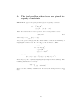
A The dual problem when there are primal inequality constraints 28
B Optimality conditions when there are primal inequality constraints
29
C Implementation files and their connections
30
D More Set Covering Problem (SCP) results
32
References
33
1
Introduction
In this report we want to solve problems of the type
min θ(u),
u ∈ U,
(1)
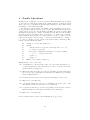
where θ : Rm → R is a convex and finite everywhere (nondifferentiable) function
and U is a nonempty convex subset of Rm . One of the most important classes of
these problems is Lagrangian duals, there θ is given implicitly by a maximization
problem where u is a parameter (called Lagrangian multiplier ). We will assume
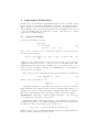
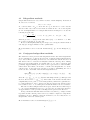
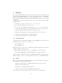
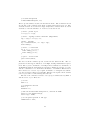
in this report that we have an oracle, which returns θ(u) and one subgradient
g(u) of θ at u, for any given u ∈ U , see Figure 1. Because of the strong
connection with Lagrangian duals, algorithms solving (1) are often referred to
as dual algorithms.
In bundle methods one stores information θ(ui ), g(ui ) about previous iterations in a set β, the bundle, to be able to choose a good descent direction
d along which the next points are generated. Having access to this ”memory”
makes it possible to construct a better search direction than so called subgradient
methods that only utilize the information from the present point.
In Chapter 2, we will describe Lagrangian relaxation, and see how it gives
rise to problems of the type (1). In Chapter 3, we describe different types of dual
algorithms, including bundle methods, that solve (1). Chapter 4 will be devoted
to a more detailed study of the bundle algorithm. Chapter 5 will contain the
manual for our bundle implementation.
θ()
“real” function
g(u 2 )
θ(u 2 )
1
1
θ(u 1 )
g(u 1 ) (negative)
g(u 3 )
θ(u 3 )
1
u1
u3
u2
u
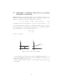
Figure 1: The function θ(u) is defined as the maximization of a
set of linear functions. These linear functions underestimate the
”real” function but are tight in the three points, u1 , u2 and u3 . Each
linear function is given by the oracle as a function value θ(u) and a
subgradient g(u) for any u ∈ U .
3
2
Lagrangian Relaxation
In this section we will describe Lagrangian relaxation. It is a technique to find
upper bounds on an arbitrary maximization problem. We will start with a
rather general problem and as the theory reveals itself, requirements will be
added. This is because we mostly are interested in problems that can be solved
to global optimality with the methods we describe. The theory is to a high
degree based on Lemaréchal [1].
2.1
General technique
Consider an optimization problem
max
s.t.
f (x),
x ∈ X ⊆ Rn ,
cj (x) = 0, j ∈ {1, . . . , m},
(2)
R and cj : Rn → R, hereafter called the primal problem. We
where f : Rn →
introduce the Lagrangian
L(x, u) := f (x) −
m
uj cj (x) = f (x) − u c(x),
(x, u) ∈ X × Rm ,
(3)
j=1
a function of the primal variable x and of the dual variable u ∈ Rm . The last
equality introduce the notation c for the m-vector of constraint values. The
Lagrangian has now replaced each constraint cj (x) = 0 by a linear ”price” to be
paid or received, according to the sign of uj . Maximizing (3) over X is therefore
closely related to solving (2).
The dual function associated with (2) and (3) is the function of u defined by
θ(u) := max L(x, u),
x∈X
u ∈ Rm ,
(4)
and the dual problem is then to solve
min θ(u).
u∈Rm
(5)
Lagrangian relaxation accepts almost any data f, X, c and can be used in
many situations. One example is when we have both linear and nonlinear constraints, some of them covering all variables, making it impossible to separate.
The only crucial assumption is the following; it will be in force throughout:
Assumption 1 Solving (2) is ”difficult”, while solving (4) is ”easy”. An oracle
is available which solves (4) for given u ∈ Rm .
Lagrangian relaxation then takes advantage of this assumption, and aims at
finding an appropriate u. To explain why this is the same as solving the dual
problem (5), observe the following: by the definition of θ,
θ(u) ≥ f (x),
for all x feasible in (2) and all u ∈ Rm ,
simply because u c(x) = 0. This relation is known as weak duality, which gives
us two reasons for studying the dual problem:
4
- θ(u) bounds f (x) from above. Minimizing θ amounts to finding the best
possible such bound.
- For the dual function (4) to be any good it must produce some argmax
xu of L(·, u) which also solves the primal problem (2). This xu must be
feasible in (2) and therefore satisfy θ(u) = f (xu ). From weak duality, we
see that the only chance for our u is to minimize θ.
Remark 1 Suppose the primal problem (2) has inequality constraints:
max
s.t.
f (x),
x ∈ X ⊆ Rn ,
cj (x) ≤ 0, j ∈ {1, . . . , m},
Then the dual variable u must be nonnegative and the dual problem becomes
min θ(u).
u∈Rm
+
To see why, read Appendix A. Rm changes to Rm
+ in all the theory above.
We can now draw the conclusion that the dual problem (5) fulfil the requirements of problem (1).
2.2
Minimizing the dual function
In this section we will state a very important theorem when minimizing the dual
function. The fundamental result is:
Theorem 1 Whatever the data f, X, c in (2) can be, the function θ is always
convex and lower semicontinuous 1 .
Besides, if for given u ∈ Rm (4) has an optimal solution xu (not necessarily
unique), then gu := −c(xu ) is a subgradient of θ at u:
θ(v) ≥ θ(u) + gu (v − u),
which is written as gu ∈ ∂θ(u).
for any v ∈ Rm ,
(6)
A consequence of this theorem is that the dual problem (5) is well-posed
(minimizing a convex function). We also see that every time we maximize
the Lagrangian (4) we get ”for free” the value θ(u) and the value −c(xu ) of a
subgradient, both important to solve the dual problem. Observe that −c(xu ) is
the vector of partial derivates of L with respect to u, i.e. ∇u L(xu , u).
As a result, solving the dual problem (5) is exactly equivalent to minimizing
a convex function with the help of an oracle [the dual function (4)] providing
function and subgradient values.
1 A function θ is lower semicontinuous if, for any u ∈ Rm , the smallest value of θ(v) when
v → u is at least θ(u):
lim inf f (y) ≥ f (x).
y→x
Lower semicontinuity guarantees the existence of a minimum point as soon as θ ”increases at
infinity”.
5
2.3
Primal-dual relations
How good is the dual solution in terms of the primal? We know that θ(u)
bounds f (x) from above, but when can we expect to obtain an optimal primal
solution when the dual problem (5) is solved?
2.3.1
Everett’s Theorem
Suppose we have maximized L(· , u) over x for a certain u, and thus obtained
an optimal xu , together with its constraint-value c(xu ) ∈ Rm ; set gu := −c(xu )
and take an arbitrary x ∈ X such that c(x) = −gu . By definition, L(x, u) ≤
L(xu , u), which can be written
f (x) ≤ f (xu ) − u c(xu ) + u c(x) = f (xu ).
Theorem 2 (Everett) With the above notation, xu solves the following pertubation of the primal problem (2):
max
s.t.
f (x),
x ∈ X ⊆ Rn ,
c(x) = −gu .
If gu is small in the above pertubed problem, xu can be viewed as approximately optimal. If gu = 0, we are done, xu is the optimal solution for the primal
problem (2).
2.3.2
Differential study of the dual function
In this section we will study the solutions of the dual function (4). We introduce
the notation
X(u) := {x ∈ X : L(x, u) = θ(u)},
G(u) := {g = −c(x) : x ∈ X(u)},
(7)
for all solutions xu for a certain u and its image through ∇u L. Because a
subdifferential is always a closed convex set, we deduce that the closed convex
hull of G(u) is entirely contained in ∂θ(u). The question is if they are the same?
Definition 1 (Filling Property) The filling property for (2)–(4) is said to
hold at u ∈ Rm if ∂θ(u) is the convex hull of the set G(u) defined in (7).
So when does the filling property hold? The question is rather technical and
will not be answered in this report. But we will list some situations when it
does hold. To get a positive answer, some extra requirements of a topological
nature must be added to the primal problem (2):
Theorem 3 The filling property of Definition 1 holds at any u ∈ Rm
- when X is a compact set on which f and each cj are continuous;
- in particular, when X is a finite set (such as in the usual Lagrangian
relaxation of combinatorial problems);
6
- in linear programming and in quadratic programming;
- more generally, in problems where f and each cj are quadratic, or even
lp -norms, 1 ≤ p ≤ +∞.
When the filling property holds at u, any subgradient of θ at u can be written
as a convex combination of constraint-values at sufficiently but finitely many
x’s in X(u). For example
αk c(xk ),
g ∈ ∂θ(u) =⇒ g = −
k
where the αk ’s are convex mulitpliers, i.e.
k αk = 1 and αk ≥ 0, ∀k. A u
minimizing θ (5) has the property 0 ∈ ∂θ(u), which means that there exists
sufficiently many x’s in X(u) such that the c(x)’s have 0 in their convex hull:
Proposition 1 Let u∗ solve the dual problem (5) and suppose the filling property holds at u∗ . Then there are (at most m+1) points xk and convex multipliers
αk such that
αk c(xk ) = 0.
L(xk , u∗ ) = θ(u∗ ) for each k, and
k
Remark 2 Suppose the primal problem (2) has inequality constraints as in Remark 1. Then the property 0 ∈ ∂θ(u) is not a necessary condition for optimality.
It is instead enough (and also necessary) that the complementary conditions
u gu = 0,
u ≥ 0,
gu ≥ 0,
where gu ∈ ∂θ(u)
are fulfilled, which means that either uj or gj , for each j, has to be 0. To see
why, read Appendix B. Proposition 1 changes in the corresponding way.
2.3.3
The primal solution
With the use of the x’s and α’s from Propostion 1 we build the primal point
x∗ :=
αk xk .
(8)
k
∗
Under which conditions does x solve the primal problem (2)?
We will give the result in three steps with increasing requirements:
- If X is a convex set: then x∗ ∈ X. Use Everett’s Theorem 2 to see to
what extent x∗ is approximately optimal.
- If, in addition, c is linear: then
c(x∗ ) =
αk c(xk ) = 0
k
and thus x∗ is feasible. Because L(x∗ , u∗ ) = f (x∗ ) − (u∗ ) c(x∗ ) = f (x∗ ),
the duality gap θ(u∗ ) − f (x∗ ) tells us to what extent x∗ is approximately
optimal in (2). Remark: If the primal problem (2) has inequality constraints it is enough if c is convex.
7
- If, in addition, f is concave and thus L is concave then
αk L(xk , u∗ ) = θ(u∗ ).
f (x∗ ) = L(x∗ , u∗ ) ≥
k
Combine this with weak duality and x∗ is optimal.
Remark 3 Observe that the algorithm solving the dual problem has no information about the above requirements. If X is not a convex set, X will be enlarged
to its convex hull. It is then up to the user of Lagrangian duality, with the help
of the list above, to analyze the optimality of the solution.
Remark 4 If X is a convex set, the equality constraints are linear, the inequality
constraints are convex and f is concave then x∗ from (8) [with α from Proposition
1] is optimal.
3
Dual Algorithms
In this section we will forget about the primal problem (2) and focus on methods
solving the dual problem (5). First we will restate Assumption 1 with more
details about the problem we have to solve:
Assumption 2 We are given a convex function θ, to be minimized.
- It is defined on the whole of Rm .
- The only information available on θ is an oracle, which returns θ(u) and
one subgradient g(u), for any given u ∈ Rm .
- No control is possible on g(u) when ∂θ(u) is not the singleton ∇θ(u). Remark 5 If the primal problem (2) has inequality constraints, Rm changes to
Rm
+ in the assumption above and in all theory that follows in this section. We
will not remark on this further.
The third assumption above means that it is impossible to select a particular
maximizer of the Lagrangian, in case there are several. Also notice that the
assumptions above do not require the problems to be Lagrangian duals; any
problem that fulfills them can be solved with these algorithms.
Definition 2 (Bundle) The bundle β is a container of information about the
function θ:
θ(ui ), g(ui ), i ∈ {1, . . . , I},
where I is the number of pairs θi , gi in the bundle. Notice that different methods
store different numbers of pairs θi , gi ; thus I can be the number of iterations
made, or a lower number, i.e., we don’t save all pairs θi , gi that have been
generated.
There are essentially two types of methods, subgradient and cutting-plane
methods, lying at opposite sides of a continuum of methods. In between we
find, among others, bundle methods. We will first describe methods derived
from subgradients and then from cutting-planes. Last, we will present a scheme
visualizing the connections between the methods.
In the following, we will denote by gk the vector g(uk ) obtained from the
oracle at some iterate uk . Further we let uK be the current iterate.
8
3.1
Subgradient methods
Subgradient methods are very common because of their simplicity. At iteration
K, select tK > 0 and set
uK+1 = uK − tK gK .
No control is made on gK to check if it is a good direction or even a descent
direction. The only control of the method’s behaviour is to choose the stepsize
tK . In our implementation of a subgradient method in Chapter 5.5 we use the
following step-size rule:
tk ∈
µ
M ,
,
b+k b+k
b > 0,
0 < µ ≤ M < ∞,
k ∈ {1, . . . , K},
which is proved to converge in the sense that θ(uK ) → θ∗ when K → ∞. The
proof can be found in [2], pp. 295–296.
However, this simplicity has its price in speed of convergence and the method
can only give an approximation of the optimal value.
More information can be found in Lemaréchal [1], pp. 22–24; Frangioni [3],
p. 5.
3.2
Conjugated subgradient methods
The main theoretical problem with subgradient methods is that subgradients
are not guaranteed to be directions of descent. Conjugated subgradient methods
try to detect this by making an exact line search LS in the current direction. If
this direction is not of descent, LS will just return the current point ū. During
such a LS a new subgradient, in a neighbourhood of ū, can be generated: this
possibility suggests making some form of inner approximation of the subdifferential, where the bundle β is meant to contain some subgradients of θ at the
current point. A new direction can then be found by minimizing the vector
norm over the convex hull of the known subgradients at ū:
gi ϕi : ϕ ∈ Φ} = min {g : g ∈ conv({gi : i ∈ β})},
(9)
min {
ϕ
i∈β
g
where Φ = {ϕ : i∈β ϕi = 1,
ϕ ≥ 0} is the unit simplex in the |β|-dim space and
the new direction is d = − i∈β gi ϕi . The result of the iteration is thus either
a significantly better point u, or a new subgradient g which is not guaranteed to
be a subgradient in ū, but to yield a new direction in the next iteration; since
it is obtained ”close” to ū, it still gives relevant information about θ around ū.
The base for this technique is that the steepest descent direction with respect
to θ at u is the minimum norm vector g ∈ ∂θ(u); the problem (9) is therefore
an approximation of the problem of finding the steepest descent direction.
A major drawback with this method is that every time a good improvement
is possible and the current point ū is moved, β must be emptied, loosing all the
information about θ. This is because the elements of β do not really need to be
subgradients of the new current point.
More information can be found in Frangioni [3], pp. 5–6.
9
3.3
ε-subgradient methods
Instead of using the somewhat nontheoretical rules, by which subgradients are
used in the conjugated subgradient methods, we can instead define approximate
subgradients, as follows:
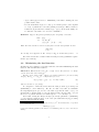
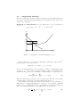
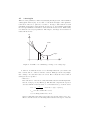
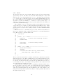
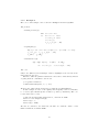
Definition 3 (ε-subgradient) Let ε ≥ 0. The vector g is an ε-subgradient of
θ at u if
θ(v) ≥ θ(u) + g (v − u) − ε, for any v ∈ Rm .
θ()
α
ε
g
v
u
Figure 2: ε-subgradient g and its linearization error α.
Now we fix some ε > 0 and solve (9) further restricted to the known εsubgradients at the current point ū:
min {g : g ∈ conv({gi : αi ≤ ε, i ∈ β})},
g
where α is the linearization error, see Figure 2. Instead of eliminating all the
gi ’s with αi > ε, the αi can be used as ”weights” of the corresponding vector.
In that way any gi with a big α will have a ”small influence” on the direction:
min {
gi ϕi :
αi ϕi ≤ ε, ϕ ∈ Φ}.
(10)
ϕ
i∈β
i∈β
This is the first method referred to as a bundle method. The size of the bundle
β is much larger compared to the subgradient methods above.
The critical part of this approach is the introduction of the parameter ε,
which has to be dynamically updated to achieve good performance. This has
turned out to be difficult and it is not clear what sort of rules that should be
used. For example, this further ”smoothing” has been introduced:
1 gi ϕi 2 +
αi ϕi : ϕ ∈ Φ},
min { t
ϕ
2
i∈β
i∈β
10
(11)
which can be viewed as a Lagrangian relaxation of (10) (with some additional smoothing) where 1/t is a parameter used to dualize the constraint
i∈β αi ϕi ≤ ε.
Now, we have t instead as a parameter which has turned out to be a little easier to update than ε. Different rules for updating t are explained in Chapter 4.1.
More information can be found in Frangioni [3], pp. 6–8.
3.4
Cutting-plane methods
In this section we will present another type of methods, in which a piecewise
affine model of θ will be minimized at each iteration.
Every result from the oracle, with uk as input, defines an affine function
approximating θ from below:
θ(u) ≥ θ(uk ) + gk (u − uk ),
for all u ∈ R,
where gk ∈ ∂θ(u), with equality for u = uk . After K iterations we can construct
the following piecewise affine function θ̂ which underestimates θ:
θ(u) ≥ θ̂(u) := max {θ(ui ) + gi (u − ui ) : i ∈ β},
for all u ∈ R.
The problem is now to calculate an optimal solution (uK+1 , rK+1 ) to
min r,
(u, r) ∈ Rm+1 ,
r ≥ θ(ui ) + gi (u − ui ),
for all i ∈ β.
(12)
The next iterate is uK+1 , with its model-value θ̂(uK+1 ) = rK+1 . A new call
to the oracle with uK+1 gives a new piece θ(uK+1 ), g(uK+1 ) to the bundle,
improving (raising) the model θ̂ and the process is repeated.
The nominal decrease, defined as
δ := θ(uK ) − rK+1 = θ̂(uK ) − θ̂(uK+1 ) ≥ 0,
(13)
is the value that would be reduced in the true θ if the model were accurate. It
can also be used to construct bounds for the optimal value:
θ(uK ) ≥ min θ ≥ θ(uK ) − δ = rK+1 ,
and can therefore be used as a stopping test: the algorithm can be stopped
as soon as δ is small. Observe that the sequence {θ(uK )} is chaotic while the
sequence {rK } is nondecreasing and bounded from above by any θ(u). We can
therefore say that rK → min θ.
The main problem with these methods is that an artificial box constraint
has to be added to (12), at least in the initial iterations, to ensure a finite solution. (Think of K = 1: we get r2 = −∞ and u2 at infinity.) The cutting-plane
algorithm is inherently unstable and it is very difficult to find ”tight” enough
box constraints that do not ”cut away” u∗ .
More information can be found in Lemaréchal [1], pp. 24–26.
11
3.5
Stabilized cutting-plane methods
To get rid of the unstable properties in (12), we introduce a stability center
ū: a point we want uK+1 to be near. We choose a quadratic stabilizing term,
u−ū2 , whose effect is to pull uK+1 toward ū, thereby stabilizing the algorithm.
We then let t > 0 (dynamically if we want) decide the effect of the stabilizing
term:
1
(14)
θ̆(u) := θ̂(u) + u − ū2 , for all u ∈ Rm .
2t
Minimizing θ̆ over Rm is equivalent to the quadratic problem
1
u − ū2 , (u, r) ∈ Rm+1 ,
2t
r ≥ θ(ui ) + gi (u − ui ), for all i ∈ β,
min r +
(15)
which always has a unique optimal solution (uK+1 , rK+1 ). The two positive
numbers
δ := θ(ū) − θ̂(uK+1 ),
1
δ̆ := θ(ū) − θ̆(uK+1 ) = δ − uK+1 − ū2 ,
2t
still represent the expected decrease θ(ū) − θ(uK+1 ).
To complete the iteration, we have to update the stability center ū. This
will only be done if the improvement is large enough relative to δ:
θ(uK+1 ) ≤ θ(ū) − κδ,
κ ∈]0, 1[,
(16)
κ being a fixed tolerance. The bigger κ, the better must the model θ̂ be to
satisfy the condition; if satisfied: ū = uK+1 . If the condition is not satisfied, we
will at least work with a better model θ̂ in the next iteration. This is the key
concept in bundle methods.
The bundle β is updated after each iteration. The new element θK+1 , gK+1 from the oracle is added, while old information is deleted if not in use for a
certain time. For example, if an element θi , gi ∈ β from a previous iteration
does not define an active piece of the model defined by θ̂ during many iterations,
in other words, strict inequality holds in the corresponding constraint in (15)
for several consecutive iterations. Then we may conclude that it is unlikely that
it will be part of the final model θ̂ that defines an optimal solution.
The last piece to study is the stopping test. Because uK+1 minimizes θ̆
instead of θ̂, and because θ̆ need not to be smaller than θ, neither δ nor δ̆ are
good stop indicators. But uK+1 minimizes the model (14), which is a convex
function and therefore:
1
0 ∈ ∂ θ̆(uK+1 ) = ∂ θ̂(uK+1 ) + (uK+1 − ū)
t
=⇒ uK+1 − ū = −tĝ for some ĝ ∈ ∂ θ̂(uK+1 ),
which reveals that ĝ = (ū − uK+1 )/t and can be calculated. Thus we can write
for all u ∈ Rm :
θ(u) ≥ θ̂(u) ≥ θ̂(uK+1 ) + ĝ (u − uK+1 )
= θ(ū) − δ + ĝ (u − uK+1 ),
12
(17)
with the conclusion that we can stop when both δ and ĝ are small.
How effective these methods are depend crucially on how t is dynamically
updated, which leads to t-strategies, studied in Chapter 4.1.
More information can be found in Lemaréchal [1], pp. 28–30.
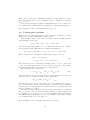
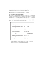
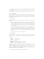
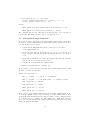
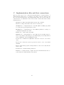
3.6
Method connection scheme
Here follows a connection scheme that reveals how the methods described are
related to each other. Observe how the parameter t can be used to move between
them. All methods, except subgradient methods (bundle size = 1), are variations
of bundle methods because they store data about previous iterations. But in
the literature, it is often only methods based on the two subproblems (11) and
(15) that are referred to as bundle methods. Also notice that (11) and (15) are
dual to each other and therefore in reality, the same.
Subgradient method
↓
Conjugated subgradient method
(9)
↓
(10)
ε-subgradient method
t →∞
+
(11)
Lagrangian relaxation
Bundle methods
dual
Stabilized cutting-plane method
(15)
t →∞
↑
(12)
Cutting-plane method
Figure 3: Method connection scheme, where (9), (10), etc. represent
the subproblems in the stated methods in the figure.
13
4
Bundle Algorithms
In this section we will take a closer look at the bundle algorithm, based on (11)
or (15), the two dual subproblems in the bundle methods. A subsection will
also be devoted to t, the single most important parameter for the behaviour and
performance of the bundle algorithm.
As described earlier, bundle algorithms collect information θ(ui ), g(ui )
about previous iterations in a set β, the bundle. The information is given by
a user-created oracle, the only information available about the problem. This
information is then used to compute a tentative descent direction d along which
the next points are generated. Since d need not to be a direction of descent,
bundle methods use some kind of control system to decide to either move the
current point ū (SS, a Serious Step), or use the new information to enlarge β
to be able to compute a better d at the next iteration (NS, a Null Step). Here
follows a generic bundle algorithm:
01
initiate ū, β, t and other parameters ;
02
repeat
03
find new direction d, generate a new trial point u = ū + τ d ;
04
oracle(u) =⇒ θ(u), g(u);
05
if ( a large enough improvement has been obtained ) then
06
07
08
09
ū = u;
// SS, else it is a NS
update β ;
update t ;
until ( some stopping condition );
Explanations to some of the rows:
01: ū is usually set to all zeros and a call to the oracle gives the first piece to
β. Other parameters control strategies for β and t, as well as decide the
precision in the stopping test.
03: This is the same as solving one of the two quadratic problems, (11) with a
line search or (15). A fast QP -solver is therefore a must in a good bundle
method implementation.
04: A call to the user-created oracle gives new information about θ at u.
05: This can be a test like (16).
07: β is updated with the new piece of information from the oracle. Old
information is deleted if not in use for a certain time.
08: t is updated, increased or decreased, depending on the model’s accuracy.
Further details are found in the next subsection: t-strategies.
09: This can be a test like (17).
A more detailed version can be found in Frangioni [3], pp. 63–70.
14
4.1
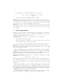
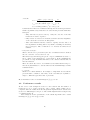
t-strategies
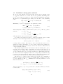
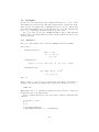
What does the parameter t affect? By studying the subproblem of the stabilized
cutting-plane method (15), we see that t controls the strength of the quadratic
term whose effect is to pull uK+1 toward ū. A large t will result in a weak
stabilization and will be used when the model is good, and a small t will result
in a strong stabilization and will be used when the model is bad. This is why
t is called the trust-region parameter. The larger t, the larger area around ū is
trusted in the model.
θ()
small t
large t
u
u
u K+1
u K+1
Figure 4: A small t =⇒ a small step. A large t =⇒ a large step.
So when do we trust the model or not? A simple answer is ”yes” when a SS
has occurred and ”no” when a N S has occurred. This give us the very simple
rule: enlarge t if a SS and reduce t if a N S. Here follows the most common
strategies used to update t:
- Heuristics:
Here follows two of the most common heuristics used in bundle implementations, both proposed by Kiwiel [4]. The first rule compares the expected
decrease with the actual decrease, i.e., it measures how good the model is:
δ
, there ∆θ = θ(ū) − θ(uK+1 ),
2(δ − ∆θ)
is reduced when ∆θ < 0.5δ,
is enlarged when ∆θ > 0.5δ.
tnew = t
tnew
tnew
Observe that this is the same test as (16), the SS test, with κ set to 0.5.
The second rule is based on checking if the tentative new step is of descent
15
or ascent:
tnew = t
2α
2(∆θ − g (ū − uK+1 ))
=t
,
2∆θ − g (ū − uK+1 )
α + ∆θ
tnew is reduced when g (ū − uK+1 ) > 0,
tnew is enlarged when g (ū − uK+1 ) < 0.
Combinations of these two heuristics build up the most strategies used in
bundle algorithms today. But there are some known problems with these
strategies:
- They lack any long-term memory. Only the outcome of the last
iterations are used to update t.
- Only relative increments are measured, and the absolute magnitude
of the obtainable increments is disregarded.
- After some initial iterations, t starts to rapidly decrease and soon
the algorithm is working with a very small t, resulting in extremely
slow convergence. The conditions for t to increase are almost never
satisfied.
- Long-term strategies:
Tries to fix the above problems by the use of heuristics and are divided
into two versions: one hard and one soft.
The hard long-term strategy keeps an ”expected minimum decrease” ε̄,
the so called ”long-term memory” of the method. If the maximum improvement of a step is smaller than this ε̄, it is considered useless and t is
increased instead.
The soft version also tries to avoid small t’s, but rather than forcing t to
increase it just inhibits t to decrease whenever the maximum improvement
is smaller than ε̄.
- t constant:
Shall not be underestimated. It is simple to implement and avoids the
problem with too small t’s, but it has, on the other hand, no dynamic to
adapt to different types and scales of problems.
More information can be found in Frangioni [3], pp. 63–70.
4.2
Performance results
At the end of each example in Section 5.3 the solution and the number of
iterations it took to reach convergence can be found. These results can be
compared with the results from the subgradient implementation described in
Section 5.5. This will give some proof of the bundle implementation’s superiority
over simpler methods.
More results about the performance of the bundle algorithm can be found
in Frangioni [3], pp. 46–50, pp. 69–70.
16
5
Manual
The bundle implementation is built around professor Antonio Frangioni’s [3]
code developed during his Ph.D. research. It’s written in C++ and is highly
advanced with many settings not covered in this report. The code is built to
work on a UNIX system and demands that ILOG CPLEX, version 8 (or newer),
is installed.
Here follows a list of steps necessary to solve a problem with this bundle
implementation:
0: Relax the problem you want to solve. See Section 2.1.
1: Do some preparations. See Section 5.1.
2: Create an oracle (Oracle.h and Oracle.C), or copy one of the five provided examples. Put the files in the Bundle directory. See Section 5.2.1.
3: Optional, modify initial parameters. See Section 5.2.2.
4: Optional, modify Main.C to change the printouts. See Section 5.2.3.
5: Compile the program with the command: make.
6: Run the program with the command: bundle.
5.1
Preparations
You will need the following files: Bundle.tar and Examples.tar. Start by unpacking them into a directory of your choice:
tar xvf Bundle.tar
tar xvf Examples.tar
This will create two directories containing the bundle implementation and the
examples explained in Section 5.3.
The CPLEX environment needs to be initialized once before its use:
setenv ILOG_LICENSE_FILE /usr/site/pkg/cplex-8.1/ilm/access.ilm
Observe that it contains the path to the CPLEX installation which may have
changed. This row can be copied and pasted from the top of the Makefile file.
5.2
Files
There are many files in the implementation but there are mainly four files the
user will have to interact with, these are:
- Oracle.C: The only file containing information about the problem.
- Oracle.h: Oracle header file.
- Parameters: Contains initial parameters.
- Main.C: Controls, among other things, the printouts.
For a description of all the files and their connections, see Appendix C.
17
5.2.1
Oracle
As described earlier, the oracle returns a function value θ(u) and a subgradient
g(u) for any u ∈ Rm . We have also seen, that when solving the ”easy” dual
function (4), we get this information for ”free”. But still, the problem has
to be solved and for this task we have chosen ILOG CPLEX. This gives us
the obvious limitation: the maximization problem defining the dual function
(4) must be solvable in CPLEX, i.e. it must be a linear problem (LP) or a
quadratic problem (QP) or a linear integer problem (LIP). More information is
found in the CPLEX manual [5].
The technique we use to represent problems is called ILOG Concert Technology and is a C++ library of classes and functions making it easy to input
various problems. We will describe this technique through some guided examples in Section 5.3, but for more details you have to read the CPLEX manuals
[6] and [7].
The oracle is a C++ class made up by two files, Oracle.h and Oracle.C.
Oracle.h contains the class declarations and Oracle.C, the class implementations. Here follows a compressed Oracle.h:
01
class Oracle
02
{
03
private:
//----- Private ----------------------------------
04
IloEnv env;
05
IloModel model;
06
...
07
IloInt uSize;
08
IloInt xDims;
09
...
10
public:
// Global Concert Technology variables
// Global necessary variables
//----- Public ------------------------------------
11
Oracle(char* filename);
12
~ Oracle();
13
void Solve(const double uVector[], double &fValue,
14
double sgVector[], double xVector[]);
15
16
...
}
The problem is modelled in the constructor Oracle (row 11) and solved in the
function Solve (row 13). The communication between them is handled by the
global variables in the private part of the declaration. Because the constructor
is only run once and Solve is run every time the algorithm asks for a new piece
to the bundle, we try to do as much work as possible in the constructor, such
as reading data and creating the model.
Observe that the constructor takes one argument, a filename, which can be
used if you build a solver for a class of problems with data read from different
files. The function Solve takes a u as in parameter and returns the function
value θ(u), the subgradient g(u) and the primal x-point of the solution to the
inner problem in (4). The x-point is necessary to build a primal solution when
the dual is found as in (8).
18
The details of how to create an oracle are explained in the provided examples,
see Section 5.3. The easiest way to create your own oracle is to modify one of
these examples.
Last, put the two files, Oracle.h and Oracle.C, in the bundle directory.
5.2.2
Parameters
The file Parameters contains initial settings and can be left untouched. The
settings control the bundle size, the t-strategy, the stopping conditions and
some other features. A full description of each parameter can be found in the
file bundle.h, row 227.
5.2.3
Main.C
The Main.C file initiates and creates all parts of the program. It contains three
sections:
- Create: Creates the oracle and the solver object. The x-matrix, containing all the primal solutions, is also created. Notice that x can at most
have two indexes. If you want more indexes you have to add this to the
code. But observe that the memory use increases exponentially with the
number of indexes.
- Solve: Here is the optimal value, the dual solution and the primal solution
printed. The primal solution is calculated as a convex combination of the
saved solutions in the x-matrix as in (8). The multipliers, αk ’s, are given
by the solver object. More about this can be found in the file bundle.h,
row 600.
- Delete: All the created objects are destroyed.
5.2.4
Makefile
The file Makefile contains all the compiler directives and links all the files
together with the ILOG CPLEX environment. The most important rows are
these:
# System
SYSTEM
LIBFORMAT
= ultrasparc_5_5.0
= static_pic_mt
# CPLEX directories
CPLEXDIR
= /usr/site/pkg/cplex-8.1/cplex81
CONCERTDIR = /usr/site/pkg/cplex-8.1/concert13
The first two describe the system and the last two contain the paths to ILOG
CPLEX and ILOG Concert Technology. If the system is updated or a new
version of CPLEX is installed these settings have to be changed. If so, try to
find the correct Makefile for all examples CPLEX sends along each system and
version. The current ones can be found in:
<cplex81 directory>/examples/<machine>/<libformat>
19
5.3
Examples
In this section we will present some examples showing how to create oracles
with ILOG Concert Technology. The first example will be explained in detail,
while only the new things will be highlighted in the second one. All the files
are found in the Example directory unpacked in Section 5.1. The examples will
also be a good starting point when creating your own oracles.
It’s good to have access to the CPLEX manuals [6] and [7], while studying
the files. Any code starting with Ilo is either a class or function in the Concert
Technology library.
5.3.1
Example 1
The code to this example can be found in: <Examples directory>/EX1
The problem:
- Primal problem (2):
max
x1 + 2x2 ,
s.t. x1 + 4x2 ≤ 8,
0 ≤ x ≤ 4.
- Lagrangian (3):
L(x, u) := x1 + 2x2 − u(x1 + 4x2 − 8),
0 ≤ x ≤ 4,
u ∈ Rm .
- Dual function (4):
θ(u) = max L(x, u),
x
u ∈ Rm
s.t. 0 ≤ x ≤ 4.
The code:
First we have to create the Concert Technology environment, an instance of
IloEnv, to handle memory management for all Concert Technology objects:
IloEnv env;
This variable has to be available in all functions and is therefore declared in
the private part of the Oracle.h file.
Now we can start with the model, located in the constructor. First the basic
variables:
// m (rows), n (cols)
m = 1;
n = 2;
// x (primal variables)
x.add(IloNumVarArray(env, n, 0, IloInfinity));
20
// u (dual multipliers)
u.add(IloNumVarArray(env, m));
All are global variables declared in the Oracle.h file. The elements m and n
are the size of the x-matrix, used when creating arrays and in for-loops. The
elements x and u are declared as empty arrays and to initiate them we add n
elements to x and m elements to u. Now let’s create the model:
// model: primal object
cx = x[0] + 2 * x[1];
// model: lagrange relaxed constraint (subgradient)
lag = -(x[0] + 4 * x[1] - 8);
//model: maximize
obj = IloMaximize(env, cx + u[0] * lag);
model.add(obj);
// model: x constraints
for (j = 0; j < n; j++) {
model.add(x[j] >= 0);
model.add(x[j] <= 4);
}
// cplex: extract model
cplex.extract(model);
Also here is all the variables global, declared in the Oracle.h file. The expressions cx and lag are instances of IloExpr, holding mathematical expressions. The objective, an instance of IloObjective, is initiated to an instance of
IloMaximize with the Lagrangian as expression. Finally we add the objective
and the constraints of x to the model, an instance of IloModel. This model is
then extracted to a solver object cplex, an instance of IloCplex, used whenever the problem is a linear program (LP). Whenever we update the model this
solver object will be notified and updated as well.
The rest of the constructor is used to set a group of variables used by Main.C
and the solver object. These are:
// u size
uSize = m;
// x dimensions and size
xDims = 1;
xDim1Size = n;
// Add all unconstrained multipliers u, and with an InINF
ucVector = new unsigned int[1];
ucVector[0] = InINF;
// Is the primal problem of min type
isMinProblem = false;
21
The most of them are obvious, but the ucVector will need some explanations.
The bundle algorithm must know which u’s are constrained and which are not.
All u’s are constrained to Rm
+ as default, i.e. the primal problem (2) has inequality constraints. This is true for this example so all we have to do is to
put the stop value InInf in the first position of the ucVector. If the problem
has equality constraints we have to add the corresponding u’s to the ucVector.
Example 2 will show an example of this.
Now we are ready to study the code solving the model. This is done in the
Solve function which is called every time the algorithm needs a new piece to
enlarge the bundle. The first thing we have to do is to update the model:
// Update u
u.clear();
for (i = 0; i < m; i++)
u.add(uVector[i]);
// Update model
model.remove(obj);
obj = IloMaximize(env, cx + u[0] * lag);
model.add(obj);
u is updated and the old objective is removed. The same code as above creates
the new objective and is added to the model.
The cplex object is automatically updated with the ”new” model and we
can now solve it:
// Solve model
cplex.solve();
The last thing to do is to create the return values of the function Solve, the
objective value θ(u), the subgradient g(u) and the x-point:
// fValue
fValue = cplex.getValue(obj);
// sgVector
sgVector[0] = cplex.getValue(lag);
// xVector
for (j = 0; j < n; j++)
xVector[j] = cplex.getValue(x[j])
Here we use the function getValue(), not only to read the objective, but also to
read the current values of different parts of the model like lag and the x-point.
The rest of the code is left to the user to study. It contains some code for
printouts and some necessary get-functions for the class.
Results:
Optimal solution in 5 iterations.
f = 6,
22
x = [4, 1],
u = [0.5].
5.3.2
Example 2
The code to this example can be found in: <Examples directory>/EX2
The problem:
- Primal problem (2):
min 3x1 + 5x2 − 4x3 ,
s.t. 2x1 + x3 = 6 relax,
x1 + 2x2 ≥ 4 relax,
x2 + 3x3 ≤ 6,
x1 , x2 , x3 ∈ {1, . . . , 10}.
- Lagrangian (3):
L(x, u) := 3x1 + 5x2 − 4x3 + u1 (2x1 + x3 − 6) + u2 (4 − x1 − 2x2 );
x2 + 3x3 ≤ 6, x1 , x2 , x3 ∈ {1, . . . , 10},
u 1 ∈ Rm , u 2 ∈ Rm
+.
- Dual function (4):
θ(u) = min L(x, u),
x
u 1 ∈ Rm ,
s.t. x2 + 3x3 ≤ 6,
u 2 ∈ Rm
+,
x1 , x2 , x3 ∈ {1, . . . , 10}.
The code:
Only some differences from Example 1 will be highlighted, the rest follow the
same structure as before.
When we define the primal x variables we can set the bounds directly instead
of giving them as constraints to the model:
// x (primal variables)
x.add(IloIntVarArray(env, n, 0, 10));
We have also defined them as integers, by using the IloIntVarArray.
In this example we have both equality and inequality relaxed constraints,
i.e. u1 is free (unconstrained) and u2 must be positive (constrained). The code
for the ucVector becomes:
// Add all unconstrained multipliers u, and with an InINF
ucVector = new unsigned int[2];
ucVector[0] = 0;
ucVector[1] = InINF;
We add one element to the ucVector, the first one, with the ”name” 0 and
finish off with the end mark InINF.
23
The bundle algorithm always expects a max problem to be solved, but in
the current example we have a min problem. The solution to this is to change
the sign of the function value and the subgradient when returned in the Solve
function:
// fValue (with "-" because min problem)
fValue = -cplex.getValue(obj);
// sgVector (with "-" because min problem)
sgVector[0] = -cplex.getValue(lag1);
sgVector[1] = -cplex.getValue(lag2);
Results:
Optimal solution in 5 iterations.
f = 4.30769,
x = [2.15385, 0.923077, 1.69231],
24
u = [0.0769231, 3.15385].
5.4
Tutorials
Three of the provided examples are tutorials solving two groups of problems,
Set Covering Problems (SCP) and Generalized Assignment Problems (GAP).
For GAP we have created two different lagrangian relaxations, with different
performances as result.
To run these examples you have to follow the same list as before with some
modifications. Step 0 will of course not be necessary. In step 2 you will not only
copy the oracle files, but also some data file. You find other data files at [8]. In
step 6 will the run-command change to: bundle <data file>.
Set Covering Problem (SCP)
5.4.1
The code to this example can be found in: <Examples directory>/SCP
The problem:
- Primal problem (2):
n
min
j=1
n
s.t.
cj xj ,
aij xj ≥ 1
for i = 1, . . . , m,
j=1
xj ∈ {0, 1} for j = 1, . . . , n.
- Lagrangian (3):
L(x, u) :=
n
cj xj +
j=1
m
⎛
ui ⎝1 −
n
i=1
⎞
aij xj ⎠ ,
x ∈ {0, 1}n,
u ∈ Rm .
j=1
- Dual function (4):
θ(u) = min
x
s.t.
L(x, u),
u ∈ Rm ,
x ∈ {0, 1}n.
The format of the data files is:
1: Number of rows (m), number of columns (n).
2: The cost of each column c(j), j = 1, . . . , n.
3: For each row i (i = 1, . . . , m): the number of columns which cover row i
followed by a list of the columns which cover row i.
Results:
- scp41.txt: Optimal solution in 135 iterations. f = 429.
- small.txt: Optimal solution in 399 iterations. f = 1.6575e + 06.
(Increase the ”maximum value for t” parameter in the file Parameters
and see how this effects the number of iterations!)
- More results can be found in Appendix D.
25
5.4.2
Generalized Assignment Problem (GAP)
The code to this example can be found in: <Examples directory>/GAP[1/2]
The problem:
- Primal problem (2):
min
s.t.
m n
cij xij ,
i=1 j=1
m
xij = 1
i=1
n
for j = 1, . . . , n,
aij xij ≤ ri ,
for i = 1, . . . , m,
j=1
xij ∈ {0, 1} for
i = 1, . . . , m, j = 1, . . . , n.
- Dual function (4), GAP1:
θ(u) = min L(x, u) := min
x
x
s.t.
⎧
m n
⎨
⎩
cij xij +
i=1 j=1
n
n
uj
j=1
aij xij ≤ ri ,
for
m
xij − 1
i=1
⎫
⎬
⎭
,
i = 1, . . . , m,
j=1
xij ∈ {0, 1} for
i = 1, . . . , m, j = 1, . . . , n.
- Dual function (4), GAP2:
θ(u) = min L(x, u) := min
x
x
s.t.
⎧
m n
⎨
⎩
cij xij +
i=1 j=1
m
xij = 1
m
i=1
⎛
ui ⎝
n
j=1
⎞⎫
⎬
aij xij − ri ⎠ ,
⎭
for j = 1, . . . , n,
i=1
xij ∈ {0, 1} for i = 1, . . . , m, j = 1, . . . , n.
As can be seen, the two relaxations results in two different problems, the first
one can be recognized as the knap-sack problem and the second one as the simple
assignment problem. Which one is to prefer? One usually say that you shall not
relax ”too much” of the original problem, and in that case, the first relaxation
is the preferred one. Can this be seen in the result?
The format of the data files is:
1: Number of agents (m), number of jobs (n).
2: For each agent i (i = 1, . . . , m) in turn:
cost of allocating job j to agent i (j = 1, . . . , n).
26
3: For each agent i (i = 1, . . . , m) in turn:
resource consumed in allocating job j to agent i (j = 1, . . . , n),
resource capacity of agent i (i = 1, . . . , m).
Results:
- GAP1, gap11.txt: Near optimal solution in 48 iterations. f = 337.
- GAP2, gap11.txt: Solution in 18 iterations. f = 343.587.
The optimal solution is 336. The first problem is harder to solve, but gives a
better result. The answer is thus ”yes” to our question above.
5.5
Subgradient implementation
To be able to make comparisons between the bundle implementation and a simple method, we have implemented the subgradient method described in Section
3.1. Follow these steps to run it:
1: Unpack the file Subgradient.tar into a directory of your choice:
tar xvf Subgradient.tar
2: Create an oracle (Oracle.h and Oracle.C), or copy one of the five provided examples. Put the files in the Subgradient directory. See Section
5.2.1.
3: Optionally, modify Main.C to change the step-size rule and printouts. The
rule used is the one described in Section 3.1.
5: Compile the program with the command: make.
6: Run the program with the command: sg.
As you can see, you use it in the same way as the bundle implementation with
the same oracles as problem files.
Results after 1000 iterations:
- EX1: f = 6.04031,
x = [3.96, 1],
u = [0.506076].
- EX2: f = 4.25305,
x = [2.11, 0.906, 1.694],
u = [0.084553, 3.15582].
- SCP, scp41.txt: f = 427.264.
- SCP, small.txt: f = 52.3913.
- GAP1, gap11.txt: f = 357.375.
- GAP2, gap11.txt: f = 343.742.
If we compare these results with them from the bundle implementation, we
see that the optimal solution is never reached, even after 1000 iterations. The
subgradient implementation has also large problems to adapt to different scales
of problems, notice for example the SCP, small.txt. With these result as
proof, we can truly say that the bundle implementation is far superior to this
simple subgradient algorithm.
27
A
The dual problem when there are primal inequality constraints
Theorem 4 Suppose the primal problem (2) has inequality constraints:
max
s.t.
f (x),
x ∈ X ⊆ Rn ,
cj (x) ≤ 0,
j ∈ {1, . . . , m}.
Then the dual variable u must be positive and the dual problem becomes:
min θ(u),
u∈Rm
+
(18)
where θ(u) = maxx∈X f (x) − u c(x).
Proof. To get the form (2), introduce slack variable s and use the flexibility of
Lagrangian relaxation: set X̄ := X × Rm
+ , so that we have to dualize
max f (x),
s.t. x ∈ X ⊆ Rn ,
s ≥ 0 ∈ Rm ,
c(x) + s = 0 ∈ Rm .
The Lagrangian is
L̄(x, s, u) := f (x) − u (c(x) + s) = L(x, u) − u s
where L(x, u) is the ”ordinary” Lagrangian (as though we had equalities). The
resulting dual function θ̄ is clearly
+∞ if some uj < 0,
θ̄(u) =
θ(u) otherwise,
where θ is the ”ordinary” dual function. In a word, the dual problem becomes
(18).
28
B
Optimality conditions when there are primal
inequality constraints
Theorem 5 Suppose the primal problem (2) has inequality constraints as in
Theorem 4. Then the property 0 ∈ ∂θ(u) is not a necessary condition for optimality. It is instead enough if the complementary conditions,
u gu = 0,
g u ∈ R+ ,
u ∈ R+ ,
where gu ∈ ∂θ(u),
(19)
are fulfilled, which means that either uj or (gu )j has to be 0 for all j ∈ {1, . . . , m}.
Proof. We will show the condition for one dimension, then it’s easy to convince
us of the general case. Our problem is then to show the optimality conditions
when minimizing the convex 1-dimensional function:
min θ(u),
s.t. u ≥ 0.
We get two scenarios:
θ()
θ()
g u> 0
gu= 0
u
u
u>0
u=0
Figure 5: Two scenarios for optimality.
From the figures we can see that we have a minimum when either gu = 0
or u = 0 in combination with a gu > 0. The optimality conditions for one
dimension becomes: u · gu = 0, gu ≥ 0.
These conditions must be true for every dimension and the general case
becomes (19).
29
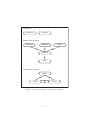
C
Implementation files and their connections
There are three types of C++ files in the implementation, .h (header files), .C
(implementation files) and .o (compiled object files). In some classes is only
the object file included and not the implementation file, the reason for this are
restrictions in code distribution. Here follows a list of all the files in the bundle
implementation:
- OPTtypes.h: Help class with standard types and constants.
- OPTvect.h: Help class with scalar and vector functions.
- CMinQuad.h/.o: Implementation of the TT (Tall and Thin) algorithm
for solving the typical Quadratic Problem.
- BMinQuad.h/.o: Implementation of the BTT algorithm for solving boxconstrained Quadratic Problems.
- Bundle.h/.o: The bundle algorithm.
- QPBundle.h/.o: Implementation of the (QP) direction finding subproblem for the Bundle class using the specialized (QP) solvers implemented
in the CMinQuad class and BMinQuad class.
- Solver.h/.C: Inherits the QPBundle class and connects to the Oracle
class.
- Oracle.h/.C: The user provided problem we want to solve. Uses ILOG
CPLEX.
- Main.C: The main program creating instances of the Solver class and the
Oracle class.
- Parameters: Contains initial parameters.
- MakeFile: Contains all the compiler directives and links all the files together with the ILOG CPLEX environment.
30
Used by all:
OPTtypes.h
OPTvect.h
Bundle solver structure:
CMinQuad
or
BMinQuad
Bundle
QPBundle
Solver
Main program structure:
Main.C
Solver
Oracle
Figure 6: Connection scheme for bundle implementation.
31
D
More Set Covering Problem (SCP) results
Here follow some more results produced with the SCP tutorial. Five problems with increasing size have been solved to optimality. Each problem has
been solved with three different strategies: pure heuristic, heuristic with soft
long-term strategy and heuristic with hard long-term strategy; all described in
Section 4.1.
All the example files can be found in: <Examples directory>/SCP. More
data files can be found at [8]. The parameter controlling the strategy of the
solver is found in the file Parameters.
Results:
File
scp45.txt
scp51.txt
scp61.txt
scpa1.txt
scpc1.txt
File size
20
44
44
95
167
kB
kB
kB
kB
kB
Iterations
heuristic soft
64
64
173 173
225 225
772 759
723 624
Optimal value
hard
123
257
228
437
317
512
251.225
133.14
246.836
223.801
As can be seen from these results, the long-term strategies (especially the
hard one) seem to be best on large problems and the pure heuristic seems to be
best on the smaller problems.
32
References
[1] C. Lemaréchal. Lagrangian Relaxation, Computational Combinatorial Optimization M. Juenger and D. Naddef (eds.) Lecture Notes in Computer
Science 2241, 115-160, Springer Verlag, 2001
[2] T. Larsson, M. Patriksson, A.-B. Strömberg. Ergodic, primal convergence
in dual subgradient schemes for convex programming, Math. Program. 86,
283-312, Springer Verlag, 1999
[3] A. Frangioni. Dual Ascent Methods and Multicommodity Flow Problems,
Ph.D. Thesis, Part 1: Bundle Methods, 1-70, 1997
[4] K.C. Kiwiel. Proximity Control in Bundle Methods for Convex Nondifferentiable Optimization, Math. Program. 46, 105-122, 1990
[5] ILOG. CPLEX 8.1, Getting Started, 2002
[6] ILOG. Concert Technology 1.3, User’s Manual, 2002
[7] ILOG. Concert Technology 1.3, Reference Manual, 2002
[8] J.E. Beasley. OR-Library: distributing test problems by electronic mail,
Journal of the Operational Research Society 41(11), 1069-1072, 1990
website: http://mscmga.ms.ic.ac.uk/info.html
33