Download Lunar Landing Trajectory Optimization with SOCS

Program lunland
Lunar Landing Trajectory Optimization with SOCS
This document is the user’s manual for a Fortran computer program called lunland that uses the
Sparse Optimal Control Software (SOCS) object code library developed by Boeing Phantom Works
(www.boeing.com/phantom/socs/) to solve the finite burn lunar landing trajectory optimization
problem. The trajectory is modeled as a single phase with user-defined initial and final boundary
conditions. This computer program attempts to maximize the final spacecraft mass, or minimize the
total flight time. The type of optimization is selected by the user.
The important features of this scientific simulation are as follows:

Automated deorbit delta-v algorithm

User-defined flight path angle and altitude at the descent interface

2-DOF flight path equations of motion relative to a spherical, non-rotating Moon

Thrust magnitude and thrust direction control variables
SOCS is a direct transcription method that can be used to solve a variety of trajectory optimization
problems using the following combination of numerical methods:

collocation and implicit integration

adaptive mesh refinement

sparse nonlinear programming
Additional information about the mathematical techniques and numerical methods used in SOCS
can be found in the book, Practical Methods for Optimal Control Using Nonlinear Programming by
John. T. Betts, SIAM, 2001.
The lunland software consists of Fortran routines that perform the following tasks:

main program that sets algorithm control parameters and calls the SOCS
transcription/optimal control subroutine

define problem definition and perform initialization related to scaling, lower and upper
bounds, initial conditions, etc.

evaluate the right-hand-side differential equations

define and compute any point and path constraints

display the optimal solution results
The SOCS software will use this information to automatically transcribe the user’s problem and
perform the optimization using a sparse nonlinear programming method. The software allows the
user to select the type of collocation method and other important algorithm control parameters.
With the appropriate substitution of fundamental constants, this simulation can also be used to
model landings on other airless celestial bodies.
page 1
Typical input file
The lunland software is “data-driven” by a user-created text file. The following is a typical input
file used by this computer program. In the following discussion the actual input file contents are in
courier font and all explanations are in times italic font.
This data file defines a typical descent analysis starting from a 100 kilometer circular lunar orbit
and ending at an altitude of 10 meters and a speed of 1 meter per second. This simulation
maximizes the final spacecraft mass.
Each data item within an input file is preceded by one or more lines of annotation text. Do not
delete any of these annotation lines or increase or decrease the number of lines reserved for each
comment. However, you may change them to reflect your own explanation. The annotation line
also includes the correct units and when appropriate, the valid range of the input. ASCII text input
is not case sensitive but must be spelled correctly.
The first six lines of any input file are reserved for user comments. These lines are ignored by the
software. However the input file must begin with six and only six initial text lines.
****************************************
** lunar landing trajectory optimization
** optimal thrust level and steering
** lunland1.in
** October 31, 2005
****************************************
The first program input is an integer that defines the type of trajectory optimization to perform.
type of trajectory optimization
*******************************
1 = maximize final mass
2 = minimize flight time
-----------------------1
The following series of data items are reserved for user-defined initial conditions. This information
includes initial flight conditions, propulsive characteristics and lower and upper bounds for the
thrust angle. Please note the units and valid data range for each item.
altitude of initial circular lunar orbit (kilometers)
100.0
altitude at descent interface (meters)
10000.0d0
flight path angle at descent interface (degrees)
-1.0d0
initial spacecraft mass (kilograms)
1000.0d0
maximum thrust (newtons)
5000.0d0
minimum thrust (newtons)
1000.0d0
page 2
specific impulse (seconds)
300.0d0
lower bound for thrust angle (degrees)
-90.0d0
upper bound for thrust angle (degrees)
+90.0d0
The following series of data items allow the user to define guesses for the final time, flight
conditions and spacecraft mass. To fix one or more conditions, the user should input identical
lower and upper bounds. Please note the units and valid data range for each item. Also note that
the final speed must be greater than zero.
**************************************
final time, mass and flight conditions
**************************************
initial guess for final time (seconds)
50.0
initial guess for final spacecraft mass (kilograms)
900.0d0
initial guess for final altitude (meters)
10.0d0
lower bound for final altitude (meters)
10.0d0
upper bound for final altitude (meters)
10.0d0
initial guess for final speed (meters/second)
1.0d0
lower bound for final speed (meters/second)
1.0d0
upper bound for final speed (meters/second)
1.0d0
initial guess for final flight path angle (degrees)
-90.0d0
lower bound for final flight path angle (degrees)
-90.0d0
upper bound for final flight path angle (degrees)
-90.0d0
The next series of program inputs are algorithm control options and parameters for the SOCS
software. The first input is an integer that specifies the type of collocation method to use during the
solution process. For most simulations, the trapezoidal method is recommended.
*********************************
discretization/collocation method
*********************************
1 = trapezoidal
2 = separated Hermite-Simpson
page 3
3 = compressed Hermite-Simpson
4 = Runge-Kutta 4-stage
-----------------------1
The next integer defines the number of initial grid points to use in the collocation modeling of the
descent trajectory.
number of initial guess grid points to use
25
The software also creates a comma-separated-variable (csv) ascii data file that contains the optimal
control solution and other flight parameters. The name of this output file is specified in the next
line of information. Please consult Appendix B for information about the contents of this file.
name of comma-delimited solution data file
lunland1.csv
This next input specifies the type of solution data file to create.
******************************************
type of comma-delimited solution data file
******************************************
1 = SOCS-defined nodes
2 = user-defined nodes
3 = user-defined step size
--------------------------1
For options 2 or 3, this input defines either the number of data points or the time step size of the
data output in the solution file.
number of user-defined nodes or print step size in solution data file
10.0
The next series of program inputs are algorithm control options and parameters for the SOCS
software.
****************************
algorithm control parameters
****************************
This input defines the relative error in the objective function.
relative error in the objective function (performance index)
1.0d-5
The next input defines the relative error in the solution of the differential equations.
relative error in the solution of the differential equations
1.0d-7
The next input is an integer that defines the maximum number of mesh refinement iterations.
maximum number of mesh refinement iterations
20
The next input is an integer that defines the maximum number of function evaluations.
page 4
maximum number of function evaluations
100000
The next input is an integer that defines the maximum number of algorithm iterations.
maximum number of algorithm iterations
10000
The level of output from the SOCS NLP algorithm is controlled with the following integer input.
***************************
sparse NLP iteration output
***************************
1 = none
2 = terse
3 = standard
4 = interpretive
5 = diagnostic
--------------2
The level of output from the SOCS optimal control algorithm is controlled with the following integer
input. Please note that option 4 will create lots of information.
**********************
optimal control output
**********************
1 = none
2 = terse
3 = standard
4 = interpretive
----------------1
The level of output from the SOCS differential equations algorithm is controlled with the following
integer input. Please note that option 5 will create lots of information.
****************************
differential equation output
****************************
1 = none
2 = terse
3 = standard
4 = interpretive
5 = diagnostic
--------------1
The level of output can be further controlled by the user with this final text input. This program
option sets the value of the SOCOUT character variable described in the SOCS user’s manual. To
ignore this special output control, input the simple character string no.
*******************
user-defined output
------------------input no to ignore
*******************
a0b0c0d0e0f0g0h0i0j1k0l0m0n0o0p0q0r0
page 5
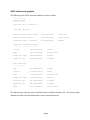
SOCS solution and graphics
The following is the SOCS trajectory summary for this example.
--------------program lunland
--------------input data file ==> lunland1.in
< maximize final mass >
initial circular orbit altitude
100.000000000000
kilometers
impulsive deorbit delta-v
23.1907400535548
meters/second
flight path angle at interface
-1.00000000000000
degrees
conditions at descent interface
------------------------------altitude
10000.0000000000
meters
speed
1693.20179797398
meters/second
flight path angle
spacecraft mass
-1.00000000000000
degrees
1000.00000000000
kilograms
time
355.040890866099
seconds
altitude
10.0000000000000
meters
speed
1.00000000000003
meters/second
final conditions
----------------
flight path angle
-90.0000000000000
degrees
spacecraft mass
555.640683701348
kilograms
propellant mass
444.359316298652
kilograms
deltav
1729.04078952476
meters/second
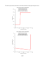
The following are trajectory plots created from the user-defined summary file. The first two plots
illustrate the behavior of the altitude and velocity during the descent.
page 6
Lunar Landing Trajectory Optimization
Maximize final spacecraft mass
10000
initial circular orbit altitude = 100 km
descent interface flight path angle = -1o
descent interface altitude = 10,000 meters
altitude (meters)
8000
6000
4000
2000
0
0
100
200
simulation time (seconds)
300
400
Lunar Landing Trajectory Optimization
Maximize final spacecraft mass
2000
initial circular orbit altitude = 100 km
descent interface flight path angle = -1o
descent interface altitude = 10,000 meters
velocity (meters/second)
1600
1200
800
400
0
0
100
200
simulation time (seconds)
page 7
300
400
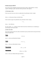
This next plot summarizes the flight path angle and spacecraft mass as a function of time since the
descent interface.
0
Lunar Landing Trajectory Optimization
flight path angle (degrees)
-20
Maximize final spacecraft mass
initial circular orbit altitude = 100 km
descent interface flight path angle = -1o
descent interface altitude = 10,000 meters
-40
-60
-80
-100
0
100
200
simulation time (seconds)
300
400
Lunar Landing Trajectory Optimization
Maximize final spacecraft mass
initial circular orbit altitude = 100 km
descent interface flight path angle = -1o
descent interface altitude = 10,000 meters
1000
spacecraft mass (kilograms)
900
800
700
600
500
0
100
200
simulation time (seconds)
page 8
300
400
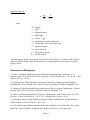
The final two plots illustrate the behavior of the thrust and thrust steering angle during the descent.
Lunar Landing Trajectory Optimization
Maximize final spacecraft mass
6000
initial circular orbit altitude = 100 km
descent interface flight path angle =-1o
descent interface altitude = 10,000 meters
5000
thrust (newtons)
4000
3000
2000
1000
0
0
100
200
simulation time (seconds)
300
400
Lunar Landing Trajectory Optimization
Maximize final spacecraft mass
80
initial circular orbit altitude = 100 km
descent interface flight path angle = -1o
descent interface altitude = 10,000 meters
thrust angle (degrees)
60
40
20
0
-20
0
100
200
simulation time (seconds)
page 9
300
400
Problem setup for SOCS
This section provides additional details about the SOCS software implementation. It briefly
explains such things as path constraints and the performance index options.
(1) Performance index
For the maximize final spacecraft mass optimization, the performance index is simply
J  mf
where m f is the spacecraft mass at the final time.
For the minimize flight time optimization, the performance index is simply
J  tf
where t f is the final time.
The value of the maxmin indicator in SOCS tells the software whether the user is minimizing or
maximizing the performance index.
(2) Path constraints
This section summarizes how the software bounds the trajectory characteristics and spacecraft mass
during the optimization.
altitude
0  h  hi
where hi is the user-defined initial altitude.
velocity
0.1  v  v0
where vi is the user-defined initial velocity.
flight path angle
900    900
spacecraft mass
0.05mi  m  1.05mi
where mi is the user-defined initial spacecraft mass.
page 10
Technical Discussion
Deorbit delta-v
The scalar magnitude of the deorbit maneuver that satisfies the user-defined altitude and flight path
angle at the descent interface is determined from the following expression:
V  Vce
where
r 
Vce 
hi  req
he  req
h
e




2  r  1 
1
1 

2
r 
 r 

 cos    1 

e 



 radius ratio

 req 
 local circular velocity at reentry altitude
 e  flight path angle at descent interface
hi  altitude of initial circular lunar orbit
he  altitude at descent interface
req  equatorial radius of the moon
  gravitational constant of the moon
This algorithm is described in “Deboost from Circular Orbits”, A. H. Milstead, The Journal of the
Astronautical Sciences, Vol. XIII, No. 4, pp. 170-171, Jul-Aug., 1966.
Equations of motion
The first-order, flight path equations of motion relative to a non-rotating, spherical Moon with the
propulsive thrust aligned opposite to the direction of motion are as follows:
altitude
dh
h 
 V sin 
dt
speed
dV
T cos 

 g sin 
V 
dt
m
flight path angle
 
d V
T sin  g cos 
 cos  

dt r
mV
V
page 11
propellant flow rate
m 
dm
T

dt
g e I sp
where
h
V
 

altitude
speed
flight path angle
thrust angle
g

r
T
m
ge 
gravity   r 2
gravitational constant of the moon
selenocentric radius of the spacecraft
propulsive thrust
spacecraft mass
Earth surface gravity
I sp  specific impulse
The thrust angle is defined with respect to the velocity of the vehicle. It is similar to the angle-ofattack for vehicles flying within an atmosphere. It is measured positive above the velocity and
negative below.
References and Bibliography
(1) “Direct Trajectory Optimization Using Nonlinear Programming and Collocation”, C. R.
Hargraves and S. W. Paris, AIAA Journal of Guidance, Control and Dynamics, Vol. 10, No. 4, JulyAugust, 1987, pp. 338-342.
(2) “Optimal Finite-Thrust Spacecraft Trajectories Using Direct Transcription and Nonlinear
Programming”, Paul J. Enright, Ph.D. Thesis, University of Illinois at Urbana-Champaign, 1991.
(3) “Improved Collocation Methods with Application to Direct Trajectory Optimization”, Albert L.
Herman, Ph.D. Thesis, University of Illinois at Urbana-Champaign, 1995.
(4) “Survey of Numerical Methods for Trajectory Optimization”, John T. Betts, AIAA Journal of
Guidance, Control and Dynamics, Vol. 21, No. 2, March-April 1998, pp. 193-207.
(5) “Parametric Study of Lunar Landing Techniques Using a Predetermined Thrust Orientation”,
Sam H. Harlin, Jr., NASA CR-61075, June 1965.
(6) “Powered Descent Guidance Methods for the Moon and Mars”, R. Sostaric and J. Rea, AIAA
2005-6287, AIAA Guidance, Navigation and Control Conference, 15-18 August 2005.
page 12
APPENDIX A
Compiling and Running the Software
This appendix describes how to compile and run the lunland computer program. This software
was created using version 6.3.3 of SOCS and Compaq Visual Fortran.
A DOS/Windows version of lunland using Compaq Visual Fortran version 6.6C can be created
with the following command:
df /arch:host lunland.f *.for c:\socs\socs633.lib advapi32.lib
This command assumes the SOCS library is located in the subdirectory c:\socs.
An input file created by the user can be run from the command line or a simple batch file with a
statement similar to the following:
lunland lunland1.in
If the software is executed without an input file on the command line, the computer program will
display the following information screen and file name prompt:
*************************************'
*
program lunland
*'
*
*'
*
lunar landing trajectory
*'
*
optimization with SOCS
*'
*
*'
*
October 31, 2005
*'
*************************************'
please input the name of the simulation definition file
The source code that reads the name of an input file included on the command line is
c
if present, use command line argument #1 for input file
call getarg(1, inputfname$, istatus)
The source code that creates the file name input prompt is as follows:
c
clear screen
isys = system("cls")
c
c
c
c
if (istatus .eq. -1) then
************************************************
input filename not on command line
request name of simulation definition input file
************************************************
print *, ' '
page 13
print *, ' '
print
print
print
print
print
print
print
print
print
print
&
*,
*,
*,
*,
*,
*,
*,
*,
*,
*,
'
'
'
'
'
'
'
'
' '
' '
*************************************'
*
program lunland
*'
*
*'
*
lunar landing trajectory
*'
*
optimization with SOCS
*'
*
*'
*
October 31, 2005
*'
*************************************'
print *,
'please input the name of the simulation definition file'
read (*, *) inputfname$
end if
If your compiler does not accept input from a command line, you will have to modify this source
code for your particular Fortran compiler. You may also choose to eliminate the code that accepts a
command line input file. Please note also that your compiler may have a different command to
clear the screen.
page 14
APPENDIX B
Contents of the Simulation Summary CSV File
This appendix is a brief summary of the information contained in the CSV data file produced by the
lunland software. The comma-separated-variable disk file is created by the odeprt subroutine
and contains the following information:
time (seconds) = simulation time since descent interface in minutes
altitude (meters) = altitude relative to a spherical Moon in meters
velocity (mps) = Moon-relative velocity in meters per second
fpa (degrees) = Moon-relative flight path angle in degrees
mass (kilograms) = spacecraft mass in kilograms
thrust (newtons) = propulsive thrust in newtons
thrust angle (deg) = thrust angle in degrees
deltav (mps) = accumulated delta-v in meters per second
downrange (meters) = downrange distance in meters
thrust-to-weight = ratio of thrust to weight in Earth g’s
Notes:
(1) The accumulated delta-v is determined from a cubic spline integration of the thrust acceleration
at all collocation nodes.
(2) The downrange distance is determined from a cubic spline integration of the range-rate at all
collocation nodes. The range-rate equation is given by
 
rm V cos 
rm  h
where rm is the radius of the Moon, h is the altitude, V is the velocity and  is the flight path angle.
page 15
APPENDIX C
Fortran Functions and Subroutines
This appendix is a brief summary of the major Fortran functions and subroutines included in the
lunland computer program.
lunland.f
- SOCS main executive program
atan3.for
- four quadrant inverse tangent function
csint.for
- cubic spline integration of tabular data subroutine
cdeorbit.for – subroutine that computes deorbit deltav
eci2orb.for
- convert eci state vector to classical orbital elements subroutine
odeinp.for
- SOCS simulation input subroutine
odeprt.for
- SOCS print subroutine – creates comma-separated-variable file
oderhs.for
- SOCS subroutine that evaluates the equations of motion and any
algebraic equations
orb2eci.for
- convert orbital elements to eci state vector subroutine
readfpn.for
- read and echo floating point number from an input file subroutine
readint.for
- read and echo an integer from an input file subroutine
readtext.for - read and echo text from an input file subroutine
utility.for
- number and text manipulation functions and subroutines
uvector.for
- unit vector subroutine
vcross.for
- vector cross product subroutine
vdot.for
- vector dot product subroutine
vecmag.for
- vector scalar magnitude function
xmod.for
- modulo 2 pi function
page 16
APPENDIX D
Example Fortran Subroutine
This appendix contains the source code for a single Fortran 77 routine and illustrates typical
programming conventions used in the lunland software. This subroutine is the differentialalgebraic equations routine required by the SOCS software.
subroutine oderhs(iphase, t, y, ny, p, np, f, nf, iferr)
c
c
computes the right hand sides of the
differential-algebraic (dae) equations
c
dynamic variables
c
c
c
c
c
c
c
c
y(1)
y(2)
y(3)
y(4)
=
=
=
=
altitude (meters)
velocity (meters/second)
flight path angle (radians)
mass (kilograms)
control variables
y(5) = thrust (newtons)
y(6) = thrust angle (radians)
************************************
implicit double precision (a-h, o-z)
include 'socscom1.inc'
integer iphase, ny, np, nf, iferr
dimension y(ny), p(np), f(nf)
c
set function error flag
iferr = 0
c
extract current flight conditions
altitude = y(1)
velocity = y(2)
fpa = y(3)
xmass = y(4)
c
extract current thrust (newtons)
thrust = y(5)
c
extract current angle-of-attack (radians)
alpha = y(6)
page 17
c
current spacecraft radius (meters)
rscm = rm + altitude
c
acceleration of gravity at altitude (m/s**2)
agrav = 1.0d9 * xmu / rscm**2
c
altitude derivative (meters)
f(1) = velocity * sin(fpa)
c
velocity derivative (meters/second)
f(2) = -agrav * sin(fpa) - thrust * cos(alpha) / xmass
c
flight path angle derivative (radians)
f(3) = ((velocity / rscm) - (agrav / velocity)) * cos(fpa)
&
- thrust * sin(alpha) / (xmass * velocity)
c
propellant flow rate (kg/sec)
f(4) = -thrust / vexhaust
return
end
page 18