1
Seasoft V2: Seasave V7 CTD Real-Time Data Acquisition Software for Windows XP, Windows Vista, or Windows 7 User’s Manual Sea-Bird Electronics, Inc. 13431 NE 20th Street Bellevue, Washington 98005 USA Telephone: 425-643-9866 Fax: 425-643-9954 E-mail: [email protected] Website: www.seabird.com 03/18/14 Software Release 7.23.2 and later Limited Liability Statement Extreme care should be exercised when using or servicing this equipment. It should be used or serviced only by personnel with knowledge of and training in the use and maintenance of oceanographic electronic equipment. SEA-BIRD ELECTRONICS, INC. disclaims all product liability risks arising from the use or servicing of this system. SEA-BIRD ELECTRONICS, INC. has no way of controlling the use of this equipment or of choosing the personnel to operate it, and therefore cannot take steps to comply with laws pertaining to product liability, including laws which impose a duty to warn the user of any dangers involved in operating this equipment. Therefore, acceptance of this system by the customer shall be conclusively deemed to include a covenant by the customer to defend, indemnify, and hold SEA-BIRD ELECTRONICS, INC. harmless from all product liability claims arising from the use or servicing of this system. 2 Manual revision 7.23.2 Table of Contents Seasave V7 Table of Contents Limited Liability Statement ............................................................................2 Table of Contents .............................................................................................3 Section 1: Introduction ....................................................................................6 Summary ............................................................................................................6 System Requirements.........................................................................................7 Instruments Supported .......................................................................................7 Section 2: Installation and Use ........................................................................8 Installation .........................................................................................................8 Seasave Use .......................................................................................................9 Seasave Window.........................................................................................9 Seasave Menus..........................................................................................11 Getting Started .................................................................................................13 Displaying Archived Data - Sea-Bird Demo Files ....................................13 Acquiring and Displaying Real-Time Data ..............................................14 File Formats .....................................................................................................15 Section 3: Configure Inputs, Part I - Instrument Configuration (.con or .xmlcon file) ......................................................................................19 Introduction......................................................................................................19 Instrument Configuration .................................................................................19 Viewing, Modifying, or Creating .con or .xmlcon File ............................20 SBE 9plus Configuration ..........................................................................22 SBE 16 SeaCAT C-T Recorder Configuration .........................................24 SBE 16plus SeaCAT C-T Recorder Configuration ..................................25 SBE 16plus V2 SeaCAT C-T Recorder Configuration.............................27 SBE 19 SeaCAT Profiler Configuration ...................................................29 SBE 19plus SeaCAT Profiler Configuration ............................................31 SBE 19plus V2 SeaCAT Profiler Configuration ......................................33 SBE 21 SeaCAT Thermosalinograph Configuration ................................35 SBE 25 Sealogger Configuration ..............................................................37 SBE 25plus Sealogger Configuration .......................................................39 SBE 45 MicroTSG Configuration ............................................................42 SBE 49 FastCAT Configuration ...............................................................43 Section 4: Configure Inputs, Part II - Calibration Coefficients .................44 Accessing Calibration Coefficients Dialog Boxes ...........................................44 Importing and Exporting Calibration Coefficients...........................................45 Calibration Coefficients for Frequency Sensors ..............................................46 Temperature Calibration Coefficients.......................................................46 Conductivity Calibration Coefficients ......................................................47 Pressure (Paroscientific Digiquartz) Calibration Coefficients ..................48 Bottles Closed (HB - IOW) Calibration Coefficients ...............................48 Sound Velocity (IOW) Calibration Coefficients.......................................48 Calibration Coefficients for A/D Count Sensors..............................................49 Temperature Calibration Coefficients.......................................................49 Pressure (Strain Gauge) Calibration Coefficients .....................................49 Calibration Coefficients for Voltage Sensors ..................................................50 Pressure (Strain Gauge) Calibration Coefficients .....................................50 Altimeter Calibration Coefficients ............................................................50 Fluorometer Calibration Coefficients .......................................................50 Methane Sensor Calibration Coefficients .................................................55 OBS/Nephelometer/Turbidity Calibration Coefficients ...........................55 Oxidation Reduction Potential (ORP) Calibration Coefficients ...............56 Oxygen Calibration Coefficients ..............................................................57 PAR/Irradiance Calibration Coefficients ..................................................58 pH Calibration Coefficients ......................................................................58 3 Manual revision 7.23.2 Table of Contents Seasave V7 Pressure/FGP (voltage output) Calibration Coefficients...........................58 Suspended Sediment Calibration Coefficients ..........................................59 Transmissometer Calibration Coefficients................................................59 User Polynomial (for user-defined sensor) Calibration Coefficients ........61 Zaps Calibration Coefficients ...................................................................61 Calibration Coefficients for RS-232 Sensors ...................................................62 SBE 38 Temperature Sensor and SBE 50 Pressure Sensor Calibration Coefficients ...............................................................................................62 SBE 63 Optical Dissolved Oxygen Sensor Calibration Coefficients ........62 WET Labs Sensor Calibration Coefficients ..............................................62 GTD Calibration Coefficients ...................................................................63 Aanderaa Oxygen Optode Calibration Coefficients .................................63 Section 5: Configure Inputs, Part III – Serial Ports, Water Sampler, TCP/IP Ports, Miscellaneous, and Pump Control .......................................64 Serial Ports .......................................................................................................64 CTD Serial Port Baud Rate, Data Bits, and Parity ....................................66 Water Sampler .................................................................................................67 Auto Fire ...................................................................................................68 Remote Bottle Firing ................................................................................70 TCP/IP Ports ....................................................................................................71 Miscellaneous ..................................................................................................72 Pump Control ...................................................................................................73 Section 6: Configure Outputs........................................................................74 Serial Data Output ...........................................................................................75 Serial Ports .......................................................................................................76 Shared File Output ...........................................................................................77 Remote Display ........................................................................................77 Notes on Viewing Shared File in XML Format ........................................78 Notes on Converting Shared File in XML Format to Format Compatible with Spreadsheet Software........................................78 Mark Variables ................................................................................................79 TCP/IP Out ......................................................................................................80 Data Format for TCP/IP Out .....................................................................80 Remote Display ........................................................................................82 TCP/IP Ports ....................................................................................................83 SBE 11plus Alarms ..........................................................................................84 SBE 14 Remote Display ..................................................................................85 PC Alarms ........................................................................................................86 Header Form ....................................................................................................87 Diagnostics ......................................................................................................89 Section 7: Display - Setting Up Seasave Displays ........................................90 Adding New Display Window .........................................................................90 Importing Display Window .............................................................................90 Editing Display Window..................................................................................91 Exporting Display Window .............................................................................91 Printing Display Window ................................................................................91 Resizing Plot Display Window ........................................................................91 Fixed Display ...................................................................................................92 Scrolled Display ...............................................................................................93 Plot Display .....................................................................................................94 Plot Setup Tab ..........................................................................................95 Axis Tabs ..................................................................................................97 Print Options Tab ......................................................................................98 Save Options Tab ......................................................................................99 Copy Options Tab ...................................................................................100 Viewing Seasave Plots ............................................................................101 Status Display ................................................................................................102 NMEA Display ..............................................................................................102 Alarms Display ..............................................................................................103 Remote Display..............................................................................................104 4 Manual revision 7.23.2 Table of Contents Seasave V7 Section 8: Real-Time Data and Real-Time Control Real-Time Data Acquisition ........................................................................105 Starting and Stopping Real-Time Data Acquisition .......................................106 Troubleshooting .............................................................................................108 Firing Bottles .................................................................................................109 Firing Bottles by Command from Seasave .............................................109 Marking Scans ...............................................................................................111 Adding NMEA Data to .nav File ...................................................................111 Turning Pump On / Off ..................................................................................112 Resetting Control Positions............................................................................112 Using Seasave with Moored Instruments .......................................................113 Section 9: Archived Data - Displaying Archived Data ..............................114 Section 10: Processing Data ........................................................................116 Appendix I: Command Line Operation .....................................................118 Running Seasave with Command Line Parameters (general instructions).....119 Running Seasave with Autostop Parameter ...................................................120 Appendix II: Configure (.con or .xmlcon) File Format ...........................121 .xmlcon Configuration File Format ...............................................................121 .con Configuration File Format ......................................................................121 Appendix III: Software Problems ..............................................................126 Known Bugs/Compatibility Issues.................................................................126 Appendix IV: Derived Parameter Formulas .............................................127 Appendix V: Seasave Remote for Remote Display and Bottle Firing ....138 Appendix VI: Java Applications for Remote Display and Bottle Firing .141 Remote Display..............................................................................................141 Firing Bottles via TCP/IP from a Remote Computer .....................................143 Appendix VII: Seasave .hex Output Data Format ....................................145 Appendix VIII: Output Variable Names ...................................................146 Index..............................................................................................................158 5 Manual revision 7.23.2 Section 1: Introduction Seasave V7 Section 1: Introduction This section includes a brief description of Seasoft V2 and its components, and a more detailed description of Seasave. Sea-Bird welcomes suggestions for new features and enhancements of our products and/or documentation. Please contact us with any comments or suggestions ([email protected] or 425-643-9866). Our business hours are Monday through Friday, 0800 to 1700 Pacific Standard Time (1600 to 0100 Universal Time) in winter and 0800 to 1700 Pacific Daylight Time (1500 to 0000 Universal Time) the rest of the year. Summary Seasoft V2 consists of modular, menu-driven routines for acquisition, display, processing, and archiving of oceanographic data acquired with Sea-Bird equipment. Seasoft V2 was designed to work with a PC running Win XP Service pack 2 or later, Windows Vista, or Windows 7. Note: The following Seasoft-DOS calibration modules are not available in Seasoft V2: • OXFIT – compute oxygen calibration coefficients • OXFITW – compute oxygen calibration coefficients using Winkler titration values • PHFIT – compute pH coefficients See the Seasoft-DOS manual. Seasoft V2 is actually several stand-alone programs: • SeatermV2 (a launcher for Seaterm232, Seaterm485, SeatermIM, and SeatermUSB), Seaterm and SeatermAF terminal programs that send commands for status, setup, data retrieval, and diagnostics to a wide variety of Sea-Bird instruments. Note: SeatermV2 is used with our newest generation of instruments, which have the ability to output data in XML. • Seasave V7 program that acquires and displays real-time and raw archived data for a variety of Sea-Bird instruments. • SBE Data Processing program that converts, edits, processes, and plots data for a variety of Sea-Bird instruments • Plot39 program for plotting SBE 39, 39-IM, 39plus, and 48 data This manual covers only Seasave, which: • acquires real-time, raw data (frequencies and voltages) and saves the raw data to the computer for later processing • displays selected raw and/or converted (engineering units) real-time or archived data in text and plot displays Additional Seasave features include the ability to: • send commands to close water sampler bottles • save user-input header information with the CTD data, providing information that is useful for identifying the data set • output selected raw and converted (engineering units) data to a computer COM port or file on the computer • set up pressure, altimeter, and bottom contact switch alarms in the computer running Seasave • output data to and set up pressure, altimeter, and bottom contact switch alarms in an SBE 14 Remote Display • set up pressure and altimeter alarms in an SBE 11plus Deck Unit • mark real-time data to note significant events in a cast • input commands from remote software via TCP/IP for controlling water sampler bottle firing • output raw data and selected converted (engineering units) data to remote software via TCP/IP 6 Manual revision 7.23.2 Section 1: Introduction Seasave V7 System Requirements Seasoft V2 was designed to work with a PC running Win XP Service pack 2 or later, Windows Vista, or Windows 7. Instruments Supported Seasave supports the following Sea-Bird instruments: • SBE 911plus and 917plus CTD system • SBE 16 SeaCAT C-T (optional pressure) Recorder • SBE 16plus SeaCAT C-T (optional pressure) Recorder • SBE 16plus V2 SeaCAT C-T (optional pressure) Recorder • SBE 19 SeaCAT Profiler • SBE 19plus SeaCAT Profiler • SBE 19plus V2 SeaCAT Profiler • SBE 21 SeaCAT Thermosalinograph • SBE 25 Sealogger CTD • SBE 25plus Sealogger CTD • SBE 45 MicroTSG Thermosalinograph • SBE 49 FastCAT CTD Sensor Additionally, Seasave supports many other sensors / instruments interfacing with the instruments listed above, including Sea-Bird oxygen, pH, and ORP sensors; SBE 32 Carousel Water Sampler, SBE 55 ECO Water Sampler; and assorted equipment from third party manufacturers. 7 Manual revision 7.23.2 Section 2: Installation and Use Seasave V7 Section 2: Installation and Use Seasoft V2 was designed to work with a PC running Win XP Service pack 2 or later, Windows Vista, or Windows 7. Installation 1. Note: Sea-Bird supplies the current version of our software when you purchase an instrument. As software revisions occur, we post the revised software on our FTP site. • You may not need the latest version. Our revisions often include improvements and new features related to one instrument, which may have little or no impact on your operation. See our website (www.seabird.com) for the latest software version number, a description of the software changes, and instructions for downloading the software from the FTP site. If not already installed, install Seasave and other Sea-Bird software programs on your computer using the supplied software CD: A. Insert the CD in your CD drive. B. Double click on SeasoftV2_date.exe (where date is the date the software release was created). C. Follow the dialog box directions to install the software. The default location for the software is c:\Program Files\Sea-Bird. Within that folder is a sub-directory for each program. The installation program allows you to install the desired components. Install all the components, or just install Seasave. 8 Manual revision 7.23.2 Section 2: Installation and Use Seasave V7 Seasave Use Notes: • When you start Seasave, you may get a message stating that Windows Firewall has blocked some features of this program to protect your computer, if TCP/IP output is enabled in the program setup (.psa) file. Click Unblock to permanently unblock the TCP/IP features of Seasave. • Seasave can be run from the command line. See Appendix I: Command Line Operation. Seasave Window To start Seasave: • Double click on seasave.exe (default location c:/Program Files/Sea-Bird/SeasaveV7), or • Left click on Start and follow the path Programs/Sea-Bird/SeasaveV7 Seasave’s main window looks like this: • Seasave title bar – The title bar shows the selected instrument type (SBE 911plus / 917plus CTD in the example above) and the path and file name for the program setup (.psa) file. The .psa file contains all information entered in Configure Inputs and Configure Outputs (instrument configuration file path and name, CTD serial port, water sampler, TCP/IP input and output ports, serial data output, etc.) as well as size, placement, and setup for each display window. • Menus - The Menus contain options for setting up the instrument and the displays, as well as for starting data acquisition. • Status display – The Status display provides the following information: If Seasave is acquiring real-time data or playing archived data. If Seasave is storing real-time data to a file; output data file name. Instrument configuration (.con or .xmlcon) file name. To display or hide the Status, select Status in the Display menu. 9 Manual revision 7.23.2 Note: Algorithms used to calculate derived parameters for output and/or display in Seasave are the same as used in SBE Data Processing’s Derive and Data Conversion modules (with the exception of the oxygen, descent rate, & acceleration calculations). See Appendix IV: Derived Parameter Formulas. Section 2: Installation and Use • Seasave V7 Data display windows - Seasave can display as many data windows as desired (within the limits of your computer’s resources). The windows can be set up to display real-time data (conductivity, temperature, pressure, etc.) as well as calculated parameters such as salinity and sound velocity. The three windows types - fixed, scrolled, and plot - are briefly described below; their setup is described in detail in Section 7: Display - Setting Up Seasave Displays. The Fixed Display has a vertical list of the selected parameters to the left, and displays their current values to the right, and can be set up with one or two columns of data. Modify or print display by right clicking in display and selecting desired option Adjust column width by placing mouse cursor over line at number column header and dragging. The Scrolled Display has a list of the selected parameters across the top, and displays the data in scrolling vertical columns. Adjust column width by placing mouse cursor over line and dragging. Modify or print by right clicking in display and selecting desired option The Plot Display plots one parameter on the y-axis and up to four parameters on the x-axis, or one parameter on the x-axis and up to four parameters on the y-axis. Toolbar Buttons Modify or print by right clicking and selecting desired option, or use toolbar buttons 10 Manual revision 7.23.2 Section 2: Installation and Use Seasave V7 Seasave Menus Notes: • The .psa file contains all information entered in Configure Inputs and Configure Outputs (instrument .con or .xmlcon file path and name, CTD serial port, water sampler, TCP/IP input and output ports, serial data output, etc.) as well as size, placement, and setup for each display window. • When you click OK in the Configure Inputs and Configure Outputs dialog boxes, and/or create/modify a display, Seasave saves the changes to a temporary location. However, the changes are not saved to the program setup (.psa) file until you select Save Setup File or Save Setup File As in the File menu. • A display setup (.dsa) file defines the size, placement, and setup for a display window. The information in the .dsa file is also incorporated into the program setup (.psa) file. You can import and export .dsa files, allowing you to create the desired displays once and then reuse them later for other instruments / deployments. See Section 7: Display – Setting Up Seasave Displays. A brief description of Seasave’s menus follows: • File – Open Setup File – Select a setup (.psa) file. In the Open dialog box, if you select Open as read only, Seasave will prompt you to enter a new file name when you next try to save the .psa file (it will not allow you to overwrite the existing file). Save Setup File – Save all the entered settings to the currently open .psa file. Save Setup File As – Save all the entered settings to a new .psa file. Restore Setup File – Discard all changes to settings (made in Configure Inputs, Configure Outputs, Display, and Options menus) since the last time you saved the .psa file. Print – Print a fixed, scrolled, or plot display. The Select Display dialog box appears when Print is selected; this allows you to select the desired display for printing. Note that you can also print a display by right-clicking in the desired display and selecting Print. Exit – Close Seasave. Recent Setup Files – Provides a list of the 10 most recently used .psa files. • Configure Inputs – setup of instrument configuration (.con or .xmlcon) file (defining sensors and sensor coefficients), serial ports, water sampler, TCP/IP ports, miscellaneous parameters, and pump control for a custom 9plus CTD (see Sections 3, 4, and 5: Configure Inputs). • Configure Outputs – Set up of serial data output, serial ports, shared file output, mark variables, TCP/IP output and ports, SBE 11plus alarm, SBE 14 remote display and alarm, PC alarm, header form, and diagnostics (see Section 6: Configure Outputs). • Display – Set up of fixed, scrolled, and plot displays, as well as displays to view status and NMEA data (see Section 7: Display – Setting Up Seasave Displays). • Real-Time Data – Acquire, process, and display real-time data (see Section 8: Real-Time Data and Real-Time Control – Real-Time Data Acquisition). • Real-Time Control – Control water sampler bottle firing, mark scans, NMEA scans to file, and (custom 9plus CTD only) turn the CTD pump on or off (see Section 8: Real-Time Data and Real-Time Control – Real-Time Data Acquisition). • Archived Data – Process and display a previously acquired data file (see Section 9: Archived Data). 11 Manual revision 7.23.2 Section 2: Installation and Use Seasave V7 • Tools Convert shared file output .xml file to spreadsheet format – Convert an output .xml file (from Shared File Output) to a tab-delimited .txt format that can be opened in Microsoft Excel. If selected, a dialog box appears, allowing you to browse to the desired .xml file and to select the path and file name for the output .txt file. After you select the input .xml file and enter the name for the output .txt file, click the Convert button. The resulting .txt file can be opened in Excel. Display log file for Seasave – Display diagnostics output for Seasave.exe, which is the user-interface portion of the program. Display log file for Seasave Acq – Display diagnostics output for SeasaveAcq.exe, which is the data acquisition portion of the program. • Options Prompt to save program setup changes - If selected, when you exit Seasave (by selecting Exit in the File menu or clicking the close button in the upper right hand corner of the window), Seasave prompts you to save the program setup (.psa) file if desired. Automatically save program setup changes on exit – If selected, when you exit Seasave (by selecting Exit in the File menu or clicking the close button in the upper right hand corner of the window), Seasave automatically saves the program setup (.psa) file before exiting. Note: The Display log file tools are available only if Keep a diagnostics log is selected on the Diagnostics tab in Configure Out. See Diagnostics in Section 6: Configure Outputs. Notes: • The program setup (.psa) file contains all information entered in Configure Inputs and Configure Outputs (instrument .con or .xmlcon file path and name, CTD serial port, water sampler, TCP/IP input and output ports, serial data output, etc.) as well as size, placement, and setup for each display window. • The configuration (.con or .xmlcon) file defines the instrument – sensors, sensor channels, calibration coefficients, etc. Seasave uses this information to convert the raw data stream into engineering units for display during real-time data acquisition. Sea-Bird supplies a .con or .xmlcon file with each instrument. The .con or .xmlcon file must match the existing instrument configuration and contain current sensor calibration information. • A display setup (.dsa) file defines the size, placement, and setup for a display window. The information in the .dsa file is also incorporated into the program setup (.psa) file. You can import and export .dsa files, allowing you to create the desired displays once and then reuse them later for other instruments / deployments. Even if you do not export the display setup to a separate .dsa file, the changes in the display are incorporated in the .psa file the next time you save the .psa file. See Section 7: Display – Setting Up Seasave Displays. • Note: If neither Prompt to save program setup changes or Automatically save program setup changes on exit is selected, Seasave will not provide a warning and will not save changes to the program setup file before exiting. Confirm Instrument Configuration Change – If selected, Save & Exit button in Configuration dialog box changes to Exit; when you click Exit, Seasave prompts you to save the configuration (.con or .xmlcon) file changes if desired. Otherwise, clicking Save & Exit automatically saves the configuration changes. Confirm Display Setup Change – If selected, when you close a Display window, Seasave prompts you to save the display setup (.dsa) file if desired. If not selected, Seasave will not save the display settings to a .dsa file. Confirm Output File Overwrite – If selected, Seasave provides a warning if you select an existing file name for a data output file and/or shared output file. Otherwise, Seasave does not provide a warning, and overwrites the data in the existing file. Check Scan Length – If selected, Seasave checks the data scan length against the expected length (based on setup of the .con or .xmlcon file) during real-time data acquisition and/or archived data playback; if the scan length does not match the .con or .xmlcon file, it provides a warning that there is an error. Otherwise, Seasave does not provide a warning. Regardless of whether Check Scan Length is selected, if there is a scan length error Seasave continues with real-time data acquisition (saving the raw data to a file), but does not show or plot data in the Seasave displays. Compare Serial Numbers – (Applicable only to Archived Data playback) If selected, Seasave checks the temperature and conductivity sensor serial numbers in the data file header against the serial numbers in the .con or .xmlcon file; if the serial numbers do not match, it provides a warning that there is an error, but continues with playback. Maximized plot may cover Seasave – If selected, when you maximize a plot display it fills the entire monitor screen, covering up the Seasave title bar, menus, and status bar. Otherwise, a maximized plot display remains within the Seasave window. Help – Help files contain much of the same information in this manual. 12 Manual revision 7.23.2 Section 2: Installation and Use Seasave V7 Getting Started Displaying Archived Data - Sea-Bird Demo Files Note: .dat files were created by older versions of Seasave (Version < 6.0) from the real-time data stream from an SBE 911plus. Seasave can be used to display archived raw data in a .hex or .dat file. Sea-Bird provides example files with the software to assist you in learning how to use Seasave. These files are automatically installed on your hard drive when you install Seasave; the default location is: C:\Program Files\Sea-Bird\SeasaveV7-Demo The demo files include: • a data file - demo.hex • an instrument configuration file - demo.con (defines instrument sensors, calibration coefficients, etc.) • a program setup file – demo.psa. The .psa file defines all information entered in Configure Inputs and Configure Outputs (instrument .con or .xmlcon file path and name, CTD serial port, water sampler, TCP/IP input and output ports, serial data output, etc.) as well as the size, placement, and setup for each display window. Follow these steps to use Seasave to display archived data: Note: When modifying and saving the program setup (.psa) file, use a new file name to avoid overwriting the demo file. 1. In the File menu, select Open Setup File. The Open dialog box appears. Browse to the desired file (default location C:\Program Files\Sea-Bird\SeasaveV7-Demo), select demo.psa, and click OK. The display windows will now correspond to the selected .psa file. 2. In the Archived Data menu, select Start. 3. The Playback Archived Data dialog box appears (see Section 9: Archived Data - Displaying Archived Data): A. On the File tab, click Select Data File. The Select Data File dialog box appears. Browse to the desired file (default location C:\Program Files\Sea-Bird\ SeasaveV7-Demo\demo.hex) and click Open. B. Click the Instrument Configuration tab. Click Open. The Select Instrument Configuration File dialog box appears. Browse to the desired file (default location C:\Program Files\Sea-Bird\ SeasaveV7-Demo\demo.con) and click Open. C. Click the File tab. Click Start. The example data will display. 4. As desired, modify and export the setup of the display windows (see Section 7: Display - Setting Up Seasave Displays). Save the modified .psa file, and repeat Steps 2 and 3. 13 Manual revision 7.23.2 Section 2: Installation and Use Seasave V7 Acquiring and Displaying Real-Time Data Follow these steps to use Seasave to acquire and display real-time data: 1. Set up the instrument, and define input parameters (see Sections 3, 4, and 5: Configure Inputs): • Instrument Configuration – Set up the instrument configuration (.con or .xmlcon) file, defining what sensors are integrated with the instrument, each sensor’s calibration coefficients, and what other data is integrated with the data stream from the instrument. • Serial Ports – Define COM ports and other communication parameters for CTD, water sampler and 9plus pump control, serial data output, and SBE 14 Remote Display. • Water Sampler - Enable and set up control of water sampler bottle firing. • TCP/IP Ports – Define ports for communication with remote display and remote bottle firing software. • Miscellaneous – Define miscellaneous parameters required for output of specific variables (depth, average sound velocity, descent rate, acceleration, oxygen, plume anomaly, potential temperature anomaly). • Pump Control – Enable user pump control for a custom SBE 9plus. 2. Define output parameters (see Section 6: Configure Outputs): • Serial Data Out - Enable and set up output of selected raw and/or converted data (engineering units) to a COM port on your computer. • Serial Ports – Define COM ports and other communication parameters for CTD, water sampler and 9plus pump control, serial data output, and SBE 14 Remote Display. • Shared File Out - Enable and set up output of selected raw and/or converted data (engineering units) to a shared file on your computer. • Mark Variables - Set up format for marking of selected data scans. • TCP/IP Out – Enable and set up output of raw or converted data to TCP/IP ports. • TCP/IP Ports – Define ports for communication with remote display and remote bottle firing software. • SBE 11plus Alarms – (for SBE 9plus / 11plus only) Enable and set up 11plus Deck Unit alarm (minimum and maximum pressure alarm, and altimeter alarm if altimeter integrated with 9plus CTD). • SBE 14 Remote Display - (if SBE 14 connected to a computer COM port) Enable and set up output of data to an SBE 14, and set up SBE 14 alarm (minimum and maximum pressure alarm, altimeter alarm if altimeter integrated with CTD, and bottom contact switch alarm if bottom contact switch integrated with CTD). • PC Alarms – Enable and set up alarm in the computer running Seasave (minimum and maximum pressure alarm, altimeter alarm if altimeter integrated with CTD, and bottom contact switch alarm if bottom contact switch integrated with CTD). • Header Form - Create a customized header for the data. • Diagnostics – Enable and set up diagnostic outputs, to assist in troubleshooting if you encounter difficulty running the program. 3. Define Seasave displays. Seasave can have an unlimited number of data displays (limited only by the resources of your computer). Three types of data displays are available: fixed, scrolled, and plot displays. Additionally, you can open a Status display and a NMEA display. See Section 7: Display - Setting Up Seasave Displays. 4. Start real-time data acquisition. If applicable (and if enabled in Steps 1 and 2), fire bottles, mark scans, and / or send Lat/Lon data to a file during acquisition. See Section 8: Real-Time Data and Real-Time Control - RealTime Data Acquisition. Note: Serial ports and TCP/IP ports can be defined in Configure Inputs and/or Configure Outputs. If you make changes in one dialog box those changes will appear when you open the other dialog box. 14 Manual revision 7.23.2 Section 2: Installation and Use Seasave V7 File Formats File extensions are used by Seasoft to indicate the file type. Notes: • Configuration files (.con or .xmlcon) can also be opened, viewed, and modified with DisplayConFile.exe, a utility that is installed in the same folder as SBE Data Processing. Right click on the desired configuration file, select Open With, and select DisplayConFile. This utility is often used at Sea-Bird to quickly open and view a configuration file for troubleshooting purposes, without needing to go through the additional steps of selecting the file in SBE Data Processing or Seasave. • We recommend that you do not open .xmlcon files with a text editor (i.e., Notepad, Wordpad, etc.). Input files: Extension Description Instrument configuration - number and type of sensors, channel assigned to each sensor, and calibration coefficients. Seasave uses this information to interpret raw data from instrument. Latest version of configuration file for your instrument is supplied by Sea-Bird when instrument is purchased, upgraded, or calibrated. If you make changes to instrument .con or (add or remove sensors, recalibrate, etc.), you must update configuration .xmlcon file. Can be viewed and/or modified in Seasave’s Configure Inputs on Instrument Configuration tab (or in SBE Data Processing). • .xmlcon files, written in XML format, were introduced with SBE Data Processing and Seasave 7.20a. Instruments introduced after that are compatible only with .xmlcon files. Seasave display setup file – defines size, placement, and setup for a display window. Information in .dsa file is also incorporated into program setup (.psa) file. You can import and export .dsa files, allowing you to .dsa create desired displays once and then reuse them for other instruments / deployments. Even if you do not save display setup in a separate .dsa file, display changes are incorporated in .psa file next time you save .psa file. 15 Manual revision 7.23.2 Section 2: Installation and Use Seasave V7 • Seasave program setup file - all information entered in Configure Inputs and Configure Outputs (instrument .con or .xmlcon file path and name, serial ports, water sampler, TCP/IP input and output ports, serial data output, etc.) as well as size, placement, and setup for each display window. The .psa file can be selected and saved in Seasave’s File menu. Note that when you start Seasave, it always opens to most recently used .psa file. - Primary .psa file default location, if available, is: %LOCALAPPDATA%\Sea-Bird\Seasave\ (Example c:\Users\dbresko\AppData\Local\Sea-Bird\Seasave\Seasave.psa) - Secondary .psa file default location is: %APPDATA%\Sea-Bird\Seasave\ (Example c:\Documents and Settings\dbresko.SEABIRD\Application Data\ Sea-Bird\Seasave\Seasave.psa) .psa Seasave.ini contains a list of paths and file names for recently used .psa files. To view, click File and select Recent Setup Files. - Primary Seasave.ini file default location, if available, is: %LOCALAPPDATA%\Sea-Bird\IniFiles\ (Example c:\Users\dbresko\AppData\Local\Sea-Bird\IniFiles\Seasave.ini) - Secondary Seasave.ini file default location is: %APPDATA%\Sea-Bird\IniFiles\ (Example c:\Documents and Settings\dbresko.SEABIRD\Application Data\ Sea-Bird\IniFiles\Seasave.ini) • Seasave Remote program setup file, comparable to Seasave program setup file described above. - Primary .psa file default location, if available, is: %LOCALAPPDATA%\Sea-Bird\SeasaveRem\ (Example c:\Users\dbresko\AppData\Local\Sea-Bird\SeasaveRem\ SeasaveRem.psa) - Secondary .psa file default location is: %APPDATA%\Sea-Bird\SeasaveRem\ (Example c:\Documents and Settings\dbresko.SEABIRD\Application Data\ Sea-Bird\SeasaveRem\SeasaveRem.psa) SeasaveRem.ini contains a list of paths and file names for recently used .psa files. To view, click File and select Recent Setup Files. - Primary Seasave.ini file default location, if available, is: %LOCALAPPDATA%\Sea-Bird\IniFiles\ (Example c:\Users\dbresko\AppData\Local\Sea-Bird\IniFiles\SeasaveRem.ini) - Secondary Seasave.ini file default location is: %APPDATA%\Sea-Bird\IniFiles\ (Example c:\Documents and Settings\dbresko.SEABIRD\Application Data\ Sea-Bird\IniFiles\SeasaveRem.ini) • Sensor calibration coefficient file. This file can be exported and/or imported from the dialog box for a sensor. This allows you to move a sensor from one instrument to another and update the instrument’s .con or .xmlcon file while eliminating need for typing or resulting possibility .xml of typographical errors. • File written by Seaterm232 for data uploaded from SBE 25plus. This file can be played back in Seasave. See .con extension above. .xmlcon 16 Manual revision 7.23.2 Section 2: Installation and Use Seasave V7 Output files: Extension .bl .bmp .dat .hdr .hex .jpg .mrk .nav Description Bottle log information - output bottle file, containing bottle firing sequence number and position, date, time, and beginning and ending scan numbers for each closure. Scan numbers correspond to approximately 1.5-sec duration for each bottle. Seasave writes information to file each time a fire confirmation is received from SBE 32 Carousel, SBE 55 ECO Water Sampler, or (only when used with 911plus) G.O. 1016 Rosette. Can be used by SBE Data Processing’s Data Conversion module. Bitmap graphic output from Plot display when you click Save to file icon in plot toolbar or right click in plot and select Save as. Data - binary raw data file created by old versions (< 6.0) of Seasave from 911plus real-time data. File includes header information. Can be used by SBE Data Processing’s Data Conversion module. Header – Includes same header information (software version, serial numbers, instrument configuration, etc.) as in data file. Data: • Hex raw data file created by Seasave from real-time data from SBE 9plus, 16, 16plus, 16plus V2, 19, 19plus, 19plus V2, 21, 25, 25plus, or 49. • Data uploaded from memory of SBE 16, 16plus, 16plus-IM, 16plus V2, 16plus-IM V2, 17plus (used with SBE 9plus CTD) 19, 19plus, 19plus V2, 21, or 25. • Converted (engineering units) data file created by Seasave from realtime data stream from SBE 45. File includes header information. Can be used by SBE Data Processing’s Data Conversion module. JPEG graphic output from Plot display when you click Save to file icon in plot toolbar or right click in plot and select Save as. Mark scan information - output marker file containing sequential mark number, system time, and data for selected variables. Seasave writes information to file when user clicks on Mark Scan during data acquisition to mark significant events in cast. Can be used by SBE Data Processing’s Mark Scan module. Navigation information - output navigation file (for system integrated with NMEA navigational device) containing latitude, longitude, time, scan number, and pressure. Seasave writes information to file when user clicks on Add to .nav File in NMEA Display during data acquisition to mark significant events in cast. 17 Manual revision 7.23.2 Section 2: Installation and Use .txt Text file: • Output file created if you configure Seasave to output data to a shared .txt file. • Program setup report file, which documents .psa file settings; created when you click Report in Configure Inputs or Configure Outputs dialog box. Seasave creates this as a temporary file; select Save and exit and enter desired file name and location to document settings. • Configuration report file, which documents .con or .xmlcon file settings, created when you click Report in Configuration dialog box. Seasave creates this as a temporary file; select Save and exit and enter desired file name and location to document settings. • Seasave Diagnostics log files (default SSLog.txt and SALog.txt), created if you enable diagnostic log(s) on Diagnostics tab in Configure Outputs. - Primary .txt file default location, if available, is: %LOCALAPPDATA%\Sea-Bird\Seasave\ (Example c:\Users\dbresko\AppData\Local\Sea-Bird\Seasave\SSlog.txt) - Secondary .txt file default location is: %APPDATA%\Sea-Bird\Seasave\ (Example c:\Documents and Settings\dbresko.SEABIRD\Application Data\ Sea-Bird\Seasave\SSlog.txt) .wmf .xml Seasave V7 • Seasave Remote Diagnostics log file (default SRLog.txt), created if you enable a diagnostic log in Seasave Remote (Options menu, Diagnostics). Default location same as for Seasave diagnostic log files. Windows metafile graphic from Plot display when you click Save to file icon in plot toolbar or right click in plot and select Save as. File in XML format: • Output file created if you configure Seasave to output data to a shared file, and select XML format. Note: You can later convert .xml file to a .txt file using the Tools menu. • Sensor calibration coefficient file. This file can be exported and/or imported from the dialog box for a sensor. This allows you to move a sensor from one instrument to another and update the instrument’s .con or .xmlcon file while eliminating need for typing or resulting possibility of typographical errors. 18 Manual revision 7.23.2 Section 3: Configure Inputs, Part I - Instrument Configuration (.con or .xmlcon file) Seasave V7 Section 3: Configure Inputs, Part I Instrument Configuration (.con or .xmlcon file) Note: Setup of all parameters in Configure Inputs, including the name and location of the selected .con or .xmlcon file, is included in the Seasave program setup (.psa) file. To save the setup, you must save the .psa file (File menu / Save Setup File) before exiting Seasave. This section describes the setup of the instrument configuration (.con or .xmlcon) file in Configure Inputs. For setup of other items in Configure Inputs, see Section 5: Configure Inputs, Part III – Serial Ports, Water Sampler, TCP/IP Ports, Miscellaneous, and Pump Control. Introduction Notes: • Sea-Bird supplies a .con or .xmlcon file with each instrument. The .con or .xmlcon file must match the existing instrument configuration and contain current sensor calibration information. • Appendix II: Configure (.con or .xmlcon) File Format contains a lineby-line description of the contents of the file. The instrument configuration (.con or .xmlcon) file defines the instrument configuration (what sensors are integrated with the instrument and what channels are used by the sensors) and the sensor calibration coefficients. Seasave uses this information to convert the raw data stream into engineering units for display during real-time data acquisition or archived data playback. The configuration file discussion is in two parts: • Instrument Configuration (in this section): Configuration dialog box for each instrument (SBE 911/917plus, 16, 16plus, 16plus V2, 19, 19plus, 19plus V2, 21, 25, 45, and 49). • Section 4: Configure Inputs, Part II - Calibration Coefficients: calculation of calibration coefficients for each type of frequency, A/D count, voltage, and RS-232 sensor. Instrument Configuration Note: Unless noted otherwise, Seasave supports only one of each auxiliary sensor model on a CTD (for example, you cannot specify two Chelsea Minitracka fluorometers, but you can specify a Chelsea Minitracka and a Chelsea UV Aquatracka fluorometer. See the sensor descriptions in Section 4: Configure Inputs, Part II – Calibration Coefficients for those sensors that Seasave supports in a redundant configuration (two or more of the same model interfacing with the CTD). The discussion of instrument configuration is in two parts: • General description of how to view, modify, or create a .con or .xmlcon file • Detailed description of the Configuration dialog box for each instrument 19 Manual revision 7.23.2 Section 3: Configure Inputs, Part I - Instrument Configuration (.con or .xmlcon file) Seasave V7 Viewing, Modifying, or Creating .con or .xmlcon File 1. To create a new .con or .xmlcon file: Click Configure Inputs. In the Configure Inputs dialog box, click the Instrument Configuration tab. Click Create. In the Select an Instrument dialog box, select the desired instrument and click OK. Go to Step 3. 2. To select and view or modify an existing .con or .xmlcon file: Click Configure Inputs. In the Configure Inputs dialog box, click the Instrument Configuration tab. Click Open. In the Select Instrument Configuration File dialog box, browse to the desired file and click Open. The configuration information appears on the Instrument Configuration tab. An example is shown for the SBE 9plus. This screen provides an easy way to view configuration, but selections cannot be modified here; click Modify to change configuration and/or to view calibration coefficients. Click Modify to bring up a dialog box to change the configuration and/or view calibration coefficients. 3. The Configuration dialog box appears. Selections at the top are different for each instrument. An example is shown for the SBE 9plus. 20 Manual revision 7.23.2 Section 3: Configure Inputs, Part I - Instrument Configuration (.con or .xmlcon file) Seasave V7 All Instrument Configuration dialog boxes include: • List of instrument configuration options at the top (instrumentspecific), such as number of auxiliary channels, pressure sensor type, and addition of Surface PAR and NMEA to the CTD data string. • Channel/Sensor Table: This table reflects the options selected at the top (for example, the number of voltage sensors listed in the table agrees with the user-selection for External voltage channels). Shaded sensors cannot be removed or changed to another type of sensor. All others are optional. To change a sensor type and input its calibration coefficients: After you specify the number of frequency and/or voltage channels at the top of the dialog box, click a (non-shaded) sensor and click Select to pick a different sensor for that channel (or right click on the sensor and select Select New . . Sensor). A dialog box with a list of sensors appears. Double click on the desired sensor. The Calibration Coefficients dialog box appears. An example is shown below for a pH sensor: Note: For details on using the Import and Export buttons in the sensor dialog box, see Importing and Exporting Calibration Coefficients in Section 4: Configure Inputs, Part II – Calibration Coefficients. Enter the desired values and click OK. To change a sensor’s calibration coefficients: In the Configuration dialog box, click a sensor and click Modify to change the calibration coefficients for that sensor (or right click on the sensor and select Modify . . Calibration, or double click on the sensor). The Calibration Coefficients dialog box appears (example shown above). See Section 4: Configure Inputs, Part II - Calibration Coefficients for calculation of coefficients. 21 Manual revision 7.23.2 Section 3: Configure Inputs, Part I - Instrument Configuration (.con or .xmlcon file) Seasave V7 SBE 9plus Configuration Channel/Sensor table reflects this choice. Typically: • 0 = SBE 3 or 4 plugged into JB5 on 9plus (dual redundant sensor configuration) • 1 = SBE 3 or 4 plugged into JB4 on 9plus and not using JB5 (single redundant sensor configuration) • 2 = no redundant T or C sensors Channel/Sensor table reflects this choice. Voltage 0 in .con or .xmlcon file corresponds to sensor wired to channel 0 on end cap connector, voltage 1 to sensor wired to channel 1 on end cap connector, etc. Total voltage words = 4; each word contains data from two 12-bit A/D channels. Deck Unit suppresses words above highest numbered voltage word used. Words to suppress = 4 - Words to Keep External Voltage (not spare) 0 or 1 Connector JT2: AUX1 Words to Keep 1 2 or 3 JT3: AUX2 2 11plus > 5.0: Seasave sends AddSpar= command to Deck Unit, consistent with configuration file selection for Surface PAR. 11plus < 5.0: Surface PAR acquisition is set in Deck Unit with dip switch. 17plus: Real-time data acquisition not available, only playback of archived data. None: Not using 11plus or 17plus; see –nodeck unit in Appendix I: Command Line Operation. • NMEA - Select if NMEA navigation device used, and select whether device is connected directly to 11plus Deck Unit or to computer (if connected to computer, define serial port and baud rate on Configure Inputs’ Serial Ports tab). If device connected to computer, you can also append NMEA depth data (3 bytes) and NMEA time data (4 bytes) after Lat/Lon data. Seasave adds current latitude, longitude, and universal time code to data header; appends NMEA data to every scan; and writes NMEA data to .nav file every time Ctrl F7 is pressed or Add to .nav File is clicked (see Adding NMEA Data to .nav File in Section 8: Real-Time Data and Real-Time Control - Real-Time Data Acquisition). • Surface PAR - Select if Surface PAR sensor used; must agree with Deck Unit setup if 11plus firmware < 5.0. Seasave appends Surface PAR data to every scan. Adds 2 channels to Channel/Sensor table. Do not decrease Voltage words suppressed to reflect this; Voltage words suppressed reflects only external voltages going directly to 9plus from auxiliary sensors. See Application Note 11S. • Scan time - Select to have Seasave append time (seconds since January 1, 1970 GMT) to each data scan. 4 or 5 JT5: AUX3 3 6 or 7 JT6: AUX4 4 IEEE-448 or RS-232C for CTD data interface between Deck Unit and computer. For full rate (24 Hz) data, set to 1. Example: If scans to average=24, Seasave averages 24 scans, saving data to computer at 1 scan/second. Shaded sensors cannot be removed or changed to another type; others are optional. New to create new .con or .xmlcon file for this CTD. Open to select different .con or .xmlcon file. Save or Save As to save current .con or .xmlcon file settings. Click a (non-shaded) sensor and click Select to pick a different sensor for that channel; dialog box with list of sensors appears. After sensor is selected, dialog box for calibration coefficients appears. Select sensors after Frequency channels suppressed and Voltage words suppressed have been specified above. Opens a .txt file (for viewing only; cannot be modified) that shows all parameters in .con or .xmlcon file. 22 Click a sensor and click Modify to view/change calibration coefficients for that sensor. Click to exit dialog box. If you made changes and did not Save or Save As, Seasave asks if you want to save changes. Manual revision 7.23.2 Section 3: Configure Inputs, Part I - Instrument Configuration (.con or .xmlcon file) Seasave V7 Shown below is an example status (DS) response in Seaterm that corresponds to the setup shown in the Configuration dialog box above. Shown below the appropriate lines are the commands used in Seaterm to modify the setup of parameters critical to use of the 9plus and 11plus with Seasave, as well as any explanatory information. SBE 11plus V 5.1f Number of scans to average = 1 (11plus reads this from .con or .xmlcon file in Seasave when data acquisition is started.) pressure baud rate = 9600 NMEA baud rate = 4800 surface PAR voltage added to scan (11plus reads this from .con or .xmlcon file in Seasave when data acquisition is started.) A/D offset = 0 GPIB address = 1 (GPIB address must be 1 [GPIB=1] to use Seasave, if Computer interface is IEEE488 (GPIB) in .con or .xmlcon file.) advance primary conductivity 0.073 seconds advance secondary conductivity 0.073 seconds autorun on power up is disabled 23 Manual revision 7.23.2 Section 3: Configure Inputs, Part I - Instrument Configuration (.con or .xmlcon file) Seasave V7 SBE 16 SeaCAT C-T Recorder Configuration Strain gauge, Digiquartz with or without temperature compensation, or no pressure sensor. If no pressure sensor or Digiquartz without Temp Comp is selected, Data button accesses dialog box to input additional parameter(s) needed to process data. Channel/Sensor table reflects this choice. Must agree with SBE 16 setup for SVn (n=0, 1, 2, 3, or 4); see reply from DS. Voltage channel 0 in .con or .xmlcon file corresponds to sensor wired to channel 0 on end cap connector, voltage channel 1 corresponds to sensor wired to channel 1 on end cap connector, etc. See reply from DS. Used to determine strain gauge pressure sensor data format. Select to have Seasave append time (seconds since January 1, 1970 GMT) to each data scan. Time between scans. Used to calculate elapsed time, if you select time as a parameter for a display window. Must agree with SBE 16 setup (SI); see reply from DS. Select if using with deck unit connected to NMEA navigation device. Seasave adds current latitude, longitude, and universal time code to data header; appends NMEA data to every scan; and writes NMEA data to .nav file every time Ctrl F7 is pressed or Add to .nav File is clicked (see Adding NMEA Data to .nav File in Section 8: Real-Time Data and Real-Time Control - RealTime Data Acquisition). Shaded sensors cannot be removed or changed to another type of sensor. All others are optional. New to create new .con or .xmlcon file for this CTD. Open to select different .con or .xmlcon file. Save or Save As to save current .con or .xmlcon file settings. Click a (non-shaded) sensor and click Select to pick a different sensor for that channel. A dialog box with a list of sensors appears. Select sensors after number of voltage channels have been specified above. Opens a .txt file (for viewing only; cannot be modified) that shows all parameters in .con or .xmlcon file. Click a sensor and click Modify to change calibration coefficients for that sensor. Click to exit dialog box. If you made changes and did not Save or Save As, Seasave asks if you want to save changes. Note: See Using Seasave with Moored Instruments in Section 8: Real-Time Data and Real-Time Control – Real-Time Data Acquisition for information on Seasave timeout settings. Shown below is an example status (DS) response in Seaterm that corresponds to the setup shown in the Configuration dialog box above. Shown below the appropriate lines are the commands used in Seaterm to modify the setup of parameters critical to use of the SBE 16 with Seasave, as well as any explanatory information. SEACAT V4.0h SERIAL NO. 1814 07/14/95 09:52:52.082 (If pressure sensor installed, pressure sensor information appears here in status response; must match Pressure sensor type in .con or .xmlcon file.) clk = 32767.789, iop = 103, vmain = 8.9, vlith = 5.9 sample interval = 15 sec (Sample interval [SI] must match Sample interval seconds in .con or .xmlcon file.) delay before measuring volts = 4 seconds samples = 0, free = 173880, lwait = 0 msec SW1 = C2H, battery cutoff = 5.6 volts no. of volts sampled = 2 (Number of auxiliary voltage sensors enabled [SVn] must match External voltage channels in .con or .xmlcon file.) mode = normal logdata = NO 24 Manual revision 7.23.2 Section 3: Configure Inputs, Part I - Instrument Configuration (.con or .xmlcon file) Seasave V7 SBE 16plus SeaCAT C-T Recorder Configuration The SBE 16plus can interface with one SBE 38 secondary temperature sensor, one SBE 50 pressure sensor, or up to two Pro-Oceanus Gas Tension Devices (GTDs) through the SBE 16plus optional RS-232 connector. Data from an SBE 50 pressure sensor is appended to the data stream, and does not replace the (optional) internally mounted pressure sensor data. Internally mounted pressure sensor: strain gauge, Digiquartz with temperature compensation, or no pressure sensor. If no pressure sensor is selected, Data button accesses a dialog box to input additional parameter needed to process data. Must agree with 16plus setup (PType=); see reply from DS. Selection applies only to 16plus internally mounted pressure sensor; if instrument has no internally mounted pressure sensor but is interfacing with SBE 50 pressure sensor, select No pressure sensor here and then select SBE 50 in Serial RS-232C sensor field below. Note: Digiquartz without temperature compensation is not applicable. Channel/Sensor table reflects this choice (0, 1, 2, 3, or 4). Must agree with 16plus setup for VoltN= (N=0, 1, 2, and 3); see reply from DS. Voltage channel 0 in .con or .xmlcon file corresponds to first external voltage in data stream, voltage channel 1 to second external voltage in data stream, etc. None, 1 SBE 38 (secondary temperature), 1 SBE 50 pressure sensor, or up to 2 GTDs (dissolved oxygen or nitrogen). Must agree with 16plus setup; see reply from DS. Channel/Sensor table lists RS-232 sensors below voltage channels. Time between scans. Must agree 16plus setup (SampleInterval=); see reply from DS. Shaded sensors cannot be removed or changed to another type of sensor. All others are optional. Select if using with deck unit connected to NMEA navigation device. Seasave adds current latitude, longitude, and universal time code to data header; appends NMEA data to every scan; and writes NMEA data to .nav file every time Ctrl F7 is pressed or Add to .nav File is clicked (see Adding NMEA Data to .nav File in Section 8: RealTime Data and Real-Time Control - Real-Time Data Acquisition). New to create new .con or .xmlcon file for this CTD. Open to select different .con or .xmlcon file. Save or Save As to save current .con or .xmlcon file settings. Click a (non-shaded) sensor and click Select to pick a different sensor for that channel. A dialog box with a list of sensors appears. Select sensors after number of voltage channels have been specified above. Opens a .txt file (for viewing only; cannot be modified) that shows all parameters in .con or .xmlcon file. Click to exit dialog box. If you made changes and did not Save or Save As, Seasave asks if you want to save changes. 25 Click a sensor and click Modify to change calibration coefficients for that sensor. Manual revision 7.23.2 Section 3: Configure Inputs, Part I - Instrument Configuration (.con or .xmlcon file) Note: See Using Seasave with Moored Instruments in Section 8: Real-Time Data and Real-Time Control – Real-Time Data Acquisition for information on Seasave timeout settings. Seasave V7 Shown below is an example status (DS) response in Seaterm that corresponds to the setup shown in the Configuration dialog box above. Shown below the appropriate lines are the commands used in Seaterm to modify the setup of parameters critical to use of the SBE 16plus with Seasave, as well as any explanatory information. SBE 16plus V 1.6e SERIAL NO. 4300 03 Mar 2005 14:11:48 vbatt = 10.3, vlith = 8.5, ioper = 62.5 ma, ipump = 21.6 ma, iext01 = 76.2 ma, iserial = 48.2 ma status = not logging sample interval = 10 seconds, number of measurements per sample = 2 (Sample interval [SampleInterval=] must match Sample interval seconds in .con or .xmlcon file.) samples = 823, free = 465210 run pump during sample, delay before sampling = 2.0 seconds transmit real-time = yes (Real-time data transmission must be enabled [TxRealTime=Y] to acquire data in Seasave.) battery cutoff = 7.5 volts pressure sensor = strain gauge, range = 1000.0 (Internal pressure sensor [PType=] must match Pressure sensor type in .con or .xmlcon file.) SBE 38 = yes, SBE 50 = no, Gas Tension Device = no (Selection/enabling of RS-232 sensors [SBE38=, SBE50=, GTD=, DualGTD=] must match Serial RS-232C sensor in .con or .xmlcon file.) Ext Volt 0 = yes, Ext Volt 1 = yes, Ext Volt 2 = no, Ext Volt 3 = no (Number of external voltage sensors enabled [Volt0= through Volt3=] must match External voltage channels in .con or .xmlcon file.) echo commands = yes output format = raw HEX (Output format must be set to raw Hex [OutputFormat=0] to acquire data in Seasave.) serial sync mode disabled (Serial sync mode must be disabled [SyncMode=N] to acquire data in Seasave.) 26 Manual revision 7.23.2 Section 3: Configure Inputs, Part I - Instrument Configuration (.con or .xmlcon file) Seasave V7 SBE 16plus V2 SeaCAT C-T Recorder Configuration Through the SBE 16plus RS-232 sensor connector, the SBE 16plus V2 can interface with an SBE 38 secondary temperature sensor, SBE 50 pressure sensor, SBE 63 Optical Dissolved Oxygen Sensor, WET Labs sensor [single, dual, or triple channel ECO; WETStar; or C-Star], Optode, or up to two ProOceanus Gas Tension Devices (GTDs). This data is appended to the data stream; SBE 38 and SBE 50 data does not replace the internal CTD data Internally mounted pressure sensor: strain gauge, Digiquartz with temperature compensation, or no pressure sensor. If no pressure sensor is selected, Data button accesses dialog box to input additional parameter needed to process data. Must agree with 16plus V2 setup (PType=); see reply from GetCD or DS. Selection applies only to internally mounted pressure sensor; if 16plus V2 has no internally mounted pressure sensor but is interfacing with SBE 50 pressure sensor, select No pressure sensor here and then select SBE 50 in Serial RS-232C sensor field below. Note: Digiquartz without temperature compensation is not applicable. Channel/Sensor table reflects this choice (0, 1, 2, 3, 4, 5, or 6). Must agree with 16plus V2 setup for VoltN= (N=0, 1, 2, 3, 4, and 5); see reply from GetCD or DS. Voltage channel 0 in .con or .xmlcon file corresponds to first external voltage in data stream, voltage channel 1 to second external voltage in data stream, etc. None, SBE 38 (secondary temperature), SBE 50 pressure sensor, SBE 63 Optical DO Sensor, WET Labs sensor (up to 3 channels), up to 2 GTDs (DO or nitrogen), or Optode. Must agree with 16plus V2 setup; see reply from GetCD or DS. Channel/Sensor table lists RS-232 sensors below voltage channels. Time between scans. Must agree with 16plus V2 setup (SampleInterval=); see reply from GetCD or DS. Select if using with deck unit connected to NMEA navigation device. Seasave adds current latitude, longitude, and universal time code to data header; appends NMEA data to every scan; and writes NMEA data to .nav file every time Ctrl F7 is pressed or Add to .nav File is clicked (see Adding NMEA Data to .nav File in Section 8: RealTime Data and Real-Time Control - Real-Time Data Acquisition). Shaded sensors cannot be removed or changed to another type of sensor. All others are optional. New to create new .con or .xmlcon file for this CTD. Open to select different .con or .xmlcon file. Save or Save As to save current .con or .xmlcon file settings. Click a (non-shaded) sensor and click Select to pick a different sensor for that channel. A dialog box with a list of sensors appears. Select sensors after number of voltage channels have been specified above. Opens a .txt file (for viewing only; cannot be modified) that shows all parameters in .con or .xmlcon file. Click to exit dialog box. If you made changes and did not Save or Save As, Seasave asks if you want to save changes. 27 Click a sensor and click Modify to change calibration coefficients for that sensor. Manual revision 7.23.2 Section 3: Configure Inputs, Part I - Instrument Configuration (.con or .xmlcon file) Note: See Using Seasave with Moored Instruments in Section 8: Real-Time Data and Real-Time Control – Real-Time Data Acquisition for information on Seasave timeout settings. Seasave V7 Shown below is an example status (DS) response in a terminal program that corresponds to the setup shown in the Configuration dialog box above. Shown below the appropriate lines are the commands used in the terminal program to modify the setup of parameters critical to use of the SBE 16plus V2 with Seasave, as well as any explanatory information. SBE 16plus V 2.0 SERIAL NO. 6001 24 Oct 2007 14:11:48 vbatt = 10.3, vlith = 8.5, ioper = 62.5 ma, ipump = 21.6 ma, iext01 = 76.2 ma, iserial = 48.2 ma status = not logging samples = 0, free = 3463060 sample interval = 10 seconds, number of measurements per sample = 1 (Sample interval [SampleInterval=] must match Sample interval seconds in .con or .xmlcon file.) pump = run pump during sample, delay before sampling = 2.0 seconds transmit real-time = yes (Real-time data transmission must be enabled [TxRealTime=Y] to acquire data in Seasave.) battery cutoff = 7.5 volts pressure sensor = strain gauge, range = 1000.0 (Internal pressure sensor [PType=] must match Pressure sensor type in .con or .xmlcon file.) SBE 38 = yes, SBE 50 = no, WETLABS = no, OPTODE = no, SBE63 = no, Gas Tension Device = no (Selection/enabling of RS-232 sensors [SBE38=, SBE50=, WetLabs=, Optode=, SBE63=, GTD=, DualGTD=] must match Serial RS-232C sensor in .con or .xmlcon file.) Ext Volt 0 = yes, Ext Volt 1 = yes, Ext Volt 2 = no, Ext Volt 3 = no, Ext Volt 4 = no, Ext Volt 5 = no (Number of external voltage sensors enabled [Volt0= through Volt5=] must match External voltage channels in .con or .xmlcon file.) echo characters = yes output format = raw HEX (Output format must be set to raw Hex [OutputFormat=0] to acquire data in Seasave.) serial sync mode disabled (Serial sync mode must be disabled [SyncMode=N] to acquire data in Seasave.) 28 Manual revision 7.23.2 Section 3: Configure Inputs, Part I - Instrument Configuration (.con or .xmlcon file) Seasave V7 SBE 19 SeaCAT Profiler Configuration Seasave always treats the SBE 19 as if it is a Profiling instrument (i.e., it is in Profiling mode). If your SBE 19 is in Moored Mode, you must treat it like an SBE 16 (when setting up the .con or .xmlcon file, select the SBE 16). Channel/Sensor table reflects this choice. Must agree with SBE 19 setup for SVn (n=0, 2, or 4); see reply from DS. Voltage channel 0 in .con or .xmlcon file corresponds to sensor wired to channel 0 on end cap connector, voltage channel 1 corresponds to sensor wired to channel 1 on end cap connector, etc. Strain gauge or Digiquartz with temperature compensation. See reply from DS. Used to determine strain gauge pressure sensor data format. • NMEA - Select if NMEA navigation device used, and select whether device is connected directly to Deck Unit or to computer (if connected to computer, define serial port and baud rate on Configure Inputs’ Serial Ports tab). You can also append NMEA depth data (3 bytes) and NMEA time data (4 bytes) after Lat/Lon data. Seasave adds current latitude, longitude, and universal time code to data header; appends NMEA data to every scan; and writes NMEA data to .nav file every time Ctrl F7 is pressed or Add to .nav File is clicked (see Adding NMEA Data to .nav File in Section 8: Real-Time Data and Real-Time Control Real-Time Data Acquisition). Notes: 1. NMEA time can only be appended if NMEA device connected to computer. 2. NMEA depth can only be appended if NMEA device connected to computer or if using SBE 19 with SBE 33 or 36 Deck Unit (firmware > 3.0) or PN 90488 or 90545 Interface Box. • Surface PAR - Select if using with deck unit connected to Surface PAR sensor. Seasave appends Surface PAR data to every scan. Adds 2 channels to Channel/Sensor table. Do not increase External voltage channels to reflect this; External voltage channels reflects only external voltages going directly to SBE 19 from auxiliary sensors. See Application Note 47. • Scan time added - Select to have Seasave append time (seconds since January 1, 1970 GMT) to each data scan. Number of 0.5 second intervals between samples. Must agree with SBE 19 setup (SR); see reply from DS. Shaded sensors cannot be removed or changed to another type of sensor. All others are optional. New to create new .con or .xmlcon file for this CTD. Open to select different .con or .xmlcon file. Save or Save As to save current .con or .xmlcon file settings. Click a (non-shaded) sensor and click Select to pick a different sensor for that channel. A dialog box with a list of sensors appears. Select sensors after number of voltage channels have been specified above. Opens a .txt file (for viewing only; cannot be modified) that shows all parameters in .con or .xmlcon file. Click to exit dialog box. If you made changes and did not Save or Save As, Seasave asks if you want to save changes. 29 Click a sensor and click Modify to change calibration coefficients for that sensor. Manual revision 7.23.2 Section 3: Configure Inputs, Part I - Instrument Configuration (.con or .xmlcon file) Seasave V7 Shown below is an example status (DS) response in Seaterm that corresponds to the setup shown in the Configuration dialog box above. Shown below the appropriate lines are the commands used in Seaterm to modify the setup of parameters critical to use of the SBE 19 with Seasave, as well as any explanatory information. SEACAT PROFILER V3.1B SN 936 02/10/94 13:33:23.989 strain gauge pressure sensor: S/N = 12345, range = 1000 psia, tc = 240 (Pressure sensor (strain gauge or Digiquartz) must match Pressure sensor type in .con or .xmlcon file.) clk = 32767.766 iop = 172 vmain = 8.1 vlith = 5.8 mode = PROFILE ncasts = 0 (Mode must be profile [MP] if setting up .con or .xmlcon file for SBE 19; create .con or .xmlcon file for SBE 16 for SBE 19 in moored mode [MM].) sample rate = 1 scan every 0.5 seconds (Sample rate [SR] must match 0.5 second intervals in .con or .xmlcon file.) minimum raw conductivity frequency for pump turn on = 3206 hertz pump delay = 40 seconds samples = 0 free = 174126 lwait = 0 msec battery cutoff = 7.2 volts number of voltages sampled = 2 (Number of auxiliary voltage sensors enabled [SVn] must match External voltage channels in .con or .xmlcon file.) logdata = NO 30 Manual revision 7.23.2 Section 3: Configure Inputs, Part I - Instrument Configuration (.con or .xmlcon file) Seasave V7 SBE 19plus SeaCAT Profiler Configuration Channel/Sensor table reflects this choice (0, 1, 2, 3, or 4). Must agree with 19plus setup for VoltN= (N= 0, 1, 2, and 3); see reply from DS. Voltage channel 0 in .con or .xmlcon file corresponds to first external voltage in data stream, voltage channel 1 to second external voltage in data stream, etc. Strain gauge (only selection applicable to 19plus). Must agree with 19plus setup (MP for Profiling mode, MM for Moored mode); see reply from DS. Interval between scans in Moored mode. Seasave uses this to calculate elapsed time, if you select time as a parameter for a display window. Must agree with 19plus setup (SampleInterval=); see reply from DS. • NMEA - Select if NMEA navigation device used, and select whether device is connected directly to Deck Unit or to computer (if connected to computer, define serial port and baud rate on Configure Inputs’ Serial Ports tab). You can also append NMEA depth data (3 bytes) and NMEA time data (4 bytes) after Lat/Lon data. Seasave adds current latitude, longitude, and universal time code to data header; appends NMEA data to every scan; and writes NMEA data to .nav file every time Ctrl F7 is pressed or Add to .nav File is clicked (see Adding NMEA Data to .nav File in Section 8: Real-Time Data and RealTime Control - Real-Time Data Acquisition). Notes: 1. NMEA time can only be appended if NMEA device connected to computer. 2. NMEA depth can only be appended if NMEA device connected to computer or if using 19plus with SBE 33 or 36 Deck Unit (firmware > 3.0) or PN 90488 or 90545 Interface Box. • Surface PAR - Select if using with deck unit connected to Surface PAR sensor. Seasave appends Surface PAR data to every scan. Adds 2 channels to Channel/Sensor table. Do not increase External voltage channels to reflect this; External voltage channels reflects only external voltages going directly to 19plus from auxiliary sensor. See Application Note 47. • Scan time added - Select to have Seasave append time (seconds since January 1, 1970 GMT) to each data scan. Number of samples to average (samples at 4 Hz) in Profiling mode. Used to calculate elapsed time, if you select time as an output parameter. Must agree with 19plus setup (NAvg=); see reply from DS. Shaded sensors cannot be removed or changed to another type of sensor. All others are optional. Click a (non-shaded) sensor and click Select to pick a different sensor for that channel. Dialog box with a list of sensors appears. Select sensors after number of voltage channels have been specified above. Opens a .txt file (for viewing only; cannot be modified) that shows all parameters in .con or .xmlcon file. 31 New to create new .con or .xmlcon file for this CTD. Open to select different .con or .xmlcon file. Save or Save As to save current .con or .xmlcon file settings. Click a sensor and click Modify to change calibration coefficients for that sensor. Click to exit dialog box. If you made changes and did not Save or Save As, Seasave asks if you want to save changes. Manual revision 7.23.2 Section 3: Configure Inputs, Part I - Instrument Configuration (.con or .xmlcon file) Note: See Using Seasave with Moored Instruments in Section 8: Real-Time Data and Real-Time Control – Real-Time Data Acquisition for information on Seasave timeout settings for a 19plus in moored mode. Seasave V7 Shown below is an example status (DS) response in Seaterm that corresponds to the setup shown in the Configuration dialog box above. Shown below the appropriate lines are the commands used in Seaterm to modify the setup of parameters critical to use of the instrument with Seasave, as well as any explanatory information. SeacatPlus V 1.5 SERIAL NO. 4000 22 May 2005 14:02:13 vbatt = 9.6, vlith = 8.6, ioper = 61.2 ma, ipump = 25.5 ma, iext01 = 76.2 ma, iext23 = 65.1 ma status = not logging number of scans to average = 1 (Scans to average [NAvg=] must match Scans to Average in .con or .xmlcon file.) samples = 0, free = 381300, casts = 0 mode = profile, minimum cond freq = 3000, pump delay = 60 sec (Mode [MP for profile or MM for moored] must match Mode in .con or .xmlcon file.) autorun = no, ignore magnetic switch = no battery type = ALKALINE, battery cutoff = 7.3 volts pressure sensor = strain gauge, range = 1000.0 (Pressure sensor [PType=] must match Pressure sensor type in .con or .xmlcon file.) SBE 38 = no, Gas Tension Device = no (RS-232 sensors (which are used for custom applications only) must be disabled to use Seasave.) Ext Volt 0 = yes, Ext Volt 1 = yes, Ext Volt 2 = yes, Ext Volt 3 = yes (Number of external voltage sensors enabled [Volt0= through Volt3=] must match External voltage channels in .con or .xmlcon file.) echo commands = yes output format = raw Hex (Output format must be set to raw Hex [OutputFormat=0] to acquire data in Seasave.) 32 Manual revision 7.23.2 Section 3: Configure Inputs, Part I - Instrument Configuration (.con or .xmlcon file) Seasave V7 SBE 19plus V2 SeaCAT Profiler Configuration Through the CTD’s RS-232 sensor connector, the SBE 19plus V2 can interface with an SBE 38 secondary temperature sensor, SBE 63 Optical Dissolved Oxygen sensor, WET Labs sensor [single, dual, or triple channel ECO; WETStar; or C-Star], Optode, or up to two Pro-Oceanus Gas Tension Devices (GTDs). This data is appended to the data stream; SBE 38 data does not replace the internal 19plus V2 temperature data. Channel/Sensor table reflects this choice (0, 1, 2, 3, 4, 5, or 6). Must agree with 19plus V2 setup for VoltN= (N=0, 1, 2, 3, 4, and 5); see reply from GetCD or DS. Voltage channel 0 in .con or .xmlcon file corresponds to first external voltage in data stream, voltage channel 1 to second external voltage in data stream, etc. Strain gauge or Digiquartz with temperature compensation. Must agree with 19plus V2 setup (MP for Profiing mode, MM for Moored mode); see reply from GetCD or DS. Interval between scans in Moored mode. Seasave uses this to calculate elapsed time, if you select time as a parameter for a display window. Must agree with 19plus V2 setup (SampleInterval=); see reply from GetCD or DS. • NMEA - Select if NMEA navigation device used, and select whether device is connected directly to Deck Unit or to computer (if connected to computer, define serial port and baud rate on Configure Inputs’ Serial Ports tab). You can also append NMEA depth data (3 bytes) and NMEA time data (4 bytes) after Lat/Lon data. Seasave adds current latitude, longitude, and universal time code to data header; appends NMEA data to every scan; and writes NMEA data to .nav file every time Ctrl F7 is pressed or Add to .nav File is clicked (see Adding NMEA Data to .nav File in Section 8: Real-Time Data and Real-Time Control - Real-Time Data Acquisition). Notes: 1. NMEA time can only be appended if NMEA device connected to computer. 2. NMEA depth can only be appended if NMEA device connected to computer or if using 19plus V2 with SBE 33 or 36 Deck Unit (firmware > 3.0) or PN 90488 or 90545 Interface Box. • Surface PAR - Select if using with deck unit connected to Surface PAR sensor. Seasave appends Surface PAR data to every scan. Adds 2 channels to Channel/Sensor table. Do not increase External voltage channels to reflect this; External voltage channels reflects only external voltages going directly to 19plus V2 from auxiliary sensor. See Application Note 47. • Scan time added - Select to append time (seconds since January 1, 1970 GMT) to each data scan. None, SBE 38 (secondary temperature), SBE 63 Optical DO Sensor, WET Labs sensor (up to 3 channels), up to 2 GTDs (dissolved oxygen or nitrogen), or Optode. Must agree with 19plus V2 setup; see reply from GetCD or DS. Channel/Sensor table lists RS-232 sensors below voltage channels. Number of samples to average (samples at 4 Hz) in Profiling mode. Used to calculate elapsed time, if you select time as an output parameter. Must agree with 19plus V2 setup (NAvg=); see reply from GetCD or DS. Shaded sensors cannot be removed or changed to another type of sensor. All others are optional. Click a (non-shaded) sensor and click Select to pick a different sensor for that channel. Dialog box with a list of sensors appears. Select sensors after number of voltage channels have been specified above. Opens a .txt file (for viewing only; cannot be modified) that shows all parameters in .con or .xmlcon file. 33 New to create new .con or .xmlcon file for this CTD. Open to select different .con or .xmlcon file. Save or Save As to save current .con or .xmlcon file settings. Click a sensor and click Modify to change calibration coefficients for that sensor. Click to exit dialog box. If you made changes and did not Save or Save As, Seasave asks if you want to save changes. Manual revision 7.23.2 Section 3: Configure Inputs, Part I - Instrument Configuration (.con or .xmlcon file) Note: See Using Seasave with Moored Instruments in Section 8: Real-Time Data and Real-Time Control – Real-Time Data Acquisition for information on Seasave timeout settings for a 19plus V2 in moored mode. Seasave V7 Shown below is an example status (DS) response in a terminal program that corresponds to the setup shown in the Configuration dialog box above. Shown below the appropriate lines are the commands used in the terminal program to modify the setup of parameters critical to use of the instrument with Seasave, as well as any explanatory information. SBE 19plus V 2.2 SERIAL NO. 4000 05 Jun 2009 14:02:13 vbatt = 9.6, vlith = 8.6, ioper = 61.2 ma, ipump = 25.5 ma, iext01 = 76.2 ma, iext2345 = 65.1 ma status = not logging number of scans to average = 1 (Scans to average [NAvg=] must match Scans to Average in .con or .xmlcon file.) samples = 0, free = 4386532, casts = 0 mode = profile, minimum cond freq = 3000, pump delay = 60 sec (Mode [MP for profile or MM for moored] must match Mode in .con or .xmlcon file.) autorun = no, ignore magnetic switch = no battery type = ALKALINE, battery cutoff = 7.5 volts pressure sensor = strain gauge, range = 1000.0 (Pressure sensor [PType=] must match Pressure sensor type in .con or .xmlcon file.) SBE 38 = no, WETLABS = no, OPTODE = no, SBE63 = no, Gas Tension Device = no (Selection/enabling of RS-232 sensors [SBE38=, WetLabs=, Optode=, SBE63=, GTD=, DualGTD=] must match Serial RS-232C sensor in .con or .xmlcon file.) Ext Volt 0 = yes, Ext Volt 1 = yes, Ext Volt 2 = yes, Ext Volt 3 = yes, Ext Volt 4 = no, Ext Volt 5 = no (Number of external voltage sensors enabled [Volt0= through Volt5=] must match External voltage channels in .con or .xmlcon file.) echo characters = yes output format = raw Hex (Output format must be set to raw Hex [OutputFormat=0] to acquire data in Seasave.) 34 Manual revision 7.23.2 Section 3: Configure Inputs, Part I - Instrument Configuration (.con or .xmlcon file) Seasave V7 SBE 21 SeaCAT Thermosalinograph Configuration In July 2009, Sea-Bird updated the SBE 21 electronics and firmware. As a result, there were some changes in capabilities and in commands. • Firmware version < 5.0 – Depending on serial number, these SBE 21s may be integrated with an SBE 38 remote temperature sensor (if SBE 21 equipped with 4-pin remote temperature connector) or an SBE 3 remote temperature sensor (if SBE 21 equipped with 3-pin remote temperature connector). • Firmware version > 5.0 – These SBE 21s are compatible with an SBE 38 remote temperature sensor, and are not compatible with an SBE 3 remote temperature sensor. Channel/Sensor table reflects this choice. Must agree with SBE 21 setup for SV=x (firmware > 5.0) or SVx (firmware < 5.0) (x=0, 1, 2, 3, or 4 channels); see reply from DS. Voltage channel 0 in .con or .xmlcon file corresponds to sensor wired to channel 0 on end cap connector, voltage channel 1 corresponds to sensor wired to channel 1 on end cap connector, etc. NMEA - Select if NMEA navigation device used, and select whether device is connected directly to Deck Unit or to computer (if connected to computer, define serial port and baud rate on Configure Inputs’ Serial Ports tab). You can also append NMEA depth data (3 bytes) and NMEA time data (4 bytes) after Lat/Lon data. Seasave adds current latitude, longitude, and universal time code to data header; appends NMEA data to every scan; and writes NMEA data to .nav file every time Ctrl F7 is pressed or Add to .nav File is clicked (see Adding NMEA Data to .nav File in Section 8: RealTime Data and Real-Time Control - Real-Time Data Acquisition). Note: NMEA time can only be appended if NMEA device connected to computer. Channel/Sensor table reflects this choice (shows RS-232 channel if SBE 38 selected, or additional frequency-based temperature channel if SBE 3 selected). Must agree with SBE 21 setup (SBE38= and SBE3=); see reply from DS. If remote temperature is selected, Seasave (and Data Conversion and Derive in SBE Data Processing) uses remote temperature data when calculating density and sound velocity. Time between scans. Used to calculate elapsed time, if you select time as as an output parameter. Must agree with SBE 21 setup (SI= for firmware > 5.0 or SI for firmware < 5.0); see reply from DS. Select to have Seasave append time (seconds since January 1, 1970 GMT) to each data scan. New to create new .con or .xmlcon file for this CTD. Open to select different .con or .xmlcon file. Save or Save As to save current .con or .xmlcon file settings. Shaded sensors cannot be removed or changed to another type of sensor. All others are optional. Click a (non-shaded) sensor and click Select to pick a different sensor for that channel. A dialog box with a list of sensors appears. Select sensors after number of voltage and frequency channels have been specified above. Opens a .txt file (for viewing only; cannot be modified) that shows all parameters in .con or .xmlcon file. Click to exit dialog box. If you made changes and did not Save or Save As, Seasave asks if you want to save changes. 35 Click a sensor and click Modify to change calibration coefficients for that sensor. Manual revision 7.23.2 Section 3: Configure Inputs, Part I - Instrument Configuration (.con or .xmlcon file) Seasave V7 Shown below is an example status (DS) response in Seaterm that corresponds to the setup shown in the Configuration dialog box above. Shown below the appropriate lines are the commands used in Seaterm to modify the setup of parameters critical to use of the SBE 21 with Seasave, as well as any explanatory information. Note: The status response shown is for an SBE 21 with firmware > 5.0. The response, and the commands used to change the sample interval and the number of auxiliary voltage sensors, differs for older firmware. SEACAT THERMOSALINOGRAPH V5.0 SERIAL NO. 4300 07/15/2009 14:23:14 ioper = 50.7 ma, vmain = 11.4, vlith = 8.8 samples = 0, free = 5981649 sample interval = 5 seconds, no. of volts sampled = 1 (Sample interval [SI=] must match Sample interval seconds in .con or .xmlcon file. Number of auxiliary voltage sensors enabled [SV=] must match External voltage channels in .con or .xmlcon file.) sample external SBE 38 temperature sensor (External temperature sensor [SBE38=] must match Remote temperature in .con or .xmlcon file; this line appears only if SBE 38 is enabled [SBE38=Y]) output format = SBE21 (Output format must be set to SBE 21 [F1] to acquire data in Seasave.) start sampling when power on = yes average data during sample interval = yes logging data = no voltage cutoff = 7.5 volts 36 Manual revision 7.23.2 Section 3: Configure Inputs, Part I - Instrument Configuration (.con or .xmlcon file) Seasave V7 SBE 25 Sealogger Configuration Channel/Sensor table reflects this choice (0 - 7). Must agree with SBE 25 setup (CC); see reply from DS. Voltage channel 0 in .con or .xmlcon file corresponds to first external voltage in data stream, voltage channel 1 to second external voltage in data stream, etc. 1, 2, 4, or 8 scans/second. Used to calculate elapsed time, if you select time as a parameter for a display window. Must agree with SBE 25 setup (CC); see reply from DS. • NMEA - Select if NMEA navigation device used, and select whether device is connected directly to Deck Unit or to computer (if connected to computer, define serial port and baud rate on Configure Inputs’ Serial Ports tab). You can also append NMEA depth data (3 bytes) and NMEA time data (4 bytes) after Lat/Lon data. Seasave adds current latitude, longitude, and universal time code to data header; appends NMEA data to every scan; and writes NMEA data to .nav file every time Ctrl F7 is pressed or Add to .nav File is clicked (see Adding NMEA Data to .nav File in Section 8: Real-Time Data and Real-Time Control - Real-Time Data Acquisition). Notes: 1. NMEA time can only be appended if NMEA device connected to computer. 2. NMEA depth can only be appended if NMEA device connected to computer or if using SBE 25 with SBE 33 or 36 Deck Unit (firmware > 3.0) or PN 90488 or 90545 Interface Box. • Surface PAR - Select if using with deck unit connected to Surface PAR sensor. Seasave appends Surface PAR data to every scan. Adds 2 channels to Channel/Sensor table. Do not increase External voltage channels to reflect this; External voltage channels reflects only external voltages going directly to SBE 25 from auxiliary sensor See Application Note 47. • Scan time - Select to have Seasave append time (seconds since January 1, 1970 GMT) to each data scan. Used to determine strain gauge pressure sensor data format. See reply from DS. Shaded sensors cannot be removed or changed to another type of sensor. All others are optional. Click a (non-shaded) sensor and click Select to pick a different sensor for that channel. A dialog box with a list of sensors appears. Select sensors after number of voltage channels have been specified above. Opens a .txt file (for viewing only; cannot be modified) that shows all parameters in .con or .xmlcon file. 37 Click to exit dialog box. If you made changes and did not Save or Save As, Seasave asks if you want to save changes. New to create new .con or .xmlcon file for this CTD. Open to select different .con or .xmlcon file. Save or Save As to save current .con or .xmlcon file settings. Click a sensor and click Modify to change calibration coefficients for that sensor. Manual revision 7.23.2 Section 3: Configure Inputs, Part I - Instrument Configuration (.con or .xmlcon file) Seasave V7 Shown below is an example status (DS) response in Seaterm that corresponds to the setup shown in the Configuration dialog box above. Shown below the appropriate lines are the commands used in Seaterm to modify the setup of parameters critical to use of the SBE 25 with Seasave, as well as any explanatory information. SBE 25 CTD V 4.1a SN 323 04/26/02 14:02:13 external pressure sensor, range = 5076 psia, tcval = -55 xtal=9437363 clk=32767.107 vmain=10.1 iop=175 vlith=5.6 ncasts=0 samples=0 free = 54980 lwait = 0 msec stop upcast when CTD ascends 30 % of full scale pressure sensor range (2301 counts) CTD configuration: number of scans averaged=1, data stored at 8 scans per second real time data transmitted at 1 scans per second (real-time data transmission [CC] must match Real time data output rate in .con or .xmlcon file.) minimum conductivity frequency for pump turn on = 2950 pump delay = 45 seconds battery type = ALKALINE 2 external voltages sampled (Number of auxiliary voltage sensors enabled [CC] must match External voltage channels in .con or .xmlcon file.) stored voltage #0 = external voltage 0 stored voltage #1 = external voltage 1 38 Manual revision 7.23.2 Section 3: Configure Inputs, Part I - Instrument Configuration (.con or .xmlcon file) Seasave V7 SBE 25plus Sealogger Configuration • New to create new .xmlcon file for this CTD. • Open to select different .xmlcon file. • Save or Save As to save current .xmlcon file settings. Must select Collect realtime data with Seasave. Selections on Serial Sensors tab are grayed out. Click a (nonshaded) sensor and click Select to pick a different sensor for that channel. A dialog box with a list of sensors appears. Shaded sensors cannot be removed or changed to another type of sensor. Click a sensor and click Modify to change calibration coefficients for that sensor. Select voltage channels that you want to view in real-time. Must match SetVOut#= (#=0-7) settings in 25plus. See Real-Time Setup for baud and real-time output rate limitations. Opens a .txt file (for viewing only; cannot be modified) that shows all parameters in .xmlcon file. Click to exit dialog box. If you made changes and did not Save or Save As, Seasave asks if you want to save changes. 39 Manual revision 7.23.2 Section 3: Configure Inputs, Part I - Instrument Configuration (.con or .xmlcon file) Note: This tab is grayed out if you selected Process .XML file uploaded from CTD memory on the first tab, because data is memory is always saved at 16 Hz, and NMEA, Surface PAR, and scan time data is not available in an uploaded file. Seasave V7 Click the Real-Time Options tab. Select if deck unit used, and select baud rate at which CTD is set to communicate. Note: If no deck unit is used, this baud rate must match CTD Serial Port baud on Serial Ports tab in Configure Inputs. Must agree with SetHistoricRate= in 25plus. See reply from GetCD. NMEA - Select if NMEA navigation device used, and select whether NMEA device is connected directly to Deck Unit or to computer (if connected to computer, define serial port and baud rate on Configure Inputs’ Serial Ports tab). You can also append NMEA depth data (3 bytes) and NMEA time data (4 bytes) after Lat/Lon data. Seasave adds current latitude, longitude, and universal time code to data header; appends NMEA data to every scan; and writes NMEA data to .nav file every time Ctrl F7 is pressed or Add to .nav File is clicked (see Adding NMEA Data to .nav File in Section 8: Real-Time Data and Real-Time Control - Real-Time Data Acquisition). Notes: 1. NMEA time can only be appended if NMEA device connected to computer. 2. NMEA depth can only be appended if NMEA device connected to computer or if using SBE 25plus with SBE 33 or 36 Deck Unit (firmware > 3.0) or PN 90488 or 90545 Interface Box. Enter/verify calibration coefficients for Surface PAR sensor. See Application Note 47. 40 Select if using with deck unit connected to Surface PAR sensor. Seasave appends Surface PAR data to every scan. Select to have Seasave append time (seconds since January 1, 1970 GMT) to each data scan. Manual revision 7.23.2 Section 3: Configure Inputs, Part I - Instrument Configuration (.con or .xmlcon file) Seasave V7 Shown below is an example status (GetCD) response in Seaterm232 that corresponds to the setup shown in the Configuration dialog box above. Shown below the appropriate lines are the commands used in Seaterm 232 to modify the setup of parameters critical to use of the SBE 25plus with Seasave, as well as any explanatory information. S>getcd <ConfigurationData DeviceType='SBE25plus' SerialNumber='0250003'> <Serial> <SerialPort0> <baudconsole>4800</baudconsole> <echoconsole>1</echoconsole> </SerialPort0> <SerialPort1> (serial sensor 1 setup data) </SerialPort1> <SerialPort2> (serial sensor 2 setup data) </SerialPort2> </Serial> <Settings> (assorted settings) </Settings> <RealTimeOutput> <outputformat>0</outputformat> <historicrate>1</historicrate> <vout0>1</vout0> <vout1>0</vout1> <vout2>0</vout2> <vout3>1</vout3> <vout4>0</vout4> <vout5>1</vout5> <vout6>0</vout6> <vout7>0</vout7> <outputrate>2</outputrate> </RealTimeOutput> </ConfigurationData> <Executed/> (Number of auxiliary voltage sensors enabled [SetVOut#=] must match real-time output selection in .xmlcon file.) 41 Manual revision 7.23.2 Section 3: Configure Inputs, Part I - Instrument Configuration (.con or .xmlcon file) Seasave V7 SBE 45 MicroTSG Configuration The SBE 45 transmits ASCII converted data in engineering units. It converts the raw data internally to engineering units, based on the programmed calibration coefficients. See the SBE 45 manual. Define data in SBE 45 data stream: • Output conductivity - Must agree with SBE 45 setup (OutputCond=). • Output salinity– Must agree with SBE 45 setup (OutputSal=). • Output sound velocity– Must agree with SBE 45 setup (OutputSV=). See reply from DS for setup programmed into SBE 45. Opens a .txt file (for viewing only; cannot be modified) that shows all parameters in .con or .xmlcon file. Time between scans. Must agree with SBE 45 setup (Interval=); see reply from DS. New to create new .con or .xmlcon file for this CTD. Open to select different .con or .xmlcon file. Save or Save As to save current .con or .xmlcon file settings. • Use junction box - Select if SBE 45 data is transmitted to computer through optional 90402 – SBE 45 Interface Box. Interface Box can append optional SBE 38 and NMEA data to SBE 45 data stream. • SBE 38 temperature added – Select if 90402 – SBE 45 Interface Box is connected to SBE 38 remote temperature sensor. Interface Box appends SBE 38 data to data stream. Seasave (and Data Conversion and Derive in SBE Data Processing) uses remote temperature data when calculating density and sound velocity. • NMEA data added - Select if 90402 – SBE 45 Interface Box is connected to NMEA navigation device. Seasave adds current latitude, longitude, and universal time code to data header; appends NMEA data to every scan; and writes NMEA data to .nav file every time Ctrl F7 is pressed or Add to .nav File is clicked (see Adding NMEA Data to .nav File in Section 8: RealTime Data and Real-Time Control - Real-Time Data Acquisition). Click to exit dialog box. If you made changes and did not Save or Save As, Seasave asks if you want to save changes. Shown below is an example status (DS) response in Seaterm that corresponds to the setup shown in the Configuration dialog box above. Shown below the appropriate lines are the commands used in Seaterm to modify the setup of parameters critical to use of the SBE 45 with Seasave, as well as any explanatory information. SBE45 V 1.1 SERIAL NO. 1258 logging data sample interval = 1 seconds (Sample interval [Interval=] must match Sample interval seconds in .con or .xmlcon file.) output conductivity with each sample (Enabling of conductivity output [OutputCond=] must match Output conductivity in .con or .xmlcon file.) do not output salinity with each sample (Enabling of salinity output [OutputSal=] must match Output salinity in .con or .xmlcon file.) do not output sound velocity with each sample (Enabling of sound velocity output [OutputSV=] must match Output sound velocity in .con or .xmlcon file.) start sampling when power on do not power off after taking a single sample (Power off after taking a single sample must be disabled [SingleSample=N] to acquire data in Seasave.) do not power off after two minutes of inactivity A/D cycles to average = 2 42 Manual revision 7.23.2 Section 3: Configure Inputs, Part I - Instrument Configuration (.con or .xmlcon file) Seasave V7 SBE 49 FastCAT Configuration • NMEA - Select if NMEA navigation device used, and select whether device is connected directly to Deck Unit or to computer (if connected to computer, define serial port and baud rate on Configure Inputs’ Serial Ports tab). You can also append NMEA depth data (3 bytes) and NMEA time data (4 bytes) after Lat/Lon data. Seasave adds current latitude, longitude, and universal time code to data header; appends NMEA data to every scan; and writes NMEA data to .nav file every time Ctrl F7 is pressed or Add to .nav File is clicked (see Adding NMEA Data to .nav File in Section 8: Real-Time Data and Real-Time Control - Real-Time Data Acquisition). Notes: 1. NMEA time can only be appended if NMEA device connected to computer. 2. NMEA depth can only be appended if NMEA device connected to computer or if using SBE 49 with SBE 33 or 36 Deck Unit (firmware > 3.0). • Surface PAR - Select if using with deck unit connected to Surface PAR sensor. Seasave appends Surface PAR data to every scan. Adds 2 channels to Channel/Sensor table. See Application Note 47. • Scan time - Select to have Seasave append time (seconds since January 1, 1970 GMT) to each data scan. Number of samples to average per scan. SBE 49 samples at 16 Hz (0.0625 seconds), averages data, and transmits averaged data realtime. Must agree with SBE 49 setup (NAvg=); see reply from DS. New to create new .con or .xmlcon file for this CTD. Open to select different .con or .xmlcon file. Save or Save As to save current .con or .xmlcon file settings. Click a sensor and click Modify to change calibration coefficients for that sensor. Opens a .txt file (for viewing only; cannot be modified) that shows all parameters in .con or .xmlcon file. Click to exit dialog box. If you made changes and did not Save or Save As, Seasave asks if you want to save changes. Shown below is an example status (DS) response in Seaterm that corresponds to the setup shown in the Configuration dialog box above. Shown below the appropriate lines are the commands used in Seaterm to modify the setup of parameters critical to use of the SBE 49 with Seasave, as well as any explanatory information. SBE 49 FastCAT V 1.2 SERIAL NO. 0055 number of scans to average = 1 (Scans to average [NAvg=] must match Scans to average in .con or .xmlcon file.) pressure sensor = strain gauge, range = 1000.0 minimum cond freq = 3000, pump delay = 30 sec start sampling on power up = yes output format = raw HEX (Output format must be set to raw Hex [OutputFormat=0] to acquire data in Seasave.) temperature advance = 0.0625 seconds celltm alpha = 0.03 celltm tau = 7.0 real-time temperature and conductivity correction disabled 43 Manual revision 7.23.2 Section 4: Configure Inputs, Part II - Calibration Coefficients Seasave V7 Section 4: Configure Inputs, Part II Calibration Coefficients Note: Setup of all parameters in Configure Inputs, including the name and location of the selected .con or .xmlcon file, is included in the Seasave program setup (.psa) file. To save the setup, you must save the .psa file (File menu / Save Setup File) before exiting Seasave. This section describes the calculation and/or source of the calibration coefficients for the configuration (.con or .xmlcon) file, for each type of sensor supported by Sea-Bird CTDs. Seasave uses the sensor calibration coefficients to convert the raw data stream into engineering units for display during realtime data acquisition. This section covers: • Accessing calibration coefficient dialog boxes • Using the Import and Export buttons in the calibration coefficient dialog boxes • Calibration coefficients for frequency sensors • Calibration coefficients for A/D count sensors • Calibration coefficients for voltage sensors • Calibration coefficients for RS-232 sensors For all other details on the setup of the .con or .xmlcon file, see Section 3: Configure Inputs, Part I – Instrument Configuration (.con or .xmlcon file). For setup of the other items in Configure Inputs, see Section 5: Configure Inputs, Part III – Serial Ports, Water Sampler, TCP/IP Ports, Miscellaneous, and Pump Control. Accessing Calibration Coefficients Dialog Boxes Note: Steps 1 through 4 are detailed in Section 3: Configure Inputs, Part I Instrument Configuration (.con or .xmlcon) File. 1. Click Configure Inputs. 2. In the dialog box, click the Instrument Configuration tab and click Open. 3. In the Select Instrument Configuration File dialog box, browse to the desired file and click Open. 4. The configuration information appears on the Instrument Configuration tab. Click Modify. 5. In the Configuration dialog box, click a sensor and click Modify to change the calibration coefficients for that sensor (or right click on the sensor and select Modify . . Calibration, or double click on the sensor); the calibration coefficients dialog box for the sensor appears (example is shown for a pH sensor). 44 Manual revision 7.23.2 Section 4: Configure Inputs, Part II - Calibration Coefficients Seasave V7 Importing and Exporting Calibration Coefficients Calibration coefficient dialog boxes contain Import and Export buttons, which can be used to simplify entering calibration coefficients. These buttons are particularly useful when swapping sensors from one instrument to another, allowing you to enter calibration coefficients without the need for typing or the resulting possibility of typographical errors. An example dialog box is shown for a pH sensor. The Export button allows you to export coefficients for the selected sensor to an .XML file. If you move that sensor onto another instrument, you can then import the coefficients from the .XML file when setting up the .con or .xmlcon file for that instrument. The Import button allows you to import coefficients for the selected sensor from another .con or .xmlcon file or from an .XML file. When you click the Import button, a dialog box appears. Select the desired file type, and then browse to and select the file: • .con or .xmlcon configuration file – opens a .con or .xmlcon file, retrieves the calibration coefficients from the file for the type of sensor you selected, and enters the coefficients in the calibration coefficients dialog box. If the .con or .xmlcon file contains more than one of that type of sensor (for example, Seasave can process data for an instrument interfacing with up to two SBE 43 oxygen sensors, so the .con or .xmlcon file could contain coefficients for two SBE 43 sensors), a dialog box allows you to select the desired sensor by serial number. If the .con or .xmlcon file does not contain any of that type of sensor, Seasave responds with an error message. • .XML file – imports an .XML file that contains calibration coefficients for one sensor. If the .XML file you select is not compatible with the selected sensor type, Seasave responds with an error message. 45 Manual revision 7.23.2 Section 4: Configure Inputs, Part II - Calibration Coefficients Seasave V7 Calibration Coefficients for Frequency Sensors For all calibration dialog boxes, enter the sensor serial number and calibration date. Many sensor calibration equations contain an offset term. Unless noted otherwise, use the offset (default = 0.0) to make small corrections for sensor drift between calibrations. Calibration coefficients are discussed below for each type of sensor. Temperature, conductivity, and Digiquartz pressure sensors are covered first, followed by the remaining frequency sensor types in alphabetical order. Temperature Calibration Coefficients Notes: • Coefficients g, h, i, j, and f0 provide ITS-90 (T90) temperature; a, b, c, d, and f0 provide IPTS-68 (T68) temperature. The relationship between them is: T68 = 1.00024 T90 • See Application Note 31 for computation of slope and offset correction coefficients from preand post-cruise calibrations supplied by Sea-Bird. • See Calibration Coefficients for A/D Count Sensors below for information on temperature sensors used in the SBE 16plus, 16plus V2, 19plus, 19plus V2, and 49. Enter g, h, i, j (or a, b, c, d), and f0 from the calibration sheet. Enter values for slope (default = 1.0) and offset (default = 0.0) to make small corrections for temperature sensor drift between calibrations: Corrected temperature = (slope * computed temperature) + offset where slope = true temperature span / instrument temperature span offset = (true temperature – instrument reading) * slope; measured at 0 °C Temperature Slope and Offset Correction Example At true temperature = 0.0 °C, instrument reading = 0.0015 °C At true temperature = 25.0 °C, instrument reading = 25.0005 °C Calculating the slope and offset: Slope = (25.0 – 0.0) / (25.0005 – 0.0015) = + 1.000040002 Offset = (0.0 – 0.0015) * 1.000040002 = - 0.001500060 Sea-Bird temperature sensors usually drift by changing offset, typically resulting in higher temperature readings over time for sensors with serial number less than 1050 and lower temperature readings over time for sensors with serial number greater than 1050. Sea-Bird’s data indicates that the drift is smooth and uniform with time, allowing users to make very accurate corrections based only on pre- and post-cruise laboratory calibrations. Calibration checks at sea are advisable to ensure against sensor malfunction; however, data from reversing thermometers is rarely accurate enough to make calibration corrections that are better than those possible from shore-based laboratory calibrations. Sea-Bird temperature sensors rarely exhibit span errors larger than ± 0.005 °C over the range –5 to +35 °C (0.005 °C/(35 -[-5])C/year = 0.000125 °C/C/year), even after years of drift. A span error that increases more than ± 0.0002 °C/C/year may be a symptom of sensor malfunction. 46 Manual revision 7.23.2 Section 4: Configure Inputs, Part II - Calibration Coefficients Note: Use coefficients g, h, i, j, Ctcor, and Cpcor (if available on calibration sheet) for most accurate results; conductivity for older sensors was calculated based on a, b, c, d, m, and Cpcor. Seasave V7 Conductivity Calibration Coefficients Enter g, h, i, j, Ctcor (or a, b, c, d, m) and Cpcor from the calibration sheet. • Cpcor makes a correction for the highly consistent change in dimensions of the conductivity cell under pressure. The default is the compressibility coefficient for borosilicate glass (-9.57e-08). Some sensors fabricated between 1992 and 1995 (serial numbers between 1100 and 1500) exhibit a compression that is slightly less than pure borosilicate glass. For these sensors, the (hermetic) epoxy jacket on the glass cell is unintentionally strong, creating a composite pressure effect of borosilicate and epoxy. For sensors tested to date, this composite pressure coefficient ranges from -9.57e-08 to -6.90e-08, with the latter value producing a correction to deep ocean salinity of 0.0057 PSU in 5000 dbars pressure (approximately 0.001 PSU per 1000 dbars). Before modifying Cpcor, confirm that the sensor behaves differently from pure borosilicate glass. Sea-Bird can test your cell and calculate Cpcor. Alternatively, test the cell by comparing computed salinity to the salinity of water samples from a range of depths, calculated using an AutoSal. Enter values for slope (default = 1.0) and offset (default = 0.0) to make small corrections for conductivity sensor drift between calibrations: Corrected conductivity = (slope * computed conductivity) + offset where slope = true conductivity span / instrument conductivity span offset = (true conductivity – instrument reading) * slope; measured at 0 S/m Note: See Application Note 31 for computation of slope and offset correction coefficients from preand post-cruise calibrations supplied by Sea-Bird or from salinity bottle samples taken at sea during profiling. Conductivity Slope and Offset Correction Example At true conductivity = 0.0 S/m, instrument reading = -0.00007 S/m At true conductivity = 3.5 S/m, instrument reading = 3.49965 S/m Calculating the slope and offset: Slope = (3.5 – 0.0) / (3.49965 - [- 0.00007]) = + 1.000080006 Offset = (0.0 - [-0.00007]) * 1.000080006 = + 0.000070006 The sensor usually drifts by changing span (slope of the calibration curve), typically resulting in lower conductivity readings over time. Offset error (error at 0 S/m) is usually due to electronics drift, and is typically less than ± 0.0001 S/m per year. Because offsets greater than ± 0.0002 S/m are a symptom of sensor malfunction, Sea-Bird recommends that drift corrections be made by assuming no offset error, unless there is strong evidence to the contrary or a special need. Wide-Range Conductivity Sensors Note: See Application Note 94 for information on wide-range calibrations. A wide-range conductivity sensor has been modified to provide conductivity readings over a wider range by inserting a precision resistor in series with the conductivity cell. Therefore, the equation used to fit the calibration data is different from the standard equation. The sensor’s documentation includes the equation as well as the cell constant and series resistance to be entered in the program. If the conductivity sensor serial number on the conductivity calibration sheet includes a w (an indication that it is a wide-range sensor; for example, 4216w): 1. After you enter the calibration coefficients and click OK, the Wide Range Conductivity dialog box appears. 2. Enter the cell constant and series resistance (from the instrument’s documentation) in the dialog box, and click OK. 47 Manual revision 7.23.2 Note: See Calibration Coefficients for A/D Count Sensors below for information on strain gauge pressure sensors used on the SBE 16plus, 16plus V2, 19plus, 19plus V2, and 49. See Calibration Coefficients for Voltage Sensors below for information on strain gauge pressure sensors used on other instruments. Section 4: Configure Inputs, Part II - Calibration Coefficients Seasave V7 Pressure (Paroscientific Digiquartz) Calibration Coefficients Enter the sets of C, D, and T coefficients from the calibration sheet. Enter zero for any higher-order coefficients that are not listed on the calibration sheet. Enter values for slope (default = 1.0; do not change unless sensor has been recalibrated) and offset (default = 0.0) to make small corrections for sensor drift. • For the SBE 9plus, also enter AD590M and AD590B coefficients from the configuration sheet. Bottles Closed (HB - IOW) Calibration Coefficients No calibration coefficients are entered for this parameter. The number of bottles closed is calculated by SBE Data Processing’s Data Conversion module based on frequency range. Sound Velocity (IOW) Calibration Coefficients Enter coefficients a0, a1, and a2. Value = a0 + a1 * frequency + a2 * frequency 2 48 Manual revision 7.23.2 Section 4: Configure Inputs, Part II - Calibration Coefficients Seasave V7 Calibration Coefficients for A/D Count Sensors For all calibration dialog boxes, enter the sensor serial number and calibration date. Many sensor calibration equations contain an offset term. Unless noted otherwise, use the offset (default = 0.0) to make small corrections for sensor drift between calibrations. Calibration coefficients are discussed below for each type of sensor: temperature and strain gauge pressure sensor. Temperature Calibration Coefficients Notes: • These coefficients provide ITS-90 (T90) temperature. • See Application Note 31 for computation of slope and offset correction coefficients from preand post-cruise calibrations supplied by Sea-Bird. For SBE 16plus, 16plus V2, 19plus, 19plus V2, and 49: Enter a0, a1, a2, and a3 from the calibration sheet. Enter values for slope (default = 1.0) and offset (default = 0.0) to make small corrections for temperature sensor drift between calibrations: Corrected temperature = (slope * computed temperature) + offset where slope = true temperature span / instrument temperature span offset = (true temperature – instrument reading) * slope; measured at 0 °C Temperature Slope and Offset Correction Example At true temperature = 0.0 °C, instrument reading = 0.0015 °C At true temperature = 25.0 °C, instrument reading = 25.0005 °C Calculating the slope and offset: Slope = (25.0 – 0.0) / (25.0005 – 0.0015) = + 1.000040002 Offset = (0.0 – 0.0015) * 1.000040002 = - 0.001500060 Sea-Bird temperature sensors usually drift by changing offset, typically resulting in lower temperature readings over time. Sea-Bird’s data indicates that the drift is smooth and uniform with time, allowing users to make very accurate corrections based only on pre- and post-cruise laboratory calibrations. Calibration checks at sea are advisable to ensure against sensor malfunction; however, data from reversing thermometers is rarely accurate enough to make calibration corrections that are better than those possible from shore-based laboratory calibrations. Sea-Bird temperature sensors rarely exhibit span errors larger than ± 0.005 °C over the range –5 to +35 °C (0.005 °C/(35 -[-5])C/year = 0.000125 °C/C/year), even after years of drift. A span error that increases more than ± 0.0002 °C/C/year may be a symptom of sensor malfunction. Note: See Calibration Coefficients for Voltage Sensors below for information on strain gauge pressure sensors used on other instruments. See Calibration Coefficients for Frequency Sensors above for information on Paroscientific Digiquartz pressure sensors. Pressure (Strain Gauge) Calibration Coefficients For SBE 16plus, 16plus V2, 19plus, and 19plus V2 configured with a strain gauge pressure sensor, and for all SBE 49s: Enter pA0, pA1, pA2, ptempA0, ptempA1, ptempA2, pTCA0, pTCA1, pTCA2, pTCB0, pTCB1, and pTCB2 from the calibration sheet. Offset is normally zero, but may be changed for non-zero sea-surface condition. For example, if the in-air pressure reading is negative, enter an equal positive value. 49 Manual revision 7.23.2 Section 4: Configure Inputs, Part II - Calibration Coefficients Seasave V7 Calibration Coefficients for Voltage Sensors Note: Unless noted otherwise, Seasave supports only one of each auxiliary sensor model on a CTD (for example, you cannot specify two Chelsea Minitracka fluorometers, but you can specify a Chelsea Minitracka and a Chelsea UV Aquatracka fluorometer. See the sensor descriptions below for those sensors that Seasave supports in a redundant configuration (two or more of the same model interfacing with the CTD). Note: See Calibration Coefficients for A/D Count Sensors above for information on strain gauge pressure sensors used on the SBE 16plus, 16plus V2, 19plus, 19plus V2, and 49. See Calibration Coefficients for Frequency Sensors above for information on Paroscientific Digiquartz pressure sensors. Note: To enter the altimeter alarm set point, alarm hysteresis, and minimum pressure to enable alarm, click the PC Alarms, SBE 11plus Alarms, and/or SBE 14 Remote Display tabs, as applicable, in Seasave’s Configure Outputs. For all calibration dialog boxes, enter the sensor serial number and calibration date. Many sensor calibration equations contain an offset term. Unless noted otherwise, use the offset (default = 0.0) to make small corrections for sensor drift between calibrations. Calibration coefficients are discussed below for each type of sensor. Strain gauge pressure sensors are covered first, followed by the remaining voltage sensor types in alphabetical order. Pressure (Strain Gauge) Calibration Coefficients Enter coefficients: • Pressure sensor without temperature compensation Enter A0, A1, and A2 coefficients from the calibration sheet For older units with a linear fit pressure calibration, enter M (A1) and B (A0) from the calibration sheet, and set A2 to zero. For all units, offset is normally zero, but may be changed for nonzero sea-surface condition. For example, if the in-air pressure reading is negative, enter an equal positive value. • Pressure sensor with temperature compensation Enter ptempA0, ptempA1, ptempA2, pTCA0, pTCA1, pTCA2, pTCB0, pTCB1, pTCB2, pA0, pA1, and pA2 from the calibration sheet. Altimeter Calibration Coefficients Enter the scale factor and offset. altimeter height = [300 * voltage / scale factor] + offset where scale factor = full scale voltage * 300/full scale range full scale range is dependent on the sensor (e.g., 50m, 100m, etc.) full scale voltage is from calibration sheet (typically 5V) Fluorometer Calibration Coefficients • Biospherical Natural Fluorometer Enter Cfn (natural fluorescence calibration coefficient), A1, A2, and B from calibration sheet. natural fluorescence Fn = Cfn * 10V production = A1 * Fn / (A2 + PAR) chlorophyll concentration Chl = Fn / (B * PAR) where V is voltage from natural fluorescence sensor 50 Manual revision 7.23.2 Section 4: Configure Inputs, Part II - Calibration Coefficients • Note: See Application Note 39 for complete description of calculation of Chelsea Aqua 3calibration coefficients. Seasave V7 Chelsea Aqua 3 Enter VB, V1, Vacetone, slope, offset, and SF. Concentration (μg/l) = slope*[(10.0(V/SF) - 10.0VB)/(10.0V1 - 10.0Vacetone)] + offset where VB, V1, and Vacetone are from calibration sheet Slope (default 1.0) and offset (default 0.0) adjust readings to conform to measured concentrations Scale factor SF = 1.0 if CTD gain is 1; SF = 2 if CTD gain is 2.0 V is output voltage measured by CTD Note: Seasave can process data for an instrument interfacing with up to two Chelsea Aqua 3 sensors. Chelsea Aqua 3 Example - Calculation of Slope and Offset Current slope = 1.0 and offset = 0.0 Two in-situ samples: Sample 1 Concentration– from Seasave = 0.390, from water sample = 0.450 Sample 2 Concentration– from Seasave = 0.028, from water sample = 0.020 Linear regression to this data yields slope = 1.188 and offset = - 0.013 • Chelsea Minitracka Enter Vacetone, Vacetone100, and offset. Concentration = (100 *[V - Vacetone]/[Vacetone100 - Vacetone]) + offset where Vacetone (voltage with 0 µg/l chlorophyll) and Vacetone100 (voltage with 100 µg/l chlorophyll) are from calibration sheet • Chelsea UV Aquatracka Enter A and B. Concentration (μg/l) = A * 10.0 V - B where A and B are from calibration sheet V is output voltage measured by CTD Note: Seasave can process data for an instrument interfacing with up to two Chelsea UV Aquatracka sensors. • Dr Haardt Fluorometer - Chlorophyll a, Phycoerythrin, or Yellow Substance Enter A0, A1, B0, and B1. These instruments may have automatic switching between high and low gains. Select the gain range switch: Output Voltage Level if the instrument indicates gain by output voltage level (< 2.5 volts is low gain, > 2.5 volts is high gain) Low gain: value = A0 + (A1 * V) High gain: value = B0 + (B1 * V) Modulo Bit if the instrument has control lines custom-wired to bits in the SBE 9plus modulo word Bit not set: value = A0 + (A1 * V) Bit set: value = B0 + (B1 * V) None if the instrument does not change gain value = A0 + (A1 * V) where V = voltage from sensor Note: See Application Note 61 for complete description of calculation of Chelsea Minitracka calibration coefficients. Dr Haardt Voltage Level Switching Examples Example: Chlorophyll a Low range scale = 10 mg/l and Gain = 10/2.5 = 4 mg/l/volt A0 = 0.0 A1 = 4.0 High range scale = 100 mg/l and Gain = 100/2.5 = 40 mg/l/volt B0 = -100 B1 = 40.0 51 Manual revision 7.23.2 Section 4: Configure Inputs, Part II - Calibration Coefficients • Seapoint Enter gain and offset. Concentration = (V * 30/gain) + offset where Gain is dependent on cable used (see cable drawing, pins 5 and 6) Note: Seasave can process data for an instrument interfacing with up to two Seapoint fluorometers. • Seapoint Rhodamine Enter gain and offset. Concentration = (V * 30/gain) + offset where Gain is dependent on cable used (see cable drawing, pins 5 and 6) • Seapoint Ultraviolet Enter range and offset. Concentration = (V * range / 5) + offset Note: Seasave can process data for an instrument interfacing with up to two Seapoint ultraviolet fluorometers. • Sea Tech and WET Labs Flash Lamp Fluorometer (FLF) Enter scale factor and offset. Concentration = (voltage * scale factor / 5) + offset where Scale factor is dependent on fluorometer range Note: See Application Note 54 for complete description of calculation of Seapoint fluorometer calibration coefficients. Note: See Application Note 77 for complete description of calculation of Seapoint ultraviolet fluorometer calibration coefficients. Notes: • See Application Note 9 for complete description of calculation of WET Labs FLF and Sea Tech fluorometer calibration coefficients. • Offset and scale factor may be adjusted to fit a linear regression of fluorometer responses to known chlorophyll a concentrations. Seasave V7 Fluorometer Sea Tech WET Labs FLF Switch-Selectable Range (milligrams/m3 or micrograms/liter) 0–3 0 – 10 (default) 0 - 30 0-100 0-300 0-1000 0 – 100 0 – 300 (default) 0 - 1000 Scale Factor 3 10 30 100 300 1000 100 300 1000 Offset is calculated by measuring voltage output when the light sensor is completely blocked from the strobe light with an opaque substance such as heavy black rubber: offset = - (scale factor * voltage) / 5 • Turner 10-005 This sensor requires two channels - one for the fluorescence voltage and the other for the range voltage. Make sure to select both when configuring the instrument. For the fluorescence voltage channel, enter scale factor and offset. concentration = [fluorescence voltage * scale factor / (range * 5)] + offset where range is defined in the following table Range Voltage < 0.2 volts > 0.2 volts and < 0.55 volts > 0.55 volts and < 0.85 volts > 0.85 volts 52 Range 1.0 3.16 10.0 31.0 Manual revision 7.23.2 Section 4: Configure Inputs, Part II - Calibration Coefficients Note: See Application Note 74 for complete description of calculation of Turner Cyclops fluorometer calibration coefficients. Seasave V7 • Turner 10-AU-005 Enter full scale voltage, zero point concentration, and full scale concentration from the calibration sheet. concentration = [(1.195 * voltage * (FSC – ZPC)) / FSV] + ZPC where voltage = measured output voltage from fluorometer FSV = full scale voltage; typically 5.0 volts FSC = full scale concentration ZPC = zero point concentration • Turner Cyclops Enter scale factor and offset, and select measured parameter (chlorophyll, rhodamine, fluorescein, .phycocyanin, phycoerythrin, CDOM, crude oil, optical brighteners, or turbidity) concentration = (scale factor * voltage) + offset where scale factor = range / 5 volts offset = - scale factor * blank voltage Range and blank voltage are from calibration sheet. Output units are dependent on selected measured parameter. Note: Seasave can process data for an instrument interfacing with up to two Turner Cyclops fluorometers. • Turner SCUFA Enter scale factor, offset, units, mx, my, and b from the calibration sheet. chlorophyll = (scale factor * voltage) + offset corrected chlorophyll = (mx * chlorophyll) + (my * NTU) + b where NTU = results from optional turbidity channel in SCUFA (see Turner SCUFA in OBS equations below) Note: Seasave can process data for an instrument interfacing with up to two Turner SCUFA sensors. • WET Labs AC3 This sensor requires two channels - one for fluorometer voltage (listed under fluorometers in the dialog box) and the other for transmissometer voltage (listed under transmissometers). Make sure to select both when configuring the instrument. Enter kv, Vh2o, and A^X. concentration (mg/m3) = kv * (Vout - Vh20) / A^X where Vout = measured output voltage kv = absorption voltage scaling constant (inverse meters/volt) Vh20 = measured voltage using pure water A^X = chlorophyll specific absorption coefficient Notes: • To enable entry of the mx, my, and b coefficients, you must first select the Turner SCUFA (OBS/Nephelometer/Turbidity). • See Application Note 63 for complete description of calculation of Turner SCUFA calibration coefficients. 53 Manual revision 7.23.2 Section 4: Configure Inputs, Part II - Calibration Coefficients • WET Labs ECO-AFL and ECO-FL Enter Dark Output and scale factor. Concentration (units) = (V – Dark Output) * scale factor where V = in situ voltage output Dark Output = clean water voltage output with black tape on detector Scale factor = multiplier (units/Volt) The calibration sheet lists either: Dark Output and scale factor, OR Vblank (old terminology for Dark Output) and Scale Factor, OR Vblank (old terminology for Dark Output) and Vcopro (voltage output measured with known concentration of coproporphyrin tetramethyl ester). Determine an initial value for the scale factor by using the chlorophyll concentration corresponding to Vcopro: scale factor = chlorophyll concentration / (Vcopro - Vblank) Perform calibrations using seawater with phytoplankton populations that are similar to what is expected in situ. Note: Seasave can process data for an instrument interfacing with up to six ECO-AFL (or ECO-FL) sensors. • WET Labs ECO CDOM (Colored Dissolved Organic Matter) Enter Dark Output and scale factor. Concentration (ppb) = (V – Dark Output) * Scale Factor where V = in situ voltage output Dark Output = clean water voltage output with black tape on detector Scale Factor = multiplier (ppb/Volt) Calibration sheet lists Dark Output and Vcdom (voltage output measured with known concentration of colored dissolved organic matter). Determine an initial scale factor value by using colored dissolved organic matter concentration corresponding to Vcdom: scale factor = cdom concentration / (Vcdom – Dark Output) Perform calibrations using seawater with CDOM types similar to what is expected in situ. Note: Seasave can process data for an instrument interfacing with up to six ECO CDOM sensors. • WET Labs WETStar Enter Blank Output and Scale Factor. Concentration (units) = (V – Blank Output) * Scale Factor where V = in situ voltage output Blank Output = clean water blank voltage output Scale Factor = multiplier (units/Volt) The calibration sheet lists either: Blank Output and Scale Factor, OR Vblank (old terminology for Blank Output) and Scale Factor, OR Vblank (old terminology for Blank Output) and Vcopro (voltage output measured with known concentration of coproporphyrin tetramethyl ester). Determine an initial value for the scale factor by using the chlorophyll concentration corresponding to Vcopro: scale factor = chlorophyll concentration / (Vcopro - Vblank) Perform calibrations using seawater with phytoplankton populations that are similar to what is expected in situ. Note: Seasave can process data for an instrument interfacing with up to six WET Labs WETStar sensors. Notes: • Units are dependent on the substance measured by the fluorometer. For example, units are µg/l for chlorophyll, ppb for Rhodamine, ppt for Phycocyanin, etc. • For complete description of calibration coefficient calculation, see Application Note 62. • For ECO-FL-NTU, a second channel is required for turbidity. Set up the second channel as a WET Labs ECO-NTU, as described below for OBS/Nephelometer/Turbidity sensors. Notes: • Units are dependent on the substance measured by the fluorometer. For example, units are µg/l for chlorophyll, ppb for Rhodamine, ppt for Phycocyanin, etc. • For complete description of calibration coefficient calculation, see Application Note 41 for WETStar. Seasave V7 54 Manual revision 7.23.2 Section 4: Configure Inputs, Part II - Calibration Coefficients Seasave V7 Methane Sensor Calibration Coefficients The Franatech (formerly Capsum) METS sensor requires two channels – one for the methane concentration and the other for the temperature measured by the sensor. Make sure to select both when configuring the instrument. For the concentration channel, enter D, A0, A1, B0, B1, and B2. Methane concentration -Vt 1 1 = exp {D ln [(B0 + B1 exp )*( – )]} [µmol / l] B2 Vm A0 – A1 * Vt Where Vt = temperature voltage Vm = methane concentration voltage For the temperature channel, enter T1 and T2. Gas temperature = (Vt * T1) + T2 [°C] OBS/Nephelometer/Turbidity Calibration Coefficients In general, turbidity sensors are calibrated to a standard (formazin). However, particle size, shape, refraction, etc. in seawater varies. These variations affect the results unless field calibrations are performed on typical water samples. Note: See Application Note 16 for complete description of OBS-3 calibration coefficients. Note: • See Application Note 81 for complete description of calculation of OBS-3+ calibration coefficients. • You can interface to two OBS-3+ sensors, or to both the 1X and 4X ranges on one OBS-3+ sensor, providing two channels of OBS-3+ data. • Downing & Associates [D&A] OBS-3 Backscatterance Enter gain and offset. output = (volts * gain) + offset where gain = range/5; see calibration sheet for range Note: Seasave can process data for an instrument interfacing with up to two OBS-3 sensors. • Downing & Associates [D & A] OBS-3+ Enter A0, A1, and A2. output = A0 + (A1 * V) + (A2 * V2) where V = voltage from sensor (milliVolts) A0, A1, and A2 = calibration coefficients from D & A calibration sheet Note: Seasave can process data for an instrument interfacing with up to two OBS-3+ sensors. • Chelsea Enter clear water value and scale factor. turbidity [F.T.U.] = (10.0V – C) / scale factor where V = voltage from sensor See calibration sheet for C (clear water value) and scale factor • Dr. Haardt Turbidity Enter A0, A1, B0, and B1. Select the gain range switch: Output Voltage Level if the instrument indicates gain by output voltage level (< 2.5 volts is low gain, > 2.5 volts is high gain) Low gain: value = A0 + (A1 * V) High gain: value = B0 + (B1 * V) Modulo Bit if the instrument has control lines custom-wired to bits in the SBE 9plus modulo word Bit not set: value = A0 + (A1 * V) Bit set: value = B0 + (B1 * V) None if the instrument does not change gain value = A0 + (A1 * V) where V = voltage from sensor 55 Manual revision 7.23.2 Section 4: Configure Inputs, Part II - Calibration Coefficients • IFREMER This sensor requires two channels - one for direct voltage and the other for measured voltage. Make sure to select both when configuring the CTD. For the direct voltage channel, enter vm0, vd0, d0, and k. diffusion = [k * (vm – vm0) / (vd – vd0)] – d0 where k = scale factor vm = measured voltage vm0 = measured voltage offset vd = direct voltage vd0 = direct voltage offset d0 = diffusion offset • Seapoint Turbidity Enter gain setting and scale factor. output = (volts * 500 * scale factor)/gain where Scale factor is from calibration sheet Gain is dependent on cable used (see cable drawing) Note: Seasave can process data for an instrument interfacing with up to two Seapoint Turbidity sensors. • Seatech LS6000 and WET Labs LBSS Enter gain setting, slope, and offset. Output = [volts * (range / 5) * slope] + offset where Slope is from calibration sheet. Range is based on sensor ordered (see calibration sheet) and cabledependent gain (see cable drawing to determine if low or high gain): High Gain: 2.25, 7.5, 75, 225, 33; Low Gain: 7.5, 25, 250, 750, 100 Note: Seasave can process data for an instrument interfacing with up to two Seatech LS6000 or WET Labs LBSS sensors. • Turner SCUFA Enter scale factor and offset. NTU = (scale factor * voltage) + offset corrected chlorophyll = (mx * chlorophyll) + (my * NTU) + b where mx, my, and b = coefficients entered for Turner SCUFA fluorometer chlorophyll = results from fluorometer channel in SCUFA (see Turner SCUFA in fluorometer equations above) Note: Seasave can process data for an instrument interfacing with up to two Turner SCUFA sensors. • WET Labs ECO-BB Enter Scale Factor and Dark Output. β(Θc) [m -1 sr -1]= (V – Dark Output) * Scale Factor where V = voltage from sensor Scale Factor and Dark Output are from calibration sheet. Note: Seasave can process data for an instrument interfacing with up to five WET Labs ECO-BB sensors. • WET Labs ECO-NTU Enter scale factor and Dark Output. NTU = (V – Dark Output) * Scale Factor where V = voltage from sensor Scale Factor and Dark Output are from calibration sheet. Note: Seasave can process data for an instrument interfacing with up to five WET Labs ECO-NTU sensors. Note: See Application Note 48 for complete description of calculation of Seapoint Turbidity calibration coefficients. Notes: • To enable entry of the mx, my, and b coefficients for the SCUFA fluorometer, you must first select the Turner SCUFA (OBS/Nephelometer/Turbidity). • See Application Note 63 for complete description of calculation of Turner SCUFA calibration coefficients. Note: See Application Note 87 for complete description of calculation of WET Labs ECO-BB calibration coefficients. Note: See Application Note 62 for complete description of calculation of WET Labs ECO-NTU calibration coefficients. Note: See Application Note 19 for complete description of calculation of ORP calibration coefficients. Seasave V7 Oxidation Reduction Potential (ORP) Calibration Coefficients Enter M, B, and offset (mV). Oxidation reduction potential = [(M * voltage) + B] + offset Enter M and B from calibration sheet. 56 Manual revision 7.23.2 Section 4: Configure Inputs, Part II - Calibration Coefficients Seasave V7 Oxygen Calibration Coefficients Notes: • See Application Notes 13-1 and 13-3 for complete description of calibration coefficients for Beckman- or YSI-type sensors. • See Application Notes 64 and 64-2 for complete description of SBE 43 calibration coefficients. • The Tau correction ([tau(T,P) * δV/δt] in the SBE 43 or [tau * doc/dt] in the SBE 13 or 23) improves response of the measured signal in regions of large oxygen gradients. However, this term also amplifies residual noise in the signal (especially in deep water), and in some situations this negative consequence overshadows the gains in signal responsiveness. To perform this correction, select Apply Tau correction on Configure Inputs’ Miscellaneous tab in Seasave. • If the Tau correction is enabled, oxygen computed by Seasave and SBE Data Processing’s Data Conversion module differ from values computed by SBE Data Processing’s Derive module. Both algorithms compute the derivative of the oxygen signal with respect to time, and require a user-input window size: Quick estimate Seasave and Data Conversion compute the derivative looking back in time, because they share common code and Seasave cannot use future values while acquiring real-time data. Most accurate results Derive uses a centered window (equal number of points before and after scan) to compute the derivative. The window size is input on Configure Inputs’ Miscellaneous tab in Seasave. • A hysteresis correction can be applied for the SBE 43. To perform this correction, select Apply hysteresis correction on Configure Inputs’ Miscellaneous tab in Seasave. H1, H2, and H3 coefficients for hysteresis correction (entered in the .con or .xmlcon file) are available on calibration sheets for SBE 43s calibrated after October 2008. • Raw oxygen voltage data saved in the output .hex file is not corrected for Tau or hysteresis; these corrections can be applied in post-processing, using SBE Data Processing’s Data Conversion module. • See Calibration Coefficients for RS-232 Sensors below for the SBE 63 Optical Dissolved Oxygen Sensor and Aanderaa Optode Oxygen sensor. Enter the coefficients, which vary depending on the type of oxygen sensor, from the calibration sheet: • Beckman- or YSI-type sensor (manufactured by Sea-Bird or other manufacturer) - These sensors require two channels - one for oxygen current (enter m, b, soc, boc, tcor, pcor, tau, and wt) and the other for oxygen temperature (enter k and c). Make sure to select both when configuring the instrument. Note: Seasave can process data for an instrument interfacing with up to two Beckman- or YSI-type oxygen sensors. • IOW sensor - These sensors require two channels - one for oxygen current (enter b0 and b1) and the other for oxygen temperature (enter a0, a1, a2, and a3). Make sure to select both when configuring the instrument. Value = b0 + [b1 * (a0 +a1 * T + a2 * T2 + a3 * T3) * C] where T is oxygen temperature voltage, C is oxygen current voltage • Sea-Bird sensor (SBE 43) - This sensor requires only one channel. In Spring of 2008, Sea-Bird began using a new equation, the Sea-Bird equation, for calibrating the SBE 43. Calibration sheets for SBE 43s calibrated after this date will only include coefficients for the Sea-Bird equation, but our software (Seasave-Win32, Seasave V7, and SBE Data Processing) supports both equations. We recommend that you use the Sea-Bird equation for best results. Sea-Bird: Enter Soc, Voffset, A, B, C, E, Tau20, D1, D2, H1, H2, and H3. OX = Soc * [V + Voffset + tau(T,P) * δV/δt] * OxSOL(T,S) * (1.0 + A*T + B*T2 + C*T3) * e (E*P / K) where - OX = dissolved oxygen concentration (ml/l) - T, P = measured temperature (ºC) and pressure (decibars) from CTD - S = calculated salinity from CTD (PSU) - V = temperature-compensated oxygen signal (volts) - Soc = linear scaling calibration coefficient - Voffset = voltage at zero oxygen signal - tau(T,P) = sensor time constant at temperature and pressure - tau20 = sensor time constant tau(T,P) at 20 C, 1 atmosphere, 0 PSU; slope term in calculation of tau(T,P) D1, D2 = calibration terms used in calculation of tau(T,P) - δV/δt = time derivative of oxygen signal (volts/sec) - H1, H2, H3 = calibration terms used for hysteresis correction - K = absolute temperature (Kelvin) - Oxsol(T,S) = oxygen saturation (ml/l); a parameterization from Garcia and Gordon (1992) OR Owens-Millard: Enter Soc, Boc, Voffset, tcor, pcor, and tau. OX = [Soc*{(V+Voffset)+(tau*dV/dt)}+Boc*exp(-0.03T)]*exp(tcor*T+pcor*P)*Oxsat(T,S) where - OX = dissolved oxygen concentration (ml/l) - Soc = linear scaling calibration coefficient - T, P = measured temperature (ºC) and pressure (decibars) from CTD - S = calculated salinity from CTD (PSU) - V = temperature-compensated oxygen signal (volts) - dV/dt = derivative of oxygen signal (volts/sec) - Oxsat(T,S) = oxygen saturation (ml/l), from Weiss Note: Seasave can process data for an instrument interfacing with up to two SBE 43 oxygen sensors. 57 Manual revision 7.23.2 Section 4: Configure Inputs, Part II - Calibration Coefficients Seasave V7 PAR/Irradiance Calibration Coefficients Underwater PAR Sensor Enter M, B, calibration constant, multiplier, and offset. PAR = [multiplier * (109 * 10(V-B) / M) / calibration constant] + offset where calibration constant, M, and B are dependent on sensor type; multiplier = 1.0 for output units of μEinsteins/m2 sec Biospherical PAR sensor - PAR sensor with built-in log amplifier (QSP-200L, QCP-200L, QSP-2300L, QCP-2300L, or MCP-2300)]: Typically, M = 1.0 and B = 0.0. Calibration constant = 10 5 / wet calibration factor from Biospherical calibration sheet. - PAR sensor without built-in log amplifier (QSP-200PD, QSP-2200 (PD), or QCP 2200 (PD)): M and B are taken from Sea-Bird calibration sheet. Calibration constant = CS calibration coefficient from Sea-Bird calibration sheet = 6.022 x 10 13 / Cw from Biospherical calibration sheet • LI-COR PAR sensor Calibration constant is in water calibration constant (in units of μamps/1000 μmoles/m2.sec) from Licor or Sea-Bird calibration sheet. M and B are taken from Sea-Bird calibration sheet. • Chelsea PAR sensor Calibration constant = 10 9 / 0.046 M = 1.0 / (log e * A1 * 1000) = 1.0 / (0.43429448 * A1 * 1000) B = - M * log e * A0 = - A0 / (A1 * 1000) where A0 and A1 are constants from Chelsea calibration sheet with an equation of form: PAR = A0 + (A1 * mV) Note: Seasave can process data for an instrument interfacing with up to two underwater PAR/irradiance sensors. • Notes: • See Application Note 11General for multiplier values for output units 2 other than μEinsteins/m sec. • See Application Notes 11QSP-L (Biospherical sensor with built-in log amplifier), 11QSP-PD (Biospherical sensor without builtin log amplifier), 11Licor (LI-COR sensor), and 11Chelsea for complete description of calculation of calibration coefficients for underwater PAR sensors. • Selection of Par / Irradiance, Biospherical / Licor as the voltage sensor is also applicable to the Chelsea PAR sensor. • For complete description of calculation of calibration coefficients for surface PAR, see Application Note 11S (SBE 11plus Deck Unit) or 47 (SBE 33 or 36 Deck Unit). Notes: • See Application Notes 18-1, 18-2, and 18-4 for complete description of calculation of pH calibration coefficients. • Seasoft-DOS < version 4.008 ignored temperature compensation of a pH electrode. The relationship between the two methods is: pH = pH old + (7 – 2087/°K) For older sensors, run pHfit version 2.0 (in Seasoft-DOS) using Vout, pH, and temperature values from the original calibration sheet to compute the new values for offset and slope. Biospherical Surface PAR Sensor A surface PAR sensor is selected by clicking Surface PAR voltage added in the Configure dialog box. Enter conversion factor and ratio multiplier. pH Calibration Coefficients Enter the slope and offset from the calibration sheet: pH = 7 + (Vout – offset) / (°K * 1.98416e-4 * slope) where °K = temperature in degrees Kelvin Pressure/FGP (voltage output) Calibration Coefficients Enter scale factor and offset. output [Kpa] = (volts * scale factor) + offset where: scale factor = 100 * pressure sensor range [bar] / voltage range [volts] Note: Seasave can process data for an instrument interfacing with up to eight pressure/fgp sensors. 58 Manual revision 7.23.2 Section 4: Configure Inputs, Part II - Calibration Coefficients Seasave V7 Suspended Sediment Calibration Coefficients The Sequoia LISST-25 sensor requires two channels – one for scattering output and the other for transmission output. Make sure to select both when configuring the instrument. For the scattering channel, enter Total volume concentration constant (Cal), Sauter mean diameter calibration (α), Clean H2O scattering output (VS0), and Clean H2O transmission output (VT0) from the calibration sheet. For the transmission channel, no additional coefficients are required; they are all defined for the scattering channel. Optical transmission = τ = VT / VT0 Beam C = - ln (τ) / 0.025 [1 / meters] Total Volume Concentration = TV = Cal * [ ( VS / τ ) - VS0 ] [µliters / liter] Sauter Mean Diameter = SMD = α * [ TV / ( - ln (τ ) ] [microns] where VT = transmission channel voltage output VS = scattering channel voltage output The calibration coefficients supplied by Sequoia are based on water containing spherical particles. Perform calibrations using seawater with particle shapes that are similar to what is expected in situ. Transmissometer Calibration Coefficients Note: See Application Note 7 for complete description of computation of M and B. • Sea Tech and Chelsea (Alphatracka) Enter M, B, and path length (in meters) Path length (distance between lenses) is based on sensor size (for example, 25 cm transmissometer = 0.25m path length, etc.). light transmission (%) = M * volts + B where M = ( Tw / [W0 – Y0] ) ( A0 – Y0 ) / ( A1 – Y1 ) B = - M * Y1 and A0 = factory voltage output in air (manufacturer factory calibration) A1 = current (most recent) voltage output in air Y0 = factory dark or zero (blocked path) voltage (manufacturer factory calibration) Y1 = current (most recent) dark or zero (blocked path) voltage W0 = factory voltage output in pure water (manufacturer factory calibration) Tw = % transmission in pure water (for transmission relative to water, Tw = 100%; or for transmission relative to air, Tw is defined by table below. Wavelength 488 nm (blue) 532 nm (green) 660 nm (red) Tw = % Transmission in Pure Water (relative to AIR) 10 cm Path Length 25 cm Path Length 99.8% 99.6% 99.5% 98.8% 96.0 - 96.4% 90.2 - 91.3% Transmissometer Example (from calibration sheet) A0 = 4.743 V, Y0 = 0.002 V, W0 = 4.565 Volts Tw = 100% (for transmission relative to water) (from current calibration) A1 = 4.719 volts and Y1 = 0.006 volts M = 22.046 B = - 0.132 Note: Seasave can process data for an instrument interfacing with up to two transmissometers in any combination of Sea Tech and Chelsea Alphatracka. 59 Manual revision 7.23.2 Section 4: Configure Inputs, Part II - Calibration Coefficients Seasave V7 • WET Labs AC3 This sensor requires two channels - one for fluorometer voltage (listed under fluorometers in the dialog box) and the other for transmissometer voltage (listed under transmissometers). Make sure to select both when configuring the instrument. Enter Ch2o, Vh2o, VDark, and X from calibration sheet. Beam attenuation = {[log (Vh2o - VDark) - log (V - VDark)] /X} + Ch2o Beam transmission (%) = exp ( -beam attenuation * X) * 100 • WET Labs C-Star Enter M, B, and path length (in meters) Path length (distance between lenses) is based on sensor size (for example, 25 cm transmissometer = 0.25m path length, etc.). light transmission (%) = M * volts + B beam attenuation coefficient (c) = - (1/z) * ln (light transmission [decimal]) where M = ( Tw / [W0 – Y0] ) (A0 – Y0) / (A1 – Y1) B = - M * Y1 A0 = Vair = factory voltage output in air (manufacturer factory calibration) A1 = current (most recent) voltage output in air Y0 = Vd = factory dark or zero (blocked path) voltage (manufacturer factory calibration) Y1 = current (most recent) dark or zero (blocked path) voltage W0 = Vref = factory voltage output in pure water (manufacturer factory calibration) Tw = % transmission in pure water (for transmission relative to water, Tw = 100%; or for transmission relative to air, Tw is defined by table below. Wavelength 488 nm (blue) 532 nm (green) 660 nm (red) Tw = % Transmission in Pure Water (relative to AIR) 10 cm Path Length 25 cm Path Length 99.8% 99.6% 99.5% 98.8% 96.0 - 96.4% 90.2 - 91.3% Transmissometer Example (from calibration sheet) Vair = 4.743 V, Vd = 0.002 V, Vref = 4.565 V Tw = 100% (for transmission relative to water) (from current calibration) A1 = 4.719 volts and Y1 = 0.006 volts M = 22.046 B = - 0.132 Note: Seasave can process data for an instrument interfacing with up to six WET Labs C-Stars. 60 Manual revision 7.23.2 Section 4: Configure Inputs, Part II - Calibration Coefficients Seasave V7 User Polynomial (for user-defined sensor) Calibration Coefficients The user polynomial allows you to define an equation to relate the sensor output voltage to calculated engineering units, if your sensor is not pre-defined in Sea-Bird software. Enter a0, a1, a2, and a3. Value = a0 + (a1 * V) + (a2 * V2) + (a3 * V3) where: V = voltage from sensor a0, a1, a2, and a3 = user-defined sensor polynomial coefficients If desired, enter the sensor name. This name will appear in the data file header. Note: Seasave can process data for an instrument interfacing with up to three sensors defined with user polynomials. Example A manufacturer defines the output of their sensor as: NTU = (Vsample – Vblank) * scale factor Set this equal to user polynomial equation and calculate a0, a1, a2, and a3. (Vsample – Vblank) * scale factor = a0 + (a1 * V) + (a2 * V2) + (a3 * V3) Expanding left side of equation and using consistent notation (Vsample = V): scale factor * V – scale factor * Vblank = a0 + (a1 * V) + (a2 * V2) + (a3 * V3) Left side of equation has no V2 or V3 terms, so a2 and a3 are 0; rearranging: (– scale factor * Vblank) + (scale factor * V) = a0 + (a1 * V) a0 = – scale factor * Vblank a1 = scale factor a2 = a3 = 0 Zaps Calibration Coefficients Enter M and B from calibration sheet. z = (M * volts) + B [nmoles] 61 Manual revision 7.23.2 Section 4: Configure Inputs, Part II - Calibration Coefficients Seasave V7 Calibration Coefficients for RS-232 Sensors Notes: • The SBE 38 is compatible only with the SBE 16plus V2, 19plus V2, and 25plus. • The SBE 50 is compatible only with the SBE 16plus V2 and 25plus. See the CTD manual for required setup for the SBE 38 and SBE 50. Note: The SBE 63 is compatible only with the SBE 16plus V2 and 19plus V2. See the CTD manual for required setup for the SBE 63. Note: WET Labs RS-232 sensors are compatible only with the SBE 16plus V2, 19plus V2, and 25plus. See the CTD manual for required setup for the WET Labs sensor. Unless otherwise noted, Seasave supports only one of each auxiliary sensor model (for example, you cannot specify two Aanderaa Optodes). SBE 38 Temperature Sensor and SBE 50 Pressure Sensor Calibration Coefficients The SBE 38 must be set up to output converted data (°C) when integrated with a CTD. The SBE 50 must be set up to output converted data (psia) when integrated with a CTD. Therefore, calibration coefficients are not required in Seasave; just enter the serial number and calibration date. Note: Seasave can acquire data for an SBE 25plus interfacing with up to two SBE 38s or two SBE 50s. SBE 63 Optical Dissolved Oxygen Sensor Calibration Coefficients The SBE 63 must be set up to output data in a format compatible with SeaBird CTDs (SetFormat=1). The SBE 63 manual lists the equation for calculating dissolved oxygen and the calibration coefficients (see the manual on our website). Enter the serial number, calibration date, and calibration coefficients. WET Labs Sensor Calibration Coefficients If you select the WET Labs RS-232 sensor, Seasave adds three lines to the Channel/Sensor table. If integrating an ECO Triplet, select sensors for all three channels. If integrating a dual ECO sensor (such as the FLNTU), select sensors for the first two channels, and leave the third channel Free. If integrating a single sensor, select the sensor for the first channel, and leave the second and third channels Free. The following WET Labs sensors are available as RS-232 output sensors: • Fluorometers – ECO CDOM, ECO-AFL/FL, and WETStar • Transmissometers – C-Star • Turbidity Meters – ECO-BB and ECO NTU These sensors are also available as voltage sensors; calibration coefficient information for these sensors is detailed above in Calibration Coefficients for Voltage Sensors. Values for the calibration coefficients are listed on the WET Labs calibration sheets in terms of both analog output (voltage) and digital output (counts); use the digital output values when calculating / entering calibration coefficients for the RS-232 sensors. Seasave calculates the converted sensor output based on the counts output (instead of the voltage output) by the sensor. For all sensors, enter the serial number, calibration date, and calibration coefficients. Note: Seasave can acquire data for an SBE 25plus interfacing with up to two RS-232 WET Labs sensors. 62 Manual revision 7.23.2 Section 4: Configure Inputs, Part II - Calibration Coefficients Notes: • The GTD is compatible only with the SBE 16plus V2 and 19plus V2. See the CTD manual for required setup for the GTD. • Seasave supports single or dual GTDs. Seasave V7 GTD Calibration Coefficients The GTD must be set up to output converted data (millibars) when integrated with a CTD. Therefore, calibration coefficients are not required in Seasave; just enter the serial number and calibration date. Aanderaa Oxygen Optode Calibration Coefficients Notes: • The Optode is compatible only with the SBE 16plus V2 and 19plus V2. See the CTD manual for required setup for the Optode. • See Calibration Coefficients for Voltage Sensors above for voltageoutput Oxygen sensors, including the SBE 43. Enter the serial number, calibration date, and information required for salinity and depth corrections. The internal salinity must match the value you programmed into the Optode (the value is ignored if you do not enable the Salinity correction). If you enable Salinity correction, Seasave corrects the oxygen output from the Optode based on the actual salinity (calculated from the CTD data). If you enable Depth correction, Seasave corrects the oxygen output from the Optode based on the depth (calculated from the CTD data). 63 7.23.2 Section 5: Configure Inputs, Part III – Serial Ports, Water Sampler, TCP/IP Ports, Miscellaneous, & Pump Control Seasave V7 Section 5: Configure Inputs, Part III – Serial Ports, Water Sampler, TCP/IP Ports, Miscellaneous, and Pump Control Note: Setup of all parameters in Configure Inputs is included in the Seasave program setup (.psa) file. To save the setup, you must save the .psa file (File menu / Save Setup File) before exiting Seasave. This section describes the setup of the following in Configure Inputs: • Serial ports • Water sampler • TCP/IP ports • Miscellaneous – parameters required for output of specific variables (depth, average sound velocity, descent rate, acceleration, oxygen, plume anomaly, and potential temperature anomaly). • Pump control (only applicable for a custom SBE 9plus CTD) For setup of the instrument configuration (.con or .xmlcon) file, see Section 3: Configure Inputs, Part I - Instrument Configuration (.con or .xmlcon file), and Section 4: Configure Inputs, Part II – Calibration Coefficients. Serial Ports The Serial Ports tab defines serial ports and other communication parameters for: • Sending commands to and receiving replies from the CTD • Sending commands to and receiving replies from a water sampler, through the SBE 11plus Deck Unit Modem Channel connector or SBE 33 Deck Unit Carousel Data connector • Sending pump control commands to a custom SBE 9plus through the SBE 11plus Deck Unit Modem Channel connector • Outputting data to a serial port for user-defined purposes • Outputting converted data through a serial port to an SBE 14 Remote Display Serial port parameters can be defined in Configure Inputs or Configure Outputs; if you make changes in one dialog box, those changes will appear when you open the other dialog box. 64 7.23.2 Section 5: Configure Inputs, Part III – Serial Ports, Water Sampler, TCP/IP Ports, Miscellaneous, & Pump Control Seasave V7 Click Configure Inputs. In the Configure Inputs dialog box, click the Serial Ports tab: Defaults are shown for instrument selected on Instrument Configuration tab, and are typical settings for that instrument. If your instrument will not communicate at settings shown: • Many instruments have a user-programmable baud rate; your instrument may have been programmed to communicate at a different baud (consult manual for baud command). AND/OR • Your instrument may have a custom modification that affects baud rate, data bits, and/or parity; consult manual that was shipped with instrument for settings. Update COM port pulldown to include connected USB ports. COM port connected to SBE 11plus Deck Unit Modem Channel connector or SBE 33 Deck Unit Carousel Data connector to send commands to and receive replies from water sampler. Note: Same COM port is used to send pump control commands to a custom 9plus; this does not interfere with water sampler operation. COM port, baud rate, data bits, stop bits, and parity for output data. Typical values for use with most computers: 9600 baud, 8 data bits, 1 stop bit, no parity. See Section 6: Configure Outputs for setup of serial data output. COM port connected to SBE 14 Remove Display. See Section 6: Configure Outputs for setup of data output to SBE 14. COM port and baud rate for NMEA device connected directly to computer. See Section 3: Configure Inputs, Part I – Instrument Configuration (.con or .xmlcon file) for selection of NMEA device connection. Make the desired selections. Click OK or click another tab in Configure Inputs. Descriptions follow for the CTD Serial Port baud rate, data bits, and parity entries for each instrument. 65 7.23.2 Section 5: Configure Inputs, Part III – Serial Ports, Water Sampler, TCP/IP Ports, Miscellaneous, & Pump Control Seasave V7 CTD Serial Port Baud Rate, Data Bits, and Parity • SBE 9plus with SBE 11plus V2 Deck Unit (with or without Water Sampler) – COM port - connected to Deck Unit SBE 11 Interface connector Baud rate - between Deck Unit and computer; must agree with Deck Unit setting (19200 baud) Parity and data bits – between Deck Unit and computer; must agree with Deck Unit setting (8 data bits, no parity) • SBE 19, 19plus, 19plus V2, or 25 with Water Sampler and SBE 33 Deck Unit or with PDIM and SBE 33 Deck Unit – COM port - connected to Deck Unit Serial Data connector (sends commands to and receives replies from the CTD through the Water Sampler) Baud rate - between Deck Unit and computer; must agree with Deck Unit setting (4800, 9600, or 19200) Parity and data bits – between Deck Unit and computer; must agree with Deck Unit setting (7 or 8 data bits, even or no parity) • SBE 19, 19plus, 19plus V2, 25, or 49 with PDIM and 36 Deck Unit– COM port - connected to Deck Unit Serial Data connector (sends commands to and receives replies from the CTD through the PDIM) Baud rate - between Deck Unit and computer; must agree with Deck Unit setting (9600 or 19200) Parity and data bits – between Deck Unit and computer; must agree with Deck Unit setting (7 or 8 data bits, even or no parity) • SBE 16, 16plus, 16plus V2, 19, 19plus, 19plus V2, 25, 45, or 49 connected directly to computer – COM port - connected to instrument Baud rate - between instrument and computer; must agree with instrument setup (user-programmed) Parity and data bits – between instrument and computer; must agree with instrument setting (SBE 16, 19, or 25: 7 data bits, even parity; SBE 16plus, 16plus V2, 19plus, 19plus V2, 45, or 49: 8 data bits, no parity) • SBE 21 with Interface Box – COM port - connected to Interface Box RS-232C connector Baud rate - between Interface Box and computer; must be greater than or equal to baud rate between SBE 21 and Interface Box, and must agree with Interface Box setup (user-programmed to 1200, 2400, 4800, 9600, or 19200) Parity and data bits – between SBE 21 and Interface Box and between Interface Box and computer; must agree with SBE 21 and Interface Box setting (user-programmed to 7 data bits, even parity) • SBE 45 with optional Interface Box – COM port - connected to Interface Box PC connector Baud rate - between Interface Box and computer; must agree with Interface Box and SBE 45 setup (user-programmed to 4800, 9600, or 19200 in both Interface Box and in SBE 45) Parity and data bits – between SBE 45 and Interface Box and between Interface Box and computer ; must agree with SBE 45 and Interface Box setting (8 data bits, no parity) 66 7.23.2 Section 5: Configure Inputs, Part III – Serial Ports, Water Sampler, TCP/IP Ports, Miscellaneous, & Pump Control Seasave V7 Water Sampler Note: See Firing Bottles in Section 8: RealTime Data and Real-Time Control Real-Time Data Acquisition for details on firing bottles. Note: When using the SBE 49 CTD with the SBE 33 and a water sampler, Seasave does not allow acquisition of Surface PAR data. A Sea-Bird CTD can be integrated with a water sampler when used with a deck unit (SBE 11plus or SBE 33 as applicable). Water sampler bottles can be fired by command from Seasave, autonomously (based on user-input, predefined pressures or depths), a mix of by command and autonomously, or from a remote computer via a TCP/IP port. Bottle firings can be recorded in the data in several ways: • 911plus with SBE 32 Carousel Water Sampler or G.O. 1016 Rosette, or SBE 19, 19plus, 19plus V2, 25, or 49 with SBE 33 Carousel Deck Unit and SBE 32 Carousel Water Sampler or SBE 55 ECO Water Sampler: Seasave automatically writes bottle sequence number, bottle position, date, time, and beginning and ending scan numbers to a bottle log (.bl) file each time a bottle fire confirmation is received from the water sampler. The beginning and ending scan numbers correspond to approximately a 1.5-second duration for each bottle. • 911plus with G.O. 1015 Rosette: Seasave automatically sets the bottle confirm bit in the data (.hex) file for all scans within a 1.5-second period after a bottle firing confirmation is received from the Rosette. • If desired, you can use Seasave’s Mark Scan feature to manually note when bottles are fired, creating a .mrk file. SBE Data Processing can use the bottle firing information, in any of these forms, to assist you in processing water bottle data. To enable and set up the water sampler, click Configure Inputs. In the Configure Inputs dialog box, click the Water Sampler tab: Make the desired selections. Click OK or click another tab in Configure Inputs. SBE Carousel (SBE 32, 32C, or 32SC), SBE ECO (SBE 55), G.O.1015 or 1016, Hydro-Bios, IOW, or None. Define serial port for water sampler operation on Serial Ports tab. Note: Hydro-Bios and IOS for custom applications only. • Sequential - When commanded to fire, bottles are fired in order of position (bottle in position #1 fired first, bottle in position #2 fired second, etc.). • User Input - When commanded to fire, Seasave prompts you to select which bottle to fire. • Table Driven - When commanded to fire, bottles are fired in order pre-defined by user-input table. Click Bottle Positions for Table Driven to input bottle positions. • Auto Fire – Fire bottles automatically at user-input, pre-defined pressures or depths (can also fire some bottles manually), on upcast. Click Auto-Fire Pressures & Positions to input parameters; see discussion below. (Note: Auto Fire on downcast is available with use of -autofireondowncast command line parameter. See Appendix I: Command Line Operation.) Total number of bottles to be closed - up to 36, depending on water sampler capacity. Control bottle firing from a remote computer through TCP/IP ports, instead of as defined by Firing Sequence. Select ports on TCP/IP Ports tab. See discussion below. Set up and test tone emitted by computer running Seasave when each bottle fire confirmation is received. Tone is provided through: • PC’s internal speaker, or • PC’s sound card (for transmission to external speakers or headphones). Note: If G.O. 1016 is selected, there is an entry for Arm offset in the dialog box. 67 7.23.2 Section 5: Configure Inputs, Part III – Serial Ports, Water Sampler, TCP/IP Ports, Miscellaneous, & Pump Control Note: Auto fire can be set up to fire on downcast instead of upcast, with the use of the -autofireondowncast command line parameter. See Appendix I: Command Line Operation. Seasave V7 Auto Fire If you select Auto Fire on the Water Sampler tab, and click Auto Fire Pressures & Positions, the Auto-Fire Table Entry dialog box appears (to define the closure order and closure pressures or depths): Upcast is enabled (has begun) when pressure/depth exceeds this value. If CTD never meets this criteria (i.e., CTD did not go as deep as anticipated), no water samples are taken. Input values for each bottle firing as pressure (db) or depth (meters). Dialog box text changes to correspond. Salt water or Fresh water – used to calculate depth from measured pressure if depth in meters is selected. • For salt water, algorithm estimates local gravity from latitude. It uses latitude from NMEA navigation device, if NMEA is enabled in .con or .xmlcon file. If your system does not have NMEA, enter desired latitude on Miscellaneous tab in Configure Inputs. • For fresh water, algorithm ignores gravity variation with latitude, because fresh water applications are usually shallow, and effect of gravity variation is insignificant. See below for discussion of setup for mixed mode (allowing manual firing of some bottles with auto fire of other bottles). Bottles may be closed in any order desired. Enter pressures/depths in any order; when you click OK Seasave reorders list from deepest to shallowest (you can see reordered list by clicking Auto-Fire Pressures & Positions again on Water Sampler tab). Surface Bottle closure pressures / depths must be in this range Fire bottles on upcast when pressure / depth is less than set close to expected maximum cast pressure / depth Make the desired selections. Click OK. 68 7.23.2 Section 5: Configure Inputs, Part III – Serial Ports, Water Sampler, TCP/IP Ports, Miscellaneous, & Pump Control Seasave V7 Mixed Mode setup (auto bottle fire, but also allowing manual bottle fire) Seasave allows manual firing of some bottles along with auto firing of other bottles, referred to as mixed mode firing. This is often used to obtain a water sample at one or more points with the water sampler held in a stationary position. Typical positions for manual firing are at the actual bottom of the cast (because the bottom of the cast cannot be predicted with certainty beforehand), and at the top of the cast. Looking at the Auto Fire dialog again, and reviewing the setup for mixed mode firing: Upcast is enabled (has begun) when pressure/depth exceeds this value. If CTD never meets this criteria (i.e., CTD did not go as deep as anticipated), no automatic water samples are taken. Input values for each bottle firing as pressures (db) or depth (meters). Dialog box text changes to correspond. Enable mixed mode (allowing manual firing of some bottles with auto firing of other bottles). Bottles with pressure or depth greater than 10,500 (for example, bottle 1 is set to fire at 15,000) or less than 0 (for example, bottle 12 is set to fire at -50) will not be fired automatically, ensuring user manual firing of those bottles. Also, bottles with pressure or depth greater than Fire bottles on upcast when pressure or depth is less than (for example, 900 db) will not be fired automatically. Other bottles can also be fired manually, but only if user fires them before water sampler reaches specified pressure or depth. Salt water or Fresh water – used to calculate depth from measured pressure if depth in meters is selected. • For salt water, algorithm estimates local gravity from latitude. It uses latitude from NMEA navigation device, if NMEA is enabled in .con or .xmlcon file. If your system does not have NMEA, enter desired latitude on Miscellaneous tab in Configure Inputs. • For fresh water, algorithm ignores gravity variation with latitude, because fresh water applications are usually shallow, and effect of gravity variation is insignificant. Bottles may be closed in any order desired. Enter pressures/depths in any order; when you click OK Seasave reorders list from deepest to shallowest (you can see reordered list by clicking Auto-Fire Pressures & Positions again on Water Sampler tab). Bottle closure pressures / depths must be in this range (except for bottles to be fired manually) Make the desired selections. Click OK. 69 Surface (0 m and 0 db) Fire bottles on upcast when pressure / depth is less than set close to expected maximum cast pressure / depth 7.23.2 Section 5: Configure Inputs, Part III – Serial Ports, Water Sampler, TCP/IP Ports, Miscellaneous, & Pump Control Seasave V7 Remote Bottle Firing If you select Enable remote firing on the Water Sampler tab, bottle firing is controlled from a remote computer connected via TCP/IP ports to the computer that is running Seasave. Note: As an alternative to using the software provided by Sea-Bird, you can develop your own application for remote bottle firing using your desired software. Software on the remote computer is required to control bottle firing via TCP/IP. Sea-Bird provides two methods for performing this function: • Seasave Remote has many of the same display and plotting capabilities as Seasave. It can be used to display data on a remote computer that is transmitted in XML format (via TCP/IP or to a shared file), and to fire bottles from a remote computer. See Appendix V: Seasave Remote for Remote Display and Bottle Firing or Seasave Remote’s Help files. • FixedDisplay.jar and FireBottles.jar are sample Java applications. FixedDisplay.jar allows you to view a Fixed display on a remote computer, to display data that is transmitted via TCP/IP in XML format. FireBottles.jar allows you to fire bottles from a remote computer. You can use the provided sample applications or modify them as desired. See Appendix VI: Java Applications for Remote Display and Bottle Firing. 70 7.23.2 Section 5: Configure Inputs, Part III – Serial Ports, Water Sampler, TCP/IP Ports, Miscellaneous, & Pump Control Seasave V7 TCP/IP Ports TCP/IP is Transmission Control Protocol/Internet Protocol, a communication protocol used to connect hosts on the internet and/or over networks. TCP/IP allows you to connect your CTD to a computer on deck while receiving data and firing bottles at a remote location elsewhere on the ship. TCP/IP ports can be defined in Configure Inputs or Configure Outputs; if you make changes in one dialog box those changes will appear when you open the other dialog box. Click Configure Inputs. In the Configure Inputs dialog box, click the TCP/IP Ports tab: Define TCP/IP ports to use for remote bottle firing: • Receive commands to fire bottles from another application on same computer or from another computer, through defined port. • Send status response (bottle fire confirmations) to another application on same computer or to another computer, through defined port. Define TCP/IP ports to send data: • Send converted data through defined port to another application on same computer, or to another computer. • Send raw data through defined port to another application on same computer, or to another computer. Note: Appendix V: Seasave Remote for Remote Display and Bottle Firing and Appendix VI: Java Applications for Remote Display and Bottle Firing provide information on Sea-Bird software that can be installed on a remote computer for viewing data and firing bottles. Enter the desired values. Click OK or click another tab in Configure Inputs. 71 7.23.2 Section 5: Configure Inputs, Part III – Serial Ports, Water Sampler, TCP/IP Ports, Miscellaneous, & Pump Control Seasave V7 Miscellaneous Note: See Appendix IV: Derived Parameter Formulas for details on how the values entered on the Miscellaneous tab are used in the calculations. The Miscellaneous tab defines parameters required for output of specific variables (depth, average sound velocity, plume anomaly, potential temperature anomaly, oxygen, descent rate, and acceleration,). Entries on this tab are used only if you are outputting the associated variable to a display window, shared file, remote device, TCP/IP port, etc. For example, if you do not select data from a voltage Oxygen sensor as an output variable for a display window or on any tab in the Configure Outputs dialog box, Seasave ignores the value entered for Oxygen window size and the enabling of hysteresis and Tau corrections on the Miscellaneous tab. Click Configure Inputs. In the Configure Inputs dialog box, click the Miscellaneous tab: Oxygen selections apply to voltage oxygen sensors (SBE 43, or Beckman/YSI). They do not apply to SBE 63 or Aanderaa Oxygen Optode. Enter the desired values. Click OK or click another tab in Configure Inputs. 72 7.23.2 Section 5: Configure Inputs, Part III – Serial Ports, Water Sampler, TCP/IP Ports, Miscellaneous, & Pump Control Seasave V7 Pump Control The Pump Control tab allows you to enable / disable user pump control for an SBE 9plus with custom modifications. Pump control commands are sent through the SBE 11plus Deck Unit Modem Channel connector (COM port is defined on Serial Ports tab); pump control does not interfere with water sampler operation. Click Configure Inputs. In the Configure Inputs dialog box, click the Pump Control tab: If enabled, Pump On and Pump Off functions are available in Real-Time Control menu during data acquisition. If not enabled, those functions are grayed out and unavailable. Define serial port for pump control operation on Serial Ports tab. Make the desired selection. Click OK or click another tab in Configure Inputs. 73 Manual revision 7.23.2 Section 6: Configure Outputs Seasave V7 Section 6: Configure Outputs Notes: • Setup of all parameters (except Diagnostics) in Configure Outputs is included in the Seasave program setup (.psa) file. To save the setup, you must save the .psa file (File menu / Save Setup File) before exiting Seasave. • Algorithms used to calculate derived parameters for output and/or display in Seasave are the same as used in SBE Data Processing’s Derive and Data Conversion modules (with the exception of the oxygen, descent rate, & acceleration calculations). See Appendix IV: Derived Parameter Formulas. This section describes the setup of the following in Configure Outputs: • Serial data output • Serial ports • Shared file output • Mark variables • TCP/IP output • TCP/IP ports • SBE 11plus alarms (only applicable if instrument configuration [.con or .xmlcon] file is for 911plus/917plus CTD) • SBE 14 Remote Display • PC alarms • Header form • Diagnostics Some outputs – serial data out, shared file out, SBE 11plus alarms, and remote display, and PC alarms - can be reconfigured during data acquisition without interrupting data acquisition. For example, if you start a cast and realize that you forgot to set up the serial data output, you can select Configure Outputs, and make and save the desired changes, all without interrupting the data acquisition. Once the desired changes are saved, the serial data will begin to output to the desired COM port (of course, any data that was acquired before you modified the setup will not be output in the serial data stream). For setup of the inputs, see Section 3: Configure Inputs, Part I - Instrument Configuration (.con or .xmlcon file), Section 4: Configure Inputs, Part II – Calibration Coefficients, and Section 5: Configure Inputs, Part III – Serial Ports, Water Sampler, TCP/IP Ports, Miscellaneous, and Pump Control. 74 Manual revision 7.23.2 Section 6: Configure Outputs Seasave V7 Serial Data Output Note: Your computer could crash if data is presented to the COM port faster than the COM port can transmit it at the selected baud rate. Note that outputting in XML transmits a much larger number of characters than outputting in ASCII. Because COM port capabilities vary from one computer to another, always test the setup with the computer you will be using at sea to ensure proper operation. Seasave can output selected raw data (frequencies, voltages, and/or A/D counts as applicable) and converted data, in ASCII or XML format, to a serial port on your computer. For converted data, Seasave applies calibration coefficients to the raw data to calculate converted data in engineering units. To enable and set up serial data output, click Configure Outputs. In the Configure Outputs dialog box, click the Serial Data Out tab: Output data to serial port defined on Serial Ports tab, in ASCII format. If selected, data is output in XML format instead of ASCII format. Rate at which data for selected variables is sent to COM port. Time between updates interacts with instrument’s data output baud rate, number of output variables selected, and whether transmitting ASCII or XML data (output format affects number of characters that must be transmitted for each variable). Seasave will not work properly if data is presented to COM port faster than COM port can transmit it at selected baud rate. For full rate data, set to 0. Selected variables and number of decimal points to right of decimal place for output data. Click Select Variables to change. Dialog box with list of variables appears; select desired variables and number of decimal places to right of decimal point for each variable, and click OK. Make the desired selections. Click OK or click another tab in Configure Outputs. 75 Manual revision 7.23.2 Section 6: Configure Outputs Seasave V7 Serial Ports Note: For details on the CTD communication settings, see Serial Ports in Section 5: Configure Inputs, Part III – Serial Ports, Water Sampler, TCP/IP Ports, Miscellaneous, and Pump Control. The Serial Ports tab defines serial ports and other communication parameters for: • Sending commands to and receiving replies from the CTD • Sending commands to and receiving replies from a water sampler, through the SBE 11plus Deck Unit Modem Channel connector or SBE 33 Deck Unit Carousel Data connector • Sending pump control commands to a custom 9plus through the SBE 11plus Deck Unit Modem Channel connector • Outputting data to a serial port for user-defined purposes • Outputting converted data through a serial port to an SBE 14 Remote Display Serial port parameters can be defined in Configure Inputs or Configure Outputs; if you make changes in one dialog box, those changes will appear when you open the other dialog box. Click Configure Outputs. In the Configure Outputs dialog box, click the Serial Ports tab: Defaults are shown for instrument selected on Instrument Configuration tab in Configure Inputs, and are typical settings for that instrument. If your instrument will not communicate at settings shown: • Many instruments have a user-programmable baud rate; your instrument may have been programmed to communicate at a different baud (consult manual for baud command). AND/OR • Your instrument may have a custom modification that affects baud, data bits, and/or parity; consult manual shipped with instrument for settings. Update COM port pulldown to include connected USB ports. COM port connected to SBE 11plus Deck Unit Modem Channel connector or SBE 33 Deck Unit Carousel Data connector to send commands to and receive replies from water sampler. Note: Same COM port is used to send pump control commands to a custom 9plus; this does not interfere with water sampler operation. COM port, baud, data bits, stop bits, and parity for output data. Typical values for use with most computers: 9600 baud, 8 data bits, 1 stop bit, no parity. See Serial Data Output for setup of serial data output. COM port connected to SBE 14 Remove Display. See SBE 14 Remote Display for setup of data output to SBE 14. COM port and baud for NMEA device connected directly to computer. See Section 3: Configure Inputs, Part I – Instrument Configuration (.con or .xmlcon file) for selection of NMEA device connection. Make the desired selections. Click OK or click another tab in Configure Outputs. 76 Manual revision 7.23.2 Section 6: Configure Outputs Seasave V7 Shared File Output Seasave can output selected raw data (frequencies, voltages, and/or A/D counts as applicable) and converted data to a shared ASCII .txt file or XML .xml file on your computer. For converted data, Seasave applies calibration coefficients to the raw data to calculate converted data in engineering units. To enable and set up shared file output, click Configure Outputs. In the Configure Outputs dialog box, click the Shared File Out tab: Output data to shared .txt file, in ASCII format. Output file location and name. Click Select File to browse to desired location. Note: If XML format is selected, default file extension is .xml. If XML format is not selected, default file extension is .txt. If selected, data is output in XML format instead of ASCII format. You must select XML format if planning to use Seasave Remote to view data on a remote computer. Rate at which data for selected variables is sent to shared file. For full rate data, set to 0. Selected variables and number of decimal points to right of decimal place for output data. Click Select Variables to change. Dialog box with list of variables appears; select desired variables and number of decimal places to right of decimal point for each variable, and click OK. Make the desired selections. Click OK or click another tab in Configure Outputs. Remote Display Note: As an alternative to using the software provided by Sea-Bird, you can develop your own application using your desired software. To view data output to a shared file on a remote computer on a network while Seasave continues to acquire more data: • Seasave Remote has many of the same display and plotting capabilities as Seasave. It can be used to display data on a remote computer that is transmitted in XML format (via TCP/IP or to a shared file), and to fire bottles from a remote computer. See Appendix V: Seasave Remote for Remote Display and Bottle Firing or see Seasave Remote’s Help files. • Alternatively, other software such as Microsoft Notepad can be used to open and look at data in the shared file. However, the data you are viewing will not refresh while the file is open; in other words, you must close the file and reopen it to view the latest data. 77 Manual revision 7.23.2 Section 6: Configure Outputs Seasave V7 Notes on Viewing Shared File in XML Format If you select XML format for the output shared file, the resulting .xml file cannot be opened with a web browser (such as Internet Explorer 7 or FireFox). For example, if you try to open the .xml file with Internet Explorer 7, the error message looks like this: Only one top level element is allowed in an XML document. Error processing resource . . . The output contains a top level tag for the settings, and a top level tag for each scan of data, making it incompatible with these browsers. The .xml file can be viewed using any of the following: • Microsoft Notepad • Symbol Click XML Marker • Seasave Remote (see Remote Display above) Notes on Converting Shared File in XML Format to Format Compatible with Spreadsheet Software After data acquisition is complete, you can convert an output .xml file to a tab-delimited .txt format that can be opened in Microsoft Excel. To convert the file: 1. In the Tools menu, select Convert shared file output .xml file to spreadsheet format. 2. A dialog box appears. Browse to the desired .xml input file and select the path and file name for the output .txt file, and then click the Convert button. 3. The resulting .txt file can be opened in Excel. 78 Manual revision 7.23.2 Section 6: Configure Outputs Seasave V7 Mark Variables Note: The .mrk file has the same path and file name as the data file. For example, if the data file is test1.hex, the .mrk file is test1.mrk. Mark Variables allows you set up Seasave to copy the most recent scan of data to a mark (.mrk) file as desired during real-time data acquisition. Seasave writes the sequential mark number, system time, and all selected variables to a .mrk file each time Mark Scan is clicked during data acquisition. If a plot display is set up to show mark lines, Seasave also draws a horizontal line in the plot each time Mark Scan is clicked during data acquisition. The .mrk file can be used to manually note water sampler bottle firings, compare CTD data with data acquired at the same time from a Thermosalinograph, or mark significant events in the cast (winch problems, large waves causing ship heave, etc.) for later review and analysis of the data. To enable and set up Mark Variables, click Configure Outputs. In the Configure Outputs dialog box, click the Mark Variables tab: Selected variables and number of decimal points to right of decimal place for mark variables. Click Select Variables to change. Dialog box with list of variables appears; select desired variables and number of decimal places to right of decimal point for each variable, and click OK. Sequential mark number, system time, and all selected variables are written to .mrk file each time Mark Scan is clicked during data acquisition. Make the desired selections. Click OK or click another tab in Configure Outputs. To set up a plot display to show mark lines (lines can be labeled with the sequential mark number and/or pressure) - Right click in the desired plot window. In the Plot Display dialog box, select Show Mark Lines. Change other settings as desired, and click OK (see Plot Display in Section 7: Display – Setting Up Seasave Displays). See Marking Scans in Section 8: Real-Time Data and Real-Time Control Real-Time Data Acquisition to mark the scans during data acquisition. 79 Manual revision 7.23.2 Section 6: Configure Outputs Seasave V7 TCP/IP Out TCP/IP is Transmission Control Protocol/Internet Protocol, a communication protocol used to connect hosts on the internet and/or over networks. TCP/IP allows you to connect a CTD to a computer on deck while receiving data and firing bottles at a remote location elsewhere on the ship. TCP/IP also allows multiple applications running on the same computer to communicate. Seasave can output raw and converted data through separate TCP/IP ports. To enable and set up TCP/IP output, click Configure Outputs. In the Configure Outputs dialog box, click the TCP/IP Out tab: Output raw data in ASCII format. Rate at which raw data is output. For full rate data, set to 0. If selected, data is output in XML format instead of ASCII format. Rate at which data for selected variables is converted to engineering units and output. For full rate data, set to 0. Output converted data (Seasave applies calibration coefficients to raw data to calculate converted data in engineering units) in ASCII format. If selected, data is output in XML format instead of ASCII format. You must select Converted Data in XML format if planning to use Seasave Remote or FixedDisplay.jar to view data on a remote computer. Selected variables and number of decimal points to right of decimal place for output converted data. Click Select Variables to change. Dialog box with list of variables appears; select desired variables and number of decimal places to right of decimal point for each variable, and click OK. Make the desired selections. Click OK or click another tab in Configure Outputs. Data Format for TCP/IP Out If outputting Converted data using TCP/IP, the format is identical to data output to a shared file (Shared File Out tab). You can view the format by enabling Output data to shared file on the Shared File Out tab and playing back any archived data file (Archived Data menu). If outputting Raw data using TCP/IP, the format varies depending on whether you enable XML wrapper and settings. • XML wrapper and settings not enabled: Data is output in hex, in the same format as the output .hex file. Scans are skipped, based on your selection of Seconds between raw data updates. No header information is output. • XML wrapper and settings is enabled: Data is preceded by configuration information in XML, and each data scan is wrapped in a sequential XML scan index tag. 80 Manual revision 7.23.2 Note: XML scan index tags are numbered 0, 1, 2, etc., regardless of Seconds between raw data updates. For example, if Seconds between raw data updates is 1.0 and you are using a 19plus (4 scans/second sampling), scan 0 corresponds to the 1st scan in the .hex file, scan 1 corresponds to the 5th scan in the .hex file, etc. If the scan index tags skip any numbers, Seasave is unable to process the data fast enough; increase the Seconds between raw data updates. Section 6: Configure Outputs Seasave V7 An example of the raw data output with XML wrapper and settings enabled is shown below for an SBE 19plus with several auxiliary sensors. <?xml version="1.0" encoding="UTF-8" ?> <SBE_InstrumentConfiguration SB_ConfigCTD_FileVersion="7.18.0.3"> <Instrument Type="3"> <Name>SBE 19plus Seacat CTD</Name> <PressureSensorType>1</PressureSensorType> <ExternalVoltageChannels>4</ExternalVoltageChannels> <Mode>0</Mode> <SampleIntervalSeconds>60</SampleIntervalSeconds> <ScansToAverage>1</ScansToAverage> <SurfaceParVoltageAdded>0</SurfaceParVoltageAdded> <ScanTimeAdded>0</ScanTimeAdded> <NmeaPositionDataAdded>0</NmeaPositionDataAdded> <NmeaDepthDataAdded>0</NmeaDepthDataAdded> <NmeaTimeAdded>0</NmeaTimeAdded> <NmeaDeviceConnectedToPC>0</NmeaDeviceConnectedToPC> <SensorArray Size="7"> <Sensor index="0" SensorID="58"> <TemperatureSensor SensorID="58"> <SerialNumber>4216</SerialNumber> <CalibrationDate>21-May-02</CalibrationDate> <A0>1.23634100e-003</A0> ... (temperature calibration coefficients) </TemperatureSensor> </Sensor> <Sensor index="1" SensorID="3"> <ConductivitySensor SensorID="3"> <SerialNumber>4216</SerialNumber> <CalibrationDate>21-May-02</CalibrationDate> ... (conductivity calibration coefficients) </ConductivitySensor> </Sensor> <Sensor index="2" SensorID="46"> <PressureSensor SensorID="46"> <SerialNumber>4216</SerialNumber> <CalibrationDate>08-Apr-02</CalibrationDate> ... (pressure calibration coefficients) </PressureSensor> </Sensor> <Sensor index="3" SensorID="38"> <OxygenSensor SensorID="38"> <SerialNumber>0274</SerialNumber> <CalibrationDate>5/22/02</CalibrationDate> ... (oxygen calibration coefficients) </CalibrationCoefficients> </OxygenSensor> </Sensor> <Sensor index="4" SensorID="43"> <pH_Sensor SensorID="43"> <SerialNumber>0403</SerialNumber> <CalibrationDate>4/12/02</CalibrationDate> ... (pH calibration coefficients) </pH_Sensor> </Sensor> <Sensor index="5" SensorID="33"> <OBS_SeapointTurbiditySensor SensorID="33"> <SerialNumber>1955</SerialNumber> <CalibrationDate>5/30/02</CalibrationDate> . . . (turbidity calibration coefficients) </OBS_SeapointTurbiditySensor> </Sensor> <Sensor index="6" SensorID="21"> <FluoroWetlabWetstarSensor SensorID="21"> <SerialNumber>WS3S-835P</SerialNumber> <CalibrationDate>4/12/02</CalibrationDate> ... (wetstar calibration coefficients) </FluoroWetlabWetstarSensor> </Sensor> </SensorArray> </Instrument> </SBE_InstrumentConfiguration> (end of configuration information) <SecondsBetweenUpdates>0.0</SecondsBetweenUpdates> (input on TCP/IP Out tab) <scan index=‘0’>03EA4709F0A0080202777B93DC52E100030952</scan> (start of hex data) <scan index='1'>03EA4909F0A0080203777A93EC52C900010949</scan> . . . 81 Manual revision 7.23.2 Section 6: Configure Outputs Seasave V7 Remote Display Software on the remote computer is required to view data output via TCP/IP. Sea-Bird provides two methods for performing this function if outputting converted data in XML format: Note: As an alternative to using the software provided by Sea-Bird, you can develop your own application using your desired software. • Seasave Remote has many of the same display and plotting capabilities as Seasave. It can be used to display data on a remote computer that is transmitted (via TCP/IP or to a shared file), and to fire bottles from a remote computer. See Appendix V: Seasave Remote for Remote Display and Bottle Firing or Seasave Remote’s Help files. • FixedDisplay.jar and FireBottles.jar are sample Java applications. FixedDisplay.jar allows you to view a Fixed display on a remote computer, to display data transmitted via TCP/IP. FireBottles.jar allows you to fire bottles from a remote computer. You can use the provided sample applications or modify them as desired. See Appendix VI: Java Applications for Remote Display and Bottle Firing. 82 Manual revision 7.23.2 Section 6: Configure Outputs Seasave V7 TCP/IP Ports TCP/IP is Transmission Control Protocol/Internet Protocol, a communication protocol used to connect hosts on the internet and/or over networks. TCP/IP allows you to connect your CTD to a computer on deck while receiving data and firing bottles at a remote location elsewhere on the ship. TCP/IP ports can be defined in Configure Inputs or Configure Outputs; if you make changes in one dialog box those changes will appear when you open the other dialog box. Click Configure Outputs. In the Configure Outputs dialog box, click the TCP/IP Ports tab: Define TCP/IP ports to use for remote bottle firing: • Receive commands to fire bottles from another application on same computer or from another computer, through defined port. • Send status response (bottle fire confirmations) to another application on same computer or to another computer, through defined port. Define TCP/IP ports to send data: • Send converted data through defined port to another application on same computer, or to another computer. • Send raw data through defined port to another application on same computer, or to another computer. Note: Appendix V: Seasave Remote for Remote Display and Bottle Firing and Appendix VI: Java Applications for Remote Display and Bottle Firing provide information on Sea-Bird software that can be installed on a remote computer for viewing data and firing bottles. Make the desired selections. Click OK or click another tab in Configure Outputs. 83 Manual revision 7.23.2 Section 6: Configure Outputs Seasave V7 SBE 11plus Alarms Notes: • Altimeter alarm is available only if selected configuration (.con or .xmlcon) file has a 9plus CTD with altimeter. • The 11plus alarm also operates on input from a bottom contact switch on the 9plus. No setup is required in Seasave for the bottom contact switch. Seasave can set up an alarm in the SBE 11plus Deck Unit based on minimum and maximum pressures, and/or for an altimeter integrated with the SBE 9plus CTD. Click Configure Outputs. In the Configure Outputs dialog box, click the SBE 11plus Alarms tab. Enable minimum / maximum pressure alarm in 11plus; see drawing below. Enable altimeter alarm in 11plus; see drawing below. Set Alarm set point at altimeter reading where you want alarm to sound. Set Alarm hysteresis greater than expected ship heave (swell) to prevent on-off-on-off sounding of alarm caused by ship heave. Example: You want alarm to turn on at 10 m; set set point = 10 m. There is a 0.5 m swell; set hysteresis = 1 m, which should be sufficient to account for possible 0.5 m upward movement due to ship heave. Alarm sounds at 10 m above sea bottom and stays on until altimeter goes above 11 m, when it shuts off until it falls to 10 m again. Set Minimum pressure to enable alarm greater than approximately 20 db to prevent alarm from turning on while CTD is on ship deck or as it is entering water (when altimeter is measuring distance to deck or to top of water surface). Enter the desired values. Click OK or click another tab in Configure Outputs. Sea Surface Alarm on when pressure in this range Altimeter alarm not on, regardless of altimeter reading Minimum pressure alarm Maximum pressure alarm Alarm on when pressure in this range Minimum pressure (db) to enable altimeter alarm Altimeter alarm set point (m) Sea Bottom 84 Atimeter alarm hysteresis (m) – altimeter alarm stays on in this range after set point reached Altimeter alarm on when altimeter in this range Manual revision 7.23.2 Section 6: Configure Outputs Seasave V7 SBE 14 Remote Display Notes: • SBE 14 setup in Seasave applies if SBE 14 is connected to a COM port. If SBE 14 is connected to 11plus Deck Unit, SBE 14 setup is done by sending commands to the 11plus in Seaterm. • Altimeter alarm is available only if selected configuration (.con or .xmlcon) file has a CTD with altimeter. • Bottom contact switch alarm SBE 9plus: Always available. All other CTDs: Available only if selected configuration (.con or .xmlcon) file has a CTD with bottom contact switch. The SBE 14 Remote Display can display depth, pressure, and/or altimeter height for a CTD system, and can be set up to turn on an alarm based on minimum and maximum pressures, an altimeter integrated with the CTD, and/or a bottom contact switch integrated with the CTD. To enable and set up the SBE 14, click Configure Outputs. In the Configure Outputs dialog box, click the SBE 14 Remote Display tab: Select converted data to display: • Altimeter Height (3 digits) • Depth (4 digits) • Pressure (4 digits) • Altimeter Height + Depth - altimeter height and depth alternate on display • Altimeter Height + Pressure - altimeter height and pressure alternate on display Note: Altimeter height available only if altimeter included in configuration (.con or .xmlcon) file. Enable sending data to SBE 14, using serial port defined on Serial Ports tab. Affects Seasave’s depth calculation: • Salt water – Program estimates local gravity from latitude from NMEA navigation device (if NMEA enabled in .con or .xmlcon file). If system does not have NMEA, enter latitude on Miscellaneous tab in Configure Inputs. • Fresh water – Program ignores gravity variation with latitude (fresh water applications are usually shallow; effect of gravity variation is insignificant). Updates at very fast rate make display hard to read. Also, time between updates interacts with data output baud (set in SBE 14 to 300 baud; cannot be changed) and number of variables transmitted. Seasave will not work properly if data is presented to COM port faster than port can transmit it to SBE 14. Enable minimum / maximum pressure alarm in SBE 14; see drawing below. Enable altimeter alarm in SBE 14. Set Alarm set point at altimeter reading where you want alarm to sound. Set Alarm hysteresis greater than expected ship heave (swell) to prevent on-off-on-off sounding of alarm caused by ship heave. See drawing below. Example: You want alarm to turn on at 10 m; set set point = 10 m. There is a 0.5 m swell; set hysteresis = 1 m, which should be sufficient to account for possible 0.5 m upward movement due to ship heave. Alarm sounds at 10 m above sea bottom and stays on until altimeter goes above 11 m, when it shuts off until it falls to 10 m again. Set Minimum pressure to enable alarm greater than approximately 20 db to prevent alarm from turning on while CTD is on ship deck or as it is entering water (when altimeter is measuring distance to deck or to top of water surface). Enable bottom contact switch alarm in SBE 14. Make the desired selections. Click OK or click another tab in Configure Outputs. Sea Surface Alarm on when pressure in this range Altimeter alarm not on, regardless of altimeter reading Minimum pressure alarm Maximum pressure alarm Alarm on when pressure in this range Minimum pressure (db) to enable altimeter alarm Altimeter alarm set point (m) Sea Bottom 85 Atimeter alarm hysteresis (m) – altimeter alarm stays on in this range after set point reached Altimeter alarm on when altimeter in this range Manual revision 7.23.2 Section 6: Configure Outputs Seasave V7 PC Alarms Notes: • After you enable one or more alarms on the PC Alarms tab, you can enable a visual alarm in Seasave, in addition to the sound alarm, by selecting Alarms in the Display menu. See Alarms Display in Section 7: Display – Setting Up Seasave Displays. • Altimeter alarm is available only if the selected configuration (.con or .xmlcon) file has a CTD with altimeter. • Bottom contact switch alarm SBE 9plus: Always available. All other CTDs: Available only if the selected configuration (.con or .xmlcon) file has a CTD with bottom contact switch. Seasave can set up an alarm in the personal computer (PC) that is running Seasave, based on minimum and maximum pressures, an altimeter integrated with the CTD, and/or a bottom contact switch integrated with the CTD. To enable and set up the alarms in the computer, click Configure Outputs. In the Configure Outputs dialog box, click the PC Alarms tab: Enable minimum / maximum pressure alarm in PC; see drawing below. Enable altimeter alarm in PC. Set Alarm set point at altimeter reading where you want alarm to sound. Set Alarm hysteresis greater than expected ship heave (swell) to prevent on-off-on-off sounding of alarm caused by ship heave. See drawing below. Example: You want alarm to turn on at 10 m; set set point = 10 m. There is a 0.5 m swell; set hysteresis = 1 m, which should be sufficient to account for possible 0.5 m upward movement due to ship heave. Alarm sounds at 10 m above sea bottom and stays on until altimeter goes above 11 m, when it shuts off until it falls to 10 m again. Set Minimum pressure to enable alarm greater than approximately 20 db to prevent alarm from turning on while CTD is on ship deck or as it is entering water (when altimeter is measuring distance to deck or to top of water surface). Enable bottom contact switch alarm in PC. Set up and test alarm tone emitted by computer running Seasave. Tone is provided through PC’s internal speaker, or PC’s sound card (for transmission to external speakers or headphones). For a visual alarm, see Alarms in Section 7: Display – Setting Up Seasave Displays. Make the desired selections. Click OK or click another tab in Configure Outputs. Sea Surface Alarm on when pressure in this range Altimeter alarm not on, regardless of altimeter reading Minimum pressure alarm Maximum pressure alarm Alarm on when pressure in this range Minimum pressure (db) to enable altimeter alarm Altimeter alarm set point (m) Sea Bottom 86 Atimeter alarm hysteresis (m) – altimeter alarm stays on in this range after set point reached Altimeter alarm on when altimeter in this range Manual revision 7.23.2 Section 6: Configure Outputs Seasave V7 Header Form Notes: • A header is automatically included in the data (.hex) file and in the header (.hdr) file. The header includes software version, sensor serial numbers, instrument configuration, date and time of start of data acquisition, etc. There can be up to two date/time listings in the header. The first, System Upload Time, is always the date and time from the computer. The second, UTC Time, is the date and time from an optional NMEA navigation device. • The .hdr file has the same path and file name as the data file. For example, if the data file is test.hex, the header file is test.hdr. Seasave can write a user-input descriptive header to the data file, which is useful in identifying the data set. To set up the header, click Configure Outputs. In the Configure Outputs dialog box, click the Header Form tab. Select the desired Header Choice and enter the header or header prompts. Select how header information is to be included: • Prompt for header information - User will be prompted to fill out header form at start of data acquisition. Only lines with text prompts on them will appear. Completed header, along with system time, instrument type, and serial numbers, will be written to beginning of data file and also output to file with same name as data file but with .hdr extension. • Include Default Header Information in File User will not be prompted to add any header information at start of data acquisition. Userdefined default header form will be written asis to beginning of data file and also output to file with same name as data file but with .hdr extension. • Don’t Include Header Information in File – User-input header information will not be added to data file or placed in .hdr file. If Prompt for Header Information was selected above, these user prompts will appear to left of blank fields for user to input information at start of data acquisition. If Include Default Header Information in File was selected above, this would be all the user-input information in the file. Click OK or click another tab in Configure Outputs. 87 Manual revision 7.23.2 Section 6: Configure Outputs Seasave V7 If you selected Prompt for Header Information on the Header Form tab, when you begin data acquisition, (if you chose to store the data on disk) the header form appears for you to fill in. The user-selected prompts from the Header Form tab (Ship, Cruise, Station, Latitude, and Longitude) appear to the left of the blank fields. 88 Manual revision 7.23.2 Section 6: Configure Outputs Seasave V7 Diagnostics Notes: • Unlike all other information in Configure Inputs and Outputs, diagnostic selections are not included in the program setup (.psa) file. Seasave.ini indicates whether diagnostics are enabled (log=0 if not enabled, log=1 if enabled) and the path for the diagnostics file(s). See File Formats in Section 2: Installation and Use for Seasave.ini location. • For default location of the .txt diagnostics files, see File Formats in Section 2: Installation and Use. You can also view the .txt files from Seasave’s Tools menu. • Changes made on the Diagnostics tab take effect immediately; if you make a change and then click Cancel at the bottom of the dialog, you have not cancelled the change. Seasave can output diagnostics, to assist in troubleshooting if you encounter difficulty running the program. To enable and set up diagnostic output, click Configure Outputs. In the Configure Outputs dialog box, click the Diagnostics tab: Select location and name for diagnostics file. Default name is SSLog.txt. Enable diagnostics output for Seasave.exe, which is userinterface portion of program. Select level of diagnostics to include in log: • Errors, • Warnings (includes errors), or • Information (includes errors and warnings) Display contents of indicated file, using Notepad. Enable diagnostics output for SeasaveAcq.exe, which is data acquisition portion of program. SeasaveAcq.exe is automatically launched when you click Start in Start Real-Time Data Acquisition dialog box (Real-Time Data menu / Start). Default name is SALog.txt.Other selections (Level, Display Log File, Erase Log File) are as described above for Seasave.exe. Make the desired selections. Click OK or click another tab in Configure Outputs. 89 Erase contents of indicated file. If not erased, Seasave appends diagnostics data to end of file. Manual revision 7.23.2 Section 7: Display - Setting Up Seasave Displays Seasave V7 Section 7: Display Setting Up Seasave Displays Notes: • Setup of all display windows in Display is included in the Seasave program setup (.psa) file. To save the setup, you must save the .psa file (File menu / Save Setup File) before exiting Seasave. • The number of display windows in Seasave is limited only by your computer’s resources and other simultaneous demands on your computer (i.e., other programs running at the same time). If too many windows are open, the displays may not update properly. • Algorithms used to calculate derived parameters for output and/or display in Seasave are the same as used in SBE Data Processing’s Derive and Data Conversion modules (with the exception of the oxygen, descent rate, & acceleration calculations). See Appendix IV: Derived Parameter Formulas. This section describes how to set up and arrange Seasave display windows. There is no limit to the number of displays. Edit a display to select desired parameters, number of digits for data display, and plot characteristics (labels, grids, etc.). This information is saved in the program setup (.psa) file. In addition, you can export the display setup to a display setup (.dsa) file for use with another instrument or for another deployment. Displays can be added and/or reconfigured during data acquisition without interrupting data acquisition. For example, if you start a cast and realize that you forgot to select some desired variables in a display, you can right click in the display to modify it, select the desired variables, and save the changes without interrupting data acquisition. Once the desired changes are saved, the display will show the additional variables (of course, any data that was acquired before you modified the display will not appear in the display). Adding New Display Window 1. Click Display, and select Add New (Fixed, Scrolled, or Plot) Display Window. 2. The display dialog box appears. The selections in the dialog box vary, depending on the display type (see Fixed Display, Scrolled Display, and Plot Display below). 1. Click Display, and select Import Display Settings (.dsa file). 2. The Open dialog box appears. Select the desired .dsa file and click OK. Importing Display Window Note: Seasave display setup (.dsa) file defines the size, placement, and setup for a display window. The information in the .dsa file is also incorporated into the program setup (.psa) file. You can import and export .dsa files, allowing you to create the desired displays once and then reuse them later for other instruments / deployments. 90 Manual revision 7.23.2 Section 7: Display - Setting Up Seasave Displays Seasave V7 Editing Display Window 1. To change the content of a display: A. Right click in the desired window and select Modify. B. The display dialog box appears. The selections in the dialog box vary, depending on the display type (see Fixed Display, Scrolled Display, and Plot Display). Make the desired selections and click OK. 2. To change the display window size and/or location: • Click Display, and select the arrangement type - horizontal tiles, vertical tiles, or cascade. Seasave automatically sizes and arranges all the windows. OR • Use standard Windows click-and-drag methods to resize and move the window(s) as desired. Exporting Display Window Note: Seasave display setup (.dsa) file defines the size, placement, and setup for a display window. The information in the .dsa file is also incorporated into the program setup (.psa) file. You can import and export .dsa files, allowing you to create the desired displays once and then reuse them later for other instruments / deployments. You can export the setup of a display window, for reuse later for another instrument and/or deployment. 1. Right click in the desired window and select Export Display Settings (.dsa file). 2. The Save As dialog box appears. Enter the desired path and file name for the .dsa file and click OK. Printing Display Window You can print a display window to provide a hard copy of the data in the display (most often used with a Plot Display). 1. Right click in the desired window and select Print. 2. The Printing dialog box appears; set up the print job as desired and click OK. Resizing Plot Display Window To enlarge a plot display to full screen: • Click Display and select Maximize All Plots. OR • Right click in a pot window and select Maximize. OR • Click on the standard Windows Maximize button at the top right of the plot display. With a plot display maximized, use the Tab key to view other displays. To return a plot display to its previous size: • Click Display and select Restore All. OR • Right click in a plot window and select Restore. OR • Click on the standard Windows Restore button at the top right of the plot display. 91 Manual revision 7.23.2 Section 7: Display - Setting Up Seasave Displays Seasave V7 Fixed Display A Fixed Display has a vertical list of the selected parameters to the left, and displays their current values to the right. To set up a Fixed Display: • Click Display, and select Add New Fixed Display Window. • Click Display, and select Import Display Settings (.dsa file). • Right click in an existing Fixed Display and click Modify. OR OR The Fixed Display dialog box looks like this: Time between each calculation of variables for updating display; each display can have different update rate. Faster than 1 sec can be difficult to view. Set to 0 for full rate data. Number of digits to display to right of decimal point. Select small, medium, or large. Text color and background color behind text. • Double click in box to change for that variable. • Double click on heading to change for all variables. Color dialog box appears; select desired color and click OK. Select to display 2 columns of data. Select to display shortened variable names. Double click in list to select variable for each row. When done, click OK. Viewing Seasave Fixed Display Shown below are example one-column and two-column Fixed Displays: Adjust column width by placing mouse cursor over line at number column header and dragging. Right click in the display to: • Modify – change setup; Fixed Display dialog box appears. • Export Display Settings (.dsa file) – export setup to .dsa file; Save As dialog box appears. • Print – print display; printing dialog box appears. Set up the print job as desired and click OK. 92 Manual revision 7.23.2 Section 7: Display - Setting Up Seasave Displays Seasave V7 Scrolled Display A Scrolled Display has a list of the selected parameters across the top, and displays the data in scrolling vertical columns. To set up a Scrolled Display: • Click Display, and select Add New Scrolled Display Window. OR • Click Display, and select Import Display Settings (.dsa file). OR • Right click in an existing Scrolled Display and click Modify. The Scrolled Display dialog box looks like this: Rows to display is number of rows that show at one time in display; Seasave uses this to determine display’s vertical size. Total rows is total number of rows in display; if Total rows > Rows to display, display has scroll bar to enable user to view more data (you can resize display manually as desired using standard Windows drag methods). Select small, medium, or large. Number of digits to display to right of decimal point. Text color and background color behind text. • Double click in box to change for that variable. • Double click on heading to change for all variables. Color dialog box appears; select desired color and click OK. Time between each calculation of variables for updating display; each display can have different update rate. Faster than 1 sec can be difficult to view. Set to 0 for full rate data. Double click in list to select variable for each row. When done, click OK. Viewing Seasave Scrolled Display Note: To minimize column width, Seasave uses abbreviations for the Scrolled Display headings. For example, Temperature [ITS-90, deg C] is abbreviated as t 90 C. Shown below is an example Scrolled Display: Adjust column width by placing mouse cursor over line and dragging. Right click in the display to: • Modify – change setup; Scrolled Display dialog box appears. • Export Display Settings (.dsa file) – export setup to .dsa file; Save As dialog box appears. • Print – print display. Printing dialog box appears. Set up the print job as desired and click OK. 93 Manual revision 7.23.2 Section 7: Display - Setting Up Seasave Displays Seasave V7 Plot Display A Plot Display can: • Plot up to 5 variables on one plot, with a single X axis and up to four Y axes or a single Y axis and up to four X axes. • Plot any variable on a linear or logarithmic scale (logarithmic scale not applicable to TS plots). For linear scale, values can be increasing or decreasing with distance from the axis. • Create contour plots, generating density (sigma-t or sigma-theta) or thermosteric anomaly contours on temperature-salinity (TS) plots. • Send plots to a printer, save plots to the clipboard for insertion in another program (such as Microsoft Word), or save plots as graphic files in bitmap, metafile, or JPEG format. To set up a Plot Display: • Click Display, and select Add New Plot Display Window. • Click Display, and select Import Display Settings (.dsa file). • Right click in an existing plot display and select Modify. 94 OR OR Manual revision 7.23.2 Section 7: Display - Setting Up Seasave Displays Seasave V7 Plot Setup Tab The Plot Setup tab defines the overall plot characteristics - number of axes, plot layout (title, color, font, grid lines, etc.), bottle firing display, mark line display, etc. The Plot Setup tab looks like this: Plot Title is placed in plot title bar on screen to save space. However, title appears at top-center of plot if you copy, save, or print plot. Plot type, Number of Axes (maximum 5): • Single X - Multiple Y: 1 X and up to 4 Y axes • Single Y - Multiple X: 1 Y and up to 4 X axes • TS Plot (always 1Y and 1X axis) • Display downcast only: Plot only downcast data. • Enable upcast line colors: Plot downcast and upcast in different colors (define with Colors button). For both, Seasave determines that upcast has begun when P > Minimum pressure to determine upcast and P has decreased from previous maximum P by Pressure decrease to determine upcast. See drawing below. Enabled if TS plot type is selected. See below. Grid Line Type (none, horizontal and vertical, horizontal, or vertical), Style (solid, dotted, or dashed), and whether to place Grid in front of plotted data, define grid. Show mark lines: Place horizontal line in plot to indicate data associated with scan marking (see Marking Scans in Section 8: RealTime Data and Real-Time Control - Real-Time Data Acquisition). Label (mark number, pressure, or both) and Style define line. • Show bottle lines: Place horizontal lines in plot to indicate data associated with closures; Label and Style define line. • Show sequence: List closure order to right of plot. • Black text axes: Label all axes in black (otherwise, label colors are defined with Colors button). • Show plot shadow: Shadow effect to bottom and right of axes. • Monochrome plot: Black and white plot. Colors defined include inside and outside background (color within and outside axes), title, grid lines, axes labels, axes plots, mark lines, bottle lines, and contour lines, as applicable. Button is not enabled if Monochrome plot was selected. Seconds between plot updates: Time between each calculation of variables for updating plot; each display can have different update rate. Faster than 1 sec can be difficult to view. Set to 0 for full rate data. Font list depends on what fonts are installed on computer. Font and font size apply to everything on plot – title, axis labels, numbers on grid, etc. For Display downcast only or Enable upcast line colors: Sea surface Pressure decrease to determine upcast - upcast enabled if pressure decrease exceeds this. Set greater than peak-to-peak ship heave, to avoid Seasave calculating that upcast has begun because of pressure change associated with ship heave. 95 Minimum pressure to determine upcast set close to expected maximum cast depth Manual revision 7.23.2 Section 7: Display - Setting Up Seasave Displays Seasave V7 For TS Plot Setup: If a TS plot type is selected on the Plot Setup tab, the TS Plot Setup button is enabled. The TS Plot Setup defines the contour lines for the plot; the user selects from the following contour types: • Density contours – Seasave calculates and plots sigma-t contours if temperature is plotted, or sigma-theta contours if potential temperature is plotted (see Axis Tabs below for selection of temperature parameter). • Thermosteric anomaly contours. The units for the parameters in the input data file do not affect the contour calculations. For example, temperature could be in °C or °F, ITS-90 or ITS-68; Seasave performs the required conversions to calculate the contours. If the TS Plot Setup button is clicked, the following dialog box appears: Variable to be calculated and plotted on contour lines – density (sigma-t or sigma-theta) or thermosteric anomaly. Starting contour value is lowest value of contour variable to be plotted. First contour line is plotted at this value; subsequent lines are plotted at every Contour Interval. Significant digits to right of decimal point for contour line labels. Define contour line smoothness (10 = least smooth, 200 = smoothest). Distance of contour line labels from Y axis as a % of X axis size (0% = label contour lines on Y axis, 100% = label contour lines at far right). Type size of contour line labels (1 = smallest, 10 = largest). Select contour line thickness. 96 Manual revision 7.23.2 Section 7: Display - Setting Up Seasave Displays Note: Line colors are defined by clicking the Colors button on the Plot Setup tab. Seasave V7 Axis Tabs Each Axis tab defines a plot variable, scale, and line type. An Axis tab looks like this (but the first axis tab does not include Line type): Click Select Variable to choose desired variable. List includes all measured parameters that are selected in configuration (.con or .xmlcon) file as well as all parameters that can be calculated from those measured parameters. Make selection and click OK. Enter axis Minimum and Maximum values to display. Values that fall outside range will plot at minimum or maximum, as applicable, unless Auto page this axis selected. Plot axis from highest to lowest value. Typically used when pressure or depth is plotted on Y axis, so pressure / depth starts at 0 at top of plot and increases as you move down vertically. Plot axis on linear or logarithmic scale. Label axis with Variable name as listed above, or enter a Custom label for axis. Number of Major divisions on axis, and number of Minor divisions between major divisions. Example: With range from 15 - 30 °C, 3 major divisions provides tick marks every 5 °C; 5 minor divisions provides tick marks every 1 °C Enter axis Minimum and Maximum values to display. Values that fall outside range will plot at minimum or maximum, as applicable, unless Auto page this axis selected. Select desired Line type (does not appear on tab for first axis - Y axis tab in this example). Number of Decimal digits to display after decimal point. 97 If Auto page this axis is selected, display pages up or down if data falls outside minimum/maximum range. If you change Auto page percent for 1 axis, it automatically changes for all axes. Example: Axis is set up for 15-30°C, but actual cast exceeds 30°C. If Auto page percent =100, minimum/ maximum adjusts to 30-45°C to continue to display data. If Auto page percent =80, minimum/maximum adjusts to 24-39°C to continue to display data. Manual revision 7.23.2 Section 7: Display - Setting Up Seasave Displays Seasave V7 Print Options Tab The print options tab defines the size and orientation for when the plot is output to the printer. The Print Options tab looks like this: Full page – If selected, scale plot to fit 8.5x11 inch page. Note: If selected, size selections are grayed out. Orientation – Landscape, Portrait, or print Driver default. Print with white background If selected, make background colors white. Size determined by – • Plot display size - dimensions of plot as shown on screen, or • Values Entered Below dimensions entered in dialog box (mm, inches, or points). 98 Manual revision 7.23.2 Section 7: Display - Setting Up Seasave Displays Seasave V7 Save Options Tab The save options tab defines output file type and size for when the plot is saved to a file (as a .wmf, .jpg, or .bmp). The Save Options tab looks like this: Default format for save – metafile (.wmf), JPG (.jpg), or bitmap (.bmp). This defines default file extension in Save to File dialog box, but one of the other file extensions can be selected at that time if desired. Size determined by – • Plot display size dimensions of plot as shown on screen, or • Values Entered Below dimensions entered in dialog box (mm, inches, or points for .wmf; pixels for .jpg or .bmp). 99 Manual revision 7.23.2 Section 7: Display - Setting Up Seasave Displays Seasave V7 Copy Options Tab The copy options tab defines the plot type and size for copying to the clipboard (as a Windows metafile, JPG, or bitmap). The Copy Options tab looks like this: Seasave automatically uses selected format (metafile, JPG, or bitmap) when copying plot to clipboard. Seasave prompts you to select format (metafile, JPG, or bitmap) when copying plot to clipboard. Size determined by – • Plot display size dimensions of plot as shown on screen, or • Values Entered Below dimensions entered in dialog box (mm, inches, or points for metafile; pixels for JPG or bitmap). 100 Manual revision 7.23.2 Section 7: Display - Setting Up Seasave Displays Seasave V7 Viewing Seasave Plots Shown below is an example plot: Toolbar – Click appropriate button to scroll, zoom, undo, print, copy to clipboard, or save. Right click in plot to make changes/selections: • Modify – change plot setup; Plot Display dialog box appears. • Modify ranges – change plot axis ranges; Modify Ranges dialog box appears. See description on next page. • Modify colors – change plot colors; Colors dialog box appears. • Export Display Settings (.dsa file) – export setup to .dsa file; Save As dialog box appears. • Print, Copy, Save as – See description below. • Toolbar – Enable / disable display of toolbar at top of plot. • Scroll/Zoom – See description below. • Undo scroll & zoom – See description below. • Disable auto page – Seasave automatically disables auto page if you scroll or zoom, or undo scroll & zoom. To re-enable, select Disable auto page. • Maximize – enlarge display to full screen. When enlarged, use Tab key to view other displays. • Restore – If maximized, return display to its previous size. Toolbar Button Right click in plot Single (<) arrows Scroll/zoom – 10% Double (<<) arrows Scroll/zoom – 80% + zoom and - zoom Scroll/zoom – in and out Undo () Undo scroll & zoom Print Print Copy Copy Save Save Picture as To zoom in to enlarge details, click and drag to select a rectangular area. You can zoom in several times before reaching program limits. To undo most recent zoom, click Undo button on toolbar; select multiple times to return to original plot. Change the plot using the toolbar buttons or by right clicking in the plot: Description Move center of plot by 10% of range in direction indicated. Move center of plot by 80% of range in direction indicated. Increase size 200% (decrease range 50%) or decrease size 50% (increase range 200%). Before zooming, scroll to area of plot you want to enlarge; Seasave zooms in at center of plot. You can zoom several times before reaching limits. You can also zoom in by clicking and dragging to select a rectangular area in plot. Undo most recent scroll or zoom. Select multiple times to return to original plot. To return to original plot in 1 step, right click in plot and select Modify, and then click OK in Plot Display dialog box. Bring up Print dialog box. Default plot size and orientation was defined on Print Options tab. However, you can change these by clicking Preferences in Print dialog box. Copy to Clipboard. Plot size and format was defined on Copy Options tab. If you selected Show dialog to select format when copying plot to clipboard on Copy Options tab, Seasave prompts you to select format (metafile, JPG, or bitmap). Bring up Save to File dialog box. Plot size and default type (jpg, .bmp, or .wmf) was defined on Save Options tab. However, you can change file type in Save to File dialog box. 101 Manual revision 7.23.2 Section 7: Display - Setting Up Seasave Displays Seasave V7 The Modify Ranges dialog box (right click on the Plot Display and select Modify Ranges) looks like this: This allows you to easily and quickly modify the range for each axis. Click Apply to see how any changes look. Click OK to exit the dialog box; all changes will be retained (but you can undo the changes if desired, using the Undo button on the plot toolbar). Status Display Note: Seasave’s title bar shows the selected instrument type and the path and file name for the program setup (.psa) file. The Status display provides the following information: • If Seasave is acquiring real-time data or playing archived data. • If Seasave is storing real-time data to a file; output data file name. • Instrument configuration (.con or .xmlcon) file name. In the Display menu, select Status. The Status Display appears just below Seasave’s title bar and menus, and looks like this: NMEA Display Notes: • System Upload Time in the data file header is always the computer time and date, regardless of whether a NMEA navigation device is transmitting data. • The Add to .NAV File button in the NMEA Data dialog box is inaccessible until you start saving data to a file. So, if you did not select Begin archiving data immediately (or selected Begin archiving data when ‘Start Archiving’ command is sent and did not yet send the Start Archiving command), the Add to .NAV File button is grayed out. • The .nav file has the same path and file name as the data file. For example, if the data file is c:\test1.hex, the .nav file is c:\test1.nav. If your system includes a NMEA navigational device, and NMEA has been selected in the instrument configuration (.con or .xmlcon) file, NMEA Display allows you to view the latitude, longitude, and time during data acquisition, and to select scans to be written to a .nav file. Each scan written to the .nav file contains latitude, longitude, time, scan number, and pressure. The source of the date and time information in the NMEA Display and in the output data file header varies, depending on your NMEA navigational system: • NMEA data includes both time and date - both the NMEA Display and the NMEA UTC Time in the output data file header show the NMEA date and time. • NMEA data includes time but not date - the NMEA Display shows the NMEA time and the date from the computer, while the NMEA UTC Time in the output data file header shows just the NMEA time. • NMEA data does not include date or time - both the NMEA Display and the NMEA UTC Time in the output data file header contain no date or time information. 102 Manual revision 7.23.2 Section 7: Display - Setting Up Seasave Displays Seasave V7 In the Display menu or the Real-Time Control menu, select NMEA Display. The Display looks like this: See Adding NMEA Data to .nav File in Section 8: Real-Time Data and Real-Time Control – Real-Time Data Acquisition. Alarms Display Note: See PC Alarms in Section 6: Configure Outputs. After you enable one or more alarms on Configure Output’s PC Alarms tab, you can enable a visual alarm in Seasave, in addition to the sound alarm. In the Display menu, select Alarms. If Seasave is not currently collecting data or playing back archived data, the Alarms display looks like this: If no alarm is on when Seasave is collecting data or playing back archived data, the Alarms display looks like this: If an alarm is on when Seasave is collecting data or playing back archived data, the display looks like this, with the two icons alternating every 0.5 seconds: 103 Manual revision 7.23.2 Section 7: Display - Setting Up Seasave Displays Seasave V7 Remote Display Note: As an alternative to using the software provided by Sea-Bird, you can develop your own application using your desired software. Software on the remote computer is required to view data output from Seasave. Sea-Bird provides two methods for performing this function: • Seasave Remote has many of the same display and plotting capabilities as Seasave. It can be used to display data on a remote computer that is transmitted via TCP/IP or to a shared file. Data transmitted via TCP/IP must be converted data in XML format; data transmitted to a shared file must be in XML format. Seasave Remote can also be used to fire bottles from a remote computer. See Appendix V: Seasave Remote for Remote Display and Bottle Firing. • FixedDisplay.jar and FireBottles.jar are sample Java applications. FixedDisplay.jar allows you to view a Fixed display on a remote computer, to display data transmitted via TCP/IP (must be converted data in XML format). FireBottles.jar allows you to fire bottles from a remote computer. You can use the provided sample applications or modify them as desired. See Appendix VI: Java Applications for Remote Display and Bottle Firing. . 104 Manual revision 7.23.2 Section 8: Real-Time Data and Real-Time Control - Real-Time Data Acquisition Seasave V7 Section 8: Real-Time Data and Real-Time Control - Real-Time Data Acquisition Note: To start acquisition without a mouse: With the cursor in the main Seasave window, press the Alt key to show the keyboard shortcuts (underlines) on menus. Press the appropriate letter (for example, R for Real-Time Data menu) and use the arrow and Enter keys to navigate. This section covers: • Starting and stopping real-time data acquisition • Troubleshooting • Firing bottles • Marking scans • Adding NMEA navigation data to a .nav file • Manually turning an SBE 9plus pump on and off • Resetting control positions • Using Seasave with moored instruments Note: For SBE 16plus, 16plus V2, 19plus, 19plus V2, and 49: Instrument must be set up to output raw hex data (OutputFormat=0) for Seasave to interpret the data. See the instrument user manual. 105 Manual revision 7.23.2 Section 8: Real-Time Data and Real-Time Control - Real-Time Data Acquisition Seasave V7 Starting and Stopping Real-Time Data Acquisition 1. In the Real-Time Data menu, select Start. The Start Real-Time Data Acquisition dialog box appears: Data Archiving Options: • Begin archiving data immediately to store raw (frequencies, A/D counts, and/or voltages) real-time data as soon as Start button is clicked and communication is established. • Begin archiving data when ‘Start Archiving’ command is sent to control when data begins to be written to file. This allows you to eliminate scans associated with deploying CTD from ship deck and soaking instrument near surface (alternatively, remove these scans later in SBE Data Processing). If you make this selection, when you click Start button and communication is established, a dialog box with Start Archiving button appears. Click this button when ready to begin saving scans to file, or select Start Archiving in Real-Time Data menu. • Do not archive data for this cast to not save data to a file. Real-time data will still appear in displays. Click Select Output Data File Name. Save Archived Data As dialog box appears; browse to desired file location, enter desired file name, and click Save. Configuration Options: Currently selected instrument configuration (.con or .xmlcon) file is shown. To select different .con or .xmlcon file or modify input configuration (.con or .xmlcon file, serial ports, water sampler, TCP/IP ports, miscellaneous, and/or pump control), click Configure Inputs. To modify outputs (serial data output, serial ports, shared file output, mark variables, TCP/IP output, TCP/IP ports, SBE 11plus alarms, SBE 14 remote display, PC alarms, header form, and/or diagnostics), click Configure Outputs. See Sections 3, 4, and 5: Configure Inputs and Section 6: Configure Outputs. • Timeout in seconds at startup: Time allowed before first data scan is received from instrument. Seasave will time out and stop attempting to acquire data if data is not received from instrument within this time period. • Timeout in seconds between scans: Maximum gap allowed between scans after first data scan is received from instrument. Seasave will time out and stop attempting to acquire data if data is not received from instrument within this time period (for example, if a shark bites cable and interrupts data acquisition, Seasave stops attempting to acquire data after this gap). See Using Seasave with Moored Instruments for appropriate settings when sampling at intervals. Appears in dialog box only if: • .con or .xmlcon file is for SBE 16, 16plus, 16plus V2, 19, 19plus, 19plus V2, 21, 25, 25plus, AND • .con or .xmlcon file indicates that NMEA data is added through deck unit. If selected, Seasave resets deck unit (SBE 33, SBE 36, or SeaCAT/Sealogger RS-232 and Navigation Interface Box) to State 1 when acquisition stops. State 1 is Echo only mode (no NMEA or Surface PAR data is sent), and is useful for setting up CTD. Start real-time data acquisition. 106 Save real-time data setup (all parameters input on or accessible through this dialog box, including .con or .xmlcon and data file names, input and output configuration, timeouts, etc.) to buffer, and exit dialog box. If you then save program setup (.psa) file, the next time you select Start in Real-Time Data menu, Start Real-Time Data Acquisition dialog box will appear with your saved selections. Manual revision 7.23.2 Section 8: Real-Time Data and Real-Time Control - Real-Time Data Acquisition 2. Notes: • If you get an error message Data acquisition is canceled – timed out while trying to acquire data, see Troubleshooting below for suggestions on possible causes and solutions. • Outputs and displays can be reconfigured without interrupting data acquisition. For example: If you start a cast and realize that you forgot to set up serial data output, you can select Configure Outputs and make and save the desired changes, without interrupting data acquisition. Once the changes are saved, serial data will output to the desired COM port. Similarly, if you forgot to select some variables for a display, you can right click in the display to modify it, select the desired variables, and save the changes without interrupting data acquisition. Once the changes are saved, the display will show the additional variables. Of course, any data that was acquired before you modified the setup will not be output / displayed. Seasave V7 Click Start to begin processing and displaying data: A. If you selected Begin archiving data immediately or Begin archiving data when ‘Start Archiving’ command is sent above, and selected Prompt for Header Information in the Header Form setup (Configure Outputs), the Header Information dialog box appears. Fill in the desired header and click OK. B. If you set up a water sampler in Configure Inputs, Seasave sends a Reset command to the water sampler, and waits up to 60 seconds for confirmation. C. If you selected NMEA position data added in the .con or .xmlcon file, Seasave initializes NMEA communications. D. If you selected Check Scan Length in the Options menu, Seasave checks the .con or .xmlcon file to verify that the scan length defined by the .con or .xmlcon file matches the instrument (i.e., number of sensors, inclusion of NMEA and/or Surface PAR is as defined in the .con or .xmlcon file). If a Scan length error appears, verify that: • You are using the correct .con or .xmlcon file. • The .con or .xmlcon file has been updated as necessary if you added or deleted sensors, added or deleted NMEA or Surface PAR inputs, etc. E. A message similar to one of the following appears (message dependent on the instrument): For an instrument that is started by movement of a switch (such as SBE 19, 19plus, 19plus V2, 25, or 25plus) - Seasave allows Timeout in seconds at startup after you click Start for you to turn on the CTD switch. Seasave will time out if data is not received from the instrument within this time. For other instruments (such as an SBE 16, 16plus, 16plus V2, 21, 45, 49, or 911plus) Notes: • Fire Bottle Control and Mark Scan Control in the Real-Time Control menu are inaccessible until you start saving data to a file. So, if you did not select Begin archiving data immediately (or selected Begin archiving data when ‘Start Archiving’ command is sent and did not yet send the Start Archiving command), these items are grayed out in the Real-Time Control menu. • The Add to .NAV File button in the NMEA Data dialog box is inaccessible until you start saving data to a file. So, if you did not select Begin archiving data immediately (or selected Begin archiving data when ‘Start Archiving’ command is sent and did not yet send the Start Archiving command), the Add to .NAV File button is grayed out. Seasave will time out if data is not received from the instrument within Timeout in seconds at startup. 3. To stop data acquisition: A. For an instrument that is started by movement of a switch (such as SBE 19, 19plus, 19plus V2, 25, or 25plus), move the switch to the off position. B. In the Real-Time Data menu, select Stop. 107 Manual revision 7.23.2 Section 8: Real-Time Data and Real-Time Control - Real-Time Data Acquisition Seasave V7 Troubleshooting Note: Not all causes listed may be applicable to your instrument configuration. For example, a 9plus CTD does not have a magnetic switch, or you may be using an instrument with a direct connection to the computer (no Deck Unit). Listed below are possible causes for receiving a Data acquisition is canceled – timed out error message at the start of real-time data acquisition: • Cause: The CTD’s switch is not in the On position. Solution: Move the switch to the On position. • Cause: (SBE 19 and 25 only) The CTD was not asleep when the magnetic switch was put in the On position. Solution: Slide the switch to the Off position, wait at least 2 minutes for the CTD to go to sleep, and then slide the switch to the On position again. • Cause: Deck Unit power is not on. Solution: Verify that the Deck Unit is connected to a power source, and that the power switch is on. • Cause: Loose or missing connections between equipment. Solution: Check all cable connections between the CTD, Deck Unit, and computer port(s). • Cause: Incorrect communication settings. Solution: Check that communication settings and COM Ports selected on the Serial Ports tab in Configure Inputs are correct. • Cause: Selection of Surface PAR voltage added in the instrument configuration file does not match the Deck Unit setup. Solution: See the Deck Unit manual for setup details. 108 Manual revision 7.23.2 Section 8: Real-Time Data and Real-Time Control - Real-Time Data Acquisition Seasave V7 Firing Bottles Note: For water sampler setup, see Water Sampler in Section 5: Configure Inputs, Part III – Serial Ports, Water Sampler, TCP/IP Ports, Miscellaneous, and Pump Control. Bottles can be fired in one of the following ways: • By command from Seasave (see below). • From a remote computer via a TCP/IP port, if Enable remote firing was selected on the Water Sampler tab in Configure Inputs. See Appendix V: Seasave Remote for Remote Display and Bottle Firing. • Automatically, if Auto Fire was selected on the Water Sampler tab in Configure Inputs. For auto fire setup, see Water Sampler in Section 5: Configure Inputs, Part III – Serial Ports, Water Sampler, TCP/IP Ports, Miscellaneous, and Pump Control. • By command from Seasave and automatically, if Auto Fire was selected on the Water Sampler tab in Configure Inputs and Allow manual firing was selected in the Auto-Fire Table Entry dialog box (see below). Firing Bottles by Command from Seasave To fire bottles Sequentially, by User Input, or by Table Driven entries: Notes: • The Fire Bottle button in the Bottle Fire dialog box is inaccessible until you start saving data to a file. If you did not select Begin archiving data immediately (or selected Begin archiving data when ‘Start Archiving’ command is sent and did not yet send the Start Archiving command), the Fire Bottle button is grayed out. • If desired, you can fire bottles without using the Bottle Fire dialog box, if you are set up for Sequential or Table Driven bottle fire. Each time you want to fire a bottle, press Ctrl F3. Note that this does not fire a bottle if set up for User Input entries, because you must select which bottle to fire. • The .bl file has the same path and file name as the data file. For example, if the data file is c:\test1.hex, the .bl file is c:\test1.bl. 1. Set up the water sampler in Configure Inputs. 2. In the Real-Time Control menu, select Fire Bottle Control. The Bottle Fire dialog box appears (you can leave this open throughout the cast); shown below is the dialog if you selected Sequential firing in the Water Sampler setup (Step 1). 3. Start real-time data acquisition. 4. If you selected Sequential or Table driven in the Water Sampler setup (Step 1), the Bottle Fire dialog box displays the number of the next bottle to be fired. If you selected User Input in the Water Sampler setup (Step 1), select the bottle you want to fire next. When desired, click Fire Bottle. When Seasave receives a bottle fired confirmation from a water sampler, it: • (for SBE 911plus with SBE 32 Carousel Water Sampler or G.O. 1016, or SBE 19, 19plus, 19plus V2, 25, 25plus, or 49 with SBE 33 Deck Unit and SBE 32 Carousel Water Sampler, or SBE 19, 19plus, 19plus V2, 25, 25plus, or 49 with SBE 33 Deck Unit and SBE 55 ECO Water Sampler) Writes a line to an output file (same filename as the data file) with a .bl extension. The .bl file contains the bottle firing sequence number, bottle position, date, time, and beginning and ending scan number (to provide 1.5 seconds of scans) for the fired bottle. • (for SBE 911plus with G.O. 1015) Sets the bottle confirm bit in the data (.hex) file for all scans within a 1.5 second duration after a bottle firing confirmation is received. Later, when the raw data file is converted in SBE Data Processing’s Data Conversion module, scans identified in the .bl file or with a bottle confirmation bit are written to a file with a .ros extension. 109 Manual revision 7.23.2 Section 8: Real-Time Data and Real-Time Control - Real-Time Data Acquisition Seasave V7 To fire bottles in Mixed Mode (auto bottle firing, but also allowing manual bottle firing): Notes: • The Fire Bottle button in the Bottle Fire dialog box is inaccessible until you start saving data to a file. If you did not select Begin archiving data immediately (or selected Begin archiving data when ‘Start Archiving’ command is sent and did not yet send the Start Archiving command), the Fire Bottle button is grayed out. • If desired, you can fire bottles without using the Bottle Fire dialog box, if you are set up for a G.O. 1015, Hydro-Bios, or IOW water sampler. Each time you want to fire a bottle, press Ctrl F3. Note that this does not fire a bottle if set up for an SBE Carousel, SBE ECO, or G.O. 1016, because you must select which bottle to fire. • You can manually fire any bottle, regardless of the pressure or depth you specified in the Auto-Fire Table Entry. • The .bl file has the same path and file name as the data file. For example, if the data file is c:\test1.hex, the .bl file is c:\test1.bl. 1. Set up the water sampler for Auto Fire in Configure Inputs; select Allow manual firing in the Auto-Fire Table Entry dialog box. 2. In the Real-Time Control menu, select Fire Bottle Control. The Bottle Fire dialog box appears (you can leave this open throughout the cast); shown below is the dialog if you selected SBE Carousel, SBE ECO, or G.O. 1016 in the Water Sampler setup (Step 1). 3. Start real-time data acquisition. 4. The Automatic fire portion of the dialog box shows the next bottle that has a valid pressure or depth in the Auto-Fire Table Entry (pressure or depth greater than 0 and less than 10,500). The Manual fire portion of the dialog box shows the next bottle that has an invalid pressure or depth in the Auto-Fire Table Entry (pressure or depth less than 0 or greater than 10,500; these are bottles that must be fired manually). Select the desired bottle to fire manually, and when desired, click Fire Selected Bottle. When Seasave receives a bottle fired confirmation from a water sampler: • (for SBE 911plus with SBE 32 Carousel Water Sampler or G.O. 1016, or SBE 19, 19plus, 19plus V2, 25, 25plus, or 49 with SBE 33 Deck Unit and SBE 32 Carousel Water Sampler, or SBE 19, 19plus, 19plus V2, 25, 25plus, or 49 with SBE 33 Deck Unit and SBE 55 ECO Water Sampler) Seasave writes a line to an output file (same filename as the data file) with a .bl extension. The .bl file contains the bottle firing sequence number, bottle position, date, time, and beginning and ending scan number (to provide 1.5 seconds of scans) for the fired bottle. • (for SBE 911plus with G.O. 1015) Seasave sets the bottle confirm bit in the data (.hex) file for all scans within a 1.5 second duration after a bottle firing confirmation is received. Later, when the raw data file is converted in SBE Data Processing’s Data Conversion module, scans identified in the .bl file or with a bottle confirmation bit are written to a file with a .ros extension. 110 Manual revision 7.23.2 Section 8: Real-Time Data and Real-Time Control - Real-Time Data Acquisition Seasave V7 Marking Scans Note: The .mrk file has the same path and file name as the data file. For example, if the data file is c:\test1.hex, the .mrk file is c:\test1.mrk. Mark Scan allows you to copy the most recent scan of data to a mark (.mrk) file as desired. The .mrk file can be used to manually note water sampler bottle firings, compare CTD data with data acquired from a Thermosalinograph at the same time, or mark significant events in the cast (winch problems, large waves causing ship heave, etc.) for later review and analysis of the data. If a plot display is set up to Show Mark Lines, Seasave also draws a horizontal line in the plot each time you mark a scan. To mark scans: Notes: • The Mark Scan button in the Mark Scan Control dialog box is inaccessible until you start saving data to a file. So, if you did not select Begin archiving data immediately (or selected Begin archiving data when ‘Start Archiving’ command is sent and did not yet send the Start Archiving command), the Mark Scan button is grayed out. • If desired, you can mark scans without using the Mark Scan Control dialog box. Each time you want to mark a scan, press Ctrl F5. 1. Set up the Mark Variables in Configure Outputs (see Mark Variables in Section 6: Configure Outputs). 2. In the Real-Time Control menu, select Mark Scan. The Mark Scan Control dialog box appears. 3. Start real-time data acquisition. 4. When desired, click Mark Scan. The dialog box displays how many scans have been marked (copied to .mrk file). Adding NMEA Data to .nav File Notes: • If the NMEA navigation device is connected directly to the computer, you must define the serial port and baud rate on the Serial Ports tab in Configure Inputs or Configure Outputs before beginning data acquisition. • The Add to .NAV file button in the NMEA Data dialog box is inaccessible until you start saving data to a file. So, if you did not select Begin archiving data immediately (or selected Begin archiving data when ‘Start Archiving’ command is sent and did not yet send the Start Archiving command), the Add to .NAV File button is grayed out. • The .nav file has the same path and file name as the data file. For example, if the data file is c:\test1.hex, the .nav file is c:\test1.nav. • System Upload Time in the output data file header is always the computer time and time, regardless of whether a NMEA navigation device transmitted time/data data. If your systems includes a NMEA navigation device and NMEA has been selected in the instrument configuration (.con or .xmlcon) file, NMEA Display allows you to view the latitude, longitude, and time during data acquisition, and to select scans to be written to a .nav file. Each scan written to the .nav file contains latitude, longitude, time, scan number, and pressure. The source of the date and time information in the NMEA display and in the output data file header varies, depending on your NMEA navigation device: • NMEA data includes both time and time – both the NMEA Display and the NMEA UTC Time in the output data file header show the NMEA date and time. • NMEA data includes time but not date – the NMEA Display shows the NMEA time and the date from the computer, while the NMEA UTC Time in the output data file header shows just the NMEA time. • NMEA data does not include date or time – both the NMEA Display and the NMEA UTC Time in the output data file header contain no date/time information 111 Manual revision 7.23.2 Section 8: Real-Time Data and Real-Time Control - Real-Time Data Acquisition Seasave V7 To add data to a .nav file: 1. In the Display menu or the Real-Time Control menu, select NMEA Display. The NMEA Data dialog box appears. 2. Start real-time data acquisition. 3. When desired, click Add to .nav File or press Ctrl F7. Turning Pump On / Off Seasave allows you to manually turn a SBE 9plus’ pump on and off during data acquisition, for a 9plus with the manual pump control option. This may be useful if your system is integrated with an acoustic instrument, to provide a quiet period during its data acquisition. Note that although the same COM port is used to operate a water sampler and to send pump control commands to the 9plus, the manual pump control does not interfere with water sampler operation. To manually turn the 9plus pump on / off: 1. Select Configure Inputs. A. On the Instrument Configuration tab, open or create a configuration (.con or .xmlcon) file for the 911plus. B. On the Pump Control tab, select Enable pump on/ pump off commands. C. On the Serial Ports tab, in the Water Sampling and 911 Pump Control Serial Port section, select the COM port connected to the SBE 11plus Deck Unit Modem Channel connector. D. Click OK to exit Configure Inputs. 2. Set up the rest of the system and displays as desired. 3. Start real-time data acquisition. 4. When desired: In the Real-Time Control menu, select Pump On or Pump Off, OR Press Ctrl F2 (pump on) or Ctrl F4 (pump off). Resetting Control Positions Seasave allows you to reset control positions (i.e., position of the NMEA Data, Mark Scan, and Fire Bottle Control displays). This may be useful if you moved a display onto a second monitor in a previous session. If the second monitor is no longer available, the display will open on that non-existent monitor (where you cannot see it). Select Reset Control Position in the RealTime Control menu to bring all displays back into the main Seasave window. 112 Manual revision 7.23.2 Section 8: Real-Time Data and Real-Time Control - Real-Time Data Acquisition Seasave V7 Using Seasave with Moored Instruments Seasave is typically used with profiling instruments, where data is acquired several times per second. For moored instruments (SBE 16, 16plus, 16plus V2; and 19, 19plus, 19plus V2 in moored mode), there may be several minutes or hours between each data acquisition, depending on the sample interval set in the instrument. Seasave has two timeout entries in the Start Real-Time Data Acquisition dialog box: • Timeout in seconds at startup - Time allowed before first data scan is received from instrument. Seasave will time out and stop attempting to acquire data if data is not received from instrument within this time period. • Timeout in seconds between scans - Maximum gap allowed between scans after first data scan is received from instrument. Seasave will time out and stop attempting to acquire data if data is not received from instrument within this time period (for example, if a shark bites cable and interrupts data acquisition, Seasave stops attempting to acquire data after this gap). You must adjust these timeouts to prevent Seasave from timing out between samples. Set the timeouts to a number much greater than the instrument sample interval. For example, if an SBE 16plus V2 is programmed to sample at 5-minute (300-second) intervals, you may choose to set both timeouts in Seasave to 1000 seconds. This allows for the possibility of data loss on a few scans without interrupting data acquisition. Note that data is stored in the instrument’s memory, so you have a backup for any lost data. 113 Manual revision 7.23.2 Section 9: Archived Data - Displaying Archived Data Seasave V7 Section 9: Archived Data - Displaying Archived Data Note: To display data without a mouse: With the cursor in the main Seasave window, press the Alt key to show the keyboard shortcuts (underlines) on menus. Press the appropriate letter (for example, A for Archived Data) and use the arrow and Enter keys to navigate. Seasave can be used to display and plot archived data: 1. In the Archived Data menu, select Start. The Playback Archived Data dialog box appears: Currently selected data file is shown. To select different file, click Select Data File. Select Data File dialog box appears. Browse to desired file and click Open. To verify you selected desired file, click Header tab to view data file header. Notes: 1. Seasave searches for .bl (bottle) file in same directory, with same name. Seasave displays bottle fire lines on plot during data playback if it finds a .bl file, a Water Sampler is selected in Configure Inputs, and plot display setup enables showing bottle lines. 2. You can also play back data uploaded from SBE 25plus memory, in a .XML file. Currently selected instrument configuration (.con or .xmlcon) file is shown. To verify you have selected desired file, select different file, or modify file, click Instrument Configuration tab. Number of scans to skip between computations: Skip data, speeding up display. To calculate/display all data, set to 0. This interacts with update rate for each display. Number of scans to skip over at start: Skip scans at beginning of data, allowing you to skip data from before cast began (i.e., when instrument was on deck and initially soaking in water). If Read to end of file not selected, enter total Number of scans to read. This allows you to view just a portion of file. Data playback rate: Adjust playback speed, simulating real-time acquisition rate of instrument, or speeding up / slowing down. To simulate real-time rate, set to CTD acquisition rate (for example, 0.25 sec for 19plus). To display at fastest possible rate, set to 0 (for quick creation of plots). Example 1: 19plus sampling every 0.25 sec Number of scans to skip between computations = 4 Seconds between updates for display window = 5 sec Seasave calculates parameters every 4 scans (4 * 0.25 sec/scan = 1 sec), but updates display every 5 sec. Example 2: 19plus sampling every 0.25 sec Number of scans to skip between computations = 20 Seconds between updates for display window = 1 sec Seasave calculates parameters every 20 scans (20 * 0.25 sec/scan = 5 sec), and updates display every 1 sec. Therefore, display shows same data 5 times before showing data from next calculation. Enable outputs selected in Configure Outputs: Send outputs to serial port, shared file, TCP/IP port, and/or SBE 14 Remote Display, as defined in Configure Outputs, as well as show data in Seasave displays. If not selected, Seasave will show data in its displays but not output data to any other device or file. Note: Diagnostics log(s) enabled on Diagnostics tab in Configure Outputs is automatically output, regardless of selection here. Save archived data setup (all parameters input on or accessible through this dialog box, including .con or .xmlcon and data file names, number of scans to skip over at start, etc.) to buffer. If you then save program setup (.psa) file, the next time you select Start in Archived Data menu, Playback Archived Data dialog box will appear with your saved selections. Start archived data playback. 114 Manual revision 7.23.2 Section 9: Archived Data - Displaying Archived Data Note: Archived data playback can be very fast if No Wait is selected, if there is no scrolled view display. For an example data file with 392,000 scans, archived data playback took 19 seconds if only a plot display was generated; adding a scrolled display caused playback to take 13 minutes! Seasave V7 2. Click Start to begin processing and displaying data. 3. To pause and restart data display: A. In the Archived Data menu, select Pause. The data display stops, but Seasave retains information on where it stopped. B. When ready to restart the display where it stopped, pull down the Archived Data menu. You will see a check mark next to Pause; select Pause to restart. 4. To adjust rate that data is displayed (rate that was entered in Playback Archived Data dialog box as Data playback rate): In the Archived Data menu, select Faster, Slower, or No Wait. No Wait plays back data at the fastest possible speed, which is useful for quick creation of plots (equivalent to setting up the playback with Data playback rate set to 0). 5. To stop data display: In the Archived Data menu, select Stop. The data display stops. 115 Manual revision 7.23.2 Section 10: Processing Data Seasave V7 Section 10: Processing Data Sea-Bird provides software, SBE Data Processing, for converting the raw data file into engineering units, editing (aligning, filtering, removing bad data, etc.) the data, calculating derived variables, and plotting the processed data. However, sometimes users want to edit the raw .hex, .dat, or .xml data file before beginning processing, to remove data at the beginning of the file corresponding to instrument soak time, to remove blocks of bad data, to edit the header, or to add explanatory notes about the cast. Editing the raw file can corrupt the data, making it impossible to perform further processing using Sea-Bird software. Sea-Bird strongly recommends that you first convert the data to a .cnv file (using the Data Conversion module in SBE Data Processing), and then use other SBE Data Processing modules to edit the .cnv file as desired. Note: Although we provide this technique for editing a raw .hex file, Sea-Bird’s strong recommendation, as described above, is to always convert the raw data file and then edit the converted file. .hex Files If the editing is not performed using this technique, SBE Data Processing may reject the edited data file and give you an error message. 1. Make a back-up copy of your .hex data file before you begin. 2. Run WordPad. 3. In the File menu, select Open. The Open dialog box appears. For Files of type, select All Documents (*.*). Browse to the desired .hex data file and click Open. 4. Edit the file as desired, inserting any new header lines after the System Upload Time line. Note that all header lines must begin with an asterisk (*), and *END* indicates the end of the header. An example is shown below, with the added lines in bold: * Sea-Bird SBE 21 Data File: * FileName = C:\Odis\SAT2-ODIS\oct14-19\oc15_99.hex * Software Version Seasave Win32 v1.10 * Temperature SN = 2366 * Conductivity SN = 2366 * System UpLoad Time = Oct 15 1999 10:57:19 * Testing adding header lines * Must start with an asterisk * Place anywhere between System Upload Time & END of header * NMEA Latitude = 30 59.70 N * NMEA Longitude = 081 37.93 W * NMEA UTC (Time) = Oct 15 1999 10:57:19 * Store Lat/Lon Data = Append to Every Scan and Append to .NAV File When <Ctrl F7> is Pressed ** Ship: Sea-Bird ** Cruise: Sea-Bird Header Test ** Station: ** Latitude: ** Longitude: *END* 116 Manual revision 7.23.2 Section 10: Processing Data 5. Seasave V7 In the File menu, select Save (not Save As). Something similar to the following message displays: You are about to save the document in a Text-Only format, which will remove all formatting. Are you sure you want to do this? Ignore the message and click Yes. 6. In the File menu, select Exit. 117 Manual revision 7.23.2 Appendix I: Command Line Operation Seasave V7 Appendix I: Command Line Operation Seasave has a number of command line parameters, for infrequently used options: Parameter Function -autostart=filename Automatically start Seasave and data acquisition, using program setup (.psa) file defined by filename. Filename must include path and extension (.psa). Seasave uses .con or .xmlcon file, setup in Configure Inputs and Configure Outputs, displays, and output file name defined in .psa file. This allows you to set up system ahead of time, and then have an untrained operator start acquisition without navigating through Seasave’s menus. -u Ignore output (.hex) file name defined in .psa file, and create a unique output (.hex) file name, based on current date and time. When used with autostart command line option, this allows you to set up system ahead of time, and then have an untrained operator start and stop acquisition multiple times without navigating through Seasave’s menus, generating a unique output file for each data acquisition. -aa=filename Automatically start Seasave and playback archived data, using program setup (.psa) file defined by filename. Filename must include path and extension (.psa). Seasave uses .con or .xmlcon file, setup in Configure Inputs and Configure Outputs, displays, and input data file name defined in .psa file. -p=filename Automatically start Seasave, using program setup (.psa) file defined by filename. Filename must include path and extension (.psa). Seasave opens with .con or .xmlcon file, setup in Configure Inputs and Configure Outputs, and displays defined in .psa file. Note: This command line parameter does not start data acquisition or playback of archived data, it simply launches Seasave. -autofireondowncast Allow user to set up auto fire for bottles at user-input, pre-defined pressures or depths on downcast (when this parameter is not specified, auto fire can only be set up for upcast, which is recommended for most applications). See Section 5: Configure Inputs, Part III – Serial Ports, Water Sampler, TCP/IP Ports, Miscellaneous, and Pump Control to set up auto fire. Note: Mixed mode firing (firing some bottles manually) is supported for firing on downcast as well as on upcast. -autostop=time Automatically stop Seasave real-time data acquisition and shut down Seasave after time (in minutes). This can be used in conjunction with a batch file script to create new data files on a defined schedule for continuous acquisition systems, such as a thermosalinograph or a towed vehicle. See example in Running Seasave with –Autostop Parameter below. List continued on next page 118 Manual revision 7.23.2 Appendix I: Command Line Operation Seasave V7 -ignorenmeachecksum Ignore checksum from a NMEA device cabled directly to computer (not cabled to a Sea-Bird deck unit or interface box). This allows data to still be acquired by Seasave even if your NMEA device incorrectly calculates checksum (when this parameter is not specified, Seasave will give an error message and will not acquire data if checksum is incorrect). -nodeckunit (9plus only) Provides smoother operation for a 9plus CTD used without an 11plus Deck Unit. Note: If specifying multiple parameters, insert a space between each parameter in the list. Running Seasave with Command Line Parameters (general instructions) Notes: • If the path includes any spaces, enclose the path in quotes (“path“). See the examples. • An alternative method of running Seasave with a Command Line Parameter is from a command prompt. To run Seasave with a Command Line Parameter: 1. In the Windows Start menu, select Run. The Run dialog box appears. Enter the command line parameter(s) as shown below: Path\seasave.exe parameter1 parameter2 . . . where Path is the location of seasave.exe on your computer, and one or more command line parameters are listed. Examples • “C:\Program Files\Sea-Bird\SeasaveV7\seasave.exe” –autostart=“C:\Test Directory\test.psa” (automatically start Seasave and data acquisition, based on setup in test.psa, and save data to .hex file specified in test.psa) • “C:\Program Files\Sea-Bird\SeasaveV7\seasave.exe”–autostart=“C:\Test Directory\test.psa” -u (enable 2 parameters shown -- automatically start Seasave and data acquisition, based on setup in test.psa, but ignore .hex file specified in .psa and save data to a uniquely named .hex file) • “C:\Program Files\Sea-Bird\SeasaveV7\seasave.exe” –autofireondowncast (automatically start Seasave. In Seasave, when you select Configure Inputs, click on Water Sampler tab, select a water sampler, select auto fire firing sequence, and click Auto-Fire Pressures & Positions button, dialog box shows that bottles will be fired on downcast instead of upcast.) 2. Seasave opens. The functions specified by the command line parameters are enabled. If –autostart was used, data acquisition starts. 119 Manual revision 7.23.2 Appendix I: Command Line Operation Seasave V7 Running Seasave with Autostop Parameter The Autostop parameter can be used in conjunction with a batch file (.bat) script to create new data files on a defined schedule for continuous acquisition systems, such as a thermosalinograph or a towed vehicle. Note the following additional requirements for this type of application: • Use the /autostart parameter, to automatically restart Seasave after each time it shuts down. • Use the /u parameter, to create a unique output (.hex) file name based on current date and time for each time that Seasave restarts. • Use MS-DOS’ /w parameter, to wait until Seasave completely closes before starting it again. Note these additional requirements when using a batch file to run Seasave with Autostop: • You must use the forward slash (/) instead of the dash (-) in front of each parameter in the batch file (for example, use /w instead of –w). • A file path in the Start line of the batch file cannot contain any spaces, regardless of whether the path is enclosed in quotes. A small amount of data is lost at the end of each specified time interval, because Seasave briefly shuts down and then restarts. Testing at Sea-Bird with several instruments showed a 10 – 20 second gap in the data each acquisition was stopped and restarted using this technique. The gap is dependent on the instrument and its setup and configuration; we suggest running a test with your specific setup before implementation in the field. Example .bat script c: cd \ cd Program Files cd Sea-Bird cd SeasaveV7 :repeat_forever start /w seasave.exe goto repeat_forever /autostart=C:\test.psa /u /autostop=60 (automatically start Seasave and data acquisition, based on setup in test.psa, but ignore .hex file specified in .psa and save data to a uniquely named .hex file. Stop acquisition after 60 minutes and shut Seasave. Repeat the sequence.) Run the .bat file using a DOS command window. When ready to stop the start / acquire data / stop sequence, simply close the DOS window. 120 Manual revision 7.23.2 Appendix II: Configure (.con or .xmlcon) File Format Seasave V7 Appendix II: Configure (.con or .xmlcon) File Format Modify a .con or .xmlcon configuration file by selecting Configure Inputs, clicking on the Instrument Configuration tab in the dialog box, and clicking on Modify. Configuration files (.con or .xmlcon) can also be opened, viewed, and modified with DisplayConFile.exe, a utility that is installed in the same folder as SBE Data Processing. Right click on the desired configuration file, select Open With, and select DisplayConFile. This utility is often used at Sea-Bird to quickly open and view a configuration file for troubleshooting purposes, without needing to go through the additional steps of selecting the file in SBE Data Processing or Seasave. .xmlcon Configuration File Format Note: We recommend that you do not open .xmlcon files with a text editor (i.e., Notepad, Wordpad, etc.). .xmlcon configuration files, written in XML format, were introduced with SBE Data Processing and Seasave 7.20a. A .xmlcon file uses XML tags to describe each line in the file. Versions 7.20a and later allow you to open a .con or a .xmlcon file, and to save the configuration to a .con or a .xmlcon file. Instruments introduced after 7.20a are compatible only with .xmlcon files. .con Configuration File Format Shown below is a line-by-line description of a .con configuration file contents, which can be viewed in a text editor (i.e., Notepad, Wordpad, etc.). Line 1 2 3 4 5 6 7 8 9 10 11 12 13 14 15 16 17 18 19 20 21 22 23 24 25 Contents Conductivity sensor serial number Conductivity M, A, B, C, D, CPCOR Conductivity cell_const, series_r, slope, offset, use GHIJ coefficients? Temperature sensor serial number Temperature F0, A, B, C, D, slope, offset, use GHIJ coefficients? Secondary conductivity sensor serial number Secondary conductivity M, A, B, C, D, PCOR Secondary conductivity cell_const, series_r, slope, offset, use GHIJ coefficients? Secondary temperature sensor serial number Secondary temperature F0, A, B, C, D, slope, offset, use GHIJ coefficients? Pressure sensor serial number Pressure T1, T2, T3, T4, T5 Pressure C1 (A1), C2 (A0), C3, C4 (A2) - parameters in parentheses for strain gauge sensor Pressure D1, D2, slope, offset, pressure sensor type, AD590_M, AD590_B Oxygen (Beckman/YSI type) sensor serial number Oxygen (Beckman/YSI type) M, B, K, C, SOC, TCOR Oxygen (Beckman/YSI type) WT, PCOR, TAU, BOC pH sensor serial number pH slope, offset, VREF PAR light sensor serial number PAR cal const, multiplier, M, B, surface_cc, surface_r, offset Transmissometer (SeaTech, Chelsea AlphaTracka, WET Labs Cstar) sensor serial number Transmissometer (SeaTech, Chelsea AlphaTracka, WET Labs Cstar) M, B, path length Fluorometer SeaTech sensor serial number Fluorometer SeaTech scale factor, offset 121 Manual revision 7.23.2 26 27 28 29 30 31 32 33 34 35 36 37 38 39 40 41 42 43 44 45 46 47 48 49 50 51 52 53 54 55 56 57 58 59 60 61 62 63 64 65 66 67 68 69 70 71 72 73 74 75 76 77 78 79 80 81 82 83 84 85 86 87 88 89 90 91 92 93 94 95 Appendix II: Configure (.con or .xmlcon) File Format Seasave V7 Tilt sensor serial number Tilt XM, XB, YM, YB ORP sensor serial number ORP M, B, offset Primary OBS/Nephelometer D&A Backscatterance sensor serial number Primary OBS/Nephelometer D&A Backscatterance gain, offset Altimeter scale factor, offset, hyst, min pressure, hysteresis Microstructure temperature sensor serial number Microstructure temperature pre_m, pre_b Microstructure temperature num, denom, A0, A1, A3 Microstructure conductivity sensor serial number Microstructure conductivity A0, A1, A2 Microstructure conductivity M, B, R Number of external frequencies, number of bytes, number of voltages, instrument type, computer interface, scan rate, interval, store system time, deck unit or Searam? Data format channels 0 - 9 Data format channels 10 - 19 Data format channels 20 - 39 SBE 16: use water temperature?, fixed pressure, fixed pressure temperature Firmware version Miscellaneous: number of frequencies from SBE 9, number of frequencies from SBE 9 to be suppressed, number of voltages from SBE 9 to be suppressed, voltage range, add surface PAR voltage?, add NMEA position data?, include IOW sensors? Add NMEA depth data? OBS/Nephelometer IFREMER sensor serial number OBS/Nephelometer IFREMER VM0, VD0, D0, K OBS/Nephelometer Chelsea sensor serial number OBS/Nephelometer Chelsea clear water voltage, scale factor ZAPS sensor serial number ZAPS m, b Conductivity sensor calibration date Temperature sensor calibration date Secondary conductivity sensor calibration date Secondary temperature sensor calibration date Pressure sensor calibration date Oxygen (Beckman/YSI type) sensor calibration date pH sensor calibration date PAR light sensor calibration date Transmissometer (SeaTech, Chelsea AlphaTracka, WET Labs Cstar) sensor calibration date Fluorometer (SeaTech) sensor calibration date Tilt sensor calibration date ORP sensor calibration date Primary OBS/Nephelometer D&A Backscatterance sensor calibration date Microstructure temperature sensor calibration date Microstructure conductivity sensor calibration date IFREMER OBS/nephelometer sensor calibration date Chelsea OBS/nephelometer sensor calibration date ZAPS sensor calibration date Secondary oxygen (Beckman/YSI type) sensor serial number Secondary oxygen (Beckman/YSI type) sensor calibration date Secondary oxygen(Beckman/YSI type) M, B, K, C, SOC, TCOR Secondary oxygen(Beckman/YSI type) WT, PCOR, TAU, BOC User polynomial 1 sensor serial number User polynomial 1 sensor calibration date User poly1 A0, A1, A2, A3 User polynomial 2 sensor serial number User polynomial 2 sensor calibration date User polynomial 2 A0, A1, A2, A3 User polynomial 3 sensor serial number User polynomial 3 sensor calibration date User polynomial 3 A0, A1, A2, A3 Dr. Haardt Chlorophyll fluorometer sensor serial number Dr. Haardt Chlorophyll fluorometer sensor calibration date Dr. Haardt Chlorophyll fluorometer A0, A1, B0, B1, which modulo bit, gain range switching Dr. Haardt Phycoerythrin fluorometer sensor serial number Dr. Haardt Phycoerythrin fluorometer sensor calibration date Dr. Haardt Phycoerythrin fluorometer A0, A1, B0, B1, which modulo bit, gain range switching Dr. Haardt Turbidity OBS/nephelometer sensor serial number Dr. Haardt Turbidity OBS/nephelometer sensor calibration date Dr. Haardt Turbidity OBS/nephelometer A0, A1, B0, B1, which modulo bit, gain range switching IOW oxygen sensor serial number IOW oxygen sensor calibration date IOW oxygen A0, A1, A2, A3, B0, B1 IOW sound velocity sensor serial number 122 Manual revision 7.23.2 96 97 98 99 100 101 102 103 104 105 106 107 108 109 110 111 112 113 114 115 116 117 118 119 120 121 122 123 124 125 126 127 128 129 130 131 132 133 134 135 136 137 138 139 140 141 142 143 144 145 146 147 148 149 150 151 152 153 154 155 156 157 158 159 160 161 162 163 164 165 Appendix II: Configure (.con or .xmlcon) File Format Seasave V7 IOW sound velocity sensor calibration date IOW sound velocity A0, A1, A2 Biospherical natural fluorometer sensor serial number Biospherical natural fluorometer sensor calibration date Biospherical natural fluorometer Cfn, A1, A2, B Sea tech ls6000 OBS/nephelometer sensor serial number Sea tech ls6000 OBS/nephelometer sensor calibration date Sea tech ls6000 OBS/nephelometer gain, slope, offset Fluorometer Chelsea Aqua 3 sensor serial number Fluorometer Chelsea Aqua 3 sensor calibration date Fluorometer Chelsea Aqua 3 scale factor, slope, offset, Vacetone, VB (static), V1ug/l Fluorometer Turner sensor serial number Fluorometer Turner sensor calibration date Fluorometer Turner scale factor, offset; or Turner-10au-005 full scale concentration, full scale voltage, zero point concentration Conductivity G, H, I, J, ctcor, cpcor Temperature F0, G, H, I, J Secondary conductivity G, H, I, J, ctcor, cpcor Secondary temperature F0, G, H, I, J WET Labs AC3 beam transmission transmissometer sensor serial number WET Labs AC3 beam transmission transmissometer sensor calibration date WET Labs AC3 beam transmission transmissometer Ch2o, Vh2o, Vdark, x, chlorophyll absorption Kv, Vh2o, a^x WET Labs WETStar fluorometer sensor serial number WET Labs WETStar fluorometer sensor calibration date WET Labs WETStar Vblank, scale factor Primary conductivity sensor using g, h, i, j coefficients calibration date Primary temperature sensor using g, h, i, j coefficients calibration date Secondary conductivity sensor using g, h, i, j coefficients calibration date Secondary temperature sensor using g, h, i, j coefficients calibration date FGP pressure sensor #0 serial number FGP pressure sensor #0 calibration date FGP pressure sensor #0 scale factor, offset FGP pressure sensor #1 serial number FGP pressure sensor #1 calibration date FGP pressure sensor #1 scale factor, offset FGP pressure sensor #2 serial number FGP pressure sensor #2 calibration date FGP pressure sensor #2 scale factor, offset FGP pressure sensor #3 serial number FGP pressure sensor #3 calibration date FGP pressure sensor #3 scale factor, offset FGP pressure sensor #4 serial number FGP pressure sensor #4 calibration date FGP pressure sensor #4 scale factor, offset FGP pressure sensor #5 serial number FGP pressure sensor #5 calibration date FGP pressure sensor #5 scale factor, offset FGP pressure sensor #6 serial number FGP pressure sensor #6 calibration date FGP pressure sensor #6 scale factor, offset FGP pressure sensor #7 serial number FGP pressure sensor #7 calibration date FGP pressure sensor #7 scale factor, offset Primary OBS/Nephelometer Seapoint turbidity meter sensor serial number Primary OBS/Nephelometer Seapoint turbidity meter sensor calibration date Primary OBS/Nephelometer Seapoint turbidity meter gain, scale Secondary OBS/Nephelometer Seapoint turbidity meter sensor serial number Secondary OBS/Nephelometer Seapoint turbidity meter sensor calibration date Secondary OBS/Nephelometer Seapoint turbidity meter gain, scale Fluorometer Dr. Haardt Yellow Substance sensor serial number Fluorometer Dr. Haardt Yellow Substance sensor calibration date Fluorometer Dr. Haardt Yellow Substance A0, A1, B0, B1, which modulo bit, gain range switching Fluorometer Chelsea Minitraka serial number Fluorometer Chelsea Minitraka calibration date Fluorometer Chelsea Minitraka vacetone, vacetone100, offset Seapoint fluorometer serial number Seapoint fluorometer calibration date Seapoint fluorometer gain, offset Primary Oxygen (SBE 43) serial number Primary Oxygen (SBE 43) calibration date Primary Oxygen (SBE 43) Soc, Tcor, offset 123 Manual revision 7.23.2 166 167 168 169 170 171 172 173 174 175 176 177 178 179 180 181 182 183 184 185 186 187 188 189 190 191 192 193 194 195 196 197 198 199 200 201 202 203 204 205 206 207 208 209 210 211 212 213 214 215 216 217 218 219 220 221 222 223 224 225 226 227 228 229 230 231 232 233 234 235 Appendix II: Configure (.con or .xmlcon) File Format Seasave V7 Primary Oxygen (SBE 43) Pcor, Tau, Boc Secondary Oxygen (SBE 43) serial number Secondary Oxygen (SBE 43) calibration date Secondary Oxygen (SBE 43) Soc, Tcor, offset Secondary Oxygen (SBE 43) Pcor, Tau, Boc Secondary sea tech ls6000 OBS/nephelometer sensor serial number Secondary sea tech ls6000 OBS/nephelometer sensor calibration date Secondary sea tech ls6000 OBS/nephelometer gain, slope, offset Secondary Chelsea Transmissometer sensor serial number Secondary Chelsea Transmissometer calibration date Secondary Chelsea Transmissometer M, B, path length Altimeter serial number Altimeter calibration date WET Labs AC3 serial number WET Labs AC3 calibration date Surface PAR serial number Surface PAR calibration date SeaCATplus temperature sensor serial number SeaCATplus temperature sensor calibration date SeaCATplus temperature sensor A0, A1, A2, A3, slope, offset SeaCATplus serial sensor, scans to average, mode Pressure (strain gauge with span TC) serial number Pressure (strain gauge with span TC) calibration date Pressure (strain gauge with span TC) ptempA0, ptempA1, ptempA2, pTCA0, pTCA1, PTCA2 Pressure (strain gauge with span TC) pTCB0, pTCB1, pTCB2, pA0, pA1, pA2, offset SBE 38 temperature sensor serial number SBE 38 temperature sensor calibration date Turner SCUFA fluorometer serial number Turner SCUFA fluorometer calibration date Turner SCUFA fluorometer scale factor, offset, units, mx, my, b Turner SCUFA OBS serial number Turner SCUFA OBS calibration date Turner SCUFA OBS scale factor, offset WET Labs ECO-AFL fluorometer serial number WET Labs ECO-AFL fluorometer calibration date WET Labs ECO-AFL fluorometer vblank, scale factor Userpoly 0 name Userpoly 1 name Userpoly 2 name Franatech (formerly Capsum) METS serial number Franatech (formerly Capsum) METS calibration date Franatech (formerly Capsum) METS D, A0, A1, B0, B1, B2, T1, T2 Secondary PAR sensor serial number Secondary PAR sensor calibration date Secondary PAR sensor cal const, multiplier, M, B, offset Secondary WET Labs WETStar Fluorometer sensor serial number Secondary WET Labs WETStar Fluorometer sensor calibration date Secondary WET Labs WETStar Fluorometer Vblank, scale factor Secondary Seapoint Fluorometer sensor serial number Secondary Seapoint Fluorometer sensor calibration date Secondary Seapoint Fluorometer gain, offset Secondary Turner SCUFA Fluorometer sensor serial number Secondary Turner SCUFA Fluorometer sensor calibration date Secondary Turner SCUFA Fluorometer scale factor, offset, units, mx, my, b WET Labs WETStar CDOM sensor serial number WET Labs WETStar CDOM sensor calibration date WET Labs WETStar CDOM Vblank, scale factor Seapoint Rhodamine Fluorometer sensor serial number Seapoint Rhodamine Fluorometer sensor calibration date Seapoint Rhodamine Fluorometer gain, offset Primary Gas Tension Device sensor serial number Primary Gas Tension Device sensor calibration date Primary Gas Tension Device type Secondary Gas Tension Device sensor serial number Secondary Gas Tension Device sensor calibration date Secondary Gas Tension Device type Sequoia LISST-25A sensor serial number Sequoia LISST-25A sensor calibration date Sequoia LISST-25A Total Volume Conc Const, Sauter Mean Diameter Cal, Clean Water Scattering, Clean Water Trans SBE 45 output conductivity? Output salinity? Output sound velocity? Use 90402 junction box? SBE 38 remote temperature? 124 Manual revision 7.23.2 236 237 238 239 240 241 242 243 244 245 246 247 248 249 250 251 252 253 254 255 256 257 258 259 260 261 262 263 264 265 266 267 268 269 270 271 272 273 274 275 276 277 278 Appendix II: Configure (.con or .xmlcon) File Format Seasave V7 SBE 21 remote temperature type SBE 50 serial number SBE 50 calibration date Secondary Chelsea Aqua 3 fluorometer serial number Secondary Chelsea Aqua 3 fluorometer calibration date Secondary Chelsea Aqua 3 fluorometer scale factor, slope, offset, vacetone, vb, v1 Chelsea UV Aquatracka serial number Chelsea UV Aquatracka calibration date Chelsea UV Aquatracka a, b SBE 49 temperature sensor serial number SBE 49 temperature sensor calibration date. SBE 49 temperature sensor A0, A1, A2, A3, slope, and offset. Secondary Turner SCUFA OBS serial number Secondary Turner SCUFA OBS calibration date Secondary Turner SCUFA OBS scale factor, offset OBS D&A 3+ serial number OBS D&A 3+ calibration date OBS D&A 3+ a0, a1, a2 Secondary OBS D&A 3+ serial number Secondary OBS D&A 3+ calibration date Secondary OBS D&A 3+ a0, a1, a2 SBE 16, 19, 19plus, 21, 25, or 49 scan time added? NMEA time added? NMEA device connected to PC? SBE 43 Oxygen sensor: use Sea-Bird equation, Soc2007, A, B, C, E, Voffset, Tau20, D0, D1, D2, H1, H2, H3 Secondary SBE 43 Oxygen sensor: use Sea-Bird equation, Soc2007, A, B, C, E, Voffset, Tau20, D0, D1, D2, H1, H2, H3 File version of SB_ConfigCTD.dll which saved the .con file IFREMER OBS/nephelometer sensor serial number Primary Beckman Oxygen Temperature sensor – calibration date Primary Beckman Oxygen Temperature sensor – serial number Secondary Beckman Oxygen Temperature sensor – calibration date Secondary Beckman Oxygen Temperature sensor – serial number IOW Oxygen Temperature sensor – calibration date IOW Oxygen Temperature sensor – serial number Methane Gas Tension, Franatech (formerly Capsum) METS sensor – calibration date Methane Gas Tension, Franatech (formerly Capsum) METS sensor –serial number Secondary WET Labs ECO-AFL fluorometer serial number Secondary WET Labs ECO-AFL fluorometer calibration date Secondary WET Labs ECO-AFL fluorometer vblank, scale factor Secondary OBS/Nephelometer D&A Backscatterance sensor serial number Secondary OBS/Nephelometer D&A Backscatterance gain, offset Secondary OBS/Nephelometer D&A Backscatterance sensor calibration date Aanderaa Oxygen Optode serial number Aanderaa Oxygen Optode calibration date Aanderaa Oxygen Optode: do salinity correction? do depth correction? internal salinity value 125 Manual revision 7.23.2 Appendix III: Software Problems Seasave V7 Appendix III: Software Problems Considerable effort has been made to test and check this software before its release. However, because of the wide range of instruments that Sea-Bird produces (and interfaces with) and the many applications that these instruments are used in, there may be software problems that have not been discovered and corrected. If a problem occurs, please contact us via phone (425-643-9866), e-mail ([email protected]), or fax (425-643-9954) with the following information: • Instrument serial number • Version of the software originally shipped with the instrument • Version of the software you are attempting to run • Complete description of the problem If the problem involves the software configuration or setup, in most cases a phone call to Sea-Bird will be sufficient to solve the problem. If you phone, please be ready to run the software during the phone conversation. If the problem involves data analysis or processing, you may be asked to send a sample of the data to Sea-Bird for evaluation. If you discover a reproducible bug, please document the steps required to create the problem and send a report to Sea-Bird. We also welcome suggestions for new features and enhancements. Known Bugs/Compatibility Issues 1. Seasoft-DOS’ terminal programs (Term19, Term25, etc.) may not run when Seasave is running. Solution: Use Seasoft V2 terminal program (SeatermV2, Seaterm, or SeatermAF as applicable), or close Seasave to run Seasoft-DOS terminal program. 2. Seasave may not run when a DOS window (such as for Seasoft-DOS) is open. Solution: Close DOS window. Use Windows software. 3. Note: The date in the System Upload Time must be in the format: Mmm dd yyyy (for example, Nov 09 2007, with the month capitalized and a space between the month, day, and year). Seasave may not be able to read and display an archived data file that was uploaded from an instrument’s memory using Seaterm version 1.58 or earlier, if the computer was set to a language other than English when the file was uploaded. This is because Seasave cannot recognize the System Upload Time date in the file header if does not contain the appropriate English abbreviation for the month (Jan, Feb, Mar, Apr, May, Jun, Jul, Aug, Sep, Oct, Nov, or Dec). Solution 1: Edit the uploaded file to change the month to one consistent with English. Follow the instructions for file editing in Section 10: Processing Data). Solution 2: Install Seaterm 1.59 or later, and upload the data again (if it is still available in the instrument). Seaterm 1.59 and later always writes the System Upload Time date with the appropriate English abbreviation, regardless of the computer’s language setting. 126 Manual revision 7.23.2 Appendix IV: Derived Parameter Formulas Seasave V7 Appendix IV: Derived Parameter Formulas Notes: • Algorithms used for calculation of derived parameters in Seasave and in SBE Data Processing’s Data Conversion, Derive, and SeacalcW modules are identical, except as noted. • Absolute Salinity (TEOS-10) is available in SBE Data Processing’s Derive TEOS-10 module and SeaCalc III seawater calculator; see the SBE Data Processing manual. Seasave outputs only Practical Salinity, and all parameters derived from salinity in Seasave are based on Practical Salinity. For formulas for the calculation of conductivity, temperature, and pressure, see the calibration sheets for your instrument. Formulas for the computation of salinity, density, potential temperature, specific volume anomaly, and sound velocity were obtained from "Algorithms for computation of fundamental properties of seawater", by N.P. Fofonoff and R.C Millard Jr.; Unesco technical papers in marine science #44, 1983. • Temperature used for calculating derived variables is IPTS-68, except as noted. Following the recommendation of JPOTS, T68 is assumed to be 1.00024 * T90 (-2 to 35 °C). • Salinity is PSS-78, and by definition is valid only in the range of 2 to 42 psu. Sea-Bird uses the PSS-78 algorithm in our software, without regard to those limitations on the valid range. Unesco technical papers in marine science 62 "Salinity and density of seawater: Tables for high salinities (42 to 50)" provides a method for calculating salinity in the higher range (http://unesdoc.unesco.org/images/0009/000964/096451mb.pdf) Equations are provided for the following oceanographic parameters: • density (density, sigma-theta, sigma-1, sigma-2, sigma-4, sigma-t) • thermosteric anomaly • specific volume • specific volume anomaly • geopotential anomaly • dynamic meters • depth (salt water, fresh water) • seafloor depth (salt water, fresh water) • practical salinity (psu) • sound velocity (Chen-Millero, DelGrosso, Wilson) • average sound velocity • potential temperature (reference pressure = 0.0 decibars) • potential temperature anomaly • plume anomaly • specific conductivity • oxygen - requires pressure, temperature, and conductivity, as well as oxygen signal (for SBE 43), oxygen current and oxygen temperature (for SBE 13 or 23), or oxygen phase and thermistor voltage (SBE 63) • oxygen saturation • oxygen percent saturation • nitrogen saturation • derivative variables (descent rate and acceleration) • corrected irradiance (CPAR) 127 Manual revision 7.23.2 Appendix IV: Derived Parameter Formulas Seasave V7 3 density = ρ = ρ (s, t, p) [kg/m ] (density of seawater with salinity s, temperature t, and pressure p, based on the equation of state for seawater (EOS80)) Density calculation: Using the following constants - B0 = 8.24493e-1, B1 = -4.0899e-3, B2 = 7.6438e-5, B3 = -8.2467e-7, B4 = 5.3875e-9, C0 = -5.72466e-3, C1 = 1.0227e-4, C2 = -1.6546e-6, D0 = 4.8314e-4, A0 = 999.842594, A1 = 6.793952e-2, A2 = -9.095290e-3, A3 = 1.001685e-4, A4 = -1.120083e-6, A5 = 6.536332e-9, FQ0 = 54.6746, FQ1 = -0.603459, FQ2 = 1.09987e-2, FQ3 = -6.1670e-5, G0 = 7.944e-2, G1 = 1.6483e-2, G2 = -5.3009e-4, i0 = 2.2838e-3, i1 = -1.0981e-5, i2 = -1.6078e-6, J0 =1.91075e-4, M0 = -9.9348e-7, M1 = 2.0816e-8, M2 = 9.1697e-10, E0 = 19652.21, E1 = 148.4206, E2 = -2.327105, E3 = 1.360477e-2, E4 = -5.155288e-5, H0 = 3.239908, H1 = 1.43713e-3, H2 = 1.16092e-4, H3 = -5.77905e-7, K0 = 8.50935e-5, K1 =-6.12293e-6, K2 = 5.2787e-8 C Computer Code - double Density(double s, double t, double p) // s = salinity PSU, t = temperature deg C ITPS-68, p = pressure { double t2, t3, t4, t5, s32; double sigma, k, kw, aw, bw; double val; t2 = t*t; t3 = t*t2; t4 = t*t3; t5 = t*t4; if (s <= 0.0) s = 0.000001; s32 = pow(s, 1.5); p /= 10.0; /* convert decibars to bars sigma = A0 + A1*t + A2*t2 + A3*t3 + A4*t4 + A5*t5 + (B0 + (C0 + C1*t + C2*t2)*s32 + D0*s*s; kw = E0 + E1*t + E2*t2 + E3*t3 + E4*t4; aw = H0 + H1*t + H2*t2 + H3*t3; bw = K0 + K1*t + K2*t2; k = kw + (FQ0 + FQ1*t + FQ2*t2 + FQ3*t3)*s + (G0 + G1*t + i2*t2)*s + (J0*s32))*p + (bw + (M0 + M1*t + M2*t2)*s)*p*p; val = 1 - p / k; if (val) sigma = sigma / val - 1000.0; return sigma; } in decibars */ B1*t + B2*t2 + B3*t3 + B4*t4)*s + G2*t2)*s32 + (aw + (i0 + i1*t + Sigma-theta = σ θ = ρ (s, θ(s, t, p, 0), 0) - 1000 [kg/m 3] Sigma-1 = σ 1 = ρ (s, θ(s, t, p, 1000), 1000) - 1000 [kg/m 3] Sigma-2 = σ 2 = ρ (s, θ(s, t, p, 2000), 2000) - 1000 [kg/m 3] Sigma-4 = σ 4 = ρ (s, θ(s, t, p, 4000), 4000) - 1000 [kg/m 3] [kg/m 3] Sigma-t = σ t = ρ (s, t, 0) - 1000 thermosteric anomaly = 10 5 ((1000/(1000 + σ t)) - 0.97266) [10 -8 m 3/kg] specific volume = V(s, t, p) = 1/ρ [m 3/kg] specific volume anomaly = δ = 10 8 (V(s, t, p) - V(35, 0, p)) p=p -4 geopotential anomaly = 10 Σ (δ x ∆p) [J/kg] = [m 2/s 2 ] ∆p, p=0 dynamic meters = geopotential anomaly / 10.0 (1 dynamic meter = 10 J/kg; (Sverdup, Johnson, Flemming (1946), UNESCO (1991))) 128 [10 -8 m 3/kg] Manual revision 7.23.2 Appendix IV: Derived Parameter Formulas Seasave V7 depth = [m] (Note: To calculate gravity for the depth algorithm, Seasave uses the latitude from a NMEA navigation device, if NMEA is enabled in the .con or .xmlcon file. If your system does not have NMEA, enter the desired latitude on the Miscellaneous tab in Configure Inputs.) Depth calculation: C Computer Code – // Depth double Depth(int dtype, double p, double latitude) // dtype = fresh water or salt water, p = pressure in decibars, latitude in degrees { double x, d, gr; if (dtype == FRESH_WATER) /* fresh water */ d = p * 1.019716; else { /* salt water */ x = sin(latitude / 57.29578); x = x * x; gr = 9.780318 * (1.0 + (5.2788e-3 + 2.36e-5 * x) * x) + 1.092e-6 * p; d = (((-1.82e-15 * p + 2.279e-10) * p - 2.2512e-5) * p + 9.72659) * p; if (gr) d /= gr; } return(d); } seafloor depth = depth + altimeter reading [m] 129 Manual revision 7.23.2 Note: Absolute Salinity (TEOS-10) is available in SBE Data Processing’s Derive TEOS-10 module and SeaCalc III seawater calculator; see the SBE Data Processing manual. Seasave outputs only Practical Salinity, and all parameters derived from salinity in Seasave are based on Practical Salinity. Appendix IV: Derived Parameter Formulas practical salinity = [PSU] (Salinity is PSS-78, valid from 2 to 42 psu.) Practical Salinity calculation: Using the following constants - A1 = 2.070e-5, A2 = -6.370e-10, A3 = 3.989e-15, B1 = 3.426e-2, B2 = 4.464e-4, B3 = 4.215e-1, B4 = -3.107e-3, C0 = 6.766097e-1, C1 = 2.00564e-2, C2 = 1.104259e-4, C3 = -6.9698e-7, C4 = 1.0031e-9 C Computer Code – static double a[6] = { /* constants for salinity calculation */ 0.0080, -0.1692, 25.3851, 14.0941, -7.0261, 2.7081 }; static double b[6]={ /* constants for salinity calculation */ 0.0005, -0.0056, -0.0066, -0.0375, 0.0636, -0.0144 }; double Salinity(double C, double T, double P) /* compute salinity */ // C = conductivity S/m, T = temperature deg C ITPS-68, P = pressure in decibars { double R, RT, RP, temp, sum1, sum2, result, val; int i; if (C <= 0.0) result = 0.0; else { C *= 10.0; /* convert Siemens/meter to mmhos/cm */ R = C / 42.914; val = 1 + B1 * T + B2 * T * T + B3 * R + B4 * R * T; if (val) RP = 1 + (P * (A1 + P * (A2 + P * A3))) / val; val = RP * (C0 + (T * (C1 + T * (C2 + T * (C3 + T * C4))))); if (val) RT = R / val; if (RT <= 0.0) RT = 0.000001; sum1 = sum2 = 0.0; for (i = 0;i < 6;i++) { temp = pow(RT, (double)i/2.0); sum1 += a[i] * temp; sum2 += b[i] * temp; } val = 1.0 + 0.0162 * (T - 15.0); if (val) result = sum1 + sum2 * (T - 15.0) / val; else result = -99.; } return result; } 130 Seasave V7 Manual revision 7.23.2 Appendix IV: Derived Parameter Formulas Seasave V7 sound velocity = [m/sec] (sound velocity can be calculated as Chen-Millero, DelGrosso, or Wilson) Sound velocity calculation: C Computer Code – // Sound Velocity Chen and Millero double SndVelC(double s, double t, double p0) /* sound velocity Chen and Millero 1977 */ /* JASA,62,1129-1135 */ // s = salinity, t = temperature deg C ITPS-68, p = pressure in decibars { double a, a0, a1, a2, a3; double b, b0, b1; double c, c0, c1, c2, c3; double p, sr, d, sv; p = p0 / 10.0; /* scale pressure to bars */ if (s < 0.0) s = 0.0; sr = sqrt(s); d = 1.727e-3 - 7.9836e-6 * p; b1 = 7.3637e-5 + 1.7945e-7 * t; b0 = -1.922e-2 - 4.42e-5 * t; b = b0 + b1 * p; a3 = (-3.389e-13 * t + 6.649e-12) * t + 1.100e-10; a2 = ((7.988e-12 * t - 1.6002e-10) * t + 9.1041e-9) * t - 3.9064e-7; a1 = (((-2.0122e-10 * t + 1.0507e-8) * t - 6.4885e-8) * t - 1.2580e-5) * t + 9.4742e-5; a0 = (((-3.21e-8 * t + 2.006e-6) * t + 7.164e-5) * t -1.262e-2) * t + 1.389; a = ((a3 * p + a2) * p + a1) * p + a0; c3 = (-2.3643e-12 * t + 3.8504e-10) * t - 9.7729e-9; c2 = (((1.0405e-12 * t -2.5335e-10) * t + 2.5974e-8) * t - 1.7107e-6) * t + 3.1260e-5; c1 = (((-6.1185e-10 * t + 1.3621e-7) * t - 8.1788e-6) * t + 6.8982e-4) * t + 0.153563; c0 = ((((3.1464e-9 * t - 1.47800e-6) * t + 3.3420e-4) * t - 5.80852e-2) * t + 5.03711) * t + 1402.388; c = ((c3 * p + c2) * p + c1) * p + c0; sv = c + (a + b * sr + d * s) * s; return sv; } // Sound Velocity Delgrosso double SndVelD(double s, double t, double p) /* Delgrosso JASA, Oct. 1974, Vol 56, No 4 */ // s = salinity, t = temperature deg C ITPS-68, p = pressure in decibars { double c000, dct, dcs, dcp, dcstp, sv; c000 = 1402.392; p = p / 9.80665; /* convert pressure from decibars to KG / CM**2 */ dct = (0.501109398873e1 - (0.550946843172e-1 - 0.22153596924e-3 * t) * t) * t; dcs = (0.132952290781e1 + 0.128955756844e-3 * s) * s; dcp = (0.156059257041e0 + (0.244998688441e-4 - 0.83392332513e-8 * p) * p) * p; dcstp = -0.127562783426e-1 * t * s + 0.635191613389e-2 * t * p + 0.265484716608e-7 * t * t * p * p - 0.159349479045e-5 * t * p * p + 0.522116437235e-9 * t * p * p * p - 0.438031096213e-6 * t * t * t * p - 0.161674495909e-8 * s * s * p * p + 0.968403156410e-4 * t * t * s + 0.485639620015e-5 * t * s * s * p - 0.340597039004e-3 * t * s * p; sv = c000 + dct + dcs + dcp + dcstp; return sv; } // sound velocity Wilson double SndVelW(double s, double t, double p) /* wilson JASA, 1960, 32, 1357 */ // s = salinity, t = temperature deg C ITPS-68, p = pressure in decibars { double pr, sd, a, v0, v1, sv; pr = 0.1019716 * (p + 10.1325); sd = s - 35.0; a = (((7.9851e-6 * t - 2.6045e-4) * t - 4.4532e-2) * t + 4.5721) * t + 1449.14; sv = (7.7711e-7 * t - 1.1244e-2) * t + 1.39799; v0 = (1.69202e-3 * sd + sv) * sd + a; a = ((4.5283e-8 * t + 7.4812e-6) * t - 1.8607e-4) * t + 0.16072; sv = (1.579e-9 * t + 3.158e-8) * t + 7.7016e-5; v1 = sv * sd + a; a = (1.8563e-9 * t - 2.5294e-7) * t + 1.0268e-5; sv = -1.2943e-7 * sd + a; a = -1.9646e-10 * t + 3.5216e-9; sv = (((-3.3603e-12 * pr + a) * pr + sv) * pr + v1) * pr + v0; return sv; } 131 Manual revision 7.23.2 Appendix IV: Derived Parameter Formulas Seasave V7 p=p average sound velocity = Σ ∆p,p=min di [m/s] p=p Σ ∆p,p=min di / vi Average sound velocity is the harmonic mean (average) from the surface to the current CTD depth, and is calculated on the downcast only. The first window begins when pressure is greater than a minimum specified pressure and salinity is greater than a minimum specified salinity. Depth is calculated from pressure based on user-input latitude on the Miscellaneous tab in Configure Inputs (regardless of whether latitude data from a NMEA navigation device is in the data file). • In Seasave and in SBE Data Processing’s Data Conversion module, the algorithm also requires user input of a pressure window size and time window size. It then calculates: d i = depth at end of window – depth at start of window [meters] v i = (sound velocity at start of window + sound velocity at end of window) / 2 • [m/sec] In SBE Data Processing’s Derive module, the algorithm is based on the assumption that the data has been bin averaged already. Average sound velocity is computed scan-by-scan: d i = depth of current scan – depth of previous scan [meters] v i = sound velocity of this scan (bin) [m/sec] Surface > Minimum specified pressure and salinity d i and v i Average sound velocity d i and v i Average sound velocity (Notes: 1. Enter the latitude on the Miscellaneous tab in Configure Inputs. Seasave uses the user-input latitude, regardless of whether latitude data [from a NMEA navigation device] is available, to calculate gravity for the depth algorithm. 2. Also enter the minimum pressure, minimum salinity, pressure window size, and time window size on the Miscellaneous tab in Configure Inputs.) 132 Manual revision 7.23.2 Appendix IV: Derived Parameter Formulas Seasave V7 potential temperature [IPTS-68] = θ (s, t, p, pr) [° C] (Potential temperature is the temperature an element of seawater would have if raised adiabatically with no change in salinity to reference pressure pr. Sea-Bird software uses a reference pressure of 0 decibars). Potential Temperature [IPTS-68] calculation: C Computer Code - // ATG (used in potential temperature calculation) double ATG(double s, double t, double p) /* adiabatic temperature gradient deg C per decibar */ /* ref broyden,h. Deep-Sea Res.,20,401-408 */ // s = salinity, t = temperature deg C ITPS-68, p = pressure in decibars { double ds; ds = s - 35.0; return((((-2.1687e-16 * t + 1.8676e-14) * t - 4.6206e-13) * p + ((2.7759e-12 * t - 1.1351e10) * ds + ((-5.4481e-14 * t + 8.733e-12) * t - 6.7795e-10) * t + 1.8741e-8)) * p + (-4.2393e-8 * t + 1.8932e-6) * ds + ((6.6228e-10 * t - 6.836e-8) * t + 8.5258e-6) * t + 3.5803e-5); } // potential temperature double PoTemp(double s, double t0, double p0, double pr) /* local potential temperature at pr */ /* using atg procedure for adiabadic lapse rate */ /* Fofonoff,N.,Deep-Sea Res.,24,489-491 */ // s = salinity, t0 = local temperature deg C ITPS-68, p0 = local pressure in decibars, pr = reference pressure in decibars { double p, t, h, xk, q, temp; p = p0; t = t0; h = pr - p; xk = h * ATG(s,t,p); t += 0.5 * xk; q = xk; p += 0.5 * h; xk = h * ATG(s,t,p); t += 0.29289322 * (xk-q); q = 0.58578644 * xk + 0.121320344 * q; xk = h * ATG(s,t,p); t += 1.707106781 * (xk-q); q = 3.414213562 * xk - 4.121320344 * q; p += 0.5 * h; xk = h * ATG(s,t,p); temp = t + (xk - 2.0 * q) / 6.0; return(temp); } potential temperature [ITS-90] = θ (s, t, p, pr) / 1.00024 [° C] potential temperature anomaly = potential temperature - a0 - a1 x salinity or potential temperature - a0 - a1 x Sigma-theta (Note: Enter a0 and a1, and select salinity or sigma-theta on the Miscellaneous tab in Configure Inputs.) 133 Manual revision 7.23.2 Note: Reference: Baker, E.T., Feely, R.A., Mottl, M.J., Sansone, F. T., Wheat, C.G., Resing, J.A., Lupton, J.E., "Hydrothermal plumes along the East Pacific Rise, 8° 40′ to 11° 50′ N: Plume distribution and relationship to the apparent magmatic budget", Earth and Planetary Science Letters 128 (1994) 1-17. Appendix IV: Derived Parameter Formulas Seasave V7 plume anomaly = potential temperature (s, t, p, Reference Pressure) – Theta-B – Theta-Z / Salinity-Z * (salinity – Salinity-B) (Note: Enter Theta-B, Salinity-B, Theta-Z / Salinity-Z, and Reference Pressure on the Miscellaneous tab in Configure Inputs.) The plume anomaly equation is based on work in hydrothermal vent plumes. The algorithm used for identifying hydrothermal vent plumes uses potential temperature, gradient conditions in the region, vent salinity, and ambient seawater conditions adjacent to the vent. This function is specific to hydrothermal vent plumes, and more specifically, temperature and potential density anomalies. It is not a generic function for plume tracking (for example, not for wastewater plumes). One anomaly for one region and application does not necessarily apply to another type of anomaly in another region for a different application. The terms are specific to corrections for hydrothermal vent salinity and local hydrographic features near vents. They are likely not relevant to other applications in this exact form. If looking at wastewater plumes, you need to derive your own anomaly function that is specific to what it is you are looking for and that is defined to differentiate between surrounding waters and the wastewater plume waters. specific conductivity = (C * 10,000) / (1 + A * [T – 25]) [microS/cm] (C = conductivity (S/m), T = temperature (° C), A = thermal coefficient of conductivity for a natural salt solution [0.019 - 0.020]; Sea-Bird software uses 0.020.) 134 Manual revision 7.23.2 Note: Oxygen [ml/l] for the SBE 63 Optical Dissolved Oxygen Sensor is calculated as described in its manual. Tau and hysteresis corrections are not applicable to the SBE 63. Note: The raw voltage saved in the output .hex file is not corrected for hysteresis; the hysteresis correction can be applied in post-processing, using SBE Data Processing’s Data Conversion module. Appendix IV: Derived Parameter Formulas Seasave V7 Oxygen [ml/l] is calculated as described in Application Note 64: SBE 43 Dissolved Oxygen Sensor or Application Note 13-1: SBE 13, 23, 30 Dissolved Oxygen Sensor Calibration & Deployment) When you select oxygen as a derived variable, there are two correction options available: • Tau correction – The Tau correction ([tau(T,P) * δV/δt] in the SBE 43 or [tau * doc/dt] in the SBE 13 or 23) improves response of the measured signal in regions of large oxygen gradients. However, this term also amplifies residual noise in the signal (especially in deep water), and in some situations this negative consequence overshadows the gains in signal responsiveness. If the Tau correction is enabled, oxygen computed by Seasave and SBE Data Processing’s Data Conversion module are somewhat different from values computed by SBE Data Processing’s Derive module. Both algorithms compute the derivative of the oxygen signal with respect to time (with a user-input window size for calculating the derivative), using a linear regression to determine the slope. Seasave and Data Conversion use a window looking backward in time, since they share common code and Seasave cannot use future values of oxygen while acquiring data in real time. Derive uses a centered window (equal number of points before and after the scan) to obtain a better estimate of the derivative. Use Seasave and Data Conversion to obtain a quick look at oxygen values; use Derive to obtain the most accurate values. • Hysteresis correction (SBE 43 only, when using Sea-Bird equation) Under extreme pressure, changes can occur in gas permeable Teflon membranes that affect their permeability characteristics. Some of these changes (plasticization and amorphous/crystalinity ratios) have long time constants and depend on the sensor’s time-pressure history. These slow processes result in hysteresis in long, deep casts. The hysteresis correction algorithm (using H1, H2, and H3 coefficients entered for the SBE 43 in the .con or .xmlcon file) operates through the entire data profile and corrects the oxygen voltage values for changes in membrane permeability as pressure varies. At each measurement, the correction to the membrane permeability is calculated based on the current pressure and how long the sensor spent at previous pressures. Hysteresis responses of membranes on individual SBE 43 sensors are very similar, and in most cases the default hysteresis parameters provide the accuracy specification of 2% of true value. For users requiring higher accuracy (±1 µmol/kg), the parameters can be fine-tuned, if a complete profile (descent and ascent) made preferably to greater than 3000 meters is available. H1, the effect’s amplitude, has a default of -0.033, but can range from -0.02 to -0.05 between sensors. H2, the effect’s non-linear component, has a default of 5000, and is a second-order parameter that does not require tuning between sensors. H3, the effect’s time constant, has a default of 1450 seconds, but can range from 1200 to 2000. Hysteresis can be eliminated by alternately adjusting H1 and H3 in the .con or .xmlcon file during analysis of the complete profile. Once established, these parameters should be stable, and can be used without adjustment on other casts with the same SBE 43. (Note: Enable the tau correction and enter the window size (seconds), and enable the hysteresis correction on the Miscellaneous tab in Configure Inputs.) oxygen [µmoles/kg] = 135 44660 Sigma-theta + 1000 oxygen [ml/l] Manual revision 7.23.2 Notes: • The oxygen saturation equation based on work from Garcia and Gordon (1992) reduces error in the Weiss (1970) parameterization at cold temperatures. • As implemented in Sea-Bird software, the Garcia and Gordon equation is valid for -5 < T < 50 and 0 < S < 60. Outside of those ranges, the software returns a value of -99 for Oxsol. • As implemented in Sea-Bird software, the Weiss equation is valid for -2 < T < 40 and 0 < S < 42. Outside of those ranges, the software returns a value of -99 for Oxsat. Appendix IV: Derived Parameter Formulas Seasave V7 Oxygen saturation is the theoretical saturation limit of the water at the local temperature and salinity value, but with local pressure reset to zero (1 atmosphere). This calculation represents what the local parcel of water could have absorbed from the atmosphere when it was last at the surface (p=0) but at the same (T,S) value. Oxygen saturation can be calculated as Garcia and Gordon, or Weiss – Garcia & Gordon: Oxsol(T,S) = exp {A0 + A1(Ts) + A2(Ts) 2 + A3(Ts) 3 + A4(Ts) 4 + A5(Ts) 5 + S * [B0 + B1(Ts) + B2(Ts) 2 + B3(Ts) 3] + C0(S) 2} where • Oxsol(T,S) = oxygen saturation value (ml/l) • S = salinity (psu) • T = water temperature (ITS-90, oC) • Ts = ln [(298.15 – T) / (273.15 + T)] • A0 = 2.00907 A1 = 3.22014 A2 = 4.0501 A3 = 4.94457 A4 = - 0.256847 A5 = 3.88767 • B0 = -0.00624523 B1 = -0.00737614 B2 = -0.010341 B3 = -0.00817083 • C0 = -0.000000488682 Weiss: Oxsat(T,S) = exp {[A1 + A2 * (100/Ta) + A3 * ln(Ta/100) + A4 * ( Ta/100)] + S * [B1 + B2 * (Ta/100) + B3 * (Ta/100)2 ]} where • Oxsat(T,S) = oxygen saturation value (ml/l) • S = salinity (psu) • T = water temperature (IPTS-68, oC) • Ta = absolute water temperature (T + 273.15) • A1 = -173.4292 A2 = 249.6339 A3 = 143.3483 A4 = -21.8492 • B1 = -0.033096 B2 = 0.014259 B3 = -0.00170 Oxygen, percent saturation is the ratio of calculated oxygen to oxygen saturation, in percent: (Oxygen / Oxygen saturation) * 100%. The Oxygen Saturation value used in this calculation is the value that was used in the Oxygen calculation – • SBE 43 -if you selected the Sea-Bird equation in the .con or .xmlcon file, the software uses the Garcia and Gordon Oxsol in this ratio; if you selected the Owens-Millard equation in the .con or .xmlcon file, the software uses the Weiss Oxsat in this ratio. • SBE 13, 23, or 30 – the software uses the Weiss Oxsat for this ratio. Note: The nitrogen saturation equation is based on work from Weiss (1970). Nitrogen saturation is the theoretical saturation limit of the water at the local temperature and salinity value, but with local pressure reset to zero (1 atmosphere). This calculation represents what the local parcel of water could have absorbed from the atmosphere when it was last at the surface (p=0) but at the same (T,S) value. N2sat(T,S) = exp {[A1 + A2 * (100/Ta) + A3 * ln(Ta/100) + A4 * (Ta/100) ] + S * [B1 + B2 * (Ta/100) + B3 * (Ta/100) 2 ]} where • N2Sat(T,S) = nitrogen saturation value (ml/l) • S = salinity (psu) • T = water temperature (oC) • Ta = absolute water temperature (oC + 273.15) • A1 = -172.4965 A2 = 248.4262 A3 = 143.0738 A4 = -21.7120 B2 = 0.025018 B3 = -0.0034861 • B1 = -0.049781 136 Manual revision 7.23.2 Appendix IV: Derived Parameter Formulas Seasave V7 Descent rate and acceleration are computed by calculating the derivative of the pressure signal with respect to time (with a user-input window size for calculating the derivative), using a linear regression to determine the slope. Values computed by Seasave and SBE Data Processing’s Data Conversion module are somewhat different from values computed by SBE Data Processing’s Derive module. Seasave and Data Conversion compute the derivative with a window looking backward in time, since they share common code and Seasave cannot use future values of pressure while acquiring data in real time. Derive uses a centered window (equal number of points before and after the scan) to obtain a better estimate of the derivative. Use Seasave and Data Conversion to obtain a quick look at descent rate and acceleration; use Derive to obtain the most accurate values. (Note: Enter the window size (seconds) for calculation of descent rate and acceleration on the Miscellaneous tab in Configure Inputs.) Note: For complete description of ratio multiplier, see Application Note 11S (SBE 11plus Deck Unit) or 47 (SBE 33 or 36 Deck Unit). Corrected Irradiance [CPAR] = 100 * ratio multiplier * underwater PAR / surface PAR [%] (Ratio multiplier = scaling factor used for comparing light fields of disparate intensity, input in .con or .xmlcon file entry for surface PAR sensor; Underwater PAR = underwater PAR data; Surface PAR = surface PAR data) 137 Manual revision 7.23.2 Appendix V: Seasave Remote for Remote Display and Bottle Firing Seasave V7 Appendix V: Seasave Remote for Remote Display and Bottle Firing Notes: • Seasave Remote can only display variables that are transmitted by Seasave; it cannot calculate derived variables based on the transmitted variables. • As an alternative to Seasave Remote, Sea-Bird also provides sample Java applications that can be used as-is or can be modified by a Java programmer; however, Seasave Remote is a more fullfeatured program. For information on the Java applications, see Appendix VI: Java Applications for Remote Display and Bottle Firing. Software on the remote computer is required to view data output via TCP/IP or to a shared file and to fire bottles remotely. Seasave Remote can perform those functions, and has many of the same display and plotting capabilities as Seasave. Data transmitted via TCP/IP must be converted data in XML format; data transmitted to a shared file must be in XML format. Seasave Remote (SeasaveRem.exe) is installed when you install Seasave, to the same folder as Seasave (default location C:\Program Files\Sea-Bird\SeasaveV7). Basic instructions are provided below for viewing data on a remote computer and firing bottles from a remote computer using Seasave Remote (see Seasave Remote’s Help files for more details). 1. In Seasave’s Configure Outputs, select one of the following methods for transmitting data to a remote computer: • On the TCP/IP Out tab, select Output converted data to socket using TCP/IP and select XML format. Click Select Variables, pick the desired variables for viewing remotely, and click OK. Click OK to exit the Configure Outputs dialog box. OR • On the Shared File Out tab, select Output data to shared file and select XML format. Click Select File; define the path and file name for the shared file, and click Save. Click Select Variables, pick the desired variables for viewing remotely, and click OK. Click OK to exit the Configure Outputs dialog box. 2. In Seasave’s Configure Inputs, on the Water Sampler tab, set up the water sampler and select Enable remote firing (see Water Sampler in Section 5: Configure Inputs, Part III – Serial Ports, Water Sampler, TCP/IP Ports, Miscellaneous, and Pump Control). 3. In Seasave’s Real-Time Control menu, select Fire Bottle Control. The Bottle Fire dialog box appears (you can leave this open throughout the cast). 138 Manual revision 7.23.2 Appendix V: Seasave Remote for Remote Display and Bottle Firing Note: To get the Server address (instructions are for Windows XP): 1. On the computer that is running Seasave, click Start -> Control Panel. 2. Double click Network Connections. 3. Double click Local Area Network Connection. Click the Support tab to see the computer’s IP address; this is the address to enter as the Server address in the Seasave Remote Fixed Display window. Seasave V7 4. On the remote computer, double click on SeasaveRem.exe. Seasave Remote has menus, a Status bar, and fixed, scrolled, and/or plot displays, as well as a bottle fire control window. 5. In Seasave Remote, click the TCP/IP Ports menu; the TCP/IP Ports dialog box appears. Define the address of the computer running Seasave, and the ports used for transmitting data (if transmitting data via TCP/IP) and for remote bottle firing commands and status; the ports must match the ports defined on Seasave’s TCP/IP Ports tab in Configure Inputs or Configure Outputs. 6. In Seasave Remote's Data menu, select Data Source; the Data Source dialog box appears. Select the Data Source for the displays: TCP/IP or Shared File. If you select Shared File, browse to the path and file name for the shared file. 7. (for remote bottle firing) In Seasave Remote's Bottle Fire menu, select Configure Bottle Firing. The Configure Bottle Firing dialog box appears. Select the bottle fire sequence: Sequential, User Input, or Table Driven. Enter the number of bottles on your water sampler. If you selected Table Driven, click Bottle Positions for Table Driven to input the desired bottle firing order. 8. In Seasave, start real-time data acquisition. 9. In Seasave Remote's Data menu, click Connect. If you already have display windows set up in Seasave Remote, you should begin to see data; the Status bar should show that you are connected. 10. If desired, modify or add display windows in Seasave Remote, using the same methods as in Seasave. 139 Manual revision 7.23.2 Appendix V: Seasave Remote for Remote Display and Bottle Firing Seasave V7 11. In Seasave Remote's Bottle Fire menu, click Bottle Fire Control. In the Bottle Fire dialog box, click Connect. The Status bar should show that you are connected to the bottle fire client (“Connected to . . . on ports . . . and . . .”); you can now fire bottles from Seasave Remote. Note: When Seasave receives a bottle fired confirmation from a water sampler, its response to remote bottle firing is identical to bottle firing from within the software: it writes bottle fire data to a file or sets a bottle confirm bit in the data file, as applicable to the equipment used. See Firing Bottles by Command from Seasave above. 12. In Seasave Remote’s Remote Bottle Fire window, click Fire Bottle when desired. When Seasave receives a bottle fired confirmation from a water sampler, it increments the #Fired and shows the bottle number that was fired in the Bottle Firing Sequence box. When Seasave Remote receives a bottle fired confirmation from Seasave, it increments the #Fired, and shows the bottle number that was fired in the Sequence box. 13. When you are done: A. To end TCP/IP transmission of data or access to a shared file In Seasave Remote's Data menu, click Disconnect. B. To end transmission of bottle fire commands and responses In Seasave Remote's Bottle Fire dialog, click Disconnect. OR In Seasave’s Remote Fire Bottle Fire dialog, click Disconnect. 14. In Seasave, stop real-time data acquisition. 140 Manual revision 7.23.2 Appendix VI: Java Applications for Remote Display and Bottle Firing Seasave V7 Appendix VI: Java Applications for Remote Display and Bottle Firing Notes: • FixedDisplay.jar can only display variables that are transmitted by Seasave; it cannot calculate derived variables based on the transmitted variables. • As an alternative to the Java applications described in this appendix, Sea-Bird also provides Seasave Remote. Seasave Remote is a more full-featured program, with many of the same display and plotting capabilities as Seasave. It can be used to display data (transmitted via TCP/IP or to a shared file) on a remote computer and to fire bottles from a remote computer. See Appendix V: Seasave Remote for Remote Display and Bottle Firing or Seasave Remote’s Help files. Software on the remote computer is required to view data output via TCP/IP and to fire bottles remotely. FixedDisplay.jar and FireBottles.jar are sample Java applications: • FixedDisplay.jar allows you to view a Fixed display on a remote computer, to display data transmitted via TCP/IP. To use it, you must select Output converted data to socket using TCP/IP and XML format on the TCP/IP Out tab in Configure Outputs. • FireBottles.jar allows you to fire bottles from a remote computer. FixedDisplay.jar and FireBottles.jar are installed when you install Seasave, to the same folder as Seasave (default location C:\Program Files\Sea-Bird\SeasaveV7). You can use the provided sample applications or modify them as desired. • To run the provided sample applications, you must have Java Runtime Environment (JRE) version 6u1 or later installed on the remote computer. • To modify the provided sample applications, you must have Java SE Development Kit (JDK) version 6u1 or later with NetBeans version 5.5.1 or later installed on the remote computer. Java is a product of Sun Microsystems. The versions cited above can be downloaded for free from http://java.sun.com/javase/downloads/index.jsp Remote Display To set up a remote display for converted data in XML format transmitted from Seasave via TCP/IP: 1. 2. Note: To get the Server address (instructions are for Windows XP): 1. On the computer that is running Seasave, click Start -> Control Panel. 2. Double click Network Connections. 3. Double click Local Area Network Connection. Click the Support tab to see the computer’s IP address; this is the address to enter as the Server address in the Seasave Remote Fixed Display window. In Seasave’s Configure Outputs, on the TCP/IP Out tab, select Output converted data to socket using TCP/IP and select XML format. Click Select Variables, pick the desired variables for viewing remotely, and click OK. Click OK to exit the Configure Outputs dialog box. On the remote computer, double click on FixedDisplay.jar. The dialog box looks like this: A. Set Server address to the address of the computer running Seasave. B. Set Port to match the Send converted data port on the TCP/IP Ports tab in Configure Inputs or Configure Outputs in Seasave. 141 Manual revision 7.23.2 Appendix VI: Java Applications for Remote Display and Bottle Firing Seasave V7 C. Click Connect. If the remote display is working properly, the labels for the variables that you selected on the TCP/IP Out tab in Configure Outputs should appear in the Remote Fixed Display (as shown in the example below). 3. In Seasave, start real-time data acquisition. You should see data appear on the remote computer display as well as on the displays in Seasave. 4. When you are done, click Disconnect on the remote computer. 142 Manual revision 7.23.2 Appendix VI: Java Applications for Remote Display and Bottle Firing Seasave V7 Firing Bottles via TCP/IP from a Remote Computer To fire bottles via TCP/IP: Note: To get the Server address (instructions are for Windows XP): 1. On the computer that is running Seasave, click Start -> Control Panel. 2. Double click Network Connections. 3. Double click Local Area Network Connection. Click the Support tab to see the computer’s IP address; this is the address to enter as the Server address in the Remote Bottle Fire for SeasaveV7 window. 1. In Seasave’s Configure Inputs, on the Water Sampler tab, set up the water sampler, and select Enable remote firing (see Water Sampler in Section 5: Configure Inputs, Part III – Serial Ports, Water Sampler, TCP/IP Ports, Miscellaneous, and Pump Control). 2. In Seasave’s Real-Time Control menu, select Fire Bottle Control. The Bottle Fire dialog box appears (you can leave this open throughout the cast). 3. On the remote computer, double click on FireBottles.jar. The dialog box looks like this: A. On the Connect tab: - Set Server address to the address of the computer running Seasave. - Set Command port to match the Receive commands port and set Status port to match the Send Status port on the TCP/IP Ports tab in Configure Inputs or Configure Outputs in Seasave. B. On the Connect tab, click Connect. On the Remote Fire Bottle Fire dialog in Seasave (Step 2), it should now show “Connected to . . . on ports . . . and . . .”. 143 Manual revision 7.23.2 Appendix VI: Java Applications for Remote Display and Bottle Firing Seasave V7 C. On the remote computer, click the Fire tab. The dialog box looks like this: If the remote software is working properly, the water sampler type and number of bottles should match the settings on the Water Sampler tab in Configure Inputs in Seasave. Note: When Seasave receives a bottle fired confirmation from a water sampler, its response to remote bottle firing is identical to bottle firing from within Seasave: it writes bottle fire data to a file or sets a bottle confirm bit in the data file, as applicable to the equipment used. See Firing Bottles in Section 8: Real-Time Data and RealTime Control – Real-Time Data Acquisition. 4. In Seasave, start real-time data acquisition. 5. On the remote computer, on the Fire tab, click Fire when desired. When Seasave receives a bottle fired confirmation from a water sampler, it increments the #Fired and shows the bottle number that was fired in the Bottle Firing Sequence box. When the remote bottle fire software receives a bottle fired confirmation from Seasave, it increments the Number fired, and shows the bottle number that was fired in the Sequence box. 6. When you have fired all the bottles, click Disconnect on the Connect tab on the remote computer or click Disconnect on the Remote Fire Bottle Fire dialog in Seasave. 144 Manual revision 7.23.2 Appendix VII: Seasave .hex Output Data Format Seasave V7 Appendix VII: Seasave .hex Output Data Format Notes: • Characters described in this appendix are all Hex characters. • See the SBE 11plus manual for details on the data output format from the Deck Unit. For most Sea-Bird instruments, Seasave saves data to the .hex data file in the following order, as applicable (each added parameter must be enabled in the .xmlcon or .con configuration file in Seasave): 1. Data from instrument 2. Surface Par (SPAR) voltage data – 4 characters 3. NMEA latitude/longitude data - 6 characters for latitude (omitting sign), 6 characters for longitude (omitting sign), 2 characters for status and sign (status indicating new position or same position, sign indicating northsouth, east-west) 4. NMEA depth data – 6 characters 5. NMEA time data – 8 characters; seconds since January 1, 2000, written with the low byte first. 6. System time (scan time added in configuration file) – 8 characters; seconds since January 1, 1970, written with the low byte first. The data order for the SBE 9plus with SBE 11plus Deck Unit varies from what is shown above. The 911plus output is in the following order (each added parameter must be enabled in the .xmlcon or .con configuration file in Seasave): 1. Data from instrument – A. Each frequency - 6 characters B. Each voltage - 3 characters 2. Surface Par (SPAR) voltage data – 2 characters of wasted space (meaningless characters) following by 4 characters of SPAR data 3. NMEA latitude/longitude data – 6 characters for latitude (omitting sign), 6 characters for longitude (omitting sign), 2 characters for status and sign (status indicating new position or same position, sign indicating northsouth, east-west) 4. NMEA depth data – 6 characters 5. NMEA time data – 8 characters; seconds since January 1, 2000, written with the low byte first 6. More data from instrument – A. Pressure temperature - 3 characters B. Status (pump status, bottom contact status, and bottle fire information) - 1 character C. Modulo byte – 2 characters 7. System time (scan time added in configuration file) – 8 characters; seconds since January 1, 1970, written with the low byte first. Example – SBE 9plus CTD with 11plus Deck Unit, with 3 frequencies (temperature, conductivity, pressure), 0 voltages, NMEA latitude/longitude, NMEA time, and system time: 0D91BD0A7FFE8115EF0C5D2F71AD29C0A166740494C2A5C298444C Breaking the data string into pieces: 1. 0D91BD0A7FFE8115EF = temperature, conductivity, and pressure frequencies 2. (not applicable) 3. 0C5D2F71AD29C0 = NMEA (latitude/longitude, status and new position) 4. (not applicable) 5. A1667404 = NMEA time with bytes reversed 6. 94C2A5 = pressure temperature, status, and modulo 7. C298444C = system time with bytes reversed Looking at #5 and #7, and reversing the bytes: 5. NMEA time with bytes reversed A1667404 = 047466A1 (74737313 decimal seconds since January 1, 2000). 7. System time with bytes reversed C298444C = 4C4498C2 (1279563970 decimal seconds since January 1, 1970.) 145 Manual revision 7.23.2 Appendix VIII: Output Variable Names Seasave V7 Appendix VIII: Output Variable Names This appendix provides a list of output variable names. The names vary, depending on whether you are viewing header information in a data file or viewing real-time data in Seasave. • Headers generated by modules in SBE Data Processing show ‘Short name: Full name’ in header. Example: # name 0 = prdM: Pressure, Strain Gauge [db] (# name 0 indicates that this is the header for the first data column; prdM is the Short name used in the software coding; Pressure, Strain Gauge [db] is the more descriptive Full name) • Seasave’s scrolled display shows a ‘Friendly name’ in heading. Example: pr M (this is the Friendly name for Pressure, Strain Gauge [db]; pr indicates pressure and M indicates metric units) • Seasave’s fixed display and plot display show 'Full name’. Example: Pressure, Strain Gauge [db] (this is the Full name) Note: The Notes/Comments column in the table below indicates 1st sensor, 2nd sensor, etc. For parameters calculated from multiple sensors (for example, salinity is a function of temperature, conductivity, and pressure), 1st refers st nd to the 1 sensor T-C pair, 2 refers to the secondary T-C pair. For CTDs that support redundant sensors: Unless noted otherwise, derived variables are calculated only from primary sensor(s). Example: Sound Velocity [Chen-Millero, m/s] can be calculated from both primary and secondary temperature and conductivity sensors on an SBE 9plus (which supports secondary temperature and conductivity sensors), as indicated by the presence of both Sound Velocity [Chen-Millero, m/s] and Sound Velocity,2 [Chen-Millero, m/s] in the table. However, Average Sound Velocity [Chen-Millero, m/s] can only be calculated from the primary temperature and conductivity sensors (there is no entry for this variable with a 2). For some parameters, there are multiple entries in the table with the same meaning for the user (but different meanings for the software). Example: Short names of c_S/m, cond0S/m, and c0S/m all have long names of Conductivity [S/m]; these parameters all provide conductivity in S/m. However, the short names are different because of differences in the conductivity equation used by the software in the calculation (equation varies, depending on the CTD). All variable selections can be made in Seasave and in SBE Data Processing’s Derive module, except as noted. 146 Manual revision 7.23.2 Short Name accM accF altM altF Appendix VIII: Output Variable Names Seasave V7 Full Name Acceleration [m/s^2] Acceleration [ft/s^2] Altimeter [m] Altimeter [ft] Average Sound Velocity [Chen-Millero, m/s] Friendly Name acc M acc F alt M alt F avgsv-C F avgsv-D M avgsv-D F avgsv-W M avgsv-W F bat bat2 batdiff wetBAttn CStarAt 1/m 1/m 1/m 2nd sensor - 1st sensor CStarAt2 1/m 2nd sensor CStarAt3 1/m 3rd sensor CStarAt4 1/m 4th sensor CStarAt5 1/m 5th sensor CStarAt6 1/m 6th sensor CStarAtDiff xmiss xmiss2 1/m % % 2nd sensor - 1st sensor 1st sensor 2nd sensor xmissdiff wetBTrans CStarTr % % % 2nd sensor - 1st sensor CStarTr2 % 2nd sensor CStarTr3 % 3rd sensor CStarTr4 % 4th sensor CStarTr5 % 5th sensor CStarTr6 % 6th sensor CStarTrdiff bpos HBBotCls nbf bct Average Sound Velocity [Chen-Millero, ft/s] Average Sound Velocity [Delgrosso, m/s] Average Sound Velocity [Delgrosso, ft/s] Average Sound Velocity [Wilson, m/s] Average Sound Velocity [Wilson, ft/s] Beam Attenuation, Chelsea/Seatech [1/m] Beam Attenuation, Chelsea/Seatech, 2 [1/m] Beam Attenuation, Chelsea/Seatech/WET Labs CStar, Diff, 2 - 1 [1/m] Beam Attenuation, WET Labs AC3 [1/m] Beam Attenuation, WET Labs C-Star [1/m] Beam Attenuation, WET Labs C-Star, 2 [1/m] Beam Attenuation, WET Labs C-Star, 3 [1/m] Beam Attenuation, WET Labs C-Star, 4 [1/m] Beam Attenuation, WET Labs C-Star, 5 [1/m] Beam Attenuation, WET Labs C-Star, 6 [1/m] Beam Attenuation, WET Labs C-Star, Diff, 2 - 1 [1/m] Beam Transmission, Chelsea/Seatech [%] Beam Transmission, Chelsea/Seatech, 2 [%] Beam Transmission, Chelsea/Seatech/WET Labs CStar, Diff, 2 - 1 [%] Beam Transmission, WET Labs AC3 [%] Beam Transmission, WET Labs C-Star [%] Beam Transmission, WET Labs C-Star, 2 [%] Beam Transmission, WET Labs C-Star, 3 [%] Beam Transmission, WET Labs C-Star, 4 [%] Beam Transmission, WET Labs C-Star, 5 [%] Beam Transmission, WET Labs C-Star, 6 [%] Beam Transmission, WET Labs C-Star, Diff, 2 - 1 [%] Bottle Position in Carousel Bottles Closed, HB Bottles Fired Bottom Contact Units Notes/Comments m/s^2 ft/s^2 m ft Chen-Millero, m/s Chen-Millero, ft/s Delgrosso, m/s Delgrosso, ft/s Wilson, m/s Wilson, ft/s 1/m 1st sensor 1/m 2nd sensor CStarTrdiff bpos HBBotCls nbf bct % 2nd sensor - 1st sensor N Buoyancy [cycles/hour] N cycles/hour N^2 nbytes Buoyancy [rad^2/s^2] Byte Count N^2 nbytes rad^2/s^2 avgsvCM avgsvCF avgsvDM avgsvDF avgsvWM avgsvWF bat bat1 batdiff wetBAttn CStarAt0 CStarAt1 CStarAt2 CStarAt3 CStarAt4 CStarAt5 CStarAtDiff xmiss xmiss1 xmissdiff wetBTrans CStarTr0 CStarTr1 CStarTr2 CStarTr3 CStarTr4 CStarTr5 avgsv-C M 147 1st sensor 1st sensor Calculated in SBE Data Processing's Buoyancy module Calculated in SBE Data Processing's Buoyancy module Manual revision 7.23.2 Short Name cdomflTC0 cdomflTC1 Appendix VIII: Output Variable Names Seasave V7 Full Name CDOM, Turner Cyclops [ppb QS] CDOM, Turner Cyclops, 2 [ppb QS] CDOM, Turner Cyclops, Diff, 2 - 1 [ppb QS] Chlorophyll, Turner Cyclops [ug/l] Chlorophyll, Turner Cyclops, 2 [ug/l] Chlorophyll, Turner Cyclops, Diff, 2 - 1 [ug/l] Friendly Name cdomflTC cdomflTC2 Units ppb QS ppb QS Notes/Comments 1st sensor 2nd sensor cdomflTCdiff chloroflTC chloroflTC2 ppb QS ug/l ug/l 2nd sensor - 1st sensor 1st sensor 2nd sensor chloroflTCdiff ug/l 2nd sensor - 1st sensor Conductivity [S/m] c S/m S/m 1st sensor Conductivity [mS/cm] c mS/cm mS/cm 1st sensor c uS/cm c2 S/m c2 mS/cm c2 uS/cm c2-c1 S/m c2-c1 mS/cm c2-c1 uS/cm cpar croilflTC croilflTC2 uS/cm S/m mS/cm uS/cm S/m mS/cm uS/cm % ppb QS ppb QS 1st sensor 2nd sensor 2nd sensor 2nd sensor 2nd sensor - 1st sensor 2nd sensor - 1st sensor 2nd sensor - 1st sensor croilflTCdiff density00 Conductivity [uS/cm] Conductivity, 2 [S/m] Conductivity, 2 [mS/cm] Conductivity, 2 [uS/cm] Conductivity Difference, 2 - 1 [S/m] Conductivity Difference, 2 - 1 [mS/cm] Conductivity Difference, 2 - 1 [uS/cm] CPAR/Corrected Irradiance [%] Crude Oil, Turner Cyclops [ppb QS] Crude Oil, Turner Cyclops, 2 [ppb QS] Crude Oil, Turner Cyclops, Diff, 2 - 1 [ppb QS] Density [density, kg/m^3] croilflTCdiff density 2nd sensor - 1st sensor 1st sensor sigma-é00 sigma-t00 Density [sigma-theta, kg/m^3] Density [sigma-t, kg/m^3 ] sigmath sigmat sigma-100 Density [sigma-1, kg/m^3 ] sigma1 sigma-200 Density [sigma-2, kg/m^3 ] sigma2 sigma-400 density11 Density [sigma-4, kg/m^3 ] Density, 2 [density, kg/m^3] sigma4 density 2 sigma-é11 sigma-t11 Density, 2 [sigma-theta, kg/m^3] Density, 2 [sigma-t, kg/m^3 ] sigmath 2 sigmat 2 sigma-111 Density, 2 [sigma-1, kg/m^3 ] sigma1 2 sigma-211 Density, 2 [sigma-2, kg/m^3 ] sigma2 2 sigma-411 D2-D1,d sigma4 2 D2-D1,d D2-D1 D2-D1,t Density, 2 [sigma-4, kg/m^3 ] Density Difference, 2 - 1 [density, kg/m^3] Density Difference, 2 - 1 [sigma-theta, kg/m^3] Density Difference, 2 - 1 [sigma-t, kg/m^3 ] D2-D1,1 Density Difference, 2 - 1 [sigma-1, kg/m^3 ] D2-D1,1 D2-D1,2 Density Difference, 2 - 1 [sigma-2, kg/m^3 ] D2-D1,2 D2-D1,4 depSM depSF depFM depFF dNMEA Density Difference, 2 - 1 [sigma-4, kg/m^3 ] Depth [salt water, m] Depth [salt water, ft] Depth [fresh water, m] Depth [fresh water, ft] Depth, NMEA [salt water, m] ppb QS density, kg/m^3 sigma-theta, kg/m^3 sigma-t, kg/m^3 sigma-1, kg/m^3 sigma-2, kg/m^3 sigma-4, kg/m^3 density, kg/m^3 sigma-theta, kg/m^3 sigma-t, kg/m^3 sigma-1, kg/m^3 sigma-2, kg/m^3 sigma-4, kg/m^3 density, kg/m^3 sigma-theta, kg/m^3 sigma-t, kg/m^3 sigma-1, kg/m^3 sigma-2, kg/m^3 sigma-4, kg/m^3 salt water, m salt water, ft fresh water, m fresh water, ft salt water, m cdomflTCdiff chloroflTC0 chloroflTC1 chloroflTCdiff c_S/m, cond0S/m, or cond0S/m c_mS/cm, cond0mS/cm, or c0mS/cm c_uS/cm, cond0uS/cm, or cond0uS/cm c1S/m c1mS/cm c1uS/cm C2-C1S/m C2-C1mS/cm C2-C1uS/cm cpar croilflTC0 croilflTC1 D2-D1,th D2-D1,t D2-D1,4 depS M depS F depF M depF F dNMEA 148 1st sensor 2nd sensor 1st sensor 1st sensor 1st sensor 1st sensor 1st sensor 2nd sensor 2nd sensor 2nd sensor 2nd sensor 2nd sensor 2nd sensor 2nd sensor - 1st sensor 2nd sensor - 1st sensor 2nd sensor - 1st sensor 2nd sensor - 1st sensor 2nd sensor - 1st sensor 2nd sensor - 1st sensor Manual revision 7.23.2 Appendix VIII: Output Variable Names Seasave V7 Short Name dz/dtM dz/dtF Full Name Descent Rate [m/s] Descent Rate [ft/s] Friendly Name dz/dt M dz/dt F Units m/s ft/s dm flag chConctr naFluor product dm flag chConctr naFluor product 10 J/kg flC ug/l 1st sensor flC2 ug/l 2nd sensor flCdiff flCM flCUVA ug/l ug/l ug/l 2nd sensor - 1st sensor flCUVA2 ug/l 2nd sensor flCUVAdiff haardtC haardtP haardtY flSP flSP2 flSPdiff flSPR flSPuv flSPuv2 ug/l 2nd sensor - 1st sensor flSPuvdiff Dynamic Meters [10 J/kg] Flag Fluorescence, Biospherical Chl Con Fluorescence, Biospherical Natural Fluorescence, Biospherical Production Fluorescence, Chelsea Aqua 3 Chl Con [ug/l] Fluorescence, Chelsea Aqua 3 Chl Con, 2 [ug/l] Fluorescence, Chelsea Aqua 3 Chl Con, Diff, 2 - 1 [ug/l] Fluorescence, Chelsea Mini Chl Con [ug/l] Fluorescence, Chelsea UV Aquatracka [ug/l] Fluorescence, Chelsea UV Aquatracka, 2 [ug/l] Fluorescence, Chelsea UV Aquatracka, Diff, 2 - 1 [ug/l] Fluorescence, Dr. Haardt Chlorophyll a Fluorescence, Dr. Haardt Phycoerythrin Fluorescence, Dr. Haardt Yellow Sub Fluorescence, Seapoint Fluorescence, Seapoint, 2 Fluorescence, Seapoint Diff, 2 - 1 Fluorescence, Seapoint Rhodamine Fluorescence, Seapoint Ultraviolet Fluorescence, Seapoint Ultraviolet, 2 Fluorescence, Seapoint Ultraviolet, Diff, 2 1 flS flT flTAu Fluorescence, Seatech Fluorescence, Turner 10-005 Fluorescence, Turner 10-Au-005 flS flT flTAu flSCC Fluorescence, Turner Cor Chl [RFU] flSCC flSCC1 Fluorescence, Turner Cor Chl, 2 [RFU] flSCC2 flSCCdiff flScufa flScufa1 Fluorescence, Turner Cor Chl, Diff, 2 - 1 Fluorescence, Turner SCUFA [RFU] Fluorescence, Turner SCUFA, 2 [RFU] flSCCdiff flScufa flScufa2 RFU RFU flScufadiff Fluorescence, Turner SCUFA Diff, 2 - 1 Fluorescence, WET Labs AC3 Absorption [1/m] Fluorescence, WET Labs CDOM [mg/m^3] Fluorescence, WET Labs CDOM, 2 [mg/m^3] Fluorescence, WET Labs CDOM, 3 [mg/m^3] Fluorescence, WET Labs CDOM, 4 [mg/m^3] Fluorescence, WET Labs CDOM, 5 [mg/m^3] Fluorescence, WET Labs CDOM, 6 [mg/m^3] Fluorescence, WET Labs CDOM, Diff, 2 - 1 [mg/m^3] Fluorescence, WET Labs Chl Con [mg/m^3] flScufadiff RFU SCUFA corrected chlorophyll; 1st sensor SCUFA corrected chlorophyll; 2nd sensor SCUFA corrected chlorophyll; 2nd sensor - 1st sensor SCUFA chlorophyll; 1st sensor SCUFA chlorophyll; 2nd sensor SCUFA chlorophyll; 2nd sensor - 1st sensor wetChAbs wetCDOM 1/m mg/m^3 1st sensor wetCDOM2 mg/m^3 2nd sensor wetCDOM3 mg/m^3 3rd sensor wetCDOM4 mg/m^3 4th sensor wetCDOM5 mg/m^3 5th sensor wetCDOM6 mg/m^3 6th sensor wetCDOMdiff wetChConc mg/m^3 mg/m^3 2nd sensor - 1st sensor WET Labs AC3 chlorophyll flC flC1 flCdiff flCM flCUVA flCUVA1 flCUVAdiff haardtC haardtP haardtY flSP flSP1 flSPdiff flSPR flSPuv0 flSPuv1 wetChAbs wetCDOM wetCDOM1 wetCDOM2 wetCDOM3 wetCDOM4 wetCDOM5 wetCDOMdiff wetChConc Calculated in SBE Data Processing's Derive module Concentration Natural fluorescence Production 1st sensor 1st sensor 2nd sensor 2nd sensor - 1st sensor 1st sensor 2nd sensor flSPuvdiff 149 Notes/Comments 2nd sensor - 1st sensor Sea Tech fluorometer or WET Labs Flash Lamp fluorometer Manual revision 7.23.2 Short Name Appendix VIII: Output Variable Names Full Name Fluorescence, WET Labs ECO-AFL/FL flECO-AFL [mg/m^3] Fluorescence, WET Labs ECO-AFL/FL, 2 flECO-AFL1 [mg/m^3] Fluorescence, WET Labs ECO-AFL/FL, 3 flECO-AFL2 [mg/m^3] Fluorescence, WET Labs ECO-AFL/FL, 4 flECO-AFL3 [mg/m^3] Fluorescence, WET Labs ECO-AFL/FL, 5 flECO-AFL4 [mg/m^3] Fluorescence, WET Labs ECO-AFL/FL, 6 flECO-AFL5 [mg/m^3] Fluorescence, WET Labs ECO-AFL/FL, flECO-AFLdiff Diff, 2 - 1 [mg/m^3] Fluorescence, WET Labs WETstar wetStar [mg/m^3] Fluorescence, WET Labs WETstar, 2 wetStar1 [mg/m^3] Fluorescence, WET Labs WETstar, 3 wetStar2 [mg/m^3] Fluorescence, WET Labs WETstar, 4 wetStar3 [mg/m^3] Fluorescence, WET Labs WETstar, 5 wetStar4 [mg/m^3] Fluorescence, WET Labs WETstar, 6 wetStar5 [mg/m^3] Fluorescence, WET Labs WETstar, Diff, 2 wetStardiff 1 [mg/m^3] flflTC0 Fluorescein, Turner Cyclops [ppb] flflTC1 Fluorescein, Turner Cyclops, 2 [ppb] Fluorescein, Turner Cyclops, Diff, 2 - 1 flflTCdiff [ppb] f0 Frequency 0 f1 Frequency 1 f2 Frequency 2 f3 Frequency 3 f4 Frequency 4 f5 Frequency 5 f6 Frequency 6 f7 Frequency 7 f8 Frequency 8 f9 Frequency 9 f10 Frequency 10 f11 Frequency 11 f12 Frequency 12 f13 Frequency 13 f14 Frequency 14 f15 Frequency 15 f16 Frequency 16 f17 Frequency 17 f18 Frequency 18 f19 Frequency 19 f20 Frequency 20 f21 Frequency 21 f22 Frequency 22 f23 Frequency 23 f24 Frequency 24 f25 Frequency 25 f26 Frequency 26 f27 Frequency 27 f28 Frequency 28 f29 Frequency 29 f30 Frequency 30 Seasave V7 Friendly Name Units Notes/Comments eco-afl mg/m^3 1st sensor eco-afl2 mg/m^3 2nd sensor eco-afl3 mg/m^3 3rd sensor eco-afl4 mg/m^3 4th sensor eco-afl5 mg/m^3 5th sensor eco-afl6 mg/m^3 6th sensor eco-afldiff mg/m^3 2nd sensor - 1st sensor WETstar mg/m^3 1st sensor WETstar2 mg/m^3 2nd sensor WETstar3 mg/m^3 3rd sensor WETstar4 mg/m^3 4th sensor WETstar5 mg/m^3 5th sensor WETstar6 mg/m^3 6th sensor wetStardiff flflTC flflTC2 mg/m^3 ppb ppb 2nd sensor - 1st sensor 1st sensor 2nd sensor flflTCdiff f0 f1 f2 f3 f4 f5 f6 f7 f8 f9 f10 f11 f12 f13 f14 f15 f16 f17 f18 f19 f20 f21 f22 f23 f24 f25 f26 f27 f28 f29 f30 ppb Hz Hz Hz Hz Hz Hz Hz Hz Hz Hz Hz Hz Hz Hz Hz Hz Hz Hz Hz Hz Hz Hz Hz Hz Hz Hz Hz Hz Hz Hz Hz 2nd sensor - 1st sensor 1st sensor 2nd sensor 3rd sensor 4th sensor 5th sensor 6th sensor 7th sensor 8th sensor 9th sensor 10th sensor 11th sensor 12th sensor 13th sensor 14th sensor 15th sensor 16th sensor 17th sensor 18th sensor 19th sensor 20th sensor 21st sensor 22nd sensor 23rd sensor 24th sensor 25th sensor 26th sensor 27th sensor 28th sensor 29th sensor 30th sensor 31st sensor 150 Manual revision 7.23.2 Appendix VIII: Output Variable Names Seasave V7 Short Name f31 f32 f33 f34 f35 f36 Full Name Frequency 31 Frequency 32 Frequency 33 Frequency 34 Frequency 35 Frequency 36 Friendly Name f31 f32 f33 f34 f35 f36 Units Hz Hz Hz Hz Hz Hz gpa GTDDOP0 GTDDOP1 GTDDOPdiff GTDDOT0 GTDDOT1 GTDDOTdiff GTDN2P0 GTDN2P1 GTDN2Pdiff GTDN2T0 GTDN2T1 GTDN2Tdiff latitude lisstBC lisstOT lisstMD lisstTVC longitude meth gpa GTDDOP GTDDOP2 GTDDOPdiff GTDDOT GTDDOT2 GTDDOTdiff GTDN2P GTDN2P2 GTDN2Pdiff GTDN2T GTDN2T2 GTDN2Tdiff latitude lisstBC lisstOT lisstMD lisstTVC longitude meth J/kg mb mb mb deg C deg C deg C mb mb mb deg C deg C deg C deg 1/m % u ul/l deg umol/l methT modError mod newpos N2sat ml/l N2sat mg/l N2sat umol/kg obs obs2 deg C obsdiff nephc obs3+ obs3+1 Geopotential Anomaly [J/kg] GTD-DO Pressure [mb] GTD-DO Pressure, 2 [mb] GTD-DO Pressure, Diff, 2 - 1 [mb] GTD-DO Temperature [deg C] GTD-DO Temperature, 2 [deg C] GTD-DO Temperature, Diff, 2 - 1 [deg C] GTD-N2 Pressure [mb] GTD-N2 Pressure, 2 [mb] GTD-N2 Pressure, Diff, 2 - 1 [mb] GTD-N2 Temperature [deg C] GTD-N2 Temperature, 2 [deg C] GTD-N2 Temperature, Diff, 2 - 1 [deg C] Latitude [deg] LISST-25A, Beam C [1/m] LISST-25A, Optical Transmission [%] LISST-25A, Sauter Mean Diameter [u] LISST-25A, Total Volume Conc. [ul/l] Longitude [deg] Methane Conc., Franatech METS [umol/l] Methane Gas Temp., Franatech METS [deg C] Modulo Error Count Modulo Word New Position Nitrogen Saturation [ml/l] Nitrogen Saturation [mg/l] Nitrogen Saturation [umol/kg] OBS, Backscatterance (D & A) [NTU] OBS, Backscatterance (D & A), 2 [NTU] OBS, Backscatterance (D & A), Diff, 2 - 1 [NTU] OBS, Chelsea Nephelometer [FTU] OBS, D & A 3plus [NTU] OBS, D & A 3plus, 2 [NTU] obsdiff nephc obs3+ obs3+2 NTU FTU NTU NTU obs3+diff haardtT diff OBS, D & A 3plus, Diff, 2 - 1 [NTU] OBS, Dr. Haardt Turbidity OBS, IFREMER obs3+diff haardtT diff NTU D&A OBS 3+; 1st sensor D&A OBS 3+; 2nd sensor D&A OBS 3+; 2nd sensor - 1st sensor stLs6000 OBS, Seatech LS6000 stLs6000 stLs60001 OBS, Seatech LS6000, 2 stLs60002 stLs6000diff obsscufa obsscufa1 obsscufadiff OBS, Seatech LS6000, Diff, 2 - 1 OBS, Turner SCUFA [NTU] OBS, Turner SCUFA, 2 [NTU] OBS, Turner SCUFA, Diff, 2 - 1 [NTU] Optical Brighteners, Turner Cyclops [ppb QS] Optical Brighteners, Turner Cyclops, 2 [ppb QS] Optical Brighteners, Turner Cyclops, Diff, 2 - 1 [ppb QS] Oxidation Reduction Potential [mV] stLs6000diff obsscufa obsscufa2 obsscufadiff NTU NTU NTU Sea Tech LS6000 or WET Labs LBSS; 1st sensor Sea Tech LS6000 or WET Labs LBSS; 2nd sensor Sea Tech LS6000 or WET Labs LBSS; 2nd sensor - 1st sensor 1st sensor 2nd sensor 2nd sensor - 1st sensor obrflTC ppb QS 1st sensor obrflTC2 ppb QS 2nd sensor obrflTCdiff orp ppb QS mV 2nd sensor - 1st sensor methT modError mod newpos n2satML/L n2satMg/L n2satumol/kg obs obs1 obrflTC0 obrflTC1 obrflTCdiff orp 151 ml/l mg/l umol/kg NTU NTU Notes/Comments 32nd sensor 33rd sensor 34th sensor 35th sensor 36th sensor 37th sensor Calculated in SBE Data Processing's Derive module 1st sensor 2nd sensor 2nd sensor - 1st sensor 1st sensor 2nd sensor 2nd sensor - 1st sensor 1st sensor 2nd sensor 2nd sensor - 1st sensor 1st sensor 2nd sensor 2nd sensor - 1st sensor From NMEA device From NMEA device 1st sensor 2nd sensor 2nd sensor - 1st sensor Manual revision 7.23.2 Short Name sbeox0V sbeox0F sbeox1V sbeox1F sbeox0ML/L sbeox0Mg/L sbeox0PS sbeox0Mm/Kg sbeox0Mm/L sbeox0dOV/dT sbeox1ML/L sbeox1Mg/L sbeox1PS sbeox1Mm/Kg sbeox1Mm/L sbeox1dOV/dT sbeox0ML/Ldiff sbeox0Mg/Ldiff sbeox0PSdiff sbeox0Mm/ Kgdiff sbeox0Mm/Ldiff sbeoxpd sbeoxpdv sbeoxpd1 sbeoxpdv1 sbeoxtv Appendix VIII: Output Variable Names Full Name Oxygen raw, SBE 43 [V] Oxygen raw, SBE 43 [Hz] Oxygen raw, SBE 43, 2 [V] Oxygen raw, SBE 43, 2 [Hz] Oxygen, SBE 43 [ml/l] Oxygen, SBE 43 [mg/l] Oxygen, SBE 43 [% saturation] Oxygen, SBE 43 [umol/kg] Oxygen, SBE 43 [umol/l] Oxygen, SBE 43 [dov/dt] Oxygen, SBE 43, 2 [ml/l] Oxygen, SBE 43, 2 [mg/l] Oxygen, SBE 43, 2 [% saturation] Oxygen, SBE 43, 2 [umol/kg] Oxygen, SBE 43, 2 [umol/l] Oxygen, SBE 43, 2 [dov/dt] Oxygen, SBE 43, Diff, 2 - 1 [ml/l] Oxygen, SBE 43, Diff, 2 - 1 [mg/l] Oxygen, SBE 43, Diff, 2 - 1 [% saturation] Oxygen, SBE 43, Diff, 2 - 1 [umol/kg] Oxygen, SBE 43, Diff, 2 - 1 [umol/l] Oxygen raw, SBE 63 phase delay [usec] Oxygen raw, SBE 63 phase delay [V] Oxygen raw, SBE 63 phase delay, 2 [usec] Oxygen raw, SBE 63 phase delay, 2 [V] Oxygen raw, SBE 63 thermistor voltage [V] Oxygen raw, SBE 63 thermistor voltage, 2 sbeoxtv1 [V] Oxygen Temperature, SBE 63 [ITS-90, deg sbeoxTC C] Oxygen Temperature, SBE 63 [ITS-90, deg sbeoxTF F] Oxygen Temperature, SBE 63, 2 [ITS-90, sbeoxTC1 deg C] Oxygen Temperature, SBE 63, 2 [ITS-90, sbeoxTF1 deg F] sbeopoxML/L Oxygen, SBE 63 [ml/l] sbeopoxMg/L Oxygen, SBE 63 [mg/l] sbeopoxPS Oxygen, SBE 63 [% saturation] sbeopoxMm/Kg Oxygen, SBE 63 [umol/kg] sbeopoxMm/L Oxygen, SBE 63 [umol/l] sbeopoxML/L1 Oxygen, SBE 63, 2 [ml/l] sbeopoxMg/L1 Oxygen, SBE 63, 2 [mg/l] sbeopoxPS1 Oxygen, SBE 63, 2 [% saturation] Sbeopox Mm/Kg1 Oxygen, SBE 63, 2 [umol/kg] sbeopoxMm/L1 Oxygen, SBE 63, 2 [umol/l] opoxML/L Oxygen Optode, Aanderaa [ml/l] opoxMg/L Oxygen Optode, Aanderaa [mg/l] opoxPS Oxygen Optode, Aanderaa [% saturation] opoxMm/L Oxygen Optode, Aanderaa [umol/l] oxC Oxygen Current, Beckman/YSI [uA] oxsC Oxygen Current, Beckman/YSI, 2 [uA] oxTC Oxygen Temperature, Beckman/YSI [deg C] oxTF Oxygen Temperature, Beckman/YSI [deg F] Oxygen Temperature, Beckman/YSI, 2 [deg oxsTC C] Oxygen Temperature, Beckman/YSI, 2 [deg oxsTF F] Seasave V7 Friendly Name sbeoxV sbeoxF sbeoxV2 sbeoxF2 sbeox ml/l sbeox mg/l sbeox %S sbeox mm/kg sbeoxMm/L sbeox dov/dt sbeox2 ml/l sbeox2 mg/l sbeox2 %S sbeox2 mm/kg sbeoxMm/L2 sbeox2 dov/dt sbeox ml/l diff sbeox mg/l diff sbeox %S diff Units V Hz V Hz ml/l mg/l % saturation umol/kg umol/l dov/dt ml/l mg/l % saturation umol/kg umol/l dov/dt ml/l mg/l % saturation Notes/Comments 1st sensor 1st sensor 2nd sensor 2nd sensor 1st sensor 1st sensor 1st sensor 1st sensor 1st sensor 1st sensor 2nd sensor 2nd sensor 2nd sensor 2nd sensor 2nd sensor 2nd sensor 2nd sensor - 1st sensor 2nd sensor - 1st sensor 2nd sensor - 1st sensor sbeox mm/kg diff sbeox mm/l diff sbeoxpd sbeoxpdv sbeoxpd2 sbeoxpdv2 sbeoxtv umol/kg umol/l usec V usec V V 2nd sensor - 1st sensor 2nd sensor - 1st sensor 1st sensor 1st sensor 2nd sensor 2nd sensor 1st sensor sbeoxtv2 V 2nd sensor sbeoxTC ITS-90, deg C 1st sensor sbeoxTF ITS-90, deg F 1st sensor sbeoxTC1 ITS-90, deg C 2nd sensor sbeoxTF1 sbeopox ml/l sbeopox mg/l sbeopox %S sbeopox Mm/Kg sbeopox Mm/L sbeopox ml/l2 sbeopox mg/l2 sbeopox %S2 ITS-90, deg F ml/l mg/l % saturation umol/kg umol/l ml/l mg/l % saturation 2nd sensor 1st sensor 1st sensor 1st sensor 1st sensor 1st sensor 2nd sensor 2nd sensor 2nd sensor sbeopox Mm/Kg2 sbeopox Mm/L2 opox ml/l opox mg/l opox %S opox Mm/l oxc oxc2 oxT C oxT F umol/kg umol/l ml/l mg/l % saturation umol/l uA uA deg C deg F 2nd sensor 2nd sensor oxT2 C deg C 2nd sensor oxT2 F deg F 2nd sensor 152 1st sensor 2nd sensor 1st sensor 1st sensor Manual revision 7.23.2 Short Name oxML/L oxMg/L oxPS oxMm/Kg oxdOC/dT oxsML/L oxsMg/L oxsPS oxsMm/Kg oxsdOC/dT iowOxML/L oxsolML/L oxsolMg/L Appendix VIII: Output Variable Names Seasave V7 Friendly Name ox ml/l ox mg/l ox %S ox mm/Kg ox doc/dt ox2 ml/l ox2 mg/l oxs %S oxs mm/Kg oxs doc/dt iowox ml/l oxsol ml/l oxsol mg/l Units ml/l mg/l % saturation umol/kg doc/dt ml/l mg/l % saturation umol/kg doc/dt ml/l ml/l mg/l oxsolMm/Kg oxsatML/L oxsatMg/L oxsatMm/Kg Full Name Oxygen, Beckman/YSI [ml/l] Oxygen, Beckman/YSI [mg/l] Oxygen, Beckman/YSI [% saturation] Oxygen, Beckman/YSI [umol/kg] Oxygen, Beckman/YSI [doc/dt] Oxygen, Beckman/YSI, 2 [ml/l] Oxygen, Beckman/YSI, 2 [mg/l] Oxygen, Beckman/YSI, 2 [% saturation] Oxygen, Beckman/YSI, 2 [umol/kg] Oxygen, Beckman/YSI, 2 [doc/dt] Oxygen, IOW [ml/l] Oxygen Saturation, Garcia & Gordon [ml/l] Oxygen Saturation, Garcia & Gordon [mg/l] Oxygen Saturation, Garcia & Gordon [umol/kg] Oxygen Saturation, Weiss [ml/l] Oxygen Saturation, Weiss [mg/l] Oxygen Saturation, Weiss [umol/kg] oxsol Mm/kg oxsat ml/l oxsat mg/l oxsat Mm/kg umol/kg ml/l mg/l umol/kg par PAR/Irradiance, Biospherical/Licor par par1 ph phycyflTC0 phycyflTC1 PAR/Irradiance, Biospherical/Licor, 2 pH Phycocyanin, Turner Cyclops [RFU] Phycocyanin, Turner Cyclops, 2 [RFU] Phycocyanin, Turner Cyclops, Diff, 2 - 1 [RFU] Phycoerythrin, Turner Cyclops [RFU] Phycoerythrin, Turner Cyclops, 2 [RFU] Phycoerythrin, Turner Cyclops, Diff, 2 - 1 [RFU] Plume Anomaly Potential Temperature [ITS-90, deg C] Potential Temperature [ITS-90, deg F] Potential Temperature [ITS-68, deg C] Potential Temperature [ITS-68, deg F] Potential Temperature, 2 [ITS-90, deg C] Potential Temperature, 2 [ITS-90, deg F] Potential Temperature, 2 [ITS-68, deg C] Potential Temperature, 2 [ITS-68, deg F] Potential Temperature, Diff, 2 - 1 [ITS-90, deg C] Potential Temperature, Diff, 2 - 1 [ITS-90, deg F] Potential Temperature, Diff, 2 - 1 [ITS-68, deg C] Potential Temperature, Diff, 2 - 1 [ITS-68, deg F] Potential Temperature Anomaly [ITS-90, deg C] Potential Temperature Anomaly [ITS-90, deg F] Potential Temperature Anomaly [ITS-68, deg C] Potential Temperature Anomaly [ITS-68, deg F] Potential Temperature Anomaly, 2 [ITS-90, deg C] Potential Temperature Anomaly, 2 [ITS-90, deg F] Potential Temperature Anomaly, 2 [ITS-68, deg C] Potential Temperature Anomaly, 2 [ITS-68, deg F] par2 ph phycyflTC phycyflTC2 RFU RFU 1st sensor 2nd sensor phycyflTCdiff phyeryflTC phyeryflTC2 RFU RFU RFU 2nd sensor - 1st sensor 1st sensor 2nd sensor phyeryflTCdiff pla potemp 90 C potemp 90 F potemp 68 C potemp 68 F potemp2 90 C potemp2 90 F potemp2 68 C potemp2 68 F RFU 2nd sensor - 1st sensor ITS-90, deg C ITS-90, deg F ITS-68, deg C ITS-68, deg F ITS-90, deg C ITS-90, deg F ITS-68, deg C ITS-68, deg F 1st sensor 1st sensor 1st sensor 1st sensor 2nd sensor 2nd sensor 2nd sensor 2nd sensor potemp diff 90 C ITS-90, deg C 2nd sensor - 1st sensor potemp diff 90 F ITS-90, deg F 2nd sensor - 1st sensor potemp diff 68 C ITS-68, deg C 2nd sensor - 1st sensor potemp diff 68 F ITS-68, deg F 2nd sensor - 1st sensor pta 90 C ITS-90, deg C 1st sensor pta 90 F ITS-90, deg F 1st sensor pta 68 C ITS-68, deg C 1st sensor pta 68 F ITS-68, deg F 1st sensor pta1 90 C ITS-90, deg C 2nd sensor pta1 90 F ITS-90, deg F 2nd sensor pta1 68 C ITS-68, deg C 2nd sensor pta1 68 F ITS-68, deg F 2nd sensor phycyflTCdiff phyeryflTC0 phyeryflTC1 phyeryflTCdiff pla potemp090C potemp090F potemp068C potemp068F potemp190C potemp190F potemp168C potemp168F potemp90Cdiff potemp90Fdiff potemp68Cdiff potemp68Fdiff pta090C pta090F pta068C pta068F pta190C pta190F pta168C pta168F 153 Notes/Comments 1st sensor 1st sensor 1st sensor 1st sensor 1st sensor 2nd sensor 2nd sensor 2nd sensor 2nd sensor 2nd sensor Biospherical, Licor, or Chelsea sensor; 1st sensor Biospherical, Licor, or Chelsea sensor; 2nd sensor Manual revision 7.23.2 Appendix VIII: Output Variable Names Seasave V7 Short Name Full Name Friendly Name Units prM Pressure [db] pr M db prE Pressure [psi] pr E psi ptempC Pressure Temperature [deg C] ptemp C deg C ptempF prDM prDE fgp0 fgp1 fgp2 fgp3 fgp4 fgp5 fgp6 fgp7 pr50M pr50E pr50M1 pr50E1 prSM or prdM prSE or prdE pumps rfuels0 rfuels1 ptemp F pr M pr E fgp fgp2 fgp3 fgp4 fgp5 fgp6 fgp7 fgp8 pr50 M pr50 E pr50 M2 pr50 E2 pr M pr E pumps rfuels fuels2 deg F db psi KPa KPa KPa KPa KPa KPa KPa KPa db psi db psi db psi ppb NS ppb NS 1st sensor 2nd sensor rfuelsdiff rhodflTC rhodflTC2 ppb NS ppb ppb 2nd sensor - 1st sensor 1st sensor 2nd sensor rhodflTCdiff wl0 wl1 wl2 wl3 wl4 wl5 sal00 or sal_ sal11 secS-priS scan Pressure Temperature [deg F] Pressure, Digiquartz [db] Pressure, Digiquartz [psi] Pressure, FGP [KPa] Pressure, FGP, 2 [KPa] Pressure, FGP, 3 [KPa] Pressure, FGP, 4 [KPa] Pressure, FGP, 5 [KPa] Pressure, FGP, 6 [KPa] Pressure, FGP, 7 [KPa] Pressure, FGP, 8 [KPa] Pressure, SBE 50 [db] Pressure, SBE 50 [psi] Pressure, SBE 50, 2 [db] Pressure, SBE 50, 2 [psi] Pressure, Strain Gauge [db] Pressure, Strain Gauge [psi] Pump Status Refined Fuels, Turner Cyclops [ppb NS] Refined Fuels, Turner Cyclops, 2 [ppb NS] Refined Fuels, Turner Cyclops, Diff, 2 - 1 [ppb NS] Rhodamine, Turner Cyclops [ppb] Rhodamine, Turner Cyclops, 2 [ppb] Rhodamine, Turner Cyclops, Diff, 2 - 1 [ppb] RS-232 WET Labs raw counts 0 RS-232 WET Labs raw counts 1 RS-232 WET Labs raw counts 2 RS-232 WET Labs raw counts 3 RS-232 WET Labs raw counts 4 RS-232 WET Labs raw counts 5 Salinity, Practical [PSU] Salinity, Practical, 2 [PSU] Salinity, Practical, Difference, 2 - 1 [PSU] Scan Count Notes/Comments User-entry for moored pressure (instrument with no pressure sensor) User-entry for moored pressure (instrument with no pressure sensor) Temperature measured by pressure sensor Temperature measured by pressure sensor Digiquartz pressure sensor Digiquartz pressure sensor 1st FGP pressure sensor 2nd FGP pressure sensor 3rd FGP pressure sensor 4th FGP pressure sensor 5th FGP pressure sensor 6th FGP pressure sensor 7th FGP pressure sensor 8th FGP pressure sensor 1st SBE 50 pressure sensor 1st SBE 50 pressure sensor 2nd SBE 50 pressure sensor 2nd SBE 50 pressure sensor strain-gauge pressure sensor strain-gauge pressure sensor rhodflTCdiff wl wl2 wl3 wl4 wl5 wl6 sal sal2 sal2-sal1 scan ppb Counts Counts Counts Counts Counts Counts PSU PSU PSU 2nd sensor - 1st sensor 1st sensor 2nd sensor 3rd sensor 4th sensor 5th sensor 6th sensor 1st sensor 2nd sensor 2nd sensor - 1st sensor nbin sfdSM sfdSF sfdFM sfdFF Scans Per Bin Seafloor depth [salt water, m] Seafloor depth [salt water, ft] Seafloor depth [fresh water, m] Seafloor depth [fresh water, ft] nbin sfdS M sfdS F sfdF M sfdF F svCM Sound Velocity [Chen-Millero, m/s] svC M svCF svDM svDF svWM svWF Sound Velocity [Chen-Millero, ft/s] Sound Velocity [Delgrosso, m/s] Sound Velocity [Delgrosso, ft/s] Sound Velocity [Wilson, m/s] Sound Velocity [Wilson, ft/s] svC F svD M svD F svW M svW F rfuelsdiff rhodflTC0 rhodflTC1 154 salt water, m salt water, ft fresh water, m fresh water, ft Chen-Millero, m/s Chen-Millero, ft/s Delgrosso, m/s Delgrosso, ft/s Wilson, m/s Wilson, ft/s Calculated in SBE Data Processing's Bin Average module 1st sensor 1st sensor 1st sensor 1st sensor 1st sensor 1st sensor Manual revision 7.23.2 Appendix VIII: Output Variable Names Seasave V7 Short Name Full Name Friendly Name svCM1 Sound Velocity, 2 [Chen-Millero, m/s] svC2 M svCF1 svDM1 svDF1 svWM1 svWF1 iowSv sbeSv-iowSv spar specc speccumhoscm speccmsm speccmmhoscm Sound Velocity, 2 [Chen-Millero, ft/s] Sound Velocity, 2 [Delgrosso, m/s] Sound Velocity, 2 [Delgrosso, ft/s] Sound Velocity, 2 [Wilson, m/s] Sound Velocity, 2 [Wilson, ft/s] Sound Velocity, IOW [m/s] Sound Velocity Diff, SBE - IOW [m/s] SPAR/Surface Irradiance Specific Conductance [uS/cm] Specific Conductance [umhos/cm] Specific Conductance [mS/cm] Specific Conductance [mmhos/cm] svC2 F svD2 M svD2 F svW2 M svW2 F iowSv svSbeC-svIOW spar specc speccumhoscm speccmsm speccmmhoscm sva Specific Volume Anomaly [10^-8 * m^3/kg] sva E Stability [rad^2/m] E E10^-8 t090Cm, t4990C, tnc90C, or tv290C t090F, t4990F, tnc90F, or tv290F t068C, t4968C, tnc68C, or tv268C t068F, t4968F, tnc68F, or tv268F t190C or tnc290C t190F or tnc290F t168C or tnc268C t168F or tnc268F Stability [10^-8 * rad^2/m] E10^-8 rad^2/m 10^-8 * rad^2/m Temperature [ITS-90, deg C] t 90 C ITS-90, deg C 1st sensor Temperature [ITS-90, deg F] t 90 F ITS-90, deg F 1st sensor Temperature [ITS-68, deg C] t 68 C ITS-68, deg C 1st sensor Temperature [ITS-68, deg F] t 68 F ITS-68, deg F 1st sensor Temperature, 2 [ITS-90, deg C] t2 90 C ITS-90, deg C 2nd sensor Temperature, 2 [ITS-90, deg F] t2 90 F ITS-90, deg F 2nd sensor Temperature, 2 [ITS-68, deg C] t2 68 C ITS-68, deg C 2nd sensor Temperature, 2 [ITS-68, deg F] Temperature Difference, 2 - 1 [ITS-90, deg C] Temperature Difference, 2 - 1 [ITS-90, deg F] Temperature Difference, 2 - 1 [ITS-68, deg C] Temperature Difference, 2 - 1 [ITS-68, deg F] t2 68 F ITS-68, deg F 2nd sensor T2-T1 90 C ITS-90, deg C 2nd sensor - 1st sensor T2-T1 90 F ITS-90, deg F 2nd sensor - 1st sensor T2-T1 68 C ITS-68, deg C 2nd sensor - 1st sensor T2-T1 68 F ITS-68, deg F 2nd sensor - 1st sensor Temperature, SBE 38 [ITS-90, deg C] t38 90 C ITS-90, deg C 1st sensor Temperature, SBE 38 [ITS-90, deg F] t38 90 F ITS-90, deg F 1st sensor Temperature, SBE 38 [ITS-68, deg C] t38 68 C ITS-68, deg C 1st sensor Temperature, SBE 38 [ITS-68, deg F] Temperature, SBE 38, 2 [ITS-90, deg C] Temperature, SBE 38, 2 [ITS-90, deg F] Temperature, SBE 38, 2 [ITS-68, deg C] Temperature, SBE 38, 2 [ITS-68, deg F] t38 68 F t38 90 C2 t38 90 F2 t38 68 C2 t38 68 F2 Thermosteric Anomaly [10^-8 * m^3/kg] tsa ITS-68, deg F ITS-90, deg C ITS-90, deg F ITS-68, deg C ITS-68, deg F 10^-8 * m^3/kg T2-T190C T2-T190F T2-T168C T2-T168F t3890C or t38_90C t3890F or t38_90F t3868C or t38_68C t3868F or t38_68F t3890C1 t3890F1 t3868C1 t3868F1 tsa 155 Units Chen-Millero, m/s Chen-Millero, ft/s Delgrosso, m/s Delgrosso, ft/s Wilson, m/s Wilson, ft/s m/s m/s uS/cm umhos/cm mS/cm mmhos/cm 10^-8 * m^3/kg Notes/Comments 2nd sensor 2nd sensor 2nd sensor 2nd sensor 2nd sensor 2nd sensor IOW sound velocity sensor SBE CTD - IOW SV sensor Calculated in SBE Data Processing's Buoyancy module Calculated in SBE Data Processing's Buoyancy module 1st sensor 2nd sensor 2nd sensor 2nd sensor 2nd sensor Manual revision 7.23.2 Appendix VIII: Output Variable Names Seasave V7 Short Name Full Name Friendly Name Units timeS Time, Elapsed [seconds] time S seconds timeM Time, Elapsed [minutes] time M minutes timeH Time, Elapsed [hours] time H hours timeJ Julian Days time J julian days timeN Time, NMEA [seconds] timeN seconds timeQ Time, NMEA [seconds] timeQ seconds timeK Time, Instrument [seconds] timeK seconds timeJV2 Time, Instrument [julian days] timeJV2 julian days timeSCP Time, Seacat plus [julian days] timeSCP julian days timeY Time, System [seconds] timeY seconds user1 User Defined Variable user user2 User Defined Variable, 2 user2 user3 User Defined Variable, 3 user3 user4 User Defined Variable, 4 user4 user5 User Defined Variable, 5 user5 156 Notes/Comments Elapsed time (seconds) based on first scan in data file and sample rate (profiling) or sample interval (moorings); sample rate is defined by configuration (.con or .xmlcon) file. Elapsed time (minutes) based on first scan in data file and sample rate (profiling) or sample interval (moorings); sample rate or interval is as defined by configuration (.con or .xmlcon) file. Elapsed time (hours) based on first scan in data file and sample rate (profiling) or sample interval (moorings); sample rate or interval is as defined by configuration (.con or .xmlcon) file. Elapsed time (Julian days) based on first scan in data file and sample rate (profiling) or sample interval (moorings); sample rate or interval is as defined by configuration (.con or .xmlcon) file. From NMEA device: Seconds since January 1, 1970; only for SBE 45 From NMEA device: Seconds since January 1, 2000; everything but SBE 45 Seconds since January 1, 2000, based on time stamp in 16plus V2 or 19plus V2 (in moored mode). Julian days, based on time stamp in 16plus V2 or 19plus V2 (in moored mode). Julian days, based on time stamp in 16plus or 19plus (in moored mode). Not applicable to V2 versions. Computer time (seconds) since January 1, 1970, appended by Seasave V7 if 'Scan time added' selected in configuration (.con or .xmlcon) file. 1st sensor; user selects variable name for file imported to ASCII In 2nd sensor; user selects variable name for file imported to ASCII In 3rd sensor; user selects variable name for file imported to ASCII In 4th sensor; user selects variable name for file imported to ASCII In 5th sensor; user selects variable name for file imported to ASCII In Manual revision 7.23.2 Short Name seaTurbMtr seaTurbMtr1 seaTurbMtrdiff turbflTC0 turbflTC1 turbflTCdiff turbWETbb0 turbWETbb1 turbWETbb2 turbWETbb3 turbWETbb4 Appendix VIII: Output Variable Names Full Name Turbidity, Seapoint [FTU] Turbidity, Seapoint, 2 [FTU] Turbidity, Seapoint, Diff, 2 - 1 [FTU] Turbidity, Turner Cyclops [NTU] Turbidity, Turner Cyclops, 2 [NTU] Turbidity, Turner Cyclops, Diff, 2 - 1 [NTU] Turbidity, WET Labs ECO BB [m^-1/sr] Turbidity, WET Labs ECO BB, 2 [m^-1/sr] Turbidity, WET Labs ECO BB, 3 [m^-1/sr] Turbidity, WET Labs ECO BB, 4 [m^-1/sr] Turbidity, WET Labs ECO BB, 5 [m^-1/sr] Turbidity, WET Labs ECO BB, Diff, 2 - 1 turbWETbbdiff [m^-1/sr] turbWETntu0 Turbidity, WET Labs ECO [NTU] turbWETntu1 Turbidity, WET Labs ECO, 2 [NTU] turbWETntu2 Turbidity, WET Labs ECO, 3 [NTU] turbWETntu3 Turbidity, WET Labs ECO, 4 [NTU] turbWETntu4 Turbidity, WET Labs ECO, 5 [NTU] turbWETntu5 Turbidity, WET Labs ECO, 6 [NTU] Turbidity, WET Labs ECO, Diff, 2 - 1 turbWETntudiff [NTU] upoly0 User Polynomial upoly1 User Polynomial, 2 upoly2 User Polynomial, 3 v0 Voltage 0 v1 Voltage 1 v2 Voltage 2 v3 Voltage 3 v4 Voltage 4 v5 Voltage 5 v6 Voltage 6 v7 Voltage 7 v8 Voltage 8 v9 Voltage 9 v10 Voltage 10 v11 Voltage 11 v12 Voltage 12 v13 Voltage 13 v14 Voltage 14 v15 Voltage 15 zaps Zaps [nmol] Seasave V7 Friendly Name seaTurbMtr seaTurbMtr2 seaTurbMtrdiff turbflTC turbflTC2 turbflTCdiff turbWETbb turbWETbb2 turbWETbb3 turbWETbb4 turbWETbb5 Units FTU FTU FTU NTU NTU NTU m^-1/sr m^-1/sr m^-1/sr m^-1/sr m^-1/sr Notes/Comments 1st sensor 2nd sensor 2nd sensor - 1st sensor 1st sensor 2nd sensor 2nd sensor - 1st sensor 1st sensor 2nd sensor 3rd sensor 4th sensor 5th sensor turbWETbbdiff turbWETntu turbWETntu2 turbWETntu3 turbWETntu4 turbWETntu5 turbWETntu6 m^-1/sr NTU NTU NTU NTU NTU NTU 2nd sensor - 1st sensor 1st sensor 2nd sensor 3rd sensor 4th sensor 5th sensor 6th sensor turbWETntudiff upoly upoly2 upoly3 v0 v1 v2 v3 v4 v5 v6 v7 v8 v9 v10 v11 v12 v13 v14 v15 zaps NTU 2nd sensor - 1st sensor 1st user polynomial sensor 2nd user polynomial sensor 3rd user polynomial sensor 1st voltage sensor 2nd voltage sensor 3rd voltage sensor 4th voltage sensor 5th voltage sensor 6th voltage sensor 7th voltage sensor 8th voltage sensor 9th voltage sensor 10th voltage sensor 11th voltage sensor 12th voltage sensor 13th voltage sensor 14th voltage sensor 15th voltage sensor 16th voltage sensor 157 V V V V V V V V V V V V V V V V nmol Manual revision 7.23.2 Index Seasave V7 Index Auto fire · 68 Average sound velocity · 72, 132 . .bl file · 17 .bmp file · 17, 99, 100 .con file · 15, 19, 44, 105, 114, 121 SBE 16 · 24 SBE 16plus · 25 SBE 16plus V2 · 27 SBE 19 · 29 SBE 19plus · 31 SBE 19plus V2 · 33 SBE 21 · 35 SBE 25 · 37 SBE 45 · 42 SBE 49 · 43 SBE 911plus · 22 SBE 917plus · 22 .dat file · 17, 105, 114 .dsa file · 15 .hdr file · 17, 105, 114 .hex file · 17, 105, 114 .hex format · 145 .ini file · 15 .jpg file · 17, 99, 100 .mrk file · 17, 105 .nav file · 17, 105 .psa file · 15 .txt file · 17 .wmf file · 17, 99, 100 .xml file · 15, 17 .xmlcon file · 15, 19, 44, 105, 114, 121 SBE 16 · 24 SBE 16plus · 25 SBE 16plus V2 · 27 SBE 19 · 29 SBE 19plus · 31 SBE 19plus V2 · 33 SBE 21 · 35 SBE 25 · 37 SBE 25plus · 39 SBE 45 · 42 SBE 49 · 43 SBE 911plus · 22 SBE 917plus · 22 B Bottle firing · 138, 141 Bottles · 67, 109 Bottom contact switch alarm · 84, 85, 86, 103 Bugs · 126 C Calibration coefficients · 44 A/D count sensors · 49 altimeter · 50 bottles closed · 48 conductivity · 47 exporting · 45 fluorometer · 50 frequency sensors · 46 GTD · 63 importing · 45 methane · 55 OBS/nephelometer/Turbidity · 55 optode · 63 ORP · 56 oxygen · 57 PAR/irradiance · 58 pH · 58 pressure · 48, 49, 50 pressure/FGP · 58 RS-232 sensors · 62 SBE 38 · 62 SBE 50 · 62 SBE 63 · 62 sound velocity · 48 suspended sediment · 59 temperature · 46, 49 transmissometer · 59 user polynomial · 61 voltage sensors · 50 WET Labs C-Star · 62 WET Labs ECO · 62 WET Labs WETStar · 62 Zaps · 61 Carousel · 67, 76, 109 Closing bottles · 109 COM ports · 64 Command line operation · 118 Communication parameters · 64, 76 Compatibility issues · 126 Computer alarm · 86, 103 Conductivity · 47 specific · 134 Configuration calibration coefficients · 44, 45 calibration coefficients – A/D count sensors · 49 calibration coefficients - frequency sensors · 46 calibration coefficients – RS-232 sensors · 62 calibration coefficients - voltage sensors · 50 file · 15, 19, 44, 105, 114, 121 SBE 16 · 24 SBE 16plus · 25 SBE 16plus V2 · 27 A A/D count sensors · 49 Acceleration · 72, 137 Adding display · 90 Alarms · 84, 85, 86, 103 altimeter · 84, 85, 86, 103 bottom contact switch · 84, 85, 86, 103 computer · 86, 103 PC · 86, 103 pressure · 84, 85, 86, 103 SBE 11plus · 84 SBE 14 Remote Display · 85 visual · 103 Algorithms · 127 Altimeter · 50 Altimeter alarm · 84, 85, 86, 103 Archived data · 13, 114 158 Manual revision 7.23.2 Index Seasave V7 SBE 19 · 29 SBE 19plus · 31 SBE 19plus V2 · 33 SBE 21 · 35 SBE 25 · 37 SBE 25plus · 39 SBE 45 · 42 SBE 49 · 43 SBE 911plus · 22 SBE 917plus · 22 Configure Inputs · 64 Configure Outputs · 74 Contour plot · 94 Control positions · 112 Corrected irradiance · 137 C-Star · 62 CTD · 76 Format .hex data · 145 Formulas · 127 Frequency sensors · 46 D I Data acquisition · 14, 105 Data format · 145 Data processing · 116 Demo files · 13 Density · 128 Depth · 72, 129 seafloor · 129 Derived parameter formulas · 127 Descent rate · 72, 137 Diagnostics · 89 Dialog box positions · 112 Display adding · 90 editing · 91 exporting · 91 fixed · 92 GPS · 102 importing · 90 Lat/Lon · 102 NMEA · 102, 111 plot · 94 printing · 91 remote · 138, 141 remote · 104 Remote · 80, 83 resizing · 91 scrolled · 93 status · 102 Dynamic meters · 128 Importing calibration coefficients · 45 Importing display · 90 Input miscellaneous · 72 pump control · 73 serial ports · 64 TCP/IP · 71 water sampler · 67 Installation · 8 Instrument configuration · 19, 121 Irradiance · 58, 137 G Geopotential anomaly · 128 Getting started · 13 GPS display · 102, 111 Gravity · 72 GTD · 63 H Header form · 87 Headings · 146 J Java application · 70, 82, 141 L Lat/Lon display · 102, 111 Latitude · 72 M Manual bottle fire · 67, 68 Mark scan · 79, 111 Mark variables · 79, 111 Menus · 11 Methane · 55 Miscellaneous · 72 Mixed mode bottle fire · 68 Moored instruments acquiring data · 113 E ECO · 62, 67, 76, 109 Editing data files · 116 Editing display · 91 Example files · 13 Exporting calibration coefficients · 45 Exporting display · 91 N Navigation display · 102, 111 Nephelometer · 55 Nitrogen saturation · 136 NMEA display · 102, 111 F O File extensions · 15 File formats · 15 Firing bottles · 109 Fixed display · 92 Fluorometer · 50 OBS · 55 Options · 118 Optode · 63 ORP · 56 159 Manual revision 7.23.2 Index Output diagnostics · 89 header · 87 mark variables · 79 SBE 11plus · 84 SBE 14 Remote Display · 76, 85 serial data · 75, 76 shared file · 77 TCP/IP · 80, 83 Output data format · 145 Overview · 9 Oxidation reduction potential · 56 Oxygen · 57, 72, 135 Oxygen saturation · 136 Oxygen solubility · 136 Seasave V7 SBE 45 · 42 SBE 49 · 43 SBE 50 · 62 SBE 55 · 67, 76, 109 SBE 63 · 62 SBE 911plus · 22 pump control · 73, 76 SBE 917plus · 22 Scrolled display · 93 Seafloor depth · 129 Seasave Remote · 77, 82, 138 Serial data output · 75, 76 Serial ports · 64, 76 Settings for moored instruments · 113 Shared file output · 77 Sigma-1 · 128 Sigma-2 · 128 Sigma-4 · 128 Sigma-t · 128 Sigma-theta · 128 Software problems · 126 Solubility · 136 Sound velocity · 48, 131 average · 72, 132 Specific conductivity · 134 Specific volume · 128 Specific volume anomaly · 128 Status display · 102 Summary · 6 Surface PAR · 137 Suspended sediment · 59 P PAR · 58, 137 Parameter formulas · 127 Parameter names · 146 PC alarm · 86, 103 pH · 58 Playback archived data · 114 Plot display · 94 Plume anomaly · 72, 133, 134 Port serial · 64, 76 TCP/IP · 71, 80, 83 Potential temperature · 133 Potential temperature anomaly · 72, 133 Pressure · 48, 49, 50, 58 Pressure alarm · 84, 85, 86, 103 Printing display · 91 Problems · 126 Processing data · 116 Pump control · 73, 76, 112 T TCP/IP port · 71, 80, 83 Temperature · 46, 49 potential · 133 Thermosteric anomaly · 128 Timeout error · 108 Toolbar · 11, 101 Transmissometer · 59 Troubleshooting · 89 Troubleshooting real-time data acquisition · 108 TS plot · 94 Turbidity · 55 R Real-time data acquisition · 14, 105 Remote bottle firing · 70, 138, 141 Remote computer · 138, 141 Remote display · 77, 80, 82, 83, 104, 138, 141 SBE 14 · 76, 85 Remote display and alarm SBE 14 · 85 Resetting control positions · 112 Resizing display · 91 Rosette · 67, 76, 109 RS-232 sensors · 62 U Updates · 8 User polynomial coefficients · 61 S V Salinity · 130 Saturation · 136 SBE 11plus alarm · 22, 84 SBE 14 Remote Display and alarm · 76, 85 SBE 16 · 24 SBE 16plus · 25 SBE 16plus V2 · 27 SBE 19 · 29 SBE 19plus · 31 SBE 19plus V2 · 33 SBE 21 · 35 SBE 25 · 37 SBE 25plus · 39 SBE 32 · 67, 76, 109 SBE 38 · 62 Variable names · 146 Velocity · 72, 137 Visual alarm · 103 Voltage sensors · 50 160 Manual revision 7.23.2 Index Seasave V7 W Z Water sampler · 67, 76, 109 WETStar · 62 Window · 9 adding · 90 editing · 91 exporting · 92, 93, 101 fixed · 92 GPS · 102, 111 importing · 90 Lat/Lon · 102, 111 NMEA · 102, 111 plot · 94 remote · 104 scrolled · 93 status · 102 Window remote · 80, 83 Zaps · 61 161


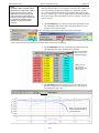

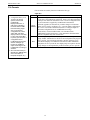
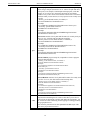
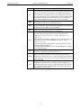

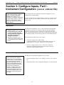
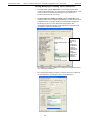
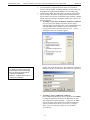
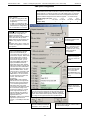
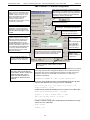
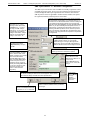
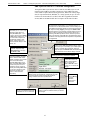
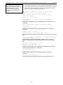
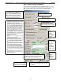
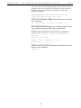

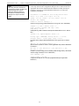
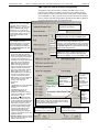
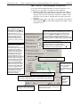
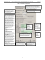

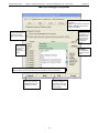

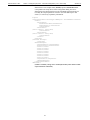

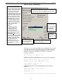
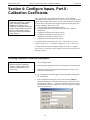

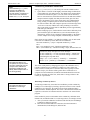


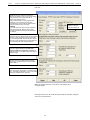

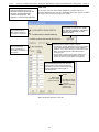

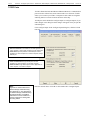


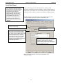
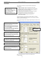
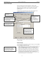
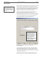


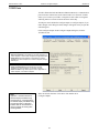
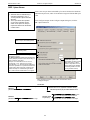
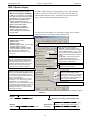

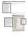
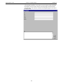
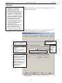
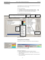


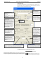

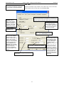


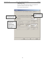

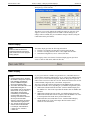
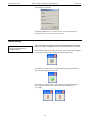


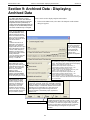
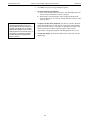
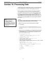
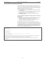


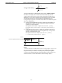
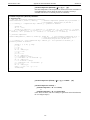


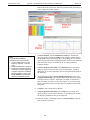


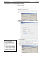
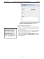
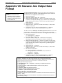

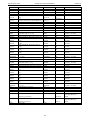


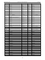

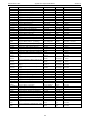


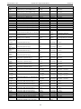

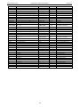


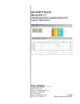
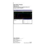


![1] n T169](http://vs1.manualzilla.com/store/data/005696581_1-b5b272b0c99ea5fca956b563015d9b67-150x150.png)