Download 4 - Carlson Software

Carlson Survey Desktop
Release 2
Carlson Software Inc.
User’s manual
July 20, 2005
ii
Contents
Chapter 1.
Product Overview
1
Product Overview . . . . . . . . . . . . . . . . . . . . . . . . . . . . . . . . . . . . . . . . . . . .
2
Installing Carlson Survey Desktop . . . . . . . . . . . . . . . . . . . . . . . . . . . . . . . . . . .
3
Authorizing Carlson Survey Desktop . . . . . . . . . . . . . . . . . . . . . . . . . . . . . . . . . .
9
Report Formatter . . . . . . . . . . . . . . . . . . . . . . . . . . . . . . . . . . . . . . . . . . . .
12
Standard Report Viewer . . . . . . . . . . . . . . . . . . . . . . . . . . . . . . . . . . . . . . . . .
13
* . . . . . . . . . . . . . . . . . . . . . . . . . . . . . . . . . . . . . . . . . . . . . . . . . . . . .
14
Chapter 2.
Tutorials
19
Field to Finish from Coordinate Data . . . . . . . . . . . . . . . . . . . . . . . . . . . . . . . . . .
20
Planned Field to Finish . . . . . . . . . . . . . . . . . . . . . . . . . . . . . . . . . . . . . . . . .
39
Network Least Squares . . . . . . . . . . . . . . . . . . . . . . . . . . . . . . . . . . . . . . . . .
47
Chapter 3.
Data Collectors
Data Collectors . . . . . . . . . . . . . . . . . . . . . . . . . . . . . . . . . . . . . . . . . . . . .
Chapter 4.
Edit-Process Raw File
Edit-Process Raw File . . . . . . . . . . . . . . . . . . . . . . . . . . . . . . . . . . . . . . . . . .
59
60
79
80
SurvNET . . . . . . . . . . . . . . . . . . . . . . . . . . . . . . . . . . . . . . . . . . . . . . . . 126
SurvNET Overview . . . . . . . . . . . . . . . . . . . . . . . . . . . . . . . . . . . . . . . 126
Network Least Squares Settings . . . . . . . . . . . . . . . . . . . . . . . . . . . . . . . . 127
Vertial Adjustment Report . . . . . . . . . . . . . . . . . . . . . . . . . . . . . . . . . . . 136
Sample Coordinate System Report . . . . . . . . . . . . . . . . . . . . . . . . . . . . . . . 139
Chapter 5.
Field to Finish
147
Field to Finish . . . . . . . . . . . . . . . . . . . . . . . . . . . . . . . . . . . . . . . . . . . . . . 148
Chapter 6.
COGO Commands
165
Inverse . . . . . . . . . . . . . . . . . . . . . . . . . . . . . . . . . . . . . . . . . . . . . . . . . . 166
Occupy Point . . . . . . . . . . . . . . . . . . . . . . . . . . . . . . . . . . . . . . . . . . . . . . 167
Traverse . . . . . . . . . . . . . . . . . . . . . . . . . . . . . . . . . . . . . . . . . . . . . . . . . 167
Side Shots . . . . . . . . . . . . . . . . . . . . . . . . . . . . . . . . . . . . . . . . . . . . . . . . 168
Enter-Assign Point . . . . . . . . . . . . . . . . . . . . . . . . . . . . . . . . . . . . . . . . . . . 169
Raw File On/Off . . . . . . . . . . . . . . . . . . . . . . . . . . . . . . . . . . . . . . . . . . . . 170
iii
Line On/Off . . . . . . . . . . . . . . . . . . . . . . . . . . . . . . . . . . . . . . . . . . . . . . . 170
Chapter 7.
Point Commands
171
Draw Locate Points . . . . . . . . . . . . . . . . . . . . . . . . . . . . . . . . . . . . . . . . . . . 172
Pick Intersection Points . . . . . . . . . . . . . . . . . . . . . . . . . . . . . . . . . . . . . . . . . 175
Bearing-Bearing Intersect . . . . . . . . . . . . . . . . . . . . . . . . . . . . . . . . . . . . . . . . 176
Bearing-Distance Intersect . . . . . . . . . . . . . . . . . . . . . . . . . . . . . . . . . . . . . . . 177
Distance-Distance Intersect . . . . . . . . . . . . . . . . . . . . . . . . . . . . . . . . . . . . . . . 178
Resection . . . . . . . . . . . . . . . . . . . . . . . . . . . . . . . . . . . . . . . . . . . . . . . . 179
Point on Arc . . . . . . . . . . . . . . . . . . . . . . . . . . . . . . . . . . . . . . . . . . . . . . . 180
Divide Between Points . . . . . . . . . . . . . . . . . . . . . . . . . . . . . . . . . . . . . . . . . 181
Divide Along Entity . . . . . . . . . . . . . . . . . . . . . . . . . . . . . . . . . . . . . . . . . . . 181
Interval Along Entity . . . . . . . . . . . . . . . . . . . . . . . . . . . . . . . . . . . . . . . . . . 182
Create Points from Entities . . . . . . . . . . . . . . . . . . . . . . . . . . . . . . . . . . . . . . . 183
Building Offset Extensions . . . . . . . . . . . . . . . . . . . . . . . . . . . . . . . . . . . . . . . 185
Erase Points . . . . . . . . . . . . . . . . . . . . . . . . . . . . . . . . . . . . . . . . . . . . . . . 186
Chapter 8.
Edit-Process Level Data
187
Edit-Process Level Data . . . . . . . . . . . . . . . . . . . . . . . . . . . . . . . . . . . . . . . . . 188
Chapter 9.
Deed Commands
191
Enter Deed Description . . . . . . . . . . . . . . . . . . . . . . . . . . . . . . . . . . . . . . . . . 192
Process Deed File . . . . . . . . . . . . . . . . . . . . . . . . . . . . . . . . . . . . . . . . . . . . 194
Deed Correlation . . . . . . . . . . . . . . . . . . . . . . . . . . . . . . . . . . . . . . . . . . . . 195
Legal Description . . . . . . . . . . . . . . . . . . . . . . . . . . . . . . . . . . . . . . . . . . . . 198
Chapter 10.
Station-Offset Commands
205
Label Station Offset . . . . . . . . . . . . . . . . . . . . . . . . . . . . . . . . . . . . . . . . . . . 206
Offset Point Entry . . . . . . . . . . . . . . . . . . . . . . . . . . . . . . . . . . . . . . . . . . . . 207
Calculate Offsets . . . . . . . . . . . . . . . . . . . . . . . . . . . . . . . . . . . . . . . . . . . . 209
Chapter 11.
Cut Sheet
213
Cut Sheet . . . . . . . . . . . . . . . . . . . . . . . . . . . . . . . . . . . . . . . . . . . . . . . . 214
Chapter 12.
Layout Commands
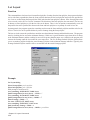
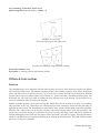
Lot Layout
219
. . . . . . . . . . . . . . . . . . . . . . . . . . . . . . . . . . . . . . . . . . . . . . . 220
Offsets & Intersections . . . . . . . . . . . . . . . . . . . . . . . . . . . . . . . . . . . . . . . . . 221
Cul-de-sacs . . . . . . . . . . . . . . . . . . . . . . . . . . . . . . . . . . . . . . . . . . . . . . . 222
Contents
iv
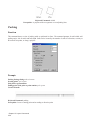
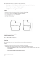
4 Sided Building . . . . . . . . . . . . . . . . . . . . . . . . . . . . . . . . . . . . . . . . . . . . 223
Parking . . . . . . . . . . . . . . . . . . . . . . . . . . . . . . . . . . . . . . . . . . . . . . . . . 224
Chapter 13.
Area Commands
225
Area Label Defaults . . . . . . . . . . . . . . . . . . . . . . . . . . . . . . . . . . . . . . . . . . . 226
Inverse with Area . . . . . . . . . . . . . . . . . . . . . . . . . . . . . . . . . . . . . . . . . . . . 227
Area by Lines and Arcs . . . . . . . . . . . . . . . . . . . . . . . . . . . . . . . . . . . . . . . . . 227
Area by Interior Point . . . . . . . . . . . . . . . . . . . . . . . . . . . . . . . . . . . . . . . . . . 228
Area by Closed Polylines . . . . . . . . . . . . . . . . . . . . . . . . . . . . . . . . . . . . . . . . 228
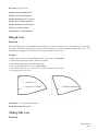
Hinged Area . . . . . . . . . . . . . . . . . . . . . . . . . . . . . . . . . . . . . . . . . . . . . . . 229
Sliding Side Area . . . . . . . . . . . . . . . . . . . . . . . . . . . . . . . . . . . . . . . . . . . . 229
Area Radial from Curve . . . . . . . . . . . . . . . . . . . . . . . . . . . . . . . . . . . . . . . . . 230
Chapter 14.
Survey Text Commands
233
Survey Text Defaults . . . . . . . . . . . . . . . . . . . . . . . . . . . . . . . . . . . . . . . . . . 234
Offset Dimensions . . . . . . . . . . . . . . . . . . . . . . . . . . . . . . . . . . . . . . . . . . . 235
Building Dimensions . . . . . . . . . . . . . . . . . . . . . . . . . . . . . . . . . . . . . . . . . . 236
Adjoiner Text . . . . . . . . . . . . . . . . . . . . . . . . . . . . . . . . . . . . . . . . . . . . . . 237
Create Point Table . . . . . . . . . . . . . . . . . . . . . . . . . . . . . . . . . . . . . . . . . . . . 237
Chapter 15.
Polyline Commands
239
2D Polyline . . . . . . . . . . . . . . . . . . . . . . . . . . . . . . . . . . . . . . . . . . . . . . . 240
3D Polyline . . . . . . . . . . . . . . . . . . . . . . . . . . . . . . . . . . . . . . . . . . . . . . . 240
Join Nearest . . . . . . . . . . . . . . . . . . . . . . . . . . . . . . . . . . . . . . . . . . . . . . . 242
Extend by Distance . . . . . . . . . . . . . . . . . . . . . . . . . . . . . . . . . . . . . . . . . . . 242
Boundary Polyline . . . . . . . . . . . . . . . . . . . . . . . . . . . . . . . . . . . . . . . . . . . 245
Shrink-Wrap Entities . . . . . . . . . . . . . . . . . . . . . . . . . . . . . . . . . . . . . . . . . . 246
Erase by Closed Polyline . . . . . . . . . . . . . . . . . . . . . . . . . . . . . . . . . . . . . . . . 247
Offset 3D Polyline . . . . . . . . . . . . . . . . . . . . . . . . . . . . . . . . . . . . . . . . . . . 248
Fillet 3D Polyline . . . . . . . . . . . . . . . . . . . . . . . . . . . . . . . . . . . . . . . . . . . . 249
Entities to Polylines . . . . . . . . . . . . . . . . . . . . . . . . . . . . . . . . . . . . . . . . . . . 249
Text Explode To Polylines . . . . . . . . . . . . . . . . . . . . . . . . . . . . . . . . . . . . . . . 250
Draw Polyline Blips . . . . . . . . . . . . . . . . . . . . . . . . . . . . . . . . . . . . . . . . . . . 250
Reverse Polyline . . . . . . . . . . . . . . . . . . . . . . . . . . . . . . . . . . . . . . . . . . . . 251
Reduce Polyline Vertices . . . . . . . . . . . . . . . . . . . . . . . . . . . . . . . . . . . . . . . . 251
Edit Polyline Section . . . . . . . . . . . . . . . . . . . . . . . . . . . . . . . . . . . . . . . . . . 251
Densify Polyline Vertices . . . . . . . . . . . . . . . . . . . . . . . . . . . . . . . . . . . . . . . . 252
Contents
v
Set Polyline Origin . . . . . . . . . . . . . . . . . . . . . . . . . . . . . . . . . . . . . . . . . . . 253
Remove Polyline Arcs . . . . . . . . . . . . . . . . . . . . . . . . . . . . . . . . . . . . . . . . . 253
Remove Polyline Segment . . . . . . . . . . . . . . . . . . . . . . . . . . . . . . . . . . . . . . . 254
Remove Polyline Vertex . . . . . . . . . . . . . . . . . . . . . . . . . . . . . . . . . . . . . . . . 255
Polyline Report . . . . . . . . . . . . . . . . . . . . . . . . . . . . . . . . . . . . . . . . . . . . . 255
Polyline Info . . . . . . . . . . . . . . . . . . . . . . . . . . . . . . . . . . . . . . . . . . . . . . 256
Polyline to RW5 File . . . . . . . . . . . . . . . . . . . . . . . . . . . . . . . . . . . . . . . . . . 256
Chapter 16.
Symbols Commands
257
Insert Symbols . . . . . . . . . . . . . . . . . . . . . . . . . . . . . . . . . . . . . . . . . . . . . 258
Edit Symbol Library . . . . . . . . . . . . . . . . . . . . . . . . . . . . . . . . . . . . . . . . . . 259
Chapter 17.
Twist Screen Commands
Twist Screen Standard
261
. . . . . . . . . . . . . . . . . . . . . . . . . . . . . . . . . . . . . . . . . 262
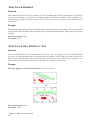
Twist Screen Line, Polyline or Text . . . . . . . . . . . . . . . . . . . . . . . . . . . . . . . . . . . 262
Twist Screen Surveyor . . . . . . . . . . . . . . . . . . . . . . . . . . . . . . . . . . . . . . . . . 263
Restore Due North . . . . . . . . . . . . . . . . . . . . . . . . . . . . . . . . . . . . . . . . . . . 263
Chapter 18.
Conversion Commands
265
Convert Points . . . . . . . . . . . . . . . . . . . . . . . . . . . . . . . . . . . . . . . . . . . . . . 266
Import Softdesk Centerline . . . . . . . . . . . . . . . . . . . . . . . . . . . . . . . . . . . . . . . 266
Chapter 19.
Configure Carlson Survey Desktop
267
Configure Carlson Survey Desktop . . . . . . . . . . . . . . . . . . . . . . . . . . . . . . . . . . . 268
Chapter 20.
Help
271
About Carlson Survey Desktop . . . . . . . . . . . . . . . . . . . . . . . . . . . . . . . . . . . . . 272
OnLine Help . . . . . . . . . . . . . . . . . . . . . . . . . . . . . . . . . . . . . . . . . . . . . . 272
Technical Support . . . . . . . . . . . . . . . . . . . . . . . . . . . . . . . . . . . . . . . . . . . . 272
Contents
vi
Product Overview
1
1
Product Overview
Carlson Survey Desktop (CSD ) is a companion program for Autodesk Autodesk Land Desktop that adds more tools
for surveying. The CSD commands include data collection, raw data processing, Field to Finish and COGO features.
These features are fully integrated into the Autodesk Land Desktop project environment.
Data Collection
The power of CSD begins with data collection. CSD handles all major collectors, from Geodimeter and TDS to
Leica, Nikon, Sokkia, and SMI. The raw data is stored in RW5 format and can be viewed, edited and processed.
The processing, or calculation of coordinates, recognizes ''direct and reverse,'' and other forms of multiple measurement, and processes sets of field measurements. Surveys can be balanced and closed by selective use of angle
balance, compass, transit, Crandall, and least squares methods-or simply by direct calculation with no adjustment.
Commands exist for finding bad angles and for plotting the traverse and sideshot legs of the survey in distinct colors as a means of searching for ''busts'' or errors. In addition to downloading data from electronic data collectors,
CSD accepts manual entry of field notes directly into spreadsheet format, permitting review, storage, and editing.
Alternatively, field notes can be entered for immediate calculation and screen plotting of points, with the ''raw notes''
stored simultaneously, permitting re-processing and re-calculation as needed.
Field to Finish
The survey world is recognizing the power of coding field shots with descriptions that lead to automatic layering,
line work, and symbol work. Office drafting time can be reduced by 50% or more with intelligent use of Field to
Finish plotting. For example, breaklines, which act as barriers to triangulation, should be placed on streams, ridges,
toe-of-slopes and top-of-banks for more accurate contouring. With the Field to Finish command, breaklines can be
created by field coding, with descriptions such as DL, for creating 3D polyline ditch lines. Without Field to Finish,
this coordinate data can be simply plotted on the screen as undifferentiated points. However, with Field to Finish,
this same data can be plotted in one step, creating 3D polyline break lines, building lines, light poles, manholes, and
edge-of-pavements, which are all distinctly layered and fully annotated. CSD's Field to Finish can even adapt to a
coding system made up on-the-fly, or one that has been received from an outsourced survey. Field crew coding and
office processing using Field to Finish can save valuable hours of drafting and eliminate misinterpretations, paving
the way for quick plat generation and supporting supplemental engineering work.
Deed Work
CSD allows you to enter old deeds and plot the linework, then add bearing and distance annotation optionally.
Distances can be entered in meters or feet, and even in the old measurement forms of chains, poles, links, and
varas. Both tangent and non-tangent arcs can be entered. Closures, distances traversed, and areas are automatically
reported. Working in reverse, the Legal Description command creates a property description suitable for deed
recording directly from a closed polyline on the screen. If that polyline has point numbers with descriptions at any
of the property corners, these descriptions will appear in the deed report (e.g. ''...thence N 45 degrees, 25 minutes,
10 seconds E to a fence post...''). Deed files can be saved, re-loaded, edited, re-drawn and printed or plotted to the
screen as a report.
Utilities
CSD contains many powerful utilities, particularly polyline utilities. You can Join Nearest disconnected polylines,
offset 3D polylines, and reverse polyline directions. Extend by Distance lets you create building ''footprints'' with
left and right entries. Reduce Vertices weeds out extra vertices and cuts down on drawing size.
Chapter 1. Product Overview
2
Installing Carlson Survey Desktop
When installing Carlson Survey Desktop, you must have permission to write to the necessary system registry
sections. Make sure that you have administrative access on the computer on which you are installing this software.
Before installing Carlson Survey Desktop, close all other applications. Make sure that you disable any
virus-checking software. Refer to your virus software documentation for instructions.
1. Insert the CD into the CD-ROM drive.
• If Autorun is enabled, the setup process will begin automatically when you insert the CD-ROM.
• To stop Autorun from starting the installation process automatically, hold down the SHIFT key when you
insert the CD.
• To start the install process without using Autorun, from the Start menu (Windows), choose Run. Enter the
CD-ROM drive letter, and setup (e.g. d:\setup).
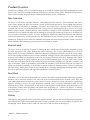
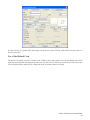
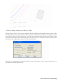
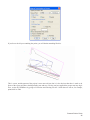
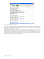
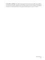
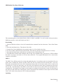
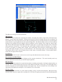
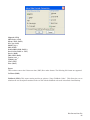
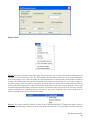
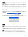
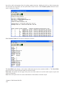
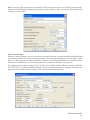
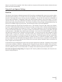
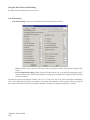
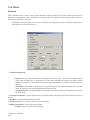
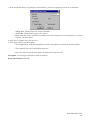
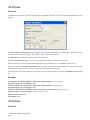
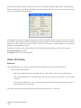
2. Windows will begin the installation of Carlson Survey Desktop. Depending on your operating system, the initial
window will look something like this:
The information dialog box initially displayed in the setup process is shown below:
Installing Carlson Survey Desktop
3
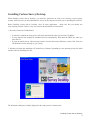
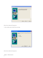
Select Next to continue the Setup process.
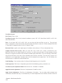
3. Choose which version of AutoCAD you are using.
Select Next to continue the Setup process.
Chapter 1. Product Overview
4
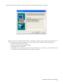
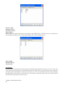
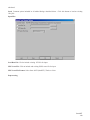
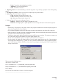
4. When Carlson Survey Desktop is ready to download , the following dialog box will appear:
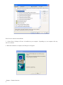
• Note: Carlson Survey Desktop installs itself as a subdirectory within Autodesk Autodesk Land Desktop. To
verify that this directory has installed correctly, a check may be done within Autodesk Land Desktop.
– from the command line, type Options
– Select the File tab within the Options dialog
– Select Support File Search Path
– Depending on your operating system and AutoCAD software, you should see a file path that reads:
C:\Program Files\Land Desktop 2004\SurveyDesktop\Support
Installing Carlson Survey Desktop
5
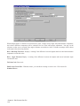
Select Next to continue the installation
5. Carlson Survey Desktop will now be installed on your computer. Depending on your computer, this may
take a few minutes.
6. When the installation is complete, this dialog box will appear:
Chapter 1. Product Overview
6
Select Finish to complete the installation.
Uninstalling Carlson Survey Desktop
CSD may be uninstalled using the standard Windows Add/Remove Programs option.
NOTE: If you uninstall Carlson Survey Desktop, and then re-install, any created special symbol libraries
will be lost.
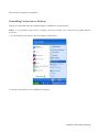
1. Use the Windows Start menu to open the Windows Control Panel
2. From the Control Panel, select Add/Remove Programs
Installing Carlson Survey Desktop
7
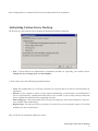
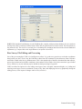
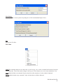
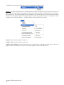
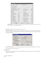
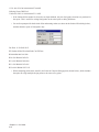
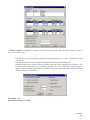
3. Add/Remove Programs generates a list of programs available for uninstall. Select Carlson Survey Desktop.
Chapter 1. Product Overview
8
Select Change/Remove to uninstall Carlson Survey Desktop and all of its components.
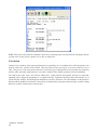
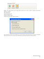
Authorizing Carlson Survey Desktop
The first time you start Carlson Survey Desktop, the Registration Wizard is displayed.
• Note: Carlson Software has implemented an automated procedure for registering your software license.
Change keys are no longer given over the telephone.
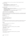
1. Please choose one of the following registration methods.
• Form: This method allows you to fill out a form that you can print, and fax or mail to Carlson Software for
registration.
• Internet: If your computer is online, you may register automatically over the Internet. Your information is
sent to Carlson Software, validated and returned in just a few seconds. If you are using a dial-up connection,
please establish this connection before attempting to register.
• Enter change key: Choose this method after receiving your change key from Carlson Software (if you previously used the Form method above).
• Register Later: You may run CSD for up to thirty (30) days before you are required to register. Choose this
method if you want to register later.
After you choose the registration method, press Next.
Authorizing Carlson Survey Desktop
9
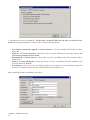
2. Determine the reason for installation. The first time you install CSD is the only time you will select New
install. All subsequent installations require a choice from the remaining options.
• New install or maintenance upgrade of Carlson Software: If you are installing CSD for the first time,
choose this.
• Home use. See License Agreement: Choose this reason if you are installing on your home computer. See
your license agreement for more details.
• Re-Installation of Carlson Software: Choose this if you are re-installing on the same computer with no
modifications.
• Windows or AutoCAD upgrade: Choose this reason if you are re-installing CSD after installing a new
version of Microsoft Windows.
• New Hardware: Choose this if you are installing CSD on a new computer, or if your existing computer has
had some of its hardware replaced (such as the hard disk, network adapter, etc.).
After completing Reason for Installation, select Next.
Chapter 1. Product Overview
10
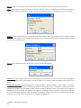
3. Enter the required information into the dialog, as shown above.
• If you are using the Form method for registration, press the Print Fax Sheet button to print out the form. You
may fax your registration to 606-564-9525, or mail it to:
Carlson Software
102 W. Second St., Suite 200
Maysville, KY 41056-1003.
• If you are using the Internet registration, press Next. After a few seconds, your registration will complete.
• If your registration is successful, you will receive a message like the one below. If your registration is unsuccessful, please note the reason why and try again. Keep in mind that each serial number should be registered
to a single computer only.
• If you do not have access to the internet and do not have a printer, you must write down the information from
the User Info tab Print Fax Sheet button (shown above in the Registration Wizard), and fax it or mail it to
Carlson Software.
IMPORTANT NOTE FOR Autodesk Land Desktop 2004 USERS: The first time you attempt to access a
CSD menu, you may receive the following message:
Authorizing Carlson Survey Desktop
11
If you receive this message, visit the Autodesk website, www.autodesk.com,and follow the links and instructions for downloading the latest Autodesk Land Desktop Service Pack before attempting to use Carlson Survey
Desktop. This service pack must be installed before Autodesk can properly communicate with CSD.
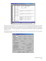
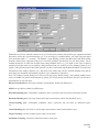
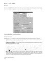
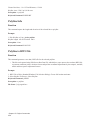
Report Formatter
A number of CSD features use the Report Formatter tool to allow you to specify how and which calculations should
be presented in the report. Anytime you see the option Use Report Formatter, as in the Cut Sheet command, you
may direct the output to the Report Formatter rather than directly to the Report Viewer. The report can be displayed
below in either the standard viewer described in the next section, Microsoft Excel or Microsoft Access.
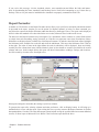
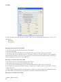
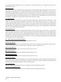
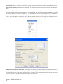
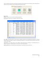
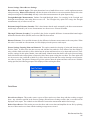
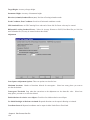
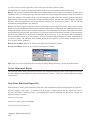
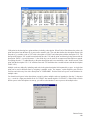
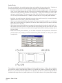
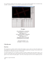
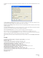
The data set in the Report Formatter may be thought of as a spreadsheet, where columns are various fields related
to a single item such as northing, easting, elevation, etc. Each new row represents a new item. Descriptions of these
field names are displayed in the Available list of the Report Formatter. To include a data field in the report, highlight
the field name in the Available list on the left and select the Add button. This moves the field name to the Used list
on the right. The order of items on the right defines the order in which they will be displayed. Items are initially
sorted by the first column, then items with the identical values in first column are sorted as specified for the second
column, and so on. In the example below, this report will show Point numbers, northings, eastings, and elevations.
It will be sorted by elevation value from high to low.
Subsequent sortings do not modify the sortings of previous columns.
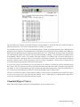
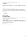
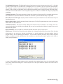
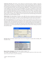
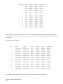
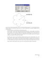
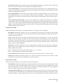
To generate the report after selecting columns and other preferences, click on Display button. It will bring up a
standard built-in viewer with the report. Upon exiting the viewer you may return to the Report Formatter for further
data manipulation, if needed. The other data output options include saving the specified data into comma-delimited
text file, or direct export to Microsoft Excel. Below is the List Points report described above.
Chapter 1. Product Overview
12
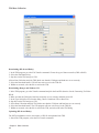
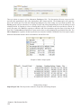
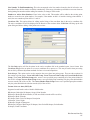
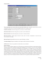
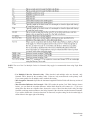
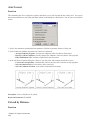
You may define new columns as equations based on existing columns. Click on the Edit User Attributes button to
add a new field name. A list of the existing attributes is available for reference.
User attributes may have one of several summation options, similar to program-generated ones (although these
options are set by program). The summation level is defined by the Total pop-up list in the middle of the dialog. By
default only the grand total will be displayed at the bottom of the list. Selecting the next item in that box provides
you with subtotals, added each time the value in the first column is changed. Use this kind of summation if the
corresponding column is sorted. For example, if the first column is ''Area Name'' and it is sorted, and Total is set
to ''Grand, Area Name,'' the report will have a sub-total for each distinct area name. This feature makes the Report
Formatter a flexible tool for results exploration, before ever using a spreadsheet. Various forms of reports may be
saved and recalled using controls in the top line of the dialog.
To save a new version of the format, type in a new name (or use default to overwrite the old one) and click on the
Save button. The next time that you choose the Report Formatter from the same CSD command it will recall this
last format. To select another format, pull down the list of formats in the left top corner and select which format to
use. To Delete an unwanted format, choose it from the list and then click the Delete button.
There are several Microsoft Excel export options provided. You may specify a spreadsheet file to load before export,
as well as a left upper cell to start with and sheet number to use. Totals which are reported when using built-in
viewer may be skipped when using Microsoft Excel export.
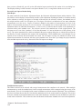
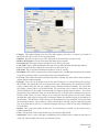
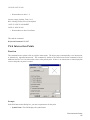
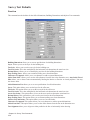
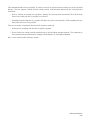
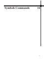
Standard Report Viewer
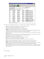
Many CSD features display output in the Standard Report Viewer as shown below.
Standard Report Viewer
13
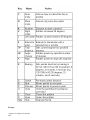
The report can be edited directly in the report viewer. Report Viewer commands are described below.
•
•
•
•
•
•
•
•
•
•
•
•
•
•
•
Open: Opens an ASCII file and displays the contents in the report viewer.
Save: Saves the contents of the report viewer to a text file.
SaveAs: Saves the contents of the report viewer to a particular file.
Append To: Appends the contents of the report viewer to another file.
Print: Prints the contents of the report viewer. This will open your regular Windows print dialog where you
can choose the printer and modify any of the printer settings before printing.
Screen: Draws the report in the current drawing. The program will prompt you for a starting point, text height,
rotation and layer.
Undo: Reverses the effect of your last action. If you inadvertently delete some text, stop and choose the Undo
command to restore it. The key combination Ctrl-Z also performs this action.
Select All: Selects all the text in the report viewer.
Cut: Deletes the selected text and places it on the Windows clipboard.
Copy: Copies the selected text to the Windows clipboard.
Paste: Inserts ASCII text from the Windows clipboard into the report viewer at the cursor.
Search: Opens the Find Text dialog, allowing you to search for specific items in the report viewer.
Replace: Opens the Find and Replace Text dialog. Allows you to search for text and replace it.
Options: Opens the Report Viewer Options dialog. In this dialog, you can specify print settings, such as lines
per page and margins. You can also specify the font (used for both the display and for printing).
Hide: Minimizes the report viewer window and returns to AutoCAD. This allows you to continue working in
AutoCAD without closing the report. You can re-examine the report at any time by selecting the minimized
report viewer icon.
*
License/Copyright
Chapter 1. Product Overview
14
Copyright ©2005 Carlson Software, Inc.
All Rights Reserved
Use of this software indicates acceptance of the terms and conditions of the Software License Agreement.
This End-User License Agreement (henceforth ''EULA'') is a legal agreement between you, the individual or single
entity (henceforth ''you''), and Carlson Software, Inc. (henceforth ''Carlson Software'') for the software accompanying this EULA, and may or may not include printed materials, associated media, and electronic documentation
(henceforth ''this software''). Exercising your right to use this software binds you to the terms of this EULA. If you
do not agree to the terms contained herein, do not use this software.
SOFTWARE LICENSE
This software is protected by United States copyright laws and international copyright treaties, as well as applicable
intellectual property laws and treaties. This software is licensed, not sold.
GRANT OF LICENSE:
This EULA grants you the following rights:
• You may install and use one copy of this software, or any prior version for the same operating system, on a
single computer. The primary user of the computer on which this software is installed may make a second
copy for his or her exclusive use.
• Additionally, you may store one copy of this software on a storage device, such as a network server, used
only to install or run this software on other computer over an internal network. However, you must acquire
and dedicate a license for each separate computer on which this software is installed or run from the storage
device. A single license for this software may not be shared or used concurrently on more than one computer,
unless a license manager has been purchased from Carlson Software.
OTHER RIGHTS AND LIMITATIONS:
• You may not reverse engineer, decompile, or disassemble this software, except and only to the extent that such
activity is expressly permitted by applicable law notwithstanding this limitation.
*
15
• This software is licensed as a single product. Its component parts may not be separated for use on more than
one computer.
• Under certain circumstances, you may permanently transfer all of your rights under this EULA, provided that
the recipient agrees to the terms of this EULA.
• Without prejudice to any other rights, Carlson Software may terminate this EULA if you fail to comply with
the terms and conditions of this EULA. In this event, you are required to destroy all copies of this software,
and all of its component parts.
COPYRIGHT:
• All title and copyrights in and to this software, including, but not limited to, any images, photographs, animations, video, audio, music, text, or ''applets'' incorporated into this software, the accompanying printed
materials, and any copies of this software, are the sole property of Carlson Software and/or its suppliers. This
software is protected by United States copyright laws and international copyright treaties, as well as applicable
intellectual property laws and treaties. Treat this software as you would any other copyrighted material.
U.S. GOVERNMENT RESTRICTED RIGHTS:
• Use, duplication, or disclosure by the U.S. Government of this software or its documentation is subject to
restrictions, as set forth in subparagraph (c)(1)(ii) of the Right in Technical Data and Computer Software
clause at DFAARS 252.227-7013, or subparagraph (c)(1) and (2) of the Commercial Computer Software
Restricted Rights at 48 CFR 52.227-19, as applicable. The manufacturer is:
Carlson Software, Inc.
102 W. Second St.
Maysville, KY 41056
LIMITED WARRANTY:
• CARLSON SOFTWARE EXPRESSLY DISCLAIMS ANY WARRANTY, EITHER EXPRESSED OR IMPLIED, INCLUDING BUT NOT LIMITED TO ANY IMPLIED WARRANTIES OF MERCHANTABILITY,
FITNESS FOR A PARTICULAR PURPOSE, OR NONINFRINGEMENT REGARDING THESE MATERIALS. CARLSON SOFTWARE MAKES SUCH MATERIALS AVAILABLE SOLELY ON AN ''AS-IS''
BASIS.
• IN NO EVENT SHALL CARLSON SOFTWARE BE LIABLE TO ANYONE FOR SPECIAL, COLLATERAL, INCIDENTAL, OR CONSEQUENTIAL DAMAGES IN CONNECTION WITH, OR ARISING OUT
OF, PURCHASE, USE, OR INABILITY TO USE THESE MATERIALS. THIS INCLUDES, WITHOUT
LIMITATION, DAMAGES FOR LOSS OF BUSINESS PROFITS, BUSINESS INTERRUPTION, LOSS OF
BUSINESS INFORMATION OR ANY OTHER PECUNIARY LOSS. IN ALL INSTANCES, THE EXCLUSION OR LIMITATION OF LIABILITY IS SUBJECT TO ANY APPLICABLE JURISDICTION.
• IF THIS SOFTWARE WAS ACQUIRED IN THE UNITED STATES, THIS EULA IS GOVERNED BY THE
LAWS OF THE COMMONWEALTH OF KENTUCKY. IF THIS PRODUCT WAS ACQUIRED OUTSIDE
OF THE UNITED STATES, THIS EULA IS GOVERNED BY THE LAWS IN ANY APPLICABLE JURISDICTION.
Chapter 1. Product Overview
16
*
17
Chapter 1. Product Overview
18
Tutorials
2
19
Field to Finish from Coordinate Data
Reactive Field to Finish
Field to Finish is used to create a partial or nearly complete drawing based on a field survey. Field to Finish features
draw not only points and coordinate data, but also add symbols and linework to designated layers, and even change
text styles according to instructions built into the Field to Finish coding.
Autodesk Land Desktop conducts Field to Finish using the raw survey data file, which is known as the Fieldbook
(.fbk) file. Carlson Survey Desktop (CSD) performs Field to Finish using the point file (typically named points.mdb
within Autodesk Land Desktop). The use of Field to Finish by surveying, engineering, construction and mining
companies places additional demands on survey crews to do intelligent coding, and on the office team to design an
effective coding system. Field to Finish is used by 30% of survey crews, depending on software and geographic
region.
Field to Finish remains the single greatest software-based method for increasing efficiency and speed of work of the
combined field and office team. The ease of Field to Finish with CSD encourages increasingly more companies to
utilize these benefits.
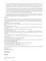
There are two approaches to Field to Finish, ''reactive'' and ''planned.'' Tutorial 1 focuses on reactive Field to Finish.
This makes no demands on the field crew to carefully code their survey points. This method can be used to get
linework and symbols drawn from surveys conducted by outside firms, over which you may have no influence on
coding, and from in-house survey crews who don't follow any particular code system. With ''reactive'' Field to
Finish, you assign instructions to whatever codes were found. You make a new code table with each job, read in the
descriptions used, assign linework, symbols and layers, then plot out the results. The process still saves much time
over standard point plotting followed by line-by-line and symbol-by-symbol drafting. It is one step on the way to
maximum efficiency, as illustrated below:
Landfill Point File
Carlson Survey Desktop includes an ASCII file called Tutorial1.txt with the software package. The file is found in
a subdirectory of Autodesk Land Desktop which, for Autodesk Land Desktop 2004, would be:
C:\Program Files\Land Desktop 2004\SurveyDesktop\Data.
This is a file of survey points in the form Pt#,N,E,Z,D (D for description). This file might represent a typical survey
conducted by an outside firm under contract, where you are not able to instruct the crew how to code their survey
shots. In this instance, your only option is to deal with whatever descriptions (codes) they used to describe the
points.
New Project
Chapter 2. Tutorials
20
Choose Create Project to start a new Project, and name it Tutorial1 as shown below, with the drawing name
Land1.dwg (or Tutorial1.dwg). The exact names are not critical, but may help you to follow along closely.
A scale of 1''=50' (imperial or English) is appropriate for this data set.
Importing Tutorial1.txt
After the project and drawing are started, select Import/Export Points under the Points menu of Autodesk Land
Desktop. From the Import/Export Points fly-out, select Import Points. Complete the dialog (shown below):
Select OK, and then select OK again to the default settings in the COGO Database Import Options Screen. The
points are then read in, added to the Points.mdb file and plotted on the screen.
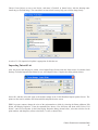
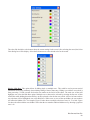
TIP: For greater contrast, change the color of the point numbers to black by selecting the Points pulldown, Edit
Points, and Display Properties. From the command line, choose S for Selection, and when asked ''Select Civil
Points:'' enter All for all points. In the Point Display Properties dialog (shown below), select the color box for the
point numbers and change the yellow to the black (7) color as shown below:
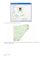
Field to Finish from Coordinate Data
21
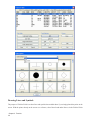
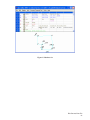
After selecting OK, the point plot appears as shown here:
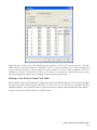
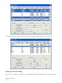
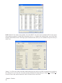
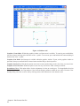
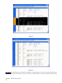
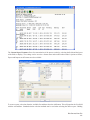
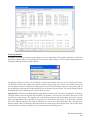
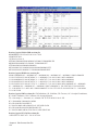
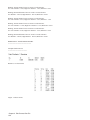
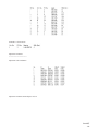
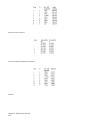
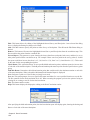
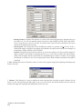
Study the point coordinates and descriptions by choosing List Points under the Points menu. Select List All Points
to bring up the following dialog:
Chapter 2. Tutorials
22
Under Raw Desc column, you see the descriptions used in this file. Code LP is used more than once. We may
assume for this exercise that it indicates a Light Pole. Code 17 is more mysterious, but it is used repeatedly, and
if you examine the drawing, you will note that these codes circle the site. Code 17 and its companion code 18 are
candidates for linework. Note that the elevations are less then 50. No matter who conducted the survey, we can
jump-start a drawing by making some assumptions that create linework and symbols.
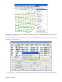
Starting a New Field to Finish Code Table
Most companies using Field to Finish have a coding system that is deliberately designed. A code such as EOP might
be ''edge of pavement'' and DL might be ''ditch line'', etc. But in our case, we must react to a coordinate file with
random descriptions. You can plot the points, but why not do more by making some automatic lines and symbols?
To begin, select Field to Finish in the Survey pulldown menu.
Field to Finish from Coordinate Data
23
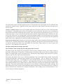
The first time you select Field to Finish, it displays a dialog to load an existing Field to Finish code table. Load
''Csurvey.fld,'' to get started.
The Possible Multiple Codes Found dialog box may appear. If this dialog box is displayed, select the default, Split
all multiple codes, and press ok.
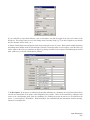
To create a table from new, unexpected or third party coordinate point descriptions, choose Code Table by Points
Chapter 2. Tutorials
24
and select New to create a new table. The dialog shown below is typical of those used in CSD to create new files.
Name the new coding file ''Tutorial1'' and click Save to create the file. The Field to Finish coding files have a .fld
extension, as shown at the top of the dialog.
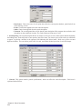
Deleting Table Entries
This brings you to a table that is preset to show all descriptions found in the coordinate file. If you examine the
drawing closely, note that many of the displayed descriptions appear once or are used as generic descriptions (e.g..
Ground Shot and gr), and therefore aren't useful for linework or for meaningful symbol selection. We can select
these as shown by holding down the Ctrl key and selecting each one (standard Windows procedure for selecting
multiple objects) and then select Cut from the dialog box to remove them from our list.
Field to Finish from Coordinate Data
25
The following shorter list remains, which can be used for assigning symbols and linework, with layering.
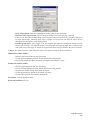
Defining Linework Coding
Select Code 17, and edit it into a 3DPline by choosing Edit under Code Definitions. There are many options here,
Chapter 2. Tutorials
26
but you will note that the program has already layerized code 17 to the same layer as the description, namely layer
17. You can change this to ''Ditch'' or ''TopofBank'' or ''BreakLine'' as desired, but for efficiency in the processing, all
we need to do is make sure the entity type (lower left in dialog) is a 3D polyline. This will assist in making accurate
contour maps and defining break lines. The default linetype will be continuous. Repeat this process for code ''18''.
You can also revise the default layers and linetypes. Try this with the EP code. Make the layer Road, the entity a 2D
Polyline and the linetype dashed.
Field to Finish from Coordinate Data
27
You can also edit two at a time, if the descriptions TB and TOPB both refer to ''top of bank.'' To make a 3D Polyline
in the layer TopOfBank, select TB then hold down the Ctrl key and select TOPB also. With both highlighted, choose
Edit.
Note that you have a smaller set of options based on your multiple selection. You can only do things that apply to
multiple codes at once. To change the layer for both, select Main Layer, then enter TopOfBank, as shown here:
Repeat the process for Entity and set it to a 3D Polyline. Any survey point can be part of a line or polyline, as well
as having a defined symbol.
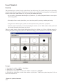
Defining Symbol Coding
Codes FP, LP and TP represent points that benefit from layering and special symbols to assist in drafting and design.
Although reactive Field to Finish makes sense for linework, some codes may be distinguishable as specific points
(e.g. LP as Light Pole, FP as Fence Pole and TP as Traverse Point). Click LP in the list above and select Edit.
Place LP in layer Utility and choose Set Symbol and choose a symbol icon such as SPT20 (scroll down to locate
this symbol) after selecting Set Symbol.
Chapter 2. Tutorials
28
For this exercise, use symbol SPT8, the triangle, for the traverse point (TP) and symbol SPT5, an open circle, for
the fence post (FP).
Use of the Default Code
This defines everything except the ''Default'' code. Whatever layer and symbol is used for the default code will be
applied to all descriptions not found in the code table. For this exercise, choose no symbol at all for the extra codes
by selecting the blank symbol (SPT0). Change the layer for default entities to Existing.
Field to Finish from Coordinate Data
29
Drawing Lines and Symbols
The purpose of Field to Finish is to draw lines and symbols that wouldn't draw if you simply plotted the points to the
screen. With the points already on the screen as a reference, select Draw found under Process in the Field to Finish
Chapter 2. Tutorials
30
dialog, and under Entities to Draw, de-select Points and select Lines and Symbols, as shown here:
If we freeze the points, the following linework and point symbols have been created.
We're done with our ''reactive'' Field to Finish. All that is necessary now is a little editing using some of the Polyline
Utilities found in CSD.
The Polyline Utilities of Carlson Survey Desktop
Reactive Field to Finish will usually require some editing. True Field to Finish techniques involve codes for starting
and stopping polylines, creating rectangles for buildings, closing polylines, and even automatically creating offset
polylines. A file that contains only raw descriptions, with no special instruction codes, can produce linework and
symbols, but there is usually a little ''chaos'' that needs correction. CSD's polyline utilities are perfect for this cleanup
process.
Field to Finish from Coordinate Data
31
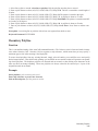
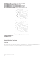
The blue ditch line (Layer 18 can be set to blue in Layer Control) is crossed in the NW corner by a wayward red,
Layer 17, polyline. In this instance, one polyline connected arbitrarily to what should have been a distinct new
polyline. This occurred because there was no start-stop logic. See Tutorial 2 for examples of polyline start-stop,
curve, rectangle and other techniques. For reactive Field to Finish these must be cleaned up. The wayward red
polyline segment in the NW corner, cutting across the blue polylines that represent a trapezoidal ditch, can be
removed by the Remove Polyline Segment command.
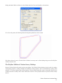
Remove Polyline Segment
Select the Survey pulldown menu, then Polyline Tools, then Remove Polyline Segment. The command line prompt
is:
Break polyline at removal or keep continuous [<Break>,Continuous]? Press B for Break or simply press Enter.
Any option in the <> brackets is the default response.
When prompted to pick the segment to remove, select as shown. This completes the process. The drawing is cleaner,
but there is still work to do.
Inverse to Determine a Distance or Find a Point
If the top of bank layer is set to magenta, you can see that the survey crew coded a combination of TB and TOPB,
where one description ended and another began, creating a gap. Gaps like these can be quickly closed using the
command Join Nearest, under Polyline Tools.
Before using the command, it's a good idea to measure the gap. You can use AutoCAD's Distance command and
snap to the endpoints, or for the true 2D distance, use CSD's Inverse command.
To locate the Inverse command, select Survey, then COGO, then Inverse. The prompting is:
Traverse/SideShot/Options/Arc/Pick point or point number: Pick one side of the gap
Chapter 2. Tutorials
32
Northing(Y) Easting(X) Elev(Z)
4078.95 4537.39 15.32
Traverse/SideShot/Options/Arc/Pick point or point number: Pick the other side of gap
Northing(Y) Easting(X) Elev(Z)
4141.59 4589.89 14.48
Bearing: N 39d58'01'' E Horizontal Distance: 81.7397854
Traverse/SideShot/Options/Arc/Pick point or point number: Enter to end
NOTE: Inverse is very handy. You can Inverse from point numbers (e.g.. 169 to 168 in this case) or by picking or
by a combination of picking and point numbers. If you do not know where point 52 is, Inverse to it and you will
''rubber band'' from it immediately! So the gap in question is about 82 units.
Join Nearest
Now that you know the gap to close is just under 82 units (feet, in this case), select Join Nearest under Polyline
tools, and enter a tolerance of 82 or less, and that the endpoints may be different elevations, as shown here:
Field to Finish from Coordinate Data
33
This means the ''join'' will directly connect the two polylines and deal with a separation of up to 82 feet, and will
also allow for different endpoint elevations. Select OK, and the result is shown below. Note that Join Nearest is also
useful for joining contour lines that are composed of small, unattached segments into single entity contours for each
elevation. In this case, you would set the ''Max separation to join'' to 1 (never try to join if the gap exceeds 1 unit)
and you would select ''Join only common elevations.'' Join Nearest has many distinct uses, as you will see below.
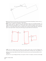
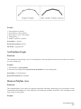
Extend by Distance
One goal might be to create a hatched area for a 30 unit wide road, by offsetting the dashed line, closing its ends,
then hatching it, then removing the two end segments. First, however, you might want to make the road a little
longer than was actually surveyed. You can do this visually, simply choosing how much to extend each end, using
the command Extend by Distance. After selecting Extend by Distance, pick very close to the left end of the dashed
polyline, then select an appropriate distance to the left to extend it. You can extend by selecting Repeat for the right
side. You may notice that the program will auto-pan in some cases, so just zoom and pan as you desire in response.
Now that you have a longer dashed line for the north road edge, use the standard AutoCAD Offset command to offset
30 units to the south. Now select Join Nearest and tolerate a 31 unit gap and require matching endpoint elevations,
and directly connect the endpoints. These controls prevent you from joining the wrong gaps-other polylines with
bigger gaps or different endpoint elevations. It is best to constrain your join effort as tight as possible, in case you
inadvertently select the wrong thing.
Chapter 2. Tutorials
34
Now you have a closed figure you can hatch. Try hatching with the dots pattern at 100 scale, and you obtain the
following:
Remove the end segments of the road, to make the drawing more appealing, by a repeat use of the command Remove
Polyline Segment, option Break.
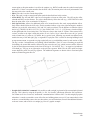
Extend by Distance by Direction and With Close
The simplest use of Extend by Distance is selecting how far to extend on the screen. More advanced usage involves
changing direction and closing the figure. If we thaw back the point numbers (layer 0 or as you assigned them), you
will note the point plot in the vicinity of our two light poles.
Field to Finish from Coordinate Data
35
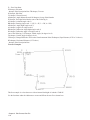
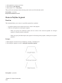
We conclude that there is a building edge from point 5 to point 6 that represents the NW portion of a 40x60 building.
Start by connecting a polyline from point 5 to 6 using the node snap. The rest can be accomplished by Extend by
Distance.
After choosing Extend by Distance, select the segment from 5 to 6 on the half of the segment closer to 6. That places
the arrowhead for the direction to extend pointing southward from point 6.
Several command line options are available (A is for angle, C for Close, etc.). The T option is for Total Distance (or
if you prefer, TO a distance). So entering T60 goes to a total distance of 60. Then you enter L40 (for left 40), then
L60 (for left 60), then C for Close, and you have your building, shown below hatched with diagonal lines.
Chapter 2. Tutorials
36
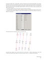
A Trick to Help Analyze your Survey Data
Reactive Field to Finish is often used by companies who have deliberate, well-designed coding systems of their
own. When Survey work is outsourced, the codes used can't be controlled. In this instance, it is possible to obtain
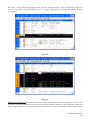
only a point file, but that is often enough to get a drawing started with decent linework and symbol plotting. Report
Codes/Points in the main Field to Finish dialog helps you analyze the source coordinate files prior to Field to Finish
processing. Click on Data Points and Sort by Codes as shown below:
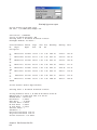
This leads to a report that helps you quickly identify the range of descriptions and how many coordinate points are
associated with each description found.
Field to Finish from Coordinate Data
37
NOTE: This report is presented in a standard Carlson Survey Desktop report screen that allows full editing, and lets
you plot to the screen, print to a printer, save to file, or simply Exit.
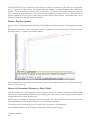
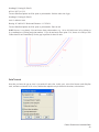
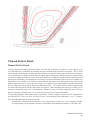
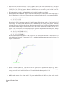
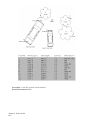
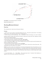
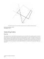
Conclusion
Carlson Survey Desktop offers increased automation by permitting use of coordinate files with descriptions to be
used for ''on-the-fly'', reactive Field to Finish. The process does not use, nor require, a raw survey data file (.rw5 or
.fbk). This process, with some advance detective work on the type of descriptions used, can jump-start a drawing
and save office personnel significant time, even when a formal Field to Finish system has not been established.
You analyze the codes, start a new Field to Finish table, assign linework and symbols and layers to particular
important codes, and get the beginnings of a complete drawing. Supplement Field to Finish with strategic use of
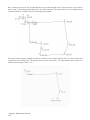
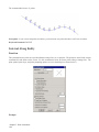
various Polyline Utilities, and the designers and drafters can take it from there. The 3D breaklines for the perimeter
ditch around the landfill saved minutes if not an hour of detailed study and point-to-point polyline creation, leading
directly to a quality contour map as shown below.
Chapter 2. Tutorials
38
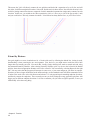
Planned Field to Finish
Planned Field to Finish
Tutorial 1 illustrated a uniquely powerful feature of Carlson Survey Desktop: the ability to ''react'' quickly to any
set of descriptions in a coordinate file and make the best possible drawing from those descriptions. This is useful
when working with third party coordinate data (from contract surveying) or when trying to make the best of in-house
survey work where no coding system has been developed. But the real promise, the real potential of Field to Finish
is to design a coding system that is used by all in-house field-crews, leading to even more complete drawings created
directly from field coding. The challenge here is to design a system of descriptions that fits your crews and fits your
data collector. For example, if you don't have a data collector with access to the full keyboard range of letters and
numbers (rare these days), you may prefer to design a very simple system, where numbers represent descriptions
like ''ep'' (edge of pavement) and ''fl'' (fence line) and codes such as ''..'' are used for end line. Some companies print
out cards with field codes that fit in a shirt pocket for reference. Other companies limit the range of codes to a list
that can be memorized easily (10 to 15 descriptions). Whatever system you design, a planned system of Field to
Finish, used daily by in-house survey crews, leads to the greatest time saving and automation.
You can follow Tutorial 2 without prior practice on Tutorial 1. Tutorial 2 requires access to two files: Tutorial2.FLD
and Tutorial2.TXT. These two files are found in your \SurveyDesktop\Data subdirectory, as in C:\Program
Files\Land Desktop 2004\SurveyDesktop\Data.
• Tutorial2.fld is a field code file developed by a New Jersey firm for in-house use. It is an example of a highly
developed coding system requiring a reference card initially, until committed to memory by the field crews.
Planned Field to Finish
39
• Tutorial2.TXT is a sample coordinate file that must be imported and then can be plotted automatically using
Field to Finish.
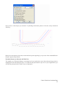
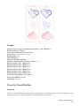
Importing the Points versus Data Collector Download
For the purpose of this Tutorial, we will use imported ASCII coordinate files (point files). Use the standard Import/Export Points command found in the Points menu. In actual practice, you will typically download points from
a data collector used by the field crew. The very first command in the Carlson Survey Desktop (CSD) pulldown
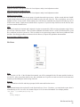
menu (titled ''Survey'' and located near the far right of your menu options), is Data Collectors. This Data Collectors
command loads the points from all collector types listed in the dialog box below:
Some of these options apply to hardware-based data collection, such as the on-board, built-in collectors on total
stations supplied by Leica and Topcon. Other options apply to software brands such as Carlson SurvCE, TDS and
SMI. CSD will download these types from a variety of hardware platforms. You can download with coordinates
(points) and raw files. When downloading raw files of survey data, the default form is the .RW5 file, but using
the SurvCE option, you can convert to the more familiar Autodesk Land Desktop Fieldbook format. However,
converting to Fieldbook is not necessary to utilize CSD's Field to Finish command.
Sometimes the conversions to Fieldbook form may take two steps, as in the case of an SMI download shown below.
First convert the SMI RAW file to RW5, then convert RW5 to Fieldbook.
Chapter 2. Tutorials
40
NOTE: With Autodesk Land Desktop, it is the Fieldbook file, complete with special note fields to do curves and start
and stop lines, that is needed for Field to Finish. With CSD, the point file drives Field to Finish. The descriptions on
the points do it all. The raw file is used only for re-calculating the coordinate data based on the selected method of
adjustment (eg. Compass Rule with Angle Balance as an option or SurvNET).
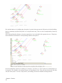
Raw Survey File Editing and Processing
One of the great strengths of CSD is its intelligent raw editor. It is good survey practice to recalculate coordinates
based on the raw data. That is why the Edit-Process Raw Data File command is placed between Data Collectors
and Field to Finish in the Survey pulldown menu. This is the normal order of business: download the data collector,
process the raw data and recalculate coordinates, then conduct Field to Finish. Only for the most basic type of radial
survey, GPS survey or pure stakeout project should raw data processing be bypassed.
CSD's raw editor has options for color coding record types (notes, foresights, instrument heights, etc.), hiding and
restoring record types for more condensed viewing of key data, and displaying the survey graphically during the
editing process, so the impact of changes can be seen (see below):
Planned Field to Finish
41
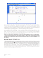
Note the description coding. The description HS has been appended with OH1. OH is a reserved expression for
''offset horizontal''. In Field to Finish, the polyline defined by HS will be drawn, and a second polyline would also
be drawn at 1 unit offset to the right, in the direction of the polyline. This might plot, for instance, the face of a wall
and the back of a wall, with only the face of wall shots actually measured in the field. The expression END is used
to end this sequence, and on foresight point 73, another use of HS would start a new polyline.
You can substitute for END, such as using ''..'' to end as noted above. Field to Finish has a button called Code Table
Settings, where all reserved special codes can be substituted with codes of your own design. This makes adapting to
CSD much easier. You don't abandon most of your existing coding system, but simply re-apply it. In fact, CSD can
import your existing coding systems from both LDD and Eagle Point.
NOTE: If you end a polyline or line sequence, the start of a new one is assumed if the same text is used. Similarly,
if you don't use END, but prefer to start a new polyline with BEG (or whatever code you select), the polyline will
end on that last use of that description, and a new polyline will be started. There is no need for simultaneous use of
BEG and END.
Importing Tutorial2.TXT at 20 Scale
To follow along with this tutorial, it is recommended that you begin a new project called Tutorial2 and a new drawing
within the project called Tutorial2 1. (Many people consider it good practice not to name the drawing the same name
as the project.) When asked for scale, choose 1''=20', Imperial. At a 20 scale, points look good if plotted about 1/10
the size of the scale, or 2 units in height. Because we plan to import the points in Autodesk Land Desktop, and the
points will plot in the process of importing, we need to set the point height ahead of time. This is done with the
command Point Settings, found at the top of the Points pulldown menu. Within Point Settings dialog box, choose
the Marker tab, and set the height to 2, as shown below:
Chapter 2. Tutorials
42
Now select Import Points, within the Import/Export Points selection, under the Points pulldown menu. Set to
PNEZD (comma delimited) and select the file Tutorial2.TXT in the SurveyDesktop/Data folder within Autodesk
Land Desktop. Press OK at the next screen, then Zoom Extents when done. Under Edit Points, Display Properties,
S for Selection, you can select all points and then change the coloring of the point numbers, elevations or descriptions
for better viewing.
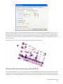
You will obtain a very dense plot of points, which appears in part as shown below:
Field to Finish Linework Only using Tutorial2.FLD
The point plot shown above is ''busy'', but with some zooming and panning, most points can be identified. But what
exactly are we looking at? Without Field to Finish, someone must sort through the maze of point data to make sense
of the entities to draw. With a planned Field to Finish coding system, the drawing will be revealed in seconds. Begin
Planned Field to Finish
43
by selecting Field to Finish in the CSD pulldown menu.
You will be confronted with a dialog asking if you wish to split multiple codes. The normal answer is Yes. When
you code a line EP END, the END might indicate the End of the polyline. If you code EP MH, that might actually be
two codes (edge of pavement and manhole at the same point). Only if your codes actually have spaces in them will
you want to not split the codes and consider the full text one description. It is far easier to design a coding system
with no spaces in field codes, and to always answer split multiple codes, as shown here:
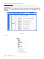
This brings you to the Field to Finish table. The table can be organized into headings. If you scroll down, you can
find the ''Fences and Walls'' portion shown below:
To draw the linework only, using this pre-defined table, click Draw. This brings up the following dialog of options,
and here under Entities to Draw, de-select Points and Symbols, but keep Lines selected, as shown:
Chapter 2. Tutorials
44
If you freeze the 0 layer containing the points, you will obtain something like this:
This is a start, and the pattern of the project is now more obvious, but it is also obvious that there is work to do.
Some of the zigzag polylines should probably start and stop. We may not have applied the proper start/stop logic.
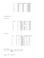
First, review the coordinates by going to List Points and selecting List All. Scroll down to look at, for example,
points 4050 to 7009.
Planned Field to Finish
45
NOTE: While ST was used to start polylines, the classic RECT was used to close rectangles and CLS was used to
close polylines in general. To make these instructions work (i.e., to adapt to this coding system), select Code Table
Settings within Field to Finish. This brings up this translation table, where you can substitute the special codes you
wish to use:
Change +7 to ST for start. Many Autodesk Land Desktop users may prefer to use BEG for starting a new polyline or
line. Change CLO to CLS to close. Now OK, and select SAVEAS. Save these changes as Tutorial2 2 or Tutorial2 2a
(so others can use this tutorial unaltered!). Back in Field to Finish, select Draw.
Chapter 2. Tutorials
46
Then when you redraw the linework, you obtain the more complete, well-defined drawing shown below:
You can also choose to plot both symbols and linework. You can choose, as well, to erase the Autodesk Land
Desktop-style points and plot points, symbols and linework with CSD's Field to Finish. This will layerize not just
linework and symbols but even the points as well. Later on, if you wish to freeze point layers, it is advisable to
define the points plotted within Field to Finish to Distinct Point Layers, using the Edit option in Field to Finish.
Network Least Squares
This tutorial is divided into four lessons covering the process of reducing and adjusting raw survey data into final
adjusted coordinates using the SurvNET program. The purpose of the tutorial is to describe the typical work flow
used to process raw data from a data collector into final coordinates. The tutorial will describe the reviewing and
editing of the raw data prior to the processing of the raw data. Next, the least squares system settings will be
described. The next lesson will cover the processing of the raw data. Lastly, the reports created by the least squares
program will be explained
The raw data file associated with this tutorial is located in the SurveyDesktop\Data folder under LDD installation
folder on your computer (ex. C:\Program Files\Land Desktop 2004\SurveyDesktop\Data). The raw file to be
processed is called Tutorial3.rw5. This data comprises a network that is to be reduced to NAD83 grid coordinates.
The zone used is North Carolina. Both direct and reverse angles were collected in the raw file.
Lesson One- Raw data Review and Editing
Step 1: Click the icon for Autodesk Autodesk Land Desktop and launch Autodesk Land Desktop. You may be
Network Least Squares
47
presented with a Startup Wizard dialog box. If so, click Exit.
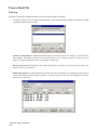
Step 2: The Carlson Survey Desktop (CSD) menu is titled ''Survey.'' Under the Survey menu, choose Edit-Process
Raw Data File. The Raw File to Process dialog box is displayed. Choose the Existing Tab and enter Tutorial3.rw5.
Once the correct file name has been entered press the Open button. Make sure both the path and file name are
correct.
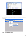
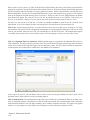
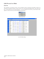
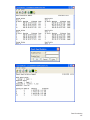
Step 3: The raw data editor is now displayed. The top half of the window is a grid view of the raw data. The bottom
half of the window displays a graphical view of the data. Use this editor to make changes to the raw data file, if
errors exist. As the raw data used in the tutorial contains no errors, we may proceed to process the data.
Chapter 2. Tutorials
48
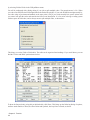
Step 4: From the Process (Compute Pts) pulldown menu choose the Least-Squares/Network Least-Squares option
as shown below.
Lesson Two - Least Squares Settings
Network Least Squares
49
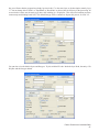
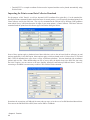
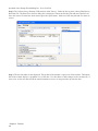
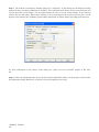
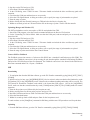
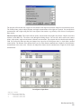
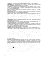
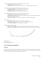
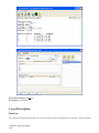
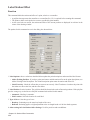
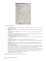
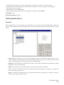
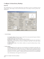
Step 5: The Network Least-Squares Settings dialog box is displayed. In this dialog box the different settings
required for the Least Squares reduction are available. The Load button at the bottom of the screen allows the user
to recall previously saved settings. The Save button allows the user to save the current settings. Press Cancel to
return to the raw data editor. When all the settings are set as desired press OK to process the raw data. For the
purpose of this tutorial, the Coordinate System settings should look as follows before proceeding to the next step.
For more information on the content of this dialog box, please review the SurvNET chapter of this manual.
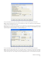
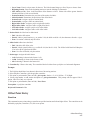
Step 6: Choose the Adjustment tab to review the least squares adjustment settings. For the purpose of this tutorial,
the Adjustment settings should look as follows before proceeding to the next step.
Chapter 2. Tutorials
50
For more information on the content of this dialog box, please review the SurvNET chapter of this manual.
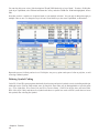
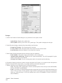
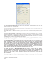
Step 7: Choose the Standard Errors tab to review the standard error settings. The standard error settings should look
as follows before proceeding to the next step.
Standard errors are an estimate of the different errors you would expect to obtain based on the type equipment and
field procedures you used to collect the raw data. For example, if you are using a 5 second theodolite, you could
expect the angles to be measured within +/- 5 seconds (Reading error).
For more information on the content of this dialog box, please review the SurvNET chapter of this manual.
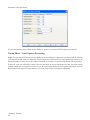
Step 8: Choose the Output Options tab to review the output settings. For the purpose of this tutorial, the Output
Options settings should look as follows before proceeding to the next step. These settings apply only to the output
of data to the report files. These settings do not affect computational precision. Press OK and the least squares
Network Least Squares
51
adjustment will be performed.
For more information on the content of this dialog box, please review the SurvNET chapter of this manual.
Lesson Three - Least Squares Processing
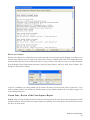
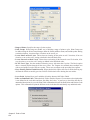
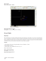
Step 9: After pressing OK from the previous dialog box the Least Squares adjustment is performed and the Network
Least-Squares Results window is displayed. If the solution converged correctly the report should look similar to the
following window. If there were errors or the solution did not converge, an error message dialog will be generated.
If there are errors you will need to return to the raw data editor to review and edit the raw data. Since the tutorial
example should have converged we will next review the reports generated by the least squares adjustment. Press the
Report button at the bottom of the window to review the results of the Least Squares adjustment.
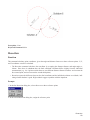
Chapter 2. Tutorials
52
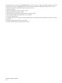
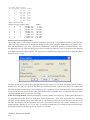
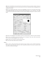
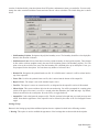
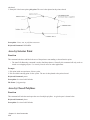
Relative Error Ellipses
Relative error ellipses are a statistical measure of the expected error between two points. Regular error ellipses are a
measure of the absolute error of a single point. Some survey accuracy standards such as the ALTA standards state the
maximum allowable error between any two points in a survey. Relative error ellipses can give you this information.
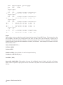
Press the Relative Error Ellipse button and enter 514 and 503 in the From Pt. and To Pt. fields. Press Calculate. The
dialog box should look as follows.
At the 95% confidence level there should only be around .06 meters of error between points 514 and 503. If you
need to compute relative error ellipses for sideshots make sure the ''Enable sideshots for error ellipse'' toggle is set
in the Settings dialog box.
Lesson Four - Review of the Least Squares Report
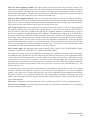
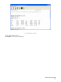
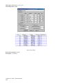
Step 10: After pressing the Report button from the previous dialog box the least squares report is displayed. In this
lesson the different sections of the least squares report are explained. To save the report to an ASCII text file use the
File/Save As menu option.
Network Least Squares
53
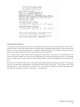
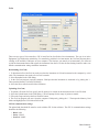
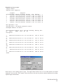
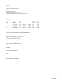
Preprocessing and Header Information
The following excerpt from the report shows the header information and the preprocessing results. The header information consists of the date and time, the input and output file names, the coordinate system, the curvature/refraction
setting, maximum iterations, and distance units.
During the preprocessing process multiple angles are reduced to a single angle and multiple slope distances, vertical
angles, HI's, and rod heights are reduced to a single horizontal distance and vertical distance. During this process
the horizontal angle, horizontal distance, and vertical difference spreads are computed. If the spreads exceed the tolerance settings from the Settings dialog box a warning message is displayed showing the high and low measurement
and the difference between the high and low measurement.
Chapter 2. Tutorials
54
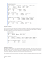
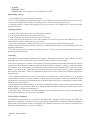
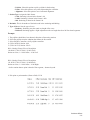
Unadjusted Measurements
The following excerpt from the report shows the unadjusted measurements. Measurements consist of some combination of control X, and Y, horizontal distances, horizontal angles, and azimuth measurements. These measurements
consist of a single averaged measurement. For example, if multiple distances were collected between two points
only the single averaged measurement is used in the least squares adjustment.
Also, standard errors for the measurements are displayed in this section of the report. The standard errors are
computed from the standard error setting in the Settings dialog box using error propagation formulas. The standard
error of an angle that was measured several times would typically be lower than an angle that was measured only
once.
Since this data was adjusted into NAD 83 coordinates both the ground distances and the grid distances are displayed.
The grid, elevation, and combined factor are displayed in this section of the report. The horizontal angles with
and without the t-T correction applied is displayed. The t-T correction is usually not significant unless the angle
measurements encompass a large area or the survey is of a high order.
Network Least Squares
55
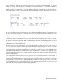
Adjusted Coordinates
The next section of the report shows the final adjusted coordinates. Additionally, the computed standard errors of
the coordinates are displayed. As this project was reduced to NAD 83 the final latitude and longitudes are displayed.
Error ellipses computed to the 95 percent confidence interval are also displayed.
Adjusted Measurements
The following section from the report shows the final adjusted measurements. This section is one of the most
important sections to review when analyzing the results of the adjustment. In addition to the adjusted measurement
the residual is displayed. The residual is the amount of adjustment applied to the measurement. The residual is
computed by subtracting the unadjusted measurement from the adjusted measurement.
The standard deviation of the measurement is also displayed. Ideally, the computed standard deviation and residual
Chapter 2. Tutorials
56
and the standard error displayed in the unadjusted measurement would all be of similar magnitude. The standard
residual is a measure of the similarity of the residual to the a-priori standard error. The standard residual is the
measurements residual divided by the standard error displayed in the unadjusted measurement section. A standard
residual greater than 2 is marked with an ''*''. A high standard residual may be an indication of a blunder. If there are
a lot of high standard residuals it may indicate that the original standard errors set in the Settings dialog box were
not realistic.
Statistics
The next section displays some statistical measures of the adjustment including the number of iterations needed for
the solution to converge, the degrees of freedom of the network, the reference variance, the standard error of unit
weight, and the results of a Chi-square test.
The degree of freedom is an indication of how many redundant measurements are in the survey. Degree of freedom
is defined as the number of measurements in excess of the number of measurements necessary to solve the network.
The standard error of unit weight relates to the overall adjustment and not an individual measurement. A value of
one indicates that the results of the adjustment are consistent with the a priori standard errors. The reference variance
is the standard error of unit weight squared.
The chi-square test is a test of the ''goodness'' of fit of the adjustment. It is not an absolute test of the accuracy of
the survey. The a priori standard errors which are defined in the project settings dialog box or with the SE record in
the raw data file are used to determine the weights of the measurements. These standard errors can also be looked at
as an estimate of how accurately the measurements were made. The chi-square test merely tests whether the results
of the adjusted measurements are consistent with the a priori standard errors. Notice that if you change the project
standard errors and then reprocess the survey the results of the chi-square test change, even though the measurements
themselves did not change.
In our example the chi-square test failed at the 95% significant level. But all distance residuals were all less than .01
meters. The largest angle residual was 42 seconds. There were some preprocessing angle spreads in the 30 to 45
seconds range. The angle standard errors in the Setting screen are probably set too low for the quality of the actual
measurements. If we were to increase the pointing and reading standard error in the Settings screen by 5-10 seconds
we would probably pass the chi-square. Also notice that if you change the standard errors by only 5-10 seconds and
reprocess the data the final coordinates will not change significantly.
Network Least Squares
57
The next part of the report displays the results of the vertical adjustment. The horizontal and the vertical adjustments are separate least squares adjustment processes. As long as there are redundant vertical measurements the
vertical component of the network will also be reduced and adjusted using least squares. In the vertical adjustment
benchmarks are held fixed.
This is the final step in the tutorial. The final adjusted coordinates are now stored in the current project point database
and can now be used for mapping and design.
Chapter 2. Tutorials
58
Data Collectors
3
59
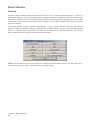
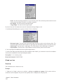
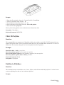
Data Collectors
Function
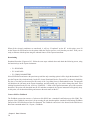
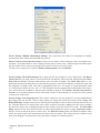
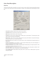
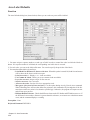
The Data Collector Programs dialog box (shown here) allows you to perform two main functions for a variety of
popular data collectors. First, this command transfers (uploads and downloads) data between the data collector and
Carlson Survey Desktop (CSD). Second, this command converts data formats between the data collector format and
CSD format. If you already have the data file on the computer, you can skip the transfer function and just run the
conversion function.
The transfer function does the conversion automatically. In most cases the download from the data collector
produces a RW5 file (field notes) and/or a Points.mdb file (coordinate points). Several of the download programs
allow you to automatically run the Edit-Process Raw File command after you download raw data. You can also
send or upload coordinates from the current project point database.
NOTE: CSD downlaods raw survey notes and processes them in the .RW5 format. However, the .RW5 files may, at
any time, be converted to classsic .FBK format for use in other features.
Chapter 3. Data Collectors
60
SurvCE/FastSurvey/G2
NOTE: Unless otherwise indicated, the term SurvCE will apply to Carlson SurvCE, SurvStar, Thales FastSurvey
and Sokkia G2 in this section.
First, connect the serial cable. Then select Data Transfer on the hand-held. Choose SurvCADD/Carlson Survey
Download. This leads to a File Transfer screen on SurvCE, which says ''Awaiting Connection''. SurvCE is ready.
Now all the action is on the PC side.
In the Survey Menu, choose Data Collection->SurvCE. This brings up the Carlson SurvCE transfer dialog.
Data Collectors
61
• Download Coordinates shows a list of the coordinate files on Carlson SurvCE. Select a file to download.
The point data will be stored in the point database for the current Autodesk Land Desktop project.
• Download Other Files shows a list of all the data files on Carlson SurvCE. Select a file to download. The
file will be transferred and stored in the Survey folder for the current Autodesk Land Desktop project. The
files are transferred in their original form without any conversion.
• Upload Coordinates transfers points from the current Autodesk Land Desktop project to Carlson SurvCE.
Before running this command, you need to supply a name in the Carlson SurvCE File edit box. This name is
used to name the point file on the Carlson SurvCE collector.
• Upload Triangulation and Alignment features will transfer triangulation surfaces and horizontal alignments
from Autodesk Land Desktop to Carlson SurvCE.
• Upload Geoid transfers a portion of the specified geoid to Carlson SurvCE. The geoid data files require a
large amount of disk space and are not included in the CSD install. Instead they are installed separately. You
can download the install for the latest geoid data files from the Carlson Software web page.
• Upload Field To Finish Codes transfers a code table to Carlson SurvCE.
When you connect the cable from Carlson SurvCE to the PC, a program such as Microsoft ActiveSync may interfere
and say ''Connect to PC?'' Answer, ''No'' to this prompt.
If any other program is using the COM port, you will not be able to connect properly and CSD may respond with
the following message:
If you receive this error, determine what program has control of the COM port and terminate this program. Programs
to look for include Microsoft ActiveSync, PalmPilot synchronization, fax programs, etc.
Chapter 3. Data Collectors
62
• Convert RW5 to Fieldbook: The Fieldbook conversion converts a Carlson raw file (RW5) into a Autodesk
Land Desktop raw file (FBK). The purpose of the Fieldbook conversion is for processing the raw data through
the Autodesk Land Desktop Fieldbook instead of the CSD Edit-Process Raw file command. The Fieldbook
conversion is also located in the Edit-Process Raw Data command under File->Export->Fieldbook.
Data Collectors
63
CG Field
In CSD, select Data Collection and choose CGField. Make sure the communication parameters in CSD are set to
the following
• Baud 9600
• Parity NONE
Receiving a Raw data File from CGField
1. In CGField, select the UTILS menu and choose C&G Transfer.
2. Select Send Raw Data
3. In CSD, leave the FILE fields blank. Press the Download Raw button to ready CSD to receive the file.
4. In CGField, select the raw data file to be sent. The transfer will begin. The C&G .RAW file will be transferred
and saved in the data folder. After the transfer is complete, you will be asked for the RW5 file name. The RAW file
will be automatically converted to a Carlson RW5 file.
Receiving a Coordinate File from CGField
1. In CGField, select the UTILS menu and choose C&G Transfer.
2. Select Send Coords, and choose the Coordinate file to send.
3. In CSD, leave the FILE fields blank. Press the Download Raw button to ready CSD to receive the file.
4. In CGField, select the points to send for all points, to select blocks of points, or from a .pts file (the set of points
in a Batch Point File).
5. The coordinates will be transferred. After the transfer is complete, you will be asked for the coordinate file name.
The C&G CRD file will automatically be converted to a Autodesk Land Desktop coordinate file.
Receiving an ASCII file from CGField
Chapter 3. Data Collectors
64
This will allow you to transfer a C&G report file (RPT) or an ASCII NEZ file to CSD
1. In CGField, select the UTILS menu and choose C&G Transfer.
2. Select Send ASCII.
3. In CSD, leave the FILE fields blank. Press the Download ASCII button to ready CSD to receive the file.
4. In CGField, select the ASCII file to send.
5. After the transfer is complete, you will see the file in the CSD editor. You can then select FILE and SAVE (or
SAVEAS) to save the ASCII file.
Sending a Coordinate File to CGField
1. In CGField, select the UTILS menu and choose C&G Transfer.
2. Select Receive Coords to ready the data collector.
3. In CSD, leave the FILE fields blank. Press the Upload (Send Coordinates) button. Select the points to send.
4. Press the Start Transfer button.
5. CSD will send the file name to CGField and a coordinate file with the same name will be automatically created
or opened in CGField.
6. If the file exists you will be asked how you want to handle duplicate points:
• Overwrite
• Don't Overwrite
• Ask for each Point
The point transfer will begin.
Convert CG .RAW to CSD .RW5
This utility allows you to convert a C&G raw data file to a Carlson raw data file. Select the C&G .RAW file to
convert. Then enter the file name of the destination Carlson RW5 file.
Convert .RW5 to Fieldbook
The Fieldbook conversion converts a Carlson raw file (RW5) into a Autodesk Land Desktop raw file (FBK). The
purpose of the Fieldbook conversion is for processing the raw data through the Autodesk Land Desktop Fieldbook
instead of the CSD Edit-Process Raw file command. The Fieldbook conversion is also located in the Edit-Process
Raw Data command under File->Export->Fieldbook.
Prerequisite: None
Keyboard Command: DATACOLT
Data Collectors
65
TDS Data Collection
Downloading (HP-48 and Husky)
1. In the TDS program, go to the File Transfer command. Choose the type of data to transfer (CRD or RAW).
2. Select the Send function key.
3. Stop here on the TDS and go to CSD.
4 Select Data Collection and pick TDS. Make sure that the COM port and baud rate are set correctly.
5. Select the Download button. CSD will now wait to receive the TDS file.
6. Within ten seconds, select the file to send on the TDS.
Downloading (Ranger and Windows CE)
1. In the TDS program, go to the Transfer command and pick the Send File function. Set the Connecting To field to
HP-48.
2. Make sure that the COM port, baud rate and parity are set correctly and then select OK.
3. In the Type field of the file selection dialog, choose Coordinate Files or Raw Files.
4. Stop here on the TDS and go to CSD.
5. Select Data Collection and pick TDS. Make sure that the COM port and baud rate are set correctly.
6. Select the Download button. The CSD program will now wait to receive the TDS file.
7. Within ten seconds, select the file to send on the TDS, and select OK in the TDS dialog.
Uploading (HP-48 and Husky)
The LDT point database can be converted to a CR5 file and uploaded into TDS.
1. Start in the TDS program, select the File Transfer command.
Chapter 3. Data Collectors
66
2. Stop here on the TDS and go to CSD.
3. Select Data Collection and pick TDS.
4. In the CSD dialog, enter a TDS File name. This name should not include the drive and directory path or file
extension.
5. Check that the COM port and baud rate are set correctly.
6. Select the CSD Upload button. A dialog now allows you to specify the range of point numbers to upload.
7. Enter the range of points.
8. Before clicking the Start Transfer button go to TDS and select the Receive function key.
9. Within ten seconds go back to CSD and click the OK on the range of points. The file will then transfer.
Uploading (Ranger and Windows CE)
The LDT point database can be converted to a CR5 file and uploaded into TDS.
1. Start in the TDS program, select the Transfer command and choose the Receive File function.
2. Set the ''Connecting To'' field to HP-48. Make sure that the COM port, baud rate and parity are set correctly and
then select OK.
3. Stop here on the TDS and go to CSD.
4. Select Data Collection and pick TDS.
5. In the CSD dialog, enter a TDS File name. This name should not include the drive and directory path or file
extension.
6. Check that the COM port and baud rate are set correctly.
7. Select the CSD Upload button. A dialog now allows you to specify the range of point numbers to upload.
8. Enter the range of points and click the Start Transfer button.
Convert .RW5 to Fieldbook
The Fieldbook conversion converts a Carlson raw file (RW5) into a Autodesk Land Desktop raw file (FBK). The
purpose of the Fieldbook conversion is for processing the raw data through the Autodesk Land Desktop Fieldbook
instead of the CSD Edit-Process Raw file command. The Fieldbook conversion is also located in the Edit-Process
Raw Data command under File->Export->Fieldbook.
SMI
Downloading
1. To send point data from the SMI data collector, go to the File Transfer command by typing [More] [NXT] [TOPC]
[COMM].
2. In SMI version 6 or later, type [Job][KERM][SEND]. Also in version 6, make sure that the first function key reads
[NE] and not [XY] in the [Job][KERM] screen. Otherwise the coordinate northing and easting will be reversed. The
[NE] stands for North-East coordinate order which is the format that CSD expects. Also in the [Job][KERM]
screen, make sure that the second function key reads [COMM] and not [SPACE]. The [COMM] stands for comma
separators.
3. Enter the first point to send, followed by the last point to send.
4. Before pressing Enter for the last point, stop here and go to CSD.
5. Run Data Collection and choose SMI. Check that the COM port and baud rate are set correctly.
6. Select the Download button.
7. Within 10 seconds go back to SMI and press Enter for the last point to send.
To send raw data, use the [Print][Raw] command in SMI along with the same CSD procedure used for point data.
Uploading
1. From the SMI data collector, go to the File Transfer command by typing [More] [NXT] [TO48] [COMM].
Data Collectors
67
2. In SMI version 6 or later, type [Job][KERM][RECV]. Also in version 6, make sure that first function key reads
[NE] and not [XY] in the [Job][KERM] screen. Otherwise the coordinate northing and easting will be reversed.
3. Enter the first point to send followed by the last point to send.
4. Enter the job name.
5. Before pressing Enter, stop here and go to CSD.
6. Run Data Collection and choose SMI.
7. In the CSD dialog, specify the same job name as entered in SMI.
8. Check that the COM port and baud rate are set correctly.
9. Select the Upload button.
10. A dialog allows you to specify the range of point numbers to upload. Enter the same range of points as entered
on the SMI.
11. Return to SMI and select Enter for job name.
12. Choose the OK button for range of points in CSD.
Chapter 3. Data Collectors
68
Leica
There are two types of Leica transfers: GIF-10 and GeoCom for all other Leica instruments. The type is set in the
Equipment Type field on the main dialog. For transferring with the Leica instruments, the GeoCom program shows
a dialog of the available COM ports on your computer. The first time you transfer to an instrument, you will need
to pick the Instruments button and register the instrument from the list. Select the Port Settings button to make sure
that the communication settings match the instrument.
Downloading (GeoCom)
1. To download a file with GeoCom, make sure that the instrument is ON and connected to the computer by serial
cable. The instrument also needs to be in GeoCom mode.
2. Select Download in the CSD dialog.
3. In the GeoCom program, open the computer COM port that the instrument is connected to by picking the '+'.
Then open the Memory Card and GSI folders.
4. Select the file to transfer and click the OK button.
Uploading (GeoCom)
1. To upload a file with GeoCom, specify the file name to be created on the instrument in the Leica File field.
2. Select the Upload button in the CSD dialog. CSD will prompt for the range of points to transfer.
3. Fill out the range and select the Start Transfer button.
4. The GeoCom program will start. Open the computer COM port by picking the '+'. Then open the Memory Card
folder and highlight the GSI folder and click OK.
GIF-10 communication settings
The upload and download file transfer works with the GIF-10 data collector. The GIF-10 communication settings
should be the following:
• Baud: 9600
• Parity: NONE
• Protocol: NONE
Data Collectors
69
• Stop Bit: 1
• End Mark: CR/LF
• Connected As: some computers use DCE and others use DTE
Downloading (GIF-10)
1. From the GIF-10, go to the file transfer command.
2. Go to CSD. Run the Data Collection and choose Leica. Check that the COM port and baud rate are set correctly.
3. Select the Download button. Within 10 seconds go back to GIF-10 and select the file to send.
4. When the transfer is complete, the program will ask you to create a CSD coordinate file if you haven't already
specified a file name.
Uploading (GIF-10)
1. From the GIF-10 data collector, go to the file transfer command.
2. Go to CSD. Run the Data Collection and choose Leica.
3. In the CSD dialog, specify the job name in the Leica File field.
4. Choose the Select File button next to the CSD coordinate File edit box and choose the coordinate file to send.
Check that the COM port and baud rate are set correctly.
5. Select the Upload button. A dialog now allows you to specify the range of point numbers to upload.
6. Before clicking the OK button for range of points, go to GIF-10 and start the receive by highlighting Receive and
pressing the Run button.
7. The GIF-10 now shows the available job numbers. Choose a job to receive the transfer using the arrow buttons
and then press the Run button.
Converting
CSD supports raw and coordinate data collected using three different Leica Operation Codes: Wildsoft, 10-20-3040, and the newer LISCAD. Data can also be in the GSI8 format or the newer GSI16 format.
Leica raw files usually have a .RAW or .GSI extension. The primary difference between the GSI8 and GSI16 formats
is that, in the GSI16 format, information is contained in data blocks of 16 characters , while it is contained in blocks
of 8 characters in the GSI8 format. Leica instruments make it possible to have both the GSI8 as well as GSI16 data
formats in the same raw file. Lines with the GSI16 format data always start with an asterisk (*) sign, to distinguish
them from the GSI8 format. There is no distinction between Leica raw files collected in the Wildsoft and LISCAD
operation codes.
1. The Convert Leica button can be used to convert any Leica format file into a CSD format file. (e.g., if you have
a Leica PCMCIA card, no serial cable transfer is needed. Instead use the Convert command to make the RW5 and
coordinate files). Since there is no distinction between Wildsoft and LISCAD files, you must know in advance which
format has been used in the file.
2. Select that particular option (Wildsoft, 10-20-30-40, or LISCAD) under the ''Coding System'' option at the bottom
of the dialog box. You must choose the order in which foresight-backsight readings were recorded in the raw file,
BFFB or BFBF, as explained in the dialog box.
3. Select the Convert Leica button. The command prompts for the input Wild/Leica File (raw file), the output RW5
file and the coordinate file, if you have not entered them.
Convert .RW5 to Fieldbook
The Fieldbook conversion converts a Carlson raw file (RW5) into a Autodesk Land Desktop raw file (FBK). The
purpose of the Fieldbook conversion is for processing the raw data through the Autodesk Land Desktop Fieldbook
instead of the CSD Edit-Process Raw file command. The Fieldbook conversion is also located in the Edit-Process
Raw Data command under File->Export->Fieldbook.
Chapter 3. Data Collectors
70
SDR/Sokkia/Leitz Data Collection
This command applies to the Sokkia SDR-20, SDR-22, SDR-31 and SDR-33 as well as other collectors that have
SDR format transfer, such as the Trimble and C & G.
Downloading
1. From the SDR data collector, select the Communications command from the main menu. Choose Data Format
SDR.
2. Select the Send function key. Then choose Select Jobs.
3. From the list of jobs, highlight the job to transfer and set it to Yes with the arrow keys.
4. In CSD, run Data Collection choose Sokkia/SDR. Check that the COM port and baud rate are set correctly.
5. Select the Download button, and within ten seconds go back to SDR and press OK.
6. The SDR format contains both coordinate and raw data. The coordinate data is converted to a CSD coordinate
file and the raw data is converted to a CSD raw data (.RW5) file. The original SDR transfer file is stored on the
computer as a RAW file.
SDR-33
The SDR-33 has different modes for storing and transferring data. In coordinate mode, the download will create
points in the coordinate file and the raw data (.RW5) file will only contain some basic header lines. In the raw
data mode, the download will create all the measurement data in the raw file and no points will be created in the
coordinate file. For this raw data mode, you will need to run Edit-Process Raw Data to calculate the points from
the raw data. The third mode in the SDR-33 creates both raw data in the raw data (.RW5) file and points in the
coordinate file. The Include Time Stamps in Notes option sets whether all the date-time records for each point are
put in the raw data (.RW5) file as description records. The Include Point Attributes in Notes option will store SDR
code 13(AT) codes to the point note (.NOT) for the point database.
Uploading
Data Collectors
71
Point data from the current project point database can be uploaded into the SDR.
1. Select the Communications command in the SDR main menu. Choose Data Format SDR.
2. In CSD, run Data Collection choose Sokkia/SDR. Check that the COM port and baud rate are set correctly.
3. Select the Upload button. A Sokkia Options dialog appears for setting the job parameters for the file to be
created on the collector. Be sure to choose the Distance Unit that matches your coordinate file (meters, US feet or
international feet).
4. Click OK. The next dialog allows you to specify the range of point numbers to upload.
5. Before clicking the Start Transfer button for range of points, go to the SDR and hit the Receive function key. The
SDR is now waiting to receive.
6. Return to CSD and click Start Transfer on the range of point dialog.
Convert .RW5 to Fieldbook
The Fieldbook conversion converts a Carlson raw file (RW5) into a Autodesk Land Desktop raw file (FBK). The
purpose of the Fieldbook conversion is for processing the raw data through the Autodesk Land Desktop Fieldbook
instead of the CSD Edit-Process Raw file command. The Fieldbook conversion is also located in the Edit-Process
Raw Data command under File->Export->Fieldbook.
Communication Settings
Besides matching the baud rate between CSD and the collector, make sure that the collector is set to word length of
eight (8), and one (1) stop bit under the communication settings.
Print File
The Receive Sokkia Print File function downloads a print report from the SDR33 data collector. This file is only
used for printing report purposes in CSD. This file is not used by CSD to generate coordinate files or raw files.
1. The first step is to choose Data format=Printed in the Communications menu of the SDR33.
2. Choose the Receive Print File button in CSD.
3. On the SDR33, choose the Send function and select a job to send. At this point the file is transferred.
4. After downloading, the job report is displayed in the CSD standard report viewer.
Nikon
Download
1. Choose the equipment and data type under the Transfer Type list. Check that the communication and data format
settings match your collector.
2. Select the Download button and follow the on-screen directions.
Upload
1. Check that the COM port and baud rate are set correctly
2. Select the Upload button. Specify the range of point numbers to upload.
3. Set the points and then click the Start Transfer button.
Convert
The Convert button will translate the Nikon raw file format (.TRN or .RAW) into CSD coordinate and raw (.RW5)
files
Chapter 3. Data Collectors
72
Convert .RW5 to Fieldbook
The Fieldbook conversion converts a Carlson raw file (RW5) into a Autodesk Land Desktop raw file (FBK). The
purpose of the Fieldbook conversion is for processing the raw data through the Autodesk Land Desktop Fieldbook
instead of the CSD Edit-Process Raw file command. The Fieldbook conversion is also located in the Edit-Process
Raw Data command under File->Export->Fieldbook.
Geodimeter
This transfer routine applies to the Geodimeter Geodat 600 collector.
Downloading
From the Geodimeter data collector, go to the file transfer command by pressing the PRG (Program) key and entering program 54. Then choose Imem (option 1) as the source. Next choose the file type to send as either Job
(measurement data) or Area (point data). The Geodimeter will then prompt for the job name. Next enter Serial
(option 3) as the destination. A confirmation screen appears showing the serial port settings. Here are some typical
settings:
COM=1,8,0,9600
Before pressing enter (ENT key), go to CSD and run Data Collection in the Survey menu and choose Geodimeter.
Then click the Download button and within 15 seconds, go back to the Geodimeter and press Enter. The file transfer
should now go. When the transfer is complete, the program will ask you for the CSD coordinate file and raw file to
create if you haven't already specified a file name in the dialog.
Uploading
In CSD, run Geodimeter under Data Collection in the Survey menu. Pick the Select File button next to the CRD
File edit box and choose the coordinate file to send. Check that the COM port and baud rate are set correctly and
then click the Upload button. A dialog now allows you to specify the range of point numbers to upload. Enter the
points to send but before clicking OK, go to the Geodimeter data collector. Start the file transfer routine by pressing
the PRG key and entering program 54. Then choose Serial (option 3) as the source. The Geodimeter will display
the serial port settings. Check these values and press enter. Next choose Area (option 2) as the destination. Then
enter the job name. The Geodimeter is now listening for data. Quickly go back to CSD and click OK on the points
to send dialog. The file transfer will now go
Convert .RW5 to Fieldbook
The Fieldbook conversion converts a Carlson raw file (RW5) into a Autodesk Land Desktop raw file (FBK). The
purpose of the Fieldbook conversion is for processing the raw data through the Autodesk Land Desktop Fieldbook
instead of the CSD Edit-Process Raw file command. The Fieldbook conversion is also located in the Edit-Process
Raw Data command under File->Export->Fieldbook.
Communication Settings
If the Geodimeter is not communicating with CSD, run function 79 on the Geodimeter and make sure that it is set
to 4. This setting is for the transfer message end of sequence format.
Surveyor's Assistant
Downloading
Data Collectors
73
1. From the Surveyor's Assistant data collector, select the Transfer command from the main menu. Fill out the
transfer screen as follows:
•
•
•
•
•
•
Direction: OUTPUT
Format: LIETZ
Data: Coordinate or All Data
Port: COM1 or COM2
Ckh Hold: NO
Protocol: NONE
2. Check the settings under the PORT menu. Typical port settings are baud=9600, parity=none, data=8, stop=1 and
handshake=XON/XOFF.
3. Now in CSD, run Data Collection and choose Surveyor's Assistant. Check that the COM port and baud rate are
set correctly.
4. Select the Download button and within ten seconds return to Surveyor's Assistant and press GO.
5. If the All Data option is used, then the Leitz format will contain both coordinate and raw data. The coordinate
data is stored to project point database and the raw data is converted to a CSD raw data (.RW5) file.
Uploading
1. Point data from the CSD coordinate file can be uploaded into the Surveyor's Assistant. First go to the Transfer
command on the main menu. Fill out the screen as follows:
•
•
•
•
Direction: INPUT
Format: LEITZ
Port: COM1 or COM2
Protocol: NONE
2. Go back to CSD and run Data Collection, selecting Surveyor's Assistant. Check that the COM port and baud rate
are set correctly.
3. Click the Upload button. A dialog now allows you to specify the range of point numbers to upload.
4. Before clicking the OK button for range of points, return to Surveyor's Assistant and hit the GO function key.
The Surveyor's Assistant is now waiting to receive.
5. Return to CSD and click OK on the range of point dialog.
Convert .RW5 to Fieldbook
The Fieldbook conversion converts a Carlson raw file (RW5) into a Autodesk Land Desktop raw file (FBK). The
purpose of the Fieldbook conversion is for processing the raw data through the Autodesk Land Desktop Fieldbook
instead of the CSD Edit-Process Raw file command. The Fieldbook conversion is also located in the Edit-Process
Raw Data command under File->Export->Fieldbook.
Topcon
The various Topcon instruments in this list can be downloaded directly from the instrument to Carlson Software,
using the appropriate cable supplied by Topcon. The cable has a round end to connect to the Topcon instrument and
a 9-pin serial port end to connect to the PC. This download is commonly used, for example, by companies who
collect data and store the data onboard the instrument itself, with no 3rd-party handheld data collector involved.
This is a fairly common practice, for example, in construction stakeout.
The procedure outlined below is for the Topcon GTS 226, which has a 4-button keyboard (F1 through F4)
Chapter 3. Data Collectors
74
providing access to all onboard commands and even allowing direct, multi-keystroke entry of coordinates. Most
Topcon instruments follow similar procedure.
Uploading
Upload Procedure (PC to Topcon): At the main menu, you will see the following options:
• F1: DATA COLLECT
• F2: LAYOUT
• F3: MEMORY MANAGER
Press the F3 key twice, paging down to DATA TRANSFER. Then select COMM. PARAMETERS (F3). Protocol
must be ''ONE-WAY'', BAUD RATE 9600 and CHAR/PARITY must be 8/NONE.
NOTE: This is a one-time process. Once the protocols are verified, you can send and receive data by going
directly to the screen shown below.
Return to the COMM. PARAMETERS selection screen, which displays the following 3 options:
• F1: SEND DATA
• F2: LOAD DATA
• F3: COMM. PARAMETERS
Press F2 to LOAD DATA. Then press F1 to select COOR. DATA. The program on the Topcon will ask you to enter
a file name. You must enter this name on the Topcon instrument, using the 4 function keys to access letters and
numbers. This will be the name of the file that you will use for stakeout. If you entered a name such as 11 or Smith
or whatever you choose, your coordinate file on the PC will be converted to this name as it stored on the Topcon.
LOAD COOR. DATA. OK? F3=YES. Press F3. The instrument will say ''Waiting Data...'' At this point,
you need to be in the Topcon data transfer option. There you pick Upload, or prior to picking upload you can
specify your coordinate file name, as shown below. After Upload is clicked, you specify the point range to send,
and click OK. You have a certain amount of time within the ''Waiting Data..'' mode to start sending the data over to
the Topcon instrument.
Data Collectors
75
When all the selected coordinates are transferred, it will say ''Completed'' on the PC. At this point, press F4
on the Topcon for STOP and review the points within the Topcon screen to verify that they are there. Then you are
ready to stakeout with the points using the onboard features of the Topcon instrument.
Downloading
Download Procedure (Topcon to PC): Follow the same steps outlined above and obtain the following screen, using
the function keys on the Topcon instrument:
• F1: SEND DATA
• F2: LOAD DATA
• F3: COMM. PARAMETERS
Select SEND DATA and answer the questions up until the only remaining option is OK to begin the download. This
gets the Topcon side poised and ready. On the PC, choose Download (Receive Topcon File), as shown in the dialog
box above. Note that you do not need to fill out any of the 3 top dialog boxes in the download screen. The program
will default to the job name on the Topcon instrument, and will prompt you if you wish to change the name. After
clicking Download on the PC side, it will say ''WAITING...''. Back on the Topcon instrument, press OK to start the
download. The points will download into the PC and when completed, the Topcon instrument will typically beep.
At this point, exit the download dialog and return to the main menu on the PC.
Convert .RW5 to Fieldbook
The Fieldbook conversion converts a Carlson raw file (RW5) into a Autodesk Land Desktop raw file (FBK). The
purpose of the Fieldbook conversion is for processing the raw data through the Autodesk Land Desktop Fieldbook
instead of the CSD Edit-Process Raw file command. The Fieldbook conversion is also located in the Edit-Process
Raw Data command under File->Export->Fieldbook.
Chapter 3. Data Collectors
76
Data Collectors
77
Chapter 3. Data Collectors
78
Edit-Process Raw File
4
79
Edit-Process Raw File
Functions
This program reads or creates a raw data (.RW5) file that contains various lines of data (records) that could be likened
to a surveyor's field book. You can specify point coordinates, job information, notes, and the angles and distances
that make up traverse or sideshots records. Once the raw data is created or read it can be processed/reduced to
coordinates that are stored in the current point database.
The raw file can also be created or appended using the Locate Point, Traverse, Sideshot, and Inverse commands. To
store the data inputs from these commands into a raw file, first toggle on the Raw File ON/OFF command on the
Cogo menu. It is possible to always have the raw data file open to store data inputs. To enable this option, choose
Configure Carlson Survey Desktop and turn on the Automatic Raw File toggle in this dialog.
The raw files created by TDS data collector programs are also compatible without conversion. The command Data
Collectors on the Tools menu has options for reading other data collectors native file formats and converting them
to raw data (.RW5) format. Within the raw data editor, the File menu includes an import menu for converting raw
data from other formats.
When you select the Edit-Process Raw Data File command you are prompted to specify the name of the raw data
(.RW5) file. The point database for the current project is used automatically.
Edit-Process Raw Data File uses a spreadsheet for editing the raw data as shown. Each row of the spreadsheet
is represented by a number located at the far left side of the editor. Various messages and reports often reference
possible problems with the data by this row number. Each row of the spreadsheet represents one record of data.
There are 14 types of data records. The type of data record is shown in the first column. Different record types use
different numbers of columns. Whenever the data record type changes between rows, a record header is added to
the spreadsheet that describes each column of data in the following row. To edit the raw data, simply highlight the
cell and type in the new value. To change the type of record, pick on the down arrow in the first column and choose
a new data type from the list. To delete a row, highlight any cell in the row and hit the Delete key or choose Delete
Row from the Edit menu. Records can be added pressing the Insert key, pressing the down arrow key from the last
line in the spreadsheet, or by choosing one of the add records from the Add menu.
Chapter 4. Edit-Process Raw File
80
The different record types are described below.
TR (Traverse)
The traverse record contains the occupied point number, foresight point number, angle mode, horizontal angle,
distance, vertical angle and description. When processed, this record will calculate and store the coordinates for
the foresight point. Traversing also moves the setup by making the traverse foresight point the next occupied point
and the traverse occupied point becomes the next backsight point. The different angle codes are NE for northeast
bearing, SE for southeast, SW for southwest, NW for northwest, AZ for azimuth, AL for angle left, AR for angle
right, DL for deflection angle left and DR for deflection angle right. To set the angle code, pick on the Code down
arrow and choose from the list. The horizontal and vertical angles should be entered as dd.mmss. For example,
45.2305 is 45 degrees, 23 minutes and 5 seconds. The vertical angle can be shown as vertical angle (0 degrees
level), zenith angle (90 degrees level) or elevation difference. The vertical angle mode is set in the Display menu.
The distance mode is also set in the Display menu as either slope or horizontal distance. The description field is
used as the foresight point description.
SS (SideShot)
The sideshot record is the same as the traverse record except that sideshot does not move the setup.
HI (Instrument and Rod Height)
This record sets the instrument and rod heights used in elevation calculations. This record should precede any
traverse and sideshot records that you want the heights applied to.
BK (BackSight)
The backsight record contains the occupied point number, backsight point number, backsight azimuth and the set
azimuth. This record should precede any traverse and sideshot records that use this setup. If no backsight point is
entered, the program uses the backsight azimuth to turn angles from. The Set Azimuth is the circle reading of the
instrument when sighting the backsight. A Set Azimuth of zero is the default.
PT (Store Point)
The store point record consists of a point number, northing, easting, elevation and description. When processing,
this data will be stored as a point in the coordinate file. If the first Occupied point and/or the initial Backsight point
Edit-Process Raw File
81
are not defined in the coordinate file set for processing to, both points will need to be added to the rw5 file as PT
(Store Point) records.
DS (Description)
The description record is an additional note that appears in the spreadsheet editor and printouts. This record can
contain various information that is recorded in data collectors during field operations. This data can vary from user,
temperature and general data to each line of data associated with ''Set Collection''. When ''Sets'' of data collected
using various brands of data collection software is converted/imported into the raw editor, the actual measurements
made during the spinning of the angles and distances are recorded as DS records and the mean value of the angle
and distance is recorded as a SS record. DS records are not used in processing.
CL (Closing Shot)
The closing shot record is the traverse record where the foresight point is the closing point for the traverse. This
record is used by the adjustment commands in the Process menu. There should be only one CL record in each
Traverse loop (Name Record) in the raw file. If there is no CL record, the process adjustment routines will prompt
for which shot is the closing shot. The closing shot can also be define in the field by using special codes defined in
the Open Settings found under the File pulldown within the editor. Please refer to the ''Open Settings'' documentation
below for more information on these codes.
AB (Angle Balance)
The Angle Balance record is the measurement data observed that closes the angles of the traverse. Typically this
record is the measurement data recorded from the closing shot to the initial backsight point. The backsight could be
either external or internal to the traverse. Angle Balance routine in the Process menu uses this record and compares
the angle between the occupied point and foresight point of this record with a user-specified reference angle. There
should be only one AB record in the raw file. If there is no AB record, then the Angle Balance routine will prompt
for which shot to use as the angle balance.
CL + AB (Closing Shot and Angle Balance)
This record is used as both the closing shot and angle balance records.
FD (Foresight Direct)
The foresight direct is a traverse record used in a direct and reverse set. When the program finds one the of directreverse measurement records, it will look for the other three records to complete the set.
FR (Foresight Reverse)
The foresight reverse is a traverse record used in a direct and reverse set.
BD (Backsight Direct)
The backsight direct is a traverse record used in a direct and reverse set.
BR (Backsight Reverse)
The backsight reverse is a traverse record used in a direct and reverse set.
EL (Elevation Only)
This record sets the elevation in the CRD file for the specified point number. Often used when an existing point with
good vertical control is being traversed through. Using this record type for the point would keep the elevation from
changing on the existing point regardless of the measurement data.
AZ (Azimuth Only)
Applies to SurvNET, the optional Network Least Squares analysis and adjustment routine.
CSE (Control Standard Error)
Applies to SurvNET, the optional Network Least Squares analysis and adjustment routine.
Chapter 4. Edit-Process Raw File
82
SSE (Set-up Standard Error)
Applies to SurvNET, the optional Network Least Squares analysis and adjustment routine.
MSE (Measurement Standard Error)
Applies to SurvNET, the optional Network Least Squares analysis and adjustment routine.
NAME (Traverse Name)
This record acts as an identifier for the group of records that make up a traverse. All the records after the NAME
record belong to that traverse up to the next NAME record or the end of the file. This record allows you to have
multiple traverses in one raw file. When running one of the Process commands, the program will bring up a list of
all the traverse names. Simply choose which traverse to process. If you have only one traverse in the raw file, then
you don't need the NAME record.
GPS
This record contains the Latitude and Longitude of a point as measured by GPS surveying equipment using Carlson
SurvCE data collection software. This record has additional information tied to it such as localization files, geoid
files, coordinate projection systems etc. This record has its own processing routine in the Process pulldown within
the editor. Processing procedures are discussed in the Process (Compute Pts) pulldown documentation.
Raw Data Editor Pulldown Menus
File Menu
Save
This saves the rw5 file. If the file hasn't been named you will be prompted for the file name and the location to
save the file. After you preform the first save, this command acts as a quick save and saves the file to the name and
location specified during the initial saving of the file.
Save As
This command saves the file and always prompts for file name and location to save.
Print
This command outputs the raw data file to the Standard Report Viewer. From here, you can print the report, draw it
in the drawing or save it to a file. See Standard Report Viewer for more information. See example printout:
Raw File> c:\scadxml\data\survey.rw5
Note
Survey Example
Edit-Process Raw File
83
TR
TR
TR
TR
TR
TR
TR
SS
PntNo
1
OcPt
1
InstHgt
5.32
OcPt
1
InstHgt
5.43
OcPt
2
InstHgt
5.4
OcPt
3
4
5
6
InstHgt
5.42
OcPt
7
7
Northing Easting
Elevation Desc
5000
5000
100
START
BsPt
SetAzi
RodHgt
6.0
FsPt
2
AR
RodHgt
6.0
FsPt
3
AR
RodHgt
6.0
FsPt
4
AR
5
AR
6
AR
7
AR
RodHgt
6.0
FsPt
8
AR
19
AR
HorzAngle SlopeDist ZenithAng Desc
268.5330 711.420
89.4050
P2
HorzAngle SlopeDist ZenithAng Desc
262.5448 457.760
89.3236
P3
HorzAngle
208.5710
247.1657
277.4835
92.4113
SlopeDist
201.310
497.120
223.980
233.880
ZenithAng
89.1803
88.5235
90.2926
90.2746
Desc
P4
P5
P6
P7
HorzAngle SlopeDist ZenithAng Desc
261.2756 387.250
91.4405
CLOSE
289.3456 112.450
91.3423
SS1
Import
These routines convert raw data from other formats into the current Carlson RW5 format. The converted raw data
will be added to the end of any existing data in the editor. In many cases, the raw data file to import can be
downloaded directly from the data collector or instrument using the Data Collectors command. The following
supported formats (along with their standard file extension) are listed here. Some Sample File Formats are listed at
the end of this section.
C&G (.CGR;.RAW;.TXT; *)
CalTrans (.DMP)
Carlson (.RW5)
Fieldbook (.FBK): From Softdesk or Land Development Desktop.
Geodimeter (.OBS; .RAW; job;*)
LandXML (.XML)
Leica (.GSI; .RAW; GRE): This reads the Leica raw file in Wildsoft, Liscad, 10-20-30-40, C&G, or GeoComp
format. There are options to specify direct-reverse shot order if any and to convert from International Feet to Leica
US Feet.
Chapter 4. Edit-Process Raw File
84
Maptech (.FLD)
MDL Laser (.CDS)
Nikon (.TRN; .RAW)
PC Cogo (.BAT)
SDMS (.prj;*)
SMI (.RAW)
Sokkia SDR (.SDR; .RAW; *)
SurvCOGO (.RAW or .TXT)
Survis (.RAW)
TDS (.RW5; RAW)
Topcon (raw;*)
Trimble (.dc)
3TA5 (.TXT)
Zeiss (.DAT)
Export
These routines convert the Carlson raw data (.RW5) file to other formats. The following file formats are supported.
CalTrans (DMP)
Fieldbook (.FBK): This export routine provides an option to ''Setup Fieldbook Codes''. This allows the user to
substitute the raw description contained in the rw5 file with the fieldbook code used in AutoDesk Land Desktop.
Edit-Process Raw File
85
FL DOT (.OBS)
GPS Data (.TXT;*)
Land XML (.XML)
MOSS (.MOS)
SDMS (.PRJ) This export routine provides an option to ''Setup SDMS Codes''. This allows the user to substitute the
raw description contained in the rw5 file with the SDMS codes used in SDMS program.
Sokkia (.SDR)
TDS (RW5;RAW)
VA Dot (TOP)
Open Settings
This option allows for defining codes that represent the closing shot and angle balance shot of a traverse. These codes
can be entered in the description of a point while in the field. When the rw5 is opened in the raw file editor, the
measurement data containing the closing shot code will be set to a CL record and the measurement data containing
the angle balance code will be set to an AB record. This allows for quick processing of the survey data and saves
the time spent setting up the file for processing.
Chapter 4. Edit-Process Raw File
86
Print Settings
Provides control of various options for printing the rw5 file in theStandard Report Viewer.
Exit
Exits the raw file editor.
Edit Menu
Undo:This command undoes the last data entry or the last copy, cut or delete command performed on keyboard
entered data only. This will not undo a change to the Type or Code columns, nor a cut or copy command to a row.
Cut:Standard windows cut command. Removes data from editor and places it in the windows clipboard.
Copy:Standard windows copy command. Copies selected data to windows clipboard.
Edit-Process Raw File
87
Delete: Deletes selected data or row of data. Will not delete headers if data is present below the header.
Find: Tool to search and find a particular word, letter, numeric value or a combination of all. Provides options to
Match whole word only and/or case. Allows for a up or down directional search from the active cell in the editor.
Replace: Tool to search and replace a particular word, letter, numeric value of a combination of all. Options to Match
whole word only and /or case is provided for the search criteria. Provides further options to Replace individual items
one at a time or to Replace All.
Go To: Tool to advance the focus of the active cell to a specified line number.
Delete Row: This command deletes the row containing the active cursor or cell. You can delete a row by placing the
cursor in any of the cells in the row that you wish to delete, or by picking on the row number at the far left of the
editor.
Modify Measurements:This option allows for a change in distance, horizontal angle or vertical angle by a specified
amount for the entire file or for a specified point number or line number range.. To modify a measurement, choose
which field to modify, enter the change in either distance or angle in dd.mmss format. Next choose how to apply the
modification. If all is selected, the change will be applied to all records in the specified field. If By Point Number is
chosen, enter the point number or range of numbers in the Range of Points field. If by Line Number is chosen, then
define the area for the change by specifying the Starting and Ending line.
Chapter 4. Edit-Process Raw File
88
Display Menu
Vertical:The options contained in this menu allow for specifying the type of vertical measurement information you
will input or is contained in the rw5 file. The Vertical Angle selection assumes the barrel or scope of the instrument is
level when reading 0 (zero). With this setting, the vertical component of a measurement record will have a header of
VertAng. The Zenith Angle selection, most commonly used, assumes the barrel/scope to be level when reading 90.
Using this setting results in a header of ZenithAng. Elevation difference displays the elevation difference between
the occupied and foresight points. If the Distance option is specified as Slope, this elevation difference will be used
to calculate the horizontal distance of the measurement. The header for this record is ElevDiff. The None selection
assumes all distances are horizontal distances and removes the vertical component for a measurement from the
editor. Switching modes can be performed at any time.
Distance: This option controls the display of either Slope or Horizontal Distances. Changing the display results in
the distance data adjusting to reflect the correct value for the selection made. The Vertical data, VertAng, ZenithAng
Edit-Process Raw File
89
or VertDiff, is used to convert the distance value when changing this display option.
Graphics: The Raw Data Editor uses an optional graphics window to display the points and traverse lines in real
time. As data is entered or edited, the graphics window will be updated to show the configuration or new configuration of the traverse. The option of whether to show sideshots is also available. When a cell is selected, the traverse or
sideshot line in the display window will change to the color yellow for a graphical reference. The graphics window
is toggled on or off from the Display — Graphics Window menu inside the raw file editor.
Graphics>On: Turns the graphics window on.
Graphics>Off: Turns the graphics window off.
Graphics>Show Sideshots: Controls the display of the sideshot data in the graphics window. Figure 1 shows the
graphics window with sideshots on. Figure 1A shows the graphics window with sideshots off.
Chapter 4. Edit-Process Raw File
90
Figure 1 Sideshots On
Edit-Process Raw File
91
Figure 1A Sideshots Off
Graphics>Zoom Mode: Within the graphics window, real time zoom is available. To zoom in press and hold the
left mouse button and drag in the direction of the + symbol. To zoom out, press and hold the left button and drag in
the direction of the - symbol.
Graphics>Pan Mode: Real time pan is available within the graphics window. To pan, set the graphics window to
pan mode, then press and hold the left mouse button and then drag to desired position.
Graphics>Resize Text: With the this option on the text becomes smaller/larger in the view when you zoom in/out.
Graphics>Fixed Text Size: With this option on, the text stays a fixed size while zooming in and out.
Spreadsheet Colors: This option allows for the assignment of colors to record types. To change/define the color
for a particular record, select Spreadsheet Colors from the Display pulldown within the raw editor. From the Color
Settings dialog select the record to edit by clicking on the select button next to the desired record.
Chapter 4. Edit-Process Raw File
92
The color slide beside the select button shows the current setting for the record. After selecting the record, the Select
Color dialog box will be display. Select the Set button next to the desired color for the record.
Display>Hide Row: This option allows for hiding single or multiple rows. This could be used to prevent crucial
information from being accidently altered during editing of data or data entry. Hiding a record does not exclude it
from processing. To hide a record click on the row number at the far left of the editor. The entire row of data will
highlight, now select the Hide Row option. Multiple rows or data can be selected by selecting the first row of data
to hide then while holding down the shift key on the keyboard, select the last row to hide. All rows in between these
two selections will be highlighted, now select Hide Row. When a row or rows of data are hidden, the row numbers
will reflect the hidden rows. For example, Figure 2 below shows a multiple selection of rows 10-17 to hide. Figure
2A shows the editor with the rows hidden. Notice that the row numbers indicate hidden rows by showing a gap from
rows 9-18.
Edit-Process Raw File
93
Figure 2
Figure 2A
Show Row:This option shows rows that have been hidden. To show hidden rows, the row above the first hidden row
and the row below the last hidden row must be selected by using the shift key selection method described in Hide
Chapter 4. Edit-Process Raw File
94
Row above. After selecting the appropriate rows, select the Show Row option. Figure 2B shows the selection of
rows 9 & 18 in order to show the hidden rows 10-17. Figure 2C shows the editor after the Show Row option has
been selected.
Figure 2B
Figure 2C
Hide Description Records:This option controls the visibility of the Description records contained in a rw5 file. The
description record is an additional note used to store useful information in addition to typical point data. Sometimes
these records clutter the raw file and make it hard to review actual survey data. The ability to control the description
Edit-Process Raw File
95
record visibility is a useful tool when reviewing survey data.
Show Description Records: This option shows (unhides) description records contained in the rw5 file.
Hide Record Headers: This option hides the in-line headers such as the PntNo, OcPt, FsPt, etc. The editor contains
''Smart Headers'' that changes with the type of data that is in the active row. These headers are not in-line and are
always displayed at the top of the editor. Figure 2D shows the editor with the record headers hidden and the Smart
Header active. Row #21 contains the active cell, the automatic header at the top of the editor shows traverse (TR)
record headers.
Figure 2D
Add Menu
Chapter 4. Edit-Process Raw File
96
Traverse: Adds a traverse record (TR) to the spreadsheet editor. The new record will be insert above the row that
contains the active cell unless this row is the last row in the file. If so, you will be prompted to insert above or below
the current row.
SideShot: Adds a sideshot record (SS) to the spreadsheet editor. The new record will be insert above the row that
contains the active cell unless this row is the last row in the file. If so, you will be prompted to insert above or below
the current row.
Backsight: Adds a backsight (BK) to the spreadsheet editor. The new record will be insert above the row that
contains the active cell unless this row is the last row in the file. If so, you will be prompted to insert above or below
the current row.
Instrument Height: Adds an instrument height (HI) record to the editor. This record contains both the instrument
and rod height setting.
Point: Adds a point (PT) record to the editor. Provides options to either add a Blank Point Record or Import From
Coordinate File.
Inserting a blank record allows for manual input to define the coordinates for the point. Import From Coordinate
File imports the coordinate values from an existing point or range of points contained in the coordinate file. Enter
the point number or range of points and select OK. The points will be read into the rw5 file at the top of the file.
Elevation: Adds an elevation (EL) record to the editor. The new record will be insert above the row that contains
the active cell unless this row is the last row in the file. If so, you will be prompted to insert above or below the
current row.
Note: Adds a note (DS) record to the editor. Note records need to be added below the measurement record containing
the foresight point that the note is intended for.
Traverse Name: Adds a traverse name (Name) to the editor. The new record will be insert above the row that
contains the active cell unless this row is the last row in the file. If so, you will be prompted to insert above or below
the current row.
GPS: Adds a GPS record to the editor. The new record will be insert above the row that contains the active cell
unless this row is the last row in the file. If so, you will be prompted to insert above or below the current row.
Reference Azimuth: Applies to SurvNET, the optional Network Least Squares analysis and adjustment routine.
Control Standard Error: Applies to SurvNET, the optional Network Least Squares analysis and adjustment routine.
Edit-Process Raw File
97
Setup Standard Error: Applies to SurvNET, the optional Network Least Squares analysis and adjustment routine.
Measurement Standard Error: Applies to SurvNET, the optional Network Least Squares analysis and adjustment
routine.
Process (Compute Pts) Menu
This menu contains tools to process raw data by various methods. The calculated coordinates and notes if specified
are stored to the active specified coordinate file. The coordinate file can be specified using the Set Coordinate file
under the Points pulldown within the drawing screen or from the tools menu of the editor discussed later in this
section. Processing Options are specified on the Process Options Dialog box. This dialog box is displayed before
processing data using any of the available methods with the exception of the Least Squares method.
Multiple Measurements To Same Point: This option sets the method of how to handle multiple measurements to
the same point. There are three available options, Use Last, Average or Use First. Use last uses the last measurement
to calculate the position of the point. Average uses the average of all the measurements for the position calculation
and Use Last takes the last measurement to the point as the data to use.
Chapter 4. Edit-Process Raw File
98
Use Backsight Reciprocals: The Backsight Reciprocal options treat reciprocal measurements ''special''. A foresight
to point 15 from a setup on 14, followed by a backsight from 15 to 14, makes a pair of ''reciprocal'' measurements.
The backsight ''reciprocal'' measurement can be ignored for its impact on recalculating the occupied point (None
Option), or the elevation of component of the reciprocal measurements can be averaged (Average Elevation option),
or both the elevation and distance can be averaged (Average Elev & Dist) to recalculate the setup (occupied point)
coordinates.
Calculate Elevations: This option determines whether the elevations of the points will be calculated and written to
the coordinate file. Options of whether to calculate All elevations or just the Sideshots Only are provided.
Direct-Reverse Vertical Angles: Specify whether to balance all or process the direct-reverse shots and use only the
foresight direct shot.
Report Angle Format: Specifies the angle format for the report. The By File option makes the report use the angle
format in the raw data (.RW5) file.
Calculate Elevations: This option controls which point elevations will be calculated. For example, if the traverse point elevations have already been adjusted and you need to recalculate the sideshot elevations, then use the
SideShots Only option.
Report SideShots: Specify whether to include the sideshot data in the process results report.
Point Protect: This option will check the point database for existing point data before processing. If the foresight
point number for any traverse or sideshot record already is a stored coordinate in the point database, then the
program shows a list of conflicting point numbers. You can either continue processing and overwrite the point
database coordinates with the calculated raw file coordinates or cancel the processing to go back to the editor to
change foresight numbers.
A report of the conflicting point numbers can be generated to the standard report viewer by selecting the Report
option on the Point Protect dialog box. From the report viewer, the report can then be printed, sent to the screen or
saved to a file.
Edit-Process Raw File
99
Create Point Notes: This option will generate a note (.NOT) file named after the coordinate file. The note file
contains additional descriptions for points. With this option active, the text from all note records (DS records) will
be stored to the note file for the foresight point number preceding the note records.
Calculate State Plane Scale Factor at Each Setup: This option will calculate a scale factor for each TR and SS
record. This scale factor is calculated as the average of the scale factors at the occupied and foresights points. At
these points the scale factor is calculated as the state plane grid factor multiplied by the elevation factor which is
the earth radius divided by the elevation plus the earth radius [SF = Grid Factor * (Earth Radius / (Elevation +
Earth Radius))]. In order to calculate these state plane scale factors, the traverse coordinates must be in state plane
coordinates. When this option is selected, the program will prompt for the state plane zone to use. The Datum to
use, NAD 27 or 83, must also be selected. This selection option becomes available after selection the Calculate State
Plane Scale Factor at Each Setup option.
Report Each State Plane Scale: This option becomes available if the Calculate State Plane Factor at Each Setup
has been selected. With this option on, the scale factor at each point will be shown in the process results report.
Scale Factor: This value is multiplied by the slope distance for the traverse and sideshot records.
Correct for Earth Curvature: This option adjusts the calculated points for the effect of the Earth's curvature.
Typically this adjustment is small and adjusts the elevation more than the horizontal.
Report Output: There are three report output options contained in the raw editor, the Standard Report Viewer, the
Custom Report Formatter and the Tabular Report Viewer. Each is documented below.
The Standard Report Viewer is the default report viewer throughout the program. Any routine that generates a
report has this option and the data contained in the report depends upon the routine executed. The report viewer is
also a text editor. It allows for addition and deletion of text in order to customize the report for printing or for saving
to a particular format for a file. Options to print, send to the screen in the drawing window as text or save to a file
are available.
Chapter 4. Edit-Process Raw File
100
The Custom Report Formatter allows for customization of the process results by selecting the fields and the layout
of the fields to display. The settings can be saved to a format name and recalled when needed. Options to Delete,
Export and Import saved Formats are also available.
To create a report, select data from the Available list and then select the Add button. This will populate the Used field
with the selected data. Standard window selection methods can be used when selecting the data to report. Holding
Edit-Process Raw File
101
the ctrl key while selecting data allows for making random selections. Holding the shift key while selecting data
will select the first item picked, last item picked and all items between. With Columnar format ''checked'' on, the
report is displayed as follows:
With Columnar Format off, the report is displayed as follows:
The Auto-Width option displays each column width based upon the data contained within it. The Fixed Width
option allows for a specified column width for each field of data.
Totals Only: This option does not apply to the process raw data results but is useful in other reports to report total
values of certain data.
Total: This field reports totals for various combinations of the attributes selected to report.
Chapter 4. Edit-Process Raw File
102
The icons and tabs at the bottom of the Report Formatter Options dialog box provide display options, Import/Export
options and User Attribute creation, editing, importing and exporting.
Report Tab:
Display: Displays the selected data and field arrangement.
Spread View: Displays the selected data in MS Excel format.
User Attrib: This option allows for the creation of attributes that allows for mathematical calculations. The math
functions allowed are addition, subtraction, multiplication and division. This option is detailed further in the General
section of this manual.
Attrib Options: This option allows for the addition, editing importing and exporting of pre-defined and user attributes. This option is detailed further in the General section of this manual.
MS Excel Tab: This tab contains options and settings for exporting the report to MS Excel.
Edit-Process Raw File
103
There are options to export to a New, Current or Existingexcel file. The New option will create a new excel file
and will begin populating the file at the Starting Row and Column specified. The Current option will export the
data to the current open excel file and willbegin populating the file at the starting row and column specified. The
Existing option will export the data to an existing excel file and will beginpopulating the file at the starting row and
column specified. If exporting to a New or Existing MS Excel file, a file name needs to be specified or selected. To
specify the name of the Sheet for exporting to within the MS Excel spreadsheet type the name of the sheet in the
sheet field. The Start Row and Col,tells the export routine where to start populating the specified MS Excel file. The
Mirror Outputoption organizes the data exported in rows instead of columns. TheInclude Text Lines option exports
the header information and the closure information to the MS Excel file.
Example of Mirror Output Option
Without Mirror Output
Import/Export Tab: This tab provides controls to Export files and manage Reports.
Chapter 4. Edit-Process Raw File
104
Export: This option contains various output options for the process report. Options to output to the following
formats are available:
XML Format (xml)
Text or CSV file (txt, csv)
MS Excel database (xls)
MS Access database (mdb)
ODBC Data sources (Misc. database formats)
After selecting the format of the destination file select the continue button and the file to save dialog will appear.
Input the file name to save, the type will be automatically selected based upon the destination format.
Edit-Process Raw File
105
Merge Report: This options merges the current report with existing reports. This option is to be used in conjunction
with the Save Report command. For example, process the file and save the report. When processing again, select
the Merge Report option and specify the previous report file created. The resulting report will have the current data
as well as the previous data.
Save Report: This option save the current report to the specified file.
Report Angle Format: This option controls the angle format displayed on the process result report. The option of By Raw File will display the angles in the format that is contained in the rawfile. The Bearing option will
display the angle in a bearing format. The Azimuth option will display the azimuth of the measurement and the
Angle Right option will display the angle right measurement of the observation.
Decimal Places for Report: This option controls the number of decimal places for the reported data.
Report Closure: This option determines whether the closure report will be displayed after processing. If processing
a topo survey where the traverse has not been closed, then turn this toggle off for quick processing..
Report Sideshots: Controls whether the sideshot data is shown on the process report.
Reference Closing Point: This is an optional field for entering the coordinates to compare the ending traverse point
with. This reference closing point is used to calculate the closure. Without using this option the program will by
default use the starting coordinate as the reference closing point.
The Tabular Report Viewer displays a report viewer consisting of tabs. Each tab organizes and displays different
data depending upon the process option chosen. The process results using the No Adjust method results in three
tabs the Report Header, Unadjusted Data and the Store Points tabs. Each of these tabs display different information
which corresponds to the tab title. Using an adjustment method results in five tabs. In addition to the three listed
above, an Angle Balance and Compass Closure tab is added. From the Tabular Report Viewer, the Standard Report
Viewer can be switched to by pressing the Report option at the bottom of the dialog. This is useful when wanting to
combine all tabs into one report for printing or saving to a file. An example of a Tabular Report for a compass rule
adjustment is shown below.
Chapter 4. Edit-Process Raw File
106
Processing Methods
No Adjust: No Adjust means that no angle balance or traverse adjustment will be applied. Options are specified in
the Process Options dialog. After picking OK for the process options dialog, a Traverse Points dialog appears for
entering the starting and ending point numbers.
The program reads the raw file to set the defaults for these point numbers which are used to calculate the closure.
The difference between the ending point and the reference closing point is the closure error and the sum of the
traverse distances from the starting to the ending point is used as the total distance traversed. After picking OK for
the second dialog, the program starts processing the raw file from the top record down. The result is displayed in the
Standard Report Viewer which can save, print or draw the report.
Angle Balance: This process method applies an angle balance to the traverse lines when calculating the coordinates.
The angle balance takes the angular error divided by the number of traverse lines and adjusts the angle of each
traverse line by this amount. The angular error is the difference between the angle balance shot and a reference
angle. The angle balance shot is specified as a type AB or CL+AB record in the raw file. If no AB record is found in
the raw file, then the program will prompt for which traverse shot to use as the angle balance shot. The angle from
the angle balance shot is calculated as the angle from the occupied point to the foresight point. The reference angle
can be specified as a bearing, azimuth or by two point numbers in the dialog shown.
Edit-Process Raw File
107
The angle balance report shows the unadjusted points, the unadjusted closure, the angular error, the adjusted points
and then the adjusted closure. Typically but not always, applying the angle balance correction will improve the
traverse closure.
Compass, Crandall, Transit: These process methods apply the selected rule to the traverse lines when calculating
the coordinates. After adjusting the traverse, the sideshots are also recalculated. The closure error is calculated as
the difference between the closing shot and a reference point. The closing shot is specified as a type CL or CL+AB
record in the raw file. If no CL record is found in the raw file, then the program will prompt for which traverse shot
to use as the closing shot. The foresight point is used as the closing coordinate. The reference point can be specified
by point number or by entering the northing, easting and elevation. The process results report shows the unadjusted
points, closure error, adjustments to each traverse point and adjusted point.
Prepare Least Squares Data: From the raw file data, this routine makes initial calculations for the coordinate points
in the traverse. This data along with the control point coordinates and angle and distance measurements is stored
to a data file with the same name as the current RW5 file except with a .LSQ extension (ie: survey.lsq goes with
survey.rw5). The constraints of the routine are:
All angle readings must be in angle right mode.
The coordinates of the starting and the ending points must be known.
The routine begins with a dialog for specifying the reference closing coordinates and any scale factors to apply to
the distance measurements. The Reference Closing Point is the last point in the traverse, whose coordinates must be
known. If an angle balance shot is used in the traverse, the Reference Angle Balance Angle must also be specified,
either as a value or as the angle between known points.
Since angles and distances have errors of different magnitudes, they are normalized using weights, based on the
accuracy and confidence with which these quantities have been measured. There is a dialog for specifying the
estimated measurement errors. The Reading Error is the horizontal angular error in the instrument. For example,
for a ''5-second'' instrument this error would be 5. The Pointing Error accounts for several factors in the horizontal
angle reading including accuracy lining up the crosshairs on the target, the target size and the optical quality of the
instrument. The Target and Instrument Centering Errors are the distance off the point due to faulty centering. The
EDM Constant Error is the accuracy of the instrument distance measurements. The EDM Scaler Error is entered in
parts per million for the increased error in longer measurements. These settings can be saved and loaded as a way
to store settings for different equipment.
Chapter 4. Edit-Process Raw File
108
The program will calculate the weights for each distance and angle measurement using these measurement errors.
The control points, points to adjust, distance and angle measurements with weights are reported. You can edit these
measurements and weights using the Edit Least-Squares Data routine or go directly to the Process Least-Squares
Data routine.
Edit Least Squares Data: This routine edits the points, measurements and weights stored in the .LSQ file associated
with the current RW5 file. The editor works through the dialog shown. You can edit, add or remove the control
points, adjust points, angle measurements or distance measurements. The program does not check that the editing is
valid. So you need to make sure that your changes keep a good set of least-squares data (i.e. don't delete a needed
control point). The Distance Error button allows you to set the distance standard error weights for all the distance
measurements to the same value. Likewise the Angle Error button sets the standard error weights for all the angle
measurements.
Least-Squares Input Data:
Control Points
Point# Northing Easting
1
5000.000 5000.000
8
5000.000 5000.000
Edit-Process Raw File
109
Distance Observations
Occupy FSight Distance
1
2
711.409
2
3
457.745
3
4
201.295
4
5
497.024
5
6
223.972
6
7
233.872
7
8
387.073
StdErr
0.018
0.017
0.017
0.018
0.017
0.017
0.017
Angle Observations
BSight Occupy FSight Angle
StdErr
7
1
2
268d53'30''
7.617''
1
2
3
262d54'48''
6.869''
2
3
4
208d57'10''
15.194''
3
4
5
247d16'57''
14.222''
4
5
6
277d48'35''
12.262''
5
6
7
92d41'13''
15.818''
6
7
8
261d27'56''
12.991''
7
1
S 01d59'18'' E 0.001''
Process Process Least Squares Data
This routine applies a least-squares adjustment to the data stored in the .LSQ associated with the current raw data
(.RW5) file. The closing errors are distributed among the other points, using the ''Method of Least Squares'' (Ref :
Wolf, P.R. and Ghilani, C.D., 1996, ''Adjustment Computations'', John Wiley and Sons, NY,Third Edition). After
the adjustment, the rest of the raw file is processed to recalculate the sideshots. There is an option to draw standard
error ellipses around the adjusted points. The ellipse axes are multiplied by Ellipse Scale Factor to make the ellipse
larger for easier viewing.
The least-squares process report shows the input data and the results. For each point, the amount adjusted and the
standard error in X and Y are reported. The Reference Standard Deviation is based on the sum of the residuals and
the initial estimated standard errors. The Chi-Squares test is a goodness-of-fit test that checks the reference standard
deviation with the least-squares model. If this test fails, there may be a blunder in the measurement data or the initial
estimated standard errors were too low or too high.
Stadia Processing Method: Provides functionality to process Stadia surveying notes. Stadia sighting depends on
two horizontal cross-hairs, known as stadia hairs, within the telescope. These hairs are parallel to the horizontal
cross-hair and are equally spaced above and below it. The distance between the two stadia hairs is known as the
intercept. The distance from the instrument to the rod is 100 times the intercept. For example, an intercept of 3.10
would represent a distance of 310 (3.10 X 100). For entering in stadia notes, you would enter the horizontal angle,
the distance (entered as the intercept X 100) and the vertical angle.
Chapter 4. Edit-Process Raw File
110
GPS: The process GPS routine allows for reduction of GPS records that reside in a raw (*.RW5) file from latitude,
longitude and WGS84 Ellipsoid Height to State Plane or local coordinates. When selected, the GPS Settings dialog
will appear as shown below.
GPS>Projection Type:
Defines the datum coordinate system to be used for converting the latitude, Longitude and WGS84 Ellipsoid height
collected from the GPS receiver into Cartesian coordinates. The supported projection types are State Plane 83, State
Plane 27, UTM, Lat/Long, Great Britain-OSGB36, Australia, New Zealand-NZGD2000, New Zealand-NZGD49,
and France NTF-GR3DF97A. A User-Defined option is also available for defining a user projection.
The supported geoids include: Geoid99 (USA), Geoid03 (USA), EGM96 (World), GDA94 (Australia), CGG2000,
HT 2.0, HT HT 1.01 (Canada) and )SGM02 (Britain). GeoUser-Defined projections are supported. To define a new
projection select the Define Projection option. This will bring up the following dialog.
Edit-Process Raw File
111
Enter a name for your system (e.g. PRVI for Puerto Rico/Virgin Islands), then select a Projection type and enter the
appropriate parameters. Note that all latitude and longitude values are in Degrees Minutes and Seconds (dd.mmss)
and False Northing and False Eastings are always presented in meters. Define a Datum shift by selecting the Select
Datum radial button. You may select a predefined Ellipsoid or set your own parameters by typing in a new ellipsoid
name in the Ellipsoid field and entering values for a and 1/f. When you enter in a new Ellipsoid name, the Datum
name field will be blank. The values for Dx, Dy, Dz, Rx, Ry, and Rz and scale are ''to WGS84''. If the values you
have are ''from WGS84'', simply reverse the sign of each value (positive becomes negative and vice versa).
You may save your system to a ''udp'' file. To Load a user defined coordinate system from a file, select the Load
radial button. A list of user defined systems will be displayed. Select the desired system and press OK.
GPS>Zone: for State Plane projections, you must select the correct state zone that you are working in. For UTM,
the Automatic Zone option will have the program automatically user the program automatically use the correct UTM
zone for your location. Otherwise for UTM, you can manually set a specific UTM zone. This manual option applies
to working on the border between zones and you want to force the program to always use one of those zones.
GPS>Use Alignment File For Localization: With this option toggle on, a prompt for the Alignment File to Process
will be displayed. This file is typically created by SurvCE (Carlson's Data Collection System) using the Localization
routine or by Carlson Field Using the Align to Local Coordinates routine. This file (*.DAT) contains the parameters
to transform the derived State Plane coordinates to the defined local coordinates.
At the end of the process, the coordinates will be written to the current point database file and a report will be
presented in the Carlson editor for saving or printing purposes.
GPS>Transformation: The transformation in the align Local Coordinates command can either be by plane similarity or rigid body methods. The difference is that the rigid body method does a transformation with a translation
and rotation and without a scale The plane similarity does a rotation, translation and scale. This option only applies
when two or more points are used in Align Local Coordinates or the Localization routine in SurvCE.
Chapter 4. Edit-Process Raw File
112
GPS>One Point Alignment Azimuth: This option applies to the rotation when using one point in Align Local
Coordinates or the Localization routine in SurvCE. For this alignment method, the state plane coordinate is translated
to the local coordinate. Then the rotation can use either the state plane grid or the geodetic as north. No scale is
applied in this transformation. The state plane and geodetic true north diverge slightly in the east and west edges of
the state plane zone. This option allows you to choose which north to use.
GPS>Two Point Alignment Method: There are two option when using this method, Fit & Rotate and Rotate
Only. Fit & Rotate will use the second point in the localization file for direction and scaling. The Rotate Only option
allows you to use the second point in the localization file for direction but not for scaling. When using the Rotate
Only option, any scale factor entered in the Project Scale Factor will be used.
GPS>Project Scale Factor: For most applications, the Scale Factor should be set to 1.0. The scale factor represents
the ''combined'' grid/elevation factor that reduces ground distances to grid. After converting the LAT/LONG from
the GPS records to state plane coordinates and applying the coordinate alignment (Localization) file, the Project
Scale Factor is applied as the final adjustment to the coordinates. This adjustment is used on the X, Y, and not the Z.
The Project Scale Factor is applied by dividing the distance between the coordinate and a base point by the Project
Scale Factor. The coordinate is then set by starting from the base point and moving in the direction to the coordinate
for the adjusted distance. The base point is the first point in the alignment (Localization) file. If there are no points
specified in the alignment file, then 0,0 is used as the base point. If using an alignment file (Localization File) this
value will be automatically calculated and displayed. Manual entry of a scale factor is also permitted and is often
used with the Two Point Alignment Method when a scale factor is known.
GPS>Geoid to Apply: The supported geoids include: Geoid99 (USA), Geoid03 (USA), EGM96 (World), GDA94
(Australia), CGG2000, HT 2.0, HT HT 1.01 (Canada) and SGM02 (Britain).
This option will account for the geoid undulation in determining the orthometric elevation of the measurement.
The definition of the geoid model as currently adopted by the national Geodetic survey is the equipotential surface
of the Earth's gravity field which best fits, in a least squares sense, global mean sea level. Orthometric elevation
measurements are used in survey calculations. In order to convert ellipsoid heights (He) as measured by GPS
into orthometric elevations (E0), you must provide for a correction between the GPS-measured ellipsoid (reference
ellipsoid) and a constant level gravitational surface, the geoid. This corrections is the geoid undulation (Ug). The
formula is He=Eo + Ug.
The program applies the Geoid model by subtracting the Geoid undulation from the GPS elevation. The resulting
elevation is then used and displayed. In practice, the Geoid model is most applicable to two types of alignment
scenarios. One of these types is when setting up the base over a know point and having no alignment control points.
The other is when there is one alignment control point. When using multiple alignment control points, the Geoid
model is not as important because the program can model the elevation difference which can generally pick up the
local Geoid undulation.
GPS>Units: Coordinates can be reduced into one of three available units, Metric, US Feet or International Feet.
Process>Process Settings: This option allows for the setting of user preferences and tolerances to be used during
processing and generation of reports.
Edit-Process Raw File
113
Process Settings>Multiple Measurement Settings: These options provide control for managing how multiple
measurements to the same pointare handled and reported.
Distance Tolerance Horizontal and Vertical: Allows for user input of desired tolerance values for multiple measurements. Exceeded tolerances will be displayed on the process results report. With the Report Residuals option
ON, the residual values of the measurements will be shown on the process results report.
The data to be averaged can be either the Distance Measurements or the Coordinates.
Process Settings>Check Point Settings: These options provide user controls for survey check points. With Report
Check Points ON, any point coded as a check point in the raw data file, will be reported. When selected the Check
Point Code and Distance Tolerance fields become active and allow forediting. The Check Point Code is a user
specified code entered in during the survey that tells the program to check the coordinates of a particular point with
the coordinates of another point. This code is configurable by the user. An example of a point description coded
as a Check Point would be as such, ''trav =8''. This description tells the program that the description of the point is
''trav'' and to check the coordinates of the this point with that of point #8. The Distance Tolerance Horizontal and
Vertical are user specified tolerances for the check point. If either of these tolerances is exceeded it will be reported
on the process results report.
Process Settings>Store Point Records: These options control how any store point (PT) record is handled during
processing of the raw data file. There are three options for storing Store Point (PT) records, Never, Always, and
When CRDEmpty. Neverprevents any Store Point (PT) Record Report in the raw file from being written to the crd
file. With this option on no existing point in the crd file would be overwritten. Always will write to the coordinate
file and will overwrite any existing point with the same number of the Store Point (PT) records. The When CRD
Empty option will only write Store Point (PT) records to thecoordinate file when it is empty. Report Store Points
displays all store points in the process results report. The Hold Store Points option will hold the coordinate values
for the store point record when measurements are taken to the store points. This will prevent the coordinates of the
point from changing if measurements to the point dictate a change in coordinate position.
Chapter 4. Edit-Process Raw File
114
Process Settings>Direct-Reverse Settings:
Direct-Reverse Vertical Angles: This option determines how to handle direct-reverse vertical anglemeasurements
when processing. Balance Direct-Reverse will take the mean of the direct-reverse measurements and use this value
when processing the file. Direct Only will only use the direct measurement to the point forprocessing.
Foresight-Backsight Measurements: Balance Foresight-Backsight allows for averaging in the Foresight and
backsight measurements when using direct-reverse sets. The Foresight Only option will average the foresight
measurements only of a direct-reverse set.
Horizontal Angle Tolerance (Seconds): This is the tolerance that the angle measured by the direct measurements
and the angle measured by the reverse measurements in a direct-reverse set must fall within.
Flip Angle Tolerance (Seconds): User specified value for the acceptable difference in measured horizontal angles
determined from the direct (BD-FD) and reverse (BR-FR) observations.
Distance Tolerance: User specified tolerance for the difference in distance measurements to the same points. When
this value is exceeded on a measurement, it will be displayed on the process results report.
Process Settings>Drawing Point and Linework: This option controls the drawing of points and linework using
Field to Finish. It differs from the draw traverse and sideshot lines under the Tools Menu of the Raw Editor by
using a field to finish code table (*.fld) to define how the points and linework are to be drawn and layerized. There
are three settings for this option, Manual, Auto and Prompt. Manual means that the file will not be processed using
the field to finish codes and no points or linework with be drawn upon existing the raw editor. The Auto option will
use the current or last used field to finish file (*.fld) to draw the points and lines on the drawing screen when the
raw editor is existed. The option of Prompt will give the option to draw the points and lines to the screen. With this
setting specified, the following prompt will be displayed when existing the editor.
Tools Menu
Direct-Reverse Report: This routine creates a report of direct and reverse shots along with the resulting averaged
shots. Any tolerance specified in the Process Settings>Direct-Reverse Settings section, that is exceeded will be
displayed in this report. The residuals are the difference between the measurement and the final average.
Reduce Direct-Reverse: This routine processes the direct and reverse shots and simplifies the raw file by replacing
the sets of direct and reverse shots with the resulting average traverse record.
Edit-Process Raw File
115
Update Raw from Points: This routine is used to update the raw data based upon the coordinates of the points
contained in the point database. For example if the raw data has been processed using the compass rule adjustment
method, the points in the crd file are now adjusted. However the raw data remains unchanged. If a record of the rw5
file reflecting the angles and distances between the points after an adjustment has been ran is desired, this routine can
be run thus updating the raw data to reflect the adjusted angles and distances. Another application for this routine
is that of building a rw5 file for future processing and adjustment. For example if a point file or text file has been
received from another engineering firm or fellow surveyor and you would like to build a rw5 file for future reference
and processing this this option can also be used to accomplish this. The rw5 file would be set up with the occupied
points, foresight points and the desired angle type to use specified for the traverse. This would be all the manual
entry of the data necessary. After creating the ''shell'' of the traverse then run the update raw from points routine
and the raw data, as contained in the coordinate file, will be imported into the rw5 file thus filling out the horizontal
angle, distance and vertical components specified.
Find Bad Angle: This routine prompts for another raw data (.RW5) file which is read and the data added to the end
of the existing raw data (.RW5) file. For example, if you are editing the raw file from the first days work and have a
separate raw file with a second days work, you can use this routine to add the second raw data to the first raw file.
Draw Traverse-Sideshot Lines: This routine draws lines for all the traverse and sideshot records. Sideshot Traverses
are traverses that do not lead to the closing or ending point. There are different layers so that the lines can be drawn
with different colors. This command does not process the raw file. Instead it reads the raw file and for each traverse
and sideshot record, the program looks up the coordinates for the occupied and foresight points in the CRD file. So it
may be necessary to run Process>No Adjust before running this routine. With the Erase Previous Traverse-Sideshot
Lines toggled on, any previous linework drawn using this method will be erased from the drawing screen before
drawing the lines again.
Renumber Points: This routine renumbers points in the raw file. This applies to all point numbers including: TR,
SS, and PT records.
Range of Points to Renumber: Enter in the range of points to change, ie 1-4.
Line Number to Begin Renumbering: This corresponds to the line number located at the far left or the raw data
editor. Enter the line number to begin the renumbering.
Chapter 4. Edit-Process Raw File
116
Line Number To End Renumbering: This also corresponds to the line number located at the far left on the raw
data editor. Enter the line number to end the renumbering. If the range of numbers specified does not occur between
the beginning line number and the ending line number, no changes will be made.
Numbers to Add to Point Numbers: Enter in the value to add. This number will be added to the existing point
number to create the new point number. For example, if the number to add is 10 and the existing point numbers 1
and 6, the new renumber points will be 11 and 16.
Coordinate File: This option allows for editing and/or listing of the coordinate data in the active coordinate file.
The active coordinate file will be displayed in the Header of the raw data editor. Edit Point will bring up the edit
point dialog and allows editing of the points one at a time.
The List Point option will list the points in the active coordinate file in the standard report viewer format. Set
Coordinate Fileprovides an option to set a new coordinate file to process to. This may be useful when processing
the raw file by different adjustment methods for later review and comparison.
Point Groups: This option can be used to organize the survey data into point groups. There are three options for
the creation of point groups, Create All Point Group, Create Traverse Point Group and Create Sideshot Point
Group. The Create All Point Groupoption, creates a user specified group containing all of the points defined in
the rw5 file. Create Traverse Point Group creates a user specified group containing only the points defined inthe
traverse records (TR) of the rw5 file. The Create Sideshot Point Group creates a user specified group that contains
only the points defined in the sideshot records (SS) of the rw5 file.
Format of the raw data (.RW5) file
Supported record header codes with their field headers:
BK &raquo; Backsight OP &raquo; Occupy Point Number
BP &raquo; Backsight Point Number (if 0 the next field's azimuth will be used for)
BS &raquo; Back Azimuth
BC &raquo; Back Circle DS &raquo; Description
LS &raquo; Line of Sight
HI &raquo; Height of Instrument
HR &raquo; Height of Rod/Target SP &raquo; Store Point PN &raquo; Point Number
N &raquo; North Coordinate
Edit-Process Raw File
117
E > East Coordinate
EL &raquo; Elevation
- &raquo; Point Description/Note TR &raquo; Traverse
SS &raquo; Side Shot
CL &raquo; Closure Record
AB &raquo; Angle Balance Record OP &raquo; Occupy Point Number
FP &raquo; Foresight Point Number (one of the following 6)
AZ &raquo; Azimuth (angle code 5)
BR &raquo; Bearing (angle code 1 = NE, 2 = SE, 3 = SW, 4 = NW)
AR &raquo; Angle Right (angle code 7)
AL &raquo; Angle Left (angle code 6)
DR &raquo; Deflection Angle Right (angle code 9)
DL &raquo; Deflection Angle Left (angle code 8)
(one of the following 3) ZE &raquo; Zenith Angle (90 degrees level)
VA &raquo; Vertical Angle (0 degrees level)
CE &raquo; Change/Difference in Elevation from Instrument Point SD &raquo; Slope Distance (if ZE or VA above)
HD &raquo; Horizontal Distance (if CE above)
- &raquo; Point Description/Note
Traverse Examples
This first example is a closed traverse with an internal backsight of azimuth 178d0'42''.
Use the functions under the Add menu to create and fill out the raw file as shown here.
Chapter 4. Edit-Process Raw File
118
Notice that the record from point 7 to 8 is set as a CL+AB record. This tells the program that point 8 is the closing
point and that the angle from 7 to 8 is the closing angle. For traverse adjustment, the closing reference point is 1
and the closure error is the difference between point 1 and point 8. For angle balance, the reference closing angle is
358d0'42'' (178d0'42'' + 180). The angle balance error is the difference between this reference angle and the angle
from points 7 to 8.
Now let's process using Compass adjustment with Angle Balance. Choose Compass under the Process menu and fill
out the dialogs as shown.
Edit-Process Raw File
119
First half of process report:
Process Results 05/23/2002 10:06
Raw file> c:/scadxml/data/example.rw5
Scale Factor: 1.00000000
Correct for Earth Curvature: OFF
Starting Point 1: N 5000.00 E 5000.00 Z 100.00
BackSight Azimuth: 178°00'42''
Point Horizontal
No.
Angle
Description
Zenith
Angle
Slope
Dist
Inst
HT
Rod
HT
Northing
Easting
Elev
2
P2
3
P3
4
P4
5
P5
19
SS1
6
P6
7
P7
8
CLOSE
AR268.5330
89.4050
711.32
5.32
6.00
5038.43
5710.27
103.29
AR262.5448
89.3236
457.76
5.43
6.00
4587.89
5791.20
106.36
AR208.5710
89.1803
201.31
5.40
6.00
4397.30
5726.43
108.22
AR247.1657
88.5235
497.12
5.40
6.00
4363.08
5230.59
117.37
AR289.3456
91.4405
112.45
5.40
6.00
4471.32
5260.88
113.36
AR277.4835
90.2926
223.98
5.40
6.00
4586.54
5245.67
114.85
AR92.4143
90.2746
233.88
5.40
6.00
4613.25
5013.33
112.36
AR261.2756
91.4405
387.25
5.42
6.00
5000.09
4999.97
100.06
Closure Results (Before Angle Balance)
Starting Point 1: N 5000.00 E 5000.00 Z 100.00
Closing Reference Point 1: N 5000.00 E 5000.00 Z 100.00
Ending Point 8: N 5000.09 E 4999.97 Z 100.06
Azimuth Error : 341°38'22''
North Error
: 0.09061
East Error
: -0.03007
Vertical Error: 0.05953
Hz Dist Error : 0.09547
Sl Dist Error : 0.11251
Traverse Lines> 7
SideShots> 1
Horiz Dist Traversed: 2712.29
Slope Dist Traversed: 2712.62
Closure Precision: 1 in 28409
Chapter 4. Edit-Process Raw File
120
Remainder of process report:
Compass Closure
Adjusted Point Comparison
Point#
2
3
4
5
6
7
8
Original
Northing
5038.445
4587.914
4397.319
4363.044
4586.509
4613.178
5000.017
Easting
5710.269
5791.222
5726.469
5230.628
5245.681
5013.335
4999.905
Adjusted
Northing
5038.440
4587.907
4397.310
4363.032
4586.496
4613.163
5000.000
Easting
5710.294
5791.263
5726.517
5230.693
5245.755
5013.416
5000.000
Dist
0.025
0.042
0.049
0.067
0.075
0.083
0.097
Bearing
S 79°46'08''
S 79°46'08''
S 79°46'08''
S 79°46'08''
S 79°46'08''
S 79°46'08''
S 79°46'08''
E
E
E
E
E
E
E
Max adjustment: 0.097
Starting Point 1: N 5000.00 E 5000.00 Z 100.00
BackSight Azimuth: 178°00'42''
Point Horizontal Zenith
No.
Angle
Angle
Description
2
P2
3
P3
4
P4
5
P5
19
SS1
6
P6
7
P7
8
CLOSE
Slope
Dist
Inst Rod
HT
HT
Northing
Easting
Elev
AR268.5326 89.4050 711.34 5.32 6.00 5038.44
5710.29
103.29
AR262.5434 89.3236 457.76 5.43 6.00 4587.91
5791.26
106.36
AR208.5704 89.1803 201.30 5.40 6.00 4397.31
5726.52
108.22
AR247.1657 88.5235 497.09 5.40 6.00 4363.03
5230.69
117.37
AR289.3456 91.4405 112.47 5.40 6.00 4471.28
5260.97
113.36
AR277.4839 90.2926 223.99 5.40 6.00 4586.50
5245.75
114.85
AR92.4130 90.2746 233.88 5.40 6.00 4613.16
5013.42
112.36
AR261.2758 91.4405 387.27 5.42 6.00 5000.00
5000.00
100.06
Shown above is the resulting process report. The angle balance had an error of 39 seconds which was divided
among the 7 traverse sides. The Compass Closure shows how each traverse point was adjusted and then the resulting
adjusted angles and distances.
Edit-Process Raw File
121
Here is another layout of the last example that shows an external backsight setup. In this case there are two known
points. Point 1 is the starting point and point 21 is the initial backsight. The setup could also use a backsight azimuth
(ie north azimuth for example) instead of a backsight point number.
The closing record setup has changed from the last example. In this example, the shot from 7 to 8 is the closing shot
with point 8 as the closing point. The closing reference point is still point 1. The angle balance shot is from 8 to 9
and the reference angle is from 1 to 21.
Chapter 4. Edit-Process Raw File
122
Example of an open traverse
The traverse starts from the known point 1 and ends at the known point 14. In this case there is no angle balance
shot. The closing shot is from 3 to 4 with point 4 being the closing point. Point 14 is the closing reference point.
The closing record setup has changed from the last example. In this example, the shot from 7 to 8 is the closing shot
with point 8 as the closing point. The closing reference point is still point 1. The angle balance shot is from 8 to 9
and the reference angle is from 1 to 21.
Here is an example of an open traverse.
Compass Report from Open Traverse example:
Process Results
Raw file> d:/scdev/data/tsurvey.rw5
Compass Closure
Adjusted Point Comparison
Point#
2
3
4
Original
Northing
5013.76
4560.69
4372.46
Easting
5711.18
5776.42
5705.08
Adjusted
Northing
5013.78
4560.72
4372.50
Point Horizontal Vertical Slope
No.
Angle
Angle
Dist
Description
2
3
4
AR133.5324 89.4050
AR262.5506 89.3236
AR208.5712 89.1803
Easting
5711.13
5776.35
5705.00
Distance
0.047
0.078
0.091
Bearing
N 63d21'19'' W
N 63d21'19'' W
N 63d21'19'' W
Inst Rod Northing Easting Elev
HT
HT
711.27 5.32 6.00 5013.78 5711.13 103.29
457.74 5.43 6.00 4560.72 5776.35 106.36
201.30 5.40 6.00 4372.50 5705.00 108.22
The traverse starts from the known point 1 and ends at the known point 14. In this case there is no angle balance
shot. The closing shot is from 3 to 4 with point 4 being the closing point. Point 14 is the closing reference point.
Edit-Process Raw File
123
Portion of typical Sokkia/SDR raw data file:
00NMSDR20 V03-05 Jan-22-98 19:14 122211
10NMW970709A
13CPSea level crn: N
02TP00015000.000005000.0000085.63500005.22000000PK-FD
08KI00035000.000005192.9200081.7450000MN-SET
07TP0001000390.00000000.00000000
09F100010003193.10000092.40416660.00000000MN-SET
09F100010100193.00000091.31388880.00000000SN-REC
Portion of typical Wild/Leica raw data file:
410001+000000SB 42....+00000000 43....+00000000 44....+00000000 45....+00000000 110002+00000002
21.124+35959590 22.104+08748240 31...1+00000000 51..0.+0012+000 110003+00000003
21.124+00000000 22.104+08748240 31...1+00267075 51..0.+0012+000 110004+00000004
21.124+00420390 22.104+08702570 31...1+00168234 51..0.+0012+000 110005+00000005
21.124+26029130 22.104+09311370 31...1+00206133 51..0.+0012+000 410006+000000IP 42....+00000000
43....+00000000 44....+00000000 45....+00000000 110007+00000006 21.124+25827090 22.104+09504550
31...1+00106228 51..0.+0012+000 110008+00000007 21.124+27151500 22.104+09312240 31...1+00106066
51..0.+0012+000
Portion of typical SMI raw data file: CM Definitions: SS: Side Shot; TR: Traverse; OC: Occupied Coordinates;
PC: Point Coordinates; CM: Comment; OS: Occupied Station;
TS = time stamp; e = electronic; m = manual; CM TS TUE 04/09/91 09:41:25P
PC 1 5000.00000 5000.00000 0.00000
SS e HI:4.000 HR:5.000 PIPE/F
0 1 2 BAZ:0.00000 AR:0.00040 ZA:91.24330 SD:92.020
SS e HI:0.000 HR:0.000 BC/BR FRAME 1ST
0 1 3 BAZ:0.00000 AR:28.47220 ZA:91.20250 SD:65.240
Portion of typical PC COGO raw data file:
* NEW SET UP INST. AT 1 359 59 59 ON 4
Chapter 4. Edit-Process Raw File
124
L ANG 1000 4 1 77 18 52 4.44 * 1000 WALL# 283.22
L ANG 1001 4 1 55 44 28 9.8 * 1001 WALL# 283.28
L ANG 1002 4 1 38 37 8 15.89 * 1002 WALL# 283.48
L ANG 1008 4 1 27 18 34 123.82 * 1008 WALL# 287.75
Portion of typical Nikon raw data file:
MP,NOR,,5000.0000,5000.0000,100.0000,1
CO,Temp:111F Press:29.9inHg Prism:666 23-May-2000 10:30:36
ST,NOR,,1,,5.0000,0.0000,0.0000
SS,1,5.0000,131.0605,91.3744,88.4935,10:36:15,CL1
SS,2,5.0000,137.6770,90.2923,88.5236,10:36:50,CL1
Portion of typical MDL/Laser raw data file:
D052097F04P52I494P01P02
H32473V-0639R016202P03
H06687V-0706R014936P91
H03840V-0483R017380
Portion of typical Geodimeter raw data file:
50=HAWTHORN
54=19398
23=3222
2=1
37=1000.00
38=5000.00
39=700.000
Portion of typical Survis raw data file:
OCCUPY PNT
621 616 5.140
148.36076
10255015.7245 3790987.2398 87.6695 ir
10255535.8009 3790669.8100 100.3900 ir
COMMENT
Thu Apr 08 08:14:14 1999
BACKSIGHT
0.00000 90.33400 609.4200 11.900 ir
SIDESHOT
100
18.47550 90.55000 17.4200 5.300 TP:gps1
Portion of typical Fieldbook raw data file:
NE 32 10696.4141 10043.5613 ''SN-SET''
AZ 32 27 0
STN 32
BS 27
AD 27 0.00000 NULL ''SN-SET''
AD 33 183.23250 183.660 ''SN-SET''
Portion of typical SurvCOGO raw data file:
19100 , 0 , 19101 , 5 , 5.25 , 4.7 , 35.15 , 550 , 91.23 ,START
19101 , 19100 , 19102 , 5 , 5.15 , 4.7 , 35.15 , 120.23 , 88.34 ,
19102 , 19101 , 19103 , 5 , 5.2 , 4.7 , 125.1444 , 180.41 , 90 ,
Edit-Process Raw File
125
19103 , 19102 , 19104 , 5 , 5.2 , 4.7 , 125.15 , 240.03 , 90 ,
19104 , 19103 , 19105 , 5 , 5.3 , 4.7 , 315.15 , 305.5 , 90 ,IRON PIN
19105 , 19104 , 19106 , 5 , 5.4 , 4.7 , 215.15 , 140.35 , 90 ,IRON PIN
19106 , 19105 , 19107 , 5 , 5.05 , 4.7 , 215.15 , 200 , 90 ,TACK IN FENCE
19107 , 19106 , 19108 , 5 , 5.2 , 4.7 , 300.23 , 400 , 90 ,
Keyboard Command: rawedit
Prerequisite: None
SurvNET
SurvNET Overview
The Network Least Squares Adjustment program (SurvNET) performs a mathematically rigorous least squares adjustment and statistical analysis of a network of raw traverse field data. SurvNET is located within the Edit-Process
Raw Data File command under the Process menu.
The SurvNET program simultaneously adjusts a network of interconnected traverses with any amount of redundancy. The raw data can contain any combination of traverse (angle and distance), triangulation (angle only),
and trilateration (distance only) measurements. It can also calculate resections, where any combination of distances
and angles can be measured from an unknown point to known points (points located in the traverse). The raw
data need not be in linear format, and individual traverses do not have to be defined using any special codes. All
measurements will be used in the adjustment.
The SurvNET program adjusts both 3D and 2D traverses. This includes 3D traverses that contain some 2D
data. If you have Vertical Adjustment turned ON in the project settings, elevations will be calculated and adjusted
only if there is enough information in the raw data file to do so. Least squares adjustment is used for elevation
adjustment as well as the horizontal adjustment. To compute elevations the instrument record must have a HI, and
the foresight record must have a rod height, slope distance and vertical angle. A 0.0 (zero) HI or ROD HEIGHT
is valid (only when the field is blank will it be considered a 2D measurement). A 3D traverse must also have
adequate elevation control in order to process the elevations. Elevation control can be obtained from the Control
File, Coordinate records in the raw data file, or Elevation records in the raw data file.
The SurvNET program can also automatically reduce field measurements to State Plane coordinates in either
the NAD 83 or NAD 27 coordinate systems. A grid factor is computed for each individual line during the reduction.
The elevation factor is computed for each individual line if the data is 3D. If the raw data has only 2D data, the user
has the option of defining a project elevation to be used to compute the elevation factor.
A full statistical report containing the results of the least squares adjustment is reported. Coordinates will be
written to the current point database.
Although the SurvNET program does not output the standard ''Error of Closure'' statement, it produces statistical information that allows a much more effective way to evaluate the strength of your traverses, and the
precision of your measurements.
Raw Data Files
The SurvNET program processes Carlson raw data files (*.RW5). Measurement, coordinate, elevation and direction
Chapter 4. Edit-Process Raw File
126
(Brg/Az) records will be recognized. Scale factor records are not processed because the software calculates the state
plane scale factors automatically.
Network Least Squares Settings
Function
The Network Least Squares Adjustment program (NLSA) performs a mathematically rigorous least squares adjustment and statistical analysis of a network of raw traverse field data. The NLSA program simultaneously adjusts a
network of interconnected traverses with any amount of redundancy. The raw data can contain any combination of
traverse (angle and distance), triangulation (angle only) and trilateration (distance only) measurements. It can also
calculate resections, where any combination of distances and angles can be measured from an unknown point to
known points (points located in the traverse). The raw data need not be in linear format, and individual traverses do
not have to be defined using any special codes. All measurements will be used in the adjustment.
The NLSA program also adjusts both 3D and 2D traverses. This includes 3D traverses that contain some 2D data.
If you have Vertical Adjustment turned ON in the project settings, elevations will be calculated and adjusted only if
there is enough information in the raw data file to do so. Least squares adjustment is used for elevation adjustment
as well as the horizontal adjustment. To compute elevations, the instrument record must have a HI, and the foresight
record must have a rod height, slope distance and vertical angle. A 0.0 (zero) HI or ROD HEIGHT is valid (only
when the field is blank will it be considered a 2D measurement). A 3D traverse must also have adequate elevation
control in order to process the elevations. Elevation control can be obtained from the Control File, Coordinate
records in the raw data file, or Elevation records in the raw data file. The NLSA program can also automatically
reduce field measurements to State Plane coordinates in either the NAD 27 or NAD 83 coordinate systems. A grid
factor is computed for each individual line during the reduction. The elevation factor is computed for each individual
line if the data is 3D. If the raw data has only 2D data, the user has the option of defining a project elevation to be
used to compute the elevation factor.
A full statistical report containing the results of the least squares adjustment is produced. Coordinates will be written
to the current coordinate (.CRD) file. Although the NLSA program does not output the standard ''Error of Closure''
statement, it produces statistical information that allows a much more effective way to evaluate the strength of your
traverses, and the precision of your measurements. See details of this statistical report later in this section.
Network Least Squares Settings dialog Choosing SurvNET from the pulldown menu displays the Network LeastSquares Settings dialog box.
SurvNET
127
Coordinate System
Scale Factor: Enter a value.
Coordinate System: Select Local (assumed coordinate system), SPC 1927 (State Plane NAD27) or SPC 1983
(State Plane NAD83).
Zone: If you choose SPC 1927 or SPC 1983, you can select the State and Zone you are in. The grid scale
factor is computed for each measured line using the method described in section 4.2 of NPAA Manual NOS NGS
5, ''State Plane Coordinate System of 1983'', by James E. Stem.
Horizontal Units: Applies to the input/output of coordinate values (Meters, US Feet or International Feet).
Compute Elevation Factor From: When you select SPC 1927 or SPC 1983, in order to calculate the combined scale factor (so as to adjust distances to sea-level), you will be given the choice of either entering a Project
Elevation, or using the elevations of the calculated coordinate points (Raw Data). If you are reducing a 2D network,
select Project Elevation, since none of the calculated points will have elevations. For most survey projects it is
sufficient to use an approximate elevation such as can be obtained from a Quad Sheet. For 3D networks, the
elevation factor is computed for each individual line.
Geoid Modeling: You can choose either Use Project Geoid Separation or Use Geoid File.
Geoid Separation: This feature is dependent upon which Geoid Modeling option you decide to use.
Coordinate System Adjustment Model: Pick between 2D - 1D Model or 3D Model.
Apply Horizontal Adjustment: Check box for adjustment of North/East values.
Apply Vertical Adjustment: Check box for adjustment of elevations. You can adjust either horizontal and
vertical data, horizontal data only, or vertical data only. If Vertical Adjustment is not checked, elevations will not be
Chapter 4. Edit-Process Raw File
128
calculated.
Load: Common option included in all tabbed dialogs described below. Click this button to load an existing
.NLQ file.
Input Files
Level Raw File: Click to include existing .LEV file for input.
GPS Vector File: Click to include and existing GSPS vector file for input.
GPS Vector File Format: Select from ASCII (StarNET), Thales or Leica.
Preprocessing
SurvNET
129
When multiple angles or distances are measured to a point, a single average angle, horizontal distance component,
and vertical difference component will be calculated for use in the least-squares adjustment. You may set the
tolerances so that you are warned if any angle or distance exceeds these values. Tolerance warnings will be shown
in the report after processing the data.
Horz. Dist/Slope Tolerance: Display a warning if the difference between highest and lowest horizontal distance
component exceeds this value.
Horz. Angle Tolerance:Display a warning if the difference between the highest and lowest horizontal angle
exceeds this value.
Tie Point Code: Enter code.
Edit/Create Closure File: With this feature, you can edit an existing or create a new .CLS closure file.
Standard Errors
Chapter 4. Edit-Process Raw File
130
Standard errors (SE) are basically realistic errors you would expect to obtain, based on the type equipment and field
procedures used to take your measurements (e.g. if you are using a 5 second theodolite, you could expect the angles
to be measured within +/- 5 seconds). The Distance, Angle Reading (Vertical and Horizontal) and PPM settings
should be based on the equipment being used. Check the published specifications for your total station. Survey
methods should also be taken into account when setting standard errors (e.g. you might set the Target Centering
standard error higher when you are sighting a held prism pole than you would if you were sighting a prism set on a
tripod). If the generated report shows that generally you have consistently high Standard Residuals for a particular
measurement value (angles, distances, etc.), then there is the chance that you have selected standard errors that are
better than your instrument and methods can obtain. (See explanation of report file).
Note: The settings from this dialog box will be used for the project default settings. These default standard errors
can be overridden for specific measurements by placing SE records directly into the Raw Data File (see the above
documentation on raw data files).
Distance Standard Error: Precision of distance measurements, obtain from EDM specs.
PPM: Parts per Million, obtain from EDM specs.
Horizontal Pointing (sec): Atmospheric conditions, optics, experience and care taken by instrument operator.
Horizontal Reading (sec): Precision of horizontal angle measurements, obtain from theodolite specs.
Vertical Pointing (sec): Atmospheric conditions, optics, experience and care taken by instrument operator.
Vertical Reading (sec): Precision of vertical angle measurements, obtain from theodolite specs.
Target Centering: Location of target (prism) relative to the point.
Instrument Centering: Location of instrument relative to the point.
SurvNET
131
Target Height: Accuracy of target height.
Instrument Height: Accuracy of instrument height.
Direction (Azimuth) Standard Error (sec): Precision of bearing/azimuth records.
North Coordinate, East Coordinate: Precision of horizontal coordinate records.
GPS Standard Errors: A GPS Centering Error value and a Vector Std. Err Factor value may be entered.
Differential Leveling Standard Errors: Values for Average Distance to BS/FS, Rod Read Err per 100 ft/m
and Collimation Err (sec) may be entered in these three fields.
Adjustment
Least Squares Adjustment Options: These two options are describe here.
Maximum Iterations: Number of iterations allowed for convergence. Select how many places you want to
see after the decimal.
Convergence Threshold: Stop when the corrections to the adjustment are less than this value. Select how
many places you want to see after the decimal.
Enable sideshots for relative error ellipses: Check box for sideshot relative error ellipses.
Use Initial Backsight As Reference Azimuth: Reported directions can be output in Bearing or Azimuth.
Coordinate Interval: Reported coordinates can be output in either North-East or East-North.
Chapter 4. Edit-Process Raw File
132
Output Options
These settings apply to the output of data to the report and coordinate files. If coordinate points already exist in the
coordinate file, they will be overwritten and updated with the new coordinate values.
North/East Precision: Select how many places you want to see after the decimal.
Elevation Precision: Select how many places you want to see after the decimal.
Distance Precision: Select how many places you want to see after the decimal.
Direction Precision: Angular output of nearest second, tenth of second, or hundredth of second for directions (Azimuths or Bearings).
Direction Format: Reported directions can be output in Bearing or Azimuth.
Coordinate Display: Reported coordinates can be output in either North-East or East-North.
Null Elevation: Value to be reported for elevations that were not calculated.
Process Network
If there is a problem with the reduction, you will be shown error messages that will help you track down the problem.
The data is preprocessed to calculate averaged angles and distances for sets of data. For a given setup, all multiple
angles and distances to a point will be averaged prior to the adjustment. The standard error as set in the Project
Settings dialog box is the standard error for a single measurement. Since the average of multiple measurements
is more precise than a single measurement the standard error for the averaged measurement is computed using the
standard deviation of the mean formula. During the preprocessing, approximate coordinate values for each point will
also be calculated. This saves the user from having to come up with a list of approximate coordinate values prior to
processing. Sideshots are separated from the raw data and processed after the adjustment. If the raw data processes
properly, a report file will be displayed and the coordinate file will be populated with the adjusted coordinates.
SurvNET
133
Once you have clicked OK, you will see the full statistical report produced by this routine in its own dialog box.
This displayed dialog is titled Network Least Squares Results. It, too, is categorized with the use of six tabs.
Network Least Squares Results dialog
Main Report
The main contain the Least Squares Adjustment Report, the Horizontal Adjustment Report and the Statistics. This
last Statistics section displays some statistical measures of the adjustment including the number of iterations needed
for the solution to converge, the degrees of freedom of the network, the reference variance, the standard error of
unit weight, and the results of a Chi-square test. The degree of freedom is an indication of how many redundant
measurements are in the survey. Degree of freedom is defined as the number of measurements in excess of the
number of measurements necessary to solve the network. The standard error of unit weight relates to the overall
adjustment and not an individual measurement. A value of one (1) indicates that the results of the adjustment are
consistent with a priori standard errors. The reference variance is the standard error of unit weight squared. The
chi-square test is a test of the ''goodness'' of fit of the adjustment. It is not an absolute test of the accuracy of the
survey. The a priori standard errors, which are defined in the project settings dialog box or with the SE record in the
raw data file, are used to determine the weights of the measurements. These standard errors can be thought of as an
estimate of how accurately the measurements were made. The Chi-square test only tests whether the results of the
adjusted measurements are consistent with the a priori standard errors. Note that if you change the project standard
errors and then reprocess the survey, the results of the Chi-square test change.
Unadjusted Observations
This tabbed section lists the reduced and averaged measurements that contribute to the network. When multiple
measurements are used, the standard error for the averaged measurement will be computed using the average of the
mean formula. There is a list included of the control coordinates used in the network adjustment. These coordinates
have been read from the raw data file. Note that the standard errors for the control points are displayed. This section
shows the azimuths and azimuth standard errors used in the adjustment. Azimuths can only be defined as a direction
record in the raw data file. This section also shows the distances and distance standard errors used in the adjustment.
Chapter 4. Edit-Process Raw File
134
These distances are horizontal distances derived from all slope distance and vertical angles for that line, including
all foresight and backsight distances. The standard error settings used to calculate the final distance standard error
include the distance standard error, the PPM standard error, the target centering standard error and the instrument
centering standard errors. The techniques and formulas used to calculate the final distance standard error are found
in section 6.12 of the textbook ''Adjustment Computations, Statistics and Least Squares in Surveying and GIS'', by
Paul Wolf and Charles Ghilani. You also will see the angles and angle standard errors used in the adjustment. These
angles are the averaged angle value for all the multiple angles collected. The standard error settings used to calculate
the final angle standard error include: the pointing standard error, the reading standard error, the target centering
standard error and the instrument centering standard errors. (For the techniques and formulas used to calculate
the final angle standard error, please reference section 6.2 of: Wolf, P.R. and Ghilani, C.D., 1997, ''Adjustment
Computations: Statistics and Least Squares in Surveying and GIS'', Interscience, Third Edition.)
Adjusted Observations
This sections lists the adjusted horizontal distance, horizontal angle, and azimuth measurements. In addition to
the adjusted measurement, the residual, standard residual and the standard deviation of the adjusted measurement
are displayed. The residual is defined as the difference between the unadjusted measurement and the adjusted
measurement. The residual is one of the most useful and intuitive measures displayed in the report. Large residuals
in relation to the standards of the survey are indications of problems with the data. The standard residual is the a
priori standard error divided by the computed standard deviation of a measurement. A standard residual of one (1)
indicates that the adjusted measurement is consistent with the standard errors defined for the measurement. One
(or a few) measurements having high standard residuals, in relation to the rest of the standard residuals, may be an
indication of an error in the survey. When all standard residuals are consistently large, an inconsistency in the a priori
standard errors and the adjustment is likely. In other words, the standard errors defined for the project are too small,
in relation to the survey methods used. The standard deviation of the measurement indicates a 68% probability that
the adjusted measurement is within (plus or minus) the standard deviation of the measurement's true value.
This tabbed section displays the computed sideshots of the network. Sideshots are filtered out of the network
adjustment as part of the preprocessing process. Least squares adjustment requires a lot of computer resources.
Sideshots are filtered out to minimize the computer resources needed in a large network adjustment. The sideshots
are computed from the final adjusted network points. The results of the sideshot computations are the same whether
they are reduced as part of the least squares adjustment or from the final adjusted coordinates.
Vertical
This tabbed portion of the report displays the results of the vertical adjustment. The horizontal and the vertical
adjustments are separate least squares adjustment processes. As long as there are redundant vertical measurements
the vertical component of the network will be reduced and adjusted using least squares. The first part of the vertical
adjustment results displays the fixed vertical benchmarks used in the vertical adjustment. These points are fixed and
will not be adjusted vertically. Next, the points that will be adjusted as part of the vertical adjustment are listed.
The third part of the vertical adjustment report displays the measurements used. The measurements consist of the
vertical elevation difference between points in vertical adjustment. The lengths between these points are used to
determine the weights in the vertical adjustment. Longer length lines are weighted less in the vertical adjustment
than shorter length lines.
Coordinates
If the adjustment of the network converges, this tabbed section displays a list of the final adjusted coordinates and
the computed standard X, Y standard error. The X, Y standard error signifies that there is a 68% probability that the
adjusted X, Y is within plus or minus the standard error of the X, Y of its true value. This section displays the error
ellipses for the adjusted coordinates. The error ellipse is a truer representation of the error of the point than the X, Y
standard error. The error ellipses are calculated to a 95% confidence interval. The error ellipse axis is larger than the
X, Y standard errors because the error ellipses in this report are calculated at a 95% probability level. The maximum
error axis direction is along the axis of the semi-major axis. The direction of the minimum error axis direction is
along the semi-minor axis and is perpendicular to the semi-major axis. If a point is located from a variety of stations,
SurvNET
135
you will see the error ellipse approach a circle, which is the strongest geometric shape.
The following four buttons are located at the bottom of the Network Least Squares Results dialog box.
Report: This report information will be shown in a Standard Report Viewer so that you can analyze the data. Select
the Printer icon if you want a hard copy. The first section of the report displays the primary settings used when the
project was adjusted. The second section of the report displays warning and error messages generated during the
preprocessing of the raw data. The primary messages displayed will be warnings when multiple angles, horizontal
distances, and vertical differences exceed the tolerance settings as set in the project settings. The low and high
measurement and the difference are displayed.
Inverse: The Inverse button is only active after a network has been processed successfully. Inverse can be used to
obtain the bearing and distance between any two points in the network. Additionally, the standard deviation of the
bearing and distance between the two points is displayed. This information can be used to determine the relative
precision between any two points in the network. If you need to certify the Positional Tolerances of your monuments,
per the ALTA Standards, use this function to determine these values (e.g. if you must certify that all monuments
have a positional tolerance of no more than 0.07 feet, inverse between the monuments in as many combinations as
you deem necessary, and make note of the standard deviations of the distances. If none of them are larger than 0.07
feet, you have met the standards).
Relative Error Ellipse: Reports the relative error ellipse from one point to another.
Draw Error Ellipses: Draws the error ellipse from one point to another.
Exit: Ends your session in the Network Least Squares Settings dialog and brings you back to the Raw Editor.
Vertial Adjustment Report
The following sections display the adjusted elevations, the computed standard deviations of the computed elevations,
the final adjusted elevation difference measurements and their residuals. Finally, the computed sideshot elevations
are displayed.
State Plane Reduction Report File
When reducing to a state plane coordinate system, there will be additional information displayed in the report file.
Note the heading of the report. It indicates that the project is being reduced into the Florida east zone of
the 1983 State Plane Coordinate System. The heading shows that the computed elevation factor is based on a
project elevation of 5 meters:
Tue Jul 16 21:25:34 2002
Input File: D:\lsdata\cgstar\CGSTAR.RW5
Curvature, refraction correction: ON
Chapter 4. Edit-Process Raw File
136
Maximum iterations: 10 , Convergence Limit: 0.001000
1983 State Plane Coordinates, zone:0901 Florida East
Elevation factor computed from project elevation,5.000000.
Elevation Units: Meters
Horizontal Units: Meters
The first distance listing in the Unadjusted Observation section of the report shows the unadjusted ground
distances:
Distances: 14 Observations
There is a new section that displays the reduced unadjusted grid distances. The grid factor, elevation factor
and combined factor, used to reduce the ground distance to a grid distance, are included in the listing:
Grid Distances: 14 Observations
SurvNET
137
In the Adjusted Coordinates section there is a new section that displays the latitude and longitude of the final adjusted points. The convergence angle, grid factor, elevation factor, and the combined factor are also displayed
for each point:
Adjusted Geographic Coordinates
The remainder of the report is the same as the Local Coordinate System report that follows.
Chapter 4. Edit-Process Raw File
138
Sample Coordinate System Report
===============================
LEAST SQUARES ADJUSTMENT REPORT
===============================
Tue Jul 16 21:03:16 2002
Input File: D:\lsdata\cgstar\CGSTAR.CGR
Output File: D:\lsdata\cgstar\CGSTAR.RPT
Curvature, refraction correction: ON
Maximum iterations: 10 , Convergence Limit: 0.001000
Local Coordinate System, Scale Factor: 1.000000
Horizontal Units: Meters
Warning, Angle spread exceeds tolerance.
Inst. at 1, Backsight 5, Foresight 2
Low Angle: 109-19'10'', High Angle: 109-19'17'', Difference: 000-00'07''
Warning, Angle spread exceeds tolerance.
Inst. at 2, Backsight 1, Foresight 6
Low Angle: 190-32'02'', High Angle: 190-32'10'', Difference: 000-00'08''
Warning, Angle spread exceeds tolerance.
Inst. at 2, Backsight 1, Foresight 3
Low Angle: 096-03'48'', High Angle: 096-03'56'', Difference: 000-00'08''
Warning, Angle spread exceeds tolerance.
Inst. at 3, Backsight 2, Foresight 4
Low Angle: 124-03'50'', High Angle: 124-03'56'', Difference: 000-00'06''
Warning, Angle spread exceeds tolerance.
Inst. at 5, Backsight 4, Foresight 10
Low Angle: 039-26'35'', High Angle: 039-26'45'', Difference: 000-00'10''
Warning, Angle spread exceeds tolerance.
Inst. at 10, Backsight 5, Foresight 11
Low Angle: 241-56'23'', High Angle: 241-56'35'', Difference: 000-00'12''
Warning, Angle spread exceeds tolerance.
Inst. at 11, Backsight 10, Foresight 12
Low Angle: 114-56'20'', High Angle: 114-56'34'', Difference: 000-00'14''
Warning, Angle spread exceeds tolerance.
Inst. at 12, Backsight 11, Foresight 3
Low Angle: 140-39'18'', High Angle: 140-39'31'', Difference: 000-00'13''
Warning, Angle spread exceeds tolerance.
Inst. at 5, Backsight 4, Foresight 1
Low Angle: 117-30'35'', High Angle: 117-30'50'', Difference: 000-00'15''
SurvNET
139
Warning, Vertical distance between 1 and 5 exceeds tolerance.
Low Vert. Distance: 7.492, High Vert. Distance: 7.523, Difference: 0.031
Warning, Horizontal distance between 2 and 3 exceeds tolerance.
Low Distance: 324.154, High Distance: 324.195, Difference: 0.042
Warning, Vertical distance between 2 and 3 exceeds tolerance.
Low Vert. Distance: 6.612, High Vert. Distance: 8.357, Difference: 1.745
Warning, Vertical distance between 3 and 4 exceeds tolerance.
Low Vert. Distance: 11.459, High Vert. Distance: 11.516, Difference: 0.057
Warning, Vertical distance between 4 and 5 exceeds tolerance.
Low Vert. Distance: 4.340, High Vert. Distance: 4.375, Difference: 0.035
Warning, Horizontal distance between 12 and 3 exceeds tolerance.
Low Distance: 144.641, High Distance: 144.661, Difference: 0.020
HORIZONTAL ADJUSTMENT REPORT
============================
Unadjusted Observations
=======================
Distances: 14 Observations
Angles: 15 Observations
Chapter 4. Edit-Process Raw File
140
Azimuths: 1 Observations
Adjusted Coordinates
====================
Adjusted Local Coordinates
Adjusted Coordinates Error Ellipses 95% CI
SurvNET
141
Adjusted Observations
=====================
Adjusted Distances
Adjusted Angles
Adjusted Azimuths
Chapter 4. Edit-Process Raw File
142
Statistics
==========
Solution converged in 2 iterations
Degrees of freedom:6
Reference variance:1.83
Standard error unit Weight: +/-1.35
Passed the Chi-Square test at the 95% significance level
0.680 <= 10.955 <= 18.550
Sideshots
=========
LEAST SQUARES VERTICAL ADJUSTMENT REPORT
Tue Jul 16 21:03:16 2002
Input File: D:\lsdata\cgstar\CGSTAR.CGR
Output File: D:\lsdata\cgstar\CGSTAR.RPT
Curvature, refraction correction: ON
FIXED VERTICAL BENCHMARKS
Station Elevation
1 900.0000
POINTS TO BE ADJUSTED
Station
5,2,3,4,10,11,12
MEASUREMENT SUMMARY
SurvNET
143
ADJUSTED ELEVATIONS
ADJUSTED MEASUREMENT SUMMARY
Sideshots
Chapter 4. Edit-Process Raw File
144
SurvNET
145
Chapter 4. Edit-Process Raw File
146
Field to Finish
5
147
Field to Finish
Function
The Field to Finish command turns data collector field notes into a final AutoCAD drawing, by matching the descriptions of the field points with user-defined codes. The points are brought into the drawing with attributes defined
by the code, including layer, symbol, size, line type, etc.
Two files are used in Field to Finish - a data file and a code file:
• The data file is the current Autodesk Land Desktop point database, consisting of point names, coordinates and
text description fields. The description fields contain codes for the Field to Finish processing.
• The code file defines the layer, symbol, size and other actions to apply with each code.
Field to Finish can translate the field points into Autodesk Land Desktop points with symbol, layer, and size defined
by the code. The Point Defaults command under the Points menu contains the settings for labeling the description,
point number, and elevation, as well as locating the point at zero or at the real Z. The Draw-Locate Points command
provides a simpler method for drawing points compared with Field to Finish.
NOTE: Carlson Survey Desktop (CSD) also allows for conversion from a Carlson raw file (RW5) into a Autodesk
Land Desktop raw file (FBK). The Edit-Process Raw file command in CSD can process an RW5 file. The purpose
of the Fieldbook conversion is for processing the raw data through the Autodesk Land Desktop Fieldbook instead.
This Fieldbook conversion is located in the Data Collection features as a button called Convert RW5 to Fieldbook
and in the Edit- Process Raw Data command under File->Export->Fieldbook.
There are two different methods for connecting linework in Field to Finish. One method creates line work by
connecting points with the same code. The line type is defined by the code, either as points only (no line work),
lines, 2D polylines, or 3D polylines (breaklines). Distinct lines with the same code are defined by adding a group
number to the end of the code name in the data file. With this method, all points with the description CODE1 will be
one line, and points with CODE2 will be another line. Both CODE1 and CODE2 use the definition for CODE (e.g.,
the code EP could be a code for edge of pavement that is to be connected as 3D polylines. If there are two separate
edge-of-pavement lines on the left and right sides of a road, all the points for the left side could have the description
EP1 and the points on the right side could be EP2).
The second method is the PointCAD format. This method also connects points with the same code. The difference
is that instead of using a number after the code for distinct lines, you use the same code with an additional code for
starting and ending the line. (e.g., +0 is used to start a line and -0 to end. So the coding for a segment of edge of
pavement could be EP+0, EP, EP, EP-0). Another special code that has been added to Field to Finish is +7, -7. This
7 code will use the line type definition of line, 2D polyline or 3D polyline defined by the Field to Finish code. (e.g.
if EP is defined as a 3D polyline, then the coding EP+7, EP, EP, EP-7 will create a 3D polyline. Otherwise codes
like +0, -0, which is defined as start and end line, will draw EP as a line).
• The advantage of the PointCAD method is that you do not have to keep track of line numbers. If you are
surveying 50 curb lines, the first method would require you to use 50 distinct curb numbers.
• The advantage to the first method is that you do not have to use the start and end codes. Additionally, the
Nearest Found connection option applies only to the first method.
The main Field to Finish dialog box (shown below) allows you to load the data and code files, view and edit the
code definitions, and then process the files.
Chapter 5. Field to Finish
148
CSD points in the drawing have point attributes, including a description. When Field to Finish draws the points, the
point description from the data file is processed to match a code. The code then defines the description drawn with
the point (e.g., consider a code of ''UP'' with a description of ''POLE'' and a data point with the description ''UP''. The
data point description ''UP'' would be matched with the code ''UP'' and the point would end up being drawn with the
description ''POLE''. A special character ''/'' (the divide key) can be used for an unprocessed description to append.
Everything after the ''/'' is added directly to the point description and is not considered a code. In other words, a data
point with the description ''UP / 150'' with the same code ''UP'' definition above would be drawn with the description
''POLE 150'').
Multiple codes are defined by including each code in the point description field separated by a space. A single data
point can be used in different lines by assigning it multiple codes. For instance, a point might be part of both a
curb line and a driveway line with a description of ''CURB DRW''. Field to Finish uses spaces as the delimiter for
multiple codes.
You should avoid spaces in the descriptions except for where multiple codes are intended or after the ''/'' character
(e.g., a code for a light post should not be ''LGT POST'' but instead might be ''LGTPOST''). When Field to Finish
detects spaces in the descriptions at start up, you will be asked whether or not to process the multiple codes.
Field to Finish
149
Using the Main Field to Finish Dialog
The main Field to Finish dialog is shown above
Code Table Settings
• Code Table Settings: Opens the Code Definition Settings dialog shown below.
– Select: Specifies a new code table. The name of the current table is shown in the field to the right of this
button.
– Process Eagle Point Coding: When selected, this option allows you to switch from interpreting coordinate files based on the Field to Finish method, to interpreting coordinate files using the Eagle Point Data
Collection method.
Currently the supported designators include, Line, Curve, Close Line, Stop Line, Insert Description and Bearing
Close. Also supported is the ability to recognize overwriting of descriptions, similar to Eagle Point, by using the
space separator instead of the Insert Description designator. Examples of supported coding are as follows:
Chapter 5. Field to Finish
150
NOTE: The use of the Use Multiple Codes for Linework Only toggle is recommended when using Eagle Point
Coding.
– Use Multiple Codes for Linework Only: When checked, and multiple codes are detected, only
linework will be drawn for the secondary codes. Points are only created based on the primary code.
If you want symbols for all multiple codes, uncheck this setting.
– Max Length for Linework: Specifies the maximum length that Field to Finish will draw any section of
linework.
– Max Elevation Difference for Linework: With CSD, under the option Code Table Settings (shown
below), you can limit the elevation difference within which linework will connect (i.e. if you were
taking fence line shots on a ridgeline fence, then took a series of fence line shots in the valley, the ridge
linework would stop and not connect to the valley linework if the elevation exceeded an entered amount).
If you wish to disable this ''elevation detection'' for linework, keep the setting for the elevation high, as
shown below in the upper right of the dialog.
Field to Finish
151
– Special Codes: This section allows you to specify your own code for commands such as start curve, end
curve, and offsets. See Special Codes below.
• Sort Table: Sorts the code table by either code name or layer.
• Report Codes/Points: Opens the dialog box shown below, and prints the code table or the data file to the
screen, file, or printer. A useful option is to print the data file and choose Sort by Codes, grouping the data
points by distinct codes.
• Code Table by CRD: Creates code table definitions based on the data file field descriptions. This is useful
when creating a code table from scratch.
Code Definitions
• Edit - This command opens the Edit Field Code Definition dialog box (shown below). The currently highlighted code will be edited.
Chapter 5. Field to Finish
152
– Category: This optional field that can to used to help organize your codes. A category is not used for
processing and only is useful in viewing and printing.
– Sequence: Specifies a sequence type code. Sequences are described above in this section.
– Define Code Sequence: Sets the code names that make up the sequence.
– Processing ON: This toggle controls whether this code will be processed.
– Code Name: The key name that identities the code and is matched with the field data descriptions.
– Layer: The point and line work for the code will be created in this layer.
– Full Name: This is an optional field that describes the code for viewing.
– Description: This value is assigned to the point description field. An additional description can be added
to a point by entering it after a forward slash in the data description field.
– Use Code: Turns off the Description field described above. Instead, the points will be drawn with their
original unprocessed descriptions.
– Linetype: Line work can be drawn in any of the special linetypes, or with the linetype for the layer
(BYLAYER). The spacing and size of the special line types is determined by the AutoCAD LTSCALE
system variable and by the line type settings from the Annotate Defaults command. The special line
type Hedge is drawn with a user specified width. The special line type Userdash is drawn with user
specified distances for the length of the dash and the length of the gap between dashes. You will be
prompted for this information when you select that line type. CSD also offers continuous linetypes to
Field-to-Finish. When you select Linetype or Set Linetype in the Edit options, you can choose among
the individual entity linetypes (first group of selections) and the true continuous linetypes (second part of
the selections). The difference in these linetypes is illustrated by the Copy command. A fence line made
up of individual entities, when copied by a single selection pick, will copy only the single entity picked
(e.g. the polyline but not the X's). A continuous linetype will copy or offset as one entity, including the
X's in the fence.
– Symbol: This is the point symbol for the code. To avoid drawing a symbol, use the Carlson Survey
symbol named SPT0.
– Color: The line work will be drawn in this color. The default is BYLAYER.
– Symbol Size: This is a scaler value that is multiplied by the horizontal scale to obtain the actual size in
AutoCAD. The horizontal scale can be set in Drawing Setup.
Field to Finish
153
– Text Size: This is a scaler value that is multiplied by the horizontal scale to obtain the actual size.
– Unit Symbol: Draws the point symbol at unit (1:1) scale (e.g. this option could be used for a symbol
that is already drawn to actual dimensions, such as a car symbol).
– Set Template: For 3D polyline codes, this option allows you to assign a template (.TPL) file to the code.
The code points act as the centerline for the template, and the program will draw parallel 3D polylines
for each break point in the template.
– Entity Type: Defines the line type to be created. Points-only does not create any line work. 3D Polyline
can be used for breaklines.
– Hard Breakline: This will tag the 3D polylines created with this code as hard breaklines. In Triangulate
& Contour, contours are not smoothed as they cross hard barriers.
– Separate Layers: Controls the layers of the point and symbol attributes. With None, the point layers
are the standard layers, PNTNO, PNTELEV and PNTDESC, and the symbol layer is PNTMARK. With
Points or Both, the point attribute layers begin with the layer for the code followed by the attribute type.
In other words, a DWL code with the layer name DRIVEWAY would have the point attributes DRIVEWAYNO, DRIVEWAYELEV and DRIVEWAYDESC. With Symbols or Both, the symbol attribute layer
begins with the layer for the code, followed by MARK.
– Smooth Polyline: This applies a modified bezier smoothing to the polyline. The smoothed polyline will
pass through all the original points.
– Connection Order: The points of a distinct code can be connected in their point number order or by
nearest found which makes the line by adding the next closest point.
– Tie: When checked, the linework drawn with this code will always close. For example if you have points
1, 2, 3, and 4 with the code BLDG (Tie is on for the code BLDG), then the linework will be drawn from
point 1 to 2 to 3 to 4 and then back to point 1, closing the figure.
– Precision: Controls the display precision for the elevation label.
– Attribute Layout ID: Controls the location of the point number, elevation and description. These attribute layouts are defined in AutoCAD drawings that are stored in the CSD SUP directory with the
file name of SRVPNO plus the ID number (i.e. SRVPNO1.DWG, SRVPNO2.DWG, etc.). If you want
to change the attribute positions for a layout ID, open and edit the associated SRVPNO drawing. This
allows you to assign a different point display Style (referred to as the attribute layout ID) with each particular code. This option is also available when multiple codes are selected. The option appears in the
Multiple Set dialog. By selecting different attribute ID's, you can set the location of the point number,
elevation and description with respect to the node of the point, change the rotation, or set the font and
color of these attributes. New ID Layouts are made by loading the file for Srvpno1.dwg or Srvpno2.dwg,
or any of the Srvpnox.dwg files found in the SUP subdirectory. The attributes and their colors can be
edited and re-saved as a new Attribute Layout ID. To save as ID 6, for example, use SaveAs and save
the file as Srvpno6.dwg.
– Locate Pts on Real Z Axis: Draw the points at the actual point elevation. Otherwise, the points are
drawn at zero elevation (e.g. you could turn this option off for the FH, for fire hydrant code to drawn
them at zero. The GND code could then have this option On, to draw the ground shots at their elevations).
– Random Rotate: Randomly rotates the symbol (e.g. this option could be used for tree symbols, in order
to have the trees drawn in various orientations).
– Line Width: Controls the width for the linework. Only applies to 2D polylines.
– Distinct Point Layer: When this toggle is selected, the line work is created in the layer defined in the
Layer field, and the points are created in the specified distinct point layer (e.g. DRIVEWAY for linework
and DRIVEWAY PNT for the points).
– Entity Type (3D and 2D): Allows polylines to be drawn as both 3D and 2D. When selected, the Additional 2D Polyline Layer option, near the top of the standard Edit dialog, allows you to place the 2D
polyline on a different layer than the 3D polyline. A curved polyline, coded with the PC or equivalent
Start Curve code, would plot with a true arc for the 2D polyline and with a series of 3D interpolated
vertices through the arc, in the case of the 3D polyline.
Chapter 5. Field to Finish
154
• Add: New code definition is inserted in the list in the position after the one currently selected. If none are
selected for positioning, the new code is placed at the top. Only one code definition may be highlighted before
running this command.
• Copy: Copy command requires that you first select and highlight a single code. It will capture all the settings
in the standard Edit dialog, but leave the code name blank, requiring entry of a new code name. Copy might
be used to add a new IPF (iron pin found) by borrowing from IP, changing nothing but the symbol, as shown
below:
• Cut: Removes the highlighted code definitions from the list and puts them in a buffer for retrieval with Paste.
• Paste: Inserts code definitions placed in the buffer by the Cut command. These codes will be inserted after
the row of the currently highlighted code, or at the top.
• Search: Allows you to search for a specific code in the list.
• Save: Saves the Field to Finish code list (.FLD) file.
Process
• Draw : Leads to a dialog (shown below) that controls the range of points to process. With CSD, this dialog
also controls whether only points, only lines, or lines and points are plotted. If you choose to plot lines only,
this will be the default until changed.
Field to Finish
155
– Range of Points: Specifies the range of points to draw.
– Point Groups: Point Groups are another way of defining a range of points to plot. Point Groups can
be defined using the Point Group Manager under the Points pulldown menu, and include points sharing
certain descriptions, elevation ranges, locations on the screen, etc.
– Locate Points on Real Z Axis: Choose between locating all the points at real Z elevation, all at zero
elevation, or to use the real Z setting as defined in the individual codes.
– Locate Linework on Real Z Axis: Choose between locating all the linework at real Z elevation, all at
zero elevation, or to use the real Z setting as defined in the individual codes.
– PC-PT Curve Type: Sets the method for drawing curves with more than 3 points. The Bezier option
draws a smooth polyline through all the curve points. The Tangent Arcs method draws multiple arcs
with arc end points at each of the curve points. These arcs are tangent to the preceding line segment.
– Erase Existing Field to Finish Linework: When checked, this option will erase from the drawing any
old linework entities created by previous Field-To-Finish runs before drawing the new entities.
– Layer Prefix: Optional layer prefix added to all entities drawn with Field to Finish.
– Pause on Undefined Codes: When checked, Field to Finish will pause if it encounters a description that
is not defined in the code table and show the dialog box below. A good way to check the data file for
unmatched descriptions is to use the Print Table command and choose the Data Points and Distinct Code
options. This command will print the different codes in the data file and identify any undefined codes.
Chapter 5. Field to Finish
156
– Abort without drawing anything: Lets you stop to correct the code table.
– Use the default settings for this point: This default is to draw a point in the MISC layer with no
linework. To set your own default, define a code called SC DFLT.
– Use the default settings for all undefined codes: Continue processing and use default code for all
undefined codes.
– Preview Only: When checked, this option will temporarily draw the points and linework and allow you
to review it with zoom and pan.
– Auto Zoom Extents: When checked, this will force a zoom extents after Field to Finish is done.
Special Codes
Field to Finish recognizes several special codes suffixes. A special code comes after the regular code. A space
separates the codes. Here is a listing of the default special codes.
• PC: Begins a three point arc. The point with this special code is the first point on the arc. The next point with
the code is considered a point on the arc, and third point with the code is the arc endpoint. Example (in point
number, X, Y, Z, description format):
– 10, 500, 500, 0, EP PC - start curve
– 11, 525, 527, 0, EP- second point on curve
– 12, 531, 533, 0, EP- end point of curve
NOTE: Point 12 (above) can be another PC, with descriptions EP PC, to create a reverse or compound curve (see
the example graphic below).
• PT: A special code that can be used with PC to define a curve with more than three points. Starting at the
point with the PC, the program will look for a PT. If the PT is found, all the points between the PC and PT are
used for the curve, which is drawn as a smoothed polyline that passes through all points, and only curves the
polyline between points. If no PT is found, then the regular three point arc is applied.
Field to Finish
157
• CLO: Forces the lines drawn between a series of points with the same code to close back to the first point
with the same code (e.g., shots 1-4 all have the BLD description with the exception of point 4. Its description
is BLD CLO. This forces the linework drawn for the BLD code to close back to point 1, which is the first
point with the description of BLD).
• NE: Represents no elevation. A point with this special code is located at zero elevation.
• OH & OV: The codes OH and OV stand for offset horizontal and offset vertical. These offset codes apply to
2D and 3D polylines. A single set of offset codes can be used to offset the polyline a set amount. Example:
– 10, 500, 500, 100, EP OH2.5 OV-.5
– 11, 525, 527, 101, EP
– 12, 531, 533, 103, EP
This creates a polyline connecting points 10,11 and 12 and an offset polyline with a 2.5 horizontal and -0.5
vertical offset. The direction of the horizontal offset is determined by the direction of the polyline. A positive
horizontal offset goes right from the polyline direction and a negative goes left. The horizontal and vertical
offset amounts start at the point with the offset codes until a new offset code is found, or the end of the
polyline. Only one horizontal and vertical offset can be applied to 2D polylines. For 3D polylines, multiple
offset codes can be used to make a variable offset. Example:
– 10, 500, 500, 100, EP OH2.5 OV-.5
– 11, 525, 527, 101, EP OH5.5 OV-.75
– 12, 531, 533, 103, EP OH7.5
This offsets the first point horizontal 2.5 and vertical -0.5, the second point horizontal 5.5 and vertical -0.75
and the third point horizontal 7.5 and vertical -0.75. A standard single horizontal and vertical offset on a 3D
polyline is shown below:
• SZ:Sets a different symbol size. The value of the new symbol size is specified after the SZ (e.g. SZ0.2).
This value is a size scaler, multiplied by the current drawing scale to determine the actual drawn size (e.g., a
drawing scale of 50 and a symbol size scaler of 0.2 would make the drawn symbol size 10).
• ROT: Sets the rotation of the point symbol. If a point number follows the ROT code, then angle from the
Chapter 5. Field to Finish
158
•
•
•
•
current point to this point number is used for the rotation (e.g., ROT45 would rotate the symbol toward point
number 45). If there is no point number after the ROT code, the rotation point is the next point number with
the same code as the current point.
SMO: This code is used to smooth the polyline.
SCA: This code is used to control multi-point symbols described later in this section.
AZI & DIST: The AZI and DIST codes are used together to locate an offset point. The AZI sets the offset
azimuth and DIST sets the distance. The values should directly follow the code (e.g., AZI25 DIST4.2 would
draw the point offset 4.2 at an azimuth of 25 degrees).
JOG Special Code: Allows for additional points to be inserted into the line work at perpendicular offsets.
Only offsets should follow the JOG code. Positive numbers indicate a jog to the right and negative numbers
indicate a jog to the left. Alternatively, ''R#'' and ''L#'' can be used where # is the distance to either the right or
the left (e.g.,''BLDG JOG R5 L12.2 L5 L12.2'' [also ''BLDG JOG 5 -12.2 -5 -12.2''] draws a closed rectangle
on the right hand side of an existing line). The offsets are always done in the X-Y plane. If the current line is
vertical, an offset to the right is along the positive X-axis. Just as ''cb pc'' shown above uses the ''pc'' special
code to launch into a 3-point arc, by default, the jog special code, following any normal user-defined code,
enables the entry of left and right ''jogs'' or segments of a polyline. This is useful for drawing buildings based
on tape measurements, as opposed to trying to physically survey each building corner by total station or GPS.
The key is to take 2 measurements on a building, which establishes a ''line'' or vector. Assuming you used bld
for building, the second bld would be followed by the reserved word ''jog'', which in turn would be followed
by the left and right measurements in the form of bld jog 10 -20 10 40 20. The ''-'' or negative sign indicates
a left-hand jog. All jogs are at right angles to the previous segment. With CSD, the JOG option no longer
creates duplicate points for each jog segment. The additional segments are drawn with no associated point
numbers, minimizing point file size.
• Straight JOG within JOG command: It is possible to add a straight jog instead of the conventional right and
left jogs. This is done by using the S# option (i.e. S10, for 10 units), which must follow the JOG expression.
You cannot use S10 as a reserved, ''understood'' command unless it follows JOG. Use this straight jog option
when there is a need to extend the vector of the first two building points surveyed. If you cannot obtain a shot
at the true, second building corner, take two shots where you can obtain them, measure the additional distance
to the true corner, and record it as a straight jog. Here is a graphic example:
Field to Finish
159
• JPN: The JPN (Join to Point Name) special code joins to the point named immediately after the code (e.g.,
JPN205 draws a line from the current point to the point 205).
• RECT: Causes a rectangle to be formed on a 2D or 3D polyline using one of two different methods. If a
number follows RECT (e.g., RECT10), a rectangle will be drawn 10 units to the right of the last two points
ending on the point with the RECT code. Use a negative offset to place the rectangle on the left side (e.g.,
RECT-2.5). If no number follows RECT, the polyline will be closed by shooting right angles from the first
point of the polyline and the current point, and creating a new point where those two lines cross.
NOTE: You may substitute your own code for any of these special codes in the Code Definition Settings dialog shown. Field to Finish will layer the points and linework according to these code definitions. If
the layers are not already defined, Field to Finish will create the necessary layers and assign different colors.
Sequences
Sequences are a way to simplify field entry of a sequence of codes. For example, a road cross-section might
Chapter 5. Field to Finish
160
be entered as SHD1 EP1 CL EP2 SHD2. Instead of entering these descriptions individually, one sequence
definition can store these descriptions in order. Then, just the sequence code (such as RD) is used in the field.
The cross-section can be shot in left right then left right order, right left then right left order, or alternating left
right then right left order (the alternating method is known as Zorro style). However, shots must always start
from a right or left edge.
1. To set up a sequence, choose the Sequence toggle in the Edit Code dialog.
2. Select the Define Code Sequence button. This brings up a dialog for entering the sequence codes in order.
3. Sequence codes should be defined as normal codes somewhere else in the Field to Finish code table (e.g.
SHD as a 3D polyline).
The illustration below demonstrates usage of a sequence code.
In the field, this template code is used for all the cross-section shots (i.e. RD for all the points). Later, Field
to Finish will substitute this template code with the sequence codes (i.e. substitute RD with SHD).
Field to Finish
161
Symbol Points
For each code definition, the symbol insertion points can be defined with up to three points. To define the
symbol insertion points, choose the Symbol Pts button in the Edit Code Definition dialog box.
– To activate symbol points, use the command 2ND 3RD after the description (e.g. CAR 2ND 3RD).
Then, for a two point rotation and scale, follow with a second point and description. For a three point
rotation and scaling (allowing distortion of the dimensions - scaling in two directions), follow with a
thrid point with description. The shortened form CAR 2ND will initiate the symbol point logic in the
case of a two point rotation and scale. CAR ROT will rotate and scale a two point symbol definition.
– By default, the symbol insertion is defined by one point at the symbol center (0,0). A one point insertion
definition can be used to insert a symbol offset from the center.
– With a two insertion point definition, the program will rotate and scale the symbol (i.e. two insertion
points can be used to insert a tree symbol to size the tree, where the first point is for the tree center and
the second is for the drip line).
– With a three insertion point definition, the program will rotate and scale the symbol in both X and Y (i.e.
three points can be used to insert a car symbol with the first point being the front driver side, the second
point as the back driver side (to rotate and scale the length) and the third as the back passenger side (to
scale the width).
– Besides the insertion point coordinates, you can define a description for each point used for the drawn
point description, for prompting in the Insert Multi-Point Symbol command. See a three point symbol
example below:
The coordinates for the insertion point definitions are for the symbol at unit size. To figure these coordinates,
you will need to open the symbol drawing (.DWG) file. By default, the symbols are located in the CSD SUP
directory (e.g., to make an insertion point for the tree drip line, open the tree symbol drawing and find the
coordinate at the edge of the tree symbol (in this case 0.5,0.0)). Shown below is a two point symbol example:
Chapter 5. Field to Finish
162
Not all of the symbol insertion points need to be used when drawing the points. If a code definition has three
insertion points, it is possible to use only one or two. There are special codes to associate multiple points to
the same symbol.
– The first code point is used as the first symbol insertion point.
– The 2ND code is used to specify the second symbol insertion point. A point number can follow the
2ND to identify a specific point. Without the point number, the program will use the next point with
the current code. So a car would be drawn by a single point with description (e.g. from point 45, Car
2ND46). 46 in this example scales the car from point 45 to 46, according to the first two reference
coordinates specified in the Symbol Points dialog.
– The 3RD code is used to specify the third symbol insertion point. Just as with the 2ND code, a point
number after the 3RD is optional. The 2ND and 3RD codes should be assigned to the first point (e.g.,
consider a code ''CAR'' with a three point symbol insertion definition. If the first point has a description
of ''CAR 2ND 3RD'', then point one will be used as the first symbol insertion point, and the next two
points with the CAR description will be used as the second and third symbol insertion points).
Field to Finish
163
Prerequisite: A data file of points with descriptions.
Keyboard Command: fld2fin
Chapter 5. Field to Finish
164
COGO Commands
6
165
Inverse
Function
This command reports the bearing/azimuth and horizontal distance between two points. The command prompts for
a series of points. Use the appropriate object snap mode to select the points from the screen or use the point numbers
to reference coordinates stored in the current coordinate database. The results are then displayed.
Prompts
Calculate Bearing & Distance from starting point?
Traverse/Sideshot/Options/Arc/Point number or pick point: 2072
Use point number 2072, as an example.
PtNo. Northing(y) Easting(x) Elev (z) Description
2072 4028.83 8229.35 394.49 B
Traverse/Sideshot/Options/Arc/Point number or pick point: 2070
Use point number 2070.
PtNo. Northing(y) Easting(x) Elev (z) Description
2070 4037.31 8253.02 394.61 B
Bearing: N 70d17'36'' E Horizontal Distance: 25.1385978
• Traverse and Sideshot: The Inverse command can be used in conjunction with the Traverse and Sideshot
commands. The last two points you specify become the Backsight and the Occupied point for the Traverse
and Sideshot commands. You can go directly from the Inverse command to the Traverse and Side shots
command. Enter T to go directly to the Traverse command. Enter SS or S to go directly to the Side shots
command. Even a single S will transmit to Sideshot. Hot keys are not case sensitive.
• Options: Several input options for Inverse are set by entering O for Options.
• Sideshot Inverse: Sideshot inverse holds the current occupied point and calculates the bearing/distance to
each entered point. When the Pairs option is set, Inverse reports the bearing/distance between pairs of points
instead of every entered point(e.g., if points 1,2,11,12 were entered, the bearing/distance would be reported
for 1,2 and 11,12 but not 2,11). The Auto Increment option uses the next point number when you press Enter.
To exit the command with Auto Increment active, enter End.
• Angle: Several angle output options are set at the second prompt in Options. The angle can be reported as
either Bearing, Azimuth, Gon, or Angle Right. You can also set an option to report with decimal seconds at
the next prompt.
• Arc: You can inverse around an arc by inversing to the PC, and then entering A, for the Arc option. The
command will ask for the radius point, the curve direction left or right, and the PT point. The curve data is
then reported. There is an unequal PC-Radius and PT-Radius distance check. The tolerance for this check is
set in the Area Label Defaults command under the Area menu.
Prerequisite: None
Chapter 6. COGO Commands
166
Keyboard Command: inverse
Occupy Point
Function
This command sets the occupied point and backsight angle for COGO commands such as Traverse.
Prompts
1. Set Occupied Point
2. Pick point or point number. When setting the occupied point, you can pick a point on the screen, enter coordinates
at the command line, or type in a point number that will be read from the current coordinate file.
3. Set backsight method [Azimuth/Bearing/None/<Point>]? Four options are available for determining the backsight direction: Azimuth, Bearing, None, and Point:
– Azimuth and Bearing: Enter the backsight angle in the selected format.
– None: Sets the backsight to an azimuth of 0 (north).
– Point: Pick a point on the screen, input coordinates, or type a point number that will be read from the
current coordinate file.
– You can also set the occupied point by using the Inverse command. If you Inverse from point 3 to point
1, you set point 1 as the occupied point and point 3 as the backsight. For more information, refer the
Inverse command section of this manual.
Prerequisite: None
Keyboard Command: occpoint
Traverse
Function
This command allows you to enter any combination of turned angles, azimuths, or bearings, to define a traverse or
figure.
• Traverse prompts for an Angle-Bearing Code that defines the angle or bearing type. Codes 1 through 4 define
the bearing quadrants: 1 being North-East, 2 South-East, 3 South-West, and 4 North-West. Code 5 is a north
based azimuth, 6 is an angle turned to the left, 7 is an angle turned to the right, 8 is a deflection angle left,
and 9 is a deflection angle right. This command always occupies the last point it calculated and backsights the
point before that.
Occupy Point
167
• For both the Angle-Bearing Code and the Distance prompt, you can enter point-defined responses(e.g. two
points separated by an asterisk, as in 2*3 for the bearing (or distance) defined by 2 to 3). You can also add
math expressions. For angles, 2*3+90 would deflect 90 degrees right from 2 to 3. For distance, 2*3/2 would
mean half the distance of 2 to 3. You do not need to enter N before entering a number-defined distance.
• The Traverse command also draws lines between located points (if the Line On/Off option in the COGO menu
is set on) and plots the points calculated and stores them in the current coordinate file if point numbering is
on. The point settings are defined in the Point Defaults command under the Points menu. If Point Protect
is turned on, the Traverse command checks whether the point numbers are already stored in the file. Point
Protect is set in the Coordinate File Utilities command under the Points menu.
• Some Angle-Bearing code input options for the Traverse command are set by entering O for Options. The
Angle Right option prompts for the angle right and skips the angle-bearing code prompt. The Azimuth option
prompts for the azimuth and skips the angle-bearing code prompt.
Prompts
1. Occupy Point? Pick point or point number. You will be prompted for the occupied point only the first time you
use the command. You can use the Inverse or Occupy Point commands to set the occupied and backsight points.
2. Exit/Options/Line/Side Shot/Inverse/<Angle-Bearing Code <7>: Press Enter. Pressing Enter uses the default
angle right code.
3. Backsight Point? Pick point or point number.
4. Enter Angle (dd.mmss) <90.0000>: 88.1324. You can also enter L or R to define an angle 90 degrees Left or
Right.
5. Number inverse/<Distance>: 100
6. Vertical Angle Type (0-3) <2>: Press Enter. You see this prompt only if Vertical Angle Prompt in Point Defaults
is set to None.
7. Enter Zenith Angle (dd.mmss) <90.0000>: Press Enter. Hz Distance > 100.00
8. Enter Point Description <>: ip
9. Exit/Options/Line/Side Shot/Inverse/<Angle-Bearing Code <7>>: 14*9-45.2045. Uses the bearing defined by
point numbers 14 & 9 and subtracts the angle 45 degrees, 20 minutes, and 45 seconds. You can use a + or - in this
type of entry.
10. Number inverse/<Distance>: N. You can enter 14*9/2 here, as well
11. Point number inverse (e.g. 10*20): 14*9/2. Causes the command to recall the distance from point number 14 to
9 and divide it by 2.
12. Enter Zenith Angle (dd.mmss) <90.0000>: Press Enter
13. Enter Point Descriptions <ip>: Press Enter
14. Exit/Options/Line/Side Shot/Inverse/<Angle-Bearing Code <7>>: L. Select Line or Polyline that defines
Bearing: select line that defines bearing
15. Number inverse/<Distance>: 100
16. Enter Zenith Angle (dd.mmss) <90.00>: Press Enter. Hz Distance >100.00
17. Enter Point Description <ip>: Press Enter
18. Exit/Options/Line/Side Shot/Inverse/<Angle-Bearing Code <7>>: E
Input to end the command. Enter S or SS to execute the Side Shots command or I to execute the Inverse command.
Prerequisite: None
Keyboard Command: traverse
Side Shots
Function
Chapter 6. COGO Commands
168
This command allows you to input any combination of turned angles, azimuths, or bearings while remaining on an
occupied point. A point is ''occupied'' by inversing to it, traversing to it, or by using the commands Occupy Point,
Draw-Locate Point, or Enter-Assign Point described in this manual.
• The command prompts for an Angle-Bearing Code that defines the angle or bearing type. Codes 1 through 4
define the bearing quadrants: 1 being North-East, 2 South-East, 3 South-West, and 4 North-West. Code 5 is a
north based azimuth, 6 is an angle turned to the left, 7 is an angled turned to the right, 8 is a deflection angle
left, and 9 is a deflection angle right.
• The Side Shot command plots the points calculated and stores them in the current coordinate file if point
numbering is on. If Point Protect is turned on, Side Shots checks if the point numbers are already stored in
the file. All points calculated radiate from the occupied point. Use the Traverse, Inverse, or Occupied Point
commands to define the occupied and backsight points.
Prompts
1. Exit/Options/Line/Traverse/Inverse/<Angle-Bearing Code <7>: 6. Code 6 for angle turned to left.
2. Enter Angle (dd.mmss) <45.5413>: 22.3524 (Angle of 22 degrees, 35 minutes, 24 seconds).
3. Number inverse/<Distance>: 120.91
4. Enter Vertical Angle (dd.mmss) <90.0000>: 88.2548. This prompt comes up only if you have Vertical angle
prompting set to 1 or 2.
5. Instrument Height <5.0>: 5.12
6. Rod-Target Height <5.0>: 5.12 Prompts 5 and 6 come up only if you have Instrument and Rod height
prompting turned on in Point Defaults.
7. Enter Point Elevation <1033.31>: Press Enter. You can accept the elevation calculated by this command.
8. Enter point description: Topo Shot
9. Exit/Options/Line/Traverse/Inverse/<Angle-Bearing Code <6>>: E
Prerequisite: None
Keyboard Command: sideshot
Enter-Assign Point
Function
This command creates a point at the coordinates you specify. The point is both stored in the current coordinate file
and drawn on the screen.
• The command prompts for northing and easting. Whether the program prompts for point number, elevation,
and description depends on the settings in the Configure Carlson Survey Desktop command. The point symbol
and layer are also set in Configure CSD.
Prompts
1.
2.
3.
4.
5.
Enter North(y): 5000
Enter East(x): 5000
Enter Point Elevation <>: 100
Enter Point Description <>: START. (5000.0 5000.0 100.00)
Enter North(y): Press Enter to end
Prerequisite: None
Keyboard Command: eapoint
Enter-Assign Point
169
Raw File On/Off
Function
This command toggles raw file creation. When this option is active, commands such as Traverse create entries in
the current raw file (.RW5). If Raw File is turned on, the Raw File On/Off menu option will have a check mark
character next to it.
Prerequisite: *.RW5 file
Keyboard Command: OPENRAW
Line On/Off
Function
This command toggles line plotting on and off for the Traverse command. If line drawing is turned on, the Line
On/Off menu option will have a check mark character next to it.
Prerequisite: None
Keyboard Command: LINEONOFF
Chapter 6. COGO Commands
170
Point Commands
7
171
Draw Locate Points
Function
The Draw-Locate Point dialog (shown below) allows you to insert both new and existing points into the drawing.
Create new points by selecting points on the screen, or by entering northing and easting coordinates. Place existing
points by entering point numbers that reference the current project point database.
Using the Main Draw-Locate Points Dialog
Selecting Point Symbol
In the Draw-Locate Point dialog, you must select the point symbol and select placement options, if necessary.
• Symbol Name: The name of the symbol file is displayed here. Choose a different symbol by clicking Select.
The selected point symbol is displayed on the right.
• Symbol Rotation Azimuth: The rotation angle used for the point symbols, used in a counterclockwise direction relative to the current twist screen.
• Layer by Desc: Inserts the points in the layer named by the point description. Using Layer by Desc organizes
the points by description and allows for layer management. You can use the Isolate Layers command to show
only points on a certain layer. If you include an invalid layer character in the description, the layer name stops
at the bad character (e.g. a point description of UP / 105 would use layer UP). The Layer Prefix is added to
the beginning of the layer name (e.g. a Layer Prefix of PT and a point with the description EP would use the
layer PT EP). Layer Prefix is optional. It allows all the point layers to be grouped.
• Draw Nodes Only: Inserts only a point entity (the node), and not the point block and symbol. This option
is most useful when you have a lot of points to insert, because inserting only the nodes alone is faster than
inserting nodes with the point block and symbol. Commands such as Triangulate & Contour and Make 3D
Grid File can use these points, and do not need the point block and symbol.
Chapter 7. Point Commands
172
• Elevation Text Only: Draws text of the point elevation without the point block, symbol, or node. The decimal
place of elevation text is placed at the northing and easting point location.
• Locate within Polyline: Inserts only the points that are inside a closed polyline. The command prompts you
to select a closed polyline. All the points in the current coordinate file are checked. Any points that are located
within the closed polyline are drawn.
• Locate within Distance: Inserts only the points that are within a specified distance from a reference point.
The command prompts you for the reference point and the search distance. All the points in the current
coordinate file are checked. Any points that are located within the search distance of the reference point are
drawn.
• Locate within Coordinate Range: Inserts only the points that are within the specified range of northing,
easting, and elevation. The command prompts you for the minimum and maximum northing, easting, and elevations. These values default to the actual minimum and maximum in the coordinate file. Then the command
prompts you for the point number range of points to check. The points that fall in both the point number range
and the coordinate range are drawn.
Prompt-Label Settings
Under Point Prompt-Label Settings, you determine attributes for which you will be prompted.
• Descriptions: Determines whether or not you are prompted for descriptions for each point, when creating
new points. When placing both new and existing points, Descriptions determines whether this attribute is
labeled with the point inserts.
• Notes: Works with the note file (.not) associated with the current coordinate file. The note file contains
unlimited point descriptions, in addition to the fixed 32 character point descriptions in the coordinate file.
When you create points with Notes on, the command will prompt you for point notes to be stored with the
point. When you draw existing points with Notes on, any notes associate with these points are drawn as text
entities, below the point description.
• Elevations: Determines whether or not you are prompted for elevations for each point when creating new
points. When you are placing both new and existing points, Elevations determine whether this attribute is
labeled with the point inserts.
• Use '+': Labels the positive elevations with a leading '+' (e.g. ''+159.43'').
• Use '-': Labels the negative elevations with a leading '-'.
• Locate on Real Z Axis: Determines if the points are placed at their elevations, or at zero elevation.
• Label Zeros: When the Elevations option is on, Label Zeros identifies points with zero elevation. When
Elevations is not on, only points with nonzero elevation are labeled.
Point Number Settings
Under Point Number Settings, you determine how points will numbered.
• Point Numbers: Determines whether the complete point block is drawn, or just the symbol and node. When
you create new points with Point Numbers off, no points are stored in the current coordinate file, only the
point symbol and node are drawn. When you draw existing points with Point Numbers off, the point attribute
block is not drawn, only the point symbol and node are drawn.
• Automatic Point Numbering: Uses the Starting Point Number for the first new point. The next point number
is automatically incremented. Before storing the point, the command checks whether the point number is used.
If the point number is used and point protect is on (set in the Coordinate File Utilities command), then the
Draw Locate Points
173
command will prompt for another point number or to overwrite the point. With Automatic Point Numbering
off, the command will prompt for the point numbers.
Determining Point Display and Layering
• Wild card match of point description: You can display only points with specific descriptions. This can be
thought of as a filter. In other words, entering IP (for Iron Pin) would display only points that are labeled with
the description IP. The default is the asterisk (*), which will display all points regardless of description.
• Layer Name: Allows you to designate a layer for the points to be displayed. You can enter a new name, or
choose an existing layer by clicking Select Layer.
– Any CSD point consists of a block insert with attributes, a point symbol, and a point entity.
– The point entity is used for picking the point by OSNAP Node in other commands.
– The block insert includes a point number, elevation, and description. These attributes are in the
PNTMARK, PNTNO, PNTELEV, and PNTDESC layers. The points are also in an overall layer as
specified in this dialog box.
– This layer setup allows you to freeze a group of points by the main layer name or freeze point attributes
for all the points in the drawing (e.g. freezing layer ''PNTS'' would freeze all the points in this layer.
Freezing layer ''PNTELEV'' would freeze the point elevation attribute for all the points).
• Draw Range: Draws existing points from the current coordinate file. The Draw Range button will prompt for
the point numbers to draw.
• Draw All: Draws all the points in the coordinate file, then zooms the extent of the display to show the points.
• Enter & Assign: This command can be used to create new points using the point northing and easting.
• Screen Pick Point: Allows you to create points by picking the point coordinate on the screen (e.g. set the
Object Snap to EndPoint and pick the end point of a building polyline to create a point at the building corner).
Prompts
To create a new point.
1.
2.
3.
4.
In the Draw-Locate Point dialog box, choose Screen Pick.
Pick point to create.
Select/<Enter Point Elevation <0.00>: Enter elevation or Press S and enter to select text to set elevation.
Enter/<Select text of elevation>: Select text entity that defines elevation of point.
These prompts appear only if elevation prompting is turned on.
5. Enter point description: HUB
This prompt only appears if description prompting is turned on.
To locate a point in the coordinate file (point number 3 in this example).
In the Draw-Locate Point dialog box, choose Draw Range.
• Point numbers to draw: 3
PtNo. North(y) East(x) Elev(z) Description
Chapter 7. Point Commands
174
3 4154.28 4147.35 0.00
• Point numbers to draw: 1-2
Locates a range of points. From 1 to 2.
PtNo. North(y) East(x) Elev(z) Description
1 4252.76 4158.32 0.00 RADPT
2 4258.11 4059.38 0.00
• Point numbers to draw: Press Enter.
This ends the command.
Keyboard Command: LPOINT
Pick Intersection Points
Function
This command creates points at line or polyline intersections. The object snap is automatically set to intersection,
or alternatively, Apparent Intersection. This command is similar to the Draw-Locate Points command, with an
additional check to see if an intersection exists at the picked point. If there is no intersection or interior polyline
vertex at the point, no point is created.
Prompts
In the Pick Intersections dialog box, you must set parameters for the point.
• Symbol Name: This field displays the symbol name.
Pick Intersection Points
175
• Select Symbol: This allows you to select a new symbol type. The symbol is displayed to the right.
Point Prompt Settings
• Prompt for Descriptions: You are prompted for point description.
• Prompt for Elevations: You are prompted for elevation.
• Locate on Real Z Axis: The point uses the elevation of the intersected lines.
Point Number Settings
• Point Numbers: Assigns point numbers to the created points.
• Automatic Point Numbering: Numbers the new points automatically. You will be prompted for point numbers if the option is not checked.
• Starting Point Number: Sets the starting point number for automatic point numbering.
• Layer Name for Points: Allows you to assign a layer for the points.
1. APParent intersection on <Yes>/No: Press Enter
2. [app on] Pick Intersection Point: pick an intersection
NOTE: Apparent Intersection object snap lets you select theoretical intersections (e.g. twolines that cross in plan
view but that are at different elevations). For more information on object snaps, see the Object Snap command in
the Settings section of this manual.
Prerequisite: None
Keyboard Command: PICKINT
Bearing-Bearing Intersect
Function
This command creates a point at the intersection of two lines. You can define a line by picking two points, selecting
a line, or typing in a bearing. After the lines are defined, a point symbol is located at the point of intersection.
Prompts
1. Click Enter to use preview point or select 1st Base point.
Pick point or point number: 1
PtNo. Northing Easting Elev(Z) Description
1 4070.77 8432.52 0.00
2. Define 1st angle by (Line/Points/Right/Azimuth/Bearing)<Bearing>: press Enter
3. Bearing (Qdd.mmss): 173.3932
4. 2nd Base point?
Pick point or point number: 2
PtNo. Northing Easting Elev(Z) Description
2 4049.28 8476.29 0.00
5. Define 2nd angle by (Line/Points/Right/Azimuth/Bearing)<Bearing>: press enter
6. Bearing (Qdd.mmss): 107.3716
Chapter 7. Point Commands
176
Prerequisite: Execute Drawing Setup to set Defaults.
Keyboard Command: bbint
Bearing-Distance Intersect
Function
This command creates a point using a bearing and a distance.
Prompts
1. [Enter] to use preview point or select known Bearing base point ? Pick point or point number. The command
prompts you for a base point from which the known bearing intersects.
2. Define bearing by (Line/Points/Bearing <Line>: Press Enter. Define the bearing by one of three methods:
picking two points, selecting a line with the same bearing, or typing in the bearing in the form of Qdd.mmss (similar
to the Locate by Bearing command).
3. Select Line or Polyline that defines Bearing: select line
4. Known distance base point. Pick point or point number: pick a point.
5. You are prompted for a base point from which the known distance radiates.
6. Pick or Type Distance: 40.41 A circle is drawn radiating from the selected base point, and a line defined by the
bearing is extended to intersect the circle.
6. [int on] Pick Intersection point ([Enter] to cancel): pick point
7. Pick the correct point for the solution desired and a point symbol is located at the selected intersection. The
command then erases the temporary circle and line.
NOTE: Except where noted, most commands leave the selection of the appropriate object snap mode up to you. If a
command turns on an object snap, the prompt line of a command notates the object snap by enclosing it in brackets
(i.e. if the midpoint object snap is on, [mid on] appears in the point prompt line). Each predefined point symbol has
a point entity at the center of the symbol. Use the NODE object snap to snap lines or other drawing entities to point
symbols.
8. Enter Point Number <55>: Press Enter. This prompt appears only if Automatic Point Numbering is
toggled off in the Point Defaults command on the Points menu.
Bearing-Distance Intersect
177
9. Enter Point Symbol Number <4>: Press Enter. Symbol number four is located at the computed coordinate
and labeled point number 55. This prompt appears only if Prompt for Symbol Numbers is toggled ON in the Point
Defaults command on the Points menu.
Prerequisite: Run Drawing Setup to set defaults.
Keyboard Command: bdint
Distance-Distance Intersect
Function
This command creates a point at the distance-distance intersection from two base points.
• The command prompts for two distances and two base points. The two possible intersections, labeled A and
B, are shown on the screen.
• Select near the desired intersection, or type in the letter A or B. The A intersection is the first possible intersection, clockwise from the first point.
Prompts
1.
2.
3.
4.
5.
Select 1st base point. Pick point or point number: 1
Points/<1st distance>: 46.72
Select 2nd base point. Pick point or point number: 2
Points/<2nd distance>: 38.96
Pick near solution or Enter [A] or [B]: pick a point
Chapter 7. Point Commands
178
Prerequisite: None
Keyboard Command: ddint
Resection
Function
This command calculates point coordinates, given the angle and distance from two or three reference points. X, Y,
and Z coordinates can all be calculated.
• The Resection command calculates the coordinate by averaging the distance-distance and angle-angle solutions. Since there is redundant data, the final calculated coordinate differs slightly from the individual
measurements (e.g. in a 3-point resection there are two different distance-distance solutions: one between the
first-second point, and one between the second-third points).
• Resection reports the difference between the final coordinate and the individual solutions as residuals, indicating whether the data is good. High residuals suggest a problem with the input data.
Prompts
1. In the first Resection dialog box, select either two or three reference points.
2. In the second Resection dialog box, assign the reference point.
Resection
179
– Point: You must enter the point number of your reference point. These reference points need to be stored
in the current coordinate file before you run this command.
– Inst. Height: You must enter the instrument height.
– Target Height: You must enter the target height.
If you need only the 2D solution, then enter the instrument and target heights as 0.0.
3. In the Manual Read dialog box, specify parameters for the calculation.
– Horizontal Angle: You must enter a horizontal angle from the resection to the reference points. The
horizontal angle is the horizontal azimuth, or angle right, from the unknown point to the reference point.
– Zenith Angle: You must enter a zenith angle. For a 2D solution, set the zenith angle to 90 degrees.
– Slope Distance: You must enter a slope distance from the reference points to the resection.
4. You are prompted for additional reference points and parameters.
5. In the results dialog box that displays the final coordinates and residuals, you can choose to store the coordinates
in the current coordinate file with a specified point number.
Prerequisite: 2 or 3 reference points
Keyboard Command: CRESECTION
Point on Arc
Function
This command creates a Point on an Arc.
Prompts
1. Define arc by, Points/<select arc or polyline>: pick arc or polyline arc segment. Pick a point on the arc
somewhere near its midpoint. The preview arrow points to the 1st endpoint, the occupied point.
Chapter 7. Point Commands
180
2. Precede distance with minus sign if distance from 2nd endpoint. Distance along arc from 1st point: 100
3. You must enter a distance. If the distance is from the 1st endpoint (PC, the one highlighted by the screen preview
arrow) use a positive value. If the distance is from the 2nd endpoint (PT), use a negative value.
4. The command then plots a point at the computed distance.
Prerequisite: Execute Drawing Setup command to set defaults.
Keyboard Command: PTARC
Divide Between Points
Function
This command divides the distance between two points, and inserts a point symbol at the specified distance. Divide
Between Points can also interpolate elevation. To interpolate the elevations, the points picked must be at their real Z
axis elevation.
Prompts
1. Interpolate elevations <N>: press enter. If you want to have the elevations calculated at the points, then respond
with Y for yes.
2. Point to divide-interpolate from? Pick point or point number: pick a point
PtNo. North(y) East(x) Elev(z) Description
1 4252.76 4158.32 0.00
3. Point to divide-interpolate to ? Pick point or point number: pick a point
4. Number of Segments-Divisions: 3
The command then locates 2 points.
Prerequisite: Locate two points to divide. If you want to interpolate elevation they should have a real Z axis
elevation.
Keyboard Command: DIVLIN
Divide Along Entity
Function
This command divides an entity such as a line, polyline, or arc. You select the entity and specify the desired number
of segments. Divide Along Entity then locates the computed points along that entity.
Prompts
1. Interpolate Elevations <N>: Press Enter. If you want to have the elevations calculated at the points, then
respond with Y for yes.
2. Select Entity to Divide: pick an entity
3. Number of Segments/Divisions: 12
Divide Between Points
181
The command then locates 11 points.
Prerequisite: If you want to interpolate elevations, you must locate two points that have real Z axis elevations.
Keyboard Command: DIVENT
Interval Along Entity
Function
This command creates points at a specified distance along a line, arc, or polyline. The points are stored in the current
coordinate file and drawn on the screen. Use this command to locate lot corner points along a frontage line. The
point symbol, point layer, and point prompting options are set in the dialog box (shown below).
Prompts
Chapter 7. Point Commands
182
1. In the Interval Along Entity dialog box, you must set parameters for the point.
– Symbol Name: Displays the symbol name.
– Select Symbol: Allows you to select a new symbol type. The symbol is displayed to the right.
2. Under Point Prompt Settings, determine the point attributes and elevation.
– Prompt for Descriptions: You are prompted for point description.
– Prompt for Elevations: You are prompted for elevation.
– Locate on Real Z Axis: Uses the elevation of the selected entity.
3. Under Point Number Settings, determine how the created points are numbered.
– Point Numbers: Assigns point numbers to the created points.
– Automatic Point Numbering: Numbers the new points automatically. You will be prompted for point
numbers if the option is not checked.
– Starting Point Number: Sets the starting point number for automatic point numbering.
4. Other Settings
– Layer Name for Points: Allows you to assign a layer for the points.
– Break Entity at points: If checked, selected entity will be broken at each point.
– Create Points at Endpoints: Creates a point at each endpoint
5. Horizontal Distance Between Points
– Distance on line segments: Specifies the horizontal distance between each point on line segments.
– Distance on Curves segments: Specifies the horizontal distance between each point on curve segments.
Prerequisite: None
Keyboard Command: PTINT
Create Points from Entities
Function
This command creates CSD points at the endpoints of selected entities. For arcs and polylines with arc segments,
points are created at the radius points of the arcs. The points are stored in the current coordinate file and drawn on
the screen. The Create Points from Entities dialog box is shown here:
Create Points from Entities
183
Prompts
1. In the Create Entities to Points dialog box, set parameters for the points created.
– Symbol Name: Displays the symbol name.
– Select Symbol: Allows you to select a new symbol type. The symbol is displayed to the right.
2. Under Elevation Settings, determine the point attributes and elevation.
– Prompt for Elevations: You are prompted for elevation.
– Locate on Real Z Axis: The point acquires the elevation of the selected entities.
– Label Elevations: Specifies whether or not to label the elevations.
3. Point Number Settings determines how the intersect points are numbered.
– Point Numbers: This option assigns point numbers to the created points.
– Automatic Point Numbering: Numbers the new points automatically. You will be prompted for point
numbers if the option is not checked.
– Starting Point Number: Sets the starting point number for automatic point numbering.
4. Description Settings provides the option to assign descriptions to all points, or to assign the same description to
all points associated with a single entity, or to prompt each time for the point description
5. Separate Attribute Layers determines layers for the point attributes
– None: The point symbol, point number, elevation, and description will use the layer names PNTMARK,
PNTNO, PNTELEV, and PNTDESC.
– Points: Layer names are determined based on the current point layer, instead of the default attribute layer
names. The layer names for these attributes begin with the current point layer, followed by the attribute
name (e.g. if the point layer is UTIL the attribute layers will be UTILMARK, UTILNO, UTILELEV,
and UTILDESC).
Chapter 7. Point Commands
184
– Symbols: Only the point symbol itself will take on the name of the current layer (e.g. UTILMARK is
created, but all other attribute layers would be PNTNO, PNTELEV, and PNTDESC).
– Both: The block reference layer will be unique (UTIL) but point attributes will PNTNO, PNTELEV,
etc.
.
6. Under Layer Name for Points, you must specify the layer name for the points
After choosing the correct settings, select OK. The Create Points from Entities dialog box will appear.
– Entities to Process: Select the types of entities you wish to process.
– Entity Layer for Description: Allows you to use the layer name of the entity as the description for the
created point.
– Avoid Duplicates with Existing Points: Allows you to prevent creation of a point, if a point with the
same coordinates already exists in the current coordinate file.
7. Select arcs, faces, points, text, lines and polylines. Select objects: select entities
Prerequisite: Entities (Points, lines, polylines, etc.) on which to locate points.
Keyboard Command: AUTOPNTS
Building Offset Extensions
Function
This command is used to calculate building corner offsets that are extensions of the building faces. The below
example was for 10' offset points to be generated starting at point number 510. Starting point number: This is the
point number that the offsets are supposed to start. Select the building object by screen picking, and then press enter.
Enter offset amount: This is the distance that the offsets are extended past the end of the building face line.
Prompts
Starting point number <373>: 510
Select building perimeter.
Select objects: 1 found
Building Offset Extensions
185
Select objects:
Enter offset amount <10.00>:
Keyboard Command: bldg pnts
Prerequisite: An object that represents a building
Erase Points
Function
This command erases Autodesk Land Desktop points from the drawing. The points to erase can be selected from the
screen or specified by point number. Erasing a Autodesk Land Desktop point will erase the point symbol and point
entity. Optionally, the points may be erased from the coordinate file. As long as the points are not deleted from the
coordinate file, they can be redrawn with the Draw-Locate Points command.
Prompts
1. Select points from screen or by point number (Screen/<Number>)? Enter
2. Point numbers to erase: 5
3. Delete points from coordinate file (Yes/<No>)? Y
Erased 1 point from file.
Erased 1 point from drawing.
Prerequisite: Points to erase.
Keyboard Command: DELPT
Chapter 7. Point Commands
186
Edit-Process Level Data
8
187
Edit-Process Level Data
Function
This command is for entering level data. It has a spreadsheet editor for entering this information, and the level
calculations are updated as the data is entered. There is also a processing and reporting feature. This routine runs
the *.lev file editor and *.lev file report functions. If you are creating a new .LEV file, you must choose either
single-wire or three-wire for your level format data entry preference.
Format choice box
Level File Editor dialog
Chapter 8. Edit-Process Level Data
188
Level File Report example
Keyboard Command: diglevel
Prerequisite: .LEV (level) file to process
Edit-Process Level Data
189
Chapter 8. Edit-Process Level Data
190
Deed Commands
9
191
Enter Deed Description
Function
The Enter Deed Description command lets you enter line and curve data, which is drawn and optionally annotated
as entered. At the end, the closure and area of the figure is reported. The command starts with the dialog box shown
here.
• Line and Curve Layer: Specify the layer name for lines and arcs.
• Annotations Layer: Specify the layer name for the annotation text
• Points Layer: Specify the layer name for the points
• Traverse by: Select between entering bearings, azimuth, gons or point numbers. The points option recalls
points from the current project point database.
• Point Format: Choose between creating CSD points in the project point database at each point in the figure,
drawing descriptions only, or having no point labels.
• Draw Linework: Specify whether or not to draw linework, if this is disabled then all annotation options are
disabled also.
• Prompt for Descriptions: Specify whether or not the program should prompt you for point descriptions. If
this is not checked, then point descriptions are blank.
• Prompt for Elevations: Specify whether or not the program should prompt you for point elevations. If this
is not checked, then point elevations are set to zero.
• Plot Point Symbols: If the Point Format is set to Descriptions Only or None, this option is available. It will
place point symbols without creating points in the project point database.
• Create Radius Points: When checked, radius points will be created for arcs. Radius points are given the
description RADPT.
Chapter 9. Deed Commands
192
• Store to Raw Data (.RW5) File: When checked, data entered will also be written to a raw data (.RW5)
file that can be opened using the Edit Process Raw Data File command. This file can be used to perform
coordinate adjustments. The compass rule, crandall rule, transit rule, angle balance adjustment and least
square adjustment commands are all available. See Edit Process Raw Data File for more information.
• Store to Deed File: When checked, data entered will be written to a deed (.PDD) file. This file can be
processed later to correct errors, create deed reports or to redraw the deed. To use this option, set the deed file
name by picking the Specify File Name button. Also set the Deed Name field.
• Deed Name: Specify the beginning deed name. This option is only available when Store to Deed File is
selected.
• Specify Deed File Name: Before specifying the deed (.PDD) file name, choose New or Append/Revise from
the Deed File Parameters below. Only available when Store to Deed File is checked on.
Prompts
1. Pick point or point Number: 1
PtNo. North(y) East(x) Elev(z) Description
1 8000.00 12000.00 0.00
In this example, the coordinate for point number one has already been stored in the project point database with the
Draw-Locate Points command.
2. Exit/Curve/<Bearing (Qdd.mmss)>: 145.3035
3. Varas/Poles/Chains/<Distance>: 210.5
4. Enter Point Elevation <>: 396.25
5. Enter Point Description <>: ip
6. Enter P to input a distance in Pole format or C for Chains format.
7. Exit/Curve/<Bearing (Qdd.mmss)>: C. Enter C to traverse through a curve.
8. Radius: 1103.5
9. Curve direction (Left/<Right>)? Press Enter for right
10. Non-tangent/Reverse-tangent/Bearing/Chord/Delta angle/Tangent/<Arc length>: N. In this example, the curve
is a non-tangent curve, so enter N. If the curve is tangent to the previous leg, then enter the arc length. Enter C for a
chord length, D to enter the delta angle, or T to enter the tangent distance.
11. Chord Bearing (Qdd.mmss): 245.2341
12. Length of Chord: 201.22
13. Undo/Exit/Curve/<Bearing (Qdd.mmss)>: 345.3218
14. Varas/Poles/Chains/<Distance>: 209.28
15. Undo/Exit/Curve/<Bearing (Qdd.mmss)>: 445.2348
16. Varas/Poles/Chains/<Distance>: 200.54
17. Undo/Exit/Curve/<Bearing (Qdd.mmss)>: E. Enter E to end the prompting and calculate the closure error.
Closure error distance> 1.35251089 Error Bearing> N 70d41'35'' E
Closure Precision> 1 in 607.63 Total Distance Traversed> 821.82
Prerequisite: None
Keyboard Command: PDD
Enter Deed Description
193
Process Deed File
Function
The Process Deed File command contains several functions for deed files (.PDD).
• A deed file consists of one or more deed descriptions. Each deed description includes a deed name, starting
coordinate, and line and curve data.
• Generate a Deed Report: Highlight the deed name in the Process Deed File dialog box, and select the
Report button. This displays the report in the standard report viewer, which you can use to print or save the
report. The report includes the closure error distance and bearing.
• Draw Deed Linework: Highlight the deed name and pick the Draw button. The draw function draws only
the lines and curves of the deed.
• Edit a Deed: Highlight the deed name and select the Edit button. This brings up a dialog box (shown below)
to edit the deed name and the starting coordinate. To edit any of the line or curve data, highlight the data row
and select the edit button.
Chapter 9. Deed Commands
194
Selecting the Edit button displays a second Edit Deed dialog box (shown below). Here, you can edit the angle and
distance of a line segment or edit the curve parameters of an arc.
Prerequisite: None
Keyboard Command: DEED
Deed Correlation
Function
This command takes a set of field and design/deed points and creates an inverse report, such as radial stakeout,
for each pair of points. It includes a routine to find the best point to hold and the best point to rotate to. This
command provides tools for the correlation of surveyed points with that of deed input points. Different points can be
specified as hold points, or rotation points, and provide a report showing the bearing and distance of all sides of the
traverse/deed, based upon the hold and rotation points. This allows for the review of different scenarios based upon
hold and rotation points. Perhaps two points in the field are in good shape, and seem to meet all the descriptions
thereof. You decide to hold these two points as good, but you would like to see what holding these points will do
to each side/call of the tract/description. This is what this routine is designed to do. In addition to allowing user
specified trials of different hold and rotation points, the routine also provides a Find Mininum Rotatation option that
will report which points specified as the hold and rotation points will result in the minimum rotation of all sides
of the tract/description. All points must be contained in the same coordinate file, and the points to be used in the
correlation must be specified as either Survey points or Deed points.
Deed Correlation
195
Edit: This button allows for editing of the highlighted/selected Survey and Deed point. Once selected the dialog
above is displayed allowing for changes to be made.
Add: Click this button to specify the points as either Survey or Deed points. Then fill out the Edit Points dialog as
desired.
Remove: This button will remove the highlighted/selected Survey and Deed points from the correlation setup. This
does not delete the points from the coordinate file.
Inverse Report: This generates a report showing the inverse data from each point, both survey and deed, to every
other point specified in the correlation set up. For example if there were four points in the survey points (1-4) then
the report would show inverse data from 1 to 2, 3,4; from 2 to 1,3,4; from 3 to 1,2,4 and from 4 to 1,2,3. This would
be the same for the corresponding deed points.
Check Rotate: This option that allows for user specified hold and rotation points, and then reports the inverse data
of each side of the tract/description. The hold point and rotation point must be points from the specified survey point
group.
Find Min Rotate: Determines the hold and rotation points that would result in the minimum rotation to each side
of the tract/description. When selected the Minimum Deed Rotation Report is displayed.
Save: Preforms a quick save if the file has previously been saved.
Save As: This option prompts for a user specified file name and allows for a user specified location to save the file.
The file extension for the deed correlation file is dcf. When executing the program you have the option of using an
existing file or creating a new file for the deed correlation.
Exit: This button end the routine.
Help: This button displays the help topics relating to the Deed Correlation routine.
After specifying the hold and rotation points, the deed correlation report will display again, showing the bearing and
distace of each side of the tract/description.
Chapter 9. Deed Commands
196
Deed Correlation
197
Keyboard Command: deed align
Prerequisite: Coordinates
Legal Description
Function
The Legal Description Writer allows you to create a detailed legal description from a polyline. This description
Chapter 9. Deed Commands
198
consists of calculated calls, point descriptions from CSD points, and numerous terms you can define. You can easily
change the values associated with these terms and store the new values as defaults. The initial dialog box is shown
below.
• Pick Boundary Polyline: Designates the polyline boundary to use. The boundary should be a closed polyline
drawn in the direction of advance.
• Pick Reference Lines: Selects lines that tie into the polyline boundary for the legal description. These should
be line entities with one endpoint exactly the same as the beginning point of the boundary polyline. If a CSD
point exists at the end of the line away from the boundary, the command picks up its description. If not, you
are prompted for the description. You can choose any number of reference lines.
• Header File: Designates the optional header text file. If a valid file name is entered, it will be written into the
top of the output file.
• Footer File: Used for the optional footer text file, this is written into the bottom of the output file.
• Report Viewer: The output is sent to the standard report viewer.
• Text File: The output is sent to an external text file, as designated in the output file section of this manual.
• Mtext Object: This creates an Mtext object in the current drawing. You will be prompted for a starting point
(which is the upper left corner), as well as a second point that determines the width and angle. By default,
Ortho is turned on for the second point. Press the F8 key to toggle Ortho off.
• Output File: Used to designate the output text file. This file can then be brought into your word processor and
edited. Note that the appearance of the output file can be affected by the status of the Use Paragraph Format
toggle.
Settings Group
Buttons in the Settings group initiate additional options that are explained in detail in the following sections.
1. Bearing: This option is used to establish the appearance of the bearings that are drawn with the description.
Legal Description
199
– Bearing Format: Designates the character or word used in each bearing direction. Standard values are
the letters N, S, E, or W. One possible option is the entire words NORTH, SOUTH, EAST, and WEST.
Keep in mind that spaces must be included. If you don't enter a space after N/S, and before E/W,a space
will not be formatted into the bearing.
– Words Quads: For bearings that are due NORTH, the default is to generate N 00 00' 00 E. If the 1Word Quads toggle is turned on, the program will substitute the single word (which you can change) for
the direction, usually NORTH, or DUE NORTH.
– Symbols: Designates the precision for bearings, as well as the symbols used. Turn on/off the toggles for
degrees, minutes, and seconds to control the precision (e.g. if you wish to round to the nearest minute,
simply clear the toggle from the second field). For each field (degrees, minutes, seconds), you can supply
the character or word to be used. You can quickly fill in these fields with the two buttons to the right of
each field.
2. Line: Establish the terms used when the course of a call is a line segment. Supply the beginning and ending terms
for these line calls.
3. Distance: This dialog box is used to establish the terms and precision used when creating a distance for the
course of a call. The precision and suffix apply to curves as well. Choose the desired distance precision from the
window, and supply the beginning and ending terms for the line calls.
Chapter 9. Deed Commands
200
If you would like to report dual distances, such as feet/metric, turn ON the toggle in the lower left corner of the
dialog box. The primary units are set in the Settings menu, Drawing Setup (e.g. if you have English as your default
unit, the alternate will be metric, etc.).
4. Curve: Establish the terms and options used when creating the course of a curve. Basic options include beginning
and ending terms and the words for left and right (if chosen). In the large table of curve options, select the items you
wish to report in the order you want them to appear, by placing a number in the sequence field indicating the desired
order. Make sure you do not enter duplicate numbers.
5. Pt Description: In the process of following the polyline definition for a boundary, the Legal Description Writer
can look for descriptions of the points at the endpoints of the polyline. These can be extracted by setting the data
source to the corresponding point from the coordinate file, meaning the points do not have to be plotted on the
screen. A second option is Point Block. With Point Block, the command reads the information from the drawing,
instead of a coordinate file.
Legal Description
201
– Data Source: Choose the source for the point data; either the current point database, point blocks from
in the drawing, or none.
– Prefix: General term applied before the actual description.
– Suffix: General term applied after the actual description.
– Unknown: The text designated here will be placed in the description if the program does not find a valid
description at that coordinate location. The words Unknown Point may be used.
6. Area Reporting: The Legal Description Writer can output several types of areas. Basic options include beginning
and ending terms. In the large table of area options, choose the items you wish to report, in the order you want them
to appear, by placing a number in the sequence field indicating the desired order. Make sure you do not enter
duplicate numbers. You can edit the prefix/suffix for each, and control decimal precision of each field output.
7. General: This option controls general specifications, which can affect the entire description. Each item is
explained in detail below.
Chapter 9. Deed Commands
202
– Body of Description: Enter the beginning and ending terms for the description.
– Reference Line General Prefix: Specify the prefix string when a reference line is selected.
– Case: Choose the button corresponding to the string case conversion desired. If you want no changes to
be made, choose none. Choosing upper, lower, or proper case conversion will affect the case of all text
throughout the description, except bearing letters.
– Line/Paragraph Style: If this toggle is on, the program will output the description without carriage
returns after each line. This approach makes a nice paragraph style when brought into a word processor
with word wrap. If the toggle is cleared, the program will place carriage returns at the end of each call.
8. Reset: This option resets the entire dialog box back to the original settings from the installation.
Minimum Procedure Outline:
– Initiate Legal Description from the Tools menu.
– Choose the Pick Boundary Polyline button and select desired polyline.
– Choose OK, and the boundary description will appear in the Report Viewer.
Standard Procedure Outline:
–
–
–
–
–
Initiate Legal Description from the Tools menu.
Choose the Pick Boundary Polyline button and select desired polyline.
Designate the Header, Footer, and Output file names.
Choose the appropriate button for the output you desire.
Choose OK to generate the boundary description.
Prerequisite: closed polyline boundary
Keyboard Command: LEGAL
Legal Description
203
Chapter 9. Deed Commands
204
Station-Offset Commands 10
205
Label Station Offset
Function
This command labels the station and offset of a point, relative to a centerline.
• A polyline that represents the centerline or a centerline file (.CL) is required before running this command.
• The points to label can be picked on screen or specified by point number.
• As the cross hairs are moved, the station and offset of the current position are displayed in real time in the
corner of the drawing window.
The options for this command are set in the dialog box shown below:
1. Label Options: the two selections described below update the point descriptions and control the label format.
• Add to Existing Pnt Desc: If you have points and want to add the station-offset to the point descriptions, use
Add to Existing Point Description. The Point Description option turns the station and offset ON.
• Label Text Only: Labels the offsets that are onscreen as text only. Label Text draws a leader to the point with
the station text above the line, and the offset below.
2. Label Position: Sets the location. The polyline should be drawn in the order of increasing stations. If the polyline
goes the wrong way, use the Reverse Polyline command as described in this manual.
• Automatic: Labeling is automatic.
• Pick Location: Select the location for each label.
3. Type of Curve: Sets the type of curve.
• Roadway: Stationing uses the actual arc length of the curve.
• Railroad: Stationing applies a slight adjustment to the arc length based on 100 foot chord segments.
4. Other settings in Label Station-Offset Settings: Used for precision and text additions.
Chapter 10. Station-Offset Commands
206
• Layer Name: Enter in a layer name for the text. The Select button brings up a list of layers to choose from.
• Beginning Station: Enter in the beginning station to start the labeling for Automatic.
• Max Offset to Calc: Enter in the maximum offset distance to label. Points with offsets greater than the
Maximum Offset to Calc are not labeled.
• Station Decimals: Determines the precision of the station for labels.
• Offset Decimals: Determines the precision of the offset labels.
• Station Prefix: Assigns a prefix to station labels.
• Station Suffix: Assigns a suffix to station labels.
• Right Offset Prefix: Assigns a prefix to right offset labels.
• Right Offset Suffix: Assigns a suffix to right offset labels.
• Left Offset Prefix: Assigns a prefix to left offset labels.
• Left Offset Suffix: Assigns a suffix to left offset labels.
5. Station Label: the label can be abbreviated.
• Full: Labels the full station.
• Partial: Labels a partial station (e.g. at station 5+89, the label would be +89, the characters after the + sign).
• None: No station is labeled, only the offset.
6. Offset Label: abbreviates the label.
• Full: Labels the full offset value.
• Partial: Labels a partial offset (e.g. at offset R 34.8, the label is 34.8). The Offset Label Partial will drop the
L for left or R for right from the label.
• None: No offset is labeled, only the station.
7. Station type: Assigns the label format.
• 1+00: Stationing is drawn in the format 1+00.
• 1+000: Stationing is drawn in the format 1+000.
• 100: Stationing is drawn in the format 100.
8. Centerline By: Chooses the entity. The centerline labeled is either from a polyline or a horizontal alignment.
Prompts
1. The Polyline should have been drawn in direction of increasing stations.
2. Select Polyline Centerline: pick the polyline centerline
3. Pick point or point number (Enter to End): pick a point. Station > 2+10.91 Offset> 57.36 Right
4. Select point number to add station description to: pick point number. This prompt will not appear if the L
option, Label Text Only, was selected.
5. Pick point or point number (Enter to End): Press Enter
Prerequisite: A polyline centerline
Keyboard Command: offsta
Offset Point Entry
Function
This command creates points along a centerline at specified stations and left and right offsets. The centerline can be
defined by a polyline, centerline (.CL) file or two points.
Offset Point Entry
207
The Store Points to Coordinate File option will store any points the the current coordinate (.CRD) file. This
includes centerline points and offset points.
When Locate Points on Centerline is checked, the program will locate points along the centerline, otherwise just
the offset points will be created.
When Label Stations & Offsets is checked, the program will label the station-offset as the point description attribute.
When Locate Intersection Points At Line Corners is checked, the program will locate points along the centerline
at the intersection points of selected lines with that of the centerline. This routine is to be used along with Locate
Points on Centerline. This is a good option to use when the exact station of where the offset points are to be created
is not known but is referenced by an existing line on the drawing.
Use Centerline from to specify whether to define the centerline by picking a polyline in the drawing, selecting a
centerline (.CL) file, or using 2 points.
Use Reference Elevation to assign elevations to the points created when locating points on the centerline of offset
points. When using a 3D Polyline for the elevation reference, points will be created at the station entered and the
offsets specified with the elevation of the same station along the 3D polyline. The Profile option will do the same as
the 3D Polyline option only it will use a profile file for the elevation reference. You will be prompted for the profile
to use for the elevation reference. None simply creates 2d point data on elevation zero. The Reference Elevation
option is good for creating points along the centerline for final grade elevation points. Profile to 3D polyline can be
used to transfer the profile data to the polyline before calculating the final grade points.
The Manual Entry option in Input Station-Offset from will prompt for the station and offset distances.
The Read File option will read the stations and offsets from a text file. The text file format is comma delimited with
point number, station, offset and elevation. The station should be just the station number without the '+' (i.e. 250
instead of 2+50). The elevation is optional. The Read File option is a quick routine to convert a station-offset data
file into coordinates.
When Offset Prompt is set to Both Left-Right, the program will prompt for left and right offsets. If you respond
Chapter 10. Station-Offset Commands
208
to an offset prompt with zero (0), no offset point is created. The Single Offset option will prompt for one offset per
station. Enter a right offset with a positive value and a left offset as a negative value.
Use Station Type to specify the stationing format to use.
Use Type of Curve to specify whether the curves are for a roadway or railroad.
Prompts
Offset Point Settings Dialog
Polyline should have been drawn in direction of increasing stations.
Select Polyline near endpoint which defines first station.
[nea on] Select Polyline to Station-Measure: select a polyline
(5309.0 4845.0) Station: 0.00
(5526.0 4917.0) Station: 228.63
Distance from beginning station along centerline (Enter to end): 110
Starting Segment Station: 0.0 Ending Segment Station: 228.633
Working Line segment...(5413.4 4879.64 0.0)
Left offset distance <10.0>: 15
Right offset distance <15.0>: 20
Distance from beginning station along centerline (Enter to end): press Enter
Keyboard Command: offpts
Prerequisite: A centerline (.CL) file, polyline, or two points
Calculate Offsets
Function
This command calculates the station and offsets of point coordinates from a centerline.
• The points used to calculate the offsets can be stored in the current project point database or picked on the
screen.
• When picking points, the station and offset of the current position of the cross hairs is displayed in the lower
screen menu.
• The centerline can be defined by either a polyline, by two point numbers, or by centerline (.CL) file.
Calculate Offsets
209
1. Calculate Offset Settings
– Beginning Station: Specify the starting station of the centerline. When using a centerline (.CL) file,
this field is not available.
– Maximum Offset to Calc.: Specify the maximum distance the program should look when calculating
an offset.
– Store Station Text to CRD File: Stores the station and offset values in the point descriptions in a
coordinate file.
– Display Offsets Ahead/Behind Centerline: Shows offsets for points or picked points located before
the beginning station and after the ending station of the centerline.
– Label Station and Offsets: Draws station-offset labels.
– Sort Report by Stations: Reports the station-offsets in station order, no matter what order the points
were calculated.
– Report Point Coordinates: Includes the point northing and easting in the report.
– Use Report Formatter: Customizes the layout of the report fields outputs the data to Microsoft Excel
or Access.
– Round Stations: Rounds the selected stations to the interval specified in the Rounding Interval field.
– Rounding Interval: Specify the amount of rounding to use when rounding stations. Available only if
Round Stations is checked.
– Report Grade Elevation From: Calculates an elevation for each point from a 3D polyline, grid (.GRD)
file, or triangulation (.FLT) file. To use this option, the Report Formatter option must be toggled ON.
The grade elevation is reported and compared with the point elevation to report the cut/fill.
– Polyline: The grade elevation is calculated by finding the elevation at the point on the 3D polyline that
is the nearest perpendicular position from the offset point. The 3D polyline that is used for elevations
does not need to be the same polyline used as the centerline for the station-offset calculations.
– Triangulation: Prompts you to specify a triangulation surface.
– None: No grade elevations are calculated.
2. Define Centerline by: Defines the type of the centerline to use.
Chapter 10. Station-Offset Commands
210
– Polyline: Select this option to pick a polyline in the drawing.
– Points: Select this option to use points representing the centerline.
– Alignment: Select this option to use a horizontal alignment.
3. Station Type: Assigns the label format.
– 1+00: Stationing is drawn in the format 1+00.
– 1+000: Stationing is drawn in the format 1+000.
– 100: Stationing is drawn in the format 100.
4. Decimals: This is the number of decimals used in the stationing and labeling.
5. Type of Curve: Sets the type of curve.
– Roadway: Stationing uses the actual arc length of the curve.
– Railroad: Stationing applies a slight adjustment to the arc length based on 100 foot chord segments.
Prompts
1.
2.
3.
4.
5.
The polyline should have been drawn in direction of increasing stations.
Select the polyline near the endpoint that defines the first station.
Select Polyline Centerline: select polyline centerline
(5309.0 4845.0) Station: 0.00
(5526.0 4917.0) Station: 228.63
PtNo. North(y) East(x) Elev(z) Description
140 4889.13 5410.25 0.00 1+10.00L10.00
Station on Line> 1+10.00 Offset> 10.00 Left
PtNo. North(y) East(x) Elev(z) Description
141 4870.15 5416.55 0.00 1+10.00R10.00
Station on Line> 1+10.00 Offset> 10.00 Right
+ before station denotes point is ahead of line segment, - denotes beyond.
6. Pick point or point numbers (Enter to End): 22-28
Calculate Offsets
211
7. Pick point or point numbers (Enter to End): Press Enter
Menu Location: Tools
Prerequisite: A polyline that represents the centerline or a centerline file (.cl).
Keyboard Command: CALCOFF
Chapter 10. Station-Offset Commands
212
Cut Sheet
11
213
Cut Sheet
Function
This command creates a report of the elevation difference between points, and a design elevation which can be
defined by a triangulation surface, 3D polyline or design points. The station and offset of the points can also be
reported if a centerline is specified.
• The Report Formatter option can be used to customize the report layout and to output the report data to
Microsoft Excel or Microsoft Access.
1. Grade Elevation From:
– Points:Reports the horizontal distance and cut/fill between two points. The points to compare can be
in the same coordinate file, or separate files. For the same coordinate file option, two ranges of point
numbers are compared. For the separate file option, the point numbers are used to match points between
the files.
– 3D Polyline: When using a 3D polyline for the grade elevation, the command calculates the elevation
along the polyline at the position perpendicular from the point.
– Triangulation File: For triangulation of surface files, the design elevation is determined by the surface
file at the point.
2. Use Report Formatter: Used to customize the report layout, and to output the report data to Microsoft Excel or
Access.
3. Decimals: Controls the decimal precision used.
4. Grade to Process: Uses the top surface or various subgrades.
5. Define Centerline by: Contain the station settings.
– Polyline: Selects a polyline in the drawing.
Chapter 11. Cut Sheet
214
– Points: Uses points representing the centerline.
– Alignment: Uses a project alignment.
– None: Centerline is not used.
6. Beginning Station: Used when defining a centerline by points or by selecting a polyline. Enter the beginning
station.
7. Sort Report by Stations: Allows you to sorts the output report by station number.
8. Station Type: The label format is assigned.
– 1+00: Stationing is drawn in the format 1+00.
– 1+000: Stationing is drawn in the format 1+000.
– 100: Stationing is drawn in the format 100.
9. Under the Type of Curve, you set the type of curve.
– Roadway: Stationing uses the actual arc length of the curve.
– Railroad: Stationing applies a slight adjustment to the arc length based on 100 foot chord segments.
Prompts
• When using a 3D polyline for the grade elevation, the program calculates the elevation along the polyline at
the position perpendicular from the point.
• For grid and triangulation surface files, the design elevation is determined by the surface file at the point.
• With section files, the grade elevation is interpolated from the offset-elevation data in the section file based on
the station-offset of the point along the centerline.
• The Points option reports the horizontal distance and cut/fill between two points. The points to compare can
be in the current project point database or separate point database files.
• For the same point database option, two ranges of point numbers are compared.
• For the separate file option, the point numbers are used to match points between the files. If point numbers
are missing in the comparison (e.g.. points 1 to 3 in the current coordinate file are being compared to points 1
and 3 in the design coordinate file), there is an option for reporting the missing points in the Compare Points
dialog (shown below).
This generates the following report.
Cut Sheet 11/29/2002 02:25
Survey Coordinate File> c:\CarlsonOEM\exist\data\points.mdb
Design Coordinate File> C:\CarlsonOEM\design\data\points.mdb
Survey Design
Pt# Elevation Elevation Delta-X Delta-Y Cut/Fill Description
——————————————————————
Cut Sheet
215
1 3511.400 3519.340 0.000 0.000 F7.940 fill
2 Missing From CRD File 2
3 3499.000 3502.110 0.000 0.000 F3.110 fill
• If the Station-Offset method is selected as an Input Method, only the final grade elevations are produced in
the report. This is useful for writing final grades on the stakes prior to taking field shots.
• You are first prompted for the desired offset and starting station (as shown in the Station Offset dialog below),
and then obtain a report of final grades only.
Cut Sheet 11/29/2002 02:55
PT# Station Offset ElevationGrade Cut/Fill Desc
PP 0.000 R0.000 3663.288
PP 0+50.0 R0.000 3662.031
PP 1+00.0 R0.000 3660.800
PP 1+50.0 R0.000 3633.005
PP 2+00.00 R0.000 3652.743
• When comparing points in the same file, the Points to Compare dialog appears (shown below), which includes
the option to assign multiple design points to the same survey point.
Chapter 11. Cut Sheet
216
1. Points to Compare: Establishes in the upper window all the point pairings that you wish to compare for the cut
sheet. This is done 3 ways:
– Entering the survey point and design point in the lower dialog boxes (e.g.. 3 and 13 as shown above) and
clicking add.
– Selecting the points from Survey Points and Design Points sections and clicking add.
– Matching points that are within a distance tolerance from each other, using Match by Tolerance. This
last option can be a huge time-saver, particularly when there is a lack of familiarity with the pairings to
analyze. When comparing points, there is an option to flag points in the report that exceed the specified
distance tolerance, as shown here.
Prerequisite: None
Keyboard Command: CUTRPRT
Cut Sheet
217
Chapter 11. Cut Sheet
218
Layout Commands
12
219
Lot Layout
Function
This command draws lots based on a front and back polyline. Starting from the front polyline, the program calculates
two lot side lines perpendicular from the front polyline that intersect the back polyline and create the specified lot
size. Lots are created along the front polyline in the order that the front polyline is drawn. If the front polyline needs
to be reversed, use the Reverse Polyline command. The direction of the back polyline does not matter. The lots can
be drawn as closed polylines or just the lot sides can be drawn. There is also an option to automatically create all
the possible lots at the specified area between the front and back polylines or to prompt for each 0.4 acre lot.
In prompt mode, the program reports the remaining area between the front and back polylines and then asks for the
lot size. The lot size can be specified either by area or frontage along the front polyline.
The lots are sized to meet the specified area and also meet the minimum frontage and backlot distances. The program
starts by checking the lot area at the minimum distances. If this area is greater than the target, then the lot is drawn
at the minimum distance and the resulting lot area will be greater than the target area. Otherwise the program will
increase the frontage until the lot reaches the exact target area. The Use Frontage Setback Polyline option allows
you to use another polyline besides the actual frontage polyline for the minimum frontage indicator. Typically, this
Frontage Setback Polyline would be offset a set amount from the actual frontage polyline.
Prompts
Lot Layout dialog
Select front polyline: pick a polyline
Select back polyline: pick a polyline
With prompt for each lot active:
Area remaining: 160326.88 S.F, 3.6806 Acres
Quit/Frontage/Enter lot area (Acres) <1.2269>: 1
Area remaining: 116766.88 S.F, 2.6806 Acres
Quit/Frontage/Enter lot ara (Acres) <1.0000>: F
Enter Frontage <50.00>: 75
Lot Area: 37807.50 S.F., 0.8679 Acres
Area remaining: 78959.38 S.F, 1.8127 Acres
Quit/Area/Enter frontage <50.00>: A
Quit/Frontage/Enter lot area (Acres) <1.0000>: press Enter
Chapter 12. Layout Commands
220
Area remaining: 35399.38 S.F, 0.8127 Acres
Quit/Frontage/Enter lot ara (Acres) <1.0000>: Q
Polylines for Lot Layout
The Front Polyline goes from right to left
Resulting lots numbered using Sequential Numbers
Keyboard Command: lotlay
Prerequisite: A frontage polyline and a backlot polyline.
Offsets & Intersections
Function
This command takes a set of centerline polylines and calculates the series of offset polylines using the user defined
offset and fillet radius values. The function recognizes primary and secondary roadways which allows for different
offsets and fillet radii to be specified for each. Up to seven sets of offsets and radii can be defined for different
features such as edge of pavement, right-of-way, sidewalk, etc.. Each set also has a layer name and description. The
Pick button lets you set the layer name by picking an entity with that layer in the drawing. The description is for
your own information and is not used by the program.
Multiple centerline polylines can be processed together which allows for the creation of an entire set of roadway
offset polylines in one step. Intersections are calculated based on the centerlines selected and the fillet radii are
applied at the intersections. The Smooth Interior and Exterior Corner options will fillet bends in the offset polylines.
Otherwise turns without an arc in the original centerline will become straight corners in the offset polylines. The
results of the calculations for the given parameters may be previewed in the dialog. Zoom and pan are available by
clicking and dragging mouse on the preview image (zoom or pan mode is selected by a toggle). Once the satisfactory
offsets are calculated, they are inserted into the drawing by clicking on Finish2D button. The Finish 3D button opens
the Elevate 2D Polylines command.
Offsets & Intersections
221
If it is preferable to handle intersections manually, you may run the command multiple times on non-intersecting
centerlines. Another alternative is to use the Offset command and the Fillet command.
Prompts
Select all PRIMARY road polylines.
Select objects: select polylines
Select objects: Enter
Select all SECONDARY road polylines.
Select objects: select polylines
Select objects: Enter
Calculating offsets for layer EOP...
Calculating offsets for layer ROW...
Keyboard Command: wayint
Prerequisite: Centerline polylines
Cul-de-sacs
Function
This command uses a polyline centerline and the offset polylines to create a cul-de-sac. These offset polylines can
be generated by the Offsets & Intersections command, or with the standard Offset command. The layer names of the
offset polylines must match the layer names set in the dialog.
To run this command, pick a set of polylines and point on roadway centerline where the cul-de-sac center is. For
cul-de-sacs with an offset center, pick a projection of that center onto the centerline and specify an offset distance
(positive value is offset to the right, negative - to the left). Like the Offsets and Intersections command, a preview
Chapter 12. Layout Commands
222
is shown of the cul-de-sac being designed. Any of the cul-de-sac parameters may be modified and reviewed before
the cul-de-sac is applied and the drawing is modified with the Finish 2D button.
Bend cul-de-sacs are created by selecting offset entities on one side of the centerline.
Prompts
Select all offset polylines to end with cul-de-sac.
Select objects: make selections
Keyboard Command: stdcul
Prerequisite: A set of offset polylines and roadway centerlines.
4 Sided Building
Function
Often only two sides of a building are surveyed in the field. This routine completes the building by drawing the
other two sides. 4 Sided Building creates a parallelogram given two connecting lines or given a polyline with two
segments. With two lines, there is an option to make the parallelogram as a polyline or as four lines.
Prompts
Options/<Pick a line or polyline>: pick a line
Pick another side (Enter for none): pick a line
Convert the lines into a polyline [<Yes>/No]? press Enter
Options/<Pick a line or polyline>: press Enter Entering O for options lets you choose whether or not to be
prompted to set the new polyline width.
4 Sided Building
223
Keyboard Command: 4sided
Prerequisite: A polyline with two segments or two adjoining lines
Parking
Function
This command draws a series of parking stalls or equilateral lot lines. The command prompts for stall width, stall
parking angle, side for stalls and stall depth. Stalls can be located by the number of stalls in a direction, as many as
fit between two points, or along a polyline.
Prompts
Parking Settings dialog make selections
Starting point? pick a point
Pick point or point number
Ending point? Pick point or point number pick a point
Created 58 stalls.
Keyboard Command: parking
Prerequisite: Locate a starting point and an ending or direction point
Chapter 12. Layout Commands
224
Area Commands
13
225
Area Label Defaults
Function
The Area Defaults dialog box (shown below) allows you to set the way areas will be labeled.
1. You must assign a sequence number to each type of label in order to control the order in which the labels are
drawn. If a sequence number is left blank, the corresponding area label value is not used.
2. For each value, you can set the label suffix name. You can also specify the precision of the labels.
3. You must determine label style and layer.
– Label Both Feet & Meters for Inverse with Area: When this option is turned ON, both feet and meters
will be shown in the Inverse with Area report.
– Label Area with +/-: Displays + or - in the area labels.
– Use Commas in Labels: Allows you to use commas in the area labels.
– Layer for area text: Assigns a layer for the area text.
– Style for area text: Sets a text style.
– Area text size scaler: Sets the text size to appropriate scale.
– Max gap to join (Area by Lines and Arcs): Use this option during Area by Lines & Arcs command.
When connecting lines and arcs that define the perimeter, this command will join endpoints if the distance between the two points is less than the specified gap. Otherwise, the program will report an error
and will not report an area.
– Different Radius Tolerance: Checks the difference between the PC-Radius and PT-Radius on curves. If
the difference between these distances is greater than this tolerance, an accurate area calculation cannot
occur, and the command displays a warning.
Prerequisite: None
Keyboard Command: DEFAREA
Chapter 13. Area Commands
226
Inverse with Area
Function
This command generates a report of the bearing and horizontal distance between a series of points. The report also
includes the northing, easting, and station of each point, and calculates the area of the closed figure defined by the
points. Curve data can also be entered and reported.
• Inverse with Area creates a polyline of the figure which can be erased or kept in the drawing. The points can
be either picked on the screen or entered by point number.
• You can also enter a range of point numbers (e.g. 1-9). The closure precision is calculated by dividing the
total distance inversed by the closure error. The distance between the starting and ending points is the closure
error.
• To report the distances in both feet and meters, select the Label Both Feet & Meters for Inverse with Area
option in the Area Label Defaults dialog box. The area can be labeled in the drawing using the settings from
the Area Label Defaults command.
Prompts
1. Station/<Pick starting point or number>: select a point
2. Pick point or point numbers (R-Radius Pt,U-Undo,Enter to end): select a point
3. Pick point or point numbers (R-Radius Pt,U-Undo,Enter to end): R for radius
4. Radius point number or pick point: select a point
5. Curve direction (Left/<Right>)? Press Enter
6. Pick End of Arc or point number (U-Undo,Enter to end): select a point
7. Pick point or point numbers (R-Radius Pt,U-Undo,Enter to end): select a point
8. Pick point or point numbers (R-Radius Pt,U-Undo,Enter to end): Press Enter. A complete report is generated.
9. Pick area label centering point: select a point
10. Erase Polyline Yes/No <Yes>: Press Enter. This option allows you to keep the polyline you have created on
the screen.
Prerequisite: None
Keyboard Command: invarea
Area by Lines and Arcs
Function
This command allows you to calculate the area of a perimeter or lot defined by lines, arcs, or polylines. The default
settings for joining the perimeter and labeling the area are defined in Area Defaults.
• One of the settings is the maximum gap size to join. If a gap is greater than this gap tolerance, the area is not
reported, and the program displays a temporary X symbol at the gap.
Prompts
1. Select lines and arcs or polylines of perimeter for area calculation.
2. Select Objects: select lines and arcs or polylines. The lines and arcs are then joined together and the area is
Inverse with Area
227
calculated.
3. Enter/pick Label center point: pick point. The area is then plotted at the point selected.
Prerequisite: Lines, arcs, or polylines on screen.
Keyboard Command: JOINAREA
Area by Interior Point
Function
This command calculates and labels the area of the perimeter surrounding a selected interior point.
• The AutoCAD Boundary command is used to find the perimeter. Generally this command will only work on
closed or overlapping objects. Use Area by Lines & Arcs for other applications.
Prompts
1. Pick point inside area perimeter: Select a point.
2. Pick area label centering point: Select a point. The area is then plotted at the point selected.
Keyboard Command: ptarea
Prerequisite: Set Area Label Defaults.
File Name: \lsp\ptarea.lsp
Area by Closed Polylines
Function
This command will calculate and report the area of multiple polylines. A typical report is shown below:
Keyboard Command: plarea
Prerequisite: Set Area Label Defaults.
Chapter 13. Area Commands
228
File Name: \lsp\ptarea.lsp
Polyline Area 05/19/2002 13:56
Polyline Area: 9392.8 sq meters
Polyline Perimeter: 572.17 meters
Polyline Area: 27808.4 sq meters
Polyline Perimeter: 847.85 meters
Total Area: 37201.2 meters
Total Perimeter: 1420.02 meters
Hinged Area
Function
This command allows you to determine the dimensions of a figure, when the area is fixed and three or more sides
are known. You define the figure by selecting a closed polyline, or by picking the known points and curves. The
command then prompts you for the area to be solved (in square units or acres).
Prompts
1.
2.
3.
4.
5.
6.
Define area by points or closed polyline (Points/<Linework>)? Press Enter.
Select polyline segment to adjust: Select the segment.
Select hinge point[endp]: Select the hinge point.
Keep existing polyline (Yes/<No>)? Press Enter.
Acres/Enter target area (s.f.): A. Enter A to specify the desired area in acres.
Enter target area (acres): 14
Prerequisite: A closed perimeter polyline.
Keyboard Command: HAREA
Sliding Side Area
Function
Hinged Area
229
This command adjusts one side of a polyline to meet a specified area.
•
•
•
•
•
The existing area can be defined by a closed polyline, or by picking each point in the perimeter.
The desired area can be entered in either square feet or acres.
The area to adjust must be represented by a closed polyline.
The program moves the selected segment of the polyline in or out.
The original direction of the segment is maintained.
Prompts
1.
2.
3.
4.
5.
Define area by points or closed polyline (Points/<Linework>)? Press Enter
Select polyline segment to adjust: pick a line segment of polyline
Keep existing polyline (Yes/<No>)? Press Enter
Acres/Enter target area (s.f.): A
Enter target area (acres): 0.45
Prerequisite: A closed perimeter polyline
Keyboard Command: SSAREA
Area Radial from Curve
Function
This command allows you to draw lines radial from a curve to reach a predetermined area.
Prompts
1. Define area by points or closed polyline [Points/<Linework>]? Press Enter
2. You define the existing area by selecting polylines or by picking each point in the perimeter.
– For the point method, the last entity you select when defining the figure should be the curve from which
you are radiating.
– For the polyline method, select front and back polylines.
Chapter 13. Area Commands
230
3. In the Area Radial from Curve dialog box (shown below), you must set parameters for the area calculation.
– Target Area: Assign a target area for the calculation.
– Area Units: Choose between square feet or acres.
– Draw Area As: Choose whether the resulting areas will be displayed as closed polylines, or as areas
with only side lines drawn.
4. Select curve to radiate from: pick the curve
5. Select back polyline: pick the polyline
– The computed lines are drawn perpendicular from the front polyline and intersect the back polyline.
– This computed line is moved to find the target area.
– Both ends of the front and back polylines are connected to close the area.
Prerequisite: An existing area defined by points or polylines.
Keyboard Command: AREARC
Area Radial from Curve
231
Chapter 13. Area Commands
232
Survey Text Commands
14
233
Survey Text Defaults
Function
This command sets the defaults for the Offset Dimensions, Building Dimensions and Adjoiner Text commands.
Building Dimensions allows you to set text specifications for building dimensions.
Layer: Allows you to set the layer for the building text.
Text Style: Allows you to set the text style for the building text.
Text Size Scaler: This value multiplied by the horizontal scale determines the actual text size.
Decimal Places: Allows you to set the display precision for the building dimensions.
Drop Trailing Zeros: Allows you to truncate trailing zeros from dimensions.
Characters To Append: Allows you to set characters to add to reported dimensions.
Offset From Line: Allows you to set the offset distance from the line to the dimension text. Auto Label Closed
Pline allows you to choose between automatically labeling the Interior or Exterior or closed polylines. You may
also choose none.
Offset Dimension Text allows you to set text specifications for offset dimensions.
Layer: This option allows you to set the layer for the offset text.
Text Style: This option allows you to set the text style for the offset text.
Text Size Scaler: This value multiplied by the horizontal scale determines the actual text size.
Arrow Size Scaler: This option allows you to set the arrow scaler to determine arrowhead size.
Decimal Places: This option allows you to set the precision for the offset dimensions.
Drop Trailing Zeros: This option allows you to truncate trailing zeros from dimensions.
Label as Feet and Inches: This option allows you to use feet and inches.
Characters To Append: This options allows you to set characters to add to reported dimensions.
Offset From Line: This option allows you to set the offset distance from the line to the dimension text.
Text Alignment allows you to align text either parallel to the line or horizontally in the drawing.
Chapter 14. Survey Text Commands
234
Position allows you to determine if you are to pick the location of the text, or if the text is automatically positioned
in the drawing.
Adjoiner Text allows you to set text specifications for adjoiner text.
Layer: Allows you to set the layer for the adjoiner text.
Text Style: Allows you to set the text style for the adjoiner text.
Text Size Scaler: Allows you to set the text scaler to determine text size.
Justification: Allows you to set the text justification. See the AutoCAD Reference Manual for details on each
justification choice.
Dimension Line Type allows you to determine the line style to use for dimensions.
Single Arrow Line: Draws a line with an arrowhead from the dimension text to the figure.
Dual Arrows Line: Draws dual arrowhead.
Standard Line: Draws a line with no arrowhead from the dimension text to the figure.
Curved Leaders: Draws a curved line with an arrowhead from the dimension text to the figure.
Dimension Only: Draws the dimension text with no line.
Keyboard Command: svtextdf
Prerequisite: None
Offset Dimensions
Function
This command labels the perpendicular distance between a point and a line or polyline. The point can be a building
corner or other object. The endpoint snap is on by default for picking this point although you may choose another
snap mode manually. There is also an option for arrow only on end of line. The text layer, size, style and the
dimensioning method are set in the Survey Text Defaults command.
Prompts
[end on] Pick Bldg/Object Corner: pick a point
Pick Line To Offset From: pick a line or polyline
Offset Dimensions
235
Offset Dimensions showing perpendicular distance from points to property line
Keyboard Command: dimentxt
Prerequisite: Line or polyline
Building Dimensions
Function
This command labels the length of line and polyline segments. The label is located in the middle of the line or
polyline segment. The options for Building Dimensions are set in the Survey Text Defaults command. One option
labels all the segments of a closed polyline with one pick of the polyline. Otherwise the procedure is to pick a line or
polyline segment and then choose an alignment. Depending where the alignment point is picked, the label is drawn
either perpendicular or parallel, above or below the line.
Prompts
Pick Line or Polyline: pick line or polyline segment to label
Pick alignment: pick point as shown
Keyboard Command: bldgtext
Prerequisite: Line or polyline
Chapter 14. Survey Text Commands
236
Adjoiner Text
Function
This command draws text that is aligned with the selected line or polyline segment. The layer, style, size and
justification for the text is set in the Survey Text Defaults command. To align text that is already drawn, use the
Rotate Text command found in the Edit menu.
Prompts
Pick Line or Polyline: pick a line or polyline for alignment
Starting point: pick a point to start the text
Text: MAIN STREET
Adjoiner Text aligns text with a line or polyline
Keyboard Command: adjntext
Prerequisite: Line or polyline
Create Point Table
Function
This command draws a table of the coordinate data of the points from the current coordinate (.CRD) file or from the
screen. The command displays the dialog shown below for setting the point table options. At the top of the dialog,
enter the range of point numbers to label. You can also specify the order and format of the table columns. To not
include a data type, set the Sequence number to blank.
Prompts
Point Table Dialog
Building Data List ... Done.
Adjoiner Text
237
Table Upper Left Corner: pick a point
Generating Table... Done.
Typical Point Table
Keyboard Command: pointtbl
Prerequisite: Coordinates
Chapter 14. Survey Text Commands
238
Polyline Commands
15
239
2D Polyline
Function
In addition to the regular AutoCAD Draw Polyline command (PL), there is the Carlson command that has several
options.
The Show Options on Startup dialog will appear every time the command is run, unless this is turned off. If it is
off, then the last settings will apply. To get the box back, choose O for Options.
The Elevation of the polyline can be set here. The default is 0.
If Use Current Drawing Layer is on, the layer of the new polyline will be the current layer.
If the current layer is not used, the Layer option allows you to Select from a list or Pick from the screen.
There are 3 options under Auto-Zoom Mode. Never will not zoom to the last point picked. Proximity will zoom to
the percent proximity set below. Always will always zoom center on every point.
If the Proximity Auto-Zoom mode is checked, the percent of the proximity is set in the Proximity Zoom Level%
box.
Prompts
[Continue/Extend/Follow/Options/<Pick point or point numbers>]: pick a point
Segment length: 0.00, Total length: 0.00
[Arc/Direction/Close/Follow/Undo/<Pick point or point numbers>]: pick a point
Segment length: 3.83, Total length: 3.83
[Arc/Direction/Close/Extend/Follow/Undo/<Pick point or point numbers>]: pick a point
Segment length: 2.94, Total length: 6.77 press Enter to end
Keyboard Command: 2DP
Prerequisite: None
3D Polyline
Function
Chapter 15. Polyline Commands
240
In addition to the regular AutoCAD Draw 3D Polyline command, there is the Carlson command that has several
options.
The Show Options on Startup dialog will appear every time the command is run, unless this is turned off. If it is
off, then the last settings will apply. To get the box back, choose O for Options.
Prompt for Elevation/Slope controls whether the elevation of each picked point will be entered in, or hit S for slope
to draw a slope line.
Use Surface Model from File will use a grid or triangulation file as a surface model. Wherever the points are picked
on the surface, the elevation of the surface will be assigned to the polyline.
If Use Current Drawing Layer is on, the layer of the new polyline will be the current layer.
If the current layer is not used, the Layer option allows you to Select from a list or Pick from the screen.
There are 3 options under Auto-Zoom Mode. Never will not zoom to the last point picked. Proximity will zoom to
the percent proximity set below. Always will always zoom center on every point.
If the Proximity Auto-Zoom mode is checked, the percent of the proximity is set in the Proximity Zoom Level%
box.
Prompts
[Continue/Extend/Follow/Options/<Pick point or point numbers>]: pick a point
Elevation <0.00>: 435
Z: 435.00, Hz dist: 0.00, Slope dist: 0.00, Slope: 0.0% Ratio: 0.0:1
[Arc/Direction/Close/Follow/Undo/<Pick point or point numbers>]: pick a point
Slope/Ratio/Interpolate/Degree/<Elevation> <0.00>: 444
Z: 444.00, Hz dist: 3.67, Slope dist: 9.72, Slope: 245.3% Ratio: 0.4:1
[Arc/Direction/Close/Extend/Follow/Undo/<Pick point or point numbers>]: pick a point
Slope/Ratio/Interpolate/Degree/<Elevation> <0.00>: 399
Z: 399.00, Hz dist: 3.16, Slope dist: 45.11, Slope: -1425.2% Ratio: -0.1:1
[Arc/Direction/Close/Extend/Follow/Undo/<Pick point or point numbers>]: press Enter to end
Keyboard Command: 2DP
Prerequisite: None
3D Polyline
241
Join Nearest
Function
This command joins lines or polylines together, and allows you to join lines that do not exactly meet. You specify
the maximum distance to join, along with other options, in the dialog box shown below. You can join several entities
at once.
1. Specify the maximum separation distance parameter. Entities beyond this distance will not join.
2. Under Connection Method, determine how entities are connected.
– Average Endpoints Together: Averages the endpoints of the two entities when joined.
– Directly Connect Endpoints: Directly connects the endpoints of the two entities with a polyline.
– Fillet With Radius Zero: Performs a tight fillet on the two entities.
3. In the Join Nearest Options dialog box, choose to join only lines with common elevations or layers.
– Convert lines into polylines: Automatically converts any lines in the selection set into polylines.
– Join only identical layers: Joins entities on the same layer.
– Join only common elevations: Joins entities with identical elevations.
Prerequisite: Lines or Polylines to be joined.
Keyboard Command: NEARJOIN
Extend by Distance
Function
Chapter 15. Polyline Commands
242
This command extends a line (or polyline), or creates a new line (or polyline) from an existing one, using a specified
distance. The new segment is drawn from the current position, in the direction indicated by the ''current position
arrowhead.''
• Start by selecting an existing line or polyline. Initially, the current position arrowhead will set itself on the
closest vertex where the line (or polyline) was selected.
• Extending from the endpoint of a polyline will add a new point to that polyline, while extending from any
other point will create a new polyline.
There are two modes of operation: draw mode (D) and move mode (M).
• In draw mode, extending will draw line or polyline segments.
• In move mode, the current position arrowhead can be moved without drawing segments. The orientation of
the current position arrowhead can be changed with the Right, Left, and Angle commands.
Here is a list of the Extend by Distance options:
Extend by Distance
243
Prompts
Chapter 15. Polyline Commands
244
1. Select line or pline to extend: select line or polyline. Pick the polyline near the place to extend.
2. Enter or pick distance to draw (A,B,C,E,L,M,N,O,P,R,S,T,U,Help): T50. The line is extended to a total length of
50 units.
3. Enter or pick distance to draw (A,B,C,E,L,M,N,O,P,R,S,T,U,Help): R. The pointer is turned to the right.
4. Enter or pick distance to draw (A,B,C,E,L,M,N,O,P,R,S,T,U,Help): 75. A polyline is drawn to 75 units.
5. Enter or pick distance to draw (A,B,C,E,L,M,N,O,P,R,S,T,U,Help): B145.0000. The pointer is turned toward NE
at a bearing of 45 degrees.
6. Enter or pick distance to draw (A,B,C,E,L,M,N,O,P,R,S,T,U,Help): 50. A polyline is drawn to 50 units.
7. Enter or pick distance to draw (A,B,C,E,L,M,N,O,P,R,S,T,U,Help): Press Enter. Press Enter to end the command.
Prerequisite: An existing line or polyline with at least one segment from which to start.
Keyboard Command: EXTENDER
Boundary Polyline
Function
This is a streamlined analog of the AutoCAD command Boundary. The Carlson version is faster and works in many
cases where Boundary fails. Boundary Polyline supports a snap tolerance, which means that you may specify a
maximum gap to close when creating a closed polyline.
To create closed polylines from any existing linework, simply select all entities you would like to use and specify
desired snap tolerance. Then click inside openings you would like to trace and the routine will generate corresponding closed polylines. The duplicate polylines are detected and not created, so that clicking more than once in the
same area does not change anything. These new polylines are always created in the current layer. Layers of the
original linework do not matter.
Prompts
Select polylines: pick an entities to be used
Enter snap tolerance or press Enter for none:
Pick an internal point: pick the points to enclose
Boundary Polyline
245
These three polylines are created from original linework by clicking at shown locations
Keyboard Command: boundpl
Prerequisite: Entities
Shrink-Wrap Entities
Function
This command creates a closed polyline which encloses a given set of entities. The resulting polyline is created in
the current layer. The program works on either point entities or polylines. For points, the program creates a closed
polyline through the points around the perimeter of the area defined by the points. For polylines, the shrink-wrap
polyline follows the outside border of the selected polylines. The polylines that are processed have to be connected
to be shrink-wrapped. The snap tolerance is the maximum gap that will be joined to make the closed polyline. For
open polylines, as in the bottom figure, the Gap method works better, as it jumps across the gaps and connects the
end points.
Chapter 15. Polyline Commands
246
Prompts
Shrink-wrap across gaps or bounded linework only [<Gap>/Bound]? G
Shrink-wrap layer <FINAL>:
Select points and linework to shrink-wrap.
Select objects: select entities to process
Reading points... 46
Inserted 46 points.
Inserted 23 breakline segments
Perimeter reduction level 0-3 (0-None, 3-Most) <2>: 2
Reduce Perimeter Pass: 1 Removed: 5
Reduce Perimeter Pass: 2 Removed: 3
Reduce Perimeter Pass: 3 Removed: 4
Reduce Perimeter Pass: 4 Removed: 2
Reduce Perimeter Pass: 5 Removed: 1
Reduce Perimeter Pass: 6 Removed: 0
Create 2D or 3D Polyline [<2D>/3D]? 2D
Keyboard Command: swplines
Prerequisite: Entities
Erase by Closed Polyline
Function
This tool is used to cleanup drawing geometry at the extents of a polyline boundary. It provides options to erase
adjacent geometry as well as trim geometry crossing the fence of the polyline.
Erase by Closed Polyline
247
First select the boundary polyline, only one can be selected. Designate the desired options in the following dialog.
The top section allows you to toggle which object types should be affected by the operation. Note that some objects
such as text and inserts cannot be trimmed.
In the middle of the dialog is a toggle that determines whether to prompt for objects to process. If you want to isolate
the drawings contents to that of the selected polyline, turn this toggle on. Note that all geometry in the drawing is
effected, even that outside of the current viewport. Many users will prefer to turn this toggle off so they will be
prompted to manipulate the geometry.
The bottom row allows you to choose whether to erase all the entities on the inside or outside of the polyline.
Keyboard Command: erasepline
Prerequisite: Entities and a closed polyline
Offset 3D Polyline
Function
This command allows you to offset a 3D polyline entity in both the horizontal and vertical directions.
• There are three offset methods.
– The Interval method applies one horizontal and one vertical offset to all the vertices of the polyline.
– The Constant method uses a horizontal offset and sets the elevation of the polyline to one constant
elevation.
– The Variable method allows you to specify each horizontal and vertical offset individually, either by
polyline segment or for each point.
The vertical offset can be specified by actual vertical distance, percent slope, or slope ratio.
Chapter 15. Polyline Commands
248
Prompts
1.
2.
3.
4.
5.
Enter the offset method (<Interval>/Constant/Variable): Press Enter
Vertical/<Horizontal offset amount>: 15
Percent/Ratio/Vertical offset amount <0>: 10
Select a polyline to offset (Enter for none): select a 3D polyline
Select side to offset: pick point
Select a point on the graphics screen in the direction of the desired offset.
Prerequisite: 3D polylines
Keyboard Command: OFFSET3D
Fillet 3D Polyline
Function
This command fillets two segments of a 3D polyline with the given radius. AutoCAD's FILLET command does not
support 3D Polyline entities. Since 3D polylines cannot have arcs, this command draws the fillet arc as a series of
short chords. The elevations along the curve are interpolated from the 3D polyline.
Prompts
Enter fillet radius <10.00>: press Enter
Select first polyline segment: pick a segment of a polyline
Select second polyline segment: pick an adjoining segment of the same polyline
Select first polyline segment (Enter to End): pressEnter
Keyboard Command: fillet3d
Prerequisite: 3D polyline
Entities to Polylines
Function
This command converts selected lines, arcs, circles, 3Dfaces, and solids into individual polylines. Use Join Nearest
to convert adjoining lines and arcs into continuous polylines.
Prompts
Fillet 3D Polyline
249
1. Select lines, arcs, circles, 3Dfaces and solids to convert.
2. Select objects: pick entities
Prerequisite: Lines, arcs or other entities to convert.
Keyboard Command: TOPLINE
Text Explode To Polylines
Function
This command converts the selected text into polylines.
Prompts
Select text to be EXPLODED.
Select objects: select the text
1 text object(s) have been exploded to lines.
The line objects have been placed on layer 0.
Reading the selection set ...
Joining ...
Converting ...
Keyboard Command: textexp
Prerequisite: Text
Draw Polyline Blips
Function
This command will draw temporary markers, ''blips'', at each polyline vertex. This allows you to identify the actual
location of each vertex.
• The Blips are temporary. Any change to the viewport (pan, zoom, regen) will make the blips disappear. In
later versions of AutoCAD, you can also click on the polyline to activate the grips which will remain visible
during and after viewport changes. See illustration under Densify Polyline Vertices in this manual.
Prompts
1. Select polylines to draw blips.
2. Select objects: select polyline(s).
Prerequisite: A polyline.
Keyboard Command: plblip
File Name: \lsp\poly3d.arx
Chapter 15. Polyline Commands
250
Reverse Polyline
Function
This command reverses the order of the line and/or arc segments of a polyline.
• Reverse Polyline can be used in conjunction with commands such as Station Polyline/Centerline and Profile
from Surface Entities, since the polyline must be plotted in the direction of increasing stations.
• If it is more convenient to draft a polyline in one direction you may do so and then use the Reverse Polyline
command to change its order.
• This command can also be used to reverse a 3D Polyline Breakline or a 3D Pad Template. Temporary arrows
are drawn along the polyline to graphically show the new polyline direction.
Prompts
1. Select the Polyline to Reverse: pick point on polyline
Prerequisite: A polyline
Keyboard Command: REVPLINE
Reduce Polyline Vertices
Function
This command removes points from a polyline without significantly changing the polyline. The offset cutoff is the
maximum distance that the polyline can move when you remove a point (e.g. in a polyline with three points in a
straight line, the middle point can be removed without changing the polyline).
Prompts
1. Enter the offset cutoff <0.1>: .5
2. Select polylines to reduce.
3. Select objects: pick polylines
Prerequisite: A polyline
Keyboard Command: REDUCE
Edit Polyline Section
Function
This command revises a segment of a polyline. Begin by picking a point on the polyline where you want to start
editing. Then pick new points for the polyline. When finished picking new points, press Enter and then pick a
point on the polyline to connect with the new points. The polyline segment between the start and end points is then
replaced with the new points.
Prompts
Reverse Polyline
251
Select polyline to edit: pick the polyline at the place to start editing
Pick intermediate point (Enter to End): pick a point
Pick intermediate point ('U' to Undo, Enter to End): pick a point
Pick intermediate point ('U' to Undo, Enter to End): press Enter
Pick reconnection point on polyline: pick the polyline at the place to join
Edit this contour by picking new points
Contour with segment replaced with new points
Keyboard Command: editpl2
Prerequisite: Polylines
Densify Polyline Vertices
Function
This command adds vertices to the selected polylines at the specified interval. These points are interpolated between
existing points in the polyline. This command is the opposite of Reduce Polyline Vertices.
Chapter 15. Polyline Commands
252
Prompts
1.
2.
3.
4.
5.
Select polylines to densify.
Select objects: select polylines
Point interval <10.0>: Press Enter.
Testing Entity> 1
Added 17 points to 1 polyline.
Prerequisite: A polyline.
Keyboard Command: densepl
File Name: \lsp\poly3d.arx
Set Polyline Origin
Function
This command sets the starting vertex of a closed polyline. Select the polyline, then pick near the point you want to
set as the starting point.
Prompts
1. Select Polyline: pick a polyline
2. Pick Near New Origin Point: pick a point on the polyline to be the starting point
Prerequisite: A closed polyline
Keyboard Command: PLCHGORG
Remove Polyline Arcs
Function
This command allows you to replace arc segments in polylines with chords. Removing arcs is a prerequisite to some
commands that don't handle arcs, such as Break by Closed Polyline and Make 3D Grid file. This command can add
many vertices to the polyline.
Prompts
Set Polyline Origin
253
1. Select polylines to remove arcs from.
2. Select objects: pick polylines
3. Offset cutoff <0.5>: Press Enter
This specifies the maximum distance that any point on the arc will be allowed to shift.
Prerequisite: A polyline
Keyboard Command: RMARC
Remove Polyline Segment
Function
This command allows you to remove a specified segment from a polyline.
• A polyline segment is the section between two vertices of the polyline.
• There are two options for removing the segment.
– When you specify the Continuous option, the two vertices of the removed segments are averaged
together to keep the polyline continuous.
– When you specify the Break option, the segment is left missing in the polyline, resulting in two separate
polylines.
Prompts
1. Break polyline at removal or keep continuous [<Break>/Continuous]? C
2. Select polyline segment to remove: pick point on polyline segment
Prerequisite: A polyline
Chapter 15. Polyline Commands
254
Keyboard Command: REMOVEPL
Remove Polyline Vertex
Function
This command allows you to remove the selected vertex from a polyline.
Prompts
1. Select polyline vertex to remove: pick point on polyline
2. Select the vertex to remove
Prerequisite: A polyline
Keyboard Command: RMVERTEX
Polyline Report
Function
This command generates a report of bearing-distance and curve data for all the points along the selected polyline.
The closure is reported between the starting and ending points of the polyline. The polyline area is also reported.
Prompts
1.
2.
3.
4.
5.
Starting station <0.0>: Press Enter
Decimal places <3>: 2
Select polyline to report: pick a polyline
Standard Report Viewer displays the report for the selected polyline.
Select polyline to report (Enter to End): Press Enter
Polyline Report 11/29/2002 04:09
NORTHING EASTING STATION BEARING DISTANCE
4094.21 8149.92 325.00
S 76°57'30'' E 50.35
4082.85 8198.97 375.35
RADIUS: 46.96 LENGTH: 68.52 CHORD: 62.60 DELTA: 83°36'22''
CHORD BRG: N 63°11'04'' E PC-R: N 14°59'15'' E PT-R: N 68°37'07'' W
RADIUS POINT: 4128.21,8211.11
4111.09 8254.84 443.87
N 21°22'53'' E 40.93
4149.21 8269.76 484.80
Closure Error Distance> 131.85 Error Bearing> S 65°20'58'' W
Remove Polyline Vertex
255
Closure Precision> 1 in 1.2 Total Distance> 159.80
Polyline Area: 3396.5 sq ft, 0.08 acres
Prerequisite: A polyline
Keyboard Command: PLREPORT
Polyline Info
Function
This command reports the length and elevation of the selected line or polyline.
Prompts
1. Pick Polyline or Line: pick a polyline
Polyline length: 145.43 Elevation: 100.0
Prerequisite: None
Keyboard Command: POLYLEN
Polyline to RW5 File
Function
This command generates a raw data (.RW5) file for the selected polyline.
• This file can be opened using Edit Process Raw Data File, which allows you to process the raw data (.RW5) file
to generate coordinate points, calculate closure and perform coordinate adjustments by the compass, crandall,
transit and least squares adjustment features.
Prompts
1. .RW5 File to Write (Standard Windows File Selection Dialog): Choose file location and name.
2. Select Polyline To Process: Select Polyline.
Keyboard Command: pl2RW5
Prerequisite: a polyline
File Name: \lsp\cogoutil.arx
Chapter 15. Polyline Commands
256
Symbols Commands
16
257
Insert Symbols
Function
This command inserts symbols from the symbol library into the drawing. The symbol library may be edited using
the Edit Symbol Library command. The locations of symbols can be specified by selecting points, specifying point
numbers in the current point database file, or by entering the northing and easting.
• If you specify a point number that already has a symbol on it, you will be prompted whether or not to replace
the existing symbol.
• Selecting the Enter coords option allows you to insert the symbol by entering a northing and easting.
• Using the Select Entities option, symbols can also be placed on arcs, points, lines or polylines.
• Under the Options command, you can turn prompting for rotation on or off. With rotation off, the symbol will
be inserted horizontal to the current twist screen.
Choose a symbol from the Select Symbol dialog (shown below) by clicking on it. Select a different category by
choosing the Symbol Category drop down list. Within each category, use the scroll bar to view all of the symbols.
Prompts
1. Layer name for symbols <PNTS>: Press Enter
2. Symbol Size <2.0>: Press Enter
3. Options/Select entities/Enter coords/<Point numbers or pick point>: pick point
4. Options/Select entities/Enter coords/<Point numbers or pick point>: 5-10. Inserts symbols at points 5-10 from
the current coordinate file.
Chapter 16. Symbols Commands
258
5.
6.
7.
8.
9.
Options/Select entities/Enter coords/<Point numbers or pick point>: S. Enter S, for Select entities.
Entities to Process, Choose the types of entities to place symbols on. Select arcs, points, line or polylines.
Select objects: pick a polyline
Rotation Angle <0.0>: Press Enter
Options/Select entities/Enter coords/<Point numbers or pick point>: Press Enter
Prerequisite: None
Keyboard Command: PTSYM
Edit Symbol Library
Function
This command allows you to customize the symbol library. The symbols are sorted alphabetically within each
category, while categories remain in the placed order. This allows the most frequently accessed categories to remain
on top.
• Add Category: Categories are a way to group symbols by type for convenient symbol selection. A new
category is added by selecting this button. An edit field then appears in the tree view on the left and waits for
you to enter the category name. Press the Enter key to finish the input.
• Rename: Select the category or symbol that you want to rename and press this button. By default, the symbol
description is the same as file name.
• Remove: Select the category or symbol that you want to remove and press this button
• Up: If a symbol is selected, this moves the symbol up into the next category. If a category is selected, this
moves the category up in the list.
• Down: If a symbol is selected, this moves the symbol down into the next category. If a category is selected,
this moves the category down in the list.
Edit Symbol Library
259
• Create Symbol: Allows you to select drawing entities to create a new symbol. The symbol should be drawn
at unit size (scale 1:1) because CSD will scale the symbol by the current drawing scale automatically when
the symbol is used.
• Import Symbols: Allows you to select existing drawing (.DWG) files to populate the selected category. If
the files you select are not in the CSD SUP directory, the program will offer an option of copying them there.
• Save: Saves the symbol library list.
• Exit: Exit the dialog. If there are unsaved changes, you will be prompted to save.
NOTE: The symbol library is stored in an ASCII file named symbols.dta in the Carlson Survey \USER directory.
Prerequisite: Field to Finish file with codes defined with Multi-Point Symbols.
Keyboard Command: EDITPTSYM
Chapter 16. Symbols Commands
260
Twist Screen Commands 17
261
Twist Screen Standard
Function
This command will twist the screen orientation to where something other than the north direction is toward the
top of the screen/drawing. It does not do a coordinate rotation, the drawing coordinates remain unchanged. Use
commands on the *Points* menu such as Rotate Points and Translate Points if you want to do a coordinate rotation
or translation.
Prompts
This routine prompts for the twist angle then adjusts the screen and cross-hairs to that angle. This is a modification
of AutoCAD's DVIEW command. The twist angle is always measured counterclockwise with 0 degrees being to the
east/right.
Keyboard Command: twist1
Prerequisite: None
Twist Screen Line, Polyline or Text
Function
This is a variation of the previous command that allows you to select a line, polyline, or text in your drawing that
you want to be aligned parallel to the east-west direction of the graphics screen. Think of the entity you select as a
pointer or arrow that will point in the east direction of the screen after you select it. Select the line, polyline, or text
closest to the end point which you want to be the horizontal or east direction of the screen.
Prompts
Pick a line, polyline or text to make horizontal: pick a line or polyline
Keyboard Command: twist2
Prerequisite: None
Chapter 17. Twist Screen Commands
262
Twist Screen Surveyor
Function
This is another variation of twisting the screen that allows you to input an angle/azimuth that you want to be aligned
parallel to the east-west direction of the graphics screen.
Prompts
Angle to set to horizontal: 0 This would align due north with respect to real world coordinates to the east or
horizontal direction of the graphics screen.
Prerequisite: None
Keyboard Command: twist3
Restore Due North
Function
This command twists the screen to make due north vertical.
Keyboard Command: twist4
Prerequisite: None
Twist Screen Surveyor
263
Chapter 17. Twist Screen Commands
264
Conversion Commands
18
265
Convert Points
Function
This group of commands converts point formats.
1. Import Point File: These commands read point data from other formats into the Autodesk Land Desktop point database for the current project.
– The supported import formats are C&G, Carlson (SurvCADD/Carlson Survey), Geodimeter, Leica and
TDS.
2. Export Point File: These commands write point from the current Autodesk Land Desktop project into other
point file formats.
– The supported export formats are C&G, Carlson (SurvCADD/Carlson Survey), Geodimeter, Leica and
TDS.
3. Convert Point Objects: These commands convert the drawing point entities between Autodesk Land Desktop
AECC POINT entities and Carlson (SurvCADD/Carlson Survey/CSD) point blocks.
Import Softdesk Centerline
Function
These commands convert centerlines from the current Land Desktop project into Carlson, Leica and Sokkia format
files. The commands first prompt to select an LDD centerline from a list of centerlines defined in the current project.
Then the program prompts for the file name of the new format to create.
Keyboard Command: ldd2cl, wildcl1, cl2sdr
Prerequisite: alignments in the current project
Chapter 18. Conversion Commands
266
Configure Carlson Survey 19
Desktop
267
Configure Carlson Survey Desktop
Function
This command allows you to set the default settings that are used each time you start a new drawing or load an
existing drawing. These settings are also used in the current project. These settings are stored in*.ini files in the
CSD directory.
1. General Settings:
– Use Notepad for Reports: When this toggle is turned ON, any report generated will appear in Windows
Notepad instead of the Carlson Report Viewer.
– Use Dview Twist Angle: Keeps text horizontal to a twist screen view.
– Date Format: Controls the display of dates in CSD reports with this drop down menu. The default is
'Windows Setting' which allows you to control it with Windows Control Panel. Several other common
formats are available.
– Coordinate Report Order: Choose whether coordinates are reported in northing-easting or eastingnorthing order.
2. COGO Settings:
– Generate Report Log: Allows output from several commands to be accumulated in a report buffer. Any
report that is displayed in the standard report viewer is also added to the report log. When activated, the
report log resides in the lower left corner of the desktop as a minimized title bar, displaying the number
of lines in the report buffer. To view the report log, maximize the icon on this title bar. You can edit the
report log, save it to a file, or print it. To quickly turn the report log on and off, you can type REPORT
at the command prompt, which toggles the report log on/off.
Chapter 19. Configure Carlson Survey Desktop
268
– Use South Azimuth: Allows you to use a south azimuth for calculations.
– Show Setup Points on Status Bar: When selected, the current occupied and backsight point numbers
are visible in the program status bar.
– Automatic Raw File On: When selected, a .RW5 file is automatically created during any of the following commands: Locate Point, Traverse, Sideshot, and Inverse.
3. Angle Mode: Determines how angles are entered and displayed.
– Bearing: Sets reporting to bearing mode for any of the Inquiry commands.
– Azimuth: Sets reporting to north based azimuth mode for any of the Inquiry commands.
– Gon: Sets reporting to gon mode for any of the Inquiry commands.
– Other: Allows you to set a custom angle mode by using the Units Control command (described later in
this chapter).
4. Vertical Angle: Selects an option to determine how the vertical angle is calculated. The Vertical Angle Prompt
applies to creating points with commands such as Traverse.
– None: The vertical angle will not be used to calculate point elevations.
– 0 Degrees Level: The vertical angle is used to calculate elevation and horizontal distance.
– 90 Degrees Level: The zenith angle is used to calculate elevation and horizontal distance.
– Elevation Difference: Use the elevation difference to calculate the elevation.
5. Point Prompt Settings:
– Descriptions: Determines whether you are prompted for a point description when creating points, and
whether the point descriptions are labeled in the point block.
– Elevations: Sets prompting and labeling for point elevations.
– Instrument & Rod Height: Turns on prompting for instrument and rod heights when creating points.
– Symbol Name: Shows file name of the point symbol you have selected.
– Select Symbol: Allows for a graphical selection of the default point symbol. Your selection then appears
to the right of the button.
– Starting Point Number: Allows you to specify the number assigned to the first point.
– Layer for Points: Specify the layer for points.
– Auto Zoom: The screen view will zoom center to the new point when it is drawn. This is useful for
keeping the display centered to the current working area.
– Use Field to Finish Table: Allows you to use the code definitions from Field to Finish for the point
symbols and/or layers when creating new points with commands such as Traverse (e.g. when creating a
point with description ''EP'' with both For Symbols and For Layers toggled ON, the command will look
up EP in the Field to Finish table and will use the symbol and layer defined in this code table, instead of
the symbol and layer set in Point Defaults).
– Set Table: Select the Field to Finish (.FLD) code table file for layer and symbols definitions for the
above options.
Prerequisites: None
Keyboard Command: CONFIG SCAD
Configure Carlson Survey Desktop
269
Chapter 19. Configure Carlson Survey Desktop
270
Help
20
271
About Carlson Survey Desktop
Function
Displays the Carlson Survey Desktop version number, serial number, license information, and copyright information.
You can run the registration wizard by clicking the Change Registration button on this dialog.
Prerequisite: None
Keyboard Command: ABOUT SCAD
OnLine Help
Function
This command opens the Carlson Survey Desktop on-line Help File.
Prerequisite: None
Keyboard Command: [F1] or HELP
Technical Support
Discussion Groups
Carlson Software operates user discussion groups. The NNTP address is news://news.carlsonsw.com.
Visit our website at http://www.carlsonsw.com for complete details on how to connect to these discussion groups.
Electronic Mail
The technical support email address is [email protected]
Internet
The following internet resources are available:
Knowledge base: http://update.carlsonsw.com/kbase main.php
Program updates and patches: http://update.carlsonsw.com
Technical support documents: http://www.carlsonsw.com
Phone or Facsimile
Phone: 606-564-5028
Fax: 606-564-6422
Fax for registrations only: 606-564-9525
Please submit your company name, product version, and serial number with all support inquiries.
Chapter 20. Help
272
Index
About Carlson Survey Desktop, 290
Adjustment, 67, 125, 126, 258, 264, 267, 268, 275
Align, 129, 249, 252
Angle Balance, 110, 111, 124, 126, 260
Angle Mode, 22
Append Another Raw File, 133
Arc, 149, 172, 186, 236
Area by Closed Polylines, 238
Area by Interior Point, 237
Area by Lines and Arcs, 236
Area Commands, 233
Area Label Defaults, 234
Area Radial from Curve, 241
Area Radial from Curve, 241
Attribute Layout ID, 146
Attributes, 95
Authorizing Carlson Survey Desktop, 11
Azimuth, 22, 109, 110, 118, 119, 122, 129, 165, 174,
275, 283, 285
Backsight, 109, 111, 171, 174, 281, 282
Bearing, 22, 42, 171–175, 177, 180, 181, 206, 210,
211, 271
Bearing-Bearing Intersect, 180
Bearing-Distance Intersect, 181
Blips, 226
Boundary, 237
Break, 40, 45, 190, 228
Breakline, 145
by Closed Polyline, 227
by Distance, 3, 43–46, 220
Calculate Offsets, 247
Centerline, 246, 249, 252
Chord Bearing, 206
Closure, 3, 206, 259
Closure Error, 230
COGO Tools, 243
Compass, 55
Configure Carlson Survey Desktop, 20
Convert, 93, 97, 195, 218
Convert Points, 194
Coordinate File, 85, 88, 253, 271
Coordinate File Utilities, 167
Crandall, 2
Create Points from Entities, 191
Custom, 248
Cut Sheet, 250
Cut Sheet, 253, 254
Data Collectors, 80
Data Collecto, 53, 80, 106, 112
Data Collectors, 79
Deed Commands, 203
Deed Description, 204
Definition, 139, 143, 156
Densify Polyline Vertices, 225
Design, 209–211, 253
Discussion Groups, 290
Distance-Distance Intersect, 183
Divide Along Entity, 188
Divide Between Points, 187
Draw, 19, 59, 133, 145, 147, 148, 165, 168, 177, 208,
241, 248
Draw Polyline Blips, 226
Drawing Setup, 145, 181, 182, 187, 212
Draw Locate Points, 164
Eagle Point, 140
Earth Curvature, 123, 127, 260
Edit, 17, 34, 36, 64, 108, 112, 114, 115, 117, 132,
143, 147, 157, 158, 208, 262, 275
Edit Symbol Library, 200
Edit Least Squares Settings, 261
Edit Process Raw File, 106
Edit Process Raw File, 105
Elevation, 23, 118, 121, 122, 125, 128, 166–168, 176,
178, 179, 188, 190, 192, 205, 206, 251, 253,
258, 266, 271, 279, 286
Elevation Difference, 22
Enter Deed Description, 204
Enter-Assign Point, 175
Entities to Polylines, 223
Erase, 170
Erase Points, 170
Extend, 219
Extend by Distance, 219
Factor, 266
Field to Finish, 136
273
Field to Finish, 2, 3, 23, 26, 30, 31, 36, 38, 40, 47, 48,
52–54, 56, 58, 61, 62, 135–141, 150, 151,
156–158
Field to Finish from Coordinate Data, 26
File Editor, 107, 114
Fillet, 218
Find Bad Angle, 133
LISCAD, 93
Locate on Real Z Axis, 166, 179, 190, 192
Locate Point, 22, 106, 164, 168, 169
Geodimeter, 98, 99, 112
GPS, 55, 112, 127–130, 154
Grid, 123, 126, 260, 280
National Geodetic Survey, 130
Nearest Found, 137
Network Least Squares, 64
Network Least Squares Adjustment, 257
Network Least Squares Settings, 265
Nikon, 97, 113
Nodes, 165
Header, 210, 216
Help, 289
Hinged Area, 239
Info, 15
Information, 72
Inquiry, 22
Insert Symbols, 198
Installing Carlson Survey Desktop, 5
Intersections, 179
Interval Along Entity, 189
Inverse, 170
Inverse with Area, 235
Inverse with Area, 234, 235
Join, 43, 156, 219, 223
Join Nearest, 218
Join Nearest, 3, 41–43
Label, 166, 172, 234, 236–238, 245, 246
Label Station Offset, 244
Label Elevations, 192
Label Zeros, 167
Layer, 36, 40, 144, 147, 150, 165, 167, 193, 194, 204,
235, 245
Layers, 23, 145, 165, 193
LDD, 56, 64
least squares, 2, 64, 70, 72, 73, 77, 129, 130, 231, 259,
278
Legal Description, 209
Legal Description Writer, 209, 213, 214
Leica, 91–93
Length, 206
License/Copyright, ix
License Agreement, ix, 13
Line, 34, 38, 58, 93, 115, 133, 140, 141, 144, 147,
149, 174, 176, 204, 205, 208, 209, 211, 215,
224, 235, 237
Line On/Off, 176
Index
274
Make, 5, 35, 64, 84, 88, 89, 165, 212, 214
Maptech, 113
Multi-Point Symbols, 201
Occupy Point, 172
Offset, 44, 227, 245–250, 254
Offset 3D Polyline, 222
OnLine Help, 290
Options, 8, 20, 28, 41, 42, 69, 96, 171, 172, 174, 175,
177, 178, 198, 199, 218, 244, 270
Origin, 227
Parameters, 205
Pick Intersection Points, 178
Planned Field to Finish, 52
Plot, 205
Point on Arc, 186
Point Defaults, 23, 178
Point Description, 175, 176, 206, 245
Point Layer, 62, 147
Point Notes, 122, 125
Point Protect, 122, 126, 174, 177
Points, 17, 22, 23, 28, 29, 32, 39, 47, 53, 56, 57, 59,
60, 80, 115, 123, 136, 141, 145, 149, 150,
158, 160, 164, 170, 174, 178–183, 186, 187,
190, 191, 193, 194, 204, 206, 239–241, 245,
249, 251–255, 262
Points Commands, 163
Polyline, 35, 36, 39, 41, 42, 48, 145, 147, 165, 175,
181, 209, 215, 216, 227, 231, 236, 238, 246,
248, 249, 251, 252
Polyline Commands, 217
Polyline Info, 231
Polyline Report, 230
Polyline to RW5 File, 231
Polylines, 219
Polyline Vertices, 226
Precision, 146, 207, 231, 270, 271
Prepare, 259
Prepare Least Squares Data, 259
Process, 38, 55, 64, 66, 70, 80, 83, 86, 89, 94–100,
104, 107, 108, 110, 111, 121, 127, 131, 133,
134, 136, 140, 144, 148, 194, 199, 205, 232,
252, 259, 261, 272
Process Deed File, 207
Process Deed File, 207
Process Least Squares Data, 264
Product Overview, 1, 2
Radius Point, 205
Railroad, 245, 249, 252
Raw File On/Off, 176
Reduce Polyline Vertices, 224
Reduce Polyline Vertices, 225
Registration, 11, 15, 290
Remove, 9–11, 45, 148, 200, 263
Remove Polyline Arcs, 227
Remove Polyline Segment, 228
Remove Polyline Vertex, 229
Remove Polyline Segment, 40
Removing, 227
Renumber Points, 134
repackaged, vii
Report, 15–18, 21, 47, 72, 121, 122, 125, 126, 142,
207, 214, 230, 248, 251, 252, 271, 274
Report Formatter, 15
Report Grade Elevation, 248
Report Log, 21
Resection, 184
Reverse, 19, 111, 132, 133, 206, 224
Reverse Polyline, 224
Reverse Polyline, 224, 245
RW, 22, 80, 83, 84, 86, 89, 93–97, 99, 100, 103, 106,
108, 112–114, 118–121, 125, 133, 136, 138,
176, 205, 231, 232, 259, 261, 264, 279
Sample Coordinate System Report, 281
Save, 18, 19, 33, 61, 67, 72, 114, 146, 148, 201
Scale, 56, 123, 126, 129, 259–261, 264, 281
Screen Pick Point, 168
Set Polyline Origin, 227
Side Shots, 177
Sliding Side Area, 240
Slope Distance, 186
SMI, 2, 54, 89, 90, 112
Smooth Polyline, 146
Softdesk, 113
Sokkia/Leitz, 94, 112
Sokkia/SDR, 95, 96
Special, 142, 151, 154
SRVPNO, 146
Standard, 68, 118–120, 211, 216, 232, 264, 268–270,
273, 285
Standard Report Viewer, 18
standard deviation, 75, 264, 272–274, 276–278
Startup Wizard, 64
State Plane, 122, 126, 128, 131, 258, 260, 266, 278,
279
Station-Offset, 245, 253
Step, 64–70, 72
Surface, 224
SurvCE, 53, 81–83, 131
SurvCOGO, 113
Surveyor’s Assistant, 99, 100
SurvNET Overview, 258
SurvStar, 81
Symbol Library, 198
Symbols Commands, 197
Symbol Size, 145, 199
TDS, 2, 53, 87–89, 106, 113, 195
Technical Support, 290
Template, 145, 224
Text, 20, 107, 116, 165, 210, 245, 246, 248
Text Size, 145
TO, xi, xii, 35, 36, 41, 46, 89, 90, 103, 224
to Points, 192
Transit, 124
Traverse, 173
Triangulation, 82, 248, 251
Trimble, 94
TS, x–xii, 101, 144, 168, 194, 199, 201, 286
Tutorial I, 25
Tutorial II, 51
Tutorial III, 63
Twist, 21
Update, 133
Vertial Adjustment Report, 278
Vertical Angle, 22, 115, 125, 132, 174, 177
View, 16, 18–21, 210, 216, 230
Wild, 94, 112, 167
Wildsoft, 93, 112
Index
275