1
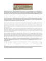
Carlson Survey 2008 Standalone
Carlson Software Inc.
User’s manual
August 17, 2007
Contents
Chapter 1.
Introduction
1
Using the Carlson Software Manual . . . . . . . . . . . . . . . . . . . . . . . . . . . . . . . . . .
2
Product Overview . . . . . . . . . . . . . . . . . . . . . . . . . . . . . . . . . . . . . . . . . . . .
2
System Requirements . . . . . . . . . . . . . . . . . . . . . . . . . . . . . . . . . . . . . . . . . .
4
Installing Carlson Software . . . . . . . . . . . . . . . . . . . . . . . . . . . . . . . . . . . . . . .
4
Authorizing Carlson Software . . . . . . . . . . . . . . . . . . . . . . . . . . . . . . . . . . . . .
10
Carlson Registration . . . . . . . . . . . . . . . . . . . . . . . . . . . . . . . . . . . . . . . . . .
12
Setting Up a Project . . . . . . . . . . . . . . . . . . . . . . . . . . . . . . . . . . . . . . . . . . .
13
Startup Wizard . . . . . . . . . . . . . . . . . . . . . . . . . . . . . . . . . . . . . . . . . . . . .
13
Command Entry . . . . . . . . . . . . . . . . . . . . . . . . . . . . . . . . . . . . . . . . . . . . .
16
Layer and Style Defaults . . . . . . . . . . . . . . . . . . . . . . . . . . . . . . . . . . . . . . . .
16
What is New . . . . . . . . . . . . . . . . . . . . . . . . . . . . . . . . . . . . . . . . . . . . . . .
17
Standard Report Viewer . . . . . . . . . . . . . . . . . . . . . . . . . . . . . . . . . . . . . . . . .
20
Report Formatter . . . . . . . . . . . . . . . . . . . . . . . . . . . . . . . . . . . . . . . . . . . .
22
Instruction Manual and Program Conventions . . . . . . . . . . . . . . . . . . . . . . . . . . . . .
25
Carlson File Types . . . . . . . . . . . . . . . . . . . . . . . . . . . . . . . . . . . . . . . . . . .
26
Quick Keys . . . . . . . . . . . . . . . . . . . . . . . . . . . . . . . . . . . . . . . . . . . . . . .
29
Obtaining Technical Support . . . . . . . . . . . . . . . . . . . . . . . . . . . . . . . . . . . . . .
30
Chapter 2.
Tutorials
32
Lesson 1: Entering a Deed . . . . . . . . . . . . . . . . . . . . . . . . . . . . . . . . . . . . . . .
33
Lesson 2: Making a Plat . . . . . . . . . . . . . . . . . . . . . . . . . . . . . . . . . . . . . . . .
42
Lesson 3: SurvNET . . . . . . . . . . . . . . . . . . . . . . . . . . . . . . . . . . . . . . . . . . .
80
Lesson 4: Field to Finish for Faster Drafting . . . . . . . . . . . . . . . . . . . . . . . . . . . . . . 105
Lesson 5: Intersections and Subdivisions . . . . . . . . . . . . . . . . . . . . . . . . . . . . . . . . 125
Lesson 6: Contouring, Break Lines and Stockpiles . . . . . . . . . . . . . . . . . . . . . . . . . . . 150
Chapter 3.
AutoCAD Overview
164
Issuing Commands . . . . . . . . . . . . . . . . . . . . . . . . . . . . . . . . . . . . . . . . . . . 165
General Commands . . . . . . . . . . . . . . . . . . . . . . . . . . . . . . . . . . . . . . . . . . . 166
Selection of Items . . . . . . . . . . . . . . . . . . . . . . . . . . . . . . . . . . . . . . . . . . . . 167
Properties and Layers . . . . . . . . . . . . . . . . . . . . . . . . . . . . . . . . . . . . . . . . . . 168
Properties Toolbar . . . . . . . . . . . . . . . . . . . . . . . . . . . . . . . . . . . . . . . . . . . . 169
i
Chapter 4.
File Menu
170
New . . . . . . . . . . . . . . . . . . . . . . . . . . . . . . . . . . . . . . . . . . . . . . . . . . . 171
Open . . . . . . . . . . . . . . . . . . . . . . . . . . . . . . . . . . . . . . . . . . . . . . . . . . . 172
Close . . . . . . . . . . . . . . . . . . . . . . . . . . . . . . . . . . . . . . . . . . . . . . . . . . 172
Save . . . . . . . . . . . . . . . . . . . . . . . . . . . . . . . . . . . . . . . . . . . . . . . . . . . 173
Save As . . . . . . . . . . . . . . . . . . . . . . . . . . . . . . . . . . . . . . . . . . . . . . . . . 173
Page Setup . . . . . . . . . . . . . . . . . . . . . . . . . . . . . . . . . . . . . . . . . . . . . . . 174
Plot Preview . . . . . . . . . . . . . . . . . . . . . . . . . . . . . . . . . . . . . . . . . . . . . . . 174
Plot . . . . . . . . . . . . . . . . . . . . . . . . . . . . . . . . . . . . . . . . . . . . . . . . . . . 174
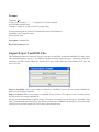
Import Xref to Current Drawing . . . . . . . . . . . . . . . . . . . . . . . . . . . . . . . . . . . . 178
Xref Manager . . . . . . . . . . . . . . . . . . . . . . . . . . . . . . . . . . . . . . . . . . . . . . 179
Import/Export LandXML Files . . . . . . . . . . . . . . . . . . . . . . . . . . . . . . . . . . . . . 181
Write Polyline File . . . . . . . . . . . . . . . . . . . . . . . . . . . . . . . . . . . . . . . . . . . 183
Draw Polyline File . . . . . . . . . . . . . . . . . . . . . . . . . . . . . . . . . . . . . . . . . . . 184
Clipboard . . . . . . . . . . . . . . . . . . . . . . . . . . . . . . . . . . . . . . . . . . . . . . . . 184
Drawing Cleanup . . . . . . . . . . . . . . . . . . . . . . . . . . . . . . . . . . . . . . . . . . . . 185
Audit . . . . . . . . . . . . . . . . . . . . . . . . . . . . . . . . . . . . . . . . . . . . . . . . . . 188
Recover . . . . . . . . . . . . . . . . . . . . . . . . . . . . . . . . . . . . . . . . . . . . . . . . . 189
Remove Reactors . . . . . . . . . . . . . . . . . . . . . . . . . . . . . . . . . . . . . . . . . . . . 189
Remove Groups . . . . . . . . . . . . . . . . . . . . . . . . . . . . . . . . . . . . . . . . . . . . . 189
Purge . . . . . . . . . . . . . . . . . . . . . . . . . . . . . . . . . . . . . . . . . . . . . . . . . . 190
Chapter 5.
Edit Menu
192
Undo . . . . . . . . . . . . . . . . . . . . . . . . . . . . . . . . . . . . . . . . . . . . . . . . . . 193
Redo . . . . . . . . . . . . . . . . . . . . . . . . . . . . . . . . . . . . . . . . . . . . . . . . . . . 193
Erase Select . . . . . . . . . . . . . . . . . . . . . . . . . . . . . . . . . . . . . . . . . . . . . . . 193
Erase by Layer . . . . . . . . . . . . . . . . . . . . . . . . . . . . . . . . . . . . . . . . . . . . . 193
Erase by Closed Polyline . . . . . . . . . . . . . . . . . . . . . . . . . . . . . . . . . . . . . . . . 194
Erase Outside . . . . . . . . . . . . . . . . . . . . . . . . . . . . . . . . . . . . . . . . . . . . . . 195
Move . . . . . . . . . . . . . . . . . . . . . . . . . . . . . . . . . . . . . . . . . . . . . . . . . . 195
Standard Copy . . . . . . . . . . . . . . . . . . . . . . . . . . . . . . . . . . . . . . . . . . . . . 196
Copy To Layer . . . . . . . . . . . . . . . . . . . . . . . . . . . . . . . . . . . . . . . . . . . . . 196
Copy Polyline Section . . . . . . . . . . . . . . . . . . . . . . . . . . . . . . . . . . . . . . . . . 197
Standard Offset . . . . . . . . . . . . . . . . . . . . . . . . . . . . . . . . . . . . . . . . . . . . . 197
Variable Offset . . . . . . . . . . . . . . . . . . . . . . . . . . . . . . . . . . . . . . . . . . . . . 197
Standard Explode . . . . . . . . . . . . . . . . . . . . . . . . . . . . . . . . . . . . . . . . . . . . 198
Contents
ii
Block Explode . . . . . . . . . . . . . . . . . . . . . . . . . . . . . . . . . . . . . . . . . . . . . 199
Trim . . . . . . . . . . . . . . . . . . . . . . . . . . . . . . . . . . . . . . . . . . . . . . . . . . . 199
Extend To Edge . . . . . . . . . . . . . . . . . . . . . . . . . . . . . . . . . . . . . . . . . . . . . 200
Extend to Intersection . . . . . . . . . . . . . . . . . . . . . . . . . . . . . . . . . . . . . . . . . . 200
Extend Arc . . . . . . . . . . . . . . . . . . . . . . . . . . . . . . . . . . . . . . . . . . . . . . . 201
Extend by Distance . . . . . . . . . . . . . . . . . . . . . . . . . . . . . . . . . . . . . . . . . . . 201
Break by Crossing Polyline . . . . . . . . . . . . . . . . . . . . . . . . . . . . . . . . . . . . . . . 203
Break Polyline at Specified Distances . . . . . . . . . . . . . . . . . . . . . . . . . . . . . . . . . 204
Break at Intersection . . . . . . . . . . . . . . . . . . . . . . . . . . . . . . . . . . . . . . . . . . 205
Break, Select Object, 2nd Point . . . . . . . . . . . . . . . . . . . . . . . . . . . . . . . . . . . . . 205
Break, Select Object, Two Points . . . . . . . . . . . . . . . . . . . . . . . . . . . . . . . . . . . . 205
Break, At Selected Point . . . . . . . . . . . . . . . . . . . . . . . . . . . . . . . . . . . . . . . . 205
Change Properties . . . . . . . . . . . . . . . . . . . . . . . . . . . . . . . . . . . . . . . . . . . . 206
Change Elevations . . . . . . . . . . . . . . . . . . . . . . . . . . . . . . . . . . . . . . . . . . . 206
Change Attribute Style . . . . . . . . . . . . . . . . . . . . . . . . . . . . . . . . . . . . . . . . . 207
Change Style . . . . . . . . . . . . . . . . . . . . . . . . . . . . . . . . . . . . . . . . . . . . . . 208
Change Block/Inserts Rotate . . . . . . . . . . . . . . . . . . . . . . . . . . . . . . . . . . . . . . 208
Change Block/Inserts Substitute . . . . . . . . . . . . . . . . . . . . . . . . . . . . . . . . . . . . 209
Change Block/Inserts Resize . . . . . . . . . . . . . . . . . . . . . . . . . . . . . . . . . . . . . . 210
Pivot Point Rotate by Bearing . . . . . . . . . . . . . . . . . . . . . . . . . . . . . . . . . . . . . 210
Rotate by Pick . . . . . . . . . . . . . . . . . . . . . . . . . . . . . . . . . . . . . . . . . . . . . . 211
Entity Insertion Point Rotate . . . . . . . . . . . . . . . . . . . . . . . . . . . . . . . . . . . . . . 211
2D Scale . . . . . . . . . . . . . . . . . . . . . . . . . . . . . . . . . . . . . . . . . . . . . . . . . 211
Scale . . . . . . . . . . . . . . . . . . . . . . . . . . . . . . . . . . . . . . . . . . . . . . . . . . . 212
Edit Text . . . . . . . . . . . . . . . . . . . . . . . . . . . . . . . . . . . . . . . . . . . . . . . . . 212
Text Enlarge/Reduce . . . . . . . . . . . . . . . . . . . . . . . . . . . . . . . . . . . . . . . . . . 212
Rotate Text . . . . . . . . . . . . . . . . . . . . . . . . . . . . . . . . . . . . . . . . . . . . . . . 213
Change Text Font . . . . . . . . . . . . . . . . . . . . . . . . . . . . . . . . . . . . . . . . . . . . 213
Change Text Size . . . . . . . . . . . . . . . . . . . . . . . . . . . . . . . . . . . . . . . . . . . . 214
Change Text Width . . . . . . . . . . . . . . . . . . . . . . . . . . . . . . . . . . . . . . . . . . . 214
Change Text Oblique Angle . . . . . . . . . . . . . . . . . . . . . . . . . . . . . . . . . . . . . . 215
Flip Text . . . . . . . . . . . . . . . . . . . . . . . . . . . . . . . . . . . . . . . . . . . . . . . . . 215
Split Text into Two Lines . . . . . . . . . . . . . . . . . . . . . . . . . . . . . . . . . . . . . . . . 215
Text Explode To Polylines . . . . . . . . . . . . . . . . . . . . . . . . . . . . . . . . . . . . . . . 216
Replace Text . . . . . . . . . . . . . . . . . . . . . . . . . . . . . . . . . . . . . . . . . . . . . . 216
2D Align . . . . . . . . . . . . . . . . . . . . . . . . . . . . . . . . . . . . . . . . . . . . . . . . 217
Contents
iii
Standard Align . . . . . . . . . . . . . . . . . . . . . . . . . . . . . . . . . . . . . . . . . . . . . 218
Fillet . . . . . . . . . . . . . . . . . . . . . . . . . . . . . . . . . . . . . . . . . . . . . . . . . . . 219
Mirror . . . . . . . . . . . . . . . . . . . . . . . . . . . . . . . . . . . . . . . . . . . . . . . . . . 219
Properties Manager . . . . . . . . . . . . . . . . . . . . . . . . . . . . . . . . . . . . . . . . . . . 220
Entities to Polylines . . . . . . . . . . . . . . . . . . . . . . . . . . . . . . . . . . . . . . . . . . . 222
Reverse Polyline . . . . . . . . . . . . . . . . . . . . . . . . . . . . . . . . . . . . . . . . . . . . 222
Reduce Polyline Vertices . . . . . . . . . . . . . . . . . . . . . . . . . . . . . . . . . . . . . . . . 223
Densify Polyline Vertices . . . . . . . . . . . . . . . . . . . . . . . . . . . . . . . . . . . . . . . . 223
Smooth Polyline . . . . . . . . . . . . . . . . . . . . . . . . . . . . . . . . . . . . . . . . . . . . . 224
Draw Polyline Blips . . . . . . . . . . . . . . . . . . . . . . . . . . . . . . . . . . . . . . . . . . . 224
Add Intersection Points . . . . . . . . . . . . . . . . . . . . . . . . . . . . . . . . . . . . . . . . . 225
Add Polyline Vertex . . . . . . . . . . . . . . . . . . . . . . . . . . . . . . . . . . . . . . . . . . . 226
Edit Polyline Vertex . . . . . . . . . . . . . . . . . . . . . . . . . . . . . . . . . . . . . . . . . . . 226
Edit Polyline Section . . . . . . . . . . . . . . . . . . . . . . . . . . . . . . . . . . . . . . . . . . 228
Remove Duplicate Polylines . . . . . . . . . . . . . . . . . . . . . . . . . . . . . . . . . . . . . . 228
Remove Polyline Arcs . . . . . . . . . . . . . . . . . . . . . . . . . . . . . . . . . . . . . . . . . 229
Remove Polyline Segment . . . . . . . . . . . . . . . . . . . . . . . . . . . . . . . . . . . . . . . 229
Remove Polyline Vertex . . . . . . . . . . . . . . . . . . . . . . . . . . . . . . . . . . . . . . . . 230
Create Polyline ID Labels . . . . . . . . . . . . . . . . . . . . . . . . . . . . . . . . . . . . . . . . 231
Change Polyline Width . . . . . . . . . . . . . . . . . . . . . . . . . . . . . . . . . . . . . . . . . 232
Set Polyline Origin . . . . . . . . . . . . . . . . . . . . . . . . . . . . . . . . . . . . . . . . . . . 232
Remove Polyline Arcs . . . . . . . . . . . . . . . . . . . . . . . . . . . . . . . . . . . . . . . . . 232
Change Polyline Elevation . . . . . . . . . . . . . . . . . . . . . . . . . . . . . . . . . . . . . . . 233
Check Elevation Range . . . . . . . . . . . . . . . . . . . . . . . . . . . . . . . . . . . . . . . . . 233
Highlight Crossing Plines . . . . . . . . . . . . . . . . . . . . . . . . . . . . . . . . . . . . . . . . 234
Offset 3D Polyline . . . . . . . . . . . . . . . . . . . . . . . . . . . . . . . . . . . . . . . . . . . 235
Fillet 3D Polyline . . . . . . . . . . . . . . . . . . . . . . . . . . . . . . . . . . . . . . . . . . . . 236
Join 3D Polyline . . . . . . . . . . . . . . . . . . . . . . . . . . . . . . . . . . . . . . . . . . . . 236
Add Points At Elevation . . . . . . . . . . . . . . . . . . . . . . . . . . . . . . . . . . . . . . . . 236
3D Polyline by Slope on Surface . . . . . . . . . . . . . . . . . . . . . . . . . . . . . . . . . . . . 237
Join Nearest . . . . . . . . . . . . . . . . . . . . . . . . . . . . . . . . . . . . . . . . . . . . . . . 238
3D Entity to 2D . . . . . . . . . . . . . . . . . . . . . . . . . . . . . . . . . . . . . . . . . . . . . 239
Select by Filter . . . . . . . . . . . . . . . . . . . . . . . . . . . . . . . . . . . . . . . . . . . . . 240
Select by Elevation . . . . . . . . . . . . . . . . . . . . . . . . . . . . . . . . . . . . . . . . . . . 241
Select by Area . . . . . . . . . . . . . . . . . . . . . . . . . . . . . . . . . . . . . . . . . . . . . . 241
Image Frame . . . . . . . . . . . . . . . . . . . . . . . . . . . . . . . . . . . . . . . . . . . . . . 242
Contents
iv
Image Clip . . . . . . . . . . . . . . . . . . . . . . . . . . . . . . . . . . . . . . . . . . . . . . . 242
Image Adjust . . . . . . . . . . . . . . . . . . . . . . . . . . . . . . . . . . . . . . . . . . . . . . 243
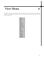
Chapter 6.
View Menu
245
Redraw . . . . . . . . . . . . . . . . . . . . . . . . . . . . . . . . . . . . . . . . . . . . . . . . . 246
Regen . . . . . . . . . . . . . . . . . . . . . . . . . . . . . . . . . . . . . . . . . . . . . . . . . . 246
Zoom - Window . . . . . . . . . . . . . . . . . . . . . . . . . . . . . . . . . . . . . . . . . . . . . 246
Zoom - Dynamic . . . . . . . . . . . . . . . . . . . . . . . . . . . . . . . . . . . . . . . . . . . . 246
Zoom - Previous . . . . . . . . . . . . . . . . . . . . . . . . . . . . . . . . . . . . . . . . . . . . . 246
Zoom - Center . . . . . . . . . . . . . . . . . . . . . . . . . . . . . . . . . . . . . . . . . . . . . . 247
Zoom - Extents . . . . . . . . . . . . . . . . . . . . . . . . . . . . . . . . . . . . . . . . . . . . . 247
Zoom IN . . . . . . . . . . . . . . . . . . . . . . . . . . . . . . . . . . . . . . . . . . . . . . . . . 247
Zoom OUT . . . . . . . . . . . . . . . . . . . . . . . . . . . . . . . . . . . . . . . . . . . . . . . 247
Zoom Selection . . . . . . . . . . . . . . . . . . . . . . . . . . . . . . . . . . . . . . . . . . . . . 248
Zoom Points . . . . . . . . . . . . . . . . . . . . . . . . . . . . . . . . . . . . . . . . . . . . . . . 248
Pan . . . . . . . . . . . . . . . . . . . . . . . . . . . . . . . . . . . . . . . . . . . . . . . . . . . 248
3D Viewer Window . . . . . . . . . . . . . . . . . . . . . . . . . . . . . . . . . . . . . . . . . . . 249
Surface 3D Viewer . . . . . . . . . . . . . . . . . . . . . . . . . . . . . . . . . . . . . . . . . . . 252
Surface 3D FlyOver . . . . . . . . . . . . . . . . . . . . . . . . . . . . . . . . . . . . . . . . . . . 252
Viewpoint 3D . . . . . . . . . . . . . . . . . . . . . . . . . . . . . . . . . . . . . . . . . . . . . . 254
Twist Screen: Standard . . . . . . . . . . . . . . . . . . . . . . . . . . . . . . . . . . . . . . . . . 255
Twist Screen: Line Pline or Text . . . . . . . . . . . . . . . . . . . . . . . . . . . . . . . . . . . . 256
Twist Screen: Surveyor . . . . . . . . . . . . . . . . . . . . . . . . . . . . . . . . . . . . . . . . . 256
Restore Due North . . . . . . . . . . . . . . . . . . . . . . . . . . . . . . . . . . . . . . . . . . . 257
Display Order . . . . . . . . . . . . . . . . . . . . . . . . . . . . . . . . . . . . . . . . . . . . . . 257
Layer Control . . . . . . . . . . . . . . . . . . . . . . . . . . . . . . . . . . . . . . . . . . . . . . 257
Set Layer . . . . . . . . . . . . . . . . . . . . . . . . . . . . . . . . . . . . . . . . . . . . . . . . 260
Change Layer . . . . . . . . . . . . . . . . . . . . . . . . . . . . . . . . . . . . . . . . . . . . . . 260
Freeze Layer . . . . . . . . . . . . . . . . . . . . . . . . . . . . . . . . . . . . . . . . . . . . . . 261
Thaw Layer . . . . . . . . . . . . . . . . . . . . . . . . . . . . . . . . . . . . . . . . . . . . . . . 261
Isolate Layer . . . . . . . . . . . . . . . . . . . . . . . . . . . . . . . . . . . . . . . . . . . . . . 261
Restore Layer . . . . . . . . . . . . . . . . . . . . . . . . . . . . . . . . . . . . . . . . . . . . . . 261
Contents
v
Chapter 7.
Draw Menu
263
Line . . . . . . . . . . . . . . . . . . . . . . . . . . . . . . . . . . . . . . . . . . . . . . . . . . . 264
2D Polyline . . . . . . . . . . . . . . . . . . . . . . . . . . . . . . . . . . . . . . . . . . . . . . . 264
3D Polyline . . . . . . . . . . . . . . . . . . . . . . . . . . . . . . . . . . . . . . . . . . . . . . . 266
Circle . . . . . . . . . . . . . . . . . . . . . . . . . . . . . . . . . . . . . . . . . . . . . . . . . . 268
3 Point . . . . . . . . . . . . . . . . . . . . . . . . . . . . . . . . . . . . . . . . . . . . . . . . . . 268
PC, PT, Center . . . . . . . . . . . . . . . . . . . . . . . . . . . . . . . . . . . . . . . . . . . . . 268
2 Tangents, Radius . . . . . . . . . . . . . . . . . . . . . . . . . . . . . . . . . . . . . . . . . . . 269
PC, Radius, Chord . . . . . . . . . . . . . . . . . . . . . . . . . . . . . . . . . . . . . . . . . . . 269
PC, Radius, Arc Length . . . . . . . . . . . . . . . . . . . . . . . . . . . . . . . . . . . . . . . . . 269
2 Tangents, Arc Length . . . . . . . . . . . . . . . . . . . . . . . . . . . . . . . . . . . . . . . . . 270
2 Tangents, Chord Length . . . . . . . . . . . . . . . . . . . . . . . . . . . . . . . . . . . . . . . . 270
2 Tangents, Mid-Ordinate . . . . . . . . . . . . . . . . . . . . . . . . . . . . . . . . . . . . . . . . 271
2 Tangents, External . . . . . . . . . . . . . . . . . . . . . . . . . . . . . . . . . . . . . . . . . . 271
2 Tangents, Tangent Length . . . . . . . . . . . . . . . . . . . . . . . . . . . . . . . . . . . . . . . 272
2 Tangents, Degree of Curve . . . . . . . . . . . . . . . . . . . . . . . . . . . . . . . . . . . . . . 272
Tangent, PC, Radius, Arc Length . . . . . . . . . . . . . . . . . . . . . . . . . . . . . . . . . . . . 272
Tangent, PC, Radius, Tangent Length . . . . . . . . . . . . . . . . . . . . . . . . . . . . . . . . . 273
Tang, PC, Radius, Chord Length . . . . . . . . . . . . . . . . . . . . . . . . . . . . . . . . . . . . 273
Tang, PC, Radius, Delta Angle . . . . . . . . . . . . . . . . . . . . . . . . . . . . . . . . . . . . . 274
Compound or Reverse . . . . . . . . . . . . . . . . . . . . . . . . . . . . . . . . . . . . . . . . . 274
3-Radius Curve Series . . . . . . . . . . . . . . . . . . . . . . . . . . . . . . . . . . . . . . . . . 275
Best Fit Curve . . . . . . . . . . . . . . . . . . . . . . . . . . . . . . . . . . . . . . . . . . . . . . 276
Curve Calc . . . . . . . . . . . . . . . . . . . . . . . . . . . . . . . . . . . . . . . . . . . . . . . 276
Spiral Curve . . . . . . . . . . . . . . . . . . . . . . . . . . . . . . . . . . . . . . . . . . . . . . . 277
Insert Symbols . . . . . . . . . . . . . . . . . . . . . . . . . . . . . . . . . . . . . . . . . . . . . 278
Insert Multi-Point Symbols . . . . . . . . . . . . . . . . . . . . . . . . . . . . . . . . . . . . . . . 280
Hatch . . . . . . . . . . . . . . . . . . . . . . . . . . . . . . . . . . . . . . . . . . . . . . . . . . 283
Raster Image . . . . . . . . . . . . . . . . . . . . . . . . . . . . . . . . . . . . . . . . . . . . . . 287
Place Image by World File . . . . . . . . . . . . . . . . . . . . . . . . . . . . . . . . . . . . . . . 289
Draw By Example . . . . . . . . . . . . . . . . . . . . . . . . . . . . . . . . . . . . . . . . . . . . 290
Sequential Numbers . . . . . . . . . . . . . . . . . . . . . . . . . . . . . . . . . . . . . . . . . . . 290
Arrowhead . . . . . . . . . . . . . . . . . . . . . . . . . . . . . . . . . . . . . . . . . . . . . . . 292
Curve - Arrow . . . . . . . . . . . . . . . . . . . . . . . . . . . . . . . . . . . . . . . . . . . . . . 292
Boundary Polyline . . . . . . . . . . . . . . . . . . . . . . . . . . . . . . . . . . . . . . . . . . . 293
Shrink-Wrap Entities . . . . . . . . . . . . . . . . . . . . . . . . . . . . . . . . . . . . . . . . . . 294
Contents
vi
Polyline by Nearest Found . . . . . . . . . . . . . . . . . . . . . . . . . . . . . . . . . . . . . . . 295
Drawing Block . . . . . . . . . . . . . . . . . . . . . . . . . . . . . . . . . . . . . . . . . . . . . 296
Write Block . . . . . . . . . . . . . . . . . . . . . . . . . . . . . . . . . . . . . . . . . . . . . . . 298
Insert . . . . . . . . . . . . . . . . . . . . . . . . . . . . . . . . . . . . . . . . . . . . . . . . . . 299
Chapter 8.
Inquiry Menu
301
List . . . . . . . . . . . . . . . . . . . . . . . . . . . . . . . . . . . . . . . . . . . . . . . . . . . 302
Point ID . . . . . . . . . . . . . . . . . . . . . . . . . . . . . . . . . . . . . . . . . . . . . . . . . 303
Layer ID . . . . . . . . . . . . . . . . . . . . . . . . . . . . . . . . . . . . . . . . . . . . . . . . . 303
Layer Report . . . . . . . . . . . . . . . . . . . . . . . . . . . . . . . . . . . . . . . . . . . . . . 304
Layer Inspector . . . . . . . . . . . . . . . . . . . . . . . . . . . . . . . . . . . . . . . . . . . . . 304
Drawing Inspector . . . . . . . . . . . . . . . . . . . . . . . . . . . . . . . . . . . . . . . . . . . 305
List Elevation . . . . . . . . . . . . . . . . . . . . . . . . . . . . . . . . . . . . . . . . . . . . . . 306
Bearing & 3D Distance . . . . . . . . . . . . . . . . . . . . . . . . . . . . . . . . . . . . . . . . . 307
Find Point . . . . . . . . . . . . . . . . . . . . . . . . . . . . . . . . . . . . . . . . . . . . . . . . 307
Curve Info . . . . . . . . . . . . . . . . . . . . . . . . . . . . . . . . . . . . . . . . . . . . . . . . 308
Polyline Info . . . . . . . . . . . . . . . . . . . . . . . . . . . . . . . . . . . . . . . . . . . . . . 309
Display-Edit File . . . . . . . . . . . . . . . . . . . . . . . . . . . . . . . . . . . . . . . . . . . . 309
Display Last Report . . . . . . . . . . . . . . . . . . . . . . . . . . . . . . . . . . . . . . . . . . . 309
Load Saved Report . . . . . . . . . . . . . . . . . . . . . . . . . . . . . . . . . . . . . . . . . . . 309
Chapter 9.
Settings Menu
310
Drawing Setup . . . . . . . . . . . . . . . . . . . . . . . . . . . . . . . . . . . . . . . . . . . . . 311
Set Project/Data Folders . . . . . . . . . . . . . . . . . . . . . . . . . . . . . . . . . . . . . . . . 313
Drawing Explorer . . . . . . . . . . . . . . . . . . . . . . . . . . . . . . . . . . . . . . . . . . . . 316
Project Explorer . . . . . . . . . . . . . . . . . . . . . . . . . . . . . . . . . . . . . . . . . . . . . 319
Store Project Archive . . . . . . . . . . . . . . . . . . . . . . . . . . . . . . . . . . . . . . . . . . 321
Extract Project Archive . . . . . . . . . . . . . . . . . . . . . . . . . . . . . . . . . . . . . . . . . 322
Preferences . . . . . . . . . . . . . . . . . . . . . . . . . . . . . . . . . . . . . . . . . . . . . . . 323
Configure . . . . . . . . . . . . . . . . . . . . . . . . . . . . . . . . . . . . . . . . . . . . . . . . 332
Mouse Click Settings . . . . . . . . . . . . . . . . . . . . . . . . . . . . . . . . . . . . . . . . . . 343
Toolbars . . . . . . . . . . . . . . . . . . . . . . . . . . . . . . . . . . . . . . . . . . . . . . . . . 344
Edit Symbol Library . . . . . . . . . . . . . . . . . . . . . . . . . . . . . . . . . . . . . . . . . . 344
Title Block . . . . . . . . . . . . . . . . . . . . . . . . . . . . . . . . . . . . . . . . . . . . . . . 345
Mortgage Block . . . . . . . . . . . . . . . . . . . . . . . . . . . . . . . . . . . . . . . . . . . . . 348
Rescale Drawing . . . . . . . . . . . . . . . . . . . . . . . . . . . . . . . . . . . . . . . . . . . . 348
Contents
vii
Set/Reset X-Hairs . . . . . . . . . . . . . . . . . . . . . . . . . . . . . . . . . . . . . . . . . . . . 349
Tablet Calibrate . . . . . . . . . . . . . . . . . . . . . . . . . . . . . . . . . . . . . . . . . . . . . 349
Save/Load Tablet Calibration . . . . . . . . . . . . . . . . . . . . . . . . . . . . . . . . . . . . . . 351
Set UCS to World . . . . . . . . . . . . . . . . . . . . . . . . . . . . . . . . . . . . . . . . . . . . 352
Units Control . . . . . . . . . . . . . . . . . . . . . . . . . . . . . . . . . . . . . . . . . . . . . . 352
Point Object Snap . . . . . . . . . . . . . . . . . . . . . . . . . . . . . . . . . . . . . . . . . . . . 354
Aperture Object Snap . . . . . . . . . . . . . . . . . . . . . . . . . . . . . . . . . . . . . . . . . . 354
System Variable Editor . . . . . . . . . . . . . . . . . . . . . . . . . . . . . . . . . . . . . . . . . 357
Chapter 10.
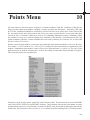
Points Menu
360
Point Defaults . . . . . . . . . . . . . . . . . . . . . . . . . . . . . . . . . . . . . . . . . . . . . . 362
Draw-Locate Points . . . . . . . . . . . . . . . . . . . . . . . . . . . . . . . . . . . . . . . . . . . 364
List Points . . . . . . . . . . . . . . . . . . . . . . . . . . . . . . . . . . . . . . . . . . . . . . . . 367
Import Text/ASCII File . . . . . . . . . . . . . . . . . . . . . . . . . . . . . . . . . . . . . . . . . 369
Export Text/ASCII File . . . . . . . . . . . . . . . . . . . . . . . . . . . . . . . . . . . . . . . . . 370
Set Coordinate File . . . . . . . . . . . . . . . . . . . . . . . . . . . . . . . . . . . . . . . . . . . 372
CooRDinate File Utilities . . . . . . . . . . . . . . . . . . . . . . . . . . . . . . . . . . . . . . . . 373
Point Group Manager . . . . . . . . . . . . . . . . . . . . . . . . . . . . . . . . . . . . . . . . . . 388
Edit Points . . . . . . . . . . . . . . . . . . . . . . . . . . . . . . . . . . . . . . . . . . . . . . . . 397
Erase Points . . . . . . . . . . . . . . . . . . . . . . . . . . . . . . . . . . . . . . . . . . . . . . . 398
Freeze Points . . . . . . . . . . . . . . . . . . . . . . . . . . . . . . . . . . . . . . . . . . . . . . 398
Thaw Points . . . . . . . . . . . . . . . . . . . . . . . . . . . . . . . . . . . . . . . . . . . . . . . 399
Translate Points . . . . . . . . . . . . . . . . . . . . . . . . . . . . . . . . . . . . . . . . . . . . . 399
Rotate Points . . . . . . . . . . . . . . . . . . . . . . . . . . . . . . . . . . . . . . . . . . . . . . 401
Align Points . . . . . . . . . . . . . . . . . . . . . . . . . . . . . . . . . . . . . . . . . . . . . . . 403
Scale Points . . . . . . . . . . . . . . . . . . . . . . . . . . . . . . . . . . . . . . . . . . . . . . . 404
Move Points . . . . . . . . . . . . . . . . . . . . . . . . . . . . . . . . . . . . . . . . . . . . . . . 406
Edit Point Attributes . . . . . . . . . . . . . . . . . . . . . . . . . . . . . . . . . . . . . . . . . . 407
Edit Multiple Pt Attributes . . . . . . . . . . . . . . . . . . . . . . . . . . . . . . . . . . . . . . . 408
Move Point Attributes Single . . . . . . . . . . . . . . . . . . . . . . . . . . . . . . . . . . . . . . 411
Move Point Attributes with Leader . . . . . . . . . . . . . . . . . . . . . . . . . . . . . . . . . . . 412
Scale Point Attributes . . . . . . . . . . . . . . . . . . . . . . . . . . . . . . . . . . . . . . . . . . 412
Erase Point Attributes . . . . . . . . . . . . . . . . . . . . . . . . . . . . . . . . . . . . . . . . . . 413
Twist Point Attributes . . . . . . . . . . . . . . . . . . . . . . . . . . . . . . . . . . . . . . . . . . 413
Resize Point Attributes . . . . . . . . . . . . . . . . . . . . . . . . . . . . . . . . . . . . . . . . . 414
Fix Point Attribute Overlaps . . . . . . . . . . . . . . . . . . . . . . . . . . . . . . . . . . . . . . 414
Contents
viii
Trim by Point Symbol . . . . . . . . . . . . . . . . . . . . . . . . . . . . . . . . . . . . . . . . . . 418
Change Point LayerColor . . . . . . . . . . . . . . . . . . . . . . . . . . . . . . . . . . . . . . . . 418
Renumber Points . . . . . . . . . . . . . . . . . . . . . . . . . . . . . . . . . . . . . . . . . . . . 419
Explode Carlson Points . . . . . . . . . . . . . . . . . . . . . . . . . . . . . . . . . . . . . . . . . 420
Convert Surveyor1 to CRD . . . . . . . . . . . . . . . . . . . . . . . . . . . . . . . . . . . . . . . 421
Convert CRD to TDS CR5/Convert TDS CR5 to CRD . . . . . . . . . . . . . . . . . . . . . . . . 421
Convert CRD to Land Desktop MDB . . . . . . . . . . . . . . . . . . . . . . . . . . . . . . . . . . 421
Convert Land Desktop MDB to Carlson Points . . . . . . . . . . . . . . . . . . . . . . . . . . . . 421
Convert Civil 3D to Carlson Points . . . . . . . . . . . . . . . . . . . . . . . . . . . . . . . . . . . 422
Convert Carlson Points to Land Desktop . . . . . . . . . . . . . . . . . . . . . . . . . . . . . . . . 423
Convert Softdesk to Carlson Points . . . . . . . . . . . . . . . . . . . . . . . . . . . . . . . . . . . 423
Convert Carlson Points to C&G . . . . . . . . . . . . . . . . . . . . . . . . . . . . . . . . . . . . 423
Convert C&G to Carlson Points . . . . . . . . . . . . . . . . . . . . . . . . . . . . . . . . . . . . 424
Convert Carlson Points to Simplicity . . . . . . . . . . . . . . . . . . . . . . . . . . . . . . . . . . 424
Convert Simplicity to Carlson Points . . . . . . . . . . . . . . . . . . . . . . . . . . . . . . . . . . 425
Convert Leica to Carlson Points . . . . . . . . . . . . . . . . . . . . . . . . . . . . . . . . . . . . 426
Convert Geodimeter to Carlson Points . . . . . . . . . . . . . . . . . . . . . . . . . . . . . . . . . 426
Convert Carlson Points to Ashtech GIS . . . . . . . . . . . . . . . . . . . . . . . . . . . . . . . . . 426
Convert Carlson Points to Softdesk . . . . . . . . . . . . . . . . . . . . . . . . . . . . . . . . . . . 426
Convert PacSoft CRD to Carlson CRD . . . . . . . . . . . . . . . . . . . . . . . . . . . . . . . . . 426
Convert Carlson Points to Eagle Point . . . . . . . . . . . . . . . . . . . . . . . . . . . . . . . . . 427
Convert Eagle Point to Carlson Points . . . . . . . . . . . . . . . . . . . . . . . . . . . . . . . . . 427
Chapter 11.
Survey Menu
429
Data Collectors . . . . . . . . . . . . . . . . . . . . . . . . . . . . . . . . . . . . . . . . . . . . . 430
Edit-Process Raw Data File . . . . . . . . . . . . . . . . . . . . . . . . . . . . . . . . . . . . . . . 454
Edit-Process Level Data . . . . . . . . . . . . . . . . . . . . . . . . . . . . . . . . . . . . . . . . . 502
SurvNET . . . . . . . . . . . . . . . . . . . . . . . . . . . . . . . . . . . . . . . . . . . . . . . . 506
Draw Field to Finish . . . . . . . . . . . . . . . . . . . . . . . . . . . . . . . . . . . . . . . . . . 593
Field to Finish Inspector . . . . . . . . . . . . . . . . . . . . . . . . . . . . . . . . . . . . . . . . 616
Enter Deed Description . . . . . . . . . . . . . . . . . . . . . . . . . . . . . . . . . . . . . . . . . 618
Deed Reader . . . . . . . . . . . . . . . . . . . . . . . . . . . . . . . . . . . . . . . . . . . . . . . 621
Process Deed File . . . . . . . . . . . . . . . . . . . . . . . . . . . . . . . . . . . . . . . . . . . . 624
Deed Linework ID . . . . . . . . . . . . . . . . . . . . . . . . . . . . . . . . . . . . . . . . . . . 626
Deed Correlation . . . . . . . . . . . . . . . . . . . . . . . . . . . . . . . . . . . . . . . . . . . . 626
Legal Description Writer . . . . . . . . . . . . . . . . . . . . . . . . . . . . . . . . . . . . . . . . 630
Contents
ix
Closure by Point Numbers . . . . . . . . . . . . . . . . . . . . . . . . . . . . . . . . . . . . . . . 637
Map Check by Pnts . . . . . . . . . . . . . . . . . . . . . . . . . . . . . . . . . . . . . . . . . . . 639
Map Check by Screen Entities . . . . . . . . . . . . . . . . . . . . . . . . . . . . . . . . . . . . . 641
Cut Sheet . . . . . . . . . . . . . . . . . . . . . . . . . . . . . . . . . . . . . . . . . . . . . . . . 643
Set Point Elevations by Surface Model . . . . . . . . . . . . . . . . . . . . . . . . . . . . . . . . . 651
Set Point Elevations by 3D Polylines . . . . . . . . . . . . . . . . . . . . . . . . . . . . . . . . . . 651
Polyline Report . . . . . . . . . . . . . . . . . . . . . . . . . . . . . . . . . . . . . . . . . . . . . 652
Polyline to RW5 File . . . . . . . . . . . . . . . . . . . . . . . . . . . . . . . . . . . . . . . . . . 653
4 Sided Building . . . . . . . . . . . . . . . . . . . . . . . . . . . . . . . . . . . . . . . . . . . . 653
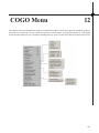
Chapter 12.
COGO Menu
655
Draw-Locate Points . . . . . . . . . . . . . . . . . . . . . . . . . . . . . . . . . . . . . . . . . . . 656
Inverse . . . . . . . . . . . . . . . . . . . . . . . . . . . . . . . . . . . . . . . . . . . . . . . . . . 656
Occupy Point . . . . . . . . . . . . . . . . . . . . . . . . . . . . . . . . . . . . . . . . . . . . . . 657
Traverse . . . . . . . . . . . . . . . . . . . . . . . . . . . . . . . . . . . . . . . . . . . . . . . . . 658
Side Shots . . . . . . . . . . . . . . . . . . . . . . . . . . . . . . . . . . . . . . . . . . . . . . . . 659
Enter-Assign Point . . . . . . . . . . . . . . . . . . . . . . . . . . . . . . . . . . . . . . . . . . . 660
Raw File On/Off . . . . . . . . . . . . . . . . . . . . . . . . . . . . . . . . . . . . . . . . . . . . 661
Line On/Off . . . . . . . . . . . . . . . . . . . . . . . . . . . . . . . . . . . . . . . . . . . . . . . 661
Visual COGO . . . . . . . . . . . . . . . . . . . . . . . . . . . . . . . . . . . . . . . . . . . . . . 662
Locate by Line-Bearing . . . . . . . . . . . . . . . . . . . . . . . . . . . . . . . . . . . . . . . . . 666
Locate by Turned Angle . . . . . . . . . . . . . . . . . . . . . . . . . . . . . . . . . . . . . . . . 667
Locate by Azimuth . . . . . . . . . . . . . . . . . . . . . . . . . . . . . . . . . . . . . . . . . . . 667
Locate by Bearing . . . . . . . . . . . . . . . . . . . . . . . . . . . . . . . . . . . . . . . . . . . . 668
Pick Intersection Points . . . . . . . . . . . . . . . . . . . . . . . . . . . . . . . . . . . . . . . . . 668
Linework Intersection Points . . . . . . . . . . . . . . . . . . . . . . . . . . . . . . . . . . . . . . 669
Bearing-Bearing Intersect . . . . . . . . . . . . . . . . . . . . . . . . . . . . . . . . . . . . . . . . 670
Bearing-Distance Intersect . . . . . . . . . . . . . . . . . . . . . . . . . . . . . . . . . . . . . . . 671
Distance-Distance Intersect . . . . . . . . . . . . . . . . . . . . . . . . . . . . . . . . . . . . . . . 672
2 Point - 2 Point Intersect . . . . . . . . . . . . . . . . . . . . . . . . . . . . . . . . . . . . . . . . 673
Create Points from Entities . . . . . . . . . . . . . . . . . . . . . . . . . . . . . . . . . . . . . . . 674
Resection . . . . . . . . . . . . . . . . . . . . . . . . . . . . . . . . . . . . . . . . . . . . . . . . 676
Benchmark . . . . . . . . . . . . . . . . . . . . . . . . . . . . . . . . . . . . . . . . . . . . . . . 678
Numeric Pad COGO . . . . . . . . . . . . . . . . . . . . . . . . . . . . . . . . . . . . . . . . . . 679
Point on Arc . . . . . . . . . . . . . . . . . . . . . . . . . . . . . . . . . . . . . . . . . . . . . . . 680
Divide Between Points . . . . . . . . . . . . . . . . . . . . . . . . . . . . . . . . . . . . . . . . . 680
Contents
x
Divide Along Entity . . . . . . . . . . . . . . . . . . . . . . . . . . . . . . . . . . . . . . . . . . . 681
Interval Along Entity . . . . . . . . . . . . . . . . . . . . . . . . . . . . . . . . . . . . . . . . . . 682
Create Points from Entities . . . . . . . . . . . . . . . . . . . . . . . . . . . . . . . . . . . . . . . 683
Line by Angle-Distance . . . . . . . . . . . . . . . . . . . . . . . . . . . . . . . . . . . . . . . . . 685
Tangent Line from Circles . . . . . . . . . . . . . . . . . . . . . . . . . . . . . . . . . . . . . . . 686
Building Offset Extensions . . . . . . . . . . . . . . . . . . . . . . . . . . . . . . . . . . . . . . . 686
Radial Stakeout . . . . . . . . . . . . . . . . . . . . . . . . . . . . . . . . . . . . . . . . . . . . . 688
Section Subdivision . . . . . . . . . . . . . . . . . . . . . . . . . . . . . . . . . . . . . . . . . . . 689
GLO Corner Proportioning . . . . . . . . . . . . . . . . . . . . . . . . . . . . . . . . . . . . . . . 690
One Way Control . . . . . . . . . . . . . . . . . . . . . . . . . . . . . . . . . . . . . . . . . . . . 690
Two Way Control . . . . . . . . . . . . . . . . . . . . . . . . . . . . . . . . . . . . . . . . . . . . 691
Three Way Control . . . . . . . . . . . . . . . . . . . . . . . . . . . . . . . . . . . . . . . . . . . 692
Four Way Control . . . . . . . . . . . . . . . . . . . . . . . . . . . . . . . . . . . . . . . . . . . . 693
Solar Observations . . . . . . . . . . . . . . . . . . . . . . . . . . . . . . . . . . . . . . . . . . . 694
Best Fit Circle . . . . . . . . . . . . . . . . . . . . . . . . . . . . . . . . . . . . . . . . . . . . . . 696
Best Fit Line by Average . . . . . . . . . . . . . . . . . . . . . . . . . . . . . . . . . . . . . . . . 697
Best Fit Line by Least Squares . . . . . . . . . . . . . . . . . . . . . . . . . . . . . . . . . . . . . 698
Chapter 13.
Centerline Menu
700
Design Centerline . . . . . . . . . . . . . . . . . . . . . . . . . . . . . . . . . . . . . . . . . . . . 701
Input-Edit Centerline File . . . . . . . . . . . . . . . . . . . . . . . . . . . . . . . . . . . . . . . . 703
Polyline to Centerline File . . . . . . . . . . . . . . . . . . . . . . . . . . . . . . . . . . . . . . . 710
Draw Centerline File . . . . . . . . . . . . . . . . . . . . . . . . . . . . . . . . . . . . . . . . . . 710
Centerline Report . . . . . . . . . . . . . . . . . . . . . . . . . . . . . . . . . . . . . . . . . . . . 711
Centerline ID . . . . . . . . . . . . . . . . . . . . . . . . . . . . . . . . . . . . . . . . . . . . . . 712
Station Polyline/Centerline . . . . . . . . . . . . . . . . . . . . . . . . . . . . . . . . . . . . . . . 712
Label Station-Offset . . . . . . . . . . . . . . . . . . . . . . . . . . . . . . . . . . . . . . . . . . . 719
Offset Point Entry . . . . . . . . . . . . . . . . . . . . . . . . . . . . . . . . . . . . . . . . . . . . 722
Calculate Offsets . . . . . . . . . . . . . . . . . . . . . . . . . . . . . . . . . . . . . . . . . . . . 724
Centerline Conversions . . . . . . . . . . . . . . . . . . . . . . . . . . . . . . . . . . . . . . . . . 726
Chapter 14.
Area/Layout Menu
727
Area Defaults . . . . . . . . . . . . . . . . . . . . . . . . . . . . . . . . . . . . . . . . . . . . . . 728
Inverse with Area . . . . . . . . . . . . . . . . . . . . . . . . . . . . . . . . . . . . . . . . . . . . 730
Area by Lines & Arcs . . . . . . . . . . . . . . . . . . . . . . . . . . . . . . . . . . . . . . . . . . 731
Area by Interior Point . . . . . . . . . . . . . . . . . . . . . . . . . . . . . . . . . . . . . . . . . . 732
Contents
xi
Area by Closed Polylines . . . . . . . . . . . . . . . . . . . . . . . . . . . . . . . . . . . . . . . . 733
Digitize Areas . . . . . . . . . . . . . . . . . . . . . . . . . . . . . . . . . . . . . . . . . . . . . . 734
Label Last Area . . . . . . . . . . . . . . . . . . . . . . . . . . . . . . . . . . . . . . . . . . . . . 735
Tag Area Descriptions . . . . . . . . . . . . . . . . . . . . . . . . . . . . . . . . . . . . . . . . . 735
Identify Area Descriptions . . . . . . . . . . . . . . . . . . . . . . . . . . . . . . . . . . . . . . . 736
Untag Area Descriptions . . . . . . . . . . . . . . . . . . . . . . . . . . . . . . . . . . . . . . . . 736
Hinged Area . . . . . . . . . . . . . . . . . . . . . . . . . . . . . . . . . . . . . . . . . . . . . . . 736
Sliding Side Area . . . . . . . . . . . . . . . . . . . . . . . . . . . . . . . . . . . . . . . . . . . . 737
Area Radial from Curve . . . . . . . . . . . . . . . . . . . . . . . . . . . . . . . . . . . . . . . . . 738
Bearing Area Cutoff . . . . . . . . . . . . . . . . . . . . . . . . . . . . . . . . . . . . . . . . . . . 740
Lot Layout . . . . . . . . . . . . . . . . . . . . . . . . . . . . . . . . . . . . . . . . . . . . . . . 740
Offsets & Intersections . . . . . . . . . . . . . . . . . . . . . . . . . . . . . . . . . . . . . . . . . 742
Cul-de-Sacs . . . . . . . . . . . . . . . . . . . . . . . . . . . . . . . . . . . . . . . . . . . . . . . 743
Elevate 2D Polylines . . . . . . . . . . . . . . . . . . . . . . . . . . . . . . . . . . . . . . . . . . 744
Parking . . . . . . . . . . . . . . . . . . . . . . . . . . . . . . . . . . . . . . . . . . . . . . . . . 746
Set Back Measure-Move . . . . . . . . . . . . . . . . . . . . . . . . . . . . . . . . . . . . . . . . 746
Lot Network Settings . . . . . . . . . . . . . . . . . . . . . . . . . . . . . . . . . . . . . . . . . . 747
Lot Network Boundary . . . . . . . . . . . . . . . . . . . . . . . . . . . . . . . . . . . . . . . . . 749
Input-Edit ROW Offsets . . . . . . . . . . . . . . . . . . . . . . . . . . . . . . . . . . . . . . . . 749
LotNet Road Network . . . . . . . . . . . . . . . . . . . . . . . . . . . . . . . . . . . . . . . . . . 750
Lot Network Linework . . . . . . . . . . . . . . . . . . . . . . . . . . . . . . . . . . . . . . . . . 754
Lot Network Subdivide Area . . . . . . . . . . . . . . . . . . . . . . . . . . . . . . . . . . . . . . 755
Lot Network Sliding Side Area . . . . . . . . . . . . . . . . . . . . . . . . . . . . . . . . . . . . . 755
Lot Network Hinged Area . . . . . . . . . . . . . . . . . . . . . . . . . . . . . . . . . . . . . . . 755
Lot Network Labels . . . . . . . . . . . . . . . . . . . . . . . . . . . . . . . . . . . . . . . . . . . 756
Lot Network Report . . . . . . . . . . . . . . . . . . . . . . . . . . . . . . . . . . . . . . . . . . . 756
Lot Network Inspector . . . . . . . . . . . . . . . . . . . . . . . . . . . . . . . . . . . . . . . . . 756
Lot Network Renumber Lots . . . . . . . . . . . . . . . . . . . . . . . . . . . . . . . . . . . . . . 757
Lot Network Output To Lot File . . . . . . . . . . . . . . . . . . . . . . . . . . . . . . . . . . . . 757
Set Lot File . . . . . . . . . . . . . . . . . . . . . . . . . . . . . . . . . . . . . . . . . . . . . . . 757
Design Lot . . . . . . . . . . . . . . . . . . . . . . . . . . . . . . . . . . . . . . . . . . . . . . . 758
Polyline to Lot File . . . . . . . . . . . . . . . . . . . . . . . . . . . . . . . . . . . . . . . . . . . 759
Lot File by Pick Interior . . . . . . . . . . . . . . . . . . . . . . . . . . . . . . . . . . . . . . . . 760
Lot File by Interior Text . . . . . . . . . . . . . . . . . . . . . . . . . . . . . . . . . . . . . . . . . 761
Lot Manager . . . . . . . . . . . . . . . . . . . . . . . . . . . . . . . . . . . . . . . . . . . . . . . 761
Lot Inspector . . . . . . . . . . . . . . . . . . . . . . . . . . . . . . . . . . . . . . . . . . . . . . 762
Contents
xii
Define Lot Attributes . . . . . . . . . . . . . . . . . . . . . . . . . . . . . . . . . . . . . . . . . . 763
Import Lot File From MDB Database . . . . . . . . . . . . . . . . . . . . . . . . . . . . . . . . . 765
Export Lot File to MDB Database . . . . . . . . . . . . . . . . . . . . . . . . . . . . . . . . . . . 765
Export Lot File To Old SurvCADD . . . . . . . . . . . . . . . . . . . . . . . . . . . . . . . . . . . 766
Set CRD File for Lot Files . . . . . . . . . . . . . . . . . . . . . . . . . . . . . . . . . . . . . . . 766
Lot File to Centerline . . . . . . . . . . . . . . . . . . . . . . . . . . . . . . . . . . . . . . . . . . 766
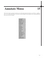
Chapter 15.
Annotate Menu
768
Annotation Defaults . . . . . . . . . . . . . . . . . . . . . . . . . . . . . . . . . . . . . . . . . . . 769
Auto Annotate . . . . . . . . . . . . . . . . . . . . . . . . . . . . . . . . . . . . . . . . . . . . . . 771
Custom Label Formatter AD . . . . . . . . . . . . . . . . . . . . . . . . . . . . . . . . . . . . . . 777
Draw End Point Leaders . . . . . . . . . . . . . . . . . . . . . . . . . . . . . . . . . . . . . . . . 778
Dynamic Annotation Note . . . . . . . . . . . . . . . . . . . . . . . . . . . . . . . . . . . . . . . 779
Switch Bearing/Azimuth Quadrant . . . . . . . . . . . . . . . . . . . . . . . . . . . . . . . . . . . 780
Mirror Selected Labels . . . . . . . . . . . . . . . . . . . . . . . . . . . . . . . . . . . . . . . . . 780
Mirror and Flip Selected Labels . . . . . . . . . . . . . . . . . . . . . . . . . . . . . . . . . . . . 781
Flip Last Label . . . . . . . . . . . . . . . . . . . . . . . . . . . . . . . . . . . . . . . . . . . . . 781
Flip Selected Labels . . . . . . . . . . . . . . . . . . . . . . . . . . . . . . . . . . . . . . . . . . . 782
Flip On/Off . . . . . . . . . . . . . . . . . . . . . . . . . . . . . . . . . . . . . . . . . . . . . . . 782
Bearing with Leader . . . . . . . . . . . . . . . . . . . . . . . . . . . . . . . . . . . . . . . . . . 782
Distance with Leader . . . . . . . . . . . . . . . . . . . . . . . . . . . . . . . . . . . . . . . . . . 783
Bearing-Distance with Leader . . . . . . . . . . . . . . . . . . . . . . . . . . . . . . . . . . . . . 784
Azimuth-Distance with Leader . . . . . . . . . . . . . . . . . . . . . . . . . . . . . . . . . . . . . 784
Fix Label Overlaps . . . . . . . . . . . . . . . . . . . . . . . . . . . . . . . . . . . . . . . . . . . 785
Global Reannotate . . . . . . . . . . . . . . . . . . . . . . . . . . . . . . . . . . . . . . . . . . . 787
Survey Text Defaults . . . . . . . . . . . . . . . . . . . . . . . . . . . . . . . . . . . . . . . . . . 788
Offset Dimensions . . . . . . . . . . . . . . . . . . . . . . . . . . . . . . . . . . . . . . . . . . . 789
Building Dimensions . . . . . . . . . . . . . . . . . . . . . . . . . . . . . . . . . . . . . . . . . . 790
Adjoiner Text . . . . . . . . . . . . . . . . . . . . . . . . . . . . . . . . . . . . . . . . . . . . . . 791
Draw Grid . . . . . . . . . . . . . . . . . . . . . . . . . . . . . . . . . . . . . . . . . . . . . . . . 791
Draw Legend . . . . . . . . . . . . . . . . . . . . . . . . . . . . . . . . . . . . . . . . . . . . . . 793
Draw North Arrow . . . . . . . . . . . . . . . . . . . . . . . . . . . . . . . . . . . . . . . . . . . 796
Draw Barscale . . . . . . . . . . . . . . . . . . . . . . . . . . . . . . . . . . . . . . . . . . . . . . 797
Create Point Table . . . . . . . . . . . . . . . . . . . . . . . . . . . . . . . . . . . . . . . . . . . . 798
Update Point Table . . . . . . . . . . . . . . . . . . . . . . . . . . . . . . . . . . . . . . . . . . . 799
Table Defaults . . . . . . . . . . . . . . . . . . . . . . . . . . . . . . . . . . . . . . . . . . . . . . 799
Contents
xiii
Table Header . . . . . . . . . . . . . . . . . . . . . . . . . . . . . . . . . . . . . . . . . . . . . . 803
Set Table Position . . . . . . . . . . . . . . . . . . . . . . . . . . . . . . . . . . . . . . . . . . . . 804
Curve Table . . . . . . . . . . . . . . . . . . . . . . . . . . . . . . . . . . . . . . . . . . . . . . . 804
Line Table . . . . . . . . . . . . . . . . . . . . . . . . . . . . . . . . . . . . . . . . . . . . . . . . 805
Railroad Curve Table . . . . . . . . . . . . . . . . . . . . . . . . . . . . . . . . . . . . . . . . . . 805
Delete Table Elements . . . . . . . . . . . . . . . . . . . . . . . . . . . . . . . . . . . . . . . . . 805
Label Arc . . . . . . . . . . . . . . . . . . . . . . . . . . . . . . . . . . . . . . . . . . . . . . . . 805
Stack Label Arc . . . . . . . . . . . . . . . . . . . . . . . . . . . . . . . . . . . . . . . . . . . . . 807
Custom Label Formatter . . . . . . . . . . . . . . . . . . . . . . . . . . . . . . . . . . . . . . . . 809
Draw Text On Arc . . . . . . . . . . . . . . . . . . . . . . . . . . . . . . . . . . . . . . . . . . . . 810
Draw Text on Tangent . . . . . . . . . . . . . . . . . . . . . . . . . . . . . . . . . . . . . . . . . . 813
Edit Text on Arc or Tangent . . . . . . . . . . . . . . . . . . . . . . . . . . . . . . . . . . . . . . . 813
Fit Text Inside Arc . . . . . . . . . . . . . . . . . . . . . . . . . . . . . . . . . . . . . . . . . . . 814
Fit Text Outside Arc . . . . . . . . . . . . . . . . . . . . . . . . . . . . . . . . . . . . . . . . . . 814
Change Polyline Linetype . . . . . . . . . . . . . . . . . . . . . . . . . . . . . . . . . . . . . . . . 814
Polyline to Special Line . . . . . . . . . . . . . . . . . . . . . . . . . . . . . . . . . . . . . . . . . 816
Polyline to Tree Line . . . . . . . . . . . . . . . . . . . . . . . . . . . . . . . . . . . . . . . . . . 817
Add Zig to Polyline . . . . . . . . . . . . . . . . . . . . . . . . . . . . . . . . . . . . . . . . . . . 818
Add Culvert to Polyline . . . . . . . . . . . . . . . . . . . . . . . . . . . . . . . . . . . . . . . . . 818
Sketch Tree Line . . . . . . . . . . . . . . . . . . . . . . . . . . . . . . . . . . . . . . . . . . . . 819
Special Line/Entity . . . . . . . . . . . . . . . . . . . . . . . . . . . . . . . . . . . . . . . . . . . 819
Guard Rail . . . . . . . . . . . . . . . . . . . . . . . . . . . . . . . . . . . . . . . . . . . . . . . . 820
Label Angle . . . . . . . . . . . . . . . . . . . . . . . . . . . . . . . . . . . . . . . . . . . . . . . 820
Label Coordinates/Elevation . . . . . . . . . . . . . . . . . . . . . . . . . . . . . . . . . . . . . . 821
Label Lat/Long . . . . . . . . . . . . . . . . . . . . . . . . . . . . . . . . . . . . . . . . . . . . . 823
Label Curb/Flow Elevations . . . . . . . . . . . . . . . . . . . . . . . . . . . . . . . . . . . . . . 824
Replot Descriptions . . . . . . . . . . . . . . . . . . . . . . . . . . . . . . . . . . . . . . . . . . . 824
Leader With Text . . . . . . . . . . . . . . . . . . . . . . . . . . . . . . . . . . . . . . . . . . . . 825
Special Leader . . . . . . . . . . . . . . . . . . . . . . . . . . . . . . . . . . . . . . . . . . . . . 826
Text Box . . . . . . . . . . . . . . . . . . . . . . . . . . . . . . . . . . . . . . . . . . . . . . . . . 827
Label Offset Distances . . . . . . . . . . . . . . . . . . . . . . . . . . . . . . . . . . . . . . . . . 827
Label Elevations Along Polyline . . . . . . . . . . . . . . . . . . . . . . . . . . . . . . . . . . . . 828
Contents
xiv
Chapter 16.
Surface Menu
830
Triangulate & Contour . . . . . . . . . . . . . . . . . . . . . . . . . . . . . . . . . . . . . . . . . 831
Contour from TIN File . . . . . . . . . . . . . . . . . . . . . . . . . . . . . . . . . . . . . . . . . 843
Draw Triangular Mesh . . . . . . . . . . . . . . . . . . . . . . . . . . . . . . . . . . . . . . . . . 844
Contour Elevation Label . . . . . . . . . . . . . . . . . . . . . . . . . . . . . . . . . . . . . . . . 846
Move Label Along Contour . . . . . . . . . . . . . . . . . . . . . . . . . . . . . . . . . . . . . . . 848
Volumes By Triangulation . . . . . . . . . . . . . . . . . . . . . . . . . . . . . . . . . . . . . . . 848
Triangulation File Utilities . . . . . . . . . . . . . . . . . . . . . . . . . . . . . . . . . . . . . . . 849
Surface Manager . . . . . . . . . . . . . . . . . . . . . . . . . . . . . . . . . . . . . . . . . . . . 855
Make 3D Grid File . . . . . . . . . . . . . . . . . . . . . . . . . . . . . . . . . . . . . . . . . . . 862
Draw 3D Grid File . . . . . . . . . . . . . . . . . . . . . . . . . . . . . . . . . . . . . . . . . . . 866
Two Surface Volumes . . . . . . . . . . . . . . . . . . . . . . . . . . . . . . . . . . . . . . . . . . 868
Volumes By Layer . . . . . . . . . . . . . . . . . . . . . . . . . . . . . . . . . . . . . . . . . . . 872
Spot Elevations By Surface Model . . . . . . . . . . . . . . . . . . . . . . . . . . . . . . . . . . . 874
Tag Hard Breakline Polylines . . . . . . . . . . . . . . . . . . . . . . . . . . . . . . . . . . . . . . 876
Untag Hard Breakline Polylines . . . . . . . . . . . . . . . . . . . . . . . . . . . . . . . . . . . . 877
Design Pad Template . . . . . . . . . . . . . . . . . . . . . . . . . . . . . . . . . . . . . . . . . . 877
Slope Zone Analysis . . . . . . . . . . . . . . . . . . . . . . . . . . . . . . . . . . . . . . . . . . 886
Profile Defaults . . . . . . . . . . . . . . . . . . . . . . . . . . . . . . . . . . . . . . . . . . . . . 890
Quick Profile . . . . . . . . . . . . . . . . . . . . . . . . . . . . . . . . . . . . . . . . . . . . . . 891
Profile from Surface Entities . . . . . . . . . . . . . . . . . . . . . . . . . . . . . . . . . . . . . . 893
Export Topcon Grid or TIN File . . . . . . . . . . . . . . . . . . . . . . . . . . . . . . . . . . . . 895
Profile from Points on Centerline . . . . . . . . . . . . . . . . . . . . . . . . . . . . . . . . . . . . 898
Input-Edit Profile File . . . . . . . . . . . . . . . . . . . . . . . . . . . . . . . . . . . . . . . . . . 899
Draw Profile . . . . . . . . . . . . . . . . . . . . . . . . . . . . . . . . . . . . . . . . . . . . . . . 901
Profile to 3D Polyline . . . . . . . . . . . . . . . . . . . . . . . . . . . . . . . . . . . . . . . . . . 916
Profile To Points . . . . . . . . . . . . . . . . . . . . . . . . . . . . . . . . . . . . . . . . . . . . . 917
Convert LDD Contours . . . . . . . . . . . . . . . . . . . . . . . . . . . . . . . . . . . . . . . . . 918
Profile Conversions . . . . . . . . . . . . . . . . . . . . . . . . . . . . . . . . . . . . . . . . . . . 919
Chapter 17.
GIS Menu
923
GIS Database Settings . . . . . . . . . . . . . . . . . . . . . . . . . . . . . . . . . . . . . . . . . 924
Define Template Database . . . . . . . . . . . . . . . . . . . . . . . . . . . . . . . . . . . . . . . 924
Input-Edit GIS Data . . . . . . . . . . . . . . . . . . . . . . . . . . . . . . . . . . . . . . . . . . . 927
GIS Inspector . . . . . . . . . . . . . . . . . . . . . . . . . . . . . . . . . . . . . . . . . . . . . . 928
GIS Inspector Settings . . . . . . . . . . . . . . . . . . . . . . . . . . . . . . . . . . . . . . . . . 929
Contents
xv
GIS Query/Report . . . . . . . . . . . . . . . . . . . . . . . . . . . . . . . . . . . . . . . . . . . . 930
Label GIS Polyline: Closed Polyline Image . . . . . . . . . . . . . . . . . . . . . . . . . . . . . . 932
Label GIS Polyline: Closed Polyline Data . . . . . . . . . . . . . . . . . . . . . . . . . . . . . . . 934
Label GIS Polyline: Open Polyline Data . . . . . . . . . . . . . . . . . . . . . . . . . . . . . . . . 935
Create Links . . . . . . . . . . . . . . . . . . . . . . . . . . . . . . . . . . . . . . . . . . . . . . . 937
Erase Links . . . . . . . . . . . . . . . . . . . . . . . . . . . . . . . . . . . . . . . . . . . . . . . 938
Audit Links . . . . . . . . . . . . . . . . . . . . . . . . . . . . . . . . . . . . . . . . . . . . . . . 938
Import SHP File . . . . . . . . . . . . . . . . . . . . . . . . . . . . . . . . . . . . . . . . . . . . . 939
Export SHP File . . . . . . . . . . . . . . . . . . . . . . . . . . . . . . . . . . . . . . . . . . . . . 940
Image Inspector . . . . . . . . . . . . . . . . . . . . . . . . . . . . . . . . . . . . . . . . . . . . . 940
Place Camera Symbol/Image . . . . . . . . . . . . . . . . . . . . . . . . . . . . . . . . . . . . . . 941
Attach Image to Entity . . . . . . . . . . . . . . . . . . . . . . . . . . . . . . . . . . . . . . . . . 942
Define Note File Prompts . . . . . . . . . . . . . . . . . . . . . . . . . . . . . . . . . . . . . . . . 942
Database File Utilities . . . . . . . . . . . . . . . . . . . . . . . . . . . . . . . . . . . . . . . . . . 944
Contents
xvi
Introduction
1
1
Using the Carlson Software Manual
This manual is designed as a reference guide. It contains a complete description of all commands in the Carlson
Software product. The chapters are organized by program menus, and are arranged in the order that the menus
appear in Carlson Software.
Product Overview
Carlson Software offers a full suite of commands for downloading, entering, and processing field survey data and for
generating final plats and drawings. Carlson Software can function as a total and complete software solution for the
land surveying firm, or as an affordable downloading, calculation, and preparatory solution used in conjunction with
the more full-featured Carlson Software. Built around the Autodesk 2007 OEM graphics engine, Carlson Software
reads and writes standard AutoCAD drawings and assures familiarity to AutoCAD trained staff.
Data Collection
The power of Carlson Survey begins with data collection. Carlson Survey downloads all major collectors ranging
from Geodimeter and TDS to Leica, Nikon, Sokkia, and SMI. The raw data is stored in ''RW5'' format and can
be viewed, edited and processed. The processing, or calculation of coordinates, recognizes ''direct and reverse''
and other forms of multiple measurement, and processes sets of field measurements. Surveys can be balanced and
closed by selective use of angle balance, compass, transit, Crandall, and least squares methods-or simply by direct
calculation with no adjustment. Commands exist for finding bad angles and for plotting the traverse and sideshot
legs of the survey in distinct colors as a means of searching for ''busts'' or errors. In addition to downloading of data
from electronic data collectors, the program accepts manual entry of field notes directly into a spreadsheet format,
permitting review, storage, and editing. Alternatively, field notes can be entered for immediate calculation and
screen plotting of points, with the ''raw notes'' stored simultaneously, permitting re-processing and re-calculation as
needed. For data that was not field-surveyed, but was provided in the form of an ASCII or binary point file, Carlson
Software offers the ''Import Text/ASCII File'' command, unrivaled in its flexibility to read foreign data sources.
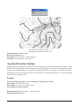
Field to Finish
The survey world is recognizing the power of coding field shots with descriptions that lead to automatic layering,
linework, and symbol work. Office drafting time can be reduced by 50% or more with intelligent use of descriptions,
leading to ''field to finish'' plotting. For example, breaklines, which act as barriers to triangulation, should be placed
on streams, ridges, toe-of-slopes and top-of-banks for more accurate contouring. With the field to finish command,
breaklines can be created by field coding, with descriptions such as DL, for creating 3D polyline ditch lines, or TB for
creating top-of-bank polylines, etc. and this coordinate data can be simply plotted to the screen as undifferentiated
points. However, with the field to finish command, the data can be plotted in one step, creating 3D polyline break
lines, building lines, light poles, manholes, edge-of-pavements, that are all distinctly layered and fully annotated.
The field to finish command within Carlson Survey is extremely robust, so much so that it can adapt to a coding
system made up on-the-fly, or a coding system that has been received from an outsourced survey. Field crew
coding and office processing using the field to finish command can save valuable hours of drafting and eliminate
misinterpretations, paving the way for quick plat generation or supporting supplemental engineering work.
Deed Work
Carlson Survey allows you to enter old deeds and plot the linework, then add bearing and distance annotation
optionally. Distances can be entered in meters and feet, and even in the old measurement forms of chains, poles,
links, and varas. Both tangent and non-tangent arcs can be entered. Closures, distances traversed, and areas are
Chapter 1. Introduction
2
automatically reported. Working in reverse, the command Legal Description creates a property description suitable
for deed recording directly from a closed polyline on the screen. If that polyline has point numbers with descriptions
at any of the property corners, these descriptions will appear in the deed report, as in ''...thence N 45 degrees, 25
minutes, 10 seconds E to a fence post...''. Deed files can be saved, re-loaded, edited, re-drawn and printed or plotted
to the screen in a report form.
Drafting and Design
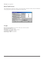
Carlson Software offers approximately 150 different symbols and north arrows, broken down by categories (for
example, points, trees, map symbols). You can create new categories or supplement or change the available point
symbols within any category. The program is designed to receive entire sets of new, customized point symbols in a
single command. Attributes of points, such as elevation and point number, can be selectively ''frozen,'' allowing the
creation of final plats with symbols and optional descriptions remaining on points, as desired. Linework, typically
in the form of polylines, can be drawn by any combination of point number and ''snap'' selection, to create property
lines, street lines, easements and right-of-ways, building lines and borders. In addition to Carlson Software's standard line types, dozens of special line types are available, including tree lines, fence lines, all manner of utility lines,
stonewalls, and customizable line types. Design features include automatic street intersections and cul-de-sacs, and
automatic lot layout. For lots, you can pick your right-of-way and back property polylines, specify desired acreages
and frontage/rear lot parameters, and the lots are automatically calculated and drawn. Hinged Area, Sliding Side
Area, and Area Radial from Curve are excellent design tools, with an easy, graphic interface. All design polylines
can be converted to point numbers at vertices and radius points for purposes of field stakeout.
Annotation
With a full slate of annotation commands, Carlson Survey is all you need to finalize your boundary surveys and plats.
There is a wide range of bearing and distance annotation options, including the Auto-Annotate command, which
allows you to annotate an entire selection set of polylines in one step. Station and offset annotating, as for right-ofway lines, is provided. Use commands such as Special Leader, Station Polyline, Draw North Arrow, and Draw Bar
Scale to dress up the drawing and give it a hand-drafted look. Commands such as Title Block and Draw Legend, as
well as sequential lot numbering and the area labeling commands, help you complete the finished drawing quickly.
Powerful Utilities
Carlson Software contains many strong utilities, particularly polyline utilities. You can Join Nearest disconnected
polylines, turn 2-sided figures into closed, 4-sided figures, offset, trim, and extend 3D polylines, create building
''footprints'' with left and right entries using Extend by Distance, even reverse polyline directions. There are over 20
significant polyline utilities available, including Reduce Vertices, which weeds out duplicate or unnecessary vertices
and cuts down on drawing size. Boundary Polyline is a simplified version of the AutoCAD command Boundary,
and its opposite, Shrinkwrap Entity. Other categories of utilities include point attribute editing, scaling, twisting and
re-sizing, text editing, font alteration and re-sizing, and advanced layer manipulation. Raster images such as aerial
photos and scanned images can be placed on drawings.
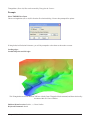
Contouring and Terrain Modeling
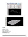
There are many higher order features in Carlson Survey. Full contouring is provided, with options for smoothing
and labeling contours, highlighting index contours and clipping contours to selected perimeters. Carlson Survey can
be used to create both grid files and TIN files (.flt format). Volumes can be computed between grid files, inside any
selected polyline perimeter. Profiles can be extracted from contour maps or hand-entered, as generic ''point-to-point''
profiles or as road profiles with vertical curves. The Design Pad Template command carves in building pads, pits,
parking lots, roads, and other 3D features into any existing terrain. Land forms created by contouring and Design
Chapter 1. Introduction
3
Pad Template can be viewed in 3D and rotated in real time, using the 3D Viewer Window command. In addition
to all the commands needed to create final drawings, Carlson Survey also contains commands to perform many
engineering tasks typically encountered by survey firms.
Carlson Software is the ideal stand-alone solution for the survey and drafting organization, but it is also the perfect
go-between product for the large civil engineering firm with in-house or outsourced survey operations. It compliments Carlson Roads. Carlson Survey enables Carlson Software to serve the full spectrum of the surveying and civil
engineering design world.
System Requirements
Carlson's system requirements are no greater than that of the AutoCAD version you are running. See your
AutoCAD installation guide for minimum system configuration. It is always recommended that you use the highest
performance PC possible.
Note: Carlson does require a minimum screen resolution of 800x600.
Carlson 2008 will operate with the following versions of AutoCAD:
•
•
•
•
AutoCAD 2008/2007/2006/2005/2004/2002/2000i/2000
AutoCAD Map 2008/2007/2006/2005/2004/R6/R5/R4.5/R4
Land Development Desktop 2008/2007/2006/2005/2004/R3
Civil 3D 2008/2007/2006/2005
64 bit version of AutoCAD 2008 is not currently supported.
Installing Carlson Software
If you're installing Carlson Software on Microsoft® Windows NT® 4.0 or Windows 2000, you must have permission
to write to the necessary system registry sections. To do this, make sure that you have administrative permissions on
the computer on which you're installing. Before you install Carlson Software, close all running applications. Make
sure you disable any virus-checking software. Please refer to your virus software documentation for instructions.
Note: If you are upgrading from an older version of Carlson Software, you must uninstall the older version before
installing Carlson Software. This is required for successful software installation and to meet the guidelines of the
EULA (End User License Agreement).
1 Insert the CD into the CD-ROM drive.
If Autorun is enabled, it begins the setup process when you insert the CD.
To stop Autorun from starting the installation process automatically, hold down the SHIFT key when you insert the
CD.
To start the installation process without using Autorun, from the Start menu (Windows), choose Run. Enter the
CD-ROM drive letter, and setup. For example, enter d:\setup.
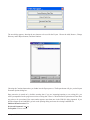
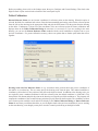
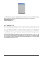
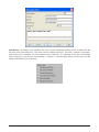
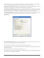
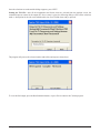
2 The Windows Installer dialog box is displayed briefly, followed by a dialog box for entering in your serial number.
Chapter 1. Introduction
4
In the Enter Carlson Software 2008 Serial Number dialog box, you must enter the serial number provided with your
copy of Carlson Software. Then click OK.
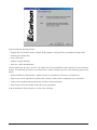
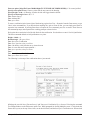
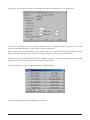
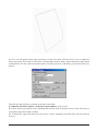
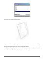
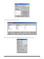
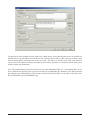
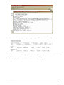
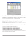
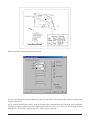
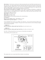
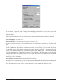
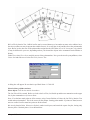
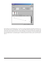
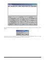
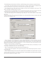
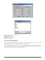
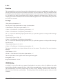
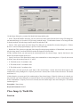
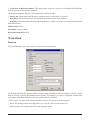
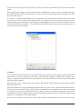
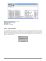
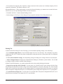
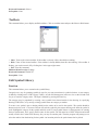
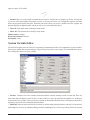
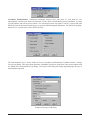
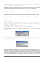
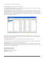
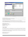
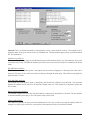
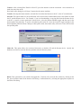
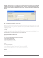
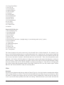
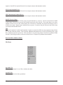
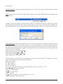
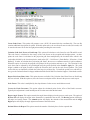
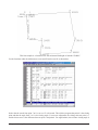
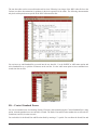
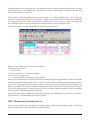
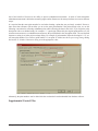
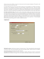
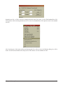
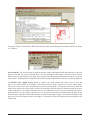
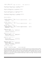
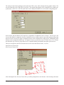
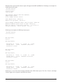
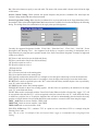
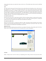
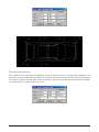
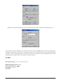
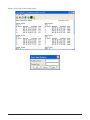
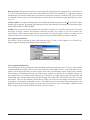
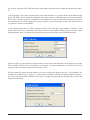
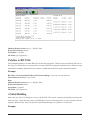
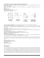
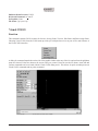
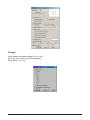
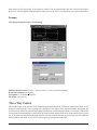
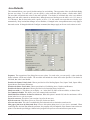
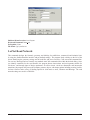
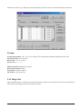
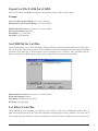
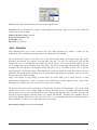
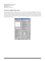
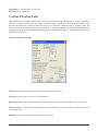
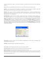
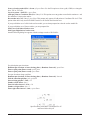
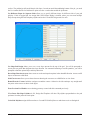
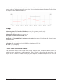
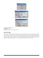
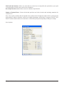
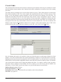
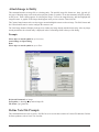
3 The Setup dialog box appears briefly, followed automatically by the Carlson Software 2008 Setup dialog. If this
is the initial installation, you will see the dialogs shown below.
Chapter 1. Introduction
5
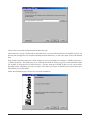
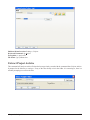
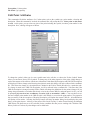
After reading this second dialog box, press Next. If this version of Carlson Software has already been installed, you
will see a a different Add/Remove dialog instead. In this case, it is recommended that you Cancel the current install
and go to Windows > Control Panel > Add/Remove Programs and remove Carlson Software 2008. After the old
installation is removed, you may start the install process once more to continue.
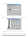
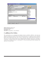
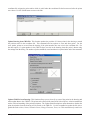
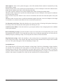
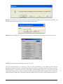
4 Review the End-user License Agreement, accept it with the correct click choice, and then click Next. You can
optionally print it out.
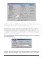
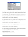
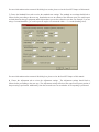
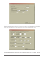
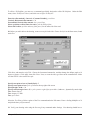
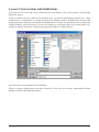
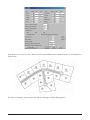
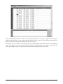
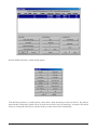
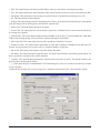
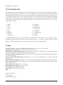
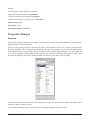
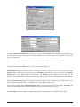
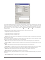
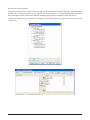
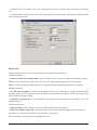
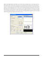
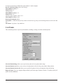
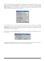
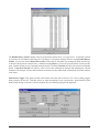
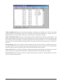
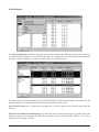
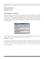
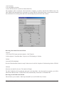
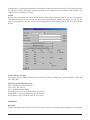
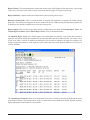
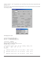
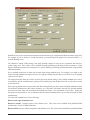
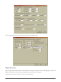
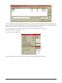
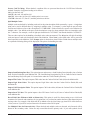
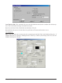
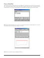
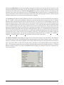
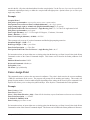
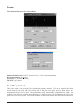
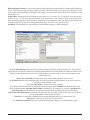
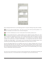
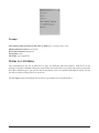
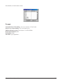
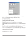
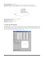
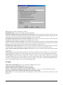
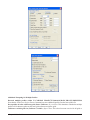
5 On the Select Installation Type dialog box, select the type of installation you want: Typical or Custom. Choose
Next.
Chapter 1. Introduction
6
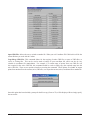
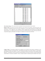
Typical installs the following features:
• Program files: Executables, menus, toolbars, Help templates, TrueType® fonts, and additional support files
• Internet tools: Support files
• Fonts: SHX fonts
• Samples: Sample drawings
• Help files: Online documentation
Custom installs only the files you select. By default, the Custom installation option installs all Carlson Software
features. To install only the features you want, choose a feature, and then select one of the following options from
the list:
• Will be installed on local hard drive: Installs a feature or component of a feature on your hard drive.
• Entire feature will be installed on local hard drive: Installs a feature and its components on your hard drive.
• Feature will be installed when required only: Installs a feature on demand.
• Entire feature will be unavailable: Makes the feature unavailable.
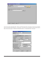
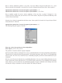
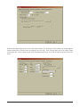
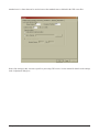
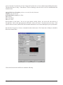
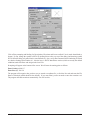
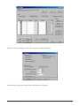
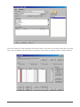
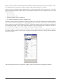
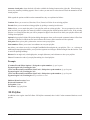
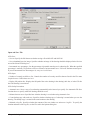
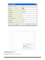
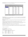
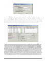
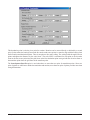
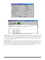
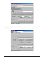
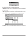
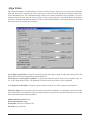
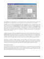
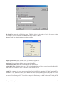
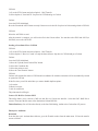
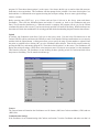
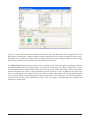
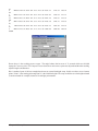
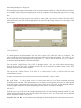
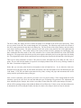
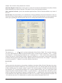
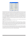
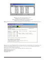
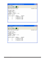
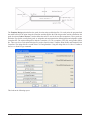
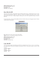
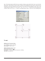
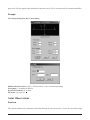
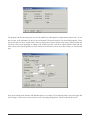
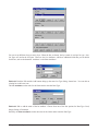
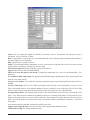
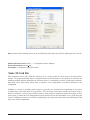
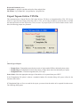
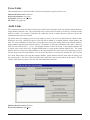
6 On the Destination Folder dialog box, do one of the following:
Chapter 1. Introduction
7
Choose Next to accept the default destination folder/directory.
Choose Browse to specify a different drive and folder where you want Carlson Software to be installed. Choose any
directory that is mapped to your computer (including network directories), or enter a new path. Choose OK and then
Next.
Setup installs some files required by Carlson Software in your system folder (for example, c:\Windows\System, or
c:\Winnt\System32). This folder may be on a different drive than the folder you specify as the installation folder
(for example, d:\Program Files\Carlson Software). You may need up to 60 MB of space in your system folder,
depending on the components you select to install. Setup alerts you if there is insufficient free space on the drive
that contains your system folder.
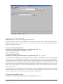
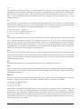
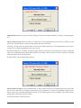
On the Start Installation page, choose Next to start the installation.
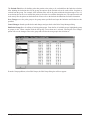
Chapter 1. Introduction
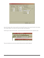
8
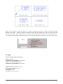
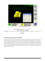
The Updating System dialog box is displayed while Carlson Software is installed.
When the installation is complete, the Setup Complete dialog box is displayed. Choose Finish to exit the installation
program.
It is strongly recommended that you restart your computer at this point in order for the new configuration settings
to take effect.
Congratulations! You have successfully installed Carlson Software. You are now ready to register your product and
Chapter 1. Introduction
9
start using the program. To register the product, double-click the Carlson Software icon on your desktop and follow
the instructions.
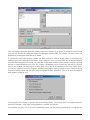
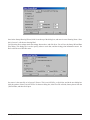
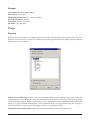
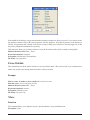
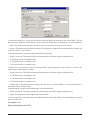
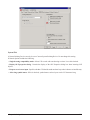
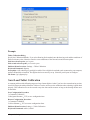
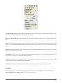
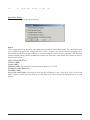
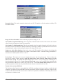
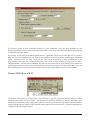
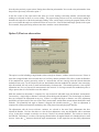
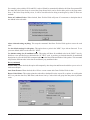
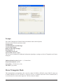
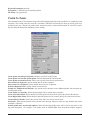
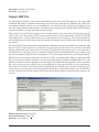
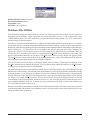
Authorizing Carlson Software
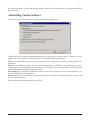
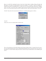
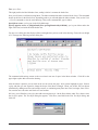
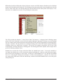
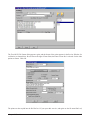
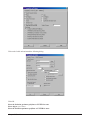
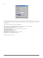
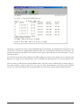
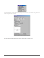
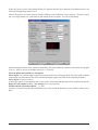
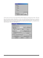
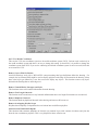
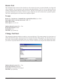
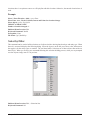
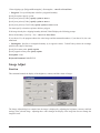
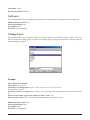
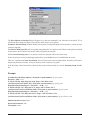
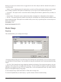
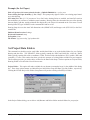
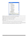
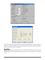
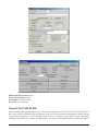
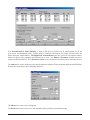
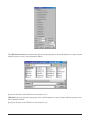
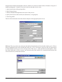
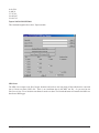
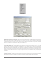
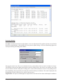
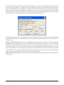
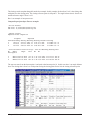
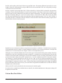
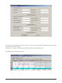
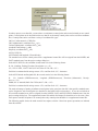
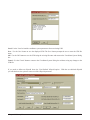
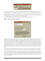
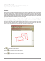
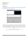
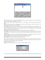
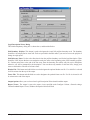
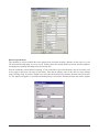
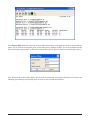
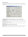
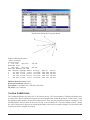
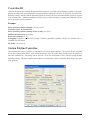
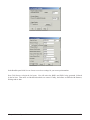
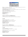
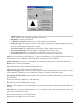
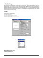
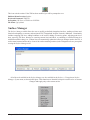
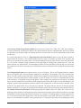
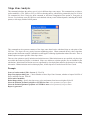
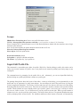
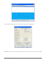
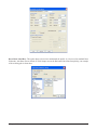
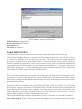
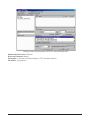
The first time you start Carlson Software, the Registration Wizard is displayed.
Carlson Software has installed an automated procedure for registering your software license. Change keys are no
longer given over the telephone. Please choose one of the following registration methods.
Form: This method allows you to fill out a form that you can print out and fax or mail to Carlson Software for
registration.
Internet: If your computer is online, you may register automatically over the Internet. Your information is sent to a
Carlson Software server, validated and returned in just a few seconds. If you are using a dial-up connection, please
establish this connection before attempting to register.
Enter change key: Choose this method after you have received your change key from Carlson Software (if you
previously used the Form method above).
Register Later: Choose this method if your want to register later. You may run Carlson Software for 30 days before
you are required to register.
After you choose the registration method, press Next
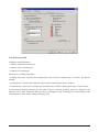
Chapter 1. Introduction
10
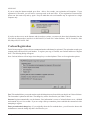
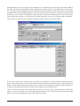
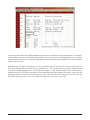
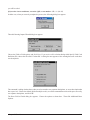
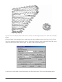
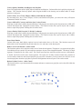
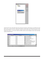
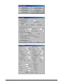
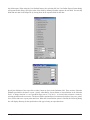
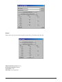
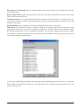
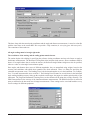
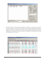
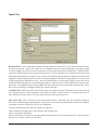
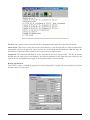
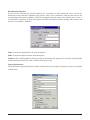
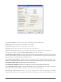
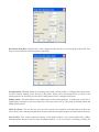
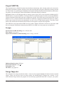
Choose the reason for installation. The very first time you install Carlson Software is the only time you will choose
the first reason. All subsequent installations require a choice from the remaining options.
New install or maintenance upgrade of Carlson Software: If you are installing Carlson Software for the first
time, choose this reason.
Home use. See License Agreement: Choose this reason if you are installing on your home computer. See your
license agreement for more details!
Re-Installation of Carlson Software: Choose this reason if you are reinstalling on the same computer with no
modifications.
Windows or AutoCAD upgrade: Choose this reason if you have reinstalled Carlson Software after installing a new
version of Microsoft Windows.
New Hardware: Choose this reason if you are installing Carlson Software on a new computer or if your existing
computer has had some of its hardware replaced such as the hard disk, network adapter, etc.
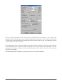
After you choose the reason for installation, press Next, and then enter the required information into the dialog.
If you are using the Form method, press the Print Fax Sheet button, to print out the form. You may fax this form
to the number printed on the form, or mail it to Carlson Software, 102 W. Second St., Suite 200, Maysville, KY
Chapter 1. Introduction
11
41056-1003.
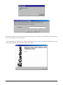
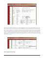
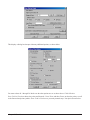
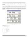
If you are using the Internet method, press Next. After a few seconds, your registration will complete. If your
registration is successful, you will receive a message such as the one below. If your registration is unsuccessful,
please note the reason why and try again. Keep in mind that each serial number may be registered to a single
computer only.
If you do not have access to the Internet, and do not have a printer, you must write down the information from the
User Info tab (shown above) and fax it to 606-564-9525, or mail it to Carlson Software, 102 W. Second St., Suite
200, Maysville, KY 41056-1003.
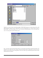
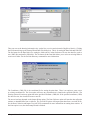
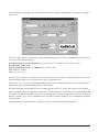
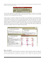
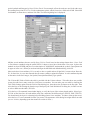
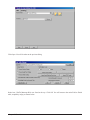
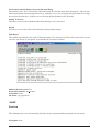
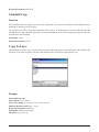
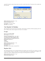
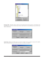
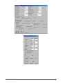
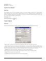
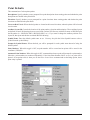
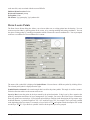
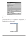
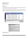
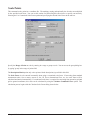
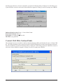
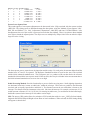
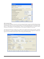
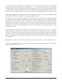
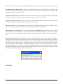
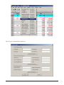
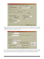
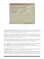
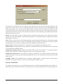
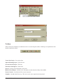
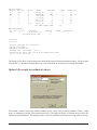
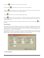
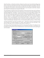
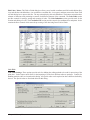
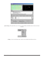
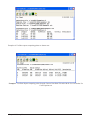
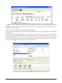
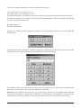
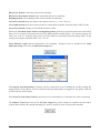
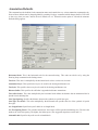
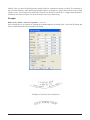
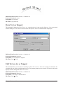
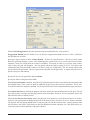
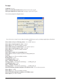
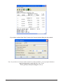
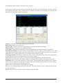
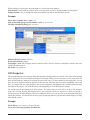
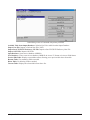
Carlson Registration
Each Carlson program is licensed for use on one workstation which must be registered. The registration records your
company name and AutoCAD serial number. To register your copy of Carlson, start Carlson and choose ''Register
Now''. The following dialog will appear.
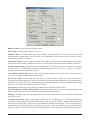
Note: Carlson Software will no longer issue change keys over the telephone. There are four registration options.
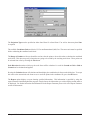
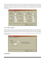
Fax: This method allows you to print out the required information on a form which you then fax to Carlson Software.
The fax number is printed on the form. The change key will be faxed back to you within 72 hours.
Internet: Register automatically over the Internet. Your information is sent to a Carlson Software server, validated
and returned in just a few seconds. If you are using a dial-up connection, please establish this connection before
attempting to register.
Enter pre-authorized change key: If you originally chose the Fax method above, you will need to choose this
method now to enter the change key that is faxed back to you.
Chapter 1. Introduction
12
Register Later: If you wish, you may defer registration up to 30 days. After this time, Carlson will enter demo
mode which displays a message each time a Carlson command is run.
After you select the registration method, choose Next and select the type of installation you are performing, choose
Next again to review the copyright information and to fill out the required information. At this point, if you are
using the Fax method, press the Print Fax Sheet button. If you are registering using the Internet method, press Next
and the process will start.
If you have any problems with Internet registration, please repeat this process and use the Fax method. The
registration form is available on the Carlson Software website at http://www.carlsonsw.com/registration.html.
Tip: If Carlson is running, you may access the registration dialog by choosing About Carlson from the Help menu,
then pick the Change Registration button.
Setting Up a Project
Over 200 Carlson Software settings can be specified in the Configure command on the Settings menu. These values
are used to initialize Carlson Software options when opening a new or existing drawing. Among these settings is
the coordinate point number format, object linking options, and settings for the COGO portion of Carlson Software.
The template drawing is the default drawing that opens up each time Carlson Software is started. To customize
the template drawing, run the OPEN command under the File pulldown menu, change the files of type setting to
Drawing Template and choose the template drawing, ''survey.dwt''. Then make your changes and SAVE the drawing
as survey.dwt in the Template folder.
When starting a new drawing, one of the first steps is to run Drawing Setup in the Settings menu. Drawing Setup
sets the drawing scale, the units mode as either english or metric, and the text, symbol and linetype size scalers. The
initial values for these Drawing Setup variables are set in Configure > General Settings. When a drawing is saved,
the Drawing Setup variables are saved with the drawing. Carlson Software will set the text height according to the
drawing scale and text size scaler set in Drawing Setup. For example, if the horizontal scale is set to 50 and the
text size scaler is 0.1, Carlson Software will draw the text with a height of 5 (50 * 0.1). Then, when the drawing is
plotted at 1''=50', the text will be 0.1 inches.
Every drawing remembers the data files that are being used for the drawing. When the drawing (.DWG) file is saved
with the SAVE or SAVEAS command, Carlson Software writes a settings file that contains all the active data file
names. Then, when the drawing is reopened, the data files default to their previous settings. For example, you won't
have to choose which coordinate file to use unless you want to change it. The settings file is stored in the same folder
as the drawing file, and has the same name as the drawing, with an .INI extension. For example, a drawing called
survey.dwg would have a settings file called survey.ini.
The Drawing Explorer command, in the Settings menu within the Project command, tracks and stores project files
associated with each saved drawing. You may use this command to generate a report of all files used in a particular
drawing. Project Explorer takes this concept one level further and allows you to group drawing files and their
associated project files. Reports can also be generated using this tool.
Startup Wizard
For creating a new drawing in Carlson Software, the Startup Wizard can guide you through starting and setting up
the drawing. This wizard is optional, and it can be turned on or off in the Settings menu by clicking Configure, then
General Settings. You can also exit out of the Startup Wizard at any time. When the Startup Wizard is turned on and
the New drawing command is executed, you will see the Select template dialog box.
Chapter 1. Introduction
13
Typically, you want to choose the drawing template SURVEY.DWT when you are using Carlson Survey, and
then click Open. Rember that for Carlson Roads you will use ROADS.DWT. For Carlson Field you will use
ROADS.DWT. The drawing template will set some of the basic drawing parameters, such as the default layer
names. The Startup Drawing Wizard dialog appears.
Here, you need to set the new drawing name and scale. Set the drawing (.dwg) name by picking the Set button. The
Drawing to Create dialog box opens. Change to the directory/folder (''Save in'' field) where you want to store the
drawing. You can either select an existing folder or create a new folder. Type in the drawing name in the File name
field and click the Save button.
Chapter 1. Introduction
14
Then you can set the drawing horizontal scale, symbol size, text size and unit mode (English or Metric). Clicking
the Next button brings up the Startup Wizard Data Files dialog box. This is for setting the Data Path and CRD File.
The Set button for the Data Path is for setting the folder where Carlson Software will store the data files, such as
raw (.RW5) files and profile (.PRO) files. The Set button for the Data Path allows you to select an existing folder or
create a new folder. See the Set Data Directory command for more information.
The Coordinate (.CRD) File is the coordinate file for storing the point data. There is an option to create a new
or existing coordinate file. The New option will erase any point data that is found in the specified CRD file. The
Existing option will retain any point data in the specified coordinate (.CRD) file. If the specified coordinate (.CRD)
file does not exist, the wizard will create a new file.
The next wizard step depends on the Import Points option. The Data Collector option will start the data collection
routines to download data from a collector. The Text/ASCII option will import point data from a text/ASCII file.
See the Data Collection and Import Text/ASCII File commands for more information on running these routines. If
the None option is set, then the Startup Wizard is finished.
Chapter 1. Introduction
15
Once point data has been imported from the data collector or text/ASCII file, the wizard guides you through drawing
the points. There are options to run Draw/Locate Points, Field To Finish or None. If None is selected, then the
Startup Wizard is finished. Draw/Locate Points will import the points into the drawing using the same symbol and
layer for all the points. From the Draw/Locate Points dialog, set the symbol, layer and point attributes to draw
(description, elevation) and then pick the Draw All button. The Field To Finish command will import the points
into the drawing using different layers and symbols depending on the point descriptions that refer to the code table
defined in Field to Finish. Also Field to Finish can draw linework. See the Draw/Locate Point and Field To Finish
commands for more information on running these routines. After drawing the points, the wizard will zoom the
display around the points. Then the wizard is finished.
Command Entry
Commands may be issued by selecting a pulldown menu, screen menu, digitizer tablet item, or by typing a command
at the AutoCAD command prompt. Pressing Enter at the command prompt repeats that last command. Pulldown
menus have a row of header names across the top of the screen. Selecting one of these header names displays the
possible commands under that name. Screen menu items are shown in the screen menu (typically on the right side
of the screen). The screen menu can be toggled off and on inside of the AutoCAD Preferences dialog. The Pulldown
menus are the primary method for Carlson command selection. Each section of this manual shows the pulldown
menu which contains the commands that are explained in that section. Pulldown menus are sometimes also referred
to as dropdown menus.
Command availability depends on which menu is loaded. Carlson menus have a mixture of both Carlson and
AutoCAD commands. This allows you to execute the commonly used AutoCAD commands from the menus while
running Carlson.
Quick Keys are user-defined short cut names that can be typed in to start commands. To review the current set of
Quick Keys, run the Quick Keys command in the Settings pulldown menu. Quick Keys are explained in more detail
in the next section.
Layer and Style Defaults
Many Carlson Software commands have default layers such as AREATXT for area labels and BRGTXT for bearing
and distance annotations. These layers can be specified in dialogs for the corresponding commands, and several can
be set in the Configure command under the Settings menu. Sometimes you may want to use the current layer, and it
can be an extra step to have to open the dialog to set the layer. In this case, instead of using the default layer that is
set in the dialog, the default layer can be set as ''CLAYER'', which will use the current layer.
For example, if the annotation layer is set to CLAYER, then annotation will be drawn in the current layer instead
of BRGTXT or whatever the annotation layer used to be. This same concept applies for text styles. Several commands have specific text styles and if you want to use the current style instead of the command style, use the name
''CSTYLE'' for the style name.
Chapter 1. Introduction
16
What is New
General Commands
• New Toolbars - Added 25+ more default toolbar icons for common commands.
• Reports - Added option to output reports directly to Microsoft Word.
• Report Formatter - Added output options to create a table in the drawing for the selected fields and to create
an html format report. Added ability to save report with all the settings, data and user defined attributes.
• Perpendicular From Osnap - Added ability to snap perpendicular from linework within the 'CL transparent
command.
• Drawing Inspector - Added option to show curve data. Added setting for high precision data display.
• New Scale 2D - New command to scale entities in x,y coordinates without effecting their elevation.
• Join Nearest - When layers or elevations don't match, add option to prompt for which one to use. Added
option to stop at intersections with more that two connections.
• Highlight Crossing Polylines - Added tolerance settings for intersection points to merge by average.
• 3D Viewer Window - Added options to show axis icon, bounding box and vertical scale amount. Lighting
conditions automatically saved and recalled. Additional formats in bitmap output.
• Insert Symbol - Added option to align symbols by centerline or polyline.
• New Draw Arc (PC,PT,Radius len) - New command to draw an arc with these inputs.
• New Draw Polyline Start/End - New command draw different symbols for the start and end points of selected
polylines.
• Layer Inspector - Added ability to select multiple layers to highlight.
Survey Commands
• Edit-Process Raw File - Added support for all grid projections for the Calculate Grid Scale Factor option.
Added option to apply a geoid for the Calculate Grid Scale Factor option. Added function to convert point
records into notes. Added function to create new raw file within editor. New processing method to calculate
coordinates from angle only measurements. Added processing option to not store point numbers from the
Chapter 1. Introduction
17
•
•
•
•
•
•
•
•
•
•
•
•
•
•
•
•
•
•
•
•
•
•
•
•
•
control coordinate file into the active coordinate file. Added Data On/Off records to comment out sections of
the raw file from processing. Added Elevation 2D/3D notes to control whether to process elevations. Added
support for angles in GONS units in spreadsheet and reports. Added report function for a summary report of
the traverse, sideshot and store points in the rw5 file. Added settings for min/max ranges of valid instrument
and rod heights that are checked during processing.
Edit-Process Level Data - Added import of Leica level data.
SurvNET - Added import of GPS vectors from LandXML and Trimble .DC formats. Added import of Leica
level data. Added functions to save/load standard error settings into the project settings. Added support for
more projections including UTM, New Brunswick and user-defined. Several improvements to the formatting
of ALTA reports. Improved processing speed by 30%.
Field-to-Finish - Added option to draw attributes as text instead of blocks with control of text style, position,
prefix, suffix, layers and precision. Added option for values to assign for custom attribute symbols. Added
functions to import Eagle Point and C&G code tables. Added option by code to truncate high digits of
elevation labels. For JOG special code, added ability to extend a line. For curves with more than 3 points,
added option to draw the best-fit curve. Added code option to align points by their associated linework.
Field-to-Finish Inspector - Added ability to select multiple codes to review at a time.
Import Text/ASCII File - Added option to create point group for new points.
Draw/Locate Points - Improved speed of using Field-to-Finish code table and added support for more coding
methods. Added option to truncate high digits from elevation labels.
New Coordinate System - Added optional coordinate system data in Drawing Setup to define drawing coordinates as either grid projection or local coordinates. For local coordinates, Define Localization uses control
points to define transformation between local and grid systems. The coordinate system setup is used in routines like List Points and Label Lat/Lon to label local, grid and lat/lon coordinates.
New Distance Scale Factor - Added distance scale factor to Drawing Setup to report and label distances in a
second system besides the drawing units such as feet-meters or ground-grid.
Inverse - Added option to report in feet and inches.
Enter Deed Description - Now auto-saves during command to enable resuming in case of cancel.
Legal Description Writer - Added option to spell out numbers and option to report interior angles. For
curves, added option to identify compound, reverse, tangential and non-tangential.
Trim By Point Symbols - Improved routine to work more reliably for more types of symbols.
Coordinate File Utilities - For Copy/Merge function, added prompt for range of points to use and description
filter and made several improvements to the merge dialog. Added function to unlink drawing points with
coordinate file. For Coordinate Transformation, added convergence angle to report.
New Freeze/Thaw Points - New functions to hide/show point entities in the drawing. Points can be selected
by range, group or screen selection.
Cut Sheet - Added runway clearance surface method.
Tangent Line From Circle - Added option to draw across circles from left to right or from right to left.
Building Offset Extensions - Added option to create points at diagonals and for edges projected across
building. Added controls to set layer and elevation for points.
New Triangle Solutions - New triangle calculator command.
Draw Legend - Added option to use description from Field-to-Finish code table as legend default.
Line/Curve Tables - Added option for header line on line/curve tables.
Angle/Distance Annotation - Added auto erase of old labels when relabeling the same linework.
Create Point Table - Added setting for text style.
Bearing Leaders - Added options to position bearing leaders above or below bearing label.
Draw Endpoint Leaders - Added support for curves.
Station Polyline/Centerline - Labels linked to centerline to update labels if centerline is changed. Added
options to label deflection angles, to label northing/easting of start, to draw symbols at curve PC/PT stations,
and to label curve radius on PC lines. Added setting for text style for labels. Added functions to save/load
settings by settings file.
Chapter 1. Introduction
18
• Input-Edit Centerline - Add function to reverse centerline. For assign point number, added option to include
CL type in description.
• Centerline Report - Added support for railroad curves.
• Hot New Lot Network - 25 new commands for subdividing a site into lot and ROW areas. Dynamically
updates areas for any changes to boundaries. Includes ability to label linework and areas and to draw setback
boundaries.
• Lot File By Interior Point - Added option to prompt for point of beginning and setting for clockwise or not.
• New Draw Lot Setback - New command to draw frontage, side and back lot setback offsets.
• New Fit Structure - New command to draw a building outline within a lot at setback offsets.
Surface Commands
• Triangulate & Contour - Added controls for generating smoother contours by applying an outlier reduction
filter and by reducing contour vertices before Bezier smoothing. Added contour collision check to prevent
crossing contours otherwise caused by smoothing adjustments. Added separate elevation range settings: one
for source data and one for contour output. Added option to draw flow arrows. Added option to draw depression contours. Added function to save/load settings to style file. The Data Error Manager is changed to a
dock-dialog to allow editing in the drawing while using the manager to zoom to the data problems.
• Volume Calculations - Improved speed of triangulation volumes by 50%.
• Draw Triangular Mesh - Added option to use inclusion/exclusion perimeters.
• Draw Grid File - Added option to reduce 3D faces resolution in areas that are fairly coplanar.
• Offset 3D Polyline - New method to offset polyline at slope to intersection with a surface model.
• Make Grid File - Added method to read source data from a coordinate file or from a text/ascii file.
• Surface Manager - Added ability to add points outside current surface.
• Triangulation File Utilities - Added function to apply subdivisonal surfaces to the triangulation.
• Design Pad Template - Added method to define slope as projected in slope direction instead of perpendicular
to pad polyline. Added setting to control side line interval at corners.
• New Slope Zone Analysis - New command to report and color slope zones of a surface.
• Profile From Surface Entities - Add support for railroad stationing.
• Profile From Grid or Triangulation Surface - Add support for railroad stationing.
• Profile From Points On Centerline - Added option to record point offsets to centerline into profile descriptions.
• Draw Profile - Added support for drawing a user-specified number of profiles at a time. Added draw grid
option to use grid ticks and dots. Added setting to control width of profile polylines. For horizontal label box,
added option for user-defined rows and option to draw above profile grid. For vertical curves, added option
to auto-place labels above highest vertical curve, added option to label high/low points, added more PVI-V
linework styles, added control of the curve symbols, added option whether to label the grades on the profile
polyline and added prefix/suffix settings for all the curve labels. For profile grid, added setting for vertical
grid adder to top and bottom. For profile crossings, added settings to control each label prefix, suffix, style,
size, decimals and rotation. For plan-profile sheets, added options to draw sheet layout border in plan view,
to draw a north arrow in plan view and to draw plan-view only sheets. For sewer/pipe profiles, added options
to draw flow direction arrows on the pipes and to close pipe connections at the structures. For pipe crossings,
added method to calculate and draw crossing on-the-fly and new method to specify swath width for drawing
any parallel pipes. For drawing additional profiles onto an existing grid, added a button to pick the existing
grid to get the grid dimensions. For station and elevation grid text, added settings for offset amount from grid
lines. Added separate settings for road, sewer, pipe and crossing labels for label size, color, style and layer.
New option to label profile name at start of profile polylines. Added Draw Grid options for grid ticks with
checks and whether to label elevations on the left side only.
• Input-Edit Profile - For road profiles, added ability to set vertical curve to make a sag/crest at the specified
through point. Added report function within editor. Added graphic display option to show slopes.
Chapter 1. Introduction
19
GIS Commands
• GIS Query/Report - Added method to query across multiple tables in a relational database.
• New Place Camera Symbol/Image - New command to draw a camera symbol with an attached image.
Data Conversions
•
•
•
•
•
•
Belgium - Added support for hBG03 geoid.
Canada - Added support for GSD95 geoid.
Finland - Added support for Finland 2000 geoid.
France RAF98 Geoid - Added support for this geoid.
Geoid 03 - Added support Alaska, Hawaii and Puerto Rico.
LandXML - Added support for sewer network data. Added import of parcel data and parcel groups from
Civil 3D.
• MOSS - Improved import of Genio files to support curves and layers.
• Northern Ireland Geoid - Added support for this geoid.
• Republic of Ireland Geoid - Added support for this geoid.
Standard Report Viewer
Many Carlson routines display output in the Standard Report Viewer as shown below. The report can be edited
directly in the report viewer. Report Viewer commands are described below.
Open: This allows you to open an ASCII file and display the contents in the report viewer.
Save: Save the contents of the report viewer to a text file.
SaveAs: This allows you to save the contents of the report viewer to a file.
Append To: This allows you to append the contents of the report viewer to another file.
Print: Print the contents of the report viewer. This will open the standard windows Print dialog where you can
choose the printer and modify any of the printer settings before you actually print.
Screen: Draws the report in the current drawing. The program will prompt you for a starting point, text height,
rotation, layer and whether you want it inserted as Mtext or Text.
Undo: Reverses the effect of your last action. If you mistakenly deleted some text, stop and choose the Undo
command to restore it. The key combination Ctrl+Z also performs this action.
Chapter 1. Introduction
20
Chapter 1. Introduction
21
Select All: Selects all the text in the report viewer.
Cut: Deletes the selected text and places it on the Windows® clipboard.
Copy: Copies the selected text to the Windows® clipboard.
Paste: Inserts ASCII text from the Windows® Clipboard into the report viewer at the cursor.
Search: Opens the Find Text dialog. Allows you to search for text in the report viewer.
Replace: Opens the Find and Replace Text dialog. Allows you to search for text and replace it.
Options: Opens the Report Viewer Options dialog. In this dialog, you can specify print settings, such as lines per
page and margins. You can also specify the font used in the report viewer. This font is used for both the display and
for printing.
Hide: This button allows you to minimize the report viewer window and give focus back to the Carlson CAD
screen. This allows you to return to working on the Carlson CAD screen without closing the report. You can
re-activate the report by picking on the minimized report viewer icon.
Report Formatter
A number of Carlson routines use a dialog box called Report Formatter Options to allow you to specify how and
which results of calculations should be presented in the report. This report routine lets you select a set of data
to report and the format of the selected data. The report can be displayed in either the standard report viewer as
described in the previous section, Microsoft® Excel or Microsoft® Access.
The data set in the Report Formatter may be thought of as a spreadsheet, where columns are various fields related to
a single item such as time period, drillhole, area and etc. Each new row represents a new item. Descriptions of these
field names are displayed in the Available list of the Report Formatter. To include a data field in the report, highlight
the field name in the Available list on the left and pick the Add button. This moves the field name to the Used list on
the right. The order of items in the right list defines the order in which they will be displayed. In addition, the items
may be sorted as specified by the user in the right column. Items are first sorted by the first column, then items with
the same value in the first column are sorted as specified for the second column, and so on.
Chapter 1. Introduction
22
These subsequent sortings do not modify sortings of previous columns. If you specify no sorting for some column
(even the first one) then no sorting will happen in subsequent columns either. For example, you may want to sort
production by mining panel name but not by month.
To generate the report after selecting columns and other preferences, click on Display button. It will bring up a
standard report viewer showing the report data. Upon exiting the viewer, you come back into the Report Formatter
for further data manipulation if needed. The other data output and destination options include saving the specified
data into a comma-delimited text or CSV file, creating a spreadsheet preview whereby the data may be exported
using several methods, and direct export to Microsoft® Excel. Due to the popularity of the Excel output choice,
you can also customize certain Excel options, including setting mirror output, just prior to export. Data can also be
merged to combine current and old reports, and it be exported to XML format files. There is an option for output to
other database formats as well.
You may define new columns as equations based on existing columns. Click on the Edit User Attributes button to
add a new field name. A list of the existing attributes is available for reference.
User attributes may have one of the several summation options just like program-generated ones (except that for
Chapter 1. Introduction
23
them these options are set by program). The summation level is defined by the ''Total'' pop-up list in the middle of
the dialog. By default only grand total will be displayed at the bottom of the list. By picking the next item in that
box, you will get subtotals added each time the value in first column is changed. It makes most sense to use this kind
to summation if the corresponding column is sorted. For example if the first column is ''Area Name'' and it is sorted,
and ''Total'' is set to ''Grand, Area Name'' the report will have a sub-total for each distinct Area Name. This feature
makes the Report Formatter a very flexible tool for results exploration, even before or without using a spreadsheet.
Various forms of reports may be saved and recalled using controls in the top line of the dialog.
To save a new version of the format, type in a new name (or use default to overwrite old one) and click on the Save
button. The next time that you come to the Report Formatter from the same Carlson routine it will recall this last
format. To pick another format just pull down on list of formats in the left top corner and pick which format to use.
To Delete an unwanted format, pick it from the list first and then click on Delete button.
There are several Microsoft® Excel export options provided. You may specify a spreadsheet file to load before
export, as well as a left upper cell to start with and sheet number to use. Totals which are reported when using
built-in viewer may be skipped when using Microsoft® Excel export.
Chapter 1. Introduction
24
For commands that process reports using perimeter polylines, the Report Formatter has an option to create GIS
links between the polylines and the database records when the Export to MS Access function is used. When the
polyline data is available for the GIS Links, there will be a report field called Handle. This Handle field is the
AutoCAD entity name for the polyline and serves as the hook for the GIS link. The Handle field does not need to
be put into the report Used list in order to create the links. When the Export function is called with the MS Access
method, there is a pop-up window prompt for whether to create the GIS links. When these links are created, you
can then use the GIS menu commands to manage and report the data.
Instruction Manual and Program Conventions
Westwood
Italic text represent responses by the user that should be typed in and followed by the Enter key.
Number/<Pick point>:
Bold text represents prompts or questions that the computer program will ask the user.
<90.0000>
Values enclosed in corner brackets represent default values obtained by pressing Enter with a blank response to
AutoCAD or Carlson commands.
[end on]
Lower case text enclosed in brackets in Command prompts denotes an OSNAP mode that is turned on by the command.
Chapter 1. Introduction
25
Carlson File Types
.AAN Auto-Annotate Settings
.ADF Annotation Default Settings
.ARX AutoCAD Runtime Extension For Carlson Program
.ATR Strata attribute definitions
.AVG Mining Composite Quality Analysis
.BLK Mining Block Model
.CAL Mining equipment calendar
.CAP Capacity file for hydrology (stage-storage)
.CDF Geology Channel Sample File Format
.CDS MDL Laser Raw Data
.CDT Mining custom date table
.CFG Configure Configuration Settings
.CFZ Cut/Fill Color Map Zones
.CGC C&G Coordinate File
.CGR C&G Raw Data
.CH Corehole definition
.CL Centerline file
.CLT Culvert Settings
.CN Hydrology CN Factors
.COG Cadvantage Coordinate Data
.COT Multiple Outlet Design Data
.CQT Mining custom quantity table
.CRB Template Curb Definition
.CRD Coordinate file (point#, northing, easting, elevation, description) in binary form
.CTL SDMS Format Raw Data
.CTR Auto-Run Strata Isopach Maps
.CUI Customized User Interface AutoCAD Menu
.CUT SMI Format Cutsheet
.CVT SEDCAD Format Hydro Network
.DAT GPS Localization Definition
.DCF Deed Correlation File
.DCL Carlson dialogs
.DEM Digital Elevation Model
.DEQ Drillhole equations
.DHF Drillhole Text File
.DHT Dragline History
.DIL StrataCalc Convert As-Determined Qualities
.DLL Carlson programs files
.DTF Drillhole Data Format
.DTS Drillhole Text Settings
.DWG AutoCAD drawings
.DXF Drawing Exchange Format
.DZR Dozer Push Settings
.EQO Mining equipment options
.EQU Mining equipment definitions
.ERD Erodible Channel Settings
.EW Earthwork Section End Areas
.EXE Carlson programs
Chapter 1. Introduction
26
.FCL Feature Code List for SurvCE
.FEN Fence Diagram Settings
.FLD Field to Finish code definitions
.FLT Triangulation mesh
.FMS Report Formatter Settings
.FRM Ferm Codes
.GCL Geologic Column Settings
.GEO Settings for Draw Geologic
.GFU Grid File Utilities macro command recorder file
.GIS GIS prompting definitions for note files
.GPF Grade Parameter File For Block Model
.GRD Grid file - a DTM surface model
.GRR Lot Edge Grading Rules
.GSQ Grid sequence history file for mining
.H1 Hydrograph
.H2I HEC-2 Water Surface Profile
.HYD Watershed settings
.HZN Horizon code definitions
.IMP Drillhole Import Format
.INI Program user preferences settings
.LAY Layer State
.LEV Level Raw Data
.LGD Annotate Draw Legend definition file
.LOT Lot file for Survey
.LPT Coordinate Transformation Point File
.LQE Least-Squares Measurement Error Settings
.LSP Carlson Lisp programs
.LSQ Least-squares input data
.LSS Localization Settings
.LTD Lot Attribute Definition
.LTN Lot Network Settings
.MAT Materials Library
.MDN Template Median Definition
.MIN Underground Mining Report
.MNC Compiled menus
.MNL Carlson Lisp programs for corresponding menu startup
.MNR Compiled menus
.MNS Compiled menus
.MNU Carlson source menus
.MNX Compiled menus
.MPD Mining Timing Project File
.MPJ Mining project definitions
.MXS Cross section alignment
.NOT Note file - additional descriptions for points in corresponding .CRD file
.OWN Mining Ownership Data
.PAN Mining Underground Panel Data
.PAR Parameters for mining quality compliance
.PAT Hatch Pattern Definitions
.PDD Enter Deed Description data file
.PFF Mining Pit Format File
Chapter 1. Introduction
27
.PFS Draw Profile Settings
.PHN Modem Settings For Carlson Field
.PIT Mining Pit Parameter File
.PLN Plan view polyline file for Dozer 2000
.PNA Mining panel attributes
.PPQ Polygon Processor Query
.PRE Pre-calculated grids for strata model
.PRF Point Range File
.PRJ Project settings file
.PRO Profile (station, elevation, descriptions)
.PSZ Pipe Size Definitions
.PTA Mining pit attributes
.PVF System Variable Settings
.PVL Sewer Network Plan View Label Settings
.PVS Mining Projection and Ventilation Settings
.RCF Drainage Runoff Library
.RCL Runoff Coefficient Layer Definitions
.RDF Road Design File
.RDN Road Network File
.RDS Roadside Ditch File
.REC Seismic Record Output
.REP Hec-Ras Report File
.RES Mining Auto-Run Residuals Settings
.RME Reame Slope Stability Settings
.RMP RiverMorph Project
.RNF Road Network Stakeout for SurvCE
.ROW Right-of-Way offsets for Lot Network
.RPT Report Formatter Data
.RSV Mining Reserve Description
.RUN Auto-Run Strata Grids definition file
.RW5 Raw file of traverse data
.SC Coal Section Configuration
.SC5 SurvCE Raw Data Archive
.SCR COGO script file
.SCT Cross section data (station, offset, elevation, descriptions)
.SDF Strata Definitions
.SDT SB-Slope Stability File
.SEQ Dragline sequence file
.SEW Sewer network file for hydrology
.SGD Slope Group Definition for Design Pad Template
.SIF Surface Inspector File
.SLB Slide library
.SLD Slide image
.SLI Symbol Library
.SST Draw Section Sheet Settings
.STG Stage-discharge data for hydrology
.STR Sewer Structure Library
.SUP Superelevation file
.TAB Hydrology Peak Flow Data
.TCF Digitizer Tablet Configuration File
Chapter 1. Introduction
28
.TCH Trench Structure Template
.TIM Mining Timing Settings
.TIN Triangulation Surface
.TKD Takeoff Material Definitions
.TOP Topsoil Definition for Road Design
.TPC Template point centerline definition
.TPL Template file for Section-Profile
.TPP Template point profile definition
.TPT Template transition file for Civil Design
.TRG Takeoff Layer Target Settings
.TRI Triangulate & Contour Settings
.TSF Road Template Series File
.UAO Report Formatter Attribute Options
.UAT Report Formatter User Attributes
.UDP User-Defined Projection For Grid Coordinates
.VOL Auto-Run Strata Quantities definition file
.WST Watershed Structure File
.XML LandXML Data Exchange File
.ZIP Compressed Data Files
.ZON Earthwork Zone Definitions
Quick Keys
''Quick Keys'' allows you to enter in the coding shown here on the left, and by doing so run the commands shown
on the right.
2DP = 2D Polyline
3DP = 3D Polyline
A = Arc
AL = Align
B = Block
BB = Bearing-Bearing Intersect
BD = Bearing-Distance Intersect
BH = Boundary Hatch
C = Circle
CH = Change Properties
CO = Color
CP = Copy
DD = Distance-Distance Intersect
DI = Distance
DT = Draw Text
E = Erase
EA = Enter-Assign Point
EX = Extend
F = Fillet
Chapter 1. Introduction
29
H = Hatch
I = Inverse
L = Line
LI = List
LP = Draw-Locate Point
LS = List
M = Move
MI = Mirror
O = Osnap
OF = Offset
OP = Occupy Point
P = Pan
PL = Polyline
PR = Properties
PREF = Preferences
R = Redraw
RE = Redo
RG = Regen
RO = Rotate
SC = Scale
SET = Set Environment Variable
SS = SideShot
ST = Style
T = Traverse
TR = Trim
UN = Undo
UT = Units
VP = Viewpoint
W = Write Block
X = Explode
Z = Zoom
ZC = Zoom Center
ZD = Zoom Dynamic
ZE = Zoom Extents
ZIN = Zoom In
ZOUT = Zoom Out
ZP = Zoom Previous
ZW = Zoom Window
Obtaining Technical Support
via Discussion Groups
• Carlson Software operates user discussion groups located at news://news.carlsonsw.com. You can participate in
user-to-user discussions on tips, tricks and problems. Our staff monitors these groups to ensure that all the issues
are addressed. Visit our website at http://www.carlsonsw.com for information on how to access these groups.
•
You may also access the Carlson Software Knowledge Base.
Visit it directly at
http://update.carlsonsw.com/kbase main.php.
Chapter 1. Introduction
30
via Electronic Mail
• The Technical Support e-mail address is [email protected].
via Phone/Fax
• Phone: (606) 564-5028
• Fax: (606) 564-6422
via Web Site
Check the Carlson Software web site at http://www.carlsonsw.com for:
• Knowledge Base, discussion groups, technical support documents and newsletters
• Carlson Software manuals (PDF) and training movies
• Training and seminar schedules
• Step by step procedures on popular called-in topics
• Carlson Software and Autodesk downloads and updates (Feel free to register for automatic update notification
of updates when you come to that area.)
via Training
• Basic, advanced and update training is available from Carlson College. Enroll on our webpage or call 606-5645028 and ask for Carlson College.
Chapter 1. Introduction
31
Tutorials
2
This section contains tutorials designed to assist you in learning this Carlson Software product. It is recommended
that you try some of these out when you are first starting to learn the software, or when you need some pointers
later on.
You will see how to enter a deed, make a plat and use Field to Finish for faster drafting. There are also lessons on
intersections and subdivisions, SurvNET, contouring, DTM and design. Using break lines and surfaces are also
covered.
Some of the tutorials will ask you to open drawing and data files that are provided to you at purchase. Good luck!
32
Lesson 1: Entering a Deed
In this short lesson you will create a simple drawing. You will enter a 6-sided deed, add a title block, bar scale, and
north arrow, add a title and certification text, and plot the deed area.
Note that the Esc key will cancel most commands, so if you choose the wrong command or enter something incorrectly and want to start over, just press Esc.
1 Click the icon for Carlson. You may be presented with a ''Startup Wizard'' dialog box. If so, click Exit.
2 Under the Settings menu, click Drawing Setup. Set the unit setting to English and the Horizontal Scale to 50.
Click OK.
3 Choose Point Defaults from the Points menu, and, in the dialog box, click Elevations off to eliminate the Elevation
prompt. Click Descriptions on and also set the point symbol name to symbol 4 (SPT4), which is the round, open
circle. Click Automatic Point Numbering on. Click OK.
4 Under the Survey menu, select Enter Deed Description. Use the default settings as shown in this dialog box image.
Chapter 2. Tutorials
33
Set the To Table Scaler option to 0.00. This places all of the deed calls in the drawing. The To Table Scaler
determines which deed calls appear in the drawing and which deed calls appear in a table. Deed calls less than the
To Table Scaler value multiplied by the Drawing Scale will be placed in a table of calls. Set the dialog box options
to match those shown above. Click OK.
The command line is the area below the graphics and to the left. When prompted to ''Pick point or point number''
at the command line, pick a point in the lower left quadrant of your screen to start the deed plotting. If you are
prompted for elevation, you failed to turn off the elevation prompt in Point Defaults. Press Esc and return to the
Point Defaults command.
The following dialog box will appear so you can specify where to store the coordinates:
Chapter 2. Tutorials
34
Select the New tab. Then, for the File Name, type in Deed. This creates a file called Deed.crd. All Carlson
points are stored in files with the ''crd'' extension, which stands for ''coordinates.'' Click Open. Now respond to the
command line prompts exactly as shown here:
When you are prompted for a description, enter ''Fence Post''.
Exit/Curve/<Bearing (Qdd.mmss)>: 125.3500
The quadrant (Q) is 1 for Northeast (2 is Southeast, 3 is Southwest and 4 is Northwest). The bearing is 25 degrees,
35 minutes, and 00 seconds. If all digits for the minutes and seconds are entered as shown above, then the deed call
will be fully plotted, including the seconds. If only the degrees and minutes were entered, as in 125.35, then the
plot would appear as ''N 25° 35' E''.
Varas/Meters/Poles/Chains/<Distance(ft)>: 200.51 Note that you can enter old deeds in the forms of Poles and
Links, Chains and Links and even Varas (a unit of measurement formerly used in the southwestern states of the
U.S.).
Enter Point Description <Fence Post>: Iron Pin
Undo/Exit/Curve/<Bearing (Qdd.mmss)>: 189.4321
Varas/Meters/Poles/Chains/<Distance>: 225.00
Enter Point Description <Iron Pin>: press Enter
Pressing Enter selects the default, which is Iron Pin.
Undo/Exit/Curve/<Bearing (Qdd.mmss)>: C
Radius: 75
Curve direction [Left/<Right>]? press Enter for right
Non-tangent/Reverse-tangent/Bearing/Chord/DeltaAng/Tangent/<Arc Len>: 118.17
If you don't know the arc length, but you know the tangent, you would choose ''T'' for tangent.
Enter Point Description <Iron Pin>: press Enter
Undo/Exit/Curve/<Bearing (Qdd.mmss)>: 200.0000 (due south)
If you were to enter just 2 (no degrees, minutes, or seconds), then the deed call would be plotted ''S 000 E''.
Chapter 2. Tutorials
35
Varas/Meters/Poles/Chains/<Distance>: 178.00
Enter Point Description <Iron Pin>: Concrete Monument
Undo/Exit/Curve/<Bearing (Qdd.mmss)>: 488.2300
This entry specifies Northwest 88 degrees, 23 minutes.
Varas/Meters/Poles/Chains/<Distance>: 300.34
Enter Point Description <Concrete Monument>: Fence Post
Undo/Exit/Curve/<Bearing (Qdd.mmss)>: 454.1109
Varas/Meters/Poles/Chains/<Distance>: 106.93
Enter Point Description <Fence Post>: press Spacebar, then press Enter
Simply pressing Enter uses the default text (Fence Post) again. To avoid drawing the text ''Fence Post'' twice on the
end point, press the spacebar, skip a blank character, and press Enter.
You have now completed the 6-sided figure (including one curve).
Undo/Exit/Curve/<Bearing (Qdd.mmss)>: E
The following results are reported:
SQ. FEET: 83921.8
SQ. YARDS: 9324.6
SQ. MILES: 0.0
ACRES: 1.93
Closure error distance> 0.01708540
Bearing> S 52d5'26'' E
Closure Precision> 1 in 66076.89
1128.95
SQ. FEET: 82302.9
Error
Total Distance Traversed>
SQ. YARDS: 9144.8
SQ. MILES: 0.0
ACRES: 1.89
The resulting deed, has a closure of 1:66077. In the initial prozmpt ''Undo/Exit/Curve...'', U for Undo would allow
you to reenter the previous deed call.
Use the Extents command on the View menu to see the entire area. Then choose Zoom Out under the View menu
giving you adequate room for the next step.
5 Under the Settings menu, select Title Block. The first dialog you will see is shown here:
Chapter 2. Tutorials
36
Select Paper Size B2 (11 x 17), and enter the layer name of BORDER, then choose OK. You will be prompted for
the border location, pick a point in the lower left of the survey.
The following dialog appears, allowing you to enter the attributes for the Title Block. After you have completed the
title block entries, as shown below, select OK.
Note that the title line is plotted in large text on the title block. Its length, therefore, should not exceed 15 characters.
Your drawing should look like the example below at this point.
Chapter 2. Tutorials
37
Use the Extents command, found in the View menu, to see the entire working area. If you want to move the border,
use the Move command on the Edit menu. Pick the border lines and the title block objecm ts (up to 3 picks total),
press Enter (to end object selection), then pick two points representing the vector of the move.
If you want to see a margin around the working area after you use the Extents command, use the Zoom Out command
on the View menu. Then use the Window command on the View menu to capture the view and margin you prefer.
If you make a mistake, enter U for undo, or select the back arrow icon that appears at the top of the screen.
6 On the Annotate menu, select Draw North Arrow.
Accept the default north arrow that is shown at the right side of the dialog, click OK, and place it in the upper right
of your drawing. Choose Move on the Edit menu (or Enter M for move at the command line) and move it.
7 On the Annotate menu, select Draw Bar Scale. Accept the defaults, and then pick an insertion point below the
north arrow and directly above the ''a'' in Farmer, and approximately the same distance from both. You can move the
bar scale using the Move command on the Edit menu, if you need to.
8 On the Draw menu, select Dynamic within the Text command. Respond to the prompts as shown below:
Specify start point of text or [Justify/Style]: J
Chapter 2. Tutorials
38
Enter an option [Align/Fit/Center/Middle/Right/TL/TC/TR/ML/MC/MR/BL/BC/BR]: C for center justified
Specify center point of text: Choose a point near the top-center of the drawing.
Specify height <4.00>:10 Entering 10 make the title text bigger than the default.
Specify rotation angle of text <E>: E
Text: Farmer Survey
Text: Ashland, KY
Text: press Enter
To enter a certification in the lower-right of the drawing, again select Text > Dynamic from the Draw menu, or type
''dtext'' at the command line. If you haven't done anything else, such as Zoom or Pan, you can simply press Enter to
repeat the last command. If pressing Enter does not repeat the Text command, press Esc to cancel. Enter Dtext at
the command prompt, and respond to the resulting prompts as shown below.
Pick a point above and to the left of the title block for the certification. You don't have to enter L for left-justification.
The Dtext command defaults to left-justification every time.
Height <10.00>: 4
Rotation angle <E>:press Enter
Text: Surveyor's Certification
Text: Press spacebar, then press Enter
Text: I do hereby certify that the survey shown hereon
Text: is a true and correct representation.....
Text: press spacebar, then press Enter
Text:
Text: Arnold James, PLS #2534
Text: press Enter twice to end
The following is a closeup of the certification that we just entered:
9 Enlarge the two title lines (''Farmer Survey'' and ''Surveyor's Certification'') by a factor of 2.0 using the command
Text Enlarge/Reduce on the Edit menu, option Text. When prompted for Scaling Multiplier, enter 2. Select both the
Farmer Survey text (at the top of the screen, not in the title block) and the Surveyor's Certification text. When asked
Chapter 2. Tutorials
39
again to Select Objects, press Enter.
When you are selecting objects, if you select something you don't want, you can enter ''R'' at the next Select Objects
prompt, and remove items from the selection set. If you want to add objects after you have removed an object, enter
''A'' at the next Select Objects prompt.
10 Make the enlarged Farmer Survey text at the top of the screen bold by changing its font to the bold font. Select
the Text command from the Edit menu, Text, then select the Change Text Font option.
Select Objects: pick the Farmer Survey Text at the top of the drawing
Select Objects: press Enter for no more selections.
Style Name: Bold
11 Select the Edit Text command (under the Edit menu, Text option) to change
S 00°00'00'' E to S 00° E. When you are prompted, ''Select Text to Edit:'' pick the due South bearing text. A dialog
box appears as follows:
The degree symbol is represented as %%d. (If you had typed N 15%%d25'35'' E in the Dtext command, Carlson
would draw that entry as N15°25'35''E.) Click in the text to the immediate right of the quotation mark and press the
Backspace key until the text reads as shown here.
Click OK. Press Enter to exit the command.
12 In the enlargement in Step 8 showing the title block and also showing point 5, notice how the linework travels
into the circle that represents the point. To clip off the linework at the edge of the corner symbols, use the Trim by
Point Symbol command on the Points menu. This command requires that all points be in view, so if you cannot see
your entire drawing, use the Extents command on the View menu (sometimes referred to as Zoom Extents). Respond
to the following prompts:
Select point symbols to trim against. Select objects: ALL
Entering ''all'' at the command line selects everything on the screen. Only the linework crossing into the corner
symbols will be trimmed.
Select objects: press Enter
You can continue to select objects until you press Enter.
The trimming is completed.
13 Prepare for area labeling by selecting the Area Defaults command on the Area menu. The dialog box shown
below appears. Change the Other Area Labels and Inverse with Area decimal precision to 4 decimal places. Also,
Chapter 2. Tutorials
40
make the Area Text Size Scaler 0.2 (doubled from the default of 0.1).
You are going to compute the area by point number. You could have chosen the Area by Lines & Arcs command. In
that command, you would pick the lines and arcs that make up the figure. But since the closure was 0.017 off (the
distance from point 7 to point 1), you would exceed the default Max gap tolerance. Unless you change that tolerance
in this dialog box to something larger than 0.017, you would get no result using the Area by Lines & Arcs command.
So do not change it for this exercise because you might forget to change it back. Instead, you will compute the area
by inversing from 1 through 7 and back to 1. Click OK to exit the Area Defaults dialog box.
14 Select Inverse with Area on the Area menu. Respond to the prompts as shown below:
Station/<Pick Starting point or point number>: 1
Pick point or point numbers (R-RadiusPt, U-Undo, Enter to end): 2
Pick point or point numbers (R-RadiusPt, U-Undo, Enter to end): 3
Pick point or point numbers (R-RadiusPt, U-Undo, Enter to end): R
Radius point number or pick point:CEN for center ''snap''
Now move the cursor, without picking, to the arc and see how the center snap becomes active. When the radius
point is found, pick on the arc.
Curve direction [Left/<Right>]?press Enter for the Right option
Pick End of Arc or point number (U-Undo, Enter to end): 4
Pick point or point numbers (R-RadiusPt, U-Undo, Enter to end): 5
Pick point or point numbers (R-RadiusPt, U-Undo, Enter to end): 6
Pick point or point numbers (R-RadiusPt, U-Undo, Enter to end): 7
Pick point or point numbers (R-RadiusPt, U-Undo, Enter to end): 1
Pick point or point numbers (R-RadiusPt, U-Undo, Enter to end): press Enter to end
A Standard Report Viewer dialog box showing the Inverse with Area results will appear. Select Exit at the top of the
dialog box and respond to the prompts as shown below:
Chapter 2. Tutorials
41
SQ. FEET: 83921.8 SQ. YARDS: 9324.6 SQ. MILES: 0.0
ACRES: 1.9266 PERIMETER: 1128.9671
Pick area label centering point (Enter for none): pick a point near the center of the figure, in its interior. The area
units you chose in Area Defaults are labeled on the screen.
Erase Polyline [<Yes>/No]: Y
This erases a polyline that has been drawn over the original lines and arcs. The Inverse with Area command draws
this polyline because often you are solving the area from points and want the new linework drawn.
You snapped to the radius point using the ''cen'' snap. Additional object snaps appear under Aperture-Object Snap
command on the Settings menu. Since all plotted points have a node, you could have inversed around this figure
by using the ''nod'' snap for points 1 through 7, and the ''cen'' snap to capture the radius point. Snaps are typically
entered at the keyboard as 3 characters (for example, ''int'' for intersect and ''end'' for endpoint).
15 Freeze the point numbers to finish the drawing by choosing Layer Control on the View menu. In the PNTNO
row, click the sun icon to change it to a snowflake icon, which freezes the PNTNO layer. Click OK. The point
numbers remain in the drawing, waiting to be ''thawed'', but they are not displayed.
The final drawing is shown here:
This completes the Lesson 1 tutorial: Entering a Deed.
Lesson 2: Making a Plat
In this lesson you will draw out a plat of a single lot, using Carlson drafting techniques. You will make the plat
from an ASCII file of points named Plat.txt.
Chapter 2. Tutorials
42
1 Click the icon for Carlson. You may be presented with a Startup Wizard dialog box, as shown below:
You will use the Wizard in Lesson 3 to quickly perform a series of commands. In this lesson, however, you will
enter the commands individually, so that you can see what each one does.
If you see the Startup Wizard dialog box, and you don't want to see it again, click the Skip Startup Wizard Next
Time option in the dialog box above. Make sure the other settings are as shown above and click Exit.
Another way to turn off the Wizard is to click it off within the Configure > General Settings command, found under
the Settings menu. You will open this General Settings dialog box now.
2 On the Settings menu, click Configure to display the following menu:
Click General Settings to display the dialog box shown here.
Chapter 2. Tutorials
43
The settings in this dialog box, along with the settings in other Configure sub-options, determine default working
conditions for Carlson. Turn on Group Point Entities, which groups point elevations, numbers, and descriptions (all
aspects of the points) into a single entity for moving, erasing and other commands.
Choose Numeric Only to store points in numeric form. This produces point numbers such as 1, 2, 3, 10 and 11. If
you selected Alphanumeric, then you could have point numbers like 1A, 1B, 1C, HUB5, CTRL, SS10, etc. There is
a slight speed advantage to working with purely numeric point numbers. The highest numeric point number allowed
is 32000. Regardless of format, point numbers are stored in a file that has a .crd extension. There is no limit to the
number of points in an alphanumeric coordinate file. In anticipation of Lesson 3, click on the Use Startup Wizard
option. Click OK at the bottom of this dialog box.
Now we want to set the data path. Another of the Configure sub-options is Project/Data Folders. Click this option
and you will see this dialog box.
For this lesson, you will keep it simple. Click on Fixed Folder at the top. Notice the Current Data Folder section
at the bottom. This specifies where data files, such as .crd files in this case, are to be stored. Set the folder to
Chapter 2. Tutorials
44
C:\Carlson2008\DATA. Click OK. You are now back to the Configure main dialog.
3 Select Drawing Setup from the Configure main dialog box.
The scale acts as a multiplier on all text annotation. For example, 100 * Text Plot Size (0.08) = 8 (text height of 8
units). The Text Plot Size is the effective height, in inches, that the text will appear when plotted at the Horizontal
Scale (here 100).
Bearings and Distances, Legends, Title Blocks, and Point Symbols will size up or down on the basis of the
Horizontal Scale set within Drawing Setup. Set the Horizontal Scale to 100. Then click OK to exit Drawing Setup.
Then click Exit to close the Configure dialog box.
4 Next, you will import the ASCII file called Plat.txt and store the points in a Coordinate file called Plat.crd.
However, since you are in a new drawing, you have not yet set a coordinate file to store the points in. You must
have a Carlson coordinate file (.crd) open and established as the container for your points.
So, under the Points menu, select the command Set CoorRDinate File to display a dialog box. Click the New tab, as
shown here. To the right of File name enter Plat and click Open. You have now created the required .crd file.
Chapter 2. Tutorials
45
You are now ready to import the points. This time, under the Points menu, select Import Text/ASCII File to display
the Text/ASCII File Format dialog box, as shown below. Click the Select Text/ASCII Files button and then choose
Plat.txt listed on the right. It is found in the default data folder (C:\Carlson2008\Data). Click Open.
Chapter 2. Tutorials
46
Plat.txt is an ASCII file containing 54 points in the form of Point Number, Northing, Easting, Elevation and
Description. The format of the points appears in the Preview Window. The format is: Point (P), Northing (Y),
Easting (X), Elevation (Z), Description (D), or, in short, P,Y,X,Z,D. You must match this format in the Coordinate
Order. If you don't see P,Y,X,Z,D in the Coordinate Order box, then select that format from the Common Formats
option. Or, you can type the list directly into the Coordinate Order box. Make sure that Draw Points is set to Off.
Click OK. The points will be saved and stored in Plat.crd. A confirming dialog appears as follows:
Click OK.
5 Choose the List Points command under the Points menu.
The List Points dialog box will typically default to the full range of points, which is 1 through 54 in this exercise.
You can control the decimal places for the Northing/Easting and the Elevation of the points in the lower portion of
the dialog box. Click OK and the settings shown above result in the report exhibited below in the Standard Report
Viewer:
Chapter 2. Tutorials
47
Exit the report by selecting the Exit icon at the top of this report viewer box, or by clicking the X in the upper right
of the window.
6 Select the Draw-Locate Points command on the Points menu to draw the points on the screen.
Chapter 2. Tutorials
48
In this figure shown above, the current Symbol Name is showing as SPT10, which stands for Survey Point symbol
10. SPT10 is an X, shown in the symbol display window. You can select a different default symbol using the Point
Defaults command on the Points menu.
In this exercise you will change the Symbol Name to null, or symbol 0, listed as SPT0 (in effect, no symbol). Later,
you will add official property corner and utility symbols. Although you are working without a default symbol, there
will always be a ''dot'' or a node at the correct insertion point of each point number.
At the top click Select. You will see the following dialog box:
Note that the scroll bar at the right of this Select Symbol dialog box leads to more pages of symbols. Click the blank
SPT0 point symbol option.
When you select a symbol, you automatically return to the Draw-Locate Point dialog box. Click Draw All to display
the rather busy drawing shown below:
Chapter 2. Tutorials
49
7 You will now be using the Scale Point Attributes command on the Points menu. Notice how the lower-right corner
of the drawing is very congested, with many point attributes overlapping. You can specify a window containing
these points and scale them down by a factor of 0.4. For Scaling Multiplier, you will enter 0.4. When you are
prompted to Select Carlson Software points, you will enter WP for Window Polygon and make a polygon around
the congested area. Press Enter when you have surrounded the points with the polygon as shown below. Here is the
command line sequence, along with the responses you will enter, after clicking Scale Point Attributes:
Scaling Multiplier <0.500>: .4
Scale symbols only, point labels only or both [Symbols/Labels/<Both>]? press Enter
Select points from screen, group or by point number [<Screen>/Group/Number]? press Enter
Select Carlson Software points.
Select objects: wp
First polygon point: start creating your polygon
Chapter 2. Tutorials
50
Once this polygon is complete, you are again prompted to select points. Press Enter. The following shows the scaled
points.
8 Next, you will prepare for drawing linework by setting the current layer. You should draft linework and symbol
work in designated layers. In this example, you will put linework and symbol work in a layer named Final. (You
could put property linework in the Final layer and utility linework in the Utility layer, but, for now, you will put all
linework and symbols in the layer Final.) To pick the current working layer, select the Layer Control command from
the View menu.
Chapter 2. Tutorials
51
Click Final. Click Current. Click OK.
9 The 2D Polyline command allows you to enter point numbers to draw a line. First, connect portions of the
property line. Select the 2D Polyline command on the Draw menu. A dialog box might appear. If it does, accept the
defaults and click OK.
[Continue/Extend/Follow/Offset/OPtions/<Pick point or point numbers>]: 1
[Arc/Close/Distance/Follow/Offset/Undo<Pick point or point numbers>]: 8
[Arc/Close/Distance/Extend/Follow/Line/Offset/Undo<Pick point or point numbers>]: press Enter
This creates a polyline. Keep this as a separate polyline because later you will turn this back lot line into a fence line.
Now, connect some of the other property lines. Repeat the 2D Polyline command. You can press Enter to
Chapter 2. Tutorials
52
repeat the command, or you can select it from the Draw menu. Connect points 8 through 10, and start an arc, by
entering as follows:
[Continue/Extend/Follow/Offset/OPtions/<Pick point or point numbers>]: 8-10
[Arc/Close/Distance/Extend/Follow/Line/Offset/Undo<Pick point or point numbers>]: a
[Radius pt/radius Length/Arc length/Chord/Second pt/Undo/<Endpoint or point number>]: 15
[Arc/Close/Distance/Extend/Follow/Line/Offset/Undo<Pick point or point numbers>]: 1
[Arc/Close/Distance/Extend/Follow/Line/Offset/Undo<Pick point or point numbers>]: press Enter to end the
command
This creates the full lot, with the arc coming off point 10 on a tangent. The line from 15 to 1 is not guaranteed to be
tangent to the previous arc.
You should have the following linework at this point:
10 You will now create a fence line on the polyline you drew from points 1 to 8. Go back to Drawing Setup from
the Settings menu and set the Horizontal Scale to 50. Click OK to exit Drawing Setup.
Now, choose the Line Types command on the Annotate menu and select the Change Polyline Linetype command.
The Line Types command creates polylines that respond as one entity when selected. When tlhe dialog box appears,
click Next twice to display the dialog box shown below.
Chapter 2. Tutorials
53
Choose the Fence S option (the solid fence line).
When prompted to Select Objects, pick the polyline you created from points 1 to 8. Press Enter to end selection.
Notice in the dialog box above that the current Line Type Scaler, governing spacing, should be 0.5 (inches) and the
Text (height) Scaler is 0.1. If your settings are different, you may want to Undo (by entering U for undo) the fence
line and select the Annotate Defaults command on the Annotate menu, and set these items to match the example.
On the View menu, select the Isolate Layers command, pick the property line, and press Enter twice. Here is the
result:
Chapter 2. Tutorials
54
11 Next, you will connect up the edge of pavement. On the View menu, select the Restore Layers command to
restore your points. Then select the 2D Polyline command under the Draw menu. Again, a dialog box might appear
as shown below. If it does, make sure that the options selected are the same. In the future you can choose not to see
this box.
Click OK. Proceed as follows to connect up the edge of pavement:
[Continue/Extend/Follow/Options/<Pick point or point numbers>]:45-47,49-51
Press Enter at the next prompt to exit the command and create the road. Press Enter one more time. Note how you
can separate range entries using a comma.
12 To smooth the edge of the road, select the Polyline Utilities command on the Edit menu, and select Smooth
Polylines.
Chapter 2. Tutorials
55
Enter the looping factor (1-10) <5>: press Enter
Enter the offset cutoff <0.05>: press Enter
Select objects: pick the edge of road polyline
Select objects: press Enter
13 To offset the smoothed edge-of-road polyline by 24 feet to make the opposite edge of the road, Select the
Standard Offset command on the Edit menu.
Specify offset distance or [Through/Erase/Layer] <Through>: 24
Select object to offset or [Exit/Undo] <Exit>: pick the edge-of-road polyline
Specify point on side to offset or [Exit/Multiple/Undo] <Exit>: pick to the right of the polyline
Select object to offset or [Exit/Undo] <Exit>: press Enter to end the command
Now, select the Isolate Layers command again from the View menu, pick on any of your linework, and only the
entities on the picked layers are displayed.
Select the Restore Layers command from the View menu to recover your points. Experiment with the ''cadence''
of Isolate and Restore Layers. Select Isolate Layers, pick the layers to isolate, then press Enter twice. Then select
Restore Layers.
14 Next, you will draw the shed. Select the 2D Polyline command on the Draw menu. To draw a two-sided shed,
connect points 5 through 7 as follows:
[Continue/Extend/Follow/Options/<Pick point or point numbers>]: 5-7, press Enter twice
This produces the 2-sided building shown here:
Select the 4 Sided Building command on the Survey menu. Turn the 2-sided shed into a 4-sided shed as follows:
Options/<Pick a line or polyline>: Pick the shed
Now your 2-sided building looks like this:
Chapter 2. Tutorials
56
15 Focus your attention on the area of tightly spaced points with point numbers ranging from 27 to 44. This is the
driveway and paving area. In the case of the driveway, assume that the surveyor who collected the points shot in
3-point arcs. They came up to a PC, shot a point on the arc, and finished up at the PT.
On the View menu, select the Window option, and pick a lower left and upper right point that windows the driveway
area. (If you wish to use the View>Previous command to zoom out, then use View>Window to zoom in again.)
Select the 2D Polyline command under the Draw menu, and walk the polyline through the two arcs as follows:
[Continue/Extend/Follow/Options/<Pick point or point numbers>]: 27
[Arc/Close/Distance/Follow/Undo/<Pick point or point numbers>]: 28
[Arc/Close/Distance/Extend/Follow/Line/Undo/<Pick point or point numbers>]: A
[Radius pt/radius Length/Arc length/Chord/Second pt/Undo/<Endpoint or point number>]: S
Use S for 3-pt arcs.
Second point or point number: 29
Endpoint or point number: 30
[Arc/Close/Distance/Extend/Follow/Line/Undo/<Pick point or point numbers>]: 31
[Arc/Close/Distance/Extend/Follow/Line/Undo/<Pick point or point numbers>]: A
[Radius pt/radius Length/Arc length/Chord/Second pt/Undo/<Endpoint or point number>]: S
Second point or point number: 32
Endpoint or point number: 33
[Arc/Close/Distance/Extend/Follow/Line/Undo/<Pick point or point numbers>]: press Enter
In the above exercise you started at point 27, went to the PC at point 28 and inserted a 3-point arc through points 29
and 30. You proceeded tangent to point 31, which was another PC, then completed a 3-point arc through points 32
and 33, and ended.
Now, connect up the basketball court area. Select the 2D Polyline command under Draw, or press Enter to
repeat the previous command.
[Continue/Extend/Follow/Options/<Pick point or point numbers>]: 27
[Arc/Close/Distance/Follow/Undo/<Pick point or point numbers>]: 44
[Arc/Close/Distance/Extend/Follow/Line/Undo/<Pick point or point numbers>]:
''backwards'' ranges)
[Arc/Close/Distance/Extend/Follow/Line/Undo/<Pick point or point numbers>]: A
Chapter 2. Tutorials
43-39 (you can enter
57
[Radius pt/radius Length/Arc length/Chord/Second pt/Undo/<Endpoint or point number>]: S
Second point or point number: 38
Endpoint or point number: 37
[Arc/Close/Distance/Extend/Follow/Line/Undo/<Pick point or point numbers>]: 36
[Arc/Close/Distance/Extend/Follow/Line/Undo/<Pick point or point numbers>]: A
[Radius pt/radius Length/Arc length/Chord/Second pt/Undo/<Endpoint or point number>]: S
Second point or point number: 35
Endpoint or point number: 34
[Arc/Close/Distance/Extend/Follow/Line/Undo/<Pick point or point numbers>]: press Enter
Shown below is your drawing to this point.
16 Next you will make a building footprint. Points 18 and 19 are two shot corners of a building. Assume that the
surveyors taped the main house, going clockwise from point 18, as follows: 10'L, 20'R, 40'L, 20'R, 20'L, 83'L, 60'L,
23'L, 10'R.
You can easily enter these ''jogs'' in the building using the Extend by Distance command. If you are zoomed in on
the driveway, use View > Zoom > Zoom Out, then View > Pan to focus on the building north of the driveway. Now
use the 2D Polyline command on the Draw menu to draw a line from 18 to 19.
Pick point or point numbers:18
Undo/Arc/Length/<Pick point of point numbers>:19, then press Enter twice to end
Select the By Distance option from the Edit menu, Extend command.
Pick line or pline to extend: pick the building line closer to point 18
This makes the arrow point toward 18 rather than 19. Now you can go clockwise:
Chapter 2. Tutorials
58
Enter or pick distance to Draw (A,B,C,E,I,L,M,N,O,P,R,S,T,U,Z,?,Help): L10 (lower case ''l'' and ''r''
work also)
Enter or pick distance to Draw (A,B,C,E,I,L,M,N,O,P,R,S,T,U,Z,?,Help): R20
Enter or pick distance to Draw (A,B,C,E,I,L,M,N,O,P,R,S,T,U,Z,?,Help): L40
Enter or pick distance to Draw (A,B,C,E,I,L,M,N,O,P,R,S,T,U,Z,?,Help): R20
Enter or pick distance to Draw (A,B,C,E,I,L,M,N,O,P,R,S,T,U,Z,?,Help): L20
Enter or pick distance to Draw (A,B,C,E,I,L,M,N,O,P,R,S,T,U,Z,?,Help): L83
Enter or pick distance to Draw (A,B,C,E,I,L,M,N,O,P,R,S,T,U,Z,?,Help): L60
Enter or pick distance to Draw (A,B,C,E,I,L,M,N,O,P,R,S,T,U,Z,?,Help): L23
Enter or pick distance to Draw (A,B,C,E,I,L,M,N,O,P,R,S,T,U,Z,?,Help): R10
Enter or pick distance to Draw (A,B,C,E,I,L,M,N,O,P,R,S,T,U,Z,?,Help): press Enter to end
17 Next, you will complete the linework for the sewer line and the electric utility line. Use the View > Extents
command so you can see all your points.
The sewer line runs from points 52 to 53 to 54. Select the 2D Polyline command from the Draw menu. To create the
sewer line, enter the following:
[Continue/Extend/Follow/Options/<Pick point or point numbers>]: 52-54, press Enter twice to end
You will next annotate the sewer polyline using the Change Polyline Linetype command, but first you must set the
default spacing for the annotation. Select the Annotate Defaults command on the Annotate menu. The following
dialog box appears.
Change the Line Type Spacing to 1.5. This will label ''S'' on the sewer line every 1.5'' at the current scale (1''=50').
To annotate the sewer line with an S, select the Line Types command on the Annotate menu, then choose Change
Polyline Linetype. Within the dialog box, click Next four times, select the Sewer linetype from the list, and then
Chapter 2. Tutorials
59
select the sewer polyline that runs next to the road. The polyline will be annotated.
Next, create the electric utility line, which runs from point 3 to point 4 to point 17. Select the 2D Polyline command
on the Draw menu.
[Continue/Extend/Follow/Options/<Pick point or point numbers>]: 3
[Arc/Close/Distance/Follow/Undo/<Pick point or point numbers>]: 4
[Arc/Close/Distance/Extend/Follow/Line/Undo/<Pick point or point numbers>]: 17
[Arc/Close/Distance/Extend/Follow/Line/Undo/<Pick point or point numbers>]: press Enter twice to end
No points were taken beyond point 17, due to obstructions from the various setups in the field. So you must extend
the polyline from point 17 to beyond the property. Under the Edit menu, choose Extend, then By Distance. Pick on
the electric utility polyline near point 17. Then pick beyond the property. Press Enter to end.
Before you annotate the electric utility line, you must offset it 25' on both sides, for a 50' total right-of-way. You will
do this using Standard Offset. Select the Offset>Standard Offset command under the Edit menu. Enter the offset
distance of 25. Pick the electric utility polyline and then pick to one side for the first offset. Repeat for the other
side, by first picking the electric utility polyline, then picking the other side for the offset. Press Enter to end.
Now annotate the central electric line with an E by selecting the Line Types command on the Annotate menu, then
choose Change Polyline Linetype. Choose the Electric linetype, which appears on the second page of linetypes.
Then select the electric utility polyline to annotate it, and press Enter.
18 Next, make the Property lines bold. Under the Edit menu, select Polyline Utilities, then Edit Polyline and then
select Change Polyline Width.
New Width <0.0>: 1.5
Select objects: pick the property polylines while holding down the Shift key Pick once for the fence line portion and
once for the remaining property lines.
Select objects: press Enter to end
19 To add color and improve layer management, make a layer for your road and driveway. Select theLayer Control
command on the View menu.
Click the New Layer button, and enter the name ''Road'' for the new layer. Choose the color cyan by clicking the
color square to the right of the layer name. Click OK.
On the View menu, select the Change Layer command.
Select entities to be changed.
Select objects: with Shift key held down, pick all driveway and road entities and press Enter
This brings up the dialog box shown below. Select ROAD and click OK.
Chapter 2. Tutorials
60
Your linework is now complete and is shown below:
If you have not already saved your drawing, now is a good time to do it. Use the Save command on the File menu,
and call the file Lesson2.dwg.
20 You will add symbols for trees, property corners, manholes and a light pole.
Start with the trees. Points 11, 12, and 20 are oak trees of different sizes, and point 14 is a pine tree. Use symbol
61 for the deciduous oak trees and symbol 53 for the pine tree. On the Draw menu select Symbols. Then select the
Insert Symbols command. The following dialog box appears.
Chapter 2. Tutorials
61
Click the Select button, and within the Select Symbol dialog box, use the down arrow at the right to scroll forward
to the tree symbols, which are several pages deep. Choose symbol SPT61. You can also choose Trees under the
Symbol category field in this dialog. You are returned to the Insert Symbols dialog box.
Click the Select Layer button, and type in TREES in the Layer Name field. This creates a Trees layer if one does
not exist. Click OK. For the Symbol Size use 18. A symbol size equal to the diameter of the tree is often effective.
Click OK.
Options/Select entities/Enter Coords/<Pick point or point numbers>: 11
Options/Select entities/Enter Coords/<Pick point or point numbers>: 20
Options/Select entities/Enter Coords/<Pick point or point numbers>: press Enter
Place symbol 61 on the larger point 12 at size 24. Press Enter to repeat the last command, or once again select the
Insert Symbols command from the Draw menu. Symbol 61 will now be the default. Change the Symbol Size to 24
and click OK.
Options/Select entities/Enter Coords/<Pick point or point numbers>: 12
Options/Select entities/Enter Coords/<Pick point or point numbers>: press Enter
Place symbol 53 on the larger point 14 at size 8. To do this, press Enter to repeat the last command, or select Insert
Symbols from the Draw menu. Select symbol 53 and a Symbol Size of 8. Click OK.
Options/Select entities/Enter Coords/<Pick point or point numbers>: 14
Options/Select entities/Enter Coords/<Pick point or point numbers>: press Enter
Place symbol 5 (representing an iron pin) on points 8-10 and point 15. Repeat Insert Symbols by pressing Enter to
repeat the last command, or again select the Insert Symbols command from the Draw menu. Select symbol 5 (first
page) and leave the Symbol Size of 8. Change the layer to FINAL. Click OK.
Options/Select entities/Enter Coords/<Pick point or point numbers>: 8-10,15
Wildcard match of point description <*>: press Enter
This puts symbols on points 8 through 10, as well as point 15.
Options/Select entities/Enter Coords/<Pick point or point numbers>: press Enter
Chapter 2. Tutorials
62
Place a concrete monument (symbol 13) on point 13 on layer FINAL. Keep the Symbol Size of 8. Press
Enter to repeat the last command, or select the Insert Symbols command from the Draw menu. Select symbol 13.
Options/Select entities/Enter Coords/<Pick point or point numbers>: 13
Options/Select entities/Enter Coords/<Pick point or point numbers>: press Enter
Place a manhole (symbol 34) on the vertices (endpoints) of the sewer line, at points 52 through 54. You
could use the above method, but you can also use S for Select entities, and place the symbol automatically at the
vertices of the selected entity.
Select the Insert Symbols command from the Draw menu. Select symbol 34 from the list. Keep with layer FINAL
and Symbol Size 8. Click OK.
Options/Select entities/Enter Coords/<Pick point of point numbers>: S
The following dialog box appears. Click OK.
Select arcs, circles, faces, points, text, lines and polylines.
Select objects: pick the sewer polyline
The symbols are inserted at the three polyline endpoints.
21 You can reduce clutter by selecting the Freeze Layer command under the View menu, and picking a point number.
The points freeze, leaving only linework and symbols. To bring the points back, use the Thaw Layer command under
the View menu. The Freeze Layer and Thaw Layer commands go together, just like the Isolate and Restore Layers
commands.
22 Next, you will create (in reduced size) your building dimensions. You can set the building dimension text size
for the current work session using the Survey Text Defaults option of the Survey Text command on the Annotate
menu. However, you can set the text size permanently using the Configure command on the Settings menu, then
selecting the Configure command. Use this last method. This dialog box appears:
Chapter 2. Tutorials
63
Select Survey Settings and the following dialog box appears:
Choose Survey Text Defaults. The following dialog box appears:
The changes you will make are in the upper-left section ''Building Dimensions.'' Change the Text Size Scaler to
Chapter 2. Tutorials
64
0.04, change Offset From Line to 0.02, and select Drop Trailing Zeros.
The Drop Trailing Zeros option will label 17.0' as 17'. To save more space, you could blank the Characters to
Append box, but not this time. Enter the name of a new layer for the building text called BTXT, so that building
dimensions can be frozen to reduce the clutter even more. It is generally a good strategy to use layers for selective
freezing and thawing.
Click OK on the above dialog box, then click Exit until you return to the command prompt. On the Annotate menu,
choose the Survey Text command, Building Dimensions option. Click on the middle of the bottom segment of the
building and then drag the alignment to the right, along the same bottom segment being dimensioned. The resulting
label is shown below.
If you had dragged the cursor to the left rather than to the right, with the same near-parallel angle to the line, the 83'
would be drawn below the building rather than above.
Another example is shown below. Select Annotate > Survey Text > Building Dimensions, and click on the leftmost segment of the building. Then click roughly perpendicular to the left. This creates a perpendicular, rather than
parallel, label as shown below.
Chapter 2. Tutorials
65
Label the rest of the building. Notice that the sides of the building that you are dimensioning are measured in even
feet. Because you had selected the Drop Trailing Zeros option when you set your Survey Text Defaults, and you set
the Decimal Places default at 0.0, the ''.0'' is not reflected in the labels,
If you choose the wrong direction while you are labeling, you can exit the command, or you can erase the incorrect
dimension by typing E for erase at the command line, or you can enter U for undo to back out your last work. Once
the labels are in place, you can type M for the Move command, and move the text to the desired position.
23 Next, you will label the offset dimension from property lines to two building corners, the SE corner as offset
from the south property line, and the SW corner as offset from the west property line. Because of the options you
set in the Survey Text Defaults dialog box above, Offset Dimensions will be created on layer DTXT, and they will
be horizontal, with arrowheads.
On the Annotate menu select Survey Text, Survey Text Defaults. The dialog previously shown will reappear. Change
the Text Size and Arrow Size Scalers to 0.040. Then select Dual Arrows Line and click OK. On the Annotate menu,
select Survey Text, Offset Dimensions option.
[end on] Pick Bldg/Object Corner: pick on the SE building corner
[perp] Pick Line To Offset From: pick on the South property line (before the arc, near the end of the driveway)
The setback is labeled 43.5 ft. Why ''ft'' and not '' ' '' for distance? If you review the Survey Text Defaults dialog box
again, you will see that you set the Characters to Append option to ''ft''.
Chapter 2. Tutorials
66
On the Annotate menu, select Survey Text > Survey Text Defaults. Under Offset Dimension Text, change the
characters to Append to an apostrophe, '' ' ''. Also, change the Text Alignment to Parallel instead of Horizontal.
Click OK. Select Annotate > Survey Text > Offset Dimensions.
[end on] Pick Bldg/Object Corner: pick on the SW building corner
[perp] Pick Line To Offset From: pick on the West property line (avoid the electric right-of-way line)
Use the Move command to move the 20' text label to the right, so that it is not overwritten by the offset dimension.
The result is shown below:
Notice the display, within the above prompts, of the [end on] and [perp] snaps. When Carlson sets a snap for
temporary use, it displays the snap within the brackets as shown. A building corner is always an endpoint, so the
end snap always applies to the first pick. The offset is the perpendicular distance to the property lines, so the [perp]
snap always applies to the second pick. The per, or perpendicular, snap applies to offsets from arcs as well. In the
case of arcs, the per snap finds the shortest, radial distance to the arc.
When you enter a snap at the keyboard in response to a ''Pick object'' request, type only the first 3 letters of the
snap, such as ''per'' or ''end''. You could use the Offset Dimension command to label the Electric utility right-of-way
distance of 50' total by entering ''nea'' (for nearest snap) for the first pick, then entering the default ''per'' snap for the
second pick on the other side of the right-of-way.
24 Next, you will add adjoiner ownership text to the property lines. Select the Survey Text Defaults command, under
the Annotate menu, and set the Adjoiner Text Justification option to C for centered, and the Text Size Scaler to 0.06.
Click OK and then select the Adjoiner Text option on the Annotate > Survey Text command.
Pick Line Or Polyline: pick the west property line
Pick Starting Point: pick a centering point west of the property for the adjoiner text
Text: Brian W. and Mary T. Jones
Text: D.B. 101, P. 37
Text: press Enter twice
This produces parallel, center-justified text on the west side of the property. Repeat the command for the north side.
Press Enter to repeat the Adjoiner Text command or select it from the menus.
Pick Line Or Polyline: pick the north property line
Chapter 2. Tutorials
67
Pick Starting Point: pick a centering point north of the north property line
Text: Stan W. Bosworth
Text: D.B. 94, P. 272
Text: press Enter twice
The results are shown here:
25 Next, you will add bearing annotation. Select the Annotate menu, choose Angle/Distance, select the BearingDistance option to place Bearing and Distance above the line.
Define bearing by, Points/<select line or polyline>: pick the northern property line to the east, or right side The
bearing direction will be labeled towards the picked end, which is northeast.
Define bearing by, Points/<select line or polyline>:pick the eastern property line Pick closest to the southern
endpoint of the line
To label the western property line on the lower (western) side of the line, select the BearingDistance option of the
Angle/Distance command.
Define bearing by, Points/<select line or polyline>: pick the western property line on the northern portion of the line
To label the southern line segment with a leader, on the Annotate menu select the Annotate w/Leader command,
Brg-Dist w/Leader option.
Options/Points/<Select line or polyline>: pick the southern property line segment on the southwest side
Pick point to start leader: pick a point to start and locate the pointed end of the arrowhead
Pick next leader point: pick a point Pick a point off to the right for the left-justified bearing and distance
Pick next leader point (Enter to end): press Enter
Options/Points/<Select line or polyline>: press Enterto end
26 Next, you will want to annotate the arc in the drawing. The label will consist of four entries: arc length, radius,
chord bearing (angle) and chord distance.
Chapter 2. Tutorials
68
Select the Annotate Arc command, on the Annotate menu, and choose the Stack Label Arc option. The Stack Label
Arc dialog box appears.
Set the sequence column to 1, 2, 3 and 4 as shown. Remember that changes to this box apply only to this work
session. To set these options permanently, go to the Settings menu, choose Configure > Survey Settings > and
choose the Stack Label Arc command. When you are done with the dialog box, click OK.
Define arc by, Points/<select arc or polyline>: pick the arc
Pick point for labels: pick a point to the right to place the label
As the cursor moves, the text ''ghosts'', allowing you to make the best possible placement decision
Pick point to start leader at ([Enter] for none): pick a point on or near the arc for the arrowhead
Define arc by, Points/<select arc or polyline>: press Enter to end
Sometimes Carlson displays an arc as a series of chords. Type Regen at the command prompt to ''regenerate'' the
arc. Even if an arc shows up on the screen as a group of jagged chords, it will plot as a smooth arc to a printer or
plotter.
27 Next, you will label the trees, the shed, and the building using a special leader, for a hand-drafted appearance.
Under the Annotate menu, select the Special Leader command.
Options/Pick Arrow Location: pick near the southern most corner of the shed
Text location: pick slightly down and to the right
Text: Shed
Text: press Enter twice to end
Repeat the process for all the special leader text items shown in the drawing below. In the case of the 18'' Oak trees,
create just one leader with text, and on the second oak tree, create only the leader, and then press Enter when asked
for Text. For the best appearance, enter 18''Oak and 24''Oak with no spaces between the characters.
Your drawing should be similar to this one:
Chapter 2. Tutorials
69
28 You can add a North Arrow and Bar Scale by selecting these options under the Annotate menu. When you place
the North Arrow, pick your North Arrow symbol, maybe change the scale, and click OK. Then pick an insertion
point. You place the Bar Scale by answering the prompts and picking a location. Both the North Arrow and the Bar
Scale can be moved to desired locations with the Move command on the Edit menu.
29 Next, you will insert a title block with a border. Select the Title Block command from the Settings menu.
Chapter 2. Tutorials
70
Choose paper size A1 (portrait view, 8-1/2 by 11). Click OK. Pick a point below and to the left of the survey in
order to locate the lower-left corner of the border outer line. Remember that the title block will be at the bottom, so
leave extra room at the bottom.
The following dialog appears, prompting you for the attributes of the title block. Be sure to also click Next in order
to enter in more attributes.
Your drawing should resemble the one shown below.
Chapter 2. Tutorials
71
30 Next, you will add a legend. On the Annotate menu, select the Draw Legend command. Choose the New tab,
then Open the default legend name. When the dialog box appears, select Add from Drawing. You will make one
pick for each symbol you want to appear in the legend. So, with the Shift key held down, select one of the sewer
manholes, one of the iron pins, the concrete monument, one oak tree and the pine tree. Press enter. You will then
see the symbols that you picked listed.
If you want to change the order of the items in the list, use the Move Up and Move Down buttons, after first selecting
and highlighting the item to be moved. After the list is ordered correctly, highlight one item on the list and click the
Edit button to edit the symbol definition.
Edit each symbol definition individually, typing the following descriptions in the description box:
SPT5 = ''Iron Pin''
SPT34 = ''Manhole''
SPT13 = ''Concrete Monument''
SPT 61 = ''Oak Tree''
SPT53 = ''Pine Tree''
Below is the symbol definition, with Description, for SPT13.
After you have entered the descriptions for the symbols, choose the Add option from the Legend Definition dialog
box, and add the Fence Line type to the list by picking the Select Linetype command, as shown below:
Chapter 2. Tutorials
72
Save the completed legend, which is shown below.
Select the Draw option from the Legend Definitions dialog box. Set the defaults as shown below.
Chapter 2. Tutorials
73
Click OK. Pick a point for the legend, at roughly 5260,4380. Then click Exit.
You may need to move the fence line portion of the legend to fit in the tight space. You also may need to move the
previously drawn bar scale. Use the Move command to do this. The following shows the drawing to this point:
If you wish to reset the spacing of the sewer and electric utility annotation, use the LTSCALE box in the Drawing
Setup dialog box, under the Settings menu, to set it. (The setting is 50, in this example).
31 Next, you will use Dtext to label the road and Mtext to create a certification block. Zoom in on the area shown
below. At the command line, type Dtext.
Specify start point of text or [Justify/Style]: R (for right-justified)
Specify right endpoint of text baseline: pick a pointas shown below, just to the left of the leader annotation
Specify height <8.00>: 10
Specify rotation angle of text <E>: pick a point as shown below by the location of the crosshair
Text: Meadow Lane
Chapter 2. Tutorials
74
Text: press Enter
This right-justifies the label Meadow Lane, ending it before it contacts the leader line.
Now you will enter a certification using Mtext. The Mtext command stretches an entire block of text. This command
breaks up the lines in the block of text, depending on how you edit and adjust the Mtext window. First, use the View
> Extents command to view the entire drawing. Then, at the command line, type in Mtext.
Specify first corner: pick a point in the 5660,4980 range
Specify opposite corner or [Height/Justify/Line spacing/Rotation/Style/Width]: pick a point below and to the
right of the first, but inside the inside border line.
You now see a dialog box that displays all the text heights that you have used in the drawing. Choose the text height
of 8. Then type the following into the dialog box:
The command adds carriage returns to the text when it runs out of space in the Mtext window. Click OK at the
upper right to place this text into the drawing.
After the Mtext is plotted, you can click on the text to activate the grips. All 4 corners highlight as grips. Pick on
a grip, and then you can expand or change the shape of the Mtext rectangle. When you do this, the text adjusts
automatically, adding more lines and carriage returns, or condensing many lines into fewer, but longer, lines of text.
You can also move the entire text block to a new location.
32 Next, you will define a text style, then add text using that style. On the Draw Menu, under Text, choose select
the Set Style option. The Text Style dialog box appears. Click New, enter Bold in the New Text Style dialog, and
click OK.
Chapter 2. Tutorials
75
Create a Bold Style consisting of the Arial Black font tilted at a 10 degree oblique angle, by entering the settings as
show below.
Then click Apply and Close. Now, run the Dtext command by typing Dtext at the command line, and place the text
at the top of the drawing as follows:
Specify start point of text or [Justify/Style]: pick a point near the northwest corner of the drawing
Specify height <10.00>: 20
Specify rotation angle of text <N 54d40'16'' E>: E for due East
Text: William T. Farmer
Text: press Enter twice
33 Next, you will create an area label for the drawing. Select the Area Defaults command, under the Area/Layout
menu, and change the Precision for Other Area Labels to 2 decimal places.
Select the Areas by Lines & Arcs command, under the Area menu. When prompted to Select objects, pick the 2
polylines that, taken together, completely enclose the property.
Pick an area labeling centering point for the area label under the William T. Farmer title at the top of the drawing.
34 Next, bring the points back and draw a contour map. To draw the points, use the Thaw Layer command under the
View menu. If you did not complete this lesson in one sitting, then Carlson won't ''remember'' what layer to thaw. In
that case, select the Layer Control command on the View menu, and thaw the PNTS layer by turning the snowflake
to a sun symbol.
Go to the Surface menu and select the Triangulate & Contour command. Click the Contour tab.
Chapter 2. Tutorials
76
In this Contour tab section, change the contour interval to 1.0. Now click on the Triangulate tab, then click on Use
Inclusion/Exclusion Areas. Press OK and then answer as follows:
Select the Inclusion perimeter polylines or ENTER for none.
Select objects: press Enter
We have no ''inclusion'' perimeter.
Select the Exclusion perimeter polylines or ENTER for none.
Select objects: select the building and the shed while holding down the Shift key, then press Enter
Since the building and shed are closed polygons acting as exclusion perimeters, the contours will not pass through
them when they are created.
Select the points and barrier lines to Triangulate: select a window around the points by picking from the lower
left to the upper right
The contour map is created. Freeze the points again by using View > Freeze Layer and picking one of the points.
35 Next, label the contours. Select the Contour Elevation Label command from the Surface menu > Contour
Labels. Select OK after matching the settings in the dialog box shown here:
Chapter 2. Tutorials
77
Now pick two points that cross through one or more contours. The contours are automatically labeled using the
current text style. You can use the Change Text Font command, part of the Text command in the Edit menu, to
change the font to Romans, or to another font, if you wish to.
The Completed Plat is shown here:
If you have not saved your drawing for awhile, now is a good time to do it. Use the Save command on the File menu.
36 Now we are ready to plot the drawing.
Chapter 2. Tutorials
78
Before plotting it's a good idea to do a Zoom Extents, then a Zoom Out (both on the View Menu) before executing
the plot command.
To get started, choose Plot from the File menu. There are many variables that can affect how the dialog box will
look, such as what version of AutoCAD you are using. Here is a common Plot dialog box:
With this layout, you have two tabs on the dialog labeled ''Plot Device'' and ''Plot settings''. We will start with ''Plot
device''. The first thing to select is your plotting device (see arrow #1). Here DWF6 ePlot.pc3 is already selected,
and that is what we want to use. Next, arrow #2 points to the ''What to Plot'' section. In this version of AutoCAD,
you are either working in the model tab or one of the layout tabs. Our example is drawn in the model tab, so the
option labeled ''Current Tab'' should be selected. If you want more than one copy of your plot, this is where you
would change that number. Arrow #3 points to the plot settings tab. Click on here next. Now the dialog should look
like this:
Chapter 2. Tutorials
79
Now we are on the ''Plot settings'' tab. Arrow #4 points to where you can change the paper size and units. Here we
chose 8.5 X 11 for our size and inches for our units. The next thing to select is the drawing orientation, arrow #5
shows you where this is. We will choose portrait.
Now looking at arrow #6, we want to choose the window button in order to select the area we want to plot. After
you select this button, the dialog will disappear and you can select the upper left and the lower right corners of the
drawing border. When you finish, the dialog will reappear.
The next thing to do (arrow #7) is choose the correct plotting scale, our drawing is 1''=100' or 1:100. Choose this
from the dropdown list. Now we are ready to preview the plot. Press the Full Preview button in the lower left corner
of the main dialog. Press ESC to return to the main dialog. One new feature starting in AutoCAD 2000 is the ability
to save all the information you have just entered in a ''Page Setup''. In the upper part of the dialog, check on the box
labeled ''Save changes to layout'', then to the right of that, click the button labeled ''Add''. A new dialog will appear,
at the top of this dialog, enter a name to save your page setup as and click OK. I chose 8.5 X 11 STD. You can see
this in the dialog shown above. If your plot preview looked OK, choose OK from the bottom of the dialog and your
plot is on its way. The advantage to saving the page setup is that you can open this drawing tomorrow or 3 weeks
later and choose 8.5 X 11 STD as your page setup, and then choose OK to plot the drawing exactly like you did
today, without having to remember all the settings yourself.
This completes the Lesson 2 tutorial: Making a Plat.
Lesson 3: SurvNET
This tutorial is divided into two lessons covering the process of reducing and adjusting raw survey data into final
adjusted coordinates, using the SurvNET program. The tutorial will describe the reviewing and editing of the raw
data prior to the processing of the raw data. Next, the least squares project settings will be described, and then the
Chapter 2. Tutorials
80
final report generated from the least squares processing will be be reviewed. This tutorial will review both a total
station only project, and a project that combines both total station and GPS vectors.
The raw data files associated with this tutorial is located in the Carlson2008\Data folder, under the installation
folder on your computer (example: \Carlson2008\DATA).
Lesson One - Processing an Assumed Coordinate System 2D Total Station Network
1 The easiest way to start the program is to select SurvNET from the Survey menu. This opens the SurvNET
window and program.
2 The first step is to open an existing project or create a new project. We will open an existing project. Choose
Open Project from the File menu. Navigate to the \Carlson2008\DATA\ folder and open the SurvNetTut01 project.
Chapter 2. Tutorials
81
3 Learning the meaning and implications of the different project settings is the most critical initial step in learning
how to use SurvNET. Let's review the different project screens. Choose Project from the Settings menu.
Least Squares Settings
4 The Network Least-Squares Settings dialog box is displayed. In this dialog, the different settings required for
the Least Squares reduction are available in the different tabbed dialog boxes. When all of the settings are set
as desired, press OK to save the changes to the project settings, or press Cancel to return to the raw data editor
without saving any project settings. For the purpose of this tutorial, the Coordinate System settings tab should look
as follows before proceeding to the next step. To use an assumed coordinate system, the 'Local' Coord. System
Chapter 2. Tutorials
82
needs to be checked, and the 2D,1D Adjustment Model must be chosen. When using a local coordinate system,
the distance units are not important other than for display purposes in the report. Computing elevation factors and
performing Geoid modeling is not applicable to assumed datums. Notice that in this example we are not performing
a vertical adjustment.
For more information on the content of this dialog box section, please review the SurvNET chapter of this manual.
5 Choose the 'Input Files' tab. This is the section of the Settings dialog box where you define the data files
that make up the project. You can have multiple raw files in a single project. The ability for multiple raw files allows
flexibility in collecting the data and processing large projects. It is typically easier in a large project to analyze
and edit subsets of the total project, before combining all the data for a final adjustment. Notice that since we are
working in a local coordinate system and using the 2D,1D Adjustment Model, GPS vectors cannot be incorporated
into this project.
Note: The sample tutorial project has the input raw file in the default data folder of C:\Carlson2008\DATA.
If you have a different data directory, then set the correct data file by highlighting the default file, pick Delete and
then pick Add and select SurvNetTut01.rw5 from your data folder.
Chapter 2. Tutorials
83
6 Choose the Preprocessing tab to review the least squares preprocessing settings. For the purpose of this tutorial,
the Preprocessing settings should look as follows before proceeding to the next step. Preprocessing consists of
reducing and averaging all the multiple measurements, applying curvature and refraction correction, reducing the
measurements to grid if appropriate, and computing unadjusted traverse closures if appropriate. Much of the data
validation is performed during the preprocessing step.
Chapter 2. Tutorials
84
For more information on the content of this dialog box section, please review the SurvNET chapter of this manual.
7 Choose the Standard Errors tab to review the standard error settings. The standard error settings should look as
follows before proceeding to the next step. Standard errors are an estimate of the different errors you would expect
to obtain based on the type equipment and field procedures you used to collect the raw data. For example, if you are
using a 5 second theodolite, you could expect the angles to be measured within +/- 5 seconds (Reading error).
For more information on the content of this dialog box, please review the SurvNET chapter of this manual.
8 Choose the Adjustment tab to review the Adjustment settings. The Adjustment settings should look as
follows before proceeding to the next step. The Adjustment settings affect how the actual least squares portion of
the processing is performed. Additionally, from the screen the user can set whether ALTA reporting is performed.
Chapter 2. Tutorials
85
9 Choose the Output Options tab to review the output settings. For the purpose of this tutorial, the Output Options
settings should look as follows before proceeding to the next step. These settings apply only to the output of data
to the report files. These settings do not affect computational precision. Press OK to return to the main SurvNET
screen.
Chapter 2. Tutorials
86
General Rules For Collecting Data for Use in Least Squares Adjustments
Least squares is very flexible in terms of how the survey data needs to be collected. Generally speaking,
any combination of angles and distances, combined with a minimal amount of control points and azimuths, are
needed. This data can be collected in any order. But there needs to be at least some redundancy in the measurements.
Redundant measurements are measurements that are in excess of the minimum number needed to determine
the unknown coordinates. Redundancy can be created by including multiple GPS, and other control points, within
a network or traverse. Measuring angles and distances to points in the network that have already been located
create redundancy. Running additional cut-off traverses, or additional traverses to existing control points, creates
redundancy. Following are some general rules and tips in collecting data for least squares reduction.
• Backsights should be to point numbers. Some data collectors allow the user to backsight an azimuth not
associated with a point number. SurvNET requires that all backsights be associated with a point number.
• There has to be at least a minimum amount of control. There has to be least one control point. Additionally, there needs to be either one additional control point or a reference azimuth. Control points can
be entered in either the raw data file, or there can be a supplemental control point file containing the
control point. Reference azimuths are entered in the raw data file. The control points and azimuths do not
need to be for the first points in the raw file. The control points and azimuths can be associated with any
point in the network or traverse. The control does not need to be adjacent to each othere. It is permissible to have one control point on one side of the project, and a reference azimuth on the other side of the project.
• At least one of the control points needs to be occupied. There may be situations where no control point is
ever occupied in the network, but only backsighted. In these situations, a preliminary value for one of the
occupied points needs to be computed and entered as a floating point control point.
• Some data collectors do not allow the surveyor to shoot the same point twice using the same point number.
SurvNET requires that all measurements to the same point use a single point number. The raw data may need
to be edited after it has been downloaded to the office computer to insure that points are numbered correctly.
• The majority of all problems in processing raw data are related to point number problems. Using the same
point number twice to different points, not using the same point number when shooting the same point,
misnumbering backsights or foresights, and misnumbering control points are all common problems.
• It is always best to explicitly define the control for the project. A good method is to put all the control for a
project into a separate raw file. A big source of problems with new users is a misunderstanding in defining
their control for a project.
• Some data collectors may have preliminary unadjusted coordinates included with the raw data. These coordinate records should be removed from the raw file. The only coordinate values that should be in the raw file
are the control points.
• When a large project is not processing correctly, it is often useful to divide the project into several raw data
files and debug and process each file separately as it is easier to debug small projects. Once the smaller
projects are processing separately, they can be combined for a final combined adjustment.
Reviewing and Editing the Raw data
Chapter 2. Tutorials
87
10 To review or edit the raw data, choose the Edit Raw Files command from the Tools menu.
11 If there are problems with the raw data, such as point numbering problems or incorrect rod heights, the raw
data can be edited from this dialog. See the section on the raw data editor in the Carlson documentation to learn the
details of the editor. Review the following Standard Errors and Control Points section before exiting the raw data
editor.
Standard Errors and Control Points
The default standard errors for points are defined in the Standard Errors sheet of the Settings dialog box. There are
times when the default values may need to be overridden. For example, the control may be from GPS and the user
has differing standard errors for his various GPS points. Or maybe some of the control points were collected with
Chapter 2. Tutorials
88
RTK methods, and other GPS points collected with more accurate static GPS methods. Standard error for individual
points can be inserted into the raw data file. The following is the menu option used to insert standard errors into the
raw file. Notice in the above raw data file that points TR1 and TR100 are the control points for this project. Also,
notice there is a standard error record, CSE, preceding the control points.
The CSE record has the character '!' in the N,E,& Z field. The character '!' designates that all following control
points will be fixed. Points that are fixed will not be adjusted during the adjustment. Placing a very small standard
error on a control point is almost equivalent to fixing the point. Points can also be designated to be floating points by
using the '#' character. The only practical use of creating a floating point is if SurvNET cannot compute preliminary
coordinates because no control point is occupied. The surveyor can compute a preliminary value for one of the
occupied points, and insert that point as a floating point. The floating point will be adjusted, and no weight will be
given to the floating coordinate values.
Standard error records effect all the records that follow the standard error record. To revert the standard errors back to the default values, a CSE record can be inserted containing the '*' character. In the following example,
point TR1 has been designated as a fixed point. TR100 has a north standard error of .02 and and east standard
error of .01. Following the TR100 point record there is a CSE record containing the '*' character. So, if there were
any control points further down in the raw data file they would use the default standard errors as set in the project
settings dialog box.
Chapter 2. Tutorials
89
There may be times when non-control standard errors need to be overridden for certain measurements. For example,
if fixed tripods were used for backsights and foresights for part of the traverse, and hand-held rods were used for
another portion of the traverse, it would be appropriate to have differing 'Rod Ctr' standard errors for the different
sections of the raw data.
Standard errors for angles and distances can also be inserted into the raw data file using the Add menu options Setup Standard Error and Measurement Standard Error. The standard errors set by these inserted records
override the default standard errors. In the following example, a setup standard record, SSE record, has been
inserted in record 12. The SSE record effects all setup data that follow until another SSE record is inserted. In the
following example, the foresight rod centering error is set to .005, the total station centering error is set to .005, the
total station meaure-up error is set to .005 and the foresight measure-up error is set to .005.
Chapter 2. Tutorials
90
The following is another example where it would be appropriate to insert a measurement standard error record,
MSE, into the raw data. If two different total stations with different accuracy specifications were used to collect the
data, it would be approriate to have different standard errors for the different sections of the raw file, depending
on which total station was used to collect the data. In the following example, a MSE record has been inserted for
record 27. The horizontal pointing and reading error has been changed to 5 seconds, and the vertical pointing and
reading error has been changed to 10 seconds. The inserted MSE record will effect all following raw data until
another MSE is inserted.
Least Squares Processing
Chapter 2. Tutorials
91
12 After exiting the raw data editor, we are ready to perform the least squares adjustment. From the Process menu,
choose the Network Adjustment option.
The least squares adjustment is performed, and the results from the adjustment are displayed. If the solution
converged correctly, the report should look similar to the following window. If there were errors or the solution did
not converge, an error message dialog will be generated.
If there are errors, you will need to return to the raw data editor to review and edit the raw data. Since the tutorial
example should have converged, we will next review the reports generated by the least squares adjustment. There
are four windows created by the least squares program during processing. These files include the .err file, which
contains any errors or warnings that were generated during processing. The .rpt file is the primary least squares
report file summarizing the data and the results from the adjustment. An .out file is created containing a listing of
the final coordinates. There is also a Graphics window that is displayed. The graphic window is temporary and
useful only for seeing the results of the survey. To bring up the Graphics window, choose under the Window menu
the Graphics command, or click the View Graphics icon on the toolbar.
Relative Error Ellipses
Relative error ellipses are a statistical measure of the expected error between two points. Regular error ellipses are
a measure of the absolute error of a single point. Some survey accuracy standards such as the ALTA standards
state the maximum allowable error between any two points in a survey. Relative error ellipses can give you
Chapter 2. Tutorials
92
this information. There is a more detailed ALTA reporting feature in SurvNET. See the manual for additional
information on creating an ALTA report.
13 Press the Relative Error Ellipse toolbar icon button, or choose, off of the Tools menu, Relative Error Ellipse.
Enter TR3 and TR7 in the From Pt. and To Pt. fields. Press OK to calculate. The dialog box should look as follows.
At the 95% confidence level there should only be around .02 feet of error between points TR3 and TR7. If you need
to compute relative error ellipses for sideshots make sure the ''Enable sideshots for error ellipse'' toggle is set in the
Adjustment tab of the Settings/Project dialog box.
Review of the Least Squares Report
14 In this section, the different sections of the least squares report are explained. If the Least Squares Report is not
already showing, choose the Window menu and select the Least Square Report item. The report viewer has tabs to
quickly access different sections of the report.
Preprocessing and Header Information
The following excerpt from the report shows the header information and the preprocessing results. The header information consists of the date and time, the input and output file names, the coordinate system, the curvature/refraction
setting, maximum iterations, and distance units.
During the preprocessing process, multiple angles are reduced to a single angle and multiple slope distances, vertical
angles, HI's, and rod heights are reduced to a single horizontal distance and vertical difference. During this process
the horizontal angle, horizontal distance, and vertical difference spreads are computed. If the spreads exceed the
tolerance settings from the Settings dialog box, then a warning message is displayed showing the high and low
measurement and the difference between the high and low measurement.
Chapter 2. Tutorials
93
Unadjusted Measurements
The following excerpt from the report shows the unadjusted measurements. Measurements consist of some combination of control X, and Y, horizontal distances, horizontal angles, and azimuth measurements. These measurements
consist of a single averaged measurement. For example, if multiple distances were collected between two points
during data collection, only the single averaged measurement is used in the least squares adjustment.
Also, standard errors for the measurements are displayed in this section of the report. The standard errors are
computed from the standard error setting in the Settings dialog box using error propagation formulas. The standard
error of an angle that was measured several times would typically be lower than an angle that was measured only
once.
If the data had been adjusted into NAD 83 coordinates both the ground distances and the grid distances would be
displayed. The grid, elevation, and combined factor would also be displayed in this section of the report.
Chapter 2. Tutorials
94
Adjusted Coordinates
The next section of the report shows the final adjusted coordinates. Additionally, the computed standard errors of the
coordinates are displayed. If this project was reduced to NAD 83, the final latitude and longitudes are also displayed.
Error ellipses computed to the 95 percent confidence interval are also displayed.
Adjusted Measurements
The following section from the report shows the final adjusted measurements. This section is one of the most
important sections to review when analyzing the results of the adjustment. In addition to the adjusted measurement,
the residual is displayed. The residual is the amount of adjustment applied to the measurement. The residual is
computed by subtracting the unadjusted measurement from the adjusted measurement.
The standard deviation of the measurement is also displayed. Ideally, the computed standard deviation and residual
and the standard error displayed in the unadjusted measurement would all be of similar magnitude. The standard
residual is a measure of the similarity of the residual to the a-priori standard error. The standard residual is the
Chapter 2. Tutorials
95
measurements residual divided by the standard error displayed in the unadjusted measurement section. A standard
residual greater than 2 is marked with an ''*''. A high standard residual may be an indication of a blunder. If there
are consistently a lot of high standard residuals it may indicate that the original standard errors set in the Settings
dialog box were not realistic.
Statistics
The next section displays some statistical measures of the adjustment including the number of iterations needed for
the solution to converge, the degrees of freedom of the network, the reference variance, the standard error of unit
weight, and the results of a Chi-square test.
The degree of freedom is an indication of how many redundant measurements are in the survey. Degree of freedom
is defined as the number of measurements in excess of the number of measurements necessary to solve the network.
The standard error of unit weight relates to the overall adjustment and not to an individual measurement. A value
of one indicates that the results of the adjustment are consistent with the a priori standard errors. The reference
variance is the standard error of unit weight squared.
The chi-square test is a test of the ''goodness'' of fit of the adjustment. It is not an absolute test of the accuracy of
the survey. The a-priori standard errors which are defined in the project settings dialog box or with the SE record in
the raw data file are used to determine the weights of the measurements. These standard errors can also be looked at
as an estimate of how accurately the measurements were made. The chi-square test merely tests whether the results
of the adjusted measurements are consistent with the a priori standard errors. Notice that if you change the project
standard errors and then reprocess the survey the results of the chi-square test change, even though the measurements
themselves did not change.
In our example the chi-square test failed at the 95% significant level. Our example failed the chi-square test on
the low end, 52.6 is less than 60.5. Failing on the low end indicates that our data is actually better than expected
compared to our a-priori standard errors. If we were to decrease the pointing and reading standard error in the
Settings screen by 5-10 seconds we would probably pass the chi-square. Also notice that if you change the standard
errors by only 5-10 seconds and reprocess the data the final coordinates will not change significantly.
Chapter 2. Tutorials
96
Sideshots
If the ''Enable sideshots for relative error ellipses'' is not set in in the Adjustment screen of the project settings
screen, sideshots are computed separately after the adjustment is completed.
If the project had valid elevation benchmarks and measured HI's and rod heights the project could have been defined
to adjust elevations. When using the 2D/1D least squares model the horizontal and the vertical adjustments are
separate least squares adjustment processes. As long as there are redundant vertical measurements the vertical component of the network can also be reduced and adjusted using least squares. In the vertical adjustment, benchmarks
are held fixed.
This is the final step in the adjustment. The final adjusted coordinates are now stored in the current project point
database and can now be used for mapping and design.
Lesson Two - Processing a 3D Network With Both Total Station Data and GPS
Vectors
In this lesson we will process a project that contains both GPS vectors and total station measurements.
1 Following is the opening SurvNET window. The first step is to open the project for lesson two. Choose the
File/Open Project.. option. Navigate to the \Carlson2008\Data\ subdirectory and open the SurvNetTut02 project.
Chapter 2. Tutorials
97
2 Let's review the project settings. Go to Settings/Project.
In order process GPS vectors, the coordinate system must be set to 'SPC 1983' with the appropriate state plane zone.
The 'Coordinate System Adjustment Model' must be set to the 3D Model. With the 3D model, horizontal units and
vertical units must be the same in regards to output and total station raw data. Geoid modeling may or may not be
important depending on the extent of the project and the accuracies required. The most accurate results are typically
obtained by using a 'Geoid File' set to GEOID03.
Chapter 2. Tutorials
98
The project raw data is defined from the 'Input Files' settings screen. Notice that the units need to be specified for
both the GPS vector data and the total station raw data. Typically, but not always, GPS vectors are in meters while
the total station and the final output may need to be in feet. Also make sure that the correct GPS vector format is
correct. Some GPS formats are binary and cannot be edited easily. Sometimes it is needed to edit the GPS vectors
usually in terms of point numbers.
Note: The sample tutorial project has the input raw file in the default data folder of C:\Carlson2008\Data. If you
have a different data directory, then set the correct data file by highlighting the default file, pick Delete and then
pick Add and select GPSAndTS.cgr (C&G format raw file) from your data folder. Do the same for the GPS Vector
files of GPSAndTS1.gps and GPSAndTS2.gps.
Chapter 2. Tutorials
99
Though this tutorial does not cover the topic, it is from this screen that you would define the traverse file needed to
compute either GPS loop closures or totals station traverse closure. See the manual for further details.
Notice the standard error settings related to GPS. The GPS instrument centering error can be defined. The vector
Chapter 2. Tutorials
100
standard error is a factor that can be used to increase the standard errors as defined in the GPS vector files.
None of the settings in this screen are specific to processing GPS vectors. See the manual for details on the settings
in the 'Adjustment' dialog box.
Chapter 2. Tutorials
101
None of the settings in this screen are specific to processing GPS vectors. See the manual for details on the settings
in the 'Output' dialog box. Press the OK to return to the main SurvNET dialog box.
3 Following is the main SurvNET window. To process the data chose the Process/Network Adjustment option.
The project should process and converge and the following windows should be displayed.
Chapter 2. Tutorials
102
Let's review sections of the report that are unique to the processing of GPS vectors and the 3D model.
Notice that now that we are working with a specific datum instead of an assumed coordinate system that latitude/longitude, state plane coordinates and geocentric coordinates are all displayed.
Chapter 2. Tutorials
103
In the above unadjusted observations section of the report, notice that distances have been converted to mark to mark
distances. Note that vertical angles are now treated as measurements in the 3D model. And lastly, notice that the
GPS vectors are also displayed. The GPS vectors are displayed as delta X,Y,&Z in the geocentric coordinate system.
In the above adjusted coordinate section of the report, notice that the grid, elevation, and combined factor are
displayed with the adjusted geographic coordinates.
Chapter 2. Tutorials
104
In the above adjusted measurements section the adjusted measurements are shown along with their residuals,
standard residuals and standard deviation.
This completes the Lesson 3 tutorial title SurvNET.
Lesson 4: Field to Finish for Faster Drafting
In this lesson, you will make a plat using field to finish techniques, with the help of the Startup Drawing Wizard.
1 Launch Carlson, or, if you are already in the program, select the File menu, and select New to start a new drawing.
Save your existing drawing first, if you'd prefer. If you are asked to use a template, choose carlsonxx.dwt, where xx
is the last two digits of the AutoCAD release that you are working with. For example, for AutoCAD 2006, you will
select carlson06.dwt.
The first of several Startup Wizard dialog boxes appears. If the Startup Wizard does not appear, then go to the
Settings menu, choose Configure and then select General Settings. In the General Settings dialog, click Use Startup
Wizard in the upper-left and click OK. Then open a new drawing again.
Chapter 2. Tutorials
105
Once in the Startup Drawing Wizard, click Set at the top of the dialog box, and enter in a new Drawing Name. Since
this is Lesson 3, call the new drawing Plat3.
Verify that the other settings match the settings shown above, and click Next. You will see the Startup Wizard Data
Files dialog. This dialog box is used to specify where to store data, and the existing point information source. Set
Plat3.crd as the new CRD file name.
Our source is the same file as in Lesson 2, Plat.txt. This is an ASCII file, so click Next, and in the new dialog box
click the option to Select Text/ASCII Files. In the next dialog box, titled Text File to Read, choose plat.txt from the
\DATA folder, and then click Open.
Chapter 2. Tutorials
106
The Text/ASCII File Format dialog appears again, and the format of the points appears in the Preview Window, for
verification, as shown below. Be sure that to the right of Draw Point, that Draw-Locate Pts is selected. Set the other
options as shown. Click OK.
The points are then copied into the file Plat3.crd. If you repeat this exercise, and again use the file name Plat3.crd,
Chapter 2. Tutorials
107
you will be asked:
[O]verwrite w/new coordinates, overwrite [A]ll, or use number <55>: A (for all)
In either case, when you correctly complete the process, the following dialog box appears:
Then this Drawing Import Wizard dialog box appears:
Choose the Field to Finish option, and click Next. If you receive a file selection dialog titled Specify Field Code
Definition File, choose the file called ''Carlson.fld''. A dialog box now appears with a warning that some codes have
two descriptions.
The command is asking whether these codes are to be treated as two separate descriptions, or as one description that
has a space in it. Choose the default (Split all multiple codes), to tell the command that codes with spaces are really
two separate descriptions, and click OK.
The Draw Field to Finish dialog box appears. Choose the options as shown here. Then click Additional Draw
Options.
Chapter 2. Tutorials
108
This displays a dialog box that provide many additional options, as shown below.
You want to draw all 1 through 54. Make sure the other options are set as shown above. Click OK twice.
Draw Field to Finish now draws the points and linework. Got to View, and then Extents to show the points, as well
as the linework and point symbols. Draw Field to Finish saves you many manual steps. Your plat is shown below:
Chapter 2. Tutorials
109
2 To understand how the above drawing was created, select Draw Field to Finish again from the Survey menu, and
then select the Edit Codes/Points button from the dialog box. This take you to the Field to Finish dialog box.
The display window shows a list of point codes, such as IP for iron pin and FL for fence line, that are converted to
Chapter 2. Tutorials
110
special symbols and linetypes by Draw Field to Finish. For an example of how the codes are used, look at the sewer
line running from point 52 to 53 to 54 (the southernmost point), which is based on a field code of MH. Select MH
for Manhole, as shown above, and then click Edit. The following dialog box is displayed.
MH has several attributes that are used by Draw Field to Finish, based on the settings shown above. Draw Field
to Finish draws a manhole using the symbol SPT34. It draws a sewer line with the letter S for sewer. It places the
manhole on layer SEWER, and plots a text description of ''MANHOLE'' underneath the symbol. (Descriptions can
be upper or lower case.) When you are done looking at the MH field code definition dialog, click OK.
Other codes have fewer attributes. LP is set only to draw a symbol and text (Light Pole), but not to draw linework.
FL, for fence line, is set to draw linework but not corner symbols or points descriptions. A code's attributes depend
on the entries in the Set Linetype, Set Symbol, Description and Entity Type options.
The ''Carlson.fld'' Field to Finish code table is provided with the Carlson software. This table shows one possible
system, but with far too many codes for a field crew to remember. You can make your own table by choosing the
Code Table Settings option from the Field to Finish dialog box, then choose the Set button at the top right. Then
select the New or the Existing tab from the top of the Specify the Code Definition File dialog box, in order to create
or select a different code table (.FLD) file.
3 Use the Layer ID command, located under Inquiry, to verify the layers of the various plotted entities. Select Layer
ID. Pick on the fence line, the road and the utility line, and notice the different layers (FENCE, EOP, UTILITY).
You should study the layers in a drawing before deciding what to freeze and thaw. To reduce clutter on the screen,
select the Layer Control command from the View menu. (The appearance of this dialog box might differ from what
you see. It varies, depending upon what AutoCAD version is in use.)
Chapter 2. Tutorials
111
Freeze the PNTS layer, the SPOT layer, and the PNTELEV layer by turning the sun into a snowflake. Then click OK.
4 Now you will do some drawing cleanup. Note that a single property line is drawn from point 8 to 9 to 10 and to
15. The chord from point 10 to 15 should be an arc. You will erase the segment from 9 to 10 and from 10 to 15, so
that you can re-draw it, establish the tangent, then draw the arc and finish back at point 1.
To eliminate part of a polyline, select the Edit menu, then select the Polyline Utilities command, then Remove
Polyline, and then click Remove Polyline Segment.
Break polyline at removal or keep continuous [<Break>/Continuous]: press Enter for Break
Select polyline segment to remove: Pick the segment from 9 to 10, then the segment from 10 to 15, then press
Enter to end
To draw the correct polyline, use the 2D Polyline command under the Draw menu. If you prefer to type in
the command, enter 2dp, which stands for 2D Polyline.
[Continue/Extend/Follow/Options/<Pick point or point numbers>]: 9
[Arc/Close/Distance/Follow/Undo/<Pick point or point numbers>]: 10
[Arc/Close/Distance/Extend/Follow/Line/Undo/<Pick point or point numbers>]: A
[Radius pt/radius Length/Arc length/Chord/Second pt/Undo/<Endpoint or point number>]: 15
[Arc/Close/Distance/Extend/Follow/Line/Undo/<Pick point or point numbers>]: 1
[Arc/Close/Distance/Extend/Follow/Line/Undo/<Pick point or point numbers>]: press Enter
Now erase the plotted traverse line that makes a ''V'' near the left side of the drawing. Then use the 4-Sided Building
command you learned in Lesson 2 to create the other two sides of the shed, located in the upper middle of the screen,
near point 17. The end result, except the house, is shown below:
Chapter 2. Tutorials
112
5 Much of the text in the above drawing, such as tree sizes and types, the manhole text, and the light pole text, can be
used in the final drawing. But some of the text, such as the text plotted for iron pins and poles, can be fully described
in the Legend without the redundancy of plotting to the screen. If you use the Erase command to remove the iron
pin and pole text, the entire point will be erased because the attributes are grouped with the point. Instead, use the
Erase Point Attributes command under the Points menu.
Select Point No., Elev, or Desc to Erase: Pick the 3 poles and the 4 iron pins
6 Next, you will use Extend by Distance command to create a building. The building will be less complex than the
building you created in Lesson 2, but you will learn the ''t'' and ''c'' options , in addition to ''l'' for left and ''r'' for
right. Under Edit, choose the Extend command. Select the By Distance option. Pick the western side of the small
line segment west of the 12'' pine and north of the driveway. Follow the prompts:
Pick line or polyline to extend:
Enter or pick distance to Draw (A,B,C,E,I,L,M,N,O,P,R,S,T,U,Z,?,Help): T50
''T'' or ''t'' means ''total'' distance or ''to'' the distance - so extend ''to'' 50 feet total.
Enter or pick distance to Draw (A,B,C,E,I,L,M,N,O,P,R,S,T,U,Z,?,Help): L62.5
Enter or pick distance to Draw (A,B,C,E,I,L,M,N,O,P,R,S,T,U,Z,?,Help): L35
Enter or pick distance to Draw (A,B,C,E,I,L,M,N,O,P,R,S,T,U,Z,?,Help): L30
Enter or pick distance to Draw (A,B,C,E,I,L,M,N,O,P,R,S,T,U,Z,?,Help): R15
Enter or pick distance to Draw (A,B,C,E,I,L,M,N,O,P,R,S,T,U,Z,?,Help): C
Enter or pick distance to Draw (A,B,C,E,I,L,M,N,O,P,R,S,T,U,Z,?,Help): press Enter
The Extend by Distance ''T'' option for total distance solves the dilemma of making an existing line, of
unknown length, extend to an exact known length.
7 Use the Twist Screen command to position the plat on the sheet. Not every drawing can be plotted ''due North.''
Sometimes North needs to be rotated so that property lines and important features run nearly left-to-right or
top-to-bottom on the plotted page, for a better fit. In this drawing, you want the western line from point 8 to point 9
to run left-to-right on a sheet that will be plotted in landscape style (longer left-to-right than top-to-bottom). Under
Chapter 2. Tutorials
113
the View menu, select Twist Screen, then Line, Polyline or Text.
Pick a line, polyline or text to make horizontal: Pick the western line from point 8 to point 9, closer to point 9
Now the drawing appears as shown below:
Notice that the north indicator (referred to as the USCICON), at the lower left, displays the rotation.
8 Now select Twist Point Attributes, under the Points menu, to twist the point descriptions and point numbers back
to a left-to-right rotation.
Twist by [<Twist screen>/Azimuth/Entity segment/Follow polyline]? press Enter
Enter angle relative to current twist screen <0.0>: press Enter
Select points from screen, group or by point number [<Screen>/Group/Number]? press Enter
Select Carlson Software points.
Select objects: ALL press Enter
The points then twist back orthogonal to the screen, reading once again left-to-right.
9 The remaining descriptions associated with the points can be used in the final drawing, but they should be moved
slightly for a better appearance. For example, the tree descriptions would look better if they were not inside the tree
canopies.
Under the Points menu, select Move Point Attributes - Single. The steps of the command are: pick text, pick the new
text position, press Enter, press Enter. Then the command repeats. Notice how the text ''ghosts'' as it moves, which
helps you place it in the best position. Try to duplicate this result:
Chapter 2. Tutorials
114
10 Because of the earlier Twist Screen command, the E's in the electric utility polyline are upside down. Choose the
Text command, from the Edit menu, and select the Flip Text option. Select the text to flip.
Select objects: pick the upside down E's individually while holding down the Shift key
11 To label the dimensions of the building automatically, you must first activate the Auto Label Closed Polyline
Exterior function. To make this a permanent setting, under the Settings menu, select Configure, then Survey Settings,
and then Survey Text Defaults. Change the dialog box as shown below:
Click OK, and Exit back out. Select Building Dimensions from the Annotate menu, which is under the Survey Text
command. Pick on the house. If the text overwrites the inside corner of the house, use the Move command (under
the Edit menu, or type M for Move at the command prompt) and move the 30' dimension beneath the line.
12 To automatically annotate bearings and distance, as well as arcs, select the Auto Annotate command from the
Annotate menu. When the dialog box appears, under the Lines tab, select the options you would like to use so
that the bearings and distance labels appear as you would like. Then pick the three polylines that fully define the
perimeter: the fence line, the polyline containing the arc, and the lower polyline, which is still the western polyline
although you have twisted the screen so that it runs along the lower portion of the drawing. Use the Move command
to move the bearing and distance labels to avoid overwriting other features.
When you move the lower distance label, 404.90' to the left, you want to move perfectly level to the screen, since
this was the line you used to twist the screen, and it runs perfectly left-to-right. To do this, press the function key F8
to activate Ortho. Then pick 404.90' and move it to the left, picking its final position. Repeat this for the S 17°05'38''
E bearing. After you move these items, press F8 again to turn off Ortho. Sometimes you will load a drawing from
another client or source, and the Ortho setting has been left on. This may initially confuse you during the Move
commands. Press F8 to deactivate Ortho. Notice that F8 works even with Twist Screen active.
13 Auto Annotate typically centers the arc annotation above and below the arc, which causes the arc data to overwrite
Chapter 2. Tutorials
115
the surveyed edge-of-pavement (EOP) polyline. You want to erase both the arc annotations, and use the Label Arc
option of the Annotate Arc command to force both the arc length and radius to be drawn beneath the arc.
At the command line, enter E for Erase.
Select objects: enter WP, then pick as shown below
Press Enter when the selection set is complete. There is no ''close'' option for window polygon and crossing polygon
selections.
For the new annotation, under the Annotate menu, select the Annotate Arc command, then the Label Arc option.
Then select the arc from the screen. The Label Arc Settings dialog box appears:
Chapter 2. Tutorials
116
You want to locate the arc text inside the arc, on positions 1 and 2. Position (Row) 1 is just under the arc, and 2 is
under 1. Be sure they are both Inside. Fill out the dialog box as shown above, and click OK.
The new arc text might overwrite the 8'' Pine, so, if it does, use the command Move Point Attributes - Single, in the
Points menu, to relocate the 8'' Pine description.
With the annotations placed in new positions, your drawing should be similar to the one shown below. Move your
annotations to match this drawing.
Chapter 2. Tutorials
117
14 To label the area of the lot, first select the Area Defaults command from the Area/Layout menu. Set the Square
Units (s.f.) to the nearest whole unit (no decimals) and the Other Area Labels to 2 decimal places. Then click OK
to exit the dialog box. Select the Area by Lines & Arcs command from the Area/Layout menu, and pick the three
polylines individually, while holding down the Shift key, that define the property perimeter. Press enter, and locate
the text to the left of the 12'' Pine.
15 Before completing the final formatting of your drawing, you need to do some minor cleanup, using procedures
you learned in Lesson 2.
You don't want point 16, the PL point, to show in the final drawing. Use the Layer ID command, under the Inquiry
menu, to verify the layer of point 16, which should be MISC. Freeze MISC using the Freeze Layer command on the
View menu, and pick point 16. Freeze the point numbers using the Layer Control command on the View menu, and
freeze the layer PNTNO.
16 To insert an A1, 8-1/2 x 11 border and title block, with the orientation landscape (not portrait), select the Title
Block command from the Settings menu. You will see this dialog box.
Be sure these above selections match your own. Click OK. For the insertion point, select a point at the very
lower-left of the screen, so that your drawing plan entities fit inside the border and somewhat nearer to the top. Pick
your screen location. You will then be prompted for the attributes of the title block. Fill them in and click OK.
Chapter 2. Tutorials
118
If you prefer, you can use the Move command, pick the title block and two border perimeters, and move them.
Never move the drawing, because you will change the coordinates if you do. Move the drawing only if changing the
coordinate locations does not matter.
17 Select the Draw Legend command, under the Annotate menu, select the Existing tab, choose the .lgd file that
you saved in Lesson 2, and click Open. Then select Draw and OK, to close out the dialog boxes that follow, and
then click Exit.
Pick an upper-left location point in the available space to the lower-left of the plat. If you did not save a legend in
Lesson 2 (or you skipped Lesson 2), follow the steps in that lesson. Use the Scale Point Attributes command, under
the Points menu, and scale up the oak tree symbol in the Legend by a factor of 1.5.
Select the Survey Text command from the Annotate menu, then select Survey Text Defaults. Change the Offset
Dimension Text alignment to Horizontal. (It may have been set to Parallel in Lesson 2.) Click OK. Now select the
Offset Dimensions command from the Annotate menu, under the Survey Text command, and pick the lower right
corner of the building, then the lower-most property line (in the current twist screen position). This labels the offset
dimension horizontal to the current twist screen.
Pick the Draw North Arrow command, under the Annotate menu, and select and find the north arrow symbol that
is shown in the figure below. Change the Symbol Size Scaler, if necessary, and click Specify Rotation On-Screen.
Click OK. Then pick an appropriate location and press Enter. Note how the arrow draws due north, respecting the
twist screen.
Choose the Draw Barscale command, under the Annotate menu, and pick a location near the lower-left portion of
the drawing.
Your drawing should now look similar to this:
Chapter 2. Tutorials
119
18 Select the Hatch command from the Draw menu.
Select the SOLID pattern from the pulldown list, then click the Select Objects button. Pick the house and the shed,
and press Enter twice.
19 To offset the EOP Polyline, first try using the Standard Offset command under the Edit menu, and try offsetting
the edge-of-pavement polyline that runs roughly parallel to the sewer line. You will see an error message because
that object is a 3D Polyline, created by the Draw Field to Finish command.
Chapter 2. Tutorials
120
To offset a 3D Polyline, you must use a command specifically designed to offset 3D Polylines. Under the Edit
menu, select 3D Polyline Utilities, and slide over to Offset 3D Polyline.
Enter the offset method [<Interval>/Constant/Variable]: press Enter
Vertical/<Horizontal offset amount>: 30
Percent/Ratio/Vertical offset amount <0>: press Enter
Select a polyline to offset (Enter for none): pick the EOP polyline
Select side to offset: pick out and away from parcel, for the other side of the road
20 Before you add a title to the drawing, create a text style for the title. Choose Set Style in the Draw menu, found
under Text.
Click New, and name the style Title. Choose the font named romant.shx, and then change the oblique angle to 10
degrees as shown. Click Apply, then click Close. Now, to create the title, type Dtext at the command line. Make
sure that TITLE is the current text style.
Specify start point of text or [Justify/Style]: C
Specify center point of text: pick a point near the top-right of the screen
Specify height <8.00>: 20
Specify rotation angle of text <E>: pick a point to right of first point with <Ortho on>, dynamically stretch right
Text: Farmer Survey
Text: August 15, 2006
Text: press Enter
Select the Text Enlarge/Reduce option of the Text command under the Edit menu. Enter a Scaling Multiplier of .8
and pick the date you just entered.
21 Verify your drawing scale using the Drawing Setup command under Settings. Your drawing should have a
Chapter 2. Tutorials
121
scale of 100 with a Text Plot Size of 0.08. Change the Text Plot Size to 0.06 to shrink the the building dimensions.
Then label the house ''2-Story'', ''Farm House'' (2 lines of labeling), select the Leader with Text command under the
Annotate menu.
Options/Pick Arrow Location: pick near or on the left side of the house
To point: pick off to the left
Next point (Enter to end): press Enter
Text: 2-Story
Text: Farm House
Text: press Enter
Pick anywhere on the leader. You see two grip squares (usually yellow), one on the left side and one of
the right side. Pick on the right grip nearest the house. Move your cursor. Note how the arrow moves. Pick
again for the new location, and note how the arrowhead and leader are now located and angled to your specifications.
22 Select the Triangulate & Contour command from the Surface menu. The Contour tab of dialog box should be
filled out as shown below:
Click on the Selection tab and fill out to match the following:
Chapter 2. Tutorials
122
Click on the Labels tab and match the following dialog:
Click OK.
Select the Inclusion perimeter polylines or ENTER for none.
Select objects: press Enter
Select the Exclusion perimeter polylines or ENTER for none.
Chapter 2. Tutorials
123
Select objects: Pick the house and the shed. Since these objects have now been filled, the selection may be a
little more tricky. We could (actually should) have placed the solids on their own layer and froze the layer before
beginning the contour command. But we can use the fact that Carlson is filtering the objects to get around the
problem. When prompted to select the objects, issue the C (for crossing) option, then pick a box that crosses the
edge of the filled polylines. Carlson will accept the polyline but reject the fill.
Select the points and breaklines to Triangulate. Select a right-to-left window of the property. A right-to-left
selection behaves as a crossing, which means that any object that is touched by the window or included inside the
window is selected. (A left-to-right selection is a window selection, which means that only objects that are fully
enclosed by the window are selected.)
Select objects: pick Window location
Other corner: pick other location
Select objects: press Enter to end
Pick the coordinate file that contains the points, plat3.crd, and click Open.
Reading points ...
Range of Point Numbers to use [<All>/Group]: press Enter
Wildcard match of point description<*>: press Enter
If the triangulation lines and faces were drawn, freeze them now. Next, pick the lower-left elevation ''502''
contour near the end. The grips are displayed. The grips near the contour end can be used for stretching. Straighten
out the end of this contour line.
** STRETCH **
Specify stretch point or [Base point/Copy/Undo/eXit]: pick a grib and pick a point
** STRETCH **
Specify stretch point or [Base point/Copy/Undo/eXit]: prck another grib and pick a point
Press Enter. Clicking the right button on your mouse is the equivalent to pressing enter.
The final drawing will look similar to this:
This completes this Lesson 4 tutorial titled Field to Finish for Faster Drafting.
Chapter 2. Tutorials
124
Lesson 5: Intersections and Subdivisions
1 Click the icon for Carlson and start up Carlson Software from Windows. Once in the program, exit the Startup
Wizard if it appears.
2 Once in Carlson, click Open under the File pulldown menu. Look for the file Plat4.dwg and click on it. When
it lights up blue, as shown below, it will appear in the Preview Window at right. It should look like the open-sided
property shown here. Plat4.dwg is found within the WORK folder of Carlson. You search for the file as you typically
would in Windows, clicking the yellow ''Up one level'' button to go to the parent folder of the current folder, or by
clicking the adjacent down arrow to find the desired path in the full tree of folder locations.
Now click Open to select and open the file Plat4.dwg.
3 Enter & Assign a Starting point for the Street Centerline. Select Draw-Locate Points, found under the Points
pulldown, and obtain the dialog shown below:
Chapter 2. Tutorials
125
Click off the prompting and labeling for Descriptions, Elevations and Locate on Real Z Axis (make them blank as
shown). Up top, change the symbol to SPT10 by picking Select at the very top of the dialog, and choosing symbol
SPT10 from the dialog of symbol choices (not shown here). Also, verify that Automatic Point Numbering is clicked
on, that the Starting Point Number is 1, that the layer is PNTS. Match these entries (which are mostly the default
conditions) and click Enter and Assign at the lower left.
Prompting will appear at the bottom of the screen. We will enter the starting point as follows:
Enter North(y): 4809.17
Enter East (x): 4391.28
The program will recognize that you have not yet started a coordinate file, so click the New tab and enter the File
Name as Plat4.crd (which should be the default). If you enter Plat4, you do not need to enter the extension .crd.
The program will add extensions automatically. You will see this:
Chapter 2. Tutorials
126
Click Open. You will be prompted again:
Enter North(y): press Enter (for no more points; we are done)
4 Traverse from PI to PI (to the two endpoints of our centerline). Select Traverse under the COGO menu, or
alternately just enter T at the command line. (T is a hot key. Other hot keys are I for Inverse and SS for Sideshot).
Reply to the prompts as follows:
Traverse, Line OFF, RAW FILE OFF
Exit/Options/Arc/Points/Line/SideShot/Inverse/Angle-Bearing Code <7>: 1
Enter Bearing Angle (dd.mmss) <90.0000>: 58.1848
Points/<Distance>: 736.73
N: 5196.15 E: 5018.19 Z: 0.00
Exit/Options/Arc/Points/Line/SideShot/Inverse/Angle-Bearing Code <1>: E (to exit)
You could keep on traversing, but we will stop here to review. You have created point 2, traversing NE from point
1. To review, code 1 is for NE, 2 for SE, 3 for SW, 4 for NW, 5 for Azimuth, 6 for Angle Left, 7 for Angle Right, 8
for Deflection Left and 9 for Deflection Right. This is the standard way that traverses and sideshots are entered in
Carlson with a code entry (followed by Enter), then the angle or bearing entry (followed by Enter). Lesson 1, the
Entering a Deed lesson, presented another method, where the angle and bearing are together in the form of 158.1848.
That is a rare form, designed to save keystrokes, and used primarily only in Enter Deed Description. Now you have
been exposed to both!
5 Line On/Off. Click Line On/Off, under the COGO menu, to turn on simultaneous linework with traversing. This
command toggles on and off each time you click it, with the On status indicated by a check mark. Now repeat the
Traverse command. Try T for Traverse this time, entered at the command line.
Traverse, Line ON, RAW FILE OFF
Exit/Options/Arc/Points/Line/SideShot/Inverse/Angle-Bearing Code <1>: 2
Chapter 2. Tutorials
127
Enter Bearing Angle (dd.mmss) <58.1848>: 75.0627
Points/<Distance>: 553.69
N: 5053.85 E: 5553.28 Z: 0.00
Exit/Options/Arc/Points/Line/SideShot/Inverse/Angle-Bearing Code <2>: E (to exit)
6 Draw a Polyline from Point 1 to Point 2, and connect the segments with Join Nearest. We could have turned
linework with traverse on before we got started, but now we will do it after-the-fact. So choose 2D Polyline under
Draw. Some users like to simply type in 2DP at the command line that starts the Polyline command, also.
[Continue/Extend/Follow/Options/<Pick point or point numbers>]: 1
[Arc/Close/Distance/Follow/Undo/<Pick point or point numbers>]: 2
[Arc/Close/Distance/Extend/Follow/Line/Undo/<Pick point or point numbers>]: press Enter (to end)
Now we have two line objects. The first, from point 2 to point 3 is a pure Line. The second, from point 1 to point 2,
is a true Polyline (even though it is only one segment long). It is officially a LWPOLYLINE, a lightweight polyline.
This can be verified by picking it using the List command under Inquiry. Polylines are linked combinations of one
or more line segments that behave as one unit. We encourage use of polylines versus lines because they offset as
a unit, will take on a thickness or width, are easier to select and have superior editing capabilities. A line can be
turned into a polyline by picking Polyedit under Edit, picking the line, and answering Y to the question ''Do you
want to turn it into one? <Y>''. To join the polyline and line objects into a single polyline, choose the very useful
command Join Nearest, found under Edit.
The defaults are good. Just click OK. Now pick the polyline from 1 to 2 and the line from 2 to 3, and then hit Enter
for no more.
Now, see the grips on the new polyline by picking it with the cursor. See how the whole thing highlights? That is
proof that it is joined up as a polyline.
7 Design a Curve with a 500' Radius. Under Draw, pick Arc and slide over to 2 Tangents,Radius.
Radius of Arc <0.00>: 500
[nea] Pick Point on 1st Tangent Line: Pick on the 1st polyline segment closer to point 2
[nea] Pick Point on 2nd Tangent Line: Pick on the 2nd polyline segment close to point 2
The arc draws in, and the centerline remains a polyline, now with 3 segments.
8 I for Inverse. Entering I for Inverse, at the command line, is a handy way to get on a point to begin another traverse.
Practice inversing. Enter I. Inverse from point 1, then to point 2, then to point 3 then back to 1. But you can also
Chapter 2. Tutorials
128
inverse (go to) a snapped position on a line or polyline, such as the midpoint of an arc. Let's do that, because we
want to traverse south from the midpoint of the arc. Enter I, for Inverse.
Calculate Bearing & Distance from starting point?
Traverse/SideShot/Options/Arc/Pick point or point number: MID (for midpoint snap) of Select the arc
Traverse/SideShot/Options/Arc/Pick point or point number: T (for traverse)
Traverse, Line ON, RAW FILE OFF
Exit/Options/Arc/Points/Line/SideShot/Inverse/Angle-Bearing Code <2>: press Enter
Enter Bearing Angle (dd.mmss) <75.0627>: 10.11
Calculated Bearing (Qdd.mmss): 210.1100
Points/<Distance>: 400
Exit/Options/Arc/Points/Line/SideShot/Inverse/Angle-Bearing Code <2>: E (to exit traverse)
Notice that you can transition from inverse, to traverse, to sideshot, etc. with these COGO options. We were
in inverse, but we did T for traverse, and could have done I for inverse to return to inverse. This cuts down on
keystrokes, and adds to the sense of fluidity of the software.
9 Turn a Line into a Polyline with Polyedit. The command Offsets & Intersections requires pure polylines, not lines,
to execute. So, since we had Line On with the last traverse, we have created a line. To use this in street design, we
need to convert it into a polyline. Select Polyedit under the Edit pulldown menu.
Select polyline or [Multiple]: Pick the side road line
Object selected is not a polyline
Do you want to turn it into one? <Y> press Enter
Enter an option [Close/Join/Width/Edit vertex/Fit/Spline/Decurve/Ltype gen/Undo]: press Enter
10 Offsets & Intersections. Under the Area/Layout menu, select Offsets & Intersections.
Select all PRIMARY road polylines.
Select objects: Enter(we will consider both these subdivision streets secondary)
Select all SECONDARY road polylines.
Select objects: Hold down the Shift key and pick the main centerline
Select objects: With shift key still down, pick the side road
Select objects: Enter (for no more)
Chapter 2. Tutorials
129
The street intersections are presented in a dynamic dialog as shown above. Try experimenting with different radii
under the Secondary Roads column, then clicking Calculate. The streets will re-draw in the upper graphical area.
But after experimenting, change the four values under Secondary Roads to those shown (ignore Primary Roads –
those don't apply here), and click Calculate. Then click Finish 2D. Note the drawn-out street intersection.
Now select Layer ID under the Inquiry menu. Pick on the outside polyline (it is layer ROW). Pick on the next
polyline in from the outside (it is layer EOP). For example, if you had clicked off EOP under the Draw column in
the above dialog, the edge-of-pavement polyline would not have drawn.
11
Standard Cul-de-Sac. Under Area/Layout, select Cul-de-Sacs. You may want to zoom into the area of the bottom
center, near point 4. When finished with the procedure below, zoom back out.
Prompting:
Select all offset polylines to end with cul-de-sac.
Select objects: Do a crossing selection from right to left across the lower side road, selecting all 5 polylines (ROWL, EOP-L, CL, EOP-R, ROW-R)
Select objects: press Enter (for no more)
Pick cul-de-sac center projection onto centerline: END (type end for endpoint snap)
Pick near the endpoint of the centerline of the lower side road near point 4. However make sure the pick is on the
centerline polyline, or the routine will say the centerline not found.
This brings up the following dialog:
Chapter 2. Tutorials
130
Again, you can change the Fillet Radius and the Outside Radius on the EOP or ROW, hit Calculate, and check out its
effect. (Don't make the Outside radii too small or it will fail Calculate if there is no workable solution). Set values
as shown above. Then click on Finish 2D.
12 Teardrop Cul-de-Sac. Now select the Cul-de-Sacs routine again, under Area/Layout.
Select all offset polylines to end with cul-de-sac.
Select objects: Do a crossing selection pick from right to left across the right main road, selecting all 5 polylines
(ROW-L, EOP-L, CL, EOP-R, ROW-R)
Select objects: Enter(for no more)
Pick cul-de-sac center projection onto centerline: END for endpoint snap Pick endpoint of the centerline of the
lower side road near point 3
For a teardrop cul-de-sac, fill out the dialog as follows, then click on Calculate and Finish 2D.
Chapter 2. Tutorials
131
Teardrop cul-de-sacs allow moving vans and other large vehicles more turning room, and have been popular in the
Cincinnati area, for instance. Our drawing now appears as shown below, with the exception of the filled reference
dots.
13 Let's make a layer called LOTS using Layer Control found under View. It's a good idea to create a layer and set
it current before beginning the design process. Select Layer Control and obtain the following dialog:
Chapter 2. Tutorials
132
Click on for New layer. When Layer1 highlights, as shown at bottom of list, type over it with LOTS, then click
under the Color column and change the color to Magenta. Then click the (Set) Current button up top to make this
layer current. Then click OK to exit the dialog.
Next, we will use Break at Selected Point, found in the Edit menu.
The Lot Layout routine under Area/Layout works nicely with reasonable polylines that run roughly parallel. Our
goal is to make 1-acre lots. Lots of zigs, zags, and jogs in the polylines cause the perpendicular offset logic to fail to
find a solution (lots will radiate perpendicular from the front polyline in Lot Layout). Not only should the front and
back lines run opposite each other, but they should end at some point before the calculation runs into difficulty with
impossible math.
The outer R-O-W polyline currently runs left-to-right, goes around both cul-de-sacs and returns right-to-left in one,
connected polyline. We need to break it near where the filled dot is pointing. It should be easy to lay out lots along
the upper portion of the subdivision, as long as we stop to break the R-O-W polyline before it turns and runs back
through the lower, more complex frontage and back property portions.
Under Edit, select Break, and slide over to At Selected Point. You will select using the filled dots, shown on the plan
above, as references.
Select Line, Arc, or Polyline at break point: Pick near the filled dot on the outer boundary polyline.
Repeat the command for the ROW polyline.
Select Line, Arc, or Polyline at break point: Pick the far right end of the Teardrop cul-de-sac R-O-W polyline.
To prove you have broken the polylines in two, click on the R-O-W polyline on the south side (only the south
portion should highlight), then click on the north R-O-W polyline (which we will use as our frontage polyline in the
command Lot Layout). Then press the ESC key twice, which gets rid of the grips, as does zooming or panning.
14 Select Lot Layout under Area/Layout. A dialog appears:
Chapter 2. Tutorials
133
Fill out as shown. In particular, click off Apply Remainder Equally to All Lots (if it is on) so that we force 1.000
acres lots and don't just get equal lots of some size such as 1.0017 (because the remainder lot that would not fit was
added onto all lots).
Making Closed Polylines means that our side lines will be doubled up, each lot sharing a side line. Click OK.
Select front polyline: Pick north R-O-W
Select back polyline: Pick northernmost polyline the back property line.
The 1.00 acres lots are laid out as far as is possible. You may get a small lot at the end of the row, which you would
erase.
15 Applications of Reverse Polyline. We can get one more lots from Lot Layout, by doing the lower R-O-W at the
left side of the drawing, and picking the southern back polyline. Let's try. Select Lot Layout under Area/Layout.
Use same dialog entries. Select the front polyline as the southern edge of the road R-O-W, near the left side of the
drawing. Select the back polyline as the southern property line. Oops! Nothing drew. It was unable to calculate.
It turns out that the direction of the polyline is important. The southern R-O-W polyline starts way off to the right,
so the program was not even considering where we were looking! We need to reverse the direction of the southern
R-O-W polyline so it starts on the left side. Select Reverse Polyline, found under the Edit pulldown, sliding over
from Polyline Utilities. It prompts:
Select polyline or line to reverse: Pick the southern R-O-W polyline.
The polyline now reverses direction, goes left-to-right, and shows phantom direction lines (which are automatically
removed when the command ends). Now repeat the Lot Layout command as outlined in the beginning of Step 15,
and we get one new lot out of the exercise, as shown below. If you get a second wedge shaped lot, erase it.
Chapter 2. Tutorials
134
16 Break at Intersection. The lower back property line is still continuous. We can work with it in small pieces rather
than as one big polyline. Say we want to break it as the inside corner identified by the arrow above. To do this, select
Edit pulldown, Break, sliding over to At Intersection. Prompting:
Select Line, Arc, or Polyline to Break: Pick the south property line
[app on] Pick Intersection to break at: Move the cursor to the intersection point indicated above, look for the INT
snap to appear as you approach the exact corner (which is an intersect), then click there.
17 Draw a Polyline from the corner indicated by the filled dot to the beginning of the R-O-W arc, also indicated by
a filled dot in the previous graphic. Select 2D Polyline under Draw.
Pick point or point numbers: End (type in end for the endpoint snap)
of ..Pick the inner back property corner
Undo/Arc/Length/<Pick point or point numbers>: End (type in end for the endpoint snap)
of ..Pick the beginning of the Arc (it will show endpt when you get close to the true start of arc)
Undo/+/-/Arc/Close/Length/<Pick point or point numbers>: Enter (to end)
18 Area by Interior Point. We have just created a new lot, but the lot is not defined by one, single, closed polyline.
If we want to verify its area, however, we can still use the command Area by Interior Point. Select Area by Interior
Point under Area.
Pick point inside area perimeter: Pick inside our new lot
SQ. FEET: 40997.2 SQ. YARDS: 4555.2 SQ. MILES: 0.0
ACRES: 0.9412 PERIMETER: 830.5026
Pick area label centering point: Press Enterhere to avoid labeling.
The lot is less than one acres. We will set as a goal to extend its lower boundary to the right to obtain one acre. That
is accomplished by using the command Hinged Area. But Hinged Area works best if we have a nice, closed polyline
for the new lot. We can get one using the command Boundary Polyline.
19 Boundary Polyline. At the command line, type in BPOLY (or BOUNDARY). When the dialog appears, pick
Chapter 2. Tutorials
135
New.
Then pick all the polylines that surround our new lot. Then after you hit Enter to Select objects, this same dialog
returns. Then you select Pick Points and pick inside the lot. This creates a new closed polyline, in the current, LOTS
layer (magenta).
20 Select Hinged Area under the Area/Layout pulldown.
Define area by points or closed polyline [Points/<Linework>]? press Enter (for linework)
Select polyline segment to adjust: Pick on the right-side line
Select hinge point [endp]: Pick on the upper right hinge point (see arrow)
Keep existing polyline [Yes/<No>]? N
Area: 40997.20 S.F, 0.9412 Acres
Remainder/Acres/<Enter target area (s.f.)>: A (for acres)
Remainder/SF/<Enter target area (acres)>: 1.0
The new lot draws, as shown below:
Chapter 2. Tutorials
136
21 Next, use the Erase command to remove the segment that is pointed to above with the text Click on This Side.
22 Make 2 More Lots with Polyline command. Instead of using Draw, 2D Polyline, we will use the straight
AutoCAD polyline command. At the command line, enter PL.
Specify start point: END (type in the endpoint snap)
of Pick the endpoint (which is the lower right corner of the new lot).
Current line-width is 0.00
Specify next point or [Arc/Halfwidth/Length/Undo/Width]: PER(type in the perpendicular snap)
to Pick on the R-O-W polyline to the right.
Specify next point or [Arc/Close/Halfwidth/Length/Undo/Width]: press Enter(to end)
Now for the second lot. Referring to the drawing below, repeat the PL command, and answer as follows:
Specify start point: NEA (enter the nearest snap)
of Pick on the property line anywhere near the circled point 1(no need to be exact)
Current line-width is 0.00
Specify next point or [Arc/Halfwidth/Length/Undo/Width]: PER (type in the perpendicular snap, which when
intersecting arcs means radial to the arc)
to Pick on the R-O-W polyline near circled point 2.
Specify next point or [Arc/Close/Halfwidth/Length/Undo/Width]: ENTER (to end)
The drawing appears below:
Chapter 2. Tutorials
137
23 Issue the Break at Intersect command, and break the back property polyline and the cul-de-sac R-O-W polyline
at the intersections with our newly drawn polyline from step 22. Repeat this command, and break the back property
polyline at the filled dot to the right of the ''Sliding Side Area'' label below.
24 Repeat Lot Layout with the same entries as before. The front and back polylines to select are shown below, along
with the results. This gives us 2 more usable lots.
Next, use the 2D Polyline command to generate a segment (above the ''Sliding Side Area'' label below) that runs
from the ENDpoint of the corner to a point PERpendicular to the R-O-W line. Then use BPOLY to create a closed
boundary inside it.
Erasing the original segment you placed is a little tricky since the newly formed polyline is on top. When two pieces
of geometry lie on top of each other, Carlson will take the one created last. Issue the Erase command, then hold
down the control key while picking the segment above the ''Sliding Side Area'' label. When the single segment
highlights, press enter to erase it, leaving the boundary polyline.
Chapter 2. Tutorials
138
25 Sliding Side Area. Because we have a small closed polyline, we can investigate another area command, the
Sliding Side Area. As shown in the graphic above, we want to slide the north side of the last, smaller lot parallel
to its current bearing such that the lot will contain 1.00 acres. Select Sliding Side Area under the Area/Layout
pulldown.
Define area by points or closed polyline [Points/<Linework>]? press ENTER
Select polyline segment to adjust: Pick the north side of the lot above (shown here containing the words Sliding
Side Area)
Keep existing polyline [Yes/<No>]? press ENTER
Area: 20375.30 S.F, 0.4678 Acres
Remainder/Acres/<Enter target area (s.f.)>: A (a for acres)
Remainder/SF/<Enter target area (acres)>: 1.0
Chapter 2. Tutorials
139
26 Complete the remaining Lots. Using the 2D Polyline command, under Draw, use endpoint snaps and perpendicular snaps (end and per) to draw the final 3 polylines, shown below marked 1, 2 and 3 for reference.
It may not be the most aesthetic subdivision, but we applied a lot of tools making it. But we're not done. There's
some real automation ahead.
27 Create Points from Entities. We have designed a subdivision, in effect, without point numbers. This is the
beauty of CAD. But we need to make point numbers in order to stakeout the subdivision. To do this, select Create
Points from Entities, under COGO. The following dialog appears:
Set the starting point number to 5, verify the dialog as shown, and click OK. A second dialog, covering what entities
to capture, appears next. Stick with the default settings and click OK.
Chapter 2. Tutorials
140
When it asks, Select objects, type in All. Press Enter for no more selections, and Enter again. All the point numbers
for stakeout are created.
28 Number the lots, clockwise from the upper left, using the command Sequential Numbers. Under Draw, select
Sequential Numbers. This dialog appears:
Choose the circled text and click OK.
Set the text size (height) to 16 and the starting text value to 10, as shown. Then click OK.
Pick point at center of label or type Polylines to label: Pick near the center of the first upper left lot.
Pick point for label alignment: Press F8 for <Ortho on> Pick to the right.
Now pick near the center of all of the lots, going clockwise.
When done, and back to the command line, press F8 again to set Ortho off.
The resulting drawing, with point numbers, is shown below:
Chapter 2. Tutorials
141
29 Lot File by Interior Text. Official lot files can be created whenever a lot number or name exists within a lot as
the sole text (other text may be present but could be frozen). So we will play it safe and first freeze the point number
layer. Before we do, take note of the point number assigned to the NW corner of Lot 10. In our case, it is point 64
(it may be different in your case, depending on how you selected the objects in the command Convert Entities to
Points).
Under View, select Freeze Layer and pick on one of the point numbers. Now go to the Area/Layout pulldown, select
Create Lots and slide over to select Lot File by Interior Text.
A dialog box will appear. Be sure that is says Block Name 1. Click OK.
Select lot lines, polylines and text.
Select objects: Pick the lots and the lot numbers
The Lot Files will be created. Before we look at the Lot Files, let's finish up and do area annotation on the upper
lots, by the command Area by Interior Point.
Note: If we had not made points at all lot corners, using Convert Entities to Points, the Lot File by Interior Text
would make point numbers. This is the reason for the prompt: Starting point number. If points are found, no new
ones are created. Lot files must have points at all the corners.
30 Area by Interior Point. Select Area Defaults, under Area/Layout, and cancel the square feet plot, leaving only
the area plot to 3 decimal places. Set as shown below:
Chapter 2. Tutorials
142
Now choose Area by Interior Point, under the Area/Layout pulldown menu, and pick inside Lots 10 through 16, as
shown below:
31 Select Lot Manager, under Area/Layout, and the following Lot Editor dialog appears:
Chapter 2. Tutorials
143
Pick on Lot 10 and click Report. This will lead to the Lot Report dialog box.
Be sure that your setting are as shown above, and then click Lot Report.
Chapter 2. Tutorials
144
This dialog is typical of the many Carlson Standard Report Viewer dialogs, first introduced in Carlson CES. You
can click on 1 or more lines, highlight them and hit the delete key on the keyboard, and these lines will delete. You
can edit lines directly in the dialog. You can also save the report to disk with the Save icon shown above. To exit,
click the Exit icon.
32 The Edit Current (lot) option within the Lot Editor dialog box can be used to describe a lot by different point
numbers, or to assign a lot to a different block. This is explained here and shown below for reference purposes only.
Click Lot Manager under the Area/Layout pulldown menu. You will see the Lot Editor dialog as shown in Step 31.
First, make sure that a .lot file is open. If it is not, open one. Then, under Selection, select a lot to edit. Click Edit
Current. You will get this dialog. Note the graphic display in the lower half, which map the Points listed above.
Chapter 2. Tutorials
145
33 Re-Drawing Lots after Editing Points. Let's assume you actually changed the point numbers that define Lot 10.
That would cause the lot to draw differently. Also, you could simply alter the coordinate values of a point in the
current lot file. That would also cause the lot to draw differently. Let's take the latter approach. Remember point
64? It is the NW corner of lot 10 (in our case your's may be different as stated above). So select Edit Points under
the Points pulldown menu. A spreadsheet appears. Scroll down to point 64 (or whatever point is your NW corner of
Lot 10).
Chapter 2. Tutorials
146
Click on the Northing and edit it to 5050. This is for illustration purposes. In reality, you might be fine-tuning your
subdivision design points. As long as the same points define the lots, you are, in effect, making a ready-made new
drawing. Now select at the top of the dialog File, then Save and Exit.
34 Draw the Lot File. Before we draw the lot file, save your drawing by selecting Save under the File pulldown
menu. Then choose New, exit the Startup Wizard (if it appears), and go straight to Lot Manager, found under the
Area/Layout pulldown menu. Lot Manager provides the tools for drawing lot files to the screen.
Chapter 2. Tutorials
147
Click the Existing tab. Select the plat4 lot file and click Open. Now select your existing crd file that you created
earlier. In the next dialog, called Lot Editor, shown below, choose all lots by clicking Select All. Then click Draw.
Chapter 2. Tutorials
148
Accept the defaults and click OK to the Draw Lots dialog box. This leads to the Auto-Annotate dialog, shown below.
Use the settings shown here. Click OK.
Next comes the Area Defaults dialog, as seen in Step 30. Fill out exactly as shown in Step 30.
Chapter 2. Tutorials
149
Click OK and then Exit. This leads to the plot shown below, created entirely from stored Lot Files, and showing our
revision of Lot 10.
This completes this Lesson 5 tutorial titled Intersections and Subdivisions.
Lesson 6: Contouring, Break Lines and Stockpiles
1 Click the icon for Carlson and start-up AutoCAD/Carlson from Windows.
Chapter 2. Tutorials
150
2 Once in Carlson, exit out of the Startup Wizard (if it appears) and click Open under the File pulldown menu. Look
for the file Mantopo.dwg and click on it.
3 Select Triangulate & Contour from the Surface pulldown menu (within the Survey module). Click the Contour
tab. Let's target contours at a 1-unit interval, and contour the area of points. You will see this dialog:
Make all settings as shown (most of them are the default). We want to make sure that the Contour Interval (top right)
is set to 1. Also, be sure to set the Index Interval to 5. Click OK.
Select the points and breaklines to Triangulate.
Select objects: Do a bottom right to upper left crossing selection by picking just to the left of the small, stockpile
contour map, near the bottom of the screen, and then picking the upper left of the screen (capturing all points).
Select objects: Enter(for no more)
A dialog box appears. Select Mantopo.crd as your crd file. Click Open and the points will be read from the crd file.
Range of Point Numbers to use [<All>/Group]: Enter (to accept All)
Wildcard match of point description <*>: Enter
Contours are drawn, but notice the unacceptable wavy look around the perimeter an area which is meant to be a
ditch.
Chapter 2. Tutorials
151
Type in U for Undo and press Enter until the new contours (at left) disappear and you are back at the command
prompt.
4 Field-to-Finish: From within the Survey module, under the Survey pulldown menu, select Draw Field-to-Finish.
You will be prompted for the CRD file to process. Choose the Existing tab, then select MANTOPO.CRD, which
resides in Carlson's data folder, and click Open. The Draw Field to Finish dialog appears.
At the lower left of the Draw Field to Finish dialog, click Edit Codes/Points. The Field to Finish dialog appears.
Chapter 2. Tutorials
152
On the left side of the Field to Finish dialog, under the heading Code Table, there is an option called Code Table
Settings. Click on it. You will see this dialog:
As you can see at the top of the Code Table Settings dialog, the default Field to Finish code definition (.FLD) file is
Carlson.fld. We want to make a new code table because the coordinate file for the field survey includes special
coding (17 and 18) for ditch lines and top of banks.
You can react and adjust to whatever a field crew uses by making a new field-to-finish table that can load up the
codes right from whatever descriptions were used in the field. To do this, click Set at the upper-right of the Code
Table Settings dialog, then choose the New tab (for new file) and you might name it Mantopo, as shown below:
Chapter 2. Tutorials
153
Click Open. You will be taken to the previous dialog.
Notice how \DATA\Mantopo.fld is now listed at the top. Click OK. You will return to the main Field to Finish
table, completely empty, as shown below:
Chapter 2. Tutorials
154
Now, jump start the table by choosing the option Code Table by CRD (located in the lower left of the dialog). Choose
Append.
In this lesson, we only care about code 17 and 18, so highlight all of the others (by holding the CTRL key down and
picking them), then choose Cut. Now highlight both 17 and 18 as shown below.
Chapter 2. Tutorials
155
Pick the middle Edit button. Another dialog appears.
Click the Entity button for yet another dialog, shown below. Make all settings as shown in this box. We will turn
them both into 3D polylines (which will act as break lines or barrier lines for contouring). Accept the 3D Polyline
choice by clicking OK, then hit Exit, which will take you back to the Field to Finish dialog.
Chapter 2. Tutorials
156
The last steps are to first to save the Field-to-Finish (.FLD) file Mantopo by clicking the Save button. Then click
Draw (lower right) to draw the 3D polylines. You will see the following dialog which allows you to control the
details of what to draw. Make sure lines is the only entity to be drawn, not points or symbols. Take a quick look at
Additional Draw Options by clicking that button. Make sure that the Point Label Settings are set so that you can see
the points properly. Click OK to both dialog boxes.
Chapter 2. Tutorials
157
The following drawing is created. All the ditch lines and top of bank lines, because they were coded 17 and 18, are
drawn in one quick procedure.
5 Because the field crew did not use start and stop logic (e.g. appending 7 or some agreed upon code to a description
could end a polyline and start another), some polylines connect that should not. In particular, the line pointed to
near the NW corner is clearly crossing the ditch line. It must be removed. Choose the Edit pulldown, then Polyline
Utilities, Remove Polyline, then Remove Polyline Segment.
Chapter 2. Tutorials
158
Break polyline at removal or keep continuous [<Break>/Continuous]? Enter
Select polyline segment to remove: Select the polyline segment to the right of point 127. You will recognize this
as a long segment running from point 127 to point 50.
Select polyline segment to remove: Enter(for no more)
6 Return back up to the Surface Menu, pick Triangulate & Contour, and set the standard contour interval to 1 (as
before), but specify Draw Index Contours. Set the index interval to 5. Then do a right-to-left crossing selection as
before (avoiding the stockpile at the lower right). Select the Mantopo.crd file again.
Now we get excellent contours, with a sharply defined ditch. Under View, do Freeze Layer and pick on a point. The
points will freeze.
Here is the improved drawing, helped out by 3D polylines, which, if selected, act as break lines, which were
produced by Draw Field-to-Finish.
7 Delete Layer. Let's say that now you don't want the break lines on there. You don't want to even freeze them, you
want to fully delete them. There is a command for that under Edit. Pick Erase, sliding over to Erase by Layer. This
dialog appears.
Chapter 2. Tutorials
159
If you know the layer names, you can just type them in. If you know where they are but not their names, then
click on Select Layers from Screen. If you'd recognize the layer name if you saw it in a list, click Select Layers by Name. Click on Select Layers by Name and pick 17 and 18, then OK twice. Notice the change in the drawing.
8 Explode. Inserted Drawings need to be exploded. Do a View pulldown, option Window and window in on the
stockpile at the lower right of the drawing. If you type E to Erase, and try to erase any aspect of the stockpile, the
whole stockpile will erase all features. That is because the Stockpile was another drawing inserted into this drawing.
Sometimes other drawings that are inserted are referred to as Blocks. In any case, this stockpile block, or inserted
drawing, needs to be exploded. Explode just breaks it up into its unit objects which then start to behave normally.
Select Explode under Edit and slide over to Standard Explode. Then pick the stockpile. It is now a set of normal
objects.
It's also worth noting that while the block has been exploded, it still exists in the drawing as a block definition.
This means that now that it's exploded it is taking up twice the amount of storage space in the drawing. As such,
you should purge the drawing of the unused block, or turn on the explode toggle when inserting one drawing into
another. As a basic rule, if it's a symbol, don't turn on the explode toggle; if it's a complete dialog, turn it on.
9 Change Elevations. Let's assume our stockpile drawing is too high and should be lowered in elevations by 540
units. To best see the effect of this command, bring back the points by selecting Thaw Layer, under View. Now
select the Edit pulldown, then Change, then Elevations.
Ignore zero elevations [<Yes>/No]? Enter
Type of elevation change [Absolute/<Differential>]: D
Change Layer for changed entities [Yes/<No>]: Enter
Positive number increases, negative number decreases elevation.
Scale/Elevation difference <0.00>: -540
Hit Enter twice.
Select objects: Do a lower right pick to upper left pick (automatic crossing) selection.
Select objects: Enter (for no more)
Notice in the drawing below how everything has change elevation, including the points, but with the exception of
the contour text.
Chapter 2. Tutorials
160
Do the command List Elevation under the Inquiry pulldown, pick on an index contour, and notice how the elevation
has indeed changed. Repeat step 7 and delete the layer Ctext, so as to remove the 5 index contour elevations, which
are no longer accurate.
10 Volumes by Layer. One of the signature commands of Carlson, Volumes by Layer will produce accurate volumes
without making any files. The only prerequisite is that the existing and final surfaces exist on the drawing in separate,
distinct layers. It is also very important to have a drawn inclusion perimeter to pick and define where the volumes
are being calculated. In our example, the original ground will be the 3D polyline connecting points 1 through 15,
and everything else above will be the final ground (including the 3D perimeter itself).
Select Volumes by Layers. This command is found under the Grading menu, within Volumes by Grid Surface.
Pick Lower Left limit of surface area: Pick below and to the left of the stockpile, but as close as possible to the
stockpile without clipping it in the window. You want to totally include it, but with little wasted margin.
Pick Upper Right limit of surface area: Pick above and to the right of the stockpile.
A dialog appears:
Chapter 2. Tutorials
161
We will stick with the defaults, as shown. Notice that we are using 50 grid cells within our window, and since our
window was not a perfect square, the cell sizes are not whole numbers. (In this example it is 6.88 x 5.77. You my
have slightly different sizes). Seeing this, if we wanted 5 x 5 cell size, we could click the Dimensions of a Cell
option and set the size to 5 x 5. Hundreds or thousands of cells in both directions will increase calculation time.
You can experiment with more cells, or if you prefer, smaller cells (which makes more cells), and see when you get
diminishing returns in terms of accuracy changes. After a while, tighter, smaller cell sizes don't add any value to the
precision of the calculation. Click OK.
Then pick the layers that define the existing ground (Perimeter) and the layers that define the final ground (Perimeter,
Barrier, Ctr, Ctrindex).
Then click OK. Notice how the Perimeter layer is common to both. If you want to be a master of volumes, remember
this as a mantra: The perimeter should be a 3D polyline in a distinct layer, common to both surfaces. A stockpile is
just a special case in that sometimes the 3D perimeter is all you know about the base surface.
When asked to Select objects, do a right-to-left (crossing) selection of the entire stockpile area. Lastly, you will be
asked for the inclusion perimeter (pick the white perimeter polyline) and the exclusion perimeter (none). This leads
to a flexible reporting and output dialog:
Elevation Zone Volumes, for example, would produce volumes in any desired increment from the base of the stockpile going up. If the stockpile consists of coal (80 lbs/c.f.), then Report Tons can be clicked on and a Density value
entered.
Click OK, and the basic report is produced, as seen below. We did not include the points in the final layer. Since
Chapter 2. Tutorials
162
there is a high point, for example, the top of the stockpile, the points would lift the volumes up slightly.
Click the Exit icon to return to the command prompt.
11 Stockpile Volumes. Our Stockpile is naturally well-suited for applying the simplest volume command of all
Stockpile Volumes. It requires that the 3D perimeter polyline for the stockpile be placed in a layer called Perimeter
which ours is. So let's try it.
Select Calculate Stockpile Volume found under the Grading pulldown menu.
Material density lbs/ftˆ3 (Enter for none): 80
Ignore zero elevations [<Yes>/No]? Enter
Reading points ...
Select Stockpile perimeter polyline: Crossing select (right-to-left picks) the entire stockpile area.
The grid resolution dialog (note that it is still at 50x50) appears again. Click OK. Done. A report is generated.
This completes the Lesson 6 tutorial: Contouring, Break Lines and Stockpiles.
Chapter 2. Tutorials
163
AutoCAD Overview
3
This chapter explains the essentials of using AutoCAD including command entry, selection sets and layers. Since
Carlson Software in built on the AutoCAD OEM engine, it is helpful to know the AutoCAD basics. Several of the
Carlson Software command are native AutoCAD commands and many others have an AutoCAD style user-interface.
164
Issuing Commands
Virtually all commands in Carlson Software have three or more ways they can be initiated. The two most common
are the menu and the toolbar , but the command line can many times be a very easy method of working through
commands. Using the menu and toolbar should be second nature to Windows users, so this section will mainly focus
on the command line usage in Carlson Software.
Command Line Prompt-Command:
Carlson Software has a command line prompt where commands are ''issued'' and the status of a command is reported.
When you select a command from the menu or toolbar, that command name is sent to the command line and is
executed. Before most commands can begin, all other commands must be terminated. The exceptions are referred
to as transparent commands. The easiest way to see if no commands are running is to look at the command line. If
it displays Command: no commands are currently in progress.
Enter
When you are required to press the Enter key in Carlson Software, you can use the Enter key on the keyboard or you
can press the spacebar or click the right mouse button.
Pressing the Enter key will perform different operations depending on your location within Carlson Software. If you
are in the process of running a command, the Enter key will end the command (if there are no available options) or
it will select one of the options available (see below). If you are at the command line Command: prompt, pressing
the Enter key will repeat the last command.
Right Mouse Button
As mentioned above, the right mouse button can be used as enter. However, you can set the right mouse button
to perform different functions. The control for the Right Mouse Button behavior is in the Mouse Click Settings
command. When you click the right mouse button, you will get a drop down list of the options and can select the
desired one. Move the cursor the desired option and click on it with the left mouse button.
Getting Out of a Command-Esc
For commands that provide no options, the Enter key (or spacebar or right mouse button) will end the command you
are using. Also, when a command is issued in Carlson Software, this action will also automatically end the previous
command. However, there are exceptions to these two rules.
To avoid any problems with using the above methods to end a command, you can press the Escape (Esc) key. For
example, if the command line displays something other than Command: or if a command you want to run does
not start because you are using another command, you will want to end the command and return to the command
prompt. Using the Escape (Esc) key will accomplish this every time.
Note: Some commands have several optional levels which will require the escape key to be pressed more than once.
If you accidentally select a location on the screen and start a selection window, the command prompt will prompt
for another corner. Either select another point on the screen to finish the selection (not advised) or press the Esc key
to return to the Command: prompt.
Commands Option
Chapter 3. AutoCAD Overview
165
When any command is issued, the command line acts as a status bar that will show the available options and ''ask''
for input from you.
When there are options for the command you are currently running, these options will be shown on the command line
with capital letters in the option name. To use one of the options, type the capital letter(s) at the prompt. For example,
if you issue the Zoom command, the command prompt will show All/Center/Dynamic/Extents/...<Realtime>: To
select the Dynamic option, type D at the command line, then press the Enter key. If you do not input an option and
just hit enter, you will be selecting the option that appears in the <> brackets. For the example shown, that is the
Realtime Zoom option.
Transparent Commands
Several commands in Carlson Software can be run transparently. This means that they can be performed while
another command is running. For example, if you are in a command and are trying to select something in the
drawing but it is too small to see, you can use the zoom command transparently. Zoom to the area where the object
is, then select the object without ending the initial command. The most commonly used commands are the View
commands of Zoom and Pan, and the Properties commands including the Layer dialog box.
To issue a transparent command, type an ' (apostrophe) before the command name. For example, 'Z would be
transparent zoom. Note that many commands will automatically be assumed to be transparent if they are issued
from the toolbar while another command is running.
When you are in a command that is running transparently, this will be indicated with a >> at the far left of the
command line preceding any options or other text. When a transparent command is complete, you will return to the
command you were previously running. If you are in a transparent command and want to end the command to get
back to the command prompt, you will need to press the Esc key twice.
Note: If you select a View command while running another command, the other command will not end. You will be
running the View command transparently. This is one of the exceptions to the rules for ending a command. If you
do not want to run the View command transparently, you need to complete the other command or end it by pressing
the Esc key.
General Commands
Enter
When you are required to press the Enter key in Carlson Software, you can use the Enter key, the spacebar on the
keyboard or click on the right mouse button.
Repeating Commands
When you press the Enter key at the command line Command: prompt, you will repeat the last command.
Cancel
The Escape key (Esc)key can be used to cancel any command. Some commands may require pressing the Escape
key more than once.
Command Options
Chapter 3. AutoCAD Overview
166
The command line changes as a command is running. When there are options available for the command you are
running, they will display at the command line. To select one of the options, type the capital letter(s) in the name of
the option and press the Enter key.
Selection of Items
Most commands in Carlson Software require the selection of objects. When you need to select objects, the command
line will prompt Select objects:. When you are at this prompt, your next step will be to create a selection set. While
creating the selection set, the prompt Select Objects: repeats and you can continue to select objects until you press
the Enter key, at which time the command you are using will continue and use the objects selected. If you are
selecting object for an Eagle Point Software command, the objects selected will be then used for that command.
Selection Sets
There are several ways to create a selection set from the Select objects: prompt. With all selection methods, the
number of objects selected will be displayed in the command line along with any objects that were duplicated.
Following are the most commonly used methods for creating a selection set:
Single
A single selection is made when you move the object selection target to an object on the screen and click on it. The
selected object will highlight and the select objects prompt will return. The cursor changes to a small square when
the command line displays Select objects:.
Window
A Window will select all objects completely inside of the rectangle drawn. Create a window by selecting a point
on the view screen and then moving the cursor right. The window will display as a solid rectangle. You can also
create a window by typing W at the select object prompt. In this case you can move the cursor to the left to create
the window.
Crossing
A crossing will select all objects within the rectangle as well as those touched by the rectangle. If you select a point
on the view screen and move the cursor to the left, you are creating a crossing. The crossing will display as a dashed
rectangle. You can force a crossing by typing C at the select objects prompt, allowing you to move the cursor to the
right and create the crossing.
Previous
After you select several objects, they will be temporarily stored as a selection set. Should you want to re-use the
same objects that were selected by the last command, you can type P at the Select objects: prompt.
Remove
Chapter 3. AutoCAD Overview
167
If you select incorrect objects, you can type R to remove objects from the selection set. When you are in Remove
mode, the prompt will be Remove objects:. Click on the objects that you do not want to include in your selection.
To return to select or add mode, type A at the command line.
Grips
Objects may also be selected before issuing the command and receiving the Select objects: prompt. This selection
will turn on Carlson Software ''grips.'' Grips appear as small blue squares in the drawing. All objects with grips will
be used when a command is issued. Grips are turned on similar to selecting objects as described in the previous
section, but with the command line at the Command: prompt, not the Select Objects: prompt. You can select
single objects by clicking on an object with the standard cursor or you can select multiple objects by clicking in the
view where there are no objects, then creating the window (right) or crossing (left). To remove grips, press the Esc
key twice.
Using Grips
Grips can also be used to edit or change the location of objects in the drawing. Move your cursor to a grip and click.
You should notice the cursor ''snap'' to the grip. The grip will turn from blue to red. The object grip is now attached
to the cursor so you can move the object to the desired location and release it by clicking again.
Properties and Layers
Properties define how an object in Carlson Software is stored. One of the most common properties is the Layer.
Layers can be turned off or frozen so the objects on that layer are hidden from the view of the drawing. Layers
that are turned off can still be selected while frozen layers are essentially removed from the working set of the
drawing. After layers are turned off or on, a redraw (which is done automatically) will update the view. A redraw
of a file is a rather quick process. After a frozen layer is thawed, a regeneration may be required to update the view.
Regenerations on large files may take a considerable amount of time depending on your hardware.
Layer Dialog Box
The Layer dialog box provides control of the drawing layers. You can turn layers on, off, freeze or thaw them,
change the layer color and linetype, set the current layer, add new layers, delete layers, etc. To perform any of these
functions, click on the Layers button
.
In the Layer dialog box, you can highlight several individual layers to perform actions on at once by holding down the
Control key and clicking on the desired layers. You can also highlight a continuous range of layers by highlighting
one layer, holding down the Shift key, and clicking on another layer. All layers between the two will be selected. To
select all of the layers, hold down the CTRL key and press A on the keyboard.
Layer Drop List
To turn layers on/off or freeze/thaw, you can also use the drop list on the toolbars. When you click on the symbols
in the list, the layer's status will be changed appropriately.
Setting Current Layer
The current layer will be the one shown in the Layer drop list box. You can change the current layer by selecting the
desired current layer from the drop list. You can also use the Set Current Layer button and select an object on the
Chapter 3. AutoCAD Overview
168
layer. The layer the object is on will become the current layer. Finally, you can highlight a layer in the Layer dialog
box and click on the Current button to make the highlighted layer current.
You cannot freeze the current layer, but you can turn that layer off (not recommended).
Changing Properties
To change the properties of an object in the drawing, use the Properties button on the toolbar or the Change command
from the command line. This command will allow you to change the layer an object is on, the color or linetype of
the object. The color and linetype can be set to bylayer or to a specific setting. Bylayer means that when the property
for a layer is changed, so does the property for the object. For example, the specific setting of an object may be the
color blue. No matter what color you set for the layer the object is on, that object will be blue.
Properties Toolbar
If this toolbar (or any toolbar) is not displayed, you can open it using the Toolbars dialog box. Type toolbars at the
command line.
Layer
The Layer dialog box is used to modify layers properties (color or linetype) or status (on/off, freeze/thaw).
Key-in: LA or ddlmodes
Toolbar:
Current Layer
The Current Layer is the layer that you are on and will be working with. The Current Layer is the one shown in the
Layer drop list. For example, in the above toolbar illustration, the Current Layer is Water.
Toolbar:
Change
The Change command allows you to modify the properties of an object, such as layer and color.
Key-in: CH
Toolbar:
Chapter 3. AutoCAD Overview
169
File Menu
4
The Carlson Software programs share some of the same pull-down menus, such as File, Edit, View, Draw, Settings
and Points. Within each program, the other pull-down menus, typically, are specific to the that program. The common pull-down menus contain general commands that are applicable within all programs. Many of these commands
are AutoCAD commands which are described in your AutoCAD Reference manual. The Carlson commands located
in the more common pull-down menus are explained in the next sections.
All the options on the File menu not described here are AutoCAD commands, which are discussed in the AutoCAD
Reference Manual.
170
New
This command allows you to create a new drawing file. This routine defines the settings for a new drawing. You
can start a new drawing file by selecting New, and then picking a template file. SURV.DWT is the default template
file for use in Carlson Survey. After choosing the template, click the Open button at the lower-right. Next, you will
either see the New Drawing Wizard dialog box or you will be taken to a blank screen. Should you use the wizard, a
new drawing name will need to be chosen in order to get to the next step.
There are two methods that you can use to create a new drawing. One is this New command. The other is Open,
also under the File pulldown menu. If you need to open an existing drawing, use the OPEN command, under File,
then choose an existing file name.
The opening dialog, Select Template, lists all template files that currently exist in the drawing template file location.
Choose a file to use as a starting point for your new drawing. A preview image of the selected file is displayed to the
right. If the wizard is in use, the following options will be available to you in the New Drawing Wizard dialog. The
New command starts a new drawing using default settings defined in either the surv.dwt or surviso.dwt template,
depending on the measurement system you've chosen. You cannot modify the surv.dwt or surviso.dwt templates.
To start a new drawing based on a customized template, see Use a Template.
Chapter 4. File Menu
171
English: This option starts a new drawing based on the Imperial measurement system. The drawing is based on the
surv.dwt template, and the default drawing boundary (the drawing limits) is 12 × 9 inches.
Metric: This option starts a new drawing based on the metric measurement system. The drawing is based on the
surviso.dwt template, and the default drawing boundary (the drawing limits) is 429 × 297 millimeters.
The New command creates a new drawing using the settings defined in a template drawing you select. Template
drawings store all the settings for a drawing and may also include predefined layers, dimension styles, and views.
Template drawings are distinguished from other drawing files by the .DWT file extension. They are normally kept
in the template directory. Several template drawings are included with Carlson Survey. You can make additional
template drawings by changing the extensions of drawing file names to .DWT.
Pulldown Menu Location: File
Keyboard Command: new
Prerequisite: None
Open
Function
This command allows you to open an existing drawing file. Carlson TakeOff displays the Select File dialog box (a
standard file selection dialog box). Select a file and click Open.
Prerequisite: None
Keyboard Command: OPEN
Close
Function
This command allows you to close the current drawing. Carlson TakeOff closes the current drawing if there have
been no changes since the drawing was last saved. If you have modified the drawing, the program prompts you to
save or discard the changes. You can close a file that has been opened in Read-only mode if you have made no
changes or if you are willing to discard changes. To save changes to a read-only file, you must use the SAVEAS
command.
Prerequisite: None
Chapter 4. File Menu
172
Keyboard Command: CLOSE
Save
Function
If the drawing is named, Carlson TakeOff saves the drawing without requesting a file name. If the drawing is
unnamed, the program displays the Save Drawing As dialog box (see SAVEAS) and saves the drawing with the file
name you specify. If the drawing is read-only, use the SAVEAS command to save the changed file under a different
name. This command allows you to save the drawing under the current file name or a specified name
Prerequisite: None
Keyboard Command: SAVE or QSAVE
Save As
Function
This command allows you to save an unnamed drawing with a file name or renames the current drawing.
Carlson TakeOff displays the Save Drawing As standard file selection dialog box. Enter a file name and type. You
can select any of the following file types:
• Carlson Software 2002/AutoCAD 2000 (*.dwg)
• AutoCAD R14/LT 98/LT 97 Drawing (*.dwg)
• AutoCAD R13/LT 95 Drawing (*.dwg)
• Drawing Template File (*.dwt)
• Carlson Software 2002 DXF (*.dxf)
• AutoCAD R14/LT 98/LT 97 DXF (*.dxf)
• AutoCAD R13/LT 95 DXF (*.dxf)
• AutoCAD R12/LT2 DXF (*.dxf)
Carlson TakeOff saves the file under the specified file name. If the drawing is already named, the program saves
the drawing to the new file name. If you save the file as a drawing template, the program displays the Template
Description dialog box, where you can provide a description for the template and set the units of measurement.
Saving a drawing in Release 14/LT 98/LT 97 format is subject to the following limitations:
• Hyperlinks are converted to Release 14 attached URLs.
• Database links and freestanding labels are converted to Release 14 links and displayable attributes.
• Database attached labels are converted to MText and leader objects, and their link information is not available.
Attached labels are restored if you open the drawing in AutoCAD 2000 or later.
• Lineweight information is not available. Lineweights are restored if you open the drawing in AutoCAD 2000 or
later.
Saving a drawing in Release 13/LT 95 format is subject to the following limitations:
• Lightweight polyline and hatch patterns are converted to R13 polylines and hatch patterns.
Chapter 4. File Menu
173
• Raster objects are displayed as bounding boxes. Raster objects are restored if the drawing is opened in AutoCAD
2000 or later.
• Draw order information is not applied for display or print.
• Xrefs that have been clipped with a boundary box are displayed in full as attached xrefs because Release 13 does
not support xref clipping. Clipping is restored if the drawing is opened in AutoCAD 2000 or later.
Saving a drawing in Release 12/LT 2 DXF format is subject to the following limitations:
• Lightweight polylines and hatch patterns are converted to R12 polylines and hatch patterns.
• All solids, bodies, regions, ellipses, leaders, multilines, rays, tolerances, and xlines are converted to lines, arcs,
and circles as appropriate.
• Groups, complex linetypes, OLE objects, and preview images are not displayed.
• Many objects are lost if you save a drawing as Release 12 and open it later in AutoCAD 2000 or later.
Prerequisite: None
Keyboard Command: SAVEAS
Page Setup
Function
This command allows you to configure your drawing for plotting. The Page Setup dialog box has the same options
as the Plot dialog box. See the PLOT command below for a detailed description of options.
Menu Location: File
Prerequisite: None
Keyboard Command: PAGESETUP
Plot Preview
Function
This option displays the drawing as it will appear when plotted on paper. To exit the print preview, right-click and
choose Exit. This command is the same as the Full Preview option under Plot.
Menu Location: File
Prerequisite: None
Keyboard Command: PREVIEW
Plot
Function
This command allows you to plot a drawing to a plotting device or file.
Carlson TakeOff displays the Plot dialog box. Choose OK to begin plotting with the current settings and display the
Plot Progress dialog box.
Chapter 4. File Menu
174
1 The Plot dialog box includes the tabs, Plot Device and Plot Settings, and several options to customize the plot.
• Layout Name: This option displays the current layout name or displays ''Selected layouts'' if multiple tabs are
selected. If the Model tab is current when you choose Plot, the Layout Name shows ''Model.''
• Save Changes to Layout: This option saves the changes you make in the Plot dialog box in the layout. This
option is unavailable if multiple layouts are selected.
• Page Setup Name: This option displays a list of any named and saved page setups. You can choose to base the
current page setup on a named page setup, or you can add a new named page setup by choosing Add.
• Add: This option displays the User Defined Page Setups dialog box. You can create, delete, or rename named
page setups.
2 Under the Plot Device Tab you can specify the plotter to use, a plot style table, the layout or layouts to plot, and
information about plotting to a file.
• Plotter Configuration: This field displays the currently configured plotting device, the port to which it's connected
or its network location, and any additional user-defined comments about the plotter. A list of the available system
printers and PC3 file names is displayed in the Name list. An icon is displayed in front of the plotting device name
to identify it as a PC3 file name or a system printer.
• Properties: The option displays the Plotter Configuration Editor (PC3 Editor), where you can modify or view the
current plotter configuration, ports, device, and media settings.
• Hints: This option displays information about the specific plotting device.
• Plot Style Table (Pen Assignments): This option sets the plot style table, edits the plot style table, or creates a
new plot style table.
• Name: This option displays the plot style table assigned to the current Model tab or layout tab and a list of the
currently available plot style tables. If more than one layout tab is selected and the selected layout tabs have different
plot style tables assigned, the list displays ''Varies.''
Chapter 4. File Menu
175
• Edit: This option displays the Plot Style Table Editor, where you can edit the selected plot style table.
• New: This option displays the Add-a-Plot-Style-Table wizard, which you can use to create a new plot style table.
• Plot Stamp: This option places a plot stamp on a specified corner of each drawing and/or logs it to a file.
• On: This options turns on plot stamping.
• Settings: This option displays the Plot Stamp dialog box, where you can specify the information you want applied
to the plot stamp, such as drawing name, date and time, and plot scale.
• What to Plot: This field defines the tabs to be plotted.
• Current Tab: This option plots the current Model or layout tab. If multiple tabs are selected, the tab that shows
its viewing area is plotted.
• Selected Tabs: This option plots multiple preselected Model or layout tabs. To select multiple tabs, hold down
CTRL while selecting the tabs. If only one tab is selected, this option is unavailable.
• All Layout Tabs: This option plots all layout tabs, regardless of which tab is selected.
• Number of Copies: This option denotes the number of copies that are plotted. If multiple layouts and copies are
selected, any layouts that are set to plot to a file or AutoSpool produce a single plot.
• Plot to File: This option plots output to a file rather than to the plotter.
• File Name: This option specifies the plot file name. The default plot file name is the drawing name and the tab
name, separated by a hyphen, with a .plt file extension.
• Location: This option displays the directory location where the plot file is stored. The default location is the
directory where the drawing file resides.
• [...]: This option displays a standard Browse for Folder dialog box, where you can choose the directory location
to store a plot file.
3 Under the Plot Settings Tab you specify paper size, orientation, plot area and scale, offset, and other options.
Chapter 4. File Menu
176
• Paper Size and Paper Units: This field displays standard paper sizes available for the selected plotting device.
Actual paper sizes are indicated by the width (X axis direction) and height (Y axis direction). If no plotter is selected,
the full standard paper size list is displayed and available for selection. A default paper size is set for the plotting
device when you create a PC3 file with the Add-a-Plotter wizard. The paper size you select is saved with a layout
and overrides the PC3 file settings. If you are plotting a raster image, such as a BMP or TIFF file, the size of the plot
is specified in pixels, not in inches or millimeters.
• Plot Device: This field displays the name of the currently selected plot device.
• Paper Size: This field displays a list of the available paper sizes.
• Printable Area: This field displays the actual area on the paper that is used for the plot based on the current paper
size.
• Inches: This option allows you to specify inches for the plotting units.
• MM: This option allows you to specify millimeters for the plotting units.
• Drawing Orientation: This option specifies the orientation of the drawing on the paper for plotters that support
landscape or portrait orientation. You can change the drawing orientation to achieve a 0-, 90-, 180-, or 270-degree
plot rotation by selecting Portrait, Landscape, or Plot Upside-Down. The paper icon represents the media orientation
of the selected paper. The letter icon represents the orientation of the drawing on the page.
• Portrait: This option orients and plots the drawing so that the short edge of the paper represents the top of the
page.
• Landscape: This option orients and plots the drawing so that the long edge of the paper represents the top of the
page.
• Plot Upside-Down: This option orients and plots the drawing upside down.
• Plot Area: This option specifies the portion of the drawing to be plotted.
• Layout: This option plots everything within the margins of the specified paper size, with the origin calculated
from 0,0 in the layout. Available only when a layout is selected. If you choose to turn off the paper image and layout
background on the Display tab of the Options dialog box, the Layouts selection becomes Limits.
• Limits: This option plots the entire drawing area defined by the drawing limits. If the current viewport does not
display a plan view, this option has the same effect as the Extents option. Available only when the Model tab is
selected.
• Extents: This option plots the portion of the current space of the drawing that contains objects. All geometry in
the current space is plotted. TakeOff may regenerate the drawing to recalculate the extents before plotting.
• Display: This option plots the view in the current viewport in the selected Model tab or the current paper space
view in the layout.
• View: This option plots a previously saved view. You can select a named view from the list provided. If there are
no saved views in the drawing, this option is unavailable.
• Window: This option plots any portion of the drawing you specify. If you select Window, the Window button
becomes available. Choose the Window button to use the pointing device to specify the two corners of the area to
be plotted or enter coordinate values.
• Plot Scale: This option controls the plot area. The default scale setting is 1:1 when plotting a layout. The default
setting is Scaled to Fit when plotting a Model tab. When you select a standard scale, the scale is displayed in Custom.
• Scale: This option defines the exact scale for the plot. The four most recently used standard scales are displayed
at the top of the list.
Chapter 4. File Menu
177
• Custom: This option creates a custom scale. You can create a custom scale by entering the number of inches or
millimeters equal to the number of drawing units.
• Scale Lineweights: This option scales lineweights in proportion to the plot scale. Lineweights normally specify
the linewidth of printed objects and are plotted with the linewidth size regardless of the plot scale.
• Plot Offset: This field specifies an offset of the plotting area from the lower-left corner of the paper. In a layout,
the lower-left corner of a specified plot area is positioned at the lower-left margin of the paper. You can offset the
origin by entering a positive or negative value. The plotter unit values are in inches or millimeters on the paper.
• Center the Plot: This option automatically calculates the X and Y offset values to center the plot on the paper.
• X: This field specifies the plot origin in the X direction.
• Y: This field specifies the plot origin in the Y direction.
• Plot Options: This field specifies options for lineweights, plot styles, and the current plot style table. You can
select whether lineweights are plotted. By selecting Plot with Plot Styles, you plot using the object plot styles that
are assigned to the geometry, as defined by the plot style table.
• Plot object lineweights: This option plots lineweights.
• Plot with Plot Styles: This option plots using the plot styles applied to objects and defined in the plot style
table. All style definitions with different property characteristics are stored in the plot style tables and can be easily
attached to the geometry. This setting can replace pen mapping in earlier versions of AutoCAD.
• Plot Paperspace Last: This option plots model space geometry first. Paper space geometry is usually plotted
before model space geometry.
• Hide Objects: This option plots layouts with hidden lines removed for objects in the layout environment (paper
space). Hidden line removal for model space objects in viewports is controlled by the Viewports Hide property in
the Object Property Manager. This is displayed in the plot preview, but not in the layout.
• Full Preview: This option displays the drawing as it will appear when plotted on paper. To exit the print preview,
right-click and choose Exit.
• Partial Preview: This option quickly shows an accurate representation of the effective plot area relative to the
paper size and printable area. Partial preview also gives advance notice of any warnings that you might encounter
when plotting. The final location of the plot depends on the plotter. Changes that modify the effective plot area
include those made to the plot origin, which you define under Plot Offset on the Plot Settings tab. If you offset the
origin so much that the effective area extends outside the preview area, the program displays a warning.
Prerequisite: None
Keyboard Command: PLOT
Import Xref to Current Drawing
Function
This command allows you to import external reference files (Xrefs) into the current drawing. Before Xrefs are
imported, the drawing data from the Xrefs can be viewed but not modified. This import routine has a simplier
method for importing than the Xref Manager command. A list is shown of the Xrefs that are attached to the current
drawing. If the Xref file is not found, you can pick the Set Path button to locate the drawing file. To import an Xref,
highlight the file name and Pick Import.
Chapter 4. File Menu
178
Prerequisite: files to import
Keyboard Command: import xref
Xref Manager
Function
Attaches, overlays, lists, binds, detaches, reloads, unloads, renames, and modifies paths to external references
(Xrefs) in the current (or host) drawing. Displays the Xrefs in the drawing in a tree view or a list view. You can use
the F3 and F4 keys to switch between list view and tree view.
Chapter 4. File Menu
179
List View: Displays a flat listing of the attached Xrefs and their associated data. You can sort the list of
references by name, status, type, file date, file size, or the saved path and file name.
Reference Name: Lists the names of the Xrefs as stored in the definition table for the drawing. Status:
Shows whether the Xref is loaded, unloaded, unreferenced, not found, unresolved, orphaned, or marked for
unloading or reloading.
•
•
•
•
•
•
Loaded: Currently attached to the drawing.
Unloaded: Marked to be unloaded from the drawing once the Xref Manager is closed.
Unreferenced: Attached to the drawing but erased.
Not Found: No longer exists in the valid search paths.
Unresolved: Cannot be read by AutoCAD.
Orphaned: Attached to another Xref that is unreferenced, unresolved, or not found.
Size: Shows the file size of the corresponding reference drawing. The size is not displayed if the Xref is unloaded,
not found, or unresolved.
Type: Indicates whether the Xref is an attachment or an overlay.
Date: Displays the last date the associated drawing was modified. This date is not displayed if the Xref is unloaded,
not found, or unresolved.
Saved Path: Shows the saved path of the associated Xref (this is not necessarily where the Xref is found).
Tree View: Displays a hierarchical representation of the Xrefs, displaying the relationships between Xref definitions. Tree view shows the level of nesting relationship of the attached Xrefs, whether they are attached or overlaid,
and whether they are loaded, unloaded, marked for reload or unload, or not found, unresolved, or unreferenced.
Attach: Displays the External Reference dialog box if an external reference is selected or displays the Select Reference File dialog box if no external reference is selected.
Detach: Detaches one or more Xrefs from your drawing, erasing all instances of a specified Xref and marking
the Xref definition for deletion from the symbol table. Only the Xrefs attached or overlaid directly to the current
drawing can be detached; nested Xrefs cannot be detached. Carlson TakeOff cannot detach an Xrefreferenced by
another Xref or block.
Reload: Marks one or more Xrefs for reloading. This option rereads and displays the most recently saved version
of the drawing.
Unload: Unloads one or more Xrefs. Unloaded Xrefs can be easily reloaded. Unlike detaching, unloading does not
remove the Xref permanently. It merely suppresses the display and regeneration of the Xrefdefinition to improve
performance.
Bind:Displays the Bind Xrefs dialog box Xref. The Bind option makes the selected Xrefand its dependent symbols
(such as blocks, teXreft styles, dimension styles, layers, and linetypes) a part of the current drawing.
Found At: Displays the full path of the currently selected Xref. This is where the Xref is actually found and is not
necessarily the same as the saved path.
Browse: Displays the Select New Path dialog boXref (a standard file selection dialog boXref), in which you can
select a different path or file name.
Save Path: Saves the path, as it appears in XrefFound At, to the currently selected Xref.
Chapter 4. File Menu
180
Prompts
Command: Xref
Overlay Xref ''example1'': ..\..\..\..\Program Files\Carlson TakeOff
2004\WORK\example1.dwg
''example1'' loaded: G:\oem4\src2\work\example1.dwg
Specify insertion point or [Scale/X/Y/Z/Rotate/PScale/PX/PY/PZ/PRotate]:
Command: Specify opposite corner:
Select objects: Enter
Prerequisite: multiple files
Keyboard Command: Xref
Import/Export LandXML Files
This command performs two functions: Export Carlson files to LandXML and Import LandXML files into Carlson.
This command supports version 1.0 of LandXML and the following Carlson file types: Coordinate (.CRD) files,
Centerline (.CL) files, Profile (.PRO) files, Section (.SCT) files, Grid (.GRD) files, Triangulation (.FLT) files, and
Lot (.LOT) files.
Export to LandXML: Allows you to export a Carlson file to LandXML. Choose a new or existing LandXML file,
then choose an existing Carlson file.
Import to Carlson: Allows you to import a LandXML file into Carlson. First, choose a new or existing Carlson
file, then choose an existing LandXML file.
You first see the Import/Export LandXML dialog. To Export, for example, first click Export to LandXML. Then
click Current Drawing Data Files button. You will then see the Select LandXML File dialog box. Select an existing
.XML file to be exported from the list of files on the right and click Open.
Chapter 4. File Menu
181
The next dialog appears, showing the new buttons to be used for the Export. Choose the Add, Remove, Change
Directory and/or Report buttons, and then Continue.
Choosing the Continue button takes you further into the Export process. The Report button will give you the Report
Formatter Options dialog box.
Data protection is turned on by default, meaning that if you are importing/exporting to an existing file, you
will be prompted before the program overwrites existing data. There is a Point Protection option that will not allow
any points to be overwritten if the same number appears more than once in the XML file being imported. If you
decide to Import From LandXML, go back to the opening dialog an choose the existing LandXML file.
Pulldown Menu Location: File
Keyboard Command: imp exp
Prerequisite: Files to convert
Chapter 4. File Menu
182
File Name: \lsp\gisutil.arx
Write Polyline File
This command creates a polyline file that contains the point data of the select polylines. The objects supported by
this tool include polylines, arcs and lines. If you want to include text, you must use the Text Explode To Polylines
command found in the Edit menu to convert the text to polylines before running this command. This polyline file is
a text file that has three formats. The Carlson format (.PLN) is used by some Carlson commands and by machine
control (Carlson Grade, Dozer 2000, GradeStar) for the plan view. Each polyline begins with a line of ''POLYLINE,
Color number''. Then the points for the polyline are listed on separate lines in X,Y,Z format. Here is a list of the
available color numbers:
0 = Black
1 = Blue
2 = Green
3 = Cyan
4 = Red
5 = Magenta
6 = Brown
7 = Light Gray
8 = Dark Gray
9 = Light Blue
10 = Light Green
11 = Light Cyan
12 = Light Red
13 = Light Magenta
14 = Yellow
15 = White
The MicroStation format (.txt) can be imported into MicroStation. This format has the coordinates as space
delimited for each polyline point. There is an extra column with a 1 or 0 where 1 specifies the start of a new
polyline. The DTM and Idan formats create linework files for the DTM and Idan programs.
Prompts
Polyline file format [<Carlson>/DTM/Idan/MicroStation]? press Enter for Carlson format
Specify File to Write dialog create a new file or append to existing
Polyline file for Grid File Utilities macro [Yes/<No>]? press Enter The option will write a polyline file that can
be used with Grid File Utilities for inclusion/exclusion perimeters.
Include Z coordinate in polyline file [Yes/<No>]? press Enter This option controls whether the polyline vertices
are written in 2D or 3D.
Specify Exclusion/Warning Polylines [Yes/<No>]? press Enter This option applies to machine control for
warning areas.
Specify WorkZone Polylines [Yes/<No>]? press Enter This option applies to machine control for working areas.
Reduce Polyline Vertices [<Yes>/No]? press Enter This option applies Reduce Polyline to the polyline vertices
before writing the file.
Enter reduce offset cutoff <0.1>: press Enter
Decimal places for coordinates <2>: press Enter
Select polylines, lines and arcs to write.
Select objects: pick the entities to process
Done.
Sample Polyline File:
POLYLINE,15
47639.82,74540.11,0.00
Chapter 4. File Menu
183
47670.49,74565.79,0.00
47701.08,74591.49,0.00
49375.61,76358.47,0.00
50066.86,76846.75,0.00
POLYLINE,15
47633.24,74547.97,0.00
47663.90,74573.65,0.00
etc...
Pulldown Menu Location: File->Polyline File
Keyboard Command: polywrite
Prerequisite: Polylines in the drawing
File Name: \lsp\scadutil.arx
Draw Polyline File
This command draws polylines from the selected polyline file. These polylines are drawn in the current layer. This
command supports the following formats: Carlson (.PLN), Idan (.DIS), MicroStation (.TXT), MOSS (.INP, .PRN)
and Topcon Pocket 3D (.TXT).
Prompts
Polyline file format [<Carlson>/DTM/Idan/MicroStation/MOSS/Topcon]? press Enter to accept Carlson
Polyline File to Read Dialog select existing .PLN file
Pulldown Menu Location: File->Polyline File
Keyboard Command: polydraw
Prerequisite: A polyline file
File Name: \lsp\scadutil.arx
Clipboard
Function
This command allows for different cut, copy, and paste options.
Cut
To cut objects to the Clipboard.
• Select the objects you want to cut.
• From the Clipboard command, choose Cut.
The objects are available to be pasted into other Windows applications.
Copy
To copy objects to the Clipboard.
• Select the objects you want to copy.
Chapter 4. File Menu
184
• From the Clipboard command, choose Copy.
Copy with Base Point
To copy objects to the Clipboard. When the objects are pasted into a drawing, the program places them relative to
the specified base point.
• Select the objects you want to copy.
• From the Clipboard command, choose Copy with Base Point.
• Specify the base point.
Paste
The objects currently on the Clipboard are pasted into the drawing at the specified insertion point.
• From Clipboard command, choose Paste.
Paste as Block
The objects currently on the Clipboard are pasted into the drawing as a block at the specified insertion point.
• From Clipboard command, choose Paste as Block.
Paste to Original Coordinates
The objects currently on the Clipboard are pasted into the drawing using the coordinates from the original drawing.
• From Clipboard command, choose Paste to Original Coordinates.
Drawing Cleanup
The Drawing Cleanup dialog box allows you to perform many functions that fix common errors, and it removes
unnecessary data found in many drawing files. It also converts incompatible data into useful entities. This command
offers many filters that audit the drawing file and allows you to select which options and settings you want to use.
A report of the cleanup results will be displayed upon completion. Always save your file when the drawing cleanup
routine is complete.
Chapter 4. File Menu
185
Set UCS to World Coordinates
This sets the UCS (user coordinate system) to the world coordinate system (WCS). Carlson works exclusively in
the world coordinate system and there is no way to change this setting. In AutoCAD, it is possible to change the
coordinate system from WCS. If you receive a drawing in which the coordinate system is not set to world, click this
on to restore the UCS.
Remove Layers With No Entities
AutoCAD drawings work with a ''BYLAYER'' concept meaning that layer definitions define the drawing. For
example, the layer named EOP might be used to display polylines at the Edge Of Pavement in the drawing. Many
times extra layers get defined by a user but not used to display any objects. This function removes any layers
defined in the drawing that are not being used.
Remove Unused Blocks, Linetypes and Styles
This functions removes this unused information from the drawing.
Remove Zero Length Linework
This function seeks out and removes any linework definition that have zero length. Point nodes are not removed.
Remove Duplicate Linework
This function finds any duplicate linework in the drawing and removes all but one set.
Remove Overlapping Polyline Loops
Polylines that completely overlap themselves are broken into two different polylines.
Join Linework With Same Endpoint
This function finds common endpoints on linework on common layers with common elevations and joins the
linework into a continuous polylines. This is very helpful for future selection sets.
Chapter 4. File Menu
186
Convert Splines, Multilines and Regions Into Polylines
Some CAD applications utilize Spline Object Definitions and Regions, Carlson utilizes basic polyline/polygon definitions. This function finds any Splines and/or Regions defined in the drawing and re-defines them as simple
polylines or polygons.
Convert Lines, Arcs, Circles, Ellipses, 3DFaces and Solids Into Polylines
By converting Lines, Arcs, Circles, Ellipses, 3D Faces, and Solids into Polylines, you can use the variety of Polyline
commands available in Carlson.
Convert LDD-AEC Contours and Points Into Carlson Format
Drawings created in the Land Development Desktop CAD program can contain special objects known as LDD-AEC
contours that define their topographic contour display. This function locates those special objects and re-defines
them as simple 2D polylines retaining their elevation values.
Convert Entities With Extrusion To World Coordinates
Drawings created in the Land Development Desktop CAD program can contain special objects known as LDD-AEC
contours that define their topographic contour display. This function locates those special objects and re-defines
them as simple 2D polylines retaining their elevation values.
Erase Hatch Entities
Carlson offers many hatch display options, however hatch entities have no 3D value. This function removes all
hatch entities in the original drawing to help reduce the size and clutter of the drawing file.
Remove Arcs From Polylines - Offset Cutoff
This function replaces arcs in polylines with a series of short chord segments. The purpose is to prepare the polylines
for modeling since arcs need to be converted into segments to be part of the triangulation model. The density of chord
segments is controlled by the offset cutoff. This cutoff represents how much the polyline can move horizontally.
A smaller cutoff will result in more chord segments. The option for 3D Only controls whether only polylines at
zero elevation or both zero and elevated polylines get processed. Sometimes you may want to leave the arcs in zero
elevation polylines when these polylines represent road alignments and are not part of the surface model.
Reduce Polyline Vertices - Offset Cutoff
This function utilizes a pre determined offset amount and removes unnecessary polyline vertices that fall within the
offset amount.
Chapter 4. File Menu
187
Set Elevations Outside Range to Zero and Elevation Range
This function comes with a ''Scan DWG'' option that audits the elevation range in the drawing file. Once the minimum and maximum elevation range has been set, manually or by a scan, all objects that fall outside the set range
are moved to elevation zero. All objects at zero elevation do not contribute to the 3D model.
Entities To Process...
This allows you to run the command for the entire drawing or for a selected set.
Default
This allows you to return to the Carlson Drawing Cleanup default settings.
Final Report
This example report displays the results of drawing cleanup. Like all reports in Carlson, this report can be saved to
a text file, sent directly to your printer, or pasted onto the screen ad text entities.
Pulldown Menu Location: File
Keyboard Command: dwg cleanup
Prerequisite: None
File Name: \lsp\poly3d.arx
Audit
Function
This command scans your current drawing and looks for any corruption and has the option to fix any errors.
Prerequisite: none
Chapter 4. File Menu
188
Keyboard Command: audit
Recover
Function
This command opens a drawing file and scans it for errors. Use this command if Carlson TakeOff crashes while
using the regular Open command.
Prerequisite: none
Keyboard Command: recover
Remove Reactors
This command removes the reactor links from the selected points, text, polylines and lines. This disables the links
for points to the coordinate (.CRD) file, annotation with linework and linework with points. Note that is General
Settings there is a section called Object Linking. This is the specific section that contains the options for creating
these reactors to the drawing entities. Reactors can be turned off for entities created later by clicking off the four
link options in General Settings. To get to this dialog go to Settings > Configure > General Settings.
Prompts
Select entities to remove reactors from:
Select objects: pick the entities
Pulldown Menu Location: File > Drawing Utilities
Keyboard Command: delreact
Prerequisite: Entities with reactors
File Name: \lsp\crdutil.arx
Remove Groups
This command is used to ''ungroup'' selected entities that, prior to using this command, were part of an AutoCAD
group. For our purposes, we might more specifically be referring to Carlson's Point Entity Grouping feature. A
group is a named selection set of objects. This routine removes selected entities from groups. It is especially useful
when dealing with our Carlson points.
More on Point Entity Grouping: As mentioned in the Points chapter, remember that for each point, the point attribute
block, node, and symbol can be bound together. This means that if you choose to use the Move command (or other
AutoCAD tools) the entire collection moves together. This is done using the grouping functionality in AutoCAD.
To disable this system altogether, go to Configure, choose General Settings, and turn off the toggle for Group Point
Entities. If you need to temporarily disable grouping in a drawing, you can use the AutoCAD toggle for grouping,
which is Ctrl-A. Holding down the Ctrl key, and pressing the letter A on the keyboard, activates this two-way toggle,
with the current status echoed to the command prompt area.
Chapter 4. File Menu
189
Prompts
Select entities to remove from groups.
Select objects: select entities
Pulldown Menu Location: File > Drawing Utilities
Keyboard Command: rmgroup
Prerequisite: Entities in group(s)
File Name: \lsp\poly3d.arx
Purge
Function
Displays a tree view summary of all named objects that can and can't be purged in the current drawing. The View
Items You Can Purge and View Items You Cannot Purge options toggle the dialog box display, showing different
options and tree view summaries.
Items Not Used in Drawing: Displays a tree view of all named object categories (blocks, layers, and so on) in the
current drawing. A plus sign appears next to the object category names that you can purge. Clicking the plus sign
or double-clicking an object category expands the tree view, displaying all unused named objects that exist for the
category. To purge all unused named objects, select All Items in the tree view, and choose Purge All. To purge a
specific named object category, select the category in the tree view, and choose Purge.
Confirm Each Item to Be Purged: Displays the Verify Purge dialog box when you purge an item.
Chapter 4. File Menu
190
Purge Nested Items: Removes all unused named objects from the drawing even if they are contained within or
referenced by other unused named objects. The Verify Purge dialog box is displayed, and you can cancel or confirm
the items to be purged.
Prerequisite: None
Keyboard Command: purge
Chapter 4. File Menu
191
Edit Menu
5
In addition to AutoCAD's powerful editing commands, the Carlson Edit menu has the additional commands which
are explained in this section. Commands that are pure AutoCAD are not detailed here. They can be found in the
AutoCAD manual.
192
Undo
Function
This command allows you to reverse the effect of previously issued commands.
Prerequisite: None
Keyboard Command: U
Redo
Function
This command allows you to reverse the effects of the previous UNDO command.
Prerequisite: None
Keyboard Command: REDO
Erase Select
Function
This command allows you to remove objects from a drawing.
Prerequisite: None
Keyboard Command: ERASE, E
Erase by Layer
This command will ERASE all the entities on the specified layers but will not delete these layers from the drawing.
The command prompts for the layer name to erase and then erases all entities on that layer. In addition to typing in
the layer name, you can also specify a layer to delete by picking an entity on that layer. To select layers by picking,
first click the Select Layers from Screen button and then select the entities on the layers to be deleted. The Select
Layers by Name button allows you to choose a layer name from a list of layers in the drawing. You can also specify
which types of entities to erase. For instance, if you have both linework and points on the same layer and you want
to erase only the linework, you can click off All and check Line and Polyline.
Chapter 5. Edit Menu
193
Pulldown Menu Location: Edit > Erase
Keyboard Command: ldel
Prerequisite: Something to erase
File Name: \lsp\dellayr.lsp
Erase by Closed Polyline
This tool is used to clean up drawing geometry at the extents of a polyline boundary. It provides options to erase
adjacent geometry as well as trim geometry crossing the fence of the polyline.
First, select the boundary polyline. Only one can be selected. Designate the desired options in the following dialog.
The top section of the dialog allows you to toggle which object types should be affected by the operation. Note that
some of the objects, such as text and inserts, cannot be trimmed.
Chapter 5. Edit Menu
194
In the middle of the dialog is a toggle that determines whether to prompt for objects to process. If you want to isolate
the drawings contents to that of the selected polyline, turn this toggle on. Note that all geometry in the drawing is
effected, even geometry that is outside of the current viewport. Many users will prefer to turn this toggle off, so that
they can be prompted to manipulate the geometry.
The bottom row allows you to choose whether to erase all the entities on the inside or outside of the polyline.
Pulldown Menu Location: Edit > Erase
Keyboard Command: erasepline
Prerequisite: Entities and a closed polyline
File Name: \lsp\poly3d.arx
Erase Outside
This command erases all the entities outside of a user specified window. This can be useful if you somehow place
entities way outside your drawing limits and want to easily erase them.
Prompts
Pick 1st corner of window to erase outside of: Pick point location
Pick 2nd corner: Pick second point location
Pulldown Menu Location: Edit > Erase
Keyboard Command: eraseout
Prerequisite: Entities to erase
File Name: \lsp\surv1.lsp
Move
Function
This command allows you to displace objects a specified distance in a specified direction.
Prerequisite: None
Chapter 5. Edit Menu
195
Keyboard Command: MOVE, M
Standard Copy
Function
This command copies all objects you select to the Clipboard. You can paste the contents of the Clipboard into a
document or drawing as an OLE object.
You can also use CTRL+C to run this command. If the cursor is in the drawing area, Carlson TakeOff copies the
selected objects to the Clipboard. If the cursor is on the command line or in the text window, the program copies the
selected text to the Clipboard.
Prerequisite: None
Keyboard Command: COPY
Copy To Layer
This command is used to copy a selected entity or entities and put the copy in a specified layer. Once copied to the
chosen layer the entity or entities will take on the characteristics of that layer (color, linetype, etc.).
Prompts
Select entities to copy.
Select objects: select entities
Select Layer dialog select a layer from list and click OK
Pulldown Menu Location: Edit > Copy
Keyboard Command: copy2layer
Prerequisite: Entities to be copied
File Name: \lsp\surv1.lsp
Chapter 5. Edit Menu
196
Copy Polyline Section
This command is used to copy a portion of a polyline, at specified points, and put the copied portion onto another
layer. The portion of existing polyline that is being copied still remains as part of the original entity (with no break)
, while the new portion, with its chosen layer designation, is a new polyline.
Prompts
Select polyline to copy: Pick a polyline
Select first break point along polyline: Pick location on the polyline
Select second break point along polyline: Pick the second location on the same polyline
Layer name <CTR>: wall
Pulldown Menu Location: Edit > Copy
Keyboard Command: copy pl
Prerequisite: Polyline to be copied
Standard Offset
Function
This command creates a new object at a specified distance from an existing object or through a specified point.
Offset does not support 3D polylines. Use Offset 3D Polyline to offset these entities.
Prompts
1 Specify offset distance or [Through] <Through>: Press Enter
The Through option allows you to screen pick the location of the offset. You can also enter a value for the interval
of the offset.
2 Select object to offset or <exit>: select entity
3 Specify through point: pick point
Menu Location: Edit
Prerequisite: None
Keyboard Command: OFFSET
Variable Offset
This is a command to offset a polyline, with different offset amounts for each polyline segment of the same polyline.
The offset distances can be variable, and you choose between a Line or a Point method at the command line.
Prompts
Vary offsets by line segments or at points [<Line>/Point]? press Enter
Select a polyline to offset (Enter for none): pick polyline
Select side to offset: pick a point on the side to offset to
As you go from segment to segment, you can enter in different offset values for each line segment.
Chapter 5. Edit Menu
197
Enter the segment horizontal offset <0.000>: 56
Enter the segment horizontal offset <56.000>: 33
Enter the segment horizontal offset <33.000>: 12
Select a polyline to offset (Enter for none): press Enter
Pulldown Menu Location: Edit > Offset
Keyboard Command: VOFFSET
Prerequisite: A polyline to offset
Standard Explode
Function
This command allows you to break a compound object into its component objects.
Results differ depending on the type of compound object you're exploding. The following is a list of objects that can
be exploded and the results for each.
• All Explodable Objects: Produces object geometry that may look the same, but the color, linetype, and
lineweight of the object may change.
• Block: Removes one grouping level at a time. If a block contains a polyline or a nested block, exploding the
block exposes the polyline or nested block object, which must then be exploded to expose its individual objects.
Blocks with equal X, Y, and Z scales explode into their component objects. Blocks with unequal X, Y, and Z scales
(nonuniformly scaled blocks) might explode into unexpected objects.
When nonuniformly scaled blocks contain objects that cannot be exploded, they are collected into an anonymous
block (named with a ''*E'' prefix) and referenced with the nonuniform scaling. If all the objects in such a block
cannot be exploded, the selected block reference will not be exploded. Body, 3D Solid, and Region entities in a
nonuniformly scaled block cannot be exploded.
Exploding a block that contains attributes deletes the attribute values and redisplays the attribute definitions.
• 2D and Lightweight Polyline: Discards any associated width or tangent information.
• Wide Polyline: Places the resulting lines and arcs along the center of the polyline. TakeOff discards any associated width or tangent information.
• 3D Polyline: Explodes into line segments. Any linetype assigned to the 3D polyline is applied to each resulting
line segment.
• Text Explode to Polylines: Explodes polylines depending on the font used for various annotations, this can
make the resulting polylines more efficient in terms of vertex count.
• Leaders: Explodes into lines, splines, solids (arrow heads), block inserts (arrow heads, annotation blocks),
Mtext, or tolerance objects, depending on the leader.
• Mtext: Explodes into text entities
• Multiline: Explodes into lines and arcs.
• 3D Solid: Explodes planar surfaces into regions. Nonplanar surfaces explode into bodies.
Chapter 5. Edit Menu
198
• Region: Explodes into lines, arcs, or splines.
• Body: Explodes into a single-surface body (nonplanar surfaces), regions, or curves.
• Polyface Mesh: Explodes one-vertex meshes into a point object. Two-vertex meshes explode into a line. Threevertex meshes explode into 3D faces.
• Circle Within a Nonuniformly Scaled Block: Explodes a circle within a nonuniformly scaled block into ellipses.
• Arc Within a Nonuniformly Scaled Block: Explodes an arc within a nonuniformly scaled block into elliptical
arcs.
Prerequisite: None
Keyboard Command: EXPLODE, X
Block Explode
This command retains the values of attributes when a block is exploded. The standard AutoCAD Explode command
changes the attribute values back to the attribute type. For example, using Explode, a Carlson point block would
become PNTNO, PNTELEV, PNTDESC. Block Explode would keep the point attribute values, such as 10, 1000.0,
EP. The layer names of the exploded block attributes can be either the insert layer of the parent block or the original
attribute layers from the block definition.
Pulldown Menu Location: Edit
Keyboard Command: explode2
Prerequisite: A block to be exploded
File Name: \lsp\blkattex.lsp
Trim
Function
This command allows you to trim objects at a cutting edge defined by other objects.
Prompts
1 Select cutting edges ...
Select objects: pick entity
2 Select object to trim or shift-select to extend or [Project/Edge/Undo]: select entity to be trimmed
• Project: You can project the object to be trimmed in order to trim objects that do not intersect.
• Edge: You can project the trimming edge in order to trim objects that do not intersect.
• Undo: This option allows you to undo the above projections.
Prerequisite: None
Keyboard Command: TRIM, TR
Chapter 5. Edit Menu
199
Extend To Edge
Function
This command allows you to extend an object to meet another object.
Prompts
1 Select boundary edges ...
Select objects: pick entity
2 Select object to extend or shift-select to trim or [Project/Edge/Undo]: pick entity
You have the option of trimming or projecting objects and edges.
Prerequisite: None
Keyboard Command: EXTEND
Extend to Intersection
This command extends the end points of two lines and/or polylines, at the same time, to their intersection point.
Prompts
Select first line or polyline to extend: pick a line or polyline
Select second line or polyline to extend: pick another line or polyline
Before Extend to Intersection
After Extend to Intersection
Pulldown Menu Location: Edit > Extend
Keyboard Command: extint
Prerequisite: Two lines or polylines
File Name: \lsp\poly3d.arx
Chapter 5. Edit Menu
200
Extend Arc
This command extends an arc entity.
Prompts
Pick arc to extend: select an arc entity
Break Arc at Extension [Yes/<No>]? N Answering Yes will create a new arc starting at the end of the existing
arc.
Enter or pick the distance to extend: 5 This extends the arc 5 units
Enter or pick the distance to extend ('U' to Undo): press Enter to end
Pulldown Menu Location: Edit > Extend
Keyboard Command: extarc
Prerequisite: An arc
File Name: \lsp\scadutil.arx
Extend by Distance
This command extends a line or polyline, or creates new lines or polylines off of an existing one. By specifying a
distance, a new segment of the line or polyline can be drawn from the current position. The current position and
direction along the line or polyline is indicated by an arrowhead. Extend by Distance starts by selecting an existing
line or polyline. Initially, the current position will be the closest vertex to where the line or polyline was selected.
Extending from the endpoint of a polyline will add a new point to that polyline, while extending from any other
point will create a new polyline.
There are two modes of operation: draw mode (D) and move mode (M). When in draw mode, extending will draw
line or polyline segments. In move mode, the current position arrowhead can be moved without drawing segments.
The orientation of the current position arrowhead can be changed with the Right, Left, and Angle commands.
The second prompt for this command offers numerous options in the form of key letters. These key letters are listed
below along with their full names and actions. The list of the Extend by Distance commands are:
# - Number: Distance to draw or extend
A# - Angle change: Rotates pointer by specified number of degrees
A - Align: Rotates pointer to align with segment
B - Bearing: Sets pointer direction by bearing in format: Qdd.mmss with Q- quadrant, d-degrees, m-minutes,
s-seconds (e.g. 130.1005 is NE 30 degrees, 10 minutes, and 5 seconds)
C - Close: Closes the polyline
Chapter 5. Edit Menu
201
D - Draw Mode: Actions draw or extend the line or polyline
E - Extend to Edge: Extends to intersection with a selected line or polyline
I - Input mode: Toggles distance input between decimal feet and feet-inches
L - Left rotate: Rotates counterclockwise 90 degrees
M - Move Mode: Actions only move the pointer
N - Next: Moves pointer forward to next point
O - Open: Opens the polyline
P - Previous: Moves pointer backward to previous point
R - Right rotate: Rotates clockwise 90 degrees
S - Switch: Reverses pointer direction
T# - Total distance: Sets current segment to specified distance
U - Undo: Undo the last Extend by Distance command
Z - Zoom mode: Toggles auto-zoom between on/off
? - Info: Displays lengths of current polyline
H - Help: The Help option also displays this Extend by Distance Commands list.
Press <Enter>: Ends the routine
The result of using the Info (?) feature
Prompts
Select line or polyline to extend: select line or polyline near the place to extend
Enter or pick distance to draw (A,B,C,E,I,L,M,N,O,P,R,S,T,U,Z,?,Help): 50 The line is extended by 50 units.
Use the Pick option to pick a distance.
Pick/Horizontal Distance to Extend ([Enter] for new line): R Rotate right 90 degrees.
Enter or pick distance to draw (A,B,C,E,I,L,M,N,O,P,R,S,T,U,Z,?,Help): 50 The line is extended by 50 units.
Use the Pick option to pick a distance.
Enter or pick distance to draw (A,B,C,E,I,L,M,N,O,P,R,S,T,U,Z,?,Help): press Enter
Extend another (<Yes>/No)? No
Note: R50 and L10 can be used to go right 50, left 10, etc.
Chapter 5. Edit Menu
202
The result of using the Help (H) option
Pulldown Menu Location: Edit > Extend
Keyboard Command: extender
Prerequisite: An existing line or polyline with at least one segment from which to start.
File Name: \lsp\scadutil.arx
Break by Crossing Polyline
This tool is used to break drawing geometry at the edge of a polyline boundary. It provides options to change the
layers of the interior and exterior geometry after it is broken.
First, select the boundary polyline. Only one can be selected. Then select the polylines and lines to be clipped. You
will be prompted for options on specifying the layers for the newly broken geometry. Respond with a ''Y'' if you
want to specify a new layer, then enter the new layer name. If the layer name does not exist, it will be created.
Prompts
Select the clip edge polyline: pick a closed polyline
Select the polylines and lines to be clipped.
Select Objects: pick the entities to break
Specify layer names for Inside segments (Yes/<No>)? Yes
Enter a layer name for the Inside segments <0>: press Enter
Specify layer names for Outside segments (Yes/<No>)? Yes
Enter a layer name for the Outside segments <0>: Final
Chapter 5. Edit Menu
203
Pulldown Menu Location: Edit > Break
Keyboard Command: clipline
Prerequisite: A closed polyline
File Name: \lsp\poly3d.arx
Break Polyline at Specified Distances
This command allows you to pick a polyline and break it at a specified distances along the polyline. Following the
prompts below, the beginning of the polyline in the illustration was broken into three 55-foot segments.
Prompts
Select polyline to break: select polyline
Total Distance: 779.429 This is the length of the polyline reported.
Distance Along Polyline For Break: 55.0
Distance Along Polyline For Break (Enter to end): 110
Distance Along Polyline For Break (Enter to end): 165
Distance Along Polyline For Break (Enter to end): press Enter
3 polyline breaks created.
Pulldown Menu Location: Edit > Break
Keyboard Command: breakpl
Prerequisite: A polyline
File Name:
Chapter 5. Edit Menu
204
Break at Intersection
This command will break a line, arc or polyline at the intersection of another line, arc or polyline. In many cases
this command is used in conjunction with the Area by Lines & Arcs command. In order to get the correct area of a
figure, it is often necessary to break it from adjoining lines.
Prompts
Select Line, Arc, or Polyline to Break
Select object: select object to break
[int on] Pick Intersection to break at: pick intersection point
Pulldown Menu Location: Edit > Break
Keyboard Command: breakat
File Name: \lsp\surv1.lsp
Break, Select Object, 2nd Point
>
Function
This command allows you to break an object by selecting theobject, then the second break point. The first break
point is the point whereyou select the object.
Prompts
1 Select object: selectentity to break
2 Specify second break point or[First point]: select second break point
Break, Select Object, Two Points
Function
This command allows you to break an object by selecting theobject, then two points. First select the object, then the
program will promptyou to select two points that define where the object will be broken.
Prompts
1 Select object: selectentity to break
2 Specify second break point or[First point]: First
3 Specify first break point: pick first point
4 Specify second break point: pick second point
Break, At Selected Point
Function
Chapter 5. Edit Menu
205
This command allows you to break an object by selecting the object. Only one pick is necessary since TakeOff both
selects the object and treats the selection point as the break point.
Prompts
1 Select object: select entity to break
Select an object to break
Prerequisite: None
Keyboard Command: BREAK
Change Properties
Function
This command allows you to change certain properties of existing objects.
1 In the Change Properties dialog box, you must choose the properties to modify.
• Color: This option allows you to change the color of the object.
• Layer: This option allows you to change the layer of the object.
• Linetype: This option allows you to change the linetype of the object.
• Linetype Scale: This option specifies the linetype scale factor for the new linetype.
• Thickness: This option specifies the distance to extrude the object above or below its elevation.
Note: The Properties command allows you to modify entity specific properties such as the radius of a circle or the
height of a text entity.
Prerequisite: None
Keyboard Command: DDCHPROP
Change Elevations
This command will change the elevation of selected entities. It can move the entity to a specified elevation from it's
current elevation (absolute) or do a differential change by adding or subtracting a value from it's current elevation.
If Carlson points are selected, their attribute text and z axis coordinate are changed.
Chapter 5. Edit Menu
206
Prompts
Ignore zero elevations (<Yes>/No)? press EnterIf you answer No, then entities with elevation 0 will be changed.
[A]bsolute or [D]ifferential Change <A>: A
Elevation to change to: 125 By using the Absolute option all entities selected are changed to the elevation 125.
Select Entities for elevation change.
Select objects: C
First corner: pick a point
Other corner: pick a point
Select objects: press Enter
If Carlson points are selected, the command warns:
This command DOES NOT change the elevations in the Coordinate file!
Use Coordinate File Utilities menu option F to update the file.
Pulldown Menu Location: Edit > Change
Keyboard Command: chgelev
Prerequisite: Something to change
File Name: \lsp\scadutil.arx
Change Attribute Style
This command will globally change the text style of attributes on the drawing. This can be very useful if all the label
styles (such as the point symbol attribute labels) on a drawing must be changed to accommodate a different plotting
specification. The default STYLE used for the point symbol attributes is PTXT.
Under Existing Style, select the style that is currently applied to the attributes you want to change. If you are unsure
of the existing text style, select the Pick Attr button, then pick an existing attribute on the screen. When the dialog
returns, the text style applied to that attribute will be selected in the list.
Select the New Style that you want to apply to the attributes.
Enter a New Height for the attributes. An entry of zero (0) will not modify the existing height.
Pulldown Menu Location: Edit > Change
Keyboard Command: chgattr
Chapter 5. Edit Menu
207
Prerequisite: You may want to use the LIST command to check the current Text size.
File Name: \lsp\chgattr.lsp
Change Style
This command will globally change the style and height of text on the drawing. This can be very useful if all the
text sizes on a drawing must be changed to accommodate a different plotting scale.
Under Existing Style, select the style that is currently applied to the text you want to change. If you are unsure of
the existing text style, select the Pick TEXT button, then pick an existing text entity on the screen. When the dialog
returns, the text style applied to that text entity will be selected in the list.
Select the New Style that you want to apply to the text.
Enter a New Height for the text. An entry of zero (0) will not modify the existing height.
Pulldown Menu Location: Edit > Change
Keyboard Command: chgstyl
Prerequisite: Text entities
File Name: \lsp\chgstyl.lsp
Change Block/Inserts Rotate
This is a command to set the angle of blocks by various methods. This command optionally can change the rotation
of a block by twist screen angle, azimuth, entity segment or by follow polyline. It will work with Carlson point
symbol blocks, or any AutoCAD block. For example, you may receive an AutoCAD drawing from another firm,
insert it in, and then want to change the rotation.
Prompts
Twist by [<Twist screen>/Azimuth/Entity segment/Follow polyline]? press Enter
Enter angle relative to current twist screen <0.0>: 30
Select Symbols to Rotate. pick symbol
Chapter 5. Edit Menu
208
Select objects: 1 found
Pulldown Menu Location: Edit > Change > Block/Inserts
Keyboard Command: TWISTSYM
Prerequisite: None
Change Block/Inserts Substitute
This command is used to replace selected block(s) with a different block. The command optionally can change the
size and rotation angle. This command will work with Carlson point symbol blocks, or any AutoCAD block. For
example, you may receive an AutoCAD drawing from another firm and want to replace certain inserts with inserts
of your own specification. In the dialog shown, we are replacing the block named NASTAR with a block named
COHNORTH, which will be inserted at 50 scale and zero rotation.
Existing Block: Select the block name to be replaced. If the block name is unknown, choose the Select from Screen
button, then select the block from the current drawing.
Replace With: Select the block that will replace the existing block. You may choose from the list of defined blocks,
select an existing block from the current drawing, choose a point symbol from the standard Carlson point library, or
select an AutoCAD drawing file.
Retain Size and Rotation: When checked, the new block will retain the size and rotation values from the old block.
New Size: Available if Retain Size and Rotation is not checked. Enter the size for the new block.
New Rotation Angle: Available if Retain Size and Rotation is not checked. Enter the rotation angle for the new
block.
Pulldown Menu Location: Edit > Change > Block/Inserts
Keyboard Command: chgblk
Prerequisite: None
File Name: \lsp\chgblk.lsp
Chapter 5. Edit Menu
209
Change Block/Inserts Resize
This command resizes blocks inserts while maintaining their insertion position. When prompted to select objects,
choose the inserts to resize. Note that this routine does not rescale attributes that may be associated with the selected
inserts.
Prompts
Scaling Multiplier <0.5>: Enter the size scale factor.
Select symbols and blocks to scale.
Select objects: select entities
Pulldown Menu Location: Edit > Change > Block/Inserts
Keyboard Command: sizeblk
Prerequisite: block/inserts in drawing
File Name: \lsp\sizeblk.lsp
Pivot Point Rotate by Bearing
This command allows you to rotate the selected entities from the drawing. The rotation angle is defined by the
difference between a reference line and an entered bearing or azimuth. The reference line is defined by two points
that can be picked on the screen or entered by point number.
Prompts
Select entities to rotate.
Select objects: select the entities
Base pivot point ?
Pick point or point number: 2 The program then reads the coordinate value for pt#2 from the current CRD file.
Reference Bearing point ?
Pick point or point number: pick a point
Reference Bearing N 44d31'1'' E The program then displays the reference bearing defined by the two points
selected.
Azimuth/<Bearing (Qdd.mmss)>: 245.3030 Enter an A to input an Azimuth or enter the bearing. The above
response is a bearing of South 45 degrees, 30 minutes, and 30 seconds East. The program then rotates the database
to the new bearing.
If Carlson Points are selected the program warns:
This command DOES NOT change the coordinates in the CooRDinate file!
Use CooRDinate File Utilities menu, Update CRD from Drawing.
This warning applies if the points entities are not linked to the CRD file. This link option is set in the Configure
command.
Pulldown Menu Location: Edit > Rotate
Keyboard Command: brot
Prerequisite: None
File Name: \lsp\scrot.lsp
Chapter 5. Edit Menu
210
Rotate by Pick
Function
This command allows you to move objects about a base point using a point as a rotation reference.
Prompts
1 Select objects: pick entities
2 Specify base point: pick point on screen as reference
3 Specify rotation angle or [Reference]: rotate to desired location
Prerequisite: None
Keyboard Command: ROTATE
Entity Insertion Point Rotate
This command allows you to rotate the selected entities from the drawing where they will follow one of the
following alignments: Twist screen, Azimuth, Entity Segment, Follow or Pick.
Prompts
Rotate by [<Twist screen>/Azimuth/Entity segment/Follow/Pick]? F
Select polyline to follow: pick a polyline
Select Entities to Rotate.
Select objects: pick entities to rotate
Flip text for twist screen [Yes/<No>]? Y
Rotating ....
Pulldown Menu Location: Edit > Rotate
Keyboard Command: ss twist
Prerequisite: None
File Name: \lsp\scrot.lsp
2D Scale
This command will scale the selected entities using specified scale factor and base point. This 2D Scale function
is the same as the AutoCAD Scale function except that this 2D Scale function only scales the entities in the x,y
coordinates and does not change the elevations of the entities. One application of this routine is to convert a drawing
from architectural to decimal units when the architectural units have the drawing x,y coordinates in inches and the
elevations in feet. In this case, 2D Scale can be used to apply a 1/12 scale factor (0.08333333) to convert the inches
to feet for the x,y coordinates and leave the elevations unchanged.
Prompts
Select entities to scale.
Select objects: pick entities to process
Chapter 5. Edit Menu
211
Specify base point: 0,0
Specify scale factor: 0.0833333333
Pulldown Menu Location: Edit > Scale
Keyboard Command: scscale
Prerequisite: None
File Name: \lsp\surv1.lsp
Scale
Function
This command allows you to enlarge or reduce selected objects equally in the X, Y, and Z directions.
Prompts
1 Select objects: pick entities
2 Specify base point: pick point on screen as reference
3 Specify scale factor or [Reference]: scale to desired size
Prerequisite: None
Keyboard Command: SC
Edit Text
Function
This command allows you to edit text and attribute labels.
1 Select Text to Edit: select the text
You can modify text in provided text field.
Prerequisite: Text
Keyboard Command: EDITXT
Text Enlarge/Reduce
This command will scale text entities up or down in size. The routine prompts for a scale multiplier and a selection
set of text objects. If you want to enlarge the text enter a value greater than one. If you want to reduce text enter a
decimal fraction such as .5. This would reduce the text size by 50%. This command is very useful if you have set up
your drawing for one plotting scale and decide to change to a new plotting scale. The Change Text Size command
can alternatively be used to set the text size to a specific value.
Pulldown Menu Location: Edit > Text
Prerequisite: Text entities to be changed
Keyboard Command: txtenl
File Name: \lsp\surv1.lsp
Chapter 5. Edit Menu
212
Rotate Text
This command sets the rotation of the selected text to the current twist screen, an entered azimuth, or to align with
a line or polyline. The text keeps the same insertion point and justification. The Twist Screen option sets the text
rotation to align horizontal with the current twist screen. With the Azimuth option you can enter the angle or pick
two points to define the text rotation. The Entity segment aligns the text with a selected line or polyline segment.
The Follow option aligns the text with the closest polyline segment.
Prompts
Rotate by (<Twist Screen>/Azimuth/Entity segment/Follow/Pick)? press Enter
Enter angle relative to current twist screen <0.0>: 23
Select Text to rotate.
Select objects: select the text
Pulldown Menu Location: Edit > Text
Keyboard Command: twisttxt
Prerequisite: Text
File Name: \lsp\twisttxt.lsp
Change Text Font
This command can change multiple text entities to a user specified style. The routine prompts for a selection set of
TEXT and/or MTEXT objects. Once the selection is made, the Select Style dialog appears. You can then select a text
Style Name, such as MONO or ROMANS, that you would like to change to. Click OK. To the right on Style Name,
you can enter a style name that does not exist. If you do, it will be created for you using the font with the same name.
Pulldown Menu Location: Edit > Text
Keyboard Command: chgtxtstyle
Prerequisite: Text entities to be changed
File Name: \lsp\chtxtst.lsp
Chapter 5. Edit Menu
213
Change Text Size
This command will change the size of the selected text objects to the user specified size. The Text Enlarge/Reduce
command also changes text size. The difference is that this routine sets the text to an absolute size whereas Text
Enlarge/Reduce scales, or relatively changes, the text size.
Prompts
Select the text to size.
Select objects: select the text
Enter new text size: enter value
Pulldown Menu Location: Edit > Text
Keyboard Command: chgtxtsize
Prerequisite: Text entities to be changed
File Name: \lsp\surv1.lsp
Change Text Width
This command changes the width of the selected text entities, after a new width factor is entered. The insertion
point of each text entity is maintained as the routine lengthens or shortens the text.
Effect of different width factors on the same text line
Prompts
Select the text to change.
Select objects: select text entities
Enter new width factor <1.0>: enter new width factor
Pulldown Menu Location: Edit > Text
Keyboard Command: chgtxtwidth
Prerequisite: Text entities to be changed
File Name: \lsp\surv1.lsp
Chapter 5. Edit Menu
214
Change Text Oblique Angle
This command allows you to change the text oblique angle on existing text in the drawing. The oblique angle for a
specific text style is defined during the creation of the style. The default value for the oblique angle for text styles
is 0 until defined to another value by the user. When changing the oblique angle, a minus (-) sign in front of the
angle indicates a backward slant and a positive value results in a forward slant. Remember that the reference base
point for the oblique change is always 0 degree. This means that if an existing text string has an oblique angle of
20, changing the oblique angle to 25 will not add 25 degrees to the existing 20 degree oblique resulting in a text
oblique angle of 45 degrees, but rather a 25 degree oblique will be established by referencing 0 oblique as the base,
and then slanting the text to 25 degrees. This works the same for slanting text backward as well as forward. Below
is an example showing original text created with the default oblique angle of zero, then changed to a backward slant
of 20 and a forward slant of 25 degrees.
Prompts
Select the text to change.
Select objects: Select text to change oblique angle on. Note that one or more text strings can be selected. When all
desired text has been selected, press Enter.
Enter new oblique angle <0.0>: Enter the desired oblique angle.
Pulldown Menu Location: Edit > Text
Prerequisite: Text entities to be changed
Keyboard Command: chgtxtoblique
File Name: \lsp\surv1.lsp
Flip Text
This command will change the alignment of text entities by 180 degrees.
Pulldown Menu Location: Edit > Text
Keyboard Command: fliptext
Prerequisite: Text entities to be changed
File Name: \lsp\surv1.lsp
Split Text into Two Lines
This tool allows you to break a single line of TEXT into two separate lines. First, select the text string you would
like to break. The Text Break dialog then appears. Initially, the slider is all the way to the right. Begin dragging it
Chapter 5. Edit Menu
215
toward the left until it reaches the point where the split is at the desired position. Then choose OK to complete the
break operation.
Pulldown Menu Location: Edit > Text
Keyboard Command: txtbrk
Prerequisite: Text entity to break
File Name: \lsp\txtbrk.lsp
Text Explode To Polylines
This command converts the selected text into polylines. This function is generally used when preparing a plan view
file for machine control, before using the Write Polyline File command.
Prompts
Select text to be EXPLODED.
Select objects: select the text
Substitute With Simple Font [<Yes>/No]? Y
1 text object(s) have been exploded to lines.
The line objects have been placed on layer 0.
Reading the selection set ...
Joining ...
Converting ...
Pulldown Menu Location: Edit > Text
Keyboard Command: textexp
Prerequisite: Text
File Names: \lsp\textexp.lsp, \lsp\poly3d.arx
Replace Text
This command will replace one text string with another. For example, if the text LEGEL is on a drawing, you could
use this command to replace it with LEGAL. In AutoCAD 2000 and later, the command Find and Replace Text
includes more options, including replacing partial strings and searching attributes and MTEXT.
Pulldown Menu Location: Edit > Text
Keyboard Command: chgtext
Chapter 5. Edit Menu
216
Prerequisite: Text entities to be changed
File Name: \lsp\chgtext.lsp
2D Align
This command will align (translate, rotate and scale) the selected objects using two pairs of source and destination
control points. The difference between the first source point and first destination point determines the translation
amount. The difference between the angle and distance from the first and second source points compared to the
angle and distance from the first and second destination points determines the rotation and scale. The scale part
of the alignment is optional. This 2D Align function is the same as the AutoCAD Align function except that this
2D Align function does not use elevations so that the alignment is always in 2D. The control points can be screen
picked or entered by point numbers.
Before and after 2D Align
Prompts
Select entities to align.
Select objects: pick entities to process
Chapter 5. Edit Menu
217
First Source Point?
Pick point or point number: pick point 84
First Destination Point?
Pick point or point number: pick point 18
Second Source Point?
Pick point or point number: pick point 85
Second Destination Point?
Pick point or point number: pick point 19
Scale factor: 1.00434258
Scale objects based on alignment points [Yes/<No>]? Y
This command DOES NOT change the coordinates in the CooRDinate file!
Use Coordinate File Utilities menu, Update CRD File from Drawing.
Pulldown Menu Location: Edit > Align
Keyboard Command: scalign
Prerequisite: None
File Name: \lsp\scalign.lsp
Standard Align
Function
Aligns objects with other objects in 2D and 3D
You use ALIGN to move, rotate, or scale objects into alignment with other objects. Add source points to the objects
you want to align, and add destination points to the objects to which you want the source objects to align. You can
add up to three pairs of source and destination points to align an object.
The first set of source and destination points defines the base point for the alignment. The second set of points
defines the angle of rotation.
When you select three point pairs, you can move and rotate the selected objects in 3D to align with other objects.
If you use two source and destination points to perform a 3D alignment on nonperpendicular working planes, you
get unpredictable results.
After you enter the points, Takeoff prompts you to scale the object. The program uses the distance between the first
and second destination points as the reference length to which the object is scaled. Scaling is available only when
you are aligning objects using two point pairs.
Prompts
1 Specify first source point: pick point
2 Specify first desitination point: pick point
3 Specify second source point: pick point
4 Specify second desitination point: pick point
5 Specify third source point or <continue>: Press Enter
6 Scale objects based on alignment points? [Yes/No] <N>: Press Enter
Prerequisite: None
Chapter 5. Edit Menu
218
Keyboard Command: ALIGN
Fillet
Function
This command allows you to round and fillet the edges of objects. You can enter a radius for rounding (default
radius is 0). You can also trim an object that extends beyond the intersection.
FILLET rounds or fillets the edges of two arcs, circles, elliptical arcs, lines, polylines, rays, splines, or xlines with
an arc of a specified radius. FILLET trims the intersecting lines to the endpoints of the fillet arc. If the selected lines
do not intersect, Carlson Survey extends or trims them so that they do. FILLET also rounds or fillets the edges of
3D solids.
If both objects you want to fillet are on the same layer, the program creates the fillet line on that layer. Otherwise,
the program creates the fillet line on the current layer. The same is true for the fillet color, lineweight, and linetype.
You can fillet line segments of a polyline that are adjacent, nonadjacent, intersecting, or separated by one segment.
If they are nonadjacent, the polyline segments are extended to accommodate the fillet. If they are intersecting, the
polyline segments are trimmed to accommodate the fillet. To create a fillet, the polyline segments must converge
within the drawing limits when limits checking is on.
The result is a single polyline that includes the fillet as an arc segment. All the properties of this new polyline, such
as its layer, color, and linetype, are inherited from the first polyline selected.
Filleting an associative hatch whose boundary is defined by lines removes hatch associativity. Carlson Survey
maintains associativity when the boundary is a polyline.
Prompts
1 Select first object or [Polyline/Radius/Trim]: select entity
2 Select second object: select entity
Menu Location: Edit
Prerequisite: None
Keyboard Command: FILLET
Mirror
Function
This command allows you to create a mirror image copy of objects. The two specified points become the endpoints
of a line about which the selected objects are reflected. In 3D, this line orients a mirroring plane perpendicular to
the XY plane of the user coordinate system (UCS) containing the mirror line.
Chapter 5. Edit Menu
219
Prompts
1 Select Objects: select objects to be mirrored
2 Specify first point of mirror line: pick point
3 Specify second point of mirror line: pick point
4 Delete source objects? [Yes/No] <No>: Press Enter
Menu Location: Edit
Prerequisite: None
Keyboard Command: MIRROR
Properties Manager
Function
Carlson Survey displays the Properties window. The Properties window is the main method for viewing and modifying properties of AutoCAD objects.
There are some general properties common to all objects. These include Color, Layer, Linetype, Linetype Scale,
Plot Style, Plot Style Table, Lineweight, and Thickness. All other object properties are specific to the type of entity.
In the example below, a line has been selected. In addition to the properties mentioned above, you may modify the
X, Y, and Z coordinate for each endpoint. Notice that you may not directly modify the delta, length or angle. These
are read-only properties. Obviously, modifying either end point will cause these values to change.
The Properties window can be docked in the drawing area. Right-click the Properties window and choose Allow
Docking or Hide to undock or hide it.
You can enter commands and work in Carlson Survey while the Properties window is open.
Chapter 5. Edit Menu
220
When you select an object in the drawing area, the Properties window displays the properties of that object. If you
select multiple objects, the Properties window displays all the properties they have in common.
Object properties are displayed either alphabetically or by category, depending on the tab you choose. To modify
properties using the Properties window select the object whose properties you want to change and use one of the
following methods:
• Enter a new value
• Select a value from a list
• Change the property value in a dialog box
• Use the Pick Point button to change a coordinate value
The Select Objects button in the Properties window provides access to the full complement of selection methods,
such as Fence and Crossing Polygon, from the Command prompt. You choose Select Objects, select the desired
objects using any selection method, and press ENTER. The properties common to the selected objects are displayed
in the Properties window. You can then modify the properties of the selected objects in the Properties window or
you can make other changes to the selected objects by entering an editing command.
In the next example, 3 circles have been selected. Each circle has a different radius, color and linetype. Notice that
these three fields do not show a default value. Remember, when multiple objects are selected, only their common
properties are shown.
This last illustration shows how the properties window can be docked inside the main application window
Chapter 5. Edit Menu
221
Menu Location: None
Prerequisite: None
Keyboard Command: Properties
Entities to Polylines
This command converts selected lines, arcs, circles, 3DFaces, ellipses, splines, multilines, regions and solids into
individual polylines. Use Join Nearest to convert adjoining lines and arcs into continuous polylines.
Prompts
Select lines, arcs, circles, 3DFaces, ellipses, splines, multilines, regions
and solids to convert.
Select objects: select entities
Pulldown Menu Location: Edit > Polyline Utilities
Keyboard Command: topline
Prerequisite: lines, arcs or other entities to convert
File Name: \lsp\poly3d.arx
Reverse Polyline
This command reverses the order of the line and/or arc segments of a POLYLINE. This can be useful in conjunction
with the commands Station Polyline, MXS by Polyline, Profile from Surface Model or CL File from Polyline, since
Chapter 5. Edit Menu
222
the polyline must be plotted in the direction of increasing stations. If it is more convenient to draft a polyline in
one direction do so and then use the Reverse Polyline command to change it's order. Temporary arrows along the
polyline are drawn to graphically show the new polyline direction.
Prompts
Select the Polyline to Reverse: pick a point on polyline
Puldown Menu Location: Edit > Polyline Utilities
Keyboard Command: revpline
Prerequisite: A polyline
File Names: \lsp\revpline.lsp, \lsp\poly3d.arx
Reduce Polyline Vertices
This command removes points from a polyline, without significantly changing the polyline. The offset cutoff is the
maximum amount that the polyline can move horizontally and vertically when removing a point. For example, in a
polyline with three points in a straight line, the middle point can be removed without changing the polyline. This
command is explained further in the Triangulate & Contour command.
Prompts
Enter the offset cutoff <0.1>: .5
Select polylines to reduce.
Select objects: pick polylines
Processed polylines: 1
Total number of vertices: 10
Number of vertices removed: 1
Pulldown Menu Location: Edit > Polyline Utilities
Keyboard Command: reduce
Prerequisite: A polyline
File Name: \lsp\tri4.arx
Densify Polyline Vertices
This command adds vertices to the selected polylines at the specified interval. These points are interpolated between
existing points in the polyline. This command is the opposite of Reduce Polyline Vertices.
Chapter 5. Edit Menu
223
Prompts
Select polylines to densify.
Select objects: select polylines
Point interval <10.0>: press Enter
Testing Entity> 1
Added 17 points to 1 polyline.
Pulldown Menu Location: Edit > Polyline Utilities
Keyboard Command: densepl
Prerequisite: A polyline
File Name: \lsp\poly3d.arx
Smooth Polyline
This command smooths the selected polylines using a modified Bezier method that makes the smooth polyline pass
through all the original points and only smooths between the original points. The looping factor controls smoothing
amount. A higher factor gives more looping. This command is explained further in the Surface menu section.
Prompts
Enter the looping factor (1-10) <5>: 7
Enter the offset cutoff <0.05>: press Enter This is the same reducing filter described above.
Select polylines to smooth.
Select objects: pick polylines
Smoothed 1 PolyLines
Total original vertices: 9 Total final vertices: 50
Pulldown Menu Location: Edit > Polyline Utilities
Keyboard Command: smoothpl
Prerequisite: A polyline
File Name: \lsp\tri4.arx
Draw Polyline Blips
This command will draw temporary markers, ''blips'', at each polyline vertex. This allows you to identify the actual
location of each vertex. The Blips are temporary. Any change to the viewport (pan, zoom, regen) will make the
blips disappear. In later versions of AutoCAD, you can also click on the polyline to activate the grips which will
remain visible during and after viewport changes.
Chapter 5. Edit Menu
224
Prompts
Select polylines to draw blips.
Select objects: select polyline(s)
Pulldown Menu Location: Edit > Polyline Utilities
Keyboard Command: plblip
Prerequisite: A polyline
File Name: \lsp\poly3d.arx
Add Intersection Points
This command adds points into lines or polylines where there are intersections. This can be useful for other commands such as Auto-Annotate. For example in the drawing shown, Add Intersection Points adds points to the boundary polyline where the lot lines intersect. Then Auto Annotate for the boundary polyline will label the boundary
distance along each lot. This routine does not add intersection points on arcs.
Prompts
Select lines and polylines to check.
Select objects: pick lines or polylines
Reading the selection set ...
Adding intersection points ...
Added 3 intersection points.
Chapter 5. Edit Menu
225
Pulldown Menu Location: Edit > Polyline Utilities > Edit Polyline
Keyboard Command: addint
Prerequisite: Polylines or lines
File Name: \lsp\poly3d.arx
Add Polyline Vertex
This command adds points into a polyline. First you select the polyline to modify. The existing polyline vertices are
marked and then you can pick or enter the coordinates for the new point(s). A new point is inserted into the polyline
at the nearest polyline segment. On a 3D polyline, the elevation of the new vertex will be calculated for you. You
can continue to pick points to add. Press Enter when you are done.
Prompts
Select polyline to add to: pick a polyline
Pick or enter point to add: pick a point
Select polyline to add to: press Enter to end
Pulldown Menu Location: Edit > Polyline Utilities > Edit Polyline
Keyboard Command: addpl
Prerequisite: A polyline
File Name: poly3d.arx
Edit Polyline Vertex
This tool allows you to make changes in the coordinates of vertices on all polyline types. Upon execution, you will
be asked to select a polyline to edit. Upon selection, a temporary marker will be placed at all of the vertices of
Chapter 5. Edit Menu
226
the polyline, making them easy to distinguish. You must then pick near the vertex you wish to edit. The following
dialog appears.
At the top of the dialog it identifies the type of polyline as being 2D or 3D. In the case of 2D polylines, it allows
you convert the polyline. You have the ability to type in new northing, easting or elevation values. You can also
determine the 3D coordinate position by using distances and slope to/from adjacent points. As you change the
values in the dialog, new values for derivatives are being calculated. For example, if you change the horizontal
distances, the coordinates will change.
Prompts
Select polyline to edit: pick a polyline
Pick point on polyline to edit: pick a point to be modified
Edit Polyline Vertex dialog click ''Pick Position''
Pick vertex position: pick a new location for the vertex
Edit Polyline Vertex dialog click OK
Make changes as needed. You will see the polyline vertices relocated based upon the new picked positions and
coordinate changes. Use Previous and Next to move along the polyline. Note the dialog values changing.
Select polyline to edit (Enter to end): press Enter to end
Pulldown Menu Location: Edit > Polyline Utilities
Keyboard Command: editpl
Prerequisite: A polyline
File Name: \lsp\poly3d.arx
Chapter 5. Edit Menu
227
Edit Polyline Section
This command revises a segment of a polyline. Begin by picking a point on the polyline where you want to start
editing. Then pick new points for the polyline. When finished picking new points press Enter, and then pick a
point on the polyline to connect with the new points. The polyline segment between the start and end points is then
replaced with the new points.
Prompts
Select polyline to edit: pick the polyline at the place to start editing
Pick intermediate point (Enter to End): pick a point
Pick intermediate point ('U' to Undo, Enter to End): pick a point
Pick intermediate point ('U' to Undo, Enter to End): press Enter
Pick reconnection point on polyline: pick the polyline at the place to join
Edit this contour by picking new points
Contour with segment replaced with new points
Pulldown Menu Location: Edit > Polyline Utilities > Edit Polyline
Keyboard Command: editpl2
Prerequisite: Polylines
File Name: \lsp\poly3d.arx
Remove Duplicate Polylines
This command analyzes the selected polylines and erases any duplicate polylines found. They must be exactly the
same for one to be deleted.
Prompts
Chapter 5. Edit Menu
228
Select lines, arcs and polylines to process.
Select objects: select linework to process
Reading the selection set ...
Removed 1 duplicate linework entities.
Pulldown Menu Location: Edit > Polyline Utilities > Remove Polyline
Keyboard Command: rmduplwork
Prerequisite: Polylines that have duplicates
File Name: poly3d.arx
Remove Polyline Arcs
This command replaces arc segments in polylines with chords. Removing arcs is a prerequisite to some Carlson
commands that don't handle arcs, such as Break by Closed Polyline and Make 3D Grid File. This process can add
many vertices to the polyline. The Offset cutoff is the maximum any point on the arc will be allowed to shift.
Prompts
Select polylines to remove arcs from.
Select objects: pick polylines
Offset cutoff <0.5>: press Enter
Pulldown Menu Location: Edit > Polyline Utilities > Remove Polyline
Keyboard Command: rmarc
Prerequisite: polyline with arcs
File Name: \lsp\poly3d.arx
Remove Polyline Segment
This command removes the user specified segment from a polyline. A polyline segment is the section between two
vertices of the polyline. There are two options for removing the segment. Either the two vertices of the removed
segments are averaged together to keep polyline continuous, or the segment is left missing in the polyline, which
creates two separate polylines. The keywords Continuous and Break respectively identify these two options. The
first image is of the Original Polyline. The second is with the Continuous Removal option. The third is using the
Break Removal option.
Chapter 5. Edit Menu
229
Prompts
Break polyline at removal or keep continuous (Break/<Continuous>)? press Enter
Select polyline segment to remove: pick point on polyline
Select polyline segment to remove: press Enter to end
Pulldown Menu Location: Edit > Polyline Utilities > Remove Polyline
Keyboard Command: removepl
Prerequisite: A polyline
File Names: \lsp\removepl.lsp, \lsp\poly3d.arx
Remove Polyline Vertex
This command removes vertices from a polyline. First you select the polyline to modify. The existing polyline
vertices are marked and then you pick near the vertex you wish to delete. You can continue to pick vertices to delete,
press Enter when you are done.
Prompts
Select polyline to remove from: pick point on polyline
Pick point to remove: pick point
Pick point to remove (Enter to end): press Enter to end
Pulldown Menu Location: Edit > Polyline Utilities > Remove Polyline
Keyboard Command: rmvertex
Chapter 5. Edit Menu
230
Prerequisite: A polyline
File Name: \lsp\poly3d.arx
Create Polyline ID Labels
This command labels the selected polylines with either the AutoCAD ''Handle'', which can be seen with a list, or
with unique text numbers, such as 1, 2, 3, 4, etc.. When using the Text option, the following window appears to
choose the text settings.
Prompts
Select Polylines to label.
Select objects: pick polyline
Label polylines by Text or Handles [Handles/<Text>]? press Enter
Chapter 5. Edit Menu
231
Pulldown Menu Location: Edit > Polyline Utilities
Keyboard Command: label polys
Prerequisite: A polyline
File Name: \lsp\poly3d.arx
Change Polyline Width
This command sets the width of the selected polylines. In later versions of AutoCAD, the command PEDIT can also
modify the width of multiple polylines.
Prompts
New width <1.0>: 2
Select Polylines/Contours to change width of:
Select objects: pick polylines
Pulldown Menu Location: Edit > Polyline Utilities > Edit Polyline
Keyboard Command: cwidth
Prerequisite: A polyline
File Name: \lsp\surv1.lsp
Set Polyline Origin
This command sets the starting vertex of a closed polyline. Simply pick the polyline and then pick near the point to
set as the starting point.
Prompts
Select Polyline: pick a polyline
Pick Near New Origin Point: pick a point on the polyline to be the starting point
Processing ...
Select Polyline: press Enter
Pulldown Menu Location: Edit > Polyline Utilities > Edit Polyline
Keyboard Command: plchgorg
Prerequisite: A closed polyline
File Name: \lsp\plchgorg.lsp
Remove Polyline Arcs
This command replaces arc segments in polylines with chords. Removing arcs is a prerequisite to some Carlson
commands that don't handle arcs, such as Break by Closed Polyline and Make 3D Grid File. This process can add
many vertices to the polyline. The Offset cutoff is the maximum any point on the arc will be allowed to shift.
Prompts
Select polylines to remove arcs from.
Select objects: pick polylines
Offset cutoff <0.5>: press Enter
Chapter 5. Edit Menu
232
Pulldown Menu Location: Edit > Polyline Utilities > Remove Polyline
Keyboard Command: rmarc
Prerequisite: polyline with arcs
File Name: \lsp\poly3d.arx
Change Polyline Elevation
Polyline Elevation/AssignC ontourE levationsS ingleE levationG roup
Check Elevation Range
This command analyzes a selection set of polylines, and highlights the ones that fall outside of a specified elevation
range. There is an option to set the polylines that are outside of the range to zero. Every polyline vertex that is
outside of the range will be highlighted with an X.
Prompts
Enter elevation range minimum: 0
Enter elevation range maximum: 4900
Select polylines to check.
Select objects: pick polylines to process
Found 1 polylines outside of elevation range.
Set polylines outside elevation range to zero elevation [Yes/<No>]? N
Pulldown Menu Location: Edit > Polyline Utilities
Keyboard Command: checkpl
Prerequisite: Polylines with elevations
File Names:
Chapter 5. Edit Menu
233
Highlight Crossing Plines
This command highlights selected polylines that are crossing in the drawing and have different elevations at the
crossing. Every intersection point where the polylines cross are marked with a temporary X. A report is provided at
the end where the X and Y of the intersection points are displayed with the two Z values and the Z difference. The
command has the ability to repair crossing polylines by inserting a vertex in each polyline at the intersection and
assigning a common elevation at this intersection.
Prompts
Chapter 5. Edit Menu
234
Select polylines to check.
Select objects: pick polylines to process
Ignore zero elevations [<Yes>/No]? press Enter for Yes to filter out polylines at zero elevation
Reading points ... 1677
Finding points on breaklines ...
19 crossing polylines are highlighted.
Use Report Formatter [Yes/<No>]? press Enter for No. Use the Report Formatter to customize the report layout
or export to Excel.
Minimum delta Z to report <0.0>: 2
Add polyline vertices at intersections [Yes/<No>]? Y
Set 3D polyline to crossing contour elev or average elevs [Set/<Average>]? press Enter for Average. The
Set option applies to crossing polylines where one polyline is a 3D polyline with varying elevations and the other
polyline is a contour polyline with a fixed elevation. For this case, the Set method will hold the elevation of the
contour polyline and set the 3D polyline elevation to match the contour. The Average method sets the elevation of
the intersection point as the average of the crossing polyline elevations at that point.
Maximum delta Z to average <1.0>: press Enter. This option will only add the intersection point with the
averaged elevation if the elevation difference is less than this tolerance.
Pulldown Menu Location: Edit > Polyline Utilities
Keyboard Command: xing plines
Prerequisite: Polylines with elevations
Offset 3D Polyline
This command allows you to offset a 3D polyline entity in both the horizontal and vertical directions. There are three
offset methods. The Interval method applies one horizontal and one vertical offset to all the vertices of the polyline.
The Constant method has a horizontal offset and sets the elevation of the polyline to one constant elevation. The
Variable method allows you to specify each horizontal and vertical offset individually either by polyline segment or
for each point. The vertical offset can be specified by actual vertical distance, percent slope or slope ratio.
Prompts
Enter the offset method [<Interval>/Constant/Variable]: press Enter
Vertical/<Horizontal offset amount>: 15
Percent/Ratio/Vertical offset amount <0>: 10
Select a polyline to offset (Enter for none): select a 3D poly
Select side to offset: pick a point
Select a point on the graphics screen that is in the direction of the side of line to offset.
Select a polyline to offset (Enter for none): press Enter
Chapter 5. Edit Menu
235
Pulldown Menu Location: Edit > 3D Polyline Utilities
Keyboard Command: offset3d
Prerequisite: Plot the 3DPoly lines to use for selection.
File Name: \lsp\poly3d.arx
Fillet 3D Polyline
This command fillets two segments of a 3D polyline with the given radius. AutoCAD's FILLET command does not
support 3D Polyline entities. Since 3D polylines cannot have arcs, this command draws the fillet arc as a series of
short chords. The elevations along the curve are interpolated from the 3D polyline.
Prompts
Fillet corner of a polyline or intersection of two polylines [<Corner>/Intersection]? press Enter
Enter fillet radius <10.00>: press Enter
Select a corner point on polyline: pick 3D polyline near meeting point of two segments
Select a corner point on polyline: pick 3D polyline near meeting point of two segments
Select a corner point on polyline: press Enter (to end command)
Pulldown Menu Location: Edit > 3D Polyline Utilities
Keyboard Command: fillet3d
Prerequisite: 3D polyline
File Name: \lsp\poly3d.arx
Join 3D Polyline
This command joins 3DPOLY entities into a single 3D polyline entity.
Prompts
Select the 3D polyline to join: pick a 3D polyline
Select the other 3D polyline to join: pick a 3D polyline that has a common endpoint with the first
3 segments added to the polyline.
Pulldown Menu Location: Edit > 3D Polyline Utilities
Keyboard Command: join3d
Prerequisite: Plot the 3DPoly lines to use for selection
File Names: \lsp\join3d.lsp, \lsp\poly3d.arx
Add Points At Elevation
This command inserts vertices into a 3D Polyline at a specific elevation, or elevation interval, by interpolating
between existing elevations in the polyline.
Prompts
Chapter 5. Edit Menu
236
Add single elevation or elevation interval [Single/<Interval>]? press Enter
Enter Elevation Interval: 50
Select 3D polylines to process. pick 3D polyline(s)
Select objects: 1 found
Select objects:
Processing polylines ...
Added 10 points to polylines.
Pulldown Menu Location: Edit > 3D Polyline Utilities
Keyboard Command: addplz
Prerequisite: 3D Polylines
File Name: \lsp\poly3d.arx
3D Polyline by Slope on Surface
This command creates a 3D polyline at a user-specified slope. The user picks the starting point and then the polyline
continues along the surface at the slope until it reaches a point where the maximum slope at the point is less than
the design slope. The surface is defined by a grid or TIN file which must be created before running this routine.
Applications for this command include designing haul roads or ditches.
Prompts
Enter the polyline layer <SLOPE ROAD>: press Enter
Select the Grid File dialog
Reading row> 51
Extrapolate grid to full grid size (Yes/<No>)? Y
Limiting length for polyline (Enter for none):
Pick origin point of 3D polyline: pick a starting point
Direction of 3D Polyline (<Up>/Down)? press EnterThe slope must go either uphill or downhill.
Direction of 3D Polyline facing up slope (<Left>/Right)? R Imagine facing uphill. Do you want the polyline to
go to the left or right?
Enter the design slope: 10 This value is in percent slope.
Chapter 5. Edit Menu
237
Pulldown Menu Location: 3D Data
Keyboard Command: surfpl
Prerequisite: Existing surface file
File Names: \lsp\slope rd.lsp, \lsp\cntr grd.arx
Join Nearest
This command joins lines, arcs and/or polylines together. While AutoCAD's PEDIT-Join command requires the
endpoints to match, Join Nearest will allow you to join entities whose endpoints do not exactly meet. You specify
the maximum separation distance to join, along with other options, in the dialog box shown below. Also you can
join many entities at once.
Chapter 5. Edit Menu
238
Max Separation to Join: Entities whose endpoints are spaced apart greater than this value will not be joined. You
may use the pick button to specify this value by picking two points on the screen.
Max Deflection Angle (degrees): This option will not join any lines if the angle between them is greater than this
angle in degrees.
Connection Method: Determines how to connect the endpoints. See the illustration below.
1. Average Endpoints Together: New vertex will be located at midpoint between two original endpoints (see
illustration below on left).
2. Directly Connect Endpoints: Original endpoints are connected with new segment (see the middle illustration
below).
3. Fillet with Radius Zero: Same as AutoCAD FILLET command using zero radius (see the illustration on
right).
Convert Lines and Arcs Into Polylines: When checked, automatically converts lines and arcs into polylines. If
not checked, lines and arcs are joined but remain separate entities.
Join Across Intersections: This option applies to cases where more than two linework endpoints come together
such as a Y intersection. In these cases, there are multiple possible connections. When this option is on, the program
will automatically choose one of the possible connections. Otherwise, the program will not connect any of them.
Join Only Identical Layers: When checked, only entities on the same layer will be joined.
Join Only Common Elevations: When checked, only endpoints located on the same elevation will be joined.
Different Layer Prompt: When Join Only Identical Layers is off, then this option will prompt for which layer to
use when it finds a connection between two different layer names.
Different Elevation Prompt: When Join Only Common Elevations is off, then this option will prompt for which
elevation to use when it finds a connection between two different elevations.
Pullown Menu Location: Edit
Keyboard Command: nearjoin
Prerequisite: Lines or polylines to be joined
File Names: \lsp\nearjoin.lsp, \lsp\poly3d.arx
3D Entity to 2D
This command changes a 3D Line, Arc, Circle, Polyline, Insert or Point to 2D, i.e. an entity with the elevations of
the endpoints at the same Z coordinate. When the program detects a 3D polyline with all vertices with the same
Chapter 5. Edit Menu
239
elevation, there is an option to convert to a 2D polyline with this elevation. Otherwise, the entered elevation here is
used.
Prompts
Select/<Enter Elevation <0.00>: press Enter
Select Lines, Arcs, Circles, Polylines, Inserts and Points for elevation change.
Select objects: pick a 3D polyline
3DPOLY to 2DPOLYLINE
Number of entities changed> 1
Pulldown Menu Location: Edit
Keyboard Command: 3dto2d
Prerequisite: None
File Name: \lsp\3dto2d.lsp
Select by Filter
This command can be used to build a selection set of objects inside a drawing based on layer and entity type. When
the tool is executed it displays the following dialog. Select the layer(s) on the left you wish to select, then turn on
the toggle(s) for the entity types to consider. The tool then builds a selection set of those objects that resides on
those layers. When you execute your command following this selection building process, when you are prompted
to select objects simply enter ''P'' for previous.
Pulldown Menu Location: Edit > Selection Sets
Keyboard Command: fsel
Chapter 5. Edit Menu
240
Prerequisite: None
File Name: \lsp\fsel.fas
Select by Elevation
This command builds a selection set of entities that are greater than, less than or in between a specified elevation
that you enter in on the command line. Entities selected, based upon this elevation criteria, go into a selection set.
With the Window selection method, the entities must be entirely inside of the inclusion area to be included in the
selection set. With the Crossing selection method, an entity is added to the selection set if any part of the entity is
inside the inclusion area.
Prompts
Select by greater, less or between elevations [<Greater>/Less/Between]? press Enter
Enter elevation for greater than: 19
Ignore zero elevations [<Yes>/No]? press Enter
Select objects to build selection set. pick objects
Processing selection set ...
Built selection of 120 objects for elev more than 19.00.
To use type 'P' at Select objects: prompt.
Pulldown Menu Location: Edit > Selection Sets
Keyboard Command: zselect
Prerequisite: Entities
File Name: \lsp\volcalc.arx
Select by Area
This command builds a selection set using inclusion and/or exclusion closed polylines. Entities within the inclusion
polylines are selected and entities within the exclusion polylines are not selected. With the Window selection
method, the entity must be entirely inside the inclusion area and entirely outside the exclusion area to be included in
the selection set. With the Crossing selection method, an entity is added to the selection set if any part of the entity
is inside the inclusion area.
Prompts
Select the Inclusion perimeter polylines or ENTER for none:
Select objects: pick the closed polyline
Select objects: press Enter
Select the Exclusion perimeter polylines or ENTER for none.
Select objects: press Enter
Type of selection (Window/<Crossing>)? press Enter
Select objects to build selection set.
Select objects: All These selected objects are checked with the inclusion/exclusion polylines.
Select objects: press Enter
Built selection set with 43 objects.
Command: Erase
Select objects: P To use previous selection set created by Select by Area.
43 found
Chapter 5. Edit Menu
241
Select objects: press Enter
Pulldown Menu Location: Edit > Selection Sets
Keyboard Command: ssgetarea
Prerequisite: Closed perimeter polylines
File Name: \lsp\volcalc.arx
Image Frame
Function
This command controls whether TakeOff displays the image frame or hides it from view.
Because you select an image by clicking its frame, setting the image frame to off prevents you from selecting an
image.
Prompts
1 Enter image frame setting [ON/OFF] <current>: enter an option or Press Enter
• On: Displays image frames so you can select images.
• Off: Hides image frames so you cannot select images.
Prerequisite: None
Keyboard Command: IMAGEFRAME
Image Clip
Function
This command allows you to create new clipping boundaries for an image object.
Prompts
1 Select image to clip: select the edge of an image
2 Enter image clipping option [ON/OFF/Delete/New boundary] <New>: enter an option or Press Enter
The boundary you specify must be in a plane parallel to the image object.
• On: Turns on clipping and displays the image clipped to the previously defined boundary.
• Off: Turns off clipping and displays the entire image and frame. If you reclip the image while clipping is turned
off, the program automatically turns clipping back on. The program prompts you to delete the old boundary even
when clipping is turned off and the clipping boundary is not visible.
• Delete: Removes a predefined clipping boundary and redisplays the full original image.
• New Boundary: Specifies a new clipping boundary. The boundary can be rectangular or polygonal, and consists
only of straight line segments. When defining a clipping boundary, specify vertices within the image boundary.
Self-intersecting vertices are valid. Rectangular is the default option. If you use the pointing device to specify a
point at the Enter Clipping Type prompt, the program interprets the point as the first corner of a rectangle.
Chapter 5. Edit Menu
242
3 Enter clipping type [Polygonal/Rectangular] <Rectangular>: enter P or Press Enter
• Polygonal: Uses specified points to define a polygonal boundary.
Specify first point: Specify a point
Specify next point or [Undo]: specify a point or enter u
Specify next point or [Undo]: specify a point or enter u
Specify next point or [Close/Undo]: specify a point, or enter c or u
You must specify at least three points to define a polygon.
If the image already has a clipping boundary defined, TakeOff displays the following prompt:
Delete old boundary? [No/Yes] <Yes>: enter N or Press Enter
If you choose Yes, the program redraws the entire image and the command continues; if you choose No, the command ends.
• Rectangular: Specifies a rectangular boundary by its opposite corners. TakeOff always draws the rectangle
parallel to the edges of the image.
Specify first corner point: specify a point
Specify opposite corner point: specify a point
Prerequisite: None
Keyboard Command: IMAGECLIP
Image Adjust
Function
This command controls the display of the brightness, contrast, and fade values of images.
The Image Adjust dialog box controls how the image is displayed by adjusting the brightness, contrast, and fade
settings of the selected image. Adjusting these values changes the display of the image but does not change the
image file itself.
Chapter 5. Edit Menu
243
• Brightness: Controls the brightness, and indirectly the contrast, of the image. Values range from 0 through 100.
The greater the value, the brighter the image and the more pixels that become white when you increase contrast.
Moving the slider to the left decreases the value; moving the slider to the right increases the value.
• Contrast: Controls the contrast, and indirectly the fading effect, of the image. Values range from 0 through 100.
The greater the value, the more each pixel is forced to its primary or secondary color. Moving the slider to the left
decreases the value; moving the slider to the right increases the value.
• Fade: Controls the fading effect of the image. Values range from 0 through 100. The greater the value, the
more the image blends with the current background color. A value of 100 blends the image completely into the
background. Changing the screen background color causes the image to fade to the new color. In plotting, the
background color for fade is white. Moving the slider to the left decreases the value; moving the slider to the right
increases the value.
• Image Preview: Displays a preview of the selected image. The preview image updates dynamically to reflect
changes to the brightness, contrast, and fade settings.
• Reset: Resets values for brightness, contrast, and fade to default settings (50, 50, and 0, respectively).
Prerequisite: None
Keyboard Command: IMAGEADJUST
Chapter 5. Edit Menu
244
View Menu
6
In addition to AutoCAD's powerful display and view commands, the Carlson View menu has some additional
commands. The commands in the top section effect the screen display size and location, and the bottom section
commands change layers.
245
Redraw
Function
This command refreshes the display in the current viewport.
Prerequisite: None
Keyboard Command: R
Regen
Function
This command regenerates the drawing and refreshes the current viewport.
Prerequisite: None
Keyboard Command: REGEN
Zoom - Window
Function
This commands zooms to display an area you specify by two opposite corners of a rectangular window.
Prerequisite: None
Keyboard Command: ZOOM, W
Zoom - Dynamic
Function
This command zooms to display the generated portion of the drawing using a view box. The view box represents
your viewport, which you can shrink or enlarge and move around the drawing. Positioning and sizing the view box
pans or zooms the viewport, filling it with the image inside the view box.
Prerequisite: None
Keyboard Command: ZOOM, D
Zoom - Previous
Function
This command zooms to display a previous view. You can restore up to 10 previous views.
Prerequisite: None
Keyboard Command: ZOOM, P
Chapter 6. View Menu
246
Zoom - Center
Function
This command zooms to display a window you define by picking a center point and a magnification value or height.
A smaller value for the height increases the magnification. A larger value decreases the magnification.
Prompts
1 Specify center point: pick a point
2 Enter magnification or height <226.66>: enter a value
Prerequisite: None
Keyboard Command: ZOOM, C
Zoom - Extents
Function
This command zooms to display the drawing extents. You can use Zoom Extents transparently, but it always regenerates the drawing.
Prerequisite: None
Keyboard Command: ZOOM, E
Zoom IN
Function
This command increases the zoom factor of the current viewport by a factor of 2.0.
Prerequisite: None
Keyboard Command: ZOOM, 2.0x
Zoom OUT
Function
This command decreases the zoom factor of the current viewport by a factor of 0.5.
Prerequisite: None
Keyboard Command: ZOOM, 0.5x
Chapter 6. View Menu
247
Zoom Selection
This command zooms the display to fit the selected entities. For example, if you run Viewpoint 3D and your viewport
only shows two small dots of entities that are far apart, then you can use Zoom Selection to select the entities of one
of these dots and quickly zoom the display to these entities.
Prompts
Select objects to zoom onto:
Select objects: select entities
Pulldown Menu Location: View
Keyboard Command: zoom on
Prerequisite: Entities
File Name: \lsp\mineutil.arx
Zoom Points
This command centers the screen to a user-specified point. The point can be specified by either the point number or
description. The command searches the current coordinate (.CRD) file. Besides centering the screen, the magnification can also be changed. The default value is the current magnification. To zoom in, enter a smaller value and to
zoom out, enter a greater value.
Prompts
Find by point number or description [<Number>/Desc]? N
Point number or range of point numbers to find <1>: 2079
We want to find point number 2079
Magnification or Height <179.50>: press Enter
Accept the default zoom magnification
Pulldown Menu Location: View
Keyboard Command: zoompnt
Prerequisite: A .CRD file
File Names: \lsp\fpoint.lsp, \lsp\crdutil.arx
Pan
Function
This command moves the drawing display in the current viewport. The cursor changes to a hand cursor. By holding
down the pick button on the pointing device, you lock the cursor to its current location relative to the viewport
coordinate system. The drawing display is moved in the same direction as the cursor.
When you reach a logical extent (the edge of the drawing space), a bar is displayed on the hand cursor on the side
where the extent has been reached. Depending on whether the logical extent is at the top, bottom, or side of the
drawing, the bar is either horizontal (top or bottom) or vertical (left or right side).
Chapter 6. View Menu
248
When you release the pick button, panning stops. You can release the pick button, move the cursor to another
location in the drawing, and then press the pick button again to pan the display from that location.
To stop panning at any time, press Enter or ESC.
Prerequisite: None
Keyboard Command: P
3D Viewer Window
This command views in 3D, the selected 3D faces, polylines, lines and points. This routine uses the OpenGL
graphics library for rendering, which gives it superior performance. Some of it's features include the ability to zoom
in and out, pan, rotate around the X,Y,Z axis and shade in user-positioned lighting.
View Control
• Ignore Zero Elevations: When checked, the 3D viewer ignore entities at zero elevation.
• Color By Elevation: This will color the contours or 3D faces by elevation. The elevation scale legend is
displayed on the left of the window.
• Vert. scale: Sets the vertical scale factor for the 3D viewer. Flat surfaces can be exaggerated by increasing
the vertical scale.
Chapter 6. View Menu
249
This control represents position of the sun in the sky if looked from above. Therefore, the position of the sun in
the center means that the sun is in a zenith, and position near the edge of the circle means that the sun is near the
horizon. To move the sun, simply drag it to a new location, or click on the new location. The slide bars on the sides
are the intensity and brightness of the display.
Zooms IN.
Zooms OUT.
Switch to Dynamic Zoom mode.
Switch to Pan mode. Click and drag to pan.
Switch to Rotation mode.
Switch to initial view.
Toggles shading on and off.
This is an inquire tool. Point the arrow to any entity to display entity data including the layer, type, elevation
and length.
Resets the 3D view to plan.
Exit the 3D viewer window.
• Clip Plane: This slider will clip the image based on the location of the slider. When the slider is all the way
to the left, the entire image is displayed. Moving the slider to the right will clip the image, going deeper as
the slider is moved to the right. This is useful to view items that are hidden behind something else.
• Scroll Bars: Use X,Y,Z scrollbars near the bottom to rotate the view. The range of these scrollbars is -180
to +180 degrees with middle being 0 which is the default position when the viewer starts. When the cursor is
near the middle of the window, the XY icon will allow for rotating the image with the mouse, while holding
the left mouse button. Move the cursor to the edge, and the icon switches to Z. This allows for rotating around
the Z axis with the mouse, while holding the left mouse button.
Chapter 6. View Menu
250
Advanced Tab
• Block Model Objects: This option has three choices when loading block model entities. 1. To leave as points.
2. To Render and 3. To prompt each time. If render is selected, it will apply to all face objects such as a TIN
or GRD.
• Block Model layers: This will display the block color scheme. Colors of the blocks can be turned on or off
to view blocks in the middle.
• Shading Mode: There are 3 shading modes to render 3D faces. They are 1. Shade Front, 2. Shade Both, and
3. Shade Back. This will render the top and bottom of the faces if desired.
• Display Axis Icon: This controls whether to show the X/Y/Z axis icon in the lower left of the graphic window.
• Display Bounding Box: This controls whether to display a 3D box around the limits of the data.
• Display Vertical Scale: This controls whether to display the current vertical scale in the graphic window.
This function exports the graphic display to an image file. Several different image file formats are supported
including bmp, png, jpg, xpm and gif. There is a Export Image Selections dialog to choose the image resolution
and color depth.
Sets the AutoCAD view to match the view shown in the 3D viewer window.
• Saved Views: This option allows for naming and saving a 3D view. These can be selected from the pulldown.
They can be deleted from the list.
Pulldown Menu Location: View
Keyboard Command: cube
Chapter 6. View Menu
251
Prerequisite: Entities to display
File Name: \lsp\cube.arx
Surface 3D Viewer
This command is identical to the 3D Viewer Window, except that this one loads a Carlson Grid GRD, TIN or FLT
file. After the file is selected, the same viewer documented in 3D Viewer Window appears.
Pulldown Menu Location: View
Keyboard Command: cube
Prerequisite: Entities to display
File Name: \lsp\cube.arx
Surface 3D FlyOver
This command allows you to view a self guided animation of following a path through a 3D surface model. There
are two variations to this command. When the command is started, you must specify whether you want to use a
surface model from file or screen entities.
Surface model from file: Using this method, you can select either a triangulation (.TIN) file or a grid (.GRD) file,
then you have the option of following a polyline or following a ''free'' path. If you choose the polyline method, then
the animation is limited to following the polyline. If you choose the ''free'' path method, you first specify two points
to obtain a starting direction, the while inside the viewer you can point the animation in any direction.
Screen entities: Using this method, you must select a 3D polyline to follow. The animation is limited to following
the polyline.
Chapter 6. View Menu
252
After making the above selections, the 3D graphics window is opened. The main window is for the animation, the
smaller upper right window shows you the overall plan view, and the smaller window located at middle right shows
you the current elevation, slope and azimuth. While following a ''free'' path, you will have a 3rd small window
located at lower right which shows you the amount of roll at your current position.
This button raises the elevation of your viewing position.
This button lowers the elevation of your viewing position.
This button turns your viewing position to the left.
This button turns your viewing position to the right.
Chapter 6. View Menu
253
This button allows you to zoom in and out.
This button allows you to rotate the main animation window in any X, Y or Z direction.
This button allows you to pan.
This button toggles shading on and off.
This button starts the animation in the main window.
This button stops the animation.
This button exits the 3D Surface FlyOver command
Control for position of the light source, viewed from above.
Prerequisite: Surface Model and optionally a 3D Polyline
Keyboard Command: flyby
Viewpoint 3D
Function
This command allows you to define 3D view settings.
Chapter 6. View Menu
254
1 Under Set Viewing Angles, you must set the direction of the view relative to either the world coordinate system
(WCS) or a user coordinate system (UCS).
• Absolute to WCS: This option sets the view direction relative to the WCS.
• Relative to UCS: This option sets the view direction relative to the current UCS.
2 You must specify the viewing angles.
• X Axis: This field specifies the angle from the X axis.
• XY Plane: This field specifies the angle from the XY plane. You can also use the sample image to specify
viewing angles. The black arm indicates the new angle. The red arm indicates the current angle. Specify an angle
by selecting the inner region of the circle or half-circle. Selecting the bounded outer regions rounds off the angle to
the value displayed in that region.
• Set to Plan View: This option sets the viewing angles to display the plan view relative to the selected coordinate
system.
Prerequisite: None.
Keyboard Command: DDVPOINT
Twist Screen: Standard
This command will twist the screen orientation to where something other than the north direction is toward the
top of the screen/drawing. It does not do a coordinate rotation, the drawing coordinates remain unchanged. Use
commands on the *Points* menu, such as Rotate Points and Translate Points, if you want to do a coordinate rotation
or translation.
Prompts
This routine prompts for the twist angle then adjusts the screen and cross-hairs to that angle. This is a modification
of AutoCAD's DVIEW command. The twist angle is always measured counterclockwise with 0 degrees being to the
east/right.
Chapter 6. View Menu
255
Pulldown Menu Location: View > Twist Screen
Keyboard Command: twist1
Prerequisite: None
File Name: \lsp\surv1.lsp
Twist Screen: Line Pline or Text
This is a variation of the previous command that allows you to select a line, polyline, or text in your drawing that
you want to be aligned parallel to the east-west direction of the graphics screen. Think of the entity you select as a
pointer or arrow that will point in the east direction of the screen after you select it. Select the line, polyline, or text
closest to the end point which you want to be the horizontal or east direction of the screen.
Prompts
Pick a line, polyline or text to make horizontal: pick a line or polyline
Pulldown Menu Location: View > Twist Screen
Keyboard Command: twist2
Prerequisite: None
File Name: \lsp\scadutil.arx
Twist Screen: Surveyor
This is another variation of twisting the screen that allows you to input an angle/azimuth that you want to be aligned
parallel to the east-west direction of the graphics screen.
Prompts
Angle to set to horizontal: 0 This would align due north with respect to real world coordinates to the east or
horizontal direction of the graphics screen.
Chapter 6. View Menu
256
Pulldown Menu Location: View > Twist Screen
Prerequisite: None
Keyboard Command: twist3
File Name: \lsp\scadutil.arx
Restore Due North
This command twists the screen to make due north vertical.
Pulldown Menu Location: View > Twist Screen
Keyboard Command: twist4
Prerequisite: None
File Name: \lsp\surv1.lsp
Display Order
Function
This command allows you to change the display order of objects by repositioning an entity from either the background to the forefront of the drawing view or from the forefront to the background of the drawing view.
Prerequisite: None
Keyboard Command: draworder
Layer Control
Function
This command allows you to manage layers and layer properties.
Chapter 6. View Menu
257
This Layer Properties Manager dialog box makes a layer current, adds new layers to the layer name list, and renames
an existing layer. You can assign properties to layers, turn layers on and off, freeze and thaw layers globally or by
viewport, lock and unlock layers, set plot styles for layers, and turn plotting on and off for layers. You can filter
the layer names displayed in the Layer Properties Manager, and you can save and restore layer states and properties
settings.
1 Under Named Layer Filters, you determine which layers to display in the list of layers. You can filter layers
based on whether they're xref-dependent, or whether they contain objects. You can also filter layers based on name,
visibility, color, linetype, lineweight, plot style name, whether they are plotted, or whether they are frozen in the
current viewport or in new viewports.
• [...]: This button displays the Named Layer Filters dialog box.
• Invert Filter: This option displays layers based on the opposites of the criteria you select when you are using a
named layer filter. Layers that fit the inverse criteria are displayed in the layer name list.
• Apply to Object Properties Toolbar: This option displays in the Object Properties toolbar only layers that
match the current filter. The layer list tooltip on the Object Properties toolbar displays the filter status of layers in
the drawing. (To display the layer list tooltip, position the pointing device over the layer list on the Object Properties
toolbar.)
• New: This option creates a new layer. After you choose New, the list displays a layer named LAYER1. You
can edit this layer immediately. To create multiple layers quickly, you can select a layer name for editing and enter
multiple layer names separated by commas. If you create a new layer, the new layer inherits the properties of the
currently selected layer in the layer list (such as Color, and On/Off state). To create layers with default settings,
make sure that there are no selected layers in the list or that you select a layer with default settings before beginning
layer creation.
• Current: This option sets the selected layer as the current layer. The CLAYER system variable stores the layer
name.
• Delete: This option deletes selected layers from the drawing file definition. You can delete only unreferenced
layers. Referenced layers include layers 0 and DEFPOINTS, layers containing objects (including objects in block
Chapter 6. View Menu
258
definitions), the current layer, and xref-dependent layers. Layers that don't contain objects (including objects in
block definitions), are not current, and are not xref-dependent can be deleted by using the PURGE command. Be
careful about deleting layers if you are working on a drawing in a shared project or one based on a set of layering
standards.
• Show/Hide Details: This option controls whether the Details section is displayed in the Layer Properties Manager.
• Save State: This option displays the Save Layer States dialog box, in which you save layer state and layer
properties settings of all layers in a drawing. You can choose which layer states and properties you want to preserve.
You save a layer state by assigning it a name.
• Restore State: This option displays the Layer States Manager, in which you can manage named layer states.
2 The Layer Properties Manager dialog box displays all layers and their properties. To modify a property, click its
icon. To quickly select all layers, right-click your pointing device and use the shortcut menu. The following are the
layer properties you can modify:
• Name: This field displays the names of the layers. You can select a name, and then click and enter a new name.
• On/Off: This field turns layers on and off. When a layer is on, it is visible and available for plotting. When a
layer is off, it is invisible and not plotted, even if Plot is on.
• Freeze/Thaw in All Viewports: This field freezes and thaws layers in all floating viewports. A frozen layer
is invisible and excluded from regeneration, hiding objects, rendering, and plotting. A thawed layer is visible and
available for regeneration, hiding objects, rendering, and plotting.
You can freeze layers to speed up ZOOM, PAN, and many other operations, improve object selection performance,
and reduce regeneration time for complex drawings. TakeOff does not display, plot, or regenerate objects on frozen
layers. Objects on frozen layers do not hide objects and are not rendered.
You can freeze layers in all viewports, in the current viewport, or in new viewports.
Freeze layers that you want to be invisible for long periods. When you thaw a frozen layer, the program regenerates
and displays the objects on that layer. If you switch between visible and invisible states frequently, use the On/Off
setting.
• Lock/Unlock: This field locks and unlocks the layers. You cannot select or edit objects on a locked layer.
Locking a layer is useful if you want to view information on a layer for reference but do not want to edit objects on
that layer.
• Color: This field changes the color associated with the selected layers. Clicking the color name displays the
Select Color dialog box.
• Linetype: This field changes the linetype associated with the selected layers. Clicking any linetype name displays
the Select Linetype dialog box.
• Lineweight: This field changes the lineweight associated with the selected layers. Clicking any lineweight name
displays the Lineweight dialog box.
• Plot Style: This field changes the plot style associated with the selected layers. If you are working with colordependent plot styles (the PSTYLEPOLICY system variable is set to 1), you cannot change the plot style associated
with a layer. Clicking any plot style displays the Select Plot Style dialog box.
• Plot/Don't Plot: This field controls whether the selected layers are plotted. If you turn off plotting for a layer,
the objects on that layer are still displayed. Turning off plotting for a layer affects only visible layers in the drawing
(layers that are on and thawed). If a layer is set to plot, but is currently frozen or off in the drawing, TakeOff does
not plot the layer. Turning off plotting for layers containing reference information such as construction lines can be
useful.
Chapter 6. View Menu
259
Prerequisite: None
Keyboard Command: LAYER
Set Layer
This command allows the user to change the current layer to a different layer by picking an entity on that layer.
Pulldown Menu Location: View
Keyboard Command: lset
Prerequisite: None
File Name: \lsp\picklayr.lsp
Change Layer
This command allows you to change the layer of a group of entities by selecting the group of entities. The layer
name to assign can be either typed it or read from an existing entity by picking an entity that is on the layer that you
want to change the group to.
Prompts
Select entities to be changed.
Select objects: pick entities
The Select Layer dialog appears select a layer from the list, or select Screen Pick
If Screen Pick is chosen,
Pick entity with layer to change to: pick another entity This assigns the selected entities to the layer of this entity.
or
Enter new layer name or pick entity with layer (Enter/<Pick>)? E
Enter new layer name: FINAL This assigns the selected entities to the FINAL layer.
Pulldown Menu Location: View
Keyboard Command: lchg
Prerequisite: None
File Name: \lsp\chglayr.lsp
Chapter 6. View Menu
260
Freeze Layer
This command will freeze layers by picking entities on that layer.
Pulldown Menu Location: View
Keyboard Command: loff
Prerequisite: None
File Name: \lsp\loff.lsp
Thaw Layer
This command thaws the layers frozen by the Freeze Layer command.
Pulldown Menu Location: View
Keyboard Command: lon
Prerequisite: None
File Name: \lsp\lon.lsp
Isolate Layer
This command freezes all the layers except the ones you select an entity on. The program prompts to see if you
would like to retain the POINT layers which keeps the Carlson point layers from freezing. By default, these layers
include PNTNO, PNTMARK, PNTDESC, and PNTELEV.
Prompts
Select objects on layers to isolate.
Select objects: pick entities
Retain POINT layers [Yes/<No>]? Press Enter
Isolate the wall layer by picking one wall line
Pulldown Menu Location: View
Keyboard Command: isolate
Prerequisite: None
File Name: \lsp\isolate.lsp
Restore Layer
This command thaws the layers that were frozen by the Isolate Layer command.
Chapter 6. View Menu
261
Pulldown Menu Location: View
Keyboard Command: restore
Prerequisite: None
File Name: \lsp\restore.lsp
Chapter 6. View Menu
262
Draw Menu
7
Most of the Draw Menu commands are AutoCAD commands for creating entities in your drawing. Carlson
commands that are part of the Draw menu are documented here. Any items not appearing in the Carlson manual are
AutoCAD commands that can be referenced in the AutoCAD manual.
263
Line
Function
This command allows you to draw a line entity by picking points on the screen or by supplying the coordinate values
using the point number and associated coordinates stored in the current coordinate file. The Line command links the
line with the points when the line is drawn using point numbers if the Link Linework with Points option is turned
on. This option is set under General Settings in the Configure command in the Settings menu. With links active,
changing a point with a command like Move Points automatically updates the line. This command always draws 2D
lines with a zero elevation.
Prompts
1 Pick point or point numbers: 1-3
You may enter a single point number or a range of point numbers
2 Undo/Distance/<Pick point or point numbers>: 16
3 Undo/+/-/Close/Distance/<Pick point or point numbers>: 35
4 Undo/+/-/Close/Distance/<Pick point or point numbers>: +
The + or - activates an additional prompt option that allows you to plot line segments at a 90 degree deflection angle
from the last line.
5 Perpendicular Distance Right: 80
6 Undo/+/-/Close/Distance/<Pick point or point numbers>: The + or - activates an additional prompt option that allows you to plot line segments at a 90 degree deflection angle
from the last line.
7 Perpendicular Distance Left: 105.12
8 Undo/+/-/Close/Distance/<Pick point or point numbers>: D
The distance option allows you to input a distance for the next line segment. The position of the cursor determines
the angle.
9 Enter distance: 174.32
10Undo/+/-/Close/Distance/<Pick point or point numbers>: C
The close option draws a line segment back to the original starting point
Prerequisite: None
Keyboard Command: 2DLINE
2D Polyline
A polyline is a series of line and/or arc segments joined together in one entity or object. In addition to the regular
AutoCAD Draw Polyline command (PL), there is this Carlson command that has several key features and options.
This command allows you to draw a polyline entity in a variety of ways, including: Continue, Extend, Follow, Arc,
Direction, Close, Pick point or point numbers. This dialog shown below automatically appears when you run the
command.
Chapter 7. Draw Menu
264
The Show Options on Startup dialog will appear every time the command is run, unless this is turned off. If you
do not want it to come up, then toggle it off. In this dialog you can set the elevation of the polyline, as well as the
layer it will appear on.
Offset from centerline allows you to make another choice. First, a unique command line appears.
[Continue/Extend/Follow/Offset/Options/<Pick point or point numbers>]:
Auto-Zoom mode regenerates the screen as you draw your polyline, to give you the best view as you are working.
Always means it will always regenerate the screen. Proximity regenerates the screen according to the Proximity
Zoom Level % value. Never toggles off this feature. The Elevation of the polyline can be set here. The default is 0. If it is off, then the last settings will apply. To get the box back, choose O for Options on the command line.
If Use Current Drawing Layer is on, the layer of the new polyline will be the current layer. If the current layer is
not used, the Layer option allows you to Select from a list or Pick from the screen.
There are three options under Auto-Zoom Mode. Never will not zoom to the last point picked. Proximity will
zoom to the percent proximity set below. Always will always zoom center on every point.
If the Proximity Auto-Zoom mode is checked, the percent of the proximity is set in the box on the right.
Chapter 7. Draw Menu
265
Annotate closed pads, when checked, will make available the Settings button on the right side. When Settings is
chosen, the Annotate pad dialog appears. Here is where you can enter in values that will result in annotation for the
closed polyline.
With regards the options available on the command line, they are explained as follows:
Continue allows you to run Arc, Direction, Close, Extend, or Follow for an existing polyline.
Extend allows you to extend an existing polyline by picking or entering in a distance.
Follow allows you to match the path of your polyline with an existing polyline. You are prompted to select the
point in which your polyline first intersects with the existing polyline and the point in which it exits. If the existing
polyline is a closed polyline than you will be prompted to approve the direction in which your polyline follows the
existing closed polyline.
Options brings up the Polyline 2D Options dialog that appears when you first run the command, unless Offset from
centerline is checked, in which case the letter indicates this feature, and a centerline will be requested.
Pick point allows you to pick a point on the screen to start your polyline.
Point numbers allows you to enter in coordinates to start your polyline.
Arc allows you to draw an arc by Arc length/Chord/Radius/Second point in your polyline. The + or - activates an
additional prompt option that allows you to plot line segments at a 90 degree deflection angle from the last line. This
is useful for plotting buildings.
Distance for an angle code, a backsight point, an angle (dd.mmss), and a distance to draw your polyline.
Close will connect the ends of your polyline making it a closed polyline.
Prompts
[Continue/Extend/Follow/Options/<Pick point or point numbers>]: pick a point
Segment length: 0.00, Total length: 0.00
[Arc/Close/Direction/Extend/Follow/Line/Undo/<Pick point or point numbers>]: pick a point
Segment length: 3.83, Total length: 3.83
[Arc/Close/Direction/Extend/Follow/Line/Undo/<Pick point or point numbers>]: pick a point
Segment length: 2.94, Total length: 6.77 press Enter to end
Pulldown Menu Location: Draw
Keyboard Command: 2DP
Prerequisite: None
File Names: \lsp\poly3d.arx
3D Polyline
In addition to the regular AutoCAD Draw 3D Polyline command, there is this Carlson command that has several
options.
Chapter 7. Draw Menu
266
The Show Options on Startup dialog will appear every time the command is run, unless this is turned off. If it is
off, then the last settings will apply. To get the box back, choose O for Options.
Prompt for Elevation/Slope controls whether the elevation of each picked point will be entered in, or hit S for slope
to draw a slope line.
Use Surface Model from File will use a grid or triangulation file as a surface model. Wherever the points are picked
on the surface, the elevation of the surface will be assigned to the polyline.
If Use Current Drawing Layer is on, the layer of the new polyline will be the current layer.
If the current layer is not used, the Layer option allows you to Select from a list or Pick from the screen.
There are 3 options under Auto-Zoom Mode. Never will not zoom to the last point picked. Proximity will zoom to
the percent proximity set below. Always will always zoom center on every point.
If the Proximity Auto-Zoom mode is checked, the percent of the proximity is set in the Proximity Zoom Level%
box.
Prompts
[Continue/Extend/Follow/Options/<Pick point or point numbers>]: pick a point
Elevation <0.00>: 435
Z: 435.00, Hz dist: 0.00, Slope dist: 0.00, Slope: 0.0% Ratio: 0.0:1
[Arc/Direction/Close/Follow/Undo/<Pick point or point numbers>]: pick a point
Slope/Ratio/Interpolate/Degree/<Elevation> <0.00>: 444
Z: 444.00, Hz dist: 3.67, Slope dist: 9.72, Slope: 245.3% Ratio: 0.4:1
[Arc/Direction/Close/Extend/Follow/Undo/<Pick point or point numbers>]: pick a point
Slope/Ratio/Interpolate/Degree/<Elevation> <0.00>: 399
Z: 399.00, Hz dist: 3.16, Slope dist: 45.11, Slope: -1425.2% Ratio: -0.1:1
[Arc/Direction/Close/Extend/Follow/Undo/<Pick point or point numbers>]: press Enter to end
Pulldown Menu Location: Draw
Keyboard Command: 3DP
Prerequisite: None
Chapter 7. Draw Menu
267
Circle
Function
This command allows you to draw a circle.
Prompts
1 Pick center point or point number or [3P/2P/TTR]: pick point or specify option
• 3P: This option draws a circle based on three points on the circumference.
• 2P: This option draws a circle based on two endpoints of the diameter.
• TTR-Tangent, Tangent, Radius: This option draws a circle with a specified radius tangent to two objects.
2 Specify radius of circle or [Diameter]: enter a value
Sometimes more than one circle matches the criteria specified in the command. The circle whose tangent points are
closest to the selected points is drawn.
Prerequisite: None
Keyboard Command: SCIRCLE
3 Point
This command draws an arc between three points. The first point is the PC, the second is a point on the arc and the
third is the PT. The points can either by picked on-screen or specified by point number.
Prompts
Pick PC point or point numbers: 101 (For point number 101.)
Pick Second point or point number: 102
Pick PT point or point number: 103
Pulldown Menu Location: Draw > Arc
Keyboard Command: 3PA
Prerequisite: None
File Name: \lsp\3ptarc.lsp
PC, PT, Center
This command draws an arc between the PC point, radius point and PT point. The points can either by picked
on-screen or specified by point number. Given these points, the arc can be drawn clockwise or counterclockwise.
The program shows one direction and asks if it is correct. If you need the arc to go the other direction, enter No.
Prompts
Pick PC point or point number: 101
Pick Radius point or point number: 102
Pick PT point or point number: 103
Chapter 7. Draw Menu
268
Is the direction of this arc correct ? No/<Yes>: N
Pulldown Menu Location: Draw > Arc
Keyboard Command: pca
Prerequisite: None
2 Tangents, Radius
This command fits a curve between two tangent lines by entering a known radius. It prompts for the radius and then
prompts to pick points on the two tangent lines.
Prompts
Radius of Arc <300.000>: press Enter
[nea] Pick Point on 1st Tangent Line:pick a point
[nea] Pick Point on 2nd Tangent Line: pick a point
Pulldown Menu Location: Draw > Arc
Keyboard Command: 2tanlin
Prerequisite: Tangent lines should be drawn before execution
File Name: \lsp\2tanlin.lsp
PC, Radius, Chord
This command draws an arc, given the PC point, radius length, chord length and chord bearing. The PC point can
either by picked on-screen or specified by point number. Given these points, the arc can be drawn clockwise or
counter-clockwise. The program shows one direction and asks if it is correct. If you need the arc to go the other
direction, enter No.
Prompts
Radius of Arc <-40.00>: 500
PC Start Point ?
Pick point or point number: pick a point
Chord bearing or chord endpoint (<Bearing>/Point)? Press Enter
Enter Bearing (Qdd.mmss) <90.0000>: 145.1041 (for NE 45d10'41'')
Chord Length <200.46>: 200
Is this arc in the correct direction (<Yes>/No)? Press Enter
Pulldown Menu Location: Draw > Arc
Keyboard Command: srcb
Prerequisite: None
PC, Radius, Arc Length
This command draws an arc given the PC point, radius length, and arc length. The PC point can either by picked
on-screen or specified by point number. Given these points, the arc can be drawn clockwise or counterclockwise.
The program shows one direction and asks if it is correct. If you need the arc to go the other direction, enter No.
Chapter 7. Draw Menu
269
Prompts
Pick PC Point or point number: pick a point
Pick Radius point or point number: pick a point
Arc length <5.00): 150
Is this arc in the correct direction (<Yes>/No)? press Enter
Pulldown Menu Location: Draw > Arc
Keyboard Command: pra
Prerequisite: None
File Name: \lsp\cenarc.lsp
2 Tangents, Arc Length
This command fits a curve between two tangent lines and a known arc length. It prompts for the arc length then pick
the P.I. (intersection of tangent lines) and points on the two tangent lines.
Prompts
Arc Length <100.00>: press Enter or enter distance
[int on] Pick P.I. of curve: pick intersection of tangent lines
[nea on] Pick pnt on 1st Tangent Line: pick a point
[nea on] Pick pnt on 2nd Tangent Line: pick a point
Pulldown Menu Location: Draw > Arc
Keyboard Command: 2tanlal
Prerequisite: Tangent lines should be drawn before execution
File Name: \lsp\2tanlal.lsp
2 Tangents, Chord Length
This command fits a curve between two tangent lines and a known chord length. It prompts for the chord length,
the P.I. and points on the two tangent lines.
Prompts
Chord Length <100.00>: press Enter
[int on] Pick P.I. of curve: pick a point
[nea on] Pick Point on 1st Tangent Line: pick a point
[nea on] Pick Point on 2nd Tangent Line: pick a point
Pulldown Menu Location: Draw > Arc
Keyboard Command: 2tanlcl
Prerequisite: Tangent lines should be drawn before execution
File Name: \lsp\2tanlcl.lsp
Chapter 7. Draw Menu
270
2 Tangents, Mid-Ordinate
This command fits a curve between two tangent lines and a known middle ordinate. It prompts for the middle
ordinate length, the Point of Intersection and points on the two tangent lines.
Prompts
Middle Ordinate <50.00>:press Enter
[int on] Pick P.I. of curve: pick a point
[nea on] Pick Point on 1st Tangent Line: pick a point
[nea on] Pick Point on 2nd Tangent Line: pick a point
Pulldown Menu Location: Draw > Arc
Keyboard Command: 2tanlmo
Prerequisite: Tangent lines should be drawn before execution
File Name: \lsp\2tanlmo.lsp
2 Tangents, External
This command fits a curve between two tangent lines and a known external secant distance. It prompts for the P.I.
and points on the two tangent lines then the external distance.
Prompts
[int on] Pick P.I. of curve: pick a point
[nea on] Pick Point on 1st Tangent Line: pick a point
[nea on] Pick Point on 2nd Tangent Line: pick a point
External Distance <50.00>: press Enter
Pulldown Menu Location: Draw > Arc
Keyboard Command: 2tanlex
Prerequisite: Tangent lines should be drawn before execution
File Name: \lsp\2tanlex.lsp
Chapter 7. Draw Menu
271
2 Tangents, Tangent Length
This command fits a curve between two tangent lines and a known curve tangent length. It prompts for the tangent
length, P.I. and points on the two tangent lines.
Prompts
Tangent Length <50.00>:press Enter
[int on] Pick P.I. of curve: pick a point
[nea on] Pick Point on 1st Tangent Line: pick a point
[nea on] Pick Point on 2nd Tangent Line: pick a point
Pulldown Menu Location: Draw > Arc
Keyboard Command: 2tanltl
Prerequisite: Tangent lines should be drawn before execution
File Name: \lsp\2tanltl.lsp
2 Tangents, Degree of Curve
This command fits a curve between two tangent lines by entering a known degree of curve. It prompts for the degree
of curve and then prompts to pick points on the two tangent lines.
Prompts
Degree of Curve (ddd.mmss) <5.0000>: press Enter
Define by [C]hord or [A]rc length <A>: press Enter
[nea on] Pick Point on 1st Tangent Line: pick a point
[nea on] Pick Point on 2nd Tangent Line: pick a point
Pulldown Menu Location: Draw > Arc
Keyboard Command: 2tanldo
Prerequisite: Tangent lines should be drawn before execution
File Name: \lsp\2tanldo.lsp
Tangent, PC, Radius, Arc Length
This command draws a curve from a perpendicular tangent line with a known radius and arc length. It prompts for
the radius, the arc length and then to pick the P.C. start point of the curve (endpoint of previously drawn tangent
line) and a point along the tangent line.
Prompts
Precede radius with - sign for curve to the right.
Radius of Arc <15.00>: 55
Arc Length <25.00>: 30
PC Start Point ?
Pick point/<point Number>: 14
PtNo. North(y) East(x) Elev(z) Desc
14 4869.06 4390.3 10.00
Chapter 7. Draw Menu
272
[nea on] Pick point along perpendicular tangent line: pick a point on tangent line
Radius Point Coordinates: (4355.2 4911.4 0.0)
Pulldown Menu Location: Draw > Arc
Keyboard Command: sral
Prerequisite: Tangent lines should be drawn before execution
File Name: \lsp\sral.lsp
Tangent, PC, Radius, Tangent Length
This command draws a curve from a perpendicular tangent line with a known radius and tangent length. It prompts
for the radius, the tangent length and then to pick the P.C. start point of the curve and a point along the tangent line.
Prompts
Precede radius with - sign for curve to the right.
Radius of Arc <300.0000>: press Enter
Tangent Length <236.0000>: press Enter
PC Start Point ?
Pick point or point number: pick a point
[nea on] Pick point along perpendicular tangent line: pick a point
(5270.39 4840.36 0.0)
Radius Point Coordinates: (5251.37 4534.71 0.0)
Pulldown Menu Location: Draw > Arc
Keyboard Command: srtl
Prerequisite: Tangent lines should be drawn before execution
File Name: \lsp\srtl.lsp
Tang, PC, Radius, Chord Length
This command draws a curve from a perpendicular tangent line with a known radius and chord length. It prompts
for the radius, the chord length and then to pick the P.C. start point of the curve and a point along the tangent line.
Prompts
Chapter 7. Draw Menu
273
Precede radius with - sign for curve to the right.
Radius of Arc <300.0000>: press Enter
Chord Length <25.0000>: press Enter
PC Start Point ?
Pick point or point number: pick a point
[nea on] Pick point along perpendicular tangent line: pick a point
(5142.38 4911.57 0.0)
Radius Point Coordinates: (5221.51 5209.63 0.0)
Pulldown Menu Location: Draw > Arc
Keyboard Command: SRCL
Prerequisite: Tangent lines should be drawn before execution
File Name: \lsp\srcl.lsp
Tang, PC, Radius, Delta Angle
This command draws a curve from a perpendicular tangent line with a known radius and delta angle. It prompts for
the radius, the delta angle and then to pick the P.C. start point of the curve and a point along the tangent line.
Prompts
Precede radius with - sign for curve to the right.
Radius of Arc <300.00>: press Enter
Enter Delta Angle <90.00>: press Enter
PC Start Point ?
Number/<Pick point>: pick a point
[nea on] Pick point along perpendicular tangent line: pick a point
Pulldown Menu Location: Draw > Arc
Keyboard Command: srda
Prerequisite: Tangent lines should be drawn before execution
File Name: \lsp\srda.lsp
Compound or Reverse
Function
This command draws a compound or reverse off an existing curve. It prompts whether the curve is reverse or
compound, for the P.C. start point (endpoint of an existing arc) and the known radius. Then the user selects the
other known from the choices of tangent length, arc length, chord length or delta angle and enters that value. This
command can be confused and malfunction if there is another entity such as a point symbol at the P.C. (If this
happens, freeze the PNTMARK layer or temporarily erase the point symbol.)
Chapter 7. Draw Menu
274
Reverse curve off an existing curve
Prompts
[end on] Select ARC at PC Start point of the curve: pick a point
Type of curve [<Compound>/Reverse]: press Enter
Enter the Radius: 300
Define arc method [Tangent/Chord/Delta/<Length>]: press Enter
Enter the arc length: 236
Pulldown Menu Location: Draw > Arc
Keyboard Command: srcr
Prerequisite: Tangent arc should be drawn before execution
File Name: \lsp\srcr.lsp
3-Radius Curve Series
This command is used to best fit a series of three curves with different radii between 2 tangents. The ''Offsets from
the Tangents'' is the distance perpendicular to the tangent from both ends of the second curve.
Chapter 7. Draw Menu
275
Offset from the tangents is the x value
Prompts
Please pick two tangents...
Pick first tangent: pick a point
Pick second tangent: pick a point
Pulldown Menu Location: Draw > Arc
Keyboard Command: 3curves
Prerequisite: Two tangents
Best Fit Curve
This command draws an arc between to endpoints with a radius that is derived from sampling points and averaging
the radius of an arc that passes though these points.
Prompts
Starting Point ?
Pick point or point number: pick a point
Ending point ?
Pick point or point number: pick a point
Select points from screen or by point number [<Screen>/Number]: press Enter
Select Points to sample.
Select objects: W Use window to select a group of points. After selecting all the points to sample, end selection by
pressing Enter.
Pulldown Menu Location: Draw > Arc
Keyboard Command: bfitcrv
Prerequisite: Points for sampling should be drawn before execution.
File Name: \lsp\bfitcrv.lsp
Curve Calc
This Curve Calculator command displays a dialog box with a series of edit boxes that are filled in with the values of
a curve. You can input two known values and the program calculates the other values. One of the known values must
be the radius or the delta angle. The 3 Points option allows you to simply select three on-screen point locations. All
of the fields will immediately be filled in after the picking of the third point. Optionally, you can also input point
numbers from a coordinate file.
Chapter 7. Draw Menu
276
Roadway or Railroad: Allows you to choose which type of curve you would like information on. Toggling between
the two, after data is entered, will reveal different values.
Select: Allows you to select an arc from the drawing. The information for the selected arc is displayed in the dialog
box.
3 Points: Allows you to specify three points on the screen to define an arc. The information for this defined arc is
displayed in the dialog box.
Plot: Allows you to plot the currently defined arc in the drawing.
Clear: Clears all edit boxes in the dialog.
Prompts
Curve Calculator dialog Enter at least two values, as described above
The dialog box first pops up without any data in the fields. The above dialog graphic is a result of entering in the
radius and the arc length values of a known curve, then the Enter or Tab key.
Pulldown Menu Location: Draw > Arc
Keyboard Command: curvcalc
Prerequisite: None
File Names: \lsp\curvcalc.lsp, \lsp\scadcfu.dcl
Spiral Curve
This command plots a spiral curve. The user must provide the P.I. (point of intersection), the length of spiral and the
radius length of the simple curve. The command will plot a symmetrical spiral or a spiral in or spiral out (choose
the S option for the first prompt if you only want to plot a spiral out). If you have an unsymmetrical spiral then
plot a spiral in using the T or P option then use the S option to plot the spiral out. The command plots a polyline
to represent the spiral as line segments at the resolution specified by the user. You can use the Calculate Offsets,
Station Polyline/Centerline or Offset Point Entry commands, found in the Centerline menu, to calculate points and/or
stations and offsets from the spiral.
Chapter 7. Draw Menu
277
Prompts
Spiral method [TS/ST/<PI>] press Enter
PI Point ?
Pick point or point number: pick intersection of tangent lines
TS Direction point (tangent in) ?
Pick point or point number: pick point along tangent in line
ST Direction point (tangent out) ?
Pick point or point number: pick point along tangent out line
Tangent in direction= N 56d24'9'' E Azimuth= 56d24'9''
Tangent out direction= S 65d9'1'' E Azimuth= 114d50'59''
Overall Delta= 58d26'50''
Point calculating distance resolution <10.0>: press Enter
Length of Spiral <350.0>: press Enter
Radius of simple curve (precede with - sign if curve to left) <954.93>: 954.93
Degree of curve: 6d0'0''
Theta of Spiral= 0.18325951 (radians) 10d30'0'' (dd.mmss)
Distance along tangent line from TS to SC= 348.82
Distance offset from tangent line to SC= 21.33
(k) Shift along tangent line of PC= 174.80
(p) Shift offset from tangent line of PC= 5.34
Distance from PI to TS= 712.00
North(Y) of TS= 4583.08 East(X) of TS= 4244.46
North(Y) of SC= 4758.34 East(X) of SC= 4546.82
North(Y) of Offset PC= 4675.36 East(X) of Offset PC= 4393.02
[P]lot spiral or
[I]ntermediate distances for staking (deflection angle calc) <P>: press Enter
Point calculating distance resolution <10.0>: 5 Enter the resolution at which you would like the line segments of
the representative polyline plotted.
North(Y) of Radius Pt= 3879.96 East(X) of Radius Pt= 4921.44
<press [Enter] for symmetrical spiral out>/[D]elta of simple curve: press Enter If you want a spiral in only
enter D then input the delta angle of the curve.
Simple Curve Delta= 37d26'50'' Length of Arc= 624.12
North(Y) of CS= 4805.10 East(X) of CS= 5158.11
Pulldown Menu Location: Draw > Arc
Keyboard Command: spiral
Prerequisite: For a symmetrical spiral, draw the tangent in and tangent out lines. For spiral in or out only, draw the
tangent line in or out.
File Name: \lsp\spiral.lsp
Insert Symbols
This command inserts symbols from the symbol library into the drawing. The symbol library may be edited using
the Edit Symbol Library command.
In the Insert Symbols options dialog, choose a symbol by entering the Symbol Name or by picking the Select
button which brings up the Select Symbol dialog. The default Symbol Category choices are Points, Trees and Map
Symbols. You may select a category by choosing the Symbol Category dropdown list. Within each category, use the
scroll bar to view all of the symbols. The Prompt For Rotation option will add a prompt for each symbol rotation.
Chapter 7. Draw Menu
278
The Rotate By Centerline option will prompt to select linework and then rotate the symbols to make them parallel
to the nearest linework. The Symbol Rotation Angle is applied relative to horizontal of the current twist screen or to
the nearest linework angle when Rotate By Centerline is active. The Erase Existing Symbols options apply if you
specify a symbol location that already has a symbol on it. There are also settings for the symbol layer name and size.
After the options dialog, the program prompts at the Command line for the symbol locations. The locations can
be specified by picking points, specifying point numbers in the current coordinate (.CRD) file or by entering the
northing and easting. Using the Select entities option, symbols can also be placed on arcs, faces, points, text, lines
and polylines. Selecting the Enter coords option allows you to insert the symbol by entering a easting, northing and
elevation in x,y,z order.
Appears at start of command
Appears when Select (symbol) is chosen
Chapter 7. Draw Menu
279
Select entities dialog box
Prompts
Insert Symbols dialog Choose parameters and click OK
Options/Select entities/Enter coords/<Pick point or point numbers>: pick a point
Options/Select entities/Enter coords/<Pick point or point numbers>: 5-10 Inserts symbols at points 5-10 from
the current coordinate file.
Options/Select entities/Enter coords/<Pick point or point numbers>: S
Insert Symbols dialog
Select arcs, faces, points, text, lines and polylines. select objects
Options/Select entities/Enter coords/<Pick point or point numbers>: press Enter to end
Pulldown Menu Location: Draw > Symbols
Keyboard Command: ptsym
Prerequisite: None
File Name: \lsp\lptsym.lsp
Insert Multi-Point Symbols
This command allows you to locate symbols using multiple insertion points. Up to three insertion points can be
defined for an individual symbol. When defining only two insertion points for a particular symbol, the symbol will
be scaled and rotated. With three insertion points defined, the symbol is rotated and scaled in both the X and Y
directions. The two point insertion definition will aid in the drawing of tree symbols with a specific drip line width.
For instance, a surveyor could locate the tree and then locate the drip line, two shots for each tree, and allow the
program to size the tree symbol accordingly so that the map will have various tree symbol sizes that reflect the actual
field conditions.
The multiple insertion points are defined in the Field to Finish codes. The Insert Multi-Point Symbols command
reads the Field to Finish code table and finds all of the codes with multi-point symbol definitions. Then you can
select from these codes for the symbol to draw. Both the two and three point insertion definitions can aid with the
insertion of concretes and buildings symbols during final drawing preparations and design phases of a project.
Here are the various steps to define two point and three point insertion point symbols. First, you must decide on
the symbol to use for the desired code, as well as the specific placement points for the symbol. Once a symbol has
been chosen, open the desired symbol drawing. To do this, identify the symbol name and then locate the symbol
by its drawing name under the SUP sub-directory found under the Carlson installation directory. Next, determine
the placement points for the symbol. As shown below, the placement points for the BLD code symbol, which will
be explored later in this section, were determined by identifying X and Y values of the desired placement points by
using the id command and specifying the end points of the lines.
Chapter 7. Draw Menu
280
Next, the symbol insertion points must be defined in the Field to Finish code table (.FLD) file. To do this, open your
FLD file by choosing Draw Field to Finish under the Survey pulldown. Then select a particular code from the list
of codes displayed in the Field to Finish dialog box. Edit it by highlighting the code and picking the Edit button, or
define a new code with the Add button. Either choice will display the Edit Field Code Definition dialog. In the Edit
Code Definition dialog, choose the desired symbol for the code by pressing the Set Symbol button and selecting
the desired symbol. Next, select the Symbol Pts button. This brings up a dialog called Define Symbol Placement
Points. Here is where you define the symbol by three points. You do this by entering an X and Y coordinate and
a description for the symbol. Enter the X and Y values for each placement point into the appropriate fields. The
description fields are used as the prompts when placing the symbol in the drawing. A two insertion point symbol is
defined in the same way. An example is the Symbol Pnts definition for the code TREE. The placement points for the
Tree code symbol were determined by opening the symbol drawing and finding the X and Y values at the insertion
points. The center of the large circle was chosen for Point 1 and the East Quadrant was chosen for point 2. In both
cases osnaps were used in picking the points.
Now that we have the codes defined, lets go through the Insert Multi-Point Symbol command and see the results.
The command starts with a dialog that lists all the codes with Multi-Point Symbols defined. At this point you can
select the symbol to draw. The symbol size applies only to using one point to place the symbol. When two or more
points are used, the symbol is scaled to fit the points. Lets look at the BLD code three point insertion definition.
Shown below are three points that represent a building pad. We want the building to be exactly the same dimensions
defined by the point locations.
The three point PAD and the tree with drip line examples follow. We start by specifying the building pad codes.
Prompts
Insert Multi-Point Symbol Dialog
Choose a symbol to draw. In this example, the Pad symbol is a 3 point multi-symbol.
Specify LTFNT PAD point.
Pick Point or Point Number (Enter to End): 15
Specify LT REAR PAD point.
Pick Point or Point Number (Enter to End): 16
Specify RT REAR PAD point.
Pick Point or Point Number (Enter to End): 17
Insert another BLD symbol [<Yes>/No]? N
Insert Multi-Point Symbol Dialog
Choose a symbol to draw. In this next example, the Tree symbol is a 2 point multi-symbol. Now specify the location
of the trunk and the drip line by point number.
Specify Trunk Location point.
Pick Point or Point Number (Enter to End): 1
Specify Drip Line Point.
Pick Point or Point Number (Enter to End): 13
Insert another TREE symbol [<Yes>/No]? N
Chapter 7. Draw Menu
281
From the Field to Finish routine
Chapter 7. Draw Menu
282
Two points symbol placement for TREE
Three points for building PAD
Two point tree with drip line
Pulldown Menu Location: Draw > Symbols
Keyboard Command: multsym
Prerequisite: Field to Finish file (.FLD) with codes defined with Multi-Point Symbols
File Name: \lsp\finish.arx
Hatch
Function
This command allows you to fill an enclosed area or selected objects with a hatch pattern.
The Hatch command first defines the boundaries of the area you want to hatch, either by computing a region or
polyline boundary from a specified point within an enclosed area, or by using selected objects as boundaries. It then
fills the boundaries with a hatch pattern or a solid color. You can create an associative hatch, which updates when
its boundaries are modified, or a nonassociative hatch, which is independent of its boundaries. You can preview any
hatch and adjust the definition.
Due to the large number of combinations of geometry that you can hatch, editing hatched geometry can produce
unexpected results. In this event, delete the hatch object and rehatch.
Chapter 7. Draw Menu
283
The Boundary Hatch dialog box defines the boundary, pattern type, pattern properties, and attributes for hatch
objects. Use the Quick Tab to work with hatch patterns and quickly create a hatch. Use the Advanced Tab to
customize how TakeOff creates and hatches boundaries.
1 Under the Quick Tab you define the appearance of the hatch pattern to be applied.
• Type: This field sets the pattern type.
• Pattern: This field lists the available predefined patterns. The six most recently used predefined patterns appear
at the top of the list. The Pattern option is available only if you set Type to Predefined.
• [...]: This button displays the Hatch Pattern Palette dialog box, in which you can view preview images for all
predefined patterns at once to help you make a selection.
• Swatch: This field displays a preview of the selected pattern. You can click the swatch to display the Hatch
Pattern Palette dialog box.
• Custom Pattern: This field lists the available custom patterns. The six most-recently used custom patterns appear
at the top of the list. The Custom Pattern option is available only if you set Type to Custom.
• Angle: This field specifies an angle for the hatch pattern relative to the X axis of the current UCS.
• Scale: This option expands or contracts a predefined or custom pattern. This option is available only if you set
Type to Predefined or Custom.
• Relative to Paper Space: This option scales the hatch pattern relative to paper space units. Using this option, you
can easily display hatch patterns at a scale that is appropriate for your layout. This option is available only from a
layout.
• Spacing: This option specifies the spacing of lines in a user-defined pattern. This option is available only if you
set Type to User Defined.
• ISO Pen Width: This option scales an ISO predefined pattern based on the pen width you choose. This option is
available only if you set Type to Predefined and set Pattern to one of the available ISO patterns.
2 Under the Advanced Tab you define how TakeOff creates and hatches boundaries.
Chapter 7. Draw Menu
284
• Island Detection Style: This option allows you to specify the method for hatching objects within the outermost
hatch boundary. If no internal boundaries exist, specifying an Island Detection style has no effect. Because you can
define a precise set of boundaries, it's often best to use the Normal style.
The illustrations that accompany each style show how the program hatches a group of three nested boundary objects
in each case.
Normal
Hatches inward from the outer boundary. If the program encounters an internal intersection, it turns off hatching
until it encounters another intersection. Thus, areas separated from the outside of the hatched area by an odd number
of intersections are hatched, and areas separated by an even number of intersections are not.
Outer
Hatches inward from the outer boundary. The program turns hatching off if it encounters an internal intersection.
Because this process starts from both ends of each hatch line, the program hatches only the outermost level of the
structure and leaves the internal structure blank.
Ignore
Ignores all internal objects and hatches through them.
Hatching concave curves with the Outer and Ignore styles can cause hatching discrepancies.
Chapter 7. Draw Menu
285
The Normal, Outer, and Ignore options are also available from a shortcut menu by right-clicking in the drawing area
while you specify points or select objects to define your boundaries.
• Object Type: This option allows you to specify whether to retain boundaries as objects, and specifies the object
type TakeOff applies to those boundary objects. Object Type controls the type of the new boundary object. TakeOff
creates the boundary as a region or a polyline. This option is available only if you select Retain Boundaries.
• Retain Boundaries: This option adds the temporary boundary objects to the drawing.
• Boundary Set: This field defines the set of objects TakeOff analyzes when defining a boundary from a specified
point. The selected boundary set has no effect when you use Select Objects to define a boundary. By default,
when you use Pick Points to define a boundary, the program analyzes all objects visible in the current viewport. By
redefining the boundary set, you can disregard certain objects when defining boundaries without having to hide or
remove those objects. For large drawings, redefining the boundary set can also produce the boundary faster because
the program examines fewer objects.
• New: This option prompts you to select the objects that define the boundary set. When you choose this option,
the dialog box temporarily closes, prompting you to select objects. TakeOff includes only the hatchable objects you
select when it constructs the new boundary set. TakeOff discards any existing boundary set, replacing it with the
new boundary set defined by the objects you select. If you don't select any hatchable objects, the program retains
any current set. Until you exit the Hatch command or create a new boundary set, TakeOff ignores objects that do
not exist in the boundary set when you define your boundaries using Pick Points.
• Island Detection Method: This option allows you to specify whether to include objects within the outermost
boundary as boundary objects. These internal objects are known as islands.
• Flood: This option includes islands as boundary objects.
• Ray Casting: This option runs a line from the point you specify to the nearest object and then traces the boundary
in a counterclockwise direction, thus excluding islands as boundary objects.
3 In the Boundary Hatch dialog box, you set the options the define the selection set.
• Pick Points: This option determines a boundary from existing objects that form an enclosed area. How TakeOff
detects objects using this option depends on the selected Island Detection Method on the Advanced tab. For example,
if the Island Detection Method is Flood, the program detects objects within the outermost boundary as islands and
includes them in the boundary definition. The Island Detection Style (which you also set on the Advanced tab) then
determines how to hatch the detected islands. When you choose Pick Points, the dialog box closes temporarily, and
the program prompts for point specification.
• Select Objects: This option allows you to select specific objects for hatching. The dialog box closes temporarily,
and the program prompts you for object selection. When you define your boundaries using Select Objects, the
program does not detect interior objects automatically. You must select the objects within the selected boundary
to hatch those objects according to the current Island Detection Style (which you set on the Advanced tab). Each
time you choose Select Objects, the program clears the previous selection set. While selecting objects, you can
right-click at any time in the drawing area to display a shortcut menu. You can undo the last or all selections, change
the selection method, change the island detection style, or preview the hatch.
• Remove Islands: This option removes from the boundary definition any of the objects that the program detects
as islands when you use Pick Points. You cannot remove the outer boundary.
• View Selections: This option temporarily dismisses the dialog box and displays the currently defined boundaries
with the hatch settings that you last previewed. This option is unavailable when you have not yet specified points or
selected objects.
• Inherit Properties: This option hatches specified boundaries using the hatch properties of one object. After
selecting the associative hatch object whose properties you want the hatch to inherit, you can right-click in the
Chapter 7. Draw Menu
286
drawing area and use the shortcut menu to toggle between the Select Objects and Pick Internal Point options to
create boundaries.
• Double: For user-defined patterns, this option draws a second set of lines positioned at 90 degrees to the original
lines, creating a crosshatch. This option is available only if you set Type to User Defined on the Quick tab.
• Associative: This option creates an associative hatch, meaning that the hatch is updated when you modify its
boundaries.
• Nonassociative: This option creates a nonassociative hatch, meaning that it is independent of its boundaries.
• Preview: This option temporarily dismisses the dialog box and displays the currently defined boundaries with
the current hatch settings. This option is not available when you have not yet specified points or selected objects to
define your boundaries.
Prerequisite: None
Keyboard Command: BHATCH
Raster Image
Function
This command allows you to manage raster images.
1 The Image Manager dialog box lists all the image files attached to the current drawing. You can view the parameters and details for selected images. You can attach new image files and detach, locate, reload, and unload existing
images.
• List View: This button lists the image definitions attached to the drawing. Each image name appears only once
regardless of how many times you attach (insert) the image. You can sort the list of images by name, status (loaded,
unloaded, or not found), size, type (TIFF, for example), date, or the saved path and file name. By default, TakeOff
displays the list alphabetically by image name.
To select multiple images, hold down SHIFT or CTRL while selecting items.
To sort the list alphabetically or numerically by a specific column, click that column's heading.
Chapter 7. Draw Menu
287
To change the width of the column, drag the line between the column headings to the right or left. The program
saves and restores the settings when you reopen the dialog box.
To change an image name, select it and then click it again, or select it and then press F2. You cannot edit names
of images that reside in external references (xrefs). Image names can include up to 255 characters and can contain
letters, digits, spaces, and any special characters not used by Microsoft® Windows® or TakeOff. The image name
can be identical to the file name, but changing the image name does not change the file name.
• Tree View: This button displays all the image definitions and the levels of nesting of images within xrefs. The top
level of the tree view shows images that you attached directly to the drawing, images nested in block references, and
the names of externally referenced drawings containing images. The names of the images attached to the externally
referenced drawings appear nested within the drawing at the next tree level. To insert a copy of an already attached
image, select it, and then choose Attach.
Tree view lists the image names only (not file names) and lists the image name just once, regardless of how many
times you attach (insert) the image.
You can edit an image name by selecting it and then clicking it again, or by selecting it and then pressing F2.
However, you cannot select more than one image at a time.
• Attach: This option displays the Select Image File dialog box. When you unload and then reload an image, the
program draws that image on top. Images remain loaded or unloaded from one drawing session to the next.
• Detach: This option removes the selected image definitions from the drawing database and erases all the associated image objects from the drawing and from the display.
• Reload: This option loads the most recent version of an image or reloads an image that was previously unloaded.
Reloading does not control whether the image is displayed, but it ensures display of the most current image.
• Unload: This option unloads image data from working memory without erasing the image objects from the
drawing. It is recommended that you unload images no longer needed for editing to improve performance. An
unloaded image cannot be displayed or plotted. You can selectively load and unload individual images from a
working list of images associated with the drawing file.
• Details: This option opens the Image File Details dialog box, which displays the image name, saved path, active
path, file creation date and time, file size and type, color system, color depth, width and height in pixels, resolution,
default size in units, and a preview image.
• Image Found At: This field shows the path of the selected image. If you select multiple images, this field remains
blank. The path shown is the actual path where the image resides.
• Browse: This option opens the Select Image File dialog box (a standard file selection dialog box). The path you
select appears under Image Found At.
• Save Path: This option stores the new path information. Press ESC while editing the path to restore the old path.
If the program cannot find the referenced image in the new path, the image's status changes to Not Found. If you
do not choose Save Path after editing the path, the program uses the original image path the next time you load the
drawing.
2 Under the Image dialog box, you can attach an image.
Chapter 7. Draw Menu
288
3 In the Image dialog box, you must first identify the image and the path.
• Name: This field identifies the image you have selected to attach, either from the Select Image File dialog box
(an unattached image) or from the list of previously attached images. To add another instance of an image file that
is already attached, select the image name from the list and choose OK.
• Browse: This option opens the Select Image File dialog box (a standard file selection dialog box). If Show
Preview is selected, the program displays a preview of the selected file.
• Retain Path: This option saves the path of the image file with the image definition. If Retain Path is not selected,
only the image name is saved and TakeOff searches the Support File Search Path.
4 Under Insertion Point, you must specify the insertion point for the selected image. Specify On-Screen is the
default. The default insertion point is 0,0.
• Specify On-Screen: This option directs input to the command line or the pointing device. If Specify On-Screen
is cleared, enter the insertion point in X, Y, and Z.
• X: This field sets the X coordinate value.
• Y: This field sets the Y coordinate value.
• Z: This field sets the Z coordinate value.
5 Under Scale, you must specify the scale factor of the selected image. Specify On-Screen directs input to the
command line or the pointing device. If Specify On-Screen is cleared, enter a value for the scale factor. The default
scale factor is 1.
6 Under Rotation, you must specify the rotation angle of the selected image. If Specify On-Screen is selected, you
may wait until you exit the dialog box to rotate the object with your pointing device or enter a rotation angle value
on the command line. If Specify On-Screen is cleared, enter the rotation angle value in the dialog box. The default
rotation angle is 0.
Prerequisite: Raster image
Keyboard Command: IMAGE
Place Image by World File
Function
Chapter 7. Draw Menu
289
This function allows you to insert Geo-Referenced TIF files into AutoCAD drawings. This process requires the
presence of an accompanying TFW file. The TFW file contains information about the location and scaling of the
actual raster image TIF file. This eliminates the guesswork in inserting, moving, and rotating raster images to the
project area. You begin by selecting the TFW or JGW file to process. If the related TIF file is present in the same
directory, the image will be inserted into the proper coordinates.
Prompts
Select World File: choose existing .TFW or .JGW file
Keyboard Command: geotiff
Prerequisite: None
Draw By Example
This command prompts you to pick an entity and then starts the appropriate draw command to begin creating another
one of the selected type of entity. The properties such as layer and color of the original entity are used for creating
the new one. For example, if you pick a polyline, this command will start the Pline command. Likewise if you pick
text, this command will begin the Text command using the layer and style of the selected text.
Prompts
Pick Object for Command: pick an entity
The remaining prompts depend on the type of the selected entity.
Pulldown Menu Location: Draw
Keyboard Command: drawbyex
Prerequisite: Entities
File Name: \lsp\drawbyex.lsp
Sequential Numbers
This command draws a text label and then increments to the next value for additional labels. The label and
optionally be placed inside a circle, square or other symbol. The size of the symbol adjusts to fit the label size.
First, pick one of the seven formats.
Chapter 7. Draw Menu
290
Specify the Text Size (height). Defaults to size set in Drawing Setup.
Specify the Text label.
Chapter 7. Draw Menu
291
Specify an optional text Prefix.
Specify an optional text Suffix.
When Auto Increment Labels is checked, the value entered in the Text field will be incremented by the value in the
Increment field.
When Prompt for Alignment Every Time is checked, you will be prompted for the alignment angle for each label,
otherwise the alignment from the first label is automatically used for the other labels.
If Auto Increment Labels is checked, Text value is incremented by the Increment value.
The label is drawn by combining the Prefix, Text and then Suffix into one text label. When placing multiple labels,
the text portion of the label will increment by the value in the Increment field. For example, this command could
be used to quickly label a series of boundaries by setting the Prefix to ''Perimeter'' and the Text field to the starting
number. Then pick points inside the boundaries to label as ''Perimeter 1'', ''Perimeter 2'', etc.
Prompts
Select Symbol for Numbers dialog select your symbol
Sequential Numbering Options dialog make your choices
Pick point at beginning of label: pick a point
Pick point for label alignment: pick a point to the right of the first point
Pick point at beginning of label: press Enter to end the routine
Pulldown Menu Location: Draw
Keyboard Command: numbers
Prerequisite: None
File Name: \lsp\cir num.lsp
Arrowhead
This command draws an arrowhead at the end of the selected line or polyline.
Prompts
Enter the arrow size <5.00>: press Enter
Pick a line or pline to add arrow: pick a line or polyline
Pick a line or pline to add arrow (Enter to End): press Enter
Pulldown Menu Location: Draw
Keyboard Command: arrowhd
Prerequisite: None
File Name: \lsp\scadutil.arx
Curve - Arrow
Curve - Arrow can be used to draw a section of contour line or create leader pointer lines. Curve - Arrow draws
a Bezier curve through user specified points. After choosing endpoints, each time an intermediate points is picked
the curve will be redrawn through all the points. There is an option to draw an arrowhead at the starting point.
Chapter 7. Draw Menu
292
The arrowhead size is determined by the AutoCAD system variable ''DIMASZ''. In order to change this size, type
DIMASZ at the AutoCAD command prompt. This routine also has a Zorro option which creates a Z leader curve.
Prompts
Create a Zorro (Yes/<No>)? N
Include an arrow (Yes/<No>)? Y
Enter the arrow head size <4.00>: press Enter This defaults to the DIMASZ system variable.
Pick a starting point: pick a point
Pick an ending point: pick a point
Pick an intermediate point (U to Undo): pick a point
Pick an intermediate point (U to Undo): press Enter
Examples of Curve - Arrow
Pulldown Menu Location: Draw
Keyboard Command: carrow
Prerequisite: None
File Names: \lsp\cir num.lsp, \lsp\scadutil.arx
Boundary Polyline
This is a streamlined analog of the AutoCAD command Boundary. The Carlson version is faster and works in many
cases where Boundary fails. Boundary Polyline supports a snap tolerance, which means that you may specify a
maximum gap to close when creating a closed polyline.
To create closed polylines from any existing linework, simply select all entities you would like to use and specify
desired snap tolerance. Then click inside openings you would like to trace and the routine will generate corresponding closed polylines. The duplicate polylines are detected and not created, so that clicking more than once in the
same area does not change anything. These new polylines are always created in the current layer. Layers of the
original linework do not matter.
Prompts
Select polylines: pick an entities to be used
Enter snap tolerance or press Enter for none:
Pick an internal point: pick the points to enclose
Chapter 7. Draw Menu
293
These three polylines are created from original linework by clicking at shown locations
Pulldown Menu Location: Draw
Keyboard Command: boundpl
Prerequisite: Entities
File Names: \lsp\scbpoly.arx
Shrink-Wrap Entities
This command creates a closed polyline which encloses a given set of entities. The resulting polyline is created in
the current layer. The program works on either point entities or polylines. For points, the program creates a closed
polyline through the points around the perimeter of the area defined by the points. For polylines, the shrink-wrap
polyline follows the outside border of the selected polylines. The polylines that are processed have to be connected
to be shrink-wrapped. The snap tolerance is the maximum gap that will be joined to make the closed polyline. For
open polylines, as in the bottom figure, the Gap method works better, as it jumps across the gaps and connects the
end points.
Chapter 7. Draw Menu
294
Prompts
Shrink-wrap across gaps or bounded linework only [<Gap>/Bound]? G
Shrink-wrap layer <FINAL>:
Select points and linework to shrink-wrap.
Select objects: select entities to process
Reading points... 46
Inserted 46 points.
Inserted 23 breakline segments
Perimeter reduction level 0-3 (0-None, 3-Most) <2>: 2
Reduce Perimeter Pass: 1 Removed: 5
Reduce Perimeter Pass: 2 Removed: 3
Reduce Perimeter Pass: 3 Removed: 4
Reduce Perimeter Pass: 4 Removed: 2
Reduce Perimeter Pass: 5 Removed: 1
Reduce Perimeter Pass: 6 Removed: 0
Create 2D or 3D Polyline [<2D>/3D]? 2D
Pulldown Menu Location: Draw
Keyboard Command: swplines
Prerequisite: Entities
File Name: \lsp\scbpoly.arx
Polyline by Nearest Found
This command draws a polyline by connecting points using a nearest found method. The points to connect can
be specified either by entering point numbers or picking POINT entities on the screen. The nearest found method
Chapter 7. Draw Menu
295
draws a polyline by starting at one of the points and then connecting to the closest of the remaining points. Then a
remaining point that is closest to one of the polyline end points is added until all points are part of the polyline.
Prompts
Create 2D polyline at zero elevation or 3D polyline [<2d>/3d]? press Enter
Select point from screen or by point number (<Screen>/Number)? press Enter
Select points.
Select objects: pick points
Pulldown Menu Location: Draw
Keyboard Command: plnear
Prerequisite: None
File Names: \lsp\crdutil.arx
Drawing Block
Function
This command allows you to create a block definition from objects you select.
Chapter 7. Draw Menu
296
1 In the Block Definition dialog box, you must first name the block. The Name field, names the block. The name
can have up to 255 characters and can include letters, numbers, blank spaces, and any special character not used
by Microsoft® Windows® and Carlson Survey for other purposes. The block name and definition are saved in
the current drawing. You cannot use DIRECT, LIGHT, AVE RENDER, RM SDB, SH SPOT, and OVERHEAD as
valid block names.
2 Under Base Point, you must specify a base point for the block. The default value is 0,0,0.
• X: This field specifies the X coordinate value.
• Y: This field specifies the Y coordinate value.
• Z: This field specifies the Z coordinate value.
• Pick Point: This option allows you to temporarily close the dialog box so that you can specify an insertion base
point in the current drawing.
3 Under Objects, you specify the objects to include in the new block and whether to retain or delete the selected
objects or convert them to a block instance after you create the block.
• Retain: This option retains the selected objects as distinct objects in the drawing after you create the block.
• Convert to Block: This option converts the selected objects to a block instance in the drawing after you create
the block.
• Delete: This option deletes the selected objects from the drawing after you create the block.
• Select Objects: This option dismisses the Block Definition dialog box temporarily while you select the objects
for the block. When you finish selecting objects, press Enter to redisplay the Block Definition dialog box.
• Quick Select: This option displays the Quick Select dialog box, which defines a selection set.
• Objects Selected: This option displays the number of selected objects.
4 Under Preview Icon, you determine whether to save a preview icon with the block definition and specify the source
of the icon.
• Do Not Include an Icon: This option specifies that no icon is created.
Chapter 7. Draw Menu
297
• Create Icon from Block Geometry: This option creates a preview icon to be saved with the block definition
from the geometry of the objects in the block.
5 In the Block Definition dialog box, you must describe and link the block.
• Insert Units: This field specifies the units to which the block is scaled when it is inserted.
• Description: This field specifies the text description associated with the block definition.
• Hyperlink: This button opens the Insert Hyperlink dialog box, which you can use to associate a hyperlink with
the block definition.
Menu Location: Draw
Prerequisite: Drawing entities.
Keyboard Command: BLOCK
Write Block
Function
This command allows you to write objects or a block to a new drawing file.
The Write Block dialog box displays different default settings depending on whether nothing is selected, a single
block is selected, or objects other than blocks are selected. For example, if you have a single block selected when
you open the Write Block dialog box, the Source radio button is set to Block.
1 Under Source, you write selected blocks and objects out as a file, and specify insertion points.
• Block: This option specifies an existing block to save as a file. Select a name from the list.
• Entire Drawing: This option selects the current drawing as a block.
Chapter 7. Draw Menu
298
• Objects: This option specifies objects to be saved as a file.
2 Under Base Point, you must specify a base point for the block. The default value is 0,0,0.
• X: This field specifies the X coordinate value.
• Y: This field specifies the Y coordinate value.
• Z: This field specifies the Z coordinate value.
• Pick Point: This option allows you to temporarily close the dialog box so that you can specify an insertion base
point in the current drawing.
3 Under Objects, you specify the objects to include in the new block and whether to retain or delete the selected
objects or convert them to a block instance after you create the block.
• Retain: This option retains the selected objects as distinct objects in the drawing after you create the block.
• Convert to block: This option converts the selected objects to a block instance in the drawing after you create the
block.
• Delete from drawing: This option deletes the selected objects from the drawing after you create the block.
• Select objects: This option dismisses the Block Definition dialog box temporarily while you select the objects
for the block. When you finish selecting objects, press Enter to redisplay the Block Definition dialog box.
• Quick Select: This option displays the Quick Select dialog box, which defines a selection set.
• Objects Selected: This option displays the number of selected objects.
4 Under Destination, specify the name, location, and unit value used for the objects in the file.
• File Name: This field specifies a file name that the block or objects will be saved to.
• Location: This field specifies the drive and directory path for the file.
• Insert Units: This field specifies the unit value to be used when the new file is inserted as a block. Enter 0 (zero)
if you do not want to scale the drawing to a specific value as you insert it.
Prerequisite: Drawing entities
Keyboard Command: WBLOCK
Insert
Function
This command allows you to place a named block or drawing into the current drawing.
Chapter 7. Draw Menu
299
1 In the Insert dialog box, you specify the block to insert and define the position for the inserted block. The last
block you insert during the current editing session becomes the default block for subsequent uses of this command.
• Name: This field specifies the name of a block to insert or the name of a file to insert as a block.
• Browse: This button opens the Select Drawing File dialog box (a standard file selection dialog box) where you
can select a block or a file to insert.
2 Under Insertion Point, you specify the insertion point for the block.
• Specify On-Screen: This option specifies the insertion point of the block using the pointing device.
• X: This field sets the X coordinate value.
• Y: This field sets the Y coordinate value.
• Z: This field sets the Z coordinate value.
3 Under Scale, you specify the scale for the inserted block. Specifying negative values for the X, Y, and Z scale
factors inserts a mirror image of a block.
• Specify On-Screen: This option specifies the insertion point of the block using the pointing device.
• X: This field sets the X coordinate value.
• Y: This field sets the Y coordinate value.
• Z: This field sets the Z coordinate value.
• Uniform Scale: This option specifies a single scale value for X, Y, and Z coordinates. A value specified for X is
also reflected in the Y and Z values.
4 Under Rotation, you specify the rotation angle for the inserted block.
• Specify On-Screen: This option specifies the rotation angle of the block using the pointing device.
• Angle: This field sets a rotation angle for the inserted block.
5 You can explode the block and inserts to the individual parts of the block. When you select Explode, you specify
only an X scale factor.
Prerequisite: None
Keyboard Command: DDINSERT
Chapter 7. Draw Menu
300
Inquiry Menu
8
Shown here is the Carlson Inquiry menu. The top section contains detailed inquiry commands. The lower section
of the menu includes report and file editing commands.
301
List
Function
This command lists the object type, object layer, andX,Y,Z position relative to the current user coordinate system
(UCS) and whether the object is in model space or paper space.
The List command reports color, linetype, and lineweight information if these items are not set to BYLAYER. The
thickness of an object is displayed if it is nonzero. Z coordinate information defines the elevation. If the extrusion
direction of the entry differs from the Z axis (0,0,1) of the current UCS, the List command also reports the extrusion
direction in UCS coordinates. The List reports additional information related to the specific object selected.
Prompts
Command:
LIST
Select objects: 3 found, 1 group
Select objects:
BLOCK REFERENCE Layer: ''PNTS''
Space: Model space
Handle = 1F3D
Group = *A1
''SPT4''
at point, X=6135023.7190 Y=2190074.2098 Z= 800.0000
X scale factor 5.0000
Y scale factor 5.0000
rotation angle 0d0'0''
Z scale factor 5.0000
BLOCK REFERENCE Layer: ''PNTS''
Space: Model space
Handle = 1F4D
Group = *A1
''SRVPNO1''
at point, X=6135023.7190 Y=2190074.2098 Z= 800.0000
X scale factor 5.0000
Y scale factor 5.0000
rotation angle 0d0'0''
Z scale factor 5.0000
ATTRIBUTE Layer: ''PNTNO''
Space: Model space
Handle = 1F4E
Style = ''PTXT''
Font file = TXT
center point, X=6135023.7190 Y=2190077.9598 Z= 800.0000
height 5.0000
Chapter 8. Inquiry Menu
302
value 1
tag PT#
rotation angle 0d0'0''
width scale factor 1.0000
obliquing angle 0d0'0''
flags normal
generation normal
ATTRIBUTE Layer: ''PNTELEV''
Space: Model space
Handle = 1F4F
Style = ''PTXT''
Font file = TXT
start point, X=6135031.2190 Y=2190071.7098 Z= 800.0000
height 5.0000
value 800
Prerequisite: an entity
Keyboard Command: LIST
Point ID
This command reports complete information pertaining to a Carlson point. Although similar in function to the
AutoCAD ID command, this routine is much more detailed. With this command, you are given the point number, as
well as the northing, easting and elevation coordinates. You also are given the point description, and you are shown
the name and the location of the coordinate file for the point.
Prompts
Pick point or point number: 255
PointNo. Northing(Y) Easting(X) Elev(Z)
Description
255
4379.83
4265.48
19.01
GROUND/SHOT
N: 4379.83 E: 4265.48 Z: 19.01
PT#: 255 CRD File: c:\Carlson2008\data\mantopo.crd
Pulldown Menu Location: Inquiry
Keyboard Command: PT ID
Prerequisite: None
File Name: \lsp\pt id.lsp
Layer ID
This command reports the layer name of the selected entity.
Prompts
Chapter 8. Inquiry Menu
303
Pick entity to read layer: pick an entity
Layer: FINAL
Pick entity to read layer: press Enter to end
Pulldown Menu Location: Inquiry
Keyboard Command: layerid
Prerequisite: None
File Name: \lsp\surv1.lsp
Layer Report
This command generates a report containing each layer name, the number of entities on each layer, the color and the
linetype applied to each layer.
Pulldown Menu Location: Inquiry
Keyboard Command: reportlayer
Prerequisite: None
File Name: \lsp\surv1.lsp
Layer Inspector
This command is used to inspect and work with layers in the drawing. This command is ideal when you are working
on a very dense and complex drawing which has many layers and you want to review the entities on different layers.
In some cases, there will be layers that you would want to erase. Another scenario might be that you'd like to
highlight a layer that is hard to find and see.
The Layer Inspector command has a dialog that docks to the bottom of the drawing window which keeps the
drawing window visible while running the command. On the left of the dialog is a list of all the layers in the
drawing. To inspect a layer, highlight the layer name from this list. You can inspect multiple layers at a time
by selecting multiple layers in the list using the Shift and Ctrl keys while picking in the list. When a layer is
selected, the Entity Count reports how many entities in the drawing are set to that layer. The Zoom toggle will
Chapter 8. Inquiry Menu
304
zoom the drawing window to the extents of the entities on the layer. The Isolate toggle will freeze all other layers.
The Highlight toggle will highlight all the entities on the layer. The Restore View On Exit will set the drawing
window to the original position when Layer Inspector was started. The magnify and arrow buttons are used to
zoom in/out and pan the drawing window. The Rename button allows you to rename the layer. The Erase Entities
button will erase all the entities on the layer. The Purge button will purge the layer from the drawing which is only
available when there are no entities on the layer. The Current button sets the layer as the current layer for the drawing.
Pulldown Menu Location: Inquiry
Keyboard Command: layer inspect
Prerequisite: None
File Name: \lsp\contour4.arx
Drawing Inspector
This command reports object properties to you as you move the cursor over an entity. You can simply move the
pointer over an entity and the selected property will be displayed either in a pop-up window next to the pointer
and/or on the status bar, depending on the selected option. Drawing Inspector is a transparent command that can
run while other commands are running. Once Drawing Inspector is started, it will stay active even while running
other commands until you turn it off. To turn off Drawing Inspector, run the command again to toggle it off by
pick Drawing Inspector from the Inquiry pull-down menu or from the toolbar or by typing the command name, or
right-click and choose Turn off Drawing Inspector. The options for this command are set in the menu that pops
up by clicking the right mouse button. The available properties are: Layer Name, Elevation, Azimuth-Distance,
Bearing-Distance, Point Data, Text Data, Curve Data, 3D Face Data, Polyline Data and Polyline Blips.
In the Drawing Inspector menu, you can choose one or more properties to display.
Display Layer Name: Allows you to display the layer name of the entity.
Display Elevation: Allows you to display the elevation of the entity.
Display Azimuth-Distance: Allows you to display the azimuth and distance of a line.
Display Bearing-Distance: Allows you to display the bearing and distance of a line.
Chapter 8. Inquiry Menu
305
Display Point Data: Allows you to display the coordinate data of point.
Display Text Data: Allows you to display the attributes of text.
Display Curve Data: Allows you to display the radius, arc length, chord length and delta angle of a curve.
Display 3D Face Data: Allows you to display the Z elevations at the face corners.
Display Polyline Data: Allows you to display the end point elevations, horizontal distance, slope distance and slope
ratios.
Display Polyline Blips: Allows you to displays temporary blip plus marks at the vertice locations of polylines.
In the Drawing Inspector menu, you can also choose how the property information is reported.
Enable Highlighting: Allows you to highlight the object that the Drawing Inspector is reporting.
Enable Tag Display: Enables you to view the information next to the cursor on the screen.
Show Data On Status Bar: Enables you to view the information on the status bar, in the lower corner of the screen.
Use Default Cursor: When enabled, only the AutoCAD cursor shows. When disabled, the mouse pointer is also
shown.
Report In High Precision: When enabled, displays 8 decimals on distance and 4 decimal seconds on angles.
Example of Drawing Inspector reporting
Bearing-Distance using the Tag Display
Pulldown Menu Location: Inquiry
Keyboard Command: inspector
Prerequisite: None
File Name: \lsp\autotag.arx
List Elevation
Function
This command displays the elevation of a polyline or line. With a 3D polyline, the elevation ofthe 3D polyline at
the pick point is reported along with the elevation of each vertex. See also,the Drawing Inspector command on the
*Inq-Set* menu.
Prerequisite: an entity
Keyboard Command: LSTELEV
Chapter 8. Inquiry Menu
306
Bearing & 3D Distance
This command reports the slope distance, slope ratio, bearing, azimuth and vertical angle between two 3D points.
Pick or enter the coordinates of two points or select a line or polyline segment to calculate between the segment
endpoints.
Prompts
Specify bearing-distance from (Line/PLine/<Points>)? press Enter
Pick point or enter point number: pick a point
Pick second point or enter point number: pick a point
Horiz Dist: 233.4 Slope Dist: 233.4 Elev Diff: 0.0 Vert Ang: 0d0'0''
Slope: 0.0% 0.0:1 Bearing: S 71d15'37'' W Azimuth: 198d44'23''
Pulldown Menu Location: Inquiry
Keyboard Command: 3DIST
Prerequisite: None
File Name: \lsp\3dist.lsp
Find Point
This command can be used to find a point in the current CRD file with a certain point number or description. For
example, if you entered RAD* the command would plot a preview arrow at all the points that have the letters RAD
as part of the description. i.e. RADPT1, RADPT2, RADPT3, etc. This command is not case sensitive (test is
considered the same as TEST). Matching points are highlighted on the graphics screen with the preview arrow and
listed on the text screen.
Prompts
Find by point [N]umber or [D]escription <N>: press Enter
Point number or range of point numbers to find <1>: 8*10
8 4856.75 4747.20 0.00
9 4909.25 4648.37 0.00
10 4223.30 4545.46 0.00 RADPT
If you respond with D for the first prompt the program prompts:
Conforms to AutoCAD's wild card matching.
Point Description(s) text to search for <>: rad*
Searching file C:\Carlson/DATA/LOT.CRD for point descriptions matching RAD* ...
7 4817.02 4662.73 0.00 RADPT
10 4223.30 4545.46 0.00 RADPT
Point(s) found 2
Pulldown Menu Location: Inquiry
Keyboard Command: fpnt
Prerequisite: None
File Name: \lsp\fpoint.lsp
Chapter 8. Inquiry Menu
307
Curve Info
This command displays information about a curve/arc. The curve can be defined by an arc entity or polyline arc
segment or by selecting three points on the arc. The three points can be defined by point number or picked on the
screen. The curve data is displayed in the text window with an option to be displayed in the Standard Report Viewer.
Click Exit to return to the graphics window.
Prompts
Define arc by, Points/<select arc or polyline>: select the arc entities
Endpoint: (4923.81 5193.15 0.0)
Other Endpoint: (5168.27 5274.03 0.0)
Radius Point Coords: (5126.6 4990.09 0.0)
Chord Bearing: N 71d41'33'' E
Chord Azimuth: 71d41'33''
Delta angle in radians: 0.9304628295
RoadWay Degree of Curve: 19d57'56''
RailRoad Degree of Curve: 20d4'4'' Chord Crv Length: 265.66 Excess: 1.36
External: 34.13 Mid Ord: 30.50 Tangent: 144.06
Delta: 53d18'42''
Chord: 257.49
Length: 267.02
Radius: 286.97
Display curve data in report viewer [Yes/<No>]? Y
Pulldown Menu Location: Inquiry
Prerequisite: None
Keyboard Command: cinfo
File Name: \lsp\curvinfo.lsp
Chapter 8. Inquiry Menu
308
Polyline Info
This command reports the length and elevation of the selected polyline or line.
Prompts
Pick Polyline or Line: pick a polyline or line
Polyline length: 7702.75 Slope distance: 7702.75 Avg elev: 1700.00 Avg slope:
0.00%
Pulldown Menu Location: Inquiry
Keyboard Command: polylen
Prerequisite: None
File Name: \lsp\polylen.lsp
Display-Edit File
This command allows you to edit or review an ASCII/text file. Files are displayed in the Standard Report Viewer
section of this manual.
Pulldown Menu Location: Inquiry
Keyboard Command: scedit
Prerequisite: A file to edit
File Names: \lsp\scedit.lsp, \lsp\scadutil.arx, \lsp\scedit.dcl
Display Last Report
This brings up the last report generated by any Carlson command that uses the standard report viewer.
Pulldown Menu Location: Inquiry
Keyboard Command: report up
Prerequisite: A previously viewed report
File Name: \lsp\quickkey.lsp
Load Saved Report
This brings up the Report Formatter for the report data file saved previously by the Report Formatter.
Pulldown Menu Location: Inquiry
Keyboard Command: load report
Prerequisite: A saved report
File Name: \lsp\scadutil.arx
Chapter 8. Inquiry Menu
309
Settings Menu
9
Shown here is the Carlson Software Settings menu. The top section contains the commands most important
for setting up the drawing. You should run Drawing Setup prior to beginning your drawing. Additional setup
and settings features are found in the middle section. The last section of the menu includes AutoCAD settings
commands, including the System Variable Editor.
310
Drawing Setup
This command allows you to specify drawing parameters, including the plotting scale, size of symbols, label
annotation size, and the angle mode.
• Specify English 1in=?ft or Metric 1m=?m as the unit mode to use. This affects the prompting and reports.
When you are working on a drawing in English units, one unit equals one foot. In metric, one unit equals one
meter.
• Specify the Horizontal Scale of the drawing. For example, if the horizontal scale is set to 50, then 1'' = 50' is
your drawing scale.
• The Symbol Plot Size value is a scaler that represents the size on the plot. The Drawing Units are determined
by multiplying the scaler by the horizontal scale. In English mode the scaler represents the plotted size in
inches. In Metric mode, this value is the plotted size in centimeters. The Drawing Units field shows the result
of the Symbol Plot Size value (the scaler) multiplied by the horizontal scale.
• The Text Plot Size value is a scaler that represents the size on the plot. The Drawing Units are determined by
multiplying the scaler by the horizontal scale. In English mode the scaler represents the plotted size in inches.
In Metric mode, this value is the plotted size in centimeters. The Text Plot Size is not entered in Drawing
Units. The Drawing Units field shows the result of the Text Plot Size value (the scaler) multiplied by the
horizontal scale.
• The Line Type Scaler option sets the linetype scale by multiplying this scaler by the horizontal scale.
• Angle Mode-Bearing sets reporting to bearing mode for any of the inquiry commands. (Modifies the settings
in the AutoCAD UNITS command.)
• Angle Mode-Azimuth sets reporting to north based azimuth mode for any of the inquiry commands. (Modifies the settings in the AutoCAD UNITS command.)
• Angle Mode-Gon sets reporting to gon mode for any of the inquiry commands. (Modifies the settings in the
AutoCAD UNITS command.)
• Angle Mode-Other lets the user determine angle mode by using the AutoCAD UNITS command.
Chapter 9. Settings Menu
311
• Coordinate System is an optional setting to define the drawing coordinate system. The coordinate system
settings are used in commands like List Points and Label Lat/Lon to report geodetic coordinates from the
drawing coordinates. The Grid System setting applies to drawing coordinates that are in a grid projection
system such as state plane coordinates. The Projection list selects the grid projection from the list of supported
projections. Along with the Projection, there are selections for the zone and datum to use with the projection.
When the drawing setup is in English mode, there is a projection setting for whether the feet are in US
Feet or International Feet units. The Local System setting applies to all other coordinate system beside grid
projections. The Define Localization button has settings to define the transformation from local coordinates to
grid coordinates. With a localization defined, you can work in a drawing in local coordinates and still report
lat/lon. The localization definition contains pairs of local and grid coordinates that define the transformation.
See the section on Localization under the Coordinate File Utilities command for more information.
• Distance Scale Factor for Labels and Reports is used to show distances in a second system besides the
drawing units. For example, this factor can be used to report distances in meters when the drawing is in
feet, or it can be used to report grid distances when the drawings is in a ground coordinate system. This
factor is applied in commands that have an option to label/report a second scaled distance such as the Inverse
command and Annotate Defaults that applies to the angle/distance label routines. The scale factor can be
entered directly into the edit box or calculated using the Calculate button which has feet-meters conversions
as well as combined scale factor calculations for grid-ground factors. See the Scale Points command for more
information on calculating the combined scale factor.
• The Set Paper button allows you to draw a rectangle on the screen that represents the edge of your paper.
After you have set the horizontal scale, press the Set Paper button and the Set Paper dialog appears.
– The Layout option lets you specify landscape or portrait paper orientation. Landscape layout is where
the width of the page is greater than the height of the page. Portrait layout is the opposite.
– The Paper Size option allows you to specify the paper size. The numbers in parenthesis represent
drawing units and will be multiplied by the horizontal scale to determine the rectangle to be drawn. If
you select the Other option, you will be prompted on the command line for the horizontal and vertical
sizes of the paper.
Chapter 9. Settings Menu
312
Prompts (for Set Paper)
Pick or Type lower left corner point for border <(5000.00 5000.00 0.0)>: pick a point
Erase existing Set Paper boundary [<Yes>/No]? Y This prompt only appears if there is an existing paper boundary in this drawing.
Set Limits [Yes/<No>]? Y If you answer Yes to Set Limits, drawing limits are enabled, and AutoCAD restricts
the coordinates you can enter to within the paper boundary. Drawing limits also determines the area of the drawing
that can display grid dots, and the minimum area displayed by the Zoom All command on the View menu. To turn
drawing limits off, type in LIMITS on the command line and set to Off.
Drawing Setup also sets the AutoCAD dimension scale (DIMSCALE) and linetype scale (LTSCALE) to the Horizontal Scale.
Pulldown Menu Location: Settings
Keyboard Command: setup
Prerequisite: None
File Names: \lsp\survset.lsp, \lsp\scadenvr.dcl
Set Project/Data Folders
This command sets both the project work folder and the data folder to use as the default folders for your Carlson
drawing and data files. The \PROJECT folder typically contain the .DWG and .BAK files, while the \DATA
folder typically contains files such as coordinate (.CRD), Field to Finish code definition (.FLD), profile (.PRO) and
centerline (.CL) files. This routine also shows you the tree structure of existing folders available on your computer.
The first dialog provides you with a choice of three for the Data Folder Setup. The three options are Project Folder,
Drawing Folder or Fixed Folder. You will choose one.
Project Folder: This option will make available the two buttons (rectangular boxes) in the middle of this dialog
box. These large option buttons are labeled Project Sub-Folders Setup and Data Type Sub-Folders, respectively.
Clicking the left-side Project Sub-Folders Setup button will produce a dialog called Project Folders.
In the Project Folders dialog you are able to Add, Rename and Delete folders and sub-folders for your project.
Chapter 9. Settings Menu
313
Clicking the Data Type Sub-Folders button on the right-side will produce a dialog that has a spreadsheet look and
function. Here you have the ability to define the Data Folders and Sub-Folders by matching them up with the Data
Types and Descriptions. Be sure to scroll down, using the scroll tool on the right, to review the dozens of rows
of Data Types in the list. You can also edit the sub-folder structure (note the dropdown arrows in the Sub-Folder
column) as described above.
Chapter 9. Settings Menu
314
Drawing Folder: When this option is clicked, all of the options below become grayed out. The drawings will
automatically be stored in the Current Project Folder, and the data files will automatically will go into the same
folder as the drawing.
Fixed Folder: With the Fixed Folder option, you will ''Set'' a folder for all of your data to be stored in. The \DATA
folder is the default folder, but you can also create and set any folder you would like.
Chapter 9. Settings Menu
315
To create a new data folder, for example, first note the Current Data Folder section at the bottom of the dialog box,
and notice the Set button to the right. Click Set. A new dialog appears that will allow you to select the data folder
of your choice. Here, you can create or remove any folder.
If you choose Create Directory, the program will prompt you for the new directory name. The Remove Directory
button allows you to delete directories that have no files inside. After you have made your choices, click OK.
Pulldown Menu Location: Settings > Project
Keyboard Command: settmpdir
Prerequisite: None
Drawing Explorer
The Drawing Explorer command presents a list of all Carlson data files that are made in association with a drawing.
The knowledge of these files is contained in the .INI file that shares the drawing name (e.g. Estates.dwg, Estates.ini).
If a drawing was not made in Carlson or does not have a companion .INI file, then Drawing Explorer will display
''No Files''. In Configure > General Settings, if Save Drawing INI Files is clicked off, then Drawing Explorer will
again display ''No Files''. Drawing Explorer will also not show any data files where the drawing name starts with
the seven letters ''Drawing''. Using any other file name, once data files are created such as a coordinate (.CRD)
file, then Drawing Explorer will track these files in the order that they are created. Drawing Explorer helps manage
drawing-related data.
Example 1
If we are working in a drawing called Estates.dwg and create a coordinate file Estates.crd, then later create a second
coordinate file called Estates-GPS.crd, Drawing Explorer would display the following:
The coordinate file created or modified last appears at the top of the list. All data files are displayed in the order of
most recent to oldest. If the Estates.crd file is set as current by the command Set Coordinate File, then added to or
Chapter 9. Settings Menu
316
revised, Estates.crd will move to the top of the list. Thus old, relatively unused files will gravitate to the bottom of
the list.
Files are displayed by category. So far, we have only the Coordinate Files category. There are also Raw Field Note
files (.RW5), profiles (.PRO), section files (.SCT) - in fact dozens of file type categories that will display once these
files are actually created.
If a data file is selected and highlighted, the Up and Down keys will become enabled, and the user can move files
up to the top of the list or otherwise alter their position. The position of files affects only the reporting of the files
using the Report option in the lower left of the dialog. When highlighted, a file can be removed from the list (but it
won't be deleted from the hard drive!). The Add option will add other older or non-referenced data files to the list
of files associated with the drawing.
Example 2
As we do more work in the file Estates.dwg, data files will begin to proliferate and will appear in Drawing Explorer.
Shown below is a more comprehensive list of files, with occasional examples of multiple files within the same
category. Categories themselves float to the top of the list if any of their data files have been used more recently than
data files in other categories.
Note that there is even a Miscellaneous Files category, that includes ASCII point files created by the command
Export Text/ASCII File.
When many data files are involved, the Report option becomes very useful. Here you can use the Report Formatter
to display, in any order, the File Name, File Type, Date last modified, Time last modified, Size in bytes, and whether
it is Found (e.g. exists) in the specified directory. For example, if a file was created in a certain directory but moved
using Windows Explorer to another directory without being further altered in Carlson, it would show up here as not
found. (''No'' would appear in the Found column).
Shown here is a summary of our data files by size, with reporting of the found status. In this case, the Estates.Lot
Chapter 9. Settings Menu
317
file has been moved or deleted.
The Report Formatter can be used to move to the right side all items that are desired for reporting, with the up-down
options used to set the report order (e.g. File type first, File name second, etc.). Click the Display button (not shown
above) that appears at the bottom of the Report Formatting Options dialog, to obtain the report shown here.
A deleted or missing file such as Estates.Lot will appear in Drawing Explorer with a special red [no entry] symbol
as shown here.
Chapter 9. Settings Menu
318
Pulldown Menu Location: Settings > Project
Keyboard Command: dwgxplore
Prerequisite: None
File Name: \lsp\gisutil.arx
Project Explorer
This tool is used for management of a complete project. A project can contain numerous drawings, and each drawing
within that project can contain numerous related files.
Think of the Project Explorer as the trunk of the hierarchical tree structure that develops into a project. While within
each drawing, Carlson keeps track of the files that you create (such as grids and coordinates). These are related
to the drawing and you can use Drawing Explorer to manage them. When management reaches the top level, the
Project Explorer is used to tie these together.
Prompts
When you initiate the Project Explorer, you will be prompted to select an existing or create a new Project File.
Project files end in the PRJ extension. Once a project file is open, the following dialog will appear.
Chapter 9. Settings Menu
319
Add: When you choose the Add button, you are prompted to select a drawing file to add to the project. The selected
drawing file is added to the project tree along with any files related to the drawing.
Remove: When any branch of the tree structure (except the top root) is selected, it is removed. Keep in mind that
removing any node of a tree structure removes all nodes under it.
Up/Down: When you select a branch of the tree structure that can be moved, the Up and Down buttons become
available. This allows you to rearrange the items vertically.
Report: This option displays the Report Formatting Options for formatting the report of the Drawing Explorer (see
Drawing Explorer).
When you choose the Add button you will be presented with a dialog to select a drawing to add to the project. Once
a drawing is selected, it will be added to the project tree along with any files related to the drawing.
The Report Formatter can be used to move to the right side all items that are desired for reporting, with the up-down
options used to set the report order (e.g. File type first, File name second, etc.). Click the Display button that
appears at the bottom of the Report Formatting Options dialog, to obtain the report shown here.
Chapter 9. Settings Menu
320
Pulldown Menu Location: Settings > Project
Keyboard Command: prjxplore
Prerequisite: None
File Name: \lsp\gisutil.arx
Store Project Archive
This command will zip and archive an entire project. The archive contains the drawing file (.dwg) and all the
associated data file such as the surfaces. The data files associated with the current project can be reviewed with the
Drawing Explorer command. The format of the archive file is a standard .zip file which can be used by WinZip. This
file can be sent to someone who can unzip it and use all the same files. If the drawing hasn't been saved recently, the
following window appears first.
Chapter 9. Settings Menu
321
Pulldown Menu Location: Settings > Project
Keyboard Command: zip project
Prerequisite: A project file
File Name: \lsp\contour4.arx
Extract Project Archive
This command will unzip an archive file that has been previously created with the command Store Project Archive.
It prompts for the directory to unzip to. If any of the files already exist in the folder it is extracting to, there is a
window prompting to overwrite the files.
Chapter 9. Settings Menu
322
Pulldown Menu Location: Settings > Project
Keyboard Command: unzip project
Prerequisite: A project file that has been zipped (ZIP)
Preferences
Function
This command opens the Options dialog box where you can customize the settings in CSI related to the CAD engine.
Some settings are available in this command that are not applicable to CSI, these settings are not documented below.
Files Tab
Under the Files Tab, you specify the directories in which the program searches for support, driver, menu, and
other files. Generally, you will never need to modify any of the settings found here. Advanced users may want to
view/modify the following:
Chapter 9. Settings Menu
323
• Automatic Save File Location: This is the location that CSI will save drawings when it performs an automatic
save.
• Temporary Drawing File Location: This is the location that CSI writes and stores any temporary drawings during
the current drawing session.
Display Tab
Under the Display Tab, you specify settings related to the graphics and text display.
1 Window Elements
• Display scroll bars in drawing window: Specify weather or not to show the scrollbars in the drawing window.
Colors: Use this command to change colors for items such as drawing background, and text background.
Fonts: Use this command to change the font for text displayed on the command line and in the text window.
2 Display resolution
• Arc and circle smoothness: Controls the smoothness of circles, arcs, and ellipses. A higher number produces
smoother objects, but CSI requires more time to regenerate, pan, and zoom the objects. The default setting is 100,
and the maximum setting is 20000
• Segments in a polyline curve: Sets the number of line segments to be generated for each polyline curve. The
default setting is 8.
3 Display performance
• Apply solid fill: Specify whether or not to show fill for hatches and wide polylines.
• Show text boundary frame only: Displays the frames for text objects instead of displaying the text objects
4 Crosshair size: Specify the crosshair size in percentage of screen size.
5 Layout elements: These options are not applicable to CSI
Chapter 9. Settings Menu
324
Open and Save Tab
1 File Save
• Save as: Specify the file formats used when saving a file with SAVE and SAVEAS.
• Save a thumbnail preview image: Specifies whether an image of the drawing should be displayed in the Preview
area of the Select File dialog box.
• Incremental save percentage: Sets the percentage of potential wasted space in a drawing file. When the specified
percentage is reached, CSI performs a full save instead of an incremental save. Full saves eliminate wasted space.
If you set Incremental Save Percentage to 0, every save is a full save.
2 File Open
• Number of recently used files to list: Controls the number of recently used files that are listed in the File menu
for quick access. Valid values are 0 to 9.
• Display full path in title: Displays the full path of the active drawing in the drawing's title bar, or in the CSI title
bar if the drawing is maximized.
3 File Safety Precautions
• Automatic save: Saves a copy of your drawing automatically at the interval you specify. See Automatic File Save
Location above to specify where the drawing should be saved.
• Minutes between saves: Specifies how often the drawing is saved when using Automatic Save
• Create backup copy with each save: Specifies whether a backup copy of a drawing is created when you save the
drawing. The backup copy is created in the same location as the drawing
• Maintain a log file: Specifies whether the contents of the text window are written to a log file. To specify the
location and name of the log file, use the Files tab in the Options dialog box
Chapter 9. Settings Menu
325
• File extension for temporary files: Specifies a unique extension for the current user to identify temporary files in
a network environment. The default extension is .ac$.
4 External References: (These options apply to external referenced drawings, you cannot create external references
with CSI, but you can open drawings that have external references).
• Demand Load Xrefs: Controls demand loading of xrefs.
• Retain changes to Xref layers: Saves changes to layer properties and states for xref-dependent layers.
Plotting Tab
1 Under Default Plot Settings For New Drawings, you control default plotting settings for new drawings.
• Use As Default Output Device: Sets the default output device for new drawings. The list displays any plotter
configuration files (PC3) found in the plotter configuration search path and any system printers that are configured
in the system.
• Use Last Successful Plot Settings: Sets the plotting settings according to the settings of the last successful plot.
• Add or Configure Plotters: Displays the Autodesk Plotter Manager (a Windows system window). You can add
or configure a plotter with the Autodesk Plotter Manager.
2 Under General Plot Options, you control options that relate to the general plotting environment.
• Keep the Layout Paper Size If Possible: Uses the paper size specified on the Layout Settings tab in the Page
Setup dialog box under the File menu as long as the selected output device can plot to this paper size. If the selected
output device cannot plot to this paper size, the program displays a warning message and uses the paper size specified
either in the plotter configuration file (PC3) or in the default system settings if the output device is a system printer.
• Use the Plot Device Paper Size: Uses the paper size specified either in the plotter configuration file (PC3) or in
the default system settings if the output device is a system printer.
Chapter 9. Settings Menu
326
• OLE Plot Quality: Determines the quality of plotted OLE objects. The values are Line Art, Text, Graphics,
Photograph, and High Quality Photograph.
• Use OLE Application When Plotting OLE Objects: Launches the application used to create the OLE object
when plotting a drawing with OLE objects. You can use this option if you want to optimize the quality of plotted
OLE objects. This setting is saved in the drawing. You can also control this option by using the OLESTARTUP
system variable.
• Hide System Printer: Controls whether Windows system printers are displayed in the Plot and Page Setup dialog
boxes under the File menu. This option hides standard Windows system printers only. You can control the size of
the list of devices in the Plot and Page Setup dialog boxes by moving a device's PC3 file out of the Plotters directory
and its subdirectories.
3 Under Default Plot Style Behavior, you control options related to plot style behavior in all drawings. Changing
the default plot style behavior using the Options dialog box does not affect the current drawing.
• Use Color Dependent Plot Styles: Uses color-dependent plot styles in both new drawings and drawings created
in earlier versions of Autodesk products. Color-dependent plot styles use the numbers from the color index to create
a plot style table with a .ctb file extension. Each color is defined by a name or number ranging from 1 to 255. You
can assign each color number to a different pen on a pen plotter to achieve different property settings in the plotted
drawing. If this option is selected, a plot style is created for each color setting. If you want to change the default
plot style behavior for a drawing, select this option or Use Named Plot Styles before opening or creating a drawing.
Changing the default plot style behavior using the Options dialog box affects only new drawings or drawings created
in an earlier release of an Autodesk product that have never been saved in CSI 2000 format. This setting is saved
with the drawing. Once a drawing is saved with either setting, it cannot be changed
• Use Named Plot Styles: Uses named plot styles in both new drawings and drawings created in earlier versions of
Autodesk products. CSI plots the drawing according to the property settings you specify in the plot style definition.
The plot style is defined in the plot style table attached to the layout or viewport. Named plot style tables are files
with the file extension .stb.
• Default Plot Style Table: Specifies the default plot style table to attach to new drawings. A plot style table is a
file with a .ctb or an .stb extension that includes and defines plot styles. If you are using color-dependent plot styles,
this option lists all color dependent plot style tables found in the search path as well as the value of None. If you are
using named plot styles, this option lists all named plot styles tables.
• Default Plot Style for Layer 0: Sets the default plot style for Layer 0 for new drawings. The list displays the
default value Normal and alphabetically displays any plot styles defined in the currently loaded plot style table.
• Default Plot Style for Objects: Sets the default plot style that is assigned when you create new objects. The list
displays a BYLAYER, BYBLOCK, and Normal style, and it alphabetically displays any plot styles defined in the
currently loaded plot style table.
• Add or Edit Plot Style Tables: Displays the Autodesk Plot Style Table Manager (a Windows Explorer window).
You can create or edit plot style tables with the Autodesk Plot Style Table Manager.
Chapter 9. Settings Menu
327
System Tab
1 Current Pointing Device can only be set to Current System Pointing Device. Do not change this setting.
2 General Options include the following:
• Single-drawing compatibility mode: Allows CSI to work with one drawing at a time. Leave this checked.
• Display OLE properties dialog: Controls the display of the OLE Properties dialog box when inserting OLE
objects.
• Beep on error in user input: Specifies whether CSI should sound an alarm beep when it detects an invalid entry.
• Allow long symbol names: If this is checked, symbol names such as layers can be 255 characters long.
Chapter 9. Settings Menu
328
User Preferences Tab
1 Windows Standard Behavior
• Windows standard accelerator keys:
• Shortcut menus in drawing area:
• Right-click Customization:
2 Priority for Coordinate Data Entry
• Running object snap: Specifies that running object snaps override coordinate entry at all times. Not Recommended
• Keyboard entry: Specifies that coordinate entry overrides running object snaps at all times.
• Keyboard entry except scripts: Specifies that coordinate entry overrides running object snaps, except in scripts.
3 Object Sorting Methods determines the sort order of objects. Generally speaking, objects are displayed in the
order they were created. This means that newer objects will display on top of older objects. Use the Display Order
commands on the View menu to change the display order.
Chapter 9. Settings Menu
329
Drafting
1 AutoSnap Settings
• Marker: Controls the display of the AutoSnap™ marker. The marker is a geometric symbol that displays the
object snap location when the crosshairs move over a snap point on an object.
• Magnet: Sets the AutoSnap magnet on or off. The magnet is an automatic movement of the crosshairs that locks
the crosshairs onto the nearest snap point.
• Display AutoSnap tooltip: Controls the display of the AutoSnap tooltip. The tooltip is a text flag that describes
which part of the object you are snapping to.
• Display AutoSnap aperture box: Controls the display of the AutoSnap aperture box. The aperture box is a box
that appears inside the crosshairs when you snap to an object.
2 Tracking Settings
• Display polar tracking vector: Sets polar tracking behavior on or off. With polar tracking, you can draw lines
along angles relative to a drawing command From or To point.
• Display Tracking tooltip: Controls the display of the AutoTrack tooltip. The tooltip is a text flag that displays
the tracking coordinates.
3 AutoSnap Marker Size allows you to set the display size for the AutoSnap marker. Values range from 1 to 20
pixels.
4 Aperture Size allows you to set the aperture size. The size of the aperture determines how close to a snap point
you can be before the magnet locks the aperture box to the snap point. The smaller the aperture, the closer you must
be to the snap point to activate the magnet.
Chapter 9. Settings Menu
330
Selection Tab
1 Selection Modes
• Noun/verb selection: Allows you to select an object before starting a command.
• Use Shift to add to selection: Adds or removes an object to the selection set when you press SHIFT and select
an object.
• Press and drag: Draws a selection window by selecting a point and dragging the pointing device to a second
point.
• Implied windowing: Initiates the drawing of a selection window when you select a point outside an object.
• Object grouping: Selects all objects in a group when you select one object in that group. Control-A also toggles
this setting.
• Associative Hatch: Determines which objects are selected when you select an associative hatch. If this option is
selected, boundary objects are also selected when you select an associative hatch.
2 Grips
• Enable Grips: Controls whether grips are displayed on an object after you select it.
• Enable Grips within blocks: Controls how grips are displayed on a block after you select it
• Unselected grip color: Determines the color of an unselected grip.
• Selected grip color: Determines the color of a selected grip.
3 Pickbox Size controls the display size of the pickbox. The pickbox is the object selection tool that appears in
editing commands. The default size is set to 3 pixels; values range from 0 to 20.
4 Grip size controls the display size of grips. The default size is set to 3 pixels; values range from 1 to 20.
Chapter 9. Settings Menu
331
Configure
This command allows you to set up the default settings that are used each time you start a new drawing, or load
an existing drawing. These settings are stored in files called Carlson.INI, COGO.INI, SCTPRO.INI, DTM.INI,
HYDRO.INI, and MINE.INI in the Carlson USER directory. Configure will restore the current drawing settings to
these default settings. These global settings can be saved and loaded on a new computer, or for a new installation of
Carlson.
The settings for the modules apply to the commands within those modules. Refer to the associated manual chapters
for additional descriptions of these settings. Under General Settings there are options that apply to all modules.
Many of these options are only accessed in Configure, and will be described here.
Chapter 9. Settings Menu
332
Use Startup Wizard: The Use Startup Wizard controls whether this wizard appears when creating a new drawing.
Generate Report Log: When the Generate Report Log option is on, output from several commands will be accumulated in a report buffer. Commands that output to the report log include Inverse, Traverse, Curve Info, etc. Also
any report that is displayed in the standard report viewer is also added to the report log. While activated, the report
log resides in the lower left corner of the desktop as a minimized title bar that shows how many lines are in the
report buffer. To view the report log, pick on the maximize icon on this title bar. You can also view the report log by
running the Display Report Log function in the Misc menu. The report log can be edited, saved to a file or printed.
To quickly turn the report log on and off, you can type REPORT at the command prompt. This function toggles the
report log on/off.
Save Drawing INI Files: Save Drawing INI Files will create an .INI with the same name as the .dwg file to store
the project data files for the drawing.
Auto Zoom Center for New Points: This option zooms the display to center the new, located point. If it is off, the
screen does not center the new point.
Ignore Zero Elevs: This option will ignore any entities with a zero elevation. It is used for many commands, such
as Triangulate and Contour or Make Grid File.
Use South Azimuth: Turning on this option will use a South Azimuth instead of a North Azimuth, which is the
default.
Use Dview Twist Angle: This will use the screen Twist Angle defined with the AutoCAD command DVIEW. This
is similar to Twist Screen.
Set Dimscale to Drawing Scale: This will set the dimension scale to match the drawing scale. By default, it is set
to 40.0.
Set PDSIZE to Symbol Size: This will set the PDSIZE scale to match the symbol size defined in Drawing Setup.
By default, it is set to 4.0.
Set INSUNITS to Unitless: This will set the INSUNITS (Insertion Units) AutoCAD system variable to Unitless
when the drawing is opened.
Point Layer: This is the default layer to draw any new points.
Coordinate Report Order: You can choose the traditional north-east format, or reverse these in reports with
east-north.
Date Format: You can control the display of dates in Carlson reports with this dropdown menu. The default is
'Windows Setting' which allows you to control it with Windows Control Panel. Several other common formats are
available.
Report Viewer: This option chooses between the Carlson Report Viewer, Windows Notepad and Microsoft Word
for the viewer to use for reports that the Carlson commands generate.
AutoCAD Menu: This option chooses which AutoCAD menu to load when picking the AutoCAD menu from the
Carlson Menus toolbar or from the Settings->Carlson Menus pull-down menu. When AutoCAD Map is installed,
there are different layouts of the Map menu to choose from. When Autodesk LandDesktop is installed, those menus
are available.
Object Linking: The Object Linking section contains options for creating reactors to the drawing entities. The Link
Points with CRD File option will attach a reactor to the Carlson point entities so that any change to the entities such
as MOVE or ROTATE will update the coordinates in the CRD file. The Link Linework with Points option will attach
reactors to line and polyline entities that are drawn by point number so that moving the points will automatically
move the linework. The Link Labels with Linework applies to bearing/distance annotation. This link with update
Chapter 9. Settings Menu
333
the annotation when the linework is modified. The Group Point Entities option joins the three entities of a Carlson
point (attribute block, symbol, node). For each point, selecting any one of these entities selects all three entities for
the point. See the Points Menu Commands and Dynamic Annotation sections of the manual for more information
about linking.
Database Format: The Database Format chooses between Microsoft® Access 97 or 2000 (and higher) format.
This database format applies to creating new database (.MDB) files in the GIS module, the drillhole database and
the Export to Microsoft® Access option in the Report Formatter.
CRD File Pt# Format: Carlson can run live on any of these coordinate file formats. The CRD File Pt#
Format option sets point number format for coordinate files as one of the following. Here are the options:
– Carlson Numeric: This is the default format upon installation. Point numbers cannot contain letters
and must be in the range from 1 to 32767.
– Carlson Alphanumeric: This native Carlson format allows letters in the point numbers, and the point
name can be up to 10 characters. Any combination of letters and numbers is acceptable.
– C&G Numeric: This format of the C&G division supports up to 5 digits, with a 65000 point limit.
– C&G Alphanumeric: This format of the C&G division supports up to 10 characters, with no limit to
the number of points.
– Simplicity ZAK: This is the Simplicity Systems coordinate file format.
– LDT Points.mdb: This is a Microsoft Access database used by Autodesk Land Desktop. The file is
typically named ''points.mdb'' and is found in a projects \COGO directory. The number limitation is
established by the database structure, but is frequently numeric and allows unlimited point numbers.
Digitizer Puck Layout & View: There are two main formats for the digitizer puck. They are numbered 1 and 2.
Selecting the View button brings up the window showing the two formats.
Use Mouse: This option allows you to use the mouse instead of the digitizer puck for the digitize commands.
Auto Tablet On for Digitize Commands: This option will activate the auto tablet when using the digitize commands.
Drawing Setup:
The settings under Drawing Setup are very similar to the AutoCAD Drawing Setup, which is also shown below for
comparison. There are a few additions, such as Vertical Scale, Point Prompt-Label Settings, Point Number Settings
and Vertical Angle Mode.
Chapter 9. Settings Menu
334
There is also the ability to maintain two different sets of defaults (English and Metric). The user can maintain a
comfortable set of settings for either unit system, especially if they constantly switch back and forth. Also added was
support for meters/metres, tons/tonnes and various date representation. This dialog is accessed from the Configure
menu choice, using the Localization Settings button.
Survey Settings:
There are five different areas for default Survey Settings. These all appear elsewhere in Survey, but if you set
them there, they will just apply for that drawing. If you make changes here, it will apply to the current and/or
future drawings. Since each is defined elsewhere in the Survey chapter, each is not detailed here, just the dialog for
viewing.
Chapter 9. Settings Menu
335
Chapter 9. Settings Menu
336
Chapter 9. Settings Menu
337
DTM-Contour Settings:
Most of the DTM-Contour commands will remember the settings and parameters used from drawing to drawing.
There are some in this screen that will be used for gridding and modeling.
Inverse Distance/LeastSquares Modeling Parameters: The modeling methods of Inverse Distance and Least
Squares are similar ways to create a grid from datapoints or drillholes. It is not recommended to use these methods
for gridding contour or breaklines. Triangulation is better for that. These methods need a search radius defined.
Anything past this distance from one data point to the next will be ignored for influence. The Max Samples are the
number of data points that will be used to influence each data point. The area is broken into 4 quadrants. The Min
and Max Quadrant are the numbers of data points that will be used in each quadrant.
Specify Grid Resolution As: There are two ways to create a grid file. Once the boundary has been selected, the
cells need to be determined. Number of Cells in X and Y will divide the boundary up into the specified number of
Chapter 9. Settings Menu
338
cells. These will then be odd shaped rectangles, with the size calculated by the boundary dimensions and the number
of cells. The Dimensions of Cells is the more commonly used method. This will allow for a set cell size for the X
and Y directions. Most of the time the grid cells should be square, where you set the size.
Grid Precision: This is the number of decimals that are stored in the grid file.
Section-Profile Settings:
This configuration box is used mainly for text and drafting settings. Items such as text size scalers and station types
are set here and will apply to the current and/or future drawings. These are very self explanatory and are up to the
user to set if something other than the defaults is desired.
Hydrology Settings:
This section contains only three configuration settings. The first is the format of the stage-storage capacity file. The
second is the location of the HEC program files. The third is the SEDCAD directory location, if it is installed on the
computer.
Chapter 9. Settings Menu
339
Mine Note Options:
These options are settings for prompting when entering the mine notes. They are simply turned on or off for
customized mine note entry.
Mine Settings:
This is the configuration screen for default settings used with the Mining Modules. Each item is detailed below.
Inverse Distance/Least Squares Search Radius, Samples and Quadrants: The modeling methods of Inverse
Distance and Least Squares are similar ways to create a grid from datapoints or drillholes in that they use the same
settings. It is not recommended to use these methods for gridding contour or breaklines. Triangulation is better for
that. These methods need a search radius defined. Anything past this distance from one data point to the next will
be ignored for influence. The Max Samples are the number of data points that will be used to influence each data
point. The area is broken into 4 quadrants. The Min and Max Quadrant are the numbers of data points that will be
used in each quadrant.
SDPS Directory: This is the directory that the SDPS program (Subsidence Deformation Prediction System) is
installed in, if it is on the computer.
Fill in Missing Strata Above/Below Existing Strata (Seam Stacking/Conformance): This important setting is
used for gridding and modeling from drillholes. It does two things. The first item it controls is to fill in missing
Chapter 9. Settings Menu
340
strata. For example, if a drillhole does not go deep enough to penetrate a deep seam, or a drillhole is drilled down
in a valley or low spot, it will either fill in (carry the seam through the hole) or pinch it out at the hole. None will
not fill it in, meaning it will pinch the seam out at the shallow or partial hole. All will not pinch the seams out at
the shallow or partial hole. Seam-Specific will use the Define Strata settings where the marker and target beds are
defined there. The second modeling concept this controls is conformance. In these same partial holes where certain
seams are not encountered, when it fills them in, it controls how it behaves. None will let each seam do want they
want, independent of any other seam. All has all the seams looking at each other and they all conform to each other.
Seam-Specific will use the Define Strata settings where the marker and target beds are defined there. The marker
bed is the ''main'' seam and other seams will conform to it. There can be more than one marker seam. There is also a
hierarchy for conformance, so if the main marker seam is not present, then the next marker seam in line will prevail.
Calculate Strata Pinchout and slide bar: This setting determines if the thickness of a seam is pinchout when it
does not occur in a drillhole. Turn it on to activate pinchout. If a seam is not present, it will pinch it out using
that drillhole. If it is off, it will carry the seam through the hole where the seam is not encountered. The slide bar
determines the distance between the drillholes for pinchout. Near zero will pinch the seam closer to the hole where it
does not appear. Non-zero will pinch the seam closer to the drillhole where it does appear. Most of the time, the best
''guess'' is to leave it in the middle, where it will pinch the seam half way between the holes. It is also recommended
to have the pinchout turned on when making thickness grids. This will model the thickness properly. But, when
modeling the bottom elevation of a seam, turn OFF pinchout. If it is on, many times it will bring the elevation of the
seam up to the next seam to pinch it out. Turning the off for elevation grids will keep them down where they belong.
Then just add the thickness and the bottom elevation to obtain the roof elevation grid.
Process Only Strata with Beds: This setting is used mostly when duplicate strata appear in a drillhole. It will only
model with strata that have a bed name, ignoring those that don't. This useful in a situation where only the KEY
strata have a bed name. It will ignore all the NONKEY strata, and just model the KEY strata. This can be used when
modeling geology such as lignite or bentonite, where thin seams have bed names and the overburden, partings and
interburdens do not.
Prompt for Advancement Pline for Quantities: When running the quantity routines in the standard mining module, turning this on will prompt for the Advancement pline for quantities.
Composite Bed Qualities by Density: When modeling the quality attributes from drillholes, and they are sampled
at multiple intervals, by default, they are averaged by thickness and that one value will be used for gridding. This
option will weight the quality attribute by a Density value instead of thickness. the Density attribute needs to be in
each drillhole and the name is entered in the box to the right. It is usually DENSITY, and is in pounds per cu. ft or
kg/cu m.
Use Strata Limit Lines: When using Strata Limit Polylines for modeling, this needs to be turned on or the program
will not use them, even if they are on screen. If just this one is on, then you will be prompted to select them for all
commands.
Auto Select All Strata Limit Lines: Turning this on will automatically select all the Strata Limit Polylines for all
commands that use them. They will not have to be selected each time.
Use 0 Values for Blank Entries in Coal Sections: When using the Coal Sections in the standard mining module, if
a value is blank, this option will assign a 0 value instead of a blank or Null value.
Report Format for Quantities by Avg/Grid Methods: This setting determines the report format from the quantity
commands in the standard mining module. Standard is the regular text editor. Column puts them in columns in the
editor and Formatter will use the powerful Report Formatter.
Key Material Name: This is the name of the KEY material you are mining. Enter in COAL or LIMESTONE or
GOLD, or whatever ore you are mining.
Include Strata Name in Bed Composite: This will add the strata name to the bed name when running the bed
composite commands, such as Split Bed by Parameters.
Chapter 9. Settings Menu
341
Startup Options:
These options are used for starting Carlson. Defaults are set here, and will be used at the beginning of each session.
Template Name: This is the drawing template file that will be used when starting a new drawing. The Browse
button allows for selecting a new file.
Carlson 2008 Folder: This is the folder where Carlson is installed. The Browse button allows for selecting a new
file.
Carlson 2008 Launch Folder: This is the folder where Carlson will initially look for, and save a drawing file. The
Browse button allows for selecting a new file.
Profile Name: This is the AutoCAD Profile that will be used when working in Carlson and AutoCAD.
AutoCAD command switches: This turns off the AutoCAD ''splash'' screen upon launching the program. The
/nologo takes the splash screen out of the start up procedure.
AutoCAD product to run: This is the AutoCAD version and flavor (Map or LDT, etc.) that Carlson is installed for,
and will run with.
Localization Options:
There are literally hundreds of default settings that can be set with this dialog. The categories that can be selected
from are:
The Settings for each Category will display all of the items that can be setup for default values. The Default value
is set in the Configuration Default Value box. The corresponding Metric or English default values are set here,
allowing for easy switching between the two systems.
Chapter 9. Settings Menu
342
Pulldown Menu Location: Settings
Keyboard Command: config scad
Prerequisite: None
File Names: \lsp\survini.lsp, \lsp\cogoini.lsp, \lsp\dtmini.lsp, \lsp\mineini.lsp, \lsp\hydroini.lsp \lsp\sctini.lsp,
\lsp\cfg scad.lsp, \lsp\cfg scad.dcl
Mouse Click Settings
This command can be used to make custom mouse click preferences. It allows you to set the preferred functionality
of your mouse wheel and mouse buttons.
The Middle Button Click options apply to a 2-button wheel mouse (with the wheel acting as the middle button) or
a 3-button mouse. Choose between using the middle mouse wheel for real-time pan, or to show an Object Snap
pop-up menu. The mouse wheel can also be clicked and depressed for panning, and it can be used for zooming in
and out by scrolling with the wheel.
In the lower section of the dialog, you can determine how the right mouse button will operate. For the right button,
there are different levels of pop-up menus that can be activated. With all these menus off, the right button will be
used like Enter on the keyboard.
Pulldown Menu Location: Settings
Chapter 9. Settings Menu
343
Keyboard Command: clickset
Prerequisite: None
Toolbars
This command allows you to display and hide toolbars. Click on a toolbar name and press the Show or Hide button.
• Show: Turns on the selected toolbar. If the toolbar is already visible, then this does nothing.
• Hide: Turns off the selected toolbar. If the toolbars is already hidden, then this does nothing. If the toolbar is
floating, you can also turn it off by clicking the x in the upper right corner.
• Exit: Exits this command
Pulldown Menu Location: Settings
Keyboard Command: TBARCFG
Prerequisite: None
Edit Symbol Library
Function
This command allows you to customize the symbol library.
Categories are a way for grouping symbols by type for your own convenience in symbol selection. A new category
is added by clicking on the ''Add Category'' button. An edit field then appears in the tree view on the left and waits
for you to enter the category name. The input is finished by pressing the Enter key.
The category may be populated by creating a new symbol from selected entities in the drawing, by specifying
drawing (.DWG) files, or by moving existing symbols from one category to another.
To create a new symbol, open a drawing which has the entities to be used in the symbol. The symbol should be
drawn at unit size (scale 1:1) because Carlson will scale the symbol by the current drawing scale when the symbol is
used. Highlight the category for the symbol and click on the ''Create Symbol'' button. A dialog appears for entering
the new symbol name. Next, specify the file name for the symbol. The file name has a .DWG extension and would
usually reside in the Carlson SUP directory, but you may use another path. Then the program will prompt you to
select the entities from the drawing for the symbol. An insertion point for the symbol must also be picked.
Chapter 9. Settings Menu
344
The ''Import Symbols'' button brings up a file selection dialog which allows you to select multiple files to be added
to the current category (to select multiple files use Shift or Control keys along with the mouse). If the files you
select are not in the Carlson SUP directory, the program will offer an option of copying them there. There are also
Import Library and Export Library buttons.
By default, the symbol description is the same as file name. The description for the symbol or category name may be
changed by highlighting that name and clicking on ''Rename'' button, the name being edited is then placed into edit
mode. To move a symbol into a different category, select the symbol to be moved on the tree and click an ''Up'' or
''Down'' button as many times a needed to reach the desired category. The symbols are sorted alphabetically within
each category, while categories are remaining in the order placed to allow the more frequently accessed categories
be on top.
Note: The symbol library is stored in an ASCII file named symbols.dta in the Carlson \USER directory.
Pulldown Menu Location: Settings
Keyboard Command: editptsym
Prerequisite: None
File Names: \lsp\scadutil.arx, \user\symbols.dta
Title Block
Function
This command draws a border and title block for the selected sheet size. At the top of the dialog, choose your
horizontal scale and sheet size. The *other* choice at the bottom of each list will allow you to add your own scale
or size if yours is not listed. Anything added to these lists will be retained for future use. Next, choose either
''landscape'' or ''portrait'' format. A blue rectangle next to this choice shows you the difference. Below this, you can
choose what layer to draw the border and title block on. The margins to use are specified next at the bottom of the
Chapter 9. Settings Menu
345
dialog. On the right hand side of the dialog. you can choose from several title blocks. As you choose each one, a
preview will be shown below this list. This routine looks for all drawings named ''tblock'' in the \SUP directory. If
you want to add your own title block, simply create a new drawing (or copy an existing one) in the \SUP directory
and give it a name that starts with tblock. Example: tblock22.dwg and tblock-Jones.dwg are both valid names for
this routine, but ''MyTitleblk.dwg'' is not. After you have made all your decisions in the dialog box, press OK.
Depending on your current zoom level, your drawing may be zoomed out to allow you to see the entire area that
will be covered by the drawing border. At this point, you have the border attached to your cursor and it is waiting
for you to pick a point for insertion. As soon as you do this, a secondary dialog will appear for you to fill out the
attributes associated with the particular title block you selected.
Chapter 9. Settings Menu
346
Pulldown Menu Location: Settings
Keyboard Command: tblock
Prerequisite: Set horizontal scale in Drawing Setup
Chapter 9. Settings Menu
347
File Names: \lsp\title.lsp, \lsp\title2.fas, \sup\tblock*.dwg(s)
Mortgage Block
This command draws a personalized title block for a mortgage survey. You may select an 8 12 '' x 11'' sheet, an 8 12 ''
x 14'' sheet, or define your own sheet size. The dialog box allows the user to edit all block information and input
unique data for every layout. The mortgage block drawing is called from the mortgage.dwg file located in the \sup
directory and can be easily opened and edited within AutoCAD, allowing for the user to alter the size, text, or any
other aspect of the drawing to fit the user's particular needs. However, this is usually unnecessary since the original
.dwg file places this block for a standard 8 12 x 11 ratio drawing. In addition to the block, the user can include the
inputs and prescribed text for a Flood Note, which is placed in the bottom left hand corner of the drawing. You
may also select a custom drawing file for your flood note. All inputs are saved and recalled from a mortgage.ini file
located in the \User directory.
The LIMITS of the drawing can be set to the lower left and upper right corners of the border. After the title block is
drawn, the contents can be edited using the Attribute Edit command under the Edit menu.
Pulldown Menu Location: Settings
Keyboard Command: mortgage
Prerequisite: Set horizontal scale in Drawing Setup
File Names: \lsp\mortgage.lsp, \sup\mortgage.dwg
Rescale Drawing
This command globally resizes selected text, symbol and block entities within the drawing by comparing the existing
drawing scale factor to a new scale factor. Entities are scaled from their individual insertion points. Lines and
polylines are not scaled.
Chapter 9. Settings Menu
348
Prompts
Old Horizontal Scale: 20
New Horizontal Scale: 30
Select text, symbols, dimensions and blocks to scale.
Select objects: select objects by window, crossing or by typing ''all'' at the command prompt, and press Enter
41 found
Select objects: press Enter
Number of symbols and blocks changed> 7
Testing Entity> 41
Number of text entities changed> 20
Pulldown Menu Location: Settings
Keyboard Command: scaledwg
Prerequisite: Drawing entities to be scaled
Set/Reset X-Hairs
Set X-Hairs sets the crosshairs either to align with the selected line or polyline or to a user-specified slope. Reset
X-Hairs restores the crosshairs alignment to horizontal.
Pulldown Menu Location: Settings > Crosshairs
Keyboard Commands: setxhairs, resetxhairs
Prerequisite: Line entity
File Names: \lsp\xh.lsp, \lsp\rh.lsp
Tablet Calibrate
This command executes the routine to perform calibration of the digitizer tablet to the drawing. There are two methods of calibration: Known Reference Points, and Drawing Scale with New Reference Points, which are explained in
detail below. The Calibrate routine must be used prior to using the Digitize Contours command.
Chapter 9. Settings Menu
349
Before proceeding, please refer to the Settings menu, then go to Configure and General Settings. Then look at the
Digitizer Puck Layout section for the selection of the correct puck layout.
Tablet Calibration
Known Reference Points uses two known coordinates for reference points on the drawing. When this option is
selected, the fields for coordinate info activate. Enter the known northing and easting values for the reference points
from the info on the drawings in the appropriate fields and pick the Pick button. Pick the points from the drawing
on the tablet. Furthermore, Carlson saves the coordinates of the two reference points for future calibrations and
displays them on the Tablet Calibration Dialog the next time it is accessed, so if you are working in the same
drawing, you can use the Known Reference Points method with the saved coordinates to digitize back to your
previous coordinates. For greater calibration accuracy, choose two points that are farther apart rather than closer
together.
Drawing Scale with New Reference Points is very convenient when you don't know the precise coordinates of
the entities on your drawing. The user must specify the drawing scale from the plan. This method establishes a
coordinate system relative to the position of the plan on the digitizer board. In addition to the drawing scale, you
are required to enter a random coordinate for the first reference point, the default coordinate is (1000,1000). You
then pick the Pick button and pick the point on the drawing to assign the specified coordinate to. The program will
compute the coordinate of the second reference point that you pick based on the first point. The coordinates of these
two reference points would be saved and will be display in the Tablet Calibration Dialog as Known Reference
Points the next time you calibrate the tablet, so you can digitize back to the previous coordinates if you are working
on the same drawing, even though you may have moved or rotated your drawing on the digitize board.
Chapter 9. Settings Menu
350
Prompts
Tablet Calibration Dialog
Specify the Calibration Methods. If you select Drawing Scale method, enter the drawing scale and the coordinate of
the first reference point. Otherwise enter the exact coordinates of the first and second reference points.
Pick first reference point: pick a point
Pick second reference point: pick another point
Pulldown Menu Locations: Settings > Tablet Calibration
Keyboard Command: digsetup
Prerequisite: Affix a drawing to your digitizer tablet. Have a digitizer board and a puck connected to your computer,
and have Wintab driver installed. The digitizer has been correctly set up. Select the puck layout in Configure .
File Name: \lsp\digsetup.lsp
Save/Load Tablet Calibration
A common problem with calibrating maps on a large format digitizer is that if you leave the current drawing session,
AutoCAD forgets the tablet calibration. Tablet save can be used to save the calibration when a drawing is taped down
properly. This calibration file can be restored at any time later and be accurate so long as the drawing did not move
on the tablet.
Save Configuration Procedure:
1) Command: TABSAVE
2) Designate filename (*.TCF) to save configuration into.
Restore Configuration Procedure:
1) Command: TABREST
2) Select filename (*.TCF) to restore configuration from.
Pulldown Menu Location: Settings > Tablet Calibration
Keyboard Commands: tablet1, tablet2
Chapter 9. Settings Menu
351
Prerequisite: None
File Name: \lsp\tablet.lsp
Set UCS to World
Function
This command sets the UCS (user coordinate system) to the world coordinate system (WCS). Carlson TakeOff
works exclusively in the world coordinate system and there is no way to change this setting. In AutoCAD, it is
possible to change the coordinate system from WCS. If you receive a drawing in which the coordinate system is not
set to world, use this command to restore the UCS.
Prerequisite: None
Keyboard Command: UCS WORLD
Units Control
Function
The Drawing Units dialog box controls coordinate and angle display formats and determines precision.
1 Under Length, you specify the current unit of measurement and the precision for the current units.
• Type: This field sets the current format for units of measure. The values include Architectural, Decimal, Engineering, Fractional, and Scientific. The Engineering and Architectural formats produce feet-and-inches displays and
assume that each drawing unit represents one inch. The other formats can represent any real-world unit.
• Precision: This field sets the number of decimal places for the current units display.
2 Under Angle you specify the current angle format and the precision for the current angle display.
• Type: This field sets the current angle format.
• Precision: This field sets the precision for the current angle display.
Chapter 9. Settings Menu
352
TakeOff uses the following conventions for the various angle measures: decimal degrees appear as decimal numbers,
grads appear with a lowercase g suffix, and radians appear with a lowercase r suffix. The degrees/minutes/seconds
format uses d for degrees, ' for minutes, and '' for seconds, for example:
123d45'56.7''
Surveyor's units show angles as bearings, using N or S for north or south, degrees/minutes/seconds for how far east
or west the angle is from direct north or south, and E or W for east or west, for example:
N 45d0'0'' E
The angle is always less than 90 degrees and is displayed in the degrees/minutes/seconds format. If the angle is
precisely north, south, east, or west, only the single letter representing the compass point is displayed.
• Clockwise: This option calculates positive angles in the clockwise direction. The default direction for positive
angles is counterclockwise.
When the program prompts for an angle, you can point in the desired direction or enter an angle regardless of the
setting specified for Clockwise.
3 Under Drawing Units for TakeOff DesignCenter blocks, you can control the unit of measurement used for block
insertions. A block created in units that differ from the units specified in this option is scaled and inserted in the
specified units. Select Unitless to insert the block as is and not scale the block to match the specified units. Source
content units and Target drawing units settings in the User Preferences tab of the Options dialog box under the
Settings menu are used when Insert Units are not defined.
4 Sample Output displays an example of the current settings for units and angles.
Direction displays the Direction Control dialog box described below.
A The Base Angle determines where 0 degrees is located when the program calculates angles. The base angle sets
the direction of the base angle. These options affect the entry of angles, object rotation angles, the display format,
and the entry of polar, cylindrical, and spherical coordinates. Choose East, North, West, or South, or choose Other
to indicate an alternative direction. The default direction for the zero angle is East. In TakeOff, the base angle is
relative to the orientation of the user coordinate system.
• East: Sets the base angle to east (default is zero degrees).
• North: Sets the base angle to 90 degrees north.
• West: Sets the base angle to 180 degrees west.
• South: Sets the base angle to 270 degrees south.
• Other: Sets a direction different from the points of the compass.
Chapter 9. Settings Menu
353
• Angle: Sets the angle. Available only when Other is selected.
• Pick an Angle: Uses the pointing device to define the angle based on the angle of an imaginary line connecting
any two points you specify. Available only when Other is selected.
Prerequisite: None
Keyboard Command: UNITS
Point Object Snap
When this toggle is turned on, you can move your cursor near a Carlson point and snap to the actual coordinates of
the point without having to use the AutoCAD NODE snap. Point Object Snap can be used alone to display the point
information or it can be turned on and used during other commands. In the example illustration, the 2DP command
(2D polyline) has been started and the first point picked was point number 2074. As the cursor nears point number
2067, the point snap marker appears and the point information is displayed, click the mouse and the next polyline
vertex will snap to the coordinates of point 2067.
Pulldown Menu Location: Settings
Keyboard Command: 'pointsnap
Prerequisite: None
File Name: \lsp\scadutil.arx
Aperture Object Snap
Function
The Drafting Settings dialog box sets object snap modes.
Chapter 9. Settings Menu
354
1 Under Object Snap, you set object snaps.
• Object Snap On: This option turns running object snaps on and off. The object snaps selected under Object
Snap Modes are active while object snap is on. This setting is also controlled by the OSMODE system variable.
• Object Snap Tracking On: This option turns object snap tracking on and off. With object snap tracking the
cursor can track along alignment paths based on other object snap points when specifying points in a command. To
use object snap tracking, you must turn on one or more object snaps.
2 Under Object Snap Modes, you turn on running object snaps.
• Endpoint: Snaps to the closest endpoint of an arc, elliptical arc, line, multiline, polyline segment, spline, region,
or ray or to the closest corner of a trace, solid, or 3D face.
• Midpoint: Snaps to the midpoint of an arc, ellipse, elliptical arc, line, multiline, polyline segment, solid, spline,
or xline.
• Center: Snaps to the center of an arc, circle, ellipse, or elliptical arc.
• Node: Snaps to a point object.
• Quadrant: Snaps to a quadrant point of an arc, circle, ellipse, or elliptical arc.
Chapter 9. Settings Menu
355
• Intersection: Snaps to the intersection of an arc, circle, ellipse, elliptical arc, line, multiline, polyline, ray, spline,
or xline. Intersection snaps to the edges of regions and curves, but does not snap to the edges or corners of 3D solids.
Extended Intersection snaps to the imaginary intersection of two objects that would intersect if the objects were
extended along their natural paths. Carlson Survey automatically turns on Extended Intersection when you select
the Intersection object snap mode. You might get varying results if you have both the Intersection and Apparent
Intersection running object snaps turned on at the same time. Intersection and Extended Intersection work with
edges of regions and curves, but not with edges or corners of 3D solids.
• Extension: Causes a temporary extension line to display when you pass the cursor over the endpoint of objects,
so you can draw objects to and from points on the extension line.
• Insertion: Snaps to the insertion point of an attribute, a block, a shape, or text.
• Perpendicular: Snaps to a point perpendicular to an arc, circle, ellipse, elliptical arc, line, multiline, polyline,
ray, solid, spline, or xline. Carlson Survey automatically turns on Deferred Perpendicular snap mode when the
object you are drawing requires you to complete more than one perpendicular snap. You can use a line, arc, circle,
polyline, ray, xline, multiline, or 3D solid edge as an object from which to draw a perpendicular line. You can use
Deferred Perpendicular to draw perpendicular lines between such objects. When the aperture box passes over a
Deferred Perpendicular snap point, the program displays a Snaptip and marker.
• Tangent: Snaps to the tangent of an arc, circle, ellipse, or elliptical arc. Carlson Survey automatically turns on
Deferred Tangent snap mode when the object you are drawing requires you to complete more than one tangent snap.
For example, you can use Deferred Tangent to draw a line that is tangent to two arcs, polyline arcs, or circles. When
the aperture box passes over a Deferred Tangent snap point, the program displays a marker and Snaptip. If you use
the From option in conjunction with the Tangent snap mode to draw objects other than lines from arcs or circles, the
first point drawn is tangent to the arc or circle in relation to the last point selected in the drawing area.
• Nearest: Snaps to the nearest point on an arc, circle, ellipse, elliptical arc, line, multiline, point, polyline, spline,
or xline.
• Apparent Intersection: Apparent Intersection includes two separate snap modes: Apparent Intersection and
Extended Apparent Intersection. You can also locate Intersection and Extended Intersection snap points while
running Apparent Intersection object snap mode is on. Apparent Intersection snaps to the apparent intersection of
two objects (arc, circle, ellipse, elliptical arc, line, multiline, polyline, ray, spline, or xline) that do not intersect in
3D space but may appear to intersect in the drawing display. Extended Apparent Intersection snaps to the imaginary
intersection of two objects that would appear to intersect if the objects were extended along their natural paths. You
might get varying results if you have both the Intersection and Apparent Intersection running object snaps turned on
at the same time. Apparent and Extended Apparent Intersection work with edges of regions and curves but not with
Chapter 9. Settings Menu
356
edges or corners of 3D solids.
• Parallel: Draws a vector parallel to another object whenever Carlson Survey prompts you for the second point
of a vector. After specifying the first point of a vector, if you move the cursor over a straight line segment of another
object, the program acquires the point. When the path of the object you create is parallel to the line segment, the
program displays an alignment path, which you can use to create the parallel object.
• Clear All: This option turns off all object snap modes.
• Select All: This option turns on all object snap modes.
Menu Location: Settings
Keyboard Command: OSNAP
Prerequisite: None
System Variable Editor
The AutoCAD engine stores the values for its operating environment and some of its commands in system variables.
Each system variable has an associated type: integer, real, point, switch, or text string. This command allows you to
list or change the values of system variables.
• List Box: Contains a list of the variables associated with the currently running version of AutoCAD. There are
more items than will display on the list box, use the scroll bar to move up and down through the list. Picking on
an item in the list box makes it the current item, causing the information about the item to be displayed, and can be
affected by most of the edit commands explained below.
• Edit Field: When an item on the list box is picked, its current setting is displayed in the edit field. If you intend to
make changes in an item, use standard editing procedures including the use of arrow keys and/or pointer movements
Chapter 9. Settings Menu
357
to make changes. Once changes have been made, you must use the CHANGE options explained below to effect
changes. Pressing enter at the edit field will have no effect on the item in the list. If the item selected is a read-only
variable, the edit field will be grayed-out and will not allow input.
• Description: When an item on the list box is picked, its definition is referenced and displayed in this field. This
can be a benefit in learning the uses of the assorted system variables. This is a display only field, so you can't change
the description given.
Under Type Group, the type of variable will be displayed indicated by one of the radio buttons. Each of these types
are explained below for your benefit. For additional information on variable types used by AutoCAD, obtain and
consult a source of AutoCAD documentation.
• Integer: Defined as a whole number in the range from -32767 to +32768, no decimal value accepted.
• Real: Defined as a real number in the range from -1.797E+308 to +1.797E+308, with extreme decimal accuracy
maintained.. Some real variables have a smaller range than previously stated.
• String: Defined as a sequential array of characters in the range from 0 to 65535 characters, with a range of ASCII
(0-255). Numbers can be included in strings, even though they have no mathematical significance.
• 2D Point: Defined as a list of two real numbers in the range from -1.797E+308 to +1.797E+308 separated by a
comma, having extreme decimal accuracy maintained. Always maintain the X,Y format, one (and only one) comma
must be used, separating the X and Y.
• 3D Point: Defined as a list of three real numbers in the range from -1.797E+308 to +1.797E+308 separated by
commas. While editing a 3D point, you must always maintain the X,Y,Z format, two (no less or no more), commas
must used, separating the X and Y and Z values.
Under Range Group, the variable displayed will usually have a range displayed. The FROM value indicating the
minimum, and the TO value being the maximum value accepted.
Under the Store Group, depending on the type of variable, AutoCAD may store the value in the drawing or the
configuration file, or it may not be stored. Each of these types are explained below for your benefit.
• Not Stored: Some variables, such as PLATFORM and CDATE, are not stored because they are system interdependent.
• In Drawing: Most variables are stored in the drawing, making the drawing format more personal than just a
database of objects. This allows you to open a drawing and have it behave just as though you had never left it.
• In Config: These are variables that remain the same regardless of the drawing opened. APERTURE and PICKBOX are just two examples of variables stored in the configuration file.
Under Access Group, depending on the type of variable, AutoCAD may not allow you to make changes to it. Each
of these types are explained below.
• Read Only: Some variables, such as PLATFORM and CDATE, are read-only and therefore cannot be changed.
Read-Only variables are marked and the edit field will be grayed indicating that you can't change the variable.
• Read/Write: Most variables are read/write and can be changed. These variables are marked and the edit field
will be active so you can change the variable.
Under Binary Group, depending on the type of variable, the value may be off or on, yes or no. If the variable type is
not binary, this group will be grayed out entirely.
• Off (0): Indicate an off condition. Some variables, such as ATTREQ, are simply on or off toggles. You may
change a binary item by clicking in this group to change the variable, or changing the value in the edit field.
• On (1): Indicate an on condition. Binary variables are simply on or off toggles. Their range is from 0 to 1. You
may change a binary item by clicking to change the variable, or changing the value in the edit field.
Chapter 9. Settings Menu
358
Control Buttons - These buttons are the main controls in the use of the Variable Editor. Each buttons purpose is
explained below.
• OK: Used to accept the changes made during the variable editing process, returning you to the command prompt
with changes in effect.
• Cancel: Used to cancel the changes made during the variable editing process, returning you to the command
prompt without the changes in effect.
• Load: Used to load a saved set of system variables. This allows you to create a drawing, save the system
variables, open a second drawing, and load those variables into that drawing. Read-only variables are skipped.
• Save: Used to save the current system variables to a disk file. All system variables are stored to the file, even
those that are marked as read-only.
• Print: Used to print the current system variables. After choosing this option, you will prompted for an output
filename, then the program will proceed to write the system variables to the file. This file can be loaded into any
editor or word processor, edited and printed.
Variable Buttons - These buttons are used to control the changes in variables, while using the Variable Editor. Each
buttons purpose is explained below.
• Change: Used to execute the changes typed into the edit field. You must use this button, simply pressing enter
will not make the change.
• Restore: Used to cancel the changes typed into the edit field. If you make a mistake or change your mind while
making changes in the edit field, press this button to restore the edit field to the value before editing.
• Status: Used to determine if the program will echo the status of changes being made to the command area. If
this toggle is on, any changes made from the dialog will echo the change. Also if a stream of change commands is
being read from a file, and the toggle is on, the changes taking place will be displayed.
Note: This command displays many more system variables than are found in the Systems Variable Chapter, which
contains a list of supported system variables. Modification of any system variable other than the supported ones
found in the Systems Variable Chapter is done at your own risk, and may result in program errors requiring a
re-installation of Carlson.
Pulldown Menu Location: Settings
Keyboard Command: VAREDIT
Prerequisite: None
Chapter 9. Settings Menu
359
Points Menu
10
All of the routines in this menu operate on points in a Carlson coordinate (.CRD) file. Coordinate (.CRD) files are
binary files that contain point numbers, northings, eastings, elevations and descriptions. Alternately, C&G CRD
& CGC files, LandDesktop MDB files or Simplicity Systems ZAK files can be used in place of the Carlson CRD
file. All routines in this menu will read from, and write to, these types of point data files. At any given time, there
can only be one (1) coordinate (.CRD) file set current. If a command is initiated that requires a coordinate (.CRD)
file, and there is not one set, Carlson will prompt for a coordinate (.CRD) file name. From that point on, this is the
current coordinate (.CRD) file. Another coordinate file can be used by choosing Set Coordinate File, or Open CRD
File in Coordinate File Utilities.
Whenever asked for point numbers you can enter any combination with commas and dashes or All to use all points.
For example 1-3,7,20-23 would use 1,2,3,7,20,21,22,23. Coordinate files have either numeric or alphanumeric point
numbers. Alphanumeric point numbers consist of nine or less digits and letters (i.e. point# 7A). The type of point
number format is set when the coordinate file is created. This setting is found under General Settings in Configure.
This setting only affects new coordinate files.
Each point is drawn by three entities: point block, point node and symbol. The point block is an AutoCAD INSERT
entity with PNTNO, PNTELEV and PNTDESC attributes. These attributes represent the point number, elevation
and description respectively. The point node is an AutoCAD POINT entity and is used for picking the point with the
NODE snap. The point node is also used as the X, Y, Z coordinate in surface modeling in the Civil Design module.
360
The symbol can be any symbol defined in the Symbol Library. (Use SPT0 for no symbol). Since points use Carlson
point symbols, the AutoCAD system variables PDMODE and PDSIZE should usually be set to 0.
Point Links
The points in the drawing can be linked to their coordinates in the coordinate file. The link updates the coordinate file
when a point is modified in the drawing. For example, when points are moved with the AutoCAD Rotate command,
their coordinates will be automatically updated in the coordinate file. To update the coordinate file without this
automatic link, you can run the command Update CRD File from Drawing in Coordinate File Utilities. This option
is called Link Points with Coordinate File and can be set in Configure under General Settings. This setting does not
affect points currently in your drawing, only points drawn after you change this setting.
Point Notes
Each point in the coordinate file has room for a 32 character description. To have a longer description, an associated
point note file can be used. The note file has the same file name as the coordinate file with a .NOT extension and is
stored in the same directory. For example, survey.not would be the note file for survey.crd. The note file is a text file
that stores a point number together with the additional description for the point. There is no limit to the length of
the note. Notes can be added to points using the command Input-Edit Point found in Coordinate File Utilities. The
List Points command can be used to print out the notes.
Point Entity Grouping
For each point, the point attribute block, node, and symbol can be bound together. This means that if you choose
to use the Move command (or other AutoCAD tools) the entire collection moves together. This is done using the
grouping functionality in AutoCAD.
To disable this system altogether, go to Configure, choose General Settings, and turn off the toggle for Group Point
Entities. If you need to temporarily disable grouping in a drawing, you can use the AutoCAD toggle for grouping,
which is Ctrl-A. Holding down the Ctrl key and pressing the letter A on the keyboard activates this two way toggle,
with the current status echoed to the command prompt area.
Extended Point Information
Carlson points include additional information on each element that makes up the point collection (attribute block,
node and symbol). This information allows Carlson to know such things as which coordinate (.CRD) the point came
from. Commands like Drawing Inspector can then display the point information for the point entities. This also
makes it easier for Carlson to identify which AutoCAD objects belong to a point, making commands like Edit Point
Attributes a single pick instead of a selection set.
Chapter 10. Points Menu
361
Point Defaults
This command sets Carlson point options.
Descriptions: Specify whether you are prompted for a point description when creating points and whether the point
descriptions are labeled in the point block.
Elevations: Specify whether you are prompted for a point elevations when creating points and whether the point
elevations are labeled in the point block.
Locate on Real Z Axis: When checked, points are located at their actual elevation, otherwise points will be located
zero elevation.
Attribute Layout ID: Controls the location of the point number, elevation and description. These attribute layouts
are defined in AutoCAD drawings that are stored in the Carlson SUP directory with the file name of SRVPNO plus
the ID number (i.e. SRVPNO1.DWG, SRVPNO2.DWG, etc.). If you want to change the attribute positions for a
layout ID, then open and edit the associated SRVPNO drawing.
Symbol Name: Enter the default symbol name to use. You may also pick the Select Symbol button to select a
symbol from the symbol library.
Prompt for Symbol Names: When checked, you will be prompted for each symbol name instead of using the
default symbol.
Point Numbers: When this toggle is OFF, no point number will be created and no points will be stored in the
coordinate (.CRD) file.
Automatic Point Numbers: When this toggle is OFF, commands that locate a point will prompt for a point number.
Otherwise, point numbers are numbered sequentially. If the Start Point Number field is set to 0, no point will be
plotted. An exception to this is when you use the Draw-Locate Points command and use the Range option, then a
point entity is plotted.
Chapter 10. Points Menu
362
The following table illustrates the effects of elevation settings:
Elevations Yes Real Z No
Picked Point Labels point, Prompts for elevation, uses 0 for z coordinate
Point Number Labels point, No Prompt, uses 0 for z coordinate
Elevations Yes Real Z Yes
Picked Point Labels point, Prompts for elevation for z coordinate
Point Number Labels point, No Prompt, uses z coordinate from file
Real Z No
Elevations No
Picked Point No Label, No Prompt, uses 0 for z coordinate
Point Number No Label, No Prompt, uses 0 for z coordinate
Real Z Yes
Elevations No
Picked Point Labels point, No Prompt, uses z coordinate of picked point
Point Number Labels point, No Prompt, uses z coordinate from file
Start Point Number: Specify the next point number to use.
Vertical Angle Mode: Specify how Carlson should prompt you for vertical angles. None means no prompt. Applies
to creating points with commands such as Traverse. The vertical angle is used to calculate the point elevation.
Separate Layers: Specify settings for point attribute layers.
None: The point symbol, point number, elevation and description use the layer names PNTMARK, PNTNO,
PNTELEV and PNTDESC.
Points: The point number, elevation and description layers are composed by concatenating the point layer and the
string NO, ELEV, and DESC respectively. For example, if the point layer is UTIL then the attribute layers will be
UTILNO, UTILELEV and UTILDESC.
Symbols: The point symbol layer is composed by concatenating the point layer and the string MARK. For example,
if the point layer is UTIL then the symbol layer will be UTILMARK.
Both: The point symbol, point number, elevation and description layers are composed by concatenating the point
layer and the string MARK, NO, ELEV, and DESC respectively. For example, if the point layer is UTIL then the
symbol/attribute layers will be UTILMARK, UTILNO, UTILELEV and UTILDESC.
Layer for Points: Specify the layer name for Carlson points.
Auto Zoom: When checked, AutoCAD will perform a Zoom—Center around new points to keep the display
centered around current working area. This only applies during commands such as Traverse. This setting is also
available in Configure under General Settings where it is called Auto Zoom Center for New Points.
Use Field to Finish For: Allows you to use the code definitions from Field to Finish for the Point Symbols, Layers, Descriptions, Attribute Layout IDs and whether to locate the point on the ''Real Z'' and whether to
Separate Attribute Layers when creating new points. For example, when creating a point with description ''EP'',
Carlson would look up ''EP'' in the Field to Finish table and will use the field code definitions to establish the point
instead of the definitions defined in Point Defaults.
GIS File: This option lets you specify a GIS file to be used when creating new points. The GIS file contains a list
of fields to prompt for. For each point that is created, the program will prompt for these fields and store the results
Chapter 10. Points Menu
363
to the note file (.not) associated with the current CRD file.
Pulldown Menu Location: Points
Keyboard Command: ptsetup
Prerequisite: None
File Names: \lsp\ptsetup.lsp, \lsp\scadenvr.dcl
Draw-Locate Points
The Draw-Locate Points dialog box allows you to insert either new or existing points into the drawing. You can
create new points either by picking points on the screen, or by entering northing and easting coordinates. You can
also place existing points by entering point numbers which reference the current coordinate file. You are prompted
to choose a coordinate file if no coordinate file is current.
The name of the symbol file is displayed in Symbol Name. You can choose a different symbol by clicking Select.
The selected point symbol is displayed on the right.
Symbol Rotation Azimuth is the rotation angle that is used for the point symbols. This angle is used in a counterclockwise direction relative to the current twist screen.
Layer by Desc inserts the points in the layer named by the point description. Using Layer by Desc organizes the
points by description and allows for layer management. For example, you can use the Isolate Layers command to
show only points on a certain layer. If you include an invalid layer character in the description, the layer name stops
at the bad character. A point description of ''UP / 105'' would use layer ''UP'', for example. The Layer Prefix is added
to the beginning of the layer name. For example, a Layer Prefix of ''PT '' and a point with the description ''EP'' would
use the layer ''PT EP''. Layer Prefix is optional. It allows all the point layers to be grouped.
Chapter 10. Points Menu
364
Draw Nodes Only inserts only a point entity (the node) and not the point block and symbol. This option is most
useful when you have a lot of points to insert, because inserting only the nodes is faster than inserting nodes with
the point block and symbol. Commands such as Triangulate & Contour and Make 3D Grid File can use these points,
and do not need the point block and symbol.
Selecting Elev Text Only draws text of the point elevation without the point block, symbol, or node. The decimal
place of elevation text is placed at the northing and easting point location.
Locate within Polyline inserts only the points that are inside a closed polyline. The command prompts you to select
a closed polyline. All the points in the current coordinate file are checked. Any points that are located within the
closed polyline are drawn.
Locate within Distance inserts only the points that are within a specified distance from a reference point. The
command asks you for the reference point and the search distance. All the points in the current coordinate file are
checked. Any points that are located within the search distance of the reference point are drawn.
Locate within Window/Coord Range inserts only the points that are within the specified window or range of
northing, easting, and elevation. The command prompts for the minimum and maximum northing, easting, and
elevations. These values default to the actual minimum and maximum in the coordinate file. Then the command
prompts for the point number range of points to check. The points that fall in both the point number range and the
coordinate range are drawn.
Under Point Prompt-Label Settings, you determine attributes for which you will be prompted.
Descriptions determines whether you are prompted for descriptions for each point when creating new points. When
you are placing both new and existing points, Descriptions determine whether this attribute is labeled with the point
inserts.
Notes works with the note file (.not) associated with the current coordinate file. The note file contains unlimited
point descriptions in addition to the fixed 32-character point descriptions in the coordinate file. When you create
points with Notes on, the command will prompt for point notes to be stored with the point. When you draw existing
points with Notes on, any notes for the points are drawn as text entities below the point description.
Elevations determines whether you are prompted for elevations for each point when creating new points. When
you are placing both new and existing points, Elevations determine whether this attribute is labeled with the point
inserts.
Use '+' labels the positive elevations with a leading '+'. For example, ''+159.43''.
Use '-' labels the negative elevations with a leading '-'.
Locate on Real Z Axis determines if the points are placed at their elevations or at zero elevation.
Label Zeros will label points with zero elevation when the Elevations option is on. Otherwise only points with
nonzero elevation will be labeled.
Elevation Prefix/Suffix set the prefix and suffix labels to apply for the elevation labels.
Elevation Integers controls the number of digits to display to the left of the decimal point for the elevation label.
The All setting will show the full elevation digits. The other settings allow you to limit the number of digits to
display for the purpose of reducing the amount of space the elevation labels take up in the drawing. For example, if
a site is in the 4000 foot elevation range, then this setting could be set to three digits (000) and an elevation of 4321
would be labeled as 321.
Elevation Decimals sets the number of decimals to the right of the decimal places for the elevation labels.
Under Point Number Settings, you determine how points will be numbered.
Chapter 10. Points Menu
365
Point Numbers determines whether the complete point block is drawn or just the symbol and node. When you
create new points with Point Numbers off, no points are stored in the current coordinate file, and only the point
symbol and node are drawn. When you draw existing points with Point Numbers off, the point attribute block is not
drawn and only the point symbol and node are drawn.
Automatic Point Numbering applies to creating new points. With this option active, the command will use the
Starting Point Number for the first new point. The next point number is automatically incremented. Before storing
the point, the command checks whether the point number is used. If the point number is used and point protect is
on (set in the Coordinate File Utilities command), then the command will prompt for another point number or to
overwrite the point. With Automatic Point Numbering off, the command will prompt for the point numbers.
Determine how the points are to be displayed and in what layer.
With Wildcard match of pt description, you can display only points with specific descriptions. This can be thought
of as a filter. For example, entering IP would display only points that are labeled with the description IP, or Iron Pin.
The default is the asterisk (*). This will display all points regardless of description.
Layer Name allows you to designate a layer for the points to be displayed. You can enter a new name or choose an
existing layer by clicking Select Layer. A Carlson Survey point consists of a block insert with attributes, a point
symbol, and a point entity. The point entity is used for picking the point by OSNAP Node in other commands. The
block insert includes a point number, elevation, and description. These attributes are in the PNTMARK, PNTNO,
PNTELEV, and PNTDESC layers. The points are also in an overall layer as specified in this dialog box. This layer
setup allows you to freeze a group of points by the main layer name or freeze point attributes for all the points in the
drawing. For example, freezing layer ''PNTS'' would freeze all the points in this layer. Freezing layer ''PNTELEV''
would freeze the point elevation attribute for all the points.
The Erase Duplicates option will erase existing point entities that match the point numbers currently being drawn.
Fix Overlapping Point Attributes will detect point number, elevation and description attributes that overlap with
other points. Rules can be applied to rearrange the point attributes to avoid the overlaps. A point overlap manager
then steps through each overlap for review or manually moving the attributes.
Draw Range will draw existing points from the current coordinate file. The Draw Range button will prompt for the
point numbers to draw.
Draw All will draw all the points in the coordinate file, and then zoom the extents of the display to show the points.
Draw Point Group will draw a point group with settings that are established in the Point Group Manager.
Enter and Assign can be used to create new points using the point northing and easting.
Screen Pick allows you to create points by picking the point coordinate on the screen. For example, you could set
the Object Snap to EndPoint and pick the end point of a building polyline to create a point at the building corner.
Prompts
To create a new point:
Draw-Locate dialog choose Screen Pick
Pick point to create: pick a point
Select/<Enter Point Elevation <0.00>: Enter elevation Press S to select text to set elevation.
Enter Point Description <>: Enter
N: 5106.57 E: 4901.96 Z: 0.00
Enter/<Select text of elevation>: Select text entity that defines elevation of point.
Chapter 10. Points Menu
366
To locate a point in the coordinate file (point number 3 in this example):
Draw-Locate Point dialog choose Draw Range
Point numbers to draw: 3
Points Drawn> 1
Locates point 3.
Point numbers to draw: 1-2
Points Drawn> 2
Locates a range of points. From 1 to 2.
Point numbers to draw: Enter
Keyboard Commands: lpoint
Prerequisite: A CRD file and you may want to execute Drawing Setup (see the Setting menu) to set the scale and
size.
File Names: \lsp\lp.lsp, \lsp\crdutil.arx
List Points
This command generates a report of point numbers, northings, eastings, elevations and descriptions.
Selection Method-Range allows you to specify the points to list by point number range
Selection Method-Area allows you to select a closed polyline to list all of the points inside of that polyline.
Selection Method-Selection Set allows you to specify the points to list by selecting them from the drawing.
Range of Points: If you are using the Range method, specify the range of points to list here. To quickly specify all
points, click the All button.
Chapter 10. Points Menu
367
Point Group allows for the selection of a specified group or multiple groups for listing. Standard windows selection
tools, ctrl and shift keys, can be utilized for selecting groups.
Description Match: Can be used to filter the point list. For example, entering ''EP'' for the Description Match
would only list those points with a description of ''EP''. An asterisk (*) is the default setting, it matches any character
sequence, meaning no filtering occurs.
Report Coordinate Range: When checked, the point list will include the minimum and maximum northing, easting
and elevation.
List Point Notes: When checked, any additional point notes assigned to the points will be included in the point list.
Point notes can be entered using the Input-Edit Point command found in Coordinate File Utilities.
Use Report Formatter: When checked, you may customize the fields and layout of the point report using the
Report Formatter. The Report Formatter can also be used to export the point report to Excel or Access.
Double Space Between Points: When checked, the report will be double spaced.
The point list report is displayed in the Standard Report Viewer which can print, draw and save the report file.
This report viewer cannot be used to edit the coordinate file. Instead use the Edit Points command in the Points menu.
Example of List Points Report:
List Points Report
File> C:\Carlson2008\DATA\POINTS.CRD
Job Description>
Job Number> 0.000 Job Date> 06/01/2002
PointNo. Northing(Y) Easting(X) Elev(Z)
1
5355.240
5000.000
91.8
2
5000.000
5000.000
90.0
1000
5355.236
5000.000
91.8
1001
4941.911
4622.029
91.4
1002
4952.629
4642.818
90.6
1003
4959.931
4634.440
89.8
Chapter 10. Points Menu
Description
CP2
CP2
CK
FPC
FH
TOE1
368
Pulldown Menu Location: Points
Keyboard Command: listpt
Prerequisite: Points in a coordinate file or on the screen
File Name: \lsp\crdutil.arx
Import Text/ASCII File
This command converts point data from an ASCII text file into the current Carlson coordinate (.CRD) file. Each line
of the text file can contain any combination of point number, northing, easting, elevation and description. All point
information should be on one line with the values separated by a comma, space or other delimiter. Under the Source
File Format setting you can choose from some specific formats or User-Defined. For User-Defined, the format of
the text file is specified in the Coordinate Order field where the value identifiers are listed with the appropriate
delimiters. For example:
For a text file with northing, easting, elevation and comma delimiters:
5100.0,5150.5,485.1
5127.1,5190.3,487.3
The Coordinate Order would be:
YXZ
For a text file with point number, easting, northing, elevation, description and space delimiters:
1 5000.0 5000.0 490.3 TRAV
2 5030.4 4930.5 495.5 TRAV
The Coordinate Order would be:
PXYZD
Common formats can be selected from the Common Format List. All the lines in the text file should contain only
point data and any header lines should be removed. To read the text file, pick the Select Text/ASCII File button
and choose the file to read. Then the selected file is displayed in the Preview Window to help with filling out the
Coordinate Order. When the Coordinate Order is set, click OK to read the text file. The Wild Card Descriptions
Match allows for only point with matching descriptions to be imported. With Point Protect active, the program will
check if a point number already exists in the CRD before importing the point. If a point conflict is found, you can
either assign a new point number or overwrite the old point. The Value to Add to Point Numbers allows you to
renumber the points as they are imported. The Header Lines to Skip value is the number of lines not to be processed
at the start of the text file. The Point Group To Assign option will create a point group with the specified name for
the coordinate file containing the point numbers imported with Import Text/ASCII File.
Multiple files can be imported at once. To do this toggle on the Enable Process Multiple Files option. After selecting
the Text/ASCII Files button, you can select multiple files by using the Shift or Ctrl keys while picking files. You
can also run Select Text/ASCII Files multiple times allowing for selection of files located in different locations.
The files to import are listed in the top scroll display window. The point data from all the import files can be stored
to the current CRD file or to separate files for each import file. The separate file option will name the resulting
CRD files with the same name as the import file with a .CRD file extension. For example, the import file job125.txt
would create job125.crd. The CRD file will be created in the same location as that of the selected text file to import.
The special formats of Leica .gsi files, TDS .cr5 files, Geodimeter .obs/.raw files, Laser Atlanta .txt files, Trimble
.pos files, Zeiss .txt files, Traverse PC .trv files, Maptech, Benchmark .dat files and Cadvantage .cog files can be
directly imported by choosing that File Format at the top of the dialog.
Chapter 10. Points Menu
369
Pulldown Menu Location: Points
Keyboard Command: readpt
Prerequisite: A text file to read
File Name: \lsp\crdutil.arx
Export Text/ASCII File
This command outputs point data from the current Carlson coordinate file to an ASCII text file. Specify the type of
file to write with the Coordinate Order radio buttons. There are several variations on point number, northing, easting,
elevation and descriptions as well as specific formats for Leica, Geodimeter, Zeiss, Maptech, D45, Cadvantage,
Multiplane and SDMS CTL formats. In addition there is an option, User-Defined Format, to define the order of
Chapter 10. Points Menu
370
the fields output. When using the User-Defined format, after selecting OK, the User-Define Export Format dialog
will appear.On this dialog, specify the order of the fields by defining a number sequence in each field. You can skip
fields and omit data in the output file by leaving None in the sequence field for this data.
Specify the Delimiter of the export file as either Comma or Space in the Delimiter field. There are three Selection
Methods provided for the data to export. Specify either Range, Screen Points or Screen Entities in the Selection
Field. A Range selection is a user specified range such as 1-10,30-50. A Screen Points selection is made by
selecting points from the screen area. The Screen Entities option allows for selection of polylines, lines, arcs, points,
faces, inserts and text to export point data from. When the Screen Entities option is selected, the following dialog
box will display allowing for the specification of the type of entity to export data from.
Chapter 10. Points Menu
371
A description filter is also available for exporting only points from the range or selection set with certain descriptions.
After selecting the OK button, another dialog appears that allows you to specify a new text?ASCII file or to append
data into an existing file. The standard file selection dialog allows you to specify the export file name.
Pulldown Menu Location: Points
Keyboard Command: writept
Prerequisite: A Coordinate File (.CRD)
File Name: \lsp\crdutil.arx
Set Coordinate File
This command allows the user to set the name of the active coordinate file. This file is used by different commands
that compute, store and recall point coordinates. Carlson coordinate (.CRD) files are binary files that contain point
numbers, northings, eastings, elevations and descriptions. Alternately, C&G CRD & CGC files, LandDesktop MDB
files or Simplicity Systems ZAK files can be used in place of the Carlson CRD file. These files are stored by default
in the configured data subdirectory. When prompted for the name, if you type in a path name the file will be stored
in the specified path. If you don't specify a path then the default path that is configured in the Configure command,
found under Settings, will be used.
When executed, the command defaults to the Existing tab for selection of an existing file. You may select a file
from the list of Recent Folders, or choose the Browse button to go to a specific location on your computer. To create
a new file, select the New tab and enter the name of the file in the file name field provided. Use the Browse button
to specify the desired location to save the file.
Chapter 10. Points Menu
372
Pulldown Menu Location: Points
Keyboard Command: setcrd
Prerequisite: None
File Names: \lsp\pcrdfile.lsp, \lsp\scadfile.dcl
CooRDinate File Utilities
This command allows you to manipulate the coordinates stored in a coordinate (.CRD) file. One of the most
important commands is the Update CRD File from Drawing which allows you to update the file after editing the
drawing with commands such as Erase, Move, Rotate or Change Elevations. Another handy option is the Draw
Entities by Point Number which allows the user to input point number ranges and plot Lines, Arcs, Polylines or
3D polylines. Coordinate files have either numeric or alphanumeric point numbers. Alphanumeric point numbers
consist of nine or less digits and letters (i.e. point number 7A). The type of point number format is displayed at the
top title bar of the main dialog.
Chapter 10. Points Menu
373
Open CRD File: Allows the user to switch to another file. When you exit Coordinate File Utilities this will be the
current file that you work with in Carlson.
Copy/Merge CRD File: This command allows for the copying of entire CRD files, or parts of CRD files, to
a new or existing files. This can be used to make a backup of your coordinate file, and it can also be very
valuable in coordinate file manipulation. For example, if a certain range of points from one CRD file was
also required in the active CRD file, this command would be used to simply copy the required range into the
active CRD file. There are two options when first executing the command. These options are whether to import
points from another file to the current (active) CRD file, or to export the current (active) coordinate file to another file.
Once this option has been decided, a prompt for the file to copy From or TO, will be displayed. Here simply specify
the correct file.
Chapter 10. Points Menu
374
Next there's a dialog to specify the range of points to transfer and some options. Here specify the points to copy.
Point numbers and ranges can be entered together, for example, 1-3,10,15 would result in points 1 through 3 and
points 10 and 15 being copied. The Description Match can be used to filter the points to transfer only the points
with matching description. The default of * will trasnfer all the points in the range. The Store Non-Conflicting
Point Automatically will set the transfer action as Store for all transfer points that don't have a point protect conflict.
The Skip Merge Dialog If No Conflicts will skip the next dialog when there are no point protect conflicts.
Next there's the Merge Points Manager dialog that shows the Source Coordinate File on the left (where the point
data is being copied from) and the Target Coordinate File on the right (where the point data is being written to).
Conflict cases are when the same point number exists in both files with different coordinates. The action choices
for conflicts are to Overwrite, Skip or Renumber. For renumber, you can either renumber with the next available
point number in the target file or to the highest point number in the target file plus one. Non-conflict cases are when
the source point number does not exist in the target file. The action choices for non-conflicts are to Store or Skip.
You can assign actions by picking on the Action field in the spreadsheet or by entering in a Point Range to apply
and picking an action button. The Show Matching Points toggle will show points with matching point data in both
files. Otherwise only point with differences are shown. The Next Conflict button will highlight the spreadsheet and
set the Point Range to the next point that needs an action assigned. Similarily, the Previous Conflict sets focus to a
lower point number that needs an action. The History button shows the point history for the selected point. The
Chapter 10. Points Menu
375
Report button creates a list points report. The Current Merge Status reports the number of unresolved and resolved
points. When all the unresolved points are resolved by assigning actions, you can pick OK.
Convert CRD File Format: This allows you to convert the current CRD file from numeric format to alphanumeric
format or visa versa. This routine will also change crd files to and from different software formats. These formats
include C&G, AutoDesk Land Desktop, and Simplicity. The current format of the active coordinate file will be
displayed as well as the options for the new file format. This command only changes the format of the active
coordinate file.
Map Points from 2nd File: This routine adds point to the current CRD file from points stored in a second CRD
file. The points to copy are specified by numbers one at a time. Prompts for the destination point number (number to
create in current crd file) and source point number (point number to be copied from second crd file) will be displayed.
Import Text/ASCII File: This routine converts point data from a text file into the current coordinate (.CRD) file.
See the Import Text/ASCII File command in this chapter for more information.
Export Text/ASCII Text File: This routine outputs point data from the current coordinate (.CRD) file to a ASCII
Text file. See the Export Text/ASCII File command in this chapter for more information.
Edit Header: Enter or edit the job information associated with the coordinate file. The fields include Job
Description, Job Number and Job Date. This information will appear on the List Point report. Non-digit characters
are not allowed in the Job Number field.
Compress CRD File: Removes unused point numbers by renumbering high point numbers into the unused spaces.
For example, for an original file with points 1,2,105,107,108,109 would be compressed to 1,2,3,4,5,6.
Chapter 10. Points Menu
376
Coordinate Transformation: Transforms coordinates between local, state plane 27, state plane 83, latitude/longitude, and Universal Transverse Mercator (UTM). Works on individually entered coordinates, by range
of point numbers and with on-screen entities. For converting between state plane 27 and 83, Carlson calls upon
NADCON from the National Geodetic Survey to apply the latitude/longitude adjustment. The NADCON program,
ndcon210.exe, is stored in the Carlson EXEC directory.
The Transformation Type is used to define the Source Coordinate and Destination Coordinate formats. Settings
for Lat/Long Datum, Lat/Long formats (dd.mmss or dd.dddd), Projections, State Plane Zones and coordinate units
are defined in the Transformation Type dialog. The format of this dialog will change depending upon the type of
transformation requested.
Example Lat/Long to Grid dialog
Chapter 10. Points Menu
377
For all Transformation types, there are three options for inputting the data to be transformed. Data can be selected
from the screen by using the Screen Entities. If a range of points or a particular point is desired, the Point
Numbers option would be used. Manual entry of coordinates to transform one at a time is accomplished with the
Enter Coordinates option. The coordinates can be typed in or use the Input Point Number option. Output Point
Number is an option to store the results in the coordinate file.
For all transformations there are two output options when using point numbers as the input data. Overwrite
Existing Coords replaces the original coordinate values with the new coordinate values after transformation. New
Point Numbers will retain the original coordinate data and point numbers and create new point numbers with the
revised coordinate data after transformation.
When transforming a Local Coordinate System, there are two options for defining the transformation as shown in
the next dialog.
The Align by Two Pairs of Points option uses two pairs of source and destination coordinates. The first pair defines
the translation as the difference between the source and destination northing and easting.
Chapter 10. Points Menu
378
This destination point is also the pivot point for rotation. Rotation can be entered directly or defined by a second
pair of points where the bearing between the first and second source points is rotated to align with the bearing from
the first and second destination points. There is an option to also apply scaling. The scaling holds the angle between
points and adjusts the distances by the scale factor. The scale factor is calculated for each point as the elevation
factor at the first source point times the grid factor at the first destination point averaged with the elevation factor at
the transform point times the grid factor at the transform point.
The Least-Squares Best-Fit option is used when there are more than two pairs for translation points. Since two
pairs of points are sufficient to define the translation and rotation, more than two pairs of points provides more than
enough information.
Chapter 10. Points Menu
379
Over Determination by Plane Similarity is used to find the least squares best fit transformation for all the
given source and destination points. Besides doing a translation and rotation, this option will also scales the
points during the transformation. The Rigid Body Transformation also does a best fit least squares transformation, but applies only translation and rotation with no scale. The Helmert 7-Parameter method can also be
used for local transformations. The 7-Parameter Values can be calculated from control points or entered by the user.
The Add button is used to define the source and destination coordinates for the points that define the transformation.
Pressing this button brings up the following dialog box.
The Edit button is used to edit existing data.
The Delete button removes the source and destination pairing from the transformation setup.
Chapter 10. Points Menu
380
The Process On/Off button allows source and destination pairings to be turned on and off. This is useful when
wanting to inspect different results using different pairings.
The Optimize option chooses which point pairings would yield the best transformation results by turning off the
processing of pairings with higher residuals. This minimizes the average residual for the control points.
The Report option displays a report of the transformation point pairings, their residuals, processing status,
transformation scale and avg. residual.
The Load and Save options allow for saving and recalling local coordinate transformation pairings and settings.
Draw Entities by Point ID: Draw Lines, Arcs, 3DLines, Polylines or 3DPolys by defining a range of point numbers.
Prompts
Plot Entities by Point Number
Type of entity, Arc/Polyline/3dpoly/2dline/Exit/<Line>: P This response causes the program to plot polylines.
Example: ‘1*4-7-10*12-5-8' would draw lines from point number's 1 through 4 then to 7, to 10 through 12,
then to 5 to 8. (limit 132 characters)
Undo/<Enter point numbers or ranges>: 1*10-20*30
The program draws a polyline from point number 1 through 10 to point number 20 through 30.
New Last Point Number: This option sets the highest point number in the CRD file. All points above this number
are erased.
Swap Northing-Easting: This option allows you to swap northing and easting coordinates for any selected range
of points. What was the northing of an existing coordinate point, or range of points, becomes the easting. And the
easting(s) becomes the northing(s).
Point Entry CRD File Links Manager: When points are created in the drawing, the program records the source
coordinate file for the points. The coordinate file names assigned to the point entities links the point entities back
to the coordinate file. These links are used by routines that process the point entities and then need to reference the
coordinate file such as Move Point which selects a point entity and updates the coordinate file. This routine checks
all the point entities in the drawing and lists all the linked coordinate files. You can use the Assign button to set the
Chapter 10. Points Menu
381
coordinate file assigned to point entities which is useful when the coordinate file has been moved after the points
were drawn. Use the Unlink button to remove the link.
Update Drawing from CRD File: This function updates the position of Carlson points in the drawing to match
the position stored in the coordinate file. This command also has options to erase and draw points. For the
erase option, points are erased from the drawing if the point number does not exist in the coordinate file. For
the draw option, if a point number in the CRD file does not exist in the drawing, then this point is drawn using
the settings from the dialog. The number of points modified, erased and drawn is reported at the end of the command.
Update CRD File from Drawing: This function allows you to select all or some of the points in the drawing and
add or update them to the .CRD file. The points can be filtered with AutoCAD's Select Objects: selection mechanism
and/or wild card matching of the point descriptions. The Update Point Descriptions option determines whether the
point descriptions from the drawing will be stored to the CRD file. Use this command to update the file after a
global edit such as Move, Rotate, Renumber Points, Change Elevations, Erase, etc. This routine directly reads Leica
Chapter 10. Points Menu
382
(Wildsoft), Softdesk, Geodimeter, InRoads, Land Development Desktop, and Eagle Point point blocks.
List Points: List the points stored in the .CRD file. See the List Points command in this chapter for more information.
Delete Points: Deletes points in the coordinate (crd) file by point number or description.
Screen Pick Point: Pick a point on the graphics screen and it's coordinate values are added to the coordinate (crd)
file. Prompts for point number, elevation and description will be displayed. This command does not plot a point,
point attributes or point symbol. Use the command Draw-Locate Points command to do this.
Scale Points: This option multiplies the point northing, easting, and elevation by the scale conversion factor. You can
use this routine for metric-English conversion. See the Scale Points command in this chapter for more information.
Translate Points: This option translates a range of points based on entered delta x and delta y, entered coordinates
or translation point numbers. See the Translate Points command in this chapter for more information.
Rotate Points: This option rotates a range of points based on entered degrees or rotation, entered azimuths, entered
bearings or rotation point numbers. See the Rotate Points command in this chapter for more information.
Align Points: This option does a translate based on a source point and destination point and then rotates to align the
first source point and a second source point with the first destination point and a second destination point. See the
Align Points command in this chapter for more information.
Description for Points: This option sets the point description field with the user-specified text for a range of point
numbers.
Elevation for Points: This option sets the elevation of a specified point or range of points.
Chapter 10. Points Menu
383
Point Number Report: This routine lists the used and the unused point numbers in the CRD file.
Duplicate Points: This function searches the CRD file for points with the same northing, easting and elevation. The
tolerances for considering points to have the same coordinate are set in the dialog separately for northing/easting
and elevation. To be counted the same coordinate, both the northing/easting and elevation must be within the
tolerance distance. The duplicate points can be erased or only reported. For the erase option, the first point number
is kept and any higher point numbers with duplicate coordinates are erased from the CRD file.
Compare Points: This function compares the coordinates in the .CRD file with either the coordinates for the
matching point numbers in the drawing file, with matching point numbers from another CRD file or with different
point numbers from the same CRD file. A report is created for any differences that shows the point numbers and the
differences. The difference can be reported as a bearing and distance between the two points, as distance North/South
and East/West or as the delta-X and delta-Y. There is an option whether to include the point coordinates in the report.
Chapter 10. Points Menu
384
Example Bearing-Distance format Compare Points Report
Renumber Points: This option renumbers points in the user-specified range starting from a new point number. The
old point numbers are erased. The condense points will renumber such that there are no unused point numbers in
the renumbered range. Otherwise the spaces between the points is maintained. In the example shown, renumbering
1-25 with points 1,2,24,25 to starting point number 101 will result in points 101,102,103,104 if condense is on or
101,102,124,125 if condense is off.
Input-Edit Point: Enter or edit the coordinate values or the description of a point. The Notes section is for
adding optional point notes which are additional point descriptions. The standard description field is limited to 32
characters. Under notes, any number of lines of text can be assigned to the point. A list box shows the lines of
notes. To add a note line, pick a blank line in the list box and then type in the note in the edit box belong the list box
and press Enter. To edit a note, highlight the line in the list box and edit the text in the edit box.
Chapter 10. Points Menu
385
Point History: All changes to the coordinate file will record the commands performed on this coordinate file and
the status of the points themselves. This makes up the coordinate file history. The history can then be reported by
point number or by command. All of the changes can be rolled back. It is important to note that if maintaining
such a history file is your objective, in the Settings > Configure > General Settings dialog you must make sure that
Maintain CRD History File is checked.
Chapter 10. Points Menu
386
The Disable History Feature button at the top of the dialog shown above is a toggle device. It should be clicked
if you prefer not to build the point history file. Clicking it a second time changes it back to saying Enable History
Feature. You can also choose Delete History File to delete the file altogether. By clicking any point from the list,
as shown in the Points tab example above, and then selecting History, you will be given the history for that specific
point. Double-clicking on any command shows the details. Clicking on Details also shows the selected command's
details. Undo thru Selected will undo the effect of all of the commands up through and including the selected
command. The changes from the undo command are themselves then added to the command list and can be undone
in the future.
Point Protect Toggle: This option, located at the bottom-left of the main Coordinate File Utilities dialog, toggles
point protection on and off. With this option on, when attempting to store a point with a point identifier (point
number) that already exists in the current coordinate file, the following dialog will be displayed.
Chapter 10. Points Menu
387
Overwrite with new coordinates will update the existing point number with the new location of the point.
The Use Another Number field displays the point number that will be used if the Use Another Number option
is selected. This number will depend upon the option chosen from the Another Number From settings. If Next
Available is chosen, the next available number will be displayed in the Use Another Number Field. If there are
number gaps in the coordinate file this number will not be the next highest number in the file. For example if points
1-10 and 20-30 exist in the crd file leaving a gap from 11-19, the Next Available number would be 11. If the desired
point number, in this example, is 31, then the option of End of File would be selected.
The Overwrite All and Renumber All options apply when more than one point with the same number exists in the
coordinate file. These options are helpful when importing points into existing CRD files.
Pulldown Menu Location: Points
Keyboard Command: cfu
Prerequisite: None
File Names: \lsp\crdutil.lsp, \lsp\crdutil.arx, \lsp\scadcfu.dcl, \lsp\scadfile.dcl
Point Group Manager
This command is used to create point groups based on inclusion and exclusion filters. The manager can perform
various functions on these point groups. Also point groups can be referenced by group name in other commands
such as Field to Finish and Data Collection.
Groups Pulldown
Create Point Group: This option creates point groups. When selected, the New Point Group dialog box is displayed.
Chapter 10. Points Menu
388
Group Name is the name of Point Group to create.
Description is the description of Point Group to create.
Use the Include Tab to define the filters to be applied when creating the point group. Inclusion rules are applied
before the exclusion rules.
When Include All is toggled on, all points in the coordinate file will be included in the selection.
When Point List is toggled on, an option of defining the point list must be selected.
DWG: Select allows for manual selection of the points to include from the drawing. The points must be drawn on
the screen prior to using this option. All standard AutoCAD selection tools, are available for selection of the points.
DWG: Add Within Circle allows for selection of the points to include by a user defined circle. The circle is defined
by specifying the center and radius of the circle. The radius can be defined by entering in a numeric value or by
picking on the screen. Points must be drawn to the screen prior to using this option.
DWG: Add Within Polyline allows for the selection of points to include by referencing a closed polyline. All
points located within the closed polyline will be included in the selection. Prompts for the inclusion polyline and the
exclusion polyline will display. The inclusion polyline limits of the selection area. The exclusion polyline defines
the area to exclude within the inclusion polyline. Points must be drawn to the screen prior to using this option.
CRD: Select allows for manual selection of the points to include from a point list. Standard window selection tools
are available for selecting the points to include.
Chapter 10. Points Menu
389
CRD: Add Within Circle allows for selection of the points to include by a user defined circle. The circle is defined
by specifying the center and radius of the circle. The radius can be defined by entering in a numeric value or by
picking on the screen. The points do NOT have to be drawn to the screen prior to selection.
CRD: Add Within Polyline allows for the selection of points to include by referencing a closed polyline. All
points located within the closed polyline will be included in the selection. Prompts for the inclusion polyline and
the exclusion polyline will display. The inclusion polyline limits of the selection area. The exclusion polyline
defines the area to exclude within the inclusion polyline. The points do NOT have to be drawn to the screen prior to
selection.
Elevation Range allows for the selection of points within a specified elevation range to be included in the group.
The minimum and maximum elevations can be entered manually in their respective data fields. The minimum and
maximum values can also be specified by the Set By Selection and Set From List options.
Set By Selection allows for selection of points to include in the group from the drawing. The points must be drawn
to the screen prior to using this selection method. Standard AutoCAD selection methods are available.
Set From List allows for selection of points to include in the group from a point list. Standard Windows selection
tools are available with this option.
Chapter 10. Points Menu
390
The Description option allows for a selection of points to include based upon the description of the point. The
description to filter for can be entered in the data field or by using the Set By Selection and/or the Set From List
options described above.
Chapter 10. Points Menu
391
The Exclude Tab allows for defining rules that pertain to the points to be excluded from the Inclusion selection.
After defining the inclusion rules for the group, the options on the Exclude tab can be used to filter for points to
exclude from the group. For example, if the inclusion rules call for all points within the elevation range of 8 to 12,
an exclusion rule can be set to exclude the points on elevation 9 or with the description tree. The options on this tab
work exactly like the options on the Include tab. Please refer to the Include tab definitions for further instruction.
Save Changes saves the point group to the group name specified based upon the Inclusion and Exclusion rules
specified.
Cancel Changes discards specified rules and changes and goes back to the Point Group Manager dialog.
Edit Point Group allows for editing of existing point groups. From the list of available groups, highlight the group
or groups to edit. When complete with the first group, if more than one is selected, selecting the Save Changes
option will save the changes to the active group and switch to the next group in the selection set.
From the Groups pulldown, select Edit Groups, the Edit Group dialog box will now appear.
Chapter 10. Points Menu
392
See Create Point Groups for further definitions of the available options.
Delete Point Groups deletes specified groups for the existing group list. One or more groups can be deleted at one
time.
Import Point Groups allows for importing filters from point group manager settings of other coordinate files. This
is a useful option when coordinate files are going to contain same point group names with the same filters. This
option only brings in the filters into the point group manager, it does not import actual points into the coordinate
file by group name. Existing points in the active coordinate file that meet the filter definitions of the imported point
groups will automatically be added to the corresponding group.
Chapter 10. Points Menu
393
Points Pulldown
The Insert into Drawing option draws the points in the group in the drawing. Individual points or point ranges can
be selected from the group to be erased from the drawing. For example points 264-275 and point 298 contained in
group Wet Lands are tagged to be erased from the drawing in the following figure.
The symbol to be used and the attribute layout are determined by the Point Default Settings. The symbol size and
the point attribute size are determined by the settings in the Drawing Setup routine.
Erase from Drawing erases specified point group/groups or specified points from within the group from the
drawing.
Erase from Coordinate File and Drawing erases the points in the specified group/groups or specified points from
within the group from the drawing and will also permanently delete the points from the CRD file. You will be
prompted with a warning as follows:
Chapter 10. Points Menu
394
Selecting Yes will complete the command and erase the points from the screen and also the coordinate file. Selecting
No will cancel the command leaving the drawing and the coordinate file unchanged.
The Report option will generate a point list of the points contained in the selected group/groups or specified points
from within the group.
The Highlight option highlights the specified objects in the drawing. This makes them distinguishable from the
other points on the screen.
The Draw 2D Line option draws a 2d polyline between the points contained in the group/groups or between specified points in a group.
The Export command exports the selected group/groups or the specified point(s) or range of points from within the
group to various formats. The available formats are ASCII/Text, Carlson Software CRD and C&G CRD files.
When ASCII/Text is selected, the Export Text/ASCII File dialog box will be displayed. Please refer to the Export
Text/ASCII File section of the manual for more information.
Chapter 10. Points Menu
395
The CRD-Carlson software command writes the selected group/groups or the specified point(s) or range of points
within the group to a new Carlson formatted CRD file.
Specify the file name of the CRD file to create and press save.
CRD-C&G writes the selected group/groups or the specified point(s) or range of points within the group to a new
C&G formatted CRD file.
Specify the file name of the CRD file to create and press save.
Chapter 10. Points Menu
396
Pulldown Menu Location: Points
Keyboard Commands: pgm
Prerequisite: A coordinate file
File Names: \lsp\crdutil.arx
Edit Points
This command edits point data in the current coordinate file or within a point range. The current coordinate file can
be set with the Set Coordinate File command. Edit Points shows all the points in the coordinate file. New points can
be added and points can be deleted by using the Insert and Delete keys.
This tool also lets you edit notes associated with each point. While the standard point description is limited to 32
characters, the drawing notes are not. When you click on a given point, you can add numerous lines of notes about
that point in the bottom of the dialog. Keep in mind that these notes are stored in a separate file with the extension
''.not'' having the same name as the CRD and residing in the same folder.
Pulldown Menu Location: Points
Keyboard Command: editpt
Chapter 10. Points Menu
397
Prerequisite: None
File Name: \lsp\rawedit.arx
Erase Points
This command erases Carlson points inserts from the drawing. The points to erase can either be selected from the
screen or specified by point number, point number range or by point group. Erasing a Carlson point will erase the
point symbol, point attributes, and point node. The points may optionally be erased from the coordinate file. As
long as the points are not deleted from the coordinate file, they can be redrawn with Draw-Locate Points.
Prompts
Select points from screen, group or by point number [Screen/Group/<Number>]? press Enter
Point numbers to erase: 1-5
Delete points from coordinate file (Yes/<No>)? press Enter
Erasing Carlson Points ....
Number of points erased> 5
Pulldown Menu Location: Points
Keyboard Command: DELPT
Prerequisite: Carlson points to be erased
File Name: \lsp\delpt.lsp
Freeze Points
This command freezes Carlson points to hide them from view without erasing them. Use the Thaw Points command
to show the points again. This command works similar on points as Freeze Layers works on layers. The points to
freeze can be selected by point number range, point group, inclusion/exclusion perimeter polyline areas, or screen
selection. There is a dialog to choose the method and specify a description match filter.
Pulldown Menu Location: Points
Keyboard Command: freezept
Prerequisite: Carlson points to freeze
File Name: \lsp\crdutil.arx
Chapter 10. Points Menu
398
Thaw Points
This command thaws Carlson points that were frozen with the Freeze Points command to show the points in the
drawing again. This command works similar on points as Thaw Layers works on layers.
Pulldown Menu Location: Points
Keyboard Command: thawpt
Prerequisite: Frozen Carlson points
File Name: \lsp\crdutil.arx
Translate Points
This command translates points in a coordinate file from one coordinate position to another. The delta X, Y, and
Z can be entered directly or calculated from original and destination coordinates. The original and destination
coordinates can be entered directly, specified by point number, selecting the point number from a point list by
selecting the list icon, or selected from the screen by selecting the pick icon. Once these points have been specified,
the Delta X,Y,Z, if Process Elevations is checked ON, fields will be filled in with their calculated values. Any points
in the drawing will be updated automatically in addition to updating the coordinate file.
Define Translation By Angle/Distance requires a specified direction, Northeast (NE), Southeast (SE), Southwest
(SW), Northwest (NW) or Azimuth (AZ) along with a specified distance in order to perform a translation. Once the
Chapter 10. Points Menu
399
direction and distance are entered, the Delta X,Y,Z will be calculated. This is a useful command when you know
that the job needs to shift, for example, to the Northeast 25 degrees for a distance of 100 feet. Here you would
simply type in 25 in the Angle (dd.mmss) field, choose NE in the Type field and then enter the distance of 100 in the
Distance field.
With Process Elevations checked, all elevations will be translated by the specified or calculated Delta Z value.
This option is very useful in correcting point elevations after performing a survey with assumed elevations and
then later surveying into a benchmark with known true elevation. In this case only the Delta Z value, use (-) to
indicate a lower correction, and the range of points to translate would be required for a translation. For example if
the entire job needed to be lowered by 5', the Delta Z would be defined as -5 and the Range of Points defined as ALL.
Ignore Zero Elevations is only available when Process Elevations has been chosen. With this option checked ON,
all points with an elevation of 0 will be ignored resulting in no translation taking place on these points.
With Translate Screen Entities checked ON, after specifying the point range or group to translate and selecting OK
on the dialog box the following command line prompt is displayed:
Select objects to rotate (points excluded):
At this prompt select the objects on the screen, polylines, lines, arc, etc., to also translate and press enter. The
translation of the points and screen entities will be completed.
Various Output Options for the translated points are available.
Overwrite Existing Coordinates will overwrite the existing coordinate points with the new translation coordinates
thus changing the coordinate values in the existing crd file.
New Point Numbers will assign new point numbers to the translated coordinate points and leave the original coordinate points unchanged and present in the coordinate file. When using this option, on the Range of Points to
Translate dialog, there is a Value to add to point numbers field. In this field, enter the value to add to the point
numbers. For example if the existing point numbers are 1-20, and the value to add is 100, the resulting new point
numbers will begin at 101 and end at 120.
New CRD File will place the translated coordinates in a new crd file. After selecting OK to the range of points
to translate dialog, the Coordinate File to Create dialog will appear. On this dialog enter the name of the new crd
file and select save. The original crd file will remain unchanged and the new file will contain the points with the
translated coordinates.
Specifying the points to be translated is accomplished either by specifying a Range of Points (1-20,33,36-40....) or
by Point Groups. If using the Point Group option, the Select Point Group(s) dialog box will be displayed allowing
for the selection of the Group(s) to rotate.
The Description Match option only translates points with the description(s) specified in this field.
Undo Last Translation restores the points to their previous location before translation. It is important to note that
if Translate Screen Entities has been checked to restore the translated objects to their previous location will require
the use of the undo command located in the Edit pulldown.
The AutoCAD command MOVE can be used to translate points on the screen but this does not update the coordinate
file unless you have the option Link Points with CRD File turned ON in Configure . (Note: This toggle must have
been turned ON prior to locating the points). If you do use the MOVE command and the CRD file needs updating,
run the command Update CRD file From Drawing found in Coordinate File Utilities.
Chapter 10. Points Menu
400
Pulldown Menu Location: Points
Keyboard Command: transpt
Prerequisite: points in a coordinate file
File Name: \lsp\crdutil.arx
Rotate Points
This command rotates points in a coordinate file. The degrees of rotation can be entered directly or calculated from
original and destination bearings or azimuths.
The Rotation Pointwill remain unchanged while the points specified for rotation rotate around it. This point can be
specified by using the List button to pick from a list of points contained in the coordinate file, or from the screen by
using the Pick button. The rotation point can also be defined by a coordinate value by manually entering in the X
and Y values of the point. This point must be defined before the rotation will take place.
The Original Bearings/Azimuths and Destination Bearings/Azimuths can be entered directly or specified by
point numbers. If using a pair of points to define the original bearing and then specifying the destination bearing
by entering in the desired Bearing/Azimuth, the From and To Pt# fields should be left blank in the destination
bearing/azimuth settings. Use the From and To Pt# fields in the Destination Bearing/Azimuth when you want
to make a direction or Bearing/Azimuth between two existing points match the Bearing/Azimuth between two
other existing points within the file. For example, to make the bearing between points 10-12 match the bearing
between points 25-26, the Original Bearing/Azimuth could be defined as From Pt#10 To Pt#12 with the Destination
Bearing/Azimuth defined as From Pt#25 To Pt#26.
With Rotate Screen Entities checked ON, after specifying the point range or group to rotate and selecting OK on
the dialog box the following command line prompt is displayed:
Select objects to rotate (points excluded).:
At this prompt select the objects on the screen, polylines, lines, arc, etc., to also rotate and press enter. The rotation
Chapter 10. Points Menu
401
of the points and screen entities will be completed.
Various Output options for the rotated points are available.
Overwrite Existing Coordinates will overwrite the existing coordinate points with the new translation coordinates
thus changing the coordinate values in the existing crd file.
New Point Numbers will assign new point numbers to the translated coordinate points and leave the original
coordinate points unchanged and present in the coordinate file. When using this option, on the Range of Points
to Translate dialog, there is a Value to add to point numbers field. In this field, enter the value to add to the point
numbers. For example if the existing point numbers are 1-20, and the value to add is 100, the resulting new point
numbers will begin at 101 and end at 120.
Specifying the points to be rotated is accomplished either by specifying a Range of Points (1-20,33,36-40....) or by
Point Groups. If using the Point Group option, the Select Point Group(s) dialog box will be displayed allowing for
the selection of the Group(s) to rotate.
The Description Match option only rotates points with the description(s) specified in this field.
The points that have been specified for rotation that are present in the drawing will be graphically updated to their
new location in addition to an automatic update of the coordinate file.
Undo Last Rotate restores the points to their previous location before rotation. It is important to note that if Rotate
Screen Entities has been checked to restore the rotated objects to their previous location will require the use of the
undo command located in the Edit pulldown.
Pulldown Menu Location: Points
Keyboard Command: rotatept
Prerequisite: points in a coordinate file
File Name: \lsp\crdutil.arx
Chapter 10. Points Menu
402
Align Points
This command translates a specified Range of Points or Points Group(s) based on a source point and destination
point and then rotates to align the first source point and a second source point with the first destination point and a
second destination point. The command basically combines the Translate and Rotate Point commands. To specify
a Range of Points to align, enter the range to align or select a point group(s) by selecting the Point Group button.
Each of the Translation and Rotation points, both Source and Destination points, can be entered manually or picked
from the point list by selecting the List button.
When Align Screen Entities is checked, after specifying the point range or group to align and selecting OK on the
dialog box the following command line prompt is displayed:
Select objects to rotate (points excluded): At this prompt select the objects on the screen, polylines, lines, arc
etc., to also align and press Enter. The alignment of the points and screen entities will be completed.
When Ignore Zero Elevations is checked, all points with an elevation of 0 will be ignored in the alignment.
Undo Last Align restores the points to their previous location before alignment. It is important to note that if Align
Screen Entities has been checked to restore the aligned objects to their previous location will require the use of the
undo command located in the Edit pulldown.
Pulldown Menu Location: Points
Keyboard Command: alignpt
Prerequisite: Points in a coordinate file
File Name: \lsp\crdutil.arx
Chapter 10. Points Menu
403
Scale Points
This command scales points in a coordinate file. The northing, easting and optionally the elevation are multiplied
by the specified scale factor. You can use this routine for Metric-English conversion or a specific conversion by
choosing the Use Customized Scale Factor option and specifying the desired Scale Factor in the edit box.
Specify the Range of Points to scale by entering in a range or group to scale. You can access the group dialog box
by typing ''group'' in the range of points field.
The Description Match option only scales points with the description(s) specified in this field.
The Scale Factor is to be entered in manually when using a customized scale factor. If converting from standard
measurement units, feet to meters, meters to feet, US Feet to International Feet, etc., the scale factor will be
calculated and entered automatically. If a combined scale factor is required for converting from ground to grid and
grid to ground coordinates, this value can be calculated by using the Calculate Combined Factor option. This
calculation process begins with the Calculate Scale Factor dialog shown below.
Chapter 10. Points Menu
404
The Projection Type must be specified as either State Plane 83 or State Plane 27 as well as what state plane Zone
is required.
The available Coordinate Units are Metric, US Feet and International (Intl) Feet. The correct unit must be specified
before calculating the combined scale factor.
The Range of Numbers to Process should be used to select the points to be used in order to calculate the combined
scale factor. This does not specify what points are going to be scaled by the resulting scale factor. These points can
be selected from a list by selecting the List button.
Scale Direction determines which way the scale factor will be calculated. A scale for Ground to Grid or Grid to
Ground can be calculated and applied.
Pressing the Calculate button will calculate and then display the combined scale factor on the dialog box. To accept
this value as the customized scale factor to use to scale the points in the coordinate file, press the OK button.
The Report option displays a report showing specified information. This information is specified by using the
report formatter found throughout the program. Simply choose the information you wish to display and the order to
be displayed. For further instruction and information on the Report Formatter please refer to the Report Formatter
section of this manual.
Chapter 10. Points Menu
405
With Align Scale Entities checked ON, after specifying the point range or group to scale and selecting OK on the
dialog box the following command line prompt is displayed:
Select objects to scale (points excluded):
At this prompt select the objects on the screen, polylines, lines, arc, etc., to also scale and press enter. The points
and screen entities will be now be scaled and updated graphically and in the active coordinate file.
With Use Customized Scale Factor Off, various conversions can be performed by specifying the Source Coordinate units and the Destination Coordinate units. This is a quick and easy way to perform Metric/English conversions.
Pulldown Menu Location: Points
Keyboard Command: scalept
Prerequisite: points in a coordinate file
File Name: \lsp\crdutil.arx
Move Points
This command allows you to move Carlson points, one at a time by selecting any part of the point. Each Carlson
point is made of three entities: an AutoCAD POINT entity, a symbol, and a point block with the point number,
elevation and description. All these parts of the point are moved together with this routine. Any point moved using
this command will result with the original source coordinate file (which is not necessarily the current coordinate
file) updated with the new position of the point.
Pulldown Menu Location: Points
Keyboard Command: mpnt
Chapter 10. Points Menu
406
Prerequisite: Carlson points
File Name: \lsp\mpnt.lsp
Edit Point Attributes
This command will edit the attributes of a Carlson point, such as the symbol type, point number, elevation and
description. When this command is invoked, the command line will prompt the user: Select point to edit (Enter
to end). At this point, you can select any part of the point including the symbol, elevation, point number or the
description. Next, a dialog will appear as shown.
To change the symbol, either type in a new symbol name in the edit box, or choose the ''Select Symbol'' button
where you can choose from a list of symbols. To change any of the other properties of the point, simply change or
replace the contents of the edit box with the new information. Both Drawing Description and CRD File Descriptions
are displayed. When a change to the Drawing description is made, this change will not be reflected in he coordinate
file. This allows the change of a description that is defined in the Field to Finish (fld) table for a particular code.
If a change is made in the CRD File description, it will be reflected in the coordinate file. Take note that if the
CRD file description is changed, running Field to Finish will change the definitions for the point(s) changed. If you
change the point number to a number that already exists in the current CRD file, and point protect is ON, you will
be prompted [O]verwrite w/new coordinates, overwrite [A]ll, or use number <1000>:. You can choose to use
the next available point number in the CRD file (this is the default), or overwrite the point number. The properties
that you modify, with the exception of Drawing Description, will update the current CRD file. All modifications
will update screen entities. Selecting the History button will bring up another dialog box that displays the point
history of the point chosen. A history of the point will be listed, but only if, under General Setting, the Maintain
CRD History File had been set to ON (selected) for the coordinate file that you are working with. With the CRD
History feature of Carlson, all point changes can be rolled back.
Chapter 10. Points Menu
407
You may also choose to use the AutoCAD DDATTE command to change the attributes of a point. If you do this,
then the CRD file will not be updated and if you change the elevation attribute, the point will not change its current
Z location.
Pulldown Menu Location: Points
Keyboard Command: editpnt
Prerequisite: Carlson points
File Name: \lsp\editpnt.lsp
Edit Multiple Pt Attributes
This function allows you to modify the properties of multiple point attributes at the same time. This command
gives you complete control over the Carlson point attributes that are present in the drawing. Changes can be made
to each attribute – the point number, elevation, description or symbol – all in one motion. For example, you could
rotate the elevation text of some points to 45 degrees, change the height of the description text for all the points in
the drawing, or change the layer for a particular attribute. Once this command is chosen, the entry Edit Multiple
Points dialog, a smaller box, appears. Here you can determine your point selection method. There is also an option
for description matching.
After the selection of the points to change, click OK, and the subsequent, larger Edit Multiple Points dialog boxes
will appear. The number of points selected will be shown at the top of the dialog boxes.
Edit Multiple Points dialog
For each attribute, you can change any number of the properties, including the layer, height and rotation.
These dialogs will reflect the current status of each attributes properties. If, for example, you select 10 points, and
5 of them have the elevation rotation set at 45 degrees, and the other 5 are set at 0 (zero) degrees, then the rotation
edit field will say *varies* to let you know that the properties of the points you selected are not the same. Here is an
example of the dialog box.
Chapter 10. Points Menu
408
The X location refers to the distance in the X direction from the center (or insertion point) of the point symbol. The
Y location refers to the distance in the Y direction from the center (or insertion point) of the point symbol.
The Layer refers to the layer of the individual attribute, not the entire attribute block. To change the layer of the
entire attribute block, use the Attribute Block Layer option. The Height is expressed in real units (generally feet
or meters), not plotted size. The Rotation angle is expressed in absolute decimal degrees. The Point Entity Layer
refers to the layer that the node of the point resides. The required layers can either be typed in manually, or the
Select button can be used to pick from the existing layers in the drawing. If a new layer is desired, simply type in
the name of the new layer and it will be created automatically. Use the layer property manager to edit the properties
of this new layer, if required.
To change a point symbol, check on the Symbol option and use the select button to choose the desired symbol. The
Attribute Layout ID refers to the attribute layout style defined in Point Defaults or Field to Finish code definitions.
This option allows you to change the particular layout with one of the other available styles or to a customized style
if defined. The Pick buttons allow you to pick two points to define a distance (or angle in the case of Rotation). If
you want to select a line to define a distance or angle, select two points on the line with the appropriate OSNAP.
Each change to an attribute is defined separately. Select the attribute to edit, make the necessary changes to
this attribute and then move on to the next attribute if required. Changes made to the attributes are remember
individually, which allows for switching back and forth though the attributes until the command is completed. After
completion the new settings for the point attributes will be retained until changed or redrawn on the screen.
Edit Multiple Points dialog
Again, the number of points selected will be shown in the dialog title. Let's now define the changes for each attribute
individually. In the following example, suppose we want to rotate the elevation text to a 45 degree angle, move the
description to the right and change the symbol. First, click on the Elevation for the Attribute to Edit. Now, select the
Rotation option and type in 45. The dialog box should be as below.
Chapter 10. Points Menu
409
Now, select the Description option for the Attribute to Edit. Select the X location from the Items to Change. Enter
1.50 in the box. This value makes the description line up better with the rotated elevation. The dialog should be as
below:
Now, for the final change, select the Symbol for the Attribute to Edit. We want to actually change the point symbol.
To do this, toggle on the option to change the symbol by clicking in the box beside the word Symbol. Next, press
the Select button and select symbol SPT5. The dialog should be as below:
Chapter 10. Points Menu
410
At this point we are ready to select the OK button to perform the changes. The following image shows the points
before and after the changes.
Before and After Changes
Pulldown Menu Location: Points
Keyboard Command: modpnts
Prerequisite: Points drawn on the screen
File Name: \lsp\crdutil.arx
Move Point Attributes Single
This command allows the user to move Carlson point attributes (including the point number, elevation or description)
one at a time.
Prompts
Chapter 10. Points Menu
411
Select Point Number, Elevation, or Description to Move: select point attribute
Pick new location: pick point
Pick new angle: pick new angle or press Enter
Pulldown Menu Location: Points
Keyboard Command: movepnt
Prerequisite: Carlson points
File Name: \lsp\surv1.lsp
Move Point Attributes with Leader
This command allows the user to move Carlson point attribute (including the point number, elevation or description)
and to draw a dynamic leader to the point node. Leaders and arrowheads may be customized by selecting Options
at the command line. The attributes are always justified left or right depending on which side the leader starts.
Prompts
Select Point Label to Move (O for Options): select point attribute
Pick label position: pick point
Select another Point Label to Move (O for Options,Enter to End): O
Minimum Leader Length Scaler: Specifies the minimum length, in terms of multiples of the attribute block's
height, that the leader must be.
Draw Arrowhead: Specifies whether or not to draw an arrowhead at the end of the leader that points to the point
entity.
Minimum Leader for Arrow Scaler: Specifies the minimum length of the leader, in terms of multiples of the
attribute block's height, that the leader must be before an arrowhead is placed on it.
Pulldown Menu Location: Points
Keyboard Command: movepntleader
Prerequisite: Carlson points
File Name: \lsp\
Scale Point Attributes
This command will scale point attribute text (number, elevation and descriptions) and point symbols up or down in
size. The routine prompts for a scale multiplier and a selection set of objects. If you want to enlarge, enter a value
Chapter 10. Points Menu
412
greater than one. If you want to reduce, enter a decimal fraction such as .5. This would reduce the text size by
50%. This command is very useful if you have set up your drawing for one plotting scale and decide to change to a
new plotting scale. This command has the added benefit that it will adjust the point attributes and symbols to a new
screen twist angle.
Prompts
Scaling Multiplier <0.500>: 2.5 This response would enlarge the point attributes and symbols by 250 percent.
Scale symbols only, point labels only or both [Symbols/Labels/<Both>]? press Enter
Select points from screen, group or by point number [<Screen>/Group/Number]? press Enter
Select Carlson Software points. pick a point
Select objects: Specify opposite corner: pick a point
Scaling Carlson Software Point Attributes ....
Number of entities changed> 174
Pulldown Menu Location: Points
Keyboard Command: pntenl
Prerequisite: Carlson points
File Name: \lsp\pntenl.lsp
Erase Point Attributes
This command allows you to erase point attributes like the number, elevation or description individually by picking
on the attribute to erase.
Prompts
Select Point No., Elev, or Desc to Erase: select point attribute
Pulldown Menu Location: Points
Keyboard Command: erasepnt
Prerequisite: Carlson points
File Name: \lsp\surv1.lsp
Twist Point Attributes
This command will rotate the orientation of the text of Carlson point attributes (point #, elevation, description) and
point symbols. The Twist Screen option aligns the point attributes to appear horizontal in the current twist screen.
The Azimuth option allows you to enter an azimuth or pick two points to align the point attributes. The Entity
Segment option aligns the point attributes by the selected line or polyline segment in the direction the entity is
drawn. The Follow Polyline option aligns the point attributes by the polyline segment that is closest to the point.
Prompts
Twist by [<Twist screen>/Azimuth/Entity segment/Follow polyline]? F
Select reference polylines to follow. pick a polyline
Select objects: 1 found
Select objects:
Select points from screen, group or by point number [<Screen>/Group/Number]? select Enter
Chapter 10. Points Menu
413
Select Carlson Software points.
Select objects: pick the Carlson point inserts
Point attributes aligned by Follow Polyline option of Twist Point
Pulldown Menu Location: Points
Keyboard Command: twistpts
Prerequisite: None
File Name: \lsp\twist pt.lsp
Resize Point Attributes
This command sets the size of the selected point attributes (point number, elevation, description) and point symbols.
This command is similar to Scale Point Attributes, but instead of scaling the size by a factor, all the select points are
set to the same specified size. Points can also be chosen based upon Point Groups.
Prompts
Enter point attribute and symbol size <4.0>: press Enter
Scale symbols only, point labels only or both [Symbols/Labels/<Both>]? press Enter
Select points from screen, group or by point number [<Screen>/Group/Number]? press Enter
Select Carlson Software points.
Select objects: pick the point entities
Finding Carlson Software Point Attributes ....
Number of entities changed> 10
Pulldown Menu Location: Points
Keyboard Command: sizepnt
Prerequisite: Carlson points
File Name: \lsp\sizepnt.lsp
Fix Point Attribute Overlaps
This command is to be used to adjust point attribute labels to avoid overlapping labels. It applies adjustment
methods based upon user-specified ordering and tolerances. The command steps you through any remaining
overlaps in an Overlap Manager, which includes the capability to manually move labels. This point overlap feature
is also available within the Draw-Locate Point and Field To Finish commands.
Chapter 10. Points Menu
414
Methods: There are different methods of automatically solving a point attribute overlap. The methods will be
applied in order from top to bottom on the Used Methods list. Unused methods appear on the Available Methods
list. The methods are:
Alternate Layout ID 0-9
These methods will simply apply the specified attribute layout ID and then check to see if the attributes of the point
in question still overlap. The different attribute layout IDs can be seen in the Point Defaults command on the Points
menu.
Flip Individual Attributes
This method tests each attribute (point #, description, and elevation) by flipping it or mirroring it the other side of
the point. The mirror is the vertical axis of the text that goes through the point entity. This method is not applied to
points that have a leader.
Slide Individual Attributes
This method tests each attribute (point #, description, and elevation) by sliding it back and forth. The maximum
distance the attribute will be moved is the horizontal length of the text. This method is not applied to points that
have a leader.
Rotate (If Only One Attribute)
This method is applied if there is only one point attribute, either point #, description, or elevation. The one attribute
is rotated around the point entity to see if the point overlap can be fixed.
Offset Attribute Block
This method is arguably the most powerful method and can solve any overlap by moving the attribute block far
enough. See Offset Options below for a description of the options that can be used with this method.
Chapter 10. Points Menu
415
Offset Options: These are the options that apply to the Offset Attribute Block method of automatically solving
point attribute overlaps.
Maximum Offset Scaler: This specifies the maximum distance, in terms of multiples of the whole attribute block's
height, that the attribute block may be offset from the point entity.
Use Leader: Specifies whether or not a leader should be drawn when offsetting the attribute block.
Minimum Leader Length Scaler: Specifies the minimum length, in terms of multiples of the height of an attribute's
text, that the leader must be.
Draw Arrowhead: Specifies whether or not to draw an arrowhead at the end of the leader that points to the point
entity.
Minimum Leader for Arrow Scaler: Specifies the minimum length of the leader, in terms of multiples of the height
of an attribute's text, that the leader must be before an arrowhead is placed on it.
Use Selection Set for Points: Check this checkbox to be given the option of selecting which points in drawing to
fix overlaps with. If not checked, then all the points in the drawing are used.
Avoid Linework Conflicts: Check this checkbox to prevent point attributes from overlapping linework in addition
to other point attributes.
Review Remaining Overlaps: Check this checkbox to have the Overlap Reviewer dockable dialog come up after
the automated process finishes. The Overlap Reviewer allows for reviewing the automated fixes as well as tools for
manually fixing any remaining overlaps. See Overlap Reviewer below for more information.
Skip Resolved Overlaps: Check this checkbox to skip overlaps that were automatically resolved and to only
review unresolved overlaps. If not checked, then both resolved overlaps and unresolved overlaps will be available
for review. This option only applies if Review Remaining Overlaps is on.
Overlap Reviewer
The Overlap Reviewer will come up after automatic overlap fixing if the Review Remaining Overlaps checkbox
was checked. This tool displays how many points were found, how many overlaps were fixed, which overlap is
currently being viewed, how many overlaps there were total, and the point # of the current overlap. Use the First,
Last, Back, and Next buttons to navigate forwards and backwards through the list of overlaps. Use the Move Block
and Move Attrs buttons to manually move either the entire attribute block or individual attributes.
Chapter 10. Points Menu
416
Pan and Zoom Controls: Use the buttons on the top to help zoom in and out and pan the drawing around. You can
also use the standard mouse controls for panning and zooming.
First, Last, Back, and Next: These buttons allow you to step through each overlap or to jump to the first or the
last.
Status: This drop-down list indicates the status of the current overlap. open means that the overlap has not been
fixed yet. resolved means that the overlap has been fixed. ignore can be chosen by you to remove the overlap from
the list.
Restore: Restores the attributes of the current point to their original location and rotation from before the Fix Point
Attribute Overlaps command was run.
Move Block: Allows you to move one or more attribute blocks in the drawing. See the documentation for Move
Point Attributes with Leader command in the Points menu.
Move Attrs: Allows you to move and rotate one or more individual attributes in the drawing. See the documentation
for Move Point Attributes command in the Points menu.
Auto-Zoom: Check this checkbox to automatically zoom and pan the view as each overlap is viewed.
Prompts
The following prompt will be displayed if the Use Selection Set for Points checkbox is on and OK is pressed.
Select the points to fix overlaps with: pick the Carlson point inserts
Chapter 10. Points Menu
417
Pulldown Menu Location: Points
Keyboard Command: overlappts
Prerequisite: None
File Name: \lsp\
Trim by Point Symbol
This command will trim lines and polylines that pass through the selected point symbols such that the lines do not
appear within the symbol. This should be a last step because this routine explodes the points and modifies the lines
and polylines by trimming which makes these entities unusable by some of the other COGO routines.
Prompts
Select Carlson Software point symbols to trim against.
Select objects: select the point symbols
Before Trim by Point Symbol
After Trim by Point Symbol
Pulldown Menu Location: Points
Keyboard Command: trimpts
Prerequisite: Carlson point symbols
File Name: \lsp\trim pts.lsp
Change Point LayerColor
This command changes the layer and optionally the color of Carlson points. The points are initially put in the layer
set in Point Defaults. The symbol, point number, elevation and description are in the layers PNTMARK, PNTNO,
PNTELEV, and PNTDESC. To change the point attribute colors, this routine creates new attribute layers based on
the new layer name. For example if the new layer name was TRAV, then the resulting layers would be TRAVMARK,
Chapter 10. Points Menu
418
TRAVNO, TRAVELEV and TRAVDESC. These new layers can be given different colors. To select an attribute
color, pick on the color button. To permanently change attribute colors, edit the drawing SRVPNO1.DWG in the
Carlson SUP directory. To permanently change a symbol color, edit the symbol drawing itself.
The selection of the points to change can be accomplished in three ways. A number range selection would require
the input of the range of points to change. An example would be 1-20,25,30, 32-36. Points groups can also be used
as a selection method. Simply specify the point group name to change, when prompted, and all the points included
in that group will be changed. The final selection method is that of Pick Points. Using this method a prompt to
select objects is displayed. When prompted select the points to change from the screen.
Pulldown Menu Location: Points
Keyboard Command: pntchg
Prerequisite: Carlson points displayed in the graphic drawing window
File Name: \lsp\pntchg.lsp
Renumber Points
This command will edit the point number attributes of a group of Carlson points. The command prompts for the user
to enter the point number difference. Enter the positive or negative amount you would like to have added/subtracted
from the current value. After selecting the point to change, a prompt to delete the old point number is displayed. If
yes is chosen the old point number is deleted from the CRD file, if no is selected the old and new point numbers are
retained in the file. This results in one coordinate position represented by two point numbers.
The following illustrates number changes from point 4, 5 and 6 to 104, 105 and 106. This prompt sequence retains
both numbers in the CRD file. If the intent is to renumber and delete the original points 4, 5 and 6, then Yes would
be selected when prompted to Delete old point numbers.
Prompts
Positive number increases, negative number decreases Point number.
Point Number difference <1>: 100 This response would add 100 to the current point number value.
Chapter 10. Points Menu
419
Select Carlson Software Points for Point Number change.
Select objects: select a point number or a group of points by window or crossing
Delete old point numbers from file [<Yes>/No]? Choose correct response. In this example the response was N,
leading to the following.
PT#: 6 changed to PT#: 106..
PT#: 5 changed to PT#: 105..
PT#: 4 changed to PT#: 104..
Number of entities changed: 3
Pulldown Menu Location: Points
Keyboard Command: renumpt
Prerequisite: Carlson points
File Name: \lsp\renumpnt.lsp
Explode Carlson Points
This command can be useful if you need to send your drawing to another firm who does not have AutoCAD/Carlson.
Drawing transfer problems occur when the recipient does not have the same block/inserts defined or available. This
command explodes all blocks and replaces the Carlson point attributes with TEXT entities of the same value. After
the points have been selected, a prompt for the layer name for each point attribute will be displayed. Point Numbers,
Point Elevations and Point Descriptions can be put on user specified layers, or the default for each prompt can be
selected. Caution: After using this command, the link between the points and the coordinate file are destroyed and
you can no longer extract the attributes from the drawing. If you want to use this command but retain your point
information, follow these steps:
1. Save your drawing
2. Run this command to explode the points
3. Execute the SAVEAS command and save the drawing as a different name (you can also choose DXF format if
you wish).
4. Exit the drawing without saving.
Prompts
This command will explode selected Carlson Software point blocks and replot the attributes as Text entities!
The resulting points will NOT be useable by most Carlson Software commands!!!!
Select Carlson Software Points to Explode. select points
Layer Name for Point Numbers <PNTNO>: press Enter
Layer Name for Point Elevations <PNTELEV>: press Enter
Layer Name for Point Descriptions <PNTDESC>: press Enter
Number of entities changed> 345
Pulldown Menu Location: Points
Keyboard Command: explode scad
Prerequisite: Carlson points
File Name: \lsp\scexp.lsp
Chapter 10. Points Menu
420
Convert Surveyor1 to CRD
This command will convert a Surveyor1 coordinate file to the current Carlson format.
Pulldown Menu Location: Points > Convert Point Format
Keyboard Command: SURVEYOR2CRD
Prerequisite: A Surveyor1 coordinate file
Convert CRD to TDS CR5/Convert TDS CR5 to CRD
These commands convert coordinate file formats between a Carlson CRD file and a TDS CR5 file. Both of these file
formats are binary which require these special routines. These commands will prompt for the file names to process.
Pulldown Menu Location: Points
Keyboard Commands: crd cr5, cr5 crd
Prerequisite: A CRD or CR5 file
File Name: \lsp\cogoutil.arx
Convert CRD to Land Desktop MDB
This command converts a Carlson CRD file into an Autodesk Land Development Desktop (LDD) point database
file in Access MDB format. The LDD point database always has the file name of POINTS.MDB. So, to specify
the LDD file to create, you only need to specify the directory/path and not the file name. This path corresponds
to the LDD project directory. The conversion program has point protect, so that if a point number from the CRD
file already exists in the LDD file, you then will be prompted to skip or replace the point. Once the command is
executed, the following dialog is displayed. On this dialog, specify the Carlson CRD file to convert as well as the
LDD (MDB) file to append, if existing, or create if creating a new LDD (MDB) file.
Pulldown Menu Location: Points > Convert Point Format
Keyboard Command: crd ldd
Prerequisite: A .CRD file
File Name: \lsp\gisutil.arx
Convert Land Desktop MDB to Carlson Points
This command converts an Autodesk Land Development Desktop (LDD, also referred to as LDT) point database
file into a Carlson CRD file. The LDD point database always has the file name of POINTS.MDB and is stored in
Chapter 10. Points Menu
421
the LDD project directory. Once the command is executed, the following dialog is displayed. On this dialog, specify the LDD file to convert as well as the Carlson CRD file to append, if existing, or create if creating a new CRD file.
Pulldown Menu Location: Points > Convert Point Format
Keyboard Command: LDD crd
Prerequisite: An LDD point database file
File Name: \lsp\gisutil.arx
Convert Civil 3D to Carlson Points
This command converts an Autodesk Land Development Desktop (LDD) point database file into a Carlson CRD
file. The LDD point database always has the file name of POINTS.MDB and is stored in the LDD project directory.
Once the command is executed, the following dialog is displayed. On this dialog specify the LDD file to convert as
well as the Carlson CRD file to append, if existing, or create if creating a new CRD file.
Chapter 10. Points Menu
422
Pulldown Menu Location: Points
Keyboard Command: ldd crd
Prerequisite: An LDD point database file
File Name: \lsp\gisutil.arx
Convert Carlson Points to Land Desktop
Function
This command converts a Carlson CRD file into a Land Desktop point file. To do this, you must specify the existing
Carlson CRD points to convert. You have the option of selecting all points, or selecting on-screen the specific points
you'd like to convert.
Prompts
Convert all or selected points [All/<Selected>]? press Enter
Select Carlson Software Points to convert:
Select objects: pick first point for window selection method
Select objects: pick second point
Processing Carlson Software point...
Pulldown Menu Location: Points > Convert Point Format
Keyboard Command: pt aec
Prerequisite: A Carlson CRD file
Convert Softdesk to Carlson Points
This command converts Softdesk point blocks in the drawing to Carlson point blocks. These point block formats
are similar and converting only requires reordering and renaming the attributes. Softdesk points can also be read
into the current CRD file by using the command Update CRD File from Drawing in Coordinate File Utilities, this
updates the CRD file without modifying the screen entities.
Pulldown Menu Location: Points > Convert Point Format
Keyboard Command: 2surv
Prerequisite: Softdesk points
File Name: \lsp\2surv.lsp
Convert Carlson Points to C&G
This command converts a Carlson CRD file into a C&G Point file.
Chapter 10. Points Menu
423
Specify the existing Carlson CRD to convert by selecting the Open Carlson CRD File button. Specify the existing
C&G CRD file to write to, or the new C&G CRD file to create, by selecting either Open C&G CRD file or Create
C&G CRD file. Press OK and the conversion is completed.
Pulldown Menu Location: Points > Convert Point Format
Keyboard Command: crd2cg
Prerequisite: A Carlson CRD file
Convert C&G to Carlson Points
This command converts C&G Points into a Carlson CRD file.
Specify the existing C&G File to convert by selecting the Open C&G CRD File button. Specify the existing Carlson
CRD file to write to, or the new Carlson CRD file to create, by selecting either Open Carlson CRD file or Create
Carlson CRD file. Press OK and the conversion is completed.
Pulldown Menu Location: Points > Convert Point Format
Keyboard Command: cg2crd
Prerequisite: A C&G point file
Convert Carlson Points to Simplicity
Function
Chapter 10. Points Menu
424
This command will convert Carlson points to Simplicity.
Select Carlson CRD file to convert by selecting the Open CRD file button.
Specify the existing Simplicity file to write to, or the new Simplicity file to create, by selecting either Open
Simplicity File or Create Simplicity File. Press Export and the conversion is completed.
Pulldown Menu Location: Points > Convert Point Format
Keyboard Command: crd zak
Prerequisite: A Simplicity point file
Convert Simplicity to Carlson Points
This command converts Simplicity Points into a Carlson CRD file.
Specify the existing Simplicity File to convert by selecting the Open Simplicity File button. Specify the existing
Carlson CRD file to write to, or the new Carlson CRD file to create, by selecting either Open CRD File or Create
CRD File. Press OK and the conversion is completed.
Pulldown Menu Location: Points > Convert Point Format
Keyboard Command: zak crd
Prerequisite: A Simplicity point file
Chapter 10. Points Menu
425
Convert Leica to Carlson Points
This command converts LisCad or Leica point blocks in the drawing to Carlson point blocks. These point block
formats are similar and converting only requires reordering and renaming the attributes. Leica points can also be
read into the current CRD file by using the command Update CRD File from Drawing in Coordinate File Utilities.
This updates the CRD file without modifying the screen entities.
Pulldown Menu Location: Points > Convert Point Format
Keyboard Command: 2surv3
Prerequisite: Leica points
Convert Geodimeter to Carlson Points
This command converts Geodimeter point blocks in the drawing to Carlson point blocks. These point block formats
are similar, and converting only requires reordering and renaming the attributes. Geodimeter points can also be read
into the current CRD file by using the command Update CRD File from Drawing in Coordinate File Utilities. This
updates the CRD file without modifying the screen entities.
Pulldown Menu Location: Points > Convert Point Format
Keyboard Command: 2surv4
Prerequisite: Geodimeter points
Convert Carlson Points to Ashtech GIS
This command converts Carlson point blocks in the drawing to Ashtech GIS point blocks. After executing the
command, you will be prompted to select the points to convert. When using this command, the setting ''Group Point
Entities'', found under General Settings of the Configure command (Settings menu) should be unchecked (turned
off).
Pulldown Menu Location: Points > Convert Point Format
Keyboard Command: 2ashtech
Prerequisite: Carlson Points
Convert Carlson Points to Softdesk
This command converts Carlson point blocks in the drawing to Softdesk point blocks. These point block formats
are similar, and converting only requires reordering and renaming the attributes.
Pulldown Menu Location: Points > Convert Point Format
Keyboard Command: 2soft
Prerequisite: Carlson points
File Name: \lsp\2soft.lsp
Convert PacSoft CRD to Carlson CRD
This command converts a PacSoft CRD file to a Carlson CRD file. PacSoft stores the point descriptions to a
separate coordinate descriptor file having an extension of PTD. This file should be present in the same directory as
the CRD file to convert. Prompts for the PacSoft CRD file to convert, and the Carlson CRD file to create, will be
Chapter 10. Points Menu
426
displayed. Once both files have been specified, the following dialog box will be displayed.
The No Coordinate Conversion option converts the file format while leaving the coordinate values unchanged.
Convert From Meters to Feet will assume the coordinates in the selected PacSoft crd file are metric, and will
convert the coordinate values to US Feet.
Pulldown Menu Location: Points > Convert Point Format
Keyboard Command: pacsoft2crd
Prerequisite: PacSoft crd file
Convert Carlson Points to Eagle Point
This command converts Carlson point blocks in the drawing to Eagle Point point blocks. A prompt for the Eagle
Point version to convert to will be displayed.
Specify the appropriate version and then select the OK button. You will then be prompted to select the Carlson
points to convert. These point block formats are similar, and converting only requires reordering and renaming the
attributes.
Pulldown Menu Location: Points > Convert Point Format
Keyboard Command: 2eds
Prerequisite: Carlson points
Convert Eagle Point to Carlson Points
This command converts Eagle Point point blocks in the drawing to Carlson point blocks. These point block formats
are similar, and converting only requires reordering and renaming the attributes. Eagle Point points can also be read
Chapter 10. Points Menu
427
into the current CRD file by using the command Update CRD File from Drawing, found in Coordinate File Utilities.
This updates the CRD file without modifying the screen entities.
Pulldown Menu Location: Points > Convert Point Format
Keyboard Command: 2surv2
Prerequisite: Eagle Point points
File Name: \lsp\2surv2.lsp
Chapter 10. Points Menu
428
Survey Menu
11
This chapter provides information on using the commands from the Survey pulldown menu, in order to download
data from data collectors, process raw data and prepare plats. The first sections of the pulldown provide information
on working with data collectors, editing and processing raw data and drawing Field to Finish. Carlson SurvNET
is Carlson's Network Least Squares Reduction (NLSA) program. Below that there are complex deed creation and
linework commands. The bottom portion of this menu provides features for creating cut sheets, polyline data and
other survey important requirements.
429
Data Collectors
This command does two main functions for a variety of popular data collectors. First, this command transfers
(uploads and downloads) data between the data collector and Carlson. Second, this command converts data formats
between the data collector format and the Carlson format. So, if you already have the data file on the computer, you
can skip the transfer function and just perform the conversion function.
The transfer function does the conversion at the same time. In most cases, the download from the data collector
produces a raw (.RW5) file (field notes) and/or a coordinate (.CRD) file (coordinate points). Several of the download
programs have an option to automatically run the Edit-Process Raw Data File command after downloading raw
data. You can also send, or upload, a coordinate (.CRD) file. The dialog shown here appears when the menu
command is selected.
Carlson SurvCE: For Carlson Software data collection programs SurvCE and SurvStar. This button produces the
SurvCOM dialog and program.
CG Field: For CG Field programs.
Magellan/Thales FastSurvey: For Magellan and Thales FastSurvey data collectors.
Surveyors Assistant: For data collectors running Surveyors Assistant software (Corvallis MC2, MC5 and Pentax
SC5).
Sokkia SDR: For SDR2 through SDR 33 and other collectors that have a SDR format like the Trimble.
Sokkia G2: Specifically for the SDR2.
TDS: For data collectors that use TDS software (Ranger, HP48, HP95, Husky FS-2 & FS-3, Corvallis MC-V and
TOPCON FS2, FC95 and FC48).
SMI: For SMI data collectors on the HP48.
Leica: For Leica GIF-10 module and Leica instruments.
Nikon: For Nikon DTM and DR-48 total stations.
Geodimeter: For the Geodimeter Geodat collector.
Topcon 210/310/220/GPT2000: Supports these Topcon models.
MDL Laser: For MDL Laser instruments.
General Kermit Transfer: For general transferring using Kermit.
Carlson SurvCE
Chapter 11. Survey Menu
430
Note: In the following text, the term SurvCE will apply to SurvCE, SurvStar, and Sokkia G2
Connect the serial cable. Select Data Transfer from the on the handheld. Choose Carlson/Carlson Survey Download.
This leads to a File Transfer screen on SurvCE, which says ''Awaiting Connection''. All the action is on the PC side.
There is no time delay in this handshake. It will wait for the PC program to catch up. When you connect the cable
from SurvCE to the PC, Microsoft ActiveSync may interfere and say ''Connect to PC?'' If you get this question,
say No or otherwise terminate the Microsoft ActiveSync linkage. Start the Carlson portion of this link by choosing
Survey, Data Collectors, then the SurvCE option. If connection is automatically established, SurvCE will display,
''Connected to PC''.
If only the left side of the screen displays data, then you do not yet have a connection. Press the Connect button
located at the bottom left of the file transfer dialog. The transfer program will respond with Retrieving File List.
Once the file list has been retrieved, the left side of the dialog box will show files located in the specified path on the
PC and the right side of the dialog displays the files located in the designated path on the remote. You can change
directories by scrolling to the top of the file list and choosing Up One Level (just like in Windows).
To transfer one or more files, simply select or highlight the desired files and select the transfer button. More than one
file can be transferred from the remote to the PC or from the PC to the remote during the transfer process. Standard
Windows selection options apply. For example, selecting one file and then while pressing the shift key on the PC,
selecting another file deeper on the list will select all the files in between the first and last selected. You can also
select the first file to transfer and press and hold down the shift key and use the down arrow to specify the range of
files to transfer. Pressing and holding the control key on the keyboard allows for the selection of multiple files in
any selection order, by picking the files with the left mouse button.
After the files have been selected, press the transfer button. When the transfer is complete, the program will return
a ''Transfer Complete'' message, and will then proceed to update the file lists on the PC and the Remote.
The following information describes the buttons on the bottom row of the SurvCOM dialog box. The button name
is on the left in bold:
Chapter 11. Survey Menu
431
Connect: After selecting Data Transfer in SurvCE, press this button to start the connection. Once connection is
made, the status line on the
file transfer utility dialog box will show Connected to the remote machine.
Transfer: Pressing this button transfers selected files from either the Remote to the PC, or the PC to the Remote.
Set Path: This option allows for the specification of the desired source and destination drives and folders for both
the PC and the Remote device. For example, if you were downloading, or copying files from the Remote device
to the PC, to specify a source path on the remote device, select the Remote Machine toggle and then type in the
desired path in the path field. To specify a destination path on the PC, select the Local PC toggle and type in the
desired path the path field. When a change to either path is made, the transfer utility will retrieve a new file list from
the specified paths.
Make dir: This option allows for creation of directories on both the PC and the Remote device. Specify the
hardware on which to create the directory and then enter the directory name.
Delete: This option allows you to delete the tagged files. To delete a file, select the file to delete by clicking on the
file, press the delete button at the bottom of the dialog. Confirm deletion by selecting the appropriate response on
the Delete File dialog.
Chapter 11. Survey Menu
432
Rename: To rename a file, click on the file to rename and select the rename button at the button of the dialog. On
the dialog that displays type in the new name and press the OK button.
Options: This command allows you to set various options for data transfer. The dialog shown below will appear.
Com Port: You must select which com port on the PC to use.
If you are transferring data via a USB port, set the com port to ActiveSync, see the Options section below for
procedures to change com ports. To transfer data using an USB port a connection between the Remote and PC
using ActiveSync is required. In ActiveSync verify that the ''Connect Settings'' have been set to ''Allow serial cable
or infrared connection to this Com port'' and Allow USB connection with this desktop computer. This will allow for
connection using an USB port or a COM port connection. Both will use ActiveSync to transfer data between devices.
Chapter 11. Survey Menu
433
File Mask: You must select a file filtering syntax. This filter allows for the setting of specific file types to display.
For example if you only wanted to see CRD files the filter would be *.CRD.
Directory Sort: You must select how to sort the list of files.
Display Special Files: Toggle whether or not you should see special files.
Confirm Overwrite: Check this to confirm before overwriting files.
Baud Rate: You must choose the baud rate for transferring data.
Protect Remote Files: Check this to protect files on the mobile device.
Archive RW5 Files: With this option set to YES, when downloading rw5 files, a second copy of the file will be
made with a .SC5 extension to serve as an archive of the original rw5 file.
Geoid: This command will carve out a portion of the Geoid 99, EGM96, Canadian CGC2000, Canadian HT2.0,
Canadian HT 1.01, Australian GDA94, Great Britain OSG-MO2 and Geoid 2003 grid files, and send it to SurvCE.
Since these geoid grids are very large, this carves out a precise portion of it and avoids overloading the memory on
the remote device running SurvCE. You will be prompted for the directory on the PC of the source Geoid grid file,
Chapter 11. Survey Menu
434
the approximate latitude and longitude of the job, and the size of the area desired in miles, kilometers or degrees of
latitude and longitude. To define a Geoid area, make sure that this criteria is met:
1. Specify the location of the geoid grid files.
2. Specify the geoid type.
3. Enter the latitude and longitude near the center of the job area.
4. Specify the Grid size either in miles, km (kilometers), or deg (degrees).
5. Name the grid file.
The file will be transferred to the data collector and place in the appropriate place for use.
F2F conv: This converts the more thorough and detailed Carlson field code file (for field-to-finish work, *.FLD) to
the more simplified Feature Code List that runs in SurvCE (*.FCL). The Feature Code List in SurvCE (not SurvStar
or Field) handles Linework (on or off), Line Type (2D or 3D), Layer (= Code) and Full Text (Description). Select
the Carlson field code (*.FLD) to convert, the conversion takes place and the file is transferred and located in the
correct location for use in the data collector.
Chapter 11. Survey Menu
435
Send Pnts: This option allows for the uploading of a user specified point number range out of the selected crd file
to unload. Use the Select button to specify the crd file to upload. The Remote File Name will default to the name of
the crd file selected to upload. You can change this name if needed. Specify the Point Range to Send and select the
OK button.
Exit: This command will exit the File Transfer Utility
The following information describes the buttons on the Data Collection Programs dialog box that come after the
Carlson SurvCE button, moving from left to right and then from top to bottom. The command/button name is on the
far left margin, in bold:
CG Field
To transfer data to and from data collectors using CGField software, first make sure that the Baud Rate is set to
9600 and the Parity is set to NONE then follow the steps outlined below.
Receiving a Coordinate File from CGField
CGField:
1) Go to the UTILS menu and select Option 1, C&G Transfer.
2) Select Option 4, ''Send Coords''
3) Select the Coordinate file to send.
Stop here in CGField and go to Carlson.
Carlson:
Leave the FILE fields blank.
Press the ''Download Coordinates'' button to ready Carlson to receive the file.
Stop here in Carlson and go back to CGField to complete the transfer process.
CGField:
Select the points to send
Chapter 11. Survey Menu
436
1) For All points
2) To select Blocks of points.
3) From .PTS file (the set of points in a Batch Point File).
The coordinates will be transferred. After the transfer is complete, you will be asked for the CRD file name. The
C&G CRD file will automatically be converted to a Carlson CRD file. With Point Protect on, the routine will check
the coordinate file for existing point data before downloading the point from the data collector.
Receiving a Raw Data File from CGField
CGField:
1) Go to the UTILS menu and select Option 1, C&G Transfer.
2) Select Option 2, ''Send Raw Data''. Stop here in CGField and go to Carlson.
Carlson:
Leave the FILE fields blank.
Press the ''Download Raw'' button to ready Carlson to receive the file. Stop here in Carlson and go back to CGField.
CGField:
Select the raw data file to be sent. The transfer will begin.
The C&G .RAW file will be transferred and saved in the data folder. After the transfer is complete, you will be
asked for the RW5 file name. The RAW file will be automatically converted to a Carlson RW5 file.
Receiving an ASCII file from CGField
This will allow you to transfer a C&G report file (RPT) or an ASCII NEZ file to Carlson.
Chapter 11. Survey Menu
437
CGField:
1) Go to the UTILS menu and select Option 1, C&G Transfer.
2) Select Option 6, ''Send ASCII''. Stop here in CGField and go to Carlson.
Carlson:
Leave the FILE fields blank.
Press the ''Download ASCII'' button to ready Carlson to receive the file. Stop here in Carlson and go back to CGField.
CGField:
Select the ASCII file to send.
After the transfer is complete, you will see the file in the Carlson editor. You can then select FILE and SAVE (or
SAVEAS) to save the ASCII file.
Sending a Coordinate File to CGField
CGField:
1) Go to the UTILS menu and select Option 1, C&G Transfer.
2) Select Option 3, ''Receive Coords'' to ready the data collector. Stop here in CGField and go to Carlson.
Carlson:
Leave the FILE fields blank.
1) Press the ''Upload (Send Carlson File)'' button.
2) Select the Coordinate file.
3) Select the points to send.
4) Press the ''Start Transfer'' button.
CGField:
Carlson will send the file name to CGField and a coordinate file with the same name will be automatically created
or opened in CGField.
If the file exists you will be asked how you want to handle duplicate points:
1) Overwrite
2) Don't Overwrite
3) Ask for each Point
The point transfer will begin.
Convert CG .RAW to Carlson .RW5
This utility allows you to convert a C&G raw data file to a Carlson raw data file. Select the C&G .RAW file to
convert. Then enter the file name of the destination Carlson RW5 file.
Thales/FastSurvey You will be taken directly to the SurvCOM dialog, similar to the Carlson SurvCE process.
Surveyor's Assistant
Download
From the Surveyor's Assistant data collector, go to the Transfer routine from the main menu. Fill out the transfer
screen as follows:
Chapter 11. Survey Menu
438
Direction: OUTPUT
Format: LIETZ
Data: Coordinate or All Data
Port: COM1 or COM2 Ckh Hold: NO
Protocol: NONE
You should also check the settings under the PORT menu. Typical port settings are baud=9600, parity=none,
data=8, stop=1 and handshake=XON/XOFF. Now in Carlson, run Data Collection in the Survey menu and choose
Surveyor's Assistant. Check that the COM port and baud rate are set correctly. Then click the Download button and
within 10 seconds go back to Surveyor's Assistant and press GO. The file transfer should now go. If the All Data
option is used, then the Leitz format will contain both coordinate and raw data. The coordinate data is converted
to a Carlson coordinate (.CRD) file and the raw data is converted to a Carlson raw data (.RW5) file. When the
transfer is complete, the program will ask you for the Carlson coordinate (.CRD) file to create if you haven't already
specified a file name in the dialog. With Point Protect on, the routine will check the coordinate file for existing point
data before downloading the point from the data collector.
Upload
Point data from the Carlson coordinate (.CRD) file can be uploaded into the Surveyor's Assistant. First go to the
Transfer routine on the main menu. Fill out the screen as follows:
Direction: INPUT
Format: LEITZ
Port: COM1 or COM2
Protocol: NONE
Go back to Carlson and choose Surveyor's Assistant from the Data Collection command in the Survey menu.
Check that the COM port and baud rate are set correctly. In the Carlson dialog, pick the Select File button next to
the Carlson coordinate (.CRD) File edit box and choose the coordinate (.CRD) file to send. Then click the Upload
button. A dialog now allows you to specify the range of point numbers to upload. Before clicking the OK button for
range of points, go to the Surveyor's Assistant and hit the GO function key. The Surveyor's Assistant is now waiting
to receive so return to Carlson and click OK on the range of point dialog. The file transfer should now go.
Chapter 11. Survey Menu
439
Sokkia SDR
This routine applies to the Sokkia SDR-20, SDR-22, SDR-31 and SDR-33 as well as other collectors that have SDR
format transfer such as the Trimble and C & G.
Download
From the SDR data collector, go to the Communications routine from the main menu. Choose Data Format SDR.
Next hit the Send function key. Then choose Select Jobs. From the list of jobs, highlight the job to transfer and set
it to Yes with the arrow keys. Now in Carlson, run Data Collection in the Survey menu and choose Sokkia/SDR.
Check that the COM port and baud rate are set correctly. Then click the Download button and within 10 seconds
go back to SDR and press OK. The file transfer should now go. The SDR format contains both coordinate and raw
data. The coordinate data is converted to a Carlson coordinate (.CRD) file and the raw data is converted to a Carlson
raw data (.RW5) file. The original SDR transfer file is stored on the computer as a RAW file. When the transfer is
complete, the program will ask you for the Carlson coordinate (.CRD) file to create if you haven't already specified
a file name in the dialog. With Point Protect on, the routine will check the coordinate file for existing point data
before downloading the point from the data collector.
The SDR-33 has different modes for storing and transferring data. In coordinate mode, the download will create
points in the coordinate (.CRD) file and the raw data (.RW5) file will only contain some basic header lines. In the
raw data mode, the download will create all the measurement data in the raw file and no points will be created in
the coordinate (.CRD) file. For this raw data mode, you will need to run Edit-Process Raw Data File in the Survey
menu to calculate the points from the raw data. The third mode in the SDR-33 creates both raw data in the raw data
(.RW5) file and points in the coordinate (.CRD) file. The Include Time Stamps in Notes option sets whether all
the date-time records for each point are put in the raw data (.RW5) file as description records. The Include Point
Attributes in Notes option will store SDR code 13(AT) codes to the point note (.NOT) for the coordinate (.CRD) file.
Chapter 11. Survey Menu
440
Upload
Point data from the Carlson coordinate (.CRD) file can be uploaded into the SDR. First go to the Communications
routine on the SDR main menu. Choose Data Format SDR. Go back to Carlson and choose Sokkia/SDR from the
Data Collection command in the Survey menu. Check that the COM port and baud rate are set correctly. In the
Carlson dialog, pick the Select File button next to the Carlson CRD File edit box and choose the coordinate (.CRD)
file to send. Then click the Upload button. Then a Sokkia Options dialog appears for setting the job parameters for
the file to be created on the collector. Be sure to choose the Distance Unit that matches your coordinate (.CRD) file
(meters, US feet or international feet). Click OK and the next dialog now allows you to specify the range of point
numbers to upload. Before clicking the Start Transfer button for range of points, go to the SDR and hit the Receive
function key. The SDR is now waiting to receive so return to Carlson and click Start Transfer on the range of point
dialog. The file transfer should now go.
Communication Settings
Besides matching the baud rate between Carlson and the collector, make sure that the collector is set to word length
of 8 and 1 stop bit under the communication settings.
Print File
The Receive Sokkia Print File downloads a print report from the SDR33 data collector. This file is only used for
printing report purposes in Carlson. This file is not used by Carlson to generate coordinate (.CRD) files or raw files.
The first step is to choose Data format=Printed in the Communications menu of the SDR33. Next pick the Receive
Print File button in Carlson. Then on the SDR33 choose the Send function and select a job to send. At this point the
file is transferred. After downloading, the job report is displayed in the Carlson standard
report viewer.
Example of Sokkia Printed Format:
SDR33 V04-04.25 (C) Copyright 1998 Sokkia May-29-80 23:39 01/29/1999
Angle Degrees
Dist Feet
Chapter 11. Survey Menu
441
Temp Farenht
Coord N-E-Elev
TRAV
Point Id Alpha (14)
Atmos crn No
C and R crn No
Record elev Yes
Sea level crn No
POS TP 1
North 10050.000
East 10000.000
Elev 0.000
POS TP 2
North 10000.000
East 10000.000
Elev 0.000
POS TP 3
North 9515.636
East 9551.975
Elev 37.611
Code T3
POS TP 403
North 4967.527
East 5074.632
Elev 0.000
NOTE TS
Jan-01-80 00:14
** End of report **
JOB
Sokkia G2 This routine takes you directly to the SurvCOM dialog, similar to the Carlson SurvCE process.
TDS
Download [HP-48 and Husky]
In the TDS program, go to the File Transfer routine. Choose the type of data to transfer (CRD or RAW). Next
pick the Send function key. Stop here on the TDS and go to Carlson to run Data Collection in the Survey
menu and pick TDS. Make sure that the COM port and baud rate are set correctly. Then pick the Download
button. The Carlson program will now wait to receive the TDS file. Within 10 seconds select the file to send
on the TDS. The file should be transferred now. When the transfer is complete, the program will ask you
for the Carlson file to create if you haven't already specified a file name in the dialog. With Point Protect on,
the routine will check the coordinate file for existing point data before downloading the point from the data collector.
Download [Ranger and Windows CE]
In the TDS program, go to the Transfer routine and pick the Send File function. Set the ''Connecting To'' field to
HP-48. Make sure that the COM port, baud rate and parity are set correctly and then pick OK. In the Type field of
the file selection dialog, choose Coordinate Files or Raw Files. Stop here on the TDS and go to Carlson to run Data
Collection in the Survey menu and pick TDS. Make sure that the COM port and baud rate are set correctly. Then
pick the Download button. The Carlson program will now wait to receive the TDS file. Within 10 seconds select
the file to send on the TDS and pick OK in the TDS dialog. The file should be transferred now. When the transfer is
complete, the program will ask you for the Carlson file to create if you haven't already specified a file name in the
dialog. With Point Protect on, the routine will check the coordinate file for existing point data before downloading
the point from the data collector.
Chapter 11. Survey Menu
442
Upload [HP-48 and Husky]
A Carlson coordinate (.CRD) file can be converted to a CR5 file and uploaded into TDS. Start in the TDS program,
by going to the File Transfer routine. Then move back to Carlson and run Data Collection in the Survey menu and
pick TDS. In the Carlson dialog, enter a TDS File name. This name should not include the drive and directory path
or file extension. For example, if the coordinate (.CRD) file is c:\scadxml\data\simo2.crd then the TDS File name
could be just SIMO2. Next pick the Select File button next to the Carlson coordinate (.CRD) File edit box and
choose the coordinate (.CRD) file to send. Check that the COM port and baud rate are set correctly. Now pick the
Carlson Upload button. A dialog now allows you to specify the range of point numbers to upload. Enter the range of
points but before clicking the Start Transfer button go to TDS and hit the Receive function key. Within 10 seconds
go back and click the OK button on the range of points. The file should then transfer.
Upload [Ranger and Windows CE]
A Carlson coordinate (.CRD) file can be converted to a CR5 file and uploaded into TDS. Start in the TDS program,
by going to the Transfer routine and pick the Receive File function. Set the ''Connecting To'' field to HP-48. Make
sure that the COM port, baud rate and parity are set correctly and then pick OK. Then move back to Carlson and
run Data Collection in the Survey menu and pick TDS. In the Carlson dialog, enter a TDS File name. This name
should not include the drive and directory path or file extension. For example, if the coordinate (.CRD) file is
c:\scadxml\data\simo2.crd then the TDS File name could be just SIMO2. Next pick the Select File button next to
the Carlson coordinate (.CRD) file edit box and choose the coordinate (.CRD) file to send. Check that the COM
port and baud rate are set correctly. Now pick the Carlson Upload button. A dialog now allows you to specify the
range of point numbers to upload. Enter the range of points and click the Start Transfer button.
SMI
Download
To send point data from the SMI data collector, go to the file transfer routine by typing [More] [NXT] [TOPC]
[COMM]. In SMI version 6 or later, type [Job][KERM][SEND]. Also in version 6, make sure that the first function
key reads [NE] and not [XY] in the [Job][KERM] screen. Otherwise the coordinate northing and easting will be
reversed. The [NE] stands for North-East coordinate order which is the format that Carlson expects. Also in the
Chapter 11. Survey Menu
443
[Job][KERM] screen, make sure that the second function key reads [COMM] and not [SPACE]. The [COMM] stands
for comma separators. Then enter the first point to send followed by the last point to send but before pressing Enter
for the last point go to Carlson. Run Data Collection in the Survey menu and choose SMI. Check that the COM port
and baud rate are set correctly. Then click the Download button and within 10 seconds go back to SMI and press
Enter for the last point to send. The file transfer should now go. When the transfer is complete, the program will ask
you for the Carlson coordinate (.CRD) file to create if you haven't already specified a file name in the dialog. With
Point Protect on, the routine will check the coordinate file for existing point data before downloading the point from
the data collector. To send raw data, use the [Print][Raw] routine in SMI along with the same Carlson procedure
used for point data.
Upload
From the SMI data collector, go to the file transfer routine by typing [More] [NXT] [TO48] [COMM]. In SMI
version 6 or later, type [Job][KERM][RECV]. Also in version 6, make sure that first function key reads [NE] and
not [XY] in the [Job][KERM] screen. Otherwise the coordinate northing and easting will be reversed. Then enter
the first point to send followed by the last point to send. Next enter the job name but before pressing Enter go to
Carlson and run SMI under Data Collection in the Survey menu. In the Carlson dialog, specify the same job name
as entered in SMI. Next pick the Select File button next to the Carlson CRD File edit box and choose the coordinate
(.CRD) file to send. Check that the COM port and baud rate are set correctly. Then click the Upload button. A
dialog now allows you to specify the range of point numbers to upload. Enter the same range of points as entered
on the SMI. Go back to SMI and hit Enter for job name followed by clicking the OK button for range of points in
Carlson. The file transfer should now go.
Leica
There are two types of Leica transfers: GIF-10 and GeoCom for all other Leica instruments. The type is set in the
Equipment Type field on the main dialog. For transferring with the Leica instruments, the GeoCom program shows
a dialog of the available COM ports on your computer. On the first time that you transfer to an instrument, you will
Chapter 11. Survey Menu
444
need to pick the Instruments button and register the instrument from the list. Pick the Port Settings button to make
sure that the communication settings match the instrument.
To download a file with GeoCom, make sure that the instrument is ON and connected to the computer by serial
cable. The instrument also needs to be in GeoCom mode. Then pick the Download in the Carlson dialog. In the
GeoCom program, open the computer COM port that the instrument is connected to by picking the '+'. Then open
the Memory Card and GSI folders. Next select the file to transfer and click the OK button. With Point Protect on,
the routine will check the coordinate file for existing point data before downloading the point from the data collector.
To upload a file with GeoCom, specify the file name to be created on the instrument in the Leica File field and pick
the Upload button in the Carlson dialog. Then the program will prompt for the range of points to transfer. Fill out
the range and pick the Start Transfer button. Then the GeoCom program will start. Open the computer COM port
by picking the '+'. Then open the Memory Card folder and highlight the GSI folder and click OK.
The upload and download file transfer works with the GIF-10 data collector. The GIF-10 communication settings
should be the following:
Baud: 9600
Parity: NONE
Protocol: NONE
Stop Bit: 1
End Mark: CR/LF
Connected As: Some computers use DCE and others use DTE
First Leica dialog
When Leica 1200 Series is chosen
Chapter 11. Survey Menu
445
All others
Download
From the GIF-10, go to the file transfer routine. Then go to Carlson and run Data Collection in the Survey menu and
choose Leica. Check that the COM port and baud rate are set correctly. Then click the Download button and within
10 seconds go back to GIF-10 and select the file to send. The file transfer should now go. When the transfer is
complete, the program will ask you for the Carlson coordinate (.CRD) file to create if you haven't already specified
a file name in the dialog. With Point Protect on, the routine will check the coordinate file for existing point data
before downloading the point from the data collector.
Upload
From the GIF-10 data collector, go to the file transfer routine. Then go to Carlson and run Leica under Data
Collection in the Survey menu. In the Carlson dialog, specify the job name in the Leica File field. Next pick the
Select File button next to the Carlson coordinate (.CRD) File edit box and choose the coordinate (.CRD) file to send.
Check that the COM port and baud rate are set correctly. Then click the Upload button. A dialog now allows you
to specify the range of point numbers to upload. Before clicking the OK button for range of points, go to GIF-10
and start the receive by highlighting Receive and pressing the Run button. The GIF-10 now shows the available job
numbers. Choose a job to receive the transfer using the arrow buttons and then press the Run button.
Converting
Carlson supports raw and coordinate data collected using three different Leica Operation Codes: Wildsoft and 1020-30-40 as well as the newer LISCAD. Moreover, data could be in the GSI8 format or the newer GSI16 format.
Some example files are shown here.
GSI8 format data file using LISCAD Operation codes:
WILD GIF-12
410149+00000001 42....+00005003 43....+00005.42 44....+00005.25 45....+00005000
110150+00005000 21.324+35959480 22.324+09238590 31..01+00228271
Chapter 11. Survey Menu
446
410151+00000005 42....+00010100
110152+00005001 21.324+35156390 22.324+09303500 31..01+00133532
410153+00000005 42....+00070100
410154+00000014 42....+00000ELM
110155+00007082 21.324+34739450 22.324+09322050 31..01+00137685
410156+00000005 42....+00070102
GSI16 format data file using LISCAD Operation codes:
*110001+0000000000000001 84..11+0000010000000000 85..11+0000003000000000
86..11+0000000001000000 87..11+0000000000005170
*410002+0000000000000009 42....+0000000000000001 43....+000010000000.000 44....+000003000000.000
45....+000000001000.000
*410003+0000000000000001 42....+0000000000000001 43....+000000000005.330 44....+000000000000.000
*410004+0000000000000004 42....+00000000178.1530
*410005+0000000000000003 42....+0000000000000002 43....+0000000000000001
*110006+00000000000000RO 21.324+0000000017815300 22.324+0000000008424260
31..01+0000000000000000
*410007+0000000000000100
*410008+0000000000000012 42....+000000000005.090
*110009+0000000000000002 21.324+0000000000831230 22.324+0000000008130270
31..01+0000000000089996
*110010+0000000000000002 21.324+0000000018831230 22.324+0000000027829250
31..01+0000000000089996
*110011+00000000000000RO 21.324+0000000035815170 22.324+0000000027539300
31..01+0000000000000000
GSI8 format data file using Wildsoft Operation codes:
410001+00000001 42....+00000013 43....+00000000 44....+00000012 45....+00981101
410002+00000002 42....+00000013 43....+00005.42 44....+00000012 45....+00000000
410003+00000032 42....+00000500 43....+00004.26 44....+00000012 45....+00000000
410004+000000TP 42....+00000000 43....+00000000 44....+00000000 45....+00000000
110005+00000501 21.124+00000000 22.104+09136260 31...1+00000000 51..0.+0012+000
110006+00000502 21.124+03741320 22.104+08915570 31...1+00246818 51..0.+0012+000
110007+00000503 21.124+03915180 22.104+08919040 31...1+00251956 51..0.+0012+000
110008+00000504 21.124+06530420 22.104+08839360 31...1+00113998 51..0.+0012+000
Leica raw files usually have a .RAW or .GSI extension. The primary difference in the GSI8 and GSI16 formats is
that information is contained in data blocks of 16 characters in the GSI16 format, while it is contained in blocks
of 8 characters in the GSI8 format. Leica instruments make it possible to have both the GSI8 as well as GSI16
data formats in the same raw file. However, lines with the GSI16 format data will always start with an asterisk (*)
character, to distinguish them from the GSI8 format. There is no distinction between Leica raw files collected in the
Wildsoft and LISCAD operation codes.
Supported Wildsoft codes:
1: Start Job
11: Assign Coords
12: Coord Offset
13: Target Height
14: Add to Tgt Ht
15: Add to Meas Dist
2: Occupy Point
Chapter 11. Survey Menu
447
21: Occupy Saved Point
3: FS to Trav Pt
31: FS to Single Pt
32: Radial Sideshots
33: Sets of Angles
4: Closing Pt
41: Closing Angle
50: BS to Benchmark
51: FS to Turn Pt
52: BS to Turn Pt
53: FS to Benchmark
60: Save Point
61: Recall Point
62: Compare Point
63: Remark
Supported LISCAD codes:
1: New instrument setup
2: New target height
3: Sets of directions
4: Fixed azimuth
5: Feature code
6: Measured offset
8: Line creation for sub-codes 1 (straight string), 2 (curved string) and 6 (arc by 3 points)
9: Fixed coordinates
11: Close string
14: Additional description
20: Start of job
27: Feature code
90: Split feature code
100+: Descriptions
The Convert button can be used to convert any Leica format file into a Carlson format file. For example, if you
have a Leica PCMCIA card then there is no serial cable transfer to do. Instead use the Convert routine to make the
Carlson raw data (.RW5) and coordinate (.CRD) files. Since there is no distinction between Wildsoft and LISCAD
files, the user must know in advance which format has been used in the file. Then, select that particular option
(Wildsoft, 10-20-30-40 or LISCAD) under the ''Coding System'' option at the bottom of the dialog box, as shown in
the previous page. Another option that the user needs to choose is the order in which foresight-backsight readings
have been recorded in the raw file, BFFB or BFBF, as explained in the dialog box. Then, the user can simply pick
the ''Convert'' button and the program prompts for the input'' Wild/Leica File'' (raw file), and the output'' Carlson
RW5 file'' and ''Carlson CRD file'', if they are not already filled.
Nikon
Download
First choose the equipment and data type under the Transfer Type list. Also check that the communication and data
format settings match your collector. Then click the Download button and follow the on-screen directions. When
the transfer is complete, the program will ask you for the Carlson coordinate file (.CRD) and raw file (.RW5) to
create if you haven't already specified a file name in the dialog. With Point Protect on, the routine will check the
Chapter 11. Survey Menu
448
coordinate file for existing point data before downloading the point from the data collector. The original data from
the collector is stored in a file name with the same name as the coordinate file except with a .TRN extension. For
example, job5.crd would have job5.trn.
Upload
Pick the Select File button next to the Carlson CRD File edit box and choose the CRD file to send. Check that the
COM port and baud rate are set correctly and then click the Upload button. A dialog now allows you to specify the
range of point numbers to upload. Set the points and then click the Start Transfer button. The file transfer should
now go.
Convert Nikon to Carlson
The Convert button will translate the Nikon raw file format (.TRN or .RAW) into Carlson coordinate (.CRD) and
raw (.RW5) files.
Portion of typical Nikon file format:
MP,1,,5000.0000,5000.0000,0.0000,T/1
CO,31-Oct-1999 11:42:38
ST,1,,2,,0.0000,0.00000,0.00000
SS,3,0.0000,152.1510,359.59590,90.44100,11:43:38,T/2
SS,4,0.0000,127.5560,0.06040,90.40110,11:44:45,CON
SS,5,0.0000,97.1820,2.19580,90.52460,11:45:43,CON
Geodimeter
Download
From the Geodimeter data collector, go to the file transfer routine by pressing the PRG (Program) key and entering
Chapter 11. Survey Menu
449
program 54. Then choose Imem (option 1) as the source. Next choose the file type to send as either Job (measurement data) or Area (point data). The Geodimeter will then prompt for the job name. Next enter Serial (option 3) as
the destination. A confirmation screen appears showing the serial port settings. Here are some typical settings:
COM=1,8,0,9600
Before pressing enter (ENT key), go to Carlson and run Data Collection in the Survey menu and choose
Geodimeter. Then click the Download button and within 15 seconds, go back to the Geodimeter and press
Enter. The file transfer should now go. When the transfer is complete, the program will ask you for the Carlson
coordinate file and raw file to create if you haven't already specified a file name in the dialog. With Point Protect on,
the routine will check the coordinate file for existing point data before downloading the point from the data collector.
Upload
In Carlson, run Geodimeter under Data Collection in the Survey menu. Pick the Select File button next to the
Carlson CRD File edit box and choose the CRD file to send. Check that the COM port and baud rate are set correctly
and then click the Upload button. A dialog now allows you to specify the range of point numbers to upload. Enter
the points to send but before clicking OK, go to the Geodimeter data collector. Start the file transfer routine by
pressing the PRG key and entering program 54. Then choose Serial (option 3) as the source. The Geodimeter will
display the serial port settings. Check these values and press enter. Next choose Area (option 2) as the destination.
Then enter the job name. The Geodimeter is now listening for data. Quickly go back to Carlson and click OK on
the points to send dialog. The file transfer should now go
Convert
The Convert button will translate the Geodimeter raw file format (.OBS) into Carlson coordinate (.CRD) and raw
(.RW5) files.
Communication Settings
If the Geodimeter is not communicating with Carlson, run function 79 on the Geodimeter and make sure that it is
Chapter 11. Survey Menu
450
set to 4. This setting is for the transfer message end of sequence format.
Supported Geodimeter Codes
The following Geodimeter codes are processed when converting the Geodimeter raw file. All other codes are
recorded as descriptions in the Carlson rw5 file.
0=Info
1=Data
2=Station No
3=Instrument Height
4=Point Code
5=Point Number
6=Signal Height
7=Horizontal Angle
8=Vertical Angle
9=Slope Distance
11=Horizontal Distance
17=Horizontal Angle
18=Vertical Angle
21=Horizontal Reference Angle
30=Atmospheric Correction
37=Northing
38=Easting
39=Elevation
40=Delta North
41=Delta East
42=Delta Elevation
45=Correction To Bearing
46=Standard Deviation
50=Job Number
51=Date
52=Time
53=Operator
54=Project Id
55=Instrument Id
56=Temperature
60=Shot Id
61=Activity Code
62=Reference Object
70=Entered Radial Offset
71=Entered Angle Offset
72=Calculated Radial Offset
73=Calculated Angle Offset
74=Air Pressure
Portion of typical Geodimeter file format
5=108
4=13POC
6=5.000
7=238.0708
Chapter 11. Survey Menu
451
8=89.2236
9=440.39
37=767.42
38=4626.07
39=699.795
Topcon 210/310/220/GPT2000
This command supports these above Topcon models.
MDL Laser
The MDL Laser outputs a raw file of angles, distances and codes as one long string of data which can be converted
into a Carlson raw data (.RW5) file. There is no coordinate data in the MDL raw file. So you need to run
Edit-Process Raw File to calculate coordinates from the raw data. The Download button will transfer the MDL raw
data from a BDI logger.
Chapter 11. Survey Menu
452
Kermit
Kermit can be also used for transferring files with accuracy. The dialog looks like this:
Pulldown Menu Location: Survey
Keyboard Command: datacolt
Prerequisite: None
File Name: \lsp\cogoutil.arx
Chapter 11. Survey Menu
453
Edit-Process Raw Data File
This program reads or creates a raw data (.RW5) file that contains various lines of data (records) that could be likened
to a surveyor's field book. You can specify point coordinates, job information, notes, and the angles and distances
that make up traverse or sideshots records. Once the raw data is created or read it can be processed/reduced to
coordinates that are stored in the current coordinate (.crd; .cgc; .mdb; .zak) file.
The raw file can also be created or appended using the Locate Point, Traverse, Sideshot, and Inverse commands on
the COGO menu. To store the data inputs from these commands into a raw file, first toggle on the Raw File ON/OFF
command on the COGO menu. It is possible to always have the raw data file open to store data inputs. To enable
this option, choose Configure from the Settings menu, then choose Survey Module, then choose General Settings.
Turn on the Automatic Raw File toggle in this dialog.
The raw files created by TDS data collector programs are also compatible without conversion. The command Data
Collectors on the Tools menu has options for reading other data collectors native file formats and converting them
to raw data (.RW5) format. Within the raw data editor, the File menu includes an import menu for converting raw
data from other formats.
When you select the Edit-Process Raw Data File command you are prompted to specify the name of the raw data
(.RW5) file. The current coordinate file is used automatically. To change the current coordinate file, use the Set
Coordinate File command in the Points menu before starting this command. If no coordinate file is current, the
program will prompt you to set the current coordinate (.CRD) file.
Edit-Process Raw Data File uses a spreadsheet for editing the raw data as shown. Each row of the spreadsheet
is represented by a number located at the far left side of the editor. Various messages and reports often reference
possible problems with the data by this row number. Each row of the spreadsheet represents one record of data.
There are 14 types of data records. The type of data record is shown in the first column. Different record types use
different numbers of columns. Whenever the data record type changes between rows, a record header is added to
the spreadsheet that describes each column of data in the following row. To edit the raw data, simply highlight the
cell and type in the new value. To change the type of record, pick on the down arrow in the first column and choose
a new data type from the list. To delete a row, highlight any cell in the row and hit the Delete key or choose Delete
Row from the Edit menu. Records can be added pressing the Insert key, pressing the down arrow key from the last
line in the spreadsheet, or by choosing one of the add records from the Add menu.
Chapter 11. Survey Menu
454
The different record types are described below.
TR (Traverse)
The traverse record contains the occupied point number, foresight point number, angle mode, horizontal angle,
distance, vertical angle and description. When processed, this record will calculate and store the coordinates for
the foresight point. Traversing also moves the setup by making the traverse foresight point the next occupied point
and the traverse occupied point becomes the next backsight point. The different angle codes are NE for northeast
bearing, SE for southeast, SW for southwest, NW for northwest, AZ for azimuth, AL for angle left, AR for angle
right, DL for deflection angle left and DR for deflection angle right. To set the angle code, pick on the Code down
arrow and choose from the list. The horizontal and vertical angles should be entered as dd.mmss. For example,
45.2305 is 45 degrees, 23 minutes and 5 seconds. The vertical angle can be shown as vertical angle (0 degrees
level), zenith angle (90 degrees level) or elevation difference. The vertical angle mode is set in the Display menu.
The distance mode is also set in the Display menu as either slope or horizontal distance. The description field is
used as the foresight point description.
SS (SideShot)
The sideshot record is the same as the traverse record except that sideshot does not move the setup.
HI (Instrument and Rod Height)
This record sets the instrument and rod heights used in elevation calculations. This record should precede any
traverse and sideshot records that you want the heights applied to.
BK (BackSight)
The backsight record contains the occupied point number, backsight point number, backsight azimuth and the set
azimuth. This record should precede any traverse and sideshot records that use this setup. If no backsight point is
entered, the program uses the backsight azimuth to turn angles from. The Set Azimuth is the circle reading of the
instrument when sighting the backsight. A Set Azimuth of zero is the default.
PT (Store Point)
The store point record consists of a point number, northing, easting, elevation and description. When processing,
Chapter 11. Survey Menu
455
this data will be stored as a point in the coordinate file. If the first Occupied point and/or the initial Backsight point
are not defined in the coordinate file set for processing to, both points will need to be added to the rw5 file as PT
(Store Point) records.
DS (Description)
The description record is an additional note that appears in the spreadsheet editor and printouts. This record can
contain various information that is recorded in data collectors during field operations. This data can vary from user,
temperature and general data to each line of data associated with ''Set Collection''. When ''Sets'' of data collected
using various brands of data collection software is converted/imported into the raw editor, the actual measurements
made during the spinning of the angles and distances are recorded as DS records and the mean value of the angle
and distance is recorded as a SS record. DS records are not used in processing.
CL (Closing Shot)
The closing shot record is the traverse record where the foresight point is the closing point for the traverse. This
record is used by the adjustment commands in the Process menu. There should be only one CL record in each
Traverse loop (Name Record) in the raw file. If there is no CL record, the process adjustment routines will
prompt for which shot is the closing shot. The closing shot can also be define in the field by using special codes
defined in the Open Settings found under the File pulldown within the editor. Please refer to the ''Open Settings''
documentation below for more information on these codes.
AB (Angle Balance)
The Angle Balance record is the measurement data observed that closes the angles of the traverse. Typically this
record is the measurement data recorded from the closing shot to the initial backsight point. The backsight could be
either external or internal to the traverse. Angle Balance routine in the Process menu uses this record and compares
the angle between the occupied point and foresight point of this record with a user-specified reference angle. There
should be only one AB record in the raw file. If there is no AB record, then the Angle Balance routine will prompt
for which shot to use as the angle balance.
CL + AB (Closing Shot and Angle Balance)
This record is used as both the closing shot and angle balance records.
FD (Foresight Direct)
The foresight direct is a traverse record used in a direct and reverse set. When the program finds one the of directreverse measurement records, it will look for the other three records to complete the set.
FR (Foresight Reverse)
The foresight reverse is a traverse record used in a direct and reverse set.
BD (Backsight Direct)
The backsight direct is a traverse record used in a direct and reverse set.
BR (Backsight Reverse)
The backsight reverse is a traverse record used in a direct and reverse set.
EL (Elevation Only)
This record sets the elevation in the CRD file for the specified point number. Often used when an existing point
with good vertical control is being traversed through. Using this record type for the point would keep the elevation
from changing on the existing point regardless of the measurement data.
AZ (Azimuth Only)
Applies to SurvNET, the optional Network Least Squares analysis and adjustment routine.
CSE (Control Standard Error)
Chapter 11. Survey Menu
456
Applies to SurvNET, the optional Network Least Squares analysis and adjustment routine.
SSE (Set-up Standard Error)
Applies to SurvNET, the optional Network Least Squares analysis and adjustment routine.
MSE (Measurement Standard Error)
Applies to SurvNET, the optional Network Least Squares analysis and adjustment routine.
NAME (Traverse Name)
This record acts as an identifier for the group of records that make up a traverse. All the records after the NAME
record belong to that traverse up to the next NAME record or the end of the file. This record allows you to have
multiple traverses in one raw file. When running one of the Process commands, the program will bring up a list of
all the traverse names. Simply choose which traverse to process. If you have only one traverse in the raw file, then
you don't need the NAME record.
GPS
This record contains the Latitude and Longitude of a point as measured by GPS surveying equipment using Carlson
SurvCE data collection software. This record has additional information tied to it such as localization files, geoid
files, coordinate projection systems etc. This record has its own processing routine in the Process pulldown within
the editor. Processing procedures are discussed in the Process (Compute Pts) pulldown documentation.
Raw Data Editor Pulldown Menus
File Menu
Open RW5 File
This command prompts for a rw5 file to load into the editor.
New RW5 File
This command clears the editor spreadsheet.
Chapter 11. Survey Menu
457
Save RW5 File
This saves the rw5 file. If the file hasn't been named you will be prompted for the file name and the location to
save the file. After you perform the first save, this command acts as a quick save and saves the file to the name and
location specified during the initial saving of the file.
Save RW5 As
This command saves the raw editor data in the spreadsheet to a rw5 file and always prompts for file name and
location to save.
Open CRD File
This command prompts for an existing coordinate file to set as the active coordinate file for the raw editor.
New CRD File
This command prompts for a new coordinate file to set as the active coordinate file for the raw editor. The coordinate
data will be initialized as empty.
Save CRD File
This command saves the current coordinate data in the raw editor to the current coordinate file.
Save CRD As
This command saves the current coordinate data to a specified coordinate file name.
Report/Print
There are three types of reports: Raw Data, Coordinates and Summary. A sample of the raw data report is shown
below. This report shows the data from the raw editor spreadsheet. The Coordinates report lists the point data (point
number, northing, easting, elevation, description) from the current coordinate file. The summary report groups the
traverse, sideshot and store point numbers along with a list of the setups and the shots from each setup.
Raw File> c:\data\survey.rw5
CRD File> c:\data\survey.crd
Note
Survey Example
PntNo
Northing Easting
Elevation Desc
1
5000
5000
100
START
OcPt
BsPt
SetAzi
1
InstHgt RodHgt
5.32
6.0
OcPt
FsPt
HorzAngle SlopeDist ZenithAng
TR 1
2
AR 268.5330 711.420
89.4050
InstHgt RodHgt
5.43
6.0
OcPt
FsPt
HorzAngle SlopeDist ZenithAng
TR 2
3
AR 262.5448 457.760
89.3236
InstHgt RodHgt
5.4
6.0
OcPt
FsPt
HorzAngle SlopeDist ZenithAng
TR 3
4
AR 208.5710 201.310
89.1803
TR 4
5
AR 247.1657 497.120
88.5235
TR 5
6
AR 277.4835 223.980
90.2926
TR 6
7
AR 92.4113 233.880
90.2746
InstHgt RodHgt
5.42
6.0
OcPt
FsPt
HorzAngle SlopeDist ZenithAng
TR 7
8
AR 261.2756 387.250
91.4405
Chapter 11. Survey Menu
Desc
P2
Desc
P3
Desc
P4
P5
P6
P7
Desc
CLOSE
458
SS 7
19
AR 289.3456
112.450
91.3423
SS1
Report/Print Settings
This dialog has settings for the report functions.
Import
These routines convert raw data from other formats into the current Carlson RW5 format. The converted raw data
will be added to the end of any existing data in the editor. In many cases, the raw data file to import can be
downloaded directly from the data collector or instrument using the Data Collectors command. The following
supported formats (along with their standard file extension) are listed here. Some Sample File Formats are listed at
the end of this section.
C&G (.CGR;.RAW;.TXT;*)
CalTrans (.DMP)
Carlson (.RW5)
Fieldbook (.FBK): From Softdesk, Land Development Desktop or Civil 3D.
Geodimeter (.OBS; .RAW; job;*)
LandXML (.XML)
Leica (.GSI; .RAW; GRE): This reads the Leica raw file in Wildsoft, Liscad, 10-20-30-40, C&G, or GeoComp
format. There are options to specify direct-reverse shot order if any and to convert from International Feet to Leica
US Feet.
Chapter 11. Survey Menu
459
Maptech (.FLD)
MDL Laser (.CDS)
Nikon (.TRN; .RAW)
PC Cogo (.BAT)
SDMS (.prj;*)
SMI (.RAW)
Sokkia SDR (.SDR; .RAW;*)
SurvCOGO (.RAW or .TXT)
SurvCE Archive (.SC5) When downloading a rw5 file from SurvCE using SurvCOM, there's an option to copy the
rw5 file to a sc5 file as a read-only backup.
Survis (.RAW)
TDS (.RW5; RAW)
Topcon (raw;*)
Trimble (.dc)
3TA5 (.TXT)
Zeiss (.DAT)
Export
These routines convert the Carlson raw data (.RW5) file to other formats. The following file formats are supported.
CalTrans (DMP)
Fieldbook (.FBK): This export routine provides an option to ''Setup Fieldbook Codes''. This allows the user to
substitute the raw description contained in the rw5 file with the fieldbook code used in AutoDesk Land Desktop or
Civil 3D.
Chapter 11. Survey Menu
460
FL DOT (.OBS)
GPS Data (.TXT;*)
Land XML (.XML)
MOSS (.MOS)
RMGeo (.txt)
SDMS (.PRJ) This export routine provides an option to ''Setup SDMS Codes''. This allows the user to substitute the
raw description contained in the rw5 file with the SDMS codes used in SDMS program.
Sokkia (.SDR)
TDS (RW5;RAW)
VA Dot (TOP)
Open/Save Settings
This option allows for defining codes that represent the closing shot and angle balance shot of a traverse. These
codes can be entered in the description of a point while in the field. When the rw5 is opened in the raw file
Chapter 11. Survey Menu
461
editor, the measurement data containing the closing shot code will be set to a CL record and the measurement data
containing the angle balance code will be set to an AB record. This allows for quick processing of the survey data
and saves the time spent setting up the file for processing.
Exit
Exits the raw file editor.
Edit Menu
Undo:This command undoes the last data entry or the last copy, cut or delete command performed on keyboard
entered data only. This will not undo a change to the Type or Code columns, nor a cut or copy command to a row.
Cut:Standard windows cut command. Removes data from editor and places it in the windows clipboard.
Copy:Standard windows copy command. Copies selected data to windows clipboard.
Delete: Deletes selected data or row of data. Will not delete headers if data is present below the header.
Chapter 11. Survey Menu
462
Find: Tool to search and find a particular word, letter, numeric value or a combination of all. Provides options to
Match whole word only and/or case. Allows for a up or down directional search from the active cell in the editor.
Replace: Tool to search and replace a particular word, letter, numeric value of a combination of all. Options
to Match whole word only and /or case is provided for the search criteria. Provides further options to Replace
individual items one at a time or to Replace All.
Go To: Tool to advance the focus of the active cell to a specified line number.
Delete Row: This command deletes the row containing the active cursor or cell. You can delete a row by placing
the cursor in any of the cells in the row that you wish to delete, or by picking on the row number at the far left of
the editor.
Modify Measurements:This option allows for a change in distance, horizontal angle or vertical angle by a specified
Chapter 11. Survey Menu
463
amount for the entire file or for a specified point number or line number range.. To modify a measurement, choose
which field to modify, enter the change in either distance or angle in dd.mmss format. Next choose how to apply the
modification. If all is selected, the change will be applied to all records in the specified field. If By Point Number is
chosen, enter the point number or range of numbers in the Range of Points field. If by Line Number is chosen, then
define the area for the change by specifying the Starting and Ending line.
Convert Points To Notes Records: This function converts point (PT) records to note (DS) records. This leaves the
information of the point coordinates in the rw5 file as display only and without having the point coordinates stored
to the coordinate file when the file is processed. The point data in the DS records can be converted back to PT
records by picking the Code field in the spreadsheet and switching DS to PT.
Edit Coordinate File: This option allows for editing and/or listing of the coordinate data in the active coordinate
file. The active coordinate file is displayed in the Header of the raw data editor. This routine brings up the edit point
dialog and allows editing of the points one at a time.
Chapter 11. Survey Menu
464
Display Menu
Angles:This option chooses the angle format between degrees/minutes/seconds (dd.mmss) and Gons-400 decimal
degree circle (dd.dddd). This setting applies to the angles in the spreadsheet editor as well as the angle format for
reports.
Vertical:The options contained in this menu allow for specifying the type of vertical measurement information you
will input or is contained in the rw5 file. The Vertical Angle selection assumes the barrel or scope of the instrument is
level when reading 0 (zero). With this setting, the vertical component of a measurement record will have a header of
VertAng. The Zenith Angle selection, most commonly used, assumes the barrel/scope to be level when reading 90.
Using this setting results in a header of ZenithAng. Elevation difference displays the elevation difference between
the occupied and foresight points. If the Distance option is specified as Slope, this elevation difference will be used
Chapter 11. Survey Menu
465
to calculate the horizontal distance of the measurement. The header for this record is ElevDiff. The None selection
assumes all distances are horizontal distances and removes the vertical component for a measurement from the
editor. Switching modes can be performed at any time.
Distance: This option controls the display of either Slope or Horizontal Distances. Changing the display results in
the distance data adjusting to reflect the correct value for the selection made. The Vertical data, VertAng, ZenithAng
or VertDiff, is used to convert the distance value when changing this display option.
Graphics: The Raw Data Editor uses an optional graphics window to display the points and traverse lines in real
time. As data is entered or edited, the graphics window will be updated to show the configuration or new configuration of the traverse. The option of whether to show sideshots is also available. When a cell is selected, the traverse or
sideshot line in the display window will change to the color yellow for a graphical reference. The graphics window
is toggled on or off from the Display — Graphics Window menu inside the raw file editor.
Graphics>On: Turns the graphics window on.
Graphics>Off: Turns the graphics window off.
Graphics>Show Sideshots: Controls the display of the sideshot data in the graphics window. Figure 1 shows the
graphics window with sideshots on. Figure 1A shows the graphics window with sideshots off.
Chapter 11. Survey Menu
466
Figure 1 Sideshots On
Figure 1A Sideshots Off
Graphics>Zoom Mode: Within the graphics window, real time zoom is available. To zoom in press and hold the
left mouse button and drag in the direction of the + symbol. To zoom out, press and hold the left button and drag in
the direction of the - symbol.
Chapter 11. Survey Menu
467
Graphics>Pan Mode: Real time pan is available within the graphics window. To pan, set the graphics window to
pan mode, then press and hold the left mouse button and then drag to desired position.
Graphics>Resize Text: With the this option on the text becomes smaller/larger in the view when you zoom in/out.
Graphics>Fixed Text Size: With this option on, the text stays a fixed size while zooming in and out.
Spreadsheet Colors: This option allows for the assignment of colors to record types. To change/define the color
for a particular record, select Spreadsheet Colors from the Display pulldown within the raw editor. From the Color
Settings dialog select the record to edit by clicking on the select button next to the desired record.
The color slide beside the select button shows the current setting for the record. After selecting the record, the Select
Color dialog box will be display. Select the Set button next to the desired color for the record.
Chapter 11. Survey Menu
468
Display>Hide Row: This option allows for hiding single or multiple rows. This could be used to prevent crucial
information from being accidentally altered during editing of data or data entry. Hiding a record does not exclude it
from processing. To hide a record click on the row number at the far left of the editor. The entire row of data will
highlight, now select the Hide Row option. Multiple rows or data can be selected by selecting the first row of data
to hide then while holding down the shift key on the keyboard, select the last row to hide. All rows in between these
two selections will be highlighted, now select Hide Row. When a row or rows of data are hidden, the row numbers
will reflect the hidden rows. For example, Figure 2 below shows a multiple selection of rows 10-17 to hide. Figure
2A shows the editor with the rows hidden. Notice that the row numbers indicate hidden rows by showing a gap from
rows 9-18.
Figure 2
Chapter 11. Survey Menu
469
Figure 2A
Show Row:This option shows rows that have been hidden. To show hidden rows, the row above the first hidden row
and the row below the last hidden row must be selected by using the shift key selection method described in Hide
Row above. After selecting the appropriate rows, select the Show Row option. Figure 2B shows the selection of
rows 9 & 18 in order to show the hidden rows 10-17. Figure 2C shows the editor after the Show Row option has
been selected.
Figure 2B
Chapter 11. Survey Menu
470
Figure 2C
Hide Description Records:This option controls the visibility of the Description records contained in a rw5 file. The
description record is an additional note used to store useful information in addition to typical point data. Sometimes
these records clutter the raw file and make it hard to review actual survey data. The ability to control the description
record visibility is a useful tool when reviewing survey data.
Show Description Records: This option shows (unhides) description records contained in the rw5 file.
Hide Record Headers: This option hides the in-line headers such as the PntNo, OcPt, FsPt, etc. The editor contains
''Smart Headers'' that changes with the type of data that is in the active row. These headers are not in-line and are
always displayed at the top of the editor. Figure 2D shows the editor with the record headers hidden and the Smart
Header active. Row #21 contains the active cell, the automatic header at the top of the editor shows traverse (TR)
record headers.
Chapter 11. Survey Menu
471
Figure 2D
Add Menu
Traverse: Adds a traverse record (TR) to the spreadsheet editor. The new record will be insert above the row that
contains the active cell unless this row is the last row in the file. If so, you will be prompted to insert above or below
the current row.
SideShot: Adds a sideshot record (SS) to the spreadsheet editor. The new record will be insert above the row that
contains the active cell unless this row is the last row in the file. If so, you will be prompted to insert above or below
the current row.
Backsight: Adds a backsight (BK) to the spreadsheet editor. The new record will be insert above the row that
contains the active cell unless this row is the last row in the file. If so, you will be prompted to insert above or below
Chapter 11. Survey Menu
472
the current row.
Instrument Height: Adds an instrument height (HI) record to the editor. This record contains both the instrument
and rod height setting.
Point: Adds a point (PT) record to the editor. Provides options to either add a Blank Point Record or Import From
Coordinate File.
Inserting a blank record allows for manual input to define the coordinates for the point. Import From Coordinate File imports the coordinate values from an existing point or range of points contained in the coordinate file.
Enter the point number or range of points and select OK. The points will be read into the rw5 file at the top of the file.
COGO Command: Adds COGO Command (CC) record with a field to specify the command (Translate, Rotate,
Scale or Align) and a field for entering the parameters. The COGO commands are executed in sequence as the rw5
file is processed from top to bottom by any of the process methods in the Process menu. The COGO commands are
all transformation commands that are applied to the points in the current coordinate file. The following list is the
syntax of the COGO commands:
Translate: Range Dx Dy Dz Process Zero Z
Rotate: Range Angle Base Y Base X
Scale: Range Scale Base Y Base X Use Z
Align: Range From1 To1 From2 To2
All the parameters are entered into one spreadsheet cell next to the COGO function. The parameters use space
separators. The following list is the parameter definitions:
Range: point numbers
Dx: delta easting (X)
Dy: delta northing (Y)
Dz: delta elevation (Z)
Process Zero Z: toggle for whether to process points with elevation of zero (0=No, 1=Yes)
Angle: rotation angle in dd.mmss format
Base Y: base point northing
Base X: base point easting
Scale: scale factor
Use Z: toggle for whether to scale the elevations (0=No, 1=Yes)
From1: point number of first source point
Chapter 11. Survey Menu
473
To1: point number of first destination point
From2: point number of second source point
To2: point number of second destination point
For example, to translate points 1-10 by a delta Z of 6.0 while filtering out zero elevation points, set the parameters
for the COGO Translate record as ''1-10 0 0 6.0 0''.
Elevation: Adds an elevation (EL) record to the editor. The new record will be insert above the row that contains
the active cell unless this row is the last row in the file. If so, you will be prompted to insert above or below the
current row.
Note: Adds a note (DS) record to the editor. Note records are for information display and do not effect processing
except for two special notes which are:
Elevation: 2D
Elevation: 3D
These special notes set the elevation mode for processing for the records that follow the note. The raw editor starts
in 3D mode. The ''Elevation: 2D'' note will switch processing to 2D mode and the ''Elevation: 3D'' note will switch
the mode back to 3D. In 2D mode, the processing will not set the elevations in the coordinate file.
Data On/Off: Adds a data on/off (DO) record to the editor. This record toggles the raw data between processing
on and off modes. The raw data starts in processing on mode. Working from top to down, when a DO record is
reached, the processing mode is turned off. Then next DO record will turn processing back on, and so on. Data
records that are in processing off mode and skipped when running the routines in the Process menu.
Traverse Name: Adds a traverse name (Name) to the editor. The new record will be insert above the row that
contains the active cell unless this row is the last row in the file. If so, you will be prompted to insert above or below
the current row.
GPS: Adds a GPS record to the editor. The new record will be insert above the row that contains the active cell
unless this row is the last row in the file. If so, you will be prompted to insert above or below the current row.
Reference Azimuth: Applies to SurvNET, the optional Network Least Squares analysis and adjustment routine.
Control Standard Error: Applies to SurvNET, the optional Network Least Squares analysis and adjustment routine.
Setup Standard Error: Applies to SurvNET, the optional Network Least Squares analysis and adjustment routine.
Measurement Standard Error: Applies to SurvNET, the optional Network Least Squares analysis and adjustment
routine.
Process (Compute Pts) Menu
This menu contains tools to process raw data by various methods. The calculated coordinates, and notes if specified,
are stored to the active specified coordinate file. The coordinate file can be specified using Set Coordinate File,
under the Points pulldown within the drawing screen, or from the Tools menu of the editor, discussed later in
this section. The options for processing are specified within either the Process Options dialog box or the Closure
Options dialog box, depending upon . This dialog box is displayed before processing data, using any of the available
methods, with the exception being the Least Squares method.
Chapter 11. Survey Menu
474
Multiple Measurements To Same Point: This option sets the method of how to handle multiple measurements to
the same point. There are three available options, Use Last, Average or Use First. Use last uses the last measurement
to calculate the position of the point. Average uses the average of all the measurements for the position calculation
and Use Last takes the last measurement to the point as the data to use.
Use Backsight Reciprocals: The Backsight Reciprocal options treat reciprocal measurements ''special''. A foresight
to point 15 from a setup on 14, followed by a backsight from 15 to 14, makes a pair of ''reciprocal'' measurements.
The backsight ''reciprocal'' measurement can be ignored for its impact on recalculating the occupied point (None
Option), or the elevation of component of the reciprocal measurements can be averaged (Average Elevation option),
or both the elevation and distance can be averaged (Average Elev & Dist) to recalculate the setup (occupied point)
coordinates.
Calculate Elevations: This option determines whether the elevations of the points will be calculated and written to
the coordinate file. Options of whether to calculate All elevations or just the Sideshots Only are provided.
Chapter 11. Survey Menu
475
Direct-Reverse Vertical Angles: Specify whether to balance all or process the direct-reverse shots and use only the
foresight direct shot.
Report Angle Format: Specifies the angle format for the report. The By File option makes the report use the angle
format in the raw data (.RW5) file.
Calculate Elevations: This option controls which point elevations will be calculated. For example, if the traverse point elevations have already been adjusted and you need to recalculate the sideshot elevations, then use the
SideShots Only option.
Report SideShots: Specify whether to include the sideshot data in the process results report.
Point Protect: This option will check the coordinate (.CRD) file for existing point data before processing. If the
foresight point number for any traverse or sideshot record already is a stored coordinate in the coordinate (.CRD)
file, then the program shows a list of conflicting point numbers. You can either continue processing and overwrite
the coordinate (.CRD) file coordinates with the calculated raw file coordinates or cancel the processing to go back
to the editor to change foresight numbers.
A report of the conflicting point numbers can be generated to the standard report viewer in Carlson by selecting the
Report option on the Point Protect dialog box. From the report viewer, the report can then be printed, sent to the
screen or saved to a file.
Chapter 11. Survey Menu
476
Create Point Notes: This option will generate a note (.NOT) file named after the coordinate file. The note file
contains additional descriptions for points. With this option active, the text from all note records (DS records) will
be stored to the note file for the foresight point number preceding the note records.
Calculate Grid Scale Factor at Each Setup: This option will calculate a scale factor for each TR and SS record.
This scale factor is calculated as the average of the scale factors at the occupied and foresights points. At these
points the scale factor is calculated as the projection grid factor multiplied by the elevation factor which is the
earth radius divided by the elevation plus the earth radius [SF = Grid Factor * (Earth Radius / (Elevation + Earth
Radius))]. In order to calculate these projection grid factors, the traverse coordinates must be in grid coordinates.
When this option is selected, the program will prompt for the projection and zone to use. The elevation for the
scale factor can be adjusted by the geoid height using the geoid specified in the Geoid To Apply list. The geoid
height is added to the point elevation to adjust the elevation value used in the scale factor equation. The geoid
surface files are not installed by default due to the large size of these files. To install the geoids to use with this option, go to the Carlson Software webpage and download the Geoid Grid Files from the Support->Downloads section.
Report Each State Plane Scale: This option becomes available if the Calculate State Plane Factor at Each Setup
has been selected. With this option on, the scale factor at each point will be shown in the process results report.
Scale Factor: This value is multiplied by the slope distance for the traverse and sideshot records.
Correct for Earth Curvature: This option adjusts the calculated points for the effect of the Earth's curvature.
Typically this adjustment is small and adjusts the elevation more than the horizontal.
Report Angle Format: This option controls the angle format displayed on the process result report. The option of
By Raw File will display the angles in the format that is contained in the raw file. The Bearing option will display
the angle in a bearing format. The Azimuth option will display the azimuth of the measurement and the Angle
Right option will display the angle right measurement of the observation.
Decimal Places for Report:This option controls the number of decimal places for the reported data.
Chapter 11. Survey Menu
477
Report Closure: This option determines whether the closure report will be displayed after processing. If processing
a topo survey where the traverse has not been closed, then turn this toggle off for quick processing..
Report Sideshots: Controls whether the sideshot data is shown on the process report.
Reference Closing Point: This is an optional field for entering the coordinates to compare the ending traverse
point with. This reference closing point is used to calculate the closure. Without using this option the program will
by default use the starting coordinate as the reference closing point.
Report Output: There are three report output options contained in the raw editor, the Standard Report Viewer, the
Custom Report Formatter and the Tabular Report Viewer. Each is documented below.
The Standard Report Viewer is the default report viewer throughout the program. Any routine that generates a
report has this option and the data contained in the report depends upon the routine executed. The report viewer
is also a text editor. It allows for addition and deletion of text in order to customize the report for printing or for
saving to a particular format for a file. Options to print, send to the screen in the drawing window as text or save to
a file are available.
The Custom Report Formatter allows for customization of the process results by selecting the fields and the layout
of the fields to display. The settings can be saved to a format name and recalled when needed. Options to Delete,
Export and Import saved Formats are also available.
Chapter 11. Survey Menu
478
To create a report, select data from the Available list and then select the Add button. This will populate the Used
field with the selected data. Standard window selection methods can be used when selecting the data to report.
Holding the ctrl key while selecting data allows for making random selections. Holding the shift key while selecting
data will select the first item picked, last item picked and all items between.
The Tabular Report Viewer displays a report viewer consisting of tabs. Each tab organizes and displays different
data depending upon the process option chosen. The process results using the No Adjust method results in three
tabs the Report Header, Unadjusted Data and the Store Points tabs. Each of these tabs display different information
which corresponds to the tab title. Using an adjustment method results in five tabs. In addition to the three listed
above, an Angle Balance and Compass Closure tab is added. From the Tabular Report Viewer, the Standard Report
Viewer can be switched to by pressing the Report option at the bottom of the dialog. This is useful when wanting to
combine all tabs into one report for printing or saving to a file. An example of a Tabular Report for a compass rule
adjustment is shown below.
Chapter 11. Survey Menu
479
Processing Methods
No Adjust: No Adjust means that no angle balance or traverse adjustment will be applied. Options are specified in
the Process Options dialog. After picking OK for the process options dialog, a Traverse Points dialog appears for
entering the starting and ending point numbers.
The program reads the raw file to set the defaults for these point numbers which are used to calculate the closure.
The difference between the ending point and the reference closing point is the closure error and the sum of the
traverse distances from the starting to the ending point is used as the total distance traversed. After picking OK for
the second dialog, the program starts processing the raw file from the top record down. The result is displayed in the
Standard Report Viewer which can save, print or draw the report.
Angle Balance: This process method applies an angle balance to the traverse lines when calculating the coordinates.
Chapter 11. Survey Menu
480
The angle balance takes the angular error divided by the number of traverse lines and adjusts the angle of each
traverse line by this amount. The angular error is the difference between the angle balance shot and a reference
angle. The angle balance shot is specified as a type AB or CL+AB record in the raw file. If no AB record is found in
the raw file, then the program will prompt for which traverse shot to use as the angle balance shot. The angle from
the angle balance shot is calculated as the angle from the occupied point to the foresight point. The reference angle
can be specified as a bearing, azimuth or by two point numbers in the dialog shown.
The angle balance report shows the unadjusted points, the unadjusted closure, the angular error, the adjusted points
and then the adjusted closure. Typically but not always, applying the angle balance correction will improve the
traverse closure.
Compass, Crandall, Transit: These process methods apply the selected rule to the traverse lines when calculating
the coordinates. After adjusting the traverse, the sideshots are also recalculated. The closure error is calculated as
the difference between the closing shot and a reference point. The closing shot is specified as a type CL or CL+AB
record in the raw file. If no CL record is found in the raw file, then the program will prompt for which traverse shot
to use as the closing shot. The foresight point is used as the closing coordinate. The reference point can be specified
by point number or by entering the northing, easting and elevation. The process results report shows the unadjusted
points, closure error, adjustments to each traverse point and adjusted point.
Prepare Least Squares Data: From the raw file data, this routine makes initial calculations for the coordinate points
in the traverse.
Chapter 11. Survey Menu
481
This data, along with the control point coordinates and the angle and distance measurements, is stored to a data file
with the same name as the current RW5 file except with a .LSQ extension (ie: survey.lsq goes with survey.rw5).
The constraints of the routine are:
All angle readings must be in angle right mode.
The coordinates of the starting and the ending points must be known.
The routine begins with a dialog for specifying the reference closing coordinates and any scale factors to apply to
the distance measurements. The Reference Closing Point is the last point in the traverse, whose coordinates must be
known. If an angle balance shot is used in the traverse, the Reference Angle Balance Angle must also be specified,
either as a value or as the angle between known points.
Since angles and distances have errors of different magnitudes, they are normalized using weights, based on the
accuracy and confidence with which these quantities have been measured. There is a dialog for specifying the
estimated measurement errors. The Reading Error is the horizontal angular error in the instrument. For example,
for a ''5-second'' instrument this error would be 5. The Pointing Error accounts for several factors in the horizontal
angle reading including accuracy lining up the crosshairs on the target, the target size and the optical quality of the
instrument. The Target and Instrument Centering Errors are the distance off the point due to faulty centering. The
EDM Constant Error is the accuracy of the instrument distance measurements. The EDM Scaler Error is entered in
parts per million for the increased error in longer measurements. These settings can be saved and loaded as a way
to store settings for different equipment.
Chapter 11. Survey Menu
482
The program will calculate the weights for each distance and angle measurement using these measurement errors.
The control points, points to adjust, distance and angle measurements with weights are reported. You can edit these
measurements and weights using the Edit Least-Squares Data routine or go directly to the Process Least-Squares
Data routine.
Edit Least Squares Data: This routine edits the points, measurements and weights stored in the .LSQ file associated
with the current RW5 file. The editor works through the dialog shown. You can edit, add or remove the control
points, adjust points, angle measurements or distance measurements. The program does not check that the editing is
valid. So you need to make sure that your changes keep a good set of least-squares data (i.e. don't delete a needed
control point). The Distance Error button allows you to set the distance standard error weights for all the distance
measurements to the same value. Likewise the Angle Error button sets the standard error weights for all the angle
measurements.
Least-Squares Input Data:
Control Points
Point# Northing Easting
1
5000.000 5000.000
8
5000.000 5000.000
Distance Observations
Occupy FSight Distance
1
2
711.409
2
3
457.745
3
4
201.295
4
5
497.024
5
6
223.972
6
7
233.872
7
8
387.073
StdErr
0.018
0.017
0.017
0.018
0.017
0.017
0.017
Angle Observations
Chapter 11. Survey Menu
483
BSight
7
1
2
3
4
5
6
7
Occupy
1
2
3
4
5
6
7
1
FSight Angle
StdErr
2
268d53'30''
7.617''
3
262d54'48''
6.869''
4
208d57'10''
15.194''
5
247d16'57''
14.222''
6
277d48'35''
12.262''
7
92d41'13''
15.818''
8
261d27'56''
12.991''
S 01d59'18'' E 0.001''
Process Least Squares Data
This routine applies a least-squares adjustment to the data stored in the .LSQ associated with the current raw data
(.RW5) file. The closing errors are distributed among the other points, using the ''Method of Least Squares'' (Ref :
Wolf, P.R. and Ghilani, C.D., 1996, ''Adjustment Computations'', John Wiley and Sons, NY,Third Edition). After
the adjustment, the rest of the raw file is processed to recalculate the sideshots. There is an option to draw standard
error ellipses around the adjusted points. The ellipse axes are multiplied by Ellipse Scale Factor to make the ellipse
larger for easier viewing.
The least-squares process report shows the input data and the results. For each point, the amount adjusted and the
standard error in X and Y are reported. The Reference Standard Deviation is based on the sum of the residuals
and the initial estimated standard errors. The Chi-Squares test is a goodness-of-fit test that checks the reference
standard deviation with the least-squares model. If this test fails, there may be a blunder in the measurement data or
the initial estimated standard errors were too low or too high.
Stadia Processing Method: Provides functionality to process Stadia surveying notes. Stadia sighting depends on
two horizontal cross-hairs, known as stadia hairs, within the telescope. These hairs are parallel to the horizontal
cross-hair and are equally spaced above and below it. The distance between the two stadia hairs is known as the
intercept. The distance from the instrument to the rod is 100 times the intercept. For example, an intercept of 3.10
would represent a distance of 310 (3.10 X 100). For entering in stadia notes, you would enter the horizontal angle,
the distance (entered as the intercept X 100) and the vertical angle.
GPS: The process GPS routine allows for reduction of GPS records that reside in a raw (*.RW5) file from latitude,
longitude and WGS84 Ellipsoid Height to State Plane or local coordinates. When selected, the GPS Settings dialog
will appear as shown below.
Chapter 11. Survey Menu
484
GPS>Projection Type:
Defines the datum coordinate system to be used for converting the latitude, Longitude and WGS84 Ellipsoid height
collected from the GPS receiver into Cartesian coordinates. The supported projection types are State Plane 83, State
Plane 27, UTM, Lat/Long, Great Britain-OSGB36, Australia, New Zealand-NZGD2000, New Zealand-NZGD49,
and France NTF-GR3DF97A. A User-Defined option is also available for defining a user projection.
The supported geoids include: Geoid99 (USA), Geoid03 (USA), EGM96 (World), GDA94 (Australia), CGG2000,
HT 2.0, HT HT 1.01 (Canada) and )SGM02 (Britain). GeoUser-Defined projections are supported. To define a new
projection select the Define Projection option. This will bring up the following dialog.
Chapter 11. Survey Menu
485
Enter a name for your system (e.g. PRVI for Puerto Rico/Virgin Islands), then select a Projection type and enter the
appropriate parameters. Note that all latitude and longitude values are in Degrees Minutes and Seconds (dd.mmss)
and False Northing and False Eastings are always presented in meters. Define a Datum shift by selecting the
Select Datum radial button. You may select a predefined Ellipsoid or set your own parameters by typing in a new
ellipsoid name in the Ellipsoid field and entering values for a and 1/f. When you enter in a new Ellipsoid name,
the Datum name field will be blank. The values for Dx, Dy, Dz, Rx, Ry, and Rz and scale are ''to WGS84''. If the
values you have are ''from WGS84'', simply reverse the sign of each value (positive becomes negative and vice versa).
You may save your system to a ''udp'' file. To Load a user defined coordinate system from a file, select the Load
radial button. A list of user defined systems will be displayed. Select the desired system and press OK.
GPS>Zone: for State Plane projections, you must select the correct state zone that you are working in. For UTM,
the Automatic Zone option will have the program automatically user the program automatically use the correct
UTM zone for your location. Otherwise for UTM, you can manually set a specific UTM zone. This manual option
applies to working on the border between zones and you want to force the program to always use one of those
zones.
GPS>Use Alignment File For Localization: With this option toggle on, a prompt for the Alignment File to
Process will be displayed. This file is typically created by SurvCE (Carlson's Data Collection System) using the
Localization routine or by Carlson Field Using the Align to Local Coordinates routine. This file (*.DAT) contains
the parameters to transform the derived State Plane coordinates to the defined local coordinates.
At the end of the process, the coordinates will be written to the current coordinate (*.crd) file and a report will be
presented in the Carlson editor for saving or printing purposes.
GPS>Transformation: The transformation in the align Local Coordinates command can either be by plane
similarity or rigid body methods. The difference is that the rigid body method does a transformation with a
translation and rotation and without a scale The plane similarity does a rotation, translation and scale. This option
only applies when two or more points are used in Align Local Coordinates or the Localization routine in SurvCE.
GPS>One Point Alignment Azimuth: This option applies to the rotation when using one point in Align Local
Coordinates or the Localization routine in SurvCE. For this alignment method, the state plane coordinate is
translated to the local coordinate. Then the rotation can use either the state plane grid or the geodetic as north. No
scale is applied in this transformation. The state plane and geodetic true north diverge slightly in the east and west
edges of the state plane zone. This option allows you to choose which north to use.
GPS>Two Point Alignment Method: There are two option when using this method, Fit & Rotate and Rotate
Only. Fit & Rotate will use the second point in the localization file for direction and scaling. The Rotate Only
option allows you to use the second point in the localization file for direction but not for scaling. When using the
Rotate Only option, any scale factor entered in the Project Scale Factor will be used.
GPS>Project Scale Factor: For most applications, the Scale Factor should be set to 1.0. The scale factor
represents the ''combined'' grid/elevation factor that reduces ground distances to grid. After converting the
LAT/LONG from the GPS records to state plane coordinates and applying the coordinate alignment (Localization)
file, the Project Scale Factor is applied as the final adjustment to the coordinates. This adjustment is used on the
X, Y, and not the Z. The Project Scale Factor is applied by dividing the distance between the coordinate and a
Chapter 11. Survey Menu
486
base point by the Project Scale Factor. The coordinate is then set by starting from the base point and moving
in the direction to the coordinate for the adjusted distance. The base point is the first point in the alignment
(Localization) file. If there are no points specified in the alignment file, then 0,0 is used as the base point. If using
an alignment file (Localization File) this value will be automatically calculated and displayed. Manual entry of
a scale factor is also permitted and is often used with the Two Point Alignment Method when a scale factor is known.
GPS>Geoid to Apply: The supported geoids include: Geoid99 (USA), Geoid03 (USA), EGM96 (World), GDA94
(Australia), CGG2000, HT 2.0, HT HT 1.01 (Canada) and SGM02 (Britain).
This option will account for the geoid undulation in determining the orthometric elevation of the measurement.
The definition of the geoid model as currently adopted by the national Geodetic survey is the equipotential surface
of the Earth's gravity field which best fits, in a least squares sense, global mean sea level. Orthometric elevation
measurements are used in survey calculations. In order to convert ellipsoid heights (He) as measured by GPS into
orthometric elevations (E0), you must provide for a correction between the GPS-measured ellipsoid (reference
ellipsoid) and a constant level gravitational surface, the geoid. This corrections is the geoid undulation (Ug). The
formula is He=Eo + Ug.
Carlson applies the Geoid model by subtracting the Geoid undulation from the GPS elevation. The resulting
elevation is then used and displayed. In practice, the Geoid model is most applicable to two types of alignment
scenarios. One of these types is when setting up the base over a know point and having no alignment control points.
The other is when there is one alignment control point. When using multiple alignment control points, the Geoid
model is not as important because Carlson can model the elevation difference which can generally pick up the local
Geoid undulation.
GPS>Units: Coordinates can be reduced into one of three available units, Metric, US Feet or International Feet.
Process>Process Settings: This option allows for the setting of user preferences and tolerances to be used during
processing and generation of reports.
Chapter 11. Survey Menu
487
Multiple Measurement Settings: These options provide control for managing how multiple measurements to the
same point are handled and reported.
Distance Tolerance Horizontal and Vertical: Allows for user input of desired tolerance values for multiple
measurements. Exceeded tolerances will be displayed on the process results report. With the Report Residuals
option ON, the residual values of the measurements will be shown on the process results report.
The data to be averaged can be either the Distance Measurements or the Coordinates.
Check Point Settings: These options provide user controls for survey check points. With Report Check Points
ON, any point coded as a check point in the raw data file, will be reported. When selected the Check Point Code
and Distance Tolerance fields become active and allow for editing. The Check Point Code is a user specified code
entered in during the survey that tells the program to check the coordinates of a particular point with the coordinates
of another point. This code is configurable by the user. An example of a point description coded as a Check Point
would be as such, ''trav =8''. This description tells the program that the description of the point is ''trav'' and to check
the coordinates of the this point with that of point #8. The Distance Tolerance Horizontal and Vertical are user
specified tolerances for the check point. If either of these tolerances is exceeded it will be reported on the process
results report.
Instrument/Rod Height Ranges: These settings are used to check the instrument and rod heights when the raw
file is processed. The program will report warnings if there are any heights that exceed the specified min/max ranges.
Angle Only Measurements: The Combine Elevations Method applies to points calculated from Angle Only
measurements. Angle Only points are calculated as part of the processing for the No Adjust, Compass, Crandall,
Transit and Angle Balance process methods. To calculate points from Angle Only measurements, there needs to be
multiple SS records with horizontal and vertical angles and no distance with the same target foresight point number
from setups at different occupy points. The elevations can be set as the average from the multiple measurements,
using the highest measured elevation, or using the lowest measured elevation. For example, to survey the top of a
tree, you could have a SS to foresight point 99 from occupy point 1 with a horizontal and vertical angle and another
SS to foresight point 99 from occupy point 2 with a horizontal and vertical angle. Then point 99 can be calculated
by angle-angle intersect which determines the horizontal distances from 99 back to occupy points 1 and 2. These
distances are then used with the vertical angles and occupy point elevation to calculate the elevation at point 99.
Store Point Records: These options control how any store point (PT) record is handled during processing of the
raw data file. There are three options for storing Store Point (PT) records, Never, Always, and When CRD Empty.
Never prevents any Store Point (PT) Record Report in the raw file from being written to the crd file. With this
option on no existing point in the crd file would be overwritten. Always will write to the coordinate file and will
overwrite any existing point with the same number of the Store Point (PT) records. The When CRD Empty option
will only write Store Point (PT) records to the coordinate file when it is empty. Report Store Points displays all
store points in the process results report. The Hold Store Points option will hold the coordinate values for the store
point record when measurements are taken to the store points. This will prevent the coordinates of the point from
changing if measurements to the point dictate a change in coordinate position.
Direct-Reverse Settings:
Direct-Reverse Vertical Angles: This option determines how to handle direct-reverse vertical angle measurements when processing. Balance Direct-Reverse will take the mean of the direct-reverse measurements and
Chapter 11. Survey Menu
488
use this value when processing the file. Direct Only will only use the direct measurement to the point for processing.
Foresight-Backsight Measurements: Balance Foresight-Backsight allows for averaging in the Foresight and
backsight measurements when using direct-reverse sets. The Foresight Only option will average the foresight
measurements only of a direct-reverse set.
Horizontal Angle Tolerance (Seconds): This is the tolerance that the angle measured by the direct measurements
and the angle measured by the reverse measurements in a direct-reverse set must fall within.
Flip Angle Tolerance (Seconds): User specified value for the acceptable difference in measured horizontal angles
determined from the direct (BD-FD) and reverse (BR-FR) observations.
Distance Tolerance: User specified tolerance for the difference in distance measurements to the same points. When
this value is exceeded on a measurement, it will be displayed on the process results report.
Measurements To Control Points: The Store To Current Coordinate File option applies when a control
coordinate file is used in addition to the active coordinate file. When processing the raw file, measurements to point
numbers that are in the control coordinate file will not be stored into the active coordinate file when this option is
on.
Drawing Points and Linework: This option controls the drawing of points and linework using Field to Finish. It
differs from the draw traverse and sideshot lines under the Tools Menu of the Raw Editor by using a field to finish
code table (*.fld) to define how the points and linework are to be drawn and layerized. There are three settings for
this option, Manual, Auto and Prompt. Manual means that the file will not be processed using the field to finish
codes and no points or linework with be drawn upon existing the raw editor. The Auto option will use the current or
last used field to finish file (*.fld) to draw the points and lines on the drawing screen when the raw editor is existed.
The option of Prompt will give the option to draw the points and lines to the screen. With this setting specified, the
following prompt will be displayed when existing the editor.
Tools Menu
Chapter 11. Survey Menu
489
Direct-Reverse Report: This routine creates a report of direct and reverse shots along with the resulting averaged
shots. Any tolerance specified in the Process Settings>Direct-Reverse Settings section, that is exceeded will be
displayed in this report. The residuals are the difference between the measurement and the final average.
Reduce Direct-Reverse: This routine processes the direct and reverse shots and simplifies the raw file by replacing
the sets of direct and reverse shots with the resulting average traverse record.
Update Raw from Points: This routine is used to update the raw data based upon the coordinates of the points
contained in the coordinate (*.crd) file. For example if the raw data has been processed using the compass rule
adjustment method, the points in the crd file are now adjusted. However the raw data remains unchanged. If a record
of the rw5 file reflecting the angles and distances between the points after an adjustment has been ran is desired,
this routine can be run thus updating the raw data to reflect the adjusted angles and distances. Another application
for this routine is that of building a rw5 file for future processing and adjustment. For example if a point file or text
file has been received from another engineering firm or fellow surveyor and you would like to build a rw5 file for
future reference and processing this option can also be used to accomplish this. The rw5 file would be set up with
the occupied points, foresight points and the desired angle type to use specified for the traverse. This would be all
the manual entry of the data necessary. After creating the ''shell'' of the traverse then run the update raw from points
routine and the raw data, as contained in the coordinate file, will be imported into the rw5 file thus filling out the
horizontal angle, distance and vertical components specified.
Find Bad Angle: This routine prompts for another raw data (.RW5) file which is read and the data added to the end
of the existing raw data (.RW5) file. For example, if you are editing the raw file from the first days work and have a
separate raw file with a second days work, you can use this routine to add the second raw data to the first raw file.
Draw Traverse-Sideshot Lines: This routine draws lines for all the traverse and sideshot records. Sideshot
Traverses are traverses that do not lead to the closing or ending point. There are different layers so that the lines
can be drawn with different colors. This command does not process the raw file. Instead it reads the raw file and
for each traverse and sideshot record, the program looks up the coordinates for the occupied and foresight points
in the CRD file. So it may be necessary to run Process>No Adjust before running this routine. With the Erase
Previous Traverse-Sideshot Lines toggled on, any previous linework drawn using this method will be erased from
the drawing screen before drawing the lines again.
Chapter 11. Survey Menu
490
Renumber Points: This routine renumbers points in the raw file. This applies to all point numbers including: TR,
SS, and PT records.
Range of Points to Renumber: Enter in the range of points to change, ie 1-4.
Line Number to Begin Renumbering: This corresponds to the line number located at the far left or the raw data
editor. Enter the line number to begin the renumbering.
Line Number To End Renumbering: This also corresponds to the line number located at the far left on the raw
data editor. Enter the line number to end the renumbering. If the range of numbers specified does not occur between
the beginning line number and the ending line number, no changes will be made.
Numbers to Add to Point Numbers: Enter in the value to add. This number will be added to the existing point
number to create the new point number. For example, if the number to add is 10 and the existing point numbers 1
and 6, the new renumber points will be 11 and 16.
Point Groups: This option can be used to organize the survey data into point groups. There are three options for the creation of point groups, Create All Point Group, Create Traverse Point Group and Create
Sideshot Point Group. The Create All Point Group option, creates a user specified group containing all of
the points defined in the rw5 file. Create Traverse Point Group creates a user specified group containing only
the points defined in the traverse records (TR) of the rw5 file. The Create Sideshot Point Group creates a user
specified group that contains only the points defined in the sideshot records (SS) of the rw5 file.
Format of the raw data (.RW5) file
The Carlson raw data format is a comma delimited ASCII file containing record types, headers, recorded data and
comments. The format is based on the RW5 raw data specification, with the exception of angle sets. Angle sets are
recorded as BD, BR, FD and FR records to allow reduction of all possible combinations. Essentially, these records
are identical to a sideshot record.
Chapter 11. Survey Menu
491
Backsight Record
Record type: BK
Field headers:
OP Occupy Point
BP Back Point
BS Backsight
BC Back Circle
Sample(s):
BK,OP1,BP2,BS315.0000,BC0.0044
Line of Sight Record
Record type: LS
Field headers:
HI Height of Instrument
HR Height of Rod*
*GPS heights may be recorded to phase center or ARP depending on GPS make.
Sample(s):
LS,HI5.000000,HR6.000000
LS,HR4.000000
Occupy Record
Record type: OC
Field headers:
OP Point Name
N Northing (the header is N space)
E Easting (the header is E space)
EL Elevation
– Note
Sample(s):
OC,OP1,N 5000.00000,E 5000.00000,EL100.000,–CP
Store Point Record
Record type: SP
Field headers:
PN Point Name
N Northing
E Easting
EL Elevation
– Note
Sample(s):
SP,PN100,N 5002.0000,E 5000.0000,EL100.0000,–PP
Traverse / Sideshot Record / Backsight Direct / Backsight Reverse / Foresight Direct / Foresight Reverse
Record type: TR / SS / BD / BR / FD / FR
Field headers:
OP Occupy Point
FP Foresight Point
(one of the following)
AZ Azimuth
Chapter 11. Survey Menu
492
BR Bearing
AR Angle-Right
AL Angle-Left
DR Deflection-Right
DL Deflection-Left
(one of the following)
ZE Zenith
VA Vertical angle
CE Change Elevation
(one of the following)
SD Slope Distance
HD Horizontal Distance
– Note
Sample(s):
TR,OP1,FP4,AR90.3333,ZE90.3333,SD25.550000,–CP
SS,OP1,FP2,AR0.0044,ZE86.0133,SD10.313750,–CP
BD,OP1,FP2,AR0.0055,ZE86.0126,SD10.320000,–CP
BR,OP1,FP2,AR180.0037,ZE273.5826,SD10.315000,–CP
FD,OP1,FP3,AR57.1630,ZE89.4305,SD7.393000,–CP
FR,OP1,FP3,AR237.1612,ZE270.1548,SD7.395000,–CP
GPS
Record type: GPS
Field headers:
PN Point Name
LA Latitude (WGS84)
LN Longitude (WGS84, negative for West)
EL Ellipsoid elevation in meters*
– Note
*GPS heights may be recorded to phase center or ARP depending on GPS make.
Sample(s):
GPS,PN701,LA42.214630920,LN-71.081409184,EL-21.8459,–C
P /Brass Disk
Alphabetical listing of Record Types
BD Backsight Direct
BK Backsight
BR Backsight Reverse
FD Foresight Direct
FR Foresight Reverse
GPS GPS Position in Lat (dd.mmss) Lon (dd.mmss - Negative for West) and WGS84 Ellipsoid Elevation in meters
Alphabetical listing of Field Headers
AD Azimuth Direction ( 0 for North, 1 for South)
AL Angle-Left
AR Angle-Right
AZ Azimuth
BC Back Circle
BP Back Point
BR Bearing (this field will be recorded as N123.4500W)
BS Backsight (when back point is not defined)
Chapter 11. Survey Menu
493
CE Change Elevation
DL Deflection-Left
DR Deflection-Right
DT Local Date (MM-DD-YYYY)
E Easting (the header is E space)
EC Earth Curvature (0 for off, 1 for on)
EL Elevation (GPS value is ellipsoid elevation in meters)
EO EDM Offset
FE Foresight Elevation
FP Foresight Point
HD Horizontal Distance
HI Height of Instrument
HR Height of Rod
LA Latitude
LN Longitude
N Northing (the header is N space)
OC Occupy Point Coordinates
OP Occupy Point
PN Point Name
SD Slope Distance
SF Scale Factor
TM Local Time (HH:MM:SS)
UN Distance Unit (0 for feet, 1 for meter, 2 for
US feet)
VA Vertical Angle
ZE Zenith
– Note
Traverse Examples
Chapter 11. Survey Menu
494
This first example is a closed traverse with an internal backsight of azimuth 178d0'42''
Use the functions under the Add menu to create and fill out the raw file as shown here.
Notice that the record from point 7 to 8 is set as a CL+AB record. This tells the program that point 8 is the closing
point and that the angle from 7 to 8 is the closing angle. For traverse adjustment, the closing reference point is 1
and the closure error is the difference between point 1 and point 8. For angle balance, the reference closing angle is
Chapter 11. Survey Menu
495
358d0'42'' (178d0'42'' + 180). The angle balance error is the difference between this reference angle and the angle
from points 7 to 8.
Now let's process using Compass adjustment with Angle Balance. Choose Compass under the Process menu and fill
out the dialogs as shown.
First half of process report:
Process Results 05/23/2002 10:06
Raw file> c:/scadxml/data/example.rw5
CRD file> C:/scadxml/DATA/example.crd
Scale Factor: 1.00000000
Correct for Earth Curvature: OFF
Starting Point 1: N 5000.00 E 5000.00 Z 100.00
BackSight Azimuth: 178°00'42''
Point Horizontal Zenith
No.
Angle
Angle
Description
2
P2
3
P3
4
AR268.5330
89.4050
Slope
Dist
711.32
Inst Rod
HT
HT
5.32
6.00
Northing
Easting
Elev
5038.43
5710.27
103.29
AR262.5448
89.3236
457.76
5.43
6.00
4587.89
5791.20
106.36
AR208.5710
89.1803
201.31
5.40
6.00
4397.30
5726.43
108.22
Chapter 11. Survey Menu
496
P4
5
P5
19
SS1
6
P6
7
P7
8
CLOSE
AR247.1657
88.5235
497.12
5.40
6.00
4363.08
5230.59
117.37
AR289.3456
91.4405
112.45
5.40
6.00
4471.32
5260.88
113.36
AR277.4835
90.2926
223.98
5.40
6.00
4586.54
5245.67
114.85
AR92.4143
90.2746
233.88
5.40
6.00
4613.25
5013.33
112.36
AR261.2756
91.4405
387.25
5.42
6.00
5000.09
4999.97
100.06
Closure Results (Before Angle Balance)
Starting Point 1: N 5000.00 E 5000.00 Z 100.00
Closing Reference Point 1: N 5000.00 E 5000.00 Z 100.00
Ending Point 8: N 5000.09 E 4999.97 Z 100.06
Azimuth Error : 341°38'22''
North Error
: 0.09061
East Error
: -0.03007
Vertical Error: 0.05953
Hz Dist Error : 0.09547
Sl Dist Error : 0.11251
Traverse Lines> 7
SideShots> 1
Horiz Dist Traversed: 2712.29
Slope Dist Traversed: 2712.62
Closure Precision: 1 in 28409
Remainder of process report:
Compass Closure
Adjusted Point Comparison
Point#
2
3
4
5
6
7
8
Original
Northing
5038.445
4587.914
4397.319
4363.044
4586.509
4613.178
5000.017
Easting
5710.269
5791.222
5726.469
5230.628
5245.681
5013.335
4999.905
Adjusted
Northing
5038.440
4587.907
4397.310
4363.032
4586.496
4613.163
5000.000
Easting
5710.294
5791.263
5726.517
5230.693
5245.755
5013.416
5000.000
Dist
0.025
0.042
0.049
0.067
0.075
0.083
0.097
Bearing
S 79°46'08''
S 79°46'08''
S 79°46'08''
S 79°46'08''
S 79°46'08''
S 79°46'08''
S 79°46'08''
E
E
E
E
E
E
E
Max adjustment: 0.097
Starting Point 1: N 5000.00 E 5000.00 Z 100.00
BackSight Azimuth: 178°00'42''
Point Horizontal Zenith Slope Inst Rod
No.
Angle
Angle
Dist
HT
HT
Description
2
P2
3
Northing
AR268.5326 89.4050 711.34 5.32 6.00 5038.44
AR262.5434 89.3236 457.76 5.43 6.00 4587.91
Chapter 11. Survey Menu
Easting
Elev
5710.29
103.29
5791.26
106.36
497
P3
4
P4
5
P5
19
SS1
6
P6
7
P7
8
CLOSE
AR208.5704 89.1803 201.30 5.40 6.00 4397.31
5726.52
108.22
AR247.1657 88.5235 497.09 5.40 6.00 4363.03
5230.69
117.37
AR289.3456 91.4405 112.47 5.40 6.00 4471.28
5260.97
113.36
AR277.4839 90.2926 223.99 5.40 6.00 4586.50
5245.75
114.85
AR92.4130 90.2746 233.88 5.40 6.00 4613.16
5013.42
112.36
AR261.2758 91.4405 387.27 5.42 6.00 5000.00
5000.00
100.06
Shown above is the resulting process report. The angle balance had an error of 39 seconds which was divided
among the 7 traverse sides. The Compass Closure shows how each traverse point was adjusted and then the resulting
adjusted angles and distances.
Here is another layout of the last example that shows an external backsight setup. In this case there are two known
points. Point 1 is the starting point and point 21 is the initial backsight. The setup could also use a backsight azimuth
(ie north azimuth for example) instead of a backsight point number.
Chapter 11. Survey Menu
498
The closing record setup has changed from the last example. In this example, the shot from 7 to 8 is the closing shot
with point 8 as the closing point. The closing reference point is still point 1. The angle balance shot is from 8 to 9
and the reference angle is from 1 to 21.
Example of an open traverse
The traverse starts from the known point 1 and ends at the known point 14. In this case there is no angle balance shot. The closing shot is from 3 to 4 with point 4 being the closing point. Point 14 is the closing reference point.
Chapter 11. Survey Menu
499
The closing record setup has changed from the last example. In this example, the shot from 7 to 8 is the closing shot
with point 8 as the closing point. The closing reference point is still point 1. The angle balance shot is from 8 to 9
and the reference angle is from 1 to 21.
Here is an example of an open traverse.
Compass Report from Open Traverse example:
Process Results
Raw file> d:/scdev/data/tsurvey.rw5
CRD file> d:/scdev/data/tsurvey.crd
Compass Closure
Adjusted Point Comparison
Point#
2
3
4
Original
Northing Easting
5013.76 5711.18
4560.69 5776.42
4372.46 5705.08
Adjusted
Northing Easting
5013.78 5711.13
4560.72 5776.35
4372.50 5705.00
Distance
0.047
0.078
0.091
Bearing
N 63d21'19'' W
N 63d21'19'' W
N 63d21'19'' W
Point Horizontal Vertical Slope Inst Rod Northing Easting Elev
No.
Angle
Angle
Dist
HT
HT
Description
2
3
4
AR133.5324 89.4050
AR262.5506 89.3236
AR208.5712 89.1803
711.27 5.32 6.00 5013.78 5711.13 103.29
457.74 5.43 6.00 4560.72 5776.35 106.36
201.30 5.40 6.00 4372.50 5705.00 108.22
The traverse starts from the known point 1 and ends at the known point 14. In this case there is no angle balance
shot. The closing shot is from 3 to 4 with point 4 being the closing point. Point 14 is the closing reference point.
Chapter 11. Survey Menu
500
Portion of typical Sokkia/SDR raw data file:
00NMSDR20 V03-05 Jan-22-98 19:14 122211
10NMW970709A
13CPSea level crn: N
02TP00015000.000005000.0000085.63500005.22000000PK-FD
08KI00035000.000005192.9200081.7450000MN-SET
07TP0001000390.00000000.00000000
09F100010003193.10000092.40416660.00000000MN-SET
09F100010100193.00000091.31388880.00000000SN-REC
Portion of typical Wild/Leica raw data file:
410001+000000SB 42....+00000000 43....+00000000 44....+00000000 45....+00000000 110002+00000002
21.124+35959590 22.104+08748240 31...1+00000000 51..0.+0012+000 110003+00000003
21.124+00000000 22.104+08748240 31...1+00267075 51..0.+0012+000 110004+00000004
21.124+00420390 22.104+08702570 31...1+00168234 51..0.+0012+000 110005+00000005
21.124+26029130 22.104+09311370 31...1+00206133 51..0.+0012+000 410006+000000IP 42....+00000000
43....+00000000 44....+00000000 45....+00000000 110007+00000006 21.124+25827090 22.104+09504550
31...1+00106228 51..0.+0012+000 110008+00000007 21.124+27151500 22.104+09312240 31...1+00106066
51..0.+0012+000
Portion of typical SMI raw data file:
CM Definitions: SS: Side Shot; TR: Traverse; OC: Occupied Coordinates;
PC: Point Coordinates; CM: Comment; OS: Occupied Station;
TS = time stamp; e = electronic; m = manual; CM TS TUE 04/09/91 09:41:25P
PC 1 5000.00000 5000.00000 0.00000
SS e HI:4.000 HR:5.000 PIPE/F
0 1 2 BAZ:0.00000 AR:0.00040 ZA:91.24330 SD:92.020
SS e HI:0.000 HR:0.000 BC/BR FRAME 1ST
0 1 3 BAZ:0.00000 AR:28.47220 ZA:91.20250 SD:65.240
Portion of typical PC COGO raw data file:
* NEW SET UP INST. AT 1 359 59 59 ON 4
L ANG 1000 4 1 77 18 52 4.44 * 1000 WALL# 283.22
L ANG 1001 4 1 55 44 28 9.8 * 1001 WALL# 283.28
L ANG 1002 4 1 38 37 8 15.89 * 1002 WALL# 283.48
L ANG 1008 4 1 27 18 34 123.82 * 1008 WALL# 287.75
Portion of typical Nikon raw data file:
MP,NOR,,5000.0000,5000.0000,100.0000,1
CO,Temp:111F Press:29.9inHg Prism:666 23-May-2000 10:30:36
ST,NOR,,1,,5.0000,0.0000,0.0000
SS,1,5.0000,131.0605,91.3744,88.4935,10:36:15,CL1
SS,2,5.0000,137.6770,90.2923,88.5236,10:36:50,CL1
Portion of typical MDL/Laser raw data file:
D052097F04P52I494P01P02
H32473V-0639R016202P03
H06687V-0706R014936P91
H03840V-0483R017380
Portion of typical Geodimeter raw data file:
Chapter 11. Survey Menu
501
50=HAWTHORN
54=19398
23=3222
2=1
37=1000.00
38=5000.00
39=700.000
Portion of typical Survis raw data file:
OCCUPY PNT
621 616 5.140
148.36076
10255015.7245 3790987.2398 87.6695 ir
10255535.8009 3790669.8100 100.3900 ir
COMMENT
Thu Apr 08 08:14:14 1999
BACKSIGHT
0.00000 90.33400 609.4200 11.900 ir
SIDESHOT
100
18.47550 90.55000 17.4200 5.300 TP:gps1
Portion of typical Fieldbook raw data file:
NE 32 10696.4141 10043.5613 ''SN-SET''
AZ 32 27 0
STN 32
BS 27
AD 27 0.00000 NULL ''SN-SET''
AD 33 183.23250 183.660 ''SN-SET''
Portion of typical SurvCOGO raw data file:
19100 , 0 , 19101 , 5 , 5.25 , 4.7 , 35.15 , 550 , 91.23 ,START
19101 , 19100 , 19102 , 5 , 5.15 , 4.7 , 35.15 , 120.23 , 88.34 ,
19102 , 19101 , 19103 , 5 , 5.2 , 4.7 , 125.1444 , 180.41 , 90 ,
19103 , 19102 , 19104 , 5 , 5.2 , 4.7 , 125.15 , 240.03 , 90 ,
19104 , 19103 , 19105 , 5 , 5.3 , 4.7 , 315.15 , 305.5 , 90 ,IRON PIN
19105 , 19104 , 19106 , 5 , 5.4 , 4.7 , 215.15 , 140.35 , 90 ,IRON PIN
19106 , 19105 , 19107 , 5 , 5.05 , 4.7 , 215.15 , 200 , 90 ,TACK IN FENCE
19107 , 19106 , 19108 , 5 , 5.2 , 4.7 , 300.23 , 400 , 90 ,
Pulldown Menu Location: Survey
Keyboard Command: rawedit
Prerequisite: None
File Names: \lsp\rawedit.lsp, \lsp\rawedit.arx, \lsp\scadcfu.dcl, \lsp\scadfile.dcl
Edit-Process Level Data
This command is for entering and calculating level data. It has a spreadsheet editor for entering the level measurements, and the level calculations are updated as the data is entered. There is also a processing and reporting feature.
The level data is stored in a file with a .LEV extension. If you are creating a new .LEV file, you must choose either
single-wire or three-wire for your level format data entry preference.
Chapter 11. Survey Menu
502
Three Wire leveling, or precise leveling, is a process of direct leveling wherein three cross hairs, or threads, are read
and recorded rather than the single horizontal cross hair. Note below, in the sample three-wire editor graphic, the
additional columns representing top and bottom readings.
The commands starts by asking you, with a dialog box, to select an existing level file (.LEV) to process or to select
a name for a new level file. The below examples are using existing files. Once this choice is made the small, Level
Format dialog appears.
Format choice box
Regardless of whether you choose Single or Three Wire, the Level Editor appears in its own window. Below we see
the editor displaying the contents of two existing files of level information. One is single wire and the other is three
wire. The pulldown menus are the same for both, as described below in detail.
In the spreadsheet, the background color of the cells indicate the data type. White cells are for user-specified values.
Blue cells are program calculated values. Black cells are data fields that aren't used by the level record for that row.
Chapter 11. Survey Menu
503
Level File Editor - sample Single Wire data
Level File Editor - sample Three Wire data
File->Settings
File: Standard File routines - Open, Save, Save As, Settings, Print and Exit. Settings brings up a dialog where you
can adjust the 3-wire tolerance and distance values. Open will allow you to open up another existing .LEV file.
File->Import->Leica: This routine imports Leica level data in GSI format into the level editor.
Chapter 11. Survey Menu
504
Edit: Cut, Copy, Paste and Go To. Go To will take you to the row of your choosing.
Add: These options provide the standard level run routines. Details on each and a graphic of the pulldown follow.
Tools: This pulldown is for adjusting and storing elevations.
The Add and Tools pulldowns at the top of the editor provide the following features:
Level Editor - Add pullown menu
Level Start (SR): Starts the level run, usually with a know starting elevation or benchmark.
Level Turning Point (TP): Turning point procedure for leveling.
Level Side Shot (LV): For entering leveling side shots.
Level End (ER): Enter your value.
Note: You can add a note, or comments, into the editor as you move through the level run.
Level Editor - Tools pullown menu
Adjust Elevations: Gives you the updated data in the Adjust Elevation report.
Store Elevations to Coordinate File: Coordinates can be saved and used outside of this editor.
Chapter 11. Survey Menu
505
Selecting Print (editor File menu) provided this Level File Report sample
Editor Columns:
Type: These are small pulldown menus with two-letter level procedure choices. The two letters are abbreviations
as indicated in the next dialog. These steps may be made with the Add pulldown or with this method. The options
are SR, TP, ER, LV and DS. DS stands for description shot.
Code: The code is used by SurvNet for network least-squares processing of networked level loops. The code can
be either EL or FE where EL is for calculated elevations and FE is for fixed elevations. FE should only be assigned
to a START or END record (where you can enter the value for the adjusted elevation). If FE is assigned to an
intermediate record it is ignored. Here is how the FE records are used. Say you run from one benchmark to another
(point 1 to point 10). Point 1 and point 10 are the START and END records of the first loop and both are FE records.
Then you start another loop at point 5 (halfway between 1 and 10). This is not a benchmark and can be adjusted so
it should be assigned an EL code. Point 5 is the START record for the second loop. You run from point 5 to point 20
which is a benchmark. Point 20 is the END record and is assigned an FE code. When SurvNET processes the file, it
will hold points 1, 10 and 20, allowing all others to be adjusted, including point 5 (even though it is a START record).
Pulldown Menu Location: Survey
Keyboard Command: diglevel
Prerequisite: .LEV (level) file to process
File Name: \lsp\rawedit.arx
SurvNET
SurvNet is Carlson's network least squares adjustment program. This program performs a least squares adjustment
and statistical analysis on a network of raw survey field data, including both total station measurements and GPS
vectors. SurvNet simultaneously adjusts a network of interconnected traverses with any amount of redundancy. The
raw data can contain any combination of traverse (angle and distance), triangulation (angle only) and trilateration
(distance only) measurements, as well as GPS vectors. The raw data does not need to be in any specified order, and
individual traverses do not have to be defined using any special codes. All measurements are used in the adjustment.
Chapter 11. Survey Menu
506
Carlson Entry Point:
Entry into the SurvNet program is easy. It can be accessed in two different ways. The easiest way to start the
program is to select SurvNet from the Survey menu. The other method is to start SurvNet from within the Raw Data
File editor. You get to this editor by selecting Edit-Process Raw Data File from the Survey menu. When in the
editor, selecting the Process (Compute Pts) menu and click SurvNet.
Survey menu shows the two ways to access SurvNet
Process menu inside of Raw Data File Editor
C&G Entry Point:
Entry into the SurvNet program is easy. It can be accessed in two different ways. You can select SurvNet from the
Chapter 11. Survey Menu
507
CGTrav menu option:
or the CGTools menu option:
The Opening SurvNet Window
Following is the SurvNet start-up dialog box. This dialog box is displayed when SurvNet is first started. SurvNet
Chapter 11. Survey Menu
508
is a project based program. Before performing a least squares adjustment an existing project must be opened or a
new project needs to be created. This opening dialog box allows the user to open or create a project on start-up. You
also can create or open a project from the 'Files' menu. Since all project management functions can be performed
from the 'Files' menu this start-up dialog box is a convenience. So, the 'Show this dialog box on start-up' can be
unchecked and the start-up dialog box will not be displayed when SurvNet is started.
Following is a view of the SurvNet main window with an existing project opened.
• SurvNet reduces survey field measurements to grid coordinates in assumed, UTM, SPC83 SPC27, and a
variety of other coordinate systems. In the 2D/1D model, a grid factor is computed for each individual line
during the reduction. The elevation factor is computed for each individual line if there is sufficient elevation
data. If the raw data has only 2D data, the user has the option of defining a project elevation to be used to
Chapter 11. Survey Menu
509
compute the elevation factor.
• SurvNet supports a variety of map projections and coordinate systems including the New Brunswick Survey
Control coordinate system, UTM, and user defined systems consisting of either a predefined ellipsoid or a
user defined ellipsoid and one of the following projections, Transverse Mercator, 1 Standard Parallel Lambert Conformal, 2 Standard Parallel Lambert Conformal, Oblique Mercator, and the Double Stereographic
projection.
• A full statistical report containing the results of the least squares adjustment is produced and written to the
report (.RPT) file. An error report (.ERR) file is created and contains any error messages that are generated
during the adjustment.
• Coordinates can be stored in a Carlson (.CRD) file, C&G (.CRD) file, Simplicity file or an LDD file. An
ASCII coordinate (.NEZ) file is always created that can be imported into most any mapping/surveying/GIS
program. The user has the option to compute unadjusted preliminary coordinates.
• There is an option to compute traverse closures during the preprocessing of the raw data. Closures can be
computed for both GPS loops and total station traverses. Closure for multiple traverse loops in the same raw
file can be computed.
• SurvNet can combine GPS vectors and total station data in a single adjustment. GPS Vector files from Leica,
Thales, Topcon and Trimble can be input, as can GPS files in the StarNet format.
• SurvNet includes a variety of blunder detection routines. One blunder detection method is effective in detecting if the same point number has been used for two different points. Additionally this blunder detection
method is effective in detecting if two different point numbers have been used for the same physical position.
This method also flags other raw data problems. Another blunder detection method included in SurvNet is effective in isolating a single blunder, distance or angle in a network. This method does not require that there be
a lot of redundancy, but is effective if there is only one blunder in the data set. Additionally, SurvNet includes
a blunder detection method that can isolate multiple blunders, distances or angles in a network. This method
does require that there be a lot of redundancy in the network to effectively isolate the multiple blunders.
• Other key features include: Differential and Trig level networks and loops can be adjusted using the network
least squares program. Geoid modeling is used in SurvNet, allowing the users to choose between the Geoid99
and the Geoid03 model. The user can alternately enter the project geoid separation. There are description
codes to identify duplicate points with different point numbers. The user can specify the confidence interval
from 50 to 99 percent.
SurvNet performs a least squares adjustment and statistical analysis of a network of raw survey field data, including
both total station measurements, differential level data and GPS vectors. SurvNet simultaneously adjusts a network
of interconnected traverses with any amount of redundancy. The raw data can contain any combination of angle
and distance measurements, and GPS vectors. SurvNet can adjust any combination of trilaterations, traverses,
triangluations, networks and resections. The raw data does not need to be in a linear format, and individual traverses
do not have to be defined using any special codes. All measurements are used in the adjustment.
General Rules for Collecting Data for Use in Least Squares Adjustments
Least squares is very flexible in terms of how the survey data needs to be collected. Generally speaking, any
combination of angles, and distances combined with a minimal amount of control points and azimuths are needed.
This data can be collected in any order. There needs to be at least some redundancy in the measurements. Redundant
measurements are measurements that are in excess of the minimum number of measurements needed to determine
the unknown coordinates. Redundancy can be created by including multiple GPS and other control points within a
network or traverse. Measuring angles and distances to points in the network that have been located from another
point in the survey creates redundancy. Running additional cut-off traverses or additional traverses to existing control
Chapter 11. Survey Menu
510
points creates redundancy. Following are some general rules and tips in collecting data for least squares reduction.
• Backsights should be to point numbers. Some data collectors allow the user to backsight an azimuth not
associated with a point number. SurvNet requires that all backsights be associated with a point number.
• There has to be at least a minimum amount of control. There has to be at least one control point. Additionally
there needs to be either one additional control point or a reference azimuth. Control points can be entered in
either the raw data file or there can be a supplemental control point file containing the control point. Reference
azimuths are entered in the raw data file. The control points and reference azimuths do not need to be for the
first points in the raw file. The control points and azimuths can be associated with any point in the network or
traverse. The control does not need to be adjacent to each other. It is permissible, though unusual, to have one
control point on one side of the project and a reference azimuth on the other side of the project.
• Some data collectors do not allow the surveyor to shoot the same point twice using the same point number.
SurvNet requires that all measurements to the same point use a single point number. The raw data may need to
be edited after it has been downloaded to the office computer to insure that points are numbered correctly. An
alternative to renumbering the points in the raw data file is to use the 'Pt Number substitution string' feature in
the project 'Settings' screen. See the 'Redundant Measurement' section for more details on this feature.
• The majority of all problems in processing raw data are related to point numbering problems. Using the
same point number twice to different points, not using the same point number when shooting the same point,
misnumbering backsights or foresights, and misnumbering control points are all common problems.
• It is always best to explicitly define the control for the project. A good method is to put all the control for a
project into a separate raw file. A big source of problems with new users is a misunderstanding in defining
their control for a project.
• Some data collectors may have preliminary unadjusted coordinates included with the raw data. These coordinate records should be removed from the raw file. The only coordinate values that should be in the raw file
are the control points. Since there is no concept of 'starting coordinates' in least squares there is no way for
SurvNet to determine which points are considered control and which points are preliminary unadjusted points.
So all coordinates found in a raw data file will be considered control points.
• When a large project is not processing correctly, it is often useful to divide the project into several raw data
files and debug and process each file separately as it is easier to debug small projects. Once the smaller
projects are processing separately they can be combined for a final combined adjustment.
SurvNet gives the user the option to choose one of two mathematical model options when adjusting raw data, the
3D model and the 2D/1D model.
In the process of developing SurvNet numerous projects have be adjusted using both the 2D/1D model and the
3D model. There are slight differences in final adjusted coordinates when comparing the results from the same
network using the two models. But in all cases the differences in the results are typically less than the accuracy of
measurements used in the project. The main difference in terms of collecting raw data for the two different models
is that the 3D model requires that rod heights and instrument heights need to be measured, and there needs to be
sufficient elevation control to compute elevations for all points in the survey. When collecting data for the 2D/1D
model the field crews do not need to collect rod heights and instrument heights.
In the 2D/1D model raw distance measurements are first reduced to horizontal distances and then optionally to
grid distances. Then a two dimensional horizontal least squares adjustment is performed on these reduced horizontal distance measurements and horizontal angles. After the horizontal adjustment is performed an optional
one-dimensional vertical least squares adjustment is performed in order to adjust the elevations if there is sufficient
data to compute elevations. The 2D/1D model is the model that has been traditionally been used in the past by nongeodetic surveyors in the reduction of field data. There are several advantages of SurvNet's implementation of the
2D/lD model. One advantage is that an assumed coordinate system can be used. It is not necessary to know geodetic
positions for control points. Another advantage is that 3D raw data is not required. It is not necessary to record rod
heights and heights of instruments. Elevations are not required for the control points. The primary disadvantage of
Chapter 11. Survey Menu
511
SurvNet's implementation of the 2D/1D model is that GPS vector data cannot be used in 2D/1D projects. Another
limitation of the 2D/1D model is that all elevation control is considered FIXED in the vertical adjustment using the
2D/1D model.
In the 3D model raw data is not reduced to a horizontal plane prior to the least squares adjustment. The 3 dimensional
data is adjusted in a single least squares process. In SurvNet's implementation of the 3D model XYZ geodetic
positions are required for control. The raw data must contain full 3D data including rod heights and measured
heights of instrument. The user must designate a supported geodetic coordinate system. The main advantage of
using the 3D model is that GPS vectors can be incorporated into the adjustment. Another advantage of the 3D
model is the ability to compute and adjust 3D points that only have horizontal and vertical angles measured to the
point. This feature can be used in the collection of points where a prism cannot be used, such as a power line survey.
Unlike the 2D/1D model, you can assign standard errors to elevation control points.
When using the 2D/1D model if you have 'Vertical Adjustment turned' ON in the project settings, elevations will be
calculated and adjusted only if there is enough information in the raw data file to do so. Least squares adjustment
is used for elevation adjustment as well as the horizontal adjustment. To compute an elevation for the point the
instrument record must have a HI, and the foresight record must have a rod height, slope distance and vertical angle.
If working with .CGR raw data a 0.0 (zero) HI or rod height is valid. It is only when the field is blank that the record
will be considered a 2D measurement. Carlson SurvCE 2.0 or higher allows you to mix 2D and 3D data by inserting
a 2D or 3D comment record into the .RW5 file. A 3D traverse must also have adequate elevation control in order to
process the elevations. Elevation control can be obtained from the supplemental control file, coordinate records in
the raw data file, or elevation records in the raw data file.
SurvNet can also automatically reduce field measurements to state plane coordinates in either the NAD 83 or NAD
27 coordinate systems. In the 2D/1D model a grid factor is computed for each individual line during the reduction.
The elevation factor is computed for each individual line if there is sufficient elevation data. If the raw data has only
2D data, the user has the option of defining a project elevation to be used to compute the elevation factor.
A full statistical report containing the results of the least squares adjustment is produced and written to the report
(.RPT) file. An error report (.ERR) file is created and contains any error messages that are generated during the
adjustment. Coordinates can be stored in the following formats:
C&G numeric (*.crd)
C&G alphanumeric (*.cgc)
Carlson numeric (*.crd)
Carlson alphanumeric (*.crd)
Autodesk Land Desktop (*.mdb)
Simplicity (*.zak)
ASCII P,N,E,Z,D,C (*.nez)
A file with the extension .OUT is always created and contains an ASCII formatted coordinate list of the final adjusted
coordinates formatted suitable for printing. Additionally an ASCII file with an extension of .NEZ containing the
final adjusted coordinates in a format suitable for input into 3rd party software that is capable of inputting an ASCII
coordinate file..
SurvNet produces a wealth of statistical information that allows an effective way to evaluate the quality of survey
measurements. In addition to the least squares statistical information there is an option to compute traverse closures
during the preprocessing of the raw data. Traverse closures can be computed for both GPS loops and total station
traverses. This option has no effect on the computation of final least squares adjusted coordinates. This option is
useful for surveyors who due to statutory requirements are still required to compute traverse closures and for those
surveyors who still like to view traverse closures prior to the least squares adjustment.
Chapter 11. Survey Menu
512
SurvNet works equally well for both Carlson users and C&G users. The primary difference between the two users
is that a Carlson user will typically be using an .RW5 file for his raw data and a C&G user will typically be using a
.CGR as the source of his raw data.
SurvNet is capable of processing either C&G (.CGR) raw data files or Carlson (.RW5) raw data files. Measurement,
coordinate, elevation and direction (Brg/Az) records are all recognized. Scale factor records in the .CGR file are not
processed since SurvNet calculates the state plane scale factors automatically. The menu option 'Global Settings'
displays the following dialog box. If the 'Use Carlson Utilites' is chosen then the .RW5 editor will be the default
raw editor and Carlson SurvCom will be the default data collection transfer program. If the 'Use C&G Utilities' is
chosen then the C&G .CGR editor will be the default raw editor and C&G's data collection transfer program will be
the default data collection transfer program.
Standard errors are estimated errors that are assigned to measurements or coordinates. A standard error is an estimate
of the standard deviation of a sample. A higher standard error indicates a less accurate measurement. The higher the
standard error of a measurement, the less weight it will have in the adjustment process.
Although you can set default standard errors for the various types of measurements in the project settings of SurvNet,
standard errors can also be placed directly into the raw data file. A standard error record inserted into a raw data file
controls all the measurements following the SE record.The standard error does not change until another SE record
is inserted that either changes the specific standard error, or sets the standard errors back to the project defaults.
The advantage of entering standard errors into the raw file is that you can have different standard errors for the
same type measurement in the same job. For example, if you used a one second total station with fixed backsights
and foresights for a portion of a traverse and a 10 second total station with backsights and foresights to hand held
prisms on the other portion of the traverse, you would want to assign different standard errors to reflect the different
methods used to collect the data.
Make sure the SE record is placed before the measurements for which it applies.
If you do not have standard errors defined in the raw data file, the default standard errors in the project settings will
be applied to the entire file.
Carlson Raw Data Editor:
Chapter 11. Survey Menu
513
The raw data editor can be accessed from the tool bar icon. Following is an image of the .RW5 editor. Refer to the
Carlson raw editor documentation for guidance in the basic operation of the editor. The following documentation
only deals with topics that are specific to the .RW5 editor and SurvNet.
You can insert or Add Standard Error records into the raw data file. Use the INSERT or ADD menu option and
select Standard Errors, or pick the SE buttons on the tool bar. Use the 'Add' menu option to insert standard error
records into the raw files.
SEc - Control Standard Errors
You can set standard errors for Northing, Easting, Elevation, and Azimuth using the 'Control Standard Error' menu
option. Azimuth standard errors are entered in seconds. The North, East and Elevation standard errors affect the PT
(coordinate) and EL (elevation) records.
You can hold or fix the North, East and Elevation fixed by entering a ''!'' symbol. You can allow the North, East and
Chapter 11. Survey Menu
514
Elevation to FLOAT by entering a ''#'' symbol. You can also assign the North, East and Elevation actual values (In
the 2D/1D model elevation control is ALWAYS fixed). If you use an ''*'' symbol, the current standard error value
will return to the project default values.
North East Elevation Azim
! ! ! (Fix all values)
# # # 30.0 (Allow the N., E. & Elevation to Float)
0.01 0.01 0.03 5.0 (assign values)
* * * * (return the standard errors back to project defaults)
When you fix a measurement, the original value does not change during the adjustment and all other measurements
will be adjusted to fit the fixed measurements. If you allow a value to float, it will not be used in the actual adjustment,
it will just be used to help calculate the initial coordinate values required for the adjustment process. Placing a very
high or low standard error on a measurement accomplishes almost the same thing as setting a standard error as float
or fixed. The primary purpose of using a float point is if SurvNet cannot compute preliminary values, a preliminary
float value can be computed and entered for the point.
Direction records cannot be FIXED or FLOAT. You can assign a low standard error (or zero to fix) if you want to
weight it heavily, or a high standard error to allow it to float.
Example:
North East Elev Azim
CSE ! ! !
PT 103 1123233.23491 238477.28654 923.456
PT 204 1124789.84638 239234.56946 859.275
PT 306 1122934.25974 237258.65248 904.957
North East Elev Azim
CSE * * *
PT 478 1122784.26874 237300.75248 945.840
The first SEc record containing the '!' character and sets points 103, 204, and 306 to be fixed. The last SEc record
contains the '*' character. It sets the standard errors for point 478 and any other points that follow to the project
settings. The Azimuth standard error was left blank.
MSE - Measurement Standard Errors
You can set the standard errors for distances, horizontal angle pointing, horizontal angle reading, vertical angle
pointing, vertical angle reading, and distance constant and PPM.
''Distance'' - distance constant and measurement error, can be obtained from EDM specs, or from performing an
EDM calibration on an EDM baseline, or from other testing done by the user.
''PPM'' - Parts per Million, obtain from EDM specs, or from performing an EDM calibration on an EDM baseline,
or from other testing done by the user.
''Pointing'' - total station horizontal angular pointing error in seconds. This value is an indication of how accurately
the instrument man can point to the target. For example, you may set it higher in the summer because of the heat
waves. Or you may set it higher for total stations running in Robotic Mode because they cannot point as well as a
manual sighted total station.
''Reading'' - total station horizontal angular reading error in seconds. If you have a 10 second theodolite, enter a
reading error of 10 seconds.
Chapter 11. Survey Menu
515
''V.Pointing'' - total station vertical angular pointing error in seconds. This value is an indication of how accurately
the instrument man can point to the target. For example, you may set it higher in the summer because of the heat
waves.
''V.Reading'' - total station vertical angular reading error in seconds. If you have a 10 second theodolite, enter a
reading error of 10 seconds.
Example:
Distance Point Read V.Point V.Read PPM
MSE 0.01 3 3 3 3 5
You can enter any combination of the above values. If you do not want to change the standard error for a particular
measurement type, leave it blank.
If you use an ''*'' symbol, the standard error for that measurement type will return to the project default values.
SSE - Setup Standard Errors
These standard errors are a measure of how accurately the instrument and target can be setup over the points.
''Rod Ctr'' is the Target Centering error. This value reflects how accurately the target prism can be set up over the
point.
''Inst Ctr'' is the Instrument Centering error. This value reflects how accurately the instrument can be set up over the
point.
''Ints Hgt'' is the Instrument Height error. This value reflects how accurately the height of the instrument above the
mark can be measured.
''Rod Hgt'' is the Target Height error. This value reflects how accurately the height of the prism above the mark can
be measured.
Example:
TargCtr InstCtr HI TargHgt
SSE 0.005 0.005 0.01 0.01
You can enter any combination of the above values. If you do not want to change the standard error for a particular
measurement type, leave it blank.
If you use an ''*'' symbol, it will return the standard error to the project default values.
C&G Raw Data Editor:
You can set standard errors for control, measurements and instrument setup using the Insert->Standard Error menu
option:
Chapter 11. Survey Menu
516
This will open a Standard Error dialog box:
Chapter 11. Survey Menu
517
This dialog allows you to create three types of standard error records: Control, Measurement, and Setup. You need
only enter the values for the standard errors you wish to set. If a field is left blank no standard error for that value
will be inserted into the raw data file.
You can hold the North, East and Elevation fixed by entering a ''!'' symbol (as shown above). You can allow the
North, East and Elevation to FLOAT by entering a ''#'' symbol. You can also assign the North, East and Elevation
actual values (In the 2D/1D model elevation control is ALWAYS fixed). If you use an ''*'' symbol (or press the ''Set
Project Defaults'' button), the current standard error value will return to the project default values.
In the above example, a Control Standard Error record (SEc) will be created:
Below are some sample values for control standard errors:
North East Elevation Azim
! ! ! (Fix all values)
# # # 30.0 (Allow the N., E. & Elevation to Float)
0.01 0.01 0.03 5.0 (assign values)
* * * * (return the standard errors back to project defaults)
When you fix a measurement, the original value does not change during the adjustment and all other measurements
will be adjusted to fit the fixed measurements. If you allow a value to float, it will not be used in the actual adjustment,
it will just be used to help calculate the initial coordinate values required for the adjustment process. Placing a very
high or low standard error on a measurement accomplishes almost the same thing as setting a standard error as float
or fixed. The primary purpose of using a float point is if SurvNet cannot compute preliminary values, a preliminary
float value can be computed and entered for the point.
Direction records cannot be FIXED or FLOAT. You can assign a low standard error (or zero to fix) if you want to
weight it heavily, or a high standard error to allow it to float.
MSE - Measurement Standard Errors
You can set the standard errors for distances, horizontal angle pointing, horizontal angle reading, vertical angle
pointing, vertical angle reading, and distance constant and PPM.
Chapter 11. Survey Menu
518
''Distance'' - distance constant and measurement error, can be obtained from EDM specs, or from performing an
EDM calibration on an EDM baseline, or from other testing done by the user.
''PPM'' - Parts per Million, obtain from EDM specs, or from performing an EDM calibration on an EDM baseline,
or from other testing done by the user.
''Pointing'' - total station horizontal angular pointing error in seconds. This value is an indication of how accurately
the instrument man can point to the target. For example, you may set it higher in the summer because of the heat
waves. Or you may set it higher for total stations running in Robotic Mode because they cannot point as well as a
manual sighted total station.
''Reading'' - total station horizontal angular reading error in seconds. If you have a 10 second theodolite, enter a
reading error of 10 seconds.
''V.Pointing'' - total station vertical angular pointing error in seconds. This value is an indication of how accurately
the instrument man can point to the target. For example, you may set it higher in the summer because of the heat
waves.
''V.Reading'' - total station vertical angular reading error in seconds. If you have a 10 second theodolite, enter a
reading error of 10 seconds.
Example:
You can enter any combination of the above values. If you do not want to change the standard error for a particular
measurement type, leave it blank. If you use an ''*'' symbol, the standard error for that measurement type will return
to the project default values.
The following SEm record will be created:
Chapter 11. Survey Menu
519
SSE - Setup Standard Errors
These standard errors are a measure of how accurately the instrument and target can be setup over the points.
''Targ Ctr'' is the Target Centering error. This value reflects how accurately the target prism can be set up over the
point.
''Inst Ctr'' is the Instrument Centering error. This value reflects how accurately the instrument can be set up over the
point.
''HI'' is the Instrument Height error. This value reflects how accurately the height of the instrument above the mark
can be measured.
''Targ Hgt'' is the Target Height error. This value reflects how accurately the height of the prism above the mark can
be measured.
Example:
Chapter 11. Survey Menu
520
You can enter any combination of the above values. If you do not want to change the standard error for a particular
measurement type, leave it blank.
If you use an ''*'' symbol, it will return the standard error to the project default values.
The following SEs record will be created:
Chapter 11. Survey Menu
521
There are several other features available in both the Carlson and C&G editors that are useful to SurvNet.
• Insert Coordinate records from file - when inputing control into a raw data file, it is more convenient to read
the control point directly from a coordinate file than it is to manually key them in. The ''Insert Coordinates''
function allows you to select points in a variety of manner making it easy to select just control points. For
example, you can select points by description, code, point blocks, point number, etc.
Chapter 11. Survey Menu
522
• Data ON/OFF records - when trying track down problems, sometimes it is convenient to remove certain
sections of raw data prior to processing. The editors have a special record (DO record) that will turn OFF or
ON certain areas of data. For example, when you insert a DO record all data following that record will be
turned OFF (it will be shown in a different color). When you insert another DO record further down, the data
following it will be turn back ON. It is simply a toggle. In the example below, the instrument setup at point
106 backsighting 105 was turned OFF.
Chapter 11. Survey Menu
523
One of the benefits of SurvNet is the ability to process redundant measurements. In terms of total station data
redundant measurement is defined as measuring angles and/or distances to the same point from two or more different
setups.
It is required that the same point number be used when locating a point that was previously recorded. However,
since some data collectors will not allow you to use the same point number if the point already exists, we use the
following convention for collecting redundant points while collecting the data in the field. If you begin the point
description with a user defined string, for example a ''='' (equal sign) followed by the original point number, we will
treat that measurement as a redundant measurement to the point defined in the description field. The user defined
character or string is set in the project settings dialog. For example, if point number 56 has the description ''=12'', we
will treat point number 56 as a shot to point number 12, not point 56. Make sure the Preprocessing Settings dialog
box has the Pt. Number Substitution String set to the appropriate value.
Alternately, the point numbers can be edited after the raw data has been downloaded from the data collector.
Supplemental Control Files
Chapter 11. Survey Menu
524
In order to process a raw data file, you must have as a minimum a control point and a control azimuth, or two control
points. Control points can be inserted into the raw data file or alternately control points can be read from coordinate
files. Control points can be read from a variety of coordinate file types:
C&G or Carlson numeric (.CRD) files
C&G Alphanumeric coordinate files (*.cgc)
Carlson Alphanumeric coordinate files (*.crd)
Autodesk Land Desktop (*.mdb)
Simplicity coordinate files (*.zak)
ASCII (.NEZ) file
ASCII latitude and longitude (3D model only)
The standard errors for the control points from a supplemental control file will be assigned from the NORTH, and
EAST standard errors from the project settings dialog box.
In the ASCII .NEZ file, the coordinate records need to be in the following format:
Pt. No., Northing, Easting, Elevation, Description<cr><lf>
103, 123233.23491, 238477.28654, 923.456, Mon 56-7B<CR><LF>
Each line is terminated with carriage-return <CR> and line-feed <LF> characters.
In the ASCII latitude and longitude file, the records need to be in the following format:
Pt.
No., Latitude (NDDD.mmssssss), Longitude (WDDD.mmssssss), Elevation (Orthometric), Description<cr><lf>
FRKN,N35.113068642,W083.234174724,649.27<CR><LF>
Each line is terminated with carriage-return <CR> and line-feed <LF> characters.
The major advantage of putting coordinate control points in the actual raw data file is that specific standard errors
can be assigned to each control point (as described in the RAW DATA section above). If you do not include an
SE record the standard error will be assigned from the NORTH, EAST, and ELEVATION standard errors from the
project settings dialog box. The supplemental control file and the final output file should never be the same. Since
least squares considers all points to be control points only control points should be in a supplemental control file.
The following graphic shows the main network least squares window. Most least squares operations are initiated
from this window.
Chapter 11. Survey Menu
525
File
Selecting the FILE menu option opens the following menu:
A Project (.PRJ) file is created in order to store all the settings and files necessary to reprocess the data making up
the project. You can create a NEW project, or OPEN an existing project. It is necessary to have a project open in
order to process the data.
The ''Save Project As Default'' can be used to create default project settings to be used when creating a new project.
The current project settings are saved and will be used as the default settings when any new project is created.
The project settings are set by selecting Settings > Project from the menu, or pressing the SE icon on the tool bar.
The project settings dialog box has six tabbed windows, Coordinate System, Input Files, Preprocessing, Adjustment,
Chapter 11. Survey Menu
526
Standard Errors, and Output Options. Following is an explanation of the different project settings tabbed windows.
Coordinate System
The Coordinate System tab contains settings that relate to the project coordinate system, the adjustment model and
other geodetic settings.
You can select either the 3D model or the 2D/1D mathematical model. If you choose 2D/1D mathematical model
you can choose to only perform a horizontal adjustment, a vertical adjustment or both. In the 3D model both
horizontal and vertical are adjusted simultaneously. The 3D model requires that you choose a geodetic coordinate
system. Local, assumed coordinate systems cannot be used with the 3D model. GPS vectors can only be used when
using the 3D model.
If using the 2D/1D mathematical model you can select Local (assumed coordinate system), or a geodetic coordinate
system such State Plane NAD83, State Plane NAD27, UTM, or a user-defined coordinate system as the coordinate
system. When using the 3D model you cannot use a local system.
Select the 'Horizontal Units for' output of coordinate values (Meters, US Feet, or International Feet). In the 3D
model both horizontal and vertical units are assumed to be the same. In the 2D/1D model horizontal and vertical
units can differ. The 'Horizontal unit' setting in this screen refers to the output units. It is permissible to have input
units in feet and output units in meters. Input units are set in the 'Input Files' tabbed screen.
If you choose SPC 1983, SPC 1927, or UTM, the appropriate zone will need to be chosen. The grid scale factor is
computed for each measured line using the method described in section 4.2 of NPAA Manual NOS NGS 5, ''State
Plane Coordinate System of 1983'', by James E. Stem.
If using the 2D/1D model and you select a geodetic coordinate system, you have a choice as to how the elevation
factor is computed. You can choose to either enter a project elevation or you can choose to have elevations factors
computed for each distance based on computed elevations. In order to use the 'Compute Elevation from Raw Data'
Chapter 11. Survey Menu
527
all HI's and foresight rod heights must be collected for all points.
If you choose a geodetic coordinate system and are using the 2D/1D model you will want to select ''Project Elevation''
if any of your raw data measurements are missing any rod heights or instrument heights. There must be enough
information to compute elevations for all points in order to compute elevation factors. For most survey projects it is
sufficient to use an approximate elevation, such as can be obtained from a Quad Sheet for the project elevation.
Geoid Modeling
If you are using either the 3D or the 2D/1D adjustment model using SPC 1983 or UTM reduction you must choose
a geoid modeling method. A project geoid separation can be entered or the GEOID99 or GEOID03 grid models
can be used. The project must fall within the geographic range of the geoid grid files in order to use GEOID99 or
GEOID03 models.
Geoid modeling is used as follows. Entering a 0.0 value for the separation is the method to use if you wish to
ignore the geoid separation. In the 2D, 1D model it is assumed that elevations entered as control are entered as
orthometric heights. Since grid reduction requires the data be reduced to the ellipsoid, the geoid separation is used
to compute ellipsoid elevations. The difference between using geoid modeling and not using geoid modeling or using
a project geoid separation is insignificant for most surveys of limited extents. In the 3D model it is also assumed
that elevations entered as control are orthometric heights. Since the adjustment is performed on the ellipsoid, the
geoid separation is used to compute ellipsoid elevations prior to adjustment. After the adjustment is completed the
adjusted orthometric elevations will be computed from the adjusted ellipsoid elevations and the computed geoid
separation for each point.
If you choose the GEOID99 or GEOID03 modeling option, geoid separations are computed by interpolation with
data points retrieved from geoid separation files. The geoid separation files should be found in the primary the installation directory. Grid files have an extension of .grd. These files should have been installed during the installation
of SurvNet. These files can be downloaded from the Carlson/C&G website, carlsonsw.com, if needed.
If you choose to enter a project geoid separation the best way to determine a project geoid separation is by using the
GEOID03 option of the NGS on-line Geodetic Toolkit. Enter a latitude and longitude of the project midpoint and
the program will output a project separation.
Working With User-defined Coordinate Systems
SurvNet allows the creation of user-defined geodetic coordinate systems (UDP). The ability to create user-defined
coordinate system allows the user to create geodetic coordinate systems based on the supported projections that are
not explicitly supported by SurvNet. A SurvNet user-defined coordinate system consists of an ellipsoid, and a map
projection,. The ellipsoid can be one of the explicitly supported ellipsoids or a user-defined ellipsoid. The supported
map projections are Transverse Mercator, Lambert Conformal Conic with 1 standard parallel, Lambert Conformal
Conic with 2 standard parallels, Oblique Mercator, and Double Stereographic projection. User-defined coordinate
systems are created, edited, and attached to a project from the Project Settings 'Coordinate System' dialog box. To
attach an existing UDP file, *.udp, to a project use the 'Select' button. To edit an existing UDP file or create a new
UDP file use the 'Edit' button.
Chapter 11. Survey Menu
528
The following dialog box is used to create the user-defined coordinate system. The ellipsoid needs to be defined and
the appropriate map projection and projection parameters need to be entered. The appropriate parameter fields will
be displayed depending on the projection type chosen.
Test - Use the 'Test' button to enter a known latitude and longitude position to check that the UDP is computing
correct grid coordinates. Following is the test UDP dialog box. Enter the known lat/long in the top portion of the
dialog box then press 'Calculate' and the computed grid coordinates will be displayed in the 'Results' list box.
Chapter 11. Survey Menu
529
Load -Use the 'Load' to load the coordinate system parameters from an existing UDP.
Save - Use the 'Save' button to save the displayed UDP. The 'Save' button prompts the user to enter the UDP file
name.
OK - Use the 'OK' button to save the UDP using the existing file name and return to the 'Coordinate System' dialog
box.
Cancel - Use the 'Cancel' button to return to the 'Coordinate System' dialog box without saving any changes to the
UDP file.
If you need to define an ellipsoid chose the 'User-Defined' ellipsoid option. With the user-defined ellipsoid
you will then have the option to enter two of the ellipsoid parameter.
Chapter 11. Survey Menu
530
Input Files
Raw Data Files: Use the 'Add' button to insert raw total station files into the list. Use the 'Delete' button to remove
raw files from the list. All the files in this list are included in the least squares adjustments. Having the ability
to choose multiple files allows one to keep control in one file and measurements in another file. Or different files
collected at different times can be processed all at one time. If you have multiple crews working on the same project
using different equipment, you can have ''crew-specific'' raw data files with standard error settings for their particular
equipment. Having separate data files is also a convenient method of working with large projects. It is often easier
to debug and process individual raw files. Once the individual files are processing correctly all the files can be
included for a final adjustment. You can either enter C&G (.CGR) raw files or Carlson (.RW5) files into the list for
processing. You cannot have both .CGR and .RW5 files in the same project to be processed at the same time. Notice
that you have the ability to highlight multiple files when deleting files
Level Raw Files: Differential and Trig level files can be entered and processed. Differential level raw files have an
.LVL extension and are created using the Carlson/C&G level editor. Carlson SurvCE 2.0 or higher allows you to
store differential or trig levels in a .TLV file which can also be processed by SurvNet.
GPS Vector Files: GPS vector files can be entered and processed. Both GPS vector files and total station raw
files can be combined and processed together. You must have chosen the 3D mathematical model in the Coordinate
System tab in order to include GPS vectors in the adjustment.
Currently, the following GPS vector file formats are supported.
Thales: Thales files typically have .obn extensions and are binary files.
Leica: Leica files are ASCII files.
StarNet ASCII GPS: See below for more information on StarNet format. These files typically have .GPS extensions.
Topcon (.tvf): Topcon .tvf files are ASCII files.
Chapter 11. Survey Menu
531
Topcon (.xml): Topcon also can output their GPS vectors in XML format which is in ASCII format.
Trimble Data Exchange Format (.asc): These files are in ASCII format
Trimble data collection (.dc): These files are ASCII.
LandXML, (*.xml)
The following is a typical vector record in the StarNet ASCII format. GPS vectors typically consist of the 'from'
and 'to' point number, the delta X, delta Y, delta Z values from the 'from' and 'to' point, with the XYZ deltas being
in the geocentric coordinate system. Additionally the variance/covariance values of the delta XYZ's are included in
the vector file.
G0 'V3 00:34 00130015.SSF
G1 400-401 4725.684625 -1175.976652 1127.564218
G2 1.02174748583350E-007 2.19210810829205E-007 1.23924502584092E-007
G3 6.06552466633441E-008 -5.58807795027874E-008 -9.11050726758263E-008
The GO record is a comment. The G1 record includes the 'from' and 'to' point and the delta X, delta Y, and delta
Z in the geocentric coordinate system. The G2 record is the variance of X,Y, and Z. The G3 record contains the
covariance of XY, the covariance ZX, and the covariance ZY. Most all GPS vector files contain the same data fields
in different formats.
Use the 'Add' button to insert GPS vector files into the list. Use the 'Delete' button to remove GPS vector files from
the list. All the files in this list will be used in the least squares adjustments. All the GPS files in the list must be in
the same format. If the GPS file format is ASCII you have the option to edit the GPS vector files. The Edit option
allows the editing of any of the ASCII GPS files using Notepad. Typically, only point numbers would be the fields
in a GPS vector file that a user would have need to edit. The variance/covariance values are used to determine the
weights that the GPS vectors will receive during the adjustment and are not typically edited..
Supplemental Control File: The supplemental control file option allows the user to designate an additional
coordinate file to be used as control. The supplemental control files can be from a variety of different file types.
C&G numeric (*.crd)
C&G alphanumeric (*.cgc)
Carlson numeric(*.crd)
Carlson alphanumeric(*.crd)
Autodesk Land Desktop (*.mdb)
Simplicity (*.zak)
ASCII P,N,E,Z,D,C (*.nez)
ASCII P,Lat,Long,Ortho,D,C (*.txt)
Note: You should never use the same file for supplemental control points and for final output. Least squares
considers all points to be measurements. If the output file is also used as a supplemental control file then after the
project has been processed all the points in the project would now be in the control file and all the points in the file
would now be considered control points if the project was processed again. The simplest and most straight-forward
method to define control for a project is to include the control coordinates in a raw data file.
Preprocessing
The Preprocessing tab contains settings that are used in the preprocessing of the raw data.
Chapter 11. Survey Menu
532
Apply Curvature and Refraction Corrections: Set this toggle if you wish to have the curvature refraction
correction applied in the 2D/1D model when reducing the slope distance/vertical angle to horizontal distance and
vertical distance. Curvature/refraction primarily impacts vertical distances.
Tolerances: When sets of angles and/or distances are measured to a point, a single averaged value is calculated for use in the least squares adjustment. You may set the tolerances so that a warning is generated if any
differences between the angle sets or distances exceed these tolerances. Tolerance warnings will be shown in the
report (.RPT) and the (.ERR) file after processing the data.
Horz./Slope Dist Tolerance: This value sets the tolerance threshold for the display of warnings if the difference between highest and lowest horizontal distance exceeds this value. In the 2D model it is the horizontal
distances that are being compared. In the 3D model it is the slope distances that are being compared.
Vert. Dist Tolerance: This value sets the tolerance threshold for the display of a warning if the difference
between highest and lowest vertical difference component exceeds this value (used in 2D model only).
Horz. Angle Tolerance: This value sets the tolerance threshold for the display of a warning if the difference
between the highest and lowest horizontal angle exceeds this value.
Vert. Angle Tolerance: This value sets the tolerance threshold for the display a warning if the difference
between the highest and lowest vertical angle exceeds this value (used in 3D model only).
Compute Traverse Closures: Traditional traverse closures can be computed for both GPS loops and total station
traverses. This option has no effect on the computation of final least squares adjusted coordinates. This option is
useful for surveyors who due to statutory requirements are still required to compute traditional traverse closures and
Chapter 11. Survey Menu
533
for those surveyors who still like to view traverse closures prior to the least squares adjustment. This option is used
to specify a previously created closure file.
To use this option the user has to first create a traverse closure file. The file contains a .cls extension. The traverse
closure file is a file containing an ordered list of the point numbers comprising the traverse. Since the raw data
for SurvNet is not expected to be in any particular order it is required that the user most specify the points and the
correct order of the points in the traverse loop. Both GPS loops and angle/distance traverses can be defined in a
single traverse closure file. More details on creating the traverse closure files follow in a later section of this manual.
Pt. Number Substitution String: This option is used to automatically renumber point names based on this string.
Some data collectors do not allow the user to use the same point number twice during data collection. In least squares
it is common to collect measurements to the same point from different locations. If the data collector does not allow
the collection of data from different points using the same point number this option can be used to automatically
renumber these points during processing. For example you could enter the string '=' in the Pt. Number Substitution
String. Then if you shot point 1 but had to call it something else such as 101 you could enter '=1' in the description
field and during preprocessing point 101 would be renumbered as point '1'.
Adjustment
Maximum Iterations: Non-linear least squares is an iterative process. The user must define the maximum number
of iterations to make before the program quits trying to find a converging solution. Typically if there are no blunders
in the data the solution will converge in less than 5 iterations.
Convergence Threshold: During each iteration corrections are computed. When the corrections are less than the
threshold value the solution has converged. This value should be somewhat less than the accuracy of the measure-
Chapter 11. Survey Menu
534
ments. For example, if you can only measure distances to the nearest .01' then a reasonable convergence threshold
value would be .005'.
Confidence Interval: This setting is used when calculating the size of error ellipses, and in the chi-square testing.
For example, a 95% confidence interval means that there is a 95% chance that the error is within the tolerances
shown.
Enable sideshots for relative error ellipses: Check this box if you want to see the error ellipses and relative error
ellipses of sideshots. This checkbox must be set if you want to use the ''relative error ellipse inverse'' function with
sideshots. When turned off this toggle filters out sideshots during the least squares processing. Since the sideshots
are excluded form the least squares processing error ellipses cannot be computed for these points. When this toggle
is off, the sideshots are computed after the network has been adjusted. The final coordinate values of the sideshots
will be the same regardless of this setting.
Large numbers of sideshots slow down least squares processing. It is best to uncheck this box while debugging your
project to avoid having to wait for the computer to finish processing. After the project processes correctly you may
turn on the option for the final processing.
Relative Err. Points File: The new ALTA standards require that surveyors certify to the relative positional error
between points. Relative error ellipses are an accepted method of determining the relative positional error required
by the ALTA standards. The points that are to be included in the relative error checking are specified by the user.
These points are defined in an ASCII file with an extension of .alt. To select an .alt file for relative error checking
use the 'Select' button and then browse to the file's location.
There is a section later in the manual that describes how to create and edit the .alt file.
Include ALTA tolerance report: Turn this toggle on if you wish to include the ALTA tolerance section of the report.
Allowable Tolerance, PPM: These fields allow the user to set the allowable error for computations. Typically the
user would enter the current ALTA error standards, i.e. 0.07' & 50 PPM.
See the later section in this manual for more detailed information on creating and interpreting the ALTA section of
the report.
Standard Errors
Chapter 11. Survey Menu
535
Standard errors are the expected measurement errors based on the type equipment and field procedures being used.
For example, if you are using a 5 second total station, you would expect the angles to be measured within +/- 5
seconds (Reading error).
The Distance Constant, PPM settings, and Angle Reading should be based on the equipment and field procedures being used. These values can be obtained from the published specifications for the total station. Or the
distance PPM and constant can be computed for a specific EDM by performing an EDM calibration using an EDM
calibration baseline.
Survey methods should also be taken into account when setting standard errors. For example, you might set the
target centering standard error higher when you are sighting a held prism pole than you would if you were sighting
a prism set on a tripod.
The settings from this dialog box will be used for the project default settings. These default standard errors can be
overridden for specific measurements by placing SE records directly into the Raw Data File (see the above section
on raw data files).
If the report generated when you process the data shows that generally you have consistently high standard residuals
for a particular measurement value (angles, distances, etc.), then there is the chance that you have selected standard
errors that are better than your instrument and methods can obtain. (See explanation of report file). Failing the
chi-square test consistently is also an indication that the selected standard errors are not consistent with the field
measurements.
You can set the standard errors for the following:
Distance and Angle Standard Errors
Distance Constant: Constant portion of the distance error. This value can be obtained from published EDM
specifications, or from an EDM calibration.
Distance PPM: Parts per million component of the distance error. This value can be obtained from published EDM
Chapter 11. Survey Menu
536
specification, or from an EDM calibration.
Horizontal Angle Pointing: The horizontal angle pointing error is influenced by atmospheric conditions, optics,
experience and care taken by instrument operator.
Horizontal Angle Reading: Precision of horizontal angle measurements, obtain from theodolite specs.
Vertical Angle Pointing: The vertical angle pointing error is influenced by atmospheric conditions, optics, experience and care taken by instrument operator.
Vertical Angle Reading: Precision of vertical angle measurements, obtain from theodolite specs.
Instrument and Target Standard Errors
Target Centering: This value is the expected amount of error in setting the target or prism over the point.
Instrument Centering: The expected amount of error in setting the total station over the point.
Target Height: The expected amount of error in measuring the height of the target.
Instrument Height: The expected amount of error in measuring the height of the total station.
Control Standard Errors
Direction (Bearing / Azimuth): The estimated amount of error in the bearing / azimuth (direction) found in the
azimuth records of the raw data.
North, East, Elev: The estimated amount of error in the control north, east and elev. You may want to
have different coordinate standard errors for different methods of obtaining control. Control derived from RTK
GPS would be higher than control derived from GPS static measurements.
GPS Standard Errors
Instrument Centering: This option is used to specify the error associated with centering a GPS receiver over a
point.
Vector Standard Error Factor: This option is used as a factor to increase GPS vector standard errors as found in
the input GPS vector file. Some people think that the GPS vector variances/covariances as found in GPS vector files
tend do be overly optimistic. This factor allows the user to globally increase the GPS vector standard errors without
having to edit the GPS vector file. A factor of 0 should be the default value and results in no change to the GPS
vector standard errors as found in the GPS vector file.
Differential Leveling Standard Errors
These setting only effect level data and are not used when processing total station or GPS vector files.
Avg, Dist. To BS/FS: This option is used to define the average distance to the backsight and foresight during
leveling.
Rod Reading Error per 100 ft./m: This option is used to define the expected level reading error.
Collimation Error: This is the expected differential leveling collimation error in seconds.
Standard Error Definition Files
The Standard error settings can be saved and then later reloaded into an existing or new project. Creating libraries
of standard errors for different types of survey equipment or survey procedures is convenient method of creating
standards within a survey department that uses a variety of equipment and performs different types of surveys.
Standard error library files, *.sef files, can be created two ways. From the 'Settings/Standard Errors' dialog box the
'Load' button can be used to import an existing .sef file into the current project. A .sef file can also be created from
the existing project standard errors by using the 'Save As..' button.
Chapter 11. Survey Menu
537
Standard error files, .sef files, can also be managed from the main 'Files' menu. Use the 'Edit Standard Error File'
menu option to edit an existing standard error file. Use the 'New Standard Error File' option to create a new standard
error file.
After choosing one of the menu options and choosing the file to edit or create, the following dialog box will be
shown. Set the desired standard errors and press the 'OK' button to save the standard error file.
Chapter 11. Survey Menu
538
These settings apply to the output of data to the report and coordinate files.
Display Precision
These settings determine the number of decimal places to display in the reports for the following types of data. The
display precision has no effect on any computations, only the display of the reports.
Coordinates (North, East, Elevation) - Chose 0-4 decimal places.
Chapter 11. Survey Menu
539
Distances - Chose 0-4 decimal places
Directions (Azimuths or Bearings) - nearest second, tenth of second, or hundredth of second.
Format
These settings determine the format for the following types of data.
Direction - Choose either bearings or azimuth for direction display. If the angle units are degrees, bearings are
entered as QDD.MMSSss and azimuths are entered as DDD.MMSSss. If the angle units are grads, bearings are
input as QGGG.ggggg and azimuths are input as GGG.ggggg.
Coordinate Display - Choose the order of coordinate display, either north-east or east-north.
Null Elevation - Choose the value for null elevations in the output ASCII coordinate NEZ file. The Null Elevation
field defaults to SurvNet's value for NO ELEVATION, .
Angle Display - Choose the units you are working int, degrees or gradians.
Coordinate File Output
These settings determine the type and format of the output NEZ file. An ASCII .NEZ and .OUT files are always
created after processing the raw data. The .OUT file will be a nicely formatted version of the .NEZ file. The .NEZ
file will be an ASCII file suitable to be input into other programs. There are a variety of options for the format of
the .NEZ file. Following are the different ASCII file output options.
P,N,E,Z,CD,DESC (fixed columns); - Point,north,east,elev.,code,desc in fixed columns separated by commas.
P,N,E,Z,CD,DESC; Point,north,east,elev.,code,desc separated by commas.
P N E Z CD DESC (fixed columns); Point,north,east,elev.,code,desc in fixed columns with no commas.
P N E Z CD DESC; Point,north,east,elev.,code,desc in fixed columns with no commas.
P,N,E,Z,DESC (fixed columns); Point,north,east,elev., desc in fixed columns separated by commas.
P,N,E,Z,DESC; Point,north,east,elev., desc separated by commas.
P N E Z DESC (fixed columns); Point,north,east,elev., desc in fixed columns with no commas.
P N E Z DESC; Point,north,east,elev.,code,desc separated by spaces.
P,E,N,Z,CD,DESC (fixed columns); - Point,east,north,elev.,code,desc in fixed columns separated by commas.
P,E,N,Z,CD,DESC; Point,east,north,elev.,code,desc separated by commas.
P E N Z CD DESC (fixed columns); Point,east,north,elev.,code,desc in fixed columns with no commas.
P E N Z CD DESC; Point,east,north,elev.,code,desc in fixed columns with no commas.
P,E,N,Z,DESC (fixed columns); Point,east,north,elev., desc in fixed columns separated by commas.
P,E,N,Z,DESC; Point,east,north,elev., desc separated by commas.
P E N Z DESC (fixed columns); Point,east,,northelev., desc in fixed columns with no commas.
P E N Z DESC; Point,east,north,elev.,code,desc separated by spaces.
You can also set the output precision of the coordinates for the ASCII output file. This setting only applies to ASCII
files, not to the C&G or Carlson binary coordinate files which are stored to full double precision.
* N/E Precision: number of places after the decimal to use for North and East values (0 -> 8) in the output NEZ
ASCII file.
Chapter 11. Survey Menu
540
* Elevation Precision: number of places after the decimal to use for Elevation values (0 -> 8) in the output NEZ
ASCII file.
If you want to write the calculated coordinates directly to a C&G or Carlson coordinate file, check the ''Write
to Carlson/C&G .CRD file'' box and select the file. You can choose the type of Carlson/C&G file to be created
when you 'select' the file to be created. You may wish to leave this box unchecked until you are satisfied with the
adjustment. Following are the different available coordinate output file options.
* NOTE: If coordinate points already exist in the CRD file, before a point is written, you will be shown the NEW
value, the OLD value, and given the following option:
Cancel: Cancel the present operation. No more points will be written to the Carson/C&G file.
Overwrite: Overwrite the existing point. Notice that if you check the 'Do Not Ask Again' box all further duplicate
points will be overwritten without prompting.
Do not Overwrite: The existing point will not be overwritten. Notice that if you check the 'Do Not Ask Again' box
all further duplicate points will automatically not be overwritten - only new points will be written.
Chapter 11. Survey Menu
541
When you select Process > Network Adjustment from the menu, or select the NETWORK ICON on the tool bar, the
raw data will be processed and adjusted using least squares based on the project settings. If there is a problem with
the reduction, you will be shown error messages that will help you track down the problem. Additionally an .err file
is created that will log and display error and warning messages.
The data is first preprocessed to calculate averaged angles and distances for sets of angles and multiple distances.
For a given setup, all multiple angles and distances to a point will be averaged prior to the adjustment. The standard
error as set in the Project Settings dialog box is the standard error for a single measurement. Since the average of
multiple measurements is more precise than a single measurement the standard error for the averaged measurement
is computed using the standard deviation of the mean formula.
Non-linear network least squares solutions require that initial approximations of all the coordinates be known before
the least squares processing can be performed. So, during the preprocessing approximate coordinate values for each
point are calculated using basic coordinate geometry functions. If there is inadequate control or an odd geometric
situations SurvNet may generate a message indicating that the initial coordinate approximations could not be computed. The most common cause of this problem is that control has not been adequately defined or there are point
number problems.
Side Shots are separated from the raw data and computed after the adjustment (unless the ''Enable sideshots for
relative error ellipses'' toggle is checked in the adjustment dialog box). If side shots are filtered out of the least
squares process and processed after the network is adjusted, processing is greatly speeded up, especially for a large
project with a lot of side shots.
If the raw data processes completely, a report file, .RPT, a .NEZ file, an .OUT file, and an .ERR file will be created in
the project directory. The file names will consist of the project name plus the above file extensions. These different
files are shown in separate windows after processing. Additionally a graphic window of the network is displayed.
.RPT file: This is an ASCII file that contains the statistical and computational results of the least squares processing.
.NEZ file: This file is an ASCII file containing the final adjusted coordinates. This file can be imported into any
program that can read ASCII coordinate files. The format of the file is determined by the setting in the project
settings dialog box.
.OUT file: The .OUT file is a formatted ASCII file of the final adjusted coordinates suitable for display or printing
.ERR file: The .ERR file contains any warning or error messages that were generated during processing. Though
some warning messages may be innocuous it is always prudent to review and understand the meaning of the messages.
The following is a graphic of the different windows displayed after processing. Notice that with the report file you
can navigate to different sections of the report using the Tabs at the top of the window.
Chapter 11. Survey Menu
542
If you have ''Write to Carlson/C&G.CRD'' checked in the output options dialog, the coordinates will also be written
to a .CRD file.
Inverse Buttons - The 'Inverse' button is found on the main window (the button with the icon that shows a line with
points at each end). You can also select the Tools->Inverse menu option. This feature is only active after a network
has been processed successfully. This option can be used to obtain the bearing and distance between any two points
in the network. Additionally the standard deviation of the bearing and distance between the two points is displayed.
The Relative Error Ellipse Inverse button is found on the main window (the button with the icon that
shows a line with an ellipse in the middle). You can also select the Tools > Relative Error Ellipse menu option.
This feature is only active after a network has been processed successfully. This option can be used to obtain the
relative error ellipse between two points. It shows the semi-major and semi-minor axis and the azimuth of the error
ellipse, computed to a user-define confidence interval. This information can also be used to determine the relative
precision between any two points in the network. It is the relative error ellipse calculation that is the basis for the
ALTA tolerance reporting. If the 'Enable sideshots for relative error ellipses' toggle is checked then all points in the
project can be used to compute relative error ellipses. The trade-off is that with large projects processing time will
be increased.
Chapter 11. Survey Menu
543
If you need to certify as to the ''Positional Tolerances'' of your monuments, as per the ALTA Standards, use the
Relative Error Ellipse inverse routine to determine these values, or use the specific ALTA tolerance reporting function
as explained later in the manual.
For example, if you must certify that all monuments have a positional tolerance of no more than 0.07 feet with 50
PPM at a 95 percent confidence interval. First set the confidence interval to 95 percent in the Settings/Adjustment
screen. Then process the raw data. Then you may inverse between points in as many combinations as you
deem necessary and make note of the semi-major axis error values. If none of them are larger than 0.07 feet +
(50PPM*distance), you have met the standards. It is however more convienent to create a Reletive Error Points File
containing the points you wish to check and include the ALTA tolerance report. This report takes into account the
PPM and directly tells you if the positional tolerance between the selected points meets the ALTA standards.
Convert GPS File to ASCII
The purpose of this option is to convert GPS vector files that are typically in the manufacturers' binary or ASCII
format into the StarNet ASCII file format. The advantage of creating an ASCII file is that the ASCII file can be
edited using a standard text editor. Being able to edit the vector file may be necessary in order to edit point numbers
so that the point numbers in the GPS file match the point numbers in the total station file. The following dialog box
is displayed after choosing this option.
Chapter 11. Survey Menu
544
First choose the file format of the GPS vector file to be converted. Next use the 'Select' button to navigate to the
vector file to be converted. If you are converting a Thales file you have the option to remove the leading 0's from
Thales point numbers. Next, use the second 'Select' button to select the name of the new ASCII GPS vector file
to be created. Choose the 'Convert' button to initiate the file conversion. Press the 'Cancel' button when you have
completed the conversions. The file created will have an extension of .GPS. Following are the different GPS formats
that can be converted to ASCII.
Thales: The Thales GPS vector file is a binary file and is sometimes referred to as an 'O' file. Notice that you have
the option to remove the leading 0's from Thales point numbers, by checking the ''Remove leading 0's from Thales
point numbers'' check box.
Leica: The Leica vector file is an ASCII format typically created with the Leica SKI software. This format is created
by Leica when baseline vectors are required for input into 3rd party adjustment software such as SurvNet. The SKI
ASCII Baseline Vector format is an extension of the SKI ASCII Point Coordinate format.
Topcon (.TVF): The Topcon Vector File is in ASCII format and typically has an extension of .TVF
Topcon (.XML): The Topcon XML file is an ASCII file. It contains the GPS vectors in an XML format. This format
is not equivalent to LandXML format.
Trimble Data Exchange Format (.ASC): The Trimble TDEF format is an ASCII file. It is typically output by
Trimble's office software as a means to output GPS vectors for use by 3rd party software.
Trimble Data Collection (.dc): The Trimble .dc format is an ASCII file. It is typically output by Trimble's data
collector. It contains a variety of measurements including GPS vectors. This option only converts GPS vectors found
in the .DC file.
LandXML (.XML): The landXML format is an industry standard format. Currently SurvNet will only import
LandXML survey point records. The conversion will not import LandXML vectors.
Convert Level Files
The purpose of this option is to convert differential level files into C&G/Carlson differential level file format. At
present the only level file format that can be converted are the level files downloaded from the Topcon digital levels.
Chapter 11. Survey Menu
545
Toolbars
Many of the most commonly used functions can be accessed using the toolbar. Following is an explanation of the
buttons found in the toolbar.
Create New Project - New project Icon.
Open an Existing Project - Open file Icon.
Save the Current Project - Disk Icon.
Print One of the Reports - Printer Icon.
Inverse - Icon has a line with points on each end..
Relative Error Ellipses - Icon has a line with points on each end and an ellipse in the middle.
Process Network - Icon that looks like a traverse network.
Graphics - Icon that looks like an eye. This icon is active once a project has been opened.
Chapter 11. Survey Menu
546
Settings - Icon has the letters SE. This takes you to the SETTINGS->STANDARD ERRORS tab.
Edit Raw Data - This icon can be used to start either the .RW5 raw data editor or the .CGR raw data editor. If
your project has multiple raw data files, you will be shown a list and asked to select the file you wish to edit. The
appropriate editor will be called depending on what type raw files are defined in the project settings. If no raw file
or project has been specified the default raw editor as defined in the Settings menu will be executed. Any changes
you make in the editor need to be saved before returning to SurvNet for processing.
Data Collector Transfer Program - This icon will run either the C&G Data Collector Transfer/Conversion program
or the Carlson SurvCom program. The C&G program allows you to transfer data from the data collector, or convert
the data collector file to a .CGR file format. It supports all major data collectors. The Carlson program connects
specifically to the Carlson SurvCE data collector.
Report File: A report file consisting of the project name with an .RPT extension is generated after successfully
processing the raw data. The report file will be shown in a text window so you can analyze the data. You can pick
the ''Printer'' icon if you want a hardcopy. Following is an example of the results from a relatively simple network
adjustment using a local coordinate system.
Sample 2D/1D, Local Coordinate System Report File
===============================
LEAST SQUARES ADJUSTMENT REPORT
===============================
Mon May 08 10:16:16 2006
2D Geodetic Model.
Input Raw Files:
C:\data\lsdata\cgstar\CGSTAR.CGR
Output File: C:\data\lsdata\cgstar\cgstar.RPT
Curvature, refraction correction: ON
Maximum iterations: 10 , Convergence Limit: 0.002000
Local Coordinate System, Scale Factor: 1.000000
Horizontal Units: US Feet
Confidence Interval: 95.00
Default Standard Errors:
Distance: Constant 0.010 ,PPM: 5.000
Horiz. Angle: Pointing 3.0'' ,Reading: 3.0''
Vert. Angle: Pointing 3.0'' ,Reading: 3.0''
Total Station: Centering 0.005 ,Height: 0.010
Target: Centering 0.005 ,Height: 0.010
Azimuth: 5''
Coordinate Control: N:0.010, E:0.010, Z:0.030,
Horizontal Angle spread exceeds tolerance:
IP: 1, BS: 5, FS: 2
Low: 109-19'10.0'' , High: 109-19'17.0'' ,
Diff: 000-00'07.0''
Horizontal Angle spread exceeds tolerance:
IP: 2, BS: 1, FS: 6
Low: 190-32'02.0'' , High: 190-32'10.0'' ,
Diff: 000-00'08.0''
Horizontal Angle spread exceeds tolerance:
IP: 2, BS: 1, FS: 3
Low: 096-03'48.0'' , High: 096-03'56.0'' ,
Diff: 000-00'08.0''
Chapter 11. Survey Menu
547
Horizontal Angle spread exceeds tolerance:
IP: 3, BS: 2, FS: 4
Low: 124-03'50.0'' , High: 124-03'56.0'' ,
Diff: 000-00'06.0''
Horizontal Angle spread exceeds tolerance:
IP: 5, BS: 4, FS: 10
Low: 039-26'35.0'' , High: 039-26'45.0'' ,
Diff: 000-00'10.0''
Horizontal Angle spread exceeds tolerance:
IP: 10, BS: 5, FS: 11
Low: 241-56'23.0'' , High: 241-56'35.0'' ,
Diff: 000-00'12.0''
Horizontal Angle spread exceeds tolerance:
IP: 11, BS: 10, FS: 12
Low: 114-56'20.0'' , High: 114-56'34.0'' ,
Diff: 000-00'14.0''
Horizontal Angle spread exceeds tolerance:
IP: 12, BS: 11, FS: 3
Low: 140-39'18.0'' , High: 140-39'31.0'' ,
Diff: 000-00'13.0''
Horizontal Angle spread exceeds tolerance:
IP: 5, BS: 4, FS: 1
Low: 117-30'35.0'' ,
High: 117-30'50.0'' ,
Diff: 000-00'15.0''
Horizontal Distance from 2 to 3 exceeds tolerance:
Low: 324.15, High: 324.20, Diff: 0.04
Vertical Distance from 2 to 3 exceeds tolerance:
Low: 6.62, High: 8.36, Diff: 1.74
Vertical Distance from 3 to 4 exceeds tolerance:
Low: 11.46, High: 11.51, Diff: 0.05
Horizontal Distance from 12 to 3 exceeds tolerance:
Low: 144.64, High: 144.66, Diff: 0.02
HORIZONTAL ADJUSTMENT REPORT
============================
Unadjusted Observations
=======================
Control Coordinates:
1 Observed Points,
0 Fixed Points,
Sta.
N:
E:
StErr N:
StErr E:
1
658428.26
2150182.70
0.01
0.01
Distances:
From Sta.
1
1
2
2
3
3
20
21
4
5
14 Observations
To Sta.
5
2
6
3
4
20
21
22
5
10
Chapter 11. Survey Menu
Dist.
290.45
292.21
52.39
324.19
275.60
134.66
116.07
50.12
309.65
129.99
0 Approx. Points
StErr
0.01
0.01
0.01
0.01
0.01
0.01
0.01
0.01
0.01
0.01
548
10
10
11
12
Angles:
BS Sta.
5
1
1
2
2
3
20
3
4
5
5
10
11
12
4
11
15
12
3
126.01
10.00
129.43
144.65
15 Observations
Occ. Sta.
FS Sta.
1
2
2
6
2
3
3
4
3
20
20
21
21
22
4
5
5
10
10
11
10
15
11
12
12
3
3
2
5
1
Azimuths:
Occ. Sta.
1
0.01
0.01
0.01
0.01
Angle
109-19'13.5''
190-32'06.0''
096-03'52.0''
124-03'53.0''
185-23'56.0''
180-15'26.0''
183-26'45.0''
093-02'11.5''
039-26'40.0''
241-56'29.0''
056-23'10.0''
114-56'27.0''
140-39'24.5''
325-54'30.0''
117-30'42.5''
1 Observations
FS Sta.
Bearing
2
N 45-00'00.0''E
StErr (Sec.)
7.7
26.2
7.3
7 .8
12.8
17.6
31.2
7.5
10.4
15.6
125.0
15.5
15.3
9.5
7.7
StErr (Sec.)
5.0
Adjusted Coordinates
====================
Adjusted Local Coordinates
Sta.
N:
1
658428.26
2
658634.88
5
658554.12
3
658887.03
4
658863.61
20
658999.28
21
659096.31
10
658657.11
11
658636.21
12
658742.89
E:
2150182.70
2150389.32
2149920.92
2150185.59
2149910.99
2150111.19
2150047.49
2150000.25
2150124.52
2150197.81
StErr N:
0.02
0.02
0.03
0.02
0.03
0.03
0.04
0.03
0.03
0.03
Adjusted Coordinates Error Ellipses, 95% CI
Sta.
Semi Major
Semi Minor
Axis
Axis
1
0.05
0.05
2
0.07
0.07
5
0.08
0 .07
3
0.10
0.07
4
0.11
0.07
20
0.13
0.10
21
0.17
0.12
10
0.09
0.07
11
0.09
0.08
12
0.08
0.08
StErr E:
0.02
0.02
0.02
0.03
0.03
0.04
0.05
0.03
0.03
0.03
Max. Error Az.
S 29-26'39.4''E
N 45-00'00.0''E
N 10-58'28.2''E
N 84-37'31.0''E
N 51-23'12.0''E
N 84-24'17.5''E
N 72-01'17.5''E
N 43-35'54.5''E
N 54-43'51.1''E
N 79-48'07.2''E
Adjusted Observations
Chapter 11. Survey Menu
549
=====================
Adjusted Distances
From Sta. To Sta.
Distance
1
5
290.46
1
2
292.21
2
3
324.17
3
4
275.59
3
20
134.66
20
21
116.07
4
5
309.65
5
10
130.00
10
11
126.01
11
12
129.44
12
3
144.66
Root Mean Square (RMS)
Adjusted Angles
BS Sta. Occ. Sta.
5
1
1
2
2
3
2
3
3
20
3
4
4
5
5
10
10
11
11
12
12
3
4
5
FS Sta.
2
3
4
20
21
5
10
11
12
3
2
1
Residual
0.01
-0.00
-0.01
-0.01
-0.00
-0.00
0.01
0.01
0.00
0.01
0.01
0.01
StdRes.
1.42
0.40
1.62
1.11
0.00
0.00
0.64
0.97
0.16
0.98
0.94
Angle
Residual
109-19'19.2''
5.7
096-03'43.4''
-8.6
124-03'48.1''
-4.9
185-23'56.0''
-0.0
180-15'26.0''
0.0
093-02'12.8''
1.3
039-26'37.1''
-2.9
241-56'27.5''
-1.5
114-56'39.8''
12.8
140-39'40.8''
16.3
325-54'33.8''
3.8
117-30'56.6''
14.1
Root Mean Square (RMS)
Adjusted Azimuths
Occ. Sta. FS Sta.
Bearing
1
2
N 45-00'00.0''E
Root Mean Square (RMS)
Residual
0.0
0.0
StdDev
0.01
0.01
0.01
0.01
0.02
0.02
0.01
0.01
0.01
0.02
0.02
StdRes
0.7
1.2
0.6
0.0
0.0
0.2
0.3
0.1
0.8
1.1
0.4
1.8
8.1
StdDev(Sec.)
9.9
9.2
10.1
21.5
29.7
9.3
14.4
21.2
21.8
20.3
13.2
9.9
StdRes
StdDev(Sec.)
0.0
8.4
Statistics
==========
Solution converged in 2 iterations
Degrees of freedom:6
Reference variance:2.84
Standard error unit Weight: +/-1.68
Failed the Chi-Square test at the 95.00 significance level
1.237 <= 17.023 <= 14.449
Sideshots
=========
From
To
2
21
10
6
22
15
Bearing
N 55-32'06.0''E
N 29-50'09.6''W
N 86-00'28.6''W
Chapter 11. Survey Menu
Dist.
52.39
50.12
10.00
N
658664.53
659139.78
658657.80
E
StDev. N
2150432.52
2150022.56
2149990.27
StDev. E
0.02
0.04
0.03
0.02
0.05
0.03
550
LEAST SQUARES VERTICAL ADJUSTMENT REPORT
Mon May 08 10:16:16 2006
2D Geodetic Model.
Input Raw Files:
C:\data\lsdata\cgstar\CGSTAR.CGR
Output File: C:\data\lsdata\cgstar\cgstar.RPT
Curvature, refraction correction: ON
FIXED VERTICAL BENCHMARKS
Station
Elevation
569.8500
1
POINTS TO BE ADJUSTED
Station
2,5,3,4,10,11,12
MEASUREMENT SUMMARY
From
To
1
1
2
3
4
5
10
11
12
Elev. Diff.
(unadjusted)
7.5040
7.5659
6.9843
-11.4907
4.3557
2.2639
1.0931
0.3828
3.3590
5
2
3
4
5
10
11
12
3
StdErr
0.0145
0.0145
0.0145
0.0146
0.0145
0.0143
0.0143
0.0143
0.0144
ADJUSTED ELEVATIONS
Station
1
2
5
3
4
10
11
12
Adjusted Elev
569.8500
577.4336
577.3363
584.4355
572.9628
579.6003
580.6935
581.0764
Standard Dev.
0.00000
0.02465
0.02465
0.02915
0.03070
0.03341
0.03641
0.03519
ADJUSTED MEASUREMENT SUMMARY
From
1
1
2
3
To
5
2
3
4
Chapter 11. Survey Menu
Elev. Diff.
(adjusted)
7.4863
7.5836
7.0019
-11.4728
Residuals
-0.0177
0.0177
0.0177
0.0179
551
4
5
10
11
12
5
10
11
12
3
Vertical Sides hots
Station
20
21
22
15
4.3735
2.2641
1.0932
0.3829
3.3591
0.0178
0.0001
0.0001
0.0001
0.0001
Elevation
571.77
581.25
580.14
579.60
Project Settings
The first section of the report displays the project settings at the time the project was processed.
Tolerances
The second section of the report displays warning and error messages generated during the preprocessing of the raw
data. The primary messages displayed will be warnings when multiple angles, horizontal distances, and vertical
differences exceed the tolerance settings as set in the project settings. The low and high measurement and the
difference are displayed. It is prudent to pay attention to any messages generated in this section of the report.
Unadjusted Observations
The next four sections list the reduced and averaged, but unadjusted measurements that make up the network. Multiple measurements of the same angle or distance are averaged to a single measurement. The standard
error of multiple averaged measurements is less than the standard error of a single measurement. When multiple
measurements are used, the standard error for the averaged measurement will be computed using the average of the
mean formula.
The first of the four sections is a list of the control coordinates used in the network adjustment. These coordinates
could have been read from the .CGR raw data file, or from the .CRD or .NEZ supplemental coordinate file. Notice
that the standard errors for the control points are displayed.
The second of the four measurement sections shows the distances and distance standard errors used in the adjustment.
These distances are horizontal distances computed from all slope distance and vertical angles for that distance,
including all foresight and backsight distances. The standard error settings used to calculate the final distance
standard error include the distance standard error, the PPM standard error, the target centering standard error and the
instrument centering standard errors. The techniques and formulas used to calculate the final distance standard error
are found in section 6.12 of the textbook ''Adjustment Computations, Statistics and Least Squares in Surveying and
GIS'', by Paul Wolf and Charles Ghilani.
The third of the four measurement sections shows the angles and angle standard errors used in the adjustment.
These angles are the averaged angle value for all the multiple angles collected. The standard error settings used
to calculate the final angle standard error include the pointing standard error, the reading standard error, the target
centering standard error and the instrument centering standard errors. The techniques and formulas used to calculate
the final angle standard error are found in section 6.2 of the textbook ''Adjustment Computations, Statistics and Least
Squares in Surveying and GIS'', by Paul Wolf and Charles Ghilani.
The fourth of the four measurement sections shows the azimuths and azimuth standard errors used in the adjustment.
Chapter 11. Survey Menu
552
Azimuths can only be defined as a direction record in the .CGR raw data file.
Adjusted Coordinates
If the adjustment of the network converges the next section displays a list of the final adjusted coordinates and the
computed standard X, Y standard error. An interpretation of the meaning of the X, Y standard error, is that there is
a 68% probability that the adjusted X, Y is within plus or minus the standard error of the X, Y of its true value.
The next section displays the error ellipses for the adjusted coordinates. The error ellipse is a truer representation
of the error of the point than the X, Y standard error. The error ellipses are calculated to the confidence interval as
defined in the settings screen. In this report the error ellipse axis is larger than the X, Y standard errors since the
error ellipses in this report are calculated at a 95% probability level as set in the Settings screens. The maximum
error axis direction is along the axis of the semi-major axis. The direction of the minimum error axis direction is
along the semi-minor axis and is perpendicular to the semi-major axis. If a point is located from a variety of stations,
you will most likely see that the error ellipse will approach a circle, which is the strongest geometric shape.
Adjusted Observations
The next three sections list the adjusted horizontal distance, horizontal angle, and azimuth measurements. In addition to the adjusted measurement the, residual, the standard residual and the standard deviation of the adjusted
measurement is displayed.
The residual is defined as the difference between the unadjusted measurement and the adjusted measurement. The
residual is one of the most useful and intuitive measures displayed in the report. Large residuals in relation to the
standards of the survey are indications of problems with the data.
The standard residual is the a priori standard error divided by the residual of a measurement. The a priori standard
errors are the standard errors of the measurements as displayed in the unadjusted measurement section. A standard
residual of 1 indicates that the adjusted measurement is consistent with the adjustment being made to the measurement. One or a few measurements having high standard residuals, in relation to the rest of the standard residuals,
may be an indication of a blunder in the survey. When all standard residuals are consistently large there is likely an
inconsistency in the a priori standard errors and the adjustments being made to the measurements. In other words
the standard errors defined for the project are too small, in relation to the survey methods used.
The standard deviation of the measurement means that there is a 68% probability that the adjusted measurement is
within plus or minus the standard deviation of the measurement's true value.
Additionally, the root mean square of each measurement type is displayed. The root mean square is defined as the
square root of the average of the squares of a set of numbers. Loosely defined, it can be described as an average
residual for that measurement type.
Statistics
The next section displays some statistical measures of the adjustment including the number of iterations needed for
the solution to converge, the degrees of freedom of the network, the reference variance, the standard error of unit
weight, and the results of a Chi-square test.
The degree of freedom is an indication of how many redundant measurements are in the survey. Degree of freedom
is defined as the number of measurements in excess of the number of measurements necessary to solve the network.
The standard error of unit weight relates to the overall adjustment and not an individual measurement. A value of
one indicates that the results of the adjustment are consistent with a priori standard errors. The reference variance is
the standard error of unit weight squared.
The chi-square test is a test of the ''goodness'' of fit of the adjustment. It is not an absolute test of the accuracy of
the survey. The a priori standard errors which are defined in the project settings dialog box or with the SE record in
the raw data (.CGR) file are used to determine the weights of the measurements. These standard errors can also be
looked at as an estimate of how accurately the measurements were made. The chi-square test merely tests whether
Chapter 11. Survey Menu
553
the results of the adjusted measurements are consistent with the a priori standard errors. Notice that if you change
the project standard errors and then reprocess the survey the results of the chi-square test change, even though the
final adjusted coordinates may change very little.
Sideshots
The next section displays the computed sideshots of the network. Sideshots are filtered out of the network adjustment
as part of the preprocessing process if the 'Enable Sideshots for Error Ellipses' toggle is off. Least squares adjustment
requires a lot of computer resources. Sideshots are filtered out to minimize the computer resources needed in a large
network adjustment. The sideshots are computed from the final adjusted network points. The results of the side shot
computations are the same whether they are reduced as part of the least squares adjustment or from the final adjusted
coordinates.
LEAST SQUARES VERTICAL ADJUSTMENT REPORT
The next part of the report displays the results of the vertical adjustment. In the 2D/1D model the horizontal and
the vertical adjustments are separate least squares adjustment processes. As long as there are redundant vertical
measurements the vertical component of the network will also be reduced and adjusted using least squares.
The first section displays the fixed vertical benchmarks used in the vertical adjustment. These points are fixed and
will not be adjusted vertically. Next, is listed the points that will be adjusted as part of the vertical adjustment.
The following section displays the measurements used in the adjustment. The measurements consist of the vertical
elevation difference between points in vertical adjustment. The lengths between these points are used to determine
the weights in the vertical adjustment. Longer length lines are weighted less in the vertical adjustment than shorter
length lines.
The next section displays the adjusted elevations and the computed standard deviations of the computed elevations.
Following the adjusted elevation section is a section displaying the final adjusted elevation difference measurements
and their residuals. Finally, the computed side shot elevations are displayed.
State Plane Reduction Report file:
When reducing to a state plane coordinate system, there is additional information displayed in the report file.
First, notice the heading of the report. The heading indicates that the project is being reduced into the North Carolina
zone of the 1983 State Plane Coordinate System. The heading shows that the elevation factor is computed based on
a project elevation of 250 feet:
Sample 2D/1D, State Plane Coordinate System Report File
===============================
LEAST SQUARES ADJUSTMENT REPORT
===============================
Tue Mar 21 17:37:27 2006
2D Geodetic Model.
Input Raw Files:
C:\data\lsdata\cgstar\CGSTAR.CGR
Output File: C:\data\lsdata\cgstar\cgstar.RPT
Curvature, refraction correction: ON
Maximum iterations: 10 , Convergence Limit: 0.002000
1983 State Plane Coordinates, zone:3200 North Carolina
Elevation factor computed from project elevation,250.000000.
Elevation Units: US Feet
Horizontal Units: US Feet
Confidence Interval: 95.00
Project Geoid Height:
0.00
Default Standard Errors:
Chapter 11. Survey Menu
554
Distance: Constant 0.010 ,PPM: 5.000
Horiz. Angle: Pointing 3.0'' ,Reading: 3.0''
Vert. Angle: Pointing 3.0'' ,Reading: 3.0''
Total Station: Centering 0.005 ,Height: 0.010
Target: Centering 0.005 ,Height: 0.010
Azimuth: 5''
Coordinate Control: N:0.010, E:0.010, Z:0.030,
Horizontal Angle spread exceeds tolerance:
IP: 1, BS: 5, FS: 2
Low: 109-19'10.0'' , High: 109-19'17.0'' ,
Diff: 000-00'07.0''
Horizontal Angle spread exceeds tolerance:
IP: 2, BS: 1, FS: 6
Low: 190-32'02.0'' , High: 190-32'10.0'' ,
Diff: 000-00'08.0''
Horizontal Angle spread exceeds tolerance:
IP: 2, BS: 1, FS: 3
Low: 096-03'48.0'' , High: 096-03'56.0'' ,
Diff: 000-00'08.0''
Horizontal Angle spread exceeds tolerance:
IP: 3, BS: 2, FS: 4
Low: 124-03'50.0'' , High: 124-03'56.0'' ,
Diff: 000-00'06.0''
Horizontal Angle spread exceeds tolerance:
IP: 5, BS: 4, FS: 10
Low: 039-26'35.0'' , High: 039-26'45.0'' ,
Diff: 000-00'10.0''
Horizontal Angle spread exceeds tolerance:
IP: 10, BS: 5, FS: 11
Low: 241-56'23.0'' , High: 241-56'35.0'' ,
Diff: 000-00'12.0''
Horizontal Angle spread exceeds tolerance:
IP: 11, BS: 10, FS: 12
Low: 114-56'20.0'' , High: 114-56'34.0'' ,
Diff: 000-00'14.0''
Horizontal Angle spread exceeds tolerance:
IP: 12, BS: 11, FS: 3
Low: 140-39'18.0'' , High: 1 40-39'31.0'' ,
Horizontal Angle spread exceeds tolerance:
IP: 5, BS: 4, FS: 1
Low: 117-30'35.0'' , High: 117-30'50.0'' ,
Diff: 000-00'13.0''
Diff: 000-00'15.0''
Horizontal Distance from 2 to 3 exceeds tolerance:
Low: 324.15, High: 324.20, Diff: 0.04
Vertical Distance from 2 to 3 exceeds tolerance:
Low: 6.62, High: 8.36, Diff: 1.74
Vertical Distance from 3 to 4 exceeds tolerance:
Low: 11.46, High: 11.51, Diff: 0.05
Horizontal Distance from 12 to 3 exceeds tolerance:
Low: 144.64, High: 144.66, Diff: 0.02
HORIZONTAL ADJUSTMENT REPORT
============================
Chapter 11. Survey Menu
555
Unadjusted Observations
=======================
Control Coordinates:
1 Observed Points,
0 Fixed Points,
Sta.
N:
E:
StErr N:
StErr E:
1
658428.26
2150182.70
0.01
0.01
0 Approx. Points
The first distance listing in the Unadjusted Observation section of the report
shows the unadjusted ground distances
Distances:
14 Observations
From Sta.
To Sta.
Ground Dist.
StErr
1
5
290.45
0.01
1
2
292.21
0.01
2
6
52.39
0.01
2
3
324.19
0.01
3
4
275.60
0.01
3
20
134.66
0.01
20
21
116.07
0.01
21
22
50.12
0.01
4
5
309.65
0.01
5
10
129.99
0.01
10
11
126.01
0.01
10
15
10.00
0.01
11
12
129.43
0.01
12
3
144.65
0.01
Angles:
BS Sta.
5
1
1
2
2
3
20
3
4
5
5
10
11
12
4
15 Observations
Occ. Sta.
FS
1
2
2
3
3
20
21
4
5
10
10
11
12
3
5
Sta.
2
6
3
4
20
21
22
5
10
11
15
12
3
2
1
Angle
109-19'13.5''
190-32'06.0''
096-03'52.0''
124-03'53.0''
185-23'56.0''
180-15'26.0''
183-26'45.0''
093-02'11.5''
039-26'40.0''
241-56'29.0''
056-23'10.0''
114-56'27.0''
140-39'24.5''
325-54'30.0''
117-30'42.5''
Grid Azimuths:
1 Observations
Occ. Sta.
FS Sta.
Bearing
1
2
N 45-00'00.0''E
StEr r (Sec.)
7.7
26.2
7.3
7.8
12.8
17.6
31.2
7.5
10.4
15.6
125.0
15.5
15.3
9.5
7.7
StErr (Sec.)
5.0
There is a new section displaying the reduced unadjusted grid
distances. The grid factor, the elevation factor, and the combined factor used
to reduce the ground distance to a grid distance are included in the listing:
Grid Distances:
14 Observations
From Sta.
To Sta.
Grid Dist.
1
5
290.41
1
2
292.18
2
6
52.38
2
3
324.15
3
4
275.57
Chapter 11. Survey Menu
Grid Factor Z Factor
Combined Factor
0.99988685 0.99998804 0.99987490
0.99988686 0.99998804 0.99987491
0.99988689 0.99998804 0.99987494
0.99988692 0.99998804 0.99987497
0.99988695 0.99998804 0.99987500
556
3
20
21
4
5
10
10
11
12
20
21
22
5
10
11
15
12
3
134.65
116.06
50.11
309.61
129.97
125.99
10.00
129.41
144.63
0.99988697
0.99988700
0.99988701
0.99988691
0.99988688
0.99988689
0.99988690
0.99988690
0.99988694
0.99998804
0.99998804
0.99998804
0.99998804
0.99998804
0.99998804
0.99998804
0.99998804
0.99998804
0.99987501
0.99987504
0.99987506
0.99987495
0.99987493
0.99987494
0.99987494
0.99987495
0.99987498
There is a new section displaying the reduced unadjusted horizontal angles with the t-T correction appli
The t-T correction is generally a small correction. For most surveys of limited size the correction is
negligible. The t-T correction is displayed in seconds.
Grid Horizontal Angles:
BS Sta.
Occ. Sta.
FS
5
1
1
2
1
2
2
3
2
3
3
20
20
21
3
4
4
5
5
10
5
10
10
11
11
12
12
3
4
5
15 Observations
Sta.
Angle
StErr (Sec.)
2
109-19'13.5''
7.7
6
190-32'06.0''
26.2
3
096-03'52.0''
7.3
4
124-03'53.0''
7.8
20
185-23'56.0''
12.8
21
180-15'26.0''
17.6
22
183-26'45.0''
31.2
5
093-02'11.5''
7.5
10
039-26'40.0''
10.4
11
241-56'29.0''
15.6
15
056-23'10.0''
125.0
12
114-56'27.0''
15.5
3
140-39'24.5''
15.3
2
325-54'30.0''
9.5
1
117-30'42.5''
7.7
t-T
0.0
0.0
0.0
-0.0
-0.0
-0.0
-0.0
-0.0
0.0
0.0
0.0
0.0
0.0
0.0
0.0
Adjusted Coordinates
====================
Adjusted Grid Coordinates
Sta.
N:
1
658428.26
2
658634.86
5
658554.11
3
658886.98
4
658863.56
20
658999.20
21
659096.23
10
658657.08
11
658636.18
12
658742.85
E:
2150182.70
2150389.30
2149920.95
2150185.59
2149911.03
2150111.20
2150047.51
2150000.27
2150124.52
2150197.81
StErr N:
0.02
0.02
0.03
0.02
0.03
0.03
0.04
0.03
0.03
0.03
StErr E:
0.02
0.02
0.02
0.03
0.03
0.04
0.05
0.03
0.03
0.03
In the Adjusted Coordinates section of the report there is a new section
displaying the latitude and longitude of the final adjusted points. Additionally
the convergence angle, the grid factor, the elevation factor, and the combined
factor are displayed for each point:
Adjusted Geographic
Sta.
Latitude
1 35-33'29.13143''N
2 35-33'31.16445''N
5 35-33'30.38930''N
3 35-33'33.66835''N
Coordinates
Longitude
Conv. Ang. Grid
78-29'42.16576''E 000-17'29.2''
78-29'39.65237''E 000-17'30.7''
78-29'45.32617''E 000-17'27.4''
78-29'42.10255''E 000-17'29.2''
Chapter 11. Survey Menu
Factor Z Factor Combined Fact.
0.99988684 0.99998804 0.99987488
0.99988689 0.99998804 0.99987493
0.99988687 0.99998804 0.99987491
0.99988695 0.99998804 0.99987500
557
4
20
21
10
11
12
35-33'33.45055''N
35-33'34.78212''N
35-33'35.74495''N
35-33'31.40380''N
35-33'31.19087''N
35-33'32.24222''N
78-29'45.42733''E
78-29'42.99610''E
78-29'43.76102''E
78-29'44.35979''E
78-29'42.85714''E
78-29'41.96349''E
000-17'27.3''
000-17'28.7''
000-17'28.3''
000-17'27.9''
000-17'28.8''
000-17'29.3''
Adjusted Coordinates Error Ellipses, 95% CI
Sta.
Semi Major
Semi Minor
Axis
Axis
1
0.05
0.05
2
0.07
0.07
5
0.08
0.07
3
0.10
0.07
4
0.11
0.07
20
0.13
0.10
21
0.17
0.12
10
0.09
0.07
11
0.09
0.08
12
0.08
0.08
0.99988695
0.99988698
0.99988701
0.99988690
0.99988689
0.99988692
0.99998804
0.99998804
0.99998804
0.99998804
0.99998804
0.99998804
0.99987499
0.99987503
0.99987505
0.99987494
0.99987493
0.99987496
Max. Error Az.
N
N
N
N
N
N
N
N
N
N
17-17'30.9''E
45-00'00.0''E
10-58'14.5''E
84-37'33.3''E
51-23'11.9''E
84-24'34.6''E
72-01'28.4''E
43-35'55.4''E
54-43'48.7''E
79-47'56.6''E
Adjusted Observations
=====================
Adjusted Distances
From Sta. To Sta.
Distance
1
5
290.43
1
2
292.17
2
3
324.13
3
4
275.56
3
20
134.65
20
21
116.06
4
5
309.61
5
10
129.98
10
11
126.00
11
12
129.42
12
3
144.64
Root Mean Square (RMS)
Adjusted Angles
BS Sta. Occ. Sta.
5
1
1
2
2
3
2
3
3
20
3
4
4
5
5
10
10
11
11
12
12
3
4
5
StdRes.
1.42
0.40
1.62
1.11
0.00
0.00
0.64
0.97
0.16
0.98
0.94
FS Sta.
Angle
Residual
2
109-19'19.2''
5.7
3
096-03'43.4''
-8.6
4
124-03'48.1''
-4.9
20
185-23'56.0''
-0.0
21
180-15'26.0''
-0.0
5
093-02'12.8''
1.2
10
039-26'37.2''
-2.8
11
241-56'27.5''
-1.5
12
114-56'39.8''
12.9
3
140-39'40.8''
16.3
2
325-54'33.8''
3.8
1
117-30'56.6''
14.1
Root Mean Square (RMS)
Adjusted Azimuths
Occ. Sta. FS Sta.
Bearing
1
2
N 45-00'00.0''E
Root Mean Square (RMS)
Chapter 11. Survey Menu
Residual
0.01
-0.00
-0.01
-0.01
0.00
0.00
0.01
0.01
0.00
0.01
0.01
0.01
Residual
-0.0
0.0
StdDev
0.01
0.01
0.01
0.01
0.02
0.02
0.01
0.01
0.01
0.02
0.02
StdRes
0.7
1.2
0.6
0.0
0.0
0.2
0.3
0.1
0.8
1.1
0.4
1.8
8.1
StdDev(Sec.)
9.9
9.2
10.1
21.5
29.7
9.3
14.4
21.2
21.8
20.3
13.2
9.9
StdRes
StdDev(Sec.)
0.0
8.4
558
Statistics
==========
Solution converged in 2 iterations
Degrees of freedom:6
Reference variance:2.84
Standard error unit Weight: +/-1.69
Failed the Chi-Square test at the 95.00 significance level
1.237 <= 17.037 <= 14.449
Sideshots
=========
From
To
Bearing
Dist.
2
21
10
6
22
15
N 55-32'06.0''E
N 29-50'09.6''W
N 86-00'28.6''W
52.38
50.11
10.00
N
E
658664.50
659139.69
658657.77
StDev. N
2150432.48
2150022.58
2149990.30
StDev. E
0.02
0.04
0.03
0.02
0.05
0.03
LEAST SQUARES VERTICAL ADJUSTMENT REPORT
Tue Mar 21 17:37:27 2006
2D Geodetic Model.
Input Raw Files:
C:\data\lsdata\cgstar\CGSTAR.CGR
Output File: C:\data\lsdata\cgstar\cgstar.RPT
Curvature, refraction correction: ON
FIXED VERTICAL BENCHMARKS
Station
Elevation
569.8500
1
POINTS TO BE ADJUSTED
Station
2,5,3,4,10,11,12
MEASUREMENT SUMMARY
From
1
1
2
3
4
5
10
11
To
5
2
3
4
5
10
11
12
Chapter 11. Survey Menu
Elev. Diff.
(unadjusted)
7.5040
7.5659
6.9843
-11.4907
4.3557
2.2639
1.0931
0.3828
StdErr
0.0145
0.0145
0.0145
0.0146
0.0145
0.0143
0.0143
0.0143
559
12
3
3.3590
0.0144
ADJUSTED ELEVATIONS
Station
1
2
5
3
4
10
11
12
Adjusted Elev
569.8500
577.4336
577.3363
584.4355
572.9628
579.6003
580.6935
581.0764
Standard Dev.
0.00000
0.02465
0.02465
0.02915
0.03070
0.03341
0.03641
0.03519
ADJUSTED MEASUREMENT SUMMARY
From
1
1
2
3
4
5
10
11
12
To
5
2
3
4
5
10
11
12
3
Vertical Sideshots
Station
20
21
22
15
Elev. Diff.
(adjusted)
7.4863
7.5836
7.0019
-11.4728
4.3735
2.2641
1.0932
0.3829
3.3591
Residuals
-0.0177
0.0177
0.0177
0.0179
0.0178
0.0001
0.0001
0.0001
0.0001
Elevation
571.77
581.25
580.14
579.60
The 'Preprocess, compute unadjusted coordinates' option allows the computation of unadjusted coordinates. If there
are redundant measurements in the raw data, the first angle and distance found in the raw data is used to compute
the coordinates. If a state plane grid system has been designated the measurements are reduced to grid prior to the
computation of the unadjusted coordinates. If the point is located from two different points the initial computation
of the point will be the value stored.
Chapter 11. Survey Menu
560
A variety of blunder detection tools are available that gives the user additional tools in analyzing his survey data,
and detecting blunders. The standard least squares adjustment processing and its resulting report can often be used
to determine blunders. No blunder detection method can be guaranteed to find all blunders. So much depends on
the nature of the network geometry, the nature of the measurements, and the intuition of the analyst. Generally, the
more redundancy there is in a network the easier it is to detect blunders.
There are three different methods that can be used to track down blunders in a network or traverse.
Option 1) Preprocess the raw data:
The 'Preprocess the raw data' option validates the raw data. It displays angle and distance spreads as well as checks
the validity of the raw data. Traverse closures are computed if specified. It also performs a ''K-Matrix'' analysis. The
''K-Matrix'' analysis compares the unadjusted, averaged measurements with the computed preliminary measurements
(measurements calculated from the preliminary computed coordinates). This method will catch blunders such as
using the same point number twice for two different points. The report will be sent to the ERR file. The ERR file
will contain the tolerance checks, closures and the K-Matrix analysis. Following is an example of the report created
using the 'Preprocess the raw data' option. Notice that the first section of the report shows the angle and distance
spreads from the multiple angle and distance measurements. The second part of the report shows the 'K-matrix
analyses.
Additionally there is a 'Point Proximity Report' section that reports pairs of different points that are in close proximity
to each other which may indicate where the same point was collected multiple times using different point numbers.
The 'Preprocess the raw data' option is one of the simplest and effective tools in finding blunders. Time spent
learning how this function works will be well spent. If the project is not converging due to an unknown blunder
in the raw data this tool is one of the most effective tools in finding the blunder. Many blunders are due to point
numbering errors during data collections, and the 'K-matrix' analysis and 'Point Proximity' search are great tools for
finding this type blunders.
Chapter 11. Survey Menu
561
=====================================
LEAST SQUARES ADJUSTMENT ERROR REPORT
=====================================
Tue Mar 21 16:04:32 2006
Input Raw Files:
C:\data\lsdata\cgstar\CGSTAR.CGR
Output File: C:\data\lsdata\cgstar\cgstar.RPT
Checking raw data syntax and angle & distance spreads.
Warning: Missing Vert. Angle. Assumption made as to whether it is direct
1
5.00 180.00050
Warning: Missing Vert. Angle. Assumption made as to whether it is direct
1
5.00 180.00070
Warning: Missing Vert. Angle. Assumption made as to whether it is direct
1
5.00 180.00100
Warning: Missing Vert. Angle. Assumption made as to whether it is direct
1
5.00 180.00020
Warning: Missing Vert. Angle. Assumption made as to whether it is direct
1
5.00 325.54320
Warning: Missing Vert. Angle. Assumption made as to whether it is direct
1
5.01 145.54300
Warning: Missing Vert. Angle. Assumption made as to whether it is direct
1
5.01 180.00020
Horizontal Angle spread exceeds tolerance:
IP: 1, BS: 5, FS: 2
Low: 109-19'10.0'' , High: 109-19'17.0'' , Diff: 000-00'07.0''
Horizontal Angle spread exceeds tolerance:
IP: 2, BS: 1, FS: 6
Low: 190-32'02.0'' , High: 190-32'10.0'' ,
Diff: 000-00'08.0''
Horizontal Angle spread exceeds tolerance:
IP: 2, BS: 1, FS: 3
Low: 096-03'48.0'' , High: 096-03'56.0'' ,
Diff:
Horizontal Angle spread exceeds tolerance:
IP: 3, BS: 2, FS: 4
Low: 124-03'50.0'' , High: 124-03'56.0'' ,
Diff: 000-00'06.0''
Horizontal Angle spread exceeds tolerance:
IP: 5, BS: 4, FS: 10
Low: 039-26'35.0'' , High: 039-26'45.0'' ,
Diff: 000-00'10.0''
Horizontal Angle spread exceeds tolerance:
IP: 10, BS: 5, FS: 11
Low: 241-56'23.0'' , High: 241-56'35.0'' ,
Diff: 000-00'12.0''
Horizontal Angle spread exceeds tolerance:
IP: 11, BS: 10, FS: 12
Low: 114-56'20.0'' , High: 114-56'34.0'' ,
Diff: 000-00'14.0''
Horizontal Angle spread exceeds tolerance:
IP: 12, BS: 11, FS: 3
Low: 140-39'18.0'' , High: 140-39'31.0'' ,
Diff: 000-00'13.0''
or reverse.
4
or reverse.
5
or reverse.
10
or reverse.
11
or reverse.
2
or reverse.
2
or reverse.
12
H&T
H&T
000-00'08.0''
Horizontal Angle spread exceeds tolerance:
Chapter 11. Survey Menu
562
IP: 5, BS: 4, FS: 1
Low: 117-30'35.0'' , High: 117-30'50.0'' ,
Diff: 000-00'15.0''
Horizontal Distance from 2 to 3 exceeds tolerance:
Low: 324.15, High: 324.20, Diff: 0.04
Vertical Distance from 2 to 3 exceeds tolerance:
Low: 6.62, High: 8.36, Diff: 1.74
Vertical Distance from 3 to 4 exceeds tolerance:
Low: 11.46, High: 11.51, Diff: 0.05
Horizontal Distance from 12 to 3 exceeds tolerance:
Low: 144.64, High: 144.66, Diff: 0.02
K-Matrix Analysis.
Distance: From pt.: 4 To pt.: 5
Measured distance:
309.61 Initial computed distance:
Difference:
-0.04
309.65
Distance: From pt.: 12 To pt.: 3
Measured distance:
144.63 Initial computed distance:
Difference:
-0.03
144.66
Distance: From pt.: 5 To pt.: 6
Measured distance:
348.51 Initial computed distance:
Difference:
-174.79
523.29
Angle: IP: 4 BS: 3 FS: 5
Measured angle:
093-02'11.5''
Initial computed angle: 093-01'45.1''
Difference: 000-00'26.4''
Angle: IP: 12 BS: 11 FS: 3
Measured angle:
140-39'24.5''
Initial computed angle: 140-40'32.6 ''
Difference: -000-01'08.1''
Angle: IP: 5 BS: 4 FS: 1
Measured angle:
117-30'42.5''
Initial computed angle: 117-31'16.4''
Difference: -000-00'33.9''
Angle: IP: 5 BS: 4 FS: 6
Measured angle:
145-30'34.0''
Initial computed angle: 079-39'46.4''
Difference: 065-50'47.6''
Point Proximity Report:
Points
3
and 30 are within
0.05 of each other.
The problem with the above project was that point 6 was accidentally used twice for two separate side shots. Because
of the point numbering problem the project would not converge, using the regular least squares processing. The
'Preprocess the raw data.' option was then used. Notice in the K-matrix section the distance from 5 to 6 shows
a difference of 174.79' and the angle 4-5-6 shows a difference of 065-50'47.6''. Then notice that the other listed
differences are in the range of .02' for the distances and less than a minute for the angles. This report is clearly
pointing out a problem to point 6.
Chapter 11. Survey Menu
563
Note the point proximity report section. During data collection point number 30 was used as the point number when
the point was previously collected as point 3.
In the first section of the report notice that there are several warnings concerning whether a horizontal angle
reading was collected in direct or reverse reading. The preprocessing software uses the vertical angle reading to
determine the angle face of the horizontal angle reading. If the vertical angle is missing the program makes its best
guess as to whether the angle was collected in direct or reverse face. Since all horizontal angle spreads in the report
are reasonable, the preprocessing software must have made the correct determination.
Option 2) Float one observation:
This option is useful in finding a single blunder, either an angle or distance, within a network or traverse. If there is
more than a single blunder in the network then it is less likely that this method will be able to isolate the blunders.
If the standard least squares processing results in a network that will not converge then this blunder detection
method will not work. Use the 'Preprocess the raw data' blunder detection method if the solution is not converging.
Also this method will only work on small and moderately sized networks. This method performs a least squares
adjustment once for every non-trivial measurement in the network. So for large networks this method may take so
long to process that it is not feasible to use this method.
With this method an adjustment is computed for each non-trivial individual angle and distance measurement.
Consecutively, a single angle or distance is allowed to float during each adjustment. The selected angle or distance
does not ''constrain'' the adjustment in any way. If there is a single bad angle or distance, one of the adjustment
possibilities will place most of the error in the ''float'' measurement, and the other measurements should have small
residuals. The potentially bad angle or distance is flagged with a double asterisk (**). Since an adjustment is
computed for each measurement this method my take a long time when analyzing large data files.
The adjustments with the lowest reference variances are selected as the most likely adjustments that have
isolated the blunder. You have the choice to view the best adjustment, or the top adjustments with a maximum
of ten. In the above example we asked to see the top 5 choices for potential blunders. The results are shown in
the ERR file. Following is a section of the report generated where an angular blunder was introduced into a small
traverse. Notice the '**' characters beside the angle measurements. In this report the two most likely adjustments
Chapter 11. Survey Menu
564
were displayed. The blunder was introduced to angle 101-2-3. Angle 101-2-3 was chosen as the 2nd most likely
source of the blunder, showing that these blunder detection methods though not perfect, can be a useful tool in the
analysis of survey measurements. Notice how much higher the standard residuals are on the suspected blunders
than the standard residuals of the other measurements.
Adjusted Observations
=====================
Adjusted Distances
From Sta. To Sta.
Distance
101
2
68.780
2
3
22.592
3
4
47.694
4
5
44.954
5
6
62.604
6
7
35.512
7
101
61.704
Root Mean Square (RMS)
Adjusted Angles
BS Sta. Occ. Sta.
7
101
101
2
2
3
3
4
4
5
5
6
6
7
FS Sta.
2
3
4
5
6
7
101
Residual
-0.006
-0.006
-0.002
-0.001
0.005
0.006
0.003
0.005
Angle
Residual
048-05'06''
-5
172-14'33''
-2
129-27'44''
-222
*
166-09'59''
11
043-12'26''
22
192-11'52''
12
148-38'19''
8
Root Mean Square (RMS)
Adjusted Azimuths
Occ. Sta. FS Sta.
Bearing
101
7
N 00-00'00''E
Root Mean Square (RMS)
Residual
0
0
StdRes.
0.608
0.573
0.213
0.069
0.472
0.539
0.314
StdDev
0.008
0.008
0.008
0.008
0.009
0.008
0.009
StdRes
0
0
7
0
1
0
0
85
StdRes
0
StdDev(Sec.)
21
27
56
**
25
21
25
25
StdDev(Sec.)
4
Statistics
==========
Solution converged in 2 iterations
Degrees of freedom:3
Reference variance:0.78
Standard error unit Weight: +/-0.88
Passed the Chi-Square test at the 95.00 significance level
0.216 <= 2.347 <= 9.348
Adjusted Observations
=====================
Adjusted Distances
From Sta.
To Sta.
Distance
101
2
68.781
2
3
22.592
3
4
47.690
4
5
44.950
5
6
62.605
6
7
35.512
7
101
61.708
Root Mean Square (RMS)
Chapter 11. Survey Menu
Residual
-0.005
-0.005
-0.006
-0.005
0.006
0.006
0.006
0.006
StdRes.
0.473
0.512
0.586
0.523
0.607
0.560
0.614
StdDev
0.009
0.009
0.009
0.009
0.009
0.009
0.009
565
Adjusted Angles
BS Sta. Occ. Sta.
7
101
101
2
2
3
3
4
4
5
5
6
6
7
FS Sta.
2
3
4
5
6
7
101
Angle
Residual
048-05'22''
11
172-11'03''
-213
129-31'23''
-3
166-09'48''
1
043-12'11''
6
192-11'50''
10
148-38'24''
13
Root Mean Square (RMS)
Adjusted Azimuths
Occ. Sta. FS Sta.
Bearing
101
7
N-00-00'00''E
Root Mean Square (RMS)
Residual
-0
0
*
StdRes
0
7
0
0
0
0
0
81
StdRes
0
StdDev(Sec.)
24
58
**
29
26
21
27
27
StdDev(Sec.)
5
Statistics
==========
Solution converged in 2 iterations
Degrees of freedom:3
Reference variance:0.89
Standard error unit Weight: +/-0.94
Passed the Chi-Square test at the 95.00 significance level
0.216 <= 2.675 <= 9.348
The blunder is most likely in the measurement containing the largest residual and standard residual. The observation
marked with ** is the observation that floated. It is also most likely the measurement containing the blunder.
Option 3) Re-weight by residuals & std err:
This method is capable of detecting multiple blunders but one is more likely to find the blunders if there is a high
degree of redundancy (network of interconnected traverses). The higher the degree of freedom the more likely this
method will find the blunders. This method will not work if the standard least squares processing will not converge.
Chapter 11. Survey Menu
566
Use the 'Preprocess the raw data' blunder detection method if the network is not converging.
First, select the number of adjustments or passes you wish to make. Each time an adjustment is completed, the
measurements will be re-weighted based on the residuals and standard errors. Hopefully, after three or four passes,
the blunders will become obvious. The results are shown in the ERR file, look for the measurements with the highest
standard residuals. These measurements are more likely to contain blunders.
The theory behind this method is that after processing, the measurements with blunders are more likely to have
higher residuals and computed standard errors. So, in the next pass the measurements are reweighted based on the
computed residuals, with less weight being assigned to the measurements with high residuals. After several passes
it is likely that the measurements with the blunders have been reweighed such that they have little effect on the
network.
As a rule of thumb three or four passes are usually sufficient. Following is a section of the report showing the results
of the 'Reweight by residuals & std. err.'. This report was generated using the same data used in the earlier example.
Notice that it has flagged the same two angle measurements.
The 'Reweight by residuals & std. err.' method performs a new adjustment for each pass. So, this method will take
longer than the standard least squares adjustment, but does not take near as long to complete processing as the 'Float
one Observation' method for larger networks.
Adjusted Observations
=====================
Adjusted Distances
From Sta. To Sta.
Distance
101
2
68.778
2
3
22.588
3
4
47.694
4
5
44.954
5
6
62.608
6
7
35.517
7
101
61.705
Root Mean Square (RMS)
Adjusted Angles
BS Sta. Occ. Sta.
7
101
101
2
2
3
3
4
4
5
5
6
6
7
FS Sta.
2
3
4
5
6
7
101
Residual
-0.009
-0.010
-0.002
-0.001
0.010
0.011
0.004
0.008
StdRes.
0.827
0.942
0.208
0.077
0.919
1.040
0.398
Angle
Residual
048-05'07''
-4
172-13'19''
-77
*
129-29'56''
-91
*
166-09'44''
-3
043-12'05''
0
192-11'40''
-0
148-38'10''
-1
Root Mean Square (RMS)
Adjusted Azimuths
Occ. Sta. FS Sta.
Bearing
101
7
N 00-00'00''E
Root Mean Square (RMS)
Residual
0
0
StdDev
0.014
0.015
0.009
0.006
0.016
0.016
0.011
StdRes
0
2
3
0
0
0
0
45
StdRes
0
StdDev(Sec.)
21
65
64
24
9
19
20
StdDev(Sec.)
2
Statistics
==========
Solution converged in 1 iterations
Degrees of freedom:3
Reference variance:1.77
Standard error unit Weight: +/-1.33
Passed the Chi-Square test at the 95.00 significance level
Chapter 11. Survey Menu
567
0.216 <= 5.322 <= 9.348
The blunder is most likely in the measurement containing
largest residual and standard residual.
the
Graphics
SurvNet provides a window that graphically displays the survey network. Additionally the user is able to display
error ellipses, and GPS vectors. The user has much control over how the network is displayed. The graphic tool is
a useful tool in debugging networks since the raw data can be displayed prior to adjustment. If there are problems
with the raw data the graphics often reflect the problem. The actual graphics cannot be output or saved. The graphics
can be shown independent of whether the project has been processed.
The following snapshot shows a view of the graphic window. The graphic window can be accessed using the eye
icon on the main tool bar. A project must be opened before the graphic window can be displayed. The graphics
window will only display error ellipses after the project has been processed.
The tool bar in the graphics window contains buttons that allow the user to pan, zoom in, zoom out, zoom extents,
and zoom to a window. Additionally there is a button that allows the user to navigate to points in the .CGR raw data
editor. Also, there are buttons that will refresh the graphic, and change the graphic settings.
Pan:
Zoom in:
Zoom out:
Use this button to pan the graphics.
Use this button to zoom in on the graphics.
Use this button to zoom out on the graphics.
Chapter 11. Survey Menu
568
Zoom extent:
Use this button to zoom to the extents of the graphics
Zoom to window:
Use this button to zoom to the extents of a user picked window.
Pick Point.
This button allows the user to navigate within the .CGR raw editor from the graphics window.
Currently this button serves no purpose when working with .RW5 data..
Settings:
This buttons is used to change the graphic display settings.
This button will refresh the graphic view. Graphics are generated from the saved raw data file. If
Refresh:
you make changes to the raw file in the raw editor you must save the file before the changes will be reflected in the
refreshed graphic screen.
Following is a description of the options in the graphics setting dialog box, which is accessed using the
bar button.
tool
Points Options
These settings determine how the different type control points are displayed in the graphics window. Different
graphic settings can be applied to standard control points, fixed control points and floating control points. The
symbol node display can be controlled as to symbol type, symbol color, symbol size. The control point name can be
displayed and its size set from this setting dialog box.
The graphic pick radius defines a search radius. This radius is used when navigating the .CGR editor using the
graphic window. You can pick a point graphically and the cursor in the editor will go to the next field containing
that point number. The radius is defined in terms of the distance units of the raw data file.
Trav/SS's Options
Chapter 11. Survey Menu
569
These settings determine how the network line work will be displayed for total station raw data. There are settings
for traverse data, side shot data, and azimuth control. The program considers any point that has only a single angle
and distance to it a side shot. The user can control the color of the traverse lines. The symbol node display can be
controlled as to symbol type, symbol color, symbol size. The point name can be displayed and its size set from this
setting dialog box.
Error Ellipses Options
These settings determine how the error ellipses will be displayed in the graphic window. Error ellipses will only be
displayed if there is a successful least squares adjustment. The display of the error ellipses is relative. The program
automatically determines a default relative error ellipse size. The user can modify the visual size of the error ellipses
using the track bar in the following dialog box. The user can also control the color of the error ellipse from the
following dialog box.
GPS Options
Chapter 11. Survey Menu
570
The settings in the following dialog box determine how GPS vectors will be displayed in the graphic window. The
user can control the color of the GPS vector lines. The symbol node display can be controlled as to symbol type,
symbol color, symbol size. The GPS point names can be displayed and their size set from this setting dialog box.
Some statutes and jurisdictions still require the computation of traditional traverse closures. SurvNet gives the
surveyor the ability to compute the closures of multiple traverses within a project as part of the preprocessing of the
project raw data. Closures for single or multiple traverses can be computed for a single project. Additionally, GPS
closures can be computed for GPS loops. To compute closures you must first create a ''Closure'' file (.CLS). Closure
files define the type of traverse loops that are to be computed and the point numbers that make up the traverse.
There are two options in the FILE menu that are used to create and edit the closure, .cls, files:
Open Traverse Closure File
New Traverse Closure File
After choosing the 'New Traverse Closure File' you will be prompted for a new file name. After choosing a file name
Chapter 11. Survey Menu
571
the following dialog box is displayed.
First enter the point sequence which defines the traverse in the bottom left edit box. Check the bottom check boxes
to set whether vertical closure and angle closures need to be computed. Then choose what type traverse is being
entered. When the bottom fields are correct press the 'Add' button and the traverse will be entered into the upper list
box.
If you need to edit one of the traverses in the top list box mouse click the traverse to be edited. The fields will be
entered in the lower edit fields. Make the appropriate edits, then click the 'Change' button to save the changes to the
upper list box.
Enter the points that define the traverse. Points can be entered in the form:
1,23,30-35,45,23,1
A comma separates the point numbers. You can select a range (30-35) when the points are sequential. You
must start with the first backsight point number and end with the last foresight point number. For example, if you
have a simple loop traverse with angle closure using points 1, 2, 3 and 4, it will be entered as ''4,1,2,3,4,1'' where 1
is the first occupied point and 4 is the initial backsight.
You can turn the ''Angle Closure'' ON or OFF. If the angle closure is ON, you will be shown the total angular error and error per angle point. If the final closing angle was not collected you can turn ''Angle Closure'' OFF
and only the linear closure will be computed.
You can turn the ''Vertical Closure'' ON or OFF. If the vertical closure is ON, you will be shown the total
vertical distance closure.
In order to calculate the traverse closure, you must select the TRAVERSE TYPE. It can be:
Pt. to Pt. Trav. - A point to point traverse is a traverse that starts at a set of known coordinates and ends
at another known coordinate. This option assumes you start from two control points and tie into two control points
if an angle closure is desired and one control point if only a linear closure is desired. The first backsight distance
and last foresight distance are not used in computing the linear closure. Following is an example.
100,101,2-5
In the above pt. to pt. list Pt 100 is the starting backsight point, Pt. 101 is the starting instrument point. Pt. 4 is the
ending instrument point and the foresight to the angle closure point is point 5. If a closing angle was not collected
the list would look as follows '100,101,2-4'.
Loop Trav., Int. Az. Ref. - A closed loop traverse that begins by backsighting the last interior point on the traverse.
Chapter 11. Survey Menu
572
Following is an example.
7,101,2-7,101
In the above example closed loop with angle balance list, point 7 is the backsight point and point 101 is the first
occupied point. If the closing angle 6-7-101 was not collected the list would be entered as follows ' 7,101,2-7'
Loop Trav., Ext. Az. Ref. - A closed loop traverse that begins by backsighting an exterior point (point not on the
traverse).
100,101,2-7,101,100
In the above example loop with exterior reference and angle balance list, point 100 is the backsight point and point
101 is the first occupied point. If the closing angle 7-101-101 was not collected the list would be entered as follows
' 100,101,2-7,101'
Chapter 11. Survey Menu
573
GPS Loop Closure: - GPS loop closures can be computed using this option.
A,E,F,A
In the above example GPS loop, closure will be computed from the GPS loop going from A-E-F-A.
After the closure, .CLS, file has been created the preprocessing project settings need to be updated to include
the closure file in the project. Following is a view of the settings screen that defines a closure file to be used in
preprocessing. Notice that the check box 'Compute Traverse Closure' is checked and a closure file has been entered
in the edit box field. Notice that the 'Edit/Create' button can be used to edit an existing closure file or create a new
closure file.
Chapter 11. Survey Menu
574
When the data is processed, the closure reports will appear in the RPT and ERR files. Following is an example of a
closed loop traverse report:
Traverse Closures
=================
Traverse points:
7,101,2-7,101
Loop Traverse; Interior direction reference;
Compute angle closure.
Do not compute vertical closure.
Total angular error: 000-04'16''
Angular error per point: 000-00'37''
Correct Ending Coordinates, North: 249369.069 East: 642232.387
Ending Coordinates, North: 249369.156 East: 642232.360
Error, N: 0.087 E: -0.026 Total: 0.091 Brg:
S 16-46'01''E
Distance Traversed:
344.651 Closure: 3776.794
Following is an example of a GPS loop closure report.
Traverse Closures
=================
GPS Loop Points:
A,E,F,A
GPS Loop Closure;
Misclosure, X: -0.0323
Closure error:
0.0376
Precision: 1:537594
Y: -0.0162
Z: -0.0105
Perimeter: 20229.3858
GPS Loop Points:
C,F,D,B,C
GPS Loop Closure;
Misclosure, X: -0.0121
Closure error:
0.0158
Precision: 1:2622216
Y: -0.0101
Z:
0.0002
Perimeter: 41332.9807
GPS Loop Points:
F,D,B,F
GPS Loop Closure;
Misclosure, X: -0.0022
Closure error:
0.0109
Precision: 1:2833226
Y: -0.0044
Z:
0.0097
Perimeter: 30814.5047
Following is a view of the closure file that created the above GPS closure report. The 'Vert. Closure', and 'Angle
Closure' toggles serve no purpose with GPS loop closures.
Chapter 11. Survey Menu
575
SurvNet provides the ability to generate reports that give the surveyor the information needed to determine if his
survey is within ALTA positional tolerances. It is required that the user define which points are to be included in the
ALTA testing. The points to be included for ALTA testing are defined in an .Alt file.
There are two options in the FILE menu that are used to create and edit the ALTA, .alt, files:
Open ALTA, Rel. Err. Ellipse File
New ALTA, Rel. Err. Ellipse File
After choosing the ALTA file to be created or edited the following dialog box is displayed.
Chapter 11. Survey Menu
576
The above dialog box allows the user to define the points to be included in the ALTA report processing. There
are two sections in the .RPT file created through the ALTA reporting. The following report shows the sections of
the ALTA report generated by the data in the dialog box. The first section of the report displays only the relative
error ellipses between points. The point sequences used in this section come from the list on the right hand side
of the above dialog box. The second section of the report performs an ALTA tolerance test and displays only
those connections that fall outside of the ALTA tolerances (as set in the ADJUSTMENT tab of the SETTINGS
dialog box). The program first checks the specific point sequences defined by the list on the right side of the dialog
box. The program then checks all the connections between all the points listed on the left hand side of the dialog box.
There can be many connections to check if the point list on the left hand side of the dialog box has a lot of
points. The user can limit the number of sequences to be displayed that fail the ALTA test by entering a number in
the ''Max. Connections to display'' field.
Notice that you can enter points based on descriptions in the left hand list box. If you wished to check connections between all points with TP, EIP, MON descriptions, enter the descriptions in the edit field and press the
'Add' button. If TP, EIP, and MON represented traverse points, existing iron pipes and monuments then ALTA
testing would be performed on those point types.
After you have created the .ALT point file you need to set a few project settings. These settings define the ALTA
tolerances, specify the .ALT file to be used, and define the type of reporting to be generated. The 'Adjustment' tab
sheet within the project 'Settings', has a relative error ellipse section where the ALTA report settings are located.
All the ALTA reporting settings reside within the Relative Error Ellipse box. If there are any side shots that need to
be included in the ALTA testing the 'Enable side shots for relative error ellipses' check box must be checked.
Chapter 11. Survey Menu
577
The 'Rel. Err. Points File:' check box must be checked, and an .ALT file must be chosen to get an ALTA report. The
.ALT file defines which points will be included in the ALTA reporting. See the previous discussion on the creation
of the .ALT file if you are unsure of how to create an .ALT file.
Check the 'Include ALTA tolerance report' check box to create the ALTA tolerance checking report section. If an
.ALT file has been chosen then the relative error section of the report will always be generated.
Next make sure the appropriate tolerance and PPM has been defined. The ALTA standards define their positional
standard as .07 plus 50 PPM. Additionally, the ALTA standards require that the computations be performed to a
95% confidence. The confidence interval is set in the 'Confidence Interval:' edit field.
The following is a sample ALTA report:
Relative Error and ALTA Tolerances
==================================
Alta Tolerance Report ,Specific Connections, 95% Confidence Interval
Actual
Allowable
Ratio
Sta.
Sta.
Dist.
Semi Major
Semi Major Actual/Allowable Semi Minor
27
500
204.5030
0.0793
0.0802
0.9890
0.0588
500
502
66.8572
0.1132
0.0733
1.5432
0.0842
34
36
237.9748
0.0731
0.0819
0.8920
0.0731
Max. Err.
S 85-06'3
S 86-05'0
N 00-00'0
Alta Tolerance Report ,All Connections, 95% Confidence Interval
Actual
Allowable
Ratio
Sta.
Sta.
Dist.
Semi Major
Semi Major Actual/Allowable Semi Minor
506
556
806.5402
1.0818
0.1103
9.8054
0.2586
507
556
827.2364
1.0832
0.1114
9.7268
0.2446
505
556
818.7994
1.0779
0.1109
9.7158
0.2386
Max. Err.
S 86-37'4
S 86-37'0
S 86-48'2
Chapter 11. Survey Menu
578
508
509
521
512
517
510
516
511
518
550
515
513
514
519
504
520
524
551
506
556
503
522
556
556
556
556
556
556
556
556
556
556
556
556
556
556
556
556
556
556
555
800
556
556
854.9436
880.6338
798.2729
793.0518
907.2084
918.6572
935.1194
941.3134
962.0899
656.1441
978.6797
981.5606
985.2691
993.3973
1004.0126
1132.1493
1152.1979
530.9691
695.5978
1161.6986
1172.1735
1164.2729
1.0836
1.0848
1.0387
1.0334
1.0856
1.0861
1.0885
1.0830
1.0893
0.9453
1.0882
1.0893
1.0895
1.0904
1.0838
1.0918
1.0948
0.8252
0.8953
1.0945
1.0945
1.0911
0.1127
0.1140
0.1099
0.1097
0.1154
0.1159
0.1168
0.1171
0.1181
0.1028
0.1189
0.1191
0.1193
0.1197
0.1202
0.1266
0.1276
0.0965
0.1048
0.1281
0.1286
0.1282
9.6108
9.5129
9.4500
9.4245
9.4106
9.3682
9.3228
9.2516
9.2231
9.1946
9.1495
9.1477
9.1349
9.1116
9.0163
8.6234
8.5796
8.5471
8.5450
8.5449
8.5101
8.5100
0.2477
0.2489
0.2318
0.2127
0.2379
0.2525
0.2426
0.2283
0.2345
0.1952
0.2484
0.2452
0.2454
0.2388
0.2643
0.2423
0.2993
0.1766
0.2389
0.2766
0.2767
0.2546
S
S
S
S
S
S
86-38'3
86-45'3
87-22'5
87-21'3
87-07'3
86-52'4
S 87-22'
S 87-33'4
S 87-36'4
S 87-09'4
S 87-34'1
S 87-42'0
S 87-41'5
S 87-32'5
S 86-11'2
S 87-17'2
S 86-39'1
S 87-17'0
S 86-24'2
S 86-03'2
S 86-03'3
S 86-47'2
If the ''Ratio Actual/Allowable'' is 1.0 or less, the positional tolerance of the two points have passed the ALTA
standards. The first part of the report labeled ''Specific Connections'' will show all selected connections whether
they passed or failed. The second part of the report, labeled ''All Connections'' will only show the connections that
''failed'' (we chose to see the worst 25).
GPS vector networks can be adjusted with the current version of SurvNet. This chapter will describe the processing
of a simple GPS network. Following is a graphic view of the GPS network that is to be adjusted. Points A and B are
control points. The red lines represent measured GPS vectors. Most GPS vendor's software can output GPS vectors
to a file as part of the post processing of GPS data.
Chapter 11. Survey Menu
579
When processing GPS vectors certain project settings are important. In the following settings dialog box notice that
the 3D-model has been chosen, and SPC 1983 with an appropriate zone has been chosen. The 3-D model and a
geodetic coordinate are required when processing GPS vectors. Though it is not require for GPS processing it is in
most cases appropriate to chose to do geoid modeling.
The following settings dialog box shows the raw files used in processing GPS files. A GPS vector file must be
Chapter 11. Survey Menu
580
chosen. GPS vector files from various GPS vendors are currently supported. Following are the formats currently
supported.
Coordinate control for the network can be in one of several files. The control can be located in the GPS vector file
itself. More typically, the control points can be regular coordinate records in the .RW5 or the .CGR file. The also
can be entered as 'Supplemental Control' in one of the available formats. When the control coordinates are in the
raw data file or supplemental coordinate file, the coordinates are expected to be grid coordinates. If the control
coordinates are found in the GPS vector file, they are assumed to be Earth centered XYZ.
It is not unusual to have different distance units for GPS, total station data, and control data. Often the GPS
vector data is in metric units but the total station raw file is in US Feet. So, the distance units must be specified for
the different raw data types.
In the Preprocessing Settings dialog box the only important setting is the 'Compute Traverse Closures:' options.
If GPS loop closures need to be computed, the loop point numbers need to be entered into a closure file. See the
chapter on traverse closures to see how to create closure files.
Chapter 11. Survey Menu
581
There are two GPS standard errors fields in the Standard Errors Settings dialog box. The GPS vector XYZ standard
errors and covariances do not need to be defined as project settings since they are typically found in the GPS vector
data files.
The following section shows the report generated by the least squares adjustment of the GPS network. Explanations
of the report are included in the report section and are in bold text.
===============================
LEAST SQUARES ADJUSTMENT REPORT
Chapter 11. Survey Menu
582
===============================
Mon May 08 13:03:02 2006
3D Geodetic Model.
Input Raw Files:
C:\data\lsdata\3dModel\gpsOnly\control.cgr
GPS File: C:\data\lsdata\3dModel\gpsOnly\chapt16.gps
Output File: C:\data\lsdata\3dModel\gpsOnly\gpsOnlyl.RPT
Traverse File: C:\data\lsdata\3dModel\gpsOnly\gpsLoops.cls
Curvature, refraction correction: OFF
Maximum iterations: 10 , Convergence Limit: 0.002000
1983 State Plane Coordinates, zone:4803 Wisconsin South
Horizontal Units: Meters
Confidence Interval: 95.00
Project Geoid Height:
0.0000
Default Standard Errors:
Distance: Constant 0.010 ,PPM: 5.000
Horiz. Angle: Pointing 10.0'' ,Reading: 3.0''
Vert. Angle: Pointing 3.0'' ,Reading: 3.0''
Total Station: Centering 0.005 ,Height: 0.010
Target: Centering 0.010 ,Height: 0.010
Azimuth: 5''
Coordinate Control: N:0.001, E:0.001, Z:0.030,
GPS: Centering:0.000, Vector Err. Factor:1.0
3-DIMENSIONAL ADJUSTMENT REPORT
===============================
The following section shows the unadjusted measurements that make up the network. The control coordinates
are displayed first followed by the GPS vectors. The control coordinates are displayed as latitude/longitude,
SPC Grid XYZ, and geocentric XYZ. If geoid modeling is set both ellipsoid and orthometric elevations are
displayed, ellipsoid elevation in the latitude/longitude section and orthometric elevation in the SPC section.
The GPS vector section shows the unadjusted delta XYZ, variances and covariances of the vectors.
Unadjusted Observations
=======================
Control Coordinates:
Sta.
Latitude
A
43-15'46.28901''N
B
43-23'46.36261''N
Grid XYZ
Sta.
N:
A
140291.2060
B
155110.5390
0 Observed Points, 2 Fixed Points,
Longitude
Z (Ellip.)
StErr N:
89-59'42.16399''W
1382.62
FIXED
89-54'00.75701''W
1235.46
FIXED
E:
600402.2380
608083.9250
Geocentric XYZ
Sta.
X:
Y:
A
402.3510 -4652995.3008
B
8086.0316 -4642712.8473
GPS Vectors:
From Sta.
To
Sta.
Z (Geoid):
1382.62
1235.46
Z:
4349760.78
4360439.08
13 Observations
Delta X
Variance Delta X
Delta Y
Variance Delta Y
Delta Z
Variance Delta Z
Chapter 11. Survey Menu
StErr N:
FIXED
FIXED
StErr X:
FIXED
FIXED
0 Approx. Points
StErr E:
StErr Z:
FIXED
FIXED
FIXED
FIXED
StErr E:
FIXED
FIXED
StErr Y:
FIXED
FIXED
StErr Z:
FIXED
FIXED
StErr Z:
FIXED
FIXED
Covariance XY
Covariance XZ
Covariance YZ
583
A
C
11644.223
3601.217
3399.255
0.001969
0.001875
0.001965
-1.916E-005
1.904E-005
-1.904E-005
A
E
-5321.716
3634.075
3173.665
0.0004316
0.0003838
0.000401
-4.2E-006
4.32E-006
-4.2E-006
B
C
3960.544
-6681.247
-7279.015
0.000461
0.0005092
0.0004504
-4.46E-006
4.14E-006
-4.46E-006
B
D
-11167.608
-394.520
-907.959
0.00054
0.0005442
0.000534
-5.5E-006
5.7E-006
-5.44E-006
D
C
15128.165
-6286.705
-6371.058
0.0002922
0.0003228
0.0002616
-2.86E-006
2.68E-006
-2.88E-006
D
E
-1837.746
-6253.853
-6596.670
0.0002462
0.0002554
0.0002566
-2.38E-006
2.44E-006
-2.42E-006
F
A
-1116.452
-4596.161
-4355.906
0.0001495
0.0001319
0.0001523
-1.58E-006
1.76E-006
-1.62E-006
F
C
10527.785
-994.938
-956.625
0.0005134
0.0004326
0.0004794
-4.5E-006
4.8E-006
-4.54E-006
F
E
-6438.136
-962.069
-1182.230
0.0001889
0.0001992
0.0001765
-1.84E-006
2.08E-006
-1.78E-006
F
D
-4600.379
5291.779
5414.431
0.0001866
0.0001975
0.0002408
-1.98E-006
1.8E-006
-1.98E-006
F
B
6567.231
5686.293
6322.392
0.0001329
0.0001493
0.000121
-1.3E-006
1.38E-006
-1.28E-006
B
F
-6567.231
-5686.303
-6322.381
0.0001103
0.0001495
0.0001326
-1.26E-006
1.22E-006
-1.26E-006
A
F
1116.458
4596.155
4355.914
0.0001324
0.0001622
0.0001875
-1.6E-006
1.8E-006
-1.64E-006
The optional Traverse Closure section shows the GPS loop closures for the GPS loops defined in the closure,
.CLS file.
Traverse Closures
=================
GPS Loop Points:
A,E,F,A
Chapter 11. Survey Menu
584
GPS Loop Closure;
Misclosure, X: -0.0323
Closure error:
0.0376
Precision: 1:537594
Y: -0.0162
Z: -0.0105
Perimeter: 20229.3858
GPS Loop Points:
C,F,D,B,C
GPS Loop Closure;
Misclosure, X: -0.0121
Closure error:
0.0158
Precision: 1:2622216
Y: -0.0101
Z:
0.0002
Perimeter: 41332.9807
GPS Loop Points:
F,D,B,F
GPS Loop Closure;
Misclosure, X: -0.0022
Closure error:
0.0109
Precision: 1:2833226
Y: -0.0044
Z:
0.0097
Perimeter: 30814.5047
Following are the final adjusted coordinates. Included in the report are point grid factor, elev. factor and
the combined factor. Following the adjusted coordinates are the error ellipses, followed by the adjusted
measurements section.
Adjusted Geographic Coordinates
Adjusted
Sta.
C
E
D
F
Grid Coordinates, (Meters)
N:
E:
145233.5553
612043.7117
145091.9380
595081.6888
154179.9383
596919.0552
146611.7860
601518.4564
Z (Geoid):
1103.10
914.98
894.01
1024.24
StErr N:
0.0062
0.0053
0.0051
0.0029
Adjusted Geocentric Coordinates, (Metric)
Sta.
X:
Y:
Z:
StErr X:
C
12046.5807 -4649394.0824
4353160.06 0.0062
E
-4919.3403 -4649361.2195
4352934.45 0.0053
D
-3081.5836 -4643107.3693
4359531.12 0.0050
F
1518.8008 -4648399.1451
4354116.69 0.0027
Adjusted XYZ Coordinates Error Ellipses, 95% CI
Sta.
Semi Major
Semi Minor
Axis
Axis
C
0.0161
0.0159
E
0.0138
0.0137
D
0.0133
0.0130
F
0.0074
0.0070
StErr E: StErr Z:
0.0062
0.0060
0.0053
0.0052
0.0050
0.0052
0.0027
0.0028
StErr Y:
0.0062
0.0053
0.0051
0.0029
Max. Error Az.
S
S
S
S
25-49'31.6''E
29-24'51.2''E
11-30'48.4''E
05-18'52.7''E
StErr Z:
0.0060
0.0052
0.0052
0.0028
Elev.
0.0157
0.0136
0.0135
0.0073
Adjusted Observations
=====================
Chapter 11. Survey Menu
585
GPS Vectors:
From Sta.
To
Sta.
13 Observations
Delta X
Residual
Delta Y
Residual
Delta Z
Residual
StdRes
StdRes
StdRes
StdDev
StdDev
StdDev
A
C
11644.2435
3601.2230
3399.2795
0.0203
0.0065
0.0245
0.4581
0.1502
0.5521
0.0062
0.0062
0.0060
A
E
-5321.7125
3634.100 5
3173.6781
0.0039
0.0251
0.0129
0.1894
1.2810
0.6429
0.0053
0.0053
0.0052
B
C
3960.5330
-6681.2418
-7279.0098
-0.0112
0.0049
0.0050
0.5219
0.2181
0.2378
0.0062
0.0062
0.0060
B
D
-11167.6067
-394.5281
-907.9606
0.0009
-0.0077
-0.0013
0.0406
0.3288
0.0568
0.0050
0.0051
0.0052
D
C
15128.1644
-6286.7131
-6371.0592
-0.0003
-0.0077
-0.0009
0.0194
0.4275
0.0573
0.0063
0.0064
0.0061
D
E
-1837.7566
-6253.8502
-6596.6687
-0.0107
0.0032
0.0010
0.6844
0.2006
0.0619
0.0056
0.0057
0.0057
F
A
-1116.4498
-4596.1557
-4355.9139
0.0025
0.0053
-0.0077
0.2079
0.4606
0.6259
0.0027
0.0029
0.0028
F
C
10527.7799
-994.9372
-956.6272
-0.0053
0.0005
-0.0026
0.2318
0.0223
0.1175
0.0061
0.0061
0.0060
F
E
-6438.1411
-962.0744
-1182.2367
-0.0047
-0.0050
-0.0062
0.3391
0.3507
0.4631
0.0050
0.0051
0.0050
F
D
-4600.3844
5291.7758
5414.4321
-0.0057
-0.0027
0.0010
0.4188
0.1889
0.0615
0.0047
0.0048
0.0050
F
B
6567.2308
5686.2978
6322.3917
-0.0003
0.0052
-0.0000
0.0220
0.4292
0.0037
0.0027
0.0029
0.0028
B
F
-6567.2308
-5686. 2978
-6322.3917
0.0003
0.0055
-0.0110
0.0248
0.4474
0.9511
0.0027
0.0029
0.0028
A
F
1116.4498
4596.1557
4355.9139
-0.0079
0.0004
-0.0002
0.6903
0.0321
0.0128
0.0027
0.0029
0.0028
The final section displays the statistic, followed by sideshots if there are any. Side shots would be a point that
Chapter 11. Survey Menu
586
has only a single GPS vector going to or from the point.
Statistics
==========
Solution converged in 2 iterations
Degrees of freedom:27
Reference variance:0.26
Standard error unit Weight: +/-0.51
Failed the Chi-Square test at the 95.00 significance level
14.573 <= 6.927 <= 43.195
Sideshots
=========
Processing a Total Station and a GPS Vector Network
Processing a GPS vector network together with conventional total station data is similar to processing a GPS network
by itself. The only difference in regards to project settings is that a raw data file containing the total station data needs
to be chosen as well as a GPS vector file. The project must be set up for the 3D model and a geodetic coordinate
system needs to be chosen. The total station must contain full 3D data, including all rod heights and instrument
heights measured. Following is a view of the Input Files Settings dialog box showing both a GPS vector file and a
total station raw data file chosen in a single project. It is not uncommon to have different distance units for GPS data
and total station data, so make sure the correct units are set for data types.
Following is a report generated from a project that combined GPS vectors and total station data. Notice that the
report is very similar to the GPS vector only project report. Explanations of the report are included in the report and
are in bold, normal text.
===============================
LEAST SQUARES ADJUSTMENT REPORT
===============================
Mon May 08 15:08:39 2006
3D Geodetic Model.
Input Raw Files:
C:\data\lsdata\3dModel\GPSCombined\rawCombined.cgr
GPS File: C:\data\lsdata\3dModel\GPSCombined\VectorJob.gps
Output File: C:\data\lsdata\3dModel\GPSCombined\gpsCombined2D.RPT
Curvature, refraction correction: OFF
Maximum iterations: 10 , Convergence Limit: 0.000200
1983 State Plane Coordinates, zone:0202 Arizona Central
Horizontal Units: Meters
Confidence Interval: 95.00
Project Geoid Height:
-30.000
Default Standard Errors:
Distance: Constant 0.002 ,PPM: 5.000
Horiz. Angle: Pointing 0.6'' ,Reading: 0.0''
Vert. Angle: Pointing 2.0'' ,Reading: 3.0''
Total Station: Centering 0.001 ,Height: 0.002
Target: Centering 0.001 ,Height: 0.002
Azimuth: 5''
Coordinate Control: N:0.010, E:0.010, Z:0.030,
GPS: Centering:0.001, Vector Err. Factor:10.0
Chapter 11. Survey Menu
587
3-DIMENSIONAL ADJUSTMENT REPORT
===============================
Notice that in this example geoid modeling was used. Notice that the ellipsoid elevation is displayed with the
latitudes and longitudes. Orthometric elevations are displayed with the SPC83 grid coordinates.
Unadjusted Observations
=======================
Control Coordinates:
0 Observed Points,
2 Fixed Points,
0 Approx. Points
Sta. Latitude
Longitude
Z (Ellip.) StErr N: StErr E: StErr Z:
17 32-58'09.73116''N 112-47'13.55718''W
179.384
FIXED
FIXED
FIXED
12 33-04'44.24403''N 112-54'36.04569''W
194.299
FIXED
FIXED
FIXED
Grid XYZ
Sta.
17
12
N:
218691.215
230946.179
E:
131994.035
120618.775
Geocentric XYZ
Sta.
X:
17
-2074605.540
12
-2082621.133
Y:
-4938403.868
-4927852.115
Z (Geoid):
209.384
224.299
Z:
3451206.784
3461405.389
StErr N:
FIXED
FIXED
StErr X:
FIXED
FIXED
StErr E:
FIXED
FIXED
StErr Y:
FIXED
FIXED
StErr Z:
FIXED
FIXED
StErr Z:
FIXED
FIXED
Notice that in the 3-D model distances are not reduced to horizontal or grid. Slope distances are reduced to
mark to mark distances. A Mark to mark distance is the computed slope distance from the monument to
monument.
Mark to Mark Slope Distances:
From Sta.
To Sta.
13
51
51
52
52
53
53
18
51
15
52
15
52
16
53
16
8 Observations
Dist.
StErr
4013.947
0.022
2208.268
0.013
2202.068
0.013
2714.298
0.016
1601.219
0.010
2499.608
0.015
2639.678
0.015
2859.648
0.016
Notice that in the 3-D model distances vertical angles are considered as separate measurements. Vertical
angles have also been converted to mark to mark vertical angles.
Mark to Mark Vertical Angles:
8 Observations
From Sta.
To Sta.
Vertical Ang.
13
51
090-04'46.6''
51
52
090-14'33.0''
52
53
089-43'23.7''
53
18
089-58'21.3''
51
15
090-27'52.0''
52
15
090-05'53.1''
52
16
090-07'37.0''
53
16
090-20'24.0''
StErr (Sec.)
3.6
3.6
3.6
3.6
3.6
3.6
3.6
3.6
Horizontal Angles:
BS Sta.
Occ. Sta.
12
13
13
51
51
52
52
53
13
51
51
52
StErr (Sec.)
0.8
0.9
0.9
0.9
0.9
0.9
Chapter 11. Survey Menu
8 Observations
FS Sta.
51
52
53
18
15
15
Angle
067-58'23.5''
160-18'01.7''
213-47'22.1''
198-52'17.3''
240-35'47.0''
320-50'46.2''
588
51
52
52
53
GPS Vectors:
From Sta.
To
Sta.
16
16
142-02'01.5''
061-14'43.7''
8 Observations
Delta X
Variance Delta X
Delta Y
Variance Delta Y
Delta Z
Variance Delta Z
Covariance XY
Covariance XZ
Covariance YZ
12
13
-507.728
-5749.936
-8484.249
6.64E-005
0.0002136
7.969E-005
7.231E-005
-1.914E-005
-6.468E-005
12
16
5291.644
-4337.804
-3048.755
4.281E-005
0.0001497
5.397E-005
4.478E-005
-1.252E-005
-4.592E-005
13
15
4725.685
-1175.977
1127.564
13
16
5799.369
1412.130
5435.492
5.779E-005
0.0001984
7.569E-005
5.987E-005
-1.63E-005
-6.123E-005
15
17
3797.625
-3625.824
-2841.898
0.0001611
0.001025
0.0003411
0.0001685
-8.94E-005
-0.000365
16
17
2723.952
-6213.925
-7149.837
6.601E-005
0.0001595
0.0001187
6.098E-005
-3.951E-005
-8.61E-005
16
18
3983.996
-2884.461
-1679.646
4.166E-005
9.022E-005
6.868E-005
3.668E-005
-2.464E-005
-4.835E-005
17
18
1260.043
3329.461
5470.192
3.331E-005
7.695E-005
6.021E-005
2.912E-005
-1.931E-005
-4.279E-005
0.0001066
0.0002265
0.0001289
0.9
0.9
6.211E-005
-5.722E-005
-9.329E-005
Adjusted Geographic Coordinates
Adjusted Grid Coordinates, (Meters)
Sta.
N:
E:
13
220822.407
122293.821
51
222914.991
125719.002
52
224634.004
127105.001
53
225289.986
129206.984
18
225217.062
131920.203
15
222134.510
127117.007
16
227273.259
127147.034
Adjusted
Sta.
13
51
52
53
18
Z (Geoid):
StErr N:
205.469
0.011
200.982
0.013
191.980
0.011
202.983
0.011
204.850
0.008
188.195
0.013
186.643
0.007
Geocentric Coordinates, (Metric)
X:
Y:
Z:
StErr X:
-2083128.851 -4933602.055
3452921.136
0.006
-2079539.552 -4933856.880
3454699.821
0.008
-2077907.135 -4933512.881
3456146.639
0.009
-2075836.064 -4933996.021
3456717.919
0.008
-2073345.496 -4935074.401
3456676.978
0.005
Chapter 11. Survey Menu
StErr E:
0.006
0.008
0.009
0.008
0.005
0.008
0.004
StErr Y:
0.011
0.013
0.011
0.011
0.008
StErr Z:
0.007
0.028
0.028
0.032
0.007
0.011
0.006
StErr Z:
0.007
0.028
0.028
0.032
0.007
589
15
16
-2078403.158
-2077329.484
-4934778.040
-4932189.930
3454048.691
3458356.627
Adjusted XYZ Coordinates Error Ellipses, 95% CI
Sta.
Semi Major
Semi Minor
Axis
Axis
13
0.030
0.013
51
0.036
0.019
52
0.029
0.020
53
0.030
0.021
18
0.022
0.010
15
0.034
0.020
16
0.021
0.009
0.008
0.004
0.013
0.007
Max. Error Az.
0.011
0.006
Elev.
N
N
N
N
N
20-10'14.1''E
21-18'08.4''E
29-51'55.4''E
19-08'38.0''E
26-26'36.4''E
N 17-51'28.5''E
N 22-55'33.0''E
0.019
0.071
0.072
0.083
0.018
0.028
0.014
Adjusted Observations
=====================
Adjusted Mark to Mark Distances
From Sta. To Sta.
Distance
13
51
4013.941
51
52
2208.258
52
53
2202.072
53
18
2714.316
51
15
1601.218
52
15
2499.610
52
16
2639.683
53
16
2859.656
Root Mean Square (RMS)
Adjusted Angles
BS Sta. Occ. Sta.
12
13
13
51
51
52
52
53
13
51
51
52
51
52
52
53
Residual
-0.005
-0.011
0.004
0.018
-0.001
0.002
0.005
0.008
0.008
FS Sta.
Angle
Residual
51
067-58'22.4''
-1.1
52
160-18'02.3''
0.6
53
213-47'22.2''
0.1
18
198-52'17.5''
0.2
15
240-35'46.5''
-0.5
15
320-50'47.2''
1.0
16
142-02'01.5''
-0.0
16
061-14'43.4''
-0.3
Root Mean Square (RMS)
Adjusted vertical angles
From Sta.
To Sta.
Vertical Ang.
13
51
090-04'55.5''
51
52
090-14'36.5''
52
53
089-43'25.0''
53
18
089-58'22.0''
51
15
090-27'53.0''
52
15
090-05'52.9''
52
16
090-07'39.9''
53
16
090-20'24.9''
Root Mean Square (RMS)
GPS Vectors:
From Sta.
To
Sta.
12
13
StdRes.
0.244
0.803
0.281
1.146
0.072
0.145
0.357
0.469
8 Observations
Delta X
Residual
Delta Y
Residual
Delta Z
Residual
-507.7297
-5749.9259
Chapter 11. Survey Menu
-0.0022
0.0102
StdRes
StdDev(Sec.)
1.3
0.4
0.7
0.7
0.1
0.7
0.2
0.9
0.5
0.9
1.2
0.7
0.0
0.8
0.4
0.7
0.6
Residual
-9.0
*
-3.5
-1.2
-0.7
-1.0
0.2
-2.9
-0.9
3.6
StdRes
StdRes
StdRes
0.267
0.699
StdDev
0.013
0.010
0.011
0.011
0.008
0.008
0.008
0.008
StdRes
2.5
1.0
0.3
0.2
0.3
0.1
0.8
0.2
StdDev(Sec.)
1.4
2.9
3.1
2.4
3.4
2.3
2.1
2.3
StdDev
StdDev
StdDev
0.0061
0.0109
590
-8484.2524
-0.0037
0.409
0.0072
12
16
5291.6464
-4337.7947
-3048.7649
0.0028
0.0096
-0.0095
0.430
0.785
1.298
0.0045
0.0074
0.0055
13
15
4725.6931
-1175.9849
1127.5557
0.0085
-0.0083
-0.0086
0.818
0.549
0.754
0.0080
0.0115
0.0100
13
16
5799.3676
1412.1252
5435.4912
-0.0014
-0.0048
-0.0010
0.185
0.339
0.116
0.0060
0.0107
0.0073
15
17
3797.6184
-3625.8277
-2841.9072
-0.0067
-0.0034
-0.0093
0.524
0.107
0.505
0.0083
0.0128
0.0109
16
17
2723.9438
-6213.9378
-7149.8428
-0.0081
-0.0129
-0.0061
0.999
1.022
0.562
0.0045
0.0074
0.0055
16
18
3983.9875
-2884.4705
-1679.6485
-0.0082
-0.0092
-0.0024
1.268
0.965
0.290
0.0054
0.0079
0.0069
17
18
1260.0437
3329.4673
5470.1943
0.0003
0.0063
0.0021
0.049
0.719
0.276
0.0052
0.0079
0.0069
Statistics
==========
Solution converged in 3 iterations
Degrees of freedom:27
Reference variance:1.32
Standard error unit Weight: +/-1.15
Passed the Chi-Square test at the 95.00 significance level
14.573 <= 35.620 <= 43.195
Sideshots
=========
On the installation disk there are a variety of different least squares projects one can use to become familiar
with least squares and SurvNet. These projects are located in the C&G/Carlson application folder under the
\Data\SurvNet\ subdirectory.
When you open a project for review, you will need to check the project settings, input data files to see if the data
files show up. If they do not, you will have to re-select them.
Simple Traverse with Traverse Closure
This project is located in \Data\SurvNet\2DTraverse. The name of the project is Traverse. This project illustrated
Chapter 11. Survey Menu
591
a basic loop traverse with two control points and a known azimuth for control. This project also illustrates how to
obtain traditional closure information as part of the least squares report. The program uses the 2D/1D model and
uses a local coordinate system.
Traverse using State Plane Coordinates
This project is located in \Data\SurvNet\SPCTraverse. The name of the project is TravSPCUSFt. This project
illustrated a basic network with three GPS control points for control. This project is computed using the SPC83 NC
Grid coordinate system. The project is set up to generate traditional loop closure data. The program uses the 2D/1D
model. No elevations are computed or adjusted as there were no HI's or rod readings collected. Notice, that the
project uses two raw data files. One file contains the raw angle & distance data. The other raw data file contains the
control for the project.
Network with ALTA Reporting
The ALTA reporting project is located in \Data\SurvNet\ALTARpt. The name of the project is ALTARpt. This
project illustrates how to perform ALTA tolerance testing on points within a network.
GPS Network with GPS Loop Closures
The GPS network project is located in \Data\SurvNet\GPSNetwork. The name of the project is GPSOnly. This
project is a simple GPS network. In addition to the least squares computation and report, GPS loop closures were
generated for various GPS loops for this project.
Level Network
The differential leveling project is located in \Data\SurvNet\LevelNetwork. The name of the project is network1.
This project is a simple differential leveling network.
Basic 3D Project
The basic 3D adjustment project is located in \Data\SurvNet\3DNetwork. The name of the project is pg08. This
project is a simple four point example network. Notice in the raw data that all set up records have an HI and all FS
readings have valid rod heights. Also note that there are valid vertical angles for every slope distance. Since the 3D
model is a true one process 3 dimensional adjustment, you must enter all valid slope distances and vertical angles.
Be aware that you cannot just enter a horizontal distance and a vertical angle of 90 from reduced field notes when
adjusting using the 3D model.
3D Project Combining Total Station and GPS Vectors
The total station raw data combined with GPS vectors example is located in \Data\SurvNet\GPSandTtlSta. The
name of the project is GPSandTtlSta. This project illustrates a 3D model adjustment that combines both GPS vectors
and data from a total station. Since there is GPS data the 3D model must be used. Notice that the GPS vectors are
in meters but the total station data is in US feet and the output coordinates are in US feet. Always make sure your
units are correct for each data type especially when using the 3D model.
Resection
The total station raw data combined with GPS vectors example is located in \Data\SurvNet\Resection. The name
of the project is Resect. This project illustrates an angle and distance resection. There is no real difference in a
resection project than any other angle and distance network in terms of how the data is collected or how the project
Chapter 11. Survey Menu
592
is set up.
Draw Field to Finish
This command turns data collector field notes into a final AutoCAD drawing by matching the descriptions of the
field points with user-defined codes. The points are brought into the drawing with attributes defined by the code,
including the layer, symbol, size and linetype. Draw Field to Finish also uses an improved coding method.
Example drawing results using the example points and example code definitions
Two files are used in Draw Field to Finish - a coordinate file and a field code definition file. The coordinate file
consists of x,y,z points with text description fields. The description fields contain codes for the Draw Field to Finish
processing. The coordinate file can be a Carlson coordinate (.CRD) file, C&G CRD file, C&G CGC file, Land
Desktop MDB file or Simplicity Systems ZAK file. An ASCII data file can be converted into a coordinate file using
the Import Text/ASCII File command. The field code definition file defines the layer, symbol, size and other actions
to apply with each code. These file names are displayed at the top line of the Draw Field to Finish dialog box.
Draw Field to Finish can translate the field points into Carlson points (also called coordinate geometry points or cogo
points) with a symbol, layer, and size defined by the code. The point settings of whether to label the description,
point number, and elevation and whether to locate the point at zero or at the real Z can be found in the Additional
Draw Options of the Draw Field to Finish dialog box. The Draw-Locate Points command has these point settings
stored separately in the Point Defaults menu. Draw-Locate Points provides a simpler method for drawing points
compared with Draw Field to Finish.
There are two different methods for connecting linework. One method creates line work by connecting points with
the same code. The linetype is defined by the code as either points only (no line work), lines, 2D polylines, both
Chapter 11. Survey Menu
593
2D and 3D polylines, or 3D polylines (breaklines). Distinct lines with the same code are defined by adding a group
number to the end of the code name in the data file. With this method, all points with the description CODE1 will
be one line while points with CODE2 will be another line. Both CODE1 and CODE2 use the definition for CODE.
For example, the code EP could be a code for edge of pavement that is to be connected as 3D polylines. If there are
two separate edge of pavement lines on the left and right sides of a road, all the points for the left side could have
the description EP1 and the points on the right side could be EP2.
The second method is the PointCAD format. This method also connects points with the same code. The difference
is that instead of using a number after the code for distinct lines, you use the same code with an additional code for
starting and ending the line. For example, +0 is used to start a line and -0 to end. So the coding for a segment of edge
of pavement could be EP+0, EP, EP, EP-0. Another special code that has been added to Field to Finish is +7, -7.
This 7 code will use the linetype definition of line, 2D polyline or 3D polyline defined by the Draw Field to Finish
code. For example, if EP is defined as a 3D polyline, then the coding EP+7, EP, EP, EP-7 will create a 3D polyline.
Otherwise codes like +0, -0, which is defined as start and end line, will draw EP as a line. Other PointCAD special
codes are: +4 starts a curved 2D polyline, *4 starts a closed curved 2D polyline, +1 begins a 3-point arc, +5 starts a
3D polyline, *5 starts a closed 3D polyline, +6 starts a 2D polyline, *6 starts a closed 2D polyline, +7 starts a line
whose type is specified by the field code definition, -05 starts a curved 3D polyline section, -50 ends that section,
+8 starts a 2D and 3D polyline combination, *8 starts a closed 2D and 3D polyline combination, -08 starts a 2D and
3D polyline combination curved section, -80 ends that section. //, followed by a field code, concatenates that field
code's description on to the point's description. For example, OAK//04 might become LIVE OAK TREE 4'' if the
field code OAK translates to LIVE OAK TREE and the field code 04 translates to 4''.
The advantage to the PointCAD method is that you don't have to keep track of line numbers. For example, if you are
surveying 50 curb lines, the first method would require you to use 50 distinct curb numbers. The advantage to the
first method is that you don't have to use the start and end codes. Also the Nearest Found connection option applies
to the first method.
Chapter 11. Survey Menu
594
Range of Points: Specify the range of points to draw.
Point Group: Specify the point group(s) to process.
Entities To Draw: The Points option draws only the points and point attributes. The Lines option draws only the
linework and the Symbols draws only the symbols. Any combination of these options can be processed as well as
individual processing of each entity.
Point Label Settings: Specify whether you want Draw Field to Finish to label the Point Numbers, Descriptions,
and/or Points Notes which are contained in the note (.NOT) file that is associated with the coordinate (.CRD) file.
Elevation Label Settings: Specify the elevation labeling options. The Label Zeros option will label the elevations
of points with z=0. Use Parentheses will place parenthesis around the elevation text. Use '+' and Use '-' will place
the appropriate symbol in front of the elevation.
Locate Points on Real Z Axis: Choose between locating all the points at real Z elevation, all at zero elevation or to
use the real Z setting as defined in the individual codes.
PC-PT Curve Type: Sets the method for drawing curves with more than 3 points. The Bezier option draws a
smooth polyline through all the curve points. The Sequential Arcs method draws multiple arcs with arc end points at
each of the curve points. These arcs are tangent to the preceding line segment. The Best Fit method creates a single
best-fit curve for all the curve points between the PC and PT.
Layer Prefix: Optional layer prefix added to all entities drawn with Draw Field to Finish.
Erase Existing Draw Field to Finish Entities: When checked, this option will erase from the drawing any old
entities created by previous Field-To-Finish runs before drawing the new entities.
In Range: This option only erases and redraws those Draw Field to Finish entities that are within the specified range
of points to process.
Creating Point Groups: Point Groups can be created in one or two different ways. Each field code definition
can specify a Point Group that all point numbers that use that code will be added to. Multiple field codes can use
the same Point Group name. Check the By Code Definition checkbox for that option. The second method is to
automatically create Point Groups for each code that is processed. Check the Automatically By Code checkbox for
that option. Ignore Code Suffix, if checked, will cause the codes to be considered after removing the numeric suffix.
Chapter 11. Survey Menu
595
For example, points with the EP10 and EP11 codes will both be automatically added to the Point Group named EP.
No matter how the Point Group is created, the Group Name Prefix can be used to add a prefix to the group name.
Note: if the Point Group already exists, it will be erased first before being created again by either of these two
methods.
Pause on Undefined Codes: When checked, Draw Field to Finish will pause if it encounters a description that is
not defined in the code table.
Abort without drawing anything: This stops the command. Run Draw Field to Finish again to correct the code
table.
Use the default settings for this point: This option draws a point in the ''MISC'' layer with no linework. To set
your own default, define a code called ''SC DFLT''.
Use default settings for all undefined codes: This option will draw all undefined codes in the ''MISC'' layer by
default or a user specified layer as defined in the ''SC DFLT'' code. A good way to check the data file for unmatched
descriptions is to use the Print Table command and choose the Data Points and Distinct Code options. This command
will print the different codes in the data file and identify any undefined codes.
Draw (continued)
Preview Only: When checked, this option will temporarily draw the points and linework and allow you to review it
with zoom and pan.
Auto Zoom Extents: When checked, this will force a zoom extents after Draw Field to Finish is done.
Report Codes/Points: This routine prints the code table or the data file to the screen, file, or printer. A useful option
here is to print the data file (CRD Points) and choose Sort by Codes which will group the data points by distinct
codes.
Chapter 11. Survey Menu
596
Edit Codes / Points: The Field to Finish dialog box allows you to load the coordinate and field code definition files,
view and edit the code definitions, view and edit the coordinate file, view reports, and then return to the Draw Field
to Finish dialog box to process the files. The top section displays the code definitions. The bottom section has three
columns of functions each pertaining to controls for different elements of the command. The Code Table section
provides controls for settings, sorting and reporting of codes. The Code Definitions section provides tools for the
creation and editing of codes. The Coordinate File section provides controls for coordinate files and points. It also
contains the Draw controls which starts the processing of the data using Draw Field to Finish.
Code Table
Code Table Settings: These options provide tools for defining the coding method to be used for processing of the
point data. Various import tools allow for the importing of codes from different software packages. Controls for
handling multiple codes are located on this dialog. All special codes can be replaced to other characters defined by
the user. The special codes are listed and edited on this dialog.
Chapter 11. Survey Menu
597
Set: Choose this button to specify a new code table. The name of the current table is shown in the field to the right
of this button.
Process Carlson Coding: When checked, this option interprets and processes coordinate files based upon the
Carlson Coding method and data collection method.
Process Eagle Point Coding: When checked, coordinate files are processed based on the Eagle Point Data Collection method. When selected the Eagle Point Codes button becomes available for selection and displays the following
dialog. This dialog allows for customization of the eagle point special designators.
Currently the supported designators include, ''Field Code'', ''Point-On-Curve'', ''Close Line'', ''Line End'', ''Insert
Description'' and ''Bearing Close''. Also supported is the ability to recognize overwriting of descriptions just as
Eagle Point does by using the space separator instead of the ''Insert Description'' designator. Examples of supported
coding are as follows:
.TC Places a node and or line per the field code library.
TC Places a node and or line per the field code library.
-TC Specifies a point on a curve.
TC- Specifies a point on a curve.
..TC Stops the line.
TC! Stops the line.
.TC+ Closes the line back to the starting point.
TC+ Closes the line back to the starting point.
.TC# Typically coded on the third corner of a rectangle to close the figure with having to locate the fourth corner.
TC# Typically coded on the third corner of a rectangle to close the figure with having to locate the fourth corner.
WV.W1 Places a node as specified by the code ''WV'' in the field code library and then begins a line as specified by
code ''W'' in the field code library.
.TC.EP.FL Results in three lines coming together.
TC1.TC2.TC3 Results in three lines coming together. All three lines are specified by the definition of the single
code ''TC'' in the field code library.
TC.TC1 When used in conjunction with the ''Draw Field Codes Without a Suffix as Points Only'' toggle, ''TC'' will
be recognized as the node and ''TC1'' will be recognized as the line so that if the code ''TC'' in the field code library
is defined as a polyline, line or 3D polyline, duplicate lines will not be unintentionally placed when this shot only
pertains to a single element. Keep in mind that all line work must have a numeric suffix when using this toggle.
TREE * OAK Result on screen would be: TREE OAK
TREE OAK * Result on screen would be: OAK TREE
TREE OAK Result on screen would be: OAK
TC1!.TC2-.VLT6# Stops ''TC1'', continues ''TC2'' as a point on a curve and closes VLT6 as a rectangle using the
''Bearing Close'' code.
Note: The use of the ''Use Multiple Codes for Linework Only'' toggle is recommended when using Eagle Point
Coding.
Chapter 11. Survey Menu
598
Process CAiCE Coding: When checked, coordinate files are processed based on the CAiCE Data Collection
method. Examples of supported coding are as follows:
169 is just the code 169.
145C10 is the code 145 and line #10.
169C25C is the code 169, line #25, and the point is on a curve.
172C12B is the code 172, line #12, and this point closes the line.
Split Multiple Codes:
Multiple codes are defined by including each code in the point description field separated by a space. A single data
point can be used in different lines by assigning it multiple codes. For instance, a point might be part of both a
curb line and a driveway line with a description of ''CURB DRW''. Field-to-Finish uses spaces as the delimiter for
multiple codes. You should avoid spaces in the descriptions except for where multiple codes are intended or after
the ''/'' character. For example, a code for light post should not be ''LGT POST'' but instead should be ''LGTPOST''.
There are three options for the handling of multiple codes when encountered. The All option will split all multiple
codes and process each code based upon their code definition. When None is select both codes will be processed
based upon their code definition. If the Prompt option is checked on, when Field-to-Finish detects multiple codes
on a point the following dialog will be displayed with options for handling the codes.
Import Land Desktop Desc Key: This option imports and converts a Land Desktop Description Key into a Carlson
Draw Field to Finish (fld) code definition file. The Land Desktop Description Key file is a mdb file and is found in
the Land Desktop Project file path. It is located in the under the COGO/DescKey directory.
Import TDS Codes: This option imports TDS codes into the Carlson Field to Finish (fld) code definition file.
Import Eagle Point Codes: This option imports Eagle Point codes into the Carlson Field to Finish (fld) code
definition file.
Import C&G Description Table: This option imports C&G code tables (tbl) into the Carlson Field to Finish (fld)
code definition file.
Import SurvCE Codes: This option imports a SurvCE Feature Code List (fcl) into a Carlson Field to Finish (fld)
code definition file.
Draw Field Codes Without a Suffix as Points Only: This option is useful for when wanting to use a field code
sometimes for linework and sometimes for just points but it is preferred to number the lines rather than using start
and stop codes. For example, if the field code EP is defined to use the Line Entity type, then EP25 will be drawn as
a Line, however if just EP is used, no linework will connect to that COGO point.
Use Multiple Codes for Linework Only: When checked, and multiple codes are detected, only linework will be
drawn for the secondary codes. Points are only created based on the primary code. If you want symbols for all
Chapter 11. Survey Menu
599
multiple codes, then this setting should not be checked.
Max Delta-Height for Linework: Use this option to specify the maximum elevation difference that Draw Field to
Finish should draw any section of linework. This option is for use with 3d polylines and lines.
Max Length for Linework: Specify the maximum length that Draw Field to Finish should draw any section of
linework.
Special Codes: This section allows you to substitute the existing predefined special codes and characters with your
own. Draw Field to Finish recognizes several special codes. A special code is placed before or after the regular code
with a space separating the code and special code. Here is a listing of the default special codes and characters.
Special Characters
The characters (*, -, +, /, and ) can be used and substituted in Draw Field to Finish. The way these characters
are used is that when the file is processed the description field is searched for these characters. If the ''+'' symbol
was changed to ''-'' then the program would look for ''-'' and change it to ''+''. This is useful when a particular data
collector may not have all the symbols available. With these substitutions you can make a character that is provided
on the data collector generate the symbol needed. Multiple characters can also be used. For example ''–'' can be used
to in order to produce a ''/'' character or any of the characters listed above.
Special Codes
''/''
Carlson points in the drawing have point attributes including a description. When Field-to-Finish draws the points,
the point description from the coordinate file is processed to match a code. The code then defines the description that
is drawn with the point. For example, consider a code of ''UP'' with a description of ''POLE'' and a data point with
the description ''UP''. The data point description ''UP'' would be matched with the code ''UP'' and the point would
end up being drawn with the description ''POLE''. A special character ''/'' (the forward slash or divide key) can be
used for an unprocessed description to append. Everything after the ''/'' is added directly to the point description and
is not considered a code and no further substitution is done on it. For example, a data point with the description ''UP
/ 150'' with the same code ''UP'' definition above would be drawn with the description ''POLE 150''.
Chapter 11. Survey Menu
600
''//''
This special code causes text after the ''//'' to be interpreted as a field code. That field code's description is then
appended to the first field code's description. For example, if the field code 02 has the description 2'' and the field
code OAK has the description oak tree, then 02//OAK will result in the point having the description of 2'' oak tree.
If the ''/'' character has been replaced with a different character, for example with a & character, then the ''//'' code
would become ''&&''.
PC
This code begins a three point arc or a curved line when used with the ''PT'' code (see below). The point with this
special code is the first point on the arc. The next point with the code is considered a point on the arc, and third point
with the code is the arc endpoint. For example (in point number, X, Y, Z, description format),
10, 500, 500, 0, EP PC - start curve
11, 525, 527, 0, EP - second point on curve
12, 531, 533, 0, EP - end point of curve
PT
This is a special code that can be used with ''PC'' to define a curve with more than three points or a tangent two-point
curve. Starting at the point with the ''PC'', the program will look for a ''PT''. If the ''PT'' is found, all the points
between the ''PC'' and ''PT'' are used for the curve which is drawn as a smoothed polyline that passes through all
points and only curves the polyline between points. If no ''PT'' is found, then the regular three point arc is applied
as explained above. If no points are found between the ''PC'' and ''PT'', then the point prior to the ''PC'' and the point
after the ''PT'' are used to create tangents for the resulting curve.
CLO
This code forces the lines drawn between a series of points with the same code to close back to the first point with
the same code. For example, shots 1-4 all have the BLD description with the exception of point 4. Its description
is BLD CLO. This will force the linework drawn for the BLD code to close back to point 1 which is the first point
with the description of BLD.
NE
This code represents no elevation. A point with this special code is located at zero elevation.
NOS
This code indicates that the point should be ''non-surface''; that is, that it should be ignored when contouring or
creating surfaces. This can also be controlled per-field code by turning on the Non-Surface toggle in the Edit Field
Code Definition dialog box.
OH & OV
The codes ''OH'' and ''OV'' stand for offset horizontal and offset vertical. These offset codes apply to 2D and 3D
polylines. A single set of offset codes can be used to offset the polyline a set amount. For example,
10, 500, 500, 100, EP OH2.5 OV-.5
11, 525, 527, 101, EP
12, 531, 533, 103, EP
This would create a polyline connecting points 10,11 and 12 and an offset polyline with a 2.5 horizontal and -0.5
vertical offset. The direction of the horizontal offset is determined by the direction of the polyline. A positive
horizontal offset goes right from the polyline direction and a negative goes left. The horizontal and vertical offset
amounts apply starting at the point with the offset codes until a new offset code or the end of the polyline. Only one
horizontal and vertical offset can be applied to 2D polylines. For 3D polylines, multiple offset codes can be used to
make a variable offset. For example,
Chapter 11. Survey Menu
601
10, 500, 500, 100, EP OH2.5 OV-.5
11, 525, 527, 101, EP OH5.5 OV-.75
12, 531, 533, 103, EP OH7.5
This would offset the first point horizontal 2.5 and vertical -0.5, the second point horizontal 5.5 and vertical -0.75
and the third point horizontal 7.5 and vertical -0.75.
SZ
This code is used to set a different symbol size. The value of the new symbol size is specified after the SZ (example
SZ0.2). This value is a size scaler that is multiplied by the current drawing scale to determine the actual drawn
size. For example, a drawing scale of 50 and a symbol size scaler of 0.2 would make the drawn symbol size
10. Two dimensional scales can be accomplished by using an ‘X' between the horizontal and vertical scales (e.g.,
''SZ0.2X3.5''). If no number follows the SZ special code, then the next point with the same field code as the current
point will be used to determine the scale factor.
ROT
This code is used to set the rotation of the point symbol. If a point number follows the ROT code, then angle from the
current point to this point number is used for the rotation. For example, ''ROT45'' would rotate the symbol towards
point number 45. If there is no point number after the ROT code, then the rotation point is the next point number
with the same code as the current point. ROT can also be used to rotate towards an angle clockwise from north by
using ‘+' or ‘-' in front of the number. For example ROT+45 rotates the point symbol to the northeast and ROT-90
rotates the point symbol to the west.
SMO
This code is used to smooth the polyline.
AZI & DIST
The AZI and DIST codes are used together to locate an offset point. The AZI sets the offset azimuth and DIST sets
the distance. The values should directly follow the code. For example, AZI25 DIST4.2 would draw the point offset
4.2 at an azimuth of 25 degrees.
JOG
The ''JOG'' special code allows for additional points to be inserted into the line work at perpendicular or straight
offsets. Only offsets should follow the JOG code. Positive numbers indicate a jog to the right and negative numbers
indicate a jog to the left. Alternatively, ''R#'' and ''L#'' can be used where # is the distance to either the right or the
left. Finally, ''S#'' can be used to make an offset straight ahead by using a positive # or behind by using a negative #.
For example, ''BLDG JOG S10.1 R5 L12.2 L5 L12.2'' or equivalently ''BLDG JOG S10.1 5 -12.2 -5 -12.2'' advances
10.1 units and then draws a closed rectangle on the right hand side of an existing line. The offsets are always done
in the X-Y plane. If the current line is vertical, an offset to the right is along the positive X-axis.
JPN
The ''JPN'' (Join to Point Name) special code joins to the point named immediately after the code. For example,
''JPN205'' causes a line to be drawn from the current point to the point ''205''.
RECT
The ''RECT'' special code causes a rectangle to be formed on a 2D or 3D polyline using one of two different methods.
If a number follows ''RECT'' (e.g., ''RECT10''), a rectangle will be drawn 10 units to the right of the last two points
ending on the point with the ''RECT'' code. Use a negative offset to place the rectangle on the left side (e.g., ''RECT2.5''). For example if locating the left side of a 10' rectangular concrete pad using the code conc for concrete, the
description of the two left points would be (conc) for the first point and (conc rect10) for the second. If no number
follows ''RECT'', then the polyline will be closed by shooting right angles from the first point of the polyline and the
Chapter 11. Survey Menu
602
current point and creating a new point where those two lines cross. This method requires three points be established
on the pad.
CIR
The ''CIR'' special code stops the linework on the previous point and causes this point to create a circle in one of
three different ways. The first way uses just the current point as the center with the CIR special code followed
immediately by the radius. For example ''CIR5.0'' will create a circle centered on this point with radius 5 and at
the elevation of the current point. The second method uses two points, the first point specifying the center and the
elevation, and the second point specifying the radius. The third method uses 3 points that specify the perimeter of
the circle in 2D with the first point specifying the elevation. The ''CIR'' code can be used with all of the linetypes
including ''points only''. The circles are always parallel to the X-Y plane.
For Multi-Point 2ND Code
When used on the first point of a multi-point symbol, the ''2ND'' code indicates that the second point of the sequence
(i.e., the next point after the current one) should be used as the second symbol insertion point for a multi-point
symbol. Please refer to Symbol Pts in the Edit Field Code Definition section below.
For Multi-Point 3RD Code
When used on the first point of a multi-point symbol, the ''3RD'' code indicates that the third point of the sequence
should be used as the third symbol insertion point. The ''3RD'' code should be used with the ''2ND'' code. Please
refer to Symbol Pts in the Edit Field Code Definition section below.
3D Special Codes
Below are the special codes that can be used for the easy creation of 3D surfaces. The resulting AutoCAD 3D face
entities can be viewed in the Carlson 3D viewer by entering ''cube'' on the command line.
FACE3D
Makes a triangle mesh of 3D face entities by triangulating points starting with the current point and contin-
Chapter 11. Survey Menu
603
uing until the line ends or another 3D special code is found. The points must be ordered along the perimeter.
Although the mesh will be built if the points are clockwise or counterclockwise along the perimeter, the visible side
in the Carlson 3D viewer, ''cube'', is the clockwise side by default. On the Advanced tab, the shading mode may be
set to Shade both or Shade back if you would prefer to see both sides or just the counter-clockwise side.
HOLE3D
Makes an exclusion area within the triangle mesh identified by the point number following this code (e.g.,
''HOLE3D101'' will start a hole in point # 101). If no point number is given (''HOLE3D''), the exclusion area is
applied to the last mesh or if there is a mesh in the process of being constructed by the current sequence of points, it
is ended and the hole is applied to it. Note that a hole can only be applied to a mesh that was created by FACE3D
(not BLOCK3D or WALL3D). Note also that it can be difficult to predict what the ''last mesh'' was if it used a
different field code since the points of the coordinate file are processed by order of field code first and then point
number. There is no limit to how many holes can be applied to a FACE3D mesh. The points of the hole itself are
not added to the FACE3D mesh; they are projected on to the best plane that contains the FACE3D mesh and then
the hole is cut-out.
Example 1:
2500 HOUSE1 FACE3D /front of house
2501 HOUSE1
2502 HOUSE1
2503 HOUSE1
2504 HOUSE1
2505 VENT1 HOLE3D2500 /applies 2505-2508 as a hole to last mesh that uses point #2500. So any point in the
range 2500-2504 would have the same effect.
2506 VENT1
2507 VENT1
2508 VENT1
Example 2:
2500 HOUSE1 FACE3D /front of house
2501 HOUSE1
2502 HOUSE1
2503 HOUSE1
2504 HOUSE1
2505 HOUSE1 HOLE3D /stops the above mesh and applies 2505-2508 as a hole
2506 HOUSE1
2507 HOUSE1
2508 HOUSE1
Example 3:
2500 HOUSE1 FACE3D /front of house
2501 HOUSE1
2502 HOUSE1
2503 HOUSE1
2504 HOUSE1
2505 WINDOW1 FACE3D HOLE3D2503 /applies 2505-2508 as a hole to above mesh 2500-2504 and starts a new
mesh using the WINDOW field code.
2506 WINDOW1
2507 WINDOW1
2508 WINDOW1
Chapter 11. Survey Menu
604
Example 4 (same result as Example 3):
2500 HOUSE1 FACE3D /front of house
2501 HOUSE1
2502 HOUSE1
2503 HOUSE1
2504 HOUSE1
2505 WINDOW1 FACE3D /starts a new mesh using the WINDOW field code.
2506 WINDOW1
2507 WINDOW1
2508 WINDOW1 HOLE3D2504 /makes the mesh 2505-2508 also be a hole in the mesh 2500-2504.
BLOCK3D
Makes a set of 3D faces to make a 3d block using the height value entered after the code (e.g., ''BLOCK3D2.3'' with
height 2.3). Heights can be positive or negative. With 3 points, makes a parallelogram base that is extruded up (or
down if height is negative) to form a 6-sided block, including top and bottom. With 4 or more points, makes a closed
polygon for the base that is then extruded by the height. The points can be laid out in clockwise or counterclockwise
order around the perimeter. The perimeter or base does not have to be a convex polygon.
WALL3D
Makes a set of 3D faces above the polyline using a height value entered after the code (e.g., ''WALL3D2.3'' with
height 2.3). The height can be negative if the points on the top of the wall have been shot. If no parameter exists,
then the height is determined by the distance from the current point to the next point. This is a signed distance so
the surveyor can shoot either the top of the wall or the bottom of the wall. Both sides of the wall will have triangles
and so both sides will always be visible in the Carlson 3D viewer ''cube''.
Example 5 – 6' high wall shot along the bottom:
2000 1000.000 1060.000 100.000 WALL1 WALL3D6.0 /wall 6'
2001 1100.000 1060.000 100.000 WALL1
2002 1100.000 1160.000 100.000 WALL1
Example 6 – 6' high wall, height specified by 1st to 2nd point, shot along the top:
2020 1100.000 1160.000 100.000 WALL2 WALL3D /height by 2nd pt
2021 1100.000 1160.000 106.000 WALL2
2022 1000.000 1160.000 106.000 WALL2
Code Table (continued)
Sort Table - This sorts the code table by either code name or layer.
Report Codes/Points - This routine prints the code table or the data file to the screen, file, or printer. A useful option
here is to print the data file (CRD Points) and choose Sort by Codes which will group the data points by distinct
codes.
Chapter 11. Survey Menu
605
Code Table by CRD - This command will create code table definitions based on the coordinate file field descriptions. This is useful when creating a code table from scratch.
Save: Saves the Draw Field to Finish field code definition (.FLD) file.
Save As: Reacts the same as Save but allows for specification of file name and location to save to.
Code Definitions
Edit: If only one field code is selected, then this command opens the Edit Field Code Definition dialog box. If
multiple field codes are selected (by holding down the control key or shift key and clicking on the rows), then the
Multiple Set dialog box will open.
Chapter 11. Survey Menu
606
Field-to-Finish will layerize the points and linework according to the code definitions. If the layers to use are not
already defined, Field-to-Finish will create the necessary layers and assign different colors. To have the same colors
for these layers in all your drawings, define the layers in the prototype drawing. The prototype drawing is the default
drawing that is loaded whenever a new drawing is created. To define layers in the prototype drawing, save your
current drawing and then start a new drawing with the New command. Don't give the new drawing a name, just
click OK. Then define the layers as desired with the Layer command. When you are done creating layers, use the
Save As command and change to Drawing Template (.DWT) under Save as Type. The default drawing template that
is used is named 18SCDRAW.DWT. This template name will correspond to the version of AutoCAD that is being
used, for example 16SCDRAW for AutoCAD 2004 users. You can overwrite this default template or make a new
drawing template. If you make a new one, you may want to edit the Carlson icon to use the new one. To edit the
icon, highlight the icon with one click and then click the right mouse button. Choose Properties and then Shortcut
and change the drawing template name.
Category: This is an optional field that can to used to help organize your codes. A category is not used for processing
and only is useful in viewing and printing.
Processing ON: This toggle controls whether this code will be processed.
Sequence: This specifies a sequence type code. Sequences are a way to simplify field entry of a sequence of
codes. For example, a road cross-section could be SHD1 EP1 CL EP2 SHD2. Instead of entering these different
descriptions, one sequence definition can store these descriptions in order. Then just the sequence code (such as
RD) is used in the field. The cross-section can be shot in left to right then left right order, right to left then right to
left order, or alternating left to right then right to left order. The alternating method is known as the Zorro style. The
one restriction is that the shots always start from a right or left edge.
To set up a sequence, choose the Sequence toggle in the Edit Code dialog. Then pick the Define Code Sequence
button. This brings up a dialog for entering the sequence codes in order. These sequence codes should be defined
as normal codes somewhere else in the Draw Field to Finish code table (ie SHD as a 3D polyline). In the field, the
one template code is used for all the cross-sections shots (ie RD for all the points). Then Draw Field to Finish will
substitute this template code with the sequence codes (ie substitute RD with SHD).
Chapter 11. Survey Menu
607
Resulting points and linework showing Zorro style template
Define Code Sequence: This sets the code names that make up the sequence.
Companion Codes: This option allows different codes to connect when defined as line, polyline or 3d polyline.
For example, a main line power pole code may be defined as PP while a service utility pole may be defined as
UP. When processing Draw Field to Finish, it may be desired to connect all PP and UP codes together. This could
be accomplished by defining a companion for UP as PP and a companion code for PP as UP. Each code needs to
reference the other as a companion code.
Chapter 11. Survey Menu
608
Code: This is the key name that identities the code and is matched with the field data descriptions. It is important to
note that the * character, used in this field, is regarded as a wildcard or ''match anything'' code. For example, a field
code definition with the code defined as TREE* will be used for any raw description of TREE. Raw descriptions of
TREEA, TREE12, TREE, etc. will match the TREE code definition. This will always be the case unless there is
a more specific code is found. For example is there was a code TREEA in the code definition file, then that code
would be used instead of the TREE code.
Full Name: This is an optional field that describes the code for viewing.
Layer: The point and line work for the code will be created in this layer.
Description: This value is assigned to the point description attribute when the point is drawn. This description can
be different than the field description. An additional description can be added to a point by entering it after a forward
slash in the data description field.
Use Raw Description: This option turns off the Description field described above. Instead the points will be drawn
with their original unprocessed descriptions.
Dual 3D Polyline Layer: Displays the layer that the 3d polyline will drawn on when using an Entity Type of 3D
and 2D. The layer name can be typed in this field.
Set 3D Layer: Sets the layer that the 3d polyline will drawn on when using an Entity Type of 3D and 2D. The layer
can be selected from the list or typed in at the bottom of the dialog box.
Set Linetype: Line work can be drawn in any of the special linetypes or with the linetype for the layer (''BYLAYER''). The spacing and size of the special linetypes is determined by the AutoCAD LTSCALE system variable
and by the field code settings Line Type Spacing Scaler and Line Type Text Scaler. The special linetype ''hedge'' is
drawn with a user specified width. The special linetype ''userdash'' is drawn with user specified distances for the
length of the dash and the length of the gap between dashes. You will be prompted for this information when you
select that linetype.
Set Symbol: This is the point symbol for the code. To avoid drawing a symbol, use the Carlson symbol named
SPT0.
Symbol Pts: For each code definition, the symbol insertion points can be defined with up to three points. To define
the symbol insertion points, choose the Symbol Pts button in the Edit Code Definition dialog box. By default, the
symbol insertion is defined by one point at the symbol center (0,0). A one point insertion definition can be used
to insert a symbol offset from the center. With a two insertion point definitions, the program will rotate and scale
the symbol. For example, two insertion points can be used to insert a tree symbol to size the tree, where the first
point is for the tree center and the second is for the drip line. With three insertion point definitions, the program
will rotate and scale the symbol in both X and Y. For example, three points can be used to insert a car symbol with
the first point being the front drivers side, the second point as the back driver side (to rotate and scale the length)
and the third as the back passenger side (to scale the width). Besides the insertion point coordinates, you can define
a description for each point which is used for the drawn point description and is used for prompting in the Insert
Multi-Point Symbol command and in Carlson Field data collection.
Chapter 11. Survey Menu
609
Three Point Symbol Drawing
The coordinates for the insertion point definitions are for the symbol at unit size. To figure these coordinates, you
will need to open the symbol drawing (.DWG) file. By default, the symbols are located in the Carlson SUP directory.
For example to make an insertion point for the tree drip line, open the tree symbol drawing and find the coordinate
at the edge of the tree symbol (in this case 0.5,0.0).
Chapter 11. Survey Menu
610
Two Point Symbol Drawing
Not all of the symbol insertion points need to be used when drawing the points. If a code definition has a three
insertion points, it is possible to use just the first two or first one. There are special codes to associate multiple
points to the same symbol. The first code point is used as the first symbol insertion point. The ''2ND'' code is used
to specify the second symbol insertion point. A point number can follow the ''2ND'' to identify a specific point.
Otherwise without the point number, the program will use the next point with the current code. The ''3RD'' code is
used to specify the third symbol insertion point and similar to the ''2ND'' code, a point number after the ''3RD'' is
optional. The ''2ND'' and ''3RD'' codes should be assigned to the first point. For example, consider a code of ''CAR''
with a three point symbol insertion definition. If point #1 has a description of ''CAR 2ND 3RD'', then point #1 will
be used as the first symbol insertion point and the next two points with the ''CAR'' description will be used as the
second and third symbol insertion points.
Chapter 11. Survey Menu
611
Multi Point Symbol Drawing
Custom Attributes: This feature allows you to use customized blocks that have customized attributes (the tag/value
pairs). This feature works for both point attribute blocks and symbols. For attribute blocks, Field-to-Finish looks
for attributes with the tags ''PT#'', ''ELEV2'', and ''DESC2''. The custom attributes feature allows you to define up
to an additional 5 attributes in their custom blocks on a per-field code basis. For example, the custom block could
have an attribute with the tag ''TREE SPECIES'' and there's a separate field code for each species of tree. Each of
those field codes can specify the value that should be assigned to the attribute that has the TREE SPECIES tag.
Then when the points are drawn, the tree species is shown. Note that the custom attributes must have their Constant
and Preset properties set to ''no''. The custom attributes settings in F2F should not use those tags that the software
already handles (PT#, ELEV2, and DESC2), or the setting will be ignored.
Set Color: The line work will be drawn in this color. The default is BYLAYER.
Text Size Scaler: This is a scaler value that is multiplied by the horizontal scale to obtain the actual size.
Chapter 11. Survey Menu
612
Symbol Size Scaler: This is a scaler value that is multiplied by the horizontal scale to obtain the actual size in
AutoCAD. The horizontal scale can be set in Drawing Setup.
Line Width: This controls the width for the linework. Only applies to 2D polylines.
Line Type Spacing Scaler: This is a scaler value that is multiplied by the AutoCAD LTSCALE system variable to
give the distance between symbols in the line.
Line Type Text Scaler: This is a scaler value that is multiplied by the AutoCAD LTSCALE system variable to give
the size of the text in a line.
Unit Symbol: This option will draw the point symbol at unit (1:1) scale. For example, this option could be used for
a symbol that is already drawn to actual dimensions such as a car symbol.
Set Template: For 3D polyline codes, this option allows you to assign a template (.TPL) file to the code. The code
points act as the centerline for the template and the program will drawn parallel 3D polylines for each break point
(grade ID) in the template. The template file is defined in the Civil Design module.
Entity Type: This defines the line entity to be created. Points only does not create any line work. 3D Polyline can
be used for breaklines. 3D and 2D entity type selection creates a 3d polyline in the layer specified in the Dual 3d
polyline layer setting and a 2d polyline in the layer identified in the Layer setting. Since 3d polylines do not display
linetypes, this is useful when needing linework in 3d for design work while also needing to display linetypes for
final plotting of the drawing. This provides an easy and quick way to turn off all 2d polylines or all 3d polylines by
using the layer control dialog or the appropriate toggles in the Draw Points dialog.
Attribute Format: This chooses the type of point entities to create. The Attribute Block format creates the Carlson
point entity which is block with attributes for point#, elevation and description. The Text Attribute format creates
text entities for each of the point attributes. When the Text Attribute format is selected, the Set button is available
where you can control which attributes to draw as text and the position, decimals, style, prefix, suffix and layer for
each attribute.
Separate Attribute Layers: This controls the layers of the point and symbol attributes. With ''None'' the point
layers are the standard layers, ''PNTNO'', ''PNTELEV'' and ''PNTDESC'', and the symbol layer is ''PNTMARK''.
With ''Points'' or ''Both'' the point attribute layers begin with the layer for the code followed by the attribute type. For
example, the ''DWL'' code shown in this dialog has a layer name ''DRIVEWAY''. The point attributes would then be
''DRIVEWAYNO'', ''DRIVEWAYELEV'' and ''DRIVEWAYDESC''. With ''Symbols'' or ''Both'' the symbol attribute
layer begins with the layer for the code followed by ''MARK''.
Chapter 11. Survey Menu
613
Hard Breakline: This will tag the 3D polylines created with this code as hard breaklines. In Triangulate & Contour,
contours are not smoothed as they cross hard barriers.
Smooth Polyline: This applies a modified Bezier smoothing to the polyline. The smoothed polyline will pass
through all the original points.
Connection Order: The points of a distinct code can be connected in their point number order or by nearest found
which makes the line by adding the next closest point.
Tie: When checked the linework drawn with this code will always close. For example if you have points 1, 2, 3, and
4 with the code BLDG and Tie is checked on for the code BLDG, then the linework will be drawn from point 1 to 2
to 3 to 4 and then back to point 1, closing the figure.
Elevation Integers: This controls the number of digits to display to the left of the decimal point for the elevation
label. The All setting will show the full elevation digits. The other settings allow you to limit the number of digits to
display for the purpose of reducing the amount of space the elevation labels take up in the drawing. For example, if
a site is in the 4000 foot elevation range, then this setting could be set to three digits (000) and an elevation of 4321
would be labeled as 321.
Elevation Decimals: This controls the display precision for the elevation label.
Elevation Prefix/Suffix: These set the prefix and suffix for the elevation label per code. In the Draw function under
Additional Draw Settings, there is an override to set the elevation prefix/suffix for all the codes.
Attribute Layout ID: Controls the location of the point number, elevation and description. These attribute layouts
are defined in AutoCAD drawings that are stored in the Carlson SUP directory with the file name of SRVPNO plus
the ID number (i.e. SRVPNO1.DWG, SRVPNO2.DWG, etc.). If you want to change the attribute positions for a
layout ID, then open and edit the associated SRVPNO drawing.
Locate Pts on Real Z Axis:This option will draw the points at the actual point elevation. Otherwise the points are
drawn at zero elevation. For example, you could turn this option off for the FH for fire hydrant code to drawn them
at zero. Then the GND code could have this option on to draw the ground shots at their elevations.
Random Rotate: This option will randomly rotate the symbol. For example, this option could be used for tree
symbols to have the trees drawn in various orientations.
Random to Line: This option applies to points that are part of Field-to-Finish linework. This option will align the
point attributes and symbol to the associated linework.
Distinct Point Layer: When this toggle is selected, the line work is created in the layer defined in the Layer field and
the points are created in the specified distinct point layer. For example, you could have DRIVEWAY for linework
and DRIVEWAY PNT for the points.
Code Definitions (continued)
Select All: This option selects all the codes. This can be used when only wanting to process a couple of codes. For
example, use the select all option to select all the codes and then turn them off. Now select the codes for processing
and turn them on. Also it can be used to make a global change to all the codes.
Add: The new code definition is inserted in the list in the position after the currently selected one. If none are
selected for positioning, the new code is placed at the top. Only one code definition may be highlighted before
running this routine.
Copy: This option copies the definition of a selected code. It opens the Edit Field Code Definition dialog and copies
the definition of the selected code to the appropriate settings. It does not copy the name of the code. It is a time
saving tool to use when creating codes that are similar with only a couple of differences.
Cut: This command will remove the highlighted code definitions from the list and puts them in a buffer for retrieval
with Paste.
Chapter 11. Survey Menu
614
Paste: This command will insert the code definitions put in the buffer by the Cut command. These codes will be
inserted after the row of the currently highlighted code or at the top.
Search: Allows you to search for a specific code in the list.
Coordinate File
Set CRD File: This command allows you to specify a coordinate (.CRD,.CGC,.MDB,.ZAK) file to process.
Edit Points: This command opens the Edit Points spreadsheet editor. See Edit Points for more details.
Draw: This command returns to the Draw Field to Finish dialog box.
PointCAD Coding
Field-to-Finish supports an early Carlson style of linework coding called PointCAD. The PointCAD codes use
numbers with +,-,* symbols as follows:
+0 Starts a regular 2D line (not a polyline) that is open.
*0 Starts a regular 2D line that is closed.
+4 Starts a curved 2D polyline that is open.
*4 Starts a curved 2D polyline that is closed.
+1 Begins a 3-point arc.
-0 or -1 or -3 or -4 or -5 or -6 or -7 Ends a line.
+5 Starts a 3D polyline that is open.
*5 Starts a 3D polyline that is closed.
+6 Starts a 2D polyline that is open.
*6 Starts a 2D polyline that is closed.
+7 starts line whose type (2D line, 2D polyline, 3D polyline) is specified by the point's field code definition. If the
field code definition is to use points, then a 2D line is started.
+2 Middle point of 3 point arc
-05 starts a curved 3D polyline section.
-50 ends a curved 3D polyline section.
+8 starts a 2D and 3D polyline combination that is open.
*8 starts a 2D and 3D polyline combination that is closed.
-8 ends a 2D and 3D polyline combination.
-08 starts a 2D and 3D polyline combination curve that is open.
-80 reverts back to a straight 2D and 3D polyline combination.
Chapter 11. Survey Menu
615
PointCAD linework coding examples
Pulldown Menu Location: Survey
Keyboard Command: fld2fin
Prerequisite: A data file of points with descriptions
File Names: \lsp\finish.arx, \lsp\field.dcl, \lsp\deffield.lsp
Field to Finish Inspector
This command reviews entities in the drawing created by Field To Finish. Point descriptions can be edited and the
drawing is updated for both the point symbols and linework, using the Field To Finish coding.
Field to Finish Inspector docks a control panel dialog at the bottom of the screen which leaves the drawing view at
the top.
Code: Lists the field codes that were found in the drawing. Clicking on a code causes the Instance list to show all
of the linework and points that use the selected code.
Instance: Lists the linework and points of the currently selected code.
Point: Lists the points that make up the currently selected linework or point in the Instance list.
Chapter 11. Survey Menu
616
Go to Point#: Type in the point # to see in the drawing and then press this button to bring the point # into view. If
the point # is not in the drawing, then a message will be printed at the top of the dialog box. If the Zoom toggle is
on, then the point # will be brought to the center of the screen even if it was already visible on the screen. Likewise,
if Isolate or Highlight are on, then those options will be applied, too.
Zoom: Check this checkbox to make the Field to Finish Inspector automatically zoom and pan the drawing so that
the selected items in the above lists are viewable. Zoom is used on the Code and Instance lists. Pan is used for all
three lists.
Isolate: Check this checkbox to make the Field to Finish Inspector only display the selected items in the above lists.
Highlight: Check this checkbox to make the Field to Finish Inspector highlight the selected items in the above lists.
Restore View On Exit: Check this checkbox to make the Field to Finish Inspector restore the zoom and pan values
when you exit.
Desc: This edit box will display the description field from the coordinate file used on the given point(s). If the
points do not all have the same description in the coordinate file, *varies* is displayed instead. If you type in a new
description and then click on Apply, the new description will be applied to the coordinate file and Field-to-Finish
will be used to process the coordinate file and update the drawing, including linework. Press the Code button to
place an existing field code into this Desc edit box.
Code: Press this button to select a field code from the current field code definition (FLD) file. The following dialog
box is an example of what you will see. The Categories on the left are the categories that are defined in the current
field code definition file. The list on the right is all of the field codes in the selected category. Select (all categories)
to see all of the codes in all of the categories. The selected field code will be placed in the Desc edit box.
Chapter 11. Survey Menu
617
Apply: Press this button to apply the modified description that is in the Desc edit box to the currently selected
points. The below dialog box will come up that lists exactly what will be changed. Optionally, the raw file that was
used to create the coordinate file will be updated as well. Press OK to continue. The description will be updated in
the coordinate file and then Field-to-Finish will be used to process that coordinate file and finally the drawing will
be updated to reflect the changes.
Pulldown Menu Location: Survey
Keyboard Command: f2f inspect
Prerequisite: Entities created by Field-to-Finish
File Name: \lsp\finish.arx
Enter Deed Description
This command lets you enter line and curve data which is drawn and annotated as entered. When entering in data,
the bearing quadrant and bearing value is input on the same line. For example, a bearing of N45-10-30E would be
entered as 145.1030, where (1) represents the NE quadrant. The numeric codes for the quadrants are 1-4 beginning
with NE as (1) and continuing sequentially in a clockwise direction to the NW quadrant (4). Distance data can be
entered in Varas, Meters, Poles, Chains or US Feet. Curve data can be entered for Non-Tangent, Reverse-Tangent
and Tangent curves. Data used to define curves includes but is not limited to Tangent Out Bearing, Radius data,
Chord Bearing, DeltaAng and Tangent Length. Prompting for curve data it determined by what curve definition data
is used. When you are finished, the closure and area of the figure is reported. The program has the option to Undo
the previous data entry in case you need to re-enter values. Also, the program auto-saves the data entered during the
Chapter 11. Survey Menu
618
command so that if the command is canceled and restarted, there's an option to resume entering data. The command
starts with the dialog shown here.
Line and Curve Layer: Specify the layer name for lines and arcs.
Annotations Layer: Specify the layer name for the annotation text.
Points Layer: Specify the layer name for the points.
Traverse by: Select between entering bearings, azimuth, gons or point numbers. The points option recalls points
from the current coordinate (.CRD) file.
Point Format: Choose between creating Carlson points in the coordinate (.CRD) file at each point in the figure,
drawing descriptions only or having no point labels.
Line-Curve Annotations: Specify whether the annotation should be drawn on the lines and arcs or should be
added to line and curve tables.
To Table Scaler: Used only when the above setting is set to On Lines. If the line or arc length is less than
this value multiplied by the horizontal scale, then that annotation will be entered in the line or curve table. For
example, if the horizontal scale is 50 and you enter a table scaler of 1.5, then all short curve and line annotation less
than 75' (1.5*50) will go to the table.
Deed Name: Specify the beginning deed name. Only available when Store to Deed File is checked on.
Draw Linework: Specify whether or not to draw linework, if this is disabled then all annotation options are disabled
also.
Prompt for Descriptions: Specify whether or not the program should prompt you for point descriptions. If this is
not checked, then point descriptions are blank.
Chapter 11. Survey Menu
619
Prompt for Elevations: Specify whether or not the program should prompt you for point elevations. If this is not
checked, then point elevations are set to zero.
Plot Point Symbols: If the Point Format is set to Descriptions Only or None, this option is available. It will place
point symbols without creating points in the coordinate (.CRD) file.
Create Radius Points: When checked, radius points will be created for arcs. Radius points are given the description
RADPT.
Store to Raw Data (.RW5) File: When checked, data entered will also be written to a raw data (.RW5) file that can
be opened using the Edit-Process Raw Data File command. This file can be used to perform coordinate adjustments.
The compass rule, crandall rule, transit rule, angle balance adjustment and least square adjustment routines are all
available. See Edit-Process Raw Data File for more information.
Store to Deed File: When checked, data entered will be written to a deed (.PDD) file. This file can be processed
later to correct errors, create deed reports or to redraw the deed. To use this option, set the deed file name by picking
the Specify File Name button. Also set the Deed Name field.
Specify Deed File Name: Before specifying the deed (.PDD) file name, choose New or Append/Revise from the
Deed File Parameters below. Only available when Store to Deed File is checked on.
Prompts
Pick point or point number: 1
PtNo. North(y) East(x)
1
8000.00
Elev(z) Description
12000.00 0.00
In this example the coordinate for point number one has already been stored in the current coordinate (.CRD) file
with the Draw-Locate Points command.
Undo/Exit/Curve/<Bearing (Qdd.mmss)>: 145.3035
Varas/Meters/Poles/Chains/<Distance(ft)>: 210.5 Enter P to input a distance in Pole format or C for Chains format.
Undo/Exit/Curve/<Bearing (Qdd.mmss)>: C Enter C to traverse through a curve.
Tangent-out/Radius: R
Radius: 1103.5
Curve direction (Left/<Right>)? press Enter for right
Non-tangent/Reverse-tangent/Chord/Delta angle/Tangent/<Arc length>: N If the curve is tangent to the previous leg then enter the arc length, enter C for a chord length, D to enter the delta angle or T to enter the tangent
distance. In this example we have a non tangent curve so we entered N.
Curve direction input [<Chord>/Radial]?: C
Chord Bearing (Qdd.mmss): 245.2341
Length of Chord: 201.22
Undo/Exit/Curve/<Bearing (Qdd.mmss)>: 345.3218
Varas/Meters/Poles/Chains/<Distance(ft)>: 209.28
Undo/Exit/Curve/<Bearing (Qdd.mmss)>: 445.2348
Varas/Meters/Poles/Chains/<Distance(ft)>: 200.54
Undo/Exit/Curve/<Bearing (Qdd.mmss)>: E Enter E to end the prompting and calculate the closure error.
Closure error distance> 1.35251089 Error Bearing> N 70d41'35'' E
Closure Precision> 1 in 607.63 Total Distance Traversed> 821.82
Chapter 11. Survey Menu
620
Pulldown Menu Location: Survey
Keyboard Command: PDD
Prerequisite: None
File Name: \lsp\locqbrg.lsp
Deed Reader
This command is used to extract deed line and curve data from the text of a deed. It shows the deed data in a
spreadsheet and also graphically. The deed data can be saved to a deed file, drawn and reported. A blank Deed
Reader dialog box appears as soon as the command is chosen.
The Text section if for entering in ASCII/TXT data for the deed. This can be accomplished by using the Paste
button at the bottom of the dialog, or loading a filing using the Load button. You can also type information directly
into this screen. Reader Warnings indicates irregularities in the deed text. The Result section is below that. This
section will give you a detailed, editable spreadsheet of the deed, which can be saved. At the very bottom of the
dialog is a section called Summary. Here is where you will see the mathematical and closure data for this deed
displayed.
Paste: This is for pasting in copied information.
Load: This option will load an existing deed text (.TXT) file. Here is an example.
Chapter 11. Survey Menu
621
Quick Settings: This option allows you to set up, in a speedy fashion, the detailed criteria for this Deed Reader
command.
Settings: A more formal settings feature, which is more methodical and dialog box driven.
Chapter 11. Survey Menu
622
Draw: This option will provides you choices as to how the date will be translated to the drawing screen.
It is in the Draw Options dialog that you can make decisions as to how detailed and involved your drawing will be.
The Points section is key if you desire to have points created to a new coordinate file, or if you want to append an
existing one. In the Annotations section, if Label Lines and Arcs is clicked on, the next dialog that you see, after
choosing a point of origin, will be Auto-Annotate. Finally, click OK.
Prompts
Deed Reader dialog: enter in or load the deed text
Pulldown Menu Location: Survey
Keyboard Command: read legal
Prerequisite: Deed text
File Name:
Chapter 11. Survey Menu
623
Process Deed File
This command contains several functions for deed (.PDD) files. A deed file consists of one or more deed descriptions. Each deed description includes a deed name, starting coordinate and line/curve data. This deed data can be
created with the Enter Deed Description command. This command begins with the Process Deed File dialog.
Edit opens the Edit Deed dialog where you can view or modify the deed name, starting coordinates, or line/curve
data. Within this dialog the following commands are available.
Edit allows you to edit the currently highlighted deed call.
Chapter 11. Survey Menu
624
Add allows you to add a new deed call (line or curve).
Remove removes the highlighted deed call.
Add opens the Edit Deed dialog where you can add a new deed.
Remove removes the currently highlighted deed.
Report generates a report for the currently highlighted deed. The report is displayed in the Standard Report Viewer.
Draw draws the currently highlighted deed in the drawing and returns to the main dialog. The actual geometry will
not appear in the drawing until you exit Process Deed File. Use the Auto-Annotate command to label the deed.
Save saves the currently loaded deed (.PDD) file.
Save As allows you to save the currently loaded deed (.PDD) file to another file name.
Pulldown Menu Location: Survey
Keyboard Command: deed
Prerequisite: None
Chapter 11. Survey Menu
625
Deed Linework ID
This command is used to report the deed name associated with selected linework. Since the Carlson deed commands
that draw deeds attach the deed name to the linework, this command will extract that information and list it out.
You can choose to select more than one deed linework entity before ending out of the command.
Prompts
Select deed linework to identify: select deed linework
Deed Name: Out Lot3 - Carlson Property
Select deed linework to identify (Enter to end): select Enter
Pulldown Menu Location: Survey
Keyboard Command: deed id
Prerequisite: A deed name assigned to the entity
File Name: \lsp\scogo1.fas
Deed Correlation
Function
This command takes a set of field and design/deed points and creates an inverse report, such as radial stakeout,
for each pair of points. It includes a routine to find the best point to hold and the best point to rotate to. This
command provides tools for the correlation of surveyed points with that of deed input points. Different points can be
specified as hold points, or rotation points, and provide a report showing the bearing and distance of all sides of the
traverse/deed, based upon the hold and rotation points. This allows for the review of different scenarios based upon
hold and rotation points. Perhaps two points in the field are in good shape, and seem to meet all the descriptions
thereof. You decide to hold these two points as good, but you would like to see what holding these points will do
to each side/call of the tract/description. This is what this routine is designed to do. In addition to allowing user
specified trials of different hold and rotation points, the routine also provides a Find Minimum Rotation option that
will report which points specified as the hold and rotation points will result in the minimum rotation of all sides
of the tract/description. All points must be contained in the same coordinate file, and the points to be used in the
correlation must be specified as either Survey points or Deed points.
Chapter 11. Survey Menu
626
Edit: This button allows for editing of the highlighted/selected Survey and Deed point. Once selected the dialog
above is displayed allowing for changes to be made.
Add: Click this button to specify the points as either Survey or Deed points. Then fill out the Edit Points dialog as
desired.
Remove: This button will remove the highlighted/selected Survey and Deed points from the correlation setup. This
does not delete the points from the coordinate file.
Inverse Report: This generates a report showing the inverse data from each point, both survey and deed, to every
other point specified in the correlation set up. For example if there were four points in the survey points (1-4) then
the report would show inverse data from 1 to 2, 3,4; from 2 to 1,3,4; from 3 to 1,2,4 and from 4 to 1,2,3. This would
be the same for the corresponding deed points.
Compare Before Align: This option compares the survey information to the deed information.
Check Align: This option that allows for user specified hold and rotation points, and then reports the inverse data
of each side of the tract/description. The hold point and rotation point must be points from the specified survey
point group.
Find Min Align: Determines the hold and rotation points that would result in the minimum rotation to each side of
the tract/description. When selected the Minimum Deed Rotation Report is displayed.
Apply Alignment: This option can be issued after the Min Align criteria is set.
Save: Performs a quick save if the file has previously been saved.
Save As: This option prompts for a user specified file name and allows for a user specified location to save the file.
The file extension for the deed correlation file is dcf. When executing the program you have the option of using an
existing file or creating a new file for the deed correlation.
Exit: This button end the routine.
Help: This button displays the help topics relating to the Deed Correlation routine.
After specifying the hold and rotation points, the deed correlation report will display again, showing the bearing and
Chapter 11. Survey Menu
627
distance of each side of the tract/description.
Chapter 11. Survey Menu
628
Chapter 11. Survey Menu
629
Pulldown Menu Location: Survey
Keyboard Command: deed align
Prerequisite: A coordinate file (.CRD)
File Name: cogoutil.arx
Legal Description Writer
The Legal Description Writer gives you the ability to create a detailed legal description from an AutoCAD polyline.
This description consists of calculated calls, point descriptions from Carlson points, and numerous user defined
terms. The programs values for these terms are easily replaced, and are stored as defaults with each use.
Chapter 11. Survey Menu
630
Legal Description Writer Dialog
This initial and primary dialog box is shown above, and described below.
Pick Boundary Polyline: This button is used to designate the AutoCAD polyline boundary used. The boundary
should be a closed polyline in AutoCAD. Tools are provided in the Edit menu if you need to reverse the polyline or
change its origin point.
Pick Reference Lines: Used to select lines that tie into the polyline boundary used for the legal description. These
should be LINE objects that have one endpoint exactly the same as the beginning point of the boundary polyline.
If a Carlson point exists at the end of the line away from the boundary, the routine will pick up its description,
otherwise you will be prompted for the description. You can choose any number of reference lines, simply press
enter to conclude the selection of reference lines.
Header File: This button and edit field are used to designate the optional header text file. If a valid file is selected
it will be written into the top of the output.
Footer File: This button and edit field are used to designate the optional footer text file. If a file is selected it will
be written at the end of the output.
Output Options allows you to select where Legal Description Writer should send the output.
Report Viewer: The output is sent to the report viewer specified under Configure Carlson->General settings:
Carlson Standard Report Viewer, Windows Notepad or Microsoft Word.
Chapter 11. Survey Menu
631
Text File: The output is sent to an external text file as designated in the output file section described below.
Mtext Object: This creates a mtext object in the current drawing. Upon choosing OK you will be prompted for a
starting point (which is the upper left corner) and well as a second point that determines the width and angle. By
default ortho is turned on for this second point. Press the F8 key to toggle its status.
Output File: This button and edit field are used to designate the necessary output text file. This file can then be
brought into your word processor and finalized. Note that the appearance of the output file can be affected by the
status of the 'Use Paragraph Format' toggle in the Legal Description's General settings.
Bearing Specifications
This section is used to establish the appearance of the bearings that are output with the description, and allows
detailed control over each aspect.
Chapter 11. Survey Menu
632
Bearing Format: Designate the character or word used in each bearing direction. Standard values are the letters N,
S, E, or W. One possible option is the entire words NORTH, SOUTH, EAST, and WEST. It is important to keep in
mind that spaces are literal, meaning that if you don't have a literal space after N/S, and before E/W, a space will not
be formatted into the bearing. To use Azimuth, place a check in the Use Azimuth box and the General Prefix will be
set to AZ.
1-Words Quads: For example bearings that are due NORTH, the default is to generate N 00 00' 00 E. If the 1-Word
Quads toggle is turned on, the program will substitute the single word (which you can change) for the direction, these
usually being NORTH, or DUE NORTH.
Symbols: This section allows you to designate the precision for bearings, as well as the symbols used. Turn on/off
the toggles for degrees, minutes, and seconds to control the precision. For example, if you wish to round to the
nearest minute, simply clear the toggle from the second field. For each field (degrees, minutes, seconds), you can
supply the character or word to be used. You can quickly fill in these fields with the two buttons to the right.
Line Segment Specifications
This section is used to establish the terms used when the course of a call is a line segment, as is often the case.
Simply supply the beginning and ending terms for these line calls.
Curve Segment Specifications
This large dialog is used to establish the terms and options used when creating the course of a curve. Basic options
include beginning and ending terms, as well as the words for left and right if chosen. In the large table of curve
options, you can choose the items you wish to report, in the order you want them to appear. Simply place a number
in the sequence field indicating the items you wish to report, making sure that there are no duplicate numbers. In
the example below, the program would output the curve direction, arc length, radius length, chord bearing, and
chord length, radius length, chord bearing, and chord length, and in that order. Each field can also have a unique
prefix/suffix. There are four different possible phrases for the start of the curve description for whether the curve
is tangential, non-tangential, compound or reverse. The Radial In/Out for Non-tangent Only option applies to the
Radial In/Out fields and tell the program to only use these fields when the curve is non-tangent. Otherwise, these
fields are always used when the Radial In/Out fields are in the sequence.
Chapter 11. Survey Menu
633
Distance Specifications
This subdialog is used to establish the terms and precision used when creating a distance for the course of a call.
The precision and suffix apply to curves as well. Simply choose the desired distance precision from the popdown,
and supply the beginning and ending terms for the line calls.
Note the availability of dual distance reporting. If you would like to report dual distances such as feet/metric, turn
on the toggle in the lower left corner of the dialog. Note that the primary units are the units set in the Settings
menu, Drawing Setup. If you have English set as your units in Drawing Setup, then the alternate units will be metric. The opposite also applies. If your units in Drawing Setup is set to metric, then the alternate units will be English.
Chapter 11. Survey Menu
634
Description Specifications
In the process of following the polyline definition for a boundary, the legal description writer can look for
descriptions of the points at the endpoints of the polyline. These can be extracted by setting the data source to the
corresponding point from the coordinate (.CRD) file, meaning the points do not have to be plotted on the screen. A
second option is point block, in which the program will read the information from the drawing, and not require the
presence of a coordinate (.CRD) file.
Prefix: General term applied before the actual description.
Suffix: General term applied after the actual description.
Unknown: The text designated here will be placed in the description if the program does not find a valid description
at that coordinate location. The words ‘Unknown Point' may be used.
General Specifications
This dialog controls general specifications which can affect the entire description. Each group of items are explained
in detail below.
Chapter 11. Survey Menu
635
Body of Description: Enter the beginning and ending terms for the description.
String Case: Choose the button corresponding to the string case conversion desired. If you want no changes
made, choose none. Choosing upper, lower, or proper case conversion will affect the case of all text throughout the
description, except bearing letters.
Spell Out Numbers: This option writes numbers as words instead of digits. For example, a distance of 123 would
be written as one hundred twenty three.
Append Lines Output Format: If this toggle is on, the program will output the description without carriage
returns after each line. This approach makes a nice paragraph style when brought into a word processor with word
wrap. If the toggle is cleared, the program will place carriage returns at the end of each call.
Area
The legal description writer can output several types of areas. Basic options include beginning and ending terms. In
the large table of area options, you can choose the items you wish to report, in the order you want them to appear.
Simply place a number in the sequence field indicating the items you wish to report, making sure that there are no
duplicate numbers. You can edit the prefix/suffix for each and control decimal precision of each field output.
Reset: This option will reset all settings to their original default values.
Save: This option saves the legal description settings to a file. The file will be saved with an extension of (LGL).
Load: This option loads previously saved legal description (*.LGL) files.
Pulldown Menu Location: Survey
Keyboard Command: legal
Prerequisite: Polyline or line boundary
Chapter 11. Survey Menu
636
File Name: \lsp\legaldes.lsp
Closure by Point Numbers
This command allows for traverse entry by point numbers, reports the closure and supports traverse adjustments.
Using an existing coordinate file, the traverse is defined by a series of point numbers. The angle and distance for
each traverse segment is calculated using the coordinates of the points. The traverse can be processed using all
adjustment routines. Refer to the Edit-Process Raw Data File command for more detail on adjustment procedures.
After selecting Closure By Point Numbers from the Survey menu, the Closure By Point Numbers dialog will appear.
In this dialog shown above, add the point numbers that make up the traverse. This can be done by entering the point
number, a range of points, or a point group into the Point Number(s) field. You can also choose points from a list
Chapter 11. Survey Menu
637
by clicking the List button. Once each point, or group of points, is entered, click the Add button. Continue in this
fashion until all of the point numbers are entered in. Clicking the Process button will display the Choose Process
Method dialog. Choose the desired process method.
After selecting the process method for any of the adjustment methods, the dialogs and prompts will follow. They all
start out with an ''options'' dialog box. These dialogs are titled either Process Options or Closure Options, depending
on which process method you chose. The prompts that follow for any of the methods are subset of, and are very
similar to, the prompting found in the Edit-Process Raw Data File command. After you have made your selections
within these dialog boxes, click OK.
When you choose No Adjust of Angle Balance
Chapter 11. Survey Menu
638
When you choose Transit, Compass or Crandall
Each of the process methods will display a report that details the closure before the adjustment, and after the
adjustment. Options to save and print this report are available. After a review of the report, pressing Exit will
remove the report from the screen. At this point a Process Results dialog, prompting whether to Update points
in CRD file with adjusted coordinates, will appear. If you choose Yes, the active coordinate (.CRD) file will be
updated with the adjusted coordinates. Choosing No will leave the active coordinate (.CRD) file in its existing state,
with the coordinates unchanged. It is important to remember that the starting and ending point in this routine must
be a different point number. For example, if the traverse starts at point 1 and ends at point 1, then another point
number should be used for the tie in shot to point 1. This logic is different in Edit-Process Raw Data File, where
the starting and ending point can be the same point number.
Pulldown Menu Location: Survey
Keyboard Command: ptrawedit
Prerequisite: Coordinate (.CRD) file
File Name: \lsp\rawedit.arx
Map Check by Pnts
This command allows you to check the closure of a figure and produce a report. The points used for the map check
should already be stored in a coordinate (.CRD) file, by using commands such as Traverse, Locate by Bearing,
Curves menu, Locate by Angle – or perhaps a file from an electronic data collector.
Prompts
Table Description: Description
Chapter 11. Survey Menu
639
Beginning Point Number: 903
PointNo. Northing(Y) Easting(X) Elev(Z) Description
903 4940.73 2490.40 0.00
eXit/Curve/<point number>: 904
PointNo. Northing(Y) Easting(X) Elev(Z) Description
904 4850.89 2388.01 0.00
BEARING> S 48d43'58'' W Hz DIST> 136.21
eXit/Curve/<point number>: 905
PointNo. Northing(Y) Easting(X) Elev(Z) Description
905 4699.39 2423.32 0.00
BEARING> S 13d07'04'' E Hz DIST> 155.56
eXit/Curve/<point number>: 906
PointNo. Northing(Y) Easting(X) Elev(Z) Description
906 4653.59 2582.19 0.00
BEARING> S 73d55'04'' E Hz DIST> 165.34
eXit/Curve/<point number>: 910
PointNo. Northing(Y) Easting(X) Elev(Z) Description
910 4941.88 2492.50 0.00
BEARING> N 17d16'54'' W Hz DIST> 301.93
eXit/Curve/<point number>: X
Closure error distance> 2.39476609 Error Bearing> N 61°10'45'' E
Closure Precision> 1 in 316.96 Total Distance Traversed> 759.04
SQ. METERS: 30403.0 SQ. KILOMETERS: 0.03
HECTARES: 3.04 CUERDAS: 7.74 PERIMETER: 759.04
Pick area label centering point: pick point on screen for label text
Erase Polyline Yes/No <Yes>: N
Typical Map Check Report:
Map Check
Description
COURSE
BEARING
903-904 S 48°43'58'' W
904-905 S 13°07'04'' E
905-906 S 73°55'04'' E
906-910 N 17°16'54'' W
Closure error distance>
Closure Precision> 1 in
327253.1 SQ. FT.
7.51 ACRES
Chapter 11. Survey Menu
04/19/2006 13:14
DISTANCE
PT# NORTHING EASTING DESCRIPTION
903 4940.73
2490.40
136.21
904 4850.89
2388.01
155.56
905 4699.39
2423.32
165.34
906 4653.59
2582.19
301.93
910 4941.88
2492.50
2.39476609 Error Bearing> N 61°10'45'' E
316.96 Total Distance Traversed> 759.04
640
Pulldown Menu Location: Survey
Keyboard Command: mc
Prerequisite: Current coordinate (.CRD) file
File Name: \lsp\scmc.lsp
Map Check by Screen Entities
This command allows you to check the closure of a figure, and produce a report from the Distance and Bearing
labels in the drawing. The Deed Reader command is used here also, for extracting the deed line and curve data
from the text of the deed. The deed data can then optionally be saved to deed file.
Chapter 11. Survey Menu
641
Prompts
Select linework to process: select the figure
Select sample text: select a label
Chapter 11. Survey Menu
642
Pulldown Menu Location: Survey
Keyboard Command: textdeed
Prerequisite: Distance and Bearing labels
File Name: \lsp\textdeed.lsp
Cut Sheet
This command creates a report of the elevation difference between points and a design elevation which can be
defined by a grid file, triangulation file, 3D polyline, section file, note file, road template file, runway airway
clearance or design points. The station and offset of the points can also be reported, if a centerline is specified.
Note the Report Formatter option in the dialog box below. This option can be used to customize the report layout,
and to output the report data to Microsoft® Excel or Microsoft® Access. The standard report can be formatted to
allow for the Cut/Fill difference to be reported in Feet-Inches, and for user specified decimal place setting for X/Y
and Z values. These options are available from the main Cut Sheet Report dialog box shown here.
The Points option reports the horizontal distance and cut/fill between two points. The points to compare can
be in the same coordinate (.CRD) file or separate files. The Output Options for the cut sheet report include
Bearing-Distance which reports the bearing and distance difference, if any, between the points selected. The
DeltaX-DeltaY reports and labels positional difference of the reference and selected points in x, y values. The same
can be said of the North-South-East-West option. This option will report the positional difference of reference and
selected points to compare but will label the differences as either North-South-East-West. With the None option
selected only cut/fill values will be reported. If the Report Coordinates option is checked, the coordinate values of
the points will be shown on the cut sheet report.
Chapter 11. Survey Menu
643
When comparing points in the same file, the Points to Compare dialog appears as shown below. The goal in this
dialog is to establish in the upper window all the point pairings that you wish to compare for the cutsheet.
The selection of the points to compare is accomplished in 4 ways:
1) By manually specifying what points are to be compared by picking the survey and design points and then
pressing the add button to add them to the selected points field at the top of the dialog. This allows for the assigning
of multiple design points to the same survey point if needed. With this method each pair is selected and added
individually to the list.
2) By specifying a range of survey and design points to be compared. This is accomplished by entering in the range
of points in the Survey Range of Points field and the Design Range of Points field and then pressing add. With
this option the points will be compared sequentially for each range. For example, if points 2000-2004 made up the
Chapter 11. Survey Menu
644
survey range, and points 2001-2005 made up the design range, point 2000 will be compared with point 2001 and so
on.
3) By point group. This option will compare the points of the defined survey group with that of the defined design
group. The points will be compared sequentially in the same manner as comparing ranges of points described in
item 2 above. Once the groups are specified, press the add button to verify the selection of the groups. If points in
the coordinate file have been categorized by groups to define surveyed and design surfaces, this option makes it
very quick to calculate cut and fill data.
4) By matching points that are within a distance tolerance from each other, using Match by Tolerance. This
option can be a time-saver, particularly when office personnel are not familiar with the pairings to analyze. When
comparing points, there is an option to flag points in the report that exceed the specified distance tolerance.
The pairs, ranges or group of points to compare can be saved for later recall and further cut/fill analysis by selecting
the Save button. The file to be saved will have a prf extension. To recall a comparison set of points for a cut sheet
report press the Load button and specify the desired *.prf file.
For the separate file option, the point numbers are used to match points between the files. If point numbers are
missing in the comparison (e.g. points 1 to 3 in the current coordinate (.CRD) file are being compared to points 1
and 3 in the design coordinate (.CRD) file), then there is an option for reporting the missing points, as seen in the
Compare Points dialog.
Chapter 11. Survey Menu
645
When using a 3D Polyline for the grade elevation, the program calculates the elevation along the 3D polyline at the
position perpendicular from the point selected. This calculated elevation is then compared to the point(s) selected
to determine the cut/fill values. For Grid and Triangulationsurface files, the design elevation is determined by the
elevation of the surface file at the point selected. With Section Files, the grade elevation is interpolated from the
offset-elevation data in the section file based on the station-offset of the point along the centerline. When using this
method, a centerline file (*.cl) must be specified for station-offset data.
The Note Fileoption reads the grade elevation from the note (.NOT) file that is associated with the current coordinate
file. For example, if the current coordinate (.CRD) file is job3.crd then the note file name is job3.not. In Carlson
Software's data collection programs (SurvCE and Field), there is an option to store stakeout data to the note file
under the Stakeout options. When storing a point in the stakeout routines (using SurvCE or Field), the target point
number, coordinates and elevation can be stored to the note file. This results with the as-staked coordinate stored
in the coordinate (.CRD) file and the target coordinate stored in the associated note file. The Cut Sheet report can
display this stakeout data using the Stakeout Point Comparison report option. The horizontal difference between the
staked point and the target point can be reported in Bearing-Distance, Delta X-Y or North-South-East-West format.
Also, in SurvCE and Field, the elevation difference routines can record the design grade elevation and station-offset
to the note file when a point is stored to the coordinate (.CRD) file. This grade data can be reported using the
Grade Elevation Report option. The note file records that the Cut Sheet report uses are TARGET X, TARGET Y,
TARGET Z, TARGET DESC, TARGET PT, STATION, OFFSET, VOFF1 and VOFF2.
The Runway Clearance option defines the target surface as the airway clearance around a runway. This method is
for clearance reports for tree and building tops by comparing points to this runway clearance surface. The runway
surface is built from a 3D perimeter polyline of the runway along with slopes for the approach lanes and runway
sides. The runway sides are offset level from the runway perimeter for the specified distances before starting the
slopes. The parameters for the runway are defined in the dialog and illustrated in the graphic shown here. The Write
Runway Clearance Surface File creates a triangulation surface file that you can draw or inspect for verification of a
correct target surface.
Chapter 11. Survey Menu
646
The Template Design option defines the grade elevation using road design files. For each point, the program finds
the station-offset for the point along the centerline and then applies the road design at that station to determine the
grade elevation. Grade to Process is used to define the surface to use for the cut sheet comparison. These grades are
defined as Top Surface, usually final grade, or subgrades and correspond to the defined grades and subgrades within
a template file. The required design files include a centerline (.CL) file, a template (.TPL) file, and a profile (.PRO)
file. There are also several optional design files such as Superelevation, Template Point Profile and Template Point
Centerline. The design files are created in the Civil Design module. Using the design files in Cut Sheet is similar to
the Process Road Design command.
This leads to the following report:
Chapter 11. Survey Menu
647
If the Station-Offset method is selected as an Input Method, then only the final grade elevations are produced in the
report. This is useful for writing final grades on the stakes prior to taking field shots. You are first prompted for the
desired offset and starting station, as shown in the Station Offset dialog. Specify left offsets with the negative sign (-).
After filling out the Station-Offset dialog with the desired information, selecting the OK button will result in the
following report showing only the final grade elevations of the specified station-offsets.
Chapter 11. Survey Menu
648
Examples of Cut Sheet reports comparing points are shown next.
Example 1: Cut Sheet Report comparing points from the Current Coordinate File and with the Use Feet-Inches For
Cut/Fill options on.
Chapter 11. Survey Menu
649
Example 2: Cut Sheet Report comparing points from Another Coordinate file, reporting coordinates for the points.
Example 3: Steps for Comparing Points in Current Coordinate file and using Report Formatter Option to customize
report output to user preference.
1) Check on Use Report Formatter on the Cut Sheet Report dialog.
2) Specify points to compare by one of the four methods described above for comparing points within the current
coordinate file.
3) Select report content by highlighting the desired data from the Available list on the left side of the dialog box
and then pressing the Add button to place the selected data in the Used list. Standard window selection methods
using the Ctrl and Shift keys can be used to select more than one item at a time. After moving the selected data to
the Used window it may be necessary to move data up or down to obtain the desired order of your report. To do this
use the up and down arrows located on the left of the Used window.
Chapter 11. Survey Menu
650
4) When the desired data has been specified in the Used window press the Display button at the bottom left of the
dialog. For more detailed information on using the report formatter see the Report Formatter section of this manual.
Pulldown Menu Location: Survey
Keyboard Command: cutrprt
Prerequisite: A coordinate (.CRD) file
File Name: \lsp\cutrprt.lsp
Set Point Elevations by Surface Model
This command assign elevations to points by surface model.
Prompts
Choose Grid or Tmesh file to process dialog choose existing GRD, TIN or FLT file
Select points from screen, group or by point number [<Screen>/Group/Number]? press Enter
Select points to elevate.
Select objects: select points
Keyboard Command: 3dpts tin
Prerequisite: A surface model
File Name: \lsp\
Set Point Elevations by 3D Polylines
This command assign elevations to points by referencing 3D polylines.
Prompts
Chapter 11. Survey Menu
651
Maximum Offset Tolerance <1.0>: press Enter
Percent slope from reference polyline <0.0>: .2
Vertical Offset <0.0>: 5
Select points from screen, group or by point number [<Screen>/Group/Number]? press Enter
Select points to elevate. select point
Keyboard Command: 3dpts 3dp
Prerequisite: 3D polylines
File Name: \lsp\
Polyline Report
This command generates a report of bearing-distance and curve data for all the point along the selected polyline.
The closure is reported between the starting and ending points of the polyline. The polyline area is also reported.
After executing the command, by pressing O for options various report options can be selected.
Prompts
Starting station <0.0>: press Enter
Options/Select polyline to report: pick a polyline
Standard Report Viewer Displays the report for the selected polyline.
Options/Select polyline to report (Enter to End): press Enter
Chapter 11. Survey Menu
652
Pulldown Menu Location: Survey > Polyline Tools
Keyboard Command: plreport
Prerequisite: A polyline
File Name: \lsp\cogoutil.arx
Polyline to RW5 File
This command generates a raw data (.RW5) file for the selected polyline. This file can be opened using Edit Process
Raw Data File, which allows you to process the raw data (.RW5) file to generate coordinate points, calculate closure
and perform coordinate adjustments by the compass, crandall, transit and least squares adjustment routines.
Prompts
RW5 File to Write (Standard Windows File Selection Dialog): choose file location and name
Select Polyline To Process: select polyline
Done.
Pulldown Menu Location: Survey > Polyline Tools
Keyboard Command: pl2rw5
Prerequisite: a polyline
File Name: \lsp\cogoutil.arx
4 Sided Building
Often only two sides of a building are surveyed in the field. This routine completes the building by drawing the
other two sides. 4 Sided Building creates a parallelogram given two connecting lines, or given a polyline with two
segments. With two lines, there is an option to make the parallelogram as a polyline or as four lines.
Prompts
Chapter 11. Survey Menu
653
Options/<Pick a line or polyline>: pick a line
Pick another side (Enter for none): pick a line
Convert the lines into a polyline [<Yes>/No]? press Enter
Options/<Pick a line or polyline>: press Enter
Entering O for options lets you choose whether or not to be prompted to set the new polyline width.
Pulldown Menu Location: Survey
Keyboard Command: 4sided
Prerequisite: A polyline with two segments or two adjoining lines
File Name: \lsp\poly3d.exp
Chapter 11. Survey Menu
654
COGO Menu
12
This chapter provides information on using the commands from the COGO menu to perform coordinate geometry
operations in your drawing. The top section provide basic COGO routines, with optional quick keys. The bottom
section provides numerous survey functions, including the easy-to-use Visual COGO and also Numeric Pad COGO.
655
Draw-Locate Points
This command is described in the Points chapter of this manual. Go there for full details. Within Carlson Software,
this important command is located in both the COGO menu and the Points menu, near or at the top.
Inverse
This command reports the bearing/azimuth and horizontal distance between two points. The command prompts for a
series of points. Use the appropriate object snap mode to select the points from the screen, or use the point numbers
to reference coordinates stored in the current coordinate (.CRD) file. The results are then displayed. This command
is also used in conjunction with the Traverse and Sideshot commands to occupy and backsight two points. The last
two points you Inverse to are the Backsight and the Occupied point for the Traverse and Sideshot commands. An
attractive feature of Inverse is that you can enter T or SS within the command and go directly to Traverse or Sideshot.
Even a single S will transmit to Sideshot. Hotkeys are not case sensitive. Press [Enter] at the point prompt to end
the command.
You can also inverse around an arc by inversing to the PC, and then entering an A for Arc option. The program will
ask for the radius point, the curve direction left or right and the PT point. The curve data is then reported. There
is an unequal PC-Radius and PT-Radius distance check. The tolerance for this is set in the Area Label Defaults
command.
There are several input options for Inverse that are set by entering O for Options on the command line. Sideshot
inverse holds the current occupied point and calculates the bearing/distance to each entered point. The Pairs option
reports the bearing/distance between pairs of points and not for every entered point. For example, if points 1,2,11,12
were entered, the bearing/distance would be reported for 1,2 and 11,12 but not 2,11. The Auto Increment option uses
the next point number by just pressing Enter. To exit the routine with Auto Increment active, End must be entered.
There are also several angle output options that are set at the second prompt in Options. The angle can be reported
as either Bearing, Azimuth, Gon or Angle Right. You can also specify to report angles with decimal seconds.
There's a setting for the number of decimals for distances and a setting t