Download Solving Linear Programs using Excel

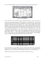
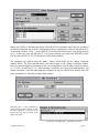
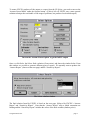
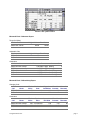
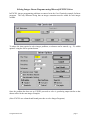
Solving Linear Programs using Microsoft EXCEL Solver
By Andrew J. Mason, University of Auckland
To illustrate how we can use Microsoft EXCEL to solve linear programming problems, consider the
following production planning problem.
Production Planning at Case Chemicals
Case Chemicals Company produces two solvents, CS-01 and CS-02, at its Cleveland plant. The plant operates 40 hours
per week and employs five full-time and two-part-time workers working 15 hours per week to run their seven blending
machines that mix certain chemicals to produce each solvent. This work force provides up to 230 hours of available
labor in the Blending Department. The products, once blended, are refined in the Purification Department, which
currently has seven purifiers and employs six full-time workers and one part-time worker who puts in 10 hours per week.
This work force provides up to 250 hours of available labor in the Purification Department. The hours required in the
Blending and Purification Departments to produce one thousand gallons of each of the solvents are listed in the table
below:
Blending
Purification
CS-01
2
1
CS-02
1
2
Blending and Purification Requirements (hr/1000 gallons)
Case Chemicals has a nearly unlimited supply of raw materials to produce the two solvents. It can sell any amount of
CS-01, but demand for the more-specialized product CS-02 is limited to at most 120 thousand gallons per week. The
accounting Department estimates a profit margin of $0.30 per gallon of CS-01 and $0.50 per gallon of CS-02. Because
all employees are salaried and thus paid the same amount regardless of how many hours they work, these salaries and the
costs of machines are considered fixed and are not included in the computation of the profit margin. As a ProductionPlanning Manager, you want to determine the optimal weekly manufacturing plan for Case Chemicals.
Let: x1 be the number of thousands of gallons of CS-01 to produce, and
x2 be the number of thousands of gallons of CS-02 to produce.
maximize
subject to
300x1 + 500x2
2x1 + x2
x1 + 2x2
x2
x 1, x 2 ≥ 0
Using EXCEL Solver
≤ 230,
≤ 250,
≤ 120,
(blending)
(purification)
(CS-02 limit)
(1)
(2)
(3)
page 1
The Case Chemicals problem is entered into an EXCEL spreadsheet in the following format.
The Case Chemicals spreadsheet
We use cells B2 and C2 to contain the values for the decision variables, x1 and x2 respectively. (If
you have not used spreadsheets before, cell B2 means the cell in column B, row 2.) The actual
formulae used in the cells are shown below. Note that there is a formula in cell D4 which calculates
the objective function (in this case, “=B4*B2+C4*C2”, where * means multiply in EXCEL), and
formulae in cells D6 to D8 which calculate the value of each constraint in terms of the decision
variables. Observe that the coefficients for the decision variables used in the constraints are located
in the cells identified by the formulae in cells D6 to D8 (A-matrix information). You can leave out
the $ symbol in these formulae; it is just a shortcut. However, using this shortcut, we can enter
=SUMPRODUCT($B$2:$C$2,B6:C6) into cell D6, and then copy and paste this formula into D7
and D8, and the appropriate changes will be made automatically by EXCEL. This can be useful in
larger problems. The ‘<=‘ , ‘Max’, ‘subject to’, and other labels are not necessary and are simply
for us... we will tell the Solver most of this information in subsequent windows. Assume that they
are only comments in the spreadsheet which help us keep track of the model.
A
1
2
3
4
5
6
7
8
B
C
CS-01 CS-02
0
0
D
E
VALUE
F
RHS
Max 300
500
=B4*B2+C4*C2
subject to
BLENDHRS 2
1
=B6*$B$2+C6*$C$2 ="<=" 230
PURIHRS 1
2
=B7*$B$2+C7*$C$2 ="<=" 250
CS02LIM 0
1
=B8*$B$2+C8*$C$2 ="<=" 120
The Case Chemicals spreadsheet - Formulae view
The $’s in the formulae are optional.
Once the problem is setup, the ‘Solver...’ option is chosen from the Tools menu. (Note that this
option may need to be installed as an Add-In using the Tools menu, if it was not installed in your
original set-up. See your user’s manual for instructions on how to do this, or come and see me).
The Solver add-in comes up, and we have to tell it about our problem as follows.
Using EXCEL Solver
page 2
The Solver entry for the Case Chemicals problem
In this case, cell D4 is chosen as the target cell for EXCEL to maximize; this is the cell we entered
our objective function into. EXCEL will maximize this by adjusting the values in cells B2 and C2,
our decision variables. (The ‘:’ in the $B$2:$C$2 formula actually means the cells going from B2
to C2. In this case, just cells B2 and C2. For a larger problem you could enter $B$2:$F$2 to tell
EXCEL that cells B2, C2, D2, E2, and F2 are all decision variables.)
The constraints are entered using the ‘Add...’ button which brings up the Change Constraint
window below. The first constraint above (and shown again in the Change Constraint window
below) is our non-negativity constraint, in this case saying that the cells B2 and C2 must be positive
(i.e., CS-01 ≥ 0, and CS-02 ≥ 0). After entering a constraint, you can use the Add button to add
another constraint. Note that while both these windows are up you can still click directly onto cells
in the spreadsheet as a shortcut to typing in their names.
Entering the first constraint for the Case Chemicals problem
(Note that if the ≤, =, and ≥ constraints are
grouped together in the constraint set, then
all of the constraints of one type can be
input at the same time, as shown in the
figure to the right.)
A faster way of entering all 3 ≤ constraints at one time.
Using EXCEL Solver
page 3
To ensure EXCEL produces all the output we expect from the LP Solver, you need to turn on the
‘Assume Linear Model’ under the Options button. (If this is left off, EXCEL uses a more general
solution technique that can handle a wide range of problems, but produces less detailed output.)
Turn on the ‘Assume Linear Option’ to get the full LP output
Once we click Solve, the Solver finds a solution (if one exists), and shows the window below. From
this window we are able to generate different types of reports. We normally want to produce the
“Answer Report” (shown on the next page) and the “Sensitivity Report”.
The Solver solution window.
The final solution found by EXCEL is listed on the next page, followed by EXCEL’s “Answer
Report” and “Sensitivity Report”. Note that the “Answer Report” tells us which constraints are
binding and the “Sensitivity Report” includes the values of the dual variables (shadow prices).
Using EXCEL Solver
page 4
EXCEL’s final optimal solution
Microsoft Excel 5.0 Answer Report
Target Cell (Max)
Cell
Name
$D$4 Max VALUE
Original Value Final Value
66000
66000
Adjustable Cells
Cell
Name
$B$2 CS-01
$C$2 CS-02
Original Value Final Value
70
70
90
90
Constraints
Cell
$D$6
$D$7
$D$8
$B$2
$C$2
Name
BlendHrs VALUE
PuriHrs VALUE
CS02LIM VALUE
CS-01
CS-02
Cell Value
Formula
230 $D$6<=$F$6
250 $D$7<=$F$7
90 $D$8<=$F$8
70 $B$2>=0
90 $C$2>=0
Status
Slack
Binding
0
Binding
0
Not Binding
30
Not Binding
70
Not Binding
90
Microsoft Excel 5.0 Sensitivity Report
Changing Cells
Cell
Name
$B$2 CS-01
$C$2 CS-02
Final
Value
70
90
Reduced
Cost
Objective Allowable Allowable
Coefficient Increase Decrease
0
300
700
50
0
500
100
350
Constraints
Cell
Name
$D$6 BlendHrs VALUE
$D$7 PuriHrs VALUE
$D$8 CS02LIM VALUE
Using EXCEL Solver
Final
Shadow
Constraint Allowable Allowable
Value
Price
R.H. Side
Increase Decrease
230 33.33333333
230
270
90
250 233.3333333
250
45
135
90
0
120
1E+30
30
page 5
Solving Integer Linear Programs using Microsoft EXCEL Solver
In EXCEL, integer programming problems are entered as in the Case Chemicals example for linear
programs. The only difference being that an integer constraint must be added for each integer
variable.
To reduce the time required to solve integer problems, a tolerance can be entered, e.g., ‘5% within
optimal’ using the Solver options button.
Once the problem has been set up, EXCEL proceeds to solve it, producing output similar to that
shown earlier for the non-integer examples.
(Note: EXCEL uses a branch-and-bound procedure to solve Integer Programs.)
Using EXCEL Solver
page 6