Download ProteoLens 1.0

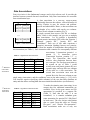
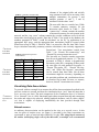
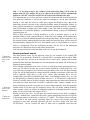
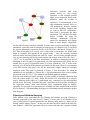
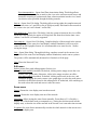
ProteoLens 1.0
User Manual
Last Date Modified: July 19, 2005
Contents
Introduction......................................................................................................................... 3
Concepts and use cases ....................................................................................................... 4
Software architecture ...................................................................................................... 4
Data Associations............................................................................................................ 5
Visualizing Data Associations ........................................................................................ 6
Network source ........................................................................................................... 6
Querying network source............................................................................................ 7
Adding annotations ..................................................................................................... 8
Complex visualizations............................................................................................... 8
Filtering and Attribute Querying ................................................................................ 9
Reference: Most Important Operations............................................................................. 10
Create Data Association................................................................................................ 10
View and Delete Data Associations.............................................................................. 11
Open Network View ..................................................................................................... 11
Attach Network Source to the View (this dialog will change soon)............................. 11
Create a Node Manually ............................................................................................... 13
Expand Node................................................................................................................. 13
Add Annotation............................................................................................................. 13
Reference: Menu Options ................................................................................................. 15
Main Window ............................................................................................................... 15
File Menu .................................................................................................................. 15
Window menu........................................................................................................... 15
Data Management menu ........................................................................................... 15
Network View............................................................................................................... 15
Network menu........................................................................................................... 15
Edit menu .................................................................................................................. 16
Zoom menu ............................................................................................................... 16
Layout menu ............................................................................................................. 17
Find menu ................................................................................................................. 17
Visualization menu ................................................................................................... 17
Filter menu ................................................................................................................ 18
Data Preview Window (flat files and database queries) ............................................... 18
File menu .................................................................................................................. 18
Query menu............................................................................................................... 19
Result menu .............................................................................................................. 19
Network View: Popup menus ....................................................................................... 19
Node popup menu ..................................................................................................... 19
Node selection popup menu...................................................................................... 21
Edge popup menu ..................................................................................................... 21
View popup menu ..................................................................................................... 22
Filesystems View popup menus.................................................................................... 22
Introduction
ProteoLens is a data mining-oriented tool for querying, visualization, and annotation of
biological networks. Its main features and capabilities include:
• Flat files in tabular column-delimited format can be attached as data sources.
• Connections to Oracle databases can be opened and results of arbitrary SQL
‘select’ queries can be attached as data sources
• Raw data can be previewed and input data can be narrowed to a relevant subset
of columns from the original table
• Multiple Network View panes can be opened; each View is a full-fledged graph
editor allowing to add/remove/move network nodes and edges and to change
node and edge graphical attributes
• A data source representing a network can be attached to a view and visual
querying methods can be used to retrieve and expand subnetworks from such
network source; an arbitrary data source can be interpreted as a network, and
multiple data sources can be successively attached to and queried from the same
view, which allows creating complex networks from multiple data sources.
• An arbitrary number of arbitrary data sources can be attached as “annotations”
providing property values for nodes and edges
• Annotation descriptors associated with each annotation allow specifying
visualization schemas: values provided by an annotation can be displayed
categorically using graphical attributes such as colors, shapes, line types, etc and
continuously (for numerical-value properties, e.g. expression data) using color
gradients, line widths, and node sizes.
Concepts and use cases
In this section the data model utilized by the ProteoLens application is described.
Multiple examples of using various types of data in different contexts are also provided.
The intent of this section is to concentrate on conceptual issues. Thus we do not describe
user interfaces here and do not explain, e.g. how to create a data association, step by step.
This information is provided in the Reference. Every time such an operation is implicitly
or explicitly mentioned in this section, the appropriate section of this manual containing
detailed instructions for the use of ProteoLens controls and dialogs is referenced in the
left margin ().
Software architecture
The software consists of two functional layers: Data Association layer and Data
Visualization layer (Fig. 1). The only common language spoken by these two layers is
provided by Data Associations. The purpose of the Data Association layer is to wrap
external data (flat files, Oracle DB tables) in a uniform way and present them as Data
Associations. Data Association layer user interface allows user to specify which
particular subsets of data from which particular sources should be available to the
application.
Data Visualization layer accepts only Data Associations and allows both drawing them as
networks (graphs) or visualizing them as graphical attributes of the network nodes and
edges. Any available Data Association can be used in either of the two ways. The
application makes no domain-specific assumptions about the nature and meaning of the
provided data, which leaves the user with responsibility of using right data at the right
place, but also allows for very high flexibility.
Data
Association
layer
Database
Data
Visualization
layer
Data
Data
associations
Local filesystem
Figure 1. Software architecture overview
(draws Data
Associations)
Data Associations
Data Association is the fundamental concept used in this software tool. It provides the
interface between external data and visualization. Only Data Associations are accessible
from visualization layer.
A data association is a two-way, many-to-many
relationship between data objects, referred hereafter as
A
B
entities.
Entities, in turn, are context- and problementity A1 entity B1
specific and unbreakable. Hence, a data association can
entity A2 entity B2
be thought of as a table with exactly two columns.
Values in each column are entities (Fig. 2).
A single external data source (flat file or database
table), which is rich enough, can give rise to multiple
data associations. Let us consider a hypothetical
protein-protein
interaction (PPI) table that contains 3
entity An entity Bn
columns: “protein ID1”, “protein ID2”, and
“confidence”. Each row of this table represents a
Figure 2. Data association
(putative) interaction (binding) between two proteins,
and a confidence score (i.e. derived from the number of independent observations) for
this interaction (see Table 1). Such interaction table contains two conceptually different
associations: 1) interactions (protein 1 ↔
protein 2); 2) interaction scores
Table 1. A hypothetical interaction table
(“interaction between proteins 1,2” ↔
score). The ProteoLens data model
Protein ID 1 Protein ID2 confidence
enforces clear distinction between these
1
2
0.8
two concepts. The first data association to
1
3
0.7
be created on top of Table 1 would
2
4
0.2
trivially treat each protein (protein ID) as a
4
5
0.4
separate entity and map first two columns
1
5
0.6
of the table as a data association. The
second data association must treat the
protein Ids in the first two columns as one
single entity (interaction), and the confidence score as the other entity (i.e. [1,2]↔0.8).
User interface requires specifying which column(s) of the raw data table constitute an
entity and thus allows creating both data associations described above (see Reference).
…
Reference:
create Data
Association
Reference:
create Data
Association
Table 2. A hypothetical annotation table
Protein ID
1
2
3
3
4
5
gene
MyGene1
MyGene2
MyGene3
MyGene3
MyGene4
MyGene5
annotation
GO_1
GO_2
GO_1
GO_3
GO_2
GO_4
To make the situation more interesting, let us
assume that few additional annotations are
available. First, let the gene names and GO
annotations be provided in a separate file
(Table 2). Note that the table 2 is not
normalized, i.e. it contains redundant gene
name annotation for protein ID=3 (MyGene3
in both rows). The two obvious associations
that we create from this table are “Protein
ID↔gene” and “Protein ID↔annotation”.
Both associations make use of only two
Reference:
create Data
Association
Reference:
create Data
Association
columns of the original table and trivially
Table 3. A summary statistics table
wrap contents of each cell as an entity. Note
Protein ID connectivity Avg. score
multiple annotations for protein 3 and
1
3
0.7
multiple proteins (1 and 3; 2 and 4)
annotated with the same “term”.
2
2
0.5
The next table that we consider here (Table
3
1
0.7
3) contains summary statistics for the
4
2
0.3
interaction table shown in Table 1. The
5
2
0.5
“connectivity” column contains the number
of interaction partners for each protein in the
network, and the “avg. score” column contains the average confidence score for all the
interactions involving given protein. Note that if Table 1 was stored in the database, the
numbers presented in Table 3 could be calculated “on the fly” by application of an
appropriate SQL query, and the appropriate data associations could be created within
ProteoLens on top of Table 1. If data of Table 1 are stored in a flat file, then Table 3 must
be pre-calculated externally (summary statistics calculation is not currently supported in
ProteoLens). Two associations created from
Table 3 are “Protein ID↔connectivity” and
Table 4. Differential expression
“Protein ID↔average interaction score”.
measurements
The last table we consider contains expression
data for our hypothetical proteins 1–5. The data
Probe ID Protein ID Log-ratio
presented in Table 4 contain a (hypothetical)
AA111
1
0.8
microarray probe IDs, a mapping of these probe
BB222
2
0.6
ids onto gene ids and measured log-ratios. A
CC333
1
1.4
“Protein ID↔probe ID”, “Protein ID↔logDD444
3
-0.9
ratio”, and “Probe ID↔log-ratio” associations
EE555
4
0.1
can be created from these table. Not all these
FF666
1
1.3
associations might be necessary, depending on
the particular problem and visualization scheme
GG777
5
-0.05
a researcher has in mind. For now, we assume,
however, that all 3 associations are created.
Visualizing Data Associations
Reference:
open Network
View
To proceed with our example let us assume that all the data associations described in the
previous section are created, and thus the visualization layer “sees” them all (note that it
never sees any raw data). The main component of the visualization layer is a Network
View. Network View is a fully functional graph editor (manual drawing and rearranging
the nodes and edges in the network, editing graphical attributes, such as colors, shapes,
etc.) that is capable of displaying automatically the data provided through Data
Associations.
Network source
An arbitrary data association can be attached to the view as a network source. In this
case, the pairs of entities (rows, see Figure 1) provided by the Data Association are
represented as pairs of network nodes linked by an edge. The string literal contents of
the entities (underlying single cells of the data table, or multiple cells concatenated
with “:” if an entity wraps a few columns of the underlying data) will be taken as
unique node ID. The unique ID of every edge in the network will be automatically
defined as “id1:id2” where id1 and id2 are ids of the nodes linked by this edge.
It is important that a view does not have to show the whole attached network and that in
most practical situations it will not be asked to (although it can do this efficiently).
Instead, a view must be seen as a visual query engine that displays only a part of the
underlying network relevant to the particular problem under investigation. Indeed, in
many practical situations the visualization of the whole interaction network, for example,
(tens of thousands of edges) gives little insight, if any, and what is actually sought is a
visualization of a particular pathway, or interrelations among a group of differentially
expressed genes etc.
When a Data Association is being attached to a view as network source, it can be
attached silently or with a concurrent query. In the first case, nothing will be displayed in
the view as yet (but the underlying network can be queried later). In the second case, only
the entities from the underlying network that satisfy the specified query will be retrieved
and immediately displayed in the view. Note that the query is not persistent: it is used to
retrieve a subnetwork from the underlying network, but the rest of the underlying
network is not filtered out forever and can be queried later.
Only one network source can be attached to the view at any given moment.
Querying network source
Reference:
attach network
source to the
view
Reference:
create a node
manually
Reference:
expand node
The most natural choice for the network source in our example is the original PPI
network. Let us attach the “Protein ID 1↔Protein ID 2” association built on top of Table
1 to a Network View, and let us do it silently first (“Connect only” option). Note that the
protein Ids from the Data Association are now interpreted as the unique Ids of the (not yet
displayed) network nodes.
Since nothing is displayed in the view, we have to start the network querying process in
some way. In order to do that, one or more entities should be created in the view. One
way to do this is to import a list of entities (network nodes) from a text file. Each element
of the list will be interpreted as a unique node ID (multiple occurrences of the same ID
will be ignored). Note, that it is the user’s choice what particular ID to use for
visualizations (LocusID, SwissProtID, gene name, local database primary key, etc), but
the IDs should be consistent across all data sources (i.e. if PPI network is specified in
terms of LocusIDs, then to be able to directly map expression data onto such network the
user must have these data in the ‘LocusID↔ expression value’ format). Another way to
query underlying network is to create one or more nodes manually. Note that manually
created nodes do not have any ID assigned to them. They are nodes without identities.
After creating a node, an Id must be manually assigned to it through the node’s pop-up
menu. Let us create a node and assign to it Id=1.
Having a node in the view, we can query the network source for the node’s neighbors.
‘Expand->without filter’ option from the node’s popup menu brings into the view all the
3 interaction partners of the node 1 (which are 2, 3, and 5). The result is shown in Figure
3. Note that if the node (strictly speaking, node Id) is not in the network, then the
expansion or any other querying operation will have no effect. Nodes with Id=6 and
Id=”MyGene1” can be created, but none of them can be expanded (note that the
application does not know that MyGene1 is the name of
protein with id=1 – MyGene1 is not an id in the attached PPI
network!)
Adding annotations
Reference:
add annotation
As it was already mentioned, any Data Association can be
used as annotation source. Only the Ids of the nodes in the
network are used for attaching annotations, hence to make
Figure 3.
the annotation useful, the association must map the Ids used
in the network onto something else (for instance, the “Probe ID↔log-ratio” annotation is
of no use for us – yet, since probeIDs are not present in the network).
First, we will create friendlier names for our proteins. In order to do that, we will request
a new Node Annotation. For the annotation we will select ‘Protein ID↔gene’ association
and specify that this annotation will be used for the node labels. As soon as the
annotation is created, the network view is updated and protein names are shown as the
node labels. Arbitrary number of annotations can be created (as long as the visualization
is intelligible). We will create here two more node annotations:
“ProteinID↔connectivity” (and request it to be displayed as an auxiliary label), and
“ProteinID↔log-ratio” (and request it to be displayed
as fill color, continuous range). In addition we will
create edge annotation “(Protein ID1, Protein
ID2)↔score”. The resulting visualization is presented
in Figure 4. Few important things to note here are: 1)
the labels of the displayed nodes changed, not their ids;
the ids of the nodes are still 1, 2, 3, 5; 2) multiple
redundant annotations are ignored (MyGene3 is
specified as the name for Protein Id 3 two times in the
table 2; only distinct annotation values count and the
name is shown once); 3) it is important to specify “use
Figure 4.
all” option if multiple annotations are expected – in the
case of MyGene1 (id=1) there are 3 different log-ratios available (from different probes),
and with the “use all” option they are shown all as a pie-chart filling of the node. 4) The
annotations are permanently attached to the view until they are manually deleted; if new
nodes are brought into the view (imported from a list, created manually, or brought in via
a query). All the currently defined annotations will be applied to them automatically, and
the new nodes will be rendered according to these annotations. Finally, annotations are
independent from the network source: annotations can be defined in a view, which is not
yet attached to any network (in which case, of course, nodes can be only added manually
or imported from the list – there is no network to query!).
Complex visualizations
Only one network source at a time can be attached to a view. However, new source can
be attached to the existing view at any given time (previous source will be automatically
detached). All the nodes and edges imported from the old source will remain in the view,
which allows for creating complex visualizations. It is possible to combine in this way
few different sources of interaction data, or add transcriptional regulation or coexpression
(relevance network) data from
another source, etc. (the current
limitation is that multiple parallel
edges are not supported, hence in the
situations when the overlap is
expected it is recommended to use
edge annotations instead). Here we
will demonstrate, however, another
use of this capability. Suppose that
we want to add GO “annotations”
from Table 2, and maybe few other
annotations. We still have the node
shapes available for using for
automatic annotations (exercise:
Figure 5.
attach GO annotations and display
them as node shapes, categorical),
but the nodes become visually overloaded. In some cases it may be preferable to display
annotations, especially such as belonging to some group, as a graph as well. Let us keep
the current annotations (expression levels) as the fill colors, and attach “Protein Id <->
GO” Data Association as a network source rather than an annotation. Set default node
shape to rectangle, and expand all the protein nodes – since the currently attached
network source associates Protein Ids with GO “terms”, the new nodes brought into the
view by such querying will be GO terms (and the Ids of these nodes will be the “GO_1”,
“GO_2”, etc as provided by the Data Association). In addition to displaying the fact of
belonging to the GO group in a graph-based way, this representation also allows for yet
another way to query for particular terms: if we now expand the “GO_2” node in the
network, we will obtain all the proteins associated with this term. Then we can reconnect
to the PPI network and query it for all the interactions (edges) among the currently
displayed nodes. The result is presented in Figure 5. Note that nodes, for which an
annotation is not available (e.g. Protein ID ↔ log-ratio annotation value is not available
for the node with ID “GO_1”), are rendered with default graphical attributes.
With the associations previously specified, it is also possible to decouple expression data
from the protein nodes, by using “Probe ID↔Protein ID” association as a network
source, drawing probe nodes in a graph-based way, connected to the corresponding
protein nodes, and using “ProbeID↔log-ratio” association to color probes according to
the expression values, rather than proteins. Such visualization might be helpful,
especially if a few probe-level parameters are available and more detailed look at the this
level is required – still maintaining the higher level information about maping the probes
onto the genes.
Filtering and Attribute Querying
Other features to be mentioned here are filtering and attribute querying. Filtering is
currently supported by the node Id only. Namely, if some node is not desirable in the
view (a false positive, a protein unrelated to the pathway under study etc), then it can be
deleted with the option “forever”. In this case, the node Id will be stored in the filter list,
and “Expand -> with filter” operation will never return such node (the “expand->without
filter” operation overrides the filter and returns all the neighbors of the node in the
currently attached network source). The filter list is local for the current Network View
(i.e. it is not shared between the views). However, the filter list from a view can be saved
into a file, and then imported into another view, or loaded when a new session is started.
Attribute querying is supported through the “Load Network -> from Data Association”
option. Although this option is used to attach network source, it is safe to re-attach the
same Data Association as the network source again and again, so that this option can be
also used for querying. If a data association D with an annotation (i.e. Protein ID ↔ GO)
is defined in the current session, it can be used to query the network being attached.
Namely, instead of using the native query interface (which allows only specifying Ids of
the nodes to be imported), the user can open the “Condition” dialog that allows to select
attributes (i.e. GO terms) of interest, and only the entities from the network source that
are annotated through the association D with the selected attribute value(s) will be
imported into the view.
Reference: Most Important Operations
Create Data Association
1. In the filesystems pane (left) browse to the data source (file or database table) [to
enable database access, right-click on the tree root and mount the required
databases].
2. If the data source if a file, it must be in column-delimited format (any file can be
pre-viewed [right click -> view], but only delimited files can be imported and
converted to data associations).
• Right-click on the file, check the “Table data” option
3. Right click on the data source, select ‘View’
4. If the data source is a file, specify delimiter symbol in the pop-up dialog
5. The contents (first few lines) of the data source is displayed as a table.
• If the data source is a database table, then the SQL query is displayed in the
top pane. An arbitrary query can be entered here (it should be executed first,
[Query->Run] to retrieve correct metadata), and the result of this query can be
wrapped as Data Association, see steps below.
6. From this table pane menu select ‘Result-> create data association’
7. The dialog will pop up asking to specify which columns of the underlying table
will be wrapped by the association; the unique name for the new association must
be also specified here
8. If only two columns of the underlying table were selected, the association is
created – each column would represent a separate data entity
9. Otherwise, another dialog will pop-up asking to specify which columns should be
combined into the first, or “leftmost” entity in the Data Association (“Key
columns”); the remaining columns will be wrapped by the second, or “rightmost”
entity
10. Repeat steps 6-9 as necessary (i.e. if more data associations have to be created
from the same data source)
Data Associations are linked directly to the underlying data source. The table views from
which an association was created can be safely closed at any moment.
View and Delete Data Associations
In the main application menu, use ‘Data Management->View Data Associations’. This
opens a dialog that allows removing or renaming a data association. If the association
wraps a database query, the associated SQL is shown and can be edited (‘Update’ must
be pressed upon the edition is finished).
Open Network View
In the main application menu, select Window -> New Window -> Network View
Attach Network Source to the View (this dialog will change soon)
1. In the Network View window menu, select Network -> Load -> from Data
Association
2. In the dialog window that opens: select network source in the upper pane [ PPI
(Id1<->Id2) selected in the screenshot];
3. If “Connect only” is checked, the selected association will be attached as a
network source, but no querying will be performed at this time and nothing will
be imported into the view.
4. Generic query (Filter data):
• If there are few known protein Ids to query for or to exclude, type them
into the text input areas (comma separated) – 1 and 2 are typed in in the
screenshot
• If these are the ids of the entities to search for, leave the default ‘IN LIST’
values of the comboboxes
• If these are the ids of the entities to be excluded, set combobox(es) to
‘NOT IN LIST’
• Set the concatenation combobox to ‘OR’ or ‘END’
• By default, the two text areas are synchronized (checkbox), which means
that only one should be filled, the typed data is automatically mirrored into
the second text area.
•
•
•
Note that the query searches for the edges with the desired properties (not
for separate proteins present in the network). Thus the query specified in
the screenshot reads: “In the PPI (id1<->id2) network, find all the
interactions, where first interactor (protein id 1) is one of the (IN LIST)
1,2 OR second interactor is one of the (IN LIST) 1,2. If OR were changed
to AND, we would be looking only for interactions among the proteins 1,2
(including self-loops).
Note also that such query does not return all the edges among all the
returned proteins. Suppose that interactions (1,3), (2,4), (1,2) and (3,4) are
present in the network. The query specified by the dialog shown in the
screenshot will look up edges, so that it will return (1,3), (2,4), (1,2) (first
interactor is 1 or 2 or second interactor is 1 or 2). Hence, 4 nodes (1,2,3,4)
will be imported into the network, but the interaction (3,4) will not be
imported!! If this is not the desired behavior and all the interactions among
all the imported proteins must be shown, check the ‘Load interaction
envelope’ checkbox or perform ‘Update edges’ operation in the view after
the network is loaded.
If ‘Respect filter’ is checked, the nodes, which are in the current view
filter will not be loaded into the view.
5. Conditional query:
• A data association that maps Ids from the network being attached to some
property (i.e. GO group) must be available.
• Select such data association (ProteinID <-> Go annotation selected in the
screenshot); select which of the two “columns” of this data association
maps onto the network entity Ids (“Data association has node Ids in:”)
• The attribute values available for the entities in the network being attached
will be shown in the Data Values pane; select desired values (GO_4,
GO_2 selected)
•
Click OK; the Ids of the nodes that possess the specified attribute values
(GO4, GO_2) in the example above will be transferred to the text input
box of the generic query (see item 3); a generic query can be further
formed using these ids as described above.
Create a Node Manually
1. The Edit->Options->Allow node creation box must be checked.
2. Click in the network view, a new node will be created.
3. If this is a “decoration” node, it can be left as is (or tweaked into a figure caption,
for example)
4. If this node represents a “real” entity, an Id must be set: right click on the node,
select “Set Id” from the popup menu.
5. Note: once set, Id can not be changed (switching one protein id for the other is
considered to be a very bad practice). Delete “wrong” nodes, create new ones,
never attempt to change Id.
Expand Node
1. A view must be attached to a network source, otherwise the operation has no
effect
2. right click on the node, select the expansion option from the popup menu (see
Reference: Menu Options for the details).
Add Annotation
1. In the Network View menu, select Visualization->Nodes->Add annotation or
Visualization->Edges->Add annotation
2. A dialog appears (screenshot for Node annotation shown)
3. In the left top pane select association to be used for annotation
4. Using comboboxes in the bottom left, select type of visualization to be used (i.e.
whether the values provided by the data association should be used for text label,
color, shape, etc)
5. Note that multiple values can be associated with a single node in the network
• If multiple annotations are allowed (labels and pie-chart node filling),
make sure that “use all” option is selected
• If a visualization scheme can not support multiple annotations (i.e.shape),
the effect of “use all” is currently undefined; use “use first” instead
(though an arbitrary annotation value out of a few available will be
displayed), or “use Max”/”use Min” for numerical properties.
6. The annotations can be
• “as is” - such as labels, the annotation values are used as text strings
• categorical - particular graphic attribute, such as color or shape, should be
assigned to each annotation value of interest. Many values can be mapped
onto the same attribute value, for example many different GO groups can
be all required to be drawn as the same color or the same shape. All
annotation values do not have to be mapped onto visualization attributes,
empty attributes (default) are allowed.
•
Continuos – allows mapping numerical values, such as expression values
onto color, size, or width gradients. Note that if Continuous annotation
visualization is requested, then the “Data Values” pane shows only
<<MIN>> and <<MAX>> values, for which the corresponding colors,
sizes, or width should be specified; the intermediate values will be drawn
as gradients between these two values. Important: <<MAX>> and
<<MIN>> specify the boundary values of the graphics attribute (such as
color), between which the gradient will be drawn; they are, generally
speaking, not the data boundary values. With the continuous visualization
type, ‘Set Limits’ button becomes enabled, that allows to specify where in
the available data range the <<MIN>> and <<MAX>> colors (or other
attributes) map to. All the data values below and above the interval
specified in the ‘Set Limits’ will be collapsed onto <<MIN>> and
<<MAX>> graphics attribute values, respectively. This allows cutting out
outliers in the data that stretch gradients over unnecessarily broad intervals
and zooming into the regions of interesting changes in the data values.
Example: log-ratios changing from -10 to 10, but everything outside, for
instance, (-3,3) is “differentially expressed”, what we really want to see
are subtle relative expression levels of the genes within the (-3,3) interval.
Then we would set the limits to (-3,3), and everything outside will be
shown with fixed colors.
7. Press OK, the current view will be re-rendered
Reference: Menu Options
Main Window
File Menu
Run Garbage Collection.
Use this option if memory problems are suspected. Memory status
is displayed in the status bar in the lower portion of the main window. This command
directly requests Java Virtual Machine to perform garbage collection.
Save session… Opens the Save Session dialog. All the data associations currently defined
in the ProteoLens session will be stored to the XML file selected through the dialog.
Opens the Load Session dialog. Data associations previously saved in the
XML file selected through the dialog will be recreated and imported into the current
ProteoLens session. Data associations are identified by their names; if the name of data
association being read from a file already exists in current session, the error message will
be displayed, and this data association will not be read in. If a data association is defined
on top of the Oracle database SQL query and the required database connection is not yet
open in the ProteoLens session, the Database Connection Dialog will open.
Load Session…
Exit
Exits the application.
Window menu
New window (menu) Opens new window in the application desktop.
Network view Opens new Network View. Newly opened view
is not attached to
any data source
Data Management menu
Opens the Data Association Viewer dialog that lists data
associations available in the current ProteoLens session, shows their properties and
allows renaming/deleting data associations.
View Data Associations
Network View
Network menu
Load
(menu) Allows loading data into the view.
From file… Opens Load File dialog. Through this dialog, previously stored network
(*.gml format) or list of object IDs (i.e. gene or protein IDs) can be loaded into the
current view. The current contents of the view will not be erased, new data will be
appended to the existing network.
Opens Load Data Association dialog. This dialog allows
selecting a data association to attach to the view as the current network source and
automatic extracting of a subnetwork from a data association into the view, based
on selection rules specified through the dialog controls.
From data association…
Save as… Opens Save File dialog. The dialog allows saving either the complete network
in the current view (as *.gml file) or list of all object (node) IDs found in the network in
the current view (as a one-column *.txt flat file).
Opens Save File dialog. Only the current selection in the view will be
saved into a file and only the option of saving node IDs from the selection (into a onecolumn *.txt flat file) is currently supported.
Save selection as…
Save image as… Opens Save File dialog. Complete display of the network in the current
view (regardless of the zoom level and display window boundaries) will be saved in
either JPG or PNG graphics format. It is recommended to set zoom level to 1 before
saving the image.
Print… Opens Print dialog. Through this dialog, complete network in the current view
(regardless of the zoom level and display window boundaries) can be sent to a printer.
The picture will be automatically downscaled, if needed, to fit the page.
Close
Closes the Network View.
Edit menu
Options (menu) Sets graph editing options for this view.
Allow node creation (checkbox) If checked, clicking
on the empty area in the view
creates a new graph node. Otherwise, clicks in the empty area have no effect.
Allow edge creation (checkbox) If checked, clicking on the node in the view, and
immediate dragging the cursor creates a new graph edge; to select the node mouse
should be clicked and released in this editing mode. If unchecked, click-and-drag on
the node selects this node and moves it after the cursor.
Zoom menu
Zoom in
Zooms the view display area into the network.
Zoom out
Zooms the view display area out of the network.
Zoom factor Allows setting the zoom factor manually. Zoom factor of 1 is fixed by a
display size of the default node (as compared to e.g. fitting the whole network into the
display area), so that the size of the network in the current view is not taken into account.
Fit network Set
zoom factor automatically to make the whole network in the current view
visible in the display area.
Layout menu
If checked, loading a subnetwork into the current view from data association
will automatically start layout calculations for the whole network in the view. Disable
this option if you have manually edited the layout and intend to add more nodes into your
network through Load Data Association dialog, otherwise your manual layout will be
lost.
Auto layout
(radiobuttons) Selected
layout type will be calculated every time layout is requested by user or internally by the
software (the layouter engines are provided through the 3rd party y-files™ library).
Organic layout, orthogonal layout, circular layout, hierarchic layout
Opens Configure Layouter dialog. Allows to fine-tune the parameters of the
currently active (selected) layouter.
Configure…
Run Enforces re-calculation of the layout in the current view using currently active
(selected) layouter.
Find menu
By node ID (menu) Finds and selects nodes with the specified IDs in the network in the
current view. IDs from the specified list that are not found in the network are silently
discarded, no special warning is given.
Specific IDs… Opens an input text dialog, where comma separated list of the IDs to
search for in the network should be typed in.
IDs from file… Opens Load File dialog. IDs to search for will be loaded from the
selected file (flat *.txt format); the list of IDs in the file must be either comma- or
newline-separated (i.e. a single long comma-separated string, or a single column
with one ID per row, respectively).
The list of IDs of the nodes currently selected in the view will be
internally stored (can be later used by Expand operations). The stored selections are not
shared between different views and are not stored between sessions.
Store current selection
Clear stored selection Removes
the previously stored list of node IDs (note: stored list is
removed, NOT the nodes from the network).
Visualization menu
Nodes
(menu) Node visualization and visual annotation options.
Default (menu) sets default node style. All the new nodes manually created or
automatically imported into the view first receive default display style.
Set… Opens Node Styles dialog. All newly added nodes will receive specified
default style; nodes already present in the network will not be affected.
Set/Update… Opens Node Styles dialog. All newly added nodes will receive
specified default style and default style of nodes already present in the
network will be updated.
Opens Create New Node Annotation Schema dialog. Through this
dialog, an arbitrary data association can be attached as the node annotation source and
annotation descriptor (specifying how to display graphically this particular annotation)
can be created.
Add annotation…
Shows the list of all annotations currently attached to the nodes in the
network and allows removing annotation/changing annotation descriptor parameters
(note: it is impossible to change the type of visualization through this option, for example
to switch from using shapes to using colors for a particular annotation, but, for instance,
used colors or shapes and their assignments to particular values can be changed for a
color or shape annotation descriptor, respectively).
Edit annotation…
(menu) See Nodes. Same functionality for edge default styles and annotations is
grouped under this menu. The only additional option is
Show direction (checkbox) If checked, all the edges are shown as directed (with
arrow on one side). Direction of an edge is determined by the order of the pair of
nodes in the network source. Note that no consistency checks are performed:
multiple edges are currently merged, and there is no distinction between directed
and undirected edges. Thus, if multiple pairs describe the same edge in a network
source, or multiple network sources contain the same edge, the edge direction will
be determined by the first encounter of a node pair describing this edge. Also, if
the option is turned on, then all the edges will be shown as directed. This option is
provided as a simple temporary way to draw directed (e.g. transcriptional
regulation network) alone; combination of directed and undirected networks in
one view will be supported in future version.
Edges
Filter menu
Filter list (menu) Loading/saving current filter list.
Load… Opens Load File dialog. List of filtered
node IDs will be loaded from the
selected plain text (*.txt) file; the IDs in the file can be either comma- or newline
separated. (See Node Popup Menu: Delete forever, Expand with filter).
Save… Saves the filter list from the current view into a newline-separated plain
text (*.txt) file.
Note: filter lists are not shared between different views and are not saved by default
between the sessions. They must be loaded/saved explicitly in each view.
Data Preview Window (flat files and database queries)
File menu
Load SQL… (Oracle data preview window only) Opens Load File dialog. Through this
dialog, SQL query previously saved as a standalone text file (default is *.sql) can be
imported into the query pane of the window (note: this allows loading queries created in
different applications, such as SQL Navigator).
(Oracle data preview window only) Opens Save File dialog. Allows saving the
query from the query pane into a standalone text file.
Save SQL…
Close
Closes Data Preview window.
Query menu
(Oracle data preview window only). Executes the query from the query pane of
the window in the database and schema the window is attached to. If query execution
failed, then the exception message will popup with short explanation of the problem (as
provided by the Oracle database JDBC driver, see Oracle documentation for error codes).
If the query executes successfully, first 10 rows of the result will be retrieved to populate
the data preview pane in the window.
Execute
Execute & Retrieve all (Oracle data preview window only). Use with caution. This is the
same as Execute, but all the query results will be retrieved to populate the data preview
pane. If the returned table is very large, it can result in unnecessary network connection
overload and can also make the application run out of memory.
Result menu
Create data association… Allows to create data association on top of the file (File data
preview window) or database query (Oracle data preview window). In Oracle data
preview window, make sure that the query was executed before the invocation of Create
data association: some metadata from the executed query result is used by the application
to build the data association. Upon selection of this option, selection dialog(s) will appear
asking to further define the data association (its name and the columns of the underlying
table to be wrapped by the association).
Network View: Popup menus
Popup menus in a Network View are activated by right clicks. Three types of popup
menus can be invoked by right-clicking on a node, edge, or in an empty area of the view:
node popup menu, edge popup menu, and view popup-menu, respectively. Special type
of node popup menu (node selection popup menu) is invoked when more than one node
are selected and right-click is performed anywhere in the view.
Node popup menu
Show info A message dialog will appear showing the node’s ID, the number of adjacent
edges (in the currently displayed network, not in the underlying network source), and the
values, for this node, of all the node annotations attached to the current view.
Delete node (menu) Deletes the node the popup was invoked on.
Once Deletes the node, no further action taken
Forever (filter out) Deletes the node and adds its ID to the filter list
associated with
this view. The node filtered out forever will not be allowed to reappear in the
view as the result of Expand operations performed on other nodes or when a
subnetwork is loaded into the view by Load → From data association operation.
Set attributes Opens Node Attributes dialog that allows editing appearance of the node: fill
color, shape, size, label text, label font, outline color, width, and line style can be
manually set from this dialog. Note: automatic annotations attached to the view through
Create Node Annotation Schema dialog override manually set graphical attributes.
Set node ID This option is enabled only if the node does not have an ID – for instance, it
was manually created. Once the node receives its ID, the option is disabled — it is not
allowed to change node ID. If enabled, this option invokes a text input dialog, where the
ID to be assigned to the node should be typed in.
Save skin Saves the “skin” (most of the graphical attributes) of the node. Skin can be
viewed as a “rubber stamp” that can be later applied to other nodes to make them look
just like this one. Note: saved skins are not shared between network views.
Apply skin Applies previously saved skin to this node. If disabled, then no skin was
previously saved. Note: saved skins are not shared between network views.
Switch layer
Experimental, no effect.
Label→ID enforces
replacement of the node ID with the value currently displayed as the
node label. Use of this option is not recommended as it can easily lead to breaking the
network integrity.
Expand (menu) Finds the neighbors of this node in the currently attached network source
and brings them into the currently displayed network. Note: network source must be
attached, otherwise this operation has no effect.
With filter The filter will be applied: out of all the neighbors of this node, only those
will be returned that were not previously filtered out (see Filter→Filter list→Load in
Network View menu section and Delete node → Forever (filter out) in this section)
Without filter All the neighbors of this node in the currently attached network source
will be retrieved
To All with filter/To stored selection with filter This option changes depending on
whether the view has a previously stored selection. If it does not, then the first
option is active and the “group” (see below) is defined as all the nodes of the
current network. If selection was stored (see Find→Store current selection in Network
View menu section), then this menu option automatically switches to its second
version and “group” is the stored selection. When this menu option is invoked, the
neighbors of this node, which are also neighbors of any node in the “group”, are
selected, and those that are not filtered out are imported into the view. This option is
thus finding all the paths of length 2 from a given node to the group not passing
through filtered nodes. (Note: all paths of lengths 1, or direct edges can be retrieved
by Update edges operation, see below).
To All with filter/To stored selection without filter The same as To All with filter/To stored
selection with filter but the filter is ignored – all the length 2 paths from the node to
the “group” will be retrieved and added to the network in the current view.
Node selection popup menu
This menu is invoked when more than one node is selected in the view, and right-click is
performed anywhere in the view. All the operations invoked through this menu apply to
all nodes in the selection.
Delete Deletes all the selected nodes from the view. Note that there is no “Delete forever”
operation here as it is considered to be important enough to deserve careful, one-node-at
a time execution.
Opens Node Attributes dialog, the graphical appearance attributes set
through this dialog will be applied to all nodes in the selection.
Set node attributes
Label→ID Executes Label→ID for each node in the selection (see Label→ID in Node popup
menu section).
(menu) Allows to retrieve and import into the current view nodes, which
neighbors of any node in the current selection. Network source must be attached to the
view, or this operation has no effect. Note that in typical networks full expansion of a
group of nodes often results in a very large and unmanageable number of neighbors, so
there are currently no simple Expand operations implemented for selections in
ProteoLens.
To All with filter/To stored selection with filter same as Expand→To All with filter/To stored
selection with filter in Node popup menu section, except it selects all the nodes,
which are simultaneously neighbors of any node in the selection and of any node in
the “group”, and which are not filtered out (all length 2 paths from selection to the
“group”, not passing through filtered out nodes).
To All with filter/To stored selection without filter The same as To All with filter/To stored
selection with filter but the filter is ignored (all length 2 paths from selection to the
“group”).
Expand selection
Edge popup menu
Show info A message dialog will appear showing the IDs of the nodes connected by this
edge (this ID pair is also the edge’s ID) and the values, for this edge, of all the edge
annotations attached to the current view.
Delete edge
Deletes the edge from the view.
Opens Edge Attributes dialog that allows editing appearance of the edge:
line color, width, and line style can be manually set from this dialog. Note: automatic
annotations attached to the view through Create Edge Annotation Schema dialog override
manually set graphical attributes.
Set attributes
Save skin Saves
skin .
the “skin” (graphical attributes) of the edge. See Node popup menu → Save
Apply skin Applies
previously saved skin to this edge. If disabled, then no skin was
previously saved.
View popup menu
Show info
Invokes a message dialog, which shows the number of nodes and edges in the
network.
Update edges Retrieves from currently attached network source and imports into the view
all the edges (relations) among the nodes currently present in the view. If there is no
attached network source, the operation has no effect.
Apply filter Removes from the current view all nodes found on the filter list (i.e. Expand
without filter was performed unadvertedly instead of Expand with filter, or a new filter was
just loaded from a file and the network in the current view has to be filtered against it).
Filesystems View popup menus
Expands the tree of child objects defined in a filesystem (subdirectories/files in a
filesystem filesystem, or schemas and tables in a database filesystem). Same as leftclicking on the tree handle on the left of the icon.
Expand
Collapse
Collapses the tree of child objects. Same as left-clicking on the tree handle.
Refresh Refreshes the tree below this filesystem object (reread the list of subdirectories
and files in a directory of a filesystem filesystem, or refresh the list of tables in a database
file system).
(only for the filesystem tree nodes that are not (sub)directories, but can contain data,
i.e. files in a filesystem filesystem and tables in a database filesystem) Opens Data
Preview window populated with the data from this filesystem object.
View
(checkbox, only for the filesystem filesystem tree nodes that represent files)
If checked, the data in the file are assumed to be in variable-width char-separated format,
and when View operation is requested, ProteoLens will attempt to read the data as table
(user will be asked to input the delimiter character). Otherwise, View will open a simple
textual view of the file (data associations can not be created from such views).
Tabular data
(available only for filesystem root nodes) Unmounts this filesystem root (e.g. a
database) and all the descendant filesystem tree nodes.
Unmount
Mount (available only for the ‘Filesystems’ root of the whole filesytems tree) Opens
Database Connection dialog and allows to mount an Oracle database as a “filesystem”
under the root.