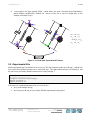
1
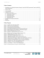
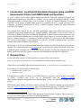
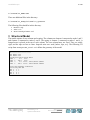
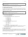
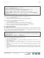
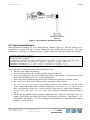
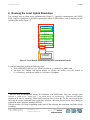
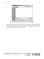
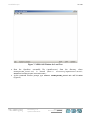
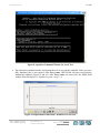
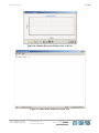
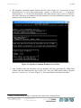
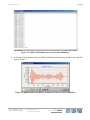
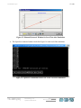
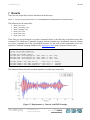
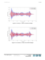
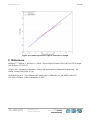
TR-2009-[ID]
OpenFresco Framework for Hybrid Simulation:
LabVIEW Experimental Control Example
Andreas Schellenberg, Hong K. Kim, Yoshikazu
Takahashi, Gregory L. Fenves, and Stephen A. Mahin
Department of Civil and Environmental Engineering,
University of California, Berkeley
Last Modified: 2009-08-03
Version: 2.6
Acknowledgment: This work was supported by the George E. Brown, Jr. Network for Earthquake Engineering Simulation (NEES)
Program of the National Science Foundation under Award Number CMS-0402490. Visit http://it.nees.org/ for more information.
LabVIEW Example
2 of 20
Table of Contents
1
2
3
4
5
6
7
8
Introduction: Local Hybrid Simulation Example Using LabVIEW Experimental Control with NEESSAM and OpenSees...............................................................................................................................3
Required Files........................................................................................................................................3
Structural Model ....................................................................................................................................4
Ground Motion ......................................................................................................................................5
OpenFresco Tcl Scripts..........................................................................................................................5
5.1 Experimental Control Point ............................................................................................................6
5.2 Experimental Control......................................................................................................................6
5.3 Experimental Setup.........................................................................................................................7
5.4 Experimental Element ....................................................................................................................8
5.5 Experimental Site............................................................................................................................9
Running the Local Hybrid Simulation.................................................................................................10
Results..................................................................................................................................................18
References............................................................................................................................................20
Table of Figures
Figure 1: OpenSees One-Bay Frame Model................................................................................................5
Figure 2: 1940 El Centro Ground Motion. ..................................................................................................5
Figure 3: OneActuator Experimental Setup. ...............................................................................................8
Figure 4: twoNodeLink Experimental Element...........................................................................................9
Figure 5: Local Hybrid Simulation using the Experimental Element. ......................................................10
Figure 6: NEES-SAM Open File Window for LabVIEW Example..........................................................11
Figure 7: NEES-SAM Window for Local Test. ........................................................................................12
Figure 8: OpenSees Command Window for Local Test............................................................................13
Figure 9: Displacement Time History Window for Local Test.................................................................13
Figure 10: Element Hysteresis Window for Local Test. ...........................................................................14
Figure 11: NEES-SAM Window for Local Test. ......................................................................................14
Figure 12: OpenSees Command Window for Local Test..........................................................................15
Figure 13: NEES-SAM Window for Local Test after Simulation. ...........................................................16
Figure 14: Displacement Time History Window for Local Test after Simulation. ...................................16
Figure 15: Element Hysteresis Window for Local Test after Simulation. ................................................17
Figure 16: OpenSees Command Window for Local Test after Simulation...............................................17
Figure 17: Displacement vs. Time for LabVIEW Example. .....................................................................18
Figure 18: Velocity vs. Time for LabVIEW Example. .............................................................................19
Figure 19: Acceleration vs. Time for LabVIEW Example........................................................................19
Figure 20: Element Hysteresis Loops for LabVIEW Example. ................................................................20
TR-2009-[ID]
Schellenberg et al.
Updated: 2009-08-03
Web it.nees.org
Email [email protected]
LabVIEW Example
3 of 20
1 Introduction: Local Hybrid Simulation Example Using LabVIEW
Experimental Control with NEES-SAM and OpenSees
As a part of phase I of the NEES hybrid simulation project, the LabVIEW experimental control was
implemented in OpenFresco. LabVIEW is a software used to control the MiniMost and MTS LBCB
(Load and Boundary Condition Box) at the University of Illinois at Urbana-Champaign. It uses the
LabVIEW NTCP plugin communication protocol to communicate over a single persistent TCP
connection. TR-2004-58 (Hubbard et al 2004), a NEESit document contains the details about the
LabVIEW NTCP plugin.
This example shows how to use the LabVIEW experimental control with NEES-SAM (Network for
Earthquake Engineering Simulation-Static Analysis Module). NEES-SAM is part of the UI-SimCor
(University of Illinois-Simulation Coordinator) distribution. It should be noticed that OpenFresco also
works with UI-SimCor and that there is a simple SDOF (Single Degree of Freedom) example in the UISimCor example directory (C:\SIMCOR\03_Examples\SDOF\05_OpenFresco) that demonstrates
this1. However, this example is not explained here, since the UI-SimCor Manual (Kwon et al 2006)
contains instructions for running such example.
NEES-SAM is used to run a fully simulated test in this example, meaning that no physical specimen is
required. The computational driver is OpenSees (http://opensees.berkeley.edu). While both a local and a
distributed hybrid simulation can be performed with the provided Tcl files, this document only shows
how to run the local test. The response results from the simulation are provided for comparison.
2 Required Files
For the LabVIEW example, the following files are required. These are located in:
User’s Directory\OpenFresco\trunk\EXAMPLES\OneBayFrame\TestLabVIEW
if OpenFresco was installed in the default location, the User’s Directory is C:\Program Files.
The following Tcl files should be in this directory:
OneBayFrame_Local.tcl
elcentro.txt
The OpenSees executable, Tcl/Tk 8.5.x, and NEES-SAM are required to run this example. If not done
so already, OpenSees and Tcl/Tk can be downloaded from the OpenSees website
(http://opensees.berkeley.edu/OpenSees/user/download.php). Follow the directions carefully on this
website.
NEES-SAM comes with the UI-SimCor software package. The UI-SimCor installer can be downloaded
from the NEES Forge UI-SimCor site (http://simcor.neesforge.nees.org). UI-SimCor needs to be
installed in the default location for NEES-SAM to work properly. NEES-SAM can be found in:
1
In order to run UI-SimCor, the MATLAB® Instrument Control toolbox is required. This toolbox does
not come with MATLAB®, but needs to be purchased separately.
TR-2009-[ID]
Schellenberg et al.
Updated: 2009-08-03
Web it.nees.org
Email [email protected]
LabVIEW Example
4 of 20
C:\SIMCOR\02_NEES-SAM
There are additional files in the directory:
C:\SIMCOR\03_Examples\SDOF\03_OpenSees
The following files should be in this directory:
Module.cfg
sdof.tcl
StaticAnalysisEnv.tcl
3 Structural Model
The model consists of two columns and a spring. The columns are element 1 connected to nodes 1 and 3
and element 2 connected to nodes 2 and 4. The spring is element 3 connected to nodes 3 and 4. A
lumped mass is placed at the top of each column. The two column bases are fixed. They are axially
rigid, and the tops are free to rotate. Imperial units were used [inches, kips, sec]. The following Tcl
script from OneBayFrame_Local.tcl defines the geometry of the model:
# Define geometry for model
# ------------------------set mass3 0.04
set mass4 0.02
# node $tag $xCrd $yCrd $mass
node 1
0.0
0.00
node 2
100.0
0.00
node 3
0.0 54.00 -mass $mass3 $mass3
node 4
100.0 54.00 -mass $mass4 $mass4
# set the boundary conditions
# fix $tag $DX $DY
fix 1
1 1
fix 2
1 1
fix 3
0 1
fix 4
0 1
TR-2009-[ID]
Schellenberg et al.
Updated: 2009-08-03
Web it.nees.org
Email [email protected]
LabVIEW Example
5 of 20
Figure 1: OpenSees One-Bay Frame Model.
4 Ground Motion
The structure is subjected horizontally to the north-south component of the ground motion recorded at a
site in El Centro, California during the Imperial Valley earthquake of May 18, 1940 (Chopra 2006). The
file, elcentro.txt, contains the acceleration data recorded at every 0.02 seconds (Figure 2).
Figure 2: 1940 El Centro Ground Motion.
5 OpenFresco Tcl Scripts
This section explains the OpenFresco Tcl commands including the LabVIEW experimental control
command in the Tcl script, OneBayFrame_Local.tcl. Each subsection highlights a Tcl command and
the part of the script that contains the command. All script excerpts are from
OneBayFrame_Local.tcl.
TR-2009-[ID]
Schellenberg et al.
Updated: 2009-08-03
Web it.nees.org
Email [email protected]
LabVIEW Example
6 of 20
# Load OpenFresco package
# ----------------------# (make sure all dlls are in the same folder as openSees.exe)
loadPackage OpenFresco
The loadPackage OpenFresco is necessary for the examples to execute properly.
5.1 Experimental Control Point
The LabVIEW experimental control command uses the previously defined experimental control points.
Experimental control points can be used to set limits on nodes. This becomes useful when the
experimental control apparatus has no limit setting capabilities. Experimental control points are defined
using the expControlPoint command.
# Define control points
# --------------------# expControlPoint tag nodeTag dir resp <-fact f> <-lim l u> ...
expControlPoint 1 3 ux disp -fact 0.003 -lim -0.01 0.01
expControlPoint 2 3 ux disp -fact [expr 1.0/0.003] ux force -fact [expr 7.0/18.0]
The expControlPoint command parameters are:
$tag is the unique control point tag.
$nodeTag is the unique node tag.
dir is the direction of the response quantity. The input parameters are:
o ux = along the X-axis
o uy = along the Y-axis
o uz = along the Z-axis
o rx = around the X-axis
o ry = around the Y-axis
o rz = around the Z-axis
resp is the response quantity. The input parameters are:
o disp = displacement
o vel = velocity
o accel = acceleration
o force = force
o time = time
$f is the factor applied to the response quantity. It is optional.
$l is the lower limit. It is optional. Whenever the lower or the upper limit is exceeded, the
program will prompt the user to stop the experiment or to use the limit as the trial value.
$u is the upper limit. It is optional.
5.2 Experimental Control
Two different experimental controls are used in this example. The left column is simulated using the
LabVIEW experimental control. The LabVIEW experimental control uses control point 1 as the trial
control point and control point 2 as the output control point. The right column is simulated using the
SimUniaxialMaterials experimental control.
TR-2009-[ID]
Schellenberg et al.
Updated: 2009-08-03
Web it.nees.org
Email [email protected]
LabVIEW Example
7 of 20
# Define experimental control
# --------------------------# expControl SimUniaxialMaterials $tag $matTags
expControl SimUniaxialMaterials 1 1
#expControl xPCtarget 1 1 "192.168.2.20" 22222 HybridControllerD3D3_1Act
"D:/PredictorCorrector/RTActualTestModels/cmAPI-xPCTarget-STS"
# expControl LabVIEW tag ipAddr <ipPort> -trialCP cpTags -outCP cpTags
expControl LabVIEW 2 "127.0.0.1" 11997 -trialCP 1 -outCP 2; # use with NEES-SAM
#expControl LabVIEW 2 "130.126.242.175" 44000 -trialCP 1 -outCP 2; # use with MiniMost at UIUC
#expControl SimUniaxialMaterials 2 2; # use for simulation
The expControl command parameters for SimUniaxialMaterials are:
$tag is the unique control tag.
$matTags are the tags of previously defined uniaxial material objects.
The expControl command parameters for LabVIEW are:
$tag is the unique control tag.
ipAddr is the IP address of the computer running the LabVIEW plugin.
$ipPort is the IP port number of the computer running the LabVIEW plugin.
$cpTags are the tags of the previously defined control points.
5.3 Experimental Setup
The OneActuator setup is used for both experimental setups (Figure 3). The left column uses the setup
tag of 1, and the setup uses the experimental control with tag 1. The right column uses the setup with tag
2, and the setup uses the experimental control with tag 2.
# Define experimental setup
# ------------------------# expSetup OneActuator $tag <-control $ctrlTag> $dir -sizeTrialOut $sizeTrial $sizeOut
<-trialDispFact $f> ...
expSetup OneActuator 1 -control 1 1 -sizeTrialOut 1 1
expSetup OneActuator 2 -control 2 1 -sizeTrialOut 1 1
The expSetup command parameters for OneActuator are:
$tag is the unique setup tag.
$ctrlTag is the tag of a previously defined control object. In this case, it is
SimUniaxialMaterials.
$dir is the direction of the imposed displacement in the element basic reference coordinate
system.
$sizeTrial and $sizeOut are the sizes of the element trial and output data vectors,
respectively.
$f are trial displacement factor, output displacement factor, and output force factor, respectively.
These optional fields are used to factor the imposed and the measured data. The default values
are 1.0.
TR-2009-[ID]
Schellenberg et al.
Updated: 2009-08-03
Web it.nees.org
Email [email protected]
LabVIEW Example
8 of 20
Figure 3: OneActuator Experimental Setup.
5.4 Experimental Element
Both experimental elements are set to twoNodeLink elements (Figure 4). The left column uses a
twoNodeLink element with tag 1, and the element uses the experimental site with tag 1. The right
column uses a twoNodeLink element with tag 2, and the element uses the experimental site with tag 2.
# Define experimental elements
# ---------------------------# left and right columns
# expElement twoNodeLink $eleTag $iNode $jNode -dir $dirs
<-orient <$x1 $x2 $x3> $y1 $y2 $y3> <-pDelta (4 $Mratio)>
expElement twoNodeLink 1 1 3 -dir 2 -site 1 -initStif 2.8
expElement twoNodeLink 2 2 4 -dir 2 -site 2 -initStif 5.6
-site $siteTag -initStif $Kij
<-iMod> <-mass $m>
-orient -1 0 0
-orient -1 0 0
The expElement command parameters for twoNodeLink are:
$eleTag is the unique element tag.
$iNode and $jNode are the end nodes that the element connects to.
$siteTag is the tag of a previously defined site object. In this example, it is the LocalSite for
the local test and the RemoteSite for the distributed test.
$dirs are the force-deformation directions in the element local reference coordinate system.
$Kij are the (row wise) initial stiffness matrix components of the element.
$x1 $x2 $x3 $y1 $y2 $y3 set the orientation vectors for the element. x1, x2, and x3 are
vector components in the global coordinates defining the local x-axis. y1, y2, and y3 are the
same except that they define the y vector which lies in the local x-y plane for the element. <orient <$x1 $x2 $x3> $y1 $y2 $y3> field is optional with default being the global X
and Y.
$Mratio are the optional P-Delta moment contribution ratios. The size of the ratio vector is 4
(entries: [My-$iNode, My-$jNode, Mz-$iNode, Mz-$jNode]) My-$iNode + My-$jNode <= 1.0,
Mz-$iNode + Mz-$jNode <= 1.0. The remaining P-Delta moments are resisted by shear couples.
(default = [0.0 0.0 0.0 0.0])
TR-2009-[ID]
Schellenberg et al.
Updated: 2009-08-03
Web it.nees.org
Email [email protected]
LabVIEW Example
9 of 20
-iMod and $m are also optional fields. -iMod allows for error correction using Nakashima’s
initial stiffness modification. Default for -iMod is false. $m is used to assign mass to the
element. Its default is zero.
ub,1 = u4 u1
ub,2 = u5 u2
0.5L ( u3 + u6 )
ub, 3 = u6 u3
Figure 4: twoNodeLink Experimental Element.
5.5 Experimental Site
Both experimental sites are defined as LocalSite. The left column uses the site with tag 1, and the site
uses a previously defined OneActuator setup with tag 1. The right column uses the site with tag 2, and
the site uses a previously defined OneActuator setup with tag 2.
# Define experimental site
# -----------------------# expSite LocalSite $tag $setupTag
expSite LocalSite 1 1
expSite LocalSite 2 2
The expSite command parameters for LocalSite are:
$tag is the unique site tag.
$setupTag is the tag of a previously defined experimental setup object.
TR-2009-[ID]
Schellenberg et al.
Updated: 2009-08-03
Web it.nees.org
Email [email protected]
LabVIEW Example
10 of 20
6 Running the Local Hybrid Simulation
This example uses no client-server communication (Figure 5). OpenSees communicates with NEESSAM using the OpenFresco LabVIEW experimental control. NEES-SAM is used to simulate the left
column of the model (Figure 1)2.
Figure 5: Local Hybrid Simulation using the Experimental Element.
To run this simulation perform the following steps:
Start NEESSAM_LabView1.exe, which is located in C:\SIMCOR\02_NEES-SAM.
An Open File window will appear (Figure 6). Choose the Module.cfg file located in
C:\SIMCOR\03_Examples\SDOF\03_OpenSees. Hit Open.
2
An error may be encountered during the simulation with NEES-SAM. The error message reads
couldn't read file "step.tcl": no such file or directory. This error will end the
simulation. It may be caused by NEES-SAM not being able to write the Tcl file fast enough before
receiving the execute command from OpenFresco. However, this error does not occur when running an
experiment with a computer running LabVIEW.
The test executes 1599 steps. Depending on the speed of the computer, the simulation could take as long
as an hour.
TR-2009-[ID]
Schellenberg et al.
Updated: 2009-08-03
Web it.nees.org
Email [email protected]
LabVIEW Example
11 of 20
Figure 6: NEES-SAM Open File Window for LabVIEW Example.
After choosing the file the NEES-SAM window looks like Figure 7. The bottom left of the
window should read Ready Standby for connection. The bottom right of the window
should read SDOF (name of the Tcl file being used), 11997 (IP port number), and OpenSees
(program used to simulate the experimental element).
TR-2009-[ID]
Schellenberg et al.
Updated: 2009-08-03
Web it.nees.org
Email [email protected]
LabVIEW Example
12 of 20
Figure 7: NEES-SAM Window for Local Test.
Start
the
OpenSees
executable file
OneBayFrame_Local.tcl is located
(openSees.exe) from the directory where
(User’s
Directory\OpenFresco\trunk\
EXAMPLES\OneBayFrame\TestLabVIEW).
At the command window prompt, type source OneBayFrame_Local.tcl and hit enter
(Figure 8).
TR-2009-[ID]
Schellenberg et al.
Updated: 2009-08-03
Web it.nees.org
Email [email protected]
LabVIEW Example
13 of 20
Figure 8: OpenSees Command Window for Local Test.
The OpenSees command window will prompt the user to zero out the controller. Since our test is
fully simulated, this is not required. After hitting enter, NEES-SAM will open two Real-time
Monitoring windows (Figures 9 and 10). After hitting enter one more time, the NEES-SAM
window looks like Figure 11. It prints Current Step 1 &.
Figure 9: Displacement Time History Window for Local Test.
TR-2009-[ID]
Schellenberg et al.
Updated: 2009-08-03
Web it.nees.org
Email [email protected]
LabVIEW Example
14 of 20
Figure 10: Element Hysteresis Window for Local Test.
Figure 11: NEES-SAM Window for Local Test.
TR-2009-[ID]
Schellenberg et al.
Updated: 2009-08-03
Web it.nees.org
Email [email protected]
LabVIEW Example
15 of 20
The OpenSees command window displays the Daq values (Figure 12). dspDaq and frcDaq
should both be 0. It gives three input options, ‘Enter’ to start the test, ‘r’ to repeat the
measurement, or ‘c’ to cancel the initialization. If the Daq values are not 0, press r to reacquire
the values. Otherwise, press enter to start the simulation3. Once the simulation commences, step
numbers will scroll down the screen.
Figure 12: OpenSees Command Window for Local Test.
3
After OpenSees starts the simulation, the step numbers will also scroll down the NEES-SAM
window until the simulation time step reaches 1599. Then the NEES-SAM window will print
Network connection closed (Figure 13). This shows that the simulation has ended.
During a real experiment, be sure to check the Daq values before starting the test.
TR-2009-[ID]
Schellenberg et al.
Updated: 2009-08-03
Web it.nees.org
Email [email protected]
LabVIEW Example
16 of 20
Figure 13: NEES-SAM Window for Local Test after Simulation.
At the end of the simulation, the two NEES-SAM Real-time Monitoring windows now look like
Figures 14 and 15.
Figure 14: Displacement Time History Window for Local Test after Simulation.
TR-2009-[ID]
Schellenberg et al.
Updated: 2009-08-03
Web it.nees.org
Email [email protected]
LabVIEW Example
17 of 20
Figure 15: Element Hysteresis Window for Local Test after Simulation.
The OpenSees command window looks like Figure 16 at the end of the simulation.
Figure 16: OpenSees Command Window for Local Test after Simulation.
TR-2009-[ID]
Schellenberg et al.
Updated: 2009-08-03
Web it.nees.org
Email [email protected]
LabVIEW Example
18 of 20
7 Results
There are now output files from the simulation in the directory:
User’s Directory\OpenFresco\trunk\EXAMPLES\OneBayFrame\TestLabVIEW
The following are the output files:
Elmt_Frc.out
Elmt_ctrlDsp.out
Elmt_daqDsp.out
Node_Acc.out
Node_Dsp.out
Node_Vel.out
These files are created using the recorder command. Below is the following script that executes this
command. The OpenFresco Command Language Manual contains more information about the element
recorder commands for all the experimental elements. For the node recorder commands refer to the
OpenSees Command Language Manual on the OpenSees website (http://opensees.berkeley.edu).
# -----------------------------# Start of recorder generation
# -----------------------------# create the recorder objects
recorder Node -file Node_Dsp.out -time -node 3 4 -dof 1 disp
recorder Node -file Node_Vel.out -time -node 3 4 -dof 1 vel
recorder Node -file Node_Acc.out -time -node 3 4 -dof 1 accel
recorder Element -file Elmt_Frc.out
-time -ele 1 2 3 forces
recorder Element -file Elmt_ctrlDsp.out -time -ele 1 2
ctrlDisp
recorder Element -file Elmt_daqDsp.out -time -ele 1 2
daqDisp
The following figures show the response quantities recorded in the output files:
Figure 17: Displacement vs. Time for LabVIEW Example.
TR-2009-[ID]
Schellenberg et al.
Updated: 2009-08-03
Web it.nees.org
Email [email protected]
LabVIEW Example
19 of 20
Figure 18: Velocity vs. Time for LabVIEW Example.
Figure 19: Acceleration vs. Time for LabVIEW Example.
TR-2009-[ID]
Schellenberg et al.
Updated: 2009-08-03
Web it.nees.org
Email [email protected]
LabVIEW Example
20 of 20
Figure 20: Element Hysteresis Loops for LabVIEW Example.
8 References
Hubbard, P., Calderon, J., and Gose, S. (2004). “Protocal Specificiation of The LabView NTCP plugin”,
NEESit Report TR-2004-58
Chopra, A.K., “Dynamics of Structures, Theory and Applications to Earthquake Engineering”, 3rd
edition, Prentice Hall, 2006, 912 pp.
Oh-Sung Kwon et al., “User Manual and Examples for UI-SIMCOR v2.6 and NEES-SAM v2.0”,
University of Illinois, Urbana-Champaign, Il, 2007.
TR-2009-[ID]
Schellenberg et al.
Updated: 2009-08-03
Web it.nees.org
Email [email protected]