Download UI-SimCor Manual - No website was found at this address

User Manual and Examples for
UI-SIMCOR v2.6
Multi-Site Substructure Pseudo-Dynamic
Simulation Coordinator
NEES-SAM v2.0
Static Analysis Module for NEESgrid
by
Oh-Sung Kwon
Narutoshi Nakata
Kyu-Sik Park
Amr Elnashai
Bill Spencer
DEPARTMENT OF CIVIL AND ENVIRONMENTAL ENGINEERING
UNIVERSITY OF ILLINOIS AT URBANA-CHAMPAIGN
URBANA, ILLINOIS
FEBRUARY 2007
TABLE OF CONTENTS
1. Introduction .....................................................................................................1
2. Simulation Framework ...................................................................................1
3. Pseudo-Dynamic Test Procedure..................................................................3
4. Sub-structuring of a Structure.......................................................................5
4.1 Concept of Static Condensation and Sub-structuring ...........................5
4.2 Effective DOFs for Dynamic Analysis .....................................................6
4.3 MOST Experiment .....................................................................................7
5. Static Analysis Module Interface ...................................................................8
6. Protocol Specification ..................................................................................10
6.1 NEESgrid Teleoperation Control Protocol (NTCP) ...............................10
6.2 TCP/IP Protocol .......................................................................................11
6.3 LabVIEW1 and LabVIEW2 Protocols for NTCP Server .........................13
6.4 OpenFresco1D Protocol .........................................................................16
6.5 NEES Hybrid Communication Protocol (NHCP) ...................................17
7. Installation of UI-SIMCOR ............................................................................27
7.1 System Requirements.............................................................................27
7.2 Installation of UI-SIMCOR and Interface Application ...........................27
7.3 Installation of Structural Analysis Software .........................................30
7.4 Downloading and Updating UI-SIMCOR Source Code .........................32
8. Numerical Examples.....................................................................................35
8.1 Cantilever Column...................................................................................35
8.2 Inelastic Cantilever Column with Initial Loading – Steel Material .......61
8.3 Inelastic Cantilever Column – Concrete Material .................................71
8.4 MOST Example ........................................................................................73
8.5 SAC Three-Story Steel Structure ...........................................................84
8.6 LBCB Example.........................................................................................94
8.7 Buckling Example using ABAQUS ......................................................103
8.8 7-DOF Model using Five Protocols ......................................................108
9. Specific Experimental Issues.....................................................................117
9.1 One-site Experiment with μNEES at UCB............................................117
9.2 Two-site Experiment between UIUC and UCB ....................................132
9.3 Two-site Experiment between UIUC and SDSC ..................................138
9.4 Three-site Experiment among UIUC, UCB, and SDSC .......................139
9.5 Two-site Experiment between UIUC and SDSC using NHCP ............158
10. References.................................................................................................161
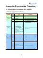
Appendix: Experimental Procedure ..............................................................162
A. Two-site Hybrid Test between UIUC and UCB .....................................162
B. Three-site Hybrid Test among UIUC, UCB and SDSC .........................178
ii
UI-SIMCOR Update History
June 2004
•
Version 1.0 release
•
•
•
•
•
•
Version 1.3 release
Renamed SIMCOR to UI-SIMCOR
Renamed FedeasMDL to NEES-FL for consistency
Inclusion of NEES-MW
Development of GUI for UI-SIMCOR
Include the latest version of OpenSees (version 1.6.2) and FEDEAS
Lab (version 2.6)
Include example input files for OpenSees and ZEUS-NL for MOST
example
Development of an adapter module, NEES-MW, by Sung Jig Kim for
experimental equipments (LBCB) in UIUC
June 2005
•
•
October 2006
•
•
•
•
•
•
•
•
•
•
•
•
•
•
November 2006
•
•
Version 2.0 release
Reconstruct the architecture of UI-SIMCOR using object-oriented
approach
Modulize the main body of analysis algorithm (α-OS scheme)
Provide improved GUI to monitor the remote site
Development of NEES-ABAQUS for ABAQUS static analysis
module by Gun Jin Yun
Include example input files for ABAQUS for buckling example
Remove NEES-MW
Update UI-SIMCOR for experimental equipment (LBCB) in UIUC by
Kyu-Sik Park
Include LBCB example
Include API for μNEES facility in UCB
Include one-site experiment using μNEES facility in UCB
Include two-site experiment between UIUC and UCB using μNEES
and MiniMOST 1 facilities
Include two-site experiment between UIUC and SDSC using
MiniMOST 1 facilities
Include three-site experiment among UIUC, UCB, and SDSC using
μNEES and MiniMOST 1 facilities
Version 2.5 release
Logo change
iii
February 2007
•
•
•
•
•
Version 2.6 release
Include OpenFresco1D and NHCP communication protocols
Include SDOF example using OpenFresco1D and NHCP
communication protocols
Include 7-DOF example using TCP/IP, LabVIEW1, LabVIEW2,
OpenFresco1D, and NHCP communication protocols
Include two-site experiment between UIUC and SDSC using
MiniMOST 1 facilities through NHCP
iv
NEES-SAM Update History
June 2004
•
Version 1.0 release
•
•
Version 1.5 release
Interact with the latest version of OpenSees (version 1.6.2), which
include soil material model and can make reaction force output. Hence
it isn’t necessary anymore to add additional nodes with stiff springs on
the control points to measure reaction forces.
Minor interface updates.
June 2005
•
October 2006
•
•
•
Version 2.0 release
Develop three NEES-SAM for TCP/IP, LabVIEW1, and LabVIEW2
protocols
Minor interface updates.
v
1. Introduction
MOST, Multi-Site Online Simulation Test, experimental example has been extensively
used to verify the NEESgrid infrastructure. The simulation coordinator for the MOST
experiment (http://it.nees.org/software/ntcp/index.php) is designed only for the MOST
experiment. Eventually, more than three sites are going to be involved in the earthquake
simulation and various structural configurations need to be tested. The UI-SIMCOR is
developed for this purpose. UI-SIMCOR can control distributed pseudo-dynamic (PSD)
test in several sites. The number of sites and number of control points are not limited.
Using this software in together with various communication protocols, we can test from a
single degree of freedom system to highly complicated structures which need to be tested
in various sites. The simulation can be either all experiments, combination of experiments
and analyses, or all analyses.
In this documentation, the simulation framework, brief theoretical background, test
procedure, protocol specification, installation guide, etc. are introduced from Section 2 to
Section 7. In Section 8, various numerical examples are introduced. Single degree of
freedom (SDOF) system is used to show how to prepare configuration files and how to
run the analysis. Inelastic SDOF system with initial loading is introduced to explain a
method to impose an initial static force. In the later version of UI-SimCor, the timeindependent static forces will be applied in UI-SimCor not in static modules. SDOF
system with concrete material is also given to demonstrate the capability of the ZEUSNL and OpenSees. MOST example and three-story three-bay steel structure, which is a
part of three-story SAC building, are given. Furthermore, example for Loading and
Boundary Condition Box (LBCB) in UIUC is explained. This example can be used as a
basis when experimental equipment has different number of actuators from the number of
effective DOFs in UI-SIMCOR. Finally, various experiments using UI-SIMCOR at
University of Illinois at Urbana-Champaign (UIUC), University of California at Berkeley
(UCB), and San Diego Supercomputer Center (SDSC) are given in Section 9 to
demonstrate the efficacy of UI-SIMCOR. Furthermore, the detailed procedure for twoand three-site experiments is explained in Appendix. This experiment procedure can be
used as a basis of other experiment with different facilities using UI-SIMCOR.
2. Simulation Framework
In the developed framework, the integration scheme (α-OS scheme, Combescure and
Pegon, 1997) is modulized which enables users to easily implement new integration
algorithm and all other modules perform static analysis or experiment. For instance, the
MOST experiment example in NEESgrid 3.2 (Nakata et. al., 2003) consists of simulation
coordinator, left column tested in UIUC, right column tested in University of Colorado
(UCOL), and remaining elements in National Center for Supercomputing Applications
(NCSA). NCSA site had pseudo-dynamic integration scheme in it. In UI-SIMCOR, all
sites, UIUC, UCOL, and NCSA, run static analysis or static experiments. Integration
scheme resides in simulation coordinator.
1
UI-SIMCOR can communicate through TCP/IP, LabVIEW1, LabVIEW2, OpenFresco1D,
and NHCP protocols with any experimental equipment or static analysis modules. These
protocols will be explained in detail in Chapter 6. Static analysis application, which can
take displacement inputs and make reaction force outputs can participate in the
simulation as a static analysis module. For this purpose, an interface for FEDEAS Lab,
ZEUS-NL, OpenSees, ABAQUS, OpenFresco, and NHCP Simulation Server are
developed. FEDEAS Lab and ABAQUS communicate with LabVIEW2 protocol. ZEUSNL, OpenSees, and experimental modules communicate with TCP/IP, LabVIEW1, and
LabVIEW2 protocols in which ASCII code is used to send and receive information.
OpenFresco communicate with OpenFresco1D protocol. NHCP Simulation Server,
MiniMOST 1 and 2 at UIUC or SDSC communicate with NHCP. However,
OpenFresco1D and NHCP are not generalized yet. The generalized version of
OpenFresco1D and NHCP will be available in the next version of UI-SIMCOR. If the
experiment site uses different protocol to communicate with actuator, then the experiment
site should provide a method of communication. Any program language which can
impose displacement and collect measured displacement and force from experiment can
be used. The Application Program Interface (API) is also need for communication
between UI-SIMCOR and experiment site. The API will be further explained through the
experiment example in Section 9.1.
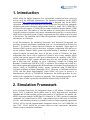
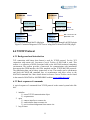
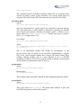
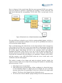
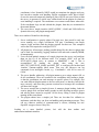
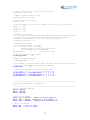
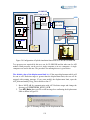
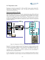
Figure 1 shows the framework of the simulation. The complete segregation of integration
scheme from static analysis module allows any combination of experiments and analyses.
Simulation Coordinator
Component 1
API
Object 1 of MDL_RF class
Object n of MDL_RF class
Simulation Monitor
MDL n
Server
Client
Static Equilibrium
Component n
API
Force
TCP/IP Network
Disp.
Client
Stiffness Evaluation
DOF Mapping
Simulation Monitor
MDL 1
Server
Main Routine
Dynamic Equilibrium
API
AUX
Equipments
Server
Client
Objects of MDL_AUX class
Simulation Control
Figure 1 Hybrid simulation framework
2
DAQ
Camera
3. Pseudo-Dynamic Test Procedure
In UI-SIMCOR, pseudo-dynamic test consists of roughly four stages; initialization, initial
stiffness formulation, static loading, and dynamic loading stages. During initialization
stage, the UI-SIMCOR makes connections to experimental sites or simulation module
and initializes each module. Most variables that will be used in later stage are also
initialized. During Initial stiffness formulation stage, UI-SIMCOR evaluate stiffness
matrix of whole structural system. There are two options to establish stiffness matrix.
When the structural dimension is large, stiffness matrix can be loaded from files each of
which defines stiffness matrix of each module. If the stiffness evaluation is affordable
through network, UI-SIMCOR sends predefined displacement for each degree of freedom
to each module and take measured forces to establish initial stiffness of the tested
structure. The established initial stiffness is used in the static loading stage and in the
dynamic loading stage to determine target displacements. Most structures are resisting
gravity forces before they are hit by earthquake. The effect of gravity forces cannot be
ignored since the inelastic behavior of columns and beams with initial loading are
significantly different from that of the elements without initial loading. During the static
loading stage, displacements due to this gravity forces are imposed. When there are no
gravity forces, this step can be skipped. During dynamic loading stage, PSD test using αOS scheme (Combescure and Pegon, 1997) is performed.
Each experimental stage, i.e., initial stiffness formulation, static and dynamic stages,
consists of similar functions such as evaluating target displacements, sending target
displacements to each module, executing the commands, checking relaxation, and
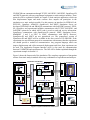
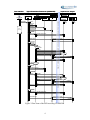
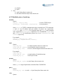
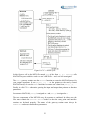
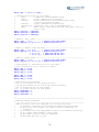
receiving the measured responses. Figure 2 describes data sequence of data flow of a
pseudo-dynamic simulation in UI-SIMCOR.
3
User Interface
1. Start simulation
Static
Static
Analysis
Analysis
Transient
Transient
Analysis
Analysis
2. Initialization
2.1 Add modules
to System
2.2 Add analysis
objects to System
2.3 Add hardware control
objects to System
3. Open connection
for each module
3.1 Connect remote site
Open TCP/IP or NTCP connection
Remote
Remote Site
Site N
N
Camera
Camera
HdwControl
HdwControl
Krypton
Krypton
HdwControl
HdwControl
DAQ
DAQ
HdwControl
HdwControl
Remote
Remote Site
Site 22
Remote
Remote Site
Site 11
NETWORK
Module
Module N
N
SupElement
SupElement
Module
22
Module
SupElement
SupElement
Module
11
Module
SupElement
SupElement
MOST
MOST
System
System
GUI or User
Hardware
Hardware other
other
than
than Actuator
Actuator
Server
standby
Server
standby
Acknowledge
Open TCP/IP or NTCP connection
NETWORK
3.2 Hardware system
4. Stiffness evaluation
for each module
4.1 Ask for stiffness
Yes,
return K
K exist?
No, evaluate K
for each DOF
SetTargetDisp
Acknowledge
Acknowledge
Execute
Acknowledge
Execute test
for each hardware
Trigger
Acknowledge
NETOWRK
Trigger DAQ
Query
Measured data
Return k
Assemble k
5. Simulation
every time step
5.1 Get displacement increment
Return displacement increment
5.2 Run experiment
for each module
Displacement
SetTargetDisp
Acknowledge
NETWORK
Monitor
experiment
Experiment or Analysis
Hybrid Simulation Framework (UI-SIMCOR)
Execute
Acknowledge
Execute test
for each hardware
Trigger
Trigger DAQ
Query
Measured Force
Acknowledge
Measured data
6. Close connection
for each module
6.1 Close remote site
Close TCP/IP or NTCP connection
Acknowledge
Close TCP/IP or NTCP connection
6.2 Close hardware system
Acknowledge
Figure 2 Flow chart of the PSD test using UI-SIMCOR
4
4. Sub-structuring of a Structure
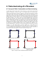
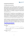
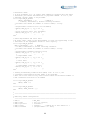
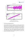
4.1 Concept of Static Condensation and Sub-structuring
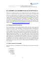
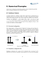
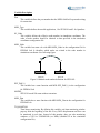
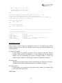
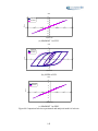
A portal frame with 16 nodes and 17 beam elements are used in this section for the
purpose of illustration as shown in Figure 3 (a). Lumped masses are located at beamcolumn joints and ground acceleration is applied in x-direction. In the equation of motion
of the frame, there will be mass and stiffness matrices with 48 by 48 elements. If we
model the same frame with 3 nodes and 4 elements as shown in Figure 3(b), the mass and
stiffness matrix size will be reduced to 9 by 9 but the analysis result will be identical to
the model in Figure 3 (a) as long as the level of mesh refinement does not affect the
analysis result. In Figure 3 (b), one node is placed in the middle of right column just to
show the displacement of the node is of our interest. Even if the structure is modeled as in
Figure 3 (a), the structure’s mass and stiffness matrix can be also reduced using static
condensation if the stiffness and mass matrices are known. If the stiffness matrix cannot
be retrieved, the condensed stiffness matrix can be determined by applying a prespecified displacement to each DOFs of interest and measuring reaction forces as shown
in Figure 3 (c). This method allows us that the stiffness of a certain DOF can be
calculated by applying certain displacement to the whole structure as shown in Figure 3
(c) or by applying certain displacement to segmented structure and take summation of
reaction forces from each segment of structure as shown in Figure 3 (d).
(a) Portal frame with 48 DOFs
(b) Portal frame with 9 DOFs
Δ
Δ
Δ
(d) Measurement of stiffness from
segmented structure
Figure 3 Concept of static condensation and sub-structuring
(c) Measurement of stiffness
5
4.2 Effective DOFs for Dynamic Analysis
A dynamic analysis can be performed for a structure using reduced DOFs. The stiffness
matrix of the structure with reduced DOFs can be established by applying known amount
of displacement to the whole structure or segmented part of the structure.
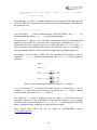
Following simple matrix manipulation shows that certain DOFs can be condensed out
from the equation of motion through static condensation. As shown in the following
derivation, remaining DOFs, or effective DOFs, are the DOFs where lumped masses
are defined or the DOFs of our interest. This is very important concept for the
preparation of input file for PSD testing using UI-SIMCOR.
DOF designation
i: DOFs where mass is defined
j: interface DOFs that are of our interest
k: internal DOFs where mass is not defined and we are not interested in.
For the PSD test, we want to know displacement at i and j DOFs to impose displacement
corresponding to inertial forces to experimental or static module. DOFs k can be condensed out
since we are not interested in them.
In the equations below, alphabet letters, M, 0, u, F, and K are matrix not scalar.
⎡M i
⎢
⎢
⎢⎣
0j
i ⎤ ⎡ K ii
⎤ ⎡u
⎢
⎥ ⎢u
⎥
⎥ ⎢ j ⎥ + ⎢ K ji
k ⎥⎦ ⎢⎣ K ki
0k ⎥⎦ ⎢⎣u
i ⎤ ⎡ K ii
⎡M i u
⎢ 0 ⎥ + ⎢K
⎢ j ⎥ ⎢ ji
⎢⎣ 0k ⎥⎦ ⎢⎣ K ki
⎡ K ii
⎢
⎢K ji
⎢ K ki
⎣
K ij
K jj
K kj
K ij
K jj
K kj
K ij
K jj
K kj
K ik ⎤ ⎡ ui ⎤
⎡M i
⎥⎢ ⎥
K jk ⎥ ⎢u j ⎥ = − ⎢⎢
⎢⎣
K kk ⎥⎦ ⎢⎣u k ⎥⎦
0j
⎤ ⎡ li ⎤
⎥ ⎢l ⎥ A
⎥⎢ j⎥( g )
0k ⎥⎦ ⎢⎣ l k ⎥⎦
K ik ⎤ ⎡ u i ⎤ ⎡ −M i l i Ag ⎤
⎥
K jk ⎥ ⎢⎢u j ⎥⎥ = ⎢⎢ 0 j ⎥⎥
K kk ⎥⎦ ⎢⎣u k ⎦⎥ ⎢⎣ 0k ⎥⎦
i ⎤ ⎡ Fi ⎤
K ik ⎤ ⎡ ui ⎤ ⎡ −M i l i Ag − M i u
⎥⎢ ⎥ ⎢
⎥ ⎢ ⎥
K jk ⎥ ⎢u j ⎥ = ⎢
0j
⎥ = ⎢0 j ⎥
⎥⎦ ⎢⎣ 0k ⎥⎦
K kk ⎥⎦ ⎢⎣u k ⎥⎦ ⎢⎣
0k
Condense out k DOfs.
⎡ K ii K ij K ik ⎤ ⎡ ui ⎤ ⎡ Fi ⎤
⎢
⎥⎢ ⎥ ⎢ ⎥
⎢K ji K jj K jk ⎥ ⎢u j ⎥ = ⎢ 0 j ⎥
⎢ K ki K kj K kk ⎥ ⎢⎣u k ⎥⎦ ⎢⎣ 0k ⎥⎦
⎣
⎦
⎛ ⎡ K ii
⎜⎜ ⎢K ji
⎝⎣
K ij ⎤ ⎡ K ik ⎤
−1
−
[K ] ⎡K
K jj ⎦⎥ ⎣⎢ K jk ⎦⎥ kk ⎣ ki
⎞ ⎡ ui ⎤ ⎡ K *
K kj ⎦⎤ ⎟ ⎢ ⎥ = ⎢ * ii
⎟ uj
⎠ ⎣ ⎦ ⎢⎣ K ji
After rearranging terms,
*
*
⎡M i 0⎤ ⎡ ai ⎤ ⎡ K ii K ij ⎤ ⎡ di ⎤
⎡M i
+
⎢
⎢
⎥
⎥ = −⎢
⎢ 0 0⎥ a
*
* ⎥ ⎢
d
⎣
⎦ ⎣ j ⎦ ⎣⎢K ji K jj ⎦⎥ ⎣ j ⎦
⎣ 0
or
0⎤ ⎡ l i ⎤
⎢ ⎥ Ag
0⎥⎦ ⎣l j ⎦
M*a* + K *d* = −M*l* Ag
6
K *ij ⎤ ⎡ ui ⎤ ⎡ Fi ⎤
⎥⎢ ⎥ = ⎢ ⎥
K * jj ⎥⎦ ⎣u j ⎦ ⎣ 0 j ⎦
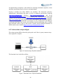
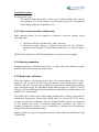
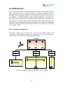
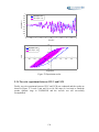
4.3 MOST Experiment
As described in the previous section, the equation of motion of a structure can be
established using only effective DOFs, i.e., DOFs where lumped masses are defined or
DOFs of our interest.
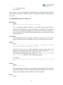
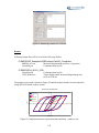
The MOST experiment example consists of two portal frames as given in Figure 4 (a).
The stiffness matrix of the structure will be a size of 11 by 11 with DOFs in Figure 4 (a).
Assuming that there are no axial deformations in columns, and we are not interested in
the rotation of hinge connections and rotation of mid-column-beam connection, the
number of DOFs can be reduced to 4 as shown in Figure 4 (b). The rotational DOF of the
left column is of our interest since the column will be tested using two DOFs on top. All
the translational DOFs should be included since mass is defined in the DOFs and inertial
forces should be applied. Also it is assumed that the lumped masses have x-directional
component only. If the lumped mass is significantly large in rotational direction, then the
rotational DOFs should be included in Figure 4 (b). Figure 4 (c) shows subdivided
structure into three parts, left column with two DOFs, mid-column and beam with four
DOFs, and right column with one DOF.
(a) MOST example
2
1
2
1
(b) MOST example with reduced DOFs
2
1
3
3
4
4
(c) Subdivided structure
Figure 4 Effective DOFs of the MOST example
7
5. Static Analysis Module Interface
In this distribution, FEDEAS Lab, ZEUS-NL, OpenSees, ABAQUS, OpenFresco, and
NHCP Simulation Server are included as static analysis modules. The static analysis
modules need to take displacements from simulation coordinator and give reaction forces
to the simulation coordinator. All these communications run through communication
protocol. Thus, it was necessary to develop an interface module for these analysis
softwares.
FEDEAS Lab
FEDEAS Lab was not need to be modified to work as a static analysis module since input
and out can be easily managed in MATLAB. A few additional scripts need to be written
to connect to UI-SIMCOR and give displacement and take forces from FEDEAS Lab.
NEES_FL_LabView2.m plays this role using LabVIEW2 protocol. In case when it is
necessary to communicate through NEESpop using NTCP for Matlab,
NEES_FL_NTCP.m can be used. But NTCP for Matlab requires several prerequisite
applications.
ZEUS-NL
Original version of ZEUS-NL was modified and recompiled. The modified solver,
NEES_Solver.exe, takes displacement input from console and makes reaction force
output into a file in each step. NEES-SAM, which stands for Static Analysis Module for
NEESgrid, gives displacement to the modified ZEUS-NL and reads the force output file.
NEES-SAM acts as an interface between UI-SIMCOR and ZEUS-NL. There are three
versions of NEES-SAM for TCP-IP, LabVIEW1, and LabVIEW2 protocols. The
protocols will be explained in detail in Section 6.
OpenSees
OpenSees was also modified to generate an output file for each step. Among the source
code files, NodeRecorder.cpp was modified. NEES-SAM also works as an interface
between UI-SIMCOR and OpenSees.
ABAQUS
It is not possible to modify the ABAQUS as it is commercial software. So, restart feature
in ABAQUS is utilized to use ABAQUS as a static analysis module. A MATLAB scripts
are developed to connect to UI-SIMCOR and give displacement to and take forces from
ABAQUS. NEES_Abaqus_LabView2.m plays this role using LabVIEW2 protocol. This
is very similar to FEDEAS Lab static analysis module interface, NEES_FL_NTCP.m.
OpenFresco
Open Framework for Experimental Setup and Control (OpenFresco) is a software
framework intended to facilitate and help standardize the local or geographicallydistributed deployment of hybrid simulation and developed by UCB (Schellenberg et. al.,
2006). OpenFresco can acts as an interface between experimental hardware and main
simulation coordinator. In addition, it also has a functionality to simulate experimental
8
hardware so that the PSD simulation can be verified without experimental setup. The
OpenFresco 2.0 was distributed with Matlab-OpenFresco examples and OpenSeesOpenFresco examples. As UI-SimCor is written in Matlab, the Matlab-OpenFresco
example was utilized so that OpenFresco can work with UI-SimCor. OpenFresco uses
TCP-IP connection to communicate with simulation coordinator written in any platform
such as Matlab, UI-SimCor, or OpenSees. The communication protocol between
MATLAB and OpenFresco is provided by Schellenberg et. al., (2006) in MEX file
format (TCPSocket.mexw32). This file is combined with UI-SIMCOR for hybrid
simulation. Currently, only 1-DOF simulation case is supported in UI-SimCor. The
protocol is referred as OpenFresco1D protocol in UI-SimCor. The original version of
OpenFresco provides two- and three-actuator cases, and also generic element for generic
FEM application. This extension will be combined with the next version of UI-SIMCOR.
NHCP Simulation Server
The NEES Hybrid Simulation Protocol (NHCP) is at the early stage of development. As a
pilot example, NEESit provided a simple example for which OpenSSL is used to encrypt
communication data and data for very simple system (1-DOF) can be transferred.
Currently, NHCP can be used for numerical simulation, and MiniMOST 1 and 2 in UIUC
or SDSC. For numerical simulation, only linear 1-DOF case is supported by NHCP
Simulation Server. A generalized version of NHCP will be implemented in UI-SIMCOR
when the development of NHCP in NEESit is completed.
9
6. Protocol Specification
6.1 NEESgrid Teleoperation Control Protocol (NTCP)
6.1.1 Background and introduction
NTCP is the first communication protocol for the hybrid simulation developed by NEESit.
Recently, NEESit has been developing new communication protocol, NHCP, but it is not
officially released yet. The further explanation about NHCP will be given latter.
UI-SIMCOR uses the NTCP Toolbox for MATLAB developed by NEESit. The setup
procedure of NTCP is very complicated compared to other protocols. The detailed
explanation of NTCP including NTCP Toolbox for MATLAB can be found in NEESit
website (http://it.nees.org). In this section, a simple explanation how NTCP works with
UI-SIMCOR will be given.
6.1.2 NTCP server connection with UI-SIMCOR
Two types of plugin are used for the NTCP server to connect to the backend client, such
as FEDEAS Lab, ZEUS-NL, OpenSees, or experimental equipment (Currently,
OpenFresco and NHCP Simulation Server do not support the NTCP). The plugins are
MATLAB plugin and LabVIEW plugin.
As FEDEAS Lab is running on the MATLAB, the connection to FEDEAS Lab is made
using MATLAB plugin. For the communication through MATLAB plugin, NTCP server
acts as a server for both ends. Thus the NTCP server waits for the connection from UISIMCOR and FEDEAS Lab with specified open ports. In the configuration of UISIMCOR and FEDEAS Lab, the URL and open port number of NTCP server should be
given. Both ends, UI-SIMCOR and FEDEAS Lab, connect to NTCP server using same
port number. Figure 5 (a) shows the connection diagram. The port number and URL in
the figure are just example.
ZEUS-NL, OpenSees, and test equipments use LabVIEW plugin to connect to the NTCP
server. As opposed to the MATLAB plugin, NTPC server act as a server for the
connection with UI-SIMCOR and act as a client for the connection to the backend, Figure
5(b). Thus, there is a URL and port number of NTCP server in UI-SIMCOR, and there is
a URL and port number of backend when the NTCP server runs.
10
UI-SIMCOR
UI-SIMCOR
Client
NTCP Server
Matlab Plugin
NTCP Server
Server
Server
LabView Plugin Client
URL: http://cee-nsp3.cee.uiuc.edu
Open Port: 11151
FedeasMDL
Client
URL: http://cee-nsp3.cee.uiuc.edu
Open Port: 11151
NEES-SAM
Client
ZEUS-NL
OpenSees
FEDEAS Lab
URL: 130.126.243.165
Server Open Port: 11150
(a) Connection through MATLAB plugin
(b) Connection through LabVIEW plugin
Figure 5 Connection diagram of NTCP server using MATLAB and LabVIEW plugin
6.2 TCP/IP Protocol
6.2.1 Background and introduction
TCP connection with binary data format is used for TCP/IP protocol. For the TCP
connection with remote site, Instrument Control Toolbox of MATLAB is used. This
toolbox is a collection of M-file functions build on the MATLAB technical computing
environment. The toolbox provides a framework for communicating with instruments
that support the GPIB interface, the VISA standard, and the TCP/IP and UDP protocols.
The transferring data can be binary (numerical) or text. The transfer can be synchronous
and block the MATLAB command line, or asynchronous and allow access to the
MATLAB command line. More details about Instrument Control Toolbox can be found
in the manual of MATLAB or MATHWORKS website (www.mathworks.com).
6.2.2 Basic sequence of commands
A typical sequence of commands from TCP/IP protocol to the control system looks like
this:
1. initialize
1) create TCP/IP communication object
2) set parameters
2. open
1) connect interface to remote site
2) send initialize data to remote site
3) receive acknowledgement from remote site
3. loop N times:
11
1)
2)
4. close
1)
2)
propose
query
send closing data to remote site
disconnect interface object from remote site
6.2.3 Detailed syntax of each step
initialize
Syntax:
Comm_obj = tcpip(IP, PORT);
set(Comm_obj, ‘PropertyName’, PropertyValue);
: to create TCP/IP object
: to set parameters
where Comm_obj is TCP/IP communication object returned from TCP connection.
IP and PORT are IP address and port number of remote site, respectively.
PropertyName and PropertyValue are a property name for Comm_obj and a property
value supported by PropertyName, respectively. For UI-SIMCOR, PropertyName
and PropertyValue for initialization process are set to ‘InputBufferSize’, and
1024×100, respectively.
For example:
Comm_obj = tcpip(127.0.0.1, 11997);
Set(Comm_obj, ‘InputBufferSize’, 1024×100);
open
Syntax:
fopen(Comm_obj);
fwrite(Comm_obj, iniData);
fread(Comm_obj, size);
to connect interface object to remote site
to send initialize data to remote site
to receive acknowledgement data from remote site
For example:
fopen(Comm_obj);
set total number of simulation steps
read 4 bytes of data
fwrite(Comm_obj, 500);
fread(Comm_obj, 4);
propose
Syntax:
fwrite(Comm_obj, T_DISP);
to write binary data to remote site
where T_DISP is target displacement calculated from UI-SIMCOR.
query
Syntax:
fread(Comm_obj, size);
to read size bytes binary data from remote site
close
Syntax:
12
fwrite(Comm_obj, closeData);
fclose(Comm_obj);
to send closing data to remote site
to disconnect interface object from remote site
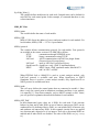
6.3 LabVIEW1 and LabVIEW2 Protocols for NTCP Server
Many users of NTCP experienced slow communication and a little cumbersome setup
process. So, LabVIEW1 and 2 protocols use direct connection between coordinator and
remote sites without NEESpop. The original version of LabVIEW1 protocol was written
for the communication between NEESPop and LabVIEW-controlled hardware. The
communication is basically conducted in ASCII format data. In UI-SimCor, the specific
ASCII-based communication is referred as LabVIEW1 or LabVIEW2. But it does not
necessarily involve LabVIEW software. These protocols are a simple ASCII format
designed for easy parsing and communications occur over a single TCP connection. This
section is based on the document about LabVIEW NTCP plugin which can be found in
NEESit website (http://it.nees.org/document/pdf/TR-2004-58.pdf).
6.3.1 Background and introduction
Any system wishing to use this protocol must be capable of having a process open and
listen on a TCP port (i.e., have threading, or some equivalent form of multitasking and
interprocess communications). All messages are tab-delimited ASCII, on a single line,
variable length (Newline is the message delimiter) and should be human-readable. The
protocol should, as much as possible, simply act as a serialization layer, with all the work
being done on the client side. This means less assumption about client functionality, and
higher implementation flexibility. As a side benefit, simper protocol code reduces
complexity and the number of bugs. Any language that can host a TCP connection and
parse string can be a full-fledged NTCP controller. This opens several doors to
lightweight control of small devices such as pan-tilt-zoom camera bases. Transaction ID
is included in every message, so that the client side can be asynchronous and
multithreaded (This is how the LabVIEW control code was implemented). LabVIEW1
protocol has Propose-Query-Execute-Query structure whereas LabVIEW2 has ProposeQuery structure.
6.3.2 Basic sequence of commands
The normal sequence of commands from LabVIEW protocol to the control system looks
like this:
1.
2.
3.
4.
open-session
set-parameter
get-parameter
loop N times:
1) propose
2) execute
13
3) get-control-point
5. close-session
where steps 2 and 3 are semi-optional, and depend on the program running LabVIEW
protocol (This is sometimes called an ‘client’ or ‘simulation coordinator’, depending on
the context).
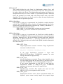
6.3.3 Detailed syntax for each verb
open-session
Syntax:
open-session TransactionID {parameter} {parameter}
This can optionally initialize hardware or do other system-specific work as
required. This should be the very first command of a connection. The parameters
are control-system-specific, meaning you can use this for whatever you need –
they are optional. The LabVIEW implementation ignores the transaction ID and
any parameters sent.
close-session
This mirrors open-session. Currently performs no work, but can be used as
required. Should be the last command received in an LabVIEW protocol session.
propose
Syntax:
propose TransactionID ControlPoint GeomType
ControlPoint GeomType ParameterType Parameter …
ParameterType
Parameter
where there can be zero to twelve parameters. The spec also allows zero
parameters, for implied commands based on the control point name. GeomType
mirros the NTCP specification, and is a single character: x, y, or z. ParamterType
also mirrors the specification, and can be: displacement, force, rotation, or
moment. Parameter is simple a scalar floating-point number.
For example:
propose Transaction0 ANCO-table x force 0.3 x displacement 3.1 y rotation
180.1
execute
Syntax:
execute TransactionID
This simply triggers execution of a previously-accepted proposal. Obviously, the
transaction ID must have been both proposal and accepted for this to be valid. The
control system should not return until the execution is complete.
cancel
Syntax:
14
cancel TransactionID
This command cancels a pending command, usually due to a proposal being
rejected by another control system somewhere else and the plugin throw an
exception. This should return OK if the transaction was canceled successfully.
get-control-point
Syntax:
get-control-point TransactionID ControlPoint
where the transaction ID is usually ignored, but required for consistent parsing.
The return format has a variable number of parameters, depending on what the
given control point supports. Mirroring the propose syntax, it returns to up to
twelve triplets of GeomType ParamType Paramter with the same types as ‘propose’
above, e.g., ‘x displacement 1.414’
For example:
get-control-point DummyTransactionID003 ANCO
replies
OK 0 DummyTransactionID003 x displacement 0.0 x force -0.113 y rotation
0.0 z rotation 0.0
This is an often-called method and should be asynchronous of the
propose/execute logic if possible. In the LabVIEW implementation, a separate
loop in the control program handles these requests and returns instant DAQ
readings, enabling real-time data as a move happens. It uses a LabVIEW
semaphore to mark the TCP send as a critical section, so that the various threads
do not collide in communicating with NTCP server.
get-parameter
Syntax:
get-parameter TransactionID ParamName
Return syntax:
OK 0 ParamName Parameter
This is mainly used by the MATLAB code to pass simulation parameters around.
set-parameter
Syntax:
set-parameter TransactionID ParamName Parameter
This is the mirror of get-parameter. The plugin sends whatever it gets, and
LabVIEW duly ignores it with an OK response.
15
6.4 OpenFresco1D Protocol
6.4.1 Background and introduction
OpenFresco1D protocol is used for OpenFresco module. OpenFresco is a software
framework intended to facilitate and help standardize the local or geographicallydistributed deployment of hybrid simulation and developed by UCB (Schellenberg et. al.,
2006). OpenFresco cannot perform hybrid simulations by itself, it simply mediates in a
modular and highly structured manner instructions between a host (client) numerical
simulation computer and laboratory equipment. It uses TCP connection to connect with
simulation coordinator (e.g., UI-SIMCOR). The communication protocol between
MATLAB and OpenFresco is also provided by Schellenberg et. al., (2006) in MEX file
format (TCPSocket.mexw32).
The MEX file is dependent on the MATLAB version. In the UI-SIMCOR there are three
different MEX files, i.e., TCPSocket_v65.mex, TCPSocket_R2006a.mexw32, and
TCPSocket_R2006b.mexw32 for MATLAB v6.5, R2006a, and R2006b, respectively.
The default MEX file for OpenFresco1D protocol sets to MATLAB version R2006b. If
user wants to MEX file for MATLAB v6.5 or MATLAB R2006a, change file name from
TCPSocket_v65.mex or TCPSocket_R2006a.mexw32 into TCPSocket.mex or
TCPSocket.mexw32. If a difference version of MATLAB is used, the user needs to create
a new MEX file based on the User Manual for OpenFresco (Schellenberg et. al., 2006).
The MEX file developed for the communication between MATLAB and OpenFresco is
utilized in UI-SIMCOR for communication with OpenFresco. Currently, only 1-DOF
simulation case is supported even though OpenFresco provides two- and three-actuator
cases, and generic element which will be implemented in the next version of UISIMCOR. This section is based on the User Manual for OpenFresco, so more details
about OpenFresco can be found in the OpenFresco project page of NEESit
(https://neesforge.nees.org/projects/openfresco).
6.4.2 Usage of OpenFrescoID protocol
setup connection
Syntax:
socketID = TCPSocket (‘openConnection’, PORT_OpenFresco, IP_OpenFresco);
is ID for connection, ‘openConnection’ for open action, and
and IP_OpenFresco are port number and IP address for
OpenFresco, respectively.
where
socketID
PORT_OpenFresco
set data sizes for remote site
Syntax:
TCPSocket (‘sendData’, socketID, dataSizes, 11);
16
where ‘sendData’ for sending data to OpenFresco. dataSizes is size of data which
will be sent to OpenFresco. For 1-DOF system dataSizes = int32([1 0 0 0 0, 0
0 0 1 0, dataSize]); where dataSize = 2 .
send target responses to remote site
Syntax:
TCPSocket(‘sendData’, socketID, sData, dataSize);
where sData is for target displacement of size 1 × 2. sData(1) = 3 for ‘sendData’
command and sData(2) is target displacement which was sent from UI-SIMCOR.
dataSize is size of sDate, i.e., 2.
get measured restoring force
Syntax:
TCPSocket(‘sendData’, socketID, sData, dataSize);
rData = TCPSocket(‘recvData’, socketID, dataSize);
where sData is scalar value of 10 for query action, dataSize is 2 which was
defined during ‘set data sizes for remote site’, rData is measured restoring force
received from OpenFresco. UI-SIMCOR assumes that the measured displacement
is same with the target displacement.
disconnect from remote site
Syntax:
TCPSocket(‘sendData’, SocketID, sData, dataSize);
TCPSocket(‘closeConnection’, socketID);
where sData is a scalar value of 99 for close action,
defined during ‘set data sizes for remote site’.
dataSize
is 2 which was
6.5 NEES Hybrid Communication Protocol (NHCP)
6.5.1 Background and introduction
Previous communication protocol of NEESit (i. e., NTCP) is designed for slow tests, over
unreliable networks, spanning one or more laboratories. Indeed, it has been used
successfully in several of these, and researchers continue to use it. NEESit has been
reworking NTCP such that it can be used for fast distributed tests. In particular, one
proposed experiment, they are using as a goal is 75 Hz over a 500 km link.
NEESit are not going toe try and address fast hybrid tests that run in hard real time,
instead they will focus on distributed tests, both slow and ‘fast’, attempting to run as fast
as possible.
One area where NEESit can contribute is streaming data. NEESit have an existing system
based on the Create Date Turbine that works well for data, video and audio. NEESit plans
17
on implementing an interface to the turbine for streaming commands, responses, events
and other experimental data for observers and participants.
Security is another area where NEESit can contribute. The framework will have
authentication, authorization and hooks or tools to administer permissions. GridAuth
(http://www.gridauth.com/), Kerberos (http://web.mit.edu/kerberos/), and JAAS
(http://java.sun.com/products/jaas/) are all intriguing here. Based on initial results and
feedback from the Denver meeting (http://it.nees.org/weblog/hybridsim/?p=3), OpenSSL
(http://www.openssl.org/) are used for TCP/IP, both plaintext and encrypted. OpenSSL
allows to leverage the considerable investments in code, infrastructure and hardware
acceleration that others have made, with confidence that the underlying code is reliable
and well-tested. Most of part of this section is based on the technical documents of
NEESit which can be found in http://it.nees.org/weblog/hybridsim/?p=67.
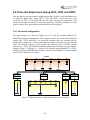
6.5.2 Abstractions and paradigms
The various systems differ in how they split up the work. Here is a pretty common setup
from a physical viewpoint.
Figure 6 Common setup of hybrid simulation
The functional view looks like as follow.
Figure 7 Functional view of hybrid simulation
18
Here is a diagram of the second design. Block in green represent TCP/IP server process,
where the program in question is responsible for accepting a TCP/IP connection, and
light brown represents the corresponding TCP/IP client. This is revised quite a bit as
follow.
Figure 8 Functional view of hybrid simulation using NHCP
The major difference is that the server is back to running multiple plugins. As before, a
coordinator can and will talk to multiple servers (one per site, probably) but each server
will load and run multiple plugins.
This is worth discussing a bit, both for how it came about and also for the consequences
of the design. First off, the server is now more event-driven, with messages arriving and
departing all the time, from given displacement. This is sent to all plugins, starting with
the security plugin. Each plugin can look at the command, source and (optional)
destination and decide if they need to act or not. It has an Observer plugin that, as
pictured, generates no messages but logs all to disk. In the example, the control plugin
would take the command, move the hardware (or simulation), compute reaction forces,
and then generate a new MSG_REACTION which the server would send to the
coordinator, and also all the plugins.
This enables a number of nice things, and makes the plugins’ interface simpler, but
requires a bit more of the server to keep it from slowing as the number of communicating
processes increases. To wit;
1. Each plugin runs in its own thread.
2. Each message queue (to/from plugin, to/from coordinator) is a thread-safe queue
of fixed maximum length. If a plugin gets too far behind, the server will drop
messages rather than wait, generating a critical error callback to the plugin upon
doing so. This keeps a slow plugin from rate-limiting the server.
3. The server has to decide whether a plugin running or not if the connection to the
19
coordinator is lost. Normally, NHCP would just terminate the plugins and reset,
but it needs to consider error handling. Did the coordinator crash? Was it killed?
Or was the network temporarily damaged? Since NHCP can not tell from within
the server, its generates a critical error callback and lets the plugins do whatever
error handling is required. The coordinator can reconnect and resume when able.
If the coordinator logs out and unloads the plugins, then they are terminated in
the normal fashion.
4. The server has a simple interface (MSG_QUERY, LOAD and UNLOAD) for
dynamic discovery and plugin management.
There are a number of benefits to this design;
1. Server configuration is greatly reduced. In most uses, there needs be only one
server running, on a single well-known TCP port. Coordinators can simply
connect, login, and then load the plugins required for their test. This compares
well to the effort required to configure NTCP.
2. All plugins see all messages, making possible things like the observer plugin that
can be used for monitoring, logging, database back ends and eventually RBNB,
all transparently.
3. Users can load multiple instances of a single plugin into the server, and configure
them on the fly to do different tasks. For example, SDSC will use the
NTCP/ASCII plugin twice, to connect to MiniMOST 1 and 2. This is
accomplished
by
loading
the
plugin,
then
using
the
new
MSG_SET_INSTANCE_NAME and MSG_SET to configure the backend and
‘instance’ (human-readable label) name. That way, the Observer can log
commands in an intelligible format, e.g. ‘Coordinator 1 tells M1 to move to
0.01m’.
4. The server handles addressing. All plugin instances get a unique numeric ID, as
do all coordinators. These are returned to the coordinator after loading a plugin,
so that the coordinator can send messages to specific places. For example, user
can send different displacements to the two mini-mosts, so that they both do the
move correctly, and when they generate reaction force messages the coordinator
will know their origin.
5. The server actually has a simpler job now. It manages plugin loading, loads the
security plugin first, and then mainly spends its time checking messages queues
and moving them around as required. All the heavy lifting is done in plugins
running in their own thread.
6. The plugin authors have a simpler job. There are less than five callbacks to
implement, and then they can focus on handling and generating messages. They
can use whatever method of communication is easiest; including our new
OpenSSL wrapper classes if they like.
Looking at a more detailed
authorization/authentication bits.
picture,
20
let's
add
the
data
turbine
and
Figure 9 Detailed functional view of hybrid simulation using NHCP
Security
There are several things to consider here;
1. Message integrity - was the data corrupted, either accidentally or deliberately?
2. Authenticity - are you talking to the process you expected, or the man in the
middle?
3. Authorization - is user J allowed to control hardware X?
4. Encryption - is you have proprietary (e.g. commercial) data, you might want to
prevent against interception.
For solution, NEESit proposes using a tiered solution;
1. OpenSSL for communications
a. Plain socket mode (default, fastest, simple)
b. Message digests, plaintext - this addresses #1
c. Encrypted with digests
2. External username/password mechanism TBD. There are many possibilities here
(kerberos, PAM, JAAS, Gridauth, Globus, etc, etc).
The use of OpenSSL does complicate the development and compilation a bit, but there
are many offsetting factors. It's a well-established standard, cross-platform, stable and
can be accelerated with crypto cards if desired. If user employ server and client
certificates, they can ensure secure communications with minimal overhead, both runtime
and administrative.
21
6.5.3 MEX file
MEX stands for MATLAB Executable, MEX files are dynamically linked subroutines
produced from C/C++ or Fortran source code that, when compiled, can be run from
within MATLAB in the same way as MATLAB M-files or built-in functions. The
external interface functions of MATLAB manual provide functionality to transfer data
between MEX-files and MATLAB, and the ability to call MATLAB functions from
C/C++ or Fortran code. The main reasons to write a MEX-file are;
1. The ability to call large existing C/C++ or Fortran routines directly from
MATLAB without having to rewrite them as M-files.
2. Speed; user can rewrite bottleneck computations (like for-loops) as a MEX-file
for efficiency.
The source code for a MEX-file consists of two distinct parts;
1. A computational routine that contains the code for performing the computations
that you want implemented in the MEX-file. Computations can be numerical
computations as well as inputting and outputting data.
2. A gateway routine that interfaces the computational routine with MATLAB by
the entry point mexFunction and its parameters prhs, nrhs, plhs, nlhs, where prhs
is an array of right-hand input arguments, nrhs is the number of right-hand input
arguments, plhs is an array of left-hand output arguments, and nlhs is the number
of left-hand output arguments. The gateway calls the computational routine as a
subroutine.
In the gateway routine, user can access the data in the mxArray structure and then
manipulate this data in your C/C++ computational subroutine. For example, the
expression mxGetPr(prhs[0]) returns a pointer of type double * to the real data in the
mxArray pointed to by prhs[0]. User can then use this pointer like any other pointer of
type double * in C/C++. After calling user’s C/C++ computational routine from the
gateway, user can set a pointer of type mxArray to the data it returns. MATLAB is then
able to recognize the output from your computational routine as the output from the
MEX-file.
The following C/C++ MEX cycle figure shows how inputs enter a MEX file, what
functions the gateway routine performs, and how outputs return to MATLAB.
22
Figure 10 C/C++ MEX cycle
In this figure a call to the MEX file named func of the form [C, D] = func(A,B) tells
MATLAB to pass variables A and B to user’s MEX-file. C and D are left unassigned.
The func.c gateway routine uses the mxCreate function to create the MATLAB arrays for
your output arguments. It sets plhs[0], [1], ... to the pointers to the newly created
MATLAB arrays. It uses the mxGet functions to extract user’s data from prhs[0], [1], ...
Finally, it calls C/C++ subroutine, passing the input and output data pointers as function
parameters.
On return to MATLAB, plhs[0] is assigned to C and plhs[1] is assigned to D.
The two components of the MEX-file may be separate or combined. In either case, the
files must contain the #include "mex.h" header so that the entry point and interface
routines are declared properly. The name of the gateway routine must always be
mexFunction and must contain these parameters.
23
void mexFunction(int nlhs, mxArray
*prhs[]){
/* more C/C++ code ... */
}
*plhs[],
int
nrhs,
const
mxArray
The parameters nlhs and nrhs contain the number of left- and right-hand arguments with
which the MEX file is invoked. In the syntax of the MATLAB language, functions have
the general form of
[a,b,c,...] = fun(d,e,f,...)
where the ellipsis (...) denotes additional terms of the same format. The
left-hand arguments and the d,e,f,... are right-hand arguments.
a,b,c,...
are
The parameters plhs and prhs are vectors that contain pointers to the left- and right-hand
arguments of the MEX file. Note that both are declared as containing type mxArray *,
which means that the variables pointed at are MATLAB arrays. prhs is a length nrhs
array of pointers to the right-hand side inputs to the MEX-file, and plhs is a length nlhs
array that contains pointers to the left-hand side outputs that your function generates.
For example, if user invokes a MEX file from the MATLAB workspace with the
command x = fun(y,z); the MATLAB interpreter calls mexFunction with the following
arguments:
Figure 11 Relationship between MATLAB and C/C++ variables
plhs is a 1-element C/C++ array where the single element is a null pointer. prhs is a 2element C/C++ array where the first element is a pointer to an mxArray named Y and the
second element is a pointer to an mxArray named Z.
The parameter plhs points at nothing because the output x is not created until the
subroutine executes. It is the responsibility of the gateway routine to create an output
array and to set a pointer to that array in plhs[0]. If plhs[0] is left unassigned, MATLAB
prints a warning message stating that no output has been assigned.
More details about MEX
(www.mathworks.com).
file
can
be
24
found
at
MATHWORKS
website
6.5.4 NHCP DLL file
The NHCP is implemented in UI-SIMCOR by modifying the existing demo files of
NHCP. There are four demo files in NHCP, i.e., simdemo.cpp, m1driver.cpp,
m2driver.cpp, baronDemo.cpp. simdemo.cpp is for the simulation demo, m1driver.cpp
and m2driver.cpp are for MiniMOST 1 and 2, respectively.
These four files are combined into one MEX file, i.e, NHCP.dll for UI-SIMCOR. If file is
compiled within MATLAB, then the file will depend on the MATLAB version, so we
compiled the source code within Microsoft Visual Studio 2005 to make Dynamically
Linked Library (DLL) file. NCS (server for NHCP) and SimServer (simulation server for
NHCP) are also modified to receive the port number for NCS and port number and
stiffness for SimServer, respectively.
6.5.5 Usage of NHCP
UI-SIMCOR will call NHCP.dll file if NHCP protocol is used for hybrid simulation.
Currently, there are three modes in NHCP, i.e., simulation mode with linear 1-DOF
system, MiniMOST 1 and 2 modes. NEESit has not generalized the NHCP, so NHCP for
UI-SIMCOR is restricted for a special case as mentioned in the above. However, when
NEESit releases the generalized NHCP, it will be implemented into UI-SIMCOR.
There are three actions in each mode of NHCP, i.e., ‘open’, ‘run’, and ‘close’. During
‘open’ action, UI-SIMCOR is connected with NHCP server (i.e., NCS) through OpenSSL
connection and NCS is connected with simulation server (i.e., SimServer) for simulation
mode or computer for Mini MOST 1 or 2 using TCP connection. During ‘run’ actions,
propose target displacement and query measurement are conducted simultaneously.
Processes for ‘execute’ or ‘query’ used in NTCP or LabVIEW protocol are not required.
Finally, the UI-SIMCOR and NCS are disconnected from NCS and SimServer (or
computer for MiniMOST 1 or 2), respectively during ‘close’ action.
open
Syntax:
NHCP(NHCPMode, ‘open’, IP_NCS, PORT_NCS, IP_SERVER, PORT_SERVER,
STIFFNESS_SIM)
where NHCPMode is one of Sim1D for simulation case with linear 1-DOF system, MM1,
MM2 for MiniMOST 1 and 2, respectively.
‘open’ command for open action, and IP_NCS, PORT_NCS, IP_SERVER, PORT_SERVER
are IP address and port number for NCS and simulation server for simulation case
with linear 1-DOF system, computer for MiniMOST 1, and computer for Mini
MOST 2, respectively. Finally, STIFFNESS_SIM is the stiffness of simulation case
and required only when NHCP is used for simulation case (i.e., NHCPMode is Sim1D).
It does not include units and units are depends on the simulation coordinator (i.e.,
UI-SIMCOR). All of input variable for NHCP should be bracketed by ‘’. For
‘open’ action, there is no return value from NHCP protocol. Instead if there are
errors during connection to NCS and SimServer (or MiniMOST 1 and 2), there are
errors messages in the NCS command window.
25
For example:
NHCP(‘Sim1D’, ‘open’, ‘127.0.0.1’, ‘11997’, ‘127.0.0.1’, ‘11998’,
‘1000’);
NHCP(‘MM1’, ‘open’, ‘127.0.0.1’, ‘11997’, ‘127.0.0.1’, ‘11998’);
run
Syntax:
For Sim1D and MM1 modes
[M_FORC] = NHCP(NHCPMode, ‘run’, T_DISP);
For MM1 mode
[M_DISP, M_ROT, M_FORC, M_MOM] = NHCP(‘MM2’, ‘run’, T_DISP, T_ROT);
where ‘run’ for running the simulation and T_DISP and T_ROT are target
displacement and rotation which are sent from UI-SIMCOR and double float,
respectively. For Sim1D and MM1 modes, there is one return variable, i.e., M_FORCE
(measured force) and UI-SIMCOR assumes that the measured displacement is
same with target displacement. For MM2 mode, there are four return variables, i.e,
M_DISP (measured displacement), M_ROT (measured rotation), M_FORC, M_MOM
(measured moment). MiniMOST 1 in UIUC or SDSC has one DOF in
translational direction (i.e, x-direction) and MiniMOST 2 in UIUC or SDSC has
two DOFs in translational direction and rotation (i.e., x- and rz-direction).
For examples:
[M_FORC] = NHCP(‘Sim1D’, ‘run’, 10);
[M_DISP, M_ROT, M_FORC, M_MOM] = NCHP(‘MM2’, ‘run’, 10, 0.1);
close
Syntax:
NHCP(NHCPMode, ‘close’);
where ‘close’ for disconnecting UI-SIMCOR from NCS and SimServer (or Mini
MOST 1 or 2 computer). There is no return value during ‘close’ action, instead
there will be error messages in the NCS if there are some errors during ‘close’
action.
For example:
NHCP(‘MM1’, ‘close’);
26
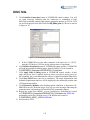
7. Installation of UI-SIMCOR
All the files necessary to run UI-SIMCOR including NEES-SAM are posted on the
NEESforge website (https://neesforge.nees.org/projects/simcor). After installation is
complete, the user should be able to run the examples in Section 8. The distributed
software is composed of following components.
• 01_SIMCOR
•
•
•
•
•
02_NEES-ABAQUS
02_NEES-FL
02_NEES-SAM
03_Examples
04_API
: Simulation coordinator, a main control and
integration module.
: Interface applications for ABAQUS
: Interface applications for FEDEAS Lab.
: Interface applications for ZEUS-NL and OpenSees
: Various examples including experimental test
: API for specific experimental site
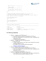
7.1 System Requirements
A MATLAB v6.5 or higher version with Instrument Control Toolbox is required UISIMCOR itself. Various structural analysis programs and some additional programs for
specific communication protocols are also required. Installation instruction for each
software will be explained.
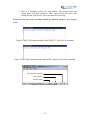
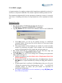
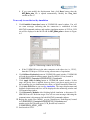
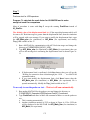
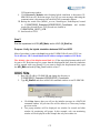
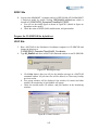
7.2 Installation of UI-SIMCOR and Interface Application
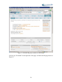
The executable file for UI-SIMCOR v2.6 can be downloaded form the NEESforge
website.
Start
from
the
NEESforge
UI-SIMCOR
page
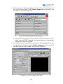
(https://neesforge.nees.org/projects/simcor) as shown in Figure 12.
27
Figure 12 UI-SIMCOR project website on NEESforge
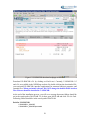
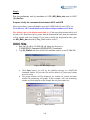
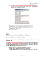
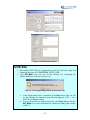
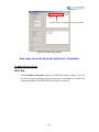
Click on any “Download” on the right side of the page. All links load the page shown in
Figure 13.
28
Figure 13 UI-SIMCOR download webpage on NEESit
Download UI-SIMCOR v2.6 by clicking on SimCor.msi. Currently, UI-SIMCOR v2.5
and v2.6 are available in the NEESforge website. By double clicking the downloaded file,
you can install UI-SIMCOR, interface applications for structural analysis programs, and
example files. When you install software, DO NOT change the default folder location.
The software should be installed in C:\SIMCOR.
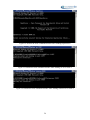
At the end of the installation process, you will see a message that some folders should be
set in the search path of MATLAB. To do that, open MATLAB and click File-Set Path.
Following folders should be in the search path of MATLAB.
Path for UI-SIMCOR
C:\SIMCOR\01_SIMCOR
C:\SIMCOR\01_SIMCOR\parmatlab
29
Path for FEDEAS Lab and NEES-FL
C:\SIMCOR\02_NEES-FL
C:\SIMCOR\02_NEES-FL\FedeasLab
C:\SIMCOR\02_NEES-FL\FedeasLab\Element_Lib
C:\SIMCOR\02_NEES-FL\FedeasLab\General
C:\SIMCOR\02_NEES-FL\FedeasLab\Geometry
C:\SIMCOR\02_NEES-FL\FedeasLab\Material_Lib
C:\SIMCOR\02_NEES-FL\FedeasLab\Output
C:\SIMCOR\02_NEES-FL\FedeasLab\Section_Lib
C:\SIMCOR\02_NEES-FL\FedeasLab\Solution_Lib
C:\SIMCOR\02_NEES-FL\FedeasLab\Utilities
Path for NEES-ABAQUS
C:\SIMCOR\02_NEES-ABAQUS
Path for API of UCB (If μNEES at UCB is used for experiment)
C:\SIMCOR\04_API\01_UCB
For simple procedure
1. Run a MATLAB
2. Click File-Set Path-Add with Subfolders in the menu bar and select
C:\SIMCOR\01_SIMCOR and click the OK button
3. Repeat step 2 for C:\SIMCOR\02_NEES-FL, C:\SIMCOR\02_NEESABAQUS and C:\SIMCOR\04_API\01_UCB
4. Click Save button to save the paths and click Close button
7.3 Installation of Structural Analysis Software
The modified analysis softwares for the multi-site simulation are included in the
distribution. Also FEDEAS Lab is included in the distribution. To edit and verify
structural model for ZEUS-NL and OpenSees, each software should be installed
separately.
The latest version of ZEUS-NL can be downloaded from the following link. By double
clicking installation file, you can install the latest version of ZEUS-NL. If you encounter
difficulties in modeling or running ZEUS-NL, contact Oh-Sung Kwon
([email protected]) or Kyu-Sik Park ([email protected]).
http://mae.ce.uiuc.edu
OpenSees can be downloaded from the following link.
http://opensees.berkeley.edu
30
In the above link, there is detailed information about OpenSees. Tcl/Tk interpreter also
should be installed to run OpenSees and OpenFresco. This is also needed for NEES-SAM
when OpenSees is used as static analysis module.
OpenFresco including user’s manual can be downloaded from the following link.
https://neesforge.nees.org/projects/openfresco
For the NHCP, the OpenSSL is required for communication between UI-SIMCOR and
NCS. OpenSSL can be downloaded from the following link.
http://www.openssl.org/
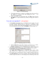
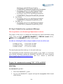
Folder List after Installation
The folder list of installed UI-SIMCOR is shown in Figure 14.
31
C:\SIMCOR
\01_SIMCOR
\@MDL_AUX
\@MDL_RF
\parmatlab
\02_NEES-ABAQUS
\02_NEES-FL
\FedeasLab
\02_NEES-SAM
\NEES_OpenSees
\NEES_Zeus
\03_Examples
\6Beam5Col
\BUCKLE_InitLoading
\MOST
\MOST_LBCB
\SAC
\SDOF
\SDOF_Concrete
\SDOF_InitLoading
\ThreeSite
\UCB
\MOST
\PushoverTest
\SDOF
\01_UCB
\04_API
Figure 14 Folder list of UI-SIMCOR
7.4 Downloading and Updating UI-SIMCOR Source Code
The source code of UI-SIMCOR is already installed in the 01_SIMCOR folder of UISIMCOR installation directory. However, if you are interested in extending the software,
the latest version of UI-SIMCOR source code is available for download using Subversion
(SV). The Subversion is a version control system for software systems, a major
component of Source Configuration Management (SCM) of SIMCOR Project in
32
NEESforge website. Subversion is commonly used in software development to record the
history of sources files and documents.
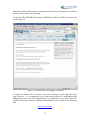
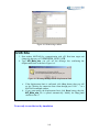
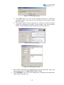
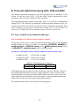
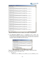
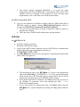
At the top of the SIMCOR Project page of NEESforge, click on “SCM” tab and you can
see the Figure 15.
Figure 15 UI-SIMCOR SCM webpage on NEESit
To browse the source code, click Brows Subversion Repository on the right side of the
page. However, it is recommended to use Subversion software for downloading and
updating the source code (Only authorized user can update the source code). The freely
available Subversion software including documentation can be found in the following
link.
http://tortoisesvn.net
33
The files in the “SCM” tab of NEESforge are the latest version of UI-SIMCOR source
code, so it may have some bug or may not working. If user wants stable UI-SIMCOR
source code, user needs install the latest version of UI-SIMCOR.
34
8. Numerical Examples
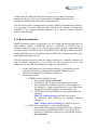
In this section, configuration and modeling guidelines for the UI-SIMCOR and NEESSAM are introduced through various numerical examples.
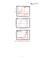
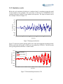
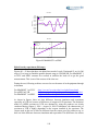
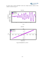
8.1 Cantilever Column
A dynamic analysis of a cantilever column with a lumped mass is introduced here to
demonstrate and verify each analysis module. The column is tested with elastic material
without initial loading using three static analysis applications (FEDEAS Lab, ZEUS-NL,
2
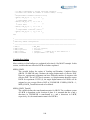
OpenSees, and ABAQUS). α -OS scheme with α = 0.05 , β = 1/ 4 ⋅ (1 + α ) and
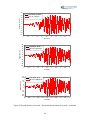
γ = 1/ 2 + α is used for all the simulation. N-S component of the ground motion recorded
at a site in El Centro, California, during the Imperial Valley earthquake of May 18, 1940
is used for all cantilever column examples.
8.1.1 Structural configuration
The column height is 3,500 mm with 10 N/(mm/sec2) of mass at the top, Figure 16.
Frame element is used to model the column. Only x-directional DOF is used for dynamic
analysis. El Centro ground motion was applied along the x-direction at the base. Lumped
mass is defined in simulation coordinator. Stiffness evaluation and static analysis is
performed in static analysis module, FEDEAS Lab, ZEUS-NL, OpenSees, ABAQUS,
OpenFresco, and NHCP Simulation Server.
x
m =10 N/(mm/sec2)
m =10 N/(mm/sec2)
x
3,500 mm
x
Ag,x
Ag,x
Column dimension
SIMCOR
Static Analysis Module
Figure 16 Column configuration
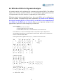
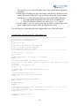
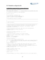
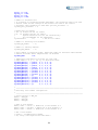
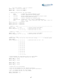
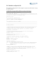
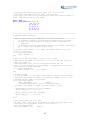
8.1.2 Simulation configuration file
Simulation configuration file contains all the information that is necessary for UISIMCOR for the multi-site simulation. Many parameters are trivial and self-explained.
35
Note that most of the parameters should be defined for all analysis and variable names
should not be modified. The MATLAB script is case sensitive.
C:\SIMCOR\03_Examples\SDOF\00_Coordinator\SimConfig.m
function [Sys, MDL, AUX] = SimConfig
MDL = MDL_RF; AUX = MDL_AUX;
% Type definition. Do not delete this line.
% =============================================================================
% Configuration parameters for SDOF experiment
%
% Unit: mm, N, sec
%
% by Oh-Sung Kwon, [email protected]
% modified by Kyu-Sik Park, [email protected]
% Univ. of Illinois at Urbana Champaign
%
% Last updated on 2007-01-26 11:05PM
% =============================================================================
% _____________________________________________________________________________
%
% Common parameters
% _____________________________________________________________________________
% Ground acceleration file name with extension. The file should contains two
% columns for time and acceleration. The unit of acceleration should be
% consistent with the mass, time, and force. (i.e. mass*acc = force)
Sys.GM_Input = 'elcentro.dat';
% Ground acceleration scale factor. This factor will be multiplied to
% acceleration before starting simulation.
Sys.GM_SC = 9810;
% Direction of ground acceleration. (x, y, or z)
Sys.GM_direction = 'x';
% Integration parameter related to the alpha-OS method.
% Alpha = (0 ~ 1/3). In most cases, SC.Alph = 0.05 worked.
Sys.Alph = 0.05;
Sys.Beta = 1/4*(1+Sys.Alph)^2;
Sys.Gamm = 1/2 + Sys.Alph;
% Evaluate Stiffness?
% Yes (1) to run stiffness evaluation test,
% No (0) to read stiffness matrix from file. In this case, there should exist
%
stiffness matrices of individual module in the files MDL01_K.txt,
%
MDL02_K.txt, etc.
Sys.Eval_Stiffness = 1;
% Number of initial static loading steps. When there exist static constant
% loading,i.e. gravity forces, apply then in Zeus-NL or OpenSees as a
% incremental loading with 'n' steps. In this file, SimConfig.m, specify the
% number of static steps in the following variable.
Sys.Num_Static_Step = 0;
% Number of dynamic analysis steps
Sys.Num_Dynamic_Step = 500;
% Dynamic analysis time steps
Sys.dt = 0.01;
36
% Rayleigh
Sys.xi_1 =
Sys.Tn_1 =
Sys.xi_2 =
Sys.Tn_2 =
damping, xi_1 and xi_2: Damping ratio, Tn_1, Tn_2: Target period
0.00;
0.00;
0.00;
0.00;
% Number of Stiffness test
% If stiffness is evaluated through experiment, the evaluation need to be done
% several times and the average of the results are used as the initial
% stiffness. This parameter is used when Sys.Eval_Stiffness = 1
Sys.Num_Test_Stiffness = 1;
% Enable GUI for SimCor?
% Yes (1) enable the GUI for SimCor
% No (0) disable the GUI for SimCor
%
Hybrid simulation will be run automatically.
%
Not recommended for the experiment.
Sys.EnableGUI
= 1;
% Use GUI for SimCor
% Number of restoring force modules.
Sys.Num_RF_Module
= 1;
% Number of auxilary modules.
Sys.Num_AUX_Module
= 0;
% Total number of effective nodes. Effective nodes are interface nodes between
% modules and nodes where lumped masses are defined.
Sys.Num_Node
= 1;
% Lumped mass assigned for each DOF for each node.
% Node number = x, y, z, rx, ry, rz directional mass
Sys.Node_Mass{1} = [10, 0, 0, 0, 0, 0];
% _____________________________________________________________________________
%
% Restoring force module configuration
% _____________________________________________________________________________
% Create objects of MDL_RF
MDL(1) = MDL_RF;
% Name of each module.
MDL(1).name = 'STATIC'; % Module ID of this module is 1
% URL of each module
% Format - IP address:port number
% ex) 'http://cee-nsp4.cee.uiuc.edu:11997'
%
for local machine - '127.0.0.1:11997'
MDL(1).URL = '127.0.0.1:11997';
% Communication protocol for each module.
%
NTCP
: communicate through NEESPOP server
%
TCPIP
: binary communication using TCPIP
%
LabView1
: ASCII communication with LabView plugin format
%
(Propose-Query-Execute-Query)
%
LabView2
: same as LabView1 but Propose-Query
%
OpenFresco1D : OpenFresco, only 1 DOF is implemented now.
%
NHCP
: NHCP, linear 1 DOF simulation mode, Mini MOST 1 and 2 at
%
UIUC or SDSC
MDL(1).protocol = 'nhcp';
% Module 1: STATIC -----------------------------------------------------------MDL(1).node
= [1];
% Control point node number
37
MDL(1).EFF_DOF = [1 0 0 0 0 0]; % Effective DOF for CP 1
% Dismplacement for preliminary test for each module
% Del_t: Translation, Del_r: Rotation in radian
MDL(1).DEL_t = 0.005;
MDL(1).DEL_r = 0.002;
% Enable GUI for each module?
% GUI for each module can only display the data.
% GUI for each module can not control the hybrid simulation.
% Yes (1) enable the GUI for each module
% No (0) disable the GUI for each module
MDL(1).EnableGUI = 1;
% _____________________________________________________________________________
%
% Advanced modular parameters
% _____________________________________________________________________________
% These parameters need to be redefined for following situations.
%
(1) Different coordinate system between UI-SIMCOR and static module
%
(2) When scale factor needs to be applied either in experiment or
%
simulation
%
(3) To define force and displacement criteria (for tolerance and safety)
%
(4) To trigger camera modules or DAQ system
%
(5) When LBCB at UIUC is used for experiment
%
(6) When NHCP protocol is used
%
% URL of remote site and NHCP mode for NHCP
for i=1:Sys.Num_RF_Module
if strcmp(lower(MDL(i).protocol), 'nhcp')
MDL(i).remote_URL = '127.0.0.1:99999';
MDL(i).NHCPMode = 'sim1d';
end
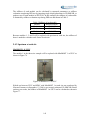
end
% Stiffness for NHCP (Only valid if NHCPMode = 'Sim1D')
for i=1:Sys.Num_RF_Module
if strcmp(lower(MDL(i).NHCPMode), 'sim1d')
MDL(i).NHCPSimK = '6.2344023e+003';
end
end
% Coordinate transformation. If it needs, the transformation matrix also
% needs to be provided.
for i=1:Sys.Num_RF_Module
MDL(i).TransM = [];
end
% Scale factor for displacement, rotation, force, moment
% Experimental specimens are not always in full scale. Use this factors to
% apply scale factors.
% The displacement scale factors are multiplied before they are
% sent to module. Measured force and moments are divided with scale factors
% before used in the PSD algorithm.
for i=1:Sys.Num_RF_Module
MDL(i).ScaleF = [1 1 1 1]; % Module i
end
%
%
%
%
Relaxation check
If this parameter is 1, UI_SimCor send commend to retrieve data and check
relaxation just before the execution of proposed command. If it's 1, the
checking criteria needs to be provided.
38
for i=1:Sys.Num_RF_Module
MDL(i).CheckRelax = 0;
% Module i
% if MDL(i).CheckLimit=1, define following variables.
% Variable size should be (number of control nodes)* 6 array
%
% Displacement variation ratio (not increment)
% MDL(i).MES_D_inc = [ a b c d e f
%
...
];
% Force variaiton ratio (not increment)
% MDL(i).MES_F_inc = [ a b c d e f
%
...
];
end
% Check displacement and force limit
% At every steps, check if the displacement or force are approaching to the
% limitation of the equipments stroke or force capacity.
for i=1:Sys.Num_RF_Module
MDL(i).CheckLimit = 0;
% Module i
% if MDL(i).CheckLimit=1, define following variables.
% Variable size should be (number of control nodes)* 6 array
%
% Displacement increment limit(not ratio)
% MDL(i).TGT_D_inc = [ a b c d e f
%
...
];
% Displacement limit
% MDL(i).CAP_D_tot = [ a b c d e f
%
...
];
% Force limit
% MDL(i).CAP_F_tot = [ a b c d e f
%
...
];
% Displacement tolerance (ratio)
% MDL(i).TOL_D_inc = [ a b c d e f
%
...
];
end
%
%
%
%
Loading and Boundary Condition Box (LBCB) case. If it's 1, the
coordinate transformation matrix needs to be provided.
This can be also used for any other actuator which has diffrence number of
DOF coordinate with those of UI-SIMCOR
for i=1:Sys.Num_RF_Module
MDL(i).LBCB = 0;
end
for i=1:Sys.Num_RF_Module
MDL(i).LBCB_TransM = [];
end
% _____________________________________________________________________________
%
% Auxiliary module configuration
% _____________________________________________________________________________
%
%
%
%
%
AUX(1)
AUX(1).URL
AUX(1).protocol
AUX(1).name
AUX(1).Command
=
=
=
=
=
MDL_AUX;
'127.0.0.1:12000';
'labview1';
'Camera';
% Module ID of this mdoule is 1
{'displacement' 'z' 3500};
Variable Description
39
Three classes are used in the simulation configuration file, i.e., Sys, MDL_RF, and
MDL_AUX
Sys Class
A structure that includes all data about PSD simulation.
MDL_RF Class
A class for restoring force module. All remote experimental specimens will
communicate with objects of this class.
MDL_AUX Class
A class for sending signals to auxiliary hardware such as DAQ and camera. This
class also has similar member functions with MDL_RF.
The detailed descriptions of variables in each class are as follows.
Sys Class
Sys_GM_Input
This variable defines the ground acceleration file name with extension. The file
should contain two columns for time and acceleration. The unit of acceleration
should be consistent with the mass, time, and force (i. e., mass×acc = force).
Sys_GM_SC
This variable defines the ground acceleration scale factor. This factor will be
multiplied to acceleration before starting simulation.
Sys_GM_direction
This variable defines the direction of ground acceleration (x, y, or z).
Sys_Alph, Sys_Beta, and Sys_Gamm
These variables define the integration parameters of α -OS scheme. The
recommend range of α is 0 < α < 1/ 3 and α = 0.05 works in the most cases.
β = 1/ 4 ⋅ (1 + α ) and γ = 1/ 2 + α are used during the simulation.
2
Sys.Eval_Stiffness
This variable defines the option of evaluation of stiffness. If YES (1), the stiffness
evaluation test will be run. If NO (0), the stiffness matrix of structure is read from
file. In this case, there should be exist stiffness matrices of individual module in
the files MDL01_K.txt, MDL02_K.txt, etc.
Sys.Num_Static_Step
40
In UI-SIMCOR, PSD test is composed of four stages as explained in Section 2.
During static loading stage, the gravity forces are applied incrementally and there
are no inertial forces from ground acceleration. The gravity forces are applied
incrementally since those forces can cause inelastic deformation such as cracking
of concrete elements and yielding. During this stage, inelastic static analysis is
performed using initial stiffness. Initial forces are applied in the static analysis
module such as ZEUS-NL and OpenSees. For now, we cannot include initial
loading in FEDEAS Lab. In this example, there is no initial loading. Thus the
number of static step is zero. Next example includes initial loading. Further
explanation will be given in next example.
Sys.Num_Dynamic_Step
This variable defines the number of dynamic analysis steps.
Sys.dt
This variable defines the dynamic analysis time steps.
Sys.xi_1, Sys.Tn_1, Sys.xi_2, and Sys.Tn_2
These variables define the Rayleigh damping parameters, i. e., Damping ratio
(Sys.xi_1 and Sys.xi_2) and target period (Sys.Tn_1 and Sys.Tn_2).
Sys.Num_Test_Stiffness
This variable defines the number of stiffness test. If stiffness is evaluation through
simulation module, one test is enough to evaluate the stiffness. However, if
stiffness is evaluation through experiment, the evaluation need to be done several
times and the average of the results are used as the initial stiffness. This parameter
is used when Sys.Eval_Stiffness = 1.
Sys.EnableGUI
This variable defines the option of GUI for UI-SIMCOR control window. If NO
(0), the hybrid simulation will be run automatically, so it is not recommended
for the experiment.
Sys.Num_RF_Module
This variable defines the number of static analysis or experimental module. In this
example, there is only one static analysis module which represents column
elements. Thus it’s 1.
Sys.Num_AUX_Module
This variable defines the number of auxiliary modules.
Sys.Num_Node
This variable defines total number of control points in the simulation coordinator.
As it was discussed in Section 4, nodes where masses are located or where the
DOFs are of interest are used in the time integration.
41
Sys.Node_Mass{i}
This variable defines nodal mass for each node. Lumped mass can be defined for
each DOF for each control points. In this example, it is assumed that there is only
x-directional mass.
MDL_RF Class
MDL(i).name
This variable define the name of each module.
MDL(i).URL
MDL(i).URL directs the address of server and port number for each module. For
local machine, MDL(i).URL = ‘127.0.0.1:port number’.
MDL(i).protocol
This variable defines communication protocol for each module. Four protocols
are available in the current version of UI-SIMCOR as follows
NTCP
: communicate through NEESPOP server
TCPIP
: binary communication using TCP/IP
LabView1
: ASCII communication with LabView plugin format
(Propose-Query-Execute-Query)
LabView2
: same as LabView1 but Propose-Query.
OpenFresco1D : OpenFresco, only 1 DOF is implemented now
NHCP
: NHCP, linear 1 DOF simulation mode, Mini MOST 1
and 2 at UIUC or SDSC
When FEDEAS Lab or ABAQUS is used as a static analysis module, only
LabView2 protocol is available until now. When OpenFresco or NHCP
Simulation Server is used as a static analysis module, only OpenFresco1D or
NHCP protocol is available until now.
MDL(i).node
This cell array defines the control points that are connected to module i. Since
there is only one control point in simulation coordinator and there is one module,
it is naturally [1]. From latter examples, such as MOST example or SAC frame,
you will get more explanation about node definition for each module.
MDL(i).EFF_DOF
In three-dimensional space, there are 6 DOFs for each node. If the structure
behaves in plane and if other DOFs are not of interest, unnecessary DOFs can be
condensed out. By defining effective DOFs, we can include DOFs of interest only
and condense out unnecessary DOFs. In this example, inertial forces are applied
in x-direction and x-direction is of our interest. Thus only x-directional DOFs are
enabled and all other DOFs are disabled. The order of the DOFs are [x y z rx ry
rz].
42
MDL(i).DEL_t, and MDL(i).DEL _r
These variables define the displacement level for the test for initial stiffness
formulation. These variables should be defined for each module. The
displacement for preliminary test may vary for each site and for translational and
rotational displacement. If the module is computational and it behaves in the
elastic range, the value is not important. If the module is experimental and it
can go to inelastic range, these variables should be chosen with care.
MDL(i).EnableGUI
This variable defines the option of GUI for each module. It cannot control the
hybrid simulation but only monitor the responses in real time (e. g., target
displacement and measured displacement and force). This GUI is very similar to
TH_MONITOR and DF_MONITOR of a static analysis module for ZEUS-NL
and OpenSees.
Besides above variables, there are advanced modular parameters in MDL_RF class.
Theses parameters need to be redefined for following situations.
ƒ
ƒ
ƒ
ƒ
ƒ
ƒ
Different coordinate system between UI-SIMCOR and static module.
When scale factor needs to be applied either in experiment or simulation.
To define force and displacement criteria for tolerance and safety.
To trigger camera modules or DAQ system.
When LBCB at UIUC is used for experiment.
When NHCP protocol is used.
MDL(i).remote_URL
MDL(i).remote_URL directs the address of remote site for each module when
NHCP protocol is used. For local machine, MDL(i).remote_URL =
‘127.0.0.1:port number’.
MDL(i).NHCPMode
This variable defines the mode for NHCP protocol. This variable one of ‘Sim1D’
for simulation case, ‘MM1’, and ‘MM2’ for Mini MOST 1 and 2 at UIUC or
SDSC, respectively. If NHCPMode is ‘Sim1D’, then MDL(i).NHCPSimK is
required.
MDL(i).NHCPSimK
This variable defines the stiffness of Simulation Server for NHCP. Currently, only
linear 1-DOF simulation case is available.
MDL(i).TransM
This variable defines the transformation matrix. If the coordinate system between
UI-SIMCOR and static module is different, transformation matrix need to be
given.
43
MDL(i).ScaleF
This variable defines the scale factor for displacement, rotation, force, and
moment. Experimental specimens are not always in full scale. These factors can
be used to apply scale factors. The displacement and rotation scale factors are
multiplied before they are sent to module or experimental specimen. Measured
forces and moments are divided with scale factors before used in the PSD
algorithm. This scale factor can also be used to adjust the target displacement
within the limit of experiment specimen.
MDL(i).CheckRelax
If the module is going to be experimented, the CheckRelax variable should be
enabled. Then UI-SIMCOR checks relaxation of displacement and force before
execution of proposed displacement in each time step. If MDL(i).CheckRelax = 1,
following variables also need to be defined.
MDL(i).MES_D_inc: Displacement variation ratio (not increment)
MDL(i).MES_F_inc: Force variation ratio (not increment)
MDL(i).CheckLimit
If the module is going to be experimented, the CheckLimit variable should be
enabled. Then UI-SIMCOR checks the target displacement, target displacement
increment, measured force, and the difference between target and measured
displacement. If MDL(i).CheckLimit = 1, following variables also need to be
defined. All of following values are defined in the hybrid simulation framework
not in the remote site.
MDL(i).TGT_D_inc
Target displacement increment constraint. Target displacement
increment is defined as below
Disp_incre = abs(TGTD{i}.Disp-TGTD_0{i}.Disp);
If the target displacement increment is larger than
MDL(i).TGT_D_incvalues, UI-SIMCOR generates an error
message and cancel the proposed step.
MDL(i).CAP_D_tot
Absolute displacement constraint. Theses values should be given
for each control points and for each DOFs. If the DOFs are not
used in the UI-SIMCOR, you can input any number except zero.
If any current displacement at each DOF is larger than the
displacement defined in MDL(i).CAP_D_tot, UI-SIMCOR
generates error message and cancel the proposed step.
MDL(i).CAP_F_tot
Absolute force constraint. This variable does same role with
MDL(i).CAP_D_tot except that it check for force.
MDL(i).TOL_D_inc
Displacement tolerance criteria. In the experimental module, the
hydraulic system cannot exactly impose the proposed target
44
displacement. There can be difference between proposed and
actually imposed displacement. If this displacement difference
ratio is larger than MDL(i).TOL_D_inc, UI-SIMCOR cancels the
current step.
MDL(i).LBCB
This variable defines the option of Loading and Boundary Condition Box (LBCB).
UI-SIMCOR only calculates the target displacements of effective DOFs. However,
experimental equipment can have difference number of actuators with effective
DOFs. The LBCB at UIUC has 6 actuators, so 6 displacements should be sent to
LBCB for experiment. If YES (1), the target displacements of all DOFs will be
assigned as zero except effective DOFs in UI-SIMCOR. If MDL(i).LBCB = 1,
MDL(i).LBCB_TransM also needs to be defined.
MDL(i).LBCB_TransM
This variable defines the transformation matrix for LBCB. The coordinate system
of LBCB is dependent on the location of plate.
MDL_AUX Class
AUX(i).URL, AUX(i).protocol, and AUX(i).name
Same as MDL(i).URL, MDL(i).protocol, and MDL(i).name for each auxiliary
module.
AUX(i).command
This variable define the command for each auxiliary module.
8.1.3 Static analysis module configuration
In section 8.1.2, a configuration file for UI-SIMCOR was explained. In this section,
configuration file for static analysis module, such as FEDEAS Lab, ZEUS-NL, OpenSees,
and ABAQUS will be explained.
FEDEAS Lab Module
Detailed description about modeling for FEDEAS Lab is not given in this document.
However, the following should be kept in mind when a FEDEAS Lab model will be used
as a part of simulation.
ƒ
clear, or CleanStart command should not be used. Those commands wipe out
all the configuration information during simulation.
45
ƒ
Do not include ‘Model = Create_Model()’ command. The command will be
called in NEES_FL_LabView2.m. The model file should have information
about nodes, elements, material and section properties, boundary conditions
only. All other parameters related to analysis will be given from
NEES_FL_LabView2.m automatically. The easiest way to start working on
FEDEAS model for distributed simulation is starting from example file, such
as SDOF.m, rather than starting from scratch.
You can find very well documented manual from following link.
http://www.ce.berkeley.edu/~filippou/FEDEASLab/FEDEASLab.htm
The following is a description of configuration file for FEDEAS Lab Module.
C:\SIMCOR\03_Examples\SDOF\01_FEDEAS\FedeasCFG.m
%==============================================================================
% Configuration parameters for FedeasMDL
% SDOF cantilever model
%
% Unit: mm, N, sec
%
% Generated by Oh-Sung Kwon, [email protected]
% Modified by Kyu-Sik Park, [email protected]
% Univ. of Illinois at Urbana Champaign
% Last updated on 2006-11-29 10:03PM
%==============================================================================
% Connection port to controller
MDL.Port = 11997;
% Module node number. Order of node number should be identical to the
% corresponding node number in the simulation coordinator
MDL.MDL_Node = [2];
% Effective DOFs. '1' specifiy the DOFs controlled by displacement.
MDL.EFF_DOF{1} = [1 0 0 0 0 0];
% Fedeas Lap input file name without extension
MDL.FEDEAS_MDL = 'SDOF';
% Dimension of the model. 2 or 3. 3 Dimensional model are not tested yet
% using FEDEAS Lab
MDL.MDL_Dim = 2;
Variable Description
MDL.Port
This variable defines the port number for LabView2 protocol.
MDL.MDL_Node
46
This variable defines the node number in the module. In SimConfig.m, it was
defined that this module has node number ‘1’. That node number was for
simulation coordinator. MDL_Node number is node number in FEDEAS Lab
which corresponds to the node number in simulation coordinator. See following
figure.
1
2
1
Ag,x
SIMCOR
FEDEAS Lab
Figure 17 Module node number definition for FEDEAS Lab
MDL.EFF_DOF{i}
This variable defines the effective DOF for the ith node. This should be identical
to that defined in SimConfig.m. In SimConfig.m it is given that only x-directional
translation will be participate in the simulation. In this configuration file,
MDL.EFF_DOF{1} should also be defined with same information.
MDL.FEDEAS_MDL
This variable defines the FEDEAS Lab model file name without extension. In the
model file, nodes, elements, boundary conditions, section properties, material
properties, etc. are defined.
MDL.MDL_Dim
This variable defines the dimension of the model, i.e., 2 or 3. 3 dimensional
model are not tested yet using FEDEAS Lab.
ZEUS-NL Module
ZEUS-NL Model and OpenSees Model can participate in the PSD test by using NEESSAM as an interface module. Original version of ZEUS-NL cannot take displacements
from the other software or user. Thus the Solver of the ZEUS-NL was modified to take
displacement input for each time step from console and make a force output file in each
time step. Following is key points for modeling of ZEUS-NL.
• Analysis type should be Static-Time History Analysis
• Time history curve should be defined. The value of the time history curve can
be any value for the modified solver. Uniform curve is used in the example.
47
The time history curve should be defined for a large enough duration for whole
simulation.
• In the Applied-Loading tab, static time-history load should be defined for each
control points and for each DOF. Any load factor can be used. In this example,
load factor of 1 is used. The order of the static time history loading should be;
1. The control points should follow the order in the configuration file.
2. The DOFs should be defined in the order of x, y, z, rx, ry, and rz.
• In this example, only one control point and one DOF is defined. Thus order
doesn’t matter. More examples will be given in the later section.
The following gives explanation about the configuration file for ZEUS-NL Module.
C:\SIMCOR\03_Examples\SDOF\02_ZEUS\Module.cfg
#==============================================================================
# Configuratino parameters for Zeus-NL
# Left column of MOST experiment
#
# Unit: mm, N, sec
#
# Generated by Oh-Sung Kwon, [email protected]
# Univ. of Illinois at Urbana Champaign
# Last updated on 2006-08-06 9:35PM
#==============================================================================
# Connection port to controller
Port = 11997
# Module application, 1 for Zeus-NL, 2 for OpenSees
MDL_Type = 1
# Effective node numbers in Simulaiton coordinator.
# The order of node number should be idntical
simulaiton
# coordinator configuration file.
SC_Node = [1]
to
that
specified
in
the
# Corresponding effective node numbers in this model.
MDL_Node = [n2]
# Effective DOFs in control point.
EFF_DOF: Use one line per each control point
1 0 0 0 0 0
# Zeus model file name without extension
MODEL = 'SDOF'
# Model dimension
MDL_Dim = 2
# Time history monitoring point, Node number, direction (x, y, z, rx, ry, rz),
D for disp or F for force
# This should be defined after SC_Node and MDL_Node
TH_MONITOR = 2, x, D
# Disp-Force monitoring point
DF_MONITOR = 2, x
48
Variable Description
Port
This variable defines the port number that the NEES-SAM will open and waiting
for connection.
MDL_Type
This variable defines the module application, 1 for ZEUS-NL and 2 for OpenSees.
SC_Node
This variable defines the effective node number in simulation coordinator. The
order of node number should be identical to that specified in the simulation
coordinator configuration file.
MDL_Node
This variable has same role with MDL.MDL_Node in the configuration file for
FEDEAS Lab. It identifies which nodes are related to the node number in
simulation coordinator. See following figure.
1
n2
n1
Ag,x
SIMCOR
ZEUS-NL
Figure 18 Module node number definition for ZEUS-NL
EFF_DOF{i}
This variable has a same function with MDL.EFF_DOF{i} in the configuration
for FEDEAS Lab.
MODEL
ZEUS-NL model file name without extension.
MDL_Dim
This variable has a same function with MDL.MDL_Dim in the configuration for
FEDEAS Lab.
TH_MONITOR
Time history monitoring. By defining this variable, real-time monitoring window
pops up from the beginning of the test. Every DOFs displacement and force can
be monitored in real time. Instead of this monitor, there are also monitoring
windows of GUI in UI-SIMCOR (see MDL(i).EnableGUI in the simulation
configuration file).
49
Figure 19 Time history monitoring window
DF_MONITOR
Deformation – Force monitor. By defining this variable, real-time monitoring
window pops up to show displacement-force relation ship. The chart is updated at
each time step. This monitor is also available in UI-SIMCOR.
Figure 20 Displacement-Force monitoring window
OpenSees Module
OpenSees Model can participate in the PSD test by using NEES-SAM as an interface
module. Original version of OpenSees was modified to make a displacement output file
for each time step. The file is read by NEES-SAM and convert displacement to reaction
forces. Detailed explanation about the modeling of OpenSees is not given in this
document. You can find very well documented manual from following link.
http://opensees.berkeley.edu/
To use OpenSees as a static analysis module in PSD test simulation using UI-SIMCOR
and NEES-SAM, following points should be accounted for.
50
• In modeling file, only node, element, material, section properties, and boundary
conditions are given. Other parameters, as shown below, should be given in a
separate file named as ‘StaticAnalysisEnv.tcl’. Please do not attempt to modify
the parameters unless you understand thoroughly.
system BandGeneral
constraints Penalty 1E20 1E20
numberer Plain
test NormDispIncr 1.0e-5 10 0
algorithm ModifiedNewton
integrator LoadControl 1
analysis Static
• Do not use recorder command. It is used by NEES-SAM to make a
displacement output for control points and attached nodes.
The following gives explanation about the configuration file for OpenSees Module.
C:\SIMCOR\03_Examples\SDOF\03_OpenSees\Module.cfg
#==============================================================================
# Configuration parameters for Open-Sees
# SDOF cantilever model
#
# Unit: mm, N, sec
#
# Generated by Oh-Sung Kwon, [email protected]
# Univ. of Illinois at Urbana Champaign
# Last updated on 2006-09-19 10:52PM
#==============================================================================
# Connection port
Port = 11997
# Module application, 1 for Zeus-NL, 2 for OpenSees
MDL_Type = 2
# Effective node numbers in Simulaiton coordinator.
# The order of node number should be idntical to that specified in the
# simulaiton coordinator configuration file.
SC_Node = [1]
# Corresponding effective node numbers in this model.
MDL_Node = [2]
# Effective DOFs in control point.
EFF_DOF: Use one line per each control point
1 0 0 0 0 0
# model file name without extension
MODEL_FILE = 'SDOF'
# Model dimension
MDL_Dim = 3
# Time history monitoring point, Node number, direction (x, y, z, rx, ry, rz),
51
# D for disp or F for force
# This should be defined after SC_Node and MDL_Node
TH_MONITOR = 2, x, D
# Disp-Force monitoring point
DF_MONITOR = 2, x
Variable Description
All parameters are same for ZEUS-NL Model.
ABAQUS Module
Detailed description about modeling for ABAQUS is not given in this document.
However, you can find very well documented information from following link.
http://www.abaqus.com/
The current static analysis module for ABAQUS is tested under ABAQUS v6.4.3 and
v6.5.1. If different version of ABQUAS uses different output format, PostResult.m in
02_NEES-ABAQUS should be modified following new output format. However, this
will be really minor modification. Furthermore, there is one restraint in ABAQUS input
file. It is option for imposing target displacement in the model. The restraints is that the
order of the DOFs in the command (*boundary) should be the same as that of
MDL(i).EFF_DOF in the ABAQUS configuration file. This will be further explained in
Section 7.5.
The ABAQUS Module is developed based on the FEDEAS Lab Module, so a description
of configuration file for ABAQUS Module is very similar to that of FEDEAS Lab.
C:\SIMCOR\03_Examples\SDOF\04_Abaqus\AbaqusCFG.m
%==============================================================================
% Configuration parameters for AbaqusMDL
% SDOF cantilever model
%
% Unit: mm, N, sec
%
% Modified by GunJin Yun, [email protected]
% Generated by Oh-Sung Kwon, [email protected]
% Modified by Kyu-Sik Park, [email protected]
% Univ. of Illinois at Urbana Champaign
% Last updated on 2006-11-29 10:09PM
%==============================================================================
% Connection port to controller
MDL.Port = 11997;
% Module node number. Order of node number should be identical to the
% corresponding node number in the simulation coordinator
MDL.MDL_Node = [2];
52
% Effective DOFs. '1' specifiy the DOFs controlled by displacement.
MDL.EFF_DOF{1} = [1 0 0 0 0 0];
% Abaqus input file with extension
MDL.ABAQUS_MDL = 'SDOF.inp';
% Dimension of the model. 2 or 3. 3 Dimensional model are not tested yet
% using Abaqus
MDL.MDL_Dim = 2;
% The number of static analysis steps for initial loading -- Added by GunJin
Yun
MDL.Num_Static_Step=0;
% Number of Stiffness test
-- Added by GunJin Yun
% If stiffness is evaluated through experiment, the evaluation need to be done
% several times and the average of the results are used as the initial
% stiffness. This parameter is used when MDL.Eval_Stiffness = 1
MDL.Num_Test_Stiffness=1;
Variable Description
All variables except following two parameters are exactly same with FEDEASE Lab
except two variables.
MDL.Num_Dynamic_Step
This variable defines the number of dynamic analysis steps. It should be same
with Sys.Num_Dynamic_Step variable in simulation configuration file.
MDL.Num_Test_Stiffness
This variable defines the number of stiffness test. It should be same with
Sys.Eval_Stiffness variable in simulation configuration file.
8.1.4 Running simulation
The PSD test for this example requires two processes, one for UI-SIMCOR and the other
one for static analysis module. Both processes can be run in a single computer or in
multiple computers. The procedure for running this example is given as below.
1. Prepare configuration file. The network setting (e.g., port number in each
static analysis module configuration file should be identical with the
simulation coordinator file.) should be carefully set.
2. Prepare static module
a. If FEDEA Lab or ABAQUS is used,
i. Start a MATLAB
ii. For FEDEAS Lab: Change current directory to the folder
where FedeasCFG.m and the model file, SDOF.m, exist.
For ABAQUS: Change current directory to the folder where
AbaqusCFG.m and the model file, SDOF.inp, exist.
53
iii. For FEDEAS Lab: Run FEDEAS Lab by inputting following
command.
NEES_FL_LabView2 [enter] for LabView2 protocol (See
Figure 21).
For ABAQUS: Run ABAQUS by inputting following
command.
NEES_Abaqus_LabView2 [enter] for LabView2 protocol
(See Figure 22).
b. If ZEUS-NL or OpenSees are used with NEES-SAM,
i. Start NEES-SAM by double clicking NEESSAM_TCPIP.exe
(tcpip protocol) or NEESSAM_LabView1.exe (LabVIEW1
protocol) or NEESSAM_LabView2.exe (LabVIEW2 protocol).
ii. Select the configuration file from the folder where
configuration file and model file exist.
iii. Check the open port and status (See Figure 23).
c. If OpenFresco is used,
i. Start WINDOW DOS command window and change current
directory to the folder where the model file, SDOF.tcl, exists.
ii. Run OpenFresco by inputting OpenFresco [enter].
iii. Load model file by inputting source SDOF.tcl [enter] (See
Figure 24).
d. If NHCP Simulation Server is used,
i. Start WINDOW DOS command window and change current
directory to the folder where the ncs.exe exists.
ii. Run NCS by inputting ncs portnumber [enter] where
portnumber is defined in the SimConfig.m file (MDL(i).URL,
see Figure 25).
iii. Start another WINDOW DOS command window and change
current directory to the folder where the simserver.exe exists.
iv. Run SimServer by inputting simserver portnumber [enter]
where portnumber is defined in the SimConfig.m file
(MDL(i).remote_URL, see Figure 26).
3. Run one MATLAB for UI-SIMCOR (Two MATLAB are required when
FEDEAS Lab or ABAQUS is used as static module, i.e., one is for
communication and the other is for UI-SIMCOR). Change current directory to
the folder where SimConfig.m and ground motion file is located. Run UISIMCOR by inputting following command.
UI_SIMCOR [enter] (See Figure 27)
4. There are two options in the UI-SIMCOR control GUI, i.e., ‘Step by step
control’ and ‘All steps by one click’.
a. ‘Step by step’ run the ‘Establish Connection’, ‘Stiffness Evaluation’,
‘Apply Static Loading’, ‘Start PSD Test’, and ‘Disconnect Modules’
in order by clicking the each button.
b. ‘All steps by one click’ run the all steps automatically by clicking the
start button.
54
5. There is a simulation monitor for each module. This monitor shows the
current status of hybrid simulation. ‘HSF’ option shows the results after
scaling whereas ‘Remote site’ shows the results before scaling.
Please note that the above procedure should be followed whenever new analysis
starts.
Figure 21 MATLAB command window after NEES_FL_LabView2.m command
Figure 22 MATLAB command window after NEES_Abaqus_LabView2.m command
static analysis module
port number
module name
Figure 23 TCP/IP protocol window
55
Figure 24 WINDOW DOS command window after running OpenFresco
Figure 25 WINDOW DOS command window after running NCS for NHCP
Figure 26 WINDOW DOS command window after running SimServer for NHCP
56
Figure 27 UI-SIMCOR control window and simulation monitor window
8.1.5 Result and verification
Following files will be generated after analysis.
C:\SIMCOR\03_Examples\SDOF\00_Coordinator
Global_K.txt
Stiffness matrix from initial stiffness evaluation
MDL01_K.txt
Stiffness matrix of module 1. In this example, only
one module exists.
MDL01_recv.txt
This file contains received data from module 1. The
displacements and forces are after coordinate
transformation and scaling, if necessary.
NodeDisp.txt
Nodal displacements. Node numbers corresponds to
the node number for UI-SIMCOR.
NetwkLog.txt
Communication log file
C:\SIMCOR\03_Examples\SDOF\01_Fedeas
57
NetwkLog.txt
Communication log file
C:\SIMCOR\03_Examples\SDOF\02_ZEUS
Cur_Disp.txt
Current displacement after each step analysis
Cur_Forc.txt
Current force after each step analysis
NetLog.txt
Communication log file
C:\SIMCOR\03_Examples\SDOF\03_OpenSees
Same as 02_ZEUS
C:\SIMCOR\03_Examples\SDOF\04_Abaqus
Same as 01_Fedeas
In the folder ‘C:\SIMCOR\03_Examples\SDOF\WholeModel’, there is a whole model for
each static analysis application.
Figures 28 and 29 show the input earthquake and the PSD test results for each static
analysis module.
0.4
0.3
Acceleration (g)
0.2
0.1
0
-0.1
-0.2
-0.3
-0.4
0
0.5
1
1.5
2
2.5
3
3.5
Time (sec)
Figure 28 El Centro earthquake
58
4
4.5
5
Displacement (mm)
25
20
Whole Model - FEDEAS Lab
15
PSD Test - FEDEAS Lab
10
5
0
-5
-10
-15
-20
-25
0
0.5
1
1.5
2
2.5
3
3.5
4
4.5
5
3
3.5
4
4.5
5
3
3.5
4
4.5
5
Time (sec)
Displacement (mm)
25
20
Whole Model - ZEUS
15
PSD Test - ZEUS
10
5
0
-5
-10
-15
-20
-25
0
0.5
1
1.5
2
2.5
Time (sec)
Displacement (mm)
25
20
Whole Model - OpenSees
15
PSD Test - OpenSees
10
5
0
-5
-10
-15
-20
-25
0
0.5
1
1.5
2
2.5
Time (sec)
Figure 29 Pseudo dynamic test result – Horizontal displacement of top node
59
Displacement (mm)
25
20
Whole Model - ABAQUS
15
PSD Test - ABAQUS
10
5
0
-5
-10
-15
-20
-25
0
0.5
1
1.5
2
2.5
3
3.5
4
4.5
5
3
3.5
4
4.5
5
3
3.5
4
4.5
5
Time (sec)
Displacement (m
25
20
Whole Model - ZEUS
15
PSD Test - OpenFresco
10
5
0
-5
-10
-15
-20
-25
0
0.5
1
1.5
2
2.5
Time (sec)
Displacement (m
25
20
Whole Model - ZEUS
15
PSD Test - NHCPSim1D
10
5
0
-5
-10
-15
-20
-25
0
0.5
1
1.5
2
2.5
Time (sec)
Figure 29 Pseudo dynamic test result – Horizontal displacement of top node - continued
60
8.2 Inelastic Cantilever Column with Initial Loading –
Steel Material
8.2.1 Structural configuration
In the previous example in Section 8.1, the cantilever column is subjected to ground
acceleration only. This example shows how to apply initial static forces in the structure.
The structural configuration is identical to the example in Section 8.1 except the column
is subjected to initial gravity force and bilinear material is used as shown in Figure 30.
The material is assumed as elasto-perfectly plastic material. The material’s elastic
modulus is 200000 N/mm2 and yield strength is 50 N/mm2.
-200,000 N
x
y
m =10
N/(mm/sec2)
x
y
m =10
N/(mm/sec2)
x
3,500 mm
y
-200,000 N
Ag,x
Column dimension
Ag,x
SIMCOR
Static Analysis Module
Figure 30 Initial load on cantilever column
The initial loading is applied to the static analysis module. As discussed in Section 3,
the PSD test stage can be subdivide into initial stiffness formulation stage, initial loading
stage, and dynamic loading stage. Note that initial loading is defined as time-history
load factor as shown in Figure 31. The load factor should be zero during initial stiffness
formulation. Since the structure has two DOFs, the load factor is zero up to the second
step. And then the factor increases up to 1 gradually. This incremental application of
static loading is to account for the inelastic behavior of structure. In this example, 10
steps are used to apply initial loading. And during this stage, UI-SIMCOR performs
inelastic static analysis, not pseudo-dynamic test using α-OS scheme. Right after the
initial loading stage, ground acceleration is applied. The inertial forces are applied
from UI-SIMCOR.
The static analysis module is controlled by displacement. In the previous example, we
were interested in x-directional displacement only. In this example, however, we should
include y-directional displacement since the initial loading will shorten the column. Thus
in the configuration file, the effective DOFs are enabled for x and y direction. From the
basics of structural analysis, we cannot control a DOF both for displacement and force.
61
Load Factor for Initial Loading
Since the control point will be displacement controlled in x- and y- direction, the initial
loading need to be applied somewhere else. To resolve this problem, a very short frame
element is attached on the control point and the initial loading is applied on that element,
Figure 32.
1.2
1.0
0.8
0.6
0.4
0.2
0.0
0
5
10
Initial Loading Stage
15
20
25
Step Number
Dynamic Loading Stage
Step for Initial Stiffness Formulation
Figure 31 Time-history of initial load factor
-200,000 N
-200,000 N
Loading Point
x
Dummy Element
Control Point
Figure 32 Application of initial loading
62
y
x
30
8.2.2 Simulation configuration file
The simulation configuration file for this model is identical to previous example in
Section 8.1 except that there is static loading step and effective DOFs are defined for xand y- direction.
C:\SIMCOR\03_Examples\SDOF_InitLoading\00_Coordinator\SimConfig.m
function [Sys, MDL, AUX] = SimConfig
MDL = MDL_RF; AUX = MDL_AUX;
% Type definition. Do not delete this line.
% =============================================================================
% Configuration parameters for SDOF experiment
%
% Unit: mm, N, sec
%
% by Oh-Sung Kwon, [email protected]
% modified by Kyu-Sik Park, [email protected]
% Univ. of Illinois at Urbana Champaign
%
% Last updated on 2007-01-26 11:55PM
% =============================================================================
% _____________________________________________________________________________
%
% Common parameters
% _____________________________________________________________________________
% Ground acceleration file name with extension. The file should contains two
% columns for time and acceleration. The unit of acceleration should be
% consistent with the mass, time, and force. (i.e. mass*acc = force)
Sys.GM_Input = 'elcentro.dat';
% Ground acceleration scale factor. This factor will be multiplied to
% acceleration before starting simulation.
Sys.GM_SC = 9810;
% Direction of ground acceleration. (x, y, or z)
Sys.GM_direction = 'x';
% Integration parameter related to the alpha-OS method.
% Alpha = (0 ~ 1/3). In most cases, SC.Alph = 0.05 worked.
Sys.Alph = 0.05;
Sys.Beta = 1/4*(1+Sys.Alph)^2;
Sys.Gamm = 1/2 + Sys.Alph;
% Evaluate Stiffness?
% Yes (1) to run stiffness evaluation test,
% No (0) to read stiffness matrix from file. In this case, there should exist
%
stiffness matrices of individual module in the files MDL01_K.txt,
%
MDL02_K.txt, etc.
Sys.Eval_Stiffness = 1;
% Number of initial static loading steps. When there exist static constant
% loading,i.e. gravity forces, apply then in Zeus-NL or OpenSees as a
% incremental loading with 'n' steps. In this file, SimConfig.m, specify the
% number of static steps in the following variable.
Sys.Num_Static_Step = 10;
% Number of dynamic analysis steps
Sys.Num_Dynamic_Step = 500;
63
% Dynamic analysis time steps
Sys.dt = 0.01;
% Rayleigh
Sys.xi_1 =
Sys.Tn_1 =
Sys.xi_2 =
Sys.Tn_2 =
damping, xi_1 and xi_2: Damping ratio, Tn_1, Tn_2: Target period
0.00;
0.00;
0.00;
0.00;
% Number of Stiffness test
% If stiffness is evaluated through experiment, the evaluation need to be done
% several times and the average of the results are used as the initial
% stiffness. This parameter is used when Sys.Eval_Stiffness = 1
Sys.Num_Test_Stiffness = 1;
% Enable GUI for SimCor?
% Yes (1) enable the GUI for SimCor
% No (0) disable the GUI for SimCor
%
Hybrid simulation will be run automatically.
%
Not recommended for the experiment.
Sys.EnableGUI
= 1;
% Use GUI for SimCor
% Number of restoring force modules.
Sys.Num_RF_Module
= 1;
% Number of auxilary modules.
Sys.Num_AUX_Module
= 0;
% Total number of effective nodes. Effective nodes are interface nodes between
% modules and nodes where lumped masses are defined.
Sys.Num_Node
= 1;
% Lumped mass assigned for each DOF for each node.
% Node number = x, y, z, rx, ry, rz directional mass
Sys.Node_Mass{1} = [10, 0, 0, 0, 0, 0];
% _____________________________________________________________________________
%
% Restoring force module configuration
% _____________________________________________________________________________
% Create objects of MDL_RF
MDL(1) = MDL_RF;
% Name of each module.
MDL(1).name = 'STATIC'; % Module ID of this module is 1
% URL of each module
% Format - IP address:port number
% ex) 'http://cee-nsp4.cee.uiuc.edu:11997'
%
for local machine - '127.0.0.1:11997'
MDL(1).URL = '127.0.0.1:11997';
% Communication protocol for each module.
%
NTCP
: communicate through NEESPOP server
%
TCPIP
: binary communication using TCPIP
%
LabView1
: ASCII communication with LabView plugin format
%
(Propose-Query-Execute-Query)
%
LabView2
: same as LabView1 but Propose-Query
%
OpenFresco1D : OpenFresco, only 1 DOF is implemented now.
%
NHCP
: NHCP, linear 1 DOF simulation mode, Mini MOST 1 and 2 at
%
UIUC or SDSC
64
MDL(1).protocol = 'LabView2';
% Module 1: STATIC -----------------------------------------------------------MDL(1).node
= [1];
% Control point node number
MDL(1).EFF_DOF = [1 1 0 0 0 0]; % Effective DOF for CP 1
% Dismplacement for preliminary test for each module
% Del_t: Translation, Del_r: Rotation in radian
MDL(1).DEL_t = 0.005;
MDL(1).DEL_r = 0.002;
% Enable GUI for each module?
% GUI for each module can only display the data.
% GUI for each module can not control the hybrid simulation.
% Yes (1) enable the GUI for each module
% No (0) disable the GUI for each module
MDL(1).EnableGUI = 1;
% _____________________________________________________________________________
%
% Advanced modular parameters
% _____________________________________________________________________________
% These parameters need to be redefined for following situations.
%
(1) Different coordinate system between UI-SIMCOR and static module
%
(2) When scale factor needs to be applied either in experiment or
%
simulation
%
(3) To define force and displacement criteria (for tolerance and safety)
%
(4) To trigger camera modules or DAQ system
%
(5) When LBCB at UIUC is used for experiment
%
(6) When NHCP protocol is used
%
% URL of remote site and NHCP mode for NHCP
for i=1:Sys.Num_RF_Module
if strcmp(lower(MDL(i).protocol), 'nhcp')
MDL(i).remote_URL = '127.0.0.1:99999';
MDL(i).NHCPMode = 'sim1d';
end
end
% Stiffness for NHCP (Only valid if NHCPMode = 'Sim1D')
for i=1:Sys.Num_RF_Module
if strcmp(lower(MDL(i).NHCPMode), 'sim1d')
MDL(i).NHCPSimK = '1000';
end
end
% Coordinate transformation. If it needs, the transformation matrix also
% needs to be provided.
for i=1:Sys.Num_RF_Module
MDL(i).TransM = [];
end
% Scale factor for displacement, rotation, force, moment
% Experimental specimens are not always in full scale. Use this factors to
% apply scale factors.
% The displacement scale factors are multiplied before they are
% sent to module. Measured force and moments are divided with scale factors
% before used in the PSD algorithm.
for i=1:Sys.Num_RF_Module
MDL(i).ScaleF = [1 1 1 1]; % Module i
end
65
% Relaxation check
% If this parameter is 1, UI_SimCor send commend to retrieve data and check
% relaxation just before the execution of proposed command. If it's 1, the
% checking criteria needs to be provided.
for i=1:Sys.Num_RF_Module
MDL(i).CheckRelax = 0;
% Module i
% if MDL(i).CheckLimit=1, define following variables.
% Variable size should be (number of control nodes)* 6 array
%
% Displacement variation ratio (not increment)
% MDL(i).MES_D_inc = [ a b c d e f
%
...
];
% Force variaiton ratio (not increment)
% MDL(i).MES_F_inc = [ a b c d e f
%
...
];
end
% Check displacement and force limit
% At every steps, check if the displacement or force are approaching to the
% limitation of the equipments stroke or force capacity.
for i=1:Sys.Num_RF_Module
MDL(i).CheckLimit = 0;
% Module i
% if MDL(i).CheckLimit=1, define following variables.
% Variable size should be (number of control nodes)* 6 array
%
% Displacement increment limit(not ratio)
% MDL(i).TGT_D_inc = [ a b c d e f
%
...
];
% Displacement limit
% MDL(i).CAP_D_tot = [ a b c d e f
%
...
];
% Force limit
% MDL(i).CAP_F_tot = [ a b c d e f
%
...
];
% Displacement tolerance (ratio)
% MDL(i).TOL_D_inc = [ a b c d e f
%
...
];
end
%
%
%
%
Loading and Boundary Condition Box (LBCB) case. If it's 1, the
coordinate transformation matrix needs to be provided.
This can be also used for any other actuator which has diffrence number of
DOF coordinate with those of UI-SIMCOR
for i=1:Sys.Num_RF_Module
MDL(i).LBCB = 0;
end
for i=1:Sys.Num_RF_Module
MDL(i).LBCB_TransM = [];
end
% _____________________________________________________________________________
%
% Auxiliary module configuration
% _____________________________________________________________________________
%
%
%
%
%
AUX(1)
AUX(1).URL
AUX(1).protocol
AUX(1).name
AUX(1).Command
=
=
=
=
=
MDL_AUX;
'127.0.0.1:12000';
'labview1';
'Camera';
% Module ID of this mdoule is 1
{'displacement' 'z' 3500};
66
Variable Description
Sys.Num_Static_Step
This variable defines the number of static step for initial loading such as gravity
as explained in 8.1.2. In this example, Sys.Num_Static_Step is 10 to increases the
initial loading gradually as explained in 8.2.1.
8.2.3 Static analysis module configuration
Static analysis modules for this example are identical to previous example except
following points.
ƒ
ƒ
The effective DOFs are defined for x- and y- direction.
Time-history static loading is defined in the model file for ZEUS-NL,
OpenSees, and ABAQUS. The time-history load factor is as shown in Figure
31.
FEDEAS Lab, OpenFresco, NHCPSim1D models are not given for this example.
8.2.4 Running simulation
Simulation procedure is identical to Section 8.1.4. Again, please note that the procedure
should be followed whenever new analysis starts.
8.2.5 Result and verification
When the column is subjected to gravity force, the column shortens -0.058333 mm.
Figures 33 and 34 shows the PSD test result that the vertical displacement reaches 0.058333 mm after 10 static steps and hold the displacement constant during dynamic
stage. During static stage, the translational displacement remains zero. Figures 33 and 34
show the vertical and horizontal displacement history from PSD test using OpenSees and
ABAQUS as a static module.
When ZEUS-NL is used for the initial loading problem, there could be a fluctuation in
translational displacement during static loading stage. It’s because ZEUS-NL always
accounts for geometric nonlinearity. Thus the estimated stiffness matrix is not diagonal
for this problem, and result in inaccurate displacement estimation. The effect of
geometric nonlinearity, however, can be controlled by choosing small displacement
during initial stiffness formulation stage.
Figure 35 shows very good correspondence between whole model run and PSD test using
UI-SIMCOR.
67
Vertical displacement (mm)
0
-0.01
-0.02
-0.03
-0.04
Static Stage
-0.05
Dynamic Stage
-0.06
-0.07
0
5
10
15
20
25
30
25
30
Step #
(a) Vertical displacement history
Horizontal displacement (mm)
0
-0.05
-0.1
-0.15
-0.2
Static Stage
Dynamic Stage
-0.25
0
5
10
15
20
Step #
(b) Translational displacement history
Figure 33 Displacement history for initial loading problem - OpenSees
68
Vertical displacement (mm)
0
-0.01
-0.02
-0.03
-0.04
Static Stage
-0.05
Dynamic Stage
-0.06
-0.07
0
5
10
15
20
25
30
25
30
Step #
(a) Vertical displacement history
Horizontal displacement (mm)
0
-0.05
-0.1
-0.15
-0.2
Static Stage
Dynamic Stage
-0.25
0
5
10
15
20
Step #
(b) Translational displacement history
Figure 34 Displacement history for initial loading problem – ABAQUS
69
15
Whole Model - ZEUS
Displacement (mm)
10
PSD Test - ZEUS
5
0
-5
-10
-15
-20
0
0.5
1
1.5
2
2.5
3
3.5
4
4.5
5
3
3.5
4
4.5
5
3
3.5
4
4.5
5
Time (sec)
15
Whole Model - OpenSees
Displacement (mm)
10
PSD Test - OpenSees
5
0
-5
-10
-15
-20
0
0.5
1
1.5
2
2.5
Time (sec)
15
Whole Model -ABAQUS
Displacement (mm)
10
PSD Test - ABAQUS
5
0
-5
-10
-15
-20
0
0.5
1
1.5
2
2.5
Time (sec)
Figure 35 Pseudo dynamic test result – Horizontal displacement of top node
70
8.3 Inelastic Cantilever Column – Concrete Material
The SDOF system in Section 8.1 is modeled using rectangular concrete section as an
example of concrete model. ZEUS-NL and OpenSees has a functionality to mesh the
element’s section into fibers and apply hysteretic concrete material model. The material
properties are given below.
FEDEAS Lab, OpenFresco, and NHCP Simulation Server model is not given for this
example. In ABAQUS, concrete material model is very unstable for this example, so
ABAUQS model is not given.
Model property
Material:
Steel:
2
E=200,000 N/mm
2
Fy = 500 N/mm
Hardening ratio = 3%
Core Conc.: fc = 40 N/mm2
ft = 4 N/mm2
ε co = 0.002
Confinement factor = 1.2
Cover Conc.: fc = 40 N/mm2
ft = 4 N/mm2
ε co = 0.002
Confinement factor = 1.0
Section:
400 mm
250 mm
x
y
Steel
300 mm
Core concrete
Cover concrete
350 mm
Figure 36 Concrete section properties
All configuration files and running procedures are identical to those of Section 8.1, thus
further explanation is not given in this section. Use this example as a reference for
modeling concrete section in ZEUS-NL and OpensSees.
Material behaviors and PSD test results are given in Figures 37 and 38.
71
Strain-stress of steel extreme fiber
Strain-stress of concrete extreme fiber
Retrieved from Zeus analysis
Retrieved from Zeus analysis
1.00E+01
6.00E+02
5.00E+00
4.00E+02
-0.0015
-0.0010
0.00E+00
0.0000
-5.00E+00
-0.0005
Stress
0.00E+00
-0.0020 -0.0010 0.0000
0.0010
0.0020
0.0030
0.0040
0.0050
0.0060
0.0070
0.0005
0.0010
-1.00E+01
-1.50E+01
0.0080
-2.00E+01
-2.00E+02
-2.50E+01
-4.00E+02
-3.00E+01
-3.50E+01
-6.00E+02
Strain
Strain
Figure 37 Steel and concrete response history
60
Whole Model - ZEUS
Displacement (mm)
40
PSD Test - ZEUS
20
0
-20
-40
-60
-80
0
0.5
1
1.5
2
2.5
3
3.5
4
4.5
5
3
3.5
4
4.5
5
Time (sec)
60
Whole Model - OpenSees
40
Displacement (mm)
Stress
2.00E+02
PSD Test - OpenSees
20
0
-20
-40
-60
-80
0
0.5
1
1.5
2
2.5
Time (sec)
Figure 38 Pseudo dynamic test result – Horizontal displacement of top node
72
8.4 MOST Example
8.4.1 Structural configuration
The MOST experiment was briefly introduced in Section 4.3 of this document to explain
the concept of control points and effective degree of freedoms. The structural properties
of the MOST experiment are well documented in the NEESgrid 3.2 documentation
(Nakata et. al., 2003). Thus this section focuses on the preparation of the configuration
file for UI-SIMCOR and static analysis modules. The former experimental parts and
computational parts can be replaced with FEDEAS Lab, ZEUS-NL, OpenSees, and
ABAUQS.
UI-SIMCOR
CP 1
CP 2
CP 3
Communication
protocol
Communication
protocol
Communication
protocol
API
API
API
CP 1
Module 1
CP 1
CP 2
CP 3
Module 2
Figure 39 Simulation configuration for MOST example
73
CP 3
Module 3
8.4.2 Simulation configuration file
As opposed to the SDOF example up to Section 8.1, the MOST experiment consists of
multiple control points and multiple modules as shown in Figure 39. Thus when the
configuration file is prepared for the distributed simulation, the user should specify the
address of server where each module communicates and node numbers and effective
DOFs where each module is connected. Explanation will be made through the example
configuration file for the MOST experiment.
C:\SIMCOR\03_Examples\MOST\00_Coordinator\SimConfig.m
function [Sys, MDL, AUX] = SimConfig
MDL = MDL_RF; AUX = MDL_AUX;
% Type definition. Do not delete this line.
% =============================================================================
% Configuration parameters for SDOF experiment
%
% Unit: mm, N, sec
%
% by Oh-Sung Kwon, [email protected]
% modified by Kyu-Sik Park, [email protected]
% Univ. of Illinois at Urbana Champaign
%
% Last updated on 2007-01-27 11:44AM
% =============================================================================
% ____________________________________________________________________________
%
% Common parameters
% _____________________________________________________________________________
% Ground acceleration file name with extension. The file should contains two
% columns for time and acceleration. The unit of acceleration should be
% consistent with the mass, time, and force. (i.e. mass*acc = force)
Sys.GM_Input = 'acc475C.dat';
% Ground acceleration scale factor. This factor will be multiplied to
% acceleration before starting simulation.
Sys.GM_SC = 9.81;
% Direction of ground acceleration. (x, y, or z)
Sys.GM_direction = 'x';
% Integration parameter related to the alpha-OS method.
% Alpha = (0 ~ 1/3). In most cases, SC.Alph = 0.05 worked.
Sys.Alph = 0.05;
Sys.Beta = 1/4*(1+Sys.Alph)^2;
Sys.Gamm = 1/2 + Sys.Alph;
% Evaluate Stiffness?
% Yes (1) to run stiffness evaluation test,
% No (0) to read stiffness matrix from file. In this case, there should exist
%
stiffness matrices of individual module in the files MDL01_K.txt,
%
MDL02_K.txt, etc.
Sys.Eval_Stiffness = 1;
% Number of initial static loading steps. When there exist static constant
% loading,i.e. gravity forces, apply then in Zeus-NL or OpenSees as a
% incremental loading with 'n' steps. In this file, SimConfig.m, specify the
74
% number of static steps in the following variable.
Sys.Num_Static_Step = 0;
% Number of dynamic analysis steps
Sys.Num_Dynamic_Step = 500;
% Dynamic analysis time steps
Sys.dt = 0.01;
% Rayleigh
Sys.xi_1 =
Sys.Tn_1 =
Sys.xi_2 =
Sys.Tn_2 =
damping, xi_1 and xi_2: Damping ratio, Tn_1, Tn_2: Target period
0.00;
0.00;
0.00;
0.00;
% Number of Stiffness test
% If stiffness is evaluated through experiment, the evaluation need to be done
% several times and the average of the results are used as the initial
% stiffness. This parameter is used when Sys.Eval_Stiffness = 1
Sys.Num_Test_Stiffness = 1;
% Enable GUI for SimCor?
% Yes (1) enable the GUI for SimCor
% No (0) disable the GUI for SimCor
%
Hybrid simulation will be run automatically.
%
Not recommended for the experiment.
Sys.EnableGUI
= 1;
% Use GUI for SimCor
% Number of restoring force modules.
Sys.Num_RF_Module
= 3;
% Number of auxilary modules.
Sys.Num_AUX_Module
= 0;
% Total number of effective nodes. Effective nodes are interface nodes between
% modules and nodes where lumped masses are defined.
Sys.Num_Node
= 3;
% Lumped mass assigned for each DOF for each node.
% Node number = x, y, z, rx, ry, rz directional mass
Sys.Node_Mass{1} = [2.54628081981000, 0, 0, 0, 0, 0];
Sys.Node_Mass{2} = [5.49705587697000, 0, 0, 0, 0, 0];
Sys.Node_Mass{3} = [2.54628081981000, 0, 0, 0, 0, 0];
% _____________________________________________________________________________
%
% Restoring force module configuration
% _____________________________________________________________________________
% Create
MDL(1) =
MDL(2) =
MDL(3) =
objects of MDL_RF
MDL_RF;
MDL_RF;
MDL_RF;
% Name of each module.
MDL(1).name = 'LeftCol'; % Module ID of this module is 1
MDL(2).name = 'Middle'; % Module ID of this module is 2
MDL(3).name = 'RightCol'; % Module ID of this module is 3
% URL of each module
MDL(1).URL = '127.0.0.1:11997';
MDL(2).URL = '127.0.0.1:11998';
75
MDL(3).URL
= '127.0.0.1:11999';
% Communication protocol for each module.
%
NTCP
: communicate through NEESPOP server
%
TCPIP
: binary communication using TCPIP
%
LabView1
: ASCII communication with LabView plugin format
%
(Propose-Query-Execute-Query)
%
LabView2
: same as LabView1 but Propose-Query
%
OpenFresco1D : OpenFresco, only 1 DOF is implemented now.
%
NHCP
: NHCP, linear 1 DOF simulation mode, Mini MOST 1 and 2 at
%
UIUC or SDSC
MDL(1).protocol = 'LabView2';
MDL(2).protocol = 'LabView2';
MDL(3).protocol = 'LabView2';
% Module 1: Left column ------------------------------------------------------MDL(1).node
= [1];
% Control point node number
MDL(1).EFF_DOF = [1 0 0 0 0 1]; % Effective DOF for CP 1
% Module 2: Middle column
MDL(2).node
= [1 2 3];
MDL(2).EFF_DOF = [1 0 0 0
1 0 0 0
1 0 0 0
and beams ------------------------------------------% Control point node number
0 1
% Effective DOF for CP 1
0 0
% Effective DOF for CP 2
0 0]; % Effective DOF for CP 3
% Module 3: Right column -----------------------------------------------------MDL(3).node
= [3];
% Control point node number
MDL(3).EFF_DOF = [1 0 0 0 0 0]; % Effective DOF for CP 3
% Dismplacement for preliminary test for each module
% Del_t: Translation, Del_r: Rotation in radian
MDL(1).DEL_t = 0.005;
MDL(2).DEL_t = 0.005;
MDL(3).DEL_t = 0.005;
MDL(1).DEL_r = 0.002;
MDL(2).DEL_r = 0.002;
MDL(3).DEL_r = 0.002;
% Enable GUI for each module?
% GUI for each module can only display the data.
% GUI for each module can not control the hybrid simulation.
% Yes (1) enable the GUI for each module
% No (0) disable the GUI for each module
MDL(1).EnableGUI = 1;
MDL(2).EnableGUI = 1;
MDL(3).EnableGUI = 1;
%
%
%
%
%
%
%
%
%
%
%
%
%
_____________________________________________________________________________
Advanced modular parameters
_____________________________________________________________________________
These parameters need to be redefined for following situations.
(1) Different coordinate system between UI-SIMCOR and static module
(2) When scale factor needs to be applied either in experiment or
simulation
(3) To define force and displacement criteria (for tolerance and safety)
(4) To trigger camera modules or DAQ system
(5) When LBCB at UIUC is used for experiment
(6) When NHCP protocol is used
76
% URL of remote site and NHCP mode for NHCP
for i=1:Sys.Num_RF_Module
if strcmp(lower(MDL(i).protocol), 'nhcp')
MDL(i).remote_URL = '127.0.0.1:99999';
MDL(i).NHCPMode = 'sim1d';
end
end
% Stiffness for NHCP (Only valid if NHCPMode = 'Sim1D')
for i=1:Sys.Num_RF_Module
if strcmp(lower(MDL(i).NHCPMode), 'sim1d')
MDL(i).NHCPSimK = '1000';
end
end
% Coordinate transformation. If it needs, the transformation matrix also
% needs to be provided.
for i=1:Sys.Num_RF_Module
MDL(i).TransM = [];
end
% Scale factor for displacement, rotation, force, moment
% Experimental specimens are not always in full scale. Use this factors to
% apply scale factors.
% The displacement scale factors are multiplied before they are
% sent to module. Measured force and moments are divided with scale factors
% before used in the PSD algorithm.
for i=1:Sys.Num_RF_Module
MDL(i).ScaleF = [1 1 1 1]; % Module i
end
% Relaxation check
% If this parameter is 1, UI_SimCor send commend to retrieve data and check
% relaxation just before the execution of proposed command. If it's 1, the
% checking criteria needs to be provided.
for i=1:Sys.Num_RF_Module
MDL(i).CheckRelax = 0;
% Module i
% if MDL(i).CheckLimit=1, define following variables.
% Variable size should be (number of control nodes)* 6 array
%
% Displacement variation ratio (not increment)
% MDL(i).MES_D_inc = [ a b c d e f
%
...
];
% Force variaiton ratio (not increment)
% MDL(i).MES_F_inc = [ a b c d e f
%
...
];
end
% Check displacement and force limit
% At every steps, check if the displacement or force are approaching to the
% limitation of the equipments stroke or force capacity.
for i=1:Sys.Num_RF_Module
MDL(i).CheckLimit = 0;
% Module i
% if MDL(i).CheckLimit=1, define following variables.
% Variable size should be (number of control nodes)* 6 array
%
% Displacement increment limit(not ratio)
% MDL(i).TGT_D_inc = [ a b c d e f
%
...
];
% Displacement limit
% MDL(i).CAP_D_tot = [ a b c d e f
%
...
];
% Force limit
77
% MDL(i).CAP_F_tot = [ a b c d e f
%
...
];
% Displacement tolerance (ratio)
% MDL(i).TOL_D_inc = [ a b c d e f
%
...
];
end
%
%
%
%
Loading and Boundary Condition Box (LBCB) case. If it's 1, the
coordinate transformation matrix needs to be provided.
This can be also used for any other actuator which has diffrence number of
DOF coordinate with those of UI-SIMCOR
for i=1:Sys.Num_RF_Module
MDL(i).LBCB = 0;
end
for i=1:Sys.Num_RF_Module
MDL(i).LBCB_TransM = [];
end
% _____________________________________________________________________________
%
% Auxiliary module configuration
% _____________________________________________________________________________
%
%
%
%
%
AUX(1)
AUX(1).URL
AUX(1).protocol
AUX(1).name
AUX(1).Command
=
=
=
=
=
MDL_AUX;
'127.0.0.1:12000';
'labview1';
'Camera';
% Module ID of this mdoule is 1
{'displacement' 'z' 3500};
Variable Description
Most variables in SimConfig.m are explained in Section 8.1 for SDOF system. In this
section, variables that are related to multiple control points and multiple modules are
further explained.
Sys.Num_RF_Module
In this example, the MOST experiment will be simulated using three analysis
modules. Thus Sys.Num_RF_Module is 3. Each module has its own module
number. The one representing left column is assigned number 1, beams and
middle column is number 2, and the right column are designated as number 3.
Sys.Num_Node
The MOST experiment consists of three control points. As discussed in Section 4,
control points are nodes with lumped masses or with DOFs of interest.
Sys.Node_Mass{i}
Lumped masses are assigned for each node. In this example it is assumed that
only x-directional masses exist.
MDL(i).name
78
Since there are three modules, three names, i. e., ‘LeftCol’, ‘Middle’, and
‘RightCol’ for each module are defined in the configuration file.
MDL(i).URL
Since there are three modules, three URL for communication are defined in the
configuration file.
MDL(i).protocol
Since there are three modules, three protocols for each module are defined in the
configuration file.
MDL(i).node
This variable defines the control points that are connected to a certain module. In
Figure 22, the left column is connected to control point 1 only. Thus in the
configuration file, MDL(1).node = [1]. The second module, where beams and
middle-column are defined, is connected to three control points. Thus in the
configuration file, MDL(2).node = [1 2 3]. Third module has only one control
point, #3.
MDL(i).EFF_DOF
Effective DOFs also need to be defined for each control point for each module. In
module 1, x-translational and rotational DOFs are effective as shown in Figure 23.
Thus Effective DOFs are [1 0 0 0 0 1].
MDL(i).DEL_t, and MDL(i).DEL _r
There are three control points in this example, so displacement level for the test
for initial stiffness formulation should defined for each module.
8.4.3 Static analysis module configuration
The configuration files for static analysis module are similar to those for SDOF system.
Thus further explanation is not given in this section. In the folder,
C:\SIMCOR\03_Examples\MOST, there are sub folders containing the structural model
file and module configuration files for FEDEAS Lab, ZEUS-NL, OpenSees, and
ABAQUS.
There is one thing that needs attention. When ZEUS-NL is used as a static analysis
module in which there are multiple control points or multiple DOFs for single control
points, the static time history load should be defined in the order of control point number
and DOFs number. For instance, the left column of the MOST experiment consists of one
control point in which two DOFs are used. In ZEUS-NL input file, time history load
should be defined in the order of control points and then DOFs.
1: time.history.loads
2:
nod.name
direction
3:
n102
x
type
displacement
79
crv.name
CV
value
1.
4:
n102
rz
displacement
CV
1.
In other words, the third and fourth line in the above script cannot be swapped.
Furthermore, the type of protocol and port number should be identical between
simulation coordinator and each module configuration file.
This and following SAC examples need to run three ABAQUS simultaneously. However,
it is impossible to run three ABAUQS under limited license. Instead of running three
ABAQUS in one computer, multiple computers can be used for example which has
modules more than three.
8.4.4 Running simulation
MOST experiment requires four processes, one for UI-SIMCOR and the other three for
static analysis modules. UI-SIMCOR requires a MATLAB. If FEDEAS Lab or
ABAQUS models are going to be used as a static analysis module, another MATLAB
should be started. If all three modules are FEDEAS Lab or ABAQUS models, then three
another MATLAB processes should be started. If ZEUS-NL or OpenSees model is used,
then NEES-SAM needs to be run.
The four processes can be run either in a single computer or in a multiple computers. As
long as network configuration is set correctly, the four processes can run in four
computers. The procedure for running this example is as given below.
1. Prepare configuration file. The network setting (e. g., port number in each
static analysis module configuration file should be identical with the
simulation coordinator file.) should be carefully set.
2. Prepare static module
a. If FEDEA Lab or ABAQUS is used,
i. Start a MATLAB for each module
ii. For FEDEAS Lab: Change current directory to the folder
where FedeasCFG.m and the model file of each module exist.
For ABAQUS: Change current directory to the folder where
AbaqusCFG.m and the model file of each module exist.
iii. For FEDEAS Lab: Run FEDEAS Lab by inputting following
command
NEES_FL_LabView2 [enter] for LabView2 protocol.
For ABAQUS: Run ABAQUS by inputting following
command
NEES_Abaqus_LabView2 [enter] for LabView2 protocol.
b. If ZEUS-NL or OpenSees are used with NEES-SAM
i. Start NEES-SAM by double clicking NEESSAM_TCPIP.exe
(tcpip protocol) or NEESSAM_LabView1.exe (LabVIEW1
protocol) or NEESSAM_LabView2.exe (LabVIEW2 protocol)
for each module.
80
ii. Select the configuration file from the folder where
configuration file and model file exist.
iii. Check the open port and status.
3. Run one MATLAB for UI-SIMCOR. Change current directory to the folder
where SimConfig.m and ground motion file is located. Run UI-SIMCOR by
inputting following command.
UI_SIMCOR [enter]
8.4.5 Result and verification
MOST and SAC (next section) examples use artificial earthquake as shown in Figure 40.
The results of PSD test using UI-SIMCOR are very good correspondence with those of
whole model run as shown in Figure 41.
0.25
0.2
Acceleration (g)
0.15
0.1
0.05
0
-0.05
-0.1
-0.15
-0.2
-0.25
0
0.5
1
1.5
2
2.5
3
3.5
Time (sec)
Figure 40 Artificial earthquake
81
4
4.5
5
0.008
Whole Model - FEDEAS Lab
Displacement (mm)
0.006
PSD Test - FEDEAS Lab
0.004
0.002
0
-0.002
-0.004
-0.006
-0.008
0
0.5
1
1.5
2
2.5
3
3.5
4
4.5
5
3
3.5
4
4.5
5
Time (sec)
0.008
Whole Model - ZEUS
0.006
PSD Test - ZEUS
Displacement (m)
0.004
0.002
0
-0.002
-0.004
-0.006
-0.008
0
0.5
1
1.5
2
2.5
Time (sec)
Figure 40 Pseudo dynamic test result – Horizontal displacement at control point 1
82
0.008
Whole Model - OpenSees
0.006
PSD Test - OpenSees
Displacement (m)
0.004
0.002
0
-0.002
-0.004
-0.006
-0.008
0
0.5
1
1.5
2
2.5
3
3.5
4
4.5
5
4
4.5
5
Time (sec)
8.00E-03
Whole Model - ABAQUS
6.00E-03
PSD Test - ABAQUS
Displacement (m)
4.00E-03
2.00E-03
0.00E+00
-2.00E-03
-4.00E-03
-6.00E-03
-8.00E-03
0
0.5
1
1.5
2
2.5
3
3.5
Time (sec)
Figure 40 Pseudo dynamic test result – Horizontal displacement at control point 1 continued
83
8.5 SAC Three-Story Steel Structure
8.5.1 Structural configuration
A three-story steel structure model is presented in this section. The structure is consists of
three-bay and three-story. Whole structural model is given for FEDEAS Lab, ZEUS-NL,
and ABAQUS. Then the whole structural model is subdivided into three modules, one
external beam-column joint, one internal column, and remaining frame. Procedure for
configuration of network and running the simulation are same with the previous examples.
The whole structure is three-story and three-bay as shown in Figure 42. Lumped masses
are assigned to every beam-column joint. One external beam-column joint and one
internal column will be physically tested. In the whole model, there is a lumped mass at
the external beam-column joint that will be tested. As discussed in Section 4, all nodes
with mass or with DOFs of interest should be defined in the SimConfig.m file and those
nodes will be displacement controlled. The external beam-column joint, however, will be
tested using only two control points. Thus, the lumped mass in the tested beam-column
joint is shifted to connection point as shown in Figure 42. The shifting of this mass has
little effect on the response of the structure since the inertial forces are acting on xdirection only and the structure deformation is caused mainly by flexure not by the axial
compression or elongation of beams. The connection points between two modules are
also defined as control points. Thus in SimConfig.m file, there are total 14 control points.
UI-SIMCOR
Whole Structure
Communication
protocol
Communication
protocol
Communication
protocol
API
API
API
Module 1
Module 3
Figure 42 Substructure PSD Test Modeling
84
Module 2
8.5.2 Simulation configuration file
C:\SIMCOR\03_Examples\SAC\00_Coordinator\SimConfig.m
function [Sys, MDL, AUX] = SimConfig
MDL = MDL_RF; AUX = MDL_AUX;
% Type definition. Do not delete this line.
% =============================================================================
% Configuration parameters for SDOF experiment
%
% Unit: m, kN, sec
%
% by Oh-Sung Kwon, [email protected]
% modified by Kyu-Sik Park, [email protected]
% Univ. of Illinois at Urbana Champaign
%
% Last updated on 2007-01-27 12:03AM
% =============================================================================
% _____________________________________________________________________________
%
% Common parameters
% _____________________________________________________________________________
% Ground acceleration file name with extension. The file should contains two
% columns for time and acceleration. The unit of acceleration should be
% consistent with the mass, time, and force. (i.e. mass*acc = force)
Sys.GM_Input = 'acc475C.dat';
% Ground acceleration scale factor. This factor will be multiplied to
% acceleration before starting simulation.
Sys.GM_SC = 32.2;
% Direction of ground acceleration. (x, y, or z)
Sys.GM_direction = 'x';
% Integration parameter related to the alpha-OS method.
% Alpha = (0 ~ 1/3). In most cases, SC.Alph = 0.05 worked.
Sys.Alph = 0.05;
Sys.Beta = 1/4*(1+Sys.Alph)^2;
Sys.Gamm = 1/2 + Sys.Alph;
% Evaluate Stiffness?
% Yes (1) to run stiffness evaluation test,
% No (0) to read stiffness matrix from file. In this case, there should exist
%
stiffness matrices of individual module in the files MDL01_K.txt,
%
MDL02_K.txt, etc.
Sys.Eval_Stiffness = 1;
% Number of initial static loading steps. When there exist static constant
% loading,i.e. gravity forces, apply then in Zeus-NL or OpenSees as a
% incremental loading with 'n' steps. In this file, SimConfig.m, specify the
% number of static steps in the following variable.
Sys.Num_Static_Step = 0;
% Number of dynamic analysis steps
Sys.Num_Dynamic_Step = 500;
% Dynamic analysis time steps
Sys.dt = 0.01;
% Rayleigh damping, xi_1 and xi_2: Damping ratio, Tn_1, Tn_2: Target period
85
Sys.xi_1
Sys.Tn_1
Sys.xi_2
Sys.Tn_2
=
=
=
=
0.03;
1.064;
0.03;
0.338;
% Number of Stiffness test
% If stiffness is evaluated through experiment, the evaluation need to be done
% several times and the average of the results are used as the initial
% stiffness. This parameter is used when Sys.Eval_Stiffness = 1
Sys.Num_Test_Stiffness = 1;
% Enable GUI for SimCor?
% Yes (1) enable the GUI for SimCor
% No (0) disable the GUI for SimCor
%
Hybrid simulation will be run automatically.
%
Not recommended for the experiment.
Sys.EnableGUI
= 1;
% Use GUI for SimCor
% Number of restoring force modules.
Sys.Num_RF_Module
= 3;
% Number of auxilary modules.
Sys.Num_AUX_Module
= 0;
% Total number of effective nodes. Effective nodes are interface nodes between
% modules and nodes where lumped masses are defined.
Sys.Num_Node
= 14;
% Lumped mass assigned for each DOF for each node.
% Node number = x, y, z, rx, ry, rz directional mass
Sys.Node_Mass{1} = [8.875, 0, 0, 0, 0, 0];
Sys.Node_Mass{2} = [8.875, 0, 0, 0, 0, 0];
Sys.Node_Mass{3} = [8.875, 0, 0, 0, 0, 0];
Sys.Node_Mass{4} = [8.875, 0, 0, 0, 0, 0];
Sys.Node_Mass{5} = [8.1875, 0, 0, 0, 0, 0];
Sys.Node_Mass{6} = [8.1875, 0, 0, 0, 0, 0];
Sys.Node_Mass{7} = [8.1875, 0, 0, 0, 0, 0];
Sys.Node_Mass{8} = [8.1875, 0, 0, 0, 0, 0];
Sys.Node_Mass{9} = [0,
0, 0, 0, 0, 0];
Sys.Node_Mass{10} = [8.1875, 0, 0, 0, 0, 0];
Sys.Node_Mass{11} = [8.1875, 0, 0, 0, 0, 0];
Sys.Node_Mass{12} = [8.1875, 0, 0, 0, 0, 0];
Sys.Node_Mass{13} = [8.1875, 0, 0, 0, 0, 0];
Sys.Node_Mass{14} = [0,
0, 0, 0, 0, 0];
% _____________________________________________________________________________
%
% Restoring force module configuration
% _____________________________________________________________________________
% Create
MDL(1) =
MDL(2) =
MDL(3) =
objects of MDL_RF
MDL_RF;
MDL_RF;
MDL_RF;
% Name of each module.
MDL(1).name = 'Joint'; % Module ID of this module is 1
MDL(2).name = 'Column'; % Module ID of this module is 2
MDL(3).name = 'Frame'; % Module ID of this module is 3
% URL of each module
% Format - IP address:port number
% ex) 'http://cee-nsp4.cee.uiuc.edu:11997'
86
%
for local machine - '127.0.0.1:11997'
MDL(1).URL = '127.0.0.1:11997';
MDL(2).URL = '127.0.0.1:11998';
MDL(3).URL = '127.0.0.1:11999';
% Communication protocol for each module.
%
NTCP
: communicate through NEESPOP server
%
TCPIP
: binary communication using TCPIP
%
LabView1
: ASCII communication with LabView plugin format
%
(Propose-Query-Execute-Query)
%
LabView2
: same as LabView1 but Propose-Query
%
OpenFresco1D : OpenFresco, only 1 DOF is implemented now.
%
NHCP
: NHCP, linear 1 DOF simulation mode, Mini MOST 1 and 2 at
%
UIUC or SDSC
MDL(1).protocol = 'LabView2';
MDL(2).protocol = 'LabView2';
MDL(3).protocol = 'LabView2';
% Module 1: Joint ------------------------------------------------------------MDL(1).node
= [9 10];
% Control point node number
MDL(1).EFF_DOF = [1 1 0 0 0 1
% Effective DOF for CP 9
1 1 0 0 0 1];
% Effective DOF for CP 10
% Module 2: Column -----------------------------------------------------------MDL(2).node
= [14];
% Control point node number
MDL(2).EFF_DOF = [1 1 0 0 0 1];
% Effective DOF for CP 14
% Module 3: Frame ------------------------------------------------------------MDL(3).node
= [1 2 3 4 5 6 7 8 9 10 11 12 13 14];
% Control point
node number
MDL(3).EFF_DOF = [1 1 0 0 0 0
% Effective DOF for CP 1 ~ 14
1 1 0 0 0 0
1 1 0 0 0 0
1 1 0 0 0 0
1 1 0 0 0 0
1 1 0 0 0 0
1 1 0 0 0 0
1 1 0 0 0 0
1 1 0 0 0 1
1 1 0 0 0 1
1 1 0 0 0 0
1 1 0 0 0 0
1 1 0 0 0 0
1 1 0 0 0 1];
% Dismplacement for preliminary test for each module
% Del_t: Translation, Del_r: Rotation in radian
MDL(1).DEL_t = 1e-5;
MDL(2).DEL_t = 1e-5;
MDL(3).DEL_t = 1e-5;
MDL(1).DEL_r = 1e-5;
MDL(2).DEL_r = 1e-5;
MDL(3).DEL_r = 1e-5;
% Enable GUI for each module?
% GUI for each module can only display the data.
% GUI for each module can not control the hybrid simulation.
% Yes (1) enable the GUI for each module
% No (0) disable the GUI for each module
MDL(1).EnableGUI = 1;
MDL(2).EnableGUI = 1;
87
MDL(3).EnableGUI = 1;
% _____________________________________________________________________________
%
% Advanced modular parameters
% _____________________________________________________________________________
% These parameters need to be redefined for following situations.
%
(1) Different coordinate system between UI-SIMCOR and static module
%
(2) When scale factor needs to be applied either in experiment or
%
simulation
%
(3) To define force and displacement criteria (for tolerance and safety)
%
(4) To trigger camera modules or DAQ system
%
(5) When LBCB at UIUC is used for experiment
%
(6) When NHCP protocol is used
%
% URL of remote site and NHCP mode for NHCP
for i=1:Sys.Num_RF_Module
if strcmp(lower(MDL(i).protocol), 'nhcp')
MDL(i).remote_URL = '127.0.0.1:99999';
MDL(i).NHCPMode = 'sim1d';
end
end
% Stiffness for NHCP (Only valid if NHCPMode = 'Sim1D')
for i=1:Sys.Num_RF_Module
if strcmp(lower(MDL(i).NHCPMode), 'sim1d')
MDL(i).NHCPSimK = '1000';
end
end
% Coordinate transformation. If it needs, the transformation matrix also
% needs to be provided.
for i=1:Sys.Num_RF_Module
MDL(i).TransM = [];
end
% Scale factor for displacement, rotation, force, moment
% Experimental specimens are not always in full scale. Use this factors to
% apply scale factors.
% The displacement scale factors are multiplied before they are
% sent to module. Measured force and moments are divided with scale factors
% before used in the PSD algorithm.
for i=1:Sys.Num_RF_Module
MDL(i).ScaleF = [1 1 1 1]; % Module i
end
% Relaxation check
% If this parameter is 1, UI_SimCor send commend to retrieve data and check
% relaxation just before the execution of proposed command. If it's 1, the
% checking criteria needs to be provided.
for i=1:Sys.Num_RF_Module
MDL(i).CheckRelax = 0;
% Module i
% if MDL(i).CheckLimit=1, define following variables.
% Variable size should be (number of control nodes)* 6 array
%
% Displacement variation ratio (not increment)
% MDL(i).MES_D_inc = [ a b c d e f
%
...
];
% Force variaiton ratio (not increment)
% MDL(i).MES_F_inc = [ a b c d e f
%
...
];
end
88
% Check displacement and force limit
% At every steps, check if the displacement or force are approaching to the
% limitation of the equipments stroke or force capacity.
for i=1:Sys.Num_RF_Module
MDL(i).CheckLimit = 0;
% Module i
% if MDL(i).CheckLimit=1, define following variables.
% Variable size should be (number of control nodes)* 6 array
%
% Displacement increment limit(not ratio)
% MDL(i).TGT_D_inc = [ a b c d e f
%
...
];
% Displacement limit
% MDL(i).CAP_D_tot = [ a b c d e f
%
...
];
% Force limit
% MDL(i).CAP_F_tot = [ a b c d e f
%
...
];
% Displacement tolerance (ratio)
% MDL(i).TOL_D_inc = [ a b c d e f
%
...
];
end
%
%
%
%
Loading and Boundary Condition Box (LBCB) case. If it's 1, the
coordinate transformation matrix needs to be provided.
This can be also used for any other actuator which has diffrence number of
DOF coordinate with those of UI-SIMCOR
for i=1:Sys.Num_RF_Module
MDL(i).LBCB = 0;
end
for i=1:Sys.Num_RF_Module
MDL(i).LBCB_TransM = [];
end
% _____________________________________________________________________________
%
% Auxiliary module configuration
% _____________________________________________________________________________
%
%
%
%
%
AUX(1)
AUX(1).URL
AUX(1).protocol
AUX(1).name
AUX(1).Command
=
=
=
=
=
MDL_AUX;
'127.0.0.1:12000';
'labview1';
'Camera';
% Module ID of this mdoule is 1
{'displacement' 'z' 3500};
Variable Description
Sys.xi_1, Sys.Tn_1, Sys.xi_2, and Sys.Tn_2
Rayleigh damping with critical damping ratio of 3% in the 1st and 2nd modes is
considered in this example.
Sys.Num_Node
There are 14 control points in this example as explained in 8.5.1, so
Sys.Num_Node = 14.
89
Sys.Node_Mass
There are 14 control points, thus there are also 14 masses for each node only in xdirection. However, there are no mass in the one of control points of module 1
and control point of module 2 as shown in Figure 42. See the static module
configuration file of each module for reference.
8.5.3 Static analysis module configuration
The configuration files for static analysis module are similar to those for MOST example.
Thus further explanation is not given in this section. In the folder,
C:\SIMCOR\03_Examples\SAC, there are sub folders containing the structural model file
and module configuration files for FEDEAS Lab, ZEUS-NL, and ABAQUS. OpenSees
model is not given for this example. There is one restraint in ABAQUS input file. It is
option for imposing targeted displacement in the model. The restraint is that the order of
the DOFs in the command (*boundary) should be the same as that of MDL.EFF_DOF{i}.
For example in SAC building,
From ABAQUS input file (Frame.inp)
….
*BOUNDARY
4,1,1,1.0
4,2,2,1.0
8,1,1,1.0
8,2,2,1.0
12,1,1,1.0
12,2,2,1.0
16,1,1,1.0
16,2,2,1.0
3,1,1,1.0
3,2,2,1.0
7,1,1,1.0
7,2,2,1.0
11,1,1,1.0
11,2,2,1.0
15,1,1,1.0
15,2,2,1.0
2,1,1,1.0
2,2,2,1.0
2,6,6,1.0
1,1,1,1.0
1,2,2,1.0
1,6,6,1.0
6,1,1,1.0
6,2,2,1.0
10,1,1,1.0
10,2,2,1.0
14,1,1,1.0
14,2,2,1.0
5,1,1,1.0
5,2,2,1.0
5,6,6,1.0
….
90
This order should be the same as in the AbaqusCFG.m file.
MDL.MDL_Node = [4 8 12 16 3 7 11 15 2 1 6 10 14 5];
MDL.EFF_DOF{1} = [1 1 0 0 0 0];
MDL.EFF_DOF{2} = [1 1 0 0 0 0];
MDL.EFF_DOF{3} = [1 1 0 0 0 0];
MDL.EFF_DOF{4} = [1 1 0 0 0 0];
MDL.EFF_DOF{5} = [1 1 0 0 0 0];
MDL.EFF_DOF{6} = [1 1 0 0 0 0];
MDL.EFF_DOF{7} = [1 1 0 0 0 0];
MDL.EFF_DOF{8} = [1 1 0 0 0 0];
MDL.EFF_DOF{9} = [1 1 0 0 0 1];
MDL.EFF_DOF{10} = [1 1 0 0 0 1];
MDL.EFF_DOF{11} = [1 1 0 0 0 0];
MDL.EFF_DOF{12} = [1 1 0 0 0 0];
MDL.EFF_DOF{13} = [1 1 0 0 0 0];
MDL.EFF_DOF{14} = [1 1 0 0 0 1];
8.5.4 Running simulation
The running procedure of SAC example is very similar to that of MOST example, so
further explanation is not give in this section.
8.5.5 Result and verification
In this example, Rayleigh damping is used as shown in Figure 43. The results of PSD test
using UI-SIMCOR are very good correspondence with those of whole model run as
shown in Figures 44 and 45.
0.1
0.09
0.08
Damping ratio
0.07
0.06
0.05
0.04
0.03
0.02
1st mode
0.01
2nd mode
0
0
5
10
15
20
25
30
35
Natural frequency (rad/sec)
Figure 43 Rayleigh damping
91
40
45
50
0.15
Whole Model - FEDEAS
PSD Test - FEDEAS
Displacement (mm)
0.1
0.05
0
-0.05
-0.1
-0.15
0
0.5
1
1.5
2
2.5
3
3.5
4
4.5
5
3
3.5
4
4.5
5
3
3.5
4
4.5
5
Time (sec)
0.1
Whole Model - ZEUS
PSD Test - ZEUS
Displacement (mm)
0.05
0
-0.05
-0.1
-0.15
0
0.5
1
1.5
2
2.5
Time (sec)
0.1
Whole Model - ABAQUS
PSD Test - ABAQUS
Displacement (mm)
0.05
0
-0.05
-0.1
-0.15
0
0.5
1
1.5
2
2.5
Time (sec)
Figure 44 Pseudo dynamic test result – Horizontal displacement at top node of left
column
92
0.08
Whole Model - FEDEAS
PSD Test - FEDEAS
0.06
Displacement (mm)
0.04
0.02
0
-0.02
-0.04
-0.06
-0.08
-0.1
0
0.5
1
1.5
2
2.5
3
3.5
4
4.5
5
3
3.5
4
4.5
5
3
3.5
4
4.5
5
Time (sec)
0.08
Whole Model - ZEUS
0.06
PSD Test - ZEUS
Displacement (mm)
0.04
0.02
0
-0.02
-0.04
-0.06
-0.08
-0.1
0
0.5
1
1.5
2
2.5
Time (sec)
0.08
Whole Model - ABAQUS
0.06
PSD Test - ABAQUS
Displacement (mm)
0.04
0.02
0
-0.02
-0.04
-0.06
-0.08
-0.1
0
0.5
1
1.5
2
2.5
Time (sec)
Figure 45 Pseudo dynamic test result – Horizontal displacement at the second floor of the
third column
93
8.6 LBCB Example
The UI-SIMCOR calculates the target displacements related to effective DOFs and send
these target displacements to actuators. However, experimental equipment can have
different number of actuators with effective DOFs. For example, the LBCB in UIUC has
6 actuators, so 6 displacements should be sent to LBCB for experiment. For this purpose,
two variables, i.e., MDL(i).LBCB and MDL(i).LBCB_TransM are used in the UISIMCOR. If the LBCB is used for experiment, the target displacements of all DOFs will
be assigned as zero except effective DOFs. Furthermore the transformation matrix for
LBCB needs to be defined and this transformation matrix is dependent on the location of
LBCB plates. More details about LBCB can be found in User’s Manual for MUST-SIM
Facility (UIUC, 2005).
8.6.1 Structural configuration
The MOST example used in Section 8.4 is used for this LBCB example. The
configuration of this example is exactly same with Section 8.4 except the left column as
shown in Figure 46 and the left column represents the LBCB.
UI-SIMCOR
CP 1
y
CP 2
CP 3
ry
rz
x
rx
z
Communication
protocol
Communication
protocol
Communication
protocol
API
API
API
CP 1
CP 2
CP 3
CP 3
All DOFs are free
LBCB
Module 2
Figure 46 Simulation configuration for MOST_LBCB example
94
Module 3
8.6.2 Simulation configuration file
The simulation configuration file of this example is exactly same with Section 8.4 except
the LBCB variables.
C:\SIMCOR\03_Examples\MOST_LBCB\00_Coordinator\SimConfig.m
function [Sys, MDL, AUX] = SimConfig
MDL = MDL_RF; AUX = MDL_AUX;
% Type definition. Do not delete this line.
% =============================================================================
% Configuration parameters for MOST_LBCB example
%
% Unit: mm, N, sec
%
% by Oh-Sung Kwon, [email protected]
% modified by Kyu-Sik Park, [email protected]
% Univ. of Illinois at Urbana Champaign
%
% Last updated on 2007-01-27 11:46AM
% =============================================================================
% _____________________________________________________________________________
%
% Common parameters
% _____________________________________________________________________________
% Ground acceleration file name with extension. The file should contains two
% columns for time and acceleration. The unit of acceleration should be
% consistent with the mass, time, and force. (i.e. mass*acc = force)
Sys.GM_Input = 'acc475C.dat';
% Ground acceleration scale factor. This factor will be multiplied to
% acceleration before starting simulation.
Sys.GM_SC = 9.81;
% Direction of ground acceleration. (x, y, or z)
Sys.GM_direction = 'x';
% Integration parameter related to the alpha-OS method.
% Alpha = (0 ~ 1/3). In most cases, SC.Alph = 0.05 worked.
Sys.Alph = 0.05;
Sys.Beta = 1/4*(1+Sys.Alph)^2;
Sys.Gamm = 1/2 + Sys.Alph;
% Evaluate Stiffness?
% Yes (1) to run stiffness evaluation test,
% No (0) to read stiffness matrix from file. In this case, there should exist
%
stiffness matrices of individual module in the files MDL01_K.txt,
%
MDL02_K.txt, etc.
Sys.Eval_Stiffness = 0;
% Number of initial static loading steps. When there exist static constant
% loading,i.e. gravity forces, apply then in Zeus-NL or OpenSees as a
% incremental loading with 'n' steps. In this file, SimConfig.m, specify the
% number of static steps in the following variable.
Sys.Num_Static_Step = 0;
% Number of dynamic analysis steps
Sys.Num_Dynamic_Step = 500;
95
% Dynamic analysis time steps
Sys.dt = 0.01;
% Rayleigh
Sys.xi_1 =
Sys.Tn_1 =
Sys.xi_2 =
Sys.Tn_2 =
damping, xi_1 and xi_2: Damping ratio, Tn_1, Tn_2: Target period
0.00;
0.00;
0.00;
0.00;
% Number of Stiffness test
% If stiffness is evaluated through experiment, the evaluation need to be done
% several times and the average of the results are used as the initial
% stiffness. This parameter is used when Sys.Eval_Stiffness = 1
Sys.Num_Test_Stiffness = 1;
% Enable GUI for SimCor?
% Yes (1) enable the GUI for SimCor
% No (0) disable the GUI for SimCor
%
Hybrid simulation will be run automatically.
%
Not recommended for the experiment.
Sys.EnableGUI
= 1;
% Use GUI for SimCor
% Number of restoring force modules.
Sys.Num_RF_Module
= 3;
% Number of auxilary modules.
Sys.Num_AUX_Module
= 0;
% Total number of effective nodes. Effective nodes are interface nodes between
% modules and nodes where lumped masses are defined.
Sys.Num_Node
= 3;
% Lumped mass assigned for each DOF for each node.
% Node number = x, y, z, rx, ry, rz directional mass
Sys.Node_Mass{1} = [2.54628081981000, 0, 0, 0, 0, 0];
Sys.Node_Mass{2} = [5.49705587697000, 0, 0, 0, 0, 0];
Sys.Node_Mass{3} = [2.54628081981000, 0, 0, 0, 0, 0];
% _____________________________________________________________________________
%
% Restoring force module configuration
% _____________________________________________________________________________
% Create
MDL(1) =
MDL(2) =
MDL(3) =
objects of MDL_RF
MDL_RF;
MDL_RF;
MDL_RF;
% Name of each module.
MDL(1).name = 'LeftCol_LBCB'; % Module ID of this module is 1
MDL(2).name = 'Middle'; % Module ID of this module is 2
MDL(3).name = 'RightCol'; % Module ID of this module is 3
% URL of each
MDL(1).URL =
MDL(2).URL =
MDL(3).URL =
module
'127.0.0.1:11997';
'127.0.0.1:11998';
'127.0.0.1:11999';
% Communication protocol for each module.
%
NTCP
: communicate through NEESPOP server
%
TCPIP
: binary communication using TCPIP
%
LabView1
: ASCII communication with LabView plugin format
96
%
(Propose-Query-Execute-Query)
%
LabView2
: same as LabView1 but Propose-Query
%
OpenFresco1D : OpenFresco, only 1 DOF is implemented now.
%
NHCP
: NHCP, linear 1 DOF simulation mode, Mini MOST 1 and 2 at
%
UIUC or SDSC
MDL(1).protocol = 'LabView2';
MDL(2).protocol = 'LabView2';
MDL(3).protocol = 'LabView2';
% Module 1: Left column ------------------------------------------------------MDL(1).node
= [1];
% Control point node number
MDL(1).EFF_DOF = [1 0 0 0 0 1]; % Effective DOF for CP 1
% Module 2: Middle column
MDL(2).node
= [1 2 3];
MDL(2).EFF_DOF = [1 0 0 0
1 0 0 0
1 0 0 0
and beams ------------------------------------------% Control point node number
0 1
% Effective DOF for CP 1
0 0
% Effective DOF for CP 2
0 0]; % Effective DOF for CP 3
% Module 3: Right column -----------------------------------------------------MDL(3).node
= [3];
% Control point node number
MDL(3).EFF_DOF = [1 0 0 0 0 0]; % Effective DOF for CP 3
% Dismplacement for preliminary test for each module
% Del_t: Translation, Del_r: Rotation in radian
MDL(1).DEL_t = 0.005;
MDL(2).DEL_t = 0.005;
MDL(3).DEL_t = 0.005;
MDL(1).DEL_r = 0.002;
MDL(2).DEL_r = 0.002;
MDL(3).DEL_r = 0.002;
% Enable GUI for each module?
% GUI for each module can only display the data.
% GUI for each module can not control the hybrid simulation.
% Yes (1) enable the GUI for each module
% No (0) disable the GUI for each module
MDL(1).EnableGUI = 1;
MDL(2).EnableGUI = 1;
MDL(3).EnableGUI = 1;
% _____________________________________________________________________________
%
% Advanced modular parameters
% _____________________________________________________________________________
% These parameters need to be redefined for following situations.
%
(1) Different coordinate system between UI-SIMCOR and static module
%
(2) When scale factor needs to be applied either in experiment or
%
simulation
%
(3) To define force and displacement criteria (for tolerance and safety)
%
(4) To trigger camera modules or DAQ system
%
(5) When LBCB at UIUC is used for experiment
%
(6) When NHCP protocol is used
%
% URL of remote site and NHCP mode for NHCP
for i=1:Sys.Num_RF_Module
if strcmp(lower(MDL(i).protocol), 'nhcp')
MDL(i).remote_URL = '127.0.0.1:99999';
MDL(i).NHCPMode = 'sim1d';
end
97
end
% Stiffness for NHCP (Only valid if NHCPMode = 'Sim1D')
for i=1:Sys.Num_RF_Module
if strcmp(lower(MDL(i).NHCPMode), 'sim1d')
MDL(i).NHCPSimK = '1000';
end
end
% Coordinate transformation. If it needs, the transformation matrix also
% needs to be provided.
for i=1:Sys.Num_RF_Module
MDL(i).TransM = [];
end
% Scale factor for displacement, rotation, force, moment
% Experimental specimens are not always in full scale. Use this factors to
% apply scale factors.
% The displacement scale factors are multiplied before they are
% sent to module. Measured force and moments are divided with scale factors
% before used in the PSD algorithm.
for i=1:Sys.Num_RF_Module
MDL(i).ScaleF = [1 1 1 1]; % Module i
end
% Relaxation check
% If this parameter is 1, UI_SimCor send commend to retrieve data and check
% relaxation just before the execution of proposed command. If it's 1, the
% checking criteria needs to be provided.
for i=1:Sys.Num_RF_Module
MDL(i).CheckRelax = 0;
% Module i
% if MDL(i).CheckLimit=1, define following variables.
% Variable size should be (number of control nodes)* 6 array
%
% Displacement variation ratio (not increment)
% MDL(i).MES_D_inc = [ a b c d e f
%
...
];
% Force variaiton ratio (not increment)
% MDL(i).MES_F_inc = [ a b c d e f
%
...
];
end
% Check displacement and force limit
% At every steps, check if the displacement or force are approaching to the
% limitation of the equipments stroke or force capacity.
for i=1:Sys.Num_RF_Module
MDL(i).CheckLimit = 0;
% Module i
% if MDL(i).CheckLimit=1, define following variables.
% Variable size should be (number of control nodes)* 6 array
%
% Displacement increment limit(not ratio)
% MDL(i).TGT_D_inc = [ a b c d e f
%
...
];
% Displacement limit
% MDL(i).CAP_D_tot = [ a b c d e f
%
...
];
% Force limit
% MDL(i).CAP_F_tot = [ a b c d e f
%
...
];
% Displacement tolerance (ratio)
% MDL(i).TOL_D_inc = [ a b c d e f
%
...
];
end
98
%
%
%
%
Loading and Boundary Condition Box (LBCB) case. If it's 1, the
coordinate transformation matrix needs to be provided.
This can be also used for any other actuator which has diffrence number of
DOF coordinate with those of UI-SIMCOR
MDL(1).LBCB = 1;
MDL(1).LBCB_TransM=[0 1 0 0 0 0;
-1 0 0 0 0 0;
0 0 1 0 0 0;
0 0 0 0 1 0;
0 0 0 -1 0 0;
0 0 0 0 0 1];
% _____________________________________________________________________________
%
% Advanced modular parameters
% _____________________________________________________________________________
% These parameters need to be redefined for following situations.
%
(1) Different coordinate system between UI-SIMCOR and static module
%
(2) When scale factor needs to be applied either in experiment or
%
simulation
%
(3) To define force and displacement criteria (for tolerance and safety)
%
(4) To trigger camera modules or DAQ system
%
% Coordinate transformation. If it needs, the transformation matrix also
% needs to be provided.
for i=1:Sys.Num_RF_Module
MDL(i).TransM = [];
end
% Scale factor for displacement, rotation, force, moment
% Experimental specimens are not always in full scale. Use this factors to
% apply scale factors.
% The displacement scale factors are multiplied before they are
% sent to module. Measured force and moments are divided with scale factors
% before used in the PSD algorithm.
for i=1:Sys.Num_RF_Module
MDL(i).ScaleF = [1 1 1 1]; % Module i
end
% Relaxation check
% If this parameter is 1, UI_SimCor send commend to retrieve data and check
% relaxation just before the execution of proposed command. If it's 1, the
% checking criteria needs to be provided.
for i=1:Sys.Num_RF_Module
MDL(i).CheckRelax = 0;
% Module i
% if MDL(i).CheckLimit=1, define following variables.
% Variable size should be (number of control nodes)* 6 array
%
% Displacement variation ratio (not increment)
% MDL(i).MES_D_inc = [ a b c d e f
%
...
];
% Force variaiton ratio (not increment)
% MDL(i).MES_F_inc = [ a b c d e f
%
...
];
end
% Check displacement and force limit
% At every steps, check if the displacement or force are approaching to the
% limitation of the equipments stroke or force capacity.
for i=1:Sys.Num_RF_Module
MDL(i).CheckLimit = 0;
% Module i
99
%
%
%
%
%
if MDL(i).CheckLimit=1, define following variables.
Variable size should be (number of control nodes)* 6 array
Displacement increment limit(not
MDL(i).TGT_D_inc = [ a b c d e f
%
...
% Displacement limit
% MDL(i).CAP_D_tot = [ a b c d e f
%
...
% Force limit
% MDL(i).CAP_F_tot = [ a b c d e f
%
...
% Displacement tolerance (ratio)
% MDL(i).TOL_D_inc = [ a b c d e f
%
...
end
ratio)
];
];
];
];
% _____________________________________________________________________________
%
% Auxiliary module configuration
% _____________________________________________________________________________
%
%
%
%
%
AUX(1)
AUX(1).URL
AUX(1).protocol
AUX(1).name
AUX(1).Command
=
=
=
=
=
MDL_AUX;
'127.0.0.1:12000';
'labview1';
'Camera';
% Module ID of this mdoule is 1
{'displacement' 'z' 3500};
Variable Description
Most variables in SimConfig.m are explained in Section 8.4 for MOST example. In this
section, variables that are related to LBCB are further explained.
MDL(i).LBCB
This variable defines the option of Loading and Boundary Condition Boxes
(LBCB). UI-SIMCOR only calculates the target displacement of effective DOF.
However, experimental equipment can have difference number of actuators with
effective DOF. The in UIUC has 6 actuators, so 6 displacements should be sent to
LBCB for experiment. If YES (1), the target displacements of all DOFs will be
assigned as zero except effective DOF in UI-SIMCOR. If MDL(i).LBCB = 1,
MDL(i).LBCB_TransM also needs to be defined.
MDL(i).LBCB_TransM
This variable defines the transformation matrix for LBCB. The coordinate system
of LBCB is dependent on the location of plate. It is assumed that the x and y
directions in UI-SIMCOR is transformed to y and x directions in LBCB,
respectively. So, the transformation matrix for LBCB is
100
⎡0
⎢ −1
⎢
⎢0
LBCB_TransM = ⎢
⎢0
⎢0
⎢
⎣0
1
0
0
0
0
0
0 0
0 0
1 0
0 0
0 −1
0 0
0⎤
0 ⎥⎥
0⎥
⎥
0⎥
0⎥
⎥
1⎦
0
0
0
1
0
0
8.6.3 Static analysis module configuration
The configuration files for static analysis module are similar to those for MOST example
except the left column. Thus further explanation is not given in this section. In the folder,
C:\SIMCOR\03_Examples\MOST_LBCB, there are sub folders containing the structural
model file and module configuration files for ZEUS-NL and those of other static analysis
modules are not given in this example.
There is one thing that needs attention. When ZEUS-NL is used as a static analysis
module in which there are 6 DOFs for single control points, the static time history load
should be defined in the order of 6 DOFs number. For instance, the left column of this
example has one control point in which two DOFs are used. However, the LBCB has 6
DOFs so time history load should be defined in the order of control points and then 6
DOFs in ZEUS-NL input file,
time.history.loads
nod.name
direction
n102
x
n102
y
n102
z
n102
rx
n102
ry
n102
rz
type
displacement
displacement
displacement
displacement
displacement
displacement
crv.name
CV
CV
CV
CV
CV
CV
value
1.
1.
1.
1.
1.
1.
8.6.4 Running simulation
The running procedure of this example is same with that of MOST example, so further
explanation is not given in this section.
8.6.5 Result and verification
The simulation results show in Figure 47 and the “Normal” and “LBCB” mean the results
from normal system and LBCB system, respectively. As shown in figure, the results of
LBCB system are identical with those of normal system.
101
0.008
Normal
Displacement (m)
0.006
LBCB
0.004
0.002
0
-0.002
-0.004
-0.006
-0.008
0
0.5
1
1.5
2
2.5
3
3.5
4
4.5
5
3
3.5
4
4.5
5
Time (sec)
0.0025
Normal
0.002
LBCB
Rotation (rad)
0.0015
0.001
0.0005
0
-0.0005
-0.001
-0.0015
-0.002
0
0.5
1
1.5
2
2.5
Time (sec)
Figure 47 Pseudo dynamic test result – Responses at control point 1
102
8.7 Buckling Example using ABAQUS
In this section, inelastic post-buckling of cantilever column with unsymmetric open
session and initial loading is briefly introduced using ABAQUS static analysis module.
Use this example as a reference for solving buckling problem in ABAQUS.
The section used in this example is shown in Figure 48.
4000 N
20 mm
100 mm
x2
G. centroid
918
# of Element
1682
Computing Time for PSDTest
1 hour 20 minutes
2000 mm
5 mm
# of Node
0.10906 rad
x1
40 mm
E=200,000 MPa
fy=400 MPa with 1.96% hardening
Ground Motion
Figure 48 Buckling example
Figure 49 shows the effect of imperfection in dynamic responses. As shown in figure,
effect of the geometric imperfection was negligible, so the imperfection was not
considered in this example.
103
1
Displacement in X (mm)
0
-1
0
0.5
1
1.5
2
2.5
-2
Whole-ABAQUS(with imperfection)
-3
Whole-ABAQUS(No Imperfection)
3
3.5
4
4.5
5
-4
-5
-6
-7
-8
Time (sec)
250
Whole-ABAQUS(with imperfection)
Whole-ABAQUS(No Imperfection)
Displacement in Y (mm)
200
150
100
50
0
0
0.5
1
1.5
2
2.5
3
3.5
4
4.5
5
3
3.5
4
4.5
5
-50
Time (sec)
5
Displacement in Z (mm)
0
0
0.5
1
1.5
2
2.5
-5
-10
-15
-20
Whole-ABAQUS(with imperfection)
Whole-ABAQUS(No Imperfection)
-25
-30
Time (sec)
Figure 49 Comparison between w/ and w/o imperfection
Figure 50 shows the 3-DOF system for PSD test and Figures 51 ~ 53 are results of PSD
test. As shown in figures, the PSD test results show good agreement with whole model.
104
Z
Y
Z
X
Dummy element for initial loading
Y
X
Translation mass
800 kg in X, Y and Z direction
So 3-DOF system
Direction for Ground Motion
Figure 50 3-DOF system for PSD test
0.10
Displacement in Y (mm)
0.00
-0.10
0
5
10
15
20
25
30
35
30
35
-0.20
PSDTest-ABAQUS
-0.30
-0.40
-0.50
-0.60
-0.70
Initial Stiffness
Formulation-0.80
Stage
Dynamic Loading Stage
Static Loading
Stage
-0.90
Load Step
0.01
Displacement in Z (mm)
0.00
0
5
10
-0.01
15
20
25
PSDTest-ABAQUS
-0.02
-0.03
Dynamic Loading Stage
-0.04
Initial Stiffness
-0.05
Formulation Stage
-0.06
Static Loading
Stage
Load Step
Figure 51 Displacement in Y and Z during PSD test
105
Displacement in Y (mm)
250
Whole-ABAQUS(No Imperfection)
200
PSDTest-ABAQUS
150
100
50
0
-50
0
0.5
1
1.5
2
2.5
3
3.5
4
4.5
5
3
3.5
4
4.5
5
4
4.5
5
Time (sec)
Displacement in Z (mm)
5
0
-5
0
0.5
1
1.5
2
2.5
-10
Mild buckling in Z direction
-15
-20
Whole-ABAQUS(No Imperfection)
-25
PSDTest-ABAQUS
-30
Time (sec)
Displacement in X (mm)
1
0
-1 0
0.5
1
1.5
2
2.5
3
3.5
-2
-3
-4
-5
Whole-ABAQUS(No Imperfection)
-6
PSDTest-ABAQUS
Mild buckling in X direction
-7
-8
Time (sec)
Figure 52 PSD test results – displacement
106
10000
PSDTest-ABAQUS
Measured Force in Y (N)
8000
6000
4000
2000
0
-50
0
50
100
150
200
250
-2000
-4000
Measured Displacement in Y (mm)
1500
PSDTest-ABAQUS
Measured Force in X (N)
1000
500
0
-8
-6
-4
-2
0
2
-500
-1000
-1500
Measured Displacement in X (mm)
100000
PSDTest-ABAQUS
Measured Force in Z (N)
80000
60000
40000
20000
0
-30
-25
-20
-15
-10
-5
0
5
-20000
-40000
Measured Displacement in Z (mm)
Figure 53 PSD test results – hysteresis loop
107
8.8 7-DOF Model using Five Protocols
8.8.1 Structural configuration
The main objective of this example is to verify the recently enhanced UI-SIMCOR
including communication. This example structure is a bridge-like structure with five
columns and six beams. This example has 7 control points and each control point only
has one horizontal DOF. The material properties of this example are similar to those of
MOST example in Section 8. 4. The hybrid simulation configuration is shown in Figure
54.
UI-SIMCOR
CP 1
CP 2
CP 3
LavView1
LavView2
TCPIP
CP 2
CP 3
Module 1
(OpenSees)
Module 2
(FedeasLab)
CP 1
CP 5
CP 4
CP 2
CP 3
CP 4
CP 6
OpenFresco1D
CP 5
CP 6
CP 7
Module 3
(ZeusNL)
CP7
NHCP: Sim1D
CP 5
Module 4
(OpenFresco)
CP 6
Module 5
(NHCPSim1D)
Figure 54 Hybrid simulation configuration
8.8.2 Simulation configuration file
Simulation configuration file contains all the information that is necessary for UISIMCOR for the multi-site simulation. Many parameters are already explained in the
other examples.
C:\SIMCOR\03_Examples\6Beam5Col\00_Coordinator\SimConfig.m
function [Sys, MDL, AUX] = SimConfig
MDL = MDL_RF; AUX = MDL_AUX;
% Type definition. Do not delete this line.
% =============================================================================
% Configuration parameters for 6Beam5Col Examples to test five protocols,
% i.e., TCPIP, LabView1, LabView2, OpenFresco1D, and NHCP
%
% Unit: m, kN, sec
%
% by Kyu-Sik Park, [email protected]
108
% Univ. of Illinois at Urbana Champaign
%
% Last updated on 2007-01-27 10:56AM
% =============================================================================
% _____________________________________________________________________________
%
% Common parameters
% _____________________________________________________________________________
% Ground acceleration file name with extension. The file should contains two
% columns for time and acceleration. The unit of acceleration should be
% consistent with the mass, time, and force. (i.e. mass*acc = force)
Sys.GM_Input = 'acc475C.dat';
% Ground acceleration scale factor. This factor will be multiplied to
% acceleration before starting simulation.
Sys.GM_SC = 9.81;
% Direction of ground acceleration. (x, y, or z)
Sys.GM_direction = 'x';
% Integration parameter related to the alpha-OS method.
% Alpha = (0 ~ 1/3). In most cases, SC.Alph = 0.05 worked.
Sys.Alph = 0.2;
Sys.Beta = 1/4*(1+Sys.Alph)^2;
Sys.Gamm = 1/2 + Sys.Alph;
% Evaluate Stiffness?
% Yes (1) to run stiffness evaluation test,
% No (0) to read stiffness matrix from file. In this case, there should exist
%
stiffness matrices of individual module in the files MDL01_K.txt,
%
MDL02_K.txt, etc.
Sys.Eval_Stiffness = 1;
% Number of initial static loading steps. When there exist static constant
% loading,i.e. gravity forces, apply then in Zeus-NL or OpenSees as a
% incremental loading with 'n' steps. In this file, SimConfig.m, specify the
% number of static steps in the following variable.
Sys.Num_Static_Step = 0;
% Number of dynamic analysis steps
Sys.Num_Dynamic_Step = 500;
% Dynamic analysis time steps
Sys.dt = 0.01;
% Rayleigh
Sys.xi_1 =
Sys.Tn_1 =
Sys.xi_2 =
Sys.Tn_2 =
damping, xi_1 and xi_2: Damping ratio, Tn_1, Tn_2: Target period
0.00;
0.00;
0.00;
0.00;
% Number of Stiffness test
% If stiffness is evaluated through experiment, the evaluation need to be done
% several times and the average of the results are used as the initial
% stiffness. This parameter is used when Sys.Eval_Stiffness = 1
Sys.Num_Test_Stiffness = 1;
% Enable GUI for SimCor?
% Yes (1) enable the GUI for SimCor
% No (0) disable the GUI for SimCor
%
Hybrid simulation will be run automatically.
109
%
Not recommended for the experiment.
Sys.EnableGUI
= 1;
% Use GUI for SimCor
% Number of restoring force modules.
Sys.Num_RF_Module
= 5;
% Number of auxilary modules.
Sys.Num_AUX_Module
= 0;
% Total number of effective nodes. Effective nodes are interface nodes between
% modules and nodes where lumped masses are defined.
Sys.Num_Node
= 7;
% Lumped mass assigned for each DOF for each node.
% Node number = x, y, z, rx, ry, rz directional mass
Sys.Node_Mass{1} = [2.54628, 0, 0, 0, 0, 0];
Sys.Node_Mass{2} = [5.49706, 0, 0, 0, 0, 0];
Sys.Node_Mass{3} = [5.49706, 0, 0, 0, 0, 0];
Sys.Node_Mass{4} = [5.49706, 0, 0, 0, 0, 0];
Sys.Node_Mass{5} = [5.49706, 0, 0, 0, 0, 0];
Sys.Node_Mass{6} = [5.49706, 0, 0, 0, 0, 0];
Sys.Node_Mass{7} = [2.54628, 0, 0, 0, 0, 0];
% _____________________________________________________________________________
%
% Restoring force module configuration
% _____________________________________________________________________________
% Create
MDL(1) =
MDL(2) =
MDL(3) =
MDL(4) =
MDL(5) =
objects of MDL_RF
MDL_RF;
MDL_RF;
MDL_RF;
MDL_RF;
MDL_RF;
% Name of each module.
% Simulation witout scale factor
MDL(1).name = 'OS_TCPIP'; % Module ID of this module is 1
MDL(2).name = 'FL_LV2';
% Module ID of this module is 2
MDL(3).name = 'ZEUS_LV1'; % Module ID of this module is 3
MDL(4).name = 'OF_OF1D';
% Module ID of this module is 4
MDL(5).name = 'Sim1D_NHCP'; % Module ID of this module is 5
% URL of each
MDL(1).URL =
MDL(2).URL =
MDL(3).URL =
MDL(4).URL =
MDL(5).URL =
module
'127.0.0.1:11991';
'127.0.0.1:11992';
'127.0.0.1:11993';
'127.0.0.1:11994';
'127.0.0.1:11995';
% Communication protocol for each module.
%
NTCP
: communicate through NEESPOP server
%
TCPIP
: binary communication using TCPIP
%
LabView1
: ASCII communication with LabView plugin format
%
(Propose-Query-Execute-Query)
%
LabView2
: same as LabView1 but Propose-Query
%
OpenFresco1D : OpenFresco, only 1 DOF is implemented now.
%
NHCP
: NHCP, linear 1 DOF simulation mode, Mini MOST 1 and 2 at
%
UIUC or SDSC
MDL(1).protocol = 'TCPIP';
MDL(2).protocol = 'LabView2';
MDL(3).protocol = 'LabView1';
MDL(4).protocol = 'OpenFresco1D';
110
MDL(5).protocol = 'NHCP';
% Module 1: OpenSees with TCPIP ----------------------------------------------MDL(1).node
= [2];
% Control point node number
MDL(1).EFF_DOF = [1 0 0 0 0 0]; % Effective DOF for CP 2
% Module 2: Fedeas Lab with LabView2 -----------------------------------------MDL(2).node
= [3];
% Control point node number
MDL(2).EFF_DOF = [1 0 0 0 0 0]; % Effective DOF for CP 3
% Module 3: ZeusNL with
MDL(3).node
= [1 2 3
MDL(3).EFF_DOF = [1 0 0
1 0 0
1 0 0
1 0 0
1 0 0
1 0 0
1 0 0
LabView2 ---------------------------------------------4 5 6 7];% Control point node number
0 0 0
% Effective DOF for CP 1
0 0 0
% Effective DOF for CP 2
0 0 0
% Effective DOF for CP 3
0 0 0
% Effective DOF for CP 4
0 0 0
% Effective DOF for CP 5
0 0 0
% Effective DOF for CP 6
0 0 0]; % Effective DOF for CP 7
% Module 4: OpenFresco with OpenFresco1D -------------------------------------MDL(4).node
= [5];
% Control point node number
MDL(4).EFF_DOF = [1 0 0 0 0 0]; % Effective DOF for CP 5
% Module 5: NHCPSim1D with NHCP ----------------------------------------------MDL(5).node
= [6];
% Control point node number
MDL(5).EFF_DOF = [1 0 0 0 0 0]; % Effective DOF for CP 6
% Dismplacement for preliminary test for each module
% Del_t: Translation, Del_r: Rotation in radian
MDL(1).DEL_t = 0.0005;
MDL(2).DEL_t = 0.0005;
MDL(3).DEL_t = 0.0005;
MDL(4).DEL_t = 0.0005;
MDL(5).DEL_t = 0.0005;
MDL(1).DEL_r
MDL(2).DEL_r
MDL(3).DEL_r
MDL(4).DEL_r
MDL(5).DEL_r
=
=
=
=
=
0.0002;
0.0002;
0.0002;
0.0002;
0.0002;
% Enable GUI for each module?
% GUI for each module can only display the data.
% GUI for each module can not control the hybrid simulation.
% Yes (1) enable the GUI for each module
% No (0) disable the GUI for each module
MDL(1).EnableGUI = 1;
MDL(2).EnableGUI = 1;
MDL(3).EnableGUI = 1;
MDL(4).EnableGUI = 1;
MDL(5).EnableGUI = 1;
%
%
%
%
%
%
%
%
%
%
_____________________________________________________________________________
Advanced modular parameters
_____________________________________________________________________________
These parameters need to be redefined for following situations.
(1) Different coordinate system between UI-SIMCOR and static module
(2) When scale factor needs to be applied either in experiment or
simulation
(3) To define force and displacement criteria (for tolerance and safety)
(4) To trigger camera modules or DAQ system
111
%
(5) When LBCB at UIUC is used for experiment
%
(6) When NHCP protocol is used
%
% URL of remote site and NHCP mode for NHCP
for i=1:Sys.Num_RF_Module
if strcmp(lower(MDL(i).protocol), 'nhcp')
MDL(i).remote_URL = '127.0.0.1:99999';
MDL(i).NHCPMode = 'sim1d';
end
end
% Stiffness for NHCP (Only valid if NHCPMode = 'Sim1D')
for i=1:Sys.Num_RF_Module
if strcmp(lower(MDL(i).NHCPMode), 'sim1d')
MDL(i).NHCPSimK = '1.5842359e+003';
end
end
% Coordinate transformation. If it needs, the transformation matrix also
% needs to be provided.
for i=1:Sys.Num_RF_Module
MDL(i).TransM = [];
end
% Scale factor for displacement, rotation, force, moment
% Experimental specimens are not always in full scale. Use this factors to
% apply scale factors.
% The displacement scale factors are multiplied before they are
% sent to module. Measured force and moments are divided with scale factors
% before used in the PSD algorithm.
for i=1:Sys.Num_RF_Module
MDL(i).ScaleF = [1 1 1 1]; % Module i
end
% Relaxation check
% If this parameter is 1, UI_SimCor send commend to retrieve data and check
% relaxation just before the execution of proposed command. If it's 1, the
% checking criteria needs to be provided.
for i=1:Sys.Num_RF_Module
MDL(i).CheckRelax = 0;
% Module i
% if MDL(i).CheckLimit=1, define following variables.
% Variable size should be (number of control nodes)* 6 array
%
% Displacement variation ratio (not increment)
% MDL(i).MES_D_inc = [ a b c d e f
%
...
];
% Force variaiton ratio (not increment)
% MDL(i).MES_F_inc = [ a b c d e f
%
...
];
end
% Check displacement and force limit
% At every steps, check if the displacement or force are approaching to the
% limitation of the equipments stroke or force capacity.
for i=1:Sys.Num_RF_Module
MDL(i).CheckLimit = 0;
% Module i
% if MDL(i).CheckLimit=1, define following variables.
% Variable size should be (number of control nodes)* 6 array
%
% Displacement increment limit(not ratio)
% MDL(i).TGT_D_inc = [ a b c d e f
%
...
];
% Displacement limit
112
% MDL(i).CAP_D_tot = [ a b c d e f
%
...
];
% Force limit
% MDL(i).CAP_F_tot = [ a b c d e f
%
...
];
% Displacement tolerance (ratio)
% MDL(i).TOL_D_inc = [ a b c d e f
%
...
];
end
%
%
%
%
Loading and Boundary Condition Box (LBCB) case. If it's 1, the
coordinate transformation matrix needs to be provided.
This can be also used for any other actuator which has diffrence number of
DOF coordinate with those of UI-SIMCOR
for i=1:Sys.Num_RF_Module
MDL(i).LBCB = 0;
end
for i=1:Sys.Num_RF_Module
MDL(i).LBCB_TransM = [];
end
% _____________________________________________________________________________
%
% Auxiliary module configuration
% _____________________________________________________________________________
%
%
%
%
%
AUX(1)
AUX(1).URL
AUX(1).protocol
AUX(1).name
AUX(1).Command
=
=
=
=
=
MDL_AUX;
'127.0.0.1:12000';
'labview1';
'Camera';
% Module ID of this mdoule is 1
{'displacement' 'z' 3500};
8.8.3 Running simulation
1. Module 1 – OpenSees with TCP/IP protocol
a. Start NEES-SAM by double clicking NEESSAM_TCPIP.exe.
b. Select the configuration file from the folder where configuration file
and model file exist.
c. Check the open port and status.
2. Module 2 – FEDEAS Lab with LabVIEW2 protocol
a. Start a MATLAB
b. Change current directory to the folder where FedeasCFG.m and the
model file, MDL02.m, exist.
c. Run FEDEAS Lab by inputting following command
NEES_FL_LabView2 [enter].
3. Module 3- ZEUS-NL with LabVIEW1 protocol
a. Start NEES-SAM by double clicking NEESSAM_TCPIP.exe.
b. Select the configuration file from the folder where configuration file
and model file exist.
c. Check the open port and status.
4. Module 4 – OpenFresco with OpenFresco1D protocol
a. Start WINDOW DOS command window and change current directory
to the folder where the model file, MDL04.tcl, exists.
113
b. Run OpenFresco by inputting OpenFresco [enter].
c. Load model file by inputting source MDL04.tcl [enter].
5. Module 5 – NHCPSim1D with NHCP protocol
a. Start WINDOW DOS command window and change current directory
to the folder where the ncs.exe exists.
b. Run NCS by inputting ncs portnumber [enter] where portnumber is
defined in the SimConfig.m file (MDL(i).URL).
c. Start another WINDOW DOS command window and change current
directory to the folder where the simserver.exe exists.
d. Run SimServer by inputting simserver portnumber [enter] where
portnumber is defined in the SimConfig.m file (MDL(i).remote_URL).
8.8.4 Result and verification
The results of PSD test using UI-SIMCOR are very good correspondence with those of
whole model run as shown in Figure 55.
114
0.025
Whole Model - ZeusNL
PSD - OpenSees with TCPIP
0.02
Displacement (
0.015
0.01
0.005
0
-0.005
-0.01
-0.015
-0.02
-0.025
0
0.5
1
1.5
2
2.5
3
3.5
4
3
3.5
4
4.5
5
Time (sec)
0.025
Whole Model - ZeusNL
PSD - FedeasLab with LabView2
0.02
0.015
Displacement (
0.01
0.005
0
-0.005
-0.01
-0.015
-0.02
-0.025
0
0.5
1
1.5
2
2.5
4.5
Time (sec)
Figure 55 Pseudo dynamic test result – Horizontal displacement
115
5
0.025
Whole Model - ZeusNL
PSD - ZeusNL with LabView1
0.02
0.015
Displacement (
0.01
0.005
0
-0.005
-0.01
-0.015
-0.02
-0.025
0
0.5
1
1.5
2
2.5
3
3.5
4
4.5
5
3
3.5
4
4.5
5
3
3.5
4
4.5
5
Time (sec)
0.025
Whole Model - ZeusNL
PSD - OpenFresco with OpenFresco1D
0.02
0.015
Displacement (
0.01
0.005
0
-0.005
-0.01
-0.015
-0.02
-0.025
0
0.5
1
1.5
2
2.5
Time (sec)
0.025
Whole Model - ZeusNL
PSD -NHCPSim1D with NHCP
0.02
0.015
Displacement (
0.01
0.005
0
-0.005
-0.01
-0.015
-0.02
-0.025
0
0.5
1
1.5
2
2.5
Time (sec)
Figure 55 Pseudo dynamic test result
116
9. Specific Experimental Issues
Every experimental site may have their own configuration of the actuators, measurement
systems, and data formats. As a result, the global data format that is sent through
communication protocol may not directly adaptable to each experimental site. In these
specific situations, it is necessary to develop an API which acts as an adapter between
experimental sites and UI-SIMCOR (strictly speaking, communication protocol).
In this section various application examples using UI-SIMCOR are explained. Various
experiments including one-site, two-site, and three-site hybrid test using UI-SIMCOR
with various specimen were conducted at UIUC, UCB, and SDSC to verify and
demonstrate the efficacy of UI-SIMCOR.
9.1 One-site Experiment with μNEES at UCB
To verify UI-SIMCOR with other experimental site, one-site experiment with μNEES
facilities at UCB was conducted during August 9, 2006 ~ August 16, 2006. This test was
conducted as preliminary test for two-site hybrid test between UIUC and UCB. The twosite hybrid test will be explained in the next section.
9.1.1 Experiment setup: μNEES laboratory
The μNEES facility at UCB was used for the hybrid test. The overview of the small scale
cantilever specimen setup is shown in Figure 56. This setup allows one or two columns to
be tested. They can be tested using the same control system or two different control
systems. There are two identical setups, each consisting of a cantilevered beam-column
element positioned in a self-equilibrating reaction frame. Each beam-column element is
attached to an actuator on one end. At the other end, a special clevis attaches the
cantilever to the supporting frame. The clevis allows free rotation, but no translation or
axial movement. To provide bending stiffness and strength at the clevis, specially
machined coupons are bolted to the clevises’ end plates. By selecting the number of
coupons, their diameter and slenderness, and the manner by which the coupons are bolted
to the clevises, a wide variety of hysteretic loop characteristics can be obtained.
117
Figure 56 Overview of μNEES specimen (Schellenberg, et. al., 2006)
The experiment setup in the μNEES laboratory uses two actuators manufactured by
Sheffer (2.5HHTF15). The brief description of 2.5HHTF15 actuator is shown in Table 1.
Table 1. 2.5HHTF15 actuator
Load capacity
±50 kN (±12 kips)
Stroke
375 mm (15 in)
Velocity
625 mm/sec (25 in/sec)
The controllers provided for the μNEES facility perform the real-time, or near real-time
digital control of the hydraulic system for the pseudo-dynamic testing. The controllers
support a local testing with real specimens only a hybrid simulation with virtual
specimens (computer models) and real specimens coupled in a complex system through
geographically distributed network. There are two separate digital control platforms
provided by MTS. The first is the MTS 493 Real-Time Controller (supporting software
called Structural Test System: STS) that performs the real time, or near real time pseudodynamic structural testing capabilities. The second digital control platform is the MTS
FlexTest GT Controller that provides a highly flexible and user configurable control
environment to support more conventional structural testing applications. In addition,
ATS Control and DAQ cart with dSpace DS1104 real-time environment are used for data
acquisition system.
During this preliminary hybrid test, only one actuator and one specimen were used.
More detailed information and documents about μNEES laboratory can be found in the
following nees@berkeley link.
http://nees.berkeley.edu/
118
9.1.2 Customization of μNEES facility for UI-SIMCOR
Following aspects were considered during the experiment at UCB to communicate with
UI-SIMCOR. This is the most important and possible difficult step depending on the
interface that people use for experiment. Any program language which can impose
displacement and collect measured displacement and force from experiment can be used.
If they use common protocol such as LabVIEW plugin via NTCP, there is no need of
customization. Otherwise, the experiment site should provide a method of
communication. In UCB, Tony and Andreas provides us a MATLAB function which runs
experiment and returns measured data.
It is recommended for user to keep in mind the communication procedure of the
experiment control program with UI-SIMCOR and followings.
• Figure out how to send the displacement command and get the feedback data
from experiment. UCB sites uses Shared Common RAM Network
(SCRAMNET) and xPC Real-time target to impose data and read feedback. A
MATLAB function is provided by Tony and Andreas for this purpose. The
functions
are
used
in
the
scripts
within
the
folder
C:\SIMCOR\04_API\01_UCB.
• Customize an interface program which can receive and send data through
TCP/IP network. For UCB site, MATLAB scripts were developed which can
receive data from UI-SIMCOR through network, call the provided MATLAB
function, and send the feedback to UI-SIMCOR through network.
• Set the IP address and port number.
Furthermore, followings should be confirmed for xPC Real-time target.
• The application name for xPC Real-time target of the experiment is
HybridControllerPoly3_1Act.
• The function which uses for initialize the xPC Real-time target, execute
experiment (propose the target displacement), and acquire the measured data is
HybridControlxPCtarget.
• The directory for initialization of xPC Real-time target is
D:\OpenSees\PredictorCorrector\RTActualTestModels\c&mCodexPCTarget-STS.
9.1.3 Pushover test
Before the hybrid test, the pushover test was conducted to calculate scale factor in UISIMCOR and to make an analytical model for comparison after test. The specimen
provided by UCB is shown in Figure 57.
119
Figure 57 Specimen at UCB
Running procedure
The procedure in this section is for the UCB site. The procedure may vary with different
experimental configurations. Figure 58 shows the configuration of hybrid simulation
framework in UCB. The most important customization was writing API for UCB site
which acts key role for communication between UI-SIMCOR and experimental site.
Before starting the experiment, make sure followings.
z Restart the PC for xPC Real-time target for every new hybrid test: After
upgrading MATLAB from 7.0 to 7.1, the PC needed to be restarted. It seems like
a version compatibility problem of MATLAB.
z Set the displacement limit of the specimen for safety.
z Zero the initial displacement and initial force of controller, both of them if
possible.
120
UI-SIMCOR
Object 1 of MDL_RF class
Ethernet
xPC Host PC
API UCB
Ethernet
MDL1
UCB
Protocol
Stiffness Evaluation
Protocol
GetRestoringForce
Simulation
Monitor
xPC
Real-time target
scramnet
Fiber
scramnet
Static Equilibrium
MTS Hybrid
Controller
scramnet
Pacific Instruments
DAQ
Dynamic Equilibrium
Simulation Controller
Figure 58 Configuration of hybrid simulation framework at UCB with UI-SIMCOR
Two processes are required for this test, one for UI-SIMCOR and the other one for API
module. Both processes can be run in a single computer or in two computers. A single
computer was used in this test. The procedure for running this test is given below.
The default value of the displacement limit is 6. If the target displacement which will
be sent to xPC Real-time target is greater than the displacement limit, the test will be
stopped with warning message. If you want modify the displacement limit, open the
API_Main and modify Disp_Limit variable at line 17.
1. Run a MATLAB for communication with xPC Real-time target and change the
directory to C:\SIMCOR\04_API\01_UCB
2. Type API_Main, then you will see the message box confirming the displacement
limit as shown in Figure 59.
Figure 59 Warning message for the displacement limit
121
a. If the displacement limit is confirmed, click Okay button, then you will see
the “Waiting for connection from client through port 11999 …” in a
MATLAB command window. IP address and port number are dependent on
experimental configuration.
b. If you want modify the displacement limit, click Reset button, then the
API_Main file is opened automatically. Modify the Disp_Limit variable at
line 17.
c. If you want to try the pushover test by numerical simulation, then type
API_Main_sim instead of API_Main.
Now ready to run the pushover test – This test will run automatically
3. Run another MATLAB for the pushover test and change the directory to
C:\SIMCOR\03_Examples\UCB\PushoverTest\00_Coordinator
4. Type PushOver and enter in MATLAB command window to run the pushover
test.
a. One GUI for monitoring window as shown in Figure 60 will popup.
b. Another simulation monitor of GUI as shown in Figure 61 for UCB site will
be displayed in the MATLAB window for API_Main.
c. The default value of maximum displacement for pushover test is 2. If
you want to modify the maximum value, open the PushOver and modify
the disp_scale variable at line 66.
d. This will run automatically, so make sure the displacement limit.
Figure 60 Monitoring window for pushover test
122
Figure 61 Monitoring window for UCB site
Results
Following output files will be saved in the following folders,
C:\SMCOR\03_Examples\UCB\PushoverTest\00_Coordinator
MDL00_recv.txt
Measured displacement and force of specimen
NetwkLog.txt
Communication log file
C:\SIMCOR\04_API\01_UCB
NetwkLog.txt
Communication log file
UCB_Results.txt
Target displacement, measured displacement and
force at UCB site
The pushover test result is shown in Figure 62 and the analytical model was developed by
using ZEUS-NL based on these results.
Pushover Test of UCB specimen
2
Experiment
1.5
K_ini
Keq
1
K_half_dis
Force
Simulation
0.5
0
-2.5
-2
-1.5
-1
-0.5
0
0.5
1
1.5
2
2.5
-0.5
-1
-1.5
-2
Displacement
Figure 62 Comparison between experiment and simulation – pushover test
123
9.1.4 SDOF example
A dynamic analysis of a cantilever column with a lumped mass explained in section 8.1 is
used here to verify the UI-SIMCOR. The column is replaced with the specimen at UCB.
The simulation configuration file for this experiment is identical to section 8.1 except the
scale factor. Calculating scale factors for experimental site will be explained in section
9.4.
Running Procedure
1. Run a MATLAB for UI-SIMCOR and change the directory to
C:\SIMCOR\03_Examples\UCB\SDOF\00_Coordinator
2. Type UI_SimCor and enter in MATLAB command window to run UI-SIMCOR.
Figure 63 Warning message
a. Click Okay button, you will see the initialize message in a MATLAB
command window. All previous files will be deleted, so if necessary backup
the previous test results.
b. Two popup windows will be displayed, one window for control and other
window for monitoring will popup. In this example, only one monitoring
window will be displayed as this example has only one remote site.
3. Run another MATLAB for communication with xPC Real-time target and
change the directory to C:\SIMCOR\04_API\01_UCB
4. Type API_Main, you will see the message box confirming the displacement
limit as shown in Figure 59.
a. Similar to the pushover test, the default value of displacement limit of the
hybrid simulation is 6.
b. If you want to modify the displacement limit, click Reset button, then the
API_Main file is opened automatically. Modify the Disp_Limit variable at
line 17.
c. If displacement limit is confirmed, click Okay button, then you will see the
“Waiting for connection from client through port 11999 …” in a MATLAB
command window. IP address and port number are dependent on
experimental configuration.
d. It is highly recommended to run the simulation by using API_Main_sim
before the real experiment.
124
Now, ready to run experiment
5. Click Establish Connection button in UI-SIMCOR control window. You will
see some messages indicating that the connection is established in both
MATLAB command windows and another simulation monitor of GUI for UCB
site will be displayed in the MATLAB for API_Main as shown in Figure 61.
a. If the UI-SIMCOR run in the other computer or the other site (i.e., UIUC),
then this GUI helps UCB site seeing current status of experiment.
6. Click Stiffness Evaluation button in UI-SIMCOR. UI-SIMCOR will either read
stiffness of specimen from file or run stiffness test depending on the parameter in
configuration file. When the stiffness is manually provided, the stiffness matrix
each module should be provided in the files located in the 00_Coordinator
folder. In this test, the predefined stiffness matrix is used.
7. Click Apply Static Loading button. In this stage, the gravity force is applied.
There is no plan to apply gravity as this exemplary test is to demonstrate the
efficacy of hybrid simulation framework.
8. Click Start PSD Test to run experiment. The target displacement and feedback
displacement and force will be displayed in the monitoring window and UCB
monitoring window.
9. Click Disconnect Modules after finishing hybrid test to disconnect UI-SIMCOR
from xPC Real-time target. You will see some messages indicating that the
communication is disconnected in both MATLAB windows.
Results
Following output files will be saved in the following folders,
C:\SIMCOR\03_Examples\UCB\SDOF\00_Coordinator
Global_K.txt
Stiffness matrix from initial stiffness evaluation
MDL01_K.txt
Stiffness matrix of module 1
MDL01_recv.txt
Measured displacement and force of module 1
NetwkLog.txt
Communication log file
NodeDisp.txt
Nodal displacements
C:\SIMCOR\04_API\01_UCB
NetwkLog.txt
Communication log file
UCB_Results.txt
Target displacement, measured displacement and
force at UCB site
Two tests with different peak ground accelerations of input earthquake were conducted
and the results are shown in Figures 64 and 65.
125
15
Experiment
10
Simulation
Displacement
5
0
0
0.5
1
1.5
2
2.5
3
3.5
4
4.5
5
-5
-10
-15
-20
Time
(a) Horizontal displacement at top node in the HSF
100000
Experiment
80000
Simulation
60000
40000
Force
20000
-20
-15
-10
-5
0
-20000 0
5
10
-40000
-60000
-80000
-100000
-120000
Displacement
(b) Force-displacement relationship at top node in the HSF
Figure 64 Pseudo dynamic test results – SDOF test 1
126
15
20
Experiment
15
Simulation
10
Displacement
5
0
-5 0
0.5
1
1.5
2
2.5
3
3.5
4
4.5
5
-10
-15
-20
-25
-30
-35
Time
(a) Horizontal displacement at top node in the HSF
100000
Experiment
80000
Simulation
60000
40000
Force
20000
0
-35
-30
-25
-20
-15
-10
-5
-20000 0
5
10
15
-40000
-60000
-80000
-100000
Displacement
(b) Force-displacement relationship at top node in the HSF
Figure 65 Pseudo dynamic test results – SDOF test 2
There are some differences between experiment and simulation, because of the
initial value in displacement and force during the experiment.
127
20
9.1.5 MOST example
MOST example used in section 8.4 is used in this section. The structural configuration is
except scale factors also same as section 8.4.
The modules 1 and 2 were simulated using the ZEUS-NL and module 3 was replaced by
the specimen at UCB.
Running procedure
The running procedure of the MOST example is very similar to that of the SDOF system
except, there are two addition simulation parts.
1. Go to C:\SIMCOR\03_Examples\UCB\MOST\01_Left_ZEUS folder and
double click the NEESSAM_LabVIEW2 to run API for simulation part (module
1). You will see the API similar with Figure 23.
2. Similar to step 1, go to C:\SIMCOR\03_Examples\UCB\MOST\02_Middle_
ZEUS folder and double click the NEESSAM_LabVIEW2 to run API for
another simulation part (module 2). You will see the API similar with Figure 23.
3. Run a MATLAB for communication with xPC Real-time target and change the
directory to C:\SIMCOR\04_API\01_UCB
4. Type API_Main, you will see the message box confirming the displacement
limit as shown in Figure 59.
a. Similar to the pushover test, the default value of displacement limit of the
hybrid simulation is 6.
b. If you want to modify the displacement limit, click Reset button, then the
API_Main file is opened automatically. Modify the Disp_Limit variable at
line 17.
c. If displacement limit is confirmed, click Okay button, then you will see the
“Waiting for connection from client through port 11999 …” in a MATLAB
command window. The IP address and port number are dependent on
experimental configuration.
d. It is highly recommended to run the simulation by using API_Main_sim
before the real experiment.
5. Run another MATLAB for UI-SIMCOR and change the directory to
C:\SIMCOR\03_Examples\UCB\MOST\00_Coordinator
6. Type UI_SimCor and enter in MATLAB command window to run UI-SIMCOR.
You will see the Figure 63 again.
a. Click Okay button, you will see the initialize message in a MATLAB
command window. All previous files will be deleted, so if necessary backup
the previous test results.
b. One control window and three monitoring windows which correspond to
each module will be displayed.
128
Now, ready to run experiment
7. Click Establish Connection button in UI-SIMCOR control window. You will
see some messages indicating that the connection is established in both
MATLAB command windows and in two APIs for simulation part. Furthermore
another simulation monitor of GUI for UCB site will be displayed in the
MATLAB for API_Main as shown in Figure 61.
a. If the UI-SIMCOR run in the other computer or the other site (i.e., UIUC),
then this GUI helps UCB site seeing current status of experiment.
8. Click Stiffness Evaluation button in UI-SIMCOR. UI-SIMCOR will either read
stiffness of specimen from file or run stiffness test depending on the parameter in
configuration file. When the stiffness is manually provided, the stiffness matrix
each module should be provided in the files located in the 00_Coordinator
folder. In this test, the predefined stiffness matrix is used.
9. Click Apply Static Loading button. In this stage, the gravity force is applied.
There is no plan to apply gravity as this exemplary test is to demonstrate the
efficacy of hybrid simulation framework.
10. Click Start PSD Test to run experiment. The target displacement and feedback
displacement and force will be displayed in the monitoring window and UCB
monitoring window.
11. Click Disconnect Modules after finishing hybrid simulation to disconnect UISIMCOR from xPC Real-time target. You will see some messages indicating that
the communication is disconnected in both MATLAB windows and in two APIs
for simulation parts.
Results
Following output files will be saved in the following folders,
C:\SIMCOR\03_Examples\UCB\MOST\00_Coordinator
Global_K.txt
Stiffness matrix from initial stiffness evaluation
MDL01_K.txt
Stiffness matrix of module 1
MDL02_K.txt
Stiffness matrix of module 2
MDL03_K.txt
Stiffness matrix of module 3
MDL01_recv.txt
Measured displacement and force of module 1
MDL02_recv.txt
Measured displacement and force of module 2
MDL03_recv.txt
Measured displacement and force of module 3
NetwkLog.txt
Communication log file
NodeDisp.txt
Nodal displacements
C:\SIMCOR\04_API\01_UCB
NetwkLog.txt
Communication log file
UCB_Results.txt
Target displacement, measured displacement and
force at UCB site
129
Two tests with different peak ground accelerations of input earthquake were conducted
and the results are shown in Figures 66 and 67.
0.008
Experiment
0.006
Simulation
Displacement
0.004
0.002
0
-0.002
0
0.5
1
1.5
2
2.5
3
3.5
4
4.5
5
-0.004
-0.006
-0.008
Time
(a) Horizontal displacement at CP3 in the HSF
15
Experiment
Simulation
10
Force
5
0
-0.008
-0.006
-0.004
-0.002
0
0.002
0.004
-5
-10
-15
Displacement
(b) Force-displacement relationship at CP3 HSF
Figure 66 Pseudo dynamic test results – MOST test 1
130
0.006
0.008
0.015
Experiment
Simulation
Displacement
0.01
0.005
0
0
0.5
1
1.5
2
2.5
3
3.5
4
4.5
5
-0.005
-0.01
-0.015
Time
(a) Horizontal displacement at CP3 in the HSF
15
Experiment
10
Simulation
Force
5
0
-0.015
-0.01
-0.005
0
0.005
0.01
0.015
-5
-10
-15
-20
Displacement
(b) Force-displacement relationship at CP3 in the HSF
Figure 67 Pseudo dynamic test results – MOST test 2
The test results are better than those of SDOF example, because most part of the
structures is analytical model except one component of horizontal DOF.
9.1.6 Summary
The two-site hybrid test between UIUC and UCB was conducted to verify and
demonstrate the efficacy of recently enhanced UI-SIMCOR. The μNEES at UCB was
used in this test and the functionality of UI-SIMCOR with μNEES specimen was verified
and UCB site is ready for three-site hybrid test.
131
9.2 Two-site Experiment between UIUC and UCB
The two-site hybrid test between UIUC and UCB using recently enhanced UI-SIMCOR
were conducted at October 4, 2006 using SDOF example in the Section 8.1.
9.2.1 Hybrid test by simulation at UCB site only
The purpose of this step is to verify the configuration of newly installed UI-SIMCOR at
UCB. The results are shown in Figure 68 and the “Expected” and “Actual” mean the
simulation results at UIUC and UCB, respectively. As shown in figure, the test results
simulated at UIUC and UCB is identical, so the configuration of newly installed UISIMCOR at UCB was verified.
HSF
Displacement
40
30
Expected
20
Actual
10
0
-10
-20
-30
-40
0
0.5
1
1.5
2
2.5
3
3.5
4
4.5
5
Time
HSF
150000
Expected
100000
Actual
Force
50000
0
-40
-30
-20
-10
-50000
0
10
-100000
-150000
-200000
Displacement
(a) Hybrid simulation framework
Figure 68 Simulation results
132
20
30
40
Remote site
4
Expected
Displacement
3
Actual
2
1
0
-1
-2
-3
-4
0
0.5
1
1.5
2
2.5
3
3.5
4
4.5
5
Time
Remote site
3
Expected
2
Actual
Force
1
0
-4
-3
-2
-1
0
1
2
3
4
-1
-2
-3
Displacement
(b) Remote site
Figure 68 Simulation results - continued
9.2.2 Hybrid test between UIUC and UCB by simulation
After verification of the configuration of UI-SIMCOR, hybrid test between UIUC and
UCB was conducted by simulation to verify the communication. The results are shown in
Figure 69 and the “Expected” and “Actual” mean the simulation results at UIUC only and
at UIUC and UCB, respectively. As shown in figure, the test results simulated at UIUC
and UIUC and UCB is identical, so the communication between UIUC and UCB was
verified.
133
HSF- UIUC site
40
Expected
Displacement
30
Actual
20
10
0
-10
-20
-30
-40
0
0.5
1
1.5
2
2.5
3
3.5
4
4.5
5
Time
HSF- UIUC site
150000
Expected
100000
Actual
Force
50000
0
-40
-30
-20
-10
-50000
0
10
-100000
-150000
-200000
Displacement
(a) Hybrid simulation framework
Figure 69 Simulation results
134
20
30
40
Remote - UCB site
4
Expected
Displacement
3
Actual
2
1
0
-1
-2
-3
-4
0
0.5
1
1.5
2
2.5
3
3.5
4
4.5
5
Time
Remote - UCB site
3
Expected
2
Actual
Force
1
0
-4
-3
-2
-1
0
1
2
3
4
-1
-2
-3
Displacement
(a) Hybrid simulation framework
Figure 69 Simulation results - continued
9.2.3 One-site experiment at UCB
The coupon will be used in this two-site hybrid test is very similar to coupon used in the
previous pushover test. Before, the hybrid test the one-site experiment at UCB was
conducted to verify the configuration of xPC Real-time target and the test results are
shown in Figure 70. It took 3 min and 20 sec for 500 steps (0.4 sec/step) to finish the
pseudo dynamic stage in UI-SIMCOR. There are little difference between simulation and
experiment because of difference of coupon at UCB specimen. The analytical model of
μNEES specimen at UCB was obtained by using the pushover test results conducted
during August 9, 2006 ~ August 16, 2006. Furthermore, the characteristic of specimen at
UCB is highly dependent on the coupon installed in the specimen. The coupon used in
this test is little bit different from the coupon used for pushover test, so there are little
difference between simulation and experiment.
135
Displacement
1
0.8
old coupon - sim
0.6
new coupon - exp
0.4
0.2
0
-0.2
-0.4
-0.6
-0.8
-1
0
0.5
1
1.5
2
2.5
3
3.5
4
4.5
0.2
0.4
0.6
0.8
5
Time (sec)
1.5
old coupon - sim
1
new coupon - exp
Force
0.5
0
-1
-0.8
-0.6
-0.4
-0.2
0
1
-0.5
-1
-1.5
Displacement
Figure 70 Experiment results
9.2.4 Two-site experiment between UIUC and UCB
Finally, two-site experiment between UIUC and UCB was conducted and the results are
shown in Figure 71. It took 3 min and 16 sec for 500 steps (0.4 sec/step) to finish the
pseudo dynamic stage in UI-SIMCOR and the two-site test was successfully
accomplished.
136
Displacement
1
0.8
old coupon - sim
0.6
new coupon - exp
0.4
0.2
0
-0.2
-0.4
-0.6
-0.8
-1
0
0.5
1
1.5
2
2.5
3
3.5
4
4.5
0.2
0.4
0.6
0.8
5
Time (sec)
1.5
old coupon - sim
1
new coupon - exp
Force
0.5
0
-1
-0.8
-0.6
-0.4
-0.2
0
-0.5
-1
-1.5
Displacement
Figure 71 Experiment results
137
1
9.3 Two-site Experiment between UIUC and SDSC
Two-site hybrid test between UIUC and SDSC was conducted at September 12, 2006 and
these experiments were very successful.
The structural configuration was similar to the MOST example with the only difference
that the left column was assumed pinned at the top to be able to conduct the test using
two MiniMOST 1 systems.
The modules 1 and 3 in MOST example are replaced with MiniMOST 1 at SDSC and
UIUC, respectively, and module 2 is simulated at UIUC using ZEUS-NL.
This test was conducted as a preliminary test for a three-site experiment among UIUC,
UCB, and SDSC, so further explanation including running procedure is not given in this
section. Instead all of related explanation will be given in the next section.
Figure 72 shows the comparison between experiment and simulation.
0.10
WholeModel_Zeus
PSD_Z-Z-Z (Small scale)
PSD_MM1sdsc-Z-MM1uiuc
0.08
Displacement (m)
0.06
0.04
0.02
0.00
-0.02
-0.04
-0.06
-0.08
-0.10
0
1
2
3
4
5
6
7
8
9
10
11
12
Time (sec)
Figure 72 Horizontal displacement of left column
138
13
14
15
9.4 Three-site Experiment among UIUC, UCB, and SDSC
One-site and two-site experiments explained in Section 9.1 and 9.3 were preliminary tests
for three-site hybrid test among UIUC, UCB, and SDSC. These tests were very
successful so UIUC, UCB, and UCB sites are ready for three-site experiment. This
section will explain the model for three-site hybrid test including calculation of scale
factors. Finally, the results of three-site hybrid test will be explained.
9.4.1 Structural configuration
The main objective of a three-site hybrid test is to verify the recently enhanced UISIMCOR including communication. The example structure for a three-site hybrid test
among UIUC, UCB, and SDSC is a bridge-like structure with four columns and five
beams. This example has 6 control points and each control point only has one horizontal
DOF. The material properties of this example are similar to those of MOST example
(Nakata et. al., 2003). The hybrid simulation configuration of this three-site experiment is
shown in Figure 73. Modules 1, 3, and 4 will be replaced with MiniMOST 1 at UIUC,
μNEES at UCB, and MiniMOST 1 at SDSC, respectively and Module 2 will be modeled
by ZEUS-NL (Elnashai et. al., 2006).
UI-SIMCOR
CP 1
CP 2
CP 3
CP 5
CP 4
CP6
Communication
Protocol
Communication
Protocol
Communication
Protocol
Communication
Protocol
API
API
API
API
CP 2
Module 1
CP 1
CP 2
CP 3
CP 4
Module 2
CP 5
CP 6
CP 4
Module 3
Figure 73 Hybrid simulation configuration of three-site experiment
139
CP 5
Module 4
9.4.2 Simulation results
Before the real experiment, hybrid test is conducted only by simulation using the model
of each module at one computer. The scale factor of each site for UI-SIMCOR will be
calculated using the stiffness of each module and responses. The input excitation used in
this example is shown in Figure 74.
0.25
0.2
Acceleration (g)
0.15
0.1
0.05
0
-0.05
-0.1
-0.15
-0.2
-0.25
0
1
2
3
4
5
Time (sec)
Figure 74 Input ground motion
Figure 75 shows the pseudo dynamic (PSD) test results and compared with whole model.
Whole model and each module of PSD test are modeled by ZEUS-NL. The PSD results
show good agreement with those of whole model.
Horizontal Displacement (m)
0.03
Whole-ZEUS
0.02
PSDTest-ZEUS
0.01
0
-0.01
-0.02
-0.03
0
0.5
1
1.5
2
2.5
3
3.5
Time (sec)
Figure 75 Horizontal displacement at CP2
140
4
4.5
5
The stiffness of each module can be calculated by structural parameters or stiffness
evaluation step during PSD test by imposing single step displacement in UI-SIMCOR, or
pushover test of each module in ZEUS-NL. In this example, the stiffness of each module
is obtained by stiffness evaluation step during PSD test and shown in Table 2.
Table 2 Stiffness of each module
Module
Stiffness (kN/m)
Module 1
1.584×103
Module 3
1.584×103
Module 4
1.584×103
Because modules 1, 3, and 4 will be replaced with specimen at each site, the stiffness of
those is needed to calculate scale factor of each site.
9.4.3 Specimen at each site
MiniMOST 1 @ UIUC
The module 1 in the three-site example will be replaced with MiniMOST 1 at UIUC as
shown in Figure 76.
Figure 76 MiniMOST 1 at UIUC
Hybrid test between UIUC and SDSC with MiniMOST 1 at each site was conducted by
Juan and Lawrence in September, 12, 2006 to test recently enhanced UI-SIMCOR. Based
on these test results, the stiffness of MiniMOST 1 at UIUC can be calculated as shown in
Figure 77.
141
Remote Site
40
Force (N)
y = 2443.7x
R2 = 0.9997
30
20
10
0
-0.015
-0.01
-0.005
-10
0
0.005
0.01
0.015
-20
-30
-40
Displacement (m)
Figure 77 Stiffness of MiniMOST 1 at UIUC
μNEES @ UCB
The specimen at UCB explained in section 9.1 is used for three-site experiment.
MiniMOST 1 @ SDSC
Figure 78 shows MiniMOST 1 at SDSC and Figure 79 shows the test results conducted
between UIUC and SDCS in September 12, 2006. The configuration of MiniMOST 1 at
SDSC is very similar to MiniMOST 1 at UIUC.
Figure 78 MiniMOST 1 at SDSC
142
Remote site
20
y = 1171.9x
2
R = 0.9966
15
Force (N)
10
5
0
-0.015
-0.01
-0.005
-5
0
0.005
0.01
0.015
-10
-15
-20
Displacement (m)
Figure 79 Stiffness of MiniMOST 1 at SDSC
9.4.4 Scale factor in UI-SIMCOR
In the configuration file of UI-SIMCOR (SimConfig.m), there is a variable,
MDL(i).ScaleF, related to scale factor for displacement, rotation, force, and moment.
Experimental specimens are not always in full scale. These factors can be used to apply
scale factors. The displacement and rotation scale factors are multiplied before they are
sent to module or experimental specimen. Measured forces and moments are divided with
scale factors before used in the PSD algorithm.
The scale factor can also be used to adjust the target displacement within the limit of
experiment specimen. For this exemplary test, the scale factor is used to insure that the
target displacement which is calculated by UI-SIMCOR and will be sent to each
experiment site is within the displacement limit of each site.
Based on the results of PSD test by simulation with original modules shown in Section
9.4.2, stiffness, maximum displacement and force of each module can be obtained as
shown in Table 3.
Table 3 Properties of each module
Module
Stiffness
Dmax
Fmax
3
Module 1 1.584×10
0.0228 36.12
3
Module 3 1.584×10
0.0228 36.12
3
Module 4 1.584×10
0.0228 36.12
Furthermore, based on the results of test which was recently conducted at UIUC, UCB,
and SDSC, following properties of each site can be obtained.
143
Table 4 Properties of each site
Site
Stiffness
Dlimit
Fmax
3
UIUC
0.01
24.44
2.444×10
UCB
1.230
2.0
2.46
3
SDSC
0.01
11.72
1.172×10
The displacement limit, Dlimit, for UIUC, UCB, and SDSC is assumed as 0.01, 2, and 0.01,
respectively. However, the actual displacement limit of each site is lager than theses
values. For this test, the displacement limit of each site is assumed little smaller than
actual one for safety issue. The MiniMOST 1 at UIUC and SDSC is linear specimen,
whereas the μNEES at UCB is nonlinear specimen. Therefore, the equivalent stiffness
obtained when the displacement is 1 is used for UCB specimen (Khalf_dis in Figure 62).
However, this stiffness may or may not appropriate for calculation of scale factor depend
on how much target displacement will be sent to the specimen.
Finally, following scale factors of each site can be obtained using above results.
Site
UIUC
UCB
SDSC
Table 5 Scale factor
Displacement Rotation Force
0.439
1
0.677
87.719
1
0.068
0.439
1
0.324
Moment
1
1
1
9.4.5 Analytical model of each site
To predict and check the target displacement which will be sent to each site during the
hybrid test, analytical model of specimen of each site is developed based on the
experimental results by using ZEUS-NL. Figure 80 shows the comparison between
experimental and analytical results of each site.
144
UIUC
40
Experiment
30
Simulation
20
Force
10
0
-0.015
-0.01
-0.005
-10
0
0.005
0.01
0.015
-20
-30
-40
Displacement
(a) MiniMOST 1 at UIUC
UCB
2
Experiment
1.5
Simulation
1
Force
0.5
0
-2.5
-2
-1.5
-1
-0.5
0
0.5
1
1.5
2
2.5
-0.5
-1
-1.5
-2
Displacement
(b) μNEES at UCB
SDSC
20
Experiment
15
Simulation
10
Force
5
0
-0.015
-0.01
-0.005
-5
0
0.005
0.01
0.015
-10
-15
-20
Displacement
(c) MiniMOST 1 at SDSC
Figure 80 Comparison between experimental and analytical model of each site
145
As shown in Figure 80, the results of analytical model are well matched with those of
experiment test, so theses analytical models could be used to estimate the target
displacement during the hybrid test
9.4.6 Simulation results
The modules in the three-site example shown in Figure 73 are replaced with the specimen
of each site as shown in Figure 81. The simulation results are shown in Figures 82 and 83
and the target displacement for each site is well within the displacement limit.
Figures 84 and 85 show the simulation results under magnified excitation. The input
excitation is increased 1.8 times to increase the target displacement. In this case, same
scale factors obtained in Section 9.4.4 are used. The target displacement for each site is
also well within the displacement limit and these estimated target displacement will be
sent to each site.
146
UI-SIMCOR
CP 1
CP 2
CP 3
CP 4
CP 5
CP6
Protocol
Protocol
Protocol
Protocol
API
API
API
API
CP 2
CP 1
CP 2
UIUC
CP 3
CP 4
ZEUS-NL
CP 5
CP 6
CP 4
UCB
CP 5
SDSC
UCB: µNEES
UIUC: MiniMOST1
SDSC: MiniMOST1
Figure 81 Hybrid simulation configuration of three-site experiment
147
UIUC
0.015
Displacement Limit
Displacement
0.01
0.005
0
0
1
2
3
4
5
4
5
4
5
-0.005
-0.01
Displacement Limit
-0.015
Time
(a) MiniMOST 1 at UIUC
UCB
2.5
Displacement Limit
2
1.5
Displacement
1
0.5
0
-0.5
0
1
2
3
-1
-1.5
-2
Displacement Limit
-2.5
Time
(b) μNEES at UCB
SDSC
0.015
Displacement Limit
Displacement
0.01
0.005
0
0
1
2
3
-0.005
-0.01
Displacement Limit
-0.015
Time
(c) MiniMOST 1 at UIUC
Figure 82 Hybrid test results – input case 1
148
UIUC
15
-0.015
Displacement Limit
Displacement Limit
Force
10
5
0
-0.01
-0.005
0
0.005
0.01
-5
0.015
-10
-15
Displacement
(a) MiniMOST 1 at UIUC
UCB
1.5
0.5
0
-2
-1.5
-1
-0.5
0
0.5
1
1.5
2
-0.5
Displacement Limit
-2.5
Displacement Limit
Force
1
2.5
-1
-1.5
Displacement
(b) μNEES at UCB
SDSC
8
4
2
0
-0.01
-0.005
-2
0
-4
0.005
Displacement Limit
-0.015
Displacement Limit
Force
6
0.01
-6
-8
Displacement
(c) MiniMOST 1 at UIUC
Figure 83 Hybrid test results – input case 1
149
0.015
UIUC
0.015
Displacement Limit
Displacement
0.01
0.005
0
0
1
2
3
4
5
4
5
4
5
-0.005
-0.01
Displacement Limit
-0.015
Time
(a) MiniMOST 1 at UIUC
UCB
2.5
Displacement Limit
2
1.5
Displacement
1
0.5
0
-0.5
0
1
2
3
-1
-1.5
-2
Displacement Limit
-2.5
Time
(b) μNEES at UCB
SDSC
0.015
Displacement Limit
Displacement
0.01
0.005
0
0
1
2
3
-0.005
-0.01
Displacement Limit
-0.015
Time
(c) MiniMOST 1 at UIUC
Figure 84 Hybrid test results – input case 2
150
UIUC
25
-0.015
15
Displacement Limit
Displacement Limit
Force
20
10
5
0
-0.01
-0.005
-5 0
0.005
0.01
-10
-15
0.015
-20
-25
Displacement
(a) MiniMOST 1 at UIUC
UCB
1.5
0.5
0
-2
-1.5
-1
-0.5
0
0.5
1
1.5
2
-0.5
Displacement Limit
-2.5
Displacement Limit
Force
1
2.5
-1
-1.5
Displacement
(b) μNEES at UCB
SDSC
15
5
0
-0.01
-0.005
0
-5
0.005
Displacement Limit
-0.015
Displacement Limit
Force
10
0.01
-10
-15
Displacement
(c) MiniMOST 1 at UIUC
Figure 85 Hybrid test results – input case 2
151
0.015
9.4.7 Experiment results
The three-site hybrid test among UIUC, UCB, and SDSC using recently enhanced UISIMCOR were conducted at October 6, 2006. Two steps were conducted to verify the
communication and hybrid test.
Hybrid test by simulation (100 steps)
The main purpose of this step is to verify the communication among UIUC, UCB, and
SDSC. The UI-SIMCOR communicates with control computer through LabVIEW plugin
and LabVIEW plugin communicates with MiniMOST 1 through NTCP server as shown
in Figure 86. The μNEES specimen at UCB communicates with xPC Real-time target PC
through SCRAMNET and UI-SIMCOR communicates with xPC HOST PC through API
as shown in Figure 58.
UI-SIMCOR
UIUC or SDSC
NEESPOP
Static Equilibrium
Ethernet
Simulation Monitor
MDL1
Protocol
Stiffness Evaluation
Collector & Distributor
LabVIEW Plugin
NTCP Server
HOST PC
ASCII
LabVIEW System
Control Deamon
Control Program
DAQ
Dynamic Equilibrium
Simulation Controller
Figure 86 Configuration of HSF at UIUC or SDSC with UI-SIMCOR
Figures 87 ~89 show the simulation results. The “Expected” in figures means the results
simulated in one computer whereas “Actual” means the results simulated with three-site,
i.e., the UI-SIMCOR, MiniMOST 1 analytical model, and ZEUS-NL model were
simulated at UIUC, μNEES analytical model was simulated at UCB, and MiniMOST 1
analytical model was simulated at SDSC.
It took 1 min and 29 sec for 100 steps (0.9 sec/per) to finish the pseudo dynamic analysis
stage in UI-SIMCOR. As shown in figures, the results simulated at each site were exactly
152
matched with those simulated at one computer. Therefore, the communication among
UIUC, UCB, and SDSC was verified through this test.
MM1-UIUC
0.001
0.0008
Expected
Actual
0.0006
Displacement
0.0004
0.0002
0
-0.0002 0
0.2
0.4
0.6
0.8
1
-0.0004
-0.0006
-0.0008
-0.001
-0.0012
Time
MM1- UIUC
2.5
2
Expected
1.5
1
0.5
0
-0.0012 -0.001 -0.0008 -0.0006 -0.0004 -0.0002-0.5 0
Force
Actual
0.0002 0.0004 0.0006 0.0008 0.001
-1
-1.5
-2
-2.5
-3
Displacement
Figure 87 MiniMOST 1 at UIUC
mNEES-UCB
0.2
Expected
Actual
0.15
Displacement
0.1
0.05
0
-0.05
0
0.2
0.4
0.6
0.8
1
-0.1
-0.15
-0.2
-0.25
Time
mNEES-UCB
0.5
Expected
0.4
Actual
0.3
0.2
Force
0.1
-0.25
-0.2
-0.15
-0.1
0
-0.05 -0.1 0
0.05
0.1
-0.2
-0.3
-0.4
-0.5
-0.6
Displacement
Figure 88 μNEES at UCB
153
0.15
0.2
MM1-SDSC
0.001
Expected
Actual
0.0008
0.0006
Displacement
0.0004
0.0002
0
-0.0002 0
0.2
0.4
0.6
0.8
1
-0.0004
-0.0006
-0.0008
-0.001
-0.0012
Time
MM1-SDSC
1
Expected
Force
Actual
0.5
0
-0.0012 -0.001 -0.0008 -0.0006 -0.0004 -0.0002
0
0.0002 0.0004 0.0006 0.0008 0.001
-0.5
-1
-1.5
Displacement
Figure 89 MiniMOST 1 at SDSC
Hybrid test by experiment (500 steps)
Figures 90 ~ 92 show the three-site hybrid test results. It took 54 min and 12 sec for 500
steps (6.5 sec/step) to finish the pseudo dynamic stage in UI-SIMCOR. For MiniMOST 1
at UIUC and SDSC consume few seconds to stabilize the load cell to get the good
measurements. This is one of the reasons of the slow test.
During the test, following websites were used to see the status of each equipment through
webcamera
For MiniMOST 1 at UIUC
For μNEES at UCB
For MiniMOST 1 at SDSC
: http://cee-axs3.cee.uiuc.edu/view/indexFrame.shtml
: http://neespopv.berkeley.edu/portal?section=local_video#
: http://users.sdsc.edu/~ljmiller/side-tools/RDVmm.jnlp
As shown in figures, there are little difference between simulation and experiment
especially at UCB site, because of difference of coupon at UCB specimen. The analytical
model of μNEES specimen at UCB was obtained by using the pushover test results
conducted during August 9, 2006 ~ August 16, 2006. Furthermore, the characteristic of
specimen at UCB is highly dependent on the coupon installed in the specimen. The
coupon used in this test is little bit different from the coupon used for pushover test, so
there are little difference between simulation and experiment. This difference also affects
154
the other results at UIUC and SDSC because the example structure consists of four
modules as shown in Figure 73.
MM1-UIUC
Displacement
0.008
0.006
Simulation
0.004
Experiment
0.002
0
-0.002
-0.004
-0.006
-0.008
-0.01
0
1
2
3
4
5
Time
MM1-UIUC
20
Simulation
15
Experiment
10
Force
5
0
-0.01
-0.008
-0.006
-0.004
-0.002
-5 0
0.002
-10
-15
-20
-25
Displacement
Figure 90 MiniMOST 1 at UIUC
155
0.004
0.006
0.008
mNEES-UCB
2
Simulation
1.5
Experiment
Displacement
1
0.5
0
-0.5
0
0.5
1
1.5
2
2.5
3
3.5
4
4.5
5
-1
-1.5
-2
Time
MM1-UIUC
2
Simulation
1.5
Experiment
1
Force
0.5
0
-2
-1.5
-1
-0.5
-0.5
0
0.5
-1
-1.5
-2
Displacement
Figure 91 μNEES at UCB
156
1
1.5
2
MM1-SDSC
0.008
Simulation
0.006
Experiment
Displacement
0.004
0.002
0
-0.002
-0.004
-0.006
-0.008
-0.01
0
0.5
1
1.5
2
2.5
3
3.5
4
4.5
5
Time
MM1-UIUC
10
8
Simulation
6
4
Force
Experiment
2
0
-0.01
-0.008
-0.006
-0.004
-0.002
-2 0
-4
0.002
0.004
0.006
0.008
-6
-8
-10
-12
Displacement
Figure 92 MiniMOST 1 at SDSC
9.4.8 Summary
The three-site hybrid test among UIUC, UCB, and SDSC was conducted to verify and
demonstrate the efficacy of recently enhanced UI-SIMCOR. The MiniMOST 1 at UIUC
and SDSC and μNEES at UCB were used in this test and the experimental results show
good agreement with the simulation results. Therefore, UI-SIMCOR could be effectively
used for hybrid test among geographically distributed equipments.
The three-site example in this report has only one DOF at each site, so it is required to
use more DOFs during the hybrid test for more extensive verification of UI-SIMCOR.
157
For this purpose, the Loading and Boundary Condition Box (LBCB) which control 6
DOF will be considered for another three-site test in the near future.
9.5 Two-site Experiment between UIUC and SDSC using
NHCP
To verify the functionality of UI-SIMCOR with NHCP, geographically distributed hybrid
simulation between UIUC and SDSC was conducted at January 29, 2007. The module 1
of MOST example structure explained Section 8.4 was replaced with MiniMOST 1 in
UIUC using LabVIEW1 protocol, module 3 is replaced with MiniMOST in SDSC using
NHCP, and module 2 is modeled by ZEUS-NL with LabVIEW2 protocol. However, the
rotational DOF of module 1 is removed because MiniMOST 1 in UIUC has only one
DOF in translational direction. The stiffness of MiniMOST 1 in UIUC and in SDSC can
be found in the report of Installation of UI-SIMCOR at SDSC and Implementation of
NHCP in UI-SIMCOR (Spencer, et al., 2006). So, the scale factor of each MiniMOST 1
can be obtained as follows.
Table 6. Scale factor of each MiniMOST 1
Site
Displacement Rotation Force Moment
UIUC
0.711
1.000
0.484
1.000
SDSC
0.711
1.000
0.243
1.000
Figures 93 and 94 show the test results and it shows good agreement between experiment
and simulation results. NEESit changed the signal conditioner of MiniMOST1 in SDSC
to improve the load cell. It took around 1.25 sec/step (average during 500 steps) for
MiniMOST1 in SDSC with new signal conditioner whereas it took around 2.89 sec/step
for MiniMOST1 in UIUC. The signal conditioner of MiniMOST 1 in UIUC will be
changed to improve the measuring time of load cell.
158
MM1UIUC_LabVIEW1
0.015
EXP
Displacement (
0.01
SIM
0.005
0
0
0.5
1
1.5
2
2.5
3
3.5
4
4.5
5
-0.005
-0.01
-0.015
Time (sec)
MM1UIUC_LabVIEW1
50
EXP
40
SIM
30
Force (N
20
10
0
-0.015
-0.01
-0.005
-10
0
0.005
-20
-30
-40
-50
Displacement (m)
Figure 93 MiniMOST 1 at UIUC
159
0.01
0.015
MM1SDSC_NHCP
0.015
EXP
Displacement (
0.01
SIM
0.005
0
0
0.5
1
1.5
2
2.5
3
3.5
4
4.5
5
-0.005
-0.01
-0.015
Time (sec)
MM1SDSC_NHCP
50
EXP
40
SIM
30
Force (N
20
10
0
-0.015
-0.01
-0.005
-10
0
0.005
-20
-30
-40
-50
Displacement (m)
Figure 94 MiniMOST 1 in SDSC
160
0.01
0.015
10. References
Combescure, D. and Pegon, P. (1997). “α-Operator Splitting Time Integration Technique
for Pseudo-dynamic Testing Error Propagation Analysis.” Soil Dynamics and
Earthquake Engineering. 16, 427-443.
Elnashai, Amr S., Papanikolaou V., Lee, D. H. (2006). User Manual for ZEUS-NL.
Department of Civil and Environmental Engineering, University of Illinois at
Urbana-Champaign.
Nakata, N., Spencer, B., Johoson, E. A., Elnashi, A. S., Kuchma, D. A. (2003). Finite
Element Modeling in MOST Simulation Code. Department of Civil and
Environmental Engineering, University of Illinois at Urbana-Champaign.
Schellenberg, A, Kim, H., Takahashi Y., Fenves G. , Mahin S. (2006). “OpenFresco
Framework for Hybrid Simulation: Installation and Example Guide.”, Department
of Civil and Environmental Engineering, University of California at Berkeley.
Schellenberg, A., Stojadinovic, B., Mahin, S. (2006). The μNEES Hybrid Simulation
Setup. Department of Civil and Environmental Engineering, University of
California at Berkeley.
Spencer, B. F., Jr., Elnashai, Amr, K. S. Park, O. S. Kwon (2006) Installation of UISIMCOR at SDSC and Implementation of NHCP in UI-SIMCOR Department of
Civil and Environmental Engineering, University of Illinois at Urbana-Champaign.
University of Illinois at Urbana-Champaign (2005) User’s Manual for MUST-SIM
Facility
161
Appendix: Experimental Procedure
A. Two-site Hybrid Test between UIUC and UCB
A-1 Step by step procedure for UIUC site
Stage
Preliminary
Stage
Step
1
2
Experiment
Stage
y Confirm
y Confirm
4
y Confirm
6
Purpose
y Answer to questions
3
5
Simulation
Stage
To do
y Receive the results from
UCB
y Check IP address and port
number
y Run the preliminary test
by simulation in UCB
(API_Main_sim)
and
UIUC (UI_SimCor)
y Does
UIUC
site
communicate with UCB
site?
y Is it running?
y Receive the results from
UCB
y Backup the results
y Understand the experiment procedure
y Backup the previous version of UISIMCOR, API_UCB, and example files
y Uninstall previous version of UISIMCOR and delete all of previous files
y Install new version of UI-SIMCOR and
copy required files for UCB site
y Verify the configuration of newly
installed UI-SIMCOR
y Verify the communication
UIUC and UCB
between
7
y Is the current specimen
similar to previous one?
y Does the pushover test
need?
y Check the properties of current specimen
y If it needs, conduct the pushover test
8
y Is it running?
y Receive the results from
UCB
y Verify the one-site experiment
162
Postexperiment
Stage
9
y Run the experiment in
UCB (API_Main) and
UIUC (UI_SimCor)
y Is it running?
y Receive the results from
UCB
y Backup the results
y Verify the hybrid test between UIUC and
UCB
10
y Make analytical model
based on the pushover test
results
y Compare the experimental
results with analytical
ones
y Customize documentation
y Send documents to UCB
y Answer to questions
y Verify the results
A-2 Step by step procedure for UCB site
Stage
Step
1
Preliminary
Stage
2
3
4
y
y
y
y
y
5
y
y
y
y
6
y
y
y
Simulation
Stage
Experiment
Stage
To do
y Print this document (UCB_Report.doc)
y Read document very carefully, especially 5. Hybrid test between UIUC
and UCB
y Is there any questions?
y Backup C:\SIMCOR folder
Uninstall UI-SIMCOR and delete C:\SIMCOR folder
Install new version of UI-SIMCOR
Copy 05_API_UCB and 06_Examples_UCB folder to C:\SIMCOR\
Add paths in MATLAB
Run the preliminary test by simulation (API_Main_sim and
UI_SimCor) in UCB site only
Is it running?
Backup the results and send to UIUC
Give IP address and port number to UIUC
Run the preliminary test by simulation in UCB (API_Main_sim) and
UIUC (UI_SimCor)
Does UCB site communicate with UIUC site?
Is it running?
Backup the results and send to UIUC
7
y Answer to questions
y If it needs, conduct pushover test
8
y Run the experiment in UCB only (API_Main and UI_SimCor)
y Is it running?
y Back up the results and send to UIUC
163
9
Postexperiment
Stage
10
y Run the experiment in UCB (API_Main) and UIUC (UI_SimCor)
y Is it running?
y Backup the results and send to UIUC
y Receive the results document from UIUC later
y Is there any questions?
A-3. Detailed procedure of each step
Installation procedure
Installation of UI-SIMCOR
Before install the UI-SIMCOR, backup C:\SIMCOR folder and remove previous version
of UI-SIMCOR (Start-Set Program Access and Defaults-Change or Remove Programs,
then select UI-SIMCOR and Remove) and delete C:\SIMCOR folder
By double clicking the distributed installation file (SimCor.msi), you can install UISIMCOR, NEES-SAM and example files. When install software, DO NOT change the
default folder location. The software should be installed in C:\SIMCOR.
After install the UI-SIMCOR, copy separately distributed files, 05_API_UCB and
06_Examples_UCB to C:\SIMCOR\ folder. These folders include the API and
example files for UCB site.
Finally, add the following paths in MATLAB. To do that, open MATLAB and click FileSet Path. Following folders should be in the path of MATLAB.
Paths for UI-SIMCOR
C:\SIMCOR\01_SIMCOR
C:\SIMCOR\01_SIMCOR\parmatlab
Paths for UCB site: This is necessary only for UCB site. Scripts in the folder
04_API\01_UCB are written to operate xPC Real-time trarget in UCB site.
C:\SIMCOR\04_API\01_UCB
Paths for FEDEAS Lab: This is necessary only for when FEDEAS Lab. is
used to model part of a structure.
C:\SIMCOR\02_NEES-FL
C:\SIMCOR\02_NEES-FL\FedeasLab
C:\SIMCOR\02_NEES-FL\FedeasLab\Element_Lib
C:\SIMCOR\02_NEES-FL\FedeasLab\General
C:\SIMCOR\02_NEES-FL\FedeasLab\Geometry
C:\SIMCOR\02_NEES-FL\FedeasLab\Material_Lib
164
C:\SIMCOR\02_NEES-FL\FedeasLab\Output
C:\SIMCOR\02_NEES-FL\FedeasLab\Section_Lib
C:\SIMCOR\02_NEES-FL\FedeasLab\Solution_Lib
C:\SIMCOR\02_NEES-FL\FedeasLab\Utilities
Path for ABAQUS
C:\SIMCOR\02_NEES-ABAQUS
For simple procedure
1. Run a MATLAB
2. click File-Set Path-Add with Subfolders in the menu bar
- Select C:\SIMCOR\01_SIMCOR and click the OK button
3. Repeat step 2 for C:\SIMCOR\02_NEES-FL,
C:\SIMCOR\02_NEES-ABAQUS, and
C:\SIMCOR\04_API\01_UCB.
4. Click Save button to save the paths
5. Click Close button
Step 5
Run the preliminary test by simulation (API_Main_sim and UI_SimCor) in UCB
site only
Purpose: Verify the configuration of newly installed UI-SIMCOR
The default value of the displacement limit is 6. If the target displacement which will
be sent to xPC Real-time target is greater than the displacement limit, then the simulation
will be stopped with error message. If you want to modify the displacement limit, open
the API_Main_sim and modify Disp_Limit variable at line 17.
1. Run a MATLAB for UI-SIMCOR and change the directory to
C:\SIMCOR\03_Examples\UCB\SDOF\00_Coordinator
2. Type UI_SimCor and enter in MALAB command window to run UI-SIMCOR
Figure A-1 Warning message
a. Click Okay button, you will see the initialize message in a MATLAB
command window. All previous files will be deleted, so if necessary backup
previous results.
b. Two popup windows will be displayed, one window for control and other
165
window for monitoring will popup. In this example, only one monitoring
window will be displayed as this example has only one remote site.
Figure A-2 Control window
Figure A-3 Monitoring window
3. Run another MATLAB for communication with xPC Real-time target and
change the directory to C:\SIMCOR\04_API\01_UCB
4. Type API_Main_sim, then you will see the message box confirming the
displacement limit as shown in Figure A-4.
Figure A-4 Warning message for the displacement limit
a. If the displacement limit is confirmed, click Okay button, then you will see
the “Waiting for connection from client through port 11999 …” in a
MATLAB command window. The IP address and port number are
dependent on experimental configuration.
166
b. If you want modify the displacement limit, click Reset button, then the
API_Main_sim file is opened automatically. Modify the Disp_Limit
variable at line 17.
Now ready to run the test by simulation
5. Click Establish Connection button in UI-SIMCOR control window. You will
see some messages indicating that the connection is established in both
MALTAB command windows and another simulation monitor of GUI for UCB
site will be displayed in the MATLAB for API_Main_sim as shown in Figure
A-5.
Figure A-5 Monitoring window for UCB site
a. If the UI-SIMCOR run in the other computer or the other site (i.e., UIUC),
then this GUI helps to UCB site seeing current status of experiment.
6. Click Stiffness Evaluation button in UI-SIMCOR control window. UI-SIMCOR
will read the predefined stiffness matrix from file (MDL01_K.txt) located in
C:\SIMCOR\03_Examples\UCB\SDOF\00_Coordinator
7. Click Apply Static Loading button in UI-SIMCOR control window. In this
stage, the gravity force is applied, however, there is no plan to apply gravity as
this exemplary test is to demonstrate the efficacy of hybrid simulation framwork.
8. Click Start PSD Test to run test by simulation. The target displacement and
feedback displacement and force will be displayed in the monitoring window and
UCB monitoring window.
9. Click Disconnect Modules after finishing hybrid simulation to disconnect UISIMCOR from xPC Real-time target. You will see some messages indicating the
communication is disconnected in both MALTAB command windows.
10. Backup the results files (MDL01_recv.txt, Netwklog.txt, NodeDisp.txt) located
in C:\SIMCOR\03_Examples\UCB\SDOF\00_Coordinator and
another results files (NetwkLog.txt, UCB_Results.txt) located in
C:\SIMCOR\04_API\01_UCB
11. Send results to UIUC
167
Step 6
Run the preliminary test by simulation in UCB (API_Main_sim) and in UIUC
(UI_SimCor)
Purpose: Verify the communication between UIUC and UCB
Most of procedure is same with Step 5 except the UI-SIMCOR will run in UIUC site.
To do this test, UIUC should know the IP address and port number of UCB site.
The default value of the displacement limit is 6. If the target displacement which will
be sent to xPC Real-time target is greater than the displacement limit, then the simulation
will be stopped with error message. If you want to modify the displacement limit, open
the API_Main_sim and modify Disp_Limit variable at line 17.
UIUC Site
1. Run a MATLAB for UI-SIMCOR and change the directory to
C:\SIMCOR\03_Examples\UCB\SDOF\00_Coordinator
2. Type UI_SimCor and enter in MALAB command window to run UI-SIMCOR
Figure A-6 Warning message
a. Click Okay button, you will see the initialize message in a MATLAB
command window. All previous files will be deleted, so if necessary backup
previous results.
b. Two popup windows will be displayed, one window for control and other
window for monitoring will popup. In this example, only one monitoring
window will be displayed as this example has only one remote site.
Figure A-7 Control window
168
Figure A-8 Monitoring window
UCB Site
3. Run another MATLAB for communication with xPC Real-time target and
change the directory to C:\SIMCOR\04_API\01_UCB
4. Type API_Main_sim, you will see the message box confirming the
displacement limit as shown in Figure A-9.
Figure A-9 Warning message for the displacement limit
a. If the displacement limit is confirmed, click Okay button, then you will
see the “Waiting for connection from client through port 11999 …” in a
MATLAB command window.
b. If you want modify the displacement limit, click Reset button, then the
API_Main_sim file is opened automatically. Modify the Disp_Limit
variable at line 17.
Now ready to run the test by simulation
169
UIUC Site
5. Click Establish Connection button in UI-SIMCOR control window. You will
see some messages indicating that the connection is established in both
MALTAB command windows and another simulation monitor of GUI for UCB
site will be displayed in the MATLAB for API_Main_sim (UCB site) as shown
in Figure A-10.
Figure A-10 Monitoring window for UCB site
6.
7.
8.
9.
10.
11.
a. If the UI-SIMCOR run in the other computer or the other site (i.e., UIUC),
then this GUI helps to UCB site seeing current status of experiment.
Click Stiffness Evaluation button in UI-SIMCOR control window. UI-SIMCOR
will read the predefined stiffness matrix from file (MDL01_K.txt) located in
C:\SIMCOR\03_Examples\UCB\SDOF\00_Coordinator
Click Apply Static Loading button in UI-SIMCOR control window. In this
stage, the gravity force is applied, however, there is no plan to apply gravity as
this exemplary test is to demonstrate the efficacy of hybrid simulation framework.
Click Start PSD Test to run test by simulation. The target displacement and
feedback displacement and force will be displayed in the monitoring window and
UCB monitoring window.
Click Disconnect Modules after finishing hybrid simulation to disconnect UISIMCOR from xPC Real-time target. You will see some messages indicating the
communication is disconnected in both MALTAB command windows.
Backup the results files (MDL01_recv.txt, Netwklog.txt, NodeDisp.txt) located
in C:\SIMCOR\03_Examples\UCB\SDOF\00_Coordinator for UIUC site
and another results files (NetwkLog.txt, UCB_Results.txt) located in
C:\SIMCOR\04_API\01_UCB for UCB site
Send results to UIUC
170
Step 7
Pushover test for UCB specimen
Purpose: To calculate the scale factor for UI-SIMCOR and to make
analytical model for comparison
Most of procedure is same with Step 5 except the running PushOver instead of
UI_SimCor.
The default value of the displacement limit is 6. If the target displacement which will
be sent to xPC Real-time target is greater than the displacement limit, then the simulation
will be stopped with error message. If you want to modify the displacement limit, open
the API_Main_sim (for simulation) or API_Main (for experiment) and modify
Disp_Limit variable at line 17.
1. Run a MATLAB for communication with xPC Real-time target and change the
directory to C:\SIMCOR\04_API\01_UCB
2. Type API_Main_sim (for simulation) or API_Main (for experiment), then you
will see the message box confirming the displacement limit as shown Figure A11.
Figure A-11 Warning message
a. If displacement limit is confirmed, click Okay button, then you will see the
“Waiting for connection from client through port 11999 …” in a MATLAB
command window.
b. If you want modify the displacement limit, click Reset button, then the
API_Main_sim (for simulation) or API_Main (for experiment) file is
opened automatically. Modify the Disp_Limit variable at line 17.
Now ready to run the pushover test – This test will run automatically
3. Run another MATLAB for the pushover test and change the directory to
C:\SIMCOR\03_Examples\UCB\PushoverTest\00_Coordinator
4. Type PushOver and enter in MALAB command window to run the pushover
test
a. This is running automatically.
b. Another simulation monitor of GUI as shown in Figure A-12 for UCB site
will be displayed in the MATLAB for API_Main_sim (for simulation) or
API_Main (for experiment).
171
c. The default value of maximum displacement for Pushover Test is 2. If
you want to modify the maximum value, please open the PushOver and
modify the disp_scale variable at line 66.
Figure A-12 Monitoring window for UCB site
5. Backup the results files (MDL00_recv.txt, Netwklog.txt) located in
C:\SIMCOR\03_Examples\UCB\PushoverTest\00_Coordinator
and another results files (NetwkLog.txt, UCB_Results.txt) located in
C:\SIMCOR\04_API\01_UCB
6. Send results to UIUC
Step 8
Run the experiment in UCB only (API_Main and UI_SimCor)
Purpose: Verify the one-site hybrid simulation
Most of procedure is same with Step 5 except the running API_Main instead of
API_Main_sim.
The default value of the displacement limit is 6. If the target displacement which will
be sent to xPC Real-time target is greater than the displacement limit, then the simulation
will be stopped with error message. If you want to modify the displacement limit, open
the API_Main and modify Disp_Limit variable at line 17.
1. Run a MATLAB for UI-SIMCOR and change the directory to
C:\SIMCOR\03_Examples\UCB\SDOF\00_Coordinator
2. Type UI_SimCor and enter in MALAB command window to run UI-SIMCOR
172
Figure A-13 Warning message
a. Click Okay button, you will see the initialize message in a MATLAB
command window. All previous files will be deleted, so if necessary backup
previous results.
b. Two popup windows will be displayed; one window for control and other
window for monitoring will popup. In this example, only one monitoring
window will be displayed as this example has only one remote site.
Figure A-14 Control window
Figure A-15 Monitoring window
3. Run another MATLAB for communication with xPC Real-time target and
change the directory to C:\SIMCOR\04_API\01_UCB
4. Type API_Main, you will see the message box confirming the displacement
limit as shown in Figure A-16.
173
Figure A-16 Warning message
a. If the displacement limit is confirmed, click Okay button, then you will see
the “Waiting for connection from client through port 11999 …” in a
MATLAB command window.
b. If you want modify the displacement limit, click Reset button, then the
API_Main file is opened automatically. Modify the Disp_Limit variable at
line 17.
Now ready to run experiment!! – real experiment
5. Click Establish Connection button in UI-SIMCOR control window. You will
see some messages indicating that the connection is established in both
MALTAB command windows and another simulation monitor of GUI for UCB
site will be displayed in the MATLAB for API_Main as shown in Figure A-17.
Figure A-17 Monitoring window for UCB site
a. If the UI-SIMCOR run in the other computer or the other site (i.e., UIUC),
then this GUI helps to UCB site seeing current status of experiment.
6. Click Stiffness Evaluation button in UI-SIMCOR control window. UI-SIMCOR
will read the predefined stiffness matrix from file (MDL01_K.txt) located in
C:\SIMCOR\03_Examples\UCB\SDOF\00_Coordinator
7. Click Apply Static Loading button in UI-SIMCOR control window. In this
stage, the gravity force is applied, however, there is no plan to apply gravity as
this exemplary test is to demonstrate the efficacy of hybrid simulation framework.
8. Click Start PSD Test to run test by experiment. The target displacement and
feedback displacement and force will be displayed in the monitoring window and
174
UCB monitoring window.
9. Click Disconnect Modules after finishing hybrid simulation to disconnect UISIMCOR from xPC Real-time target. You will see some messages indicating the
communication is disconnected in both MALTAB command windows.
10. Backup the results files (MDL01_recv.txt, Netwklog.txt, NodeDisp.txt) located
in C:\SIMCOR\03_Examples\UCB\SDOF\00_Coordinator and another
results files (NetwkLog.txt, UCB_Results.txt) located in
C:\SIMCOR\04_API\01_UCB
11. Send results to UIUC
Step 9
Run the experiment in UCB (API_Main) and in UIUC (UI_SimCor)
Purpose: Verify the hybrid simulation between UIUC and UCB
Most of procedure is same with Step 8 except the UI-SIMCOR will run in UIUC site.
To do this test, UIUC should know the IP address and port number of UCB site.
The default value of the displacement limit is 6. If the target displacement which will
be sent to xPC Real-time target is greater than the displacement limit, then the simulation
will be stopped with error message. If you want to modify the displacement limit, open
the API_Main and modify Disp_Limit variable at line 17.
UIUC Site
1. Run a MATLAB for UI-SIMCOR and change the directory to
C:\SIMCOR\03_Examples\UCB\SDOF\00_Coordinator
2. Type UI_SimCor and enter in MALAB command window to run UI-SIMCOR
Figure A-18 Warning message
a. Click Okay button, then you will see the initialize message in a MATLAB
command window. All previous files will be deleted, so if necessary backup
previous results.
b. Two popup windows will be displayed, one window for control and other
window for monitoring will popup. In this example, only one monitoring
window will be displayed as this example has only one remote site.
175
Figure A-19 Control window
Figure A-20 Monitoring window
UCB Site
3. Run another MATLAB for communication with xPC Real-time target and
change the directory to C:\SIMCOR\04_API\01_UCB
4. Type API_Main, then you will see the message box confirming the
displacement limit as shown in Figure A-21.
Figure A-21 Warning message for the displacement limit
a. If the displacement limit is confirmed, click Okay button, then you will
see the “Waiting for connection from client through port 11999 …” in a
MATLAB command window.
b. If you want modify the displacement limit, click Reset button, then the
API_Main file is opened automatically. Modify the Disp_Limit variable
at line 17.
176
Now ready to run the test by simulation
UIUC Site
5. Click Establish Connection button in UI-SIMCOR control window. You will
see some messages indicating that the connection is established in both
MALTAB command windows and another simulation monitor of GUI for UCB
site will be displayed in the MATLAB for API_Main as shown in Figure A-22.
Figure A-22. Monitoring window for UCB site
6.
7.
8.
9.
10.
11.
a. If the UI-SIMCOR run in the other computer or the other site (i.e., UIUC),
then this GUI helps to UCB site seeing current status of experiment.
Click Stiffness Evaluation button in UI-SIMCOR control window. UI-SIMCOR
will read the predefined stiffness matrix from file (MDL01_K.txt) located in
C:\SIMCOR\03_Examples\UCB\SDOF\00_Coordinator
Click Apply Static Loading button in UI-SIMCOR control window. In this
stage, the gravity force is applied, however, there is no plan to apply gravity as
this exemplary test is to demonstrate the efficacy of hybrid simulation framework.
Click Start PSD Test to run test by experiment. The target displacement and
feedback displacement and force will be displayed in the monitoring window and
UCB monitoring window.
Click Disconnect Modules after finishing hybrid simulation to disconnect UISIMCOR from xPC Real-time target. You will see some messages indicating the
communication is disconnected in both MALTAB command windows.
Backup the results files (MDL01_recv.txt, Netwklog.txt, NodeDisp.txt) located
in C:\SIMCOR\03_Examples\UCB\SDOF\00_Coordinator for UIUC site
and another results files (NetwkLog.txt, UCB_Results.txt) located in
C:\SIMCOR\04_API\01_UCB for UCB site
Send results to UIUC
177
B. Three-site Hybrid Test among UIUC, UCB and SDSC
The detailed experiment procedure for real three-site hybrid test is introduced in this
section. All the three sites (UIUC, UCB, and SDSC) should understand the whole
procedure for the successful completion of the experiment.
The experiment procedure consists of two steps. Step 1 is to verify the communication
among UIUC, UCB, and SDSC by conducting a numerical hybrid simulation. Step 2 is to
conduct the real three-site hybrid test using the actual experimental components. Each
step is divided in (a) Prepare the communication among UIUC, UCB, and SDSC, (b)
Prepare the UI-SIMCOR for hybrid simulation, and (c) Conduct the hybrid test.
B-1 Step 1: Hybrid test by simulation (100 steps)
This is simulation, so it will not send any signal to actuator.
The purpose of this step is to verify the communication among UIUC, UCB, and SDSC
through running the three-site example by simulation. UI-SIMCOR, MiniMOST 1
analytical model, and ZEUS-NL model (UIUC), μNEES analytical model (UCB),
and MiniMOST 1 analytical model (SDSC) will be simulated.
For this test, following IP address and port number of each site will be used.
For MM1 at UIUC : 130.126.240.138:44000
For μNEES at UCB : 169.229.203.152:8090
For MM1 at SDSC : 137.110.118.95:44000
Table B-1 Displacement limit of each site
UIUC
UCB
SDSC
0.01
2.0
0.01
The displacement limit of each site for this experiment is shown in Table B-1. However,
the actual displacement limit of each site is larger than theses values. For this test, the
displacement limit of each site is assumed smaller than actual one for safety issue. If the
target displacement which will be sent to each actuator is greater than the displacement
limit of each site, the test will be paused with warning message.
The expected results of this test are shown in following figures.
178
(a) MM1 at UIUC
(b) ZEUS-NL at UIUC
Figure B-1 Responses of each site
179
(c) μNEES at UCB
(d) MM1 at SDSC
Figure B-2 Responses of each site - continued
180
Prepare the communication among UIUC, UCB, and SDSC
UIUC Site
1. Log on to the MiniMOST 1 computer and run a NEES-SAM API for
MiniMOST 1 analytical model by double clicking NEESSAM_LabView1.exe
which is located in C:\SIMCOR\03_Examples\ThreeSite\01_UIUC
a. You will see the similar figure as shown in Figure B-2 (details in figure are
dependent on the model).
b. Check the status of NEES-SAM, module name, and port number
status of NEES-SAM
static analysis module
port number
module name
Figure B-2 NEES-SAM window for MM1_UIUC module – standby for connection
2. Log on to the Simulation Coordinator computer and run a NEES-SAM API for
ZEUS-NL model by double clicking NEESSAM_LabView2.exe which is
located in C:\SIMCOR\03_Examples\ThreeSite\02_Module2
a. You will see the similar figure as shown in Figure B-2 (details in figure are
dependent on the model).
b. Check the status of NEES-SAM, module name, and port number
UCB Site
3. Log on to the μNEES control computer and run a NEES-SAM API for μNEES
analytical model by double clicking NEESSAM_LabView2.exe which is
located in C:\SIMCOR\03_Examples\ThreeSite\03_UCB
a. You will see the similar figure as shown in Figure B-2 (details in figure are
dependent on the model).
b. Check the status of NEES-SAM, module name, and port number
181
SDSC Site
4. Log on to the MiniMOST 1 computer and run a NEES-SAM API for MiniMOST
1 analytical model by double clicking NEESSAM_LabView1.exe which is
located in C:\SIMCOR\03_Examples\ThreeSite\04_SDSC
a. You will see the similar figure as shown in Figure B-2 (details in figure are
dependent on the model).
b. Check the status of NEES-SAM, module name, and port number
Prepare the UI-SIMCOR for hybrid test
UIUC Site
5. Run a MATLAB in the Simulation Coordinator computer for UI-SIMCOR and
change the directory to
C:\SIMCOR\03_Examples\ThreeSite\00_Coordinator
6. Type UI_SimCor and enter in MATLAB command window to run UI-SIMCOR
Figure B-3 Warning message
a. Click Okay button, then you will see the initialize message in a MATLAB
command window. All previous files will be deleted, so if necessary backup
previous results.
b. Five popup windows will be displayed. One window for control and other
windows for monitoring of each module will popup.
c. Check the module name, IP address, and port number in the monitoring
windows.
Figure B-4 Control window
182
module name, IP address, and port number
Figure B-5 Monitoring window
Now ready to run the three-site hybrid test - Simulation
Conduct the hybrid test
UIUC Site
7. Click Establish Connection button in UI-SIMCOR control window. You will
see some messages indicating that the connection is established in a MALTAB
command window and NEES-SAM API windows of each site.
183
Figure B-6 NEES-SAM window for MM1_UIUC module – after establish connection
8. Click Stiffness Evaluation button in UI-SIMCOR control window. UI-SIMCOR
will read the predefined stiffness matrix from files (MDL01_K.txt, MDL_02.txt,
MDL_03.txt, and MDL_04.txt) located in
C:\SIMCOR\03_Examples\ThreeSite\00_Coordinator.
9. Click Apply Static Loading button in UI-SIMCOR control window. In this
stage, the gravity force is applied, however, there is no plan to apply gravity as
this exemplary test is to demonstrate the efficacy of hybrid simulation framework.
10. Click Start PSD Test button in UI-SIMCOR control window to run test by
simulation. The target displacement and feedback displacement and force will be
displayed in the monitoring windows in UIUC site. Furthermore, current status
of test will be displayed in NEES-SAM API of each site as shown in Figure B-7.
184
Figure B-7 NEES-SAM window for MM1_UIUC module – during PSD test
11. Click Disconnect Modules button in UI-SIMCOR control window after
finishing hybrid simulation to disconnect UI-SIMCOR from each site. You will
see some messages indicating the communication is disconnected in a MALTAB
command window and NEES-SAM API of each site.
z
Figure B-8 NEES-SAM window for MM1_UIUC module – after disconnecting
12. Backup the results files and send to UIUC
a. For UIUC site
y MDL01_recv.txt, MDL02_recv.txt, MDL_03_recv.txt, MDL04_recv.txt,
185
Netwklog.txt, and NodeDisp.txt located in
C:\SIMCOR\03_Examples\ThreeSite\00_Coordinator
y Cur_Disp.txt, Cur_Forc.txt, and Netlog.txt located in
C:\SIMCOR\03_Examples\ThreeSite\01_UIUC
y Cur_Disp.txt, Cur_Forc.txt, and Netlog.txt located in
C:\SIMCOR\03_Examples\ThreeSite\02_Module2
b. For UCB site
y Cur_Disp.txt, Cur_Forc.txt, and Netlog.txt located in
C:\SIMCOR\03_Examples\ThreeSite\03_UCB
c. For SDSC site
y Cur_Disp.txt, Cur_Forc.txt, and Netlog.txt located in
C:\SIMCOR\03_Examples\ThreeSite\04_SDSC
B-2 Step 2: Hybrid test by experiment (500 steps)
This is experiment, so it will send target displacement to each site.
The purpose of this step is to conduct the actual three-site hybrid experiment among
UIUC, UCB, and SDSC. UI-SIMCOR, MiniMOST 1, ZEUS-NL model (UIUC),
μNEES (UCB), and MiniMOST 1 (SDSC) will be tested.
For this test, following IP address and port number of each site will be used.
For MM1 at UIUC : 130.126.240.138:44000
For μNEES at UCB : 169.229.203.152:8090
For MM1 at SDSC : 137.110.118.95:44000
The same displacement limit with step 1 is also used in this step.
The experimental procedure introduced in this section is very simple, so if necessary
more detailed information running the MiniMOST LabVIEW code can be found in
http://users.sdsc.edu/~hubbard/neesgrid/mmost/ and User’s Manual of MUST-SIM
Facility (UIUC, 2005).
Prepare the communication among UIUC, UCB, and SDSC
UIUC Site
For MiniMOST 1 @ UIUC
1. Turn on the MiniMOST 1 system.
2. Log on to the MiniMOST 1 computer and open the lv-programs folder located
on the Desktop.
186
3. Double click on the daemon-programs icon in this folder. It should bring up a
list of LabVIEW programs. Choose Control daemon.vi from this menu, and
click OK. You will see the Figure B-9.
Figure B-9 Control daemon in daemon-programs
a. The control daemon program receives NTCP commands. In order to start its
ability to receive NTCP commands, click on the white arrow located on the
toolbar of this LabVIEW program.
4. Now double click on the mini-most icon located in the lv-programs folder that
was opened on the Desktop. Choose Control program.vi from the menu of
LabVIEW programs, and click OK. You will see the Figure B-10.
Figure B-10 Control program in mini-most
187
a. The control program commands MiniMOST 1 to execute the target
displacements sent from UI-SIMCOR by controlling the motor. None of the
variables need to be changed in this program. To start receiving target
displacements, click on the white arrow located in the toolbar.
For ZEUS-NL model @ UIUC
5. Log on to the Simulation Coordinator computer and run a NEES-SAM API for
ZEUS-NL model by double clicking NEESSAM_LabView2.exe which is
located in C:\SIMCOR\03_Examples\ThreeSite\02_Module2
a. You will see the similar figure as shown in Figure B-2 (details in figure are
depends on the model).
b. Check the status of NEES-SAM, module name, and port number
UCB Site
For μNEES @ UCB
6. Install the coupon at specimen.
7. Restart the xPC Real-time target
8. Log on to the μNEES control computer and run a MATLAB for communication
with xPC Real-time target and change the directory to
C:\SIMCOR\04_API\01_UCB
9. Type API_Main, then you will see the message box confirming the displacement
limit as shown in Figure B-11.
Figure B-11 Warning message
a. The displacement limit in the API_Main is 6, however the displacement
limit in the SimConfig of UI-SIMCOR is 2. So if the target displacement
which will be sent to xPC Real-time target is greater than 2, the test will be
paused with warning message in UI-SIMCOR control window
b. If the displacement limit is confirmed, click Okay button, then you will see
the “Waiting for connection from client through port 8090 …” in a
MATLAB command window.
c. If you want modify the displacement limit, click Reset button, then the
API_Main file is opened automatically. Modify the Disp_Limit variable at
line 17.
188
SDSC Site
For MiniMOST 1 @ SDSC
10. Turn on the MiniMOST 1 system.
11. Log on to the MiniMOST 1 computer and open the lv-programs folder located
on the Desktop.
12. Double click on the daemon-programs icon in this folder. It should bring up a
list of LabVIEW programs. Choose Control daemon.vi from this menu, and
click OK. You will see the Figure B-9.
a. The control daemon program receives NTCP commands. In order to start its
ability to receive NTCP commands, click on the white arrow located on the
toolbar of this LabVIEW program.
13. Now double click on the mini-most icon located in the lv-programs folder that
was opened on the Desktop. Choose Control program.vi from the menu of
LabVIEW programs, and click OK. You will see the Figure B-10.
a. The control program commands MiniMOST 1 to execute the target
displacements sent from UI-SIMCOR by controlling the motor. None of the
variables need to be changed in this program. To start receiving target
displacements, click on the white arrow located in the toolbar.
Prepare the UI-SIMCOR for hybrid simulation
UIUC Site
14. Run a MATLAB in the Simulation Coordinator computer for UI-SIMCOR and
change the directory to
C:\SIMCOR\03_Examples\ThreeSite\00_Coordinator
15. Type UI_SimCor and enter in MATLAB command window to run UI-SIMCOR
a. You will see the warning message shown in Figure B-3.
b. Click Okay button, then you will see the initialize message in a MATLAB
command window. All previous files will be deleted, so if you want please
backup previous results.
c. Five popup windows will be displayed. One window for control and other
windows for monitoring of each module will popup.
d. Check the module name, IP address, and port number in the monitoring
windows.
189
Now ready to run the three-site hybrid test - Experiment
Conduct the hybrid test
UIUC Site
16. Click Establish Connection button in UI-SIMCOR control window. You will
see some messages indicating that the connection is established in a MALTAB
command window.
a. Additional simulation monitor of GUI for UCB site will be displayed in the
μNEES control computer as shown in Figure B-12. This GUI helps UCB site
seeing current statues of experiment. SDSC site does not have this GUI for
current test.
b. The status of NEES-SAM window for ZEUS-NL model is changed to
Initializing from Standby for connection.
Figure B-12 Monitoring window for UCB site
17. Click Stiffness Evaluation button in UI-SIMCOR control window. UI-SIMCOR
will read the predefined stiffness matrix from files (MDL01_K.txt, MDL_02.txt,
MDL_03.txt, and MDL_04.txt) located in
C:\SIMCOR\03_Examples\ThreeSite\00_Coordinator
18. Click Apply Static Loading button in UI-SIMCOR control window. In this
stage, the gravity force is applied, however, there is no plan to apply gravity as
this exemplary test is to demonstrate the efficacy of hybrid simulation framework.
19. Click Start PSD Test button in UI-SIMCOR control window to conduct the
experiment. The target displacement and feedback displacement and force will
be displayed in the monitoring windows in UIUC site. For UCB site, the target
displacement and measured displacement and force in remote site (not HSF) will
be displayed in GUI.
190
20. Click Disconnect Modules button in UI-SIMCOR control window after
finishing hybrid simulation to disconnect UI-SIMCOR from each site. You will
see some messages indicating the communication is disconnected in a MALTAB
command window and API of each site.
21. Backup the results files and send to UIUC
a. For UIUC site
y MDL01_recv.txt, MDL02_recv.txt, MDL_03_recv.txt, MDL04_recv.txt,
Netwklog.txt, and NodeDisp.txt located in
C:\SIMCOR\03_Examples\ThreeSite\00_Coordinator
y Cur_Disp.txt, Cur_Forc.txt, and Netlog.txt located in
C:\SIMCOR\03_Examples\ThreeSite\02_Module2
b. For UCB site
y NetwkLog.txt, UCB_Results.txt located in
C:\SIMCOR\04_API\01_UCB
191