Download Integrated Seismic Risk Assessment Framework

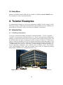
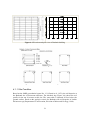
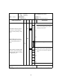
NEES Integrated Seismic Risk Assessment Framework
User Manual
Beta Version
by
Sheng-Lin Lin
Jian Li
Amr S. Elnashai
Billie F. Spencer
DEPARTMENT OF CIVIL AND ENVIRONMENTAL ENGINEERING
UNIVERSITY OF ILLINOIS AT URBANA-CHAMPAIGN
URBANA, ILLINOIS
JUNE 2011
TABLE OF CONTENTS
1. Introduction ................................................................................................................... 1 2. Installation of NISRAF ................................................................................................. 2 3. Architecture of NISRAF............................................................................................... 3 3.1 File Menu ................................................................................................................. 5 3.2 Strong Motion Menu............................................................................................... 8 3.3 Hazard Characterization Menu............................................................................. 9 3.3.1 Seismic Hazard Analysis ................................................................................... 9 3.3.2 Synthetic Time History .................................................................................... 16 3.3.3 Hazard Map Generation ................................................................................. 20 3.4 Structure Model Menu ......................................................................................... 22 3.4.1 Import from Zeus file ...................................................................................... 22 3.4.2 New Model ...................................................................................................... 23 3.4.3 New Model from Template .............................................................................. 24 3.4.4 View................................................................................................................. 24 3.4.5 Structure Model .............................................................................................. 29 3.5 Model Calibration Menu ...................................................................................... 35 3.5.1 Modal Analysis................................................................................................ 35 3.5.2 System Identification ....................................................................................... 36 3.5.3 Model Updating .............................................................................................. 37 3.6 Hybrid Simulation Menu ..................................................................................... 38 3.6.1 Dynamic Load ................................................................................................. 39 3.6.2 Static Load ...................................................................................................... 40 3.6.3 Hybrid Model .................................................................................................. 40 3.6.4 Simulation ....................................................................................................... 45 3.6.5 Results ............................................................................................................. 46 3.7 Fragility Analysis Menu ....................................................................................... 47 3.7.1 Define Limit States .......................................................................................... 47 3.7.2 Run Hybrid Simulation ................................................................................... 48 3.7.3 Hybrid Fragility Curves.................................................................................. 48 3.8 Impact Assessment Menu ..................................................................................... 49 3.8.1 MAEviz ............................................................................................................ 49 3.8.2 HAZUS ............................................................................................................ 49 3.9 Help Menu ............................................................................................................. 50 4. Tutorial Examples....................................................................................................... 50 4.1 Introduction ........................................................................................................... 50 4.1.1 Building Information....................................................................................... 50 4.1.1 Site Condition.................................................................................................. 51 4.2 Strong Motion........................................................................................................ 53 4.3 Hazard Characterization...................................................................................... 53 4.3.1 Synthetic Ground Motion ................................................................................ 53 4.3.2 Hazard Map .................................................................................................... 55 4.4 Structure Model .................................................................................................... 56 4.5 Model Calibration ................................................................................................. 56 4.5.1 System Identification ....................................................................................... 56 4.5.2 Model Updating .............................................................................................. 57 ii
4.6 Hybrid Simulation & Fragility Analysis ............................................................. 59 4.6.1 Performance Limit State ................................................................................. 59 4.6.2 Seismic Input ................................................................................................... 59 4.6.3 Hybrid Simulation ........................................................................................... 59 4.6.4 Hybrid Fragility Analysis ............................................................................... 60 4.7 Impact Assessment ................................................................................................ 62 5. Reference ..................................................................................................................... 63 iii
NISARF Update History
April 2010

Hazard@NISRAF Beta Version release

NISRAF Beta Version release
June 2011
iv
1. Introduction
NEES Integrated Seismic Risk Assessment Framework (NISRAF), a completed
MATLAB (The MathsWork, Inc.) GUI-driven software platform has been developed for
the purpose of making impact assessment more efficient and more reliable. Several
components—instrumentation, advanced hazard characterization, system identification,
model updating, hybrid simulation, advanced hybrid fragility analysis and impact
assessment tool—have been implemented and tailored with novel methods to build the
seamless, transparent and extensible framework. Below, the architecture, methodologies,
communication protocols and analysis platforms of NISRAF are discussed first. Next, a
tutorial of NISRAF will be presented.
This document is available only for the beta version of NISRAF. The beta version of
NISRAF is released to get feedback from various users for improvement of NISRAF.
There could be unexpected bugs in the beta version of NISRAF, so it is desirable to use
NISRAF only for simulation cases. If there are any questions or comments, please feel
free
contact
with
main
developers
of
NISRAF
(Sheng-Lin
Lin,
[email protected] ; Jian Li, [email protected]).
1
2. Installation of NISRAF
To install NISRAF, run the executable installation file (i.e., NISRAFSetup.exe). When
you install software, do not change the default folder location. The software should
be installed in C:\NISRAF. After installation is complete, the user should be able to run
the examples illustrated in this document.
The installed NISRAF folder should be in the search path of MATLAB. To update
MATLAB path, run a MATLAB and click File-Set Path-Add with Subfolders in the
menu bar and select C:\NISRAF and click OK button.
NISRAF has been developed based on MATLAB R2009a (v7.8.0), so there could be
unexpected bugs when it is running in lower version of MATLAB.
2
3. Architecture of NISRAF
As shown in Figure 3-1 and Figure 3-2, free-field measurements (I1) along with
nonlinear site response analysis (SR) are used to generate the advanced hazard map and
ground motion records (AH). The measured and synthetic records are then used in hybrid
simulation and fragility analysis. Meanwhile, the structural model is calibrated with the
measured structural response (I2). Next, hybrid simulations (HS) are performed with the
most critical component of the structural system tested in the laboratory and the
remainder of the structure simulated analytically. These simulations are conducted to
derive the mean seismic intensity value (PGA, for example) of the corresponding
performance limit state. The fragility curves (FA) of the structure are then generated
using the hybrid simulation data and the dispersions from the literature. Finally, the
hybrid fragility curves and the calibrated hazard map are fed into the impact assessment
tool, such as MAEviz or HAZUS (IA).
Figure 3-1 Schematic of the proposed integrated framework
3
Figure 3-2 Architecture of NISRAF
Clearly, NISRAF is composed of five main parts: namely, (i) instrumentation (I1, I2), (ii)
seismic hazard analysis (AH), (iii) model calibration and hybrid simulation (HS), (iv)
fragility analysis (FA) and (v) earthquake impact assessment (IA). For ease of use, nine
main menus with submenus are designed and arranged, following the analysis sequences
(Figure 3-3):
 File: Contains general menus (such as Open, Save, Save As, Page Setup, Print
Review, Print and Exit).
 Strong Motion: Provides an interface to download measured data from
instrumentation databases (ANSS, COSMOS, CESMD and PEER).
 Hazard Characterization: Contains three menus (Seismic Hazard Analysis,
Synthetic Time Histories and Hazard Map Generation) to perform hazard analysis.
 Structure Model: Contains five menus (Import from ZEUS File, New Model
from Template, New Model, View and Structure Model) to import, develop and
view the FE model.
 Model Calibration: Contains three menus (Modal Analysis, System Identification
and Model Updating) to improve the FE model.
 Hybrid Simulation: Contains five menus (Dynamic Load, Static Load, Hybrid
Model, Simulation and Results) to develop the hybrid model, run simulation and
check results.
4



Fragility Analysis: Contains three menus (Define Limit States, Run Hybrid
Simulation and Hybrid Fragility Curves) to derive hybrid fragility relationships
through hybrid simulation testing.
Impact Assessment: Contains two menus (MAEviz and HAZUS) to perform the
earthquake impact assessment.
Help: Contains three menus (NISRAF Manual, UI-SIMCOR Manual, and About
NISRAF) to assist users in performing the analysis. Copyright and version
information are also included here.
Figure 3-3 Welcome window and main window of NISRAF
In NISRAF, each main menu is modularized. Moreover, each method and algorithm
implemented in sub-menu is also developed in module unit. This module feature makes it
easy to understand analysis algorithms as well as to maintain this versatile and integrated
program. Most importantly, it enables the latest research finding and computation
techniques to be easily implemented. Below, development of each main menu is
presented with a focus on the novel manners used to tailor and integrate components to
build the seamless framework.
3.1 File Menu
File menu contains the general menus, such as Open, Save, Save As, Page Setup, Print
Review, Print and Exit, as shown in Figure 3-4. These submenus provide the basic
functionalities to manage files, such as opening an existing file, saving and printing the
current working file, and exiting and closing NISRAF.
5
Figure 3-4 File submenus

File-Open: Open existing NISRAF file
When existing NISRAF file is opened, NISRAF data (strong motion, hazard, structural
information, fragility, and other information) will be loaded.

File-Save: Save NISRAF data
Current NISRAF data will be saved in as default file name (i.e., NISRAF_User.mat).
6

File-Save as: Save NISRAF data as user defined file name
Current NISRAF data will be save in user defined file name (i.e., filename.mat).

File-Page Setup: Setup page for printing

File-Print Preview: Print preview
7

File-Print: Print NISRAF GUI

File-Exit: Exit NISRAF
3.2 Strong Motion Menu
In Strong Motion menu, as shown in Figure 3-5, the user is prompted to connect to a
web-based instrumentation database. Through this linkage, the user can easily download
records. Meanwhile, NISRAF allows the user to create a new folder to deposit the
downloaded records as well as other basic project information, which facilitates
maintenance. Two different types of records are required to perform analysis in NISRAF.
Ground motion (free-field) records are used to calibrate hazard models, while structural
measurements are used to calibrate structural models. The incorporation of the
instrumented data into NISRAF is not only to increase its usage, but also to improve
hazard and structural model.
8
Figure 3-5 Strong motion data GUI in Strong Motion menu
3.3 Hazard Characterization Menu
Hazard characterization menu is composed of three main parts: namely, Seismic Hazard
Analysis, Synthetic Time Histories and Hazard Map Generation, as shown in Figure 3-6.
Methodologies and analysis procedures of hazard characterization analysis have already
been illustrated and verified in Lin (2010). One of the features of the proposed advanced
hazard analysis approach is its ease of use. By tailoring the hazard models as well as
ensuring connection and compatibility between them, it simplifies the complicated and
tedious procedures in the conventional analysis. Consequently, with an interactive
interface to define inputs, hazard analysis becomes efficient and straightforward. Below,
analysis procedures in the three submenus are presented with GUIs and illustrations.
Figure 3-6 Hazard Characterization submenus
3.3.1 Seismic Hazard Analysis
In Seismic Hazard Analysis, user can check the natural records on the surface, and
perform local site effect for records on the bedrock. After clicking Seismic Hazard
Analysis, user will be prompted to select project for analysis. Based on the selected
project, NISRAF will list all the information and recorded strong motions for this
9
structure. Afterward, users can check the surface records or perform local site effect on
the bedrock records.

Click Set to confirm the selected project (i.e., 6-story steel MRF building,
Burbank, CA).

Choose surface motions and/or bedrock motions for further analysis. Click Set to
confirm.
10
3.3.1.1 Surface motions

Click Select ground motions

Select surface motions, click Done to continue
11

Click Check results to check time history and response spectra for the selected
motion
12
3.3.1.2 Bedrock motions

Click Select ground motions

Select bedrock motions for analysis, Click Done to continue
13

Click Site response analysis

Before performing site response analysis, user need to define soil profiles and
material properties
To define soil profiles and material properties, user can import input files for DEEPSOIL
(*.dp files, for example, Burbank_DP_2.dp and Burbank_NLPara_2.dp in
14
C:\NISRAF\Hazard\Projects\Burbank) or define step by step. Users need to follow the
number of each panel to fill in all the parameters. For more information about each
parameter, users can refer to the user manual of DEEPSOIL (Hashash et al., 2009).
After defining all the parameters, a DEEPSOIL file (*.dp) will be generated and saved
into current folder.

After that, NISRAF will perform site response analysis

Click Check results to check surface motions with local site effect
15
3.3.2 Synthetic Time History
NISRAF allows user to generate synthetic time histories for three different hazard levels
(i.e., 10%/50 yrs PE, 5%/50 yrs PE, or 2%/50 yrs PE). The following describes more
details for each step and the required information.


Select the hazard level for synthetic time histories, click Set to continue
Response spectrum generation, users can generate spectrum by NGA model or
define the spectrum by discrete points

Using NGA model to generate spectrum:
Here user only provides parameters for Seismic Source and Site Condition panels.
Click Set to save parameters and check duration and spectrum for each hazard
level, and click Done to next step.
User can get information for seismic source panel by conduct deaggregation
analysis for the project site.
16

User specify spectrum:
Here user can define spectrum by importing from *.txt files or define the discrete
points through the interface.
When importing from .txt files, users need to pay attention the format requirement
for
the
files.
Please
refer
to
Burbank_Sa&duration.txt
under
C:\NISRAF\Hazard\Projects\Burbank for the compatible format.

Click Customize synthetic GMs to define the intensity function for synthetic
ground motions
17
For Site Condition panel, users decide if the site response analysis will be considered or
not. Users need to provide soil profiles and material properties if the site response
analysis is considered. Please refer to section 3.3.1.2 for more detail about the definition
of soil condition.
18

Click Site Response to conduct local site effect. GMs with different duration will
be generated and saved as *.txt files in C:\NISRAF\StrongMotion\[Project
name]\Synthetic Ground Motion

Click Site Response to conduct local site effect. GMs with different duration will
be generated and saved as *.txt files in C:\NISRAF\StrongMotion\[Project
name]\Synthetic Ground Motion\Syn_Conv
19

After all the analysis, users can check the time histories and response spectrum for
each ground motion.
3.3.3 Hazard Map Generation
NISRAF allows user to generate hazard map for deterministic event. The following
describes more details for each step and the required information.
 First, user need to provide parameters for the scenario event.
 Second, define parameters for synthetic ground motions and site condition (please
refer to previous section for more detail)
 In addition, users need to provide information for the boundary of the map and the
size of cell.
 After defining all the parameters, hazard map will be generated and saved into
current folder (*.asc)
20
21
3.4 Structure Model Menu
The finite element model is a prerequisite for model calibration. To create an FE model,
the user is allowed to import an existing ZEUS-NL model or create a new model in
NISRAF. Submenus for creating an FE model (such as Import from Zeus file, New
Model from Template, New Model, View and Structural Model) are based on
SimBuild (Park et al., 2007), a pre- and post-processor for UI-SIMCOR.
Figure 3-7 Structural Model submenus
3.4.1 Import from Zeus file
NISRAF allows user to import existing Zeus file and transfer all the structural
information required for NISRAF.

After clicking Import from Zeus file, select the existing Zeus file
22

NISRAF collect structural information from Zeus file and present through its
interactive interface
3.4.2 New Model
NISRAF allows user to create new structure model.



User can select structure type as building or bridge.
Bridge type structure is implemented as test purpose in this version of NISRAF,
so there could be unexpected bugs in the bridge structure.
If building type is selected, following GUI for creating building structure will be
shown.
23

When structure is created, NISRAF GUI is updated as follows.
3.4.3 New Model from Template
NISRAF also allows user to create structure model from template.

If building type is selected, following GUI will be shown.

This menu is similar to Structure Mode/New Model, but more simple which the
properties will be defined as same as all components (i.e., bay length, story height,
frame distance).
3.4.4 View
User can check the structural information such as node, element, boundary condition, and
others by using View menu. Hybrid model including simulation platform of each
substructure can be shown in this menu by using Hybrid Model submenu. Disabled
submenus will be enabled when it is available.
24
Figure 3-8 View submenus

View-Skeleton View: Skeleton view of structure

View-Extruded View: Extruded view of structure
25

View-Mass: View or hide nodal mass

View-Node: View or hide node number and coordinate
26

View-Element: View or hide element number

View-2D View-XY or YZ or ZX: 2D view of structure
27

View-3D View: 3D view of structure

View-Hybrid Model: view or hide hybrid model (this submenu will be enabled
when setting up the hybrid model is finished)

View-Status Bar: View or hide status bar

View-Clear View: Clear view except structure
28
3.4.5 Structure Model
The default structure properties can be seen and updated by using Structure Model
menu. For example, user can update material, section, node, element, connectivity,
boundary condition, mass, and damping properties. User can also refine mesh for
simulation module by using Refine Mesh submenu.
Figure 3-9 Structure Model submenus

Structure Model-Material: Edit or add new material
User can update existing material properties or add new materials. ‘stl1’ and ‘con2’
materials defined in Zeus are available in this version of NISRAF. More materials will be
available in the later version.
29

Structure Model-Section-Edit: Edit or add new section
User can update existing material properties or add new materials. ‘css’, ‘rss’, ‘sits’, and
‘rcrs’ sections defined in Zeus are available in this version of NISRAF. More sections
will be available in the later version.

Structure Model-Section-Assign-Update: Update section properties of structure

Structure Model-Section-Assign-One by One: Assign section by selecting element
30

Structure Model-Section-Assign-Table: Assign section by using table

Structure Model-Node: Update nodal coordinates
31

Structure Model-Element-Add: Add element

Structure Model-Element-Remove: Remove element
32

Structure Model-Element-Connectivity: Update element connectivity

Structure Model-Refine Mesh: Refine mesh for simulation module (this submenu
will be enabled after defining substructure)

Structure Model-Boundary Condition-Default: Set the boundary condition as
default. For building type structure, nodes which attached ground (i.e., y=0) will
be fixed in all direction. For bridge type structure, nodes which attached ground
and two abutment nodes will be fixed in all directions except x- and rz-DOF of
right abutment node.
33

Structure Model-Boundary Condition-One by One: Set the boundary condition of
selected node. When node is selected, following GUI will be shown.

Structure Model-Mass: Update nodal mass
34

Structure Model-Damping: Define damping. Only Rayleigh damping is supported
in this version. More options for damping will be available for later version.
3.5 Model Calibration Menu
An automatic approach for system identification and model updating is developed and
incorporated into NISRAF. Based on the instrumented data, the finite element model
defined in previous section can be calibrated in NISRAF analysis platform.
Figure 3-10 Model Calibration submenus
3.5.1 Modal Analysis
Before conducting system identification and model updating, the Modal Analysis allows
user to check the modal information of structure (i.e., the mode shape and frequency).
User is allowed to define the number of interested modes, deformation multiplier, line
type, and 2D/3D view.
35
3.5.2 System Identification



The first step in System Identification is to import the instrumented sensor data.
Next, downsampling factor is defined to downsample raw data.
After that user need to locate the input and output channels to the related
structural nodes.

The second step in System Identification is to perform system identification via
ERA method.
36

After System Identification is completed, user can check the results.
3.5.3 Model Updating

The first step in Model Updating is to define the candidate parameters and
identified modes.
37



Next, an optimization algorithm is defined by user to conduct model updating.
After defining objective function, NISRAF will perform model updating.
User can check the progress and results during and after analysis.
3.6 Hybrid Simulation Menu
Under Hybrid Simulation Menu, NISRAF will assist user to create hybrid model
including definition of substructures, platform of simulation parts and auxiliary module
(i.e., cameral and data acquisition system). User can select element and/or joint to assign
element to substructure. Furthermore, unassigned elements of structures will be assigned
to the empty substructure by using Auto Assignment submenu.
Figure 3-11 Hybrid Simulation submenus
38
3.6.1 Dynamic Load
Loading scenarios for hybrid simulation can be defined in this menu. Existing loading file
can be used or user can create load.
Figure 3-12 Dynamic Load submenus

Hybrid Simulation-Dynamic Load-Define-From FIle: Open existing load file

Hybrid Simulation-Dynamic Load-Define-Create: Create loading history using
table

Hybrid Simulation-Dynamic Load-Assign-x-dir (or y-dir, z-dir, rx-dir, ry-dir, rzdir): Assign load in any direction.
39
3.6.2 Static Load
Assign static (gravity) load when conducting hybrid simulation. Only static load applied
by importing Zeus file is allowed in current version NISRAF.
3.6.3 Hybrid Model
After defining the load, under Hybrid Model menu, user will be prompted to define
substructures, analysis platform and auxiliary for hybrid simulation.
Figure 3-13 Hybrid Model submenus
 Hybrid Simulation-Hybrid Model-Define Substructure: Define substructure
First, the number of substructure should be defined. Then panel for general information
will be enabled.
40
General information of substructure such as name, communication protocol, IP and port
number can be defined in this panel. Three communication protocols, such as TCPIP,
LabView1 and LabView2 are available in this version of NISRAF.
If Auto Generation button is clicked, the name, protocol, and URL of each substructure
are defined automatically as follow.
Once general information is defined, this panel will be disabled and panel for advanced
information of substructure will be enabled.
There are four methods to assign elements to the substructure. User can select any
element and/or joint to assign element to the substructure. If user knows specific element
number, then use can type in the element box. Finally, all of unassigned elements can be
assigned to the empty substructure by clicking Auto Assignment button. This is same
function of Hybrid Model-Assign Substructure-Select Element or Select Joint or
Auto Assignment. These will be explained in the later.
41
If Select Element option is selected, following, user can select any element of structure.
The selected element is updated into element box. User can add more elements. After
defining elements, click Create Substructure button to save the defined substructure.
User can continue to define another substructure if applicable.
Meanwhile, user can use experimental template to load predefined setup of experimental
facilities. If Exp Template button is clicked, following GUI will be shown. It’s
recommended to check all the experimental setup before running test in the laboratory.
42
 Hybrid Simulation-Hybrid Model-Assign Substructure-Select Element: Assign
selected element to substructure. When the element is selected, following GUI
will be shown.
The selected element is highlighted. Also, the selected element number and available
substructure number are shown. User can update mass and effective DOFs of each node.
The first node of this element is one of boundary condition which all DOFs are fixed, so
effective DOFs check boxes of this node (i.e., Node 1) are disabled.
 Hybrid Simulation-Hybrid Model-Assign Substructure-Select Joint: Assign
element to substructure by selecting joint. When joint is selected, following GUI
will be shown.
43
When any joint is selected, adjacent elements will be divided into two to move mass on
joint node to end node. The selected joint number and available substructure number are
displayed. User needs to update effective DOFs.
 Hybrid Simulation-Hybrid Model-Assign Substructure-Auto Assignment: Auto
assignment of the unassigned element to empty substructure. This is very useful
when the structure is complicated.
 Hybrid Simulation-Hybrid Model-Define Platform: Define platform of each
substructure.
User can define platform of substructure as Zeus-NL, OpenSees, FedeasLab, Abaqus, and
Experiment. Currently, Zeus-NL, OpenSees, FedeasLab, and Experiment platform are
available in this version. If the platform of substructure is defined as Zeus-NL, OpenSees,
and FedeasLab (i.e., simulation module), the required files for hybrid simulation
(conducted by UI-SimCor) such as input file of static analysis module and configuration
44
file will be generated automatically within the folder which name is same as name of
substructure. If ‘Experiment’ is selected as platform, only folder which name is same as
name of substructure will be created.
 Hybrid Simulation-Hybrid Model-Auxiliary-Camera (or DAQ): Define camera or
DAQ module. Only camera module is supported in this version. DAQ module
will be supported in the later version.
3.6.4 Simulation
After defining the load and substructures, under Simulation menu, user will be prompted
to run hybrid simulation.
Figure 3-13 Simulation submenus

Hybrid Simulation-Simulation-Error Check: Check error of hybrid simulation
environment.
45

Hybrid Simulation-Simulation-Elastic Analysis (verification): Allow user to run
static or dynamic analysis to verify the defined hybrid model.

Hybrid Simulation-Simulation-UI-SimCor Simulation: After define and/or update
the required information, NISRAF will be ready to conduct hybrid simulation.
3.6.5 Results
After finishing hybrid simulation, NISRAF allows user to check simulation results
through displacement/force history plot, animation, and photos if applicable.
46
3.7 Fragility Analysis Menu
Fragility Analysis menu is composed of three main parts: namely, Define Limit States,
Run Hybrid Simulation and Hybrid Fragility Curves, as shown in Figure 3-14.
Methodologies and analysis procedures of fragility analysis can be found in Lin (2010).
One of the features of the proposed advanced fragility analysis approach is its ease of use.
With structural information available from Structural Model, the user defines interested
Interstory drift angle (ISDA) through the interactive structural model. Meanwhile, when
performing hybrid simulation in order to derive mean seismic intensity, NISRAF
calculates ISDAs, compares with target ISDA, calculates scale factor, and asks to
continue the next simulation. The above designs avoid the heavy and tedious calculations.
The “hold on” feature allows the user to have time to replace the experimental specimen
in the laboratory, which is really a useful and practical design.
Figure 3-14 Fragility Analysis submenus
3.7.1 Define Limit States


To derive hybrid fragility curves, user need to define parameters and select time
history for interested performance levels.
For building type, the interstory drift (ISD) is used to make comparison between
the target performance level and the hybrid simulation results. Therefore, user is
prompted to define information of the interested ISDs (i.e., the up and bottom
node).
47
3.7.2 Run Hybrid Simulation

After finishing the definition of limit states and the setup of hybrid simulation (i.e.,
substructure, platform, and others), NISRAF will run hybrid simulation in order to
derive fragility curves.
3.7.3 Hybrid Fragility Curves

After several hybrid simulation tests in order to meet the target performance
levels, NISRAF will based the mean PGA value and the dispersion defined by
user to generate the interested fragility curves. The derived fragility curves are
compatible and ready to be used in MAEviz.
48
3.8 Impact Assessment Menu
Finally, fragility curves from Fragility Analysis and the hazard map from Hazard
Characterization are fed into earthquake impact assessment packages (MAEviz, for
example) to evaluate the seismic loss (Figure 3-15).
Figure 3-15 Impact Assessment submenus
3.8.1 MAEviz

The first step to perform MAEviz under NISRAF is to ingest the generated hazard
map and fragility curves into MAEviz. Both hazard map and fragility curves are
compatible with MAEviz, no additional format transformation is required.

Once the required information is fed, user can perform all the functions of
MAEviz under NISRAF in order to evaluate the seismic losses.
3.8.2 HAZUS
HAZUS is not available in this version of NISRAF.
49
3.9 Help Menu
Manuals of NISRAF and UI-SIMCOR are available. In addition, About NISRAF states
the copyright as well as version information.
4. Tutorial Examples
An instrumented building was selected to demonstrate NISRAF in this example. In the
following sections, background information about this building and site conditions are
presented first. Thereafter, step by step analysis in NISRAF is performed.
4.1 Introduction
4.1.1 Building Information
A six-story commercial building in Burbank, California (latitude = 34.185°, longitude = 118.308°), was selected for this study (Figure 4-1). This is a steel moment resisting frame
building, in which the perimeter frames are the primary lateral load resisting system, and
the internal frames are only resisting gravity load, as shown in Figure 4-2. Reference is
made to Anderson and Bertero (1991) for detailed information about this building. This
building is instrumented by the California Strong Motion Instrumentation Program (CGS
- CSMIP Station No. 24370) in 1980 with 13 sensor channels as shown in Figure 4-3.
Several significant earthquakes were captured, such as Whittier (1987), Sierra Madre
(1991) and Northridge (1994). Data are available in the Center for Engineering Strong
Motion Data (CESMD, www.strongmotioncenter.org).
Figure 4-1 Photo of 6-story steel moment frame building in Burbank, California
50
Figure 4-2 Elevation and plan view of Burbank building
Figure 4-3 Sensor location of Burbank building (CESMD)
4.1.1 Site Condition
Based on the SMIP geotechnical report No. 131 (Fumal et al., 1979), the soil deposits at
the Burbank site is Pleistocene alluvium. The borehole log (Figure 4-4) shows the soil
profile for the top 30 meters at this site. The water table is assumed 20 feet below the
ground surface, based on the geologic criteria for Burbank with soil deposits of similar
Pleistocene age (Department of Conservation, Division of Mines and Geology, 1998).
51
Log
Depth
(meters)
Graphic
Sampling
GEOLOGIC Qc
MAO UNIT: Pleistocene alluvium
Foot
Blows/
SAMPLE DESCRIPTION
Density
DATE: 8/1/79
HOLE No. 31
SITE: BURBANK FIRE STATION
LOCATION:
Lat. 34°10'50"
Long. 118°18'15"
QUADRANGLE:
BURBANK, CA
(gm/cc)
ALTITUDE: 610'
0
10
FINE SANDY LOAM, dk, bBrown,
occasional v. coarse sand and
gravel, medium plasticity, moist,
loose.
DESCRIPTION
FINE SANDY LOAM, dk. Brown, some v.
coarse sand and fine gravel, medium
plasticity, moist, loose.
5
10
40/6"
SANDY LOAM, brown, poorly
sorted, mostly finer than coarse
sand, some granitic gravel, v.
dense.
GRAVELLY SAND, granitic.
15
2.16
SANDY LOAM and LOAMY SAND, dk.
Brown, poorly sorted, slight plasticity,
20 quick, moist, occasional fine gravel to
5mm.
P
SANDY LOAM and LOAMY SAND,
dk. Brown, poorly sorted, slight
plasticity, quick, moist, occasional
fine gravel to 5 mm.
25
30
COMMENTS:
Figure 22
LOGGED BY: T. Fumal
39
Figure 4-4 Borehole log of the Burbank site (adapted from Fumal et al., 1979)
52
4.2 Strong Motion
Either Strong Motion or Structure Model must be the first step in NISRAF. Strong
Motion was selected as the first step in this example. Through the linkage to webdatabase, free-field station records around the Burbank building site and structural sensor
histories during the past earthquakes were downloaded and deposited in NISRAF. After
that, an interactive window with already-downloaded information allows user to add
some information (background, description and image), as shown in Figure 4-5.
Figure 4-5 GUI to manage project and downloaded records
4.3 Hazard Characterization
With instrumented strong-motion records from Strong Motion, the Hazard
Characterization analysis was undertaken. Synthetic ground motions with various
hazard levels were generated for further use in Hybrid Simulation and Fragility
Analysis. The hazard map for the Northridge earthquake in the Burbank area was
generated for further use in Impact Assessment.
4.3.1 Synthetic Ground Motion
Ground motions with various hazard levels are generated based on the seismic
information specified by the users. The deaggregation results for different hazard levels
(10%, 5%, and 2% probability of exceedance in 50 years), as shown in Table 4-1 and
Table 4-2, at the Burbank site were fed into this advanced hazard method. Next, sets of
synthetic ground motions, including site response analysis and varying with duration and
hazard levels were generated automatically. These motions with compatible format were
53
further used in the hybrid simulation and fragility analysis. Figure 4-6 presents one of the
generated synthetic ground motions and its response spectrum.
Table 4-1 Deaggregation results at Burbank site
Return Period (yrs)
M
R (km) Epsilon
2%/ 50yrs
2475
6.73
6.9
1.18
5%/ 50yrs
975
6.71
8.5
0.91
10%/ 50yrs
475
6.71
10.6
0.63
Table 4-2 Contributed fault information based on deaggregation results
Name
Type
Verdugo Char
Reverse
Elysian Park Char Blind trust (reverse)
*assume
= 90°,
.
,
1
0
1
0
1
0
1
0
2
Figure 4-6 Synthetic ground motion and its response spectrum
54
4.3.2 Hazard Map
Hazard map, the exposure when calculating earthquake loss, is one of the indispensable
components of regional impact assessment. The map of PGA for the 1994 Northridge
earthquake in the Burbank area in standard gravity (g) was generated in this application.
This map is not only served to demonstrate the proposed method, but also used for impact
assessment on the selected building.
SMIP geotechnical report (Fumal et al., 1979) was used again to illustrate local site
characteristics. Step-by-step procedures to generate the hazard map were then performed.
The Northridge earthquake mechanism, the site conditions (soil profiles and material
properties) and map information (such as interested region scope and cell size) were
defined in the first step. Next, the CB-NGA (Campbell and Bozorgnia, 2008) and
duration prediction equation along with SIMQKE (Gasparini and Vanmarcke, 1976) and
DEEPSOIL (Hashash et al., 2009), were performed for each cell. Finally, PGA values
were collected and hazard map of the Burbank area was presented, as shown in Figure 47.
Figure 4-7 Hazard map at Burbank area
55
4.4 Structure Model
A finite element model was created in NISRAF, as shown in Figure 4-8. Due to the fact
that only the perimeter frames are used for the lateral load resisting system, a 2-D model
of the exterior frame was modeled to represent the whole structure. Section dimensions
and material properties for each beam and column were based on design documents.
Lumped mass was used and applied at every beam-column connection. Concrete slabs
were modeled and connected to steel girders using rigid elements, to account for their
contribution of stiffness.
Figure 4-8 2-D FE model of Burbank building in NISRAF
4.5 Model Calibration
With FE model created in Structural Model, Model Calibration is performed to tune the
FE model. Two procedures, namely, system identification and model updating, were
executed in this step.
4.5.1 System Identification
Input channels and output channels were defined first. Based on the design drawings,
exterior and interior columns are firstly supported on steel girders and reinforced concrete
girders, respectively, and both of them are in turn supported on a pair of 32 feet long and
30 inches diameter reinforced concrete piles. Therefore, it is reasonable to consider that
56
all columns are fixed. Hence, the records from the ground floor were treated as the input
motions, while other records were considered as the responses of the structure.
Consequently, channel 8 and 9 were defined as input, while channels 2 to 7 were output
channels, and, hence, the dimension of impulse function matrices was 2 by 6. Note that
channels 4 and 5 were not working properly during the Northridge earthquake of 1994.
Therefore, data from these two channels were not available and only four output channels
were available. The dimension of impulse response function matrices was 2 by 4 for the
Northridge earthquake.
The ERA method was then performed for the Northridge earthquake record. The
stabilization diagrams and the identified mode shapes were shown in Figure 4-9. The first
and second bending modes were then identified as 0.72 Hz and 2.14 Hz, respectively.
The associated damping ratios were 3.37% and 6.71% (Table 4-3).
Northridge 1994
100
80
60
60
40
40
20
20
0
0
1
2
3
Damped Natural Frequency (Hz)
Identified mode
Confirmed mode
4
0
5
Story
80
Northridge 1994
Transfer Function
Singular value retained
100
6
6
5
5
4
4
3
3
2
2
1
1
0
0
0.5
f1=0.71859Hz
1
0
-1
0
f2=2.1436Hz
Frame A-A
Transfer function
1
Frame L-L
Figure 4-9 Stabilization diagrams and identified mode shapes
Table 4-3 Frequency and δ of identified with ERA method
Mode f (Hz)
(%)
1
0.719
3.373
2
2.144
6.715
4.5.2 Model Updating
With the identified natural frequencies and mode shapes, dynamic FE model updating
was then performed to improve the FE model of the Burbank building. Selection of
candidate parameters to be updated was the first step in model updating. The selected
parameters for the Burbank building were shown in Table 4-4. To keep the physical
57
meaning of each parameter, lower and upper bounds were applied based on the degree of
uncertainties. For example, the effective widths were calculated based on AISC
specification, which was likely to be very conservative. In addition, the deflection of the
slab defined the contribution of the slab to the composite beam, thus affecting the
effective width. Therefore, the effective width of slab had large uncertainty, thus a
relatively larger range of variation (±50%) was applied.
Table 4-4 Selected parameters for model updating and updated results
Selected
Description
Parameters
2
Es (N/mm )
Young’s modulus of steel
Mass1 (1000kg)
nd
Lumped mass at 2 floor
rd
th
Initial
Bound
Updated
Change
Value
(%)
Value
(%)
2.10E+05
±5
2.21 E+05
5.00
45.65
±5
43.37
-4.99
Mass2 (1000kg)
Lumped mass at 3 -5 floor
36.53
±5
38.36
5.01
Mass3 (1000kg)
Lumped mass at top floor
54.84
±5
52.1
-5.00
762
±50
1143
50.00
914.4
±50
1371
49.93
Effective width of concrete slab
WS1 (mm)
at 2nd-5th floor
Effective width of concrete slab
WS2 (mm)
at top floor
The optimization problem defined previously was solved by the Nelder-Mead method.
The results listed in Table 4-5 show that the errors between the identified and updated
model reduced to 1% and 5.78% for the first and second natural frequency, respectively.
Meanwhile, the second mode shape was improved, which gave a value of 0.981 for the
MAC. With this refined finite element model, hybrid simulation was conducted to yield a
seismic response prediction with higher accuracy.
Table 4-5 Comparison of frequency and mode shape between the original and updated
Original FE model
Mode
frequency (Hz)
value error (%)
MAC
Updated FE model
frequency (Hz)
value error (%)
MAC
1
0.688
-4.312
0.999 0.712
-1.001
0.999
2
1.956
-8.769
0.975 2.020
-5.784
0.981
58
4.6 Hybrid Simulation & Fragility Analysis
The calibrated Burbank building model after Model Calibration and ground motions
from Hazard Characterization were used to perform the hybrid simulation and to derive
fragility curves in NISRAF.
4.6.1 Performance Limit State
Three performance limit states are specified in this step, namely, the immediate
occupancy (IO), the life safety (LS) and the collapse prevention (CP). Interstory drift
angles (ISDAs) 0.7%, 2.5% and 5% are assigned to IO, LS and CP performance level,
respectively (FEMA, 2000b).
4.6.2 Seismic Input
Ground motions representative of the local hazard characterization are essential in order
to capture the realistic structural response. In addition, various ground motions should be
considered to avoid excessive scaling on them. Excessive scaling is unrealistic and
unreasonable particularly when motion has higher earthquake intensity. Based on the
above considerations, the site specific synthetic ground motions with various hazard
levels, generated for the Burbank sits, were selected as the earthquake demand in this
example. To avoid excessive scaling, records related to 10%, 5% and 2% probability of
exceedance in 50 years hazard level are used to derive fragility curves for immediate
occupancy, life safety and collapse prevention performance limit state, respectively.
4.6.3 Hybrid Simulation
The calibrated Burbank building model and ground motions from hazard characterization
analysis were used to verify the extension of the hybrid simulation to fragility analysis as
well as the integration of hybrid simulation in earthquake impact assessment. The
calibrated 2-D structure model was divided into two sub-structures, namely, the column
(the lower part of the left exterior column at the first floor) and the frame (the remaining
structure). The frame module was simulated using Zeus-NL, while the column module—
replaced by a small scale aluminum specimen (Figure 4-10)—was tested in the laboratory.
59
Figure 4-10 Hybrid simulation with two sub-structures (column and frame)
4.6.4 Hybrid Fragility Analysis
Based on the lognormal distribution assumption, mean value of seismic intensity from
testing along with dispersions from literature are used to derive the hybrid fragility curves.
In this study, mean value of PGA from hybrid simulation tests and dispersions from
literature (FEMA, 2000a; Cornell et al., 2002; Yun and Foutch, 2000) were used to derive
the fragility curves for this 6-story steel building in Burbank. In the following section,
mean PGA values from hybrid simulation tests are presented first, followed by
discussions on the dispersions found in literature.
4.6.4.1 Mean PGA Values from Hybrid Simulation
Hybrid simulation results under different synthetic ground motions (10%, 5% and 2%
probability of exceedance in 50 years for immediate occupancy, life safety and collapse
prevention performance levels, respectively) were used to derive the mean PGA value for
each performance level. Step-by-step procedure to derive mean PGA value is given
below:
 Step 1: 10% probability of exceedance in 50 years ground motion is selected as
seismic input for hybrid simulation to derive mean PGA value for immediate
occupancy limit state.
 Step 2: Interstory drift angle (ISDA) is calculated based on testing results.
Comparison of ISDA between the calculated one and the target one (0.7% ISDA
for immediate occupancy performance limit state, for example) is then made.
 Step 3: Hybrid simulation is resumed (replaced with new specimen if nonlinear
behavior occurs in previous test) with seismic input multiplied by a scale factor
(calculated based the difference in Step 2), if the difference exceeds criterion (±5%
difference, for example).
 Step 4: Iterations from Step1 to Step 3 continues till the criterion is met.
 Step 5: Once the calculated ISDA matches the defined ISDA, PGA value of
current (scaled) record is assigned as the mean PGA value for immediate
occupancy performance limit state.
60
The above procedure is an example of how to drive the fragility curve for IO limit state,
while similar procedures were applied to derive curves for LS and CP limit states using 5%
and 2% probability of exceedance in 50 years ground motions, respectively.
Figure 4-11 shows the number of hybrid simulation tests used to derive the mean PGA
values. Table 4-6 lists the target ISDA (ISDA, interstory drift angle, are defined in
previous section for this study) as well as the mean PGA values from hybrid simulation
tests.
Interstory Drift Angle
0.05
0.025
Immediate Occupancy
Life Safety
Collapse Prevention
0.007
0
1
2
3
Number of Hybrid Simulation
4
5
Figure 4-11 Number of hybrid simulation tests to derive fragility curves
Table 4-6 Interstory drift angle (target ISDA) and PGA from hybrid simulation tests
Performance Level
Immediate
Life
Collapse
Occupancy Safety Prevention
Interstory drift angle (%)
0.7
2.5
5.0
Mean PGA (g)
0.545
1.627
2.777
4.6.4.2 Dispersions from Literature
Dispersion, a statistics vocabulary, represents the uncertainty term in fragility
relationships. Due to the limited number of tests in the hybrid fragility analysis, it is
unreasonable and also unrealistic to regress dispersion based on few testing results.
Therefore, dispersions of the proposed hybrid fragility analysis are found from the
literature.
FEMA 350 (FEMA, 2000a), the recommended seismic design criteria, is specially
developed for new steel moment frame buildings. In FEMA 350, as well as in the
literature (Cornell et al., 2002; Yun and Foutch, 2002), a method used to evaluate seismic
61
behavior of steel moment frame buildings is proposed. Within this method, uncertainties
for different building height, beam-connection type, analysis procedure (linear or
nonlinear, static or dynamic), and local and global failures under different performance
levels (IO and CP) are tabulated (Table A-3 in FEMA 350) or illustrated in the content.
Table 4-7 lists dispersions which will be utilized to derive hybrid fragility curves.
Table 4-7 Mean PGA value and dispersions for mid-rise steel building fragility curves
Performance Level
Dispersion
Immediate
Life
Collapse
Occupancy Safety Prevention
0.311
0.328
0.346
4.6.4.3 Hybrid Fragility Curves
Finally, based on mean PGA value and dispersion, and following lognormal distribution
assumption, fragility curves were generated and are shown in Figure 4-12.
Figure 4-12 Hybrid fragility curves for mid-rise steel moment resisting frame building in
Burbank
4.7 Impact Assessment
Finally, with the generated compatible hazard map and fragility curves, MAEviz under
NISRAF was conducted to perform earthquake impact assessment (Figure 4-13). Only 15%
probability for damage occurred in the immediate occupancy limit state. The results met
with the post-earthquake report made by Applied Technology Council (ATC, 2001),
which reported slight damage observed to this building from the Northridge earthquake.
62
Figure 4-13 Impact assessment for Burbank building in MAEviz
5. Reference
Anderson, J. C. and Bertero, V. V., 1991. Seismic performance of an instrumented sixstory steel building, Report UCB/EERC-91/11, University of California, Berkeley, CA
Applied Technology Council, 2001. Database on the performance of structures near
strong-motion recordings: 1994 Northridge, California, earthquake, Report No. ATC-38,
Redwood City, CA
Campbell, K. W. and Bozorgnia, Y., 2008. “NGA Ground Motion Model for the
Geometric Mean Horizontal Component of PGA, PGV, PGD and 5% Damped Linear
Elastic Response Spectra for Periods Ranging from 0.01 to 10 s,” Earthquake Spectra,
24(1): 139-172
Cornell, C. A., Jalayer, F., Hamburger, R. O., and Foutch, D. A., 2002. “Probabilistic
Basis for 2000 SAC Federal Emergency Management Agency Steel Moment Frame
Guidelines,’’ Journal of Structural Engineering, 128(4): 526-533.
Department of Conservation, Division of Mines and Geology, 1998. Seismic hazard zone
report for the Burbank 7.5-minute quadrangle, Los Angeles County, California, Seismic
Hazard Zone Report 016
63
Federal Emergency Management Agency, 2000a. Recommended Seismic Design Criteria
for New Steel Moment-Frame Buildings, Report No. FEMA-350, Washington D.C.
Federal Emergency Management Agency, 2000b. Prestandard and Commentary for the
Seismic Rehabilitation of Building, Report No. FEMA-356, Washington D.C.
Fumal, T. E., Gibbs, J. F., and Roth, E. F., 1979. In-situ measurements of seismic velocity
at 19 locations in the Los Angeles, California region, SMIP geotechnical report No. 131,
U.S. Geological Survey
Gasparini, D. A. and Vanmarcke, E. H., 1976. Simulated Earthquake Motions
Compatible with Prescribed Response Spectra, Evaluation of Seismic Safety of Buildings
Report No.2, Massachusetts Institute of Technology
Hashash, Y., Groholski, D.R., Phillips, C.A., and Park, D., 2009. DEEPSOIL V3.5beta,
User Manual and Tutorial, Department of Civil and Environmental Engineering,
University of Illinois at Urbana-Champaign, Urbana, IL
Li, J., Lin, S. -L., Zong, X., Spencer, B. F., Elnashai, A. S. and Agrawal, A. K., 2009.
“An Integrated Earthquake Impact Assessment Framework,” ANCER Annual Meeting,
August 13-14, Urbana, IL
Lin, S.-L. 2010. An Integrated Earthquake Impact Assessment System, Ph.D. dissertation,
Civil Engineering, University of Illinois at Urbana-Champaign, Urbana, IL
Park, K. S., Kwon, O. S., Spencer, B. F., Elnashai, A. S., 2007. Tutorial for Beta version
of SimBuild, Pre- and Post-processor for UI-SimCor, Department of Civil and
Environmental Engineering, University of Illinois at Urbana-Champaign, Urbana, Illinois.
Yun, S. Y., and Foutch D. A., 2000. Performance prediction and evaluation of low
ductility steel moment frames for seismic loads, SAC Background Document SAC/BD00/26, Richmond, CA: SAC Joint Venture.
64