1
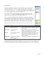
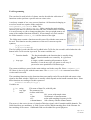
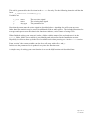
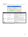
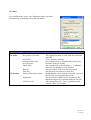
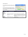
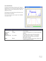
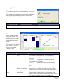
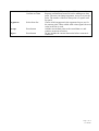
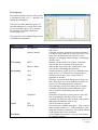
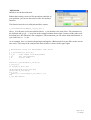
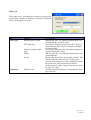
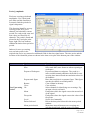
NTNU Norwegian University of Science and Technology Faculty of Engineering Science and Technology Department of Marine Technology AnalyseThis User Manual General Installation Main Window Tool Programming Load Data_v01 SaveData ImportWithWizard MatrixCalibration SelectTimeWindow AverageTimeSeries PowerSpectra MyFunction Filter_v01 Period_Amplitude 1 1 2 3 5 6 7 8 9 10 12 13 14 15 General Analysethis is a Matlab function package for analyzing time series measurements. The idea is to provide a graphical interface to common operations. The package is highly modular, and programming of new functionality should be possible without in depth knowledge of Matlab. The functions are written on windows platform, but if you are lucky it works on Linux platforms too. Installation To install the package, copy the folder AnalyseThis_v02 to a suitable location. Then start Matlab and select Set Path… from the File menu. Browse and select the AnalyseThis_v02 folder and press the button Add with Subfolders. Then save and close the window, and the package should be ready to use. The main window is started by writing analysethis on the Matlab command line. Address NO-7491 Trondheim Location O. Nielsens vei 10 Tel. Fax +47 73 59 55 01 +47 73 59 56 97 Page 1 of 16 user manual Main Window The function of the main window is to setup which files to process and what to do with them. All settings are stored in a setup (*.mat) file, which are opened and stored through the Setup File item on the main window menu. By checking the Time Series item in the Window menu, the current time series are plotted each time something happens in the window, like running a tool. The select file section of the main window lists the files to be processed. Press Selected Files to browse through paths and apply UNIX style name filters. Mark the files you want listed in the main window and press Ok. The To Do section of the main window allows you to work on the time signals. Through the buttons on the bottom you can add new and remove listed tools, change the tool settings, and rearrange the order of application. Note that the first item in this list must be a function that can load a time signal from a file. The call syntax is different for this item than the following, see the section on tool programming. In the next section you set the execution mode of the file processing. The choices are: Option Selected Tool Action Apply the selected tool on the selected file Selected File Apply all tools to the selected file Next File Select next file in list and apply all tools All listed Files Apply all tools to all files listed in selected files window Comments The debugging mode. Use this when setting up the analysis step by step. The Undo button work for this case only. Choose a file and process it. Note that error messages may be suppressed, so if strange things happen, step though all tools one by one. Analyze file by file. When at end of file list, the program tries to load the next run number, even when not listed. This mode is designed for use during experiments. The batch mode. Use when re-analyzing all files. The bottom part of the main window is a message area. If an error occurs during execution of a tool function, the program does not stop, but displays a message here. If the error occurs during batch processing, the program will continue with the next task, and you may not see the error message. Page 2 of 16 user manual Tool Programming The word tool is used in lack of a better word to describe the collection of functions used to perform a specific task on a time series. A tool may contain of one, two or more functions. All functions belonging to a tool are stored in a separate folder under the analysethis_v02\Tools folder. The analysethis_v02\Application folder contains the main window function, plot and file selection functions and some common tasks. Normally it is not necessary to edit or change anything here, but you might want to use some of the standard functions included. As an example of a tool consider the folder named LoadData_v01 wit files shown to the right. The folder must contain a function stored in an m-file with the same name as the tool. This function sets the parameters of the tool. It must accept the syntaxes: [h,p]=toolname [h,p]=toolname(p) The first syntax is used when the tool is added in the To Do list, the second is called when the edit button in the To Do section is pressed. The return variables are: h Function handle p Any type The function handle to the function that is actually doing the job. Function handles are created by h= @function name A single variable containing all parameters for the function h. It can be any type, use struct or cell array if you need to store parameters of different type. The return variables are stored in the main window and in the setup file. Since LoadData_v01 GUI there is also a fig-file with the same name. The DataFileIO.m is a remnant from earlier version and is not used. The remaining functions are the functions that can actually read a file on the disk and return a time signal to the main window. Which one is actually called depends on the handle returned above. Since these functions are reading a file their syntax are: s=functionname(file,p); Variables are file string p Any type s struct File name of data file, with full path The parameter list A struct with fields: s.t: Nx1 vector with sample times s.data NxM matrix of measurements s.Fs scalar with sampling frequency in Hz s.channelnames 1xN cellarray with the channel names The struct s is the native format of a AnalyseThis time signal, with N samples and M channels. The fields listed here are mandatory. A field s.source will be added containig parts of the filename for later tracking of file source. Additional fields can be added for special purposes. Page 3 of 16 user manual This call is generated for the first item in the To Do list only. For the following items the call has the form: s_new=functionname(s,p); Variables are s_new struct s struct p Any type The new time signal The existing time signal The parameter list Note that the return must be a time signal as described above. Anything else will create an error. Other data like statistics may be stored in additional fields or other places. The included functions for averages and spectra store this data in the function windows, a nice feature of using GUIs. When finished writing your own tool, make a folder with the name of the tool and store it in the Tools folder. Make sure to add it to your Matlab path as described in the Installation section. Hopefully it will now show up in the list of available tools when pressing Add in the To Do section. From version 3 the return variable can also be a cell array with cells s and p. In this case the parameter list is updated every time the function runs. A simpler way of writing your own function is to use the MyFunction tool described later. Page 4 of 16 user manual Load Data_v01 Load time series data from file. This function only works in the first position in the To Do list. The settings dialog is: Item File Type Create Time Field Sampling Frequency Options AnalyseThis native format Descrpition Matlab datafile (.mat) with data stored in a struct as described in tool programming section ASCII without head Uses dlmread function in matlab to read TAB delimited data. ASCII with Head Text file. The program searches line by line until it finds something that looks like data, e.g tab separated numbers. Matlab variables Matlab data file with each channel in separate variables. Time field must s with t or T Checked: Create a time field Some data formats do not store time signal, in Unchecked: First column of which case you should check this option. The first column is then assumed to be a data column. If not data is time checked, it is assumed that the first column is the time stamps. Sampling frequency in Hz If you create a time field, you must supply a sampling frequency. This function requires no user input while running. Page 5 of 16 user manual SaveData Save modified time series. New filenames can be generated automatically according by filter and run number. Item Browse Path File Name Options Button Keep source file name Select File Automatically create new file name Name Filter File Formats Run No Step Size AnalyseThis native format Workspace ASCII text file Description Browse for path in which to store files The original file name is used, with new extension and path Give a filename manually Use settings below to automatically create a new file name at the given path. The constant part of the file name. a ‘*’ indicates where the run number is to be inserted The run number of the next file to be stored Increment on run number for each file. Matlab datafile (.mat) with data stored in a struct as described in tool programming section The current time signal struct is exported to the Matlab workspace in a variable named as for files Tab separated text file. Time is included as first column. There is no heading Page 6 of 16 user manual ImportWithWizard Use the Matlab import wizard to load time series data. This function only works in the first position of the To Do list. For the time being this requires that the columns are named, thus text file with no heading will not work. The ‘Create vectors from each column using column names’ option appears in the last window of the wizard and is NOT default Item Column name for time stamps Create Time Field Sampling Frequency Options string Description Name of the column that contains time signal Checked: Create a time field Some data formats do not store time signal, in Unchecked: First column of which case you should check this option. The first column is then assumed to be a data column. If not data is time checked, it is assumed that the first column is the time stamps. Sampling frequency in Hz If you create a time field, you must supply a sampling frequency. Page 7 of 16 user manual MatrixCalibration Perform linear combination and scaling of channels. The only setting is a Matlab data file that contains two variables: matrix double array channelnames cell array The calibration matrix, see below The names of the new channels This function performs the matrix multiplication xT = Cy T on the data matrix y. If the data matrix in the current time signal has M samples and N channels, y is a MxN matrix. The calibration matrix C must have N columns, but a user specified number K rows. The new data matrix x then is a MxK matrix, and the array of channel names should have K items. As an example, in an experiment three sensors are used to measure the total force on a body. In addition the speed is measured in the last channel. The total force is given by the sum of the three signals. The calibration matrix to convert the raw data (N=4) to a total force and speed (K=2) then is: 1 1 1 0 C = 0 0 0 1 The entries do not have to be unity, so calibration factors can be applied here. Page 8 of 16 user manual SelectTimeWindow Use this to extract parts of a time series. Typical applications are to use only the steady state part of a signal, or when several measurements is done in a single file (or run). The function will return the part of the time series between the two red lines. Note that this function does require user feedback every time it runs. Item File Time series window Slide bar Window Size (s) Apply Options print close Channel Any number Button Description Print the time series plots Close window Choose which channels to see when selecting time window. Move and/or click to move the time window Length of the time window, i.e. the distance between the red vertical lines in the figures. Measured in seconds. Press this to accept the selected time window and continue program execution. Page 9 of 16 user manual AverageTimeSeries Take the average of the current time series, and store it. The arguments are the ordinate axes on the trend curve, and typical represents target values in a test matrix Item Argument Loop Options Numeric vector Description The arguments of the averaged data points. Enter as you would a vector in Matlab. When called with a time series a window with two plots appears. The left plot shows values for the current series, while the right window show trend. The results can be stored and retrieved, see file menu. Note that no sorting is done Item File Edit Options Open Save Description Load previously stored data Save data to a matlab data file. The variables are argument -the argument vector, one entry for each data point. average -averages for all channel. Each row corresponds to a data point stddev -standard deviations foe all channels sources -a cell array with the name of the source files. Export to workspace Export data to a variable in Matlab workspace. The variable is a struct named TimeAverage with fields as described for save. Select a point in the trend plot with the mouse. The marker of the selected point changes to a square. You can now change argument, accept or reject the point. Select Point Page 10 of 16 user manual Clear Averages Confirm new data Argument Select from list Accept Press button Reject Press button Clear the memory. The trend plot will have no entries. Request confirmation from user before adding new data point. The user can change argument, accept or reject the point. The marker of the new data point is a square until accepted. Choose which argument in the argument loop to use for the current point. When called with a time signal, the next value in the list is used. Add the current data point to the stored data set, and continue program execution. Do not include the current data point before program is continued. Page 11 of 16 user manual PowerSpectra Find and store power spectra. The spectra is calculated by the pwelch function, see Matlab documentation. The tool can either show the spectra of selected channels for a single time series (as shown in the figure), or it can show the spectrum of a single channel for several time series. The top menu is the standard figure menu, se Matlab documentation. Item Channel Selector Options All Channels Named Channel FFT settings NFFT Remove Mean Plot Settings Ch # Scale Type Normalize Export Clear Data File Work Sp. Description Calculate the spectra for all channels in the current time series. Calculate and store spectrum for selected channel. Use this to track peaks for several time series. You must clear all data before the selection can be changed, so changing channel means recalculating all time series. Number of bins for the Fast Fourier Transform. This decides the resolution of the spectrum. Subtract the mean value (DC signal) of the time series before calculating the spectrum. Channel numbers to plot, given as a Matlab vector. Only active if All Channels are selected above Choose scale on the y-axis: Linear, Base 10 logarithm or decibel. Plot type. In normal mode the spectra is shown as lines. Stair plots are used to indicate resolution of spectra. In Color Map mode the values are represented by colors in an image, this is usually preferable when plotting many channel or time series. Each line in the image represents one spectrum. Normalize all spectra to values between zero and one, by dividing by the max value of each spectrum. Use this when the location of the peak is important, but absolute value is not. Select file and save spectra Export spectra to Matlab workspace. This creates a struct variable named Pxx in the workspace with fields for frequency and values. The legend and title of the current plot is also exported. Clear all data from memory. You can now change the channel selection. Page 12 of 16 user manual MyFunction Include a user defined function. Rather than writing a new tool for operations particular to your problem, you can use this tool to call a user defined function. The function must be in a valid path and have syntax: s_out=functionname(s_in,p1,p2,…) Here s_in is the time series struct defined above. s_out must have the same form. The parameters in the function call (p1,p2,…) are given in the settings window shown right. Contrary to the other tools described here, this function is not a singleton. This means that you can add as many MyFunction as you wish in the To Do list. As an example, here is a function that designs and applies a Butterworth low pass filter to the current time series. The setup in the AnalyseThis main window is shown in the upper right. % % % % % % % % Butterworth filter for AnalyseThis time series s_out=butfilt(s_in,fc,N); s_in fc N -time signal from AnalyseThis -Cut off frequency -filter order function s_out=butfilt(s_in,fc,N); s_out=s_in; if nargin<3; N=2; end [B,A]=butter(N,2*fc/s_out.Fs); [m,n]=size(s_out.data); for i=1:n fdata(:,i)=filter(B,A,s_out.data(:,i)); end s_out.data=fdata; Page 13 of 16 user manual Filter_v01 Filter time series. All channels are filtered, except for the inertia filter. Number of instances is allowed, so different filters can be applied in series. Item Filter Type Options Butterworth Low Pass FFT band pass Impulse response band pass FIR lp Inertia Parameters Matlab vector Description Butterworth filter, see Matlab documentation. Set cutoff frequency and filter order. Fast Fourier Transform and inverse FFT. This is a ideal band pass filter. Set low frequency and high frequency limits Use impulse functions and convolution integrals to create an ideal filter. Slow! FIR low pass filter. See Matlab documentation. Set cutoff and order. Remove dry inertia force from single channel. This function takes the time derivative of the given velocity measurement (V_chan), multiplies it with the given mass, and corrects the given force measurement (F_chan). Sign of correction is given by sign of F_chan. Comma separated parameters as indicated by filter type selection Page 14 of 16 user manual Period_Amplitude Find zero crossing period and amplitudes. Use a ideal pand pass filter and this function to accurately find the period of a signal component. This function identifies zero up crossing points for a given channel, and calculates a mean period. For each period, max and min values are found for all channels. The result is listed and plotted in the Trend plot at the upper right. The bars indicate standard deviation from period to period. Indexes for zero up crossing, max and min points in the original time series are returned as additional fields in the time signal struct. The time series and the location of the identified points are shown in the time series plot at the bottom part of the window. Item File Options Open Save Export to Workspace Export trend figure Zero Upcrossing Period Restart Close Ch: Mean First point Level Delete Selected Mean period result Description Import existing trend data Save trend data, same format as when exporting to workspace. Export trend data to workspace. The result is a struct variable named paResult with fields for zero crossing time intervals and max and min values for all channels. Draw the trend plot in a separate figure. This figure can then be edited, saved and printed. Clear all data in memory Close window Select channel for identifying zero crossings. E.g. an input velocity reference. Find points where the signal crosses the mean level of the signal Find points where the signal crosses the value of the first point. Set the level manually Delete the data point selected in the mean period window. Mean time interval between zero crossings are calculated and listed with the source file name Page 15 of 16 user manual Trend View Select Time Series Channels Argument Ordinate Channel selection Set channel and type of argument for the trend plot. Only the peak to peak amplitude option A_pp depends on the channel selection. Set the vertical axis of the trend plot. Select which channels to display in the time series window. The zero up crossings are displayed as circles, max and min for each channel is displayed with triangle pointing up and down respectively. Only the last time series is displayed. Page 16 of 16 user manual