Download Cleaning Massive Sonar Point Clouds

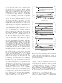
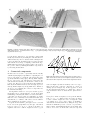
Cleaning Massive Sonar Point Clouds
Lars Arge∗
Kasper Green Larsen∗
Aarhus University
Aarhus, Denmark
[email protected]
Aarhus University
Aarhus, Denmark
[email protected]
Thomas Mølhave†
Freek van Walderveen∗
Duke University
Durham, NC, USA
[email protected]
Aarhus University
Aarhus, Denmark
[email protected]
ABSTRACT
1
We consider the problem of automatically cleaning massive
sonar data point clouds, that is, the problem of automatically removing noisy points that for example appear as a
result of scans of (shoals of) fish, multiple reflections, scanner self-reflections, refraction in gas bubbles, and so on.
We describe a new algorithm that avoids the problems of
previous local-neighbourhood based algorithms. Our algorithm is theoretically I/O-efficient, that is, it is capable of
efficiently processing massive sonar point clouds that do not
fit in internal memory but must reside on disk. The algorithm is also relatively simple and thus practically efficient,
partly due to the development of a new simple algorithm for
computing the connected components of a graph embedded
in the plane. A version of our cleaning algorithm has already
been incorporated in a commercial product.
Due to the developments in terrain scanning technology during the last twenty to thirty years, very detailed terrain data
can now relatively easily be produced at very high rates.
Especially light detection and ranging (LIDAR) technology,
operating lasers from airplanes, has significantly increased
the size of digital terrain models of land areas. For scanning the seabed, the shift from single- to multibeam echo
sounders (MBES) and further technological advances have
caused a significant increase in the data collection rate: current echo sounders can make up to 2.2 billion soundings a
day [19].
Obvious basic use of terrain data is the construction of
digital elevation models (DEMs), height maps or nautical
charts. The data is also used in many more complicated terrain analysis applications such as for analysing the sea floor,
for example in the search for oil. Once oil has been found
and pipelines have been laid, seabed data (obtained by periodical MBES scannings) is used to maintain the pipeline,
for example by controlling the position of the pipe and the
movement of the seabed around and below it. However, all
of the uses of modern detailed terrain data are hampered
by the size of the data. Not only is the often massive data
hard to handle, but it also makes the need for manual intervention in various processes a major bottleneck. In this
paper we consider the problem of automatically removing
spurious measurements from massive sonar data (or sonar
data “cleaning”).
Categories and Subject Descriptors: F.2.2 [Analysis
of algorithms and problem complexity]: Nonnumerical algorithms and problems—Geometrical problems and computations
General Terms: Algorithms, Experimentation, Theory
Keywords: MBES, noise removal, I/O-efficient algorithms,
connected components
∗ Supported
by MADALGO — Center for Massive Data Algorithmics, a Center of the Danish National Research Foundation, as
well as by the Danish Strategic Research Council and by the US
ARO. Kasper Green Larsen (has previously published as Kasper
Dalgaard Larsen) is a recipient of the Google Europe Fellowship
in Search and Information Retrieval, and this research is also supported in part by this Google Fellowship.
† Supported by NSF under grants CNS-05-40347, CCF-06-35000,
IIS-07-13498, and CCF-09-40671, by ARO grants W911NF-07-10376 and W911NF-08-1-0452, by an NIH grant 1P50-GM-0818301, and by a grant from the U.S.–Israel Binational Science Foundation.
1.1
Introduction
Problem motivation
In order to make further processing feasible, raw data from
a sonar scanning mission first needs to be cleaned. This
cleaning is necessary because the raw data — supplied as
a set of three-dimensional points — includes a lot of noise
such as (shoals of) fish and other non-permanent objects
(see Figure 1). Similarly, spurious measurements also create problems. Such measurements appear for example due
to multiple reflections, refraction in gas bubbles, influence
of the ship’s propeller noise, as well as local differences in
sound speed due to turbid water [15]. Inaccuracy and miscalibration of measurement devices and the various systems
correcting for external influences (such as the pitching and
rolling of the ship), can also negatively affect the accuracy
of a scan or even result in gross mismeasurements due to
scanners detecting their own presence. An example of this
type of structural noise is shown in Figure 2(a). For most
Permission to make digital or hard copies of all or part of this work for
personal or classroom use is granted without fee provided that copies are
not made or distributed for profit or commercial advantage and that copies
bear this notice and the full citation on the first page. To copy otherwise, to
republish, to post on servers or to redistribute to lists, requires prior specific
permission and/or a fee. ACM GIS’10, November 2–5, 2010. San Jose, CA,
USA. Copyright 2010 ACM ISBN 978-1-4503-0428-3/10/11 ...$10.00.
1
• Constructing a lower-resolution approximation of the
surface to compare against.
applications, one needs to filter out non-permanent features
and gross errors, while for some applications also minor noise
has to be filtered out or levelled.
1.2
• Using an existing low-resolution, high-quality scan of
the area to compare against.
Previous work
Currently, sonar data is often cleaned by hand, possibly with
the help of commercially available tools relying on statistical
analysis of the data. Often, this is a very tedious and time
consuming process. Canepa et al. [9] give a good overview
of different types of algorithms and tools that have been
proposed in the literature.
Most of the commercially available tools for sonar data
cleaning rely on the CUBE algorithm (Combined Uncertainty and Bathymetry Estimator) [8]. The main goal of
this algorithm is not so much to remove noise from the data
as it is to give depth estimates at the vertices (called estimation nodes) of a grid laid over the terrain. The algorithm
processes the input points one at a time while maintaining depth estimates at each estimation node, along with
information about the accuracy of the estimates based on
a statistical analysis of the height and inaccuracy of data
points in the neighbourhood of the node. This results in a
number of depth hypotheses for each estimation node, each
supported by a subset of the data points that roughly agree
on the depth at that location. After all data points have
been processed, a selection needs to be made as to which of
these hypotheses are correct and which are formed by spurious data points. After this is done the data can be cleaned
by comparing each input data point to the grid estimates.
The hypothesis selection is handled differently by different
implementations, but is typically based on one or more of
the following methods:
As high-quality scans are often not available for comparison, the last method is not an option in most cases. The
other methods work well for single, isolated outliers, but for
clustered noise as in Figures 1 and 2 they often fail to recognize noise, or if they do they often tend to also classify
points on the top of pipes lying on (or above) the seabed as
noise. The latter is obviously a major problem if the scan
was made for pipeline maintenance.
Overall, one main problem with the CUBE method [8]
for sonar data cleaning is that only a local neighbourhood
around each estimation node is considered, and it may not
contain enough information to make the right decision. Indeed, according to the CUBE User’s Manual [7], for CUBE
to work properly, separate preprocessing is required to eliminate systematic errors and outliers. Also, determining the
best way to use information from the local neighbourhood to
select hypotheses is seen as an open problem [8]. Most other
methods such as the ones reviewed by Canepa et al. [9] also
base their decisions in one way or another on local neighbourhoods, leading to essentially the same problem as with
CUBE.
1.3
I/O-efficient algorithms
We consider the problem of cleaning massive sonar data
clouds that likely cannot be stored in main memory, and
must reside on a much larger and slower secondary storage
device. In such a case movement of data between secondary
storage (disk) and main memory, rather than CPU time,
is often the performance bottleneck. Therefore we consider
the problem in the standard I/O-model of computation [3],
where the memory system consists of a main memory of size
M elements and a disk of unlimited size. Data is moved between main memory and disk in blocks of B consecutive elements. Such a movement of B elements is called an I/O and
the complexity of an algorithm is measured in terms of the
number of I/Os it performs. Since B elements can be read
in one I/O, scanning an input dataset of N elements can be
done in Θ(scan(N )) = Θ(N/B) I/Os. Sorting N elements
requires Θ(sort(N )) = Θ(N/B logM/B N/B) I/Os [3].
In the last decade many results have been obtained in the
I/O-model. Refer for example to surveys by Vitter [20] and
Arge [4]. Of particular importance to this paper, several
O(sort(N )) algorithms for triangulating a set of N points
in the plane (for computing a TIN DEM) have been developed [14, 17, 1], including algorithms that work well in
practice [1, 16]. Several algorithms have also been developed
for the problem of computing the connected components of a
graph, including an algorithm by Munagala and Ranade [18]
that uses O(sort(|E|) log2 log2 (|V |B/|E|)) I/Os, where |V |
is the number of vertices and |E| the number of edges of the
graph. However, this algorithm is rather involved (for example requiring the computation of Euler tours in trees) and is
therefore not of practical interest. Currently the best known
practical algorithm for computing connected components is
a modified version of an O(sort(N ) log2 (N/M )) union–find
algorithm due to Agarwal et al. [2].
• Selecting the hypothesis that is supported by the most
data points.
• Considering a local neighbourhood around each estimation node with multiple hypotheses, finding the
closest estimation node v for which there is only one
hypothesis, and then choosing the hypothesis at the
current node that is closest in depth to the hypothesis at v. The neighbourhood is chosen as an annulus
(ring) around the estimation node of a certain predefined size (rather than a disc), since it seems to give
better results for bursty noise.
Figure 1. Noise caused by fish. Black dots represent the input points.
The overlays show the front and back sides of one group of points.
Data source: StatoilHydro.
2
ribbons of noise
(a)
noise cloud
pipeline
pipeline
(b)
pipeline
pipeline
Figure 2. Pipeline spanning a valley surrounded by a lot of structural noise. (a) Pictures showing the same area from three different angles
with a dot for each input point. (The distortion of the pipeline in the horizontal direction is likely the result of a failure to compensate for the
motion of the scanner.) (b) TIN visualization of a cleaned version of the same data.
Data source: StatoilHydro.
1.4
Our results
sumption that any horizontal line intersects at most M edges
of the graph. In practice this assumption means that we
can handle graphs with O(M 2 ) edges,
√ as one would expect
a horizontal line to hit at most O( N ) edges. Thus the
assumption certainly holds for practically realistic memory
sizes and datasets. We believe that this algorithm is of independent interest since it only requires a sorting step followed
by two scans over the graph. Using the practical algorithm
of Agarwal et al. [2] instead of our new connected component
algorithm would result in a cleaning algorithm without the
assumption but using O(sort(N ) log2 (N/M )) I/Os. Using
the algorithm by Munagala and Ranade [18] we would obtain
an O(sort(N ) log log B) algorithm. However, as discussed,
this algorithm is not practical.
Overall we have obtained a theoretically and practically
efficient algorithm for cleaning massive sonar point clouds
that seems to work very well in practice. In fact, a version of the algorithm has been incorporated in a commercial
product called SCAN (SCALGO Combinatorial Anti Noise)
by EIVA and SCALGO [13].
In this paper we describe a new algorithm for automatic
cleaning of massive sonar data, which avoids the problems
of local-neighbourhood based algorithms while still allowing
an efficient implementation.
In Section 2 we first characterize the different types of
noise we found in real datasets provided by the companies
StatoilHydro, EIVA and others, and discuss why existing
local-neighbourhood based algorithms perform poorly for
some of these types. Then we describe our new algorithm,
and finally we discuss how it performs very well on various
real datasets containing all the different noise types. In particular, we show that (unlike existing local-neighbourhood
methods) our algorithm is capable of identifying large clusters of noisy points — even clusters with large extent — while
for example distinguishing them from points on top of pipes
on (or more importantly, above) the seabed.
In Section 2 we also describe how our cleaning algorithm
can be implemented in O(sort(N )) I/Os under a practically realistic assumption about the input data. The main
ingredients in the algorithm are sorting of N elements, triangulation of a set of N points in the plane, and computation of the connected components of a graph of size N
embedded in the plane. As discussed, the two first problems can be solved in O(sort(N )) I/Os with algorithms
that are practically efficient. To obtain a practically efficient O(sort(N ))-I/O cleaning algorithm, we in Section 3
describe a new simple and practical algorithm for computing the connected components of a graph embedded in the
plane. The algorithm uses O(sort(N )) I/Os under the as-
2
Cleaning sonar point clouds
In this section we describe our new theoretically and practically efficient algorithm for cleaning massive sonar point
datasets. In Section 2.1 we first try to characterize the different types of noise we have experienced in real-life datasets
and discuss why existing methods perform poorly for some
of these types. Then in Section 2.2 we describe our new
algorithm, and finally in Section 2.3 we discuss how the al3
gorithm performs on various test datasets containing all of
the different noise types.
2.1
Sonar data noise
Different types of noise can often be found in MBES datasets:
1. Points that appear apparently at random above and
below the seabed; sometimes in larger groups. See
Figure 3 for an example.
2. Points resulting from physical objects such as fish,
forming larger groups of outliers (as in Figure 1).
3. Structural noise, often in the form of ribbons of points
appearing along the direction of movement of the echo
sounder (as in Figure 2).
A main complication in the recognition and removal of
noise of the above types is that one typically also finds features on the seabed that are of prime importance for the end
user but can be hard to distinguish from noise. Typically
such features are objects lying on the seabed or pipelines
that either lie on the seabed or span a “valley” while being supported by “hills” on one or both sides (see Figure 2).
Existing algorithms can often handle the first type of noise
described above, since most points in the neighbourhood
of random and spiky noise points have approximately the
same height (different from the outliers). Thus it is easy to
conclude on statistical grounds that a point is an outlier.
For the second type of noise, the effectiveness of traditional
cleaning methods typically depends on the size of the local
neighbourhood they consider. They typically work well if
the neighbourhood is so large that it includes a considerable amount of real data points (clean seabed). If on the
other hand the group of outliers is so large that a good fraction or even the majority of points in the neighbourhood is
noise, the neighbourhood-based algorithms fail (since they
basically need to make an arbitrary decision as to which
points are noise and which are from the seabed or an object on the seabed). Finally, in terms of structural noise the
neighbourhood-based algorithms face the same problems as
for type-2 noise: for example, a pipeline spanning a valley
may be locally indistinguishable from a ribbon of structural
noise, making it impossible to make a well-founded decision
based on local information only.
Since the main problem of most existing methods is the
limited size of the considered local neighbourhood, a natural way of improving them is to enlarge the neighbourhood.
However, this often makes it harder to compute a good estimate of the terrain (seabed) height at a given position,
since the terrain may be very complex in a relatively large
neighbourhood. Furthermore, since the running times of the
estimation methods are often very dependent on the neighbourhood size, choosing a large neighbourhood may lead to
impractical running times.
2.2
Figure 3. Noisy points above and below the seabed (resulting in
spikes in the terrain model).
Data source: StatoilHydro.
location. Next it computes a TIN from P̃ by projecting the
points onto the plane (ignoring the vertical coordinates of
the points), constructing a two-dimensional Delaunay triangulation of the projected point set (a triangulation where
no points of P̃ lie inside the circumscribed circle of any triangle [5]), and lifting this triangulation back to the original
heights at the vertices. Next, for each non-boundary edge
e of the TIN an edge called e’s diagonal is added between
the two vertices opposite to e in the two triangles incident
to e (see Figure 4). From this new graph G (embedded in
R3 ) the algorithm then removes all edges (u, v) where the
difference in z-coordinate between u and v is larger than a
threshold τ to obtain a graph Gτ . Finally, the connected
components of Gτ are computed and all vertices that do not
belong to the largest component are marked as noise.
e
e0
Figure 4. Adding the diagonal e0 for an edge e in a TIN.
Our cleaning algorithm can easily be implemented to run
in O(sort(N ) log log B) I/Os: in order to give all input
points a unique horizontal position we simply sort the points
lexicographically by their x- and y-coordinate, and then we
can in a simple scan perturb each member of a group of
points that share the same x- and y-coordinate. As mentioned, the triangulation can be obtained in O(sort(N ))
I/Os [14, 17, 1], and the diagonals can then easily be added
and the relevant edges removed using a few sorts and scans.
Since both the number of vertices and the number of edges in
G is O(N ), the connected components can then be computed
in O(sort(|E|) log2 log2 (|V |B/|E|)) = O(sort(N ) log log B)
I/Os [18]. Finally, after sorting the vertices by their con-
Our cleaning algorithm
Given a point set P the algorithm first perturbs the horizontal positions of the points in such a way that no two points
have the same x- and y-coordinate, resulting in a point set
P̃ . This perturbation can be done by moving the members of
a set of points with the same horizontal position to random
positions within a small disc centred around their original
4
(a)
nected component, all noise vertices/points can be marked
in two scans: one for counting component sizes and one for
marking all points that are not in the largest component.
Hence, the total number of I/Os is O(sort(N ) log log B).
Most of the steps of our algorithm can be implemented
not only theoretically I/O-efficiently but also practically efficiently, since as discussed in the introduction practical Delaunay triangulation and sorting algorithms have been developed and implemented. As also discussed, the known
O(sort(N ) log log B) connected component algorithm [18]
is too complicated to be of practical interest, whereas the
simpler practical algorithm [2] uses O(sort(N ) log2 (N/M ))
I/Os. However, in Section 3 we describe a new algorithm
that is relatively simple and practically efficient, and which
under a realistic assumption uses only O(sort(N )) I/Os.
We have implemented and tested the resulting algorithm on
a number of massive MBES datasets.
2.3
(b)
Algorithm performance
In this section we study the performance of our algorithm in
terms of cleaning quality. We also intuitively motivate the
different parts of the algorithm and discuss the effect of the
threshold τ .
Overall cleaning performance. We first discuss the overall performance of our algorithm in terms of the noise types
identified in Section 2.1. Noise caused by fish (type 2 above)
provides a useful example to get intuition about how and
why the algorithm works. Consider the TIN shown in Figure 5(a), where a fish above the surface is scanned. It is
easy to see what happens when we remove all edges of the
TIN with a height difference more than τ : if the fish swims
further away from the seabed than this threshold, the edges
connecting its points to the points on the seabed are removed
and the points on the fish form a small connected component in Gτ and are therefore classified as noise. Even though
we do not catch fish swimming too close to the seabed, this
is probably the best we can do. If a fish swims too close
to the seabed it could just as well be a stone lying on the
seabed. It is quite clear however that the fish in Figure 5(a)
is not an object on the seabed. The reason for this (and a
rule of thumb amongst manual data cleaners) is that if an
object is resting on the sea floor, also points on the side of
the object will be captured by the sonar since it is scanning
the object at an angle. A cleaned version of the area around
Figure 5(a) is shown in Figure 9(b).
For the same reasons as for physical objects such as fish,
our algorithm also handles random outliers (type 1 above)
well, as long as they are far enough from the sea floor. Refer
for example to the spikes below the terrain in Figure 9(a),
visible as lines of dark spots on the top side, that are removed by our algorithm as shown in Figure 9(b).
For structural noise (type 3 above) the situation is more
interesting. If the noise forms dense ribbons we, as argued
previously, get a pattern that is locally indistinguishable
from an elevated pipeline (for example Figure 2(a)). Still, as
illustrated in Figure 2 and 9(c)–(d), the algorithm correctly
removes ribbons of noise while keeping the pipeline intact.
The reason is that if one looks along the whole length of the
pipeline it will at some point rest on the seabed or a sandbank. This enables our algorithm to distinguish pipes from
noise: points on a pipe will be part of the same connected
Figure 5. (a) TIN of points on a fish that swims approximately 60
cm above the seabed. (b) A stone blocking the view for the echo
sounder (scanning from the right).
Data source: StatoilHydro.
component as the seabed in Gτ because the pipe physically
“connects” to the seabed. On the other hand, the points of
a ribbon of noise are typically connected to each other but
not to the sea floor.
Algorithm intuition. The above discussion of how our algorithm handles the different noise types also to some extend gives the intuition behind the algorithm: defining a
“closeness” relation on the input points by constructing a
surface graph from them, and then disconnecting parts of
the graph that are far away from the predominant surface.
As surface graph we use a Delaunay triangulation (a TIN
DEM) but we could of course have used other graphs. However, the Delaunay triangulation has a few specific advantages. First of all, it always yields a connected and somewhat
regular graph. This property is useful especially in lowerresolution areas of the terrain (see Figure 5(b)) where for
example a graph based on fixed-size neighbourhoods would
leave holes and might even disconnect the graph (note however, that this is not directly related to the main problem
with neighbourhood-based algorithms). A second advantage
of the Delaunay triangulation is that practical and efficient
construction algorithms are available. A possible alternative
to using a TIN (with diagonals) would be to use a 3D Delaunay triangulation. However, the worst-case complexity
of this triangulation is O(N 2 ), and although a worst-case
optimal O(N 2 /B)-I/O algorithm is known [17], the size of
the triangulation would make the cleaning algorithm inhibitingly slow both in theory and in practice. Note that a consequence of using a planar triangulation is that it does not
allow points at different heights to share the same x- and
y-coordinate. Our algorithm works around this limitation
by perturbing points with the same horizontal position.
5
(a)
(a)
(b)
removed
(b)
Figure 6. (a) TIN of points on a pipe and below it. (b) Pipeline
partially separated from the seabed, causing the algorithm without
diagonals to remove the black points, which are also on the pipeline.
Data source: StatoilHydro.
What is maybe less intuitive about our algorithm is the
addition of diagonals. This added connectivity is needed
to handle some cases of type-3 noise, or rather, to distinguish such noise from a pipeline above the surface. When an
echo sounder scans a terrain with overhangs (where at some
horizontal positions multiple true surfaces exist at different
heights), it usually reports points at the different heights
because it is scanning at an angle. The triangulation of
such a point set typically consists of many spikes (both up
and down), because points on for example a higher surface
may happen to only have edges to points on a lower surface
(see for example the close-up in Figure 6(a), where each line
of points on top of the pipe forms a separate component).
Removing all these long edges would result in the points being wrongly classified as noise (as in Figure 6(b), where the
black points are removed by the algorithm when diagonals
are not added). By adding the diagonals we make it much
more likely that a point is connected to at least one other
point on the same surface. This is actually what happens
in most practical situations because of the high resolution
of MBES point sets and the properties of the Delaunay triangulation. Because the top of the pipe will be more or less
evenly sampled, points along the pipe connect to each other
in Gτ through the diagonals. The points at the place where
Figure 7. Excerpt of dataset I. (a) Raw. (b) Cleaned.
Data source: EIVA.
the pipe is supported by the seabed then provide a connection, so there will be a path of neighbouring points between
the top of the pipe and the seabed. Hence, these points and
the ones on the seabed form one component in Gτ and the
points will not be removed (see for example Figure 9(d)).
Detailed cleaning performance (threshold selection). The
threshold τ obviously has a major influence on the performance of our cleaning algorithm. In the remainder of this
section we discuss the effect of varying τ while also further
describing the algorithm’s cleaning performance.
In the examples shown in Figure 9 we used a threshold τ of
5 cm, which is on the order of the scanner accuracy in those
datasets. In general, we expect picking τ a bit higher than
the scanner accuracy (a few standard deviations, if that is
known) to yield a good result. The intuition behind this rule
of thumb is that when the terrain is sampled densely enough,
sample points that are close to each other on the surface of
the terrain have a height difference that mainly depends on
6
(a)
Presumed good points: removed
3.5%
1%
Presumed noise that was not removed
(false negatives)
Presumed good points that were removed
(false positives)
0.5%
5%
0.2%
2%
0%
0%
0
20
60
6%
60%
Presumed noise that was not removed
Presumed good points that were removed
4%
40%
3%
30%
2%
20%
1%
10%
0%
Presumed noise: not removed
Presumed good points: removed
40
Threshold τ (cm)
(b)
0%
0
20
40
60
Threshold τ (cm)
6.5%
(c)
6%
60%
Presumed noise that was not removed
Presumed good points that were removed
4%
40%
3%
30%
2%
20%
1%
10%
0%
Presumed noise: not removed
Presumed good points: removed
10%
Presumed noise: not removed
the scanner accuracy. Then, we know that for two points on
the same surface, there will be a path of connected points
in the triangulation for which each two consecutive points
have a height difference lower than τ . We have a similar
situation when an object is lying on the sea floor. For any
point p on an object of interest there will be a path of close
points in G from p to a point on the seabed. Because they
are often scanned at an angle, at least on one side there will
be a curtain of points reaching from the top of the object to
the sea floor, establishing a connection that our algorithm
will use to determine that the points forming the object are
not noise. Any point for which such a path does not exist is
therefore very likely noise.
In some cases a threshold corresponding to the scanner
accuracy might be too low and result in parts of the seabed
being disconnected from the rest of the seabed (due to low
local point resolution). In such cases one would have to use
a higher threshold, and our experience is that in many cases
it is still possible to remove a large amount of noise using
a relatively high threshold. Below we discuss the effect of
varying the threshold using four datasets that contain moderate to extreme amounts of noise, as well as different features on the seabed. Excerpts of the raw data are shown in
Figures 7(a) (dataset I), 9(c) (dataset III), and 2(a) (dataset
IV). Dataset II looks similar to dataset I. For datasets I, II
and IV we also had access to a manually cleaned version,
allowing for direct comparison. It should be noted though
that some of this manual cleaning was rather “rough”, so
not all outliers were removed. Also for an operator it is not
always clear which points should be classified as outliers,
so two well-cleaned datasets (by different operators or automated methods) may still have a large number of differently
classified points. Nevertheless, we have compared the number of points that are classified differently by our algorithm
and the manual process. The results of this comparison are
shown in Figure 8 (note that the scale on the left indicates
the percentage of presumed good points that were removed
by the algorithm, while the scale on the right indicates the
percentage of presumed outliers that were kept).
For datasets I and II we consider the results to be very
convincing: at a threshold of 5 cm 99.6% and 87% of the
noise was removed, while only 0.4% and 0.3% of the points
that were kept during manual cleaning were also removed.
For both datasets threshold values of 2 or even 1 cm still
visually give very good results, but as one can see the falsepositive rates increase rapidly. For dataset I there also exist
some points in isolated parts of the point set at the far end of
the viewing angle of the scanner that are removed while they
probably represent the real sea floor. For most applications
this would not be a big problem, as such data is considered
to be of inferior quality anyway. In both datasets, increasing
the threshold results (as one would expect) in an increase
of the false-negative rate and a decrease of the false-positive
rate. Still, at for example 50 cm the most visible and in that
sense important outliers were removed in both datasets.
For dataset III we did not have access to a manually
cleaned dataset. However, visual inspection shows that at a
threshold of 5 cm (with 5.7% of the points marked as noise),
the cleaning is effective and the pipeline is kept intact (see
for example Figure 9(d)). Like with datasets I and II, setting τ to 2 cm keeps most of the terrain and specifically the
pipeline intact, while at τ = 1 cm some parts with poor
resolution and parts of the pipe were removed.
0%
0
20
40
60
Threshold τ (cm)
Figure 8. Classification differences between manual and automatic
cleaning for: (a) dataset I (Figure 7(a)) of about 7 million points
(manual cleaning removed 0.5% of these); (b) dataset II of about
7 million points (manual cleaning removed 1.7% of these); (c)
dataset IV (Figure 2(a)) of about 6 million points (manual cleaning removed 20.5% of these).
Dataset IV is the most noisy dataset we have seen. According to the manual cleaning, 20% of the points are outliers. At the same time the dataset contains a poorly sampled pipeline spanning a valley, which creates problems at
low thresholds (where parts of the pipe are classified as
noise). Therefore, increasing the threshold to 35 cm results in a visually nicely cleaned dataset where all ribbons of
noise are removed, and compared to manual cleaning 81% of
all outliers and only 0.8% non-outliers are removed. Up to
τ = 50 cm this is still the case, but with higher thresholds
more and more ribbons of noise start appearing.
We conclude that for datasets with moderate noise and
relatively good sampling conditions, our cleaning algorithm
7
(a)
(c)
(b)
(d)
Figure 9. (a) Noise caused by fish, with a ribbon of noise in the front left, and some noise below the seabed visible as dark lines on the top
(indicated by arrows). (b) Cleaned version of (a). (c) A pipeline spanning a valley (close-up in Figure 6(a)), with structural noise on the left.
(d) Cleaned version of (c).
Data source: StatoilHydro.
u
is both effective and leads to very few false positives with
hardly any intervention (and using the same threshold for
different datasets). Also for datasets with overhangs in the
form of pipelines the algorithm works very well. For data
with extreme noise and poor sampling conditions the algorithm still works effectively, but may require some work by
the operator, either by marking misclassified components or
by increasing the threshold.
3
v
`v
w
Connected components
In this section we describe a practically and theoretically
efficient O(sort(N ))-I/O algorithm for computing the connected components of a graph G embedded in the plane
(possibly with intersecting edges). The algorithm assigns a
label to each vertex of G, such that two vertices have the
same label if and only if they are in the same connected component of G. However, it only works under the assumption
that any horizontal line intersects at most O(M ) edges of G.
Our algorithm is inspired by an algorithm due to Danner et
al. [10, 11] for computing the connected components in a
two-dimensional bitmap.
Our algorithm consists of a down phase and an up phase.
Both phases sweep a horizontal line over the plane while
maintaining connectivity information for vertices incident to
edges that cross the sweep line. For simplicity, we assume
that G does not contain any vertices without incident edges,
and that the y-coordinates of all vertices of G are distinct.
These assumptions can easily be removed.
Consider a horizontal line `v through a vertex v of G and
let G+
v denote the graph induced by all edges of G with at
least one vertex on or above `v . In the down phase, we
augment each vertex v with no neighbours below `v (open
Figure 10. Status during the down phase when processing vertex v.
Open vertices do not have any lower neighbours; square vertices are
the lowest in their component; arrows indicate augmented vertices.
vertices in Figure 10) with an arbitrary vertex w below `v
that is in the same connected component as v in G+
v , if
existing (arrows in Figure 10). In the up phase we then
use the augmented information to compute the connected
component labels. Below we discuss the two phases in more
detail.
Down phase. In the down phase, we sweep a horizontal line
from y = ∞ to −∞. Whenever the sweep line encounters
a vertex v with no neighbour below `v we augment v with
w as defined above. To be able to find w we maintain a
data structure D in internal memory during the sweep. The
structure D maintains upwards connected component information, that is, it maintains information about which of the
vertices on or below `v are in the same connected component
8
in G+
v (in Figure 10, the vertices with a grey background are
in the upwards connected component of v in D). The structure D is essentially a union–find data structure supporting
the following operations:
G+
v , if existing. To determine v’s label we first check if v is
already stored in internal memory. If it is, that is, if it has
a lower neighbour, it has already been assigned a label. If
not and v is augmented with a vertex w, which must then
be in internal memory, we assign the label of w to v. If v is
not augmented with a vertex we assign it a new label. Next
we load all edges with v as their lowest vertex into internal
memory, while adding v’s neighbour vertices to the vertices
stored in internal memory and assigning each such vertex
the same label as v. Finally, we remove all edges that have
v as their highest vertex from internal memory, while also
removing vertices from internal memory that are left with
no incident edges among the edges in internal memory.
To see that the above algorithm maintains the invariant,
first note that if v’s label is correctly assigned then so are
all other labels assigned when processing v (since they are
all assigned v’s label and are connected to v). In the case
that v is assigned the label of vertex w in internal memory,
we know that v is in the same connected component as w
in G+
v and thus in G, and therefore the label is correctly
assigned. In case v is assigned a new label, we know that v
is not connected to any vertex below `v in G+
v and thus not
to any vertex below `v in G. Therefore the newly assigned
label maintains the invariant.
• Insertion of a vertex.
• Merging of two upwards connected components.
• Extraction of a vertex in D in the same upwards connected component as the top vertex in D, if such a
vertex exists.
• Removal of a vertex.
The assumption that the sweep line intersects O(M ) edges
ensures that D fits in internal memory.
More precisely, the sweep proceeds as follows: We scan
the vertices of G in decreasing order of y-coordinate. When
processing a vertex v, we first insert v in D if it is not there
already. Then we load all edges having v as highest vertex
into memory. We do so by scanning the edges of G in order
of the y-coordinate of their highest vertex, along with the
scan of the vertices. For each edge (v, w) we then check
whether w is already in D. If not, we insert w in D and
merge the upwards connected component of v with the newly
created component of w. Otherwise, we simply merge the
component of v with that of w. If no such edge (v, w) exists,
that is, v has no neighbour below `v , we instead extract
a vertex in D in the same upwards component as v and
augment v with this vertex w, if existing. Finally, we remove
v form D.
It is easy to realize that D is maintained correctly during
the sweep, that is, when the sweep line is at v, it contains
information about which vertices on or below `v are in the
same connected component in G+
v . It immediately follows
that the down phase correctly augments each vertex v that
has no neighbour below `v with a vertex below `v that is in
the same connected component as v in G+
v (that is, in the
same upward component).
I/O-complexity. The down phase requires the vertices to
be ordered by decreasing y-coordinates and the edges by
decreasing y-coordinates of their highest vertices. Similarly,
the up phase requires the vertices to be ordered by increasing
y-coordinates and the edges by increasing y-coordinate of
their lowest vertex. To bring the edges and vertices in this
order, we simply sort them, using O(sort(N )) I/Os. The
remainder of the two phases consist only of scanning over
sorted lists of vertices and edges taking O(N/B) I/Os. Thus
the total cost is O(sort(N )) I/Os.
Remark. We actually only need to sort the edges and vertices for the down phase. The down phase can then simply
push vertices and edges to I/O-efficient stacks after they are
processed. This will reverse the order for the up phase and
thus save a sorting step. Note that if the vertices and edges
are given in the correct order for the down phase, the cost
of the algorithm can be reduced to O(N/B) I/Os.
Up phase. In the up phase we compute the connected components of G and assign a label to each vertex. To achieve
this, we also sweep a horizontal line, but this time from
y = −∞ to ∞. During the sweep, we maintain the invariant
that any vertex that has a neighbour below the sweep line
has had its component label assigned, that is, any two such
vertices have the same label if and only if they are in the
same connected component of G. Thus, when the sweep line
reaches ∞ we have computed the connected components of
G, that is, labelled all vertices correctly.
While performing the sweep, we store all edges of G intersecting the sweep line in internal memory. We also separately store all vertices incident to these edges in internal
memory, where each such vertex also stores the label assigned to it. The assumption that the sweep line intersects
O(M ) edges ensures that these vertices and edges fit in internal memory.
The sweep now proceeds as follows: We scan the vertices of G in order of increasing y-coordinate, along with the
edges of G in order of the y-coordinate of their lowest vertex. From the down phase we know that when processing
a vertex v with no lower neighbour, it is augmented with
a vertex w below `v that is in the same component as v in
4
Conclusion and future work
In this paper we described an algorithm for removing noisy
points from multibeam sonar data that can handle arbitrarily large clusters of noisy points. As opposed to previous algorithms that base their decisions only on a local neighbourhood around each point, our algorithm can distinguish noise
clusters from points on top of physical objects like pipelines.
We showed that the algorithm can be implemented to be
both theoretically and practically I/O-efficient, in part due
to the development of a new practical connected components
algorithm. A version of the algorithm has already been incorporated in a commercial product.
Our results open up a number of interesting theoretical
questions. First of all, it would be interesting to quantify why our algorithm works so well. To do so, one needs
a mathematical model of noise. Existing such models are
mostly only concerned with noise caused by scanner inaccuracy and sample points are assumed to be relatively close
9
to the actual surface [12]. An algorithm is then asked not
to discard certain points, but to make the best estimate of
the surface’s position and topology. However, in our case a
model would need to consider the addition of high amounts
of outliers to a terrain sample and ask for algorithms to
classify points to be noise or not. An interesting approach
might be to take a simple model of clustered outlier noise
that considers samples in a confined region of a smooth terrain to have a given probability of being an outlier (and
thus lying relatively far away from the actual terrain). In
this model, our algorithm classifies a point p on the terrain
within this region correctly, if and only if there is a path
in graph G from p to a point on the terrain outside the
region such that all consecutive points on the path are on
the terrain. One can model this as a colouring of the vertices of graph G: points on the terrain are white and noise
points are black. The cleaning quality of our algorithm then
depends on the connectivity of the subgraph of G induced
by the white points. The connectivity properties of graphs
coloured randomly like this are studied in the field of percolation theory. Indeed, a result that may shed light on
the cleaning quality of our algorithm has been obtained by
Bollobás and Riordan [6]. They consider random Voronoi
percolation, which corresponds to connectivity in randomly
coloured Delaunay triangulations (without diagonals) of infinite random point sets. The result they obtain concerns the
critical probability in the setting where vertices are coloured
white or black independently with a given probability. The
critical probability can be thought of as the highest possible
probability of vertices being coloured black, before it becomes very likely that the white vertices get separated into
small connected components (as opposed to one big component). Bollobás and Riordan prove this critical probability
to be 1/2. In short, percolation theory could be a possible
way of quantifying how well an algorithm like ours handles
clustered noise. Thus it would open up the possibility of
comparing different variations of it, for example based on
other types of neighbourhood graphs.
[5]
[6]
[7]
[8]
[9]
[10]
[11]
[12]
[13]
[14]
[15]
Acknowledgements. We thank Morten Revsbæk and Adam
Ehlers Nyholm Thomsen for various discussions and further
development of the algorithms presented in this paper, as
well as Herman Haverkort for discussion and the suggestion
to add diagonals. We would also like to thank EIVA and
StatoilHydro for introducing us to the problem and for providing a large number of test datasets.
[16]
[17]
[18]
References
[19]
[1] P. K. Agarwal, L. Arge, and K. Yi. I/O-efficient construction of constrained Delaunay triangulations. In
Proc. 13th Annual European Symposium on Algorithms,
pages 355–366, Sept. 2005.
[2] P. K. Agarwal, L. Arge, and K. Yi. I/O-efficient batched
union-find and its applications to terrain analysis. In
Proc. 22nd Annual Symposium on Computational Geometry, pages 167–176, June 2006.
[3] A. Aggarwal and J. S. Vitter. The input/output complexity of sorting and related problems. Communications of the ACM, 31(9):1116–1127, Sept. 1988.
[4] L. Arge. External memory data structures. In J. Abello,
P. M. Pardalos, and M. G. C. Resende, editors, Hand-
[20]
10
book of massive data sets, pages 313–357. Kluwer Academic Publishers, 2002.
M. de Berg and O. Cheong and M. van Kreveld and
M. Overmars. Computational Geometry: Algorithms
and Applications. Springer-Verlag, third edition, 2008.
Chapter 9.
B. Bollobás and O. Riordan. The critical probability for
random voronoi percolation in the plane is 1/2. Probability Theory and Related Fields, 136(3):417–468, 2006.
B. Calder and D. Wells. CUBE user’s manual. Technical report, Center for Coastal and Ocean Mapping and
NOAA/UNH Joint Hydrographic Center, University of
New Hampshire, Jan. 2007. Version 1.13.
B. R. Calder and L. A. Mayer. Automatic processing of high-rate, high-density multibeam echosounder data. Geochemistry, Geophysics, Geosystems,
4(6):1048, June 2003.
G. Canepa, O. Bergem, and N. G. Pace. A new algorithm for automatic processing of bathymetric data.
IEEE Journal of Oceanic Engineering, 28(1):62–77,
Jan. 2003.
A. Danner. I/O efficient algorithms and applications in
geographic information systems. PhD thesis, Duke University, 2006. Section 3.4.1.
A. Danner, T. Mølhave, K. Yi, P. K. Agarwal, L. Arge,
and H. Mitasova. TerraStream: from elevation data
to watershed hierarchies. In Proc. 15th ACM SIGSPATIAL GIS, Nov. 2007.
T. K. Dey and S. Goswami. Provable surface reconstruction from noisy samples. Computational Geometry:
Theory and Applications, 35:124–141, 2006.
EIVA. AntiNoise plugin for NaviModel, May 2010.
Press release at http://www.hydro-international.
com/news/id3899-Antinoise_Plugin.html.
M. T. Goodrich, J.-J. Tsay, D. E. Vengroff, and J. S.
Vitter. External-memory computational geometry. In
Proc. 34th Annual Symposium on Foundations of Computer Science, pages 714–723, Nov. 1993.
J. E. Hughes Clarke. Applications of multibeam water
column imaging for hydrographic survey. Hydrographic
Journal, 120:3–14, Apr. 2006.
M. Isenburg, Y. Liu, J. Shewchuk, and J. Snoeyink.
Streaming computation of Delaunay triangulations. In
Proc. 33rd SIGGRAPH, pages 1049–1056, Aug. 2006.
P. Kumar and E. A. Ramos. I/O-efficient construction
of Voronoi diagrams. Technical report, Dec. 2002.
K. Munagala and A. Ranade. I/O-complexity of graph
algorithms. In Proc. 10th Annual Symposium on Discrete Algorithms, pages 687–694, Jan. 1999.
RESON SeaBat 7125: high-resolution multibeam echosounder system. Spec sheet at http://www.reson.com/
graphics/design/Specsheets/SeaBat/7125.pdf.
J. S. Vitter. Algorithms and data structures for external
memory. Foundations and Trends in Theoretical Computer Science, 2(4):305–474, 2006.