1
August 2006
Software Review
Maple 10:
From symbolic computer to universal math machine.
By Jason Schattman
I knew it in my heart, my theorem just had to be true. This beautiful result — that a
particularly ugly objective function was convex — was to be a jewel in the crown of my
Ph.D. thesis. But the rascal repulsed every angle of attack I mounted to prove it, in the
end killing 50 sheets of scratch paper and two weeks of my life. Hoping a proof-bypicture might yet vindicate me, I graphed the function with a program called Maple
(version 5 in 1998) that I'd found on one of the stonier of my grad department's stone age
computers. Maple's 3-D plot, which I could rotate using the mouse, showed me why my
theorem had been so hard to prove: it was false! For behold, blemishing my lovely vaseshaped graph, just starboard of the x-z plane, was a small yet undeniably non-convex
bump.
Though glad for the insight, I soon forgot about Maple and went back to using what other
O.R. grad students were using in 1998: AMPL for modeling, CPLEX for solving, C++
for simulation, MATLAB for crunching data and SAS for torturing it, PowerPoint for
drawing (I'll admit it), LaTeX for documenting, and a box of pencils for deriving. If I had
known then that Maple 5 could also do pencil-math (like differentiate the Black-Scholes
formula symbolically), I could have saved myself meters of pencil lead and millimeters
of hairline.
In the eight years and nine millimeters since, Maple has diversified well beyond its staple
crop of symbolic computation. Maplesoft now pitches Maple 10 as a universal math
machine that can support every link in the chain of mathematical modeling: deriving the
models, solving the model equations, coding the algorithms, crunching the data, running
simulations, visualizing the outputs, testing sensitivities, building point-and-click
applications for clients, and — Maple 10's best new trick — producing journal-quality
reports with full math type-setting. Can Maple 10 really subsume, as its makers suggest,
the cavalcade of software tools that researchers normally use to do all of the foregoing?
Previous versions certainly didn't, but version 10, even with some notable gaps and
annoyances, comes close enough to command attention from anyone who practices or
teaches operations research.
A Design Problem
In lieu of a standard feature-by-feature review of the software, I illustrate how an O.R.
practitioner could use Maple to solve an applied problem from start to finish, beginning
with the algebraic derivation of the model and ending with the creation of a blackbox
application that the client can run. (By "start," I'll assume we have already talked to the
client and understood their problem.) Along the way, Maple's core strengths and
limitations will come to the fore. One of these strengths is that Maple 10 allows us to
document our methods and assumptions as we go, a feature I test-piloted by writing this
review as a Maple 10 document and exporting to RTF. In what follows, formulas in red
are executable Maple inputs that I entered using version 10's new and very slick GUI
math editor; formulas in blue are Maple's outputs; and formulas in black, which I
also entered with the editor, are plain text.
Problem Description
Suppose our client wants us to design a 40-ml aftershave bottle that is aesthetically
pleasing but cheap to package and ship. The shipping cost per box is proportional to the
volume of the box. We wish to minimize the volume of the box while preserving the
bottle's volume, aesthetic appeal and physical stability. Market research shows that men
who use aftershave prefer simple, convex bottles (exotic wavy shapes need not apply),
and so our team proposes an ellipsoid as a model for the bottle. We enter the equation of
an ellipsoid as a Maple variable called bottleShape.
(When viewed in a Maple document, the equation above is "live" math, meaning you can
perform algebraic or graphical operations on it by choosing an operation from a rightclick context menu, or by using the name bottleShape in a later formula.) We have four
decision variables: the three shape-parameters a, b and c, plus the z-value h at which the
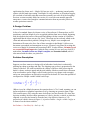
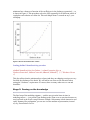
ellipsoid is cut off at the bottom to form the base. Our objective function, a 2-D
projection of which is shown in Figure 1, is just boxVolume = length • width • height, or
in terms of our decision variables:
boxVolume := 2•a•2•b•(c-h) = 4 a b (c—h)
Figure 1: 2-D projection of objective function.
Stage 1: Exploring
Before we charge boldly and blindly at the hydra of nonlinear constraints that await us,
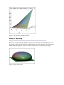
let's apply a lesson we all learned in middle school: start with a picture! The four sample
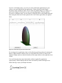
bottle shapes in Figures 2-5 give us a sense of the levers we can pull in our design.
Figure 2: Sample bottle shape.
Figure 3: Sample bottle shape.
Figure 4: Sample bottle shape.Figure 4: Sample bottle shape.
Figure 5: Sample bottle shape.
Maple provides many graphical primitives, from plain arrows to stellated
icosidodecahedra, but an amputated ellipsoid is not among them. So to create the
graphics, I wrote a short Maple procedure that takes a, b, c and h as inputs and draws the
corresponding graphic. (Maple 10's new glossy 3-D rendering is great for showing off for
clients.)
So where is the code for this procedure? I hid it from view inside a document block,
another novelty of Maple 10. In a document block, you can hide Maple source code and
commands so that they run in the background without cluttering the document with
unsightly syntax. Unfortunately, document blocks have some quirks that will confound
new users. For instance, Maple will not hide a document block that doesn't produce some
kind of output when the code is first loaded, a briar I hacked my way out of by tacking
the following print statement onto the end of the document block:
Loading a cool Maple procedure needed for the four graphics below...done
Stage 2: Building the Model
Now that we have a visual feel for the kind of designs the ellipsoid model affords us, we
can develop an NLP to optimize it. One constraint is to keep the bottle volume above 40
ml, which we can enter in Maple as follows, even before assigning the variable
bottleVolume:
volumeConstraint := 40≤= bottleVolume
Computing bottleVolume as a function of a, b, c and h takes a bit of work, a bit that we
cheerfully subcontract to Maple. We need to integrate the area of a horizontal crosssection of the ellipsoid from z = h to z = c. Treating z and c as constants, the equation of
this cross-section is x2 / α(z,c)2 + y2 / β(z,c)2 = 1 for some functions α(z,c) and β(z,c) that
need solving for. This cross-section is just an ellipse with area Π α(z,c) β(z,c).
To solve for α(z,c) and β(z,c), we have Maple subtract z2 / c2 from both sides of
bottleShape and then normalize the RHS, producing the following:
We can now write down the area of the cross-section by copying and pasting α(z,c)2 and
β(z,c)2 from the two denominators above.
assume(a > 0, b > 0, c > 0, z ≥ —c, z ≤ c)
[New users beware! Maple is like that grumpy T.A. you had in college who docked a
point off your quiz because you wrote ∫dx / x = ln x instead of ln |x|. Maple computes
over the field complex numbers, a technological wonder that's as aggravating as it is
wondrous. That's why we had to tell Maple our restrictions on a, b, c and z using the
assume statement above. Without it, Maple refuses to simplify that last square root, or
worse, starts coughing up piecewise expressions laced with complex numbers.]
The final step is to integrate the cross-section. Maple performs the integration with poise,
sparing us the sign error that I made when I tried to do it by hand on a cocktail napkin in
a bar.
Let's have Maple do one more check on the bottleVolume formula. When h = —c, does
the formula reduce to the volume of a whole ellipsoid? Maple's eval command can
answer that for us.
eval( bottleVolume, h = — c) = 4 Π a b c / 3
Touchdown!
We have two more constraints to go. First, our client has asked for a "sleek and tall"
design (no golf balls please), so we'll impose the soft constraints b ≥≥ 2a and c ≥ b. (We'll
play with that coefficient of 2 during the sensitivity analysis in Stage 4.) In Maple, I
labeled these sleeknessConstraint1 and sleeknessConstraint2. Secondly, the shorter
dimension of the base must be at least 2 cm so that the bottle doesn't tip over when you
blow on it. This just means α(h, c) ≥ 2. I labeled this inequality as balanceConstraint.
Our model to-date is summarized in Figure 6, which I created as a dynamic Maple table
(a new tool in Maple 10) simply by referring to the variable names I gave to the objective
function and constraints (e.g. boxVolume, volumeConstraint, etc.) In a Maple document,
the table would update itself automatically if we changed any of the problem data and
then reexecuted the document.
Figure 6: Model summary, created as a dynamic table.
Stage 3: Solving the Model
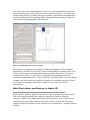
To knock down this nonlinear monster, we roll onto the field one of Maple's most
powerful cannons: the gallantly named Interactive Optimization Assistant, which lets us
enter, edit, set an initial solution for, and solve the above optimization problem, all by
pointing and clicking, as shown in Figure 7. We can invoke the assistant from the Tools
menu and populate the text fields for the objective function and constraints by entering
their variable names into text boxes, or we can accomplish the same thing by typing the
following command:
bottleSolution := Interactive( boxVolume, {volumeConstraint, sleeknessConstraint1,
sleeknessConstraint2, balanceConstraint, hBounds})
Figure 7: Interactive Optimization Assistant in action.
The lower-right corner of Figure 7 tells us the smallest volume we can achieve in this
model is 100.94 cm3. Unfortunately, for working with the optimal values of a, b, c and h,
we have to leave our warm, cozy assistant and learn a bit of syntax. For instance, to test
which constraints are tight, we need the following abstruse code:
eval([volumeConstraint, sleeknessConstraint1, sleeknessConstraint2, balanceConstraint,
hBound1, hBound2], bottleSolution[2])
evalf(%) = [40. ≤ 39.99999998, 4.284155072 ≤ 4.284155072, 4.284155072 ≤ 4.
284155072, 2. ≤ 2.000000000, 1.53427008 ≤ 4.284155072, 1.53427008 ≥ -4.284155072
]
This output tells us that all of the "design" constraints are tight, and the only constraints
with any slack are the upper and lower bounds on h.
To draw the optimal bottle, we need to extract the optimal decision variables from the
second entry of the list-data-structure bottleSolution (hence the [2]).
A := eval( a, bottleSolution[2] )
B := eval( b, bottleSolution[2] )
C := eval( c, bottleSolution[2] )
H := eval( h, bottleSolution[2] )
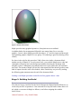
Finally we call the bottle-drawing procedure on those values.
drawBottle(A, B, C, H)
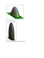
The final picture is shown in Figure 8. Is this the optimal aftershave bottle? It is,
according to our NLP model, but the client can veto this solution or the entire model, in
which case we have to change the constraints or the objective. Maple 10 makes it easy for
us to do both.
Figure 8: Is this the optimal aftershave bottle?
Stage 4: Testing the Solution
How much would we have to pay (in volume) for a sleeker bottle? Maple's flexible
graphics are well suited for sensitivity analysis. In an invisible document block, I have
written a 10-line Maple procedure called plotVolumeSensitivity that plots the optimized
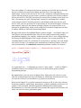
box volume vs. any single parameter we choose. As one illustration, a plot of the
minimum box volume as a function of the coefficient s in the sleekness constraint b ≥ s a
is shown in Figure 9. This procedure solves the NLP repeatedly for 20 different values of
s and plots each solution as a blue dot. This took Maple about 3 seconds on my 5-yearold laptop.
Figure 9: Plot of the minimum box volume.
Loading plotBoxVolumeSensitivity procedure
plotBoxVolumeSensitivity( boxVolume, { volumeConstraint, b ≥ s a,
sleeknessConstraint2, balanceConstraint, hBound1, hBound2 }, 1, 5, "Sleekness Factor
s")
This plot tells us that the minimum box volume (and thus, our shipping costs) grows very
fast with the sleekness of the bottle. We will advise our client to use discretion when
setting the "sleekness" requirement. Of course, there are many other tests we can and
should do.
Stage 5: Passing on the knowledge
The final step of the modeling ziggurat — and the one given the least air time in
modeling courses — is to present your findings to the client so as to convince them not to
send you back to the Explore stage. Because a Maple 10 document is both interactive and
easily formatted for presentation, you can use it as the medium of presentation, instead
of, say, PowerPoint or LaTex.
If you're a real Maple jockey, you can even create push-button applications for your
clients to run, and embed them (the applications, I mean) directly into the Maple
document. In the example in Figure 10, our client can simulate Stage 1 by setting a, b, c
and h and clicking Draw Bottle to view the corresponding bottle. Clicking Optimize
Parameters condenses Stage 3 for the client by solving the NLP on the problem data and
then setting the slider bars to their optimal levels. Draw Bottle again draws the optimal
bottle.
Figure 10: Push-button apps let client draw bottle.
For creating such an application, there are friendly drag-and-drop palettes for placing the
buttons, sliders and plot windows where you want them. But you have to know a fair
amount of Maple syntax to make the buttons call the right routines on the right data when
clicked.
You could also place this same functionality within an applet-like application
(eponymously called a Maplet) that the client can launch by double-clicking an icon
without having to open your Maple document.
How steep is the road to learning Maple? Novices can cruise through basic derivations
and plots using just the palettes (three of which are shown in Figure 11), the right-click
context menus and the very handy interactive assistants, which besides the optimization
assistant include dialogs for analyzing ODEs, importing and analyzing data, doing unit
conversions and drawing graphics and animations.
Figure 11: Palettes help ease-of-use for novices.
But to do more in-depth analysis in Maple, including building those nifty embedded
applications, you'll have to invest a day or three learning Maple's command syntax. This
is time well spent and is no harder than learning to program Excel macros. A printed
"Getting Started Guide," "User Manual," "Introductory Programming Guide" and
"Advanced Programming Guide" come with the box. The online help is excellent, though
a beginner can find it almost too helpful: for instance, the main Help menu has 10 items,
two of which are submenus that contain a further 23 items, some of which are
subsubmenus.
What Else is New—and Missing—in Maple 10?
Maple 10's user interface, despite a few kinks, has made a quantum leap in this version.
Ease-of-use and presentability have improved dramatically and have surpassed
competitors MathCad and Mathematica along many dimensions. This chrome exterior
can weigh down performance, though. For instance, Maple 10 often took 10 or more
seconds to load the procedures I wrote for this review, a task Maple 9.5 performed almost
instantly.
The tools in Maple 10's enhanced Optimization package are powerful and user-friendly,
but more of them are needed before Maple can claim to be a one-stop-shop for
optimization. Version 10 has solvers for LP, IP, QP, continuous NLP and nonlinear leastsquares. Missing (perhaps to come in later versions) are heuristics for discrete problems
such as min-set-cover and TSP, and solvers for network flow problems such as min-cost
flow. Also missing are quick "helping-hand" routines for examining slack variables,
constructing the dual LP from the primal LP (which Maple could easily do, but you'd
have to write your own procedure for it) and solving an LP with dual-simplex or interiorpoint methods. And given the richness of Maple's graphics, I'm surprised there is no
package for graph drawing, which I really could have used when I taught network flows
to masters students at Universität Passau using Maple.
But gaps such as these also highlight Maple's greatest strength — and sharpest edge over
other players in the optimization game: that you can extend its functionality using its
programming language. (For example, without too much effort, I wrote a Maple package
for drawing weighted digraphs when I taught at Passau.) One exciting possibility for
extending Maple for the O.R. community lies in the Statistics package, one of the bright
new stars in version 10. In addition to the standard heap of statistics routines, Statistics
also has functionality for symbolically manipulating random variables. For instance:
myVar := RandomVariable( Uniform( 0, 1 ) ) • RandomVariable( Normal( 0, 1 ) )
An experienced user — or Maplesoft in version 11, hint! cough! — could wed Maple's
probability smarts to its existing LP/NLP solvers to build a home-grown stochastic
programming package.
But optimization is just one entrée at Maple's diner. Math geeks will salivate over the
other 90+ math packages that come with Maple 10, which range from the practical (e.g.
ScientificErrorAnalysis) to the sublime (e.g. QDifferenceEquations).
Kinks and all, Maple 10 is a good investment for anyone in O.R. It is the only software
that brings symbolics, optimization, data analysis, symbolic probability, interactive 3-D
graphics, code generation, embedded application building and textbook-quality
documentation, as well as the point-and-click assistants that support all of the above, all
under one roof. Oh, to be a grad student again!
Where to Buy It
Maple 10 is available from Maplesoft
615 Kumpf Drive
Waterloo, Ontario, Canada N2V 1K8
Phone: 519.747.2373; toll free: 800.267.6583 (U.S. &
Canada)
Fax: 519.747.5284
E-mail: [email protected]
Web site: www.maplesoft.com; webstore.maplesoft.com
Pricing information:
Professional version: $1,995. Upgrade, volume, academic and
student discounts available. Contact Maplesoft for details.
Jason Schattman holds a Ph.D. in operations research from Rutgers University and
a B.S. in mathematics from the University of Chicago. As an applications engineer,
he has given seminars on mathematical software to companies and universities
throughout North America, Europe and Asia. He recently taught mathematical
modeling at Universität Passau in Germany and is now pursuing a B.Ed. at the
University of Toronto in preparation to teach high school mathematics. Schattman
worked for Maplesoft from June 2000 through December 2004. Since then, he has
had no financial ties to the company.