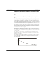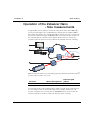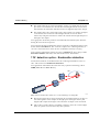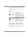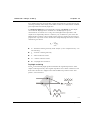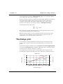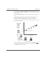
1
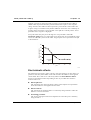
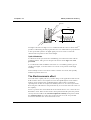
11 Size theory Introduction The aim of this chapter is to describe the basic size principles behind the Zetasizer Nano series. This will help in understanding the meaning of the results achieved. The chapter is divided into two major sections. What is Dynamic light scattering? and Operation of the Zetasizer Nano - Size measurements. The first section describes the theory, while the second describes the physical operation of how a size measurement is performed. What is Dynamic light scattering? The Zetasizer Nano series performs size measurements using a process called Dynamic Light Scattering (DLS) Dynamic Light Scattering (also known as PCS - Photon Correlation Spectroscopy) measures Brownian motion and relates this to the size of the particles. It does this by illuminating the particles with a laser and analysing the intensity fluctuations in the scattered light. Scattering intensity fluctuations If a small particle is illuminated by a light source such as a laser, the particle will scatter the light in all directions. If a screen is held close to the particle, the screen will be illuminated by the scattered light. Now consider replacing the single particle with thousands of stationary particles. The screen would now show a speckle pattern as shown alongside. ill 7676 Zetasizer Nano Page 11-1 11 Chapter 11 Size theory The speckle pattern will consist of bright and dark areas. What causes these bright and dark areas? The diagram below shows the propagated waves from the light scattered by the particles. The bright areas of light are where the light scattered by the particles arrives at the screen with the same phase and interferes constructively to form a bright patch. The dark areas are where the phase additions are mutually destructive and cancel each other out. From Laser Most light passes through unscattered Detector Average intensity The scattered light falling on the detector. ill 6091 In the above example we said that the particles were stationary. In this situation the speckle pattern will also be stationary - in terms of both speckle position and speckle size. In practice, particles suspended in a liquid are never stationary. The particles are constantly moving due to Brownian motion. Brownian motion is the movement of particles due to the random collision with the molecules of the liquid that surrounds the particle. An important feature of Brownian motion for DLS is that small particles move quickly and large particles move more slowly. The relationship between the size of a particle and its speed due to Brownian motion is defined in the Stokes-Einstein equation. As the particles are constantly in motion the speckle pattern will also appear to move. As the particles move around, the constructive and destructive phase addition of the scattered light will cause the bright and dark areas to grow and diminish in intensity - or to put it another way, the intensity at any particular point appears to fluctuate. The Zetasizer Nano system measures the rate of the intensity fluctuation and then uses this to calculate the size of the particles. Page 11-2 MAN 0317 Size theory Chapter 11 Interpreting scattering intensity fluctuation data We know that the Zetasizer measures the fluctuation in scattering intensity and uses this to calculate the size of particles within the sample - but how does it do this? Within the instrument is a component called a digital correlator. A correlator basically measures the degree of similarity between two signals over a period of time. If we compared the intensity signal of a particular part of the speckle pattern at one point in time (say time = t) to the intensity signal a very short time later (t+t) we would see that the two signals are very similar - or strongly correlated. If we then compared the original signal a little further ahead in time (t+2t), there would still be a relatively good comparison between the two signals, but it will not be as good as at t+ t. The correlation is therefore reducing with time. Now consider the intensity of the signal at ‘t’ with the intensity at a much later time - the two signals will have no relation to each other as the particles are moving in random directions (due to Brownian motion). In this situation it is said that there is no correlation between the two signals. With DLS we are dealing with very small time scales. In a typical speckle pattern the length of time it takes for the correlation to reduce to zero is in the order of 1 to ten's of milliseconds. The "short time later" (t) will be in the order of nanoseconds or microseconds! If we compare the signal intensity at (t) with itself then we would have perfect correlation as the signals are identical. Perfect correlation is reported as 1 and no correlation is reported as 0. If we continue to measure the correlation at (t+3t), (t+4t), (t+5t), (t+6t), etc, the correlation will eventually reach zero. A typical correlation function against time is shown below. Correlation 1.00 0 t=0 Time t= ill 6092 Zetasizer Nano Page 11-3 Chapter 11 Size theory Using the correlation function How does the correlation function relate to the particle size? We mentioned earlier that the speed of particles that are being moved by Brownian motion is related to the size of the particles (Stokes-Einstein equation). Large particles move slowly, while smaller particles move quickly. What effect will this have on the speckle pattern? If large particles are being measured, then, as they are moving slowly, the intensity of the speckle pattern will also fluctuate slowly. And similarly if small particles are being measured then, as they are moving quickly, the intensity of the speckle pattern will also fluctuate quickly. The graph below shows the correlation function for large and small particles. As can be seen, the rate of decay for the correlation function is related to particle size as the rate of decay is much faster for small particles than it is for large. Perfect Correlation Correlation 1.00 Large particles Small particles 0 t=0 t= Time ill 6093 After the correlation function has been measured this information can then be used to calculate the size distribution. The Zetasizer software uses algorithms to extract the decay rates for a number of size classes to produce a size distribution. A typical size distribution graph is shown below. Size distribution by Intensity 1.00 Amplitude 0.75 0.50 0.25 0.0 0.1 1 10 100 1000 1.0E+004 Diameter (nm) ill 6218 Page 11-4 MAN 0317 Size theory Chapter 11 The x-axis shows a distribution of size classes, while the y-axis shows the relative intensity of the scattered light. This is therefore known as an intensity distribution. Although the fundamental size distribution generated by DLS is an intensity distribution, this can be converted, using Mie theory, to a volume distribution. This volume distribution can also be further converted to a number distribution. However, number distributions are of limited use as small errors in gathering data for the correlation function will lead to huge errors in distribution by number. Intensity, volume and number distributions What is the difference between intensity, volume and number distributions? A very simple way of describing the difference is to consider a sample that contains only two sizes of particles (5nm and 50nm) but with equal numbers of each size particle. The first graph below shows the result as a number distribution. As expected the two peaks are of the same size (1:1) as there are equal number of particles. The second graph shows the result as a volume distribution. The area of the peak for the 50nm particles is 1000 times larger the peak for the 5nm (1:1000 ratio). This is because the volume of a 50nm particle is 1000 times larger that the 5nm particle (volume of a sphere is equal to 4/3(r)3). The third graph shows the result as an intensity distribution. The area of the peak for the 50nm particles is now 1,000,000 times larger than the peak for the 5nm (1:1000000 ratio). This is because large particles scatter much more light than small particles, the intensity of scattering of a particle is proportional to the sixth power of its diameter (from Rayleigh’s approximation). 1 5 10 50 100 Diameter (nm) Intensity Relative % in class 1 Volume Relative % in class Relative % in class Number 1000 1 5 10 50 100 Diameter (nm) 1,000,000 1 5 10 50 100 Diameter (nm) ill 6094 It is worth repeating that the basic distribution obtained from a DLS measurement is intensity - all other distributions are generated from this. Zetasizer Nano Page 11-5 Chapter 11 Size theory Operation of the Zetasizer Nano - Size measurements A typical DLS system comprises of six main components. First of all a laser is used to provide a light source to illuminate the sample particles within a cell . Most of the laser beam passes straight through the sample, but some is scattered by the particles within the sample. A detector is used to measure the intensity of the scattered light. As a particle scatters light in all directions, it is (in theory), possible to place the detector in any position and it will still detect the scattering. B 6 3 5 90° A 175° 2 3 4 1 ill 8683 With the Zetasizer Nano series, depending upon the particular model, the detector position will be at either 175° or 90°. Zetasizer Optical Arrangement Detection path (above) Nano S / ZS 175° Nano S90 / ZS90 90° The intensity of the scattered light must be within a specific range for the detector to successfully measure it. If too much light is detected then the detector will become overloaded. To overcome this an “attenuator” is used to reduce the intensity of the laser and hence reduce the intensity of the scattering. Page 11-6 MAN 0317 Size theory Chapter 11 For samples that do not scatter much light, such as very small particles or samples of low concentration, the amount of scattered light must be increased. In this situation, the attenuator will allow more laser light through to the sample. For samples that scatter more light, such as large particles or samples of higher concentration, the amount of scattered light must be decreased. This is achieved by using the attenuator to reduce the amount of laser light that passes through to the sample. The appropriate attenuator position is automatically determined by the Zetasizer during the measurement sequence. The scattering intensity signal for the detector is passed to a digital signal processing board called a correlator . The correlator compares the scattering intensity at successive time intervals to derive the rate at which the intensity is varying. This correlator information is then passed to a computer , where the specialist Zetasizer software will analyse the data and derive size information. 175° detection optics - Backscatter detection The Zetasizer Nano Z, S and ZS measure the scattering information at close to 180°. This is known as backscatter detection. The application of the Backscatter detection is by a patented technology called NIBS (Non-Invasive Back-Scatter). 175° Why measure backscatter? There are several advantages to doing this: Zetasizer Nano ill 8684 Because the backscatter is being measured, the incident beam does not have to travel through the entire sample. As the light passes through a shorter path length of the sample, then higher concentrations of sample can be measured. This reduces an effect known as multiple scattering, where the scattered light from one particle is itself scattered by other particles. Page 11-7 Chapter 11 Size theory Contaminants such as dust particles within the dispersant are typically large compared to the sample size. Large particles mainly scatter in the forward direction. Therefore, by measuring the backscatter, the effect of dust is greatly reduced. The effect of multiple scattering is at a minimum at 180º - again, this allows higher concentrations to be measured. Moveable lens A movable lens allows the focus position within the cell to be changed. This allows a much larger range of sample concentrations to be measured. Sample ill 6772 Sample For small particles, or samples of low concentration, it will be beneficial to maximise the amount of scattering from the sample. As the laser passes through the wall of the cell and into the dispersant, the cell wall will cause “flare”. This flare may swamp the scattering signal. Moving the measurement point away from the cell wall, towards the centre of the cell will remove this effect. Large particles or samples of high concentration, scatter much more light. In this situation, measuring closer to the cell wall will reduce the effect of multiple scattering. In this instance the flare from the cell wall will have less impact. Any flare will be proportionally reduced compared to the scattering signal. ill 6773 The measurement position is automatically determined by the Zetasizer software. 90° detection optics - Classical arrangement The 90° models, Zetasizer Nano S90 and ZS90, have been included in the Zetasizer Nano instrument range to provide continuity with other systems that have 90° detection optics. These models do not utilise a movable optical arrangement but use the ‘classical’ fixed detection arrangement of 90° to the laser and the centre of the cell area. This arrangement reduces the detectable size range on these models. Page 11-8 MAN 0317 12 Molecular weight theory Introduction The aim of this chapter is to describe the basic molecular weight principles behind the Zetasizer Nano. This will help in understanding the meaning of the results achieved. The chapter is divided into two major sections. What is Static light scattering? and The Debye plot. The first section describes the molecular weight theory, while the second shows how a molecular weight measurement is displayed. What is Static light scattering? The Zetasizer Nano series performs molecular weight measurements using a process called Static Light Scattering (SLS). This is a non-invasive technique used to characterise the molecules in a solution. In a similar way to Dynamic Light Scattering - the size theory - the particles in a sample are illuminated by a light source such as a laser, with the particles scattering the light in all directions. But, instead of measuring the time-dependent fluctuations in the scattering intensity, Static light scattering makes use of the timeaveraged intensity of scattered light instead. The intensity of light scattered over a period of time, say 10 to 30 seconds, is accumulated for a number of concentrations of the sample. This time averaging removes the inherent fluctuations in the signal, hence the term ‘Static Light Scattering’. From this we can determine the Molecular weight (MW) and the 2nd Virial Coefficient (A2). The 2nd Virial Coefficient (A2) is a property describing the interaction strength between the particles and the solvent or appropriate dispersant medium. Zetasizer Nano Page 12-1 12 Chapter 12 Molecular weight theory For samples where A2>0, the particle ‘likes’ the solvent more than itself, and will tend to stay as a stable solution. When A2<0, the particle ‘likes’ itself more than the solvent, and therefore may aggregate. When A2=0, the particle-solvent interaction strength is equivalent to the molecule-molecule interaction strength – the solvent can then be described as being a theta solvent. Static light scattering - theory The molecular weight is determined by measuring the sample at different concentrations and applying the Rayleigh equation. The Rayleigh equation describes the intensity of light scattered from a particle in solution. The Rayleigh equation is KC 1-------- = ------+ 2A 2 C P MW R R:The Rayleigh ratio - the ratio of scattered light to incident light of the sample. MW : Sample molecular weight. A2 : 2nd Virial Coefficient. C : Concentration. P : Angular dependence of the sample scattering intensity. Please refer to the Rayleigh scattering section. K : Optical constant as defined below. 2 2 4 - dn ------ n K = ----------o 4 o N A dc NA : Avogadro’s constant. o : Laser wavelength. no : Solvent refractive index. dn/dc : The differential refractive index increment. This is the change in refractive index as a function of the change in concentration. For many sample/ solvent combinations this may be available in literature; while for novel combinations the dn/dc can be measured by use of a differential refractometer. Page 12-2 MAN 0317 Molecular weight theory Chapter 12 The standard approach for molecular weight measurements is to first measure the scattering intensity of the analyte used relative to that of a well described ‘standard’ pure liquid with a known Rayleigh ratio. A common standard used in Static light scattering is Toluene, for the simple reason that the Rayleigh ratios of toluene are suitably high for precise measurements, are known over a range of wavelengths and temperatures and, maybe more importantly, toluene is relatively easy to obtain in a pure form. The Rayleigh ratio of toluene can be found in many reference books, but for reference purposes the expression used to calculate the sample Rayleigh ratio from a toluene standard is given below. 2 IA no -R R = --------2 T IT nT IA : Residual scattering intensity of the analyte (i.e. the sample intensity – solvent intensity). IT : Toluene scattering intensity. no : Solvent refractive index. nT : Toluene refractive index. RT : Rayleigh ratio of toluene. Rayleigh scattering The P term in the Rayleigh equation embodies the angular dependence of the sample scattering intensity. The angular dependence arises from constructive and destructive interference of light scattered from different positions on the same particle, as shown below. Destructive Interference Constructive Interference ill 6746 Zetasizer Nano Page 12-3 Chapter 12 Molecular weight theory This phenomenon is known as Mie scattering, and it occurs when the particle size is of the same order as the wavelength. However when the particles in solution are much smaller than the wavelength of the incident light, multiple photon scattering will be avoided. Under these conditions, P will reduce to 1 and the angular dependence of the scattering intensity is lost. This type of scattering is known as Rayleigh scattering. The Rayleigh equation will now be: KC 1-------- = ---+ 2A 2 C M R We can therefore stipulate that if the particle is small, Rayleigh scattering can be assumed and the Rayleigh approximation used. With the Zetasizer Nano series the applicable molecular measurement weight range is from a few hundred g/mol to 500,000 for linear polymers, and over 20,000,000 for near spherical polymers and proteins. The Debye plot The intensity of scattered light that a particle produces is proportional to the product of the weight-average molecular weight and the concentration of the particle. The Zetasizer Nano S and ZS measure the Intensity of scattered light (KC/R) of various concentrations (C) of sample at one angle; this is compared with the scattering produced from a standard (i.e. Toluene). The graphical representation of this is called a Debye plot and allows for the determination of both the Absolute molecular weight and 2nd Virial Coefficient. Debye Plot 300. Intensity 1.3e-5 250. Debye 1.2e-5 200. 1.1e-5 0 2.00e-4 4.00e-4 6.00e-4 8.00e-4 0.001 0.0012 Intensity (kcps) KC/Rop (1/Da) 1.4e-5 150. 0.0014 Concentration (g/mL) ill 7675 Page 12-4 MAN 0317 Molecular weight theory Chapter 12 The weight-averaged molecular weight (Mw) is determined from the intercept at zero concentration i.e. KC/R = 1/Mw (for c--> 0) where the Mw is expressed in Daltons (or g/mol). The 2nd Virial Coefficient (A2) is determined from the gradient of the Debye plot. Each plot and molecular weight measurement is performed by doing several individual measurements; from the solvent used (a zero concentration measurement), through sample preparations at various concentrations. Standard sample i.e. pure solvent 1 kC/Rθ - Intensity of scattered light The diagram below shows how the molecular weight and 2nd Virial Coefficient are derived from the Debye plot. Gradient 4 3 2 1 Intercept point 0 2 C - concentration 3 Samples of varying concentration 4 ill 8208 As only one measurement angle is used in this case, a plot of KC/R versus C should give a straight line whose intercept at zero concentration will be 1/Mw and whose gradient is proportional to A2. Zetasizer Nano Page 12-5 Chapter 12 Page 12-6 Molecular weight theory MAN 0317 13 Zeta potential theory Introduction The aim of this chapter is to describe the basic Zeta potential measurement principles behind the Zetasizer Nano. This will help in understanding the meaning of the results achieved. The chapter is divided into two major sections. What is Zeta Potential? and Operation of the Zetasizer Nano - Zeta potential measurements. The first section describes the zeta potential theory, while the second describes the physical operation of how a zeta potential measurement is performed. What is Zeta potential? The Zetasizer Nano series calculates the zeta potential by determining the Electrophoretic Mobility and then applying the Henry equation. The electrophoretic mobility is obtained by performing an electrophoresis experiment on the sample and measuring the velocity of the particles using Laser Doppler Velocimetry (LDV). These techniques are described in the following sections. Zeta potential and the Electrical double layer The development of a net charge at the particle surface affects the distribution of ions in the surrounding interfacial region, resulting in an increased concentration of counter ions (ions of opposite charge to that of the particle) close to the surface. The liquid layer surrounding the particle exists as two parts; an inner region, called the Stern layer, where the ions are strongly bound and an outer, diffuse, region where they are less firmly attached; thus an electrical double layer exists around each particle. Within the diffuse layer there is a notional boundary inside which the ions and particles form a stable entity. When a particle moves (e.g. due to gravity), Zetasizer Nano Page 13-1 13 Chapter 13 Zeta potential theory ions within the boundary move with it, but any ions beyond the boundary do not travel with the particle. This boundary is called the surface of hydrodynamic shear or slipping plane. The potential that exists at this boundary is known as the Zeta potential. Electrical double layer Stern layer + + + + ++ + + - ++ + + + + + + + ++ + + + + ++ + + + Diffuse layer Slipping plane - Surface potential Zeta potential mV Distance from particle surface ill 8491 The magnitude of the zeta potential gives an indication of the potential stability of the colloidal system. A colloidal system is when one of the three states of matter: gas, liquid and solid, are finely dispersed in one of the others. For this technique we are interested in the two states of: a solid dispersed in a liquid, and a liquid dispersed in a liquid, i.e. an emulsion. If all the particles in suspension have a large negative or positive zeta potential then they will tend to repel each other and there is no tendency to flocculate. However, if the particles have low zeta potential values then there is no force to prevent the particles coming together and flocculating. The general dividing line between stable and unstable suspensions is generally taken at either +30mV or -30mV. Particles with zeta potentials more positive than +30mV or more negative than -30mV are normally considered stable. The most important factor that affects zeta potential is pH. A zeta potential value on its own without a quoted pH is a virtually meaningless number. Page 13-2 MAN 0317 Zeta potential theory Chapter 13 Imagine a particle in suspension with a negative zeta potential. If more alkali is added to this suspension then the particles will tend to acquire a more negative charge. If acid is then added to this suspension a point will be reached where the negative charge is neutralised. Any further addition of acid can cause a build up of positive charge. Therefore a zeta potential versus pH curve will be positive at low pH and lower or negative at high pH. The point where the plot passes through zero zeta potential is called the Isoelectric point and is very important in prectical terms. It is normally the point where the colloidal system is least stable. A typical plot of zeta potential versus pH is shown below. 60 Zeta potential (mV) 40 20 0 -20 Isoelectric point -40 -60 2 4 6 8 10 12 pH ill 6749 Electrokinetic effects An important consequence of the existence of electrical charges on the surface of particles is that they will exhibit certain effects under the influence of an applied electric field. These effects are collectively defined as electrokinetic effects. There are four distinct effects depending on the way in which the motion is induced. These are: Zetasizer Nano Electrophoresis : The movement of a charged particle relative to the liquid it is suspended in under the influence of an applied electric field. Electroosmosis : The movement of a liquid relative to a stationary charged surface under the influence of an electric field. Streaming potential : The electric field generated when a liquid is forced to flow past a stationary charged surface. Page 13-3 Chapter 13 Zeta potential theory Sedimentation potential : The electric field generated when charged particles move relative to a stationary liquid. Electrophoresis When an electric field is applied across an electrolyte, charged particles suspended in the electrolyte are attracted towards the electrode of opposite charge. Viscous forces acting on the particles tend to oppose this movement. When equilibrium is reached between these two opposing forces, the particles move with constant velocity. The velocity of the particle is dependent on the following factors: Strength of electric field or voltage gradient. The dielectric constant of the medium. The viscosity of the medium. The zeta potential. The velocity of a particle in an electric field is commonly referred to as its Electrophoretic mobility. With this knowledge we can obtain the zeta potential of the particle by application of the Henry equation. The Henry equation is: where: z : Zeta potential. UE : Electrophoretic mobility. : Dielectric constant. : Viscosity. ƒ(Ka) : Henry’s function. Two values are generally used as approximations for the f(Ka) determination either 1.5 or 1.0. Electrophoretic determinations of zeta potential are most commonly made in aqueous media and moderate electrolyte concentration. f(Ka) in this case is 1.5, and is referred to as the Smoluchowski approximation. Therefore calculation of zeta potential from the mobility is straightforward for systems that fit the Smoluchowski model, i.e. particles larger than about 0.2 microns dispersed in Page 13-4 MAN 0317 Zeta potential theory Chapter 13 electrolytes containing more than 10-3 molar salt. The Smoluchowski approximation is used for the folded capillary cell and the universal dip cell when used with aqueous samples. For small particles in low dielectric constant media f(Ka) becomes 1.0 and allows an equally simple calculation. This is referred to as the Huckel approximation. Non-aqueous measurements generally use this. Measuring Electrophoretic Mobility It is the electrophoretic mobility that we measure directly with the conversion to zeta potential being inferred from theoretical considerations. How is electrophoretic mobility measured? The essence of a classical micro-electrophoresis system is a cell with electrodes at either end to which a potential is applied. Particles move towards the electrode of opposite charge, their velocity is measured and expressed in unit field strength as their mobility. Electrode + - + Electrode + + - Capillary + - - + The technique used to measure this velocity is Laser Doppler Velocimetry. ill 6750 Laser doppler velocimetry Laser doppler velocimetry (LDV) is a well established technique in engineering for the study of fluid flow in a wide variety of situations, from the supersonic flows around turbine blades in jet engines to the velocity of sap rising in a plant stem. In both these examples, it is actually the velocity of tiny particles within the fluid streams moving at the velocity of the fluid that we are measuring. Therefore, LDV is well placed to measure the velocity of particles moving through a fluid in an electrophoresis experiment. The receiving optics are focused so as to relay the scattering of particles in the cell. Zetasizer Nano Page 13-5 Chapter 13 Zeta potential theory be am Detector Cell ing + Sc at ter - - - - + 17° Intensity of scattered light c In e id n e tb am Time ill 6777 The light scattered at an angle of 17° is combined with the reference beam. This produces a fluctuating intensity signal where the rate of fluctuation is proportional to the speed of the particles. A digital signal processor is used to extract the characteristic frequencies in the scattered light. Optical Modulator A refinement of the system involves modulating one of the laser beams with an oscillating mirror. This gives an unequivocal measure of the sign of the zeta potential. A second benefit of the modulator is that low or zero mobility particles give an equally good signal, so measurement is as accurate as for particles with a high mobility. This technique ensures an accurate result in a matter of seconds, with possibly millions of particles observed. The Electroosmosis effect The walls of the capillary cell carry a surface charge so the application of the electric field needed to observe electrophoresis causes the liquid adjacent to the walls to undergo electroosmotic flow. Colloidal particles will be subject to this flow superimposed on their electrophoretic mobility. However, in a closed system the flow along the walls must be compensated for by a reverse flow down the centre of the capillary. There is a point in the cell at which the electroosmotic flow is zero - where the two fluid flows cancel. If the measurement is then performed at this point, the particle velocity measured will be the true electrophoretic velocity. This point is called the stationary layer. It is where the two laser beams cross; the zeta potential measured is therefore free of electroosmotic errors. Page 13-6 MAN 0317 Zeta potential theory Chapter 13 - - - - - - - - - - - + + + + + + + + + + + + Zero electroosmosis + Stationary Layer + + + + + + + + + + + + - - - - - - - - - - - - Zero electroosmosis ill 7672 Avoiding Electroosmosis The stationary layer technique described above has been in use for many years. Because of the effect of electroosmosis the measurement can only be performed at specific point within the cell. If it was possible to remove electroosmosis altogether then it would be possible to perform the measurement on the particles at any point in the cell and obtain the true mobility. This is now possible. With a combination of Laser Doppler Velocimetry and Phase Analysis Light Scattering (PALS) this can now be achieved in Malvern’s patented M3-PALS technique. Implementation of M3-PALS enables even samples of very low mobility to be analysed and their mobility distributions calculated. The M3-PALS technique To perform measurements at any point within a cell and obtain the electrophoretic mobility, Malvern has developed its patented M3-PALS technique. This is a combination of Malvern’s improved laser doppler velocimetry method - the M3 measurement technique, and the application of PALS (Phase Analysis Light Scattering). The M3 technique As discussed earlier traditional electrophoretic measurements are performed by measurement of particles at the stationary layer, a precise position near the cell walls. With M3 the measurement can be performed anywhere in the cell, though with the Zetasizer Nano series it is performed in the centre of the cell. M3 consists of both Slow Field Reversal (SFR) and Fast Field Reversal (FFR) measurements, hence the name ‘Mixed Mode Measurement’. Measurement position in the cell The M3 method performs the measurement in the middle of the cell, rather than at the stationary layer. In principle the M3 measurement could be done at any Zetasizer Nano Page 13-7 Chapter 13 Zeta potential theory position in the cell, however there are a number of reasons for choosing to work at the centre. The measurement zone is further from the cell wall, so reduces the chance of flare from the nearby surface. The alignment of the cell is less critical. The charge on the cell wall can be calculated. Reversal of the applied field All systems that measure mobilities using LDV (Laser Doppler Velocimetry) reverse the applied field periodically during the measurement. This is normally just the slow field reversal mentioned below. However, M3 consists of two measurements for each zeta potential measurement, one with the applied field being reversed slowly - the SFR measurement; and a second with a rapidly reversing applied field - the FFR measurement stage. Slow Field Reversal (SFR) This reversal is applied to reduce the polarisation of the electrodes that is inevitable in a conductive solution. The field is usually reversed about every one second to allow the fluid flow to stabilise. Significant fluid flow - - - - - - - - - - - + + + + + + + + + + + + + Stationary Layer - + + + + + + + + + + + + - - - - - - - - - - - ill 7673 Fast Field Reversal (FFR) If the field is reversed much more rapidly, it is possible to show that the particles reach terminal velocity, while the fluid flow due to electroosmosis is insignificant. (The residual flow in the diagram below is exaggerated). This means that the mobility measured during this period is due to the electrophoresis of the particles only, and is not affected by electroosmosis. The mean zeta potential that is calculated by this technique is therefore very robust, as the measurement position in the cell is not critical. However, as the velocity of the particles is sampled for such a short period of time, information about the distribution is degraded. This is what is addressed by M3, Page 13-8 MAN 0317 Zeta potential theory Chapter 13 the PALS technique is used to determine the particle mobility in this part of the sequence. Insignificant fluid flow - - - - - - - - - - - + + + + + + + + + + + + + Stationary Layer - + + + + + + + + + + + + - - - - - - - - - - - ill 7674 M3 measurement sequence An M3 measurement is performed in the following manner: A Fast field reversal measurement is performed at the cell centre. This gives an accurate determination of the mean. A Slow field reversal measurement is made. This gives better resolution, but mobility values are shifted by the effect of electroosmosis. The mean zeta potentials calculated from the FFR and SFR measurements are subtracted to determine the electroosmotic flow. This value is used to normalise the slow field reversal distribution. The value for electroosmosis is used to calculate the zeta potential of the cell wall. Benefits of M3 Using M3 the entire zeta potential measurement is simplified. It is no longer necessary for the operator to select any system parameters for the measurement, as the appropriate settings are calculated as part of the M3 sequence. With a reduction in the number of measurement variables, both measurement repeatability and accuracy is improved. Additionally, alignment is no longer an issue as there are no concerns about the location of the stationary layer. M3 is now combined with the PALS measurement. Adding PALS and what is it? PALS (Phase Analysis Light Scattering) is a further improvement on traditional Laser Doppler Velocimetry and the M3 implementation described above. Zetasizer Nano Page 13-9 Chapter 13 Zeta potential theory Overall, the application of PALS improves the accuracy of the measurement of low particle mobilities. This can give an increase in performance of greater than 100 times that associated with standard measurement techniques. This allows the measurement of high conductivity samples, plus the ability to accurately measure samples that have low mobilities. Low applied voltages can now be used to avoid any risk of sample effects due to joule heating. How PALS works Rather than use the Doppler frequency shift caused by moving particles to measure their velocity, Phase Analysis Light Scattering, as the name suggests, uses the phase shift. The phase is preserved in the light scattered by moving particles, but is shifted in phase in proportion to their velocity. This phase shift is measured by comparing the phase of the light scattered by the particles with the phase of a reference beam. A beam splitter is used to extract a small proportion of the original laser beam to use as the reference. The phase analysis of the signal can be determined accurately even in the presence of other effects that are not due to electrophoresis, for example thermal drifts due to joule heating. This is because the form of the phase change due to the application of the field is known so the different effects can be separated. As electroosmosis is insignificant due to the implementation of M3 then the difference between the two phases will be constant, so if there is any particle movement then this phase relationship will alter. Detection of a phase change is more sensitive to changes in mobility, than the traditional detection of a frequency shift. Phase plot Phase (radians) 0 -5. Electrophoretic mobility distribution 3.e+5 0.1000 0.2000 0.3000 0.4 Time (s) Intensity (kcps) -10. 2.e+5 1.e+5 0 -12. -11. -10. -9. -8. -7. -6. -5. -4. -3. -2. -1. 0 1. 2. 3. 4. 5. 6. 7. 8. 9. 10. 11. 12. Mobility (umcm/Vs) Electrophoretic mobility and consequently the zeta potential is then determined by summing the phase shifts measured during the FFR part of the measurement. Page 13-10 ill 7670 MAN 0317 Zeta potential theory Chapter 13 Operation of the Zetasizer Nano - Zeta potential measurements In a similar way to the typical DLS system described in the size theory chapter, a zeta potential measurement system comprises six main components. First of all a laser is used to provide a light source to illuminate the particles within the sample; for zeta potential measurements this light source is split to provide an Incident and Reference beam . The reference beam is also ‘modulated’ to provide the Doppler effect necessary. The laser beam passes through the centre of the sample cell , and the scattering beam at an angle of 12.8° is detected. 6 2 7 B C A 12.8° 3 1 5 4 ill 8685 When an electric field is applied to the cell, any particles moving through the measurement volume will cause the intensity of light detected to fluctuate with a frequency proportional to the particle speed. A detector sends this information to a digital signal processor . This information is then passed to a computer , where the Zetasizer software produces a frequency spectrum from which the electrophoretic mobility and hence the zeta potential information is calculated. The intensity of the scattered light within the cell must be within a specific range for the detector to successfully measure it. If too much light is detected then the Zetasizer Nano Page 13-11 Chapter 13 Zeta potential theory detector will become overloaded. To overcome this an “attenuator” is used to reduce the intensity of the laser and hence reduce the intensity of the scattering. For samples that do not scatter much light, such as very small particles or samples of low concentration, the amount of scattered light must be increased. The attenuator will automatically allow more light through to the sample. For samples that scatter more light, such as large particles or samples of higher concentration, the amount of scattered light must be decreased. The attenuator will automatically reduce the amount of light that passes through to the sample. To correct for any differences in the cell wall thickness and dispersant refraction, compensation optics are installed within the scattering beam path to maintain alignment of the scattering beams. Page 13-12 MAN 0317