Download ACES BRIDGE ANALYSIS SYSTEM USER MANUAL

ACES
BRIDGE ANALYSIS
SYSTEM
USER MANUAL
February 2007
This page intentionally left blank
ACES V6.4 User Manual
February 2007
ACES HELP SYSTEM
CONTENTS
PART 1
1.1
1.2
1.3
1.4
1.5
1.6
1.7
1.8
1.9
PART 2
2.1
2.2
2.3
2.4
2.5
2.6
2.7
2.8
2.9
PART 3
3.1
3.2
3.3
3.4
3.5
3.6
3.7
3.8
3.9
PART 4
4.1
4.2
4.3
4.4
4.5
4.6
GETTING STARTED
Setup
Menus
User Interface
Units
Coordinate System
Sign Convention
Saving Model Data Files
Retrieving Model Files
System Limitations & Restrictions
CREATING THE MODEL GEOMETRY
How to Create a Model
Parametric Modelling Using Templates
Changing the Model Geometry
Defining Lanes
Member Properties
Adding New Sections to the Data Base
Section Properties Calculator
Composite Sections Calculator
Element Properties
STATIC & MOVING LOADS
Creating & Deleting Load Cases
Moving Vehicle Loads
Patch & Lane Loads
Nodal Loads
Member Loads
Element Loads
Hydrostatic Loads
Temperature Expansion/Contraction Loads
Other Static Loads & Dead Load
ANALYSIS
Analysis Options
Frame & Beam Analysis
Grillage Analysis
Finite Element Analysis
Dynamic Analysis
Second Order Analysis
ACES V6.4 User Manual
February 2007
ACES HELP SYSTEM
CONTENTS
PART 5
5.1
5.2
5.3
5.4
5.6
RESULT & REPORTS
Graphical Results
Tabular Reports
Envelopes
Combinations
Finite Element Results
PART 6
INCREMENTAL LAUNCHING MODULE - Main
Index
PART 7
CONTINUOUS BEAM MODULE - Main Index
PART 8
MODEL TEMPLATES - Main Index
ACES V6.4 User Manual
February 2007
PART 1
GETTING STARTED
Page 3 of 235
ACES V6.4 User Manual
PART 1.1
1.0
February 2007
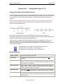
Setting up and Uninstalling ACES
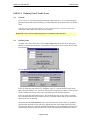
Installation
Insert the installation CD into the PC then bring up Explorer (from the Start/Programs menu).
List the contents of the CD drive and locate the Setup program. Double click on Setup.exe to run
the installation program then follow any instructions that may be given.
ACES will be installed by default into the C:/Program Files/Aces6 folder. If you wish to install
it into another folder (e.g. C:/Aces) refer to the installation instructions that came with the CD or
contact ACES Analysis Systems for assistance.
2.0
Creating an ACES Icon on the Desktop
Use Windows Explorer to display the contents of the folder into which ACES was installed (e.g.
C:/Program Files/Aces6). Locate the file called aces6.exe (it will be prefixed with a small
bridge icon), click onto it with the right mouse button then drag it out to a free spot on the desktop and release the button.
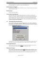
A short menu will pop up on the screen. Scroll down the list of items with the left button and
select Create Shortcut(s) Here. Windows will create an ACES icon at that spot on your desktop.
You can now move it to another position on your desktop and rename it if you wish.
3.0
Removing (Un-Installing) ACES
Click on Start / Settings / Control Panel / Add-Remove Programs , highlight ACES Bridge
Analysis System, click Add/Remove.. then respond accordingly. Note that the full contents of the
ACES folder may not always be deleted - you may need to use Windows Explorer to complete the
task.
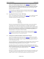
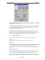
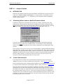
PART 1.2 Menus & User Interface
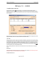
1.0
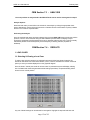
GENERAL OVERVIEW
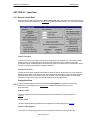
The ACES graphical interface is based on the standard Windows environment with its now
familiar menu structure, tool bar layout and message prompts.
Pull-down menus are generally self-explanatory. Most have a menu option labelled
MenuHELP.. that, when selected, displays a dialogue box containing a brief description of all
other options in that menu. Some of the key menus also have an option called HowTo.. that
provides a brief description of the more frequently asked questions.
All help dialogue boxes can be printed using the commands File/Print/Last help file.
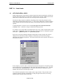
2.0
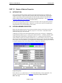
MENU BAR OPTIONS
File
This menu option enables a range of file-related operations to be performed. Refer to File /
Menu HELP for a short description of all file options in this menu.
Structure
Page 4 of 235
ACES V6.4 User Manual
February 2007
This menu option enables changes to be made to the base model. Refer to the main contents page
for a complete list of all features or to Structure / Menu HELP for a short description of all
options in this menu.
Loads
This menu option enables loadings to be applied to the model. Refer to the main contents page
for a complete list of all features or to Loads / Menu HELP for a short description of all options
in this menu.
Analyse
This menu option contains options for performing a range of different types of analyses (frame,
grillage, finite element, second order and dynamic). Refer to PART 4.1 for details.
Results
This menu option enables results of the analysis to be viewed graphically. Refer to PART 5.1 for
detailed instructions in doing this.
Reports
This menu option produces tabular reports (i.e., results are presented as numeric text values in a
table rather than graphically). Refer to PART 5.2 for detailed instructions in creating tabular
reports.
View
This menu option enables the structural model and graphical results to be viewed from many
angles. It also allows you to view any lanes that may have been created and to toggle on the
background grid if required.
Zoom-Pan
This menu option allows you to zoom and pan around the model.
Activate
This menu option enables parts of the structure to be activated and de-activated i.e., groups and
blocks of nodes, members and elements can be selectively “suppressed” (not shown on the screen
or in reports). Note that they are not deleted from the model but merely de-activated.
This can be very useful in complex 3D frames and FE models where you wish to view and
interrogate only one visible part of the model in order to better see its attributes or results. Once
you have created these special “views” they can be saved to a database and recalled later.
Inquire
This menu option enables “spot” inquiries to be made on a large number of model attributes
including:
ƒ
ƒ
ƒ
ƒ
ƒ
ƒ
ƒ
ƒ
ƒ
ƒ
Exact coordinates of selected nodes
Distances between any two nodes
The number of a selected node, member or element
The largest node, member or element number in the model and its location
The location of a node, member or element of a specified number
Page 5 of 235
ACES V6.4 User Manual
ƒ
ƒ
ƒ
ƒ
February 2007
Type and length of a specified member
Element type and area
Shortcuts
This option saves the last ten menu commands used. In effect it mimics a macro that
continuously retains the last series of menu accesses made by you during the current session. It is
particularly useful if you are repeating a series of actions that are deeply nested within several
layers of menus and submenus (such as adjusting the path of a vehicle or selecting a new member
range).
LastMenu
This displays the last menu or submenu that was accessed. It is particularly useful if you are
repeating a series of actions that are deeply nested within several layers of menus and submenus.
MyMenu
This option allows you to display a menu of up to 15 of your favorite command strings and
actions. It can be customised to suit your own requirements by selecting the menu options
Settings/Customise MyMenu. Refer to Customise MyMenu in PART 1.3 of this help system for
further details.
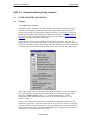
Settings
The Settings option in the menu bar allows a large number of diagram and model attributes and
defaults to be customised then saved for future sessions. These include:
ƒ
ƒ
ƒ
ƒ
ƒ
ƒ
ƒ
ƒ
ƒ
ƒ
ƒ
ƒ
ƒ
ƒ
ƒ
ƒ
Screen windows, diagram and text colours and line styles
Background grid
Display of symbols
Node, member and element numbers and local axes
Member and element property type colours
Customising MyMenu
Decimal places
Axes
Refer to PART 1.3 for more information
Help
This menu option provides information about the current ACES system and contains the help
system.
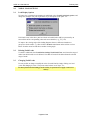
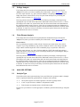
3.0
TOOL BARS
3.1
Main Tool Bar
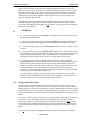
This extends across the top of the screen, immediately below the menu options. To quickly
determine the function of a tool bar icon, let the cursor hover over it for a moment. A yellow
description bar will pop up. Most buttons are self-explanatory and will not be described in any
further detail here. However, the following require some elaboration.
Begin the analysis. The problem will be solved using the current
analysis settings.
Displays the attributes dialog box for the last-drawn, or currently
Page 6 of 235
ACES V6.4 User Manual
February 2007
selected, results diagram. It allows attributes such as vector type, colour,
scale and so on to be selected. The contents of the dialog box will
depend on the nature of the current, or previously drawn, results diagram
i.e., whether it was a moment diagram, shear, reaction, displacement
diagram etc.
Redraws the graphical results diagram that was last displayed (i.e., before
it was cleared). The diagram will be redisplayed using the currently
active settings and attributes. It is particularly useful after a zoom action
is performed.
Redisplays the tabular report that was last generated.
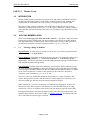
PART 1.2 Text Editing Options & Side Menu
The side menu contains icons to assist in adding, editing, moving and deleting text and other icons to
allow member ranges, active views and member and element node numbers to be easily displayed. Click
the Up-arrow button at the bottom of the right-hand (side) menu to bring up the following icon help panel:
Detailed Description of Icons
Add a new text string. Clicking this icon will display a text entry dialog box. Type in the text you
would like to place on the current diagram, select a font size and colour, then click OK to insert
the text. ACES will prompt you to click on the spot in your screen drawing where you would like
the text placed. Note that the text string will also be inserted into a text library for re-use on other
drawings (refer to the last icon for details).
Page 7 of 235
ACES V6.4 User Manual
February 2007
Edit a text string. ACES will ask you to click on the first character of the text string you wish to
edit. The string will then be echoed into a text edit panel that will allow you to perform edit
operations.
Delete a text string. After clicking this icon ACES will prompt you to click on the first character of
the string that you would like to delete. Continue deleting other strings or select another
operation.
Move a text string. After clicking this icon ACES will prompt you to click on the first character of
the string that you would like to move. Click and drag the string to its new location. Continue
moving other strings or select another operation.
Add text from a list. Displays a menu selection of up to 10 frequently used text strings. New
strings can be added, but they must already exist in the text library (refer to the next icon, shown
below). Once a button is clicked, the text is displayed in an editing box and can be modified as
required or applied as is. ACES will then prompt you to click on the spot on the drawing at which
you want the text to be placed.
Select text from table: Displays a dialog box of all available text strings. Check or uncheck
strings that you would like to appear on the current diagram. Click Apply to display the selected
text strings on the diagram. Note that all strings can be manually edited within this dialog box and
their location and attributes changed if required. New strings can be added or unwanted strings
deleted.
Whenever a new string is created using the “Add a new string” icon, it is also added to the next
available line in this list (together with all its attributes). A maximum of only 20 strings can be
stored in the table.
Clear current member range. Click this button to clear the currently selected member range.
Select a range of straight members. Click this button to select one or more members to add to
the current range. Note that this will select all members lying on a continuous straight line. If you
wish to select only a part of a full line of members then use the menu options: Results / Select a
range of members / Members on part of a straight line. Note that to add another member to the
current member range all members in the model must be active. To do this, click the Activate all
members/nodes/elements button described below.
Show/Hide node numbers. This button acts as an On/Off toggle. When clicked the first time it
will show all nodes and their respective numbers. When clicked again the node numbers will
disappear.
Show/Hide member numbers. This button acts as an On/Off toggle. When clicked the first time
it will show all member numbers. When clicked again the member numbers will disappear.
Show/Hide member orientation. This button acts as an On/Off toggle. When clicked the first
time it will show the orientation of all member in the model. When clicked again the member
orientation symbols will disappear. Note that for 2D structures ACES will display the model in as a
3D perspective in order that the orientation symbols can be properly viewed.
Select from a list of active views. Up to 20 active views can be stored at various stages of
building and interrogating the model then retrieved using this option. For example, the currently
selected range of members can be saved as an active view using the commands: Results / Select
a range of members / Add current range to active views list.
Activate all members/nodes/elements. This button will make all nodes, members and elements
in the model active. (Note that parts of the model will be de-activated if an active view is selected
using the Select from a list of active views icon described above).
Page 8 of 235
ACES V6.4 User Manual
February 2007
PART 1.3 The ACES User Interface
1.0
SETTINGS
The Settings option in the menu bar allows a large number of diagram and model attributes to be
customised then saved for future sessions. Not all will be described here-under since they are
relatively self-evident. The following, however, warrant comment:
1.1
Customise ‘MyMenu’
This option allows MyMenu to be customised. In order to use this feature, however, the menu
actions that you wish to include in MyMenu must first exist in the Shortcuts menu. In other
words, you will have to manually perform the required actions on your model at least once in
order that they can be ‘recorded’ and placed into the Shortcuts menu.
Once there, Customise MyMenu can be used to copy them across into MyMenu. To allocate a
command string to one of the menu buttons, click on the target button then select the required
action from the Shortcuts menu list that will appear. Click Save to save the entries in MyMenu for
future sessions.
1.2
Background Grid
This option allows the colour, mesh spacing and reference point of the background grid to be
changed. By default ACES will draw the grid using the origin (X=0, Y=0) as the reference point.
This can be changed to any defined node (or point) on the model.
1.3
Line Styles
ACES creates all model drawings and results diagrams using a palette of 33 line “styles”. Line
styles are not only used in drawing the model but also for displaying member types, axes, labels,
added text, graphical results and so on. This feature allows the default attributes for these 33 line
styles to be changed. Lines can be changed in terms of their colour, thickness and style (solid,
dashed etc).
1.4
Member, Element, Results Colours
This option allows default colours to be assigned to member and element property types and to
graphical results (moments, shears, deflections etc).
1.5
Save/Retrieve Settings
This option allows you to save your customised settings to one of two attribute sets - a normal set
and an alternate set. The normal set is the one ACES always uses when it starts up. If you wish
to use the alternate set it must be activated either just after a new model has been generated or
once an existing model has been loaded from disk. Retrieve Settings allows either of the two
attribute sets to be reloaded.
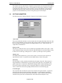
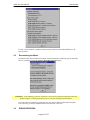
1.6
Session Options
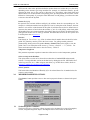
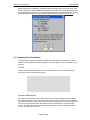
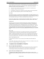
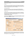
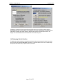
1.7
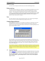
This feature enables a number of global options to be set for the current session. Note, however,
that they will not be saved as system defaults settings for future use. The following dialog box
will be displayed:
Page 9 of 235
ACES V6.4 User Manual
February 2007
• • Prevent access to results if changes are made: If any of the member/element properties
or load case menus are accessed, or the respective values viewed or edited and this option is
checked on, ACES will require that you reanalyse the problem before access is allowed to
results or reports.
• • Set scale of M,V diagrams & reactions to zero: If this option is checked on ACES will
always reset the scale of moment, shear and torsion diagrams to zero prior to displaying the
results i.e., ACES will automatically select a scale for the diagrams.
• • Write results to OUT output file: ACES saves all model and results data to two different
files - a binary graphics file (PLT extension) and a text file (OUT extension). Only the
graphics file is used by the program to display model and results diagrams - the text file is
ignored (it may be thought of as a “backup” option to be used as and when needed).
For large models with thousands of members and nodes and hundreds of vehicle loadings the
OUT output file may take a long time to write. This will not only slow the analysis
considerably but will also create a very large (and unnecessary) additional file in the
...\output directory.
• • Display solution messages: If this option is checked on ACES will display the progress
of the analysis via messages on the bottom status line.
• • Suppress Do and Redo functions: If this option is checked on ACES will deactivate the
Do and Redo functions (which may consume significant disk space and, for large models
being processed on older PCs, slow the modelling).
1.7
Structure Colours
This option allows the colour in which nodes, members, elements, supports and their associated
numbers are displayed on the drawing.
1.8
Text & Member Axes Sizes
This option allows the size, angle and line style for node, member, element and results values to
be set . It also allows the length of member local axes to be specified. All sizes are in mm units.
Element axes are automatically scaled as a proportion of the element size.
Page 10 of 235
ACES V6.4 User Manual
2.0
February 2007
Creating and Manipulating Text
Text can be added to the diagram and manipulated by using the series of icons on the right-hand
vertical tool bar. Refer to Part 1.2 for an explanation of what the text icons do and how they can
be used.
PART 1.4
1.0
Units
Geometry, Loadings & Results
Although ACES is essentially non-dimensional it recognises and uses the standard range of
metric and imperial units. Irrespective of which units are used, however, they must be consistent.
For example, if metres (m) and kilonewtons (kN) are chosen as the desired units, output will be
given as follows:
kN
kN.m
kN.m/m
Mpa
Radians
Degrees
2.0
for forces
for moments in linear members
for bending moments at centroids of elements
for stresses in finite elements
for rotations
for principal angles
Finite Element Moments
Moments at centroids of finite elements are given as moments per unit width. Rotations are
always in radians and the principal angles are given in degrees:
3.0
Lane Loads
Lane loading is given as a value per linear metre spread over the full lane width. (E.g. 12.5
kN/m over a 3 metre lane width. This is equivalent to 4.17 kN/m2)
Page 11 of 235
ACES V6.4 User Manual
PART 1.5
1.0
February 2007
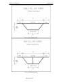
Coordinate System
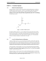
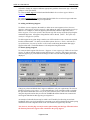
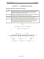
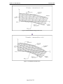
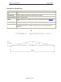
Global Coordinate System
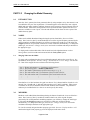
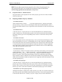
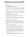
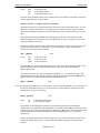
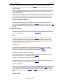
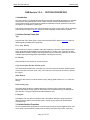
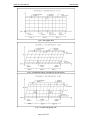
Structural models in ACES are based on the RIGHT-HANDED ORTHOGONAL CARTESIAN
coordinate system as shown in Figure 1. However, for interpreting output results, distinction
must be made between the global (or nodal) co-ordinate system and the local (member or
element) co-ordinate system. In the terminology to be used in this section of the User Guide the
parameters U1, U2, U3 will correspond to forces and displacements while U4, U5, U6 correspond
to moments and rotations.
Figure 1 Global Coordinate System
The global coordinate system (X, Y, Z) is an arbitrarily chosen system for the entire structure.
The origin of the system may be located at any arbitrary point and the direction of the axes are
chosen to suit the structure. All input data is described with respect to the global co-ordinate
system and all nodal distortions, forces, and reactions are similarly given. Two-dimensional
structures are always assumed to be contained in the X-Y plane.
2.0
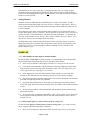
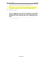
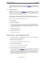
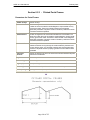
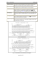
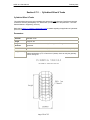
Local Co-Ordinate System for Members
A local co-ordinate system (x, y, z) is associated with each member, and all member input data
and member output forces are specified in terms of this system. The local x axis coincides with
the long-itudinal axis of the member running from the Start to the End of the member, while the
direction of the other principal axes are based on the right-hand-rule. To determine the direction
of member axes select Settings/Show Symbols and place a tick in the Member local axes item.
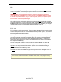
Unless the member is axially symmetric (as is the case in all parametrically generated models),
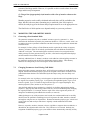
the orientation of one of the principal axes of the member with respect to the global axes needs to
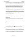
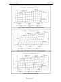
be specified. This quantity is called the BETA angle (B in Figure 2). For plane structures BETA
should be omitted or specified as zero.
Referring to Figure 2 on the next page, let A be a plane containing the member x axis and a line
parallel to the global Y axis. Let y' be a vector in this plane and perpendicular to the x axis. The
direction of y' is taken so that the projection of y' on the Y axis is in the positive Y direction. Then
B is the angle from y' to y, positive by the right-hand rule around x.
Page 12 of 235
ACES V6.4 User Manual
February 2007
This definition is not sufficient if the x axis is parallel to the Y axis, in which case the plane A is
indeterminate. Then B is the angle from the -X axis to the y axis if the x axis is in the same
direction as the Y axis, and from the +X axis if not. The default value if B is not specified is zero.
For plane structures, the local axis and the direction of y is determined according to the right-hand
rule. Because of this convention, the direction of the local y axis will not necessarily always be in
the positive direction of the global Y axis.
WARNING: Note that the directions of the local axes may be changed if a plane structure is
redefined and analysed as a space structure.
Viewing & changing member axes sizes: To view member axes select Settings/Show Symbols
and place a tick against Member local axes. To change the size in which member axes are
displayed on the diagram select Settings/Text & local axes size/Member local axes and enter a
size in mm units.
Figure 2: Local Coordinate System for Members
3.0
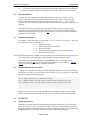
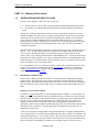
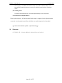
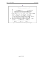
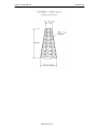
Local Coordinate System for Finite Elements
A similar local coordinate system (x' y' z') is associated with each element. For plane stress,
plane strain, plate bending and tridimensional cases, this local co-ordinate system will coincide
with the global coordinate system. To determine the direction of element axes select
Settings/Show Symbols and place a tick in the Element local axes item.
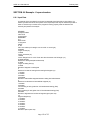
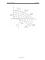
For shells, the x' axis (local) will be parallel to the line joining the first numbered node to the
second numbered node. The y' axis is perpendicular to the x' axis, lies in the plane of the
element, and is directed towards the remaining node(s). The z' axis is normal to the plane of the
element (refer to Figure 3).
Page 13 of 235
ACES V6.4 User Manual
February 2007
Figure 3: Local Coordinate System for Finite Elements
Page 14 of 235
ACES V6.4 User Manual
PART 1.6
1.
February 2007
Sign Convention
Nodal Deflections, Rotations, Forces & Moments
These are given with respect to the Global coordinate system. Their positive directions are in
accordance with the right-handed coordinate system. To view nodal results in 2D grillage and
slab models you may need to change the viewing angle. Click on the Isometric view icon in the
tool bar then on the Redraw last-diagram icon to do this.
2.
Reactions
These are given with respect to the Global coordinate system. Their positive direction is in
accordance with the right-handed coordinate system. To view reactions in 2D grillage and slab
models you may need to change the viewing angle. Click on the Isometric view icon in the tool
bar then on the Redraw last-diagram icon to do this.
3.
Member End Forces
Member end forces (moments, shears, torsions, axial forces), are given with respect to the Local
coordinate system. Positive directions are in strict accordance with the right hand rule when
applied to the local coordinate system. A positive axial force at the start node of a member will
therefore correspond to compression in that member.
In a 2D frame, for example, where the Global Y axis is upwards and the Z axis is out of the page,
a positive bending moment Mz at the start node corresponds to bending tension stresses on the
positive Y face of the member. In numeric, or printed, output reports, therefore, a member under
constant member force will experience a change in sign of the force between its start and end
nodes. (Results displayed graphically already makes allowance for this).
4.
Element Bending Moments
These are given with respect to the local element axis. Positive element moments will induce
tension on the +z (local system) face. Note with care that Moment X calculated for an element
is parallel to the local x axis (i.e. it is about the local y-axis). For two dimensional analysis, the
local axis system always coincides with the global system. Results are given per unit length
(e.g. kN.m/m).
Page 15 of 235
ACES V6.4 User Manual
February 2007
NOTE: When creating contour or solid shadediagrams it is very important that local
axes of all elements are all orientedin the same direction, otherwise the diagrams will
becomemeaningless.
To check their orientation click Settings/Show
symbols
from the top menu and
tick the Element local axes
box.If any element axis does not align itself with the
corresponding global axes then such elements will need to be considered separately.
Although ACES has routines for reversing and rotating local element axes and aligning
the axes of groups of elements, (refer to Structure/Finite Elements), it may not always be
possible to align them exactly, particularly if irregularly shaped triangles are used.
Alternatively, use only the principal values rather than the basic x and y values.
5.
Element Stresses & Strains
Element stresses and strains are given with respect to the local axis system. Stresses (and strains)
are considered positive if, on the 'positive faces', they are in the positive direction of the axes.
Thus, tensile stresses are always considered as positive and compressive stresses as negative.
This convention remains true for two dimensional analysis, in which only Stress-X, Stress-Y and
Stress-XY (same as Stress-YX) will be present. For two dimensional analysis, the local axis
system always coincides with the global system.
Stresses and strains are normally calculated at element centroids, unless the analysis option for
displaying values at element nodes is invoked. Note that in bending cases, stresses and strains are
given in accordance with plate bending theory (i.e. 'Moment X' means the moment parallel to the
local x-axis).
NOTE: When creating contour or solid shadediagrams it is very important that local
axes of all elements are all orientedin the same direction, otherwise the diagrams will
becomemeaningless.
To check their orientation click Settings/Show
symbols
from the top menu and
tick the Element local axes
box.If any element axis does not align itself with the
corresponding global axes then such elements will need to be considered separately.
Although ACES has routines for reversing and rotating local element axes and aligning
the axes of groups of elements, (refer to Structure/Finite Elements), it may not always be
possible to align them exactly, particularly if irregularly shaped triangles are used.
Alternatively, use only the principal values rather than the basic x and y values.
Element Shears: Refer to Part 5.5 for a detailed discussion regarding the interpretation of shear
forces and shear stresses.
6.
Curvatures/Rotations
Curvatures are the reciprocals of radii of curvature. A positive curvature will correspond to a
positive strain on the +z face.
Rotations are measured around an apprpriate axis. For example, if the main girders are parallel to
the Global X axis then the main rotation would be a "Rotation-z" for a 2D frame model (PLANE
FRAME type) , or "Rotation-y" for a 2D grillage model (PLANE GRID type).
Page 16 of 235
ACES V6.4 User Manual
7.
February 2007
Horizontal Patch Loads
Face the direction in which the patch extends on the model (ie from its start coordinates to its end
coordinates). The positive y-direction will then be to your left and the negative y-direction to your
right (i.e. the convention follows the right hand rule). You can check the direction that ACES has
used by selecting <Results><Applied Loadings> but remember that the patch loads are applied as
nodal loads in global directions.
In situations where a patch, (or sub-patch in the case of a curved patch load), is not parallel to
either the global-X or global-Y axis, then two nodal forces are generated which, when added
vectorially, equal the intended load.
PART 1.7
1.
Saving & Retrieving Model Data Files
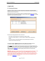
Saving Job Data
To save all model data and any results files that may have been generated click in turn on File /
Save all model data or Save model data as.. and provide file information as requested. Note that
the graphical results files (designated with extensions PLT, PLM, PLF) can be quite substantial if
the structural model is very large - you may not be able to save them to a 1.4Mb floppy disk.
Periods, (the "." symbol), are permitted in data file names.
To check the size of files generated by ACES use Windows Explorer to view the contents of the
folder in which output results are stored (e.g. C:\Program Files\Aces\Outpdat, OR
C:\aces5\outpdata etc). Use the option, File / Set project directory to specify the default directory
for your ACES model and results files (the initial default path will be set to ..\USERDATA).
If changed, the new path will be written to a file call Proj_dir.dat in the ..\TEMPDATA subfolder.
It will be read and used in subsequent runs. Note that if you open a previous job and change the
project directory, the previous job's default file path will be retained when you try to save it
again.
2.
Retrieving Saved Job Data
At start-up ACES will give you the option to load the last file worked on. If you wish to retrieve
a model file that was generated and saved earlier use one of the two File options: Open an
existing file or Open a file last used. If a results file is available ACES will ask if you want it
loaded into the system. (Some results files can be very large and may not be required in the
immediate session).
Page 17 of 235
ACES V6.4 User Manual
PART 1.9
February 2007
System Limitations & Restrictions
1.0
MODEL LIMITS
1.1
Geometric & Loading Limits
1.1.1 General Modelling Limitations
The following geometric limits generally apply to all models (refer also to Section 1.3 for
limitations associated with Dynamic Analysis):
Nodes
Members
Elements
Member Property Types
6000
6000
6000
500
Although ACES has the ability to handle mixed 2D/3D frame and FE models (such as slab
grillages and pier/pile cap/pile combinations), there are a number of significant structure types
that it is not capable of modelling viz:.
•
Variable modulus elasticity across the section (i.e., non linear element/member
stiffness)
•
Members subject to tension or compression only (such as cables)
•
One-way supports (such as non-uplifting bearings)
•
Non-linear behaviour
•
Forced-function dynamic response
1.1.2 Loading Limitations
ACES allows up to 99 individual load cases to be created with up to five (5) identical or different
vehicles in each load case. Vehicles in any one load case can either move in exactly the same path
or along different paths. The static location of all vehicles at one particular point along their paths
within a load case constitutes an individual vehicle loading. Refer also to Section 3.1 for further
details regarding vehicle loads. The table below summarises the total number of individual
vehicle loadings that can be generated in any one ACES run:
2D Grillages
3D space frames and FE shell
models
Trusses
2000
1000
3000
1.1.3 Envelope Limitations
The maximum number of envelopes that can be created in any one run is 50.
Page 18 of 235
ACES V6.4 User Manual
1.2
February 2007
Moving Load Analysis Problems
The limitations given in Section 1.1 above will vary depending on the total number of individual
loadings generated by all load cases containing moving vehicle loads. (Actual limits are
dependent on the total number of discrete nodal loads). Unfortunately, there is no simple way of
determining these limits. If the program aborts during analysis it is probably due to the fact that
there are too many vehicle loadings. In this event you may need to take one or more of the
following actions:
ƒ
ƒ
ƒ
ƒ
ƒ
ƒ
1.3
ƒ
ƒ
ƒ
ƒ
ƒ
ƒ
Reduce the number of moving load cases
Remove vehicles from multi-vehicle load cases
Shorten vehicle travel paths
Reduce vehicle movement increments
Remove large patch loads from vehicle load cases
Don’t include Dead Load in a moving vehicle load case
Dynamic Analysis Limitations
Due to the way in which ACES has traditionally implemented dynamic analysis there are severe
limitations placed on the total number of nodes that the model can have. The following node
limits apply to different model types when performing Dynamic Analysis:
Space trusses
Space frames
Shell elements
All other types
455
227
227
500
If your model is much larger than this you may consider creating a scaled-down version for
performing the dynamic analysis prior to generating the more complex version.
2.0
PARAMETRIC MODELS
When changes are made to the base model parameters ACES always regenerates the model “from
scratch” using its own default material property types and assignment rules. Therefore, if you
change any of these basic parameters (such as the number of spans or main girders, the skew
angle, and so on), you may affect the member (and element) property assignments throughout the
regenerated model. So, always check your model carefully after parameters are changed or
modified.
Note also that any sub or super-structure manually added to the original base model geometry (or,
indeed, any additions or deletions of nodes, members and elements that you may have made), will
also be lost.
3.0
MOVING VEHICLE LOADS
3.1
Swapping Movement Direction
To swap the direction of movement of a vehicle don’t set the Start X coordinate of the vehicle
path to be larger than the End X coordinate – the vehicle will be flipped over and the reference
axis will be aligned with the top wheels of each axle. Instead, use the menu commands: Loads /
Edit vehicle loads / Vehicle # / Swap movement direction where # represents the vehicle number
whose direction of movement is to be swapped.
Page 19 of 235
ACES V6.4 User Manual
February 2007
This page intentionally left blank
ACES V6.4 User Manual
February 2007
PART 2
CREATING THE MODEL GEOMETRY
Page 20 of 235
ACES V6.4 User Manual
February 2007
HOW TO CREATE A MODEL
1.0
GETTING STARTED
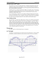
This section of the Manual will step you through the process of creating and analysing a basic 2dimensional grillage, slab, frame or continuous beam structure using the parametric modelling
technique (often referred to as the “template” method). It is based on the concept of selecting a
“template” that most closely resembles the structure you are attempting to model and entering
parameters and dimensions expressed in real engineering terms. The program then generates the
model geometry.
For a quick overview of the modelling process refer to the document: Bridge Modelling Made
Easy (it's in Microsoft WORD format).
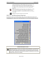
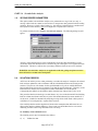
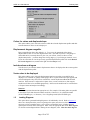
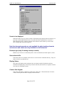
Otherwise, follow the more detailed tutorial outlined here-in. Run ACES, either from the Start
Menu or from the icon on your desktop (if you have one). A dialogue box will appear with a
number of options:
•
•
•
•
•
•
Start a completely new job
Reload the last job that was run on the PC you are now using
Open an existing job file that was previously created and saved to disk
Select the Section Properties, Continuous Beam or Incremental Launching module
Select a job file from a list of up to five previously run jobs
Exit from ACES altogether
Click the option that suits your requirements.
1.1
Job Identification
A job identification window will pop up. This allows basic job identification information to be
entered. A heading/title of some description must be provided - all other Job ID data is optional.
When finished, click Next>>. Note that if you press ENTER after any data is keyed in this will
have the same effect as pressing the Next>> button. All data currently entered will be accepted
and control will transfer to the next dialogue box.
1.2
Selecting a Modelling Option
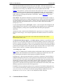
A menu of modelling options will be displayed. They provide a number of different ways in
which the model geometry can be created viz:
By default the first option, Using parametric data entry, is already highlighted. Click Next>>
to accept it and to continue with the modelling process. If you wish to create the model geometry
by reading in a list of 2D/3D node coordinates refer to Reading Node Coordinates & Member
Numbers.
Page 21 of 235
ACES V6.4 User Manual
1.3
February 2007
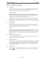
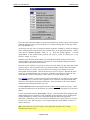
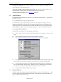
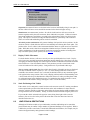
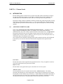
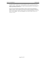
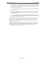
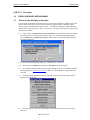
Selecting a Structure Category
A panel displaying a range of generic structure types will appear, together with a list of options
labelled Select a structure category (as shown on right). Option 3, Grillages, should be
highlighted. If you wish to create a grillage model click Next>> to accept the selection.
If you are creating a different model type (such as a slab, frame or continuous beam), highlight
that option with the left mouse button then click Next>> to continue.
Note carefully that if you select the wrong structure category at this point there is no way of
tracking back through the previous options. You will have to continue through to the last panel in
the model generation wizard then start from the beginning with File / New Job... (The last
dialogue box is the Tips panel).
Refer to PART 8 for all available generic structure types together with a complete list of
parameters relevant to the templates representing each model type.
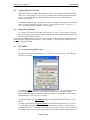
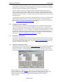
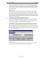
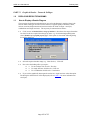
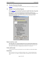
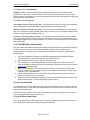
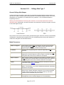
1.4
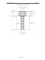
Selecting a Structure Type
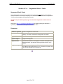
After selecting the required structure category (e.g. the Grillage Category), a panel with nine
different grillage types will be displayed together with a dialogue box describing each type.
Similar panels will be displayed for continuous beams, frames and slabs. Click on the required
grillage type (e.g Type 2 grillage with parallel girders and uniformly skewed supports) and press
Next>>. (Part 8 of the User Manual lists all model templates available in ACES and the
parameters required to define them).
Note that the template icons displayed under the various structure categories represent the overall
layout of the structural model and not its intricate details. They are, in effect, large pictorial
“icons” that show only the main girders and principal support lines. Exact support conditions,
transverse grillage members, bearing points, diaphragms and so on are not shown (Part 8 of the
User Manual detail all parameters required for a given model template). Click here to display the
next step in the modelling process.
Section 2 below describes other ways in which a model can be created.
2.0
OTHER WAYS OF CREATING A MODEL
2.1
Entering Node Coordinates Directly
Page 22 of 235
ACES V6.4 User Manual
February 2007
Option 2 in the modelling options dialogue box (refer to Section 1.2) enables the basic model
geometry to be created by manually entering X, Y (an Z) node coordinates directly into the
system. The geometry manipulation tools in the Structure menu are then used to add members,
elements, supports and so on. Member and element property types will also have to be created
and manually assigned to the different parts of the model. Refer to the relevant parts of this
Manual for instruction in doing this.
If vehicle loads are to be applied to the model, you will also be required to specify a running
surface for these vehicles. This must be done by activating the relevant nodes, members and
elements just prior to performing the analysis.
2.2
Importing Node Geometry From a CAD Package
Option 3 in the modelling options dialogue box (refer to Section 1.2 above) enables basic model
geometry to be imported from a CAD package in DXF format. However, the only DXF
commands recognised by this module are as follows:
POINT
LINE
POLYLINE
SEQUEND
AcDb2dVertex
Therefore, if the model imported into ACES does not look right, you may need to modify the
CAD drawing so that it contains only points and lines. For example, structural elements
represented by circles, arcs and curves would need to be converted to short line segments. Once
read into ACES you will also have to manually create and assign member and element property
types to the various model elements. (Alternatively, you could dump point coordinates to a text
file then use the ACES functions File/Merge/2D-3D Node Lists and File/Merge/Members to
generate the model - refer to Section 2.3 below for details)
If vehicle loads are to be applied to the model, you will also be required to specify a running
surface (Section 3.2) for these vehicles. This must be done by activating the relevant nodes,
members and elements just prior to performing the analysis.
2.3
Reading Node Coordinates & Member Attributes from Text Files
Option 4 in the modelling options dialogue box (refer to Section 1.2) enables the basic model
geometry to be created by reading in a list of 2D or 3D node coordinates. Node coordinates can
be determined using a spreadsheet, calculator or another CAD package and must be saved to a
text file in the format given below.
After the coordinates have been created another text file containing members with their associated
node numbers and property type attributes can be read in to complete the model using the
File/Merge/Members menu options (refer to Section 2.3.2 below).
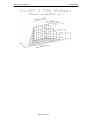
Note that this feature also allows "topographical" contours and shaded contours of the values
represented by the nodal "Z" values to be produced. It could, for example, be used to monitor the
shape of an embankment, highway slope or distorted bridge deck. Refer to Section 5.1 (subsection
1.5) for a detailed description of how this technique can be used.
2.3.1 Node Coordinates File
Either spaces or commas can be used as delimiters between node numbers and coordinate values.
Any number of nodes may be included in the list. There is no requirement to specify the exact
number in the file nor is there a limit on the total number of nodes that can be read in.
Page 23 of 235
ACES V6.4 User Manual
February 2007
Note that line 2 is only a label - the actual number of coordinates is entered in line 3. If a 3dimensional list of nodes is to be read in, line 3 should read ‘3’ and each node must have an X,Y
and Z coordinate.
Line 1:
Line 2:
Line 3:
Line 4:
Line 5:
“
“
Header information (e.g. Coordinates of substructure)
The following label - “Number of dimensions”
The number of dimensions expressed as an integer (e.g. 2)
The node number and X,Y coordinates of the first node in the list
The node number and X,Y coordinates of the second node in the list
“
“
“
“
“
“
“
“
2.3.2 Member Attributes File
After the coordinates have been created another text file containing members with their associated
node numbers and property type attributes can be read in to complete the model using the
File/Merge/Members menu options. Either spaces or commas can be used as delimiters between
member and node numbers and the property type attribute. Any number of members may be
included in the list. There is no requirement to specify the exact number of members in the file
nor is there a limit on the total number that can be read in.
Note that line 2 is only a label - the actual number of coordinates is entered in line 3. If a 3dimensional list of nodes is to be read in, line 3 should read ‘3’ and each node must have an X,Y
and Z coordinate.
Line 1: Header information (e.g. Coordinates of substructure)
Line 2: Member number, start node number, end node number, member property
type
Line 3: Member number, start node number, end node number, member property
type
“
“
“
“
“
“
“
“
“
“
Page 24 of 235
ACES V6.4 User Manual
PART 2.2
February 2007
Parametric Modelling Using Templates
2.0
ENTER GEOMETRY PARAMETERS
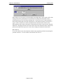
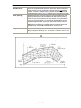
2.1
Grillages
2.1.1 Grillage Types 1-6 and8
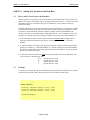
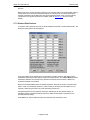
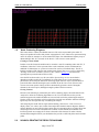
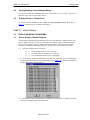
The default template displayed by ACES is a schematic representation of a bridge deck with
uniformly skewed supports together with a data entry window labelled GRILLAGE TYPE 2 Parallel Girders (refer to an example of the dialogue box below). Note that Part 8 of the User
Manual lists all model templates available in ACES and the parameters required to define them.
For a quick overview of the whole modelling process refer to the document: Bridge Modelling
Made Easy (it's in Microsoft WORD 2000 format).
Default values have been preset by ACES for most parameters in the table. They may all be
changed to suit your own unique requirements. If any part of the schematic diagram is obscured
by the data entry window, simply click anywhere within the diagram to bring it to the foreground.
To continue entering data into the parameter fields click on any visible part of the dialogue box.
At this stage you may wish to experiment with the parametric modeller by selectively changing
some of the parameters and observing the resultant effect on the generated geometry. Enter a
value into the Number of Spans field (e.g 2). Note that nothing happens. A scaled
representation of the current model geometry can only be viewed by clicking the Verify
Geometry button.
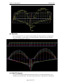
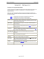
Referring to the schematic representation of a uniformly skewed grillage structure, enter other
parameters as appropriate. From time to time click the Verify Geometry button to see the effect
your data values have on the geometric layout. Note in particular the way in which the model is
meshed when skew angles are varied and the Mesh Type option is toggled between Rectangular
lateral member layout and Skewed member layout.
Page 25 of 235
ACES V6.4 User Manual
February 2007
Select the lateral member layout that best suits your own model - ACES does not presume to
suggest the best representation of a grillage mesh. That is left for you, as the designer, to do. The
system will issue a warning if you attempt to create an unacceptable structural model.
Z-Offset - This parameter is used to convert the basic 2D model to 3D. It does not represent the
distance between the centroids of the deck slab and longitudinal girders. If a non-zero value
(either positive or negative) is entered it will be appended as a Z coordinate to all generated 2D
nodes, effectively converting the model into a 3D structure. (Refer to Section 2.4 for a more
detailed explanation).
Girder Width - This parameter should only be used if the main longitudinal girders are Super-T
sections and you wish to more accurately model the transverse effects caused by the much stiffer
top soffit and flanges of that type of section. Check the effect this parameter has on the grillage
mesh by entering a value and clicking the Verify Geometry button. (Refer also to PART 6,
Grillage Types 1,2,3)
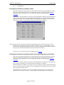
To enter span lengths click the Span lengths.. button. A list of all spans will be displayed with
default lengths preset to 20 metres (or feet, depending on the length unit you are working with).
Change the lengths by clicking in the required data fields and entering the appropriate
dimensions.
Alternatively, enter a value into the field labelled Click Apply button to set all Span Lengths to
this value and click Apply. Once all span lengths have been defined, click OK to return to the
menu.
TIP: If most spans have the same length, set the global span length first then change
individual span values to suit.
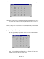
The Mesh divisions between supports.. and Girder spacing.. parameters are specified in exactly
the same way as span lengths. Mesh divisions determine the density of transverse members and
hence the accuracy of the solution. They are set to 10 by default, but this value can be changed to
suit your modelling requirements (a value of 10 means that nine transverse beam elements will be
generated between support points in that particular span). Parameters that are not required in the
structure (such as cantilever overhangs in grillage models) should be set to zero.
2.1.2 Grillage Types 7 and9
Part 8 of the User Manual lists all available grillage model templates and the parameters required
to define them. The main difference between these two grillage types and the others lies in the
way in which girder and cantilever beam spacings are applied to the model.
In grillage types 7 and 9 the girder and cantilever spacings are assumed to be measured along a
straight line orthogonal to the X axis. These spacings are first summed up then converted into a
series of proportions. The position of each cantilever and girder along every support line is then
calculated as a proportion of the overall width of that line. While support lines are defined by the
X,Y coordinates of their end points, the actual location of girders and cantilevers along the
support lines is calculated as a fixed proportion of the total distances between those points. Note
that these proportions remain the same for all support lines.
EXAMPLE: If the top and bottom cantilevers have a spacing of 2m each and 4 main girders are
at 3 m centres measured along a notional vertical line, their proportional spacing ratios are 0.125
(2/16), 0.25 (4/16), 0.25, 0.25 and 0.125 while the spacing along any abutment or pier line is
calculated as: 0.125L, 0.25L etc., where L is the length between their end points.
2.2
Continuous Beams & Frames
Page 26 of 235
ACES V6.4 User Manual
February 2007
The general comments made for Grillages also apply to continuous beams and frames. For
example, entering a value into the Number of Spans field (e.g 3) will have no effect on the
currently displayed diagram. A scaled representation of the actual model geometry will only be
displayed if the Verify Geometry button is clicked.
When modelling frames, click the Verify Geometry button from time to time to see the effect
your data values have on the geometric layout. The system will issue a warning if you attempt to
create an unstable or unacceptable structural model.
The parameter Offset of the beam in Y direction is used to convert the continuous beam model
into a 2D frame structure. It does not represent the distance between the centroids of the deck
slab and longitudinal girders. If a non-zero value (either positive or negative) is entered, it will be
appended as a Y coordinate to all generated beam nodes, effectively converting the model into a
2D structure. For a more detailed discussion of this parameter refer to Section 2.4 in this Manual.
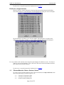
To enter span lengths click the Span lengths.. button. A list of all spans will be displayed with
default lengths preset to 20 metres (or feet, depending on the length unit you are working with).
Change the lengths by clicking in the required data fields and entering the appropriate
dimensions. Alternatively, enter a value into the field labelled Click Apply button to set all Span
Lengths to this value and click Apply. Once all span lengths have been defined, click OK to
return to the menu.
TIP: If most spans have the same length, set the global span length first then change
individual span values to suit.
Parameters in the Span Divisions.. panel are specified in exactly the same way. ACES performs
member and vehicle load distribution to nodes and calculates results at nodal points using a
default value of 10 span divisions. If you require greater accuracy or smoother bending moment,
shear and deflection diagrams then change this value to suit.
2.3
FE Slabs
The general comments made for Grillages apply also to FE slabs. For example, entering a value
into the Number of Spans field (e.g 3) will have no effect on the displayed model image. A
scaled representation of the current model geometry will only be displayed if the Verify Geometry
button is clicked.
A schematic representation of a bridge deck with uniformly skewed supports will be displayed
together with a data entry window labelled SLAB TYPE 2. Default values have been preset by
ACES for most parameters in the table. They may all be changed to suit your own unique
requirements.
Page 27 of 235
ACES V6.4 User Manual
February 2007
If any part of the schematic diagram is obscured by the data entry window, simply click anywhere
within the diagram to bring it to the foreground. To continue entering data, click on any visible
part of the dialogue box.
At this stage you may wish to experiment with the parametric modeller by selectively changing
some of the parameters and observing the resultant effect on the generated geometry. Enter a
value into the Number of Spans field (e.g 2). Note that nothing happens. A scaled
representation of the current model geometry can only be viewed by clicking the Verify
Geometry button. Try it now.
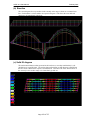
Referring to the schematic representation of a uniformly skewed slab structure shown in the
drawing window, enter other parameters as appropriate. Note that plate bending elements are
used to model a finite element slab structure.
From time to time click the Verify Geometry button to see the effect your data values have on the
geometric layout. Note in particular the way in which the model is meshed when skew angles
and mesh divisions are varied. The system will issue a warning if you attempt to create an
unacceptable structural model. Click on Mesh divisions between supports.. and enter the mesh
density for each span that suits your own model - ACES does not presume to suggest the best
representation of a finite element mesh. That is left for you, as the designer, to do.
The Z-Offset parameter is used to convert the basic 2D model to 3D. If a non-zero value (either
positive or negative) is entered it will be appended as a Z coordinate to all generated 2D nodes,
effectively converting the model into a 3D structure. Refer to Section 2.4 for a more detailed
description of this parameter and how it is used.
The Deck Width dimension represents the structure width excluding cantilevers (if any). Check
the effect this parameter has on the FE mesh by entering a value and clicking the Verify Geometry
button.
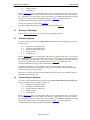
To enter span lengths click the Span lengths.. button. A list of all spans will be displayed with
default lengths preset to 20 metres (or feet, depending on the length unit you are working with).
Change the lengths by clicking in the required data fields and entering the appropriate
dimensions. Alternatively, enter a value into the field labelled Click Apply button to set all Span
Lengths to this value and click Apply. Once all span lengths have been defined, click OK to
return to the menu.
TIP: If most spans have the same length, set the global span length first then change
individual span values to suit.
Page 28 of 235
ACES V6.4 User Manual
February 2007
The Mesh divisions between supports.. parameters are specified in exactly the same way.
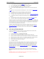
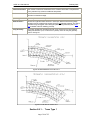
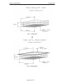
2.4
Z-Offset (Y-Offset)
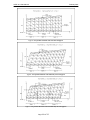
A number of structure templates employ the Z Offset parameter (or, for beam models, the Y
Offset parameter). This is an optional dimension that allows the basic 2-Dimensional structure to
be quickly and easily converted into a 3-Dimensional model. (For beam types the conversion is
from 1-D to 2-D).
The diagram below indicates the concept. Mesh generation of grillages and slabs is normally
performed in the X-Y plane where the Z coordinate is effectively zero. If a Z-Offset value is
specified it will be added to all generated nodes, in effect creating a 3-D model. (For continuous
beams the offset value is a Y-coordinate which is added to every node to create a 2-D model).
Note that any substructure (or superstructure) that forms part of the model must be manually
added by the user using the geometry tools provided in the Structure menu (refer to PART 2.3 for
instruction in adding nodes, members and elements to the model). Vehicles applied to the
structure will still move over the deck in the normal way but the analysis will be performed on the
complete 3D model.
3.0
Completing the Model
After all parameters have been defined click OK. The screen will be cleared and a Tips window
will be displayed to give you some guidance in assigning member properties and loads to the
model. Click OK on the Tips panel. ACES will now generate and display a scaled representation
of the full model geometry.
Note that all members belonging to a logical structural element type will be displayed in their
own unique colour c.f. main longitudinal girders will be shown in one colour, cantilever edge
beams in another and so on. Each colour represents a pre-defined section and material property
type, with default properties set to either zero or 1. To define and assign member properties refer
to Part 2.5 (Member Properties).
Page 29 of 235
ACES V6.4 User Manual
PART 2.3
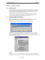
1.0
February 2007
Changing the Model Geometry
INTRODUCTION
After the “base” geometry has been generated (either by using templates or by other means) it can
be modified to suit your own requirements. Unwanted supports can be deleted (or new supports
added) and new nodes, members and finite elements can be created or existing elements removed
from the model. End releases and rigid links can be specified and other options in the Structure
menu are available to create “layers” of nodes and members and to mirror the active parts of the
model about any plane.
2.0
NODES
Nodes can be added, deleted and changed using the options found in the Structure/Nodes..
menu. Note, however, that if you add nodes that lie out of the original 2D plane generated by the
ACES parametric modelling templates you will have to change the model type to 3D (unless the
Z-Offset parameter was specified, in which case ACES will do this automatically). To change the
model type, use Structure / Change coord system and set the coordinate and analysis attributes to
the appropriate type.
To display nodes on the model either click the node icon in the right hand menu or select
Settings/Show symbols from the main menu and tick the Node symbols option.
2.1
Merging Nodes into the Model
To merge node coordinates that have been calculated separately and saved to a text file (e.g. in a
spreadsheet) use the options: Structure / Merge / 2D-3D node list or File / Merge / 2D-3D node
list. Data in the merged file must conform to the following format:
Line 1:
Line 2:
Line 3:
Line 4:
Line 5:
“
“
Header information (e.g. Coordinates of substructure)
The following label - “Number of dimensions”
The number of dimensions expressed as an integer (e.g. 2)
The node number and X,Y coordinates of the first node in the list
The node number and X,Y coordinates of the second node in the list
“
“
“
“
“
“
“
“
Note that line 2 is a label and must be typed in as shown. If a 3-dimensional list of nodes is to be
merged, Line 3 should read ‘3’ and each node must have an X,Y and Z coordinate. Either spaces
or commas can be used as delimiters between node numbers and coordinates. Any number of
nodes may be included in the list - there is no need to specify how many.
3.0
MEMBERS
Members can be added, deleted and changed using the features found in the Structure/Members..
menu. Note, however, that if you add new members that lie out of the original 2D plane
generated by the ACES parametric modelling templates you will have to change the model type
to 3D (unless the Z-Offset parameter was specified, in which case ACES will do this
automatically). To change the model type, use Structure / Change coord system and set the
coordinate and analysis attributes to the appropriate type.
To view the currently assigned member property types click Structure / Display members. All
members having the same property type will be displayed in the same colour.
Page 30 of 235
ACES V6.4 User Manual
February 2007
Note that there are two ways of selecting a rectangular member range. If you drag out out a
rectangle from left to right ACES will include only those members that are wholly within the
selected area. When dragging from right to left all members, or any part of a member, within the
boxed area will be selected.
3.1
Adding Members
Members can only be added between predefined points, or nodes, on the model. To add a
member between nodes that already exist select Structure / Members /Add members / Between
existing nodes then click on the first node with the left mouse button and drag an elastic line out
to the second node.
If a node does not exist at the required location along a member you will first need to create it.
Use the menu options Structure / Members / Divide /Add node at specified distance from start of
member to do this. The default distance is the mid-point along the member. To determine the
start node for the member use the Settings / Show symbols / Member local axes options. (You
may need to zoom in to see the member local axes clearly).
To add members using a background grid of points, first turn the grid on using View/Grid on,
change the grid density or reference node (if required) via menu options Settings/Background
grid/Change parameters, then add members with the commands Structure/Members/Add
members/Snap to a grid.
EXAMPLES
3.1.1 Add a member at right angles to another member
To add a member at right angles to another member (i.e. at right angles to an existing member
and passing through a target node that also exists elsewhere on the model):
• •
Select Structure/Members/Add members/Normal to an existing member & end node
• •
Click on the required member with the left mouse button then, holding the button down,
drag an elastic line out to the target node. Release the button. (TIP: The dragged line need
only be approximately at right angles to the member).
• •
If the dragged line crosses any other members ACES will ask you if you wish those
members to be connected to the new member (generally you will). Reply accordingly.
• •
The program will then realign the dragged line so that it passes through the selected target
point and is at right angles to the source member.
• •
If you had replied affirmatively to the prompt for connecting all intersecting members,
ACES will create nodes at the intersection points of the new member with all other members it
crosses.
• •
All intersecting members will be automatically sub-divided into shorter members lying
between these points.
• •
To view the newly created nodes and members select: Settings/Show symbols and toggle
on the appropriate drawing attributes (such as node and member numbers, node symbols,
member axes etc).
3.1.2 Add a member offset by a relative distance from an existing node
To add a member offset by a relative distance from an existing node (e.g to create a vertical
pier at a support node and at right angles to the deck):
• •
Select Structure/Members/Add members/With end points offset from an existing node
Page 31 of 235
ACES V6.4 User Manual
February 2007
• •
Click on the required node with the left mouse button then enter the offsets from that node.
To create other members with the same offsets at other nodes, simply click on those nodes.
3.2
Deleting Members
To delete one or more members from the model click in turn Structure / Members / Delete
members then select one of the options from the submenu. For example, to delete the edge
beams generated by ACES for a model with cantilever footpaths, select … / Delete a line of
members then click in turn on any member lying along each of the two edge lines. Both lines will
disappear.
Note that there are two ways of selecting a rectangular member range. If you drag out out a
rectangle from left to right ACES will include only those members that are wholly within the
selected area. When dragging from right to left all members, or any part of a member, within the
boxed area will be selected.
3.3
Renumbering Members
To renumber a group of members use the options: Structure / Members / Renumber/.. then select
the range that you wish to renumber viz:
• • Individual members
• • Whole or partial lines of members
• • Blocks of members
• • Members selected by passing a fence line through them
• • By member property type
ACES will first display the current number of the first member in the nominated range then prompt you to
enter a new number. Renumbering is performed from left to right and top to bottom.
If you retain the default analysis setting of No renumbering prior to the solution being
performed, ACES will not check for duplicate member numbers - refer to PART 4.1, Analysis
Options, (Renumbering the Model), for further information.
3.4
Merging Members into the Model
To merge a list of members (and their associated nodal links) that have been separately compiled
and saved to a text file (e.g. in a spreadsheet) use the options File / Merge / Members. Data in the
file must conform to the following format:
Line 1: Header information (e.g. Substructure for Job)
Line 2: Member number, start node number, end node number, member property type
Line 3: Member number, start node number, end node number, member property type
“
“
“
“
“
“
“
“
“
“
Either spaces or commas can be used as delimiters between the data values in each line. Any
number of members may be included in the list - there is no need to specify the exact number.
4.0
ELEMENTS
4.1
Modifying Elements
Elements can be added, deleted and changed using the options found in the Structure/Elements..
menu. Note, however, that if you add elements that lie out of the original 2D plane generated by
the ACES parametric modelling method you will have to change the model type to 3D (unless the
Z-Offset parameter was specified, in which case ACES will do this automatically).
Page 32 of 235
ACES V6.4 User Manual
February 2007
To change the model type, use Structure / Change coord system and set the coordinate and
analysis attributes to the appropriate type.
To view the currently assigned element property types click Structure / Display elements. All
elements having the same property type will be displayed in the same colour.
To release plate element forces refer to Section 6.1 for details.
4.2
Adding Elements
To add elements to the model select Structure / Finite Elements /Add Elements / .. then click on
the option you want.
4.2.1 Adding Elements Using a Background Grid
To add elements using a background grid of points, first turn the grid on using View/Grid on,
change the grid density or reference node (if required) via menu options Settings/Background
grid/Change parameters, then add elements with the commands Structure/Finite Elements/Add
elements/Single triangular element by snapping to grid point. Ditto for rectangular elements.
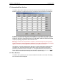
4.2.2 Adding a Block of Elements
To add a block of elements to, say, the top edge of the model:
• •
Select Structure/Finite Elements/Add Elements/Block of rectangular elements in any
plane
• •
Select a starting node for the block (click on it with the crosshairs)
• •
The dialogue box shown below will be displayed. Enter parameters as required.
• •
Note that if you want the new elements to line up exactly with those already existing along
the horizontal or vertical line you must enter the exact value of element width or height.
• •
The direction and side of the line in which element generation will occur will depend on
the sign of the element width and height. If both are positive, elements will be generated in
the (+)ve X,Y directions. If negative, they will run in the -X and -Y directions.
• •
4.3
Click the button labelled: Add block of rectangles
Deleting Elements
To delete one or more elements from the model click in turn Structure / Finite Elements / .. then
select one of the deletion options from the submenu. Prompt messages on the bottom line will
give you instruction on how to do this.
Page 33 of 235
ACES V6.4 User Manual
4.4
February 2007
Aligning Element Local Axes
When new elements are added to the model their local x-y axes may not be aligned in the same
direction as existing elements. This may cause problems later when displaying and interpreting
results. It is important, therefore, that the direction of element axes are aligned prior to
performing the analysis.
To check the alignment select: Settings/Show symbols and toggle on the display of element axes.
Now use one of the alignment options : Structure / Finite Elements /Rotate.. or Reverse.. or
Align.. to align element axes in the direction you require.
4.5
Renumbering Elements
To renumber all elements in the model use the options: Structure / Finite Elements / Renumber
then enter the element number from which renumbering is to begin. Renumbering is performed
from left to right and top to bottom.
If you retain the default analysis setting of No renumbering prior to the solution being performed, ACES
will not check for duplicate element numbers - refer to PART 4.1, Analysis Options, Renumbering the
Model, for further information.
5.0
SUPPORTS
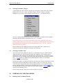
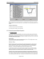
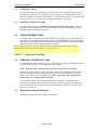
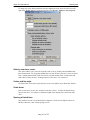
5.1 Creating & Editing Support Types
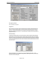
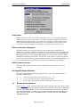
To create a new support type select Structure / Supports / Create support Type. The following
dialog box will appear:
To change the colour of the support click the button labelled < 2 >. The current support colour
can be identified by the number on the first button as well as the colour of the text label
associated with that button. To make this support type fully restrained simply click the button
labelled Make this a FULL support. To change
To make this support type fully restrained simply click the button labelled Make this a FULL
support.
To change or individually set support conditions click the button labelled Set X,Y,Z restraints.
For a 2D grillage generated using one of the standard templates and subject only to loadings
normal to the X-Y plane, ACES will automatically create a support type that is only restrained in
the vertical Z direction. If you apply non-orthogonal loads (such as in-plane braking forces) you
Page 34 of 235
ACES V6.4 User Manual
February 2007
will need to change the support conditions appropriately (and also the structure type - from a 2D
grillage to a 3D space frame).
To create an elastic support click the button labelled Make this an elastic support. Refer to
Section 5.3 for details.
To create an inclined support click the button labelled Make this an inclined support and enter
the parameters in accordance with your requirements.
5.2 Adding and Deleting Supports
To add one or more supports to the model (or delete one or more supports) select Structure /
Supports / Add supports (or Delete supports) then indicate the range of supports that are to be so
affected. For example, to delete all supports generated under cantilever edge beams select … /
Delete supports / From a line of nodes then successively click on any two nodes lying along the
nominated edge beam. All supports along that line will be deleted. (NOTE: This option only
works for a straight line of nodes).
To add a support at any point along a member you will first need to create a node at the required
location on that member. To do this, use the menu options Structure / Nodes / Add node at a
specified distance from start of member to first create a node along the member then apply a
support at that node. The default distance is the mid-point along the member.
5.3 Elastic (Spring) Supports
To create an elastic support click Structure / Supports / Create support type / Make this an elastic
support. To edit an exisiting elastic support click Structure / Supports / Edit support propsand
select the support type you would like to change. In either case, the following dialog box will be
displayed:
Change any values and default elastic support conditions to suit your requirements. The tick box
labelled "Calculate spring values..." is a flag that indicates if you would like ACES to calculate
the equivalent nodal eleastic forces for you. If you tick the box, these values will be calculated
using the subgrade reaction that you enter into the kZ field and the element areas connected to
each support node that has this support type assigned to it.
An example of when this feature may be useful is an FE model of a raft resting on an elastic
foundation. In this case it will probably be convenient to get ACES to determine the elastic spring
constant based on the subgrade reaction of the soil and the area supported by the node.
Note, however, that this flag can only be used in plate-bending and shell type FE models where
all elements joined at the support nodes contribute to the spring support.
Page 35 of 235
ACES V6.4 User Manual
February 2007
If, for example, the nodes along the junction between a slab and a wall are connected by vertical
elements (in the wall) and horizontal elements (in the slab) then this flag cannot be used for
supports at these nodes. In such cases the spring constant must be calculated manually and
entered into a new elastic support type.
Note on Bearings
If spring constants have been specified they can be derived from the physical properties of the
bearing. Note that even pot bearings have a certain amount of elasticity and it is often beneficial
to account for this in your model.
For example, the current Australian Bridge Design Code (see, for example, Section 4,
Commentary), gives details of the physical properties of a range of elastomeric bearing sizes. For
bearing 040902R (page C4.10), the "Calc. Comp Stiffness at zero shear" is 657E3 kN/m. If you
want to model this bearing in a 2D grillage model (PLANE GRID) and your units are kilonewtons
and metres, then you would need to specify an elastic Kz value of 657E+03. For pot-type
bearings you can usually calculate an approximate stiffness using the serviceability load rating,
the rotational capacity and the dimensions of the bearing (the rotation and dimensions are used to
calculate an approximate deflection).
6.0
END RELEASES
To specify end releases use the options: Structure / End releases / Specify release conditions to
define the type and location of the end release(s) followed by Structure / End releases / Apply a
member release /.. to apply those conditions to selected members. (You will be prompted to
click on the members to which the end release conditions are to apply).
6.1
Releases for Plate Elements
ACES does not have plate release facilities but there are several ways that hinges in finite
element models can be modelled.
First, an extra line of nodes will need to be created with either a horizontal or vertical
offset (say 50mm) from the hinge nodes. Using a vetical offset will allow you to model
the hinge more accurately, but the drawback is that it will introduce extra plate bending if
in-plane forces are significant. (Note that a vertical offset would not be allowed in 2D
problems).
Once the extra lines of nodes is created, the existing elements to the right (or left) of the
hinge will need to be deleted and replaced with ones which connect to the new offset
nodes. The offset nodes then need to be connected to the original hinge nodes. There are
three ways of doing this:
(1) Using rigid links with the approriate direction/rotation links
This is probably the most mathematically correct way of modelling the hinge but I have
found that they use a lot of dynamic array space and reduce the number of loadings that
can be solved. Also, result values across the hinge nodes will not be available.
(2) Using a line of thin finite elements
Being thin the elements will transmit only a small moment, but the modulus of elasticity
will need to be "tweaked" to avoid shear displacements (if the offset is horizontal) or
axial displacements (if the offset is vertical). This is probably the quickest but least
Page 36 of 235
ACES V6.4 User Manual
February 2007
accurate of the hinge models. However, it is possible to derive results values close to the
hinge and this may be important.
(3) Using a line of appropriately sized members with a line of member releases at the
hinge
Member properties can be readily calculated and result values will be available at the
hinge, but this is the most time-consuming way to model the joint. If this option is
chosen, the analysis type for the frame analysis option must be set to the appropriate one.
The final choice of which option to use depends mainly on your own preference.
7.0
MODIFYING THE PARAMETRIC MODEL
7.1
Generating a Non-Standard Mesh
The parametric templates only allow “standard” structure types to be generated i.e., those
confined to the limitations imposed by the parameters themselves. However, certain “tricks” can
be employed to create a parametric model that can then be massaged to produce the desired final
structural model.
For example, if a finer grillage or Finite Element mesh is required in the vicinity of supports,
“dummy” parametric spans can be initially specified that reflect the different mesh densities
within the “real”spans. The unwanted supports can then be removed or reassigned once the
model geometry has been generated leaving, in effect, a final mesh configuration that displays
variable mesh divisions within each span.
Similarly, additional lines of “dummy” members can be added to a slab and grillage structure in
the parametric model in order to allow for slab haunches between girders. These dummy
members can subsequently be removed using the member deletion tools.
7.2
Changing Parameters of an Existing CAD Model
During the model geometry generation phase, ACES will preset a number of model attributes.
Support, member and element property types will be assigned to the model in accordance with
predefined defaults that have been determined by the developers using "the most likely case"
scenario.
For example, in the case of grillages, vertical supports are placed under each longitudinal girder at
the support lines, member property Type 1 is assigned to all longitudinal girders, Type 2 to all
transverse girders, Type 3 to cantilever edge beams and Type 4 to support diaphragms. Key
member properties (areas, inertias etc) are also preset to 1.
After the final model has been completed, or "detailed", (by defining and assigning member
properties, applying static and moving vehicle loads etc), it can be modified again by changing
the original parameters. For example, the skew angle of one of the supports may need to be
changed or an additional girder added to the structure (or removed).
Although changes to any of the parameters can be made, the resultant model must be carefully
checked, since the parametric modelling process will regenerate all nodes, members, elements
and supports using the new set of parameters. Element and member property types, vehicle load
groups, load cases and envelopes which were originally created and defined will remain
unchanged.
However, any nodes, members, elements, releases, rigid links or supports that were added to, or
deleted from, the original model will be lost. They will have to be recreated. Similarly, the
assignment of additional property types (over and above those automatically created by ACES),
Page 37 of 235
ACES V6.4 User Manual
February 2007
will be lost. They too will have to be re-assigned (but not recreated - all property type groups are
retained by the system).
If you envisage having to change any of the parameters it is advisable, therefore, not to make
significant changes to the final model geometry.
Page 38 of 235
ACES V6.4 User Manual
PART 2.4
1.0
February 2007
Defining Vehicle Traffic Lanes
General
If you wish to use any of the automated Austroads vehicle load cases, or if you intend applying
patch and vehicle loads to lanes manually, you must first define the location of lanes you intend
using.
Note that, once lanes have been defined, it is not strictly necessary to use them in load cases.
ACES will simply ignore them if they are not referred to.
WARNING: Lanes cannot be defined for frame or continuous beam structures
2.0
Defining Lanes
To define one or more traffic lanes, select Loads / Define lanes then click on the appropriate
buttons to enter the lane parameters. (Note that these same options can be used to edit or modify
lane parameters).
Click on Define lane geometry. The following window will appear:
Lanes are defined by start and end X,Y coordinates, where Y is measured between the bottom
edge of the lane and the X axis. The Re-set button in the lane data panel simply sets the start and
end X coordinates of the lane to the values calculated at the left and right abutments.
Lanes can begin and end off the structure. This situation may arise in cases where you require
auto-generated Austroads vehicle loads to traverse a path that requires them to start well before,
and end well clear of, the deck.
The parameter Lane load subdivision size is specified in the same units as the X,Y coordinates
and represents the patch size into which any applied lane load will be subdivided. Lane load is
represented by ACES as a uniformly distributed load which is first subdivided into small patches
when being distributed to adjacent nodes in the model. This parameter should therefore be less
Page 39 of 235
ACES V6.4 User Manual
February 2007
than the horizontal transverse grillage member spacing and also less than the smallest girder
spacing in the model.
Default lane colours can be preset using Settings / Lane colours and current lane locations can
be viewed by selecting View / View lanes.
3.0
Lane Load Reduction Factors
To specify lane load reduction factors click onto Lane reduction factors and select the option you
require (or enter the factors manually to suit your requirements. Note that AUSTROADS lane
reduction factors will be applied to Austroads vehicles and Austroads lane loads that have been
“automatically” assigned to a load case.
They will also be applied to vehicles that are manually assigned to a lane within a load case (see
PART 3, Moving Vehicle Loads, for details).
Page 40 of 235
ACES V6.4 User Manual
PART 2.5
1.0
February 2007
Member & Material Properties
INTRODUCTION
This section describes the manner in which section and material properties are defined and
assigned to members. When generating a grillage model ACES automatically assigns unique
colours (representing member property types) to each structural element of the model (main
girders, transverse beams, cantilever edge beams and support diaphragms - refer to Section 2.2,
Parametric Modelling Using Templates for further details).
If the result is exactly what you require, then all you need do is enter the appropriate properties
for each of the member property types. Otherwise, you will need to create new property types
and assign them to the relevant members in the model.
2.0
DEFINING MEMBER PROPERTIES
Either click the member property icon on the top menu bar (shown as an I-beam) or select the
following menu options: Structure / Member properties / Create-Edit. A maximum of 500
member property types can be defined.
A dialogue box listing all currently defined member property types will appear. Highlight the
required member property type (e.g. Main girders) then click Edit. A member properties panel
will be displayed as shown below, with default values of 1.0 assigned to all major property
values (with the exception of E, density and shear area, Ay, all of which are set to zero). Change
these to suit your own requirements. To navigate between property types Click the left and right
arrow buttons. The colour and line style assigned to the current member property type is shown in
a colour bar adjacent to the Colour button (click it to change these attributes).
Uniform Properties
Enter values for Ax, Ay (shear area), Iy, Iz, Ix (torsion) and Poisons’ ratio as appropriate. For
properties of tapered sections refer to Section 3.4 (Properties of Tapered Sections).
Shear Area (Ay)
Page 41 of 235
ACES V6.4 User Manual
February 2007
ACES uses the value in the Ay field to define the member shear area in either the y or z directions,
depending on the structure type being modelled. For example, in a 2D frame structure, Ay will
represent the shear area in the vertical (y) direction. In a 2D grillage, where both global and
member Z axes are oriented normal to the grillage plane, Ay will represent the area in the vertical
Z direction. Consequently, if you require shear deflections in a 2D grillage, you will need to enter
a non-zero value into the Ay field.
Inertias (Ix, Iy, Iz)
Ix represents the torsional stiffness and Iy, Iz the stiffness about the corresponding axis. For
example, in a 2D frame model where the global X,Y axes lie in the plane of the structure, the local
member z axis will be oriented normal to this plane. Iz will therefore need to be defined since it
represents the moment of inertia about the member z-z axis. In a 2D grillage, where both global
and member Z axes are oriented normal to the grillage plane, Iy will need to be defined since the
principal local member axis is in the y-y direction. For further discussion of the axis system used
in ACES please refer to Section 1.5
Densities
Enter density as Force/Unit^3 (e.g. kN/m^3) and note that for models where the deck lies in the
global X-Y plane they must be given in the correct sense. For grillage models generated
parametrically, density must correspond to Density - Global Z and must be negative, since the
global Z axis is out of the plane of the screen e.g. Density - Global Z = -77 (kN/m3). For
frames and continuous beams enter a value for Density - Global Y.
Temperature Coefficient
This parameter represents expansion /contraction effects and not vertical temperature gradients.
Select section from the DataBase
This option allows a section to be selected from a data base of standard BHP and Austroads
sections. You may add other sections to the data base by editing the text file SECPROPS.DAT
in the Program Files\Aces folder using any text editor (e.g NOTEPAD or similar). Refer to
Section 2.6, Adding New Sections to the Data Base.
Select E from list
This button allows the Modulus of Elasticity (E) to be selected from a list of standard values for
concrete, steel & timber.
3.0
MEMBER PROPERTIES OPTIONS
The Options.. button provides access to other section properties features as shown in the panel
below:
3.1
Section Properties Calculator
The Section Properties Calculator allows properties to be calculated for a range of rectangular,
circular, octagonal and general shapes. Rectangular and circular sections can be hollow
Page 42 of 235
ACES V6.4 User Manual
February 2007
(achieved by entering a wall thickness) while octagonal sections are solid only (this is useful for
determining section properties of solid octagonal piles). The general section properties calculator
also allows properties of arbitrary shapes to be determined.
Arbitrary shapes are created by specifying the number of internal and external nodes in the
section, a symmetry option (if any) and the system to be used for defining internal and external
node coordinates (absolute values or offsets from previous nodes). Internal nodes need only be
specified if the section is hollow. Coordinates are then entered separately for each of the external
and internal nodes.
An option has been provided to calculate the torsional inertia in one of two ways: either using the
bubble analogy (membrane) theory or a simple formulation based on rectangular plate theory.
Once calculated, the geometry and properties for the section can be saved to a file for future use.
Refer to Section 2.7, Section Properties Calculator, for details.
3.2
Composite Section Calculator
The Composite Section Calculator allows slab properties to be specified for composite girders.
ACES will calculate the composite properties and display the resultant values. Note that this
feature is entirely optional - you may choose to either calculate the composite properties yourself,
(entering them directly as Ax, Ix, Iy, Iz values), or you can allow ACES to do this for you. In this
case the values entered into the main properties panel will be assumed to represent the girder
properties only, while those supplied in the Composite Section panel represent the slab properties
only. Refer to Section 2.8, Composite Section Calculator, for details.
3.3
Properties of 3D Sections
For 3D frames and grillage models having members whose principal axes do not line up with the
global axes (or 2D grillages with sections lying out of the Y-Z plane) section properties will have
to be specified using Alpha and Beta angles. Refer to PART 1.5, Coordinate System, of the User
Guide for a definition of these angles.
3.4
Properties of Tapered Sections
This option allows section properties for the current property type to be specified at the beginning
and end of the member. If start and end properties are different, ACES will perform a proper
tapered section analysis. The following dialog box will be displayed when the Tapered Section
Properties button is clicked on the Member Properties Options form shown in Section 3.0 above:
When the dialog box is displayed, the start properties are imported from the main Member
Properties dialog box (refer to Section 2 above). Note that start and end properties can be made
the same as those of any other existing member propery type by clicking the appropriate
buttons. Alternatively, the end property can be calculated using the Section Properties
Calculator button.
Page 43 of 235
ACES V6.4 User Manual
February 2007
HINT: If you really require the start properties to be, in fact, the end properties on
entry into this dialog box, first calculate the end properties then click the button
labelled Swap properties at start and end to change them!
3.5
Properties Same as Another Section
This option allows section properties for the current property type to be set to those of another
member property type.
3.6
Displaying Member Property Attributes
3.6.1 MemberNumbers :
Either click the Member Number
icon on the right menu bar or, from the top menubar,
click onto Settings / Show symbols. In the dialog box check the box labelled Member numbers.
Note that the member number icon is a toggle that switches the numbers on and off with repeated
presses.
3.6.2 MemberColours :
Click onto Structure / Display Members to view the model drawn in its constituent member
colours. Alternatively, click the member properties icon on the top menu bar and scroll through
all member property types. The corresponding colour is show in a colour bar at the top of the
dialog box.
3.6.3 Member LocalAxes
:
To view the member local axes click onto Settings / Show symbols and, in the dialog box, check
the box labelled Member local axes. ACES displays the axes with a small axis symbol that has
arrow heads on the ends of the stems that represent the local x and y directions. When the model
is viewed in 3D the arrow head is left off the axis in the local z direction. Using the right hand
rule it then becomes possible to quickly determine the orientation of the axes (the middle finger
of the right hand represents the local z axis).
3.6.4 MemberOrientation
:
To determine the orientation of member localaxes (particularly when working on 3D space frame
models), eitherclick
the
Member Orientation
icon on the right menu bar or, from the
top menubar, click onto Settings / Show symbols. In the dialog box check the box labelled
Member orientation. ACES represents all members using an "I" girder shape where that the
largest moment of inertia is about the local axis that runs parallel to the top and bottom "flanges"
of the section. Note that the member orientation icon is a toggle that switches the numbers on and
off with repeated presses..
3.6.5 Member PropertyTypes :
Click onto Structure / Display Members to view the model drawn in its constituent member
property type colours. To display the property type numbers on the model diagram, click onto
Settings / Show symbols from the main menu bar and, in the dialog box, check the box labelled
Member type number. (Note that a maximum of 500 member property types can be defined).
3.6.6 Members of a select property typeonly
:
Although each member is displayed in a unique property type colour, for very dense meshes you
may wish to quickly check whether member property types have, in fact, been assigned correctly.
To do this click onto Structure / Member properties / Display then, for each of the Member
Page 44 of 235
ACES V6.4 User Manual
February 2007
Types shown in the dialogue box, click on each in turn. Only those members will be separately
highlighted.
3.7
Creating & Deleting Member Property Types
To create a new member property type either click the member property icon (designated by the
I-beam shape) or select the following menu options: Structure / Member properties / CreateEdit. Note that a maximum of 500 member property types can be defined.
A dialogue box listing all currently defined member property types will appear as shown below:
Click the New button. The main member properties panel will be displayed (go to Section 2.0 for
a display of this dialog box and for guidance as to how section properties can be entered into it).
Clicking the Delete button will remove the highlighted member property type from the list.
4.0
ASSIGNING MEMBER PROPERTY TYPES
Properties are assigned to members in one of two ways:
• •
• •
By selecting a property type first then assigning it to a specified range of members
By selecting a range of members first then assigning a specified property type to all
members in that range
4.1
Select a Property Type & Assign it to a Range
Select a property type by clicking on the section icon and choosing one of the already defined
property types. It will be echoed on the status line just below the drawing area. Scroll in turn
through the menu options: Structure / Member properties / Assign current type to.. and select the
member range you require from the submenu of range options.
Now follow any instructions that may appear on the lower prompt line (they will help you to
identify the range). Once the range has been delineated, all members in the range will be
assigned the currently active property type. They will be drawn in the current member type
colour.
Note that there are two ways of selecting a rectangular member range. If you drag out out a
rectangle from left to right ACES will include only those members that are wholly within the
selected area. When dragging from right to left all members, or any part of a member, within the
boxed area will be selected.
4.2
Select a Range of Members & Assign a Property Type to Them
Page 45 of 235
ACES V6.4 User Manual
February 2007
Select a range of members in the model by cascading through the menu options: Structure /
Member properties / Assign selected type to.. and select the member range you require from the
submenu of range options. Follow any instructions that may appear on the lower prompt line
(they will help you to identify the range). Once the range has been delineated a list of current
member property types will be displayed. Select the property type you wish to assign to the
members in the range then click OK.
Note that there are two ways of selecting a rectangular member range. If you drag out out a
rectangle from left to right ACES will include only those members that are wholly within the
selected area. When dragging from right to left all members, or any part of a member, within the
boxed area will be selected.
EXAMPLES
4.3
• •
To assign a property type to a straight line of members the line is selected by clicking on
any member lying along the line.
• •
To assign a property type to only one part of a straight line of members click on the first
member in the required range and drag out an elastic band to the last member in the range.
• •
To assign a property type to only one single member select the range as ..individual, select
members.
• •
To assign a property type to a rectangular block of members place the crosshairs at some
point on the screen, click the LEFT button once, drag out a box of a size that encompasses the
required members then release the button. All members whose centroids fall within the
delineated area will be changed to the current (or selected) member property type.
• •
To assign a property type to all members whose centroids lie within an arbitrary
trapezoidal area, the area must be defined using two unconnected but opposing straight lines.
Each line must be drawn in an anti-clockwise sense, but the lines themselves need not be
parallel - they can be oriented in any general direction. However, the area delineated by their
notional “boundaries” must incorporate that part of the model within which the target
members lie. All members whose centroids fall within the delineated “area” will be changed
to the current (or selected) member property type.
Lines are created by clicking at a point on the screen that is to represent one corner of the
notional area then, holding down the left mouse button, dragging out a fence line in an anticlockwise direction to an end point representing the adjacent corner.
4.4
Merging Material Properties
To merge material properties that have been defined and saved in a previous model, use the
options: Structure / Merge / Member properties or File / Merge / Member properties (ditto for
element properties). This feature can sometimes be useful in situations where an iterative process
is being used to refine a structural model (in preliminary design, for example). Once generated in
the first iteration, material property types can be saved then reloaded into the next iteration of the
model.
File / Merge / Member Properties will allow you to read a member properties type file formatted
in one of two ways: either with the properties of each member type listed on the same line
separated by commas; or with a single property per line. The option will appear after you have
selected the data file containing the property types to be merged into the model. Note that gaps
can be left in the member type numbering and that current properties for existing types are not
zeroed.
If you do leave gaps in the numbering and one of the new types is greater than the number of
Page 46 of 235
ACES V6.4 User Manual
February 2007
currently defined types, then all of the types between the current maximum and the new type
number will be zeroed.
When reading/merging members from a text file into the model a warning will be given if a
member property type assigned to an imported member does not exist (i.e. if it is undefined).
When enquiring on a member whose type has not been defined, ACES will warn you that a
property type has not been assigned.
Page 47 of 235
ACES V6.4 User Manual
February 2007
PART 2.6 Adding New Sections to the Data Base
1.1
How to Add a New Section to the Data Base
Section properties are stored in a text file called Secprops.dat located in the \Program Files\Aces
folder. The contents of this folder may be viewed using Windows Explorer. Locate Secprops.dat
then double click on it to load it into Notepad or, alternatively, use any other text editor to
perform the editing.
Scroll through the file to get an appreciation of its structure and layout. You will notice a number
of instructions at the top of the file. Please read these carefully and follow all directions exactly
as instructed. Note that the file contains a number of unique section CATEGORIES, each
category consisting of a specified number of individual sections. You can add one or more new
categories at any point in the file providing you adhere to the correct layout and formatting viz:
• • Each category must have a label or name consisting of no more than 30 alpha-numeric
characters separated from the previous data by at least one blank line (e.g. WELDED
BEAMS).
• • The total number of sections in the category must appear on the title line & separated from
the title by a comma (e.g. WELDED BEAMS, 23). Section properties are entered beneath the
title, the first record only separated from the title by at least one blank line. Do not use blanks
between each individual section.
• • Properties must be entered in the exact format and positions shown in the data below and,
for each section, in the following order:
Area
(current units are
Ix
(current units are
Iy
(current units are
J
(current units are
1.2
mm2)
mm2)
mm2)
mm2)
Example
To insert a new category into the file immediately following WELDED COLUMNS leave a blank
line after the last record in that category then insert your own data as shown below.
……….
……….
SUPER-T BEAMS, 3
ST-1600-115 14600.0000 1150.0000 41.7000
ST-1600-130 16600.0000 1400.0000 52.1000
ST-1800-150 19100.0000 1710.0000 65.2000
UNIVERSAL BEAMS, 28
……….
……….
Page 48 of 235
0.8880
1.5100
2.6900
ACES V6.4 User Manual
February 2007
SECTION 2.7 - Section Properties Calculator
2.7.1 Introduction
The Section Properties Calculator allows properties to be calculated for a range of rectangular,
circular, octagonal and general shapes. Rectangular and circular sections can be hollow
(achieved by entering a wall thickness) while octagonal sections are solid only (this is useful for
determining section properties of solid octagonal piles).
The general section properties calculator allows properties of arbitrary shapes to be determined. It
can be accessed either from the opening dailog box when the program first starts or from its own
icon on the tool bar. When accessed in this way the module will act in stand-alone mode. If
accessed from the member properties dialog box (Structure/Member Properties/Other Options)
the calculated properties will be automatically transfered into the relevant properties fields.
Please read the comments in Section 2.7.6 if you elect to change any of the torsional
parameters.
2.7.2 Standard Shapes
Selecting the Section Properties Calculator from the Member Properties dialog box will bring up
the following panel.
The first three options allow simple solid and thin-walled shapes to be quickly generated. (Voided
sections can be generated for rectangular and circular sections by entering a membrane
thickness). Only solid sections are available for the Octagonal shape.
2.7.3 General Shapes
The general section properties calculator allows properties of arbitrary shapes to be determined. It
can be accessed either from the opening dailog box when the program first starts or from its own
icon on the tool bar. When accessed in this way the module will act in stand-alone mode.
If accessed from the member properties dialog box (Structure/Member Properties/Other
Options/General Section) the calculated properties will be automatically transfered into the
relevant properties fields in the member properties dialog box. Which-ever method is selected, the
following dialog box will appear:
Page 49 of 235
ACES V6.4 User Manual
February 2007
Description of Section
Enter a description as required.
Length Unit
Enter a length unit as required. When accessed through the member properties dialog box the
relevant unit will automatically appear in this field. Note that in stand-alone mode this field is a
label only - calculations will be performed in accordance with standard shape theory using the
values strictly as entered by the user (i.e., the system does not actually "know" that the label "m"
designates "metres").
Section Geometry
To generate an arbitrary section you must first enter the number of external nodes defining the
shape (Number of external nodes), specify a symmetry option (Symmetry Options) and indicate
the system you wish to use for specifying the node coordinates (System for external Coordinates).
Finally, click the Enter/edit external node coords button and enter the coordinates into the dialog
box that will be displayed (shown below). Node coordinates should be defined entered in the anticlockwise direction.
Note that the shape will only be drawn once you click the Redraw sketch button - it is not
dynamically displayed as coordinates are being entered. Click Accept to lock-in the coordinates
and return to the main dialog box.
Page 50 of 235
ACES V6.4 User Manual
February 2007
Hint: There is no need to specify nodes on the axes if they do not contribute to the shape
of the section. The exception to this is if there is symmetry about any or both axes, in
which case a minimum of 3 nodes is required.
Voided Sections
If a void is inserted into the model (either circular or non-circular), both internal and external node
coordinates must be defined in the anti-clockwise direction. In some programs a void is modelled
by defining its node coordinates in the opposite sense to that of the external nodes. However,
ACES has adopted a different convention - both external and internal nodes must be defined in
the same direction, preferably anticlockwise. Internally, ACES will automatically reverse the
direction of the void coordinates (this is transparent to the user). Consequently, the properties of
the voided shape will be subtracted from those of the external section.
If the external node coordinates are entered in one direction but the internal nodes are entered in
the other direction, ACES will internally reverse the order of the internal coordinates. As a
consequence, both internal and external coodinates will be aligned in the same sense. In this
situation the properties of the internal (voided) shape will be added to those of the external
section.
Both external and internal nodes must be defined in the same direction, preferably anticlockwise!
Note that any symmetry options defined for the external shape will also apply to the internal void.
Hence if the external shape is symmetrical but the internal void is not (or vice-versa), then do not
use any of the symmetry options.
Calculation of Torsional Constant
Refer also to Section 2.7.6 for further details, particularly if you elect to calculate Ix using
membrane theory and wish change the default parameters.
2.7.4 Circular Shapes & Voids
To create a circular shape or a circular internal void just click the appropriate button. Note that a
circle in ACES is approximated by straight line segments connecting node points, the number of
segments being determine by the number of nodes you specify. Therefore the more nodes you
use, the smoother will be the curve.
Note: Only a single circular void is allowed in the section.
Nodes are generated in the anti-clockwise direction. Therefore, if using a circular void with an
arbitrarily defined external shape the external nodes must also be defined in the anti-clockwise
Page 51 of 235
ACES V6.4 User Manual
February 2007
direction.
Note that once the section has been created you can manually edit any of the generated nodes by
clicking either of the two buttons Enter/edit external (or internal) node coords and entering the
required coordinates into the dialog box that will be displayed (similar to the one shown above).
This allows more complex sections to be created. (Refer to Section 2.7.3 above for further
details).
2.7.5 Stacked Plate Sections
To create or edit a plated section click the button labelled Create/edit - Stacked Plate Section. The
dialog box shown below will be displayed:
Up to eight plates can be stacked on top of each other to create a section. Web plates can be
modelled by assuming the plate width is equal to the web thickness. The Lateral Shift represents
the distance between the centroids of the plate and the section reference axes. It allows nonsymmetrical shapes to be created.
Note that if a standard BHP section is selected the bottom flange of the section is referenced as
Plate 2. Plate 1 is intentionally left zero in order to allow you to spacify a bottom plate cover (if
required). ACES will ignore this entry if the dimensions are left zero.
Composite sections can be created by entering a modular ratio for the relevant plate(s). In
calculating section properties ACES will reduce the width of these plates in proportion to the
specified modular ratio(s).
Click Clear if you wish to delete all values from the table and reset them to zero.
Page 52 of 235
ACES V6.4 User Manual
February 2007
2.7.6 Assembled Plate Sections
To create or edit a section made up of a series of horizontal and vertical plates click the button
labelled Create/Edit - Assembled Plate Section. The dialog box shown below will be displayed:
A mixture of up to eight horizontal and/or vertical plates can be arranged in any order to create a
section (e.g. a steel box with flanges and a concrete deck on top). Vertical web plates can be
modelled by setting the actual plate thickness to the Plate Width. Plates are located and oriented
in space by specifying the position of their lower left corner.
Warning! If modular ratios are specified for a plate, its transformed shape may not be properly
located on the section when the diagram is displayed. This is due to a shortcoming in the drawing
algorithm and does not necessarily mean that all section properties are incorrect.
For example, in a typical composite section that has a top slab symmetrically located about the
centroidal Y-axis, the transformed deck section will be shown in the diagram at the position
specified by the bottom left corner of the slab i.e., it will appear offset from the centroid of the
section. Although calculated properties will be correct about the horizontal Y-axis they will not be
correct about the vertical Z-axis. This may not, however, be important to you.
2.7.7 Box Sections
To create or edit a plated section click the button labelled Create/Edit - Box Section. The dialog
box shown below will be displayed:
Page 53 of 235
ACES V6.4 User Manual
February 2007
Enter box parameters as required. Note that for a composite steel-concrete section no provision
has been made for a concrete modular ratio, so the calculation of true composite properties is not
possible.
Limitations & Restrictions
A maximum of only two cells can be specified.
A top flange width and depth must be specified.
2.7.8 Torsional Constant & Plastic Properties
(a) Torsional Constant
The torsional constant can be calculated in one of two ways:- either using an exact formula for
simple shapes; or standard membrane theory for more complex sections. However, it should be
noted that except for a few basic shapes (triangles, rectangles and circles), there is no direct way
of calculating the torsional constant.
Simple Shapes
4
For simple shapes ACES uses the standard relationship: Ix = Ax / (40 * Ip) where Ax is the
section area and Ip is the polar moment of inertia.
Membrane Theory
Membrane theory is based on the property that a membrane subjected to a uniform pressure,
(such as a soap bubble), will take on the same shape as the distribution of shear stress of a
section under torsion. However, there is no exact formula that can be used to calculate this
distribution - an iterative (finite difference) technique must therefore be used.
A fundamental requirement of this method is that the complete section is divided into a large
number of small squares. These squares are either included or excluded from the calculation,
depending on whether their centroid lies inside or outside of the section boundary.
The default torsion calculation parameters are generally fine for geometrically small sections (I
beams etc). On larger, more complex, sections (particularly box girder shapes) a much finer grid
and a smaller convergence tolerance should be used. There is generally no exact solution for Ix
for an arbitrarily shaped voided section - the iterative finite difference solution only approximates
Page 54 of 235
ACES V6.4 User Manual
February 2007
the true value and its accuracy depends on a number of factors (such as the shape factor and
void ratio).
Open & Closed Sections
When modelling voided sections (such as box girders) care must be taken not to create an "open"
section (rather than the proper closed section) by inadvertently using re-entrant nodes i.e., where
the nodes defining the void are part of the total number defining the external shape and form part
of a continuous, unbroken, "line" that wraps back onto itself. (Other CAD packages allow this to be
done in order to be able to calculate properties of complex voided shapes).
The problem comes when you attempt to calculate Ix. ACES will assume there is a "slit" through
the section making it, in effect, "open" (even if the gap is infinitesimally small). The torsional
stiffness of an "open" section is significantly lower than that of a closed section, resulting in the
wrong torsional stiffness.
Care must therefore be taken when using the symmetry option with voided shapes. The correct
way of modelling a closed, voided, section using the symmetry/mirror options is to create the
outside face using external nodes and the inside face using internal nodes. Note that the inside
face must be defined in the same direction as the outside face.
If an open section is intended then the gap should be of a reasonable size.
Convergence Target
The finite difference technique is based on the calculation of the required property using
successive iterations. In theory this can continue indefinitely, but for practical purposes some
target value is required. This is set using the convergence factor, a value that represents the
difference between successive iterations. The default value (0.0001) is considered adequate, but
should be changed if the section becomes more complex.
Note, however, that if the Grid Resolution is increased by 100 then the Convergence Target
should also be decreased by a factor of around 10. For example, a Grid Resolution of 200 will
generally require a Convergence Target of .00001 (1.0E-5). A resolution of 300 will require a
convergence factor of .000001 (1.0E-6) and so on. (Linear interpolation between these values is
permitted). The maximum allowable grid resolution is 600, but the solution time and diagram
drawing time for grid resolutions above 200 on complex shapes start becoming very long, even on
a fast PC.
Grid Resolution
This parameter controls the number of horizontal and vertical squares that will be mapped onto
the section during the finite difference calculation process. The larger this number, the more
"accurate" will be the calculation of the torsional constant. On some shapes, small changes to the
resolution can have a significant effect on the result. You may find, under some circumstances, a
difference in the calculation of Ix when a complex section (such as a box girder) is created with
and without using one of the symmetry options. There are a number of reasons why this may
occur:
•
•
•
The internal geometric "construction" of the model (influenced by the use of symmetry
options);
The precision with which lines and nodes are stored and manipulated (the section
properties module only uses single precision arithmetic); and
The magnitude of the torsional membrane parameter values (for example, the default
parameters of 100 for grid resolution and 0.0001 for convergence are generally
considered to be "coarse" for complex shapes). If these values are changed to 500 and
0.000001 respectively, the calculated Ix results are identical to about the 3rd or 4th
decimal place.
(b) Plastic Properties
Page 55 of 235
ACES V6.4 User Manual
February 2007
Plastic properties are calculated by clicking the Plastic properties button on the main panel. Note,
however, that the only plastic properties calculated are the location of the origin of the plastic axis
and the plastic Z values. More-over, results are approximate only, since they are derived by using
a finite grid analysis based on the grid resolution specified in the main panel (Section 2.7.3).
2.7.9 Importing Node Coordinates
This option allows a section to be defined outside of the module then imported into it for further
refinement and calculation of member properties. The section geometry can be imported in one of
two ways:
Text File
Create a text file using Notepad, Excel or any other text editor. The file must be formatted in
accordance with the instructions given below:
Line 1: Header information (e.g. Kerb section)
Line 2: The following label - "Number of dimensions"
Line 3: The number of dimensions expressed as an integer (e.g. 2)
Line 4: The node number and X,Y coordinates of the first node in the list
Line 5: The node number and X,Y coordinates of the second node in the list
"
"
“
“
“
“
“
“
“
“
From the ACES Interface
Run ACES in the normal way, select Start a new job from the opening dialog box then create a
new model by Entering node coordinates directly. Create a shape using the CAD tools available
under the Structure menu option, then select the Section Properties icon on the top icon bar. Click
the Import node coordinates button then select From the ACES interface. The current shape
shown in the main ACES drawing window will be imported into the Section Properties module.
You can now modify it as you wish.
Page 56 of 235
ACES V6.4 User Manual
February 2007
2.7.10 Printing Results & Saving & Retrieving Section Data
Click the Print button to obtain a report that contains all of the following information:
- A list of all section properties
- A scaled diagram of the section
- Offsets of all nodes from the centroidal X and Y axes
NOTE: If you do not have a colour printer and some or all of the output is not visible then
refer to Section 2.7.9 (Setting Display & Print Colours). Ditto if your colour printer is only
printing in black.
To save or retrieve a section click the relevant buttons.
NOTE: Sections created in versions earlier than 5.3 may not have all attributes present.
Please check section details carefully and recalculate all properties.
2.7.11 Setting Display & Printing Colours
To change the default colours in which diagrams are displayed on screen and results printed in
hard copy click the Settings button. Two separate windows will be shown together:
A Dialog Box of Current Default Colours: This panel lists the colours of all drawing
attributes that you can customise to suit your system viz:
- Section Outline and Section Fill colours
- Main Headings and Axes colours
- Table Headings, Outlines and Values colours
The number on the button adjacent to each attribute corresponds to a line style shown in the
second window (Current Line Styles). To change the colour, or style, of one of the attributes click
the button adjacent to its decription. A line style selector window will pop up. Click the radio
button of the number corresponding to the style you require followed by OK.
Note: If an attribute colour is selected that is identical to the background colour of the
dialog box the attribute description will not be visible on the dialog box! (Since it's the
same colour).
A Palette of Available Line Colours & Styles: This panel shows all currently available line
colours and styles. It serves no other purpose than to help you to identify and match the default
line style numbers with their corresponding colours.
Set all printed values to black: If you do not have a colour printer you will need to tick this
check box, otherwise very light colours on a black screen background may not be visible when
results are printed on white paper.
Print node numbers: By default ACES will not print node numbers on the diagram of the
section. Tick this check box if you want these numbers printed.
Select colour of drawing window: Click this button if you wish to change the background
colour of the drawing window.
Save colour settings: Click this button if you wish to save the settings for future use.
PART 2.8
1.0
Composite Section Calculator
INTRODUCTION
Page 57 of 235
ACES V6.4 User Manual
February 2007
The Composite Section option allows composite section parameters to be defined and included as
part of the overall girder cross-section. ACES assumes the slab section is made up of a single
rectangular block offset from the girder centroid by a user-specified distance. The parameters
entered in this panel are used to convert the concrete slab into an equivalent steel slab whose
properties are then added directly to those of the girder just prior to the analysis.
2.0
SECTION PARAMETERS
The following panel is displayed when the Composite Section buttoen is pressed:
Actual width
The actual width of the deck slab is used to calculate the self weight (dead load) of the slab. Note
that if you are modelling a grillage structure and you elect ACES to calculate DL effects for you,
then you should set the density of transverse grillage members to zero - otherwise their selfweight will be included twice.
Effective width
The effective width of the slab is used to calculate the longitudinal stiffness of the girder. Under
certain conditions design codes will not allow the full slab width to be used in the analysis owing
to factors such as shear lag, cracking and so on. (Refer to your Design Code for guidance).
Modular ratio
The Modular Ratio (defined as E girder/E slab) is used to convert the concrete slab into an
equivalent steel section - its properties are then added directly to those of the girder.
Slab density
The slab density is used to calculate the dead load (self-weight) of the slab. If the structure is
being modelled as a combined Slab+grillage type the slab weight will not be included in the
girder weight, since it is taken into consideration during the finite element modelling process.
Nor will its in-plane contribution to the overall girder stiffness be considered (for the same
reason). Refer to the discussion regarding the theoretical basis on the following page.
Centroidal offset
The centroidal offset is the distance between the centroids of the girder and slab. Typically the
slab will be cast directly onto the top flange of the girder or, as often happens, a haunch is
included (which increases the effective slab offset further). In this event, the offset should be
calculated as the girder-slab centroidal distance and include the haunch depth (if any).
Page 58 of 235
ACES V6.4 User Manual
February 2007
Axis about which properties are calculated
This indicates the direction of the local axis when calculating composite properties. For 2D/3D
grillage models the appropriate local axis is likely to be the y axis, while for 2D frame structures
it will be the z axis. ACES will issue a warning if it considers the selected axis direction is not
appropriate. You may, however, ignore the warning.
Include slab in calculations
Not-with-standing the fact that parameters may be present in this panel the section will not be
considered composite unless the parameter Include slab in calculations is checked on (i.e. ticked).
Note too that the girder and slab properties will always be displayed separately in the Member
properties dialogue box - they will only be combined into a single composite section just prior to
the analysis.
Display composite properties
To view the composite properties click the button labelled Display composite properties.
(Note that the ACES.INP input file created by the system just prior to the analysis will reflect the
composite properties and not the separate girder and slab properties - a message will be included
in the file to remind you of this fact).
3.0
THEORETICAL BASIS & ASSUMPTIONS
Knowing the effective width, thickness and modular ratio the system transforms the slab area into
an equivalent steel area (As). Using the slab-girder Centroidal Offset the program then
determines the location of the centroid of the composite section and calculates the distances Yg
and Ys. Finally it uses the relationship given below to calculate the composite moment of inertia
of the transformed section:
Ic = Ig + Ag.Yg.Yg + Is + As.Ys.Ys
Ic, Ig and Is represent the moments of inertia of the composite section, the girder and the slab
respectively. For Slab+Grillage models Is will be excluded from Ic since the stiffness of the slab
is taken into consideration during the finite element modelling process. Similarly, the slab area is
excluded from the total area. The torsional constant for the composite section is approximated by
considering the section made up of narrow rectangles and summing the total.
Page 59 of 235
ACES V6.4 User Manual
PART 2.9
1.0
February 2007
Element Properties
INTRODUCTION
This section will describe the manner in which section and material properties are defined and
assigned to elements. As already pointed out in Section 2.2, when generating an FE slab model
ACES automatically assigns unique colours (representing element property types) to each
structural element of the model (main deck, cantilevers etc).
If the result is exactly what you require, then all you need do now is enter the appropriate
properties for each of the element property types. Otherwise, you will need to create new
property types and assign them to the relevant elements in the model.
2.0
DEFINING ELEMENT PROPERTIES
Either click the element property icon (shown as a small rectangular block) or select the
following menu options: Structure / Element properties / Create and change.
A dialogue box listing all currently defined element property types will appear.
Highlight the required element property type (e.g. Deck slab) then click Edit. An element
properties panel will be displayed as shown, with default values of 1.0 assigned to all major
property values (with the exception of E and density, which are both set to zero). Change these to
suit your own model requirements.
Densities
Enter as Force/Unit^3 (e.g. kN/m^3) and note that for models where the deck lies in the global
X-Y plane they must be given in the correct sense. For FE slab models generated parametrically
Page 60 of 235
ACES V6.4 User Manual
February 2007
(using one of the model templates), density must correspond to Density - Global Z and must be
negative, since the global Z axis is out of the plane of the screen e.g. Density - Global Z = -24
(kN/m3)
Select E From List
This button allows the Modulus of Elasticity (E) to be selected from a list of standard values for
concrete, steel & timber.
3.0
DISPLAYING ELEMENT PROPERTY TYPES
Once all properties have been entered for element property Type 1 click onto the Select another
property type button to choose the next element property type to edit (or to create a new property
type). Repeat the above steps for as many property types as required. Once all element property
types have been defined click OK to exit from the section properties panel and to redisplay the
model geometry.
Although each element is displayed in a unique property type colour, for very dense meshes you
may wish to quickly check whether element property types have, in fact, been assigned correctly.
To do this click onto Structure / Element properties / Display same type then, for each of the
Element Types shown in the dialogue box, click on each in turn. Only those elements will be
separately highlighted.
4.0
CREATING NEW ELEMENT PROPERTY TYPES
To create a new element property type take one of the following two actions: either click the
element property icon (designated by the brick shape) or select the following menu options:
Structure / Element properties / Create and change.
A dialogue box as shown in Section 2 above listing all currently defined member property types
will appear. Click the New button. An element properties panel will be displayed. Now return
to Section 2 for guidance in specifying actual section properties.
4.1
Assigning Property Types to Selected Elements
Select a range of elements in the model by cascading through the menu options: Structure /
Element properties / Assign to.. and select the element range you require from the submenu of
range options. Follow any instructions that may appear on the lower prompt line (they will help
you to identify the range). Once the range has been delineated a list of current element property
types will be displayed. Select the property type you wish to assign to the element in the range
then click OK.
• To assign a property type to only one single element select the range as ..single then click the
cross-hairs on the element(s) you wish to change.
• To assign a property type to a rectangular block of elements place the crosshairs at some
point on the screen, click the LEFT button once, drag out a box of a size that encompasses the
required elements then release the button. All elements whose centroids fall within the
delineated area will be changed to the current (or selected) element property type.
• To assign a property type to all elements whose centroids lie within an arbitrary trapezoidal
area, the area must be defined using two unconnected but opposing straight lines. Each line
must be drawn in an anti-clockwise sense, but the lines themselves need not be parallel - they
can be oriented in any general direction. However, the area delineated by their notional
“boundaries” must incorporate that part of the model within which the target elements lie. All
elements whose centroids fall within the delineated “area” will be changed to the current (or
selected) elements property type.
Lines are created by clicking at a point on the screen that is to represent one corner of the
notional area then, holding down the left mouse button, dragging out a fence line in an anticlockwise direction to an end point representing the adjacent corner.
Page 61 of 235
ACES V6.4 User Manual
February 2007
PART 3
STATIC & MOVING LOADS
Page 62 of 235
ACES V6.4 User Manual
February 2007
PART 3.1 Creating Load Cases
1.0
LOAD CASES & LOADINGS
Loadings are applied to the structure via the Loadings option in the menu bar. It is important that
the distinction between load cases and applied (or generated) loadings is clearly understood,
particularly as it applies to moving vehicle loads.
Load cases can be a mixture of self-weight, nodal loads, member loads, patch loads and vehicle
loads. In practice, of course, it is best to separate them into separate load cases then combine or
envelope them once the analysis has been performed. A maximum of 99 load cases can be
created and applied to the model in any one run.
However, any one load case can consist of up to 5 individual moving vehicle loads that in
themselves might generate many hundreds of separate loadings as they move along and across
the structure. In this situation each generated vehicle loading represents a snapshot of the
structure showing the position of all vehicles in that load case at that instant as they travel along
their designated paths.
1.1
Loading Restrictions
Although ACES allows models of up to 6000 nodes, members and elements to be created the
practical limits may be smaller if large numbers of generated loadings are to be applied. Up to 99
individual load cases can be created with the following total number of generated vehicle
loadings permitted in any one run (the static location of all vehicles at one particular point in their
paths within a load case constitutes a loading):
2D Grillages
2000
3D space frames and FE shell
1000
models
Trusses
3000
In reality, the limitation imposed on the system is the total number of nodal loads generated by
all load cases in the model. It is important, therefore, to avoid including uniformly distributed
loads (such as lane loads) within a vehicle load case, since they have the potential for generating
large numbers of nodal loads. If it is essential to combine lane loads with moving vehicle loads,
create a separate “patch” load case then envelope it with the relevant vehicle load cases when
interrogating the results.
2.0
CREATING, EDITING & DELETING LOAD CASES
2.1
Creating a Load Case
To apply loads to the model you must first define at least one load case. This can be done by
either selecting Loads/Add-Edit load case or by clicking on the Select a load case icon (the
button displaying a large down-arrow and the letter ’F’).
If this is the first load case the identification panel will be displayed:
Page 63 of 235
ACES V6.4 User Manual
February 2007
You need not enter a load case title, or description, but it may make identification of that load
case difficult later. You may also indicate in the check box provided if the structure self-weight
(dead load) is to be included as part of the load case. Generally, dead load should be treated as a
separate load case and should not be included as part of a moving vehicle loading (refer to
Section 1.1 above for details).
If this is not the first load case a dialogue box will appear showing all of the currently defined
load cases.
You may either:
•
•
•
•
•
• Edit the title of an existing load case using Edit title
• Create (add) a new load case using New load
• Copy all loadings from the currently highlighted load case into a new load case using
Copy load
• Delete one of the existing load cases using Delete load (but refer to Section 2.2 for
details)
• Select a load case which you would like to view, edit or to which other loadings are
to be applied. Just highlight it in the list then click Select.
Once a load case has been selected, (or activated), any loadings associated with that load case (if
any) will be displayed on the model. You may now apply new, or additional, loads to that load
case or delete any of the existing loadings. To delete all loads in the load case select
Loads/Delete loadings/All loads.
2.2
Editing a Load Case
To edit an existing load case, click on the loading icon (the button showing the down-arrow and
the red letter ‘F’) and highlight the load case you wish to edit. Press Select. All loadings
Page 64 of 235
ACES V6.4 User Manual
February 2007
associated with the selected load case will be graphically displayed on the model. You can now
add other loadings to the model or delete any that are no longer required.
HINT: To change the value of a static nodal or member loading you must first delete that
loading from the appropriate nodes and/or members then reapply new value(s).
2.3
Deleting a Load Case
To delete a complete load case (as against individual loadings within it), click on the loading icon
(the button showing the down-arrow and the red letter ‘F’) and highlight the load case you wish
to remove. Press Delete load. ACES will warn you of the consequences of doing this and allow
you to abort the operation. The main thing to be aware of is that if you delete a load case that
forms part of existing envelopes or combinations, those envelopes or combinations will no longer
be valid.
Note that to delete all loadings in a particular load case you must use the menu commands:
Loads/Delete loadings/All loads.
Page 65 of 235
ACES V6.4 User Manual
PART 3.2
1.0
February 2007
Moving Vehicle Loads
MODELLING MOVING VEHICLE LOADS
Vehicles can be applied to a load case in one of two ways:
• •
• •
By choosing one or more vehicles from the data base and manually defining their paths
By selecting one of the standard Austroads loading templates (automatic generation of
paths)
In both cases ACES will expand each vehicle load case at solution-time and create a series of
individual loadings that each represent a snapshot of the position of all vehicles on the structure
in that load case at any point of travel along their designated paths. Results values (moments,
shears, torsions, reactions and deformations) are calculated and stored for every one of these
generated vehicle loadings, enabling any one of them to be viewed and interrogated at any stage.
The distribution of the moving wheel and patch loads is done only in the XY plane and the Z
coordinates are ignored.
Note that vehicle wheel loads in 3D models are always displayed as if they are located in the X-Y
plane (i.e. at Z = 0). If the running surface has a non-zero Z-coordinate value and an isometric
view is selected, the defined vehicle(s) may sometimes appear to be applied at the wrong
location. This is only a display problem and not a load modelling issue - vehicle loads will always
be distributed to nodes with non-zero Z values providing those nodes are valid participants in the
distribution process. To confirm that the vehicle location is correct, you should view the model in
2D (by clicking the "Plan" icon on the toolbar).
For a comprehensive over-view of the way in which vehicles can be applied and moved over the
structure refer to Section 4 (changing the vehicle path attributes) and Section 5 (changing the
vehicle movement attributes). Note also the limitations and restrictions imposed on moving
vehicle loads as discussed in Section 6
1.1
Distribution of Wheel Loads
Wheel loads are distributed to the nearest three or four nodes using a mathematical algorithm
based on statics. The formulation ensures that the centroid of the loads distributed to adjacent
nodes lies at the same point as the position of the wheel itself. In the vicinity of skewed supports
there will generally be three nearest nodes while for continuous beams and 2D frames only two
nodes.
Modified or Non Parametric Models:
If a model is not generated using one of the standard parametric templates, or if other nodes are
added to it, the associated internal moving load distribution keys will also not be auto-generated.
Therefore, when the model is analysed the system has to generate them using a temporary finiteelement "overlay" mesh based on all available active nodes. This results in a pseudo set of
triangular elements which is somewhat random (and is displayed during anlaysis) but, more
importantly, results in wheel loads being distributed only to the closest three nodes rather than the
normal four. This can produce a "skewed" distribution of loaded nodes, where three may be
loaded but the fourth is not.
A better way to distribute moving loads to non-generated models (or to highly modified models)
is to explicitly define a set of finite elements linking the nodes that you want to be included in the
moving load distribution (i.e. the "running surface"). This is because ACES uses the elements as
the moving load keys, hence giving you better control of how the loads will be distributed. Note,
however, that prior to the analysis you must first set the analysis type to "No finite element
Page 66 of 235
ACES V6.4 User Manual
February 2007
analysis". This device forces the system into using the finite elements when distributing the
moving vehicle loads but ignores them in the actual analysis of the structure.
1.2
Horizontal & Transverse Trains of Moving Loads
Both horizontal and transverse moving loads, as well as the usual vertical wheel loads, can be
applied to the model, either individually or simultaneously. Horizontal and transverse trains of
wheel loads can represent longitudinal braking and centrifugal force effects respectively. They
must, however, be created and saved as individual, user-defined vehicles. Refer to Section 7,
Create & Save a New User Vehicle, for further information.
1.3
Defining the Vehicle Running Surface
When model templates are used to create the model geometry ACES automatically assigns a
running surface based on the type of parametric model selected. If you create the model
geometry in another way (e.g., by importing node coordinates from a CAD package) the system
has no inherent ability of determining the surface on which any applied vehicles are to run. To do
so it is necessary to define an active plane in which the vehicles will run. This can be done by
using the Activate / Nodes /… or Activate / Mixed… menu options and suppressing or enabling
those parts of the model that will either form, or be excluded from, the vehicle running surface.
Normally this should be done just prior to the analysis, after which the entire structure can be
made active again (for the purpose of interrogating results). It should also be noted that the
process of de-activating parts of the model does not exclude those parts from the analysis
process. It only ensures that wheel loads are distributed to active nodes during load case
generation.
Once an active view of the running surface has been created it can be stored for future use via the
menu commands: Activate / Store (ACES will ask that you provide a descriptive name for this
view). To recall the view at a later time simply click the penultimate icon on the right hand menu
bar and select it from the list of all available active views.
Note on viewing vehicle loads: Note that vehicle wheel loads in 3D models are always displayed
as if they are located in the X-Y plane (i.e. at Z = 0). If the running surface has a non-zero Zcoordinate value and an isometric view is selected, the defined vehicle(s) may sometimes appear
to be applied at the wrong location. This is only a display problem and not a load modelling issue
- vehicle loads will always be distributed to nodes with non-zero Z values providing those nodes
are valid participants in the distribution process. To confirm that the vehicle location is correct,
you should view the model in 2D (by clicking the "Plan" icon on the toolbar).
1.4
Circular Curved Paths
For circular vehicle paths ACES now assumes that the full vehicle reference line, from one end of
the vehicle to the other, is also circular i.e., all axles will now point radially towards the centre of
the circle. This ensures that all axles follow the line delineated by the circular vehicle path.
(Consequently the rear portions of long vehicles will no longer "swing" outside the path).
It is important to bear in mind, however, that the mathematics used to calculate the wheel
positions of vehicles on circular paths differs from that of a straight vehicle. For a radius of
10,000m and a structure length of 20 metres, for example, a vehicle can track 5mm off a straight
line. This may be enough to make a 1 or 2 kNm difference in the maximum girder moments.
Shear and reaction values may also differ noticeably, since they are very dependant on the exact
location of vehicle wheels.
2.0
MANUALLY APPLYING VEHICLES
To add one or more user-nominated moving vehicle loads to the model:
Page 67 of 235
ACES V6.4 User Manual
•
•
•
•
•
•
•
•
•
•
•
•
February 2007
Create a load case as described in PART 3.1 of the user guide
Select Loads/Apply vehicle loads/User selected vehicles/Vehicle #
• Select the vehicle number (#) that is to be added e.g. Vehicle 1
• Choose Select vehicle from file, highlight the required vehicle in the list box and click
Open
• • Specify the vehicle path details in the dialogue box (refer to Section 4, Change Vehicle
Path)
Click OK to generate the vehicle and display its path on the model
Repeat the above steps to add other vehicles to the same load case
• To change vehicle movement characteristics refer to Section 5, Change Vehicle Movement
• To display the vehicle(s) moving across the structure select Loads / Display vehicle
movement
• • Add other nodal or member loads to the load case if required (but see Section 6 first!)
• • To locate a vehicle in a static position on the model refer to Section 5.3
Vehicles in any load case can all be identical or all mixed. A single T44 truck, for example, can
constitute one load case while a T44 truck in combination with an HLP400 moving independently
across the bridge structure can be considered as another. Yet a third load case could consist of
two T44 trucks moving simultaneously with an HLP.
To delete a vehicle from the load case select Loads/Delete loadings/Vehicle loads/Vehicle #,
where # refers to the vehicle number you wish to remove. Refer also to Section 7, Create &
Save a New User Vehicle, if you wish to create your own vehicles and save them to the data
base.
3.0
APPLYING AUSTROADS VEHICLES
To add an AUSTROADS vehicle to the model you must first define at least one lane on the
model (refer to PART 2.4 for instruction in doing this) then:
•
•
•
•
•
•
•
•
•
From the menu bar select Loads/Apply vehicle loads
Select the required AUSTROADS loading code followed by the vehicle type
•
•
•
Specify a vehicle movement increment (be careful not to make the increment too small!)
Indicate the lanes to which a vehicle is to be added (not applicable to continuous beams)
Indicate if the lane reduction factors are to apply to vehicles in this load case
•
Read carefully the message in the dialog box
•
Click OK to continue.
ACES will generate the vehicle loads and display their travel paths (represented by a series of
dashed lines). The chosen AUSTROADS vehicle will be added to all nominated lanes. Each
vehicle will have the same start and end X coordinates and the same longitudinal movement
increment. If you wish to modify the path or movement characteristics for any of the autogenerated vehicles refer to Section 4, Changing Vehicle Path and Section 5, Changing Vehicle
Movement Attrbutes.
If the lane reduction flag has been ticked on, vehicles in all lanes will be multiplied by the
appropriate lane factor (select Structure/Define lanes/Lane Reduction Factors to check these
factors).
WARNING! If this is not a new load case then any existing vehicle loadings in this load case will
first be deleted before the new vehicle loads are applied.
Page 68 of 235
ACES V6.4 User Manual
4.0
February 2007
CHANGING THE VEHICLE PATH
If the Define vehicle path dialogue box is already displayed, skip these bullet points. Otherwise,
to change the vehicle path:
• •
Select Loads/Edit vehicle loads/Vehicles # /Specify path of vehicle (where # represents
the vehicle number whose path is to be changed).
• •
Alternatively, if you have previously edited the path of any Vehicle #, click on Shortcuts
in the menu bar and select that command string from the pop-up menu.
• • Change the path parameters to suit your requirements (refer to the parameter definitions
below).
• •
• •
Click OK to apply the changes to the vehicle path and exit from the dialogue window.
To locate the vehicle in a static position on the model refer to Section 5.3
X,Y coordinates at start & end of path
These coordinates define the vehicle travel path. Coordinates are measured with respect to the
position of the reference line (the dashed line) where it touches the leading (front) axle of the
vehicle. By default ACES positions the leading axle at the origin (select Settings/Place axes at
origin to see where this is) and moves the vehicle from left to right along the structure. The
dashes represent, to scale, the vehicle movement increments. (The Y-coordinate will be
suppressed for continuous beams and frames).
Note that vehicle paths may begin and end off the model - ACES keeps track of where they are
during the load distribution process. If you want the vehicle to move in the opposite direction,
refer to Section 5, Changing Vehicle Movement Attributes.
Movement increment along path
This parameter governs the number of vehicle movement increments in the longitudinal direction
i.e. along the structure. Movement increments are shown to scale as dashed lengths of line
representing the vehicle path. Take care not to use too small an increment, since the number of
generated vehicle loadings may exceed the capacity of the system (refer to Section 6 for a
discussion of this issue).
If the path is not parallel to the X-axis this parameter represents the incremental (diagonal)
distance along the path, the positive direction of movement being in the same general sense as the
X axis.
Movement increment normal to the path and Number of increments normal to path
Page 69 of 235
ACES V6.4 User Manual
February 2007
These parameters specify the number of parallel paths that will be swept by the vehicle in the
transverse direction across the structure. They do not apply to continuous beams and frames. For
example, if the Number of increments normal to path is set to 1 and a value is entered for
Movement increment normal to path, ACES will:
•
•
•
•
•
•
•
•
Move the vehicle along the structure using the start and end X,Y co-ordinates then
Return the vehicle to its start X,Y position;
Increment the start and end Y co-ordinates by the offset distance normal to the path and
Move the vehicle along the new path to its end coordinates, then stop.
Path radius
If the vehicle is to move on a circular curve enter the path radius. Note that if the vehicle is very
long it will not articulate properly as it moves along the path. It may therefore be necessary to
sub-divide the vehicle into several shorter components which can then be all added to the load
case as individual vehicles (up to 5 vehicles are permitted in any one load case).
In this event it will be necessary to offset the path of each individual vehicle “component” by an
appropriate longitudinal distance such that, when taken in total, they model the entire vehicle.
Vehicle Factor
This factor can be used to specify a lane load reduction value, a dynamic load allowance or a
vehicle multiplier (e.g. if only 0.5 of a T44 is to be applied to the structure). It should not be
confused with the load factors used in creating final envelopes - they normally represent limit
state factors prescribed by design codes. The default value for the Vehicle factor is 1. Note that
any lane load reduction factor associated with the lane in which the vehicle is placed will be
reflected in this field. If two vehicle factors are to be applied simultaneously (e.g. lane reduction
and dynamic impact) they will have to be manually multiplied then entered into the Vehicle factor
field.
Place in lane
Click this button if the vehicle path is to be centrally located within a previously defined lane.
ACES will prompt you to choose the required lane number if more than one lane has been
defined. To check on lane numbers select View/View lanes. Note that any lane load reduction
factor associated with that lane will be applied to the vehicle loading and will be echoed in the
Vehicle factor field (see above). This option is not relevant to continuous beams and 2D frames.
Reset X to full length of structure
Click this button if you want to reset (or set) the end X coordinate to the full length of the
structure.
To edit another vehicle path, repeat the above steps or click Shortcuts or LastMenu to retrieve the
last series of commands relating to vehicle path editing.
5.0
5.1
CHANGING VEHICLE MOVEMENT ATTRIBUTES
Reverse Vehicle Movement Direction
Select Loads/Edit vehicle loads/ Vehicle # /Swap movement direction, where "#" represents the
vehicle number whose direction you wish to reverse. The direction of movement will be
reversed. Repeat as often as you wish, either for the same vehicle or for other vehicles.
5.2
Specify Movement of Multiple Vehicles
To choose the way in which all vehicles in a multiple-vehicle load case are to move select
Loads/Edit vehicle loads/Set type of movement and select the required movement mode from the
table:
Page 70 of 235
ACES V6.4 User Manual
February 2007
Sequential movement will move each vehicle in the load case individually along its own path i.e.
the first vehicle will move across and off the structure before the next begins moving.
Simultaneous movement means just that - all vehicles in the load case will move across the
structure together and by the same increment, albeit within their own paths. Vehicle movement
increments and distance travelled are governed by the path attributes of the first vehicle in the
group. This option is useful for moving articulated locomotives, particularly if the combined
effects of vertical load and braking effects need to be modelled.
All vehicle position combinations will generate loadings of all possible vehicle positions. In this
mode one vehicle is fixed while the others are incrementally moved along their entire paths. The
position of the “fixed” vehicle is then incremented and the others are again moved over their full
paths. While this mode is ideal for ensuring that a blanket envelope is created of all possible
vehicle combinations, it has the potential for generating an enormous number of loadings that
may exceed the capacity of the system (refer to Section 6 for details).
5.3
Display Vehicle Movement
To check that the vehicle(s) will move correctly over the specified path select Loads / Display
vehicle movement and enter appropriate parameters into the dialogue box. Since there is no way
of stopping the animated display once it has begun the number of animation increments should be
selected with care. Note also that this feature is only meant to provide a visual check on the
correct orientation of the vehicle path(s) - load generation is not performed at this stage.
Note on viewing vehicle loads: Note that vehicle wheel loads in 3D models are always displayed
as if they are located in the X-Y plane (i.e. at Z = 0). If the running surface has a non-zero Zcoordinate value and an isometric view is selected, the defined vehicle(s) may sometimes appear
to be applied at the wrong location. This is only a display problem and not a load modelling issue
- vehicle loads will always be distributed to nodes with non-zero Z values providing those nodes
are valid participants in the distribution process. To confirm that the vehicle location is correct,
you should view the model in 2D (by clicking the "Plan" icon on the toolbar).
5.4
Static Positioning of the Vehicle
If the vehicle is to be analysed in a static location on the structure set the X,Y starting coordinates
to the required static position of the lead axle then set the end coordinates to values that will
orient the vehicle in the left-to-right sense on the bridge deck (note that the end X coordinate must
be larger than the start X coordinate). Finally, set the movement increment along the path to zero.
If you want the vehicle oriented in the opposite sense (facing from right to left across the
structure), first set it to face in the positive direction then reverse the direction of travel as
described in Section 1.4.1.
6.0
LIMITATIONS & RESTRICTIONS
Although ACES allows models of up to 6000 nodes, members and loadings to be created the
practical limits may be smaller if large numbers of generated loadings are to be applied. While it
is difficult to prescribe exact limits, a model with 3000 nodes and members, for example, may be
restricted to approximately 1000 generated vehicle loadings.
Page 71 of 235
ACES V6.4 User Manual
February 2007
In reality, the limitation imposed on the system is the total number of nodal loads generated by
all load cases in the model. It is important, therefore, to avoid including uniformly distributed
loads (such as lane loads) within a vehicle load case, since they have the potential for generating
large numbers of nodal loads. If it is essential to combine lane loads with moving vehicle loads,
create a separate “patch” load case then envelope it with the relevant vehicle load cases when
interrogating the results.
Modifying Vehicles
Be aware that when a vehicle is edited then resaved to the vehicle database ACES will not
automatically change any of those vehicles that may have already been applied to the model.
Whatever vehicle configuration has already been applied to an existing load case (or cases) is
irrevocably tied to that load case and will be stored in the model as such. If you edit a vehicle and
want those changes to be reflected in load cases that contain that vehicle you must first delete the
said vehicle from those load cases then reapply them. Alternatively, make changes to your vehicle
first before creating the load cases.
7.0
CREATING & SAVING USER DEFINED VEHICLES
To create a new vehicle and save it to the data base for future use select in turn Loads/CreateEdit vehicles/Create. Enter a vehicle file name and click OK. The vehicle editor dialogue box
shown below will be displayed. Input parameters as required. Note that the vehicle will be
redrawn to scale as each parameter (or group of parameters) is entered.
Be aware that when a vehicle is edited then resaved to the vehicle database ACES will not
automatically change any of those vehicles that may have already been applied to the model.
Whatever vehicle configuration has already been applied to an existing load case (or cases) is
irrevocably tied to that load case and will be stored in the model as such. If you edit a vehicle and
want those changes to be reflected in load cases that contain that vehicle you must first delete the
said vehicle from those load cases then reapply them. Alternatively, make changes to your vehicle
first before creating the load cases.
Type of Axle Load
This parameter allows horizontal and transverse trains of moving loads to be defined as well as
the usual vertical loads (the default). The following panel will be displayed:
Page 72 of 235
ACES V6.4 User Manual
February 2007
The negative, (downwards), sense is considered the normal direction when creating models of
vehicles that represent vertical wheel loads. ACES makes allowance for load signs with this
loading type.
Axle Spacing
Axle spacing is measured relative to the previous axle. If most axles are uniformly spaced enter a
value in the top left field then click the Apply button to set all axle distances to that value. Now
change the spacing of axle 1 to zero and set any others to their true values. Note the positive
sense of axle spacings (shown in the bottom right corner of the drawing area).
Axle Loads
If most axles have the same load enter a value in the top left field then click the Apply button to
set all axle loads to that value. Now change the load on any axle to its true value.
Wheel Spacing
Wheel spacings for all axles can either be all uniform or every axle can have a different spacing
configuration. The panel on the left will be displayed when this option is selected:
The ALL option assumes that all axles will have the same wheel spacing. Clicking OK will
display the panel on the right. This allows the number of wheels per axle to be entered, after
which the window below is shown:
Page 73 of 235
ACES V6.4 User Manual
February 2007
Wheel offsets are given relative to the immediately preceeding wheel, with a negative offset value
causing wheels to be positioned downward from the preceeding wheel and positive values
positioning them upwards from the preceeding wheel. (The positive sense of wheel spacings is
shown in the bottom right corner of the drawing area). Note that the first wheel can also have a
negative offset, in which case it will be located below the horizontal vehicle reference line.
When applying vehicle loads to the model, ACES positions the vehicle on the structure using this
datum line. Locating the reference line at the centre of the axle will therefore allow vehicles to be
placed on the model with respect to the centre of the leading axle and not the bottom wheel.
Save / Save As
To save the vehicle to the vehicle data base with the name originally specified when entering this
procedure click Save. To save it under a new file name click Save as
Page 74 of 235
ACES V6.4 User Manual
February 2007
PART 3. 3 Patch & Lane Loads
1.0
INTRODUCTION
Although patch loads are strictly static loads they are most often used in ACES to model lane
loads and are, therefore, considered as a form of "vehicle loading". (Note that patch loads cannot
be applied to 2D frames and continuous beams). Patch loads can be added to the model in two
different ways:
• •
• •
By defining and applying them manually (refer to Section 2.1 below)
By selecting one of the standard Austroads lane loading templates (refer to Section 2.5)
2.0
ADDING PATCH & LANE LOADINGS
2.1
Adding Patch Loads Manually
Create a load case as described in Section 1.1, then select the following menu options:
Loads/Apply static loads/Patch loads/Add. Change the patch parameters in the dialogue box to
suit your requirements then click the Add button.
Load Value
This is the uniformly distributed load per unit length that is to be applied over the specified width
of the patch. For example, the default value of -12.5 kN per metre length shown in the dialog box
above would be applied by ACES across the full patch width specified in the Patch Width field of
3m (see below). In reality this is equivalent to a UDL of -12.5/3 = -4.167 kN/m2. The negative
sign indicates that the load is acting downwards (in the negative global Z direction).
Patch Width
This is the width across which the patch is to be distributed. (Refer to the example given under
Load Value above).
Page 75 of 235
ACES V6.4 User Manual
February 2007
Start & End X,Y Coordinates
These coordinates define the beginning and end points of the patch load. The patch can begin and
end off the structure - the system will ensure that only those portions on the structure will form
part of the actual applied load (but see the note on Division Size). Patch loads can only be
rectangular - skewed patches are not available in this version of ACES.
Division Size
During the load distribution process (just prior to analysis) the patch is subdivided into a series of
sub-patches that are assigned a width and length specified by the Division size parameter. If the
centroids of these sub-patches are located on the structure their associated load will be applied to
the model. This could, in the case of skewed structures, lead to slight over or under estimation of
applied load in the nodes lying along the support lines.
The load in each sub-patch is aggregated and notionally applied to the structure at the sub-patch
centroid. It is then distributed to the nearest nodes using the method of least squares.
Radius
This parameter allows curved patch loads to be applied to the structure. The patch radius is
measured with respect to the patch definition points (generally the bottom edge of the patch). If
left zero the system assumes a straight, parallel sided patch.
Creating the Patch Load
After clicking the button labelled Click here to apply changes the loaded patch will be displayed
to scale on the model with the unit value of the loading shown in the middle of the patch.
Multiple patch loads can be added to the same load case by repeating the command options
described above.
Load Value Type
This parameter allows you to apply patch loads that act either across the whole width of the patch
or per unit area.
Load Direction
The "direction" of the patch load must be specified when adding or changing patch loads as
follows:
(a) Patch x-axis (Tangential): This will apply the load parallel to the axis of the patch
load if the patch is straight, or tangential to the path radius of each sub-patch if the
patch is curved. Typical uses for this would be the modelling of braking or
acceleration forces. See also the note below on the sign convention adopted for patch
loads applied in the x-axis (horizontal) direction.
(b) Patch y-axis (Radial): This will apply the load at right angles to the axis of the patch
load if the patch is straight, or radial to each sub-patch if the patch is curved. Typical
uses for this would be the modelling of centrifugal force.
(c) Global Z-axis (Vertical): This is the default loading direction. If you read in model
files that contain patches created in previous versions of ACES the orientation of all
patche loads should default to this direction.
To display the direction set for each patch, click on the Display load vector item in the Load
display options dialog box.
Page 76 of 235
ACES V6.4 User Manual
February 2007
2.1.1 Sign convention for horizontal patch loads:
Face the direction in which the patch extends on the model (ie from its start coordinates to its end
coordinates). The positive y-direction will then be to your left and the negative y-direction to your
right (i.e. the convention follows the right hand rule). You can check the direction that ACES has
used by selecting <Results><Applied Loadings> but remember that the patch loads are applied as
nodal loads in global directions.
In situations where a patch, (or sub-patch in the case of a curved patch load), is not parallel to
either the global-X or global-Y axis, then two nodal forces are generated which, when added
vectorially, equal the intended load.
WARNING! If you create models with patch types (a) or (b) above, they will not be read
correctly by previous versions of ACES.
2.2
Deleting a Patch Load
To delete a patch load, select Loads/Delete loadings/Patch loads and click onto the patch you
would like to delete. Note that for circular curves you must place the cursor in the vicinity of the
origin of the patch (generally at the bottom tip of the left side of the curve) in order to delete it not at the apex of the curve!
2.3
Changing a Patch Load
To change a patch load click onto Loads/Apply static loads/Patch loads/Change and click onto
the required patch with the cursor crosshairs. Edit the patch parameters then click the button
labelled Click here to apply changes.
2.4
Adding Multiple Patch Loads
Multiple patch loads can be added to the model by repeating the steps described in Section 2.1 or
by selecting the appropriate command string from the Shortcuts menu option. Patch loads can be
superimposed over one another if necessary.
2.5
Adding AUSTROADS Lane Loads
This is done in the same way as applying a vehicle load viz. Select Loads / Apply vehicle loads
/ AUSTROADS .. then choose the type of lane load you require. A dialogue panel will appear
with a field for entering the lane load value (expressed as a force/unit length applied over the full
width of the lane). A note is also displayed indicating that the patch loads will be applied along
the entire length of every defined lane and that they will be modified by the lane load reduction
factors (refer to PART 2.4 for lane reduction factor details).
When ACES generates Austroads lane loads, the loading is not applied as one long, continuous
patch whose length is equal to the lane length. Rather, each patch is subdivided into segments
equal to the span length that the lane traverses. Consequently, it becomes possible to quickly
generate various patterns of alternating loaded lanes by deleting unwanted segments of patch
loads.
3.0
ADDING MOVING VEHICLES TO PATCH LOADS
Although moving vehicles can be applied concurrently with patch loads to simulate complex lane
load conditions, it is advisable in very large models not to do so (refer to PART 3.1 for a
discussion on this issue). However, any other static loads in any numbers can be safely applied.
Page 77 of 235
ACES V6.4 User Manual
February 2007
To apply moving vehicle loads to a patch load refer to PART 3.2
Page 78 of 235
ACES V6.4 User Manual
PART 3.4
1.0
February 2007
Nodal Loads
APPLYING NODAL LOADS
Nodal loading options cascade down to separate menus that contain comprehensive facilities for
applying either single instances of such loads or multiple blocks of loads. Multiple static nodal
loads can be included in the same load case as moving vehicles and patch loads.
Note that for bridge structures modelled as 2D grillages these loads will generally be acting
downwards (or into the plane of the screen) i.e., in the negative Z direction. Therefore negative
values should be specified for nodal loads unless you specifically require the load to be acting
upwards.
To add nodal loads to a load case select in turn Loads/Apply static loads/Add nodal loads
(constant)/ To a .. and choose a range of nodes from the pop-up menu.
For example, if you wish to add a concentrated load to only a few, widely separated points on the
model, select ..single node. If the target nodes all lie on the same line in a continuous sequence
select either .. a full line of nodes or .. a partial line of nodes.
In all cases you will be prompted to identify the target node or range of nodes, after which a
dialogue box as shown below will be displayed. It will allow you to select the load type,
direction of action and load magnitude. Note that all nodal loads must be applied with respect to
the Global axis system.
If, for example, you wish to add a concentrated load normal to the plane of a 2D grillage model,
set the load type to Force and change the value of the load in the Z direction to, say, -150 (kN).
Now click the button Add load as above. The load as specified in the dialogue box will be
applied to the previously selected range of nodes.
You will then be prompted to choose another node or range of nodes. This procedure can be
repeated as often as required or terminated by clicking the right mouse button (or selecting
another function from the menu or tool bars).
Page 79 of 235
ACES V6.4 User Manual
2.0
NODAL LOAD OPTIONS
2.1
Load Display Options
February 2007
To better view a graphical representation of nodal loads, select Loads/Load display options and
change the settings to suit your requirements as per the options in the panel viz:
If all check boxes in the above panel are ticked each nodal load would be represented by an
arrowed line and its corresponding value and vector identifier (e.g. [Fz] 150.)
To improve the viewing angle of the loading diagrams choose a different orientation or
perspective for the model e.g. either click the Isometric view button on the tool bar or select
View/.. from the menu bar and choose another viewing angle.
2.2
Deleting Nodal Loads
To delete a nodal load select Loads/Delete loadings/Nodal loads/From.. and choose the range of
nodes from which loads are to be deleted. Note that all loads will be deleted from the selected
range of nodes.
2.3
Changing Nodal Loads
It is not possible to change or modify the value of a nodal load by simply clicking on a load
vector and changing its value. The process must be done in two steps; viz:
You must first delete that loading from the node(s) in question then reapply it with a new
value(s)
Page 80 of 235
ACES V6.4 User Manual
PART 3.5
1.0
February 2007
Member Loads
INTRODUCTION
Member loading options cascade down to separate menus that contain comprehensive facilities
for applying either single instances of such loads or multiple blocks of loads. Multiple static
member loads can be included in the same load case as moving vehicles and patch loads.
Note that for bridge structures modelled as 2D grillages these loads will generally be acting
downwards (or into the plane of the screen) i.e., in the negative Z direction. Therefore negative
values should be specified for member loads unless you specifically require the load to be acting
upwards.
2.0
APPLYING MEMBER LOADS
Select in turn Loads/Apply static loads/Add member loads/To .. and choose a range of members
from the pop-up menu. Member loads can also be added to a specified list of member numbers.
Each individual number, or number group, must be separated by a comma. A dash symbol (not
the underscore) designates a contiguous group of members. e.g. 4, 5, 6, 25-35, 49
2.1
2.1
Selecting a Range of Members
Single Member: To add a uniformly distributed load to only a few, widely separated members
on the model, select ..a single member.
Line of Members: If the target members all lie on the same line in a continuous sequence select
either .. a full line of members or .. a partial line of members or to all members of same
property type. The latter is particularly useful when adding dead and superimposed dead loads to
main longitudinal girders and edge beams.
List of Members: Member loads can be added to a specified list of member numbers by using
the option To a range of members. A dialog box will appear with a single data entry field. Enter
a the required list of member numbers into this field. Each individual member number, or number
group, must be separated by a comma. A dash symbol (not the underscore) designates a
contiguous group of members (e.g. 4, 5, 6, 25-35, 49).
In all cases you will be prompted to identify the target member or a range of members, after
which a dialogue panel, (similar to that shown below), will be displayed. It will allow you to
select the loading type, direction of action and the magnitude of the load.
Range selection for a partial line of members is accomplished by dragging out an elastic line
between two nodes on the target line. Note that the two nodes must define the precise range
required. For a full line of members simply click on any one member lying in the required line.
Rectangular and arbitrary areas must encompass member centroids if the specified load is to be
applied to those members. Refer also to PART 2.5, Member Properties, for a description of the
way in which the area of these ranges is defined.
Page 81 of 235
ACES V6.4 User Manual
February 2007
Once all parameters have been entered click the button Add load as above. The loading
specified in the dialogue box will be applied to the selected range of members and you will then
be prompted to choose another range.
If adding member loads to a full line of members you will have the option of either: redisplaying
the member loads dialogue box by left clicking on a member in another line; or, by right clicking
on it, applying the current loads to that selected line of members immediately (without first
displaying the member loads dialogue box).
To add multiple member loads to the model in the same load case this procedure can be repeated
as often as required or terminated by clicking the right mouse button. Note, however, that the
right mouse button cannot be used to terminate load addition to a full line of members - this can
only be done by selecting another function from one of the menus or from the tool bar).
2.2
2.2
Member Load Parameters
Referring to the previous screen panel, the member load parameters are described below:
Reference Axes
Member loads can be applied with respect to the Global or Local axis system.
Load Values
For concentrated or uniform member loads enter a load value in the first field only (values in the
other fields will be disregarded). Trapezoidal loads will require both values (refer also to Section
2.3, Trapezoidal Loads, below). The Distance to load start must also be provided for
concentrated loads, otherwise ACES will assume that the load is applied at the beginning of the
member.
Distance to load Start & End
For a single member subject to uniform or trapezoidal loading, Distance to load start represents
the distance from the Start node of the member to the beginning of the applied force, while
Distance to load end represents the distance from the Start node to the end of the force.
If the load is to be applied over a line of members, (full line or part of a line), Distance to load
start only refers to the first member in the range and Distance to load end to the last member. If
Page 82 of 235
ACES V6.4 User Manual
February 2007
the load is to be applied from the beginning of the first member to the end of the last, set both of
these values to zero.
To determine the Start of a member, select Settings/Show symbols/Member local axes and
observe the direction of the local x-axis. It always points towards the member End node.
Add load as above
Once all parameters have been entered, clicking this button will cause all loadings specified in the
dialogue box to be applied to the selected range of members, after-which you will be prompted to
choose another range of members.
2.3
2.3
Trapezoidal Loads
This feature is useful for situations where the loading varies trapezoidally along a line of
members (when modelling, for example, soil pressure on the sides of a culvert or wind loading on
the external columns of a building). First read the comments made in the previous paragraph
regarding the parameters Distance to load start and Distance to load end. Note that the
trapezoidal loading will be applied with the first load value placed on the lowest member number
and the Load value at end placed on the larger member number.
2.4
2.4
Prestress Loads
Member prestress loading refers to those prestress moments that produce parasitic (secondary)
effects in the structure. ACES does not determine stress profiles across the section due to applied
prestress.
2.5
2.5
Load Display Options
To better see the graphical representation of member loads, select Loads/Load display options
and change the settings to suit. To improve the viewing angle of the loading diagrams choose a
different orientation or perspective for the model e.g. either click the isometric view button on the
tool bar or select View/.. from the menu bar and choose another viewing angle.
3.0
DELETING MEMBER LOADS
To delete member loads select Loads/Delete loadings/Member loads/From.. and choose the
range of members from which loads are to be deleted. Note that all member loads will be deleted
from the selected range of members.
4.0
EDITING MEMBER LOADS
To change or edit an existing load case that contains member loadings, click on the loading icon
(the button showing the down-arrow and the red letter F) and highlight the load case you wish to
edit. Press OK. All loadings associated with the selected load case will be graphically displayed
on the model and can now be changed, added to or deleted.
TIP: To change a static member load you must first delete the existing loadings from the
relevant members then reapply them with the new, required, values
Page 83 of 235
ACES V6.4 User Manual
February 2007
PART 3.6 Element Loads
1.0
INTRODUCTION
Element loading options cascade down to separate menus that contain comprehensive facilities
for applying either single instances of such loads or multiple blocks of loads. Multiple static
element loads can be included in the same load case as moving vehicles and patch loads.
Note that for bridge structures modelled as 2D finite elements these loads will generally be acting
downwards (or into the plane of the screen) i.e., in the negative Z direction. Therefore negative
values should be specified for element loads unless you specifically require the load to be acting
upwards.
2.0
APPLYING ELEMENT LOADS
Select in turn Loads/Apply static loads/Add uniform element loads/To .. and choose a target
range of elements from the pop-up menu. For example, if you wish to add a uniformly
distributed load to only a few, widely separated elements on the model, select ..a single element.
Rectangular and fenced areas must encompass element centroids if the specified load is to be
applied to those elements. (Refer to PART 2.9, Element Properties, for a description of the way
in which the range of an arbitrary area is defined).
Once a range has been identified, a dialogue panel similar to that shown below will be displayed.
It will allow you to select the direction of action and the magnitude of the applied element
load(s).
Load Values
Element load values must be applied in the appropriate direction. They are applied as uniformly
distributed loads normal to the plane of the element.
Reference Axes
Element loads can be applied with respect to the Global or Local axis system.
Add load as above
Once all parameters have been entered click the button Add load as above. The loading
specified in the dialogue box will be applied to the selected range of elements and you will then
be prompted to choose another range of elements. To add multiple element loads to the model in
the same load case this procedure can be repeated as often as required or terminated by clicking
the right mouse button (or by selecting another function from the menu or tool bars).
Page 84 of 235
ACES V6.4 User Manual
2.1
February 2007
Load Display Options
To better see the graphical representation of element loads, select Loads/Load display options
and change the settings to suit. To improve the viewing angle of the loading diagrams choose a
different orientation or perspective for the model e.g. either click the isometric view button on the
tool bar or select View/.. from the menu bar and choose another viewing angle.
3.0
DELETING ELEMENT LOADS
To delete element loads select Loads/Delete loadings/Element loads/Delete from.. and choose
the range of elements from which loads are to be deleted. Note that all element loads will be
deleted from the selected range of elements.
4.0
EDITING ELEMENT LOADS
To change or edit an existing load case that contains element loadings, click on the loading icon
(the button showing the down-arrow and the red letter F) and highlight the load case you wish to
edit. Press OK. All loadings associated with the selected load case will be graphically displayed
on the model and can now be changed, added to or deleted.
TIP: To change the value of an element load you must first delete the existing loadings from the
relevant elements then reapply them with the new, required, values
PART 3.7 Hydrostatic Loadings
1.0
CREATING A HYDROSTATIC LOAD
To add hydrostatic loads to tanks and walls it is first necessary to identify a node that lies on the
free surface of the structure. Do this using the menu commands:
Loads / Apply static loads / Add hydrostatic element load / Select node at zero surface
Generally any node along the top edge of the tank or wall can be nominated as the free-surface
node. Once this has been done, select the element range to which the hydrostatic load will be
applied. For example, use the command string: Loads / Apply static loads / Add hydrostatic
element load / To a rectangular block of elements
You will then be asked to identify the rectangular block of elements. If hydrostatic water
pressure is to be applied to the internal walls of a tank, for example, drag out a rectangular area
that encompasses the entire structure. Once this has been done, a dialogue box similar to that
shown below will pop up.
1.1
Hydrostatic Pressure Parameters
The dialog box shown below has a number of parameters:
Page 85 of 235
ACES V6.4 User Manual
February 2007
Slope of grade line
This parameter defines the pressure change per unit length. It is multiplied by the distance of
each element centroid from the free surface and applied as a pressure at the element centroid.
The pressure will have the same sign as the slope if the element centroid lies below the free
surface of the structure (i.e., if it lies in the global negative direction from the free surface). The
converse will also apply.
Reference Axis
The hydrostatic pressure may be applied relative to either axis system. In the case of
parametrically generated tanks, the wall elements have all been organised with their local axes
already pointing in the “outside” direction. Therefore, selecting Local axes with a positive
pressure slope will model the internal water pressure automatically.
Direction of load
The actual direction of the applied vector depends on the reference axis selected. If the Local
axis system is used then the Z direction of the load will apply a pressure normal to the element
surface (i.e., in the element local z-direction).
Coordinate direction in which load varies
This parameter essential identifies the orientation of the free surface plane. For the tank example
used above, the free surface would be parallel to the global X-Y plane, in which case the variation
of the hydrostatic load will occur in the global Z direction. For 2-dimensional structures the free
surface is likely to be parallel to the global X axis and the variation will therefore be in the global
Y-direction (e.g. when applying earth pressure to 2D culvert models).
PART 3.8
1.0
Temperature Expansion-Contraction
CREATING THE LOAD CASE
To add a temperature expansion or contraction loading, create a load case and on the load case
title dialog box (shown below) enter the temperature change in degrees: (+) for expansion, (-) for
contraction.
Page 86 of 235
ACES V6.4 User Manual
February 2007
Note that this is applicable for frame and grillage members only (not recommended for FE slabs).
1.1
Temperature Coefficient
The coefficient of temperature expansion/contraction is a material property and as such must be
entered in the material property type dialog box as a strain per degree rise/fall viz:
Page 87 of 235
ACES V6.4 User Manual
PART 3.9
1.0
February 2007
Dead Load
DEAD LOAD (SELF-WEIGHT)
Select Loads/Add-Edit Load Case.. or click the loading icon. If this is the first load case you are
creating (generally recommended), the dialog box shown below will appear. Enter a load case
title then tick the box labelled Include self weight ...
Dead load is normally specified as a separate load case and should not be included as part of a
moving vehicle load. Note that ACES makes no allowance for the “doubling” effect of selfweight at member intersection points. This may, or may not, be an important factor in deciding
whether to use this option.
Alternatively, you may wish to model dead load effects using strings of member loads (Part 3.5).
Refer also to PART 3.1, Creating Load Cases, for further discussion of this issue, particularly as
it relates to concurrent application with moving loads.
Page 88 of 235
ACES V6.4 User Manual
February 2007
This page intentionally left blank
ACES V6.4 User Manual
February 2007
PART 4
ANALYSIS
Page 91 of 235
ACES V6.4 User Manual
PART 4.1
1.0
February 2007
Analysis Options
INTRODUCTION
If the base 2D parametric model has not been modified to 3D and there are no options to be set,
simply select Analyse / Begin normal analysis to solve the problem. This holds true for all
structure types (see sections 1.2 – 1.4). Alternatively, click the button with the red lightning
symbol to initiate analysis.
1.1
Distributing Wheel Loads to a Modified Parametric Model
If geometric changes have been made to the structure (for example, by deleting some of the
parametrically generated members and supports and adding new members and support nodes),
and the model contains one or more moving vehicle load cases, the system will issue a warning
regarding the manner in which vehicle wheel loads are to be distributed to nodes viz:
You may elect to have the wheel loads distributed to the original, parametrically-generated,
model or to all active nodes in the modified structure. The method you choose will depend
entirely on whether it is important that vehicle loads be distributed to the modified parts of the
structure.
If, for example, a sub-structure, (such as piers), has been added to a grillage model representing a
bridge deck, then providing no new nodes were created in the deck the vehicle wheel loads can be
distributed to the original parametric model. However, if the piers were connected to transverse
diaphragms at nodes that were newly created for this purpose, then the distribution should be to
all active nodes in the deck. In some cases it may be necessary to de-activate parts of the
structure in order that load distribution does not occur to them.
1.2
Frame & Beam Analysis
If no changes have been made to the original parametric model then simply click onto the
Analysis icon (unless you wish to renumber parts of the model – refer to Section 2.2 here-in).
If the original 2D frame model is modified with the addition of Z coordinates it will need to be set
to a 3D space-frame model prior to performing the analysis. Refer to Section 2.1, Analysis Type.
If moving vehicle load cases have been defined, ACES may also display a warning message
regarding the way in which wheel loads will be distributed to nodes (refer to Section 1.1 above).
Providing no new nodes were created in the deck, the vehicle wheel loads can be distributed to
the original parametric model. However, if the piers are connected to transverse diaphragms at
nodes that were newly created for this purpose, then the distribution should be to all active nodes
in the deck. In some cases it may be necessary to de-activate parts of the structure in order that
load distribution does not occur to them.
Page 92 of 235
ACES V6.4 User Manual
1.3
February 2007
Grillage Analysis
If no changes have been made to the original parametric model then simply click onto the
Analysis icon (unless you wish to renumber parts of the model – refer to Section 2.2 here-in).
If a sub or super-structure, (e.g. piers), has been added to a 2D grillage model representing a
bridge deck, then it will need to be set to a 3D space-frame model prior to performing the
analysis. Refer to Section 2.1, Analysis Type.
If moving vehicle load cases have been defined, ACES may also display a warning message
regarding the way in which wheel loads will be distributed to nodes (refer to Section 1.1 above).
Providing no new nodes were created in the deck, the vehicle wheel loads can be distributed to
the original parametric model. However, if the piers are connected to transverse diaphragms at
nodes that were newly created for this purpose, then the distribution should be to all active nodes
in the deck. In some cases it may be necessary to de-activate parts of the structure in order that
load distribution does not occur to them.
1.4
Finite Element Analysis
If no changes have been made to the original parametric model then simply click onto the
Analysis icon (unless you wish to renumber parts of the model – refer to Section 2.2 here-in).
Element Shears
Prior to performing the analysis ACES will ask if element out-of-plane shear forces will be
required. If you reply affirmatively, they will be calculated. However, the analysis will take
longer and the resultant output files will be considerably larger (in particular ACES.OUT).
If a sub or super-structure, (e.g. piers), has been added to a 2D FE slab model representing a
bridge deck, then it will need to be set to a 3D shell type model prior to performing the analysis.
Refer to Section 2.1, Analysis Type.
If moving vehicle load cases have been defined, ACES may also display a warning message
regarding the way in which wheel loads will be distributed to nodes (refer to Section 1.1 above).
Providing no new nodes were created in the deck, the vehicle wheel loads can be distributed to
the original parametric model. However, if the piers are connected to transverse diaphragms at
nodes that were newly created for this purpose, then the distribution should be to all active nodes
in the deck. In some cases it may be necessary to de-activate parts of the structure in order that
load distribution does not occur to them.
2.0
ANALYSIS OPTIONS
2.1
Analysis Type
The facilities in this menu option need only be accessed if the basic geometric model is changed
from its original parametrically generated form. Examples of this include:
•
•
•
•
•
•
Out-of plane supports or loads are applied to a 2D slab or grillage model
A sub- or super-structure is added to a 2D parametric model
Finite elements are introduced into a 2D/3D frame model
In such cases you will have to set the appropriate coordinate system and structural type using this
option.
Page 93 of 235
ACES V6.4 User Manual
February 2007
If a sub or super-structure is added to a 2D parametric model it will be transformed into a 3D
space frame etc.
2.2
Renumbering the Model
By default ACES will retain the current node, element and member numbering system unless this
action is switched off using the Analyse / Renumber the model option.
WARNING: If the numbering system is retained, no check will be performed on duplicate node and
member numbers, resulting in possible errors or run-time termination of the analysis
If you do select the renumbering option then any new node or member numbers that may have
been created by you will be renumbered and your sequences will be lost.
3.0
ERROR REPORTING
Page 94 of 235
ACES V6.4 User Manual
February 2007
By default all input data and errors encountered during the analysis are written to the text file
ACES.OUT in the ../Outpdata folder. If the solution is error-free, model data and results for all
loadings, including every position of every vehicle in all moving load cases, will be written to a
binary output file labelled ACES.PLT.
If an error is encountered during data validation or analysis, ACES will beep and display a
diagnostic message. In the event that the on-screen error message is not helpful in isolating the
problem you may need to consult the ACES.OUT file for more detailed information. This can be
done by selecting Results / View current output file and scrolling through it until the error
message is reached.
Page 95 of 235
ACES V6.4 User Manual
PART 4.5
1.0
February 2007
Dynamic Analysis
INTRODUCTION
The Dynamic (or Vibration) Analysis Module is used to determine the natural modes and
frequencies of vibration of structures. It will calculate and display the deflected shape vectors for
the number of modes requested, either as a static maximum-displacement diagram or in animated
form. These vectors are pre-multiplied so that the largest value is 1.
The Dynamic Analysis Module determines the natural modes and frequencies of vibration of the
structure assuming that all structural mass is located at the nodes. The more finely the structure is
divided, the more closely the result will approach the theoretical value.
Extra lumped masses which do not contribute to the structural stiffness may be simulated using
nodal loads (refer to PART 3.4 for instruction in applying nodal loads).
The calculation of natural frequencies is based on the method detailed in WANG, C.K.,
"Computer Methods in Advanced Structural Analysis". Section 4 summarises the theory.
1.1
Limitations
Due to the way in which the theoretical methodology has been implemented within ACES, the
dynamics module has an inherent limitation in the model size that can be analysed. The total
number of nodes in the model must not exceed:
455
225
500
For space trusses
Space frames and finite element shell structures
All other structure types
If the model you wish to analyse exceeds these limits you will need to simplify it for the purpose
of obtaining the natural frequencies. In most cases this will not produce significant error,
particularly if small structural detailing is excluded.
WARNING: All vehicle load cases should be deleted prior to performing the analysis, otherwise the nodal
loads from all vehicle loadings will be applied as lumped masses to the model!
2.0
DYNAMIC ANALYSIS PARAMETERS
To determine the fundamental frequencies and modes of vibration of the structural model click on
Analyse / Extract frequencies. The following dialog box will be displayed:
Page 96 of 235
ACES V6.4 User Manual
2.1
February 2007
Modes & Frequencies
Select the highest mode you require – all frequencies up to, and including, that mode will be
calculated. Note the warning concerning the exclusion of vehicle loads! Normally all loads
except dead loads should be removed from the model prior to extracting fundamental frequencies.
Otherwise all loads from all load cases will be applied as lumped masses at the nodes.
2.2
Convergence
When extracting fundamental frequencies, ACES uses an iterative process controlled by the
convergence factor specified in the dialog box. If calculations have not converged within a
reasonable number of cycles, abort the process by pressing the ESC key and try a higher
convergence factor (.00001 for example).
Then gradually decrease the convergence factor until the extracted frequencies seem independent
of the chosen factor. Note that selecting a convergence factor less than the default (1.0E-12) will
result in reduced accuracy, particularly in the higher modes.
2.3
Units
Units must be consistent. The length unit must be either: m, mm, ft, or in and the force unit used
for the elastic constant E must be the same as the force unit used for the nodal loads and bodyforces (densities). Dynamic analysis will terminate if the length unit specified is not one of the
above. Units may be set via the Structure / Set units menu options.
Preset values for the gravity constant for these units are contained in the Dynamics Module.
Consistency of units is required because the Dynamics Module generates a mass matrix by
dividing the nodal loads and body-forces by the gravitational constant applicable for the defined
length unit. This approach has been adopted so that the user is not required to mix force and mass
units in the input.
The advantage of this system is that the actual force unit used becomes irrelevant. For example,
the user could specify the E value in terms of kilograms per square metre, the nodal loads in
kilograms and the body-forces in kilograms per cubic metre and get the same result as if the E
Page 97 of 235
ACES V6.4 User Manual
February 2007
value was in kiloNewtons per square metre, the nodal loads in kiloNewtons and the body-force in
kiloNewtons per cubic metre.
Users should be aware that this approach fails if the structure is being designed for an
environment where the gravitational constant is not the same as that on the surface of the earth
(such as on the Moon). In such cases the nodal loads and body-forces used in the general solution
module must be those applicable to the design environment, whereas the nodal loads and bodyforces used in the dynamics module must be those applicable at the surface of the Earth.
Note that the vibrational characteristics of a structure are independent of the gravitational
environment. For example a beam at the surface of the earth will vibrate at the same frequency if
placed on the Moon, although its self-weight deflection will be roughly one sixth.
2.4
Body-Forces (Structural Mass)
The structural mass is applied at the nodes by calculating the member and element body-force
contribution at each node (using the BODYFORCE or Density values for the members and/or
elements BFX, BFY, BFZ) and then dividing by the gravitational constant applicable for the
defined length unit.
Body-forces (or densities) BFX, BFY and BFZ are defined in the member and element properties
dialog boxes. Body forces applied under individual loadings as BODYFORCE are ignored.
The user may restrict the vibration analysis to one or more global degrees of freedom by
specifying only the relevant body-force. For example only vibration in the Global-Y direction
will be produced if only the BFY (Y-density) value is specified and the others are set to zero.
2.5
Nodal Loads (Lumped Mass)
Extra lumped forces not associated with the structural mass may be applied by specifying adding
nodal loads (see PART 3.4). Nodal loads are converted to mass by dividing by the gravitational
constant as described in previously.
Such things as the effect of machinery bases or the placement of extra mass to control vibration
may be examined by this method. Note that all nodal loads in all loadings are included as
lumped masses.
The direction of the applied mass is assumed to act in the direction of the nodal load. If, for
example, a machinery base is supported in the Global-Y direction but free to move in the GlobalX direction, it would be modelled as a Nodal Load Force Y (refer to EXAMPLE 5).
3.0
THEORETICAL BASIS
Hookes Law states that the force required to extend a spring is given by:
F = ks
where:
(1.1)
F is the force
k is the spring constant
s is the extension.
Similarly, the classical elastic representation of a structure requires that it be described as a series
of linked nodes which react to applied loads according to:
[Pd] = [K][x]
(1.2)
Page 98 of 235
ACES V6.4 User Manual
where:
[Pd]
[K]
[x]
February 2007
is the load vector
is the stiffness matrix
is the displacement vector
The load vector and displacement vector contain entries for each degree of freedom at each node
and are single dimension arrays of order:
(Number of nodes) x (Number of degrees of freedom)
The stiffness matrix is a two dimensional array of the same order for both dimensions. It is now
necessary to imagine the structure as consisting of masses (derived from the properties of the
members and elements) attached to each node and being in some sort of motion relative to each
other.
How this motion is initiated and the effect of damping is irrelevant to the calculation of the
natural frequencies but it can be proved [1] that this motion is cyclic or vibratory in nature with
respect to a definite time period.
Newton's second law of motion states that the force required to accelerate a mass is given by the
product of the mass times the acceleration. This can be applied to the previously defined
structure by expressing in matrix notation:
[Pa] = [M][ddx]
where:
[Pa]
[M]
[ddx]
(1.3)
is the load vector
is the mass vector
is the acceleration
Note that ddx is the double differential with respect to time of the nodal displacement dx. Note
also that the mass vector is a single dimension array of the same order as the load and
displacement vectors.
Given that the structure is in a state of dynamic equilibrium, (i.e., no external forces of a timedependent nature are being applied), the load vector due to structural deformation [Pd] must be
equal to the load vector due to nodal acceleration [Pa] and therefore:
[K][x] = -[M][ddx]
(1.4)
If it is assumed that deformations are a cosine function, (true for small deformations), use can be made of
the fact that the double derivative of a cosine function is a linear multiple of the function itself
and Equation 1.4 may be re-written as:
[K][A] = pp[M][A]
where:
[A]
pp
(1.5)
is the nodal displacements
is the frequency squared.
The problem of calculating natural frequencies is therefore reduced to that of finding the
displacement vector [A] which, when multiplied by the stiffness matrix [K], gives the same result
as multiplying the frequency function pp by the mass matrix [M]. This is the classical eigenvalue
problem, where the set of displacement vectors [A] satisfying Equation 1.5 are called the
eigenvectors.
It can be shown that the number of possible eigenvectors (or modes of vibration) is equal to the
order of the displacement vector i.e. equal to the total number of degrees of freedom in the
structure.
Page 99 of 235
ACES V6.4 User Manual
February 2007
For all but the most trivial of examples, it is impractical to solve for the eigenvectors directly.
Consequently ACES uses the Power Iteration Method [see Reference 1] to determine them. Note
that for numerical reasons, ACES operates on the flexibility matrix (the inverse of the stiffness
matrix).
3.1
Analytical Process
The module uses the Power Iteration [see Reference 1] technique to determine the various modes
of vibration. The iteration process for each mode will continue until the difference between
successive iterations is less than the prescribed tolerance. By specifying a low tolerance (say 1.E3) the iterative process will be faster but less accurate.
After every 100 iterations the module displays the current cumulative number of iterations.
Pressing the ESC key will terminate the iterative process and initiate the graphical output module.
The analysis procedure generally takes the following course:
(a) Data Validation
(b) Assembly of mass matrix
From the member/element linkages and body-forces (and applied NODAL LOADS if any),
ACES determines the force applied in each displacement direction at each node. The mass
matrix is then generated by dividing by the gravity constant applicable for the specified
length unit (eg 9.8 for metres).
(c) Assembly of stiffness matrix
(d) Assembly of unit force matrix
This is a unit matrix of order :
Number of Nodes x Number of degrees of Freedom
The matrix is treated as a set of loadings by the solution module and contains the flexibility
matrix at the completion of the solution phase.
(e) Determination of the flexibilty matrix
Solve by using the modified Gaussian Elimination technique.
(f) Generation of the dynamic matrix
The mass matrix is multiplied by the flexibility matrix.
(g) Determination of the current vibration mode
The Power Iteration technique, [Reference 1], is used to accomplish this. ACES starts with
a unit displacement vector and multiplies it by the dynamic matrix. This gives another
displacement vector. The new displacement vector is checked against the original vector. If
all values are within predefined tolerances the mode shape vector has been found and the
frequency can be calculated. If not, then the new vector is substituted for the old and
multiplied by the dynamic matrix and checked again.
Page 100 of 235
ACES V6.4 User Manual
February 2007
The frequency is calculated from the mode shape vector and the deflected shape vector is
determined by multiplying the mass vector by the flexibility matrix and the mode shape
vector.
(h) Printing results
Frequencies and unitised forcing vectors and displaced shape vectors are printed.
(i) Reduction of the dynamic matrix
Knowing the frequency, the last determined mode shape is stripped from the dynamic matrix
to produce a new dynamic matrix from which the next mode shape may be determined.
(j) Iterate if more modes required - repeat from step (g)
3.2
Reference
[1] WANG, C.K., "Computer Methods in Advanced Structural Analysis"
Page 101 of 235
ACES V6.4 User Manual
February 2007
PART 4.6 Second Order Analysis
1.0
SECOND ORDER PARAMETERS
This option enables a Second Order Analysis to be performed on a single load case only. A
moving vehicle load case cannot be selected since it incorporates many potential vehicle loading
positions. However, a single vehicle loading (i.e. the vehicle(s) in that load case considered at a
fixed position on the structure), can be investigated as a separate static load case.
To perform an analysis select Analyse / Second order analysis. The following dialog box will
appear:
Accuracy of the solution process can be controlled by specifying either the number of cycles
(iterations) that ACES should perform or, alternatively, the convergence error of global structure
deformation. The latter is expressed as a percentage difference between successive iterations.
WARNING: Second Order Analysis is not applicable to 2D slab, grillage and plate structures
where all loads are normal to the model plane.
2.0
SOLUTION PROCESS
ACES uses an iterative process when performing a second order analysis. It analyses the selected
load case then updates the node coordinates with the calculated deflections and re-analyses the
structure. This process will continue for the specified number of cycles or until the difference
between deflections of successive iterations is less than the specified tolerance. Therefore, as the
loaded structure deforms, the loads applied to nodes and members are also displaced.
Consequently the stiffness of the members and/or elements may change from cycle to cycle.
This procedure has been found to give results that are very close to the theoretical Euler buckling
load for columns and frames and is able to preict if the model ultimately becomes unstable. It is
not, however, suitable for automatically analysing moving vehicle loads. Each vehicle position
would have to be investigated as a separate static load case.
Note carefully that the solution algorithm is based on the assumption that deflections have no
effect on the member/ element stiffnesses. Hence great care should therefore be exercised in
modelling structures where large deformations are occurring.
2.1 Summary of the Solution Process:
The solution process may be summarized as follows :
a) a)
Validate the data.
Page 102 of 235
ACES V6.4 User Manual
February 2007
b) b)
Analyse the problem and calculate the deflection for the nominated load case. Modify
the stiffness matrix on successive iterations as the size of the element/member changes when
nodes move closer or further apart. If the distortion causes a rectangular element to become
non-rectangular, the analysis will stop.
c) c)
If a convergence factor has been specified, check the maximum current deflection with
that of the previous cycle.
d) d)
If the maximum deflection is within the specified convergence OR if the specified
number of cycles has been reached then print the results and stop processing. (Otherwise
continuing with the next cycle).
e) e)
Validate the data as in (a) but modify the node coordinates by the deflections calculated
in (b). The modified coordinates are display in the output file (ACES.OUT) along with the
original node coordinates. Return to step (b).
The second order procedure is fully automated, the analysis iterating until either the nominated
number of cycles has been reached or the convergence, (if given), has dropped below the
specified limit. In models where buckling is occurring the deflections tend to increase, rather
than decrease, from cycle to cycle.
Note that the deflections are not accumulated as the cycles proceed. In other words the base from
which the node coordinates are modified remains the originally input values. Only the results
from the final cycle are printed out and available for graphical display. The results for
intermediate cycles are not saved nor printed.
Page 103 of 235
ACES V6.4 User Manual
February 2007
This page intentionally left blank
ACES V6.4 User Manual
February 2007
PART 5
RESULTS & REPORTS
Page 104 of 235
ACES V6.4 User Manual
February 2007
PART 5.1 Graphical Results – Frames & Grillages
1.0
DISPLAYING RESULTS DIAGRAMS
1.1
How to Display a Results Diagram
The procedure for displaying and printing any type of results diagram in graphical form is the
same no matter what type of result vector is selected. It applies equally to moments, shears,
torsions, reactions, displacements and curvatures and to all forms of output - envelopes,
combinations and single load cases. The steps may be summarised as follows:
• •
Click, in turn, on Results/Select a range of members/.. then choose the range of members
for which results are required from the pop-up menu e.g. for all main longitudinal girders
select Members of a specified property type. If this option is selected the following dialog
box will be displayed:
• •
Select the required member range (e.g. Main Girders). Click OK.
• •
Now select the loading effect you require:
⇒ ⇒
⇒ ⇒
⇒ ⇒
For an envelope click Results / Envelope
For single load case click Results / Load case
For a combination click Results / Combination
• •
If you wish to graphically interrogate the results for a single load case select that option.
The dialog box shown below will be displayed (refer to PART 5.3 for more information on
envelopes).
Page 105 of 235
ACES V6.4 User Manual
February 2007
• •
Scroll down to the required load case, highlight it, then click OK. A submenu of results
options will be displayed as illustrated below:
• •
Select the type of results you require:
⇒
⇒
⇒
⇒
⇒
⇒
⇒
⇒
⇒
⇒
bending moments, shears & torsional moments
reactions
node displacements & rotations
loading diagrams
node contour diagrams
Selecting results type from the main menu
If a member range and load case/envelope have already been selected and you wish to view other
result types, an alternative method for doing this is to click on the Results item in the main menu
bar then select the required results option from the pop-up menu.
1.2
Moment, Torsion and Shear Diagrams
Refer to Section 1.1 above for a description of the process in getting to this point. Once you have
reached this stage, a results dialog panel as shown below will appear. Enter values as appropriate
then click Draw. To clear the current diagram before drawing the new diagram, select Clear.
Page 106 of 235
ACES V6.4 User Manual
February 2007
To change any of the diagram attributes after the diagram has been drawn click the icon to the
right of the Analyse button or, from the menu bar, select Results / Moments, shear diagrams.
Select a new force vector
This option enables you to select the required results vector by clicking onto the Select a new
force vector button. For 2D grillage models there will only be three valid force vectors to choose
from - bending moment BMY, shear force SFZ or torsional moment TOR. For 2D beams and
frames there will also be three - bending moment-Z, shear force-Y or Axial force.
Colour and line style
Click this button to select the required results vector colour and line style (thick, thin, dashed).
Scale factor
Enter a scale factor (if set to zero ACES will calculate a value). To make the diagram larger
decrease the value. For example, to double the height of the diagram, halve the current scale
value.
Spacing of hatch lines
This parameter is used to create hatched force diagrams. If left zero the diagram will not be
hatched. Otherwise, enter a hatch spacing (in mm).
Page 107 of 235
ACES V6.4 User Manual
February 2007
Calculate values at 20th points
This parameter is used to create smooth results curves. Normally ACES plots the values at the
nodes then joins those points with straight lines. This can lead to misleading results diagrams,
particularly in situations where there might be static loads applied along individual members that
have not been divided into sub-members.
If absolute accuracy is required in depicting the resultant vector diagrams, place a tick in this box.
ACES will then calculate and plot the true value at 20th points along each member. Note that this
is generally not required for moving vehicle loads, since individual wheel loads are always
distributed to adjacent member nodes.
One of the disadvantages of displaying vector diagrams calculated at 20th points is that numeric
values are only displayed at nodes (i.e. at member ends). So although the member force diagram
itself will be correctly shown (such as a parabola, for example), any peak values occuring within
the member will not be displayed (unless one or more nodes has been inserted along it).
Value display options
This option allows you to determine whether numeric results are to be displayed on the graphical
diagram. Often you may not require the actual values to be displayed e.g., in situations where a
simple comparison of the resultant force curves for a range of members. In this case, select the
first option. The second option will display values for the selected vector at the beginning and
end of every member in the currently active range. Depending on the complexity of the geometry
and the selected scale this could lead to over-lap of values at each node, since the value at the end
of one member may be superimposed onto the value at the beginning of the next. The last two
options enable this problem to be circumvented.
Diagram type
This option enables one of three diagram types to be displayed:
(a) Overlayed
The diagram is overlayed onto the base model as shown in the example below. This may produce
results that are confusing and difficult to read, particularly if there are many active members.
Page 108 of 235
ACES V6.4 User Manual
February 2007
(b) Baseline
The vector diagram for every member in the currently active range is drawn on a common baseline. Each member is colour-coded to its respective diagram. This allows the worst affected
members to be immediately picked out:
(c) Solid fill diagram
The maximum-minimum results spectrum for the load case (or envelope/combination) is subdivided into 10 equal divisions. The results along each member are then drawn as solid fill lines
that are colour-coded to their respective scaled division. This allows the worst affected areas in
the currently active member range to be immediately picked out:
Page 109 of 235
ACES V6.4 User Manual
February 2007
Solid Fill Colours
Click this button to change the solid fill colours used in the solid fill diagram above.
Define scale lines
This option brings up a Member force diagram scale lines dialog box that enables up to 10 scale,
or reference, lines to be superimposed onto either of the first two diagram types (overlay or
baseline). These lines are purely optional and can represent a number of different diagram
properties. As an example, they could be used as scale lines or as girder capacity levels. In either
case you determine the number of lines that are applied to the diagram and their reference values.
To include the lines in the diagram tick the box labelled Include scale lines on diagrams?
Reference values can be positive or negative.
Save
This option enables the values associated with the selected vector, member range and diagram
type to be saved to a text file and simultaneously displayed on the screen.
Changing Diagram Attributes
After the diagram has been draw, you can change any its attributes by clicking the icon located
immedtiately to the right of the Analyse button or, from the main menu bar, select Results /
Moments, shear diagrams. If the Baseline option is used, however, the following dialog box will
appear when this button is clicked:
This will enable you to fine-tune the scale and location of the diagram. It will also allow you to
display only the single maximum and minimum value for the entire member range rather than all
values for every member. Note, however, that one of the value display options in the Member
forces dialog box must be selected for this to work. The Options button will return you to the
Member forces dialog box.
Once a load case, envelope or combination has been defined or selected for one result type it will
remain active for all other types of results. After viewing, for example, the envelopes of moments
and shears, the reactions could be displayed for that envelope by selecting Results/Support
reactions.
1.3
Reaction Diagrams
Refer to Section 1.1 above for a description of the process in getting to this point. Once you have
reached this stage, a results dialog panel as shown below will appear. Enter values as appropriate
then click Display reactions. To clear the current diagram before drawing the new diagram,
select Clear then display. To change any of the diagram attributes after the diagram has been
drawn click the icon to the right of the Analyse button or, from the menu bar, select Results /
Support reactions.
Page 110 of 235
ACES V6.4 User Manual
February 2007
Scale factor
Enter a scale factor (if set to zero ACES will calculate a value). To increase the length of the
reaction vectors decrease the scale value. For example, to double the length of the vectors as
drawn, halve the current scale value. Note that if you are displaying reaction results for 2D
grillages and slabs with the model shown in plan view you will not, in fact, be able to see the
vector lines – you must change the viewing angle (e.g. by selecting an isometric view).
Select vectors to be displayed
This option enables you to select one or more reaction vectors that you would like to be
displayed. For a 2D slab or grillage model lying in the X-Y plane with vertical pin supports and
vertical loadings the only valid vectors would be the vertical reaction force Fz and the Mx and
My bending moments. For pin supports, Mx and My are zero and would not, therefore, need to
be displayed concurrently on the model – only Fz itself. If the structure is subjected to in-plane
forces, or non-vertical forces, then support conditions will have to be modified appropriately. In
this case the model must be converted into a 3D space frame and analysed accordingly.
Select colour for vector
This option enables you to select the colour in which the selected results vectors are to be
displayed.
Set diagram display attributes
This option enables the following display attributes for the vectors to be either included, or
excluded, from the diagram:
1.4
Values (the actual numeric value of the vector (e.g. 150)
¾ ¾
Vector arrows (the arrowed line representing the vector)
¾ ¾
¾ ¾
The direction label to indicate the nature of the vector (e.g. Fz, Mx, etc)
¾
Displacements & Rotations
Refer to Section 1.1 above for a description of the process in getting to this point. Once you have
reached this stage, a results dialog panel as shown below will appear. Enter values as appropriate
then click Show displacements. To clear the current diagram before drawing the new diagram,
select Clear then display. To change any of the diagram attributes after the diagram has been
drawn click the icon to the right of the Analyse button or, from the menu bar, select Results /
Node displ+rotations.
Page 111 of 235
ACES V6.4 User Manual
February 2007
Colour for values and displaced shape
This option enables you to select the colour in which the selected displacement profiles and their
associated numeric values are to be displayed.
Displacement diagram magnifier
Enter a magnification factor (the default is 1). To increase the magnitude of the drawn
displacement vectors increase the magnification value. Note that if you have a 2D grillage or
slab model and it is currently shown in plan view you will not, in fact, be able to see the
displacement profile – you must change the viewing angle (e.g. by selecting an isometric view).
If you do so and wish to view the previously specified displacement profile click on the Redraw
last results diagram icon (second on the right from the Analyse icon).
Include values on diagram
Tick this box if you want the numeric displacement values to be displayed on the screen together
with the displacement profile.
Vector value to be displayed
This option enables you to select the displacement/rotation vector that you would like to be
displayed. For a 2D slab or grillage model lying in the X-Y plane with vertical pin supports and
vertical loadings the only valid vectors would be the vertical displacement Z and the X and Y
rotations. If the structure is subjected to in-plane forces, or non-vertical forces, then support
conditions will have to be modified appropriately. In this case the model must be converted into
a 3D space frame and analysed accordingly.
Rotations:
Rotations are measured around an appropriate axis. For example, if the main girders are parallel
to the Global X axis then the main rotation would be a "Rotation-z" for a 2D frame model
(PLANE FRAME type) , or "Rotation-y" for a 2D grillage model (PLANE GRID type).
1.5
Loading Diagrams
This option allows generated loading diagrams to be individually viewed. Refer to Section 1.1
above for a description of the process in getting to this point (note, however, that it will not be
necessary to select a member range). Once you have reached this stage, a loading diagram
options panel as shown below will appear. Enter values as appropriate then click Draw diagram.
To clear the current diagram before drawing the new diagram, select Clear then draw diagram.
Page 112 of 235
ACES V6.4 User Manual
February 2007
To change any of the diagram attributes after the diagram has been drawn click the icon to the
right of the Analyse button or, from the menu bar, select Results / Generated loadings.
Scale factor
Enter a magnification factor (the default is 1). To increase the length of the reaction vectors
decrease the scale value. For example, to double the length of the vectors as drawn, halve the
current scale value. Note that if you have a 2D grillage or slab model and it is currently shown in
plan view you will not, in fact, be able to see the loading vectors – you must change the viewing
angle (e.g. by selecting an isometric view). If you do so and wish to view the previously
specified loading diagram click on the Redraw last results diagram icon (second on the right
from the Analyse icon).
Display load direction symbols
Tick this box if you want the load direction labels to be displayed on the drawing (e.g. Fz, My
etc). This must be activated in conjunction with Display loaded nodes, members and elements.
Display load values on the drawing
Tick this box if you want the numeric load values to be displayed on the drawing (e.g. Fz, My
etc). This must be activated in conjunction with Display loaded nodes, members and elements.
Display loaded nodes, members and elements
Tick this box if you want all nodal loads, members and elements to be displayed. If this is the
only option ticked only arrowed lines representing the loads will be shown on the drawing.
Numeric values will only be shown if Display load values on the drawing is toggled on.
Display vehicle axle positions
Tick this box if you want axle positions for the currently selected vehicle loading to be displayed
on the drawing. This option can be toggled on with any of the other options and is useful for
checking the distribution effect of the vehicle axle loads to nodes in the model.
Increment load number then draw
This option is useful for quickly checking the effect a moving vehicle has in terms of its load
distribution to nodes. When used in conjunction with Display vehicle axle positions and Display
loaded nodes… it shows the way in which wheel loads are distributed to adjacent nodes.
A typical diagram of nodal loadings for a particular position of an HLP400 vehicle is shown
below.
Page 113 of 235
ACES V6.4 User Manual
1.6
February 2007
Node Contouring Diagrams
This feature allows contours and shaded contours of the values represented by the nodal "Z"
values to be produced. In effect this permits "topographical" views of data to be represented using
ACES. It could, for example, be used to monitor the shape of an embankment, highway slope or
distorted bridge deck. It is accessed via the Results / Node Contours menu options.
Creating a Contour Model
In order to use this feature the model must be created as a text file containing nodes with X,Y, Z
coordinates, where the Z value represents either a real coordinate (such as an abutment face
modelled in 3 dimensions) or a point on a contour line (such as an inclined slope). The file is
initially read into ACES using the main opening menu option "Start a new project" followed by
"Reading 2D/3D node coordinates from a text file". (Refer to Section 2.3 for information
regarding the layout and format of this text file).
Once the file has been read in, use Structure/Other Options/Swap Axes to ensure that the
dependent variable (usually the Z coordinate) lies in the global Z-axis. Node contouring is
performed in ACES using the inbuilt FE contouring engine. Because of this, all nodes must be
joined with finite elements utilising the tools available in the Structure/Finite Elements/Add
element menu menu option. Getting ACES to automatically generate a mesh of triangular
elements is the easiest option, although rectangles produces the best contours.
Viewing Contours
Because node contouring is performed by the ACES contouring engine, the model must first be
"analysed" to allow the contouring algorithms to work. You will therefore need to provide
notional supports to the model and define at least one load case before performing the analysis.
Turning on the auto calculation of self-weight in the first load case should be sufficient "loading".
Ignore any error messages that may occur during the analysis.
After analysing the model with its single nominal loading, click Results / Node Contours to
display values, save values, draw contour lines and produce shaded contours diagrams. Shaded
contour diagrams are more effective than contour lines in representing this type of data. Note that
contouring is based on values calculated at the centroid of each element, the centroidal value
itself being based on averaging the Z values at the nodes of the elements. In order to obtain
smooth and meaningful contours you should therefore provide a sufficiently dense mesh of nodal
points.
2.0
SAVING & PRINTING THE RESULTS DIAGRAMS
Page 114 of 235
ACES V6.4 User Manual
2.1
February 2007
Printing the Diagram
To obtain a printed copy of the current diagram select File / Print / Current diagram.
2.2
Saving the Diagram as a Bitmap
To save the diagram as a bit-mapped image use File / Save diagram as bitmap
3.0
3.1
OTHER INFORMATION
Sign Convention
For information on the sign convention refer to PART 1, Section 6.
3.2
Viewing Member Numbers
To view member numbers on the vector diagram select Settings / Show symbols / Member
numbers. Note that only numbers for all active members in the currently selected range will be
displayed.
3.3
Annotating the Diagram
To annotate the diagram, add text or to move any of the results values and labels, click on the T
(text) icon in the tool bar. Refer also to PART 1.3, User Interface, for further instruction in using
the text icons and menu options.
3.4
Viewing/Deleting Current Member Range
To view the currently active member range click on the Display current member range icon. To
delete the range click the icon to the left of it.
3.5
Display Results in Tabular Form
To view the results in tabular form select Reports / Current graphical results. See also PART
5.2, Tabular Results.
Page 115 of 235
ACES V6.4 User Manual
PART 5.2
1.0
1.1
February 2007
Tabular Reports
DISPLAYING RESULTS IN TABULAR FORM
How to Display a Tabular Report
The procedure for displaying and printing any type of results in tabular (report) form is the same
no matter what type of result vector is selected. It applies equally to moments, shears, element
stresses, strains, torsions, reactions, displacements and curvatures and to all forms of output envelopes, combinations and single load cases. The steps may be summarised as follows:
• •
If you have just created a graphical view of the results in question and would now like to
convert them to tabular form, select Reports / Current graphical results. The results will be
displayed in a scrollable window.
Note that cutting or copying of tabulated results directly from this window cannot be
performed in this version of ACES. However, it can be copied to the clipboard using
File / Copy report to clipboard
• •
If you have not created a graphical representation of the results and your model represents
a frame, beam or grillage, click in turn on Reports/Select output range then choose the range
of members for which tabulated results are required. A number of range options are available
from the pop-up menu e.g. Currently active items or, if you wish to interrogate main
longitudinal girders only, select By member property type.
• •
If By member property type is selected a small dialog box will open up and ask you to
enter the required property type number. Enter the required member property type number
e.g. 1 (Main Girders) and click OK.
• •
For 3D finite element models you may wish to first activate one particular part of the
model (such as a web or soffit slab in box girder structures) before creating a tabular report.
• •
Now select the format in which you would like the report to be created by clicking
Reports/Select format and choosing either Standard or Spreadsheet. The latter ensures that all
headings, titles and other textual information in the report is enclosed in quotes for easy
importing into spreadsheets.
• •
Finally, select the type of results you require by again clicking on Reports/ and choosing
either:
⇒
⇒
⇒
⇒
⇒
1.2
⇒ Moments and shears (& torsional moments)
⇒ Displacements & rotations
⇒ Reactions
⇒ Element Moments
⇒ Element Moments, Shears, Stresses and Strains
Moments, Torsions and Shears (Frames, Beams & Grillages)
Refer to Section 1.1 above for a description of the process in getting to this point. Once you have
reached this stage, a pop-up menu of loading types will be displayed. Select the type you require
viz:
⇒ ⇒ Envelopes of maximum & minimum values
⇒ ⇒ Envelopes of maximum & minimum values of one vector with corresponding values of
all others
⇒ ⇒ Results sorted by load case number for each member in the selected range
⇒ ⇒ Results for a single loading only
Page 116 of 235
ACES V6.4 User Manual
⇒ ⇒
February 2007
Combinations
Envelopes of maximum & minimum values
If at least one envelope has already been created a dialog box will pop-up allowing you to either
select one of the existing envelopes or to create a new envelope. In either case the envelope
parameters window will appear. If you are unfamiliar with the envelope dialog box, click here
for details.
Otherwise, the envelope dialog box will give you the opportunity to change any of the parameters
(if you wish) or, alternatively, to simply click OK if no changes are required. Finally, another
dialog box will allow you to enter the number of decimal places you require in the output report.
Once done, click OK. A report similar to that shown below will be displayed.
This report type provides a summary of maximum and minimum values of all valid vectors for every
member in the currently active range. Four lines of output are given for each member. Lines 1
and 2 show the maximum and minimum values respectively at the start of the member and lines 3
and 4 give the maximum and minimum values at the end of the member.
To print, save, or copy the report to the clipboard refer to Section 2.
Envelopes of maximum & minimum values & corresponding values of all others
If at least one envelope has already been created a dialog box will pop-up allowing you to either
select one of the existing envelopes or to create a new envelope. In either case the envelope
parameters window will appear. If you are unfamiliar with the envelope dialog box, click here
for details.
Otherwise, the envelope dialog box will give you the opportunity to change any of the parameters
(if you wish) or, alternatively, to simply click OK if no changes are required.
The next dialog box will allow you to select the vector for which you require maximum/minimum
values i.e., the vector to be enveloped. The corresponding values of all other force vectors will be
shown with the enveloped vector.
The final dialog box will allow you to enter the number of decimal places you require in the
output report. Once done, click OK. A report similar to that shown below will be displayed.
Page 117 of 235
ACES V6.4 User Manual
February 2007
This report type provides a summary of maximum and minimum values of one nominated force vector for
every member in the currently active range. Corresponding values of all other force vectors are
also shown as well as the loading number producing the maximum/minimum effect.
Four lines of output are given for each member. Lines 1 and 2 show the maximum and minimum values
respectively of the selected vector at the start of the member (in this case My) and lines 3 and 4
give the maximum and minimum values at the end of the member.
To print, save, or copy the report to the clipboard refer to Section 2.
Results sorted by load case number
This option will simply display a dialog box that will allow you to enter the number of decimal
places you require in the output report. Once done, click OK. A report similar to that shown
below will be displayed.
For every member in the currently active range this report displays all valid vectors ranked by loading
number. Two lines of output are given for each loading. Line 1 shows the values at the start of
the member and line 2 gives values at the end of the member.
Page 118 of 235
ACES V6.4 User Manual
February 2007
To print, save, or copy the report to the clipboard refer to Section 2.
Results for a single load case
When this option is selected a dialog box showing all directly defined and generated loading
cases will be displayed. Scroll through the list and highlight the loading you wish to interrogate.
The next dialog box will allow you to enter the number of decimal places you require in the
output report. Once done, click OK. A report similar to that shown below will be displayed.
For every member in the currently active range this report displays all valid force vectors. Two lines of
output are given for each member. Line 1 shows the values at the start of the member and line 2
gives values at the end of the member.
To print, save, or copy the report to the clipboard refer to Section 2.
1.3
Element Moments, Shears, Stresses, Strains
To create a report of element moments, shears, stresses and strains select Reports/Element.. then
choose the results range you wish to report on viz:
ƒ
ƒ
ƒ
ƒ
ƒ
ƒ
Envelopes of maximum values
Envelopes of minimum values
Results sorted by loading case
Page 119 of 235
ACES V6.4 User Manual
ƒ
ƒ
ƒ
ƒ
February 2007
Single load case
Combinations
Refer to Section 1.1 above for a description of the process in getting to this point. For envelopes
and combinations you will need to either create one first, (if none exists), or select one from the
list. Alternatively, you may wish to create a new envelope. For additional information on sorting
by load case, single load case and combinations refer to PART 5.1 (Graphical Results).
Comments made there-in apply equally to tabulated reports.
For help on creating envelopes refer to PART 5.3
For a more detailed discussion of Finite Element results refer to PART 5.5
1.4
Envelope of Envelopes
Refer to PART 5.3, Envelopes, for a discussion on enveloping envelopes.
1.5
Reaction Diagrams
To create a report of reactions select Reports/Reactions then choose the loading range you wish
to report on viz:
ƒ
ƒ
ƒ
ƒ
ƒ
ƒ
ƒ
ƒ
ƒ
ƒ
Envelopes of maximum values
Envelopes of minimum values
Results sorted by loading case
Single load case
Combinations
Refer to Section 1.1 above for a description of the process in getting to this point. For envelopes
and combinations you will need to either create one first, (if none exists), or select one from the
list. Alternatively, you may wish to create a new envelope. For additional information on sorting
by load case, single load case and combinations refer to PART 5.1 (Graphical Results).
Comments made there-in apply equally to tabulated reports.
If creating an envelope you will be asked to select the reaction (force) vector you wish to
envelope (for 2D grillages it will generally be Fz). The corresponding values of all other valid
vectors will also be given in the report.
In all cases, you will be asked to specify the number of decimal places you would like results to
be displayed in the output report.
1.6
Displacements & Rotations
To create a report of displacements or rotations select Reports/Displacements and rotations then
choose the loading range you wish to report on viz:
ƒ
ƒ
ƒ
ƒ
ƒ
ƒ
ƒ
ƒ
ƒ
ƒ
Envelopes of maximum values
Envelopes of minimum values
Results sorted by loading case
Single load case
Combinations
Refer to Section 1.1 above for a description of the process in getting to this point. For envelopes
and combinations you will need to either create one first, (if none exists), or select one from the
list. Alternatively, you may wish to create a new envelope. For additional information on sorting
by load case, single load case and combinations refer to PART 5.1 (Graphical Results).
Comments made there-in apply equally to tabulated reports.
Page 120 of 235
ACES V6.4 User Manual
2.0
February 2007
SAVING, PRINTING & COPYING REPORTS
To print the current report select File / Print / Current report. Note that the current report, (also
known as the report last generated), can be printed at any time, even though it is not visible on the
screen at the time. It will not be deleted until you exit out of ACES.
To save the report to an ASCII text file select File / Save current report.
To copy the report to the clipboard select File / Copy report to clipboard.
Note that cutting or copying of tabulated results directly from this window cannot be
performed in this version of ACES. However, it can be copied to the clipboard using
File / Copy report to clipboard
3.0
3.1
OTHER INFORMATION
Sign Convention
For information on the sign convention refer to PART 1, Section 6, of the User Guide.
3.2
Viewing Member Numbers
To determine the numbering system used by ACES you will need to display member numbers for
the currently selected range of members. To do so select the following menu options: Settings /
Show symbols / Member numbers.
3.3
Viewing/Deleting Current Member Range
To view the currently active member range click on the Display current member range icon. To
delete the range click the icon to the left of it.
Page 121 of 235
ACES V6.4 User Manual
PART 5.3
1.0
1.1
February 2007
Envelopes
DISPLAYING ENVELOPE DIAGRAMS
How to Create & Display an Envelope
The procedure for displaying and printing any type of envelope diagram in graphical form is the
same no matter what type of result vector is selected. It applies equally to moments, shears,
torsions, reactions, displacements and curvatures. To interrogate output for combinations and
single load cases refer to Parts 5.2 and 5.1 respectively. The steps in creating an envelope may be
summarised as follows:
• •
Click, in turn, on Results/Select a range of members/.. then choose the range of members
for which results are required from the pop-up menu e.g. for all main longitudinal girders
select Members of a specified property type. If this option is selected the following dialog
box will be displayed:
• •
Select the required member range (e.g. Main Girders). Click OK.
• •
Now return to the Results menu and select Envelope from the options list.
• •
An envelope parameters dialog window will be displayed. If you are unfamiliar with the
envelope dialog box click here for details. Otherwise, enter parameters as appropriate and
click OK.
• •
Click OK once all parameters have been entered A submenu of results options will be
displayed as shown below:
• •
Select the type of results you require then use the browser’s Back key to return to this
same spot:
Page 122 of 235
ACES V6.4 User Manual
1.2
February 2007
Envelope Parameters Dialog Box
Click here to view this dialog box and its parameters then use the browser’s Back key to return to
this spot.
1.3
Moment, Torsion and Shear Diagrams
Refer to Section 1.1 above for a description of the process in getting to this point. Once you have
reached this stage, a results dialog panel as shown below will appear. Enter values as appropriate
then click Draw. To clear the current diagram before drawing the new diagram, select
Clear+Draw. To change any of the diagram attributes after the diagram has been drawn click the
icon immediately to the right of the Analyse button or, from the menu bar, select Results /
Moments, shear diagrams. A description of the dialog box buttons and attibutes is given
immediately below this diagram.
Select a new force vector
This option enables you to select the required results vector by clicking onto the Select a new
force vector button. For 2D grillage models there will only be three valid force vectors to choose
from - bending moment BMY, shear force SFZ or torsional moment TOR. For 2D beams and
frames there will also be three - bending moment-Z, shear force-Y or Axial force.
Colour and line style
Click this button to select the required results vector colour and line style (thick, thin, dashed).
Scale factor
Enter a scale factor (if set to zero ACES will calculate a value). To make the diagram larger
decrease the value. For example, to double the height of the diagram, halve the current scale
value.
Page 123 of 235
ACES V6.4 User Manual
February 2007
Spacing of hatch lines
This parameter is used to create hatched force diagrams. If left zero the diagram will not be
hatched. Otherwise, enter a hatch spacing (in mm).
Calculate values at 20th points
This parameter is used to create smooth results curves. Normally ACES plots the values at the
nodes then joins those points with straight lines. This can lead to misleading results diagrams,
particularly in situations where there might be static loads applied along individual members that
have not been divided into sub-members. If absolute accuracy is required in depicting the
resultant vector diagrams, place a tick in this box. ACES will then calculate and plot the true
value at 20th points along each member. Note that this is generally not required for moving
vehicle loads, since individual wheel loads are always distributed to adjacent member nodes.
Show maximum/minimum values only
Tick this box if you want only the maximum and minimum (largest negative) values to be
displayed on the diagram. Note that you must also switch on one of the Display Values options
for this option to work.
Value display options
This option allows you to determine whether numeric results are to be displayed on the graphical
diagram. Often you may not require the actual values to be displayed e.g., in situations where a
simple comparison of the resultant force curves for a range of members. In this case, select the
first option. The second option will display values for the selected vector at the beginning and
end of every member in the currently active range. Depending on the complexity of the geometry
and the selected scale this could lead to over-lap of values at each node, since the value at the end
of one member may be superimposed onto the value at the beginning of the next. The last two
options enable this problem to be circumvented.
Diagram type
This option enables one of three diagram types to be displayed:
(a) Overlayed
The diagram is overlayed onto the base model as shown in the example below. This may produce
results that are confusing and difficult to read, particularly if there are many active members.
Page 124 of 235
ACES V6.4 User Manual
February 2007
(b) Baseline
The vector diagram for every member in the currently active range is drawn on a common baseline. Each member is colour-coded to its respective diagram. This allows the worst affected
members to be immediately picked out:
(c) Solid fill diagram
The maximum-minimum results spectrum for the load case (or envelope/combination) is subdivided into 10 equal divisions. The results along each member are then drawn as solid fill lines
Page 125 of 235
ACES V6.4 User Manual
February 2007
that are colour-coded to their respective scaled division. This allows the worst affected areas in
the currently active member range to be immediately picked out:
Define scale lines
This option brings up a dialog box that enables up to 10 scale, or reference, lines to be
superimposed onto either of the first two diagram types (overlay or baseline). These lines are
purely optional and can represent a number of different diagram attributes. As an example, they
could be used as scale lines or as girder capacity levels. In either case you determine the number
of lines that are applied to the diagram and their reference values. To include the lines in the
diagram tick the box labelled Include scale lines on diagram. Reference values can be positive
or negative.
To change any of the diagram attributes click the icon immediately to the right of the Analyse
button or, from the menu bar, select Results / Moments, shear diagrams.
Once a load case, envelope or combination has been defined or selected for one result type it will
remain active for all other types of results. After viewing, for example, the envelopes of moments
and shears, the reactions could be displayed for that envelope by selecting Results/Support
reactions.
1.4
Reaction Diagrams
Refer to Section 1.1 above for a description of the process in getting to this point. Once you have
reached this stage, a results dialog panel as shown below will appear. Enter values as appropriate
then click Display reactions. To clear the current diagram before drawing the new diagram,
select Clear then display. To change any of the diagram attributes after the diagram has been
drawn click the icon to the right of the Analyse button or, from the menu bar, select Results /
Support reactions.
Page 126 of 235
ACES V6.4 User Manual
February 2007
Scale factor
Enter a scale factor (if set to zero ACES will calculate a value). To increase the length of the
reaction vectors decrease the scale value. For example, to double the length of the vectors as
drawn, halve the current scale value. Note that if you are displaying reaction results for 2D
grillages and slabs with the model shown in plan view you will not, in fact, be able to see the
vector lines – you must change the viewing angle (e.g. by selecting an isometric view).
Select vector to envelope
This option enables you to select one of the available reaction vectors to envelope. For a 2D slab
or grillage model lying in the X-Y plane with vertical pin supports and vertical loadings the only
valid vectors would be the vertical reaction force Fz and the Mx and My bending moments. For
pin supports, Mx and My are zero and would not, therefore, need to be enveloped – only Fz itself.
If the structure is subjected to in-plane forces, or non-vertical forces, then support conditions will
have to be modified appropriately. In this case the model must be converted into a 3D space
frame and analysed accordingly.
Select vectors to be displayed
This option enables you to select one or more corresponding reaction vectors that you would like
to be displayed concurrently with the enveloped vector. The vector to be enveloped is selected by
clicking onto the preceeding button.
Select colour for vector
This option enables you to select the colour in which the selected results vectors are to be
displayed.
Set diagram display attributes
This option enables the following display attributes for the vectors to be either included, or
excluded, from the diagram:
¾
¾
¾
¾
¾
¾
Values (the actual numeric value of the vector (e.g. 150)
Vector arrows (the arrowed line representing the vector)
The direction label to indicate the nature of the vector (e.g. Fz, Mx, etc)
Page 127 of 235
ACES V6.4 User Manual
February 2007
Display maximum values at:
This option enables the maximum enveloped reactions to be displayed at either:
¾
¾
¾
¾
All valid and active support nodes in the model; OR
At a single nominated support node only
Maximum reaction plus corresponding vales
If you select the latter option, ACES will ask you to nominate the required support node number.
Once this has been entered, the maximum (or minimum) reaction will be displayed at that node
together with the corresponding values at all other active support nodes. To determine support
node numbers click onto Settings / Show symbols and tick the Node numbers check box before
you display the reactions dialog box.
Note also that the results title in the top left corner of the diagram will incorporate the loading
number producing that maximum reaction value as well as a check sum value for the total
reaction for that envelope. This will enable you to interrogate the results for that one single load
case only (e.g. to obtain curvatures). Refer to PART 5.1 for instructions in doing that.
1.5
Displacements & Rotations
Refer to Section 1.1 above for a description of the process in getting to this point. Once you have
reached this stage, a results dialog panel as shown below will appear. Enter values as appropriate
then click Show displacements. To clear the current diagram before drawing the new diagram,
select Clear then display. To change any of the diagram attributes after the diagram has been
drawn click the icon to the right of the Analyse button or, from the menu bar, select Results /
Node displ+rotations.
Colour for values and displaced shape
This option enables you to select the colour in which the selected displacement profiles and their
associated numeric values are to be displayed.
Displacement diagram magnifier
Enter a magnification factor (the default is 1). To increase the magnitude of the drawn
displacement vectors increase the magnification value. Note that if you have a 2D grillage or
slab model and it is currently shown in plan view you will not, in fact, be able to see the
displacement profile – you must change the viewing angle (e.g. by selecting an isometric view).
Page 128 of 235
ACES V6.4 User Manual
February 2007
If you do so and wish to view the previously specified displacement profile click on the Redraw
last results diagram icon (second on the right from the Analyse icon).
Include values on diagram
Tick this box if you want the numeric displacement values to be displayed on the screen together
with the displacement profile.
Envelope type
Click the required radio button.
Vector value to be displayed
This option enables you to select the displacement/rotation vector that you would like to be
displayed. For a 2D slab or grillage model lying in the X-Y plane with vertical pin supports and
vertical loadings the only valid vectors would be the vertical displacement Z and the X and Y
rotations. If the structure is subjected to in-plane forces, or non-vertical forces, then support
conditions will have to be modified appropriately. In this case the model must be converted into
a 3D space frame and analysed accordingly.
1.6
Enveloping & Summing Envelopes
ACES provides a number of very powerful enveloping features. Once you have created two or
more envelopes using the Results / Envelope or Reports menu options, the envelope dialog box
will include an option to either envelope two or more envelopes that have already been created or
to create the sum of a number of envelopes.
Clicking Sum one or more envelopes or Envelope of envelopes will display a dialog box that will
enable you to select those envelopes that you wish to include in the new, combined, envelope.
Enveloping Envelopes:
At every node in the model, ACES will compare the maximum and minimum vector values in
each selected envelope and extract the largest positive and negative values.
Summing Envelopes:
At every node in the model, ACES will separately add together the positive and negative vectors
from each selected envelope then extract the largest maximum and minimum values. In effect,
summation is performed using every possible combination of envelopes. It is important, therefore,
that a particular load case (e.g. Dead Load, T44 etc) is not included more than once in the
Page 129 of 235
ACES V6.4 User Manual
February 2007
envelopes being summed (otherwise it will be added twice). If individual load cases, (such as
Dead Load), are to be included in the enveloping process, they must either:
- already appear at least once in an existing envelope;
- or they must constitute their own unique envelope.
NOTE: A similar effect can be more easily achieved by using the Polarised feature found on the
Envelope Factors dialog box (refer to Section 1.2 for details).
EXAMPLE - Summing Envelopes:
Assuming you have a 5 span structure, you might generate the following load cases:
Case 1 - Self Weight
Case 2 - Superimposed dead load
Case 3 - UDL span 1
Case 4 - UDL span 2
Case 5 - UDL span 3
Case 6 - UDL span 4
Case 7 - UDL span 5
Case 8 - Moving vehicle
Having solved the problem, you would need to create the following individual envelopes using
appropriate factors for each load case within each envelope:
Envelope 1 - Load cases 1 and 2 as permanent, exclude all others
Envelope 2 - Load case 3, not permanent, exclude all others
Envelope 3 - Load case 4, not permanent, exclude all others
Envelope 4 - Load case 5, not permanent, exclude all others
Envelope 5 - Load case 6, not permanent, exclude all others
Envelope 6 - Load case 7, not permanent, exclude all others
Envelope 7 - Load case 8, not permanent, exclude all others
Note that in Envelopes 2-6 it is not strictly necessary to have load cases 3, 4, 5, 6 and 7 designated
as "not permanent" because they are the only loads included in their respective envelope.
However, specifying them as non-permanent may help remind you how they will be treated in the
"Sum of Envelopes" routine.
When you are ready to display your results or reports, select "Sum of Envelopes" from the
envelopes panel and specify all 1 - 7 envelopes to be included in the summation process. The
results and reports will then contain the dead load values specified in load cases 1 and 2 together
with the summed values from all other load cases i.e., the summation process automatically
accounts for alternately loaded spans together with the vehicle loads. Instead of looking at a series
of load cases and selecting the maximum and minimum values this option in effect adds the
results if they contribute to a maximum or minimum value or ignores them if they don't.
NOTE: A similar effect can be more easily achieved by using the Polarised feature found on the
Envelope Factors dialog box (refer to Section 1.2 for details).
2.0
2.1
SAVING & PRINTING ENVELOPE DIAGRAMS
Printing the Diagram
To obtain a printed copy of the current diagram select File / Print / Current diagram.
2.2
Saving the Diagram as a Bitmap
To save the diagram as a bit-mapped image use File / Save diagram as bitmap
Page 130 of 235
ACES V6.4 User Manual
3.0
3.1
February 2007
OTHER INFORMATION
Sign Convention
For information on the sign convention refer to PART 1, Section 6, of this help system.
3.2
Viewing Member Numbers
To view member numbers on the vector diagram (for the currently selected range of members)
select Settings / Show symbols / Member numbers.
3.3
Annotating the Diagram
To annotate the diagram, add text or to move any of the results values and labels, click on the T
(text) icon in the tool bar. Refer also to PART 1.3, User Interface, for further instruction in using
the text icons and menu options.
3.4
Viewing/Deleting Current Member Range
To view the currently active member range click on the Display current member range icon. To
delete the range click the icon to the left of it.
3.5
Display Results in Tabular Form
To view the results in tabular form select Reports / Current graphical results. Refer also to
PART 5.2, Tabular Reports, for further information.
Page 131 of 235
ACES V6.4 User Manual
PART 5.4
February 2007
Combinations
1.0
DISPLAYING COMBINATION DIAGRAMS
1.1
How to Create & Display a Combination
The procedure for displaying and printing any type of combination diagram in graphical form is
the same no matter what type of result vector is selected. It applies equally to moments, shears,
torsions, reactions, displacements and curvatures. To interrogate output for envelopes and single
load cases refer to PART 5.1, Frames & Grillages, and PART 5.3, Envelopes, respectively. The
steps in creating a combination may be summarised as follows:
• •
Click, in turn, on Results/Select a range of members/.. then choose the range of members
for which results are required from the pop-up menu e.g. for all main longitudinal girders
select Members of a specified property type. If this option is selected the following dialog
box will be displayed:
• •
Select the required member range (e.g. Main Girders). Click OK.
• •
Now return to the Results menu and select Combination from the options list.
• •
The dialog box shown below will be displayed. Enter a combination description then
select the loadings and factors required for the combination. Note that for moving vehicle
load cases you should only select one specific location of a single given vehicle. To create an
envelope of all possible vehicle positions refer to PART 5.3, Envelopes.
Page 132 of 235
ACES V6.4 User Manual
February 2007
Common Factor
If factors for all load cases in the combination are all more or less the same, enter a
value in the field labelled Common factor then click the button labelled Click here
to apply this factor to all load cases. You can now change the factor for any load
case to what it should really be. This is useful in situations where there are many
loadings and you wish to set most of them to one particular value (e.g. zero). Any
loading with a zero load factor will be excluded from the combination.
• •
Click OK once all parameters have been entered A submenu of results options will be
displayed as shown below:
• •
Select the type of results you require then refer to the following sections of the help system
for further information (comments made in the graphical results section pertain also to
combinations):
2.0
2.1
SAVING & PRINTING COMBINATION DIAGRAMS
Printing the Diagram
To obtain a printed copy of the current diagram select File / Print / Current diagram.
2.2
Saving the Diagram as a Bitmap
To save the diagram as a bit-mapped image use File / Save diagram as bitmap
3.0
3.1
OTHER INFORMATION
Sign Convention
For information on the sign convention refer to PART 1, Section 6, of this help system.
3.2
Viewing Member Numbers
To view member numbers on the vector diagram (for the currently selected range of members)
select Settings / Show symbols / Member numbers.
3.3
Annotating the Diagram
To annotate the diagram, add text or to move any of the results values and labels, click on the T
(text) icon in the tool bar. Refer also to PART 1.3, User Interface, for further instruction in using
the text icons and menu options.
Page 133 of 235
ACES V6.4 User Manual
3.4
February 2007
Viewing/Deleting Current Member Range
To view the currently active member range click on the Display current member range icon. To
delete the range click the icon to the left of it.
3.5
Display Results in Tabular Form
To view the results in tabular form select Reports / Current graphical results. Refer also to
PART 5.2, Tabular Reports, for further information.
PART 5.5
Finite Elements
1.0
DISPLAYING RESULTS DIAGRAMS
1.1
How to Display a Results Diagram
The procedure for displaying and printing any type of results diagram in graphical form is the
same no matter what type of result vector is selected. It applies equally to element moments,
shears, stresses, strains, reactions, displacements and curvatures and to all forms of output envelopes, combinations and single load cases. The steps may be summarised as follows:
• •
Select the loading results you require:
⇒ ⇒
⇒ ⇒
⇒ ⇒
For an envelope click Results / Envelope
For single load case click Results / Load case
For a combination click Results / Combination
• •
If you wish to graphically interrogate the results for a single load case select that option.
The dialog box shown below will be displayed (refer to PART 5.3 for further information on
creating and working with envelopes).
• •
Scroll down to the required load case, highlight it, then click OK. A submenu of results
options will be displayed as illustrated below:
Page 134 of 235
ACES V6.4 User Manual
• •
1.2
February 2007
Select the type of results you require:
Element Moment Diagrams
Element moments are only available for plate bending elements while stresses and strains are
only available for shell elements.
Element moments are calculated and dispkayed by ACES in accordance with normal plate
bending theory i.e. 'Moment X' means the moment parallel to the local x-axis.
NOTE: When creating contour or solid shadediagrams it is very important that local
axes of all elements are all orientedin the same direction, otherwise the diagrams will
becomemeaningless.
T
o check their orientation click Settings/Showsymbols from the top menu and tick the
Element local axes
box.
If any element axis does not align itself with the
corresponding global axes then such elements will need to be considered separately.
Although ACES has routines for reversing and rotating local element axes and aligning
the axes of groups of elements it may not always be possible to align them exactly,
particularly if irregularly shaped triangles are used. Alternatively, use only the principal
values rather than the basic x and y values.
Refer to Section 1.1 above for a description of the process for displaying element moments. Once
you have reached this stage, a results dialog panel as shown below will appear. Enter values as
appropriate then click one of the four action buttons. To clear the current diagram before drawing
the new diagram, select Clear. To change any of the diagram attributes after the diagram has
been drawn click the icon to the right of the Analyse button or, from the menu bar, select Results
/ Element moments.
Page 135 of 235
ACES V6.4 User Manual
February 2007
Vector to be displayed
Select the results vector you wish to examine. When analysing reinforced concrete structures it is
generally recommended that the Moment-Triad (Wood-Armer formulation) be used, since it
makes allowance for the "twisting" moment in the elements. In this instance you will need to
enter a design angle (specified in degrees).
Note that element moments are only available for plate bending elements
and stresses and strains are only available for shell elements.
Envelope type (only if viewing envelope results)
Indicate if you wish to view maximum positive values or minimum (maximum negative) values.
Save values to file
This button will save the tabular results values to a text file in the nominated directory. They can
then be read into a spread-sheet etc.
Display Values
This option will display results in numeric form at element centroids. By default results are
calculated and displayed by ACES only at element centroids, unless shears are required, in which
case values are calculated at nodes.
Contour line diagram
This option will display a diagram of results using contour lines. When this button is clicked a
contour-control panel will first be displayed as shown below:
Page 136 of 235
ACES V6.4 User Manual
February 2007
Enter the parameters as required then click one of the two draw buttons. The parameter Repeat
spacing of annotations represents the distance (in centimetres) between annotations along any one
contour line. The Options button contains features to assist in performing contour smoothing,
interval specification and accuracy parameters
Shaded contour diagram
This button will display a diagram using either hatched lines, stippled shading or solid fill. When
clicked, a shading-control panel will appear. Enter values as appropriate then click Draw
diagram.
Number of nearest data points
Specifies a parameter that controls contour smoothing and accuracy. For smoother curves, enter a
higher value.
Font size for legend
Indicate the font size (in mm) in which to display legend scale values.
Stippled fill
Solid fill diagrams may take a long time to draw. If you require only a quick over-view of the
worst affected areas of the model leave this box ticked and select a medium to very coarse
Page 137 of 235
ACES V6.4 User Manual
February 2007
shading resolution. You may need to experiment to determine the best combination of both of
these values
Colour legend
Indicates if the scaled legend diagram is to be drawn vertically down the screen or horizontally
across it. The maximum-minimum results spectrum for the load case (or envelope/combination)
is sub-divided into 10 equal divisions.
Overlay structure mesh on diagram
This parameter indicates if you want the FE mesh to be overlayed on the final drawing.
Changing diagram attributes
To change any of the diagram attributes after it has been drawn click the icon to the right of the
Analyse button or, from the menu bar, select Results / Moments, shear diagrams.
Once a load case, envelope or combination has been defined or selected for one result type it will
remain active for all other types of results. After viewing, for example, the envelopes of moments
and shears, the reactions could be displayed for that envelope by selecting Results/Support
reactions.
1.3
Shears
1.3.1 Out-of-Plane Shear Forces
Out-of-plane shears will only be calculated by ACES if you click the Yes button in the dialog box
that appears just prior to the beginning of the analysis. They are not given as stresses but as
values in units of Force/Unit element width (e.g., in kN/m). However, they can easily be
converted to stresses by dividing by the element thickness.
In effect they can be visualised as "punching" shear forces at the column/slab interface. They are
calculated and displayed across an orthogonal plane drawn through the element centroid. You
will be required to nominate the plane prior to the display - either the local x-plane (i.e. parallel to
the local x axis) or the local y-plane (parallel to the local y axis). Refer also to the comments
given in Section 1.3.2 regarding the interpretation of shear results.
Out-of-plane element shear forces are derived from the local z forces acting at element nodes and
are calculated with respect to the Local element axis system.
In determining shear forces ACES first establishes a local reference system at the centroid of each
element. For SHELL type elements the local x axis will always be aligned with the side joining
the first two nodes (refer to Figure 2). In the case of plate bending elements the local axis system
will correspond with the Global X-Y axis system which may not necessarily line up with any of
the element sides (refer to Figure 1).
Page 138 of 235
ACES V6.4 User Manual
February 2007
The height, h, and width, w, of each element is assumed to be the vertical and horizontal distance,
respectively, between the node extremities. Note that these distances may, in some
circumstances, exceed the base length (or width) of the element as, for example, in highly skewed
triangular SHELL elements or plate bending elements whose sides are not aligned with the global
reference system.
The shear force Vx is calculated as the sum of all local z nodal forces to the left of the centroidal y
axis divided by the element height, h, and Vy as the sum of all local z nodal forces below the
centroidal x axis divided by the element width, w. If a node lies on one of the centroidal axes its
contribution is ignored unless the value would tend to increase the shear force.
1.3.2 Interpreting Out-of-Plane Shears
It is important to be aware of the sign convention when interpreting out-of-plane shear results in
FE models. For example, Shear-x acts in a plane that is parallel to the local element x-axis while
Shear-y acts in a plane parallel to the local element y-axis (both planes intersect at the centroid of
the element). Shear-y will generally behave in accordance with normal beam theory. This is not
the case for Shear-x.
In some cases, such as highly skewed decks with irregular skewed triangular elements, it is
possible for Shear-x to be greater at the centre of the span than that at the supports, particularly
towards the outside edges of the deck. This is due to the fact that loads at the edge of the plate are
distributed towards the plate centre by a shear acting across a plane parallel to the direction of the
span.
The interpretation of shear values from these highly skewed triangular meshes will be affected
by:
(a) The shape of the triangle (a symmetrically shaped triangle is preferred)
(b) Edge effects
(c) Skew effects
(d) Reversal of local x-axes to ensure that local z-axes are all in the same direction
The shape of the triangle is important because the displayed value is calculated at the centroid of
the element. For skewed meshes the centroids of adjacent triangles may not be colinear in either
the global-X or Y directions, so that shear values in adjacent triangular elements will not act in
the same plane.
Generally speaking it is recommended that shear values from models containing skewed
triangulated meshes not be used. Our advice would be to use reactions instead, particularly in
conjunction with spring supports which have the tendency of evening out the load distributed
between supports.
1.3.3 In-Plane Shear Stresses
In-plane shears are given as stresses and will only be calculated by ACES if the analysis type
permits (e.g. Plane Stress and Shell type models) They may be visualised as web shear in a steel
I girder. In-plane shear stresses are one of the three primary vectors available to be displayed, the
other two being stresses in the local x and y directions. Refer also to the comments given in
Section 1.3.3 regarding the interpretation of shear results.
1.3.4 Displaying Shear Forces
To display shear forces for individual load cases or envelopes refer first to Section 1.1 above.
1.4
Stresses & Strains
It is important to be aware of the sign convention used in interpreting results of a FE analysis. In
general, a result given relative to an axis acts in the direction of that axis. For example, Stress-x is
Page 139 of 235
ACES V6.4 User Manual
February 2007
in the direction of the local element x-axis. For further information on the sign convention and
related issues refer to PART 1, Section 6, of the User Guide.
NOTE: When creating contour or solid shadediagrams it is very important that local
axes of all elements are all orientedin the same direction, otherwise the diagrams will
becomemeaningless.
To check their orientation click Settings/Show symbols from the top menu and tick the
Element local axes
box. Refer also to
Section 1.6
for further comments relating to
thisissue.
1.5
Envelopes of Moments, Shears, Stresses & Strains
When enveloping most FE vectors ACES will generally display the maximum or minimum
values only. There is no facility for displaying maximum and minimum values together in the
same diagram nor for reporting on maximum and minimum values of one force vector with
corresponding values of all others.
Note: All references to “minimum” values in this context implies the maximum negative values of
either element moments, shears, stresses or strains.
For additional information on creating envelopes refer to PART 5.3 or click here for parameters
associated with the envelope specification dialog box.
2.0
2.1
SAVING & PRINTING THE RESULTS DIAGRAMS
Printing the Diagram
To obtain a printed copy of the current diagram select File / Print / Current diagram.
2.2
Saving the Diagram as a Bitmap
To save the diagram as a bit-mapped image use File / Save diagram as bitmap
3.0
3.1
OTHER INFORMATION
Sign Convention
For information on the sign convention refer to PART 1, Section 6.
3.2
Viewing Element Numbers
To view element numbers on the vector diagram select Settings / Show symbols / Element
numbers.
3.3
Annotating the Diagram
To annotate the diagram, add text or to move any of the results values and labels, click on the T
(text) icon in the tool bar. Refer also to PART 1.3, User Interface, for further instruction in using
the text icons and menu options.
3.4
Viewing the Current Element Range
To view all active elements in the model select Structure/Display Elements. If you wish to
display only elements of a particular property type use the menu options Structure/Finite
Elements/Display same type.
Page 140 of 235
ACES V6.4 User Manual
3.5
February 2007
Display Results in Tabular Form
To view the results in tabular form select Reports / Current graphical results. Refer also to
PART 5.2, Tabular Reports, for further information.
3.6
Problems with Element Supports
In some situations if elements have supports on all four sides this can occasionally cause the
solution process to fail. This is due to the fact that the calculated elemental values become
infinitesimally small, a condition that will cause some of the older PC processors to crash.
In most cases when using finite elements it may be preferable to support the structure on spring
supports in the major force direction. This reduces the tendency for fluctuations in the sign of
adjacent support reactions and is particularly important when dealing with directly supported,
highly skewed, slabs.
3.7
Wood Armer Moments (Moment Triads)
When analysing reinforced concrete structures it is generally recommended that the
Moment-Triad (Wood-Armer formulation) be used, since it makes allowance for the
"twisting" moment in the elements. In this instance you will need to enter a design angle
(specified in degrees).
Note that the sign convention for finite elements is different to that for frame members. A
Moment-x is actually a moment in the direction of the local x-axis (i.e. it acts about the local yaxis). Therefore, to design for reinforcement parallel to the local x-axis, enter an angle of 0
degrees. For reinforcement parallel to the local y-axis, enter an angle of 90 degrees. For example,
in the case of a rectangular concrete plate oriented with the long edge in the x-direction and the
short edge in the y-direction and reinforcement designed for moment about the y-axis, the Design
Angle would be 0.
Page 141 of 235
ACES V6.4 User Manual
February 2007
PART 6
INCREMENTAL LAUNCHING
MODULE
Page 142 of 235
ACES V6.4 User Manual
February 2007
PART 6: ILB - Main Index
6.1 General Concepts & Features
6.1.1
General Launch Process
6.1.2
Limitations & Restrictions
6.2 Program Operation
6.2.1
Main Data Entry Panel
6.2.2
Entering Model & Launching Data
6.2.3
Viewing, Printing & Saving Results
6.2.4
Printing Input Data
6.2.5
Setting Colours & Line Styles
6.2.6
Loading & Saving Model Files
6.3 Input Data
6.3.1
General Launch Data
6.3.2
Casting Bed Data
6.3.3
Model Geometry
6.3.4
Nose Properties
6.3.5
Segment Properties
6.3.6
Assigning Segment Properties
6.3.7
Loadings
6.3.8
Printing Input Data
6.4 Analysis
6.4.1
Setting Analysis Options
6.4.2
Performing the Analysis
6.5 Output Results
6.5.1
Viewing Envelopes Graphically
6.5.2
Viewing Envelopes in Tabular Form
6.5.3
Viewing Reactions & Deformations
6.5.4
Printing Results
6.5.5
Saving Final Results
6.5.6
Saving Results at Intermediate Launch Positions
6.6 Example Problem
6.6.1
Input Data
6.6.2
Output Results
Page 143 of 235
ACES V6.4 User Manual
February 2007
SECTION 6.1 - General Concepts & Features
6.1.1 General Launch Process
The Incrementally Launched Beam (ILB) module calculates and displays moments, shears,
torsions, support reactions and deflections of an incrementally launched girder. An iterative linearelastic analysis is performed for each launch increment, with the structure being modelled as a
series of line elements.
Note that consistency of units must be maintained in all input data. All lengths, distances and
section properties must be in the length unit specified and all loads and densities must be in the
force unit specified.
The following steps would typically be involved in the incremental launch process:
1. A casting or assembly area some distance behind the first permanent support (called the left
abutment in the ILB system) is established. The girder is cast or assembled in sections in this
area and pushed into position in small increments.
2. A specially fabricated nose structure is attached at the start of the girder to allow the first
segment to be launched before the second one is attached.
3. A series of supports are constructed for the girder in its final position. These may include
temporary supports within one or more spans which reduce the launching stresses but are
removed once the girder is in its final position.
4. A series of temporary supports between the left abutment and the casting bed may also be
necessary.
6.1.2 Limitations & Restrictions
1. The girder may be straight or curved in plan. For a curved girder a three dimensional (SPACE
FRAME) analysis is performed. For a straight girder a two dimensional (PLANE FRAME)
analysis is performed.
2. The girder is made up of a number of segments of varying length which are attached to the
girder during the launch process. Only those segments which are attached at the current stage
of the launch are included in the structural model. Section properties must be uniform within a
segment but different segments may have different properties.
3. ACES allows for temporary supports to be included between fixed piers and abutments (by
specifiying "dummy" spans) as well as supports in the casting bed and supports between the
abutment and the casting bed.
4. Spring supports as well as support settlements may be specified. However, both cannot be
assigned to the same support node.
5. For thermal and prestress moments, the primary moments are analysed and the secondary
effects are calculated by subtracting the primary moment in each segment.
6. The launching nose is assumed to be uniformly tapered between its ends.
Page 144 of 235
ACES V6.4 User Manual
February 2007
6.2.1 Main Data Entry Panel
A screen image of the main data entry panel is shown below. Menu options are displayed in
groups that reflect their function. A brief description of each button group is given in Sections 6.2.2
- 6.2.6 below. A detailed description of model input data is given in Section 6.3
To exit from the Incremental Launching Module click the Close button followed by the X icon at
the top right hand corner of the screen (or use the conventional File/Exit menu commands). To
minimise the ILB interface, first click Close followed by the Windows minimisation icon. Click the
Change model parameters icon in the icon bar to redisplay the main control panel when remaximising the screen.
Performing the Analysis
To analyse the model click the button labelled Begin Analysis. ACES will display a launching
screen that can dynamically show the progress of the analysis. If either of the last two options in
the Intermediate Results group are checked, the moment and shear diagrams for the current
increment will be superimposed onto the cumulative envelopes of maximum and minimum
moments and shears.
Display all with pauses causes the analysis to stop after each launch increment has been
processed, while Display all continuously automatically analyses each increment and displays
the results. There are no pauses between increments. The option Do not display any will not
produce a dynamic display of intermediate results - only the final moment and shear envelope
diagrams will be shown together with the maximum tip deflection.
If you wish to save the results generated at every launch increment tick the box labelled Save
results for every launch increment. Otherwise, only the final enveloped results will be retained
by the system and be available for viewing, saving and printing (refer to Section 6.2.3 below).
Refer also to Section 6.4 for details of the analysis process.
6.2.2 Entering Model & Launching Data
The structure model is created by sequentially accessing the options in the Model Data group of
buttons and specifying key launch parameters via the Other Launch Data group. A detailed
description of all input data required to create the model is given in Section 6.3). Replace the
default values shown in the various dialog boxes with data to suit your structural model.
Note that when accessing the Model Data options ACES will only display a schematic
representation of an incrementally launched structure. This will assist you in identifying more
easily the key parameters and dimensions required. A scaled representation of your model will be
displayed whenever you return to the main control panel shown in Section 6.2.1 above.
To begin the analysis click the button labelled Begin Analysis. Refer to Section 6.2.1 for further
details regarding model analysis.
To exit from the Incremental Launching Module click the Close button followed by the X icon at
the top right hand corner of the screen (or use the conventional File/Exit menu options).
6.2.3 Viewing, Printing & Saving Results
Viewing, printing and saving results is accomplished using the options available in the View
Results, Print and Save Tabulated Results button groups (Section 6.2.1).
View Results
View Graphical Envelopes
Page 145 of 235
ACES V6.4 User Manual
February 2007
Click this button to view (and optionally print) the previously generated envelopes of moments and
shears and the maximum nose tip deflection. These diagrams will represent envelopes
corresponding to either the fully launched position of the structure or to the final position of a partly
launched structure (as defined by the start and end positons in Other Launch Data).
View Tabulated Results
Click this button to view final results in tabular form. These results will represent envelopes
corresponding to either the fully launched position of the structure or to the final position of a partly
launched structure (as defined by the start and end positons in Other Launch Data). The report
will contain a summary of uplift conditions encountered during the launch as well as envelopes of
maximum and minimum moment, shear and torsion (for curved structures only) together with
corresponding values of the other vectors. The launch position at which the maxima occured is
also given.
Print
Input and Envelope Data
Click this button to print both the input data as well as the final results (described under View
Tabulated Results - see above).
Graphical Model
Click this button to print a scaled representation of the structural model.
Select Printing Colours
Click this button to select black and white printing only. This option should be selected if your
printer cannot print in colour. If you fail to do so you may find that some of the detail in your
diagram may either be lost or too faint to see.
Save Tabulated Results
Final Envelope Only
Click this button to save both the input data as well as the final results (as described under View
Tabulated Results - see the first part of this section above). Data will be saved to your nominated
file in Ascii (text) form so that it can be imported into a spread-sheet or other post-processing
application.
Intermediate Results
Click this button to if you wish to save the results of every launch increment. Note, however, that
the box labelled Save results for every launch increment must be ticked prior to the analysis
(refer to Section 6.2.1).
6.2.4 Printing Input Data
To print a summary of all input data click the button labelled Input and Envelope Data within
the Print options group. Note that final results of moment and shear envelopes will also be printed
(refer to Section 6.2.3, View Tabulated Results, for details).
6.2.5 Setting Colours & Line Styles
To change the default colours in which the geometry and results diagrams are displayed on
Page 146 of 235
ACES V6.4 User Manual
February 2007
screen (and printed in hard copy) click the Colours and Line Styles button. Two separate windows
will be shown together:
Drawing Colours & Line Styles
This panel lists all drawing attributes (Segment Fill, Launching Nose etc) together with their
currently set line style/colour combination (in the form of a numbered button). The number on the
button corresponds to a line style shown in the right hand window (Current Line Styles - see
below). To change the colour, or style, of one of the attributes click the button adjacent to its
decription. A line style selector window will pop up. Click the radio button of the number
corresponding to the style you require followed by OK.
Current Line Styles
This panel shows all currently available line styles. It serves no other purpose than to help you to
identify and match the default line style numbers with their corresponding colours and line
thicknesses.
6.2.6 Loading & Saving Model Files
Save Model
Click this button to save structural model data using the conventional Windows saving routine.
Load Model
To load another structural model into ACES you must first click the Close button then use the
File/Open an existing file option in the top menu bar.
Page 147 of 235
ACES V6.4 User Manual
February 2007
SECTION 6.3 - Input Data
6.3.1 General Launch Data
General launching data is specified in the Other Launch Data fields in the main ILB control panel (refer to
the screen image shown below and in Section 6.2). Replace the default values to suit your structural model.
Launch Increment
The launch increment is the step interval at which the girder is to be analysed. It is also the approximate
spacing at which the nodes defining the girder and nose members are placed. Note that the node
coordinates may be modified slightly by the module during the course of the launch so that there is always
a node over each support and at the nose/girder interface
Start & End Position
The start and end values designate the positions at which the launch will start and end. If both values are
left zero then the girder will be launched over its full length. If the end position value is zero then the girder
will be launched from the start value to the end of the girder. Note that values entered into these fields
represent the distances in metres from the left abutment to the nose attachment.
Casting Bed Data
6.3.2 To enter casting bed data click on the button labelled Casting Bed in the main ILB control panel
(refer to the screen image shown in Section 6.3.1). Replace the default values to suit your
structural model.
Distance to Bed
This is the distance from the centre of the left abutment to the start of the casting bed (refer to
Figure 4).
Length of Bed
This is the distance between the start and end supports in the casting bed (refer to Figure 4).
Number of Bed Supports
The number of notional support points to use in modelling the effect of the casting bed on the
Page 148 of 235
ACES V6.4 User Manual
February 2007
bottom soffit of the segment being cast (refer to Figure 4). Note that the casting bed would
normally provide a continuous support, so this number represents an approximation to the actual
support conditions.
The actual position of each point support within the casting bed must be specified by clicking the
button labelled Bed Support Locations. This will bring up a dialog box that will enable you to
enter support distances.
All distances should be positive and given with respect to the start of the casting bed (assumed to
be the edge nearest the left abutment). A negative value for a support distance will place that
support to the right of the start of the casting bed. Bed supports need not be uniformly spaced.
Number of Intermediate Supports
Intermediate supports refers to supports which may be placed anywhere between the left
abutment and the right hand edge of casting bed (see Figure 4). They are defined by clicking the
button labelled Intermediate Support Locations and entering the distance in metres from the left
abutment. If the distance entered is negative, the support will be placed to the right of the left
abutment.
6.3.3 Model Geometry
To enter casting model geometry data click on the button labelled Model Geometry in the main
ILB control panel (refer to the screen image shown in Section 6.3.1). Replace the default values to
suit your structural model.
Radius
The radius of curvature of the final structure (refer to Figure 1). If the value is zero the girder is
assumed to be straight. If the value is non-zero then a full three dimensional analysis will be
performed. Note that for curved structures all dimensions, such as segment and span lengths,
must be measured along the curved centreline of the structure. Support settlements are also
not permitted for curved structures.
Length of Nose
The nose length is measured from the right hand end of the girder (Figure 2). Note that the
properties of the start (tip) of the nose correspond to the free end of the nose. Properties at the
end of the nose correspond to the end attached to the girder (refer to Figure 2).
Overhang of Segment 1 from Left Abutment
The left overhang is the amount by which the girder end overhangs the left abutment bearing
position when the girder is in its final position (refer to Figure 4).
Overhang of Last Segment Past Right Abutment
The right overhang is the amount by which the girder end overhangs the right abutment bearing
position when the girder is in its final position (refer to Figure 4).
Number of Segments
Enter the number of segments then click the button labelled Segment Lengths to enter the length
of each segment. Please note carefully that the total of the segment lengths minus the left and
right overhangs must equal the distance between the abutments. ACES will warn you if these
distances do not match (refer also to Figure 3 and Figure 4). Each segment can have a different
length.
Number of Spans
Page 149 of 235
ACES V6.4 User Manual
February 2007
Enter the number of spans then click the button labelled Span Lengths to enter the length of each
span. Note that span lengths are not necessarily the same as segment lengths. It is generally
more usual to arrange the segments such that the final spans provide supports in the middle of a
segment.
ACES inserts support points at the beginning and end of the structure and between each adjacent
span. No distinction is made by the program between permanent supports and temporary
supports. Temporary supports are often provided only during the launch phase and are
subsequently removed once the entire girder is in its final position. Therefore, if you require
temporary supports, spans must be defined in a way that includes all temporary supports.
6.3.4 Nose Properties
To enter nose property data click on the button labelled Nose Properties in the main ILB control
panel (refer to the screen image shown in Section 6.3.1). Replace the default values to suit your
structural model.
The nose is modelled using tapered members whose properties are calculated according to their
longitudinal position between the start and end of the nose. If the nose properties are uniform then
the start and end properties must be set to the same values. The depth of the nose is assumed to
vary linearly along its length. Therefore ACES calculates the area, Ax, at any intermediate location
on the basis of a linear variation along the length of the nose and calculates Iz and Ix values
according to the cube of the section depth.
Ax at End and Start
These two parameters define the area of the nose at the start (the free end, or nose tip) and the
end (connected to the first segment). The areas must be specified in metre units.
Iz at End and Start
The moment of inertia at the end and start (tip) of the nose. The inertias must be specified in
metre units.
Ix at End and Start
Torsion at the end and start (tip) of the nose (these values are not used if the radius of curvature
is zero).
E
Modulus of elasticity of the nose material.
Density
The density of the nose material. This value must be negative. Note that ACES will calculate the
self weight (dead load) effect by multiplying this value by the section area at the location
concerned.
6.3.5 Segment Properties
To enter segment properties click on the button labelled Define Segment Properties in the main
ILB control panel (refer to the screen image shown in Section 6.3.1). A Member Properties Type
list will be displayed showing four default member property types already created by ACES.
Select the member property type you wish to edit then click the Edit button. If you wish to create a
new member property type, click Add New. In either case the member properties dialog box
shown below will be displayed. Replace all default values to suit your structural model.
Page 150 of 235
ACES V6.4 User Manual
February 2007
Description
Enter a member property type description into the field immediately below the label Member
Property Type X.
Section Area Ax
Enter the area of the section in metre units. The Shear Area, Ay, is not required.
Inertias Ix, Iy, Iz
For a straight girder only the moment of inertia Iz is required. Set the other values to zero. For a
curved structure, enter the torsional moment of inertia, Ix. All inertias must be specified in metre
units.
Poissons Ratio
Enter an appropriate value.
E
Modulus of elasticity of the segment material (metre units). Either enter a value or click the button
labelled Select E from list to pick a value from a selected list of common material types.
Density - Global Y
The density of the nose material must be entered about the Global Y axis only and must be
negative. Note that ACES will calculate the self weight (dead load) effect by multiplying this value
by the section area at the location concerned.
Select Another Property Type
Click this button if you wish to edit or create another member property type.
Select Section from Database
Page 151 of 235
ACES V6.4 User Manual
February 2007
Click this button if you wish to select a standard section from the database.
Options...
Click this button if you wish to use the ACES section properties calculator to calculate the section
properties of the section. Refer to Part 2 of the Manual for a description of this feature.
6.3.6 Assigning Segment Properties
To assign segment properties to segments click on the button labelled Assign Segment
Properties in the main ILB control panel (refer to the screen image shown in Section 6.3.1). A
Member Properties Type list will be displayed showing all currently defined member property types
together with a dialog box that will allow you to specify the appropriate property type for each
segment.
The quickest and easiest way to assign property types for a model with many segments is to first
preset all segments to the most common property type, then individually change only those
segments whose property type number is different.
Page 152 of 235
ACES V6.4 User Manual
February 2007
SECTION 6.4 - Analysis
6.4.1 Setting Analysis Options
During analysis ACES will display a launching screen that can, if required, dynamically show the
progress of the analysis. This mode can be set by selecting either one of the last two options in
the Intermediate Results group (refer to Section 6.2 for details). If one of these options is checked,
the moment and shear diagrams are not only displayed for every increment but they are also
superimposed onto the cumulative envelopes of maximum and minimum moments and shears.
Display all with pauses - this option causes the analysis to stop after each launch increment has
been processed. You will be prompted to continue with the next increment.
Display all continuously - this option automatically analyses each increment and displays the
results. There are no pauses between increments - the analysis proceeds continuously, without a
break.
Do not display any - this option will not produce a dynamic display of intermediate results. Only
the final moment and shear envelope diagrams will be shown together with the maximum tip
deflection.
If you wish to save the results generated at every launch increment tick the box labelled Save
results for every launch increment. Otherwise, only the final enveloped results will be retained
by the system..
6.4.2 Performing the Analysis
To analyse the model click the button labelled Begin Analysis (Section 6.2). For each launch
increment the system creates an ACES.INP file in the standard ACES Command Language
format, then analyses the current structural configuration, displays the moment and shear
diagrams for that configuration and superimposes onto each diagram the cumulative moment and
shear envelopes. The analysis may be aborted at any stage by hitting the ESC key.
Note that if a support experiences uplift at any stage, that support will be removed for that stage
and the structure re-analysed. A listing of the supports experiencing uplift at each launch position
will be included as part of the final results. Launching will terminate with a diagnostic error if the
structure becomes unstable because of insufficient supports. Common causes for this condition
may include:•
•
•
Inappropriate support positions
Inadvertent specification of duplicate support locations
Support settlements specified at a launch position where the girder has become simply
supported as a result of supports being removed due to uplift
Page 153 of 235
ACES V6.4 User Manual
February 2007
SECTION 6.5 - Output Results
6.5.1 Viewing Envelopes Graphically
Click View Graphical Envelopes in the View Results options group to view (and optionally print)
the previously generated envelopes of moments and shears and the maximum nose tip deflection.
These diagrams will represent envelopes corresponding to either the fully launched position of the
structure or to the final position of a partly launched structure (as defined by the start and end
positons in Other Launch Data).
6.5.2 Viewing Envelopes in Tabular Form
Click View Tabulated Results in the View Results options group to view final results in tabular
form. These results represent envelopes that correspond to either the fully launched position of
the structure or to the final position of a partly launched structure (as defined by the start and end
positions in Other Launch Data).
The report contains:
- a summary of uplift conditions encountered during the launch
- for each section along the structure (given by the parameter DIST as measured from the left end
of the fully launched structure), the maximum and minimum moment, shear and torsion (the latter
for curved structures only)
- corresponding values of all other vectors
- the launch position (measured from the tip of the nose) at which the maxima occured
6.5.3 Viewing Reactions & Deformations
To view reaction envelopes and the maximum tip deflection click View Tabulated Results in the
View Results options group. Reaction maxima and minima are given for all permanent supports
(piers and abutments) as well as temporary, intermediate and casting bed supports. The launch
positions at which maximum values occur are also given.
6.5.4 Printing Results
To print a summary of all input data and results click the button labelled Input and Envelope
Data within the Print options group. All results viewable in tabular form (see Sections 6.5.2 and
6.5.3 above) will be printed.
6.5.5 Saving Final Results
Click the button labelled Final Envelope Only within the Save Tabulated Results options group to
save both the input data as well as the final results. Data will be saved to your nominated file in
ASCII (text) form so that it can be imported into a spread-sheet or other post-processing
application.
6.5.6 Saving Results at Intermediate Launch Positions
Click the button labelled Intermediate Results within the Save Tabulated Results options group if
you wish to save the results of every launch increment. Note, however, that the box labelled Save
results for every launch increment on the main control panel must be ticked prior to the
analysis.
Page 154 of 235
ACES V6.4 User Manual
February 2007
Data will be saved in standard ACES output format to a series of default files labelled
Interm_Launch_Env_0000.txt (in Ascii text form). Although you may change the results file name,
the last five characters (before the .txt extension) must end with an underscore and four zeros (viz:
filename _0000).
Page 155 of 235
ACES V6.4 User Manual
February 2007
SECTION 6.6 Example - 6 span structure
6.6.1 Input Data
An example of the input data for a six span incrementally launched girder is given below. It is
written by ACES-ILB into the front portion of the output report and may be viewed and printed. In
order to check that your version of the program is working properly enter the data into ILB
manually and perform the analysis.
HEADING
Example Problem
JOB TITLE
6 span bridge
DESIGNER
P.C.
DATE RUN
10 Aug 2001
UNITS
m, kN
Plan curve radius (0 for straight +ve curve left -ve curve right)
0.000000
Length of nose (m)
14.0000
Launch increment (m)
1.65000
Launch Range from X1 to X2. If both zero then increment over full length. (m)
45.0000 60.0000
Distance to casting bed (behind abutment)
9.10000
Length of casting bed (m)
16.2000
Number of supports in casting bed
4
Distance from start of casting bed to casting bed support (m)
1 16.2000
2 10.8000
3 5.40000
4 0.000000
Number of intermediate supports between casting bed and abutment
2
Distance from abutment to Intermediate supports (m)
1 2.50000
2 5.50000
Left overhang of main girder from C/Line abutment bearing (final)
0.510000
Right overhang of main girder from C/Line abutment bearing (final)
0.510000
Number of segments and number of segment types (max 100)
74
Segment lengths (m)
1 15.2600 1
2 16.5000 1
3 16.5000 1
4 16.5000 1
5 16.5000 1
6 16.5000 1
7 15.2600 1
Number of spans (max 100)
Page 156 of 235
ACES V6.4 User Manual
February 2007
6
Span lengths (m)
1 23.0000
2 16.5000
3 16.5000
4 16.5000
5 16.5000
6 23.0000
Ax for start (tip) of nose
0.100000
Ax for end of nose (at junction with Main Girder)
0.108400
Iz for start (tip) of nose
0.257000E-01
Iz for end of nose
0.393000E-01
Ix for start of nose (not used if curve radius is 0)
0.100000E-01
Ix for end of nose (not used if curve radius is 0)
0.100000E-01
E for nose
0.200000E+09
BFY for nose (MUST be negative)
-91.7000
Ax for girder segment type 1
6.24900
Iz
1.58100
Ix (not used if curve radius is 0)
0.000000
E
0.310000E+08
BFY for girder (MUST be negative)
-25.5000
Ax for girder segment type 2
1.00000
Iz
1.00000
Ix (not used if curve radius is 0)
1.00000
E
0.000000
BFY for girder (MUST be negative)
0.000000
Ax for girder segment type 3
1.00000
Iz
1.00000
Ix (not used if curve radius is 0)
1.00000
E
0.000000
BFY for girder (MUST be negative)
0.000000
Ax for girder segment type 4
1.00000
Iz
1.00000
Ix (not used if curve radius is 0)
1.00000
E
0.000000
BFY for girder (MUST be negative)
Page 157 of 235
ACES V6.4 User Manual
February 2007
0.000000
Dead load factor (0 if DL is not required)
1.00000
Construction live load per segment (kN/m) NOTE: MUST BE NEGATIVE
1 -5.00000
2 -5.00000
3 0.000000
4 0.000000
5 0.000000
6 0.000000
7 0.000000
Thermal moment and prestress moment; + for hog; per segment
1 0.000000 0.000000
2 0.000000 0.000000
3 0.000000 0.000000
4 0.000000 0.000000
5 0.000000 0.000000
6 0.000000 0.000000
7 0.000000 0.000000
Support settlement (one for each abutment and piers, MUST be -ve.)
1 0.000000
2 0.000000
3 0.000000
4 0.000000
5 0.000000
6 0.000000
7 0.000000
Support springs (0 for no spring support)
1 0.000000
2 0.000000
3 0.000000
4 0.000000
5 0.000000
6 0.000000
7 0.000000
Number of applied point loads (max of 20)
0
Point loads (-P, Distance from nose attachment, Launch distance when applied)
0.000000 0.000000 0.000000
Printer Setting
1
Structure outline colour (DOS colour 0-15 [0 for black])
12
Segment fill colour (DOS colour 0-15 [0 for black])
9
Casting bed supports colour (DOS colour 0-15 [0 for black])
3
Top dimensions colour (DOS colour 0-15 [0 for black])
2
Bottom dimensions colour (DOS colour 0-15 [0 for black])
8
Launching nose colour (DOS colour 0-15 [0 for black])
4
Diagram border colour (DOS colour 0-15 [0 for black])
7
Bending moment diagram colour (DOS colour 0-15 [0 for black])
14
Shear force diagram colour (DOS colour 0-15 [0 for black])
12
Bending moment envelope max colour (DOS colour 0-15 [0 for black])
14
Bending moment envelope min colour (DOS colour 0-15 [0 for black])
13
Page 158 of 235
ACES V6.4 User Manual
February 2007
Shear force envelope max colour (DOS colour 0-15 [0 for black])
12
Shear force envelope min colour (DOS colour 0-15 [0 for black])
11
Temporary envelope colour (DOS colour 0-15 [0 for black])
7
6.6.2 Results
Please note that the results shown below only represent a sub-set of the complete output report.
They should prove sufficient in performing an audit check on the version of the program you are
currently using.
SUMMARY OF NEGATIVE SUPPORT CONDITIONS
Negative Reactions Found at Position 45.0000
The following support nodes were removed
Stress Bed 5
Stress Bed 6
Negative Reactions Found at Position 46.6500
The following support nodes were removed
Stress Bed 5
Stress Bed 6
Negative Reactions Found at Position 48.3000
The following support nodes were removed
Stress Bed 5
Stress Bed 6
Negative Reactions Found at Position 49.9500
The following support nodes were removed
Stress Bed 5
Stress Bed 6
Negative Reactions Found at Position 51.6000
The following support nodes were removed
Stress Bed 5
Stress Bed 6
Negative Reactions Found at Position 53.5000
The following support nodes were removed
Stress Bed 5
Stress Bed 6
Negative Reactions Found at Position 54.9000
The following support nodes were removed
Stress Bed 5
Stress Bed 6
Negative Reactions Found at Position 56.5500
The following support nodes were removed
Stress Bed 5
Stress Bed 6
Negative Reactions Found at Position 58.2000
The following support nodes were removed
Stress Bed 5
Stress Bed 6
Negative Reactions Found at Position 59.8500
The following support nodes were removed
Stress Bed 4
Page 159 of 235
ACES V6.4 User Manual
February 2007
Stress Bed 5
Stress Bed 6
_____________________________________________________________________________
FINAL RESULTS
Maximum downward nose tip deflection = -5.6mm
at launch position = 54.90
ENVELOPE OF SHEARS (kN)
V = Shear
Mc = Corresponding Moment
Lp = Launch Position
33
40
50
60
70
80
85
Max
Dist
48.26
58.07
73.76
88.76
104.32
119.24
127.02
Vmin
0.0
-35.0
-1422.6
-1614.9
-1806.0
-143.8
-38.8
-1882.5
Mc
0.0
154.9
5761.8
3640.8
5532.8
238.0
0.0
6549.5
Lp
0.00
53.50
53.50
59.85
45.00
46.65
56.55
48.30
Vmax
288.6
567.4
1799.4
785.4
1314.1
73.1
0.0
1859.6
Mc
0.0
154.9
5761.8
-2764.9
5532.8
282.0
0.0
6148.7
Lp
58.20
53.50
53.50
45.00
45.00
48.30
0.00
45.00
ENVELOPE OF MOMENTS (kN.m)
M = Moment
Vc = Corresponding Shear
Lp = Launch Position
33
40
50
60
70
80
85
Max
Dist
48.26
58.07
73.76
88.76
104.32
Mmin
0.0
-809.8
-2652.6
-4464.5
-1796.5
Vc
0.0
0.9
775.8
-75.3
-106.1
Lp
0.00
58.20
59.85
49.95
56.55
Mmax
0.0
154.9
5761.8
3640.8
5532.8
Vc
0.0
-35.0
-1422.6
-1614.9
-1806.0
Lp
0.00
53.50
53.50
59.85
45.00
119.24
127.02
-219.3
0.0
-4685.6
-54.5
0.0
68.2
59.85
0.00
45.00
282.0
0.0
6580.8
73.1
0.0
-1877.9
48.30
0.00
49.95
REACTIONS (kN)
SUPPORT Minimum
Reaction
1
2895.4
2
3120.2
3
94.7
4
38.8
5
0.0
0.0
6
7
0.0
Launch
Position
48.30
45.00
Minimum
Reaction
3347.3
3528.1
45.00
2139.7
56.55
0.00
0.00
127.5
0.0
0.0
Launch
Position
45.00
51.60
59.85
59.85
0.00
0.00
0.00
0.0
0.00
Page 160 of 235
ACES V6.4 User Manual
February 2007
REACTIONS ON STRESSING BED (kN)
SUPPORT Minimum
Launch
Minimum
Reaction Position Reaction
1
0.0
0.00
0.00
2
288.6
58.20
1579.80
3
602.4
53.50
1556.9
4
134.0
45.00
1112.5
Launch
Position
0.00
53.50
59.85
48.30
REACTIONS ON INTERMEDIATE SUPPORTS (kN)
SUPPORT Minimum
Launch
Minimum
Launch
Reaction Position Reaction Position
1
0.00
0.00
0.00
0.00
2
0.00
0.00
0.00
0.00
Page 161 of 235
ACES V6.4 User Manual
February 2007
PART 7
CONTINUOUS BEAM MODULE
Page 162 of 235
ACES V6.4 User Manual
February 2007
ACES PART 7: Continuous Beam Module
Main Index
7.1 General Concepts & Features
7.1.1
General Modelling Process
7.1.2
Limitations & Restrictions
7.2 Model Data
7.2.1
Job Identification
7.2.2
Geometry
7.2.3
Supports
7.2.4
Section Properties
7.2.5
Loadings
7.2.6
User-Defined Vehicles
7.3 Analysis
7.3.1
Analysis Options
7.3.2
Performing the Analysis
7.4 Output Results
7.4.1
Individual Load Cases
7.4.2
Envelopes
7.5 Settings
7.5.1
Default Program Settings
7.5.2
Browser & User Model File Paths
7.5.3
Line Colours & Styles
Page 163 of 235
ACES V6.4 User Manual
February 2007
CBM Section 7.1 - OVERVIEW
1. General Modelling Process
A continuous beam model is created as follows:
- Enter the requisite jod identification information on the Job ID panel or browse for an existing
CBM file.
- Enter geometry data on the Geometry tab.
- Set the support conditions on the Supports tab.
- Enter the relevant section properties on the Sec Props tab.
Define load cases on the Loadings tab (if you wish to use your own vehicle it must first be
- created on the Vehicles tab).
- Select the load cases you wish to analyse then perform the analysis via the Analysis tab.
- Interrogate the results on the Results tab.
2. Limitations & Restrictions
The following limitations and restrictions apply:
- Tapered section properties at intermediate points are based on averaging member start and
end properties.
- Only 3 intermediate results points are allowed per span
CBM Section 7.2.1 - JOB IDENTIFICATION
This panel enables job ID data to be cleared, loaded, entered, edited, or saved to a user-specified
directory.
Number of Spans
Any number of spans can be specified. However, it may be difficult to interpret some of the graphical
diagrams if too many spans are defined. To generate a beam on an elastic foundation enter a large
number of spans but set the span lengths and span divisions to a small value. An elastomeric support
can then be assigned to each support point.
Units
Specification of units is purely for documentation purposes. The user must ensure that all units are
consistent.
Bridge Design Code
This option allows you to automatically create and analyse vehicle load cases in accordance with a
specified Bridge Design Code (subject to certain limitations). Only the Australian Standard 5100 (2004)
catering for the MS1600 traffic loading has been implemented at this stage. Please refer to Section 7.2.5
for further details and for restrictions and limitations on each bridge design code.
CBM Section 7.2.2 - GEOMETRY
This panel enables structure geometry data to be edited or entered. Note that support data is specified
via the "Supports" tab. Click here to return to the Main CBM Index
Page 164 of 235
ACES V6.4 User Manual
February 2007
No Divisions
During analysis ACES divides each span into the number of divisions specified in this column and
creates a "node" between each segment. Results are reported, both graphically and in tabular form, at
these nodes. Therefore, if you wish to interrogate results at various points along each span and you
want smooth-looking moment and deflection diagrams, specify a reasonable number of divisions (e.g.
10, 15, 20 etc).
WARNING! When ACES generates the continuous beam model and performs the analysis, nodes
defined by the No. Divns (number of divisions) value in this table will be moved so that they line up with
any "additional" span points that may have been inserted into the model. In other words, new nodes are
not created but the position of some of the initial regularly spaced sections are simply adjusted.
DLA
This field allows an optional span-based Dynamic Load Allowance (DLA) factor to be specified as a
value between 0 and 1. It cannot exceed unity. ACES will multiply all vehicle axle loads in a particular
span by one plus the relevant factor prior to performing the analysis (i.e. by 1+DLA).
Note that factors entered into this table will take precedence over any vehicle-specific DLA factors. They
will also be applied to all vehicles in all load cases irespective of whether the DLA check-box on the
vehicle loadings form has been ticked on or off.
If all DLA factors are set to zero in this table it is still possible to apply a global vehicle DLA factor. Refer
to Section 7.2.5, Loadings, for further details.
Point 1, Point 2, Point 3
ACES-BEAM allows you to specify up to three points on each span at which a unique result is required.
Internally, the program does this by moving the closest defined nodes in the model to coincide with
these new points. For long spans you may therefore wish to increase the number of span divisions in
order to create sufficient nodes that will lie in close proximity to the added points. (This will create
smoother and more accurate bending moment,deflection and shear force diagrams). Note that the
distance to each node is measured from the left support of each span and not from the far left abutment.
Copy row data into all other spans
This option allows all data in the current row to be copied into all other remaining rows in the table.
Place the cursor in any cell on the source row then click this button to perform the copying.
Print all geometry data
This button allows all geometry and support data to be viewed through a browser and optionally printed.
Note that the location (path) for the browser must be specified through the Settings tab. (The default is
C:\Program Files\Internet Explorer\iexplorer.exe).
Page 165 of 235
ACES V6.4 User Manual
February 2007
CBM Section 7.2.3 - SUPPORTS
This panel enables support data to be entered and edited.
Type
ACES-BEAM allows six support types:Cantilever (C), Hinge (H), Fixed (F), Pinned (P, also referred to as a knife edge support), Roller (R)
and Spring (S, also referred to as an elastic support).
Enter a letter corrresponding to the required support type (upper or lower case are both permitted)
and press ENTER. The pin support has restraints in both the X and Y directions; the roller only a
restraint in the vertical (Y) direction.
Elastic Constant 'k'
If spring (elastic) supports are specified enter an elastic constant 'k' for each spring support (in
consistent units). The system will ignore elastic constant values if the associated support type is
not set to 'S'.
Other Buttons
Most of the buttons on this tab assist in quickly setting global values for support type, elastic
constant and for selectively displaying diagram attributes.
Print geometry & support data
This button allows all geometry and support data to be viewed through a browser and optionally
printed. Note that the location (path) for the browser must be specified through the Settings tab.
(The default is C:\Program Files\Internet Explorer\iexplorer.exe).
Page 166 of 235
ACES V6.4 User Manual
February 2007
CBM Section 7.2.4 - SECTION PROPERTIES
1. Introduction
The current version of ACES-BEAM allows both uniform (U) and variable (V) girders to be specified
and analysed. Although all profiles can be created using the variable properties dialog box, the
program will eventually be enhanced with wizards that will allow the quick generation of haunched
(H), tapered (T) and plated (P) girder types.
Enter a letter corrresponding to the required structure type (upper or lower case are both permitted)
and press ENTER. Refer to Section 3 below for details regarding variable section properties.
2. Uniform Section Properties
Type
Enter the letter "U" in either upper or lower case and press ENTER. Refer to Section 3 below for
details regarding variable section properties.
E, Iz, Area, Density
Enter values as required (in consistent units). When analysing a structure uniform along its entire
length, parameters E, Iz and Area can be arbitrarily set to 1. Density is only required if you want
ACES-BEAM to calculate and apply self-weight (dead load) as a load case. (Refer also to the item
at bottom regarding the diagramatic representation if Iz along the structure).
Ix (Torsion)
This parameter is only required for curved structures.
Copy current span data into all other spans
This option allows all data in the current span (or row) to be copied into all other remaining spans
(rows) in the table. Place the cursor in any cell on the source row then click this button to perform
the copying.
Other Buttons
Most of the other buttons on this tab assist in quickly setting global values for E, Ix, Iz, Area and
Density.
Print section props
This button allows all section properties data to be viewed through a browser and optionally
printed. Note that the location (path) for the browser must be specified through the Settings tab.
(The default is C:\Program Files\Internet Explorer\iexplorer.exe).
Iz Diagram
The diagram of Iz only gives an indicative view of the stiffness distribution along the structure.
Although uniform sections are accurately shown, linearly varying regions are represented as
averaged blocks.
3. Variable Section Properties
To enter variable section properties for a particular span specify its property Type as V then click
on the Other Properties button located just above Help (in the bottom right corner of the form).
Page 167 of 235
ACES V6.4 User Manual
February 2007
Dist
This is the distance along the current span at which Iz changes. The first section must be defined
at the left support (Dist = 0) and subsequent section distances are measured from the left support
of the current span. Enter values as required (in consistent units).
WARNING! When ACES generates the continuous beam model and performs the analysis,
nodes defined by the No. Divns (number of divisions) value in the Geometry table will be moved
to coincide with points that define a change in section properties. Therefore, the regularly spaced
sections initially created in the Sec Props tab will, in the final ACES model, be adjusted to account
for the locations at which the Iz profile changes.
Note carefully the above warning when defining cut-off points that do not coincide with a standard
sub-division node point. If you wish to preserve the exact sub-division spacing then you must adjust
the Dist parameter so that it coincides with one of the generated nodes. Alternatively, use a larger
number of subdivision points (for example 20 instead of the default value of 10).
Iz, Ix, Area
Enter values as required in consistent units. To set properties at the start of the span equal to those
at the end of the previous span click the button labelled Set start properties. (Note: Ix, the torsional
stiffness, will only be required for curved beam models or those in which a vehicle loading is
transversely offset from the deck centreline).
The dialog box also has two other options for quickly setting properties for the current span. They
are located immediately underneath the properties table. One allows you to set the properties of
the current span to those of a previously defined span while the other allows you to perform the
same task but with properties mirror-imaged. Type the appropriate span number into the relevant
field and press the ENTER key.
To create a sharp "step" variation in Iz enter two identical values for Dist with two different Iz
values. If adjacent Dist values differ (as well as their respective Iz values) the girder profile is
assumed to vary linearly between the two sections. However, the analysis will be based on a
tapered member properties profile i.e., ACES will vary Iz and Ix between node points using a cubic
parabola distribution while Area will vary linearly.
The last Iz value entered into the table will apply uniformly from that section through to the end of
the current span.
Note that the Iz diagram only gives a schematic view of the stiffness distribution along the
structure. Although uniform sections will be accurately shown, linearly varying regions are only
represented as averaged blocks.
Page 168 of 235
ACES V6.4 User Manual
February 2007
CBM Section 7.2.5 - LOADINGS
1. Add/Edit a Static Load Case
Click this button to create a new static load case i.e. one consisting of member loads or support
settlements. To edit an existing load case, highlight it in the Current Load Cases window then click the
Edit load case button or double click the load case you wish to edit. In either case the following dialog box
will be displayed:
Enter a load case name then click one of the buttons immediately underneath the loading table to add an
appropriate loading. Click OK to accept the values and close this window.
Add a load
Clicking this button will add a single row to the table. By default the Type will be set to "U" (uniform load),
the distance X will be set to the full length of the structure and a loading value of unity will be inserted into
the "W1/P/M/S" field. In effect, this constitutes a UDL distributed along the entire length of the structure
and as such can easily represent dead load, super-imposed DL and so on. You may add as many rows
as needed. Note that the load case can be a mixture of all valid loading types and that the loaded length
must be provided for UDL and trapezoidal loadings.
When modelling settlements, distance X must be measured from the far left abutment to the required
support.
Delete load
Clicking this button will delete the loading row in which the cursor is located. Note: No warning is given if
this button is clicked, so be sure that you do want to delete it!
Set loads/settlements to..
Page 169 of 235
ACES V6.4 User Manual
February 2007
Click this button to enter a global value for the load/moment/settlement (W1/P/M/S). A small dialog box
will pop up to enable you to do this.
Create DL
Click this button if you want ACES-BEAM to automatically create a self-weight load case. A separate
loading row will be generated for each span, with the load value, W1, calculated by multiplying the area of
each span by the respective span density. For spans with variable section areas the system will take an
average of the areas between adjacent sections when calculating W1.
Create span-based UDLs
This is similar to the previous button, Create DL, with the exception that the separate loading rows
generated for each span have a load value set to the default standard Lane Load as defined in the
Settings tab (e.g. 12.5 kN/m). Alternating patch loads can be quickly created by deleting unwanted spans.
All supports settle
Click this button if you want ACES-BEAM to create a support settlement load case. A separate loading
row will be generated for every support, with the settlement value for each set to 0.05. The distance of
each support from the far left abutment will be entered into the Distance X column. In order to create the
required support settlement configuration, delete the unwanted row(s).
2. Add/Edit a Vehicle Load Case
Click this button to create a new vehicle load case. To edit an existing load case highlight it in the Current
Load Cases window then click the Edit load case button or double click the load case you wish to edit. In
either case the following dialog box will be displayed:
Enter a load case name then click Get vehicle from Database to apply a vehicle to this load case. If you
have defined your own vehicle in the Vehicles tab it will automatically appear in the Vehicle name & file
fields (with UserVehicle.veh inserted in the file name field). In this case there is no need to get a vehicle
from the database - your own vehicle will be applied.
Page 170 of 235
ACES V6.4 User Manual
February 2007
2.1 Vehicle Path Data
Start position of first axle: This defines the position at which the leading axle of the vehicle will be
located on the structure. (The default is zero, over the left-hand abutment). To move the vehicle in the
reverse direction ensure that the start position is less than the end position and set the Movement
Direction to Reverse.
End position of last axle: This defines the position at which the last axle of the vehicle will be located
on the structure. (The default is set to the overall length of the structure i.e., over the right-hand
abutment). If the vehicle is moved in both directions the leading axle will be placed in this position for the
return trip. To move the vehicle in the reverse direction only ensure that the start position is less than the
end position and set the Movement Direction to Reverse.
Movement increment: This defines the incremental distance by which the vehicle will be moved when
stepping from the start position to the end position. The default is set to 1.
Lateral offset in the X-Z plane: This parameter allows the vehicle to be notionally offset from the
centreline of the structure in order to calculate torsional effects. This feature has not yet been
implemented in this version.
2.2 Movement Direction
Both directions: The leading axle will be moved from its start position until the last axle is at the
designated end position. The first axle will then be placed at the end position and moved backwards until
the last axle is at the start position. This option is disabled for MS1600 vehicles auto-generated using the
AS5100 (2004) option (see Clause 3 below).
Forward direction only (L-R): The leading axle will be moved from its start position at the left end of
the structure until the last axle is at the designated end position (to the right of the start position).
Reverse direction only (R-L): The leading axle will be moved from the designated end position of the
last axle (located to the right of the structure) until the last axle is at the designated start position of the
first axle. This option is disabled for MS1600 vehicles auto-generated using the AS5100 (2004) option
(see Clause 3 below).
2.3 Vehicle Dynamic Load Allowance Data
Note! If DLA factors have been entered into the geometry data table they will take precedence over the
vehicle-specific value on this form. Span-based DLA values will be applied to all vehicles in all load cases
irrespective of whether the DLA flag described below is toggled on or off.
Exclude dynamic impact from the analysis: If this option is toggled on the Dynamic Load Allowance
factor will not be applied to the vehicle, even if a value has been defined in the DLA field. Note, however,
that even if this option is switched off and a DLA value exists, then DLA factors entered into the geometry
data table they will take precedence over the vehicle-specific DLA value.
Apply DLA values: If the 'Exclude DLA...' flag is off, vehicle axle loads will be multiplied by (1+DLA),
where DLA is the value shown in the DLA field. If this is zero, then span-based factors entered into the
geometry data table will be used. If they are also zero then DLA will not be applied. You may wish to
include a reference to the DLA factor in the load case title in order to quickly identify that it has been
applied to the vehicle.
DLA factor or fundamental frequency: If this is a DLA value it must be less than 1 and greater than
zero. Vehicle axle loads will be multiplied by (1+DLA) prior to the analysis being performed.
Page 171 of 235
ACES V6.4 User Manual
February 2007
2.4 Vehicle Axle Load Multiplier
Multiplier factor: Vehicle axle loads will be multiplied by this factor prior to the analysis being
performed. You may wish to include a reference to this factor in the load case title in order to quickly
identify that it has been applied to the vehicle. (Note also that any DLA factor specified for this vehicle will
also be applied to the axle loads).
2.5 Vehicle Axle Group Data
Axle number defining start of axle group: This represents the number of the last axle immediately
before the gap defining the variable spacing (numbering begins from the leading axle).
Maximum spacing of variable axle group: This is the maximum allowable spacing of the variable
axle group. It must be an integer multiplier of the spacing increment. If not, the increment distance will be
internally changed during the analysis so that it is.
Variable axle group spacing increment: The spacing increment. Note that the maximum variable
axle group spacing must be an integer multiplier of this increment. If it's not, the increment distance will
be internally changed during the analysis so that it is. However, this calculated value will not be reflected
back into this field.
3. AS 5100 (MS1600) Loading Option
This option allows the M1600 and S1600 traffic loadings is AS5100 (2004) to be automatically analysed.
No other load cases (apart from two pre-generated static loadings to cater for dead load and
superimposed DL) are permitted and any that do exist will be deleted. The following restrictions and
limitations apply:
1.
Each vehicle (M1600 and S1600) must be analysed separately and the resulting envelopes
combined manually (or the results saved then imported into EXCEL).
2.
Both vehicles can only travel in one direction (from left to right).
3.
The Polarise option on the envelope dialog box is permanently set ON. This forces ACES to
create all possible envelopes and sum them automatically to determine the worst effects. (Refer to
Section 7.4.0 for further details).
4.
There are no restrictions on the maximum axle group spacing or the spacing increment. Note,
however, that if the axle group spacing is not an exact multiple of the increment, the latter will be
changed in order to accomplish this.
5.
Default vehicle parameters (such as DLA values, axle group spacing and increment etc) may
need to be changed to suit local conditions.
6.
Apart from two pre-generated static loadings (to cater for dead load and superimposed DL) and a
single vehicle load case, no other loadings are permitted in the run.
4. Print Load Case Data
The two top buttons in the right-hand button group allow load case data to be viewed through a browser
then optionally printed. The top button will display data for the current load case. The second button will
display data for all load cases.
Note that the location (path) for the browser must be specified through the Settings tab. (The default is
C:\Program Files\Internet Explorer\iexplorer.exe).
5. Copy & Delete Load Cases
The Copy and Delete buttons allow load cases to be copied and deleted. Copies can be made of any of
the currently defined load cases (including moving vehicle loadings).
Page 172 of 235
ACES V6.4 User Manual
February 2007
CBM Section 7.2.6 - USER VEHICLES
Vehicle Name
If you are creating a new vehicle enter its name/title or description. If you wish to modify an existing
vehicle that already exists in the vehicle database click the button labelled Browse for vehicle.
No. of Axles
Enter an integer value and hit ENTER. A maximum of 99 axles is allowed.
Vehicle Axle Data
For each axle enter the axle load and axle spacing. Spacing is relative to the previous axle, so the
first axle must have a spacing of zero. To clear axle data only, click the button labelled Clear axle
data. To clear all data on the form click Create a new vehicle.
Replicate Rows
This option allows all data for the current axle (or row) to be copied into all other remaining axles
(rows) in the table. Place the cursor in any cell on the source row then click this button to perform
the copying.
Create a New Vehicle
All vehicle data on the form will be cleared (including the vehicle name, number of axles and axle
data table). To clear axle data only, click the button labelled Clear axle data..
Print Vehicle Details
This button allows vehicle data to be viewed through a browser and optionally printed. Note that the
location (path) for the browser must be specified through the Settings tab. (The default is
C:\Program Files\Internet Explorer\iexplorer.exe).
Save Vehicle to Database
This option allows all vehicle data to be saved to the ACES vehicle database. When clicked a
dialog box will appear that asks you to nominate an axle width (the default is 2 units) and vehicle
file name. A file extension of .veh will be automatically appended to the name you specify. This
must not be changed.
Note that if you only wish to perform a one-off analysis it is not essential to save the vehicle to this
database. ACES-BEAM will still allow you to apply this vehicle to one or more load cases even if it
has not been saved.
Page 173 of 235
ACES V6.4 User Manual
February 2007
CBM Section 7.3 - ANALYSIS
You must perform an analysis before the RESULTS tab can be used to interrogate the output!
Analysis Options
Select the load cases you would like to be included in the analysis by ticking the appropriate check
boxes. Alternatively, use the Select all load cases or Deselect all load cases buttons to quickly initialise
the list to one of the two required states.
Performing the Analysis
Once the required load cases have been selected click the large ANALYSE button to begin the solution
process. If an error is encountered during the data validation process ACES will display a report
showing the generated input file together with an error message at the end of the file. This will normally
indicate the problem encountered (usually some inadequacy in defining member properties or
attributes).
CBM Section 7.4 - RESULTS
1. LOAD CASES
1.1 Selecting & Viewing a Load Case
To select, view and print results for an individual load case click the large button located in the
Results for Individual Load Cases frame. Before you do, however, first select the number of decimal
points you want your results displayed to on the graphical diagram.
Once the button "View & print results for all load cases" is pressed the system will display a dialog
box of all static load cases and generated vehicle loadings (see below). A separate loading will be
shown for each vehicle position.
Any one of these loadings can be selected for interrogation. Highlight the required load case and
Page 174 of 235
ACES V6.4 User Manual
February 2007
click OK. The bending moment diagram for the selected load case will be displayed together with a
floating menu bar at the top left corner of the drawing window (refer to item 1.2 below). The options
in the menu bar will allow you to display other relevant vectors, to print the diagram or to change
various diagram attributes (the drawing scale, diagram colour etc).
WARNING! When ACES generates the continuous beam model and performs the analysis, nodes
defined by the No. Divns (number of divisions) value in the Geometry table will be moved to
coincide with points that define a change in section properties. Therefore, the regularly spaced
sections initially created in the Sec Props tab will, in the final ACES model, be adjusted to line up
with the locations at which the Iz profile changes. The same holds true for additional, inserted,
points. (Refer to Section 7.2.2 for details).
Because of this, results diagrams may look a little strange.
1.2 Diagram Menu Options
Load Case Display the load case dialog box (to select another loading).
Prev. Load View the results diagram for the previous loading and show the vehicle
position.
Next Load
View the results diagram for the next loading and show the vehicle
position.
Animate
Automatically step through all loading diagrams. Press ESC to stop the
animation.
Options
Display the diagram attributes dialog box (refer to item 1.3 below).
Print
Print the current graphical diagram.
Table
Display the current graphical results in summarised tabular form.
Moment
Display the bending moment diagram for the current loading.
Shear
Display the shear force diagram for the current loading.
Reaction
Display the reaction diagram for the current loading.
Deflection
Display the deflection diagram for the current loading. (Note: the
number of decimal places must be selected from the main Results
form).
Torsion
Display the torsional moments diagram for the current loading (this
option will only apply if the structure is curved or if one of the load cases
has a vehicle loading that has been applied off-centre). A warning
message will be given if this button is clicked and the model has no
torsional loading.
Veh Posn
Display the position of the vehicle on the current diagram.
Return
Return to the main Results form.
1.3 Changing Diagram Options & Attributes
Click on the Options button in the menu bar. One of the following member force attributes dialog
boxes will be displayed, depending on the type of results vector currently being displayed. The left
hand window (shown below) appears if moments, shears or torsions are selected and the right-hand
dialog box for reactions. Deflections have a similar dialog box.
Page 175 of 235
ACES V6.4 User Manual
February 2007
If displaying a diagram for the first time leave the Scale factor zero and let the system select an
appropriate scale for you. There-after you can adjust it to suit your requirements. Click either Draw or
Clear+Draw to display the results diagram. (Note that the number of decimal points used in the
display must first be selected from the Results tab in the data entry form).
1.4 Displaying Vehicle Position
To display the vehicle position for a particular load case, select the load case first (click Load Case)
then click the button labelled Veh Posn. Alternatively, click either Next Load or Prev Load and step
through the load cases until you get to the one you require.
Page 176 of 235
ACES V6.4 User Manual
February 2007
2. ENVELOPES
2.1 Creating an Envelope
Click New Envelope to create a new load case envelope. The dialog box shown below will be
displayed. Tick the load cases you want to include in the envelope, enter suitable load factors and
select the loads that are permanent.
Note that the result vectors for permanent loads will be separately added to each of the transient
load results prior to the extraction of maximum / minimum values. Refer to Section 2.4 for a detailed
explanation of the Polarised Envelope option.
Now select the following attributes from the Results tab:
- The number of decimal points to be used (enter an integer number)
- The type of envelope (maximum + minimum values or maximums plus corresponding
values)
- The type of values you would like displayed in the graphical diagram (all values or
maximum and minimums values only)
To view the envelope in graphical (diagram) form click View & print envelope graphically
To view the envelope in tabular (report) form click Tabulated envelope results.
If the graphical option is selected the bending moment envelope will be displayed together with a
floating menu bar at the top left corner of the drawing window (see item 2.1 below). This menu will
allow you to view all results vectors and to print, save and tabulate their maximum and minimum
values. Refer also to Section 2.3 for details regarding maximum/minimum results with their
corresponding values.
WARNING! When ACES generates the continuous beam model and performs the analysis, nodes
defined by the No. Divns (number of divisions) value in the Geometry table will be moved to
coincide with points that define a change in section properties. Therefore, the regularly spaced
sections initially created in the Sec Props tab will, in the final ACES model, be adjusted to line up
with the locations at which the Iz profile changes. The same holds true for additional, inserted,
points. (Refer to Section 7.2.2 for details).
Page 177 of 235
ACES V6.4 User Manual
February 2007
Because of this, results diagrams may look a little strange.
2.2 Diagram Menu Options
The options in the menu bar will allow you to display other relevant vectors, to print the diagram or to
change various diagram attributes (the drawing scale, diagram colour etc).
Node No On Turn node numbers on.
Node No Off Turn node numbers off.
Decimals
Select the number of decimal points to be used in the graphical
display and tabular reports.
Options
Display the diagram attributes dialog box (the exact form of the dialog
box will depend on the type of results vector currently being displayed
and will be identical to those described in Item 1.3 above).
Print
Print the current graphical diagram.
Table
Display the current graphical results in summarised tabular form (not
yet implemented).
Moment
Display the bending moment diagram for the current loading.
Shear
Display the shear force diagram for the current loading.
Reaction
Display the reaction diagram for the current loading.
Deflection
Display the deflection diagram for the current loading.
Torsion
Display the torsional moments diagram for the current loading (only if
the structure is curved or if one of the load cases has a vehicle
loading that has been applied off-centre). A warning message will be
given if this button is clicked and the model has no torsional loading.
Return
Return to the main Results form.
2.3 Maximum + Corresponding Values
Two envelope types are available for viewing and printing maximum/minimum results vectors
together with their corresponding values. Both can only be viewed in tabular form. If a summary
envelope is required click View & print envelope graphically on the Results tab followed by the Table
option on the floating menu at the top of the screen. The report contains tables for all valid force
vectors - scroll down the list to view all results.
If a detailed report is required click the button labelled Tabulated envelope results on the Results tab.
A small dialog box will appear that will enable you to select the vector for which the maximum values
is required (e.g. either Mz, Vy or Axf). Once this has been done the tabular report will be displayed.
It will show the maximum positive and negative values of the selected vector at the start and end of
each member together with the corresponding values of all other vectors, together with the vehicle
loading number at which the maximums were found.
2.3.1 Reactions
To view the maximum reaction at one support with corresponding values at the others first display
maximum/minimum reactions then click the Options button. A reaction dialog box similar to the one
shown in Section 1.3 above will be displayed, the difference being that it will have an additional
Page 178 of 235
ACES V6.4 User Manual
February 2007
frame labelled "Display maximum values at".
Click the second option, "One support + corresponding values at others" and enter a support number
(you will need to turn node numbers on and set decimal points before accessing this option). Note
that the vehicle loading number producing that reaction will also be echoed in the title.
To view maximum values at other supports simply click the Reactions button again and enter
another support node number. To view minimum reactions click Options followed by the Max Fy
button then repeat the above steps.
2.4 Polarised Envelopes
Polarised Envelopes are, in effect, a series of envelopes that are automatically and transparently
generated by ACES then internally summed to produce the worst effects.
At every node in the model, ACES will separately add together the positive and negative vectors
from each load case and extract the largest maximum and minimum values. In effect, summation is
performed using every possible combination of load cases that you select for inclusion in the
Polarised envelope. It is important, therefore, that a particular loading (e.g. Dead load) is not
included more than once in the load cases being summed (otherwise it will be added twice).
EXAMPLE:
Assuming you have a 5 span structure, a single static load case (representing Dead Load) and a
single M1600 moving vehicle load case, ACES will generate the following loadings:
Case 1 - Self Weight (permanent effect)
Case 2 - UDL in span 1
Case 3 - UDL in span 2
Case 4 - UDL in span 3
Case 5 - UDL in span 4
Case 6 - UDL in span 5
Case 7 - M1600 moving vehicle
If the Polarised envelope option is switched on ACES will internally create the following individual
envelopes using the load factors specified against each load case:
Envelope 1 - Load case 1 only with all others excluded
Envelope 2 - Load case 2 only with all others excluded
Envelope 3 - Load case 3 only with all others excluded
Envelope 4 - Load case 4 only with all others excluded
Envelope 5 - Load case 5 only with all others excluded
Envelope 6 - Load case 6 only with all others excluded
Envelope 7 - Load case 7 only with all others excluded
All seven envelopes will then be summed. The results and reports will contain the dead load values
specified in load case 1 together with the summed values from all other load cases i.e., the
summation process will automatically account for all combinations of loaded spans together with the
superimposed moving vehicle loads. Instead of looking at a series of separate envelopes and
selecting the maximum and minimum values (as in a normal envelope) the Polarise option in effect
adds the results if they contribute to a maximum or minimum value or ignores them if they don't.
Polarised Envelopes are equivalent to the summing envelopes option found in the main ACES
program. (Refer to Section 5.3, Item 1.6, for further details).
Page 179 of 235
ACES V6.4 User Manual
February 2007
PART 8
MODEL TEMPLATES
Page 180 of 235
ACES V6.4 User Manual
February 2007
Index To Model Templates
8.1 Beams
8.1.1
Continuous Beams
8.1.2
Beams on Elastic Foundations
8.2 Frames
8.2.1
Culverts
8.2.2
Frames With Inclined Legs
8.2.3
Pitched Portal Frames
8.2.4
Multibay Portals (Types 4, 5)
8.3 Grillages
8.3.1
Parallel Main Girders (Types 1, 2, 3)
8.3.2
Non-Parallel Main Girders (Types 4, 5, 6)
8.3.3
Main Girders on a Circular Curve (Type 8)
8.3.4
Grillages Having an Arbitrary Shape (Types 7, 9)
8.4 Slabs
8.4.1
Parallel-Sided Slabs (Types 1, 2, 3)
8.4.2
Non-Parallel Sided Slabs (Types 4, 5, 6)
8.4.3
General Multispan Shape (Type 7)
8.4.4
Slabs on a Circular Curve (Types 8, 9)
8.5 Grillage Slabs
8.5.1
Parallel Main Girders (Types 1, 2, 3)
8.5.2
Non-Parallel Main Girders (Types 4, 5, 6)
8.5.3
General Multispan Shape (Type 7)
8.5.4
Girders & Slabs on a Circular Curve (Types 8, 9)
8.6 Trusses
8.6.1
Pitched Truss (Type 1)
8.6.2
Pratt Truss (Type 2)
8.6.3
Modified Pratt Truss (Type 3)
8.7 Walls, Silos, Tanks
8.7.1
Wingwalls & Retaining Walls (Types 1, 2)
8.7.2
Silos & Tanks - Cylindrical
8.7.3
Silos & Tanks - Tapered
8.7.4
Silos & Tanks - Segmented
8.7.5
Rectangular Tanks (Types 1, 2)
8.8 Box Girders, 3D Sections
8.8.1
Box Girders (Types 1, 2)
8.8.2
Box Culverts & Crown Units (Types 1, 2, 3)
8.8.3
Culvert Headwall
Page 181 of 235
ACES V6.4 User Manual
February 2007
Section 8.1.1 - Continuous Beams Template
Multispan Continuous Beams Parameters
No. Spans
Number of spans (maximum of 99). ACES will generate a pin restraint in the X,Y
direction under the left-most support and roller (Y) restraints under all other supports.
Y Offset
Offset of the beam in the global-Y direction. This will enable the linear model to be
converted to a 2D frame structure. Refer to Section 2.4 for details.
Span Lengths
List all span lengths.
Span Divisions
Enter the number of segments, (or "members"), into which each span is to be divided.
Output results are only given at nodes separating each member. Therefore to obtain
smooth vector diagrams (particularly animation of dynamic modes of vibration) a
sufficient number of divisions should be specified. The default is 10 divisions.
Page 182 of 235
ACES V6.4 User Manual
February 2007
Section 8.1.2 - Foundation Beam Template
Parameters for Beams on Elastomeric Foundations
No. Spans
Number of spans (maximum of 99). ACES will generate a pin restraint in the X,Y direction
under the left-most support and roller (Y) restraints under all other supports. After the
model has been generated you will need to change the support property types to
elastomeric and specify appropriate elastic constants.
Y Offset
Offset of the beam in the global-Y direction. This will enable the linear model to be
converted to a 2D frame structure. Refer to Section 2.4 for details.
Span Lengths
List all span lengths. This allows models to be created of beams (or 1D-rafts) where the
characteristics of spring supports (i.e. of soil elasticity) varies between spans.
Span Divisions Number of segments, (or "members"), into which each span is to be divided. Output
results are only given at nodes separating each member. Therefore to obtain smooth
vector diagrams (particularly animation of dynamic modes of vibration) a sufficient
number of divisions should be specified. The default is 10 divisions.
Page 183 of 235
ACES V6.4 User Manual
February 2007
Section 8.2.1 - Culverts
Parameters for 2D Culverts
This template allows three types of 2D culvert unit to be modelled: Crown, Inverted-U and Closed Box sections. Note that
the structural analysis will be based on section properties defined after the base model has been generated. These
properties must incorporate the culvert width if it is less than or greater than unity (for example, a 1.2 metre wide unit).
To create 3D culvert and box section models refer to Section 8.8.2 (note that Section 8.8.3 also includes the special case of
a 3D box culvert with monolithic headwalls, wingwalls and apron).
Dimension A
Internal span.
Dimension B
Internal height.
Slab Thickness
Slab thickness.
Leg Thickness
Leg thickness.
Slab Divisions
Number of divisions ("nodes") along the top (and bottom) slabs. Output results are only given at these
nodes. Therefore to obtain smooth vector diagrams (particularly if animation of dynamic modes of
vibration is required) a sufficient number of divisions should be specified.
Leg Divisions
Number of divisions along each leg. Output results are only given at the nodes. Therefore to obtain
smooth vector diagrams (particularly animation of dynamic modes of vibration) a sufficient number of
divisions should be specified.
Page 184 of 235
ACES V6.4 User Manual
February 2007
Section 8.2.2 - Frames With Inclined Legs
Parameters for Frames With Inclined Legs
ACES will generate a model in which the left and right supports are X,Y pin restraints and the inclided
pier legs are fixed at the base.
Number of Frames
Number of parallel frames to be created. Note that if a vehicle is run over a
multi-framed structure it will only be applied to the first frame.
Transverse Divisions Number of divisions into which the transverse distance between adjacent
frames is to be divided. The area between adjacent frames will be
subdivided into rectangular FE plate elements whose total number will
depend on this spacing and the number of divisions given by the Segment
Divisions parameter below. The resultant 3D structure will be analysed as a
combined 3D space frame/plate bending problem.
X Coordinates ..
Specify X-coordinates of points A, B, C, D, E
Y Coordinates ..
Specify Y-coordinates of points A, B, C, D, E.
Segment Divisions ..
Specify the number of divisions in segments 1, 2, 3, 4, 5. Output results are
only given at the nodes. Therefore to obtain smooth vector diagrams
(particularly animation of dynamic modes of vibration) a sufficient number of
divisions should be specified.
Frame Spacing ..
Specify spacing between adjacent parallel frames.
Page 185 of 235
ACES V6.4 User Manual
February 2007
Section 8.2.3 - Pitched Portal Frames
Parameters for Portal Frames
Number of Bays
Number of bays.
Column Divisions
Number of segments into which columns are to be divided. The larger the
number the more accurate the results diagrams. Output results are only
given at the nodes. There-fore to obtain smooth vector diagrams
(particularly animation of dynamic modes of vibration) a sufficient number
of divisions should be specified.
Beam Divisions
Number of segments into which beam members are to be divided. The
larger the number the more accurate the results diagrams. Output results
are only given at the nodes. Therefore to obtain smooth vector diagrams
(particularly animation of dynamic modes of vibration) a sufficient number
of divisions should be specified.
Number of Frames Number of parallel frames to be created. Horizontal purlins will be inserted
between all frames running through the nodes created by the beam and
column division points. You will need to assign each of these transverse
members a separate member property type after the full model has been
generated.
Transverse
Divisions
Number of divisions into which the transverse members between adjacent
frames are to be divided.
Bay Widths ...
Column bay widths.
Column Heights ... Column heights.
Heights (H) ...
Portal peak heights.
Distance (X) ...
Distance of the roof peak from the left column in each bay.
Frame Spacing ...
Spacing between adjacent parallel frames.
Page 186 of 235
ACES V6.4 User Manual
February 2007
Section 8.2.4 - Mulitbay Portal Frames (Types 4, 5)
Parameters for Multi-bay Portal Frames
Number of Bays
Number of bays in the frame.
Column Divisions
Number of segments into which columns are to be divided. Output results are
only given at the nodes. Therefore to obtain smooth vector diagrams
(particularly animation of dynamic modes of vibration) a sufficient number of
divisions should be specified.
Beam Divisions
Number of segments into which beam members are to be divided. Output
results are only given at the nodes. Therefore, to obtain smooth vector
diagrams, (particularly animation of dynamic modes of vibration), a sufficient
number of divisions should be specified. If a flat slab is to be included at each
floor level, (see Include Floor Slab parameter below), this value will determine
the FE mesh size.
Number of Floors
Number of floors in the structure.
Number of Frames
Number of parallel frames to be created.
Transverse Divisions
Number of divisions into which the transverse members between adjacent
frames are to be divided. They will be assigned a separate member property
type. If the Floor Slab parameter is toggled to Yes this will determine the
number of FE mesh divisions between adjacent frames.
Include Floor Slab?
Include a floor slab in the model? If Yes, ACES will model all floors using
rectangular FE plate bending elements. Mesh density will be determined by
the number of Transverse Divisions and the number of Beam Divisions and
the model will be analysed as a combined 3D space frame + FE plate
bending problem. (Note that for complex multi-bay, multi-storey models the
resultant total number of elements can become very large).
If this parameter is toggled to No the model will be analysed as a 3D space
frame structure. Finite elements will not be generated.
Bay Widths ...
Bay widths (distance between columns).
Floor Heights ...
Floor heights.
Frame Spacing ...
Spacing between adjacent frames. This will only be required if the number of
frames is larger than 1.
Page 187 of 235
ACES V6.4 User Manual
February 2007
Page 188 of 235
ACES V6.4 User Manual
February 2007
Section 8.3.1 - Grillage Types 1, 2, 3
Parameters for Parallel-Sided Grillages
Grillage Types 1,2 and 3 represent a category of grillage models in which all main longitudinal
girders are parallel. Three types of grillage templates are available (refer to the diagrams at the
bottom of the table):
Type 1
Type 2
Type 3
All support lines in the structure are orthogonal to the main girders
All support lines in the structure are uniformly skewed
Each support line in the structure can have a different skew
Number of Spans Total number of spans, or support lines, in the structure. This should not be
confused with individual points of support (otherwise referred to as supports).
Span Length
Span lengths measured along the X axis (with respect to the bottom
cantilever edge beam).
X Divisions
Number of X divisions in each span. This is a measure of mesh density. It
defines the number of transverse division lines, (and hence transverse
members), within each span of the grillage.
Number of
Girders
Number of main longitudinal girders (excluding cantilever edge beams).
Girder 1 is assumed to lie closest to the bottom cantilever. Note that the CAD
Modeller will allow you to define these girders as composite members (refer
to Section 2.8 for details).
Girder Spacings
Spacing of longitudinal girders. Girder 1 represents the first longitudinal main
girder nearest to Node 1 (it is not the cantilever edge beam).
Top Cantilever
Width of top cantilever (measured at right angles to the main girder). Set to
zero if a top cantilever is not required.
Bottom
Cantilever
Width of bottom cantilever (measured at right angles to the main girder). Set
to zero if a bottom cantilever is not required.
Skew Angle
Skew angle of supports (measured in Degrees). It is not required for Type 1
grillages. A data entry dialog box will appear for Type 3 models to allow skew
angles to be entered for all lines of support.
Z Offset
Z coordinate offset of the X-Y plane to convert the 2D structure into a 3D
model. Refer to page Section 2.2 for details.
Mesh Type
Select the required mesh - Rectangular or Skewed. If Rectangular, the
transverse grillage members are created at right angles to the bottom edge
of each span. Otherwise they are uniformly skewed.
Girder Width
Nominal girder width. The transverse grillage members will be modelled
using two separate member property types. One type, assigned to members
on each side of the girder centreline, will have a length equal to half this
dimension. The other type will be assigned to the remainder of the
transverse girder-girder spacing. This will enable Super-T sections and
similar girders to be modelled.
Page 189 of 235
ACES V6.4 User Manual
February 2007
Type 1 - Rectangular deck
Type 2 - Parallel sided grillage with uniformly skewed supports
Type 3 - Parallel sided grillage with
Page 190 of 235
ACES V6.4 User Manual
February 2007
Section 8.3.2 - Grillage Types 4, 5, 6
Parameters for Grillages With Non-Parallel Main Girders
Grillage Types 4, 5 and 6 represent a category of grillage models in which all main longitudinal
girders are non-parallel but straight throughout the length of the structure. Three types of grillage
templates are available (refer to the diagrams at the bottom of the table):
Type 4
Type 5
Type 6
All support lines in the structure are orthogonal to the first (bottom)
main girder
All support lines in the structure are uniformly skewed
Each support line in the structure can have a different skew
Number of Spans Total number of spans, or support lines, in the structure. This should not be
confused with individual points of support (otherwise referred to as supports).
Span Length
Span lengths measured along the X axis (i.e. with respect to the bottom
cantilever edge beam).
X Divisions
Number of X divisions in each span. This is a measure of mesh density. It
defines the number of transverse division lines, (and hence transverse
members), within each span of the grillage.
Number of
Girders
Number of main longitudinal girders (excluding cantilever edge beams).
Girder 1 is assumed to lie closest to the bottom cantilever. Note that the CAD
Modeller will allow you to define these girders as composite members (refer
to Section 2.8 for details).
Girder Spacings
Girder spacing as measured along the left support line. Girder 1 represents
the first longitudinal main girder nearest to Node 1 (it is not the bottom
cantilever edge beam).
Top Cantilever
Width of top cantilever (measured at right angles to the top edge of the first
span at the left support line). It will then splay out to the far support in the
same ratio as the main girders. Set to zero if a top cantilever is not required.
Bottom
Cantilever
Width of bottom cantilever (measured at right angles to the bottom edge of
the first span at the left support line). It will then splay out to the far support in
the same ratio as the main girders. Set to zero if a bottom cantilever is not
required.
Skew Angle
Skew angle of supports (measured in Degrees). It is not required for Type 4
grillages. A data entry dialog box will appear for Type 6 models to allow skew
angles to be entered for all lines of support.
Z Offset
Z coordinate offset of the X-Y plane to convert the 2D structure into a 3D
model. Refer to page Section 2.2 for details.
Mesh Type
Select the required mesh - Rectangular or Skewed. If Rectangular, the
transverse grillage members are created at right angles to the bottom edge
of each span. Otherwise they are uniformly skewed.
Right Width (W2)
Width (W2) of right support normal to the X axis. W1 is calculated by the
system from the parameters given above.
Page 191 of 235
ACES V6.4 User Manual
February 2007
Type 4 - Grillage with non-skewed supports & non-parallel sides
Type 5 - Grillage with uniformly skewed supports & non-parallel sides
Type 6 - Grillage with non uniformly
Page 192 of 235
ACES V6.4 User Manual
February 2007
Section 8.3.3 - Grillage Type 8
Parameters for Main Girders Lying on a Circular Curve
Grillage Types 8 represents a model in which all main longitudinal girders are straight within each
span but lie on a circular curve when measured along the length of the structure.
Number of Supports Total number of supports (or lines of support) in the structure.
Span Length
Span lengths measured along the radius of curvature.
Longitudinal
Divisions
Number of divisions in each span. This is a measure of mesh density. It
defines the number of transverse division lines, (and hence transverse
members), within each span of the grillage.
Number of Girders
Number of main longitudinal girders (excluding cantilever edge beams).
Girder 1 is assumed to lie closest to the bottom cantilever. Note that the
CAD Modeller will allow you to define these girders as composite
members (refer to Section 2.8 for details).
Girder Spacings
Girder spacing measured along the left-most support line.
Top Cantilever
Width of top cantilever, measured at right angles to the top edge of the
first span. This will be uniform along the full length of the deck. Set to
zero if a top cantilever is not required.
Bottom Cantilever
Width of bottom cantilever, measured at right angles to the bottom edge
of the first span. This will be uniform along the full length of the deck. Set
to zero if a bottom cantilever is not required.
Z Offset
Z coordinate offset of the X-Y plane to convert the 2D structure into a 3D
model. Refer to page Section 2.2 for details.
Mesh Type
Select the required mesh - Rectangular or Skewed. If Rectangular, the
transverse grillage members are created at right angles to the bottom
edge of each span. Otherwise they are uniformly skewed.
Radius
Radius of curvature. The radius is measured with respect to the
centreline of the deck and not the bottom edge.
Page 193 of 235
ACES V6.4 User Manual
February 2007
Page 194 of 235
ACES V6.4 User Manual
February 2007
Section 8.3.4 - Grillage Types 7, 9
Parameters for Grillages Having an Arbitrary Shape
Grillage Types 7 and 9 represent a category of grillage models of a general, arbitrary, shape i.e.,
the main longitudinal girders may be non-parallel to one another and may not lie in a straight line
along the full length of the deck. Two types of grillage templates are available as illustrated in the
diagrams at the bottom of the table:
Number of Supports Total number of support lines in the structure. This should not be
confused with individual points of support (otherwise referred to as
supports).
Support Geometry
Enter the (X,Y) start and end coordinates of all support lines in the
model. For each support line A-B as shown in the schematic diagram, A
refers to the end closest to the bottom edge of the bottom cantilever (if
any) and B to the end closest to the top edge of the top cantilever (if
any).
Long. Divisions
Number of longitudional divisions in each span. This is a measure of
mesh density. It defines the number of transverse division lines, (and
hence transverse members), within each span of the grillage.
Number of Girders
Number of main longitudinal girders (excluding cantilever edge beams).
Girder 1 is assumed to lie closest to the bottom cantilever. Note that the
CAD Modeller will allow you to define these girders as composite
members (refer to Section 2.8 for details).
Girder Spacings
Girder spacing along the far left support line. Girder 1 represents the first
longitudinal main girder nearest to Node 1 (and not the cantilever edge
beam). If the girders are splayed, the spacing at the right support line in
that span will vary in direct proportion to the spacing along the left
support line. ACES will check that the length A-B at the first support line
is compatible with the cantilever widths and girder spacings. If not, the B
coordinate will be moved until it is.
Top Cantilever
Width of top cantilever (measured at right angles to the top edge of the
first span at the left support line). It will then splay out to the far support
in the same ratio as the main girders. Set to zero if a top cantilever is not
required.
Bottom Cantilever
Width of bottom cantilever (measured at right angles to the bottom edge
of the first span at the left support line). It will then splay out to the far
support in the same ratio as the main girders. Set to zero if a bottom
cantilever is not required.
Z Offset
Z coordinate offset of the X-Y plane to convert the 2D structure into a 3D
model. Refer to page Section 2.2 for details.
Mesh Type
Select the required mesh - Rectangular or Skewed. If Rectangular, the
transverse grillage members are created at right angles to the bottom
edge of each span. Otherwise they are uniformly skewed.
Page 195 of 235
ACES V6.4 User Manual
February 2007
Type 7 - Grillages of arbitrary shape
Type 9 - Grillage of arbitrary shape
Page 196 of 235
ACES V6.4 User Manual
February 2007
Section 8.4.1 - Slab Types 1, 2, 3
Parameters for Parallel-Sided Slabs
The slab (or bridge deck) is modelled using rectangular or triangular plate bending elements and is
based on the theory developed by O.C. Zienkiewicz. For details refer to: "The Finite Element Method in
Engineering Science".
Slabs are generated using either rectangular plate bending elements or a combination of triangular and
rectangular elements. Slabs Type 1,2 and 3 represent FE models in which all lines of elements are
straight and parallel. Three types of slab meshing templates are available (refer to the diagrams at the
bottom of the table):
Type 1
Type 2
Type 3
All support lines in the structure are orthogonal to the global X-axis
All support lines in the structure are uniformly skewed
Each support line in the structure can have a different skew
Number of Spans Total number of spans, or support lines, in the structure. This should not be
confused with individual points of support (otherwise referred to as support
points) located at selected nodes.
Span Length
Span lengths measured along the X axis (refer to individual diagrams for concise
definition).
X Divisions
Number of longitudinal mesh divisions in each span. The slab is modelled using
rectangular and/or triangular plate bending elements (refer to Part 2.2 for details
of the modelling process).
Y Divisions
Number of transverse mesh divisions (excluding top and bottom cantilevers).
The slab is modelled using rectangular and/or triangular plate bending elements
(refer to Part 2.2 for details of the modelling process).
Deck Width
Width of deck - excluding top and bottom cantilevers (if any).
Top Cantilever
Width of top cantilever (measured at right angles to the top edge). Set to zero if a
top cantilever is not required.
Bottom
Cantilever
Width of bottom cantilever (measured at right angles to the bottom edge). Set to
zero if a bottom cantilever is not required.
Skew Angle
Skew angle of supports (measured in Degrees). It is not required for Type 1
slabs. A data entry dialog box will appear for Type 3 models to allow skew
angles to be entered for all lines of support.
FE Type
Type of Finite Element with which to model the deck slab. This parameter is only
available for Type 1 slab structures (in all other cases triangular elements used).
See diagram below.
Z Offset
Z coordinate offset of the X-Y plane to convert the 2D structure into a 3D model.
Refer to page Section 2.2 for details.
Page 197 of 235
ACES V6.4 User Manual
February 2007
Type 1 - Rectangular deck
Type 2 - Parallel-sided slab with uniformly skewed supports
Type 3 - Parallel sided slab with non uniformly skewed supports
Page 198 of 235
ACES V6.4 User Manual
February 2007
Section 8.4.2 - Slab Types 4, 5, 6
Parameters for Nonparallel-Sided Slabs
The slab (or bridge deck) is modelled using triangular plate bending elements and is based on the
theory developed by O.C. Zienkiewicz. For details refer to: "The Finite Element Method in
Engineering Science".
Slabs Type 4, 5 and 6 represent FE models in which all lines of elements are straight but not
necessarily parallel. Three types of slab meshing templates are available (refer to the diagrams at
the bottom of the table):
Type 4
Type 5
Type 6
All support lines in the structure are orthogonal to the global X-axis
All support lines in the structure are uniformly skewed
Each support line in the structure can have a different skew
Number of Spans Total number of spans, or support lines, in the structure. This should not be
confused with individual points of support (otherwise referred to as support
points) located at selected nodes.
Span Length
Span lengths measured along the X axis (refer to individual diagrams for
concise definition).
X Divisions
Number of longitudinal mesh divisions in each span. The slab is modelled
using triangular plate bending elements (refer to Part 2.2 for details of the
modelling process).
Y Divisions
Number of transverse mesh divisions (excluding top and bottom cantilevers).
The slab is modelled using triangular plate bending elements (refer to Part
2.2 for details of the modelling process).
Deck Width (W1)
Width of deck normal to the X axis (excluding any top and bottom
cantilevers).
Top Cantilever
Width of top cantilever (measured at right angles to the top edge). Set to
zero if a top cantilever is not required.
Bottom
Cantilever
Width of bottom cantilever (measured at right angles to the bottom edge).
Set to zero if a bottom cantilever is not required.
Skew Angle
Skew angle of supports (measured in Degrees). It is not required for Type 4
slabs. A data entry dialog box will appear for Type 6 models to allow skew
angles to be entered for all lines of support.
Z Offset
Z coordinate offset of the X-Y plane to convert the 2D structure into a 3D
model. Refer to page Section 2.2 for details.
Right Width (W2)
Width (W2) of the far right support measured normal to the X axis.
Page 199 of 235
ACES V6.4 User Manual
February 2007
Type 4 - Non-parallel sided slab with non-skewed supports
Type 5 - Non-parallel sided slab with uniformly skewed supports
Type 6 - Non-parallel sided slab with non-uniformly skewed supports
Page 200 of 235
ACES V6.4 User Manual
February 2007
Section 8.4.3 - Slab Type 7
Parameters for Slabs of General Shape
The slab (or bridge deck) is modelled using triangular plate bending elements and is based on the
theory developed by O.C. Zienkiewicz. For details refer to: "The Finite Element Method in Engineering
Science".
Slab Type 7 represents a FE model in which all lines of elements within individual spans are straight
but not necessarily parallel (refer to the diagram at the bottom of the table).
Number of Supports
Support Geometry
Long. Divisions
Total number of spans, or support lines, in the structure. This should not
be confused with individual points of support (otherwise referred to as
support points) located at selected nodes.
Select a support and enter its (X, Y) start and end coordinates. When
activated, a list of support lines will be displayed in the panel. For each
support line A-B as shown in the schematic diagram, A refers to the end
closest to the bottom edge of the bottom cantilever (if any) and B to the
end closest to the top edge of the top cantilever (if any).
The number of longitudinal mesh divisions in each span. When activated,
a list of spans with default span divisions will be displayed. This
parameter is essentially used to create the number of longitudinal slab
elements in the mesh. The slab is modelled using triangular plate bending
elements (refer to Part 2.2 for details of the modelling process).
Y Divisions
Number of transverse mesh divisions (excluding top and bottom
cantilevers). The slab is modelled using triangular plate bending elements
(refer to Part 2.2 for details of the modelling process).
Top Cantilever
Width of top cantilever. Enter zero if no top cantilever is required. Note
that the outside edge of the cantilever will be parallel to the outside top
main girder only for the first span. There-after the width will vary in the
same proportion as the splay of the main girders.
Bottom Cantilever
Width of bottom cantilever. Enter zero if no bottom cantilever is required.
Note that the outside edge of the cantilever will be parallel to the first main
girder only for the first span. There-after the width will vary in the same
proportion as the splay of the main girders.
Z Offset
Z coordinate offset of the X-Y plane to convert the 2D structure into a 3D
model. Refer to page Section 2.2 for details.
Page 201 of 235
ACES V6.4 User Manual
February 2007
Page 202 of 235
ACES V6.4 User Manual
February 2007
Section 8.4.4 - Slab Types 8, 9
Parameters for Slabs on a Circular Curve
The slab (or bridge deck) is modelled using triangular plate bending elements and is based on the
theory developed by O.C. Zienkiewicz. For details refer to: "The Finite Element Method in
Engineering Science".
Slabs Type 8 and 9 represent FE models in which the span geometry follows a circular curve. Two
types of slab meshing templates are available (refer to the diagrams at the bottom of the table):
Type 8
Type 9
Each span is straight but the support lines are oriented on a circular
curve
All spans are curved and all support lines lie on a circular curve
Number of Supports Total number of support lines in the structure. This should not be
confused with individual points of support (otherwise referred to as
support points) located at selected nodes.
Span Length
Span lengths measured along the radius of curvature at the centre-line of
the deck.
Longitudinal
Divisions
Number of longitudinal mesh divisions in each span. When activated, a
list of spans with default span divisions will be displayed. This parameter
is essentially used to create the number of longitudinal triangular plate
bending elements in the mesh (refer to Part 2.2 for details of the
modelling process).
Y Divisions
Number of transverse mesh divisions (excluding top and bottom
cantilevers). The slab is modelled using triangular plate bending
elements (refer to Part 2.2 for details of the modelling process).
Top Cantilever
Width of top cantilever (measured at right angles to the top edge). Set to
zero if a top cantilever is not required.
Bottom Cantilever
Width of bottom cantilever (measured at right angles to the bottom
edge). Set to zero if a bottom cantilever is not required.
Z Offset
Z coordinate offset of the X-Y plane to convert the 2D structure into a 3D
model. Refer to page Section 2.2 for details.
Width
Overall width of deck.
Radius
Radius of curvature. The radius is measured with respect to the
centreline of the deck and not the bottom left corner.
Page 203 of 235
ACES V6.4 User Manual
February 2007
Type 8 - Parallel sided deck along circular curve
Type 9 - Curved deck on circular curve
Page 204 of 235
ACES V6.4 User Manual
February 2007
Section 8.5.1 - Grillage Slab Types 1, 2, 3
Grillage Slabs With Parallel Main Girders
In these model types the girders are represented as straight grillage members and the top deck slab as a
mesh of plate bending elements. Finite Element analysis is based on the theory developed by O.C.
Zienkiewicz. (For details refer to the publication: "The Finite Element Method in Engineering Science").
Warning! The offset between the slab and girder centroids is not accurately represented in the final
generated model. Geometrically, the slab is assumed to be located at the centroid of the girder, as
shown in the model diagram at right.
Note, however, that once the mesh has been generated the program does have a facility for
automatically calculating the composite section properties of the main longitudinal girders, where proper
allowance is made for the slab-girder centroidal offset distance.
The slab mesh is generated using either rectangular plate bending elements or a combination of
triangular and rectangular elements. Grillage-slabs Type 1,2 and 3 represent FE models in which all lines
of elements are straight and parallel. Three types of grillage-slab meshing templates are available (refer
to the diagrams at the bottom of the table):
Type 1
Type 2
Type 3
All support lines in the structure are orthogonal to the global X-axis
All support lines in the structure are uniformly skewed
Each support line in the structure can have a different skew
Parameters:
Number of Spans
Total number of spans in the structure.
No. Girders
Number of main longitudinal girders. Cantilever edge beams are not
generated for this structure type.
Top Cantilever
Width of top cantilever (measured at right angles to the top edge). Set to zero
if a top cantilever is not required.
Bottom Cantilever
Width of bottom cantilever (measured at right angles to the bottom edge). Set
to zero if a bottom cantilever is not required.
FE Type
Type of Finite Element with which to model the deck slab. This parameter is
only available for Type 1 slab structures (in all other cases triangular
elements used). See diagram below.
Z Offset
Z coordinate offset of the X-Y plane to convert the 2D structure into a 3D
model. Refer to page Part 2.2 for details.
Transverse Divisions The number of transverse subdivisions of the slab between the main girders.
This parameter is only used to subdivide the slab mesh transversely between
the main girders.
Page 205 of 235
ACES V6.4 User Manual
February 2007
Cantilever Divisions
The number of transverse subdivisions of the cantilever deck slabs. This
parameter is only relevant if top or bottom cantilevers are present.
Span Lengths ...
Span lengths measured along the X axis with respect to the bottom edge of
the bridge deck (refer to individual diagrams for concise definition).
Mesh Divisions ...
Number of longitudinal mesh divisions in each span. Note that transverse
grillage members are only created at the support lines and not between
supports. The slab is modelled using rectangular and/or triangular plate
bending elements (refer to Part 2.2 for details of the FE modelling process).
Girder Spacing ...
Spacing of main longitudinal girders. Edge beams are not generated for these
structure types. Girder 1 is closest to Node 1 (i.e to the bottom edge of the
deck).
Skew Angle ...
Skew angle of supports (measured in Degrees). It is not required for Type 1
slabs. A data entry dialog box will appear for Type 3 models to allow skew
angles to be entered for all lines of support.
Verify Geometry
This button enables the generated FE mesh to be viewed from the three
different orthogonal directions (X-Y, X-Z and the Y-Z planes). Use it to verify
the geometry prior to clicking OK.
Type 1 - Rectangular deck
Type 2 - Parallel-sided deck slab with uniformly skewed supports
Page 206 of 235
ACES V6.4 User Manual
February 2007
Type 3 - Parallel sided deck with non uniformly skewed supports
Page 207 of 235
ACES V6.4 User Manual
February 2007
Section 8.5.2 - Grillage Slab Types 4, 5, 6
Grillage-Slabs With Non-Parallel Main Girders
In these model types the girders are represented as straight grillage members and the top deck slab as a
mesh of triangular plate bending elements. Finite Element analysis is based on the theory developed by
O.C. Zienkiewicz. (For details refer to the publication: "The Finite Element Method in Engineering
Science").
Warning! The offset between the slab and girder centroids is not accurately represented in the final
generated model. Geometrically, the slab is assumed to be located at the centroid of the girder, as
shown in the model diagram at right.
Note, however, that once the mesh has been generated the program does have a facility for
automatically calculating the composite section properties of the main longitudinal girders, where proper
allowance is made for the slab-girder centroidal offset distance.
The slab mesh is generated using triangular plate bending elements. Grillage-slabs Type 4,5 and 6
represent FE models in which main longitudinal beam members and lines of elements are not
necessarily parallel. Three types of grillage-slab meshing templates are available (refer to the diagrams
at the bottom of the table):
Type 4
Type 5
Type 6
All support lines in the structure are orthogonal to the global X-axis
All support lines in the structure are uniformly skewed
Each support line in the structure can have a different skew
Model Parameters:
Number of Spans
Total number of spans in the model.
Main Girders
Number of main longitudinal girders. Cantilever edge beams are not
generated.
Top Cantilever
Width of top cantilever (measured at right angles to the top edge). It will then
splay out to the far support in the same ratio as the main girders. Set to zero if
a top cantilever is not required.
Bottom Cantilever
Width of bottom cantilever (measured at right angles to the bottom edge). It
will then splay out to the far support in the same ratio as the main girders. Set
to zero if a bottom cantilever is not required.
Right Width (W2)
Width of the far right support measured normal to the X-axis. (Note that W1
will be calculated by the system from the other parameters given in this table).
Transverse Divisions The number of transverse subdivisions of the slab between the main girders.
This parameter is only used to subdivide the slab mesh transversely between
the main girders.
Page 208 of 235
ACES V6.4 User Manual
February 2007
Cantilever Divisions
The number of transverse subdivisions of the cantilever deck slabs. This
parameter is only relevant if top or bottom cantilevers are present.
Span Lengths ...
Span lengths measured along the X axis with respect to the bottom edge of
the bridge deck (refer to individual diagrams for concise definition).
Mesh Divisions ...
Number of longitudinal mesh divisions in each span. Note that transverse
grillage members are only created at the support lines and not between
supports. The slab is modelled using rectangular and/or triangular plate
bending elements (refer to Part 2.2 for details of the FE modelling process).
Girder Spacing ...
Spacing of main longitudinal girders. Edge beams are not generated for these
structure types. Girder 1 is closest to Node 1 (i.e to the bottom edge of the
deck).
Skew Angle ...
Skew angle of supports (measured in Degrees). It is not required for Type 4
grillage slabs. A data entry dialog box will appear for Type 6 models to allow
skew angles to be entered for all lines of support.
Verify Geometry
This button enables the generated FE mesh to be viewed from the three
different orthogonal directions (X-Y, X-Z and the Y-Z planes). Use it to verify
the geometry prior to clicking OK.
Type 4: Non-parallel sided deck with no-skewed supports
Page 209 of 235
ACES V6.4 User Manual
February 2007
Type 5: Non-parallel sided deck with uniformly skewed supports
Type 6: Non-parrallel sided deck with non-uniformly skewed supports
Page 210 of 235
ACES V6.4 User Manual
February 2007
Section 8.5.3 - Grillage Slab Type 7
General Grillage-Slab Shapes
In these model types the girders in each span are represented as straight grillage members and the top
deck slab as a mesh of triangular plate bending elements. Finite Element analysis is based on the theory
developed by O.C. Zienkiewicz. (For details refer to the publication: "The Finite Element Method in
Engineering Science").
Warning! The offset between the slab and girder centroids is not accurately represented in the final
generated model. Geometrically, the slab is assumed to be located at the centroid of the girder, as shown
in the model diagram at right.
Note, however, that once the mesh has been generated the program does have a facility for automatically
calculating the composite section properties of the main longitudinal girders, where proper allowance is
made for the slab-girder centroidal offset distance.
Model Parameters:
Number of Supports
Total number of support lines in the structure. This is not to be confused
with vertical support points that are created by ACES under each main
longitudinal girder where they intersect the support lines.
No. Girders
Number of main longitudinal girders. Cantilever edge beams are not
generated.
Top Cantilever
Width of top cantilever (measured at right angles to the top edge at the left
support line). It will then splay out to the far support in the same ratio as the
main girders. Set to zero if a top cantilever is not required.
Bottom Cantilever
Width of bottom cantilever (measured at right angles to the bottom edge at
the left support line). It will then splay out to the far support in the same ratio
as the main girders. Set to zero if a bottom cantilever is not required.
Z Offset
Z coordinate offset of the X-Y plane to convert the 2D structure into a 3D
model. Refer to page Part 2.2 for details.
Girder Divisions
The number of transverse subdivisions of the slab between the main
girders. This parameter is only used to subdivide the slab mesh transversely
between the main girders.
Cantilever Divisions
Number of transverse FE mesh subdivisions of the slab cantilever slab (only
relevant if top or bottom cantilevers are present). This is used to subdivide
the slab mesh transversely within the cantilevers. Both top and bottom
cantilevers will be subdivided using this number.
Support Coordinates ... Span lengths measured along the X axis with respect to the bottom edge of
the bridge deck (refer to individual diagrams for concise definition).
Page 211 of 235
ACES V6.4 User Manual
February 2007
Mesh Divisions ...
Number of longitudinal mesh divisions in each span. Note that transverse
grillage members are only created at the support lines and not between
supports. The slab is modelled using rectangular and/or triangular plate
bending elements (refer to Part 2.2 for details of the FE modelling process).
Girder Spacing ...
Girder spacing along the far left support line. When activated a list of all
girder-to-girder spacings will be displayed with default values preset by
ACES. You may change these to suit. Edge beams are not generated for
this structure type and Girder 1 is closest to the bottom edge of the deck..
Girder spacings at all other support lines will be calculated by ACES in
proportion to the splay of the main girders. ACES will check that the length
A-B at the first support line is compatible with the cantilever widths and
girder spacings. If not, the B coordinate will be moved until it is.
Verify Geometry
This button enables the generated FE mesh to be viewed from the three
different orthogonal directions (X-Y, X-Z and the Y-Z planes). Use it to verify
the geometry prior to clicking OK.
Page 212 of 235
ACES V6.4 User Manual
February 2007
Section 8.5.4 - Grillage Slab Types 8, 9
Main Girders and Deck on a Circular Curve
In these two model types the girders are represented as straight grillage members and the top deck slab as a
mesh of triangular plate bending elements. Finite Element analysis is based on the theory developed by O.C.
Zienkiewicz. (For details refer to the publication: "The Finite Element Method in Engineering Science").
Warning! The offset between the slab and girder centroids is not accurately represented in the final generated
model. Geometrically, the slab is assumed to be located at the centroid of the girder, as shown in the model
diagram at right.
Note, however, that once the mesh has been generated the program does have a facility for automatically
calculating the composite section properties of the main longitudinal girders, where proper allowance is made
for the slab-girder centroidal offset distance.
The slab mesh is generated using triangular plate bending elements. Grillage-slabs Type 8 and 9 represent FE
models in which main longitudinal beam members and lines of elements lie on a circular curve. Two types of
grillage-slab meshing templates are available (refer to the diagrams at the bottom of the table):
Type 8
Type 9
All girders and elements in each span are straight but the support lines lie on a
circular curve.
All girders in each span are straight but the deck is curve in plan and support
lines lie on a circular curve.
Model Parameters:
Number of Supports
Total number of support lines in the structure. This is not to be confused with vertical
support points that are created by ACES under each main longitudinal girder where
they intersect the support lines.
No. Girders
Number of main longitudinal girders. Cantilever edge beams are not generated.
Girder Spacing
Spacing of main longitudinal girders at the left support. Note that all girders have the
same spacing and edge beams are not generated for these structure types. Girder 1
is closest to Node 1 (i.e to the bottom edge of the deck).
Top Cantilever
Width of top cantilever (measured at right angles to the top edge). Set to zero if a top
cantilever is not required.
Bottom Cantilever
Width of bottom cantilever (measured at right angles to the bottom edge). Set to zero
if a bottom cantilever is not required.
Z Offset
Z coordinate offset of the X-Y plane to convert the 2D structure into a 3D model.
Refer to page Part 2.2 for details.
Transverse Divisions The number of transverse subdivisions of the slab between the main girders. This
parameter is only used to subdivide the slab mesh transversely between the main
girders.
Page 213 of 235
ACES V6.4 User Manual
February 2007
Cantilever Divisions
The number of transverse subdivisions of the cantilever deck slabs. This parameter
is only relevant if top or bottom cantilevers are present.
Radius
Radius of curvature. The radius is measured with respect to the centre line of the
deck and not the bottom edge.
Span Lengths ...
Span lengths measured along the radius of curvature of the deck at the centre line..
Mesh Divisions ...
Number of longitudinal mesh divisions in each span. Note that transverse grillage
members are only created at the support lines and not between supports. The slab is
modelled using rectangular and/or triangular plate bending elements (refer to Part
2.2 for details of the FE modelling process).
Verify Geometry
This button enables the generated FE mesh to be viewed from the three different
orthogonal directions (X-Y, X-Z and the Y-Z planes). Use it to verify the geometry
prior to clicking OK.
Type 8: Parallel-sided deck on circular curve
Type 9: Curved deck on circular curve
Section 8.6.1 - Truss Type 1
Page 214 of 235
ACES V6.4 User Manual
February 2007
Parameters for Pitched Truss
Span Length
Span length
Rise
Rise
Chord Divisions
Number of bottom chord divisions (it must be an even number).
Number of Trusses Number of parallel trusses.
Y Offset
Offset of the beam in the Y direction (e.g. to allow for integral piers). Refer to Section 2.4 for
details.
Truss Spacing ...
Spacing between adjacent trusses.
Verify Geometry
This button enables the generated truss geometry to be viewed from three different
orthogonal directions (X-Y, X-Z and the Y-Z planes). Use it to verify the model prior to
clicking OK.
Page 215 of 235
ACES V6.4 User Manual
February 2007
Section 8.6.2 - Truss Type 2
Parameters for Pratt Truss
Span Length
Span length
Rise
Rise
Chord Divisions
Number of bottom chord divisions (must be an even number).
Number of
Trusses
Number of parallel trusses.
Y Offset
Offset of the beam in the Y direction (e.g. to allow for integral piers). Refer to Section 2.4 for
details.
Truss Spacing ...
Spacing between adjacent trusses.
Verify Geometry
This button enables the generated truss geometry to be viewed from three different
orthogonal directions (X-Y, X-Z and the Y-Z planes). Use it to verify the model prior to
clicking OK.
Page 216 of 235
ACES V6.4 User Manual
February 2007
Section 8.6.3 - Truss Type 3
Parameters for Modified Pratt Truss
Number of Spans
Number of spans
Span Lengths
Span length
Rise
Rise
Chord Divisions
Number of bottom chord divisions (must be an even number).
Number of Trusses Number of parallel trusses.
Y Offset
Offset of the beam in the Y direction (e.g. to allow for integral piers). Refer to Section 2.4 for
details.
Truss Spacing ...
Spacing between adjacent trusses.
Verify Geometry
This button enables the generated truss geometry to be viewed from three different
orthogonal directions (X-Y, X-Z and the Y-Z planes). Use it to verify the model prior to
clicking OK.
Page 217 of 235
ACES V6.4 User Manual
February 2007
Section 8.7.1 - Walls Types 1, 2
Wingwalls & Retaining Walls
These two structure types enable wingwalls and retaining walls to be modelled using rectangular
and triangular plate bending elements. Finite Element analysis is based on the theory developed by
O.C. Zienkiewicz. (For details refer to the publication: "The Finite Element Method in Engineering
Science").
Two types of wall meshing templates are available (refer to the diagrams at the bottom of the
table):
Type 1 Conventional
wingwalls
Type 2 Elephant-ear walls
Parameters:
Top Length
Length of top of wall.
Base Length
Base length.
Base Height
Height at base of wall. (Ignore this parameter for TYPE 1 wingwalls.)
Height Left
Height at left of wall.
Height Right
Height at right of wall.
Grid Spacing
Maximum allowable horizontal grid spacing. ACES will determine the
appropriate number of mesh divisions.
Wall Thickness
Thickness of wall slab.
Triangular Pressure Slope of the triangular earth pressure acting on the wall (applied as a
pressure per unit depth e.g. 20 kPa/m). ACES will determine the vertical
distribution to each element using the assumption that the surface of the
soil follows the top free edge of the wall.
The resultant trapezoidal earth pressure loading on the elements is
converted into uniformly distributed loads, with appropriate allowance
being made for triangular elements. (Tests have shown that if reasonable
mesh subdivisions are used the reduction in accuracy is negligible).
Uniform Pressure
Uniform horizontal pressure acting on the wall. This will be applied to all
elements as a uniformly distributed load.
Left Supported?
Is the left end of the model supported?
Right Supported?
Is the right end of the model supported? (Ignore this parameter for TYPE
2 walls).
Base Supported?
Is the base of the model supported?
Verify Geometry
This button enables the generated FE mesh to be viewed from the three
different orthogonal directions (X-Y, X-Z and the Y-Z planes). Use it to
verify the geometry prior to clicking OK.
Page 218 of 235
ACES V6.4 User Manual
February 2007
Type 1: Wingwall
Type 2: Elephant-ear wall
Page 219 of 235
ACES V6.4 User Manual
February 2007
Section 8.7.2 - Cylindrical Silos & Tanks
Cylindrical Silos & Tanks
This 3-dimensional structure type is modelled using rectangular shell elements. Finite Element analysis
is based on the theory developed by O.C. Zienkiewicz. (For details refer to the publication: "The Finite
Element Method in Engineering Science").
Refer also to Part 3.7.1 (Creating a Hydrostatic Load) for details regarding the application of hydrostatic
pressure loads to the internal walls of the structure.
Parameters:
Diameter
Diameter of silo.
Height
Height of silo.
Height
Divisions
Number of mesh divisions vertically. Rectangular SHELL type elements will be
generated.
Radial Divisions Number of radial mesh divisions (i.e., around the circumference of the cylinder).
Verify Geometry This button enables the generated FE mesh to be viewed from the three different
orthogonal directions (X-Y, X-Z and the Y-Z planes). Use it to verify the geometry
prior to clicking OK.
Page 220 of 235
ACES V6.4 User Manual
February 2007
Section 8.7.3 - Tapered Silos & Tanks
Tapered Silos & Tanks
This 3-dimensional structure type is modelled using rectangular shell elements. Finite Element
analysis is based on the theory developed by O.C. Zienkiewicz. (For details refer to the publication:
"The Finite Element Method in Engineering Science").
Refer also to Part 3.7.1 (Creating a Hydrostatic Load) for details regarding the application of
hydrostatic pressure loads to the internal walls of the structure.
Parameters:
Diameter at Top
Diameter of silo at the top of the structure.
Diameter at Bottom Diameter of silo at the bottom of the structure.
Height
Height of silo.
Height Divisions
Number of mesh divisions vertically. Rectangular SHELL type elements will
be generated.
Radial Divisions
Number of radial mesh divisions (i.e., around the circumference of the
cylinder).
Verify Geometry
This button enables the generated FE mesh to be viewed from the three
different orthogonal directions (X-Y, X-Z and the Y-Z planes). Use it to verify
the geometry prior to clicking OK.
Page 221 of 235
ACES V6.4 User Manual
February 2007
Page 222 of 235
ACES V6.4 User Manual
February 2007
Section 8.7.4 - Segmented Silos & Tanks
Segmented Silos & Tanks
This 3-dimensional structure type is modelled using rectangular shell elements. Finite Element
analysis is based on the theory developed by O.C. Zienkiewicz. (For details refer to the publication:
"The Finite Element Method in Engineering Science").
Note that only one element property type is created and assigned to all elements in the
model!
Refer also to Part 3.7.1 (Creating a Hydrostatic Load) for details regarding the application of
hydrostatic pressure loads to other parts of the structural model.
Parameters:
Number of Segments
Number of segments in silo structure.
Radial Divisions
Number of radial mesh divisions (i.e., around the circumference of the
cylinder). This value is constant for all segments in the model.
Segment Diameters ... Diameter of each segment.
Segment Heights ...
Height of each segment.
Height Divisions
Vertical mesh divisions in each segment. A mixture of triangular and
rectangular SHELL type elements will be generated as shown in the
diagram.
Verify Geometry
This button enables the generated FE mesh to be viewed from the
three different orthogonal directions (X-Y, X-Z and the Y-Z planes). Use
it to verify the geometry prior to clicking OK.
Page 223 of 235
ACES V6.4 User Manual
February 2007
Page 224 of 235
ACES V6.4 User Manual
February 2007
Section 8.7.5 - Rectangular Tanks Types 1, 2
Rectangular Tanks
These 3-dimensional structure types are modelled using rectangular shell elements. Finite Element
analysis is based on the theory developed by O.C. Zienkiewicz. (For details refer to the publication:
"The Finite Element Method in Engineering Science").
Two types of rectangular tank meshing templates are available (refer to the diagrams at the bottom
of the table):
Type 1 Tanks with no ring beams
Type 2 Tanks with a ring beam
Refer also to Part 3.7.1 (Creating a Hydrostatic Load) for details regarding the application of
hydrostatic pressure loads to other parts of the structural model.
Parameters:
Length
Length of tank.
Width
Width of tank.
Depth
Depth of tank.
Width Ring
Beam
Width of ring beam. (Ignore this parameter for tank Type 1).
Length
Divisions
Number of divisions along the length of the tank.
Width Divisions
Number of divisions along the width of the tank.
Depth Divisions
Number of divisions along the depth of the tank.
Ring Divisions
Number of divisions transversely within the ring beam. (Ignore for tank Type
1).
Verify Geometry This button enables the generated FE mesh to be viewed from the three
different orthogonal directions (X-Y, X-Z and the Y-Z planes). Use it to verify
the geometry prior to clicking OK.
Page 225 of 235
ACES V6.4 User Manual
February 2007
Type 1 - No Ring Beam
Type 2 - With Ring Beam
Page 226 of 235
ACES V6.4 User Manual
February 2007
Section 8.8.1 - Box Girders Types 1, 2
Box Girder Structures
These 3-dimensional structures are modelled using shell elements. Finite Element analysis is based on
the theory developed by O.C. Zienkiewicz. (For details refer to the publication: "The Finite Element
Method in Engineering Science").
ACES will generate meshes consisting of rectangular SHELL elements for straight structures and
triangular SHELL elements for curved structures. Note that triangular elements are inherently less
accurate than rectangular elements and should be used with caution (or a finer mesh should be
employed when modelling the structure).
Use caution when selecting the number of mesh divisions, since very large models may result if a fine
mesh is used.
Two types of box girder meshing templates are available (refer to the diagrams at the bottom of the
table):
Type 1 Single celled box girder
Type 2 Twin-celled box girder
Parameters:
Number of Spans
Number of spans in structure.
Deck Radius
Radius of curvature of deck (this value should be +ve if the structure
curves down when moving from left to right and -ve if it curves up). The
radius is measured from the centreline of the deck.
Span Lengths ...
Span lengths.
Section Dimensions ...
Section dimensions.
Support Diaphragms ... Indicate if support diaphragms are present. For each support line toggle
the flag to Yes if a diaphragm is to be included or No if not.
Mesh Divisions ...
Mesh divisions in deck, webs and cantilevers. Use caution when selecting
the number of mesh divisions, since very large models may result if fine
meshes are used. ACES will generate meshes consisting of rectangular
SHELL type elements for straight structures and triangular SHELL type
elements for curved structures.
Note that triangular elements are inherently less accurate than rectangular
elements and should be used with caution (or finer meshes should be
employed in modelling the structure).
Verify Geometry
This button enables the generated FE mesh to be viewed from the three
different orthogonal directions (X-Y, X-Z and the Y-Z planes). Use it to
verify the geometry prior to clicking OK.
Page 227 of 235
ACES V6.4 User Manual
February 2007
Type 1 - Single celled box girder
Type 2 - Twin celled box girder
Page 228 of 235
ACES V6.4 User Manual
February 2007
Section 8.8.2 - Box Culverts Types 1, 2, 3
Box Culverts & Crown Units
These 3-dimensional structures are modelled using shell elements. Finite Element analysis is based on
the theory developed by O.C. Zienkiewicz. (For details refer to the publication: "The Finite Element
Method in Engineering Science").
Use caution when selecting the number of mesh divisions, since very large models may result if a fine
mesh is used.
Three types of box culvert templates are available (refer to the diagrams at the bottom of the table):
Type 1 Crown units
Type 2 Crown units with a rectangular hole in the top slab
Type 3 Open-ended box
Refer also to Part 3.7.1 (Creating a Hydrostatic Load) for details regarding the application of hydrostatic
pressure loads to other parts of the structural model.
Parameters:
Span
Length of culvert unit.
Width
Width of culvert unit.
Height
Height of culvert unit.
Span Divisions
Number of mesh divisions along span.
Width Divisions
Number of mesh divisions along span width.
Depth Divisions
Number of mesh divisions down unit leg..
Hole Diameter
Diameter of hole (leave zero if there is no hole). Ignore for crown unit (Type 1)
and box shell (Type 3) structures. Note that the hole may not appear circular on
the screen drawing.
Hole Distance X
Hole distance X. Ignore for crown unit (Type 1) and box shell structures (Type 3).
Hole Distance Y
Hole distance Y. Ignore for crown unit (Type 1) and box shell structures (Type 3).
Verify Geometry This button enables the generated FE mesh to be viewed from the three different
orthogonal directions (X-Y, X-Z and the Y-Z planes). Use it to verify the geometry
prior to clicking OK.
Page 229 of 235
ACES V6.4 User Manual
February 2007
Type 1 - Crown Unit
Type 2 - Crown Unit with Hole in Top Slab
Type 3 - Open Ended Box
Section 8.8.3 - Culvert Headwall
Page 230 of 235
ACES V6.4 User Manual
February 2007
Parameters For Culvert Headwall
This model type enables a culvert headwall structure with integral wingwalls and apron to be
modelled using rectangular and triangular plate bending elements. Finite Element analysis is based
on the theory developed by O.C. Zienkiewicz. (For details refer to the publication: "The Finite
Element Method in Engineering Science").
Top Length
Length at the top of the wingwall part of the structure.
Base Length
Length at the bottom of the wingwall part of the structure.
Height Left
Height at the headwall/wingwall junction.
Height Right
Height at the right (free end) of the wingwall.
Grid Spacing
Maximum allowable horizontal grid spacing. ACES will determine the
appropriate number of mesh divisions based on this dimension.
Apron Width
Width of apron.
Length Headwall
Length of headwall.
Triangular Pressure Slope of the triangular earth pressure acting on the wall (applied as a
pressure per unit depth e.g. 20 kPa/m). ACES will determine the vertical
distribution to each element using the assumption that the surface of the
soil follows the top free edge of the wall.
The resultant trapezoidal earth pressure loading on the elements is
converted into uniformly distributed loads, with appropriate allowance
being made for triangular elements. (Tests have shown that if reasonable
mesh subdivisions are used the reduction in accuracy is negligible).
Refer also to Part 3.7.1 (Creating a Hydrostatic Load) for details
regarding the application of hydrostatic pressure loads to other parts of
this structural model.
Uniform Pressure
Uniform horizontal pressure acting on the wall (e.g. 10 kPa). This will be
applied to all elements as a uniformly distributed load.
Verify Geometry
This button enables the generated FE mesh to be viewed from the three
different orthogonal directions (X-Y, X-Z and the Y-Z planes). Use it to
verify the geometry prior to clicking OK.
Page 231 of 235
ACES V6.4 User Manual
February 2007
Page 232 of 235