1
COLOR SPACES,
COLOR MODELS AND
DIGITAL IMAGE REPRESENTATION
Table of Contents
a. Color Spaces and Color Models in Brief . . . . . . . . . . . . . . . . . . . . . . . . . . . . . . . . . . 1
– Digital Representation of an Image . . . . . . . . . . . . . . . . . . . . . . . . . . . . . . . . . . . . 1
b. Manipulating Your Digital Image . . . . . . . . . . . . . . . . . . . . . . . . . . . . . . . . . . . . . . . 5
c. Putting All This Together . . . . . . . . . . . . . . . . . . . . . . . . . . . . . . . . . . . . . . . . . . . . . . 7
d. Descriptions and Definitions . . . . . . . . . . . . . . . . . . . . . . . . . . . . . . . . . . . . . . . . . . . 7
– Color . . . . . . . . . . . . . . . . . . . . . . . . . . . . . . . . . . . . . . . . . . . . . . . . . . . . . . . . . . . . 7
– CIE . . . . . . . . . . . . . . . . . . . . . . . . . . . . . . . . . . . . . . . . . . . . . . . . . . . . . . . . . . . . . 8
– Color Model . . . . . . . . . . . . . . . . . . . . . . . . . . . . . . . . . . . . . . . . . . . . . . . . . . . . . . 9
– Color Space . . . . . . . . . . . . . . . . . . . . . . . . . . . . . . . . . . . . . . . . . . . . . . . . . . . . . . . 9
– Grayscale Image . . . . . . . . . . . . . . . . . . . . . . . . . . . . . . . . . . . . . . . . . . . . . . . . . . . 9
– Luminance, Intensity, Value . . . . . . . . . . . . . . . . . . . . . . . . . . . . . . . . . . . . . . . . . . 9
– Luminance. . . . . . . . . . . . . . . . . . . . . . . . . . . . . . . . . . . . . . . . . . . . . . . . . . . . . . . 10
– Tristimulus Values . . . . . . . . . . . . . . . . . . . . . . . . . . . . . . . . . . . . . . . . . . . . . . . . . 10
– Primary Colors . . . . . . . . . . . . . . . . . . . . . . . . . . . . . . . . . . . . . . . . . . . . . . . . . . . 10
– Secondary Colors . . . . . . . . . . . . . . . . . . . . . . . . . . . . . . . . . . . . . . . . . . . . . . . . . 10
– Tertiary Colors. . . . . . . . . . . . . . . . . . . . . . . . . . . . . . . . . . . . . . . . . . . . . . . . . . . . 10
– Hue . . . . . . . . . . . . . . . . . . . . . . . . . . . . . . . . . . . . . . . . . . . . . . . . . . . . . . . . . . . . 11
– Saturation. . . . . . . . . . . . . . . . . . . . . . . . . . . . . . . . . . . . . . . . . . . . . . . . . . . . . . . . 11
– Asiva Saturation . . . . . . . . . . . . . . . . . . . . . . . . . . . . . . . . . . . . . . . . . . . . . . . . . . 11
– Pixel. . . . . . . . . . . . . . . . . . . . . . . . . . . . . . . . . . . . . . . . . . . . . . . . . . . . . . . . . . . . 11
– Image Size. . . . . . . . . . . . . . . . . . . . . . . . . . . . . . . . . . . . . . . . . . . . . . . . . . . . . . . 12
– Resolution . . . . . . . . . . . . . . . . . . . . . . . . . . . . . . . . . . . . . . . . . . . . . . . . . . . . . . . 12
e. Frequently Asked Questions . . . . . . . . . . . . . . . . . . . . . . . . . . . . . . . . . . . . . . . . . . 12
f. More on Color Models Supported By Asiva Sharpen+Soften Plug-in . . . . . . . . . . 14
– The RGB Color Model . . . . . . . . . . . . . . . . . . . . . . . . . . . . . . . . . . . . . . . . . . . . . 14
• The RGB Color Cube . . . . . . . . . . . . . . . . . . . . . . . . . . . . . . . . . . . . . . . . . . . . 14
– Hue-based Color Models . . . . . . . . . . . . . . . . . . . . . . . . . . . . . . . . . . . . . . . . . . . 15
• Hue . . . . . . . . . . . . . . . . . . . . . . . . . . . . . . . . . . . . . . . . . . . . . . . . . . . . . . . . . . 15
• Saturation. . . . . . . . . . . . . . . . . . . . . . . . . . . . . . . . . . . . . . . . . . . . . . . . . . . . . . 16
• Brightness . . . . . . . . . . . . . . . . . . . . . . . . . . . . . . . . . . . . . . . . . . . . . . . . . . . . . 16
• The HSV Hex-Cone . . . . . . . . . . . . . . . . . . . . . . . . . . . . . . . . . . . . . . . . . . . . . 16
• The HSI Double Hex-Cone. . . . . . . . . . . . . . . . . . . . . . . . . . . . . . . . . . . . . . . . 17
• Comparing the HSI Model with the RGB Model. . . . . . . . . . . . . . . . . . . . . . . 17
– The CMYK Color Model . . . . . . . . . . . . . . . . . . . . . . . . . . . . . . . . . . . . . . . . . . . 18
• The CMYK Cube . . . . . . . . . . . . . . . . . . . . . . . . . . . . . . . . . . . . . . . . . . . . . . . 19
• Generating Colors Subtractively . . . . . . . . . . . . . . . . . . . . . . . . . . . . . . . . . . . . 19
– The YUV Color Model . . . . . . . . . . . . . . . . . . . . . . . . . . . . . . . . . . . . . . . . . . . . . 20
i
List of Figures
Figure 1.01
Figure 1.02
Figure 1.03
Figure 1.04
Figure 1.05
Figure 1.06
Figure 1.07
Figure 1.08
Figure 1.09
Figure 1.10
Innards of a Typical Computer Monitor
RGB Color Cube
The HSV Hex-cone
The HSI Double Hex-cone
CMYK Color Reflection and Absorption
CMYK Color Cube
Mixing CMYK primary colors to generate secondary colors
Mixing red, green and blue inks as in the CMYK Model
Color Image
Color Image Decomposed into luminance and blue - luminance and red Luminance and YUV components
ii
COLOR SPACES, COLOR MODELS AND DIGITAL IMAGE REPRESENTATION
Color Spaces and Color Models in Brief
When we talk about the red area of an image and the saturation of this red area, we are
speaking the language of color models. Simply put, a color model is a method of describing
each part of your image as a combination of multiple components. For example, a very
commonly used color model is known as the RGB color model. The RGB color model
describes each area of your image as a combination of red, green and blue colors, or
components, mixed together. In other words, the RGB color model uses red, green and blue
components in various amounts to make a given color.
The saturation of an area refers to another color model called the HSI color model. The HSI
color model describes each piece of an image as a combination of the hue (basic color), the
saturation (amount of that color), and the intensity (brightness of that color). The HSV color
model is a similar color model except the ‘V’ in HSV, or value, is expressed differently than the
‘I’ in the HSI model. The primary difference between these two models is the computation of
the brightness components, value and intensity.
Asiva Software can represent your images in a variety of color models. This manual will further
explain the characteristics of supported color models. You’ll see how certain color models are
better suited for some tasks than others (i.e. displaying an image versus printing an image).
Closely allied to the concept of a color model is the concept of a color space. A color space is
the set of component values allowable in a color model. Put another way, a color space is an
implementation of a color model that generates actual colors. For example, the RGB color
model describes every area of the image as a mixture of red, green and blue; the RGB color
space defines the particular red, green and blue values. RGB values are represented by whole
numbers, who’s value depends on the bits per component. For 16-bit components, the range
would be 0 to 65,535.
Later in the chapter, you’ll read more about color models, color spaces and bits representation.
Digital Representation of an Image
The key to placing values on the components of a color model in the image is the digital
representation of the image. To understand this, all you need is a little arithmetic combined with
terminology.
Let’s draw a distinction between two modes of measurement: analog and digital. An analog
measurement allows for a theoretically infinite number of measurements of some quantity. For
example, a light dimmer has (in theory) an infinite number of dial positions; if you have a
super-sensitive touch you could turn a light dimmer to a rather large number of positions. In
contrast, a digital measurement allows for a finite number of measurements of some quantity.
For example, a light switch has two and only two positions: on and off. Your super-sensitive
touch won’t help you here; the light is either on or off. Period.
As you’ve figured out by now, a digital representation of an image uses various measurements
1
to represent attributes of the image. Taking this further, you could say that a digital
representation of an image allows you to measure or assign values to the color components of
some color model representative of that image.
But what is the area we are measuring when we say we measure color components. Just where
are these color components in the digital image, anyway? When we use a phrase like the red area
of an image, just what red area are we talking about? Is it the red area in the upper left corner, the
center, the bottom right corner or somewhere else in the image?
Common sense tells us that in order to measure, or assign a value to, a component we must be
able to reference that unique component. Put differently, we must be able to clearly select (take
a measurement of) and operate on (change the value of) components in our digital images.
Saying red area of the image doesn’t sound like a unique component, right? How do we make
the leap from a vague expression like red area of the image to some uniquely identifiable area
of the image that can be measured?
The answer is, a digital image is composed of pixels (that’s the area), which is short for picture
elements. Each pixel is composed of components according to a color model. For the RGB
color model, each pixel has a red, green and blue component; for the YCrCb color model, each
pixel has a luminance (think brightness) and a chrominance (think color) component.
A digital image is represented as a set of pixels. Think of these pixels as being arranged in rows
and columns – a rectangular grid of pixels. By convention, image enhancement professionals
designate the upper left corner of the image as the start, or origin of the pixels. Conventionally,
the pixel in the upper left corner is labeled (0,0); the pixel to the right of the start is labeled
(0,1); the pixel under the start is labeled (1,0). Using this convention, Asiva Software can
identify any pixel in your digital image. Once the pixel is identified, the software can read the
measurement of the color component (corresponding to a color model) and perform some
image enhancement effect (change the value of the color component) on the identified pixel.
Note that this pixel representation is independent of how the image is stored on disk. An image
can be stored as a file in a wide variety of formats. Software applications, like Asiva, have the
job of reading the image and preparing the image data for display, printing, transmission,
manipulation, etc. Luckily, you need not know how Asiva Software reads and prepares your
images; this part of the software is totally transparent. Also, you need not know the details of
the file formats. You will need to know that if you want Asiva Software to read and/or write an
image file so that Adobe Photoshop™ can read the file, you need to have the file in JPEG, TIFF
or PICT format; you need not know anything about the actual format itself.
Time For Some Large, Colorful Numbers
Asiva Software allows some color components to have 65,535 discrete values. For example, if
you are working with the RGB color model, you have access to 65,535 shades of red, blue and
green each.
Lower color values are darker than higher color values. Black is where red, green and blue all
have a value of 0 and white is where red, green and blue all have a value of 65,535.
2
If you have 65,535 shades of red, green and blue each to combine in different ways, how many
different combinations of red, green and blue values can you get. Here’s a hint: it’s a pretty big
number…
Let’s cut to the chase. The number of discrete red, green and blue combinations supported by
Asiva Software is 65,535 times 65,535 times 65,535, which equals about 2.81514, or over a 281
trillion possible combinations.
Studies have shown that on a good day humans can detect about three million different colors.
At first glance, you might think that Asiva Software has impressive but useless color
capabilities. Why would we design Asiva to have the capability to work with far more colors
than your eyes can perceive? The short answer is that, for some Asiva Software tasks like
converting an image from one color space to another, the extra color combinations are useful.
Also, for image manipulation operations the extra colors give Asiva Software more bandwidth
to work with so you avoid unwanted side-effects.
Some image enhancement programs allow you to work with 255 shades of red, green and blue.
These programs support the RGB color model, like Asiva, but use a 24 bit RGB color space
instead of a 48 bit. The difference is significant, as each additional bit-per-component yields a
doubling of the bandwidth or possible values.
You may be curious about how many pixels a typical digital image contains. Of course, there’s
no such thing as a typical digital image, but we can pick an image type we’re all familiar with:
an image broadcast by a TV station. A TV station sends a stream of images. Assuming this TV
station sends digital signals, each image has 648 pixels across by 486 down. So, imagine a grid
with 486 rows and 648 columns. By multiplying the row and column numbers together, we get
314,928 pixels per image.
Color Models and Spaces – Some Odds and Ends
Some color models, like RGB, have components with an intuitive sense about them. Just about
anyone with eyes can see the sense of expressing a color as a blend of red, green and blue (or
other colors too). Some color models, like HSI, are even more intuitive, where a color is
represented as a basic hue (what color it is), a saturation component (the purity of that color)
and a brightness component. Some color models, like YCrCb, are not intuitive at all, as these
models were developed for a particular need – like television signal transmission. However, all
color models supported by Asiva Software have a use.
To further complicate matters, not all components have measurements from 0 to 65,535. In the
HSI and HSV color models, the hue component is measured in degrees: red is at 0 degrees,
primary colors are 120 degrees apart and secondary colors are 60 degrees from a primary color.
The saturation component is measured as a real number between 0.0 and 1.0, where 0.0 is the
absence of the color referenced in the hue component and 1.0 is the pure color. The intensity in
the HSI model and the value in the HSV model are both expressed as a number between -1.0
and 1.0, though intensity has twice the bandwidth as value.
3
All This Seems Pretty Complicated
Actually, understanding the color model/color space is extremely complicated. NASA uses
technology based on this color model to clean up fuzzy photos of Neptune or the rings of
Saturn. Various intelligence agencies use this technology to resolve satellite photos. You get the
idea, right?
You may think you have to be aware of what color model you’re using when you perform some
image enhancement task. Well, not really. As you work with your digital images, Asiva
Software translates image data (color component measurements) from one color model to
another depending on what you’re doing to the image. Asiva Software is smart enough to
handle this transformation. Your job is to know the overall effect of changing the various color
components. If you want to alter the brightness of an image by tinkering with the blue RGB
component, you’re not going to get too far.
You may think you have to be aware of the difference between a green color component value
of 32,767 and a value of 65,535 in your minds’ eye, but you don’t. Your job is to know how to
tell Asiva Software how to change the green value on a set of pixels in your image. Oh, by the
way, changing the value of one of the color components for all the pixels in an image produces
somewhat counter-intuitive, and often undesirable, results, such as throwing off the white
balance.
You may think you have to be aware of the color component values of specific pixels in your
images. If you think you’ll need to know the luminance values for, say, the pixel located 10 to
the right and 20 down from the start (you remember – (19,9)), you’re mistaken. Asiva Software
gives you the capability to do just that: inspect your image down to the pixel level and measure
and change a component value of that pixel. At times, you may want to know component
values for certain pixels. However, as a rule, you don’t have to know or keep track of
component values for individual pixels. Asiva does that for you.
Actually, for practical purposes, the terms ‘color space’ and ‘color model’ are somewhat
interchangeable. You could use Asiva Software for manipulation without knowing the difference
between a color space and a color model. You will need to know how to measure the color model
components and how to change the values of these components to values allowable in the
appropriate color space, but that’s what you’re learning now.
Here’s the Skinny On Color Models, Color Spaces, and Digital Image Representations:
• A digital representation of an image involves measuring and assigning measurements to
parts of that image.
• The values used in these measurements must come from a discrete list of values.
• It is the color components of a color model that are being measured.
• These components are combined to form pixels in accordance to a color model.
• Asiva Software has algorithms that can identify any continuous 4-dimensional range of
pixel values in an image, change the value of one or more color components and replace the
pixels with modified color components.
• The pixels, with the constituent color component measurements, are the digital
representation of an image.
4
• You do not need to know how your images are stored on disk or how Asiva reads and writes
image files.
• Asiva Software can use some color spaces containing over 281 trillion colors.
• Asiva easily handles the complexity inherent in color models and color spaces so you don’t
have to.
Later, we’ll provide more details on the color models supported by Asiva Software. Most of
these details are ‘FYI’ sort of items.
Manipulating Your Digital Image
Sharpening any part or all of an image is an example of an Image Manipulation Operation.
Asiva Software provides many tools that allow you to manipulate your images. For example,
Asiva Software allows you to use Operations to achieve various visual effects, such as soften or
sharpen the edges, blur all or just certain colors in an image or make only the greens greener.
You don’t need to have schooling in mathematics to enhance your images in Asiva. You do
need an understanding of the overall effect of a various image manipulation Operation.
Fortunately, this user manual contains several Before and After snapshots to assist you. We
encourage you to spend some quality time with these image comparisons and their associated
Operation Sequences.
Again, the subject may be complicated but that’s the job of Asiva Software – tending to the
complexities, leaving you free to concentrate on the job of enhancing and improving your
images.
Now that you have a sense of color component values for certain color spaces, we can spend a
bit of time examining some common operations implemented by Asiva. You’ll not be dealing
with any mathematics here, but you’ll have some terminology, and get a sense of how digital
image enhancement works.
The Shift and Gain Operation
The Shift and Gain Operations are two common, relatively straightforward and powerful image
Operations.
• The Shift Operation adds or subtracts from the component value of source pixels.
• The Gain Operation multiplies the component values of the source pixels by a constant.
Point-to-Point Operations
Shift and Gain Operations are typical of a class of image manipulation Operations called pointto-point Operations. Point-to-point Operations apply some mathematical formula to a specified
component value in the source image to produce the image target, without taking into account
any surrounding pixels. For shift and gain, the formula is to add a number to and multiply a
number by, respectively.
Shift and gain are important Operations and will be used quite a bit when you are improving the
quality of your images. The world is full of images that require brightness and contrast
5
adjustments.
As you’ve probably figured out by now, a point-to-point Operation need not be a simple
arithmetic formula. However, experience has shown, aside from Shift and Gain, there are few
simple arithmetic formulas that can be applied to an image as a point-to-point Operation to
produce consistent, meaningful results. Put another way, a simple formula applied point-topoint to one image may produce good results but fail to produce anything resembling good in
other images.
A Momentary Digression
Here’s a good place to mention an important and frequently overlooked point about digital image
manipulation. We use software to manipulate images either to correct a fault or flaw in the image
(like remove a scratch) or to make the image more aesthetically pleasing to the eye. If you think
this is splitting hairs, you’re mistaken. Here’s why: in the first case, all sane people will agree that
an image having certain features (like a scratch) is faulty and should be corrected, in the second
case, people may disagree on what is pleasing to the eye. When you know an image has an
obvious flaw, you’ll be able to correct the problem; when you think an image just doesn’t look
right, you’ll have no problem to correct. You want your image to look a certain way, neither the
right or wrong way, but your way.
No standard image or templates representing the perfect image exist. Much image enhancement
is subjective and takes a keen, practiced hand and eye. What you think represents a good image
may not be what your customer thinks. Some examples in the manuals and tutorials use Asiva
Software to perform various operations, or achieve certain effects. We are not stating that, given
a source similar to the Before image, your idea of quality or aesthetics should resemble the After
image. We are not making any artistic statements here. After all, beauty is truly in the eye of the
beholder and Asiva gives you tools to extend your eye as you see fit.
More Elaborate Image Manipulation Operations – Matrices or Kernels
The point-to-point Operations we’ve discussed work with each source component value
independently of any surrounding pixels. The effect of the point-to-point Operation on the
component value of pixel A has no bearing on the component value of pixel B; the Operation
affects only one pixel at a time. Also, applying the Operation to the component value of pixel A
uses the value of that component only; no other component values from other pixels are
required.
Several image enhancement tasks require taking into account the characteristics of neighboring
pixels. A window, or Matrix Operation, uses values of components of neighboring pixels to
generate a new component value. The underlying concept is that the Matrix Operation applies
some arithmetic formula that combines the component values of a grid of touching pixels to
derive a new value. The usual size of the grid of pixels used for a Matrix Operation is an odd
number such as 9 (a 3 by 3 grid) or 25 (a 5 by 5). Sometimes a Matrix Operation is called a
Kernel Operation or convolution matrix.
Many Operations require looking at component values of touching pixels. For example:
6
• Detect an edge by determining if the difference in hue amounts of neighboring pixels
exceeds a threshold.
• Sharpen an image by increasing the difference of the value amounts of neighboring pixels.
• Smooth an image by decreasing the difference of the saturation amounts of neighboring
pixels.
To implement these Operations for a 3 by 3 grid, Asiva Software would examine 9 pixel values
and take some action depending on the results of the examinations, or implement matrix
operations that provide a consistent manner of doing the above three Operations and others.
Now, you do not need to know what these matrices are or what values they contain in order for
you to use them. You select a Matrix Operation, such as High Sharpen, and Asiva does the
detail work of applying these Operations.
Putting All This Together
Asiva Software uses convolution matrices (or matrix operators or window operators) to perform
edge sharpening or softening. You know the statement about the red values between 32,767 and
65,535 refers to the red component of the RGB color space. In brief, you use Asiva Software to
select pixels of the image where the red components satisfy the stated criteria. Once done, you
can apply a Matrix Operation. You need not know Asiva uses matrices to perform edge
detection and sharpening.
You select red pixels whose components are within the indicated range by setting Asiva
Operation Maps (or functions) and changing a curve set to apply to the indicated range. You’ll
see Asiva Software lets you display a map of the image’s hue , saturation and luminance
components and how to tell it to operate on only what is specified. If you are pleased with your
results and think you’ll need this specific Operation’s maps and curves to manipulate other
images, you can save them as an Operation.
In summary visual effects are easy to achieve with Asiva Software, provided you perform
proper Operations on the proper components of the proper color models.
Why You Need to Read The Rest Of This Chapter
Earlier on in the chapter you read a bit about color spaces, color models and how an image is
described with pixels. Here, you’ll read more details about these topics.
The character of this chapter is threefold: descriptions and definitions of terms you’ll see
throughout the user manuals as well as throughout literature on image enhancement and
manipulation; a Frequently Asked Questions list; information on color models supported by
Asiva. You may think of this as a reference for digital image manipulating terminology or as
expanding your growing knowledge of said technology.
Descriptions and Definitions
Color
Color is what you perceive when light within a certain wavelength range hits your eyes. This
7
definition may sound a bit trite, but there is an important implication contained within: color
does not exist in the physical world. Indeed, color is entirely subjective and dependent on the
observer’s eyes, brain and connecting hardware; color is truly in the brain of the beholder.
In other words, color is not an absolute characteristic of an object, but a human perception. The
color stimulants registered by the retina of the eye are made up of the energy distribution and
spectral properties of the visible light passing through or reflected by an object. The sensation
of color only comes about after a complex operation, in which the brain processes the
information relating to the incoming stimuli.
The photoreceptors of the retina (rods and cones) convert light into nerve impulses. Three kinds
of cones with different sensitivities for different wavelengths are responsible for color vision;
i.e. responding to stimuli in the visible spectrum. The ability to see colors, over a broad range,
is independent of the brightness of the visible light. This is a way of saying our eyes use
different hardware (cones) to perceive color than the hardware (rods) we use to perceive
brightness.
In the case of radiation-sensitive systems, e.g. measuring devices, photographic films, printing
materials and the human eye, we talk not of color sensitivity, but of spectral sensitivity.
The upshot of this non-objective existence of color is we need methods of easily describing a
certain perceived color to a person, piece of software, machine, etc. After all, how can you
manipulate or reproduce something unless you can describe it? To say that a color is dark red
has an intuitive meaning, but is somewhat meaningless for the purposes of digital image
manipulation. The subjectivity of color is one reason why we need color models to describe
colors.
As you’ve read in the Introduction, you use Asiva Software to select color components of
certain color models to specify what area of your image you wish to alter and how you want
that area altered.
CIE
The subjective nature of color described above cries out for techniques of accurate
measurement. You’ve already read a bit about color models and how these models allow for a
clear representation of color. Well, someone had to do the research, study, writings and
experiments to derive color models and explore various topics in color science. A large part of
collecting the results of color science research and coming to terms with various issues relating
to color was, and is, done by the Commission Internationale de L’Eclairage, or CIE. In
literature dealing with color and manipulating color images, you’ll read phrases like, ‘the CIE
defines…’, and, ‘the CIE standard…’. The CIE is the accepted expert commission on matters
relating to color.
The CIE uses the concept of a Standard Observer. This hypothetical pair of eyes serves as a
benchmark for various measurements taken over the years by them. You’ll see this hypothetical
observer cited from time to time in the literature.
8
Color Model
A color model is a mathematically consistent way of expressing colors. The mathematics of a
color model allow you to express any perceived color as a combination of the components of
the model. For example, a color represented in the RGB color model is a mixture of three
values: a value for red, green, and blue.
You cannot escape working with various color models when you use Asiva Software. You will
read how to manipulate the components of various, supported color models. You’ll read why,
for example, the YUV color model is better suited to manipulate luminance than the RGB color
model.
The importance of gaining more than a passing familiarity with color models cannot be
overemphasized. Throughout this chapter, we include additional information on color models.
Color Space
Whereas a color model allows you to specify relationships among color components, a color
space is the result of plugging numbers into the components of a color model. The color space
is a realization of sorts of a color model. In other words, the range of values allowable by a
particular implementation of a color model defines a color space.
One way of looking at a color space is the values of the color model’s components are
analogous to the coordinates on a map. Mapmakers have different map projections used for
different reasons. Some projections preserve areas and some display latitudes and longitudes as
straight lines. The point is, no one map projection can satisfy the needs of all mapmakers. This
story with color models; no single color space can satisfy the myriad needs of image
enhancement.
Grayscale Image
A grayscale image is an image without any color information; the image is shades of gray. We
care about grayscale images when working with color images because they allow us to focus on
the luminance component.
Luminance, Intensity and Value
We can look at luminance in two lights. First, brightness, like color, is a subjective entity;
something looks brighter than something else. Second, Brightness is a component of the HSB
color model. Here, we care about the component meaning.
The brightness component of HSB is a measure of the intuitive notion of brightness; the
intensity component of HSI is also a measure of this notion, as is the value component of HSV.
For now, we can say the brightness, value and intensity components are numbers from 0.0
(black) to 1.0 (white) but are calculated differently from one another. Later, you’ll read how to
use Asiva Software to manipulate images by exploiting features of these color models and their
respective components.
9
Luminance
Loosely speaking, luminance is a measure of brightness projected over some area. Our friends
at the CIE have standardized the measurement of luminance so you can use it to manipulate
your images in a meaningful way (as opposed to using color to manipulate your images).
Luminance is also a component found in several color models, including YUV and YCrCb
models (the Y component). Asiva Software uses luminance values ranging from 0 (black) to
65,535 (white).
Our vision system has a non-uniform perceptual response to luminance. Put differently, looking
at an image with all pixels having luminance value of 16,384 does not appear half as light as an
image with all pixels having a luminance value of 32,768. The word we’re looking for here is
nonlinear.
Why is this piece of apparent trivia useful? While using Asiva, if you halve the values of
luminance over a selected group of pixels and the image doesn’t look half as light, it’s not the
software’s fault. Of course, Asiva gives you tools to manipulate luminance and other
components logarithmically.
Tristimulus Values
Tristimulus values are three sets of values which describe a color (like Red, Green and Blue).
You’ll only find the word tristimulus values, in this chapter. You may encounter it in image
enhancement and manipulation literature. However, you do not need to know this term to use
Asiva Software.
Primary Colors
Our eyes and brain (when working properly) have hardware which allow us to see millions of
colors. Our eyes are equipped with cones we use to detect color, and rods used to detect
brightness. Our cones can detect light from short, medium and long wavelengths over the
visible spectrum. It turns out, all we need are mixtures of three colors to represent any color we
can see. This set of three colors is also called primary colors.
Red, green and blue are a set of primary colors and so are yellow, cyan and magenta. You can
mix amounts of red green and blue or yellow, cyan and magenta and create any color you
please.
Secondary Colors
Secondary colors are colors gained by combining equal amounts of two primary colors. Refer
to the listing of colors in the definition of hue for a list of secondary colors when red, green
and blue are selected as primary colors.
Tertiary Colors
When you combine unequal amounts of two or more primary colors, you get tertiary colors. For
example in additive models like RGB, take two amounts of red and combine with one amount
of green and you get orange. Again, the designation of tertiary, like secondary, is totally
10
dependent on what you are using as your primary colors.
Hue
Hue is what we think of when we think of a basic color. For example, aqua is a variant of the
basic hue of blue. Our friends at the CIE are a bit more specific: hue is the attribute of a visual
sensation according to which an area appears to be similar to one of the perceived colors, red,
yellow, green and blue, or a combination of two.
Hue is measured identically in the HSV and HSI color models. Hue is measured as an angle (0
to 360 degrees); the primary colors are at 120 degree intervals; the secondary colors are 60
degrees from the primaries. In particular,
Red
Yellow
Green
Cyan
Blue
Magenta
0 or 360 degrees
60 degrees
120 degrees
180 degrees
240 degrees
300 degrees
Primary
Secondary
Primary
Secondary
Primary
Secondary
(Green + Red)
(Blue + Green)
(Red + Blue)
You’ll see how hue ties into the other color components when you read about the HSV, HSI and
HSB color models later.
Saturation
Saturation is a measure of the purity of the color specified by the hue component. For example,
navy blue is more saturated than sky blue.
As a color component, saturation assumes a measure from 0.0 to 1.0. A saturation of 0.0
indicates the absence of color, or a shade of gray. A saturation of 1.0 indicates a pure color as
specified by the hue component.
CIE defines saturation as the colorfulness of an area judged in proportion to its brightness. This
definition implies saturation and brightness are intimately connected. However, Asiva allows
you to operate on saturation independently of other color components.
Asiva Saturation
One point worth mentioning is that the engineers at SCGI have developed custom algorithms
for working with the saturation component. Without going into the messy details, we can say
the calculations for saturation in Asiva Software is a bit different than the standard calculations.
The manuals make mention of this because you’ll encounter the term Asiva Saturation. Most of
the time you can safely assume the terms saturation and Asiva saturation are interchangeable.
Pixel
A digital image is represented by a grid of pixels. As mentioned in the Introduction, these pixels
contain values of color components according to a color model. You can use Asiva to see these
component values for any pixel you select. However, rarely will you use Asiva Software to
11
change the values of any individual or particular pixel.
Image Size
An image’s size is the number of pixels it contains horizontally and vertically. For example, 720
x 486 would refer to an image that is 720 pixels wide by 486 pixels high. Resolution is the
number of pixels contained on a display monitor or in an image, usually expressed as a grid
(rows by columns) – so many pixels across by so many down. Sometimes the highly technical
term size is used to refer to the resolution of an image; the size of an image can be 486 rows by
720 columns.
Resolution
Resolution is the measure of pixels that will fit in a given unit of length. Commonly, printers
reproduce images at 300 or 600 DPI. In this terminology, DPI stands for dots per inch, which
is the same as pixels per inch. Of course, the more dots per inch, the better the quality of the
printed image.
Sometimes, DPI is used to refer to the density of pixels in an image. The DPI measure gives an
indication of how densely packed these pixels are. An image 600 by 600 pixels with a DPI of
100 will be 36 square inches; the same image displayed with a DPI of 300 will be 4 square
inches. Typically, images are shown on computer monitors with a DPI of 72.
One consequence of DPI, resolution and image size is that images, when printed, are almost
always a different size than the same image displayed on a monitor. If you’re working on an
image that covers half your screen at 72 DPI and you print that image at 300 DPI, your printed
image will be much smaller than your displayed image.
Frequently Asked Questions
How is Color Specified for an Image?
Colors are specified for an image by using a color model. The color model’s components must
be mapped to values (to generate a color space) and these values combined in a meaningful way
for each pixel in the image. In English, this means for an image represented by the RGB color
model, each pixel needs a red, green and blue value assignment. Software like Asiva must have
the ability to get these red, green and blue values from each and every pixel. If you are working
in a different color model, the software needs to extract component values for that model as
well.
It just so happens three colors are enough to generate all remaining colors. We refer to these
three colors as primary colors. Different color models based on combining, or mixing, colors
may use different sets of primary colors; there is no one set of primary colors that are
universally used for all color models. Yes, the definition and description for hue shows a chart
with red, green and blue labeled primary and yellow, cyan and magenta labeled secondary.
These labels are for convenience only and are commonly used when working with the RGB and
hue-based color models.
12
What is the File Format Used By Asiva Software?
For Asiva Plug-ins, you can use any file format supported by Adobe® Photoshop®. Asiva Photo
currently supports PICT, TIFF CMYK or RGB (8 or 16 bit), and JPEG.
What Color Models are Used By Asiva Software?
RGB or CMYK and HSV images only. We will be adding support for Lab and YUV color
models.
Note: For Asiva Plug-ins, to work on individual channels, do NOT disable other channels in
Photoshop® because Asiva Plug-ins will think it is a grayscale image and not be able to
process it. Use the Color Component Check-box Controls (pp. 10-11) to enable or disable
individual channels.
What is Additive Color? Subtractive Color?
There are two types of color mixing: the mixing of lights and the mixing of pigments. If you
take two differently colored light beams and project them onto a screen, the mixing of these
colors is additive. If you mix two differently colored paints, the mixing of these colors is
subtractive.
Put differently, when you combine colors from emitted light sources, the resultant colors are
additive; when you combine colors from reflective light sources, the resultant colors are
subtractive.
Some color models derive different colors by combining a set of three primary colors. If these
colors are emitted, additive, if reflective, the combining of these colors is subtractive.
For example, in the RGB color model used for computer monitors and television displays, red
light plus green light yields yellow light. You’ll see white when all three primary colors
overlap.
The CMYK color model is used for printing. Clearly, to print an image the printer must mix
together paints (pigments) to generate pictures. The CMYK color model is subtractive in nature.
The primary colors in the CMYK model (cyan, magenta, yellow) are mixed together to make
hues. Black is added because the inks cannot produce a pure black, only a dark brown. This
subtraction happens when the mixture of pigments absorbs (subtracts) some colors. The colors
not absorbed are reflected, or seen by an observer.
Later in this chapter, you’ll read more about the RGB, CMYK and other color models
supported by Asiva Software.
Will I have to save a version of my image especially for printing?
No. Of course, you can save as many versions of your images as you like, but Asiva Software
places no requirement for you to have display copies versus printable copies. Put another way,
any image you enhance in Asiva can be saved, printed and displayed.
13
More on Color Models Supported By Asiva Software
The RGB Color Model
As you know the RGB color model represents colors by combining amounts
of red, green and blue. The RGB color model is well suited to display images
on computer monitors and television sets. Monitors and TVs have screens that
contain small clusters of red, green and blue dots arranged together, sometimes
called phosphors. A beam of electrons excites the phosphors thereby causing
the emission of light. Figure 1.01 depicts a monitor and its guns.
Figure 1.01 The innards
of a Typical Computer
Monitor
RGB has a somewhat intuitive sense to it, but can be very difficult to work with if you really
don’t understand additive color spaces. Were you to add green to a color combination that was
mostly green the color would change to a lighter shade of green, as opposed to a deeper shade
of green.
Asiva Software uses a color space derived from the RGB color model with the red, green and
blue components having a value range from 0 to 65,535. The lower the value for a color
component, the darker that color component is (red with a value of 16,383 is darker than red
with a value of 32,767 when the green and blue values are 0).
RGB is an additive color model. By additive, we mean you generate colors by combining
amounts from a set of primary colors. In the case of the RGB color model, our primaries are
red, green and blue, however, any set of colors that stimulate the different cones of our eyes
will do. Later in this section, you’ll read about properties of the RGB model, which include
how you get different colors by combining various amounts of red, green and blue.
The RGB Color Cube
Since you need three numbers (red, green and blue value) to specify a color in
the RGB color model, it can be represented pictorially as a three dimensional
object. Furthermore, since the range of values for red, green and blue (each
dimension) is the same, this object is a cube. Figure 1.02 shows a picture of
the RGB color model.
Figure 1.02 The RGB
Color Cube
Here’s what this cube represents:
Color component values range from 0.0 to 1.0. with 0.0 representing the absence of the color
and 1.0 representing a pure color. In this picture, the color component values have been
normalized.
Recall that Asiva Software uses a color space or a range of 0 to 65,535 for RGB color
components. Hence, the corner (0,0,1) in this cube represents a color Asiva Sharpen+Soften
Plug-in would represent as red = 0, green = 0, blue = 65,535. The origin point, (0,0,0) is the
absence of any color, or black; the point (1,1,1) represents white. The diagonal, which is not
shown, from point (0,0,0) to point (1,1,1) represents equal values of red, green and blue. Points
on this line appear gray, with varying brightness. Colors other than red, green and blue shown
on the cube are formed by mixing red, green and blue in pairs.
14
Hue-Based Color Model
You can also generate colors by taking a basic color and altering its brightness, or intensity, and
altering its purity, or saturation. Color models that allow for the generation of colors this way
are known as Hue-based color spaces.
Hue-based color models speak the language of artists. These color models are nearly
identical; by discussing one, you’ll get a good idea of several. The difference between these
models is the calculation that derives the brightness, or intensity, component. Of course,
Asiva handles all necessary calculations, so you need not be troubled with the mathematics.
The hue-based color models discussed here are HSV (Hue, Saturation and Value) and HSL
(Hue, Saturation and Lightness). Sometimes, these models are called HSI or HSB. Regardless
of the acronyms used, the difference among these is the V, or value, component in the HSV
model is computed differently than the L, or lightness, component of the HSL model.
Intuitively, the value component and the lightness component measure perceived brightness; the
term brightness used in this section will refer to the appropriate color model component of the
HSV or HSL color model.
Before we jump right into the properties of hue-based color models, let’s spend a bit of time
exploring the color components of hue, saturation and brightness (value or lightness).
Hue
Hue is the primary wavelength of a color. In English, hue is what we think of when we think
of a basic color. To get shades, tints and tones of this basic color, the hue is combined with
the brightness and saturation components.
Hue is measured in degrees on a color wheel. The hue measurement is an angle with a degree
measurement between 0 and 360. The primary colors are spaced 120 degrees apart; the
secondary colors are 60 degrees from the primary colors. We’ll use red, green and blue as
primary colors but, in theory, any three colors spaced 120 degrees apart from each other can be
primary colors.
The definition of hue presented earlier in this chapter shows a list of degree values of the
primary and secondary colors. This list is presented here for convenience.
Red
Yellow
Green
Cyan
Blue
Magenta
0 or 360 degrees
60 degrees
120 degrees
180 degrees
240 degrees
300 degrees
Primary
Secondary
Primary
Secondary
Primary
Secondary
Notice you do not add hue values to get other colors. You don’t get cyan at 180 degrees by
adding yellow at 60 degrees with green at 120 degrees.
15
Saturation
The saturation component represents the purity or vividness of a color specified by the hue
component. For example, fire engine red is a purer red than is pink. Hue-based models measure
the saturation component as a number between 0.0 and 1.0; 0.0 means the absence of any hue,
1.0 means the color is totally saturated.
Grey shades, being absent of any color, have a saturation component of zero. Another way of
looking at this is the hue angle is undefined for all points having a saturation of zero.
You may think a hue with low saturation is darker than the same hue with higher saturation, but
you would be wrong. The darkness or brightness of a color is gauged by another color
component in hue-based models, called brightness.
Brightness
As previously mentioned, the value component in HSV and the lightness component in HSI
models correspond to brightness. The brightness component is measured from 0.0, which is
black, to 1.0, which is white.
So any hue with a brightness component of zero, regardless of its saturation, is perceived as
black; any hue with a brightness component of 1.0, regardless of its saturation is perceived as
white.
Adding white to a color produces a tint of that color. In the language of hue-based color models,
adding white is increasing the brightness of that color.
Adding black to a color produces a shade of that color. In the language of hue-based color
models, adding black is decreasing the brightness of that color.
Let’s look at a picture of some hue-based color models.
The HSV Hex-Cone
Like the RGB color model, you need three quantities to describe a color using
a hue-based color model. Three-dimensional solid figure can pictorially
represent the model. Unlike the RGB model, you cannot use a cube to do so;
the color components of hue-based color models do not assume the same
values. The chosen representation for hue-based color models is cone-shaped
(Figure 1.03).
Figure 1.03 The HSV
Hex-cone
Here’s what this inverted pyramid represents:
•
The vertical axis represents brightness. Note the measurement starts at
0.0 at the bottom and ends at 1.0 at the top.
• The horizontal axis represents saturation. Note the measurement starts at 0.0 at the bottom
and ends at 1.0 to the side of the hex-cone.
• The angle with the three endpoints of a given color, the center, vertical line and the color
red represent hue. Note the primary colors are spaced at 120 degree intervals.
16
• All points on the vertical axis appear gray. Put differently, all points on this vertical axis
represent the set of colors having 0.0 saturation.
• Pure, or fully saturated, colors are located on the edges at the top of the pyramid at the
edges.
Given a color as a hue, saturation and value coordinate in the HSV color model, how would
you place or locate it, on the HSV hex-cone? First, locate the hue by going counterclockwise
the number of degrees from red at the top of the hex-cone. Next, locate the saturation by
moving inward toward the center (horizontal) axis. Finally, locate the value by moving up and
down the center axis.
Let’s take a look at a pictorial representation of another hue-based color model, the HSI color.
The HSI Double Hex-Cone
Figure 1.04 is a pictorial representation of the HSI color model.
The main points of the HSI color model are identical to those shown for the HSV
hex-cone, except the fully saturated colors are in the middle of the double hexcone. Another point worth mentioning is the lightness in the hexagon contains the
pure colors is 0.5. The upshot of this seemingly odd fact is that pure (saturation =
1.0) colors have a lightness of 0.5, not 1.0 as in the HSV model.
You may be tempted to say you get twice as many colors from the HSI color model
Figure 1.04 The HSI
than the HSV color model. Recall that a three dimensional solid contains an
Double Hex-cone
infinite number of points – it doesn’t matter how large the solid is. Since a point
inside the solid hex-cone, double hex-cone, or RGB cube, represent a color, in
theory, you get as many colors in the double hex-cone as the hex-cone. However, in practice the
double hex-cone allows for twice the brightness range or bandwidth of the single hex-cone.
Remember Asiva Software translates your images from one color model and space to another
depending on the operations you select. Displayed images are in the RGB color model. If you
want to increase the saturation of an area of your image, Asiva will perform the necessary
translations from RGB to HSI so you can work on the saturation component. It makes sense for
Asiva to translate the RGB values to a hue-based model allowing for more values, like the HSI
model.
Comparing the values from the HSI color model to those from the RGB color model
In one color model you may have to change multiple color components to get a different color,
whereas, in another color model, you can get that different color by changing only one
component. You can also get drastic changes in color by changing only one component.
The color models discussed so far are additive. We’ve yet to discuss into an often-used color
model, subtractive, called the CMYK color model. This color model is the subject of the next
section.
17
The CMYK Color Model
CMYK is a color model used for printing. It generates by combining pigments, or paints, for
the model’s three primary colors: cyan, magenta and yellow. For convenience, CMYK also uses
black (K, not B, to avoid confusion with blue) because to generate black with CMYK would
take mixing the paints from the three primaries; it’s much easier to have black ink to create a
really dark black on paper. It’s hard to get a true, dark black from mixing the CMY primary
colors. The upshot of having the black component in the CMYK color model, in theory, deals
with the three primary colors but, in practice, always includes a black color component. That’s
why your color inkjet printer includes four pens, including black, and why some color printing
processes are called four-color printing.
As previously mentioned, CMYK is a subtractive color model. Light reflected from surfaces
behaves differently than light emitted from light sources. When light strikes a surface, one or
more of the following happens:
1. Some of the light, or some colors, is absorbed by the material in the surface.
2. Other light, or other colors, pass through the material in the surface (the material is
transparent).
3. Other light is reflected off the surface.
As light hits a surface, the portion of the spectrum, or some colors of this light, are absorbed by
the surface. Assuming no light passes through the surface (it is opaque), what’s reflected back is
what you see, or what is printed on a piece of paper.
The assumption of dealing with an opaque surface is pervasive throughout this discussion of the
CMYK color model.
The characteristic of light being absorbed is the essential property of a subtractive color model.
When you think absorption, think subtraction as the absorbed light is taken away from what is
reflected and seen.
What we perceive as color on a surface actually is the result of ink (or paint, etc.) absorbing
some of the frequencies of the light striking it. When you compare CMYK to RGB, you will
see that they are exactly complementary. This is because cyan ink absorbs red light and reflects
green and blue – remember that green light+ blue light = cyan. If we want a printed surface to
appear blue, we need both cyan ink (to absorb red), and magenta ink (to absorb green) – so the
only additive color left to be reflected is blue.
We say red is the complementary color of cyan because cyan absorbs red light and reflects all
else. Likewise, with magenta and green; magenta absorbs green light and reflects all else.
Complementary colors are 180 degrees apart on a color wheel.
In theory, if the amount of a color were a measurement from 0.0, the total absence of that
color, to 1.0, the maximum amount of that color (see the RGB cube), the complement of that
color would be 1 minus the color. For example, if a color can be represented by a red value of
6,554 in Asiva Sharpen+Soften Plug-in, then, out of a total of 65,536 colors, the measurement
18
from 0 to 1 would be about 0.10. The complementary color of red, which is cyan, in theory,
would have a measurement of 0.90. However, this rarely happens in practice because of the
precise properties of inks.
Figure 1.05 shows how the CMYK primaries absorb their complementary colors
and what colors remain to be reflected (seen).
Figure 1.05 CMYK
Color Reflection and
Absorption
The top picture shows red, green and blue light being reflected off a white surface.
These light sources can be three colored flashlights or a single beam of light
composed of (not necessarily equal) amounts of red, green and blue light. Since
white reflects all light, none of the red, green and blue light is absorbed by the
white surface, or none of the colors are subtracted, and the observer sees the light
as originally produced.
The second from the top picture shows the same light striking a cyan colored surface. Cyan
absorbs red light, or subtracts red light, and reflects green and blue light.
Skipping to the bottom (remember that K stands for black), you see that a black surface absorbs
all light. The ultimate in subtraction, black is the absence of color; no light is reflected off a
black surface.
The CMYK Cube
Like the RGB color model, you’ll need three color quantities to produce a
color in the CMYK color model. Also like the RGB model, each color
component assumes the same range of values and each color component uses
the same unit of measurement (unlike the hue-based models, where the hue is
measured as an angle and the other components are measured as a number
between 0.0 and 1.0). The CMYK color model can be represented as a cube
similar to the RGB cube. Figure 1.06 shows the CMYK cube.
It looks like the RGB cube except the primaries for CMYK are different than
those for RGB.
Figure 1.06 The CMYK
Color Cube
Looking at the cube above, a reasonable question would be why you would need to use the
CMYK color model for printing. Why not use the RGB color model instead?
To answer this question, let’s look at how CMYK and RGB generate colors by
subtracting colors.
Generating Colors Subtractively
Figure 1.07 shows the set of primary CMYK colors showing how they
combine, or mix, to create other colors.
If you have a tube of yellow paint and mix an equal amount of cyan paint, you
get green paint. Here’s a list of the color mixtures available from the CMYK
color model:
19
Figure 1.07 Mixing CMYK
primary colors to generate
secondary colors
cyan mixed with magenta
cyan mixed with yellow
magenta mixed with yellow
= blue
= green
= red
Equal amounts of cyan, yellow and magenta produce grays; the luminosity of
the gray depends on the luminosity of the primary colors (like the RGB color
model). As previously mentioned, maximum intensity cyan, magenta and
yellow produce black, but this is not done in practice.
Figure 1.08 Mixing red,
green and blue inks as in
the CMYK Model
In case you’re thinking you could use any three colors to print as long as they
are different, forget it. Figure 1.08 shows what you’d get if you replaced your
printing ink with red, green and blue ink.
Not quite what you thought, right? Turns out that red, green and blue don’t
subtract enough. Put differently, you couldn’t generate all colors by mixing the RGB
primaries like you would by mixing CMYK primaries.
green mixed with red
green mixed with blue
red mixed with blue
red mixed with green and blue
=
=
=
=
orange-like color
aqua-like color
rust-like color
gray-like color
Anything Else?
You’ve read about the RGB color model, which is how colors are typically displayed on a
computer or television screen. You’ve read about hue-based color models, which is how an
artist or other color professional views colors. And here, you’ve read about the CMYK color
model used by printers.
You have to fall into one of these categories, right?
It turns out you can use certain techniques to enhance your images by working on its luminance
independently from its chrominance. The closest we’ve seen to a separation of luminance and
chrominance is with the hue-based models, where the model contains a basic color component
and a brightness component. But we can go further by examining a color model that has only
these two components, called the YUV color model.
The YUV Color Model
The color models discussed thus far were designed for specific purposes: RGB for color image
display, CMYK for printing and HSV (HSI, HSB) for an artistic view of color. However, there
is one glaring omission from these color models. None of the them leverage an important
property of human vision. Human vision is more sensitive to changes in light intensity than
changes in color. Perhaps that’s why we have more rods than cones on our retinas. The YUV
color model takes advantage of this interesting property of human vision.
Actually, there are a few color models that take advantage of this luminance-sensitive nature of
20
our vision. Like the group of hue-based color models that share many similarities, these
luminance-sensitive color models are pretty much the same. The color model you’ll read about
here is called YUV.
The YUV color model and its cousins – the YCrCb and YIQ models, were developed in part to
transmit television signals. As you’ll see, these luminance-sensitive color models allow
transmission of color information (color components) in less time than what would be required
for, say, RGB. Also, these models work equally well for black and white image as for color
image transmission. The major difference between the YUV, YCrCb and YIQ models is each
one is tweaked for a particular type of transmission (For example, American television signal
transmission as compared to European television signal transmission).
Before we go into what the Y, U and V represent, a bit of background on this group of color
models is in order.
In the RGB and CMYK color models, each color component includes luminance information.
This information allows you to view each color independently of the others. Put differently, if
you had an image that was all red, no green and blue, you could see the red because of the
included luminance information. Of course, you recall that any image of zero luminance is
black.
Another way of looking at color components carrying luminance information is a pixel
represented in the RGB color model has red, green and blue component values; each
component value includes this luminance information. The burning question put before us is:
why should this pixel have to save the same luminance information three times? Sounds a bit
wasteful of storage and bandwidth, doesn’t it?
The above begs the question: is there some way to code color information by storing the
luminance once instead of three times? The YUV color model does just that. YUV stores the
luminance separately from the color information, called the chrominance. You derive the
chrominance component by subtracting the luminance component from the red and blue
components. Since the human eye is less sensitive to color changes than luminance changes, we
can get away with using less storage to represent the color information in one component,
chrominance, and still get pretty accurate color representation. What this means is an image
represented (saved on disk) as a YUV color image takes less storage than the same image
represented as an RGB image.
Don’t Hue-Based Models Do This?
Yes, you’re thinking the hue-based color models have a separate component for luminance.
Why do we need yet another color model? The obvious answer is that hue-based color models
are different than YUV.
First of all, luminance is not quite the same thing as the intensity, value or brightness
component used in hue-based models. The CIE defines Luminance as a measure of brightness
over a defined area as seen by the so-called Standard Observer. While all of these components
may have an intuitive meaning of brightness, luminance is more. Luminance is what is left of
21
an image after you remove the color information from it. Put another way, a black and white
image, sometimes called a grayscale image, contains luminance information.
Let’s continue with comparing the hue-based models with YUV for a moment before getting
into the gritty details of YUV. With the YUV color model, you represent a grayscale image by
using one component, luminance. To represent a grayscale image from a hue-based color
model, you set the saturation to 0.0. However, you still need information on two color
components, hue and intensity. To represent a grayscale image in the YUV model requires half
the data as the same grayscale image in a hue-based model.
The Gritty Details
You’ve already read the YUV color model contains two color components, the luminance and
chrominance. The chrominance is the color information apart from the luminance. Here are the
gritty details on how you’d generate a YUV image from, say, an RGB image.
The luminance is a combination of red, green and blue (about 30% red, 59% green and 11%
blue). Once you get the luminance, you can pull it out of the red, green and blue components.
As luck would have it, you only need to pull out the luminance from the red and blue
components; mathematically, working with the green component when you have the red, blue
and luminance is redundant. Anyway, given that the luminance, called Y, is the above mixture
of red, green and blue, the U and V parts of the YUV color model are defined as:
U
V
=
=
Blue – Y
Red – Y
Since red, blue and luminance all range from 0 to 65,535 (in a 16-bit per component color
space), the U and V values ranges from 65,535 (where luminance is 65,535 and red or blue is
0.0) to 65,535 (where luminance is 0.0 and red or blue is 65,535). However, an equivalent form
of calculation allows these variables to use the range 0.0 to
65,535.
Figure 1.09 shows an image; Figure 1.10 shows the image
decomposed into the luminance component; the difference
between the blue and luminance (U) and the difference between
the red and luminance (V).
Figure 1.09 Color Image
Hard to believe you can construct the original image above by
using these three images, isn’t it? Looks like the luminance is a
vital part of the blue and red components; taking luminance out
generates the washed-out images
above.
Figure 1.10 Color image decomposed into luminance and blue – luminance and
red – luminance and YUV components
22
What is Chrominance?
Don’t confuse U and V with
chrominance. Chrominance is both U and V, not U or V by themselves or U and V added
together. Sound strange? The chrominance component is the value of U for odd pixels and V
for even pixels.
By odd and even pixels, you’ll have to go back to the grid pixel scheme mentioned in the Asiva
Manuals. You recall the rectangular grid of pixels starting in the upper-left hand corner at (0,0)
and proceeding left-to-right as (0, 1), (0, 2), top-to-bottom as (1, 0), (2, 0), etc. Think of the
pixel at (0, 0) as the first pixel, the pixel at (0, 1) as the second pixel, and so on. Now, you can
also think of the first pixel as an odd pixel, the second as an even pixel, and so on.
For images represented in the YUV color model, every pixel has two color components:
luminance and chrominance. The first pixel has a value for luminance from 0.0 (black) to
65,535 (white), and a value for chrominance equal to the luminance value subtracted from the
blue value (what we’re calling U). The second pixel has a luminance value and a value for
chrominance equal to the luminance value subtracted from the red value (what we’re calling V).
The value for the chrominance component alternates from U to V, from pixel to pixel.
What’s Next?
You’ve read much about color science in this chapter. We at SCGI know the time and effort
you’ve made in reading this Color Spaces, Color Models and Digital Image Representation
Manual will pay off. You’ll apply this understanding of color science when you enhance your
images using Asiva Software.
We hope this manual has taken some of the mystery out of the topic of color science by
bringing the topic down to Earth and made it suitable for human consumption. With this topic
under your belt, you can begin to study the components of Asiva Software more thoroughly.
23
COLOR SPACES,
COLOR MODELS AND
DIGITAL IMAGE REPRESENTATION
609 Castle Ridge Road Suite 335 Austin Texas
phone 512.732.2886
fax 512.732.2884
www.asiva.com
78746