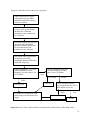
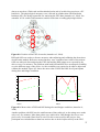
1
VTI särtryck 362A • 2004 Blink behaviour based drowsiness detection – method development and validation Master’s thesis project in Applied Physics and Electrical Engineering Reprint from Linköping University, Dept. Biomedical Engineering, LiU-IMT-EX-04/369 Linköping 2004 Ulrika Svensson VTI särtryck 362A · 2004 Blink behaviour based drowsiness detection – method development and validation Master’s thesis project in Applied Physics and Electrical Engineering Reprint from Linköping University, Dept. Biomedical Engineering, LiU-IMT-EX-04/369 Linköping 2004 Ulrika Svensson ISSN 1102-626X Reprint from Linköping University, Dept. Biomedical Engineering with kind permission from Göran Salerud Blink behaviour based drowsiness detection – method development and validation Ulrika Svensson LiTH-IMT/BIT20-EX- -04/369- Linköping 2004 Linköpings tekniska högskola Institutionen för medicinsk teknik Rapportnr: LiU-IMT-EX--04/369-Datum: 2004-09-07 Svensk titel Blinkbeteendebaserad trötthetsdetektering – metodutveckling och validering. Engelsk titel Blink behaviour based drowsiness detection – method development and validation. Författare Ulrika Svensson Uppdragsgivare: Rapporttyp: Rapportspråk: VTI Examensarbete Engelska Sammanfattning Abstract Electrooculogram (EOG) data was used to develop, adjust and validate a method for drowsiness detection in drivers. The drowsiness detection was based on changes in blink behaviour and classification was made on a four graded scale. The purpose was to detect early signs of drowsiness in order to warn a driver. MATLAB was used for implementation. For adjustment and validatation, two different reference measures were used; driver reported ratings of drowsiness and an electroencephalogram (EEG) based scoring scale. A correspondence of 70 % was obtained between the program and the self ratings and 56 % between the program and the EEG based scoring scale. The results show a possibility to detect drowsiness by analyzing blink behaviour changes, but that inter-individual differences need to be considered. It is also difficult to find a comparable reference measure. The comparability of the blink based scale and the EEG based scale needs further investigation. Nyckelord Keyword EOG, Blinks, EEG, Drowsiness, Detection, Driver, Thesis, VTI Bibliotekets anteckningar: Abstract Electrooculogram (EOG) data was used to develop, adjust and validate a method for drowsiness detection in drivers. The drowsiness detection was based on changes in blink behaviour and classification was made on a four graded scale. The purpose was to detect early signs of drowsiness in order to warn a driver. MATLAB was used for implementation. For adjustment and validatation, two different reference measures were used; driver reported ratings of drowsiness and an electroencephalogram (EEG) based scoring scale. A correspondence of 70 % was obtained between the program and the self ratings and 56 % between the program and the EEG based scoring scale. The results show a possibility to detect drowsiness by analyzing blink behaviour changes, but that inter-individual differences need to be considered. It is also difficult to find a comparable reference measure. The comparability of the blink based scale and the EEG based scale needs further investigation. Preface This Master of Science thesis project is the final part of the educational program in Applied Physics and Electrical Engineering with focus on Biomedical Engineering at the University of Linköping. The project was carried out at the Swedish National Road and Transport Research Institute (VTI) and the purpose was to further develop and test a model for detection of drowsiness in drivers, based on electrooculogram (EOG) analysis. I would like to thank all people who have helped me to complete this thesis by discussing the work, answering questions and by giving me comments on the report. Table of contents 1 Introduction ..................................................................................................................1 1.1 Background.............................................................................................................1 1.2 Problem definition...................................................................................................1 1.3 Outline of the thesis ................................................................................................1 2 Drowsiness and driving ................................................................................................3 2.1 Accidents caused by drowsy drivers ........................................................................3 2.2 Methods used for drowsiness detection ...................................................................3 2.2.1 Physiological measures....................................................................................3 2.2.2 Driving performance measures ........................................................................4 2.2.3 Self-report .......................................................................................................4 2.2.4 Expert ratings ..................................................................................................5 3 Electrooculogram (EOG)..............................................................................................7 3.1 Origin of the EOG signal.........................................................................................7 3.2 Measurement of EOG..............................................................................................7 3.3 Blink detection........................................................................................................8 4 Electroencephalogram (EEG) ....................................................................................11 4.1 Origin of the EEG signal .......................................................................................11 4.2 Classification of EEG............................................................................................11 4.3 Measurement of EEG............................................................................................12 4.4 EEG measurement problems .................................................................................13 5 Changes in EOG and EEG during drowsiness ..........................................................15 5.1 EOG as an indicator of drowsiness ........................................................................15 5.1.1 PERCLOS .....................................................................................................16 5.2 EEG as an indicator of drowsiness ........................................................................16 5.3 Objective Sleepiness Scoring (OSS)......................................................................17 6 Drowsiness stages based on blink behaviour .............................................................19 6.1 Model for drowsiness stages..................................................................................19 6.2 Drowsiness detection program ..............................................................................20 7 Background Summary................................................................................................23 8 Material.......................................................................................................................25 8.1 Drowsiness program..............................................................................................25 8.2 Collection of data..................................................................................................26 9 Method and procedure ...............................................................................................29 9.1 Method .................................................................................................................29 9.1.1 Common concepts .........................................................................................29 9.1.2 Hypothesis ....................................................................................................30 9.1.3 Data processing and blink detection...............................................................30 9.1.4 Modifications of the program ........................................................................31 9.2 Procedure..............................................................................................................31 10 Results from development of method.....................................................................35 10.1 Blink detection......................................................................................................35 10.1.1 Errors found in program ................................................................................35 10.1.2 Modification of the blink detection program..................................................35 10.2 Blink frequency replaced by blink intervals...........................................................36 10.3 Linear model for boundaries..................................................................................36 10.4 Drowsiness program with KSS as reference ..........................................................38 10.4.1 Choice of linearity constants and boundaries .................................................38 10.4.2 Adjustment of boundaries..............................................................................39 10.4.3 Adjustment of conditions for ten blink intervals.............................................40 10.4.4 Choice of reference value for alert state.........................................................40 10.4.5 Removal of short blinks.................................................................................41 10.4.6 Modified conversion of KSS to drowsiness stages .........................................41 10.4.7 Adjustment of threshold for long durations....................................................42 10.4.8 Final boundaries of the program ....................................................................42 10.5 Drowsiness program with OSS as reference ..........................................................42 10.5.1 Conversion of the OSS scale to drowsiness stages .........................................42 10.5.2 Choice of linearity constants and boundaries .................................................43 10.5.3 Adjustment of boundaries..............................................................................44 10.5.4 Adjustment of conditions for ten blink intervals.............................................45 10.5.5 Removal of short blinks and adjustment of threshold for long durations ........45 10.5.6 Higher resolution possible in OSS model.......................................................45 11 Results from validation of method .........................................................................47 11.1 Drowsiness program with KSS as reference ..........................................................47 11.2 Drowsiness program with OSS as reference ..........................................................49 11.3 Error analysis ........................................................................................................51 11.3.1 Mathematical model ......................................................................................51 11.3.2 KSS boundaries.............................................................................................53 11.3.3 OSS boundaries.............................................................................................54 11.4 Comparison with incident and accident blocks ......................................................55 12 Discussion ................................................................................................................57 12.1 Model for boundaries ............................................................................................57 12.2 Conversion of KSS and OSS to drowsiness stages.................................................57 12.3 KSS model............................................................................................................58 12.3.1 Performance of the program ..........................................................................58 12.3.2 Boundary for duration difference...................................................................58 12.3.3 Blink intervals ...............................................................................................58 12.4 OSS model............................................................................................................59 12.4.1 Performance of the program ..........................................................................59 12.4.2 Choice of adjustment participants ..................................................................59 12.5 Comparison between the models and with results from previous study..................59 12.6 Improvements of the method.................................................................................60 13 Conclusions .............................................................................................................61 13.1 Future possibilities ................................................................................................61 References ...........................................................................................................................63 Appendices..........................................................................................................................65 A1 User instructions .........................................................................................................65 A1.1 Data requirements ................................................................................................65 A1.2 User’s manual ......................................................................................................65 A2 Figures........................................................................................................................68 A2.1 Blink detection program .......................................................................................68 A2.2 Eye parameters versus KSS ratings.......................................................................69 A2.3 Eye parameters versus OSS ratings.......................................................................70 A2.4 Relationship between KSS and OSS.....................................................................71 A2.5 Correspondence between program rating and KSS rating .....................................72 A2.6 Correspondence between program rating and OSS rating .....................................73 A3 Parameter settings when recording physiological data .................................................74 A4 Common words and definitions...................................................................................75 1 Introduction 1.1 Background Many traffic accidents are caused by drivers falling asleep at the wheel (Åkerstedt & Kecklund, 2000). It would thus be beneficial to find a way to detect drowsiness before it occurs and to be able to warn the driver in time. Some systems have already been developed, based on recording of head movements, steering wheel movements, heart rate variability or grip strength. Systems that use a video camera for the tracking of eye movements have also been developed. However, so far no system has proved to be sufficient reliable (Kircher et al., 2002). In a previous Master’s Thesis Project, a method for detection of drowsiness in drivers was developed (Thorslund, 2003). The drowsiness detection was based on eye blink measurements in electrooculogram (EOG) data. The method was based on the linear relationship between blink amplitude and blink velocity, found by Hargutt and Krüger, and on their suggestion of how to define different stages of drowsiness (Hargutt & Krüger, 2000). In Thorslund’s study, also EOG data collected during an experiment in the VTI truck driving simulator was used. Based on EOG measurements, changes in blink amplitude, blink duration and blink frequency were detected and drowsiness was scored on a four graded scale. Driver reported ratings (self ratings) were used as reference, both for adjustment and validation of the method. A correspondence with the self ratings greater than 75 % was obtained for five out of six participants (Thorslund, 2003). The disadvantages with the previous project were the small amount of EOG material and the use of self ratings as the only reference measure. Another disadvantage was that the drivers participating in the experiment were professional drivers and perhaps differed from the average population in the way of developing drowsiness. 1.2 Problem definition The aim with this project was to further develop, adjust and validate the method for drowsiness detection developed by Thorslund (2003). EOG data, recorded from 20 non professional drivers during an experiment in the VTI driving simulator, was used for blink detection. To adjust and validate the method, two different reference measures were used; driver reported ratings, as was used in the previous project, and an electroencephalogram (EEG) based scoring scale. The EEG based scoring scale was considered a better reference measure and the presumption was that it would result in a well adjusted method. If it is found possible to detect early signs of drowsiness, the method may be transformed to a video based warning system able to detect changes in the eye parameters and warn the driver. 1.3 Outline of the thesis Chapter 1-6 are intended to give the reader the background theory and is summarized in chapter 7. Chapter 8 Material describes the data collection and the original drowsiness program designed by Thorslund. In chapter 9 Method and procedure the method and the different steps in the development of the method are described. The results are divided into 1 two chapters; chapter 10 Results from development of method and chapter 11 Results from validation of method. The last chapters, 12 and 13, contain discussion and conclusions. Appendices are included at the end of the thesis, containing user instructions for the program, figures and a list of common words and definitions. 2 2 Drowsiness and driving Drowsiness is the state where a person is almost asleep or very lightly asleep. It refers to an inability to keep awake or a drive to sleep (Encarta, 2004; Åkerstedt & Kecklund, 2000). In this thesis drowsiness and sleepiness are considered synonymous, but the term drowsiness will be used. Another concept commonly used is fatigue, which is an extreme tiredness that results from physical or mental activity. Drowsiness can also be described by the grade of wakefulness or vigilance. Wakefulness is the same as alertness or a state of sleep inability, whereas vigilance can be described as watchfulness or a state where one is prepared for something to happen (Encarta, 2004; Sternberg, 2001). According to Thorén (1999) and Åkerstedt and Kecklund (2000) several factors have been found to affect the grade of wakefulness. The time spent to carry out a task (time on task) and the amount of sleep during night are the most obvious factors. Other factors contributing are the amount of light, sound, temperature and oxygen content. Motivation and monotony of the task will also have an effect on the grade of wakefulness 2.1 Accidents caused by drowsy drivers The official number of traffic incidents on highways related to drowsiness is 1-3%, according to statistic analyses made by the American National Highway Traffic Safety Administration (NHTSA) (Åkerstedt & Kecklund, 2000). However, scientific studies the last years reveal that the actual number probably is much higher. According to Åkerstedt and Kecklund (2000) the number should be as much as 10-20 %. One reason can be that people that report traffic accidents lack the practice in judging the role of drowsiness as a contributing factor. It is difficult to give an exact measure of drowsiness in the way that is possible with for example alcohol. Furthermore, drowsiness is a transient state, which also makes the detection difficult. 2.2 Methods used for drowsiness detection Drowsiness can be measured through physiological measures, performance measures, selfreport or expert ratings (Belz, 2000; Kircher et al., 2002; Thorén, 1999). The different methodologies are described below. 2.2.1 Physiological measures Physiological measures have frequently been used for drowsiness detection as they can provide a direct and objective measure. Possible measures are EEG, eyelid closure, eye movements, heart rate, pupil size, skin conductance and production of the hormones adrenaline, noradrenaline and cortisol (Belz, 2000; Kircher et al., 2002; Thorén, 1999). EEG has shown to be a reliable indicator of drowsiness. The amount of activity in different frequency bands can be measured to detect the stage of drowsiness or sleep. For a further description of EEG as a drowsiness detection method, see chapter 5.2. Several studies (Belz, 2000; Galley & Schleicher, 2002; Thorén, 1999) also reveal that eye parameters such as blink duration, blink frequency, delay in lid reopening and the occurrence of slow eye movements (SEM) are good indicators of drowsiness. These parameters can be measured by EOG (see chapter 5.1 for a more detailed description). In a paper by Renner and Mehring (1997) it has been suggested that drowsiness should be defined based on a combination of brain and eye 3 measures. EEG could be used to detect deficiencies in information processing, which can occur even though the eyes are wide open, and the slow eye closures would detect insufficient perceptual capabilities. The problems with both EOG and EEG are the requirement of obtrusive electrodes which make them unsuitable to use in cars, as cabling of the drivers would not achieve any acceptance. Hence, they are not feasible to be used in a real-time drowsiness detection system. A decrease in heart rate and an increase in heart rate variability have shown to be indicators of drowsiness, as well as decrease in pupil size, spontaneous pupillary movements and decrease in skin conductance. A decreased production of adrenaline, noradrenaline and cortisol are other possible indicators of drowsiness (Belz, 2000; Kircher et al., 2002; Thorén, 1999). 2.2.2 Driving performance measures Driving performance measures include steering wheel movements, lateral position, speed variability and reaction time. Studies indicate that the steering wheel variability increases with the amount of drowsiness. The steering movements also become larger and occur less often, and the lateral position variability increases as the driver gets drowsier. Also, the speed variability increases and the minimum distance to any lead vehicle decreases. The reaction time to any unexpected events also gets longer with increased drowsiness. One problem concerning using driving performance measures as indicators of drowsiness is inter- and intraindividual differences in driving performance, which could be solved by a combination of different measures. It has been suggested that the combination of performance measures with physiological measures would give a sufficient reliable detection method (Belz, 2000; Kircher et al., 2002; Thorén, 1999). 2.2.3 Self-report Self-report refers to the subjective rating made by the driver and can be obtained through various rating scales. It is important that the scales are displayed in such a way that they are unobtrusive and don’t alert the driver, since that would affect the drivers state. Various rating scales have been constructed, for example the Stanford Sleepiness Scale (SSS) and the Karolinska Sleepiness Scale (KSS) (Åkerstedt & Gillberg, 1990). KSS is a nine graded absolute rating scale that has been validated against EEG and EOG indicators of sleepiness (Gillberg et al., 1994; Åkerstedt & Gillberg, 1990). Step 1, 3, 5, 7 and 9 contain a verbal description of drowsiness. The original KSS has been modified by Reyner and Horne (1995) who have added descriptions to the intermediate steps as well. The reason for this is that people seemed to report the steps with verbal descriptions more often than the intermediate steps. The modified KSS will be used in this thesis and is described in Table 2.1. 4 Modified version of KSS Here are some descriptors about how alert or sleepy you might be feeling right now. Please read them carefully and CIRCLE the number that best corresponds to the statement describing how you feel at the moment. 1 2 3 4 5 6 7 8 9 Extremely alert Very alert Alert Rather alert Neither alert nor sleepy Some signs of sleepiness Sleepy – but no difficulty remaining awake Sleepy, some effort to keep alert Extremely sleepy, fighting sleep Table 2.1: Modified version of KSS by Reyner and Horne (1995). When used in driving experiments the scale is memorized by the driver before the experiment and a verbal rating shall be made, to avoid disturbing the driver. 2.2.4 Expert ratings Expert ratings refers to the rating made by an observer and are made on a similar scale as the self-report. Results from earlier studies indicate that these ratings are reliable and consistent (Wierwille et al., 1994). The observer looks for behavioural indicators of drowsiness, for example eyelid closures, yaws, a vacant stare, body movements or the head falling backward or forward (Galley & Schleicher, 2002). 5 6 3 Electrooculogram (EOG) 3.1 Origin of the EOG signal Electrooculography is a method used for measuring the potential difference between the front and back of the eye ball. The EOG can thus be used for detection of eye movements and blinks. The eye is a dipole with the positive cornea in the front and the negative retina in the back and the potential between cornea and retina lies in the range 0.4 – 1.0 mV. When the eyes are fixated straight ahead a steady baseline potential is measured by electrodes placed around the eyes. When moving the eyes a change in potential is detected as the poles come closer or farther away from the electrodes, see Figure 3.1. The sign of the change depends on the direction of the movement (Andreassi, 2000; Thorslund, 2003). Figure 3.1: Change in EOG potential when looking 30 º to the right (Butler, 1995b). 3.2 Measurement of EOG EOG is measured by placing electrodes around the eyes. Usually silver-silver chloride electrodes are used as they show negligible drift and develop almost no polarization potentials. The electrodes should be placed as near the eyes as possible to maximize the measured potential. Problems with EOG measurement are artefacts that arise from muscle potentials and small electromagnetic disturbances that can be induced in the cables. To reduce the impedance between skin and electrode, the skin must be cleaned carefully before measurement and electrode paste should be used (Andreassi, 2000; Stern et al., 2001). It is important to be able to separate horizontal eye movements from vertical, and eye movements from eye blinks. By using different kinds of electrode placements the obtained recordings can be either vertical or horizontal (Muzet, 2002). In vertical recording electrodes are placed under and above the eye, and in horizontal recording they are placed at the outer edges of the eyes. Vertical recording is usually monocular, which means that the recording is made across one eye, whereas horizontal recording usually is binocular. Figure 3.2 shows how the electrodes are placed. Eye blinks are detected by using vertical recording (Andreassi, 2000; Stern et al., 2001; Thorslund, 2003). When measuring blink related characteristics, the sampling frequency should be high (at least 500 Hz) as a high resolution is required to measure small differences in for example blink duration. DC recording is preferable, while filtering the low frequency components away makes the detection of long blinks difficult. One problem with DC recording however, is the risk of slow baseline drift, which makes it important to monitor the EOG signal and adjust for the drift during the measurement (Peters & Anund, 2004). 7 Figure 3.2: Electrode placement (Kircher, 2001). 3.3 Blink detection According to Andreassi (2000) an eye blink is defined as when the upper and lower lids are touching each other and the eye is temporarily hidden. A typical blink has an amplitude of 400 µV and lasts for about 200 - 400 ms. A blink can be recognized in the EOG by its sharp rise and fall, see appendix A2.1 and Figure 3.3 for a trace of blinks in the EOG signal. Blinks in the EOG signal are sometimes referred to as blink artefacts (Pebayle, 2004). It is important to be able to distinguish eye blinks from vertical eye movements, since a change in the form of the blink artefact can be used for hypovigilance detection (Peters & Anund, 2004; Thorslund, 2003). Parameters used to describe the blink behaviour, extractable from the EOG signal, are for example blink frequency [blinks/minute], amplitude or eyelid opening level [mV] and duration [ms]. According to Andreassi (2000), a relaxed person blinks about 15-20 times per minute, although only 2-4 are needed from a physiological viewpoint. When performing cognitive tasks the blink frequency drops to as little as 3 blinks per minute, whereas an increase in blink frequency indicates reduced vigilance (Hargutt & Krüger, 2000). A common definition of blink duration is the time difference between the beginning and the end of the blink, where the beginning and end points are measured at the point where half the amplitude is reached. However, this definition will cause a problem when a vertical eye movement occurs at the same time as the blink, since this causes a vertical shift in the signal. The amplitude thus becomes difficult to define. As this is often the case, a better definition of blink duration is the sum of half the rise time and half the fall time in the blink complex. The first part of the duration is measured from half the rise amplitude to the top, and the second part is measured from the top to half the fall amplitude, see Figure 3.3 (Andreassi, 2000; Peters & Anund, 2004; Thorslund, 2003). The reason for measuring the beginning and end points where half the amplitude is reached, is because of the difficulties to exactly determine the beginning and end points of the blink complex in the EOG signal. The points where half the amplitude is reached, however, can be determined more exactly, as they are rather unaffected by small errors in the location of the blink beginning and end points. 8 Figure 3.3: Definition of blink duration, T, in EOG (Anund et al., 2004). The definition of a blink is separated from that of an eye closure. The definition of eye closure is commonly a blink with duration exceeding one second (Quartz et al., 1995). When using the definition of blink duration described above the definition of eye closure will instead be a blink with duration exceeding 0.5 seconds. 9 10 4 Electroencephalogram (EEG) 4.1 Origin of the EEG signal Electroencephalography is a method for measuring the electrical activity generated by the nerve cells of the brain, mainly the cortical activity. The EEG-activity is present all the time and recording show both random and periodic behaviour. The main origin of the EEG is the neuronal activity in the cerebral cortex, but some activity also originates from the thalamus and from subcortical parts of the brain. The EEG represents the summation of excitatory and inhibitory postsynaptic potentials in the nerve cells. The rhythmic activity is due to the synchronous activation of the nerve cells (Andreassi, 2000). The signal is classified on the basis of its amplitude and frequency range, see chapter 4.2. The recorded pattern differs during the different sleep stages, but also when performing cognitive tasks, focusing attention, preparing manual tasks or by brain diseases, for example epilepsy or tumours (Stern et al., 2001). 4.2 Classification of EEG As mentioned earlier, the EEG-signal can be classified on the basis of its amplitude and frequency range. The patterns most reliable in consistence and occurrence are beta waves, alpha waves, theta waves and delta waves, see Figure 4.1 (Andreassi, 2000). Other patterns exist as well, but as they are of no relevance for this thesis a further description will not be made. Beta waves (13-25 Hz) are common in the alert condition, during physical activity and when performing cognitive tasks. They can also be present in the first stages of sleep. The beta waves are irregular and have a small amplitude (2-20 µV) and relatively high frequency (Andreassi, 2000; Muzet, 2002; Stern et al., 2001). Alpha waves (8-12 Hz) are common in the awake and relaxed condition and can be used as a first measure of drowsiness. They are rhythmic and have an amplitude of 20-60 µV. When drowsiness appears the first sign is a rise in alpha activity. Later in the process the alpha waves diminish and are replaced by theta waves. Up to 10 % of the population do not show alpha activity at all. When alpha activity shows during relaxation, a sudden exposure to a cognitive task will make it disappear and be replaced by beta activity. This state is called alpha blocking (Andreassi, 2000; Gottlieb et al., 2004; Lowden, 2004). Theta waves (5-7 Hz) have an amplitude of 20-100 µV and will occur in the early stages of sleep, by hypnagogic imagery, focusing of attention or by problem solving. There exist two types of theta activity, one that is associated with performance of cognitive tasks and one associated with the early stages of sleep (Andreassi, 2000; Cohen, 2001; Stern et al., 2001). Delta waves (0,5-4 Hz) occur during the deepest sleep or by brain tumours. Their amplitude is in the range 20-200 µV. Existence of frequencies in the delta range in the awake condition is not normal and probably due to artefacts, but can also be an indicator of a brain tumour (Andreassi, 2000; Muzet, 2002; Stern et al., 2001). 11 Figure 4.1: EEG waves (Butler, 1995a). 4.3 Measurement of EEG EEG was developed by the German psychiatrist Hans Berger in 1929. EEG is normally registered by placing about 20 electrodes on the scalp, but as many as 256 electrodes can be used. The number and the placement are dependent on the purpose of the recording (Cohen, 2001; Nationalencyklopedin, 1998; Stern et al., 2001). The signal is either measured pair-wise between two electrodes on the scalp (bipolar recording) or between each electrode and one reference site (monopolar recording). The reference site is usually one ear or the nose. The sampling frequency should be at least 128 Hz. The measured signal is small, only a few microvolts (compared to EOG ~100 µV), which requires a large amplification factor. Amplification is necessary to minimize the load on the body, which reduces the current density between the skin and the electrodes. A high current density otherwise implies polarization of the electrodes. The amplification can make it difficult to separate the real signal from artefacts (Jacobson, 1995; Muzet, 2002; Stern et al., 2001). An international system for positioning of the electrodes has been constructed which is called the International 10/20 system. The name indicates that the electrodes are placed at positions 10 % and 20 % of the distance between four anatomical landmarks. The landmarks are the nasion (bridge of nose), the inion (projection of bone at the back of the head) and the left and right preauricular points (depressions in front of the ears). The points are labelled with a letter and a subscript index. The letters refer to the regions of the brain; F = frontal, O = occipital, C = central, P = parietal and T = temporal. The subscript indices are z which indicates the midline and numbers indicating the lateral placement and degree of displacement from the midline. An odd number refers to the left hemisphere, an even to the right. The number gets 12 higher the farther away it is from the midline (Andreassi, 2000; Stern et al., 2001). Figure 4.2 shows how the electrodes are placed. Figure 4.2: Electrode placement (Butler, 1995a). 4.4 EEG measurement problems The major problem with the measurement is the small amplitude, which makes it difficult to separate it from artefacts. Blinking and tension in the face muscles induce artefacts in the EEG. The amplitude of the artefacts varies but can be as high as 50µV (Lowden, 2004). Another problem is the small electromagnetic disturbances induced in the cables. The person should also be as still as possible and a proper electrode preparation is necessary to minimize the impedance between skin and electrode (Andreassi, 2000). 13 14 5 Changes in EOG and EEG during drowsiness Both EOG and EEG have shown to be valid indicators of drowsiness (Galley & Schleicher, 2002; Gottlieb et al., 2004). This chapter will describe the parameters used to detect drowsiness in the EOG and EEG respectively. 5.1 EOG as an indicator of drowsiness According to Galley and Schleicher (2002) EOG is a suitable measure for an objective characterization of drowsiness. It has been well documented that eyelid parameters provide a good measure of drowsiness. The parameters that describe the eyelid movements are usually the blink amplitude, blink duration and blink frequency. Sometimes the delay in lid reopening or the velocity of lid opening and closure are measured as well (Galley & Schleicher, 2002; Hargutt & Krüger, 2000). Figure 5.1 shows vertical EOG recording, both in alert and drowsy condition. Another parameter commonly used is the PERCLOS measure, which was first defined as the proportion of time in a minute the eyes are at least 80 % closed (Wierwille et al., 1994). PERCLOS will be described further in chapter 5.1.1. As drowsiness arises the blink duration gets longer, the blink amplitude smaller and the blinks occur more often. The delay in lid reopening increases and velocity of lid opening and closure decreases. These parameters can be detected by the EOG. A problem with EOG measurements is that when the blink duration increases it entails a difficulty to separate blinks from vertical eye movements, as they become very similar in shape. The sharpness of the wave, however, is distinctive for eye blinks. Another indicator of drowsiness is the slow eye movements, which often occur late in the drowsiness process (Muzet et al., 2000). Awake Very drowsy Vertical recording Figure 5.1: Vertical EOG recording from awake and drowsy condition (Kircher, 2001). It has been suggested that different sub processes control drowsiness and that the different processes can be detected by different eyelid parameters. In a study made by Hargutt and Krüger (2000) it has been suggested that there is one process controlling the level of attention that is connected to the blink frequency. When attention or vigilance decreases the blink frequency increases. Moreover, there is another process connected to the development of fatigue which is described by the blink duration. The development of fatigue will imply an increase in blink duration. According to Gottlieb and co-workers (2004) the drowsiness process consists of three different sub processes. The first one is decreasing arousal, which is represented by increasing theta power in the EEG and decreasing velocities of lid and eye movements. The second one is a sleep propensity, described by the blink durations and delay of lid reopening, and the third one is a loose of interest in the environment described by the blink rate. The sleep propensity process described by Gottlieb and co-workers could be 15 compared to Hargutt and Krüger’s development of fatigue, whereas loss of interest in the environment could be compared to a decrease in attention. 5.1.1 PERCLOS PERCLOS is a measure used for drowsiness detection that was established in 1994 by Wierwille (1994). It was first defined as the proportion of time in a minute that the eyes are at least 80 % closed. Eyes wide open represents 0 % and eyes closed represent 100 %. Today there are three PERCLOS measures in use: • • • P70, the proportion of time the eyes where closed at least 70 %; P80, the proportion of time the eyes where closed at least 80 %; and EYEMEAS (EM), the mean square percentage of the eyelid closure rating. PERCLOS has been evaluated in a study made by the Federal Highway Administration and has shown to be one of the most promising real-time measures of drowsiness (Knipling, 1998). The PERCLOS measure has two main weaknesses; the first one is that drowsiness is reported too late and the second one is that it fails to detect drowsiness in participants that have a diminished mental capacity although their eyes are wide open (Galley & Schleicher, 2002). 5.2 EEG as an indicator of drowsiness EEG is widely accepted as a good indicator of the transition between wakefulness and sleep as well as between the different sleep stages. It is often referred to as the golden standard. In the alert condition, or when performing cognitive tasks, the appearance of beta activity is common in the EEG. Alpha activity is also normally found in the occipital regions (O1 and O2) in the awake and relaxed condition (Andreassi, 2000; Gottlieb et al., 2004; Stern et al., 2001). When a driver gets drowsy a burst of alpha activity can often be seen in the central regions of the brain (C3 and C4). An increase in alpha activity is thus the first indicator of drowsiness. However, as mentioned before, some people do not show any alpha activity. As the driver gets drowsier, alpha activity is replaced by theta activity. When delta activity occurs in the EEG the driver is no longer awake, this is an indicator of deep sleep (Gottlieb et al., 2004). In summary the transition from wakefulness to sleep can be described as a shift towards slower frequencies in the EEG. The process differs between individuals but seems to be consistent within the individual (Andreassi, 2000; Gottlieb et al., 2004). To determine the drowsiness level a score can be given based on the amount of activity in different frequency bands during a certain time interval. OSS is the scoring method used in this thesis, and is described in chapter 5.3. Figure 5.2 and Figure 5.3 show EEG patterns in awake and drowsy condition. 16 Figure 5.2: EEG pattern in awake condition. Figure 5.3: EEG pattern in drowsy condition with alpha activity present. 5.3 Objective Sleepiness Scoring (OSS) Objective Sleepiness Scoring (OSS) is a scoring method developed to define the state of vigilance based on the information derived from EEG analysis and from the examination of blinks and eye movements in the EOG. The EEG content and the blinks are examined simultaneously during a period of 20 seconds and a vigilance score from 0 to 4 is given. Every 20 second a new score is given (A. Muzet, 2002). The five OSS scores are described in Table 5.1. 17 Vigilance score 0 1 2 3 4 EEG content Background of continuous beta waves, no alpha, no theta waves Occurrence of alpha and/or theta waves, in at least two regions of the brain, for less than a cumulative length of 5 second Occurrence of alpha and/or theta waves, in at least two regions of the brain, for less than a cumulative length of 5 second or occurrence of alpha and/or theta waves, in at least two regions of the brain, for more than a cumulative length of 5 second Occurrence of alpha and/or theta waves, in at least two regions of the brain, for more than a cumulative length of 5 second Continuous alpha and/or theta waves Blinks and eye movements Normal blinks and eye movements Normal blinks and eye movements and slow blink (s) or eye movement (s) and normal blinks and eye movements and slow blink (s) or eye movement (s) Slow blinks and eye movements Table 5.1: Objective Sleepiness Scoring (OSS) derived from EEG and blink data (Muzet, 2002). The EEG data is examined either visually or by spectral analysis to detect occurrence of theta, alpha or beta activity. When performing spectral analysis the absolute power values for the different frequency bands are given. Occurrence of low frequencies (< 4 Hz) in the awake EEG is probably due to artefacts and will not be classified as delta activity, as delta activity only occurs during sleep. The regions of the brain are the occipital, temporal, parietal, frontal and central region. To eliminate cases where only localized EEG patterns arise, the activity shall be found in at least two regions of the brain (Muzet, 2002). 18 6 Drowsiness stages based on blink behaviour This chapter describes the method for drowsiness detection developed by Hargutt and Krüger (2000) and the original drowsiness program based on this method, developed by Thorslund (2003). 6.1 Model for drowsiness stages In a study made by Hargutt and Krüger (2000), a model for defining different stages of drowsiness was developed. The model was based on a linear relationship between blink amplitude and blink velocity and on the suggestion that different eye parameters represented different stages in a progressive drowsiness process. Hargutt and Krüger found that the blink velocity was linearly related to the blink amplitude in the alert condition. Blink velocity is defined as the velocity of the eyelids when blinking. They stated that there seems to be a control process that strives to maintain constant blink duration. This control process estimates the planned amplitude and then determines the blink velocity based on the estimated blink amplitude (Hargutt & Krüger, 2000). The blink duration is defined as the amplitude divided with the velocity, if using the definition of blink duration described in chapter 3.3. In this thesis, the blink amplitude is calculated as a mean value of the rising and falling amplitudes. Hargutt and Krüger found that the linear relationship changed during the development of drowsiness, resulting in longer blink durations. Figure 6.1 shows the relationship between amplitude and velocity in the alert condition. amplitude and velocity of blinks normal effort - baseline 0.16 0.12 0.08 0.04 velocity [m/s] 0.00 0.000 0.16 0.008 0.016 0.000 VP: 1 0.008 0.016 0.000 VP: 2 0.008 0.016 0.000 VP: 3 0.008 0.016 VP: 5 0.12 0.08 0.04 0.00 0.000 0.16 0.008 0.016 0.000 VP: 6 0.008 0.016 0.000 VP: 8 0.008 VP: 9 0.016 0.000 0.008 0.016 VP: 10 0.12 0.08 0.04 0.00 0.000 0.008 VP: 11 0.016 0.000 0.008 0.016 VP: 12 amplitude [m] Figure 6.1: Relationship between amplitude and velocity in alert condition. VP refers to the different participants (Hargutt & Krüger, 2000). The linear relationship identified in the alert condition, could thus be used to calculate an expected blink duration for each blink, based on the blink amplitude. A polynomial of first degree was fitted to data from the alert condition. The slope determined the set point for the 19 duration and the intersection with the y-axis the minimum possible velocity. In the evaluation condition, an expected blink velocity was calculated for each amplitude by using the regression equation and accordingly an expected duration was calculated. The expected duration was then compared to the measured duration to find out if a difference existed (Hargutt & Krüger, 2000). Hargutt and Krüger (2000) also found that a separation could be made between blink frequency and blink duration and that these measures represented different stages of drowsiness. The blink frequency increased in the beginning of the drowsiness process, representing a stage of reduced vigilance. As drowsiness increased, an increase in blink duration and later also a decrease in blink amplitude was found. This was used for defining different stages of drowsiness, see Table 6.1. Drowsiness stage Awake Low vigilance Drowsy Sleepy Description Long blink intervals and short blink durations. Short blink intervals and short blink durations. Long blink durations. Very long blink durations and/or single sleep events and/or a low eyelid opening level. Table 6.1: Drowsiness stages based on blink behaviour (Hargutt & Krüger, 2000). 6.2 Drowsiness detection program Thorslund (2003) used the method for defining stages of drowsiness, developed by Hargutt and Krüger, to develop a drowsiness detection program. EOG data recorded during driving in a truck driving simulator was used for blink detection. The drivers drove both in alert and in drowsy condition. Data from the first ten minutes of the alert drive was used to calculate regression coefficients for the linear relationship between blink amplitude and blink velocity. The hypothesis was that the linear relationship between blink amplitude and blink velocity was universal. Thus, there were no adjustments made for individual differences. The expected duration was calculated as described in chapter 6.1 and the difference between measured and expected duration was compared to the boundary set in the program to determine if the blink duration was high enough to be classified as drowsy. The same procedure was done for each blink frequency and blink amplitude; the program compared each blink frequency and blink amplitude with the boundaries set in the program to determine if they were exceeded. The boundaries were based on mean values and standard deviations of the variables in the alert condition as this was thought to be a measure of the individual differences in the development of drowsiness. The program then examined ten blinks at a time to see how many of the blinks that were exceeding the boundaries. A classification was made in four stages, as described in Table 6.1. The stages were checked in priority, beginning with the drowsiest stage (Thorslund, 2003). Evaluation of the performance of the program was done by comparing the result with KSS ratings made by the drivers. The program showed a correspondence with the KSS ratings higher than 75 % for five out of six participants. Two participants had been chosen to adjust boundaries of the program and the remaining four were used for validation of the program (Thorslund, 2003). 20 Figure 6.2 describes a flow chart of the program: Find coefficients for linear relationship between blink amplitude and blink velocity in alert condition. Calculate expected blink velocity and expected blink duration for each blink amplitude in the condition to be evaluated. Determine difference between expected and found blink duration (duration difference) for each duration in the condition to be evaluated. Determine allowed deviations (boundaries) for blink amplitude, duration difference and blink frequency. Check if duration > 0.5 s or if blink amplitude exceeds boundary for more than 5 out of 10 blinks. None Check if duration difference exceeds boundary for more than 2 out of 10 blinks. Exceeding Normal Either 4 Sleep onset Evaluation by comparison with KSS ratings converted into four stages. 3 Drowsy Check if blink frequency exceeds boundary for one or more blinks out of ten. High Low 2 Low vigilance 1 Awake Figure 6.2: Flow chart of the model for categorization of drowsiness (Thorslund, 2003). 21 22 7 Background Summary According to the literature, both EOG and EEG are valid indicators of drowsiness. Drowsiness is characterized by increased blink duration, decreased blink amplitude and increased blink frequency and EOG can be used to measure changes in these parameters. According to Hargutt and Krüger (2000), different eye blink parameters can be used for classifying different stages of drowsiness and four different stages can be distinguished. Increased blink frequency indicates reduced vigilance, which is the first stage in the drowsiness process, and the blink duration and blink amplitude indicate increased drowsiness. In the EEG, drowsiness is characterized by a shift towards lower frequencies. Increased alpha activity and sometimes also theta activity is common during drowsiness. The problem with both measuring methods is the requirement of electrodes, which makes them unsuitable for use in cars, as cabling of the drivers wouldn’t achieve any acceptance. An objective with this thesis is to use a new data set to further develop the method for drowsiness detection developed by Thorslund (2003) and to validate it against OSS, i.e. an EEG based reference measure. The purpose is to detect early signs of drowsiness in order to warn a driver in time. To make the validation of the method against the OSS scale, this scale has to be converted to match the four graded scale developed by Hargutt and Krüger (2000). Another objective is thus to find a way to convert the OSS scale. It should be pointed out though, that even if a correspondence is found, the scales are two different measures. The scale developed by Hargutt and Krüger is based on changes in blink behaviour and OSS is an EEG based scale. 23 24 8 Material 8.1 Drowsiness program This chapter describes the original drowsiness program. For a further description, see (Thorslund, 2003). The drowsiness program first found start-, peak- and stop positions in the blinks, both in alert and drowsy condition, and calculated the blink amplitude. Regression coefficients for the linear relationship between blink amplitude and blink velocity were then calculated from the first ten minutes of the alert condition. The regression equation was used to calculate an expected blink velocity and accordingly expected blink duration for each eye blink. The program then calculated boundaries for the drowsiness classifying criteria, formulated as allowed deviations from normal state for amplitude, difference between expected and found duration and blink frequency. Mean values and standard deviations of the variables, taken from the first ten minutes of the alert condition, were used for determining boundaries. The boundaries set in the program are presented in Table 8.1. Variable Amplitude Duration difference Frequency Boundary M - 3σ M+σ M + σ/2 Table 8.1: Boundaries for the variables. M = mean, σ = standard deviation (Thorslund, 2003). After determining the regression coefficients and boundaries, ten blinks were examined at a time and a drowsiness stage was returned based on the amount of blinks exceeding the boundaries. The difference between expected and measured blink duration was calculated by using the regression equation. The program searched in descending order for indicators of stage four (see Table 8.2), stage three and stage two. If none of the conditions were fulfilled the program responded with diagnose one, i.e. awake. The program then shifted one blink forward and repeated the calculation of the diagnose. The reason for looking at ten blinks at a time was to be able to detect quick changes in the state of drowsiness. Level 4 Sleep onset 3 Drowsy 2 Low vigilance 1 Awake Condition for ten blink intervals Half of the blinks contain an eye closure or a low eyelid opening level (blink amplitude). Difference between expected and found duration is exceeding the boundary for more than two of the blinks. At least one blink of exceeding frequency is found. None of the conditions in level 2, 3 or 4 fulfilled. Table 8.2: Conditions for categorisation of blinks in ten blink intervals (Thorslund, 2003). The KSS ratings were converted by the program into a four graded scale described in Table 8.3. The conversion was based on the verbal descriptions of the KSS steps. 25 KSS Drowsiness Stage 1 2 3 4 5 6 7 8 Extremely alert Very alert Alert Rather alert Neither alert or sleepy Some signs of sleepiness Sleepy – but no difficulty remaining awake Sleepy, some effort to keep alert 1 1 1 2 2 2 3 3 Awake Awake Awake Low vigilance Low vigilance Low vigilance Drowsy Drowsy 9 Extremely sleepy, fighting sleep 4 Sleep onset Table 8.3: KSS converted to drowsiness stages (Thorslund, 2003). Finally mean values of the drowsiness stages given in five minute intervals were calculated. These values were then compared to the converted KSS ratings and the number of corresponding intervals was given (Thorslund, 2003). One disadvantage with this method was that the KSS ratings were given only in five minute intervals. To be able to evaluate the performance of the program a mean value of the drowsiness stages thus had to be calculated and the purpose of detecting quick changes in drowsiness was lost. Another disadvantage was that the EOG data was taken from professional drivers, who perhaps differed from the average population in the way of developing drowsiness, and that only the KSS ratings were available as a reference measure. 8.2 Collection of data The data used in this thesis was EOG data collected at VTI during a driving simulator experiment in the AWAKE project (Peters & Anund, 2004). The aim of the AWAKE project was to develop an unobtrusive, reliable system which should monitor the driver and the environment to detect in real time hypo-vigilance, based on multiple parameters (Anund et al., 2004). The aim of the experiment was to evaluate the integrated AWAKE system in a passenger car simulator environment. The experiment was done with help of an advanced moving based driving simulator (Nilsson, 1993) and totally 20 drivers participated. The experimental design was a repeated measures design. Ten drivers represented young drivers (aged 18-24 years) and ten represented old drivers (aged 55-64 years). The participants visited VTI twice, the first time for training and the second time for the experiment. The participants performed their first drive during an alert condition in the afternoon. They stayed at VTI during the night without any sleep and drove sleep deprived late at night/early in the morning. Physiological data was collected with the Vitaport 2 system from TEMEC Instruments B.V., Kerkrade, the Netherlands, which is a portable digital recorder with sixteen channels for physiological measures, one channel for skin conductance measurement and one marker signal that can adopt four values. Electroencephalogram (EEG), vertical and horizontal Electrooculogram (EOG) and Electromyogram (EMG) were recorded. EEG was measured through three bipolar derivations, positioned at Fz-A1, Cz-A2 and Oz-Pz, see Figure 8.1. The sampling frequency was 256 Hz when recording EEG and 512 Hz when recording EOG. The 26 data was stored on a Flash card and downloaded at the end of each driving session to a PC hard drive. The physiological measures were collected in collaboration with Karolinska Institutet (KI), also being responsible for analyzing the EEG data (Anund et al., 2004). See appendix A3 for a table with parameter settings used when recording physiological data. Figure 8.1: Position of the EEG electrodes (Anund et al., 2004). KSS and OSS was used as reference measures when adjusting and validating the drowsiness classification method. Reference means that they were considered true values of drowsiness. OSS was achieved after analyzing the EEG data and the KSS ratings were reported by the drivers every five minutes. The problems with both OSS and KSS were an unequal variability over the different steps of the scales. A wide variability was required to be able to adjust and validate the method. Figure 8.2 shows the mean value of KSS and OSS for all participants during alert and fatigue condition. 9 ,5 8 ,4 7 6 ,3 5 ,2 3 COND KSS 2 Alert Fatigue 1 10,0 15,0 MINUTE 20,0 25,0 30,0 35,0 40,0 45,0 Mean OSS 4 COND ,1 Alert Fatigue 0,0 10,0 15,0 20,0 25,0 30,0 35,0 40,0 45,0 MINUTE Figure 8.2: Mean value of KSS and OSS during alert and fatigue condition (Anund et al., 2004). Another problem with KSS was the small amount of data achieved, as the ratings were made only every five minutes. More data points were achieved for OSS though; the scores were given every 20 seconds. Data from 18 out of 20 drivers was used for this project. One participant was excluded due to data loss and one due to lack of alpha activity in the EEG. 27 28 9 Method and procedure This chapter is divided into two parts, the first part describing the method and common concepts used during the development of the method and the second part describing the different steps in the development of the method. 9.1 9.1.1 Method Common concepts Two different reference measures were used to validate the method, KSS and OSS. Two separate models were therefore set up, one that used KSS as reference in the program and one that used OSS. The models will be referred to as the KSS model and the OSS model. Three different scales were used in the program, KSS, OSS and the blink behaviour drowsiness scale or shortly drowsiness scale, used in the program. The drowsiness scale is a four graded scale, which stages will be referred to as drowsiness stages. KSS is a nine graded scale, which steps will be referred to as KSS steps. OSS is a five graded scale and the steps of this scale will be referred to as OSS steps. The steps of KSS and OSS have been reduced to match the drowsiness scale. The reduced scales will be referred to as the converted KSS and the converted OSS. The steps of the converted scales will be called converted KSS steps and converted OSS steps. The variable limits used in the program are referred to as boundaries and conditions. The boundaries are limits for the allowed deviations from normal state for blink amplitude, duration difference and blink intervals. The conditions are limits for the amount of blinks out of ten allowed to exceed the boundaries. The program diagnose depends on which conditions of the program that are fulfilled and consequently on the boundaries set for the variables. The boundaries and conditions are thus connected and influence each other. When developing the model the terms set and adjust will be used. To set boundaries or conditions means that the variables are given values and to adjust boundaries or conditions means that the given values are changed to get as good correspondence with the reference measure as possible. The terms sensitivity and specificity are used to describe the performance of the program. High sensitivity means that the program detects a high proportion of the drivers that are drowsy, but is often related to a high proportion of false alarms, i.e. high risk of classifying a not drowsy driver as drowsy. High specificity means that the number of false alarms is low, but is often related to a high risk of missing a drowsy driver. Good performance of any classifying system is defined by high sensitivity and specificity. 29 According to the system Impaired Non Impaired According to the reference Impaired according Not Impaired True Positive (Hit) False Negative (Miss) False Positive (False Alarm) True Negative (Pass) Table 9.1: Possible outcome of an impairment diagnose (Anund et al., 2004). Sensitivity and specificity are defined as follows, when using the terminology from Table 9.1: Hits ⋅ 100 • Sensitivity = ( Hits + Misses) Passes • Specificity = ⋅ 100 ( Passes + False alarms ) 9.1.2 Hypothesis The aim of this project was to use a new data set to further develop, adjust and validate the program designed by Thorslund (2003). Adjustment and validation should be made both against KSS and against an EEG based reference measure (OSS). The hypothesis was that EEG was a better reference measure than the KSS ratings and that using EEG as reference would make it possible to improve the program. Two different versions of the program were tested, one that used the KSS ratings as reference (the KSS model) and one that used the EEG-based OSS ratings as reference (the OSS model). Reference implies that these measures were considered true values of drowsiness. It was also presumed that six participants could be randomly chosen to adjust boundaries used in the program so that it would be valid also for the remaining participants. This should apply for both the KSS model and the OSS model. Twelve participants were used for validation of the program, as there was only useful data from 18 out of 20 participants. 9.1.3 Data processing and blink detection Based on the collected EOG data, blinks were detected in the EOG signal with a MATLAB program, originally designed by Thierry Pébayle at CNRS-CEPA and modified by Joakim Östlund at VTI. The program took a continuous binary file of 16 bits signed integer as input. The EOG data was first converted from European Data Format to Binary Format with another MATLAB program, designed at VTI. This program first performed a bandpass filtration of the signal with cutoff frequencies 0.005 Hz and 8 Hz. The lowpass filtration was made for the purpose of reducing muscle artefacts from the signal and the highpass filtration removed the drift in the signal. The results were stored in a text file. The blink detection program detected start-, peak- and stop positions in the blink complexes. Peak positions were detected as local maxima of the blink complexes above an adjustable threshold value. To detect the start- and stop positions the program searched for the position where the slope went below a predefined value by starting from the peak. The program was only semi-automatic, which implied that all data had to be inspected visually to adjust the threshold value and to correct for falsely detected blinks and blinks missed out on. This was done by looking at a 30 second window and shifting forward. 30 9.1.4 Modifications of the program The original program was tested with both reference measures (KSS and OSS). As the correspondence was only about 50 %, both when using KSS and OSS as reference, new boundaries had to be found. A linear model was chosen for the boundaries as it was found that the standard deviation not was a good measure of the development of drowsiness. The model based on the standard deviation of the variables in the alert condition was used as it was presumed that the standard deviation reflected individual differences in the development of drowsiness. As no such relationship was found, a linear model was chosen, based on figures of the variables plotted against the reference measures. The linear model assumed that the variables blink amplitude, duration difference and blink intervals changed in a linear way over the drowsiness stages without inter-individual differences. A regression line was fitted to the data by using a least square method. Boundaries were set based on calculated linearity constants and adjusted to get optimal correspondence with the reference measure for the six participants chosen for adjustment. The model was adjusted to get as good correspondence with the drowsy condition as possible. Modifications of the program leading to improvement of the results were also made. 9.2 Procedure This chapter gives an overview of the different steps in the development of the method. The results are described in chapter 10. Blink detection: Blinks were detected in the EOG data by using the blink detection program. Errors were found in the program and a program was designed for identifying these errors. Blink frequency replaced by blink intervals: The variable blink frequency used in the original program was replaced by the variable blink intervals. Linear model for boundaries: A linear model was chosen for the boundaries. The model assumed that the variables change in a linear way over the drowsiness stages. Drowsiness program with KSS as reference: • • • • • • Constants were calculated for the linear relationship between the variables (blink amplitude, duration difference and blink intervals) and the KSS ratings. Boundaries were set in the program based on the calculated constants and were adjusted to get as good correspondence with the KSS ratings as possible for the participants chosen to adjust the boundaries. Conditions for the amount of blinks out of ten that was allowed to exceed the boundaries were adjusted. The reference value for the alert state was set to depend on the KSS rating in the beginning of the alert condition. Participants that had a KSS rating corresponding to drowsiness stage two got different boundary than participants with a KSS rating corresponding to drowsiness stage one. Blinks that occurred when the participants were looking down were removed, as looking down could give rise to “fake” blinks. The boundary for “very long blink duration” that was part of the criteria for reaching drowsiness stage four was adjusted. 31 Drowsiness program with OSS as reference: • • • • • • • Different ways of converting the steps of the OSS scale to the drowsiness stages of the program were investigated. Constants were calculated for the linear relationship between the variables (blink amplitude, duration difference and blink intervals) and the OSS ratings. Boundaries were set in the program based on the calculated constants and were adjusted to get as good correspondence with the OSS ratings as possible for the participants chosen to adjust the boundaries. Conditions for the amount of blinks out of ten allowed to exceed the boundaries were adjusted. Blinks that occurred when the participants were looking down were removed, as looking down could give rise to “fake” blinks. The boundary for “very long blink duration” was adjusted. Higher resolution possible in OSS model. Figure 9.1 shows a flow chart over the program with places where changes have been made pointed out. The major changes are made when determining boundaries for the program. 32 Find coefficients for linear relationship between amplitude and velocity in alert condition. Remove blinks when looking down: Blinks that have a ratio between falling and rising amplitude below 36 % were removed. Calculate expected blink velocity and expected blink duration for each blink amplitude in the condition to be evaluated. New boundaries in the program, based on a linear model. Determine difference between expected and found blink duration (duration difference) for each duration in the condition to be evaluated. Boundaries dependent on KSS rating in alert condition in KSS model. Determine allowed deviations (boundaries) for blink amplitude, duration difference and blink frequency. Check if duration > 0.3 s or if blink amplitude exceeds boundary for more than 6 out of 10 blinks. New boundary for long blink durations. None New conditions for ten blink intervals. Check if duration difference exceeds boundary for more than 2 out of 10 blinks. Exceeds Normal Either 4 Sleep onset Evaluation by comparison with KSS/OSS ratings converted into four/three stages. OSS as reference as well. 3 Drowsy Check if blink interval exceeds boundary for more than 3 out of 10 blinks. Exceeds Normal 2 Low vigilance 1 Awake Blink frequency replaced by blink interval. Figure 9.1: Flow chart of the drowsiness program with changes included. 33 34 10 Results from development of method The first part of the results concerns the development of the method; an outline of this chapter has already been presented in chapter 9.2. 10.1 Blink detection Start-, peak- and stop positions were detected in the blink complexes by using the blink detection program. Data was inspected visually to adjust the threshold value and to correct for falsely detected and missed blinks. Appendix A2.1 presents a flow chart of the blink detection program. The results were stored in a text file in four columns containing start-, peak- and stop position as well as duration for each blink complex detected in the EOG data. The duration was calculated based on the definition described in chapter 3.3. A total of 38 text files were obtained, two for each participant, representing alert and drowsy condition. Participant number 1 was excluded due to data loss. 10.1.1 Errors found in program The blink detection program was first tested on a data file not supposed to be used in the further study. It was found that start- or stop positions sometimes coincided with the wrong blink complexes, when using the peak position as reference for the blink complex. Occasionally it was also found that the same peak position was detected two or three times but with different start- and stop positions. This resulted from blinks with abnormally long durations which were found and which were inspected more closely. To identify falsely detected blinks, an additional program was constructed. The program detected positions where the stop position for one blink complex was found after the start position for the next blink complex and positions where the same peak was detected twice. The program also detected positions where the stop position for one blink complex coincided with the start position for the next blink complex. 10.1.2 Modification of the blink detection program A modification of the blink detection program, made by Thierry Pébayle, could be used to run the program with the text file containing the results and thereafter do adjustments. The program designed for identification of falsely detected positions, see chapter 10.1.1, was used for finding the positions and the errors were manually corrected for. This was found to be the only alternative, as the source of the errors was unknown. After running some of the new files it became clear that there were just a few problems with this data set. 35 10.2 Blink frequency replaced by blink intervals The variable blink frequency in the model was replaced by blink intervals, i.e. time between blinks. The reason for this choice was that a problem was found with the calculation of the blink frequency. The problem was as follows: The program calculated the blink frequency for each blink and then detected the amount of blinks exceeding the boundary for the purpose of classifying stage two, low vigilance. The boundary was based on mean value and standard deviation of the blink frequency in the beginning of the alert condition. The blink frequency for one blink was calculated as f i = 1 / Ti , where Ti was the time interval between two blinks. The mean value of the blink frequency was then calculated as a mean value of all frequencies within the time n interval: f = ∑f i =1 i . This definition of mean value did not reflect n the true number of blinks per time interval, unless the blink Figure 10.1: EOG data intervals were equidistant. To reflect the true number of blinks per time interval, the blink frequency had to be defined as the amount of blinks in a time interval, n +1 i.e. the amount of blink intervals plus one, divided with the length of the time interval: n . ∑ Ti i =1 An adjustment was thus made in the program so that blink intervals were calculated instead of blink frequency. Drowsiness stage two would then be reached if the blink intervals were lower than normal. 10.3 Linear model for boundaries A linear model was chosen for the boundaries. These were earlier based on mean values and standard deviations taken from the first ten minutes of the alert condition, see Table 8.1. The model considered individual differences, but was built on the assumption that the standard deviation of the variables in the alert condition was a general measure of the individual differences in the development of drowsiness. A person with a large variation in for example amplitude during the alert condition got a less strict boundary than a person with a small variation. In other words, the model assumed that a person with large variation of a variable during the alert condition would develop drowsiness later than a person with small variation. Y −M This was investigated by calculating the relationship , where Y was the variable σ (amplitude, duration difference or blink interval), M was the mean value of the variable in the alert condition and σ the standard deviation of the variable in the alert condition. The calculation was done for different participants and the value was compared between participants within every KSS interval representing a drowsiness stage. The values should be approximately constant within the KSS interval to consider the model appropriate, but a difference was found. The values varied between approximately the values 1 and 7. 36 Plotting the blink amplitude, duration difference and blink intervals against KSS and OSS ratings, revealed the use of a linear model for the boundaries for both the KSS and the OSS model. The variables were taken both from the alert and the fatigue drive and the original KSS and OSS scales were used. See appendix A2.2 and A2.3 for figures of the relationship for four of the six the participants chosen for adjustment. The linear model assumed that the variables change linearly over the different drowsiness stages for both the KSS model and the OSS model, see Figure 10.2. The most interesting assumption was that the model assumed that all individuals develop drowsiness in the same way, which means that the variables had to change equally in magnitude for all people when they got drowsy. A percentage change was calculated for the blink amplitude and the blink intervals and a fixed value for the blink duration. This was a strict assumption, but as the program was supposed to predict drowsiness based only on three calculated eye parameters in the beginning of the alert condition, this was found to be the only alternative. An individual model would require that some information could be achieved about how the parameters changed when the individual got drowsy and that was not possible when data was used from the first part of the alert condition. 37 Relation betw een am plitude and drow siness stages Relation betw een duration difference and drow siness stages Duration difference (s) Amplitude (µV) 400 300 200 100 0 1 2 3 4 0,25 0,2 0,15 0,1 0,05 0 1 Drow siness stage 2 3 4 Drow siness stage a) Relation between amplitude and drowsiness stages. b) Relation between duration difference and drowsiness stages. Blink intervals (s) Relation betw een blink intervals and drow siness stages 2,5 2 1,5 1 0,5 0 1 2 3 4 Drow siness stage c) Relation between blink intervals and drowsiness stages. Figure 10.2 a-c: Linear model for boundaries. As can be seen in the figure over the blink intervals (figure c), data is missing at the last two drowsiness stages. This is because the model didn’t say anything about the blink intervals at the drowsiness stages after stage 2. The blink intervals could either increase or decrease. 10.4 Drowsiness program with KSS as reference This chapter describes the choice of boundaries for the KSS model together with modifications made in the program. The final boundaries are presented in the end of this chapter. 10.4.1 Choice of linearity constants and boundaries Six participants, three from the young age group and three from the old age group, were chosen for setting boundaries of the program. As described in chapter 10.3, a linear model was chosen by plotting the variables (blink amplitude, duration difference and blink intervals) against the KSS ratings for five participants. Participant number 10 was excluded as this 38 participant had a higher KSS rating in the alert condition than in the drowsy condition. This was incompatible with the prerequisites of the program. After inspection of the figures, a linear relationship was found for the amplitude and the duration difference. No relationship was found for the blink intervals for the three participants that had rated themselves in corresponding interval (KSS 1-6, corresponding to the first two drowsiness stages). Linearity constants were thus calculated only for blink amplitude and duration difference for the five participants. The amplitude values were normalized with the first value to decide if a percentage value would be a better choice for the boundary than a fixed value. Normalization could not be made with the duration difference as its reference value ideally would be zero. The expected duration was based on the measured duration in the alert condition and hence the difference would be close to zero. As the linearity constants differed between the individuals, a best value had to be found. The constants received after normalizing the amplitude with the first value were found to vary less between the individuals. A percentage value was thus chosen for the amplitude. The constants for amplitude and duration difference were first calculated as mean values of four of the constants. One of the constants was excluded due to large variation in data. Another one, corresponding to participant number 10, was also excluded as described in the first part of this chapter. Boundaries were calculated based on the chosen linearity constants and the program was tested on the participants chosen for adjustment. A modification was made so that only the first five minutes of the alert condition were used as reference value as the constants had been calculated based on mean values over five minute intervals. 10.4.2 Adjustment of boundaries The chosen boundaries were set based on data from both alert and drowsy condition. The boundary for the duration difference in the drowsy condition was not found strict enough; a very bad correspondence was obtained. The program did not classify the participants as drowsy (stage three) even though KSS indicated that they were. It was considered more important to correctly detect all drivers that were drowsy than to correctly detect all alert drivers, i.e. high sensitivity was preferred over high specificity. A choice was thus made to adjust the boundaries to get as good correspondence with the KSS ratings in the drowsy condition as possible. This implied that the boundary for the duration difference had to be more strictly set. Constants could not be calculated only for the drowsy condition as the variability in data was too low. The participants often reached the last KSS steps (step 8 or 9) quite fast and then remained there. The boundaries were adjusted in the order of priority that the conditions were checked, see Figure 9.1. The boundary calculated for the amplitude was kept as this showed to be the best value possible. The duration boundary was adjusted until the best possible correspondence with KSS was obtained. The material used for choosing boundaries for the blink intervals did not indicate that they got lower between drowsiness stage one and two. A boundary was set for the blink intervals without any basis. The validity of this boundary is thus uncertain. A simplification was made when adjusting boundaries; it was assumed that the diagnose obtained in a five minute interval was based on all blinks in the interval. The boundaries and conditions could then be adjusted in the order of priority that the conditions were checked, i.e. with stage four first. Adjusting boundaries and conditions of lower priority would not affect adjustments already made. In reality a diagnose was given for each ten blink interval and the 39 diagnose obtained in a five minute interval was a mean value of all diagnoses obtained during five minutes. The difference between the results with and without the simplification was investigated, and it was small enough to consider the simplification appropriate. Without the simplification the adjustment of boundaries would be more complicated, as each adjustment would influence the adjustments already made. The reason is that the program diagnose was a mean value of diagnoses. 10.4.3 Adjustment of conditions for ten blink intervals The program looked at ten blinks at a time and gave a diagnose based on conditions set for each ten blink interval, see chapter 8.1. An adjustment of these conditions was made to get as good correspondence with the KSS ratings as possible for the chosen participants. This adjustment was made after the boundaries were set but before they were adjusted. After adjusting the boundaries it was assured that the adjustments of the conditions were valid. The modified conditions are presented in Table 10.1. Level 4 Sleep onset 3 Drowsy 2 Low vigilance 1 Awake Condition for ten blink intervals More than 60 % of the blinks contain an eye closure or a low eyelid opening level (blink amplitude). Difference between expected and found duration is exceeding the boundary for more than 20 % of the blinks. Short blink intervals are found in more than 30 % of the blinks. None of the conditions in level 2, 3 or 4 fulfilled. Table 10.1: Modified conditions for ten blink intervals. 10.4.4 Choice of reference value for alert state The reference value for alert state was chosen to be the first five minutes of the alert drive as this was the time when participants were expected to be most alert. The program presumed that this reference value corresponded to drowsiness stage one, the alert stage. The problem however, was that most of the participants already had reached stage two (corresponding to KSS 4-6) at that moment, and never reached stage one. Therefore one suggestion was to use measurements made before the alert drive, the Karolinska Drowsiness Test (KDT), as reference in the program. EOG data was available from this measurement but it was found that most participants had reached drowsiness stage two also when this measurement was made. However, more people had rated themselves at step four on the original KSS. Another suggestion was to modify the drowsiness scale to include also step four of the original KSS in drowsiness stage one and use the KDT measurement. It seemed though as the signal time of five minutes was too short, not to use as reference but for the calculation of the constant between blink amplitude and blink velocity in the alert condition. The choice was therefore to compensate for the differences in KSS ratings by giving the KSS rating from the alert condition as an input to the program. Different boundaries were set for the variables depending on the KSS rating in the alert condition. A participant who had a lower KSS rating in alert condition was given a less strict boundary than one that had a higher rating. The boundaries for the participants that had rated themselves at KSS step 1-3 did not change. Participants that had rated themselves at KSS step 4-6 got a stricter boundary, 40 calculated and adjusted in similar way as the former boundary, see chapter 10.4.1 and 10.4.2. The boundaries are presented in chapter 10.4.8. 10.4.5 Removal of short blinks To improve the program it was suggested to remove short blinks as a result of participants looking down at the dashboard and blinking at the same time. These blinks could be considered abnormal and probably just a result of the participant looking down at a printout of the KSS scale. The threshold was set by printing the ratio between falling and rising amplitude for an amount of blinks for four participants that were looking down frequently. The EOG data was then inspected to see which limit would be the best choice. This ratio was lying in the range 10-35 % for blinks that should be removed and over 60 % for normal blinks. The threshold was thus set to 36 %. There was a small risk that some blinks have been removed that should not but the data inspection indicated that the threshold value was properly set. The amount of blinks removed were about 1-5 % of the total amount of blinks. The effect of the removal of blinks on the results was also investigated. This was done by printing all the diagnoses the program gave for each ten blink interval before and after removal. After removal it became harder to reach drowsiness stage four, easier to reach stage three and harder to reach stage two. This would indicate that the blinks removed had a smaller amplitude and shorter duration, assuming that the blinks were caused by looking down and thus not relevant indicators of drowsiness. As blinks were removed the blink intervals became longer which made it harder to reach drowsiness stage two. 10.4.6 Modified conversion of KSS to drowsiness stages A suggestion of how to convert KSS to the drowsiness stages of the program had earlier been made, described in chapter 8.1. A small modification of this conversion was made, so that step six of the KSS scale was converted to drowsiness stage three. It could be assumed that the drivers already were drowsy at this step. The modified conversion is showed in Table 10.2. KSS Drowsiness Stage 1 2 3 4 5 6 7 8 Extremely alert Very alert Alert Rather alert Neither alert or sleepy Some signs of sleepiness Sleepy – but no difficulty remaining awake Sleepy, some effort to keep alert 1 1 1 2 2 3 3 3 Awake Awake Awake Low vigilance Low vigilance Drowsy Drowsy Drowsy 9 Extremely sleepy, fighting sleep 4 Sleep onset Table 10.2: KSS converted to drowsiness stages. When this modification had been made, the boundary for duration difference was adjusted again, see chapter 10.4.8 for the boundaries set in the program. 41 10.4.7 Adjustment of threshold for long durations A final modification was made, so that the threshold for “very long duration”, which was one condition for reaching drowsiness stage four, was lowered from 0.5 seconds to 0.3 seconds. This was done as 0.5 seconds was considered a too high threshold and lowering it improved the results for the participants chosen for adjustment. Remember the fact that half the real blink duration was measured with the “half amplitude” technique, described in chapter 3.3. 10.4.8 Final boundaries of the program The boundaries achieved after program modifications are presented in Table 10.3 in a chronological order from left to right. Boundaries are only presented in case they had to be readjusted. The final boundaries are the boundaries achieved after modification of the conversion of KSS. Variable Blink amplitude Duration difference Blink intervals After adjustment of boundaries and conditions. Boundary 0.68*M After modification of reference value for alert state. Boundary Boundary KSS = 1-3 KSS = 4-6 0.68*M 0.8*M After modification of KSS conversion. Boundary KSS = 1-3 0.68*M Boundary KSS = 4-5 0.8*M M + 0.011 M + 0.011 M + 0.011 M + 0.01 M + 0.01 0.75*M 0.75*M M 0.75*M M Table 10.3: Boundaries for amplitude, duration difference and blink intervals in the KSS model. M is the mean value of the variables in the first five minutes of the alert condition. 10.5 Drowsiness program with OSS as reference The second model used the OSS ratings as reference for setting boundaries. This chapter treats the conversion of the OSS scale, the choice of boundaries and the modifications made in the program. See chapter 5.3 for a description of OSS. Two versions of OSS were tested, scored by two different persons. There was a small difference between the results achieved from the two versions, but results will only be presented from the version chosen by the two scorers together. 10.5.1 Conversion of the OSS scale to drowsiness stages The five graded OSS scale had to be converted to the four different drowsiness stages of the program to be able to compare the two scales. The first suggestion was either to put the first or the last two steps of OSS together to achieve a four graded scale. One difficulty was that there were no descriptions of sleepiness level for the different OSS steps; they were only described in terms of EEG content and eye activity. The motive for putting the first two steps together was that according to the descriptions of OSS no differences could be seen in eye activity between these steps. This would indicate that both of these steps correspond to drowsiness stage one, the alert stage. However, the eye 42 parameters that were used in the OSS rating were blinks and eye movements, not blink intervals. The blink intervals could still have changed between the first two OSS steps. Moreover, blinks and eye movements were examined visually, which indicated that a considerable change in blink duration had to be present if it should be found in EOG. Slow eye movements would furthermore be an indicator of sleep onset and could therefore only be present in the latest drowsiness stage, stage four. The other suggestion was to put the last two OSS steps together. The motive for this suggestion was that it was important to be able to warn the driver as early as possible. Keeping the last step and converting it directly to drowsiness stage four might give a too late detection. A comparison between OSS and KSS converted to the drowsiness stages was made for both types of conversions, see appendix A2.4. In both cases the KSS ratings were higher than the OSS ratings, but the later type of conversion gave better correspondence. The choice was therefore to put the last two steps together rather than the first two. Another type of conversion was also tested. In this conversion step zero of the OSS scale was converted to drowsiness stage one and two, step one and two of the OSS scale to drowsiness stage three and step three and four of the OSS scale to drowsiness stage four. The conversion is also presented in Table 10.5 in the following chapter. There were two motives for this suggestion. The first was that it could be seen that the duration difference had increased already at OSS step one. In fact it had increased more than twice as much as the boundary set for the model with KSS as reference. This was found when determining boundaries for this model, see chapter 10.5.3. The other motive was that no differences could be detected in OSS when the persons rated themselves at step 4-6 on the KSS scale. As these steps correspond to drowsiness stage two this would imply that stage two couldn’t be found in OSS and therefore must be disregarded if this comparison should be possible. The ideas of how to convert OSS to the drowsiness stages of the program are only suggestions. OSS was going to be used as reference for setting boundaries of the program and thus there was no right answer of how to convert the scale. Descriptions of OSS, experiences from running the program and comparisons with the KSS scale have been used as basis for the suggestions of how to convert the scale. 10.5.2 Choice of linearity constants and boundaries The participants chosen for the KSS model had a very poor variability in OSS; they were all at step zero during the whole session. As a maximum range of OSS ratings was required for setting boundaries, six new participants were chosen based on the criteria of having a wide distribution over the different OSS steps. Three participants from each age group were chosen. The three variables blink amplitude, duration difference and blink intervals were plotted against the OSS scale for the six persons chosen for adjustment. The linear model was chosen, as described in chapter 10.3. See appendix A2.3 for figures of the relationship. Two different types of conversions of the OSS scale were tested. The conversion where the first two OSS steps were put together was not tested. The two types of conversions tested are presented in Table 10.4 and Table 10.5. 43 Drowsiness Stage 1 Awake 2 Low vigilance 3 Drowsy 4 Sleep onset OSS 0 1 2 3+4 Table 10.4: First type of conversion. Drowsiness Stage 1 + 2 Awake 3 Drowsy 4 Sleep onset OSS 0 1+2 3+4 Table 10.5: Second type of conversion. Linearity constants were calculated as mean values of the constants obtained for the six participants for both types of conversions. The figures of the variables plotted against the OSS ratings indicated that the second type of conversion was more correct as the duration had increased already at OSS step 1, but both versions were tested. The constants differed from each other, but were more alike than in the KSS model. Boundary settings were based on the calculated constants. The blink intervals gave contradictory indications for the first type of conversion; they decreased for some participants but increased for some. The boundary for blink intervals was set without any basis also when testing the first type of conversion in the OSS model. 10.5.3 Adjustment of boundaries The boundaries were adjusted to obtain as good correspondence as possible for the six participants chosen for adjustment. The boundaries were adjusted in the order of priority that the conditions were checked, as in the KSS model. It turned out however, that the best results were achieved with the first boundaries, prior to adjustment. The results showed that the last type of OSS scale conversion, described in Table 10.5, was better. In most of the five minute intervals where the program gave the diagnose low vigilance in the first type, OSS gave the diagnose awake. To get the diagnose drowsy, radical changes in the boundary for duration difference had to be made. It was also obvious that this parameter had changed much already at step one of the OSS scale. Therefore the second type of conversion was chosen. According to the description of OSS, step one should correspond to normal blinks and eye movements in EOG. However, as blinks and eye movements were examined visually in the EOG signal, a considerable change in blink duration had to be present for the participant to reach step two of the OSS scale. Moreover, as slow eye movements indicate sleep onset they would not be present already at drowsiness stage three. The boundaries of the program are shown in Table 10.6. Variable Amplitude Duration difference Boundary a = 0.67*M d = M + 0.029 Table 10.6: Boundaries for amplitude and duration difference in the OSS model. M is the mean value of the variables in the first five minutes of the alert condition. 44 10.5.4 Adjustment of conditions for ten blink intervals Except from setting boundaries for the program, the conditions for ten blink intervals had to be set. See chapter 8.1 for the original conditions. These were adjusted to get as good correspondence with OSS as possible for the six participants chosen for adjustment. The conditions used were the same as for the KSS model, see Table 10.7. Level 4 Sleep onset 3 Drowsy 2 Low vigilance 1 Awake Condition for ten blink intervals More than 60 % of the blinks contain an eye closure or a low eyelid opening level Difference between expected and found duration is exceeding the boundary for more than 20 % of the blinks Short blink intervals are found in more than 30 % of the blinks. None of the conditions in level 2, 3 or 4 fulfilled. Table 10.7: Modified conditions for ten blink intervals. 10.5.5 Removal of short blinks and adjustment of threshold for long durations Also for the OSS model blinks were removed when participants were blinking and looking down at the same time. See chapter 10.4.5 for the criteria set for removing blinks. The threshold for “very long duration”, which was one criterion for reaching drowsiness stage four, was also changed from 0.5 seconds to 0.3 seconds as in the KSS model. This was done as the threshold was considered too high and lowering it improved the results for the six adjustment participants. 10.5.6 Higher resolution possible in OSS model OSS made it possible to achieve a higher resolution in the program as OSS was scored in 20 second intervals. A high resolution was preferable to be able to detect quick changes in the state of drowsiness. To make a comparison of the models easier, however, the detection was made in five minute intervals also in the OSS model. It was investigated though, how the program ratings and OSS varied within a five minute interval if the detection was made every second minute. Two minutes was the minimum possible detection interval for the program on this data set, as it required at least ten blinks within each time interval. Figure 10.3 and Figure 10.4 below show KSS in five minute intervals and the ratings from the drowsiness program and OSS in two minute intervals. A variation in OSS and the program ratings can be seen within some five minute intervals. 45 Figure 10.3: KSS rating (red), OSS rating (blue) and program rating (black) for participant number 12. Figure 10.4: KSS rating (red), OSS rating (blue) and program rating (black) for participant number 20. 46 11 Results from validation of method The results are presented as the correspondence in percent between the program rating and the reference measure (KSS or OSS). This is done both for the participants chosen for adjustment and for all participants after validation. All results achieved after changes made in the program (see chapter 10.4 and 10.5) are presented as the mean value of the correspondences for all participants. When all changes have been made, the final results are presented for all participants. Figures showing the final correspondences are also presented in appendix A2.5 and A2.6. All results presented are based on data received from the drowsy condition as the model has been adjusted to obtain as good correspondence with this condition as possible. The correspondence in the alert condition will be discussed later in the thesis. 11.1 Drowsiness program with KSS as reference A linear model was chosen for determining boundaries of the program and six participants were chosen to adjust the boundaries. The conditions for the amount of blinks allowed to exceed the boundaries were adjusted accordingly. After adjusting boundaries and conditions for ten blink intervals, a correspondence of 78 percent was obtained for the adjustment participants and 57 percent for all participants. The next modification made was an adjustment of the reference value for the alert condition. The KSS rating from the alert drive was given as input to the program and the boundaries were set to depend on the self rating made by the participants in the beginning of the alert drive. This modification improved the results for all participants and the correspondence increased to 59 percent. By removing blinks where the participants were looking down and blinking at the same time the correspondence increased to 62 percent for all participants and modifying the conversion of the KSS scale to drowsiness stages increased the correspondence to 68 percent. Finally an adjustment of the threshold for “very long duration” was made which increased the correspondence to 70 percent for all participants. The correspondence in the alert condition was 40 percent after all adjustments were made. Table 11.1 presents the results achieved after each adjustment, both for the adjustment participants and for all participants after validation. The results are presented as the mean value of the results from all participants. Table 11.2 presents the final results for each participant after all adjustments made in program. The correspondence for a randomly chosen participant is shown in Figure 11.1. More figures over the correspondences are shown in appendix A2.5. 47 Correspondence [%] Adjustment participants All participants Adjustment of boundaries and conditions. Modification Removal Modification of reference of short of KSS value for blinks. conversion. alert state. Adjustment of threshold for long durations. 78 78 78 85 87 57 59 62 68 70 Table 11.1: Average correspondence between program and KSS ratings after each adjustment made in program. Participant 2 3 4 5 6 7 8 10 11 12 13 14 15 16 17 18 19 20 Average Correspondence [%] 100 89 89 67 89 22 11 67 56 89 89 67 100 44 67 56 100 56 70 Table 11.2: Correspondence between program and KSS ratings for each participant after all adjustments had been made. (Participants chosen for adjustment marked with grey.) It can be seen that participant number 7 and 8 had a very low correspondence. This is due to an offset, i.e. the program diagnoses were consequently higher than the KSS ratings. Also participant number 16 has a quite low correspondence. In this case the program diagnoses were consequently one stage lower than the KSS ratings for all positions where a difference was found. 48 Figure 11.1: Correspondence between KSS rating and program rating. 11.2 Drowsiness program with OSS as reference After deciding how to best convert OSS to the drowsiness stages of the program the boundaries and conditions for ten blink intervals were adjusted. The linear model was used for determining boundaries. The best possible correspondence obtained was 69 percent for the adjustment persons and 55 percent for all participants after validation. Short blinks that occurred when the participant was looking down and blinking at the same time were then removed, which resulted in a correspondence of 56 percent for all participants. Finally the threshold for long durations was adjusted which improved the results for the adjustment persons. The correspondence for all participants was still 56 percent. The correspondence in the alert condition was 85 percent after all modifications were made. Table 11.3 shows the results after each modification made in the program, both for the adjustment participants and for all participants after validation. The results are presented as the mean value of the results from all participants. Table 11.4 presents the final results for each participant after all adjustments made in program. The correspondence for a randomly chosen participant is shown in Figure 11.2. More figures over the correspondences are shown in appendix A2.6. Correspondence [%] Adjustment participants All participants Adjustment of boundaries and conditions. Removal of short blinks. Adjustment of threshold for long durations. 69 70 72 55 56 56 Table 11.3: Average correspondence between program and OSS ratings after each adjustment made in program. 49 Participant 2 3 4 5 6 7 8 10 11 12 13 14 15 16 17 18 19 20 Average Correspondence [%] 22 67 11 78 78 100 0 100 56 56 11 0 78 67 78 100 78 22 56 Table 11.4: Correspondence between program and OSS ratings for each participant after all adjustments had been made. (Participants chosen for adjustment marked with grey.) It can be seen that there was no correspondence at all for participant number 8 and 14. In this case the OSS ratings were consequently at step zero although the program gave a higher diagnose. The program diagnoses were consequently four for participant number 8 and consequently three for participant number 14. The correspondence was also low for participant number 2, 13 and 20. Also here the program diagnoses were consequently higher than OSS for all positions where a difference was found. . Figure 11.2: Correspondence between OSS rating and program rating 50 11.3 Error analysis An error analysis was made to investigate which effect a variation in the boundaries or conditions had on the correspondence with the reference measures. The boundaries were varied 10 % and 20 % in each direction. The conditions were varied 10 % in each direction. When one boundary or condition was varied, all others were kept constant. 11.3.1 Mathematical model The outcome of the program in a ten blink interval can be described mathematically by the equations below. Each equation represents one condition and the outcome of each condition is either true or false, depending on whether the program gives the specific diagnose or not. There are two possibilities to get diagnose four from the program, therefore the condition for stage four has been separated into 4a and 4b. 10 y 4 a = h( ∑ h( M i =1 a ⋅ (1 − ba ) − Ai ) 10 − v4 ) , Equation 11.1: Result from condition 4a. 1 if where h( x) = 0 if x≥0 , x<0 y4a gives true (1) if the program diagnose is four, otherwise it gives false (0), Ma is the mean value of the amplitude in the alert condition, Ma (1- ba) is the amplitude boundary, Ai is the amplitude for blink number i, v4 is the condition for stage four. 10 y 4 b = h( ∑ h( Dur − b i i =1 10 ld ) − v4 ) , Equation 11.2: Result from condition 4b. 1 if where h( x) = 0 if x≥0 , x<0 y4b gives true (1) if the program diagnose is four, otherwise it gives false (0), bld is the threshold for very long durations, Duri is the duration for blink number i, v4 is the condition for stage four. 51 10 ∑ h( D y 3 = h( i =1 i − ( M d + bd )) 10 − v3 ) , Equation 11.3: Result from condition 3. 10 y 2 = h( ∑ h( M i =1 b ⋅ (1 − bb ) − Bi ) 10 − v2 ) , Equation 11.4: Result from condition 2. 1 if where h( x) = 0 if x≥0 , x<0 y3 gives true (1) if the program diagnose is three, otherwise it gives false (0), Md is the mean value of the duration difference in the alert condition, Md + bd is the boundary for the duration difference, Di is the duration difference for blink number i, v3 is the condition for stage three. 1 if where h( x) = 0 if x≥0 , x<0 y2 gives true (1) if the program diagnose is two, otherwise it gives false (0), Mb is the mean value of the amplitude in the alert condition, Mb (1- bb) is the boundary for blink interval, Bi is the blink interval for blink number i, v2 is the condition for stage two. Example: Consider ten blinks, having following amplitude values: Ai = [240, 242, 235, 235, 234, 232, 234, 230, 230, 233] µV. The boundary for the blink amplitude is 0.68·Ma, where Ma = 347 µV. The condition for stage four is v4 = 6/10. The outcome of Equation 11.1 will thus be: y 4 = h( 8 6 h(236 − 240) + h(236 − 242) + ...h(236 − 233) 6 − ) = h( − ) = h(0.2) = 1 , 10 10 10 10 which means that the program will give the diagnose four. The model is a simplified model, set up only to show how the program outcome depends on the different boundaries and conditions. A more complex model has not been set up; instead it has been investigated which effect variations in the boundaries and conditions had on the correspondence with the reference measures by running the program. 52 11.3.2 KSS boundaries Boundaries were varied 10 % and 20 % in each direction to see which influence it had on the correspondence with the KSS ratings. The boundaries and correspondences are presented in Table 11.5 and Table 11.6. Correspondences are presented as a mean value of the correspondences for all participants. Variable Blink amplitude KSS 1-3 Blink amplitude KSS 4-6 Duration difference Blink intervals Very long duration Boundary 0.65*M 0.71*M 0.78*M 0.82*M M + 0.009 M + 0.011 0.73*M 0.78*M 0.27 0.33 Correspondence [%] 68 67 68 67 69 69 70 70 69 69 Table 11.5: Average correspondence with KSS ratings if varying boundaries 10 % in each direction. Correspondence before varying boundaries was 70 %. Variable Blink amplitude KSS 1-3 Blink amplitude KSS 4-6 Duration difference Blink intervals Very long duration Boundary 0.62*M 0.74*M 0.76*M 0.84*M M + 0.008 M + 0.012 0.73*M 0.78*M 0.24 0.36 Correspondence [%] 67 65 68 64 69 67 70 70 69 68 Table 11.6: Average correspondence with KSS ratings if varying boundaries 20 % in each direction. Correspondence before varying boundaries was 70 %. A variation in the amplitude boundary had more influence on the correspondence than a variation in the boundary for the duration difference. The poorest correspondence achieved was 67 % when varying the boundaries 10 % and 64 % when varying 20 %. All changes except the change of the boundary for blink intervals implied poorer correspondence, which would indicate that the chosen boundaries were well chosen. A variation of the boundary for blink intervals had no influence on the correspondence which indicates that the choice of boundary for blink intervals was appropriate even though it was set without any basis. The conditions for ten blink intervals were varied 10 % in each direction, see Table 11.7. 53 Level 4 Sleep onset 3 Drowsy 2 Low vigilance Condition More than 50 % of the blinks contain an eye closure or a low eyelid opening level. More than 70 % of the blinks contain an eye closure or a low eyelid opening level. Difference between expected and found duration is exceeding the boundary for more than 10 % of the blinks. Difference between expected and found duration is exceeding the boundary for more than 30 % of the blinks. Short blink intervals are found in more than 20 % of the blinks. Short blink intervals are found in more than 40 % of the blinks. Correspondence [%] 62 66 69 65 70 70 Table 11.7: Average correspondence with KSS ratings if varying conditions in each direction. Correspondence before varying boundaries was 70 %. The correspondence decreased most when lowering the condition for stage four. Changing the condition for stage two had no effect on the results. 11.3.3 OSS boundaries Boundaries were varied 10 % and 20 % in each direction to see which influence it had on the correspondence with the OSS ratings. Boundaries and correspondences are presented in Table 11.8 and Table 11.9. Correspondences are presented as a mean value for all participants. Variable Blink amplitude Duration difference Very long duration Boundary 0.64*M 0.70*M M + 0.026 M + 0.032 0.27 0.33 Correspondence [%] 56 53 54 56 55 56 Table 11.8: Average correspondence with OSS ratings if varying boundaries 10 % in each direction. Correspondence before varying boundaries was 56 %. Variable Blink amplitude Duration difference Very long duration Boundary 0.60*M 0.74*M M + 0.023 M + 0.035 0.24 0.36 Correspondence [%] 57 50 53 57 54 55 Table 11.9: Average correspondence with OSS ratings if varying boundaries 20 % in each direction. Correspondence before varying boundaries was 56 %. 54 A variation in the amplitude boundary had more influence on the results than a variation in the boundary for duration difference. No change in correspondence was found if decreasing the amplitude boundary or increasing the boundary for the duration difference with 10 %; when varying the boundaries 20 % the results even got slightly better. Increasing the boundary further implied poorer correspondence though. The conditions for ten blink intervals were varied 10 % in each direction, see Table 11.10. Level 4 Sleep onset 3 Drowsy Condition More than 50 % of the blinks contain an eye closure or a low eyelid opening level. More than 70 % of the blinks contain an eye closure or a low eyelid opening level. Difference between expected and found duration is exceeding the boundary for more than 10 % of the blinks. Difference between expected and found duration is exceeding the boundary for more than 30 % of the blinks. Correspondence [%] 51 55 54 58 Table 11.10: Average correspondence with OSS ratings if varying conditions in each direction. Correspondence before varying boundaries was 56 %. The correspondence decreased most when lowering the condition for stage four. Increasing the limit for condition three improved the correspondence for all participants. When increasing the limit further the correspondence got poorer. 11.4 Comparison with incident and accident blocks For a further evaluation of the diagnose given by the program, a comparison was made with blocks (i.e. five minute intervals) before the driver had an incident or an accident in the simulator, driving partly (incident) or completely (accident) outside the road lane markings. An incident referred to the driver having 2 wheels outside the edge or centre line and an accident referred to the driver having 4 wheels outside the edge or centre line (Anund et al., 2004). The program diagnose that was evaluated was the one corresponding to the five minute block before a block with an incident or an accident. The reason for this was that the driver could have been woken up during the block with the incident or accident. Incidents and accidents were grouped together when evaluating the diagnose. Both the KSS model and the OSS model were evaluated, see Table 11.11. 55 Evaluated blocks Program diagnose (KSS) 20 min 3 25 min 4 30 min 4 35 min 4 40 min 4 a) Participant number 3. Program diagnose (OSS) 3 4 3 3 3 Evaluated blocks Program Program diagnose diagnose (KSS) (OSS) 15 min 3 3 20 min 3 3 25 min 4 3 30 min 4 4 35 min 4 4 40 min 4 3 c) Participant number 17. Evaluated blocks Program Program diagnose diagnose (KSS) (OSS) 25 min 3 3 30 min 3 3 35 min 4 4 b) Participant number 16. Evaluated blocks Program Program diagnose diagnose (KSS) (OSS) 15 min 3 3 25 min 3 3 30 min 3 3 40 min 3 3 d) Participant number 18. Evaluated blocks Program Program diagnose diagnose (KSS) (OSS) 15 min 4 4 20 min 4 4 25 min 4 4 30 min 4 4 35 min 4 3 40 min 4 3 e) Participant number 20. Table 11.11 a-e: Comparison between program diagnoses and blocks before incidents or accidents for five participants. Both the KSS model and the OSS model have been evaluated. The program either gave diagnose three or four at blocks before incidents or accidents occurred. It would be desirable though, that the program would give diagnose four at these blocks, as this must indicate that the driver was about to fall asleep. This must imply an uncertainty in the detection of stage four. The results were better for the KSS model than the OSS model though. 56 12 Discussion 12.1 Model for boundaries The linear model chosen for the boundaries assumed that the variables changed in a linear way over the drowsiness stages, without inter-individual differences. It was not possible to set up model considering individual differences, as the boundaries should be based on information derived only from the first five minutes of the alert drive. The program identified some participants as more drowsy and some as less drowsy compared to the references. This would imply an existence of inter-individual differences in the development of drowsiness, which made it difficult to find boundaries connected to blink related measures that were valid for all participants. The pattern seemed to be consistent within the individuals though; the program rating was either consequently higher or consequently lower than the reference measure for one individual. Comparing the program diagnoses to five minute intervals with incidents or accidents also indicated individual differences as the program diagnose sometimes was three when it should be four. When adjusting boundaries for the KSS based model it was also found that it was hard to get good correspondence for both alert and drowsy drivers. A possible explanation could be that the relationship between the variables and KSS was not as predicted linear. The model was based on figures over the relationship, but they contained few data points since the KSS ratings had been made only in five minute intervals. Perhaps KSS measured something else than what was measured by changes in blink behaviour. KSS could indicate earlier signs of drowsiness than the blink parameters. Another explanation could be that the participants had reached the last steps of KSS too soon in the drowsy condition. Many participants were at the last KSS steps already in the beginning of the drowsy drive. KSS is an absolute rating scale but the participants may still have used it as a relative scale and when reaching the last steps realizing that they could get even drowsier. Another possibility could be that they were reporting boredom instead of drowsiness. 12.2 Conversion of KSS and OSS to drowsiness stages Both reference measures had to be converted to the drowsiness scale to make a comparison possible. KSS had steps with verbal descriptions, which made the conversion easier. Still it is not sure that the drowsiness reported by the driver corresponded to the physiological drowsiness level indicated by the program. The reported level was a subjective choice made by the driver and it is likely that individual differences also existed in this choice. Converting OSS to the drowsiness stages of the program was more difficult as the steps had no verbal description of drowsiness level. It was hard to know if drowsiness scale and OSS covered the same physiological states and in which way they could be compared. The increase of duration already at step one of the OSS scale though indicated that this step corresponded to drowsiness stage three. Many participants had got OSS zero even though changes in blink behaviour were found, which complicated the comparison. It could be believed that the drowsiness scale was more sensitive than OSS and could find earlier signs of drowsiness or that the two scales measured different physiological processes. 57 12.3 KSS model 12.3.1 Performance of the program The program performed quite well in the drowsy condition, an average correspondence of 70 % was achieved for all participants. It was also seen that the program rating either was higher or lower than KSS within the individual. This would indicate that the program would work even better if considering individual differences in the model as well. The correspondence in the alert condition was not as good though, only about 40 %. The program detected many participants as being drowsy when KSS indicated they were alert, which mainly was due to the strict boundary set for the duration difference. A program giving so many false alarms is not reliable and this indicates a need for a new model for the boundaries or an uncertainty in the KSS ratings. 12.3.2 Boundary for duration difference The boundary set for the duration difference was very strict. In fact the value (0.01) was in some cases as low as the standard deviation of the blink duration in the alert condition. The boundary was adjusted to get as good correspondence as possible with the adjustment participants in the drowsy condition. The correspondence was good also for all participants after validation and the error analysis showed that it was the best possible boundary. It could yet be discussed if this small increase in duration difference really could be an indicator of drowsiness. A possible explanation could otherwise be, as mentioned earlier, that the participants reached the last steps of KSS too soon or that they were reporting boredom instead of drowsiness. 12.3.3 Blink intervals The blink intervals did not decrease between drowsiness stage one and two for the participants that had rated themselves in corresponding interval. Only six participants out of eighteen had rated themselves as alert in the beginning of the alert drive, and almost nobody had started to rate themselves at any of the first two KSS steps. This could be an explanation for why no indicators of decreasing blink intervals were found. If the material would consist of data from participants being more alert, a detection of stage two might have been possible. A boundary was set for the blink intervals without any basis since no support was found for decreasing blink intervals in the EOG material. A better solution could have been to remove stage two as was done in the OSS model. But as the conditions were checked in priority and stage one never was reached in the drowsy condition, the lack of correspondence could not depend on the boundary for the blink intervals. The error analysis also showed that a variation of 20 % in the boundary for blink intervals had no effect on the correspondence. The boundary had an effect in the alert condition though and if the model should have been adjusted also to correspond with this condition it would require more subjects being alert. 58 12.4 OSS model 12.4.1 Performance of the program A correspondence of 56 % was obtained for all participants in the drowsy condition. The program found more participants being drowsy than was indicated by OSS, even though step one of OSS was converted to drowsiness stage three. Perhaps EEG and eye parameters are measures of different physiological processes and EEG finds drowsiness later than the eye parameters. This would hence indicate that eye parameters are better for an early detection of drowsiness, and could be more useful in a warning system. Another possibility could be that OSS did not reflect the EEG content in a good way. OSS required alpha activity to be found in at least two regions of the brain. This might have been a too strict criterion. The correspondence for the OSS model was very good (85%) in the alert condition. This was due to the removal of stage two and to the fact that the boundaries were not so strictly set. The problem with the OSS ratings was that they were low also when the variables changed in the drowsy condition. 12.4.2 Choice of adjustment participants It was found that the participants chosen for adjustment of boundaries in the KSS model were at OSS step zero all the time, also in the drowsy condition. They could thus not be used as adjustment participants in the OSS model and instead six participants were chosen based on the criteria of having a wide distribution over the different OSS steps. It turned out however, that the adjusted boundaries were too strict for the remaining participants after validation. The program ratings were higher than the OSS ratings for the remaining participants and the program thus gave a poorer correspondence after validation. It could be assumed that the participants chosen for adjustment had something in common and that a random selection would have been better. It could be seen in the error analysis that the correspondence improved if the boundaries were a bit less strictly set. The difference was not big however, and when increasing the boundaries further the correspondence got poorer again. This was due to the many participants being at step zero of OSS even though changes in blink amplitude and blink duration were found. 12.5 Comparison between the models and with results from previous study The KSS model corresponded better than the OSS model to the drowsy condition, but the OSS model corresponded better in the alert condition. Both models were adjusted to correspond well in the drowsy condition. The main reason for the lower correspondence of the OSS model in the drowsy condition was that many participants didn’t reach the higher OSS steps even though changes in the eye parameters were detected, they were still at OSS step zero. The lower correspondence of the KSS model in the alert condition was due to the strict boundary for the duration difference. The reason for this might be that the participants reached the last KSS steps too soon in the drowsy condition or that the relationship between the variables and KSS was not completely linear. Most participants had better correspondence in the KSS model than in the OSS model. Five participants out of 18 had better correspondence in the OSS model. 59 Hargutt and Krüger found in their study that changes in the subjective rating of drowsiness made by the driver, occurred before changes in the eye parameters were found (Hargutt, 2003). The participants thus found themselves being drowsy before the eye blink based method indicated that they were. When reaching the higher drowsiness stages however, drowsiness was not subjectively distinguished even though changes in the eye parameters were detected. This could explain the strict boundary for the duration difference and the ceiling effect in the KSS model, i.e. that the participants seemed to reach the last KSS steps too soon and then stayed there. Inter-individual differences were also found in Hargutt and Krüger’s study, which was explained by the subjectivity of the rating, i.e. the inter-individual differences in the subjective rating. 12.6 Improvements of the method The modifications made in the original drowsiness program have improved the correspondences with the reference measures. One improvement was that the model now does not anymore use the standard deviation of the variables in the beginning of the alert condition as a measure of the individual differences in the development of drowsiness. Yet, a linear model for the boundaries is perhaps not the final solution; this needs to be further investigated. Another improvement was that the model now considers participants not being at the first KSS steps in the beginning of the alert drive, which emphasizes the problem of finding a reference value for being alert in the program. Some participants are never at drowsiness stage one, but the original program presumed that everyone was in the beginning of the alert drive. The removal of blinks occurring when participants were looking down emphasized the problem with these “fake” blinks, and the importance of placing the printout of the KSS scale where drivers can see it without having to look down when using KSS in driving experiments. The use of EEG as reference was presumed to improve the method, but the results were not as good as expected. Possible reasons for this have already been discussed. 60 13 Conclusions The results indicate that it is possible to detect drowsiness by analyzing blink behaviour changes, but inter-individual differences exist. This is a problem, as the model assumes that all participants develop drowsiness in the same way. It is also difficult to find a comparable reference measure. A better correspondence was obtained in the model with KSS as reference than in the model with OSS as reference for most participants. Unexpectedly, KSS was found a better reference measure than OSS. The reason was a sometimes very low variability in OSS. The problem with KSS however, was a ceiling effect, i.e. the participants seemed to reach the last steps too soon. Drowsiness was in many cases not found in the EEG even though a change in the eye parameters was detected. It could thus be assumed that the eye parameters were better than EEG for an early detection of drowsiness. The comparison of the scales was difficult as it was not sure if they covered the same physiological states. When analyzing the results it was shown that the program identified some participants as being more drowsy and some less compared to the references. If believing that the reference measures were true measures of drowsiness, this implies that inter-individual differences exist in the development of drowsiness. Drowsiness stage two (“low vigilance”) was not found possible to detect in this project. The reason was a lack of participants feeling themselves alert. To find a reliable boundary for this stage, more data from people being alert would be required. 13.1 Future possibilities Future possibilities could be to consider inter-individual differences in the model. This would probably require information about the change of the eye parameters during the development of drowsiness though. It would be preferable to be able to predict drowsiness based only on the eye behaviour in the beginning of the alert condition. It is also necessary to further investigate the comparability of the drowsiness scale with EEG to see if it is possible to compare changes in blink behaviour with changes in the EEG content, or if they measure different physiological processes. 61 62 References Andreassi, J. (2000). Psychophysiology. Human Behavior & Physiological Response. London: Lawrence Erlbaum Associates, Publishers. Anund, A., Peters, B., Sehammar, H., & Lowden, A. (2004). Pilot 15 - Report: VTI (Swedish National Road and Transport Research Institute). Belz, S. (2000). An On-Road Investigation of Self-Rating of Alertness and Temporal Separation as Indicators of Driver Fatigue in Commercial Motor Vehicle Operators. Blacksburg, VA: Faculty of the Virginia Polytechnic Institute and State University. Butler. (1995a). Electroencephalography. Retrieved June, 2004, from http://butler.cc.tut.fi/~malmivuo/bem/bembook/13/13.htm Butler. (1995b). Other Bioelectromagnetic Phenonema. Retrieved June, 2004, from http://butler.cc.tut.fi/~malmivuo/bem/bembook/28/28.htm Cohen, J. (2001, 010223). Electroencephalography. Retrieved 040212, 2004, from http://www.accessscience.com/serverjava/Arknoid/science/AS/Encyclopedia/2/22/Est_221300_frameset.html Encarta, M. (2004). Retrieved 040217, 2004, from http://encarta.msn.com/encnet/features/dictionary/dictionaryhome.aspx Galley, N., & Schleicher, R. (2002). Fatigue indicators from the electrooculogram - a research report. Gillberg, M., Kecklund, G., & Åkerstedt, T. (1994). Relations between performance and subjective ratings of sleepiness during a night awake. Sleep 17(3), 236-241. Gottlieb, W., Galley, L., Schleicher, R., Galley, N., & Churan, J. (2004). EEG and Ocular Parameters while Driving in a Simulation Study. Hargutt, V. (2003). Das Liedschlussverhalten als Indikator für Aufmerksamkeits- und Müdigkeitsprozesse bei Arbeitshandlungen., Universität Würzburg, Würzburg. Hargutt, V., & Krüger, H.-P. (2000). Eyelid Movements and their Predictive Value for Fatigue Stages. Würzburg: Psychologisches Institut der Universität Würzburg. Horne, J., & Reyner, L. (1995). Sleep Related Vehicle Accidents. Br Med J310: 565-567. Jacobson, B. (1995). Medicin och teknik (fourth ed.). Lund: Studentliteratur. Kircher, A. (2001). General Information Vitaport II. Linköping: VTI (Swedish National Road and Transport Research Institute). Kircher, A., Uddman, M., & Sandin, J. (2002). Vehicle control and Drowsiness. Linköping: VTI (Swedish National Road and Transport Research Institute). Knipling, R. (1998). PERCLOS: A Valid Psychophysiological Measure of Alertness As Assessed by Psychomotor Vigilance. Washington: Federal Highway Administration Office of Motor Carrier Research and Standards. Lowden, A. (2004). Stockholm: Karolinska Institutet. Muzet, A. (2002). Driver physiological measures for pilot. Muzet, A., Pebayle, T., Moessinger, M., & Roge, J. (2000). Is drowsiness occurring during driving in a similar manner in professional and non professional young drivers? Strasbourg: CEPA-CNRS. Nationalencyklopedin. (1998). Nilsson, L. (1993, October 11 - 15). Behavioural Research in an Advanced Driving Simulator - Experiences of the VTI System. Paper presented at the 37th Annual Meeting of the Human Factors and Ergonomics Society, Seattle USA. Pebayle, T. (2004). Strasbourg. 63 Peters, B., & Anund, A. (2004). System for effective Assessment of driver vigilance and Warning According to traffic risK Estimation - Preliminary Pilot Plans - Revision II. Linköping: VTI (Swedish National Road and Transport Research Institute). Quartz, S. R., Stensmo, M., Makeig, M. S., & Sejnowski, T. J. (1995). Eye blink rate as a practical predictor for vigilance. Society for Neuroscience, San Diego. Renner, G., & Mehring, S. (1997). Lane Departure and Drowsiness - Two Major Accident Causes - One Safety System (No. TRL Report 220): Transport Research Laboratory. Stern, R., Ray, W., & Quigley, K. (2001). Psychophysiological Recording: Oxford University Press, Inc. Sternberg, R. (2001). Cognitive Psychology. Thorén, B. (1999). Mätning av vakenhetsgrad - Utvärdering av ett befintligt mätsystem. Chalmers Tekniska högskola, Göteborg. Thorslund, B. (2003). Electrooculogram Analysis and Development of a System for Defining Stages of Drowsiness. Linköping University, Linköping. Wierwille, W., Ellsworth, L., Wreggit, S., Fairbanks, R., & Kirn, C. (1994). Research on vehicle based driver status/performance monitoring; development, validation and refinement of algorithms for detection of driver drowsiness. (No. DOT HS 808 247): National Highway Safety Administration Final Report. Åkerstedt, T., & Gillberg, M. (1990). Subjective and Objective sleepiness in the active individual. International Journal of Neuroscience, 52, 29-37. Åkerstedt, T., & Kecklund, G. (2000). Trötthet och trafiksäkerhet - en översikt över kunskapsläget. Stockholm: Institutet för psykosocial medicin och Karolinska institutet. 64 Appendices A1 User instructions This appendix presents the data requirements and instructions for the drowsiness program along with an example of running the program. A1.1 Data requirements The data needed to run the drowsiness program is listed below: • • • • EOG data in binary form for the alert condition and the condition to be evaluated. The values must be stored as 32 bits floating point data type. Text files with four columns containing start-, peak-, and stop positions as well as duration for the blinks for the alert condition and the condition to be evaluated. Excel files containing KSS or OSS ratings for the condition to be evaluated. The KSS ratings measured every 5 minutes and the OSS ratings every 20 second. The values shall be stored in the first column. Excel files containing KSS ratings for the alert condition for the case of using KSS as a reference. A1.2 User’s manual The program can be used either with KSS ratings or with OSS ratings as a reference. The program is used similarly in both cases, except that the last input parameter is given only when KSS is used as a reference, otherwise it is left out. The time interval chosen for diagnoses must be 5 minutes when KSS is measured. When measuring OSS this time can be chosen differently, but not smaller than 2 minutes to ensure that there are at least ten blinks in every interval. The output given is the rating made by the program, the KSS or OSS rating and the correspondence in percent. The correspondence is also demonstrated in a figure. The program is called by following command: drowsiness_interval(‘fname1’, ‘fname2’, ‘fname3’, ‘fname4’, num1, num2, ‘reference’, f, ‘kss_alert’) The input parameters are described below: • • • • • • • fname1: The path to the binary file for the alert condition. fname2: The path to the text file for the alert condition. fname3: The path to the binary file for the evaluation condition. fname4: The path to the text file for the evaluation condition. num1: The signal time in minutes. num2: The time interval in minutes chosen for diagnoses. When KSS is used as a reference this time must be set to 5 minutes. reference: The path to the Excel file containing KSS or OSS ratings for the evaluation condition. 65 • • f: The sample frequency in Hz. kss_alert: The path to the Excel file containing KSS ratings for the alert condition. This is given only if KSS is used as reference. Below an example of running the program with KSS is demonstrated: drowsiness_interval( 'C:\Program\Matlab\work\fp03alert_eog_v.bin', 'C:\Program\Matlab\work\fp03alert.txt', 'C:\Program\Matlab\work\fp03fatigue_eog_v.bin', 'C:\Program\Matlab\work\fp03fatigue.txt', 45, 5, 'C:\Program\Matlab\work\KSS_fp03fatigue.xls', 512, 'C:\Program\Matlab\work\KSS_fp03alert.xls') drowsiness_interval = 3 3 3 3 4 4 4 4 3 4 4 4 selfrating_drowsiness = 3 3 3 3 4 4 Current plot held correspondence = 89 % An example of running the program for the same participant but with OSS instead is presented below: drowsiness_interval( 'C:\Program\Matlab\work\fp03alert_eog_v.bin', 'C:\Program\Matlab\work\fp03alert.txt', 'C:\Program\Matlab\work\fp03fatigue_eog_v.bin', 'C:\Program\Matlab\work\fp03fatigue.txt', 45, 5, 'C:\Program\Matlab\work\OSS_fp03fatigue.xls', 512) drowsiness_interval = 2 2 2 3 4 3 3 3 3 66 oss_rating = 2 3 3 3 4 4 3 3 3 Current plot held correspondence = 67 % Drowsiness_interval presents the rating made by the program for every time interval chosen by the user. In this case the time interval is chosen to be 5 minutes for both cases. Selfrating_drowsiness and oss_rating presents the KSS and OSS ratings respectively for the same time interval. The correspondence is given in percent and also demonstrated in a figure, which is presented in appendix A2.5 and A2.6. The reduction of the OSS scale to three steps implies that the scale now only includes step two, three and four where step two represents the alert condition. 67 A2 Figures A2.1 Blink detection program Below a sample from the blink detection program is shown. The blink complexes can be clearly distinguished from the EOG signal. The green markings are start and stop positions detected in the blink complexes and the red markings are top positions. The threshold can be adjusted by moving the scroll bar. By using the buttons “Ajouter” and “Suprimer”, blinks can be added and removed and the arrow buttons are used for shifting the signal in time. The time window is chosen between 5 seconds and 2 minutes. In this sample a 30 second window is used. 68 A2.2 Eye parameters versus KSS ratings The figures below show the variables blink amplitude, duration difference and blink intervals plotted against the KSS ratings for two participants. The reason why data is missing at the middle steps of the KSS scale is that the participants drove totally 90 minutes in each condition, but in this project data was only used from the first 45 minutes. The figures were used as basis for the linear model chosen for the boundaries. 69 A2.3 Eye parameters versus OSS ratings The variables blink amplitude, duration difference and blink intervals plotted against the OSS ratings for two participants are shown. The figures were used as basis for the linear model chosen for the boundaries. 70 A2.4 Relationship between KSS and OSS The figures below show the relationship between KSS and OSS for two participants. In this case the two last OSS steps have been put together to achieve a four graded scale. The KSS has also been converted into four steps. It can be seen that the KSS ratings are higher than the OSS ratings in most cases. Red markings show the KSS ratings, blue markings the OSS ratings. The time is shown in five minute intervals on the x-axis. 71 A2.5 Correspondence between program rating and KSS rating The correspondence between the program ratings and the KSS ratings is shown for two participants in the figures below. The red markings are the program ratings and the blue markings the KSS ratings. When looking at the points where the program rating differs from the KSS rating a consequent pattern can be seen. The program ratings are either consequently higher than the KSS ratings or the reverse within one individual. 72 A2.6 Correspondence between program rating and OSS rating The correspondence between the program ratings and the OSS ratings is shown for two participants in the figures below. The red markings are the program ratings and the blue markings are the OSS ratings. When looking at the points where the program rating differs from the OSS rating a consequent pattern can be seen. The program ratings are either consequently higher than the OSS rating or the reverse within one individual. The program ratings are in most cases higher than the OSS ratings. 73 A3 Parameter settings when recording physiological data This appendix contains a table with the parameter settings used when recording EEG, EOG and EMG. General Filters Range Name: Data format: State: Sampling rate: Storage rate: Lowpass (Frequency): Highpass (Time constant): Nulling of DCsignal: Display unit: Amplification: Full scale: Max./ Min.: Full scale / Offset Voltage: Current: EEG EEG1 (3) WORD On 256 Hz 256 Hz 34.8 Hz EOG EOG (3) WORD On 512 Hz 512 Hz 70.1 Hz EMG EMG (1) WORD On 256 Hz 256 Hz 70.1 Hz 0.330 sec D.C. 0.068 sec n.a. Adjust DCoffset uV 1000.4 2.4990 mV 1249.1 uV / -1249.7 uV 2498.9 uV / 1249.7 uV 4.2 Volt 1.5 mA n.a. uV 4999.6 500.04 uV 249.95 uV / -250.08 uV 500.03 uV / 250.08 uV 4.2 Volt 1.5 mA uV 6992.8 357.51 uV 178.72 uV / -178.81 uV 357.52 uV / 178.81 uV 4.2 Volt 1.5 mA 74 A4 Common words and definitions This appendix presents a list of common words and definitions used in thesis. Blink amplitude The amplitude of the blink complex measured in the EOG. Commonly between 200-400 µV. Defined in the drowsiness program as a mean value of rise amplitude and fall amplitude. Blink behaviour The four graded scale developed by Hargutt and Krüger and used drowsiness scale in the drowsiness program. Shortly called drowsiness scale. Blink duration The sum of half the rise time and half the fall time in the EOG. The first part measured from half the rise amplitude to the top, the second part measured from the top to half the fall amplitude. Blink frequency Blinks per time unit. Blink intervals The time between two blinks, measured between the top positions of the blinks in the EOG. Blink velocity The velocity of eyelids when blinking. Boundaries Variable limits for blink amplitude, duration difference and blink intervals. Conditions Limits for the amount of blinks out of ten allowed to exceed the boundaries. Drowsiness The four graded scale developed by Hargutt and Krüger and used scale in the drowsiness program. Also called blink behaviour drowsiness scale. EEG Electroencephalography (Electroencephalogram). Method used for registration of the electrical activity generated by the nerve cells of the brain. EMG Electromyography (Electromyogram). Method used for recording the electrical activity in the muscle cells. EOG Electrooculography (Electrooculogram). Method used for recording of the potential difference between the front and back of the eye ball. Eye blink Eyelid closure followed by a reopening within 0,5 seconds. Eye closure Eyelid closure with a duration longer than 0,5 seconds. KSS Karolinska Sleepiness Scale. Nine graded scale used for self report of sleepiness level. OSS Objective Sleepiness Scoring. Method used to define vigilance level based on information derived from EEG analysis and simultaneous examination of blinks and eye movements. Sensitivity The amount of drivers correctly detected as drowsy. Specificity The amount of drivers correctly not detected as drowsy. 75