1
VStar User Manual Lead Developer David Benn [email protected] 1 Table of Contents Introduction......................................................................................................................................3 Observation Sources........................................................................................................................ 6 Load from AID............................................................................................................................ 6 Load from File...........................................................................................................................10 Additive Loads.......................................................................................................................... 13 The Plot Pane................................................................................................................................. 14 Observation List.............................................................................................................................23 Observation Details Dialog............................................................................................................31 Plot Control Dialog........................................................................................................................ 34 Information Dialog.........................................................................................................................38 Filtering Observations....................................................................................................................42 Phase Plots..................................................................................................................................... 51 Period Analysis.............................................................................................................................. 58 Introduction............................................................................................................................... 58 DCDFT in Detail.......................................................................................................................60 Harmonics................................................................................................................................. 63 Creating Fourier Series Models................................................................................................ 64 Other DCDFT options: Period and Frequency Range.............................................................. 68 CLEANest................................................................................................................................. 70 Polynomial Fit................................................................................................................................80 Time-Frequency Analysis.............................................................................................................. 91 Plug-ins........................................................................................................................................ 100 Preferences...................................................................................................................................102 Scripting VStar............................................................................................................................. 111 Variable star names used in VSX................................................................................................. 116 Introduction............................................................................................................................. 116 Greek Letter Names (Bayer Designations)............................................................................. 116 Argelander’s System for Naming Variable Stars.....................................................................116 Other Naming Conventions.....................................................................................................117 Glossary....................................................................................................................................... 122 References and Useful Links....................................................................................................... 127 General Information on VStar and Variable Star Observing...................................................127 Useful Links for ANOVA........................................................................................................128 Useful Links for Period and Time Series Analysis (TS and WWZ).......................................128 Useful Links for Polynomial Fit............................................................................................. 128 Useful Links for Regular Expressions (for Observation List Pattern Search)........................129 Further Reading........................................................................................................................... 130 License Information..................................................................................................................... 132 Revision History.......................................................................................................................... 133 2 Introduction VStar is a free, open source, multi-platform application for visualizing and analyzing time-series data. It is primarily intended for use with variable star data, but any data that can be represented in terms of a Julian Date and magnitude (or other numerical values) is suitable. The following figure shows that VStar is able to load observations from a variety of sources, including the AAVSO International Database (AID), files, and other sources (such as http streams). The Observation Sources section describes what kinds of data can be loaded into VStar and from what sources. 3 When in “online mode” (loading from AID), VStar also requests information from the Variable Star Index (VSX) about the requested object, such as period, variable type, spectral type and discoverer. VStar allows data to be viewed and filtered via plots or tables. The details of each observation can be viewed individually or in tabular form. Data and plots can be saved or printed. A mean plot can counteract the effect of noise in data and provide an indication of the extent of signal present. Phase plots can be created, assuming a certain period, revealing the shape of a star’s light curve in a way that a raw data plot may not. Period analysis can be applied to reveal one or more periods in the data. Models can be created to represent the essence of a light curve and to subtract one or more periods from the data, the “residual data” being amenable to further analysis. Time-frequency analysis permits changes in period over time to be discovered. VStar is written in the Java programming language, requiring at least version 1.6 to run on Windows, Mac OS X, Linux, and OpenSolaris. New functionality can be added via plug-ins (from a plug-in library) or can be written by anyone with knowledge of Java or other languages that target the Java Virtual Machine. The following figure shows the main window’s toolbar and tabs. 4 The two toolbar buttons below switch between “raw data mode” (or “raw mode” or “light curve mode”) and “phase plot mode” (or “phase mode”). The tabs labeled Plot, Observations, Means, Model, and Residuals show the same data in different forms or reveal different facets of the underlying data. In both raw and phase mode the Plot pane contains a multi-series plot of the loaded dataset along with any “synthetic” series, such as means, model, residuals, or filtered observations. Various attributes of the plot can be customized. See the Plot Pane section for more detail. The Observations pane reflects the Plot pane in tabular form. It also provides the ability to search the data and create filtered subsets from search results or a manual selection of observations. See the Observation List section for more detail. The remaining 3 panes – Means, Model, and Residuals – show “synthetic” data in simple tabular form. The remainder of this document describes different aspects of VStar’s functionality. To learn more about the context in which VStar was developed, see Benn (2012). 5 Observation Sources Observations can be loaded into VStar from a variety of sources. Out of the box, observations can be loaded from the AAVSO International Database (AID) or files conforming to one of two formats (described in the Load from File section). Observations from other sources (e.g. other AAVSO sources, Kepler, SuperWASP, ASAS) can be loaded via plug-ins found in the AAVSO Plug-in Library (http://www.aavso.org/vstar-pluginlibrary). Load from AID To load a set of observations from the AID, ensure you are connected to the Internet, then select New Star from AAVSO Database... from the File menu or click the button at the left of the toolbar. 6 7 The following dialog will appear: If a name or AAVSO Unique ID (AUID) of a variable star is entered into the Other Star text box, this will be used instead of the currently selected object in the Star drop-down. The Citizen Sky group (see the Group drop-down) contains all stars from the “10 star” tutorial. Other groups can be created via the Preferences dialog. If the Add to current? Checkbox is selected, observations loaded from AID will be added to those already loaded into VStar. See the Additive Loads section below for further details. Either a Julian Date range must be specified or all data requested. This determines the time range over which data should be loaded. 8 If the requested object does not exist or there is no data for the object in AID or for the specified date range, a message box will appear to that effect, otherwise the available data will be loaded, the light curve plot, observation list, and mean series created. If visual or V band data exists, corresponding observations will be initially visible; this can subsequently be changed via the Plot Control Dialog (see View menu). Otherwise, the band with the most observations will be displayed initially. 9 Load from File To load observations from an AAVSO download format file or “simple” file, select the New Star from File... menu item from the File menu or click the second-to-left-most button in the toolbar. Files must conform to one of two formats: ● AAVSO download format ○ http://www.aavso.org/data-download ○ http://www.aavso.org/format-data-file ● Simple format, consisting of lines of the form: Julian Date,Magnitude,[Uncertainty],[Observer Code],[Validation Flag] or simply: Julian Date,Magnitude In both cases (AAVSO download and simple formats), lines can either be comma or tab separated. For the simple format, a space may instead be used as a delimiter. Notice that delimiters must be retained for optional values, e.g. in the following simple file example, observer code and validation flag are omitted: 2456423.123,4.2,,BDJB, Comments may be used in simple format and AAVSO files by starting a line with a “#” character. Everything else on that line will be ignored. Magnitude values may be prefixed by negative signs, e.g. -4.2. Observations of other kinds can be loaded via observation source plug-ins. See the AAVSO plugin library for more. Selecting this menu item invokes the following file chooser: 10 Selecting a conformant file and clicking the Open button will load the observations, leading to the same result as a Load from AID operation. If the file is not of a suitable format, an error dialog will be displayed. Some observation source plug-ins may be able to accept a URL (Uniform Resource Locator or web page address) instead of a file to read observations from. In such cases, the dialog will have a Request URL button as follows: 11 Selecting the button will yield this dialog: Some observation source plug-ins may only accept a URL as input in which case the following form of the Enter URL dialog will be presented to the user. 12 The second file dialog above also shows that observation source plug-ins may handle additional file extensions (e.g. “.fits”), aiding in file list filtering in the file chooser. Additive Loads If the Add to current? checkbox is selected in any observation source dialog, the loaded observations will be added to any already loaded, irrespective the object. In this way, observations from different sources can be combined in a single VStar session. If the newly loaded observations use Heliocentric Julian Dates (HJD), the previously loaded observations will be converted to use HJD or vice versa. If the first data set loaded is from the AID, the object’s Right Ascension (RA) and Declination (Dec) necessary for the HJD conversion is taken from VSX. In other cases, dialogs permit the entry of the RA and Dec for non-AID loads, such as this one (both RA and Dec currently assume B1950.0 rather than J2000.0 epoch): Further, AAVSO Upload Format files (used for the online WebObs tool; see AAVSO Plug-in Library) and ASAS are currently the only supported observation source that can contain explicit HJD observations, so the data must be loaded from AID and then from one of these file types for HJD conversion to occur. If HJD conversion takes place for a given additive load, a dialog will inform the user of this. 13 The Plot Pane The Plot Pane provides a view of the currently loaded dataset as a scatterplot of observations, graphing brightness vs time (or phase). This is referred to as a “light curve”. Here is a light curve for LX Cyg: The same dataset in phase plot mode, folded on a period of ~582.188 days, is shown below: 14 Other than the fact that this shows a phase plot, the other differences from the light curve view are that: ● ● ● A mean series has been added. See Plot Control Dialog section. Period and epoch are shown as a sub-title. The X axis is labelled “Phase” instead of “Time (JD)”. Selecting a data point with the mouse sets the cross-hairs, e.g. 15 Once selected, a number of operations can be carried out: ● the observation can be excluded via Edit → Exclude Selection; ● the details of the observation can be viewed via the Observation Details Dialog or Observation List (see the corresponding sections for more detail); ● attributes of the selected observation can be made available for observation filtering (see the Filtering Observations section); ● the Plot Pane can be zoomed or panned; these operations are covered next. On the W UMa plot above, it would be useful to be able to see more detail on a smaller time scale. This is possible in a number of ways: 16 ● Drawing a bounding box with the mouse (click and drag) around an area of the plot. To zoom out again, a click-drag-left mouse gesture is used. ● Selecting a point on the plot then using the zoom buttons in the toolbar or the View menu’s Zoom In and Zoom Out items: ● Use the zoom items of the context menu (e.g. by right-clicking on Windows, ctrl-click on Mac OS X): Consider the following W UMa light curve. 17 Using the first method above, drawing a bounding box around the section near the cross-hairs to the lower left (JD range: 2454881 to 2454949, magnitude range: 7.5 to 8.75), gives a view like this: Even at this “magnification” level, one can begin to glimpse that something other than vertical lines exists in this plot. Zooming in further, this time from around JD 2454904 to 2454905 18 (magnitude 7.7 to 8.4), the following is revealed: When looking at a magnified view, the pan left, right, up, down View menu items or toolbar buttons can be used to move to regions of the plot not visible. For example, the following is the result of panning the above plot left and down several times: 19 The following shows a phase plot of this dataset at a period (from VSX) of 0.33363749 days: The contents of the Plot Pane can be saved to a file as a PNG image or printed via the File menu’s Save... and Print... items or the corresponding toolbar buttons. 20 An example of the Save Dialog is shown below. All plot image files are saved in PNG format. If the filename entered does not have a “.png” or “.PNG” suffix, VStar will add this. In the example below, when the Save button is clicked, the current plot will be saved to a file called “omiCetLC.png”. The Print Dialog looks like this on a Mac OS X machine: 21 22 Observation List VStar’s observation list is selected via the Observations tab in the main window and consists of a tabular view of the loaded observations and a Search Creation pane. The following shows the observations list with eta Aql observations loaded from AID. The most obvious feature is the tabular list of observations consisting of columns relating to each observation, e.g. Magnitude, Band, Comp Star 1. The figure shows a row having been selected by the user. Switching to the Plot tab would reveal that the cross-hair was pointing to the same observation in the light curve or phase plot. Columns can be rearranged by dragging the column headers, and observations can be sorted by column by single-clicking on the column header. In any mode (raw or phase plot), the default is for observations to be sorted by Julian Date. The set of columns that appear in the observation list varies with the observation source (e.g. 23 AID, files of particular type). Something not obvious at first glance is that the observation list mirrors the plot. In other words, if a particular band/series is visible on the plot, it will also be visible in the observation list. It is possible to override this by selecting the Show all data? checkbox. Note this will not affect the plot. The same is true for Pattern Search feature. Typing a regular expression into the text box to the left of the Apply button, followed by clicking that button will: ● ● Look for a match across values in all columns. Filter the list based upon the match. If no match is found, no observations will be displayed. Clicking the Reset button will restore the normal observation list. Note that when Show all data? is selected, the Search pane is disabled. The following shows a pattern search for the word “moon”, resulting in a listing that consists only of observations in which the word “moon” appears somewhere, specifically: in the Comments column. In this example, the comments column needs to be expanded to see some occurrences of the pattern, e.g. those near the middle beginning with “Clear. Wa...” when expanded, show “Clear. Waxing moon.” 24 Rather than asking VStar to match across all columns, a particular column can be targeted, as in the following example that looks for observations whose Calendar Date column matches “2011 OCT 31” or “2013 APR 23” via the pattern 2011 OCT 31|2013 APR 23 where the vertical bar character (“|”) means “or” or “alternatively”. 25 The following shows the result of applying the pattern ^\d{2}$ to the Comp Star 2 column so that only those observations whose second comparison star consists of 2 digits will be shown: 26 The caret (“^”) means “start of string”, dollar (“$”) means “end of string”, “\d” means decimal digit characters (0 to 9), “{2}” means two of those (digit characters). This reduces to: “comp star 2 must only consist of 2 decimal digits to be included in the observation list.” Regular expressions can be simple strings or extremely complex patterns, but a VStar user need not be troubled by using anything more complex than he or she requires. A complete treatment of regular expressions is beyond the scope of this document. See Regular Expressions subsection in References and Further Reading. A search will disrupt the synchronization between plot and list, as will clicking the Reset button. If one or more observations are selected in the list by single-clicking, shift-clicking, or ctrlclicking, those observations may: ● be excluded via Edit → Exclude Selection; ● form the basis of an observation filter via the Create Selection Filter button. See the Filtering Observations section for more information. 27 Note that the Select All button is useful for selecting all observations currently in view in order to create a selection filter or exclude observations. Each Observation List row also contains a Discrepant? checkbox indicating whether an observation is “discrepant” and permitting an observation to be reported as discrepant. See the Observation Details Dialog section for details. The contents of the Observation List can be saved to a text file or printed via the File menu’s Save... and Print... items, or the corresponding toolbar buttons. An example of the Save Dialog is shown below. 28 In the example above, when the Save button is clicked, the current Observation List will be saved to a file called “omiCetLC.tsv”. Files can be saved as rows of tab, comma, or space separated values. The first two are preferable over the latter since spaces in some fields lead to ambiguity if loading back into VStar or other software is required. From experience, tabs are less frequent, compared to commas, in fields such as comments (as found in AAVSO download files), so tab separation is a good choice. The Print Dialog looks like this on a Mac OS X machine: 29 30 Observation Details Dialog The details of an individual observation can be viewed by selecting an observation in the Plot pane such that the cross hair is upon it, e.g. Selecting a row in the observation list is equivalent to this, e.g. The observation details dialog is invoked from the View menu or via the corresponding toolbar button: 31 The observation in this example was a visual estimate of R Car made by the author: 32 If a phase plot has been created, the phase will also be shown. If the time is a Heliocentric Julian Date rather a Julian Date, this will be indicated. Other details will differ depending upon the kind of observation (e.g. visual vs photometric), the observer, comment codes, band, and so on. Note that the same information is available in the Observation List; however it can be useful to have multiple observation details dialogs open simultaneously, especially when observations are separated widely in time. Selecting the Discrepant? checkbox relegates the observation to the discrepant series. This can be made visible on the plot via the Plot Control Dialog. If the dataset was loaded from the AID, another dialog will be opened, asking whether to submit a discrepant report to AAVSO HQ, e.g. Of course, this particular observation is fine and no discrepant report was actually submitted. Before the observation report is sent, you will be asked to authenticate with your AAVSO web credentials. This same Discrepant checkbox and reporting capability also exists in each Observation List row. To find out more about the criteria for reporting an observation as discrepant, see the Zapper tool's online help: http://www.aavso.org/sites/default/files/software/zapper/zapperhelp.pdf 33 Plot Control Dialog Selecting the View → Plot Control... item: opens the plot control dialog. The example below shows the Plot Control Dialog resulting from an AID load of R Car. The dialog has a few distinct features: ● Visibility checkboxes. Toggling these immediately changes the series that are visible on the plot and in the observation list. Select All and Deselect All buttons make it easier to work with many series. ● Mean series source radio buttons. Selecting a radio button changes the series that is used to create a mean series. If the mean series is not already visible, changing this selection makes it so. A mean series source change is acted upon immediately. ● Checkboxes for showing or hiding error bars or cross-hairs. ● Binned mean series update: ○ Checkbox to join mean data points. ○ Spinner and text-box for number of days or phase steps per bin. The Apply button must be clicked for a change to this value to be acted upon. The first two sections vary according to the number of series in the currently loaded dataset. 34 The resulting plot (after clicking Apply) would look somewhat like this, depending upon JD range. 35 When in Phase Plot view mode, the Mean Series Update section changes to refer to Phase steps per Mean Series bin instead of Days per Mean Series bin as shown below. The resulting phase plot (after clicking Apply) would look somewhat like this. 36 37 Information Dialog Selecting File → Info... invokes the Information Dialog for the currently loaded dataset or from the corresponding toolbar button. Here is an example Information Dialog for 2 years of R Car data: 38 The dialog is divided into Summary, Series, and Statistics sections. The Summary section includes information about the source of the dataset, AAVSO Unique ID (AUID), and if known, period, epoch, variable type, spectral type, and coordinates. For an AID loaded dataset like this VSX is consulted for such information. 39 For an observation source other than AID (e.g. AAVSO upload or download files, ASAS, Kepler), VSX is not consulted so the summary information will be different. Here is an example of an Information Dialog for ASAS R Car data: The Series section lists all series present in the dataset (e.g. the filter band or visual observations) along with the number of observations in each series. The Statistics section provides statistical information including the standard confidence interval of mean error bars, the series that is currently selected to yield the binned mean series, and the ANOVA (analysis of variance) statistic based upon this mean series. The ANOVA p-value indicates whether there is sufficient evidence to reject the null hypothesis that there is no non-trivial signal (of some kind). A low p-value indicates that the probability of there being no non-trivial signal is low. A high value indicates that the probability of there being no non-trivial signal is high. A low p-value does not mean that there is a high probability of a signal being present. Also, the question of what kind of signal there may be is a separate issue, e.g. it could be, for example, the result of actual variability in the star's brightness, observer bias, 40 or an artifact observation frequency. As Grant Foster (2010) says in Analyzing Light Curves: A Practical Guide: It's also important never to forget that...a "statistically significant" result doesn't mean that our model is correct, only that the null hypothesis is false. See the References and Further Reading section (especially Foster (2010)) for more information. 41 Filtering Observations It is often useful to work with a subset of the data based upon criteria other than the series in which the data resides, e.g. magnitude or time range, observer code, or some combination. VStar has four mechanisms by which to create a filtered subset: ● ● ● ● The Observation Filter Dialog (View → Filter...). Creation of a filter from the current plot view (View → Filter From Plot). An Observation List selection filter (Create Selection Filter button). A custom observation filter plug-in. Consider the following W UMa observations: Notice that the cross-hairs are on an observation at the leftmost time extent of a particular block of Johnson V observations. Selecting View → Filter... or the corresponding toolbar button opens the Observation 42 Filter Dialog. 43 Here, “Use selected observation” has been checked such that when “Julian Day” is selected from a drop-down field menu, the text box is populated with the JD of the selected observation (under the cross-hairs). Selecting “greater than or equal” from the middle drop-down menu then dismissing the dialog with the OK button yields the following: 44 Notice that all observations with JDs greater than or equal to the selected observation are shown as being in the Filtered series (see legend at bottom of plot), regardless of series. This filter could be refined to restrict the JD range and series included. The following example creates a filtered subset of observations where the JD is greater than or equal to 2454880 and the JD is less than or equal to 2454930, and the band is Johnson V. Operators differ with field type: ● For numeric fields such as JD, magnitude, and error, the usual relational operators are provided (equal, not equal, less than, greater than, less than or equal, greater than or equal). ● For string fields such as observer code or object name, equal and not equal are permitted. The constrained filter mentioned above and the resulting observation plot are shown below. Notice the implicit “and”s represented by the filter dialog selections. Currently, 8 such “conjunctive” terms are permitted in a single filter. 45 46 Note that the “Filter Name” text box at the top of the observation filter dialog can be modified to give a filter a meaningful name, e.g. “2454880...2454930 V.” A filter series can be hidden from view just like any other series, via the Plot Control Dialog. The current filter can be completely removed by selecting View → No Filter. Previously created filter series for the currently loaded dataset can be retrieved and viewed by selecting View → Previous Filters... 47 Filters can also be deleted and new series can be created from them, to be treated just like any other series in the Plot Control Dialog, preferences and so on. Each filter has a description that can be viewed via the Show Description button, e.g. 48 49 The second method of creating an observation filter is via an Observation List selection filter. The following observation list screenshot shows a pattern search (see Observation List section) being used to narrow down observations to just Johnson V (this could also have been done via the Plot Control dialog) and a selection (via shift + mouse-click) of multiple observations. Clicking the Create Selection Filter button would yield the same filtered subset as above (assuming the end date was appropriately selected). Note that the Select All button is useful for selecting all observations currently in view in order to create a selection filter. Selecting View → Filter From Plot creates a filter from the observations currently visible in the raw mode plot. See the Plug-ins section for details of custom filters, also available in the View menu. 50 Phase Plots The Period Analysis section details how VStar can be used to analyze a dataset for candidate periods (the time taken for a star’s variability to complete one full cycle). If a star is assumed to have a particular period, VStar can be asked to create a so-called phase plot or folded light curve, in which all observations are plotted into a “window” of a particular size: the period in days. To accomplish this, each observation’s time is converted to a phase according to the following equation: where is the phase, t is the observation time, epoch is some initial time, and P is the assumed period. The epoch can be one of a number of values from the current dataset, such as the time of the first observation, the time closest to the mid-point, the mean of the first and last time, a time of minimum or maximum. The most appropriate epoch to use may depend upon the binary type. If one is not available from VSX for the star (and only for an AID loaded dataset), the default epoch computed by VStar is the mean of the first and last time in the current dataset. Assume the following eta Aquilae dataset is loaded: 51 Using the period and epoch for eta Aquilae shown on VSX (http://www.aavso.org/vsx/index.php?view=detail.top&oid=2802), the following phase plot can be created. 52 To create a phase plot like this one, select Analysis → Phase Plot... yielding the phase plot parameter dialog and click OK to create the phase plot: 53 If a dataset is loaded from AID, VStar will retrieve this information from VSX and populate the phase plot parameter dialog text fields. A phase plot for which the specified period is incorrect compared to the actual period, results in a “messy” (or out of phase) plot. For example, here is eta Aquilae with a phase plot using a period of 7.5 days instead of 7.176641 days: 54 The Analysis menu’s Previous Phase Plots... item yields a dialog that permits previously created phase plots to be selected or deleted, e.g. The first two items in the View menu allow you to switch between phase plot and raw view 55 modes. There are corresponding toolbar buttons. If no phase plot exists the first time Phase Plot view mode is selected, the phase plot parameter dialog will be invoked. Here is another example that demonstrates the visualization power of a phase plot given the right period. The following shows a V0838 Cyg dataset loaded via the Kepler observation source plugin. As described in detail elsewhere (http://dbenn.wordpress.com/2013/03/29/obtaining-andanalysing-kepler-data-with-vstar), the following phase plot reveals the nature of the star as an RR Lyr star variable (RRAB) with a period of around 0.48 days. 56 The observation list is also affected when phase plot mode is enabled: a phase column is added, e.g. By default, observation rows are still sorted by JD, but clicking the Phase column will order by phase. The Period Analysis section shows how to create a phase plot from the result dialog of a period search. See also the Further Reading section. 57 Period Analysis Introduction The purpose of period analysis is, as the term suggests, to identify candidate periods for a variable star from the available data. There are a number of ways to do this. Sometimes, one can simply inspect the light curve to find the time taken for the brightness change to go through one full cycle. For less obvious cases, an algorithm such as AoV, PDM, or Fourier analysis can be used to search for candidate periods. VStar implements the Date Compensated Discrete Fourier Transform (DCDFT) algorithm (Ferraz-Mello 1981), yielding a power spectrum and a table of “top-hits” given a specified series, frequency (or period) range, and resolution. The “date compensated” part of the name indicates that gaps in the data, common for variable star observations, are compensated for by the algorithm. From within the DCDFT result window, a phase plot can be created (see Phase Plots section for more information). In addition, one or more periods each with one or more harmonics can be selected to create a model. A model’s Fourier coefficients can be viewed along with relative amplitudes and phases. Optionally, multiple periods found by DCDFT can subsequently be refined via the CLEANest (Foster 1995) algorithm. When a model is created, it is also subtracted from observations in the series on which the DCDFT was performed to yield a second, “residuals,” series. DCDFT can then be applied to these residuals to look for further signals (periods), a process often called “pre-whitening.” The following shows eta Aquilae data from AAVSO International Database (AID) in the JD range 2455695.8431 to 2456419.8604, a DCDFT “power spectrum”, and a phase plot resulting from a top-hit selection. 58 59 DCDFT in Detail DCDFT menu items are available in the Analysis menu. As shown below, the options are DCDFT standard scan, DCDFT with frequency range, or with period range. Looking at the eta Aql example above in more detail, selecting DCDFT Standard Scan... yields the series selection dialog, since period search is only applied to a single series: 60 Here, the Visual series is selected. Clicking the OK button leads, after a short time, to the result dialog: 61 By default, the Power vs Frequency plot (sometimes called the “power spectrum”) is shown. Notice that Show top hits? is checked here, again, by default. The small brightly colored squares correspond to “top hits,” those frequencies/periods at the peaks of the plot (those with highest power value). These are the best candidates for the actual frequency (period). As with all plots in VStar, zooming in to a DCDFT plot can be done by click-dragging a rectangular area of the plot or using the context menu (e.g. via right-click in Windows or ctrlclick on Mac OS X) Zoom In/Out items, as was done for the power spectrum shown in the Introduction section. Before leaving this tab, notice the Logarithmic? checkbox. If selected, the power (or amplitude in the case of the Amplitude vs Frequency plot) axis will become a base-10 log scale. This can sometimes help to reveal frequencies of interest. Selecting the Top Hits tab shows the top hits, referred to above, in tabular form. 62 Clicking the New Phase Plot button with the shown top-hit selected will result in the phase seen earlier in this section. Harmonics The Find Harmonics button will show a list of harmonics of the main frequency (or period which is ) in the data. VStar adopts the convention (from Foster 2010) that the first harmonic is the fundamental frequency. This can be used as a decision support aid for model creation. 63 Creating Fourier Series Models The Create Model button creates a Fourier series from the selected period and one or more harmonics selected from the following dialog. In this case, 4 harmonics are selected, which is to say, the fundamental and the next 3 harmonics. Clicking OK gives the following if phase plot mode is selected: 64 or the following if VStar is in raw data mode, by means of contrast immediately revealing the allure of the combination of period analysis, phase plots and models: 65 66 Previous models can be revisited via the models dialog, invoked by Analysis → Models... Models can be deleted or selected for plotting or inspection. Clicking the Show Model button opens a dialog that shows the selected model function in different forms. The model equations can be selected and copied with the mouse (via manual selection or selectall/copy keyboard shortcuts) and used as part of a script. For example, from the dialog above, the R Fourier series equation: 67 model <- function(t) 3.90735950+ 0.22801206 * cos(2*pi*0.13946226*(t-2455968.0))+0.18642782 * sin(2*pi*0.13946226*(t-2455968.0))+ -0.09565610 * cos(2*pi*0.27892453*(t-2455968.0))+0.03678474 * sin(2*pi*0.27892453*(t-2455968.0))+ 0.01725381 * cos(2*pi*0.41838679*(t-2455968.0))-0.02887188 * sin(2*pi*0.41838679*(t-2455968.0))+ 0.00455999 * cos(2*pi*0.55784905*(t-2455968.0))-0.00786789 * sin(2*pi*0.55784905*(t-2455968.0)) can be used in conjunction with observations, model data and the script available at the following location to plot the model equation: https://sourceforge.net/p/vstar/code/HEAD/tree/trunk/script/plot_model.R The Excel formula should be copied and pasted into a text editor and linefeeds removed before pasting into Excel. In the presence of a model with harmonics, the model information dialog will include a pane titled Relative Amplitudes & Phases by fundamental frequency. This is a standard way of describing the shape of a waveform, especially for pulsating stars with close-toperfect periodicity. For more information about this, see Foster (2010). Having created a model, looking at the residuals series can provide information about any remaining signal (via binned means, ANOVA). The residuals series can, like any other series, have DCDFT applied to it to search for additional periods. Other DCDFT options: Period and Frequency Range Up to this point, only the DCDFT standard scan has been mentioned. As can be seen from the Analysis menu, DCDFT with frequency range and period range are also available. VStar’s DCDFT Java implementation is a direct translation of AAVSO’s TS program. The following is adapted from the documentation accompanying the Fortran TS implementation created by Matthew Templeton, which in turn was translated from a BASIC implementation by Grant Foster (see References section): The simplest choice is DCDFT Standard Scan. The smallest frequency (longest period) 68 tested by the standard scan is T, where T is the total time span of the data. The standard scan will test frequencies from T to T, where N is the number of data, in steps of T. Because VStar utilizes a discrete form of the Fourier transform, the computation time will increase as the square of the number of data points. For 100,000 data points or more, consider averaging or filtering the data points prior to processing. As it tests each frequency, VStar records the frequency, period, and power. Frequencies with the highest power levels are the most likely possibilities for the actual frequency of a periodic fluctuation in the data (if it has one; after all, not all data are periodic). VStar keeps a record of the top (highest power) 100 frequencies/periods (see Top Hits pane in the DCDFT result dialog). To specify a range of frequencies or periods to test, choose option the DCDFT with Frequency Range or DCDFT with Period Range options. VStar requests the low frequency or period to test, the high frequency or period, and for the resolution. The resolution is the spacing between test frequencies or periods. For instance, to test a range of periods, from as low as 100 days to as high as 150 days, if a resolution of 1 is specified, VStar will test all periods from 100 to 150 in 1-day steps. Note that non-zero values must be entered in the parameter dialog. The following figure shows an example of the parameter dialog for the scenario described above: The DCDFT with Frequency Range option populates the dialog with an initial frequency 69 range and resolution as described for Standard Scan above. CLEANest The TS documentation cited above goes on to make the following comment: When you run a Fourier analysis of the data, it is possible that the "peak" signal or signals you detect may not be the precise frequency actually detected in the data set, because the sampled frequencies tested might be offset slightly from the true signals. Like TS, VStar is capable of refining one or more periods simultaneously via the CLEANest (Foster 1995) algorithm. Grant Foster’s 1995 CLEANest Fourier Spectrum paper (Foster 1995) gives a number of examples of applying the CLEANest algorithm to datasets, artificial and real. Two of these use AAVSO visual magnitude estimates: S Ori and AA Cas. What follows will show VStar’s CLEANest implementation applied to AA Cas. Foster (1995) uses an AA Cas dataset in the JD range 2447500 to 2449500. Here is that dataset loaded from the AAVSO International Database (AID). A DCDFT with frequency range can be initiated from VStar’s Analysis menu, selecting the 70 Visual band and specifying minimum and maximum frequencies, the range over which to scan (0.0001 to 0.02), and frequency resolution (0.000001) over the range. This results in the following power spectrum (in the Power vs Frequency pane) with the orange squares showing peaks or “top hits”. These top hits are shown in the next diagram in tabular form. Notice that seven top hits are shown as being selected using combinations of shift-click and 71 control-click (Windows) or command-click (Mac). The initial input values to CLEANest are not stated in Foster (1995; section 5, page 1900), but the rows selected above fairly closely correspond to what the paper presents. Clicking the CLEANest button from the Top Hits pane opens this dialog. 72 Clicking OK here adds seven new top hits with the same power value, shown multiply-selected in the top hits list and annotated on the power spectrum. 73 74 Now click Create Model in the Top Hits pane and the following dialog will open. 75 Click OK and the main plot will have an additional “model” series added. Dismiss the main DCDFT dialog to return to the main VStar window. The residuals for this model can be viewed by opening the Plot Control dialog from the View 76 menu and setting it as shown, including changing the Days per Mean Series Bin (and clicking Apply). Dismissing the dialog changes the plot to look like this: 77 The ANOVA value in the Info dialog (File menu) also suggests that there is unlikely to be any signal remaining to be found in the residuals. 78 We can say this since the p-value of ~0.48 suggests that what is observed in the residuals is likely to be due to noise rather than the presence of a non-trivial signal. For another example of using CLEANest in VStar, see the following: http://dbenn.wordpress.com/2011/07/13/bz-uma-model-and-cleanest/ 79 Polynomial Fit Just as a mean curve can be thought of as a model of a dataset that has a smoothing effect, a polynomial model can also be used as a smoothing mechanism to capture key aspects of a dataset without all the “rough edges.” Suppose you want to determine the time of maximum for the following Mira maximum light curve segment. One way to do this is by fitting a polynomial to the data and using that to determine what the time of maximum is. The relationship between a sequence of x (time) values and corresponding dependent y (magnitude) values can be modeled as an nth order polynomial. A polynomial model of degree n is defined as a function of time with the following form: where t is time (e.g. Julian Date) and βn is a coefficient. The sum of these coefficients multiplied 80 by corresponding time values, each raised to a power (the number or index of the coefficient: 0...n), creates a curve that approximates the data. Notice that β0 is just β0 t0. The process through which the coefficients are determined is beyond the scope of this document. See References and Further Reading for more background information about polynomial models and data fitting. The degree of the polynomial will have a bearing on the values of the minima or maxima (critical points or extrema) found since (roughly speaking) the higher the degree, the better the polynomial approximates the features of the data. In VStar, a polynomial fit can be created via the Analysis → Polynomial Fit... menu item or the corresponding toolbar button. Selecting one of these will result in a Series Selection Dialog being invoked 81 In this case, the Visual series is selected and clicking the OK button yields the polynomial degree dialog. This is used to specify the number of degrees for the polynomial to be created, 7 in this case. Clicking the OK button creates the polynomial fit of the Visual series and adds a Model series as follows: 82 Foster (2010) discusses essentially the same example except that R (a statistical programming language) is used rather than VStar. The Model tab contains a list of the polynomial fit data points visible on the plot. The Residuals tab contains a list of the residuals (observation minus model for each such pair of values) from the polynomial fit. 83 This series can also be viewed on the Plot pane by selecting the Residuals series in the Plot Control Dialog series visibility checkboxes. In addition, as shown above, if the Residuals mean series source radio button is selected and Days per Mean Series bin set to 2, as shown, the Plot Pane will look like this: 84 As for a model or residuals plot, mean plot data points can be viewed in tabular format in the Means list by selecting the corresponding tab, for example: Looking at the ANOVA statistic in the Information Dialog (File → Info…), it would appear that there is no significant signal remaining, so the fit is apparently a good one. We can say this since the p-value of ~0.98 suggests that what is observed in the residuals is likely to be due to noise rather than the presence of a non-trivial signal. 85 Additional information about created models can be obtained via the Model Information dialog. This can be invoked from the Analysis menu’s Models… item: 86 A model can be deleted via the Delete button. The Select button is used to select the highlighted model in the list for viewing on the Plot Pane and the Model and Residuals lists. Selecting the Show Model button invokes the following dialog: The Model Information dialog gives: ● ● ● ● 87 Excel and R functions for the polynomial. The Root Mean Square (RMS) value for the fit. Akaike and Bayesian Information Criteria, goodness of fit measures (AIC, BIC). Where they can be determined, extrema (minimum and maximum magnitude and JD). Note that some details of this list may change in future VStar versions, e.g. additional function representations, information criteria, extrema determination methods. Notice that the Excel and R functions reveal the polynomial degree in the number of coefficients as explained earlier in this section. Notice also that each time term has a Julian Date zero-point subtracted from it, reflecting the way in which the polynomial fit was created, in order to reduce the magnitude of values (and possible loss of precision) when higher powers are involved. The R function can be used in conjunction with observations, model data and the script available at the following location to plot the model equation: https://sourceforge.net/p/vstar/code/HEAD/tree/trunk/script/plot_model.R The Excel formula should be copied and pasted into a text editor and newlines removed before pasting it into Excel. A treatment of RMS and Information Criteria is beyond the scope of this document. See Foster (2010) and the relevant “Polynomial Fit” sub-section of References and Further Reading. A polynomial fit can also be useful to characterize the overall shape of some light curves. Take for example the following light curve for Nova Delphini 2013: 88 A polynomial of degree 8 gives this: 89 Note that this could also be useful in determining the rate of decline after maximum magnitude is reached. 90 Time-Frequency Analysis VStar provides time-frequency analysis functionality in the form of Weighted Wavelet ZTransform (WWZ) (Foster 1996). The user specifies a series (e.g. Visual, Johnson V), a frequency or period range, and a resolution; the result is a visualization of how the period changes over time. This can be viewed as a 2D graph, a contour plot, a rotatable 3D graph, or in tabular form. Periods at particular points in time can be selected for phase plot creation. A detailed explanation of the statistical analysis techniques being utilized here is beyond the scope of this document. The interested reader is referred to Foster (2010) and References and Further Reading. The following shows the period change for T UMi in the year range 1913 to 2009. Here the color represents the WWZ statistic, the strength of a periodicity, at a particular time. This example is discussed in Foster (2010). This section explores WWZ via T UMi. The T UMi dataset below, taken from the AAVSO International Database (AID), spans the JD range 2,420,000 to 2,455,000. Even a visual inspection suggests amplitude and possible period 91 change. Creating a phase plot with periods taken from DCDFT (Date Compensated Discrete Fourier Transform) in VStar does not result in an obviously "clean" fit over the time range, as evidenced by DCDFT high-power top-hits (via Analysis → DCDFT Standard Scan...): 92 WWZ helps to explain why. It is available via two Analysis menu items and a toolbar button. The toolbar button corresponds to the WWZ with Period Range item of the Analysis menu. Applying WWZ to the dataset requires selecting the series to be analyzed, then the following parameters: 93 ● ● ● ● Minimum frequency or period. Maximum frequency or period. Frequency or period step: this is the resolution in the frequency domain. Decay: this is the wavelet window; smaller values yield better resolution of variation. ● Time divisions: this gives the time resolution, defined as ; this is revealed by the extent of “vertical banding” in the contour plot (as we see in the first figure of this section. For T UMi, selecting Analysis → WWZ with Period Range, selecting the Visual series and entering values of 100 days (min period), 500 days (max period), 1 day (period resolution), 0.001 (decay) and 200 (time divisions) for the above parameters, gives a plot of period vs time: 94 The contour plot at the start of this section adds the WWZ statistic to the Period vs Time plot above. The Result dialog provides a number of other plots and tables. One of these is a 3D plot that provides the same information as the contour plot but allows rotation in all axes. 95 The WWZ algorithm generates the following statistics for the specified series and frequency or period range and time resolution which VStar presents in plot or tabular form (adapted from the AAVSO Fortran WWZ implementation documentation): ● ● ● ● Time: The time being examined, in JD. Frequency: The frequency being tested, in cycles per time unit. Period: The corresponding period under test, in JD. WWZ: Value of the WWZ; this is approximately an F-statistic with Effective number of data and 2 degrees of freedom, and expected value 1. In short, it indicates whether or not there is a periodic fluctuation of the given frequency at the given time. ● Semi-amplitude: Weighted wavelet amplitude; if the signal is periodic at the frequency being tested, this gives the (real semi-) amplitude of the corresponding best-fit sinusoid. ● Mean magnitude: Mean apparent magnitude of the object at the corresponding time. ● Effective number of data: The effective number of data for the given time and frequency being tested. The maximal WWZ table shows the points at which the WWZ statistic was maximal: 96 A phase plot can be created from a selected result table row or plot datapoint in the WWZ results dialog via the New Phase Plot button. 97 The AAVSO Fortran WWZ implementation’s documentation has a section on suggested parameter values, minimally adapted below: The chosen frequency range should only cover the range of frequencies of astrophysical interest to reduce computation time. For Mira and Semiregular variables, choosing a frequency range between 0.0001 (P = 10000 days) and 0.02 (P = 50 days) with delta f of 0.00001 is reasonable, and should not oversample the frequency spectrum too severely. Be sure to choose frequency values that are physically relevant to the system you are studying, and to the data available. The decay constant, c, defines the width of the wavelet "window". It defines the number of cycles of a given frequency f expected within the window. Smaller values of c will produce wider windows. Reasonable values of c are between 0.001 and 0.0125. Note that using small values of c will result in improved frequency resolution of variations, but will smear out temporal variations. Conversely, large values of c will improve the temporal resolution, but will generate larger uncertainties in peak frequency. WWZ scans the data set starting from the earliest data and progressing to the latest. If you notice that the program returns zero values of the WWZ statistic, then you probably have a large data 98 gap just prior to the point where the zero values begin. Consider truncating the data set to include only data before or after the gap, or split the data and analyze both sets separately. For another example of using WWZ in VStar, see the following which includes the R Dor example from Foster (2010) mentioned at the start of this section. http://dbenn.wordpress.com/2011/08/30/weighted-wavelet-z-transform-wwz-in-vstar 99 Plug-ins VStar’s capabilities can be extended in various ways by installing plug-ins, e.g. ● ● ● ● Loading observations from sources such as Kepler and ASAS. Filtering the loaded dataset in a custom way. Creating models, e.g. Loess fit. Performing period analysis using an algorithm other than the in-built ones. See http://www.aavso.org/vstar-plugin-library for details of how to install plug-ins manually. Alternatively, use VStar's plug-in manager, which is accessible from the Tool menu. After selecting the Plugin-Manager... menu item, VStar will ask for an AAVSO web user name and password. The plug-in manager dialog will then open: Scrolling through the list of plug-in descriptions and selecting each one will indicate whether a plug-in can be installed or updated. If neither the Install nor the Update button is enabled, then the plug-in is up-to-date on your local machine with respect to the AAVSO plug-in archive. A plug-in can be deleted from your system via the Delete button and the Delete All button allows all locally installed plug-ins to be deleted. Some plug-ins require AAVSO membership status to run (e.g. APASS, BSM), so these will only be listed if the user is a member. 100 After installing, updating, or deleting a plug-in, dismiss the dialog, then close and restart VStar to see the changes. The menu in which a plug-in will appear in VStar depends upon its type. Observation source plug-ins appear in the File menu. Custom filter plug-ins appear in the View menu's Custom Filters sub-menu. Model creation and period analysis plug-ins appear in the Analysis menu. Observation and general tools appear in the Tool menu. See the Preferences section for information about plug-in preferences. Follow these links to learn about how to develop plug-ins for VStar: ● https://sourceforge.net/p/vstar/code/HEAD/tree/trunk/plugin/doc/vstar_plugin_dev.pdf ● https://sourceforge.net/p/vstar/code/HEAD/tree/trunk/doc/vstar_docs.zip The first is a document titled “Developing VStar Plug-ins.” The second is a zip file containing the latest VStar Java API in standard “javadoc” form. 101 Preferences VStar allows some aspects of its functionality to be customized; currently these are: ● ● ● The color and size of observations in a series as they appear on a plot. The precision of numbers, i.e. the number of decimal places. The objects that appear in the Load from AAVSO International Database (AID) dialog. To open the Preferences dialog, select the File → Preferences... menu item or the corresponding toolbar button. 102 The first tabbed pane shown above controls the color of a series observation as it appears on a plot. The series is selected from a list and the color selected. Clicking the Apply or OK buttons confirms the color change. Like all preference settings, this change persists across VStar invocations. A change can be cancelled via the Cancel button. The Set Default Colors button resets all series colors back to their “factory settings.” This is particularly important for series colors since AAVSO defines a set of standard colors for many series. This does not include synthetic series such as Filtered, Model, Residuals, Means, Excluded. The Series Size tab controls the size of a series observation as it appears on a plot. The series is selected from a list and the size selected from another list. Clicking the Apply or OK buttons confirms the size change. The Set Default Sizes button resets all series sizes back to their “factory settings.” 103 On a related note, while not part of VStar Preferences, some other aspects of a plot can be configured (for the current VStar session only) by selecting Properties… from the context menu (e.g. by right-clicking on Windows, ctrl-click on Mac OS X): 104 The Numeric Precision tab permits the number of decimal places to be customized for various categories of numeric values that appear as in VStar’s user interface, e.g. parameter dialog fields. The Set Default Precision Values button resets all precision values back to their “factory settings.” 105 The Star Groups tab permits new groups of stars to be added to the dialog that opens when File → New Star from AAVSO Database… is selected. 106 Suppose we want to add a new group for novae. To do so, click the Add Group button and enter the text “Novae” into the dialog, as shown. 107 The Preferences dialog now shows an empty Novae group. The next step is to click the Add Star button and enter the text “V0339 Del” into the dialog, as shown. VStar will show the busy mouse cursor as it goes away to the Variable Star Index (VSX) to ask if this object exists. If so, it will be added to the group. The Group and Stars sections of the pane 108 should now look like this: Click the Apply or OK button to save the change. Doing so will make the change available immediately and across VStar runs. The Delete Star button deletes a star from the currently selected group. The Delete Group button deletes the currently selected group. Now suppose we want to add a new group with multiple stars all at once. To do so, click the Add Group & Stars button and populate the dialog that opens as shown: See the References and Further Reading section for details of “Southern Gems”. The Star List text to be entered is: X Sgr, W Sgr, eta Aql, kap Pav, zet Phe, bet Dor, V Pup, alf Ori, R Dor, l Car, R Car After each object has been checked (the busy mouse cursor will stop), click the Apply button to save the new group and its stars. Doing so will make the change available immediately and across VStar runs. 109 The New Star from AAVSO Database dialog will now have Novae and Southern Gems groups from which objects can be selected for loading. The Clear button will set the groups back to “factory settings” (the Citizen Sky “10 Stars” group remains). As with all the other operations above, clicking the Apply or OK button will make the change available beyond the current run of VStar. The Plug-in Settings preferences tab appears as follows: and it allows: • • • 110 plug-in loading to be controlled, i.e. whether or not to load plug-ins next time VStar is started; all locally installed plug-ins to be deleted; the plug-in location URL to be changed; you would not want to modify this in normal use, but it can be used to cause plug-ins to be loaded from a different repository. Scripting VStar VStar permits some of its operations to be automated by writing a script: ● ● ● ● ● ● Loading observations from a file. Loading observations from the AAVSO International Database (AID). Switching between raw and phase plot mode. Creating a phase plot given a period and epoch. Saving a phase plot or light curve as a PNG image file. Saving a light curve to a data file. The VStar API documentation should be consulted for full function details: http://sourceforge.net/p/vstar/code/HEAD/tree/trunk/doc/vstar_docs.zip It is intended that more functionality will be made available via the scripting API (Application Programming Interface) in future. The following gives a summary of the available API functions. 111 Currently, only the JavaScript language is supported but others may be permitted in future, such as Python or Ruby. 112 To run a script in VStar, select Tool → Run Script… Doing so opens a file chooser requesting the script file to be executed. The file chooser shows example.js being selected. Clicking the Open button will cause the script to be executed. The example script will load data for eta Aquilae in the JD range 2455821.5...2456552.5, create a phase plot, and save it as a PNG file. It will repeat this for beta Lyrae. To try this, create a file called example.js (or whatever name you choose) with a text editor (e.g. Notepad, vi), paste in the following code, and save the file. 113 root = "/Users/david/tmp/" objs = ["eta Aql", "bet Lyr"] periods = [7.176641, 12.94061713] epochs = [2436084.656, 2455434.8702] for (i=0;i<objs.length;i++) { obj = objs[i] vstar.loadFromAID(obj, 2455821.5, 2456552.5) vstar.phasePlot(periods[i], epochs[i]) path = root + obj.replace(" ", "_") + "phase_plot.png" vstar.savePhasePlot(path, 600, 400) } The root path should be replaced with a path of your choosing: root = "/Users/david/tmp/" Once the script has completed executing, you will see a phase plot for beta Lyrae appear in VStar and the following files will be in the location corresponding to the root directory: bet_Lyr_phase_plot.png eta_Aql_phase_plot.png Opening the second of these will reveal a phase plot for eta Aquilae, as follows: 114 115 Variable star names used in VSX (contributed by Mike Simonsen) Introduction This section details the names, prefixes and designations that are used specifically for naming variable stars. The one major exception is the Greek letter names used by Bayer. There are many variables whose names are derived from the sky survey they were cataloged in, such as Guide Star Catalog (GSC), USNO CCD Astrograph Catalog (UCAC), Bonner Durchmusterung (BD), etc. These are not included these because many of these stars will eventually receive a VSX designation or are also known by other names. This list is not exhaustive, but it includes most of the prefixes and naming conventions typically encountered in searching VSX or using VSTAR. Greek Letter Names (Bayer Designations) A Bayer designation is a stellar designation in which a specific star is identified by a Greek letter, followed by the genitive form of its parent constellation's Latin name. Most of the brighter stars were assigned their first systematic names by the German astronomer Johann Bayer in 1603, in his star atlas Uranometria. Bayer assigned a lower-case Greek letter, such as alpha (α), beta (β), gamma (γ), etc., to each star he catalogued, combined with the Latin name of the star’s parent constellation in genitive (possessive) form. For example, Aldebaran is designated α Tauri (alpha Tauri), which means "alpha of the Bull". A single constellation may contain fifty or more stars, but the Greek alphabet has only twentyfour letters. When these ran out, Bayer began using lower-case Latin letters: hence s Carinae and d Centauri. Within constellations having an extremely large number of stars, Bayer eventually advanced to upper case Latin letters, as in G Scorpii and N Velorum. The last upper-case letter used by Bayer was Q. As luck would have it, many of these bright stars turned out to be variable stars, so they are often known by their Bayer designations. Examples are alpha Orionis, beta Lyrae, delta Cephei and eta Aquilae. AAVSO and VSX use a specific set of abbreviations for these names. To learn more see- http://www.aavso.org/greek-letters Argelander’s System for Naming Variable Stars Frederich W. A. Argelander invented the traditional system used to name variable stars today. Under this system, variable stars are named using a variation on the Bayer designation format, combining an identifying label with the Latin genitive (possessive) of the name of the constellation in which the star resides. He started with the letter R to avoid confusion with the Bayer designated stars. As each new variable in a constellation was discovered it received the next letter combination in line. The rules for naming stars in order of their discovery is this: Stars with existing Greek letter Bayer designations are not given new designations. 116 Otherwise, start with the letter R and go through Z. Continue with RR through RZ, and then use SS through SZ, TT through TZ and so on until ZZ. Then it reverts to the beginning of the alphabet, AA through AZ, BB through BZ, CC through CZ and so on until reaching QZ, omitting J in both the first and second positions. Note that the first letter is never further up the alphabet than the second, that is to say no star can be BA, CA, CB, DA or so on. The Latin script is abandoned after 334 combinations of letters and numbers are used, starting with V335, V336, and so on. Other Naming Conventions As if that weren't confusing enough, there are now a host of other prefixes and numbers assigned to variable stars and objects. The following is an alphanumerical guide to help you understand what these names mean and where they came from. 1SWASP Jxxxxxx.xx+xxxxxx.x – Variables discovered serendipitously by SuperWASP, a UK extra-solar planet detection program. SuperWASP consists of two robotic observatories (LaPalma and South Africa) that operate continuously all year round. The observatories each consist of eight wide-angle cameras that simultaneously monitor the sky for planetary transit events. http://www.superwasp.org/ 2MASS Jxxxxxx+xxxxxx – Variables discovered by The Two Micron All-Sky Survey (2MASS), a survey of the whole sky in three infrared wavebands around 2 micrometers. http://irsa.ipac.caltech.edu/Missions/2mass.html 2QZ Jhhmmss.s-ddmmss – Objects discovered by the 2dF QSO Redshift Survey. The aim is to obtain spectra of QSOs out to redshifts so high the visible light emitted by these objects has shifted into the far infrared. The observations are actually of the ultra-violet part of the spectrum that has been redshifted into the visible. As with most QSO surveys, a serendipitous byproduct is the discovery of CVs and other blue stars. A description and awesome pictures of the equipment can be found here: http://www.2dfquasar.org/Spec_Cat/basic.html Home site: http://www.2dfquasar.org/index.html 3C xxx – These are objects from the Third Cambridge (3C) catalog (Edge et al. 1959), based on radio-wavelength observations at 158 MHz. There are 471 3C sources, numbered sequentially by right ascension. All 3C sources are north of -22 declination. The 3C objects of interest to variable star observers are all active galaxies (quasars, BL Lacs, etc.). Antipin xx – Variable stars discovered by Sergej V. Antipin, a junior researcher working for the General Catalogue of Variable Stars Group. ASAS hhmmss+ddmm.m – This is the acronym for All Sky Automated Survey, which is an ongoing survey monitoring millions of stars down to magnitude 14. The survey cameras are located at the Las Campanas Observatory in Chile, so it covers the southern sky from the pole to 117 about +28 degrees declination. http://www.astrouw.edu.pl/asas/ ASASSN-XXaa – Supernovae and cataclysmic variables discovered by the All Sky Automated Survey for SuperNovae, a survey running instruments in Hawaii and Chile. Some galactic novae have been discovered and are given the prefix ASASN. CSS yymmdd: hhmmss+ddmmss – The prefix stands for Catalina Sky Survey followed by the date in yymmdd form, then the coordinates in an unscientific, unsatisfactory format. These are assigned to transient events or cataclysmic variables, mostly. http://www.lpl.arizona.edu/css/ CSS_Jxxxxxx.x+xxxxxx – Variables from the Catalina Surveys Periodic Variable Star Catalog, an on-line catalog containing periods, amplitudes, and classifications for ~61,000 periodic variables. http://arxiv.org/pdf/1405.4290.pdf EUVE Jhhmm+ddmm – These are objects detected by NASA's Extreme Ultraviolet Explorer, a satellite dedicated to studying objects in far ultraviolet wavelengths. The first part of the mission was dedicated to an all-sky survey using the imaging instruments that cataloged 801 objects. Phase two involved pointed observations, mainly with the spectroscopic instruments. One of the highlights of the mission was the detection of Quasi Periodic Oscillations (QPOs) in SS Cyg. FBS hhmm+dd.d – Stands for First Byurakan Survey and the coordinates of the object. The First Byurakan Survey (FBS), also known as the Markarian survey, covers about 17,000 square degrees. FSVS Jhhmm+ddmm – Discoveries from the Faint Sky Variability Survey, the first deep wide field, multi-color, time-sampled CCD photometry survey. It was specifically aimed at detecting point sources as faint as 25th magnitude in V and I and 24.2 in B. Targets were faint CVs, other interacting binaries, brown dwarfs and low mass stars and Kuiper Belt Objects. HAT-xxx-xxxxxxx – Stars with exoplanet transits discovered by the Hungarian-made Automated Telescope Network (HATNet) Exoplanet Survey. http://hatnet.org/ HadVxxx – This represents variables discovered by Katsumi Haseda. Haseda's most recent discovery was Nova 2002 in Ophiuchus, V2540 Oph. He-3 xxxx – Variables from Henize, K. G. 1976, "Observations of Southern Emission-Line Stars", Ap.J. Suppl. 30, 491. HS hhmm+ddmm – The Hamburg Quasar Survey is a wide-angle objective prism survey searching for quasars in the northern sky, avoiding the Milky Way. The limiting magnitude is approximately 17.5B. The taking of the plates was completed in 1997. http://www.hs.unihamburg.de/EN/For/Exg/Sur/hqs/index.html HVxxxxx – Preliminary designations of variables discovered at Harvard Observatory. Lanning xx – Discoveries of UV-bright stellar objects by H. H. Lanning from Schmidt plates centered primarily on the galactic plane. In all, seven papers entitled "A finding list of faint UVbright stars in the galactic plane" were published. LD xxx – Variables discovered by Lennart Dahlmark, a Swedish retiree living in southern France are given this prefix. Dahlmark has been conducting a photographic search for new variable stars; discovering several hundred to date. 118 Markarian xxxx – The widely used abbreviation for Markarian objects is Mrk. These are active galaxies from lists published by the Soviet Armenian astrophysicist B.E. Markarian. Markarian looked for galaxies that emit unusually strong UV radiation, which comes from either pervasive star-formation HII regions or from active nuclei. In 1966, Markarian published 'Galaxies With UV Continua'. Around that time, he started the First Byurakan Spectral Sky Survey (FBS), which is now completed. In 1975, Markarian initiated a Second Byurkan Survey (SBS). His collaborators continued the SBS after his death. MASTER OT Jxxxxxx.xx+xxxxxx.x – Supernovae, cataclysmic variables and other variable objects discovered by the MASTER (Mobile Astronomical System of TElescope Robots) project. http://observ.pereplet.ru/ MisVxxxx – The stars are named MisV after MISAO Project Variable stars. The MISAO Project makes use of images taken from all over the world, searching for and tracking astronomically remarkable objects. Few of these stars have light curves, and the type and range of many are still undetermined. The project website url is: http://www.aerith.net/misao/ NSV xxxxx – These are stars in the Catalog of New and Suspected Variable Stars, produced as a companion to the Moscow General Catalog of Variable Stars (GCVS) by B.V. Kukarkin et al. All stars in the NSV have reported but unconfirmed variability, in particular, lacking complete light curves. Some NSV stars will eventually prove truly variable; others will be spurious. Information about this and the General Catalog of Variable Stars can be found at: http://www.sai.msu.su/groups/cluster/gcvs/gcvs/intro.htm NSVS Jxxxxxx+xxxxxx – Variable stars discovered as a result of the Northern Sky Variability Survey (NSVS). http://skydot.lanl.gov/nsvs/nsvs.php OGLE Jxxxxxx.xx-xxxxxx.x – The Optical Gravitational Lensing Experiment is a Polish astronomical project that is chiefly concerned with discovering dark matter using the microlensing technique. As a byproduct of the constant monitoring of hundreds of millions of stars, one of the largest catalogs of variable stars was constructed, and the first exoplanets discovered using the microlensing technique were detected. http://ogle.astrouw.edu.pl/ OGLE-LMC-RCBxx – R CrB stars discovered by OGLE. OGLE-RRLYR-xxxxx – RR Lyrae stars discovered by OGLE. PG hhmm+DDd – Palomar Green Survey conducted to search for blue objects covering 10714 square degrees from 266 fields taken on the Palomar 18-inch Schmidt telescope. Limiting magnitudes vary from field to field, ranging from 15.49 to 16.67. The blue objects detected tend to be quasars and cataclysmic variables. The CVs were documented in Green, R. F., et al. 1986, "Cataclysmic Variable Candidates from the Palomar Green Survey", Ap. J. Suppl. 61, 305. PKS hhmm+ddd – This was an extensive radio survey (Ekers 1969) of the southern sky undertaken at Parkes (PKS), Australia, originally at 408 MHz and later at 1410 MHz and 2650 MHz. These sources are designated by their truncated 1950 position. For example 3C 273 = PKS 1226+023. This is still the most common, and useful, system of naming quasars. ROSAT is an acronym for the ROentgen SATellite. ROSAT was an X-ray observatory developed 119 through a cooperative program between Germany, the United States, and the United Kingdom. The satellite was designed and operated by Germany, and was launched by the United States on June 1, 1990. It was turned off on February 12, 1999. Prefixes for x-ray sources detected by ROSAT include, 1RXS, RXS and RX. The J2000 coordinates for the source are then stated according to the accuracy of the X-ray position and the density of stars in the field. arcsecond accuracy → RX J012345.6-765432 tenth-arcmin accuracy → RX J012345-7654.6 arcmin accuracy → RX J0123.7-7654 Distressingly, these can all refer to a single object! Rosino xxx or N xx – Variables discovered by Italian astronomer L. Rosino, primarily in clusters and galaxies through photographic surveys. ROTSE1 thru 3 Jhhmmss.ss+ddmmss.s - The Robotic Optical Transient Search Experiment (ROTSE) is dedicated to the observation and detection of optical transients on time scales of seconds to days. The emphasis is on gamma-ray bursts (GRBs). Objects detected by this survey are designated with positions to 0".1 precision. http://www.rotse.net/ S xxxxx – These are preliminary designations of variables discovered at Sonneberg Observatory. SBS hhmm+dd.d – Indicates objects discovered by the Second Byurakan Sky Survey, plus the coordinates of the object. SDSSp Jhhmmss.ss+ddmmss.s – These are discoveries from the Sloan Digital Sky Survey. The positions of the objects are given in the names. SDSS- (Sloan Digital Sky Survey), p(preliminary astrometry), Jhhmmss.ss+ddmmss.s (the equinox J2000 coordinates). In subsequent papers on CVs detected by SDSS (Szkody et al) the p was dropped and the names became simply SDSS Jhhmmss.ss+ddmmss.s. SN YYYYaa – IAU named supernovae. SVS xxx – Soviet Variable Stars, indicates preliminary designations of Soviet-discovered variables. TAV hhmm+dd – The Astronomer Magazine, in England, has a program that monitors variable stars and suspected variable stars. TAV stands for The Astronomer Variable, plus the 1950 coordinates. TASV hhmm+dd – TASV stands for The Astronomer Suspected Variable, plus the 1950 coordinates. The Astronomer Variable star page can be found at this url: http://www.theastronomer.org/variables.html TKx – TK stands for T.V. Kryachko. The TK numbers of new variables continue a numbering system first introduced in Kryachko and Solovyov (1996). The authors invented this acronym. VSX Jhhmmss.s+ddmmss – This is the system used by the International Variable Star Index (VSX), maintained by the AAVSO. These J2000 coordinate designations are applied to newly 120 cataloged objects in VSX. http://www.aavso.org/vsx/ XTE Jhhmm+dd – These are objects detected by the Rossi X-Ray Timing Explorer Mission. The primary objective of the mission is the study of stellar and galactic systems containing compact objects. These systems include white dwarfs, neutron stars, and possibly black holes. http://www.nasa.gov/centers/goddard/missions/rxte.html 121 Glossary Term or Acronym Meaning AAVSO International Database A collection of tens of millions of variable star observations spanning over a century. Maintained by the AAVSO, it is the largest digital database of variable stars in the world [http://www.aavso.org/aavso-international-database]. AAVSO Unique ID A unique reference “name” for a star using the format 000XXX-000, where the 0's are numbers (0-9) and the X’s are letters. AIC See Akaike Information Criteria. AID See AAVSO International Database. Akaike Information Criteria A measure of how well a statistical model fits a given set of data, balancing how complicated the model is. Alternate models can be compared in this way. See also BIC. Analysis of Variance A statistical test that checks whether or not variations in the data are simply noise or are statistically significant. ANOVA See Analysis of Variance. APASS The AAVSO Photometric All-Sky Survey; an ongoing project to use automated telescopes to create a photometric catalog of all stars between approximately 10th and 17th magnitude using five filters: Johnson B and V, and Sloan g′, r′, i′. [http://www.aavso.org/apass]. ASAS All Sky Automated Survey; an ongoing project to use photometric automated telescopes to discover and observe all stars with variability (including exoplanet systems and variable stars) brighter than 14th magnitude [http://www.astrouw.edu.pl/asas/?page=main]. AUID See AAVSO Unique ID. Band A narrow region of the electromagnetic spectrum in which the magnitude is measured. A number of standard bands are frequently used, including the visual (V) band (centered on 551 Angstroms). See http://en.wikipedia.org/wiki/Photometric_system and http://spiff.rit.edu/classes/phys440/lectures/filters/filters.html. 122 Bayesian Information Criteria Like the AIC, a statistical method for selecting which of multiple models best fits the data; it weighs the relative complexity of each model more harshly than AIC. BIC See Bayesian Information Criteria. Binned Data that is grouped by a certain range of values, for example grouping variable star observations in increments of 5 Julian days. See http://pic.dhe.ibm.com/infocenter/spssstat/v20r0m0/index.jsp? topic=%2Fcom.ibm.spss.statistics.help %2Fidh_webhelp_scatter_options_palette.htm. BSM Epoch Photometry Data Data from the Bright Star Monitor AAVSO database; currently there are 14 million photometric observations of approximately one million stars. See http://www.aavso.org/bright-star-monitorepoch-photometry-database. Catalina Sky Survey An automated telescope survey of Near Earth Objects [http://www.lpl.arizona.edu/css/]. Transient phenomenon of many types (such as variable star outbursts) are also surveyed [http://crts.caltech.edu/]. CLEANest A method of refining multiple periods in variable star data simultaneously. In VStar, this can be applied to a period analysis (DCDFT) result. Comparison Star A star of known, constant magnitude that a nearly variable star is compared to in order to estimate the variable’s apparent brightness. Confidence Level The range of values for a mathematical variable for which there is high confidence (usually 95%) that the actual value lies within that range. Cousins A standard set of photometric filters. See http://www.company7.com/library/optec/filter_monograph.pdf. Discrepant Data A data point that appears to vary significantly (well outside of normal error bars) from the mean and/or other observations taken at the same time. The AAVSO has a tool called Zapper which can be used to flag discrepent data for further investigation [http://www.aavso.org/zapper]. Epoch In a phase plot, the initial time selected to begin the cycle (e.g. the time of the first observation or the time of minimum). Error Bar On a graph, lines extending above and below and/or to the right and left of a data point that signify uncertainty in the 123 measurement (usually to 95% confidence level). In VStar only error bars in magnitude are included, since uncertainty in times are not recorded in AAVSO data. Fainter Than A null observation of a variable star that was too faint for the instrument/observer. Since the star was not actually seen/imaged, it can only be said that at that time it was “fainter than” some limiting magnitude. FITS Flexible Image Transport System is a digital file format commonly used in astronomy and other sciences for the storage, transmission and processing of images. Fourier Analysis A power spectrum (see below) that is based on sinusoids. Harmonics The fundamental period divided by an integer (i.e. half the period, one-third the period). Heliocentric Julian Day A recalculation of the Julian date to take into account the earth’s distance from the sun; i.e. the Julian Date if the star were measured from the center of the sun. See http://www.physics.sfasu.edu/astro/javascript/hjd.html. HJD See Heliocentric Julian Day. JD See Julian Day. Johnson Band A standard set of photometric filters. See http://www.company7.com/library/optec/filter_monograph.pdf. Julian Day A continuous account of the days (and fractions of a day) from noon Universal Time on January 1, 4713 BCE. See http://aa.usno.navy.mil/data/docs/JulianDate.php. Kepler An exoplanet-seeking space telescope that records variations in brightness for approximately 150,000 stars in a single field of view near the Cygnus/Lyra border. In addition to discovering exoplanets (via the transit method) it also captures observations of numerous variable stars. Light Curve A plot of variations in magnitude over time. Mean Series Calculating the mean of observations for equal sized bins of Julian Dates or phase “steps” to construct a mean light curve. Observer Code A unique 3 or 4 letter code assigned to each observer by the AAVSO. Individual observations are tagged by the observer code in the database. 124 Period The time between two repetitions of a cycle (often peak-topeak). Phase Plot A plot in which the periodic data is “folded” such that, if the correct period is selected, each individual instance of the cycle aligns with the others. Polynomial model (polynomial fit) Representing data as a sum of terms of the form βiti where i=0,1,2.... See Foster (2010). Power Spectrum Also known as a periodogram; A plot of frequency versus power that is used when a trial frequency is presumed in order to find periodicity in the data. Here power is a measure of the statistical significance of the fit of the trial frequency to the actual data. Pre-whitening In order to examine residuals in the data set, the strongest signal (highest peak) is removed. This permits additional periods to be searched for. Regular Expressions In computer programming a regular expression is a special text string used to describe a search pattern. See http://www.regular-expressions.info/. Residuals The difference between the raw data and the model of the data. Residuals can sometimes contain valuable information, such as the existence of a second periodicity. RMS See root mean square. Root Mean Square In statistics this is the square root of the mean of a sum of a squared values (i.e. the square root of the mean of x12 + x22 + x32…). Standard Error A measure of how precise an average value of data is expected to be. SuperWASP A UK-based exoplanet detection consortium. See http://www.superwasp.org/. Variable Star Index An online"clearinghouse" for timely information on variable stars, including suspected suspected. See http://www.aavso.org/vsx/. VSX See Variable Star Index. Weighted Wavelet ZTransform An algorithm designed for analyzing variable star data, especially cases where there are period changes and/or transient phenomena (e.g. mode switching). See Foster (1996) 125 and Templeton (2004). WWZ 126 See Weighted Wavelet Z-Transform. References and Useful Links General Information on VStar and Variable Star Observing AAVSO VStar Overview and Download page: The starting point for using VStar; includes instructions for downloading the program (including helpful hints for dealing with firewalls and other vagaries) as well as links for further instructions and tutorials. [http://www.aavso.org/vstar-overview] VStar SourceForge Project page: A source for downloading VStar for those who have difficulty downloading directly from the AAVSO website (for example, when firewalls are in use). Also, the downloadable distribution archive contains additional documents and resources that are not easy to make available via the WebStart™ download method. [https://sourceforge.net/projects/vstar] AAVSO Plug-in Library page: Instructions for installing various plug-ins for VStar as well as links to those currently available. [http://www.aavso.org/vstar-plugin-library] AAVSO VStar Forum: The home page for all ongoing and past discussion of VStar, its usage, and problems users have encountered with it. [http://www.aavso.org/forums/about-aavso/vstar] AAVSO Download Format: A detailed list and explanation of the format and terms used in AAVSO data sets. [http://www.aavso.org/format-data-file] WebObs: A portal on the AAVSO website for uploading new observations of variable stars and searching for previously uploaded observations. Note: solar observations are not included in this data set, and are found at http://www.aavso.org/solar. [http://www.aavso.org/webobs] Southern Gems: A part of the Citizen Sky Project (http://www.aavso.org/citizensky); ten nakedeye southern hemisphere variable stars. [http://www.citizensky.org/teams/southerngems/important-southern-gems-resources] 127 Useful Links for ANOVA StatSoft, Introduction to ANOVA/MANOVA: An overview of ANOVA techniques from the publisher of a statistics textbook. The page links to a great deal of other information on statistical analysis. [http://www.statsoft.com/textbook/anova-manova/?button=1] Wikipedia - One-way ANOVA (analysis of variance): Standard Wikipedia entry summarizing the basics of the ANOVA technique. [http://en.wikipedia.org/wiki/One-way_analysis_of_variance] How to Calculate and Understand Analysis of Variance (ANOVA) F Test. [https://explorable.com/anova] (video) Useful Links for Period and Time Series Analysis (TS and WWZ) AAVSO Software Directory: A collection of software that was developed with variable star observations and data analysis in mind. [http://www.aavso.org/software-directory] TS (Fortran): A direct link for downloading the time series statistical program. [http://www.aavso.org/sites/default/files/software/ts.tar.gz] WWZ (Fortran): A direct link for downloading a Fortran version of WWZ. [http://www.aavso.org/sites/default/files/software/wwz.tar.gz] Useful Links for Polynomial Fit Lutus, P., Interactive Polynomial Regression Data Fit: An interactive example using JavaScript. [http://www.arachnoid.com/polysolve] Weisstein, E.W. Root-Mean-Square: Concise explanation from Wolfram MathWorld with useful links. [http://mathworld.wolfram.com/Root-Mean-Square.html] Wikipedia - Polynomial Regression: Standard Wikipedia entry, including history and references. [http://en.wikipedia.org/wiki/Polynomial_regression] Wikipedia - Akaike Information Criteria (AIC): Standard Wikipedia entry, including history and references. [http://en.wikipedia.org/wiki/Akaike_information_criterion] 128 Wikipedia - Curve Fitting. [http://en.wikipedia.org/wiki/Curve_fitting] Useful Links for Regular Expressions (for Observation List Pattern Search) Regular Expressions: A detailed website on the use of regular expressions in data searches, including numerous examples and tutorials. [http://www.regular-expressions.info] Regular Expressions Quick Start: A quick tutorial on the basics of using regular expressions in data searches. [http://www.regular-expressions.info/quickstart.html] Wikipedia - Regular Expressions: Standard Wikipedia entry, including history and references. [http://en.wikipedia.org/wiki/Regular_expression] Regular Expressions - User Guide: An overview of regular expressions that explains the basics very thoroughly. [http://www.zytrax.com/tech/web/regex.htm] 129 Further Reading Benn, D., 2012, Algorithms + Observations = VStar, JAAVSO, vol 40, p 852. An overview of the history and possible future of VStar. [http://www.aavso.org/sites/default/files/jaavso/v40n2/852.pdf] Benn, D. VStar Blog. An ongoing blog (with archive) that discusses the usage of VStar as well as updates to the program. [http://dbenn.wordpress.com/category/astronomy-science/vstar] Ferraz-Mello, S. 1981, Estimation of Periods From Unequally Spaced Observations, Astron. J., vol 86, p 619. A technical article on the use of Fourier Transforms as applied to time series data with gaps in observations. [http://adsabs.harvard.edu/full/1981AJ.....86..619F] Foster, G. 1995, The CLEANest Fourier Spectrum, Astron. J., vol 109, no 4, p 1889. A technical article describing the development and application of the CLEANest algorithm. http://adsabs.harvard.edu/full/1995AJ....109.1889F Foster, G. 1996, Wavelets for Period Analysis of Unevenly Sampled Time Series, Astron. J., vol 112, p 1709. A technical article describing the development and application of the Weighted Wavelet Z-transform (WWZ. [http://adsabs.harvard.edu/full/1996AJ....112.1709F] Foster, G., Analyzing Light Curves: A Practical Guide, 2010, Lulu. Considered the standard introduction to variable star light curve analysis; details the application of various statistical approaches and algorithms to variable star data. http://www.lulu.com/shop/grant-foster/analyzing-light-curves-a-practicalguide/paperback/product-11037112.html Foster, G., Understanding Statistics: Basic Theory and Practice, 2013, Lulu. An introduction to statistical principles and techniques utilizing basic, everyday examples. [http://www.lulu.com/shop/grant-foster/understanding-statistics-basic-theory-andpractice/paperback/product-20680689.html] Templeton, M., 2004, Time-Series Analysis of Variable Star Data, JAAVSO vol 32, p 41. An introduction to the application of Time-series Analysis to variable star data; based on an AAVSO meeting workshop. [http://www.aavso.org/files/jaavso/v32n1/41.pdf] Variable Star Astronomy Chapter 12: Variable Stars and Phase Diagrams: A very basic introduction to the statistics of variable star data written for the Variable Star Astronomy 130 (formerly Hands-on Astrophysics) curriculum. http://www.aavso.org/sites/default/files/Chapter12.pdf 131 License Information VStar itself is licensed under the GNU Affero General Public License, the details of which can be found here: http://www.gnu.org/licenses/agpl.html Like most modern software, VStar is dependent upon libraries of code written by others for some of its functionality, most notably for plotting, database access, and some statistical operations. See https://sourceforge.net/p/vstar/code//trunk/extlib/ReadMe.txt for the most up to date information about the libraries used by VStar. This document is licensed under a Creative Commons Attribution (CC BY) license: This license lets others distribute, remix, tweak, and build upon your work, even commercially, as long as they credit you for the original creation. This is the most accommodating of licenses offered. Recommended for maximum dissemination and use of licensed materials. See the following links for license information: • • 132 http://creativecommons.org/licenses/by/3.0 http://creativecommons.org/licenses/by/3.0/legalcode Revision History Date Primary Authors Comments Fri, 27 Sep 2013 David Benn, Kristine Larsen Initial document release; for VStar 2.15.3. Sun, 29 Sep 2013 David Benn Resized context diagram. Added AAVSO logo to title page. Removed 2.15.3 from title page. Sat, 15 Mar 2014 David Benn Added note about Excel model equation format. Fri, 9 May 2014 David Benn Added Plugin-Manager material to Plug-ins section. Sun, 22 Jun 2014 David Benn, Mike Simonsen Corrections and improvements from VStar CHOICE course, May 2014 course participants (Paul York and Brad Walter). Star naming section by Mike Simonsen. Thur, 17 Jul 2014 David Benn Added URL request and non-AID load HJD conversion information to observation sources section. Changed Model Information dialog figures to show tabs. Fri, 8 Aug 2014 David Benn Additive load changes for 2.16.3. Wed, 24 Sep 2014 David Benn Glossary updates. Thu, 18 Dec 2014 David Benn Scripting section update. Fri, 3 Jul 2015 David Benn Updates for 2.16.8. Tue, 11 Aug 2015 David Benn Added information about use of commas to observation source section. 133

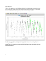
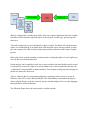
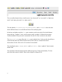

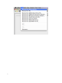
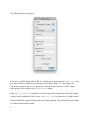

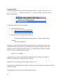
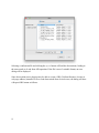
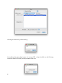
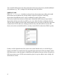
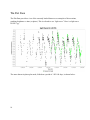

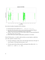
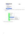
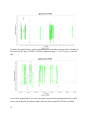
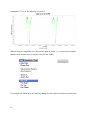
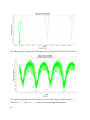
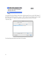
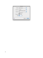
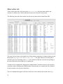
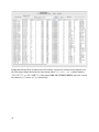

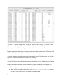
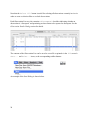
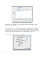

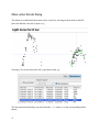
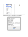
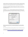
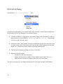
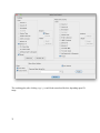
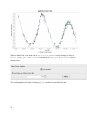
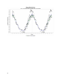

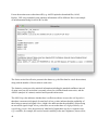

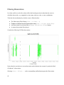

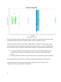
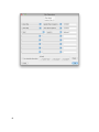
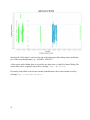
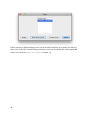
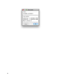
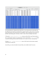
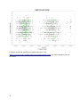
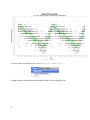
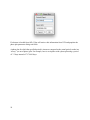


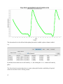
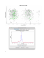
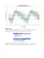
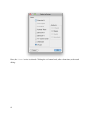
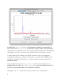
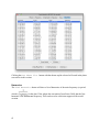
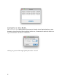
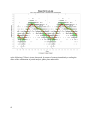
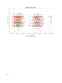
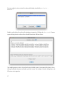
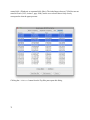
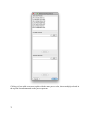
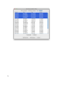
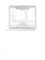
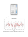
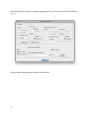
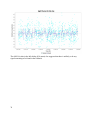
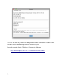
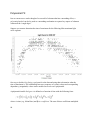
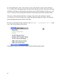
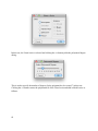
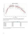
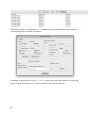
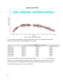
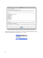
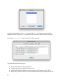

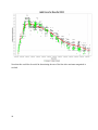
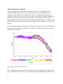
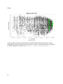
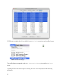

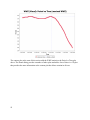
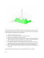
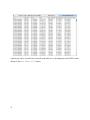
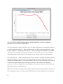

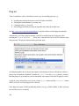
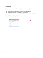
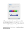
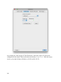
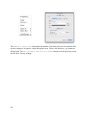
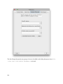

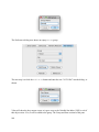
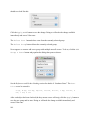
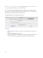
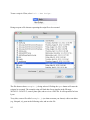
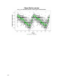


![110_022_CWT_Compact_InstMaint[Icon]](http://vs1.manualzilla.com/store/data/006013284_1-4f7fdcae5c6c12a2f521c9690c1b7c83-150x150.png)