1
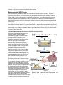
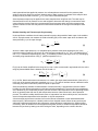
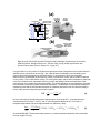
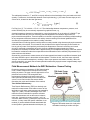
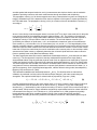
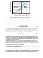
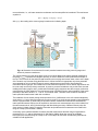
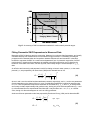
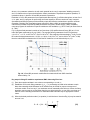
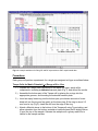
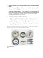
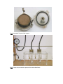
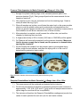
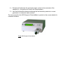
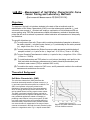
LAB #3 – Measurement of Soil Water Characteristic Curve – Sensor Pairing and Laboratory Methods (Environmental Measurements CE/ENVE 320-04) Objectives The purpose of the lab is to introduce students to the state-of-the-art methods used for determination of Soil Water Characteristic (SWC) curve that relates matric potential (ψm) and volumetric water content (θv). Students will employ a combination of field techniques such as sensor pairing using TDR and tensiometers coupled with laboratory methods to obtained data points that will serve as a basis for parametric model estimation and assessment of data quality and limitations. The specific objectives are: (1) To use pressure flow cells (Tempe cells) containing disturbed soil samples to determine the matric potential – volumetric water content (ψm-θv) relationship for the matric potential (ψm) range of from 0 to -10 m (-1 bar). (2) To use a pressure plate device (Richard’s pressure plate apparatus) and disturbed soil samples to obtain ψm-θv pairs for the ψm range from -10 to -30 m (-3 bar or -0.3 MPa). (3) To use a Dewpoint Potentiameter to obtain ψm-θv pairs for the ψm range from -50 to -150 m (-15 bar or -1.5 MPa). (4) To install tensiometers and TDR probes in a soil column (simulating a soil profile in the field) and obtain simultaneous measurements of matric potential (tensiometers) and volumetric water content (TDR) to establish SWC in-situ). (5) To combine the results, construct a SWC curve, and fit parametric models to the combined measurements and discuss the results. Theoretical Background Soil Water Characteristic (SWC) The soil water characteristic (SWC) describes the functional relationship between soil water content (θm or θv) and matric potential under equilibrium conditions. The SWC is an important soil property related to the distribution of pore space (sizes, interconnectedness), which is strongly affected by texture and structure, as well as related factors including organic matter content. The SWC is a primary hydraulic property required for modeling water flow, for irrigation management, and for many additional applications related to managing or predicting water behavior in the porous system. A SWC is a highly nonlinear function and is relatively difficult to obtain accurately. Because the matric potential extends over several orders of magnitudes for the range of water contents encountered in the field, the matric potential is often plotted on a logarithmic scale. Fig.1-1 depicts several SWC Fig.1-1: Soil water characteristic curves for soils of different texture. curves for soils of different textures demonstrating the reduced porosity (saturated water content) and the relatively large pores for coarse-textured media such as sand. Measurement of SWC Curves Several methods are available to obtain the measurements required for SWC estimation. The basic requirement is for pairs of ψm-θ measurements over the wetness range of interest. Among the primary experimental problems in determining a SWC are: (i) the limited functional range of the tensiometer, which is often used for in-situ measurements; (ii) inaccurate or imprecise θV field measurements (no longer as significant a problem due to availability of TDR); (iii) the difficulty in obtaining undisturbed samples for laboratory determinations; and (iv) a slow rate of equilibrium under low matric potential values associated with dry soils. In-situ (in place) methods are considered the most representative techniques for determining SWC's, particularly when a wide range of ψm-θ values are obtained. An effective method for obtaining simultaneous measurements of ψm and θV utilizes TDR probes installed in the soil at close proximity to transducer tensiometers, and recording the changing values of each attribute through time as the soil wetness varies. Large changes in ψm and θV can be induced under highly evaporative conditions (e.g., a fan), or in the presence of active plant roots. Laboratory Measurements with Pressure Flow Cell and Pressure Plate The pressure plate apparatus consists of a pressure chamber enclosing a watersaturated porous plate, which allows water but prevents air flow through its pores (Fig.1-2). The porous plate is open to atmospheric pressure at the bottom surface, while the top surface is at the applied pressure of the chamber. Sieved soil samples (<2mm) are placed in retaining rubber rings in contact with the porous plate and left to saturate in water. After saturation is attained, the porous plate with the saturated soil samples is placed in the chamber and a known gas (commonly N2 or air) pressure is applied to force water out of the soil and through the plate. Flow continues until equilibrium between the force exerted by the air pressure and the force by which soil water is being held by the soil (ψm) is reached. (a) Pressure/Flow Cell (Tempe Cell) Gas Pressure Soil Sample Porous Plate (b) Pressure Plate Pressure Gauge Atmospheric Pressure Soil water retention in the low suction range Soil Samples of 0 to 10 m (0-1 bar) is strongly influenced on Porous Plate by the soil structure and its natural pore size Soil distribution. Hence, "undisturbed" intact soil Sample samples (cores) are preferred over repacked Pressure samples. The pressure flow cell (also known Porous Pc Chamber (Chamber Plate as Tempe cell) can hold intact soil samples Pressure) encased in metal rings. The operation of the cell follows that of the pressure plate, except Pa (Atmospheric the pressure range for the Tempe cell is Pressure) usually lower, 0 to 10 m (1 bar or 0.1 MPa). Fig.1-2: (a) Pressure and flow cell (Tempe cell); and (b) The porous ceramic plates for both the pressure pressure plate apparatus used to desaturate soil plate and the flow cell must be completely samples to desired matric potential. saturated, a process which may take a few days to achieve. Following equilibrium between soil matric potential and the applied air pressure, the soil samples are removed from the pressure plate, weighed, and oven dried for gravimetric determination of water content. An estimate of the sample's bulk density must be provided to convert θm to θv in the case of disturbed samples. Several pressure steps may be applied to the same samples when using flow cells. The cells may be disconnected from the air pressure source and weighed to determine the change in mass hence water content from the previous step, then reconnected to the air pressure and a new higher pressure step applied. Outflow from the cells may also be monitored and related to the change in the sample's water content. Relative Humidity and Thermocouple Psychrometry Under equilibrium conditions the soil water potential is equal to the potential of water vapor in the ambient soil-air. A psychrometer can measure the relative humidity (RH) of the water vapor which is related to the water potential (ψw) of the vapor through: Mw ψ w e RH = = exp ρ w R T e0 (1) where e is water vapor pressure, eo is saturated vapor pressure at the same temperature, Mw is the molecular weight of water (0.018 kg/mol), R is the ideal gas constant (8.31 J K-1 mol-1 or 0.008314 kPa m3 mol-1 K-1), T is absolute temperature (K), and ρw is the density of water (1000 kg/m3 at 20 oC). Rearranging and taking a log-transformation of Eq.(1) yields an expression for ψw: ψw = R T ρw e ln Mw e0 (2) Eq.(2) can be further simplified for the range of e/eo near 1 often encountered in agricultural soils; the entire range of plant-available water is between e/eo=0.98 and 1.0: ψw = R T ρw Mw e e − 1 ≈ 462 T − 1 e0 e0 (3) for ψw in kPa. Note that because most salts are non volatile, the vapor based measurement of the soil's ψw is the sum of the osmotic and matric potentials (ψw=ψm+ψs). The soil-air interface acts as a diffusion barrier in allowing only water molecules to pass from liquid to vapor state. Several methods are available for determination of relative humidity. A psychrometer infers the relative humidity from the difference between dry bulb and wet bulb temperatures. The dry bulb is the temperature of the ambient air (non-evaporating surface), and the wet bulb is the temperature of an evaporating surface which is generally lower than the dry bulb temperature because of latent heat loss in the evaporation process. The relative humidity determines the rate of evaporation from the wet bulb junction, and thus the extent of temperature depression below ambient or dry bulb temperature. A thermocouple psychrometer consists of a fine wire chromel-constantan or other standard bimetallic thermocouple. A thermocouple is a double junction of two dissimilar metals. When the two junctions are subjected to different temperatures they generate a voltage difference explained as the Seebeck effect. Conversely, when an electrical current is applied through the junctions it creates a temperature difference between the junctions by heating one while cooling the other, depending on the current's direction. (a) Gold Thermister Pins Thermocouple Mounting Plate Processor and Digital Readout SC10X Sample Chamber Thermocouple Soil Sample Sample Cup Sample Lever SC10X Body (b) Copper-Constantan Junction Ceramic Shield Fine-wire or Stainless Thermocouple Steel Screen Junction Fig.1-3: (a) SC10X sample chamber for psychrometric laboratory measurements of soil water potential (Source: Decagon Devices Inc., Pullman, WA); and (b) A field psychrometer with porous ceramic shield (Source: Wescor Inc., Logan, UT) For typical soils use, one junction of the thermocouple psychrometer is suspended in a thin-wall ceramic or stainless screen cup buried in the soil (Fig.1-3b), while the other is embedded in an insulated plug to measure the ambient temperature at the same location. In psychrometric mode, the suspended thermocouple is cooled below the dew point by means of an electrical current until pure water condenses on the junction. This is called Peltier cooling. The cooling then stops, and as water evaporates it draws heat in the form of latent heat of vaporization from the junction, depressing it below the temperature of the surrounding air until it attains a wet bulb temperature. The warmer and dryer the surrounding air, the higher the evaporation rate and the greater the wet bulb depression. The difference in temperatures between the insulated dry bulb and the wet bulb thermocouples is measured and used to infer the relative humidity or relative vapor pressure using the psychrometer equation: RH = s+γ e = 1− ∆T e0 e0 (4) where s is the slope of the saturation water vapor pressure curve (s=deo/dT), γ is the psychrometric constant (about 0.067 kPa K-1 at 20oC), and ∆T is the temperature difference (K). The slope s is temperature-dependent and can be approximated from (Brutsaert, 1982): ( d e 0 373.15 e 0 = 13.3185 − 3.952 t R − 1.9335 t R 2 − 0.5196 t R 3 2 dT T ) (5) where tR=1-373.15/T. The saturated vapor pressure eo is also temperature dependent and is estimated from the integral of Eq.(5): e 0 = 101.325 exp (13.3185 t R −1.9760 t R 2 −0.6445 t R 3 −0.1299 t R 4 ) (6) The relationship between e, T, and RH is uniquely defined, so that knowledge of any two leads to the third quantity. Furthermore, the relationship between e and vapor density (ρv), the mass of water vapor per unit volume of air, is based on the ideal gas law as: ρv = mw e = [g m 3 ] −4 Va 4.62 × 10 T (7) For Eqs.(4) to (7), T is in Kelvin = 273.15 + oC. The relationships between temperature, pressure, and relative humidity may be conveniently expressed in graphical format, e.g. A typical temperature depression measurable by a good psychrometer is on the order of 0.000085 oC per kPa. This means that any errors in measuring wet bulb depression can introduce large errors into psychrometric determinations. Thermal equilibrium is therefore a prerequisite for obtaining reliable readings, as any temperature difference between wet and dry sensors resulting from thermal gradients will be erroneously incorporated into the relative humidity calculation. A second means of inferring relative humidity and thus water potential using thermocouple psychrometers is called the dew point method. This is based on the principle that the wet thermocouple junction would not lose or gain any water if held precisely at the dew point temperature. Electronic monitoring and control circuitry is employed to essentially do just this, through a feedback system whereby the junction temperature is constantly measured and the applied cooling current adjusted accordingly. Note that ambient heat transfer mechanisms other than evaporation and condensation must be nullified (compensated for) in order to achieve this balance. Summarizing, psychrometric measurements of soil water potential are based on equilibrium between liquid soil water and water vapor in the ambient soil atmosphere. The drier the soil, the fewer water molecules "escape" into the ambient atmosphere, resulting in lower vapor pressure and relative humidity. When the osmotic potential is very small, the soil water potential measured by a psychrometer is approximately equal to the soil matric potential. Field Measurement Methods for SWC Estimation - Sensor Pairing Despite the paramount importance of SWC determination in situ, suitable measurement techniques are severely TDR Cable Tester lacking at present. The most common approach is to use (Tektronix 1502B) paired sensors such as TDR waveguides and tensiometers to determine soil water content and Waveform matric potential simultaneously and in the same soil volume. Let us first introduce the sensors before discussing the merits and limitations of the method, BNC Connector Time Domain Reflectometry Time Domain Reflectometry (TDR) is a relatively new method for measurement of soil water content. Its first application to soil water measurements was reported by Topp et al. (1980). The main advantages of the TDR method over other methods for repetitive soil water content measurement such as the neutron moisture meter are: (i) superior accuracy to within 1 or 2% of volumetric water content; (ii) calibration requirements are minimal - in many cases soil-specific calibration is not needed; (iii) averts radiation hazards associated with neutron probe or gamma-attenuation techniques; (iv) 3-Rod Probe Fig.1-4: TDR cable tester with 3-rod probe embedded vertically in surface soil layer. excellent spatial and temporal resolution; and (v) measurements are simple to obtain, and the method is capable of providing continuous soil water measurements through automation and multiplexing. The propagation velocity (v) of an electromagnetic wave along a transmission line (probe or waveguide) of length L embedded in the soil is determined from the time response of the system to a pulse generated by the TDR cable tester. The propagation velocity (v=2L/t) is a function of the soil bulk dielectric constant (εb) according to 2 ct c ε b = = v 2 L 2 (8) where c is the velocity of electromagnetic waves in vacuum (3x10⁸ m/s), and t is the travel time for the pulse to traverse the length of the embedded waveguide (down and back = 2L). The definition of the dielectric constant is given in Eq.(8); it simply states that the dielectric constant of a medium is the ratio squared of propagation velocity in vacuum relative to that in the medium. The soil bulk dielectric constant (εb) is governed by the dielectric of liquid water εw ≅ 81, as the dielectric constants of other soil constituents are much smaller, e.g., soil minerals εs=3 to 5, frozen water (ice) εi=4, and air εa=1. This large disparity of the dielectric constants makes the method relatively insensitive to soil composition and texture and thus a good method for liquid soil water measurement. Note that because the dielectric constant of frozen water is much lower than for liquid, the method may be used in combination with a neutron probe or other technique which senses total soil water content, to separately determine the volumetric liquid and frozen water contents in frozen or partially-frozen soils (Baker and Allmaras, 1990). Two basic approaches have been used to establish the relationships between εb and volumetric soil water content (θv). The first approach is empirical, whereby mathematical expressions are simply fitted to observed data without using any particular physical model. Such an approach was employed by Topp et al. (1980) who fitted a third-order polynomial to the observed relationships between εb and θv for multiple soils. The second approach uses a model of the dielectric constants and the volume fractions of each of the soil components to derive a relationship between the composite (bulk) dielectric constant and soil water (i.e., a specific component). Such a physically-based approach, called a dielectric mixing model, was adopted by Birchak (1974) and Roth et al. (1990). TDR calibration establishes the relationship between εb and θv. For this discussion we assume that calibration is conducted in a fairly uniform soil without abrupt changes in soil water content along the waveguide. The empirical relationship for mineral soils as proposed by Topp et al. (1980): θ v = −5.3 × 10 −2 + 2.92 × 10 −2 ε b − 5.5 × 10 −4 ε b + 4.3 × 10 −6 ε b 2 3 (9) provides adequate description for the water content range <0.5, which covers the entire range of interest in most mineral soils, with an estimation error of about 0.013 for θv. However, Eq.(9) fails to adequately describe the εb-θv relationship for water contents exceeding 0.5, and for organic soils or mineral soils high in organic matter, mainly because Topp's calibration was based on experimental results for mineral soils and concentrated in the range of θv<0.5. Birchak et al., (1974) and Roth et al. (1990) proposed a physicallybased calibration model which considers dielectric mixing of the constituents and their geometric arrangement. According to this mixing model the bulk dielectric constant of a three-phase system may be expressed as: [ β β ε b = θ v ε w + (1 − n )ε s + (n − θ v )ε a ] 1 β β (10) Bulk Dielectric Constant 80 Topp 60 Practical Range of Water Content Measurement 40 Mixing Model 20 0 0 0.2 0.4 0.6 0.8 1 Volumetric Water Content (m^3/m^3) Fig.1-5: Relationships between bulk soil dielectric constant and θv expressed by two commonly used TDR calibration approaches where n is the soil's porosity, -1<β<1 summarizes the geometry of the medium in relation to the axial direction of the wave guide (β=1 for an electric field parallel to soil layering, β=-1 for a perpendicular electrical field, and β=0.5 for an isotropic two-phase mixed medium), 1-n, θv and n-θv are the volume fractions and εs, εw and εa are the dielectric constants of the solid, aqueous and gaseous phases, respectively. Note that θv = Vw /VT, (1-n) = Vs/VT, and (n-θ) = Vair/VT, so these components sum to unity. Rearranging Eq.(10) and solving for θv yields θv = ε b β − (1 − n )ε s β − n ε a β β εw − εa β (11) which determines the relationship between εb measured by TDR and θv. Many have used β=0.5 which is shown by Roth et al. (1990) to produce a calibration curve very similar to the third-order polynomial proposed by Topp for the water content range of 0<θv<0.5. If we introduce into (11) common values for the various constituents such as β=0.5, εw=81, εs=4, and εa=1 we obtain the simplified form θv = ε b − (2 − n ) 8 (12) Note that the soil's porosity must be known or estimated when using the mixing model approach. A comparison between Topp's expression (Eq.(9)) and a calibration curve based on Eq.(10) with n=0.5 is depicted in Fig.1-5. Summarizing, Eq.(9) establishes an empirical relationship between bulk soil dielectric and volume water content, while Eqs.(8) and (10) are based on physical and geometrical considerations. Eq.(12) provides a simplified version of (10). Limitations or disadvantages of the TDR method include relatively high equipment expense, potential limited applicability under highly saline conditions due to signal attenuation, and the fact that soil-specific calibration may be required for soils having large amounts of bound water or high organic matter contents. Tensiometer for Soil Matric Potential (ψm) Measurement A tensiometer consists of a porous cup, usually made of ceramic and having very fine pores, connected to a vacuum gauge through a water-filled tube (Fig.1-6). The porous cup is placed in intimate contact with the bulk soil at the depth of measurement. When the matric potential of the soil is lower (more negative) than inside the tensiometer, water moves from the tensiometer along a potential energy gradient to the soil through the saturated porous cup, thereby creating suction sensed by the gauge. Water flow into the soil continues until equilibrium is reached and the suction inside the tensiometer equals the soil matric potential. When the soil is wetted, flow may occur in the reverse direction, i.e., soil water enters the tensiometer until a new equilibrium is attained. The tensiometer equation is: ψ m = ψ gauge + (z gauge − z cup ) (13) with ψgauge the reading at the vacuum gauge location and z indicating depth. Fig.1-6: Illustration of tensiometers for matric potential measurement using vacuum gauges and electronic pressure transducers. The vertical distance from the gauge plane to the cup must be added to the matric potential measured by the gauge, ψgauge, expressed as a negative quantity, in order to obtain the matric potential at the depth of the cup. This accounts for the positive head exerted by the overlying tensiometer water column at the depth of the ceramic cup. Note that using the difference in vertical elevation is appropriate only when potentials are expressed per unit of weight. Electronic sensors called pressure transducers often replace the mechanical vacuum gauges. The transducers convert mechanical pressure into an electric signal which can be more easily and more precisely measured. In practice, pressure transducers can provide more accurate readings than other gauges, and in combination with data logging equipment are able to supply continuous measurements of matric potential. The tensiometer range is limited to suction values (negative of the matric potential) of less than 100 kPa, i.e., 1 bar or 10 m head of water. Therefore other means are needed for matric potential measurement under drier conditions. The limitations of most sensor pairing techniques stem from: (i) differences in the soil volumes sampled by each sensor, e.g. large volume averaging by a neutron probe vs. a small volume sensed by heat dissipation sensor or psychrometer; (ii) while many in-situ water content measurement methods are instantaneous, matric potential sensors require time for equilibrium; hence the two measurements may not be indicative of the same wetness level; and (iii) limited ranges and deteriorating accuracy of different sensor pairs; this often results in limited overlap in retention information and problems with measurement errors within the range of overlap (Or and Wraith, 1999a,b). A summary of the methods available for matric potential measurement and their range of application is presented in Fig.1-7, and are discussed in Or and Wraith (1999a). Note that most of the available techniques have a limited range of overlap or do not overlap at all, and most are laboratory methods not suitable for field applications. 1000 Matric Potential (-m) Psychrometer 100 Pressure Plate 10 Tempe Cell Tensiometer 1 Hanging Water Column 0 r s Soil Water Content Fig.1-7: A summary of SWC measurement methods for various matric potential ranges. Fitting Parametric SWC Expressions to Measured Data Measuring a SWC is laborious and time consuming. Measured θ-ψ pairs are often fragmentary, and usually constitute relatively few measurements over the wetness range of interest. For modelling and analysis purposes and for characterization and comparison between different soils and scenarios it is therefore beneficial to represent the SWC in a continuous and parametric form. A parametric expression of a SWC model should: (i) contain as few parameters as possible to simplify its estimation; and (ii) describe the behaviour of the SWC at the limits, wet and dry ends, while closely fitting the nonlinear shape of ψm- θV data. An effective and commonly used parametric model for relating volumetric water content, θv, to the matric potential, ψm, was proposed by van Genuchten (1980) and is denoted here as VG: θ − θr 1 = Θ= θ s − θ r 1 + (α ψ m ) n m (14) where θr and θs are the residual and saturated water contents, respectively, and α, n, and m are parameters directly dependent on the shape of the θ(ψ) curve. Considerable simplification is gained by assuming that m=1-1/n. Thus the parameters required for estimation of the model are θr, θs, α, and n. θs is usually known and is easy to obtain experimentally with good accuracy, leaving only three unknown parameters (θr, α and n) to be estimated from the experimental data. Note that θr may be taken as θ-1.5 MPa, θair dry, or a similar value, though it is often advantageous to use it as a fitting parameter. Another well known parametric model was proposed by Brooks and Corey (1964) and is denoted as BC: θ − θ r ψ b Θ= = θ s − θ r ψ m λ ψ m >ψ b (15) Θ =1 ψ m ≤ψ b where ψb is a parameter related to the soil matric potential at air entry (b represents "bubbling pressure"), and λ is related to the soil pore size distribution. Matric potentials are expressed as positive quantities, i.e. in absolute values, in both the VG and BC parametric expressions. Estimation of VG or BC parameters from experimental data requires: (i) sufficient data points, at least 5 to 8 ψm-θV pairs; and (ii) a program for performing non-linear regression. Recent versions of many computer spreadsheet software programs provide relatively simple and effective mechanisms to perform nonlinear regression. Details of the computational steps required for fitting a SWC to experimental data using commercially-available computer spreadsheet software are given in Wraith and Or (1998). In addition, computer programs for estimation of specific models are also available, e.g., RETC code (van Genuchten et al., 1991). Fig.1-8 depicts fitted parametric models of van Genuchten (VG) and Brooks and Corey (BC) to LCV silt loam SWC data measured by Or et al. (1991). The resulting best-fit parameters for the VG model are: α=0.417 m-1; n=1.75; θs=0.513 m3/m3; and θr=0.05 m3/m3, with coefficient of determination r2=0.99. For the BC model the best parameters are: λ=0.54; ψb=1.48 m; θs=0.513 m3/m3; and θr=0.03 m3/m3 (with r2=0.98). Note the main difference between the VG and the BC model fits is in the discontinuity at ψ=ψb. Fig.1-8: VG and BC parametric models fitted to measured silt loam SWC data from Owens Valley, CA. Key steps in fitting VG model to experimental SWC data using Excel are: (1) Enter the experimental data in two columns corresponding to θv and ψm. (2) Establish a cell for each fitting parameter (θr, θs, α, n), and assign an initial value estimate to each. Note that reasonable initial estimates for all variables may be critical for proper convergence of nonlinear models. That is to say, if your estimates are not reasonably near their true values, the fitting algorithm may converge on a local rather than the true global minimum, or even fail to converge on a solution at all. Consulting the literature for reasonable initial estimates may be appropriate in some cases. (3) Write the desired prediction model (i.e. equation) in a third column. Note that Eq.(14) may be stated in terms of θ as: 1 θ = θ r + (θ s − θ r ) 1 + (α h ) n m (16) and in terms of h as: θ − θ r θ − θ r s 1 − m h= α 1 n − 1 (17) Refer to the pre-assigned cells containing your initial guesses for the fitting parameters where appropriate in the equation. This column will thus contain predicted θv values (θv model) for each measured value of ψm. (4) Form in a fourth column a deviate (or error) squared between θv and θv model, i.e. (θv-θv model)2. (5) Establish a cell containing the sum of squared deviations (errors) between measured and predicted values. (6) Apply the nonlinear solver (Solver in the Tools menu for Excel; Optimizer under the Tools menu for Quattro Pro) to the problem by minimizing the sum of squared errors (SSE) cell using variable cells as defined in Step 2. You should include the following constraints: 0 ≤ m ≤ 1, and θr ≥ 0. (7) Compute the variance of measured θv (a built-in spreadsheet function). The coefficient of determination (r2) for the curve fit may then be calculated using: r2 = 1 - (sum of squared errors) / (# of data points x variance of measured θv). (8) Record the resulting "best fit" values of the variable cells for subsequent use. Fig.1-9: A sample worksheet for fitting VG and BC expressions to SWC experimental data. Procedures Each group will perform experiments for a single pre-assigned soil type as outlined below. Tempe Cells for Matric Potential (ψm) Range of 0 to -10m 1.) Prepare two Tempe cells (duplicates of the same soil type); weigh all its components, including a saturated ceramic plate (Fig.1), and record the results. 2.) Assemble the bottom part of the Tempe cell by placing the o-rings into the appropriate grooves, and inserting the saturated ceramic plate. 3.) Insert an empty brass-ring into the bottom part; pour known amounts of ovendried soil into the ring and tap gently on the brass ring; fill the ring to about 2-3 mm from its top (Fig.2); clean the soil from the edge of the ring. 4.) Attach a Mariotte tower to the bottom of the Tempe cell using Tygon tubing, and allow saturation from the bottom; maintain a hydraulic head that is slightly below (2 mm) the top of the sample. Saturate the sample until a glossy water film is visible on the sample surface. 5.) Attach the top portion of the Tempe cell and weigh the cell including the saturated sample. 6.) Connect the saturated Tempe cell to the pressure manifold and attach an outflow collector to the bottom (Fig.3) (we will try to keep track of the outflow to doublecheck changes in water content). 7.) We will apply 3 pressure steps of 1, 4, and 8 meters of H2O. After each pressure step we will disconnect the Tempe cell from the pressure manifold and determine the weight. To double check we will also determine the weight of the outflow collected (please keep track of the amounts!). 8.) The schedule for pressure changes is as follows: We will start applying a pressure of 1m during the laboratory on Tuesday On Wednesday between 2 and 3 pm we will increase the pressure to 4 m On Thursday between 2 and 3 pm (during lab session) we will increase the pressure to 8 m On Friday at 2 PM (one hour before the ENVE 400 seminar) pressure will be disconnected, weigh and disassemble the cells; brass rings containing the soil should be placed in a drying oven to determine the water content and the bulk density of the soil. At least one member of each group should be present on, Wednesday and Friday to weigh the Tempe cells (and for other data collection duties). Fig.1: Tempe cell parts Fig.2: Assembled Tempe cell with sample Fig.3: Tempe cells connected to pressure lines and outflow flasks. Pressure Plate Apparatus for Matric Potential (ψm) Range of -10 to -50m 1.) Arrange four plastic retaining rings on the saturated pressure plate in the pressure chamber (Fig.4). Each group will perform the measurements for two samples of each soil. 2.) Use a spoon to pour oven dry and sieved soil into the retaining rings. Create a small pile within the ring (Fig.4) 3.) When all samples are in place, we will raise the water level on the pressure plate slowly to cover the plate's surface and to saturate the soil samples from the bottom (in general samples should be left overnight for saturation, however due to time limitations we will allow a saturation time of a few minutes). 4.) After saturation is complete, we will connect the outflow tube, and seal the chamber by fastening the cover bolts. 5.) A single pressure step of 25 m of water (2.45 bars or 0.245 MPa) will be applied. 6.) On Friday we will remove the samples from the pressure chambers. Make sure that the pressure supply line is closed, and the pressure is released before opening the chambers! 7.) We will transfer the samples from the pressure plate to pre-weighed drying dishes, weigh the wet samples, and place the drying dish in to the oven to determine the gravimetric water content. Fig.4: Pressure chamber with saturated ceramic plate and retaining rings. Dewpoint PotentiaMeter for Matric Potential (ψm) Range from -50 to -150m 1.) This measurement will be explained and assisted by the instructor. 2.) We will use pre-wetted soil samples to prescribed gravimetric water contents of approximately: 0.02, 0.04, 0.08, and 0.1, [g/g] (moist soil samples were stored in ziplock bags for more than 48 hrs to equilibrate). 3.) The instructor will perform the Dewpoint PotentiaMeter readings and provide four values of matric potential for each soil (one for each water content) 4.) Students will determine the gravimetric water content in the remainder of the samples (i.e., the portion not used in the Potentiameter). 5.) Use the bulk densities determined during the first laboratory session to convert gravimetric to volumetric water contents. The user manual for the WP4 Dewpoint PotentiaMeter is posted on the course website for interested students. Fig.6: WP4 Dewpoint PotentiaMeter. In-Situ SWC Determination from Tensiometeric and TDR Measurements 1.) Identify the column, soil type (similar to previous section), TDR probes, Tensiometers, etc.; pack the column while keeping track of the weights to estimate bulk density. 2.) Based on an estimate of θs for your soil type, and assuming that θr=0.02, determine the amount of water needed to fill 1/3 of the free pores in the soil contained in the column (to avoid excessive drainage and allow for redistribution). 3.) Install two three-rod TDR probes horizontally through pre-drilled holes in the column (each probe is 0.1 m long) – the vertical distance between the probes is 120 mm. 4.) Install two vertical tensiometers through the top surface and ensure that center of the ceramic cups are aligned with the two TDR probes (measure the distance from the soil surface and from the gauge to the cup). 5.) The tensiometers will be equipped with pressure transducers connected to a datalogger to provide an accurate and continuous measurement (in case of complications, we will use a either a Tensimeter or a mechanical gauge). 6.) Record the tensiometers response during the first 10 min. 7.) Apply the water carefully (avoid disturbance of soil surface) and continue recording the tensiometers response vs. time since water application. 8.) Direct an air fan toward the soil surface to enhance evaporation. 9.) Hook the TDR probes to an SDM-50 multiplexer controlled by WinTDR program through a laptop (instructor will assist with TDR system initial setup). Be prepared to take manual measurements in case of complications. Record measurements at 15 min intervals. If manual measurements were made, record the positions of the reflection points vs. time; convert to volumetric water contents. 10.) Continue sampling at least once a day for 3-4 days (following sampling schedule of other elements above). Lab Report (Due Tue 03/09/04) 1.) Follow the guidelines in the syllabus 2.) Write a short introduction and a briefly discuss SWC curves and field and laboratory methods for their measurement. 3.) Report on a worksheet all measurements of soil water content, bulk density and matric potential (show raw data and final results). 4.) Combine and plot your ψm-θv data obtained by the four methods. Use the format of θv on the x-axis in units of (m3/m3) and ψm in units of m of water (use log scale for ψm). Convert gravimetric water contents to volumetric water contents using the bulk densities obtained in the first laboratory. 5.) Fit the van Genuchten parametric SWC model to the data using the procedure outlined in the handout. Include the fitted curve on the plot and report the parameters. 6.) Discuss (briefly) advantages, disadvantages, and possible errors associated with each method. Discuss why is it possible to use disturbed soil samples to determine the ψm-θv relationships at relatively high values of suction (or low matric potential range).