Download Field Estimation of Soil Water Content

Field Estimation of Soil
Water Content
A Practical Guide to Methods,
Instrumentation and Sensor Technology
VIENNA, 2008
T R A I N I N G
C O U R S E
S E R I E S
30
TRAINING COURSE SERIES No. 30
Field Estimation of Soil
Water Content
A Practical Guide to Methods,
Instrumentation and Sensor Technology
INTERNATIONAL ATOMIC ENERGY AGENCY, VIENNA, 2008
The originating Section of this publication in the IAEA was:
Soil and Water Management & Crop Nutrition Section
International Atomic Energy Agency
Wagramer Strasse 5
P.O. Box 100
A-1400 Vienna, Austria
FIELD ESTIMATION OF SOIL WATER CONTENT: A PRACTICAL GUIDE TO METHODS,
INSTRUMENTATION AND SENSOR TECHNOLOGY
IAEA, VIENNA, 2005
IAEA-TCS-30
ISSN 1018–5518
© IAEA, 2008
Printed by the IAEA in Austria
February 2008
FOREWORD
During a period of five years, an international group of soil water instrumentation experts
were contracted by the International Atomic Energy Agency to carry out a range of
comparative assessments of soil water sensing methods under laboratory and field conditions.
The detailed results of those studies are published elsewhere. Most of the devices examined
worked well some of the time, but most also performed poorly in some circumstances. The
group was also aware that the choice of a water measurement technology is often made for
economic, convenience and other reasons, and that there was a need to be able to obtain the
best results from any device used. The choice of a technology is sometimes not made by the
ultimate user, or even if it is, the main constraint may be financial rather than technical. Thus,
this guide is presented in a way that allows the user to obtain the best performance from any
instrument, while also providing guidance as to which instruments perform best under given
circumstances.
That said, this expert group of the IAEA reached several important conclusions: (1) the field
calibrated neutron moisture meter (NMM) remains the most accurate and precise method for
soil profile water content determination in the field, and is the only indirect method capable of
providing accurate soil water balance data for studies of crop water use, water use efficiency,
irrigation efficiency and irrigation water use efficiency, with a minimum number of access
tubes; (2) those electromagnetic sensors known as capacitance sensors exhibit much more
variability in the field than either the NMM or direct soil water measurements, and they are
not recommended for soil water balance studies for this reason (impractically large numbers
of access tubes and sensors are required) and because they are rendered inaccurate by changes
in soil bulk electrical conductivity (including temperature effects) that often occur in irrigated
soils, particularly those containing appreciable amounts of clays with high ion exchange
capacities, even when using soil specific calibrations; (3) all sensors must be field calibrated
(factory calibrations were inaccurate in most soils studied) in order to obtain reasonable
accuracy; (4) the one exception to conclusion (3) is conventional time domain reflectometry
(TDR, with waveform capture and graphical analysis), which is accurate to ±0.02 m3 m–3 in
most soils when using a calibration in travel time, effective frequency and bulk electrical
conductivity (see Chapter 4); (5) with the possible exception of tensiometers and the granular
matrix resistance sensors, none of the sensors studied is practical for on-farm irrigation
scheduling; they are either too inaccurate (capacitance sensors) or too costly and difficult to
use (TDR and NMM); (6) for research studies, only the NMM, conventional TDR and direct
measurements have acceptable accuracy.
In light of the intense commercial introduction of electromagnetic (EM) soil water sensors in
the 1990s and to date, these conclusions are somewhat disappointing. However, the joint work
of the expert group has resulted in numerous scientific publications detailing the problems
with EM sensors, including the theoretical underpinnings of these problems, and sparked a
special issue of the Vadose Zone Journal (Evett and Parkin, 2005) summarizing much of the
fundamental work to date. Now that the problems are well understood, research and
development of new sensor systems to overcome these problems can, and will, proceed to a
satisfactory conclusion for both scientific studies and on-farm irrigation management.
The IAEA officer responsible for this publication is Lee Kheng Heng of the Joint FAO/IAEA
Division of Nuclear Techniques in Food and Agriculture.
EDITORIAL NOTE
The use of particular designations of countries or territories does not imply any judgement by the
publisher, the IAEA, as to the legal status of such countries or territories, of their authorities and
institutions or of the delimitation of their boundaries.
The mention of names of specific companies or products (whether or not indicated as registered) does
not imply any intention to infringe proprietary rights, nor should it be construed as an endorsement
or recommendation on the part of the IAEA.
CONTENTS
CHAPTER 1. DIRECT AND SURROGATE MEASURES OF
SOIL WATER CONTENT ................................................................................ 1
1.1. Purpose of this manual.................................................................................................... 1
1.2. Soil water measurement — Background ........................................................................ 1
1.3. The basics: How is soil water content described? .......................................................... 2
1.3.1. Calculation of water content of a volume of soil (e.g. the root zone) .................. 3
1.3.2. How much water can a soil hold?......................................................................... 3
1.4. Factors affecting direct measurement accuracy, precision and variability ..................... 5
1.5. Surrogate measures of soil water content ....................................................................... 7
1.6. Factors affecting accuracy and variability of water contents derived from
surrogate measures ....................................................................................................... 10
1.7. Accuracy, precision and the calibration process........................................................... 14
1.7.1. The manufacturer’s calibration........................................................................... 14
1.7.2. The calibration process....................................................................................... 15
1.7.3. Checking a calibration........................................................................................ 18
1.8. Summary ....................................................................................................................... 20
References to Chapter 1........................................................................................................ 21
CHAPTER 2. GRAVIMETRIC AND VOLUMETRIC DIRECT MEASUREMENTS OF
SOIL WATER CONTENT .............................................................................. 23
2.1. Equipment description .................................................................................................. 23
2.1.1. Manufacturers, instruments and parts references ............................................... 23
2.1.2. Measurement general principle .......................................................................... 24
2.1.3. Accessories and documents provided by the manufacturer ............................... 27
2.1.4. Software.............................................................................................................. 27
2.2. Taking measurements ................................................................................................... 27
2.2.1. Required equipment and procedures .................................................................. 27
2.2.2. Handling of data ................................................................................................. 34
2.2.3. “Hints and tricks” ............................................................................................... 35
References to Chapter 2........................................................................................................ 37
CHAPTER 3. NEUTRON MOISTURE METERS ................................................................. 39
3.1. Equipment description .................................................................................................. 39
3.1.1. Manufacturers, instruments and parts references ............................................... 40
3.1.2. Measurement general principle .......................................................................... 40
3.1.3. Safety.................................................................................................................. 43
3.1.4. Accessories and documents provided by the manufacturer ............................... 43
3.1.5. Software.............................................................................................................. 43
3.2. Field installation............................................................................................................ 44
3.2.1. Required equipment............................................................................................ 44
3.2.2. General procedure .............................................................................................. 45
3.2.3. “Hints and tricks” ............................................................................................... 46
3.3. Taking measurements ................................................................................................... 50
3.3.1. General procedure .............................................................................................. 50
3.3.2. Handling of data ................................................................................................. 51
3.4. Calibration..................................................................................................................... 52
References to Chapter 3........................................................................................................ 54
CHAPTER 4. CONVENTIONAL TIME DOMAIN REFLECTOMETRY SYSTEMS......... 55
4.1. Equipment description .................................................................................................. 55
4.1.1. Manufacturers, instruments and parts references ............................................... 56
4.1.2. Measurement general principle .......................................................................... 57
4.1.3. Accessories and documents provided by the manufacturer ............................... 60
4.1.4. Software.............................................................................................................. 60
4.2. Field installation............................................................................................................ 61
4.2.1. Required equipment............................................................................................ 61
4.2.2. General procedure .............................................................................................. 61
4.2.3. “Hints and tricks” ............................................................................................... 65
4.3. Taking measurements.................................................................................................... 67
4.3.1. General procedure .............................................................................................. 67
4.3.2. Handling of data ................................................................................................. 67
4.4. Calibration..................................................................................................................... 68
References to Chapter 4........................................................................................................ 71
CHAPTER 5. CAPACITANCE SENSORS FOR USE IN ACCESS TUBES........................ 73
5.1. Equipment description .................................................................................................. 73
5.1.1. Manufacturer, instrument and parts references .................................................. 75
5.1.2. Measurement principle ....................................................................................... 75
5.2. Field installation............................................................................................................ 78
5.2.1. Access tube installation ...................................................................................... 78
5.2.2. EnviroSCAN sensor string installation .............................................................. 81
5.3. Hints and tips ................................................................................................................ 81
5.3.1. Access tubing...................................................................................................... 81
5.3.2. Number of access tubes needed for a given precision........................................ 81
5.3.3. Tube installation in problem soils ...................................................................... 82
5.3.4. Customizing reading depths ............................................................................... 82
5.3.5. Moisture in access tubes..................................................................................... 83
5.3.6. Salinity (bulk electrical conductivity) effects..................................................... 83
5.4. Taking readings............................................................................................................. 83
5.4.1. Diviner 2000....................................................................................................... 83
5.4.2. EnviroSCAN....................................................................................................... 84
5.4.3. Delta-T PR1/6..................................................................................................... 85
5.5. Handling data ................................................................................................................ 86
5.6. Calibration..................................................................................................................... 86
References to Chapter 5........................................................................................................ 89
CHAPTER 6. TRIME® FM3 MOISTURE METER AND T3 ACCESS TUBE PROBE...... 91
6.1. Equipment description .................................................................................................. 91
6.1.1. Manufacturer ...................................................................................................... 91
6.1.2. Measurement general principle .......................................................................... 91
6.1.3. Instrument and parts references.......................................................................... 91
6.1.4. Accessories and documents provided by the manufacturer ............................... 92
6.1.5. Software.............................................................................................................. 92
6.2. Field installation............................................................................................................ 93
6.2.1. Required equipment............................................................................................ 93
6.2.2. General installation procedure............................................................................ 94
6.2.3. “Hints and tricks” ............................................................................................... 94
6.3. Taking readings............................................................................................................. 96
6.3.1. General procedure .............................................................................................. 96
6.3.2. Signal processing................................................................................................ 96
6.3.3. Handling of readings .......................................................................................... 98
6.4. Calibration..................................................................................................................... 98
References to Chapter 6...................................................................................................... 100
CHAPTER 7. CS616 (CS615) WATER CONTENT REFLECTOMETER.......................... 101
7.1. Equipment description ................................................................................................ 101
7.1.1. Manufacturer .................................................................................................... 101
7.1.2. Measurement principle ..................................................................................... 101
7.1.3. Instruments and parts references ...................................................................... 102
7.2. General methodology.................................................................................................. 103
7.2.1. Installation kit needed and tools description .................................................... 104
7.2.2. “Hints and tricks” ............................................................................................. 104
7.3. Taking readings........................................................................................................... 105
7.3.1. General procedure ............................................................................................ 105
7.3.2. Handling of data ............................................................................................... 106
7.4. Calibration................................................................................................................... 107
7.4.1. Recommended procedure ................................................................................. 107
7.4.2. Calculating water content and other values of interest..................................... 110
References to Chapter 7...................................................................................................... 110
CHAPTER 8. TENSIOMETERS........................................................................................... 113
8.1. Equipment description ................................................................................................ 113
8.1.1. Manufacturers and parts references.................................................................. 114
8.1.2. Measurement general principle ........................................................................ 115
8.1.3. Accessories, documents and software .............................................................. 116
8.1.4. Installation of tensiometer ................................................................................ 117
8.1.5. “Hints and tricks” ............................................................................................. 118
8.1.6. When to take readings and irrigate................................................................... 119
8.1.7. Interpretation of tensiometer readings.............................................................. 119
8.1.8. Maintenance ..................................................................................................... 119
8.1.9. Advantages of tensiometers.............................................................................. 120
8.1.10. Disadvantages of tensiometers ....................................................................... 120
References to Chapter 8...................................................................................................... 120
CHAPTER 9. ELECTRICAL RESISTANCE SENSORS FOR
SOIL WATER TENSION ESTIMATES ....................................................... 123
9.1. Equipment description ................................................................................................ 123
9.1.1. Manufacturers................................................................................................... 123
9.1.2. Measurement principle ..................................................................................... 124
9.1.3. Accessories, documents and software provided by the manufacturer.............. 126
9.2. Field installation and use ............................................................................................ 126
9.2.1. Required equipment.......................................................................................... 126
9.2.2. Some tips for installation.................................................................................. 127
9.2.3. Reading the sensors .......................................................................................... 128
9.2.4. Advantages and disadvantages ......................................................................... 128
9.3. Calibration................................................................................................................... 129
References to Chapter 9...................................................................................................... 129
CONTRIBUTORS TO DRAFTING AND REVIEW ........................................................... 131
CHAPTER 1
DIRECT AND SURROGATE MEASURES OF SOIL WATER CONTENT
C. HIGNETT and S. EVETT
1.1. PURPOSE OF THIS MANUAL
The purpose of this manual is to provide guidance for field scientists who are not
instrumentation experts but who wish to determine soil water content as part of their work.
This publication is targeted to help those setting up soil water monitoring projects in the
developing countries where expertise in many technologies is not readily available. However,
it also has value to anyone planning a project involving the determination of field soil water
content. Most importantly, it will also give some guidance as to what corroborative
measurements are needed to check the performance of water sensing technology being used.
A substantial suite of soil water sensors and technologies are available today. Some are well
understood as to their technical capability and are both mechanically and electronically
reliable. However, some technologies that claim to measure soil water content are quite
unsuited to some applications and produce results that have little, if any, relation to soil water
content in the field.
This manual sets out a decision making process and critical factors for matching various water
measurement technologies to project objectives. The first factor is the accuracy required by
the user. The second is the degree of water content variability across the field to be measured.
The third is the presence of interferences to the measurement process. And the fourth consists
of the capabilities of the available devices in light of the spatial variability of water content
and the interferences that are present. A successful outcome can only be obtained if all four
factors are considered.
Because this manual is intended to be a practical guide, it cannot be a simple one. Only
reliable measurements are practically useful. The techniques involved in obtaining reliable
values of soil water content are not simple, nor are the potential problems, pitfalls, and sensor
interferences that can prevent good values from being obtained. The manual is divided into
chapters that treat classes of measurement systems, or individual sensors/methods if they do
not belong to one of the major classes, which include neutron moisture meters, capacitance
sensors that work from within a plastic access tube, time domain reflectometry systems that
employ waveform capture and analysis, tensiometers, and direct sampling methods.
Obviously, not all sensor systems could be included in the studies that led up to this manual.
Much of the work supported by the IAEA involves determination of the soil water balance to
determine crop water use and water use efficiency. Thus, many of the systems studied were
those that work in access tubes so that measures could be made to well below the crop root
zone. However, a few other widely used systems employing probes that are inserted into the
soil were also studied.
1.2. SOIL WATER MEASUREMENT — BACKGROUND
Since farming began, farmers have measured soil water by its effect on plants; if the plant was
wilting, water was needed. Irrigation, if any, was not uniform. There was little control of
water applied, and thus little point in getting an accurate measurement of soil water. As
irrigation based farming developed, water management became important, engendering the
need to measure soil water content and the water use of plants.
The first proposal to use fast neutron thermalization as a means of sensing soil water was
1
made prior to 1950. The neutron moisture meter (NMM) developed from that proposal was
used throughout the world, but its dominance in the 1970s and 1980s is now being challenged
by ever cheaper and more convenient electronic sensors and logging systems. The use of
radiation based methods, no matter how safe and effective, is being discouraged in many
countries.
Since the late 1970s, a wide range of competing technologies has each been hailed as ‘the
answer’ for sensing soil water. Most have been found deficient in some way. The aim of this
manual is to provide information whereby a relatively unskilled user of soil water
measurement technology can best match the design aims of the project, the properties of the
soil on which the project is to occur, and the capabilities of available technologies. Several
references give more detail on soil water estimation technologies (Dane and Topp, 2002;
Evett, 2001; Evett, 2003a, b; Evett, 2007).
1.3. THE BASICS: HOW IS SOIL WATER CONTENT DESCRIBED?
The standard method of soil water content measurement involves taking a physical sample of
the soil, weighing it before any water is lost, and drying it in an oven before weighing it
again. The mass of water lost on drying is a direct measure of the soil water content. This
measure is normalized either by dividing by the oven-dry mass of the soil sample, in which
case the units are Mg Mg–1, or by converting the mass of water to a volume (by dividing the
mass of water by the density of water) and dividing this volume of water by the volume of the
sample, in which case the units are m3 m–3. This method is standard and reliable but there are
some problems to look out for (Dane and Topp, 2002, p. 419) if high accuracy is required.
Details of useful direct sampling equipment, its use, and calculation of water contents are
given in Chapter 2 of this Guide. Because the water content is determined by direct weighing,
this method is called gravimetric.
The mass basis water content of a field soil can be used for comparative purposes and is
useful when soil volume changes, as with tillage. However, for most irrigation, crop water
use, and irrigation and water use efficiency work, what is required is the volume of water in a
certain volume of soil or the equivalent depth of water in a certain depth of soil. Both of these
require knowledge of the volumetric water content.
The symbol for mass basis water content used in this Guide is θm, and the symbol for
volumetric basis water content used is θv. Even though units for both mass basis and volume
basis water contents can be considered non-dimensional, this does not mean that they are
equivalent.
If the volume of the soil sample (Vs, m3) is known, then the volumetric water content (θv, m3
m–3) can be calculated by converting the mass of water lost on drying, Mw, to a volume, and
then dividing by the sample volume
θv = (volume of water lost)/(total soil volume) = (Mw/ρw)/Vs ................................... [1.1]
where ρw is the density of water (typically assumed to be 1 Mg m–3).
The θv and θm are related by the soil bulk density (ρb), which is the oven-dry weight of soil
per unit volume of field soil (ρb = Md/Vs). Volumetric water content can be calculated as
follows: For example, if ρb is 1.6 Mg m–3 and θm is 0.14 Mg Mg–1, then the water content can
be stated as 0.23 m3 m–3 on a volumetric basis. Some clay soils change volume as they dry, so
the bulk density may not be a constant and hence this relationship may not be constant for
such soils. Also, if ρs is not determined from the same sample as the mass basis water content,
there will be error in the calculation of θv. This is because bulk density is one of the most
spatially variable soil properties. Thus, it is generally more accurate to obtain θv using
2
samplers of known volume and applying Eq. [1.1].
1.3.1. Calculation of water content of a volume of soil (e.g. the root zone)
The measures of soil water described above only apply to the position in the soil that was
sampled. A single such sample is of limited value to an irrigator, crop or environmental
scientist, or hydrologist. For example, an irrigator needs to know how much water remains in
the depth of soil accessed by a plant. This requires some knowledge of the depth of rooting of
the crop and the acquisition of multiple samples of water content throughout the rooting
depth. The rooting depth varies widely for different crops and varies according to maturity.
Some perennials like trees and vines can have roots going to many metres depth. Root zones
of market garden crops can vary from 0.1 m to 0.5 m deep. Mature cereal crops and forage
crops may extend their roots to depths of from 1 to >3 m.
Sometimes the rooting depth is restricted by physical barriers (rock layers, high strength soil)
or the chemical properties (high pH, Boron, salinity), so knowledge of the soil is a vital part
of this calculation.
The plant extracts water preferentially according to the length of roots per unit soil volume.
Usually the greatest root density is in surface soil, so this dries first. Water content will
usually vary with depth throughout the root zone, so soil water measures should be taken at
several depths within the root zone. The volumetric water content may be obtained either by
direct sampling of a known soil volume, or by the use of a sensor that accurately estimates θv.
The root zone water content (Wrz) can be calculated as a depth of water by calculating the sum
of the θv at each depth, multiplied by the depth of soil layer represented by that water content.
For example,
Wrz = θ v1d1 + θ v 2d 2 + θv 3d 3 ......................................................................................... [1.2]
where θv1, θv2 and θv3 are volumetric water contents at three soil depths representing the root
zone; d1, d2 and d3 are the thickness of each of the three soil layers sampled; and Wrz has the
units of d. More soil layers may be used. Besides the simple Eulerian summation shown here,
there are other ways in which to perform this summation (integration) of soil water content
over a depth range (profile) of the soil. These are discussed in Chapter 6 of this Guide.
Here we use ‘depth of water’ in the same way that we use ‘depth of rain’: if the water could
somehow be extracted from the root zone it would form a pond of that depth across the field.
For irrigation scheduling we are usually concerned mostly with the water in the root zone, but
for determinations of crop water use by the soil water balance and for many other studies we
are concerned with soil water content to depths well below the bottom of the root zone.
1.3.2. How much water can a soil hold?
A full description of the physics of soil–plant–water relations is beyond the scope of this
Guide, but there are two concepts that identify the effective maximum and minimum of the
water content range that is useful to plants.
A certain fraction of soil water is ‘held’ so strongly by the soil that it is not available to plants.
When a soil is at this minimum ‘available’ water content it is said to be at ‘wilting point’
(originally it was termed ‘permanent wilting point’ but this term is misleading, as many
species can recover from modest exposure to this water environment).
At the wet end of soil water content there is a maximum value of water content that can be
maintained without the water draining rapidly. This is called the ‘field capacity’. Soils can
hold more water than field capacity, but excess water usually drains within a day back to the
3
field capacity level. The difference between field capacity and wilting point is termed the
available water storage. The actual water contents at which a soil reaches wilting point or
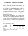
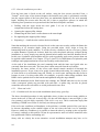
field capacity depend on the clay content and soil structure (pore space). Table 1.1 gives
common values of the field capacity and wilting point water contents and the available water
storage for some soil types.
Table 1.1. Typical field capacity and wilting point values (m3 m–3) for different soil textures
Soil texture
Field capacity
Wilting point
Available water
Coarse sand
0.06
0.02
0.04
Fine sand
0.10
0.04
0.06
Loamy sand
0.14
0.06
0.08
Sandy loam
0.20
0.08
0.12
Light sandy clay loam
0.23
0.10
0.13
Loam
0.27
0.12
0.15
Sandy clay loam
0.28
0.13
0.15
Clay loam
0.32
0.14
0.18
Clay
0.40
0.25
0.15
Self-mulching clay
0.45
0.25
0.20
Another soil water reference point often used by irrigators is the ‘refill point’. This is the soil
water content at which plant production begins to decrease as the plant begins to suffer water
stress. The actual water content used for a ‘refill point’ will vary depending on the soil type,
the evaporation conditions, the crop, and the management practices used. For example some
crops (e.g., wine grape vines) produce a better quality product if they are subject to mild
water stress at particular times in the growth cycle.
Near refill point, plants may begin to show signs of wilting late in the day, particularly in hot
and dry conditions. This is an indication that the soil has dried in the zone immediately
adjacent to the roots. This zone will usually refill with water overnight as the soil redistributes
its water, and the wilting will not be visible in the morning. This condition should not to be
confused with ‘wilting point water content’ as described in Table 1.1, when the whole body of
the soil has dried.
The refill point is a water content that is intermediate between field capacity and wilting
point. This means that the range of water contents within which irrigation management is
done is smaller, often by half, than the range of available water given in Table 1.1. For the
soils listed in Table 1.1, the range of water contents for irrigation management could be as
small as 0.04 m3 m–3 in a loamy sand to as large as 0.09 m3 m–3 in a clay loam. Thus, for
effective irrigation management based on soil water content sensing, the accuracy (not
precision) of water content estimates should be of the order of 0.01–0.02 m3 m–3.
4
1.4. FACTORS AFFECTING DIRECT MEASUREMENT ACCURACY, PRECISION
AND VARIABILITY
Accuracy, precision and variability are concepts that are important to obtaining useful values
of water content. Other works (Dane and Topp, 2002. p. 15) go into more detail, but for the
purposes of this manual they are defined as follows:
Precision is the variability of repeated measures in place or how well a value is known.
For example, if the standard deviation associated with the mean of a number of replicate
values is small compared with the mean of those values, then we can say that the precision of
this value is high.
Accuracy refers to how close the value of water content, indicated by the measurement
process, is to the actual value of water content measured directly in the field.
In addition to being both accurate and precise, a measurement can be precise but inaccurate,
or accurate but imprecise. If the mean value is close to the actual water content, but the
standard deviation of repeated measures is large, then the measurement is accurate (if
properly replicated) but imprecise. If the mean value is far from the actual water content, but
the standard deviation of repeated measures is small, then the value is inaccurate, though
precise. The best measure would be one that is both accurate and precise. Furthermore, the
variability of repeated measures in place should not be confused with the natural variability of
actual water content in the field. The former is due to measurement error and is often
expressed as such, while the latter is real variability in water content, not error.
For direct soil water measurement, the error margin on the mass basis water content of a
sample is based in part on the accuracy of the device used to weigh the sample (typically
±0.01 g for samples of around 100 g), and this source of error can usually be assumed to be
trivial. Other sources of error may include any water lost from the sample between the time of
its extraction and the time of first weighing, inadequate drying time or temperature, excessive
drying time or temperature such that crystalline water is lost, and water adsorbed from the air
into dry samples before they are weighed. With good practice these sources of error can be
minimized such that mass basis water contents may easily be accurate to better than 0.001 Mg
Mg–1. Error of θv is influenced by additional factors related to the determination of the volume
measured. These error sources include inexact trimming of core samples to length,
compression or dilation of the sample during extraction, and errors in sampler volume, the
latter usually being negligible. With good practice, θv values can easily be accurate to better
than 0.01 m3 m–3.
If several water content samples are removed from a particular depth in the field, and each is
processed with good practice, then we will have several values for water content, all measured
to high accuracy. However, it is unlikely that all these values will be identical, because a large
number of factors may cause the water content in the field to change from location to
location. This variation is termed ‘field water content variation’. It is not ‘field error’. If the
variation is a small fraction of the mean value, then the measure is said to be ‘precise’ or ‘the
measurement precision is high’.
The factors affecting field variation (or precision) will change as the scale of the sampled field
changes. If the samples are taken within an area of <1 m2, the factors affecting the variation
range will include:
•
gravel content,
•
bulk density variations,
•
water content variations,
•
the time since wetting,
5
•
•
•
the existence of macropores and shrinkage cracks,
the proximity of plant roots (plant spacing), and
small scale surface features (sample taken from under an irrigation furrow, or under a
wheel track, or between furrows).
If the sampled field is at the scale of an experimental plot (~0.1 ha), additional sources of
error may include:
•
•
•
•
•
•
position in the landscape,
effects of ponding, run-on and runoff,
proximity to irrigation sprays and water distribution of sprays,
variation in soil texture (clay content),
proximity to trees, and
type of plants (e.g., cereal crop, vegetables or trees).
If the sampled field is on a catchment scale (>10 ha), additional sources of variation may
include:
•
•
•
•
•
aspect (is the site facing the midday sun),
position in the landscape (ridge top or valley),
soil type (water holding properties in particular),
soil substrate (nature of local drainage system), and
land use (forest, row crop, etc.).
The apparent field variation also increases as the sample size decreases — particularly as the
sample size approaches the dimensions of gravel, cracks, soil structural units, plant roots, and
macropores caused by soil animals or rotting roots. There is a minimum soil sample volume,
called the representative elemental volume (REV), below which the variability of a soil
property increases rapidly. The size of the REV varies for different soil properties and for
different soils. Therefore, no simple number can be given for the size of the REV. It can be
stated that many current sensor technologies, as well as direct sampling methods, have
measurement volumes < REV for many soils. This has important implications in the context
of sensor technology and affects the variability of values reported by some technologies,
many of which sample small soil volumes.
The variations induced by each of these factors are cumulative, i.e., a trial at catchment scale
will still be subject to measurement variations due to the gravel content and proximity to roots
as well as all the other factors previously mentioned. To state, for example, that the field θv at
a depth of 0.2 m is 0.23 m3 m–3 does not tell the full story. To be more meaningful, the value
needs to be associated with a range of variation, e.g. 0.23 ± 0.05 m3 m–3, where 0.05 is (for
example) the standard deviation of the mean. This says that, on average, 75% of the values
measured in this field varied between 0.23 + 0.05 and 0.23 – 0.05. If the variation approaches
50% of the mean value, there is some question as to whether the measured value of field
water content has any useful meaning.
If the variation of m3 m–3 is large and can be attributed to variable soil type, it may be useful
to look at the variation of the ‘available’ water content at each site. In big catchments in
particular, much of the water content variation will be due to variation in clay content, and
this method allows that to be considered.
6
1.5. SURROGATE MEASURES OF SOIL WATER CONTENT
The discussion to this point applies to direct soil sampling with standard oven-drying
techniques. However, the use of direct soil sampling is destructive of the field, labour
intensive, is often slow, not timely and may be costly. Also, by its nature, direct sampling
cannot measure the water content in the same place twice. For work that depends on the
change in water content with time, this fact adds further variability to the data due to the
inherent small scale variability of water content.
Where labour costs are not an important consideration, there is much to be said for using
direct sampling methods, because they largely avoid the accuracy problems discussed below,
provided that plot size is sufficiently large so that site or crop destruction is not an issue.
Many alternative methods for measuring θv have been devised to avoid the problems of direct
sampling. Unfortunately, none of the alternative methods actually measure θv. They each
measure something else that changes as soil water changes. This ‘something else’ is called a
‘surrogate’ for θv (Table 1.2). By measuring this surrogate we hope we can estimate the
probable value of θv by means of a ‘calibration’, the calibration being the relationship
between the surrogate measurement and the soil water content. This is usually expressed as a
graph or a formula. Sometimes it is a simple linear relationship like
θv = ay + b ................................................................................................................ [1.3]
where y is the value of the surrogate measurement, and the slope, a, and intercept, b, are
constants determined by calibration. Often, the relationship is more complex.
The main advantage of these methods is that they are usually non-destructive. After
calibration, the soil is only disturbed once, during installation. Many of these methods add the
benefit of being loggable — readings may be taken at, for example, 10 min intervals so that θv
change during short duration events, such as during a tropical storm, can be sensed with ease.
However, this convenience comes at some cost. Not only must the user have knowledge of
the calibration (the relationship between the surrogate and the soil water content), but new
sources of errors are introduced. In all surrogate methods, the calibration is affected in some
way by factors other than the soil water.
For example, the NMM is affected by soil hydrogen, chloride, boron and soil density. The
electromagnetic (EM) methods (capacitive, time domain reflectometry (TDR) and frequency
domain reflectometry (FDR)) are affected by salinity, temperature, and by metallic soil
components such as ironstone. The degree of interference depends on the frequency used and
the specific way in which the measurement of travel time or frequency is made. Also, many of
these EM systems are sensitive to soil volumes that are smaller than the REV of the soil. They
are thus so responsive to the small scale variability of θv that their measurements exhibit a
great deal of variability that is not indicative of water content variability on the scale that
influences crops. The electronics of the systems that have been studied are relatively
insensitive to temperature changes, but the soil water readings from EM sensors tend to be
very sensitive to temperature changes. The temperature effect is due to the dependence of soil
bulk electrical conductivity on temperature. Added to this are additional problems associated
with faulty equipment, caused by wear and tear, or more likely, water and soil getting into
electronics — sometimes causing faults that are not readily apparent.
Another problem is that some surrogate measures work well over a certain range of θv but are
insensitive over another range (i.e., the surrogate does not change much when θv changes).
Heat dissipation methods are such a case. The surrogate in this case is either the heat capacity
or heat conductivity of the water. They work well between 0 and 0.3 m3 m–3 water content;
7
however, if the soil is wetter than this, the surrogate measures (soil heat properties) change
very little for quite substantial changes in θv. This makes this sensor a good choice for sands
and sandy loams, but a poor choice for soils with high clay contents. Another example would
be a capacitance sensor for which the calibration of θv vs. frequency shift is curvilinear, with
the frequency changing relatively little for large changes in θv at the wet end.
The EM soil water sensors, whether buried directly in the soil, fixed in a plastic pipe, or
housed in a probe that is lowered into a tube set in the soil, will respond to the ‘soil dielectric
permittivity’, which increases with θv. However, the permittivity also increases with bulk
electrical conductivity (BEC), and for non-zero values of BEC it increases with temperature.
Such sensors actually measure the oscillation frequency of an electronic circuit, changes in
frequency, or the travel time of an electronic pulse along a waveguide (Table 1.2). They do
not measure water content, despite the reassurances of some manuals; nor do they measure
electrical permittivity or dielectric constant. An additional complication for electrometric
sensors is that the effective frequency of the sensor influences the value of the electrical
permittivity. That is, the electrical permittivity actually changes in value, depending on what
signal frequency is applied.
If the instrument display reads directly in soil water content, this means that the manufacturer
has assumed a calibration and has built it into the instrument. Sometimes the calibration is
acceptably accurate for a wide range of soils and conditions, but frequently there are serious
errors.
Some manufacturers claim that their instruments do not need calibration. This is true only
under ideal conditions for the instrument concerned. The conditions for which each
instrument is acceptably accurate using the factory calibration (or fails) are detailed in the
literature, but seldom provided in the manufacturer’s instructions. Searching the literature for
technical detail is not a task to be undertaken lightly; and even then, there is a possibility that
the field site being studied has a critical property not covered in the literature.
A quicker, cheaper, and more reliable procedure is to routinely calibrate each new sensor or
method, preferably in the field and for each distinct soil horizon where it is to be used. This
process will not only produce a more accurate, site specific calibration, but will also help
identify problems with installation, measurement and technique.
The expert group agreed that, for all types of sensors, calibration in the soil in which they
were to be used was a necessary prerequisite to detecting problems and obtaining the best
accuracy and precision. The sole exception to this would be for conventional TDR. In a broad
range of mineral soils that do not contain large amounts of 2:1 lattice clays with large ion
exchange capacities, TDR with waveform capture and analysis is accurate to ±0.02 m3 m–3
(see the chapter on TDR in this Guide).
8
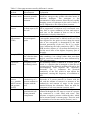
Table 1.2. Surrogate measures used by different θv sensors
Surrogate
Method
Measurement
Explanation
Neutron
Count of slow
A radioactive source emits fast neutrons (5 MeV),
moisture meter neutrons around a which lose energy as they collide with other atoms, in
source of fast
particular hydrogen. The surrogate is the
neutrons
concentration of slow neutrons. Since the only rapidly
changing source of hydrogen in the soil is water, θv
can be calibrated vs. the count of slow neutrons.
Thermal
Heat conductivity A pulse of heat is generated and the subsequent rise or
sensors
or heat capacity of fall in temperature of adjacent soil is measured over
the soil
time. Soil is a poor conductor of heat, and water a
good one, so the amount of heat or rate of heat
transmission is closely related to θv.
Time domain
Travel time of an
A fast rise time electromagnetic pulse is injected into
reflectometer
electromagnetic
a waveguide inserted into or buried in the soil. The
(TDR)
pulse
time required for the pulse to travel along the metal
rods of the waveguide is determined by the bulk
electrical permittivity of the soil. The θv is a major
factor influencing the bulk permittivity (BEC). True
TDR involves capture of a waveform and analysis to
find the travel time of the highest frequency part of
the pulse.
Campbell FDR Repetition time
See TDR sensors; same, except reliance on reflected
for a fast rise time pulse reaching a set voltage rather than waveform
electromagnetic
analysis causes the method to be more influenced by
pulse
BEC and temperature.
Capacitive
Frequency of an
An oscillating current is induced in a circuit, part of
sensors
oscillating circuit
which is a capacitor that is arranged so that the soil
becomes part of the dielectric medium affected by the
electromagnetic field between the capacitor’s
electrodes. The θv influences the electrical
permittivity of the soil, which in turn affects the
capacitance, causing the frequency of oscillation to
shift.
Conductivity
Electrical
An alternating current voltage is placed on two
sensors
conductivity of a
electrodes in a porous material in contact with the
(e.g., granular
porous medium in soil, and the amount of current is a measure of the
matrix sensors
contact with the
conductivity and amount of water in the porous
and gypsum
soil
material between the electrodes. These are used for
blocks)
estimation of soil water tension (suction), not θv.
Tensiometers
Matric and
Capillary forces retaining water in the soil pores are
gravitational soil
connected through the soil water to water in a porous
water potential
cup connected to a tube filled with water. This
components
generates a negative pressure within the tube, which
can be measured with a vacuum gauge. These are used
for estimation of soil water tension (suction), not θv.
9
1.6. FACTORS AFFECTING ACCURACY AND VARIABILITY OF WATER
CONTENTS DERIVED FROM SURROGATE MEASURES
All factors that affect variability of directly measured θv also affect variability of water
contents derived from surrogate measures. In addition, the calibration accuracy places an
absolute limit on accuracy of these water content values. The calibration process will be
discussed below, but it is a fact that field calibrations of sensors often do not result in
accuracy as good as that claimed by the manufacturers, due to several factors. First,
manufacturers generally calibrate in repacked soils of uniform composition, water content and
temperature, with no macropores, and with small clay content and bulk electrical conductivity
(BEC). This minimizes the error in θv determination during calibration, and it minimizes any
interference in the surrogate measure due to BEC and temperature variations. Thus, factory
calibrations and error ranges reported for them probably represent the best that can be
expected from a given sensor under ideal conditions.
If a user were to replicate the factory calibration conditions of repacked soil with uniform
temperature and low BEC for a calibration with the user’s soil, the resulting calibration would
not be applicable to the field situation. Only calibration in an undisturbed field soil can result
in a realistic calibration, with statistics of coefficient of determination (r2) and root mean
square error (RMSE) of regression that reflect the actual reliability and accuracy of θv
determination in that field. That said, there are several impediments to achieving surrogate
measures and accurate field calibrations.
As previously stated, there is a minimum REV for θv, and the size of the REV changes with
soil type (texture, structure, existence of macropores, etc.), and with the density and spatial
variation of plant roots. The REV also changes with drying and wetting, with the REV being
smaller soon after a substantial wetting, and increasing in size as the soil dries. That is, θv
measurement variability tends to increase as the soil dries after a substantial wetting.
Unfortunately, a large body of evidence shows that many sensors do not measure a volume at
least as large as the REV. For example, data of Paltineanu and Starr (1997) showed that >80%
of the sensed volume is within 2.5 cm of the access tube for the EnviroSCAN capacitance
sensor. Also, Evett et al. (2002c, 2006) showed that the capacitance probes used in access
tubes have limited axial response, the response being in some cases smaller than the height of
the sensor (Table 1.3). Sensed volumes vary widely, depending on sensor technology and size
(Table 1.4).
Table 1.3. Axial response to the soil–air interfacea
Sensor
Height (cm) of 90%
height/diameter
response window
Instrument
(cm)
Dry
Wet
b
Delta-T PR1/6
4.8/2.5
7.4
5.6
Sentek Divinerb
6.3/4.7
6.2
3.1
b
c
Sentek EnviroSCAN
6.2/5.05
NA
3.9
Neutron probe
13.2/3.8
27.7
15.6
Trime T3
17.5/4.2
16.9
18.3
a
Measured incrementally from >30cm above to >30cm below the surface.
Capacitance type sensors.
c
Not available.
b
10
Ratio of response
to sensor heights
Dry
Wet
1.54
1.16
0.99
0.50
NA
0.63
2.10
1.18
0.97
1.04
Table 1.4. Characteristics of some types of soil water sensor
Technology
Sensed volume
NMM
3 × 104 cm3 (wet soil)
28 × 104 cm3 (dry soil)
TDR
Soil volume along length of probe rods, and
~10 mm above and below the plane of the
rods, and 10 mm to the side of the plane of
the rods (e.g., ~320 cm3 for a 20 cm probe
with 3 rods and 3 cm rod-to-rod spacing).
Capacitive, FDR Highly variable — usually 90% of reading
comes from within 20 mm of the sensitive
face of the sensor, but sometimes the sensed
volume is smaller than the height of the
sensors. Typically ~200– 400 cm3.
Heat dissipation Highly variable —
20 mm zone around sensor, which is small.
Conductivity
Will equilibrate with a volume of soil that is
sensors
determined by the soil hydraulic
(e.g. gypsum
conductivity. Typically 500 cm3 in wet soil,
blocks)
but much smaller in dry soil.
Interferences
Cl, B, Fe, C
Salt, electrical
conductivity of soil and
temperature, magnetic
minerals (uncommon)
Salt, electrical
conductivity of soil
(including clay type,
content, and water
content) and temperature
Metallic soil components
Temperature, salts other
than the CaSO4 used in
the sensor
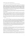
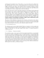
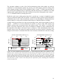
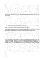
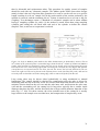
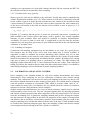
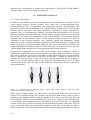
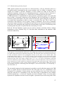
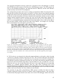
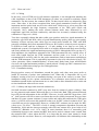
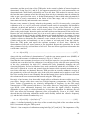
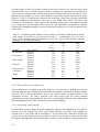
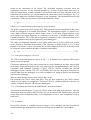
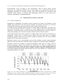
The data in Tables 1.3 and 1.4 indicate that measurements by different sensors in the field can
result in very different views of the spatial variability of θv, and that some of these views are
dominated by very small scale variability that occurs in volumes that are much smaller than
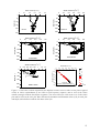
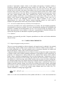
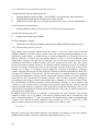
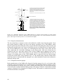
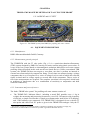
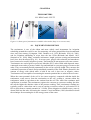
those explored by the roots of individual plants. An example drawn from a field study of three
capacitance sensors, a NMM and a quasi-TDR sensor illustrates this (Fig. 1.1). In the field
study, increased variability of θv below 110 cm depth was real, and expected due to the
presence of prairie dog burrows; these rodents burrow preferentially in the softer, CaCO3-rich
soil horizon below 110 cm. The reduced variability of θv for depths <110 cm in the wetter
100% treatment plot was expected due to previous observations of reduced variability in soil
water content under wetter conditions by several authors. The NMM did the best job of
integrating this small scale variability (due to its large measurement volume). The Trime T3
quasi-TDR system, with a much smaller measurement volume, reported more variability,
which was particularly noticeable in the drier 33% treatment plot. In fact, the Trime showed
as much variability in the soil above the 110 cm depth as it did for the soil below that depth, a
result that is not realistic. It is likely that the REV in the soil above 110 cm depth in the 33%
plot was larger than the measurement volume of the Trime sensor.
Results for the EnviroSCAN and Diviner 2000 capacitance sensors were similar to each other,
but these sensors exhibited much more variability than did the NMM and Trime, particularly
in the drier soil of the 33% treatment plot. Like the Trime, they showed mostly less variability
in the wetter 100% treatment plot at depths <110 cm than in the 33% plot at those depths. The
greater apparent variability of the capacitance systems is probably partly due to the sensed
volume being much smaller than the REV in this soil. However, the volume sensed by the
Trime is of the same order of magnitude as that sensed by the EnviroSCAN and Diviner 2000,
but data from the Trime show much less spatial variability. This points out a basic difference
between the capacitance sensors, which act like antennas in the frequency domain, and the
Trime, which acts like a waveguide in the time domain. The electromagnetic field of the
capacitance sensors is expected to preferentially invade parts of the soil matrix that exhibit
larger bulk electrical conductivity, usually associated with larger water content. This means
11
that sensor response will vary with the soil structure and size, shape and arrangement of
moieties of water content. In the time domain sensors, the electronic pulse is forced down a
waveguide and must pass soil moieties regardless of whether they are wet or dry, conductive
or non-conductive. Thus, with equivalent sensed volumes, the time domain sensors should
indicate smaller variability in soil water content than do capacitance sensors.
The capacitance sensors were also inaccurate when using the factory calibration in this soil,
which has a field capacity of 0.33 m3 m–3 and a porosity of 0.42 m3 m–3. Readings were taken
when the field was at field capacity or drier. Using the factory calibration for a clay soil, the
Delta-T PR1/6 instrument reported even more unrealistic θv values, with some values
exceeding the soil volume. Even though all readings with the PR1/6 were above the 110 cm
depth, the variability was large, indicating that the sensed volume was much larger than the
REV. Also, variability in the wetter 100% treatment plot was in some cases larger than that in
the drier plot, which is implausible, and which was probably due to the calibration curve
being very insensitive to water content change at the wet end.
A check was made on the reproducibility of readings in order to eliminate the possibility of
sensor malfunction in these data. Since the EnviroSCAN and Diviner 2000 sensors operate in
the same access tubes, readings from the two systems were plotted against each other for each
access tube and depth (Fig. 1.1, lower right). A slight difference in calibration caused the data
points to deviate from the one-to-one line. However, the plot shows a linear relationship
between readings from the two systems, indicating that the surrogate measures are responsive
to the same soil properties at each reading location, and in a reproducible manner. An
important point is that the soil properties to which the capacitance sensors respond are not the
same as the mean water content in a volume equivalent to the soil explored by a single plant’s
roots, but are much more variable, resulting in a misleading view of θv variability. A second
important consequence is that the number of access tubes required to determine a plot mean
profile water content to within a reasonable range of values (precision) becomes large (Table
1.5). The profile water content, WRZ, as described in Eq. [1.2], is essentially a mean of the
values determined at the various depths in the profile. Even if the separate values are not
normally distributed, the mean values will tend to be normally distributed (central limit
theorem). Thus, the number of samples (profile water content values), N, required to
determine a mean value to within a value d of the real mean, can be described as
2
⎛u S⎞
N = ⎜ α / 2 ⎟ ............................................................................................................ [1.4]
⎝ d ⎠
where S is the standard deviation of profile water content values, and uα/2 is the value of the
standard normal distribution at the (1 – α) probability level. For the study illustrated in Fig.
1.1, the values of S are given, and the number of samples, N, is calculated for two scenarios
(Table 1.5). The number of access tubes needed for the capacitance sensors is too large to be
practical.
12
3
3
-3
Water Content (m m )
0.1
0.2
0.3
0.4
0
0.5
0
0
50
50
Depth (cm)
Depth (cm)
0
100
150
200
150
200
Neutron
Trime T3
250
3
0
3
-3
Water Content (m m )
0.1
0.2
0.3
0.4
0.5
0
0
0
50
50
Depth (cm)
Depth (cm)
0.5
100
250
100
150
Diviner2000
3
0
-3
3
0
0
50
0.1
3
-3
EnviroSCAN (m m )
0
150
200
250
Delta-T PR1/6
EnviroSCAN
250
Water Content (m m )
0.2 0.4 0.6 0.8 1 1.2 1.4
100
0.5
150
200
250
-3
Water Content (m m )
0.1
0.2
0.3
0.4
100
200
Depth (cm)
-3
Water Content (m m )
0.1
0.2
0.3
0.4
0.1
-3
Diviner2000 (m m )
0.2 0.3 0.4 0.5
3
4
5
6
0.3
7
0.4
0.6
1
2
0.2
0.5
0.6
8
Field Test
DOY 323, 19 November 2003
9
10
1:1 line
Figure 1.1. Soil water contents reported by five different sensors in access tubes in two plots irrigated
weekly to 100% replenishment of soil water to field capacity (squares) and to 33% of the 100%
amount (triangles indicate this deficit irrigation). Ten access tubes for each sensor were in the 100%
plot and ten each in the 33% plot. Bars indicate the maximum and minimum values of θv for each plot
and depth, and solid lines indicate the mean value of θv.
13
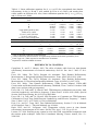
Table 1.5. Number of access tubes (profile water contents, WRZ) required to determine plot
mean profile water content to within a value, d, of the true mean for an experiment in a clay
loam soil for which there were ten access tubes in the wetter plot (‘Irrigated’) and ten tubes in
the drier plot (‘Dryland’). The standard deviation of profile water content value is S, and uα/2
is the value of the standard normal distribution at the (1 – α) probability level.
Method
Diviner 2000a
EnviroSCANa
Delta-T PR1/6a
Trime T3
Gravimetric
NMM
a
Soil condition
Irrigated
Dryland
Irrigated
Dryland
Irrigated
Dryland
Irrigated
Dryland
Irrigated
Dryland
Irrigated
Dryland
α=
uα/2 =
d (cm) =
S
1.31
2.42
1.52
2.66
2.72
12.16
0.75
2.38
0.45
0.70
0.15
0.27
0.05
1.96
1
N
6.6
22.5
8.9
27.2
28.4
568.0
2.2
21.8
0.8
1.9
0.1
0.3
0.10
1.64
0.1
N
464
1584
625
1914
2002
40006
152
1533
55
133
6
20
Capacitance type sensors.
1.7. ACCURACY, PRECISION AND THE CALIBRATION PROCESS
In addition to measurement volume, accuracy and precision determine the usefulness of a
sensor system for determination of water content. It is usually more important that sensed
water contents be accurate than it is that they be precise. Precision is typically measured by
repeated measures in place, and when assessed in this manner it is a property of the
measurement system itself. The concept of precision is misapplied if it is related to how
variable the water contents are across a field. Accuracy is largely a property of the surrogate
measurement used, any interfering factors such as BEC and temperature, and the calibration
curve used to convert the surrogate to θv. The accuracy of a sensor system can vary for
different soil types, different horizons or even different parts of a field. In particular, accuracy
is very much affected by the ‘interfering factors’ mentioned above — those factors that
change the surrogate value even when the water content is the same.
1.7.1. The manufacturer’s calibration
At some stage in the process of taking a measurement with a modern instrument, a surrogate
measure is taken by the sensor system and either displayed directly or converted into θv by the
system’s internal electronics before display. Good quality equipment should be able to bypass
the conversion process and provide the surrogate measure directly. If this is not possible, the
number displayed should not be regarded as a value of θv but as just ‘the output number’ for
the purposes of the following discussion.
A manufacturer’s calibration is commonly performed in a temperature controlled room, with
distilled water and in easy to manage homogeneous soil materials (loams or sands) which are
14
uniformly packed around the sensor. This produces a very precise and accurate calibration for
the conditions tested. The θv value is precise because the soil is mixed so that the water
content is uniform; and if there is any variability between repeated readings, as with the
NMM, then the surrogate reading can be made as accurate as required by averaging a number
of readings. Unfortunately, conditions such as these do not exist in the field, and thus the
results obtained are, at best, a rough estimate of the field calibration.
In the field, the presence of gravel and stones, plant roots, and variation in clay content and
type are normal, as are cavities or compressed soil, adjacent to the sensor and within its zone
of measurement. Add to this the effect of bulk EC, whether due to salinity or to the clay
content and type; direct effects of temperature on the BEC; and the indirect effects of
temperature changes on water distribution and movement; and the manufacturer’s calibration
is rarely applicable. In fact, the RMSE of regression for the manufacturer’s calibration will
normally be much smaller than that obtained in a field calibration. This smaller RMSE value
does not mean that the manufacturer’s calibration is more accurate than the user’s field
calibration. Rather, it means that the manufacturer’s RMSE value is unrealistically small if
applied to a situation of normal field soil heterogeneity.
The process of field calibration evaluates the level of accuracy for that device in the chosen
field. It may (or may not) also reveal the interferences for the device, the most common being
the effects of temperature and soil BEC. Unless these are measured as covariates and included
in the calibration equation, the accuracy of the calibration equation will suffer.
1.7.2. The calibration process
The calibration process can be simply described. However, in practice it is often complex and
time consuming when done properly. Specific guidelines for calibration are given in separate
chapters of this Guide for each major method. What follows is a general discussion of
calibration processes.
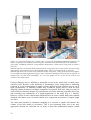
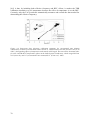
1.7.2.1. Calibration — Destructive methods
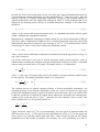
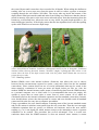
First, install the sensors in the required soil horizons using the manufacturer’s recommended
procedures. For studies covering large areas (e.g. catchment studies), a recommended design
is to place identical sensor installations perhaps 3 m apart, then take the surrogate reading and
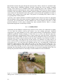
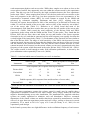
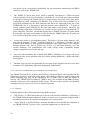
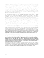
sample one location under wet conditions, and repeat surrogate readings and sampling at the
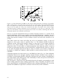
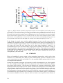
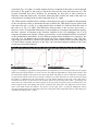
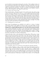
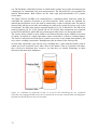
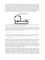
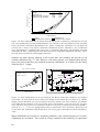
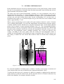
other location under dry conditions (Fig. 1.2). For each pair of installations it is reasonable to
assume that the soil of the wet installation and that at the dry installation is the same. In this
way, the slope of the calibration (the most critical factor in water balance studies) can be
compared for different parts of the field. In uniform soils, all the points may be combined to a
single calibration. In variable conditions it may be necessary to have different calibrations for
different parts of the field (e.g., different soil types).
15
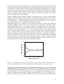
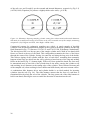
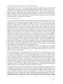
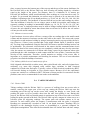
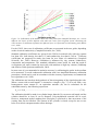
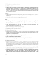
Figure 1.2. Field calibration of a NMM in a soil with two distinct horizons, one having a clay and the
other a loam texture, using three pairs of access tubes in each horizon. Regressions (dashed lines)
show clear differences in slope for the loam and clay soils. The common regression shows a similar
slope to the clay (offset by ~0.02), but is biased for the loam. The profile water content change
calculated using the common calibration will be considerably in error due to its inaccuracy in the
loam. For each horizon, slopes for the paired access tubes were similar, indicating that only one
calibration equation was needed for each horizon.
Next, try to set the measurement device to read the surrogate measure (i.e., switch off any
internal calibration). If this is not possible, treat the value obtained as ‘a number’ not as a
water content. Then take a reading, again by the recommended procedure, which may involve
taking long duration readings or several readings in quick succession and calculation of an
average.
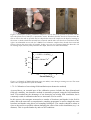
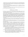
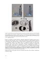
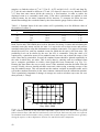
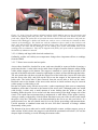
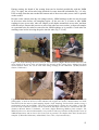
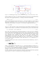
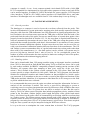
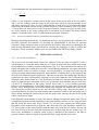
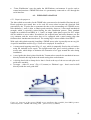
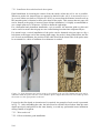
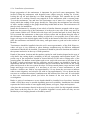
Then either remove the sensor and collect the soil in its immediate vicinity, or take soil
samples as close to the sensor as possible (Fig. 1.3). The samples should be taken by
volumetric means. With typical sampler volumes, at least three or four samples should be
taken for every sensor reading, in order to obtain an accurate mean θv value for the soil
around the sensor. If soil texture or chemical properties vary down the profile, it may be
necessary to repeat this procedure in each soil horizon. Calculate both the value of θv and of
ρb for each soil sample and plot the data in order to examine it for outliers (compressed,
incomplete or dilated soil samples), which should be removed before mean θv values are
calculated.
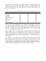
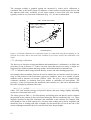
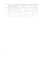
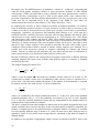
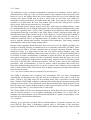
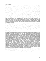
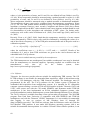
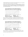
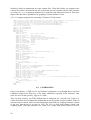
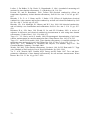
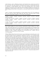
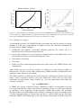
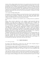
Calibration equations for some sensors (e.g., the NMM) are linear (Fig. 1.4). If the calibration
relationship between the surrogate property and the directly measured water contents is
curvilinear, measurements should be repeated at different soil water contents, including those
near field capacity and wilting point. If the relationship is linear, the process need only be
repeated for ‘wet’ and ‘dry’ conditions.
Once the mean θv values have been determined from the soil samples corresponding to each
sensor reading, graph the sensor readings against these values. If possible, use linear or nonlinear regression to fit a mathematical function to the resulting relationship. The root mean
squared error (RMSE) of regression is a measure of the accuracy of the calibration.
16
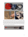
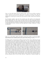
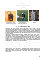
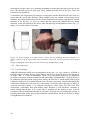
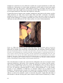
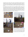
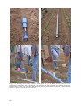
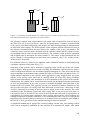
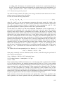
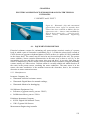
Figure 1.3. Examples of taking volumetric samples as close to the sensor position as possible. On the
left is the plastic access tube for a capacitance sensor. Bevelled cylinders have been inserted into the
soil as close to the tube as possible and to a depth that centres the sample on the depth of reading of
the sensor. A third cylinder has already been removed, and the other two have been excavated. On the
right is an aluminium access tube for a NMM. Four volumetric samples have already been extracted
from as close to the access tube as possible. In this case, two were extracted from just above the 110
cm reading depth, and two from just below this depth, and all were taken horizontally.
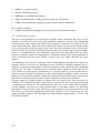
0.4
θ v = -0.070 + 0.1978(C R )
r2 = 0.96
3
-3
RMSE = 0.014 m m
3
-3
θv (m m )
0.3
0.2
0.1
0.0
0
0.5
1
1.5
2
2.5
Count Ratio (C R )
Figure 1.4. Example of NMM calibration using wet and dry sites during a training exercise. The count
ratio is the surrogate measure from the NMM.
1.7.2.2. Calibration of an existing field installation (non-destructive method)
As noted above, an essential part of the calibration process includes the three dimensional
field soil variability. An alternative method is sometimes proposed, using the field installation
itself. This method has the advantage of not destroying an existing field installation, but it
commonly results in calibrations that are so inaccurate as to be useless.
In this process, the surrogate measured at a number of locations (and depths) in the field is
taken, and at the same time a comprehensive sampling programme is used to sample the same
locations and depths using direct soil sampling techniques. The samples should be taken as
close to the sensors as possible without damaging the value of the sensor installation (say, 1 m
distance). This is repeated under dry and wet soil conditions.
17
The surrogate reading is graphed against the measured θv values and a calibration is
calculated. Due to the small volume of influence of most indirect measurement devices and
the inherent small scale variability of soil water content in most field soils, this method
typically results in very inaccurate calibrations (Fig. 1.5). It is not recommended.
Site 1, Austria, Diviner 2000
0.40
0.30
VWC = 0.039 + 0.567(SF)
2
Adjusted r = 0.533
3
-3
RMSE = 0.038 m m
5.276
3
-3
Water Content (m m )
0.35
0.25
0.20
0.15
0.10
0.05
0.60
0.65
0.70
0.75
0.80
0.85
0.90
Scaled Frequency
Figure 1.5. Example calibration of a capacitance probe in a sandy loam using direct sampling at 1 m
from the access tube. Due to the small scale variability of soil water content, this calibration is not
useful.
1.7.3. Checking a calibration
The best way to check an existing installation (and manufacturers’ calibration) is to follow the
procedure set out in Section 1.7.2 above. In some cases this may be too costly, so below are
suggested less reliable methods that may produce useful information at minimal cost.
1.7.3.1. Calibration check using soil bulk density, texture and water holding properties
Soil samples taken around the field can be used to identify the soil texture (sand, silt, loam or
clay) at each position in the field where sensors are installed; there are a number of quick
methods used to measure soil texture (USDA, 1998). The soil ρb may be sampled using
volumetric methods, or obtained from prior studies or published soil descriptions. The
porosity, f, of the soil represents the maximum water content, θmax, that can be attained when
the soil is completely saturated with water:
θmax = f = 1 – ρb/2.65 ................................................................................................. [1.5]
where 2.65 is the assumed average soil particle density (this may change slightly depending
on the mix of minerals in the soil).
The values given in Table 1.1 for field capacity and wilting point can then be used to estimate
the probable water content of each soil texture during dry and wet conditions (Fig. 1.6). These
might be described as the field ‘maximum’ and ‘minimum’ water contents. For example, field
soils should be close to field capacity for a few days after soaking rain or heavy irrigation, and
should be close to wilting point after a healthy crop has dried the soil out at the end of the
season, although sometimes the soil is not dried out at the deeper depths.
18
The surrogate readings at each of the field measurement points, taken under wet and dry
conditions, are then graphed against the porosity, the field capacity and the wilting point
water contents, giving a check on the calibration (Figs 1.6 and 1.7). Where good accuracy is
not essential, the calibration may be adjusted so that the data from wet conditions lie at field
capacity on the graph and those from dry conditions lie near the wilting point water content.
1.7.3.2. Calibration check by wetting up an area
Ideally the soil is near wilting point when this is carried out. A sensor is installed to sense
water to a sufficient depth in the soil profile. A minimum of three replicate profiles should be
established, more if one of the electrometric sensors is used. Readings are obtained from the
sensors and the θv of the profile calculated with whatever calibration data are available.
A bank is built to pond water in a large area around the sensor, and a known depth of water is
applied — sufficient to wet the measured soil profile to just less than field capacity but
without causing water movement below the deepest sensor. The surface is covered with
plastic to prevent evaporation, and a layer of insulation is applied to reduce condensation on
the underside of the plastic (100 mm of straw is effective). After redistribution of the water
(usually a day or two), the sensors are again read and the soil water content is calculated. The
change in stored water is calculated from the water contents recorded before and after wetting.
EnviroSCAN Water Content (m3 m-3)
0
0.2
0.4
0.6
10
10
30
50
70
90
110
e
Cliff Hignett
Depth (cm)
Depth (cm)
3 -3 -3
3 m
Neutron Probe
Probe Water
Neutron
WaterContent
Content(m
(m
m) )
0
0.2
0.4
0.6
60
110
160
Day 148
Mean
Day 148
Mean
Day 204
FC & WP
Day 204
FC & WP
Figure 1.6. (Left) Comparison of field capacity (FC) and wilting point (WP) water contents to water
contents from a neutron probe measured on the day during the irrigation season when the soil was
most dry (day 148 after planting) and on the day when the soil was most wet (day 204 after planting).
(Right) Comparison between FC and WP values and water contents reported by a capacitance probe
in the same field. The neutron probe calibration is more accurate than that for the capacitance probe.
Also observed is greater scatter in the data from the capacitance probe, something that calibration
will not be able to fix.
19
Figure 1.7. Water contents reported by capacitance sensors at several depths in a soil with a porosity
of 0.42 m3 m–3. Two of the sensors (at 10 and 20 cm depth) report readings that are higher than is
physically possible in this soil. The θv at wilting point in the soil is approximately 0.18 m3 m–3. Two of
the sensors (at 80 and 100 cm depth) report readings that are close to this value. It is typical with this
kind of sensor that the greatest errors are on the wet end. The sensor at 40 cm depth reports θv values
that are near or at saturation for several weeks. This was checked by soil sampling and was shown to
be far from the truth. The soil at that depth was actually at less than field capacity (0.33 m3 m–3).
If the change in stored water and the applied amount of water are the same, then the
calibration is reasonably accurate. Note that this method works poorly if the ponded area is
too small. It should be approximately 4 m on a side. This is because lateral redistribution of
soil water will cause the soil water flux to be other than completely vertical. It is
recommended to use two concentric banks, keeping water ponded in the outer area as long as
the water applied to the centre area is still ponded on the surface. The depth of water applied
to the centre area is measured. The water applied to the outer area will typically be greater in
total depth per unit area, but some of this water will move laterally out of the area
encompassed by the outer bank.
1.8. SUMMARY
Direct soil sampling for water content is time consuming, inconvenient, costly, and is often
destructive of a field study area. However, this method usually provides a measure of soil
water content that is accurate and reliable. It is the standard method against which all others
are compared and calibrated.
Sensors that respond to surrogate soil properties (usually electromagnetic) are often loggable
(i.e. take readings automatically) and are less destructive of the field. Unfortunately, they do
not measure water content — they measure the change in the ‘surrogate’ measurement, which
hopefully indicates the change in water content. In all of the expert group’s case studies there
were important interferences that caused the change in the surrogate property to be not
uniquely related to the soil water content. In many cases, the sensed volume was smaller than
the representative elemental volume for the soil in which the sensor was tested, leading to (i)
an unrealistically large estimate of the variability of soil water content, and (ii) a requirement
for excessive numbers of access tubes in order to obtain a mean profile water content of
20
acceptable precision. Other chapters in this Guide describe the major sensing methods, giving
the theory of operation, important interferences, and suggestions for effective calibration and
use. These chapters also describe situations in which the various technologies are unlikely to,
or definitely will not, work well.
To ensure that a sensor method produces reasonable values of θv, it is mandatory to check that
the maximum and minimum values reported by the sensors are within the values of field
wettest and driest conditions.
To ensure that a sensor technology produces results of known accuracy and precision, some
form of calibration in the soil concerned is necessary.
REFERENCES TO CHAPTER 1
IAEA, 2001. Comparison of soil water measurement using the neutron scattering, time
domain reflectometry and capacitance methods. International Atomic Energy Agency, Vienna,
Austria, IAEA-TECDOC-1137 (2000).
Dane, J.H., and G.C. Topp (eds.) 2002. Methods of Soil Analysis. Part 4 — Physical Methods.
Evett, S.R. 2001. Exploits and Endeavors in Soil Water Management and Conservation Using
Nuclear Techniques. In Proc. International Symposium on Nuclear Techniques in Integrated
Plant Nutrient, Water and Soil Management. Vienna, Austria, 16-20 October 2000
International Atomic Energy Agency, Vienna, Austria. (CDROM) Available at
http://www.cprl.ars.usda.gov/programs/ (Posted 24 Oct. 2000; verified 1 Jan. 2001).
Evett, S.R. 2003a. Measuring soil water by time domain reflectometry. In B.A. Stewart and
Terry A. Howell (editors). Encyclopedia of Water Science, Marcel Dekker, Inc. New York.
Pp. 894–898.
Evett, S.R. 2003b. Measuring soil water by neutron thermalization. In B.A. Stewart and Terry
A. Howell (editors). Encyclopedia of Water Science, Marcel Dekker, Inc. New York. Pp.
889–893.
Evett, S.R. 2007. Soil water and monitoring technology. p. 25–84. In R.J. Lascano and R.E.
Sojka (ed.) Irrigation of agricultural crops. Agron. Monogr. 30, 2nd ed. ASA, CSSA, and
SSSA, Madison, WI.
Evett, S.R., N. Ibragimov, B. Kamilov, Y. Esanbekov, M. Sarimsakov, J. Shadmanov, R.
Mirhashimov, R. Musaev, T. Radjabov, and B. Muhammadiev. 2002a. Soil moisture neutron
probe calibration and use in five soils of Uzbekistan. 17th World Congress of Soil Science,
August 14–21, 2002, Bangkok, Thailand, Transactions, pp. 839-1 – 839-10. (CD-ROM)
Evett, Steven, Jean-Paul Laurent, Peter Cepuder, and Clifford Hignett. 2002b. Neutron
Scattering, Capacitance, and TDR Soil Water Content Measurements Compared on Four
Continents. 17th World Congress of Soil Science, August 14-21, 2002, Bangkok, Thailand,
Transactions, pp. 1021-1 – 1021-10. (CD-ROM)
Evett, S.R., B.B. Ruthardt, S.T. Kottkamp, T.A. Howell, A.D. Schneider, and J.A. Tolk.
2002c. Accuracy and Precision of Soil Water Measurements by Neutron, Capacitance,
and TDR Methods. 17th World Congress of Soil Science, August 14–21, 2002,
Bangkok, Thailand, Transactions, pp. 318-1 – 318-8. (CD-ROM).
Evett, S.R., J.A. Tolk, and T.A. Howell. 2005a. TDR laboratory calibration in travel time,
bulk electrical conductivity, and effective frequency. Vadose Zone J. 4:1020–1029
(2005). Special Section: Soil Water Sensing. doi:10.2136/vzj2005.0046.
Evett, S.R., and G. W. Parkin. 2005b. Advances in Soil Water Content Sensing: The
Continuing Maturation of Technology and Theory. Vadose Zone J. 2005 4: 986–991.
Special Section: Soil Water Sensing. doi:10.2136/vzj2005.0099.
21
Evett, S.R., J.A. Tolk, and T.A. Howell. 2006. Soil profile water content determination:
Sensor accuracy, axial response, calibration, temperature dependence and precision.
Vadose Zone J. 5:894–907.
Hignett, C., and S.R. Evett. 2002. Neutron Thermalization. Section 3.1.3.10 In Jacob H. Dane
and G. Clarke Topp (eds.) Methods of Soil Analysis. Part 4 — Physical Methods. pp.
501–521.
Laurent, J.-P., P. Ruelle, L. Delage, A. Zaïri, B. B. Nouna, and T. Adjmi. 2005. Monitoring
Soil Water Content Profiles with a Commercial TDR System: Comparative Field Tests
and Laboratory Calibration. Vadose Zone J. 4:1030–1036..
Paltineau, I.C. and J.L. Starr. 1997. Real-time soil water dynamics using multisensor
capacitance probes: laboratory calibration. Soil Sci. Soc. Am. J. 61(6):1576–1585.
USDA. 1998. Estimating Soil Moisture by Feel and Appearance (Program Aid 1619). United
States Department of Agriculture, Natural Resource Conservation Service. (Can be
found at http://www.mt.nrcs.usda.gov/technical/ecs/agronomy/soilmoisture/)
22
CHAPTER 2
GRAVIMETRIC AND VOLUMETRIC DIRECT MEASUREMENTS OF SOIL
WATER CONTENT
S. EVETT
2.1. EQUIPMENT DESCRIPTION
Equipment for direct soil water content measurements varies widely, and is available from
many manufacturers. Ordinarily such equipment consists of devices for taking soil samples,
devices for determining the volume of soil excavated (if volume is not determined directly by
using a volumetric sampling device), containers for retaining and transporting the samples
without loss of water, ovens for drying the samples, and scales for weighing the samples.
Sampling equipment for mass basis water contents (θm, g g–1) may be as simple as a shovel,
scoop or tube to be thrust into the soil. Since volume is not a consideration for θm, the exact
volume of the sampling equipment is not a concern, nor is any sample compaction or dilation.
Equipment for volumetric water content (θv, m3 m–3) determination is of known dimensions,
and typically consists of tubes or cylinders with a bevelled cutting edge to ease insertion of
the sampler into the soil. There are many different samplers, each with its own advantages
and disadvantages.
2.1.1. Manufacturers, instruments and parts references
Eijkelkamp Agrisearch Equipment
•
Sampling cylinders, 100 cm3 volume, 0.053 m inside diameter, part no. 07.01.53.NN
(case of 24 with plastic end caps);
•
Sampling guide/handle, part no. 07.05.01.53.
Precision Machine Company
•
Volumetric soil sampling equipment (Madera probe), catalogue descriptions: SOS
Regular Bit, SOS Regular Clay Bit, SOS Heavy Duty Bit, SOS Knives (Regular bit has
thinnest wall).
AMS Inc.
•
Model numbers are too numerous to mention;
•
Soil augers: sand, mud, clay, bucket, Edelman, etc.;
•
Split barrel samplers;
•
Hydraulic hammer/push and auger drive machines.
Giddings Machine Company
•
Models too numerous to mention;
•
Soil sampling tube bits, several types;
•
Soil sampling tubes for attachment to bits;
•
Hydraulic coring machines for inserting tubes into soil and withdrawing them.
UMS GmbH, Umweltanalytische Mess-Systeme
•
Different auger types for augering and sampling to a depth of 5 m;
•
Soil sampling set.
23
2.1.2. Measurement general principle
The measurement of water content is direct, being simply the mass of water (Mw, g) lost on
drying in a convective oven at a specified temperature (usually 105ºC) until mass remains
constant (usually 24 h or longer). Samples containing more than a few per cent organic matter
may lose mass due to volatilization of organic matter at temperatures higher than 50ºC. A
more thorough discussion of sample drying times and temperatures is given by Gardner
(1986). The data are typically normalized by dividing by the sample dry mass or sample
volume. Direct water content measurements are called gravimetric measurements because
they are based on weighing of the amount of water lost on drying. This is so whether the
reported water contents are based on sample dry mass (g g–1) or on sample volume (m3 m–3).
Thus, it is not sufficient to report only that gravimetric samples were taken. The units must
also be given.
The mass basis water content (θm, g g–1) is
θm = (mass of water)/(mass of soil solids) = Mw/Md ................................................ [2.1]
where Md is the mass of the soil after drying, and Mw = Ms – Md, where Ms is the mass of the
soil immediately after it is sampled (or before any water is lost). If the volume of the sample
(Vs, m3) is known, then the volumetric water content (θv, m3 m–3) can be calculated by
converting the mass of water lost on drying to a volume
θv = (volume of water)/(total soil volume) = (Mw/ρw)/Vs ......................................... [2.2]
where ρw is the density of water (typically assumed to be 1 Mg m–3).
If the volume of the sample is not known, but the bulk density (ρb, Mg m–3, which is the
density of the soil including the pore space but excluding the mass of water, ρb = Md/Vs) of
the soil can be estimated, then the volumetric water content can be estimated from
θv = (Mw/ρw)/(Md/ρb) .................................................................................................. [2.3]
Note that Eq. [2.3] is not equivalent to Eq. [2.2], where the sample volume was known. In
practice, Eq. [2.3] often leads to errors. The bulk density value used is typically an average
value determined for the soil, and the value may come from a prior study. Because bulk
density, like water content, is quite spatially variable, the actual bulk density of the sample
may be quite different from the average value.
As all soil properties, water content is variable in three dimensional space and in time. This
variability complicates the tasks of measuring, modelling, estimating or forecasting of soil
properties. Variability has been dealt with in numerous ways, including compositing of
multiple samples into one, and through various statistical approaches. Sample compositing
averages sample variability but can have unintended consequences, as when sample mixing is
incomplete or when sample value statistical distribution is skewed. Statistical approaches
range from simple descriptive statistics, such as the mean, range and standard deviation, to
more complex analyses involving estimation of the statistical distribution representing the
samples (e.g. Gaussian, log-normal, Poisson, etc.), skewness and kurtosis of the distribution,
or analyses in space or time such as spatial variogram analysis followed by kriging to derive
maps of sample value estimates, or time series analysis. A full discussion of statistical
treatments is beyond the scope of this work, but useful discussions are given by several
authors in Chapter 1 of Methods of Soil Analysis (Dane and Topp, 2002) on sampling theory,
descriptive statistics and geostatistics; and by Nielsen and Wendroth (2003) on time series
and state space analysis and geostatistics.
24
Classical research methods for dealing with soil spatial variability include selection of plot
sizes large enough to average out small scale variability, blocking of plots (two or more areas
or blocks, all of which include all of the experimental treatments), randomization of treatment
plots within blocks, and inclusion of measurements of important properties that are correlated
with the properties under study (covariate analysis). Statistical methods that include
covariates include the general linear model as applied to analysis of covariance (ANCOVA),
and covariogram analysis and cokriging.
Spatial variability studies usually find that variance between soil water content samples
increases with the distance between samples, the separation distance. But the same studies
indicate that there is a nugget effect, that is, the variance between samples does not go to zero
at small distances. For most measurement systems, it is this small scale (<1 m), non-zero
variance that influences the variability of a single measurement.
The sample support size or volume has a large effect on the ability to measure this small scale
variability. Support volume is tied to the concept of the representative elemental volume
(REV), illustrated in Fig. 2.1. For example, a sample size smaller than the size of soil pores
could obtain a sample in pore water, in soil solids or in an air filled pore. For samples in pore
water, the water content would be 1 m3 m−3, and for the latter two the water content would be
zero. As sample volume increases, more and more of the small scale variability in the soil
fabric is integrated into each sample, and the range of possible values decreases. The REV is
the sample volume at which most of the small scale variability is integrated. The REV is
different for different soil properties, and changes over time for some properties, including
soil water content. An important result of the REV concept is that the variance between
samples may actually increase for smaller separation distances as sample volume decreases,
so that samples do not overlap at the smaller separation distances.
Water content (m3 m-3)
1.0
0.8
0.6
0.4
0.2
0.0
1.E+00
1.E+01 1.E+02 1.E+03
Sample volume (cm3)
1.E+04
Figure 2.1. Example bounds on likely sample values as sample volume increases. The representative
elemental volume (REV) can be chosen according to the acceptable variability in sample values.
The concept of an REV is supported by field measurements. Hawley et al. (1982) studied the
relationship between sample volume and variance of water content samples, using eight
different sample volumes ranging from 7 to 825 cm3, and concluded that variance increased
for smaller volumes. The same was true when a 15 cm3 sampler was compared with a 60 cm3
sampler for neutron moisture meter (NMM) calibration (Allen et al., 1993; Dickey et al.,
1993). Most other studies of soil water variability used only one sample size or did not report
25
the sample size. The NMM measures, at minimum, a volume of ~14 000 cm3. Comparing this
with the much smaller sampling volumes of most gravimetric methods, or time domain
reflectometry (TDR) and capacitance probes, indicates that more measurements would be
needed with these technologies to give a field or plot mean profile water content with a
precision comparable to that from neutron thermalization. This was recognized as early as the
1960s and was an important factor in the adoption of the NMM for crop water use
measurements based on soil water balance (Calif. Dept. Water Res., 1963).
In comparing the variance in water content as measured by different methods, it is useful to
keep in mind that measured variation of water content in a field is likely to increase as the
volume of soil that is measured decreases. Small scale variation of soil water is controlled by
topography, vegetation, soil properties and sampling depth (Hawley et al., 1982); and for a
particular location, variability increases with time since wetting (Schmitz and Sourell, 2000)
and decreases as water content increases (Famiglietti et al., 1999; Hawley et al., 1982; Hupet
and Vanclooster, 2002; Schmitz and Sourell, 2000). These studies indicate that more samples
will be needed in drier soils to attain the same precision of measurement as in wetter soils.
Therefore, no simple statement of the desired sample volume can be given, other than to state
that fewer large volume samples will be needed to determine the mean value within a given
confidence interval than would be needed if smaller volume samples were obtained. For a
parallel and useful discussion relevant to irrigation scheduling see Schmitz and Sourell
(2000). Variance in observed soil properties can also affect the precision of calibration of
water content sensors, as is discussed in other sections of this work.
Because of differing volumes and varying effects of sample compression or dilation, different
sampling methods will report water contents with different degrees of variance or standard
deviation in the field.
The sample standard deviation (S) is
(
)
2⎞
⎛ 1 N
S =⎜
xi − x ⎟
∑
⎝ N − 1 i =1
⎠
0.5
......................................................................................... [2.4]
where xi is the ith sample, x is the mean of N samples, and the value of N is at least 30. The
variance due to sample volume size is in addition to other sources of error or variation. For a
given value of measurement standard deviation, S, the number of measurements, n, required
to estimate a mean value with an error <d can be estimated as
⎛u S ⎞
n = ⎜ α /2 ⎟
⎝ d ⎠
2
........................................................................................................... [2.5]
where S is estimated by the sample standard deviation, uα/2 is the (α/2) value of the standard
normal distribution, and (1 – α) is the probability level desired (e.g. 0.95 or 0.90). Equation
[2.5] is valid for normally distributed values that are independent of one another and for S
estimated from a large number of samples.
The above example assumes that samples are taken from an area small enough that large scale
spatial variability does not come into play. In the event that spatial variability is important, the
number of samples must be increased such that an adequate number of samples is available
for each spatially different area (Vauclin et al., 1984). In most cases, these analyses may be
applied to values of soil profile water storage that are calculated on the basis of samples at
multiple depths.
In addition to the question of appropriate sample volume in relation to the REV, there is the
26
question of appropriate sample volume or the number and spacing of samples needed to
accurately represent the phenomenon being studied. For field crops, the volume to be
represented would ordinarily be at least as large as the crop root zone. For trees, the volume
extends out to at least the outer edge of the canopy, since tree roots often extend laterally to at
least the same extent as the leafy canopy. For soil water balance studies, the volume would
extend to well below the root zone. Direct soil sampling to adequately represent water content
and water content changes under these conditions have always been problematic, since
repeated sampling would cause severe damage to the system under study. This is why the
indirect water content sensing methods described in other chapters of this work are so
important. However, the sampling volume of the indirect methods is key to their
appropriateness for various tasks. Indirect method sampling volumes are often small in
relation to the phenomenon under study and in relation to the REV.
2.1.3. Accessories and documents provided by the manufacturer
Accessories provided by the various manufacturers vary widely. For soil sampling equipment,
documentation is often not available. For ovens, documentation detailing safe installation and
operation is standard, but documentation for use of an oven for drying soil samples is not.
Where documentation is not available, it is the user’s responsibility to search the literature for
articles like the present one that detail acceptable operating procedures.
2.1.4. Software
Software is not generally provided. Computer spreadsheets are often used for data tabulation
and processing.
2.2. TAKING MEASUREMENTS
2.2.1. Required equipment and procedures
There are two main methods by which volumetric soil samples may be obtained. One method
involves using a metal cylinder, scoop or other device of known volume to take a sample — a
so-called undisturbed core. The other method involves extracting a disturbed soil sample and
then measuring the volume of the void left by this extraction.
Volumetric samples (undisturbed cores) are subject to errors arising from sample compression
or dilation. Some of the available sampling equipment is ill-designed to avoid compression. In
particular, soil compression is likely using soil core samplers that employ metal cylinders
inside a larger, cylindrical sampling body with a bevelled cutting edge. Compression is due to
the large cross-sectional area of the cutting edge normal to the axis of insertion. Compression
can usually be avoided by using a thin walled cylinder with an acutely bevelled cutting edge.
For minimal compression, the cylinder should be machined behind the cutting edge to have a
larger inside diameter than that of the cutting edge. Sample rings or cylinders are often cut to
length to provide a known volume. Also, the cross-sectional area of the cylinder wall should
not exceed 5% of the cross-sectional area of the soil core obtained. Thus, the desired sampler
has an inside radius r ≥ 0.975 R, the outside radius (Hignett and Evett, 2002) (Fig. 2.2).
Another standard for coring rings suggests that
Awall
= (De2 − Di2 )/ Di2 < 0.1 ..................................................................................... [2.6]
Acore
where Awall is the cross-sectional area of the cylinder wall and Acore is the cross-sectional area
27
of the soil core, and De and Di are the external and internal diameters, respectively (Fig. 2.2)
(ASTM, 1999). Equation [2.6] allows a slightly thicker tube wall (r ≥ 0.95 R).
Figure 2.2. Schematics depicting sampling cylinder cutting face relative inside and outside diameters
that make for a small facial cutting area relative to the cross-sectional area of the sample, minimizing
compaction. (Left: Hignett and Evett, 2002. Right: ASTM, 1999.)
Commercial systems for volumetric sampling vary widely. A good example of bevelled
cylinders used for taking undisturbed samples is the system of bevelled cylinders and driving
head illustrated in Fig. 2.3 (Part nos. 07.05.01.53 and 07.01.53.NN, Eijkelkamp, Netherlands).
The driving head fits over the top part of the sample cylinder and is held in one hand while
blows are struck at the top of the shaft. This configuration transmits the force of the blows
through the centre of the cylinder, forcing it to enter the soil along the long axis of the holder.
This reduces tipping of the cylinder with the force of each blow, something that commonly
happens when rings are driven into the soil by placing a board on top of the ring and striking
blows on the board (Fig. 2.3, bottom right). With every blow against the board, the force may
be transmitted more to one side of the cylinder than to the other, causing the cylinder to tip
and resulting in soil fractures at the cutting edge of the cylinder. These fractures become part
of the sampled soil, often resulting in lower than actual bulk density and water content values.
A combination slide hammer driver and cylinder holder is an ideal method for inserting
cylinders into the soil (Fig. 2.4). The slide hammer ensures that the force of each blow is
transmitted directly along the axis of the cylinder. The long centre rod of the slide hammer is
held in one hand, allowing the user to control the direction of insertion into the soil.
28
Figure 2.3. (Top) Bevelled volumetric sampling cylinders (100 cm3), one shown with plastic caps for
sample retention (caps may not prevent water loss). (Left) Same cylinders during sampling around the
access tube. One cylinder is shown fully driven into soil with no visible compression (top of left
photo); another is shown resting on the soil surface prior to sampling; and a third is being driven into
the soil with the cylinder holder/driver. (Right) A sampling cylinder made from plastic tubing is shown
being driven incorrectly into the soil using a piece of wood as a hammering anvil. This method does
not ensure that the force from each blow is transmitted directly down the axis of the cylinder. Off-axis
force will cause the cylinder to tip downward on the side where the force is the greatest, causing the
soil to shear at the cutting edge as the cylinder rotates.
29
Figure 2.4. (Top) Slide hammer fitted with sampling cylinder. (Left) Close-up of holder for sampling
cylinder, showing the internal shoulder against which the cylinder rests during driving. When the
cylinder is fully inserted into the soil, the slide hammer is removed and the soil surface is examined for
compression by comparing the elevation of the surface inside the cylinder with the surface outside the
cylinder.
Not all hammer samplers work well. One common type often results in soil compression
during sampling (Fig. 2.5). This is due to the large surface area of the cutting edge normal to
the axis of penetration. The large surface area is due to the extra sampler diameter necessary
to enclose the rings that contain the soil sample. Because the top of the sampler is threaded, it
is often difficult to remove, with the result that inspection for sample compaction is seldom
accomplished.
Figure 2.5. A slide hammer sampler that employs internal brass cylinders to contain the sample,
disassembled (left) and assembled (right). The cross-sectional surface area of the cutting edge is
easily twice the area of a directly driven bevelled cylinder as shown in Figs 2.3 and 2.4.
The Madera probe, developed by the USDA for neutron moisture meter calibration, has some
of the qualities of a good volumetric sampler (Fig. 2.6). It is constructed of thin walled
stainless steel tubing, has a sharply bevelled cutting edge, and has an inside diameter for most
of its length that is larger than the diameter of the cutting edge (Fig. 2.6, right). The latter
characteristic reduces sample compression caused by friction between the soil core and the
probe inside wall. The Madera probe has a bayonet connection on one end so that it can be
attached to a shaft and used to obtain samples at the bottom of an augered hole. However, if
the probe is used in this way, it is easy to compress the sample, shatter the sample, or sample
loose material that has fallen to the bottom of the augered hole, all without being aware of a
problem. Better quality control results from inserting the Madera probe into the soil from the
side of a pit, or vertically into the top of a soil layer, so that the soil inside the probe can be
observed after insertion. If the soil inside the probe is at the same distance from the proximal
end of the sampling tube as is the soil outside, then it is clear that sample compression did not
occur. If the soil inside shatters during insertion, which would cause the bulk density to
decrease (dilation), this too can be clearly observed. Compressed or shattered samples can
30
then be discarded and replacements taken. This procedure for quality control of samples
should be used with any volumetric sampler. The Madera probe differs from other designs
mainly in that it has two slots that allow spatulas to be used to cut the soil core to a specific
length, resulting in a 60 cm3 sample. Soil in the probe outside of the section enclosed by the
spatulas is removed, and the remaining 60 cm3 volume is transferred to a soil can or bag for
weighing. Two advantages ensue: (i) hundreds of volumetric samples can be taken without
having a sampling cylinder for each; (ii) the method is much faster than using sampling
cylinders and cutting the soil flush with each end of the cylinder to define the volume
sampled. Thus, water lost to evaporation is reduced.
Figure 2.6. (Left) A Madera probe made at the IAEA Labouratories at Seibersdorf, Austria. The 80
cm3 volume of the pictured probe is somewhat larger than the 60 cm3 volume of commercial Madera
probes. Also pictured are spatulas for cutting the soil core to length, and a rod for turning the probe
to break the soil core at the cutting edge before extracting the core from the soil. (Right) The spatulas
(cut-off knives) are inserted into the two slots, first the one nearer the left end, followed by the one
nearer the right end. The rod is placed in the bayonet fixture at the left end of the probe, and used to
twist the probe to break the soil at the cutting edge, then to remove the probe from the soil.
Long coring tubes may be driven either hydraulically or using mechanical or manual
hammering. The sample should be checked for compression after the tube is driven by
measuring from the top of the tube to the soil surface both inside and outside of the tube. To
minimize friction between the soil core and the tube inner wall, and between the tube outer
wall and the surrounding soil, the cutting bit for long tubes typically has a smaller inside
diameter than does the tube, and the bit usually has a larger outside diameter than that of the
tube (Fig. 2.7, left). For these reasons, the cross-sectional area of the cutting bit is usually
large relative to the sample cross-sectional area, and compression of samples may occur.
31
Figure 2.7. (Top left) Example of a “Quick relief” coring tube bit (Giddings Machine Company). To
reduce compressive force ahead of the cutting bit, remove the bit material outside of the dotted line.
(Top right) A Giddings hydraulic coring machine mounted on a farm tractor being used to obtain a
soil core.
(Bottom left) Soil core that has been pushed from the coring tube into a semi-circular tray for cutting
into samples representative of user chosen depth ranges. The tray is marked at 10 cm intervals.
(Bottom right) Once the core has been pushed out of the coring tube, cutting and protection of samples
in watertight and vapourtight plastic bags or other containers should proceed as quickly as possible to
minimize loss of water to the atmosphere. A 1.5 m core sample can be cut into 10 cm sections and
sealed in cans within 3 min.
Coring techniques may be difficult or impossible to use in dry, hard, stony or sandy (noncohesive) soils. Because of the difficulty of determining if any compression or shattering
occurred, it is not recommended to sample in auger holes where the sampler may be out of
sight. Hydraulically or manually pushed long, cylindrical probes may be used for deep
sampling without trenching, but sample compaction is common. With care, long cores may be
used to obtain volumetric samples by extracting the core intact from the probe tube into a tray
and sectioning into subsamples of a length appropriate to the study (Fig. 2.7, bottom).
However, values of water content thus obtained tend to be more variable than water contents
obtained with shorter cores for which control over compaction and control of sample length
are easier.
The other main method of volumetric sampling is to excavate a sample and measure the
volume of the hole made by excavation. This is not commonly done, but is the only
appropriate method for soils that are so stony or hard that undisturbed samples cannot
32
otherwise be obtained. Several methods exist for measuring the volume of the excavation.
The device shown in Fig. 2.8 (top) consists of a guide plate that is fixed in place on the soil
surface, and a volume measurement device that is fitted with a graduated glass cylinder and
an air pump. A rubber balloon is attached to the bottom of the cylinder. To use the device, the
cylinder is partially filled with water; the guide plate is fixed in position over the soil surface;
and an initial volume measurement is made with air pressure applied to the top of the cylinder
so that the rubber balloon is forced to occupy all of the volume below. The cylinder and
balloon are removed, leaving the plate in place, and a soil sample is excavated and saved,
after which the cylinder is again positioned on the guide plate and a second volume
measurement is made. The difference between the two volumes is the volume of the
excavated soil.
A similar method uses free water (Fig. 2.8, bottom) (Grossman and Reinsch, 2002). The guide
plate is placed over the foam ring and the threaded rods are forced into the soil through the
three holes in the plate. The wing nuts on the rod are used to level the plate while forcing it
firmly into contact with the foam ring. A thin plastic sheet is placed in the hole in the guide
plate and filled with a measured volume of water. The hook gage is used to find the height of
the water. After the soil has been excavated, the plastic sheet is again put in place and filled
with water up to the point of the hook gage. The difference in the two volumes of water is the
volume of the excavation.
For either excavation method, having determined the volume of the excavated soil, its
volumetric water content is calculated by dividing the volume of the water lost on ovendrying by the volume of the sample excavated. With care, the excavation methods can be
accurate, the chief impediments being the difficulty in maintaining the soil left in the hole
after the excavation in a state as similar to its original state as possible, and the difficulty of
obtaining the sample rapidly enough to avoid evaporative loss of water. The characteristics of
the soil being measured largely determine the success of the method. Fine sand has been used
in place of water in similar volume displacement methods, for example, the sand cone
method.
For any of the direct methods, sample size relative to the REV is a concern. Soil structure,
cracking and other sources of macroporosity may influence the REV so that several samples
may be needed to obtain a good mean value. This consideration also applies to the volume of
soil sensed by indirect methods. The use of the data is also to be considered. For example,
Evett and Steiner (1995) found that four Madera probe samples (volume of 60 cm3)
adequately represented the volume sampled by the neutron moisture meter, but may have
been taken outside the volume sampled by a capacitance type sensor from the same access
tube. Although direct methods are the standard against which indirect methods are compared,
there are many sources of error, including compression or dilation of the soil during sampling,
possible loss of water before samples are weighed, loss of chemically bound water or
volatilization of soil liquids or solids other than water during drying, etc.
33
Figure 2.8. Equipment for the balloon method for measuring excavation volume (top) includes a guide
plate, balloons, and a volumetric cylinder that fits on the guide plate. Equipment for the compliant
cavity method (bottom) includes a flexible foam ring (A), a guide plate (B), a hook gage (C), and
threaded rods that are forced into the soil and which serve to level the guide plate while pushing it
firmly in contact with the foam ring (Grossman and Reinsch, 2002).
2.2.2. Handling of data
Data are commonly recorded manually, although computerized weighing systems may be
used with modern electronic scales, in which case the data may be made to appear directly in
a spreadsheet. Basic data processing is simply a matter of reproducing Eqs [2.1] and/or [2.2]
in a spreadsheet column. One common error is to aggregate (average) raw data before
computing water content values. This practice removes the possibility of plotting the
individual water content data for examination of outliers. Examination for outliers is a
necessary quality control practice for water content data. This is commonly done by plotting
the data sequentially and/or vs. depth. For volumetric data, both the water content and bulk
density should be plotted. The bulk density (ρb, Mg m–3) should be calculated in a separate
column: ρb = Md/Vs. Compressed samples will have larger than average bulk densities, and
dilated samples will have smaller than average values.
Both initial and oven-dry masses must be corrected for the mass of the container, often known
as the tare weight.
34
An example line from a spreadsheet is the following:
Container
number
145
Tube Depth
number (cm)
1
10
Container
mass
(g)
50.05
Gross initial Gross dry Net initial
Net dry
mass
mass
mass
mass (g)
(g)
(g)
(g)
147.26
135.53
97.21
85.48
Water
content
(m3/m3)
0.1955
Bulk
density
(Mg/m3)
1.425
This example is drawn from a field NMM calibration for which the volume of soil samples
was 60 cm3. In other work, the columns for tube number and depth might be replaced by plot
number and sample within plot number, or some other scheme for identifying samples. The
container number is unique; and the container mass is usually determined with a scale before
sampling, and recorded along with the container number. The gross initial mass is the mass of
the sample and container before any water has been lost (mass at time of sampling); and the
gross dry mass is the mass of sample and container after oven-drying of the soil sample. Each
of these is adjusted by subtracting the container mass in order to find the net initial mass and
net dry mass. For this example, the water content is calculated by applying Eq. [2.2] to the net
initial mass (Ms) and the net dry mass (Md), with Vs = 60 cm3 and the density of water = 1 g
cm–3, i.e.
Net initial mass = 147.26 – 50.05 = 97.21 g
Net dry mass = 135.53 – 50.05 = 85.48 g
Water content = [(147.26 – 135.53)/1]/60 = 0.1955 cm3/cm3 = 0.1955 m3/m3
Bulk density = 85.48/60 = 1.425 g/cm3 = 1.425 Mg/m3
2.2.3. “Hints and tricks”
2.2.3.1. Weighing in the field
Avoiding loss of water from samples during the time between sampling in the field and
weighing in the laboratory can be difficult. An alternative is to weigh samples in the field
using a portable, battery driven electronic scale. These are often reasonably priced (e.g. model
GE812, 810 g capacity, 0.01 g resolution, Sartorius, Göttingen, Germany). The same scale
should be used to obtain oven-dry weights. For field use, the scale should be protected from
wind (often by placing it in a box) and direct sunlight (umbrella). A new scale for use in the
field should also be tested for temperature stability using a calibration mass.
2.2.3.2. Sampling for calibration of indirect methods
Calibration of indirect methods is one of the most important uses of direct measurement
methods. However, sample placement and volume are often not adequate to the task, due to
differences in sampling volumes of the indirect and direct methods, inability to take direct
samples within the volume sampled by the indirect method (e.g. close enough to an access
tube containing a capacitance probe), or misconceptions about small scale uniformity in the
field. For example, Evett and Steiner (1995) showed that four 60 cm3 samples taken within 11
cm radially and 12 cm vertically from the centre of measurement with an indirect device were
adequate to represent each reading from a neutron moisture meter such that calibration
accuracy was better than 0.01 m3 m–3. However, the same sampling strategy was inadequate
to calibrate a capacitance sensor in the same experiment. This was due to the much smaller
sampling volume of the capacitance device. Measurements with four capacitance sensors in
the access tubes proved that the sensors all responded to the same variations in water content
(r2 ≥ 0.96 for regression of capacitance sensors readings vs. each other); however, these
35
readings were representative of such small volumes that they did not represent the REV for
the soil and could not be measured by direct sampling.
2.2.3.3. Problem soils: stony, gravelly
Stony or gravelly soils may be difficult to dry uniformly. Usually they must be sampled using
volume displacement methods (Fig. 2.8). Water content of such soils is commonly corrected
for the volume of gravel or stones present such that the water content of the material less than
2 mm in diameter is reported. To correct this value so that it represents the water content (θvh)
of the entire soil horizon in the field, the fraction of the soil that is stone or gravel (fs, 0–1)
must be known:
θvh = θv (1 – fs) ........................................................................................................... [2.7]
Equation [2.7] assumes that the gravel or stones are practically non-porous, containing no
plant available water. Porous gravels and stones, such as pumices, may contain important
amounts of plant available water and should be included in moisture determinations.
Availability of water to plant in such soils is complicated by the fact that the moisture
retention curve for the porous gravel may be quite different from that of the soil material with
a diameter of less than 2 mm.
2.2.3.4. Making soil samplers
Commercial soil sampling equipment may be unavailable or too costly for a given project.
Soil samplers may be built in the user’s shop from tubing that is locally available. If
equipment (a lathe) is available for accurate machining, then cylinders may be cut from
tubing so that volumes are the same for each cylinder. Otherwise, the volume of each cylinder
should be determined by measurement and marked on that cylinder. Bevelling of the cutting
edge may be done on a grinding wheel or (preferably) in a lathe. The slide hammer and
sampling cylinder illustrated in Fig. 2.4 were constructed in the user’s shop. Thin walled steel
tubing is preferred, but samplers may be made from thin walled plastic tubing. Care should be
taken during sampling to prevent distortion of plastic sampling cylinders.
2.3. CALIBRATION AND QUALITY CONTROL
Direct sampling is the standard method for soil water content determination, and values
determined by direct sampling are used for calibration of indirect water content sensing
methods. Thus, calibration is not an issue for direct soil sampling in the same way that it is for
the indirect methods discussed in other chapters of this guide, all of which must be calibrated
(with the possible exception of conventional TDR, which is accurate within ±0.02 m3 m–3
water content for many soils). Nevertheless, the user should check the volume of volumetric
samplers for accuracy and consistency across samplers.
Sample compression and dilation are two ways in which volumetric samples may be rendered
unrepresentative of the in situ soil. The user can guard against these by choosing equipment
and sample collection protocols that allow inspection of the soil sample before it is removed
from the surrounding soil. In particular, sampling methods that involve driving the sampler
into the bottom of an augered hole do not allow for inspection of the sample for compression
and dilation, and so should be avoided where possible. Such methods also may result in the
sample containing loose soil that has fallen from the sides of the hole. If such methods cannot
be avoided, there should be adequate space above the sampling cylinder such that the sample
is not compressed by the driving head if the cylinder is overdriven.
36
Quality control measures also include comparing sample values vs. means, and plotting data
vs. sampling depth or position in order to visually identify outlying values. Both water content
and bulk density values should be examined. Keeping in mind that outliers may be true,
though extreme, values, the user can decide whether to discard or keep outlying values.
REFERENCES TO CHAPTER 2
Allen, R.G., G. Dickey, and J.L. Wright. 1993. Effect of moisture and bulk density sampling
on neutron moisture gauge calibration. p. 1145– 1152 In R.G. Allen and C.M.U. Neale (eds.)
Management of Irrigation and Drainage Systems, Integrated Perspectives. Proc. 1993 ASCE
National Conference on Irrigation and Drainage Engineering, Park City, UT, July 21–23,
1993. Am. Soc. Civil Engr., New York, NY.
ASTM. 1999. Standard test method for density of soil. D 2937-94. Annual Book of ASTM
Standards (I), Vol. 04.08:278–281. American Society for Testing and Materials, Philadelphia.
PA.
California Department of Water Resources. 1963. Vegetative Water Uses Studies. 1954–1960.
Bulletin No. 113. Calif. Dept. Water Resour., Sacramento, CA.
Dane, J.H., and G.C. Topp. 2002. Methods of Soil Analysis, Part 4, Physical Methods. Soil
Science Society of America, Madison, Wisconsin, USA.
Dickey, G., R.G. Allen, J.L. Wright, N.R. Murray, J.F. Stone, and D.J. Hunsaker. 1993. Soil
bulk density sampling for neutron gauge calibration. p. 1103–1111 In R.G. Allen and C.M.U.
Neal (ed.) Management of irrigation and drainage systems, integrated perspectives. Am. Soc.
Civil Engr. New York, NY. Proc. Natl. Conf. on Irrigation and Drainage Engineering, Park
City UT. July 21–23, 1993. Am. Soc. Civil Eng., New York, NY.
Evett, S.R., and J.L. Steiner. 1995. Precision of neutron scattering and capacitance type
moisture gages based on field calibration. Soil Sci. Soc. Amer. J. 1995. 59: 961–968.
Famiglietti, J.S., J.A. Devereaux, C.A. Laymon, T. Tsegaye, P.R. Houser, T.J. Jackson, S.T.
Graham, M. Rodell, and P.J. van Oevelen. 1999. Ground-based investigation of soil moisture
variability within remote sensing footprints during the Southern Great Plains 1997 (SGP97)
Hydrology Experiment. Water Resour. Res. Vol. 35. No. 6. pp. 1839–1851.
Gardner, W.H. 1986. Water Content. Chapter 21 in Methods of Soil Analysis, Part I, Physical
and Mineralogical Methods. American Society of Agronomy and Soil Science Society of
America, Madison, WI, USA.
Hawley, M.E., R.H. McCuen, and T.J. Jackson. 1982. Volume-accuracy relationship in soil
moisture sampling. J. Irrig. Drain. Div. ASCE 108(1): 1–11.
Grossman, R.B., and T.G. Reinsch. 2002. Section 2.1, Bulk Density and Linear Extensibility.
Pp. 201–228 In J.H. Dane and G.C. Topp (eds.) Methods of Soil Analysis, Part 4, Physical
Methods. Soil Science Society of America, Inc., Madison, Wisconsin, USA.
Hignett, C., and S.R. Evett. 2002. Neutron Thermalization. Section 3.1.3.10 In Jacob H. Dane
and G. Clarke Topp (eds.) Methods of Soil Analysis. Part 4, Physical Methods. pp. 501–521.
Hupet, F., and M. Vanclooster. 2002. Intraseasonal dynamics of soil moisture variability
within a small agricultural maize cropped field. J. Hydrology. Vol. 261. pp. 86–101.
Nielsen, D.R., and O. Wendroth. 2003. Spatial and Temporal Statistics: Sampling Field Soils
and their Vegetation. Catena Verlag GMBH, 35447 Reiskirchen, Germany.
Schmitz, M., and H. Sourell. 2000. Variability in soil moisture measurements. Irrig. Sci. 19:
147–151.
Vauclin, M., R. Haverkamp, and G. Vachaud. 1984. Error analysis in estimating soil water
content from neutron probe measurements: 2. Spatial standpoint. Soil Sci. Vol. 137, No. 3, pp.
141–148.
37
CHAPTER 3
NEUTRON MOISTURE METERS
S. EVETT
Campbell Pacific Nuclear
model 503DR (courtesy CPNI)
Troxler Electronics
Labouratories model 4300
Solo NMM
3.1. EQUIPMENT DESCRIPTION
Versions of the neutron moisture meter (NMM) were previously made by several
manufacturers. Currently there are only two major manufacturers, both in the United States of
America. Meters manufactured in some European countries are no longer commercially
available, including the Solo series of NMMs previously made in France. Despite initiatives
to manufacture meters in South Africa and China, there are currently no commercial offerings
from those countries.
The NMM is available as both a surface meter, which lies flat on the soil surface, and as a
profiling meter. The latter consists of a cylindrical probe which is connected by a cable to a
case containing the power supply, display, keypad and microprocessor. During use, the probe
is lowered into an access tube in the soil for readings, while the case remains at the surface.
When not in use, the probe is locked inside the case, which contains a high density plastic
shield. The surface meter has not proved to be useful for agricultural and environmental uses
(Hignett and Evett, 2002), and so will not be covered here.
The NMM employs a source of fast neutrons (mean energy of 5 MeV) and a detector of slow
neutrons (~0.025 eV at 300°K or 27°C). Currently, source strengths are either 10 or 50 mCi
(0.37 or 1.85 Gigabecquerel). Although source strengths are relatively small, and sources are
sealed, the radioactivity of these sources leads to requirements for safety training, monitoring,
and regulation of shipping and handling. In the profiling NMM, both the source and the
detector are located in the probe.
Useful references include the chapter by Hignett and Evett (2002) in Methods of Soil
Analysis, the chapter by Evett (2003), the IAEA’s Training course Series No. 16: Neutron and
Gamma Probes: Their Use in Agronomy, second edition (2003), and the book edited by
Greacen (1981).
39
3.1.1. Manufacturers, instruments and parts references
Campbell Pacific Nuclear International, Inc.
•
•
•
Profiling NMM, models 503DR1.5 and 503DR2.0 (38 and 48 mm probe diameters);
Profiling NMM with density measurement, model 501DR;
Cable between probe and case (in length as requested by user, 3.6 m is recommended).
Troxler Electronic Labouratories
•
Profiling NMM, models 4301 and 4302 (38 and 48 mm probe diameters).
Soil Measurement Systems, Inc.
•
Depth control stand for the NMM.
Precision Machine Company
•
Volumetric soil sampling equipment designed for NMM calibration (Madera probe).
3.1.2. Measurement general principle
High energy (fast) neutrons emitted from the source (~109/s) are either slowed through
repeated collisions with the nuclei of atoms in the soil (scattering and thermalization) or are
absorbed by those nuclei. A small fraction of scattered neutrons are reflected back to the
detector (helium3). Of these, an even smaller fraction (~103/s) is slowed to thermal (room
temperature) energy levels and can be detected. Two of the most common atoms in soil
(aluminium and silicon) scatter neutrons with little energy loss because they have much
greater mass than a neutron. However, if a neutron strikes a hydrogen nucleus, its energy is
halved, on average, because the mass of the hydrogen nucleus is the same as that of the
neutron. On average, 19 collisions with hydrogen are required to thermalize a neutron.
Carbon, nitrogen and oxygen are also relatively efficient as neutron thermalizers (about 120,
140 and 150 collisions, respectively). On the timescales of common interest in irrigation
research and management, changes in soil carbon and nitrogen content are minor and have
little effect on the concentration of thermal neutrons. Also, on these timescales, changes in
soil hydrogen and oxygen content occur mainly due to changes in soil water content. Thus,
the concentration of thermal neutrons is most affected by changes in water content; and
volumetric water content can be accurately and precisely related to the count of thermal
neutrons through empirical calibration. Soil density has a small but measurable effect on the
concentration of thermalized neutrons around the detector. The effect is small enough to be
ignored in most calibrations.
In modern meters the source is a mixture of americium-241 and beryllium. The nuclear
reaction is (9Be(α, n)12C), in which 241Am emits an alpha particle that is absorbed by a Be
atom, which then produces 12C and a fast neutron. The measurement volume is approximately
a sphere. For a soil of specified volumetric water content (θv, m3 m−3), about 95% of the
measured slow neutrons are from a sphere of radius R (cm) (IAEA, 1970).
R = 15(θv ) −1 / 3 ........................................................................................................... [3.1]
Recently, Evett et al. (2003) showed that the axial distance of influence (A, cm) for a modern
NMM (model 503DR1.5) may be smaller than that indicated by Eq. [3.1]
40
A = 9(θ v ) −1/ 3 ............................................................................................................. [3.2]
Because the source activity decreases slowly over time, the count of thermalized neutrons for
a particular water content will decline over time (the half-life of 241Am is 433 years). Also, the
detector efficiency is slightly temperature dependent, enough so that seasonal changes in
ambient temperature can cause appreciable changes in count. A count parameter that is not
influenced by declining source activity or seasonal temperature changes is the count ratio,
defined as
CR = x / xs ................................................................................................................ [3.3]
where x is the count in the measured material and xs is a standard count taken with the probe
within a standard and reproducible material.
Manufacturers’ calibration equations are seldom useful for soil water determination (Hignett
and Evett, 2002). Calibration of NMMs involves correlating measured count ratio values with
independently determined volumetric water contents, θv (m3 m−3). For modern meters and the
normal range of values of soil water content, the calibration is linear:
θv = a + bCR ............................................................................................................. [3.4]
where a and b are the calibration coefficients as determined by linear regression (see Figs 1.2
and 1.4for examples).
Use of the count ratio is only one of several important quality control practices, some of
which involve recording the standard count and examining its statistics over time. A standard
count is really the mean value of N counts. The sample mean, m, is computed as
m=
1
N
N
∑x
i
............................................................................................................ [3.5]
i= 1
where xi is the value of a single count and N is the number of counts (all taken with the probe
in one position). The sample standard deviation, S, is computed as
⎡ 1 N
⎤
S=⎢
( xi − m ) 2 ⎥
∑
⎣ N − 1 i =1
⎦
0.5
....................................................................................... [3.6]
The random process of neutron emission follows a Poisson probability distribution. An
important property of the Poisson distribution is that, for a series of counts over equal time
periods, the standard deviation is equal to the square root of the mean value. One result of this
is that the coefficient of variation of counts can be reduced by increasing the counting time.
Another result is that the ratio of S/(m)1/2, called the chi ratio, should be close to unity. This
ratio is related to the χ2 (chi squared) statistic by
1/ 2
⎡ χ2 ⎤
S
=
m1/ 2 ⎢⎣ N − 1 ⎥⎦
..................................................................................................... [3.7]
Upper and lower values of χ2 for a given probability level are given in statistical tables for
different values of (N – 1). We may write the right hand side of Eq. [3.7] for the upper and
lower values of χ2 and thus obtain upper and lower values of the chi ratio for the chosen
probability level and number of samples. For example, for a 95% probability level and 32
41
samples, we find the values of χ2 as 17.5 for P = 0.975 and 48.1 for P = 0.025; and from Eq.
[3.7] the chi ratio should be between 0.75 and 1.25 about 95 times in every hundred (Table
3.1). Note that some meters divide the count by a fixed number, in order to reduce the
displayed count to a reasonably small value. If the above calculations are applied to such
reduced counts, the chi ratios computed will be incorrect. To compute chi ratios, the user
should first multiply the recorded counts by the factor that the gauge used to reduce them.
Table 3.1. Example limits of chi ratio values at 95% probability level for different values of
the number of counts, N
N
20
32
100
200
Value of χ2 at P value
P = 0.975
P = 0.025
9.6
31.2
17.5
48.1
74.2
129.6
162.7
241.1
Limits from Eq. [3.7]
Lower limit
Upper limit
0.71
1.34
0.75
1.25
0.87
1.14
0.90
1.10
Both Troxler and CPNI NMMs have built-in functions for taking N counts and calculating the
standard count (the mean) and the chi ratio. It is up to the user to then screen and process
standard counts before using this information to compute count ratios. Two types of screening
should be used. First, omit any standard counts for which the chi ratio is far from unity. The
probability level can be chosen by the user, but 95% is reasonable. Using the value of N
employed by a particular meter for its standard count, the user can evaluate the range of chi
ratio values that is permissible. Second, the standard counts should be plotted sequentially in
the order in which they are taken. This is easily done by entering each new standard count
into a computer spreadsheet in which a data graph has been constructed (e.g. Fig. 3.1).
Plotting the data allows the user to easily assess if the standard count has deviated from the
average. Finally, the user should calculate count ratio values using a running average of the
last ten standard counts. This will smooth out the random variation in standard counts, and it
will reduce random fluctuation in the water contents estimated from the calibration equation.
This is particularly important if changes in storage are used to calculate crop water use over
short periods (1–5 days).
9000
8000
7000
6000
5000
4000
0
365
730 1095 1460 1825 2190
Day, 1994 - 2000
Figure 3.1. Standard counts from a NMM plotted sequentially over a period of several years. Small
scale variability from day to day and some temperature effect can be seen. Also visible are probe
failures between days 1460 and 1825 and between 1825 and 2190. Each time the probe was repaired,
the standard count took on another value, possibly due to small changes in detector/source geometry
during the repairs, or due to differences between new and old electronic components.
42
3.1.3. Safety
The radioactive source is doubly encapsulated in stainless steel cylinders, each of which is
machined from a solid rod. Caps are fusion welded to each cylinder in turn. In the fifty-year
history of use of the NMM, meters have been dropped from the top of tall buildings onto
concrete (the surface NMM may be used to detect leaks in flat roofs), and crushed by
steamrollers during construction of earthen dams and roads. Even with the severity of these
accidents, no sealed source has ever been broken open in the field. Despite this excellent
safety record, leak tests are required every six months.
The International Atomic Energy Agency states that “with regard to radiation safety, it may
be concluded that the use of neutron probes poses not only acceptable health and safety risks,
but, in fact, negligible risks” (IAEA, 2003). Guidance on meeting basic safety standards for
occupational protection is provided in the IAEA Safety Guides, published jointly with the
International Labour Office (IAEA and ILO, 1999). However, in each country there should be
a regulatory authority that is responsible for specifying rules and practices for safe use of
radioactive materials. This is an important source of guidance for users. Rules cover items
such as periodic training and inventory, personnel dose monitoring, leak testing, transport
documentation, and record keeping, among others.
Because of the negligible health and safety risks involved, use of the NMM is guided by the
principle of keeping exposure to radiation as low as reasonably achievable (ALARA). There
are four ways to achieve ALARA: minimize time of exposure, maximize distance from the
radioactive source (e.g. place meters in the rear of a vehicle during transport, away from
passengers), maximize shielding, and avoid rework. Of course, we only use the NMM when it
is necessary to make a measurement, or maintain or repair the meter. We store meters away
from spaces occupied by workers, in order to maximize distance when the meters are not in
use. However, arguably the largest source of unnecessary exposure is due to work that is done
incorrectly in the first place and must be repeated. This can be the result of poor calibration
procedures, lack of maintenance, or lack of quality control procedures that would have
detected a malfunctioning meter before a season’s work was lost. Guidance given in this and
other sections of this Guide will point the user to quality assurance procedures that minimize
the necessity of rework.
3.1.4. Accessories and documents provided by the manufacturer
The NMM is provided with a transport case and manual. The case meets international
requirements for shipping of the type and activity of radioactive source that is used in the
meter. Usually a few cable stops will be provided, along with a screwdriver for installing
them. With the CPNI NMM, a spanner is provided for unscrewing the electronic/detector tube
package from the probe. Users should be aware that the default cable length provided is too
short for many uses, and the default number of cable stops provided is too few. Users should
specify a longer cable (≥3.5 m) and at least 15 cable stops.
The Troxler Model 4301/02 has a notebook feature in it that allows the user to tailor entry of
data for research analysis or for irrigation scheduling requirements. Up to 1000 lines of
readings, notes and autonotes can be stored and transferred to a printer or spreadsheet; it can
also store up to 64 individual calibrations.
3.1.5. Software
Software is not generally provided. Data are downloaded to a personal computer over the
serial (RS232) port using a third-party program such as ProComm or the shareware
HyperTerminal Program, which is downloadable via the Internet (htpe63.zip). Data are then
43
imported into a spreadsheet. A program for controlling the CPNI model 503DR NMM is
available at http://www.cprl.ars.usda.gov/programs/
3.2. FIELD INSTALLATION
3.2.1. Required equipment
In addition to the NMM, access tubes and equipment for installing them are required. Useful
access tubing materials include stainless steel; mild steel; electro-galvanized steel;
polyvinylchloride (PVC), polycarbonate, and polyethylene plastics; and aluminium. The
hydrogen in plastics affects calibration. The neutron absorber chlorine in PVC tubes and the
absorber iron in steel tubes both affect calibration. Aluminium is nearly transparent to
neutrons. Thus, it is important that a NMM be calibrated in the same tubing as will be used in
the field. Although calibration precision decreases slightly if plastic tubes are used, precision
and accuracy are much more dependent on the tube installation and calibration methods
employed than on tube material. Choice of tube material should be made on the basis of
availability in the necessary diameter, cost, durability, rigidity and straightness. Tubing
diameter will affect both the calibration coefficients and the reproducibility of counts. If the
tubing is over-large, the probe position within the tube is not well defined, and counts will
change depending on whether the probe is centred in the tube or has moved closer to one side.
Typical tubing inside diameters are 4 mm larger than probe outside diameters.
Equipment for installation of access tubes varies greatly, from completely manual to
sophisticated, hydraulically driven coring machines. The basic equipment needed is an auger
that will fit within the access tube, and a ladder or other platform that the user can mount in
order to operate the auger from the top of the access tube. A spatula or similar tool for
cleaning soil from the auger is useful. The auger design should match the soil material at
hand, e.g. clay or sand augers for those soils. Generally, an Edelman auger (Fig. 3.2) works
well in all but sandy soils. The auger action should not compress soil outside of the access
tube outer diameter.
Figure 3.2. Example of an Edelman auger (taken from SDEC France), http://www.sdecfrance.com/us/tariereedelman.html
When using a coring machine, the entire hole is usually made before the access tube is
inserted. Care should be taken not to compress the soil more than necessary and to create a
hole that is very slightly smaller in diameter than the tube, so that a tight fit between tube and
hole is ensured. This may require machining off some of the coring bit outer diameter (Fig.
3.3). A hammer and pounding block may be needed to insert the access tube. An adjustable
wrench or pipe plier is useful for crimping inward the bottom end of the access tube. This will
create a nose that follows the cored hole such that the tube does not dig into one side or
another of the hole. It will also prevent the probe from passing through the bottom of the tube
44
in the case that the probe becomes detached from the meter.
The two models (Troxler & CPNI) have slightly different design in the positioning of the
source relative to the detector tube. Troxler model 4300 has the source centred at one side of
the detector tube, while in the CPNI model 503DR the source is at the bottom of the detector.
Hence calibration efforts should ensure that the augered hole extends well beyond the lowest
depth of reading. It is advisable that the bottom of the hole should be at least 15 cm below the
bottom of the probe at the lowest depth to be measured; and the top of the access tube should
be approximately 15 cm above the soil surface.
3.2.2. General procedure
Access tubes should be installed so as to minimize disturbance, including compaction of soil
outside the access tube, while maintaining a tight fit between access tube and soil to avoid
preferential water movement along the outsides of the tube. No voids should be created
between the tube outside wall and the soil. For these aims, the “auger from within” technique
is the best method. A short (~10 cm) hole is made with the auger, and the access tube is
inserted into this hole, shaving some soil from the sides of the hole. The tube is held steady
while the auger is inserted from the top of the tube to clean the soil from the bottom end,
taking care not to deepen the hole much beyond the bottom end of the tube. The tube is then
pressed or hammered down a short distance (~10 cm), and soil in the bottom of the tube is
again removed with the auger. This process is repeated until the tube is fully installed.
Typically 10–15 cm of tubing is left exposed above the soil surface. In order to avoid soil at
the bottom of the hole from influencing the deepest reading, the tube should be installed at
least 15 cm below the bottom of the probe when the probe is at the deepest reading depth.
Insertion will probably require a hammer and pounding block, or a driving head that is fitted
to the tube inside diameter so as to avoid damaging the tube end. A driving head with attached
slide hammer is ideal. Thin walled tubing may be used without bevelling the bottom of the
tube. Thicker walled tubing should be bevelled on the inside bottom edge to ease insertion
and movement of soil upward into the tube during insertion.
The inside of the access tube is then cleaned using a wire brush, pushing it to the bottom
where it is picked up with the auger. To prevent entry of dirt or animals, the tube is then
capped at the top using a rubber bung, or a can or plastic bottle with the top cut off and
inverted over the top of the tube.
In some situations there is the likelihood that access tubes will become flooded due to water
coming up from below. In that case a seal of some kind is placed at the access tube bottom.
Screw type expanding plugs are used in the plumbing industry as temporary plugs for pipe
testing. These may be used, but are expensive. Hydraulic cement has been used successfully.
This is applied through a tube or hose that is inserted inside the access tube to the bottom. A
funnel is then used to pour a measured quantity of cement down the hose, thus avoiding
coating the inside wall of the access tube with cement. Another solution is to drive a rubber
bung to the bottom of the tube using a measured rod so as to avoid driving the bung out of the
bottom of the tube. The bung outside diameter should be only slightly larger than the inside
diameter of the access tube. Bungs made from wood do not work well.
A hydraulic coring machine is a convenient and rapid means of making holes for access tubes
and pushing them into the holes, but there are three common problems. One problem is severe
soil compression outside the access tube, which will bias the readings. Another problem is the
lack of a tight fit between the access tube and the hole due to the use of an oversized coring
tube and bit. It is also common, but usually unnoticed, that pushing of access tubes down premade holes results in voids along one side of the tube. This occurs because tubes are usually
installed as-is or with an inside bevel to shave soil from the side of an undersized hole. During
45
insertion of the tube, there is no centring mechanism to make the tube follow the axis of the
hole. The inserted end of the tube may easily wander from the axis of the hole. There are
solutions to each problem.
To minimize soil compression, first choose a coring tube with bit diameter that is the next size
larger than the access tube diameter. Then machine away the outside of the coring bit, to
minimize the radial distance between the inside diameter of the cutting edge and the outside
diameter of the bit (Fig. 3.3, left). To ensure that the access tube follows the hole during
insertion, crimp the bottom of the access tube inward using an adjustable wrench (Fig. 3.3,
right), or bevel the outside of the tube.
Figure 3.3. (Left) Example of a “Quick relief” coring tube bit (Giddings Machine Company). To
obtain a tighter fit of the access tube in the cored hole, remove the bit material outside of the dotted
line.
(Right) Crimping the end of an access tube inward using an adjustable wrench.
3.2.3. “Hints and tricks”
3.2.3.1. Access tubing
Although aluminium tubing was recommended in the past, it is very expensive, difficult to
find for purchase in many locales, easily dented, and likely to be stolen in some locales due to
its high value. It is not recommended. There is no detectable difference in calibration
precision or accuracy between aluminium and steel tubing. Although there is a small decrease
in calibration precision when using plastic tubing, the decrease is much smaller than typical
calibration accuracies (root mean squared errors of linear regression). Electro-galvanized thin
walled steel tubing has been used very successfully. In locales where this type of tubing is
used for electrical conduit, it is relatively inexpensive. Also, rigid PVC has been used
successfully, particularly that with thinner walls. Because of wall thickness variations in
plastic tubing manufacture, it is a good idea to purchase all the tubing at once to avoid
variations between manufacturing runs. If possible, avoid the use of polyethylene tubing. It
typically has thicker walls, does not have uniform wall thickness, and is too flexible to ensure
a straight tube once installed.
46
3.2.3.2. Cabling
The most common equipment problem encountered in NMM use is the failure of cables. This
typically occurs at or near the cable ends where they connect to the probe or the meter/shield
case, and is due to metal fatigue from repeated bending of the stranded conductor wires.
Because such failure can be intermittent, it may be difficult to detect at first. One good
practice that helps detect cable failures is to plot the standard count and chi ratio values over
time. Changes in the standard count and/or chi ratio are usually due to cable failure, although
they may be due to mechanical or electronic failures within the probe itself. The CPNI 503DR
NMM uses a single cable to connect the probe to the meter/shield case. This cable is
connected at either end using a weather resistant, five-pin plug with threaded locking ring. It
may be replaced by the user in the field. The Troxler 4300 NMM uses two cables. One
connects the probe to the meter/shield case and is not replaceable by the user. The other cable
resembles a telephone cord and has a similar plug on either end. This cable may be replaced
by the user. Unfortunately, the plug is not the same size as that of a telephone cord, so the
cable must be ordered from the manufacturer. This plug is not weather resistant, so the
contacts may become dirty over time, leading to loss of counts. Because the cable between
probe and case is not user replaceable, any failure in it will require sending the entire NMM
back to the manufacturer for repair. This may cause difficulties due to regulations on shipping
of radioactive materials.
Probe depths within the access tube are set by placing metal clamps around the cable. These
clamps, called cable stops, may change position over time due to slippage, cable stretching, or
insulation sliding over the cable wires, causing the reading depths to change. It is a good
practice to check cable stop positions at the beginning of each field season and periodically
during the season. Guidance for calculating the position of cable stops along the length of the
cable in order to achieve the desired depth placement of the probe is given next.
3.2.3.3. Depth control stand
It is highly recommended that users employ a depth control stand to control the height of the
NMM body above the soil surface (Fig. 3.4). The NMM method has been criticized as
inaccurate for shallow measurements (<30 cm depth). It is in this shallow zone that many
plants have the largest root density and water uptake, and where infiltration and evaporation
typically cause the largest changes in water content. Evett et al. (2003) showed how neutron
probe depth influences soil water readings in the top 30 cm of soil, and they described a depth
control stand that serves to control probe depth relative to the soil surface so that probes may
be accurately calibrated and successfully used in the field for measurements at shallow
depths. Using the stand, calibrations for the 10 cm depth may be obtained routinely with
linear regression r2 values >0.98 and root mean squared errors of calibration <0.01 m3 m–3.
The stand is also useful for elevating the gauge high enough above the surface so that
standard counts are not influenced by the water content or nature of the surface, thus
enhancing accuracy of both the calibration and subsequent water content readings, both of
which depend on standard count values. Also, the stand serves to prevent repetitive strain
injuries to backs and knees caused by bending and kneeling to place the gauge on top of
access tubes, but without additional occupational exposure to radiation.
Instructions for building a depth control stand from either steel or aluminium are available in
PDF file format at http://www.cprl.ars.usda/programs/. A journal article on the stand is
available in PDF file format at http://www.cprl.ars.usda.gov/wmru/wmpubs.htm
47
Stop
reference plate
36.83 cm
Schematic of Campbell Pacific Nuclear Model 503DR
Neutron Moisture Meter with dimensions relevant to
placement of cable stops so that the center of
measurement of the probe will be placed at specified
depths below the soil surface when a depth control
stand is used.
Dimensions in cm unless noted. Drawing not to scale.
33.02 cm
Center of measurement
13.59 cm
5.72 cm
Adapter
2.54 cm
81.2 cm
Depth
Control
Stand
Soil
surface
The depth control stand is 81.2-cm in height. The
inside lip of the adapter is at the same elevation as
the bottom of the gauge body. This is the lip that rests
on top of the depth control stand. So, the bottom of
the gauge body is 81.2 cm above the soil surface. The
center of measurement is 13.59 cm above the bottom
of the gauge body when the probe is locked in the
shield. To place the center of measurement at 10-cm
depth, place a stop on the cable at 81.2 + 13.59 + 10
= 104.8 cm distance from the top of the stop reference
plate. The top of the cable connector is 6.5 cm above
the top of the reference plate. To place the center of
measurement at 10-cm depth, put a stop on the cable
at 81.2 + 13.59 + 10 - 6.5 = 98.3 cm distance from the
top of the connector.
Figure 3.4. Schematic diagram of the NMM placed on a depth control stand to control depth
placement of the probe. Given are dimensions of the stand and meter case, and calculations needed to
place cable stops so that the probe is set at the desired depths.
3.2.3.4. Repair and maintenance
The user should never attempt to remove the radioactive sealed source from the probe. Users
may replace batteries, taking care not to mix battery chemistries. For CPNI NMMs, cables
may be replaced by unscrewing the safety ring at both ends and pulling the plugs from the top
of the probe and the meter case, then reversing the process to attach the new or repaired cable.
The Troxler NMMs have two cables, one connecting the meter body to the probe and the
other connecting the removable datalogger to the meter body. Only the second may be
replaced by the user. Any other repairs of the Troxler NMMs require shipping of the entire
meter to the factory. The Troxler meters are not meant to be disassembled by the user. In
contrast, all working parts of the CPNI NMMs may be removed from the shield casing,
leaving the sealed source safely shielded (Fig. 3.5). The shield casing with the sealed source
inside may then be locked inside the transport case, which should be stored in the radioactive
materials storage room.
3.2.3.5. Disposal of nuclear gauges
Both manufacturers of the NMM offer disposal of nuclear gauges for a fee, as do some other
companies. In most jurisdictions it is a requirement to obtain authorization to transfer a gauge
to the manufacturer (or anyone else). Once a transfer has taken place, the user should receive
a letter from the recipient acknowledging receipt of the gauge. Under no circumstances should
a gauge be disposed of by dumping or selling for scrap. Only transfer to authorized recipients
of nuclear materials is acceptable.
48
Figure 3.5. (Left) Using the spanner included with the CPNI NMM to unscrew the electronics and
detector tube package from the probe tube. The sealed source is encased in the bottom of the black
probe tube. (Right) The probe tube is left inside the meter shield while the electronics and probe are
removed. The datalogger is held to the shield case with six screws, which may be removed to allow
removal of the datalogger. The shield case with the radioactive source inside is then locked in the
meter case and stored in the radioactive materials storage room. The probe electronics and detector
tube package, the cable and the datalogger are the working parts of the CPNI NMM. None of the
working parts are radioactive. They may be shipped to the factory for repair with no requirement for
declaration of radioactive material.
3.2.3.6. Salinity and large bulk electrical conductivity
Ordinarily, neither soil salinity nor temperature changes have important effects on readings
from the NMM.
3.2.3.7. Water in access tube and wet probe
Access tubes should be checked for water, and water should be removed before lowering a
probe into the tube. A tube bailer can be made from a length of smaller diameter tubing fitting
with a rubber stopper on the bottom. The stopper is attached to a steel rod that reaches to the
top end of the bailer tube and is turned at right angles so that it will not fall through the bailer.
The user pushes the rod down to push the stopper out of the bailer tube, lowers the bailer tube
into the access tube fully, and pulls up the rod to seat the stopper in the bottom end of the
bailer tube. The bailer tube is then removed from the access tube to bail out the water.
Residual water at the bottom of the access tube and on its inside surfaces may be removed
with a sponge or cloth tied to a rod.
Because the probe nearly fills the access tube, it takes surprisingly little water to completely
inundate a probe that is lowered to the bottom of the access tube. Although probes are sealed
with O-rings, it takes only a small amount of water leaking into the probe to cause the
humidity inside the probe to rise to the level that causes arcing of the high voltage side of the
circuit. This could cause miscounts that go undetected, or total failure of the probe circuitry.
Arcing is usually evidenced by a black carbon film that covers part of the circuit boards inside
the probe. Only the CPNI probe can be disassembled by the user to see this (see below). If a
probe becomes wet, the user should wait for it to dry before proceeding with measurements.
Careful attention to standard count and chi ratio will allow detection of leakage without
disassembly of the probe.
The bottom of an access tube can be sealed with hydraulic cement, a rubber stopper, epoxy or
other sealant. If this is done, the stopper or seal should be positioned well below (>20 cm) the
deepest depth of reading, to avoid affecting the neutron count.
49
3.2.3.8. Problem soils: shrink/swell, stony, gravelly
Some soils are problematic for any method of measurement. Among these are stony or
gravelly soils, which are difficult for access tube installation and for the volumetric soil
sampling needed for calibration. Access tube installation can often be aided by using a power
auger and making a slightly oversized hole. The access tube is then “slurried” in place. This
process involves making a slurry with Portland cement, fine soil (<2 mm diameter) and water.
If the soil does not shrink on drying (very sandy soils), the use of Portland cement is not
necessary. The slurry is poured into the bottom of the hole and the access tube (plugged) is
inserted, displacing the slurry and forcing the slurry to move upward in the hole, forcing out
air and filling voids between the access tube and hole wall. Due to the large measurement
volume of the NMM, measurement inaccuracy will be minimized when the hole diameter and
slurry thickness are minimized. Readings will not reflect the soil water content until the slurry
has come into equilibrium with the soil. Even so, if the pore size distribution of the slurry is
not close to that of the soil, the slurry water content will not match that of the soil even at
equilibrium. This is why soil from the hole is used in making the slurry. Methods for
obtaining volumetric soil samples for volumetric water content determination in gravelly or
stony soils are given in the section of this Guide on gravimetric/volumetric direct
measurements.
3.3. TAKING MEASUREMENTS
3.3.1. General procedure
If personal dosimetry is required by the licensing and/or regulatory authorities, the first step in
measurement is to attach the dosimeter to the user’s clothing at a place below the neck and
above the legs. If the NMM is to be transported away from the research station, appropriate
shipping papers should be obtained and arrangements made for transport meeting regulatory
requirements. More information regarding safe transport of radioactive material and
management of radioactive waste can be found at the Department of Nuclear Safety and
Security website of the IAEA (http://www-ns.iaea.org/). However, in all cases the regulations
of the country in which the NMM is being used take precedence.
A depth control stand (Section 3.2.3.3 above) should be used to accurately control the depth
of the probe below the soil surface, and to place the NMM high enough above the soil surface
during standard counts so that soil wetness does not influence the standard count.
Format the memory storage of the NMM to allow the required number of readings (depths)
for each access tube.
Take standard counts (minimum of three, unless a running average is used) by placing the
NMM on the depth control stand with the probe locked in the shield and accessing the
standard count function through the keyboard (see user manual). A standard count consists of
at least 20 counts over equal time periods. The mean count rate and chi ratio are computed;
both Troxler and CPNI NMMs have a function that does this automatically when accessed by
the user. Record each standard count and count ratio.
Move to the access tube and place the depth control stand over it, then place the NMM on the
stand (Fig. 3.6). If there is any chance that the tube has water in it, check for water first and
remove any water present (see hint above and Fig. 3.7 below). Unlock the probe and lower it
quickly into the access tube to the deepest depth at which readings will be taken, using the
appropriate cable stop to fix the probe depth. Use the keyboard to make a count and store it.
Lift the probe to the next reading depth, fix the depth using the cable stop, and take and record
50
the count. Repeat until counts have been recorded for all depths. When taking the shallowest
reading, take one or two steps away from the meter in order to reduce exposure to neutrons
escaping through the soil surface (ALARA). The access tube top inside the bottom of the
depth control stand prevents the stand and meter from falling over. Make sure that the data are
stored in memory, then move to the next access tube and repeat. Note that measuring from the
bottom up, as described here, allows the user an easy check for probe depth position vs. the
meter datalogger interface. If the display states that the last depth has been read, then pulling
up the cable should reveal no more depth stops.
Figure 3.6. (Left) Using a NMM on a depth control stand during water content determinations in a
winter wheat field near Tashkent, Uzbekistan. (Photograph courtesy of Dr. N. Ibragimov, Uzbekistan
National Cotton Growing Research Institute, Tashkent.) (Right) A photograph taken earlier in the
season shows the base of the depth control stand. Note the plastic bottle bottom that was used to
protect the access tube.
3.3.2. Handling of data
Modern NMMs come with internal software (firmware) that allows the user to choose
between having measurements reported as counts, count ratio (based on the last standard
count taken), water content (based on one of several calibrations that may be stored in the
meter memory), centimetres of water per metre soil depth, inches per foot, etc. Also, the
modern NMM has internal memory and a means of transferring data from the NMM memory
to a personal computer over a serial cable. It is recommended that users not employ the
options to report data as count ratios or some form of water content, all of which are
calculated based on the internal calibration equations and last standard count taken. Instead,
users should choose to have the data reported as counts; and users should record all standard
counts and chi ratios for entry into a computer spreadsheet.
Using a spreadsheet, the user should compute a running mean of the last ten standard counts
and use this mean to calculate count ratios from the raw count data. Then the user can apply
calibration equations that are specific to different soil horizons, and to the near surface
reading (e.g. at 10 cm depth) for which neutron escape to the atmosphere causes a separate
calibration to be needed. This procedure has several advantages. First, it avoids user
confusion about what the NMM measures. It does not measure water content; it counts
51
thermalized neutrons that pass through the detector tube. Water contents are estimated from
these counts using a calibration equation. Second, it allows the user to employ a running
average of the last ten or so standard counts, thus eliminating most of the variability in the
standard count from influencing the water content estimates. Third, the raw data are always
available in the spreadsheet with this method; and the calibration equations used to estimate
water content are documented because they must be entered into the spreadsheet in order to
calculate water contents from count ratios. The practice of recording only counts is, thus, a
very good quality control practice.
Typically, water content estimates for different depths in the same access tube are integrated
into an estimate of the mean water content or depth of water stored in the entire profile depth
covered by the measurements. Several methods have been proposed, but there is little
practical difference in the values estimated by these methods (IAEA, 2003). A simple
trapezoidal integration is sufficiently accurate.
3.4. CALIBRATION
Calibrations for the NMM are influenced by nearness to the surface (for calibrations at depths
<30 cm from the surface), and by soil texture (e.g. clay content and type), chemical
composition (e.g. large amounts of CaCO3), and to some extent by soil bulk density. Common
calibration problems include lumping of data from two or more soil horizons that have
different calibrations, and inadequate range of water content for each soil horizon. Calibration
equations for modern NMMs are linear, a fact that allows calibration efforts to concentrate on
acquiring water content values for the dry and wet ends. Typically, a dry field site is found, or
created by growing a crop that will dry out the profile (e.g. sunflower or winter wheat). At
least six access tubes are installed in two groups of three or more each, with spacing between
access tubes of ≥1.5 m. One group will constitute the dry site. An earthen dike is thrown up
around the other group of access tubes and at least 1.5 m from any of the tubes (Fig. 3.7).
Water is ponded inside the dike until the wetting front has passed below the bottom of the
access tubes, thus creating a wet site. The wet site is allowed to drain to field capacity before
sampling, thus allowing the period of rapid drainage to pass before sampling begins. The wet
site/dry site procedure ensures a wide range of water contents for each soil horizon.
Figure 3.7. Creation of a wet site. In the training site depicted, only two access tubes were installed,
although three would be preferred for an accurate calibration.
52
During wetting, the depth of the wetting front can be checked periodically with the NMM
(Fig. 3.8, right), the access tube being checked for water intrusion beforehand (Fig. 3.8, left).
If the wetting front has not reached the bottom end of the access tubes, more water is ponded
on the surface.
Because water content at the dry site changes slowly, NMM readings at this site may be made
in all access tubes before soil sampling begins. At the wet site, it is better to take NMM
readings in one access tube, take soil samples at all depths around this access tube, and then
refill the soil pit. Repeat this process at each of the other two access tubes, so that soil samples
at a particular tube are taken as soon after the NMM readings as is possible. Check tubes for
standing water before lowering the probe into the tube (Fig. 3.8, left).
Figure 3.8. (Left) Checking the access tube for water intrusion. (Right) Measurements taken over the
entire depth of the access tube will determine the location of the wetting front. Although no depth
control stand is shown, one will be used when taking readings for the calibration. (Syrdarya Branch
Station, Uzbekistan.)
Figure 3.9. Two methods of obtaining volumetric soil samples during NMM calibration. In both
photographs, a mark on the access tube indicates the original soil surface. Measurements are made
downward from this mark to find sampling depths. (Left) Sampling with bevelled cylinders using a
combination guide rod and holder. The centre of measurement is below the soil surface, which has
been cut away so that the cylinders will be centred on that depth when they are inserted into the soil.
(Syrdarya Branch Station, Uzbekistan;. silt loam.) (Right) Removing Madera probe samples. The
Madera probes were inserted horizontally, two just above and two just below the depth of the centre of
NMM measurement, and as close to the access tube as practical. Two depths above have already been
sampled. (USDA-ARS Laboratory at Bushland, Texas, USA; clay loam and clay.)
53
Soil sampling should be done using volumetric samplers (see the section of this Guide on
gravimetric/volumetric direct measurements) with at least four samples obtained around each
depth of NMM measurement at each access tube (Fig. 3.9).
Careful field calibrations done using the wet site/dry site method and the depth control stand
should attain root mean squared errors <0.01 m3 m−3 and r2 values >0.9, even for depths near
the surface (e.g. 10 cm in Evett et al., 2003). As with any indirect method, calibration
involves obtaining independent volumetric water content values by direct sampling. For each
depth of neutron probe reading, four or more samples should be taken such that the mean
sample value provides a representative value integrating the volume of soil sampled by the
neutron probe.
The use of repacked soils in drums or other containers for calibration should be avoided.
Repacking destroys soil heterogeneity that is important in determining the accuracy of water
content determination that can be obtained in the field. Also, at the smaller water contents,
soil containers are seldom large enough to contain all of the fast neutrons — an important
number being lost out of the sides of the container — but are large enough to contain all of
the fast neutrons when the soil is wet. This causes a bias in the calibration equation. Thus,
calibration equations determined using repacked soils in containers tend to have root mean
squared error (accuracy) values that are smaller than is realistic in the field, and tend to be
biased.
Other useful calibration methods, including one useful for larger scale projects in which the
soil may vary in important ways across the project area, are discussed by Hignett and Evett
(2002).
REFERENCES TO CHAPTER 3
Evett, S.R. 2003. Measuring soil water by neutron thermalization. In B.A. Stewart and Terry
A. Howell (editors). Encyclopedia of Water Science, Marcel Dekker, Inc. New York. Pp.
889–893.
Evett, S.R., J.A. Tolk, and T.A. Howell. 2003. A depth control stand for improved accuracy
with the neutron probe. Vadose Zone Journal. Vol. 2. pp. 642–649.
Greacen, E.L. (ed.) 1981. Soil Water Assessment by the Neutron Method, CSIRO, Melbourne,
Australia.
Hignett, C., and S.R. Evett. 2002. Neutron Thermalization. Section 3.1.3.10 In Jacob H. Dane
and G. Clarke Topp (eds.) Methods of Soil Analysis. Part 4 — Physical Methods. pp. 501–
521.
IAEA. 2003. Neutron and gamma probes: Their use in agronomy. 2nd edition. Training
course series 16. International Atomic Energy Agency, Vienna, Austria.
IAEA. 1970. Neutron moisture gauges. Tech. Rep. Ser. No. 112. International Atomic Energy
Agency, Vienna, Austria.
IAEA, International Labour Organization. 1999. Occupational Radiation Protection, Safety
Standards Series No. RS-G-1.1. International Atomic Energy Agency, Vienna, Austria.
54
CHAPTER 4
CONVENTIONAL TIME DOMAIN REFLECTOMETRY SYSTEMS
S. EVETT and L.K. HENG
(b) Campbell Scientific Inc.
(a) Tektronix TDR cable
(d) Trase TDR
(photo courtesy Soil Moisture Corp.)
(c) Vadose TDR (photo courtesy Dynamax Inc.)
(e) Multiplexer
Figure 4.1. Conventional TDR: (a) Tektronix TDR cable tester, (b) Campbell Scientific Inc. TDR100,
(c) Vadose TDR, (d) Trase TDR and (e) multiplexer.
4.1. EQUIPMENT DESCRIPTION
Equipment suitable for time domain reflectometry (TDR) measurements in soils is made by
several manufacturers. Systems may be purchased whole from some manufacturers, but
researchers often purchase components of a system from different manufacturers and
sometimes make parts of the system themselves to suit particular needs. In the latter case, the
probe length and width can be chosen to fit a particular measurement need, one of the
advantages of TDR over other methods.
55
The manufacture and use of TDR for finding faults in metallic (as opposed to optical) cables
preceded the use of TDR for soil moisture estimation by many years. These TDR cable testers
are manufactured by Tektronix, Inc., Agilent (formerly Hewlett Packard), and other
companies worldwide. The Tektronix 1502 series of cable testers was one of the less
expensive of these; and the newer 1502B and C models can be computer controlled, allowing
for a programmable interface and flexible use for unattended, automatic data acquisition. The
Tektronix instruction set is such that it is very appropriate for optimizing soil moisture TDR
data acquisition.
The early TDR soil moisture system from Campbell Scientific, Inc. (CSI) used the Tektronix
1502B/C cable testers, as did the Vadose TDR system from Dynamax, Inc. In the 1990s, the
CSI and Soil Moisture, Inc. companies developed their own TDR instruments, replacing the
Tektronix units. The CSI TDR instrument operates in much the same way as the Tektronix
TDR, and like the Tektronix it requires a datalogger or computer for operation. The Soil
Moisture Trase instrument contains a datalogger, display and data storage, making it a
standalone instrument for data acquisition.
4.1.1. Manufacturers, instruments and parts references
Tektronix, Inc.
Metallic TDR cable tester, model 1502B and 1502C (Fig. 4.1(a)).
Campbell Scientific, Inc. (CSI)
•
•
•
•
•
•
Metallic TDR cable tester, model TDR100 (Fig. 4.1(b));
Coaxial multiplexer, model SDMX50, 8 channels;
Probes (waveguides), models CS605 and CS610, 30 cm length (the CS610 and CS605
differ only in their cables; the CS610 is usually used in applications requiring cable
lengths longer than 15 m, whereas the CS605 is typically used with cable lengths
shorter than 15 m);
Datalogger to interrogate reflectometer, run multiplexers and store data, models CR10X
and CR23X with firmware PROMS for TDR installed;
Cabling;
Software, PCTDR for MS Windows.
Dynamax, Inc., Vadose TDR system
•
•
•
•
•
Metallic TDR cable tester, model 1502B and 1502C (reseller) (Fig. 4.1(c));
Coaxial multiplexer, model TDR-200, 16 channels;
Probes (waveguides), model TDR-100 (user chosen length);
Cabling;
Software, TACQ for MS DOS or PC-DOS compatible operating systems.
Soil Moisture Equipment Corporation (SEC), USA
•
•
•
•
•
•
•
56
Trase System I TDR, product no. 6050X1 (portable) (Fig. 4.1(d));
Trase BE TDR, product no. 6050X2;
Mini Trase TDR, product no. 6050X3 (very portable);
Coaxial multiplexer, product no. 6021C16, 16 channels;
Multiplexer control board, product no. 6022;
Probes (waveguides), buriable, product no. 6005L2 (20 cm length);
Mini buriable probe, product no. 6111 (8 cm length).
4.1.2. Measurement general principle
TDR systems measure the travel time of a short-rise-time (~150 ps) electronic pulse in a
waveguide (probe) surrounded by the porous medium (soil) for which a volumetric water
content (θv) estimate is desired. Estimates of water content are made on the basis of
calibration equations, which may be relationships between θv and travel time or between θv
and apparent dielectric permittivity (εa), which itself is estimated from the travel time.
A TDR instrument is a combination of a pulse generator, generating a square wave pulse that
travels along a waveguide connected to the instrument, and an oscilloscope or equivalent
electronic system that captures the pulse reflected from many points along the waveguide at
very small time increments in order to create a waveform (Fig. 4.2). The X axis of the
waveform is time and the Y axis is relative voltage or impedance. The X axis is commonly
converted to units of distance by dividing the travel time by an assumed propagation velocity
of the pulse. The instrument may capture the reflected pulse at any time, even showing value
occurring before the pulse is injected into the circuit (Fig. 4.2, left).
Both the CSI and Dynamax systems may be used to measure waveform relative voltages
(impedances) at key locations (Fig. 4.2, left) that allow calculation of the medium’s bulk
electrical conductivity.
BIFILAR TDR PROBE
1st DERIVATIVE
VI
VR
}
0
L
tt/2
V01 VMIN
1st rising limb
VOLTAGE
STEP
-0.5
S
VF
V02
0.5
1
1.5
ROD
DIAMETER, d
2nd rising limb
1st descending limb
PROBE
WAVE
FORM
2
2.5
3
3.5
4
600
4.5
t1
WAVE FORM
t
2
DISTANCE (m)
Figure 4.2. (Left) Plot of waveform and its first derivative from a Tektronix 1502C TDR cable tester
set to begin at −0.5 m (inside the cable tester). The voltage step is shown to be injected just before the
zero point (cable connector on instrument front panel). The X axis has been converted from travel time
to units of distance based on the propagation velocity of the pulse in the coaxial cable. The
propagation velocity factor, vp, was set to 0.67 because electricity travels at 0.67 of the speed of light
in the coaxial cable used here. At 3 m from the instrument, a TDR probe buried in a wet sand is
connected to the cable. The relative voltage levels, VI, VR, etc., are used in calculations of the bulk
electrical conductivity of the medium in which the probe is inserted. Inflections in the first derivative
of the waveform are used in software or firmware to help determine pulse travel times, which, for the
probe, are proportional to water content. (Right) Schematic of a typical bifilar TDR probe and the
corresponding waveform, illustrating probe rod length, L; one-way travel time, tt/2; rod spacing, s;
and rod diameter, d.
The waveguide connected to the instrument is typically a coaxial cable that transmits the TDR
pulse to a probe buried or inserted into the soil. The probe acts as a continuation of the
waveguide. For estimation of water content, we only need know the travel time of the pulse
along the rods that are surrounded by soil. This travel time is dependent on the complex
electrical permittivity, ε, of the soil. Typically, the head (“Handle” in Fig. 4.2) of the probe
represents an impedance increase in the waveguide, represented by the first rising limb of the
57
waveform (Fig. 4.2, right). A certain amount of time is required for the pulse to travel through
the head of the probe to the point at which the rods exit the head and enter the soil. The
systems described here have facilities for accounting for this time in their software or
firmware codes that analyse the waveform. When the pulse reaches the ends of the rods it is
reflected back, resulting in the second rising limb (Fig. 4.2, right).
The TDR systems considered here include a microprocessor code for graphical interpretation
of the waveform in order to determine the time at which the TDR pulse exits the probe head
and enters the soil (t1 in Fig. 4.2, right) and the time at which it is reflected from the ends of
the rods (t2 in Fig. 4.2, right). The difference between these is the two-way travel time, tt.
However, there are important differences in the methods of waveform interpretation used by
the three systems. In contrast to the firmware installed in the CSI dataloggers, the TACQ
computer program used with the Vadose system allows visual confirmation of the correctness
of the interpretation and allows several different interpretation methods to be chosen by the
user (Fig. 4.3). In addition, the waveform from the Trase system includes a “dip” (Fig 4.4),
caused by the inclusion of a diode in the probe head, that is absent from waveforms from the
CSI and Vadose systems. Because of the “dip”, the waveform analysis methods of the Trase
system are necessarily different.
Figure 4.3. Examples of graphical interpretation of waveforms in a wet soil (left) and a dry soil (right)
made using the TACQ software. For the wet soil, two different algorithms are being used to find t1 and
the transit time (offset) of the pulse across the probe head. The point in time at which the coaxial cable
is separated to attach to the centre rod (inner conductor of cable) and outer two rods (coaxial braid of
the cable) is indicated by the intersection of a line drawn tangent to the first rising limb and a
horizontal line drawn at the mean of the baseline before the first rising limb. Time t1 is found by the
intersection of a horizontal line drawn tangent to the top of the first peak in the waveform and a line
drawn tangent to the descending limb of the waveform after that peak. The difference between these
times is the head transit time (offset). For the dry soil at right, time t1 is found by adding the transit
time to the time found at the beginning of the first rising limb. More algorithm choices and settings are
available for finding times t1 and t2.
58
Figure 4.4. A TRASE® signal, using a connector probe, 30 cm long, 12 ns time base (Laurent, 1998).
In their seminal work, Topp et al. (1980) assumed that the travel time was only influenced by
the real part of the complex permittivity, ε, resulting in a theoretical relationship
2L/(ttco) = (ε μ)−0.5 .................................................................................................... [4.1]
where L is the length of the probe rods in the soil, co is the speed of light in a vacuum, and μ is
the magnetic permeability of the soil, usually taken as unity. Having measured tt with the
TDR system, and knowing L for our probe, we can calculate an apparent permittivity, εa:
εa = [cott/(2L)]2.......................................................................................................... [4.2]
Topp et al. (1980) found that a single polynomial function described the relationship between
volumetric water content, θv, and values of εa determined from Eq. [4.2] for four mineral soils:
θv = ( −530 + 292ε a − 5.5ε 2a + 0.043ε 3a ) / 104 ................................................................ [4.3]
Since 1980, other researchers have noted that the quantity [cott/(2L)] in Eq. [4.2] is quadratic,
and have shown that the relationship between θv and cott/(2L) is practically linear (e.g., Ledieu
et al., 1986; Yu et al., 1997). Unfortunately, Eq. [4.3] has been shown not to apply to many
soils, particularly those containing clays with large CEC values (smectites, illites,
montmorillonites), some volcanic soils, organic soils, etc. Increasingly, in the literature we
find calibrations for particular soils analysed in terms of water content vs. the quantity
[cott/(2L)]. Indeed, Topp and Reynolds (1998) found that Eq. [4.3] is equivalent to θv =
0.115cott/(2L) – 0.176.
Conventional TDR may be used to assess the soil bulk electrical conductivity, σa(S m–1),
(Wraith, 2002):
σa =
⎞
ε οc ο Z o ⎛ 2V02
⎜⎜
− 1⎟⎟  ............................................................................................ [4.4]
L Z u ⎝ VF
⎠
where εo is the permittivity of free space (F m–1), co is the speed of light in a vacuum (m s–1),
L is the probe length (m), V02 and VF are relative voltages measured from the waveform (see
Fig. 4.1, left), Zo is the characteristic impedance of the probe (Ω), and Zu is the characteristic
impedance of the cable tester (50 Ω for 1502B/C and TDR100).
For BEC calculations, the probe characteristic impedance may be determined from replicated
measurements of V02 and VMIN in deionized water, using (Wraith, 2002)
59
Z o = Z u ε 0.5
w
VMIN
............................................................................................. [4.5]
2V02 − VMIN
where εw is the permittivity of water, and V02 and VMIN are defined in Evett (2000a,c) (see Fig.
4.2, left). Water temperature should be measured using a method traceable to where εw is the
permittivity of water, and V02 and VMIN are defined in Evett (2000a,c) (see Fig. 4.2, left).
Water temperature should be measured using a method traceable to international standards.
The permittivity of pure water can be calculated from the temperature according to Weast
(1971). The CSI TDR manual details methods used by CSI for determination of the probe
impedance (constant). However, more recently Castiglione and Shouse (2003) have shown
that cable length affects the BEC values obtained, and a more rigorous method should be used
for determination of probe impedance and calculation of BEC values. For further study,
readers may refer to the works of Robinson et al. (2003), Ferré and Topp (2002), and Evett et
al. (2005).
Recently, Evett et al. (2005, 2006) found that the temperature sensitivity of water content
values determined by TDR in clayey soils could be eliminated by including the values of σa
and of the effective frequency, fvi, of the TDR pulse measured at the end of the probe rods in a
calibration equation:
θv = a + b[cott/(2L)] + c[σa/(2πfviεo)]0.5 ..................................................................... [4.6]
where the coefficients were a = –0.182, b = 0.1271 and c = –0.005027. Details of the
calculation of fvi and σa from TDR waveforms are given in the cited references and are
embedded in the TACQ software.
4.1.3. Accessories and documents provided by the manufacturer
The TDR instruments are not weatherproof, but suitable weatherproof cases may be obtained
from the manufacturers or electrical suppliers. Operating manuals are available from the
manufacturers’
web
sites
(or,
for
the
Vadose
system,
from:
http://www.cprl.ars.usda.gov/programs/).
4.1.4. Software
Tektronix, Inc. does not provide software suitable for multiplexing TDR systems. The CSI
PCTDR software is not suitable for unattended data acquisition, which is instead done using
one of the CSI dataloggers with the TDR firmware installed. The datalogger must be
programmed by the user. The TACQ software for the Vadose system is designed for
unattended data acquisition from multiplexing systems. It is intended for PC compatible
computer systems running a version of DOS and will interface with the Tektronix 1502C and
1502C cable testers and with the CSI model SDMX50 and Dynamax model TDR-200
multiplexers. It has been implemented on PC104 embedded computers (remote, solar
powered installations) and on multicomputer systems linked through Ethernet (Evett 2000ab).
The TACQ software is available from http://www.cprl.ars.usda.gov/programs/. The WinTDR
program from Utah State University is compatible with both SDMX50 and TDR-200
multitplexers and with the Tektronix 1502B/C instruments. It is not suitable for unattended
data logging. It runs on versions of MS Windows from 95 through XP
(http://soilphysics.usu.edu/). The WinTrase software from Soil Moisture works only with the
Soil Moisture TDR products. It runs under MS Windows operating systems, and is not
suitable for unattended data acquisition. As with the CSI and Vadose software products, it can
60
be used to set up a multiplexing data logging system that can then run unattended after
WinTrase is finished. The Soil Moisture TDR products include their own internal data
logging microprocessor.
4.2. FIELD INSTALLATION
4.2.1. Required equipment
The most simple automated TDR system consists of a single probe, a TDR instrument
(Tektronix, CSI TDR100 or Trase), and a datalogger with firmware or computer with
software capable of interrogating and controlling the TDR instrument. The Trase TDR
contains an internal datalogger. A 12 VDC power supply must be included with any of these
systems for long term data logging. Dataloggers and computers may be obtained with internal
batteries. More complex systems consist of multiple probes and one or more multiplexers,
which can be connected together for up to 256 probes. A multiplexer is a switching device
with connectors for several probes to be attached. It can be controlled to switch each probe
into connection with the TDR instrument through a single, separate connector. Multiplexers
require a 12 VDC power supply. Commercially available probes are of the trifilar or three-rod
variety with standard lengths of 8, 20 or 30 cm, with attached coaxial cable and BNC
connectors for attachment to the TDR instrument or multiplexer. Cables are commonly of the
RG58 type or, rarely, the lower loss RG8. For a multiplexed system, five-conductor control
and power supply cables are required. Usually these are shielded to minimize external
electromagnetic noise that might induce erroneous switching signals. Cable must be
terminated with BNC connectors to match the BNC sockets on multiplexers and TDR
instruments.
4.2.2. General procedure
The TDR probe is buried in or inserted into the porous medium at the desired location, and its
cable is connected to the TDR instrument or multiplexer. Burial is indicated if the soil is so
stony or hard that insertion is impossible. An alternative in hard soils is to wet the soil before
insertion. Usually, in this case the wetted soil must equilibrate with its surroundings before
meaningful measurements can be made. Because TDR measures from a volume of soil only
approximately 1 cm above and below the plane of the rods, it can be used to provide precise
information on water content change with depth, but only if probes are installed at accurate
depths and parallel to the soil surface. A jig for precise installation at user chosen depths is
illustrated in Fig. 4.5.
Cables should be buried in shallow (~10 cm) trenches or placed in plastic or metal conduit to
protect against destruction by animals. Burying cable in trenches will also minimize the daily
temperature change and thus minimize movement of the waveform within the pre-selected
acquisition window (see window selection description in the following). If conduit is placed
on or above the soil surface, it should be insulated to minimize temperature change.
Cables from probes are connected to multiplexers that are themselves protected by
weatherproof cases installed above ground. Cables should be protected from the point where
they exit the soil to the point where they enter the multiplexer case. This can be done using
conduit or, more easily, using flexible polyvinylchloride (PVC) tubing cut lengthwise,
wrapped around the cable and secured with PVC tape. Entry points in the case should be
protected from animal and insect entry using steel wool or electrician’s putty.
If more than one multiplexer is needed, multiplexers should be connected in a star
configuration with one primary multiplexer connected to the TDR instrument and one or more
secondary multiplexers connected to the primary one. A daisy chain configuration of
61
multiplexers connected in series should be avoided due to signal attenuation in cables and
multiplexers. Some probes in a daisy chain configuration will be subject to much more signal
attenuation than will other probes. With modern systems it is no longer necessary to have
exactly the same cable length between each probe and the TDR instrument, but it is still wise
to have approximately the same total cable length for each probe.
Connections between primary and secondary multiplexers and between the primary and the
TDR instrument are made with coaxial cable fitted with BNC connectors. In addition,
multiplexers must be connected by five-conductor control and power cables to the power
supply and the datalogger or computer controlling the system. See Evett (2000c) for details of
cable pin outs and connections for the Vadose system, or see the CSI documentation.
Figure 4.5. TDR probe placement jig. The right angle square and clear plastic spacers are used to
ensure that the probe rods are parallel to the soil surface. The spacers, which have identical
dimensions, are slotted on one side to slip on and off the probe rods. The plastic spacers also ensure
that the rod separation distance is the same at the point where rods enter the soil as it is at the head of
the probe, thus minimizing any air pockets along the rods that might be created during insertion. A
rule in metric units on each yellow leg allows accurate placement of the aluminium cross bars. The
probe rods are set on top of a bar before squaring the probe axis to be perpendicular to the yellow
backplate. The probe is pushed partly into the soil, the distal spacer is removed, the probe is inserted
further, the proximal spacer is removed, the probe is inserted further, the crossbar is removed, and the
probe is inserted fully so that the head is in firm contact with the soil.
Once all connections are made, the system must be configured by the user to recognize all the
connected multiplexers and probes, and to properly record the waveforms from the probes.
This involves programming in the case of the CSI dataloggers, and it involves using the
software setup window of the TACQ program for the Vadose system. Using TACQ, the user
first uses an interactive selection process to specify which multiplexer is in the primary
position, its type (SDMX50 or TDR-200), its electronic address (set by jumpers on the
multiplexer, see manual) and to which of its channels the secondary multiplexers (or probes)
are connected. The user then specifies for each secondary multiplexer its type, its electronic
address, to which of its channels a probe is connected, the probe’s length, and what kind of
data should be collected for that probe (water content or bulk electrical conductivity, or both).
62
The equivalent information must be written into a program for the CSI datalogger or entered
into PCTDR for a CSI system or WinTrase for a Soil Moisture system. The CSI systems can
only use the SDMX50 multiplexer, not both that and the TDR-200; and the Soil Moisture
system can only use the 6021C16 multiplexer.
The configuration procedure also involves setting an acquisition window for each probe such
that only the waveform from the probe is recorded. To do this, the user must find the apparent
length of the cable between the instrument and the probe, and set the waveform window width
so that the second rising limb will always remain in the acquisition window as water content
changes and the apparent distance between the first and second rising limbs changes. For
example, it is necessary to have a waveform that looks more like Fig. 4.2 (right) than Fig. 4.2
(left). It is recommended that the location of the first rising limb be set to occur at one tenth of
the waveform window width from the left side of the window. An example of a waveform
that is positioned too far to the right is given in Fig. 4.6.
Figure 4.6. Waveform manipulation screen in TACQ after first attempt to find the probe
waveform assuming a propagation velocity (Vp) of 0.66 and a cable length of 2.7 m. Note that in
TACQ the user can enter a value of maximum water content (VWC) for the soil, and the program
will give, based on probe length, recommended values of Vp and apparent distance per division
(there are ten divisions across the window) that will ensure that the second rising limb remains in
the window when the maximum water content (and travel time and thus apparent probe length)
are reached.
In TACQ, the user can interactively adjust the apparent distance to the probe, either by using
a cursor or by entering a distance value (Figs 4.6–4.8). The waveform often does not look like
those pictured in Figs 4.6 and 4.7, which are for a 20 cm probe in wet sand. For example, Fig.
4.8 illustrates a properly positioned waveform for a dry sand. Note that the apparent distance
between the first and second rising limbs is much smaller for a dry soil than for a wet soil.
When the soil wets, the second rising limb will move to the right while the first rising limb
remains at a constant apparent distance from the cable tester. Following the TACQ
recommendations for propagation velocity factor and distance per division setting will ensure
that the second rising limb does not move so far to the right that it moves out of the waveform
window and is not recorded. See Evett (2000c) for more details.
The procedure for the CSI or Soil Moisture TDR systems is similar, but relies on using a
computer running PCTDR or WinTrase to find the value of apparent distance. This value then
is entered into the program that the user must write for the CSI datalogger which will run the
63
unattended multiplexing system in the field. The CSI documentation lists values of apparent
waveform window width to use with probes of varying lengths.
In TACQ, once the waveforms for all probes have been found in the interactive “Find cable
length” part of the program, these settings may be saved and the program may be set to run
for unattended data acquisition. Using the CSI datalogger, once the cable length settings and
window widths have been programmed into the datalogger memory, the datalogger may be
set to acquire data unattended.
Figure 4.7. Waveform manipulation screen of TACQ showing a properly positioned waveform.
Note that the Vp value has been changed to 0.64 and the distance per division value has been
changed to 0.1 m to match the program’s recommendation. The apparent (not actual) cable
length (distance) has been changed to position the first rising limb at the first vertical division
line.
Figure 4.8. Waveform for a dry sand properly positioned in the acquisition window in TACQ.
Note that in this case the second rising limb occurs in the fourth from the left of ten intervals
across the screen. The waveform after the second rising limb consists of multiple reflections that
are not used in waveform analysis for travel time.
64
4.2.3. “Hints and tricks”
4.2.3.1. Cabling
In the early years of TDR use for soil moisture estimation, it was thought that matching the
cable impedance to that of the TDR instrument (50 ohm) was essential to minimize signal
attenuation. For that reason, the common RG58, 50 ohm coaxial cable was adopted by most
users. Since then, it has been recognized that most signal attenuation between the TDR
instrument and the probe head occurs in the cable itself, which acts as a low-pass filter and
selectively attenuates the high frequency components of the TDR pulse (Hook and
Livingston, 1995), making the water content estimate much more influenced by soil
temperature and bulk electrical conductivity and thus less accurately estimated using the
calibration of Topp et al. (1980).
Tests have repeatedly shown that other cable types produce much less signal attenuation. In
particular, type RG8 and RG6 cables of good manufacturing quality (there are poor quality
instances of these and any other cable type) are much more suitable for TDR, with RG8
generally exhibiting the lowest attenuation. However, RG8 cable is relatively more expensive,
is difficult to bend, and has a diameter of ~12 mm, making it too large to use easily in
multiplexed systems. Good quality RG6 cable is of smaller diameter and much more flexible,
and nearly matches the signal attenuation properties of RG8. Although the RG6 type has a 75
ohm impedance, the impedance mismatch at the TDR instrument has only a minor effect. If
total cable length between the TDR instrument and the probe is to exceed 5 m, it is
recommended to use RG6 cable for the probe manufacture and to interconnect multiplexers
and the TDR instrument. This is particularly important in clay soils with relatively large CEC
values (smectites, illites, montmorillonites). In most sand, sandy loam, loam, and kaolinitic
clay soils, the signal attenuation problem is much reduced. Clamp type BNC connectors have
proved more reliable than crimp type for field applications.
4.2.3.2. Installation timing
Burying probes causes soil disturbance around the probe rods; thus, most users prefer to
install by insertion of probes into undisturbed soil. When this is impossible due to soil
hardness, wetting of the soil or installation during a wet part of the season is a must. Thus,
installation timing can be a prime consideration. It is sometimes more feasible to make an
installation months before measurements are to start, both to allow disturbed soil to settle and
to time installation when soils are wetter.
4.2.3.3. Salinity and large bulk electrical conductivity
Soil bulk electrical conductivity (BEC) may arise from its content of solutes (salinity), from
its clay properties and content (discussed above), or from both. Both TDR systems discussed
here will provide information on the soil BEC. However, in soils with BEC larger than ~4 dS
m–1, both systems will fail to return waveforms that can be reliably interpreted for travel time
and thus for water content estimates. Longer cables and cables that attenuate the TDR pulse
more (e.g. RG58) will worsen this problem so that even for BEC values less than 4 dS m–1 the
waveform may not be interpretable. However, reliable BEC estimates can be made for BEC
values up to ~20 dS m–1. The BEC of soils is strongly temperature dependent (Persson and
Berndtsson, 1998) and also increases strongly with soil water content for a given value of soil
solution EC (Rhoades et al., 1976, 1989). In some situations, there is a reasonably good
relationship between water content and BEC that can be used to estimate water content from
the measured BEC values when the BEC is so large that the travel time cannot be found
reliably from the waveform. However, soil temperature will influence this relationship so that
65
it is less reliable for measurements made near the soil surface. Under conditions of large soil
BEC, measurement of temperature at the TDR probe locations is recommended. Also, it has
recently been found that the characteristic impedance of the TDR probe increases with cable
length. The characteristic impedance of the probe is essential for calculating the soil BEC
from the TDR measurements of relative voltage. Therefore, the probe impedance should be
measured with the appropriate cable length, not a shorter cable.
4.2.3.4. Memory needs for data storage
Each waveform requires ~1500 bytes of memory space (251 data values). By contrast, storing
a water content value along with travel times t1, t2, tt and the apparent permittivity calculated
from Eq. [4.2] requires ~80 bytes. To save storage space, both the Vadose and CSI systems
allow the user to choose between storing or not storing the water content and waveform data.
The CSI systems are limited to 16 Mb of storage, and the Soil Moisture system is limited to
4000 waveforms. Since a TDR system with many probes can create many megabytes of data
per day, storing waveform data in the CSI system requires nearly daily visits to the system to
exchange data storage devices. The Vadose system running TACQ on an embedded computer
may take advantage of solid state storage (flash disks) with memory exceeding 1 Gb, so that
visits to the system in the field may be made much less frequently.
4.2.3.5. Building probes for custom needs
Probes from the manufacturers are optimized to be useful in a variety of common
measurement scenarios. Probe lengths are between 20 and 30 cm, long enough to provide
good resolution in the determination of travel time but short enough not to cause too much
attenuation due to signal conduction between the rods, which worsens with probe length.
Common rod to rod spacings and rod diameters are 3 cm and 2.6 mm, respectively. However,
many researchers make their own probes to meet measurement needs. Examples include
semicircular rods in a radial flow experiment, and 5 cm long probes with 1.3 mm rod diameter
to sense moisture in desert crusts. Guidance for making trifilar probes is found in “A Primer
on TDR Probe Construction” along with “Instructions to Build & Use a Shear to Cut TDR
Probe Rods” (both at http://www.cprl.ars.usda/programs/).
Custom built probes may be used with both the CSI and Vadose TDR systems. Custom
probes do not work well with the Soil Moisture Trase TDR system, because that system
employs a diode in the head of the probe to cause a dip in the waveform so that the system
can identify the start of the waveform. Waveforms from custom built probes will not have this
dip and will be incorrectly interpreted by the Soil Moisture system. A work-around is to use
the Soil Moisture system only to collect the waveforms, and then use other software such as
TACQ to interpret the waveforms. A bifilar probe system is available for the Soil Moisture
system in lengths from 15 to 75 cm, which may be cut to specific length by the user. This
system uses a waveguide connector head into which the waveguide rods are inserted. Because
of the large size and cost of the connector head, this system is not economical for large scale
multiplexed systems with many probes.
4.2.3.6. Embedded computers for solar powered, wide temperature range data acquisition
There are distinct advantages to using a computer with keyboard and graphical interface to
configure and run a TDR data acquisition system. These include ease of configuration and
access to large solid state devices for storing waveforms. However, common laptop
computers tend not to work well in the temperature extremes found in the field, and often use
more power than necessary. Evett (2000a) described a solar powered PC-104 embedded
computer system used to control a system of 64 TDR probes at a remote site in Egypt. Solar
power needs assessment for a TDR system is detailed in Evett (2000c). A PC-104 embedded
66
computer is a small (~9 cm × 9 cm) computer printed circuit board (PCB) with a 16 bit IBM
PC/AT compatible bus implemented as a pin and socket connector so that several such PCBs
can be stacked together. Available PC-104 PCBs include DC power supplies, LCD flat panel
video interfaces, PCMCIA (PC-CARD) socket interfaces for flash RAM drives, and other
interfaces. Weathertight cases are available from PC-104 vendors (http://www.pc104.org/).
4.3. TAKING MEASUREMENTS
4.3.1. General procedure
The datalogger or computer is used to locate the waveform reflected from the probe. This
involves determination of a start point and a stopping point, both usually reported as distance
along the cable from the TDR instrument, but really measured as signal propagation time. For
best resolution, the waveform must represent the TDR pulse reflection from the head of the
probe and from the ends of the probe, but not too much before or beyond these points. Once
properly located as described in Section 4.2.3.2 b, the waveform is acquired and firmware or
software automatically determines the travel time of the TDR pulse along that portion of the
probe rods that extends beyond the probe head. Also automatic is an estimate of water content
based on an internal calibration equation. In most cases the travel time can be saved for use
with a user determined calibration equation different from that of the manufacturer. The CSI
and Vadose systems accommodate entry of a probe head transit time so that probes other than
those sold by the manufacturer (i.e., user-built probes) can be utilized. All systems may be
pre-set to log data on intervals from 1 min (or less) to 1 d. In a multiplexed system, the
number of probes will determine the time required to make one reading of each of the probes,
and thus determines the minimum logging interval.
4.3.2. Handling of data
Data can be downloaded from CSI storage modules using an electronic interface purchased
from CSI. For data stored on flash RAM disks using TACQ or WinTrase, these can be read
by card readers available for IBM PC compatible computers running current versions of MS
Windows. All systems allow time stamping of data (year, serial day of the year, hour,
minute). This is default in the Vadose system, optional in the CSI system. Data from both
systems provide a unique identifier for each probe. With the TACQ program, this identifier
includes the multiplexer number and channel number on that multiplexer to which a probe
was connected. It is incumbent on the user to make a record of the depths and locations of the
TDR probes and their identifiers. It is important to label data files in PC storage as to the field
or plot in which the data were collected.
It is recommended that users store the entire waveform and requisite information for later reanalysis of the waveforms if needed. This can be a great aid to debugging a system or
correcting errors in waveform interpretation caused by unforeseen field conditions that cause
odd waveform shapes. The CSI system does not allow re-analysis of data. But this can be
done by TACQ for either system. Requisite data include propagation velocity, number of data
points in the waveform, window length, probe length and probe offset (probe head transit
time). All of these but the probe offset are automatically saved along with the waveform data
in a Vadose system. The Vadose system assumes that all probe offset values are identical. All
requisite values are stored in a CSI system when waveform storage is enabled. A short BASIC
program for converting from CSI to TACQ data formats is given below. Waveforms acquired
using the Trase system can only be interpreted using the WinTrase software.
It is up to the user to manipulate the water content data as desired. The TACQ program
67
includes a utility for transposing its water content files. Using this facility, the original water
content file can be read in and a new file created that lists on a separate line all water contents
(or values of t1, t2, tt or apparent permittivity) recorded at each acquisition interval. This eases
input of the data into a spreadsheet for graphing of water content vs. time.
4.3.2.1. Computer program for converting CSI data to TACQ format
'BASIC program to read in TDR waveform data from CSI system (CR10X and TDR100)' and convert it to a
format that can be read by TACQ for waveform' interpretation to travel times.
' The program assumes that data from the CSI system are in a file named' CSIDATA.TXT.
' The program writes data to a file compatible with TACQ named TACQDATA.OUT.
' The program writes data to a file compatible with Excel named EXCLDATA.OUT.
OPEN "i", #1, "CSIDATA.TXT"
OPEN "o", #2, "TACQDATA.OUT"
OPEN "o", #3, "EXCLDATA.OUT"
npoints = 251
DIM datapoint(npoints)
WHILE NOT EOF(1)
INPUT #1, arrayid
INPUT #1, year
'year (4 digit format)
INPUT #1, julianday
'day of the year
INPUT #1, time
'hour and minute of day
INPUT #1, numwaveforms 'number of waveforms averaged together
INPUT #1, vp
'propagation velocity factor (fraction of c)
INPUT #1, npoints
'number of data in waveform
INPUT #1, windowstart 'meters
INPUT #1, windowlength 'meters
INPUT #1, probelength 'meters
INPUT #1, offset
'meters
INPUT #1, multiplier
INPUT #1, intercept
REDIM datapoint(npoints)
FOR i = 1 TO npoints
INPUT #1, datapoint(i)
NEXT i
PRINT #2, LTRIM$(STR$(year)) + LTRIM$(STR$(julianday)); ",";
PRINT #2, LTRIM$(STR$(time)); ",";
PRINT #2, arrayid;
PRINT #2, vp;
PRINT #2, windowlength / 10!;
PRINT #2, "2"; 'indicate distances in meters
PRINT #2, probelength;
PRINT #2, npoints;
FOR i = 1 TO npoints
PRINT #2, datapoint(i) * 1000!;
NEXT i
PRINT #2,
PRINT #3, "yearday"; ","; LTRIM$(STR$(year)) + LTRIM$(STR$(julianday))
PRINT #3, "time"; ","; LTRIM$(STR$(time))
PRINT #3, "array ID"; ","; arrayid
PRINT #3, "vp"; ","; vp
PRINT #3, "length unit code"; ","; "2" 'indicate distances in meters
PRINT #3, "window length"; ","; windowlength
PRINT #3, "probe length"; ","; probelength
PRINT #3, "number of data"; ","; npoints
PRINT #3, "window length (m)"; ","; windowlength
PRINT #3, "offset (m)"; ","; offset
PRINT #3, "offset (ns)"; ","; offset * 1 * 10 ^ 9 / (vp * 299792485)'299792485 m/s 'note that this
line wrapped in this document
FOR i = 1 TO npoints
PRINT #3, datapoint(i) * 1000!
NEXT i
PRINT #3,
WEND
CLOSE
4.4. CALIBRATION
Early in the history of TDR use for soil moisture estimation it was thought that a universal
calibration might exist. However, of the many calibrations reported in the literature, only
some are close to that given by Topp et al. (1980).
Thus, for best accuracy, the TDR method must be calibrated for a specific soil. Topp et al.
(1980) and others used a calibration method that involved packing coaxial cylinders with soil
of known water content, which was determined gravimetrically by weighing a known volume
of the soil, then drying in an oven at 105ºC for 24 h or until mass change ceased, and
weighing again. The water contents were varied over a range from nearly air-dry to close to
68
saturation, and the travel time of the TDR pulse in the coaxial cylinder of known length was
determined. Using Eqs [4.1] and [4.2], the apparent permittivity for each measurement was
determined and a third order polynomial was fit to the data. This method is onerous, due to
the fact that water contents across the full range from air-dry to saturation must be obtained in
order to get a good fit of the curve. A further disadvantage is that a third order polynomial fit
to the data is poorly constrained at the limits of the data range, and so will tend to be
inaccurate near air-dry and saturated water contents.
Because water content is linearly related to the quantity cott/(2L) for most soils, a two-point
calibration of θv vs. cott/(2L) will work well and is much easier to accomplish. Soil should be
collected, air-dried and packed to a bulk density close to that of the field soil. A plastic
cylinder of 15 cm diameter works well for most probes. The cylinder long axis may be the
same as the probe length. Insert the probe and take replicate measurements of the travel time.
Remove the soil, determine its mass, dry it in an oven, and re-weigh it to determine the mass
of water lost on drying. From the cylinder diameter and length determine its volume. Convert
the water mass to volume using the density of water, and divide the water volume by the
cylinder volume to determine the volumetric water content of the air-dry soil. Repack the
cylinder and wet the soil uniformly, or wet a volume of soil and pack it into the cylinder.
Insert the TDR probe and repeat the replicate measures of travel time, followed by
determination of the soil water content as just described. Repeat this procedure for at least
three columns of air-dry soil and three of wet soil. Then use linear regression to determine the
coefficients a and b of
θv = a + b[cott/(2L)] ..................................................................................... [4.7]
along with the coefficient of determination (r2) and the root mean squared error (RMSE) of
fitting (a useful measure of calibration accuracy) (Fig. 4.9, Table 4.1).
Note that the water contents do not have to be exactly the same for every packed column. Use
air-dried, not oven-dried soil for calibration. Oven-drying of clay soils can cause partial firing
of the clay, particularly for high CEC, shrink-swell soils, potentially changing the soil
electrical properties. Several researchers have used a method in which the soil column of airdried soil is placed on a scale and wetted from the bottom while repeated measurements of
travel time and mass are obtained. Because TDR provides an accurate arithmetic average of
the permittivity of the soil along the axis of the rods, this method can be made to work well.
But if the wetting front is not reasonably flat and horizontal, there can be differences between
the column mean water content and that sensed using the TDR signal.
Recently it has become clear that cable length affects calibration because cables act as low
pass filters. Longer cables thus cause loss of high frequency components of the TDR step
pulse. Values of permittivity are relatively independent of frequency in the GHz range
characteristic of TDR systems with short (<3 m) cables. However, long cables, particularly of
type RG58, cause substantial frequency loss such that the signal effective frequency
diminishes to the range in which permittivity is frequency dependent. In addition, the soil
BEC also affects the measured (apparent) value of permittivity. Evett et al. (2005, 2006)
showed that the following calibration model could usefully include the effective frequency
(fvi) and the bulk electrical conductivity (σa):
θv = a + b[cott/(2L)] + c[σa/(2πfviεo)]0.5 ..................................................................... [4.8]
where fvi is defined primarily by the slope of the second rising limb of the waveform and the
BEC is measured using the TDR system.
Table 4.1. lists examples of calibrations using both Eqs [4.7] and [4.8]. The importance of Eq.
69
[4.8] is that, by including both effective frequency and BEC effects, it renders the TDR
calibration insensitive to soil temperature because the effect of temperature is on the BEC.
Currently, only the TACQ software automatically measures and records the data needed for
determining the effective frequency.
Figure 4.9. Regression lines depicting calibration equations for conventional time domain
reflectometry in terms of column mean water content vs. column mean travel time for three soils (A, B
and C), disregarding effects of temperature and coaxial cable length. The inset shows horizontal jitter
for soils A and B due to temperature effects on the bulk electrical conductivity, which ranged between
0.05 (at air-dry) and 1.7 (at saturated water content) dS m–1 (Evett et al., 2005).
70
Table 4.1. Linear calibration equations for θv vs. cott/(2L) for conventional time domain
reflectometry in the A, B and C soils studied by Evett et al. (2005), and results from
earlier studies on different soils. Also, linear calibration equations for θv vs. cott/(2L), σa
and fvi (Evett et al., 2006).
Soil
a
b
Combined data
–0.156
0.1121
A
–0.146 ab
0.1095 b
B
–0.148 b
0.1071 c
C
–0.184 c
0.1223 a
Topp and Reynolds (1998)
–0.176
0.115
Ledieu et al. (1986)
–0.176
0.114
Yu et al. (1997) silt loam
–0.180
0.122
Yu et al. (1997) sand
–0.142
0.114
Yu et al. (1997) sandy loam
–0.200
0.122
θv = a + b[cott/(2L)] + c[σa/(2πfviεo)]0.5
r2 a
0.988
0.997
0.997
0.999
...
0.97
0.989
0.999
0.988
RMSE
(m3 m–3)
0.0196
0.0085
0.0097
0.0058
0.013c
0.013d
0.0114
0.0043
0.0104
RMSE
(m3 m–3)
a
b
c
r2 a
Combined data
–0.182
0.1271
-0.005027
0.997
0.0100
A
–0.183
0.1310
-0.005957
0.999
0.0062
B
–0.159
0.1130
-0.001606
0.997
0.0095
C
–0.197
0.1307
-0.005646
0.999
0.0053
a
Value is adjusted coefficient of determination.
b
Values followed by different letters are significantly different at the 0.001 probability level.
c
From Topp et al. (1980) reported as standard error of estimate.
d
Reported as residual standard deviation.
REFERENCES TO CHAPTER 4
Castiglione, P., and P. J. Shouse. 2003. The effect of ohmic cable losses on time-domain
reflectometry measurements of electrical conductivity. Soil Sci. Soc. Am. J. 2003 67: 414–
424.
Evett, S.R. 2000a. The TACQ Program for Automatic Time Domain Reflectometry
Measurements: I. Design and Operating Characteristics. Trans. ASAE 43(6):1939–1946.
Evett, S.R. 2000b. The TACQ Program for Automatic Time Domain Reflectometry
Measurements: II. Waveform Interpretation Methods. Trans. ASAE 43(6):1947–1956.
Evett, S.R. 2000c. Time Domain Reflectometry (TDR) System Manual. USDA-ARS
Conservation and Production Research Laboratory, Bushland, Texas. Verified 1 October 2004.
(http://www.cprl.ars.usda.gov/programs/)
Evett, S.R., J.A. Tolk, and T.A. Howell. 2005. TDR laboratory calibration in travel time, bulk
electrical conductivity, and effective frequency. Vadose Zone J. 4:1020–1029 (2005). Special
Section: Soil Water Sensing. doi:10.2136/vzj2005.0046.
Evett, S.R., J.A. Tolk, and T.A. Howell. 2006. Response to “Comments on ‘TDR Laboratory
Calibration in Travel Time, Bulk Electrical Conductivity, and Effective Frequency’”. Vadose
Zone J. 2006 5: 1073–1075. DOI: 10.2136/vzj2006.0062.
Ferré, P.A., and G.C. Topp. 2002. Time Domain Reflectometry. Section 3.2.3.4 In Methods
of Soil Analysis, Part 4 — Physical Methods. pp. 434–446.
Hook, W.R., and N.J. Livingston. 1995. Propagation velocity errors in time domain
reflectometry measurements of soil water. Soil Sci. Soc. Am. J. Vol. 59, pp. 92–96.
Laurent, J.P. 1998. Profiling water content in soils with TDR: experimental comparison with
the neutron probe technique. IAEA/FAO Consultants' Meeting, Vienna, Austria, Nov. 23–
25th 1998
71
Ledieu, J.; De Ridder, P.; De Clerck, P.; Dautrebande, S. 1986. A method of measuring soil
moisture by time-domain reflectometry. J. of Hydrology, 88, 319–328.
Persson, M., and R. Berndtsson. 1998. Texture and electrical conductivity effects on
temperature dependency in time domain reflectometry. Soil Sci. Soc. Am. J. Vol. 62. pp. 887–
893.
Rhoades, J. D., P. A. C. Raats, and R. J. Prathe. 1976. Effects of liquid-phase electrical
conductivity, water content, and surface conductivity on bulk soil electrical conductivity. Soil
Sci. Soc. Am. J. Vol. 40. pp. 651–655.
Rhoades, J.D., N.A. Manteghi, P.J. Shouse, and W.J. Ives. 1989. Soil electrical conductivity
and soil salinity: new formulations and calibrations. Soil Sci. Soc. Am. J. Vol. 53. pp. 433–
439.
Robinson, D.A., S.B. Jones, J.M. Wraith, D. Or, and S.P. Friedman. 2003. A review of
advances in dielectric and electrical conductivity measurement in soils using time domain
reflectometry. Vadose Zone J. Vol. 2. Pp. 444–475.
Topp, G.C., J.L. Davis, and A.P. Annan. 1980. Electromagnetic determination of soil water
content: measurements in coaxial transmission lines. Water Resour. Res. 16(3):574–582.
Topp, G.C., and W.D. Reynolds. 1998. Time domain reflectometry: A seminal technique for
measuring mass and energy in soil. Soil Tillage Res. Vol. 47, Nos. 1,2, pp. 125–132.
Weast, R.C. 1971. Handbook of Chemistry and Physics, 51st Edition. Page E-61. The
Chemical Rubber Company, Cleveland, Ohio.
Wraith, J.M. 2002. Time domain reflectometry. Section 6.1.4.4. In J.H. Dane and G.C. Topp
(eds.) Methods of Soil Analysis, Part 4, Physical Methods. Pp. 1289–1296.
Yu, C., A.W. Warrick, M.H. Conklin, M.H. Young, and M. Zreda. 1997. Two- and threeparameter calibrations of time domain reflectometry for soil moisture measurement. Water
Resour. Res. Vol. 33. No. 10, pp. 2417–2421.
72
CHAPTER 5
CAPACITANCE SENSORS FOR USE IN ACCESS TUBES
S. EVETT and P. CEPUDER
Figure 5.1. Examples of capacitance sensors: Sentek Diviner 20005 (above), Sentek Enviro-SCAN
(right), and Delta-T PR1/6 (far right).
5.1. EQUIPMENT DESCRIPTION
Several manufacturers produce capacitance type sensors for use in plastic access tubes. Some
are intended for long term data acquisition with sensors fixed in place, while others are
intended to be portable with measurements triggered manually by the user (Fig. 5.1). The
common characteristics of this type of sensor include the use of a capacitor consisting of two
hollow cylindrical metal electrodes arranged coaxially but separated by several millimetres
with an insulating plastic (Fig. 5.2), and the use of an electronic oscillator that produces a
sinusoidal waveform. The capacitor forms part of the oscillating circuit, and the electrodes are
arranged so as to be very close to the inside of the access tube, the idea being that the fringing
field of the capacitor will interact with the soil outside of the tube such that the capacitance is
influenced by the soil bulk electrical permittivity and thus by soil water content. In any of
these systems, the frequency of oscillation decreases as soil water content increases. Such
sensors are also known as frequency domain sensors. All of the sensors in this class are to
some extent similar to the early design of Dean and Bell (Dean et al., 1987; Bell et al., 1987).
The following discussion will concern systems from three manufacturers: Delta-T, Sentek and
Troxler (see Section 1a for manufacturer details).
The EnviroSCAN and Diviner 2000 from Sentek are two frequency domain measurement
systems based on similar electronics but having very different uses. The Diviner 2000
employs a single capacitance type sensor housed in a cylindrical plastic probe, which is
inserted into a plastic access tube and withdrawn in order to obtain 16 readings at depths from
10 to 160 cm in 10 cm increments. The instrument is intended only for manual use. Readings
are stored in a datalogger and can later be transferred to a personal computer. The
EnviroSCAN uses capacitance sensors of similar design, which are fixed by the user to a
plastic ‘backbone’ at predetermined intervals of 10 cm or at intervals that are multiples of 10
73
cm. The backbone with affixed sensors is sealed inside a plastic access tube and connected to
a datalogger for unattended, long term measurements. The EnviroSCAN is not intended for
manual measurements. Both sensors use the same rigid polyvinylchloride (PVC) plastic
access tubes.
The Delta-T PR1/4 and PR1/6 are constructed as a cylindrical plastic shaft into which are
embedded the capacitor electrodes at pre-fixed intervals. These systems are intended for
manual data acquisition. In use, the shaft is connected by a cable to a display unit. The shaft is
inserted fully into the access tube and readings are taken with a single key press at all of the
fixed depths. The PR1/4 has sensors centred at depths of 10, 20, 30 and 40 cm. The PR1/6 has
sensors centred at 10, 20, 30, 40, 60 and 100 cm. As of 2005, these instruments were replaced
by the PR2/4 and PR2/6, which did not perform appreciably better (see discussion below).
The Troxler Sentry 200AP is most similar to the neutron moisture meter (NMM) in its mode
of employ. It consists of a single capacitance sensor connected by a cable to a readout display.
The sensor is allowed to descend down a plastic access tube to any depth determined by the
user, where a reading is then taken. Readings may thus be taken for the entire profile.
Several other capacitance type sensors exist, including the C probe and the Gopher, both of
which are for use in plastic access tubes. Due to the authors’ lack of experience with them,
they will not be discussed here except to say that they use similar technology as those
discussed, and share their limitations.
Figure 5.2. Schematic of capacitance probe in an access tube illustrating the two cylindrical
electrodes, the fringing field that enters the soil outside the access tube, and the main electromagnetic
field that lies directly between the two electrodes.
74
5.1.1. Manufacturer, instrument and parts references
Delta-T Devices
•
•
•
•
•
•
•
Model PR2/4, profile probe, depths to 40 cm in 10 cm increments;
Model PR2/6, profile probe, depths of 10, 20, 30, 40, 60 and 100 cm;
Model HH2, moisture meter for reading probes;
Model DL6, soil moisture logger for unattended data acquisition;
Model PR-ASK1-L, access tube installation kit;
Model ATS1, access tube — short, 554 mm × 28 mm diameter; includes cap, bung and
collar; for use with PR2/4.
Model ATL1, access tube — long, 1154 mm × 28 mm diameter; includes cap, bung and
collar; for use with PR2/6.
Sentek Sensor Technologies
•
•
•
•
•
•
•
•
EnviroSCAN sensor;
Plastic backbone;
Access tube;
Top cap for access tube;
Plug for access tube;
RT6 datalogger for EnviroSCAN;
Installation kit for access tube;
Diviner 2000 sensor with datalogger.
Troxler Electronic Labouratories, Inc.
Sold by Irrigation Scheduling Methods, Inc.
Model Sentry 200AP.
•
5.1.2. Measurement principle
Capacitance sensors employ an electronic circuit called an oscillator, which produces a
repetitive sinusoidal waveform. The measured property is the frequency of oscillation, which
decreases as the soil bulk electrical permittivity (and water content) increases. In some of
these systems, the oscillator frequency may exceed 100 MHz when the access tube with
sensor inside is surrounded by air. The frequency would be much less if the sensor/access
tube system were surrounded by water. Actual measurements with 21 EnviroSCAN sensors
showed the frequency to be ~75 MHz with the sensor/access tube system surrounded by air,
and ~48 MHz with the sensor/access tube system surrounded by deionized water.
Corresponding counts with the Diviner 2000 were ~330 and ~240 MHz. Frequencies for the
Delta-T and Troxler devices are unavailable. The base frequency is a concern. It should be
>>100 MHz to lessen direct current (DC) conductivity effects. Even 250 MHz does not avoid
such effects. The circuits employed use an oscillator coupled electrically to a capacitive
element (C2 in Fig. 5.3) that consists of two metal hollow, cylindrical electrodes. Typically,
such circuits employ capacitive elements (C), inductive elements (L) and resistive elements
(R), and so are called RLC circuits. The exact nature of the oscillator in these probes is
unknown to the general public.
A typical oscillator employs an RLC circuit with capacitive elements in parallel (Fig. 5.3).
Capacitance C is on the circuit board, and its value is well known. Capacitance C2 is formed
by the electrodes (rods, plates, cylinders, etc.) of the probe and in part by the soil itself, which
75
acts as part of the dielectric medium for C2. The degree to which the soil acts as part of the
dielectric medium for C2 is determined by the probe design. If the probe capacitive element
consists of two or three rods buried or inserted into the soil, then the soil makes up a large part
of the dielectric medium for that element (Zegelin et al., 1989, Ferré et al., 2000). The probe
handle makes up a part as well. In the case of a capacitive element made up of two cylindrical
electrodes, one above the other in an access tube (Fig. 5.2), the soil may make up only a small
part of the dielectric medium of the element. In the latter case, the soil is affected by only a
part of the electromagnetic field between the plates, and this is called the fringing field.
Signal generator
VAC
L
R
C2 fringe/soil
C
Figure 5.3. Simplified schematic of an RLC oscillator coupled to a capacitive element, C2, in contact
with the soil, either directly or through the wall of an access tube.
The design of these systems is similar to that of Dean et al. (1987), which used a capacitor
made up of two cylindrical electrodes, one stacked above the other (Fig. 5.2). This was
lowered into a plastic access tube, or could be buried directly in the soil. The capacitance of
the soil access tube system, C (farads), is given by:
C2 = gεa ..................................................................................................................... [5.1]
where εa is the system apparent permittivity, and g has units of farads and a value dependent
on the geometry of the system. The resonant frequency, ωr (Hz), is (Dean et al., 1987):
ωr = [2π(L)0.5]−1 (C2−1 + Cb−1 + Cc−1)0.5 .................................................................... [5.2]
where Cb and Cc are the electrode capacitances including the capacitances of internal circuit
elements to which the electrodes are connected, C2 is the capacitance of the soil access tube
system defined in Eq. [5.1], and L is the inductance (henries) of the coil in the LC circuit.
Dean et al. (1987) found that the region of influence is restricted to a relatively narrow discshaped region surrounding the probe and centred on the gap between the electrodes. The
probe is most sensitive to the region immediately adjacent to this gap. This means that the
probe is very sensitive to any air gap between the probe, access tube and soil, and that special
care must be exercised in installation (Bell et al. 1987).
Typically, the volume sensed by capacitance systems used in access tubes is relatively small
compared with the volume sensed by the NMM. For instance, in a field calibration of several
NMMs of two manufactures and four Sentry 200AP instruments, Evett and Steiner (1995)
found that the NMMs could be calibrated with RMSE < 0.01 m3 m−3 and r2 > 0.9, while the
capacitance probe calibration r2 values ranged from 0.041 to 0.712 with RMSE values ranging
from 0.036 to 0.058 m3 m−3. Soil samples were taken with the Madera probe, four samples at
76
each measurement depth at each access tube. While these samples were taken as close to the
access tube as feasible, they apparently were not within the volume sensed by the capacitance
probe. That this was true was shown by the high correlation between the four capacitance
probes used. With r2 values ranging from 0.96 to 0.99, the four probes all were sensitive to the
same soil properties in the same way, but these properties were not representative of the
representative elemental volume (REV) for water content as sensed by the NMM and
measured by volumetric sampling. Paltineanu and Starr (1997), working with the
EnviroSCAN system, showed that over 80% of the sensitivity of an EnviroSCAN sensor was
within 2.5 cm of the outside of the access tube, and over 90% of the sensitivity was within 3
cm of the access tube (Table 5.1). Kelleners et al. (2004) found that most of the
electromagnetic field from these sensors does not go into the soil outside of the access tube.
Evett et al. (2002a, 2006) tested the axial sensitivity of the Diviner 2000 and PR1/6
capacitance probes along with the NMM and the Trime T3 tube probe. They found that the
Diviner 2000 did not sense above and below the top and bottom of the sensor capacitor
electrodes in dry soil, and that in saturated soil the axial response was actually less than the
vertical height of the sensor body (Table 5.1). Performance of the EnviroSCAN was similar to
that of the Diviner 2000. The range of axial sensitivity of the PR1/6 also decreased as water
content increased, but was always larger than the distance between the top of the top electrode
and the bottom of the bottom electrode. Not only did the sensed volume decrease as water
content increased for all sensors, but the sensed volume was inversely proportional to the base
frequency of the system, which decreased in the order Diviner 2000 > EnviroSCAN > PR1/6.
The volume sensed is small enough to make field calibration problematic, as shown by the
poor calibration results reported by Evett et al. (2002b).
Table 5.1. Axial and radial zones of sensitivity to a soil–air interface
Instrument
Sensor height
(cm)
(cm)
Dry
Wet
Ratio of response to sensor heights
Dry
Wet
Axial response (90% response from top to bottom)
Diviner 2000
6.3
6.2
3.1
0.99
0.50
EnviroScan
6.2
—a
3.9
NA
0.63
PR1/6
4.8
7.4
5.6
1.54
1.16
Radial response (90% response from outside surface of access tube)
EnviroSCAN
NA
3
3
NA
NA
a
Fields that are not applicable are designated NA; fields for which data were unavailable are
filled with —.
Thus, for many capacitance systems the volume sensed is small, may be smaller than a
representative elemental volume for soil water content, and is largely within the zone that
might be disturbed during access tube installation. The installation kits supplied with these
systems are usually optimized to minimize such soil disturbance. However, measured
dimensions of the sensed volume are smaller than those reported by manufacturers. And the
effect of air gaps between capacitance probes and soil is large, causing a decrease in sensed
permittivity of as much as 28% for a gap of 0.2 mm (de Rosny et al., 2001) for one
capacitance probe design.
In the Sentek systems, there are slight differences in the oscillation frequency of each sensor.
77
To accommodate this, the manufacturer suggests the use of a scaled frequency (Fs):
Fs =
Fa − F
............................................................................................................ [5.3]
Fa − Fw
where F is the frequency (counts) read with the sensor in the access tube in the soil, and Fa
and Fw are the readings with the sensor in the access tube, which is itself surrounded by air
and water, respectively. Here, we use F rather than the ωr used in Eq. [5.2] because the counts
reported by the Sentek systems are the resonant frequency values divided by 2048. The DeltaT system does not allow access to the frequency measured. Outputs are given in units of m3
m–3 water content, or the sensor voltage may be measured and recorded. The Sentry 200AP
outputs a ‘frequency shift’ value, D, rather than the measured frequency.
5.1.3. Accessories and documents provided by the manufacturer
Manuals describing the hardware, its installation and use, and suggestions for calibration are
provided. Software and manuals are provided for manipulation of the data on personal
computers. Fabric transport cases are provided for the Diviner 2000 and for its datalogger, the
latter having adjustable straps convenient for carrying the datalogger so that its screen and
keypad are easily accessible. Similar cases are provided for the PR1/6 and Sentry 200AP.
5.2. FIELD INSTALLATION
5.2.1. Access tube installation
The access tubes for both Sentek sensors are identical. They are made of rigid PVC with a
wall thickness of 2 mm and inside diameter of 50 mm. In most soils they install easily using
the installation kit available from the manufacturer (Fig. 5.4). The installation kit consists of a
tripod with guide tube to hold the access tube vertical during installation, steel pins to hold the
tripod securely to the soil surface, an auger, a driving head (Fig. 5.5) that fits over the top end
of the access tube and protects the plastic, and a hammer. A shallow hole is first augered into
the soil from within the tripod’s guide tube. Then the access tube with cutting edge attached is
pushed into this hole. Subsequently, augering of soil from within the tube is alternated with
driving the tube further down in 10 cm increments. In hard soils, manual hammering may not
suffice to push the tube downward. In this case a hydraulic push machine may be used (Figs
5.4 and 5.5). Installation of the Sentry 200AP access tube is a very similar procedure.
However, no installation kit is provided, and the user must provide a guide plate (Evett and
Steiner, 1995). Because there is no metal cutting edge supplied, the bottom end of the access
tube should be bevelled inward by the user to form a cutting edge. Because the plastic is
somewhat flexible, the lack of a metal cutting edge sometimes results in the tube going out of
shape during installation, which can prevent the probe from entering the tube at the depth
where it went out of shape.
If the hydraulic push machine is used, care must be taken not to bend the plastic tube. This is
accomplished by both careful positioning of the push machine, and the use of a long steel tube
that fits inside the access tube (Figs 5.4 and 5.5). The steel tube replaces the driving head.
Regardless of the method used to push the tube downward, the tube should be marked (Fig.
5.4, lower right) so that when installed with the mark even with the soil surface, the top cap
fits on to the top of the tube such that its bottom skirt is flush with the soil surface (Fig. 5.4,
lower left). Installation is complete when a plug is installed in the bottom of the tube to
prevent moisture (either in vapour or liquid form) from rising into the access tube.
78
In soils that are free of gravel, stones or other very hard material, the Sentek access tube
installation kit suffices to obtain a very tight fit of the access tube in the hole. A tight fit is
essential, because any air gaps have a very strong influence on the measurements. In dry soils,
an air gap or void will cause readings to be smaller than normal; and in soils that have just
been wetted, the same voids may fill with water, causing the readings to be larger than
normal.
The installation tools for the PR1/6 are not as well adapted or complete as those for the
Sentek systems. A spiral auger is provided for making an undersized hole into which the 25.4
mm outside diameter access tube is to be pushed. In firm soils, this proves difficult to
impossible. Access tube insertion may be eased by reaming the augered hole with a 25.4 mm
outside diameter steel tube with the bottom edges bevelled inward. However, there is no
guarantee that the steel tube will not deviate from the axis of the augered hole, resulting in a
void along one side of the installed access tube. The small size of the access tube precludes
installation methods using the auger from within, described above.
Figure 5.4. Installation of Sentek access tubes,
clock-wise from upper left: 1) Tripod adjusted to the
vertical, pinned to the ground, and with access tube
inserted; 2) Lowering auger into tube from a ladder;
3) Tube nearly installed with horizontal mark that
will be at soil surface when finished; 4) Installed
tube with top cap; 5) Using a Giddings hydraulic
push machine to push the tube 10 cm into the soil
79
Figure 5.5. Installing access tubes, clockwise from upper left: (1) the Sentek driving head; (2) a steel
tube used in conjunction with the hydraulic push machine; the long steel tube prevents the plastic tube
from bending. (3) and (4) Using the hydraulic push machine with another steel tube to finish pushing
the tube in after the tripod has been removed.
80
5.2.2. EnviroSCAN sensor string installation
The Diviner 2000 is intended for manual and portable readings, whereas the EnviroSCAN
system is intended for long term, unattended data acquisition. The EnviroSCAN datalogger
has connections for two sets of cables (Run A and Run B), each capable of addressing up to
16 sensors in a sensor string for a maximum of 32 sensors addressable from one datalogger.
Each sensor on a string must have a different digital address, which can be set by moving
jumpers on a pin header on the sensor circuit board (see manual). Sensors may be placed on
the plastic backbone at any of the pre-set connection points, which are at 10 cm intervals on
the backbone. By use of weathertight junction boxes, each cable may be split to serve more
than one access tube. For example, systems have been put in place using four access tubes on
each run, for a total of eight access tubes with four sensors in each.
A common system installed in the field would employ a solar panel to supply 10 W at 12
VDC to the datalogger in order to maintain its internal Ni–Cd battery at full charge. An
intermediate deep cycle marine battery may be used if long periods of cloudy weather are
expected (see manual for connection details). Once all sensor string connections have been
made and power is supplied to the datalogger, the latter must be programmed using the Sentek
utility software and a personal computer. Programming consists of entering the logger
identification, the date and time, the sampling interval, the number of sites, number of probes
at each site (access tubes, up to eight maximum), the number of sensors on each probe
(maximum 16 for each of Run A and Run B) and the depth of each sensor. Note that the
program does not allow the address of each sensor to be entered. It is assumed that sensor
addresses are assigned sequentially by the user using the jumpers. After this information has
been entered, a ‘normalization’ process must be completed. This consists of taking a reading
for each sensor with the sensor string inserted into an access tube that is held in the air, after
which the readings are repeated with the access tube immersed in water. Individual air and
water readings are necessary due to sensor-to-sensor variations. After normalization, the
system may be put in data logging mode. Note that the normalization process and
programming may be done before going to the field.
5.3. HINTS AND TIPS
5.3.1. Access tubing
Except for the Sentry 200AP, only access tubing from the manufacturer should be used. The
diameter and wall thickness of the tubing are not found from other suppliers. The inside
diameter of the tubing is carefully controlled so that the sensors will self-centre when inserted
in the tube. The wall thickness is also controlled to minimize variations along a tube and
between tubes. Because the measurement volume is small, deviations from precise centring or
in distance from the sensor to the soil will cause variability in the measurements. The Sentry
200AP is designed to work with Schedule 40 PVC plastic water pipe of the kind commonly
found in the United States of America.
5.3.2. Number of access tubes needed for a given precision
Studies of the number of access tubes required to determine the soil profile water storage to a
given precision have shown that at least 75 times more Sentek access tubes would be needed
to determine a profile water content to a given precision than would be needed to determine
the storage to the same precision using the neutron moisture meter (Table 5.2). Thus, if six
NMM access tubes were sufficient to determine a field plot water storage to a given precision,
81
it would require at least 450 Sentek system access tubes to deliver the same precision. Data
from the PR1/6 were even more prone to noise, resulting in a requirement for thousands of
access tubes to reach the same measurement precision. Results from Evett and Steiner (1995)
indicate that the number of access tubes needed for the Sentry 200AP would also be large.
However, Table 5.2 should not be interpreted to mean that a large field, catena or watershed
could be adequately represented by only one or two NMM access tubes. The large scale
variation of soil properties, slope, aspect and vegetation implies that a representative sample
over a larger area would require access tubes in each identifiable representative subarea.
Discussion of sampling strategies for areas beyond the field plot size is well beyond the scope
of this work.
Table 5.2. Calculation of the number of access tubes (N) needed to find the mean profile
water storage in a field to a precision d (cm) at the (1 – α) probability level (μα/2 is the
value of the standard normal distribution at α/2) for a given field measure standard
deviation (S, cm) of profile storage
α=
μα/2 =
d (cm) =
Method
Soil condition
S (cm)
Diviner 2000
Irrigated
1.31
Dryland
2.42
EnviroSCAN
Irrigated
1.52
Dryland
2.66
Delta-T PR1/6
Irrigated
2.72
Dryland
12.16
Trime T3
Irrigated
0.75
Dryland
2.38
Overall
3.78
Sentry 200APa
Gravimetric
Irrigated
0.45
Dryland
0.70
NMM
Irrigated
0.15
Dryland
0.27
a
Estimated from data of Evett and Steiner (1995).
0.05
1.96
1
N
6.6
22.5
8.9
27.2
28.4
568.0
2.2
21.8
54.9
0.8
1.9
0.1
0.3
0.10
1.64
0.1
N
464
1584
625
1914
2002
40006
152
1533
3866
55
133
6
20
5.3.3. Tube installation in problem soils
Access tubes may be installed in gravelly, stony or very hard soils by drilling an oversized
hole and using the slurry technique as described in the chapter on the neutron moisture meter.
However, this is not recommended, due to the small volume of measurement of the
capacitance devices. The slurry material, even after drying and soil water potential
equilibration with the surrounding soil, may have a considerably different water content than
the surrounding field soil. This will bias the water content readings.
5.3.4. Customizing reading depths
For the Sentek systems, depths at which readings are taken are determined by the elevation of
the top cap. If the bottom skirt of the cap is flush with the soil surface, then readings are
centred at the 10 cm depth and at increments of 10 cm below that. With the EnviroSCAN
system, sensors may be placed on the backbone at each 10 cm interval, or some intervals may
be skipped, although this is not recommended. Another way to customize reading depths is to
82
place a spacer between the bottom part of the top cap and the top of the sensor backbone (for
the EnviroSCAN) or the Diviner 2000 cap, thus elevating all reading depths by a distance
equal to the length of the spacer. For instance, there is a limitation of 16 sensors per
EnviroSCAN backbone, which would ordinarily allow readings at 10 cm intervals to only 1.6
m depth. To get around this limitation, ten sensors may be placed at 20 cm intervals on the
backbone, beginning at the 20 cm depth position (e.g. 20, 40, 60, 80, 100, 120, 140, 160, 180
and 200 cm positions). The backbone is inserted into the access tube and readings are taken.
Then the backbone is raised by 10 cm, using a spacer to hold it in position, and readings are
repeated, resulting in readings at intermediate depths (e.g. 10, 30, 50, 70, 90, 110, 130, 140,
170 and 190 cm). A similar procedure may be used to change reading depths of the PR1/6. In
all cases, the user should be aware that sensors that are elevated to or above the soil surface
will not provide useful readings.
5.3.5. Moisture in access tubes
Liquid moisture in access tubes will have a strong effect on readings due to the small sensed
volume and the nearness of moisture on tube side walls to the sensor. The access tube system
is designed to avoid moisture buildup by using a bottom plug and a top cap sealed with an Oring. However, if there is any question that a tube might contain liquid, it should be wiped
dry. For long term installations using the EnviroSCAN sensors, moisture buildup in tubes can
be problematic. The electronic circuit boards in the sensors and the communications circuit
board at the head of the sensor string are not completely sealed and may develop corrosion.
Also, the sensors are connected via a ribbon cable using a press fit pin connector whose pins
push through the cable insulation to make contact with the wires within. Corrosion may also
develop at this connection. Therefore, careful attention to sealing of the access tube is
important, as is periodic maintenance and checking for moisture. The use of water absorbent
gel packs can retard the buildup of moisture.
5.3.6. Salinity (bulk electrical conductivity) effects
Soils irrigated with brackish or saline water, other salt affected soils, and soils irrigated nonuniformly (e.g. most drip irrigated soils) exhibit large variations in bulk electrical
conductivity in both time and space. Typically, values of bulk electrical conductivity (BEC)
will increase during an irrigation or crop growth season. Because all of the capacitance
systems are sensitive to variations in BEC, and none of them provide for corrections for this
problem, none can be recommended for use under such conditions.
5.4. TAKING READINGS
5.4.1. Diviner 2000
Taking readings with the Diviner 2000 is a process of walking from one access tube to
another, removing the upper part of the top cap, mating the Diviner 2000 cap onto the
remaining part of the top cap on the access tube, setting the display to ‘scan’ mode, and
pushing the probe as far as possible down into the tube, then pulling it out. During this
process, the Diviner 2000 cap should remain in position on top of the access tube even while
pulling the probe upward in the hole. The Diviner 2000 cap has a magnet in it that serves as a
reference point for triggering readings. The square push rod contains sensors at 10 cm
intervals. As each sensor passes the magnet, a measurement with the probe is triggered.
Readings are automatically recorded at each 10 cm depth increment. Readings may be
displayed on the datalogger display screen or downloaded to a personal computer for
subsequent manipulation. Note that the downloaded data will include date and time stamps,
83
scaled frequency values, calibration parameters and calculated water contents, but not the air
and water counts. The latter should be written down when taken. The downloaded data may
be exported to comma-separated value (CSV) files containing either water contents
(calculated based on the scaled frequencies and the calibration parameters entered into the
datalogger) or scaled frequency values (Table 5.3). The Diviner 2000 must be normalized by
taking readings with the sensor in a short piece of access tube immersed in water, and then in
air.
Table 5.3. Example of data downloaded to a comma-separated value (CSV) file. Readings for
three access tubes are shown. Data include date, hour of day, and sixteen values of scaled
frequency corresponding to depths of 10–160 cm in 10 cm increments.
12 Mar 2003 21:03:15, 0.525005, 0.634966, 0.720309, 0.711930, 0.760919, 0.810382,
0.824437, 0.827027, 0.829595, 0.847028, 0.870768, 0.862727, 0.833716, 0.811958,
0.817679, 0.827545
12 Mar 2003 21:03:50, 0.528181, 0.642016, 0.719183, 0.711930, 0.759838, 0.810922,
0.824437, 0.827027, 0.830631, 0.846532, 0.870273, 0.863245, 0.834752, 0.811958,
0.818220, 0.827545
12 Mar 2003 21:04:58, 0.532596, 0.644944, 0.724206, 0.716953, 0.764703, 0.811958,
0.823400, 0.826509, 0.829595, 0.846014, 0.869777, 0.863741, 0.833716, 0.811958,
0.817161, 0.827027
Before taking readings, the sensor should be normalized by taking readings in air and in
water. These will be used in Eq. [5.3] to calculate the scaled frequency. An air reading is done
with the sensor inserted into a short length of access tubing and held in the air. For a water
reading, the sensor inside a short length of access tube (which is sealed at the bottom) is
immersed in water. Complete instructions for accomplishing these readings using the
datalogger (display unit) are given in the user guide.
5.4.2. EnviroSCAN
Taking readings with the EnviroSCAN system is an automated process that takes place at the
time interval chosen when the equipment is installed (see Section 5.2.2). In ordinary usage,
the plastic backbone, with sensors attached, is inserted into the access tube and sealed inside
using the screw-on top part of the top cap. A cable passes from the communications circuit
board at the top of the sensor string through a watertight fitting in the cap, and is connected to
the datalogger (either RT5 or RT6) for automatic readings at a predetermined time interval
(from 1 min to 1 d). The datalogger has an RS-232 serial port for use when downloading data
to a personal computer, and when programming the datalogger using a personal computer.
The datalogger memory and microprocessor are housed in a small plastic case with a 25 pin
D-Sub RS-232 interface connector, and may be removed from the weathertight datalogger
case and transported to the office for downloading to a personal computer using the ‘DL’
utility software. Data may then be transformed into a comma-separated value (CSV) file (e.g.
Table 5.4). This file is self-explanatory. Site, probe and sensor ID values are as entered by the
user during system installation, as are depths. The air count and water count for each sensor
are included, as are the calibration equation coefficients (A, B and C) for each sensor. The day
of year (DOY) is in decimal units, with the value to the right of the decimal point being the
fraction of a day. Water contents are in values of 100 × m3 m–3. To convert to units of m3 m–3,
simply divide by 100.
84
Table 5.4. Example of data downloaded from an EnviroSCAN system and converted to water
contents
Sentek Data
Logger ID,fieldexp1
Sample Interval,1 minutes
Number of Sensors,10
First Date,13/03/2003 10:57:00
Last Date,13/03/2003 12:23:00
Sensors
Site ID,wheat,wheat,wheat,wheat,wheat,wheat,wheat,wheat,wheat,wheat,
Probe ID,1,1,1,1,1,1,1,1,1,1,
Sensor ID,1,2,3,4,5,6,7,8,9,10,
Depth,10,20,30,40,50,60,70,80,90,100,
Address,1,2,3,4,5,6,7,8,9,10,
Air Count,36945,37814,36742,36920,37079,36684,38084,36938,36803,36987,
Water Count,25092,25414,25039,25191,25292,25099,25779,25088,24984,24994,
A,0.1957,0.1957,0.1957,0.1957,0.1957,0.1957,0.1957,0.1957,0.1957,0.1957,
B,0.404,0.404,0.404,0.404,0.404,0.404,0.404,0.404,0.404,0.404,
C,0.02852,0.02852,0.02852,0.02852,0.02852,0.02852,0.02852,0.02852,0.02852,0.02852,
,,,,,,,,,,,
DOY,Reading,Reading,Reading,Reading,Reading,Reading,Reading,Reading,Reading,Reading
72.4562,(6) Reset Blocks,(6) Reset Blocks,(6) Reset Blocks,(6) Reset Blocks,(6) Reset Blocks,(6) Reset Blocks,(6) Reset
Blocks,(6) Reset Blocks,(6) Reset Blocks,(6) Reset Blocks
72.4563,–38006,9.258263,20.263302,22.601217,29.73958,31.054573,36.080627,30.58222,28.49007,32.256775
72.4569,–38004,9.258263,20.263302,22.594299,29.73148,31.046112,36.071918,30.574024,28.482195,32.240055
72.4576,–38004,9.258263,20.256811,22.587389,29.723373,31.046112,36.063206,30.574024,28.474316,32.231697
72.4583,–38004,9.262106,20.256811,22.580473,29.715273,31.037655,36.063206,30.557638,28.458567,32.223343
72.4590,–38004,9.262106,20.256811,22.580473,29.715273,31.029192,36.054501,30.557638,28.458567,32.223343
5.4.3. Delta-T PR1/6
Data collected using the HH2 moisture meter may be downloaded to a personal computer
using the software supplied by the manufacturer. The files are easily input into spreadsheet
software (Table 5.5). Data are in per cent volume, which is units of m3 m–3 multiplied by 100.
85
Table 5.5. Example of data downloaded from the Delta-T HH2 moisture meter (PR1/6 probe)
into a comma-separated value (CSV) file
Delta-T Devices. HH2 Data Recor Delta-T Devices. HH2 Data Record
Versions:,PC Software:,2.0,HH2 Firmware:,1.08
Table >>,ML1 1.0,,,ML2 1.0,,,PR1 2.0,,,PR1 2.0,,,
,Ready ,,,Ready ,,,Ready ,,,Ready ,,,
Units >>,mV,Sq.Rt.E,,mV,Sq.Rt.E,,mV,Sq.Rt.E,,mV,Sq.Rt.E,,
,0000,001.000,,0000,001.000,,0025,001.020,,0025,001.020,,
,0068,001.476,,0090,001.590,,0050,001.230,,0050,001.230,,
,0101,001.621,,0220,002.210,,0075,001.470,,0075,001.470,,
,0137,001.792,,0360,002.770,,0100,001.730,,0100,001.730,,
,0201,002.089,,0480,003.170,,0125,002.000,,0125,002.000,,
,0458,003.154,,0590,003.580,,0150,002.280,,0150,002.280,,
,0553,003.556,,0690,003.990,,0175,002.550,,0175,002.550,,
,0658,004.014,,0800,004.520,,0200,002.820,,0200,002.820,,
,0764,004.489,,0900,005.050,,0225,003.080,,0225,003.080,,
,0933,005.416,,1000,005.850,,0250,003.360,,0250,003.360,,
,1000,005.837,,1050,006.800,,0275,003.640,,0275,003.640,,
,1100,008.964,,1110,008.960,,0300,003.960,,0300,003.960,,
,0000,000.000,,0000,000.000,,0325,004.320,,0325,004.320,,
,0000,000.000,,0000,000.000,,0350,004.760,,0350,004.760,,
,0000,000.000,,0000,000.000,,0375,005.290,,0375,005.290,,
,0000,000.000,,0000,000.000,,0400,005.940,,0400,005.940,,
,0000,000.000,,0000,000.000,,0425,006.750,,0425,006.750,,
,0000,000.000,,0000,000.000,,0450,007.750,,0450,007.750,,
,0000,000.000,,0000,000.000,,0475,008.960,,0475,008.960,,
,0000,000.000,,0000,000.000,,0500,008.960,,0500,008.960,,
Soil >>,Organic,Mineral,Soil 1,Soil 2,Soil 3,Soil 4,Soil 5
A0 >>,1.3,1.6,1.0,1.0,1.0,1.0,1.0
A1 >>,7.7,8.4,7.0,7.0,7.0,7.0,7.0
Field Capacity,0.380,0.380,0.380,0.380,0.380,0.380,0.380
Device >>,PR1 special (in soil access tube)
Root Depth >>,,,,0
Sensor Depth >>,,,,100 ,,,,200 ,,,,300 ,,,,400 ,,,,600 ,,,,1000,,,,
Soil >>,,,,Mineral,,,,Mineral,,,,Mineral,,,,Mineral,,,,Mineral,,,,Mineral,,,,
Time,Sample,Plot,Device,% Vol,Error,mV,Error,% Vol,Error,mV,Error,% Vol,Error,mV,Error,% Vol,Error,mV,Error,%
Vol,Error,mV,Error,% Vol,Error,mV,Error,
11/05/2059
11/05/2059
11/05/2059
11/05/2059
10:03:37,1
10:03:48,2
10:03:57,3
10:04:09,4
,A,0
,A,0
,A,0
,A,0
,12.9
,13.5
,13.3
,14.1
, ,188.0
, ,192.0
, ,190.0
, ,197.0
, ,22.2
, ,22.5
, ,22.2
, ,19.8
, ,260.0
, ,262.0
, ,259.0
, ,241.0
, ,17.8
, ,17.7
, ,17.7
, ,18.3
, ,226.0
, ,226.0
, ,226.0
, ,230.0
, ,11.2
, ,11.4
, ,11.2
, ,13.1
, ,175.0
, ,176.0
, ,174.0
, ,189.0
, ,14.8
, ,14.5
, ,14.8
, ,15.8
, ,202.0
, ,200.0
, ,202.0
, ,210.0
, ,70.4
, ,69.8
, ,69.9
, ,74.3
, ,444.0
, ,443.0
, ,443.0
, ,452.0
,,
,,
,,
,,
5.5. HANDLING DATA
Data from all systems can be converted to comma-separated value (CSV) files that are easily
input into modern computer spreadsheet software for data manipulation, graphing and
statistical analysis. The included Sentek software is very useful for data visualization, and it
has some irrigation scheduling features.
5.6. CALIBRATION
Several studies have shown that the factory calibrations of these capacitance systems are not
accurate for all soils (Fig. 5.6) (Baumhardt et al., 2000; Cepuder et al., 2002; Evett et al.,
2002a,b, 2006; Evett and Steiner, 1995; Paltineanu and Starr, 1997). Thus, it is important to
calibrate each system for the specific soil in which the sensors will be used. The frequency of
oscillation in these capacitance systems is affected not only by soil water content, but also by
clay content and type, bulk electrical conductivity (BEC) and temperature (Baumhardt et al.,
86
2000; Cepuder et al., 2002; Evett et al., 2002b). Because clay content and type change only
very slowly in soils, calibrations for these may be established. However, soil bulk electrical
conductivity is a very labile soil property, which typically increases with water content and
temperature. In fact, most of the temperature dependence of capacitance probes may be due to
the temperature dependence of BEC. In soils, BEC may arise from salt content or from the
content of certain clay types, particularly high surface area, expanding lattice clays (smectites,
montmorillonites, and some clays derived from volcanic materials). Values of BEC due to
clay type and content in non-saline soils can approach 2 dS m–1 near saturation (Evett et al.,
2005, 2006). A BEC of this order of magnitude can cause water contents reported by the
Diviner 2000 to vary by 3% (Cepuder et al., 2002). For the EnviroSCAN, an increase of soil
BEC to ~2 dS m–1 in a saturated soil caused water content estimations to increase from 0.42
m3 m–3 (the porosity of the soil) to 0.63 m3 m–3 (Baumhardt et al., 2000). Because none of the
capacitance systems measures BEC or temperature, it is not possible to directly include BEC
or soil temperature into a calibration. These properties would have to be measured by some
other means. Because BEC varies greatly in time and space in salt affected soils, soils
irrigated with brackish waters and some effluent waters (particularly under drip irrigation),
and in soils with appreciable expanding lattice clays, calibration in these soils is not practical;
therefore, use of these sensors in such situations is not recommended.
The EnviroSCAN factory calibration can be inverted to
θ = (0.792 Fs − 0.0226) 2.475 ...................................................................................... [5.4]
where θ is water content (m3 m–3) and F is the scaled frequency. The factory calibration is for
scaled frequency as a function of water content, so that F values can be calculated from the
water contents reported by the system. Scaled frequency values thus calculated from the
EnviroSCAN system can be used in non-linear regressions of directly measured water content
vs. scaled frequency to establish soil specific calibrations. The calibration is non-linear for all
of the capacitance devices discussed here; so measurements must be made in dry soil, in wet
soil, and in soil at intermediate water contents in order to obtain a well defined curve. This
can be difficult to accomplish in field soils. At least two access tubes should be installed for
each moisture content (total of six access tubes). Calibration should employ direct soil
sampling using volumetric samplers (see Direct Measurement chapter) to obtain at least three
samples at each depth of sensor measurement at each access tube. Due to the small soil
volume sensed by these sensors, samples should be taken as close to the access tube as
possible. Care should be taken to minimize moisture changes due to drainage and internal
redistribution that might occur between the time that sensor readings are made in an access
tube and the time that soil samples are taken around it. For access tubes in the wet and
intermediate moistures, this means that soil sampling should occur at each access tube as soon
as possible after sensor readings are taken in that access tube. If soil properties (e.g. clay
content) change with depth, care should be taken to obtain a sufficient number of samples and
a wide range of water contents for each soil horizon such that a separate accurate calibration
may be obtained for each different horizon.
87
0.5
3
Factory:
Baumhardt et al.:
Paltineanu & Starr, laboratory:
Paltineanu & Starr combined:
Water content (m3 m-3)
0.4
-3
2
r
RMSE (m m )
----0.974
0.027
0.971
0.009
0.992
0.026
0.947
0.3
0.2
0.1
0.0
0
0.2
0.4
0.6
0.8
1
Scaled frequency
Factory
Paltineanu & Starr, laboratory
Baumhardt et al.
Palttineanu & Starr combined
Figure 5.6. Four calibrations for the Sentek EnviroSCAN system. A laboratory calibration in a Texas
soil with considerable smectitic/montmorillonitic clay content is the most different from, and plots
below, the factory calibration (Baumhardt et al., 2000). A laboratory calibration in a silt loam soil
with 9% clay is closer to the factory calibration (Paltineanu & Starr, laboratory); but a calibration
curve determined for combined data from soils in Californa, Maryland, and Adelaide, Australia
(Paltineanu & Starr, combined) plots well above the factory calibration (Paltineanu and Starr, 1997).
Only the Texas soil had clay content higher than 20%.
Samples not taken directly adjacent to the access tube will normally not provide for an
accurate calibration (Fig. 5.7, left). However, with some systems, even samples taken directly
next to the access tube have not resulted in accurate calibrations, as is shown for the Sentry
200AP in Fig. 5.7 (right).
Site 1, Austria, Diviner 2000
0.40
0.35
)
0.30
VWC = 0.039 + 0.567(SF)5.276
2
Adjusted r = 0.533
3
-3
RMSE = 0.038 m m
Wet site
0.25
0.20
{
}
Dry site
0.15
W
0.10
C
0.05
0.60
0.65
0.70
0.75
0.80
0.85
0.90
(
Scaled Frequency
Figure 5.7. (Left) Calibration was not successful for the Diviner 2000 when volumetric soil samples
were taken 1 m away from the access tube in an attempt to not disturb the site (Evett et al., 2002b).
(Right) A field calibration was not successful for the Sentry 200AP even when volumetric soil samples
were taken directly adjacent to the access tube (four at each depth), a wet site and a dry site were
used, and three access tubes were installed in both sites. The best fit calibration was linear (RMSE =
0.036 m3 m–3, r2 = 0.70) even though theoretically it should have been curvilinear. Removal of the
access tubes after installation showed that there were no air gaps or disturbed soil (Evett and Steiner,
1995).
When calibrations are in terms of a frequency parameter value (scaled frequency or D value),
calibrations are curvilinear. This results in a large variation in the sensitivity of capacitance
88
systems across the range of possible water contents. At small water contents, large changes in
the frequency parameter result in small changes in predicted water content; while at large
water contents, much smaller changes in the frequency parameter can result in larger changes
in predicted water content. Implications are twofold. First, because the effects of BEC and
temperature are greater in wetter soils, these effects are magnified at the wet end by the nature
of the calibration relationship. Second, the degree of noise induced in field measurements can
be expected to be smaller in dry soils and larger in wet soils (Evett et al., 2006).
REFERENCESTO CHAPTER 5
Baumhardt, R.L., R.J. Lascano, and S.R. Evett. 2000. Soil material, temperature, and salinity
effects on calibration of multisensor capacitance probes. Soil Sci. Soc. Amer. J. 64(6): 1940–
1946.
Bell, J.P., T.J. Dean, and M.G. Hodnett. 1987. Soil moisture measurement by an improved
capacitance technique: Part II. Field techniques, evaluation and calibration. J. Hydrol. 93: 79–
90.
Cepuder, Peter, Martin Koch, Genia Hauer, Angelika Zartl. 2002. Experiences with different
soil water measuring systems on diverse locations in Lower Austria. Biennial Report. Project
number 302-D1-AUS-11184. Presented to the International Atomic Energy Agency, Vienna,
Austria.
de Rosny, G., A. Chanzy, M. Pardé, J-C. Gaudu, J-P. Frangi, and J-P. Laurent. 2001.
Numerical modeling of a capacitance probe response. Soil Sci. Soc. Am. J. Vol. 65. pp. 13–18.
Dean T.J., Bell J.P. and Baty A.J.B. 1987. Soil moisture measurement by an improved
capacitance technique. Part 1: sensor design and performance. Journal of Hydrology 93:67.
Evett, S.R. and Steiner, J.L. 1995. Precision of neutron scattering and capacitance type soil
water content gauges from field calibration. Soil Sci. Soc. Am. J. 59(4): 961–968.
http://www.cprl.ars.usda.gov/wmru/pdfs/NP_CAP.PDF
Evett, S.R., B.B. Ruthardt, S.T. Kottkamp, T.A. Howell, A.D. Schneider, and J.A. Tolk.
2002a. Accuracy and Precision of Soil Water Measurements by Neutron, Capacitance, and
TDR Methods. 17th World Congress of Soil Science, August 14–21, 2002, Bangkok,
Thailand,
Transactions,
pp.
318-1
–
318-8.
(CDROM).http://www.cprl.ars.usda.gov/wmru/pdfs/wcss0318.pdf
Evett, S.R., J-P. Laurent, P. Cepuder, and C. Hignett. 2002b. Neutron Scattering, Capacitance,
and TDR Soil Water Content Measurements Compared on Four Continents. 17th World
Congress of Soil Science, August 14–21, 2002, Bangkok, Thailand, Transactions, pp. 1021-1
– 1021-10. (CD-ROM).
http://www.cprl.ars.usda.gov/wmru/pdfs/wcss1021.pdf
Evett, S.R., T.A. Howell, and J.A. Tolk. 2005. TDR laboratory calibration in travel time, bulk
electrical conductivity and effective frequency. Vadose Zone J. 4:1020–1029 (2005). Special
Section: Soil Water Sensing. doi:10.2136/vzj2005.0046.
Evett, S.R., J.A. Tolk, and T.A. Howell. 2006. Soil profile water content determination:
Sensor accuracy, axial response, calibration, temperature dependence and precision. Vadose
Zone J. 5:894–907.
Ferré, P.A., J.H. Knight, D.L. Rudolph, and R.G. Kachanoski. 2000. A numerically based
analysis of the sensitivity of conventional and alternative time domain reflectometry probes.
Water Resour. Res. Vol. 36. No. 9. pp. 2461–2468.
Heng, L.K., Cayci, G., Kütük, C., Arrillaga, J.L. and P. Moutonnet. 2002. Comparison of Soil
Moisture Sensors between Neutron Probe, DIVINER 2000 and TDR Under Tomato Crops.
17th World Congress of Soil Science, August 14–21, 2002, Bangkok, Thailand, Transactions,
pp. 1021-1 – 1021-10. (CD-ROM).
89
Kelleners, T.J., R.W.O. Soppe, D.A. Robinson, M.G. Schaap, J.E. Ayars, and T.H. Skaggs.
2004. Calibration of capacitance probe sensors using electric circuit theory. Soil Sci. Soc. Am.
J. Vol. 68, pp. 430–439.
Paltineau, I.C. and J.L. Starr. 1997. Real-time soil water dynamics using multisensor
capacitance probes: laboratory calibration. Soil Sci. Soc. Am. J. 61(6): 1576–1585.
Zegelin, S.J., I. White, and D.R. Jenkins. 1989. Improved field probes for soil water
content
and
electrical
conductivity
measurement
using
time
domain
reflectometry. Water Resour. Res. 25(11): 2367–2376.
90
CHAPTER 6
TRIME® FM3 MOISTURE METER AND T3 ACCESS TUBE PROBE
*
J.P. LAURENT and S. EVETT
Figure 6.1. The TRIME system from IMKO for profiling soil water content.
6.1. EQUIPMENT DESCRIPTION
6.1.1. Manufacturer
IMKO Micromodultechnik GmbH, Germany.
6.1.2. Measurement general principle
The TRIME-FM with the T3 tube probe (Fig. 6.1) is a quasi-time-domain-reflectometry
(TDR) system designed by IMKO for sensing soil water content using plastic access tubes. It
is one of the few systems based on electromagnetic technique dedicated to soil water content
profiling. Others described in this work are the two Sentek devices. Unlike conventional TDR
systems, the TRIME-FM does not acquire a waveform, nor does it perform an internal or
external waveform analysis by tangent line fitting. Travel times are measured using a voltage
comparator that is set in sequence to a series of voltage levels at each of which the reflected
signal is timed until its voltage equals or exceeds that of the comparator. Thus a series of
travel time measurements are acquired. The complete waveform is not acquired, which leads
to problems of interference due to a combination of sensitivity to temperature and bulk
electrical conductivity.
6.1.3. Instrument and parts references
The Imko “TRIME tube system” for profiling soil water content consists of:
•
The TRIME-FM3 ‘Moisture Meter’, including a metal IP65 portable case (<1 kg in
weight), the measuring and processing electronics, a set of Ni–Cd batteries with a capacity
of 600 mA, a simple user interface (a single press button and a small 4-line LCD display),
and 3 DIN military type connectors. The TRIME-FM3 is designed for use with the T3
tube probe and a three-rod ‘P3’ probe as given in the TRIME-FM catalogue. Only the T3
*
The mention of trade or manufacturer names is made for information only and does not imply any
endorsement, recommendation or exclusion by USDA–Agricultural Research Service.
91
tube probe will be covered here. Incidentally, the two-rod probes manufactured by IMKO
cannot be used on the TRIME-FM3.
•
The TRIME-T3 access tube probe, which is partially equivalent to a TDR waveguide
with two parallel 18 cm long waveguides, each made of a set of four metal plates mounted
on springs to ensure good contact with the cylindrical inner wall of the access tube and to
compensate for small variations of its diameter. The T3 tube probe has a standard 2.5 m
long cable terminated by the DIN connector that has to be connected to the top of the
TRIME-FM case. It is important to point out that the entire TRIME-FM + T3 probe is
factory calibrated and identified by the same and unique serial number. Moreover, the
corresponding calibration coefficients (see Section 3b) are stored in a chip inside the T3
probe connector. Therefore, one should not plug into a TRIME-FM with a T3 probe which
does not have the same serial number. In the case that the TRIME-FM or the T3 probe has
to be replaced, the whole set has to be recalibrated.
•
Access tubes made of polycarbonate plastic. These have a 42 mm inside diameter, 44.3
mm outside diameter (Tecanat®, Ensinger GmbH & Co., Nufringen, Germany) and are
available from IMKO or from plastics manufacturers and supply houses (for example,
Polymer Plastic Corp., Part no. PCRT1.621.75CLR, 41.2 mm inside diameter, 44.5 mm
outside diameter). The manufacturer also vends cutting heads, expandable bottom
stoppers, and plastic caps for the tube top.
•
An access tube installation kit, available from IMKO, including a screw auger and jig for
holding the tube in one position at the soil surface during installation, a guide tube and a
driving head.
•
Edelman auger for soils not penetrable by the spiral auger supplied with the access tube
installation kit (Eijkelkamp Agrisearch Equipment, Netherlands).
6.1.4. Accessories and documents provided by the manufacturer
The TRIME-FM and the T3 probe are delivered in a waterproof plastic case together with the
following accessories: serial and power supply cable, analog connector, battery charger and
plastic clamping rings that can be installed on the T3 probe cable to mark the depths of
interest. The “TRIME-FM User Manual” [IMKO, 2001], also available on the IMKO website,
describes all aspects of the operation of this system. The access tubes and the corresponding
installation kit (see Section 6.2) are to be ordered separately.
6.1.5. Software
Different utilities can be downloaded from the IMKO website:
•
‘SM-TOOLS’ is a DOS utility that gives access to the internal calibration coefficients of
the TRIME-FM and connected probes. It does not work on every personal computer and a
preliminary test has to be carried out to determine if it runs properly.
•
‘Trime WinCal’ is an MS-Windows software that allows one to handle the calibration of
the TRIME-FM and T3 probe set for a particular application (see Section 6.4).
92
•
‘Trime WinMonitor’ runs also under the MS-Windows environment. It can be used to
control and monitor a TRIME-FM when it is permanently connected to a PC through the
serial interface.
6.2. FIELD INSTALLATION
6.2.1. Required equipment
The thin walled access tubes for the TRIME tube system need to be installed first into the soil.
Plastic polymers (not metal) have to be used for access tubes because the electrical field
generated by the T3 probe has to penetrate the tube to the surrounding soil. TRIME access
tube thickness (1 mm) is thin, to obtain good sensitivity; however, it has small mechanical
strength, which is especially critical during the tube installation process. Three standard
lengths are available from IMKO in 1, 2 and 3 m length. Other plastic types like PVC might
also be suitable as access tubes. Nevertheless, the required inner and outer diameters are not
very common, and the access tubes have to be equipped with a metal cutting edge that
facilitates their introduction into the soil. The cutting edge is also available from IMKO.
With such a thin plastic material, installing a TRIME access tube is generally not an easy job!
A specific installation tool kit (Fig. 6.2) has to be employed. It consists of:
•
A strong metal augering stand (Fig. 6.2, top), which is temporally fixed to the soil surface
using the included screw augers. The upright metal tube gives vertical guidance to the
access tube, which helps to minimize the formation of air gaps around the tube during
installation.
•
A steel guide tube that is placed inside the Tecanat tube to transfer the mechanical stresses
directly from the driving head to the metal cutting shoe at the bottom.
•
A driving head with a clamp device that is fixed at the top of the access tube plus steel
guide tube assembly.
•
An auger – either of ‘screw’ (Fig. 6.2, bottom) or ‘Edelman’ type – that is used to drill
directly inside the steel guide tube.
Figure 6.2. Overview of the various TRIME access installation kits available from IMKO (pictures
extracted from the “TRIME-FM catalog 2003”, photo courtesy of IMKO).
93
6.2.2. General installation procedure
First the base plate is fixed on the soil surface, using the four screws provided. Next, a
Tecanat® access tube of the desired length with internal steel guide is positioned vertically
into the support pillar of the base plate (they are maintained together by the steel ramming
head). Inserting the access tube into the soil is then a progressive process in which the
following four operations are repeated until the final desired depth is reached:
•
Drilling with the auger inside the steel guide 5–10 cm of soil (depending on its
compaction) below the cutting shoe.
•
Opening the support pillar clamps.
•
Hammering the tube until it comes down to the same depth.
•
Re-tightening the support pillar clamps.
•
Repeating 1– 4 until the tube reaches the desired depth.
Note that marking the successive desired levels on the outer access tube surface facilitates the
monitoring of its insertion depth. Using the provided nylon ‘dolly’ helps to keep the
hammering head in good condition. To avoid excessive vibrations, the use of a heavy plastic
or rubber hammer is preferred. In dense, hard clay soils, the plastic tube may collapse during
installation, or it may simply stop moving downward no matter how hard the hammer blows.
In this case a hydraulic push machine may be used to gradually apply more pressure than can
be applied with a hammer. See Chapter 5, Figs 5.4 and 5.5 for illustrations of a hydraulic push
technique and equipment that have been successfully used in hard soils.
At the end of the installation, the steel ramming head and the inner steel guide tube are
extracted from the access tube. The base plate is then removed from the soil surface.
Normally, the inner surface of the access tube should remain unsoiled all through the
installation process. If not, it has to be gently cleaned afterwards using, for example, a piece
of cloth fixed on a sufficiently long rod. Finally, to avoid water entering the tube from its
bottom (in case of a rising water table, for example), a specific rubber bung available from
IMKO can be pushed down at the bottom and tightened using the auger handle.
When left unattended in the field between the readings, the TRIME tubes have to be covered
with a waterproof plastic cap provided with each tube. A rubber ring can also be placed
around the tube on the soil surface to avoid preferential water flow.
6.2.3. “Hints and tricks”
6.2.3.1. Problem soils for access tube installation (hard, stony, gravelly)
The above described procedure is only applicable when: (i) there are not too many pebbles or
stones in the soil; (ii) the soil is not too dry; (iii) the soil bulk density is not too high; (iv) the
clay content is not too high, especially if the soil is very wet. These restrictions imply that
installing a TRIME access tube is obviously not always possible.
If the soil water condition (soil hardness) is the problem, a suitable period of the year has to
be chosen (depending on the rainfall regime at the site where the tube is to be installed).
However, under dry conditions, it is possible to insert the tubes by wetting up the soil profile.
Of course, readings on this profile will not be representative until soil water around the tube
has equilibrated with its surrounding soil.
Stony soils are clearly the worst situation: several installation attempts may have to be
94
undertaken, which can be time consuming. As a last resort, if the classical installation
procedure failed, the ‘slurry technique’ can be applied. In this case, a hole slightly larger than
the access tube’s outer diameter (44 mm) is drilled into the soil by any manual or mechanical
means. Slurry, obtained by mixing water with the finest fraction of the removed soil (<2 mm)
and adding some Portland cement to control shrinkage and cracking, is poured into the hole.
The access tube with rubber bung installed at the bottom is then pushed down into the hole,
forcing the slurry to move upward, filling the space and any irregularities between the tube
and the wall of the hole. The guide tube should be installed inside the access tube during this
procedure, and removed after the slurry has set, to ensure the access tube is not deformed
during this process. There is no absolute guarantee that such an installation method will
ensure a durable good contact between the soil and the tube. Soil water content readings will
be strongly weighted to the slurry material immediately next to the access tube, and thus will
not be truly representative of the bulk surrounding soil. Comparative soil water content
measurements will thus have to be done with other techniques to validate the TRIME
readings.
In situations where hammering of the tube into hard soil is not practical, installations may still
be carried out if a hydraulic push machine (e.g. Giddings part no. 15-TS Model GSRT) is
available (see Chapter 5 for example). Such machines are commonly used to push soil coring
tubes into the soil. In the absence of the soil coring tube, the machine may be used to push the
access tube into the soil. The force generated by a hydraulic push machine lacks the shock
effect of a hammer. Thus, more force can be applied without damaging the access tube.
Soils that consist of a dense Bt clay horizon overlying a more porous carbonate horizon are
particularly difficult. The access tube tends to be held in the Bt horizon like in a vise such that
the portion extending into the softer underlying horizon acts like a spring. With every hammer
blow the guide tube transmits force to the cutting edge, which is glued with epoxy to the
access tube. The access tube below the Bt horizon elongates in response to this force, while
the tube held in the Bt horizon does not move. While the use of a hydraulic push machine
does help in this situation, it may prove necessary to purchase access tubes from another
supplier in order to find tubes with a very slightly smaller diameter. This causes the cutting
edge to enlarge the tube slightly when glued in place inside the end of the tube. This slightly
enlarged diameter of the tube/cutting edge ensemble causes a small amount of relief to be
created between the soil and the access tube above the cutting edge, leading to less friction
between access tube and soil in the Bt horizon.
6.2.3.2. Bulk electrical conductivity problems
Soil bulk electrical conductivity (BEC) occurs due to the presence of salts and/or certain high
surface area clay types (e.g. smectitic, montmorillonitic). Both sources of BEC are
problematic for the Trime T3 device, which is advertised as working at BEC values up to 0.2
dS m–1. Many soils exhibit BEC that increases with water content, exceeding the 0.2 dS m–1
value (Rhoades et al., 1999), particularly in irrigated soils in semi-arid and arid regions. In
soils exhibiting BEC > 0.2 dS m–1, the Trime T3 system is also sensitive to soil temperature
due to the temperature effect on BEC (Evett et al., 2006). Although the T3 system will output
a “salinity too high” message if BEC is large, this message does not appear until well after the
system has become susceptible to temperature interference. Temperature dependence of up to
0.02 (m3 m–3) ºC–1 has been reported (Evett et al., 2006). In addition, field calibrations in arid
soils with BEC > 0.2 dS m–1 and with large carbonate content have resulted in root mean
squared errors of regression >0.05 m3 m–3, much larger than is acceptable (Laurent et al.,
2005). The Trime T3 system is not appropriate in this situation and should not be used.
95
6.2.3.3. Battery problems
The Ni–Cd battery in the Trime-FM has proved problematic. The Ni–Cd battery is susceptible
to a ‘memory’ effect that prevents it from taking full charge after many charging cycles; and it
is somewhat undersized for full-day use. A solution is to carry a 12 VDC sealed lead–acid
battery (e.g. Power Sonic part no. PS1250, sealed lead–acid gel-cel battery, 12 VDC, 5.0
A/hour) connected to the DC power input jack on the meter case. This prevents spurious
“salinity too high” messages that may occur when the Ni–Cd battery runs low.
6.3. TAKING READINGS
6.3.1. General procedure
First, the plastic cap has to be removed from the top of the tube and one has to ensure that
there is no water either at the bottom (if the rubber bung is not installed or not effective) or on
the inner surface if condensation has occurred. If some water is detected, the tube has first to
be wiped dry with the same cleaning procedure as described above.
Then, with the TRIME tube system, a soil water content reading is performed in three steps:
•
The probe is manually positioned inside the access tube at the desired depth where a
reading is to be taken. Use of a depth control stand is recommended to ensure repeatable
depth positioning.
•
Then the user presses the only button of the TRIME-FM front panel to start the
measurement procedure.
•
After approximately 30 s, the estimated soil water content at this depth is displayed on the
4-line LCD panel of the TRIME-FM moisture meter. Since there is no internal memory to
store the readings inside the TRIME, the data have to be recorded manually.
The sequence above is repeated for every depth where the soil water content is to be
determined.
Alternatively, the SM-TOOLS software can be run on a laptop computer operating under
DOS, and the value of pseudo transit time for each depth can be recorded in a file. For
exacting work, this is the preferred method since it allows the user to apply a user determined
calibration equation.
6.3.2. Signal processing
What is actually measured by the TRIME-FM3 is a “transit time”. For that purpose, an
original voltage comparator technique is used [IMKO, 2000]. This measured transit time is
then transformed into a “pseudo transit time” (PTT) by applying a simple linear relationship:
PTT =
TT + Offset
..................................................................................................... [6.1]
Divisor
where Offset and Divisor are two parameters adjusted normally only once by a “basic
calibration” of the TRIME-FM3 with its associated T3 probe [IMKO, 2001].
A “standard moisture” θ1 (m3 m–3) is then calculated using a 5th degree polynomial (“standard
96
calibration”) adjusted using measurements taken on several soils at various water contents
[Stacheder, 1996]:
θ1 = C0 + C1 PTT + C2 PTT2 + C3 PTT3 + C4 PTT4 + C5 PTT5 ...................................................... [6.2]
Finally, a “material moisture” θ2 (m3 m–3) is evaluated with a second 5th degree polynomial
(“material calibration”) and displayed on the LCD screen on the TRIME-FM3 front panel:
2
3
4
5
θ 2 = C ' 0 +C '1 θ1 + C ' 2 θ1 + C ' 3 θ1 + C ' 4 θ1 + C '5 θ1 ................................................ [6.3]
The coefficients appearing in Eqs [6.1]–[6.3] can be obtained using the SM-TOOLS software
utility. They are not published in the user manual, but are specific to each system. Table 6.1
gives two examples of Eq. [6.2] coefficients for TRIME-T3 systems, and Fig. 6.3 (Left)
shows two plotted factory calibration curves. The fact that these are not linear in travel time
indicates that there are differences between the pseudo transit time determined by the TRIME
system and the transit time determined with a conventional TDR system. Soil specific
calibrations done in two clayey soils did not match the factory calibration well (Fig. 6.3,
Right) and indicated that the factory calibration overestimated water content in these soils
(Evett et al., 2006), which was later confirmed by field trials.
Table 6.1. Examples of standard configuration for two TRIME tube systems
Serial Number:
7491
9112
Offset:
–15133
–16598
Divisor:
373
333
Standard
calibration
Material
calibration
C0
C1
C2
C3
C4
C5
C′0
C′1
C′2
C′3
C′4
C′5
Coefficients
Coefficients
–1.839363E-1
1.99462E-3
–4.529337E-6
5.225229E-9
–8.551452E-13
6.55E-17
0.0
1.0
0.0
0.0
0.0
0.0
–1.839363E-1
1.99462E-3
–4.529337E-6
5.225229E-9
–8.551452E-13
6.55E-17
0.0
1.0
0.0
0.0
0.0
0.0
Note: Coefficients Cx displayed by the TRIME SM-TOOLS software have been divided here by 100 so that water
contents calculated with Eqs [6.2]–[6.3] appear in units of m3 m–3 rather than the per cent units displayed by the
TRIME T3 system.
97
Standard Calibration, Trime FM
0.4
3
-3
Water Content (m m )
0.5
0.3
0.2
0.1
0.0
0
200
400
600
800
Pseudo Tranist Time
Figure 6.3. (Left) Example of calibration curves for the two TRIME-FM systems for which coefficients are
given in Table 6.1. (Right) Example of difference between factory calibration for clayey soils and actual
soil specific calibrations determined in two clayey soils (Evett et al., 2006).
6.3.3. Handling of readings
As mentioned previously, the TRIME-FM does not include any built-in memory for storing
readings. It is the user’s responsibility to handle the data. The minimum information to
precisely identify TRIME readings is:
•
TRIME-FM serial number. Concerning calibration problems (see Section 6.4), it is
important to know which system has been used.
•
Access tube references. It is a good practice to identify uniquely each profile and to write
this information directly on the corresponding tube itself.
•
Date and time of readings.
•
User name.
•
Depth, soil water content and pseudo transit time values read on the TRIME-FM for each
measurement.
Again, IMKO does not provide any software to manage soil water content readings on
different sites. The user can use other commercially available products or build his/her own
application under MS Excel, for example.
The IMKO program for DOS may be used to log data, including the pseudo transit time
values, using a computer’s RS-232 serial port. When this is done, the user may enter
information on tube number, depth, location, etc., for each measurement taken using the
computer’s keyboard.
6.4. CALIBRATION
A TRIME tube system is delivered factory calibrated by IMKO. As mentioned in Section
6.3.2, this means that the “Offset” and “Divisor” parameters in Eq. [6.1] have been adjusted
by realizing a “basic alignment” of that particular TRIME tube system. The procedure
described in the user manual [IMKO, 2001] consists of making two reference readings on the
T3 probe positioned inside its Tecanat tube: the first in a bucket filled with dry fine glass
beads (the TRIME-FM should display a soil water content value around 3% in this test) and a
98
second in a bucket filled with water saturated glass beads. The displayed soil water content
should then be close to 44%. If there is any doubt on the behaviour of a particular TRIME
tube system, the basic alignment can be carried out by the user. For that purpose, a
“calibration set” has to be purchased from IMKO. It includes: two plastic buckets of 10 litre
20 kg glass beads, two 60 cm long Tecanat tubes closed at one end and a special DIN
connector. When this connector is plugged on the left hand side of the TRIME-FM, the basic
alignment procedure starts automatically.
More generally, a specific “material calibration” can be undertaken to improve the accuracy
of the TRIME soil water content readings at any particular site. It consists of adjusting the C′
coefficients in Eq. [6.3], which are initially given only as an intercept of zero and slope of 1,
as can be seen at the bottom rows in Table 6.1. To perform this calibration, samples have to
be taken close to the TRIME access tube as described in the section of this guide on neutron
moisture meter calibration using wet and dry sites to obtain a wide soil water content range.
Taking samples and readings at different times may also help widen the range of water
contents obtained. Because the calibration is non-linear, it is important to obtain water
contents at both the extremes (near field capacity and wilting point) and at intermediate
values. Taking samples at different depths in order to obtain a wide range of water contents is
to be avoided because of the confounding effect of soil texture and bulk electrical
conductivity, both of which commonly vary with depth, on the reported water content and
pseudo transit time. That said, taking samples throughout the profile in order to obtain horizon
specific calibrations is important, since calibration curves tend to differ depending on texture
and salinity (Evett et al., 2006). Taking samples far enough away from the tube such that the
tube might be left in place for subsequent readings will not prove workable due to the very
small volume of soil sensed outside of the access tube by the TRIME and the large small scale
heterogeneity of water content in most soils.
Soil sample water contents will then be determined gravimetrically and transformed into
volumetric data using the volume of the sampler employed. For accurate work, and since
calibrations may vary with depth, it is recommended to read the pseudo transit time and
perform a non-linear regression between the measured volumetric water contents and the
pseudo transit time. Calibration curves for different horizons should be compared to see if
there is appreciable difference between them. If so, different curves may be applied to pseudo
transit times from different depths in order to estimate water contents in future.
The manual recommends that these soil water content reference values may be input into the
TRIME WinCal computer program for recalculating the material calibration coefficients. The
TRIME WinCal utility can be used to modify directly the TRIME-FM internal configuration.
Nevertheless, since a TRIME tube system is generally used on several tubes, it is simpler to
leave the internal TRIME-FM configuration unchanged and to apply externally and
afterwards the correction on the standard soil water content as displayed by the TRIME-FM.
This approach also allows for the determination of horizon specific “corrections” that are in
fact horizon specific calibrations.
For scientific work, it is recommended that calibrations be performed in terms of the pseudo
transit time readings vs. volumetric water contents determined from direct sampling. Using
this approach, the user would routinely collect the pseudo transit time values and use the user
determined calibration equation(s) to calculate estimates of soil water content.
99
REFERENCES TO CHAPTER 6
Evett, S.R., J.A. Tolk, and T.A. Howell. 2006. Soil profile water content determination:
Sensor accuracy, axial response, calibration, temperature dependence and precision. Vadose
Zone J. 5:894–907.
Imko GmbH, 2000, Theoretical Aspects on Measuring Moisture Using TRIME,
www.imko.de/Peter/THEORY.pdf, 22p.
Imko GmbH, 2001, TRIME-FM User Manual, www.imko.de/Peter/FM-manual_e.pdf, 22p.
Imko GmbH, 2003. TRIME®-TDR Catalog, www.imko.de, 25p.
Laurent, J.-P., P. Ruelle, L. Delage, A. Zaïri, B. B. Nouna, and T. Adjmi. 2005. Monitoring
soil water content profiles with a TDR commercial system: Comparative field tests and
laboratory calibration. Accepted for publication in Vadose Zone Journal.
Rhoades, J.D., F. Chanduvi, and S. Lesch. 1999. Soil Salinity Assessment: Methods and
interpretation of electrical conductivity measurements. FAO Irrigation and Drainage Paper 57.
Food and Agriculture Organization of the United Nations. Rome, Italy.
Stacheder, M., 1996, “Die Time Domain Reflectometry in der Geotechnik, Messung von
Wassergehalt, elektrischer Leitfähigkeit und Stofftransport”, PhD Thesis, Schriftenreihe
angewandte Geologie, Karlsruhe, 179p.
100
CHAPTER 7
CS616 (CS615) WATER CONTENT REFLECTOMETER
P. RUELLE and J.P. LAURENT
Figure 7.1. CS615 and CS616 sensor depiction (courtesy Campbell Scientific, Inc.).
7.1. EQUIPMENT DESCRIPTION
7.1.1. Manufacturer
Campbell Scientific, Inc., USA
7.1.2. Measurement principle
The CS615/616 water content reflectometers are frequency domain reflectometers (FDR) that
measure the frequency at which an electronic pulse is reflected back from the ends of the
probe rods. Like other electromagnetic sensors, they do not measure water content. Like
TDR, they are sensitive to changes in signal propagation velocity along the waveguide of the
sensor. Changes in propagation velocity are, in large part, caused by the changes in the soil’s
dielectric constant that occur due to changing water content. The signal is a very fast rise time
pulse. According to CSI, “The return of the reflection from the ends of the rods triggers a
logic state change which initiates propagation of a new wavefront.” This differs from
conventional TDR in that it uses a specific voltage level of the signal reflected from the end
of the waveguide to trigger the next pulse instead of analysing the entire waveform as in
TDR. However, the rise time of the reflected pulse changes with soil bulk electrical
conductivity (BEC), clay type and content, soil temperature and organic matter content (Evett
et al., 2005; Robinson et al., 2003; Wraith and Or, 1999). The result is that the sensor
oscillation frequency is dependent not only upon the average water content of the medium
surrounding the rods, but it is also quite dependent on soil bulk electrical conductivity, clay
type and content, and temperature. The sensor output is a stepped down frequency that is the
internal oscillation frequency divided by an integer value so as to render a number small
enough to be easily datalogged.
The sensor consists of two 30 cm stainless steel rods or waveguides connected to a small,
portable, epoxy encapsulated circuit board. The waveguide and soil operate as a capacitor.
When an oscillating current is sent along the waveguide, the resulting oscillation frequency
101
relates to the capacitance of the circuit. The oscillation frequency increases when the
capacitance decreases. As the electrical permittivity of water is much larger than those of
other soil components, a small variation of soil moisture induces a large variation in the soil
bulk electrical permittivity (εa), which modifies the capacitance value according to Eq. [7.1]
below and changes the oscillation frequency of the instrument. The relationship between the
capacitance C and εa can be written (Seyfried and Murdock, 2001):
C = gε a ..................................................................................................................... [7.1]
where g is a constant related to the geometry of the capacitor.
The probe is powered by direct current (DC). High speed electronic components on the circuit
board are configured as a bistable multivibrator. The multivibrator output is a square wave
with a high oscillation frequency which ranges from 15 to 45 MHz. Digital circuitry scales
down linearly the output frequency to a frequency of the order of kilohertz (Bilskie, 1997;
Campbell Scientific, 2001). This lower frequency is compatible with a data acquisition device
such as a multimeter and can be registered by most dataloggers.
The values are frequently reported as wave pulse transit time or period, which is the inverse
of the frequency. From the measurement of the frequency or output period (t, μs) it is then
possible to assess the εa value, but usually the measured output period value is directly related
to volumetric water content θ through a calibration relationship:
θ = f (t ) .................................................................................................................... [7.2]
7.1.3. Instruments and parts references
The CS616 probe dimensions are given in Fig. 7.1. A shielded four conductor cable carries
signal, power and ground.
Continuous monitoring of soil water content can be easily obtained at any time interval with
such probes. Typically the probes have to be connected to a standard datalogger (the CS616 is
compatible with Campbell Scientific’s CR510, CR10X, CR23X, CR1000 and CR5000
dataloggers but not with the 21X, CR7 or CR9000). One can use a keypad/LCD interface to
read the data from the datalogger, or a pocket computer or a laptop to transfer and download
data from the datalogger.
What are the differences between the CS615 and CS616?
One could buy the CS615 sensor until 2002. They are now replaced by the CS616 sensors,
which are less sensitive to temperature. The latest CS625 is a further modified version for use
with the Campbell Scientific CR200 series dataloggers.
7.1.3.1. Documents provided by the manufacturer: Instrument manual
An instrument manual (about 33 pages for CS616) comes with each probe purchase. All basic
information about the probes and procedures for use described in the manual can be assessed
online (http://www.campbellsci.com/, www.campbellsci.co.usa or www.campbellsci.co.uk or
local sites).
7.1.3.2. Software
No specific software is available for these sensors; a few standard softwares provided by
numerous datalogger manufacturers can be used. Data can be handled in a spreadsheet.
102
7.2. GENERAL METHODOLOGY
Probe installation must be carried out carefully because of the small sensing volume around
the rods. As air permittivity is about 80 times less than water and 5 times less than dry soil, air
gaps around the rods must be avoided.
The probe rods can be buried horizontally, vertically, or at any orientation in the soil or
inserted into the soil surface. A vertical orientation will give a value of the mean soil water
content for a 30 cm deep layer. A probe installed at an angle of 45° to a horizontal surface,
will give the soil water content mean value for the corresponding 21.2 cm deep layer. A
horizontal buried probe at a particular depth will give the mean soil water content at that
depth ± approximately 1.5 cm.
datalogger
When a precise monitoring of near surface soil water content is desired, a series of sensors
can be installed horizontally. To avoid flux modification and interferences between probes,
vertically installed sensors should not be all placed along the same vertical depth; adjacent
probes can be placed at some horizontal distance (Fig. 7.2). The recommended distance
between probes is 20 cm, or the probes must not be powered up at the same time. When using
the pulse count technique, interference can also be encountered with other sensors (e.g. the
model 107 soil temperature sensor, Campbell Scientific, Inc.) if they are placed in the
vicinity. According to the user’s guide, when the model 107 soil temperature sensor is
enabled, the electromagnetic field around the sensor is modified; and if a CS616 sensor is in
the vicinity, it induces an extra current that would be taken in account when counting the
pulses.
datalogger
furrow
0
30
60
90
120
Figure 7.2. Example of a measuring site in a cornfield under surface irrigation.
For seasonal installation in annual crops, a number of probes are necessary to monitor soil
water content in the root zone on different sites (Quinones and Ruelle, 2001).
To place the rods in the soil, a pressure (by hand, for example) is applied on the upper part
(epoxy block) to push the sensor down. As the electronic device is located in this part, any
strike with a hammer, for example, should be avoided.
103
7.2.1. Installation kit needed and tools description
Hand installation by inserting the sensors from the surface when the soil is wet is possible.
Whenever probes are inserted into (as opposed to buried in) the soil, it is necessary to use a
jig or tool (either user built or CSI part no. 14383) to ensure that the distance between rods at
the insertion point is identical to that at the head of the probe. This ensures that air gaps will
not be formed as the probe is inserted. In an oblique installation, it is highly recommended to
use a simple pilot tool (CSI part no. 14384) to obtain the right angle.
For a horizontal and permanent installation, a pit is needed. An insertion guide or pilot tool
can be useful to ensure that air gaps are not created during insertion into compacted layers.
For annual crops, vertical installation of the probe can be obtained using an auger to dig a
hole down to the upper end of the sensing depth range; the probe is then pushed down into the
soil. In such an installation, the position of the cable fixed on the lateral side of the probe must
be accounted for; a hole of minimum 9 cm diameter is needed.
Figure 7.3. (Left) Insertion tool with a sensor to be pushed in the soil. The bottom end of the tool is
notched to hold the probe rods the correct distance apart. (Right) Insertion tool to be taken off when
the sensor is in the right position in the soil.
Except for the first depth, an insertion tool is required. An example of such a tool is presented
in Fig. 7.3. After embedding the rods, the hole must be refilled with soil taken from the same
depths previously and packed to the same density, to avoid any preferential water infiltration
during rainfall or irrigation.
7.2.2.”Hints and tricks”
7.2.2.1. How to obtain a good installation
104
Accuracy of the readings depends on the absence of air gap between the rods and soil, as this
will result in underestimation in dry soil, and overestimation at saturation due to free water
surrounding the rods. Installing by directly pushing the rods into the soil without preparing
the hole with a drill rod is only recommended in wet and less compacted soils. This is because
the CS615/616 rods are thin and flexible. One should therefore wait for optimum soil water
content for such an installation. Study showed that 50% of the sensed volume is concentrated
in the first 6 mm around and between the rods; hence heterogeneity of materials or air gaps
should be avoided.
7.2.2.2. Factors affecting reading values
One should be aware that the readings are not only affected by soil water content but also by
soil bulk electrical conductivity, temperature, clay type and content, and organic matter
content. The temperature influence varies with soil water content (Campbell Scientific, 2001),
with bulk electrical conductivity, and with clay type and content.
As indicated above, installation is not advisable in dry or cracking soils, due to possible air
gaps.
Salinity affects electrical conductivity in soils, resulting in signal attenuation. Both the
amplitude of the signal and the shape of the oscillating signal will be modified. The
manufacturer states that the factory calibration curve will give an accuracy of ±0.025 m3 m–3
for soils with BEC ≤ 0.5 dS m–1, and a bulk density ≤1.55 Mg m–3, over the range 0 ≤ θv ≤ 0.5
m3 m–3. For soil BEC exceeding 0.5 dS m–1, specific calibration curves must be established.
According to the user manual, the probe output becomes unstable at electrical conductivity
values higher than 5 dS m–1. Many soils exhibit BEC > 0.5 dS m–1, and so will require a
specific calibration. Unfortunately, the temperature effect changes as BEC changes, and BEC
increases as water content increases. Also, there is evidence that the temperature effect differs
depending on the source of soil BEC. The magnitude of the temperature effect is apparently
different if the BEC is due to salinity rather than to clay type and content.
Temperature compensation is provided by the manufacturer as given in the user manual. For
the CS615, field measurements showed that this compensation is not satisfactory for most
soils; hence a problem may exist for upper soil layers under low leaf area index with high
temperature variation. This result is not surprising, since the sensor is sensitive to bulk
electrical conductivity and to clay type and content. Temperature bias can be avoided or at
least diminished by using daily values taken at the same time each day.
7.3. TAKING READINGS
7.3.1. General procedure
The output of the CS616 probe is a square wave (±0.7 VDC) with a frequency range of
approximately 600–1500 Hz, depending on soil water content.
The normal power supply voltage is 9 VDC minimum and 18 VDC maximum. For CS616 the
power consumption corresponds to an intensity of around 65 mA (with 12 VDC supply) when
enabled and less than 45 μA quiescent. The output is a square wave with an amplitude swing
of ±0.7 VDC.
As the electronic oscillator is contained in the head of the waveguide, there is no constraint on
cable length. The cable does not have an effect on the waveform or the oscillation frequency,
since the circuit is located in the sensor itself. The cable is only used for transmission of
power supply (usually a datalogger) to the sensor, and transmission of the square wave output
105
signal from the sensor to the measurement equipment (multimeter or datalogger). Hence it has
no length limit (standard length is 3 m; cable length up to 100 m has been used) unless it is a
potential receptor for lightning during storms. The datalogger should have a good earth
ground; and for large cable length, junction boxes with additional protective earth rods would
be useful.
To minimize possible interferences between probes or others sensors such as soil temperature
sensors, each probe should only be powered when actually taking a reading. As the sensor
output is affected by temperature, simultaneous temperature measurement is needed if
compensation is to be applied, especially at depths (near the surface) where temperature
variations between series of readings are likely. When monitoring under a crop, such a
situation is more common for the upper soil layers at the beginning of the cropping season
when the leaf area index is small.
According to the user guide, the resolution for volumetric water content is approximately 10–6
m3 m–3 when period measurement is used. When pulse count measurement is used with an
execution interval of 1.0 s, the resolution is approximately 10–4 m3 m–3 for a pulse period of
1.3 ms, but it decreases to 10–2 m3 m–3 for an execution interval of 0.1 s, which becomes
insufficient. For the CS616, when a long term experiment is planned with many sensors,
energy consumption should be carefully evaluated, and most of the time a solar panel or
additional batteries are needed for the datalogger.
The Number of probes that can be connected depends on the datalogger type. For experiments
with many probes, a multiplexer will be needed to facilitate the experimental set-up.
The Time interval for readings should be adapted to the phenomenon monitored. Many
dynamic water fluxes such as infiltration or evaporation can easily be analysed and be of
interest using readings every 15 or 30 min. However, in many cases hourly or twice daily
reading is sufficient: the capacity of the data storage unit and energy consumption must be
considered.
Whether to store averaged or instantaneous values is the last question to be considered. With
short time steps, instantaneous reading is preferred, as an erroneous value can easily be
identified and eliminated. On the other hand, for daily or twice daily readings, the average
value of a large set of about 20 or 30 instantaneous values taken in a short time interval
should be preferred.
7.3.2. Handling of data
7.3.2.1. Example of spreadsheet
Typical stored data files in dataloggers can include time of reading, battery voltage, soil
temperatures at each probe and the calculated soil water content.
106
An example of the ASCII data file for three probes is shown below:
183,1045,12.77, 27.17, 27.29, 24.77, 1.221, 1.141, 1.27, .233, .296, .344
where the values correspond to the following variables:
JJJ H
Batt
temp1 temp2 temp3 t1
t2
t3
θ1
θ2
θ3
and where JJJ stands for sequential day of the year; H is time (hour and minute) of reading;
Batt is voltage of the battery; temp1, temp2, temp3 are temperature values of each probe; t1, t2
and t3 are output time period in milliseconds for each CS615/616 probe; and θ1, θ2, and θ3 are
estimated soil volumetric water contents in m3 m–3.
It is usually recommended to measure battery voltage at each time step, to identify at once
possible power problems. For the same reason it is advised to make a quick initial analysis of
the last collected values when downloading field (or laboratory) experimental values; and that
is why volumetric soil water content calculated using a standard calibration curve is needed
(e.g. θ1, θ2, θ3 above).
7.3.2.2. Processing data: Downloading, storage
The downloading procedure depends on the datalogger used to collect and store data. In most
cases data are transferred using a cable connecting the datalogger to a serial port of a pocket
or notebook computer. Modem or radio transmission also exists for most dataloggers.
7.4. CALIBRATION
7.4.1. Recommended procedure
The device must be calibrated. Due to the effects of clay type and content, and of soil bulk
electrical conductivity, separate calibrations are required for different soil types. Ruelle et al.
(2003) determined eight different calibration equations for soils under one centre pivot
sprinkler irrigation system (Fig. 7.4). Problems can exist in wet, electrically lossy clays and in
stony soils. Precision may decrease for larger water contents. The user should be aware that it
may not be possible to obtain a calibration that is not temperature sensitive in soils exhibiting
bulk electrical conductivity >0.5 dS m–1, or electrically lossy clays (clays with large surface
area and ion exchange capacity, e.g. smectitic, montmorillonitic and some volcanic clays).
Calibrations in such soils should take temperature into account. Before committing to the
CS616 or similar sensors for a project, the user should seriously consider the variability in
soils and the time and effort necessary to do soil specific calibrations. Also, if one soil grades
into another, the user should be aware that the calibration for either soil may not be accurate
in the intermediate position.
Standard calibration curves are given by the manufacturer with the following quadratic form:
θ(t ) = Co + C1t + C2t 2 ................................................................................................. [7.3]
where θ is volumetric soil water content in m3 m–3 and t is CS615 or CS616 output period in
milliseconds.
107
Figure 7.4. Calibrations of the model CS615 soil water probe from Campbell Scientific, Inc., in nine
different soil layers of three different soils under one centre pivot irrigaton system, illustrating the
wide variance in calibration equations for different layers in a particular soil and among soils (Ruelle
et al., 2003).
For the CS615, three sets of calibration coefficients are presented in the user guide, depending
on the electrical conductivity (Campbell Scientific, Inc., 2001).
Standard calibration coefficients are given for the CS616 for mineral soils with clay content
less than 30%, bulk density less than 1.55 and conductivity less than 0.5 dS m–1. Different
coefficients are proposed for sandy clay loam for two values of conductivity (Campbell
Scientific, Inc., 2003). However, calibration is influenced by clay content, conductivity,
compaction and temperature. The standard calibration seems useful for sand but tends to
overestimate soil water content for most soils with medium or high clay content (Veldkamp
and O'Brien, 2000; Quinones and Ruelle, 2001).
In most cases it is recommended to optimize accuracy by calibrating the probe in the medium
to be measured. To avoid cumbersome calibration work, two simplified laboratory calibration
procedures, which can be used in accordance with the accuracy requirement, are summarized
here (Quinones et al., 2003).
The calibrations are based on the hypothesis of linear integration of the signal along the rods.
When a sensor with a total length L is inserted to a length x (Fig. 7.5) in a soil with a very
homogeneous water content θ1, an equivalent moisture (θ2) can be calculated for the
embedded sensor by the following expression:
θ2 = ( x / L)θ1 ............................................................................................................. [7.4]
The calibration should be made in a cylinder longer than the 30 cm sensor rod length, and the
cylinder should be at least 10 cm in diameter. Polyvinylchloride material can be used;
however, transparent methyl methacrylate (Plexiglas) is preferred so that movement of the
wetting front can be followed. The bottom of the cylinder is closed except for one or two
holes to avoid air entrapment and to allow drainage.
108
L
x
V
Figure 7.5. Schematic of calibration device with progressive insertion of the sensor in a column of wet
soil and determination of an equivalent soil water content.
The cylinder is packed with a representative soil sample (this is repeated for each soil layer in
the field). The soil is sieved to about 1 mm size for homogeneity. Cylinders are packed with
air-dry soil to a uniform bulk density, and samples are taken during packing for determination
of mass basis water content. The filled cylinder is then weighed, and the total mass of water in
the column is determined from the mass basis water content of the air-dry soil samples. The
volumetric water content is then calculated from the cylinder volume and the volume of water
as calculated from the mass of water and its density. The cylinder is then wetted to saturation
and weighed again to determine the water content θ1. The sensor is then introduced into the
soil to a length x corresponding to an equivalent water content θ2 (Eq. [7.4]), and the period t
of the sensor is measured.
For different values of x, data of θ are obtained, and a calibration relation is established using
a quadratic equation of the form of Eq. [7.3].
Saturation of the cylinder can be obtained by applying water on the top of the soil column
using a dripper. With precaution to avoid exceeding the infiltration capacity and free surface
water, homogeneous moisture can be obtained without entrapped air. After observing the first
drops of drainage at the bottom of the column, the holes are closed with self-adhesive tape. To
obtain uniform saturation in the cylinder, water application is only stopped when free water
appears at the surface (extra water can be carefully taken off using filter paper). Readings
must be made immediately after saturation, to avoid evaporation at the surface of the column.
Alternatively, the column can be wetted from the bottom, the advantage being that entrapment
of air is less problematic. In this case, a system is needed to distribute water uniformly to the
bottom of the soil column. This typically consists of a network of shallow channels cut into
the top of the base plate, covered by some filter fabric and, in some cases, a thin layer of sand.
A tube is connected to a fitting in the base plate to supply water to the network. The water
contained in this distribution system and water supply tube is not part of the soil water, so
care must be taken to account for this water in the column total mass and to not include it in
computations of column mean volumetric water content. About twelve paired readings are
enough to obtain an acceptable calibration. It is recommended to take a set of six values at the
beginning of the insertion and a second set of six readings before accessing the total length of
the sensor, so as to get values for the smallest and largest observed moisture.
A simplified method can be applied for on-farm readings. In that case, one reading is taken
with a sensor completely embedded in a dry and then in a saturated soil sample, after which
109
the soils are sampled using direct, volumetric methods. From the two pairs of values (t and
θv), a linear relationship can be obtained:
θ(t ) = Ao + A1t ........................................................................................................... [7.5]
For a loamy clay (20% clay), the difference in water content obtained when using Eq. [7.5]
instead of Eq. [7.3] calibration equations was shown to be approximately 0.025 m3 m–3 and
nearly constant between wilting point and field capacity (Quinones et al., 2003).
As for every calibration, validation using field values is recommended, if possible. Finally,
one should be aware that probe-to-probe variability exists; its typical value is 0.015 m3 m–3 for
a saturated soil according to the CS616 user manual.
7.4.2. Calculating water content and other values of interest
As indicated above, CS615 and CS616 sensors give mean volumetric soil water content
depending on their position in the soil. For a vertically embedded sensor, assuming a mean θ
value of 0.30 m3 m–3, the corresponding water storage S (mm) for this layer is calculated by
multiplying the layer thickness (mm) by the θ value:
S (mm ) = θ × 300 ...................................................................................................... [7.6]
Using a set of such sensors at successive depths as shown in Fig. 7.2, it is possible to
determine cumulative water storage change in the root zone (Quinones and Ruelle, 2001).
REFERENCES TO CHAPTER 7
Bilskie, J., 1997. Using dielectric properties to measure soil water content. Sensors Magazine
14: 26–32.
Campbell Scientific, Inc., 2001. CS615 Water Content Reflectometer User Guide. 17pp.
Campbell Scientific, Inc., 2003. CS616 Water Content Reflectometer User Guide. 33pp.
Evett, S.R., J.A. Tolk, and T.A. Howell. 2005. TDR laboratory calibration in travel time, bulk
electrical conductivity, and effective frequency. Vadose Zone J. 4:1020–1029 (2005). Special
Section: Soil Water Sensing. doi:10.2136/vzj2005.0046.
Quinones H., P. Ruelle, I. Nemeth, 2003. Comparison of three calibration procedures for TDR
soil moisture sensors. Irrig. and Drain. 52: 203–217.
Quinones H., P. Ruelle, 2001 Operative calibration methodology of a TDR sensor for soil
moisture monitoring under irrigated crops. Subsurface Sensing Technology and Applications
2, No. 1, 31–45.
Robinson, D.A., S.B. Jones, J.M. Wraith, D. Or, and S.P. Friedman. 2003. A review of
advances in dielectric and electrical conductivity measurement in soils using time domain
reflectometry. Vadose Zone J. Vol. 2. Pp. 444–475.
Ruelle, P., H. Quinones, J.P. Laurent, and A. Zanolin. 2003. Campbell CS615 sensor:
Calibration methods and field monitoring tests in different locations. Report to the
Consultants Meeting on “Comparison of Soil Moisture Sensors between Neutron Probe, Time
Domain Reflectometry, and Capacitance Probes”, International Atomic Energy Agency,
March 24–28, 2003, Vienna, Austria.
Seyfried M.S. and M.D. Murdock, 2001. Response of a new soil water sensor to variable soil,
water content, and temperature. Soil Sci. Soc. Am. J. 65: 28–34.
110
Veldkamp E.and J.J. O’Brien, 2000. Calibration of a frequency domain reflectometry sensor
for humid tropical soils of volcanic origin. Soil Sci. Soc. Am. J. 64: 1549–1553.
Wraith, J.M., and D. Or. 1999. Temperature effects on soil bulk dielectric permittivity
measured by time domain reflectometry: Experimental evidence and hypothesis development.
Water Resour. Res. Vol. 35. No. 2, pp. 361–369.
111
CHAPTER 8
TENSIOMETERS
L.K. HENG and S. EVETT
Figure 8.1. Some types of tensiometers available in the market (http://www.sowacs.com/).
8.1. EQUIPMENT DESCRIPTION
The tensiometer is one of the oldest and most widely used instruments for irrigation
scheduling around the world. Its use for measuring soil water potential has been documented
since early last century (Livingston, 1908; Gardner et al., 1922; Richards, 1928; Or, 2001),
and for irrigation scheduling of crops since the late 1950s (Richards and Marsh, 1961;
Smajstrla et al., 1998). Many variations in diameter, length, pressure sensing and automation
have since been developed (Fig. 8.1). In recent years, gauges with solenoids and transducers
have been used to control irrigation systems. Tensiometers do not measure soil water content.
Tensiometers are sealed glass or polyvinyl chloride (PVC) tubes filled with degassed water,
connected at one end to a porous ceramic cup and attached to a pressure gauge or sensor at the
other. They are normally buried permanently in the soil at a specific depth. They measure the
combined expression of matric and gravitational potentials in the field. Matric potential is the
amount of energy with which water is held in the soil; it has zero or negative values.
Tensiometers are not capable of measuring the osmotic potential due to salts in the soil water.
When the water potential of the soil is low (more negative) compared with that inside the
tensiometer, water moves from the tensiometer to the soil, creating a vacuum within the
tensiometer which is equivalent to the suction from the soil. The water flow continues until
equilibrium is reached. The tensiometer registers the vacuum as a pressure reading: the drier
the soil the higher the absolute value of the pressure reading. Thus, tensiometer readings are
typically positive values that can be seen as suction or tension values (A soil suction of 10
kPa is equivalent to a matric potential of –10 kPa). When irrigation or rainfall occurs, water is
drawn back into the tube, decreasing the vacuum. Cassel and Klute (1986) described in detail
the technique for measuring the in situ energy status of the water.
113
8.1.1. Manufacturers and parts references
Delta-T Devices Ltd
•
Offers a range of electronic, pressure transducer tensiometers, including miniature and
rugged-use models. Typical usage is in multiple arrays, automatically recorded by a field
datalogger. They measure soil water potential to an accuracy of ±0.2 kPa over the range
+100 to –85 kPa. These sensors can also monitor water table height when submerged (and
the overburden, if present).
Irrometer
•
Offers traditional tensiometers with pressure gauges in several lengths (15, 30, 45, 60, 90
and 120 cm).
•
Also offers smaller tensiometers for greenhouse pot work.
SDEC
•
A full range of tensiometers equipped optionally with mercury manometer, Bourdon
pressure gauge, pressure transducer, or rubber septum for use with a portable pressure
transducer (Tensimeter, see below).
•
Also, micro-tensiometers for use with soil columns, and small tensiometers with
electronic transducers for greenhouse pots.
•
Tools for installation, ordered separately (augers).
•
Instructions in PDF files on the web site.
Soil Moisture Equipment Corp.
•
Tensiometers in fixed lengths (15, 30, 45, 60, 90, 120, 150 cm) with plastic tube, ceramic
cup and a pressure gauge in millibars. Also, versions in the same lengths with the ‘Jet Fill’
feature for easy field maintenance.
•
Replacement plastic tubes with ceramic cups attached.
•
Tools for installation, ordered separately.
•
Documentation and operating instructions are very good on the web site.
Soil Measurement Systems
•
Tensiometers in any length from 5 to 183 cm, made from 2.15 cm O.D. plastic tube with a
2.22 cm ceramic porous cup, and closed with a rubber septum stopper at the upper end.
Designed for use with a Tensimeter (below). Can be used with a T-pipe connection at the
top for connection to a pressure transducer, in which case the pressure can still be checked
with a Tensimeter.
•
Also available are pencil tensiometers (1 cm O.D.), elbow tensiometers with 1 cm O.D.,
and column tensiometers with 0.67 cm O.D. and a 1-bar pressure transducer.
•
Tensimeter (Marthaler et al., 1983) and Pocket Tensimeter: a handheld, battery operated
meter. It consists of two parts: the transducer probe and the digital read-out. The
transducer probe contains a high quality pressure transducer with attached needle. To take
114
a reading with a Tensimeter, the transducer probe is placed over a tensiometer placed in
the soil. The needle inside the probe penetrates the septum stopper of the tensiometer. The
range of operation is from –1 bar to +2 bar, with a sensitivity of 1/1000 of a bar or 1 mbar.
8.1.2. Measurement general principle
The total soil water potential, ΨT (kPa), is the energy contained in unit amount of soil water,
relative to pure, free water at the soil surface.
It is the sum of the following components:
ψ T = ψ M + ψ P + ψO + ψ Z ........................................................................................... [8.1]
where ΨM and ΨO are the most important components: the matric potenti al, related to the
capillary and absorptive forces; ΨP is the pressure potential, related to variations in pressure;
ΨO is the osmotic potential, related to variations in solute concentration; and ΨZ is the
gravitational potential, related to position in the earth’s gravitational field.
Of the above, ΨM and ΨO are the most important components as far as plant stress is
concerned. In unsaturated soil, water and air both exist in the soil pores. The interface
between water and air follows a compound curved surface, the degree of curvature being
dictated by the surface tension of the water, inversely proportional to the size of the pore, and
influenced by the surface material of the pore. If water adheres to the surface of the pore, then
that force is transmitted to the free water surface, exerting a pull, called the capillary force, on
the water that makes the water move towards the air. Gravity exerts a counteracting force that
pulls the water downward. The capillary force is inversely proportional to the size of the pore.
The matric potential, ΨM, is the energy invested in this capillary force plus the energy of
absorptive effects. The latter become large at small water contents. Hence, above the water
table, in the unsaturated zone, ΨP = 0 and ΨM is negative (−∞ ≤ ΨM ≤ 0, assuming the air in
the soil pores is not being pressurized by an overlying saturated wetting front). At the water
table, ΨM = ΨP = 0, and below the water table when the soil is saturated, ΨM = 0 and ΨP is
positive.
The SI units for soil water potential are J/m3. However, 1 J = 1 N.m, hence
1 J/m3 = 1 N.m/m3 = 1 N/m2 = 1 Pa
Other units commonly used are kiloPascal (kPa) and bars, with kPa being the preferred SI
unit. Useful conversions are:
1 bar = 1000 mb = 100 kPa ≈ 10.22 m head of water
10.35 m head of water ≈ 1 atmosphere = 14.7 psi
1 cbar = 1 kPa
Most commercially available tensiometers use a vacuum gauge with a scale from 0 to 100 kPa
or 0 to 100 cbar. However, the practical operating range is from 0 to 75 kPa. A zero reading
indicates saturated soil conditions. Readings of around 10 kPa correspond to field capacity for
coarse textured soils, while field capacity of finer textured soils is around 30 kPa. The upper
limit of 75 kPa corresponds to as much as 90% depletion of total available water for the
coarse textured soils, but is only about 30% depletion for silt loam, clay loams and other fine
textured soils. This limits the practical use of tensiometers to coarse textured soils or to high
frequency irrigation where soil water content is maintained at high values.
Plant extraction of water from the soil must work against three forces: those signified by the
matric potential, the osmotic potential and the gravitational potential. Tensiometers cannot
115
measure the osmotic potential; and if ΨO is large, a tensiometer reading will overestimate the
availability of soil water to the plant. In most cases, tensiometer readings include the
gravitational potential, the difference in elevation between the pressure gauge and the
tensiometer cup, in addition to the matric potential. For example, a tensiometer installed at 1
m depth will need to subtract the gravitational component from its reading to obtain the actual
matric potential. In this case, the gravitational potential would be the potential difference
between the elevation of the pressure gauge and that of the ceramic cup (typically ~1.1 m
when the pressure gage is 0.1 m above the soil surface). Dividing 1.1 m by 10.22 m per bar
gives 0.108 bars, or 10.8 cbar. Subtracting 10.8 cbar from the tensiometer reading will give
the matric potential at the tensiometer cup.
The preceding gives a clue as to why traditional tensiometers are not offered in lengths
greater than ~1.2 m. If the total suction in the tensiometer tube increases to more than 1
atmosphere, the water in the tube will boil at ambient temperature. Thus the effective
operating range (for ΨM) of a tensiometer decreases as the depth of installation increases.
Nevertheless, the use of several tensiometers at different depths allows calculation of the
hydraulic gradients in the soil profile and enables potential gradients for water movement to
be measured. Such measurement is particularly important in the region below the rooting zone
where the direction and magnitude of water movement cannot be easily ascertained otherwise.
For example, if ΨM,1, ΨM,2, ΨM,3 … ΨMn are the matric potential in centimetres of water head
(millibars) at depths d1, d2, d3 … dn measured in centimetres below the surface, the average
hydraulic gradient i between depths dn and dn+1 is (Hillel, 1980)
i = [( ψ M,n +1 + d n +1 ) − ( ψ M,n + d n )] /( d n +1 − d n ) ............................................................ [8.2]
If the hydraulic potential of water in the soil is equal between any two points, then the
potential gradient between the points is zero and no net upward or downward movement of
water would be expected. This condition is known as a zero flux plane between the points.
When gradients in total potential exist, water flux exists in direct proportion to the size of the
gradient and to the value of the soil hydraulic conductivity, and flux occurs in the direction
from higher to more negative potentials. Note that hydraulic potential does not include ΨO.
8.1.3. Accessories, documents and software
Manufacturers vary widely in the quality of documentation provided, and none provide
specific software. All provide basic operating instructions. The tensiometer has been in use
for so long and is such a simple instrument that guidelines for its use are widely published in
methods books (e.g. Dane and Topp, 2002, SSSA, Methods of Soil Analysis). Readings are
typically entered into a computer spreadsheet for graphing and further manipulation. When a
datalogger is used to read pressure transducers on tensiometers, the datalogger software is
used for downloading to a personal computer.
Tensiometers can take time to equilibrate, especially in heavier soil types; this should be
accounted for in determining an irrigation scheduling regime. The relationship between the
ceramic cup size, cup conductance and its response time to potential change in the soil can be
important in interpreting the data (Klute and Gardner, 1962; Cassel and Klute, 1986).
116
8.1.4. Installation of tensiometer
Proper preparation of the tensiometer is important for good soil water management. This
involves filling the tensiometer with degassed water (degas water by boiling for 10 min),
leaving the cap off and allowing it to drain through overnight. This saturates the tip and
ensures that it is working. Remove any trapped air in the tensiometer with a vacuum pump.
To test the tensiometer, cap and leave the tensiometer out of water for a couple of hours,
during which the reading on the gauge should rise. Then place the tensiometer into a bucket
of water, and the reading on the gauge should drop within half an hour. The tensiometer will
then be ready for installation.
Install the tensiometer by inserting it into a hole of similar diameter prepared with an auger.
Make sure the porous cup of the tensiometer is in the active root zone of the crop and is in
good contact with the soil. Fill the hole with loose soil if needed and pack it down. Heap the
soil up around the tensiometer so that water will not collect and run down along the tube of
the tensiometer. In situations where drilling a tight hole is not possible, bore a hole with a
bigger soil auger to the desired depth, make a slurry in the bottom of the hole with sieved soil,
place the tensiometer and backfill with slurry, and again ensure a good seal at the surface of
the hole.
Tensiometers should be installed where the soil is most representative of the field. However,
where soil type is very different or where drainage conditions may be different, additional
tensiometers should also be installed. Tensiometers should be placed in locations accessible to
the operator and not be in the way of field operations.
Depth of placement, location and the number required at each location depend on the type of
crop (hence the rooting depth), variability of the soil, topography and irrigation layout. The
porous cup of the tensiometer should be located directly in the active rooting zone of the
growing plant. For shallow-rooted plants such as row crops with root zones of less than 40 cm
in depth, a single tensiometer may be sufficient, and its ceramic cup should be located 3/4
depth down into the root zone. The tensiometer may be located near the surface for the young
plant and lowered as the root system develops. For deep-rooted plants (crops and trees with
longer and larger root systems), it is necessary to use two or more tensiometers at each
location: a shallow one with its cup approximately 1/4 way down the root zone to indicate
when to start irrigation, and a deeper one with its cup approximately 3/4 way down into the
root zone to evaluate the moisture conditions near the bottom of the root zone. It is advisable
to have two tensiometers placed just below the bottom of the root zone to check for
overirrigation.
Banks or pairs of tensiometers at two depths should be installed in at least three locations
within a field. More may be needed depending upon soil variability. Installation sites should
represent the field in terms of water application patterns, soil types, slopes and exposure.
Also place the tensiometer directly in the row for row crops, while for drip irrigated orchards,
place them at the drip line of a tree. If sprinkler irrigation is used, make sure they are not
shielded by a low hanging branch or flooded by runoff.
117
Figure 8.2. (Left) Newly installed tensiometer with Tensimeter (Marthaler et al., 1983) being
used to sense the tension through a rubber septum that closes the top of the tensiometer tube.
(Right) Example of reading a previously installed tensiometer. The black tube of the
Tensimeter is pushed downward over the top of the white tube of the tensiometer, causing a
needle inside the black tube to penetrate the rubber septum.
8.1.5. “Hints and tricks”
8.1.5.1. Signs that a tensiometer is not working correctly (Gillett, 2000)
• Gauge always reads zero (if working properly, a zero reading means the soil is saturated
from irrigation, rainfall or poor drainage).
Possible causes: No water in the tensiometer, or lost suction due to low water level: service
and refill. The gauge is faulty: check and replace. A connection is leaking: check the general
assembly including ceramic tip and all O-ring seals.
• Tensiometer does not seem to record the true soil moisture potential.
Possible causes: There is poor contact between the ceramic tip and the soil: reinstall correctly.
The gauge is faulty: check and replace. The soil has become too dry and the tensiometer has
lost suction.
• Tensiometer requires frequent refilling.
Possible causes: Filler cap or filler cap seal leaking: replace the seal or cap. Check for other
seal leaks.
• Tensiometer responds slowly to irrigations.
Possible causes: Water is slow to infiltrate between the ceramic tip and the soil. The ceramic
tip may be sealed by salts: clean or replace. The gauge sticks (from minor damage): tap to
test, and replace if faulty.
8.1.5.2. Problem soils
Skrink-swell clay soils may shrink away from the porous cup during drying, causing a loss of
contact with the soil. Very coarse sands create a capillary barrier at the interface between the
relatively fine pores in the porous cup and the relatively large pores in the sand. In both soil
types the ability of the tensiometer to track soil water potential changes is doubtful.
118
8.1.6. When to take readings and irrigate
Frequent reading allows irrigation frequency to correspond with plant requirements,
minimizing irrigation water wastage or leaching of fertilizer. Readings should be taken as
often as possible, ideally at the same time each day. In general, readings should be taken just
before irrigation, and one or two days after that to determine the timing of the next irrigation.
In light sandy soils or during periods of high crop water use such as in summer, take daily or
more frequent readings. During winter or periods of low crop water consumption, readings
can be less frequent. Use the reading from the deeper tensiometer to see if irrigations are too
deep.
8.1.7. Interpretation of tensiometer readings
0–10 kPa:
Saturation (0 kPa) to near saturation; this can occur following heavy rain or
due to overirrigation. Plant roots may suffer from lack of oxygen if readings in this range
persist.
10–30 kPa: Field capacity, no irrigation is necessary.
30–50 kPa:
Mild stress on well drained soils.
50–70 kPa:
Soil is getting dry. Usual range to start irrigation, to ensure maintenance of
readily available soil water and provide a safety factor to compensate for practical problems
of delayed irrigation, or inability to obtain uniform distribution of water to all parts of the
field.
70 kPa and above: Stress range for many soils and crops, especially shallow-rooted crops.
The readily available water may be below that required for maximum growth. However, in
some soils there may still be easily plant available water at this tension. Tension is likely to
exceed the tensiometer’s air entry potential, causing air to enter the tensiometer, which will
stop functioning correctly, especially in coarser textured soils. It is common to exceed this
tension if deficit irrigation is practiced, but tensiometers will not be useful to measure the
increased tension.
8.1.8. Maintenance
While tensiometers are simple instruments, they require routine maintenance to function
properly. This includes removing air bubbles; small diameter tubing can be inserted for such
purposes. The reservoir of the tensiometers should also be filled with degassed water
regularly (the air gap should not be allowed to fall by more than 2 cm). Under hot and drying
conditions, water may be lost from the tensiometer, causing it to break suction and give zero
readings. Tensiometers also break suction when improperly installed, when there are air leaks,
or when there is too much air in the water used to fill the tube. Most tensiometer
manufacturers provide maintenance kits that include a hand vacuum pump for checking for
leaks, drawing air bubbles out. In cold climates, insulate or remove tensiometers during
winter months. During frost periods, cover tensiometers; freezing temperatures can ruin the
gauges. Replace the stoppers annually.
119
8.1.9. Advantages of tensiometers
•
They measure the matric potential of the soil with good accuracy in the wet range.
•
They are inexpensive and easy to use, suitable for irrigation scheduling purposes for some
crops and soils, particularly crops that must remain well watered (vegetables). They work
well if properly installed and maintained.
•
They measure soil suction directly, hence calibration for soil type, salinity or temperature
is not needed.
•
A set of tensiometers installed at increasing depths in the soil is a basic tool for assessing
gradients of hydraulic heads and movements of soil water and solutes according to the
Darcy law (Chen and Payne, 2001; Wildenschild et al., 2001). The same set is used for
measuring the soil hydraulic conductivity through the “internal drainage” process as
described by Hillel et al. (1972).
8.1.10. Disadvantages of tensiometers
•
Point measurement.
•
They are not affected by the osmotic potential of the soil solution (the amount of salts
dissolved in the soil water). This means that the tensiometer reading does not reflect the
entire soil water potential experienced by the plant, which does feel the effect of the
osmotic potential.
•
Slow reaction time due to hydraulic resistance of cup and surrounding soil, or contact
zone between cup and soil.
•
Operation only between 0 and approximately –80kPa, not useful for drier ranges
experienced under deficit irrigation practices or in dryland agriculture.
•
Tensiometers need periodic maintenance and are thus labour intensive. Tensiometers are
simple instruments, but without regular maintenance they are likely to give wrong
readings. They require frequent servicing for proper function, refill after dry periods or
when it breaks air entry potential.
•
Measures matric potential only in the vicinity of the sensor; several units are needed to
give a reliable spatial average.
•
Susceptibility to hysteresis of the relationship between soil water content and soil water
potential of wetting/drying soils. Not useful for estimation of soil water content.
REFERENCES TO CHAPTER 8
Cassel, D.K., and A. Klute. 1986. Water potential: Tensiometry. p. 563–596. In A. Klute (ed.)
Methods of soil analysis. Part 1. 2nd ed. Agron. Monogr. 9, ASA, and SSSA, Madison, WI.
Chen, C. and Payne, W. A. 2001. Measured and Modeled Unsaturated Hydraulic
Conductivity of a Walla Walla Silt Loam. Soil Sci. Soc. Am J. 65:1385–1391.
Dane, J.H., and G.C. Topp. 2002. Methods of Soil Analysis, Part 4, Physical Methods.
Section 3.2.2. Tensiometry. Soil Sci. Soc. Am., Madison, Wisconsin, USA.
FactSheet 44/86 ‘Interpreting tensiometer and testwell readings’ published by the Department
of Agriculture, South Australia.
Gardner, W., Israelsen, O.W., Edlefsen, N.E. and Clyde, D. 1922. The capillary potential
function and its relation to irrigation practice. Phys. Rev. 20:196.
120
Gillett, J. 2000. Tensiometers need periodic maintenance. NSW Department of Primary
Industries (http://www.agric.nsw.gov.au/reader/soilwater/tensio2.htm).
Hillel, D., Krentos, V.D. and Stylianou, Y. 1972. Procedure and test of an internal drainage
method for measuring soil hydraulic characteristics in situ. Soil Sci. 114: 395–400.
Hillel, D. 1980. Introduction to soil physics. Academic Press.
Klute, A., and Gardner, W.R. 1962. Tensiometer response time. Soil Sci. 93:204–207.
Livingston, B.E. 1908. A method for controlling plant moisture. Plant World 11:39–40.
Marthaler, H.P., Vogelsanger, W., Richard, F., and Wierenga, P.J. 1983. A Pressure
Transducer for Field Tensiometers. Soil Sci. Soc. Am. J. 47:624–627.
Or, D. 2001. Who Invented the Tensiometer? Soil Sci. Soc. Am. J. 65:1–3.
Richards, L.A. 1928. The usefulness of capillary potential to soil moisture and plant
investigators. J. Agric. Res. (Cambridge) 37:719–742.
Richards, S.K. & Marsh, A.W. 1961. Irrigation based on soil suction measurements. Soil
Science Society Proceedings 25: 65–69.
Smajstrla, A.G., Harrison, D.S. and Duran, F.X. 1998. Tensiometers for soil moisture
measurement and irrigation scheduling. Ext. Circ. 487. Fla. Coop. Ext. Svc., Univ. Of Fla.,
Gainesville.
Wildenschild, D., Hopmans, J.W. and Simunek, J. 2001. Flow Rate Dependence of Soil
Hydraulic Characteristics. Soil Sci. Soc. Am. J. 65:35–48.
121
CHAPTER 9
ELECTRICAL RESISTANCE SENSORS FOR SOIL WATER TENSION
ESTIMATES
C. HIGNETT and S. EVETT
Figure 9.1. ‘Watermark’ (left) and conventional
gypsum block sensor (right). In Australia, these
sensors have been renamed as GBLite (best for
light texture soils — loam or sand) and GBheavy
(best for heavy texture soils — >30% clay soils).
(Photo courtesy Measurement Engineering
Australia.)
9.1. EQUIPMENT DESCRIPTION
Electrical resistance sensors for estimating soil water tension (suction) consist of a porous
body in which a pair of electrodes is embedded (Fig. 9.1). Either the sensor itself is made of
CaSO4 (known as gypsum or hydrated plaster of Paris) or there is a pellet of CaSO4 embedded
in the sensor body. The sensor may be buried at any desired depth in the soil. The porous
sensor exhibits a water retention characteristic in the same way as does a soil. So, as the
surrounding soil wets and dries, the sensor also wets and dries. A two-wire lead from the
sensor is connected to a meter, which is used to read the sensor resistance using an alternating
current, usually at 1 kHz or more. Calcium sulfate is a weakly soluble salt which dissolves in
the water in the porous sensor, rendering the water conductive. The more water is in the
sensor, the more conductive is the medium between the electrodes, that is, the resistance
decreases as water content increases.
9.1.1. Manufacturers
Irrometer Company, Inc.
• Watermark electrical resistance sensor;
•
Watermark Digital Meter for manual readings;
•
Watermark Monitor for datalogging.
Soil Moisture Equipment Corp.
• B-Sensor (a gypsum sensor), part no. 5201F1;
•
SoilMoisture Meter, part no. 5910A.
Delmhorst Instrument Company
• KS-D1 Digital Soil Moisture Tester;
•
GB-1 Gypsum Soil Sensors.
Measurement Engineering Australia
123
•
GBHeavy, a gypsum sensor;
•
GBLite, a Watermark sensor;
•
GBReader, for reading single sensors;
•
GBug, for automatically reading up to four sensors at 2 h intervals;
•
GTBug, for automatically reading up to three sensors and soil temperature.
M.K. Hansen Company
• AM400 soil moisture datalogger (for use with up to six Watermark sensors).
9.1.2. Measurement principle
The pore size distribution of an electrical resistance sensor influences the range of soil
suctions over which the sensor will easily equilibrate with the soil water. The relationship
between sensor water content and sensor water potential is hysteretic, as is that of the soil
water. This means that a particular water content in the sensor can occur at more than a single
value of water potential energy in the sensor. Since this same uncertainty is true for the water
in the soil, there is no direct relationship between sensor water content and soil water content.
However, at equilibrium the water potential in the sensor will equal that in the soil. Thus,
electrical resistance sensors are appropriately calibrated in terms of the energy potential of
water, specifically the soil water tension (suction) (Fig. 9.2), rather than the soil water
content.
The calibration of an electrical resistance sensor is independent of the material in which it is
installed. However, the pore size distribution of the soil and its hydraulic conductivity as a
function of soil water potential (K(ψ)) affect how quickly a sensor will come into equilibrium
with the soil. The zone of influence varies with soil texture: smaller in sand, larger in fine
soils. Within 24 h, the pressure equilibrates over at least a radius of 10 cm. Sensors may be
placed at almost any depth. Resistance of cables could influence readings if cables were very
long, but is not a problem normally. Because the gypsum salt buffers the water in the sensor,
the effects of soil water salinity on the electrical resistance measured are minimized.
Gypsum sensors are highly variable in output from one sensor to the other, and must be
calibrated. The electrical resistance of the sensor is related to the soil water potential through
a calibration curve. However, the calibration drifts over time as the sensor dissolves and its
porosity changes. The pore size of the gypsum matrix is such that it drains very little from
saturation to 150 kPa; most of the water in the sensor drains as the suction increases to 600
kPa, with very little water remaining to drain after 600 kPa, so the conductivity does not
change at higher suctions. Thus, the range of useful readings is approximately −150 to −600
kPa matric potential.
124
70
Resistance kohms
60
50
40
Conventional
Watermark
Experimental
30
20
10
0
10
100
1000
10000
Suction kPa
Figure 9.2. Calibration (draining only) of three different electrical resistance sensors. Sensors are a
conventional gypsum block sensor, a Watermark, and an experimental sensor illustrating the effect of
changing the pore size distribution.
The calibration and sensitive range of a conductivity sensor depends on the pore size
distribution of the material between the electrodes. The Watermark and similar sensors are
electrical resistance sensors with a porous body consisting of a mixture of different sized
silica sand particles. They are also called granular matrix sensors (GMS). A CaSO4 pellet is
included in the sand to provide the buffering solution. In a GMS, the sand is packed into a
perforated stainless steel cylinder lined with a polyester plastic fabric to keep the sand from
passing through the perforations (Fig. 9.1, left). Because the sand does not appreciably
dissolve in water, the pore size distribution of these sensors does not change over time,
making the calibration more stable over time.
The effective range of a Watermark sensor (known as Gblite or GBL in Australia) is from 10
kPa to 150 kPa. Some further change occurs to 350 kPa, but variability between sensors
increases. These sensors are manufactured to reasonably controlled specifications and would
not require calibration for most commercial purposes. For exacting research tasks, calibration
of each sensor is needed. The accuracy is about 10 kPa within a range of 50–150 kPa, larger
for tensions >150 kPa. Readings are highly repeatable over time but exhibit hysteresis.
One possible difficulty with electrical resistance sensors is that they contain a finite volume of
solution, and it takes time for water to flow into and out of the sensor to equilibrate with the
surrounding soil. The time to equilibration depends on four factors: (i) volume of the sensor,
(ii) hydraulic conductivity of the soil at the time, (iii) hydraulic conductivity of the sensor
matrix material, (iv) the contact between sensor and soil.
The response time of electrical resistance sensors at saturation is less than one minute. If the
soil changes rapidly from one unsaturated condition to another, the response is slower due to
the lower flow rates of water in both the soil and the unsaturated matrix of the sensor. At
tensions less than 30 kPa, Taber et al. (2002) found that tensiometers responded more rapidly
than GMS sensors in silt loam, loam and coarse sand. The coarser matrix of the Watermark
sensor would suggest that the response time would be rapid while wet but degrade faster than
the conventional sensor. Study showed that the Watermark sensor took 200 min to reach 80%
of its final value at 20 kPa and 700 min to reach 80% of the final value at 30 kPa. While this
seems to be a long time, in the field this is not of great significance, as the soil itself takes a
similar time to change at these relatively low water contents.
125
9.1.3. Accessories, documents and software provided by the manufacturer
Documentation varies according to the manufacturer. Most of them supply general
instructions for installing resistance sensors and guidance for reading them. Meters and
dataloggers dedicated to resistance sensors come with instructions for connection and
operation. Some software is provided with datalogging systems, but many users prefer
computer spreadsheets for manipulating data.
9.2. FIELD INSTALLATION AND USE
9.2.1. Required equipment
Equipment for installation of resistance sensors consists of an auger of a diameter at least
slightly larger than that of the sensor and a container for mixing a soil slurry to be used for
ensuring contact between the sensor and soil at the bottom of the auger hole.
It is relatively easy to install gypsum sensors to various depths in auger holes. The sensors are
read with a hand-held meter or connected to a data logging system for unattended data
acquisition. A resistance meter is used to read the values; high values (a scale of 0–100 or 0–
200) corresponding to low electrical resistance indicate lower soil water suction.
Good contact between the sensor and soil is essential, and in some soils this contact may be
problematic (sandy soils or cracking clays). While they have their place in irrigation
scheduling, gypsum sensors are not accurate enough to determine the soil water potential
gradient for soil water flux calculations.
Resistance sensors can be automatically read and the readings recorded using equipment
dedicated to this use (Irrometer and M.K. Hansen companies) or general purpose dataloggers.
Resistance sensors are suitable for irrigation scheduling, where they are widely used for
timing of irrigations (Shock, 2003; Shock et al., 2003) (Fig. 9.3). However, judgement must
be used for decisions on the amount of irrigation because soil water content cannot be
accurately inferred from resistance sensor readings. Automatic irrigation scheduling has been
successfully implemented using GMS for high value row crops (Shock et al., 2002a) and for
landscapes (Qualls et al., 2001).
Figure 9.3. Soil water potential in a sprinkler irrigated potato field as sensed with six GMS
datalogged using a Hansen model AM400 datalogger, showing very good control of soil water
potential. Note the dry down period at the end of the irrigation season (Shock et al., 2003)
126
9.2.2. Some tips for installation
The following installation method is adapted from suggestions of Measurement Equipment
Australia:
General considerations:
•
Before burying each sensor, label the loose end of the wire with a tag marked with the
depth of the sensor, or it might have to be dug up again to find out at what depth it was
installed.
•
Make sure that there is at least 5 cm of soil between the sensor and any bentonite mixture
used to fill the auger hole.
•
Make sure that the sensor is not placed directly under a dripper.
•
Make sure that surface water cannot flow down the hole that was dug to install the sensor,
or else the sensor will be giving some rather strange readings (see use of bentonite below).
•
Installation of sensors in the autumn preceding a winter’s rainfall will allow the sensors
time to ‘settle in’ properly.
Installation steps:
•
Locate each of the four sensors in its own hole. This avoids the tedious business of
replacing carefully preserved backfill when four sensors are placed in a single hole. It also
avoids preferential movement of rain or irrigation water down the extra wires, which
would create artificial moisture levels at the deeper sensors. To limit the spatial separation
of the sensors, holes are located on the circumference of a small circle of about 15 cm
diameter, the hole being centred under the dripper.
•
The sensor is prepared by removing its protective foil wrapping, and soaking for 10 min in
distilled water or rainwater.
•
The sensor size is cylindrical, 23 mm diameter by 50 mm length. Therefore, augering a
hole 25–100 mm in diameter (depending on availability of augers) is sufficient. Put the
soil from the last 150 mm (6 in.) of the hole into a container and add water to make a thick
slurry.
•
Pour the slurry to cover the sensor to a depth of about 150 mm, sufficient to completely
surround the sensor after installation. Pouring water down the hole and leaving it to soak
may be an adequate alternative.
•
Double check the depth of the hole. Label the (above ground) end of the sensor wire with
the depth, and lower the gypsum sensor to the bottom of the hole. The still saturated
sensor is pushed down into the slurry until submersed. Add a little extra soil to force the
slurry into intimate contact with the sensor.
•
Then make a mix of bentonite, a 20–30% mix of bentonite with sand (or local soil if it
isn’t too lumpy or stony), and backfill the hole with this mix, tamping it gently. Bentonite
is used because it swells to 17 times its dry volume when wet and will stop surface water
from flowing down through the loose material in the hole, avoiding strange readings on
the sensor. In many soils bentonite may not be needed; but if the sensor shows increased
water content at 1 mr within minutes of turning on the sprinkler, then bentonite or some
other seal is needed to prevent preferential flow.
127
•
Stop the bentonite 20–30 mm (around 1 in.) from the surface. Fill the rest of the hole with
the material removed from the hole.
•
Once all four sensors are in place, strip 1 cm of insulation from the end of each wire, to
accommodate connection to either a hand-held sensor reader, to a datalogger or to a
wireless data link.
9.2.3. Reading the sensors
Electrical resistance sensors must be read with a circuit that applies an alternating voltage
(AC current) to avoid polarization of the electrodes which would lead to false readings. The
meters listed above all use some form of alternating voltage. If a datalogger not specifically
designed for these sensors is used, the user should determine the correct datalogger instruction
to provide an AC reading. Some meters display an arbitrary reading (0–100 or 0–200), while
others display a resistance in kilo-ohms (kΩ). Both will work, but the latter are preferable for
careful work.
9.2.4. Advantages and disadvantages
Gypsum sensors can be made easily by unskilled labour and can be very low-cost (~US$12
each).
In soils with good hydraulic conductivity (well structured loams and clays), where water can
flow freely, sensors will equilibrate with a large volume of soil and be unaffected by small
stones, cavities or plant roots adjacent to the sensor.
Resistance sensors can be automatically read and readings recorded (datalogging) using
equipment dedicated to this use (Irrometer, M.K. Hansen and Measurement Engineering
Australia companies); general purpose dataloggers with a capacity for AC resistance may also
be used.
Gypsum sensors only work from the refill point to approximately six bars, much less than the
wilting point suction for most plants. Changes in soil water tension in wetter or drier ranges
produced no change in the resistance of the sensor.
In a sand or loamy soil, the conventional gypsum sensor is of limited value, as much of the
soil water is gone before the fine pores in the gypsum begin to drain and the sensor registers a
change, hence the limited utility of this device in its conventional form. The different porosity
of the GMS sensor causes its useful range to be better adapted to sand or loam soils. The
limited suction range of the conventional sensor is not such a problem in clay soils,
particularly for crops that are not sensitive to mild stress. When a clay dries and reaches 150
kPa soil water tension (the point at which the sensor starts to change), the water content in
most clays is still near the saturated water content. At the dry end of the gypsum sensor range
(600 kPa), most clay will still deliver a large amount of water to a plant; and for many crops
this range is ideal. For example, on clay soils the conventional gypsum sensor registers soil
water tension in an ideal range for wine grapes, which are grown under controlled stress for
fruit quality.
Neither kind of electrical resistance sensor can be reliably used to deduce soil water content.
They are effective in determining the time to irrigate, but the decision as to how much to
irrigate will depend on knowledge of the crop, soil and accumulated evapotranspiration.
Gypsum sensors do not last indefinitely. Gypsum sensors rely on a continuing supply of
calcium sulphate. As they wet and dry, the supply of calcium sulphate is leached from the
sensor. Because the gypsum dissolves over time, the pore size distribution of gypsum blocks
128
changes over time, which causes the calibration to change. In neutral or alkaline soils the
conventional sensor is expected to last around five years. In acid soils, however, the gypsum
dissolves more quickly and the sensors may need to be replaced annually. Gypsum sensors
cannot be recommended for soils with pH < 5. Need for replacement is usually obvious as the
sensors remain ‘open circuit’ (large resistance) even in wet conditions. Caution is needed
when using GMS sensors in mildly saline acid soils, as they may fail due to complete
dissolution of the CaSO4 pellet without it being obvious.
Because the conductivity of ionic solutions is temperature sensitive, resistance sensors are
temperature sensitive (as much as 20 kPa per 10°C, Shock, 2003), which is less problematic
with deeper installation where soil temperature is more constant.
Like most other porous materials, the electrical resistance sensor is subject to hysteresis. This
means that any given soil suction may correspond to several different soil water contents,
depending on the prior water content history of the soil. In some applications this is a serious
impediment to its use, but in irrigated agriculture and horticulture, this is not a critical factor
because the irrigation process generally ensures that the sensor is returned to near saturation at
the beginning of each irrigation cycle. Hysteresis can, however, present difficulties in soil
water studies where wetting is incomplete, such as with some forms of subsurface drip
irrigation.
9.3. CALIBRATION
Electrical resistance sensors can be calibrated using a pressure plate chamber, giving the
drying curve of soil water potential vs. electrical resistance (Shock et al., 1998). Calibration
should be done in the soil into which the sensors will be installed in the field. Using the field
soil will elucidate some problems with soil–sensor contact and capillary barriers that may
form if the pore size distribution of the sensor is quite different from that of the soil.
Additional
information
from
studies
by
R.
Allen
is
available
at
http://www.kimberly.uidaho.edu/water/swm/, and information on the use of GMS in irrigation
scheduling from C. Shock is available at http://www.cropinfo.net/granular.htm.
REFERENCES TO CHAPTER 9
Qualls, R.J., J.M. Scott, and W.B. DeOreo. 2001. Soil moisture sensors for urban landscape
irrigation: effectiveness and reliability. J. Am. Water Resour. Assoc. June 2001. v. 37 (3) p.
547–559.
Shock, C.C. 2003. Soil water potential measurement by granular matrix sensors. Pp. 899–903
In B.A. Stewart and Terry A. Howell (editors). Encyclopedia of Water Science, Marcel
Dekker, Inc. New York, NY.
Shock, C.C., E.B.G. Feibert, L.D. Saunders. 2002. Plant population and nitrogen fertilization
for subsurface drip-irrigated onions. Special Report 1038. Oregon State University
Agricultural
Experiment
Station.
http://www.cropinfo.net/AnnualReports/
2001/ondrip01.htm (accessed 31 March 2004).
Shock, C.C., K. Kimberling, A. Tschida, K. Nelson, L. Jensen, and C.A. Shock, 2003. Soil
moisture based irrigation scheduling to improve crops and the environment. In Oregon State
University Agricultural Experiment Station, Special Report 1038:227–234.
Shock, C.C., J. Barnum, and M. Seddigh. 1998. Calibration of Watermark soil moisture
sensors for irrigation management. Irrigation Association. Proceedings of the International
Irrigation Show pp. 139–146. San Diego, CA.
Taber, H.G., V. Lawson, B. Smith, and D. Shogren. 2002. Scheduling microirrigation with
tensiometers or Watermarks. International Water Irrig. Vol. 22, No. 1. pp. 22, 23, 26.
129
CONTRIBUTORS TO DRAFTING AND REVIEW
Main authors
Cepuder, P.
Evett, S.
Heng, L.K.
Hignett, C.
Laurent, J.P.
Ruelle, P.
Institute for Hydraulics and Rural Water Management, University of
Natural Resources and Applied Life Sciences, Austria
USDA–ARS Bushland, USA
International Atomic Energy Agency
Soil Water Solutions, Australia
Laboratoire d’Étude des Transferts en Hydrologie et Environnement, France
Unité de Recherche “Irrigation”, CEMAGREF, France
Peer reviewers
Evett, S.
Heng, L.K.
Moutonnet, P.
Nguyen, M.L.
USDA–ARS Bushland, USA
International Atomic Energy Agency
France
International Atomic Energy Agency
Overall coordinator
Evett, S.
USDA–ARS Bushland, USA
131
ISSN 1018–5518