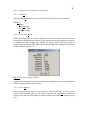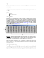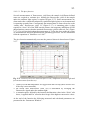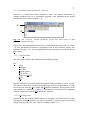
1
Hansatech
Instruments
Fluorescence Monitoring System
FMS 2
User Manual.
Hansatech Instruments Ltd.
Narborough Road, Pentney,
King’s Lynn, Norfolk, PE32 1JL,
England.
Tel: +44 (0)1760 338877 Fax: +44 (0)1760 337303
E-mail:[email protected]
Web Site:http://www.hansatech-instruments.com
Part Number: 900038
Issue Level: 1.01
Introduction.
The FMS 2 field-fluorescence monitoring system is a versatile pulse-modulated
instrument, designed to measure chlorophyll fluorescence emission from samples
engaged in photosynthesis under ambient light conditions in the field.
It consists of a control unit housing all of the electronics, optics and light sources. A
custom fibre optic interface module links the control unit to the sample which is
oriented in a leaf-clip.
The system may be operated in several different modes: serial connection to a
Windows PC enables real-time instrument control and data presentation. Captured
data is simultaneously presented as a real-time chart recorder emulation and parameters-only format for easy identification of key experimental events. This “PC” mode
of operation is suitable for development of complex protocols which may be programmed into the instrument using the simple “drag and drop” editor to generate
user-defined scripts. These scripts automate the execution of experiments, allowing
complex protocols involving many control events to be operated with the same ease
as single control event measurement such as Fv/Fm.
Once programmed, the FMS 2 can be used as a stand-alone fluorometer in either
laboratory or field situations, running off internal batteries with all measurement data
and calculated parameters saved to integral protected memory. The unit can store up
to six experimental protocols, any one of which may be accessed and executed using
the built-in menu system. When data collection is complete the FMS can be downloaded to the Windows software for full analysis in the laboratory.
This document aims to briefly cover the measurement principles used by FMS2,
optimum hardware configuration, system operation and data handling with the
“Modfluor” and “Parview” software packages. The document is separated into three
chapters:
n Chapter 1: Measurement principles and hardware.
n Chapter 2: Software installation, instrument operation and data handling.
n Chapter 3: Stand-alone instrument operation and data upload.
Chapter 1.
Measurement Principles,
FMS 2 Hardware.
Chapter 1.
Contents.
Page no:
1
1
2
1.0.
1.1.
1.2.
Introduction.
What is Chlorophyll Fluorescence?
How Does the FMS Measure Chlorophyll Fluorescence.
2.0.
2.1.
2.2.
2.3.
Hardware.
The Multi-Charger.
4
Inserting / Removing Batteries from the Control Unit.
6
Connections to the FMS 2 Control Unit.
7
2.3.1.
Electrical Connections.
7
2.3.2.
Optical Connections.
8
FMS Leaf-Clips.
9
2.4.1.
The PAR / Temperature Leaf-Clip.
9
2.4.2.
The Dark-Adaptation Leaf-Clip and Fibre-Optic Adapter.11
2.4.
Appendix A Hardware Maintenance.
Appendix B The External User Interface.
13
15
1.
1.0. Chlorophyll Fluorescence Measurement.
The FMS 2 is a powerful tool for photosynthesis research. However, to fully utilise
its functionality and achieve optimum performance it is important to appreciate the
measurements that FMS 2 is designed to make and some of the principles behind its
operation. The following introductory sections are only intended as a very limited
introduction to chlorophyll fluorescence measurement, more comprehensive
information can be found from the references cited in the text.
1.1. What is chlorophyll fluorescence?
When light energy is absorbed by a chlorophyll molecule the electronic configuration
of the molecule is temporarily altered. This “excited” configuration is inherently
unstable and short lived (typically less than 10-8 sec) as several processes compete to
dissipate the absorbed energy. In photosynthetic systems these processes can be
categorised into two groups:
Photochemical Processes:
These processes utilise absorbed energy for photochemistry, during which electron
donation from pigment to an acceptor molecule occurs. Such processes direct energy
for the chemical work involved in photosynthesis.
Non-Photochemical Processes:
These processes dissipate energy from the photosynthetic apparatus in a manner
which does not drive photosynthesis. Energy is usually re-emitted from the sample
in the form of infra-red radiation (heat) and red / far-red radiation which is known as
chlorophyll fluorescence.
The competition between these processes for absorbed energy ensures that a
reduction in the rate of one process will be associated with a corresponding increase
in the rates of competing processes e.g. a reduction in the dissipation of energy by
photochemistry will be reflected in an increase in energy dissipation by nonphotochemical processes such as heat production and chlorophyll fluorescence.
Consequently measurement of changes in the extent of fluorescence emission with
FMS 2 can be used to infer information about changes in the efficiency of light use
for photochemistry (Reviewed in Krause and Weis 1991 and Govindjee 1995)
Since the work of Emerson et al. (1932) it has been widely accepted that there are
two separate photochemical steps during photosynthesis which are associated with
different groups of pigments; these groups have become known as photosystem I and
photosystem II. In practice differences in the functionality of photosystem I and II
mean that at least 95% of the chlorophyll fluorescence signal observed under
physiological temperatures is derived from chlorophyll molecules associated with
photosystem II (PSII). Hence the fluorescence signal detected by FMS reflects
changes in the efficiency with which absorbed light is used for PSII photochemistry.
2.
1.2. How does the FMS measure chlorophyll fluorescence?
At physiological temperatures peak fluorescence emission occurs in the red region of
the spectrum ( 685 nm) and extends into the infra-red region to around 800 nm
(Krause and Weiss 1984) (Figure 1-1).
Fig. 1-1. Room temperature chlorophyll fluorescence emission spectra. (Adapted
from Krause and Weis 1984)
Accurate determination of fluorescence requires a detection system which is
sensitive to fluorescence wavelengths yet blind to the actinic (or excitation) light
which drives photochemistry. In continuous excitation instruments such as the Plant
Efficiency Analyser signal discrimination is achieved using a custom designed 650
nm actinic light source to drive photochemistry; optical filtering of the detector
prevents detection of non-fluorescence wavelengths of light. Unfortunately such
systems must be shielded from ambient light during use, otherwise the red / far-red
component of day-light will be super-imposed on the fluorescence signal.
This problem is avoided by the FMS 2 as it uses an electronic method, commonly
referred to as modulated fluorometry, to separate actinic light from the fluorescence
signal (Ögren and Baker 1985). During measurement the tissue sample is exposed to
a pulsed amber (or optional blue) LED light source (the modulating beam) which
induces a pulsed fluorescence signal from the sample under conditions where
ambient light is excluded (A, Figure 2). When ambient light is applied the optical
filtering of the FMS 2 allows three types of light signal to reach the detector:
·
•
•
ambient light of fluorescence wavelengths,
non-pulsed fluorescence signal induced by the ambient light,
and pulsed fluorescence signal induced by the modulating beam (B, Figure 1-2).
Addition of ambient light changes the physiology of the sample, altering the
proportion of energy that is re-emitted as fluorescence. Thus the magnitude of the
peaks of the pulsed fluorescence signal that are induced by the modulating beam will
reflect changes sample physiology. It is these signals that the rapid pulse peak
tracking electronics amplify and measure; ambient and non-pulsed fluorescence
signal are discarded (C, Figure 1-2).
3.
Fig. 1-2. Fluorescence signal detected by the FMS under modulating beam only
conditions (A), under actinic light plus modulating beam before (B) and after (C) the
rapid pulse peak tracking electronics.
The pulsed fluorescence that is induced by the modulation beam is effectively used
to probe the efficiency of light-use for photosystem II photochemistry. Clearly it is
important that the measuring technique itself does not induce changes in the
physiology of the sample under investigation.
Exposure of a sample to a powerful pulsed light source may be expected to introduce
a significant artifact into the measurement. However, FMS has been specifically
designed to avoid such problems by using a modulating beam of very short duration
pulses (1.8 µsec) with long off period between pulses. The net result is that the
integrated amount of radiation incident upon the sample from the modulating beam
is very small (<0.05 µmolm -2s-1), too small to induce significant physiological change
in the sample (Schreiber et al. 1986), yet powerful enough to provide a reliable signal
for fluorescence analysis.
The interpretation of fluorescence signals has developed considerably since the early
experiments of Kautsky and Hirsch (1931) with several techniques employed to
determine information about the photosynthetic performance of PSII (Baker 1991).
The FMS hardware and software has been designed to incorporate these techniques
into simple routines which store appropriate fluorescence measurements and
automatically calculate key parameters. The principles and procedures behind these
are discussed in relation to instrument control with the FMS Windows software and
scripting language (Chapter 2).
Several “non-specific” parameter functions have also been included. The aim of these
is to give sufficient flexibility to experiment and develop novel protocols. These are
also discussed in chapter 2.
4.
2.0. Hardware.
The FMS 2 is supplied with the following hardware components:
Control Unit:
Houses all of the electronics, optics and light sources. Power is provided from an
on-board inter-changeable lead acid battery.
Fibre-Optic Interface:
Connects the internal optics to the sample.
Leaf-Clips:
Used to hold the sample relative to the fibre-optic. The PAR / Temperature clip
allows simultaneous measurement of environmental conditions. Dark-adaptation
clips allow rapid screening of multiple samples.
Multi-battery charger:
Allows over-night charging of up to four instrument batteries simultaneously.
Discharged batteries may be swapped in a matter of seconds in the field.
15 V mains adapter
Powers the battery multi-charger or FMS control unit.
These components must be correctly assembled before the system can be operated.
The first step after un-packing should be to set up the battery multi-charger as the
lead-acid batteries will probably be discharged following shipment.
2.1. The Multi-Charger.
The FMS 2 is supplied with five lead-acid batteries which will probably need to be
charged before the system can be made operational. A maximum of four batteries
may be recharged simultaneously with the multi-charger unit.
The multi-charger should be placed in a flat, well ventilated area. Each battery inserts
into a “slot” with the black upper surface facing out and the metal terminals facing
forward to meet the charger contacts (Figure 1-3). The multi-charger has been
designed so that the battery terminals and charger contacts can only meet in one
orientation, so in normal use it should be virtually impossible to connect the battery
incorrectly.
The multi-charger can charge a maximum of four batteries
simultaneously. There is no problem operating the unit with less
than four batteries. Each battery “slot” is an independant
charging channel and there is no danger associated with
touching exposed contacts during operation.
5.
A
C
D
B
E
Fig. 1-3. The multi-charger unit (B) with batteries (A). Mains power is supplied from
the mains adapter unit (C) which plugs into the side socket of the charger unit (E).
The mains cable locates unit the front of the mains adapter unit (D)
Power is supplied to the multi-charger via the 15 V mains adapter. The 3-pin DIN
output plug should be connected to the socket that is mounted in the side of the
multi-charger (E, Figure 1-3). Mains power is connected through the mains cable
input in the front of the mains adapter (D, Figure 1-3).
After power-up the LED indicators on each of the charging channels will take several
seconds to settle and read the status of the batteries. The LED indicators will display
one of two possible states:
Red Light -
indicates a discharged battery drawing current at the maximum
regulated rate.
Green Light - indicates that the battery is at least 98 % fully charged. A trickle
current of 50 mA keeps the battery topped up until use.
After inserting discharged batteries it is good practice to watch
as the LED indicators switch to red to ensure that the batteries
are re-charging. Old or damaged batteries will not draw current
and thus the indicators may remain permanently green.
Fully discharged batteries will require approximately 8 hours to reach maximum
capacity. It is therefore advisable to run the charger over-night. Once the batteries are
charged the multi-charger may be switched off and the batteries removed.
6.
2.2. Inserting / Removing Batteries From the Control Unit .
One of the batteries may be placed in the base of the FMS 2 carrying bag; a second
should be inserted into the FMS 2 control unit. This is done by:
1. Orientating the battery at 45° to the battery compartment in the FMS 2 control
unit. The black-upper surface of the battery should face forward with terminals facing
into the battery slot,
2. Lift the battery compartment catch with the corner of the battery,
3. Push the corner of the battery into the slot, re-align and fully insert (Figure 1-4).
Fig. 1-4. Inserting the battery into the FMS2.
The spring loaded contacts inside the battery compartment will automatically make
contact with the battery terminals whilst the catch on the end of the compartment
should firmly hold the battery in position.
The control unit cannot be damaged by inserting the battery in
the wrong orientation as the battery terminals and control unit
contacts will not meet. However the instrument will not operate
until the battery is re-inserted correctly.
The rate of battery discharge during operation is determined principally by the use of
the halogen lamp. A high rate of pulsing or pro-longed use of high output actinic light
will drain the battery relatively quickly. The following estimates of battery capacity
and re-charge period should be considered when planning experiments:
Max. number of consecutive 85 unit, 0.7 sec pulses ≅ 800 pulses
Max. duration 50 unit actinic illumination ≅ 60 min
The electronics are designed to maintain constant light intensities throughout the
discharge period of the battery. Warning messages are generated when the battery
capacity reaches the threshold where this is no longer possible in both stand-alone
(Appendix B) and PC operation (Chapter 2). At this point it is recommended that the
instrument is switched off and a fresh battery installed.
7.
Battery removal in the field is simply a matter of switching the instrument off, lifting
the catch on the battery compartment and tilting the control unit until the battery
slides out. The instrument memory is protected by an internal capacitor. As a result
data should not be lost even after several days without a battery.
It is always good practice to upload data to a PC at the end of
each day. This allows multiple copies of the data to be generated
for back-up purposes.
2.3. Connections to the FMS 2 Control Unit.
Once a fully charged battery has been inserted, the control unit can be placed in its
carrying bag. A number of electrical and optical connections should be made to the
control unit before operation.
2.3.1. Electrical Connections.
The following electrical connections can be made to ports in the right-hand side panel
of the FMS 2 control unit (Figure 1-5). It should be noted that for field-portable
operation without a PC the instrument may be operated without connection to these
sockets.
A
B
C
D
E
Fig. 1-5. The right side panel of FMS2 contains the power switch (A), Fuse (B),
“User Interface (C), Serial I/O (D) and DC input socket (E).
Serial I/O socket (D) -
Must be connected to a PC COMM port via the serial
cable for computer controlled operation or data upload.
Not required for “Local mode” use without a PC.
DC Inputs socket (E) Available for connection of external DC power supplies
such as:
12 V external battery via optional battery cable,
12 V output from optional mains adapter,
15 V mains adapter for re-charging the on-board battery
without multi-charger.
User Interface socket (C) - Provides access to four digital and one digital to
analogue control line for optional control over external
devices (Chapter 2).
8.
2.3.2. Optical Connections.
The control unit houses the light sources and detector which must be optically linked
to the sample under investigation. This is achieved via a custom fibre-optic which
locates onto the front of the control unit via the optic interface module.
When the instrument is first unpacked the interface module should be covered by a
blanking plate which protects the optics in transit. The plate is removed by carefully
pulling it from the control unit. The fibre-optic cable is correctly positioned on the
optic interface module by inserting the small key-way block of the fibre-optic
termination (A, Figure 1-6) into the corresponding groove in the optic interface
module (B, Figure 1-6). The cable is secured by carefully threading the collar which
surrounds the fibre-optic termination onto the optic interface module until it is
hand-tight (D, Figure 1-6). This procedure ensures that the light guides within the
fibre-optic are automatically aligned with the appropriate light source or detector
within the control unit.
A
D
C
E
B
Fig. 1-6. A small key-way (A) on the end of the fibre-optic (E) locates into a
complimentary groove (B) in the optics interface module of the FMS control unit (C).
The fibre-optic is secured by gently threading the ferrule surrounding the fibre (D)
clockwise onto the thread of the optics interface.
The fibre optic cable is designed to be as rugged as possible.
However its core is made of thousands of individual glass fibres
which can break if the cable is dropped or flexed through tight
angles. Damage to the cable will significantly impair the
performance of FMS.
9.
Finally the sample end of the fibre-optic should be positioned close enough to the
tissue under investigation to detect a strong signal. Typically it will have to be within
1.5 cm of the tissue, usually orientated in a manner which minimises fibre-induced
shading. A pair of leaf-clip systems are available for this purpose.
2.4. FMS Leaf-Clips.
2.4.1. The PAR / temperature leaf-clip.
The PAR / temperature leaf-clip is designed for measurements made under ambient
light conditions. It consists of a sprung upper section which gently grips the tissue in
a gentle clamping action (C, Figure 1-7A). A grooved neck mounted at 60° to the
plane of the sample (B, Figure 1-7A) accommodates the fibre-optic (A, Figure 1-7A)
which is slid into position. Marked graduations on the neck can be aligned with
graduations on the fibre-optic termination to reference its position for future work, a
retaining screw (B, Figure 1-7A) locks it into position throughout the experiment.
The rest of the fibre may be looped over the leaf-clip and hooked to the rear of the
clip to help support its weight.
An electrical connection to the “Leaf-clip” socket on the front panel of the control
unit enables use of the remote trigger switch (F, Figure 1-7A) to activate / abort
measurements in “Local” mode (Chapter 3) and connect on-board thermocouple and
light sensor (C, Figure 1-7A) to the control unit. The leaf-clip may be held in the hand
if multiple samples are being studied or mounted on a standard tripod mount (E,
Figure 1-7A) via a thread in the lower clip section for fixed-position work.
A
F
B
C
D
E
Fig. 1-7A. A broad leaf sample under investigation in the PAR / temperature
leaf-clip. The fibre-optic (A) is retained in the grooved neck by a screw (B) whilst the
sample (D) is gripped between the upper and lower clip sections. Simultaneous
measurements of ambient light are made with the co-sine corrected PAR sensor (C)
and sample temperature monitored by a thermocouple in contact with the underside
of the sample at (D). The leaf-clip is supported by a tripod mount (E) and
measurements initiated with the remote trigger button (F).
10.
The PAR sensor has been designed for both recording of ambient light intensities
during fluorescence analysis and measurement of FMS actinic and saturating light
sources during instrument set-up. It may be mounted in one of two positions on the
leaf-clip:
Upper side mount
Lower front mount
- prevents shading by broad leaf samples, suitable for
ambient light measurement during analysis (Figure 1-7A).
- suitable for ambient light measurement during analysis of
narrow leaves which do not shade the sensor (Figure 1-7B).
- aligns sensor level with sample for calibration of fibre-optic
light output when upper section slid forward (see below).
A
B
Fig. 1-7B. The PAR sensor (A) located in the cup on the lower section of the clip. This
position is suitable for actinic light calibration (described below) or simultaneous
PAR monitoring during analysis of narrow samples (B) which do not cover the sensor
in this position.
Prior to commencing an experiment it is often useful to measure the output of the
saturating lamp and reference the intensities of actinic light settings that are to be
used. In order to do this the fibre-optic and PAR sensor must be placed in the same
geometry and distance that the sample and fibre would occupy during fluorescence
analysis. This can be achieved simply by gently sliding the upper section of the clip
down and forward through its full range of travel so that the PAR sensor is under the
fibre’s field of view. The various light-sources can then be activated and readings
noted from the software display. When light calibration is complete the upper section
should be pushed down and back over the full range of travel to return the fibre to its
measurement position.
Sample temperature is also monitored simultaneously with PAR and fluorescence. A
thermocouple which stands slightly proud of the lower section is designed to
maintain contact with the lower surface of the sample.
It is important to note that the thermocouple is proud of the
lower leaf-clip section. Therefore care should be taken to avoid
snagging the thermocouple when samples are being inserted or
removed.
11.
2.4.2. The Dark-Adaptation Leaf-Clip and Fibre-Optic Adapter.
A separate leaf-clip system has been developed for situations where ambient light is
to be excluded from the sample during measurement. This is suitable for experiments
requiring dark-adapted measurements e.g. screening applications measuring Fv/Fm
or situations which require adaptation of tissue to standardised doses of actinic light.
The first step in the process is to attach the fibre-optic adapter (Figure 1-8) to the
sample end of the fiber optic. This is done by sliding the fibre-optic (A, Figure 1-8)
into the adapter mounting collar (B, Figure 1-8) and securing it in position by
tightening the side mounted retaining screw (C, Figure 1-8). The adapter / fibre-optic
assembly can then be sealed into the top of the dark-adaptation clip (D, Figure 1-8)
and the position of the fibre-optic fine-tuned by unthreading the retaining screw in
the adapter collar and sliding the fibre-optic into the desired position before locking
it by re-tightening the collar screw.
A
B C
F
D
E
Fig. 1-8. The dark-adaptation leaf-clip and fibre-optic adapter. The fibre-optic (A) is
held in the adapter mounting collar (B) by the side-mounted retaining screw (C). The
adapter / fibre combination locate onto a dark-adaptation clip (D). The sample (E)
is supported on a foam pad and exposed to the FMS when the sliding shutter (F) is
opened.
The geometry of the fibre-optic will determine how evenly the
sample will be illuminated and the strength of fluorescence
signal received. It maybe useful to make several trial
measurements with sample in order to optimise the system for
each particular application.
When the fibre-optic has been locked into position the dark-adaptation clip can be
removed and clipped into the experimental sample. The tissue is dark-adapted by
sliding the shutter plate forward (F, Figure 1-8). After a suitable period the tissue
should be dark-adapted and ready for measurement. The adapter / fibre-optic
assembly can then be sealed over the dark-adaptation clip and the shutter blade
opened to expose the tissue to the FMS. The adapter ensures that the sample is
completely shielded from ambient light throughout the measurement.
12.
In rapid screening measurements it may be more efficient to
dark-adapt a number of samples simultaneously with several
clips. Repetitive measurements can then be made by moving the
fibre-optic from clip to clip.
13.
Appendix A.
Hardware Maintenance.
The hardware is designed with a minimum of consumable components. The most
likely components to require attention are the halogen lamp, battery and fuses. This
section details the procedures to replace both of these items.
Bulb Replacement.
The halogen lamp is an OSRAM 64255 8 V, 25 W unit. The following steps should
be followed during replacement:
1.
2.
3.
4.
5.
6.
7.
8.
Switch off the instrument and allow several minutes for the lamp to cool down.
Place the instrument on its end, battery compartment facing up. Remove the
four screws and washers that retain the instrument side panel and remove the
panel.
Use a screw-driver to gently prise off the connection to the lamp base (A).
Locate the bulb near the front of the unit (B).
Un-clip each of the wire bulb-retainers (D).
Unscrew the knurled lamp support pillar and remove (C).
Remove bulb.
Re-insert new bulb being careful to avoid touching the lamp envelope or inside
of the reflector. It is a wise idea to wear rubber gloves to avoid depositing
grease on the lamp. Holding the lamp in position, re-insert removable support
pillar and tighten.
C
D
B
A
9.
10.
Adjust lamp so it is correctly seated and fix into position with the wire retainers.
Push electrical connector on to the base of the lamp. Polarity is not important.
14.
Fuse Replacement.
The instrument is protected by two fuses. An external fuse is located beneath the “On
/ Off” switch on the right-hand side panel. This protects the instrument from external
12 V supplies, such as car batteries, that have been connected through the “DC input”
socket. If this fuse fails the external battery and associated wiring to the “DC input”
socket should be checked before replacement. The fuse is replaced using a flat blade
screw driver to open the fuse cover by pushing in and gently turning anti-clockwise.
The old fuse should be replaced with a 3.15 A anti-surge fuse.
An internal fuse protects the circuitry from the on-board power supply and mains
adapter connection to the 12 V “DC input” socket. The fuse is accessed by removing
the right-hand side panel (panel with “On /Off” switch) with a screw driver. The fuse
is located under a label in the black acetal battery block at the bottom of the control
unit. It can be gently levered out with a flat blade screw-driver and replaced with a
2.5 A anti-surge fuse.
A blown fuse may be a symptom of a more serious fault with the
instrument. Hansatech Instruments Ltd should be contacted if
a replacement fuse blows within a short period of time.
15.
Appendix B.
The External User Interface.
Measurements with the FMS 2 can be triggered from external devices via one of four
digital control lines which are connected to the User Interface Socket of FMS (B,
Figure 1-5). The Digital IN connections are presented below:
Channel Number:
0
1
2
3
Ground
Pin Connection:
4
5
6
7
3 and 11
The FMS 2 may also be used to trigger measurements using the Digital OUT
connections:
Channel Number:
0
1
2
3
Ground
Pin Connection:
12
13
14
15
3 and 11
Analogue output channel connections are:
Analogue Output
Analogue Ground
Pin Connection:
10
2
Chapter 2.
Software Installation,
System Operation,
Data Handling.
Chapter 2.
Contents.
Page no:
1
1
2
2
1.0.
1.1.
1.2.
1.3.
FMS Software.
Installing FMS Software.
Executing “Modfluor” and “Parview”.
Troubleshooting Communications Problems.
2.0.
2.1.
2.2.
2.3.
2.4.
Operating the FMS.
3
“PC Mode” Operation Under “Modfluor”.
3
The Recording Screen.
3
Testing the FMS.
5
“Drop-Down” Menu Functions.
8
2.4.1.
Configuration of Hardware and Software.
9
2.4.1.1.
Hardware.
9
2.4.1.2.
Instrument Status.
9
2.4.1.3.
Clear Memory.
9
2.4.1.4.
Set Time / Date.
10
2.4.1.5.
Config Settings.
10
2.4.2.
View Functions.
11
2.4.3.
Graph Functions.
12
2.4.3.1.
Clear.
12
2.4.3.2.
Autoscale.
13
2.4.3.3.
Zoom.
13
2.4.3.4.
Set Axis.
13
2.4.4.
Tools.
14
2.4.4.1.
Tabulate.
14
2.4.4.2.
Event Marker Colour.
14
2.4.5.
Data Handling and Export.
15
2.4.5.1.
File Management with the Files Menu.
15
2.4.5.1.1.
Save Data.
16
2.4.5.1.2.
Load Data.
17
2.4.5.1.3.
Text Search.
17
2.4.5.2.
Exporting Data to Other Windows Applications. 18
2.4.5.2.1.
Params to Clipboard and Params to ASCII. 18
2.4.5.2.2.
Data to Clipoard and Data to ASCII.
20
2.4.5.3.
Printing.
22
Instrument Programming Via User-Defined Scripts.
23
2.5.1.
The Script Recorder.
23
2.5.2.
Running a Script Under Windows.
24
2.5.3.
The Script Editor.
25
2.5.3.1.
Creating an Example Script.
26
2.5.3.2.
Script Editor “Drop-Down” Menu.
30
2.5.3.2.1.
Edit.
30
2.5.3.2.2.
Files.
31
2.5.3.2.3.
Download.
31
The Instrument Toolbar.
32
2.6.1.
Recording Functions.
32
2.5.
2.6.
2.6.2.
Light Source Controls.
33
2.6.2.1.
The Modulating Beam.
33
2.6.2.2.
The Actinic Light Source.
33
2.6.2.3.
The Saturating Light Source.
34
2.6.2.4.
The Far-Red Light Source.
34
2.6.3.
Measurement Functions.
34
2.6.3.1.
Dark-Adapted Measurement Routines.
34
2.6.3.1.1.
Fo (fluorescence origin).
35
2.6.3.1.2.
Fm (fluorescence maximum)
35
2.6.3.1.3.
Fv/Fm (maximum quantum efficiency of
PSII)
35
2.6.3.2.
Light-Adapted Measurement Routines.
36
2.6.3.2.1.
The PSII Function.
37
2.6.3.2.2.
The PSIIR Function.
38
2.6.3.2.3.
The Fs Function.
40
2.6.3.2.4.
The Fo’ Function.
40
2.6.3.2.5.
Logging PAR and Temperature.
40
2.6.4.
External Device Interface and Event Markers.
40
2.6.4.1.
External Control Interface.
40
2.6.4.2.
Event Markers.
41
Appendix A Hansatech Scripting Language Elements.
42
1.
1.0. FMS Software.
The FMS is supplied with two Windows software applications:
“Modfluor32” - Instrument control and trace data presentation program.
“Parview”
- Parameter data upload and viewer program.
All of the software and on-line help documents are supplied on CD ROM. The CD
also contains reference lists and links through to the Hansatech Instruments web site
where updated versions of software may be downloaded as and when they are released.
1.1. Installing FMS Software.
The installation is launched from the Install button on the CD opening splash screen.
Follow the on-screen prompts in order to install Modfluor32 and Parview on your PC.
The installation automatically sets up a program group called “Hansatech
Instruments”. This contains a sub directory with icons for running both the
“Modfluor” and “Parview” applications, an “Uninstall” program and links to the help
documentation.
Please note that the FMS software is a 32 bit Windows®
program. Therefore, this software is not compatible with PC’s
running Win 3.1.
1.2. Executing “Modfluor” and “Parview”.
Both programs may be run without connection to the FMS. However in most
circumstances they will be used to communicate with the control unit. The RS232
serial cable must be connected from either COMM 1 or COMM 2 serial port on the
PC to the “Serial I/O” port on the FMS, the control unit should be switched on and
“PC” button pressed to select the “PC-mode” of operation (Chapter 2, Section 2.1).
If you are using the system with the HAN/USB USB - RS232 adapter, ensure that
you have correctly installed the drivers for the adapter and that the adapter is securely
connected to an available USB port on the PC.
During initialisation the software tests the communications link. If the software is
unable to communicate a prompt box will be generated requesting to use
“demonstration mode” or a re-test.
2.
Most commonly communications problems occur because the control unit is not
switched on or set to “PC-mode”. However if anything other than COMM 1 is being
used, the command line for the program will need to be changed. This is done by
closing the program, selecting the appropriate icon with a right mouse click and select
Properties from the menu. The command line will need to be changed from:
C:\Program Files\Hansatech Instruments\FMS\Modfl32.exe
to:
C:\Program Files\Hansatech Instruments\FMS\Modfl32.exe /x
(where x is the port number that the FMS is connected to. Please note that the space
between the modfl32.exe and /x is required)
The program should then be re-started.
Please note that the process described above is also true of Parview.
1.3. Troubleshooting Communications Problems.
The default communications between the PC and the FMS are set through COMM 1
at 38,400 baud rate. Some older serial port chip-sets may not be able to cope with this
speed of data transfer, resulting in communications problems or file uploading
problems.
The following procedure should be followed to troubleshoot such communications
issues:
1. Check the serial cable connection to both the PC and the FMS control unit.
2. Check that the /x is entered into the command line if anything other than COMM
1 is being used (Section 1.2.).
3. Adjust the baud setting of the FMS control unit. This is achieved by switching off
the control unit and keeping the lower control key on the display panel de-pressed
whilst it is switched on. As the instrument boots-up a menu will display the new
baud setting of 19,200 baud. The procedure may be repeated to switch to 9,600
baud or repeated again to loop forward to 38,400 baud.
4. Once a baud rate has been selected it will be retained in memory by the control
unit and used each time the instrument is switched on.
5. The “Modfluor” and “Parview” software should be re-booted if the baud setting
is changed. Both programs automatically detect, and switch to the appropriate
baud setting during initialisation.
Use of a slower communications rate will not impair the real-time data acquisition
performance of the FMS. However data upload of multiple files from instrument
memory will take longer.
3.
2.0. Operating the FMS.
The FMS is designed to accommodate two different operating modes:
• “PC mode” -
the control unit is serially linked to the PC with commands
issued from “Modfluor” under “real-time” control from the PC
keyboard
• “Local mode” - (Chapter 3) the control unit is used autonomously with
measurement commands issued via pre-loaded scripts accessed
via the four-button keyboard on the control unit display panel.
When the instrument is first used it will only contain two default scripts for
measurement of Fv/Fm and PSII. It is therefore sensible to use “PC mode” to test the
system and generate further scripts which are more suited to individual applications.
“Local mode” operation is discussed in chapter 3.
2.1. “PC Mode” Operation Under Modfluor.
Once the “Modfluor” program has successfully communicated with the control unit,
it loads the data recording screen.
2.2. The Recording Screen.
The default recording screen which is generated when the software is first initialised
consists of four areas:
•
•
•
•
the data recording area (A, Figure 2-1),
instrument monitor bar (B, Figure 2-1),
“drop-down” menu bar (C, Figure 2-1),
instrument tool bar (D, Figure 2-1).
C
D
A
B
Fig. 2-1. The data recording screen contains the data recording area (A), instrument
monitoring bar (B), “drop-down” menu bar (C) and instrument toolbar (D).
4.
The data recording area is a graphic display area where acquired fluorescence data
expressed as output from the analogue to digital (A/D) converter in bits (Y-axis) is
plotted against time (X-axis) to give a “real-time” chart recorder emulation. Both
axes may be scaled either automatically to display all data or manually to zoom
regions of particular interest via the Graph function in the “drop-down” menu
(Section 2.4.3.). The maximum range of the A/D converter is 4095 bits; the plot area
above this value is greyed-out to indicate that any output above 4095 bits is overscale (Section 2.3.).
Automatic scrolling of the plot ensures that data collection is continuous up to a
maximum length of approximately 50 minutes. The PAUSE button in the instrument
toolbar may be used to suspend data collection, operating as the computer equivalent
of lifting the pens off a chart recording. If this function is used to limit data logging
to specific periods of interest much longer experimental protocols may be run.
Data is digitally displayed throughout the experiment on the instrument monitoring
bar (B, Figure 2-1). Fluorescence information is continuously up-dated even when
the PAUSE function is used to suspend data logging, allowing estimation of steady
state fluorescence prior to resumption of logging during a measurement. Data from
external devices such as the PAR and temperature leaf-clip are also presented on the
monitoring bar along with information relating to the status of digital control lines.
In the event that external devices are not being used it is possible to switch off the
monitoring bar via a toggle switch in the View function of the “drop-down” menu bar
(Section 2.4.2.).
Software configuration, file handing and instrument programming facilities are
grouped according to function on the “drop-down” menu. They are accessed via the
mouse or accelerator keys.
Example:
Files
Script
Hardware
Graph
Tools
View
Help
Graph functions are opened by pressing ALT G together.
When a group is selected a sub-menu of related functions is opened. The required
function can be selected with accelerator keys (Key) or by moving the blue-highlight
with UP and DOWN cursor keys to the desired function and pressing RETURN.
Navigation to other the sub-menus is achieved with LEFT and RIGHT cursor keys or
mouse. Specific details of each of the menu function are given in section 2.4.
Direct control of FMS light sources and FMS measurement operation is made
through the instrument tool bar (D, Figure 2-1). Light sources are activated by
clicking in the appropriate toggle button with the left hand mouse button. The
modulation beam, actinic and far-red light sources remain illuminated (indicated by
an indented button) button until their respective buttons are re-pressed. The extent of
actinic illumination is determined by the numeric value (0 to 50) in the edit box
located next to the “Actinic” button (Section 2.6.2.2.).
Changes in the actinic output level only take effect when the
actinic source is initialised. The actinic light must be toggled off
and then on to effect an intensity change (Section 2.6.2.2.).
5.
The saturation-pulse is activated each time the “Pulse” button is pressed. The button
remains indented during pulse application and automatically re-sets upon
termination. Both pulse intensity (0 - 100) and duration (0.3 - 5.0 sec) are set from
accompanying edit boxes on the toolbar (Section 2.6.2.3.).
Measurement functions are only available whilst the FMS is recording. A fresh
recording is started by pressing the “Record” button. This automatically triggers the
modulation beam which is essential for fluorescence detection and disables menu
functions that should be kept constant during the recording e.g. instrument
configuration settings. Common fluorescence parameters may be logged via the
various parameter buttons located on the instrument toolbar. Detailed descriptions of
each measurement function are given in section 2.6.3.. The digital values of each
parameter are written to a “Parameter Window” within the software. Under default
settings the “Parameter Window” is not displayed to save screen space. However the
software display may be customised to suit individual requirements via the View
function in the “drop-down” menus (Section 2.4.2.).
Throughout the recording period individual FMS-driven illumination events are
marked by arrows to mark light on and arrows to mark light off events. User
events such as herbicide treatment etc. may be marked using the buttons on the
instrument toolbar (Section 2.6.4.). All markers tag corresponding data in the
tabulated data output from FMS by colour-coding data for easy reference (Section
2.4.4.2.).
The next stage in operating the FMS is to test the system with spare sample and
configure the instrument to achieve optimum performance.
2.3. Testing the FMS.
Before running an experiment several functional aspects of the instrument should be
checked:
• the signal is sufficiently strong to be acceptable,
• the modulation beam does not change the physiology of the sample,
• the saturation pulse is sufficiently powerful to saturate the sample,
• and the maximum fluorescence yield is within the range of the instrument.
The following section briefly describes two experiments which can be run to verify
each of these aspects on spare sample tissue.
1.
2.
Dark-adapt a piece of spare experimental tissue using the dark-adaptation clip
or by covering the sample in the PAR / temperature clip.
Start a new recording by pressing the “Record” button on the instrument
toolbar. The dark-adapted fluorescence yield should plot across the data
recording area. This is the minimum fluorescence signal from the sample and
should be within the range of 10 - 700 bits for reliable measurement. If the
signal is too small the test recording should be stopped (re-press the “Record”
button) and the sensitivity of the instrument adjusted by increasing gain
(Section 2.4.1.5.) or by moving the fire optic closer to the sample. If the signal
is too great (>700 bits) the instrument will probably over-scale when the
saturating pulse is used. Instrument gain should be reduced. This effect can
also be achieved by moving the fibre-optic away from the sample.
6.
It is also important to check that the signal recorded in the experiment above remains
constant. In the example below (Figure 2-2.) the dark-adapted fluorescence signal is
around 500 bits (suitable for further measurement) but gradually increases with time.
This indicates that the modulation beam setting is too high and that it is inducing a
physiological effect on the sample. The most common symptom is a gradual rise in
the fluorescence signal known as “variable” fluorescence which occurs as the
modulating beam drives a significant amount of photochemistry (Section 2.6.3.1.1.).
Variable
Fluorescence
Fig. 2-2. The sample in this experiment is maintained in the dark under the
modulation beam. The gradual rise in the fluorescence signal is attributable to the
modulation beam driving significant PSII photochemistry. This increase in
fluorescence is known as variable fluorescence.
This phenomena will cause an error in the estimation of several commonly referenced
fluorescence parameters (Section 2.6.3.1.1.). Corrective action requires a reduction
in the frequency of the modulating beam by using a lower modulating beam setting
(Section 2.4.1.5.) or a reduction in modulation intensity by increasing the distance
between the sample and fibre optic.
It is also important to check that the instrument is correctly configured to record the
maximum level of fluorescence when the saturation lamp is used. This may achieved
with the following short experiment:
1.
2.
3.
4.
Dark-adapt a second piece of spare tissue for a minute of two.
Press the “Record” button to start a fresh recording.
Set the “Pulse” intensity to medium value in the edit box (e.g. 50 units) and
initiate a pulse by pressing the “Pulse” button. After a further 30 seconds
increase the pulse intensity by 10 units and pulse. Repeat this procedure
incrementing the pulse intensity up to 100 units.
After the final pulse stop the recording and autoscale the trace (under the
Graph function in the “drop-down” menu).
7.
A typical trace from this test on a healthy leaf is shown below (Figure 2-3).
Fig. 2-3. Fluorescence trace from a healthy leaf sample. Initially the sample is
adapted to the modulating beam and then subjected to pulses of increasing intensity
to determine the correct setting to achieve light saturation of PSII.
The maximum fluorescence yield from the sample is generated by application of a
saturating pulse of light (Section 2.6.3.1.2.). In this test several pulses are applied
whilst the power of the saturating lamp is incremented between pulses. The resulting
trace contains six fluorescence peaks (Figure 2-3) which correspond to pulses of 50,
60, 70, 80, 90 and 100 units respectively. The gradual increase in the magnitude of
the pulsed fluorescence signal up to the 80 unit pulse indicates that a pulse intensity
smaller than 80 units is not powerful enough to saturate PSII. Consequently the pulse
intensity should be set to 80 units to ensure accurate measurement of Fm and PSII.
A second important function of the light pulses is to check that the maximum
fluorescence signal is within the detection range of the instrument. The A/D works
over the range 0 - 4095 bits. Any signal below zero or above 4095 will appear as a
flat line at the bottom or top of the data recording area. The electronics of the FMS
are designed to prevent a negative signal. However if the fibre-optic is oriented close
to the sample it is possible that the detected signal will exceed 4095 bits and border
the greyed-out area of the recording area. An example trace is shown in figure 2-4.
8.
Fig. 2-4. During the saturation pulse (marked by the arrows) the fluorescence signal
exceeds the range of the A/D converter. The peak of the pulse is cut from the trace
but sampled (incorrectly) as 4095 bits by the software.
The peak fluorescence signal is effectively cut from the recording. This situation may
be corrected by reducing instrument gain (Section 2.4.1.5.) or re-orienting the
fibre-optic further away from the sample. If left un-corrected erroneous
measurements of Fm and PSII will be stored when measurements are made.
As referenced above, all of the FMS configuration and data management facilities are
accessed from the “drop-down” menu (C, Figure 2-1) whilst execution of
measurements and on-line control of instrument light sources is initiated via the
instrument toolbar (D, Figure 2-1). The following sections detail the configuration
and data management facilities available from the “drop-down” menu. Description
of each item on the instrument toolbar is given in Section 2.6.
2.4. “Drop-Down” Menu Functions.
The “drop-down” menu contains seven groups of related functions under the
following headings:
Files
Script
Hardware
Graph
Tools
View
Help
In this section the groups are described in three broad catagories:
• Configuration of hardware & software
(Hardware, Graph, Tools and View)
• Data Handling & Export
(Files)
• Instrument Programming via User-Defined (Script)
Scripts
9.
2.4.1. Configuration of Hardware and Software.
2.4.1.1. Hardware.
When the Hardware menu is selected the following sub-menus are presented:
Hardware
Status
Clear memory
Set Time / Date
Config settings
2.4.1.2. Instrument Status.
Before operating FMS in a remote situation it is useful to know what user-defined
script files are loaded into the memory of the instrument, how much memory capacity
is available for data storage and whether the battery holds sufficient charge to
complete the experiment. The status command interrogates the instrument to generate
a status window (Figure 2-5).
Fig. 2-5. Instrument Status Display.
Appropriate action can then be taken using other commands to prepare the instrument
such as clearing memory for new data.
2.4.1.3. Clear memory.
Before initiating a new series of experiments it may be necessary to clear old files
from the FMS to make space for new data. In this case the clear memory should be
selected. The software will prompt to establish which files should be deleted (Figure
2-6).
10.
Fig. 2-6. Delete files selection prompt.
The software will delete from the file number entered by the user to the end of the
memory space. If file number 5 is entered into the above prompt box (Figure 2-7),
files 5 through 10 (inclusive) will be deleted (Figure 2-7).
Fig. 2-7. File deletion prompt indicating that files 5 through 10 (inclusive) will be
deleted.
2.4.1.4. Set Time / Date.
The FMS has an on-board timing chip which can be used to log when experiments
are executed in “Local” mode. The Set Time / Date hardware function allows the
information within this chip to be up-dated. The software will initially prompt to set
the FMS clock to match that of the PC. If this is not acceptable the user can manually
enter the appropriate information into the time / date prompt box that is generated
(Figure 2-8).
Fig. 2-8. Insert time / date prompt box.
2.4.1.5. Config settings.
The Config settings sub-menu contains information on the current modulation beam
setting and amplification (gain) settings used by the instrument (Figure 2-9).
11.
Fig. 2-9. Hardware configuration settings menu with modulation intensity setting of
3 (maximum) and 50 % gain applied to the signal.
Default settings which should provide acceptable performance in most circumstances
(Figure 2-9) are automatically loaded when the software is first executed. It is
recommended that the tests described in section 2.3. are carried out before any
experiments in order to verify that the settings are suitable. Adjustments to the
settings are written to the MODFLUOR.INI file when the program is exited and
re-applied when the program is next operated.
Once the instrument has been configured it is useful to set the software for a clear
display of the data as it is acquired. These options are located under the View menu.
2.4.2. View Functions.
When the program is first run the default screen displays both the instrument
monitoring bar (B, Figure 2-1) and instrument toolbar (D, Figure 2-1); the rest of the
screen is devoted to the data recording area. At the of end experiment when recording
is finished the instrument monitoring bar is no longer required. The View menu
allows the each of these items to be de-activated individually. The tick mark next an
item indicates that it is displayed; de-activation is achieved by clicking on the item to
remove the tick mark.
View
√ Toolbar
√ Monitoring bar
Parameters window
The parameters window is also activated from the View menu. This is a separate
window used to log fluorescence parameters as their measurement is initiated from
the instrument toolbar. The window may be dragged to any convenient position on
the display and re-sized by stretching the box (Figure 2-10). Unwanted parameters
may be removed by high-lighting with the mouse and pressing the “Delete” key.
12.
Fig. 2-10. “Parameters Window”.
A scroll bar allows data browsing in the event that the list of data exceeds the
dimensions of the window (Figure 2-10). All of the parameters in the window are
available for export using the Params to clipboard function (Section 2.4.5.2.1.) in the
Files menu (Section 2.4.5.1.) to copy the data into the Windows® clipboard for
pasting into another Windows® package. Each of the parameters measured by FMS
is defined in section 2.6.3.
2.4.3. Graph Functions.
Initial data recording screen settings are designed to display to the full fluorescence
detection range of the instrument on time-base of 0 to 2 min. Data from experiments
that exceed this time-base is automatically scrolled during recording so that some of
the data is off-screen. The Graph menu contains several commands which may be
operated either during or post recording to clarify the chart-recorder emulation and
remove unwanted data from the display.
Graph
Clear
Autoscale
Zoom
Set axis
2.4.3.1. Clear.
The Clear command can be used to remove all data from the recording screen and the
parameters window (Section 2.4.2.). It is important to note that such data is not
retrievable unless it has been saved to a data file on floppy or hard drive (Section
2.4.5.1.). A prompt is generated to remind the user each time the command is used
(Figure 2-11).
13.
Fig. 2-11. Clear trace prompt.
2.4.3.2. Autoscale.
The Autoscale function re-sets both fluorescence and time axis to accommodate all
of the currently recorded data on a single screen. It may be used at any time after a
recording to “un-scroll” the chart-recorder emulation.
2.4.3.3. Zoom.
After selecting the zoom function the mouse cursor should be moved to the area of
interest in the data recording area. The left mouse button should be held down whilst
the area to be zoomed is defined by dragging the cursor across the data recording
area. A box is generated to outline the area of the zoom before it is enlarged to fill the
data recording area.
2.4.3.4. Set Axis.
Manual control over axis setting and other plotting attributes are accessed via the Set
axis sub-menu (Figure 2-12).
Fig. 2-12. Axis settings menu. The fluorescence axis set over the range 0 to 5000 bits
with recording from time zero to 5 min. A solid trace is selected with 10 gridlines per
axis.
The on-screen ranges for both axes are set by entering “Start” and “End” points for
each data range on the appropriate axis “edit” boxes, allowing a user-defined degree
of trace zoom. Other display attributes include control over the background grid and
whether data is plotted as individual data points or a solid trace chart-emulation.
The short duration of pulses means that there are a relatively
small number of plotted data points during each pulse. When
individual data points are plotted it may be difficult to visualise
the pulse without zooming the trace.
14.
The individual data points which make up the recording may be accessed from the
Tools menu.
2.4.4. Tools.
The Tools menu contains items which relate to the raw data output from the A/D
converter.
Tools
Tabulate
Event marker colour
2.4.4.1. Tabulate.
Raw data can be presented during, or after recording in tabulated form by selecting
the Tabulate function. The bit values of each data point are presented in rows of ten
data points (A, Figure 2-13) against time (B, Figure 2-13) with a scroll bar to allow
movement throughout the trace. Data is exported for pasting into other Windows
packages with the Data to clipboard function (Section 2.4.5.2.2.) which is located
under the Files menu (Section 2.4.5.1.).
C
B
A
Fig. 2-13. Tabulated output of data collected from the A/D converter. Data is
presented in rows of 10 data points (A) with the time of the first point at the start of
each line (B). Event-marked data are colour-coded for easy reference (C).
Data points which correspond to trace event marks are tagged with colour-coded
labels (C, Figure 2-13). The colours associated with each type of event marker can be
defined by the user.
2.4.4.2. Event marker colour.
The addition and removal of FMS light sources to the sample is event marked on the
data recording screen with a different coloured arrow for actinic, pulse and far-red
light sources. The default colours and data tags (in the tabulated output) for these are
15.
yellow, white and red respectively with blue
reserved for user-applied event markers. The
colour of each type of marker can be specified by
selecting the appropriate marker type from the
sub-menu presented and double-clicking on the
required colour from the palette that is generated
and selecting OK (Figure 2-14).
Fig. 2-14. Paint Palette used for definition of
event marker colour.
The final colour settings in place when the
program is shut-down will automatically be
saved to the MODFLUOR.INI file to become
default values when the FMS is next is used.
2.4.5. Data Handling and Export.
Once an experiment has been completed the data recording area should contain a
trace with associated parameters stored in the “Parameters Window” (Section 2.4.2.).
It is important to store this information to disc and to be able to retrieve previous
work.
2.4.5.1. File Management With the Files Menu.
The Files menu contains the following functions. Many of which are common to any
computer package.
Files
Save data
Load data
Upload to screen
Upload to file
Text search
Params to clipboard
Params to ASCII
Data to clipboard
Data to ASCII
Print graph
Print params
Set printer page
Exit
16.
In the case of FMS, “Modfluor” is used to transfer trace data which has been stored
to the control unit’s on-board memory (Upload to screen, Upload to file). These
functions are discussed in relation to “Local mode” use of the instrument in Chapter
3.
2.4.5.1.1. Save data.
Data can be stored on floppy or hard drive using the Save data function. The software
will prompt to determine the final storage destination via the “Save data” prompt box
(Figure 2-15).
Fig. 2-15. Save data prompt box.
The mouse should be used to specify the drive and directory for data storage with the
file name typed into the File name box. When correctly set the OK button closes the
“Save data” prompt box and opens the “File description” prompt box (Figure 2-16).
Fig. 2-16. File description prompt box.
Up to 250 characters of text may be attached to the file as a reference which can be
searched on during data retrieval (Section 2.4.5.1.3.). When finished both trace and
associated parameter data (if measured) are saved to file which is stored with a
*.DAT extension.
17.
2.4.5.1.2. Load Data.
Data files can be retrieved into the FMS software package using the Load data
function. If a trace is already present on screen the program will prompt to overlay
the existing data.
The first step in the process is to select the file to be opened by defining the file path
in the “Load data” prompt box which is generated (Figure 2-17).
Fig. 2-17. Load data prompt box
In the above example the software is set to load a file named fr720.dat which is
stored on drive C: in a directory called FMS. When the OK button is selected a
further prompt box displays any text reference that was attached to the file when it
was saved and requests confirmation of the action (Figure 2-18). Once confirmed the
file will load with data recording area and “Parameters Window” updated accordingly.
Fig. 2-18. Confirmation box for file loading.
2.4.5.1.3.. Text search
As described in section 2.4.5.1.1. a descriptive text reference can be attached to each
data file as it is saved. The Text search function is provided for searching these
references for a particular text string in the event that a particular file name is
forgotten. When selected the “File notes” prompt box is displayed (Figure 2-19).
18.
Fig. 2-19. File notes search prompt box.
Initially the Browse button should be used to view the PC drive and directory
structure and the search directory selected by clicking on it and selecting OK. The
text string of interest should then be entered or the default wildcard (*) used. The
search initiated by pressing the “Search” button. In the above example all files
contained in the C:\FMS directory were searched from the string “720”. Only one
file had “720” in its associated reference; the name of the file (FR720.DAT) and the
full reference (F-RED 720, 40 ACTINIC UNITS) are presented in a search results
window (Figure 2-19).
2.4.5.2. Exporting Data to Other Windows® Applications.
The data recording screen contains two types of information at the end of a “PC
mode” experiment: trace data is graphically displayed as a chart-recorder emulation
and parameter data is stored in the “Parameters window”. Both types of information
can be cut to the Windows® clipboard for pasting into other applications via the
Params to clipboard and Data to clipboard functions or exported as ASCII files via
the Params to ASCII and Data to ASCII finctions.
2.4.5.2.1. Params to clipboard and Params to ASCII.
When selected the Params to clipboard function copies the contents of the
“Parameters window” as text to the clipboard. The updated contents of the clipboard
are suitable for pasting into data analysis or spreadsheet packages such as “Lotus” or
“Excel”. The example below refers to Microsoft Excel but the procedure is virtually
the same for all Windows® applications.
Once recording is completed select the Params to clipboard function; all of the
parameters are automatically copied to the clipboard. The ALT + TAB keys should
then be used to switch to the destination application or in the event that the
destination application is not running, it should be initiated from the Windows®
taskbar. The contents of the clipboard are then pasted into the destination application.
In the case of “Excel” the “paste” function is located in the Edit menu. The contents
of the clipboard should appear on the spreadsheet (Figure 2-20).
19.
Fig. 2-20. FMS parameters data pasted directly into Excel.
The parameters are listed as they were measured in descending order with the final
parameter at the bottom of the list. This basic format means that data from several
replicate experiments can be pasted next to earlier data in the same spreadsheet. With
replicate data pasted in a row across the spreadsheet calculation of mean and standard
errors becomes a simple matter of typing the appropriate formulae and high-lighting
the range of replicate data to be included. Once analysis of the top row has been
completed calculations for all susequent rows can be made automatically using the
Fill Down command (Figure 2-21).
Fig. 2-21. Sorted and formatted experimental data.
20.
The Params to ASCII function writes the contents of the Parameters Window to a
user-named ASCII file in two column, comma delimited format:
Parameter label,
Value
Fo,
400 etc.
These files are suitable for import as columns into most DOS and Windows data
packages.
2.4.5.2.2. Data to Clipboard and Data to ASCII.
The raw fluorescence data which forms the recorder-emulation trace is also available
for export via the Data to clipboard command. This operates in a similar manner to
parameter export (Section 2.4.5.2.1.) with numeric values transferred as a text string.
The procedure for pasting to the clipboard contents remains unchanged. However,
the increased quantity of data involved means that several passes through the
clipboard may be required.
When pasting to the clipboard the software will prompt for the first and last data point
in the range of data to be transferred. If the specified range is small enough all of the
data is pasted to the clipboard in one pass. If it is too large the software will paste as
much data as possible and report the number of the last point pasted. The clipboard
contents should then be pasted into the destination application and a second clipboard
pass made using the reported data number as the first point in the second pass. A
maximum of four passes may be required to paste a maximum length trace.
The data is pasted in the destination application as a single of column of sequential
readings (Figure 2-22).
Fig. 2-22. Tabulated trace pasted directly into into Excel.
21.
Data points are stored every 0.11 sec. As a result a column of time information may
be added by entering 0.11 in the cell next to the first data point (A2, Figure 2-23) and
the formula (=A2+0.11) to the cell below. This formula can be “filled down” to add
a time-base to all of the data (Figure 2-23).
Fig. 2-23. Time-base added to exported data.
Once in this format it is simple to plot the data as an X,Y plot for presentation (Figure
2-24).
Fig. 2-24. Data plot of signal against time using Excel “Chart-Wizard”.
The Data to ASCII function writes all of the trace data to a user-named ASCII file in
two column, comma-delimited format:
22.
Time of reading (sec),
0.11,
0.22,
Signal value (bits)
100
101 etc.
The files are suitable for importation into most DOS and Windows manipulation
packages.
2.4.5.3. Printing.
The contents of the data recording screen (A, Figure 2-1) and the “Parameters
Window” may be printed to most Windows® printer drivers using the Print graph and
Print params commands respectively. When selected the print dialogue box shows
the current default printer driver and permits the selection of colour or monochrome
printing depending upon the type of printer selected (Figure 2-25).
Fig. 2-25. Print dialogue box.
The selected printer settings can be changed through the “Print setup” dialogue box
(Figure 2-26) which is accessed from the Setup button.
Fig. 2-26. “Print setup” dialogue box.
The Print graph function prints all of the graphics information which is displayed
within the boundary of the data recording area plus event markers whilst the Print
params functions outputs each of the parameters in a single column in descending
order as they were recorded.
23.
The size of the print output can also be adjusted to fit different areas on the page with
the Set printer page feature (Figure 2-27).
Fig. 2-27. Set printer page dialogue box.
The default settings give minimal margins. The print area may be changed by altering
the height and width settings with a constant height / width aspect ratio maintained
by ticking the “Auto Height” option box. The printer page settings apply to output
from both Print graph and Print params functions.
2.5. Instrument Programming Via User-Defined Scripts.
The FMS has been developed in parallel with Hansatech Scripting Language (HSL).
The latter consists of a simple, yet extremely versatile, method for pre-programming
a maximum of six user-defined control event / measurement sequences (referred to
as protocols or scripts) into the instrument. Once programmed the protocols are
available for operation by a single-key press under “Local mode” outside of the
laboratory or from the Windows software. The Script function on the “drop-down”
menu allows access to the Script Editor for creation / editing of protocols, the Script
Recorder which logs commands used in “PC mode” to automatically generate a script
and the script Run command for Windows operation.
2.5.1. The Script Recorder.
The principles behind the Script Recorder are very similar to those of “Macro
Record” functions found in spreadsheet packages. When active the recorder logs the
sequence and timing of every command that the user issues during the experiment
and automatically creates a script which during play-back precisely replicates the
original series and timing of commands that were issued.
24.
The Script Recorder is activated / de-activated by clicking the Record option under
the Script menu. A tick signifies that the recorder is set to operate as soon as a new
recording is initiated from the “Record button” on the instrument toolbar (Section
2.6.1.).
Script
Run
Edit
√ Record
Script recording is automatically stopped when the experiment is terminated from the
instrument toolbar (Section 2.6.1.). The software then prompts before loading the
newly recorded script into memory as any currently loaded script will be overwritten. Once loaded the script may be viewed, Run, saved to file or edited using the
script editor.
Time intervals between command statements are always
interpreted by the script recorder as WAIT elements of
appropriate duration. There are several different types of
“script pause” element which may be more suitable for “Localmode” applications. These must be manually edited into
recorded scripts using the script editor (Section 2.5.3.).
2.5.2. Running a Script Under Windows.
The Run command executes the current script that is loaded in the script editor with
data presented in the data recording area and parameters window (if open, Section
2.4.2.) as it is acquired.
Most of the individual script elements (Appendix A) are designed to operate in the
same manner regardless of whether they are executed from the control box in “Local
mode” (Chapter 3) or whether they are operating under the Windows software. There
are however some exceptions in the way Script Pause and plot identification elements
(Appendix A) are interpreted. These differences are necessary to account for the
different operating environments and may be need to be considered when creating
scripts with the script editor.
Element
Windows Operation:
Local Operation:
WAIT
Pauses script for defined duration.
Delays execution of subsequent script elements for a fixed
duration.
WKEY
Pauses script indefinitely until the
SPACE-BAR is pressed.
Delays execution of subsequent script elements until a key
is pressed.
WMON
Pauses script indefinitely until the
SPACE-BAR is pressed
Delays execution of subsequent script elements until a key
is pressed whilst displaying updated fluorescence level.
WLEV
Pauses script indefinitely until signal
changes by less than a defined amount.
Delays execution of subsequent script elements until rate of
signal change is smaller than defined amount.
ID
Not operated
Requests plot identification information each time the script
is executed in “Local-mode” (Section 2.5.3.1.).
25.
It is recommended that the TEXT element is used to insert information before use of
certain Pause Elements to indicate that user-intervention is required for the script to
proceed (e.g. WKEY, WMON, WDON, WOFF). The following example displays a
text prompt (“Press SPACE-BAR“) above the instrument monitoring bar whilst the
script is paused and clears the text after user input has been received:
TEXT :
WKEY :
CLR :
Press SPACE-BAR
2.5.3. The Script Editor.
The script editor is a graphics-based window where the contents of a script are listed
and made available for editing with the iconised tool functions (Figure 2-28).
A
B
C
Fig. 2-28. The script editor is used to display and edit each script. The script title is
presented in the title box (A) with the command lines or script elements displayed in
a box below (B). Further script elements can be added by “dragging” them from the
iconised selection (C).
Each script consists of two parts: a title, presented in the title box (A, Figure 2-28),
which is used to identify the script when loaded into the FMS and a
sequence of script elements which are to be executed in descending order during the
experiment (B, Figure 2-28).
26.
Editing, down-loading and script file handling functions are contained within the
“drop-down” menu whilst further commands may be added using a “drag and drop”
procedure to select items from the two pages of iconised script elements (C, Figure
2-28).
The best way to appreciate the principles behind the script editor is to create an
example script.
2.5.3.1. Creating an Example Script.
The first step is to create a new file from the Files group on the “drop-down” menu.
The editor will prompt for a script title (maximum of 10 characters) which is also
used to identify the script on the FMS display screen after it has been downloaded.
As a result the title should be as descriptive as possible. In this example the script is
called “Test” (Figure 2-29).
Fig. 2-29. “Test” example script with first elements automatically added.
A pair of essential script elements are always added at the beginning of each script
automatically. These are GAIN and MOD which set instrument amplification and
modulation beam intensity respectively. The editor uses the following format when
listing all script elements:
Name of script element:
GAIN :
MOD:
Element Parameters:
50
3
27.
The name of the script element is listed, followed by a colon (:) and numerical
parameter(s) which define the element’s function. In the above case gain is applied
at instrument setting 50 and the modulating beam is switched on at setting 3.
Further elements may then be added to the script in the desired order of execution.
Available elements are presented as two pages of icons next to the developing script.
Page one contains control events such as actinic light control and event timers such
as “wait for X secs” or “wait for instrument key press” before continuing script
whilst page two contains direct measurement functions including temperature, PAR
and common fluorescence parameters. The purpose of the Script Editor is to allow
the user to string individual elements together in any order, generating complex
experiments which can be operated from a single key-press on the FMS when away
from a PC or executed automatically under the Windows software.
A full description of each script element, the control events initiated with associated
parameters and the data that is measured during its operation are listed in Appendix
A. It is important to remember that each element is an independent unit and thus can
be inserted in any position within a script after the initial GAIN and MOD functions.
In this example the script for a simple light-response measurement will be created
and the FMS will be commanded to LOG all trace data to give a full chart recorder
emulation of the experiment upon return to the laboratory. The FMS will also be set
to request experimental plot identification information with the ID script element.
Once the new script file has been created (Figure 2-29) the next step is to select the
ID element. This function is added to the script by clicking on the “Page 1” tab to
open the correct icon page and moving the mouse cursor over the ID icon. After a
second, a yellow box beneath the icon automatically opens to provide further
information on the icon. The element is incorporated into the script by holding the
left mouse button down and “dragging” the ID icon beneath the MOD element in the
script and releasing the left mouse button. A prompt box is generated requesting a
pair of values M,N. These can be considered as number of treatments (M) and
number of replicates (N). Thus 5,5 would denote a 25 plot experiment with 5
treatments replicated 5 times. When entered the following line is added to the script:
ID : 5,5
When this script is run in “Local mode” (Chapter 3) the FMS will prompt each time
the script is run for a plot number. The first run the default number will be 1,1
indicating that treatment 1, replicate 1 is to be measured. This can be accepted or an
alternative plot ID entered with the keys. The entered plot information is saved with
the file at the end of the measurement and displayed in the parameters window when
the data is uploaded. When the script is executed a second time the default plot
number is automatically incremented (1,2 , 1,3 , 1,4 , 1,5 , 2,1 etc.).
The next element to add to the script is the command to LOG all of the trace data for
detailed analysis on upload. The LOG element (clipboard and pen icon) should be
dragged beneath the ID element and the parameter “1” entered into the parameter
prompt box.
28.
A LOG element with parameter “0” may be used to stop anywhere during the script.
In our script logging is required until the end of the script. Hence the following line
is added:
LOG : 1
Once the set-up elements have been entered the measurement elements should be
added. The first such measurement is dark-adapted Fv/Fm. Upon addition the editor
will prompt for parameter values which define the Fv/Fm measurement, giving
default numeric values which should be suitable for most circumstances (Figure 2-30).
Fig. 2-30. Modify Fv/Fm settings.
The measurement of Fv/Fm requires two control events: averaging of data to
determine Fo and application of a saturating light pulse to determine Fm.
Consequently the parameters are:
Parameter:
DurationIntensityPulse Width-
Definition:
Period over which element runs
Intensity of saturation light pulse
(1-100 units)
Duration of light pulse
(0.7 - 5.0 sec)
Default Value:
2.5 sec
100 sec
0.7 sec
If the default values are accepted the following command line is added to the script:
FVFM: 2.5, 100, 0.7
The need for defined parameters adds complication to script development but their
presence makes it possible to customise scripts to suit individual requirements and
thus optimise the performance of the instrument. A complete listing of the parameters
associated with each script element is given in appendix A.
The next stage is to switch on the actinic light at a predetermined level. This is done
by selecting the “Actinic Light” icon from page 1 of the script elements and
“dragging it below the Fv/Fm measurement (Figure 2-31).
29.
Fig. 2-31. Actinic Light Icon
Once released the program will prompt for the intensity of illumination with a default
value of 30 units. In this case light should be set to 10 units by entering 10 and
pressing RETURN. The following command line should be added:
ACT: 10
The fluorescence signal normally passes through a series of changes immediately
after illumination whilst the photosynthetic processes become light adapted.
Measurement is often delayed until the sample has reached “steady state”. The
scripting language contains several “Wait” commands which are suitable in different
contexts e.g. waiting for a key-press from the user, waiting for a defined period of
time or waiting for a digital input from some external apparatus (Appendix A). In this
example the “wait for a fixed period of time” command will be used by “dragging”
the clock icon from page 1 to the script (Figure 2-32); the program will prompt for
the wait duration in units of seconds.
Fig. 2-32. Wait for fixed period Icon.
A value of 100 sec should be entered to generate the following command line.
WAIT: 100.0
After 100 sec the next command will be executed. This will be a measurement of the
quantum efficiency of PSII (φPSII) which is available from page 2 of the icons. The
control functions required for φPSII measurement are similar to those of Fv/Fm. Hence
the same types of parameters are used. Although it should be noted different values
for any parameter may be used. If default parameters are used the following
command line should be inserted:
φPSII : 2.5, 100, 0.7
The final script should appear similar to that in figure 2-33.
30.
Fig. 2-33. Final “Test” example script.
The above example is rather trivial containing only eight commands. The full
potential of HSL caters for around 30 script elements which may be assorted into a
maximum script of 500 bytes (equates to approximately 80 Fv/Fm elements). When
dealing with larger scripts some of the editing and file handling functions are
extremely useful. These are accessed from the “drop-down” menu.
2.5.3.2. Script Editor “Drop-Down” Menu.
The “drop-down” menu in the Script Editor operates in a similar manner to the main
“drop-down” menu in the recording screen; the individual commands are divided into
groups and accessed under headings which broadly describe their function. There are
three headings: Files, Download and Edit.
2.5.3.2.1. Edit
The Edit menu contains commands suitable for adding, deleting or changing the
parameters of commands within a script.
Edit
Add
Insert
Modify
Delete
Some of these functions can be duplicated using the mouse to “drag” in new
commands from the icons or delete existing commands by “dragging” then to the
waste paper basket.
31.
2.3.3.2.2. Files.
Once a script has been created it is sensible to store it to disc. Scripts may be stored
to or retrieved from *.SCR files using options under the Files menu.
Files
New Script
Save Script
Load Script
Text Search
Close
The procedures for operating Files are the same as those described in section 2.4.5.1..
2.5.3.2.3. Download.
A maximum of six script files can be down-loaded to the FMS and executed in the
absence of a computer via “Local mode” operation (Chapter 3). The Download menu
is used to transfer the script that is currently displayed in the Script Editor into one of
the six protocol locations within the control unit. The appropriate location is selected
from the Download menu with the mouse or accelerator key; a prompt indicates
successful script transfer to the control box.
Download
Protocol 1
Protocol 2
Protocol 3
Protocol 4
Protocol 5
Protocol 6
When the instrument is first used Protocols 1 and 2 will contain default screening
scripts which measure Fv/Fm and φPSII. These, and any other script can only be
over-written if they are unused and thus do not have experimental data stored with
them. This safe-guard is essential as the FMS uses the loaded script to interpret the
data that is stored on-board. Hence it is only possible to re-use script locations if the
data files from the instrument are up-loaded (Chapter 3) and the memory cleared
(Section 2.4.1.3.).
32.
2.6. The Instrument Toolbar.
In “PC mode” FMS light sources and measurement features are selected from buttons
presented on the instrument toolbar (Figure 2-34).
D
B
A
C
Fig. 2-34. Instrument toolbar.
The features can be categorised into four functional groups:
•
•
•
•
Recording Functions (A, Figure 2-34),
Light Source Controls (B, Figure 2-34),
Measurement Commands (C, Figure 2-34),
External Device Interface and Event Markers (D, Figure 2-34).
2.6.1. Recording Functions.
Recordings are initiated with the “Record” button. This also triggers the modulation
beam, essential for fluorescence detection (Chapter 1), and if the script record
function is ticked (Section 2.5.1.) will start recording the sequence of measurement
commands that are issued from the toolbar during the experiment. A good analogy is
the recording of key strokes by spreadsheet software to create re-usable “macro”
programs.
Throughout each experiment data is plotted to the data recording screen and
presented on the instrument monitoring bar (if active) every 0.11 sec for a maximum
of approximately 50 minutes. Experiments may be run over longer periods if the
“Pause” button is used to conserve memory space by suspending data logging during
periods of the experiment where measurements are not required (e.g. during
adaptation to a new light regime). Fluorescence readings are continuously up-dated
on the instrument monitoring bar even if data logging is “Paused”.
Recording is terminated by re-pressing the record button. All active light-sources are
switched off and script recording (if active) is stopped. A dialogue box will prompt
to determine whether the newly recorded script should be allowed to over-write the
script which is currently open in memory. Further details regarding script creation
and editing are located in section 2.5.3.1.
33.
2.6.2.Light Source Controls.
The FMS control unit has four integral light sources which are controlled from the
instrument toolbar.
2.6.2.1. The Modulation Beam.
For most experiments the modulation beam must be switched on at the beginning of
the recording and switched off at the end. This is done automatically during initiation
and termination of recording with the “Record” button. However, it is possible to turn
the modulating beam off during an experiment by clicking the “Mod” button (Figure
2-34). When this is done the fluorescence signal will drop to zero bits and remain at
this level until the beam is restored. This function may be useful in a experimental
situation where it is important to stop all photochemistry for a period; the only certain
method for achieving this is to prevent any light from reaching the sample. It may be
useful to pause data logging in this situation as the instrument is unable to detect a
fluorescence signal.
The modulating beam can be operated at one of three set intensities with control
provided through the Hardware function of the “drop-down” menu. The fluorescence
signal that is detected by FMS is directly proportional to the intensity of the
modulating beam incident upon the sample. Only by keeping this constant during an
experiment is it possible to monitor changes that relate to sample photochemistry. As
a result the optimum modulation intensity should be configured prior to starting the
experiment on a piece of test tissue (Section 2.3.), as the FMS software will not allow
changes whilst recording is in progress.
2.6.2.2. The Actinic Light Source.
Actinic light is provided by operating the halogen saturation lamp at reduced power.
The actinic output range is 0 to 3000 µmolm -2s-1 (measured at the end of the fibre
optic) selectable in 50 steps via the numeric value entered in the edit box next to the
“Actinic” button. The “Actinic” button initiates illumination and remains indented
until re-clicked to switch the lamp off. It is important to note that the lamp must be
switched off and re-started with a new numeric value in the edit box to change
illumination intensity.
Whilst the actinic lamp is active the contribution from the modulating beam to the
total amount of absorbed irradiation by the sample becomes negligible. As a result it
is possible to increase the rate of modulation beam pulsing without significantly
affecting the extent of variable fluorescence (Section 2.3.). The FMS automatically
performs this to maximise the signal to noise performance of the instrument. The
extra data generated by this process is averaged to maintain an overall data logging
rate of 10 readings per second.
34.
If there is a large distance between the fibre-optic and the
sample it is possible that the increased modulation rate used
when the actinic light is active can be used to improve the signal
to noise ratio without inducing variable fluorescence in darkadapted samples. This can be tried by switching on the actinic
light with a setting of zero intensity.
2.6.2.3. The Saturating Light Source.
The on-board halogen lamp is also used to deliver saturating pulses to the sample.
The pulse can be set to deliver from 180 to 18,000 µmolm -2s-1 selectable in 100 steps
via the numeric value entered into the “Pulse” edit box (Figure 2-34). The minimum
pulse duration is 0.3 sec with 0.1 sec increments up to a maximum of 5 sec; pulse
duration is determined by the numeric value entered in the second “Pulse” edit box
(Figure 2-34).
Pulses are initiated by pressing measuring buttons which require pulses (Section
2.6.3.) or the “Pulse” button. Whilst the pulse lamp is active the button remains
indented to signify that it is in use. The button is automatically re-set when the pulse
terminates.
2.6.2.4. The Far-Red Light Source.
Far-red light is provided by an LED source with typical peak wavelength 735 nm. It
is activated via the “Far-red” button (Figure 2-34) in a similar manner to the actinic
source. When active the LED operates at maximum output; the small output in
relation to ambient or other actinic light sources means that care should be taken
when using the far-red lamp to ensure that its effectiveness is not diminished by the
presence of other light.
2.6.3. Measurement Functions.
The FMS incorporates routines to execute commonly referenced fluorescence
measurements. The most common fluorescence parameters can be classified into two
distinct groups: those made on dark-adapted tissue and those made on tissue which
is actively engaged in photosynthesis under ambient or FMS actinic light source.
Both sets of measurement are initiated by pushing the appropriate button on the
instrument toolbar (C, Figure 2-34).
2.6.3.1. Dark-adapted measurement routines.
Dark-adaptation inhibits all light-dependent reactions. The resulting absence of
photochemistry for a sufficient length of time allows complete re-oxidation of PSII
electron acceptor molecules, opening PSII reaction centres and thus maximising the
probability that absorbed light can be used for photochemistry. Commonly measured
parameters from tissue in this state are used to calculate the maximum quantum
efficiency of PSII and are usually used to reference measurements made on lightadapted samples.
35.
2.6.3.1.1. Fo (fluorescence origin).
The fluorescence origin (Fo) is defined as the fluorescence yield following dark
adaptation when all of the PSII reaction centres and electron acceptor molecules are
fully oxidised and hence “open” for photochemistry. As a result Fo is often measured
at the beginning of an experiment when only the modulating beam is illuminated.
The “Fo” button triggers data averaging over a 1.6 sec period with the result stored
as Fo in the “Parameter Window”. It is important to note that this function cannot
determine whether the sample is correctly dark adapted. Hence if it is used in the
presence of ambient light or if the output from the modulating beam is bright enough
to drive significant photochemistry (Section 2.3.), the Fo value stored will not relate
to the common definition of Fo.
2.6.3.1.2. Fm (fluorescence maximum).
The maximum fluorescence yield (Fm) is attained when the dark-adapted sample is
exposed to an intense saturating pulse of light. This temporarily reduces all PSII
electron acceptors preventing PSII photochemistry. The temporary absence of
competition from photochemistry for absorbed energy ensures maximum
fluorescence emission from the sample. The “Fm” button initiates a saturating pulse
of light using the intensity and duration settings specified in the respective “Pulse”
edit boxes (Section 2.6.2.3.). During the pulse the fluorescence rise is monitored with
the highest average of two consecutive points stored as the Fm value in the
“Parameter Window”. As a result the Fm value that is presented will be slightly
different to the maximum fluorescence value observed in a tabulated output of the
full data set. This procedure is used to minimise the effects of random noise on the
accuracy of the measurement.
2.6.3.1.3. Fv/Fm (Maximum quantum efficiency of PSII photochemistry).
The difference between the Fo and Fm fluorescence yield relates the maximum
capacity for photochemical energy quenching by the sample (Figure 2-35) and is
defined as variable fluorescence (Fv).
36.
Fm
Fv
Fo
Fig. 2-35. Fluorescence trace following measurement of Fv/Fm.
Calculation of the rate constants for competing energy dissipation pathways in tissue
under dark-adapted (Fo) and light-saturated (Fm) conditions have shown that the
ratio of variable to maximal fluorescence (Fv/Fm) is directly proportional to the
quantum efficiency of PSII photochemistry (Butler 1977, 1978). Close correlation
with other measures of quantum efficiency of photochemistry in a wide range of
species (Björkman and Demmig 1987) has resulted in widespread use of Fv/Fm as a
screening parameter for stress response.
The “Fv/Fm” button initiates a routine to measure Fo, Fm and calculate Fv, Fv/Fm.
The routine operates in three stages:
1. the modulation beam only signal is averaged for 1.6 sec to determine Fo,
2. a saturation pulse is applied to determine Fm (Figure 2-35),
3. Fv and Fv/Fm are automatically calculated and presented with Fo and Fm in the
“Parameters Window” (Figure 2-36).
Fig. 2-36. “Parameters Window” following measurement of Fv/Fm
2.6.3.2. Light-adapted measurement routines.
In the case of light-adapted tissue, a proportion of PSII electron acceptors are
reduced, “closing” some PSII reaction centres. Hence the probability that absorbed
energy is used for photochemistry is not maximal as competing non-photochemical
processes are operating (Chapter 1). The instrument toolbar allows access to routines
which determine the relative extent of each of these processes. When coupled with
measurement of the light-adapted ratio of variable to maximal fluorescence ratio they
permit the estimation of PS II quantum efficiency ( PSII) using the model of Genty et
al. 1989.
37.
2.6.3.2.1. The φPSII function.
Several measurements of fluorescence yield from the sample in different defined
states are required to estimate φPSII. Initially the fluorescence yield of the sample
under the ambient light regime is required (Figure 2-37). Such measurements are
often made after a sample has adapted to a particular light-regime or environment and
is operating at steady state. Consequently the measurement is often referred to as the
“steady state” fluorescence yield, Fs (Figure 2-37). A saturating pulse is then
required to “close” all of the PSII reaction centres; the temporary inhibition of PSII
photochemistry ensures that the maximal fluorescence yield is achieved, Fm’ (Figure
2-37). If a previous dark-adapted measurement of Fv/Fm has been made the extent
of photochemical and non-photochemical quenching processes can be determined
from the equations of Schreiber et al. 1987.
The φPSII function automatically executes the protocol shown in boxed area of figure
2-37:
Fm’
Fs
Fig. 2-37. Fluorescence trace observed after Fv/Fm , adaptation to actinic light and
φPSII measurement (boxed area).
1. values of PAR and temperature are logged from the leaf-clip (these will be zero
if the clip is not connected),
2. the steady state fluorescence value (Fs) is determined by averaging the
fluorescence signal under the ambient light,
3. a saturation pulse, defined by the intensity and duration values in the “Pulse” edit
boxes, is applied and Fm’ stored as the average of the highest consecutive values.
At the end of the function the following measured and calculated parameters are
presented in the “Parameters Window”:
Parameter: Measurement:
Units:
Derivation:
PAR
Incident photosynthetically active radiation
µmolm -2s-1
Temp
Temperature
°C
Fs
Steady state fluorescence yield
Bits
Fm’
light-adapted fluorescence maximum
Bits
φPSII
quantum efficiency of PSII
No units
= (Fm’-Fs) / Fm’
(Genty et al. 1989)
qP
photochemical quenching co-efficient
No units
= (Fm’-Fs) / (Fm’- Fo)
qNP
Non-photochemical quenching co-efficient
No units
= (Fm-Fm’) / (Fm-Fo)
NPQ
Alternative definition of non-photochemical quenching
No units
= (Fm-Fm’) / Fm’
ETR
Electron transport rate
No units
=PAR * 0.5 * φPSII *
0.84
It is important to note that in some of the derived parameters such as the quenching
coefficients reference data that is not encompassed within the φPSII measurement
function. As a result it is possible to make perfectly valid measurements of φPSII
(which does not require referencing to data outside of the measurement function)
whilst calculating invalid measurements of quenching coefficients (which require
referencing to a dark-adapted measurement of Fo and Fm). Error trapping routines
have been built into FMS which operate according to the following rules:
1.
2.
3.
4.
Fm must ≥ Fm’
Fs must ≥ Fo
PAR ≥ 1 µmolm -2s-1 (effectively
checks presence of the PAR sensor)
Fs must ≤ Fm’
If the measured values used during the calculation of a derived parameter do not obey
the above rules any suspect calculated parameter will be flagged in the format “??
calculated number”. The cause of such flags is usually easy to trace by manually
calculating the parameter from the “raw” data that is always presented in the
“Parameters Window”.
2.6.3.2.2. The φPSIIR function.
Adaptation to high irradiance can involve significant changes in the conformation of
the photosynthetic apparatus which result in non-photochemical energy dissipation
in the PSII antennae, before energy reaches the reaction centres (Horton et al. 1991
Horton and Ruban 1994). Failure to account for this effect can lead to inaccuracies in
calculation of the relative contributions of photochemical and non-photochemical
energy dissipation. This problem can be overcome by transiently shading the sample
and using a far-red light source to preferentially excite PSI relative to PSII; electrons
39.
are drawn through the electron transport chain effectively “opening” PSII reaction
centres and allowing measurement of a light-adapted Fo, usually given the notation
Fo’. The φPSIIR function initiates the following sequence of events to make these
measurements:
1. values of PAR and temperature are logged from the leaf-clip (these will be zero
if the clip is not connected),
2. the steady state fluorescence value (Fs) is determined by averaging the
fluorescence signal under the ambient light,
3. a saturation pulse, defined by the intensity and duration values in the “Pulse” edit
boxes, is applied and Fm’ stored as the average of the highest consecutive values,
4. 3 sec after the pulse the sample should be temporarily dark-adapted by shading
the sample (the FMS actinic source is automatically switched off), and a 5 sec
far-red pulse is applied ,
5. the fluorescence decline is tracked during the far-red pulse with the minimum
yield stored as Fo’,
6. at the end of the function the FMS actinic source is switched back on.
The φPSIIR function calculates and writes the following parameters (using the
measurement of Fo’) to the “Parameters Window”. The error trapping rules described
in Section 2.6.3.2.1. are used during calculation of derived parameters with the
addition Fo’ must ≤ Fo.
Parameter:
Measurement:
Units:
Derivation:
PAR
Incident photosynthetically active radiation
µmolm -2s-1
Temp
Temperature
°C
Fs
Steady state fluorescence yield
Bits
Fm’
light-adapted fluorescence maximum
Bits
Fv’
Light-adapted variable fluorescence
Bits
=Fm’- Fo’
Fv’/Fm’
Antennae efficiency of PSII
No units
= (Fm’-Fo’) / Fm’
φPSIIR
quantum efficiency of PSII
No units
= (Fm’-Fs) / Fm’
(Genty et al. 1989)
qP
photochemical quenching co-efficient
No units
= (Fm’-Fs) / (Fm’- Fo)
qNP
Non-photochemical quenching co-efficient
No units
= (Fm-Fm’) / (Fm-Fo)
NPQ
Alternative definition of non-photochemical quenching
No units
= (Fm-Fm’) / Fm’
ETR
Electron transport rate
No units
=PAR * 0.5 * φPSII * 0.84
40.
2.6.3.2.3. Fs function.
The steady state fluorescence yield (Fs) is automatically measured when the PSII and
PSIIR functions are active. However, there may be occasions where it is desirable to
log the Fs value without initiating a saturating pulse. This should be done by clicking
the “Fs” measurement function. When activated the following 1.6 sec of data are
averaged with the result written as Fs in the “Parameters Window”.
2.6.3.2.4. Fo’ function.
Measurements of Fo’ can be made independently of the PSIIR function by operating
the “Fo’” button. When active the actinic light is switched off, far-red light initiated
for 5 sec and the fluorescence decline tracked. The minimum value is written to the
“Parameters Window” as Fo’. At the end of the far-red pulse the actinic light is
switched back on to its original setting.
The sample should be shaded from ambient light during the
far-red illumination to ensure that preferential PSI excitation
occurs. If too much ambient light is present the effect the far-red
illumination will be swamped.
2.6.3.2.5. Logging PAR and Temperature.
The “PAR” and “Temp” functions on the instrument toolbar allow logging of
incident PPFD and temperature at the sample. They write a latest measurement
displayed on the instrument monitoring bar to the “Parameters Window”. It is
therefore important that the instrument monitoring bar is displayed (Section 2.4.2.).
A value of zero will be recorded for both parameters if the leaf-clip electronics are
not connected to the control unit.
2.6.4. External Device Interface and Event Markers.
The remaining buttons on the instrument toolbar control the external device interface
and application of user-specified event markers.
2.6.4.1. External Control Interface.
The FMS1 is provided with a digital control interface to aid interfacing of controls
with third party equipment. It is possible to trigger external devices which are
connected to line 0 directly from the instrument toolbar whilst experiments are being
run using “O/P” button or during a script using the DIGIT element (Appendix A).
This approach is suitable for triggering an external device to log an event in parallel
with FMS. Conversely the FMS accepts up to four digital inputs which trigger the
FMS in response to control from an external device. The status of input lines 0 and 1
is shown on the instrument monitoring bar during manual operation (B, Figure 2-1)
and may be used to advance scripts that have been paused using the WDON, WOFF
elements (Appendix A).
41.
A digital to analogue (D/A) line is also provided for control of devices such as
external LED light sources which require variable voltage (0 to 4095 mV) control.
The D/A line is toggled on / off from the “DAC” button with required voltage output
(in mV) set in the adjacent edit box. Control is also possible during script operation
using the DAC element with the required voltage as the element parameter. N.B. A
DAC value of 0 switches off the channel.
Utilisation of either DAC or digital control lines requires appropriate wiring
connections between instruments. Pin connections to the FMS are explained in
Chapter 1, Appendix B. A bare ended connector cable is also available upon request
from Hansatech Instruments Ltd.
2.6.4.2. Event Markers.
Whilst recording data all FMS-controlled illumination events are event-marked with
coloured arrows. The Up and Down arrow buttons on the instrument toolbar can be
used to mark user-specified events such as addition of herbicide or change of
temperature etc. Each time one of the event marker buttons is used an arrow is
displayed above the data recording area and the corresponding fluorescence data in
the tabulated output is coloured-coded for easy retrieval. The colour-codes may be
customised to suit individual applications (Section 2.4.4.2).
42.
Appendix A.
Hansatech Scripting Language Elements.
The are a total of 32 script elements which make up the Hansatech Scripting
Language. This appendix contains a complete listing of:
• the script editor icon,
• its control functions,
• user-defined settings for respective control functions,
• and logged measurements that are saved to on board memory in “Local mode” or
written to the “Parameters Window” under “PC” operation.
For clarity the list is separated into four groups of elements.
Instrument Control Elements - set instrument functions and light sources without
logging data.
Element:
Editor
Icon:
Function(s):
Required Setting(s):
Logged Measurement
Parameter(s):
GAIN
None
Sets gain
Gain setting (1-100)
Gain setting (1-100)
MOD
None
Mod beam on
Mod level (0-3)
None
ID
Use plot ID in
“Local mode”
N= Treatment no.
M= Replicate no.
Plot location
(Section 2.5.3.1.)
ACT
Actinic lamp
Intensity (0-50), zero
switches off.
None
SAT
Sat lamp
Intensity (0-100), N.B.
automatically shuts down
after 5 sec if left on.
None
RED
Far- red source
N = 1 ON
N = 0 OFF
None
BEEP
Beeper
Beep duration (sec)
None
DAC
User Interface
Socket
Voltage output (mV)
None
DIG
User Interface
Socket
N= 0 sets all lines off
N= 1 sets line 1
N= 2 sets line 2
N= 4 sets line 3
N= 8 sets line 4
e.g. N= 12 sets lines 3 + 4
None
TEXT
Display text
20 characters max.
None
CLR
Remove text
None
None
43.
Script Pause Elements - halt script execution until a condition is fulfilled. The LOG
function sets the system to log data during each pause for
full trace analysis.
Element:
Editor
Icon:
Function(s):
Required Setting(s):
Logged Measurement
Parameter(s):
LOG
Store data during
script pauses
N = 1 Log data
N= 0 No logging
None
WAIT
Pause script for
period of time
Pause duration (sec)
None
WKEY
Pause script until
key-press
None
None
WMON
Pause script until
key-press
Display data
during pause
None
None
WDON
Pause script until
digital input goes
high.
N= 1 waits for line 1
N= 2 waits for line 2
N= 4 waits for line 3
N= 8 waits for line 4
e.g. N= 12 waits for 3 + 4
None
WOFF
Pause script until
digital input goes
low.
N= 1 waits for line 1
N= 2 waits for line 2
N= 4 waits for line 3
N= 8 waits for line 4
e.g. N= 12 waits for 3 + 4
None
WLEV
Pause script until
change in signal
is less than N i.e.
pause until steady
state
N = max. size of signal
change (bits)
None
44.
Trace Logging Elements - used in conjunction with the PAR / temperature leaf-clip
to log sample environment and basic parameters relating
to the trace.
Element:
Editor
Icon:
Function(s):
Required Setting(s):
Logged Measurement
Parameter(s):
PAR
Store PAR measurement
None
PAR reading
PARH
Store high range PAR
measurement
None
PAR reading
TEMP
Store temperature
measurement
None
TEMP reading
FLAV
Average data for period,
Store average value
Duration of averaging (sec)
FLAV (average)
FMAX
Track signal over period,
Store max value
Duration of tracking (sec)
FMAX (maximum)
FMIN
Track signal over period,
Store min value
Duration of tracking (sec)
FMIN (minimum)
RATE
Track signal over period,
Calculate and store rate
of signal change
Duration of rate calculation (sec)
RATE
45.
Fluorescence Parameter Logging Elements - automatically measure, calculate &
store commonly referenced
chlorophyll fluorescence parameters.
Element:
Editor
Icon:
Function(s):
Required Setting(s):
Logged Measurement
Parameter(s):
Fo
Average data over period,
Store average as Fo
Duration of signal averaging (sec)
Fo (Section 2.6.3.1.1.)
Fm
Sat Pulse
Store max. signal as Fm
Duration of sat pulse (0-5 sec)
Intensity of pulse (0-100)
Fm (Section 2.6.3.1.2.)
Fs
Average data over period,
Store average as Fs
Duration of signal averaging (sec)
Fs (Section 2.6.3.2.3.)
Fo’
Actinic light off,
Far-red pulse,
Track signal,
Store minimum signal as
Fo’
Duration of signal tracking (sec)
Fo’ (Section 2.6.3.2.4.)
.
FvFm
Average data over period,
Duration of element (sec)
Store average as Fo,
Intensity of saturating pulse (0-100)
Sat pulse
Pulse width (0-5 sec)
Store max signal as Fm
Fo,
Fm,
Fv/Fm
(Section 2.6.3.1.3.)
φPSII
Log PAR,
Duration of element (sec)
Log TEMP,
Intensity of saturating pulse (0-100)
Average data over period,
Pulse width (0-5 sec)
Store average as Fs,
Sat pulse
Store max signal as Fm’
PAR,
TEMP,
Fs,
Fm’,
ΦPSII
(Section 2.6.3.2.1.),
QP,
qNP,
NPQ
ETR
φPSIIR
Log PAR,
Duration of element (sec)
Log TEMP,
Intensity of saturating pulse (0-100)
Average data over period,
Pulse width (0-5 sec)
Store average as Fs,
Sat pulse
Store max signal as Fm’
Switch off actinic
Far-red Pulse
Track and store minimum
signal as Fo’
Re-apply actinic.
PAR,
TEMP,
Fs,
Fm’,
Fv’,
Fv’/Fm’
φPSII
(Section 2.6.3.2.2.),
qP
QNP
NPQ
ETR
Chapter 3.
Stand-alone Instrument Operation and
Data Upload.
Chapter 3.
Contents.
1.0.
1.1.
1.2.
“Local Mode” Operation Without a PC.
The “Run” Menu.
1.1.1.
Running the Script.
1.1.2.
Selecting a Different Script.
1.1.3.
Checking the Instrument Status.
Data Upload to PC.
1.2.1.
Uploading Trace Data to “Modfluor”.
1.2.1.1.
Upload to Screen.
1.2.1.2.
Upload to file.
1.2.2.
Uploading Parameter Data to Parview.
1.2.2.1.
The File Menu.
1.2.2.2.
Upload Params.
1.2.2.3.
Configuring the Parameters Display.
1.2.2.4.
Parameter Data Export From Parview.
1.2.2.5.
Other “Parview” Functions.
Appendix A. “Local mode” Error Codes.
Appendix B. “Local mode” Menu Structure.
References.
Page no:
1
1
2
3
4
5
5
5
6
7
7
7
8
10
10
11
12
13
1.
1.0. “Local Mode” Operation Without a PC.
Once the FMS has been loaded with user-defined scripts it can be disconnected from
the computer and the external power supply for operation outside of the laboratory.
This mode of operation has been termed “Local mode” as instrument functions are
accessed via the control unit’s built-in firmware.
Work outside the laboratory is often carried out by relatively untrained personnel in
sub-optimal environmental conditions. As a result the philosophy behind the FMS
has been to prepare as much of the difficult work in the laboratory in the form of
down-loaded scripts, with data gathering in the field controlled by single key-strokes
from a simple menu system. User-input to the control unit is made via the four-button
keypad on the display panel of the control unit; the function of each button being
defined by the label displayed on each of the four lines of the LCD display. Thus as
the user works through the menu structure the function of each key is up-dated. In
practice the menu structure has been kept as simple as possible with affirmative
actions generally initiated from the upper key and negative responses initiated from
the lower key.
The FMS defaults to “Local mode” when it is switched on. A brief introductory
screen presents the instrument version identification (essential information when
contacting Hansatech Instruments Ltd for customer support) before entering the
“Run” menu.
1.1. The “Run” menu.
The “Run” menu always defaults to the last script that was executed with the upper
key reserved to initiate the script (Figure 3-1). (When the instrument is switched on
for the first time it will automatically default to script number 1). It displays
information on memory availability and the length of time it will take to complete the
script.
#1 Fv/Fm
Free mem 100%
6.0 sec
Run
Exp
PC
Stat
Fig. 3-1. Run menu
There are four options available to the user:
•
•
•
•
Run - initiates the currently displayed script (Section 1.1.1.),
Exp - choose an alternative script for execution (Section 1.1.2.),
PC - set the control box as a slave in “PC mode”,
Stat - view instrument status (Section 1.1.3.).
A flow diagram of the overall menu structure is shown in appendix B.
2.
1.1.1. Running the script.
The script that is displayed in the “Run” menu is executed by pressing the “Run key”.
The FMS will then scroll through the script sequentially executing each of the
functional elements. Those elements which record fluorescence parameters
(fluorescence parameter logging elements, Chapter 2, Appendix A) write their
respective parameters on the middle pair of lines on control unit display as the
element is completed. This allows the operator to monitor the progress of the
experiment and resume the script where key-presses are required to complete script
functions (Chapter 2, Appendix A). In the example below the default Fv/Fm script is
being operated.
#1 Fv/Fm
Fo: 28 Fm: 100
Fv/Fm: 0.72
Abort
The script consists of three lines:
GAIN: 50
MOD: 3
FVFM: 2.5, 100, 0.7
These set the gain, modulating beam and initiate the fluorescence measurement. The
FVFM element is set to operate the element over a 2.5 second period, averaging the
Fo signal for (2.5-0.7) = 1.8 sec before applying 100 unit saturating pulse over a 0.7
sec duration to determine Fm. Thus the Fo, Fm and calculated Fv/Fm values are
presented at the end of the script. Any subsequent fluorescence logging element
would then initiate and the displayed data would be replaced. Despite being replaced
on screen, all of the data is stored to memory in “Full trace” mode (Section 1.1.3.),
whilst “Parameters only” mode stores parameters without any trace data (Section
1.1.3.). At the end of the script the operator must confirm the data storage in memory
by selecting “Yes” at the “Save Data?” prompt.
#1 Fv/Fm
Fo: 30 Fm: 53
Fv/Fm: 0.433
Save Data?
Yes
No
When confirmed the data is given a file number and saved as “Full data” or “params
only” depending upon the setting in the “Status” menu (Section 1.1.3.).
Saved as # 1
Full Data
Throughout the script the FMS makes checks to determine that the instrument has
sufficient power to finish the script and that the recorded signals are within the range
3.
of the A/D (Appendix A). If the FMS fails one of these checks it automatically
terminates the script and prompts to determine whether data should be saved from the
partially completed script. A complete list of the error codes and the appropriate
remedy is given in Appendix A. In virtually all cases the memory will retain data for
down-load to a PC. Even in the event of battery failure an internal capacitor will
power the memory for several days.
Provision has also been made for the operator to terminate a script; the upper-key
(labelled “Abort” during script execution) or the remote trigger on the leaf-clip
terminates the script giving the option to store the partial data set.
Yes
Run aborted
Save Data?
No
1.1.2. Selecting a different script to run.
There are six memory locations in the FMS control unit which can accommodate a
single experiment each. Thus under “Local mode” operation it is important to be able
to change location and execute any of the stored scripts. The “Exp” function under
the “Run” menu initiates the “Select” menu which can be used to select a particular
experiment for display and hence execution from the “Run” menu.
Select Exp #1
Fv/Fm
OK
Next
Prev
Esc
The “Next” key toggles forward through the six memory locations, incrementing the
memory location number i.e. in the above example the next location is number 2, φPSII
whilst the “Prev” key toggles backward, decreasing the memory location number.
The title of each resident script is shown on the display; if a location does not contain
a script the title display will show “* Empty *”.
When the desired script is displayed it is selected by pressing the “OK” button. The
FMS returns to an up-dated “Run” menu with the experiment location number and
script title shown on the display.
It is possible to exit the “Select” menu at any time without changing the script
selection; the “Esc” (lower key) returns the instrument to the “Run” menu without
changing the selected script.
4.
1.1.3. Checking instrument status.
The status of the FMS may be checked at any time between scripts from the “Run”
menu by pressing the lower key (labelled “Stat”). The following information is
displayed:
←→
Full Data
Files
10
Free mem 99%
Battery 12.0 V
More
Esc
“Full Data” refers to the information that is saved each time a script is executed. In
“Full Data” mode all of the data is recorded during measurement elements plus
associated parameters. When uploaded (Section 1.2.) the data set is displayed as a
chart recorder emulation in the data recording area with parameters written to the
“Parameters Window”.
Data is only recorded during script elements which involve
measurements. If a full trace (including fluorescence signal
during script pause elements) is required the “Log” script
element must be used.
The default instrument setting stores full data information. However if fluorescence
trace information is not a priority it is possible to save memory space by selecting
“Params only” mode with the upper key (labelled ← →). In this mode only the
measurement parameters associated with logging elements (Chapter 2, Appendix A)
are recorded. They should be uploaded into “Parview” (Section 1.2.2.) feature is
useful for screening procedures where the emphasis is on a high throughput of
numerical information rather than in-depth analysis of fluorescence trace features.
The reduced requirement for data storage during the execution of each script also
ensures that a much larger number of scripts can be performed between instrument
down-loads.
The “Status” menu also shows the number of data files currently stored in memory,
the available memory space and a spot reading of the instrument operating voltage.
The instrument will automatically issue a warning message before shutting down if
the operating voltage drops below 10.5 V
The “More” key displays a new screen with real-time updated values of fluorescence,
PAR and temperature.
Par:
1200
Temp: 10.1
Fluor: 2030
Backlight
Esc
ON
←→
This may be helpful for checking environmental conditions prior to executing a
script. The lower key can be used to toggle the display back-light on and off to
configure the display for maximum visibility.
5.
1.2. Data Upload to PC.
After “Local mode” operation it is sensible to up-load data from the control unit as
soon as possible. This allows multiple copies of data to be generated for “back-up”
purposes and enables clearance of instrument memory for further experimentation.
Full trace data must be uploaded into “Modfluor” as the trace plotting functions are
required to display the chart-recorder emulation of trace data. Parameter-only data
should be uploaded into “Parview” which has facilities to tabulate data from multiple
replicates (Section 1.2.2.).
Before data transfer can begin the PC serial link to the control unit must be connected
and the unit set as a slave device for interrogation by the computer in “PC mode”.
This is done via the “PC” button in the “Run” menu. Further information to
troubleshoot communications problems may be found in Software Operation Section
of this manual (Chapter 2).
1.2.1. Uploading Trace Data to “Modfluor”.
There are two different methods for transferring data from the control unit. Individual
data files may be selected by file storage number for display on screen (Section
1.2.1.1.) or multiple files may be selected by script type and stored to sequential data
files on disc (Section 1.2.1.2.). Both data transfer functions are located under the
Files group on the “drop-down” menu.
1.2.1.1. Upload to screen
Individual data files may be up-loaded for display in the data recording screen with
the Upload to screen function. When this function is selected both the data and script
used to generate the data are loaded into the FMS software together. As a result the
software will initially prompt to verify that any existing script can be over-written.
The “OK” button should be pressed to proceed with the transfer. The next stage is to
enter the ID number of the file to be transferred into the “Select File” prompt which
is generated (Figure 3-2).
Fig. 3-2. Select file prompt box.
The file ID number refers to the number given to the data when it was saved during
“Local mode” operation. File numbers are issued chronologically in the sequence that
recorded data is saved to memory as files. Hence in the above example, file number
1 contains data which was gathered when the first script was executed in “Local
mode”.
6.
Once a valid file number has been entered the computer will interrogate the
instrument’s memory to retrieve a copy of both the appropriate data set and the
experimental script that was used to generate the data. If “full data” mode has been
used trace data is presented in the data recording area. The “Parameters Window” is
up-dated with the file number, date and time of script execution and associated
parameters.
The data is then available to further analysis, storage or export via a “drop-down”
menu in “Modfluor” software. The script that was used to generate the data can be
viewed or refined with the “Script Editor”.
Edited scripts cannot be down-loaded into the control unit to
over-write existing scripts until all of the data has been cleared.
Before down-loading edited scripts for further experimentation
it is advisable to down-load the instrument and clear memory.
1.2.1.2. Upload to file.
The Upload to screen function only allows single files to be retrieved in each data
transfer session. Multiple files may be retrieved in a single session using the Upload
to file function. The following file selection screen is generated (Figure 3-3):
Fig. 3-3. Select files prompt box from the Upload to files function.
Files may be selected by protocol type (i.e. the script that was used to generate the
data) or as a complete memory upload by opening the protocol edit box and selecting
the “All” option. Data retrieval can be limited to a specified range of files by setting
retrieval limits in the “First file” and “Last file” edit boxes.
A destination file / file series must be specified on the PC. The desired name should
be entered into the fulldata file box. The first file uploaded will be saved to
name01.dat, second to name02.dat etc. Each of these files can be loaded into the
software and reviewed individually.
7.
1.2.2. Uploading Parameter Data To “Parview”.
“Parview” is a stand-alone utility designed to allow easy upload and transfer of
multiple parameter files to a spreadsheet program. After initialisation the default
parameter screen is loaded (Figure 3-4).
A
B
Fig. 3-4. The “Parview” default parameter screen with main menu (A) and
parameter display area (B)
Data access and manipulation functions are located under the main menu (A, Figure
3-4) with parameters presented in spreadsheet form in the parameter display area
beneath (B, Figure 3-4). The data upload and storage functions are located under the
Files menu.
1.2.2.1. The File Menu.
The Files menu contains the following data handling options:
File
Clear
Load data
Save data
Upload params
Text Search
Convert to ASCII
Print
Exit
Initially data must be opened within the program before parameters can be viewed.
This can be achieved by searching and loading previously saved parameter (*.PAR)
files from disc with the Text search and Load data functions. These operate in the
same manner as “Modfluor” (Chapter 2) Alternatively new data must be uploaded
from the control unit with the Upload params function.
1.2.2.2. Upload params.
When selected the Upload params function interrogates the control unit to list the
instruments memory contents. Files can be uploaded by protocol type with defined
ranges using the “first file” and “last file” settings (Figure 3-5).
8.
Fig. 3-5. “Select files” for upload prompt.
When “OK” is pressed the selected files are uploaded to the “Parview” program. At
this stage only three columns of file identification parameters are displayed in
columns within the parameter display area; experimental replicates are loaded by row
(Figure 3-6).
Fig. 3-6. Parameter presentation after upload. The file identification parameters of
File number, Date of execution and Time are presented in three columns. Replicates
are presented by row.
At this stage the full set of parameters plus a copy of the script used to generate them
are resident in PC memory. They may be stored to disc as a *.PAR file using the Save
data function.
The parameter display area must be configured to display further parameters.
Appropriate functions are located under the Column headings menu.
1.2.2.3. Configuring the Parameters Display.
When a script is executed the various parameters associated with each script element
are stored in the sequence in which they were measured. Each parameter can be
assigned to a column within the parameter display area; “Parview” can display a
maximum table of 255 parameter columns by 12,800 replicate rows. Parameters are
assigned to columns via the “Set Parameter Columns” prompt box (Figure 3-7).
Fig. 3-7. Set Parameters Prompt Box.
In the above example the script used to generate the data contains a simple Fv/Fm
measurement. The default setting on upload assigns columns 1,2 and 3 to display File
#, Date and Time respectively. The Autoset button assigns columns 4 through 255 to
the next 255 parameters in the sequence. If the sequence contains more than 255
parameters blocks of 255 parameters may be displayed at a time ( e.g. parameters 1 255 then 256 - 510) by following the prompts that are generated.
Individual types of parameter can be included or excluded from the data set by
pressing the Parameters button. This generates a list of types of parameters measured
during a script which is split into those parameters types that ate currently displayed
(Used) and those which have been excluded (Available) (Figure 3-8).
Fig. 3-8. Selecting which parameter types are displayed.
Specific parameter types may be selected with the mouse and transferred between
lists with the appropriate “Add” and “Remove” buttons. The example above displays
all of the parameters recorded during the Fv/Fm script (Figure 3-9).
Fig. 3-9. Displayed parameters after parameter selection.
10.
The font size of the displayed text may be adjusted to improve readability with the
Text size command on the main menu.
1.2.2.4. Parameter Data Export From “Parview”.
Once the parameter display has been configured the data set should be converted to
ASCII for export into other data analysis applications. This can be achieved with the
Convert to ASCII command under the Files menu. The command operates in a
similar manner to that used in “Modfluor” (Chapter 2) and generates a comma
de-limited file containing all of the data in the parameter display area. Such files may
be opened or imported into most common spreadsheet packages such as “Excel” or
“Lotus”.
It is important to note that parameters which have been
excluded from the display area are NOT included in the ASCII
file output. The ASCII file output will only contain displayed
parameter types.
If more than 255 parameters have been measured during a script it will be necessary
to export the data in at least two ASCII files. The first 255 parameters should be
configured and exported to file1.asc then the display should be re-configured to show
parameters 256 through 510. The latter display should be exported to file2.asc.
1.2.2.5. Other “Parview” Functions.
The Files menu additionally contains a Print option which allows all complete rows
and columns of data visible within the current window view to be printed at the
selected Text Font size.
The main menu also contains commands to view and edit scripts (Script), and to
check the status of the control unit (Hardware). Both of these commands operate in
the same manner as the “Modfluor” program and are described in Chapter 2.
11.
Appendix A.
“Local mode” Error Codes.
The FMS contains several functions which check both the status of the instrument
and the validity of the data that is collected. A brief list of possible error codes and
their appropriate remedies is given below:
System Errors.
Error:
Problem:
Action:
Battery Low
Battery potential has dropped
below 10.5 V. The current script
has been aborted. It is not
possible execute further scripts.
Connect external 12 V
supply, re-charge
battery by connecting
mains power supply.
Memory Full
Data storage memory full. The
current script is aborted and no
further scripts may be run. It is
possible to save parameters from
the aborted script.
Upload data to a PC
and clear instrument
memory.
Memory Fail
The control unit has been subject
to a hard re-set or the data has
become corrupted.
Clear instrument
memory. Re-load
scripts. If problem
persists contact
Hansatech Instruments
HANSA01 +
HANSA02
Hardware device failures
Please contact
Hansatech Instruments
Error:
Problem:
Action:
Overscale
Saturation pulse signal exceeds
4095 bits
Reduce gain, increase
fibre-optic / sample
distance or reduce
modulating beam
frequency.
Underscale
Modulating beam only signal
(Fo) or far-red (Fo’) signal is less
than 10 bits
Increase gain,
modulating beam
intensity or bring
sample closer to fibreoptic.
Fm < Fo
Sample absent of moved during
measurement.
Check orientation of
sample.
Data Errors.
12.
Appendix B.
“Local mode” menu structure.
13.
References.
Björkman, O. and B. Demmig (1987). Photon yield of O 2 evolution and chlorophyll
fluorescence characteristics at 77K among vascular plants of diverse
origins.
Planta, 170, 489-504.
Baker, N.R., (1991). A possible role for photosystem II in environmental perturbations
of photosynthesis. Physiologia Plantarum, 81, 563-570.
Butler, W. L., (1977). Chlorophyll fluorescence: a probe for electron transfer and
energy transfer. In Encyclopedia of Plant Physiology, ed. A. Trebst, M.
Avron, 5, 149-167. Berlin: Springer-Verlag.
Butler, W. L., (1978). Energy distribution in the photochemical apparatus of
photosynthesis. Annual Review of Plant Physiology, 29, 345-378.
Emerson, R. and W. Arnold (1932). A separation of the reactions in photosynthesis
by means of intermittent light. Journal of General Physiology, 15, 391420.
Genty, B., Briantais, J-M. and N.R. Baker (1989). The relationship between the
quantum yield of photosynthetic electron transport and quenching of
chlorophyll fluorescence. Biochimica et Biophysica Acta, 990, 87-92.
Govindjee (1995). Sixty-three years since Kautsky: Chlorophyll a fluorescence.
Australian Journal of Plant Physiology, 22, 131-160.
Horton, P., Ruban, A.V., Rees, D., Pascal, A. A., Noctor, G. and A. J. Young (1991).
Control of the light-harvesting function of chloroplast membranes by
aggregation of the LHCII chlorophyll-protein complexes. FEBS Lett.,
292,1-4.
Horton, P. and A. Ruban (1994). The role of light-harvesting complex II in energy
quenching. In Photoinhibition of photosynthesis from molecular
mechanisms to the field ed. N. R. Baker and J. R. Bowyer pp. 111-128.
Oxford: BIOS
Scientific Publishers Ltd.
Kautsky, H. and A. Hirsch (1931). Chlorophyllfluoreszenz und
Kohlensäureassimilation. Naturwissenschaften, 19, 964.
Krause, G. H. and E. Weis (1984). Chlorophyll fluorescence as a tool in plant
physiology. II. Interpretation of fluorescence signals. Photosynthesis
Research, 5, 139-157.
Krause, G. H. and E. Weis (1991). Chlorophyll fluorescence and photosynthesis: the
basics. Annual Review of Plant Physiology and Plant Molecular Biology,
42, 313-349.
Ögren, E. and N. R. Baker (1985). Evaluation of a technique for the measurement of
chlorophyll fluorescence from leaves exposed to continuous white light.
Plant, Cell and Environment, 8, 539-547.
Schreiber, U., Schliwa, W. and U. Bilger (1986). Continuous recording of
photochemical and non-photochemical chlorophyll fluorescence
quenching with a new type of modulation fluorimeter. Photosynthesis
Research, 10, 51-62.