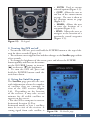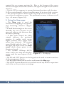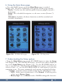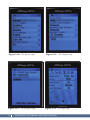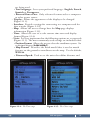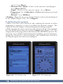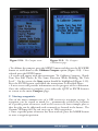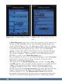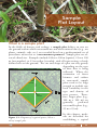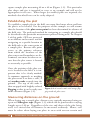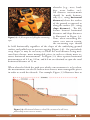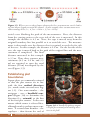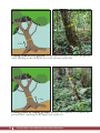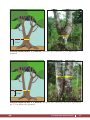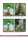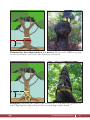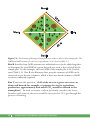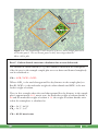
1
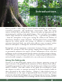
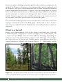
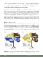
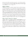
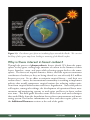
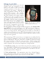
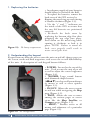
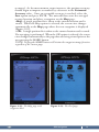
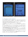
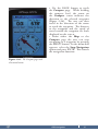
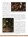
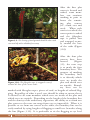
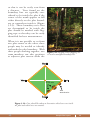
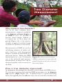
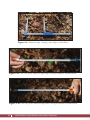
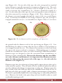
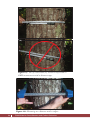
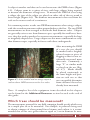
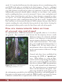
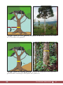
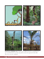
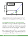
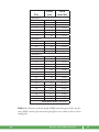
Woods Hole Research Center
Field Guide for
Version 1.0
Purpose
This field guide provides an introduction to the basic tools and techniques
used in obtaining ground-based estimates of aboveground forest biomass and
carbon. It was written for a general audience, emphasizing fundamental skills
and real-world examples. A modular approach was taken such that additional
topics (chapters) could be added as desired. Specifically, Version 1.0 of this
field guide:
• Explains the basics of GPS and GPS navigation
• Describes how to establish sample plots used in obtaining forest measurements
• Explains how to take tree diameter measurements used in forest biomass
estimation
• Demonstrates how to compute estimates of forest carbon storage from
sample plot data
• Serves as a reference for both field and office use
• Incorporates graphical illustrations for multi-lingual users
• Is not a substitute for formal instruction and hands-on training
Produced by:
Woods Hole Research Center/Dr. Wayne Walker; Version 1.0, June 2011
Suggested citation:
Walker, W., A. Baccini, M. Nepstad, N. Horning, D. Knight, E. Braun,
and A. Bausch. 2011. Field Guide for Forest Biomass and Carbon
Estimation. Version 1.0. Woods Hole Research Center, Falmouth,
Massachusetts, USA.
Funding provided by:
Gordon and Betty Moore Foundation
Google.org
The David and Lucile Packard Foundation
Norwegian Agency for Development Cooperation/Forum on Readiness for
REDD
Layout adapted from:
2009 Commonwealth of the Northern Mariana Islands (CNMI) Erosion and
Sediment Control Field Guide, CNMI Department of Environmental Quality.
CHAPTER
1
Introduction
CHAPTER
2
GPS Navigation
CHAPTER
3
Sample Plot Layout
CHAPTER
4
Tree Diameter
Measurement
CHAPTER
5
Biomass and Carbon
Estimation
CHAPTER
6
Additional Resources
License information:
This field guide is licensed under the Creative Commons Attribution-NonCommercial 3.0 Unported License. To view a copy of this license, visit
http://creativecommons.org/licenses/by-nc/3.0/ or send a letter to Creative
Commons, 444 Castro Street, Suite 900, Mountain View, California, 94041,
USA.
You are free to adapt, copy, distribute, and transmit the guide under the following conditions:
• You must attribute the work in the manner specified by the author or licensor (but not in any way that suggests that they endorse you or your use of the work).
• You may not use this work for commercial purposes.
If you make reference to this field guide we ask that you use the citation suggested on the inside front cover.
Chapter 1
Introduction
What’s in Chapter 1:
What is a forest? What is carbon? Why is there interest in forest carbon? This
chapter answers these and other fundamental questions, laying a foundation
for understanding the role that forests play in the global carbon cycle and
for learning the tools and techniques most commonly used in estimating the
carbon content of forests.
Introduction
Forests provide a wide range of natural benefits including air purification,
watershed protection, and biodiversity conservation while also being
sources of food, fiber, and medicine. Forests also play an important role in
maintaining the stability of the global climate. Trees and other forest plants
remove large amounts of carbon dioxide (CO2) – a greenhouse gas (GHG)
– from the atmosphere as they grow, storing the carbon in the biomass of
their leaves, branches, stems, and roots. Because forests have a tremendous
capacity for carbon uptake and storage, in addition to reducing GHG
emissions from fossil fuels, one of the most effective ways to remove carbon
from the atmosphere is through the sustainable management of forests.
Recognition of the important connections between forests, carbon, and
climate has prompted calls from groups ranging from indigenous peoples
to government ministries for sources of basic information on the tools and
techniques used to obtain ground-based estimates of carbon storage in forests.
This field guide, written for a general audience, emphasizing fundamental skills
and real-world examples, is intended to be one such source of information.
Using this field guide
Version 1.0 of this field guide consists of six chapters spanning a range of
topics relevant to the ground-based estimation of forest biomass and carbon.
A modular approach was taken such that further topics (chapters) could be
added as desired. First-time readers of the guide are encouraged to study
the chapters in order, as concepts presented in the latter chapters build on
those presented in the earlier chapters. Chapter 1 (this chapter) serves as
an introduction to the topic of ground-based forest biomass and carbon
estimation and includes definitions for several frequently used terms. Chapter
2 focuses on understanding GPS technology and the role that hand-held GPS
Introduction
1
devices can play in finding and marking the locations of forest sample plots in
the field. In Chapter 3, the process of setting up sample plots is explained, and
in Chapter 4, the types of measurements that are most commonly obtained
within sample plots are described. Chapter 5 uses an example data set derived
from actual forest measurements to illustrate how data collected in the field
can be converted to estimates of aboveground forest biomass and carbon.
Finally, Chapter 6 presents a list of additional resources for readers interested
to learn more about the specific topics covered in the guide.
The sections that follow provide a basic introduction to some of the terms and
concepts commonly used in this field guide. Terms such as forest, biomass,
and carbon are defined and the fundamental relationships between them are
explained.
What is a forest?
Forests cover approximately 30% of the planet’s total land area, or nearly
4 billion hectares, and grow in a variety of shapes, sizes, and densities. As
a result, the term forest can have many different meanings depending on
where you are in the world and the purpose of the definition. For example,
the boreal forests of Russia and Canada appear very different from the
tropical rainforests of Brazil and Vietnam (Figure 1.1). Additionally, within
(a)
(b)
Figure 1.1: The forests of the world, such as the (a) boreal forests of northeastern Russia
or the (b) tropical rainforests of southern Vietnam, can be very different from one another.
2
Field Guide for Forest Biomass and Carbon Estimation
a given region, similar forest types can serve a variety of different purposes.
For example, a Canadian plantation of Douglas-fir established for timber
production will appear quite different from a Canadian old-growth tract of
Douglas-fir designated for biodiversity conservation.
Given the diversity of forests globally, many definitions of the term forest exist,
and several have been proposed in the context of measuring and monitoring
forest biomass and carbon. For example, under the Kyoto Protocol, a forest
is defined as an area of land having a minimum size of 0.5-0.1 hectares, tree
crown cover of greater than 10-30%, and trees having the potential to reach a
minimum height of 2-5 meters at maturity. Such a broad definition is useful
in the context of this field guide because it is generally inclusive of the wide
range of forest types and associated biomass densities observed around the
world.
What is biomass?
The biomass of a tree refers to the weight or mass of its living plant tissue
and is generally expressed in units of metric tons (t). Live biomass can be
separated into above ground (leaves, branches and stems) and below ground
(roots) components. It is most common to estimate the aboveground live
dry biomass (AGB) of a tree, which is the weight of the living aboveground
(a)
(b)
Figure 1.2: The relative proportion of carbon (C), Water (H2O), and other elements
(e.g., N, P, K, Ca, Mg, etc.) contained in the (a) wet and (b) dry biomass of trees.
Introduction
3
plant tissue after all the water has been removed, i.e., after the leaves, branches, and stems have been dried thoroughly, often using a special laboratory
oven. In general, water accounts for approximately 50% or ½ of the weight
(or wet biomass) of a live tree (Figure 1.2).
What is carbon?
Carbon is one of the most abundant chemical elements on Earth and is present in all living things. It is also a naturally occurring component of Earth’s
atmosphere. Denoted by the symbol C, carbon is found in large quantities in
the leaves, branches, stems, and roots of trees. In addition to being made up
of 50% water, the biomass of a live tree contains approximately 25% carbon
(Figure 1.2). The remaining 25% is made up of varying amounts of other
elements including Nitrogen (N), Phosphorous (P), Potassium (K), Calcium
(Ca), Magnesium (Mg) and other trace elements. However, if all the water
contained in a live tree were removed, the proportion of the remaining dry
biomass that consists of carbon would increase from 25% to 50% (Figure
1.2). Therefore, carbon makes up roughly ½ of the total AGB of a tree. For
example, if a tree has an AGB of 2.4 metric tons, then the carbon found in
that tree has a weight of 1.2 metric tons (i.e., 2.40 t ÷ 2 = 1.20 t) (Figure 1.2).
Why is there interest in carbon?
Carbon is found in the chemical compounds carbon dioxide (CO2) and
methane (CH4), two greenhouse gases that occur naturally in the atmosphere but are also produced in large quantities through human activities,
namely the burning of fossil fuels such as coal and oil. Greenhouse gases act
like a blanket above the Earth, trapping heat near the surface, keeping the
temperature of the planet warm enough to support life (Figure 1.3). However, as the concentration of theses gases in the atmosphere increases, the thickness of the blanket also increases, causing temperatures around the world to
rise. Too much warming can have dramatic effects on the global climate,
making some areas of the planet unsuitable for plant, animal, and human
existence.
4
Field Guide for Forest Biomass and Carbon Estimation
Figure 1.3: Greenhouse gases form an insulating layer around the Earth. The excessive
build up of these gases traps heat, leading to warming of the Earth’s surface.
Why is there interest in forest carbon?
Through the process of photosynthesis, forests absorb CO2 from the atmosphere as they grow, storing large amounts of carbon in the biomass of their
leaves, branches, stems, and roots while releasing oxygen back to the atmosphere. The forests of tropical America, Africa, and Asia represent enormous
storehouses of carbon yet they are being cleared at a rate of nearly 8.0 million
hectares per year. In an effort to maintain tropical forests – and their vast
carbon stores – intact, the international community is working to implement
policies that would compensate tropical nations for reducing carbon emissions from tropical deforestation and forest degradation. Successful policies
will require, among other things, the development of operational forest measurement and monitoring systems to track gains and losses in forest carbon
over time. This field guide describes some of the basic tools and techniques
that would likely form the foundation for any forest measurement and monitoring system. For further information on these and other topics, please see
the Additional Resources section at the end of the guide.
Introduction
5
Chapter 2
GPS Navigation
What’s in Chapter 2:
Obtaining ground-based measurements of forests typically requires field crews
to navigate to specific, pre-determined locations where measurements are to
be taken or record the positions of specific locations after measurements have
been acquired. Finding and marking measurement locations is most easily
accomplished using a hand-held GPS receiver. In this chapter you will learn
what GPS is, how it works, and how GPS receivers can be used in the field
for efficient and accurate navigation.
GPS Navigation
What is GPS?
The Global Positioning System (GPS)
is a worldwide navigation and positioning system consisting of a constellation
of 24 satellites orbiting the Earth (Figure
2.1). These satellites work together with
hand-held GPS receivers (Figure 2.2) to
accurately determine where we are (position), where we are going (distance and
direction), and how fast we are moving
(speed) on the surface of the Earth. The
information provided by GPS is available Figure 2.1: The Global Positioning
24 hours a day, and can be accessed in System consists of a constellation of 24
any weather conditions from anywhere in satellites. Graphic courtesy of GPS.gov.
the world.
How does GPS work?
Each GPS satellite sends out a continuous stream of signals toward the Earth.
These signals are received and processed by GPS receivers. A GPS receiver
must receive signals from at least four satellites simultaneously for an accurate
position to be computed and the location to be displayed on the receiver’s
screen. Specific locations, commonly referred to as waypoints, are displayed
by a GPS receiver using one of several global coordinate systems, which rely
on sets of numbers to precisely identify positions on the Earth’s surface. Examples include the geographic latitude/longitude and Universal Transverse
Mercator (UTM) coordinate systems.
GPS Navigation
7
Things to consider
Hand-held GPS receivers have become
popular tools for navigating to waypoints in the field as well as recording
waypoint positions so that they can be
re-located in the future. Working in
some environments requires the use of
special GPS receivers. For example,
navigating beneath dense forest canopies
like those found in the tropics requires
a GPS receiver that is capable of receiving and processing relatively weak satellite signals. Because many recreational
grade GPS units are not equipped to receive weak signals, care should be taken
when selecting a GPS receiver to ensure Figure 2.2: The Garmin GPSmap
that the unit is appropriate for the type 60CSx handheld GPS receiver.
of environment where it will be used.
For the purposes of this tutorial on GPS navigation, the Garmin GPSmap 60CSx has been selected (Figure 2.2). This unit features a high-sensitivity receiver providing for improved satellite reception even in heavy
tree cover or deep canyons. Before going into the field, it is advisable to
evaluate the performance of any GPS unit (particularly if you are unfamiliar with its operation) by testing it under conditions similar to those
expected on the ground.
When preparing a GPS receiver for use, it is important to confirm that the
unit is properly configured so that the data being collected will meet all
project requirements. Receivers often have a number of optional settings
that users can adjust to allow for easier operation. Other settings must
be carefully selected so as to be certain that accurate position information
will be acquired. Five of the most important settings include:
. Coordinate system: It is critical that the preferred coordinate system
1
(e.g., geographic or UTM) and associated parameters be identified and
correctly set in the GPS. Often this information is specified in the measurement protocol (see Chapter 3).
. Units and precision: The appropriate units (e.g., decimal degrees,
2
degrees/minutes/seconds, meters, or feet) and the precision (i.e., number
of significant figures) of those units must be set in the GPS.
8
Field Guide for Forest Biomass and Carbon Estimation
. Acquisition mode: Some GPS units require that the acquisition mode
3
be specified. Options typically include 2-D or 3-D navigation. In 2-D
(two-dimensional) mode, elevation (the third dimension) is not calculated by the GPS and only three satellites are needed to fix the position.
In 3-D (three-dimensional mode), elevation is calculated by the GPS and
four satellites are required to fix the position. In general, 3-D navigation
should be used, as it provides more accurate position estimates.
4. Waypoint list: If the GPS unit is capable of storing waypoints, e.g.,
the locations of sample plots to be visited in the field, it is important to
confirm that these points are loaded properly onto the unit. The Garmin
GPSmap 60CSx can store up to 1000 waypoints. Nevertheless, carrying a
paper record of all waypoints as a backup is always advisable.
5. Compass configuration: If the GPS is equipped with a compass (as is
the Garmin GPSmap 60CSx), it must be properly calibrated and configured before it can be used.
The remainder of this chapter provides information specific to the usage
of the Garmin GPSmap 60CSx. For further general information on GPS
technology, please see the Additional Resources section located at the
end of the guide. If you are using a GPS receiver other than the Garmin
GPSmap 60CSx, please consult the user manual specific to that unit for
further information.
Using the Garmin GPSmap 60CSx
In this section, the following topics are discussed:
1.
2.
3.
4.
5.
6.
7.
8.
9.
10.
Replacing the batteries
Understanding the keypad
Turning the GPS on/off
Using the Satellite page
Using the Map page
Using the Main Menu page
Understanding the Setup options
Calibrating the compass
Storing waypoints
Navigating to stored waypoints
GPS Navigation
9
1. Replacing the batteries
Figure 2.3: The battery compartment.
• An adequate supply of spare batteries
should always be carried in the field.
• To replace the batteries, remove the
back cover of the GPS receiver by
flipping the metal ring up and turning
it counter-clockwise (Figure 2.3).
• Use the “+” and “-” indicators on
the inside of the GPS to ensure that
the two AA batteries are positioned
correctly.
• Re-attach the back cover by
replacing the bottom edge first then
snapping the top edge into place.
Press down on the metal ring while
turning it clockwise to lock it in
place. NOTE: Failure to attach the
back cover properly could result in
water entering the unit.
2. Understanding the keypad
Keypad buttons allow the user to turn the unit on and off, change pages on
the screen, mark and find waypoints, and access the overall functionality
of the unit. A description of each keypad button follows.
Figure 2.4: The On/Off button.
10
• POWER: Located at the top of the
unit. Used to turn the unit on or off
as well as adjust the screen brightness
(Figure 2.4).
• ROCKER: Large round button
with diamond-shaped arrows (tupq) used to scroll around maps
or menus as well as select options
(Figure 2.5).
• IN/OUT: Allows the user to zoom
in and out while navigating the Map
page (Figure 2.5).
• PAGE: Allows the user to move
among the various pages or screen
views like the Map, Satellite, or
Compass pages (Figure 2.5).
• MENU: Provides access to all
menus and submenus of a particular
page (Figure 2.5).
Field Guide for Forest Biomass and Carbon Estimation
• ENTR: Used to execute
selected options (Figure 2.5).
• QUIT: Allows the user to
exit out of the current menu
or page. The user is taken to
the previous menu or page
(Figure 2.5).
• MARK: Allows the user
to store the location of a
waypoint (Figure 2.5).
• FIND: Allows the user to
navigate to the location of a
previously stored waypoint
(Figure 2.5).
Figure 2.5: The keypad.
3. Turning the GPS on/off
• To turn the GPS on, press and hold the POWER button at the top of the unit for three seconds (Figure 2.4).
• The welcome screen appears first and then changes to the Satellite page within
a few seconds.
• To change the brightness of the screen, press and release the POWER button quickly and then use the arrows
on the ROCKER button to increase
(p) or decrease (q) the brightness.
• To turn the GPS off, press and
hold the POWER button until the
unitshuts down.
4. Using the Satellite page
The Satellite page provides the user
with information about the number
of satellites that are currently in
view of the GPS receiver (Figure
2.6). Depending on the location
of the receiver, it may take several
minutes for all visible satellites to
appear on the screen.
• For the GPS to compute its current
horizontal location (2-D or horizontal mode) at least 3 satellites
must be in view of the receiver. A
strong signal from each satellite is
Figure 2.6: The Satellite page.
GPS Navigation
11
required for an accurate position fix. Bars at the bottom of the screen
increase in height and become darker as the signal strength of each satellite
increases.
• For the GPS to compute its current horizontal position and elevation (3-D or vertical mode), at least 4 satellites must be in view of the receiver.
• The current location is shown at the top of the screen in units of the user-selected coordinate system. The positional accuracy is shown as well
(e.g., ± 8 meters; Figure 2.6).
5. Using the Map page
• The Map page is used for
orientation, navigating to waypoints,
and measuring distances (Figure
2.7).
• A small black triangle on the screen
identifies the user’s location on the
map and indicates the direction that
the unit is pointing.
• A blue circle around the black
triangle indicates the positional
accuracy (a smaller circle means
higher accuracy and a larger circle
means lower accuracy). The rotating
arrow labeled with the letter “N” in
the upper left of the screen is a north
arrow, which always points in the
direction of north.
• The Garmin GPSmap 60CSx
comes with a base map that displays
major roads for most regions of the Figure 2.7: The Map page.
world.
• The IN and OUT buttons on the keypad can be used to zoom in and out
of the current map display.
• The ROCKER button can be used to scroll around the Map page.
• The QUIT button allows the user to back out of any menu or operation
and return to the previous menu/page.
12
Field Guide for Forest Biomass and Carbon Estimation
6. Using the Main Menu page
• Press the PAGE button until the Main Menu page is reached
(Figure 2.8). The most commonly used options on this page include:
Tracks: Used to save the track (or path) of current progress toward a destination.
Setup: For a detailed description, see the next section (Section 7) below.
Calculator: Includes calculator functions useful for standard and scientific calculations.
Figure 2.8: The Main Menu page.
Figure 2.9: The Setup menu.
7. Understanding the Setup options
• From the Main Menu page use the ROCKER button to select the Setup
icon (Figure 2.8). Press the ENTR button. Several icons will be displayed
on a new Setup Menu page (Figure 2.9). Use the ROCKER button to
select a specific icon. Note that not all Setup icons can be viewed on the
screen at once, i.e., use the ROCKER button to scroll down to view the
remaining icons. The most commonly used options are described below.
– System: Controls various useful settings for the GPS (Figure 2.10).
• GPS: Under most circumstances set to Normal. If battery power
is low, set to Battery Saver.
• BatteryType: Set to Akaline unless NiMH/rechargeable batteries
GPS Navigation
13
Figure 2.10: The System setup.
Figure 2.11: The Display setup.
Figure 2.12: The Interface setup.
Figure 2.13: The Map setup.
14
Field Guide for Forest Biomass and Carbon Estimation
are being used.
• Text Language: Set to your preferred language: English, French,
Spanish or Portuguese.
• External Power Lost: Only relevant if connected to a computer or other power source.
– Display: Allows the appearance of the display to be changed
(Figure 2.11).
– Interface: Provides settings for connecting to a computer and for
data transfer (Figure 2.12).
– Map: Allows the user to change how the Map page displays
information (Figure 2.13).
– Time: Allows the user to set the current time zone and display
format (Figure 2.14).
– Units: It is very important that the following options are set correctly
(Figure 2.15). The most commonly used settings are included below.
• Position Format: Allows the user to select the coordinate system. Set to decimal degrees (hddd.dddddo).
• Map Datum: Describes the Earth model that is used to match
features on the ground to coordinates on the map. Use the default,
WGS 84.
• Distance/Speed: Used to set the units that define distance and Figure 2.14: The Time setup.
Figure 2.15: The Units setup.
GPS Navigation
15
speed. Set to Metric.
• Elevation (Vert. Speed): Used to set the units for vertical progress.
Set to Meters (m/sec).
• Depth: Used to set the units for depth. Set to Meters.
• Temperature: Set to Fahrenheit or Celsius depending on personal
preference.
• Pressure: Set to Millibars.
• Heading: Allows the user to specify how North is referenced and displayed
by the compass (Figure 2.16). Set to Magnetic.
8. Calibrating the compass
• When a new unit is first turned on, after replacing the batteries or before
navigating to a waypoint, it is wise to recalibrate the electronic compass. This
will ensure that the compass is functioning properly during navigation.
• Make sure that the unit is turned on and a position fix has been acquired.
Press the PAGE button until you reach the Compass page (Figure 2.17). The
compass dial on this page points in the direction that the GPS is oriented. The
top of the screen displays useful information including speed of movement,
straight-line distance to a selected waypoint, and estimated time of arrival at
the waypoint given the current rate of progress.
Figure 2.16: The Heading setup.
16
Figure 2.17: The Compass page.
Field Guide for Forest Biomass and Carbon Estimation
Figure 2.18: The Compass menu.
Figure 2.19: The Compass
Calibration page.
• To calibrate the compass, press the MENU button and then use the ROCKER
button to scroll down to the Calibrate Compass option (Figure 2.18). Once
selected, press the ENTR button.
• A screen will appear with the instructions “To Calibrate Compass: Slowly
Turn Two Full Circles In The Same Direction While Holding The Unit
Level.” On the screen, the Start option should be highlighted (Figure 2.19).
Press the ENTR button, and follow the instructions as described above.
• A new screen will provide information on the progress of the calibration.
Once the calibration is complete, press either the QUIT or ENTR buttons
to return to the main Compass page.
9. Storing waypoints
One of the most common uses of a GPS receiver is waypoint storage. A
waypoint can be stored to mark (i.e., permanently record) the location
of a specific point of interest such as the center of a forest sample plot so
that the plot can be efficiently and accurately re-located in the future. The
Garmin GPSmap 60CSx can store up to 1000 waypoints.
• Once a specific point of interest has been reached, press the MARK button
to store a waypoint position.
GPS Navigation
17
Figure 2.20: The Mark Waypoint page.
Figure 2.21: The Average Location
page.
– A Mark Waypoint page opens where the waypoint can be named, the
location of the waypoint can be viewed and/or changed and notes
can be added (Figure 2.20). To add text to a field, move the cursor
to the line to be edited using the ROCKER button and press ENTR.
A small keyboard will appear on the screen. Use the ROCKER button to move the cursor to the character to be selected and press
ENTR to select the character. Continue selecting characters until the entry is complete. When finished, select OK and then press ENTER to return to the Mark Waypoint page.
– The coordinates of the user’s current position appear in the Location
field and are used by default when saving the waypoint unless
alternative coordinates are entered.
– The bottom of the Mark Waypoint page includes the Avg, Map,
and OK options. Descriptions of these options are included below.
• Avg: Used to generate a more accurate waypoint position by averaging multiple position fixes. When Avg is highlighted and
ENTR is pressed, the Average Location page opens and the GPS unit
begins to average successive position acquisitions for the current
location (Figure 2.21). The Measurement Count field includes
the number of position fixes that have been averaged (remember that
the unit is constantly acquiring position fixes, each having variable
18
Field Guide for Forest Biomass and Carbon Estimation
accuracy). As the measurement count increases, the position accuracy
should begin to improve as marked by a decrease in the Estimated
Accuracy value. Once an acceptable accuracy is reached, select the
Save option and press ENTR. The unit will then store the averaged
average location and place a waypoint on the Map page.
•Map: A single position fix is taken at the current location and is
stored. When the Map option is selected, the screen view changes
automatically to the Map page where the new waypoint is displayed (Figure 2.22).
• OK: A single position fix is taken at the current location and is stored.
No averaging is performed. When the OK option is selected, the screen
view changes automatically to the page that was being viewed prior to the
user pressing the MARK button.
NOTE: Pressing the MARK button will initiate the waypoint storage function
regardless of the current page.
Figure 2.22: The Map page with
waypoint label.
Figure 2.23: The Find page.
GPS Navigation
19
Figure 2.24: The Waypoint List page.
Figure 2.25: The Find Waypoint page.
10. Navigating to stored waypoints
Often a GPS user wants to navigate to (i.e., find) a known location that
was previously stored as a waypoint. For example, one might want to
revisit a previously established (i.e., permanent) forest sample plot so that
updated measurements can be acquired.
• To navigate to a stored waypoint, press the FIND button.
• The Find page opens (Figure 2.23). Select the Waypoints icon and press
ENTR.
• A screen appears with a list of stored waypoints and a small keyboard.
The keyboard allows the user to search the list for a particular waypoint
(to remove the keyboard from view, press QUIT; Figure 2.24). Select the
waypoint that you wish to find and press ENTR.
• The Find Waypoint page appears (Figure 2.25). Use the ROCKER
button to select the Go To option at the bottom of the page (waypoints
can also be deleted from this screen using the Delete option at the bottom
of the page). Press the ENTR button.
• Selecting the Go To option starts the unit navigating to the selected
waypoint. The user is initially taken to the Map page where the straightline path to the selected waypoint is displayed.
20
Field Guide for Forest Biomass and Carbon Estimation
• Use the PAGE button to reach
the Compass page. While holding
the compass level, the arrow on
the Compass screen indicates the
direction to the selected waypoint
(Figure 2.26). The user can then
travel in the direction of the arrow
to reach the waypoint. The distance
to the waypoint and the speed of
travel toward the waypoint are both
displayed on the screen.
• From either the Map or the
Compass page the user can stop
navigating to a waypoint by pressing
the MENU button. In the menu that
appears, select the Stop Navigation
option and press ENTR. This cancels
the navigation function.
Figure 2.26: The Compass page with
directional arrow.
GPS Navigation
21
Chapter 3
Sample Plot Layout
What’s in Chapter 3:
Forest measurements of the sort used in the estimation of aboveground
biomass and carbon are typically obtained within sample plots. Sample
plots are relatively small areas, carefully delineated in the field, within which
measurements of individual trees and/or shrubs are obtained. In this chapter
you will learn about the various tools and techniques used to establish sample
plots suitable for obtaining estimates of aboveground biomass and carbon.
Sample
Plot Layout
What is a sample plot?
40
In the fields of forestry and ecology, a sample plot defines an area on
the ground within which measurements and observational data (e.g., on
plants, animals, soils, etc.) are recorded based on a predetermined set of
procedures referred to as a measurement protocol. Sample plots are often of a fixed size. Examples include 100 m x 100 m (square), 25 m x 100
m (rectangular), or 25-m radius (circular), with all representing a clearly
defined area on the ground. The size and shape of a plot can vary greatly
depending on the type
of data that is being
collected. Where the
North
estimation of forest
biomass and carbon
is concerned, sample
Plot
Corner
plots need to be large
enough to include any
local variability in the
type and density of
West
East
trees present. TherePlot
Center
fore, larger plots (e.g.,
100 m x 100 m) are
generally
preferred
over smaller plots (e.g.,
25 m x 25 m).
40
m
m
28 m
South
Figure 3.1: Diagram of a typical square (40 m x
40 m) sample plot.
In this chapter, methods are described for
establishing a typical
Sample Plot Layout
23
square sample plot measuring 40 m x 40 m (Figure 3.1). This particular
plot shape and size is intended to serve as an example and will not be
appropriate in all cases. When larger (or smaller) plots are required, the
methods described here can be easily adapted.
Establishing the plot
To establish a sample plot in the field, one must first know where and how
the plot is to be located. For the purposes of this example, we will assume
that the location of the plot center point has been determined in advance of
the field visit. The preferred method for navigating to a sample plot should
be described in the particular measurement protocol being used. In Chapter
2 of this guide, GPS was presented
as an efficient and accurate tool for
navigating to a specific location in
the field such as the center point of
a sample plot. Because this point
serves as the primary reference
from which the locations of the
plot corners and boundaries are determined, care must be taken to ensure that the plot center is located
as accurately as possible.
Once the position of the plot center is located in the field, it is important that it be clearly marked.
A common approach to marking
the plot center is to drive a tall (~2
m) wooden stake securely into the
ground. The top of the stake is
then wrapped with brightly colored
flagging so that it can be easily seen
from a distance (Figure 3.2).
Figure 3.2: A wooden stake with orange flagging marks the plot center.
Measuring distances on the ground
When laying out a sample plot, distances are typically measured using an
open-reel fiberglass tape (Figure 3.3), which can be purchased in varying
lengths up to 100 m. Regardless of the size and shape of the plot being
used, it is critical that all distances be measured accurately. Hence, care
must be taken when laying out plots in areas with uneven terrain and
24
Field Guide for Forest Biomass and Carbon Estimation
obstacles (e.g., trees, boulders, water bodies, etc.).
All distance measurements
should be made horizontally (i.e., using horizontal
distances) above the surface
of the ground as opposed to
along the surface (i.e., using
slope distances). The difference between horizontal
distances and slope distances
is illustrated in Figure 3.4.
Figure 3.3: A 50-m open-reel fiberglass measuring
Thus, when measuring distape.
tances over uneven terrain,
the measuring tape should
be held horizontally regardless of the shape of the underlying ground
surface and pulled taut to prevent sagging (Figure 3.4). On particularly
steep slopes, it may be necessary to break the total distance being measured into shorter, more manageable pieces in order to obtain more accurate horizontal measurements. In Figure 3.4, three separate horizontal
measurements of 4.2 m, 2.8 m, and 6.0 m are obtained to span the total
horizontal distance of 13 m.
When obstacles block the path over which a measurement is to be taken,
the measurement can also be broken into shorter, more manageable pieces
in order to avoid the obstacle. For example, Figure 3.5 illustrates how to
Figure 3.4: Horizontal distances should be measured at all times,
particularly across uneven terrain.
Sample Plot Layout
25
Figure 3.5: When a tree or other feature obstructs the line, measurements can be broken
up into shorter lengths to avoid the obstacle. In this example, three measurements were
taken totaling 10 m (i.e., 4.5 m + 2.0 m + 3.5 m = 10 m).
avoid a tree blocking the path of the measurement. First, the distance
from the starting point to the near side of the tree is measured. In this
example the distance is 4.5 m. Next, the tape is moved away from the
original boundary line but parallel to it to avoid the tree. The measurement is then made over the distance that is required to reach the far side
of the tree. In this example, the distance is 2.0 m. On the far side of the
tree, the tape is moved back to the path of the original line and the measurement is completed. The final
distance measured in this example
is 3.5 m. Thus, three separate measurements (4.5 m, 2.0 m, and 3.5
m) are required to span the total
distance (10 m) interrupted by the
tree (Figure 3.5).
Establishing plot
boundaries
Square plots are commonly oriented
so that the plot corners are in line
with the four cardinal directions
(i.e., north, south, east and west; Figure 3.1). One team member – the
navigator – uses a handheld compass (Figure 3.6) to determine the
direction (i.e., azimuth) to the first
of the four plot corners. It does not
matter which corner is selected first,
although north is perhaps most common. A second team member – the
tapelayer – then fastens the end of
26
Figure 3.6: A handheld sighting compass
is useful for accurately determining direction in the field.
Field Guide for Forest Biomass and Carbon Estimation
one fiberglass tape to the
center stake (Figure 3.7)
and begins walking slowly in the direction of the
plot corner, reeling out
the tape as he/she walks
(Figure 3.8). It is the job
of the navigator to keep
the tapelayer on a straight
path toward the plot corner. In areas with dense
undergrowth, it may be
necessary to have a line Figure 3.7: The fiberglass tape is looped over and
cutter (a team member fastened securely to the base of the center stake.
skilled in the use of a machete) walk ahead of the tapelayer, clearing a narrow path along which the
tapelayer can walk more easily (Figure 3.9). Note that the clearing of undergrowth should be done only where absolutely necessary. As the tapelayer
walks, care must be taken to ensure that the tape is kept as straight, horizontal,
and taut as possible. If obstacles such
as trees or boulders are encountered
along the path, the line should be offset as shown in Figure 3.5.
Figure 3.8: The tapelayer keeps the tape
low and taut while walking a straight line.
Once the tapelayer reaches the location
of the first plot corner, which is 28 m
away from the center point of a 40 m
x 40 m plot (Figure 3.1), the corner
point is marked with a stake similar
to that used at the plot center (Figure
3.2). The tape is then pulled taut and
wrapped securely around the base of
the corner stake (Figure 3.10). At this
stage, it is critical that both team members double-check the position of the
line, confirming that the tape is straight,
horizontal, and taut before moving on.
If the line is observed to meander, the
tape must be reeled in so that the line
can be laid properly.
Sample Plot Layout
27
Figure 3.9: The clearing of undergrowth should be done with
care and only where absolutely necessary.
After the first plot
corner is located and
staked, team members can continue
working in pairs to
locate the remaining plot corners
(i.e., south, east, and
west). When each
corner is reached, the
corner point is staked
and the fiberglass
tape is pulled taut
and wrapped securely around the base
of the stake (Figure
3.10).
After the four plot
corners have been
located
(Figure
3.1), the next step
is to mark the four
boundary lines. The
purpose of marking
the boundary lines
is to identify which
trees are inside the
Figure 3.10: The fiberglass tape is wrapped securely
plot and which trees
around the base of the corner stake.
are outside. Boundary lines can be
marked with fiberglass tapes, pieces of cord, or lengths of colored flagging. Regardless of what is used, care should be taken to ensure that it
is obvious to all team members which trees are inside of the plot and
which trees are outside. Depending on the length of the boundary line
and the density of the understory vegetation, the ability to see from one
plot corner to the next can range from easy to impossible. When it is
possible to see from one corner to the other, the boundary line can be
easily marked by tying lengths of flagging to small tree branches along
the line (Figure 3.11). It is preferable to tie the flagging at eye level
28
Field Guide for Forest Biomass and Carbon Estimation
so that it can be easily seen from
a distance. Trees found on the
boundary line are typically considered to be inside the plot if the
center of the trunk appears to fall
either directly on the plot boundary or somewhere inside it (Figure
3.12). Those boundary trees that
are determined to be inside the
plot should be marked with flagging tape so that they can be easily
identified for later measurement.
When it is not possible to see from
one plot corner to the other, three
people may be needed to identify
and mark the plot boundary. With
three people working together, two
team members can take positions
at adjacent plot corners while the
Figure 3.11: Brightly colored flagging can
be used to mark plot boundary lines.
North
West
Trees
Inside Plot
East
Tree
Outside Plot
South
Figure 3.12: Care should be taken to determine which trees are inside
the plot and which trees are outside.
Sample Plot Layout
29
third person walks slowly back and forth between them and along the
boundary line until he/she can see the other team members at the corners. If possible, team members at the corners can use their compasses
to help confirm the accuracy of the third member’s position along the
boundary. Once all team members are satisfied that the boundary line
has been identified, the third person can begin marking the line with
flagging tape, working first toward one corner and then back toward the
other, with the goal of making it clear to all which trees are inside and
which trees are outside the plot. By wearing brightly colored clothing
and shaking branches as appropriate, team members can increase the
likelihood of seeing one another through dense undergrowth.
Notes: In general, a team of 3-5 people is needed for the efficient set-up
and sampling of a 40 x 40 m plot. A complete list of the equipment
items described in this chapter can be found in the Additional Resources section located at the end of the guide.
30
Field Guide for Forest Biomass and Carbon Estimation
Chapter 4
Tree Diameter
Measurement
What’s in Chapter 4:
Diameter measurements of individual trees form the basis for many of
the commonly used approaches to obtaining ground-based estimates of
aboveground forest biomass and carbon. In this chapter you will learn
how tree diameter is measured, including the tools and techniques used in
the field to obtain accurate diameter measurements quickly and efficiently.
Because trees come in a variety of shapes and sizes, you will also learn
how to accurately measure the diameter of trees having unusual trunk
characteristics.
Tree Diameter
Measurement
Why measure tree diameter?
One of the most common forest
measurements acquired worldwide
is the diameter at breast height or
the DBH of trees. In the field of
forestry, breast height, defined at
1.3 meters (or 4.5 feet) above the
ground (Figure 4.1), is the internationally recognized standard height
at which tree diameter is measured. Measurements of DBH are used in
calculating estimates of timber volume, basal area, and aboveground
biomass (carbon) of individual trees
and entire forests. Taking the DBH
measurement of a tree is relatively
easy to do, and with some practice,
measurements of many trees can be
obtained quickly and accurately in
the field.
1.3m
Figure 4.1: Diameter at breast height
(DBH) is measured at 1.3 meters above the
ground. Exceptions to this rule are discussed
later in this chapter.
How is tree diameter measured?
An appropriate measuring device should be used to obtain the DBH of a tree. The two most common tools used for DBH measurement are the diameter
tape and the caliper (Figure 4.2). A diameter tape is a special measuring
device that typically has two different scales, one on each side of a white steel
Tree Diameter Measurement
31
Figure 4.2: Diameter tape (orange) and caliper (silver/blue).
Figure 4.3a: The side of the diameter tape that is used for distance measurement.
Figure 4.3b: The side of the diameter tape that is used for diameter measurement.
32
Field Guide for Forest Biomass and Carbon Estimation
tape (Figure 4.3). On one side of the tape, the scale corresponds to standard
units of distance, typically measured in centimeters (Figure 4.3a). This scale
can be used to determine the position of breast height (1.3 m) on a tree
trunk or measure the circumference (i.e., distance around the trunk) of a
tree. On the other side of the tape, the scale corresponds to units of diameter,
also often measured in centimeters (Figure 4.3b). Here, diameter refers to
the distance measured straight through the center of the tree trunk (Figure
4.4a). To measure the DBH of a tree using a diameter tape, the steel tape is
wrapped around the tree (i.e., its circumference; Figure 4.4b) at 1.3 m above
(a)
(b)
Figure 4.4: The (a) diameter and (b) circumference of a typical tree.
the ground with the diameter scale of the tape facing out (Figure 4.5). Care
should always be taken to ensure that the tape is held in a level position as
it is wrapped around the tree. The diameter measurement is then read from
the tape to the nearest tenth of a centimeter. Although the tape is wrapped
around the circumference of the tree when obtaining a DBH measurement,
diameter tapes are designed so that the conversion from circumference to
diameter is done automatically. Because the diameter tape has two different scales (distance and diameter), it is important that diameter measurements be taken using the correct side of the tape, i.e., the side with the
diameter scale (Figure 4.3).
Diameter tapes have the advantage of being small, compact devices that can be
easily carried in a pocket. They are made of steel or reinforced nylon that will not
stretch or deform with changes in temperature or when wet. Diameter tapes also
have a hook at the end of the tape that can be embedded in the bark of a tree to
hold the end of the tape in place while a diameter measurement is being taken. The hook is particularly helpful when measuring large or awkwardly positioned
trees. However, the hook is also quite sharp and care should be taken to avoid
accidentally injuring oneself.
Tree Diameter Measurement
33
(a)
(b)
Figure 4.5: The (a) correct and (b) incorrect way to take a
DBH measurement with a diameter tape.
Figure 4.6: Measuring tree diameter with a caliper.
34
Field Guide for Forest Biomass and Carbon Estimation
A caliper is another tool that can be used to measure the DBH of trees (Figure
4.2). Calipers come in a variety of sizes, with large calipers being required
to measure the diameters of large trees. To measure the DBH of a tree using
a caliper, the jaws of the caliper are placed on either side of the tree trunk at
breast height (Figure 4.6). The diameter measurement is then read from the
scale to the nearest tenth of a centimeter.
It is common practice to take two DBH measurements when using a caliper,
with the second measurement taken perpendicular to the first. The two DBH
measurements are then averaged to obtain the final diameter value. Calipers
are generally easier to use than diameter tapes, especially for small trees; however, they also tend to produce less accurate measurements, especially for large
or irregularly shaped trees. Large calipers are also more cumbersome to carry
than diameter tapes, especially in forests with dense undergrowth.
After measuring the DBH
of a tree, the tree should
be marked with a brightly
colored crayon or piece of
flagging so that it is not accidentally measured more
than once. Commonly, a
large “X” or similar mark
is placed on the tree (Figure 4.7). Marks should
be placed consistently at
the same height and position on each tree so that
Figure 4.7: A tree marked with an orange crayon to
one can quickly determine
indicate that a DBH measurement has been taken.
from a distance if a tree has
already been measured.
Note: A complete list of the equipment items described in this chapter
can be found in the Additional Resources section located at the end of
this guide.
Which trees should be measured?
The measurement protocol for any field campaign should specify which trees
in a sample plot are to be measured. For example, in protocols being used
to obtain estimates of aboveground forest biomass and carbon, it is recommended that all live trees greater than or equal to 5 cm in diameter be meaTree Diameter Measurement
35
sured. A 5-cm threshold ensures that the majority of trees contributing to the
total AGB of the plot are included in the final estimate. Trees (i.e., saplings)
less than 5 cm in diameter are often not measured because they tend to have
very little biomass overall and are often too numerous to measure efficiently. Additionally, protocols should address whether or not lianas, vines, palms
and/or standing dead trees are to be measured. Lianas, vines, and palms tend
to have lower wood densities and, hence, lower biomass compared to other
tree species. As a result, measurements may not be taken, particularly if this
group represents only a small proportion of the forest stand. Standing dead
trees tend not to be measured as part of AGB estimates because they tend to
remain standing for only relatively short periods of time before leaving the
aboveground carbon pool to join the litter layer and soil carbon pools. How are measurements taken on trees
of unusual size and shape?
As explained above, DBH measurements are typically taken at 1.3 m above
the ground. This standard is used because for the majority of trees, trunk
diameter tends to be relatively uniform
above 1.3 m. However, it is not uncommon in nature to find trees that have unusual trunk characteristics. For example, a tree trunk may be buttressed at 1.3
m (Figure 4.8). In cases such as this, a
measurement taken at breast height will
not be representative of the tree’s average
diameter. General rules have been established for
measuring the DBH of “special-case”
trees. What follows is a series of illustrations and accompanying photographs
that can be used in the field to determine
how best to obtain DBH measurements
of trees with unusual trunk characterisFigure 4.8: A tree with buttresses
extending well above 1.3 m.
tics. If a special-case tree is encountered
that is not described in this guide, common sense should be used together with
the information provided in the following illustrations and photographs to
determine at what point on the trunk the DBH should be measured to obtain
a diameter estimate that is representative of the tree’s average diameter.
36
Field Guide for Forest Biomass and Carbon Estimation
1.3m
Upright trunk on level ground (standard condition): Measure the DBH
at 1.3 m above the ground.
1.3m
Upright trunk on sloping ground: Measure the DBH at 1.3 m above the
ground while standing on the uphill side of the tree.
Tree Diameter Measurement
37
1.3m
Leaning trunk on level ground: Measure the DBH at 1.3 m above the ground
while standing on the side of the tree in the direction of the lean.
1.3m
Leaning trunk on sloping ground: Measure the DBH at 1.3 m above the
ground while standing on the uphill side of the tree.
38
Field Guide for Forest Biomass and Carbon Estimation
1.3m
Forked trunk above 1.3 meters: Measure the DBH at 1.3 m above the
ground.
1.3m
Forked trunk below 1.3 meters: Measure the DBH of each stem separately
at 1.3 m above the ground.
Tree Diameter Measurement
39
1.3m
Buttressed trunk at 1.3 meters: Measure the DBH above the buttressed
(tapered) portion of the trunk at a point where the trunk diameter becomes
uniform. Ladders or climbing equipment may be required in some cases.
1.3m
Stilted roots at 1.3 meters: Measure the DBH above the stilted portion of
the trunk at a point where the trunk diameter becomes uniform.
40
Field Guide for Forest Biomass and Carbon Estimation
1.3m
Deformed or branched trunk at 1.3 meters: Measure the DBH at a point
on the trunk above (or below) the deformity or branch.
1.3m
Stranglers: Estimate the DBH of the host tree at 1.3 m above the ground (or
where appropriate) depending on the size and shape of the trunk.
Tree Diameter Measurement
41
1.3m
Lianas: Measure the DBH at 1.3 m above the ground.
Dead trees and palm trees: Measure the DBH of dead trees and palms as
you would other live trees but only if the measurement protocol states that
these trees are to be included.
42
Field Guide for Forest Biomass and Carbon Estimation
Chapter 5
Biomass and Carbon
Estimation
What’s in Chapter 5:
Often the best way to learn new concepts is by example. In this chapter
you will be provided with an example data set that includes tree diameter
measurements (as explained in Chapter 4) obtained within a typical forest
sample plot (as explained in Chapter 3). A series of exercises are used to
demonstrate how diameter measurements can be used to compute treelevel, plot-level, and per-hectare estimates of aboveground biomass and
carbon. You will also learn how to calculate estimates of carbon dioxide
emissions to the atmosphere for an area of forest that has been cleared.
Biomass and
Carbon Estimation
Estimating aboveground biomass in the field
The most direct approach to estimating the aboveground biomass of a tree
involves a number of steps including (1) harvesting the tree, (2) cutting the
tree, including the leaves, branches, and stem, into small, more manageable
pieces, (3) oven drying the pieces, and (4) carefully weighing the pieces once
they are thoroughly dried and all water has been removed. Although very accurate, this method is also very time consuming, expensive, and destructive.
Hence, it is not a practical approach to obtaining biomass estimates for many
trees or entire tracts of forest.
The limitations associated with direct methods have led numerous researchers
to develop mathematical relationships, commonly referred to as allometric
equations, which relate the aboveground biomass of individual trees to other
tree characteristics that are more easily measured in the field. These characteristics include diameter at breast height (DBH; see Chapter 4), total height,
and wood density. Hundreds of allometric equations have been developed
for individual tree species and groups of tree species by researchers all over
the world.
Examples of allometric equations that relate AGB to DBH and wood density
for three different groups of topical forest tree species are shown in Figure
5.1. These groups include dry tropical forest (red line), wet tropical forest
(green line), and moist tropical forest (blue line). As described in Chapter 4,
DBH measurements are easily obtained in the field. Wood density estimates
are typically obtained by computing the dry weight (i.e., mass) per unit volume of stem samples collected in the field, and several compilations of wood
density values have been published by various researchers, e.g., Brown (1997)
(see the Additional Resources section for more information).
Biomass and Carbon Estimation
43
40
30
20
10
13.3
●
7.9
●
0
Aboveground Live Dry Biomass (t)
Moist tropical forest
Wet tropical forest
Dry tropical forest
0
50
100
150
Diameter at Breast Height (cm)
Figure 5.1: Examples of allometric equations developed by Chave et al. (2005) for use with
groups of tropical forest tree species. The equations relate measurements of diameter at breast
height (DBH) to estimates of aboveground live dry biomass (AGB). For example, a moist
tropical forest tree species with a DBH of 100 cm would have an AGB of 13.3 t. Similarly, a
wet tropical forest tree species with a DBH of 100 cm would have an AGB of 7.9 t.
Understanding biomass and carbon calculations
In the remainder of this chapter, an example data set is used to illustrate how
DBH measurements (see Chapter 4) obtained within a typical sample plot (see
Chapter 3) can be used together with allometric equations such as those shown
in Figure 5.1 to compute tree-level, plot-level, and per-hectare estimates of AGB
and carbon. The data set includes DBH measurements taken from 28 tropical
moist forest trees found within a 40 m x 40 m sample plot. The DBH measurements for all 28 trees are listed in Table 5.1, and the approximate location of each
tree within the sample plot is shown in Figure 5.2.
Box A describes how the ABG of a single tree (e.g., the first tree listed in Table
5.1) can be calculated using the allometric equation for moist tropical forest trees
shown in Figure 5.1. Using this equation, it is possible to calculate the AGB of
any moist tropical forest tree. The last column in Table 5.1 includes the AGB
estimates for each of the 28 trees found in the example sample plot.
44
Field Guide for Forest Biomass and Carbon Estimation
Tree
DBH
(cm)
AGB
(tons/ha)
Quadrant 1
1
2
3
4
5
6
7
6.3
60.9
5.1
8.8
5.2
7.0
6.6
0.012
4.283
0.007
0.029
0.007
0.016
0.013
17.6
94.2
9.4
28.4
6.3
0.179
11.987
0.034
0.628
0.012
16.6
7.8
6.6
54.3
6.8
13.0
19.2
35.1
5.6
0.154
0.021
0.013
3.237
0.014
0.080
0.226
1.084
0.009
8.4
7.4
11.5
42.1
12.1
8.6
27.5
0.025
0.018
0.058
1.719
0.066
0.027
0.578
Quadrant 2
8
9
10
11
12
Quadrant 3
13
14
15
16
17
18
19
20
21
Quadrant 4
22
23
24
25
26
27
28
Total Plot AGB = 24.536
Table 5.1: Diameter at breast height (DBH) and aboveground live dry biomass (AGB) estimates for 28 moist tropical forest trees within a 40 m x 40 m
sample plot.
Biomass and Carbon Estimation
45
North
40
13
12
18
16
17
20
m
14
15
21
West
3
11
19
9
2
10
22
24
8
5
4
1
23
6
7
East
3
4
25
26
2
1
40
28
m
27
South
Figure 5.2: The locations of 28 tropical moist forest trees within a 40 m x 40 m sample plot. The
DBH and AGB estimates for each tree in quadrants 1-4 are listed in Table 5.1.
Box B describes how AGB estimates for individual trees can be added together
to determine the total AGB of a given forested area such as that covered by the
sample plot. In this example, the total AGB of the sample plot is 24.5 metric
tons (Table 5.1). Box B also illustrates how per-plot estimates of AGB can be
converted to per-hectare estimates, which is how area-based estimates of AGB
are most commonly reported.
Box C answers the question, “if all of the trees in a given area were cut
down and burned, for example, to prepare the site for agriculture
production, approximately how much CO2 would be emitted to the
atmosphere?” In such a scenario, carbon previously stored in the leaves,
branches and stems of the trees would be converted to CO2 gas through the
process of burning.
46
Field Guide for Forest Biomass and Carbon Estimation
Box A: Aboveground live dry biomass calculation for a single tree.
Using the Chave et al. (2005) allometric equation for moist tropical forest species
(see Figure 5.1), the aboveground live dry biomass (AGB in metric tons) of a
single tree can be calculated as:
Thus, for the first tree in the first quadrant of the plot (see Figure 5.2), which has a
wood density of 0.60 g/cm3 and a DBH of 6.3 cm, the AGB is calculated as:
AGBtree = (0.60 * exp(-1.499 + (2.148 * ln(6.3)) + (0.207 *
ln(6.3)2) – (0.0281 * ln(6.3)3)) * 0.001
AGBtree = 0.012 metric tons
Biomass and Carbon Estimation
47
Box B: Aboveground live dry biomass calculation for a sample plot.
Table 5.1 contains estimates of AGB for each of the 28 trees contained in the
example sample plot shown in Figure 5.2. The estimates were calculated using
the Chave et al. (2005) allometric equation for moist tropical forest species as
explained in Box A.
The AGB values calculated for each tree can be added together to obtain an estimate of the total AGB for the sample plot. In this example, the total AGB for
the plot is estimated to be 24.5 metric tons (see Table 5.1).
Typically, AGB is reported on a per hectare basis. Figure 5.3 illustrates the spatial relationship between the 40 m x 40 m sample plot and a one-hectare parcel.
The formula for converting from a per plot estimate of AGB (in metric tons) to
a per hectare estimate (in metric tons per hectare) can be calculated as:
AGBh = (Ah/Ap) * AGBp
where AGBh is the estimate of aboveground biomass in metric tons per hectare,
Ah is the area of one hectare in square meters, Ap is the area of the plot in square
meters and AGBp is the plot level estimate of aboveground biomass in metric
tons.
Thus, in this example where the area of one hectare is 10,000 m2, the area of the
plot is 40 m x 40 m or 1600 m2, and the above-ground live dry biomass in the
plot is approximately 24.5 metric tons, the per hectare estimate of biomass is
calculated as:
AGBh = (10,000/40*40) * 24.5
AGBh = (10,000/1600) * 24.5
AGBh = (6.25*24.5)
AGBh = 153.13 metric tons/hectare
48
Field Guide for Forest Biomass and Carbon Estimation
0
10
m
0.16 Hectare
13
12
15
16
1.0 Hectare
14
3
18
2
11
9
17
20
19
21
10
8
5
22
24
4
1
23
26
25
6
7
3
4
2
27
1
10
0
m
28
Figure 5.3: The relationship in area between a 40 m x 40 m sample plot and a
one-hectare parcel. The one-hectare parcel is 6.25 times larger than the
40 m x 40 m plot.
Box C: Carbon dioxide emissions calculation for an area deforested.
The amount of carbon dioxide (CO2) that would be emitted to the atmosphere
if the 28 trees in the example sample plot were cut down and burned completely
can be calculated as:
C02 = AGBp* MWC02/MWC
Where AGBp is the total aboveground live dry biomass in the sample plot (see
Box B), MWC02 is the molecular weight of carbon dioxide and MWC is the molecular weight of carbon.
Thus, in this example where the total aboveground live dry biomass in the sample
plot is approximately 24.5 metric tons, the molecular weight of carbon dioxide is
44 and the molecular weight of carbon is 12, the weight of carbon dioxide emitted to the atmosphere is calculated as:
C02 = 24.5 * 44/12
C02 = 24.5 * 3.67
C02 = 89.92 metric tons
Biomass and Carbon Estimation
49
Additional
Resources
Additional Resources
What’s in Chapter 6:
This chapter includes a variety of resources that expand on the topics
covered in this field guide.
Additional
Resources
Resources I: Further Reading
The following books, reports, articles, and websites were consulted during the preparation of this field guide. Readers in search of
additional information on the topics covered here are encouraged
to consider these useful resources.
Books
Field Measurements for Forest Carbon Monitoring
2010, C.M. Hoover, ed.
Tree and Forest Measurement 2 nd Edition
2009, P.M. West
Forest Mensuration 4 th Edition
2003, B. Husch, T.W. Beers, and J.A. Kershaw Jr.
Forest Measurements 5 th Edition
2001, T.E. Avery and H.E. Burkhart
Conservation Research in the African Rain Forests. A Technical Handbook.
2000, L. White and A. Edwards, eds.
Reports and Articles
Tree allometry and improved estimation of carbon stocks and
balance in tropical forests.
2005, J. Chave et al. Oecologia.
Estimating biomass and biomass change of tropical forests. A
primer.
1997, S. Brown. FAO Forestry Paper 134.
Additional Resources
51
Websites
Forests, Carbon, and Climate
Woods Hole Research Center
www.whrc.org
Center for International Forestry Research
www.cifor.org
RealClimate
www.realclimate.org
The REDD Desk
www.theredddesk.org
United States Forest Service
www.fs.fed.us/ccrc
GPS
Garmin GPS
www.garmin.com/aboutGPS
Garmin GPSmap 60CSx Owner’s Manual
static.garmincdn.com/pumac/GPSMAP60CSx_OwnersManual.pdf
National Aeronautics and Space Administration
gpshome.ssc.nasa.gov
National Air and Space Museum
www.nasm.si.edu/gps
United States Geological Survey
education.usgs.gov/common/lessons/gps.html
Field Equipment
Ben Meadows Company
www.benmeadows.com
Forestry Suppliers, Inc.
www.forestrysuppliers.com
52
Field Guide for Forest Biomass and Carbon Estimation
Resources II: Equipment List
Chapters 2-4 of this field guide describe the various pieces of equipment
that are most commonly used to locate, establish, and measure sample
plots intended for the estimation of aboveground forest biomass and
carbon. What follows is a complete list of the equipment items referenced in this guide.
•Handheld GPS receiver (e.g., Garmin GPSmap 60CSx)
•Diameter tape
•Sighting compass
•Fiberglass measuring tapes (as many as the plot dimensions
require)
•Flagging (brightly colored for marking plot boundaries)
•Lumber crayons (brightly colored for marking trees)
•Camera (for taking photographs of the plot)
•Paper (for printing plot forms)
•Pencils
•Clipboard
•Backpack (for carrying all of the above)
For further information on these items, please visit the websites listed
under Field Equipment on the preceding page.
Additional Resources
53
Obtaining copies
Electronic copies of this field guide are available in Adobe Acrobat PDF for
download from the following websites:
Woods Hole Research Center (www.whrc.org)
The REDD Desk (www.theredddesk.org)
A limited number of printed copies may be available from the Woods Hole
Research Center upon written request.
Contact information
If you have questions or comments on this field guide, please contact:
Dr. Wayne Walker, [email protected],Woods Hole Research Center
149 Woods Hole Road, Falmouth, Massachusetts 02540-1644 USA
Photography and graphics
Max Nepstad, Tina Cormier, Wayne Walker, and Mike Loranty
Acknowledgements
Support for the production of this field guide was provided by the Gordon and
Betty Moore Foundation, Google.org, the David and Lucile Packard Foundation, and the Norwegian Agency for Development Cooperation/Forum on
Readiness for REDD. Lisa Cavanaugh, Tina Cormier, Tracy Johns, Connie
Johnson, Nadine Laporte, Chris Meyer, Kristin McLaughlin, André Nahur,
Kathleen Savage, and Allison White provided valuable comments on an earlier
draft.
The Woods Hole Research Center conducts interdisciplinary scientific research
on forests, soils, water, and energy for the benefit of sustained human wellbeing on Earth. We are leaders at the nexus of science, economics, and public
policy through innovative communication and education about environmental
challenges and solutions. The Center has initiatives in the Amazon, the Arctic,
Africa, Asia, Russia, Boreal North America, the Mid-Atlantic, and New England including Cape Cod. Center programs focus on the global carbon cycle,
forest function, land cover/land use, water cycles and chemicals in the environment, science in public affairs, and education, providing primary data and
enabling better appraisals of the trends in forests.
Mention of trade names or commercial products, if any, does not constitute endorsement.
Woods Hole Research Center