1
MacTempas User Manual
Chapter
I
Installing the
Hardware Protection Key
Activating the
Hardware Key and
Personalizing the
Program
Changing Hardware or Versions
of the MacOS
Installation
The application MacTempas and its associated files are installed
by double clicking on the installer package. After authorizing
the installer with the administrator password, the installer will
install MacTempas into a directory in your applications folder.
The driver for the hardware key will also be installed.
MacTempas uses a hardware copy protection key which must
be installed on your computer. If you already have installed a
key for use with CrystalKit, you do not need a second key to run
MacTempas and you can proceed to the next paragraph describing how to activate the key for running MacTempas. Just plug
the USB key into an open USB slot on your computer, keyboard
or display.
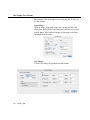
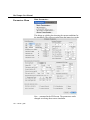
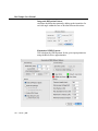
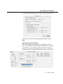
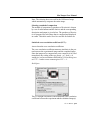
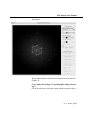
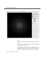
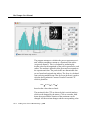
When MacTempas is run for the first time it will put up its
installation screen. Enter your name and affiliation as appropriate together with the installation code for the hardware key. T
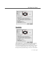
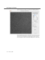
If you have just changed your computer or installed a new clean
version of the MacOS, you must ensure that the driver for the
USB key is installed. Run the installation program for MacTempas once more to install the driver. Without the driver in place,
the program will not recognize the hardware key and MacTempas will run in demonstration mode.
Ch.
Installation - p.1
MacTempas User Manual
Ch.
Installation - p.2
MacTempas User Manual
Chapter
1
Introduction to
Image Simulation
The best High Resolution Transmission Electron Microscopes
(HRTEM) have a resolution approaching 1 Å which sometimes
leads to the erroneous conclusion that using an electron microscope, all atoms in a structure can be resolved. However, it is
not the inter-atomic distances that matter, but rather the projected distances between atoms seen from the direction of the
incident electron. In order to obtain interpretable results, it is
necessary to orient the specimen such that atomic columns are
separated by distances that are of the order of the resolution of
the microscope or larger. This is a condition that very often is
difficult to satisfy and often limits the use of the HRTEM to
studies of crystals only in low order zone-axis orientations.
The HRTEM image is a complex function of the interaction
between the high energy electrons (typically 200keV - 1MeV)
with the electrostatic potential in the specimen and the magnetic
fields of the image forming lenses in the microscope. Although
images obtained from simple mono-atomic crystals often show
white dots separated by spacings that correspond to spacings
between atomic columns, these white dots fall on or between
atomic columns depending on the thickness of the specimen
and the focus setting of the objective lens (O’Keefe et al.,1989).
Fortunately, in many cases it is only necessary to see the general
pattern of image intensities to gain the desired knowledge.
However, in general, the image can be best thought of as a complex interference pattern which has the symmetry of the projected atomic configuration, but otherwise has no one-to-one
correspondence to atomic positions in the specimen. It is
because of this lack of directly interpretable images that the
need for image simulation arose. Image simulation grew out of
an attempt to explain why electron microscope images of complex oxides sometimes showed black dots in patterns corre-
Ch. 1 Introduction to Image Simulation - p.3
MacTempas User Manual
sponding to the patterns of heavy metal sites in complex oxides,
and yet other images sometimes showed white dots in the same
patterns (Allpress et al.,1972). This first application was therefore to characterize the experimental images, that is to relate the
image character (the patterns of light and dark dots) to known
features in the structure.
Most simulations today are carried out for similar reasons, or
even as a means of structure determination. Given a number of
possible models for the structure under investigation, images
are simulated from these models and compared with experimental images obtained on a high-resolution electron microscope.
In this way, some of the postulated models can be ruled out until
only one remains. If all possible models have been examined,
then the remaining model is the correct one for the structure.
For this process to produce a correct result, the investigator
must ensure that all possible models have been examined, and
compared with experimental images over a wide range of crystal thickness and microscope defocus. It is also a good idea to
match simulations and experimental images for more than one
orientation.
The simulation programs can also be used to study the imaging
process itself. By simulating images for imaginary electron
microscopes, we can look for ways in which to improve the performance of present-day instruments, or even find that the performance of an existing electron microscope can be improved
significantly by minor changes in some instrumental parameter.
Alternatively, based on imaging requirements revealed by test
simulations, we can adjust the electron microscope to produce
suitable images of some particular specimen, or even of some
particular feature in a particular specimen.
Ch. 1 Introduction to Image Simulation - p.4
MacTempas User Manual
Describing the
Transmission
Electron Microscope
In order to simulate an electron microscope image, we need
firstly to be able to describe the electron microscope in such a
way that we can model the manner in which it produces the
image. As a first step, we can consider the usual geometrical
optics depiction of the transmission electron microscope
(TEM).
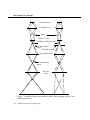
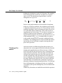
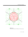
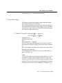
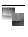
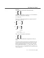
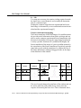
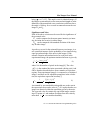
Figure 1 shows such a diagram of a TEM operated in two distinct modes, set up for microscopy (a), and for diffraction (b). In
microscopy mode we see that the TEM consists of an electron
source producing a beam of electrons that are focused by a condenser lens onto the specimen; electrons passing through the
specimen are focused by the objective lens to form an image
called the first intermediate image (I1); this first intermediate
image forms the "object" for the next lens, the intermediate
lens, which produces a magnified image of it called the second
intermediate image (I2); in turn, this second intermediate
image becomes the "object" for the projector lens; the projector
lens forms the greatly-magnified final image on the viewing
screen of the microscope. In microscopy mode, electrons that
emerge from the same point on the specimen exit surface are
brought together at the same point in the final image.
At the focal plane of the objective lens, we see that electrons are
brought together that have left the specimen at different points
but at the same angle. The diffraction pattern that is formed at
the focal plane of the objective lens can be viewed on the viewing screen of the TEM by weakening the intermediate lens to
place the microscope in diffraction mode (b).
Ch. 1 Introduction to Image Simulation - p.5
MacTempas User Manual
Electron Source
Condenser Lens
Object
Objective Lens
Focal Plane of Objective lens
1'st Intermediate
Image
Selected Aperture
Intermediate Lens
2'nd Intermediate
Image
Projecter
Lens
Imaging Mode (a)
Diffraction Mode (b)
Figure 1. Geometrical optics representation of the TEM in imaging mode (a), and
diffraction mode (b)
Ch. 1 Introduction to Image Simulation - p.6
MacTempas User Manual
Simplifying the
Description of the
Microscope
Consideration of the description of the electron microscope in
figure 1 shows that the projector lens and the intermediate lens
(or lenses) merely magnify the original image (I1) formed by
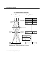
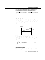
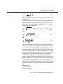
the objective lens. For the purposes of image simulation we can
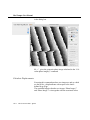
reduce the TEM to three essential components; (1) an electron
beam that passes through (2) a specimen, and then through (3)
an objective lens (fig. 2).
Our next step in describing the electron microscope for image
simulation is to move from the geometrical optics description of
the TEM to a description based on wave optics. In this description of the microscope we examine the amplitude of the electron wavefield on various planes within the TEM, and attempt
to determine how the wavefield at the viewing screen comes to
contain an image of our specimen.
By treating the electrons as waves, and considering our simplified electron microscope (Figure 2), we see that there are three
planes in the TEM at which we need to be able to compute the
(complex) amplitude of the electron wavefield.
(1)The image plane:
Working backwards, we start at our desired information, the
electron wavefield at the image plane; this wavefield is derived
from the wavefield at the focal plane of the objective lens by
applying the effects of the objective aperture and the phase
changes introduced by the objective lens.
(2)The focal plane of the objective lens:
In turn, the electron wavefield at the focal plane of the lens is
derived from the wavefield at the exit surface of the specimen
by a simple Fourier transformation.
(3)The specimen exit surface:
In order to know the exit-surface wavefield, we must know with
which physical property of the specimen the wave interacts, and
describe that physical property of our particular specimen.
Ch. 1 Introduction to Image Simulation - p.7
MacTempas User Manual
The Reduced Electron Microscope
Electron Microscope
Image Calculation
Incident Beam
Specimen
Plane
Specimen
Structure Factors
Ug
Projected Potential
Vp(x,y)
Object Transmission
Function
q(x,y)
Objective Lens
Objective
Lens
Objective
Aperture
Diffraction
Amplitude
Φg
Lens Transfer Function
exp{-iχ(g)}
Lens Aperture Function
Αg
Image
Image Amplitude
Ψ(x,y)
Plane
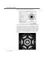
Fig. 2. The simplified TEM (left) and the calculations required for the image
simulation (right). The three principal planes are marked.
Ch. 1 Introduction to Image Simulation - p.8
MacTempas User Manual
Cowley and Moodie (1957) showed that the interaction of an
electron beam with a specimen could be described by the socalled multislice approximation, in which electrons propagate
through the specimen and scatter from the crystal potential, the
electron scattering is described by the so-called phase-grating
function, a complex function of the potential, and the electron
propagation is computed with a propagation function dependent
on the electron wavelength. Since then there have been numerous formulations of the multislice approximation derived from
the Schrödinger equation.
Simulating TEM
Images
The problem of simulating images thus becomes a problem of
computing the electron wavefields (wavefunction) at three
microscope planes. Currently the best way to produce simulated
images is to divide the overall calculation into three parts:
(1)
Model the specimen structure to find its potential in the
direction of the electron beam.
(2)
Produce the exit-surface wavefield by considering the
interaction of the incident electron wave on the specimen potential.
(3)
Compute the image-plane wavefield by imposing the
effects of the objective lens on the specimen exit surface
wave.
Each of these steps will be covered in the next sections. However, because of space constraints, it is impossible to cover
everything in great depth. For detailed derivation, the reader is
encouraged to read the many excellent texts on the subject.
Ch. 1 Introduction to Image Simulation - p.9
MacTempas User Manual
Ch. 1 Introduction to Image Simulation - p.10
MacTempas User Manual
Chapter
2
Modeling the
Specimen
Theory of Image
Simulation
The specimen is a three dimensional objects consisting of a
huge number of atoms. From a modeling point of view, it is necessary to reduce the number of parameters to a more manageable number. For crystalline materials described by a repeat of
perfect unit cells this is easily accomplished. The unit cell in
this case is defined by the lattice parameters A,B and C where A
and B are in the plane the specimen perpendicular to the electron beam and C is in the main direction of the incoming electrons. A,B and C are related to the normal lattice vectors a,b,
and c depending on the orientation of the specimen. The specimen is thus reduced to M number of unit cells, where M*C is
equal to the thickness of the sample, giving in the end a 2D
image which covers the area given by A and B.
In the case of a defect structure which no longer can be modeled
as a small repeating structure, it is necessary to limit the extent
of the calculation by defining a supercell which contains the
defect. The resulting image obtained from the calculation will
contain artifacts which arise from limiting the structure at arbitrary boundaries and care must be taken to ensure that the image
gives a faithful representation of the area of interest.
The entire electrostatic potential of the specimen is now defined
by one unit cell with axes a,b, and c, angles alpha, beta and
gamma, and N atoms with coordinates x,y,z. For simplicity, we
use the nomenclature of the crystallographic unit cell even
though we are referring to the transformed unit cell (A,B,C) as
described above.
The electrostatic potential in the crystal can be written
(r) = ∫ d r'
3
(r' )
r − r'
1
Ch. 2 Theory of Image Simulation - p.11
MacTempas User Manual
where ρ(r), the charge density is:
∑
(r) =
i (r
− ri )
2
all
atoms i
with the sum extending over all atoms i at positions ri, each giving rise to a charge density
i (r)
= Zi e (r) − e
i (r)
2
3
where Zi : atomic number, e: electronic charge, (r) : the
quantum mechanical many electron wavefunction for the atom.
The potential φ(r) is described by its Fourier transform Φ(u)
through the relationship
(r) = ∫ Φ(u)e −2
iu⋅r
du = ∑ Φ(H)e −2
iH⋅r
H
4
since because of the periodicity of the unit cell, Φ(u) is nonzero only when u = H = ha*+kb*+lc* , H being a reciprocal lattice vector.
The potential Φ(H) is given as a sum over all atoms in the unit
cell
Φ(H) =
∑ f iel (H)e 2 iu⋅r
i
all
atoms i
=
e
4
2
∑
0 all
atoms i
Z i − fi x ( H 2) 2
e
H2
iu⋅ri
5
where the electron scattering factors fiel and the x-ray scattering
factors fix have been calculated from relativistic electron wavefunctions and parameterized. They can be found in various
tables (Doyle and Turner, 1968) and are in use by most image
simulation programs such as SHRLI (O’Keefe at al., 1978),
NCEMSS (Kilaas, 1987) and EMS (Stadelman, ).
Taking into account any deviation from full occupancy at a particular site and the thermal vibration of the atom, the Fourier
Ch. 2 Theory of Image Simulation - p.12
MacTempas User Manual
coefficients of the crystal potential from one unit cell is calculated as:
Φ(H) =
∑ f iel (H)Occ(ri )exp[−Bi H2 ]e 2
iH⋅ri
6
unit cell
atoms i
B: Debye Waller factor; Occ(ri) : The occupancy at position ri
Simulating the
Interaction
Between the Electrons and the
Specimen
The interaction between an electron of energy E and the crystal
potential φ(r) is given by the Schrödinger equation
[−
h2
2
∇ − e (r)]Ψ(r) = EΨ(r)
8 2m
7
where m is the relativistic electron mass and h is Planck’s constant.
Before entering the specimen, the electron is treated as a plane
wave with incident wavevector k0, k0 =2π/λ, so that the incident electron wave is written
Ψ0(r) = exp{i( t − 2 k 0 ⋅ r)}
8
It is useful to define the quantity V(r) which will loosely be
referred to as the potential as:
V(r) =
8
2
h
me
2
(r)
9
Ch. 2 Theory of Image Simulation - p.13
MacTempas User Manual
The Schrödinger equation above cannot be solved directly without making various approximations. Depending on how the
problem is formulated, one can derive the most common solutions to the electron wavefield at a position T within the specimen.
The Weak Phase Object Approximation
In the Phase Object Approximation (POA) (Cowley and Iijima,
1972), the phase of the electron wavefunction after traversing a
specimen of thickness T is given as
Ψ( x, y, z = T ) ≈ Ψ(x, y, z = 0) exp[−i Vp (x, y)T ]
10
with
eE 2
h
= 2 me 1 +
mc
11
where V(x,y) is the average potential per unit length. The specimen is considered thin enough so that electrons only scatter
once and are subject only to an average projected potential. In
the weak phase object approximation, the exponent is considered much less than one, so that the electron wavefunction
emerging from the specimen is:
(x, y,z = T ) ≈
(x, y, z = 0)(1 − i Vp (x, y)T)
12
The WPOA only applies to very thin specimens of the order of a
few tenths of Å, depending on the atomic number of the atoms
in the structure (Gibson, 1994). The FT of the wavefunction
gives the amplitude and phase of scattered electrons and in the
WPOA one has:
Ψ(u) = (u) − i Vp (u)T
Ch. 2 Theory of Image Simulation - p.14
13
MacTempas User Manual
where u is a spatial frequency.
Again, for periodic crystals, Vp(u) are non-zero only for frequencies u=H where H is a reciprocal lattice vector in the crystal.
We will now use V to mean Vp. Thus for single electron scattering and when the Fourier coefficients V(H) are real (true for all
centro-symmetric zone axis), the WPOA illustrates clearly that:
i) Upon scattering, the electron undergoes a -90° phase shift.
ii) The amplitude of a scattered electron is proportional to the
Fourier coefficient of the crystal potential.
The Bloch Wave Approximation
In the BWA the electron wavefunction of an electron with
wavevector k is written as a linear combination of Bloch waves
b(k,r) with coefficients ε (Howie, 1963). Each Bloch wave is
itself expanded into a linear combinations of plane waves which
reflect the periodicity of the crystal potential.
(r) = ∑
( j ) ( j)
b
(k, r) = ∑
j
j
( j)
∑ c(g j) exp[−2
g
i(k 0 + g) ⋅ r] 14
(j)
The formulation above gives rise to a set of linear equations
expressed as
[k 0 − (k
2
( j)
+ H) ]cH + ∑ V (H' )cH −H' = 0
2
( j)
(j)
15
H'
which needs to be solved. Detailed derivation of the Bloch
wave approximation can be found elsewhere.
Characteristics of the Bloch wave formulation are:
- Requires explicit specification of which reflections g are
included in the calculation.
- Easy to include reflections outside the zero order Laue zone.
- Very good for perfect crystals, not suited for calculating
images from defects.
- The solution is valid for a particular thickness of the specimen.
Ch. 2 Theory of Image Simulation - p.15
MacTempas User Manual
-
Allows rapid calculation of convergent beam electron diffraction patterns.
Includes dynamical scattering.
The Multislice Approximation
The multislice formulation (Goodman and Moodie, 1974 & Self
et al., 1983) i s by far, the most commonly used method of calculating the electron wavefield emerging from the specimen.
Although it does not as easily include scattering outside the
zero order Laue zone as the BWA, the multislice formulation is
more versatile for use with structures containing any kind of
defects, either they be point-defects, stacking faults, interfacial
structures, etc. The multislice solution gives the approximate
solution to the electron wavefunction at a depth z+dz in the
crystal from the wavefunction at z. In the multislice approximation one has:
(x, y, z + dz) ≈ exp[−i dz∇ x ,y ]⋅ exp[−i
2
z +dz
∫z V( x, y, z' )dz' ]
(x, y, z)
16
Thus starting with the wavefunction at z=0, one can iteratively
calculate the wavefunction at a thickness n*dz, by applying the
multislice solution slice by slice, taking the output of one calculation as the input for the next. Equation 16 is solved in a two
step process.
The potential due to the atoms in a slice dz is projected onto the
plane t=z, giving rise to a scattered wavefield
1 (x, y, z
+ dz ) = exp[ −i
z+ dz
∫z V(x, y, z' )dz' ]
(x, y, z) ≡ q(x, y) (x, y, z)
17
The function q(x,y) is referred to as the phasegrating.
Ch. 2 Theory of Image Simulation - p.16
MacTempas User Manual
Subsequently, the wavefield is propagated in vacuum to the
plane t=z+dz, according to
(x, y, z + dz) = exp[−i dz∇ x ,y ] ⋅
2
1 (x, y, z)
18
The last equation represents a convolution in real space and is
solved more efficiently in Fourier space (Ishizuka and Uyeda,
1977), where the equation transforms to
Ψ(H,z + dz) = exp[−i
dzH ]⋅ Ψ1(H, z) ≡ p(H,dz )⋅ Ψ1 (H, z) 19
2
where Ψ(H,z) are the Fourier coefficients of ψ(x,y,z). p(H,dz) is
called the propagator.
The multislice formulation is a repeated use of the last two
equations and will give the wavefield at any arbitrary thickness
T of the specimen. If the slice-thickness is chosen as the repeat
distance of the crystal in the direction of the electron beam, only
the zero order Laue reflections are included in the calculation as
the unit cell content is projected along the direction of the electron beam. Three dimensional information which involves
including higher order Laue reflections can be included by
reducing the slice thickness (Kilaas et al, 1987).
Sampling Criteria
Any numeric calculation must be performed for a limited set of
data points (x,y) or reciprocal spatial frequencies u. Working
with periodically repeated structures; if the lateral dimensions
of the unit cell is a and b, which we for simplicity make orthogonal so that the axes are associated with an orthogonal x,y coordinate system, then for a given sampling interval dx=dy, we
have
N=
a
;
dx
M =
b
dy
20
Ch. 2 Theory of Image Simulation - p.17
MacTempas User Manual
defining the calculation to a grid of N*M points. The sampling
interval automatically restricts the calculation in reciprocal
space as well. The maximum reciprocal lattice vector for
orthogonal axes is given as
2
2
N
M
2
H max = hmax a * +k maxb * = +
2a
2 b
2
21
Because most implementations of the multislice formulation
makes use of Fourier transforms, the calculation grid N and M
is adjusted so that both are powers of 2. This is because Fourier
transform algorithms can be performed much faster for powers
of 2 rather than arbitrary dimensions. This results in uneven
sampling intervals dx,dy when a ≠ b. In order to not impose an
arbitrary symmetry on the calculation, a circular aperture is
imposed on the propagator. In practice, this aperture is set to 1/2
of the minimum of (hmax, kmax) as defined above in order to
avoid possible aliasing effects associated with digital Fourier
transforms. The sampling must be chosen such that the calculation includes all (or sufficiently enough) scattering that takes
place in the specimen.
The Image Formation
After the electron wavefield emerge from the specimen, it is
subjected to the varies magnetic field of the lenses that form the
imaging and magnification part of the microscope. Of these
lenses, only the first lens, the objective lens, is considered in the
image formation calculation. Since the angle with which the
electron forms with the optic axis of the lens varies inversely
with the magnification, only the aberrations of the objective
lens are important. The remaining lenses serve to just magnify
the image formed by the objective lens. The effects of the lens
which normally are included in the calculation are spherical
aberration, chromatic aberration and lens defocus. Two-fold and
three-fold astigmatism, including axial coma, are considered
correctable by the operator although they can be included in the
equations.
Without any aberrations, no instabilities and with the specimen
Ch. 2 Theory of Image Simulation - p.18
MacTempas User Manual
in the focal plane of the objective lens, the image observed in
the electron microscope would be am magnified version of
I(x, y) =
2
(x, y, z = exitplane of specimen) =
e (x,
y)
∗
e (x,
y)
22
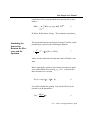
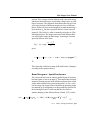
Objective Lens Defocus
Consider an electron traveling from the plane defined by the
exit surface of the specimen to the plane given as the plane of
focus for the objective lens. This distance is referred to as the
objective lens defocus ∆f.
Object plane
Exit plane
∆f/cosα
α
α = Hλ
∆f
The electron traveling along the optic axis will have a path
length of ∆f while an electron that has been scattered an angle
α=Hλ, will travel a distance ∆f /cosα. This can be expressed as
a phase difference
2
(∆f cos
)
− ∆f ≈
∆fH 2
23
Spherical Aberration
Electrons crossing the optic axis with an angle a at the focal
Ch. 2 Theory of Image Simulation - p.19
MacTempas User Manual
plane of the objective lens should form parallel paths emerging
from the lens.
α
δ(α)
f
However, the spherical aberration of the lens causes a phase
shift relative to the path of the unscattered electron (α=0) which
is written as (Scherzer, 1949):
2
∗1 4 Cx
4
= 1 2 Cs 3H 4
24
If there were no other effects to consider, the image would be
obtained as follows:
Calculate the wavefield emerging from the specimen
according to one of the approximations.
Fourier transform the wavefield which gives the amplitude and phase of scattered electrons.
Add the phase shift introduced by the lens defocus and
the spherical aberration to the Fourier coefficients.
Inverse Fourier transform to find the modified wavefunction.
Calculate the image as the modulus square of the wavefield.
However, there are two more effects that are usually considered. Variations in electron energy and direction.
Chromatic Aberration / Temporal Incoherence
Electrons do not all have exactly the same energy for various
Ch. 2 Theory of Image Simulation - p.20
MacTempas User Manual
reasons. They emerge from the filament with a spread in energy
and the electron microscope accelerating voltage varies over the
time of exposure. The chromatic aberration in the objective lens
will cause electrons of different energies to focus at different
planes. Effectively this can be thought if as rather than having a
given defocus f0, one has a spread in defocus values centered
around f0. The value f0 is what is normally referred to as ∆f as
indicating defocus. The images associated with different defocus values add to make the final image. Assuming a Gaussian
spread in defocus of the form
D( f − f0) ∝ exp[−
( f − f0 )2
∆2
25
]
gives:
I=
∫ Ψ( f
2
[ 1 2(
− f0 ) D( f − f0 )df ⇒ Ψ(H) → Ψ(H) e x p −
∆H ) ]
2 2
26
This states that each Fourier term (diffracted beam) is damped
according to the equation above].
Beam Divergence / Spatial Incoherence
The electron beam is not an entirely parallel beam of electrons,
but form rather a cone of an angle α. This implies that electrons
instead of forming a point in the diffraction pattern form a disk
with a radius related to the spread in directions. As for a variation in energy, the images formed for different incoming angles
are summed up by integrating over the probability function for
the incoming direction. It turns out that this also leads to
another damping of the diffracted beam (Frank, 1973) so that:
I(r) =
∫
2
(r, ) D( )d
⇒ Ψ(H) → Ψ(H)exp[
( Cs H2
2
+ ∆f )]2
27
Ch. 2 Theory of Image Simulation - p.21
MacTempas User Manual
The Final Image
Equation 26 and equation 27 are only valid when the intensities
of the scattered beams are much smaller than the intensity of the
central beam. Thus the image results from scattered beams
interfering with the central beam, but not with each other. This
is referred to as linear imaging. Although the formulation is
slightly more complicated in the general case, the expressions
above give sufficient insight into the image formation. Image
simulation programs do however include the more general formulation which include non-linear imaging terms (O’Keefe,
1979). Each Fourier component is damped by the spread in
energy and direction and the image is formed by adding this to
the recipe in section 4.2
The Contrast Transfer Function CTF
When reading about HRTEM, it is impossible not to encounter
the expression "Contrast Transfer Function". Loosely speaking,
the CTF of the microscope refers to the degree with which Fourier components of the electron wavefunction (spatial frequencies) are transferred by the microscope and contribute to the
Fourier transform of the image. Although the CTF only holds
for thin specimen and linear imaging, it is often generalized and
wrongly applied to all conditions. However, the CTF does provide insight into the nature of HRTEM images. In order to
derive the expression for the CTF, we start by calculating the
image intensity as given by the Weak Phase Object approximation. In the WPOA:
Ψ( x, y, z = T) ≈ 1− i Vp (x, y)T
28
and
Ψ(H) = (H) − i Vp (H)T
29
Applying the phase shift due to the spherical aberration and the
Ch. 2 Theory of Image Simulation - p.22
MacTempas User Manual
objective lens defocus which we will call χ(H), we get that the
FT of the wavefunction is (for simplicity V = Vp):
Φ(H) = (H) − i V(H)e
i ( H)
A(H)
30
where A(H) is the damping terms arising from partial coherence.
The FT of the intensity is now given as
I(H) = FT(
∑(
⋅
∗
) = ∑ Ψ(H' )Ψ * (H − H' ) ≈
H'
(H' ) − i A(H' )V(H' )ei
(H')
H'
)(
(H − H' ) − i A(H − H' )V(H − H' )e i
(H − H')
)≈
(H) + 2 A(H)V (H)sin (H)
31
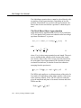
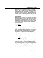
The last result is very useful and it leads to the frequently used
concept of the Contrast Transfer Function (CTF). The CTF is
defined as A(H)⋅sinχ(H) The equation above states that each
reflection H contributes to the image intensity spectrum with a
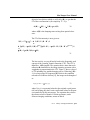
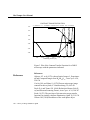
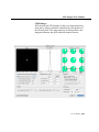
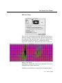
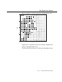
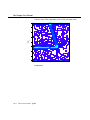
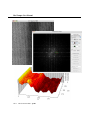
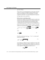
weight that is proportional to the CTF. Figure 3. shows a plot of
a CTF including sinχ and the damping curves. When sinχ (H) =
-1 for a large range of frequencies H, which is the condition
referred to as Scherzer defocus[11], the image can be thought of
as:
I(x, y) ≈ 1 − 2 U(x, y)
32
where U(x,y) is a potential related to the original crystal potential, but keeping only the Fourier coefficients related to frequencies transferred by the microscope. The equation above shows
the often used rule of thumb. For thin specimens, under
Scherzer imaging conditions, atoms are black.
Ch. 2 Theory of Image Simulation - p.23
MacTempas User Manual
CONTRAST TRANSFER FUNCTION
1.00
V = 200.0 kV Cs = 1.0 mmDef = -560.00 Å Del = 50.00 Å Div = 0.60 mrad
0.70
0.40
0.10
-0.20
-0.50
-0.80
0.06
0.14
0.22
0.30
-1
0.38
0.46
0.54
Scattering Vector [Å ]
Figure 3. Plot of the Contrast Transfer Function for a 200kV
microscope with the parameters indicated.
References
References
Allpress J.G. et al (1972) n-beam Lattice Images. I. Experimental and Computed Images from W4Nb26O77, Acta Cryst. A 28,
528-536
Cowley J.M. and Iijima S. (1972) Electron microscope image
contrast for thin crystals, Z. Naturforschung 27a, 445-451
Doyle P.A. and Turner P.S. (1968) Relativistic Hartree-Fock Xray and Electron Scattering Factors, Acta Cryst.. A 24, 390-397
Frank J (1973) The envelope of electron microscope transfer
functions for partially coherent illumination, Optik 38, 519-536
Gibson J.M. (1994) Breakdown of the weak-phase object
Ch. 2 Theory of Image Simulation - p.24
MacTempas User Manual
approximation in amorphous objects and measurement of highresolution electron optical parameters, Ultramicroscopy 56, 2632
Goodman P, Moodie A.F. (1974) Numerical evaluation of Nbeam wave functions in electron scattering by the multislice
method, Acta Cryst. A30, 322-324
Howie A. (1963) Inelastic scattering of electrons by crystals,
Proc. Roy. Soc. A271, 268-275
Ishizuka K. and Uyeda N. (1977) A new theoretical and practical approach to the multislice method, Acta Cryst. A 33, 740
Kilaas R. et al. (1987) On the inclusion of upper Laue layers in
computational methods in High Resolution Transmission Electron Microscopy, Ultramicroscopy 21, 47-62
Kilaas R. (1987) Interactive software for simulation of high
resolution TEM images, Proc. 22nd MAS, R. H. Geiss (ed.),
Kona, Hawaii, 293-300.
Kilaas R. (1987) Interactive simulation of high resolution electron micrographs. In 45th Ann. Proc. EMSA, G.W. Bailey (ed.),
Baltimore, Maryland, 66-69.
O’Keefe MA, Buseck PR, Iijima S (1978) Computed crystal
structure images for high resolution electron microscopy. Nature 274, 322-324.
O’Keefe M.A. (1979) Resolution-damping functions in non-linear images, Proc. of EMSA 37, 556-557
O’Keefe M.A. et al. (1989) Simulated Image Maps for use in
Experimental High-Resolution Electron Microscopy, Mat. Res.
Soc. Symp. Proc. 159, 453-458
Scherzer O. (1949) The Theoretical Resolution Limit of the
Electron Microscope, Journal of Applied Physics 20, 20-29
Self P.G.et al. (1983) Practical computation of amplitudes and
phases in electron diffraction, Ultramicroscopy 11, 35
Ch. 2 Theory of Image Simulation - p.25
MacTempas User Manual
Ch. 2 Theory of Image Simulation - p.26
MacTempas User Manual
Chapter
3
Introduction to
MacTempas
Since the simulation of a HRTEM phase contrast image can be
subdivided into independent calculations involving the structure, the scattering process and the imaging process, MacTempas allows one to invoke these independent calculations
separately through the “Calculate” menu.
The Three Simulation Steps
Full Calculation
This command will start the calculation from the required starting point and proceed to calculate final images.
Projected Potential
generates the crystal potential that produces electron scattering
from the structural data, unit cell dimensions, symmetries, and
atom positions, occupancies, and temperature factors.
Exit Wavefunctions(s)
generates the electron wavefield at the specimen exit surface; it
uses the projected potential combined with information about
the accelerating voltage of the electron microscope, the specimen thickness and tilt. The computation algorithm is the multislice approximation.
Image(s) normal calculation
generates the image intensity at the microscope image plane;
the effects of the objective lens phase changes and resolutionlimiting aberrations are included via parameters like defocus,
spherical aberration, incident beam convergence, spread of
defocus, and the position and size of the objective aperture.
Image Plane Wavefunctions(s)- generates the electron wavefunction at the imaging plane in the microscope. This is equiva-
Ch. 3 Introduction to MacTempas - p.27
MacTempas User Manual
lent to the application of the Contrast Transfer Function to the
Fourier transform of the electron wavefunction at the exit surface of the specimen followed by an inverse Fourier transform.
The calculation of the image plane wavefunction is used for
comparing with the electron wavefunction found by the use of
electron holography. The remaining commands in the Calculate menu will be covered under the Menus chapter.
Thus “Projected Potential” calculation considers only the specimen structure, “Exit Wavefunctions(s)” calculation treats the
interaction of the specimen with the electron wave, and the
“Image(s)” calculation simulates how the wave leaving the
specimen interacts with the lens system of the electron microscope. Once a simulation has been made, any additional simulation will usually not require a full re-calculation; any change in
microscope parameters will not affect the results of the “Projected Potential” and “Exit Wavefunctions(s)” calculations, and
only Image(s) will need to be re-run; any change in microscope
voltage or in specimen thickness and tilt will not affect the output of “Projected Potential”, but “Exit Wavefunctions(s)” and
“Image(s)” will need to be re-run. Of course, any change in the
specimen structure will require the re-running of all three subprograms.
Generated Files
MacTempas generates and stores various files in the course of a
simulation. The 6 possible data files are:
(1)
<structurename>.at stores all the structure and microscope information needed to run the simulation. This
information is derived from user input and the supplied
data files. In particular, the string “structurename” is a
unique name for the structure, input by the user when
creating the structure file. This is an editable file of type
‘TEXT’.
(2)
<structurename>.pout is the result of running the projected potential routine from the information stored in
Ch. 3 Introduction to MacTempas - p.28
MacTempas User Manual
<structurename>.at; it contains the specimen potential
in the direction of the electron beam. This is a BINARY
file of type Real 4. The first 80 bytes consists of record
information and the data starts at byte 80. The first line
of data contains the data for the bottom line of the
“image” since the coordinate system for MacTempas is
at the lower left corner of the image/unit cell. Thus if the
data is imported into a program for viewing, the image
will appear flipped.
(3)
<structurename>.mout is the result of running the
multislice routine using the data in <structurename>.pout with those in <structurename>.at; it contains the exit-surface wavefunction at one or more
selected specimen thicknesses. This is also a BINARY
file with the same structure as <structurename>.pout,
except for the fact that the data is complex, pairs of
numbers (real and imaginary). The data starts at byte 80
and the file can contain more than one exit wavefunction.
(4)
<structurename>.iout is the result of running the
image formation routine to apply the effects of the
microscope parameters in the <structurename>.at file
to the exit-surface wave; it contains one or more images
ready to be displayed. This again is a BINARY file with
data starting at byte 80 and the file can contain more
than one image. Data is Real 4
(5)
<structurename>.hout is the result of calculating the
image plane electron wavefunction(s) instead of calculating the simulated images. The data is complex, pairs
of numbers (real and imaginary). The data starts at byte
80 and the file can contain more than one image plane
exit wavefunction.
(6)
<structurename>.aout contains the complex amplitudes of several diffracted beams at one-slice increments
Ch. 3 Introduction to MacTempas - p.29
MacTempas User Manual
in specimen thickness. The beams are specified by the
user, and can be plotted as a function of specimen thickness.
In addition, two “print” files are produced (but rarely printed)
just in case additional information about a computation is
required by the user. These files are:
(7)
<structurename>.p_prnt contains information about
the way in which the “Projected Potential” subprogram
processed the <structurename>.at data to produce the
specimen potential.
(8)
<structurename>.m_prnt contains information about
the way in which the “Exit Wavefunctions(s)” subprogram processed the <structurename>.pout data with
the <structurename>.at to produce the exit-surface
wave; that is, it contains information from the multislice
computation.
Ch. 3 Introduction to MacTempas - p.30
MacTempas User Manual
Chapter
4
Running MacTempas
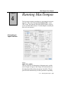
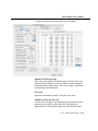
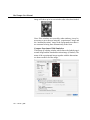
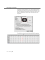
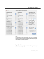
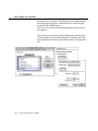
The first step in running a simulation is generating the structure
input file. This is done through New Structure File... in the
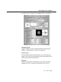
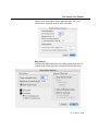
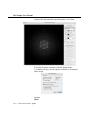
FILE menu. This generates the input dialog window with values for a default cubic structure. Use this template to modify the
date to fit your structure..
Generating an
Input Structure
a, b, c,
alpha, beta, gamma
These are the unit cell dimensions in Ångstrøm units, and the
unit cell angles in degrees. MacTempas will automatically set
the angles depending on the spacegroup, if possible. The program will also automatically set lattice parameters depending
Ch. 4 Running MacTempas - p.31
MacTempas User Manual
on the spacegroup. Thus if the user chooses a cubic system, b
and c are set equal to a
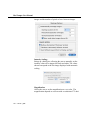
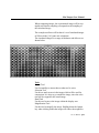
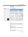
Space group#
MacTempas generates symmetry operators for the any one of
the 230 space groups when selecting the number or the symbol
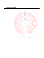
of the space group (as listed in the International Tables for Crystallography). By clicking on the pop up menu “Space Group”
one can choose one of the 230 spacegroups by first selecting the
type of crystal-structure, i.e. hexagonal or cubic. The user can
choose one of the spacegroups by clicking on the symbol for the
spacegroup or by entering the number for the spacegroup.
The input also allows for choosing the second setting for a specific spacegroup if one exists. If no space group is required, one
should use the space group P1 (1), in which case the only symmetry operator is x,y,z. Additional symmetry operators can be
Ch. 4 Running MacTempas - p.32
MacTempas User Manual
entered by opening the dialog displaying the symmetry operators.
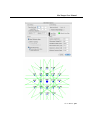
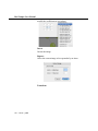
Show (Basis atoms)
Use this button to bring up the dialog window that enables the
input of the atoms in the basis.
Number of Atoms in the Basis
This value is the number of independent atom positions in the
basis or asymmetric unit of the cell. When operated on by the
symmetry operators, the basis generates all the atom positions
within the cell. This value is never modified by the user since
the program always recalculates this number depending on the
data entered.
Ch. 4 Running MacTempas - p.33
MacTempas User Manual
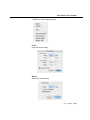
Show (Symmetry Operators)
The symmetry operators are automatically created by specifying the spacegroup. By clicking on this button, a window displaying the symmetry operators are shown.
Show (Atoms in Unit Cell)
The atoms in the unit cell are automatically created by the operation of the symmetry operators on the atoms in the basis. The
number of atoms is given and by clicking on the button “Show”,
Ch. 4 Running MacTempas - p.34
MacTempas User Manual
a window displaying the atoms in the unit cell appears.
Number of different atoms
This value is the number of different types of atoms in the specimen structure; difference is due to a different atomic number or
a different Debye-Waller factor. The correct value is calculated
by MacTempas and displayed.
Zone Axis
Specimen orientation in relative real space axes units.
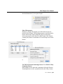
Number of slices per unit cell
For unit cells with large repeat distances in the beam direction,
moderate values of Gmax may allow the Ewald sphere to
approach the so-called pseudo upper-layer line that the multi-
Ch. 4 Running MacTempas - p.35
MacTempas User Manual
slice allows at the reciprocal of the chosen slice thickness. In
this case MacTempas will sub-divide the slice into two or more
subslices. How this is done depends upon the potential setting
chosen in the Option menu.If 2-D calculation is set and the
checkbox “sub-divide unit cell” is NOT checked, the projected
potential is calculated for the entire unit cell in the zone-axis
orientation and is used n times to cover the unit cell. If 2-D calculation is set and the checkbox “sub-divide unit cell” is
checked, n-potentials are calculated from the atoms within each
sub-layer and used to cover the unit cell. If 3-D calculation is
set, n-potentials are calculated by appropriate integration of the
potential from all atoms in the unit cell.
Gmax
The maximum value (in reciprocal Ångstrøm units) of any scattering vector to be included in the multislice diffraction calculation. This value imposes an “aperture” on the diffracted beams
included in the dynamic scattering process. It should be large
enough to ensure that all significant beam interactions are
included. The default value is 2.0. MacTempas will compute
phase-grating coefficients out to twice Gmax in order to avoid
aliasing in the multislice calculations.
Specimen Thickness
The thickness of the specimen foil is entered as a beginning
thickness, an ending thickness and an incremental thickness. All
numbers are in Ångstrøm units. A series of thicknesses represented by the upper and lower bounds and a thickness step; e.g.
100 50 250 will cause MacTempas to store the exit wavefield at
specimen thicknesses of 100Å to 250Å in steps of 50Å (a total
of four thicknesses).
Store Ampl./Phases - Set...
Clicking this button allows a number of diffracted beams to be
selected for plotting of their intensity and phase variation as a
Ch. 4 Running MacTempas - p.36
MacTempas User Manual
function of specimen thickness. The reflections to be tracked
are determined by entering the hkl values for the reflection.
Only 10 reflections can be tracked this way.
Center of the Laue Circle
Specimen tilt is specified by entering the center of the Laue circle in units of the h and k indices of the projected two-dimensional reciprocal-space unit cell. Equivalently the tilt angle and
azimuthal angle can be specified instead. The new indices and
their relationship to the original reciprocal cell is found in the
data file <structurename>.p_prnt
Type of Absorption
Absorption can be included in the program by introducing an
Ch. 4 Running MacTempas - p.37
MacTempas User Manual
imaginary projected potential.
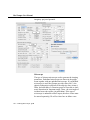
Microscope
The type of electron microscope used to generate the imaging
parameters. Predefined microscopes are shown in the popup
menu together with one undefined microscope. If a predefined
microscope is used, MacTempas provides values for Cs, the
spherical aberration coefficient of the objective lens (in mm.);
Delta, the halfwidth of a Gaussian spread of focus due to chromatic aberration (in Ångstrøm units); Theta., the semi-angle of
incident beam convergence (in milliradian). If the type of
microscope is unknown to MacTempas, the above values must
be entered separately (We will see later how to define a new
Ch. 4 Running MacTempas - p.38
MacTempas User Manual
microscope).
Voltage
The electron microscope accelerating voltage in kilovolts.
Objective Lens Defocus
The defocus of the objective lens is entered in Ångstrøm units
with a negative value representing underfocus (weakening of
the lens current). As for the speciment thickness parameter, the
input is a range specified by the upper and lower bounds and an
increment.
Min. Intensity in the lens
This specifies a cutoff in intensity for which a beam is included
in the calculation. Normally the default is adequate and saves
Ch. 4 Running MacTempas - p.39
MacTempas User Manual
computation time. However, for large structures containing
defects, diffuse scattered beams are very weak and a lower cutoff may be needed in order to compute the correct contrast..
Strong Central Beam
If this box is checked, only linear terms to the image intensity
contribute. Normally both linear and non-linear terms are
included in the calculation..
Cs, Spherical Aberration
The spherical aberration of the objective lens in mm.
Convergence Angle
This is the spread in angle for the cone of incoming electrons
depending on the condenser lens aperture. The angle is given in
mrad.
Spread of Defocus
This is the effective spread in defocus which results from the
distribution of energies of the imaging electrons and the chromatic aberration of the objective lens. The unit is Å.
Aperture Radius
The radius of the objective aperture is specified in Å-1
Both an inner aperture and an outer aperture can be specified.
Normally the inner aperture would be zero.
Center of objective Aperture
The center of the objective lens aperture is defined in units of h
and k of the two dimensional reciprocal space unit cell, as for
the Laue circle center. Again, tilt angle and azimuthal angle can
be specified instead.
Center of the Optic Axis
The center of the optic axis of the electron microscope is specified in terms of the h and k indices of the two-dimensional
reciprocal-space unit cell, just as for the Laue circle center and
the aperture center.
Ch. 4 Running MacTempas - p.40
MacTempas User Manual
Two-fold astigmatism
The two fold astigmatism of the objective lens and the angle
with the x-axis. The magnitude is given in Å.
Three-fold astigmatism
The two fold astigmatism of the objective lens and the angle
with the x-axis. The magnitude is given in Å.
Coma
The coma of the objective lens and the angle with the x-axis.
The magnitude is given in Å.
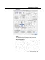
Mechanical Vibration
This simulates the effect of a slight vibration of the microscope.
One finds that often the simulated images show details that are
not present in the experimental data regardless of other imaging
conditions. This may be due to image degradation caused by
microscope vibration or other effects not included and thus one
can introduce a slight mechanical vibration in an attempt to create more realistic simulated images. It is possible to specify an
anisotropic vibration by introducing the amplitude in two perpendicular directions with the diagonal of the ellipse at an angle
with the a axis (as in the unit cell viewed in the zone axis orientation).
Ch. 4 Running MacTempas - p.41
MacTempas User Manual
Ch. 4 Running MacTempas - p.42
MacTempas User Manual
Chapter
5
Windows
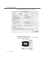
This chapter explains the windows of Mactempas, the information presented in each and how one interacts with the contents
of the windows.
Status Window
This window shows the current status of the program indicating
the number of phasegrating coefficients calculated, the current
slice number being calculated, the current image being calculated etc.
Atom Window
This window shows which atoms are present in the structure,
the color the atom will be drawn in (if colored atoms are set)
and the relative sizes of the atoms to be drawn. To change the
color of an atom, choose the Color Picker tool from the Tools
Window, click on a color in the Color Bar in the Image Control
Window and deposit that color on an atom by clicking on the
colored circle representing the atom. The color of the atom will
be set to the new color.
Ch. 5 Windows - p.43
MacTempas User Manual
To change the atomic radius, double-click on the chemical sym-
bol. A dialog window will pop up and a new value for the
atomic radius can be entered (units in Å).
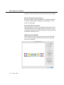
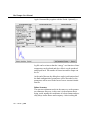
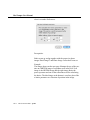
Image ControlWindow
Ch. 5 Windows - p.44
This window is used primarily to control the appearance of
images. The active image can be the image in a image window
or the selected image in the MacTempas main window. The
black and white values of the current selected image is shown
and can be changed by typing in new values. The contrast and
brightness can be changed by using the appropriate sliders. An
image can be shown on a logarithmic scale which is the default
for images in frquency space (reciprocal space). The line in the
graph represents how input image values are mapped to output
display values. Thus an image can be pseudo colored by choosing a color from the color bar with the color picker tool selected
and “depositing” this color in the vertical gray scale bar showing the display vlaues. The histogram of the current image is
shown and black and white values can be chosen by clicking
and dragging to select a region of the histogram. To invert the
display, click in the “Invert” button. Similarily the image is reset
to the original values through the “Reset” button. This window
is also used to set the color of a particular atom species and the
color of lines and text. To choose a color, the Color Picker Tool
must have been chosen.
MacTempas User Manual
Tools Window
The following tools are currently defined:
Pointer
Used for general moving around objects in the display window.
If an object is selected and the “Option” key is held down while
dragging an object, a copy is made of the object. In an image
window, the pointer tool will also act as a hand tool if nothing is
selected.
Text Tool
Clicking on this tool turns the cursor into an i-beam cursor
which can be used to select an insertion point for text. To set the
insertion point for text to be typed in the image window click
the mouse at the desired point. The Font, Size and style of the
text is determined from the menu bar. The text will be drawn in
the current foreground color and can be left, canter or right justified.
Magnifying Glass
When selected the cursor turns into a magnifying glass which
can be used to zoom in on a selected part of the display. Each
time the mouse is clicked in the image window, the image is
zoomed by a factor of two. By holding down the Option key
while clicking, the image will be zoomed out by a factor of 1/2
for every click. Double-clicking the magnifying glass returns
the image to normal.
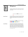
Line Tool
This tool is used to draw lines on the display. If the Shift key is
down, only vertical or horizontal lines will be drawn.
Selection Tool
This tool is used to select a portion of the screen for several possible operations such as copying, cutting, histogram computation etc. To select an area, click at a point in the display and
drag the cursor while the mouse button is pressed. In the main
Ch. 5 Windows - p.45
MacTempas User Manual
MacTempas window, all objects intersecting the selection rectangle will be selected.
Trace Tool
This tool is used to get a line trace for the line drawn with the
Trace Tool being the current tool. The integration width can be
changed by double clicking on the trace-line or choosing “Edit
Object” when the line is selected.
Color Picker Tool
This tool when selected, allows the user to pick a color from the
Color Window and color atoms, selecting fore-/back-ground
colors and pseudo-color atoms. The selection of color is
described under Color Window above
Hand Tool
Use this tool to move images around in the image window.
Ruler Tool
Use this tool to measure distances in an image. An image can be
calibrated from the menu command under Process after a line is
drawn using the ruler tool..
Rotate Tool
This tool is used to rotate drawings of crystal structures. In
order for it to be active, the structure must be selected and the
mouse click must occur within an atom.
Masking Tools
The last 5 tools are masking tool normally used in reciprocal
space, but they can be used in real space as well. The masks are
a) Spot mask. A reflection and its conjugate is selected.
b) Lattice mask. A mask defined by two lattice vectors.
c) Band Pass mask. This mask is defined by an inner and an
outer circle.
d) Wedge mask. Defined by two lines.
e) Line mask. Defined by a line and a single lattice vector.
All these masks can be transparent or opaque, meaning they
Ch. 5 Windows - p.46
MacTempas User Manual
work on the region within or outside of the mask. The mask
parameters can be edited by double clicking on the mask or
selecting the mask and choosing “Edit Mask” from the “Process” menu. The number of lattice spacings for the vector(s) for
the lattice mask and line mask can also be changed by clicking
in the end point of the vector with the “Option” key down. Each
click increments the number of lattice spacings to the endpoint
by one. Holding down the “Shift” key and the “Option” key
decreases the number of lattice spacings by one.
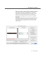
Info Window
This window shows the current position of the cursor within the
image window and the intensity of the underlying pixel. When
dragging a rectangle, the dimensions of the rectangle are shown.
Line lengths and angles are also displayed. Image statistics is
displayed in this window when invoked through the “Statistics”
in the “Process” menu.
Display Window
Use this window to define which part of the calculation to display. The choices are:
Projected Potential - Essentially the output of the projected
potential routine. There is a one to one correspondence between
the points in the projected potential and those in the image if
displayed under equivalent conditions.
Exit Wavefunction - This is the output of the multislice component of the programand shows the distribution of electrons as
they emerge from the bottom of the specimen, or at a predefined
depth in the specimen. By holding down the Option key when
selecting the button, one can select to display either the magni-
Ch. 5 Windows - p.47
MacTempas User Manual
tude squared (default), the complex amplitude or the complex
phase of the electron wavefunction at the exit surface of the
specimen.
Diffraction Pattern - Select this option to display the diffraction pattern for one of the selected specimen thicknesses. This is
a dynamical diffraction pattern including multiple scattering in
the specimen.
Image - When selected, one of the calculated images becomes
the source of the operations defined by clicking in the Operand
Window. By holding down the Option key when selecting the
button, one can select to display either the image intensity
(magnitude squared, default), or if the image plane wavefunction(s) has been calculated, the complex amplitude or the com-
Ch. 5 Windows - p.48
MacTempas User Manual
plex phase of the electron wavefunction at the image.
FFT
Use this to perform a Fourier Transform on the selected source.
Operating on the Projected Potential will yield the structure factors, operating on the Exit Wavefield will yield the diffraction
pattern and operating on the image will give the Power spectrum of the image.
#Unit cells
Use this to specify the number of unit cells that should be displayed. The input determines the number of cells in the a-direction and b-direction.
Zoom
Use this selection to Zoom the object to either magnify the
object or to reduce the object. A zoom factor greater than 1.
magnifies and a zoom factor less than 1. reduces the object.
Display
Before the result of operating on a selected source is displayed
in the image window, Display must have been clicked. Choosing the source and operations only selects the functions to be
performed. When Display gets activated, the functions get executed.
->File
This will allow for output of the numeric values of images,
amplitudes and phases to a file. Options allow for writing the
data in ascii format or binary format. Images can also be written
Ch. 5 Windows - p.49
MacTempas User Manual
as TIFF files in this fashion.
Cancel:
Use this button in case the wrong sequence of commands was
chosen or anything else was entered wrong. This cancels the set
functions.
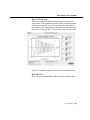
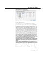
Main Display Window
Ch. 5 Windows - p.50
Main MacTempas Display Window
This is where most of the results of a calculation are displayed.
All objects such as images, diffraction patterns, unit cell drawiings, etc in this window are all objects which can be manipulated. Objects are moved with the pointer tool. If the Option key
is held down, a copy of the object will be created. The magnifying tool operates on each object separately. Several objects can
be selected and copied onto the clipboard and can be pasted into
other applications. Images in this window if double-clicked will
open up in their own separate window. The selection tool will
select any object which intersects the selection rectangle. Each
object have different properties. An image can be scaled directly
by dragging its corner. A kinematical SAD pattern can be
MacTempas User Manual
rotated by using the rotation tool when the object is selected and
the mouse-down event takes place in one of the diffraction
spots. A drawing of the atomic structure can be magnified and
rotated into different viewing directions.
Ch. 5 Windows - p.51
MacTempas User Manual
Ch. 5 Windows - p.52
MacTempas User Manual
Chapter
6
File Menu
Menus
Many of the functions in MacTempas are run from one of the
MacTempas menus, including the multislice calculation. In
addition, most options are set from one of the menus. This is a
list of the currently available menus and a description of their
function.
This menu contains the following commands:
Ch. 6 Menus - p.53
MacTempas User Manual
New Normal Structure...
Create a new structure file. A name is prompted for before input
is made. Enter a unique structure name, the program will
append the extension .at. Make sure that you do not add an
extension of the type .at in which case MacTempas will not
properly deal with the file later on. Also make sure the filename
does not have a period in it. This opens a new structure with
default values for all the parameters. Change the input to reflect
Ch. 6 Menus - p.54
MacTempas User Manual
the structure that you want to create
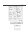
New Layered Structure...
Create a new layered simulation file. A name is prompted for
before input is made. Enter a unique structure name, the program will append the extension .lay. A layered structure is characterized by being made up of a sequence of pre-calculated
projected potantials. Thus a layered simulation file does not
contain atomic positions. The structure information in the input
dialog is replaced by .
Only A and B and Gamma have meaning for a layered “structure”. The buttons “Define PGratings” and “Define Stacking”
are used to choose the different projected potentials and to
define their sequence to make up the entire specimen.
Open Structure File...
Open an existing structure or a leyered file. The standard Macintosh file open dialog is presented and only files of the type
‘TEXT” with the extension “.at” or “lay” are displayed as
selectable. The name of the display window will change to
reflect the name of the current structure.
Close
Close the file, image or window currently selected
Save Structure
Save the current data for the structure file in use. The current
data will be written to the file, overwriting any old data.
Save Structure As...
Save the current structural information. Do not use a name with
Ch. 6 Menus - p.55
MacTempas User Manual
an extension if the file being saved is a structure file for later use
by MacTempas.
Open Image...
Open an image. Supported images are currently tiff files and
binary files. RGB tiff files and compressed tiff files are not supported. Binary files can be of integer or float types with different length and byte order.
New Image...
Create a new image of specified size and content..
Ch. 6 Menus - p.56
MacTempas User Manual
Save Image...
Saves the content of the image window into a file. MAL input
files are binary files used by the mal or TrueImage program for
exit wave reconstruction from a through focal series.
Save Image As...
Similar to “Save Image”.
Import PICT File...
Import a PICT file and display it in the MacTempas image window.
Save Window...
Saves the content of the image window as a PICT file..
Page Setup...
Set the options for the page to be printed.
Print...
Print the front window..
Ch. 6 Menus - p.57
MacTempas User Manual
Edit Menu
Undo
Undo / Redo the last operation. These operations do not currently work in MacTempas.
Cut
Cut the selected Object or the Selection made by the selection
tool.
Copy
Copy the selection or the selected object.
Paste
Paste the content of the paste buffer into the display window.
The source for the paste can be an image cut out from another
application or through the cut/copy commands of MacTempas.
If the object is an image, the image will be pasted into the display window if it is currently selected or into a separate image
window if not.
Clear
Clears the selected objects made by the selection tool
Select All
Select all objects in the display window or an entire image.
Ch. 6 Menus - p.58
MacTempas User Manual
Edit Object...
Shows the information associated with a selected object if the
object is editable. The displayed dialog box will depend on the
object being edited,
Arrange Object
Will arrange objects in the main MacTempas window in terms
of their stacking order.
Ch. 6 Menus - p.59
MacTempas User Manual
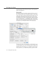
Options Menu
Live Microscope Control...
When a calculated image is selected, this command can be
invoked to bring up an interactive window for changing the calculation parameters for this image. Changes in the parameters
Ch. 6 Menus - p.60
MacTempas User Manual
are reflected live as long as the calculation time is reasonable..
Automatic Erase
Toggles whether previous content in the MacTempas display
window is erased when a new object is displayed.
Atom Overlay
If set, the atom positions will be drawn in as circles on top of
images. The circles are scaled to the atomic radius and the color
is the color set for that atom species.
Montage...
Brings up a dialog box, allowing the user to select automatic
montage of a series of images, the position of the series of
Ch. 6 Menus - p.61
MacTempas User Manual
images and the number of pixels to leave between images.
Intensity Scaling...
Brings up a dialog box, allowing the user to manually set the
intensity values to be mapped to black and white. The values
shown correspond to the last image displayed with automatic
scaling.
Magnification
Allows the user to set the magnification to a set value. The
magnification depends on a screen with a resolution of 72 dots/
Ch. 6 Menus - p.62
MacTempas User Manual
inch. If Auto-scaling is set, images will scale to fit the window.
CTF Scaling...
Brings up a dialog box, allowing the user to set the maximum
scale of the reciprocal axis during plotting of the Contrast
Transfer Function.
Diffraction Pattern...
Displays a dialog box, allowing the user to select the position of
the diffraction pattern, the camera length and the minimum diffracted intensity that can be displayed. The user can also choose
whether the objective lens aperture should be superimposed on
the diffraction pattern. The indices of the diffracted beams can
be superimposed on the diffraction pattern as well as the corresponding real space distances. Selecting Circular Diffraction
spots instead of Gaussian Diffraction Spots results in solid circles. One can also set a cut-off such that diffracted beams with
Ch. 6 Menus - p.63
MacTempas User Manual
g-vectors larger than the cut-off will not be displayed.
Min Lens Intensity...
Displays a dialog box, allowing the user to manually set the
minimum intensity required of a diffracted beam for inclusion
in the formation of the image.
Slice Method...
Allows the user to select the option to perform a three dimensional calculation of the projected potential by summing over
Ch. 6 Menus - p.64
MacTempas User Manual
the third dimension (l) in reciprocal space.
Show Microscopes...
Displays a dialog, showing the user which microscopes are
known to MacTempas. The default parameters associated with a
known microscope can be changed by the user and a new
microscope may be made known to MacTempas. MacTempas
currently only allows a maximum of 10 microscopes to be made
known
n.
Use Fit For Electron Scattering Factors / Use Fit For X-Ray
Scattering Factors
MacTempas can use either the 8 parameter fit for the Electron
Scattering Factors or the 9 parameter fit for the X-Ray ScatterCh. 6 Menus - p.65
MacTempas User Manual
ing factors. The menu item text will reflect the current setting.
Edit Scattering Factor Parameters...
Brings up a table of the fitting parameters. Double clicking in
the value -field brings up a dialog box prompting for a new
value. See next page.
Unit Cell is Entire Specimen
When this option is set, the calculation treats the unit cell as a
non-repeating structure such that the entire specimen is represented by a single unit cell with the thickness of the specimen as
the thickness of the unit cell.
Modify Specimen Bounds
When the unit cell is the entire specimen, this will allow the
user to trim the bouning volume for the cell in the specified
zone axis orientation..
Ch. 6 Menus - p.66
MacTempas User Manual
Ch. 6 Menus - p.67
MacTempas User Manual
Commands Menu
Erase Display
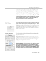
Erases the MacTempas display window.
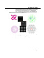
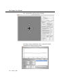
Draw Atomic Model...
Displays a dialog box, from which the user can select to display
the original or transformed unit cell from any direction, including perspective view. The transformed cell corresponds to the
unit cell that MacTempas uses in the multislice calculation. To
view the cell as “seen” by the electrons, the transformed (new)
unit cell should be viewed in the 001 orientation. It should be
noted that the viewing direction is in units of the real space unit
cell axes. One can also view a cross-section of the material in a
given direction. A dialog box allows the user to specify the
field of view in Å for the two directions.
Ch. 6 Menus - p.68
MacTempas User Manual
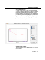
Draw CTF -Sin (chi)
Draws the Contrast Transfer Function for the current microscope values. The original microscope values are taken from the
structure data, but the user is free to change the values associated with the CTF independent of the values used in calculating
the image. Clicking in the CTF will show a bar with the values
of the CTF and the resolution. The bar moves with the mouse.
Draw 2D CTF...
Draw various representations of the 2D contrast transfer func-
Ch. 6 Menus - p.69
MacTempas User Manual
tion, for both linear and non-linear imaging.
Non-linear image contributions can be examined in detail
through the non-linear analysis button.
Ch. 6 Menus - p.70
MacTempas User Manual
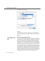
Draw Pendelløssung Plots...
In case the user has selected to store a set of diffracted beams
for plotting of amplitudes and phases as a function of specimen
thickness, this brings up a dialog box allowing the user to set
the plotting conditions. One can choose to have the amplitudes
or the intensities plotted as well as the phases of the diffracted
beams. Each reflection can be plotted by itself, or several
reflections can be superimposed on the same plot. Instead of
plotting the values, the values can also be written to a file for
further manipulation or inspection.
Define Projected Potentials...
This allows the user to specify which potentials to be used in a
layered structure.
Ch. 6 Menus - p.71
MacTempas User Manual
Stack Potentials...
This allows the user to specify the sequence of potentials that
should be used in the multislice calculation. This applies only to
layered structures. See Chapter 9 for a more detailed instruction on how to create a layered structure.
Slice Unit Cell...
Use this option to subdivide a structure into separate layers for
use in a layered structure calculation. The direction perpendicular to the slices and the number of slices must be specified.
Ch. 6 Menus - p.72
MacTempas User Manual
Ch. 6 Menus - p.73
MacTempas User Manual
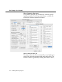
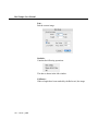
Parameters Menu
Main Parameters...
This brings up a dialog box showing the current conditions for
the simulation. The values are taken from the input given to the
New... command in the FILE menu. The parameters can be
changed as to bring about a new simulation.
Ch. 6 Menus - p.74
MacTempas User Manual
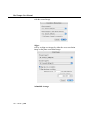
Atomic Basis...
Brings up the list of all the atoms forming the set of basis atoms
for the current structure. The atomic coordinates etc. can be
edited and atoms can be added to or deleted from the list.
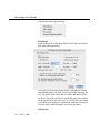
Symmetry Operators...
This brings up the list of symmetry operators either associated
by the space group or entered manually by the user. The symmetry operators can be edited, and new ones may be added to
Ch. 6 Menus - p.75
MacTempas User Manual
the list or existing ones deleted.
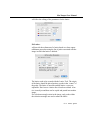
Atomic Coordinates...
This shows all the atoms within the unit cell. This list of atoms
are generated by applying the symmetry operators on to the set
of basis atoms above. This list can not be changed, the changes
must take place in the atomic basis or the symmetry operators.
Ch. 6 Menus - p.76
MacTempas User Manual
Calculate Menu
The active commands in this menu depends on the current sta-
tus of the calculation. If the simulation has already been carried
out for the current set of parameters, then no commands will be
active. If a change has been made or the file is a newly created
structure file, the commands showing which subprograms needs
to be run are shown active.
Full Calculation
Use this command if you would like the program to run the
multislice calculation to its end starting from the point required
by the last change made to the simulation parameters.
Projected Potential
Only calculate the projected potential(s)
Exit Wavefunctions(s)
Only calculate the exit wave-functions(s)
Image(s) (normal calculation)
Calculates the image by using using partial coherence envelope
Ch. 6 Menus - p.77
MacTempas User Manual
functions and the lens contrast transfer function.
Image-Plane Wavefunctions(s)
Calculates the wave-function at the image plane. This would be
equivalent to what would be reconstructed using holography.
Image(s) (incoherent summation)...
Calculates the image(s), but sums up incoherent images produced by electrons from different incoming directions and different energy.
Image(s) (frozen phonons)...
Calculates the image by summing over images calculated from
different atomic configurations consistent with random displacements of atoms according to their debye-waller factors..
Weak Phase Object Images
is a separate module that allows the calculation of images that
would be produced in the case of an ideal Scherzer lens and
Ch. 6 Menus - p.78
MacTempas User Manual
validity of the weak phase object approximation. The “wpo”
calculation is discussed more in detail elsewhere.
Ring Pattern...
calculates the diffraction pattern by adding up the intensities for
each tilt angle within the cone of incident electron directions.
Ch. 6 Menus - p.79
MacTempas User Manual
Kinematical SAD Pattern...
calculates the diffraction pattern by adding up the intensities for
each tilt angle within the cone of incident electron directions.
Ch. 6 Menus - p.80
MacTempas User Manual
Ch. 6 Menus - p.81
MacTempas User Manual
Integrated Diffraction Pattern
calculates the diffraction pattern by adding up the intensities for
each tilt angle within the cone of incident electron directions.
Kinematical CBED Pattern...
Will calculate the CBED pattern for the given input parameters
using the Bloch-Wave approximation.
Ch. 6 Menus - p.82
MacTempas User Manual
CBED Pattern...
Will calculate the dynamical CBED pattern for the given input
Ch. 6 Menus - p.83
MacTempas User Manual
parameters using the Bloch-Wave approximation.
The x-axis of the pattern can be set by dragging the green selection rectangle of the x-axis arrow to a diffraction spot. The pattern will rotate so that the “selected” spot is along the x-axis of
the pattern. The part of the pattern that will be shown in the calculated image is that which is within the red “Image” rectangle
which can be sized and dragged around. The spot-size (convergence angle) is modified by changing the size of the central
disk.
Ch. 6 Menus - p.84
MacTempas User Manual
STEM Image...
Will calculate the STEM image for the given input parameters
using the by doing a multislice simulation for each position of
the electron probe. The image intensity for that position is the
integrated intensity that falls within the annular detector.
Ch. 6 Menus - p.85
MacTempas User Manual
Tables
Tables Menu
The current operations in this menu are:
Reciprocal Space Info...
Displays information about reciprocal space data for the current
structure. The data can be sorted on the reciprocal vector or the
structure factor/extinction distance.
Seaech for Angle...
One cacn search for reflections which satisfy a search criteria
based on the ratio of the length of the vectors and/or the angle
between the measured reflections. This can be used when trying
Ch. 6 Menus - p.86
MacTempas User Manual
to index diffraction patterns. One can give aan accepted toler-
anse for the ratio, the measured spacings and the measured
angle.
Spacing and Angle Calculator...
Shows the lengths and d-spacing for a type/family of reflections. Two reflections can be displayed and the zone in which a
set of reflection exist and the angle between them is shown in
the right part of the window.The reflections can be typed in and
Ch. 6 Menus - p.87
MacTempas User Manual
when the “Calculate?Update Angles” button is clicked, the
angls between the family of reflections and the zone in which
they occur will show to the right. The length of the vectors and
the corresponging plane spacing is updated live when typing in
a new reflection. The lattice parameters can be changed and
invoked through the “Update Lattice Parameter” such that the
calculator can be used for structures different from the one that
is loaded.
Quantitative Menu
This is the menu for quantitative comparison between experimental images and exit wavefunctions with calculated data.
Structure refinement and imaging parameter refinement is also
invoked from this menu.
Operating The Routines
All the routines except for the “Symmetry Transform Calculator” requires the presence of an image that is considered the
experimental image. The purpose of this package is to provide
the user with tools that permit the following attempts:
•Q
Quantitative comparison of experimental images with those
simulated from a structure model
•A
Automatic refinement of parameters such as the thickness of the
specimen, the defocus of the objective lens, crystal tilt, aberrations, etc..
Ch. 6 Menus - p.88
MacTempas User Manual
•A
Automatic refinement of structural parameters such as atomic
positions, debye- waller factors and occupancy factors for
selected atoms in the structure.
The experimental image can be compared with the computed
images using a number of goodness of fit criteria. A sub-area of
the experimental image can also be compared to a sub-area of
the simulated image. For more information on quantitative comparison methods and structure refinement see the chapter on
“Introduction to Quantitative Comparison of simulated HRTEM
images with experiment”.
Note: All the procedures expect that the experimental image
covers the exact area of that of the unit cell used in the calculation. Thus it is up to the user to make sure that the unit cell
motif is extracted from the experimental data prior to usage.
The term Unit Cell is loosely used since it only refers to the size
of the model used in the simulation. The experimental image
does not need to be sampled equal to the simulation, since the
routines will resample the experimental data to fit that of the
simulation.
For parameter refinement and structure refinement, there are a
number of algorithms that attempt to look for the “one” solution
of parameters that maximize the fit between the experiment and
the simulation. This plug-in uses an algorithm based on simulated thermal annealing which is described further in the chapter at the end of this manual. No claims are made as to the
effectiveness of this method and there is no guarantee that the
final solution represents the global maximum/minimum in the
goodness-of-fit parameter. The effectiveness of optimization
routines depend on the starting parameters. There is no recipe
for setting the initial starting condition and it is necessary to
develop some experience using the optimizing routine in this
program. Some trial and error is a definitive part of the parameter/structure refinement. Suffice it to say, “good hunting”.
Ch. 6 Menus - p.89
MacTempas User Manual
Load Experimental Image
Load Experimental Image is the starting point for loading in the
image to be used in the comparison. The command will bring
up a standard File Open dialog with a look that depend on the
version of the MacOS you are using and what else of Finder
utilities you have loaded.
The dialog will show you all files and it is up to you to select an
appropriate file to read in. Currently, two distinct types of files
are supported. These are
1) Binary Files
The data can be Real 4 or Integer 1,2,4 byte
2) TIFF
Real 4, Integer 1,2,4 byte
If the routine recognizes the file as a TIFF file, it will just open
the file and display the image.
For Binary files, you will need to specify the data type, the
width and the height of the image. Byte swapping is also supported. If the program does not recognize the file as type TIFF it
Ch. 6 Menus - p.90
MacTempas User Manual
will bring up the following dialog
Although the dialog box indicates that the program supports
input of text files, this is currently unsupported.
The dimensions of the simulated image are shown at the bottom
of the dialog box for binary files.
Once the routine has read in the file, it will display the image in
a separate window.
Load Standard Deviation Image
This command allows you to read in a standard deviation image
to be used together with the average experimental image for
comparison with simulated images. The standard deviation
image will be used in conjunction with the average image for
computing c-square deviations between the experimental data
and the computed data. Otherwise the input works exactly as for
the loading of the average experimental image. Again, the
Ch. 6 Menus - p.91
MacTempas User Manual
image will show up in its own window after it has been loaded.
Note: If the windows are covered by other windows, it may be
necessary to move these to bring the “experimental” image and
the “standard deviation” image to the foreground since there is
no command to bring these automatically to the front.
Compare Experiment With Simulation
This brings up a dialog window which shows the loaded experimental image and the standard deviation image (if loaded). The
name of the experimental image together with the dimensions
are shown to the left of the image.
Ch. 6 Menus - p.92
MacTempas User Manual
When comparing images, the experimental image will be resampled such that the sampling corresponds to the sampling of
the calculated image.
The example used here will be that of a set of simulated images
of Silicon in the [110] zone axis orientation
The simulated images for a range of thickness and defocus are
shown below.
Tools
Pointer Tool
Used essentially to ensure that no other tool is active
Selection Tool
Use this to mark an area in the image which will be used for
comparison. It is okay to go outside the image, since the selection will be cropped to the actual image.
Hand Tool
Use this tool to move the image within the display area.
Magnification Tool
Use this tool to magnify the image. Holding down the Option
key when clicking within the image will reduce the magnificaCh. 6 Menus - p.93
MacTempas User Manual
tion. Holding down the shift key when clicking will increase/
decrease the magnification by a factor of 2.
Reset View
Click here to reset the view/pan/zoom of the image.
Selecting an area for comparison
The user choose to compare the entire image region or only a
selection of the image.
Two radio buttons are provided:
Compare Entire Image
By clicking on this radio button, the selection area will automatically be set to be that of the entire image. The comparison area
is shown as a red rectangle.
Set/Compare Selection
The user must first use the selection tool to mark a region of the
image. Upon clicking on the radio button, the selection will be
marked in red and this area will be used for comparing images.
For changing an already defined regions, mark a new one and
click again in the radio button.
Ch. 6 Menus - p.94
MacTempas User Manual
Note: The selection does not work for the Difference Image
which automatically compares the entire image.
Selecting a method of comparison
The method of comparison or goodness of fit criteria is chosen
by a set of radio buttons and the choices and the corresponding
description and output is given below. The goodness of fit criteria is computed for each image that is compared and displayed
in a table. This table can be saved in a text file for further use.
Statistical cross correlation coefficient (CCC):
A note about the cross correlation coefficient:
The cross correlation coefficient measures similarity in the pattern between the experimental image and the computed image.
Since the images to be compared are set to a mean level of 0 and
normalized, any scaling of the type I(exp) = a * I(calc) + b
would give a cross correlation coefficient of 1. Exact fit is given
as CCC = 1 and a reverse contrast gives CCC = -1.
Real Space
This is a straight calculation of the normalized cross correlation
coefficient between the experiment and the calculated image(s).
Ch. 6 Menus - p.95
MacTempas User Manual
For it to give meaningful results, the origin of the experimental
image neeeds to coincide with the calculated image.
Reciprocal Space
There are two options for calculating the cross correlation in
reciprocal space.
The first is an exact calculation which is equivalent to the real
space CCC. The entire Fourier transform of the experimental
image is compared with the Fourier transform of the simulated
image and the CCC is just the reciprocal space equivalent of the
calculation in real space. Thus the reciprocal space CCC is
equal to the real space CCC.
Exact
Ch. 6 Menus - p.96
MacTempas User Manual
.
Only Amplitudes
This calculates the CCC based only on the Fourier amplitudes
and (optionally) the program will try to estimate the shift
between the experimental and the calculated image. This can be
very useful for aligning images and to compare images when
the origin of the experimental image is not known. The numbers
Ch. 6 Menus - p.97
MacTempas User Manual
given are the shift of the origin that should be attempted to be
made on the experimental image before the experimental data is
compared to the simulation using the exact formulation.
Chi-Square
This computes the chi-square deviation between the calculated
image(s) and the experimental images, optionally using the
standard deviation image for obtaining the uncertainty associated with the average pixel value.
Ch. 6 Menus - p.98
MacTempas User Manual
If no standard deviation image is given, the uncertainty in the
pixel value is set to 10% of the intensity in the pixel. The Chisquare goodness of fit criteria is sensitive to the mean level of
the images and the scales the calculated images so that they
have the same mean as the experiment before computing chisquare. Lower values indicate better fit, with a value of 1 meaning that the experiment and simulation agree within the uncertainty of the experimental values.
Root Mean Square Difference
This calculates the root mean square difference between the
Ch. 6 Menus - p.99
MacTempas User Manual
experiment and the simulation. Lower values indicate better fit
with 0 being exact fit between experiment and simulation. Since
the values depend on the mean level of the images that are compared, the simulation is scaled to have the same mean as the
experiment.
The table below shows the result from the RMSD comparison.
Ch. 6 Menus - p.100
MacTempas User Manual
Difference Image
There are two calculations performed in this case. One gives a
difference image(s) which are pseudo colored such that where
the experiment and simulation agree within one standard deviation, the pixel is black, less than 1.5 standard deviations,
the pixel is colored green, and outside the pixels are shown in
shades of red or blue
depending on whether the values in the simulation are lower or
higher than those in the experiment.
In addition to the difference image(s), the chi-squared value is
Ch. 6 Menus - p.101
MacTempas User Manual
also computed for each image and shown in its own table.
Fractional Mean Absolute Difference
This calculates the fractional mean absolute difference between
the experimental data and the simulated data.
Ch. 6 Menus - p.102
MacTempas User Manual
Compare XW Amplitue/Phase with simulation works as with
images, but the experimental data is compared with the exit
wave-function (either amplitude or phase)
Refine Parameters
Refine Parameters... will attempt to find the image simulation
parameters that produce a simulated image that gives the “best”
fit between the experiment and the theory. The search routine is
based on the concept of “Simulated Thermal Annealing” and
requires a starting configuration of parameters, a starting temperature and an ending temperature, a maximum change in
parameters and a goodness of fit criteria that measures the
“Energy” of the system. For further explanation of Simulated
Thermal Annealing, see the last chapter in this manual.
Invoking the command brings up the following dialog which is
Ch. 6 Menus - p.103
MacTempas User Manual
used to give the input parameters to the algorithm.
Setting Image Comparison region
The area to be used for the comparison is set using the button
“Set Image Comparison Region”
Ch. 6 Menus - p.104
MacTempas User Manual
Selecting the image region is done in the same fashion as under
comparing images in the previous section.
Running the parameter refinement
After selecting the area (not needed if the entire image is compared, which is the default) and selecting the parameters to be
refined and clicking OK, a progress window for the parameter
refinement appears. If the refinement is not progressing in a satisfactory way, the computation can be canceled by hitting the
Ch. 6 Menus - p.105
MacTempas User Manual
Apple-Command Key together with the Period. Optionally, a
log file can be written so that the “energy” as a function of time/
temperature can be plotted and also a Movie can be produced
and played back. The number of frames/second for output can
be set.
At the end of the run, the dialog box can be just dismissed and
the final configuration of parameters will be discarded, or the
parameters can be saved in the form of a new structure/simulation file.
Refine Structure
The structure refinement works in the same way as the parameter refinement. However, in this case it is the structure that is
being varied, notably the coordinates of selected atoms and possibly debye-waller factors and occupancy. After invoking the
Ch. 6 Menus - p.106
MacTempas User Manual
command, the following dialog box appears.
There are several options associated with the structure refinement, such as which elements are active, which coordinates to
be varied, etc.. The standard parameters for the simulated thermal annealing need to be specified, together with the goodness
of fit parameter. Output options such as a log file and movie are
identical to that under parameter refinement. In addition, it is
possible to include in the calculation of the “Configuration
Energy” terms that depend on selected bond distances and
selected bond valence sum.
Set Active Elements
brings up the following dialog. By default all elements are
active. Selecting an active element and clicking on the “Make
inactive” button will move the selected element to the Inactive
list. Just because an element is listed under active elements does
Ch. 6 Menus - p.107
MacTempas User Manual
not mean that one of its types will be used in the refinement pro-
cedure. It is necessary to specify the area used for comparison
and which atoms are to be optimized before the simulated thermal annealing is carried out.
Set Are to Compare & Active Atoms
is used to set the image comparison region (as previously
explained) and to select atoms for refinement. The following
window appears.
Ch. 6 Menus - p.108
MacTempas User Manual
Area used for comparison
Selection
Sets the comparison region to the selection rectangle.
Entire Image
Sets the comparison region to the entire image.
Atoms to optimize
Add Selection
Includes in the list of atoms the ones that fall within the selection rectangle set in the model window.
Add/Group Selection
Adds the atoms to the refinement list, but constrains all the
atoms in this list to move as a unit.
Ch. 6 Menus - p.109
MacTempas User Manual
Atoms Within the Comparison rectangle
Sets the refinement list to include the atoms that lie within the
rectangle set for comparing images.
Optimize...
Specifies which properties of the selected atoms (those in the
refinement list) that are varied. The following window appears.
Normally varying the z-coordinate will not have any effect
since the image simulation procedure uses a 2d projection of the
atoms in the unit cell. However, in the case where symmetry
operators are used, changing he z-position may result in
changes in x and y for symmetry related atoms.
Each time an atom (or group) is varied, a new set of parameters
for this atom/group is created and tested. If “Test each variable
separately” is checked, each try will only vary one parameter.
Thus if x and y are checked above, both x and y for an atom are
changed at the same time unless “Test each....” is checked, in
which case one time x is varied and another time y is varied.
Deselect All Atoms
clears the refinement list and allows the user to start all over,
defining the set of atoms to optimize.
Ch. 6 Menus - p.110
MacTempas User Manual
Show only symmetry related atoms/Use Symmetry elements
If the structure is a perfect crystal defined by a set of basis
atoms and a set of symmetry operators, it is possible to refine
positions of the atoms in the basis and to move symmetry
related atoms accordingly such as to preserve the crystalline
spacegroup.
Checking this options will result in only atoms in the basis to be
visible in the model. Thus the atoms to be refined is selected
from the basis and any change in the basis is reflected in the
entire structure.
Ch. 6 Menus - p.111
MacTempas User Manual
Set Chemical Constraints
brings up the following window.
which can be used to specify a configuration energy that
includes terms that depend on bond distances. It is possible to
specify the optimum bond distance between two atoms, whether
it is a 2d or 3d constraint, and to specify the weight of the term
in the energy calculation. Even though bond distances have
been defined, the inclusion of a bond-distance energy term can
be turned off/on from the main “Refine Structure” window.
Include Bond Valence Sum Optimization
This allows the bond valence sum to be used to measure the
energy of the configuration. It brings up the following window
in which the active bonds are specified, the maximum distance
between atoms for calculating the bond valence sum, the
valence of the first atom in the atom-pair and the bond constant.
Each “bond” has its own weight and the entire bond-valence
Ch. 6 Menus - p.112
MacTempas User Manual
energy terms has an overall weight.
Running the Refinement
Once the parameters are set and OK has been clicked, a
progress window appears. The current atomic configuration is
shown together with the corresponding simulated energy. The
energy as a function of “time/temperature” is shown in its own
window and can be monitored to ensure that the system moves
in a desirable fashion. It is important to understand that no specific recipe can be given to ensure that the system finds a meaningful minimum in the configuration energy. The success of the
optimization depends on how far the starting configuration is
from the “solution” and the choice of annealing parameters. It is
not a straight forward, just run and you get the correct answer,
black box approach. An understanding of the system, a good
feel for choosing a reasonable starting structure and some experience in choosing “annealing parameters” is definitely a
requirement in order to have confidence in the resulting ending
configuration. Experimenting with different input parameters is
advised.
As with refining simulation parameters, it is possible to save a
log file or to produce a movie of the annealing process. Saving a
movie can be very useful when the refinement takes hours/days
and it is necessary to see how the system varied over time. It is
important to realize that a movie file grows quickly in size and
that the number of frames/second should be chosen appropri-
Ch. 6 Menus - p.113
MacTempas User Manual
ately if the movie is to cover a period of many hours.
At the end of the run, the final structure can be dismissed or
saved as a structure file for later use. The run can also be
aborted by the normal “Apple + Period” key combination.
Symmetry Transform Calculator
Choosing the “Symmetry Transform Calculator” brings up a
modal dialog window that can help the user find another set of
symmetry operators and basis atom positions in the case of a
change in axis and origin of the unit cell. Input is the original
symmetry operators which come from the spacegroup that is in
use together with the original basis atoms. The new unit cell
axes a’,b’ and c’ are given by the transformation matrix T such
Ch. 6 Menus - p.114
MacTempas User Manual
that
T 11 T 12 T 13 a
a'
b' = T 21 T 22 T 23 b
c'
T 31 T 32 T 33 c
together with a translation of the origin specified in the old unit
cell system (fractional coordinates).
Invoking the command brings up the following window.
Lists
Original Operators
This list shows the symmetry operators of the current spacegroup. Initially these are those of the crystal in use, but the
spacegroup can be changed by the command “Switch Spacegroup”.
Ch. 6 Menus - p.115
MacTempas User Manual
Original Basis
The basis atoms are the atoms of the current crystal.
Original Unit Cell Atoms
This list gives the atoms that are produce by the operation of the
symmetry operators of the spacegroup in use on the original
basis atoms.
New Operators
These operators are the result of applying the transformation
operations that are given by the change in coordinate system
together with a translation of the origin to the generators of the
original spacegroup.
New Basis
This is the transformed basis.
Original Unit Cell Atoms
This list gives the atoms that are produced by the operation of
the new symmetry operators of the spacegroup used on the new
set of basis atoms.
Convert
Clicking on this button initiates the computation of the transformed set of symmetry operators, the transformed basis and
the new atomic positions.
Ch. 6 Menus - p.116
MacTempas User Manual
Note:
It is important to realize that arbitrary input does not result in a
symmetry which still can be presented by the same spacegroup
with a change in symmetry operators.
Export New Set
Allows the user to export the new basis and the symmetry operators as a new structure file.
Ch. 6 Menus - p.117
MacTempas User Manual
Process Menu
Ch. 6 Menus - p.118
The Process menu is the largest menu and is the source of all
image processing functions. There are menu sub-menus as well.
MacTempas User Manual
Image Calculator
Perform polish notation (HP style calculator).mathematics on
images and numbers
FFT
Perform a Fourier transform on a 2-dimensional image. Unlike
many implementations, the image is not required fo have
dimensions that are powers of two. However, the image must be
square.
Hanning Masked FFT
Perform a Fourier transform on a 2-dimensional image. The
image is first maksed with a circular 2-dimensional Hanning
mask.
Soft Circular Masked FFT
Perform a Fourier transform on a 2-dimensional image. The
Ch. 6 Menus - p.119
MacTempas User Manual
image is first maksed with a circular 2-dimensional mask.
Inverse FFT
Perform an Inverse Fourier transform on a 2-dimensional
image. Unlike many implementations, the image is not required
fo have dimensions that are powers of two. However, the image
must be square.
Power Spectrum
Computes the Power spectrum of a rreal square image.
Edit Mask...
Allows the specific settings associated with a mask of a given
type. Example of the properties of a lattice mask is shown
below.
Apply Mask(s)
Applies the defined maks(s) on the image.
Fourier Filters
Contains the following filters
Ch. 6 Menus - p.120
MacTempas User Manual
The Wiener filter is an automatic filter that tries to determine the
power spectrum of the “noise” and the creates an optimal filter
based on the estimate of noise and signal.
.
Spatial Filters
Contains the following filters
Convolution...
brings up the following dialog for defining the kernel. Pre-
defined kernels are defined for your convenience, but you can
Ch. 6 Menus - p.121
MacTempas User Manual
modify the coefficients as you please.
Invert
Inverts the image.
Repeat...
Allow the current image to be repeated n by m times.
.
Transform
Ch. 6 Menus - p.122
MacTempas User Manual
Contains the following operations
Scale...
Scale the current image
Rotate...
Rotate the current image
Ch. 6 Menus - p.123
MacTempas User Manual
Pad...
Pad the current image
Statistics
Contains the following operations
The data is shown in the Info window.
Calibrate...
When a length have been marked by the Ruler tool, the image
Ch. 6 Menus - p.124
MacTempas User Manual
can be calibrated. If there is no line drawn, the menu command
is inactive. The image can also be calibrated through the “Edit
Object...” menu command. In that case no line needs to be
drawn.
Extract From Complex
If the front image is complex, images can be created from various component of the complex values.
Correlation / Convolution
Ch. 6 Menus - p.125
MacTempas User Manual
Contains the following operations
Auto Correlation
operates on a single image and calculates the auto-correlation
function of the image.
Cross Correlation...
calculates the cross correlation image for two images.
Phase Correlation...
calculates the correlation function based on the phases of the
two images disregarding the amplitude of the Fourier compo-
Ch. 6 Menus - p.126
MacTempas User Manual
nents.
Convolute...
will calcululate the convolution image from two images.
Deconvolute...
will produce a third image which is the first image deconvoluted
Ch. 6 Menus - p.127
MacTempas User Manual
with the second image.
Align...
will try to align two images by either the cross correlation
image or the phase correlation image.
Azimuthal Average
Ch. 6 Menus - p.128
MacTempas User Manual
Contains the following operations
1D Image
calculates the azimuthal average and siplays it as a one-dimension trace.
2D Image Split Plane
will display the original left half of the image and replace the
right half with the 2D azimuthal average.
2D Image
will create a 2D image from the azimuthal average.
Template Matching...
will calculate an image containing the cross correlation coefficient for the template as a function of its position in the image.
The cross correlation coefficient is calculated for each pixel
position in the original image.
Peak/Lattice Analysis
Ch. 6 Menus - p.129
MacTempas User Manual
Contains the following operations
Find Peaks...
Finds all the peaks in the image which satisfy the criteria specified in the following dialog.
The peaks will be marked on the image. Changing the criteria
and refinding peaks will mark a new set of peaks, replacing the
old. The peaks can be selectedm as a whole and deleted as for
an object. The peaks can also be copied and pasted into another
image (preferably of the same size). A list of peaks can be used
in a displacement analysis in conjunction with an associated lattice that can be refined through a set of peak positions.
Edit Lattice..
Ch. 6 Menus - p.130
MacTempas User Manual
will allow the editing of the parameters for the lattice.
Fit Lattice..
will provide the refinement of a lattice based on a least square
refinement procedure using the list of peaks associated with the
image in which the lattice is defined.
The lattice needs to be created with the Lattice Tool. The origin
of the lattice should be placed on/near a peaks in the “center” of
the peaks. The lattice is movable and the lattice vectors are
adjustable. Don’t move a lattice after it has been refined. A lattice is an object and thus can be copied and pasted into another
image.
If a selection rectangle exists in the image, only peaks within
the selection rectangle are used to refine the lattice.
Ch. 6 Menus - p.131
MacTempas User Manual
Analyze Displacements...
Allows for the analysis of displacements. The displacements are
relative to a reference lattice which normally come from a
refined lattice.
Geometric Phase Analysis...
allows for displacement analysis from variations around spatial
Ch. 6 Menus - p.132
MacTempas User Manual
frequencies..
The geometric phase calculation is described in more detail in
Chapter 11.
Cryst. Image Processing...(Crystallographic Image Processing...)
Can be invoked on a real space image which is square or has a
Ch. 6 Menus - p.133
MacTempas User Manual
square selection. In order to get started, the Hanning Masked
Fourier transform need to be calculated. Once the Fourier transform has been calculated, the reciprocal space lattice needs to
be set using the a* and b* tools and clicking on two consecutive
Ch. 6 Menus - p.134
MacTempas User Manual
reflections that defines the reciprocal space. The number of
reflections used in the lattice refinement and information extraction can be limited by the circular aperture tool. Once the lattice
reflections have been marked, the next action is to invoke the
command “Refine Lattice”.
Ch. 6 Menus - p.135
MacTempas User Manual
After the lattice has been refined, click on “Find Motif”. This
will extract all the phases and amplitudes from the Fourier
transform at the lattice points and one can test for possible symmetries of the motif.
Each symmetry can be tested and imposed on the reflections to
form a new unit cell motif. The origin of the unit cell motif is
dhown on the right and can be changed.
Once a solution has been chosen, a new image can be created
with the imposed symmetry and can be used as an image to
compare with simulation.
Ch. 6 Menus - p.136
MacTempas User Manual
Focus Determination
Contains the following operations
Finding focus from a HRTEM image is outlined in more detail
in chapter 12
Always Create New Image
Determins whether an operation on an image always should
produce another image instead of modifying the original image.
Ch. 6 Menus - p.137
MacTempas User Manual
Text Menu
This menu determines the appearance of text drawn in the
MacTempas image window. The following text attributes can be
set:
Windows Menu
Use this menu to bring a window to the top of the screen in case
it has been completely covered by another window.
Ch. 6 Menus - p.138
MacTempas User Manual
Chapter
7
Input File Format
The structure file created by New... in the File Menu is a file of
type ‘TEXT’ and can be produced by a text editor. At times it is
desirable to edit the file directly, rather than using MacTempas
to create this file. In fact the user may sometimes want to write a
program to generate the data in the structure file. For that purpose in particular, the format of the structure file <structurename>.at is given below:
Line # Parameter(s)
1
Title
Meaning
Arbitrary description of this
structure
2
SpaceGroupNumber Just as is says, one of the 230
spacegroups, (1-230).
3
abcabg
The lattice parameters and angles
4
Gmax
The maximum reciprocal lattice
vector in the multislice calculation. The potential is evaluated
out to twice this value, units Å-1.
5
iu iv iw
The direction of the electron
beam in units of the real space
crystal lattice vectors.
6
NSymops Nslices
(I3d)
Number of symmetry operators,
number of slices per unit cell,
and a flag indicating 2d (0) or 3d
(1) potential calculation only if
Nslices is different from 1.
Ch. 7 Input File Format - p.139
MacTempas User Manual
Line # Parameter(s)
Meaning
7
NBasis Ntypes
The number of atoms in the basis,
the number of different types of
atoms. A different type is associated with a different chemical
symbol or a different DebyeWaller factor.
8
it symb x y z
dw occf
The type of atoms (a number
from 1 - NTypes), Chemical symbol, x-,y-,z coordinates in relative
units of the lattice vectors,
Debye-Waller factor and occupancy factor.
9
The same as line 8 for atom number 2.
10
The same as line 8 for atom number 3.
.
8+NBasis
MicName Cs Del Th The name of the microscope, the
spherical aberration (mm), the
spread of defocus (Å) and semiangle of divergence (mrad).
9+NBasis
Voltage
10+NBasis
Lh Lk
Ch. 7 Input File Format - p.140
Accelerating voltage (kVolt).
The center of the Laue circle in
units of the h and k of the transformed reciprocal unit cell. (Real
numbers).
MacTempas User Manual
Line # Parameter(s)
11+NBasis
Thickness
12+NBasis
IPlot
13+NBasis
ih ik il
Defocus
D1,D2,DD
14+NBasis
+NAmp
ApertureRad.
15+NBasis
+NAmp
Ah Ak
16+NBasis
+Namp
Oh Ok
Meaning
The specimen thickness or
T1,T2,DT First thickness, last
thickness, increm. The commas
are required.
Amplitudes to be stored as for
possible plotting, (YES/NO).
The indices of the reflection to be
stored, or if IPlot == NO then :
Objective lens defocus or
First defocus, last defocus, increment. The commas are required.
Radius of the objective lens
Aperture in units of Å-1.
The center of the objective lens
aperture in units of h,k of the
transformed reciprocal unit cell.
The center of the optic axes in the
same units as Ah,Ak.
Ch. 7 Input File Format - p.141
MacTempas User Manual
Line # Parameter(s)
17+NBasis
+Namp
s1,s2,s3
.
17+NBasis
+Namp
+NSymop
istat
18+NBasis
+Namp
+NSymop
Vibration
Meaning
Symmetry operator number 1. An
example is x+1/3,y+5/6,z+1/3.
The commas are required.
The calculation status of this
structure. For a new structure this
should be 1
Halfwidth of mechanical Vibration in A.
Note: If different wordprocessing software is used, Microsoft
Word, Write Now etc., make sure that the text file is saved at the
end as type TEXT.
Ch. 7 Input File Format - p.142
MacTempas User Manual
Chapter
8
Sample Calculation
As an example of a calculation using MacTempas we consider a
BCSCO super-conductor structure. Using the structure determined by Tarascon et al (1988), we show the steps necessary to
input the model structure, examine it, compute the diffraction
pattern and simulated images, and display and print them.
The Structure
As published by Tarascon et al in Phys. Rev. B 37 (1988)
p.9382-9389, the tetragonal structure has the following parameters Space group: I4/mmm
Cell parameters: a=b=3.814Å, c=30.52Å, a=b=g=90
with nine atom positions in the basis:
Atom
Ca
Sr
Bi
Bi
Cu
O(1)
O(2)
O(3)
O(4)
Wyckoff notation
2a
4e
4e
4e
4e
8g
4e
4e
4d
x
0
0
0
0
0
0.5
0
0
0.5
y
0
0
0
0
0
0
0
0
0
z
Occupancy
0
1
0.1097 1
0.3022 0.87
0.2681 0.13
0.4456 1
0.446
1
0.375
1
0.205
1
0.25
0.065
Isotropic thermal parameters for all atoms are fixed at 3.6 Å2.
Ch. 8 Sample Calculation - p.143
MacTempas User Manual
Entering the
Structure
To enter a new structure into MacTempas, we first go to the
FILE menu (Section 3.3), and select New Structure File...
After entering a filename in the New File dialog, MacTempas
will put up a dialog into which the relevant information must be
entered. Note that the program shows a default cubic structure.
We need to change the data to reflect that of our structure.
Filename
BCSCO
Specify a filename under which to file the input data. It should
be descriptive enough to be easily remembered when you need
to open it later. Make sure you use no extension.
Space group #
139
From the structure information, we know that the cell is tetrago-
Ch. 8 Sample Calculation - p.144
MacTempas User Manual
nal with a space group I4/mmm. From Table 6.2.1 of the International Tables for Crystallography, we find that the space
group number for I4/mmm is 139. Choose the correct spacegroup from the popup menu.
a
3.814
Enter the correct value for the lattice parameter a. In this example MacTempas knows that b is equal to a for the tetragonal
space group #139, and so enters b automatically once a has
been set. Similarly, MacTempas puts in the correct unit cell
angles, since they are defined by the space group (in this particular example). Note that cell parameters are input in Å, not in
nm.
c
The value of the C cell parameter is input in Å.
30.52
Gmax
(default=2)
Gmax is the size of the “multislice aperture” and defines how
far out in reciprocal space the diffraction calculation will
extend. The value of Gmax is automatically set to 2.0 reciprocal
Ångstrøm units, so that MacTempas will compute all of the
dynamically-diffracted scattered beams out to this value, by
considering all their interactions with phase-grating coefficients out to twice Gmax (a default of 4.0 reciprocal Ångstrøm
units). Note that these default values (2 for the multislice and 4
for the phase-grating) are normally large enough to ensure that
all significant contributions to the dynamic scattering are
included; however Gmax is displayed in the MacTempas menu
so that it can be set to a larger value if greater precision is
required with a structure that includes heavy atoms.
Zone Axis
0,1,0
The correct response is the set of three integers that defines the
direction of the electron beam with respect to the specimen (or
the specimen orientation with respect to the incident electron
beam direction). In this example we choose to enter 0,1,0 in
order to image the specimen down the b-axis.
Ch. 8 Sample Calculation - p.145
MacTempas User Manual
Number of slices per unit cell
(default=1)
This value will be computed by MacTempas from the repeat
distance of the structure in the beam direction and the current
value of Gmax. This number can be changed if desired (as, of
course, can all the parameters entered in response to the
prompts listed in this chapter).
Show (Basis)
9
Click on the command to bring up the dialog box for entering
the information regarding the number of atoms in the basis. We
enter the nine different atom positions listed for the basis atoms.
For each of the atoms in the basis, MacTempas requires the
chemical symbol, x,y,z coordinates, DW factor and occupancy
factor. From the information given above, we use the following
information for the nine atoms that are given in the structural
basis.
Chemical Symbol
Ca
x,y,z
0,0,0
Debye-Waller Factor
3.6
Occupancy
1
The data for the first atom include the chemical symbol for calcium (used by MacTempas to select the correct scattering factor
table), the atom coordinates, the temperature factor (or DebyeWaller factor), and the occupancy factor.
The second atom position is entered in the same way with
responses of Chemical Symbol
Sr
x,y,z
0,0,0.1097
Debye-Waller Factor
3.6
Occupancy
1
The third atom position is similar, except that the occupancy is
set at 0.87 Chemical Symbol:
x,y,z:
Ch. 8 Sample Calculation - p.146
Bi
0,0,0.3022
MacTempas User Manual
B Factor:
Occupancy:
3.6
0.87
After all nine atom positions have been entered, MacTempas
will need the parameters of the electron microscope for which
to compute the simulation.
Microscope
4000EX
If the input microscope name is listed in MacTempas’s microscope file, various operating parameters will be set automatically. If the entered name is unknown to MacTempas, values
will need to be given for each of the operating parameters. In
this example, we use 4000EX, and find that MacTempas sets the
spherical aberration coefficient to 1.0mm, the Gaussian halfwidth of depth of focus to 80Å, and the semi-angle of beam
convergence to 0.5milliradian.
Specimen Thickness
40 20 80
The foil thickness response may be in one of two forms, either a
single value in Ångstrøm units, or a construction combining a
starting and ending thickness with an incremental value. The
Ch. 8 Sample Calculation - p.147
MacTempas User Manual
construct that we have entered requests MacTempas to store diffraction results for thicknesses starting at 40Å and continuing
through 80Å in steps of 20Å. That is, at specimen thicknesses
of 40Å, 60Å and 80Å.
Store Ampl./Phases
No
As well as storing all the beam amplitudes at specified specimen thicknesses, MacTempas can store a selected few beam
amplitudes at each single-slice increment in thickness, then plot
amplitude (or intensity) and phase as a function of thickness for
any of the stored beams. To store beams for plotting, click on
the command to enter the indices for the reflections that will be
stored. In this starting example we will not be entering any
information here.
Voltage
(400)
The voltage would need to be entered if an unknown microscope type were selected. Since we have selected a 4000ex,
MacTempas will choose a value of 400keV.
Center of the Laue Circle
0,0
The pair of values specified as the Laue circle center are used by
MacTempas to define the direction and amount by which the
specimen is tilted from the exact zone-axis orientation specified
above, and, in fact, specify the center of the Laue circle in units
of the h and k coordinates in the diffraction plane. Note that the
values supplied need not be integers, but should not define a tilt
of more than a few degrees. The default values of 0,0 specify
exact zone-axis orientation.
Objective Lens Defocus
-200 -200 -800
So far, we have supplied all the information MacTempas
requires to carry out the dynamical diffraction part of the simulation; now we input the imaging conditions. The first imagingcondition prompt is for the objective lens defocus. We choose to
enter four values of defocus by specifying defocus values from 200Å to -800Å in steps of -200Å. Note that a negative value
denotes an objective lens weakened from the Gaussian condi-
Ch. 8 Sample Calculation - p.148
MacTempas User Manual
tion; that is, underfocus is negative.
Aperture Radius
0.67
The value for the radius of the objective aperture should correspond to the radius in reciprocal Ångstrøm units, as measured
from a diffraction pattern exposed with the aperture superimposed. We will enter 0.67 to represent a typical value.
Center of the Objective Aperture
0,0
In order to simulate dark-field images, MacTempas provides for
an objective aperture displaced from the center of the diffraction pattern. As for the Laue circle center, the aperture center is
defined in units of h and k. We leave the default values of 0,0.
Center of the Optic Axis
0,0
To provide for microscope misalignment, or for conditions of
tilted-beam imaging, the coordinates of the diffraction pattern at
which the optic axis lies can be specified in the same manner as
the center of the aperture. Again, we use default values of 0,0.
Verifying the
Input
To display the input information click on the "Main Parameters"
in the Parameters menu. At this stage any desired changes can
be made by just modifying the input field.
When all the data in the top field are satisfactory, we go to
"Atomic Basis" in the parameters menu to check that all atom
parameters have been entered correctly. At this stage it is also
worthwhile getting MacTempas to display a model of the structure by.going to the Commands menu and clicking on "Draw
the Unit Cell".
Running the Calculation
When we are satisfied that all data are correct, we run the simulation by.clicking on "Full Calculation" in the calculate menu.
Note that MacTempas displays the current status of the calculation in the Status Window. First, MacTempas computes the
Ch. 8 Sample Calculation - p.149
MacTempas User Manual
phase-grating for the structure (the status window shows the
number of coefficients generated so far), then the dynamical
diffraction for each slice of the specimen (current slice number
is shown in the Status Window), then four images are computed
at each of the three specimen thicknesses that we specified (the
image number is shown in the window).
Displaying the
Results
Once MacTempas has finished the computation, the results (diffraction patterns, images and diffractograms) can be displayed.
(Also beam amplitude and phase plots if any of these has been
stored).
To display the images, we.go to the Display Window and select
"IMAGE", then "DISPLAY". MacTempas will ask which of
the 12 images is to be displayed, then display the requested
image in the center of the screen. The image can be moved
around with the pointer tool
To get all 12 images onto the display screen simultaneously,
select the options menu and the "Montage" option. Back in the
source window, set "ZOOM" to 0.5 (to reduce the image magnification in order to fit all 12 images on the screen), then "DISPLAY".
Now go back to the montage option and deselect "Montage".
To display the projected potential for comparison with images,
select "PROJ.POT" in the source window, then "DISPLAY".
To display the diffraction patterns at the stored specimen thicknesses, select "DIFFR.PATT" in the source window, then "DISPLAY". To change the size of the patterns, choose "Diffr. Patt".
from the Options Menu and choose a different camera length.
The size of the diffraction spots also depend on the divergence
angle set in the main parameters. It may be necessary to adjust
both the camera length and the divergence angle to get a suit-
Ch. 8 Sample Calculation - p.150
MacTempas User Manual
able display of the diffraction pattern.
To display the power spectrum of one of the images, we choose
"IMAGE" from the source window. Respond by answering
which image and then choose "FFT" from the operand window.
Finally click on "DISPLAY" to view the power spectrum. The
options for the power spectrum are the same as those for display
of diffraction patterns. The circle drawn in diffraction patterns
and power spectra corresponds to the objective aperture and can
be turned off from the diffraction option.
Ch. 8 Sample Calculation - p.151
MacTempas User Manual
Ch. 8 Sample Calculation - p.152
MacTempas User Manual
Chapter
9
The Weak Phase
Object Approximation
The Weak Phase Object (WPO) approximation is a useful tool
to find out what kind of information about a specific structure
may be revealed at different levels of resolution.
The WPO approximation has already been described earlier,
and some of that information is repeated here.There are two
important assumptions that are made in the WPO approximation.
Wavefunction
Approximations
The wavefunction of the electron can be written as
Ψ ( x, y ) = 1 – iσtΦ ( x, y )
where Ψ ( x, y ) is the electron wavefunction at a point (x,y) and
Φ ( x, y ) is the projected electrostatic potential at the same point.
Sigma is the interaction parameter between the electron and the
potential of the atoms and t is the specimen thickness. This first
approximation is good for very thin specimens containing light
atoms.
Ideal Scherzer
Lens
An ideal Scherzer lens is a lens that transfers all diffracted
beams with a g-vector that is less or equal to 1/resolution, and
blocks all diffracted beams with a larger g-vector. In addition it
adds a phaseshift of 90 degrees (relative to the central beam) to
all beams passing through the lens. This in addition to the 90
degree phaseshift introduced by the scattering event itself (the
‘i’ in the equation for Ψ ( x, y ) above) causes all scattered
beams that pass through the lens to be 180 degrees out of phase
Ch. 9 The Weak Phase Object Approximation - p.153
MacTempas User Manual
with the central beam.
Under the two assumptions above, the image intensity in the
WPO approximation can be written as
Ψ ( x, y ) = 1 – iσtΦ ( x, y )
such that the image intensity is low in areas of high electrostatic
potential, the location of atoms. Atoms of higher atomic number show up as larger and darker regions in the image. This
type of image will often be similar in appearance to images calculated by a full multislice calculation for equivalent resolution
for a thin specimen for Scherzer defocus.
The WPO approximation is invoked from the menu bar in the
same fashion as the multislice calculation. The input to the
WPO calculation is a starting resolution in Å and an ending
resolution. The steps in resolution can be fixed (user determined) or automatic. When automatic steps are chosen, the
program will calculate the first image corresponding to the
reflections that lie within 1/BeginningResolution and each new
image will be calculated for the next set of reflections corresponding to a higher resolution until the end resolution is
reached.
Ch. 9 The Weak Phase Object Approximation - p.154
MacTempas User Manual
Ch. 9 The Weak Phase Object Approximation - p.155
MacTempas User Manual
Ch. 9 The Weak Phase Object Approximation - p.156
MacTempas User Manual
Chapter
10
Creating a Layered
Structure
A layered Structure is a special type of “structure” where the
composition varies in the direction of the electron beam. An
example of this would be a crystalline material having surface
layers of amorphous material. Another example would be a
crystalline structure where the repeat distance in the electron
beam direction is too large for the repeat to be used as the slicethickness and the unit cell must be sub-divided into several
Ch. 10 Creating a Layered Structure - p.157
MacTempas User Manual
slices with different atomic content. As an example we will
work with three layers which we will call LayA,
LayB and LayC. Each of these “layers” are what we would call
a “single” structure. That means they are defined as a unit cell
with lattice parameters and atomic content. The one thing they
have in common is that the lattice parameters A and B with
respect to the electron beam are the same and that we will use
identical sampling in each case, see figure above.
The idea of the layered structure is that the 3 layers can be
arranged in any chosen sequence to make up the total structure.
The steps in creating and calculating the image for a “layered”
structure are as follows.
1)
Define the 3 layers LayA, LayB and LayC as single
structures with the same unit cell dimensions perpendicular to
the electron beam (A and B).
2)
Calculate the phasegrating for each structure LayA,
LayB and LayC using the same value for Gmax.
3)
Now create a “New” Structure in MacTempas using the
Ch. 10 Creating a Layered Structure - p.158
MacTempas User Manual
option “Layered Structure”. You will be asked to fill out infor-
mation regarding the lattice parameters A and B etc. There are
no input for atoms, because a layered structure has no atom
information per se. Even though you are asked to fill out a
specimen thickness, this value has no meaning at this time,
because the content of the structure has not been defined. The
values of A and B come from the structures LayA, LayB and
Ch. 10 Creating a Layered Structure - p.159
MacTempas User Manual
LayC. When you create the layered structure, a default value of
2 Å-1 is supplied and you must change it in the main parameters
if a different value was used in calculating the phase-gratings
for LayA, LayB and LayC.
4)
Once the information in 3) has been filled out, the file is
created and you must define the “structural” or “phasegrating”
content of the layered structure. This is done by going to the
Command Menu and executing the command “Stack Phasegratings”. If this is a new file, there will be no phasegratings
listed and the command “New” must be used to define the layers. By invoking “New”, you get a list of the available phaseg-
rating files (—.pout). Double Click on LayA.pout and fill in
the value for the slice-thickness that was used in the calculation
of LayA.pout. Continue and do the same for LayB and LayC.
Now the program has information as to which phase-gratings it
can use and the final part is to define the sequence of these phasegratings up to the desired thickness. Use “Stack” and the
sequence can be defined in different ways. One way is to type
Ch. 10 Creating a Layered Structure - p.160
MacTempas User Manual
in the sequence as
1,1,1,1,1,1,2,2,2,2,2,23,3,3,3,3,1,1,1 where 1 stands for LayA,
2 for LayB and 3 for LayC. One can also use the commands to
define the sequence. At all times the specimen is drawn as a
colored bar at the left. Once this is done, you have defined the
structure.
5)Now check the Main Parameters to see that everything is correct and finally run the calculation. The calculation will begin
with multislice.
Ch. 10 Creating a Layered Structure - p.161
MacTempas User Manual
Ch. 10 Creating a Layered Structure - p.162
MacTempas User Manual
Chapter
11
The Geometric
Phase
Background
The Geometric phase routines attempt to determine displacement and strain relative to a reference lattice by analyzing the
the variations around specific reciprocal lattice frequencies.
Many of the routines will be illustrated using an example of a
HRTEM image of a stair rod calculation.
Invoke the “Geometric Phase Analysis” from the menu with the
image to be analyzed as the front window.
Ch. 11 The Geometric Phase - p.163
MacTempas User Manual
Note:
1) The image must be square and the dimensions must be powers of 2.
Alternatively, a selection satisfying the criteria above must exist
for the image to be analyzed.
2) By default the program automatically computes the Fourier
transform of the image and sets it as the “Current Displayed
Image”. The original image can be shown by selecting it from
Ch. 11 The Geometric Phase - p.164
MacTempas User Manual
the pull down menu “Current Displayed Image”.
Create Phase Image
This routine calculates the geometric phase and other images
associated with the chosen reflection.
The calculation performed is the inverse Fourier transform of
the masked Fourier transform of the original image. The mask
in question is a mask of the type defined below and centered on
the reciprocal spatial frequency g.
−1
F (Masked F(Image))⇒ A(r) exp{2 i[g ⋅ r + g(r) ⋅r]}
A(r)exp{2 i[g⋅ r + g ⋅ u(r)]}
giving rise to an
amplitude image A(r)
and a
phase image P(r) = -2πg.∂u(r)
The term 2πg.r has been subtracted from the phase, which is
equivalent to moving the origin to the position of the reflection
g.
∂u(r) is the displacement field with respect to the lattice planes
defined by the frequency g.
For calculating the local value of everywhere, this is done as:
g(r) = -∂/∂r P(r) + g
Usage:
1) A G-vector must have been chosen using either the G1 or G2
tool for the Calculate Phase Image button to be activate. By
clicking on a reflection a circle will be drawn around the chosen
reflection, The size of the mask will be determined by the radius
of the drawn circle which can be changed by its handles or by
Ch. 11 The Geometric Phase - p.165
MacTempas User Manual
typing in the desired radius and clicking the “set” button.
2) Invoke the menu command Calculate Phase Image...
3) A dialog will give you the options available or creating the
phase image.
Options:
Mask
Ch. 11 The Geometric Phase - p.166
MacTempas User Manual
The following choices to the type of mask can be made
-A sharp circular mask,
M = 1, r <= R, M = 0, r > R
-A soft circular mask, using a Gaussian edge
with a halfwidth of 1/5 of the radius
M=1, r < 0.8R;
M = exp{- (r-0.8R)2/sigma2}
for r >= 0.8R, sigma = 0.2R
-A Gaussian mask, exp(-r2/sigma2)
Output
Keep the geometric phase image(default). Normally this is what
you want.
Calculate and display the local g-vector.
This calculates two images containing the x and y components
of g(r) at each point in the image.
Keep and display the amplitude image.
Keep and display the masked FT from which the amplitude and
phase images are calculated.
The resulting phase image is calculated by subtracting out the
term
P 0 = 2π g 0 ⋅ r
where g0 is given by the value returned from finding the position for the peak intensity in the power spectrum.
The resulting images are by default named Phase Image &
Ch. 11 The Geometric Phase - p.167
MacTempas User Manual
Amplitude Image
Note:
1) After the phase image is calculated the next operation is to
refine the local g vector. This is performed by selecting an area
in the phase image over which the lattice spacing are considered
constant and invoking the menu-command Find local average gvector. This implies that the spacings found this way becomes a
reference to which subsequent calculations are related.
2) Before calculating displacements and strain, two non-colinear frequencies g1 , g2 must be defined.
3) After refining g1, the next step would be to set g2 using the
G2 tool in the same fashion as the previous step, refining the
local vector for the same area as when refining g2.
Ch. 11 The Geometric Phase - p.168
MacTempas User Manual
Refine local g-vector
Background:
In order to calculate displacements or strain one needs a reference lattice. The vector g that is found when creating the phase
image in the previous command is the one with the highest
amplitude and is not necessarily the one that one would like to
choose for the reference lattice. In order to further refine the
vector g one chooses an area with the selection tool that is the
area that is to become the reference area from which to calculate an average lattice-spacing. In order to define a reference lattice one needs two vectors g1 and g2 which both will need to be
refined with respect to the same area.
Usage:
Mark an area with the selection tool where you want to find the
average g-vector.
Run the command “Find local average g-vector”. The command
will determine if there is a residual ramp 2π∂g.r within the
selected area that should be subtracted out. The correction ∂g is
added to the vector g that was found during “Calculate phase
image...”. The routine can be used iteratively to refine the vector
g, by using successively larger selections if the first selection
needs to be small because of phase-jumps.
Ch. 11 The Geometric Phase - p.169
MacTempas User Manual
The images below show the original phase image with a selec-
tion marking the area which will be used to find the average
local g-vector. To the right, is displayed the result of the operation.
Note:
Ch. 11 The Geometric Phase - p.170
MacTempas User Manual
As mentioned above, two vectors g1 and g2 are used for defining a reference lattice. Thus normally this command is used for
each vector g from which a phase image is calculated before the
phase image is referred to as phase image #1,2.
Add Phase
Add Phase
This routine adds a constant phase to the image “Phase Image”.
Under normal operation this command is not used. It can be
used to remove discontinuities associated with wrap around
effects as the phase crosses 2π
Create Moiré
Usage:
Use this routine to create a Moiré image calculated from the
image “Phase Image” It is equivalent to moving the origin for
the reciprocal space inverse FFT to the point |g|/M along the
line from the origin to the spatial frequency g. Mathematically,
the Moiré image becomes
P(r) = 2πg.r/M -2πg.∂u(r) where M is the magnification chosen
Ch. 11 The Geometric Phase - p.171
MacTempas User Manual
in the dialog box.
M -> ∞ gives the geometric phase image calculated in the “Calculate phase image(s)” command.
Calculate Displacements
Executing this command produces two images ux and uy which
are the local x,y displacements with respect to the lattice
defined by g1 & g2.
The command requires that the two images “Phase Image 1”
and “Phase Image 2” exist together with the associated values
Ch. 11 The Geometric Phase - p.172
MacTempas User Manual
for g1 and g2.
Ch. 11 The Geometric Phase - p.173
MacTempas User Manual
Invoking the command brings up the following dialog box.
Ch. 11 The Geometric Phase - p.174
MacTempas User Manual
producing the following output as the result of the operation.
Prerequisite:
Both g1 and g2 including the associated images “Phase Image
1” & “Phase Image 2” must exist prior to executing this command.
Note:
MacTempas currently has no capability of displaying the disCh. 11 The Geometric Phase - p.175
MacTempas User Manual
placements as a vector plot. The following section demonstrates
how the program Spyglass Transform may be used to display
the data for the displacements.
The user is free to represent the displacements in any form he/
she chooses.
The first step is to export/save the displacements as binary files.
Then open the files from within Spyglass Transform and fill in
the required data so that the program knows how to interpret the
file.
Ch. 11 The Geometric Phase - p.176
MacTempas User Manual
Below is shown a vector plot using the x-displacements as the
0
row
125
250
375
500
0
125
250
col
375
500
length of the x-component of the vector and the y-displacement
as the y-component of the vector.
The data can also be shown as a surface plot depicting the mag-
Ch. 11 The Geometric Phase - p.177
MacTempas User Manual
nitude of the displacement.
Alternatively the magnitude of the displacement can be shown
as a contour map as illustrated below.
0
row
125
250
375
500
0
Ch. 11 The Geometric Phase - p.178
125
250
col
375
500
MacTempas User Manual
Calculate Strain
This command calculates the strain with respect to the reference
lattice defined by g1 & g2.
Prerequisite:
The two phase images “Phase Image 1” and “Phase Image 2”
must have been calculated.
Results:
Depending on the requested output, the result will be one or
more of the following
a) the Deformation Matrix
b) the Symmetric Strain Matrix
c) the Rotation Angle
d) the Principal Strain Components
The images on the next page illustrate the output produced by
choosing to calculate and display the principal strain components e1 and e2. Four images are produced, the x and y components of e1 and the x and y components of e2.
Ch. 11 The Geometric Phase - p.179
MacTempas User Manual
Ch. 11 The Geometric Phase - p.180
MacTempas User Manual
Procedure:
The program first calculates the deformation matrix
D =
e xx e xy
e yx e yy
which relates the positions of a point r' (x',y') to its unstrained
location r (x,y) through the relationship
r' = (1+D)r = Sr
The matrix S is then decomposed into a symmetric matrix S'
and a rotation matrix W
S =
1 + e' xx
e' xy
e' yx
1 + e' yy
and
cos δ sin δ
– sin δ cos δ
W =
with
cos δ ≈ 1
1
sin δ ≈ δ ≈ ---( e xy – e yx )
2
Thus we have the symmetric strain matrix
e' =
e' xx e' xy
e' yx e' yy
which is calculated and the three components are shown as
images.
The strain can also be represented as two principal strain components along the principal strain directions. The two components are represented as the two vectors e1 and e2. These are
also calculated and the images e1x,e1y and e2x and e2y are displayed. These are the x,y components of the two principal strain
vectors respectively.
Ch. 11 The Geometric Phase - p.181
MacTempas User Manual
Contour map of the magnitude of one of the principal strain
0
row
125
250
375
500
0
125
components.
Ch. 11 The Geometric Phase - p.182
250
col
375
500
MacTempas User Manual
Pseudo colored image of the magnitude of a principal strain
0
row
125
250
375
500
0
125
250
375
500
component.
Calculate Local Lattice
This command is used to calculate the local lattice parameters a
and b at different points in the image. It uses the local values for
g1 and g2 at each point together with the Miller indices of the
two reflections to refer to a lattice given by the vectors a and b.
Not that the y-coordinate can either refer to picture coordinates
(0,0 top left) or a normal coordinate system (x,y) depending on
Ch. 11 The Geometric Phase - p.183
MacTempas User Manual
what is set under Preferences.
Prerequisite:
Both vectors g1 and g2 together with the respective phase
images Phase Image 1 and Phase Image 2 must have been set.
Example
The images shown on the next page illustrate the use of the routine on a HRTEM image of a quantum well in In(Ga)N. Left
image is the HRTEM image and the right image shows the
power spectrum and one of the reflections used for calculating
the lattice. The third image at the bottom is a surface plot of the
a-lattice parameter as a function of position in the image.
Ch. 11 The Geometric Phase - p.184
MacTempas User Manual
Ch. 11 The Geometric Phase - p.185
MacTempas User Manual
Ch. 11 The Geometric Phase - p.186
MacTempas User Manual
Unwrap Phase (x,y)
The command “Unwrap Phase(x,y)” will try to unwrap the
phase in the image “Phase Image”.
The user is prompted for a starting position which is assigned
the phase at that point. The routine then moves first along each
row, trying to preserve continuity in the phase value. Instead of
making a jump from π-∂ to -π+∂, the phase will take on the
value π+∂ and continue to increase or decrease when crossing
phase jumps.
This command first does the rows and then the columns of the
image.
Unwrap Phase (y,x)
The command “Unwrap Phase(y,x)” will try to unwrap the
phase in the image “Phase Image”.
The user is prompted for a starting position which is assigned
the phase at that point. The routine then moves first along each
column, trying to preserve continuity in the phase value. Instead
of making a jump from π-∂ to -π+∂, the phase will take on the
value π+∂ and continue to increase or decrease when crossing
phase jumps.
This command first does the columns and then the rows of the
image.
Ch. 11 The Geometric Phase - p.187
MacTempas User Manual
Ch. 11 The Geometric Phase - p.188
MacTempas User Manual
Chapter
12
Finding Focus from a
HRTEM Image
Background
The amount of defocus in a HRTEM image can be determined
from its power spectrum if sufficient amount of amorphous
material is present. Under these conditions it assumed that the
weak phase object approximation can be applied to describe the
features in the power spectrum that derives from the effect of
the objective lens on the scattered electrons passing through a
thin amorphous material. Under the weak phase object approximation, the power spectrum for a HRTEM image is proportional to:
r
sin 2 (u,Cs, , f0 ,∆f , )
where
r
u = reciprocal lattice vector
Cs = spherical aberration coefficient
= electron wavelength
f0 = objective lens defocus
∆f = spread of focus
= convergence angle
In the absence of any astigmatism and ignoring the effect of the
spread of focus (temporal incoherence) and convergence (spatial incoherence), the intensity in the power spectrum is approx-
Ch. 12 Finding Focus from a HRTEM Image - p.189
MacTempas User Manual
imately proportional to
r
sin 2 ( u ,Cs, , f0 )
where
=
2
(Cs 3u 4 − 2 f0 u 2 )
This shows that there will be maxima in the power spectrum
whenever
=
(Cs u − 2 f0 u ) = n
3 4
2
for n = odd integer
2
2
Thus if the spherical aberration is known, the focus can be
determined by finding the locations of the maxima in the power
spectrum, assigning indices (n) to the various maxima (rings)
and solving for focus (f0).
With several rings in the power spectrum, the value for focus
obtained from each ring will vary and the focus is expressed as
the average value together with a standard deviation.
Before you do anything with these routines, you will need to
specify the microscope parameters that are used in the calculation of the focus from the HRTEM image. The parameters that
you will need to set are “Microscope Voltage” and “Objective
Lens Spherical Aberration Constant”.
In addition, there are a number of parameters used by the program in its search for rings in the image power spectrum and the
assignment of ring indices. It is recommended that you first
accept the default parameters until a better understanding of the
Ch. 12 Finding Focus from a HRTEM Image - p.190
MacTempas User Manual
influence of the parameters is gained by use of the program.
Microscope Parameters
Voltage
This is the accelerating voltage of the microscope in kV. It is
used in determining the contrast transfer function for the microscope.
Spherical Aberration
This is the spherical aberration coefficient of the objective lens
in mm. It is used in determining the contrast transfer function
for the microscope.
Spread of Defocus
This is the effective spread of defocus which is a due to of the
chromatic aberration of the objective lens in conjunction with
fluctuations in accelerating voltage, lens current and the energy
of the electrons emerging from the filament. It is given in Å and
is used in determining the contrast transfer function for the
Ch. 12 Finding Focus from a HRTEM Image - p.191
MacTempas User Manual
microscope.
Convergence Angle
This is the half angle for the cone of incoming electrons onto
the specimen in mradians. It is used in determining the contrast
transfer function for the microscope.
Peak Finding Criteria
When search for ring maxima in the power spectrum, the program uses adjustable parameters in order to exclude spurious
peaks and to determine the “exact” position of a ring.
Minimum distance between peaks
If two peaks are closer than the specified distance in Å-1, the
smaller of the two are discarded.
Use center of mass (Intensity) within given distance.
If the option is to use center of mass, the peak position will be
refined by using the intensities within the given distance in Å-1
to obtain a new position for the peak.
Report all peaks found
If this option is set, the program outputs data on all the peaks
that it finds.
Focus Determination Criteria
In assigning the ring indices, the first maxima will be assigned
the index 1 provided that the first ring gives a focus that lies
within the range of acceptable focus values. If it doesn’t, the
program will move to the next maximum in the power spectrum. Following rings are given indices 3,5,7, etc.. Generally
the first ring has a large uncertainty associated with the location
of its maximum and the program will not use the focus value
obtained from the first ring if that option is set (default).
Exclude the first ring
This makes the program not include the focus calculated from
the first ring when it finds the average focus value.
Ch. 12 Finding Focus from a HRTEM Image - p.192
MacTempas User Manual
Use maximum # rings
The program might find many maxima which increasing uncertainty with respect to whether they should be included in the
focus determination. The program will not use any more than
the number specified.
Focus Range
The program will use this range to help the algorithm determine
if certain peaks are spurious and should not be used in assigning
ring indices.
Find Focus from Image
This will attempt to find the focus value from a single HRTEM
image. The accuracy to which the focus can be determined
depends on many factors; the resolution of the image, the size
of the Fourier transformed region (the resolution in reciprocal
space), the number of rings in the power spectrum (the value of
the focus) and the amount of amorphous material present in the
image.
Ch. 12 Finding Focus from a HRTEM Image - p.193
MacTempas User Manual
Procedure:
You will first need to calibrate the image you are working on.
Use the line Ruler tool to create a line of known dimension in
the HRTEM image.
Ch. 12 Finding Focus from a HRTEM Image - p.194
MacTempas User Manual
and calibrate the line.
Ch. 12 Finding Focus from a HRTEM Image - p.195
MacTempas User Manual
The calibration should be in Å or nm for the routine to work.
Once this is done, select an area that is square with dimensions
being powers of 2 (hold down the Option key when you select
the area) that contains some amorphous region. In this example,
the area is a 512 square region of a 1024 image. If no selection
is set, the routine will use the entire image. In this particular
example, choosing a 256 square region would give insufficient
sampling in reciprocal space to give good results.
Ch. 12 Finding Focus from a HRTEM Image - p.196
MacTempas User Manual
Before you execute the command “Find Focus from Image”,
make sure that there is only one selection set in the image.
Executing the command brings up the following result window.
Ch. 12 Finding Focus from a HRTEM Image - p.197
MacTempas User Manual
The program attempts to calculate the power-spectrum associated with the amorphous content as a function of the radius
(reciprocal distance). This is calculated by producing the
median value for the magnitude of the power spectrum for each
radius. The median is plotted in blue-green and corresponds to
the experimental data. The peaks in the one dimensional data
set are found and assigned ring indices. The focus is calculated
from each ring and the mean value for focus (defocus) is used to
calculate the hypothetical Contrast Transfer Function CTF
which is plotted as
r
sin 2 (u,Cs, , f0 ,∆f , )
based on the values that are listed.
The maxima for the CTF are shown by their vertical markers
which can be dragged by the mouse. Click on a marker, hold
down the mouse and the location of the maximum can be
changed. All the maxima changes and the corresponding value
Ch. 12 Finding Focus from a HRTEM Image - p.198
MacTempas User Manual
for focus is shown. As an inset, the experimental power-spectrum is shown with a region showing the average data that the
program uses for finding the rings. Superimposed on the experimental data are the rings corresponding to the current value for
the focus. By moving the markers, the rings change position and
the user can manually try to obtain the best fit for the value of
focus.
Ch. 12 Finding Focus from a HRTEM Image - p.199
MacTempas User Manual
Ch. 12 Finding Focus from a HRTEM Image - p.200
MacTempas User Manual
Chapter
13
HOLZ Interactions
& Sub-slicing
With suitable algorithms, it is possible to include in the diffraction calculation the effects of out-of-zone scatterings, or nonzero (or higher-order) Laue zone (HOLZ) interactions. Basically, there are four ways to produce the set of phasegratings (or
projected potentials) that describe the “multisliced” crystal. For
structures with short repeat distances in the beam direction, the
simplest method is to use one slice per unit cell. For structures
with large repeats in the beam direction, several methods may
be used, three of which rely on sub-dividing the slice into “subslices”. Any of the four methods can be used in MacTempas.
Identical slices with only one sub-slice per unit cell repeat
distance
A multislice computation in which every slice is identical contains no information about the variation in structure along the
incident beam direction, and includes scattering interactions
with only the zero-order Laue zone (ZOLZ) layers. For structures with short repeat distances in the beam direction such a
computation is adequate, since the Ewald sphere will not
approach the (relatively distant) high-order zones.
Identical sub-slices with n sub-slices per unit cell repeat distance
For structures with large repeats in the beam direction, a
method of sub-dividing the slice is required in order to compute
the electron scattering with sufficient accuracy. The simplest,
Ch. 13 HOLZ Interactions & Sub-slicing - p.201
MacTempas User Manual
but most approximate method, is to compute the projected
potential for the full repeat period then use 1/n of the projected
potential to form a phase-grating function that can be applied n
times to complete the slice. This method avoids interaction
with any “pseudo-upper-layer-line” (Goodman and Moodie,
1974), but ignores real HOLZ layers.
Sub-slices based on atom positions
An improvement on sub-dividing the projected potential is to
sub-divide the unit cell atom positions. In this procedure the list
of atom positions within the unit cell is divided into n groups
depending upon the atom position in the incident beam direction. From these sub-sliced groups, different projected potentials are produced to form n different phase-gratings, which are
applied successively to produce the scattering from the full
slice.
Sub-slices based on the three-dimensional potential
A further improvement on sub-dividing the atom positions, is to
sub-divide the three-dimensional potential of the full slice,
since an atom with a position within one sub-slice can have a
potential field that extends into the next sub-slice. Rather than
compute a full three-dimensional potential and then integrate
over appropriate sub-slices (a 128x128x128 potential would
require over two million samples to be stored), it is possible to
derive an analytical expression for the potential within the subslice z0 ± ∂z projected onto the plane at z0 (Self et al., 1983). It
is possible to apply this method routinely to structures with
large repeats in the beam direction, thus generating several different phase-gratings for successive application, and even to
structures (perhaps with defects) that are aperiodic in the beam
direction and require a large number of individual non-repeating phase-gratings (Kilaas et al., 1987).
Ch. 13 HOLZ Interactions & Sub-slicing - p.202
MacTempas User Manual
MacTempas sub-slicing
While ensuring that the calculation remains sufficiently accurate, MacTempas will normally choose the simplest (and quickest) method of specifying how slices are defined for any
particular combination of specimen, zone axis, accelerating
voltage, and maximum g. To this end, the user can choose to
neglect HOLZ interactions if these are judged to be unimportant. If HOLZ interactions are important, then the user should
select the “3D-Potential Calculation” radiobutton in the Options
menu, rather than “2D-Potential Calculation”.
When a two-dimensional calculation is selected, MacTempas
will use one slice per cell if the cell repeat distance in the beam
direction is small. If the repeat distance is too large for one
slice per unit cell, MacTempas will avoid pseudo-upper-layerlines by producing n identical sub-slices.
When a three-dimensional calculation is selected, (3D-Potential
Calculation activated), MacTempas uses a sub-divided threedimensional potential when the repeat distance is large, and
defaults to one slice per cell if the distance is small enough.
Note that the number of sub-slices per unit cell can be forced to
be greater than one by setting it explicitly in the Parameter
menu; this will ensure that any HOLZ interactions are included
even for small repeat distances. Of course, if the repeat distance
is very small, leading to a distant HOLZ in reciprocal space,
Ch. 13 HOLZ Interactions & Sub-slicing - p.203
MacTempas User Manual
both the calculation and the experiment it is modeling will
interact only very weakly with the HOLZ reflections.
Use of the Layered Structure option to produce the scattering
from a structure that is layered or aperiodic in the incident beam
direction is effectively an application of the method of sub-slicing based on atom positions. Thus the user could create a number of sub-slices by assigning selected atoms to different
structure files, then forming a phasegrating for each sub-slice,
and using the Stack Phasegratings command to specify how the
sub-slices are to be used to describe the specimen structure.
This is the suggested method to try first if upper Laue layers are
to be included or 3-dimensional effects are important as it is
much faster than using a complete 3D calculation.
Other methods
Van Dyck has proposed other methods to include the effects of
HOLZ layers, including the second-order multislice with potential eccentricity (Van Dyck, 1980) and the improved phase-grating method (Van Dyck, 1983). Tests of these procedures show
that the extra computation involved in using potential eccentricity may be worthwhile, but that the improved phase-grating
method diverges too easily to be useful.
Goodman P, Moodie AF (1974) Numerical evaluation of Nbeam wave functions in electron scattering by the multislice
method. Acta Cryst. A30, 322-324.
Kilaas R, O’Keefe MA, Krishnan KM (1987) On the inclusion
of upper Laue layers in computational methods in high resolution transmission electron microscopy. Ultramicroscopy 21,
47-62.
Self PG, O’Keefe MA, Buseck PR, Spargo AEC (1983) Practical computation of amplitudes and phases in electron diffraction. Ultramicroscopy 11, 35-52.
Ch. 13 HOLZ Interactions & Sub-slicing - p.204
MacTempas User Manual
Van Dyck D (1980) Fast computational procedures for the simulation of structure images in complex or disordered crystals: A
new approach. J. Microscopy 119, 141-152.
Van Dyck D (1983) High-speed computation techniques for the
simulation of high resolution electron micrographs. J. Microscopy 132, 31-42.
Ch. 13 HOLZ Interactions & Sub-slicing - p.205
MacTempas User Manual
Ch. 13 HOLZ Interactions & Sub-slicing - p.206
MacTempas User Manual
Chapter
14
Structure Refinement Through
Matching of Experimental and Simulated HRTEM
Images
Introduction
The goal of performing simulation of HRTEM images is to
compare these with the experimental data in order to determine
the structure. In practice this means that various models are proposed and that images are calculated until a match is found. At
that point, the structure is presumed to be known (atomic positions and atomic numbers) with some given uncertainty. Alternatively, one starts with a given model and varies the model in a
systematic fashion searching for a global maximum in the fit
between experiment and simulation. This entails that one needs
an efficient method to compare the experimental and the calculated image. It also requires knowledge of the uncertainty in the
measurement (image intensities in the experimental image) and
a way to relate this uncertainty to the uncertainty in chemical
composition and atomic positions. This area of quantitative
electron microscopy is fairly new and most images are still
compared visually. However, it is an active area of research and
many techniques from statistics are just now beginning to be
used in HRTEM.
Ch. 14 Structure Refinement Through Matching of Ex-
MacTempas User Manual
Acquiring quantitative data
In order to extract quantitative information from electron micrographs, the data must be represented by a set of numbers. Usually, images from TEMs are brought into a digital
representation by one of the following methods.
i)Recording the image on a photographic plate and using a
scanner to convert the film density into numbers which are
stored in a computer.
ii)Recording the image on an image plate.
iii)Recording the image on a slow scan CCD camera with readout of deposited charge into a computer.
The first approach yields data that is not directly comparable to
computer calculations because of the non-linear response of the
film. It is however possible to calibrate the response of the film
based upon a sequence of controlled exposures using varying
exposure times and mapping the resulting scan values versus
electron dosage[1]. The image plate and the CCD camera both
yield numbers that are linear with respect to the electron dosage
and only require a scaling of the data in order to compare to
computed values[2]. There has been much discussion about the
relative merits of the various recording media above and each
has its own advantage. The CCD camera is currently limited to
2K by 2K pixels, although it may be possible to go to 6K by 6K
by using multiple chips in the near future. Since its Modulation
Transfer Function (MTF) can be characterized, it is straight forward to use deconvolution to compensate for the drop in high
frequency response due to spread of electrons and due to spill
over of charge to neighboring cells[3]. The image plate has
many of the advantages of the CCD camera and covers a larger
image area. However, the imaging plate is not gaining as much
popularity as the CCD camera. Many laboratories are now starting to do much of the recording on CCD cameras, while still
retaining the use of film.
Ch. 14 Structure Refinement Through Matching of Experimental and Simulated HRTEM Images - p.208
MacTempas User Manual
Pre-processing of data
Once the image data has been converted to numbers, any necessary processing or transformation of the data can take place.
The required pre-processing of the data depends on the nature
of the information that is sought and thus there is no one optimal method, but rather a number of possible options.
Sampling and resampling of data
If the image is distorted over the image field of view, either by
the action of the imaging system or the recording system, the
data can be re-transformed by a warping transformation of the
image. This can be done if the transformation can be determined by imaging a perfectly crystalline material and noting
deviations from where the atoms are known to be and where
they are imaged[4]. On some systems, i.e. the Gatan Imaging
Filter, the distortions are measured by recording the image of a
square grid of circular holes.
An image of a crystalline material can be resampled onto lattice
relative coordinates, such that the unit cell dimensions are represented by an integer number of pixels and commensurate with
the dimensions of the final image. This will eliminate streaking
in the Fourier transform of the image which is due to the truncation of the image by the edges on boundaries that do not represent a periodic continuation of the image. Streaking can be
reduced by multiplying the image with a circular mask. The
mask is represented by a circle of pixels with value 1 up to a
specified radius and then falling off gradually to 0 within 5 to 10
pixels close to the borders of the image. A side-effect of masking is the increase in noise in the Fourier transform which is discussed below.
If only the image of a single unit cell of the crystalline material
need to be determined and compared with the image obtained
through an image simulation calculation, the image of the unit
cell can be resampled onto the coordinate system and sampling
interval used in the computation. This is equivalent to determining the matrix M defined through the equations
as = Mae
1)
Ch. 14 Structure Refinement Through Matching of Ex-
MacTempas User Manual
bs = Mbe
Two steps are necessary; the rotation /scaling required to make
the lattice base vectors identical; and secondly the determination of a common origin.
Finding the common origin between experimental and calculated image is determined by cross-correlation between the simulated and the experimental image[5].
Fourier transforms and masking
The Fourier transform of HRTEM images of crystalline materials provides useful information about lattice spacings and can
also be used to compare experimental Fourier amplitudes with
theoretical calculations. Because the image being transformed
is rarely a periodic function in W (width) and H (height), the
Fourier transform of the image of a pure crystalline material is
the convolution of the Fourier transform of a perfectly periodic
signal (the crystal) with the transform of a window the size of
the image dimensions, making a Bragg peak take on the shape
of the transform of the window.
Table 1:
name
none
cosine
Von
Hann
window
1 cos x
2
2
1 + cos( x)
function
transform
sin( k)
cos(k k)
2
1 − 4k
sin( k)
k(1 − k )
2
peak profile
falloff
1
k1
2
k
1
3
k
rel.
noise
level
1
1.23
1.5
The use of a mask changes the transform of the window and can
be used to make the peak profiles decay faster, but at the
expense of increasing the noise level. This is illustrated above,
Ch. 14 Structure Refinement Through Matching of Experimental and Simulated HRTEM Images - p.210
MacTempas User Manual
showing the effects of employing masks on a 1-dimensional
signal[6]. This also has an effect on locating peak positions in
order to determine lattice spacings and on the estimate of the
amplitude of the Fourier component. The standard error in both
estimates increases as a function of applying a mask, with the
cosine window being a good compromise.
Noise reduction
In addition to reducing noise, it is also important to have an estimate for amount of noise present and to quote a signal to noise
ratio. From two equivalent regions, the noise can be estimated
from obtaining the cross-correlation coefficient for two regions.
Given a cross-correlation coefficient ccf, the signal to noise
ratio can be estimated as
CCF
2)
N ≈ 1− CCF
In order to reduce noise and to obtain a statistical average of the
image of a single unit cell (motif), the positions of individual
motifs can be determined by cross-correlation. Once these are
found, statistically equivalent regions can be averaged to find
the average motif and to determine the signal to noise ratio
associated with individual pixels as a function of position
within the unit cell. This determines a standard deviation for
each pixel i and can be used to set confidence levels associated
with matching of the experimentally averaged image with a calculated image[7].
S
2
(i) =
1 M 2
2
∑ (I j (i) − I(i) )
M − 1 j =1
3)
where M is the number of equivalent regions being averaged.
Using a low pass filter to perform a smoothing of the image
may be effective depending on the noise level present, particularly when averaging over statistically equivalent regions can
not be performed. Smoothing helps the eye see features more
clearly; but has the disadvantage that it causes correlation
between image pixels, which may distort the significance
threshold of simulation mismatch criteria.
Ch. 14 Structure Refinement Through Matching of Ex-
MacTempas User Manual
Averaging can also be performed through symmetrization
which is to average the motif with copies of itself to which symmetry operations known to be present are performed. This will
reduce noise levels by a further factor of 1 M when M symmetry related copies are averaged, but may also just disguise
defects in imaging conditions.
Matching experimental and simulated images
There are a number of various ways to measure similarity or
mismatch between two images. Below are a few of these[8].
The mean square difference:
D =
2
(I1 − I2 )2
=
1
N
∑ ( I1 − I2 )2
4)
The Root Mean Square Difference:
Drms = D
2
The mean modulus difference:
1
Dmmd = I1 − I 2 = ∑ I1 − I2
N i
5)
6)
The Cross-correlation Coefficient:
∑ (I1 (i) − I1 ) ⋅ (I2(i) − I 2 )
7)
i
CCF =
2
2
∑ (I1(i) − I1 ) ∑ (I 2(i) − I 2 )
The brackets <> all indicate the mean of the enclosed quantity.
In each of these equations, the sum is over all the pixels i in the
image and N is the total number of pixels. The cross-correlation
coefficient above is a normalized coefficient where the images
are normalized to zero mean.
The CCF (which measures similarity rather than difference) can
also be interpreted as the cross-product between two n-dimensional vectors (n being the number of pixels in the image). In
that case, one can associate an angle with the CCF,
CCF = cos , in the general interpretation of an inner product
between two vectors as I1 • I 2 = I1 ⋅ I2 cos with the angle
Ch. 14 Structure Refinement Through Matching of Experimental and Simulated HRTEM Images - p.212
MacTempas User Manual
being = cos−1 (CCF) .This angle is zero for identical images. If
the images are normalized to zero mean and unit length as in the
definition of the normalized cross-correlation coefficient above,
the angle is 180 deg. for a reversal in contrast between the two
images I1 and I2.
Significance and Noise
Each of the above criteria must be tested for the significance of
the measured value.
2
D can be compared to the mean square intensity (or intensity deviation due to noise) in either image.
Drms can be compared with standard deviation of the intensity in either image
A good way to test for the mismatch between two images, is to
use a statistical measure for the probability of two images being
equal given knowledge of the noise in the images. If one
assumes Gaussian uncorrelated noise for each pixel in the
experimental image, the optimum statistical measure is given by
1 ( I (i) − I (i))
= ∑ 1 2 2
N
(i)
2
2
8)
where N is the number of pixels in the image[9]. The value
2
(i ) is the standard deviation associated with the pixel i and
can be found as described above from a number of equivalent
regions. If an experimental image Ie is compared to a calculated
image Ic and there are M adjustable parameters in the calculation, the equivalent expression becomes[7]
2
( Ie (i) − Ic (i))
1
=
∑
2
( N − M)
e (i)
2
9)
A mismatch by one standard deviation adds one to the sum in
the expressions above and a value of χ2 of 1 implies that the two
images are identical within the uncertainty given by the noise.
The expected value for statistically equivalent images consisting of N points is 1 and random deviations from this value by
more than 2 / N are considered unlikely.
Ch. 14 Structure Refinement Through Matching of Ex-
MacTempas User Manual
Writing
( I1 (i) − I2 (i)) = 1
1
= ∑
2
(i)
N
N
2
2
∑ f 2 (i)
10)
leads to the definition of a Residual Image f (i) [10]
which is used to visualize and to quantify the (mis)match
between two images. It has the advantage that instead of presenting a single number for how well two images match, it is a
two-dimensional mapping of the local fit. Thus a difference
image will more clearly reveal areas of greater mismatch. The
optimum match is still defined by minimizing χ2.
It is important to note that the fitting parameters can also be
applied to the Fourier transforms of the images which sometimes will lead to a reduction in the number of the data-points to
be compared[11]. In the case of images of crystalline material
containing no defects, the Fourier components will be non-zero
only for frequencies corresponding to Bragg-reflections of the
lattice, although this is strictly only true if the motif has been
averaged over many repeating regions and resampled onto lattice coordinates such that streaking due to discontinuities at the
boundaries is eliminated. The complex values for the Fourier
coefficients take the place of the image intensities.
It is interesting to note that the use of different matching criteria
can lead to slightly different values for optimized parameters[12].
Adjusting for different means and contrast levels
Since absolute values for image intensities are not known and
an experimental image may be linearly related to a calculated
image, a useful way of normalizing the image intensities is to
subtract the mean and divide by the standard deviation. This
ensures that D2 = 0 for linearly related images and a value of
around 2 for unrelated data.
Similarly, the Cross-correlation coefficient will lie in the range
from -1 to 1, taking the extreme values when the two images are
linearly related and being near 0 for unrelated data.
Another approach is to scale the images to the same mean. This
is done as follows
Ch. 14 Structure Refinement Through Matching of Experimental and Simulated HRTEM Images - p.214
MacTempas User Manual
Icalc =
Icalc
Icalc
I exp
11)
where the calculated image is scaled to the mean of the experimental image.
In order to understand how the mean value, contrast and image
pattern affect the image matching criteria, it is useful to consider how the Root Mean Squared Difference Drms can be
separated into three terms[13].
( I1 − I2 ) 2
Drm =
=
12)
where
1,2
=
( I1
− I1,2
I1,22
2
− I2
) +[
2
1
−
]
2
2
+ 2(1 −
)
1 2
13)
and
=
I1 I2 − I1 I2
1
14)
2
The first term measures the difference in the mean of the two
images and vanishes if both images are normalized to the same
mean value. The second term measures the difference in contrast between the two images, while the third term (where is the
same as the normalized cross correlation coefficient) measures
the difference (similarity) in the pattern of the two images. Thus
it is important to note that the normalized cross correlation
coefficient CCF only measures similarity in patterns and
ignores variation in contrast and differences in mean levels. It is
generally found that most of the mismatch between experimental and computer simulated images is due to the difference in
contrast[14]. The difference in contrast can be an order of magnitude and the cause is generally attributed to the following factors.
misalignment
specimen vibration
inelastic scattering
Ch. 14 Structure Refinement Through Matching of Ex-
MacTempas User Manual
specimen damage
There is however an ongoing debate as to the nature of the discrepancy in contrast as calculations indicate that the factors
above are not sufficient to resolve the disparity. A possible
explanation is that there is a general background in experimental images that is not accounted for.
Effect of noise on matching criteria
In order for two images to be considered equal, we need to consider the effect of the uncertainty or error in the matching criteria due to noise and the parameters determining the image.
A study of the effect of noise on the cross-correlation factor
reveals that in the presence of noise, the cross-correlation coefficient CCF for the two images I1 and I2+η, where η represent
random noise superimposed on image I2, can be written as[13]
CCF(I1 , I2 , ) = CCF(I1 , I 2 )
1+
15)
2
2
( )
= CCF(I1 , I 2 )
( I2 )
1+
2
n
with
2
≡
2
2
( )
(I )
16)
−1
= cos (CCF) is in the small
The effect on the hyper-angle
angle approximation
(I1 .I 2 , ) ≈
2
(I1 .I2 ) +
2
17)
If two images are identical except for a small error in one of the
image-formation parameters (defocus, thickness, etc.) the error
in the angle
is proportional to the parameter error. The error
in the angle due to independent parameter errors is
=
∑
2
i
18)
Ch. 14 Structure Refinement Through Matching of Experimental and Simulated HRTEM Images - p.216
MacTempas User Manual
Typical mismatches in CCF (pattern matching) due to parameter errors are
Table 2:
Parametet
Error
Noise
theta(mrad)
0.06
Composition
±0.03
0.02
Thickness
±2nm
0.2
Defocus
±15nm
0.4
Beam Tilt
<1.5mrad
0.8
Astigmatism
<15nm
0.2
Crystal Tilt
<2mrad
0.6
Beam Diverg.
<0.3mrad
0.1
Focal Spread
<5nm
0.15
Vibration
<0.04nm
0.2
Chi-Square or Chi-based criteria
Although all the methods above measure either the match or
mismatch between two images, the important questions is not to
what degree do they match, but how well do they match given
systematic and non-systematic errors. Thus the fitting parameter
must take into account the statistical nature of the data and the
accuracy to which we know the data-points. Thus the fitting
parameter should depend on a maximum-likelihood (probability) model and be a measure of the probability that A is equal to
B, given knowledge of the probability distribution of the datapoints. In the presence of Gaussian distribution of uncorrelated
noise, each data point has a Gaussian probability distribution
with the noise in one pixel uncorrelated to the noise in adjacent
pixels, which leads to a χ2 criteria. The criteria takes into
Ch. 14 Structure Refinement Through Matching of Ex-
MacTempas User Manual
account the number of adjustable parameters and the error in
each data point.
As mentioned above, any data point lying one sigma away from
the expected value will add 1 to the sum in χ2.
Similarly, any data point which has only 1% probability of
being measured given A = B, adds a value of 6.63 to the sum in
χ2. Thus values of χ2 greater than about 6 states that there is
less than 1% probability that A is equal to B.
The fitting parameter depends on the model of the distribution
of data-points due to statistical noise with a Gaussian distribution of uncorrelated noise leading to the criteria. However, it is
important to determine the statistical nature of the noise in the
image. This can be done by examining the noise distribution
determined from a large number of image regions considered to
be equivalent except for noise. A non-Gaussian distribution will
lead to a modified criteria, but still based upon [7].
Structure determination
In order to determine the "unknown" structure, it is necessary to
perform a comparison between calculated images, exit wavefunctions or diffraction patterns and experimentally obtained
data. As described above the comparison can be done using different matching/mismatching criteria. Ideally, the determination
of the structure is done by modifying the structure until the mismatch between the experimental and calculated data is within
the error in the experimental data. In principle the imaging
parameters themselves can be allowed to vary together with the
atomic coordinates. However, in practice the imaging parameters are optimized separately if possible. This reduces the complexity of the problem and reduces the number of steps involved
in the search for a solution which optimizes the matching criteria. In cases involving unknown defects in the presence of a
"known" structure, the imaging parameters and specimen thickness are first determined from the known structure.
Determination of an unknown set of input parameters requires
the following
1)An image (in real or reciprocal space) obtained from the
experimental data.
Ch. 14 Structure Refinement Through Matching of Experimental and Simulated HRTEM Images - p.218
MacTempas User Manual
2)A computational method yielding an image to be compared to
the 1).
3)A method for comparing 1) and 2)
4)A criteria based upon 3) for when 1) and 2) are statistically
equivalent.
5)An initial set of adjustable input parameters which are to be
optimized so that the final configuration results in satisfying 4)
6)A method for varying the adjustable parameters so that the
final configuration is found within finite time.
There is an essential assumption being made above, which
states that the computational method used in 2) will produce the
image in 1) given the correct choice of input parameters. This is
a separate issue which will not be addressed here. The validity
of this assumption can be debated and it is acknowledged that
computational methods are in need of further refinement. However, in what follows, the assumption is presumed to be valid.
Matching Images or Exit Wavefunctions
In order to compare calculation with experiment, one can compare either images or diffraction patterns. For perfect structures
it may be beneficial to compare diffraction patterns since the
number of data points to compare are given by the possible
Bragg reflections of the structure[11]. However, for defect
structures, the information that describes the defect is located in
the diffuse scattering between Bragg spots, and it is more efficient to compare images. The entire discussion relates to both
real space and reciprocal space, although only real space images
will be referred to.
Simulated Thermal Annealing
Simulated thermal annealing is a relatively new technique for
finding the global minimum of a multivariate function[15]. The
algorithm is based upon assigning an energy to the system
which is a function of the parameters being varied, with the
optimum configuration of the system being the minimum
energy state, the ground state. A temperature is also assigned to
the system and the temperature is slowly being reduced as the
configuration is changed. From the initial configuration
Ch. 14 Structure Refinement Through Matching of Ex-
MacTempas User Manual
E0(x1,x2,....xn), the parameters are varied in a random fashion
and for each variation the new energy Ej(x1,x2,....xn) is calculated. The new configuration is always accepted if ∆E =
Ej(x1,x2,....xn) - Ej-1(x1,x2,....xn) < 0. Otherwise the new configuration has a probability P of being accepted, where
P=e
− ∆E
T
19)
E and T being dimensionless quantities.
For each temperature, the system undergoes a given number of
variations, accepting or rejecting the new configuration based
upon the above criteria. When a specified number of successful
transitions have taken place, the temperature is lowered by a
certain amount, and the parameters are changed again. As a
function of iterations, the energy of the system decreases
towards what is hoped to be the minimum energy configuration
and the process is terminated when either no more successful
variations are made for a given number of attempts or the temperature reaches a lower limit.
When comparing calculated and experimental images, the
energy of the system can be chosen to be χ2 or any of the other
quantities that measures image-mismatch. When basing the
comparison on the cross-correlation coefficient, the energy can
be taken as 1-CCF.
Simulated thermal annealing is a straight forward technique that
has proven to be very powerful for finding global minimum
without getting trapped in local minima. It is sensitive to the
starting conditions and the choice of starting temperature and
some experimentation may be required. Near the minimum, it
tends to be less optimal than search techniques based upon gradient methods and switching to a different search algorithm
may be an alternative once the simulated annealing algorithm
has terminated.
Simulated Evolution
Simulated evolution is another technique for obtaining the global minima which is modeled after Darwin’s principle of "survival of the fittest"[16] It starts with an initial configuration of
Ch. 14 Structure Refinement Through Matching of Experimental and Simulated HRTEM Images - p.220
MacTempas User Manual
all the variables to be fitted and produces a number of sets l
from the initial set using a random generator (mutation generator). This set l represents the first generation of children. The
algorithm proceeds in the following way:
i)Evaluate a quality function Q (goodness of fit) for all l children.
ii)Select a subset (µ < l) of survivors which will be he parents of
the next generation.
iii)Create a new generation by applying the random generator,
after selecting and mixing a part of the parent’s parameter vectors.
iv)Loop back to i) until one of the following criteria are met: a)
a maximum number of generations have been reached or b) a
critical goodness-of-fit has been reached.
Other Techniques
There are other ways to do the refinement which is based upon
changing the input parameters so that the system moves in a
path where the gradient with respect to the fit is the largest[17].
Each method has its advantages. Simulated thermal annealing
and simulated evolution are good techniques for getting close to
the optimum fit. Once close to the minimum, gradient methods
may be used for further refinement until the match is within the
uncertainty of the measurement.
References
1. Völkl E. et al (1994) Density correction of photographic
material for further image processing in electron microscopy,
Ultramicroscopy 55, 75-89
2. Ruijter W.J. de and Weiss J.K. (1992) Methods to measure
properties of slow-scan CCD cameras for electron detection,
Rev. Sci. Insts. 63, 4314
3. Mooney P.E. et al. (1993) MTF restoration with slow-scan
CCD cameras, Proc. Annual Meeting of the Microsc. Soc. of
America 51, 262-263
4. Ruijter W.J. de and Weiss J.K. (1993) Detection limits in
quantitative off-axis electron holography, Ultramicroscopy 50,
269-283
Ch. 14 Structure Refinement Through Matching of Ex-
MacTempas User Manual
5. Frank J. (1972) Two-dimensional correlation functions in
electron microscope image analysis, Electron Microscopy, The
Institute of Physics, 622
6. Saxton W.O. (1996) Pre-processing of data, registration, distortions,resampling,noise removal, and noise estimation,
NCEM workshop on quantitative HRTEM, April 18-20,
NCEM/LBNL Berkeley CA, USA
7. Zhang H. et al (1995) , Structure of planar defects in
(Sr0.9Ca0.3)1.1CuO2 infinite-layer superconductors by quantitative high-resolution electron microscopy, Ultramicroscopy 57,
103-111
8. Smith A.R. and Eyring L. (1982) Calculation, display and
comparison of electron microscope images modeled and
observed, Ultramicroscopy 8, 65-78
9. Press, W.H. et al (1986) Numerical Recipes, The art of scientific computing. Cambridge University Press 1986 ISBN 0 521
30811 9, p. 502
10. King W.E. and Campbell G.H. (1994) Quantitative HREM
using non-linear least-squares methods, Ultramicroscopy 56,
46-53
11. Thust A and Urban K. (1992) Quantitative high-speed
matching of high-resolution electron microscopy images, Ultramicroscopy 45, 23
12. Möbus G. and Rühle M. (1994) Structure determination of
metal-ceramic interfaces by numerical contrast evaluation of
HRTEM micrographs, Ultramicroscopy 56, 54-70
13. Hÿtch M.J. and Stobbs W.M. (1994) Quantitative criteria
for the matching of simulations with experimental images,
Microsc. Microanal. Microstruct. 5, 133-151
14. Hÿtch M.J. and Stobbs W.M. (1994) Quantitative comparison of high resolution TEM images with image simulations,
Ultramicroscopy 53, 191-203
15. Thust A., Lentzen M. and Urban K. (1994) Non-linear
reconstruction of the exit plane wave function from periodic
high-resolution electron microscopy images, Ultramicroscopy
53, 101-120
16. Möbus G. (1996) Retrieval of crystal defect structures from
HREM images by simulated evolution I. Basic technique, Ultra-
Ch. 14 Structure Refinement Through Matching of Experimental and Simulated HRTEM Images - p.222
MacTempas User Manual
microscopy 65, 205-216
17. Press, W.H. et al (1986) Numerical Recipes, The art of scientific computing. Cambridge University Press 1986 ISBN 0
521 30811 9, p. 521
Ch. 14 Structure Refinement Through Matching of Ex-