Download CLONETRACKER DB™ CLONETRACKER DB™

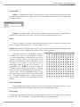
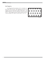
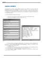
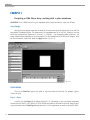
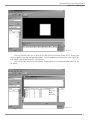
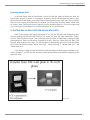
MICROARRAY DESIGN USING
CLONETRACKER DB™
A Supplement to the CloneTracker DB™
VERSION 2.0 USER MANUAL
MICROARRAY DESIGN USING CLONETRACKER DB™
A Supplement to the CloneTracker DB™
Version 2.0
User Manual
January 30th, 2002
Microarray Design Using CloneTracker DB™
Version 2.0 • USER MANUAL
Every effort has been made to ensure the accuracy of this document. However,
BioDiscovery makes no warranties with respect to this documentation and disclaims
any implied warranties or merchantability and fitness for a particular purpose.
BioDiscovery shall not be liable for any errors or for any accidental or consequential
damages in connection with the furnishing, performance or use of this document or
the examples herein. The information in this document is subject to change.
Trademarks
CloneTracker DB™, ImaGene™, GeneSight™, and GeneDirector™ are trademarks of BioDiscovery,
Inc. Other product names mentioned in this document may be trademarks or registered trademarks of their respective companies and the sole property of their respective manufacturers.
Copyright 2002 BioDiscovery, Inc. All Rights Reserved.
Written at BioDiscovery, Inc., Marina Del Rey, CA, 90292
Printed in the United States of America
4640 Admiralty Way, Suite 710, Marina del Rey, CA 92092
Phone 310.306.9310 Fax 310.306.9101
E-mail: [email protected]
3
CONTENTS
CHAPTER 1 - Introduction to CloneTracker DB and its role in Array Design . . . . . . . . . . .5
Microarray Experimental Design to Assist Normalization of Data . . . . . . . . . . . . . . .6
CHAPTER 2 - CloneTracker DB terminology . . . . . . . . . . . . . . . . . . . . . . . . . . . . . . .8
Experimental Terms . . . . . . . . . . . . . . . . . . . . . . . . . . . . . . . . . . . . . . . . . . .9
Array Designs . . . . . . . . . . . . . . . . . . . . . . . . . . . . . . . . . . . . . . . . . . . . . .9
Arrays . . . . . . . . . . . . . . . . . . . . . . . . . . . . . . . . . . . . . . . . . . . . . . . . . .10
Clones . . . . . . . . . . . . . . . . . . . . . . . . . . . . . . . . . . . . . . . . . . . . . . . . .10
Plates . . . . . . . . . . . . . . . . . . . . . . . . . . . . . . . . . . . . . . . . . . . . . . . . . .10
Array Design Terms .
Field . . . . . . . . .
Layout Mode . . .
Sector . . . . . . . .
Pin Configuration
Pin Spacing . . . .
Spot Staggering .
.
.
.
.
.
.
.
.
.
.
.
.
.
.
.
.
.
.
.
.
.
.
.
.
.
.
.
.
.
.
.
.
.
.
.
.
.
.
.
.
.
.
.
.
.
.
.
.
.
.
.
.
.
.
.
.
.
.
.
.
.
.
.
.
.
.
.
.
.
.
.
.
.
.
.
.
.
.
.
.
.
.
.
.
.
.
.
.
.
.
.
.
.
.
.
.
.
.
.
.
.
.
.
.
.
.
.
.
.
.
.
.
.
.
.
.
.
.
.
.
.
.
.
.
.
.
.
.
.
.
.
.
.
.
.
.
.
.
.
.
.
.
.
.
.
.
.
.
.
.
.
.
.
.
.
.
.
.
.
.
.
.
.
.
.
.
.
.
.
.
.
.
.
.
.
.
.
.
.
.
.
.
.
.
.
.
.
.
.
.
.
.
.
.
.
.
.
.
.
.
.
.
.
.
.
.
.
.
.
.
.
.
.
.
.
.
.
.
.
.
.
.
.
.
.
.
.
.
.
.
.
.
.
.
.
.
.
.
.
.
.
.
.
.
.
.
.
.
.
.
.
.
.
.
.
.
.
.
.
.
.
.
.
.
.
.
.
.
.
.
.
.
.
.
.
.
.
.
.
.
.10
.10
.11
.11
.11
.11
.12
CHAPTER 3 - Moving from CloneTracker DB v1.x to v2
Database Converter . . . . . . . . . . . . . . . . . . . .
User Interface Changes . . . . . . . . . . . . . . . . .
Naming Convention Changes . . . . . . . . . . . . .
.
.
.
.
.
.
.
.
.
.
.
.
.
.
.
.
.
.
.
.
.
.
.
.
.
.
.
.
.
.
.
.
.
.
.
.
.
.
.
.
.
.
.
.
.
.
.
.
.
.
.
.
.
.
.
.
.
.
.
.
.
.
.
.
.
.
.
.
.
.
.
.
.
.
.
.
.
.
.
.
.
.
.
.
.
.
.
.
.13
.14
.15
.16
CHAPTER 4 - Design examples . . . . . . . . . . . . . . . . . . . . . . . . . . . . . . . . .
Example 1: Designing a cDNA macro Array– working with a nylon membrane
Example 2: Designing a a High density Array– working with glass slides . . .
Example 3: Plate-to-plate-to-slide mapping . . . . . . . . . . . . . . . . . . . . .
Example 4: Designing an array with replicated / Duplicated spots . . . . . . .
Example 5: Exercise for practice . . . . . . . . . . . . . . . . . . . . . . . . . . . . .
.
.
.
.
.
.
.
.
.
.
.
.
.
.
.
.
.
.
.
.
.
.
.
.
.
.
.
.
.
.
.19
.20
.26
.29
.32
.36
APPENDIX 1: FAQ - Frequently Asked Questions
APPENDIX 2: Solution to Exercise in Chapter 5
References . . . . . . . . . . . . . . . . . . . . . . . . .
New Features . . . . . . . . . . . . . . . . . . . . . . .
.
.
.
.
.
.
.
.
.
.
.
.
.
.
.
.
.
.
.
.
.38
.39
.40
.41
.
.
.
.
.
.
.
.
.
.
.
.
.
.
.
.
.
.
.
.
.
.
.
.
.
.
.
.
.
.
.
.
.
.
.
.
.
.
.
.
.
.
.
.
.
.
.
.
.
.
.
.
.
.
.
.
.
.
.
.
.
.
.
.
.
.
.
.
.
.
.
.
.
.
.
.
.
.
.
.
.
.
.
.
.
.
.
Microarray Design Using CloneTracker DB™
Version 2.0 • USER MANUAL
CHAPTER
ONE
CLONETRACKER DB AND ITS
ROLE IN ARRAY DESIGN
CHAPTER 1
CloneTracker DB and its role in Array Design
Introduction
Microarray projects involve acquisition and validation of large data sets. Each study typically
requires iterations of series of processes, which start with experimental design and array fabrication, proceed with array scanning, image analysis, and finally gene expression data analysis.
The initial data resources required to design and fabricate gene expression microarrays that need
to be documented include cDNA sequence data, cDNA clones information, experimental procedures, physical location of materials, and others. This information needs to be integrated within the data flow during array design, analysis, and interpretation of results (Figure 1-1).
Fig. 1-1
The software tool CloneTracker DB from BioDiscovery, Inc. (Marina Del Rey, CA; www.biodiscovery.com) has been
designed to make management of array fabrication data easy and rewarding.
The CloneTracker DB software offers:
Laboratory information management. A management system that provides access interface to the
underlying fabrication database. It helps the user monitor the overall fabrication process by allowing
queries of fabrication data, updating data step by step according to the progress, or tracing a
particular spot on a particular array back to the originating plate and well position.
Array design. An easy-to-use visual interface that allows the user to design or adjust the array layout
based on the type of arrayer used. It can also export the settings for the arrayer or even generate
complete programs to control the arrayer robot directly.
Utilities for complex data manipulation. The information flow in the fabrication process involves
several transformations that cannot be handled using simple database operations. Examples: (i)
transformation of clone data from a set of plates (plate data) into spot data on the array (array data);
(ii) generation of fabrication data in the format recognized by the image analysis system ImaGene and
the data-mining tool GeneSight; (iii) tracking clone transfer-processes from 96 well to 384 well plates
to a DNA array, and back.
6
Microarray Design Using CloneTracker DB™
Version 2.0 • USER MANUAL
The primary goal of this document is to illustrate uses of CloneTracker DB with examples while
explaining to existing users new features and terminology. Readers should review the CloneTracker DB
User’s Manual when using this software.
CloneTracker DB is useful not only as a virtual design tool to facilitate visualization before printing of the array and organizing data, but also to help the actual experimental design.
Microarray Experimental Design to Assist Normalization of Data
A designed experiment is a test or series of tests, in which purposeful changes are made to the
input variables of a process or system so that we may observe and identify reasons for changes in the
output response (Montgomery, 1991).
The basics principles of experimental design are replication, randomization, and blocking.
Approaches for experimental design in microarray experiments are as follows:
• Use more than one cDNA spot for normalization purposes - spot replication. CloneTracker DB
offers an easy approach for creating duplicates, triplicates, and more spot replications. This information
is submitted to the data analysis tool GeneSight (BioDiscovery) for data normalization procedures.
• Replicate the array on the same slide - array replication. This is a blocking strategy (performing
an experiment on a homogenous material, i.e. the same slide), which can be achieved by the click of the
mouse with CloneTracker DB.
• Use control spots. CloneTracker DB keeps track and can color-code control spots.
• Replicate the experiment on different slides - experiment replication. CloneTracker allows you to
use an array design that is automatically applied to many slides.
• Randomize the spot replicates on the array. You may use CloneTracker Replicates Editor to design
your array.
7
CHAPTER 2
CloneTracker DB Terminology
CHAPTER
TWO
CLONETRACKER DB
TERMINOLOGY
Microarray Design Using CloneTracker DB™
Version 2.0 • USER MANUAL
Due to the flexibly associated with various parts of the arraying processes, CloneTracker DB has
developed a unique terminology covering various design aspects. The terms listed below reoccur throughout the usage of CloneTracker DB. As a result, users are encouraged to have a working knowledge of their
meaning. Most terms covered below are found throughout microarray design and clone management. For
additional information, please consult the CloneTracker DB v.2 User’s Manual.
EXPERIMENTAL TERMS
Array Designs
Array Designs are templates of spotted arrays, describing how a particular array is spotted (Figure
2-1) and from which plates the clones are taken (Figure 2-2). Array Designs are used to create multiple
Arrays of the same template, or design. Some of the parameters used to describe an Array Design include
the array dimensions (whether for a slide or a membrane), pin and spot configurations, pin and spot spacing, and sectors.
Fig. 2-1
Fig. 2-2
Example: If a particular set of genes (we denote any length of DNA whether an EST or cdna
as a gene for simplicity) needs to be printed on hundreds of slides by a core facility then the set up
applying to each slide is the array design. This blue print contains all the information about the dimension of the slide, how many pins are used for printing, what plates with DNA probes were utilized, etc.
9
CHAPTER 2
CloneTracker DB Terminology
Arrays
Arrays are particular instances of Array Designs corresponding to physical arrays. The plates used
in the Array Design are the plates used in the Array. Additional information such as barcode information
can be applied to each Array.
Clones
Clones are the biological materials contained in Plate wells. Therefore a clone may mean a PCR
product, cdna, or other material to be printed. Clones may be imported into the database along
with Plate Importation, or they may be added to existing plates that are not populated with Clone data.
Plates
Plates are small plastic containers consisting of 96, 384, and 1536 wells. These wells contain the
material to be spotted onto the microarray slide. Within CloneTracker DB, the Plate Type indicates
whether the plate is 96, 384, or 1536 well plate.
ARRAY DESIGN TERMS
Field
A field is the largest design element within a slide
(Figure 2-3). A field typically consists of the arraying
done by a single print head on the slide. For example,
if the arrayer has a print head with 8 pins in a 2 x 4
configuration, the region of the slide containing the
resulting printing is a field. For most experiments and
arrayers, users will only have a single field. However,
CloneTracker DB 2 fully supports the creation of multiple
fields if necessary.
Common uses for multiple fields include:
Fig. 2-3
• Generating slides which contain arrays of different geometries: for example, some microarray core
facilities procedures include a set of designated genes on each slide produced in the facility for calibration purposes. These genes are not within the field with the genes under investigation. Such sets of
genes will be located in a separate field. CloneTracker DB 2 offers the flexibility and ease-to-use to create this field.
• Generating slides with duplicated arrays next to each other. This will be needed if you decide to
replicate the whole array on the same slide as discussed in Lee et al. (2000).
10
Microarray Design Using CloneTracker DB™
Version 2.0 • USER MANUAL
Layout Mode
Regular - In Regular Mode (Figure 2-4) the printing is done in such a way that each pin prints the
required number of spots from a single plate as to use all samples from all wells. See the examples in
following chapters.
Fig. 2-4
Compact - In Compact Mode, users are free to design the rows and columns to be printed irregardless of the relationship to the plate. This allows for more complicated array design.
Sector
A sector is a region on the array containing spots printed by one pin. The source for a sector could
be one or several plates depending on the Layout Mode. (Fig. 2-5)
Example: when printing in Regular Mode, a sector is the printing done by a single pin from a single plate.
In this case, each sector is displayed as a different color within the software.
Please note that when the Layout Mode is switched
to Compact, the notion of a sector increases in complexity. Under Compact Mode, a sector defines the rows and
columns of printing; however, this may or may not be
equal to the printing done from a single plate. Sector
Size refers to the number of rows and columns of
clones/spots placed on the slide by a single pin. In
Regular Mode this is FIXED to a size which allows the
print head to dip to every well of the plate. In Compact
Mode, the sector size can be modified to virtually any values by the user. Due to the gap between pins on the pin
head, researchers can spot several Sectors between each
pin. CloneTracker DB allows this to be done by specifying the Number of Sector Rows and Number of Sector
Columns.
Fig. 2-5
Pin Configuration
The arrangement and number of individual pins on the print head. CloneTracker allows you to use
either hand-held devices with 96 pins or any arrayer with any combination of pins.
Pin Spacing
Pin Spacing determines whether the pins on the print head dip into wells next to one another or whether
the pins skip a well in the middle. Typically, users should select Consecutive wells.
11
CHAPTER 2
CloneTracker DB Terminology
Spot Staggering
Spot Staggering allows researchers to fit an increased number of spots within an array. Spot Staggering prints spots in a
hexagonal structure minimizing the space between spots. Left
staggered means the initial row is spotted to the left of the row
below it. Right staggered means the opposite where the top row
is position slightly to the right of the row below it. (Fig. 2-6)
Fig. 2-6
12
Microarray Design Using CloneTracker DB™
Version 2.0 • USER MANUAL
CHAPTER
THREE
MOVING FROM CLONETRACKER DB
VERSION 1.X TO VERSION 2
CHAPTER 3
Moving from CloneTracker DB version 1.x to version 2
DATABASE CONVERTER
CloneTracker DB 2 includes a handy database conversion utility designed to transition data from
CloneTracker version 1.4.4 and higher to CloneTracker DB version 2. User with older versions of
CloneTracker DB will need to export plates from version 1 then recreate the slides within CloneTracker DB
2. Through use of the DB Converter, all information within the database is automatically transferred to
the new MySQL database.
To convert the database, perform the following:
1. From within the Start Menu, click DB Converter within the CloneTracker DB 2 menu.
2. Read the initial message. click OK to continue. (Fig. 3-1)
Fig. 3-1
Fig. 3-2
3. The next window is the Database Transfer Window. For most users, the correct parameters will
be provided. However, the user must enter the source password. By default, this password is: sql.
There is no need to enter a Target password.
4. Click OK to continue.
5. The information is transferred and Log window is then displayed. If the same data exists within the new database, the user is prompted what to do with the data. (Fig.3-2)
6. Upon completion, “Logout... Succeeded” is displayed in the Log window. The data is now
available within CloneTracker DB 2.
14
Microarray Design Using CloneTracker DB™
Version 2.0 • USER MANUAL
USER INTERFACE CHANGES
CloneTracker DB 2 has included the best aspects of version 1 and applied several new options for
the main user interface, which were required by a world-wide group of scientists employing CloneTracker
DB in their research. The user interface in version 2, as it was in 1.x, is primarily geared to virtual array
design. Within this virtual design, the key elements, slide, array geometry, clones and mapping information, are placed predominantly before the user. Please see diagram below for similarities.
Virtual
Design
Fig. 3-3
Experiment
Information
Mapping
Information
Fig. 3-4
15
CHAPTER 3
Moving from CloneTracker DB version 1.x to version 2
CloneTracker DB 2 also adds several new features as outlined below. (Fig. 3-5)
When zoomed in, spotting orders become visible.
All Arraying Parameters conveniently displayed on main screen.
New Toolbar for quick access to important features.
Fig. 3-5
Ability to edit individual “Replicate Patterns”
Ability to control the mapping information that is displayed.
NAMING CONVENTION CHANGES
CloneTracker DB 2 uses a unique naming convention which allows for the description of highly
complicated arraying design. Note, although there have been terminology changes between previous versions of CloneTracker DB and version 2, the same designs can still be created.
CloneTracker 1 used the notions of spot layout, subgrid and super grid to describe all the design
elements of the slide. CloneTracker DB 2 also has a set of terms, sector, sub-grid and field, which perform the same task. The following information explains the relationship between naming conventions.
16
Microarray Design Using CloneTracker DB™
Version 2.0 • USER MANUAL
Fig. 3-6
Fig. 3-7
The smallest level of design in v1 is the spot layout. (Fig 3-6) In v2, this is the Sector. (Fig. 3-7)
When arraying in Regular Mode, spot layout and sector represent the same thing.
Note: When performing more complicated arraying this is not true; however, such arraying is beyond the
scope of this document.
In v1, all the spot layouts generated by a single pin are grouped into a subgrid. (Fig. 3-8) In v2,
the sectors are grouped into a subgrid, (Fig. 3-9) but are loosely called simply Rows and Columns of
Sectors. The subgrid term is not used much in v2 except to indicate to which direction printing should
continue upon filling the allocated sector rows and columns.
Fig. 3-8
Fig. 3-9
The top level of design in v1 is the supergrid. The supergrid was simply all the subgrids printed
within the slide. However, the problem of a supergrid is that it only allows for a single supergrid design
per slide. For example, this prevents users from generating a slide where extra marker genes are placed
outside of the supergrid, as is displayed below.
It also prevents different arraying designs, or shapes, to occur on a single slide. V2 addresses these
issues by introducing the concept of a field.
17
CHAPTER 3
Moving from CloneTracker DB version 1.x to version 2
Typically, a single field represents a the entire supergrid structure on the slide. For example, if the
slide has a supergrid structure of 1x3, (Fig 3-10) then this design would be contained within a single
field in v2. (Fig. 3-11) The two versions differ because v2 allows users to create multiple or different
fields for additional designs within the same slide.(Fig. 3-12)
Fig. 3-10
Fig. 3-12
18
Fig. 3-11
Microarray Design Using CloneTracker DB™
Version 2.0 • USER MANUAL
CHAPTER
FOUR
DESIGN EXAMPLES
CHAPTER 4
Design Examples
EXAMPLE 1
Designing a cDNA Macro Array: working with a nylon membrane
OBJECTIVE: Print a cDNA array on a nylon membrane with a hand held device, which has 96 pins.
Array Design
Specify the array design name and the name of the user under the Array Design tab. Let us call this
array design “Membrane Mouse”. The dimensions of this membrane are 20 cm x 20 cm. Therefore you may
enter the corresponding dimensions in microns, i.e. 200,000 – (see frequently asked questions). You
many choose margins depending on your experiment. For this example enter 10,000 for all margins. After
all the information is specified, press the Apply button (Fig. 4.1.1)
Fig. 4.1.1
FIELD DESIGN
Click on the Field Tab. Specify the name of the field under the Field tab. For example, type in
“Device 96 pins”.
Step 1 - Plates
Initially, only the Plates tab is enabled (Figure 4.1.2). Depending on your microarray experiment,
choose either 96 (8x12), 384 (16x24) or 1536 (32x48) well plates to be used for the final stage of printing by selecting from the Plate Type drop-down menu. For this experiment we need to choose 96 (8x12).
20
Microarray Design Using CloneTracker DB™
Version 2.0 • USER MANUAL
Fig. 4.1.2
Click on the Add Plate icon to bring up the Edit Plate List window (figure 4.1.3). Choose your
choice of plate(s) from the Available Plates panel. For this membrane-printing project, select “8x12 (96well plates)” and choose Plates 501, 502 and 503.
Click on the right arrow icon to bring your chosen plate(s) to the Selected Plates panel. Hit the
OK button.
Fig. 4.1.3
21
CHAPTER 4
Design Examples
If initially there are no plates listed or you would like to import plates then click on the Plates
icon in the toolbar. Alternatively, select Plates under View menu (Figure 4.1.4).
Click on the “Import Plates From Text” icon on the right icon bar selection (Figure 4.1.5). A “Plates
Importer” window shows up. Click on Browse and find the folder Samples (located in your CloneTracker
folder). Choose 96 plates.txt file, which contains clone information for four 96 well plates called 501,
502, and 503, i.e. they are concatenated. A file can also contain information for one plate only. You may
want to view or edit this file by using Excel. Once editing within Excel is complete, remember to save
the file as a tab delimited text file for compatibility with CloneTracker.
Fig. 4.1.4
Fig. 4.1.5
In the “Plates Importer” click on the selection buttons (squares) for the columns you wish to
import (Figure 4.1.6). In this case, select all columns. The selected columns will be colored in red. Click
on the first row of plate 501 and select it. Scroll down to the last row of plate 503. Hold the SHIFT key
on your keyboard to select all rows including the last one (row h, column 12 of plate 503). All the
columns become highlighted. Click the Down Arrow button at the bottom of the “Plates Importer” window. The selected plates appear in the lower half of the Importer window (Figure 4.1.7). You may enter
some remarks about each plate in the column termed “Info”. Click OK. Now you may go to the Field Tab
and click on the “Add Plates” icon. Select plate 501, 502, and 503. Click the right arrow. Now plate 501,
502, and 503 are added to the Selected Plates panel. And then click on the OK button.
Fig. 4.1.6
22
Microarray Design Using CloneTracker DB™
Version 2.0 • USER MANUAL
Fig. 4.1.7
Fig. 4.1.8
Step 2 - Pins
The Pins tab allows you to customize the desired pin configuration. You could modify the pin spacing by selecting either Consecutive wells or Every other well. Choose the 8x12 pin configuration for
this experiment as shown if Figure 4.1.8.
Several well-dipping order patterns could be selected by clicking on the Well-Dipping Order dropdown menu. The most common dipping pattern used by most arraying machines is “Left to Right, TopDown”.
Step 3 - Spots
For simplicity purposes, we will not change the default values under the Spots tab. Researchers
usually change the spot spacing and diameter to achieve special printing patterns. Depending on the
type of arrayer machine, one is able to decrease the vertical and horizontal spot spacing to fit more spots
into each sector area. Decreasing the spot diameter allows one to further decrease the spacing between
each spot.
Step 4 - Sectors
A sector is most easily defined as the total number of spots printed by one pin from one plate in
Regular mode (please see the following examples for further discussion).
The sector size specifies the layout of all those spots. In our case, we have 96 wells that are printed by 96 pins. There is only one spot in one sector. Therefore, the only sector size possible is 1x1 in
Regular Mode. (96 wells/96 pins = 1). In fact, in this case one spot is equivalent to a sector.
The numbers of Sector Rows and Sector Columns define in what pattern the sector, as a geometrical entity, will be repeated. Enter the number of Sector Rows and Sector Columns and then change to
another pair of numbers to see how the printing pattern alters. Let us choose 4x4.
23
CHAPTER 4
Design Examples
Select a specific order for Sector Ordering from the pull down menu. The Sector Ordering refers to
the order of clones that are spotted by one pin. If you choose Left-to-right, Top-down (and the well
dipping order is Left to Right, Top-Down), the then the first spot (row one, column one) in the first sector will come from well a1 in plate 501, the second spot left to right (row one, column two) will come
from well a1 in plate 502, and so on.
Let us consider the following design. Now your objective is to replicate the same clone (material
from the same well) on the same array twice. Several research teams print the spots resulting from the
same well adjacent to each other. For example, the material from well a1 plate 501 will be printed in
row 1 column 1 and row 1, column 2. To achieve this we need to enter the plates in a different order.
In the Plate importer enter the plate (in this case 501) twice as shown in Figure 4.1.9. Then do the same
with plate 502, 503, and so on.
Additionally, some researchers like to leave blank spots for either background corrections or other
reasons. Let us imagine that in row 4, column 4, for each pin you would like to leave a BLANK spot. The
easiest way is to create a fake plate with all gene IDs = BLANK. Then import this plate in such an order
after all the others so that the spots coming from this plate appear in row 4, column 4.
Fig. 4.1.9
Step 5 - General
For this project, we will stay with the Regular layout and keep the default settings under the
General tab. Select the Regular layout mode ensures that the spots from one plate are spotted in a rectangular sector. The Compact layout mode will be explained in another project example.
24
Microarray Design Using CloneTracker DB™
Version 2.0 • USER MANUAL
Step 6 - Saving the Design
There are two ways to save the array design that you have created.
By using either method, the Array Design can be easily recalled for future
analysis or modification.
Saving to the CloneTracker Database
Click on File > Save on the menu bar (Figure 4.1.10). This will save
the current Array Design to the CloneTracker database.
Saving to a Specific Location
Click on File > Export on the menu bar. The Save dialog box is displayed, where you can browse to the location of where you would like your
array design exported to. Click the Save button and your slide set is saved
in .xml format in the desired location.
Fig. 4.1.10
25
CHAPTER 4
Design Examples
EXAMPLE 2
Designing a High-Density Array - working with glass slides
OBJECTIVE: Design a high-density array, which will be printed on a glass slide. This example will require
2x2 pins and 96 well plates.
Array Design
Specify the array design name and the name of the user under the Array Design tab. Let us call
this array design “Slide Mouse”. The dimensions of the slide by default are width 75,000µ x height
25,000µ (7.5 cm x 2.5 cm). The frosted part of the slide is 25,000µ. With these dimensions the slide
width is horizontal to the viewer and the frosted side is to your right (Figure 4.2.1). If you wish to rotate
the slide, then you can enter 75,000µ for the height and 25,000µ for the slide bottom margin. Let us
leave the slide with the default settings.
Fig. 4.2.1
Field Design
Click on the Field Tab. Specify the name of the field under the Field tab. Enter 2x2 for Pin
Configuration.
26
Microarray Design Using CloneTracker DB™
Version 2.0 • USER MANUAL
Step - 1 Selecting Plates
To select the plates you wish to use in CloneTracker, click on the Add Plates icon on the right, vertical toolbar in the Plates Panel. The Edit Plate List window is displayed. If there are no plates listed see
Example 1 for details on importing plates.
Select plates 501, 502, and 503 and click on the right arrow to the right to import these plates.
Select plate 501 again and import it so we can work with 4 plates in this experiment.
Step 2 - Pins
Select 2x2 pin configuration.
Step 3 - Sector
Click on the Sector Size tab. Your Sector Size pull down Menu gives you
options, which are all combinations of 24, i.e. 1x24, 2x12, 3x8, 4x6, etc (Figure
4.2.2). The reason for this is that 24 is the number of times each pin will touch
the slide from one plate during the printing. If this number is denoted by N then
N = [ W / P ] x SR, where W is the number of wells in the plate, P is the number of pins, and SR is the number of duplicate spots. In this case 96 wells / 4
pins (only one gene replicate) yields 24.
Let us choose sector size 3x8 (3 rows x 8 columns)
Enter the number of Sector rows = 3 and Sector columns = 2. Watch the
array. Flip these numbers and see the design. In this way you will understand the
architecture of the array and the flexibility of CloneTracker DB to create your
designs.
Fig. 4.2.2
To understand the design of the finished array and to conceptualize what will be printed by one
pin, we can compute a subgrid size. The subgrid is simply the total numbers of rows and columns of
spots printed by a pin from several plates. The actual calculation is:
(Number of sector rows) x (number of rows in each sector) = total number of rows of each subgrid.
(Number of sector columns) x (number of columns in each sector) = total number of columns of
each subgrid.
So in the above example, we have 3x3=9 rows and 2x8= 16 columns in each subgrid.
Step 4 - Spot Information
To create a high-density array, we will need to change the information regarding the size and position of spots. Click on the Spots tab to access this information. First, let us change the spot staggering to Staggered Right . Upon selection, the array design to the right will be updated to reflect the new
27
CHAPTER 4
Design Examples
design. To further increase the number of possible spots within the array, let us decrease the Spot Space
Horizontal and Spot Space Vertical. The default values of 250 should be changed to 225. As a result,
by manipulation the parameters under the Spot tab, users can design arrays for machines capable of
high-density printing.
Exportation of a gene ID file
After generating an array design, you can export the gene ID file to your image analysis software.
ImaGene from BioDiscovery automatically imports gene ID files generated by CloneTracker.
Select “Export Mapping” under the File menu in CloneTracker. Choose ImaGene format (Figure
4.2.3). You have the option to assign the name “blank” to all empty spots. Those are the spots where
nothing is printed. This is particularly useful if you want to carry out your background corrections based
on such spots for the data analysis. Alternatively, you can choose not to export any empty spots.
With the Browse button select the directory and folder where you would like to save the file.
Assign a name to the file and click the save button.
Fig. 4.2.3
28
Microarray Design Using CloneTracker DB™
Version 2.0 • USER MANUAL
EXAMPLE 3
Plate-to-plate-to-slide mapping
OBJECTIVE: It is a common practice to perform a PCR reaction in 96 well plates and then transfer some
volume of the PCR reaction from each well to a well in a 394 well plate. Subsequently, the printing of
the microarray will be carried out by using the 384 well plate (Figure 4.3.1). This protocol allows for
printing of high density arrays and storing some of the initial PCR material for future use. Therefore, we
need to map the clone IDs from a 96 well plate to a 384 plate and then to the glass slide array.
Fig. 4.3.1
Alternatively, some protocols call for transfer of biological material from 384 well plates to 96
well plates, which are subsequently used as a source for printing the arrays. CloneTracker has a module,
which assists in mapping clones in such protocols.
A. MERGING FOUR PLATES INTO ONE
Under the “View” pull down menu, select “Plates”. Click the “Merge Four Plates into One” icon on
the right, vertical toolbar of the Plates Panel to display the Plate Merger dialog box. Select the four plates
that you want to merge from the “All Available Plates” list. Click the left arrow button to move these
plates to the Four Plates list. For example, if you have the plates 501, 502, and 503 then transfer them
to the left. Now select plate 501 again and transfer it to the left (Figure 4.3.2).
29
CHAPTER 4
Design Examples
Fig. 4.3.2
Click the Merge button to merge the plate tables Figure 4.3.3). Specify a name for the merged plate under
Plate ID (as an example, Mouse Scale Up) and click the OK button to save your changes. You should
always enter notes about the created plate in the “Description” field. These notes prove always useful in
future data analysis.
Return to the CloneTracker Plates Panel.
Fig. 4.3.3
30
Microarray Design Using CloneTracker DB™
Version 2.0 • USER MANUAL
Importing Merged Plate
In the Array Design Panel of CloneTracker, click on the Field tab. Under the Plates tab, select the
type of plate you wish to import. In this project, we want to use the 384-well plate we had just created from the four 96-well plates, so we select 16x24 (384-well plates) as the Plate Type. Click on the Edit
Plate List icon to bring up the Edit Plate List window. You will see that the newly created “Mouse Scale
Up” plate is there. Choose your choice of plate(s) from the Available Plates list, click on the right arrow
icon to bring your chosen plate(s) to the Selected Plates list. Hit the OK button.
B. SPLITTING ONE 384 WELL PLATE INTO FOUR 96 WELL PLATES
Some of your projects may require performing PC in a 394 well PCR plate and subsequently splitting the materials into 96 well plates (Figure 4.3.4). Under the “View” pull down menu select “Plates”.
Click the “Split One Plate into Four” icon on the right, vertical toolbar of Plates Panel to display the Split
plates dialog box. Select the 384 button for plates to be split. Select the “Mouse Scale Up” plate. Click
the right pointing arrow on the right. The 384 well plate is automatically split into four 96 well plates,
which have the following names: “Mouse Scale Up-0”, “Mouse Scale Up-1”, “Mouse Scale Up-2”, and
“Mouse Scale Up-3”.
If you decide to design an array with 96 well plates and repeat the plate import procedure as outlined in example 1, you will see that the newly created 96 well plates are available for mapping to the
glass slide array.
Fig. 4.3.4
31
CHAPTER 4
Design Examples
EXAMPLE 4
Designing an Array with Replicated / Duplicated Spots
As discussed in Chapter 1, replication is one of the basic principles of experimental design. Many
researchers prefer to have replicates of their genes on the same array. There are a two ways to achieve
this in CloneTracker.
The easiest way to duplicate spots is to copy the entire field to a different location on the slide.
In the Array Design Panel, start off by loading some plate files. (See Example 1: Step 1 - Plates)
Copy Field
1. Select Copy Field from the Fields menu.
2. Click the Field Mode button on the toolbar.
3. Click on the new field and drag it into the desired position.
Fig. 4.4.1 – Duplicated Fields
Some researchers prefer to have their duplicate clones positioned differently in each field.
Changing the Spot Ordering or Sector Ordering in the duplicated field easily does this.
Change Spot Ordering
1. Select the duplicated field tab (typically Field 2).
2. Select the Spot tab.
3. Click the drop-down triangle under Spot Ordering to change the ordering to
something different than the original field.
32
Microarray Design Using CloneTracker DB™
Version 2.0 • USER MANUAL
Change Sector Ordering
1. Select the duplicated field tab (typically Field 2).
2. Select the Sector tab.
3. Click the drop-down triangle under Sector Ordering to change the ordering to
something different than the original field.
The other way to duplicate spots is to make duplicates within the same sector as the original spots.
This is called editing the Replicates Pattern. This tool is a little complicated, but it is very powerful.
Edit Replicates Pattern
1. Under the Field tab, click on the Spots sub-tab.
2. Click the Edit Replicates Pattern button to display the Replicates Editor
dialog box.
In the left panel is an empty grid, and on the right panel is a grid full of spots. The left grid represents the layout of every sector in this field. A blank grid indicates a default layout.
Equals
Fig. 4.4.2 – A blank grid means a default layout
Indicate Spot Layout
1. On the right grid, click on the spot that you wish to replicate.
2. On the left grid, click on the location(s) that you wish to have the selected
spot in.
3. Repeat steps 1 and 2 for all of your desired spot(s) to be replicated.
In the example below, we have indicated that we want the first clones to be duplicated three more times
(marked in red). Any left grid boxes that you do not explicitly select are assumed to be empty.
33
CHAPTER 4
Design Examples
doesn’t equal
Fig. 4.4.3 – Blank areas on the grid does NOT mean a default layout.
Fig 4.4.3 Blank areas on the grid does NOT mean a default layout.
Looking at the right grid above, you may wonder what happened to clones 1a2, 1a3, and 1a4. Since
they are not on the grid, they will not be printed.
In order to have all the clones in the sector AND have duplicated spots, you must increase the size
of the sector and add the missing clones back in (marked in green).
Change Sector Size
1. Enter the new number of rows to use in the Number of Rows field.
2. Enter the new number of columns to use in the Number of Columns field.
3. Press <ENTER> on your keyboard to apply the changes.
Fig. 4.4.4 – Expanded sector with missing clones added back in.
34
Microarray Design Using CloneTracker DB™
Version 2.0 • USER MANUAL
Now that we have our customized Replicates Pattern, we can apply the changes by clicking OK and
exiting the Replicate Pattern Editor. Our new slide design now shows up on the Spotted Array window
box.
Fig. 4.4.5 – New Slide Design after editing Replicates Pattern
After creating this customized Replicates Pattern, we may want to save our design and load it back
in at a later time.
Export Replicates Pattern
1. Click the Export Replicates Pattern button to display the Save dialog box.
2. Select a destination folder for the replicates file.
3. Click the Save button to save the file to the designation location.
Import Replicates Pattern
1. Click the Import Replicates Pattern button to display the Open dialog box.
2. Locate and select a replicates file to import.
3. Click the Open button to display the selected file.
35
CHAPTER 4
Design Examples
EXAMPLE 5
Exercise for practice
Using the examples outlined in the previous sections try to perform the following exercise by yourself. The proposed design configurations are given in an Appendix of this tutorial.
Let us try to design the following experiment. You will print your arrays with an arrayer equipped
with 4x4 pins. You will use 384 well plates (the distance between spots is 240 um). The printing of the
array sectors will be performed Right-to-Left, Top-to-Bottom. Genes will be replicated on this array by
creating a duplicate meta-grid. The slide should be aligned vertically and there is no frosted area. You
need to print the spots in sectors of 18x18 (Figure 4.5.1). Additionally, the objective is to have 12x4
such sectors.
Fig. 4.5.1
36
Microarray Design Using CloneTracker DB™
Version 2.0 • USER MANUAL
APPENDIXES
1 FREQUENTLY ASKED QUESTIONS
2 SOLUTIONS TO EXERCISE IN
CHAPTER 5
APPENDIXES
Appendix 1: Frequent Asked Questions
APPENDIX I
FAQ - Frequently Asked Questions
Q: Why does CloneTracker DB use microns instead of millimeters?
A: Using microns allows CloneTracker DB to be highly accurate within it internal calculations. Also,
as spot size and spacing is typically determined in microns, CloneTracker DB maintains unit consistency.
Q: Why does CloneTracker DB offer so many possible combination of arraying styles?
A: CloneTracker DB 2 has been designed from the start as a comprehensive clone management system capable of performing virtually any task required of researchers. As a result, CloneTracker DB provides greater flexibility than any proprietary solution available.
Q: Is CloneTracker DB cross platform compatible?
A: Currently, CloneTracker DB is only available for the windows platform. However, BioDiscovery is
actively porting to Unix systems and the Mac OS X. Please contact BioDiscovery Support for the latest
listing of supported OS.
38
Microarray Design Using CloneTracker DB™
Version 2.0 • USER MANUAL
APPENDIX II
Solution to Exercise in Chapter 5
Exercise 1 - Solution:
1. Open CloneTracker.
2. Click on the Array Design Tab.
3. Enter “Exercise 1” as the name for this design.
4. Set slide height to 75,000µ and the width to 25,000µ because we would like to have the slide
positioned vertically.
5. Assign 300µ to all margins. This will remove the frosted area.
6. Click on the Field Tab.
7. Select the Plates Tab.
8. Select 384 as the plate type.
9. Click the Add Plates button.
10. Pick any plate from the Available Plate list.
11. Click the Right Arrow button to add this plate to the Selected Plates list.
12. Click OK. This will activate all other Field sub-tabs.
13. Select the Pins Tab
14. Pick 4x4 from the Pin Configuration list.
15. Click on the sub-tab General.
16. Choose Compact layout mode. Because we need to print spots in a structure 18x18 = 324 we
cannot use regular mode as explained earlier in one of the examples. If we use regular mode then we will
have to choose a sector size equal to a combination of two numbers which have been multiplied and
their result is 24 = 384 / (4x4).
17. Enter 4,000 for Field Location X and 15,000 for Field location Y to position it.
18. Click on the Sectors sub-tab.
19. Type 18x18 in sector size (this size will NOT appear on the list).
20. Select Left-to-Right, top-down sector ordering.
21. Type in 1 for sector rows and for sector columns. After we have created this array (field) with
4x4 sectors and each sector with 18 rows and 10 columns we need to print to more arrays on the same
slide with the same configuration.
22. Click on the Apply button to apply these changes to the current field.
23. Select Copy Field from the Fields menu at the top of the screen. CloneTracker DB will now identify the first Field as Field 1 and the new one as Field 2.
24. Click on the Field 2 tab.
25. Select the general sub-tab.
26. Type 4,000 for Field location X and 53,000 for Field location Y.
27. Click on the Apply button to apply these changes to the current field.
39
REFERENCES
REFERENCES
Lee, M-L., Kuo, F.C., Whitemore, G.A., and Sklar, J. 2000.
Importance of replication in microarray gene expression studies: statistical methods and evidence from repetitive cDNA hybridizations. PNAS USA, 29:9834-9839.
Montgomery, D.C. 1991.
Design and analysis of experimental design. John Wiley & Sons, New York, NY.
40
Microarray Design Using CloneTracker DB™
Version 2.0 • USER MANUAL
NEW FEATURES
Dynamically Structured Database - Unlike common databases, CloneTracker DB’s has been
designed to grow with new data and information. For example, virtually any type of additional clone
data, whether assesion number or chromosomal info, can be added to the database during import.
Extremely Flexible File Formats supporting XML - Researchers are now free to import files in various formats with virtually any number of columns including, using the use of XML.
Enhanced Visual Manipulations - Zoom, move and align arrays with a mouse click.
Advanced Spot Duplication Tools - CloneTracker DB includes the replicates editor allowing for
almost any form of spot replication pattern.
New Online Help System - Java based help system.
Enhanced Query Capability - New built in query tools allow researchers to retrieve information on
a variety of microarray information.
Java Core - Java allows CloneTracker DB to be a robust, cross platform application with enhanced
memory management.
Staggered Spotting - Users whose machine’s support spot staggering are now supported within
CloneTracker DB 2.
MySQL Database - CloneTracker DB includes a powerful, cross platform, relational database system.
41
4640 Admiralty Way, Suite 710, Marina del Rey, CA 92092
©2002 All rights resrved.