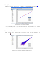
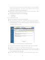
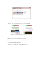
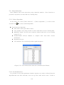
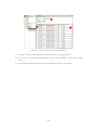
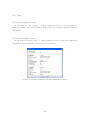
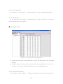
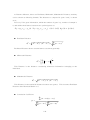
1
GenPlex Introduction <Version 3.0> Istech has all rights of this manual and this product. You cannot reprint, copy or distribute this manual and this product, without permission of Istech Corp. in advance. We will consider all, who have installed and who are using our product, will agree on this policy. Istech Inc. Copyright ⓒ 2008 ISTECH Inc. i Table of Contents Copyright ⓒ 2008 ISTECH Inc. .......................................................................................... i Introduction .......................................................................................................................... 8 1. GenPlex Introduction .................................................................................................... 9 1.1. Summary......................................................................................................... 9 1.2. Main Function ............................................................................................... 10 1.3. 1.2.1. Easy Data Importing.............................................................................. 10 1.2.2. Preprocessing ....................................................................................... 10 1.2.3. DEG (Differentially Expressed Gene) Finding ..................................... 10 1.2.4. Clustering .............................................................................................. 11 1.2.5. Classification ......................................................................................... 11 1.2.6. Pathway Analysis .................................................................................. 11 1.2.7. Biological Annotation & Data Mining ................................................... 12 Recommended Computer Requirements ...................................................... 13 Preprocessing .................................................................................................................... 14 2. Preprocessing ............................................................................................................. 15 2.1. 2.2. File................................................................................................................ 15 2.1.1. Import Affymetrix Gene Chip Data....................................................... 15 2.1.2. Import One-dye Chip Data ................................................................... 20 2.1.3. Import Two-dye Chip Data................................................................... 21 2.1.4. Open Analysis ....................................................................................... 24 2.1.5. Recent Analysis..................................................................................... 24 2.1.6. Save Analysis ........................................................................................ 24 2.1.7. Save Analysis As .................................................................................. 24 2.1.8. Close Analysis....................................................................................... 24 2.1.9. Analysis Properties............................................................................... 24 2.1.10. Configure............................................................................................... 24 2.1.11. Exit ........................................................................................................ 24 Preprocessing............................................................................................... 25 2.2.1. Experimental Information ..................................................................... 25 2.2.2. Filtering Error Spot............................................................................... 26 2.2.3. Normalization ........................................................................................ 31 2.2.4. Set Detection......................................................................................... 36 ii 2.2.5. 2.3. 2.4. 2.5. Log Transform ...................................................................................... 37 Statistics/Plot ............................................................................................... 38 2.3.1. Statistics................................................................................................ 38 2.3.2. Box Plot................................................................................................. 39 2.3.3. Histogram .............................................................................................. 40 2.3.4. MA Plot.................................................................................................. 41 2.3.5. QQ Plot .................................................................................................. 42 2.3.6. Correlation Scatter Plot ........................................................................ 42 2.3.7. Correlation Matrix Plot ......................................................................... 43 Analysis Data................................................................................................ 44 2.4.1. DEG Finding .......................................................................................... 44 2.4.2. Clustering .............................................................................................. 45 2.4.3. Classification ......................................................................................... 46 Reference ..................................................................................................... 48 DEG Finding ....................................................................................................................... 49 3. DEG Finding ................................................................................................................ 50 3.1. 3.2. 3.3. File................................................................................................................ 50 3.1.1. New Analysis ........................................................................................ 50 3.1.2. Open Analysis ....................................................................................... 51 3.1.3. Recent Analysis..................................................................................... 51 3.1.4. Save Analysis ........................................................................................ 51 3.1.5. Save Analysis As… ............................................................................... 51 3.1.6. Close Analysis....................................................................................... 52 3.1.7. Import Data ........................................................................................... 52 3.1.8. Analysis Properties............................................................................... 54 3.1.9. Exit ........................................................................................................ 54 Preprocessing............................................................................................... 55 3.2.1. Check & Match Data ............................................................................. 55 3.2.2. Filter Missing Data................................................................................ 55 3.2.3. Impute Data ........................................................................................... 56 3.2.4. Log Transform ...................................................................................... 56 DEG Finding ................................................................................................. 57 3.3.1. Fold Change .......................................................................................... 57 3.3.2. 2-Class Paired Test ............................................................................. 65 3.3.3. 2-Class Unpaired Test ......................................................................... 66 3.3.4. Multi-Class Test ................................................................................... 68 iii 3.4. 3.5. 3.3.5. Combine Results ................................................................................... 69 3.3.6. Import Gene List ................................................................................... 69 3.3.7. Export to Clustering Module................................................................. 69 3.3.8. Export to Pathway Analysis Module .................................................... 69 3.3.9. Save Result(s) As Text......................................................................... 70 Statistics/Plot ............................................................................................... 71 3.4.1. Basic Statistics...................................................................................... 71 3.4.2. Sample Correlation Matrix.................................................................... 71 3.4.3. Box Plot................................................................................................. 72 3.4.4. Correlation Scatter Plot ........................................................................ 73 3.4.5. Correlation Matrix Plot ......................................................................... 73 3.4.6. Venn Diagram........................................................................................ 74 3.4.7. Volcano Plot .......................................................................................... 74 Reference ..................................................................................................... 77 Clustering ........................................................................................................................... 78 4. Clustering.................................................................................................................... 79 4.1. 4.2. 4.3. File................................................................................................................ 79 4.1.1. New Analysis ........................................................................................ 79 4.1.2. Open Analysis ....................................................................................... 80 4.1.3. Recent Analysis..................................................................................... 80 4.1.4. Save Analysis ........................................................................................ 80 4.1.5. Save Analysis As .................................................................................. 80 4.1.6. Close Analysis....................................................................................... 80 4.1.7. Import Data ........................................................................................... 81 4.1.8. Analysis Properties............................................................................... 82 4.1.9. Exit ........................................................................................................ 82 Preprocessing............................................................................................... 83 4.2.1. Experimental Information ..................................................................... 83 4.2.2. Log Transform ...................................................................................... 83 4.2.3. Gene Filtering ....................................................................................... 84 4.2.4. Missing Data Filtering........................................................................... 85 4.2.5. Imputation.............................................................................................. 85 4.2.6. Column Editing ...................................................................................... 85 Clustering ..................................................................................................... 88 4.3.1. Hierarchical Clustering ......................................................................... 88 4.3.2. K-means Clustering.............................................................................. 92 iv 4.3.3. 4.4. 4.5. Self Organizing Map .............................................................................. 94 Validation....................................................................................................101 4.4.1. GDI.......................................................................................................101 4.4.2. K-value Prediction..............................................................................102 Reference ...................................................................................................105 Classification....................................................................................................................106 5. Classification.............................................................................................................107 5.1. 5.2. 5.3. 5.4. File..............................................................................................................107 5.1.1. New Analysis ......................................................................................107 5.1.2. Open Analysis .....................................................................................108 5.1.3. Recent Analysis...................................................................................108 5.1.4. Save Analysis ......................................................................................108 5.1.5. Save Analysis As ................................................................................108 5.1.6. Close Analysis.....................................................................................109 5.1.7. Load Training Data File(s)..................................................................109 5.1.8. Load Test Data File(s) ........................................................................110 5.1.9. Transpose Data ...................................................................................110 5.1.10. Analysis Properties.............................................................................110 5.1.11. Exit ......................................................................................................110 Preprocessing.............................................................................................111 5.2.1. Check & Match Data ...........................................................................111 5.2.2. Filter Missing Data..............................................................................111 5.2.3. Impute Data .........................................................................................112 Gene Selection ...........................................................................................113 5.3.1. Select Algorithm .................................................................................113 5.3.2. Set Parameter(s) .................................................................................113 5.3.3. Run.......................................................................................................114 5.3.4. Combine Results .................................................................................116 5.3.5. Set As Active Gene Selection.............................................................117 5.3.6. Export to Clustering ...........................................................................117 5.3.7. Export to Pathway Analysis Module ..................................................117 5.3.8. Save Result(s) .....................................................................................118 Classification ..............................................................................................119 5.4.1. Select Distance ...................................................................................119 5.4.2. Select Algorithm .................................................................................119 5.4.3. Set Parameter(s) .................................................................................120 v 5.4.4. 5.5. 5.6. 5.7. Classify Test Data ..............................................................................120 Error Estimation .........................................................................................122 5.5.1. Select Algorithm .................................................................................122 5.5.2. Set Parameter(s) .................................................................................122 5.5.3. Run.......................................................................................................122 5.5.4. Whole Computation .............................................................................124 View............................................................................................................126 5.6.1. Show Sample 3D View ........................................................................126 5.6.2. Show Summary View ..........................................................................126 Reference ...................................................................................................127 Pathway Analysis.............................................................................................................128 6. Pathway Analysis......................................................................................................129 6.1. 6.2. File..............................................................................................................129 6.1.1. New Analysis ......................................................................................129 6.1.2. Open Analysis .....................................................................................130 6.1.3. Recent Analysis...................................................................................130 6.1.4. Save Analysis ......................................................................................130 6.1.5. Save Analysis As ................................................................................130 6.1.6. Close Analysis.....................................................................................131 6.1.7. Import Data .........................................................................................131 6.1.8. Analysis Properties.............................................................................131 6.1.9. Exit ......................................................................................................132 Pathway List...............................................................................................133 6.2.1. Pathway (Image) .................................................................................133 6.2.2. Pathway (XML)....................................................................................134 Algorithms........................................................................................................................135 7. 8. 9. DEF Finding Algorithm .............................................................................................136 7.1. Fold Change................................................................................................136 7.2. Two-sample (unpaired) t-test...................................................................137 7.3. Volcano Plot ...............................................................................................138 7.4. Analysis of Variance (ANOVA)..................................................................139 Clustering Algorithm.................................................................................................140 8.1. Hierarchical Clustering (HC)......................................................................140 8.2. K-means.....................................................................................................144 8.3. Self Organizing Map (SOM)........................................................................145 Classification Algorithm ...........................................................................................146 vi 9.1. Gene Selection ...........................................................................................147 9.2. Classifier ....................................................................................................148 9.3. Generalization Error Estimation ................................................................149 vii Introduction 1. GenPlex Introduction 1.1. Summary Microarray (DNA Chip) that is able to monitor the intensity of thousands and millions of gene information at the same time, had become the main tool in biotechnology research field in the 21st Century. The use of Microarray allows us to verify the significant status on the gene level of the gene inside the cell, and through this significant information, we can understand inclusively the relation between these genes. However, because of the complicatedness of the out-coming data, Microarray requires recent method of all kinds of algorithm and bio-informatics such as Mathematics, Statistics and Computer Science, etc. GenPlex is a Microarray analyzing software which offers useful information to scientists in analyzing the data suitably to the users in providing various visualization of the results, and also possible to analyze the experiment data through various statistical algorithm. 9 1.2. Main Function 1.2.1. Easy Data Importing It is easy to input data for users, because it recognizes automatically various types of raw data. Supporting Format z Affymetrix Gene Chip Data(CEL) z ABI Chip Data z Illumina Chip Data(BeadStudio output) z GenePix Result z ImaGene Data 1.2.2. Preprocessing It provides the information of the raw data quality through statistical figure and various plot, also provides the Preprocessing function of the data which will be used for future analysis. Box Plot Histogram MA Plot QQ Plot Sample Correlation Scatter/Matrix Plot: showing the relationship between replications Global centering/scaling, Global/Print-tip Lowess, Quantile Normalization, etc. Convenient Gene Expression Matrix (GEM format) generation 1.2.3. DEG (Differentially Expressed Gene) Finding It is possible to apply various conditions of Fold Change, and it also offers us the various statistical analysis methods to compare 2-class or multi-class. It is possible to compare the out-coming DEG using Venn Diagram, and we can verify visually the difference between Fold Change and the statistic analysis result using Volcano Plot. Fold Change: One-dye, Two-dye Parametric Test for 2-class comparison: Student T-test, Welch’s T-test, Z-test Nonparametric Test for 2-class comparison: Mann-Whitney test Paired Test: Paired T-test, Wilcoxon signed rank test Parametric Multi-class Comparison: One way ANOVA Nonparametric Multi-class Comparison: Kruskal-Wallis H-test Multiple Test Correction: Bonferroni correction, Holm’s procedure, Benjamini-Hochberg FDR Volcano Plot: Fold Change vs. Statistical Test Venn Diagram: combining results from various methods 10 Statistics, Box Plot, Correlation Scatter Plot, Correlation Matrix Plot 1.2.4. Clustering It provides various clustering methods and visualization and it is also possible to verify statistically the clustering result. In case of K-means, it helps the users to conclude (judge) in predicting the most suitable number of cluster. Hierarchical Clustering with useful Linkage methods K-means Clustering SOM (Self Organizing Map) : U-matrix Topographic Profiling Statistical Clustering Validation K-Value Prediction for K-means Clustering Dendrogram with various graphical options for publication 1.2.5. Classification It is the analysis method mostly used for diagnosis, prognosis and estimation, providing various statistical methods to find out the marker gene. We can avoid the data over-fitting through Generalization Error Estimation of classification, and enables the analysis estimation more accurate and easier with the whole computation. Feature selection: finding marker genes for diagnosis Classification: classifying samples into pre-defined classes Error Estimation: estimating generalized misclassification error rate Whole Computation: all-in-one approach for optimal classification Sample PCA: powerful visualization with various graphical options for publication 1.2.6. Pathway Analysis It is able to analyze the biological mutual relationship of genes from DEG Analysis, Clustering Analysis, Classification Analysis, etc., to biological genes. It researches the genes related to common pathway using the biological pathway information of KEGG (Kyoto Encyclopedia of Genes and Genomes) database, and in mapping the DNA Chip expression results, it is understood in the pathway level, the changes of the expression quantity according to the experiment condition. Pathway Search: given gene lists, all related KEGG pathways explored Pathway Mapping: mapping genes onto pathways Up-/Down-regulation display with heatmap 11 1.2.7. Biological Annotation & Data Mining For gene group from the statistical analysis result of DEG Finding, Clustering, etc., we can pull out all kinds of biologic information, like GO Annotation, KEGG Pathway, etc. And also can analyze statistically the biological linkage of each group using Gene Ontology. Basic Information: NCBI Gene ID, UniGene ID, Gene Symbol, Gene Title, Chromosome Location Protein Information: InterPro, Pfam, Prosite, EC Number, Uniprot PANTHER Category: PANTHER Family Name, PANTHER Subfamily Name, PANTHER Function, PANTHER Process Gene Ontology: GO Molecular Function, GO Biological Process, GO Cellular Component Pathway: KEGG Pathway ID Conversion: Public ID 12 1.3. Recommended Computer Requirements Microsoft Windows 2000/XP System CPU: Pentium 4, higher than 2.4GHz RAM: minimum 1GB 13 Preprocessing 14 2. Preprocessing You can have the image file of Microarray experiment results and it is the process of preprocessing of the raw data issued from image scanning. 2.1. File First, input raw data using Import Data Menu. Import Data Menu is classified in three kinds and is supporting data format as follows: Affymetrix Gene Chip Data (go to 2.1.1 ▷) z CEL File z CHP File One-Dye Chip Data (go to 2.1.2 ▷) z ABI Chip Data z Illumina Chip Data(BeadStudio-Exported Gene/Probe Profile Data) z Agilent Chip Data(GenePix Results format(*.gpr)) Two-Dye Chip Data (go to 2.1.3 ▷) z GenePix Result z ImaGene Data 2.1.1. Import Affymetrix Gene Chip Data On the menu bar, click [File] → [Import Affymetrix Gene Chip Data], or click the first icon , then Analysis information input window appears. GenPlex is able to analyze two kinds of data which are 3’ IVT Expression Chip and Gene ST array. Among preprocessing procedure of 3’ Expression array and Gene ST array, Step 1 and Step 2 are identical but only Step 3 is different from other two Steps. 15 ① Step 1 <Figure 2-1> Step 1: Analysis information input window z Analysis Name: Input the file name of creating Analysis file. z Directory: Click […] button to select the location of a new creating Analysis file. z Description: Input the information on the Analysis (can be omitted). z Click [Next>] button, then the Analysis will be created, and the data selecting window which is Step 2 will appear. ② Step 2 <Figure 2-2> Step 2: Data Selecting Window 16 z Click [Add] button to select the file to be input, then it will be added to the list on the left side of the window. Click [Remove] and [Remove All] button to delete the item. z Use z Library Path : Select the pathway where the files are saved, .cdf file for Chip type in case buttons to range the files in order. of 3’ IVT and .clf, .bgp, .pgf file of Chip type in case of ST array. If there is no library file of corresponding Chip type, click [Library Download] button to download the file. z Click [Next] button, then the preprocessing method window will appear. Library Download Window: As seen on the <Figure 2-3>, the file list to recognize corresponding Chip Type will be showed, and there are 3 ways to download. z Automatic Download from http://affymetrix.com z Automatic Download from http://genplex.co.kr z Manual Download from http://affymetrix.com <Figure 2-3> Library Download Window ③ Step 3 3’ IVT Expression Chip <Figure 2-4> Step 3(3’ IVT Expression Chip): Preprocessing Method Selecting Window 17 z z z z Quantification Methods ▪ RMA(Robust Multichip Analysis) ▪ Plier 1 (Probe Logarithmic Intensity Estimate) ▪ MAS5(Microarray Suite 5) Normalization Methods ▪ Global Median ▪ Quantile ▪ Sketch-Quantile PM Intensity Adjustment ▪ PM-only ▪ PM-MM CHP Type: Select the item of ‘Save CHP files in GCOS format’ new file .chp will be created in the folder where .cel file is saved. z Click [Finish] button to operate preprocessing (go to 2.2 ▷). 3’ IVT Expression Chip Preprocessing Result <Figure 2-5> 3’ IVT Expression Chip Preprocessing Result Window 1 Use Affymetrix Power Tools(APT) for RMA, Plier and other calculations http://www.affymetrix.com/support/developer/powertools/index.affx 18 Gene ST array <Figure 2-6> Step 3 (Gene ST array): Preprocessing Method Selecting Window z z z z Quantification Methods ▪ RMA(Robust Multichip Analysis) ▪ Plier 2 (Probe Logarithmic Intensity Estimate) Normalization Methods ▪ Global Median ▪ Quantile ▪ Sketch-Quantile PM Intensity Adjustment ▪ PM-only ▪ PM-GCBG CHP Type: Select the item of ‘Save CHP files in AGCC format’ .chp file will be created in the folder where .cel file is saved. z 2 Click [Finish] button to operate preprocessing (go to 2.2 ▷). Use Affymetrix Power Tools(APT) for RMA, Plier and other calculations http://www.affymetrix.com/support/developer/powertools/index.affx 19 Gene ST array Preprocessing Result <Figure 2-7> Gene ST array Preprocessing Result Window 2.1.2. Import One-dye Chip Data On the menu bar, select [File] → [Import One-Dye Chip Data], or select the second icon then Analysis Input Window appears. <Figure 2-8> One-Dye Chip Data: Analysis Information Input Window 20 , ① Analysis Name: Input the name of Analysis File to be created. ② Directory: Click […] button to select the location where Analysis File will be created. ③ Description: Input information on Analysis File (can be skipped). ④ File Format: Select file format of data input. z ABI chip data z Illumina chip data(BeadStudio – Exported Gene/Probe Profile Data) z Agilent chip data(GenePix Results format(*.gpr)) ⑤ Species: Select type of the input data (Provides different Species according to Chip kind) z Others (If no species corresponding) z All (If species is unknown, browse all species when using annotation function afterwards) ⑥ Click [Next>] button, then the Analysis will be created and the window as below will appear. ⑦ [Click [Add] button to select file to be added, then the file will be added on the list on the left side of the window, and use [Remove] and [Remove All] button to delete the item. ⑧ Detection (“Present Call”) Threshold: This only appears when Illumina chip data is selected and set the range of the Present Call. If you select ‘0.05’, all Probe ID which Detection Pvalue is under 0.05 will be treated as Present Call, and the rest Probe ID will be processed as Absent Call. ⑨ Click [Finish] button to input the selected data. (go to 2.2 ▷) <Figure 2-9> One-Dye Chip Data: Illumina Data Selecting Window 2.1.3. Import Two-dye Chip Data On the menu bar, select [File] → [Import Two-Dye Chip Data], or click on the third icon then Analysis Information Input Window appears. 21 , <Figure 2-10> Two-Dye Chip Data: Analysis Data Input Window ① Analysis Name: Input the name of the Analysis File to be created. ② Directory: Click […] button to select location where Analysis file will be created. ③ Description: Input information related on Analysis File (can be skipped). ④ ID Type: Select ID Type of the input data. z z z Commercial Product Probe ID ▪ Agilent Probe ID(Two-dye) ▪ CodeLink Probe ID ▪ Illumina Probe ID ▪ Operon Probe ID Public Database ID ▪ IMAGE Clone ID ▪ NCBI Clone ID ▪ NCBI GenBank Accession ▪ NCBI Gene ID (LocusLink) ▪ NCBI UniGene ID Others (If ID unknown) ⑤ Species: Select type of the data input (Provide different species according to each ID Type) z C.elegans z Human z Mouse z Rat z Others (If no species corresponding) z All (If species unknown, browse all kind when using annotation function) ⑥ File Format: Select file format for the input data. z GenePix Results format(*.gpr) 22 z ImaGene Data ⑦ Click [Next>] button, then Analysis File will be created and the window appears to select data as seen in the figure below. <Figure 2-11> Two-Dye Chip Data: Data Selecting Window <Figure 2-12> Two-Dye Chip Data: Data Selecting Window (ImaGene Data) ⑧ Click [Add] button to select file to input, then the selected file will be added on the left side list. To delete the file, use [Remove] and [Remove All] button. designate Cy5 and Cy3 in Pair to input. ⑨ Click [Finish] button to input data selected (go to 2.2 ▷). z If there is an error in data format. 23 In case of ImaGene Data, You can retry after adjusting the error with document editor. 2.1.4. Open Analysis On the menu bar, select [File] → [Open Analysis], or click on the fourth icon , then you can open saved Analysis File. 2.1.5. Recent Analysis On the menu bar, select [File] → [Recent Analysis], then you can open the latest analyzed Analysis File. This list can be deleted if you click [Clear History] menu. 2.1.6. Save Analysis On the menu bar, select [File] → [Save Analysis], or click on the fifth icon , then you can save currently working Analysis File. 2.1.7. Save Analysis As On the menu bar, select [File] → [Save Analysis As....], or click on the sixth icon , then you can save Analysis file in different name. 2.1.8. Close Analysis On the menu bar, select [File] → [Close Analysis], then you can close Analysis File. 2.1.9. Analysis Properties On the menu bar, select [File] → [Analysis Properties], then you can change the attribute of currently working Analysis File. 2.1.10. Configure On the menu bar, select [File] → [Configure], then you can adjust set screen. 2.1.11. Exit On the menu bar, select [File] → [Exit], then you can close the program. 24 2.2. Preprocessing 2.2.1. Experimental Information This is the input process of inputting the experiment information of the data. On the menu bar, select [Preprocessing] → [Experimental Information], or click on the seventh icon . Sample Attributes Input Sample Attributes needed for further analysis. User can classify in different attributes or select data attributes needed only, according to the value that user has input. If no attributes are input, then it may not progress to the next analysis step. <Figure 2-13> Sample Attributes Input Window ① Attribute Name: Input Attribute name. Type, Time, Dose are input as basic value. To adjust, use [Add] and [Remove] button to add or delete attributes. ② Var. Type: Select either Categorical or Continuous as attribute type (Currently, supporting only Categorical type). ③ Double click each cell to input attributes, and use [Fill Down], [Copy], [Paste] button for easier input. ④ If there is no duplicate experiment data, click [OK] button to complete. But if duplicate experiment data exists, proceed following Duplication Setting procedure as you can see below. 25 Duplication Setting Even if the duplicating experiment data exists, set it up. But in case of no duplicate experiment data existing, or in case of Affymetrix GeneChip Data, this procedure does not concern, so this can be skipped. <Figure 2-14> Duplication Setting Window ① Select duplicate experiment data from the list on the left side of the window (use Ctrl or Shift key) and click [Set Dup.>>] button to duplicate experiment data setting, then it will be added in the list on the right side of the window. in same color. Set up data will be shown in the right side figure To cancel duplicate experiment data, use [Remove] or [Remove All] button. 2.2.2. Filtering Error Spot On the menu bar, select [Preprocessing] → [Filtering Error Spot], or just click on the eighth icon , and this corresponds to One-dye Chip Data and Two-dye Chip Data. 2.2.2.1. One-Dye Chip Data ① Flagged Data Removal This is the procedure to exclude the spot which has bigger value than the user have set up the Flag item value. This method must be applied, otherwise cannot proceed to the following step. Click [Apply] button, then you can see the number of spots before and after applying on 26 the right side of the table, and click [Next >] button to go to next step. <Figure 2-15> Flagged Data Removal Set up Window ② Miscellaneous Spot Removal Input unnecessary spot ID list for further analysis, or select option to be deleted, then select [Apply] button, the user can confirm the number of spot before and after applying on the right side list of the window. Click [< Back] button to go to prior step, and click [Finish] and [Cancel] button to complete Filtering Error Spot procedure or delete. <Figure 2-16> Miscellaneous Spot Removal Set up Window 27 ③ Filtering Result <Figure 2-17> One-Dye Chip Data: Filtering Result Window z Input data name will be shown on the browse window. z Double click each data name to confirm each signal spot and related items after applying Filtering. z ▪ Probe ID: Probe own ID ▪ Signal: Value of each probe Signal Intensity ▪ S/N: Value of each probe Signal/Noise ▪ Flags: Flag data of each probe (True : Valid Spot, False : Filtered Spot) Select Before Normalization folder, then right click on the mouse and select [Save Data As Text] menu, then user can save data in text file. 2.2.2.2. Two-Dye Chip Data ① Background Correction Compare the Background Intensity with Foreground Intensity of the Spot. procedure to exclude the Spot which Background Intensity is higher. applied, otherwise it cannot proceed to the following step. 28 This is the This step must be <Figure 2-18> Background Correction Set up Window z Click [Apply] button to confirm the number of Spot before and after applying on the right side table of the window. z Click [Next >]button to proceed to the following step, and use [Finish] and [Cancel] button to complete Filtering Error Spot procedure or delete. ② Intensity Range Set up the smallest value and the greatest value of Spot intensity, and exclude spot out of this range. <Figure 2-19> Intensity Range Set up Window z In Input the smallest value and the greatest value of the Intensity, then click [Apply] button to exclude spot out of this range, and confirm the number of spot before and after applying, on the table right side of the window (Basic Value : Greatest value of GenePix Scanner is 65,535). 29 z Click [< Back] and [Next >] button to go to previous step or following step, and click [Finish] and [Cancel] button to complete Filtering Error Spot procedure or delete. ③ Flagged Data Removal Exclude Flagged Spot in the Image Scanner. <Figure 2-20> Flagged Data Removal Input Window z Click [Apply] button to confirm the number of Spot before and after applying on the table right side of the window. z Click [< Back] and [Next >] button to go to previous step or to the following step, and click [Finish] and [Cancel] button to complete Filtering Error Spot Procedure or delete. ④ Miscellaneous Spot Removal Possible to exclude unnecessary Spot for further analysis from input data. <Figure 2-21> Miscellaneous Spot Removal Input Window z Input ID list of the unnecessary for further analysis, or select empty ID deleting option, 30 click [Apply] button to confirm the number of Spot applying before and after on the table right side of the window. z Click [< Back] button to go to previous step, click [Finish] and [Cancel] button to complete Filtering Error Spot Procedure or delete. ⑤ Filtering Result <Figure 2-22> Two-Dye Chip Data: Filtering Result Window z The name of input data will be shown on the browse window. z Double click each name of the data to confirm each Intensity spot after applying Filtering and related item. z ▪ Block: Number of Block of the Spot ▪ ID: ID of the Spot ▪ R: Intensity Value of Red (treatment) Dye (lo2 transformed value) ▪ G: Intensity Value of Green (control) Dye (log2 transformed value) ▪ A: Average of R and G item ▪ M: Ratio of R and G item ▪ Flags: Flag Information (true: valid spot, false: filtering spot) Select Before Normalization folder, then right click on the mouse and select [Save Data As Text] menu to save data in to text file. 2.2.3. Normalization On the menu bar, select [Preprocessing] → [Normalization], or click on the ninth icon the set up window will appear. 2.2.3.1. Affymetrix Gene Chip Data 31 , then Importing Affymetrix Chip Data in [2.1.1], Normalization is proceeded at the same time, so this procedure can be skipped. But it can be used when you change the Normalization method, the new Normalization method will be newly operated overlapping existing Normalization method. <Figure 2-23> Affymetrix Gene Chip Data: Normalization Setup Window ① Global Scale Normalization: This is the method to adjust average signal value of each array according to the option selected as follows [2-2] (It can be selected only when Probe Level Analysis Result is not transformed to log2 value). z Scale to all probe sets z Scale to selected probe sets z Defined scaling factor ② Lowess Normalization: There is a trend of Lowess Line bending in MA-plot region where intensity range is low or high. Lowess Normalization plays a role to straighten the bended part of the Lowess Line using Local Regression technique [2-3] (This can be selected only when Probe level analysis result is transformed into log2 value). z Data Fraction: Possible to set up the data ratio used for the calculation. z Iteration No: Possible to set up repetition frequency. z Reference Array: Pseudo Median-valued array z Reference Array: Pseudo Mean-valued array z Selection of Reference Array: Possible to set up Reference Array. ③ Quantile Normalization: This is the method to adjust identically all array distributions [2-4]. ④ Click [Start] button, then Normalization will be activated. 32 Normalization Result <Figure 2-24> Affymetrix Gene Chip Data: Normalization Result Window ① Normalization Result will be added in the browse window. ② Double click each data name, and after applying Normalization, it is able to confirm Signal of each spot and related items. ③ Right click on the After Normalization folder and click [Save Data As Text] menu to save each data in to text file. Click [Save Gene Expression Matrix As Text…] menu to save data in to GEM format text file. 2.2.3.2. One-Dye Chip Data <Figure 2-25> One-Dye Chip Data: Normalization Set up Window ① Global Shift 33 z Mean z Median ② Lowess Normalization: There is a trend of Lowess Line bending in MA-plot where intensity range is low or high. Lowess Normalization plays a role to straighten the bended part of the Lowess Line using Local Regression technique [2-3]. z Data Fraction: Possible to set up the data ratio used for the calculation. z Iteration No: Possible to set up repetition frequency. z Reference Array: Pseudo Median-valued array z Reference Array: Pseudo Mean-valued array z Selection of Reference Array: Possible to set up Reference Array. ③ Quantile Normalization: This is the method to control array distribution equally [2-4]. ④ Click [Next >] button to go to next step. Signal-to-Noise Filtering Possible to exclude the spot that has smaller value than the user have set up for the Signalto-Noise value. This procedure is applied after Normalization is over. <Figure 2-26> One-Dye Chip Data: Signal-to-Noise Set up Window ① Input the standard value of Signal-to-Noise(S/N) item and click [Apply] button to confirm the number of spot applied before and after, on the table right side of the window. Click [< Back] button to go back to previous step and click [Finish] button to activate Normalization and Filtering. 34 Normalization Result <Figure 2-27> One-Dye Chip Data: Normalization Result Window ① Normalization Result will be added in the browse window. ② Double click each data name, and after applying Normalization, it is possible to confirm Signal of each spot and related items. ③ Right click on the After Normalization folder and click [Save Data As Text] menu to save each data into text file. Click [Save Gene Expression Matrix As Text…] menu to save data into GEM format text file. 2.2.3.3. Two-Dye Chip Data <Figure 2-28> Two-Dye Chip Data: Normalization Set up Window 35 ① Array-wise Centering : Method to revise classified median value z Global: Method to correct Mean or Median value. z Intensity dependent (Global Lowess Normalization): Method to correct using Lowess function [2-3]. ② Block-wise Centering (Print-tip Lowess Normalization): Method to correct using Lowess function to classified block of the slide [2-3]. z Block-wise Scaling: Method to correct with MAD value to classified block scale of the slide. ③ Multi-array Scaling: Method to correct with MAD value the scale of the slide [2-3]. ④ Click [Start] button to accomplish Normalization. Normalization Result <Figure 2-29> Two-Dye Chip Data: Normalization Result Window ① Normalization Result will be added in the browse window. ② Click each data name and after applying Normalization, user can confirm Intensity of each spot and related items. ③ Right click on the After Normalization folder and click [Save Data As Text] menu to save each data into text file. Click [Save Gene Expression Matrix As Text…] menu to save data into GEM format text file. 2.2.4. Set Detection This concerns only to One-Dye Chip Data, and can set up (change) the Detection Threshold. For the Threshold set up value, double click Nod (Analysis file name) on the top in the browse window, 36 or can verify selecting [Analysis Properties] on the menu bar. 2.2.5. Log Transform This concerns only to One-Dye Chip Data, and can transform to Log value. transformable only if it is already transformed, or negative number in Signal. 37 But it is not 2.3. Statistics/Plot Confirm the Statistics of the input data before and after Preprocessing through various Plots. It provides Statistics, Box Plot, Histogram, MA Plot, QQ Plot, Correlation Scatter Plot, Correlation Matrix Plot. All set up windows are as the figure shown below, first select corresponding tab then select data and data format, click [OK] button to confirm the result. <Figure 2-30> Statistics/Plot Setup Window 2.3.1. Statistics It is possible to confirm basic statistic value of input data. [Statistics/Plot] → [Statistics]. 38 On the menu bar, just select <Figure 2-31> Statistics Result Window ① Shows basic statistics of the selected data in table format. z Max: Greatest value of the selected data z Min: Smallest value of the selected data z Median: Median value of the selected data z Mean: Average value of the selected data z Stdev: Standard deviation valued of the selected data z 3Q: 3rd Quartile of the selected data z 1Q: 1st Quartile of the selected data Items are as follows. ② If a Flag value exists, following item will be shown additionally. z No. of Flags: Number of false Flag value from the selected data (percentage) ③ In case Affymetrix Gene Chip Data, following items are shown additionally. z No. of Present Call: Number of P call of each sample (percentage) z No. of Marginal Call: Number of M call of each sample (percentage) z No. of Absent Call: Number of A call of each sample (percentage) 2.3.2. Box Plot On the menu bar, select [Statistics/Plot] → [Box plot], or just click on the tenth icon 39 . <Figure 2-32> Box Plot Result Window ① Selected data will be shown in a Box Plot, and in case of Two-Dye Chip Data Box Plot of classified Block is supported additionally. 2.3.3. Histogram On the menu bar, select [Statistics/Plot] → [Histogram], or just click on the eleventh icon . <Figure 2-33> Histogram Result Window ① Can confirm the Histogram of the selected data in classified Array. It is possible to show the Plot, before and after Normalization in a same window or separated window according to set up.. 40 2.3.4. MA Plot On the menu bar, select [Statistics/Plot] → [MA plot], or just click on the twelfth icon . In case of One-Dye Chip Data, set up window will be shown as below, and designate Reference and Target Class. <Figure 2-34> One-Dye Chip Data: MA Plot Set up Window <Figure 2-35> MA plot Result Window ① Can confirm MA Plot in each tab of the selected data, and it is possible to see the Plot before and after Normalization in a same window or separated window according to set up form. 41 2.3.5. QQ Plot On the menu bar, select [Statistics/Plot] → [QQ Plot], or just click on the thirteenth icon . <Figure 2-36> QQ Plot Result Window ① Can confirm the QQ Plot in each tab of the selected data. It is possible to show the Plot, before and after Normalization in a same window or separated window according to set up. 2.3.6. Correlation Scatter Plot On the menu bar, select [Statistics/Plot] → [Correlation Scatter Plot], or just click on the fourteenth icon . <Figure 2-37> Correlation Scatter Plot Result Window 1 42 <Figure 2-38> Correlation Scatter Plot Result Window 2 ① Can confirm the Correlation Scatter Plot. ② Possible to show before and after Normalization in a same or separated window according to set up, and also possible to show each Plot in one Result Window. 2.3.7. Correlation Matrix Plot On the menu bar, select [Statistics/Plot] → [Correlation Matrix Plot], or just click on the fifteenth icon . <Figure 2-39> Correlation Matrix Plot Result Window ① Can confirm data selected in Correlation Matrix Plot. 43 2.4. Analysis Data This is the procedure creating GEM to analyze preprocessed data, and possible to export the created GEM in DEG Finding, Clustering, Classification module. 2.4.1. DEG Finding This is the DEG Finding module where user can find DEG (Differentially Expressed Gene), can export data. On the menu bar, select [Analysis Data] → [DEG finding], or click on the sixteenth icon to export input data to DEG Finding module. <Figure 2-40> DEG Finding: GEM Creating Window ① Output Path: Set up pathway for the creating Analysis file. ② Analysis Information z Name: Input name of the creating Analysis file. z Note: Input information relating to input data (can skip) z GEM Format ▪ Basic GEM This is the basic GEM format, it includes each Array Signal (Intensity). ▪ Basic GCOS output It corresponds only in case of Affymetrix Gene Chip Data, and GEM is created including Signal, Detection, Detection P-value. ▪ GCOS output: Signal+Detection It corresponds only in case of Affymetrix Gene Chip Data, and GEM is created including Signal, Detection ③ Class File Construction 44 z For Single Class: It corresponds only in case of Two-Dye Data, create selected data in one class. z Select an attribute: Sample Attribute item set up when inputting data will be shown and will be classified according to the user’s choice. Click [Apply] button, then selected data only will be shown on the table right side of the window, and it is shown in different color for each Class which will be very easy to verify. z Selected Attributes: Show the selected Attribute list. ④ Duplication Mode Not in case of Affymetrix Gene Chip Data. z Array: Select Mean-Merge in case of analyzing average value of the duplication experiment data. If the user does not set up duplication experiment data (Ref.: 2.2.1) Mean-Merge will inactivate. z Spot: Select Mean-Merge in case of analyzing average value of the same ID Spot within the Array. ⑤ It shows the data only corresponding to the selected Sample Attribute. ⑥ Click [OK] button, the only selected data will be exported and automatically DEG Finding module will activate. 2.4.2. Clustering Export input data in to Clustering module which is possible for Clustering analysis. On the menu bar, select [Analysis Data] → [Clustering], or click on the seventeenth icon the input data to Clustering module. <Figure 2-41> Clustering: GEM Creating Window 45 , then it will export ① Output Path: Set up the pathway of Analysis file to be created. ② Analysis Information (Ref.: 2.4.1) ③ Sample Selection z Select an attribute: Shows Sample Attribute item set up when inputting data, and click [Apply] button, then Sample Attribute selected by the user will only be shown on the table right side of the window. z Selected Attributes: Shows selected Attribute list. ④ Duplication Mode (Ref.: 2.4.1) ⑤ It shows the data, only corresponding to the selected Sample Attribute. ⑥ Click [OK] button to export selected data only and will automatically activate the Clustering module. If Clustering module is already activated, created GEM in working Analysis File will only be added. 2.4.3. Classification It is possible to Export data to the Classification module used for diagnosis, prognosis and prediction. On the menu bar, select [Analysis Data] → [Classification], or click eighteenth icon to export input data to Clustering module. <Figure 2-42> Classification: GEM Creating Window ① Output Path: Set up the pathway of the created Analysis file. ② Analysis Information (Ref.: 2.4.1) ③ Class File Construction z Select an attribute: Sample Attribute item which is set up inputting data is shown and it is classified according to the user's selection. 46 Click [Apply] button, then selected data only will be shown on the table right side of the window, and it is shown in different colors by Class to easy to distinguish. z Selected Attributes: Shows selected Attribute list. ④ Data Fraction The Training Data and the Test Data is composed in random according to the ratio that user has set up based on the number of selected data. ⑤ Duplication Mode (Ref.: 2.4.1) ⑥ It shows the data only corresponding to the selected Sample Attribute. ⑦ Click [OK] button to export selected data and Classification module will automatically activate. 47 2.5. Reference [2-1] E. Hubbell, W. Liu, R. Mei (2002) Robust estimators for expression analysis. Bioinformatics, 18(12):1585-1592. [2-2] Affymetrix (2001) Statistical algorithms reference guide, Technical report, Affymetrix. [2-3] Y.H. Yang et al. (2002) Normalization for cDNA microarray data: a robust composite method addressing single and multiple slide systematic variation. Nucleic Acids Res. 30:e15. [2-4] B.M. Bolstad et al. (2003) A comparison of normalization methods for high density oligonucleotide array data based on variance and bias. Bioinformatics, 19(2):185-193. 48 DEG Finding 3. DEG Finding This is the procedure to finding DEG (Differentially Expressed Gene), a procedure to find differentially expressed gene statistically between analysis groups (eg. compare from the reference group to target group). 3.1. File 3.1.1. New Analysis In Preprocessing module, if the data is exported, the Analysis File will be created automatically, so this procedure does not correspond (go to 3.2 ▷). On the menu bar, select [File] → [New Analysis], or click on the first icon , then Analysis Creating Window will appear. <Figure 3-1> Analysis Creating Window ① Analysis Name: Input the name of the Analysis File to be created. ② Directory: Click […] button to select where Analysis File will be created. ③ Description: Input additional information related to the Analysis File (it can be skipped) ④ Probe ID Type: Select ID Type to be input. z Commercial Product Probe ID ▪ Affymetrix GeneChip Probe ID ▪ Agilent Probe ID(One Dye) ▪ Agilent Probe ID(Two Dye) 50 z z ▪ Applied Biosystems 1700 Probe ID ▪ CodeLink Probe ID ▪ Illumina Probe ID ▪ Operon Probe ID Public DataBase ID ▪ IMAGE Clone ID ▪ NCBI Clone ID ▪ NCBI GenBank Accession ▪ NCBI GeneID (LocusLink) ▪ NCBI UniGene ID Others (If ID is unknown) ⑤ Species: Select the species of the data to be input. ⑥ Click [OK] button to create Analysis, then the Data Selecting Window will appear (go to 3.1.7 ▷). 3.1.2. Open Analysis On the menu bar, select [File] → [Open Analysis], or click on the second icon to open saved Analysis. 3.1.3. Recent Analysis On the menu bar, select [File] → [Recent Analysis] to open updated analyzed Analysis. This list can be deleted using [Clear History] menu. 3.1.4. Save Analysis On the menu bar, select [File] → [Save Analysis], or click on the third icon to save Analysis under operation. 3.1.5. Save Analysis As… On the menu bar, select [File] → [Save Analysis As...], or click on the fourth icon to save Analysis under operation in different name. 51 3.1.6. Close Analysis On the menu bar, select [File] → [Close Analysis] to close Analysis under operation. 3.1.7. Import Data On the menu bar, select [File] → [Import Data], or click on the fifth icon , then Data Selecting Window will appear. GEM Matrix <Figure 3-2> Data Selecting Window ① Click [Add] button to select the file to be input, then it will be added in the list on left side of the window, and use [Remove] and [Remove All] button to delete item. ② GEM Format z Basic GEM: ID+(Gene description)+Intensities ▪ Intensity Start column: In case of Basic GEM, user can set up the position where the Intensity Column will be started. You can use the Description information in case Description Column exists between ID Column and Intensity. 52 z Basic GCOS output: Signal+Detection+Detection p-value z Basic GCOS output: Signal+Detection ③ Data condition: Select the Log transformed data which will be input. ④ z The data was not log-transfomed z The data was log-transformed with base 2 z The data was log-transformed with base 10 z The data was log-transformed with base e Click [OK] button to input data. Illumina BeadStudio Result It is able to use Illumina file from BeadStudio to input into DEG Finding module, and create Detection column setting up the Threshold value of Detection P-value within the file. <Figure 3-3> Illumina Data Selecting Window ① Click [Add] button to select file to be input, then the list will be added in the list on the left side of the window. Use [Remove] and [Remove All] button to delete item. ② Detection(“Present Call”) Threshold 53 z There is no Detection column as “Signal+Detection P-value” as file from BeadStudio. Create Detection column setting up the Threshold value of the Detection P-value, then it is possible to delete with Detection Call from the DEG Filtering method when selecting DEG. Data Input Result ; <Figure 3-4> Input Data Verifying Window z To confirm input data, double click on the name of the data in the browse window. Missing Value will be marked in Yellow. 3.1.8. Analysis Properties On the menu bar, select [File] → [Analysis Properties] to adjust Analysis information under operation. 3.1.9. Exit On the menu bar, select [File] → [Exit] to close the program. 54 3.2. Preprocessing 3.2.1. Check & Match Data On the menu bar, select [Preprocessing] → [Check & Match Data] to confirm whether the number of gene of inputting data matches with the ID. If it does not match, Analysis cannot be processed. 3.2.2. Filter Missing Data On the menu bar, select [Preprocessing] → [Filter Missing Data], then the window as you can see below appears, and it is possible to delete Missing Entry from the input data. ① ② ③ <Figure 3-5> Missing Data Delete Window ① Shows genes' information with Missing value in table format. z Line No: Order of genes from the input data z ID: ID of each gene z Total: Total of missing value of each Class z Name of each Class: Number of missing value of each Class ② Missing Entries: Select the standard and click [Select] button to properly select genes to be deleted. z Number: Select genes to be deleted based on the Total Number (column) of missing value. z Total Percentage: Select genes to be deleted based on the ratio of Total 55 Number of Samples and Total Number (column) of missing value. z Class-specific Percentage: Select genes to be deleted based on the ratio of the missing value in each class. ③ Click [Remove] button to delete Missing Entry. 3.2.3. Impute Data On the menu bar, select [Preprocessing] → [Impute Data], then it is able to complete Missing Value according to the regular rule. 3.2.4. Log Transform On the menu bar, select [Preprocessing] → [Log Transform] to transform input data into Log value. 56 3.3. DEG Finding 3.3.1. Fold Change 3.3.1.1. Fold Change One Dye On the menu bar, select [DEG Finding] → [Fold Change] → [Fold Change One Dye], then set up window appears. ① ② ③ ④ ⑤ <Figure 3-6> Fold Change One Dye Set Up Window ① Result Name: Input the name of the result to be created. ② Select the cut off to be applied. z Fold Change Cutoff: Value of Fold Change which is not transformed to Log value (Basic value : 2) z log2 Fold Change: Value of Fold Change which is transformed to Log2 value (Basic value : 1) z Separate Up/Down Results: Each up-regulation gene and down- regulation gene list will be created based on the Fold Change result. ③ Select reference class and target class of the applying data. ④ Select the method to be applied. z Average over all combinations: Genes with more than average cut off of all Cold Change combination of reference class and target class will be selected. ▪ Show Fold Change Values for All Genes: Shows the Fold Change Value of 57 all genes. If [Separate Up/Down Results] option is selected as seen above, this function will not activate. z Satisfying the threshold over □% of all combinations: Genes with more than ratio that user have set up from all Fold Change Combination. ⑤ Click [OK] button to see the result window. 3.3.1.2. Fold change Two Dye On the menu bar, select [DEG finding] → [Fold change] ->[Fold Change Two Dye], then set up window appears. ① ② ③ ④ ⑤ <Figure 3-7> Fold Change Two Dye Set Up Window ① Result Name: Input the name of the Result which will be created. ② Select the cut off to be applied. z log2 Fold Change: Value of the Fold Change which is Log2 transformed (Basic value : 1) z Separate Up/Down Results: Each up-regulation genes and down-regulation genes' list will be created resulting from Fold Change. ③ Single Class Analysis: It is applied when significant genes are selected from each single class. z Common DEGs across all samples: The genes’ intensity that is above cut off of all samples from each class, is selected. 58 z More than □% common across all samples: The genes’ ratio that user have set up from all sample is over the cut off, is selected. z Separate DEGs each sample: The genes over each sample’s cut off are selected. If this option is selected [Separate Up/Down Results] function as seen above does not activate. ④ Two Class Comparison: It is applied when comparing Two Classes. First select reference class and target class of the data and then select the method to be applied (Ref.: 3.3.1.1.) z Common DEGs across all combinations: The genes of all Fold Change combinations over cut off are selected. ⑤ Click [OK] button, then the result window will appear. 3.3.1.3. Fold Change ① ② ③ ④ ⑤ ⑥ ⑦ ⑧ ⑨ <Figure 3-8> Fold Change Result Window ① Shows the DEG Finding Algorithm and Parameter set up which user have selected. ② Annotation 59 z Annotation: It shows all Annotation Information in one table. z Annotation Search Tree z ▪ Top Assignment: Search top assigned information setting up as default ▪ All Assignment: Search all assigned information Can identify the information on Chip Type and Species as seen on the search window. z Click Search to search Annotation. z In case of Commercial Platform, it includes all Annotation information provided from each Platform, but in case of KEGG and Uniprot information is added. <Figure 3-9> Annotation Search Window 60 <Figure 3-10> Annotation Result Window ③ Clustering: Export to Clustering module only for selected genes. ④ Classification: Export to Classification module only for selected genes. ⑤ Pathway Analysis: Export to Pathway Analysis module only for selected genes. ⑥ Plot z Correlation Scatter Plot: This visual shows the relation between selected Differentially Expressed Genes <Figure 3-11> Correlation Scatter Plot Result Window 61 z Correlation Matrix Plot: This visual shows the relation between selected Differentially Expressed Genes. <Figure 3-12> Correlation Matrix Plot Result Window z Scatter Plot (p vs. SD): This visual is taken with two axes, Standard Deviation and Log (P-value), on the Differentially Expressed Genes list in statistical method. <Figure 3-13> Scatter Plot Result Window z Sample PCA ▪ Confirm the recurrence between samples expressed in 3D visual whether selected genes show the difference between groups, and can also confirm 62 the reliability of the Differentially Expressed Genes. ▪ Same groups are expressed in identical color. Click each ball to see the name of the sample on the Sample identifier. <Figure 3-14> Sample PCA Result Window ⑦ DEG Filtering z Minimum Signal Intensity: In the select Gene list, the user can confirm the result with genes deleted, which include smaller Signal value than the user have set up. z Detection Call In case of One-Dye Chip Data, it is possible to confirm the result after applying Filtering based on Detection (PMA Call) of selected genes. ▪ Remove the Probe IDs with Present Calls for less than □ arrays: Genes that Present Call is less than the number of Array in □ will be deleted. ▪ Remove the genes with A or No Call grade at all arrays: Delete all genes which Detection is all A or No call in Array. ▪ Select the genes with P grade at all arrays: You can confirm the result with genes which the average difference between signals of two classes is deleted from the selected gene list. z Difference Between Averages (2-class only): You can confirm the result with genes which the average difference between signals of two classes is deleted from the selected gene list. ⑧ Browse tool and Heat Map Set Up z Search: Search with ID or Line No. Select Search type, and input the ID or 63 Line No. on the text window, then click [Search] button to see the result table with reversed related gene. Then select [Case Sensitive] option to search separately, the capital letters and small letters. z Image width: Change the width of Heat Map seen on the result window. Input the width to be adjusted and click [Enter] key. z Select Heat Map: Change the color of Heat Map. ▪ Red/Green ▪ Blue/Yellow ⑨ List of DEG Finding result z Line No: It shows the order of genes of input data. z ID: It shows the ID of each gene. Click Hyper Link, then it will be linked to related database URL and it is possible to see the detailed information of corresponding genes. To have exact information, we must select exact ID Type when Analysis is creating. <Figure 3-15> Related Database URL Linked Window z Average log2 (Fold Change): Shows Log2 (Fold Change) value of each gene. z Average Fold change: Shows Fold Change value of each gene. z Regulation: It is marked UP, when Average Log2 (fold change) value is bigger than cut off and marked DOWN, when smaller than cut off. This means that it is Up-regulated and Down-regulated. z Heat Map: It shows the Heat Map of extracted expressed genes, and can 64 easily verify in one view, the intensity information of each gene. 3.3.2. 2Class Paired Test. 3.3.2. 2-Class Paired Test ① ② <Figure 3-16> Paired Test Parameter Set Up Window 3.3.2.1. Paired T-test In the Paired T-Test [3-1], select [DEG finding] → [2-Class Paired Test] → [Paired T-test] on the menu bar, then the Parameter set up window appears. ① Parameter Setting z Significance Level: Select significant genes below level that user has set up. z Number of Genes: Select genes in higher scored order that user have set up. z Class specific Number of Genes: Select genes in higher score order of class. z Statistical Significance Computation: Select the method to seek for P-value. ▪ Asymptotic Distribution: In case of assuming the data ratio distribution as the regular distribution ▪ Permutation Test: In case of no assumption of data ratio distribution 65 z Multiple Test Correlation: Select the method to revise P-value ▪ None ▪ Bonferroni ▪ Holm’s procedure ▪ Benjamini-Hochberg FDR ② Matching Pairs z Select Reference class and Target class, and then set up the sample Pair. z [In Given Order>>]: Set up the pair with given order. z [Set Pairs>>]: Set up the sample pair which user have selected. z [<<Remove], [<<Remove All]: Set up or cancel pair. ③ Click [OK] button to see the result. 3.3.2.2. Wilcoxon Signed Rank Test In Wilcoxon Signed Rank Test[3-1], select [DEG finding] → [2-Class Paired Test] → [Wilcoxon Signed Rank Test] on the menu bar, then set up appears. Parameter is identical with Paired T-Test (Ref.: 3.3.2.1) 3.3.3. 2-Class Unpaired Test <Figure 3-17> 2-Class Unpaired Test Parameter Set Up Window 66 window 3.3.3.1. Student T-test In Student T-Test, just select [DEG finding] → [2-Class Unpaired Test] → [Student T-Test] on the menu bar. Parameter is identical with Welch’s T-test (Ref.: 3.3.3.2) 3.3.3.2. Welch’s T-test In Welch’s T-Test[3-2], select [DEG finding] →[2-Class Unpaired Test] → [Welch’ s T-test] on the menu bar, then set up window appears. ① Parameter Setting z Significance Level: Select genes below significant standard that user have set up. z Number of Genes: Select genes in higher score order that user have set up the number. z Class specific Number of Genes: Select genes in higher score order of class. z Statistical Significance Computation: Select the method of P-value. ▪ Asymptotic Distribution: In case of assuming the data ratio distribution as regular distribution ▪ z Permutation Test: In case of not assuming the data ratio distribution Multiple Test Correlation: Select the method to revise P-value ▪ None ▪ Bonferroni ▪ Holm’s procedure ▪ Benjamini-Hochberg FDR ② Multiple Class Case If the Class is more than two, it is possible to select two classes and apply Welchh’s T-Test. Select two classes from the list on the left side of the window (use Ctrl or Shift key), then click [pairs>>] button to set up. ③ Click [OK] button to see the result window (Ref.: 3.3.1.3) 67 <Figure 3-18> Welch’s T-test Result Window 3.3.3.3. Z-test In the Z-Test[3-3], just select [DEG Finding] → [2-Class Unpaired Test] → [ZTest] from the menu bar. Parameter is identical with Welch’s T-Test (Ref.: 3.3.3.2) 3.3.3.4. Mann-Whitney Test In Mann-Whitney Test[3-1], just select [DEG finding] → [2-Class Unpaired Test] → [Mann-Whitney Test] on the menu bar. Parameter is identical with Welch’s T-Test (Ref.: 3.3.3.2) 3.3.4. Multi-Class Test This is used in comparing more than 3 classes statistically. 68 3.3.4.1. One Way ANOVA In One Way ANOVA[3-1], just select [DEG Finding] → [Multi-Class Test] → [One Way ANOVA] on the menu bar. Parameter is similar to Welch’s T-test (Ref.: 3.3.3.2) 3.3.4.2. Kruskal-Wallis H-test In Kruskal-Wallis H-Test[3-1], just select [DEG Finding] → [Multi-Class Test] → [Kruskal-Wallis H-Test] on the menu bar. Parameter is similar to Welch’s T-Test (Ref.: 3.3.3.2) 3.3.5. Combine Results It is possible to combine genes of DEG Finding Results in various methods. Select [DEG Finding] → [Combine Results] on the menu bar, then the set up window appears. Select DEG Finding Results to be combined from the list, then click [Combine] button to see the result. [AND], [OR], [Complement] operation is possible to figure out the Intersection, Union and Complement of each list. For [Common Gene Count], it will show gene list common in more than the user have set up from the result selected from the list. 3.3.6. Import Gene List In case of the text file in form of gene ID input in each row, it is possible to input this for the result of DEG Finding. On the menu bar, select [DEG Finding] →[Import Gene List], then the Data Selecting Window appears. 3.3.7. Export to Clustering Module On the menu bar, select [DEG Finding] → [Export to Clustering Module], it is possible to export various DEG Finding Results in to Clustering module. 3.3.8. Export to Pathway Analysis Module On the menu bar, select [DEG Finding] → [Export to Pathway Analysis Module], it is possible to export various DEG Finding Results in to Pathway Analysis module. 69 3.3.9. Save Result(s) As Text On the menu bar, select [DEG finding] → [Save Result(s) As Text...], it is possible to select DEG Finding Result and save it in to text file. 70 3.4. Statistics/Plot It is possible to verify the input data statistically through various plots. 3.4.1. Basic Statistics You can verify basic statistics of the input data. On the menu bar, select [Statistics/Plot] → [Basic Statistics], then user can see the result. <Figure 3-19> Basic Statistics Result Window ① The result of each Class is shown separately in tab. z ID: ID of gene z Maximum: Greatest value of classified gene z Minimum: Smallest value of classified gene z Median: Median value of classified gene z Mean: Average (Mean) of classified gene z Standard Deviation: Standard Deviation of classified gene z Coefficient of Variation: CV value of classified gene 3.4.2. Sample Correlation Matrix This shows the Correlation of the Sample. On the menu bar, select [Statistics/Plot] → [Sample Correlation], then user can verify the result. Each Class Result is shown separately in the tab. 71 <Figure 3-20> Sample Correlation Matrix Result Window 3.4.3. Box Plot On the menu bar, select [Statistics/Plot] → [Box Plot], or click on the eighth icon to see the Box Plot for each Class. <Figure 3-21> Box Plot Result Window 72 , 3.4.4. Correlation Scatter Plot On the menu bar, select [Statistics/Plot] → [Correlation plot], or click on the ninth icon , to see the Correlation Plot for each Class. <Figure 3-22> Correlation Scatter Plot Result Window 3.4.5. Correlation Matrix Plot On the menu bar, select [Statistics/Plot] → [Correlation Matrix Plot], or click on the tenth icon , to see Correlation Matrix Plot for each Class. <Figure 3-23> Correlation Matrix Plot Result Window 73 3.4.6. Venn Diagram On the menu bar, select [Statistics/Plot] → [Venn Diagram], or just click on the eleventh icon , we can verify the Venn Diagram and gene list of each combination with 2~3 DEG Finding Result. <Figure 3-24> Venn Diagram Result Window ① Select 2 or 3 DEG Finding Results from the table on the right side of the window and click [Apply] button, then the result will be shown on the Venn Diagram on the left side. Click [ ] button on the result below the table, corresponding gene list will be added in the tree on the left side as DEG Finding result. 3.4.7. Volcano Plot In Volcano Plot[3-4], select [Statistics/Plot] → [Volcano Plot] on the menu bar, or just click on the twelfth icon . 74 <Figure 3-25> Volcano Plot Set Up Window ① Set up Reference and Target Class to add in the list on the right side of the window, select Statistical Test, then click [OK] button to see the Volcano Plot Result Window. <Figure 3-26> Volcano Plot Result Window ② Control Fold Change Threshold and P-value to have them reflected on the right side Plot. It is possible to verify the distribution in Plot adding, already known gene list or wanted gene list. 75 ③ Double click on the wanted range on the right side Plot, to verify the information of corresponding gene of the selected range. Click [ ] button to add the corresponding gene list as DEG Finding result on the gene list on the left side of the window. 76 3.5. Reference [3-1] J.H. Zar, ‘Biostatistical Analysis’, 4th Edition, Prentice Hall Inc. [3-2] B.L. Welch (1947) The generalization of ‘students’ problem when several different population variances are involved. Biometrika, 34:28-35. [3-3] J.G. Thomas, J.M. Olson, S.J. Tapscott, L.P. Zhao (2001) An efficient and robust statistical modeling approach to discover differentially expressed genes using genomic expression profiles. Genome Res. 11:1227-1236. [3-4] X. Cui & G.A. Churchill (2003) Statistical tests for differential expression in cDNA microarray experiments. Genome Biol. 4:210. 77 Clustering 4. Clustering This is the method of gene Clustering or sample Clustering according to similar significant pattern. Gene Clustering is used for gene function search, and Sample Clustering is mostly studied for diagnosis, prognosis and prediction in medical field. Clustering module provides various clustering method and visualization. Also it is possible to operate statistical verification of Clustering result. 4.1. File 4.1.1. New Analysis If data is exported from the Preprocessing module, Analysis File is automatically created. So this procedure can be skipped (go to 4.2 ▷). On the menu bar, select [File] → [New Analysis], or click on the first icon , then Analysis creating window appears. <Figure 4-1> Analysis Creating Window ① Name: Input the name of the Analysis File to be created. ② Location: Click […] button to select location where Analysis File will be created. ③ Description: Input supplement information in to Analysis File (can be skipped). ④ Probe ID Type: Select ID Type of the input data. z Commercial Product Probe ID ▪ Affymetrix GeneChip Probe ID ▪ Agilent Probe ID(One-dye) ▪ Agilent Probe ID(Two-dye) ▪ Applied Biosystems 1700 Probe ID ▪ CodeLink Probe ID 79 z z ▪ Illumina Probe ID ▪ Operon Probe ID Public DataBase ID ▪ IMAGE Clone ID ▪ NCBI Clone ID ▪ NCBI GenBank Accession ▪ NCBI GeneID (LocusLink) ▪ NCBI UniGene ID Others (If ID is unknown) ⑤ Species: Select the species of the input data. ⑥ [Click [Create] button, then Analysis File will be created and data selecting window will appear (go to 4.1.7 ▷). 4.1.2. Open Analysis On the menu bar, select [File] → [Open Analysis], or click on the second icon to open the saved Analysis File. 4.1.3. Recent Analysis On the menu bar, select [File] → [Recent Analysis] to open updated analyzed Analysis File. This list can be deleted using [Clear History] menu. 4.1.4. Save Analysis On the menu bar, select [File] → [Save Analysis], or click on the third icon to save working Analysis File. 4.1.5. Save Analysis As On the menu bar, select [File] → [Save Analysis As...], or click on the fourth icon to save working Analysis File in different name. 4.1.6. Close Analysis On the menu bar, select [File] → [Close Analysis] to close working Analysis File. 80 4.1.7. Import Data On the menu bar, select [File] → [Import Data], then the data selecting window appears. <Figure 4-2> Data Selecting Window ① Click [Add] button to select input file, then it will be added in the list on the left side of the window. Use [Remove] and [Remove All] button to delete item. ② GEM Format z Basic GEM: ID+(Gene description)+Intensities ▪ Intensity Start column: In case of Basic GEM, it is possible to fix the location where column is started. It is also possible to use description information in case there is description column between ID column and intensity. z Basic GCOS output: Signal+Detection+Detection p-value z Basic GCOS output: Signal+Detection ③ Click [Finish] button to input data. 81 ■ Input Data Result <Figure 4-3> Input Data Result Window ① To see the input data, double click the name of the input data in the search window. Missing value is marked in yellow. 4.1.8. Analysis Properties On the menu bar, select [File] → [Analysis Properties] to adjust information of working Analysis File. 4.1.9. Exit On the menu bar, select [File] → [Exit] to exit the program. 82 4.2. Preprocessing 4.2.1. Experimental Information This is the procedure to input the experiment information of the input data, just select [Preprocessing] → [Experimental Information] on the menu bar. <Figure 4-4> Experimental Information Input Window ① Select Gene Expression Matrix: Select GEM to input or change the attribute. ② Attr. Name: Input the name of the attribute. Type, Time, Dose are input as basic attribute. It is possible to adjust these attributes, and use [Add], [Remove] button to add or delete attributes. ③ Var. Type: This is the type of attribute, can select Categorical or Continuous (Now supporting Categorical type only). ④ Double click the cell to input the attribute, use [Fill Down], [Copy], [Paste] button for easier input. ⑤ Click [OK] button, the input attribute will be applied. 4.2.2. Log Transform On the menu bar, select [Preprocessing] → [Log Transform] to transform input data into Log value. 83 4.2.3. Gene Filtering On the menu bar, select [Preprocessing] → [Gene Filtering], or click on the seventh icon to select high ranking genes using statistical method of input data. <Figure 4-5> Gene Filtering Set Up Window ① Select Gene Expression Matrix: Select GEM which Filtering will be applied. ② Filtering Option z Standard Deviation (SD): Select genes same as the figure that the user has set up in bigger SD order. z Coefficient of Variation (CV): Select genes same as the figure that the user has set up in bigger CV order. z Max value – Min Value (MM): Select genes same as the figure that the user have set up in bigger difference between Maximum Value and Minimum Value. ③ Click [Filtering] button, selected gene figure are shown below. ④ [Click [OK] button to add filtered GEM. 84 4.2.4. Missing Data Filtering On the menu bar, select [Preprocessing] → [Missing Data Filtering] to delete missing entry optionally from input data (Ref.: 3.2.2) 4.2.5. Imputation On the menu bar, select [Preprocessing] → [Imputation] to fill up missing value according to regular rule. 4.2.6. Column Editing On the menu bar, select [Preprocessing] → [Column Editing] to edit or combine each sample of input data in various ways. ① Delete It can create GEM excluding selected sample. Deletion <Figure 4-6> Column Editing: Delete Set Up Window 85 ② Average Create GEM adding column with average value of selected sample. Double click on each item of the new column to change the name. Average <Figure 4-7> Column Editing: Average Set Up Window ③ Operation (+/-) Create GEM adding column with value added or extracted of reference sample of selected sample. Double click on each item of the new column to change the name. Operation <Figure 4-8> Column Editing: Operation (+/-) Set Up Window 86 ④ Sequence Create GEM with column order relocated. Sequence <Figure 4-9> Column Editing: Sequence Set Up Window ⑤ Rename Change the name of selected sample. 87 4.3. Clustering 4.3.1. Hierarchical Clustering For Hierarchical Clustering[4-1], select [Clustering] → [Hierarchical Clustering]on the menu bar, or click on the eighth icon to see set up window. <Figure 4-10> Hierarchical Clustering Set Up Window ① Select Gene Expression Matrix: Select GEM when apply Clustering. ② Objects: Select standard to apply Clustering. z Gene: Standard on gene. z Experiment: Standard on Sample. ③ Distance Measure: This is used to calculate the distance between two individuals (Ref.: 8.1). z Euclidean Distance: Geometrical distance between two individuals z Manhattan Distance: Distance between two individuals considering the importance of each variables z Pearson using Correlation(centered): Measure similarity of two individuals coefficient of correlation after transforming the average of each individuals in 0, and decentralization to 1 88 z Pearson Correlation (uncentered): Measure similarity of two individuals using calculated correlation coefficient with actual signal value of two individuals. z Absolute Pearson: Use the absolute value of Pearson correlation coefficient ④ Linkage: This is the method to calculate the distance between Clusters. z Average Linkage: This is the method to adjust in to similarity of entire Clusters after having the outcome of the similarity average between all individuals in two Clusters composing a new Cluster. z Complete Linkage: This is the method to adjust the lowest similarity value in to similarity value of entire Clusters, among the similarity value between all individuals in two Clusters composing a new Cluster. z Single Linkage: This is the method to adjust the highest similarity value in to similarity of entire Clusters, among the similarity value between all individuals in two Clusters composing a new Cluster. z Ward’s Method: This is the method to operate clustering in a way of minimizing after calculating the sum of the squares among the group, from the average value of each cluster to each individual after calculating the average value of each cluster on all variables. ⑤ Input the name of the Clustering Result, and click [Clustering] button to verify the Clustering Result (Dendrogram). 89 ■ Hierarchical Clustering Result (Dendrogram) <Figure 4-11> Hierarchical Clustering Result Window (Dendrogram) ① Click [Matrix] button to save GEM in to text file. Click [Image] button to save Dendrogram in to picture file. Click [Initialize] button to adjust the cell size of the Dendrogram using basic set up size or fix whole screen. Click [X] and [Y] button to control the width and length of the cell size. ■ Dendrogram Pop Up Menu Right click on the mouse in Dendrogram to see the pop-up menu. ① Heatmap Color: Scale around row average: Control the color of Up/Down, based on each average of gene. ② Heatmap Color: Yellow/Blue (up/down): Can change the color of Heat Map in to Yellow and Blue. ③ Heatmap Color: Brightness Scale: Can control the brightness of Heat Map. ④ Dendrogram Shape: Sample Tree: It only shows the Sample Tree of the Dendrogram. 90 <Figure 4-12> Dendrogram Shape: Sample Tree Result Window ⑤ Dendrogram Branch Coloring: After selecting each Node from Dendrogram, click this menu, then it is possible to fix the name and color of Node. <Figure 4-13> Select Node Change Color Set Up Window (Left) and Set Up Result (Right) ⑥ Reset Branch Coloring: Can reset the color of Node. ⑦ Dendrogram Color scale bar: Can see the color of scale bar. ⑧ Retrieve Annotation Data: Can verify the Annotation Information of genes corresponding with the selected Node. ⑨ Heatmap+Annotation: Can see in one view, the Annotation Information on the right side of the Dendrogram. But not Illumina Probe ID. 91 <Figure 4-14> <Figure 4-13> Select Node Change Color Set Up Window (Left) and Set Up Result (Right) ⑩ Branch-cut Value: Can divide the cluster inputting Distance Measure that user has input. <Figure 4-15> Cutting value Clustering Set Up Window ⑪ Create Cluster: In case of fixing the Cluster that user have input moving the green Moving Bar, or input the Branch-cut Value. Based on this, user can create each Cluster and verify the result. ⑫ Save Sub Tree Matrix: Can save GEM data of Node selected from Dendrogram in to text file. 4.3.2. K-means Clustering In K-means Clustering [4-2] [4-3], select [Clustering] → [K-means Clustering] on the menu bar, or click on the ninth icon , then set up window appears. 92 <Figure 4-16> K-means Clustering Set Up Window ① Select Gene Expression Matrix: Select GEM to apply Clustering. ② Objects: Select standard to apply Clustering. z Gene: Standardize the gene. z Experiment: Standardize the Sample. ③ Distance Measure: Select the method used for the calculation of Clustering distance (Ref.: 8.1). z Euclidean Distance: Geometrical distance between two individuals z Manhattan Distance: 각 Distance between two individuals considering specific gravity that each variable occupies z Pearson Correlation(centered): Measure the similarity grade of two individuals using the correlation coefficient after transforming each individual's average 0, and diversity 1 z Pearson Correlation (uncentered): Measure the similarity grade of two individuals using actual signal value calculated correlation coefficient of two individuals. z Absolute Pearson: Use the absolute value of Pearson correlation coefficient. ④ Initialization Method: Select the method of initialization. z Pseudo Random: Generate similar random number every repetition z Totally Random: Generate random number optionally every repetition ⑤ Number of Cluster: Input the number of Cluster. Click [Prediction] button to search for the most suitable K value first, then continue the operation (Ref.: 4.4.2). ⑥ Max Iteration: Input maximum repetition frequency (Basic value: 100). 93 ⑦ Input the name of the Clustering Result, then click [Clustering] button to verify the Clustering Result. 4.3.3. Self Organizing Map In Self Organizing Map (SOM) [4-4], select [Clustering] → [Self Organizing Map] on the menu bar, or click on the tenth icon , then the set up window appears. <Figure 4-17> Self Organizing Map Set Up Window ① Select Gene Expression Matrix: Select GEM which will be applying Clustering. ② Objects: Select the standard applied with Clustering. z Gene: Standardize the gene. z Experiment: Standardize the Sample. ③ Geometry: Fix the number of Cluster in second dimension Geometry form (Basic value: 4×4). ④ Possible to fix Initial Alpha Value (Basic value: 0.05), Radius Value (Basic value: 3.0), Max. Iteration Value (Basic value: 1,000). ⑤ Select Mathematical function composing SOM. z z Neighborhood Function ▪ Bubble ▪ Gaussian Distance Measure (Ref.: 8.1) ▪ Euclidean Distance : Geometrical distance between two individuals ▪ Manhattan Distance: Distance between two individuals considering the 94 gravity occupying in each variable ▪ Pearson Correlation(centered): Measures the similarity grade of two individuals using the correlation coefficient after transforming each individual's average 0, and diversity 1 ▪ Pearson Correlation (uncentered): Measures the similarity grade of two individuals using actual signal value calculated correlation coefficient of two individuals ▪ Absolute Pearson: Use the absolute value of Pearson correlation coefficient z z Initializing Method ▪ Linear ▪ Random Topology ▪ Hexagonal: Define the Neighborhood radius in hexagon form ▪ Rectangular: Define the Neighborhood radius in rectangular form ⑥ Input the name of the Clustering Result and click [Clustering] button to verify Clustering Result. ■ Self Organizing Map Result It is easy to classify the similarity between each Cluster with color, and provide various options if the user click the button on the top of the Result Window. <Figure 4-18> Self Organizing Map Result Window (U-Matrix) 95 z Distance View: As seen below figure, it is easy to classify the similarity. <Figure 4-19> U-Matrix (Distance View) z Show Cluster Information: Can verify the information (Cluster order, Number of genes including in Cluster) of each Cluster. z Show Similarity: Can verify the similarity between Clusters. <Figure 4-20> U-Matrix (Show cluster Information, Show Similarity) z Save Image: Possible to save U-matrix in picture file. 96 Profiling Matrix <Figure 4-21> Self Organizing Map Profiling Matrix ① Save Image: It is possible to save Profiling Matrix in picture file. ② Complete Display: It shows entire gene profiling in the graph of each Cluster. Initial graph set up will only show Maximum, Median, Minimum. Entire Cluster Result Window ① ② ③ <Figure 4-22> Entire Cluster Result Window 97 ① Profiling Graph Range: It shows the profile (only Maximum, Median, Minimum) of each Cluster. ② Heatmap Range: It shows the Heat Map of used data of Clustering. z Heatmap Pop Up Menu ▪ Heatmap+Annotation: On the right side of the Heatmap, user can see the Annotation Information in one screen. But Illumina Probe ID excluded. ▪ Color: Scale around row Average: It is possible to control color of Up/Down based on the average of each gene. ▪ Color: Yellow/Blue(up/down): It is possible to change the color of Heatmap in to Yellow and Blue. ▪ Color: Brightness Scale: It is possible to control the brightness of Heatmap. ▪ Copy image to Clipboard: It is possible to copy Heatmap image in to clipboard. ▪ Save Image: It is possible to save Heatmat in to picture file. ③ Data Range: It shows the Cluster Order and Signal Intensity value among each genes in form of table. Click hyperlink of each ID to be connected to the URL database of the corresponding gene to verify detailed information of the corresponding gene. 98 Result Window of each Cluster ① ② ③ ④ <Figure 4-23> Result Window of each Cluster ① Menu Bar on the Top z Click [Save] button to save the information of corresponding Cluster. ▪ [Matrix]: save gene data (ID and Signal intensity) among corresponding Cluster in to text file. ▪ [Profile]: save Profiling graph of corresponding Cluster in to picture file. ▪ [Heatmap]: save Heat Map image of corresponding Cluster in to picture file. z Click [Full Profile] button to see all profiling of gene in Profiling graph of corresponding Cluster, it will be changed in [Simple Profile] to transform flexibly the graph of the Simple Profile and Full Profile. z Click [Annotation] button to verify in form of table the Annotation Information of genes among corresponding Cluster. 99 z Pathway Analysis: Export genes of corresponding Cluster to the Pathway Analysis module. z Annotation: Show the Annotation information of the genes of corresponding Custer. ② Profiling Graph Range: It shows the graph of corresponding Cluster Profiling. Genes of corresponding Cluster that the significant value is maximum, is marked in green, median in red, and minimum in blue. ③ Heatmap Range: It shows the Heatmap of gene among corresponding Cluster. ④ Data Range: Data Range. 100 4.4. Validation 4.4.1. GDI For GDI (The Generalized Dunn’s Index) [4-5], click [Validation] → [GDI] on the menu bar, or click on the eleventh icon to see the set up window. <Figure 4-24> The Generalized Dunn’s Index (GDI) Set Up Window ① Clustering Type: Select standard format of comparing clustering result. z Gene: Standardize the gene. z Experiment: Standardize the Sample. ② InterCluster Measure: Select the method of calculating the linkage. z Single Linkage z Complete Linkage z Average Linkage z Centroid Linkage z Average to Centroids z Hausdorff z All Linkage ③ Click [Add] button on the list of left side of the window to select comparing Clustering Result. ④ Distance Measure: Select the method of calculation of the distance between Clusters (Ref.: 8.1). z Euclidean Distance: Geometrical distance between two individuals 101 z Manhattan Distance: Distance between two individuals considering the gravity occupied in each variable. z Pearson Correlation (centered): Measures the similarity grade of two individuals using the correlation coefficient after transforming each individual's average 0, and diversity 1. z Pearson Correlation (uncentered): Measures the similarity grade of two individuals using actual signal value calculated correlation coefficient of two individuals. z Absolute Pearson: Using absolute value of Pearson correlation coefficient. ⑤ GDI Input the name of the GDI result, and click [Validation] button to verify the result. GDI 결과 <Figure 4-25> GDI Result Window ① It is possible to verify the GDI detailed result from the left side table, and shows the name of the best rest on the bottom of the table. The result which has higher score than other Clustering result is marked in red cell on the table. ② It shows the GDI result on the right side range in graph format. 4.4.2. K-value Prediction For K-value Prediction [4-6], select [Validation] → [K-value Prediction] on the menu bar, or click on the twelfth icon to see the set up window. 102 <Figure 4-26> K-value Prediction Set Up Window ① Select Gene Expression Matrix: Select the GEM to apply Clustering. ② Objects: Select the standard to apply Clustering. z Gene: Standardize with gene. z Experiment: Standardize with Sample. ③ Distance Measure: Select the method to calculate the distance (Ref.: 8.1). z Euclidean Distance: Geometrical distance between two individuals. z Manhattan Distance: The distance between two individuals considering the gravity occupying each variable. z Pearson Correlation (centered): Measures the similarity grade of two individuals using the correlation coefficient after transforming each individual's average 0, and diversity 1. z Pearson Correlation (uncentered): Measure the similarity grade of two individuals using actual signal value calculated correlation coefficient of two individuals. z Absolute Pearson: Using absolute value of Pearson correlation coefficient ④ Initialization Method: Select initializing method. z Pseudo Random: The method generating similar random number in every repetition. z Totally Random: The method generating optional random number in every repetition. ⑤ Number of Cluster: Input the range of predicted Cluster Number (K). 103 ⑥ Max Iteration: 최대 Input maximum repetition frequency (Basic value: 50). ⑦ The name of the Prediction Result, and click [Prediction] button to verify the result. ■ Prediction Result <Figure 4-27> K-Value Prediction Result Window ① It is possible to verify the result of FOM according the K value from the left side table. ② It shows the result in graph format on the right side range. 104 4.5. Reference [4-1] M.B. Eisen, P.T. Spellman, P.O. Brown, and D. Botstein (1998) Cluster analysis and display of genome-wide expression patterns. Proc. Natl Acad. Sci. USA, 95, 14863-14868. [4-2] J.A. Hartigan & M.A. Wong (1979) A k-means clustering algorithm. Appl. Statist. 28:100-108. [4-3] S. Tavazoie et al. (1999) Systematic determination of genetic network architecture. Nat. Genet., 22, 281-285. [4-4] P. Tamayo et al. (1999) Interpreting patterns of gene expression with SOMs – methods and application to hematopoietic differentiation. Proc. Natl Acad. Sci. USA, 96, 2907-2912. [4-5] F. Azuaje (2002) A cluster validity framework for genome expression data. Bioinformatics, 18, 319-320. [4-6] K.Y. Yeung et al. (2001) Validating clustering for gene expression data. Bioinformatics, 17, 309-318. 105 Classification 5. Classification 5.1. File 5.1.1. New Analysis In case of exporting data from Preprocessing module, Analysis file is automatically created, so this procedure can be skipped (Go to 5.2 ▷). On the menu bar, select [File] → [New Analysis], or click on the first icon , then the Analysis creating window appears. <Figure 5-1> Analysis Creating Window ① Analysis Name: Input the name of the Analysis File. ② Directory: Click […] button to select the position where Analysis File will be created. ③ Description: Input the additional information related to Analysis (can be skipped). ④ Probe ID Type: Select the ID Type of the input data. z Commercial Product Probe ID ▪ Affymetrix GeneChip Probe ID ▪ Agilent Probe ID(One-dye) ▪ Agilent Probe ID(Two-dye) ▪ Applied Biosystems 1700 Probe ID 107 z z ▪ CodeLink Probe ID ▪ Illumina Probe ID ▪ Operon Probe ID Public DataBase ID ▪ IMAGE Clone ID ▪ NCBI Clone ID ▪ NCBI GenBank Accession ▪ NCBI GeneID (LocusLink) ▪ NCBI UniGene ID Others (In case ID unknown) ⑤ Species: Select the species of the input data. ⑥ Click [OK] button to have Analysis File created, then the data selecting window will appear (Go to 5.1.7 ▷). 5.1.2. Open Analysis On the menu bar, select [File] → [Open Analysis], or click on the second icon to open saved Analysis File. 5.1.3. Recent Analysis On the menu bar, select [File] → [Recent Analysis] to open recently analyzed Analysis File. This list can be deleted using [Clear History] menu. 5.1.4. Save Analysis On the menu bar, select [File] → [Save Analysis], or click on the third icon save the working Analysis File. 5.1.5. Save Analysis As On the menu bar, select [File] → [Save Analysis As...], or click on the forth icon to save working Analysis File in a different file name. 108 to 5.1.6. Close Analysis On the menu bar, select [File] → [Close Analysis] to close working Analysis File. 5.1.7. Load Training Data File(s) On the menu bar, select [File] → [Load Training Data File(s)], or click on the fifth icon , then the data selecting window will appear. <Figure 5-2> Class Data Selecting Window ① Click [Add] button to add inputting file, it will be added on the list on left side of the window, and use [Remove] and [Remove All] button to delete the item. ② Condition Column Start Position: Fix the position where intensity column in input data. ③ Click [Check] button to input data. 109 Input Data Result <Figure 5-3> Input Data Verifying Window ① Double click the input data name on the browse window to verify input data. Missing Values are marked in yellow. 5.1.8. Load Test Data File(s) On the menu bar, select [File] → [Load Test Data File(s)], or click on the sixth icon , then data selecting window will appear (Ref.: 5.1.7). 5.1.9. Transpose Data On the menu bar, select [File] → [Transpose Data] to transform the Row and the Column of the input data. 5.1.10. Analysis Properties On the menu bar, select [File] → [Analysis Properties] to adjust the information of working Analysis File. 5.1.11. Exit On the menu bar, select [File] → [Exit] to complete the program. 5.1.11. Exit On the menu bar select [File] → [Exit], then you can finish the program. 110 5.2. Preprocessing In the Preprocessing menu, it is possible to verify whether input data format matches or delete Missing Data. Then, to continue the analysis, input data format has to match and no Missing Data. 5.2.1. Check & Match Data On the menu bar, select [Preprocessing] → [Check & Match Data] to verify whether input data gene figure and ID is identical. In case each input data gene figure or ID does not match, it is possible to match based on gene ID. 5.2.2. Filter Missing Data On the menu bar, select [Preprocessing] → [Filter Missing Data], then the window as seen below will appear, and it is possible to delete missing entry from input data. <Figure 5-4> Filter Missing Data Input Window ① Missing Entries: Select the standard and click [Select] button to select proper genes to be deleted. z Number: Select genes to be deleted based on the Total Column of the Missing Value. z Percentage: Select genes to be deleted based on the Ratio of Total Number of sample and Total Column of Missing Value. 111 ② Click [Remove] button to delete all selected missing entry from Training Data and Test Data. 5.2.3. Impute Data On the menu bar, select [Preprocessing] → [Impute Data] for the user to complete the missing value according to regular rule. 112 5.3. Gene Selection Select Marker Gene from input data using statistical method. Gene Selection is possible if only there are more than two Training Data. 5.3.1. Select Algorithm On the menu bar, select [Gene Selection] → [Select Algorithm...], or click on the seventh icon to select wanted Algorithm. Gene Selection Algorithm z Null: Select entire gene (Basic value). z Two-sample t-test: Only possible to select when there are two Training data. z BSS/WSS: cluster Use the error between clusters and ratio of error among cluster [5-1]. z Kruskal-Wallis H-Test: Method to compare more than three cluster distribution. z Regularized t-test z User defined: User can directly define significant genes. <Figure 5-5> User Defined Gene Selection Communication Window 5.3.2. Set Parameter(s) It is possible to set up the parameter (number of genes or p-value) of Gene Selection Algorithm that user have selected, if not set up, basic value will be used. If Null or 113 User defined is selected as Gene Selection Algorithm, then this menu will inactivate because there is no parameter. On the menu bar, select [Gene Selection] → [Set Parameter(s)...], or just click on the eighth icon . 5.3.3. Run On the menu bar, select [Gene Selection] → [Run], or click on the ninth icon to see the Gene Selected Result which the user have selected and set up an Algorithm and Parameter. The last operation result will be fixed to basic Gene Selection Result and will be used to Test data distinction. ① ② ③ ④ ⑤ ⑥ ⑦ ⑧ <Figure 5-6> Gene Selection Result Window ① Browse Engine and Heat Map Set Up z Search: Search with ID or Line No. Select search type, and input the ID or Line No. on the text window and click [Search] button, then the corresponding gene will be shown reversed on the result table. Click [Case Sensitive] to search classified by the Capital Letter and the Small Letter of alphabet. z Image width: Change the width of the Heat Map shown on the Result window. Input the width to be changed and just click [Enter]. 114 z Select Heat Map: The color of Heat Map will be changed. ▪ Red/Green ▪ Blue/Yellow ② Annotation: Can verify the Annotation Information on the selected genes (Ref.: 3.3.1.3) ③ Clustering: Export selected gene data only to the Clustering module. ④ Pathway Analysis: Export selected gene data only to the Pathway Analysis module. ⑤ Result Graph: Gene Selection Result will be shown in the graph. X axis is the Rank, Y axis is the Result Value of the calculation. Drag the mouse point following the graph, then the user can verify the rank and the result value of the calculation. ⑥ Visualization: Can verify visually in three-dimension of Training Data distinctive or not of the Gene Selection Result. z 3-Gene based: It shows in 3D using only high ranked 3 genes among Gene Selection Result. z PCA: It shows PCA Result in 3D, using all Gene Selection Result. z Each ball shows Training Data or Test Data of each sample and when user selects this ball, the Sample Information will be shown on the table below. <Figure 5-7> Visualization Result Window 115 ⑦ It shows set up of Gene Selection Algorithm and Parameter that user have selected. ⑧ It shows the result of Gene Selection. z Line No: It shows the rank of input data genes. Click hyperlink to see the gene profile graph. Gene profile graph shows the average of study data in dotted line, and shows corresponding gene significant pattern in bended line graph. <Figure 5-8> Gene Profile Result Window z ID: It shows the ID of each gene. Click hyperlink to verify the detailed information of corresponding gene in connecting related database URL. To have exact information, exact ID Type should be selected when Analysis is created. When ID Type is selected as Other or All, then it will not be connected. z Score: It is the calculation result value of each gene. This value shows the variation progress in the result graph, so it can be used to predict visually the gene which shows the variation of significant value. z It shows the Heat Map of the extracted significant genes. User can easily verify with eyes the significant information of each gene. 5.3.4. Combine Results On the menu bar, select [Gene Selection] → [Combine Results], or click on the tenth 116 icon to associate several Gene Selection Result using AND, OR operation. If there is already a Marker gene, or if it is needed to use certain genes which, the biological information are known for useful distinction, use [User Defined] to select directly corresponding genes and possible to use in associating with existing Gene Selection result. <Figure 5-9> Combined Gene Selection Communication Window 5.3.5. Set As Active Gene Selection On the menu bar, select [Gene Selection] → [Set As Active Gene Selection], then it will be activated to Gene Selection Result used to Test data distinction. 5.3.6. Export to Clustering On the menu bar, select [Gene Selection] → [Export to Clustering Module], then it is possible to export several Gene Selection results in to Clustering module. 5.3.7. Export to Pathway Analysis Module On the menu bar, select [Gene Selection] → [Export to Pathway Analysis Module], then it is possible to export Gene Selection result in to Pathway Analysis module. 117 5.3.8. Save Result(s) On the menu bar, select [Gene Selection] → [Save Result(s)...] to save selected Gene Selection result in to text file. 118 5.4. Classification It is possible to distinct the Test Data using Gene Selection result. Classification is possible if only there are more than two Training Data and more than one Test Data. 5.4.1. Select Distance In Classification, distance calculation between vectors is used, and the user can select the method of distance calculation at this point. On the menu bar, just select [Classification] → [Select Distance...] (Basic value: Euclidean Distance - Ordinary). Classification Distance (Ref.: 8.1) z Euclidean Distance Ordinary: The method using the geometrical distance between two vectors SD-weight: Use the calculated distance with weight with standard deviation between two vectors z Manhattan Distance: Calculate considering the ratio of each variation occupying. z Minkowski Distance z 3~9 Pearson Correlation Coefficient: The method using the Correlation Coefficient of two vectors. 5.4.2. Select Algorithm On the menu bar, select [Classification] → [Select Algorithm...], or just click on the eleventh icon (Basic value: Weighted K-Nearest Neighbor). Classification Algorithm z Weighted K-Nearest Neighbor: Decide the class of the given individual considering the class that this K unit of individual belongs, after calculating nearest K unit of individual with given individual. z Prototype Matching with indeterminacy parameters. z Multi-FLDA: The method to assign to class forming the linear distinction. 119 5.4.3. Set Parameter(s) It is possible to set up the parameter of Classification Algorithm that the user has selected, but if not set up basic value will be used. In case of Classification Algorithm and selected Multi-FLDA is selected, corresponding menu will inactivate because there is no parameter. On the menu bar, select [Classification] → [Set Parameter(s)…], or just click on the twelfth icon . Weighted K-Nearest Neighbor (KNN) Select whether using K value and weight or not (Basic value: K=5, weighted). <Figure 5-10> Weighted KNN Parameter Input Window Prototype Matching with indeterminacy parameters If the calculation result is under designated C value, it is determined as indeterminate (Basic value: C=0.1). <Figure 5-11> Prototype Matching Parameter Input Window 5.4.4. Classify Test Data On the menu bar, select [Classification] → [Classify Test Data], or click on the thirteenth icon to verify the Classification result. 120 ① ② ③ <Figure 5-12> Classification Result Window ① It shows Classification Algorithm and Parameter set up information. ② It is easy to verify the distinguished result on each sample of Test data in table form. ③ It provides detailed information of distinguished result in tree format. 121 5.5. Error Estimation It can measure the Error Estimation using Gene Selection set up and Classification set up that the user have selected. Error Estimation is possible only if there are more than two Training Data. 5.5.1. Select Algorithm On the menu bar, select [Error Estimation] → [Select Algorithm...], or just click on the fourteenth icon (Basic value: LOOCV). Error Estimation Algorithm[5-3] z LOOCV: z K-Fold: Divide the data into K unit of fold. This is the method when K=n in K-fold method. Use K-1 unit as training set and another one as test set to sort out Error Estimation of K times and then calculate misclassification rate. z Bootstrap: bootstrap Calculate misclassification rate through bootstrap sampling. 5.5.2. Set Parameter(s) It is possible to set up the parameter of Error Estimation Algorithm that user have selected. If it is not set up, Basic Value will be used. On the menu bar, select [Error Estimation] → [Set Parameter(s)…], or just click on the fifteenth icon . LOOCV (Basic Value: Incomplete) K-Fold (Basic Value: Incomplete, Fold Number=10, Iteration Number=100) Bootstrap (Basic Value: B=50) 5.5.3. Run On the menu bar, select [Error Estimation] → [Run], or click on the sixteenth icon to verify the Error Estimation Result. It is possible to verify Error Estimation Algorithm and Parameter set up information and detailed information of the result through result window. 122 <Figure 5-13> Error Estimation Result Window (LOOVC) <Figure 5-14> Error Estimation Result Window (K-Fold) 123 <Figure 5-15> Error Estimation Result Window (Bootstrap) 5.5.4. Whole Computation On the menu bar, select [Error Estimation] → [Whole Computation], or click on the seventeenth icon , then the Whole Computation Set Up window appears. <Figure 5-16> Whole Computation Set Up Window Select each Algorithm of Gene Selection, Classification, Error Estimation, and click [Run] button to verify once for all the Error Estimation following number of genes. In the Whole Computation Result Window, drag the mouse point through the graph, then it is possible to verify number of each gene and Error Estimation, and also can save the result graph in to picture file. 124 <Figure 5-17> Whole Computation Result Window 125 5.6. View 5.6.1. Show Sample 3D View On the menu bar, select [View] → [Show Sample 3D View] to verify visually in 3 Dimension, whether the Training Data is distinctive or not of 3 genes that the user have designated. 5.6.2. Show Summary View On the menu bar, select [View] → [Show Summary View] to verify the summarized information of Error Estimation and to save it in to text file. <Figure 5-18> Error Estimation Result Summarizing Window 126 5.7. Reference [5-1] S. Dudoit et al. (2002) Comparison of discrimination methods for the classification of tumors using gene expression data. J. Amer. Stat. Association, 97, 77-87. [5-2] R. Tibshirani et al. (2002) Diagnosis of multiple cancer types by shrunken centroids of gene expression. Proc. Natl Acad. Sci. USA. 99, 6567-6572. [5-3] C. Ambroise and G.J. McLachlan (2002) Selection bias in gene extraction on the basis of microarray gene expression data. Proc. Natl Acad. Sci. USA. 99, 6562-6566. [5-4] R.L. Somorjai, B. Dolenko, R. Baumgartner (2003) Class prediction and discovery using gene microarray and proteomics mass spectroscopy data: curses, caveats, cautions. Bioinformatics, 19(12):1484-1491. 127 Pathway Analysis 6. Pathway Analysis Pathway Analysis is the method to survey the Pathway Information of input data (the list of genes with significant value). Pathway Analysis Result provides easy biological interpretation applying various visual functions and editing function. 6.1. File 6.1.1. New Analysis In case of the data is exported from other module, the Analysis File will be created automatically, so this procedure does not correspond (Go to 6.2 ▷). On the menu bar, select [File] → [New Analysis], or click on the first icon , then Analysis creating window appears. < Figure 6-1> Analysis Creating Window ① Name: Input the name of created Analysis File. ② Location: Click […] button to select the position where Analysis File will be created. ③ Description: Input added information in to the Analysis File (it can be skipped). ④ ID Type: Select the ID Type of the inputting data. z Commercial Product Probe ID ▪ Affymetrix GeneChip Probe ID ▪ Agilent Probe ID(One-dye) ▪ Agilent Probe ID(Two-dye) 129 z z ▪ Applied Biosystems 1700 Probe ID ▪ CodeLink Probe ID ▪ Illumina Probe ID ▪ Operon Probe ID Public DataBase ID ▪ IMAGE Clone ID ▪ NCBI Clone ID ▪ NCBI GenBank Accession ▪ NCBI GeneID (LocusLink) ▪ NCBI UniGene ID Others (If ID not known) ⑤ Species: Select the species of input data. ⑥ Click [Create] button, then the Analysis File will be created and the data selecting window appears (Go to 6.1.7 ▷). 6.1.2. Open Analysis On the menu bar, select [File] → [Open Analysis], or click on the second icon to open the saved Analysis File. 6.1.3. Recent Analysis On the menu bar, select [File] → [Recent Analysis] to open recently analyzed Analysis File. This list can be deleted using [Clear History] menu. 6.1.4. Save Analysis On the menu bar, select [File] → [Save Analysis] or click on the third icon save working Analysis File. 6.1.5. Save Analysis As On the menu bar, select [File] → [Save Analysis As...] or click on the fourth icon to save working Analysis File in different name. 130 to 6.1.6. Close Analysis On the menu bar, select [File] → [Close Analysis] to close working Analysis File. 6.1.7. Import Data On the menu bar, select [File] → [Import Data], or click on the fifth icon, then the data selecting window will appear. ■ Data Input Result < Figure 6-2> Input Data Verifying Window ① Double click the name of the input data to verify the input data on the searching window. ② Click the button on the upper side of the Data Verifying Window to save it in to text file, or can verify Annotation Information of corresponding genes. 6.1.8. Analysis Properties On the menu bar, select [File] → [Properties Analysis] to adjust the information on 131 working Analysis File. 6.1.9. Exit On the menu bar, select [File] → [Exit] to close the program. 132 6.2. Pathway List ① In the Pathway List folder, right click on the mouse [Pathway Search], [Pathway P-Value] menu, and then it is possible to verify KEGG Pathway corresponding input data and P-Value of the corresponding Pathway. <Figure 6-3> KEGG Pathway Search Result ② If you select [Sort by Gene counts] menu, it will show the Pathway list in bigger number order of the number of related genes in an array. ③ If you select [Save List] menu, it will save the Pathway list in text file. 6.2.1. Pathway (Image) ① Double click the name of Pathway on the left side tree to see the KEGG Pathway image. ② Genes related with corresponding Pathway is marked in red box. ③ Right click on the mouse to see the popup menu. z Click [Hide Gene] to hide the marked related genes. z Click [Show Heat Map] to see each Heat Map (expressed information) to the related genes. 133 z Click [Heatmap color: up/down] to fix the color of the gene expressed value. z Click [Save Image] to save as picture file. ④ Below, it provides related gene Signal and Annotation Information. 6.2.2. Pathway (XML) ① Simple editing is possible in [Pathway (XML)] tab. <Figure 6-4> Pathway Map Figure 134 Algorithms 135 7. DEF Finding Algorithm This is the method called DEG (Differentially Expressed Gene) Finding, that is to find out genes expressed differently in statistics between analysis group (e.g.: compare between control group and treatment group). 7.1. Fold Change This method was mainly used in early days of DNA chip analysis, because of its strong points which is, simplicity in applying and easy interpretation of result. These are generally used until recent days. Calculate the significant figure between control sample (reference sample) and treatment sample of each gene, and then it is to see how much the treatment sample expressed relatively compared to the control sample. Generally, fold change is known as the ratio value itself, but sometimes value transformed in Log2 format is also called fold change (for convenience, we will understand fold change as transformed in Log value, hereafter). For Fold Change, we have to set up the threshold of ratio value to obtain DEG sampling, generally 2 fold is the standard, it can be lowered to 1.5 fold or raised up to more than 4 fold according to the data. But, it can be a problem applying this kind of batch processing. For example, when 2 fold is applied, there are relatively more genes satisfying corresponding condition in low expressed region. But on the other side it is hard to satisfy 2 fold condition in high expressed region. Also fold change does not consider statistical significance of variance among the group of gene expressed figure when comparing between groups. For example, if 3 control class samples and 3 experiment class samples are given, we take an average calculating total 9 case of fold change of each gene to have DEG in fold change method. But it is hard to say that this average value represents all 9 cases without mentioning how much we trust on the statistics. Because of it can be distorted, even if there are one or two outliers among these 9 cases. For these reasons, we can figure out that the fold change is more an experimental method than the statistical method 136 7.2. Two-sample (unpaired) t-test This method is broadly used together with Fold Change in obtaining DEG, but it is contrary to the Fold Change because it gives statistical significance. It is true that we can find out the linkage with Fold Change when we carefully see the T-Test modulation. But essentially T-Test (which represents Fold Change) is the difference of average significance between analyzed groups (this corresponds to molecule of modulation) divided by the variance among the groups. Therefore, absolute value of T-Score become bigger, when the difference among each group is smaller, and also the difference of average significance between two groups are bigger. Bigger the absolute value of T-Score, the statistical significant will be more guaranteed. This statistical significance is known through P-Value, we can divide in ways of obtaining P-Value following the assumption of the data. The Welch approximation method is used in case of assuming that the data is following regular distribution, and generally permutation test is used when no other ratio distribution is assumed. But, we have to keep in mind that generally, to obtain the best result of T-Test, it needs to apply at least 5-6 or more replications among each group. T= X1 − X 2 S /n 1 + S 22 /n 2 2 1 where υ = → approximately t - distributed with d.o.f, υ (S12 /n 1 + S 22 /n 2 ) 2 (S12 /n 1 ) 2 /(n 1 − 1) + (S 22 /n 2 ) 2 /(n 2 − 1) 137 7.3. Volcano Plot This name is given because it looks like the eruption of volcano. This is a useful visualization method to see the distribution in one view, the genes extracted in Fold Change method and T-Test method. For example, among more than 2-fold DEG, statistically expressed genes (small P-Value) are our concern. To select these genes, we will have to be concerned on genes in the corner of the upper side of the figure as seen below (grey part of the figure below). 138 7.4. Analysis of Variance (ANOVA) The experimental design for DEG finding, it does not have to have always 2 groups to compare. For example, if there are 2 groups to compare, there is no problem to apply Fold Change or T-Test method, but if there are more than 3 groups, what shall we do? There are 2 ways to solve this problem. First, apply the T-Test to all possible pairs, second, apply ANOVA to all groups in one time. For example, if there are 7 groups to compare, there will be 21 pairs to analyze when applying the first way, and numerous DEG lists will out come from each pair. But if it is to find out DEG which shows significantly different in statistical meaning among 7 groups, this method is not the appropriate way. Even if the statistical significance level is set up in p=0.05 for each 21 T-Test, it is possible to expect to be false positive for approximately 21*0.05 ≅ 1 Test result. Accordingly, in case there are more than 3 groups to compare, the statistical significance level that the user has set up is guaranteed, and the useful way of analyzing at once is ANOVA method 139 8. Clustering Algorithm This is the method to clustering genes or sample following similar significant pattern, the former one is called gene clustering and the other one is called sample clustering. Gene clustering is used for gene function search, and sample clustering is used for diagnosis, prognosis and prediction of disease in clinical field 8.1. Hierarchical Clustering (HC) Hierarchical Clustering is a classical and a general Clustering Algorithm used in statistics. This gene clustering method which used broadly after Eisen et. al thesis that is a study of external stimulus of yeast molecule genetic reaction through DNA Chip. Hierarchical Clustering can be divided in Divisive Approach and Agglomerative Approach, but Agglomerative Approach is generally used. Divisive Approach is called top-down method because it approaches from the bigger group to detailed group, and Agglomerative Approach is called bottom-up method because it approaches cluster from nearest individuals to the bigger group. Followings are gene clustering method using Hierarchical Clustering. For example, suppose there are 1,000 genes. First Step: Algorithm activates considering each gene in one cluster. Second Step: Cluster in one, after finding most similar two clusters in significant pattern among 1,000 clusters. This procedure leaves us 999 clusters. Recalculate the similarity value and cluster in one, after finding most similar two clusters in significant pattern among 999 clusters. This procedure leaves us 998 clusters. left. Repeat this procedure to 999th step, finally one cluster will be And the result of this clustering will be shown in Dendrogram of a tree format (figure below). 140 One thing we have to notice from the above Algorithm. That is, how much is it near between two clusters? In other words, how define the similarity and the dissimilarity. Following this definition, linkage type and distance measure of two clusters will be fixed. Among the linkage method, Single Linkage method is a procedure to renovate with entire cluster similarity selecting high similarity value with the cluster of counterpart among former clusters composing new cluster. Complete Linkage method is a procedure to renovate with entire cluster similarity selecting low similarity value with the cluster of counterpart among former clusters composing new cluster. Average Linkage method is a procedure to renovate with entire cluster similarity calculating the average similarity with two former clusters each and counterpart cluster composing new cluster. 141 As Distance Measure, there are Euclidean, Minkowski, Mahalanobis Distance, and they can be shown as following formula. The distance to compare for gene i and j is shown as dij. Let's say X for gene information, which the number of gene is p, number of sample is n, and define the distance between two optional genes as; X iR = ( xi1 , xi 2 ,..., xin ) 과 X Rj = ( x j1 , x j 2 ,..., x jn ) 사이의 거리를 d ijR 이라고 정의하자. Euclidean Distance n ∑ (x d ijR = ( X iR − X Rj ) T ( X iR − X Rj ) = k =1 ik − x jk ) 2 Euclidean Distance shows actual distance used most generally. Minkowski Distance 1 m⎤m ⎡n d ijR = ⎢∑ xik − x jk ⎥ ⎦ ⎣ k =1 This Distance is the distance considering dimension information belonging to the individual. Mahalanobis Distance d ijR = ( X iR − X Rj ) T S −1 ( X iR − X Rj ) This Distance is the statistical distance between two genes. This becomes Euclidean Distance when Identical Matrix is S. Correlation Coefficient n ρ ij = ∑ (x k =1 ik − xi. )( x jk − x j . ) n ∑ ( xik − xi. ) 2 k =1 142 n ∑ (x k =1 jk − x j. ) 2 The strong point of Hierarchical Clustering is to show in visualization, and when it is clustering, it is no need to input directly the parameter value. That is to say, there is no need to input the estimated number of cluster in advance like K-means or SOM. Also, in Dendrogram, there is a good point that we can fix the size and number of cluster that user desires. In other side, the weak point of Hierarchical Clustering is, when once clustered in each step, in further step, because of remains without going through refinement procedure, the tightness of each cluster can be less than K-means method. So clustering result cannot be satisfied than other method 143 8.2. K-means This is the method to find out the cluster of the optimum K unit through repeating calculation procedure. It operates the repeating procedure till it reaches to a certain level based on the judgment how much the constituent (it means gene in case of gene clustering) of each cluster is massed in each central group (centroid: it means average vector mathematically). The strong point of K-means is that the resulting clusters are relatively good in clustering together in operating mathematic optimizing through repeating procedure. But, the user have to input the unit (K) of cluster in advance, and the result can come out differently following the given method of centroid of K unit given initially 144 8.3. Self Organizing Map (SOM) SOM is the method relatively developed recently in Computer Science field and is used broadly in other fields. This is used generally after publication of Tamayo et al., and Golub et al. of DNA Chip analysis. The most strong point of SOM is that, we can consider this, as a high-dimension data transformed in to low-dimension (generally 2 Dimension) to see it visually. This characteristic has given help in analyzing high- dimension DNA Chip data. Also, SOM can be understood as the generalized format of K-means, the user can control the parameter value, and can have desired result format. But, this point can rather be annoying to biologists. The good point of SOM which is the visualization, is to show the similar cluster pattern in neighborhood 145 9. Classification Algorithm There are some people who think that if only DNA Chip experiment is successful, the result can be easily translated with basic procedure without any effort. Let's say, they think if the material is the best, the food will be tasty. But, even if you have best material, it has to go through best cook's hands, and then the food will taste delicious with best flavor of the material. In case of DNA Chip is the same. It needs to go through detailed analyzer's hands. For a good example, there is a method of sample Classification analysis which is called generally Classification. The figure below shows us clearly how different the result can be, following the data analysis The ultimate goal of the Classification is to have more accurate classified result with less number of genes. To do this, it is needed to select genes (gene selection procedure) to classify that show characteristics of cluster, classify samples (classifier selection procedure), and then for the last procedure, Error Estimation for confidence (Generalization Error Estimation procedure) which is most important 146 9.1. Gene Selection Gene Selection is a method to find out the genes which distinguish each cluster and also shows each cluster characteristically. Generally thousands and millions of gene expression figures are given to the DNA Chip. Among these genes it is the object of this procedure to find out tens and hundreds, or even several marker genes. Gene selection method can be divided in to two. One is Uni-Variate Approach and the other one, Multi-Variate Approach. The first one is the method to select the genes with highest expression capacity after calculating individually the expression capability of each individual gene. And the second one is the method to select several genes in one time considering correlation between genes. According to the short time of calculation and expectation of effective classification result Uni-Variate Approach is generally used in gene selection, but also the Multi-Variate Approach is adopted to complement the correlation between genes which is not considered in the former method. In Multi-Variate Approach, the dimension decrease methods like PCA or SVD are used generally 147 9.2. Classifier If the gene selection is done, this will be basic to classify samples. Classifying the sample this way is the Classifier, there are various methods from Fisher's Linear Discriminant Analysis (FLDA) which is used in general traditionally, to Support Vector Machine (SVM) which is the most recent way, and artificial neural network. Let's try to understand Classifier through the figure below. Red circles are the samples of cluster 1, and black squares are the sample cluster 2. Now, let's draw a line of boundary between two groups. Following this boundary, samples in the future will be classified. Then, how do we know that we have drawn the boundary properly to divide the field of two groups? Among dotted line and solid line, which boundary is more convenient to classify cluster 1 and 2? questions. 148 Classifier is the answer to these kinds of 9.3. Generalization Error Estimation This is not the part which actually operates the Classifier, but this can be the most important part in Classification analysis for Error Estimation judgment standard. The core of Classification analysis is to obtain the accuracy with the classified genes and classifier. Especially, because of the classification analysis practical field is the medical field like diagnosis, prognosis and prediction, so calculation Error Estimation is very important. When we inspect the methods reported as high Error Estimation of DNA Chip data in certain thesis generally, with other similar characteristically individual data, there are few cases that show the lower Error Estimation than reported figure. In case of DNA Chip, because there are only a few numbers of samples, it is not easy to obtain the reliable Error Estimation with these samples. Estimation method is required in this circumstance. Thus, adequate Error The graph below shows that if the adequate Error Estimation method is not applied the accuracy can be pumped up. Ambroise et. al. has mentioned the difference between external validation and internal validation of Leave-One-Out Cross Validation (LOOCV) which is generally applied, and to complement this, compared the method like Bootstrap, 10-fold CV (see the graph below). 149