1
Spiral
User's Manual
By Marc Goetschalckx
Spiral User's Manual, Version 4.10, May 31, 1999
Copyright 1987-1999, Marc Goetschalckx. All rights reserved.
All trademarks used in this manual are the property of their respective corporations. "Microsoft" and "MS-DOS" are
registered trademarks of Microsoft Corp. "Windows NT" is a trademark of Microsoft Corp. "AutoCad" is a registered
trademark of Autodesk Inc.
Marc Goetschalckx
4031 Bradbury Drive
Marietta, GA 30062-6165
+1-770-578-6148
+1-770-565-3370
Fax: +1-770-578-6148
Contents
Disclaimer
1
Warranty ....................................................................................................................................1
Proprietary Notice......................................................................................................................2
Version.......................................................................................................................................2
Chapter 1. Installation
3
Installing Spiral..........................................................................................................................3
Removing Spiral ........................................................................................................................4
Chapter 2. Tutorial
7
Creating a Small Tutorial Project...............................................................................................7
Designing Adjacency Graphs and Block Layouts ....................................................................18
Using Spiral Graphs and Layouts in Other Windows Programs ..............................................23
Chapter 3. Project Data
29
Specifying and Editing Project Data ........................................................................................29
Importing Externally Generated Layouts .................................................................................33
Importing Data Files from Previous Versions..........................................................................39
Chapter 4. Design Algorithms
41
Introduction..............................................................................................................................41
Graph Algorithms ....................................................................................................................43
Block Algorithms .....................................................................................................................47
Parameters................................................................................................................................49
Statistics ...................................................................................................................................51
Examples..................................................................................................................................52
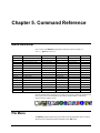
Chapter 5. Command Reference
63
Menu Overview........................................................................................................................63
File Menu.................................................................................................................................63
Edit Menu ................................................................................................................................75
Algorithms Menu .....................................................................................................................95
View Menu.............................................................................................................................107
Windows Menu ......................................................................................................................112
Help Menu .............................................................................................................................116
References
119
Book and Journal References.................................................................................................119
World Wide Web Sites ..........................................................................................................120
Spiral User's Manual
Contents • i
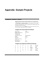
Appendix: Sample Projects
121
Tompkins (Tutorial Project)...................................................................................................121
Furniture.................................................................................................................................122
ii • Contents
Glossary of Terms
125
Index
127
Spiral User's Manual
Disclaimer
Warranty
Marc Goetschalckx's entire liability and your exclusive remedy under this warranty
(which is subject to you returning the program to Marc Goetschalckx) will be, at
Marc Goetschalckx's option, to attempt to correct or help you around errors with
efforts which Marc Goetschalckx believe suitable to the problem, to replace the
program or diskettes with functionally equivalent software or diskettes, as
applicable, or to refund the purchase price and terminate this agreement.
Marc Goetschalckx warrants that, for a period of ninety (90) days from the date of
delivery to you as evidenced by a copy of your receipt, the diskettes or CD-ROM on
which the program is furnished under normal use will be free from defects in
materials and workmanship and the program under normal use will perform without
significant errors that make it unusable.
Except for the above express limited warranties, Marc Goetschalckx makes and you
receive no warranties, express, implied, and statutory or in any communication with
you and Marc Goetschalckx specifically disclaims any implied warranty of
merchantability or fitness for a particular purpose. Marc Goetschalckx does not
warrant that the operation of the program will be uninterrupted or error free. It is
your responsibility to independently verify the results obtained by this program.
In no event will Marc Goetschalckx be liable for any damages, including loss of
data, lost profits, cost of cover or other special, incidental, consequential or indirect
damages arising from the use of the program or accompanying documentation,
however caused and on any theory of liability. This limitation will apply even if
Marc Goetschalckx or any authorized dealer has been advised of the possibility of
such damage. You acknowledge that the license fee reflects this allocation of risk.
Some states do not allow the exclusion of implied warranties so the above exclusions
may not apply to you. This warranty gives you specific legal rights. You may also
have other rights, which vary from state to state.
Spiral User's Manual
Disclaimer • 1
Proprietary Notice
Marc Goetschalckx owns both the Spiral software program and its documentation.
Both the program and the documentation are copyrighted with all rights reserved by
Marc Goetschalckx. No part of this publication may be produced, transmitted,
transcribed, stored in a retrieval system, or translated into any language in any form
without the written permission of Marc Goetschalckx.
Version
Version 4.10, May 31, 1999.
2 • Disclaimer
Spiral User's Manual
Chapter 1. Installation
Installing Spiral
To install Spiral you must run the Setup program on the distribution disk. The
exact method of executing the Setup program depends on the version and type of
Windows operating system that is installed on your computer.
Copying the files from the distribution disk to your computer or executing the
program from a file or application server is not sufficient to run Spiral. Several
dynamic link libraries, such as the Scientif application library, and active-x controls,
such as the grid control, are required for the proper execution of the Spiral program
and must be registered on your computer. The Setup program copies and registers
these libraries and controls during its installation process.
To remove the Spiral application completely and safely from your computer see the
instructions in the section on Removing Spiral.
Installation Instructions for Windows NT 4.00 and
Windows 95 and 98
1.
Insert the distribution disk 1 into the floppy or CD-ROM disk drive a:.
2.
In the Control Panel, select Add/Remove Programs and then
press the Install/Uninstall tab.
3.
The Windows operating system will search for the installation program
on the floppy or CD-ROM drives a: and will identify a:\setup.exe as
the installation program.
4.
Press Finish to start the installation procedure.
5.
Follow the instructions of the SETUP program.
If your floppy or CD-ROM disk drive is not drive a:, substitute the appropriate disk
drive letter with colon for a: in the above instructions.
Alternatively, you can also install Spiral using the installation instructions for
Windows NT version 3.51.
Spiral User's Manual
Chapter 1. Installation • 3
Installation Instructions for Windows NT 3.51
1.
Insert the distribution disk 1 into the floppy or CD-ROM disk drive a:.
2.
In the Windows Program Manager, select the Run command from the
File menu.
3.
In the Command Line box type:
a:\setup
4.
Choose OK to start the installation procedure.
5.
Follow the instructions of the SETUP program.
If your floppy or CD-ROM disk drive is not drive a:, substitute the appropriate disk
drive letter with colon for a: in the above command.
Installation Notes
Write Access Privileges
When installing to a Windows NT system, make sure that you have write access
privileges to the directory where Spiral will be installed and to all the files in this
directory and its subdirectories. You must also have write access privileges to the
\Winnt\System32 directory and the scienmfc.dll file in that directory. We
recommend that you install Spiral while being logged on as administrator.
Grid Control grid32.ocx
Several commands, such as the All Relations command of the Edit menu, require
that the active-x grid control grid32.ocx is present and registered on the computer
that is executing the Spiral program. The automated Setup program copies and
registers the grid control during its installation process. If you run Spiral from a file
or application server, the control must be installed on every client computer. Many
commercial applications use the same grid control, so it might already be installed on
your computer. To verify the presence and registration of the grid control, open the
Tompkins project, which is provided on the distribution disk, and execute the All
Relations command. If the two-dimensional relationship matrix is not shown, the
grid control is not installed or registered. In that case run the Setup program to
install Spiral and the grid control on this computer.
Removing Spiral
You can remove the Spiral program and its application libraries from your
computer, as well as remove its keys from the Registry. The exact method of
removing Spiral depends on the version and type of Windows operating system that
is installed on your computer.
Since the removal procedure actually deletes files from your computer, some of
which may be system level libraries or common controls, it is strongly recommended
that you make a complete backup of all the files on your computer before proceeding
with the removal procedure.
4 • Chapter 1. Installation
Spiral User's Manual
To install Spiral on your computer see the instructions in the section on Installing
Spiral.
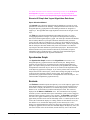
Removal Instructions for Windows NT 4.00 and
Windows 95 and 98
Select the Add/Remove Programs command in the Control Panel of your
computer. Spiral will be listed as one of the applications that can be automatically
removed. Select Spiral and press Add/Remove. All the files specific to Spiral,
such as the executable program file, the application help file and the Scientif
application library, will be removed from your computer. All keys associated with
Spiral will also be removed from the Registry. Common libraries, such as the
Microsoft Foundation class library and the Microsoft C runtime library will not be
removed. Spiral project files that you created in different directories will not be
removed either.
Removal Instructions for Windows NT 3.51
During installation, an icon to remove Spiral from your computer was placed in the
same program group that you selected for the Spiral program. Press this Uninstall
icon. All the files specific to Spiral, such as the executable program file, the
application help file and the Scientif application library, will be removed from your
computer. All keys associated with Spiral will also be removed from the Registry.
Common libraries, such as the Microsoft Foundation class library and the Microsoft
C runtime library will not be removed. Spiral project files that you created in
different directories will not be removed either.
Spiral User's Manual
Chapter 1. Installation • 5
This page left intentionally blank.
6 • Chapter 1. Installation
Spiral User's Manual
Chapter 2. Tutorial
Creating a Small Tutorial Project
Following are the step by step instructions to create a small project and design its
layout in an interactive manner. For large projects it might be more convenient to
create the necessary data files outside Spiral with a file editor capable of creating
pure ASCII files and then to import the project from these data files.
Spiral follows the standard Windows graphical user interface (GUI) conventions.
This tutorial will focus on the features unique to the Spiral program and assumes
that you are familiar with the Windows environment and the execution of Windows
applications. More information on the Windows user interface can be found in the
Windows User's Guide.
More detailed explanations and instructions can be found in the sections on the
Project Data and Design Algorithms. A summary of all the available actions in
Spiral can be found in the section on the Command Reference. A list of traditional
and World Wide Web (WWW) references for further reading is given in the
Reference section. Finally, we will be using the classical Tompkins layout example
in this tutorial and the data for this project are summarized in the section on Sample
Projects.
Steps to Be Done Before Starting A New Project
Create a project directory
Determine in which directory you want to save this new project. It is strongly
recommended that you use a separate directory for each project. If necessary, create
this directory on your hard drive. Note that some versions of the Windows operating
environment allow you to create this directory from the Save As dialog box while
executing the Spiral program. Spiral is compatible with long file names and
directory names.
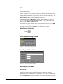
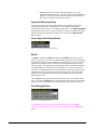
Defining a New Project
Create a new project
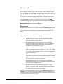
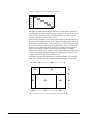
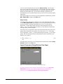
Select the New command from the File menu or press the New button on the
toolbar. The New dialog window will be shown. The New dialog window for this
project is illustrated in Figure 2.1. Enter a project name with a maximum of 63
Spiral User's Manual
Chapter 2. Tutorial • 7
characters. Only letters, digits, spaces, and underscores are allowed in the project
name. Enter the building width and building depth of the rectangular building. The
building width and depth are displayed horizontally and vertically on the screen,
respectively. For this tutorial project, enter "Tutorial", ten, and seven for project
name and building width, and depth, respectively. Press OK and a new project
without any departments will be created.
Note that any data item of this project can be changed later on from inside the project
with commands from the File and Edit menu. You can also get context sensitive
help for any dialog window by pressing the Help button when the dialog windows is
displayed.
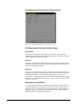
Figure 2.1. New Dialog Window for the Tutorial Project
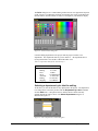
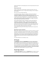
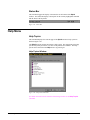
Display all Views simultaneously
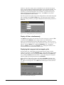
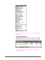
The Spiral program shows four cascaded views of the new project. Select the Tile
command from the Window menu to display all the views simultaneously.
Each view has individual characteristics and display attributes. The type of view is
indicated by an icon in the top left corner of the title bar of each view. The four view
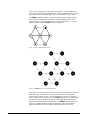
types are 1) project Notes view, 2) algorithm Statistics view, 3) hexagonal
adjacency Graph view, and 4) block Layout view. Changing the attribute of one
view does not affect the same attribute in other views.
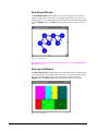
Displaying the hexagonal and rectangular grids
Select the third view, which displays the hexagonal adjacency graph, by either
clicking on its title bar or from the Window menu. Toggle the display of hexagonal
adjacency graph in this view by selecting the Grid command from the View menu
or by pressing the Grid button on the toolbar. You can also display the hexagonal
adjacency graph by pressing the shortcut keys Ctrl+Alt+G.
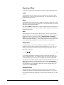
Set the grid size for this project equal to one with the Grid Size command of the
Edit menu. The Grid Size dialog box for this tutorial project is illustrated in Figure
2.2. Enter one for the grid size. Press OK and the tutorial project will use this new
grid size.
Figure 2.2. Edit Grid Size Dialog Box
8 • Chapter 2. Tutorial
Spiral User's Manual
If you have selected to display the grid in the layout view, then this view is updated
to reflect the new grid size. All project data items, such as the grid size, have a
single value that is used by all the views.
Select the fourth view, which displays the block layout, by either clicking on its title
bar or from the Window menu. Toggle the display of rectangular grid in this view
by selecting the Grid command from the View menu or by pressing the Grid button
on the toolbar. You can also display the rectangular grid by pressing the shortcut
keys Ctrl+Alt+G.
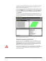
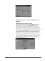
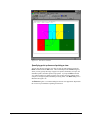
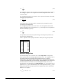
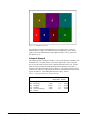
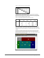
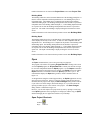
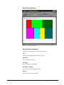
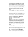
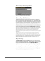
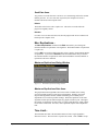
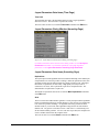
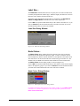
The different views of the current project at this time are illustrated in Figure 2.3. If
you wish you can also display the orthogonal grid in the fourth or layout view in the
same manner. Observe that the view titles indicate that this is a new project that not
has been saved yet.
Figure 2.3. Initial Views for the New Project
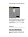
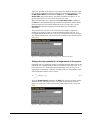
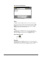
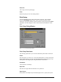
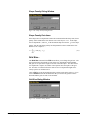
Saving the new project for the first time
Save the current project with the Save As command from the File menu. In the
Save As dialog box, select the directory where you want to save the project file.
Specify a name for the project data file, which by default has the spiral extension.
The Save As dialog box for this tutorial project is illustrated in Figure 2.4. Press
OK and the file for the current project will be saved to disk.
Some versions of the Windows operating environment will truncate the default
spiral extension to the three letters spi, so we recommend that you explicitly add the
spiral extension to the file name in the Save As dialog window when saving a
project for the first time.
Spiral User's Manual
Chapter 2. Tutorial • 9
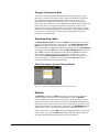
Figure 2.4. Save As Dialog Box for the Tutorial Project
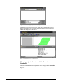
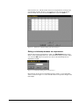
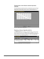
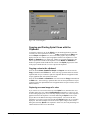
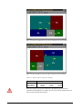
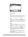
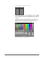
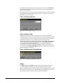
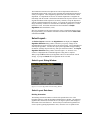
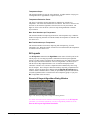
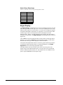
The different views of the current project at this time are illustrated in Figure 2.5.
Observe that the titles of the views have changed from New Project to Tutorial to
indicate that this project has been saved.
Figure 2.5. Initial Views for the Tutorial Project
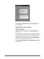
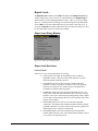
Changing Project Information with the Properties
Command
The project title and other project information can be changed with the Properties
command of the File menu. The properties of the tutorial project are illustrated in
Figure 2.6.
10 • Chapter 2. Tutorial
Spiral User's Manual
Figure 2.6. Project Properties Dialog for the Tutorial Project
At this time the project has neither departments nor department relationships. The
number of departments in the project and the sum of all relationships are always
shown in the Notes view.
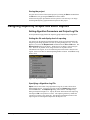
Adding Departments to a Project
Adding a Department
Add one by one the departments to the current project by selecting the Add
Department command from the Edit menu. The Add Department dialog box
will be displayed.
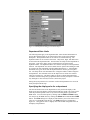
Since we are defining a new department, only the items on the page with the Input
tab are relevant. Enter the label of the department as the single letter A, enter the
name of the department as "Receiving", and set the area of the first department to 12.
The maximum shape ratio has been set to its default 2.5 value and we will leave it
unchanged. Set the layout position to free, and set the area and border color of the
department to palette colors green and black, respectively. The Add Department
dialog window for the first department is shown in Figure 2.7.
If you press OK in the Add Department dialog box, the department will be added
to the project with its current attributes. If you press Cancel the department will not
be added to the project.
Spiral User's Manual
Chapter 2. Tutorial • 11
Figure 2.7. Add Department Dialog for the Tutorial Project
Department Data Limits
The following limits apply to the department data. More detailed information on
project data and their limits can be found in the section on the project database
description. The department label can be at most seven characters long. The
department name can be at most 63 characters. Only letters, digits, and underscores
are allowed in the department label. The label must be unique for this department in
the project. Only letters, digits, spaces, and underscores are allowed in the
department name. The department name can contain a description of the department
function. The department area must be smaller than or equal to the building area and
be expressed in units compatible with the building dimensions, i.e., if the building
dimensions were given in feet then the department areas must be given in square
feet. The shape factor is the maximum ratio of length to width or width to length of
the department. The maximum value for the shape factor is 99 but more realistic
values are less than five. The shape penalty is the rate at which departments that
exceed the maximum shape ratio get penalized in the block layout objective function.
Any nonnegative value will do, but enter 1,000 for this project.
Setting the layout position to free will later on allow the department to be moved in
the layout improvement steps.
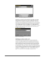
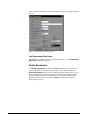
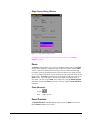
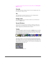
Specifying the display color for a department
The area and border colors of the department are only used in the display of the
block layout, not in the display of the hexagonal adjacency graph. The colors can be
either the predefined palette colors or any color for which you have specified the
RGB values. You select this option by clicking either the RGB or Palette buttons.
You can specify the RGB values by clicking the Select button underneath the RGB
button. The Color dialog box is displayed, which allows you to select from a set of
colors or to set the RGB values directly. The Color dialog box is illustrated in
Figure 2.8. Using palette colors is slightly more efficient than using RGB colors in
the display of departments.
12 • Chapter 2. Tutorial
Spiral User's Manual
The Color dialog box is a common dialog window and its exact appearance depends
on the version of your Windows operating environment, the version of the Microsoft
runtime libraries, and the number of colors or color depth of your Windows display.
Figure 2.8. Common Color Dialog Box
Continue adding departments to the project until the project contains seven
departments. The department data are given in Table 2.1. All departments have a
layout position that is free and have a BLACK border color.
Table 2.1. Department Data for the Tutorial Project
Label
A
B
C
D
E
F
G
Name
Area Area Color
Receiving
12 GREEN
Milling
8 CYAN
Press
6 RED
Screw
12 MAGENTA
Assembly
8 YELLOW
Plating
12 OCEAN
Shipping
12 FOREST
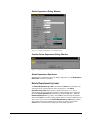
Selecting a department by its label for editing
At this time, you can edit the data for any department in the project. The department
to be edited can be selected by its label with the Department by Label command
from the Edit menu. A drop down list box with the labels of all the currently
defined departments will be shown. The Select Department dialog box is
illustrated in Figure 2.9.
Figure 2.9. Select Department by Label Dialog Box
Spiral User's Manual
Chapter 2. Tutorial • 13
Select department D. Press Ok to edit the selected department or Cancel to cancel
the Select Department dialog box and not to edit any department.
Editing the date of a department
When you press OK, the Edit Department dialog box will be shown. This dialog
box is illustrated in Figure 2.10.
Figure 2.10. Edit Department Dialog Box
Since we are still entering and editing initial department data, only the Input page of
the Edit Department dialog box is relevant. Change the name of department D
from "Screw" to "Drilling". Since at this time no adjacency graph or block layout
have been created, the department data on the Continuous page is still zero. The
data on the Discrete page shows the number of unit squares in this department
based on the current Grid Size. You can change the grid size with the Grid Size
command from the Edit menu.
Deleting a department from the project
You can also completely delete a department from the project with the Delete
Department by Label command from the Edit menu.
Saving the project
Save the current version of the tutorial project by selecting the Save command from
the File menu or by pressing the Save button on the toolbar.
Adding Department Affinities to a Project
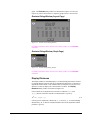
Selecting a relationship between two departments
At this time, we will enter all the affinities between departments or relationships to
the project. Select the All Relations command from the Edit menu. The Select a
Relation dialog will be shown, which displays the relations in a two dimensional
array. The initial Select a Relation dialog is shown in Figure 2.11. Initially all
14 • Chapter 2. Tutorial
Spiral User's Manual
relations will be zero. Edit the relation between two departments by clicking on the
corresponding element in the array. You can also move the cursor to the desired
relation with the arrow keys and click the Edit button or press the Alt-E key.
Figure 2.11. Initial Select a Relation Dialog of the Tutorial Project
Editing a relationship between two departments
Edit the relation between departments A and B. The Edit Relation dialog will be
shown. Set the relationship value to 45. The Edit Relation dialog is shown in Figure
2.12. Press the OK button to accept the new value for the relationship between
departments A and B.
Figure 2.12. Edit Relation Dialog for the Tutorial Project
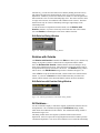
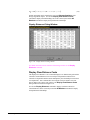
Repeat this for all the non-zero relationships shown in Table 2.2. The relationship
values are shown in Figure 2.13. Press the OK button to accept all the changes to the
relationships.
Spiral User's Manual
Chapter 2. Tutorial • 15
Table 2.2. Relationship Data for the Tutorial Project
Department Department Relation
A
B
45
A
C
15
A
D
25
A
E
10
A
F
5
B
D
50
B
E
25
B
F
20
C
E
5
C
F
10
D
E
35
E
F
90
E
G
35
F
G
65
Figure 2.13. Select a Relation Dialog Window for the Tutorial Project
Saving the project
Save the current version of the tutorial project by selecting the Save command from
the File menu or by pressing the Save button on the toolbar.
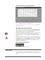
Setting Department Shape Constraints and Penalty
Changing the maximum shape ratio for all departments in
the project
Departments with long and narrow shapes are often not acceptable in layouts. The
shape ratio of a department is the length to depth ratio of the smallest rectangle
completely enclosing the department. While each department has its own maximum
16 • Chapter 2. Tutorial
Spiral User's Manual
shape ratio depending on its function, we can specify the maximum allowable shape
ratio for all the departments in this particular project with a single command. Select
the Max Shape Ratio command from the Edit menu. The Edit Maximum
Shape Ratio dialog will be shown. This dialog is illustrated in Figure 2.14. Set
the maximum value to two. Press Ok to accept the new value.
When maximum shape ratio is changed with the Max Shape Ratio command of
the Edit menu, the maximum shape ratio of all current departments and the default
maximum shape ratio for all future departments is also set to this value. Use the
Department command to change the maximum shape ratio for individual
departments.
The perimeter ratio is the ratio of the current perimeter length of a department
divided by the perimeter length of a square department with the same area. For
rectangular departments there exists a one to one correspondence between the shape
ratio and the perimeter ratio. The perimeter ratio is an output-only variable and you
cannot set it.
Figure 2.14. Edit Maximum Shape Ratio Dialog for the Tutorial Department
Setting the shape penalty for all departments in the project
If the shape ratio of a department violates its maximum allowable shape ratio for that
department, then a penalty should be added to the distance score of the layout. Let si
be the shape ratio, let Si be the maximum allowable shape ratio, and let pi be the
shape penalty of department i, then the total shape penalty for all departments P that
will be added to the distance score is equal to
P=
N
i =1
pi ⋅ max{0, si − Si }
(2.1)
Select the Shape Penalty command of the Edit menu to specify the shape penalty.
The Shape Penalty dialog will be shown. The Shape Penalty dialog is shown in
Figure 2.15. Enter a new value of 1000 for the penalty and press Ok to accept this
value.
Figure 2.15. Shape Penalty Dialog for the Tutorial Project
Spiral User's Manual
Chapter 2. Tutorial • 17
Saving the project
Save the current version of the tutorial project by selecting the Save command from
the File menu or by pressing the Save button on the toolbar.
At this time all project input data haven been specified. The next step is to design
the hexagonal adjacency graphs and block layouts for this project.
Designing Adjacency Graphs and Block Layouts
Setting Algorithm Parameters and Output Log File
Several parameters apply both to the adjacency graph and block layout algorithms.
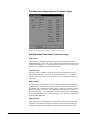
Setting the file and display level of reporting
You can specify the amount of information shown on the screen and printed to the
Output Log file during algorithm execution by setting the Report Level. To set the
Report Level execute the Report Level command from the File or Edit menu. The
Report Level dialog will be shown. The Report Level dialog is shown in Figure
2.16. There are six possible levels, range from zero for no pauses and no
information to the log file, to five for numerous pauses and extensive details to the
log file. Select level three for uninterrupted algorithm execution. Press Ok to accept
the new level.
Figure 2.16. Report Level Dialog
Specifying a Algorithm Log File
Spiral will save the results of any algorithm in a log file, if such a file has been
defined for the project. To specify a log file execute the Output Log command
from the File menu. The Output Log dialog will be shown. The Output Log
dialog is illustrated in Figure 2.19. Specify the name and location of the output log
file and press Ok to accept the new values. The output log file has by default the
extension .log and is a pure ASCII file. The amount of information written to the
output log file for each algorithm depends on the Report Level.
18 • Chapter 2. Tutorial
Spiral User's Manual
Figure 2.17. Open Output Log Dialog for the Tutorial Project
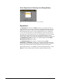
Specifying a maximum time limit for algorithm execution
During the execution of algorithms, the program will periodically check if the
algorithm has been computing longer than the allowable run time. If the limit has
been exceeded, then the algorithm will be terminated and no results of the algorithms
will be retained. To set the maximum amount of execution time for an algorithm,
select the Time Limit command from the Edit menu. The Time Limit dialog
window will be shown. The Time Limit dialog box is shown in Figure 2.18. Enter a
limit of 120 seconds, which is more than sufficient for this small tutorial project.
Press Ok to accept the new value.
Figure 2.18. Time Limit Dialog
Specifying a random number seed
Several algorithms must make random choices at certain points during their
execution. For example, the graph construction algorithms randomly select the
location for a department node from a list of equivalent locations, and the layout
simulated annealing improvement algorithms pick randomly the next departments
that are considered for an exchange. These random choices are made based on the
next pseudo-random number. The sequence of these random numbers depends on
the starting number of the sequence, which is called the seed. When started from the
same state, algorithms will generated the same solution if it has been given the same
seed. You can set the random number seed by executing the Seed command from
the Edit menu. The Seed dialog will be shown. The Seed dialog is shown in
Figure 2.19. Set the seed to 12345. Press Ok to accept the new value.
Spiral User's Manual
Chapter 2. Tutorial • 19
Figure 2.19. Seed Dialog
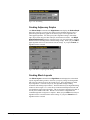
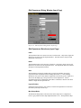
Creating Adjacency Graphs
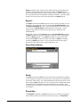
The Select Graph command of the Algorithms menu displays the Select Graph
dialog box which lets you specify the settings for the algorithm that will create a
planar hexagonal adjacency graph for the current project. These algorithms are
called graph algorithms. You must specify three algorithm settings: relationship
tuple, improvement step procedure and tuple, and location tie breaker. The Graph
Algorithm Selection dialog box is shown Figure 2.20. Select the Binary, Steepest
Descent with Two Exchange and Centroid Seeking settings. When you press OK the
graph algorithm will be executed with the current settings. If you press Cancel, no
algorithm will be executed.
Figure 2.20. Select a Graph Algorithm Dialog
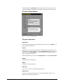
Creating Block Layouts
The Select Layout command of the Algorithms menu displays the Select Block
Layout Algorithm dialog window, which lets you specify settings for the algorithm
that will create a block layout for the current project. These algorithms are called
layout algorithms. You must first specify two algorithm settings: building
orientation and exchange improvements. The Select Block Layout Algorithm dialog
window is shown Figure 2.21. Select the Up orientation and Steepest Descent with
Two Exchanges improvement procedure. The Layered space allocation procedure is
the only one available at this time. Because of its extensive computations this
command might take a long time to complete. When you press OK the block layout
algorithm will be executed with the current settings. If you press Cancel then no
algorithm will be executed.
20 • Chapter 2. Tutorial
Spiral User's Manual
Figure 2.21. Select a Layout Algorithm Dialog
Sensitivity Analysis and Evaluating Graphs and
Layouts
Evaluating the current layout or graph
You manual modify the data with the Department and Relation commands. To
evaluate the impact of you changes you use the Evaluate command of the
Algorithms menu. The Evaluate command computes the adjacency score of the
adjacency graph and the distance score and adjacency score of the block layout if
these have been created. It displays the distance score without shape penalty, called
the flow distance score, for the block layout in the Delta Objective field. The results
are displayed in the Notes and Statistics views. The Evaluate command is most
frequently used after you have edited interactively the relationships after you have
dragged a department in the adjacency graph to a new location. The Evaluate
command does not create a new graph or block layout, but rather computes the cost
of the current graph and layout based on the current relationship values. The
command also displays in a dialog window the total distance score, the flow distance
score, and the total shape penalty for the current layout. It also displays for each
department the actual area, shape ratio, and perimeter ratio. The Evaluate dialog
window is illustrated in Figure 2.22.
Figure 2.22. Evaluate Dialog Window
Spiral User's Manual
Chapter 2. Tutorial • 21
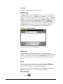
Displaying the current distances between department
centroids
You can also display the individual centroid-to-centroid distances between each pair
of departments with the Display Distances command of the Algorithms menu. The
Display Distances dialog window will be shown as is illustrated in Figure 2.23.
Figure 2.23. Display Distances Dialog Window
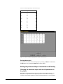
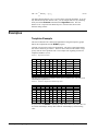
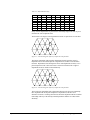
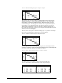
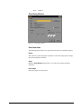
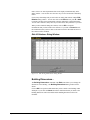
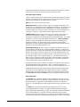
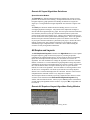
Displaying a history of algorithm statistics
The Statistics View displays the history of algorithm statistics. This view can be
printed to the default printer with the Print command of the File menu. Move and
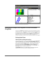
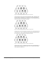
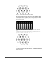
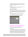
size this window to suit your taste. The result of the graph and layout algorithm that
you have executed so far is illustrated in Figure 2.24. The corresponding Graph
view and Layout view are shown in Figure 2.25.
Figure 2.24. Algorithm Statistics View for the Tutorial Project
22 • Chapter 2. Tutorial
Spiral User's Manual
Figure 2.25. Final Views for the Tutorial Project
Using Spiral Graphs and Layouts in Other Windows
Programs
The results of the Spiral design algorithms can be used in other Windows programs
in basically three ways. Unless otherwise indicated, the actions described below can
be executed on all four of the Spiral views. First, we will print the Spiral views to
any installed printer, then we will copy and paste Spiral views into other Windows
applications. Finally, the current project can be send as an attachment to an
electronic mail message, if you have an active mail client installed on your computer.
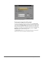
Printing Spiral Views
Selecting and specifying print options
Select the printer on which you wish to print the Spiral views with the Print Setup
command of the File menu. This command presents a Print Setup dialog box,
where you specify the printer and its connection. This printer and these options will
then be used by all subsequent Print operations. The same changes can also be
made from the main Windows Control Panel. The printer must have been
previously installed from the Windows Control Panel or Print Manager. The
Print Setup dialog box is illustrated in Figure 2.26.
The Print Setup dialog box is a common dialog box and its exact appearance
depends on the version of your Windows operating environment.
Spiral User's Manual
Chapter 2. Tutorial • 23
Figure 2.26. Print Setup Dialog Box
Previewing the image that will be printed
You can preview the image that will be printed by selecting the Print Preview
command from the File menu. When you choose this command, the main window
will be replaced with a Print Preview window in which one or two pages will be
displayed in their printed format. The toolbar of the Print Preview window offers
you options to view either one or two pages at a time; move back and forth through
the document; zoom in and out of pages; and initiate a print job. The Print
Preview dialog box is illustrated in Figure 2.27.
The Print Preview dialog box is a common dialog box and its exact appearance
depends on the version of your Windows operating environment.
24 • Chapter 2. Tutorial
Spiral User's Manual
Figure 2.27. Print Preview Window
Specifying print options and printing a view
You can also directly select the view that you wish to print and then execute the
Print command from the File menu. This command presents a Print dialog box,
where you may specify the range of pages to be printed, the number of copies, the
destination printer, and other printer setup options. If you press OK the selected
view will be printed. For graph or layout views of large projects, printing such a
complex view might require substantial processing times. The Print dialog box is
illustrated in Figure 2.28.
The Print dialog box is a common dialog box and its exact appearance depends on
the version of your Windows operating environment.
Spiral User's Manual
Chapter 2. Tutorial • 25
Figure 2.28. Print Dialog Box
Copying and Pasting Spiral Views with the
Clipboard
To paste the contents of one of the Spiral views in another application, select the
view that you wish to paste then execute the Copy command from the Edit menu.
For the Graph and Layout views, the section of the graph or layout currently
displayed in the view will be copied in graphical format to the clipboard. For the
Notes and Statistics views, all the text, whether it is currently displayed or not,
will be copied in text format to the clipboard. For the Notes and Statistics a
header will generated which indicates the version of the Spiral program, the name
of the project and the date the view was copied to the clipboard.
Copying a view to the clipboard
Select in turn the Notes, Statistics, Graph, and Layout view and execute the
Copy command from the Edit menu. After each copy operation either activate the
clipboard and verify its contents or paste the clipboard data into an application that
accepts graphical data, such as Microsoft Word.
Select in turn the Notes and Statistics view and execute the Copy command from
the Edit menu. After each copy operation either activate the clipboard and verify its
contents or paste the clipboard data into an application that accepts text data, such as
Microsoft Excel.
Capturing a screen image of a view
If you want to use a screen shot from one of the Spiral views, maximize this view
and then capture the view with the Alt-PrintScreen command. For all views, the
section of the graph, layout, or text currently displayed in the view will be copied in
graphical format to the clipboard. No header indicating the Spiral version or the
project data will be added to the image on the clipboard. You can use the same
techniques if you want a screen shot from the main Spiral window as it is currently
displayed. The same technique can also be used to capture images of the various
dialog boxed used by Spiral to the clipboard. In this case, obviously the dialog box
cannot and does not have to be maximized.
26 • Chapter 2. Tutorial
Spiral User's Manual
Select in turn the Notes, Statistics, Graph, and Layout view and maximize this view.
Execute the Alt-PrintScreen command. After each copy operation activate the
clipboard and verify its contents or paste the clipboard data into an application that
accepts graphical data, such as Microsoft Word.
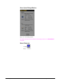
Sending the saved project as an electronic mail attachment
You can send the current layout project as an attachment to an electronic mail
message, if you have an active mail client installed on your computer. The currently
saved project will be sent, so you should save the project before sending it.
Select the Send command from the File menu to activate your mail client and to
send the saved version of the current project as an attachment.
This concludes the tutorial. Further information on the project data can be found in
the Project Data chapter, further information on the design algorithms can be found
in the Design Algorithms chapter. A complete list of all commands is given in the
Command Reference chapter. You can also find more information in the references
given in the References chapter. Finally, the data used in the tutorial correspond to
the classical layout example in Tompkins and Moore (1978) and are listed in the
appendix Sample Projects.
Spiral User's Manual
Chapter 2. Tutorial • 27
This page left intentionally blank.
28 • Chapter 2. Tutorial
Spiral User's Manual
Chapter 3. Project Data
Specifying and Editing Project Data
Project Data
Every project has a number of data items associated with for which there is only one
value per project.
Project Title
Every project has a title, assigned to it when the project was created with the New
command or when the projected was read from an external ASCII file with the
Import command. Both these commands are on the File menu. The project title
should be a maximum of 63 characters and should contain only letters, digits, spaces,
and underscore characters. The term project name is used synonymously with project
title.
The project title can be changed with the Summary Info command of the File
menu.
Note that the Import command does not allow a project title to contain spaces. A
project title that is first exported and then imported again will be truncated at the first
space character.
Building Width
The building width refers to the horizontal dimension of the building ground plan. It
must be in units compatible with the department areas. The building always has a
rectangular shape. The building area is computed as the product of the building
width and building depth. The building and department areas should be expressed in
compatible units to the building width and depth, i.e., if the building depth and width
are expressed in feet then the building and department areas must be expressed in
square feet.
The building width of a project is set when the project is created with the New
command or when the project is read from an external ASCII file with the Import
command of the File menu. The building width can be modified at any time by the
Building Dimensions command of the Edit menu.
Spiral User's Manual
Chapter 3. Project Data • 29
Building Depth
The building depth refers to the second dimension of the building ground plan (which
will be displayed vertically on the screen). It must be in units compatible with the
department areas. The building area is computed as the product of the building
width and building depth. The building and department areas should be expressed in
compatible units to the building width and depth, i.e., if the building depth and width
are expressed in feet then the building and department areas must be expressed in
square feet.
The building depth of a project is set when the project is created with the New
command or when the project is read from an external ASCII file with the Import
command of the File menu. The building depth can be modified at any time by the
Building Dimensions command of the Edit menu.
Report Level
The Report Level controls the level of detail written to the Output Log file and the
number of pauses during algorithm execution. There are six levels ranging from zero
to five, which generate increasingly more detailed output and frequent algorithm
pauses.
Levels of Detail
There are six levels of detail and pauses for reporting:
0.
NONE generates no output per algorithm and does not halt the
algorithm execution. This level is used when maximum execution
speed and minimal reporting is desired.
1.
DATABASE generates one line of strictly numerical output per
algorithm. No titles or headers are included. This level is primarily
used to create a data base file, which can then be manipulated in a
spreadsheet or statistical analysis program.
2.
SUMMARY displays the total cost plus the algorithm run time. It is
useful if you is only interested in the final results. This level of output
should be used if you is interested in performing timing studies. Higher
level of details corrupt timing results due to user interaction delays and
graphics creation delays.
3.
STANDARD generates the total cost for each of the algorithm
components. The program runs without interruption until the complete
algorithm is finished. If you have selected ALL, then the program runs
uninterrupted for the 18 different combinations.
4.
EXTENDED displays the total cost during each of the algorithm
modules and the run time so far. The program halts frequently to allow
you to observe the algorithm process.
5.
DEVELOP generates extremely detailed output plus a very large
number of intermediate results. This mode is only useful for debugging
purposes or to observe the most detailed workings of the algorithms.
The output is extremely long for large problems.
The Report Level can be modified at any time with the Report Level command of
the Edit menu. It can also be changed by pressing the Report Level button of the
Pause dialog window, when an algorithm is paused. The algorithm will then use this
new report level for the rest of its execution.
30 • Chapter 3. Project Data
Spiral User's Manual
Department Data
For the following data items, each department can have a different individual value.
Label
The department label can consist of at most seven characters. Only letters, digits,
and underscores are allowed in the department label. The label must be unique for
this department in the project.
Name
The department name can be at most 63 characters. Only letters, digits, spaces, and
underscores are allowed in the department name. The department name can contain a
description of the department function.
Note that the Import command does not allow a department name to contain spaces.
Department names that are first exported and then imported again will be truncated at
the first space character.
Area
The department area is desired area for the department. The area must be smaller
than the building area. The sum all department areas must be less than or equal to the
building area, which is equal to the product of building width and building
depth. The building and department areas should be expressed in compatible units
to the building width and depth, i.e., if the building depth and width are expressed in
feet then the building and department areas must be expressed in square feet.
Shape Ratio
The department shape ratio is the maximum of the length to width and width to
length ratios of the smallest rectangle enclosing the department. Let li and wi be
the length and width of the smallest rectangle enclosing the department, then the
shape ratio si is given by
si = max
RS l , w UV
Tw l W
i
i
i
i
(3.1)
For rectangular departments the smallest rectangle enclosing the department is of
course the department itself. For example the shape ratio of a square department is
one and the shape ratio of a three by one rectangular department is equal to three.
The shape ratio is an output variable, computed by the program based on the current
shape of the department. If the department shape ratio exceeds the maximum
shape ratio then the shape adjusted distance score is the sum of the normal distance
score and the excess of the department shape ratio over the maximum shape ratio
multiplied by the shape penalty.
Perimeter Ratio
The perimeter ratio of a department is the ratio of the current perimeter length
divided by the perimeter of a square department with the same area. Let pi and ai
be the perimeter and area of department i, respectively, the perimeter ratio ci is then
given by:
Spiral User's Manual
Chapter 3. Project Data • 31
ci =
pi
(3.2)
4 ai
For example the perimeter ratio of a square is one and the perimeter ratio of a four by
one rectangle is equal to 1.25. A higher value indicates a department with a more
convoluted shape.
For rectangular departments, the perimeter can be expressed in function of the width
and length of the department as:
ci =
2(li + wi )
(3.3)
4 ai
The perimeter ratio is an output variable, computed by the program based on the
current shape of the department.
For rectangular departments there exists a one to one correspondence between the
perimeter and shape ratio of a department. Let si be the shape ratio of a department,
then this relationship is given by:
ci =
si + 1
2 si
(3.4)
The equivalent values for the most practical range of the shape and perimeter ratio
are given in the following table.
Table 3.1. Equivalent Values of Shape and Perimeter Ratios for Rectangular Departments
Shape Complexity
1.5
1.02
2.0
1.06
2.5
1.11
3.0
1.15
3.5
1.20
4.0
1.25
5.0
1.34
6.0
1.43
Maximum Shape Ratio
The maximum shape ratio is the limit value for the shape ratio of a department
before it gets penalized in the shape adjusted distance score. The acceptable value of
the maximum shape ratio depends on the department function, so different
departments can have different maximum shape ratios. If the department shape ratio
exceeds the maximum shape ratio then the shape adjusted distance score is the sum of
the normal distance score and the excess of the department shape ratio over the
maximum shape ratio multiplied by the shape penalty. Let si be the shape ratio of
department i, let Si be the maximum shape ratio of the department, and let pi be the
shape penalty, then the total shape penalty for all departments P that is added to the
distance score is equal to
P=
N
i =1
32 • Chapter 3. Project Data
pi ⋅ max{0, si − Si }
(3.5)
Spiral User's Manual
The term shape factor is also commonly used for shape ratio. The acceptable value
of the maximum shape ratio depends on the department function, so different
departments can have different maximum shape ratios.
Only the block exchange algorithms use the maximum shape ratio to penalize block
layouts to avoid excessively narrowly shaped departments. The Maximum Shape
Ratio is an input parameter set by the user. You can use the Department command
from the Edit menu to set the maximum shape ratio of individual departments. You
can use the Max. Shape Ratio command of the Edit menu to set the maximum
shape ratio of all departments simultaneously.
Shape Penalty
The Shape Penalty is the factor by which the excess of the department's shape ratio
over the maximum shape ratio gets multiplied if it exceeds the maximum shape
ratio and this product gets added to the distance score to yield the shape adjusted
distance score. The purpose of the shape penalty is to avoid long and narrow
departments. A higher shape penalty will tend to make departments more like
squares. A low or a shape penalty equal to zero will allow more long and narrow
departments. The shape penalty cannot be negative. The penalty of exceeding the
maximum shape ratio depends on the department function, so different departments
can have different shape penalties.
Only the block exchange algorithms use the shape penalty to penalize block layouts
to avoid excessively narrowly shaped departments. The Shape Penalty is an input
parameter set by the user. You can use the Department command from the Edit
menu to set the maximum shape ratio of individual departments. You can use the
Shape Penalty command of the Edit menu to set the maximum shape ratio of all
departments simultaneously.
Maximum Perimeter Ratio
The Maximum Perimeter Ratio is the limit value for the perimeter ratio of the
department.
For rectangular departments there exists a one to one correspondence between the
perimeter ratio of a department and the shape ratio. In SPIRAL the maximum
perimeter ratio is computed from the Maximum Shape Ratio assuming
rectangular departments and only used as an output variable, i.e., it is displayed as
information for the user.
Importing Externally Generated Layouts
The current version of the Spiral program can import data files created by the
Export command of the Spiral program with the Import command of the File
Menu. The description of the data files for this version of Spiral is given next.
A project is completely described by two files. The first file is the Project Data file
that holds all the scalar information about this project. The second file is the
Department Data file that contains all department and relationship data.
The easiest way to import an externally generated layout is to execute the following
steps:
Spiral User's Manual
1.
define the project interactively inside Spiral
2.
generate any layout
Chapter 3. Project Data • 33
3.
export the project
4.
modify the generated files to represent the external layout
5.
import the modified files and evaluate the layout
Project Data File
The Project Data file can be created with any editor or word processor capable of
generating pure ASCII files. Word processors usually insert special formatting codes
into their regular document files, such as page breaks, which cannot be read by the
SPIRAL program, so special care should be taken when using a word processor to
generate a pure ASCII file. The project file also should not contain any blank lines.
Once an input file has been created, it can be used repeatedly by the Spiral program.
Each line in the input file is associated with a single data item and contains two
fields. The first field is the description or name of the data item. The name of the
item is enclosed in square brackets and may not contain any spaces. The second field
is then the value of the item to be used. The two fields are separated by one or more
space or tab characters. For example:
[data_version]
[project_name]
[number_of_departments]
[department_file_name]
[building_width]
[building_depth]
[number_of_layout_rows]
[number_of_layout_cols]
[seed]
[tolerance]
[time_limit]
[number_of_iterations]
[report_level]
[max_shape_ratio]
[shape_penalty]
20002
Furniture
10
Furniture.dep
10.0
7.0
3
4
12345
0.00010
120.0
20
2
2.5
500.0
Data Version
The first item is the data version of the current project. The data version is an integer
number larger than 20000 generated by Spiral during the Export command.
Project Name
The next item is the name of the current project. This name should be a maximum of
15 characters and should contain only letters, digits, and underscore characters.
In the version 4.0 of Spiral or higher the name of this data field has been changed to
Project Title and its size expanded and space characters are allowed. However, the
old name of Project Name still should be used in export and import files and it
should not contain any spaces.
Number of Departments
The second item is the number of departments in this problem. The minimum
number of departments is one. The maximum number of departments depends on the
34 • Chapter 3. Project Data
Spiral User's Manual
version of the SPIRAL program. For industrial versions the limit is 255
departments. For educational versions the limit is 10 departments.
Department File Name
The third item is the name of the department data file, which contains the department
names, codes, and interdepartmental relationships, respectively. A path must precede
the file name if it is not in the current directory or in the data path. An example of a
department data file is the file FURN.DEP that holds the department information.
This file is included in the appendix and on the distribution diskette. This file must
be created outside the SPIRAL program with an editor capable of generating pure
ASCII files.
Building Width
The building width refers to the horizontal dimension of the building ground plan. It
must be in units compatible with the department areas. The building always has a
rectangular shape. The building area is computed as the product of the building
width and building depth. The building and department areas should be expressed in
compatible units to the building width and depth, i.e., if the building depth and width
are expressed in feet then the building and department areas must be expressed in
square feet.
Building Depth
The building depth refers to the second dimension of the building ground plan (which
will be displayed vertically on the screen). It must be in units compatible with the
department areas. The building area is computed as the product of the building width
and depth. The building area is computed as the product of the building width and
building depth. The building and department areas should be expressed in
compatible units to the building width and depth, i.e., if the building depth and width
are expressed in feet then the building and department areas must be expressed in
square feet.
Seed
The graph construction algorithms often need to make a random choice among
several alternative locations for the current department. This random choice is made
based on pseudo random numbers, generated from an initial seed. An algorithm will
always make the same random choices if it is given the same random seed, and hence
will create the same adjacency graph. The seed has to be a positive number in the
range of [1,32767]. If a seed of zero is given, then the computer will pick a random
seed based on the computer clock.
Tolerance
At the current time the tolerance parameter is not used in the program.
Time Limit
The maximum time limit is the maximum amount of time a single algorithm is
allowed to execute. The time limit is expressed in seconds. Currently, the time limit
is only used to terminate the two and three exchange algorithms if they have
exceeded the time limit after one complete iteration, i.e. after all possible two or three
exchanges have been tested. So it is possible that the execution time of the
improvement algorithm is actually larger than the time limit specified. The time limit
is also used to terminate combination algorithms such as All Graph, All Layout, and
Spiral User's Manual
Chapter 3. Project Data • 35
All Combo Algorithms if the combination algorithm has exceeded the time limit after
a component algorithm.
Number of Iterations
The graph construction and improvement algorithms often need to make a random
choice among several equivalent locations to place the next department. Different
replications of the same algorithm can thus provide different adjacency graphs. The
higher the number of replications, the more likely a good adjacency graph will be
constructed. Of course, more replications require more computation time. The
default number of replications is equal to 20. In version 4.0 or higher of SPIRAL,
the name of this field has been changed to Number of Replications.
Report Level
Report level is the level of detail the program will use in generating output reports.
There are six levels of detail, ranging from 0 through 5. The higher the report level
the more information is written to the Output Log File and the more frequent halts
during program execution.
Number of Layout Rows
The number of layout rows is the number of horizontal layers in the rectangular
layout. This value should be set to zero for a new problem unless the user wants to
specify a given layout.
Number of Layout Cols
The number of layout columns is the maximum number of departments in any
horizontal layer or row of the rectangular layout. This value should be set to zero for
a new problem unless the user wants to specify a given layout.
Maximum Shape Ratio
The maximum shape ratio is the limit value for the shape ratio of a department before
it gets penalized in the shape adjusted distance score. The department shape ratio is
the maximum of its length to width and width to length ratios. For example the shape
ratio of a square is one and the shape ratio of a three by one rectangle is equal to
three. If a department shape ratio exceeds the maximum shape ratio then it will get
penalized. If the department shape ratio exceeds the maximum shape ratio then the
shape adjusted distance score is the sum of the normal distance score and the excess
department's shape ratio over the maximum shape ratio times the shape penalty. The
term shape factor is also commonly used for shape ratio. The acceptable value of the
maximum shape ratio depends on the department function, so different departments
can have different maximum shape ratios. Only the block exchange algorithms use
the maximum shape ratio to penalize block layouts to avoid excessively narrowly
shaped departments.
Shape Penalty
The shape penalty is the factor by which a department shape ratio gets multiplied and
this product gets added to the shape adjusted distance score to avoid long narrow
departments. A higher shape penalty will tend to make departments more like
squares. A low or zero shape penalty will allow more long narrow departments. The
shape penalty cannot be negative.
36 • Chapter 3. Project Data
Spiral User's Manual
The next paragraphs describe the contents and formatting of the Department Data
File.
Department Data File
The department data file can be created with any editor or word processor capable of
generating pure ASCII files. Word processors usually insert special formatting codes
into their regular document files which cannot be read by the Spiral program, so
special care should be taken when using a word processor to generate a pure ASCII
file. The department data file also should not contain any blank lines.
In the first section of the department data file, there is one line per department and on
each line there are eight fields. The fields are the facility code, grid x coordinate,
grid y coordinate, area, layout x column, layout y row, color, and name of the
department, respectively. An example is given in the next table, where the column
header line is not part of the department data file.
Table 3.2. Sample Department Data Line
Code Grid X Grid Y Area Layout X Layout Y Color Name
SA
5
4
4
3
1 RED Sawing
Label
The facility label may be a maximum of seven letters, digits, and underscore
characters, and cannot contain any spaces.
Grid X and Y Coordinates
The grid x and y coordinates of the department are the column and row coordinates
of the department circle in the underlying hexagonal grid. For a new project these
coordinates must be set to zero.
Area
The next field is the department area, which must be smaller than the building area.
The sum all department areas must be equal to the building area, which is equal to the
product of building width and depth. The building and department areas should be
expressed in compatible units to the building width and depth, i.e., if the building
depth and width are expressed in feet then the building and department areas must be
expressed in square feet.
Layout X and Y Origin and Size
The layout x and y coordinates of the department are the column and row coordinates
of the department rectangle in the rectangular block layout. For a new project these
coordinates must be set to zero unless the user wants to specify a given layout. The y
coordinate indicates the row or horizontal layer in the block layout, starting with one
for the bottom row and increasing for higher layers. The x coordinate indicates the
position of the department in a particular layer or row, starting with one for the
leftmost position and increasing towards the right.
Color
The next field contains the color in which the department block will be drawn in the
block layout. The list of valid colors is given in Table 3.3. In version 4.0 or higher
Spiral User's Manual
Chapter 3. Project Data • 37
of SPIRAL the color of a department can be one of the palette colors here specified
or a RGB color.
Table 3.3. Allowable Colors for Edges and Departments
BLACK
BLUE
GREEN
CYAN
RED
MAGENTA
YELLOW
WHITE
DARKGRAY
NAVY
FOREST
OCEAN
BROWN
PURPLE
OLIVE
GRAY
Name
The last field on each line contains the department name. The department name can
be at most 31 characters long and cannot contain any spaces or tab characters. In
version 4.0 or higher of the SPIRAL program, the department name may contain
space characters, but any department name that is imported will be truncated at the
first space character.
Relations
In the second section of the department data file, there is one line per non-zero
interdepartmental relationship. Each line contains three fields. The fields are the
from department, the to department codes, and the relationship between the from and
to departments. The department codes must have been defined in the first section of
the data file or must be equal to OUT, which indicates a relationship with the outside.
The relationship can be positive or negative in the range [-32767, 32767]. To
indicate the end of the list of non-zero relationships, the last line in the department
data file must contain the following dummy relationship:
OUT
OUT
0
The program will convert the asymmetric relationships to one symmetric one, i.e. the
relationships from department 1 to department 2 and from department 2 to
department 1 are added together to form a single relationship between departments 1
and 2.
Corner Coordinates
If a layout has been created when the file was exported or if an externally generated
layout is to be imported, the third section contains the coordinates of the corner
points of each department. Since a department has a rectangular shape, each
department has exactly four corner points. For each department, there are five lines.
The first line contains the number of corner points and must be equal to four. The
next four lines contain the x and y coordinates of the four corners of the department.
The coordinates can be fractional numbers. The department shape based on the
coordinates of its corners must be a rectangle with horizontal and vertical sides.
4
2.000
6.000
6.000
2.000
38 • Chapter 3. Project Data
0.000
0.000
3.000
3.000
Spiral User's Manual
Importing Data Files from Previous Versions
The current version of the Spiral program can import data files created by the
previous version 3.63 of the Spiral program with the Import command of the File
Menu.
A project is completely described by two files. The first file is the Project Data file
that holds all the scalar information about this project. The second file is the
Department Data file that contains all department and relationship data.
The differences in the data files for this previous version of Spiral compared to the
current version are given next.
The Project Data file does not contain a [data_version] field. Projects imported
from the previous versions of Spiral will get internally the data version 363
assigned.
The Department Data file does not contain the corner coordinates of the
departments, even if the project has been exported whit a layout. The last line in the
Department Data file is always the terminating line of the relationships
"OUT OUT 0".
Spiral User's Manual
Chapter 3. Project Data • 39
This page left intentionally blank
40 • Chapter 3. Project Data
Spiral User's Manual
Chapter 4. Design Algorithms
Introduction
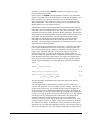
General Model and Algorithm Characteristics
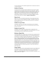
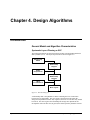
Systematic Layout Planning or SLP
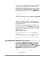
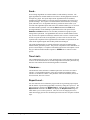
The following definitions are based upon the Systematic Layout Planning method or
SLP by Muther (1973). The major steps in SLP are shown in Figure 4.1.
Relationship
Matrix
Relationship
Diagram
Space
Requirements
Space
Relationship
Diagram
Other
Considerations
Block Layout
Figure 4.1. SLP Block Diagram
A relationship chart is the quantitative matrix containing the level of interaction
between pairs of departments. The more positive the element in the matrix the
stronger two departments interact and, in general, the closer to each other they should
be located. The more negative the relationship the stronger two departments are
incompatible with each other and, in general, the farther apart they should be located.
Spiral User's Manual
Chapter 4. Design Algorithms • 41
A relationship diagram is a spatial arrangement of the departments to represent the
relationship data in a graphical way. This diagram is also called an adjacency graph.
When the space requirements for the departments are added to this relationship
diagram, then a space relationship diagram has been constructed.
Finally, any number of other considerations and constraints, that are not captured in
the relationship data or the space data, can be incorporated in the space relationship
diagram to generate a layout alternative. Hence, the spatial relationship diagram is
not a layout, because it does not incorporate other considerations such as building
shape and area and department shape constraints.
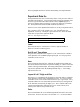
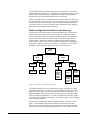
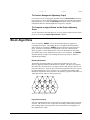
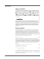
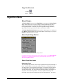
Model and Algorithm Classification and Hierarchy
The theoretical layout models and their solution algorithms can be classified and
organized based upon the properties shown in Figure 4.2. Graph based models
generate an adjacency graph, while area based models generate a conceptual block
layout. Primal models maintain a feasible solution while attempting to obtain an
optimal solution. Dual models maintain an optimal solution while attempting to
obtain a feasible solution. In discrete area models the departments and building are
composed of a number of equal sized unit squares. In continuous area models the
dimensions of the building and departments can have fractional values.
Layout
Models
Graph
Based
Area
Based
Primal
Dual
SPIRAL-G
Deltahedron
Match
Discrete
QAP, QSSP
AP, ALDEP,
CORELAP,
CRAFT
MULTIPLE,
LayOPT,
SABLE
Continuous
Block
Layout
Material
Handling
Layout
SPIRAL-L
FactoryOPT
BLOCPLAN,
FLEX-BAY,
HOPE
Montreuil
AISLES
Figure 4.2. Theoretical Layout Models Hierarchy
The completed block layout can be represented as a graph. Similarly, the original
relationship matrix can be represented as a complete undirected graph, where each
department corresponds to a node and pairwise relationships form the edges. The
adjacency graph is constructed from the relationship diagram by deleting all edges
between non-adjacent departments, i.e. an edge is included in the adjacency graph if
and only if the two departments are adjacent. The adjacency graph is thus a subgraph
of the relationship diagram.
The block layout graph and the adjacency graph are related, in fact they are dual
graphs. The relationship diagram can be constructed from the block layout by
placing a node inside each department and by drawing the connecting relationship
edge if and only if the two departments are adjacent, i.e. have a common wall. The
42 • Chapter 4. Design Algorithms
Spiral User's Manual
resulting adjacency graph is planar. A graph is planar if it can be drawn in a twodimensional plane without crossing edges.
From an adjacency graph a block layout can be constructed if and only if the
adjacency graph is planar, see Seppanen and Moore (1970). The concepts of layout
graph, adjacency graph and their dual relationship are shown in Figure 4.3.
B
D
A
C
E
F
P
Figure 4.3. Adjacency Graph and Layout as Dual Graphs
The graph theoretic models are concerned with determining the best relative location
of departments, ignoring the complexities of department and building shape and area.
Their objective is to maximize the adjacency score. But in order to construct a block
layout, the adjacency graph must be planar. Hence the problem is to extract a planar
subgraph out of the relationship diagram, so that its edge weight is maximized and
the graph is planar. This problem is called the Maximum (Weight) Planar Subgraph
Problem (MPSP). This problem is NP-Complete and cannot be solved for practical
problem size in reasonable amount of computer time.
SPIRAL Algorithm Characteristics
The SPIRAL algorithm consists of two major steps, denoted by SPIRAL G and
SPIRAL L in Figure 4.2. In the first step, the fundamental principle of the SPIRAL
algorithm is to grow a high weight, planar, hexagonal adjacency graph in a greedy
fashion. In the second step, this graph is converted into a block layout with all
rectangular departments and with material handling aisles parallel to one of the
hexagon axes.
The SPIRAL program contains a collection of algorithms. These algorithms either
construct a planar hexagonal adjacency or create a block and are called graph and
layout algorithms, respectively.
You have the option of selecting one single design algorithm to be executed next or
to select the execution of all possible combinations of algorithms. If you choose the
latter, the program will execute a number of algorithms in sequential order. It also
maintains the best adjacency score, the best efficiency, and the best shape adjusted
distance score obtained by the algorithms for this project.
Graph Algorithms
The SPIRAL algorithm grows the relationship diagram in a crystalline, spiraling
fashion. The original, manual form of this algorithm was first mentioned in Reed
Spiral User's Manual
Chapter 4. Design Algorithms • 43
(1967). It relied completely on the insight of the engineer. A more sophisticated
version that incorporates relationships with the outside, neighborhood improvement
steps, and is based on hexagonal graphs is given in Goetschalckx (1986, 1992).
The SPIRAL technique constructs a guaranteed planar graph with high adjacency
score based on an underlying hexagonal grid. The hexagonal grid where each
department has six neighboring departments is illustrated in Figure 4.4. A typical
adjacency graph created by SPIRAL is shown in Figure 4.5.
Figure 4.4. Hexagonal Grid Illustration
Figure 4.5. SPIRAL Adjacency Graph Illustration
The objective is to maximize the adjacency score based on a qualitative or numerical
relationship chart. Departments are represented by standard, size independent
symbols such as squares or circles. The data requirements are either a qualitative
letter or quantitative relationship chart. The SPIRAL algorithm is one of the manual
techniques to construct an adjacency graph or relationship diagram based upon a
quantitative relationship matrix or flow matrix. The SPIRAL technique grows the
graph in a crystalline manner by adding the department, which has the highest
adjusted relationship, next to the graph so that the graph adjacency score is
44 • Chapter 4. Design Algorithms
Spiral User's Manual
maximized. As such the manual SPIRAL algorithm is an example of a greedy,
heuristic construction procedure.
In the first phase, the SPIRAL technique attempts to construct a good relationship
diagram. The quality of the relationship diagram is measured by the adjacency score.
Hence, the objective is to maximize the positive flow or relationships between
adjacent departments and to minimize the negative flow or relationships between
adjacent departments. Observe that later on the objective is to minimize the shape
adjusted distance score of the final block layout.
Departments are entered in the hexagonal adjacency graph based on their adjusted
relationship. The relationship tuple indicates on how many departments the adjusted
relationship is based. Possible options are null, unary, binary, and ternary. The
departments then enter the graph by decreasing adjusted relationship. The null tuple
indicates that the next department will be chosen at random, without any regard to its
relationships with other departments. The unary adjusted relationship sums the
relationships of a department with all other departments. The binary adjusted
relationship is the relationship between the current department and one other
department. The ternary adjusted relationship is the relationship between the current
department and two other departments.
Next, the relationships with the outside are incorporated. A department with a high
positive spiral relationships will tend to be located early on in the procedure and
hence on the inside of the graph. Similarly, a department with a small positive or a
negative spiral relationship will tend to be located late and hence towards the
perimeter of the graph. To incorporate the relationships with the outside in a
consistent manner each spiral relationship is adjusted by subtracting the relationship
of the departments in the tuple with the outside. For example, the adjusted unary,
binary, and ternary spiral relationship (denoted by the subscript adj) are computed
from the original relationships in the relationship matrix (denoted by the subscript
orig) as:
radj (i ) =
M
rorig (i , j ) − rorig (i ,0)
(4.1)
radj (i , j ) = rorig (i , j ) − rorig (i ,0) − rorig ( j ,0)
(4.2)
j =1
radj (i , j , k ) = rorig (i , j ) + rorig (i , k ) + rorig ( j , k )
(4.3)
−rorig (i ,0) − rorig ( j ,0) − rorig ( k ,0)
M is the total number of departments in the layout and 0 indicates the artificial
outside department.
After the original graph is constructed three possible improvement steps can be
executed. The options are none, two exchange, and three exchange. None does not
execute an improvement step. Two exchange attempts to improve the graph in a
steepest descent manner by attempting two department exchanges. It computes the
savings generated by removing two departments out of the graph and swapping their
position. The savings are based on an increase in the adjacency score. The exchange
with the largest savings among all possible combinations of two departments is
determined and if these savings are positive then those two departments are
exchanged. The process repeats until no further improvements can be made. Three
exchange attempts to improve the graph in a steepest descent manner by attempting
three department exchanges. It computes the savings generated by removing three
departments out of the graph and swapping their position. The savings are based on
an increase in the adjacency score. The exchange with the largest savings among all
Spiral User's Manual
Chapter 4. Design Algorithms • 45
possible combinations of three departments is determined and if these savings are
positive then those three departments are exchanged. The process repeats until no
further improvements can be made. Computational processing time increases sharply
with the amount of improvement processing.
When locating a department in the partial adjacency graph often alternative positions
are possible. Two possible tie breaker rules can be used. The first one is random
which places the department randomly in one of the alternative positions based on a
random number. The second one is centroid seeking which places the department in
the position closed to the centroid of the current (partial) adjacency graph. If there
are still alternative positions after the first tie breaker then a position is chosen at
random. For further information see Goetschalckx (1992).
In the case of the hexagonal grid, an upper bound on the adjacency score of the graph
can be computed based on the following integer programming formulation, where o
(zero) represents the artificial outside department:
N −1 N
Max.
i =1 j >i
i −1
rij xij +
N
i =1
(4.4)
rio yi
i = 1.. N
(4.5)
yi ≤ xoi
i = 1.. N
(4.6)
xoi ≤ 6 yi
i = 1.. N
(4.7)
yi ∈ {0,1}
i = 1.. N
(4.8)
xij ∈{0,1}
i = 1.. N − 1, j = i + 1.. N
(4.9)
xoi ≥ 0
i = 1.. N
s.t.
j =0
x ji +
N
xij = 6
j =i +1
(4.10)
The following notation is used:
xij is 1 if departments i and j are adjacent, 0 otherwise. For the artificial outside
department xij represents the number of times department i is adjacent to the outside
perimeter.
yi is 1 if department i is adjacent to the outside, 0 otherwise.
rij is the binary relationship between departments i and j.
The formulation maximizes the adjacencies between departments and between a
department and the outside (4.2), subject to the constraint that each department must
have exactly six neighbors (4.3). These neighboring departments can be the artificial
outside department. If a department has at least one outside department as a neighbor
the relationship with the outside is satisfied and included in the objective function
(4.4) and (4.5). All the adjacencies are binary variables, except the adjacencies with
the outside department which are linear (4.6), (4.7) and (4.8).
The value of the formulation lies in the fact that it provides bound on the optimal
solution quality and on the maximum deviation of the heuristic solutions. The value
returned by the algorithm in SPIRAL is the solution of the linear relaxation of the
above formulation. In a linear relaxation all variables that originally were restricted
to be either zero or one now can take any value between zero and one. In other
words:
s.t.
46 • Chapter 4. Design Algorithms
0 ≤ xij ≤ 1
i = 1.. N − 1, j = i + 1.. N
(4.11)
Spiral User's Manual
0 ≤ yi ≤ 1
i = 1.. N
(4.12)
To Create a Hexagonal Adjacency Graph
If you want to execute a single graph algorithm select the Select Graph command.
If you want to execute all graph algorithms in sequence and retain the graph with the
highest adjacency score, select the All Graphs command. Because of its extensive
computations this last command might take a long time to complete.
To Compute an Upper Bound on the Graph Adjacency
Score
You can compute the maximum adjacency score any graph can obtain for the current
project by executing the Graph Upper Bound command.
Block Algorithms
In the second phase, SPIRAL converts the hexagonal adjacency graph into a
rectangular block layout. The building has to be rectangular and all department
shapes will also be rectangular. SPIRAL constructs the block layout based upon
layers. Each layer corresponds to all departments on an axis of the hexagonal
adjacency graph. Once the departments in a layer are determined, the area of this
layer and the shape of each department in the layer can be computed. The SPIRAL
algorithm attempts to improve the resulting block layout by using two and three
department interchanges.
Building Orientation
The building orientation indicates to which of the possible three axes of the
adjacency graph the building width dimension is parallel. The adjacency graph has
three main axes, horizontal or level, 60 degrees upward, and 60 degrees downwards
of the horizontal level. The block layout construction algorithms will create a layout
by putting departments in rows, where the rows are parallel to the building width
dimension. Departments whose positions in the adjacency graph are on the same axis
will be placed in the same row in the block layout.
A
C
D
B
F
E
G
Figure 4.6. Main Axes of Adjancency Graph
Layout Improvement
After the original block layout is constructed four possible improvement steps can be
executed. The options are none, steepest descent exchange and annealing exchange.
Each exchange improvement procedure can be based either on exchanging two or
three departments at a time.
Spiral User's Manual
Chapter 4. Design Algorithms • 47
None does not execute an improvement step.
Steepest Descent exchange attempts to improve the graph in deterministic and
greedy manner by attempting two or three department exchanges. The exchange with
the largest savings among all possible combinations of two or three departments is
determined and if these savings are positive then those two or three departments are
exchanged. The process repeats until no further improvements can be made.
Two Exchange attempts to improve the layout in a steepest descent manner by
attempting two department exchanges. It computes the savings generated by
removing two departments out of the graph and swapping their position. The savings
are based on a decrease in the shape adjusted distance score. Three Exchange
attempts to improve the graph in a steepest descent manner by attempting three
department exchanges. It computes the savings generated by removing three
departments out of the graph and swapping their position. The savings are based on
a decrease in the shape adjusted distance score.
Annealing Exchange attempts to improve the graph in stochastic, non steepest
descent manner by attempting two or three department exchanges. There exists an
analogy between the optimization method of simulated annealing and the laws of
thermodynamics, specifically with the way in which liquids freeze and crystallize or
metals cool and anneal. The algorithm computes the savings generated by removing
three departments out of the graph and swapping their position. The savings are
denoted by S. The savings are based on a decrease in the shape adjusted distance
score. The three departments are chosen at random. If the savings are positive then
the exchange is made. If the savings are negative, i.e. the distance score after the
exchange is higher, then the exchange can still be made with a certain probability
depending on the how long the simulated annealing algorithm has been executing.
This time by convention is called the temperature of the annealing process and is
denoted by T. The probability of an exchange based on savings S, denoted by P(S) is
then computed as:
P( S | S > 0) = 1
P( S | S ≤ 0) = e S / T
(4.13)
During the algorithm execution the temperature T is systematically reduced. This
allows early on exchanges with large negative savings. As the temperature is
lowered, the number of such exchanges and the size of the allowed negative savings
are gradually reduced. The objective of these non-improving exchanges is to avoid a
steepest descent into a local minimum. The process repeats until no further
improvements can be made.
For further information on two and three exchanges see Goetschalckx (1992). For
further information on simulated annealing see Kirkpatrick et al. (1983) and Vechi
and Kirkpatrick (1983).
Computational processing time increases sharply with the amount of improvement
processing.
Space Allocation
The Layered space allocation method divides the building area in strips or layers
parallel to the orientation of the building. All departments located on an axis of the
hexagonal adjacency graph parallel to the building orientation are assigned to a
single layer. The algorithm then assigns department areas from left to right in each
layer. The Layered method has the advantage that it creates natural material handling
aisles in the building.
48 • Chapter 4. Design Algorithms
Spiral User's Manual
The Tiled space allocation method divides the building area into a set of nonoverlapping rectangular departments. The position of the department rectangles is
derived from the hexagonal adjacency graph. The Tiled space allocation method
recursively divides a partial building area along all possible vertical and horizontal
rows and columns of the hexagonal adjacency graph and keeps the best layout
generated so far. The Tiled space allocation method has more flexibility than the
Layered space allocation method and on the average will yield layouts with a lower
distance score. However, the resulting layout may not have the structure that aligns
departments along parallel material handling aisles. For individual project instances
the Layered method may generate a layout with lower distance score than the Tiled
space allocation method. Because the Tiled method examines many more
alternatives than the Layered method, it requires substantially longer computation
times.
To Create a Block Layout
If you have already created a graph, then you can create a block layout next. If you
want to execute a single layout algorithm, select the Select Layout command. If you
selected the Tiled space allocation method, generating even a single layout for large
projects might take a long time to complete. If you want to execute all block layout
algorithms in sequence and retain the block layout with the minimum shape adjusted
distance score, select the All Layouts command. Because of its extensive
computations this last command might take a long time to complete.
Finally, if you want to execute all graph algorithms and for each graph algorithm
execute all layout algorithms, select the All Graphs and Layouts command.
Because of its extensive computations this command might take a long time to
complete.
To Evaluate the Current Graph and Layout
If you have made some changes to the project data, the current graph or the current
layout, then you can evaluate quickly the effect of these changes by executing the
Evaluate command. This command does not create a new graph or layout but
merely evaluates the current graph and or layout.
Parameters
Setting several algorithm parameters can modify the execution of the various
algorithms. Not all algorithms use all parameters.
Maximum Replications...
The graph algorithms create random adjacency graphs when breaking ties for the
location of department nodes in the adjacency graphs. When graph algorithms are
executed again with a different seed, a different graph might be generated. The
layout improvement algorithms based on simulated annealing select random pairs of
departments to be tested for possible exchange. Different replications of the same
algorithm can thus provide different adjacency graphs or block layouts. The higher
the number of replications, the more likely a high quality block layout will be
constructed. But this comes at an increase in computation time. You can set the
maximum number of replications the graph algorithm executes with the
Max. Replications command of the Edit menu.
Spiral User's Manual
Chapter 4. Design Algorithms • 49
Seed...
Several design algorithms use random numbers to make arbitrary decisions. The
graph algorithms use random numbers to break ties in locating department nodes in
the adjacency graph. The layout improvement algorithms based on simulated
annealing use random numbers to select the next two departments to be tested for a
possible exchange. The sequence of random numbers is determined by its starting
point, called the seed. An algorithm will always produce the same results if you
select the same algorithm options and set the same random number seed. You can set
the random number generator seed with the Seed command of the Edit menu.
If an algorithm has executed multiple replications then the seed reported in the
Statistics and Notes windows is the seed that yielded the best graph or layout
among all the replications. An algorithm that does not use random numbers or that
only executes one replication will always return the same seed as it was started with.
In order to repeat the results for an algorithm, you must set the seed to the value
reported at the completion of the algorithm and set the number of replications to one.
Then run the algorithm again with all other parameters unchanged.
The actual random numbers are generated from the seed with a standard pseudo
random number generation process. This process is dependent on the combination of
processor and compiler, so computers with different processors and compiler version
may give different random number sequences. SPIRAL has no control over this
process.
Time Limit...
This command allows the user to set the maximum time a single algorithm is allowed
to run or for the maximum time in seconds an algorithm can execute a particular step.
Once the time limit has been reached the algorithm is terminated.
Tolerance...
The Parameters menu's Tolerance Command queries the user for the new relative
tolerance. The algorithm terminates, if the current solution is within the relative
tolerance of current best solution. This parameter cannot be modified by the user at
the current time, but is set to 0.001.
Report Level...
You can control the level of detail the program will use in generating output reports
and the number of pauses during algorithm execution by setting the report level. The
output reports are written to the Output Log file, if this one has been defined. The
Report Level command of the Edit menu displays the Report Level dialog box
which allows you to set the report level. There are six levels ranging from 0 to 5,
which increasingly generate more detailed reports and cause more frequent execution
stops.
50 • Chapter 4. Design Algorithms
Spiral User's Manual
Statistics
Adjacency Statistics
If all departments have been located then the adjacency and efficiency of the graph
are computed. To score the graph, the sum of all positive relationships between
adjacent departments will be denoted by PA. The sum of all negative relationships
between non-adjacent or separated departments will be denoted by NS. The sum of
all positive relationships between non-adjacent or separated departments will be
denote by PS, and the sum of all negative relationships between adjacent department
will be denoted by NA. The adjacency (A) and efficiency (e) are then computed as
A = PA + NA
e=
(4.14)
PA − NS
PA + PS − NS − NA
(4.15)
The efficiency has its numerator all relationships that are desirable, namely positive
adjacent and negative separated ones. It has in the denominator the sum of all
relationships. The efficiency is thus a measure of the quality of the adjacency graph
with values between 0 and 1 and invariant with respect to the magnitude of the
relationships. A diagram which maximizes the adjacency will also maximize the
efficiency since the numerator of the efficiency is equal to adjacency minus the
constant (NS + NA).
Distance Statistics
The shape adjusted distance score D is computed as the sum of the flow distance
score and the shape penalties. The flow distance score itself is composed of the
internal and the external flow distance score. The internal flow distance score is
equal to the sum of the products of the rectilinear distance between the centroids of
two departments and the relationship between those departments. In other words, if
the centroids of two departments are located at coordinates ( xi , yi ) and ( x j , y j ) then
the rectilinear centroid to centroid distance is given by:
dijR =| xi − x j |+| yi − y j |
(4.16)
The external flow distance score is equal to the sum of the shortest rectilinear
distance of the centroid of the department to the perimeter of the building multiplied
by the relationship of that department with the outside. In other words, if the origin
of a department is denoted by (x, y), its size by (w, l), and the building dimensions by
(W, L), then the rectilinear distance between the department and the perimeter is
given by
l
q
dioR = min x + w / 2, y + l / 2, W − x − w / 2, L − y − l / 2
(4.17)
The total flow distance is then equal to
D=
N −1 N
dijR ⋅ rij +
i =1 j =i +1
N
i =1
dioR ⋅ rio
(4.18)
For each individual department the shape ratio is denoted by si , the maximum shape
ratio is denoted by Si , and the shape penalty is denoted by pi . The shape adjusted
distance score SD is then equal to:
Spiral User's Manual
Chapter 4. Design Algorithms • 51
SD = D +
N
i =1
max{0, si − Si } ⋅ pi
(4.19)
The shape adjusted distance score is reported at the end of the algorithms. If you are
only interested in the flow distance score, you can compute this score by evaluating
the layout with the Evaluate command of the Algorithms menu. The flow
distance score is reported as the Delta Objective value and also shown in the
Evaluate dialog window.
Examples
Tompkins Example
This section illustrates the construction algorithm for hexagonal adjacency graphs
that has been implemented in the SPIRAL program.
Consider a layout project with seven departments. The space requirements and the
flow from-to-chart are given below. The flow chart is based on the number of trips
per day with an electric platform truck. This example was originally presented in
Tompkins and Moore (1978).
Table 4.1. Departmental Data
A
B
A
B
C
D
E
F
G
C
45
D
15
E
25
30
F
20
10
25
5
35
5
25
G
5
15
10
65
Function Area
Receiving
12,000
Milling
8,000
Press
6,000
Lathing
12,000
35 Assembly
8,000
65 Plating
12,000
Shipping
12,000
The first step converts the asymmetric matrix into a symmetric one. The sum of all
relationships is equal to 435.
Table 4.2. Symmetric Department Relationship Data
A
A
B
C
D
E
F
G
B
C
45
D
15
E
25
50
F
10
25
5
35
G
5
20
10
90
Function Area
Receiving
12,000
Milling
8,000
Press
6,000
Lathing
12,000
35 Assembly
8,000
65 Plating
12,000
Shipping
12,000
Step two creates the SPIRAL relationships, which in this case is easy since there are
no outside relationships, and step three ranks the relationships by non-increasing
value.
52 • Chapter 4. Design Algorithms
Spiral User's Manual
Table 4.3. Ranked Relationships
Index
1
2
3
4
5
6
7
Pair Value Index
EF
90
8
FG
65
9
BD
50
10
AB
45
11
DE
35
12
EG
35
13
AD
25
14
Pair Value Index
BE
25
15
BF
20
16
AC
15
17
AE
10
18
CF
10
19
AF
5
20
CE
5
21
Pair Value
AG
0
BC
0
BG
0
CD
0
CG
0
DF
0
DG
0
In step four the departments are placed in the relationship diagram in such way as to
maximize the sum of adjacent flows.
The flow EF is the largest, hence departments E and F are placed next to each other.
F
E
Figure 4.7. Partial Hexagonal Adjacency Graph with 2 Departments
The largest relationship with an anchor department already located is now FG.
Department G will be located adjacent to department F, but there exist alternative
locations. Department G has both positive flows with departments F and E, so it is
placed adjacent to both. There still exists a tie between locations left or right of
departments E and F, which is broken arbitrarily.
F
E
G
Figure 4.8. Partial Hexagonal Adjacency Graph with 3 Departments
The next largest relationship with a department already in the layout is relationship
DE. Department D will be placed adjacent to department E, but there exist
alternative locations. Checking down the list shows that department D has no further
relationship with any of the already located departments and the tie is thus broken
arbitrarily.
Spiral User's Manual
Chapter 4. Design Algorithms • 53
D
F
E
G
Figure 4.9. Partial Hexagonal Adjacency Graph with 4 Departments
The next largest flow with an already located department is BD. Department B will
be placed adjacent to department D. To break the tie, the first located department
down the list with a relationship with B is department E. Hence department B will be
located in the unique location adjacent to D and E.
D
B
F
E
G
Figure 4.10. Partial Hexagonal Adjacency Graph with 5 Departments
The largest flow is now AB. Department A has positive flows with departments B, D
and E in that order. There is a single unique location adjacent to departments B and
D, so department A is placed adjacent to departments B and D.
A
D
B
F
E
G
Figure 4.11. Partial Hexagonal Adjacency Graph with 6 Departments
The largest flow is now AC. Department C has positive flows with departments A, F
and E. It cannot be adjacent to A and to either F or E, so it is placed in an arbitrary
location adjacent to department A.
54 • Chapter 4. Design Algorithms
Spiral User's Manual
A
C
D
B
F
E
G
Figure 4.12. Complete SPIRAL Hexagonal Adjacency Graph
Since all the relationships are positive, the evaluation is done immediately with the
original adjacency matrix. The adjacency matrix is multiplied element by element
with the symmetric relationship matrix to generate the adjacency score.
Table 4.4. Adjacency Matrix
A
B
A
B
C
D
E
F
G
C
1
D
1
1
E
1
1
F
G
1
1
1
1
1
1
The adjacency score is equal to 385. The efficiency is then equal to 385/435 or
89 %.
If random location ties are broken differently, then the diagram of Figure 4.13 is
generated. Its efficiency is equal to 405 / 435 = 93 %.
A
C
D
B
E
F
G
Figure 4.13. Alternative SPIRAL Hexagonal Adjacency Graph
When the layout construction algorithm is executed on the adjacency graph of Figure
4.12 with a level main axis and no improvement steps, then the block layout shown in
Figure 4.14 is created.
Spiral User's Manual
Chapter 4. Design Algorithms • 55
Figure 4.14. SPIRAL Block Layout
The rectilinear centroid-to-centroid distance score is equal to 2171. Since all
departments have a shape ratio smaller than their maximum shape ratio, which is
equal to two for all departments, the shape adjusted distance score is equal to the
flow distance score.
Autoparts Example
The company produces stamped metal parts, to be used in automotive assembly, from
sheetmetal coils. The plant consists of five major departments. Some of the parts
have to be treated with corrosion resistive paint and then dried in an oven. Forklift
trucks are used for all material handling transportation operations in the plant. A
summary of the department data is given in Table 4.5. The number of truck trips per
week between each pair of departments and between each department and the outside
is given in Table 4.6. The building dimensions are 200 by 120 feet.
Table 4.5. Department Data for the Autoparts Example
Label Function
SHI
REC
STA
PAI
STO
OUT
56 • Chapter 4. Design Algorithms
Shipping
Receiving
Stamping
Painting
Steel Coil Storage
Outside
Area
4,000
2,000
10,000
6,000
2,000
Maximum Shape
Shape Ratio Penalty
3.0
15,000
3.0
10,000
1.5
25,000
2.0
50,000
4.0
10,000
Spiral User's Manual
Table 4.6. Material Handling Trips for the Autoparts Example
OUT
SHI
REC
STA
PAI
STO
OUT SHI REC STA PAI STO
50
300
15
35
240
60
60
35
We will first create a hexagonal adjacency graph and block layout following the
SPIRAL methodology. For the graph construction phase, we will use the binary
relationships, not use improvement interchanges, and break location ties by the
centroid-seeking rule. For the graph, we will show first the symmetrical adjusted
relationships in a two-dimensional matrix. We then will show the sorted list of
adjusted binary relationships. Third, we will show the adjacency graphs after we
have added each department. Finally, we will compute and show the adjacency and
efficiency score of the final graph.
We first convert the asymmetrix material handling trips to a symmetric relationship
table, where all relationships are shown above the main diagonal.
Table 4.7. Symmetric Relationships for theAutoparts Example
OUT
SHI
REC
STA
PAI
STO
OUT SHI REC STA PAI STO
300
50
240 60
15
35
60 35
Next the adjusted binary relationships, that incorporate the relationships with the
outside, are computed. Because several departments have positive relationships with
the outside, many of the adjusted relationships are negative.
Table 4.8. Binary Adjusted Relationships for the Autoparts Example
SHI REC STA PAI STO
SHI
-350 -60 -240 -300
REC
-35 -50 -15
STA
60 35
PAI
0
STO
The adjusted binary relationships are then sorted in decreasing order.
Table 4.9. Sorted Binary Adjusted Relationships for the Autoparts Example
Index Dept. 1 Dept. 2 Relation Index Dept. 1 Dept. 2 Relation
1
STA
PAI
60
6
REC
PAI
-50
2
STA
STO
35
7
SHI
STA
-60
3
PAI
STO
0
8
SHI
PAI
-240
4
REC
STO
-15
9
SHI
STO
-300
5
REC
STA
-35
10
SHI
REC
-350
Spiral User's Manual
Chapter 4. Design Algorithms • 57
The first two departments to enter the hexagonal adjacency graph are the two
departments in the first element of the list, i.e. STA and PAI. They are placed at
random in two adjacent vertices of the hexagonal grid.
STA
PAI
Figure 4.15. Adjacency Graph with 2 Departments for the Parts Example
The next relationship selected must have one department in the graph and one
department not in the graph. These departments are called the anchor department
and the new department, respectively. The anchor department also must have an
open adjacent grid position. Element two of the list satisfies all those conditions:
department STA is in the graph, department STO is not, and department STA has an
empty adjacent grid position. All empty grid positions adjacent to the anchor
department are possible locations for the new department, and because of the
relationship selection rule there exists at least one open adjacent grid position. The
grid position with the highest adjacency score based on the original symmetric
relationships is selected. Ties are broken by the centroid-seeking rule, i.e. the new
department is located in the open grid location adjacent to the anchor department that
tied for the highest adjacency score and that is closest to the centroid of the current
adjacency graph. Department STO has only a relationship with department STA, and
thus all open grid positions adjacent to department STA are tied. There are three grid
position closest to the centroid of the graph and the one above the centroid is selected
at random.
STO
STA
PAI
Figure 4.16. Adjacency Graph with 3 Departments for the Autoparts Example
58 • Chapter 4. Design Algorithms
Spiral User's Manual
Element four is the next relationship selected from the list. Department STO is in the
graph, department REC is not, and department STO has an open adjacent grid
position. Deparment REC has a positive relationship with departments STA and
STO and so the open grid position adjacent to both those department is the selected
location for department REC.
REC
STO
STA
PAI
Figure 4.17. Adjacency Graph with 4 Departments for the Parts Example
Department SHI is the only remaining free department. Element seven is the next
selected relationship, since department STA is in the graph, deparment SHI is not in
the graph, and department STA has an open adjacent grid location. All open grid
positions adjacent to department STA are candidate locations. Since department SHI
has positive relationships only with departments STA and PAI, it will be located in
the open grid location adjacent to those two departments.
REC
STO
STA
PAI
SHI
Figure 4.18. Adjacency Graph with 5 Departments for the Parts Example
To compute the adjacency score, we construct the adjacency matrix for the graph
above.
Spiral User's Manual
Chapter 4. Design Algorithms • 59
Table 4.10. Adjacency Matrix for the Autoparts Example
OUT
SHI
REC
STA
PAI
STO
OUT SHI REC STA PAI STO
1
1
1
1
1
1
1
1
1
1
1
1
The adjacency matrix is then multiplied element by element with the symmetrical
relationship matrix and the sum of the product is computed. The sum is equal to 795.
Since the sum of the absolute values of all relationships is also equal to 795, the
efficiency of the above graph is equal to 100 %.
For the block layout phase, we will use the graph axis with the most departments in
the graph as the building orientation, not use improvement interchanges, and use the
layered space allocation method. For the layout phase, we will first show the layout
drawn to scale with all departments properly dimensioned. Next, we will show all
distances in a two-dimensional matrix of which we will only fill in the upper half.
Third, we will compute and show the inter-department distance score and the
distance score with the outside. Fourth, we will compute and show the shape penalty
score for each individual department and the total shape penalty. Finally, we will
compute and show the shape adjusted distance score.
The graph axis with the most departments is oriented downwards. The conceptual
block layout with the layered space allocation method is shown in the next figure.
50
150
STO
PAI
40
REC
STA
SHI
25
125
50
80
Figure 4.19. Block Layout for the Given Graph for the Autoparts Example
60 • Chapter 4. Design Algorithms
Spiral User's Manual
Table 4.11. Distance Matrix for the Autoparts Example
OUT
SHI
REC
STA
PAI
STO
OUT SHI REC STA PAI STO
25.0 12.5 40.0 20.0 20.0
162.5 87.5 110.0 210.0
75.0 72.5 72.5
97.5 122.5
100.0
The distance matrix is then multiplied element by element with the symmetrical
relationship matrix and the sum of the products is computed. This sum is the flow
distance score and is equal to 49,525, of which 41,400 is between two departments
and 8,125 is between departments and the outside.
Table 4.12. Penalty Shape Computations for the Autoparts Example
Dept.
SHI
REC
STA
PAI
STO
Actual
Shape
1.6
3.2
1.5625
3.75
1.25
Maximum Delta
Penalty
Shape
Shape
Shape
Rate
Penalty
3
0
15000
0
3
0.2
10000
2000
1.5
0.0625
25000
1563
2
1.75
50000
87500
4
0
10000
0
The total shape penalty is computed as the sum of the individual department shape
penalties and is equal to 91,063. The total shape distance score for the layout is
computed as the sum of the flow distance score and the shape penalty and is equal to
140,588.
The block layout without exchange improvements, the best block layout with the
layered space allocation method, and the best block layout with the tiled space
allocation method are shown in the next three figures. The distance statistics for the
three layouts are shown in the next table.
Figure 4.20. Unimproved Block Layout for the Given Graph for the Parts Example
Spiral User's Manual
Chapter 4. Design Algorithms • 61
Figure 4.21. Best Layered Block Layout for the Given Graph for the Parts Example
Figure 4.22. Best Tiled Block Layout for the Given Graph for the Parts Example
Table 4.13. Distance Statistics for the Parts Example
Unimproved Best Layered Best Tiled
Flow Distance
49,525
49,375
43,169
Shape Penalty
91,063
1,563
6,042
Shape Distance
140,588
50,938
49,211
While the computer can provide evaluations of the different layouts based on
centroid-to-centroid distances, it remains up to the user to decide which layout is best
suited for their particular layout project.
62 • Chapter 4. Design Algorithms
Spiral User's Manual
Chapter 5. Command Reference
Menu Overview
An overview of the Spiral program menu structure is shown in Table 5.1.
Table 5.1. Spiral Menu Structure
File
Edit
Algorithms
View
Window
Help
New...
Add Department
Select Graph...
Department Labels
New Notes View
Help Topics...
Open...
Delete Department
All Graphs
Edge Labels
New Statistics View
About SPIRAL...
Close
Delete Department by Label…
Graph Upper Bound
Edges...
New Graph View
Save
Department
Select Layout...
Grid
New Layout View
Save As...
Department by Label...
All Layouts
Label Size...
Cascade
Import...
Relation...
All Graphs and Layouts
Node Colors...
Tile
Export
Relation with Outside
Synchronize Graph
Edges Display...
Arrange Icons
Send...
All Relations
Evaluate
Zoom
Toolbar
Properties...
Building Dimensions
Display Distances
Zoom Previous
Status Bar
Output Log...
Max. Shape Ratio…
Zoom Original
Close Log
Shape Penalty…
Redraw
Print...
Grid Size…
Print Preview...
Report Level
Print Setup...
Seed
Exit
Max Replications
Time Limit
Copy
Several commands have shortcut keys so that you can easily control the program with
the keyboard. Several commands are also shown on the toolbar, to allow easy
program control with the mouse.
Figure 5.1. Spiral Toolbar
File Menu
The Spiral program requires the project data before any algorithm can be executed.
The projects are managed with the commands on the File menu.
Spiral User's Manual
Chapter 5. Command Reference • 63
New
The New command of the File menu allows you to interactively create a new
facilities design project.
If there is a project currently open and if it has been modified, then the program will
display the Save Changes dialog window and ask if you wish to save those
changes, discard the changes, or if you wish to abort the creation of new project. The
Save Changes dialog window is illustrated in Figure 5.2.
The command displays the New dialog window, which is illustrated in Figure 5.3.
To save the new project use the Save As command. To open a previously saved
project use the Open or Import commands.
To create the new project with the values shown in the dialog window press the OK
button. When this project is created it has no departments and all relationships will
be equal to zero. If you press Cancel, no new project will be created.
New Project Shortcuts
Toolbar:
Keys:
CTRL+N
Save Changes Dialog Window
Figure 5.2. Save Changes Dialog Window
New Project Dialog Window
Figure 5.3. New Project Dialog Window
New Project Data Items
Project Title
The project title refers to the title of the project to be used in reports and printouts. It
consists of a maximum of 63 alphanumeric, spaces, or underscore characters.
Punctuation marks, or tab characters are not allowed. The title is also included in the
project Properties. The term project name is used synonymously with project title.
64 • Chapter 5. Command Reference
Spiral User's Manual
Further information can be found in the Project Data section under Project Title.
Building Width
The building width refers to the horizontal dimension of the building ground plan. It
must be in units compatible with the department areas. The building always has a
rectangular shape. The building area is computed as the product of the building
width and building depth. The building and department areas should be expressed in
compatible units to the building width and depth, i.e., if the building depth and width
are expressed in feet then the building and department areas must be expressed in
square feet. The width of the building is displayed along the horizontal axis on the
screen.
Further information can be found in the Project Data section under Building Width
Building Depth
The building depth refers to the second dimension of the building ground plan (which
will be displayed vertically on the screen). It must be in units compatible with the
department areas. The building area is computed as the product of the building width
and building depth. The building and department areas should be expressed in
compatible units to the building width and depth, i.e., if the building depth and width
are expressed in feet then the building and department areas must be expressed in
square feet. The depth of the building is displayed along the vertical axis on the
screen.
Further information can be found in the Project Data section under Building Depth
Open
The Open command allows you to read a previously saved project.
The program will read the corresponding Project Data File. Starting with version
4.0 of the Spiral program, the Project Data File is a binary file that can no longer
be viewed or manipulated outside the Spiral program. Use the Import command to
import project data created with previous versions of the Spiral program or with the
Export command. The default extension for Spiral project files is .spiral. The
command then displays the Open dialog window, which is illustrated below in
Figure 5.4.
As all applications using the Scientif support library, the Spiral application can only
open one project at the time. If there is a project currently open and if it has been
modified, then the program will display the Save Changes dialog window and ask
if you wish to save those changes, discard the changes, or if you wish to abort the
opening of another project or the creation of new project. The Save Changes
dialog window is illustrated in Figure 5.2.
However, you can still compare two projects side by side by opening a second copy
of the Spiral application itself, opening the second project with this copy of Spiral,
and then arranging the two application windows on your desktop.
Open Project Shortcuts
Toolbar:
Keys:
Spiral User's Manual
CTRL+O
Chapter 5. Command Reference • 65
Open Project Dialog Window
Figure 5.4. Open Project Dialog Window
Close
The Close command of the File menu allows you to close the current project.
If the current project has been modified, then the program will display the Save
Changes dialog window and ask if you wish to save those changes, discard the
changes, or if you wish to abort the closing of the current project. The Save
Changes dialog window is illustrated in Figure 5.2.
Save
The Save command of the File menu will save the current project data in the
Project Data File. If no file name for the current Project Data File has been
defined, then the Save command will execute as the Save As command.
Save Project Shortcuts
Toolbar:
Keys:
CTRL+S
Save As...
The Save As command of the File menu will query you for the file name of the
Project Data File with the Save As dialog window. If you press the Save button
the current project will then be saved as if the Save command was executed.
66 • Chapter 5. Command Reference
Spiral User's Manual
Save As Dialog Window
Figure 5.5. Project Save As Dialog Window
Save As Data Fields
File Name
Spiral is compatible with long file and directory names that follow the Windows
conventions. Some versions of the Windows operating environment will truncate the
default spiral extension to the three letters spi, so we recommend that you explicitly
add the spiral extension to the file name in the Save As dialog window.
File Type
Starting with version 4.0 of the Spiral program, the Project Data File is a binary
file that can no longer be viewed or manipulated outside the Spiral program. Use
the Export command to create a set of ASCII files that contain the major data for the
current project. These files can then be manipulated outside the Spiral program with
an ASCII text editor and then imported again into the Spiral program using the
Import command.
Import...
The Import command of the File menu allows you to read project data saved in
ASCII files with a version of the Spiral program earlier than 4.0, created with the
Spiral Export command, or created manually outside the Spiral program with an
ASCII editor.
Starting with version 4.0 of the Spiral program, the Project Data File is a binary
file that can no longer be viewed or manipulated outside the Spiral program. Use
the Open command to read project data files created with the Save command of
version 4.0 or higher of Spiral. The default extension for Spiral project files is
.spiral, the default extension for the Spiral project files of previous versions or
exported data files is .dat.
The command then displays the Open dialog window, which is illustrated in
Figure 5.4. The program will read the corresponding Project Data File (*.dat) and
Department Data File (*.dep).
The Project Data File and the Department Data File can be created with any
text editor or word processor capable of generating pure ASCII files or with the
Spiral User's Manual
Chapter 5. Command Reference • 67
Export command. Since word processors usually insert special formatting codes
into their regular document files, which cannot be read by the Spiral program,
special care should be taken when using a word processor to generate a pure ASCII
file. The project data file also should not contain any blank lines. Once these input
files have been created, they can be used repeatedly by the Spiral program.
Export...
The Export command of the File menu will save the current project data in a set of
ASCII files. The program will create the corresponding Project Data File (*.dat)
and Department Data File (*.dep). Once these data files have been created, they
can be read by the Spiral Import command and by an ASCII editor. Not all
program settings will be saved, but only the major project, department, and
relationship data.
Starting with version 4.0 of the Spiral program, the Project Data File created by
the Save command is a binary file which can no longer be viewed or manipulated
outside the Spiral program. Use the Open command to read project data files
created with the Save command of version 4.0 or higher of Spiral. The default
extension for Spiral project files is .spiral, the default extension for the Spiral
project files of previous versions or exported data files is .dat.
Export Dialog Window
Figure 6. Export Dialog Window
Send...
The Send command of the File menu uses the electronic mail application installed
on your computer to send the saved version of the current project as an attachment to
an electronic mail message. It is recommended that the current project first be saved
before using the Send command. The exact execution of this command will depend
on which electronic mail application has been installed on your computer. This
command will not be enabled if you do not have an electronic mail client installed on
your computer.
Properties...
The Properties command of the File menu allows you to add project information,
such as authors, subjects, and comments to the current project. The Properties
68 • Chapter 5. Command Reference
Spiral User's Manual
command displays the Properties dialog window for the current document. You
can provide additional information in this dialog window about the current project.
Properties Dialog Window
Figure 5.7. Properties Dialog Window
Properties Data Items
Application
The name of the application creating this dialog window. In this case, Spiral. You
cannot change this data field.
Project
The project title. This is the only place where the title of the current project can be
changed after it has been initially entered in the New Project dialog window or was
imported from the Project Data file. The project title can contain letters, digits,
spaces, and underscore characters.
Further information can be found in the Project Data section under Project Title.
Subject
The subject of the current project.
Author
The author of the current project.
Keywords
A list of one or more keywords describing this project.
Data Version
The data version of the current project. You cannot change this data field. It is
displayed for information purposes only.
Spiral User's Manual
Chapter 5. Command Reference • 69
Comments
You can enter comments about the current project.
Output Log
The Output Log command of the File menu allows you to specify the file name for
the log file created and used by the Spiral program. Spiral writes the results and
intermediate information generated by the various design algorithms to the Output
Log file. The amount of information written to the Output Log File depends on
the level of detail selected with the Report Level command in the Edit menu. The
file and all of its previous contents will be erased every time the Output Log
command is executed. To select another log file or to restart the current log, execute
the Output Log command again. To stop recording algorithm results without
deleting the log file itself, use the Close Log command of the File menu.
Output Log Dialog Window
Figure 5.8. Output Log Selection Dialog Window
Close Log
Use this command to close the current output log. No further information or
algorithm results will be written to the output log, but the output log file itself will not
be deleted. Reopening the same log file with the Output Log command will erase
all the information in the log file, since the Output Log command always creates a
new file.
Print
Use this command to print a document. This command presents a Print dialog
window, where you may specify the range of pages to be printed, the number of
copies, the destination printer, and other printer setup options.
You can also copy the all views to the clipboard with the Copy command of the
Edit menu and then paste the views in other Windows applications.
Print Shortcuts
Toolbar:
70 • Chapter 5. Command Reference
Spiral User's Manual
Keys:
CTRL+P
Print Dialog Window
Figure 5.9. Print Dialog Window
Print Data Items
The following options allow you to specify how the current view should be printed:
Printer
This is the active printer and printer connection. Choose the Setup option to change
the printer and printer connection.
Setup
Displays a Print Setup dialog window, so you can select a printer and printer
connection.
Print Range
Specify the pages you want to print:
Spiral User's Manual
Chapter 5. Command Reference • 71
Table 5.2. Print Range Options
Option
All
Selection
Pages
Legend
Prints the entire document.
Prints the currently selected text.
Prints the range of pages you specify in the From and To boxes.
Copies
Specify the number of copies you want to print for the above page range.
Collate Copies
Prints copies in page number order, instead of separated multiple copies of each
page.
Print Quality
Select the quality of the printing. Generally, lower quality printing takes less time to
produce.
Print Progress Dialog
The Printing dialog window is shown during the time that Spiral is sending output to
the printer. The page number indicates the progress of the printing.
To abort printing, choose Cancel.
Print Preview
Use this command to display the active view as it would appear when printed. When
you choose this command, the main window will be replaced with a Print Preview
dialog window in which one or two pages will be displayed in their printed format.
The toolbar of the Print Preview window offers you options to view either one or two
pages at a time; move back and forth through the document; zoom in and out of
pages; and initiate a print job.
Print Preview Shortcuts
Toolbar:
72 • Chapter 5. Command Reference
Spiral User's Manual
Print Preview Window
Figure 5.10. Print Preview Window
Print Preview Commands
The print preview toolbar offers you the following options:
Print
Bring up the print dialog window, to start a print job.
Next Page
Preview the next printed page.
Prev Page
Preview the previous printed page.
One Page / Two Page
Preview one or two printed pages at a time.
Zoom In
Take a closer look at the printed page.
Spiral User's Manual
Chapter 5. Command Reference • 73
Zoom Out
Take a larger look at the printed page.
Close
Return from print preview to the editing window.
Print Setup
Use this command to select a printer and a printer connection. This command
presents a Print Setup dialog window, where you specify the printer and its
connection. This printer and these options will then be used by all subsequent Print
commands. The same changes can also be made from the main Windows Control
Panel.
Print Setup Dialog Window
Figure 5.11. Print Setup Dialog Window
Print Setup Data Items
The following options allow you to select the destination printer and its connection.
Printer
Select the printer you want to use. Choose the Default Printer; or choose the Specific
Printer option and select one of the current installed printers shown in the box. You
install printers and configure ports using the Windows Control Panel.
Orientation
Choose Portrait or Landscape.
Paper Size
Select the size of paper that the document is to be printed on.
Paper Source
Some printers offer multiple trays for different paper sources. Specify the tray here.
74 • Chapter 5. Command Reference
Spiral User's Manual
Options
Displays a dialog window where you can make additional choices about printing,
specific to the type of printer you have selected.
Network...
Choose this button to connect to a network location, assigning it a new drive letter.
Most Recently Used Files
Every time a project is saved, Spiral adds the fully qualified path and file name of
the project data file to the list of the most recently used (MRU) files. The eight most
recently used files are listed in the File Menu and saved in the Registry between
sessions. You can bypass the Open command and open one of those projects
directly by clicking on its file name.
Exit
The Exit command of the File menu terminates the Spiral program.
If there is a project currently open and if it has been modified, then the program will
display the Save Changes dialog window and ask if you wish to save those
changes, discard the changes, or if you wish to abort the termination of the
application. The Save Changes dialog window is illustrated in Figure 5.2.
The Spiral program can be terminated in the same way as all Windows programs by
double clicking on the system menu box or by selecting the Exit command.
Edit Menu
All the data items of the current project can be modified while executing the Spiral
program. Most of the data items can be edited with commands from the Edit menu.
Some overall project characteristics can be changed with commands on the File
menu. Finally, some algorithm parameters can be changed with the commands on
Algorithms menu.
Add Department
The Add Department command of the Edit menu allows you to interactively add a
department to the current layout project. The command displays the Add
Department dialog window in which the department data can be entered. Choose
OK to add the department with the entered department data. Choose Cancel to
cancel the dialog window and not to add the new department.
The new department will have all relations equal to zero with the other departments
and the outside. You can change the relations with the Relation and Relation with
Outside, or All Relations commands.
Add Department Dialog Window
The Add Department dialog window contains three pages, each selected by a one
of the tabs: Input, Continuous, and Discrete. When you are adding a
department, only the input page is relevant. You can view the continuous and
Spiral User's Manual
Chapter 5. Command Reference • 75
discrete department data pages after all the required data on the input page have been
entered.
Figure 5.12. Add Department Dialog Window
Add Department Data Items
The data items are identical to those for editing a department. See the Department
Data Items for further information.
Delete Department
The Delete Department command of the Edit menu allows you to interactively
delete a department from the current layout project. The command displays the
Delete Department dialog window in which the department data can be reviewed.
If you press Ok you will be asked to confirm the deletion of the department, since
deleting the department will permanently remove all the data associated with this
department from the project. If you press Cancel, the department will not be
deleted from the project.
76 • Chapter 5. Command Reference
Spiral User's Manual
Delete Department Dialog Window
Figure 5.13. Display of Department to be Deleted Dialog
Confirm Delete Department Dialog Window
Figure 14. Confirm Deletion of a Department Dialog Window
Delete Department Data Items
The data items are identical to those for editing a department. See the Department
Data Items for further information.
Delete Department by Label
The Delete Department by Label command of the Edit menu will display a list
with all the labels of the departments in the current project. The Select
Department by Label dialog window is illustrated in Figure 5.15. After a
department has been selected with its label, the department data can be deleted just
like in the Delete Department command by pressing the Ok button. While the
Delete Department dialog is shown, choose OK to retain the delete department
and choose Cancel to cancel the dialog window and not to delete the department. In
either case, you are returned to the Select Department by Label dialog window
and can then select the next department to be deleted by its label. Pressing the
Cancel button will terminate the department selection dialog window.
Spiral User's Manual
Chapter 5. Command Reference • 77
Select Department to Delete by Label Dialog Window
Figure 5.15. Select a Department to Delete by Its Label Dialog
Department
The Department command of the Edit menu allows you to change the data of a
single department. After you have selected the command from the menu, the cursor
changes to a selection arrow and you can select the department by clicking the left
mouse button while the cursor is over the department node or area. Alternatively,
you can select the department to be edited immediately without using the menu by
moving the cursor on top of the node or area of the department you want to edit and
then clicking the right button of the mouse and selecting Edit from the context
sensitive menu. Finally, you can also select a department for editing by its label with
the Department by Label command. The command displays then the Select
Department by Label dialog window.
The Edit Department dialog window is contains three pages: Input,
Continuous, and Discrete. The Input page contains the initial department data,
the Continuous page contains the data related to continuous algorithms. Finally, the
Discrete page contains the data when the department consists of unit squares.
Edit the department data. Choose OK to retain the edited department data. Choose
Cancel to cancel the dialog window and not to change the department data.
78 • Chapter 5. Command Reference
Spiral User's Manual
Edit Department Dialog Window (Input Page)
Figure 5.16. Edit Department Dialog Window (Input Page)
Edit Department Data Items (Input Page)
Label
The department label can consist of at most seven characters. Only letters, digits and
underscores are allowed in the department label. The label must be unique for this
department in the project.
Name
The department name can be at most 63 characters. Only letters, digits, spaces, and
underscores are allowed in the department name. The department name can contain a
description of the department function.
Area
The department area must be smaller than or equal to the building area and be
expressed in units compatible with the building dimensions, i.e., if the building
dimensions were given in feet then the department areas must be given in square feet.
The area on the Input page is the specified area for the department. Various
algorithms might create a department with either a continuous or discrete area that is
smaller or larger than the specified area.
Layout Position
Setting the layout position to free will later on allow the department to be moved in
the block layout improvement steps.
Max. Shape Ratio
The Maximum Shape Ratio is the limit value for the shape ratio of a department
before it gets penalized in the shape adjusted distance score. The department shape
Spiral User's Manual
Chapter 5. Command Reference • 79
ratio is the maximum of the length to width and width to length ratio of the smallest
rectangle that completely encloses the department. For example the shape ratio of a
square is one and the shape ratio of a three by one rectangle is equal to three. If a
department shape ratio exceeds its maximum shape ratio then it will get penalized. If
the department shape ratio exceeds the maximum shape ratio then the shape adjusted
distance score is the sum of the flow distance score and the department shape ratio
excess over the maximum shape ratio times the Shape Penalty. The term shape
factor is also commonly used for shape ratio. The acceptable value of the maximum
shape ratio depends on the department function, so each department can have a
different maximum shape ratio. Only the block exchange algorithms use the
maximum shape ratio to penalize block layouts to avoid excessively narrowly shaped
departments.
Use the Max. Shape Ratio command of the Edit menu to change the maximum
shape ratio for all departments simultaneously.
Max. Perimeter Ratio
The Maximum Perimeter Ratio is the limit value for the ratio of the department
perimeter divided by the perimeter length of a square department with the same area.
For example the perimeter ratio of a square is one and the perimeter ratio of a four by
one rectangle is equal to 1.25. A higher value indicates a department with a more
convoluted shape.
For rectangular departments there exists a one to one correspondence between the
perimeter ratio of a department and the shape ratio. In Spiral the maximum
perimeter ratio is computed from the Maximum Shape Ratio and only used as an
output variable, i.e., it is displayed as information for the user.
Shape Penalty
The Shape Penalty is the factor by which the excess of the department's shape ratio
over the maximum shape ratio for this department gets multiplied if it exceeds the
maximum ratio and this product gets added to the shape adjusted distance score to
avoid long narrow departments. A higher shape penalty will tend to make
departments more like squares. A low or zero shape penalty will allow more long
and narrow departments. The shape penalty cannot be negative. The acceptable
value of the shape penalty depends on the department function, so each department
can have a different shape penalty. Only the block exchange algorithms use the
shape penalty to penalize block layouts to avoid excessively narrowly shaped
departments.
Use the Shape Penalty command of the Edit menu to change the shape penalty for
all departments simultaneously.
Area and Border Color
The area and border colors of the department are only used in the display of the block
layout, not in the display of the hexagonal adjacency graph. The colors can be either
the predefined palette colors or any color for which you have specified the RGB
values. You select this option by selecting either the RGB or Palette options.
Using palette colors is slightly more efficient than using RGB colors in the display of
departments. You can select one of the palette colors from the dropdown list. The
list of predefined palette colors is given in Table 5.3.
80 • Chapter 5. Command Reference
Spiral User's Manual
Table 5.3. Palette Colors for Department Area and Border
BLACK
BLUE
GREEN
CYAN
RED
MAGENTA
YELLOW
WHITE
DARKGRAY
NAVY
FOREST
OCEAN
BROWN
PURPLE
OLIVE
GRAY
You can specify the RGB values by clicking the Select button underneath the RGB
button. The Color dialog window is displayed, which allows you to select from a set
of colors or to set the RGB values directly. The Color dialog window is illustrated
in Figure 5.17.
The Color dialog window is a common dialog window and its exact appearance
depends on the version of your Windows operating environment, the version of the
Microsoft runtime libraries, and the number of colors or color depth of your
Windows display that are currently installed on your computer.
Figure 5.17. RGB Color Selection Dialog Window
Spiral User's Manual
Chapter 5. Command Reference • 81
Edit Department Dialog Window (Continuous Page)
Figure 5.18. Edit Department Dialog Window (Continuous Page)
Edit Department Data Items (Continuous Page)
Grid X and Y
The grid x and y coordinate indicate the location of the department node in the
hexagonal adjacency graph. The y-axis is oriented downwards and left along the axis
of the hexagonal graph, i.e., y coordinates increase from the top of the screen to the
bottom. The x coordinates increase from left to right.
Layout X and Y
The layout x and y coordinate indicate the location of the department in the twodimensional layout matrix. The y-axis is oriented downwards, i.e., y coordinates
increase from the top of the screen to the bottom. The x coordinates increase from
left to right.
Origin X and Y
The origin x and y of a departments are the horizontal (width) and vertical (depth)
coordinates of the top left corner of the department relative to the top left corner of
the building. The x coordinate increases from left to right, the y coordinate increases
from top to bottom of the screen. The coordinates are real numbers, i.e. they can
have fractional values. The department located in the top left corner of the building
has by definition origin x and y coordinates equal to (0, 0). The units are the same as
for the building dimensions.
Extent X and Y
The x and y extent of a department are the horizontal (width) and vertical (depth)
dimensions of the smallest rectangle that completely encloses the department. For
rectangular shaped departments this is equal to the department dimensions. The
82 • Chapter 5. Command Reference
Spiral User's Manual
dimensions are real numbers, i.e. they can have fractional values. The units are the
same as for the building dimensions.
Centroid X and Y
The x and y centroid coordinates of a department are the horizontal and vertical
coordinates of the center of gravity of the department. For rectangular shaped
departments the centroid is located halfway between the two boundaries. The
coordinates are real numbers, i.e. they can have fractional values. The units are the
same as for the building dimensions.
Area
Some algorithms might create a department with a continuous area smaller (or larger)
than the specified area. The actual continuous area is computed and shown on this
page.
Perimeter
The actual perimeter length of the department is shown on this page.
Shape Ratio
The shape ratio of a department is the maximum of the depth to width and width to
depth ratio of the smallest rectangle that completely encloses the department. For
example the shape ratio of a square is one and the shape ratio of a three by one
rectangle is equal to three.
Perimeter Ratio
The perimeter ratio of a department is the ratio of its actual perimeter length divided
by the perimeter length of a square department with the same area. For example the
perimeter ratio of a square is one and the perimeter ratio of a four by one rectangle is
equal to 1.25. A higher value indicates a department with a more convoluted shape.
For rectangular departments there exists a one to one correspondence between the
perimeter ratio of a department and the shape ratio. In Spiral the perimeter ratio is
only displayed as information for the user.
Spiral User's Manual
Chapter 5. Command Reference • 83
Edit Department Dialog Window (Discrete Page)
Figure 5.19. Edit Department Dialog Window (Discrete Page)
Edit Department Data Items (Discrete Page)
Grid Squares
The number of unit squares in the department. This number will be an integer
number, equal to the department area divided by the square of the grid size and then
rounded to the nearest integer if necessary.
Grid Size
The grid size determines the number of unit squares in a department and the building.
The grid size is equal to the length of the side of the unit square. The units are the
same as for the building dimensions.
Grid Area
The grid area of a department is equal to its number of unit squares multiplied by the
unit square area, which is equal to the square of the grid size. Because of round off
effects the discrete grid area of a department might not be exactly equal to its
specified area. The grid area must be expressed in units compatible with the building
dimensions, i.e., if the building dimensions were given in feet then the grid area must
be given in square feet.
Department Context Menu
You can also display and execute commands from the department context menu by
clicking the right button of the mouse when the cursor is over the department area in
the layout view or over the department node in the graph view. Right clicking on a
department and then selecting an action is equivalent to selecting an action from the
Edit menu and then left clicking on a department.
84 • Chapter 5. Command Reference
Spiral User's Manual
Dragging a Department Node
You can also change the position of the department node in the adjacency graph
directly by moving the cursor onto the node symbol of the department you want to
move and then pressing and holding down the left button of the mouse. The
department node will then track or follow the cursor as long as you keep the left
button of the mouse depressed. To stop dragging the department node release the left
button of the mouse. The department node will be placed in the nearest vertex
position of the hexagonal adjacency graph if this position is unoccupied by another
department. If you drag the department node outside the world coordinate boundary
box or if its new vertex position is occupied, then the department node will be
returned to its original location.
Department by Label...
The Department by Label command of the Edit menu will display a list with all
the labels of the departments in the current project. The Select Department by
Label dialog window is illustrated in Figure 5.20. After a department has been
selected with its label, the department data can be edited just like in the Department
command by pressing the Ok button. While the Edit Department dialog is shown,
choose OK to retain the edited department data and choose Cancel to cancel the
dialog window and not to change the department data. In either case, you are
returned to the Select Department by Label dialog window and can then select
the next department to be edited by its label. Pressing the Cancel button will
terminate the department selection dialog window.
Select Department by Label Dialog Window
Figure 5.20. Select to be Edited Department by Label Dialog Window
Relation
The Relation command of the Edit menu allows you to interactively change the
original asymmetric relation between two departments. Select the Relation
command and the cursor will change to an up arrow in the graph and layout views.
Move the cursor on top of the node or area of the first department and click the left
button of the mouse. Then move the cursor on top of the node or area of the second
department and click the left button of the mouse again. The Edit Relation dialog
window will be shown. The relation dialog window is illustrated in Figure 5.21.
Edit the relation value. Click on OK to accept the modifications that you have made
to the relation. If you click on Cancel then all the modifications that you made to
the relation will be discarded and the relation will not be modified.
Spiral User's Manual
Chapter 5. Command Reference • 85
Alternatively, you can select the relation to be edited by holding down the Ctrl key
and clicking the right mouse button while the cursor is over the first and second
department. A third way to select the relation to be edited is to click the right mouse
button while the cursor is on the relationship edge itself. The context sensitive menu
for edges will be shown, from which the edit command can be selected. This latter
method works only for nonzero relationships in the upper right triangle of the
relationship matrix.
To edit the relation of a department with the outside, use the Relation with
Outside command. If you have incorrectly selected the first node of the relation,
select the Relation command again to start anew with the first node.
Edit Relation Dialog Window
Figure 5.21. Edit Original Relation Dialog Window
Relation with Outside
The Relation with Outside command of the Edit menu allows you to interactively
change the original asymmetric relation between a department and the outside.
Select the Relation with Outside command and the cursor will change to an up
arrow in the graph and layout views. Move the cursor on top of the node or area of
the department and click the left button of the mouse. The Relation dialog window
will be shown. The Edit Relation dialog window is illustrated in Figure 5.22.
Click on OK to accept the modifications that you have made to the relation with the
outside. If you click on Cancel then all the modifications that you made to the
relation with the outside will be discarded and the relation will not be modified.
Edit Relation with Outside Dialog Window
Figure 5.22. Edit Original Relation with Outside Dialog Window
All Relations...
Use this command to display or edit all the original, asymmetrical relations between
the departments. The command will display the All Relations dialog window,
which allows the modification of the relations. The All Relations dialog window is
illustrated in Figure 5.23.
This dialog window shows the original, asymmetrical relations between the
departments. Each row represents an origin department and each column represents
a destination department. You can use the scrollbars to move around the relationship
86 • Chapter 5. Command Reference
Spiral User's Manual
matrix, if there are more departments than can be displayed simultaneously in the
dialog window. You can also move the arrow keys to move around the relationship
matrix.
Click on any relationship and you will be able to modify that relation with the Edit
Relation dialog window. You can also click on the Edit button or press E or Alt E
to edit the currently selected relationship, which is indicated by a thin black border.
You can edit a relation as many times as you want and as many relations as you want.
When you have finished editing the relations, click on OK to accept the
modifications that you have made to the relations. If you click on Cancel then all
the modifications that you have made to the relations will be discarded and none of
the relations will be modified.
Edit All Relations Dialog Window
Figure 5.23. Edit All Original Relations Dialog Window
Building Dimensions...
The Building Dimensions command of the Edit menu allows you to change the
dimensions of the building. The Building Dimensions dialog window will be
shown.
Click on OK to accept the modifications that you have made to the building width
and depth. If you click on Cancel then all the modifications that you made to the
building dimensions will be discarded and the building dimensions will not be
modified.
Spiral User's Manual
Chapter 5. Command Reference • 87
Building Dimensions Dialog Window
Figure 5.24. Edit Building Dimensions Dialog Window
Building Dimensions Data Items
Building Width
The building width refers to the horizontal dimension of the building ground plan. It
must be in units compatible with the department areas. The building always has a
rectangular shape. The building area is computed as the product of the building
width and building depth. The building and department areas should be expressed in
compatible units to the building width and depth, i.e., if the building depth and width
are expressed in feet then the building and department areas must be expressed in
square feet.
Building Depth
The building depth refers to the second dimension of the building ground plan (which
will be displayed vertically on the screen). It must be in units compatible with the
department areas. The building area is computed as the product of the building width
and building depth. The building and department areas should be expressed in
compatible units to the building width and depth, i.e., if the building depth and width
are expressed in feet then the building and department areas must be expressed in
square feet.
The building area, which is computed as the product of the building width times the
building depth, must be larger than or equal to the sum of all the department areas
before a layout construction algorithm can be executed.
Max. Shape Ratio...
The Max. Shape Ratio command of the Edit menu allows you to change the
maximum shape ratio simultaneously for all departments. The Maximum Shape
Ratio dialog window will be displayed.
Click on OK to accept the modifications that you have made to the maximum shape
ratio. The Maximum Shape Ratio of all departments will be set to this new value. If
you click on Cancel then all the modifications that you made to the maximum shape
ratio will be discarded and the maximum shape ratio will not be modified. If you
want to the change the Maximum Shape Ratio of a single department, use the
Department command for that department.
88 • Chapter 5. Command Reference
Spiral User's Manual
Maximum Shape Ratio Dialog Window
Figure 5.25. Maximum Shape Ration Dialog Window
Maximum Shape Ratio Data Items
The Maximum Shape Ratio is the limit value for the shape ratio of a department
before it gets penalized in the shape adjusted distance score. The department shape
ratio is the maximum of the length to width and width to length ratio of the smallest
rectangle that completely encloses the department. For example the shape ratio of a
square is one and the shape ratio of a three by one rectangle is equal to three. If a
department shape ratio exceeds its maximum shape ratio then it will get penalized. If
the department shape ratio exceeds the maximum shape ratio then the shape adjusted
distance score is the sum of the flow distance score and the department shape ratio
excess over the maximum shape ratio times the Shape Penalty. The term shape
factor is also commonly used for shape ratio. The acceptable value of the maximum
shape ratio depends on the department function, so each department can have a
different maximum shape ratio. Only the block exchange algorithms use the
maximum shape ratio to penalize block layouts to avoid excessively narrowly shaped
departments.
The perimeter ratio is the ratio of the current perimeter length of a department
divided by the perimeter length of a square department with the same area. For
rectangular departments there exists a one to one correspondence between the shape
ratio and the perimeter ratio. The Maximum Perimeter Ratio is computed from the
Maximum Shape Ratio and is an output only variable, it cannot be set by you.
Shape Penalty...
This Shape Penalty command of the Edit menu allows you to change the shape
penalty for all departments simultaneously. The shape penalty is the factor by which
the excess of the department's shape ratio over the Max. Shape Ratio gets
multiplied if it exceeds the maximum ratio and this product gets added to the shape
adjusted distance score to avoid long narrow departments. A higher shape penalty
will tend to make departments more like squares. A low or zero shape penalty will
allow more long and narrow departments. The shape penalty cannot be negative.
Click on OK to accept the modifications that you have made to the shape penalty. If
you click on Cancel then all the modifications that you made to the shape penalty
will be discarded and the shape penalty will not be modified.
Spiral User's Manual
Chapter 5. Command Reference • 89
Shape Penalty Dialog Window
Figure 5.26. Shape Penalty Dialog Window
Shape Penalty Data Items
If the shape ratio of a department violates the maximum allowable shape ratio, then a
penalty will be added to the flow distance score of the layout. Let si be the shape
ratio of department i, and let Si be the maximum shape ratio and let pi be the shape
penalty, then the total shape penalty for all departments P that is added to the flow
distance score is equal to
N
P = ∑ pi ⋅ max{0, si − Si }
(5.1)
i =1
Grid Size...
This Grid Size command of the Edit menu allows you to change the grid size. The
grid size determines the number of unit squares in a department and the building.
The grid size is equal to the length of one side of the unit square. The discrete area
of a department is equal to its number of unit squares times the square of the grid
size. Because of round off effects the discrete area of a department might not be
exactly equal to its continuous area.
Click on OK to accept the modifications that you have made to the grid size. If you
click on Cancel then all the modifications that you made to the grid size will be
discarded and the grid size will not be modified.
Grid Size Dialog Window
Figure 5.27. Grid Size Dialog Window
90 • Chapter 5. Command Reference
Spiral User's Manual
Report Level...
The Report Level command of the Edit menu displays the Report Level dialog
window, which allows you to set the level of detail written to the Output Log file
and the number of pauses during algorithm execution. There are six levels ranging
from 0 to 5, which generate increasingly more detailed output and algorithm pauses.
Click on OK to accept the modifications that you have made to the report level. If
you click on Cancel then all the modifications that you made to the report level will
be discarded and the report level will not be modified.
Report Level Dialog Window
Figure 5.28. Report Level Dialog Window
Report Level Data Items
Levels of Detail
There are six levels of detail and pauses for reporting:
Spiral User's Manual
0.
NONE generates no output per algorithm and does not halt the
algorithm execution. This level is used when maximum execution
speed and minimal reporting is desired.
1.
DATABASE generates one line of strictly numerical output per
algorithm. No titles or headers are included. This level is primarily
used to create a data base file, which can then be manipulated in a
spreadsheet or statistical analysis program.
2.
SUMMARY displays the total cost plus the algorithm run time. It is
useful if you is only interested in the final results. This level of output
should be used if you is interested in performing timing studies. Higher
level of details corrupt timing results due to user interaction delays and
graphics creation delays.
3.
STANDARD generates the total cost for each of the algorithm
components. The program runs without interruption until the complete
algorithm is finished. If you have selected ALL, then the program runs
uninterrupted for the 18 different combinations.
4.
EXTENDED displays the total cost during each of the algorithm
modules and the run time so far. The program halts frequently to allow
you to observe the algorithm process.
Chapter 5. Command Reference • 91
5.
DEVELOP generates extremely detailed output plus a very large
number of intermediate results. This mode is only useful for debugging
purposes or to observe the most detailed workings of the algorithms.
The output is extremely long for large problems.
Algorithm Executing Pause
If you have selected a report level higher than three, the algorithms will pause at
certain points during their execution and give you the option to continue the
execution, abort the execution, or to change the report level. The Pause Algorithm
dialog window will be shown. Choose Continue to continue the algorithm execution,
Abort to terminate this algorithm, or Report Level to bring up the Report Level
dialog window.
Pause Algorithm Dialog Window
Figure 5.29. Pause Algorithm Dialog Window
Seed...
The Seed command of the Edit menu displays the Seed dialog window, which
allows you to set the new seed for the random number generator. Several algorithms
use the random numbers to make random choices during their execution. The graph
algorithms use random numbers to break ties in locating department nodes in the
adjacency graph. The layout improvement algorithms based on simulated annealing
use random numbers to select the next two departments to be tested for a possible
exchange. An algorithm that uses the random numbers will always produce the same
identical results if you select the same algorithm settings and set the same random
number seed. The algorithm most likely will yield a different result for different
random number seeds.
Click on OK to accept the modifications that you have made to the random number
seed. If you click on Cancel then all the modifications that you made to the random
number seed will be discarded and the random number seed will not be modified.
Seed Dialog Window
Figure 5.30. Seed Dialog Window
For further information on the function of this dialog window see the Seed
command. For a detailed explanation of the seed parameters see the Seed Data
Items
92 • Chapter 5. Command Reference
Spiral User's Manual
Seed Data Items
Any positive seed value between 1 and 32767 is a valid starting seed for the random
number generator. If a zero seed value is specified, the computer will create a
random seed based on the computer clock.
Default
The default value for the seed is equal to one. This is the seed value when the
program is originally started.
Random
If a value of zero is entered for the seed, then the program will select a random seed
based upon the computer clock.
Max. Replications...
This Max. Replications command of the Edit menu allows you to change the
maximum number of replications of an algorithm. The default number of replications
is equal to 20.
Click on OK to accept the modifications that you have made to the maximum number
of replications. If you click on Cancel then all the modifications that you made to
the maximum number of replications will be discarded and the maximum number of
replications will not be modified.
Maximum Replications Dialog Window
Figure 5.31. Maximum Replications Dialog Window
Maximum Replications Data Items
The graph construction algorithms often need to make a random choice among
several equivalent locations to place the next department. Similarly, the layout
improvement algorithms based on simulated annealing select random pair of
departments to be tested for possible exchange. Different replications of the same
algorithm can thus provide different adjacency graphs or block layouts. The higher
the number of replications, the more likely it is that a good adjacency graph or block
layout will be constructed. Of course, more replications require more computation
time.
Time Limit...
The maximum time limit is the maximum amount of time a single algorithm is
allowed to execute. The time limit is expressed in seconds. Click on OK to accept
Spiral User's Manual
Chapter 5. Command Reference • 93
the modifications that you have made to the time limit. If you click on Cancel then
all the modifications that you made to the time limit will be discarded and the time
limit will not be modified.
If an algorithms exceeds the time limit, then you will asked either to abort or continue
the algorithm with the Time Expiration dialog window. At that time you have also
the option to set a new time limit.
Time Limit Dialog Window
Figure 5.32. Time Limit Dialog Window
Time Limit Data Items
Currently, the time limit is only used to terminate the two, three and annealing
exchange algorithms if they have exceeded the time limit after one complete iteration,
i.e. after all possible two or three exchanges have been tested or when the annealing
temperature is decreased. So it is possible that the execution time of the
improvement algorithm is actually larger than the time limit specified. The time limit
is also used to terminate combination algorithms such as All Graph, All Layout,
and All Graph and Layout Algorithms if the combination algorithm has
exceeded the time limit after a component algorithm. Finally, the time limit is also
used to terminate the Graph Upper Bound algorithm, which checks periodically if
the time limit has been exceeded.
Time Limit Expiration Dialog Window
Figure 5.33. Time Limit Expiration Dialog Window
Copy
The Copy command of the Edit menu copies the contents of the currently active
view to the Windows Clipboard. The contents can then be pasted into other
Windows applications such as CAD to design the layout in further detail. The Graph
and Layout views copy the view as currently displayed to the clipboard. The Notes
and Statistics views copy all the data in text format to the clipboard.
94 • Chapter 5. Command Reference
Spiral User's Manual
Copy View Shortcuts
Toolbar:
Keys:
CTRL+C
Algorithms Menu
Select Graph...
The Select Graph command of the Algorithms menu displays the Select Graph
dialog window which lets you specify settings for the algorithm that will create a
planar hexagonal adjacency graph for the current project. These algorithms are
called graph algorithms. You must specify three algorithm settings: relationship
tuple, improvement step procedure and tuple, and location tie breaker.
The Graph Algorithm Selection dialog window is shown Figure 5.34. When you
press OK the graph algorithm will be executed with the current settings. If you press
Cancel, no algorithm will be executed.
Select Graph Dialog Window
Figure 5.34. Graph Algorithm Selection Dialog Window
For further information on the function of this dialog window see the Select Graph
command. For a detailed explanation of the graph algorithm parameters see the
Select Graph Data Items
Select Graph Data Items
Relationship Tuple
The relationship tuple indicates on how many departments the adjusted relationship is
based. Possible options are null, unary, binary, and ternary. The departments then
enter the graph by decreasing adjusted relationship. The null tuple indicates that the
next department will be chosen at random, without any regard to its relationships
with other departments. The unary adjusted relationship sums the relationships of a
department with all other departments. The binary adjusted relationship is the
relationship between the current department and one other department. The ternary
Spiral User's Manual
Chapter 5. Command Reference • 95
adjusted relationship is the relationship between the current department and two other
departments.
Graph Improvement
After the original graph is constructed three possible improvement steps can be
executed. The options are none, or steepest descent exchange with two exchange or
three exchange.
None does not execute an improvement step.
Two Exchange attempts to improve the graph in a steepest descent manner by
attempting two department exchanges. It computes the savings generated by
removing two departments out of the graph and swapping their position. The savings
are based on an increase in the adjacency score. The exchange with the largest
savings among all possible combinations of two departments is determined and if
these savings are positive then those two departments are exchanged. The process
repeats until no further improvements can be made.
Three Exchange attempts to improve the graph in a steepest descent manner by
attempting three department exchanges. It computes the savings generated by
removing three departments out of the graph and swapping their position. The
savings are based on an increase in the adjacency score. The exchange with the
largest savings among all possible combinations of three departments is determined
and if these savings are positive then those three departments are exchanged. The
process repeats until no further improvements can be made.
Computational processing time increases sharply with the amount of improvement
processing.
Department Location Tie Breaker
When locating a department in the partial adjacency graph often alternative positions
are possible. Two possible tie breaker rules can be used. The first one is Random,
which places the department randomly in one of the alternative positions based on a
random number. The second one is Centroid Seeking that places the department in
the position closest to the centroid of the current (partial) adjacency graph. If there
are still alternative positions after the first tie breaker then a position is chosen at
random.
For further information see Goetschalckx (1992).
All Graphs
The All Graphs command of the Algorithms menu creates a planar hexagonal
adjacency graph for the current project by executing all possible combinations of
graph algorithm settings and retaining the adjacency graph with the highest adjacency
score. In other words, it runs four relationship tuple times three improvement steps
times two tie breakers for a total of 24 algorithms. For each combination of options
the algorithm is run for the maximum number of iterations. The best adjacency graph
is retained and displayed at the conclusion of the algorithm. Because of its extensive
computations this command might take a long time to complete.
Graph Upper Bound
The Graph Upper Bound command of the Algorithms menu computes the upper
bound or maximum value of the hexagonal adjacency score for the current project.
96 • Chapter 5. Command Reference
Spiral User's Manual
The formulation maximizes the adjacencies between departments and between a
department and the outside, subject to the constraint that each department must have
exactly six neighbors. These neighboring departments can be the artificial outside
department. If a department has at least one outside department as a neighbor the
relationship with the outside is satisfied and included in the objective function. In the
original formulation all the adjacencies are binary variables, except the adjacencies
with the outside department that are integer. To compute the graph upper bound all
integer and binary variables are relaxed to their continuous equivalent, i.e. a linear
relaxation is used. For further information see the formulation in Graph
Algorithms and Goetschalckx (1992).
Since the computation of the upper bound may require a significant amount of time,
the program allows you to limit the maximum execution time with the Time Limit
command of the Edit.
Select Layout...
The Select Layout command of the Algorithms menu displays the Layout
Algorithm Selection dialog window, which lets you specify settings for the
algorithm that will create a block layout for the current project. These algorithms are
called layout algorithms. You must first specify three algorithm settings: building
orientation, exchange improvement step, and space allocation method. The Layout
Algorithm Selection dialog window is shown Figure 5.35. Because of its
extensive computations this command might take a long time to complete.
When you press OK the block layout algorithm will be executed with the current
settings. If you press Cancel then no algorithm will be executed.
Select Layout Dialog Window
Figure 5.35. Layout Algorithm Selection Dialog Window
Select Layout Data Items
Building Orientation
The building orientation indicates to which of the possible three axes of the
hexagonal adjacency graph the building width dimension is parallel. The adjacency
graph has three main axes, horizontal or level, 60 degrees upward, and 60 degrees
downwards of the horizontal level. The block layout construction algorithms will
create a layout by putting departments in rows, where the rows are parallel to the
Spiral User's Manual
Chapter 5. Command Reference • 97
building width dimension. Departments whose positions in the adjacency graph are
on the same axis will be placed in the same row in the block layout.
Exchange Improvements
After the original block layout is constructed five possible improvement steps can be
executed. The options are none, steepest descent two exchange and three exchange,
and annealing exchange two exchange and three exchange.
None does not execute an improvement step.
Steepest Descent exchange attempts to improve the graph in deterministic and
greedy manner by attempting two or three department exchanges. The exchange with
the largest savings among all possible combinations of two or three departments is
determined and if these savings are positive then those two or three departments are
exchanged. The process repeats until no further improvements can be made.
Two Exchange attempts to improve the layout in a steepest descent manner by
attempting two department exchanges. It computes the savings generated by
removing two departments out of the graph and swapping their position. The savings
are based on a decrease in the shape adjusted distance score. Three Exchange
attempts to improve the graph in a steepest descent manner by attempting three
department exchanges. It computes the savings generated by removing three
departments out of the graph and swapping their position. The savings are based on
a decrease in the shape adjusted distance score.
Annealing Exchange attempts to improve the graph in stochastic, non steepest
descent manner by attempting two or three department exchanges. It computes the
savings generated by removing three departments out of the graph and swapping their
position. The savings are based on a decrease in the shape adjusted distance score.
The two or three departments are chosen at random. If the savings are positive then
the exchange is made. If the savings are negative, i.e. the shape distance score is
higher, then the exchange can still be made with a certain probability depending on
the how long the simulated annealing algorithm has been executing. The process
repeats until no further improvements can be made.
For further information on two and three exchanges see the Block Layout section in
the Algorithms chapter and Goetschalckx (1992). For further information on
simulated annealing see Kirkpatrick et al. (1983) and Vechi and Kirkpatrick (1983).
Computational processing time increases sharply with the amount of improvement
processing. Since the computation of the upper bound may require a significant
amount of time, the program allows you to limit the maximum execution time with
the Time Limit command of the Edit menu or by pressing the Parameters button.
Space Allocation
The Layered space allocation method divides the building area in strips or layers
parallel to the orientation of the building. All departments located on an axis of the
hexagonal adjacency graph parallel to the building orientation are assigned to a
single layer. The algorithm then assigns department areas from left to right in each
layer.
The Tiled space allocation method divides the building area into a set of nonoverlapping department rectangles. The position of the department rectangles is
derived from the hexagonal adjacency graph. The Tiled space allocation method has
more flexibility than the Layered space allocation method and will yield on the
average layouts with a lower distance score. However, the resulting layout may not
have the structure that allows parallel material handling aisles. There is no guarantee
98 • Chapter 5. Command Reference
Spiral User's Manual
that the Tiled space allocation method will yield a lower distance score than the
Layered space allocation method for a particular layout project. Because the Tiled
method examines many more alternatives than the Layered method, it requires
substantially longer computation times.
Parameters
All layout improvement parameters can be set by pressing the Parameters button.
The Exchange Parameters dialog window will be shown.
Set Layout Parameters
The pages with the shape, time, and annealing parameters of the Layout Parameters
dialog window are shown in Figures 5.36, 5.37, and 5.38, respectively. Click on OK
to accept the modifications that you have made to the layout algorithm parameters. If
you click on Cancel then all the modifications that you made to the layout algorithm
parameters will be discarded and the layout algorithm parameters will not be
modified.
Further information on the annealing algorithm to construct block layouts can be
found in the Block Layouts section of the Design Algorithms chapter.
Layout Parameters Dialog Window (Shape Page)
Figure 5.36. Layout Improvement Parameters Dialog (Shape Page)
For further information on the function of this dialog window see the Set layout
Parameters command. For a detailed explanation of the graph algorithm
parameters see the Layout Parameters Shape Page Data Items.
Layout Parameters Data Items (Shape Page)
Max. Shape Ratio
The maximum shape ratio is the limit value for the shape ratio of a department before
it gets penalized in the shape adjusted distance score. The department shape ratio is
the maximum of the length to width and width to length ratio of the smallest rectangle
that completely encloses the department. For example the shape ratio of a square is
one and the shape ratio of a three by one rectangle is equal to three. If a department
shape ratio exceeds its maximum shape ratio then it will get penalized. If the
department shape ratio exceeds its maximum shape ratio then the shape adjusted
distance score is the sum of the flow distance score and the department shape ratio
Spiral User's Manual
Chapter 5. Command Reference • 99
excess over the maximum shape ratio times the Shape Penalty. The term shape
factor is also commonly used for shape ratio. The acceptable value of the maximum
shape ratio depends on the department function, so different departments can have
different maximum shape ratios. Only the block exchange algorithms use the
maximum shape ratio to penalize block layouts to avoid excessively narrowly shaped
departments.
The maximum shape ratio can also be set for all departments simultaneously with the
Max. Shape Ratio command of the Edit menu.
Shape Penalty
The Shape Penalty is the factor by which the excess of the department's shape ratio
over the Max. Shape Ratio gets multiplied if it exceeds the maximum ratio and this
product gets added to the shape adjusted distance score to avoid long narrow
departments. A higher shape penalty will tend to make departments more like
squares. A low or zero shape penalty will allow more long and narrow departments.
The shape penalty cannot be negative.
If the shape ratio of a department violates the maximum allowable shape ratio, then a
penalty will be added to the flow distance score of the layout. Let si be the shape
ratio of department i, and let Si be the maximum shape ratio and let pi be the shape
penalty, then the total shape penalty for all departments P that is added to the flow
distance score is equal to
N
P = ∑ pi ⋅ max{0, si − Si }
(5.2)
i =1
The shape penalty can also be set for all departments simultaneously with the Shape
Penalty command of the Edit menu.
Layout Parameters Dialog Window (Time Page)
Figure 5.37. Layout Improvement Parameters Dialog (Time Page)
For further information on the function of this dialog window see the Set layout
Parameters command. For a detailed explanation of the graph algorithm
parameters see the Layout Parameters Time Page Data Items.
100 • Chapter 5. Command Reference
Spiral User's Manual
Layout Parameters Data Items (Time Page)
Time Limit
The maximum time limit is the maximum amount of time a single algorithm is
allowed to execute. The time limit is expressed in seconds.
The Time Limit can also be set with the Time Limit command of the Edit menu.
Layout Parameters Dialog Window (Annealing Page)
Figure 5.38. Layout Improvement Parameters Dialog (Annealing Page)
For further information on the function of this dialog window see the Set layout
Parameters command. For a detailed explanation of the graph algorithm
parameters see the Layout Parameters Annealing Page Data Items.
Layout Parameters Data Items (Annealing Page)
Replications
The layout improvement algorithms based on simulated annealing select random pair
of departments to be tested for possible exchange. Different replications of the same
algorithm can thus provide different adjacency graphs or block layouts. The higher
the number of replications, the more likely a high quality block layout will be
constructed. Of course, more replications require more computation time. The
default number of replications is equal to 20.
The number of replications can also be set with the Max. Replications command
of the Edit menu.
Seed
The new seed for the random number generator. The layout improvement algorithms
based on simulated annealing use random numbers to select the next two departments
to be tested for a possible exchange. An algorithm will always produce the same
identical results if you select the same algorithm settings and set the same random
number seed. Any positive seed value between 1 and 32767 is a valid starting seed
for the random number generator. If a zero seed value is specified, the computer will
create a random seed based on the computer clock.
The seed can also be set with the Seed command of the Edit menu.
Spiral User's Manual
Chapter 5. Command Reference • 101
Temperature Steps
The maximum number of steps for each replication. A higher number of steps gives
each algorithm more opportunities to improve the layout.
Temperature Reduction Factor
The factor by which the current temperature is multiplied to yield the next
temperature. The factor must fall between zero and one. The lower or closer to zero
the factor is, the faster the algorithm is forced to settle for a layout solution. The
higher or closer to one the factor is, the more steps the algorithm has to find the
layout solution.
Max. Good Iterations per Temperature
The maximum number of improving iterations for each temperature step. When the
number of improving iterations exceeds this bound, the temperature is reduced to the
next lower level.
Max Total Iterations per Temperature
The maximum number of iterations, improving and non-improving, for each
temperature step. When the number of iterations exceeds this bound, the temperature
is reduced to the next lower level.
All Layouts
The All Layouts command of the Algorithms menu creates a block layout for the
current project by executing all possible combinations of block layout algorithm
settings. In other words its runs three side orientations times five improvement steps
time two space allocation methods for a total of 30 algorithms. The block layout
with the lowest shape adjusted distance score is retained and displayed at the
conclusion. Because of its extensive computations this command may take a long
time to complete. The Tiled space allocation method is especially computation time
intensive, and its execution can be disabled with the Execute All Layouts dialog
window, which is illustrated below. When you press Yes all possible combinations
of layout algorithms will be executed for the current adjacency graph. If you press
No, no algorithm will be executed.
Execute All Layout Algorithms Dialog Window
Figure 5.39. All Layout Algorithms Configuration Dialog Window
For further information on the function of this dialog window see the All Layouts
command. For a detailed explanation of all layout algorithms parameters see the
Execute All Layout Algorithms Data Items.
102 • Chapter 5. Command Reference
Spiral User's Manual
Execute All Layout Algorithms Data Items
Space Allocation Method
The Layered space allocation method divides the building area in strips or layers
parallel to the orientation of the building. All departments located on an axis of the
hexagonal adjacency graph parallel to the building orientation are assigned to a
single layer. The algorithm then assigns department areas from left to right in each
layer.
The Tiled space allocation method divides the building area into a set of nonoverlapping department rectangles. The position of the department rectangles is
derived from the hexagonal adjacency graph. The Tiled space allocation method has
more flexibility than the Layered space allocation method and will yield on the
average layouts with a lower distance score. However, the resulting layout may not
have the structure that allows parallel material handling aisles. There is no guarantee
that the Tiled space allocation method will yield a lower distance score than the
Layered space allocation method for a particular layout project. Because the Tiled
method examines many more alternatives than the Layered method, it requires
substantially longer computation times. It therefore can be disabled during the
execution of all layout algorithm combinations.
All Graphs and Layouts
The All Graphs and Layouts command of the Algorithms menu creates a planar
hexagonal adjacency graph for the current project by executing all possible
combinations of graph algorithm settings. In other words its runs four relationship
tuples times three improvement steps times two tie breakers for a total of 24
algorithms. For each combination of settings the algorithm is run for the maximum
number of iterations. For each combination of graph algorithm settings all possible
combinations of block layout algorithm settings are executed. In other words its runs
three side orientations times five improvement steps time two space allocation
methods for a total of 30 algorithms. The total number of combo algorithms is then
24 times 30 or 720 algorithms. The block layout with the lowest shape adjusted
distance score is retained and displayed at the conclusion. Because of the extensive
computations this command will take a very long time to complete.
The Tiled space allocation method is especially computation time intensive, and its
execution can be disabled with the Execute All Graph and Layouts dialog
window, which is illustrated below. When you press Yes all possible combinations
of graph and layout algorithms will be executed. If you press No, no algorithm will
be executed.
Execute All Graph and Layout Algorithms Dialog Window
Figure 5.40. All Layout Algorithms Configuration Dialog Window
Spiral User's Manual
Chapter 5. Command Reference • 103
For further information on the function of this dialog window see the All Graphs
and Layouts command. For a detailed explanation of all layout algorithms
parameters see the Execute All Graph and Layout Algorithms Data Items.
Execute All Graph And Layout Algorithms Data Items
Space Allocation Method
The Layered space allocation method divides the building area in strips or layers
parallel to the orientation of the building. All departments located on an axis of the
hexagonal adjacency graph parallel to the building orientation are assigned to a
single layer. The algorithm then assigns department areas from left to right in each
layer.
The Tiled space allocation method divides the building area into a set of nonoverlapping department rectangles. The position of the department rectangles is
derived from the hexagonal adjacency graph. The Tiled space allocation method has
more flexibility than the Layered space allocation method and will yield on the
average layouts with a lower distance score. However, the resulting layout may not
have the structure that allows parallel material handling aisles. There is no guarantee
that the Tiled space allocation method will yield a lower distance score than the
Layered space allocation method for a particular layout project. Because the Tiled
method examines many more alternatives than the Layered method, it requires
substantially longer computation times. It therefore can be disabled during the
execution of all graph and layout algorithm combinations.
Synchronize Graph
The Synchronize Graph command of the Algorithms menu creates a new
hexagonal adjacency graph based on the current block layout. During normal
operation, the block layout is created based on the current hexagonal adjacency
graph. The improvement procedures of the block layout algorithms may rearrange
the departments in the block layout. However, the location of the department nodes
in the adjacency graph has not changed. If you want to perform some sensitivity
analysis based on the current layout, you first must rearrange the graph to correspond
to the layout since sensitivity analysis uses the graph. This command will
synchronize the graph with the location of the departments in the block layout. You
can then further manipulate the graph interactively.
Evaluate
The Evaluate command computes the adjacency score of the adjacency graph or the
shape adjusted distance score and adjacency score of the block layout if these have
been created. It displays the distance score without shape penalty, called the flow
distance score, for the block layout in the Delta Objective field. The results are
displayed in the Notes and Statistics views. This command is most frequently
used after you have edited interactively the relationships or after you have dragged a
department in the adjacency graph to a new location. The Evaluate command does
not create a new graph or block layout, but rather computes the cost of the current
graph and layout based on the current relationship values. If a block layout has been
created, the command also displays in a dialog window the total distance score, the
flow distance score, and the total shape penalty for the current layout. It also
displays for each department the actual area, shape ratio, and perimeter ratio. If only
an adjacency graph has been created, the command displays the adjacency score, the
sum of the absolute values of all relations, and the efficiency score of the current
104 • Chapter 5. Command Reference
Spiral User's Manual
graph. The Evaluate dialog windows are illustrated in Figures 5.41 and 5.42,
respectively when a block layout or a adjacency graph only have been created.
Evaluate Dialog Window (Layout Page)
Figure 5.41. Evaluate Layout Dialog Window
For further information on the function of this dialog window see the Evaluate
command.
Evaluate Dialog Window (Graph Page)
Figure 5.42. Evaluate Graph Dialog Window
For further information on the function of this dialog window see the Evaluate
command.
Display Distances
The Display Distances command displays a two dimensional grid with the centroidto-centroid distances between each pair of departments and between a centroid of a
department and the outside. This command does not compute a new layout or new
distances, but merely displays the current distances in detail. The Display
Distances dialog window is illustrated in Figure 5.43.
If the centroids of two departments are located at coordinates ( xi , yi ) and
( x j , y j ) then the rectilinear centroid-to-centroid distance is given by:
dijR =| xi − x j |+| yi − y j |
(5.3)
If the origin of a department is denoted by (x, y), its size by (w, l), and the building
dimensions by (W, L), then the rectilinear distance between the department and the
perimeter is given by
Spiral User's Manual
Chapter 5. Command Reference • 105
l
q
dioR = min x + w / 2, y + l / 2, W − x − w / 2, L − y − l / 2
(5.4)
Further information can be found in the section on Distance Statistics of the
Design Algorithms chapter. See also the Display Flow-Distance Costs
command to display material handling costs in the current layout and the All
Relations command to display the departmental relationships.
Display Distances Dialog Window
Figure 5.43. Display Distances Dialog Window
For further information on the function of this dialog window see the Display
Distances command.
Display Flow-Distance Costs
The Display Flow-Distance Costs command displays a two dimensional grid with the
centroid-to-centroid distances between each pair of departments and between a
centroid of a department and the outside multiplied by the relationship between those
two departments. This command does not compute new flow-distance costs, but
merely displays the current costs in detail. The Display Flow-Distance Costs
dialog window is illustrated in Figure 5.44.
See also the Display Distances command to display rectilinear centroid-tocentroid distances in the current layout and the All Relations command to display
the departmental relationships.
106 • Chapter 5. Command Reference
Spiral User's Manual
Display Flow-Distance Costs Dialog Window
Figure 5.44. Display Flow-Distance Costs Dialog Window
For further information on the function of this dialog window see the Display FlowDistance Costs command.
Aborting an Executing Algorithm
While the algorithms are executing, they will display the Abort Algorithm dialog
window. The algorithms check at certain points during their execution if you have
pressed the Abort button and, if so, will terminate at that time.
Note that for computationally intensive algorithms, there may be a significant delay
between the moment you press the Abort button and the moment the algorithm
checks for the button press. This is especially true for computers with single or slow
processors.
Since the algorithm did not run to completion, the reported scores for the graph and
layout may be incorrect. It is strongly recommended that you execute immediately
the Evaluate command from the Algorithms menu if you plan to use the graph or
layout shown to ensure that the correct adjacency score and distance scores are
computed for this graph and layout.
Abort Algorithm Dialog Window
Figure 5.45. Abort Algorithm Dialog Window
View Menu
All settings and switches in the View menu apply only to the currently active view.
The equivalent setting in other views will not be affected by the commands of this
menu.
Spiral User's Manual
Chapter 5. Command Reference • 107
Department Labels
The Department Labels command is a toggle switch that displays or hides the
department labels.
The size of the displayed labels can be set with the Label Size command from the
View menu
Department Labels Shortcuts
Toolbar:
Keys:
CTRL+ALT+L
Edges
The Edges command is a toggle switch that displays or hides the relationship edges.
Which edges are displayed is specified with the Edges Display command.
Edges Shortcuts
Toolbar:
Keys:
CTRL+ALT+E
Edge Labels...
The Edge Labels command is a toggle switch that displays or hides the labels of
the relationship edges. Which labels are displayed is specified with the Edges
Display command. The edges themselves have to be displayed before the edge
labels can be displayed. The display of the edges is controlled with the Edges
command.
Edge Labels Shortcuts
Toolbar:
Keys:
CTRL+ALT+D
Grid
The Grid command is a toggle switch which displays or hides the hexagonal grid in
the Graph view and the rectangular, unit square grid in the Layout view. This grid
is primarily of use when you want to add departments to the project or when you
want to adjust the created graph manually, since department nodes can only be
located on the vertices of the hexagonal grid. The size of the unit squares in the
Layout view can be changed with the Grid Size command of the Display menu.
Grid Project Shortcuts
Toolbar:
Keys:
108 • Chapter 5. Command Reference
CTRL+ALT+G
Spiral User's Manual
Label Size...
The Label Size command allows the user to specify the size of the text labels used
to identify the departments and the edges. Windows displays the labels in a font size
that most closely matches the desired label size.
The display of the department and edge labels is controlled by the Department
Labels and Edge Labels command of the View menu, respectively.
Click on OK to accept the modifications that you have made to the label size. If you
click on Cancel then all the modifications that you made to the label size will be
discarded and the label size will not be modified.
Label Size Dialog Window
Figure 5.46. Edit Label Size Dialog Window
Node Colors...
The Node Colors dialog window allows the selection of the colors to draw the
internal and external nodes in the adjacency graph. A node is external if it has at
least one adjacency with the outside, internal if it is not adjacent to the outside at all.
The colors have to be selected from the list of valid colors given in Table 5.4. The
standard colors are RED for the internal nodes and BLUE for the external nodes.
The Node Colors selection dialog window is shown in Figure 5.47.
Click on OK to accept the modifications that you have made to colors used to display
nodes in the adjacency graph. If you click on Cancel then all the modifications that
you made will be discarded and the node colors will not be modified.
Node Colors Dialog Window
Figure 5.47. Edit Graph Node Colors Dialog Window
For further information on the function of this dialog window see the Node Colors
command. For a detailed explanation of all layout algorithms parameters see the
Node Colors Data Items.
Spiral User's Manual
Chapter 5. Command Reference • 109
Node Colors Data Items
Table 5.4. Allowable Colors for Edges and Departments Nodes
BLACK
BLUE
GREEN
CYAN
RED
MAGENTA
YELLOW
WHITE
DARKGRAY
NAVY
FOREST
OCEAN
BROWN
PURPLE
OLIVE
GRAY
Edges Display...
The Edges Display command allows the selection of displaying the edges, the edge
labels, the edge widths, and the edge colors. You select to display none, all, or only
adjacent relation edges between the facilities. You also select to display the original
or adjusted relationships as edge labels or no edge labels. You can select the width
of all the edges to thin or to be proportional to the relationship between the
department pairs. Finally, you select the colors used to display edges with positive
and negative relationships. The Edges Display election dialog window is shown in
Figure 5.48.
Click on OK to accept the modifications that you have made to which edges will be
displayed. If you click on Cancel then all the modifications that you made will be
discarded and which edges will be displayed will not be modified.
The adjusted interdepartmental relation is used in the graph construction procedures
to incorporate relations with the outside. For further information see the Graph
Algorithms section in the Design Algorithms chapter.
The dialog window allows the selection of the colors to draw the positive and
negative edges in the graph and block layout. The colors have to be selected from
the list of valid colors given in Table 5.4. The standard colors are FOREST for the
positive edges and BROWN for the negative edges.
110 • Chapter 5. Command Reference
Spiral User's Manual
Edge Display Dialog Window
Figure 5.48. Edge Display Dialog Window
For further information on the function of this dialog window see the Edges
Display command.
Zoom
The Zoom command allows you to select a rectangular portion of the current View
window and to enlarge that rectangular region so that it will fill the complete View
window. After the command has been selected you start a rubber band bounding
rectangle by pressing and holding down the left mouse button in any graph or layout
view. The rectangle will shrink or grow following the cursor until you release the left
mouse button. The Zoom operation preserves the length to width aspect ratio of the
View window. The zoom option is most useful to display the graph or layout in
more detail. The full, original View can be displayed by using the Zoom Original
command. The previous View screen can be viewed by using the Zoom Previous
command.
Zoom Shortcuts
Toolbar:
Keys:
CTRL+ALT+Z
Zoom Previous
The Zoom Previous command displays again the previous View window before
the last Zoom command was executed.
Spiral User's Manual
Chapter 5. Command Reference • 111
Zoom Previous Shortcuts
Toolbar:
Keys:
CTRL+ALT+P
Zoom Original
The Zoom Original command displays the original, full View window before any
Zoom command was executed for the current case.
Zoom Original Shortcuts
Toolbar:
Keys:
CTRL+ALT+O
Redraw
The Redraw command of the Display menu redraws the currently active view
immediately, be it either a Graph View, Layout View, Notes View or Statistics View.
It is used primarily to remove any remaining screen artifacts created by either a zoom
operation on the current view or dragging a department in the current view.
Redraw Shortcuts
Keys:
CTRL+R
Windows Menu
The Windows menu allows the opening, closing, arrangement, and selection of the
Graph Views, the Layout Views, the Notes Views, and the Statistics Views. In
addition, the windows can be tiled and cascaded in standard Windows fashion as
described in the Windows User's Guide.
New Notes Window
The New Notes View command displays a new window showing the overall,
aggregate project data. This view can be printed to the default printer with the Print
command of the File menu. This window can be moved and sized to suit your taste.
112 • Chapter 5. Command Reference
Spiral User's Manual
Figure 5.49. Notes View
For further information on the function of this dialog window see the New Notes
Window command.
New Statistics Window
The New Statistics View command displays a new window showing the history of
algorithms statistics. This view can be printed to the default printer with the Print
command of the File menu. This window can be moved and sized to suit your taste.
Figure 5.50. Statistics View
For further information on the function of this dialog window see the New
Statistics Window command.
Spiral User's Manual
Chapter 5. Command Reference • 113
New Graph Window
The New Graph View command adds a new window that displays the hexagonal
adjacency graph of the current project. The display options for the new view are the
standard options. You can then modify these options in the normal fashion described
under the Display menu. Each View window can be moved and sized to suit your
taste.
Figure 5.51. Graph View
For further information on the function of this dialog window see the New Graph
Window command.
New Layout Window
The New Layout View command adds a new window that displays the block layout
of the current project. The display options for the new view are the standard options.
You can then modify these options in the normal fashion described under the
Display menu. Each View window can be moved and sized to suit your taste.
Figure 5.52. Layout View
114 • Chapter 5. Command Reference
Spiral User's Manual
For further information on the function of this dialog window see the New Layout
Window command.
Cascade
This command cascades or arranges all child views in an overlapping manner, with
the currently active child view on top.
Tile
This command tiles or arranges all child views in a non-overlapping manner,
attempting to make each view window the same size.
Arrange Icons
This command arranges all icons of child views that have been minimized at the
bottom of the Spiral window.
Opened Windows
You can activate any of the opened view windows by clicking on its name in the
Window menu or by clicking anywhere in the window area. When you activate a
window it displayed on top of all other child view windows.
Toolbar
This command toggles the display of the toolbar of the Spiral program. The toolbar
contains short cut buttons to the most commonly used commands. When the mouse
point is held immobile for a short time on any button of the toolbar a tool tip which
gives the buttons functions will be displayed.
Figure 5.53. Spiral Toolbar
The toolbar is dockable, i.e. it can be moved to any part of the application window
and be reshaped. There exists an error in Microsoft Foundation Classes (MFC) that
does not display the last row of buttons in the toolbar correctly, if the toolbar is not a
single horizontal or vertical strip of buttons. We are in process of developing a work
around for this particular display error.
Figure 5.54. Dockable Spiral Toolbar
Spiral User's Manual
Chapter 5. Command Reference • 115
Status Bar
This command toggles the display of the status bar at the bottom of the Spiral
window. The Status Bar displays a description of the currently highlighted command
and the status of the keyboard.
Figure 5.55. Status Bar
Help Menu
Help Topics
This command displays the Contents page of the Spiral interactive help system as
shown in Figure 5.56.
The Spiral program contains an interactive help system. The instructions in the help
system always take precedence over those in the printed User's Manual. The Help
system can be started from the Help menu or by pressing F1.
Help Topics Window
Figure 5.56. Help Contents Window
For further information on the function of this dialog window see the Help Topics
command.
116 • Chapter 5. Command Reference
Spiral User's Manual
Help Shortcuts
Toolbar:
Keys:
CTRL+H
F1
Context Sensitive Help
You can request help for a specific topic by pressing SHIFT-F1 or by clicking the
button for context sensitive help in the toolbar. The Spiral application is placed in
Help mode. You can then specify the topic by a mouse click on a menu command or
an area of the screen or by the key stroke(s) for a menu command. The help file will
be opened on that particular topic.
Pressing the Esc button while the application is in Help mode will cancel the Help
mode and return the application to its normal operation.
Pressing the Help button in the various dialog windows will also activate the context
sensitive help for that dialog window. Usually, an image of the dialog window will
be shown. Browse one page back to display the help on the dialog window.
Context Sensitive Help Shortcuts
Toolbar:
Keys:
Shift+F1
About Spiral
The About command of the Help menu shows the About Spiral dialog window
with the Spiral program and the Scientif library information. This information
includes the name, version, date, and copyright. It also shows the program and library
icon. The About Spiral dialog window is illustrated it Figure 5.57.
Spiral User's Manual
Chapter 5. Command Reference • 117
About Spiral Dialog Window
Figure 5.57. About Dialog Window
For further information on the function of this dialog window see the About Spiral
command.
About Shortcuts
Toolbar:
Keys:
118 • Chapter 5. Command Reference
CTRL+I
Spiral User's Manual
References
Book and Journal References
1.
Francis, R. L., L. F. McGinnis, and J. A. White, Second Edition (1992).
Facility Layout and Location: An Analytical Approach. Prentice
Hall, Englewood Cliffs, New Jersey.
2.
Goetschalckx, M., (1992). "An interactive layout heuristic based on
hexagonal adjacency graphs.", European Journal of Operational
Research, Volume 63, pp. 304-321, 1992.
3.
Goetschalckx, M., (1984). "Computer-Aided Layout with the
Expanded Spiral Technique." Computer and Industrial Engineering,
Vol. 9, Supp. 1, pp. 159-163.
4.
Heragu, S., (1996). Facilities Design. PWS Publishing Company,
Boston, Massachusetts.
5.
Kirkpatrick, S., C. Gelat, and M. Vechi, (1983). Science, Vol. 220, pp
671-680.
6.
Levary, R. R. and S. Kalchik, (1985). "Facilities Layout - A Survey of
Solution Procedures". Computers and Industrial Engineering, Vol. 9,
No. 2, pp. 141-148.
7.
Montreuil, B., H. D. Ratliff, and M. Goetschalckx, (1987). "Matching
Based Interactive Facility Layout." IIE Transactions, Vol. 19, No. 3,
pp. 271-279.
8.
Muther R., 2nd Edition (1973). Systematic Layout Planning. Cahners
Books, Boston, Massachusetts.
9.
Reed, R., (1967). Plant Location, Layout and Maintenance.
10. Schrage, L., (1986). Linear, Integer, and Quadratic Programming
with LINDO. The Scientific Press.
11. Seppanen, J. and J. M. Moore, (1970). "Facilities Planning with Graph
Theory". Management Science, Vol. 17. No. 4, pp. B242-B253.
12. Sule, D. R., Second Edition (1994). Manufacturing Facilities:
Location, Planning and Design. PWS Publishing Company, Boston,
Massachusetts.
Spiral User's Manual
References • 119
13. Tompkins, J. A. and J. M. Moore, (1978). "Computer Aided Layout: A
User's Guide." Facilities Planning and Design Monograph, IIE,
Norcross, Georgia.
14. Tompkins, J. A. et al., Second Edition, (1995). Facilities Planning,
John Wiles & Sons, New York, New York.
15. Vechi, M. and S. Kirkpatrick, (1983). IEEE Transactions on
Computer Aided Design, Vol. CAD-2, pp. 215.
World Wide Web Sites
16. Goetschalckx, Marc. www.isye.gatech.edu/~mgoetsch/index.html
17. Facilities Planning and Design Division, Institute of Industrial
Engineers. www.iienet.org/index.htm
18. Material Handling Institute. www.mhia.org
120 • References
Spiral User's Manual
Appendix: Sample Projects
Tompkins (Tutorial Project)
This project was first described in Tompkins and Moore (1978). The project file
Tompkins.spiral will be copied to the Projects directory by the installation program.
The Project Data and Department Data files are listed below, but are no longer
included on the distribution disk. The files correspond to the Tompkins project when
no graph or layout has been created.
Export files created by versions of Spiral less than 4.0 have an implicit data version
of 3.63 and do not contain department corner coordinates.
Tompkins.dat Project Data File Example
[data_version]
[project_name]
[number_of_departments]
[building_width]
[building_depth]
[department_file_name]
[seed]
[tolerance]
[time_limit]
[number_of_iterations]
[report_level]
[max_shape_ratio]
[shape_penalty]
20000
TOMPKINS
7
10
7
TOMPKINS.DEP
6821
0.00010
120
20
2
2.00
500.00
Tompkins.dep Department Data File Example
A
B
C
D
E
F
G
A
Spiral User's Manual
0
0
0
0
0
0
0
B
0
0
0
0
0
0
0
45
12
8
6
12
8
12
12
0
0
0
0
0
0
0
0
0
0
0
0
0
0
Green
Cyan
Red
Magenta
Yellow
Ocean
Forest
Receiving
Milling
Press
Screw
Assembly
Plating
Shipping
Appendix: Sample Projects • 121
A
A
A
A
B
B
B
C
C
D
E
E
F
OUT
C
D
E
F
D
E
F
E
F
E
F
G
G
OUT
15
25
10
5
50
25
20
5
10
35
90
35
65
0
Furniture
This project was first described in Montreuil et al (1987). The project file
Furniture.spiral will be copied to the Projects directory by the installation program.
The Project Data and Department Data files, as exported by the current version
of Spiral, are listed below and are included on the distribution disk, but are not
copied to your computer during the installation process.
Note that the data version of files exported by the current version of Spiral is 20000
or higher. The files have been exported after a layout has been created for the project
and the number of corners and the location of the corners of each department are
given in the file.
Furniture.dat Project Data File Example
[data_version]
[project_name]
[number_of_departments]
[building_width]
[building_depth]
[department_file_name]
[max_shape_ratio]
[shape_penalty]
[number_of_layout_rows]
[number_of_layout_cols]
[report_level]
[number_of_iterations]
[seed]
[time_limit]
122 • Appendix: Sample Projects
20000
Furniture
10
10.000000
9.000000
Furniture.dep
2.000000
500.000000
3
4
1
10
11463
120
Spiral User's Manual
Furniture.dep Department Data File Example
SA
RE
FR
UP
FS
CU
SE
SH
OF
ST
SA
SA
SA
SA
RE
RE
RE
RE
RE
RE
RE
FR
FR
FR
UP
UP
UP
UP
UP
FS
FS
FS
FS
CU
CU
SE
SE
SH
SH
SH
OF
OF
OUT
4
6.667
10.000
10.000
6.667
4
7.059
10.000
10.000
7.059
Spiral User's Manual
21
21
20
23
22
22
23
23
22
21
RE
FR
UP
OF
OUT
FR
UP
FS
CU
OF
ST
UP
OF
ST
CU
SE
SH
OF
ST
CU
SE
SH
OF
SE
OF
OF
ST
OUT
OF
ST
OUT
ST
OUT
21
20
20
21
22
21
22
20
20
19
22
35
1
-17
45
2
1
12
4
4
10
28
-17
1
6
14
42
3
4
35
9
2
3
16
3
3
1
55
4
4
10
3
0
12.0
10.0
12.0
12.0
2.0
6.0
12.0
12.0
6.0
6.0
3
3
2
1
3
2
2
1
1
4
3
2
3
3
1
1
2
2
1
1
Red
Yellow
Cyan
Green
Brown
Olive
Forest
Magenta
White
Gray
Sawing
Receiving
Framing
Upholstery
Fab_Storage
Cutting
Sewing
Shipping
Offices
Storage
5.400
5.400
9.000
9.000
2.000
2.000
5.400
5.400
Appendix: Sample Projects • 123
4
3.333
6.667
6.667
3.333
4
0.000
3.333
3.333
0.000
4
6.000
7.000
7.000
6.000
4
3.000
6.000
6.000
3.000
4
3.529
7.059
7.059
3.529
4
0.000
3.529
3.529
0.000
4
0.000
3.000
3.000
0.000
4
7.000
10.000
10.000
7.000
124 • Appendix: Sample Projects
5.400
5.400
9.000
9.000
5.400
5.400
9.000
9.000
0.000
0.000
2.000
2.000
0.000
0.000
2.000
2.000
2.000
2.000
5.400
5.400
2.000
2.000
5.400
5.400
0.000
0.000
2.000
2.000
0.000
0.000
2.000
2.000
Spiral User's Manual
Glossary of Terms
ASCII
ASCII is an acronym in computer science for American Standard Code for
Information Interchange. It is a standardized coding scheme that assigns numeric
values to letters, numbers, punctuation marks, and certain other characters. By
standardizing the values used for these characters, ASCII enables computers and
computer programs to exchange information. ASCII provides for 256 codes divided
into two sets of 128 each. The standard ASCII character set consists of the first 128
codes. The first 32 values of standard ASCII are assigned to communication and
printer control codes, i.e., non-printing characters, such as backspace, carriage return,
and tab, that are used to control the way information is transferred from one computer
to another or from a computer to a printer. The remaining 96 codes are assigned to
common punctuation marks, the digits 0 through 9, and the uppercase and lowercase
letters of the Roman alphabet. Since ASCII characters just consists of characters,
numbers, and punctuation marks and none of the special formatting codes associated
with word processors, most programs are able to read ASCII files. Common
synonyms are "DOS text" or "text".
GUI
GUI is the abbreviation for graphical user interface. Spiral follows the conventions
of the standard Windows user interface.
MRU
MRU is the abbreviation for Most Recently Used. Most applications display a list of
most recently used files in their File menu to allow quick access to the project and
document files that have been recently saved.
RGB
RGB is an acronym for Red-Green-Blue and it denotes a color described by three
numbers for its red, green, and blue components, respectively. Windows allows
values from 0 to 255 for each component for a total of more than 16.7 million colors.
Spiral User's Manual
Glossary of Terms • 125
Scientif
Scientif is a library containing common scientific functions used in Windows
programs. The current implementation is scienmfc.dll, which is the 32 bit dynamic
link library required to run the Spiral application program. Scientif in turn requires
a 32 bit Windows operating system, which is denoted by Win32. The safest location
for scienmfc.dll is in the directory where Spiral was installed. For the 32 bit
Windows NT operating system scienmfc.dll can also be placed in the system32
directory of the directory where Windows NT has been installed. Usually this
directory is c:\winnt\system32. For the Windows 95 and 98 operating systems
scienmfc.dll can also be placed in the system directory of the directory where
Windows 95 or 98 has been installed. Usually this directory is c:\windows\system.
The automated Setup program with its default selections will place all the
application and library files in the appropriate directories.
Setup
Setup is the automated, Windows based installation program which copies the
Spiral program, help, libraries, and example data files to your hard disk. In
addition, it installs Spiral in the selected program group on your desktop. The
Setup program file is setup.exe and it is located on the first distribution diskette or
CD-ROM.
SLP
SLP is the abbreviation of the Systematic Layout Planning method developed by
Muther (1973) to create conceptual block layouts. The method successively adds
complicating data categories until a block layout has been generated.
Win32
Spiral is a 32 bit Windows program and as such requires a 32 bit version of the
Windows operating environment, denoted by Win32. Current implementations of
Win32 are Windows NT (all versions), Windows 95 (all versions), and Windows 98
(all versions). This version of Spiral is no longer compatible with the 32 bit
extensions Win32s to the 16 bit Windows 3.1.
WWW
WWW is the acronym for the World Wide Web and denotes the collection of sites on
the Internet that contain a large variety of information.
126 • Glossary of Terms
Spiral User's Manual
Index
A
About Spiral 117
Add Department 75
Adjacency Statistics 51
Algorithms 95
Adjacency Graph 43
Block Layout 47
Parameters 49
Statistics 51
All Graphs 96
All Graphs and Layouts 103
All Layouts 102
All Relations 86
Area 31, 37
Arrange Icons 115
ASCII 125
B
Block Algorithms 47
Building Depth 30, 35
Building Dimensions 87
Building Width 29, 35
C
Cascade 115
Close 66
Close Log 70
Color 37
Commands
About Spiral 117
Add Department 75
All Graphs 96
All Graphs and Layouts 103
All Layouts 102
All Relations 86
Arrange Icons 115
Building Dimensions 87
Spiral User's Manual
Cascade 115
Close 66
Close Log 70
Context Sensitive Help 117
Copy 94
Delete Department 76
Delete Department by Label 77
Department 78
Department by Label 85
Department Labels 108
Display Distances 105
Display Flow-Distance Costs 106
Edge Labels 108
Edges 108
Edges Display 110
Evaluate 104
Exit 75
Export 68
Graph Upper Bound 96
Grid 108
Grid Size 90
Help Topics 116
Import 67
Label Size 109
Layout Parameters 99
Max. Replications 93
Max. Shape Ratio 88
Most Recently Used Files 75
New 64
New Graph Window 114
New Layout Window 114
New Notes Window 112
New Statistics Window 113
Node Colors 109
Open 65
Opened Windows 115
Output Log 70
Print 70
Print Preview 72
Print Setup 74
Properties 68
Redraw 112
Relation 85
Relation with Outside 86
Report Level 91
Save 66
Save As 66
Seed 92
Select Graph 95
Select Layout 97
Send 68
Shape Penalty 89
Status Bar 116
Synchronize Graph 104
Tile 115
Index • 127
Time Limit 93
Toolbar 115
Zoom 111
Zoom Original 112
Zoom Previous 111
Context Sensitive Help 117
Copy 94
Corner Coordinates 38
D
Data Version 34
Delete Department 76
Delete Department by Label 77
Department 78
Area 31, 33
Label 31
Maximum Shape Ratio 32
Name 31
Perimeter Ratio 31
Shape Penalty 33
Shape Ratio 31
Department by Label 85
Department Data File 37
Department File Name 35
Department Labels 108
Display Distances 105
Display Flow-Distance Costs 106
Distance Statistics 51
Furniture.dat 122
Furniture.dep 123
Furniture.spiral 122
G
Goetschalckx 44, 46, 96
Graph Algorithms 43
Graph Upper Bound 96
Grid 108
Grid Size 90
Grid X Coordinate 37
Grid Y Coordinate 37
grid32.ocx 4
GUI 125
H
Help 116
Help Topics 116
I
Import 67
Installation 3
K
Kirkpatrick 48
E
L
Edge Labels 108
Edges 108
Edges Display 110
Edit 75
Evaluate 104
Exit 75
Export 68
Label 31, 37
Label Size 109
Layout Parameters 99
Layout X Origin 37
Layout X Size 37
Layout Y Origin 37
Layout Y Size 37
F
M
File 63
Files
Department Data 37
Furniture.dat 122
Furniture.dep 123
Furniture.spiral 122
grid32.ocx 4
Project Data 34
scienmfc.dll 4, 126
setup.exe 3, 126
Tompkins.dat 121
Tompkins.dep 121
Tompkins.spiral 121
Max. Shape Ratio 88
Maximum Perimeter Ratio 33
Maximum Replications 49, 93
Maximum Shape Ratio 32, 36
Menu 63
Algorithms 95
Edit 75
File 63
Help 116
Overview 63
Toolbar 63
View 107
Windows 112
128 • Index
Spiral User's Manual
Montreuil 122
Most Recently Used Files 75
MRU 125
Muther 41
N
Name 31, 38
New 64
New Graph Window 114
New Layout Window 114
New Notes Window 112
New Statistics Window 113
Node Colors 109
Number of Departments 34
Number of Iterations 36
Number of Layout Cols 36
Number of Layout Rows 36
O
Open 65
Opened Windows 115
Output Log 70
P
Parameters 49
Perimeter Ratio 31
Print 70
Print Preview 72
Print Setup 74
Project Data File 34
Project Name 34
Project Title 29
Properties 68
Select Graph 95
Select Layout 97
Send 68
Seppanen 43
Setup 3, 126
setup.exe 3, 126
Shape Penalty 33, 36, 89
Shape Ratio 31
SLP 41, 126
Statistics 51
Adjacency 51
Distance 51
Status Bar 116
Synchronize Graph 104
Systematic Layout Planning 41
T
Tile 115
Time Limit 35, 50, 93
Tolerance 35, 50
Tompkins 27, 52, 121
Tompkins.dat 121
Tompkins.dep 121
Tompkins.spiral 121
Toolbar 115
U
Uninstall 4
V
Vechi 48
View 107
W
R
Redraw 112
Reed 43
Relation 85
Relation with Outside 86
Relations 38
Removal 4
Report Level 30, 36, 50, 91
RGB 12, 80, 125
Win32 126
Windows 112
WWW 126
Z
Zoom 111
Zoom Original 112
Zoom Previous 111
S
Save 66
Save As 66
scienmfc.dll 4, 126
Scientif 3, 117, 126
Seed 35, 50, 92
Spiral User's Manual
Index • 129