Download Next Generation Sequencing So ware User`s Manual Version 1.5

Next Generation Sequencing So�ware
User’s Manual
Version 1.5
from the makers of Pa�ernHunter
Bioinformatics Solutions Inc.
BIOINFORMATICS SOLUTIONS INC
ZOOM Studio User’s Manual
© Bioinformatics Solutions Inc.
470 Weber St. N. Suite 204
Waterloo, Ontario, Canada N2L 6J2
Phone 519-885-8288 • Fax 519-885-9075
Please contact BSI for questions
or suggestions for improvement.
Table of Contents
1. INTRODUCTION TO ZOOM............................................................................ 5 Terminology and Abbreviations Glossary .............................................................................................. 5 2. GETTING STARTED WITH ZOOM .................................................................... 8 2.1 PACKAGE CONTENTS .................................................................................................................... 8 2.2 SYSTEM REQUIREMENTS ................................................................................................................ 8 2.3 INSTRUMENTATION ....................................................................................................................... 8 2.4 INSTALL ZOOM STUDIO............................................................................................................... 8 2.5 REGISTERING ZOOM .................................................................................................................. 10 Registration Instructions (Internet Connection).................................................................................. 10 Registration Instructions (No Internet Connection)............................................................................ 11 Re-registration Instructions.................................................................................................................. 14 2.6 SET UP YOUR WORKING ENVIRONMENT..................................................................................... 14 Configuration of the client side (Computer A) ..................................................................................... 16 Configuration of the server side (Computer B)..................................................................................... 17 Setup job batch size ............................................................................................................................... 18 2.7 COMMAND LINE USAGE OF ZOOM ........................................................................................... 19 3. QUICK START TO USE ZOOM .......................................................................21 3.1 SAMPLE DATA ............................................................................................................................. 21 3.2 THE MAIN WINDOWS OF ZOOM ................................................................................................ 21 3.3 SET UP YOUR WORKING ENVIRONMENT..................................................................................... 22 3.4 CREATE A JOB .............................................................................................................................. 22 Basic information .................................................................................................................................. 23 Input reads ............................................................................................................................................ 25 Reference sequences............................................................................................................................... 27 Mapping parameters ............................................................................................................................. 28 3.5 MONITOR THE JOB ....................................................................................................................... 28 Progress Bar .......................................................................................................................................... 29 Job View panel....................................................................................................................................... 29 Running status of the job...................................................................................................................... 30 Control the job....................................................................................................................................... 30 3.6 DISPLAY MAPPING RESULTS....................................................................................................... 31 3.7 FINDING SNP CANDIDATES ....................................................................................................... 40 3.8 EXPORT DATA INTO FILES............................................................................................................ 44 3.9 CHANGE PARAMETERS TO GET MORE MAPPING RESULTS ......................................................... 44 3.10 SHOW MAPPING RESULTS OF SEVERAL JOBS TOGETHER .......................................................... 47 3.11 REMOVE JOBS ............................................................................................................................... 49 ii
3.12 PAIRED-END/MATE-PAIR READ MAPPING EXAMPLE................................................................ 49 4. DATA FORMAT ........................................................................................54 4.1 ILLUMINA DATA .......................................................................................................................... 54 FASTA format ...................................................................................................................................... 54 *_seq.txt and *_prb.txt Files ................................................................................................................. 55 *_prb.txt Files........................................................................................................................................ 55 FASTQ Format ..................................................................................................................................... 56 One read per line with quality scores.................................................................................................... 56 4.2 ABI SOLID COLOR SPACE DATA ................................................................................................ 57 Applied Biosystems SOLiD *.csfasta File ............................................................................................. 57 Applied Biosystems SOLiD *.csfasta and * _QV.qual File................................................................... 57 Applied Biosystems SOLiD *.fastaq File .............................................................................................. 58 4.3 REFERENCE SEQUENCE FILE FORMAT ......................................................................................... 59 4.4 CREATE A NEW JOB...................................................................................................................... 59 Basic information .................................................................................................................................. 60 Input reads ............................................................................................................................................ 61 Reference sequences............................................................................................................................... 63 Mapping parameters ............................................................................................................................. 64 4.5 PARAMETERS ............................................................................................................................... 65 Organism .............................................................................................................................................. 65 Pair-end Settings .................................................................................................................................. 66 Read Qualities....................................................................................................................................... 66 Mapping Criteria .................................................................................................................................. 67 Collecting Results ................................................................................................................................. 69 4.6 OPEN A JOB .................................................................................................................................. 70 4.7 ORIENTING YOURSELF ................................................................................................................ 71 Job View Panel ...................................................................................................................................... 71 Job Running Monitor Panel ................................................................................................................. 72 Job Properties Panel .............................................................................................................................. 73 4.8 CONTROL JOBS AND TASKS ......................................................................................................... 74 4.9 EXTRACT UNMAPPED READS TO CREATE A NEW JOB................................................................. 75 4.10 SYSTEM CONFIGURATION ........................................................................................................... 77 Default storing directory ...................................................................................................................... 77 The size of split files .............................................................................................................................. 77 Reads file suffix ..................................................................................................................................... 77 Quality score file suffix ......................................................................................................................... 78 Paired-end / Mate-pair files suffix ........................................................................................................ 78 5. MAPPING RESULTS ...................................................................................79 5.1 SHOW MAPPING RESULTS........................................................................................................... 79 Mapping results illustrating window................................................................................................... 80 Scaling tools .......................................................................................................................................... 83 Reference sequence selecting bar ........................................................................................................... 84 Reference offset bar................................................................................................................................ 84 Switch button........................................................................................................................................ 85 iii
Detailed information panel ................................................................................................................... 86 5.2 SHOW MAPPING RESULTS SUMMARY ........................................................................................ 89 5.3 SHOW MAPPING RESULTS TOGETHER ....................................................................................... 91 6. SNP AND SMALL INDELS CALLER...................................................................94 6.1 FIND SNPS AND SMALL INDEL CANDIDATES ........................................................................... 94 6.2 VIEW SNP CANDIDATES ............................................................................................................. 97 Operations on the Table ........................................................................................................................ 98 6.3 SNP SUMMARY............................................................................................................................ 99 6.4 EXPORT ALL SNPS ..................................................................................................................... 100 7. EXPORT............................................................................................... 102 7.1 EXPORT MAPPING RESULTS ...................................................................................................... 102 ZOOM format .................................................................................................................................... 103 BED format ......................................................................................................................................... 107 GFF format.......................................................................................................................................... 109 WIG format ......................................................................................................................................... 110 7.2 EXPORT ASSEMBLED CONSENSUS SEQUENCE ......................................................................... 112 Consensus sequence in FASTA format............................................................................................... 112 Consensus segments in FASTA format .............................................................................................. 113 8. 100% SENSITIVITY CASES ......................................................................... 116 8.1 CASES FOR ILLUMINA/SOLEXA DATA ..................................................................................... 116 8.2 CASES FOR AB SOLID DATA .................................................................................................... 116 9. FREQUENTLY ASKED QUESTIONS................................................................ 119 10. ABOUT BIOINFORMATICSSOLUTIONS INC. ................................................... 123 11. ZOOM SOFTWARE LICENSE ..................................................................... 124 12. REFERENCE: ZOOM PAPER...................................................................... 126 iv
Chapter
1
Introduction
1.
Introduction to ZOOM
OOM (Zillions Of Oligos Mapped) is designed to map millions of short reads, produced by
next-generation sequencing technology, back to the reference genome, and carry out postanalysis in a user-friendly way. Based on a newly designed multiple spaced seeds theory,
ZOOM guarantees great mapping accuracy with unparalleled speed. Both single and
paired-end reads of various lengths from 12bp to 240bp can be handled. Any number of
mismatches and one insertion/deletion of various lengths between the read and its target region on the
reference sequence are allowed. Uniquely mapped results or best (top N) results for each read will be
reported, according to the minimal mismatches and indel length between the read and its target
positions.
Z
ZOOM supports both Illumina/Solexa and ABI SOLiD instruments. For Illumina/Solexa data,
quality scores generated by the sequencer for each of the short sequenced reads can be
incorporated to reduce ambiguity of read mapping. For ABI SOLiD data, ZOOM directly aligns
a color space read to a base space reference sequence. ZOOM is therefore able to differentiate a
true polymorphism on the base space from the sequencing errors on the color space, and
automatically corrects sequencing errors during the mapping process. Reads in color space will
be decoded into base space, with both sequencing errors on color space and true polymorphisms
to their target region on the reference genome marked, respectively.
Terminology and Abbreviations Glossary
Base space:
reads represented in the alphabet of nucleotides {A, C, G, T, N}, such as ACGTAAA
BSI (Bioinformatics Solutions Inc.):
the maker of PEAKS, PatternHunter, RAPTOR, ZOOM and
other fine bioinformatics software
5
Color space:
also called di-base alphabet. This is the data format produced by the ABI SOLiD
sequencer. Reads are represented as colors, in the way that two adjacent nucleotides are encoded
by one color letter, represented as {0, 1, 2, 3}. The convert from base space to color space uses
the following table:
A C G T A 0 1 2 3 C 1 0 3 2 G 2 3 0 1 T 3 2 1 0 Coverage:
the number of reads that one segment/area of the reference sequence is sequenced. It
also means the number of reads mapped back to one position or one area of the reference
sequence.
Edit distance:
the summation of the number of mismatches and the lengths of indels
Hamming distance:
the number of mismatches between a read and its target region on the
reference sequence
Indel:
insertion and deletion mutations
Mismatch:
A mismatch occurs when the nucleotide base from the read and the reference
sequence are different, or when either of the sequences has an ‘N’ at that position. If the
sequencing qualities are also used, the mismatches occurring at low quality sites (determined by
a quality threshold) will be ignored.
Multiple spaced seeds:
Multiple spaced seeds, which further enhance the sensitivity, are several
spaced seeds optimized simultaneously against a given level of similarity. PatternHunter II using
multiple spaced seeds would approach the sensitivity of the Smith-Waterman algorithm while
gaining Blastn speed.
Oligos:
oligonucleotides, short DNA or RNA sequences
Optimal spaced seed: a novel idea proposed first in PatternHunter to enhance both sensitivity
and speed of filtering in the pairwise homology search process. Compared to a consecutive seed
which requires the query sequence and the target sequence to share a sequence block of same
nucleotides, optimal spaced seed requires only designated positions to be the same. The strategy
was proven in PatternHunter to enhance sensitivity and speed greatly when compared to BLAST.
Quality score:
the quality or confidence score of each nucleotide sequenced. It is a hint of the
probability of this position is correctly sequenced.
6
Reference offset:
the leftmost position where a read is mapped onto the reference sequence.
Paired-end reads:
two reads sequenced from both ends of the DNA fragment. The paired-end
reads from the same region of the reference sequence are expected to be located on the same
chain and separated by a known distance range. The orientation and distance limit help to locate
unambiguous reads. They are also helpful in finding insertion/deletion and structural variations.
the full capacity to find all target regions within user-defined mismatches on the
reference sequence for each read
100% Sensitivity:
Single Nucleotide Polymorphism. SNP is a DNA sequence variation occurring when a single
nucleotide — A, T, C, or G — in the genome (or other shared sequence) differs between members
of a species (or between paired chromosomes in an individual).
SNP:
Single-end reads:
Target region:
reads that were sequenced separately
reference sequence segment where the read is mapped
Uniquely mapped read:
Each read might be mapped to multiple target regions in the reference
sequence. The best mapping results of one read are the ones with smallest edit distance, or in the
case of an equal edit distance, the shortest indel length (under the assumption that indels are less
probable than mutations). If there is only one such best mapping result for the read, this is a
uniquely mapped read. Otherwise, if there are multiple such mappings, the read will be
considered ambiguously mapped.
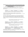
For example, let A and B be two reference positions:
ƒ
ƒ
ƒ
ƒ
ƒ
If a read can be mapped to position A and position B on the reference genome, with two mismatches for
A, and one mismatch for B, then B is reported as the unique mapping position for this read.
If both A and B contain two mismatches, then this read is not reported
If there are two mismatches and an indel of length one for A, one mismatch and an indel of length two
for B, then A is reported.
If there are two mismatches for both A and B, an indel of length one for A, an indel of length two for B,
then A is reported.
If, there are two mismatches and an indel of length one for both A and B, then this read is not reported.
The depth of mapped reads / Coverage:
The amount of mapped reads covering the position of
the reference sequence is called the depth of mapped reads on the position or the coverage of the
position on the reference sequence.
ZOOM:
Zillions Of Oligos Mapped, a next generation sequencing analysis tool
7
Chapter
Installation
2.
Getting started with ZOOM
2.1
Package contents
2
The ZOOM package should contain:
ƒ
ƒ
This manual (hardcopy and/or electronic version)
ZOOM software
2.2
System requirements
ZOOM will run on most platforms with the following requirements:
ƒ
ƒ
ƒ
ƒ
Processor: Equivalent or superior processing power to an IntelTM Pentium 4 Processor 1.6GHz
Memory: 2 GB memory (8 GB RAM is recommended for processing large data set)
Operation System: Microsoft Windows XP or above, and/or 64bit Unix/Linux operation system
Display: 800 pixels by 600 pixels minimal
2.3
Instrumentation
ZOOM will work with both single-end reads and paired-end reads of length ranging from 12bp
to 240bp from the following next generation sequencing instruments:
ƒ
ƒ
Illumina/Solexa: *_seq.txt and *_prb.txt, *.fastq
Applied Biosystems Inc. SOLiD: *.csfasta, *_QV.qual, *.fastq
2.4
Install ZOOM Studio
Note: If you already have an older version of ZOOM installed on your system, please uninstall it
before proceeding.
8
1.
Close all programs that are currently running.
2.
Insert the ZOOM disc into the CD-ROM/DVD-ROM drive. If loading ZOOM via the
download link, skip to step 4, after downloading and running the file.
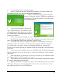
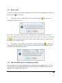
3.
Auto-run should automatically load the installation
software. If it does not, find the CD-ROM drive and open it to
access the disc. Click on the autorun.exe. (On Linux system,
click ZOOMsetup.bin)
4.
A menu screen will appear. Select the top
item “ZOOM Installation”. The installation utility
will begin the install. Wait while it does so. When
the “ZOOM Studio” installation dialogue appears,
click the “Next” button.
5.
Basic system requirements will be presented. “Click Next”.
6.
Read the license agreement. If you agree with it, change the radio button at the bottom to
select “I accept the terms of the License Agreement” and click “Next”.
7.
Choose the folder/directory in which you would like to install ZOOM. To change the
default location press the “Choose…” button to browse your system and make a selection, or
type a folder name in the textbox. Please avoid installing ZOOM in the “Program Files”
directory as well as in any directory for which the ZOOM user will not have write-permissions.
Click “Next”.
8.
Choose where you would like to place icons for ZOOM Studio. The default will put these
icons in the programs section of your start menu. A common user preference is on the desktop.
Click “Next”.
9.
Review the choices you have made. You can click “Previous” if you would like to make
any changes or click “Next” if those choices are correct.
10.
ZOOM Studio will now install on your system. You may cancel at any time by pressing
the “Cancel” button in the lower left corner.
11.
When the installation is complete, click “Done”. The ZOOM Studio menu screen should
still be open. You may view movies and materials from here. To access this menu at a future
date, simply insert the disc in your CD-ROM drive.
9
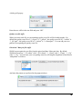
2.5
Registering ZOOM
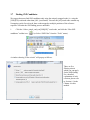
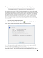
The first time ZOOM is run, the “About dialogue”
containing license wizard will appear automatically.
Click “launch license wizard” button to register your
copy of ZOOM :
Registration Instructions (Internet Connection)
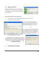
1.
2.
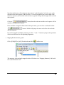
Select “Request a license file (has Internet connection)” and click “Next”.
The following window will appear:
If you have purchased ZOOM and have a
registration key, select “Registration Key”.
Enter your registration key as well as your
name and email address and click “Next”.
OR
If you are trying a demo of ZOOM and do not
have a registration key, select “Request a 30
days evaluation license (No registration key
required). Enter your name, email address, as
well as your institution. Click “Next”.
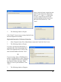
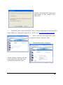
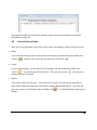
3.
The following window will appear:
An automated BSI service will generate the license file
(license.lcs) and email it to the provided email account from
the License Wizard. You can either save the attachment to a
local directory or copy the content between '===>' and
'<===' in
n the email. Click “Next”.
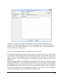
4.
The following window will appear:
10
Select “paste the license content from the
email” to paste the license information
between '===>' and '<===' in the email
or select “import the license file (the
email attachment) and browse to locate
the license file (license.lcs). Click
“Next”.
5.
The following window will open:
Click “Finish” if you receive a message that the license
has been imported successfully.
Registration Instructions (No Internet Connection)
1.
2.
Select “Request license file (without Internet connection)” and click “Next” twice.
The following window will open:
If you have purchased ZOOM and have a
registration key, select “Registration Key”.
Enter your registration key as well as your
name and email address and click “Next”.
OR
If you are trying a demo of ZOOM and do
not have a registration key, select “Request a
30 days evaluation license (No registration
key required). Enter your name, email
address, as well as your institution. Click
“Next”.
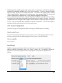
3.
The following window will appear:
11
Select the “Save Request File” button to save
license.request to your computer (PC1).
Click “Next”.
4.
Transfer the license.request file from PC1 onto a computer with an Internet connection (PC2)
using a USB key or a removable storage device. On PC2, go to http://www.bioinfor.com/lcs20/
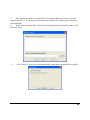
5.
Select “I have the license request file. I want
to register the software” and click “Next”.
6.
The following window will appear:
Click the “Browse” button to select the
license.request file, type in the visual
verification code and click “Next”.
12
7.
After the license email is received on PC2, save the attachment, license.lcs, as is and
copy the file to PC1. If you do not receive the license.lcs file in your inbox, please check your
junk mail folder.
8.
In the license wizard on PC1, click the 'browse' button below to select the license.lcs file
and click “Next”.
9.
Click “Finish” if you receive a message that the license has been imported successfully.
13
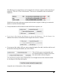
Re-registration Instructions
Re-registering ZOOM may be necessary if your license has expired or if you wish to update the
license. You will need to obtain a new registration key from BSI. Once you have obtained this
new key, select “About” from the Help menu. The “product information” dialogue box will
appear:
Click the “launch license wizard” button to continue. Then follow the instructions listed above
for registering ZOOM Studio.
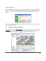
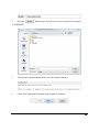
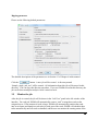
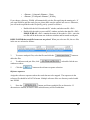
2.6
Set up your working environment
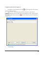
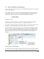
The ZOOM Studio works in client-server mode. The following graphical user interface (called
“ZOOM GUI”) is the main work space for you to load your data, submit them to server(s) for
computational tasks, monitor the working progress, and view the analysis results:
14
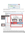
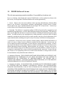
ZOOM GUI relies on one or more components to perform the actual time-consuming
computational tasks. These components are called “ZOOM servers” (or “servers” for short in
this manual), which do not necessarily have to reside in the same machine as the ZOOM GUI.
Generally, the more ZOOM servers that are used, the faster and less time you will need to
process data, illustrated below:
B ZOOM server 1
192.168.1.5 [20001]
A ZOOM GUI
ZOOM server 2
192.168.1.4
ZOOM server 3
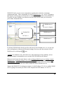
By default, ZOOM Studio already provides and started a local ZOOM server, so you can start
your work right now without more advanced settings (You can verify the existence of local
ZOOM server by clicking the
icon).
NOTICE: For Windows users, the built-in server has limited processing capability, and we
therefore strongly recommend the user to use the LINUX ZOOM servers instead.
If the user needs more advanced features such as starting multiple servers or starting a remote
ZOOM server, or utilizing multiple cores of modern CPUs, please follow these steps to add a
ZOOM server manually. The user is required to configure both the client side (computer A,
where ZOOM GUI is) and the server side (computer B, where ZOOM server is).
Suppose the ZOOM GUI is running on computer A with IP address 192.168.1.4, and the ZOOM
server is going to run on the port 20001 on the computer B with IP address 192.168.1.5).
15
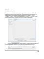
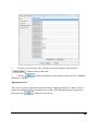
Configuration of the client side (Computer A)
icon on the right side of the toolbar to
1.
On computer A, in the ZOOM GUI click the
launch the configuration dialog.
2.
Input 192.168.1.5 in the address box and 20001 in the port box, then click the
button (the user may wish to remove the existing servers first). The new ZOOM
server appears in the list but is deactivated ( on the left), because it has not been launched on
computer B yet.
3.
Close the dialog.
16
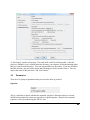
Configuration of the server side (Computer B)
Important: each copy of ZOOM server requires its own directory to run, and multiple servers
should NEVER be launched within same directory.
Computer B can have either a Windows or LINUX platform, and the users should choose the
appropriate distribution of server binary file for their system. If B is Windows platform, the
ZOOM server file is called zoomsrv.exe (together with supporting pthreadGC2.dll and
mingwm10.dll), and if B has LINUX platform, the ZOOM server file is called ZOOM. Copy the
proper ZOOM server file in the ZOOM package to computer B.
For Windows platform:
1.
On computer B, create a new directory and transfer zoomsrv.exe, pthreadGC2.dll,
mingwm10.dll, start_server.bat into it. You should always create a new directory for each copy of
ZOOM server.
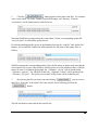
2.
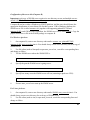
Use file editor (such as Notepad) to open start_server.bat , search for corresponding lines
and change as follow:
3.
Tell the ZOOM server where the ZOOM GUI is:
set ZOOMGUI=192.168.1.4 4.
Specify the port the ZOOM server is going to use:
set SERVER_PORT=20001 5.
Specify how many cores the ZOOM server will use (assuming a quad-core CPU):
set MAX_CLIENT=4 6.
Execute start_server.bat to start up the ZOOM server.
For Linux platform:
1.
On computer B, create a new directory and transfer ZOOM, start_server.sh into it. You
should always create a new directory for each copy of ZOOM server.
2.
Use file editor (such as vim) to open start_server.sh, search for corresponding lines and
change as follow:
17
3.
Tell the ZOOM server where the ZOOM GUI is:
export ZOOMGUI=192.168.1.4 4.
Specify the port the ZOOM server is going to use:
export SERVER_PORT=20001 5.
Specify how many cores the ZOOM server will use (assuming a quad-core CPU):
export MAX_CLIENT=4 6.
Execute start_server.bat to start up the ZOOM server.
Back on computer A, in the ZOOM GUI click the
icon again to verify that the newly added
ZOOM server is activated. If the icon turns to , then the new server has been correctly
launched.
The user can repeat these steps to start up more servers on different ports on computer B, or start
up more servers on other computers or even different platforms.
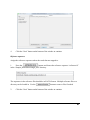
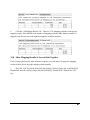
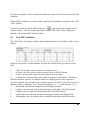
Setup job batch size
ZOOM will split large reads data into several small data files. According to the number of CPUs
you assigned, these small data will automatically be scheduled to run in parallel on multiple
CPUs. To fit the multiple small data files in the RAM of server, you’d better modify the size of
the split files according to the RAM per CPU can use. For example, if you have a server with 8G
RAM and you have set MAX_CLIENT=4 (i.e. four tasks can be run in parallel), then the RAM
18
each CPU can use is 8G / 4 = 2G. The default data size is 4 million reads per small file, which is
good for 2G RAM per CPU. If the RAM per CPU on your server is smaller or larger, click
choose “System Configuration” and decrease or increase the batch file size.
,
We use the RAM per CPU rather than the total RAM of the server as the criteria to decide the
amount of reads of each task is because different servers might have different architectures. For
example, some architecture is multiple CPUs sharing the same RAM, while others are multiple
CPUs which have their own RAMs.
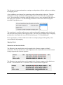
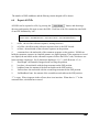
2.7
Command line usage of ZOOM
Starting from version 1.3.0, computational tasks are carried out and completed between ZOOM
GUI and ZOOM server cooperatively, but the users can still use the ZOOM server as a command
line tool.
19
20
Chapter
3
Quick Start
3.
Quick Start to Use ZOOM
T
his section of the manual will walk you through most of the basic functionality of
ZOOM. After completing this section you will see how easy it is to map a huge
amount of reads with automatic scheduling, view mapping results and find SNPs and
short Insertions/Deletions on both single-end reads and paired-end reads for both
Illumina/Solexa instrument and ABI SOLiD instrument.
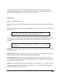
3.1
Sample Data
ZOOM provides two sets of sample data in the “Sample_Data” directory. The “Solexa” directory
contains an Illumina/Solexa test data set and the “SOLiD” directory has ABI SOLiD test data set.
1.
In the Solexa directory, there are two directories:
ƒ
ƒ
2.
In the SOLiD directory, there are two directories:
ƒ
ƒ
3.2
“single_end” directory: “read.fastq” and “reference.fa”;
“paired_end” directory: “read_1.fastq”, “read_2.fastq” and “reference.fa”;
“single_end” directory: “read.fastq” and “reference.fa”;
“paired_end” directory: “read_F3.csfasta”, “read_F3_QV.qual” and “reference.fa”;
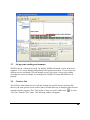
The main windows of ZOOM
The following picture shows the main windows of ZOOM:
21
3.3
Set up your working environment
ZOOM works in a client-server mode. By default, ZOOM will launch a server in the local
computer. Let’s use the default configuration in this quick start section. If you want to use
different servers or multiple CPUs on multiple servers, refer to the “Set up your working
environment” section in Chapter 2 to configure the ZOOM GUI client and ZOOM server
properly.
3.4
Create a Job
This will be a rather simple job as it will only contain one read file and one reference file,
however, the same process can be used for jobs with reads directory or multiple reads files and
multiple reference sequence files. Click on the “Create a new job” toolbar icon “
“New Job” from the “File” menu. The following window will appear:
” or select
22
Basic information
This part is used to assign a name for your job and a directory to store the data related to your
job. After you finished the job, you can load the job to display results or post-analysis.
1.
Enter a name for your job in the blank field beside the “Job Label”, for example
“Solexa_single_end_test”.
23
2.
Press the “
“F:\ZOOMDB”.
” button to specify a directory to save your job. For example,
3.
You can enter any descriptions about your job for later reference.
4.
Click “Next” button on the bottom of the window to continue.
24
Input reads
All reads data are input here.
There are two ways to input reads files, by selecting read files or directories. ZOOM will
automatically search for all the reads file inside. Please note that the read file should be in a
standard format of next generation sequencing technologies. For example, “*_seq.txt”,
“*_qual.txt”, “*.fastq”, “*.fasta” files for Illumina data, or“*.csfasta”, “*_QV.qual”,“*.fastq”
files for ABI SOLiD data. For details, please refer to Chapter 4 in this manual.
1.
Click the “
” button, navigate to “Sample_Data\Solexa\single_end”
directory and select the “read.fastq” file. The file will be selected in the read file list.
25
Click the “
2.
” button again to select other reads files. For example,
select “read.csfasta” file in the “Sample_Data\SOLiD\single_end” directory. Then the
“read.csfasta" will be loaded into the read file list too.
Note that ZOOM also recognizes that the “read.csfasta” file has a corresponding quality file
“read_QV.qual”. It will load the quality file too.
By clicking and dragging the mouse on the boundary between the “read file” and “quality file”
headers, you can tune the width of the tablet and show the full name of the quality files, as
follows:
ZOOM recognizes the corresponding quality file by the file names so please make sure that the
read sequence file is in the same directory with the quality score file and the prefixes of the file
names are same. For Illumina/Solexa data, the “<filename>_seq.txt” will be matched with
“<filename>_qual.txt”. For ABI SOLiD data, the “<filename>.csfasta” will be matched with
“<filename>_QV.qual”. The quality score in the FASTQ format will be loaded directly.
”, you can remove
3.
By selecting the files you don’t want and clicking “
these files. Select the “read.csfasta” file in the read file list as following and click the
“
” button.
This file will then be removed from the read file list.
26
4.
Click the “Next” button on the bottom of the window to continue.
Reference sequences
Assign the reference sequences where the reads data are mapped to.
1.
Press the “
” button, and choose the reference sequence “reference.fa”
in the “Sample_Data\Solexa\single_end” directory.
The sequences in the reference files should be in FASTA format. Multiple reference files or a
directory can be loaded in. Use the “
2.
” button to remove files if needed.
Click the “Next” button on the bottom of the window to continue.
27
Mapping parameters
Please use the following default parameters:
The detailed descriptions of the parameters are in Section 4.3 of Chapter 4 in this manual.
” button. A new job will be created. A directory named
Click the “
“Sample_single_end_test” will be created. All information about this job will be stored in this
directory. You can copy this directory anywhere. If you use ZOOM to load in this directory, the
job can be shown and post-analysis can be carried out on it.
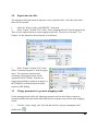
3.5
Monitor the job
After the job is created, the job will be shown in the “Job View” panel in the left window of the
interface. For each job, ZOOM will automatically create a “task” to map these reads on the
assigned server. If the amount of reads is large, ZOOM will automatically partition the reads
into several parts and launch several tasks for each part of the reads. ZOOM will schedule these
tasks automatically until all reads are handled, and the user can monitor the running status of the
28
jobs and the tasks according to the corresponding progress bars in the “Running Monitor”
window.
Progress Bar
Depending on the data size, it may take some time to load the data. The time is related to the
data size of the reads data file. A progress bar will pop up showing the progress of loading data.
ZOOM won’t respond until the progress bar has disappeared.
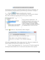
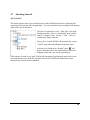
Job View panel
After loading the data, you will see the job in the “Job View” panel:
The “Job View” panel which is shown in the upper
left hand corner displays the organization of a
particular job. Use the ‘+’ and ‘-’ boxes to expand
and collapse the job in order to know the
organization of this job. In each job node, there is a
29
“Scheduling” node and a “Results” node.
The “Scheduling” node shows all the tasks this job has been split to and scheduled on the server.
The “Results” node will not appear until all reads mapping tasks are finished. It will contain the
uniquely mapped results (suffixed by “[UNIQUE]”) and the top N mapping results (suffixed by
“[ALL]”) according to the running parameters.
Running status of the job
Clicking on the job node, the “Running Monitor” will show the progress of the job.
” button to display the
Click the “
properties of this job, including the read files and the
reference files, using parameters and mnemonic notes.
Click on a task node. The progress of the task will be shown.
Control the job
If you want to cancel or restart a job or several jobs, choose the corresponding job nodes, and
then click the “
” tool bar icon or the “
” toolbar icon.
30
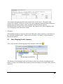
3.6
Display Mapping Results
When the job icon turns into “ ”, the job is finished. You can show mapping results or carry
out SNP analysis now. Make sure that you select the node under the “Results” node when
choosing data to be analyzed.
1.
Select the “UNIQUE” node in the “Results” node on the “Job View” panel and click the
“Display mapping result” toolbar icon “
”.
2.
ZOOM will assemble the mapped reads into a consensus sequence and show the read
depth overview along the reference sequence. This will take some time depending on the amount
of mapped reads and the length of the reference sequence. A progress bar will pop up.
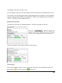
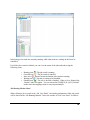
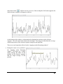
3.
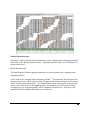
After the progress is finished, you can see a tabbed window containing the mapping
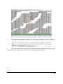
results on the right hand of the main window of ZOOM as follows:
31
The line in the graph is the overview of the read depth of those mapped reads along the reference
sequence. The horizontal ruler denotes the positions on the reference sequence. The vertical
ruler denotes the read depth.
4.
Press “ ” button
to zoom in the graph or
press “ ” to zoom out in
the graph.
5.
Click the left
button on your mouse and
drag along the graph to
form a rectangle region,
and then release the mouse
button.
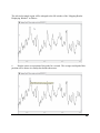
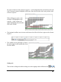
32
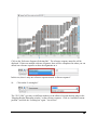
The selected rectangle region will be enlarged to the full window of the “Mapping Results
Displaying Window” as follows:
6.
Rest the cursor on a position of the peaks for a second. The average read depth of this
position will be shown in a tooltip box besides the mouse.
33
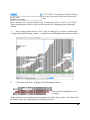
7.
Click on a place in the “Mapping Results Displaying window”. The detailed alignments
of the mapped reads along the reference sequence will be shown as follows:
Difference between this read and the reference sequence Read sequence
Consensus sequence Reference sequence The sequence at the bottom of the window is the reference sequence. The sequence with green
background over the reference sequence is the consensus sequence generated by the mapped
reads along the reference sequence.
The orange background of the nucleotides on the read or the consensus sequence highlights the
difference from the nucleotide on the position of the reference sequence.
The default display of the read is in the nucleotide space. For ABI SOLiD data, the default
display is the decoded nucleotide reads according to the mapping results. Press “
switch the reads display from the nucleotide space to the color space, and “
reads shown in color space look like the following:
” button to
” vice versa. The
34
8.
Click or drag the horizontal scrollbar will let you navigate along the reference sequence.
9.
Click or drag the vertical scrollbar on the right to show more reads aligned to this region
when all the reads mapped here cannot fit in the “Mapping Results Window”.
35
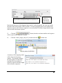
Click on the “Reference Sequence Selecting Bar”. The reference sequence name list will be
displayed. If there are multiple reference sequences, there will be a dropdown list where you can
choose one reference sequence to show the alignments on it.
In this case, there is only one reference sequence named “reference sequence”.
10.
Click on the “Locating bar”.
The “2513-2500” (you may see different numbers) is the offsets of current showing range in the
“Mapping Results Illustrating window” on the reference sequence. Click on “remember current
position”, and click the “Locating bar” again. You will see:
36
“0:2513-2590” is recorded here, and by selecting
this entry, you can go back to this region at any
time.
Enter a new position or a position range in the “Locating bar” such as “1234” or “1234-4560”.
Then read alignments in the new region will be shown in the “Mapping Results Illustrating
window”.
11.
Enter a single position such as “1234” in the “Locating bar” or click on a column in the
““Mapping Results Illustrating window”. A light blue bar will highlight this position as follows:
12.
Click on any read in the “Mapping Results Illustrating window”.
The read will be highlight by a red
rectangle.
At the same time, more information of this mapped read will be shown in the “read information”
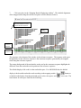
tab window below the “Mapping Results Illustrating window”:
37
Each black block indicates the quality score on this position. The higher the block is, the higher the quality score of this position is. The red nucleotide is the difference between the read and the reference sequence segment. Note that the direction of the alignment shown in the “read information” tab is the same as the
direction of the read sequence in the read files. If a read is mapped to the reverse chain of the
reference sequence, the reference segment is reversed and the left offset is larger than the right
offset as shown in the above picture.
13.
Click the “
will be copied to the clipboard of system.
14.
” button, then the read name and the read sequence
Click the “Solexa_single_end_test” job node and click “
” toolbar icon.
A summary of the mapping results
will be shown in the pop up
window. The summary includes
the total number of reads in the
read data files, the number of
reference sequences and the length
of the reference sequences:
38
Click on the “Unique Mapping Results” tab to show the number of reads mapped uniquely and
the statistics of the uniquely mapping results:
15.
Click the “UNIQUE” results node, and click the “
” toolbar icon.
The summary of the uniquely mapped results will be show in a “Mapping Summary” tab
window beside the “read information” tab.
39
3.7
Finding SNP Candidates
We suggest that users find SNP candidates only using the uniquely mapped reads (i.e. using the
[UNIQUE] result node other than [ALL] result node). Because the [All] result node contains top
N mapping results for each read, those reads mapped to multiple positions of the reference
sequence will make the SNP finding process unreliable.
1.
Click the “Solexa_single_end_test[UNIQUE]” result node, and click the “filter SNP
candidates” toolbar icon “
” (or Select “SNP Filter” from the “Tools” menu).
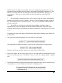
A window showing “Filter criteria” will pop up as follows:
There are five
filtering criteria
which you can apply
for the SNP finding.
For a detailed
explanation of each
criterion, please refer
to Section 6.1 in the
Chapter 6 in this
manual.
40
2.
Click on the checkbox of the filtering criterion “At least … reads are mapped to this
position” and revise the value to 10.
3.
Press “OK” button. Then SNP
finding on all the reference sequences
will be carried out. A progress bar
will pop up:
4.
When all SNP candidates are located, a table containing SNP candidates will appear in
the “SNP Caller” tab as follows:
41
Each row of the table is a SNP candidate. The table has 9 fields showing 9 features of each SNP.
The description of each field is in Section 6.2 in Chapter 6.
” button. The
Click the “
amount of SNP candidates satisfying the
filtering criteria and the filtering criteria
adopted will be shown:
5.
Double click the first row in the table to show the first SNP.
The light blue bar
will highlight the
SNP
position.
You can check the
alignment around
this position in
detail. You can
double click each
row in the table to
see
the
SNP
candidate details.
1.
2.
42
6.
Click one read in this position and click the “read information” tab. You can check the
quality of the position of this read to know whether the SNP candidate is more likely a true SNP
or a sequencing error.
7.
Click the “SNP Caller” tab to show the SNPs (show what??). Click the “
” or the
“
” button to jump to the previous or the next SNP candidate.
8.
Click the “Read Depth” field in the header of the SNP table to sort the candidates
according to the read depth in ascending order. Click it again to sort in descending order.
Similarly each field in the SNP table can be sorted.
9.
Click the “
” button to export the SNP candidates into a file. All SNP
candidates will be exported in a format of the nine fields as each line in the SNP table.
43
3.8
Export data into files
The mapping results and consensus sequence can be exported to files. Note that only results
nodes can be exported.
1.
Select the “Solexa_single_test[UNIQUE]” result node.
2.
Select “Export” from the “File” menu. Select “Mapping Results” from the popup menu.
There are four output formats to export mapping results into. Please refer to Section 7.1 in
Chapter 7 in this manual for the description of each format.
3.
Select “Export” from the “File” menu.
Select “Consensus Sequences” from the popup
menu. The consensus sequence built
according to the mapping results will be
exported in FASTA format. Note that we
suggest only building a consensus sequence on
the [UNIQUE] result node based on similar
reason for SNP finding.
3.9
Change parameters to get more mapping results
For the unmapped reads of this job, adjusting parameters such as the reference sequences,
mismatch number allowed between reads and reference sequences may achieve more mapping
results.
1.
Click the “Solexa_single_end” job node and click the “reprocess unmapped reads”
toolbar icon “
”.
44
The following windows will pop up:
The process is similar to creating a new job, except that the reads data is the unmapped reads of
the selected job. Assign a name to the new job for these unmapped reads. The default name is
the original name suffixed by “.more”.
2.
Click “Next” twice to the “mapping parameters” step.
3.
Check the radio box from the “the unique …” to “top…”, and modify the value to 2, to
keep up to 2 mapping results for each read.
4.
Modify the mismatch
number from 2 to 4, which will
allow up to four mismatches
between the reads and the
reference sequences.
5.
Click the check box to “achieve high sensitivity”.
45
This will achieve full sensitivity to find all the mapping results with up to 4 mismatches. For
more information on using this parameter, please refer to step 4 in Section 4.3 in Chapter 4.
6.
Click the “
” button to create this new job. A new job
“Solexa_single_end_test.more” will be created and processed. After the new job is finished,
there will be an additional job appearing in the “Job View panel” as follows:
The new job has two Results nodes --- the
[UNIQUE] and the [ALL] node because we set
the parameters to collect top two mapping
results for each read. The uniquely mapped
result is in [UNIQUE] result node, while the top
two mapping results are in the [ALL] node.
Click the “
” toolbar icon. The job summary window will appear:
1983 reads are unmapped in the “Solexa_single_end_test” job. There are two summaries for
uniquely mapped results and the top two mapped results, respectively.
7.
Click the “Unique Mapping Results” tab. You can see that 1783 reads are mapped after
increasing the mismatch number from 2 to 4 between the reads and the reference sequence.
46
8.
Click the “All Mapping Results” tab. There are 1795 mapping positions in the top two
mapping results. Note that this is the number of mapping positions rather than the number of
mapped reads, because one read might be mapped to multiple positions.
3.10 Show Mapping Results of Several Jobs Together
If two or more jobs have the same reference sequence, you can choose to merge the mapping
results of these jobs to show the mapping results together.
1.
Press the “Ctrl” key on the keyboard, and click the “Solexa_single_end_test[UNIQUE]”
Results node and the “Solexa_sinlge_end.more[UNIQUE]” Results node. Release the “Ctrl”
key.
47
2.
Click the “
results window”.
” toolbar icon, to display the merged mapping results in the “mapping
You can do any operation on it as single result node, or SNP finding on these merged mapping
results.
48
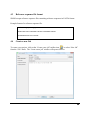
3.11 Remove jobs
If you want to remove jobs from the workspace or disk, click the corresponding job nodes, and
then click the “
” tool bar icon.
1.
Click on the “Solexa_single_end_test” job node and click the “
confirming dialog will pop up:
” tool bar icon. A
Press “OK”. The “Solexa_single_end_test” job node will be removed from the “Job View”
panel. This operation will only remove the job node from the “Job View” panel. You can click
the “ ” open icon, and select the directory where “Solexa_single_end_test” is stored to load
the job into your workspace again.
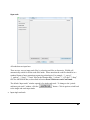
2.
Click on the “Solexa_single_end_test.more” job node and click the “ ” tool bar icon.
Click on the checkbox and press “OK”. All the items related to the job including the directory
on the disk will be deleted permanently.
3.12 Paired-end/Mate-pair read mapping example
We assume that you have gone through the above single-end reads mapping process. Now we
will explain how to map paired-end/mate-pair reads, focusing only on the operations that are
different from mapping single-end reads.
49
1.
Click “
2.
Click the “
Click “
” to create a new job named “ABI_mate_pair_test” as follows:
” button to move to the “Input reads” step.
” to change to the mode of inputting mate-pair reads as follows:
50
The read file list window is split into two windows, each window load each end of the mate-pair
reads file. Make sure every two files in the same row of the left and the right window are paired.
” button. Choose both “read_F3.csfasta” and
3.
Click the “
“read_R3.csfasta” files in “Sample_Data\SOLiD\mate-pair\” directory. ZOOM will
automatically recognize the possible paired files and put them in one row together with their
quality file if any.
ZOOM automatically finds paired read files according to the suffix of the files:
<filename>_F3.csfasta will be paired with <filename>_R3.csfasta; and <filename>_1.fastq will
be paired with <filename>_2.fastq.
If you choose a directory, ZOOM will automatically pair the files satisfying the naming rule.
Thus if you want ZOOM to pair the read files for you, please make sure the file suffixes are
correct. You can choose to add some patterns of recognizing paired-end files as described in
Section 4.10. Otherwise, you will need to feed in the reads files one pair by one pair by yourself
as follows:
o Double click the left “forward read file” window, and select the
“Sample_Data\Solexa\pair-end\read_1.fastq”.
o Double click the right “reverse read file” window, and select the
“Sample_Data\Solexa\pair-end\read_2.fastq”.
PLEASE KEEP IN MIND that two reads files in one row are paired. When you select one
file, the two files in the row are both selected as follows:
51
o Select the Solexa data and click the “
” button to
delete the file. We will not be using this set of data in the following
tour.
4.
Click “
” to move on to the “Reference sequences”. Choose the “reference.fa”
file in the ““Sample_Data\SOLiD\mate-pair\” directory. Click “
” to move on to the
“Mapping Parameters”.
5.
The estimated range of the distance between two reads of one mate-pair is [800, 2000].
Set the paired-end parameters as follows:
Keep the top two mapping results for each read:
Click “
” to create the “ABI_mate_pair_test” job.
6.
After the job is finished, click the “ABI_mate_pair_test[UNIQUE]” result node and click
the “
7.
” toolbar icon to show the mapping results.
Click any place in the “Mapping Results Illustrating window”, select a read, and press the
“
” button. ZOOM will then jump to the pair of the selected read.
52
53
Chapter
4
Load Data
4.
Data Format
Before loading any data files into ZOOM, please make sure that the data is in an acceptable
format.
ZOOM accepts reads from both Illumina/Solexa data and ABI SOLiD color space data. ZOOM
can handle data files in the following formats:
4.1
Illumina data
ZOOM accepts five types of Illumina/Solexa read files as input. These file formats are
automatically recognized. The letters of the read sequences are case insensitive. The length of
the reads can be different.
FASTA format
Example of FASTA format:
>read1A_1 AGGACTATATTGCTCTAATAAATTTGCCGGTTCTTA >read1A_2 TCTAATAAATTTGCCGGTTCTTAAAAACTCAAT >read1A_3 54
In ZOOM, FASTA format files have no sequencing quality scores, thus all the read bases
including N are considered equally relevant.
*_seq.txt and *_prb.txt Files
Please put the *_seq.txt and *_prb.txt in the same directory. ZOOM will pair the
<filename>_seq.txt and <filename>_prb.txt automatically.
Example of *_seq.txt file format:
1 1 125 701 GCTACCCTTTAGGTTTAA Each line of the sequence file records the channel number, tile number, x position, y position of
each sequence read, and the sequence of the read. The labels of each read sequence are in the
format of <channel number>_<tile number>_<x position>_<y position>.
Example of *_prb.txt file format:
40 ‐40 ‐40 ‐40 40 ‐40 ‐40 ‐40 40 ‐40 ‐40 ‐40 40 ‐40 ‐40 ‐40... The *_prb.txt file contains the quality score of each possible nucleotide base for the given cycle
number. Four numbers, such as -40 40 -40 -40, each separated by a space, are the sequencing
quality scores associated for each possible nucleotide, ACGT, respectively. The tab character is
used to separate the bases of each cycle. Each line of *.prb is associated with the corresponding
line of *_seq.txt.
*_prb.txt Files
Example file:
40 ‐40 ‐40 ‐40 40 ‐40 ‐40 ‐40 40 ‐40 ‐40 ‐40 40 ‐40 ‐40 ‐40... *_prb.txt file is the same as the description in part 2 above. ZOOM can process this file without
corresponding *_seq.txt file as input. The difference is that the labels of each read sequence are
automatically assigned.
55
FASTQ Format
ZOOM accepts FASTQ format, where four lines represent one read in the following format:
@read_name read sequence Example of FASTQ format:
@071113_EAS56_0053:1:1:756:463 GTGATTAGTGAAACATAAAATAGTTTCATGTTGAAA + IIIIIIIIIIIIIIIIIIIIIIIIIIIIIIIIGIAI @071113_EAS56_0053:1:1:813:752 The FASTQ format includes Sanger FASTQ format and the Illumina/Solexa FASTQ format,
which scale differently. For Sanger FASTQ format, the quality score of each position equals
ord($q)-33, while for Illumina/Solexa FASTQ format, the quality score of each position equals
ord($q)-64. When creating a job, ZOOM has a combo box in the parameter selection part to
assign whether the FASTQ format is Sanger FASTQ format or the Illumina/Solexa FASTQ
format.
One read per line with quality scores
Example format:
4_87_872_656 ACGTACNT 40 40 40 40 35 60 0 70 56
The first column contains the read sequence label or description, the second column contains the
sequence data of the read, and the third column contains the quality scores for each base. Note
that the read sequence label or description should not have a space inside.
4.2
ABI SOLiD color space data
Applied Biosystems SOLiD *.csfasta File
ABI SOLiD represents their reads in color spaces. Any two adjacent nucleotide bases from the
read are represented by one of four colors. The mapping relationship between base space
(nucleotide) and color space is denoted in the definitions section under “color space”.
In this release, ZOOM accepts the color space data (*.csfasta) from SOLiD, in which each read
is a numeric string prefixed by a single base. The base that precedes the numeric (color code)
data is the final base of the sequencing adapter.
Example of *.csfasta file format:
>1_6_678_F3 T0030011000002120322220223 >1_6_1142_F3 T1011010321313123321022222 >1_6_1616_F3 T2220012213121322223113320 Applied Biosystems SOLiD *.csfasta and * _QV.qual File
ABI SOLiD data stores color space sequence of reads in *.csfasta file and corresponding quality
score of each read in *_QV.qual file. Note that ZOOM load the quality score file along with the
*.csfasta file automatically. So please put the *.csfasta file and the *_QV.qual file together in
one directory and set the prefix file name the same.
Example of *_QV.qual file of the above *.csfasta:
57
>1_6_678_F3 10 8 24 10 14 8 11 10 5 8 5 10 5 7 2 3 9 2 3 5 2 7 4 4 5 >1_6_1142_F3 8 11 8 17 14 8 25 20 15 14 16 17 11 10 19 16 25 15 5 16 13 19 10 6 12 >1_6_1616_F3 2 11 8 8 6 7 3 4 11 8 5 16 8 10 11 6 3 14 16 9 5 19 7 10 8 >1_6_1634_F3 Applied Biosystems SOLiD *.fastaq File
The contents in *.csfasta and *_QV.qual can be integrated as a CSFASTQ file. It is similar to
the FASTQ format, where four lines represent one read. The only difference is that the read
sequence is in color space format.
@read_name read sequence The quality score of each position is denoted by a nucleotide. The numerical score is ord($q)-33.
Example of CSFASTQ format:
@SRR015241.1 CLARA_20071207_2_CelmonAmp7797_16bit_26_88_34_F3 length=50 T32322133300002330031001022230020232002203222030231 +SRR015241.1 CLARA_20071207_2_CelmonAmp7797_16bit_26_88_34_F3 length=50 !21(()+%'+%40*.%%**)&%&*&%%%&%%%%%%%%%%%%%%%(+%%%%' There are two sequences in the above two example. Note that the first character of the quality
score string will be viewed as the quality of the adapter nucleotide.
58
4.3
Reference sequence file format
ZOOM accepts reference sequence files containing reference sequences in FASTA format.
Example format of a reference sequence file:
>Reference_sequence_1_name AGGACTATATTGCTCTAATAAATTTGCGGTTCTTAAAAACTCAATGT TGTAAAAATGTCACTTCTTCCCAAA… 4.4
Create a new Job
To create a new project, click on the “Create a new job” toolbar icon “ ” or select “New Job”
from the “File” menu. The “Create a new job” window will open as follows:
59
There are four steps to create a job.
Basic information
This section is used to assign a name for your job and a directory to store the data related to your
job. After you have finished the job, you can load the job to show the mapping results or
perform post-analysis by selecting the directory.
1.
Enter a name for your job in the blank field beside the “Job Label”:
If the job name you input already exists in the directory, there will be a tool tip icon below the
Browse button as follows:
You can choose to change the job name or to overwrite the existing directory.
2.
3.
” button. Select a directory to save your job.
Press the “
You can enter any descriptions about your job for future reference.
4.
Click the “
” button at the bottom of the window.
60
Input reads
All reads data are input here.
There are two ways to input reads files: by selecting read files or directories. ZOOM will
automatically search for all the reads files inside. Please note that the read file should be in a
standard format of next generation sequencing technologies. For example, “*_seq.txt”,
“*_qual.txt”, “*.fastq”, “*.fasta” files for the Illumina data, “*.csfasta” “*_QV.qual” “*.fastq”
files for ABI SOLiD data, as described in Section Error! Reference source not found..
The default “Input reads” window opened is for single-end reads. To change to the “pairedend/mate-pair reads” window, click the “
to the single-end reads input mode.
ƒ
” button. Click it again to switch back
Input single-end reads
61
1.
Click the “
” button. Choose the read file(s) or directories which
contain the read files. By default, ZOOM will find all the files suffixed by “*_seq.txt”,
“*_qual.txt”, “*.fastq”, “*.fasta”, “ *.csfasta ” “ *_QV.qual” files to load in as the reads file.
2.
To remove the files you don’t want, select the files and click the “
button. The files will be removed.
ƒ
3.
To add more files, click “
4.
Click the “
”
” again as step 1).
” button to move on to the reference sequence selection window.
Input paired-end reads or mate-pair reads
By default, the two mates of one pair are stored in two files separately, but you are allowed to
store the two mates of one pair next to each other in one file. However, in that case, please use
single-end reads mode to load reads and assign mapping in paired-end mode in the “Mapping
Parameters” section.
1.
Click the “
” button to change to paired-end reads input mode. The read
list window is split into two windows, each of which is for loading the file containing one mate
of a pair.
2.
Click the “
” button and select the read files or directories.
ZOOM will automatically pair these read files according to the file names. The paired file will
be on the same row of the two windows. ZOOM recognizes the read file pairs according to the
following file name patterns:
62
o <filename>_1.fastq and <filename>_2.fastq
o <filename>_F3.fastq and <filename>_R3.fastq
If you choose a directory, ZOOM will automatically pair the files satisfying the naming rule. If
you want ZOOM to pair the reads for you, please make sure the suffixes are correct. Otherwise,
you will need to upload the reads file pair by pair by yourself as follows:
o Double click the left “forward read file” window, and select one file <file1>.
o Double click the right “reverse read file” window, and select the other file <file2>.
MAKE SURE that <file2> contains the mates of the reads in <file1>, since the
two files will be in the same row in the two windows and be treated as read pairs.
KEEP IN MIND that reads file in one row are paired. When you select one file, the two files
in the row are selected as follows:
3.
To remove read pair files, select the files and click the “
delete the files.
4.
To add more read pair files, click “
windows as above.
5.
Click the “
” button to
” or double click the two
” button to the reference sequence selection.
Reference sequences
Assign the reference sequences where the reads data are to be mapped. The sequences in the
reference file should be in FASTA format. Multiple reference files or a directory can be loaded
into ZOOM.
” button, and choose multiple files or directories. If
1.
Press the “
directories are chosen, all FASTA files in this directory will be loaded there.
63
2.
To remove some reference files, click these reference sequences and click the
“
” button to remove these files.
3.
Click the “
parameters” window.
” button at the bottom of the window to proceed to the “Mapping
Mapping parameters
There are five groups of parameters in the following “Mapping parameters” window. The five
groups of parameters will be explained in next section. After choosing the proper parameters,
please press the “
” button to create the job.
64
A “Processing” window will pop up. The reads in the read files will be loaded. After this
process is finished, a job is created inside the directory you assigned. All the information about
this job is stored in this directory. You can copy this directory anywhere. If you use ZOOM to
load this directory, the job can be shown and post-analysis can be carried out on it. You can
inspect the status of this job in the “Job view window”.
4.5
Parameters
There are five groups of parameters that you can select from as prefered.
Organism
This is a checkbox to decide whether the organism is diploid. When the option is selected,
ZOOM will assemble the consensus sequence as a diploid genome. Bases in the consensus
sequence will be presented using the IUPAC code.
65
Pair-end Settings
Check the box when you want to align reads in paired-end mode.
If you check the box and there are no read files added in “paired file mode”, ZOOM will treat
every two sequences in the file added in “single file mode” as the two mates of a pair.
When selecting this box, please remember to assign the distance range between the two reads
that make up the read pairs as follows:
Read Qualities
Quality score of read reflects the sequencing quality of each base. The quality score of each base
denotes the probability that this base is correctly sequenced. By default, ZOOM displays the
quality scores along with the alignment between the read sequence and its target region on the
reference sequence, to give the users an intuitive impression about which bases have low quality
score., as follows:
Quality score can be utilized to enhance the mapping results as well.
If the reads files are in FASTQ format, according to the different methods of coding numerical
quality score into alphabet, there are two types of FASTQ format ------ “Sanger type” and
“Illumina type”. For Sanger FASTQ format, the quality score of each position equals ord($q)33, while for Illumina/Solexa FASTQ format, the quality score of each position equals ord($q)64.
Choose the correct type by
clicking the combo box.
ZOOM adopts two ways to utilize quality scores to enhance mapping results.
66
The first way is to ignore mismatches occurring on read positions with low quality scores during
the mapping process.
A low confidence score denotes low sequencing quality at that position in the read. Therefore,
mismatches occurring at positions with low quality scores are more likely due to sequencing
error. Thus mismatches on positions with high quality scores are more meaningful than those at
low quality score positions. Use the following combo box or enter some value to assign the
threshold of high quality score.
The second way is to utilize quality scores to rank several possible mapping results of each read
and choose the best position as the mapping results. Since the process happens after all mapping
positions have been found, this way will be described in part “5. Collecting Results”.
In our experiments, we observed that more reads were uniquely mapped when quality scores
were included to help mapping.
Mapping Criteria
Mismatches and insertion/deletion
The following is an example that a read is mapped to the reference sequence with only
mismatches. The four red characters in the alignment are the mismatches between the read and
its target region on the reference sequence.
The following is an example that a read is mapped to the reference sequence with a deletion on
the read. The read deletes an “A” nucleotide. There is one deletion of length one.
67
The following is an example that a read is mapped to the reference sequence with an insertion of
length one. The red “A” base is the insertion. There are two mismatches and one insertion of
length one.
ZOOM will map reads to the target regions on the reference sequence within a given mismatch
number or insertion /deletion length.
ƒ
If only mismatches are allowed between reads and reference sequences, use
ƒ
If you want to allow insertion and deletions, you can use edit distance too. The edit distance is the
addition of the number of mismatches and the length of the insertion / deletion.
ƒ
If you want to allow indels AND you want to assign the length of the indel, check the radio box and
the check box and assign the number you want as follows:
This will allow up to two mismatches and
one insertion/deletion of length one between
the reads and the reference sequence.
You can choose to assign a ratio of mismatches to read length instead of the mismatch number
by checking the following checking box:
Assign the ratio of mismatches of the read length.
68
Commonly, the ratio criterion is useful for those read files containing reads of various lengths.
Getting High Sensitivity Results
ZOOM adopts the optimal multiple seeds strategy to guarantee 100% sensitivity for a wide range
of read lengths and mismatch numbers. However, using these seeds might be time-consuming
especially for very long reference sequences. By default, ZOOM adopts the seeds guaranteeing
100% sensitivity to find all mapping positions having up to 2 mismatches with the reads. To get
high sensitivity, please click the following check box.
Then ZOOM will select the seeds with high sensitivity according to the mismatch number you
assigned. For cases where ZOOM can achieve 100% sensitivity, please refer to Chapter 8.
Note that this option might be time-consuming when your reference sequences are long. One
way to enhance the speed is to map reads without selecting this option first, then extract those
unmapped reads to utilize this option. Please refer to Section 4.7 for more information.
Collecting Results
Each read may be mapped to multiple target regions in the reference sequence. The best
mapping results of one read are the ones with the smallest edit distance, or in case of equal edit
distance, the shortest insertion/deletion length (under the consideration that insertion/deletions
are less probable than mutations). If there is only one such best mapping result for the read, this
is a uniquely mapped read. Otherwise, if there are multiple such mappings, the read will be
considered ambiguously mapped.
ZOOM finds all possible mapping positions satisfying the mapping criteria for each read.
However, you can choose to reserve the uniquely mapped reads or the top N mapping results for
each read. Choose the following radio box to switch between the two modes.
You can utilize quality scores to assess the mapping probability of possible mapping results of
each read and rank the mapping positions for each read according to the mapping probability
scores by clicking the following checkbox:
69
Note that only if top N mapping results are chosen, this option is available.
ZOOM adopts a re-score scheme. First, it finds all possible mapping positions of each read
within the mismatch threshold or edit distance threshold. Then it picks the multiple positions
(the addition of
and extra
) to compute
the probability of the alignments between the reads and these target regions. The mapping scores
(log10 (probability of the alignment)) are sorted to get the top N results as mapping results. In
our experiments, more reads can be uniquely mapped after re-scoring using quality scores.
The rescore function for the ABI SOLiD data has used the priori SNP probability of the organism,
therefore if the data set is ABI SOLiD data, please assign a priori SNP probability of the organism.
For example, for Human, this value can be set as 0.001.
4.6
Open a Job
1.
To open an existing job, select “Load Job” from the file menu or using the “Load job”
icon “ ” on the toolbar.
2.
Select the location of the data for that job.
3.
The job will be loaded in the Job View Panel. You can continue to rerun the job or
analyze mapping results for those finished jobs.
This option is useful when you want to close the client windows. After jobs are created, you can
close the ZOOM main windows. The jobs are running on the ZOOM server. You can open the
ZOOM main windows and load the job to inspect the running status or analyze the results at any
time.
70
4.7
Orienting Yourself
Job View Panel
This frame appears in the upper left hand corner of the ZOOM main window, displaying the
organization of particular jobs (if applicable). You can control these jobs and inspect the running
status of the jobs in this panel.
The jobs are organized as a tree. Each job is a job node
having two nodes. One is a “Scheduling” node, and the
other is a “Results” node. Use the ‘+’ and ‘-’ boxes to
expand and collapse each job.
After a job is created, ZOOM will automatically create a
“TASK” node under Scheduling to map these reads.
After the job is finished, the “Results” node “ ” will
appear containing one or two results nodes to show the
mapping results and carry out the post-analysis.
If the amount of reads is very large, ZOOM will automatically partition the reads into several
parts and launch several tasks for each part of the reads. ZOOM will schedule these tasks
automatically until all reads are handled.
71
In this image, four tasks are currently running, while other tasks are waiting on the list to be
scheduled.
For all the jobs created or loaded, you can view the status of the jobs and tasks using the
following icons:
o
o
o
o
o
Running icon “ ”: The job or task is running.
Canceled icon “ ”: The job or task is canceled.
Error icon “ ”: An error occurred when the job or task was running.
Waiting icon “ ”: The task is waiting to be scheduled.
Finished icon “ ”: The job or the task is finished. When a job is finished, the
“Results” node will appear. You can choose the [UNIQUE] or [ALL] “Results”
node to show the mapping results or carry out post-analysis.
Job Running Monitor Panel
When clicking a job or a task in the “Job View Panel”, the running information of this job or task
will be shown in the “Job Running Monitor” below the window of “Job View Panel” as follows:
72
Description panel
Inspector panel When a job is selected, the number of tasks in this job and the overall progress of this job will be
shown in the “Description panel”. The total number of tasks of this job and the progress of these
tasks will be shown in the “Inspector panel”. In the “Inspector panel”, each row is the running
status of a task. There are three columns denoting: the name of the task; the progress of this task;
the total running time of this task (appear until the task is finished). The running time is in the
format of “hours: minutes: seconds”.
When clicking a task in the “Job View Panel”, the
detailed progress of each step of the task will be shown.
Each row is a step of the task.
Usually, three steps are included in each task:
o Upload dataupload the reads sequences of this task to the server.
o Map readsmap the uploaded reads to the reference sequence according to
the parameters assigned.
o Get results
collect the mapping results from the server to the client to
show the mapping results and post-analysis.
Job Properties Panel
Select a job in the “Job View Panel” and click the “Job Properties” button. The properties of this job
will be shown in the popup tabbed windows.
73
The properties include the reads file list, reference sequence file list, the parameters used and the
description note of the job.
4.8
Control jobs and tasks
There are several operations on the jobs or tasks which will change the status of the job or task:
•
Rerun
A job canceled or having errors can be rerun by selecting the job and clicking the toolbar icon
“Rerun” “
•
”. After the job is rerun, the job node icon will turn into “ ”.
Cancel
If a job is still running, you can cancel it by selecting the job and clicking the toolbar icon
“cancel “ ”. The job will stop and be canceled. The icon will turn into “ ”. Note that only
running jobs can be canceled.
•
Remove
A job can be removed at any time. You can choose to remove the job from the workspace or
delete all the information about the job from the computer RAM and harddrive. Select the job
you want to remove and click the remove toolbar icon “
follows:
”. A confirming dialog will pop up as
74
Press the “OK” button if you want to remove the job from the work space, which will result in
the removal this job from the Job View Panel and the computer memory. However, you can load
in the job once again at any time.
If you don’t need a particular job anymore, you can choose to delete the job from the computer.
Click the check box as follows, and press “OK” button to delete all the information about the job.
4.9
Extract unmapped reads to create a new job
If you want to survey the unmapped reads of a job, you can choose to map these reads to other
reference sequences, or map these reads to the same reference sequence with different
parameters, for instance to allow more mismatches or edit distances.
1.
Select a job
2.
Press the reprocess unmapped reads toolbar icon “
”.
The following window will pop up:
75
The process is similar to creating a new job whose reads data is the unmapped reads of the
selected job. Assign a name to the new job for these unmapped reads. The default job name is
the name of the selected job suffixed by a “.more”. By pressing “Next”, you can assign proper
reference sequences and parameters.
There are several examples of why you might want to use this option:
ƒ
ƒ
You want to find some novel transcripts from the read data you sequenced. First, you can create a job
to use the known transcriptome sequence as the reference sequences and map all the reads to them.
Then extract the reads unmapped to the known transcriptome, and map them to the whole human
genome sequence. Those reads mapped to the whole human genome might come from novel
transcripts.
Since the mapping allowing insertion/deletion detection takes much more time than the mapping
allowing only mismatches. You can map the reads allowing only zero mismatches, and then extract
the unmapped reads to map with insertions/deletions. You even can choose to increase the length of
insertion/deletion step by step. First, map reads with insertion/deletion length of one, then length of
two as so forth. Finally show all the mapping results together. This will save a lot of running time
especially when the dataset is huge and the reference sequence is long.
76
ƒ
ƒ
ZOOM adopts the multiple spaced seeds strategy, which can guarantee to find all the alignments
satisfying the mismatches threshold set by you (100% sensitivity). However, when the reference
sequence is long, the process will consume more time. You can run the mapping without clicking
“achieve high sensitivity” parameter first, and then extract those unmapped reads by choosing the
“achieve high sensitivity” parameter later. Lastly, display the mapping results together.
If you want to find a long insertion / deletion using mate-pair library sequencing, start by creating a
job to map all the reads in paired-end mode given the range of the two mates in one pair. After the job
is finished, extract the unmapped reads to align the reads in shorter or longer range of the two mates in
one pair. Here you will find those candidates of insertion and deletion. You can also map these
unmapped reads in single-end mode to find some translocations.
4.10 System Configuration
There are five types of configuration which will help your ZOOM run more smoothly.
Default storing directory
If you are used to using a directory to store your jobs, you can click “Browse” button to set the
directory you preferred as the default storing directory of new created ZOOM jobs.
The size of split files
See Section 2.6.
Reads file suffix
ZOOM can automatically load read files in the directories you selected by recognizing the
suffixes of the files. By default, *.fasta, *.fa, *.fastq, *.csfasta, *.fq, *_seq.txt and *_prb.txt will
be loaded. If you need more patterns, click the dropdown list and choose “add pattern” as
follows:
77
A dialog will pop up:
Enter the new suffix in the text field and press “OK”.
Quality score file suffix
When you select reads file, its corresponding quality score file will be loaded together. By
default, the quality score file of “*_seq.txt” is “*_prb.txt”; the quality score file of “*.csfasta” is
“*_QV.qual” ; the quality score file of “*.csfasta” is “*.csfasta.qual”. You can add your own
pattern of recognizing the quality score file.
Paired-end / Mate-pair files suffix
ZOOM can recognize the two files from the paired-end data / Mate-pair data. By default,
ZOOM will mate up “*_F3.csfasta” with “*_R3.csfasta”, “*_1.fastq” with “*_2.fastq”, “*_1.fq”
with “*_2.fq”. You can enter your own pairing criteria by clicking the dropdown list and choose
“add pattern” as follows:
And enter the pattern you preferred in the popup windows:
78
Chapter
5
5.
Mapping Results
5.1
Show Mapping Results
After the job icon turns to “ ”, the job is finished. ZOOM will help survey the mapping results
in a preferred scale. Make sure that the node under the “Results” node is selected when choosing
data to be analyzed.
1.
Select an “UNIQUE” or “ALL” Results node of a Job in the “Job View” panel.
2.
Click the “Display mapping result” toolbar icon “
”.
ZOOM will assemble the mapped reads into a consensus sequence and show the read depth
overview along the reference sequence. This will take some time depending on the amount of
mapped reads and the length of the reference sequence. The progress bar will pop up to display
the progress:
79
By default, ZOOM will assemble the mapped reads into a consensus sequence by treating the
organism as a diploid genome.
After the procedure is finished, you can see a tab window containing the mapping results on the
right hand side of the main window of ZOOM as follows:
Mapping results illustrating window Scaling tools Switch button reference sequence selecting bar reference offset bar Detailed information panel The tab window contains the six parts.
Mapping results illustrating window
This window will show the reads mapped to the whole reference sequence or specific region of
the reference sequence in different scales subject to your preference. After you select a result
80
” toolbar icon, the overview of the read depths of all reads mapped to the
node and click the “
whole reference sequence will appear as follows:
At the bottom of the window is a horizontal ruler denoting the positions on the reference
sequence. The left vertical ruler denotes the read depth. You can get an idea about the coverage
at different position of the reference sequence using the read depth line.
There are several operations allowed on the “mapping results illustrating window”:
ƒ
Resting the cursor over a position in
the “mapping results illustrating
window”, will bring up a yellow
tooltip showing the offset of this
position on the reference sequence
and the rough coverage of this
position.
81
ƒ
Scale on the region you are interested
in by clicking the left button of the
mouse and dragging it into a
rectangle, then releasing the left
mouse button.
The region in the rectangular region will then be
enlarged to the full window of the “Mapping
Results Displaying Window” as follows:
ƒ
Click on a region that you
are interested in or if the
length of the focusing
region is less than 130bp,
the graph will adjust to
show
the
detailed
alignments between the
reads and the reference
sequence.
The sequence with a green background is the consensus sequence generated by the mapped reads
along the reference sequence. The reads are shown in different scales according to the length of
82
the region of interest on the reference sequence. A red background of the nucleotides on the read
or the consensus sequence highlights a difference from the nucleotide in the same position on the
reference sequence.
When clicking on a read, a read
rectangle will highlight the read
sequence. A blue column will
appear highlighting the nucleotides
in the same column.
ƒ
The horizontal scrollbar acts to increase and decrease the offset of the focus region on the reference
sequence.
ƒ
The scrollbar on the right helps to observe
the reads mapped to this position that do not
fit in the window.
Scaling tools
There are three scaling tools which can help you see the mapping results in different scales,
,
,
83
.
ƒ
: Press this button for the display of the mapping results to go back to the overview of the read
depths of all reads mapped to the WHOLE reference sequence.
ƒ
: Press this button to display mapping results at a zoomed in rate of 1.2x.
ƒ
: Press this button to display the results zoomed out by a factor of 1.2x.
Reference sequence selecting bar
This selecting bar is useful when there are multiple reference sequences.
You can click the dropdown list box to choose a desired reference sequence whose mapping results to
be shown. The reads mapped to the selected reference sequence will then be assembled along this
reference sequence and displayed. A progress bar will pop up to show the progress.
Reference offset bar
The reference offset bar shows the offset range of the reference sequence shown in the current
“mapping results illustrating window”.
There are two operations that you can operate on this reference offset bar.
ƒ
Locating to a given offset or a offset range
84
If you want to see the mapping results on a specific position of the reference sequence or a
specific range of the reference sequence, type in the offset or the offset range in the locating bar
and press the “Enter” key on the keyboard.
or
The mapping results around this position will then be shown in the “mapping results illustrating
window”.
ƒ
Remember current position
You can choose to store an offset range and go back to this region afterwards.
Let us assume that “2513-2500” is our current offset range displayed within the “Mapping
Results Illustrating window” on the reference sequence. Click “remember current position” and
click the “Reference offset bar” again. You will see that:
“0:2513-2590” is recorded here. You can go back
to this region at any time you want.
Switch button
The default display of the read is in nucleotide space (Available only for ABI SOLiD data). For
ABI SOLiD data, the default display is the nucleotide reads decoded according to the mapping
results. Press the “
or click the “
” button to switch the reads display from nucleotide space to color space,
” button to go backwards. The reads shown in color space are as follows:
85
Detailed information panel
This panel is used to show the detailed information in the “Mapping results illustrating window”.
Such items as the “Read Information Panel”, “Mapping Summary Panel”, and “SNP panel” are
shown on this panel.
ƒ
Read information panel
This panel displays detailed mapping information of a selected reads in the “mapping results
illustrating window”.
Click a read on the “mapping results illustrating window”. The read name, the direction of the
mapping, the reference offset where the read is mapped to (the leftmost position) will be shown
in the “read base information panel”. The alignment between the target region on the reference
and the read will be shown in the alignment panel. If the quality score file is provided when
creating the job, the sequencing quality will be illustrated as black blocks. The larger is the
length of the block, the higher the quality score of the base.
86
Note that the direction of the alignment is according to the original direction of the read
sequence. The start offset and the end offset of the alignment is marked. When the left offset is
less than the right offset, the read is mapped to the reverse chain of the reference sequence. The
difference between the reference sequence and the read sequence will be marked as red.
For ABI SOLiD reads, both the color space read sequence with the adapter and the nucleotide
read sequence decoded from the mapping results by ZOOM will be shown in the following
image. Both the sequencing errors on the color space reads and the differences between the
decoded reads and the reference sequence will be marked as red.
Clicking “Copy the read sequence” button will copy the read name and the read sequence to the
clipboard. If the read is ABI SOLiD data, the color space read sequence will be copied to the
clipboard too.
At the same time, more information of this mapped read will be shown in the “read information”
tab window below the “Mapping Results Illustrating window”:
Each black block is the hint of the quality score on this position. The higher the block is, the larger the quality score of this position is. The red nucleotide is the difference between the read and the reference sequence segment. 87
Note that the direction of the alignment shown in the “read information” tab is the same as the
direction of the read sequence in the read files. If a read is mapped to the reverse chain of the
reference sequence, the left offset of the reference segment is larger than the right offset as in the
above picture.
Click the “
copied to the clipboard of system.
” button, then the read name and the read sequence will be
If the read data is mapped in Paired-end / Mate-pair mode, you can select a read and click the
“
and the alignment.
” button. ZOOM will jump to the mate read of the selected reads
If a read is mapped to multiple positions, press the “<” and “>” button to jump to other positions
of this read and show the corresponding alignments.
ƒ
Mapping Results Summary panel
Click a [UNIQUE] or [ALL] Result node and click “
” toolbar icon.
The summary of the uniquely mapped results will be show in a “Mapping Summary” tab beside
the “read information” tab.
88
Total number of mapping positions and a statistic table will be shown. The statistic table
contains four columns. Each row will show how many mapping positions(the third column) are
mapped to the reference sequence with x mismatches (the first column) and one
Insertion/deletion of length y (the second column), and what the ratio of these mapping results
over all mapping results (the fourth column).
ƒ
SNP panel
SNP candidates found are listed in a table in the SNP panel, which is shown as a tab window in
the “Detailed information panel”. Please refer to Section 6.2 in Chapter 6 in this manual for
detailed information.
5.2
Show Mapping Results Summary
Click a job node and click the mapping results summary toolbar icon “
”.
The summary of the mapping results will be shown in the pop up window including: the total
number of reads in the read data files; number of reference sequences; the length of the reference
sequences;
89
Click on the “Unique Mapping Results” tab will show the number of reads mapped uniquely and
the statistics of the uniquely mapping results in the following picture.
If the mapping results of a job include a [ALL] Results node, there will be one “All Mapping
Results” tab showing the number of positions mapped in the top N mapping results. Note that
the number of the mapped reads is in fact the number of mapping positions, since one read could
be mapped to multiple positions since top N mapping results will be kept and output.
90
The statistic table contains four columns. Each row will show how many mapping positions(the
third column) are mapped to the reference sequence with x mismatches (the first column) and
one Insertion/deletion of length y (the second column), and what the ratio of these mapping
results over all mapping results (the fourth column).
5.3
Show Mapping Results Together
If two or more jobs have the same reference sequence, you can choose to merge the mapping
results of these jobs to show the mapping results together.
Press “Ctrl” on the keyboard and click
the Results nodes you want to show
together in the “Job View Panel”, then
click the “
” toolbar icon.
91
The merged mapping results will be shown in the “mapping results window”. Make sure to
select the Results nodes, rather than the tasks. The [UNIQUE] Results node and the [ALL]
Results node of one job cannot be selected together. We suggest not select the [UNIQUE]
Results node and the [ALL] Results node together even they are from different jobs because
showing both uniquely mapped results and top N mapped results might mess up what you really
want.
92
93
Chapter
6
6.
SNP and Small InDels Caller
6.1
Find SNPs and small InDel Candidates
ZOOM builds consensus sequences according to the mapped reads along the reference sequence.
If the organism is haploid, there is only one type of nucleotide on each position of the genome.
Thus all other nucleotide types of the reads covering this position are caused by sequencing
errors or mapping error. ZOOM therefore chooses the majority nucleotide letters of the reads
covering this position as the consensus sequence. If the organism is diploid, the nucleotides on
the positive chain and the reverse chain could be different. ZOOM adopts a method similar to
MAQ 1 to compute the post-probability of each possible genotype and choose the genotype with
maximum probability as the consensus sequence. The genotype is coded by the IUPAC code.
The mapping relationship of the IUPAC code and the genotype is as follows:
IUPAC code
G
A
T
C
R
Y
M
K
S
W
Genotype of this position
<G, G>
<A, A>
<T, T>
<C, C>
<G, A> or <A, G>
<T, C> or <C, T>
<A, C> or <C, A>
<G, T> or <T, G>
<G, C> or <C, G>
<A, T> or <T, A>
1
Mapping short DNA sequencing reads and calling variants using mapping quality scores. Li H, Ruan J, Durbin R. Genome Res.
2008 Nov;18(11):1851-8.
94
ZOOM identifies the differences (including mismatches and insertions/deletions) between the
consensus sequence and the reference sequence as a primal SNP and InDel candidates set. Note
that this version of ZOOM can only find SNPs and short insertions/deletions which occur on
read sequences. There are two factors which can affect the confidence of the SNP/InDel
candidates:
1.
the read number covering the position. More reads covering this position means that the
position is more likely to be a true variation. However, if the read depth is too high, it might be
due to the mapping results of repeated sequences. Thus you can set both the minimal and the
maximal read depths.
2.
the quality score of a base on a read reflects the probability of whether a base is
sequencing error or not. The quality score on the position or the quality scores of the bases
around the position affects the probability of whether the difference on the position is a true SNP
or not.
According to the above listed factors, ZOOM lists the following five filtering criteria to filter out
possible SNPs.
ƒ
The requirement of minimal read depth. At least k reads cover this position.
The requirement of maximal read depth. At most k reads are allowed to cover this position.
If quality score files are included, quality score can be utilized to filter SNPs:
ƒ
ZOOM will compute the sum of the quality score of each read sequence, and discard those reads
whose sum of base quality score is less than k, because the reads of low quality might be a mapping
error.
ƒ
The requirement that the variation position should have high quality score, which is measured by the
average quality score on the SNP position of all reads covering this position.
95
ƒ
The requirement that the positions around the variation position should be of high quality score.
You can choose one or several [UNIQUE] Results nodes to utilize these factors to filter out the
SNP candidates satisfying their requirement. Multiple [UNIQUE] Results nodes of jobs with the
same reference sequences are allowed to be selected to analyze SNPs together. We suggest the
user find SNP candidates only using the uniquely mapped reads. That is to say, only select the
[UNIQUE] result nodes rather than [ALL] result nodes to carry out SNP candidate analysis.
This is due to the fact that the [All] result node contains top N mapping results for each read,
those reads mapped to multiple positions of the reference sequence will make the SNP finding
process unreliable.
1.
Select one or more [UNIQUE] Results nodes.
2.
Click the “filter SNP candidates” toolbar icon “
”, or Select “SNP Filter” from the
“Tools” menu. A window showing “Filter criteria” will be shown as follows:
3.
Click on the checkbox of the filtering criteria which you want to apply towards SNP
finding and modify the values in the value fields as you prefer.
4.
Press “OK” and the SNP finding will commence on all the reference sequences. A
progress bar will pop up. This process may take some time depending on the data size, since all
96
the reference sequences will be assembled and filtering criteria will be carried out on all the SNP
candidates.
When all SNP candidates are located, a table containing SNP candidates will appear in the “SNP
Caller” window.
If you are not satisfied with the SNPs found, press “
” again and try more stringent or less
stringent criteria. After this, another tab window entitled “SNP Caller” will be displayed in
addition to the existing SNP Caller tab window.
6.2
View SNP Candidates
The “SNP Caller” tab window will show the detailed information of each SNP in a table view as
follows:
Each row of the table is an SNP candidate. The table has 9 fields showing 9 features of each
SNP:
1.
refID: the id of the reference sequence, starting from zero
2.
ref offset: the offset on the reference sequence where is the SNP located.
3.
ref base: the nucleotide of the reference sequence on the position.
4.
consensus base: the nucleotide of the consensus sequence on the position. ZOOM can
build the consensus sequence in a haploid genome or a diploid genome. If the organism is
viewed as a diploid, the nucleotide on the consensus sequence is IUPAC code, which can use one
alphabet to denote a haplotype. Say S denotes the haplotype <G , C>, while R means <G, A>.
5.
Read Depth: the amount of mapped reads covering the position.
6.
best base: the nucleotide with the largest amount of read depth on the SNP position.
7.
bestBaseCount: the amount of the best nucleotide on the SNP position.
8.
2nd best base: the nucleotide with the second largest amount on the SNP position.
9.
2nd BestBaseCount: the amount of the second best nucleotide on the SNP position.
97
“ * ” is a gap. When it appears in the ref base, then there is an insertion. When “ * ” is in the
consensus base, a deletion occured.
Operations on the Table
ƒ
Double click a row in the table. Then the cursor in the “mapping results illustrating window” will
jump to the position of this SNP. The column of the position will be highlighted by a blue
background.
ƒ
You can check the bases on this position in detail. Furthermore, you can click the read you are
interested in and check the alignment and the quality score of this position in the “read information”
panel.
98
ƒ
“>” Forward button and “<” backward button.
Press the “<” button or the “>” button. The previous or next row of the SNP will be selected in
the table. At the same time, the cursor in the “mapping results illustrating window” will jump to
this newly selected SNP.
ƒ
Sort the columns in the SNP Table.
The nine columns of the SNP Table can be sorted. By default, the table is sorted according to
the refId and the reference offset. SNPs with larger read depth might be more reliable. You can
choose to sort the SNPs according to the read depth. Click the name of the column and the rows
of the table will be sorted according to the contents of this column in ascending order. Click the
name once more and the rows will be shown in descending order.
6.3
SNP Summary
Press the “
window:
” button in the SNP Caller panel to show the “SNP Summary”
99
The number of SNP candidates and the filtering criteria adopted will be shown.
6.4
Export all SNPs
All SNPs can be exported to a file, by pressing the “
” button, and choosing a
directory and input the file name to store the SNPs. Each line of the file contains the nine fields
of one SNP delimited by “tab”.
<refId> <ref offset> <ref base> <consensus base> <Read Depth> <best base> <bestBaseCount> <2nd best base> <2nd BestBaseCount> 1.
refID: the id of the reference sequence, starting from zero
2.
ref offset: the offset on the reference sequence where is the SNP located.
3.
ref base: the nucleotide of the reference sequence on the position.
4.
consensus base: the nucleotide of the consensus sequence on the position. ZOOM can
build the consensus sequence in a haploid genome or a diploid genome. If the organism is viewed
as a diploid, the nucleotide on the consensus sequence follows the IUPAC code, which uses one
letter to denote a haplotype. Say S denotes the haplotype <G, C>, while R means <G, A>.
5.
Read Depth: the amount of mapped reads covering the position.
6.
best base: the nucleotide with the largest amount on the SNP position.
7.
bestBaseCount: the amount of the best nucleotide on the SNP position.
8.
2nd best base: the nucleotide with the second largest amount on the SNP position.
9.
2nd BestBaseCount: the amount of the second best nucleotide on the SNP position.
“*” is a gap. When it appears in the ref base, there is an insertion. When there is “*” in the
consensus base, a deletion has occurred.
100
101
Chapter
7
7.
Export
ZOOM can export the mapping results, the consensus sequences built and SNP candidates into
files. Several commonly used formats are supported to help users to exchange data or get more
information in the UCSC genome browser, such as checking whether the alignments fall in the
exon regions. The mapping results can be exported into ZOOM format, BED format, GFF
format, and WIG format. The consensus sequence can be exported into FASTA format.
7.1
Export Mapping Results
Select the “Results node” of the job that you want to export from the “Job View Panel”.
Select “Export” from the “File” menu. Select “Mapping Results” from the popup menu. There
are four output formats to export mapping results into.
Select the output directory and output filename from the popup browse window.
ZOOM will output mapping results of the selected results node to the output file. If a [UNIQUE]
Results node is selected, the content of the output file is the mapping results of uniquely mapped
reads. If an [ALL] Results node is selected, the content of the output file is the top N mapping
102
results of each read. Note that the mapping results are sorted by the offset of the reference
sequences in ascending order. Thus, the top N results of one result might not be listed one by
one. The two mates of one pair are not listed one by one either.
ZOOM format
ƒ
Output for Illumina/Solexa reads
By default, ZOOM will output the mapping results of each mapped read in the selected Results
node.
Each line of the file corresponds to a mapped position, which contains six basic fields delimited
by tabs as follows:
<Read label> <Reference name> <Reference offset> <Strand> <Mismatch number> <Insertion/deletion information> If you use “rescore” parameter, which utilizes quality scores to evaluate the mapping probability
of the alignment of each mapping result, there is one more field log10 (probability of the
alignment).
<Read label> <Reference name> <Reference offset> <Strand> <Mismatch number> <Insertion/deletion information> <Log of mapping probability> Read label:
the name of the mapped read. If there is a tab in the read label, ZOOM will transfer
the tab into a space.
Reference name:
the name of the reference sequence which this read is mapped to. If there is a
tab in the reference name, ZOOM will transfer the tab into the space.
Reference offset:
the position that the read mapped on this reference sequence, starting from
zero. By default, the leftmost position is always returned, no matter whether the read is mapped
to the positive or negative strand.
Strand:
the strand of the reference sequence that the read is mapped to. A “+” means the read is
mapped to the positive strand of the reference sequence. A “-” means the read is mapped to the
negative strand of the reference sequence.
103
Mismatch number:
the Hamming distance, or the number of mismatches between the read and
the target region on the reference sequence it maps to.
Insertion/deletion information:
the information relating to the insertion/deletion between the
read and the target region of the reference sequence on this offset. The field will be the
following three cases:
o ‘M’: No insertion/deletion. Only mismatches found.
o I<length>_<offset>: There is one insertion of length <length> behind <offset>.
o D<length>_<offset>: There is one deletion of length <length> starting from <offset>.
Note that the offset is the offset on the original read sequence, starting from zero, no matter if the
read is mapped to the positive chain or the complement chain of the reference sequence.
An example output file:
1427 chr6 9 ‐ 1 M 5952 chr6 72 + 0 I2_33 How to interpret the results:
o read 1427 is mapped to the offset 9 of the negative strand of chr6 with only one
mismatch.
o read 5952 is mapped to the offset 72 of the positive strand of chr6 with zero
mismatches and one insertion of length 2 starting at the 34th base of the read.
o read 6353 is mapped to the offset 109 of the negative strand of chr6 with two
mismatches and one deletion of length one starting at the 36th base of the read.
Log of mapping probability:
log10 (the probability of the alignment). This value is computed
using the quality scores of each base. This is a negative number, and the bigger the better.
An example with mapping probability:
ƒ
1427 chr6 9 ‐ 1 M ‐6.244083 5952 chr6 9 ‐ 0 I2_33 ‐1.193035 Output for ABI SOLiD reads
104
ZOOM can map ABI SOLiD reads within a given Hamming distance, which is the number of
mismatches allowed between the read and its target region on the reference sequence. ABI SOLiD
reads use the color space format. The differences between the read in color space and the reference
sequence are caused either by sequencing error or genomic differences, such as mutations or SNPs.
Sequencing errors may cause some reads to be mapped incorrectly to the reference sequence. ZOOM
is able to distinguish sequencing errors from genomic differences by correcting the sequencing errors,
and allows more reads to be correctly mapped. ZOOM is also able to decode mapped color space
reads after error correction and highlight both genomic differences and sequencing errors.
Each line of the file corresponds to a mapped position, which contains eight basic fields
delimited by a tab as follows:
<Read label> <Reference name> <Reference offset> <Strand> <Total error number> <Insertion/deletion information> <Decoded nucleotide sequence> <Mark of sequencing error position> If you use the “rescore” parameter, which utilizes quality scores to evaluate the mapping
probability of the alignment of each mapping results, there is one more field ----log10
(probability of the alignment).
<Read label> <Reference name> <Reference offset> <Strand> <Total error number> <Insertion/deletion information> <Decoded nucleotide sequence> <Mark of sequencing error position> <Log of mapping probability> Read label:
the name of the mapped read. If there is a tab in read label, ZOOM will transfer the
tab into a space.
Reference name:
the name of the reference sequence which this read is mapped to. If there is
tab in the reference name, ZOOM will transfer the tab into a space.
Reference offset:
the position that the read mapped on this reference sequence, starting from
zero. By default, the leftmost position is always returned, no matter whether the read is mapped
to the positive or negative strand.
Strand:
the strand of the reference sequence that the read is mapped to. A “+” means the read is
mapped to the positive strand of the reference sequence. A “-” means the read is mapped to the
negative strand of the reference sequence.
Total error number:
Total error number is the summation of the number of mismatches due to
genomic differences and sequencing errors of the read. ZOOM will decode the color space read
105
into nucleotides, in order to separate genomic differences from sequencing errors. The number
of the two types of errors will be denoted in the <Decoded nucleotide sequence> and <Mark of
positions of sequencing error> fields, respectively.
Insertion / deletion information:
the information relating to the insertion/deletion between the
read and the target region of the reference sequence on this offset. The field will be the
following three cases:
o ‘M’: No insertion/deletion. Only mismatches found.
o I<length>_<offset>: There is one insertion of length <length> behind <offset>.
o D<length>_<offset>: There is one deletion of length <length> starting from <offset>.
Note that the offset is the offset on the original read sequence, starting from zero, no matter
whether the read is mapped to the positive chain or the complement chain of the reference
sequence.
Decoded nucleotide sequence: decoded
nucleotide sequence of the read after error correction.
Genomic differences will be highlighted by lowercase letters. Notice that the first position of the
color space read is coded by the first base of the read and the last base of the adapter. ZOOM
doesn’t include the last adapter base at the beginning of the decoded sequence.
Mark of positions of sequencing errors: This is a binary string which marks the positions of
sequencing errors by “1”, and the positions without sequencing errors by “0”.
An example of <output> file:
Interpretation of the results:
o read 9278 is mapped to the offset 10 of the negative strand of the reference
sequence chr1 with one error and no insertion/deletions, where there is one
sequencing error and no genomic difference.
o read 14743 is mapped to the offset 29 of the negative strand of the reference
sequence chr1 with two errors, which is the number of polymorphisms on the base
space plus sequencing error numbers, and no insertion/deletion.
The
polymorphism occurs on the last base pair of the nucleotide read while the
sequencing error occurs on the 26th base of the color space read.
106
o read 7222 is mapped to the offset 32 of the positive strand of the chr1, with one
error and one insertion of length one starting from the 34th base of the read. The
error is a sequencing error on the antepenultimate base of the color space read.
o read 4063 is mapped to the offset 51 of the positive strand of the chr1, with one
error and one deletion of length one starting from the 34th base of the read. The
error is a sequencing error on count-down 7th base of the color space read.
Log of mapping probability:
log10(the probability of the alignment). The value is computed by
combining the quality scores of each color space base and the prior probability of SNP
occurrence on nucleotide base space. This is a negative number, and the bigger the better. The
two values are delimited by a colon.
An example with mapping probability:
ƒ
Output for paired-end reads data
The output format is same as the output of single-end reads described in the above two sections.
The only difference is that the reads in paired-end reads data are mapped in pairs. Each read of a
pair is mapped to the reference sequence within the allowed mismatches or edit distances, as is
done for the single-end read case. The user needs to judge whether the pair is a correct mate-pair,
has an insertion/deletion or is a translocation according to the strand and the offset where they
are mapped to.
BED format
BED format provides a flexible way to define the data lines that are displayed in an annotation
track of the UCSC browser. The BED file is used to show the alignments between the reads and
the reference sequences.
If there are several reference sequences, each BED file may have several tracks. Each track
shows the read alignments in this reference sequence.
Each BED track has one annotation line on the heading of the file describing the features of this
file and the configuration needed to show the results in UCSC genome browser. You can revise
the head of the file to get the display effect as you like.
107
track name="Reads Alignments on Chr1" description="Reads alignments show" visibility=2 itemRgb="On" useScore=0 The mapping results will be shown line by line, which are described by nine BED fields in each
line of the file with the tab delimited.
1.
chrom – The name of the chromosomes (e.g. chr3, chrY, chr2_random), which is the
names described in the reference sequence files. Thus if you want the BED file be shown
correctly in the UCSC genome browser, please make sure that the reference names in the
reference sequence files are accepted in the UCSC genome browser.
2.
chromStart – The starting position of the alignment in this reference sequence. The first
base in a chromosome is numbered as 0.
3.
chromEnd – The ending position of the alignment in this reference sequence. The
chromEnd base is not included in the display of the alignment. For example, an alignment
defined as chromStart=0, chromEnd=50, spans the bases numbered 0-49.
4.
read name – The name of the read.
5.
score -- A score between 0 and 1000. We use this item to store the edit distances between
the read and the reference sequence, i.e. the addition of the mismatch number and the length of
the insertion/deletion.
6.
strand -- The mapping direction of the read. '+' means the read is mapped to the positive
chain of the reference sequence, while '-' means the read is mapped to the reverse chain.
7.
same as 2
8.
same as 3
9.
itemRgb – An RGB value of the form R, G, B (eg. 255,0,0). If the track line itemRgb
attribute is set to “On”, this RBG value will determine the display color of the data contained in
this BED line. If item 6 is '+', the item is "255,0,0". If item 6 is '-', the item is "0,0,255". In this
way, the read mapped to the positive chain will be shown in the color red. The read mapped to
the reverse chain will be shown in the color blue.
Here is an example of a BED file containing mapping results on two chromosomes:
108
track name="Reads Alignments on chr7" description="Reads alignments show" visibility=2 itemRgb="On" chr7 127471196 127472363 4_87_829_866 0 + 127471196 127472363 255,0,0 chr7 127472363 127473530 4_87_923_316 0 + 127472363 127473530 255,0,0 chr7 127473530 127474697 4_87_239_596 0 + 127473530 127474697 255,0,0 chr7 127474697 127475864 4_87_199_751 0 + 127474697 127475864 255,0,0 chr7 127475864 127477031 4_87_345_944 0 ‐ 127475864 127477031 0,0,255 chr7 127477031 127478198 4_87_863_562 0 ‐ 127477031 127478198 0,0,255 chr7 127478198 127479365 4_87_810_633 0 ‐ 127478198 127479365 0,0,255 chr7 127479365 127480532 4_87_647_665 0 + 127479365 127480532 255,0,0 chr7 127480532 127481699 4_87_872_656 0 ‐ 127480532 127481699 0,0,255 track name="Reads Alignments on chrY" description="Reads alignments show" visibility=2 itemRgb="On" For more information about the BED format, please refer to the website of UCSC.
http://genome.ucsc.edu/FAQ/FAQformat#format1.
GFF format
GFF (General Feature Format) lines are based on the GFF standard file format. GFF lines have
nine required fields that must be tab-separated. If the fields are separated by spaces instead of
tabs, the track will not display correctly. For more information on GFF format, refer to
http://www.sanger.ac.uk/Software/formats/GFF.
1.
2.
3.
seqname - The name of the reference sequence. Must be a chromosome or scaffold.
source - The data source. This field is “solexa” or “solid” according to the data type.
feature – The name of the read
109
4.
start - The starting position of the alignment in the reference sequence. The first base is
numbered 1.
5.
end - The ending position of the alignment in the reference sequence. This end is
included in the display of the alignment. For example, an alignment defined as start=1, end=50,
spans the bases numbered 1-50.
6.
score - A score between 0 and 1000. We use this item to store the edit distances between
the read and the reference sequence, i.e. the addition of the mismatch number and the length of
the insertion/deletion.
7.
strand - The mapping direction of the read. '+' means the read is mapped to the positive
chain of the reference sequence, while '-' means the read is mapped to the reverse chain.
8.
frame - ZOOM set this field to be ‘.’
Example:
track name="Reads Alignment on DH10B" \ description="Reads alignments show" DH10B solid 2852_R3 13 63 2 + . DH10B solid 4085_R3 13 63 0 + . DH10B solid 7489_R3 13 63 1 + . For information about GFF format, please refer to
http://www.sanger.ac.uk/Software/formats/GFF/GFF_Spec.shtml
WIG format
The wiggle (WIG) format is for display of dense, continuous data such as transcriptome data.
ZOOM uses this format to store the coverage (read depth) of each genome position in the
selected regions.
Each WIG file has several annotation lines on the head of the file describing the features of this
file and the configuration about how to show the results in UCSC genome browser. You can
revise the head of the file to get the display effect as desired.
110
track type=bedGraph name="Bed Format" description="BED format" visibility=full color=200,100,0 altColor=0,100,200 priority=20 The mapping results will then be shown line by line, which are described by nine BED graph
fields in each line of the file with tab delimited. We adopt the BED Graph format with four
fields since there could be different genomes in the reference sequences.
1.
2.
3.
4.
chrom: The name of the reference sequence
chromStartA: The offset of the position, start from zero
chromEndA: The offset of the position, the same as chromStartA
dataValue: The coverage / read depth of this position
WIG file format Example:
track type=bedGraph name="Bed Format" description="BED format" visibility=full color=200,100,0 altColor=0,100,200 priority=20 chr1 556776 556776 50 chr1 556777 556777 50 chr1 556778 556778 50 chr1 556779 556779 50 chr1 556780 556780 50 chr1 556781 556781 38 chr1 556782 556782 38 chr1 556783 556783 38 chr1 556784 556784 38 The description of WIG format is on the website of UCSC
(http://genome.ucsc.edu/goldenPath/help/wiggle.html).
111
7.2
Export Assembled Consensus Sequence
Select a [UNIQUE ] Results node of a job or several [UNIQUE ] Results nodes of jobs with the
same reference sequences.
Select “Export” from the “File” menu. Select “Assembled Sequences” from the popup menu.
The assembled consensus sequence built according to the mapping result will be exported in
FASTA format. There are two ways to export the assembled consensus sequence:
o Consensus sequences
o Consensus segments
The difference is that:
if you choose “Consensus sequences”, one reference sequence will export one assembled
consensus sequence. Those bases with no reads covering will be denoted by “.”.
If you choose “Consensus segments”, the consensus sequence of one reference sequence may be
exported in several segments separated by the “gap” regions where no reads cover.
Several jobs with the same reference sequence can be selected together to output one consensus
sequence. Note that we suggest only building consensus sequences on the [UNIQUE] result
nodes. Because the [All] result node contain top N mapping results for each read, those reads
mapped to multiple positions of the reference sequence will make the SNP finding process
unreliable.
Consensus sequence in FASTA format
The output file contains the assembly of mapped reads along the reference sequence. If multiple
reference sequences are used, multiple consensus sequences will be output in multi-FASTA
112
format in one file. If there are some bases without any reads mapped to, these positions on the
consensus sequence are denoted by “.”.
When the organism is selected to be treated as diploid genome, the nucleotides on the positive
chain and the reverse chain could be different. ZOOM adopts a way similar to MAQ to compute
the post-probability of each possible genotype and chooses the genotype with maximal
probability as the consensus sequence. The genotype is coded by the IUPAC code.
The mapping relationship of the IUPAC code and the genotype is as follows:
IUPAC code
G
A
T
C
R
Y
M
K
S
W
Genotype of this position
<G, G>
<A, A>
<T, T>
<C, C>
<G, A> or <A, G>
<T, C> or <C, T>
<A, C> or <C, A>
<G, T> or <T, G>
<G, C> or <C, G>
<A, T> or <T, A>
When the organism is selected to be treated as haploid genome, the assembly process constructs
a consensus sequence using the following major vote process:
If [#deletion] > [#A+#C+#G+#T+#N], then there is a deletion at this position, otherwise the
nucleotide with the highest frequency will be chosen. If the read coverage is less than
<mincov>, the letter is lowercase (unreliable base), otherwise it is uppercase (reliable).
If [#insertion] > [#continuous] (the number of reads which do not agree that there should be an
insertion), then there is an insertion after this position, and the sequence segment with the highest
frequency (collected from reads) will be inserted into the consensus sequence.
Consensus segments in FASTA format
The output file contains the assembly of mapped reads along the reference sequence. Since it is
probable that no reads are mapped to some regions of the reference sequence, there are gaps in
the assembly. ZOOM can export the assembly sequence as several segments separated by gaps
of length that you prefer. This option is quite useful in some applications such as RNA-seq.
113
After you choose to export the “assembly sequence” in “Consensus segments”, a window will
pop up asking you to enter the minimal gap size. ZOOM will split the sequence with gaps larger
than the minimal gap size into two segments.
Each segment will in the following format:
><reference sequence name>_Contig_<the number of the current segment> StartPos <the offset of the start position of this segment> the segment sequence Here is an example:
> gi|224384768|gb|CM000663.1| Homo sapiens chromosome 1_Contig_15 StartPos 11234 TACGTAGCTTGAACAAAAACCTCGATG 114
115
Chapter
8
8.
100% sensitivity cases
T
his chapter lists all cases where the current release of ZOOM can guarantee 100%
sensitivity. ZOOM designs a framework to construct the efficient spaced seeds sets
which can achieve 100% sensitivity for a large range of read lengths and mismatch
numbers. These spaced seeds sets guarantee great accuracy and speed of ZOOM. The
cases that guarantee 100% sensitivity in this release are listed in the following table. For cases
with more mismatch numbers and cases with insertion/deletion, ZOOM still has good sensitivity.
If you do require 100% sensitivity beyond the listed cases, please contact us. We will be happy
to design seeds specifically for your requirement.
8.1
Cases for Illumina/Solexa data
Read Length Range (bp)
12-256
14-250
25-246
30-236
78-191
91-178
8.2
Mismatch Numbers
No more than 0
No more than 2
No more than 3
No more than 4
No more than 5
No more than 6
Cases for AB SOLiD data
Since the data format of ABI SOLiD is color space, ZOOM extends the multiple spaced seeds set
used for Illumina/Solexa data. Spaced seeds are used between the color space of reads and the
color space of reference sequences. Note that in the following table, the mismatch number is the
summation of the polymorphism number on base space and the sequencing error number on
color space. However, since one polymorphism occurs on base space, there are two adjacent
mismatches on the color space. So the mismatch number on the color space is in fact at most the
summation of sequencing error number on color space and two times the polymorphism number
on base space.
116
For example, if a read of length 50bp has four polymorphisms with its target region on the
reference sequence, there are at most eight mismatches between the color space of this read and
its target region.
For example, for reads of length 35 bp, ZOOM will find all the mapping results which have:
ƒ
ƒ
ƒ
ƒ
Three polymorphisms on the base space (in total, six mismatches between the color space of reads and
the reference sequence).
Two polymorphisms on the base space and one sequencing error on the color space (in total, five
mismatches between the color space of reads and the reference sequence).
One polymorphism on the base space and two sequencing errors on the color space (in total, four
mismatches between the color space of reads and the reference sequence).
Zero polymorphisms on the base space and three sequencing errors on the color space. (in total, three
mismatches between the color space of reads and the reference sequence)
Read Length range (bp )
24-244
25-255
30-242
42-228
Mismatch numbers
No more than 1
No more than 2
No more than 3
No more than 4
117
5.
118
Chapter
9
9.
Frequently Asked Questions
Question: Can I put reads of different lengths in the same file?
Answer: Yes, ZOOM will automatically call different parameter sets for different read lengths,
and the results will be merged
Question: Is the input read data case sensitive?
Answer: No, “a”= “A”, “c”= “C”, “g”= “G”, “t”= “T”= “u”= “U”, and all other letters are “N”.
If you have different requirements, please contact us.
Question: Can I get all mapped positions for each read, in addition to the uniquely mapped
information?
Answer: Yes, set the parameter in the “collecting results” part as follows to output the top N best
mapping results for each read. Set N very large if you want all mapping results for each read.
Question: In which cases can ZOOM achieve 100% sensitivity?
Answer: ZOOM designs a framework to construct the efficient spaced seeds sets which can
achieve 100% sensitivity for a large range of read lengths and mismatch numbers. All cases in
this release are listed in Chapter 8. For cases with more mismatch numbers and cases with
119
insertion/deletion, ZOOM also has good sensitivity. If you do need 100% sensitivity beyond the
listed cases, please contact us.
Question: How do I get better sensitivity using 100% sensitivity seeds without too much
running time?
Answer: Run ZOOM without setting the “achieve high sensitivity” option first. Then extract
the unmapped reads to run with ZOOM by clicking the “achieve high sensitivity” option.
Question: Can ZOOM find short indels?
Answer: Yes. However, ZOOM can only find one gap with any length on the read sequence.
The speed is about five times slower than the mode that only allows mismatches when each indel
is allowed.
Question: The quality of 3’-end reads is not very good, what should I do?
Answer: You can set a threshold between high quality bases and low quality bases. Check the
box and modify the threshold in the following text field:
ZOOM will neglect those low quality bases when mapping.
Question: How many reads can ZOOM deal with in 8G RAM?
Answer: For command-line version, we suggest 25~30 million reads for 8G RAM. If you
double your RAM doubles, you can also double the data size. For GUI version, ZOOM can split
reads into small pieces. You can modify the size of the small pieces to run on different size of
RAM. Please refer to Section 2.6.
120
Question: Can ZOOM schedule multiple jobs on multiple CPUs of one server or multiple
servers?
Answer: Yes. Please configure the server address using the Configuration button “
” on
toolbar, and ZOOM will split the job into several tasks, schedule among these servers and collect
the mapping results automatically. You can also choose the data size of each task running on
each CPU according to the RAM of your server.
Question: Can ZOOM utilize the quality score of reads to enhance mapping results?
Answer: Yes. For Illumina/Solexa data, ZOOM adopts two ways to utilize quality scores to
enhance mapping results. The first way is to only count mismatches occurring on high quality
positions. The second is to utilize quality score of each base of the read to compute the mapping
probability of possible alignments for each read and choose the best or top N mapping results
according to the mapping probability. For ABI SOLiD data, because ZOOM can differentiate
possible genomic differences from sequencing errors on color space, ZOOM computes the
mapping probability of alignments for each read utilizing both quality scores and the probability
of an SNP occurring in the organism you sequenced. Then it uses the mapping probability to
assess and choose the best or top N mapping results for each read. Please refer to Section 4.3 for
more information.
Question: Can ZOOM output the SNP candidates or the INDEL variation candidates?
Answer: Yes. You can ask ZOOM to carry out the post-analysis to find SNP candidates and
view them in an intuitive way.
Question: Can ZOOM output the structural variation according to the output of paired-end
mapping?
Answer: Not yet. In this release, ZOOM outputs those read pairs mapped in the distance range.
You should judge whether there is structural variation by the mapping offsets and direction of
the two mates of one pair. ZOOM offers the “process unmapped reads” function which will map
121
those unmapped reads with a different distance range or map them in single-end mode. This
might help you to identify structural variation.
Question: Are there restrictions on the length of reads label?
Answer: No. However, please don’t use spaces inside the label for the ‘one read per line’ format,
because spaces aid in identifying where the read data field begins.
Question: Can ZOOM deal with 454 data or Helicos data?
Answer: ZOOM is optimized for Illumina/Solexa and ABI SOLiD data. ZOOM can get good
mapping results on these two instruments. However, the sequencing error types of 454
instrument and Helicos instrument are quite different, which contain many short indels. ZOOM
can’t guarantee good mapping results because currently ZOOM can only handle one gap of any
length rather than many gaps. However, you could give it a try could since ZOOM can handle
reads over 200bp and can deal with reads of variable lengths automatically. Any feedback is
appreciated. We would like to support these two instruments in the future.
122
10. About BioinformaticsSolutions Inc.
BSI provides advanced software tools for analysis of biological data.
Bioinformatics Solutions Inc. develops advanced algorithms based on innovative ideas and research,
providing solutions to fundamental bioinformatics problems. This small, adaptable group is
committed to serving the needs of pharmaceutical, biotechnological and academic scientists and to the
progression of drug discovery research. The company, founded in 2000 in Waterloo, Canada,
comprises a select group of talented, award-winning developers, scientists and sales people.
At BSI, groundbreaking research and customer focus go hand in hand on our journey towards
excellent software solutions. We value an intellectual space that fosters learning and an understanding
of current scientific knowledge. With an understanding of theory, we can focus our talents on
providing solutions to difficult, otherwise unsolved problems that have resulted in research
bottlenecks. At BSI, we are not satisfied with a solution that goes only partway to solving these
problems; our solutions must offer something more than existing software.
The BSI team recognizes that real people will use our software tools. As such, we hold in principle
that it is not enough to develop solely on theory; we must develop with customer needs in mind. We
believe the only solution is one that incorporates quality and timely results, a satisfying product
experience, customer support and two-way communication. So then, we value market research,
development flexibility and company-wide collaboration, evolving our offerings to match the
market/user’s needs.
Efficient and concentrated research, development, customer focus and market analysis have produced:
PEAKS software for protein and peptide identification from tandem mass spectrometry data,
RAPTOR for threading based 3D protein structure prediction, PatternHunter software for all types of
homology search sequence comparison and ZOOM for next generation sequencing.
123
11. ZOOM Software License
This is the same agreement presented on installation. It is provided here for reference only.
If we are evaluating a time limited trial version of ZOOM and we wish to update the software to the
full version, we must purchase ZOOM and obtain a full version registration key.
1. License. Subject to the terms and conditions of this Agreement, Bioinformatics Solutions (BSI)
grants to you (Licensee) a non-exclusive, perpetual, non-transferable, personal license to install,
execute and use one copy of ZOOM (Software) on one single CPU at any one time. Licensee may
use the Software for its internal business purposes only.
2. Ownership. The Software is a proprietary product of BSI and is protected by copyright laws and
international copyright treaties, as well as other intellectual property laws and treaties. BSI shall at all
times own all right, title and interest in and to the Software, including all intellectual property rights
therein. You shall not remove any copyright notice or other proprietary or restrictive notice or legend
contained or included in the Software and you shall reproduce and copy all such information on all
copies made hereunder, including such copies as may be necessary for archival or backup purposes.
3. Restrictions. Licensee may not use, reproduce, transmit, modify, adapt or translate the Software, in
whole or in part, to others, except as otherwise permitted by this Agreement. Licensee may not
reverse engineer, decompile, disassemble, or create derivative works based on the Software. Licensee
may not use the Software in any manner whatsoever with the result that access to the Software may be
obtained through the Internet including, without limitation, any web page. Licensee may not rent,
lease, license, transfer, assign, sell or otherwise provide access to the Software, in whole or in part, on
a temporary or permanent basis, except as otherwise permitted by this Agreement. Licensee may not
alter, remove or cover proprietary notices in or on the Licensed Software, or storage media or use the
Licensed Software in any unlawful manner whatsoever.
4. Limitation of Warranty. THE LICENSED SOFTWARE IS PROVIDED AS IS WITHOUT ANY
WARRANTIES OR CONDITIONS OF ANY KIND, INCLUDING BUT NOT LIMITED TO
WARRANTIES OR CONDITIONS OF MERCHANTABILITY OR FITNESS FOR A
PARTICULAR PURPOSE. LICENSEE ASSUMES THE ENTIRE RISK AS TO THE RESULTS
AND PERFORMANCE OF THE LICENSED SOFTWARE.
5. Limitation of Liability. IN NO EVENT WILL LICENSOR OR ITS SUPPLIERS BE LIABLE
TO LICENSEE FOR ANY INDIRECT, INCIDENTAL, SPECIAL, OR CONSEQUENTIAL
DAMAGES WHATSOEVER, EVEN IF THE LICENSOR OR ITS SUPPLIERS HAVE BEEN
ADVISED OF THE POSSIBILITY OF SUCH DAMAGE OR CLAIM, OR IT IS FORESEEABLE.
LICENSOR'S MAXIMUM AGGREGATE LIABILITY TO LICENSEE SHALL NOT EXCEED
THE AMOUNT PAID BY LICENSEE FOR THE SOFTWARE. THE LIMITATIONS OF THIS
124
SECTION SHALL APPLY WHETHER OR NOT THE ALLEGED BREACH OR DEFAULT IS A
BREACH OF A FUNDAMENTAL CONDITION OR TERM.
6. Termination. This Agreement is effective until terminated. This Agreement will terminate
immediately without notice if you fail to comply with any provision of this Agreement. Upon
termination, you must destroy all copies of the Software. Provisions 2,5,6,7 and 10 shall survive any
termination of this Agreement.
7. Export Controls. The Software is subject at all times to all applicable export control laws and
regulations in force from time to time. You agree to comply strictly with all such laws and regulations
and acknowledge that you have the responsibility to obtain all necessary licenses to export, re-export
or import as may be required.
8. Assignment. Customer may assign Customer's rights under this Agreement to another party if the
other party agrees to accept the terms of this Agreement, and Customer either transfer all copies of the
Program and the Documentation, whether in printed or machine-readable form (including the
original), to the other party, or Customer destroy any copies not transferred. Before such a transfer,
Customer must deliver a hard copy of this Agreement to the recipient.
9. Maintenance and Support. BSI will provide technical support for a period of thirty (30) days from
the date the Software is shipped to Licensee. Further maintenance and support is available to
subscribers of BSI's Maintenance plan at BSI's then current rates. Technical support is available by
phone, fax and email between the hours of 9 am and 5 pm, Eastern Time, excluding statutory
holidays.
10. Governing Law. This Agreement shall be governed by and construed in accordance with the laws
in force in the Province of Ontario and the laws of Canada applicable therein, without giving effect to
conflict of law provisions and without giving effect to United Nations Convention on contracts for the
International Sale of Goods.
125
12. Reference: ZOOM Paper
Please use the following references when publishing a study that involved the usage of ZOOM.
ZOOM! Zillions of Oligos Mapped. Hao Lin, Zefeng Zhang, Michael Q. Zhang, Bin Ma, and
Ming Li. Bioinformatics 2008 24(21):2431-2437
126