1
AN IDIOTYPIC IMMUNE NETWORK FOR MOBILE
ROBOT CONTROL
Submitted September 2005, in partial fulfilment of the conditions of the
award of the degree M.Sc. in Management of IT
Amanda Marie Whitbrook
School of Computer Science and Information Technology
University of Nottingham
I hereby declare that this dissertation is all my own work, except as indicated in the text:
Signature-----------------------------
Date------/------/------
ACKNOWLEDGEMENTS
My sincerest thanks to my supervisors, Uwe Aickelin and Jamie Twycross for all their
help and support. Thanks also to my son, Charlie for filming and editing footage of
the Pioneer robot carrying out its task.
2
ABSTRACT
Two behaviour based controllers for mobile robots are described and their abilities to
solve highly confined goal-seeking problems are compared, both using a physical
robot and a simulator. The first code implements fixed responses to environmental
stimuli and thus has no adaptability or flexibility. The second program uses an
idiotypic artificial immune network to act as an independent behaviour arbitration
mechanism and hence provide a degree of autonomy. This network is coupled with a
reinforcement learning technique to allow initial random networks to develop into
fully functioning systems that permit effective and efficient task completion.
Both goal-seeking problems require the robot to explore a small pen and discover and
pass through a gate of known width, avoiding any obstacles encountered. To solve the
short-term problem the robot must stop having passed through the gate. The long-term
task demands that the gate is discovered and reached as many times as possible in a
set period. As well as assessing the performance of the controllers in solving these
problems, a number of different obstacle avoidance strategies are compared and
results are interpreted.
The fixed code is highly competent at solving the short-term problem, both in the
simulator and using a real robot. However, due to problems navigating through small
gaps it is not suitable for use with the long-term task. The immune code solves the
short-term problem equally as well as the fixed code, but also demonstrates a
consistent ability to guide the robot successfully through the gaps. Simulation
experiments with the immune code and the long-term problem demonstrate that it is
possible for robots with initial random network structures to acquire the essential
obstacle avoidance, navigation and goal-seeking skills necessary to accomplish the
task successfully. The emergent behaviour is shown to be intelligent, adaptive,
flexible and self-regulatory. Furthermore, improved performance is obtained by using
a genetic algorithm to evolve virtual robots with network structures more suited to the
exercise. A Pioneer 3 robot, Player device server software and a Player/Stage
simulator are used throughout.
3
CONTENTS
INTRODUCTION.................................................................................................................................. 7
1.
THE PROBLEM ........................................................................................................................... 9
1.1.
DETAILED DESCRIPTION ................................................................................................... 9
1.2.
MOTIVATION ......................................................................................................................... 9
2.
SCIENTIFIC APPROACH - PART 1 ....................................................................................... 12
2.1.
STRATEGIES FOR EFFECTIVE ROBOT CONTROL ................................................... 12
2.1.1.
BEHAVIOUR BASED ARCHITECTURES.................................................................... 12
2.1.2.
NEURAL NETWORKS..................................................................................................... 13
2.1.3.
GENETIC ALGORITHMS............................................................................................... 15
2.1.4.
REINFORCEMENT LEARNING.................................................................................... 15
2.1.5.
FUZZY SYSTEMS ............................................................................................................. 17
3.
SCIENTIFIC APPROACH - PART 2 ....................................................................................... 18
3.1.
BACKGROUND TO THE IMMUNE SYSTEM ................................................................. 18
3.2.
THE IDIOTYPIC NETWORK THEORY ........................................................................... 19
3.2.1.
MODELLING THE IDIOTYPIC IMMUNE NETWORK ............................................ 20
3.2.2.
IDIOTYPIC MODELS AND MOBILE ROBOT NAVIGATION ................................. 22
4.
PROPOSED SOLUTION ........................................................................................................... 24
4.1.
HARDWARE USED............................................................................................................... 24
4.1.1.
PHYSICAL ROBOT AND THE NETWORK CONFIGURATION ............................. 24
4.1.2.
SENSORS............................................................................................................................ 26
4.2.
SOFTWARE USED ................................................................................................................ 26
4.2.1.
THE PLAYER ROBOT DEVICE SERVER ................................................................... 26
4.2.2.
PLAYER C++ CLIENT LIBRARY.................................................................................. 28
4.2.3.
STAGE SIMULATIONS ................................................................................................... 28
4.3.
THE FIXED BEHAVIOUR BASED CODE (GOALSEEK) .............................................. 29
4.3.1.
EXPLANATION OF METHODOLOGY ........................................................................ 30
4.3.2.
EXPERIMENTAL PROCEDURES FOR THE SIMULATOR ..................................... 35
4.3.3.
SIMULATOR RESULTS .................................................................................................. 36
4
4.3.4.
EXPERIMENTAL PROCEDURES FOR THE PHYSICAL ROBOT.......................... 39
4.3.5.
PHYSICAL ROBOT RESULTS ....................................................................................... 41
5.
THE AMENDED GOALSEEK CODE ..................................................................................... 46
5.1.
DESCRIPTION OF AMENDMENTS .................................................................................. 46
5.2.
EXPERIMENTAL PROCEDURES AND RESULTS FOR THE SIMULATOR............. 46
5.3.
EXPERIMENTAL PROCEDURES AND RESULTS FOR THE PHYSICAL ROBOT . 48
6.
THE IMMUNE NETWORK CODE ......................................................................................... 50
6.1.
MOTIVATION ....................................................................................................................... 50
6.2.
METHODOLOGY ................................................................................................................. 50
6.2.1.
IMMUNE NETWORK ANALOGY ................................................................................. 50
6.2.2.
NETWORK DYNAMICS .................................................................................................. 53
6.2.3.
REINFORCEMENT LEARNING.................................................................................... 54
6.2.4.
CONTROLLER PROGRAM STRUCTURE .................................................................. 56
6.2.5.
CHANGES TO THE ROBOT CLASS ............................................................................. 58
6.3.
EXPERIMENTAL PROCEDURES AND RESULTS FOR THE SIMULATOR............. 59
6.4.
EXPERIMENTAL PROCEDURES AND RESULTS FOR THE PHYSICAL ROBOT . 61
6.5.
TESTING GAP NAVIGATION ............................................................................................ 62
6.6.
LONG TERM DEVELOPMENT OF THE BEHAVIOUR MAPPINGS .......................... 64
6.6.1.
DEVELOPMENT OF THE HAND-DESIGNED MAPPING ........................................ 64
6.6.2.
DEVELOPMENT OF THE EQUAL MAPPING ............................................................ 65
6.6.3.
DEVELOPMENT OF THE RANDOM MAPPING........................................................ 66
6.6.4.
DISCUSSION OF REINFORCEMENT LEARNING .................................................... 67
6.7.
6.7.1.
THE USE OF GENETIC ALGORITHMS TO EVOLVE PARATOPE MAPPINGS ..... 67
GENETIC ALGORITHM RESULTS .............................................................................. 68
6.8.
RESULTS SUMMARY .......................................................................................................... 70
6.9.
FUTURE RESEARCH ........................................................................................................... 71
CONCLUSION .................................................................................................................................... 72
REFERENCES..................................................................................................................................... 73
APPENDICES ...................................................................................................................................... 78
APPENDIX A – IDIOTYPIC IMMUNE NETWORK CODE – IMMUNOID.CC........................ 78
5
APPENDIX B – ANTIBODY CLASS – ANTIBODY.H................................................................... 86
APPENDIX C – ROBOT CLASS HEADER FILE – ROBOT.H .................................................... 89
APPENDIX D – ROBOT CLASS IMPLEMENTATION FILE – ROBOT.CPP........................... 91
APPENDIX E – FIXED BEHAVIOUR CODE – GOALSEEK.CC ................................................ 99
APPENDIX F – GENETIC ALGORITHM CODE – GENALG.CC ............................................ 102
APPENDIX G – WORLDREADER CLASS CODE – WORLDREADER.H .............................. 105
APPENDIX H – ROBOT CLASS USER DOCUMENTATION.................................................... 107
APPENDIX I – ANTIBODY CLASS USER DOCUMENTATION .............................................. 112
APPENDIX J – WORLDREADER CLASS USER DOCUMENTATION................................... 115
APPENDIX K – WORLD FILE ....................................................................................................... 116
APPENDIX L – P3 DX-SH INCLUDE FILE (FOR USE WITH WORLD FILE) ..................... 117
6
Introduction
Aims of the study
•
•
•
•
•
•
To use an idiotypic immune network as a model for constructing a robot
navigation controller. Ideally the control system should act as a decentralised
behaviour arbitrator, i.e. the robot must respond to its sensors using a set of
dynamically changing rules, modelled as antibodies.
To test the adaptability and flexibility of the code by using it to control real and
virtual robots that are required to complete two specific goal-seeking exercises.
These tasks are to be carried out in a highly confined area and their successful
completion should demonstrate the robustness of the chosen architecture.
To integrate the idiotypic methodology with a reinforcement learning technique.
To investigate whether the above approach permits robots to acquire the necessary
task skills autonomously.
To design a fixed behaviour based code with crisp rules and to compare its
performance with that of the immune system code by using it to solve the same
goal-seeking problems.
To compare various different obstacle avoidance strategies within the two codes,
highlighting those methods that translate well from the simulator to the real world.
These experiments were motivated by an interest in applying idiotypic networks and
reinforcement learning to highly constrained problems where robots have very little
space to move around and yet must navigate through tight gaps and pass through a
relatively small gate. Although the idiotypic approach has been used to solve other
less confined mobile robotics problems (see section 3.2.2), it has not been widely
applied to problems like these.
Background
Traditional robot navigation methods used modelling to map sensor data to high level
symbolic representations of the world, (see for example [37]). The internal world
models were then used to plan paths. Although such systems were useful for
navigation through static environments, they were less robust when applied to real
dynamic environments, (Ram et al. [36]).
Reactive control is an alternative approach that links sensory input directly to
behaviour, without the need for a world model. These systems are much more robust
to dynamically changing environments and are simpler to implement than modelling
complex worlds. The subsumption architecture of Brooks [38], a purely reactive
method, was first described in 1986 and comprised of a set of functions that worked
together to display emergent behaviour not built into the system.
Most behaviour based approaches have been coupled with learning techniques, which
require robots to accomplish their goals by making discoveries and adjusting their
reactions to sensory input accordingly. The emphasis is on the interaction between the
robot and its surroundings and the assessment of performance, which should evolve
the control system in some way, [23]. In addition, the system should be completely
self-contained. A variety of adaptive control strategies have been successfully
7
implemented in the literature, using tools such as neural networks, genetic algorithms
and reinforcement learning.
More recently researchers have been exploiting the learning and adaptive properties of
the immune system in order to design effective sensory response systems for
autonomous robot navigation. In particular, Jerne’s idiotypic network theory [7] has
been used as a model for behaviour mediation and has produced encouraging results.
Most designs have modelled behaviours as antibodies and environmental situations as
antigens, using their interactions to govern behaviour selection. In idiotypic systems
antibodies are linked both to environmental stimuli and to each other, forming a
network. Immune system metadynamics and learning techniques keep the network in
a state of constant flux, ensuring that behaviour selection is flexible, self-regulatory
and adaptable to environmental change.
Organisation
Section 1 discusses the motivation for the study and gives a brief overview of the two
goal-seeking problems tackled. These comprise a short-term task that terminates as
soon as the goal is reached and a long-term scenario where the robot must reach the
goal as many times as possible within a fixed period. Section 2 illustrates some of the
strategies and learning methods that have been applied to solving similar problems,
for example neural networks and fuzzy systems. A detailed account of reinforcement
learning is also presented.
Section 3 provides a brief introduction to the immune system and explains the
principles behind the idiotypic network theory modelled in this research. The
application of the network theory to autonomous robot navigation is then treated, and
recent work in this field is reviewed.
Section 4 presents a description of the hardware and software architectures used
throughout this research and explains the structure of the fixed behaviour based code.
The results of solving the short-term problem using both a simulator and a physical
robot are then presented in the form of a comparison between the various navigation
strategies. A summary and explanation of the main weaknesses of the program when
applied to both domains is also given. Section 5 describes an amendment to the code
that allowed better results to be achieved, both in the simulator and with the physical
robot.
Section 6 discusses the methodology and structure of the adaptive immune system
code and uses it to solve the short-term problem, comparing performance with the
fixed code. The abilities of both codes to guide the robot through small gaps are also
compared and the adaptive code is used to solve the long-term problem, owing to the
under performance of the fixed code at gap navigation. During solution of the longterm problem, the development of initially random network structures through
reinforcement learning is examined and an attempt is made to evolve network
structures through a genetic algorithm to obtain sensor-behaviour mappings
successively more adept at solving the problem. The section concludes with an
overview of the results of the study and some ideas for future research are presented.
8
1.
1.1.
The problem
Detailed description
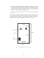
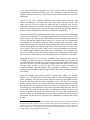
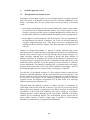
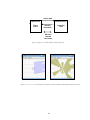
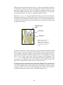
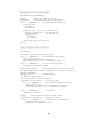
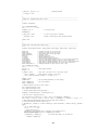
A Pioneer 3 robot equipped with laser and sonar sensors was given the task of passing
through a gate (AB) in a small pen, see figure 1. The pen was 2.50 metres wide, 4.00
metres in length and 0.46 metres high and the gate measured 0.97 metres across. The
side gap widths were 0.62 metres, (just wide enough for the robot to pass through, see
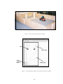
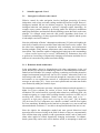
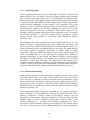
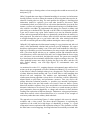
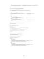
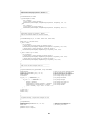
section 4.1.1) and the post bases were 0.145 by 0.13 metres. The real world and a 2dimensional simulated world (a scale model of the pen, robot and gate, see section
4.2.3) are shown in figures 2 and 3 respectively.
A short-term version of the problem required the robot to navigate safely around the
pen and stop once it had passed through the gate once. It was not allowed to pass
through gaps XA or BY at any time, nor through the gate in wrong direction DC. It
was given 3 minutes only to complete the task. In addition, a long-term version of the
problem allowed the robot to navigate freely around the pen, requiring that it discover
and travel to the goal as many times as possible in a fixed period. For the long-term
exercise passing through the gate in either direction was acceptable.
These problems were difficult because the world was small in comparison to the
robot, allowing it little freedom to move. In addition, no prior knowledge of the gate’s
location was given, only its width.
1.2.
Motivation
Mobile robot navigation has a wide variety of real world applications such as garbage
collection, moving supplies through factories and mail delivery. In addition, robots
are capable of carrying out vital tasks in potentially hazardous environments, for
example handling dangerous chemicals, rescuing fire and earthquake victims and
exploring the terrain of other planets. In order to accomplish their tasks effectively
they need to be equipped with a number of sensors so that they can perceive their
environment and make intelligent decisions about the actions that they should take,
for example avoiding obstacles.
The problems described above involve goal seeking in a confined space and were
selected for several reasons.
•
The constrained nature of the problems made them sufficiently difficult to warrant
investigation. A high degree of precision is required to steer towards the centre of
the small gate and the robot needs to be able to navigate through tight gaps to
solve the long-term problem effectively.
•
Although much attention has been given to goal seeking and obstacle avoidance in
mobile robotics there has been little research effort directed towards solving
highly confined problems, which makes their solution both interesting and
valuable. Moreover, it would be useful to find out whether it is possible to develop
a control system capable of learning in such an environment. If this was
achievable the code developed could be applied to similar constrained problems.
9
•
The solution could have many useful applications, for example in a factory
scenario, where a robot might be required to work in a small space, transporting
boxes from one shelf to another or delivering mail in an office where doors are a
fixed width. In these situations, the ability to achieve the tasks efficiently and
effectively (i.e. with no collisions), would be essential.
•
Lastly, it was impractical to build a larger world due to laboratory space
restrictions.
The next section examines the approaches that have been used in the past to solve
similar problems in mobile robotics. In particular behaviour based architectures,
neural networks, genetic algorithms, reinforcement learning and fuzzy controllers are
explained and some examples of their application to robot control are given.
TOP - D
1.10 m
A
B
a1 a2
b1 b2
X
post
Y
4.0 m
pen
2.77 m
robot
BOTTOM - C
2.5 m
Figure 1 – Showing the dimensions of the robot world
10
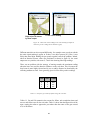
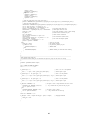
Figure 2 – The real pen, gate and Pioneer P3-DX8
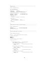
Post
Laser rays
Robot
oriented
at 0°
Sonar rays
Figure 3 – The simulated pen and gate world with virtual Pioneer P3-DX8
11
2.
2.1.
Scientific approach - Part 1
Strategies for effective robot control
Effective control for robot navigation involves intelligent processing of sensory
information, such as laser and sonar readings and their directions of origin. However,
intelligence methods fall into two distinct categories; Top down processing selects
intelligent behaviour and attempts to replicate it through explicit knowledge, for
example expert systems. Bottom up processing studies the biological mechanisms
underlying intelligence and simulates them by building systems that work on the same
principle, for example neural networks and genetic algorithms (both forms of
evolutionary methodology). In these approaches knowledge is implicit and the system
is both adaptive and self-contained.
Since the publication of Brooks’ subsumption architecture [38] in the mid-eighties the
main focus of mobile robot research has been behaviour based reactive control. This
has often been implemented in conjunction with evolutionary and reinforcement
learning methods, chiefly because autonomous robots must function without human
intervention. They should be capable of adapting their behaviour to their surroundings
“…without external supervision or control”, McFarland [25]. Furthermore, they need
to perform in a broad range of dynamically changing environments and often have to
make use of sensors that can produce uncertain readings.
2.1.1. Behaviour based architectures
In the mid-eighties, driven by dissatisfaction with robot performances in the real
world, Brooks [38] developed a methodology known as the subsumption architecture.
Behaviour based modules (for example exploring, wandering and avoiding obstacles)
mapped environmental states directly into low level actions, without the need for an
intervening world model. This was achieved through the connection of the sensors
and actuators to an asynchronous network of computational elements that passed
messages to each other, [20]. Layers were run in parallel and new behaviour models
were obtained by adding new network layers.
The subsumption architecture represents a hierarchical behaviour based approach; i.e.
higher level layers subsume the actions of lower levels through a suppression
mechanism. This can be beneficial, especially when robots have conflicting goals, (for
example navigating to a target whilst avoiding obstacles) and have no other way of
assessing their relative importance. Brooks states that robots need to be “…
responsive to high priority goals whilst servicing low level goals”, [38]. In Brooks
[38] the lowest level of competence was obstacle avoidance, and the next highest
level was wandering. Wandering used a heuristic to plan paths every ten seconds and
subsumed obstacle avoidance, i.e. was able to incorporate that behaviour into its own.
Since the eighties the subsumption method and more general behaviour based
approaches have been used widely in the field of robotics as they are computationally
more efficient than using symbolic world representation models, and are much more
robust when applied to realistic dynamically changing environments. Co-ordinatebased systems only tend to work well in abstract worlds, as attempting to model real
12
environments can be extremely complex. Another advantage of reactive systems is
that controllers can be built and tested incrementally. However, reactive methods are
generally heavily dependent on parameter optimisation, as single parameters can
affect multiple behaviours and their interactions [36]. Some examples of reactive
approaches are discussed below.
Brooks et al. [22] used the behaviour based subsumption architecture for vision based
obstacle avoidance on a monocular mobile robot. Their strategy involved the use of
three vision processing modes based on brightness, RGB value and HSV value. (This
scenario has important applications for the autonomous exploration of Mars.)
Obstacle detection was reactive, i.e. locations were not stored. Camera images were
converted to motor commands through a fusion of the outputs from the three vision
modules. The robot turned away from obstacles nearby with the angle of turn and the
speed dependent on the nearness of the obstacle. The system was tested in Mars like
environments with a high success rate, although shadows and bright sunlight caused
the robot to detect false obstacles.
Goldberg and Matarić [34] used a reactive approach to control four physical R2e
robots performing a mine collection task using grippers. They defined behaviours as a
collection of asynchronous rules that acquire input from the sensors and respond via
the actuators or through other behaviours. The modules used were wandering,
avoiding obstacles, mine detecting (through the use of colour), homing, creeping and
reverse homing. The state of the environment, time scales and statistics were used to
select an appropriate mode.
The mapping of sensory information to a particular behaviour can be either learned or
hard coded. When hard coded systems are used the results often work well for fixed
environments, but lack the adaptability to perform well in changing ones, [39]. In
such dynamic environments, the reactive approach is frequently coupled with learning
methods, for example neural networks (see section 2.1.2) and reinforcement learning
(see section 2.1.4).
2.1.2. Neural networks
Neural networks are modelled on the human brain, with processing elements
representing neurons. These are arranged in an input layer (perception neurons), a
hidden layer (associative cortex) and an output layer (motor neurons) and are linked
by weights (synaptic strengths). Intelligent behaviour emerges through selforganisation of the weights in response to input data, i.e. through training the system.
During training the weights are continually adjusted until the desired response is
obtained. Supervised training involves supplying a set of correct responses to given
inputs in order for the system to adapt its weights to replicate the output response.
Unsupervised learning requires only a set of inputs as weights are updated
competitively. There is a wealth of examples of mobile robot control using neural
networks in the literature. A few examples are given below for clarification.
Floreano and Mondada [23] used a recurrent (feedback) neural network to develop a
set of behaviours for a small mobile robot with the tasks of navigating through a
corridor with sharp corners and of locating and using a battery charger. Results using
13
a real robot showed that navigation was more effective and far smoother than
compared with a simple Braitenberg1 Vehicle [26]. Furthermore, the robot did not get
trapped at any point. Discovery of the battery charger and its effective use took 240
generations.
Tani et al. [2] used a hybrid of Kohonen and recurrent neural networks with
supervised training on a real robot with a laser range sensor and three cameras. The
robot’s task was to loop in figures of eight and zero in sequence, with no prior
information about the environment. The task was learned by guiding the robot from
each of several starting points. After ten training sessions the robot always followed
the desired path, although noise affected the performance substantially.
Floreano and Urzelai [21] argue that neural networks only perform well if the training
conditions are maintained, i.e. in different environments the software can fail. They
propose that it is the rules used for determining connection strengths that should be
evolved, and that the weights should emerge as a result of this. As unpredictable
environments are a common problem for robot navigation they developed a more
robust neural network code, based on these principles and tested it on a small, mobile
robot in a rectangular environment, using vision as the main sensor. The robot’s task
was to travel to a grey area when a light was on. Using conventional neural networks,
even slight changes in lighting affected the robot’s performance. For the adapted code
success was achieved even when extreme changes were made such as using a larger
robot and arena, switching the colours and changing from a simulated to a real robot.
Yamauchi and Beer [58, 59] used a continuous time recurrent neural network
(CTRNN) as a control system for a robot that was required to find a target with the aid
of a light. Sometimes the light was on the same side as the target and at other times it
was on the opposite side. The robot had to decide whether the light was associated
with the target in order to reach its goal. The control system consisted of an
assessment module, and anti-guidance and pro-guidance mechanisms. Following
training the robot learned to ignore the light and use other means to identify the target
successfully.
Supervised learning with neural networks is usually done offline. For example
Reigner et al. [39] used supervised learning to train a 4-wheeled rectangular robot to
follow a boundary, using 24 sonar sensors. Initially a human operator guided the robot
along the edge using only two basic commands, “move” and “turn”. The resulting
sensory data was saved to a file of perception-action associations and was then fed to
the neural network for training. After this the network was used to guide the robot, but
if the behaviour was unsatisfactory the operator regained control and a new data file
was created. The robot was thus trained in an incremental fashion. It did not learn
merely to reproduce the actions of the operator, but was able to make generalisations
and successfully steer around boundaries not previously encountered. An advantage of
this method was that once past experience was established the robot did not need to
re-learn.
1
These machines proposed by Valentino Braitenberg had very basic internal structures for example
two light sensors and two motors, and were connected using simple, direct relationships. A connection
might consist of the two motors driving the left and right wheels independently according to the output
from the light sensors. The nature of the connections determined the behaviour of the vehicle, for
example light-avoiding or light-seeking behaviours.
14
2.1.3. Genetic algorithms
Genetic algorithms search state space by mimicking the mechanics of genetics and
natural selection. They can quickly converge to optimal solutions after examining
only a small fraction of the search space; i.e. the population of solutions is often
optimised after only a small number of generations. An initial population of solutions
is selected at random and encoded into a binary representation. A fitness function then
assigns selection probabilities to each member of the population. The genetic
operators crossover (controlled swapping of binary bits between two members for
potentially better solutions) and mutation (changing one binary bit to provide
diversity) are applied at set levels of probability. Each iteration results in a new
population, and the algorithm continues until certain conditions are met. The result is
an increasing aptitude for a given task through successive generations. Evolved
solutions are not always optimal but can provide useful compromises between
constraints, [48].
The technique first received attention in the nineteen eighties when it was seen as a
branch of alternative computing along with neural networks [48]. Since then it has
become accepted as a useful learning mechanism in autonomous mobile robotics as it
reduces the quantity of prior assumptions that have to be built. The method has also
been widely applied to parameter optimisation, as manual tuning of control
parameters is notoriously difficult and costly in terms of time, especially using real
robots. For example Ram et al. [36] applied genetic algorithms to the problem of
parameter optimisation for goal seeking and obstacle avoidance, using navigation
performance as a fitness measure. They assigned a set of virtual robots a set of fixed
parameters to control their behaviours. The performances in the simulator were
evaluated so that new parameters could be evolved and assigned to a new population
of robots. A good set of parameters was obtained after several generations. The fitness
measure was based on task time, distance travelled and the number of collisions.
2.1.4. Reinforcement learning
Reinforcement learning occurs when knowledge is implicitly coded in a scalar reward
or penalty function. There is no teacher and no instruction about the correct action,
just a score that is yielded by the robot’s interaction with its environment. Control
designers thus need to structure the reward system so that it defines the goal. (This is
analogous to pleasure and pain in a biological system.) Reinforcement learning is
distinct from supervised learning as the latter teaches the system to produce a desired
output given an input, [19].
Both reinforcement learning and genetic algorithms use an evaluation function to
assess performance. The main difference is that genetic algorithms use the fitness
function to determine a strategy’s chances of becoming a parent in the next
generation. In reinforcement learning the function is used to provide immediate
feedback about an action’s usefulness. Reinforcement learning is thus a more
localised methodology, i.e. it usually scores individual components of a robot’s
performance. Genetic algorithms operate at a more global level, for example scoring
time taken to complete the overall task. Both methods help to reduce the burden of
15
behaviour designers, allowing robots to learn strategies that would not necessarily be
anticipated, [33].
Hailu [1] argued that some degree of domain knowledge is necessary in reinforcement
learning schemes, in order to reduce the amount of discovering that robots need to do,
otherwise learning takes too long. The main problem for designers is deciding what
information should be explicitly given and what should be discovered. Hailu
recommended a basic set of reflex rules or safe actions that should be given in the first
instance, to allow safe navigation. Once reinforcement learning was established these
rules could be overridden. He implemented this strategy for obstacle avoidance and
goal seeking on a simulated TRC robot and a real B21 robot in a labyrinth world with
a gate and a concave trap region. Belief matrices were used to determine possible
actions and environmental knowledge was dynamically encoded into the matrices as
time progressed. The robot had a camera, infra-red, tactile and sonar sensors and had
to navigate through the gate to a goal on the other side. After training both robots
were able to reach the goal successfully without entering the concave trap region.
Gullapalli [19] implemented reinforcement learning for a peg insertion task with real
robots, where handcrafted solutions had previously proved inadequate. (He argues
that direct reinforcement learning is one of the most useful methods for achieving a
high level of flexibility, precision and robustness for many complex and unpredictable
tasks.) The robots began with the peg at a random position and orientation and the
reward function (a scalar value between 0 and 1) was evaluated from the forces acting
on it, (the closer it was to the hole, the higher the reward). The system was controlled
by a neural network that continually adjusted the weights according to the score. The
robots gradually became more adept at placing the pegs in the holes, and after 150
trials worked robustly, even with high degrees of environmental noise and
uncertainty.
As mentioned in section 2.1.1, mappings between environmental states and low-level
actions can be pre-programmed or learned. Michaud and Matarić [33] were interested
in the effective control of multiple robots given a foraging task. They developed a set
of robust behaviour based modules and a set of initial state to action mappings that
allowed safe task completion. The modules were implemented along with a
reinforcement learning algorithm so that choice of behaviour could be dynamically
adapted based on past history and performance measures. Time was used as the
primary behaviour evaluation parameter, i.e. penalties were awarded if performance
took longer than in the past and rewards were issued if time was shorter. Chosen
behaviours and their sequences of use were stored within a tree structure that allowed
alternative behaviours to be selected. The use of time as a reward measure provided a
good compromise between adaptability to change and tolerance for bad decisions
resulting from exploration of different strategies. Furthermore, using past performance
rather than external criteria allowed behaviour to be assessed on the strength of
consistency rather than some arbitrary hard-coded rule.
The approach was tested using Pioneer I robots equipped with sonar for obstacle
avoidance and a vision system. The robots showed competence in exploiting the
regularities of the world and a high degree of adaptability to change, i.e. a good
compromise between exploration and exploitation strategies. They learned to override
the initial state to action mappings, choosing behaviours not normally associated with
16
particular conditions. All behaviours were selected through past experience once
learning was complete and interestingly, each robot learned to specialise in how it
accomplished the task, as individual experiences were different.
2.1.5. Fuzzy systems
In first order predicate calculus set membership is binary and has a value either 0
(false, not a member) or 1 (true, a member). However, fuzzy set membership ranges
between 0 and 1; i.e. an object can be a member of a set to some degree. Similarly,
under fuzzy rules the assignment of a possibility distribution can represent the truth of
a logical proposition, (see [40], Chapter 7 for further details).
Fuzzy control systems, i.e. a set of rules with associated possibility distributions, have
frequently been employed in mobile robotics. In reactive control methods the use of
classical fuzzy systems is a way of hard coding the mapping from environmental state
to behaviour [39], i.e. mappings are created off-line and there is no learning.
Takeuchi and Nagai [8] used a fuzzy controller in order to guide a purpose built
mobile robot around obstacles using CCD camera images of the floor as system input.
The fuzzy control rules were based on human driving processes and objects were
detected on the basis of floor brightness. Detected boundary lines provided a means
for calculating object distances. Information from the vision system was fed into the
fuzzy controller and output was in the form of independent speed commands to the
two wheels. The fuzzy controller consisted of a set of IF…THEN rules for motion
direction, gain and acceleration, combined into a fuzzy relation. The velocity was
related to the width of the passageway detected by the vision system. Results showed
that the system performed well but sometimes failed due to imaging errors such as
glare from the floor being mistaken for obstacles.
The next section focuses on the use of the vertebrate immune system as a model for
adaptive behaviour. These systems have recently been used as inspiration for mobile
robot control strategies under a wide variety of situations.
17
3.
3.1.
Scientific approach - Part 2
Background to the immune system
The purpose of the immune system is to expel foreign material, or antigens from the
body. The ability to distinguish self from non-self is therefore fundamental to its
design. Essentially there are two systems that work co-operatively as described
below:
•
In the innate system phagocyte cells are immediately able to ingest a large number
of bacteria that show common molecular patterns. No previous exposure to these
bacteria is necessary and the system is constant throughout life and the same for
all individuals. Infection is controlled whilst the adaptive system is getting started.
•
In the adaptive system lymphocyte cells (B-cells and T-cells) are responsible for
the identification and removal of antigens. The T-cells are activated when they
recognise antigen-presenting cells. They divide and secrete lymphokines that
stimulate B-cells to attack the antigens. They thus contribute to the protection of
self-cells.
Epitopes are antigen determinants, i.e. patches on antigen molecules that present
patterns that can be recognised (with varying degrees of accuracy) by complementary
patterns on the surface receptors of B-cells. Each B-cell has surface receptors of a
single specificity, although there are millions of B-cells and hence millions of
different specificities in circulation. The clonal selection theory [53] states that once
an epitope pattern is recognised the B-cell is stimulated to divide until the new cells
mature into plasma cells that secrete the matching receptor molecules or antibodies
into the bloodstream. The antibody combining sites or paratopes bind to the antigen
epitopes, which causes other cells to assist in the elimination of the antigen. Some of
the matching lymphocytes act as memory cells, circulating for a long time.
The efficiency of the immune response to a given antigen is hence governed by the
quantity of matching antibodies, which in turn depends on previous exposure to the
antigen. Under the clonal selection theory the concentrations of useful lymphocytes
are increased at the expense of the randomly generated proportion so that the
repertoire mirrors the antigenic environment [18]. In other words, cells with high
affinities enter the pool of memory cells.
Following birth, the antibody repertoire is random. Diversity is maintained by
replacement of the B-cells at the rate of about 5% per day [18] in the bone marrow
during which time mutation (reorganisation of the DNA) can occur. In addition, the
reproduction of the B-cells upon stimulation also causes a high rate of mutation.
Through mutation, weakly matching B-cells may produce antibodies with higher
affinities for the stimulating antigen. The diversification process ensures that an
almost infinite number of surface receptor types is possible. If self-recognising
antibodies are produced they are suppressed and eliminated.
18
3.2.
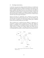
The idiotypic network theory
In 1974 Jerne [7] proposed the immune system network theory as a mechanism for
regulating the antibody repertoire, although it has not gained wide acceptance within
the field of immunology. The theory is based on the fact that as well as paratopes (for
epitope recognition), antibodies also possess a set of epitopes and so are capable of
being recognised by other antibodies even in the absence of antigens. Under the clonal
selection theory all immune responses are triggered by the presence of antigens, but
under the network theory antibodies can be internally stimulated. (Experiments have
shown that the number of activated lymphocytes in germ free mice is similar to that of
normal mice [60], which supports the argument.)
Paratopes and epitopes are complimentary and are analogous to keys and locks.
Paratopes can be viewed as master keys that may open a set of locks (epitopes), with
some locks able to be opened by more than one key (paratope), [30]. N. B. Epitopes
that are unique to an antibody type are termed idiotopes and the group of antibodies
that share the same idiotope belong to the same idiotype.
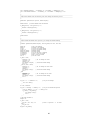
When an antibody type is recognised by other antibodies it is suppressed i.e. its
concentration is reduced, but when an antibody type recognises other antibodies or
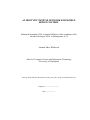
antigens it is stimulated and its concentration increases. The theory explains the
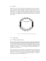
suppression and elimination of self-antibodies and presents the immune system as a
complex network of paratopes that recognise idiotopes and idiotopes that are
recognised by paratopes, see figure 4. This implies that B-cells are not isolated, but
are communicating with each other via collective dynamic network interactions, [42].
Figure 4 – Showing suppression and activation between antibodies,
adapted from [7]
19
The network is self-regulating and continually adapts itself, maintaining a steady state
that reflects the global results of interacting with the environment [7], although a
single antibody may be more dominant. (The cell with the paratope that best fits the
antigen epitope contributes more to the collective response, [44].) This is in contrast
to the clonal selection theory, which supports the view that change to immune
memory is the result of single antibody-antigen interactions.
The network theory also states that suppression must be overcome in order to elicit an
immune response. In other words, the system is governed by suppressive forces, but
open to environmental influences, [7]. The suppression models the immune system’s
mechanism for removing useless antibodies [5] and maintaining diversity. The
increase in useful antibody concentrations models the immune system’s memory.
(However, it is worth noting that the exact mechanism of immune memory is still
relatively poorly understood [44]. In 1989 Coutinho [51] postulated that networks
may not contribute to memory as their capacity is probably too small to store the vast
quantity of data required to record previous antigen attacks.)
3.2.1. Modelling the idiotypic immune network
The learning, retrieval, memory, tolerance and pattern recognition capabilities of
artificial immune systems make them highly suitable as models for machine learning.
Furthermore, the behaviour of an idiotypic network can be considered intelligent, as it
is both adaptive at a local level and shows emergent properties at a global level, [42].
The dynamics ensure that antibodies closely matching antigens and yet distinct from
one another are selected, whereas sub-optimal matches are removed, [31].
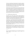
In 1986 Farmer et al. [30] presented a general method for modelling the idiotypic
immune network in computer simulations and this is described below. A differential
equation models the suppressive and stimulating components and binary strings of a
given length, l represent epitopes and paratopes. Each antibody thus has a pair of
binary strings, [p, e] and each antigen has a single string, [e]. The estimate of degree
of fit between epitope and paratope strings is analogous to the affinities between real
epitopes and paratopes, and uses the exclusive OR operator to test the bits of the
strings, (0 and 1 yields a positive score).
Exact matching between p and e is not required and as strings can match in any
alignment one needs only to define a threshold value s below which there is no
reaction. For example if s was set at 6 and there were 5 matches (0 and 1 pairs) for a
given alignment, the score for that alignment would be 0. If there were 6 the score
would be 1 and if there were 7 the score would be 2. The strength of reaction for a
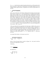
given alignment is thus:
G = 1+ δ ,
where δ is the number of matching bits in excess of the threshold. The measure of
strength of reaction for all possible alignments, mij between an antibody, i and
another, j, is given by:
mij = ∑ G .
20
When two antibodies interact the extent to which one proliferates and one recedes is
governed by the degree of matching. In a system with N antibodies:
[x1 , x2 ... x N ] ,
and n antigens
[y1 , y2 ... yn ] ,
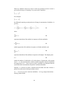
the differential equation governing the rate of change in concentration of antibody xi is
given by:
N
n
N
x ′i = c ∑ m ji xi x j − k 1 ∑ mij xi x j + ∑ m ji xi y j − k 2 xi ,
j =1
j =1
j =1
3.1
where
N
∑m
ji
3.2
xi x j
j =1
represents stimulation of the antibody in response to all other antibodies,
N
k1 ∑ mij xi x j
3.3
j =1
models suppression of the antibody in response to all other antibodies, and
n
∑m
j =1
ji
3.4
xi y j
represents stimulation of the antibody in response to all antigens. The damping term
3.5
k2 xi
models the tendency of antibodies to die in the absence of interactions, with constant
rate k2. c is a rate constant and k1 models possible inequalities between stimulation
and suppression. (If k1 = 1 these forces are equal.) Antibodies are eliminated from the
system when their concentrations drop below a minimum threshold.
Equation 3.1 is known as Farmer’s equation and the authors note that it follows a
general form often seen in biological systems, that is:
∆xi = internal interactions (between antibodies) + driving (antigen interactions) –
damping (natural death).
21
3.2.2. Idiotypic models and mobile robot navigation
Artificial immune networks are particularly useful tools for controlling autonomous
mobile robot navigation as they can be used as a means of behaviour arbitration and
are suited for solving dynamic problems in unknown environments [6]. Some
examples of recent work in this field are presented below.
Luh and Liu [3] used a reactive immune network for robot obstacle avoidance, trap
escapement and goal reaching in an unknown and complex environment with both
static and dynamic obstacles. Their architecture consisted of a combination of prior
behaviour based components and an adaptive component modelled on the immune
network theory. In their system conditions detected by the sensors were analogous to
antigens with multiple epitopes, for example “obstacle ahead” with epitopes “distance
away from robot”, “sensor position” and “orientation of goal with respect to the
obstacle”. Antibodies were defined as steering directions:
[θ 1 ,θ 2 ...θ N ],
where
0 ≤ θ i ≤ 2π .
A given antigen was recognised by several antibodies, but only one antibody was
allowed to bind to one of that antigen’s epitopes. The antibody with the highest
concentration was selected, and concentrations were determined using Farmer’s
dynamic equation, (3.1). Their strategy was tested on a simulator and proved flexible,
efficient and robust to environmental change, although optimisation of parameters
was not achieved.
Krautmacher and Dilger [4] applied Farmer’s immune network model to robot
navigation in a simulated maze world in which a building had collapsed due to an
earthquake. The robot’s task was to find victims, determine their situation and
location and record the information on a data sheet. No a priori knowledge of the
maze or object locations was given; fuzzy identification of objects was achieved
through image processing and comparison with stored information. Location and
identification of a given object was analogous to the presence of an antigen, and its
type and location were used as epitopes. Many potentially useful antibodies
representing basic behaviours were used and as the system evolved new antibodies
emerged and were added to the system.
Watanabe et al. [6] used an artificial immune network to control behaviour arbitration
for a garbage collecting mobile robot, a problem originally posed by Michelan and
Von Zuben [54]. The robot had a finite energy supply and was required to collect
garbage and place it in a waste basket, recharging its power as required at a charging
station. Competence modules (“move forward”, “turn right”, “turn left”, “search
station”, “wander”, “collect garbage”) were prepared in advance for use as antibodies
and antigens were represented by object types, distances and the energy level, for
example, “garbage in front”, “charging station right”, “energy level high”. Antibody
concentration dynamics were maintained by Farmer’s differential equation, (3.1) and
a squashing function, (see section 6.2.2). A roulette wheel method selected an
antibody based on probabilities assigned by concentration values and a genetic
algorithm was used to establish initial antibody concentrations and determine
affinities between connections. Simulations and trials using a real robot with infra-red
sensors and a CCD camera demonstrated the validity of their approach.
22
Vargas et al. [5] constructed a hybrid robot navigation system (CLARINET) that
merged ideas from learning classifier systems, (introduced by Holland in the midseventies, see [32]) and the immune network model of Farmer et al. [30].
Environmental conditions were matched to classifiers (similar to production rules)
with varying strengths. The classifiers competed to execute their action components
and were continually evolved using crossover and mutation to produce the next
generation.
Learning classifier systems have been likened to artificial immune systems by Farmer
et al. [30] and Vargas et al. [45]. Antibodies can be thought of as classifiers with a
condition and action part (the paratope) and a connection part (the idiotope). The
action part must be matched to a condition (antigen epitope) and the connections show
how the classifier is linked to others. The presence of environmental conditions causes
variations in classifier concentration levels in the same way that antigens disturb
antibody dynamics.
Vargas et al. [5] selected the antibody with the highest activation level (match
strength multiplied by concentration). Hence, the best-matched classifier was not
necessarily selected. This is intuitive since useful classifiers with high concentrations
should be given more influence than weak ones in order for the system to learn [30].
CLARINET was applied to the same problem as Watanabe et al. [6] and four actions
were used, “right”, “left”, “forward” and “explore”. Classifiers were initially random
with crossover used on those with the same condition part and with a 10% probability.
Mutation was at 1%. Results showed that the robot discovered alternative paths
around obstacles, responding quickly to environmental changes. The use of non-fixed
rules allowed the selection of classifiers that were tailored towards immediate
environmental conditions.
Learning classifier systems have frequently been used to solve mobile robotics
problems. Stolzmann and Butz [56] applied them to robot learning in a T-shaped
maze environment and Carse and Pipe [57] used a fuzzy classifier system. Webb et al.
[46] used classifiers with reinforcement learning for the autonomous navigation of
simulated mobile Khepera robots that were required to find and travel to target
locations. The action parts of the classifiers were “move forward”, “rotate right”,
“rotate left” and “do nothing”. Initially, an equal chance of choosing a random action
and of choosing the action with the highest reward was coded. Reinforcement learning
based on past history was used to determine future classifiers.
The next section describes the physical hardware and software used to solve the
problems described in section 1.1. The fixed behaviour based code is also described
and the results of solving the short-term problem using a simulator and a real robot are
presented.
23
4.
Proposed solution
4.1.
Hardware used
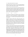
4.1.1. Physical robot and the network configuration
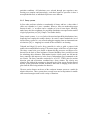
An ActivMedia Pioneer P3-DX8 with a range finding laser was used, see figures 5
and 6. This is a mobile, two-wheeled robot with reversible DC motors, on-board
microcontroller, server software and an integrated onboard PC. The wheels are
supported by a rear caster and the robot is capable of both translational and rotational
motion. The chassis is 38 cm wide, 44 cm deep and 22 cm high (not including the
laser), [11]. The laser unit is 19 cm high.
These robots act as the server in a client-server paradigm, with the on-board
microcontroller handling the low-level details of mobile robotics, for example setting
speed and acquiring sensor readings, [10]. The onboard PC routes the sensor values to
the host and the motor commands back from it.
Control
panel
Range
finding laser
Rear sonar
array
Front sonar
array
Drive
wheel
Caster
Figure 5 – The Pioneer P3-DX8 with laser, adapted from [10]
24
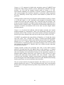
Range finding laser
Front sonar
Figure 6 – The Pioneer robot used throughout this research
Connection between the on-board host computer and the laboratory PC (a Pentium 4
with 3.6 GHz running Linux) was via a Cisco Aironet local wireless network, (see
figures 7 and 9). Client software running on the remote PC provided all high-level
control.
Private robot lab network
Public wired network
Figure 7 – Laboratory network architecture for the Pioneer robots
25
4.1.2. Sensors
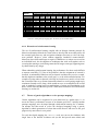
Sixteen sonar and 1 SICK LMS-200 laser range-finder were used, see figure 6.
Pioneer 3 robots have fixed sonar with 2 on each side and the others spaced at 20degree intervals, see figure 8. Readings are possible in ranges from 15 cm to 7 m
approximately, [11]. The laser provides 2 readings for each degree covering the front
180° sector, i.e. 361 readings in total. (Note that a pan-tilt camera was also installed
above the laser and a gripper was positioned at the front, but these were not used in
this research.)
3
4
2
5
-10° 10°
1
-30°
30°
6
-50°
50°
Front of Pioneer
0
-90°
90°
7
15
-90°
90°
8
14
-130°
130°
-150°
150°
9
-170° 170°
13
10
12
11
Figure 8 – Sonar arrangement on the Pioneer, adapted from [10]
4.2.
Software used
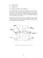
4.2.1. The Player robot device server
Player, a robot device server was used to control the sensors and actuators. This
software acts as an interface to the robot and runs on the on-board PC. Connection to
the client program (running on the laboratory PC) was through a standard TCP socket,
see figure 9. Player is both language and platform independent, meaning that control
programs can be written in C, C++, Java etc. All controllers developed as part of this
research were written in C++ to take advantage of the object-oriented Player C++
Client Library, see section 4.2.2.
Player was selected as it does not place any constraints on how control programs
should be written and it can also be used to interface with the 2D Stage simulator used
throughout this research, see section 4.2.3. Furthermore, it provides a visualisation
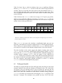
tool, PlayerViewer that can display the sensor output graphically, see figure 10.
Further details about Player are available in [13].
26
Sensor data
Onboard PC
Player
server
Remote lab PC
Actuator
commands
Controller
client
Wireless
network
connection
Figure 9 – Player server and controller client architecture
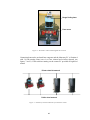
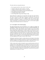
Figure 10 – PlayerViewer showing the real Pioneer’s laser and sonar output (left and right respectively)
27
4.2.2. Player C++ client library
The Player C++ library uses classes as proxies for local services. There are two kinds,
the single server proxy, PlayerClient and numerous proxies for the devices used,
for example the SonarProxy class. Connection to a Player server is achieved by
creating an instance of the PlayerClient proxy. Devices are registered by creating
instances of the appropriate proxies and initialising them through the established
PlayerClient object. Device access levels are set through their device proxy
constructor methods. See [9] for full details of the attributes and methods of the
various classes.
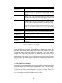
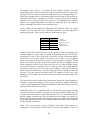
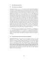
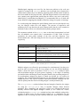
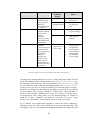
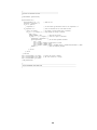
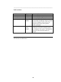
The proxies used throughout this research and a brief description of them are given in
table 1 below.
Proxy
Description
PlayerClient
Server proxy, used to establish a connection to the Player
server by specifying a host or port
Used to obtain the latest position data, (x-co-ordinate, y-coordinate and orientation) and set the internal odometry
Holds the latest scan data for the laser
Holds the latest sonar range measurements
PositionProxy
LaserProxy
SonarProxy
Table 1 – Description of the Player C++ client library proxies
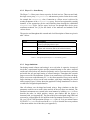
4.2.3. Stage simulations
Developing control software and testing it on a real robot is expensive in terms of
clock time, experimental logistics and the potential damage to the robot. Artificial
worlds and virtual robots are therefore frequently used to overcome these problems
and enable the safe and rapid testing of control strategies. Throughout this research
Stage was used for 2D simulations. As there is no connection to a real robot, the Stage
Player server runs on the laboratory PC, i.e. the client controller, Player server and the
Stage simulator are all run on the same machine, with Stage controlling the virtual
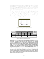
robots created. Figure 11 below shows the graphical 2D Stage simulation of a robot in
a world full of irregular shaped obstacles.
Here all software was developed and tested using a Stage simulator so that free
parameters could be set to useful values and risk to the real robot was minimal. The
simulated environment was created in the usual manner by building a world file to
describe the robot, its initial position, sensors, port number and the objects it
interacted with, (see Appendix K). The plan of the pen was designed using GIMP and
converted to a zipped pnm file for inclusion in the environment section of the world
file, (see [12] for a full description of Stage world files). N. B. A pre-written Pioneer
P3 DX-SH include file was used in the world file to describe the exact positions
of the sonar and the size of the robot, (see Appendix L).
28
obstacles
robot
Figure 11 – Example 2D Stage world and virtual robot
4.3.
The fixed behaviour based code (goalseek)
A behaviour based approach was adopted because it has been well documented that
this has proved computationally cheaper and less complex to implement than world
mapping techniques. Furthermore, the method lends itself to object oriented
programming.
The controller was separated into a main method, a Robot class, and a
WorldReader class. (WorldReader was only used during initial testing with the
simulator to obtain the start co-ordinates automatically.) The Robot class was
created to act as an interface to the main program, providing different modes of
operation, for example:
taylor.obstacleAvoid(true);
commands a robot called taylor to go into obstacle avoidance mode, steering away
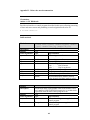
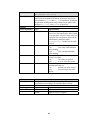
from the minimum laser or sonar reading. Table 2 below summarises the public
methods in the Robot class and explains their functions, (see Appendices C and D
for a listing of the class code and Appendix H for user documentation).
29
Method
constructor
connect
position
getSensorInfo
getLaserArray
getCoords
obstacleAvoid
goFixedGoal
goNewGoal
escapeTraps
explore
Description of functionality
Sets the robot's maximum allowed speed and distance tolerance for
obstacles.
Sets the connection parameters to those supplied with the run
command, (if none are specified the control program uses the
default).
Sets the robot’s internal odometry to the starting co-ordinates
supplied. (This is only necessary for testing with fixed goals and
simulated robots. If the goal is unknown then the start position is not
important and can be arbitrarily set to [0,0,0] for example.)
Gives the positions of the sensors giving the minimum and
maximum readings and gives the minimum and average readings.
The same method is used for laser and sonar information processing.
This method is used for averaging the laser readings over 8 sectors
at the front. The array of averages rather than the full array of 361
values is then passed to the getSensorInfo method for
processing.
Gives the robot’s current x and y co-ordinates and its orientation.
Avoids obstacles by either turning to the direction of the maximum
laser or sonar reading, or turning away from the minimum reading.
Travel to a goal where the co-ordinates are known. (This method
was only used for simulated robots during initial testing.)
Travel to a discovered goal, (i.e. head through the gate).
Used to free the robot when it has collided, is cornered or is standing
still.
Wander around and examine the laser output until a goal is
recognised.
Table 2 – Public Robot class methods
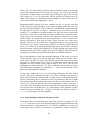
The main program allowed several different parameters to be set. Laser or sonar could
be specified for obstacle avoidance, and in addition two methods were possible. The
robot could move towards the maximum laser or sonar reading or move away from
the minimum when it encountered an obstacle. The option of using laser readings
averaged across sectors was also available. In addition, the robot could be set as
simulated or real. For simulated robots the goal could be set as known (for code
testing purposes) or as unknown. However, the goal was always set as unknown when
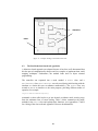
using real robots. The control program architecture is simplified and illustrated in
figure 12.
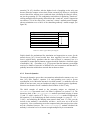
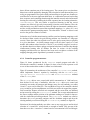
4.3.1. Explanation of methodology
Processing of the sensor information, (sonar or laser) yielded a minimum reading and
its position, the position of the maximum reading and the average of all the readings.
The minimum reading was used to detect a collision and the average reading was used
to check that there was no corner entrapment, see figure 13. If either situation was
detected the robot was sent into trap escape mode. If neither were detected then a
Robot class method was assigned according to table 3 below.
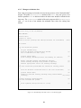
30
create robot;
connect to robot;
DO forever
{
IF one second has passed
{
get position;
IF goal reached stop;
work out distance travelled;
get maximum / minimum sensor positions and minimum
reading;
IF no collision AND not cornered
{
IF minimum reading < tolerance avoid obstacles;
IF minimum reading > tolerance AND goal found head for
goal;
IF minimum reading > tolerance AND goal not found explore;
}
}
IF distance travelled zero OR collision occurred OR robot
cornered
{
escape trap;
}
}
Figure 12 – Control program architecture
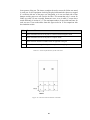
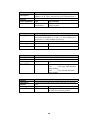
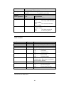
Method
Assignment conditions
explore
If goal is not known and minimum sensor reading is above or
equal to a tolerance value
If goal is known and minimum sensor reading is above or equal
to a tolerance value
If minimum sensor reading is below a tolerance value
goNewGoal
obstacleAvoid
Table 3 – Mapping of methods to conditions
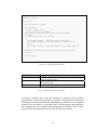
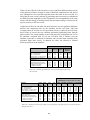
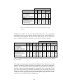
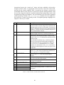
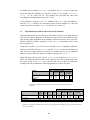
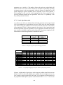
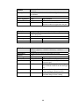
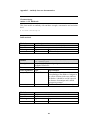
In obstacle avoidance mode either the minimum or maximum sensor positions
determined the steering angle and speed. For example a minimum position directly in
front required a greater turn and slower speed than one towards the side. As minimum
positions at the two sides (i.e. from sonar 0 and 7) did not present serious problems,
these readings were not considered when computing the minimum. Table 4 below
shows the fixed linear and rotational velocities used with each strategy.
31
Position
0
1
2
3
4
5
6
7
Turn towards
maximum sensor
reading
Angle
(Degrees)
30°
20°
10°
0°
0°
-10°
-20°
-30°
Speed
m/s
0.05
0.05
0.10
0.10
0.10
0.10
0.05
0.05
Turn away from
minimum sensor
reading
Angle
(Degrees)
-20°
-30°
-45°
45°
30°
20°
-
Speed
m/s
0.10
0.05
-0.10
-0.10
0.05
0.10
-
Table 4 – Speeds and angles used in the two different obstacle avoidance strategies
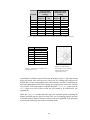
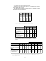
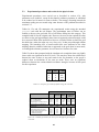
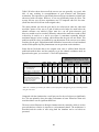
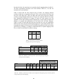
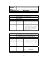
Sector
Laser positions
0
1
2
3
4
5
6
7
315 - 360
270 - 314
225 - 269
180 - 224
135 - 179
90 - 134
45 - 89
0 - 44
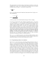
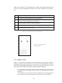
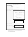
Figure 13 – Showing how
average front sensor readings
reduce when the robot is
trapped in a corner
Table 5 – How the laser readings were
divided into sectors
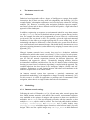
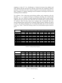
Laser obstacle avoidance worked on the same principle as sonar, i.e. the same steering
angles and speeds were used. However, as there are 361 readings, the positions were
divided into 8 sectors corresponding to the sonar positions, see table 5. In addition, the
maximum and minimum of all laser readings or averages across each of the 8 sectors
were possible. Following obstacle avoidance the public found_goal property of the
Robot object was reset to false so that the goal needed to be rediscovered, (see
Appendix H).
Under the goNewGoal method the robot moved at maximum speed, computing the
distance travelled since the goal was found. This was for stopping purposes and also
so that the obstacle distance tolerance could be reduced on approach to the gate posts
to prevent the robot going into obstacle avoidance mode.
32
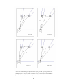
In explore mode the robot wandered around searching for a goal. Recognition of the
gate as the goal was achieved by extracting the two maximum changes in the laser
readings and their angular positions. Computation of an estimate for gap distance was
given by:
d = ( x 2 + y 2 ) − (2 xy cosθ ) ,
where x and y are the lower valued laser readings before the change and θ is the angle
between them, see figures 14a – 14d. The gap estimate was compared with the known
figure, using a tolerance value of 0.4 metres derived from experimentation. Note that
depending on the robot's position, the gate width could be estimated as any of the
lines d shown in figures 14a –14d (or their mirror images), and the tolerance had to
allow for this. Although the shape of the gate yielded 4 large changes in reading,
maximum changes at positions a1 and a2 or b1 and b2, (see figure 1), did not record a
goal as the gap estimate was too small. (Maximum changes at positions a2 and b1
showed the gap as in figure 14a, positions a1 and b2 as in figure 14b, positions a1 and
b1 as in figure 14c and positions a2 and b2 as in figure 14d.) N. B. The private method
getDistance in the Robot class ensured that the lower values at the change points
were used for x and y in each case.
If the gap estimate did not approximate the known gate width then the gap was
assumed to be something other than the gate and the robot carried on exploring. If a
match was achieved then other checks were enforced, including that the two
maximum changes were greater than a tolerance value and that the difference between
them was less than another threshold. After passing these tests the goNewGoal
method was invoked and the public found_goal property of the Robot object was
set to true.
An estimate of the distance, h to the gate was given by:
2
d
d
h = ( x + ) − (2 x cos ϕ ) ,
2
2
2
where φ is the side angle between x and d (see figures 14a – 14d), and h is the line
from the robot origin that cuts d in half.
Substituting
x2 + d 2 − y 2
cos ϕ =
,
2 xd
this simplifies to
h=
x2 d 2 y2
−
+
.
2
4
2
33
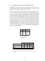
Figure 14b
Figure 14a
Figure 14d
Figure 14c
Figures 14a – 14d – Showing the different estimates of the gate width, depending on which laser
paths produce the maximum change in reading. N. B. The robot is shown in the same position
for simplicity, but in reality its position would have to vary to obtain different maximum change
points. Mirror images of the line d are also possible.
34
The approximation for h and the estimate of the distance travelled were used as the
stopping criteria. In order to move in the direction of the goal the robot was oriented
towards the centre of the gate, i.e. was turned by µ degrees where
µ=
γ −π
2
−ω ,
and ω is the angle between the left hand laser beam and the line h in figures 14a –
14d, calculated from
2
d
x2 + h2 −
2 .
cos ω =
2 xh
γ is the array number of the left hand maximum change in the laser readings.
If a goal was not detected the robot wandered at maximum speed, i.e. the private
wander method of the Robot class was invoked. Wander mode presented a choice of
exploration (random turn) and exploitation (turn towards the maximum sensor
reading) strategies. Random numbers were used both to assign strategies and to
choose a random turn angle between –45° and 45°. The random element was added
because exploitation strategies are not always optimal, but this made the method
rather ad hoc due to the fact that random directions can be good or bad. A 60% chance
of choosing the exploration strategy and a 40% chance of choosing the exploitation
strategy were coded, as the robot’s priority was to explore new directions rather than
maintain a safe path. (Future research could examine the effect of varying the
probability ε of choosing a random direction. However, Kaelbling et al. [29] have
noted that there is no technique that adequately resolves the trade off between
exploration and exploitation strategies for complex problems.)
The escapeTraps method was used to reverse the robot initially and then to send it
into wander mode at zero speed. This meant that it could use either the exploration or
exploitation strategy to free itself from becoming cornered or stalled.
4.3.2. Experimental procedures for the simulator
The aim was to solve the short-term goal-seeking problem described in section 1.1.
The goalseek code was run 90 times for each of the 6 different obstacle avoidance
strategies, (turning towards the maximum sensor reading and turning away from the
minimum sensor reading for each of sonar, single laser and average laser readings),
i.e. the program was run 540 times in all. For each strategy 6 different starting
positions, (see figure 15) and 5 different orientations were used, (0°, 45°, 90°, 135°
and 180°). The start locations were selected as a representative sample covering the
lower quarter of the pen. (Higher positions were not selected since pre-trials had
shown that goal discovery was too difficult when high up and close to the edges.) The
robot was allowed to explore for 3 minutes before being stopped. If it was successful
in its task the time taken was noted. If it was unsuccessful the causes were recorded,
(see table 6). The robot was not stopped as soon as it failed, hence multiple causes for
35
failure were possible. N. B. Throughout this research, the maximum allowed speed
was 0.17ms-1 and all significance testing was at the 95% confidence level using a ttest.
Code
1
2
Unsuccessful outcome
Passed through the gate but did not know the goal had been reached and did not
stop. However, passed through the gate and stopped later.
Passed through the gate but did not know the goal had been reached and did not
stop. Did not pass through the gate and stop later.
3
Passed through the gate the wrong way and stopped.
4
Passed through one of the gaps XA or BY, see figure 1.
5
Became trapped and could not escape.
Table 6 – Unsuccessful outcomes for the simulator
Figure 15 – Start positions for
the virtual robots
4.3.3. Simulator results
Tables 7, 8a and 8b below summarise the experimental results using the simulator.
During pre-trials it was found that success was very heavily dependent on the correct
choice of the following free parameters. (In fact this was true for all codes tested as
part of this research, both in the simulator and in the physical domain.)
d - The tolerance for the distance between the robot and an obstacle. When this was
too small collisions with the gate posts and walls were frequent and the robot often
got trapped.
a - The tolerance for the average of the sensor readings, used for escaping from the
corners of the pen. Increasing this effectively caused the robot to back up further.
36
r - By how much d was reduced on approach to the gate.
p - The proximity to the gate when the reduction in r was made. Increasing this gave
the robot a higher chance of success.
s - The small number representing the distance between an obstacle and the robot
after a collision, (used for escaping traps).
FREQ
% FREQ
CODE
(causes of
failure)
(all failed
trials)
1
2
3
4
5
2
12
2
1
11
12%
71%
12%
6%
65%
%
FREQ
(causes of
failure)
7%
43%
7%
4%
39%
Table 7 – Frequency of reasons for failure using the simulator
TIME TO PASS THROUGH GATE (SECONDS)
SCENARIO
MEAN
STANDARD STANDARD
DEVIATION
ERROR
Sonar - turn away from min
Sonar - turn towards max
Laser - turn away from min
Laser - turn towards max
Laser (averages) - turn away from min
Laser (averages) - turn towards max
SUMMARY
All experiments
All sonar experiments
All single reading laser experiments
All average reading laser experiments
Turn away from min strategy
Turn towards max strategy
19.97
18.23
20.87
19.33
22.10
20.23
5.87
2.51
5.82
6.10
11.50
9.76
1.07
0.46
1.06
1.11
2.10
1.78
22.07
19.13
22.95
21.52
26.21
23.73
17.86
17.33
18.78
17.15
17.99
16.74
20.12
19.10
20.10
21.17
20.98
19.27
7.62
4.60
6.01
10.71
8.22
6.85
0.57
0.59
0.78
1.38
0.87
0.72
21.24
20.26
21.62
23.88
22.68
20.68
19.01
17.94
18.58
18.46
19.28
17.85
95 %
CONFIDENCE
INTERVAL
Table 8a – Summary of statistics for time to pass through the gate using the
simulator
NUMBER OF PASSES FOR EACH [x,y] POSITION
SCENARIO
Sonar - turn away from min
Sonar - turn towards max
Laser - turn away from min
Laser - turn towards max
Laser (averages) - turn away from min
Laser (averages) - turn towards max
SUMMARY
All experiments
All sonar experiments
All single reading laser experiments
All average reading laser experiments
Turn away from min strategy
Turn towards max strategy
GRAND
TOTAL
PASSES
86
86
88
88
87
88
GRAND
TOTAL
FAILS
4
4
2
2
3
2
PASS
RATE
FAIL
RATE
MEAN
STANDARD
DEVIATION
STANDARD
ERROR
96%
96%
98%
98%
97%
98%
4%
4%
2%
2%
3%
2%
14.33
14.33
14.67
14.67
14.50
14.67
1.11
0.75
0.47
0.47
0.50
0.47
0.45
0.30
0.19
0.19
0.20
0.19
15.22
14.93
15.04
15.04
14.90
15.04
13.45
13.74
14.29
14.29
14.10
14.29
523
172
176
175
261
262
17
8
4
5
9
8
97%
96%
98%
97%
97%
97%
3%
4%
2%
3%
3%
3%
14.53
14.33
14.67
14.58
14.50
14.56
0.69
0.94
0.47
0.49
0.76
0.60
0.11
0.27
0.14
0.14
0.18
0.14
14.75
14.87
14.93
14.86
14.85
14.83
14.30
13.80
14.40
14.30
14.15
14.28
95 % CONFIDENCE
INTERVAL
Table 8b – Summary of statistics for number of successful passes through the gate for each start
position using the simulator
37
For example, when using d = 0.4 metres for laser obstacle avoidance the robot
occasionally came too close to the bottom of the pen and then went into escape mode.
Having freed itself it detected a goal but could not turn by the computed angle as it
did not have enough room. It consequently began to head towards a false goal on the
right hand side. However, changing d to 0.5 metres overcame this problem. Adequate
parameter choice is not particular to this research, it is an important issue in mobile
robotics, for example Krautmacher and Dilger [4] found that their AIS code was
heavily dependent on the choice of free parameters used.
As no reliable and fast method for determining truly optimum values was readily
available, trial and error was used to determine reasonable values that appeared to
produce good results. Table 9 below shows the values that were used:
Parameter Value (m)
d
a
r
p
s
0.50
0.65
0.45
0.85
0.10
Table 9 –
Reasonable
parameter values
determined
during pre-trials
Tables 8a and 8b show that the pass rate was very good over all the experiments, with
the robot taking an average of just 20 seconds to pass through the gate and failing to
get through it in only 17 out of 540 trials. As expected, in terms of the mean number
of passes for each position and the time taken to pass, there was no significant
difference between using the laser and sonar sensors for obstacle avoidance. This is
because the simulator provides an ideal environment and does not highlight the real
world drawbacks associated with using sonar. (In the real world readings include
noise and this problem is particularly severe with sonar where for example multiple
reflections of ultra sonic waves can cause false readings.) In addition, although the
world is highly confined there were many starting positions for which the robot did
not need to go into obstacle avoidance mode. For example, in most cases when
starting at 90°, all it had to do was discover the goal, shift its orientation slightly and
keep going.
The confidence intervals in tables 8a and 8b also show that the use of the minimum or
maximum average laser reading across the sectors produced no significant difference
to using a single maximum or minimum reading from each sector. Again, this can be
attributed to the idealised environment.
Additionally, there was no significant difference between the two strategies, turning
towards the maximum reading or turning away from the minimum reading. This was
in terms of the mean number of passes and task time. However, observations showed
that the strategy of turning away from the minimum sensor reading was superior for
the sub-task of avoiding obstacles as maximum readings were often orientated straight
ahead when obstacles were to the side, meaning that the robot made no turn and hence
collided with the side objects.
Table 7 shows the frequency of causes of failure. (This figure is then shown as a
percentage of the total number of failed trials, (17) and the total number of causes of
38
failure, (28).) The most frequent reason for under performance was the robot locating
its goal and heading towards it but coming in too close to one of the posts and going
into obstacle avoidance mode so that after passing through the gate it did not stop.
This occurred in 71% of all failed trials and was usually the primary reason for
failure. The problem was anticipated when developing the control code and is the
reason for the introduction of parameters, r and p.
Entrapment usually occurred in the more confined top end, i.e. once the robot had
already failed by passing through the gate without stopping. Whilst the robot was
good at freeing itself from the corners of the pen, it had difficulty navigating through
the tight gaps XA and BY, see figure 1, (although success was achieved in some
instances). If it attempted to navigate through at an angle the sensors would often
detect that it was too close to the wall or post and it would go into escape mode. Here,
escape mode proved inadequate with the robot tending to back into the wall and
remain trapped. In subsequent tests reducing parameters a and s enabled more
effective navigation of these gaps but made escape from the pen corners more
difficult. There are two issues here. First, travelling backwards to escape traps in the
first instance is not always a good strategy. Whilst it is useful for escaping from the
corners, it is ineffective for navigating through tight spaces. Second, there is clearly a
trade off between setting useful parameters for steering through small gaps and for
escaping from the pen corners. (Chapter 6 describes an adaptive control architecture
that provides a satisfactory method for tackling these two different situations.)
Most of the problems occurred when starting orientations of 180° and 0° were used,
or when positions closer to the left and right edges of the pen were chosen. This is
intuitive since the robot was facing away from the goal at these angles and was more
susceptible to collisions when close to the side. In addition, the turn angle for goal
alignment was also generally greater when starting at 180° and 0°, which led to
misalignment in some instances. (N. B. These orientations and positions proved the
most troublesome throughout all experiments, i.e. with all codes and both in the
physical world and with the simulator.)
In some cases, despite the use of several checking mechanisms, the robot headed
toward a false goal. Sometimes this led to task failure, although in other cases it
simply went into obstacle avoidance mode or escape mode on reaching the false goal,
and was subsequently able to complete the task. The phenomenon was due to slight
discrepancies between the computed turn angles and those executed by the robot, (see
section 4.3.5) and meant that instead of passing through the centre of the gate, it
veered off course. The problem was more serious when the approach to the goal was
steep and the robot was further away, as a slight change in turn produced a greater
deviation from the intended path. (Chapter 5 describes an amended version of
goalseek, which helps to solve this problem.)
4.3.4. Experimental procedures for the physical robot
The bottom of the pen was divided into 8 equal sized start areas, (see figure 16). The
goalseek code was set up to solve the short-term goal-seeking problem and run with
the physical Pioneer at approximately 0º, 90º and 180º orientations in each of the
areas. Again, these positions were selected as a representative sample covering the
39
lower quarter of the pen. The time to complete the task or reason for failure was noted
in each case. In all experiments involving the physical domain the robot was stopped
if a collision with one of the posts was anticipated, as it was not fitted with a front
bumper and the posts were not fixed to the floor. This meant that only 1 reason for
failure (see table 10) was recorded. Parameters were set as in table 9, except where
stated differently in section 4.3.5. The maximum number of successful outcomes for
each area was 3, but results tables show this figure scaled to 15 for comparison with
the simulation results.
Code
Unsuccessful outcome
1
Robot would have hit one of the posts in “travel to discovered goal” mode
2
Robot would have hit one of the posts in “explore” mode
3
Robot went into obstacle avoidance mode on approach to the goal
4
Robot failed to find the goal and passed through without stopping
Table 10 – Unsuccessful outcomes for the real robot
Figure 16 – The start areas used in the real world
40
4.3.5. Physical robot results
The code was initially tested using single laser readings and the strategy of turning
away from the minimum reading. However, as the failure rate proved extremely high
(71%) further testing with the code as it stood was abandoned. (It was expected that
other obstacle avoidance strategies would not fair any better since it is well
documented that laser out performs sonar in the real world and the strategy of turning
to the maximum reading proved inferior in the simulator.)
The high fail rate was chiefly due to the robot performing inaccurate turns towards the
goal. The angles were correctly computed but the actual orientations executed differed
from those calculated. With physical robots there are often errors in carrying out
motor commands due to imprecise odometry, slippage between the wheels and floor,
and uneven terrain. Furthermore, delays between sensing and acting (0.2 seconds for
Pioneers, [33]) means that turns (even when executed accurately) can be made too late
if the robot is continually moving. Any small rotational errors can lead to large
translational errors and there is also the added problem of sensor noise, which can
mean that even the computed angles are not exact.
Here, the difference between the computed and actual turn was usually great enough
to prevent the Pioneer from aligning with the centre of the goal. The discrepancy was
approximately proportional to the angle of turn itself, although other factors such as
the presence of grates on the floor also contributed. Brooks reported a similar
phenomenon in [38]. When commanded to turn through an angle α his robots actually
turned by α + δα. In addition, Ambastha et al. [47] calculated the imprecision of their
estimated goal location by examining the size of the computed turn angle. (If the
imprecision was low their robots were more likely to move to the target.)
In the simulator there were differences between the actual and computed turns but
they were very small, meaning that the virtual robot could achieve a 97% success rate.
(The main discrepancy in the simulator is the controller’s assumption that the robot
executes a command every second exactly. Since the robot is instructed with angular
speeds not specific turn values, the slight variation in execution time causes the
differences.) The virtual robot only failed when turn angles were very large, causing it
to approach the goal too close to the posts, go into obstacle avoidance mode and pass
through without stopping (see section 4.3.3).
In order that goalseek could be tested on the real robot the code was amended to
compute the difference between the actual turn and that calculated and to make an
appropriate correction. The program was then run 24 times for each of the obstacle
avoidance strategies. Results showed that the fail rate went down to 30% but
innacurate turns were still the primary cause of failure. This was because the angular
adjustments needed were quite often too small for the robot to execute them
accurately, although they were large enough to cause misalignment. In addition, large
adjustments caused the robot to spin indefinitely, continually trying to correct itself. It
is worth noting that the real robot also under performed in comparison to the
simulator since it was not allowed to continue after making errors (such as heading
towards one of the posts). The virtual robot was permitted to carry on after collisions
and was often able to solve the problem subsequently.
41
When using sonar, the obstacle tolerance value, d had to be reduced from 0.50 metres
to 0.40 metres to help prevent the robot from going into obstacle avoidance mode on
approach to the gate. The sonar sensors read distances as smaller than the laser in the
real world, probably because the laser is positioned approximately 10 cm back from
the anterior of the robot. The effects are illustrated in figure 17 below.
When the PlayerViewer image was produced the robot was just in front of the gate.
The minimum reading was caused by the presence of the left post and was given as
0.426 metres by the sonar and 0.564 metres by the laser. If the tolerance had been set
at 0.50 metres in sonar mode the robot would have gone into obstacle avoidance mode
on approach to the gate.
Position of left
post
Laser rays
Sonar ray
Figure 17 – PlayerViewer
image showing how the
minimum sensor reading is
smaller for sonar. (False high
sonar readings can also be
seen.)
In addition, the obstacle avoidance strategy of turning towards the maximum reading
did not work well using sonar with the real robot. This was due to large inaccuracies
in the readings, which often suggested a safe path but in reality caused the robot to
push against the boundaries of the pen and move them. To avoid damage to the robot
and its world, testing using sonar with this method was discontinued. The
PlayerViewer images in figure 18 below illustrate the problem and show that it was
not an issue in the simulator, where sonar readings were reasonably accurate. The
purple lines correspond to the edge of the pen, as seen by the laser.
In the real world sonar can often produce unexpected readings and it is not unusual for
two identical sensors to demonstrate sensitivities that can differ by as much as a factor
of 2, [20]. In addition there are many angles for which the beam can bounce around
(acting as if objects were mirrors) before returning to the emitter. This is known as
secondary reflection and is a major cause of false high readings, [49].
42
SIMULATOR
PHYSICAL ROBOT
Edge of pen as shown
by laser output
False sonar reading
Figure 18 – Inaccurate sonar readings in the real world (left) compared
with more precise readings in the simulator (right)
Different materials can also respond differently, for example some woods can absorb
the entire signal making it appear as if there is no object present [20]. Here, it was
likely that metal bolts holding the pen panels together caused the problem. Indeed,
when an identical Pioneer robot was positioned as shown in figure 18, the sonar
output was very similar, with sonar 2, 5 and 6 also showing false high readings.
There was no problem with the strategy of turning towards the maximum reading
when the laser was used for obstacle avoidance on the real robot. This is because the
laser beam is more highly focused and is not as readily distorted or absorbed by the
reflecting medium as sonar. Laser generally gives far fewer false positive readings.
CODE
1
2
3
4
FREQ % FREQ
24
9
3
0
67%
25%
8%
0%
Table 11 – Frequency of reasons for failure using the real robot
Tables 11, 12a and 12b summarise the reasons for failure, task completion times and
success and failure rates for the real robot. Table 11 shows that the imprecision of the
turns, causing the robot to approach a post rather than the centre of the gate caused
67% of all failures.
43
Tables 12a and 12b below show that there was no significant difference between any
of the obstacle avoidance strategies in terms of both task completion time and success
rate. Although laser was expected to perform better than sonar in the real world, it is
likely that the more serious problem of performing turns inaccurately overshadowed
any differences that might have existed. Furthermore, the incompatability of the sonar
sensors with the strategy of turning towards the maximum reading is evidence for the
superior accuracy of the laser sensor.
Comparison of table 8a with table 12a shows that there was no significant difference
between task completion time for the simulator and the real robot, with both
averaging about 20 seconds over all experiments. However, tables 8b and 12b show
that in terms of success rates the simulator performed significantly better than the
physical robot. The average number of successful passes for each position was 14.5 in
the simulator, compared with 10.5 for the real robot. This is intuitive since the
simulator represents an idealised environment with executed turns matching those
calculated much more closely. In addition the robot was allowed to continue
following collisions in the simulator.
TIME TO PASS THROUGH GATE (SECONDS)
STANDARD STANDARD
DEVIATION
ERROR
95 %
CONFIDENCE
INTERVAL
SCENARIO
MEAN
Sonar - turn away from min
Laser - turn away from min
Laser - turn towards max
Laser (averages) - turn away from min
Laser (averages) - turn towards max
SUMMARY
All experiments
All sonar experiments
All single reading laser experiments
All average reading laser experiments
Turn away from min strategy
Turn towards max strategy
18.54
19.58
19.67
21.54
20.69
3.85
6.49
5.02
9.04
9.89
0.93
1.67
1.26
2.19
2.27
20.37
22.87
22.13
25.84
25.13
16.71
16.30
17.21
17.24
16.24
20.00
18.54
19.63
21.11
19.89
20.18
7.45
3.85
5.78
9.51
6.98
8.05
0.81
0.93
1.04
1.59
1.00
1.36
21.60
20.37
21.66
24.22
21.84
22.85
18.41
16.71
17.59
18.01
17.93
17.51
Table 12a – Summary of statistics for time to pass through the gate using
the real robot
NUMBER OF PASSES FOR EACH [x,y] POSITION
[MAXIMUM WAS 3, THIS IS SCALED TO 15 HERE]
SCENARIO
Sonar - turn away from min
Laser - turn away from min
Laser - turn towards max
Laser (averages) - turn away from min
Laser (averages) - turn towards max
SUMMARY
All experiments
All sonar experiments
All single reading laser experiments
All average reading laser experiments
Turn away from min strategy
Turn towards max strategy
GRAND
TOTAL
PASSES
85
75
80
85
95
GRAND
TOTAL
FAILS
35
45
40
35
25
PASS
RATE
FAIL
RATE
MEAN
STANDARD
DEVIATION
STANDARD
ERROR
71%
63%
67%
71%
79%
29%
38%
33%
29%
21%
10.63
9.38
10.00
10.63
11.88
3.00
3.00
3.54
3.00
2.42
1.06
1.06
1.25
1.06
0.86
12.70
11.45
12.45
12.70
13.55
8.55
7.30
7.55
8.55
10.20
420
85
155
180
245
175
180
35
85
60
115
65
70%
71%
65%
75%
68%
73%
30%
29%
35%
25%
32%
27%
10.50
10.63
9.69
11.25
10.21
10.94
3.12
3.00
3.29
2.80
3.05
3.17
0.49
1.06
0.82
0.70
0.62
0.79
11.47
12.70
11.30
12.62
11.43
12.49
9.53
8.55
8.07
9.88
8.99
9.38
95 % CONFIDENCE
INTERVAL
Table 12b – Summary of statistics for number of successful passes through the gate for each start position
using the real robot
44
The next section describes a change to the architecture of the goNewGoal method in
the Robot class. This allowed much better results to be achieved, both with the
simulator and the real robot.
45
5.
5.1.
The amended goalseek code
Description of amendments
An amended version of goalseek was created to overcome the problems described
in section 4.3.5. Here turn angles were re-assessed when the robot was a quarter of the
way towards the goal. After the initial goal detection and turn the robot was required
to re-discover the goal in order to make the turn calculation once again. As it was
heading in the correct general direction when this re-discovery took place, a new
public boolean variable onPath was created and set to true. This allowed the
exploratory part of goal seeking, (with random and often large turns) to be suppressed
and meant that the robot carried on along the current vector, thus being able to rediscover the goal quickly and easily. Furthermore as the robot was on the right course
and was closer to the goal, the new calculated turn was small and hence differences
between actual and calculated turns was slight. Once the obstacle tolerance was
reduced (when the robot was 0.85 metres from the gate), goal re-discovery was not
undertaken. This meant that the required orientation was recalculated approximately
three times, depending on the distance between the robot and the goal when it was
initially discovered. The re-alignments allowed the robot to meet the goal much more
squarely and closer to the centre. This also helped to prevent it from going into
obstacle avoidance mode on approach to the gate, as it was kept away from the posts.
Turn corrections were still allowed but if they were greater than 1.5˚ they were not
implemented to prevent the physical robot from spinning continuously.
It is important to note that although this work is described as an amendment to
goalseek, all alterations were carried out on the Robot class code that it interfaces
with. In particular the public goNewGoal and explore methods were extended. This
meant that the improvements were available for any other controllers that needed to
make use of these methods, (for example the idiotypic learning code discussed in
Chapter 6).
5.2.
Experimental procedures and results for the simulator
Experimental procedures were carried out as described in section 4.3.2, with
parameters set as in table 9. Tables 13a and 13b summarise the results using the
amended code with the simulator. Comparison of tables 8a and 13a shows that overall
there was no significant difference between completion time for the original
goalseek and the new version. The amendments did not improve task speed.
However, for the amended code the overall strategy of turning towards the maximum
sensor reading was slightly faster than that of turning away from the minimum. This
may have been because alignment with the maximum reading generally served to
place the robot in a better position for goal discovery. Further tests should help to
pinpoint whether this phenomenon was real. There were no other significant
differences in terms of task speed.
46
TIME TO PASS THROUGH GATE (SECONDS)
SCENARIO
MEAN
STANDARD STANDARD
DEVIATION
ERROR
Sonar - turn away from min
Sonar - turn towards max
Laser - turn away from min
Laser - turn towards max
Laser (averages) - turn away from min
Laser (averages) - turn towards max
SUMMARY
All experiments
All sonar experiments
All single reading laser experiments
All average reading laser experiments
Turn away from min strategy
Turn towards max strategy
21.23
19.20
21.03
19.33
20.37
19.23
6.09
2.14
5.01
2.20
4.63
2.74
1.11
0.39
0.91
0.40
0.85
0.50
23.41
19.96
22.83
20.12
22.02
20.21
19.05
18.44
19.24
18.55
18.71
18.25
20.07
20.22
20.18
19.80
20.88
19.26
4.18
4.68
3.96
3.85
5.29
2.37
0.31
0.60
0.51
0.50
0.56
0.25
20.68
21.40
21.19
20.77
21.97
19.75
19.46
19.03
19.18
18.83
19.78
18.77
95 %
CONFIDENCE
INTERVAL
Table 13a – Summary of statistics for time to pass through the gate using the
simulator
Comparison of tables 8b and 13b shows that overall there was a significant
improvement in success rate compared with the original version, in fact 100% success
was achieved in the simulator with the new code. Since the pass rate was 100% there
were no significant differences within the various obstacle avoidance strategies.
NUMBER OF PASSES FOR EACH [x,y] POSITION
SCENARIO
Sonar - turn away from min
Sonar - turn towards max
Laser - turn away from min
Laser - turn towards max
Laser (averages) - turn away from min
Laser (averages) - turn towards max
SUMMARY
All experiments
All sonar experiments
All single reading laser experiments
All average reading laser experiments
Turn away from min strategy
Turn towards max strategy
GRAND
TOTAL
PASSES
90
90
90
90
90
90
GRAND
TOTAL
FAILS
0
0
0
0
0
0
PASS
RATE
FAIL
RATE
MEAN
STANDARD STANDARD
DEVIATION
ERROR
100%
100%
100%
100%
100%
100%
0%
0%
0%
0%
0%
0%
15.00
15.00
15.00
15.00
15.00
15.00
0.00
0.00
0.00
0.00
0.00
0.00
0.00
0.00
0.00
0.00
0.00
0.00
15.00
15.00
15.00
15.00
15.00
15.00
15.00
15.00
15.00
15.00
15.00
15.00
540
180
180
180
270
270
0
0
0
0
0
0
100%
100%
100%
100%
100%
100%
0%
0%
0%
0%
0%
0%
15.00
15.00
15.00
15.00
15.00
15.00
0.00
0.00
0.00
0.00
0.00
0.00
0.00
0.00
0.00
0.00
0.00
0.00
15.00
15.00
15.00
15.00
15.00
15.00
15.00
15.00
15.00
15.00
15.00
15.00
95 % CONFIDENCE
INTERVAL
Table 13b – Summary of statistics for number of successful passes through the gate for each start position
using the simulator
The changes to the program overcame the chief weakness of the original code, i.e. the
adoption of obstacle avoidance behaviour on approach to the goal was significantly
reduced. The re-calculations of the turn meant that once the robot was near the goal it
was able to advance almost perpendicular to it and much closer to the centre, so the
posts were rarely detected as obstacles. Furthermore, the virtual robot did not get
trapped or stuck since it did not attempt to navigate through the side gaps from bottom
to top and it always stopped once it had passed through the gate, hence there was no
reason to have to navigate back down through them.
47
5.3.
Experimental procedures and results for the physical robot
Experimental procedures were carried out as described in section 4.3.4, with
parameters set as in table 9, except for the obstacle avoidance parameter, d, which had
to be reduced to 0.4 metres for sonar as before. The strategy of turning towards the
maximum reading was not tested using sonar because of the problems described in
section 4.3.5.
Tables 14, 15a and 15b summarise the experimental results using the amended
goalseek code with the real Pioneer. The predominant cause of failure was an
inability to discover the goal with 58% of all failures falling into this category. This
compared with 0% for the original code. However, the new version required the robot
to rediscover the goal approximately three times on approach so that turn angles could
be re-assessed. Most of the ineffective trials were a result of failure to detect the goal
the third time, (when the robot was very close to it). It thus passed through without
stopping. The remaining 42% of unsuccessful trials were attributed to the robot
adopting obstacle avoidance behaviour on approach to the goal when in sonar mode,
even though the tolerance parameter, d was lowered to 0.4 metres for sonar.
Table 15a shows that compared with the simulator task completion time was slightly
slower (this was significant at the 95% level). This may have been due to differences
between the time it takes to stop and restart in the two domains, as the speed is
reduced when re-calculations of the turn are made. There were no significant
differences between the various obstacle avoidance strategies in terms of task speed
for this experiment.
CODE
FREQ % FREQ
1
2
3
4
0
0
5
7
0%
0%
42%
58%
Table 14 – Frequency of reasons for failure using the real robot
TIME TO PASS THROUGH GATE (SECONDS)
SCENARIO
MEAN
STANDARD STANDARD
DEVIATION
ERROR
Sonar - turn away from min
Laser - turn away from min
Laser - turn towards max
Laser (averages) - turn away from min
Laser (averages) - turn towards max
SUMMARY
All experiments
All sonar experiments
All single reading laser experiments
All average reading laser experiments
Turn away from min strategy
Turn towards max strategy
21.83
23.83
21.90
22.13
21.19
4.19
5.79
2.64
4.44
2.93
1.02
1.18
0.56
0.91
0.64
23.83
26.15
23.00
23.90
22.44
19.84
21.52
20.79
20.35
19.93
22.18
21.83
22.86
21.66
22.60
21.54
4.46
4.19
4.90
3.97
5.25
2.74
0.43
1.02
0.72
0.59
0.65
0.42
23.02
23.83
24.28
22.82
23.87
22.36
21.33
19.84
21.45
20.50
21.32
20.72
95 %
CONFIDENCE
INTERVAL
Table 15a – Summary of statistics for time to pass through the gate using the
real robot
48
Table 15b below shows that overall the success rate was generally very good, with
90% of runs resulting in accomplishment of goal detection and subsequent
termination. This represents a significantly better total pass rate than the original code
when used with real robots. However, it was not significantly better for sonar. The
average fail rate over all laser experiments was 5% compared with 29% for sonar.
(Sonar also had a 29% fail rate in the original code.)
The main problem was that the goal had to be rediscovered when the robot had
travelled a quarter of the way to it and all rediscoveries had to be made before the
obstacle tolerance was reduced. (There must be a cut off point otherwise goal
discovery would never be recorded.) When the robot tried to make the second or third
re-discovery b1 and b2 or a1 and a2 (see figure 1) sometimes repeatedly held the
maximum changes in laser reading, which meant that the goal was not found. This
problem could have been exacerbated by non-adjustment of the current vector when
searching for the goal. Slight dimensional differences between the real and simulated
worlds could explain why this phenomenon was not prevalent on the simulator.
Sonar did not fair better than in the original code, since it suffered both from the
problem described above and the tendency to go into obstacle avoidance mode on
approach to the gates, (see section 4.3.5 for a full explanation).
NUMBER OF PASSES FOR EACH [x,y] POSITION
[MAXIMUM WAS 3, THIS IS SCALED TO 15 HERE]
SCENARIO
Sonar - turn away from min
Laser - turn away from min
Laser - turn towards max
Laser (averages) - turn away from min
Laser (averages) - turn towards max
SUMMARY
All experiments
All sonar experiments
All single reading laser experiments
All average reading laser experiments
Turn away from min strategy
Turn towards max strategy
GRAND
TOTAL
PASSES
85
120
110
120
105
GRAND
TOTAL
FAILS
35
0
10
0
15
PASS
RATE
FAIL
RATE
MEAN
STANDARD
DEVIATION
STANDARD
ERROR
71%
100%
92%
100%
88%
29%
0%
8%
0%
13%
10.63
15.00
13.75
15.00
13.13
3.00
0.00
2.17
0.00
3.48
1.06
0.00
0.77
0.00
1.23
12.70
15.00
15.25
15.00
15.54
8.55
15.00
12.25
15.00
10.71
540
85
230
225
325
215
60
35
10
15
35
25
90%
71%
96%
94%
90%
90%
10%
29%
4%
6%
10%
10%
13.50
10.63
14.38
14.06
13.54
13.44
2.78
3.00
1.65
2.63
2.69
2.91
0.44
1.06
0.41
0.66
0.55
0.73
14.36
12.70
15.19
15.35
14.62
14.87
12.64
8.55
13.56
12.77
12.46
12.01
95 % CONFIDENCE
INTERVAL
Table 15b – Summary of statistics for number of successful passes through the gate for each start position
using the real robot
Compared with the simulator the overall pass rate for the real robot was significantly
less. This was primarily due to the under performance of sonar. When laser alone was
considered there was no significant difference.
The next section illustrates an idiotypic immune network controller, which is used to
govern behaviour selection in response to environmental stimuli. The architecture is
described and the results of tests using both the simulator and a real robot are
presented.
49
6.
6.1.
The immune network code
Motivation
Behaviour based approaches allow a degree of intelligence to emerge from module
interactions, but on their own they often lack adaptability and flexibility, [41]. For
example Brooks’ subsumption architecture used a fixed priority scheme for selecting
modules, [38]. However, as mobile robot navigation problems represent complex,
non-linear systems and are hence difficult to model and predict, a rigid behavioural
approach is often inadequate.
In addition, engineering set responses to environmental stimuli in a top down manner
(as with goalseek) can lead to deadlock and can produce systems that are hard to
tune. For example, the robot can be programmed to reverse if there is a collision and
go forward if the way ahead is clear. It is possible, (given the right environmental
conditions), for the robot to get caught up doing this in a never-ending loop. A selfmaintaining and adaptive framework is clearly needed as the system must be able to
cope with continuous environmental change, and should ideally demonstrate an overt
approach (exploring alternatives) rather than merely assigning a current action (a tacit
approach), [45].
Idiotypic immune networks have recently been used as a behaviour mediation
mechanism for mobile robot control, (see section 3.2.2 for a review). In such systems,
the mapping of response to environmental stimuli is linked to affinities between them,
past use and the network connections between the different behaviours, (the
stimulatory and suppressive effects). Dynamically changing affinities between
environmental conditions and behaviour can also be obtained when reinforcement
learning (or some form of evolutionary algorithm) is coupled with the approach. The
resultant behaviour has been shown to be intelligent, adaptive, flexible and selfregulatory. Furthermore, as each element interacts with others and contributes to the
collective response there is no central control.
An immune network system thus represents a genuinely autonomous and
decentralised methodology, with adaptation to change occurring continuously, [42].
For this reason it is useful for application to problems such as autonomous robot
navigation, where there is no single solution that suits all circumstances.
6.2.
Methodology
6.2.1. Immune network analogy
Following the work of Watanabe et al. [6, 41] and many other research groups that
have linked immune networks with mobile robot control, environmental situations
were modelled as the epitopes of antigens and responses to them were modelled as
antibodies. An Antibody class was designed to interface with the controller, so that
multiple Antibody objects could be created. The class had public double attributes
strength, concentration and activation and a public double array
paratope_strength to hold the degree of match (a value between 0 and 1) for each
antigen. There was also a public integer array idiotope_match to hold disallowed
50
mappings (a value of 1 for a disallowance, 0 otherwise) between the antibody and
each antigen and thus represent the idiotypic suppression and stimulation between
antibodies. The behaviour of the robot in response to environmental conditions was
hence analogous to external matching between antibodies and antigens and internal
matching between antibodies.
For solution of the short-term goal-seeking problem and comparison with the
amended goalseek program the degrees of paratope matching were initially hand
designed. They were allowed to change dynamically through reinforcement learning,
(although this was expected to have little effect since solution time averaged less than
23 seconds). Table 16 below shows the 9 antigens and 12 antibodies that were
selected and the match values that were initially assigned. Positive matches are shown
in yellow. The idiotope mappings were also designed by hand, but were not developed
in any way. Table 17 shows the idiotope values used, with disallowed pairs shown in
green.
PARATOPE
Antibodies
0
1
2
3
4
5
6
7
8
9
10
11
Reverse
Slow right 20
Slow left 20
Fwd centre
Fwd left 20
Fwd right 20
Go to goal
Discover goal
Slow right 50
Slow left 50
Fwd left 40
Fwd right 40
0
Object left
0.00
1.00
0.00
0.50
0.00
0.75
0.00
0.00
1.00
0.00
0.00
0.75
1
Object
centre
0.00
1.00
1.00
0.00
0.75
0.75
0.00
0.00
1.00
1.00
0.75
0.75
2
Object
right
0.00
0.00
1.00
0.50
0.75
0.00
0.00
0.00
0.00
1.00
0.75
0.00
3
Average >
t
0.00
0.25
0.25
0.50
0.50
0.50
0.00
0.50
0.50
0.50
0.75
0.75
Antigens
4
Average
<t
1.00
0.50
0.50
0.00
0.00
0.00
0.00
0.00
0.50
0.50
0.00
0.00
5
Goal
known
0.00
0.00
0.00
0.00
0.00
0.00
1.00
0.00
0.00
0.00
0.00
0.00
6
Goal
unknown
0.00
0.00
0.00
0.00
0.00
0.00
0.00
1.00
0.00
0.00
0.00
0.00
7
Robot
stalled
1.00
0.50
0.50
0.00
0.00
0.00
0.00
0.00
0.50
0.50
0.00
0.00
8
Blocked
behind
0.00
0.50
0.50
0.75
0.25
0.25
0.00
0.00
0.50
0.50
0.25
0.25
Table 16 – Initial paratope mapping
IDIOTOPE
Antibodies
0
1
2
3
4
5
6
7
8
9
10
11
Reverse
Slow right 20
Slow left 20
Fwd centre
Fwd left 20
Fwd right 20
Go to goal
Discover goal
Slow right 50
Slow left 50
Fwd left 40
Fwd right 40
0
1
2
3
Antigens
4
5
6
7
8
Object left
Object
centre
Object
right
Average >
t
Average
<t
Goal
known
Goal
unknown
Robot
stalled
Blocked
behind
0
0
1
0
1
0
0
0
0
1
1
0
0
0
0
1
0
0
0
0
0
0
0
0
0
1
0
0
0
1
0
0
1
0
0
1
0
0
0
0
0
0
0
0
0
0
0
0
0
0
0
0
0
0
0
0
0
0
0
0
0
0
0
0
0
0
0
0
0
0
0
0
0
0
0
0
0
0
1
0
0
0
0
0
0
0
0
0
0
0
0
0
0
0
0
0
1
0
0
0
0
0
0
0
0
0
0
0
Table 17 – Idiotope mapping
51
Hand-designed mappings were used for the short-term problem as the code was
required to compete with goalseek and there was not enough time to begin with a
random matrix and develop it. In addition, beginning with a random matrix would not
have been suitable for the physical robot. The hand-designed matrices were thus based
on a common sense approach that would allow the robot to carry out its task safely.
(Both Hailu [1] and Michaud and Matarić [33] recommended the use of initial safe
sensor-behaviour mappings that should be allowed to change in response to learning.)
It is worth noting that although the initial idiotope matrix was not developed in any
way, the idiotypic results were still adaptive. The presence of suppressive and
stimulatory forces was based on the static idiotope matrix but the scores awarded or
deducted for these effects were taken from the dynamic paratope matrix.
The constructor method of the Antibody class set the initial concentration level and
here all antibodies were started with a concentration of 1,000. Table 18 below
summarises the other public methods of the class and their functions. User
documentation and a full code listing for the class are given in Appendices I and B
respectively.
Method
Description of functionality
matchAntigens
idiotypicEffects
changeMatching
setConcentration
setActivationLevel
Loops through the presenting antigen set and calculates the
strength of match to it
Adjusts the strength of match to the antigen set by
considering idiotypic effects
Alters the paratope_strength array values according
to a scalar reward and penalty system based on performance
Computes an antibody’s current concentration level
Computes an antibody’s current activation level (concentration * strength)
Table 18 – Public methods of the Antibody class
Multiple antigens were allowed to present themselves simultaneously, but they were
given an order of priority so that for every antigen set, one was deemed dominant.
Table 19 shows the order of precedence. In the matchAntigens method a match
with the dominant antigen was given greater weighting, i.e. the degree of matching
was doubled when calculating the total strength of match to the presenting antigen set.
For non-dominant antigens the degree of match was divided by 4 to weaken its
weighting. The rationale behind this approach was that although the behaviour of an
immune network is the result of collective interactions between antibodies, the one
with the paratope that best fits the invading antigen is usually dominant [42].
The idiotypicEffects method adjusted the total strength of match to the antigen
set, using the idiotope_match array to calculate idiotypic effects between
antibodies. Here, stimulatory and suppressive effects were considered between the
antibody with the initial highest strength of match (i.e. the “round one” winner,
calculated using the matchAntigens method) and any other antibodies with positive
strength of match scores for the presenting antigen set. A justification for this
approach is that in learning classifier systems, which have been likened to immune
52
networks [30, 45], classifiers with the highest levels of matching are the only ones
that are allowed to compete to have their actions executed [45]. However, it should be
stressed that all the antigens were considered when calculating the idiotypic effects,
not just the presenting set. This combination worked best for producing “round two”
winning antibodies that frequently differed from the “round one” winner. Suppression
was taken as 75% of the value of the “round one” winner’s antibody match strength,
whereas stimulation was at 100% of the stimulating antibody’s match strength, (see
figure 20).
Antigen
Priority
Average sensor reading > threshold
Goal known
Goal unknown
Object left, object centre, object right
Average sensor reading < threshold
Robot stalled (collision)
Path blocked behind
Lowest
Highest
Table 19 – Order of precedence for antigens
Explicit details for mechanisms like stimulation and suppression are scarce for the
network theory [45]. Several models have been suggested, but each is different.
Jerne’s original theory postulates that the entire network is connected, but it is
reasonable to assume that the immune response should be limited to a localised region
of antibodies, [44]. Chowdhury et al. [52] proposed that the immune system might
consist of a number of networks of different sizes and connections and that there is
probably interaction within these networks but not between them.
6.2.2. Network dynamics
The network dynamics govern how concentrations and molecular structures vary over
time, [45]. Here Farmer’s equation (3.1) and squashing were used to govern
concentration levels. Molecular structures were held constant, i.e. antibodies were not
killed off and new ones were not introduced (using for example genetic algorithms).
Selection was from the fixed 12 antibodies listed in tables 16 and 17 only.
The initial strength of match to the presenting antigen set calculated in
matchAntigens represented term 3.4 in Farmer’s equation, (see section 3.2.1). The
alterations made in the idiotypicEffects method represented bringing in terms
3.2 and 3.3, with k1 equal to 0.75. The setConcentration method completed the
full equation (3.1) by multiplying the final calculated strength (i.e. terms 3.2 – 3.3 +
3.4) by c and subtracting the damping term (natural death, term 3.5). This gave the
increase in the antibody’s concentration, and here c and k2 were set at 40 and 10
respectively. New concentrations were then computed using the stored previous value
and the calculated increase. The setActivationLevel method calculated the
antibody’s activation level as its current strength multiplied by its concentration.
53
Many studies involving artificial idiotypic networks, for example [6] and [31], have
used a squashing function to prevent concentrations of antibodies becoming too high
or to keep the total number a constant. Studies with mice have suggested that an
almost constant number of B-cells are active, so it is likely that there is a mechanism
in nature that controls this, [43]. Here the total concentration was kept at 12,000 by
the squashConc() method in the main control program, which divided each
antibody concentration by the new total and multiplied by the initial total.
During code development it was found that goal seeking often built up high
concentrations of antibodies, and when coupled with other environmental messages,
the “goal known” message could lead to selection of the goal-seeking antibody for
this reason. To eliminate this problem and ensure that the system was not too heavily
dependent on concentrations and idiotypic effects a 50% chance of selecting an
antibody as the winner of “round one” was used, (i.e. there was a 50% chance of
selection being dependant upon strength of match only). This further ensured that a
variety of strategies were available for all environmental situations and overcame the
tendency of the idiotypic effects to over-suppress the “reverse” antibody. (This may
have been caused by non-optimisation of the idiotope mapping in figure 17.)
6.2.3. Reinforcement learning
The initial paratope match array was allowed to develop dynamically by using a
reinforcement learning technique. Successful implementation of an antibody in
response to a given set of presenting antigens increased the degree of match to the
dominant antigen, (a reward was given). However, antibodies that were deemed
unsuccessful had their degree of match to the dominant antigen and any concentration
increase awarded as a result of winning deducted, (a penalty was issued). Reducing
the concentration back down to its previous level is intuitive since useful rules should
gain strength, not counter productive ones. In this model, concentration level
represents memory and when bad decisions are made, forgetting is as important as
learning [55] and allows exploration of new strategies to take place. Furthermore, in
machine learning in general a careful balance between over fitting (keeping too much
data) and under fitting (discarding too much data) must be maintained, [34].
Timescale for reward is very important. If it is too small the robot is not given enough
time to respond and if it is too large new environmental situations may cause
inappropriate feedback to be given, [35]. Here, antibodies were selected each second,
so it was convenient to measure their performance against the dominant antigen half a
second later. This was achieved by calling one of the reinforcement learning methods
from the main control program. Table 20 summarises the functions of these 3 methods
and lists the antigens that they were used with.
54
Method
rewardAntibody
rewardGoalKnown
rewardMinChange
Description
Used by
dominant
antigen
Compares two
parameters. If the
first is greater the
antibody is
rewarded otherwise
it is penalised.
Rewards a
particular antibody
directly. This is
similar to
supervised
learning. A penalty
is awarded for any
other antibody.
Takes four
parameters.
Compares the third
and fourth. If the
third is greater than
the fourth the
antibody is
rewarded. It is
penalised if the
fourth is greater
than the third and
the first and second
are the same.
•
Average < t
•
•
Robot stalled
Blocked behind
Parameter values
taken
1.
2.
1.
2.
New average
Old average
Distance travelled
in half second
0.01
•
Goal known
1.
ID number of “go
to goal” antibody
•
Goal unknown
1.
ID number of
“discover goal”
antibody
•
•
•
Object left
Object centre
Object right
1.
New minimum
sensor position
Old minimum
sensor position
New minimum
sensor reading
Old minimum
sensor reading
2.
3.
4.
Table 20 – Reinforcement learning methods in the main control program
A heterogeneous scoring technique was used i.e. reward and penalty values were not
fixed. The magnitude of the reward or penalty was 0.2 for rewardGoalKnown, twice
the difference between the first and second parameters for rewardAntibody and
twice the difference between the third and fourth parameters for rewardMinChange.
As there was no easy way of scoring the antibody used when the antigen “average >
threshold” was dominant (as this meant that everything was in order), it was scored in
a reverse manner when “average < threshold”, “robot stalled”, “blocked behind” or
the three “object present” antibodies were scored. For example if “forward centre”
scored negatively when “robot stalled” was the dominant antigen, its strength of
match for “average > threshold” was increased. Conversely, if “reverse” scored
positively for “robot stalled”, it scored negatively for “average > threshold”.
In [35] Matarić used reinforcement learning to control R2 robots conducting a
foraging exercise. Part of the required behaviour was to grasp and drop pucks with
their grippers. However, the grasping and dropping behaviours were hard coded and
55
hence did not constitute part of the learning space. The reasons given were that these
behaviours could be potentially damaging if the robot had to learn them and they were
easily pre-programmed. Here goal-seeking and travelling to the goal once found were
considered to be the most important behaviours. A compromise between hard-coding
these responses and controlling them through the immune network and reinforcement
learning was achieved by building the desired responses into the learning subroutine,
rewardGoalKnown. This was similar to supervised learning in that the correct
response was effectively given by incorporating it into the reward function. Thus, the
robot had only to try these behaviours under the right environmental conditions once,
and the scoring mechanism ensured that maximum mappings (i.e. values of 1) were
written into the paratope-matching matrix. The robot hence “learned” to discover and
travel to the goal in a matter of seconds.
So that the use of reinforcement learning could be tested and paratope mappings could
be developed from scratch, the goal-seeking problem was extended to a long-term
exercise, where the robot was required to arrive at the goal as many times as possible
in a given timeframe. An initial paratope matrix with all values equal to 0.5 and
another with random values between 0.5 and 0.75 were initially assigned, in order to
see whether obstacle avoidance and gap navigation behaviours would develop through
reinforcement learning after 45 minutes run time. In section 6.6 the resulting
mappings and behaviours are discussed and some work on further evolution of the
mappings through genetic algorithms is presented in section 6.7.
6.2.4. Controller program structure
Figure 19 shows pseudocode for the immunoid control program and table 21
describes the controller’s methods. In figure 19 where a line of code represents a call
to one of these methods the number is shown in red afterwards.
Figure 20 summarises the architecture of the controller’s chooseAntibody method,
which implements Farmer’s equation by interfacing with the matchAntigens,
idiotypicEffects, setConcentration and setActivationLevel methods
of the Antibody class.
The Antibody objects were created with initial concentrations of 1,000 and were
then declared as an array of antibodies. After the Robot object was created and
connection was made, the paratope and idiotope arrays for each antibody (see tables
16 and 17) were read in from files. The read-think-act loop of the controller checked
every second for goal accomplishment, and if this was achieved stopped the program.
Each second the distance travelled was computed and the sensor data was obtained
and processed by calling the getSensorData method. The average and minimum of
the sensor readings and the position of the minimum reading were stored for later use
with the reinforcement learning methods. The getAntigens method was called to
determine the set of presenting antigens and the dominant antigen and then the
winning antibody was selected using the chooseAntibody method, see figure 20.
Selection of the winning antibody was either a one or two stage process and involved
selection of a “round one” winner based on strength of match. Fifty percent of the
time there was also a “round two” winner based on concentration levels and idiotypic
56
interactions between the “round one” winner and other antibodies with positive
strength of match values. An appropriate action was thus carried out each second,
governed by the chosen antibody. Half a second later the distance travelled was
recalculated and the sensor data was re-processed so that the winning antibody could
be scored by comparison with the saved environmental data and paratope arrays could
be adjusted according to performance. The concentration levels were then re-squashed
(initial squashing occurred in the chooseAntibody method) since they might have
been altered as a result of any penalty awards. The updated paratope mappings were
output to a file every 5 seconds.
No
Method
Description
1
getAntigens
2
getMax
3
chooseAntibody
4
processSensorData
5
getDistance
6
getInitialMatches
7
updateMatches
8
getRandomMatches
9
10
11
12
squashConc
rewardAntibody
rewardGoalKnown
rewardMinChange
Uses sensory data to detect which antigens are present and
writes the results to a binary integer array. Determines the
dominant antigen and stores its ID number. The dominant
antigen is determined using the priority ranking illustrated
in table 19. Uses the rear sonar to determine the presence
of the “blocked behind” antigen.
Loops through the antibodies to find the one with the
highest strength (round one) or activation (round two).
Implements Farmer’s equation. Loops through the
antibody array, matching the paratopes to the presenting
antigens. Calls getMax to determine the antibody with the
highest strength.
Loops through the antibody array, considering idiotypic
effects once the antibody with the highest strength has
been determined. Sets the concentrations by calling the
setConcentration method of the Antibody class.
Squashes the concentrations. Calls getMax to determine
the antibody with the highest activation. See figure 20 for
pseudocode.
Calls the getSensorInfo or getLaserArray method
of the Robot class, using the appropriate parameters for
sonar, single laser or averaged laser readings.
Calculates distance travelled by calling the getCoords
method of the Robot class and using Pythagoras’
theorem.
Reads in an initial paratope matrix and an idiotope matrix
from a file at the start of the program.
Writes the updated paratope matrix (after reinforcement
learning) to an output file.
Generates a random initial paratope matrix and reads in an
idiotope matrix.
Keeps the total antibody concentration at a constant value.
Reinforcement learning methods - see table 20 for a full
description.
Table 21 – Main controller methods and their functions
57
6.2.5. Changes to the Robot class
Rear sonar processing was introduced to test for the presence of the “blocked behind”
antigen. The public getSensorInfo method of the Robot class was given a new
boolean parameter rear to indicate whether the back sonar should be included in the
data array. The getAntigens method of the main program called getSensorInfo
with rear set to true to test whether the minimum sonar value was coming from
behind.
create antibodies and set initial concentrations to 1000;
declare array of the antibodies;
MAIN METHOD:
create robot;
connect to robot;
read-in initial paratope and idiotope matches for antibodies;
DO forever
{
IF one second has passed
{
IF goal reached stop;
work out distance travelled this second;
set co-ordinates for next cycle;
(6 or 8)
(5)
process sensor data;
store average, minimum position and reading for sensors;
(4)
detect antigens present and dominant antigen;
choose winning antibody using Farmer’s equation;
execute appropriate action for winning antibody;
(1)
(3)
}
IF half second has passed AND one second has already passed
{
work out distance travelled since it was last calculated;
(5)
process sensor data;
(4)
reward or penalise winning antibody using reinforcement
learning;
(10, 11 or 12)
}
squash antibody concentrations;
IF five seconds have passed
{
write updated paratope matrix to a file;
}
}
Figure 19 – Pseudocode for the main immunoid control program
58
(9)
(7)
In addition a new method steerRobot was added to the Robot class to control the
speed and angles for antibodies 0-5 and 8-11 in table 16, for example steerRobot
(0.03, 20) for “Slow left 20”. This method also prevented the robot from
exceeding the maximum allowed speed of 0.17ms-1.
N. B. Antibody 6 used the goNewGoal method of the Robot class and antibody 7
used the explore method. The amended versions of these methods (i.e. with goal
rediscovery) were used with immunoid in all cases, see section 5.1.
6.3.
Experimental procedures and results for the simulator
Experimental procedures were carried out as described in section 4.3.2 and parameters
were set as in table 9. Response to obstacles was governed by the immune network
with steering angle dependent on the antibody selected, thus there were only three
different obstacle avoidance strategies for the immunoid experiments, (laser, sonar
and averaged laser).
Comparison of tables 13a and 22a shows that there was no significant difference
between overall task time for goalseek and for immunoid when the simulator was
used, (both were approximately 20 seconds). In addition, there were no significant
differences between the three obstacle avoidance strategies for immunoid.
Table 22b shows that the pass rate for immunoid was identical to goalseek, i.e.
100%. The similarity between results is not surprising since both codes interface with
the same version of the Robot class and the task was too short for differences
resulting from the accumulation of learning and memory to have any effect.
TIME TO PASS THROUGH GATE (SECONDS)
SCENARIO
MEAN
STANDARD STANDARD
DEVIATION
ERROR
95 %
CONFIDENCE
INTERVAL
Sonar
Laser
Laser (averages)
SUMMARY
All experiments
19.90
21.30
21.20
4.26
6.51
5.23
0.78
1.19
0.95
21.42
23.63
23.07
18.38
18.97
19.33
20.80
5.45
0.57
21.93
19.67
Table 22a – Summary of statistics for time to pass through the gate using the
simulator
NUMBER OF PASSES FOR EACH [x,y] POSITION
SCENARIO
Sonar
Laser
Laser (averages)
SUMMARY
All experiments
GRAND
TOTAL
PASSES
90
90
90
GRAND
TOTAL
FAILS
0
0
0
PASS
RATE
FAIL
RATE
MEAN
100%
100%
100%
0%
0%
0%
15.00
15.00
15.00
0.00
0.00
0.00
0.00
0.00
0.00
15.00
15.00
15.00
15.00
15.00
15.00
270
0
100%
0%
15.00
0.00
0.00
15.00
15.00
STANDARD STANDARD
DEVIATION
ERROR
95 % CONFIDENCE
INTERVAL
Table 22b – Summary of statistics for number of successful passes through the gate for each start position
using the simulator
59
FOR each antibody, i
{
call matchAntigens;
}
set strength of antibody i to 0;
FOR each antigen, j
{
IF antigen was present
{
increase strength of i by
affinity i,j;
}
}
select antibody with highest strength as winner of round one
FOR each antibody, i
{
call idiotypicEffects;
}
FOR each antibody, i
{
call setConcentration;
}
FOR each antigen, j
{
IF winner has affinity for j AND
idiotope i,j = 1 AND strength of i
> 0
{
reduce strength of i
by K1 * winner affinity for j;
}
IF winner has idiotope i,j = 1 AND
i has affinity for j AND strength
of i > 0
{
increase strength of i
by affinity i,j;
}
}
increase concentration of i by 40
times its strength minus natural
death rate;
squash concentrations;
FOR each antibody, i
{
call setActivationLevel;
}
set activation of i to strength
times concentration;
select antibody with the highest activation and execute its action;
Figure 20 – Pseudocode for the chooseAntibody method of the main control
program. Calls to methods in the Antibody class are shown in bold and their methods
are also shown as pseudocode in boxes.
60
6.4.
Experimental procedures and results for the physical robot
Experimental procedures were carried out as described in section 4.3.4, with
parameters set as in table 9. The obstacle avoidance parameter, d, was reduced to 0.4
metres for sonar, as in all of the physical robot experiments.
Table 23 shows that 63% of all unsuccessful runs were caused by an inability to rediscover the goal for the third time. This figure is comparable with 58% for
goalseek. However, for immunoid these failed trials all occurred when using the
sonar obstacle avoidance method. The paratope mapping in table 16 was developed
through simulation trials using the single laser method and so may not have been
suited for use with a real robot using sonar. In addition, the secondary cause of failure
for goalseek was going into obstacle avoidance mode on approach to the goal but
this did not occur with the immunoid program. Here, other causes of nonperformance were collision with one of the posts when exploring (25%) and when
travelling to the goal (13%), which all occurred during average-value laser obstacle
avoidance. Although the use of average values can be beneficial as it reduces the
impact of false readings [1], it also decreases precision and means that robots can be
more susceptible to collision with obstacles. Again, this may have been prevalent in
the immunoid code (and not the goalseek code) because the paratope mapping was
developed for single laser readings.
CODE
FREQ
% FREQ
1
2
3
4
1
2
0
5
13%
25%
0%
63%
Table 23 – Frequency of
reasons for failure using the
real robot
TIME TO PASS THROUGH GATE (SECONDS)
SCENARIO
MEAN
STANDARD STANDARD
DEVIATION
ERROR
Sonar
Laser
Laser (averages)
SUMMARY
All experiments
21.98
24.79
23.46
4.19
9.22
5.96
0.96
1.88
1.30
23.86
28.48
26.01
20.09
21.10
20.91
23.41
7.07
0.88
25.14
21.68
95 %
CONFIDENCE
INTERVAL
Table 24a – Summary of statistics for time to pass through the gate using the
real robot
61
Table 24a shows that, as with the simulator, there was no significant difference
between goalseek and immunoid in terms of task time, (both averaged around 23
seconds). This was as expected since both codes use the same methods of the Robot
class and both reduce the robot’s speed when goal re-discovery takes place. There
were no significant differences between the various obstacle avoidance strategies in
terms of task time.
Table 24b shows that immunoid achieved an average of 13.33 passes per position,
which was not significantly different to the figure of 13.50 for goalseek. Here the
single laser method proved significantly better than both sonar and the average laser
method, for the reasons specified above.
NUMBER OF PASSES FOR EACH [x,y] POSITION
[MAXIMUM WAS 3, THIS IS SCALED TO 15 HERE]
SCENARIO
Sonar
Laser
Laser (averages)
SUMMARY
All experiments
GRAND
TOTAL
PASSES
95
120
105
GRAND
TOTAL
FAILS
25
0
15
PASS
RATE
FAIL
RATE
MEAN
STANDARD
DEVIATION
STANDARD
ERROR
95 % CONFIDENCE
INTERVAL
79%
100%
88%
21%
0%
13%
11.88
15.00
13.13
2.42
0.00
2.42
0.86
0.00
0.86
13.55
15.00
14.80
10.20
15.00
11.45
320
40
89%
11%
13.33
2.36
0.48
14.28
12.39
Table 24b – Summary of statistics for number of successful passes through the gate for each start
position using the real robot
When immunoid was run on the simulator a significantly higher pass rate was
achieved, (a maximum of 15.00 passes compared with 13.33 for the physical Pioneer).
These results are as expected and are consistent with goalseek, which also showed
an average of 15.00 passes in the simulator compared with 13.50 for the real robot.
The trials described in this section suggest that adaptive learning codes such as
immunoid can solve short-term confined goal-seeking problems equally as well as
fixed codes like goalseek, so long as initial behaviour arbitration mappings are
carefully selected. Although immunoid does not appear to have improved on
goalseek, further tests in sections 6.5 and 6.6 show that it out-performs goalseek for
the solution of problems involving navigation of tight gaps. It can hence be used to
solve the long-term goal-seeking problem described in section 1.1, whereas
goalseek is shown to be inadequate for this purpose.
6.5.
Testing gap navigation
The ability to navigate through one of the small gaps at the side of the pen was tested
using the simulator only to prevent damage to the physical robot. The virtual robot
was placed in the top left-hand corner of the pen facing the side gap and was
prevented from turning away from it by placing a block at the side, see figure 21
below. Three trials were conducted for each obstacle avoidance strategy using the
goalseek code and 6 were carried out for each using the immunoid program, as this
had only 3 strategies. The maximum score possible was thus 18 for each code.
62
Tolerance parameters were set as in table 9, except that d was reduced to 0.4 metres
when using sonar as this had proved most effective. For immunoid the initial
paratope and idiotope mappings shown in tables 16 and 17 were used. If the robot
became trapped and failed to free itself after 60 seconds the run was counted as a
failure. Table 25 summarises the results.
The immunoid code provided a robust methodology for tight gap navigation,
succeeding in all of the trials. Gap navigation usually took between 10 and 20
seconds, with the robot adopting an oscillatory motion when passing through. Success
was attributed to the system’s ability to adapt. If the robot became wedged against the
side of the pen for example and the winning antibody’s action did not free it, the
effects of reinforcement learning and changes in immune system metadynamics meant
that another strategy was tried.
Figure 21 – Starting position for gap navigation trials
No. of successful passes through gap
Sonar
Single laser
Average laser
Controller
Max
goalseek
immunoid
Min
0
1
6
Max
Min
1
1
6
Max
Min
2
1
6
Pass
rate
33%
100%
Table 25 – Results of gap navigation experiments
When using goalseek the robot became stuck against the sides of the pen in 67% of
all trials and was unable to free itself in the time allowed. The code called the
escapeTraps method of the Robot class whenever the robot came too close to an
object. This caused it to reverse and eventually become stalled against the wall. On
stalling, escapeTraps was also called, but further reversal was not possible. Since
the ability to steer around gaps is essential for solving the long-term goal-seeking
problem described in section 1.1, goalseek proved unsuitable for this purpose. It is
possible that amendments to the escapeTraps method, (such as the use of the rear
sonar to detect obstacles behind, or forcing movement in random directions) could
make the code more robust for gap navigation. The use of separate escape routines for
corner entrapment, collisions and stalling could also improve the controller. However,
with the adaptive learning code, these details are taken care of by the immune network
and the burden is lifted from the designer.
63
6.6.
Long term development of the behaviour mappings
The short-term goal-seeking problem does not provide a suitable testing bed for the
memory and adaptation properties of the immunoid code. Furthermore, when all
affinities are pre-defined the system is not truly dynamic, [42] and can lead to
unnecessary bias in the robot’s performance. Although the hand-designed mapping
has demonstrated adequate navigation skills, it is limited by initial values of 0 and
other biases that may prevent particular antibodies from being selected. In order to
address these issues the program was set up to solve the long-term goal-seeking
problem in the simulator and the obstacle avoidance method was set to single laser as
this had proved most robust. Parameters were set as in table 9. The code was allowed
to run for 45 minutes, first using a paratope mapping with all elements set to 0.5 and
then with a random mapping. (Random values in the range 0.5 – 0.75 were used, to
help reduce any initial bias.) The behaviour of the robot, in terms of how quickly it
learned to avoid obstacles, discover the goal, travel to the goal and navigate through
the side gaps was observed and the final paratope mappings after 45 minutes of
reinforcement learning were examined. For comparison the hand-designed mapping
shown in table 16 was also allowed to develop for 45 minutes.
6.6.1. Development of the hand-designed mapping
The robot began with good obstacle avoidance behaviour using a strong turning action
and it was also able to discover and travel to the goal immediately. If it became
trapped near the sides of the posts it was able to free itself throughout the duration of
the experiment. Initially, the robot proved competent at travelling quickly through the
side gaps using an oscillatory motion, but after approximately 15 minutes there was a
noticeable improvement in efficiency. The speed with which the robot was able to
free itself after becoming trapped also increased throughout. The final paratope
mapping after the 45-minute trial is shown in table 26. The differences between the
developed mapping and the initial mapping are shown in table 27.
PARATOPE
0
Antibodies
0
1
2
3
4
5
6
7
8
9
10
11
Object left
Reverse
Slow right 20
Slow left 20
Fwd centre
Fwd left 20
Fwd right 20
Go to goal
Discover goal
Slow right 50
Slow left 50
Fwd left 40
Fwd right 40
0.00
1.00
0.00
0.50
0.00
0.92
0.00
0.73
0.96
0.00
0.00
0.92
1
Object
centre
0.00
0.48
0.48
0.00
0.47
0.51
0.00
0.00
0.56
0.53
0.35
0.51
2
Object
right
0.00
0.00
0.96
0.50
0.80
0.00
0.00
0.96
0.00
0.88
0.55
0.00
3
Average >
t
0.00
0.00
0.12
0.00
0.20
0.12
0.00
0.60
0.00
0.20
1.00
0.08
Antigens
4
Average
<t
1.00
0.42
0.23
0.00
0.00
0.00
0.00
0.00
1.00
0.40
0.00
0.00
5
Goal
known
0.00
0.00
0.00
0.00
0.00
0.00
1.00
0.00
0.00
0.00
0.00
0.00
6
Goal
unknown
0.00
0.00
0.00
0.00
0.00
0.00
0.00
1.00
0.00
0.00
0.00
0.00
7
Robot
stalled
1.00
0.21
0.40
0.00
0.00
0.00
0.00
0.07
0.17
0.34
0.00
0.00
8
Blocked
behind
0.00
0.35
0.46
1.00
0.25
0.25
0.00
0.39
0.33
0.45
0.25
0.25
Table 26 – Final paratope mapping after 45 minutes for the hand-designed matrix
The largest changes were increases of 0.73 and 0.96 for the “discover goal” antibody
used with the “object left” and “object right” antigen respectively. These changes
64
provide a good example of the importance of using adaptive strategies. The mappings
were initially coded as 0, which was an obvious oversight on the part of the designer
since discovering the goal can involve turning in random directions and steering
towards the maximum reading, both of which are also good strategies for avoiding
obstacles.
CHANGES
0
Antibodies
0
1
2
3
4
5
6
7
8
9
10
11
Reverse
Slow right 20
Slow left 20
Fwd centre
Fwd left 20
Fwd right 20
Go to goal
Discover goal
Slow right 50
Slow left 50
Fwd left 40
Fwd right 40
Object left
0.00
0.00
0.00
0.00
0.00
0.17
0.00
0.73
-0.04
0.00
0.00
0.17
1
Object
centre
0.00
-0.52
-0.52
0.00
-0.28
-0.24
0.00
0.00
-0.44
-0.47
-0.40
-0.24
2
Object
right
0.00
0.00
-0.04
0.00
0.05
0.00
0.00
0.96
0.00
-0.12
-0.20
0.00
3
Average >
t
0.00
-0.25
-0.13
-0.50
-0.30
-0.38
0.00
0.10
-0.50
-0.30
0.25
-0.67
Antigens
4
Average
<t
0.00
-0.08
-0.27
0.00
0.00
0.00
0.00
0.00
0.50
-0.10
0.00
0.00
5
Goal
known
0.00
0.00
0.00
0.00
0.00
0.00
0.00
0.00
0.00
0.00
0.00
0.00
6
Goal
unknown
0.00
0.00
0.00
0.00
0.00
0.00
0.00
0.00
0.00
0.00
0.00
0.00
7
Robot
stalled
0.00
-0.29
-0.10
0.00
0.00
0.00
0.00
0.07
-0.33
-0.16
0.00
0.00
8
Blocked
behind
0.00
-0.15
-0.04
0.25
0.00
0.00
0.00
0.39
-0.17
-0.05
0.00
0.00
Table 27 – Changes to the paratope mapping after 45 minutes for the hand-designed matrix
6.6.2. Development of the equal mapping
The robot initially became trapped facing the lower right hand side of the pen. After
15 seconds it developed the ability to reverse to escape but this was followed
immediately by moving forwards causing another collision. However, after almost 3
minutes the robot had learned how to turn after reversing and was able to escape
completely. After approximately 5 minutes adequate gap navigation, obstacle
avoidance and goal seeking and discovery behaviours were also acquired. The robot
proved that it was able to free itself from traps fairly easily and the oscillatory
behaviour that it adopted when passing the gaps was both effective and efficient.
After 15 minutes the obstacle avoidance behaviour had improved considerably, with
generally fewer collisions. After 25 minutes a steady behaviour was reached and the
robot showed that it was able to pass through the left-hand side gap in less than 2
seconds, using a much smoother motion. The final mapping is shown in table 28.
PARATOPE
Antibodies
0
1
2
3
4
5
6
7
8
9
10
11
Reverse
Slow right 20
Slow left 20
Fwd centre
Fwd left 20
Fwd right 20
Go to goal
Discover goal
Slow right 50
Slow left 50
Fwd left 40
Fwd right 40
0
Object left
0.50
0.50
0.50
0.38
0.50
0.50
0.58
0.38
1.00
0.50
0.50
0.50
1
Object
centre
1.00
0.34
0.46
0.38
0.38
0.38
0.30
0.00
0.50
0.50
0.34
0.42
2
Object
right
0.50
0.46
0.50
0.42
0.50
0.42
0.27
0.14
0.50
1.00
0.42
0.46
3
Average >
t
0.00
0.72
0.63
0.00
0.64
0.72
0.91
0.89
0.00
0.03
0.76
0.63
Antigens
4
Average
<t
0.50
0.48
0.41
0.36
0.48
0.50
0.50
0.02
0.40
0.97
0.50
0.50
5
Goal
known
0.50
0.30
0.50
0.30
0.50
0.30
1.00
0.30
0.30
0.50
0.50
0.50
6
Goal
unknown
0.50
0.50
0.50
0.50
0.50
0.50
0.50
1.00
0.50
0.50
0.50
0.50
Table 28 – Final paratope mapping after 45 minutes for the equal matrix
65
7
Robot
stalled
1.00
0.50
0.50
0.50
0.50
0.48
0.44
0.03
0.49
0.48
0.48
0.49
8
Blocked
behind
0.50
0.50
0.50
1.00
0.50
0.50
0.50
1.00
0.50
0.50
0.50
0.50
The above table shows strong links between:
•
•
•
•
•
•
•
Reversing when stalled or when an object is at the centre
Turning 50° right slowly when an object is to the left
Turning 50° left slowly when an obstacle is to the right
Travelling forward or looking for the goal when blocked behind
Discovering the goal when it is unknown
Travelling to the goal when it is known
Not reversing when average sensor readings are high
These behaviours are intuitive but it is interesting to note that some counter-intuitive
behaviours, such as turning right when an object is to the right, do not have scores of
zero. This is because it is the relative weightings of the degrees of match that
contribute to antibody selection. Once an antibody’s affinity for a particular antigen
falls below a threshold, it is unlikely to get selected as the response to that antigen,
(unless concentrations of the others become low). Since it is not selected, negative
scoring ceases and the match value never reaches zero.
6.6.3. Development of the random mapping
The robot discovered the goal and travelled to it in a matter of seconds, but
immediately collided with the top wall of the pen. It remained trapped there for
approximately 2 minutes, but eventually reversed and turned to free itself. Despite
this, it did not develop a reliable obstacle avoidance technique for quite some time and
became trapped again, spending almost 7 minutes trying to free itself. However, after
25 minutes obstacle avoidance techniques began to emerge and the robot was able to
navigate up though the left-hand gap using a very gentle oscillatory motion, freeing
itself from entrapments much more easily. After approximately 40 minutes the left
hand gap was cleared in a matter of seconds using a much smoother motion. Excellent
obstacle avoidance techniques were also developed before the end of the experiment.
The final mapping after 45 minutes is shown in table 29 below.
Although the acquisition of obstacle avoidance behaviour took longer for the random
mapping than the equal mapping, experiments with other random mappings showed
that these techniques were learned much more quickly. There may have been some
bias in the initial random mapping that made this behaviour difficult to learn.
Table 29 shows that the robot developed the same essential manoeuvres that were
acquired when the equal mapping was used, although it did not have such a heavy
dependence on reversing when an object was at the centre. It also showed a preference
for looking for the goal when blocked behind rather than travelling forward to the
centre. Interestingly both robots showed a high affinity for turning slowly left when
cornered but a much lower affinity for turning right. This may have been because a
slight right spin was coded into reversing.
66
PARATOPE
Antibodies
0
1
2
3
4
5
6
7
8
9
10
11
Reverse
Slow right 20
Slow left 20
Fwd centre
Fwd left 20
Fwd right 20
Go to goal
Discover goal
Slow right 50
Slow left 50
Fwd left 40
Fwd right 40
0
Object left
0.54
0.57
0.65
0.55
0.51
0.51
0.53
0.78
1.00
0.59
0.65
0.96
1
Object
centre
0.60
0.50
0.58
0.47
0.47
0.38
0.26
0.00
0.63
0.56
0.42
0.49
2
Object
right
0.58
0.53
0.69
0.51
0.56
0.56
0.55
0.72
0.56
1.00
0.53
0.56
3
Average >
t
0.00
0.70
0.08
0.89
1.00
1.00
1.00
0.68
0.00
0.00
1.00
0.04
Antigens
4
Average
<t
0.54
0.69
0.92
0.62
0.54
0.62
0.64
0.32
0.37
1.00
0.50
0.57
5
Goal
known
0.44
0.54
0.55
0.53
0.54
0.54
1.00
0.23
0.52
0.56
0.51
0.48
6
Goal
unknown
0.52
0.54
0.58
0.41
0.53
0.51
0.54
1.00
0.61
0.50
0.58
0.65
7
Robot
stalled
1.00
0.55
0.50
0.55
0.58
0.56
0.51
0.07
0.47
0.46
0.58
0.52
8
Blocked
behind
0.72
0.53
0.58
0.59
0.76
0.59
0.51
1.00
0.74
0.70
0.50
0.54
Table 29 – Final paratope mapping after 45 minutes for the random matrix
6.6.4. Discussion of reinforcement learning
The use of reinforcement learning coupled with an idiotypic immune network for
behaviour arbitration allowed the virtual robot to develop and successfully utilise all
the essential goal-discovery and navigation techniques necessary to solve the longterm problem. However, when random mappings introduced counter-intuitive
behaviours, these skills took longer to acquire. Furthermore, as actions were scored on
an individual basis, the development of techniques that work well together such as
reversing then turning to avoid being cornered took longer to emerge, happening more
by chance than by any design.
When undertaking reinforcement learning, the performance of a robot can be difficult
to measure externally, [33]. Part of the problem is that the assignment of rewards is
localised. A maintenance behaviour such as obstacle avoidance may receive a reward,
but this might not contribute to the overall goal, i.e. to the achievement behaviour. For
example reversing when an obstacle is directly in front deserves merit in a local sense
but it would be better to go forward around the obstacle to avoid getting caught up in
continuous forward-reverse loops, which would not serve to accomplish to the overall
goal. A method of scoring based on combinations of actions and contribution to the
task’s overall aim would therefore provide a much better framework for reinforcement
learning, see section 6.9.
6.7.
The use of genetic algorithms to evolve paratope mappings
Genetic algorithms can be engineered to score behaviour in a global sense, i.e. to
assess the robot’s performance in terms of its ultimate goal. Here 3 initially random
paratope mappings were developed through reinforcement learning for 30 minutes.
An attempt was then made to evolve the developed mappings using a genetic
algorithm to obtain generations of robots that could discover and travel to the goal
progressively more times in a set period.
For each developed mapping the immunoid code was run on the simulator with
single laser as the obstacle avoidance tool (as this had proved most robust) and
67
parameters set as in table 9. The number of times the goal was reached during 20
minutes run time was used as a fitness function to determine the probability of passing
on paratope arrays to the next generation. After the fitness was obtained for each
parent mapping the genetic algorithm listed in Appendix F was used to generate 3
child mappings. In all cases the child mappings and the fittest parent from the
previous generation formed the next generation. There was a 3% probability of an
array having a mutated element.
6.7.1. Genetic algorithm results
As a fitness score of 24 was obtained from the fourth generation and an upper bound
of 30 was estimated, only 4 generations were used. (There were also time constraints
since fitness testing was conducted in real time and took 20 minutes for each member
of the population.) Table 30 below summarises the results for the 4 generations and
shows the potential of genetic algorithms to evolve populations of robots successively
more suited to solving the long-term goal-seeking task. The paratope mapping for the
fittest member of the fourth generation is illustrated in table 31.
Generation
Average
fitness
Highest
fitness
1
2
3
4
15
16
19
20
18
21
21
24
Table 30 – Emergence of greater fitness through generations
PARATOPE
Antibodies
0
1
2
3
4
5
6
7
8
9
10
11
Reverse
Slow right 20
Slow left 20
Fwd centre
Fwd left 20
Fwd right 20
Go to goal
Discover goal
Slow right 50
Slow left 50
Fwd left 40
Fwd right 40
0
Object left
0.63
0.65
0.63
0.64
0.69
0.61
0.90
0.50
1.00
0.68
0.65
0.50
1
Object
centre
1.00
0.49
0.64
0.48
0.57
0.30
0.50
0.00
0.70
0.50
0.42
0.54
2
Object
right
0.50
0.67
0.96
0.60
0.50
0.62
0.57
0.39
0.65
1.00
0.53
0.55
3
Average >
t
0.00
0.80
0.04
0.73
0.76
0.20
0.79
0.08
0.00
0.00
0.20
0.00
Antigens
4
Average
<t
1.00
0.91
0.70
0.75
0.64
0.67
0.65
0.17
0.54
0.53
0.50
0.63
5
Goal
known
0.55
0.67
0.58
0.59
0.69
0.10
1.00
0.53
0.61
0.68
0.51
0.64
6
Goal
unknown
0.69
0.69
0.60
0.64
0.51
0.62
0.59
1.00
0.71
0.63
0.58
0.55
7
Robot
stalled
1.00
0.65
0.63
0.53
0.51
0.63
0.58
0.34
0.62
0.66
0.58
0.58
8
Blocked
behind
0.64
0.74
0.65
0.20
0.65
0.50
0.71
0.94
0.70
0.57
0.50
1.00
Table 31 – The paratope mapping for the fittest member of the fourth generation
In theory, a high number of goal passes in the long-term problem should also mean an
ability to solve the short-term problem more quickly and with a higher success rate,
since it implies good navigation skills all round. To test whether the fittest member of
the population could improve upon the results obtained when immunoid was run on
68
the physical robot, the experiment was repeated using the mapping shown in table 31.
All other experimental procedures were held constant. Tables 32, 33a and 33b
summarise the results obtained.
Table 32 shows that the most frequent cause of failure was adopting obstacle
avoidance behaviour on approach to the goal. This occurred mostly with sonar, but
also once with single laser. Table 33b shows that sonar and average laser obstacle
avoidance strategies both demonstrated a 75% pass rate compared with 92% for single
laser, although the differences in number of passes for each position were not
significant. As the fittest fourth generation mapping was evolved using the single laser
method, it is possible that optimisation was not achieved for the other strategies.
Tables 33a and 33b show that both task speed and pass rate were not significantly
different from trials using the hand-designed mapping. It is quite likely that the shortterm problem cannot be solved any more efficiently using physical robots and current
goal discovery techniques, or perhaps as mentioned above, a separate mapping needs
to be evolved for each obstacle avoidance strategy.
CODE
FREQ % FREQ
1
2
3
4
3
0
6
5
21%
0%
43%
36%
Table 32 – Frequency of reasons for failure
using the fourth generation mapping
TIME TO PASS THROUGH GATE (SECONDS)
SCENARIO
MEAN
STANDARD STANDARD
DEVIATION
ERROR
Sonar
Laser
Laser (averages)
SUMMARY
All experiments
23.13
21.44
21.50
6.64
4.17
4.30
1.56
0.89
1.01
26.19
23.18
23.48
20.06
19.69
19.52
22.02
5.13
0.67
23.34
20.70
95 %
CONFIDENCE
INTERVAL
Table 33a – Summary of statistics for time to pass through the gate using the
fourth generation mapping
NUMBER OF PASSES FOR EACH [x,y] POSITION
[MAXIMUM WAS 3, THIS IS SCALED TO 15 HERE]
SCENARIO
Sonar
Laser
Laser (averages)
SUMMARY
All experiments
GRAND
TOTAL
PASSES
90
110
90
GRAND
TOTAL
FAILS
30
10
30
PASS
RATE
FAIL
RATE
MEAN
STANDARD STANDARD
DEVIATION
ERROR
75%
92%
75%
25%
8%
25%
11.25
13.75
11.25
4.15
2.17
3.31
1.47
0.77
1.17
14.12
15.25
13.54
8.38
12.25
8.96
290
70
81%
19%
12.08
3.51
0.72
13.49
10.68
95 % CONFIDENCE
INTERVAL
Table 33b – Summary of statistics for number of successful passes through the gate for each start position
using the fourth generation mapping
69
6.8.
Results summary
When solving the short-term problem, both the fixed behaviour code and the adaptive
code demonstrated a heavy dependence on choice of free parameters such as tolerance
for obstacle distance. (This consistently needed to be set to a lower value when using
sonar obstacle avoidance with the real robot due to the tendency of sonar to read
distances as smaller.) For both real and simulated trials significant improvements in
pass rate were achieved when turn angles were repeatedly re-calculated, although
speed of task completion did not increase.
There were no significant differences, either between the two codes or between real
and simulated trials for task time, except that when goalseek was used the real robot
was slightly slower than the virtual robot. This may have been due to differences
between the time it takes to stop and re-start in the two domains, although the trait
was not observed for the immunoid code. Further trials should confirm whether this
phenomenon is real.
The success rate was consistently better when using the simulator; in fact a pass rate
of 100% was achieved in this domain. For goalseek the under performance of the
real robot was attributed to the sonar obstacle avoidance method. This had a much
higher propensity for going into obstacle avoidance mode on approach to the goals,
despite lowering the tolerance parameter. When using immunoid the chief causes of
failure were an inability to rediscover the goal when using the sonar method and
heightened susceptibility to post collision when average laser readings were used.
These weaknesses may have been caused by a failure to optimise the paratope
mappings for physical robots using these strategies. Although the reasons for failure
were not the same there were no significant differences between the two codes in
terms of success rates.
The obstacle avoidance strategy of turning to the maximum reading proved
inadequate when using sonar on a real robot, due to the high number of false readings.
In the simulator no significant differences were found apart from a slightly faster
average task speed when turning toward the maximum reading to avoid obstacles.
There were no speed differences between the obstacle avoidance methods when using
real robots, but sonar demonstrated a significantly lower pass rate using goalseek,
and both sonar and average laser under performed in this respect using immunoid.
Although both codes solved the short-term problem equally well, the immune code
proved superior to the fixed code for the task of navigation through small gaps and
was hence used to solve the long-term problem.
When the long-term problem was tackled using the immunoid code and initially
random network mappings, results proved that a virtual Pioneer could acquire the
necessary navigation skills autonomously. Furthermore, generations of virtual robots
progressively more suited to the task were produced when network mappings
developed through reinforcement learning were evolved using genetic algorithms.
However, a sensor-behaviour mapping deemed highly fit for the long-term problem
did not solve the real world short-term task more efficiently or effectively than a
hand-designed matrix. It could be that the short-term problem has already reached its
limit in terms of speed and success rate using real world robots and this particular
70
methodology. A more robust strategy for goal discovery might lead to improved
performance in this domain, (see section 6.9).
6.9.
Future research
To improve learning speed in the immune code, sequences of actions could be
assessed rather than isolated behaviours. (Michaud and Matarić [33] used this
approach by storing action patterns in a tree structure and scoring them on past
history.) This strategy should eliminate the problem of awarding positive scores to
actions that are only useful in local sense. Reinforcement learning could also provide
a method for establishing non-engineered idiotope mappings. If degree of match
scores become negative they are automatically set back to 0, but this information
could be used to establish disallowed mappings and thus drive the idiotypic effects.
In addition, a more robust methodology for goal discovery could be developed by
identifying the 4 maximum changes in laser reading and selecting the inner 2
positions. This should overcome the problem of blind spots, where the laser detects
the 2 sides of the post as the maximum change points and hence misses the goal.
Results for the physical robot, where such blind spots were identified as a chief cause
for failure, should thus improve. This work could be underpinned by an attempt to
introduce greater autonomy by allowing the robot to discover the width of the gate
that it needs to pass through. This could be achieved by storing laser sensor data and
evaluating the patterns of maximum changes that occur most frequently when
exploring. The width of the goal could then be varied to test the adaptability of the
code. In particular, a smaller gate could be used to provide a more difficult problem.
The work using genetic algorithms to evolve efficient network mappings could also
be greatly expanded. Experiments using much larger populations could be undertaken
and crossover using columns of network mappings rather than rows could be
investigated. Indeed a number of trials using different crossover methods could be
conducted to establish the most effective technique. Following Ambastha et al. [47]
the use of a fitness function that considers the cost of reaching the target (for example
by counting the number of collisions) as well as a measure of success could also be
employed.
The problem itself could be extented by introducing wooden blocks and requiring that
the robot move them from one side of the gate to the other, using its grippers. In
addition, tests could be conducted to see how well the codes described perform in
other, perhaps less confined worlds with moving obstacles.
Finally, some work could be done to introduce new antibodies into the repertoire
rather than using a fixed set. This could be accomplished by introducing new
combinations of steering angle and speed to replace those antibodies that have been
deemed ineffective or by varying certain tolerance parameters as a means of
optimising these values. Adaptive parameter optimisation should make the code more
extensible to previously unexplored and more dynamically changing worlds.
71
Conclusion
An idiotypic immune network has been used as model for designing a behaviour
based robot control program, with sensor-action mappings driven by reinforcement
learning. The resulting code has successfully solved both a short-term and long-term
goal-seeking problem and results have demonstrated that it provides decentralised
control, mediating behaviour selection in a way that is adaptable to environmental
change. In particular, the contoller has shown itself to be highly robust for guiding
virtual robots through tight gaps, whereas a fixed behaviour based approach proved
inadequate for these purposes and hence unsuitable for solving the long-term goalseeking problem. Furthermore, when the long-term problem was tackled with initially
random sensor-action mappings, immune system metadynamics and reinforcement
learning allowed virtual robots to acquire all necessary task skills autonomously.
The idiotypic approach has not previously been applied to constrained robotics tasks
such as the ones described here. This research has thus shown that the chosen control
architecture provides a suitable methodology for the autonomous solution of highly
confined goal-seeking problems. It has also highlighted some of the factors involved
in achieving a high success rate both in the simulator and in the physical world,
suggesting useful tolerance parameters and pinpointing which obstacle avoidance
methods translate well between the two domains.
This study has also stressed the importance of incorporating re-assessment strategies
into code design when dealing with rotational motion and real robots. Such
adjustments have dramatically increased physical robot performance although success
rates are still inferior to simulations. Part of the under performance can be attributed
to noise, uncertainty and stricter experimental logistics, but it is likely that a more
robust strategy for goal discovery, (as suggested in section 6.9) would improve
performance in the physical domain even further.
72
References
[1]
Hailu, G., (2000) Towards real learning robots, Peter Lang, Frankfurt am Main
[2]
Tani, J., Fukumura, N., (1997) “Self-organising internal representation in
learning navigation: A physical experiment by the mobile robot YAMABICO”,
Neural Networks, Vol. 10, No. 1, pp: 153-157
[3]
Luh, G. C., Liu, W. W., (2004) “Reactive immune network based mobile robot
navigation”, Lecture Notes Computer Science, 3239, pp: 119-132
[4]
Krautmacher, M., Dilger, W., (2004) “AIS based robot navigation in a rescue
scenario”, Lecture Notes Computer Science, 3239, pp: 106-118
[5]
Vargas, P. A., de Castro, L. N., Michelan, R., (2003) “An immune learning
classifier network for autonomous navigation”, Lecture Notes Computer
Science, 2787, pp: 69-80
[6]
Kondo, T., Ishiguro, A., Watanabe, Y., Shirai, Y., Uchikawa, Y., (1998)
“Evolutionary construction of an immune network-based behaviour arbitration
mechanism for autonomous mobile robots”, Electrical Engineering in Japan,
Vol. 123, No. 3, pp: 865-973
[7]
Jerne, N. K., (1974) “Towards a network theory of the immune system”, Ann.
Immunol. (Inst Pasteur), 125 C, pp: 373-389
[8]
Takeuchi, T., Nagai, Y., (1988) “Fuzzy control of a mobile robot for obstacle
avoidance”, Information Sciences, 45, pp: 231-248
[9]
Gerkey, B. P., Vaughan, R. T., Howard, A., (2004) Player C++ Client Library
Version 1.5 Reference Manual, available at: http://playerstage.sourceforge.net,
accessed May – July 2005
[10] ActivMedia Robotics, LLC, (2004) Pioneer 3TM Operations Manual, version 1
[11] ActivMedia, Pioneer 3 General Purpose Robot, available at:
http://www/activrobots.com/ROBOTS/p2dx.html, accessed May – July 2005
[12] Gerkey, B. P., Vaughan, R. T., Howard, A., (2003) Stage Version 1.3.3 User
Manual, available at: http://playerstage.sourceforge.net, accessed May – July
2005
[13] Gerkey, B. P., Vaughan, R. T., Howard, A., (2004) Player Version 1.5 User
Manual, available at: http://playerstage.sourceforge.net, accessed May – July
2005
[14] Howard, A., Koenig, N., (2004) Gazebo Version 0.4.0 User Manual, available
at: http://playerstage.sourceforge.net, accessed May – July 2005
73
[15] Vaughan, R. T., Gerkey, B. P., Howard, A., (2003) “On device abstractions for
portable, reusable robot code”, in Proceedings of the IEEE/RSJ International
Conference on Intelligent Robots and Systems (IROS 2003), pp: 2121-2427,
Las Vegas, Nevada, October 2003
[16] Vaughan, R. T., Gerkey, B. P., Howard, A., (2003) “The Player/Stage project:
Tools for multi-robot and distributed sensor systems”, in Proceedings of the
International Conference Advanced Robotics (ICAR 2003), pp: 317-323,
Coimbra, Portugal, June 30 – July 3, 2003
[17] Vaughan, R. T., Gerkey, B. P., Howard, A., Stoy K., Sukhatme, G. S., Matarić
M. J., (2001) “Most valuable Player: A robot device server for distributed
control”, in Proceedings of the IEEE/RSJ International Conference on
Intelligent Robots and Systems (IROS 2001), pp: 1226-1231, Wailea, Hawaii,
29 October – 3 November, 2001
[18] de Castro, L. N., Timmis, J., (2002) Artificial immune systems: A new
computational intelligence approach, Springer-Verlag, London
[19] Gullapalli, V., (1995) “Skillful control under uncertainty via direct
reinforcement learning”, Robots and Autonomous Systems, 15, pp: 237-246
[20] Brooks, R. A., (1991) “The role of learning in autonomous robots”, in
Proceedings of the Fourth Annual Workshop on Computational Learning
Theory, (COLT ’91), Santa Cruz, CA, Morgan Kaufman Publishers, pp: 5-10
[21] Floreano, D., Urzelai, J., (2000) “Artificial evolution of robust adaptive
software: An application to autonomous robots”, in Proceedings of the 3rd
International Conference on Human and Computer, The University of Aizu
(Japan)
[22] Lorigo, M., Brookes, R. A., Grimson, W. E. L., (1997) “Visually-guided
obstacle avoidance in unstructured environments”, in Proceedings of IROS ’97,
Grenoble, France, September 1997, pp: 373-379
[23] Floreano, D., Mondada, F., (1996) “Evolution of homing navigation in a real
mobile robot”, IEEE Transactions on Systems, Man and Cybernetics – Part B
Cybernetics, 26 (3), pp: 396-407
[24] ActivMedia Robotics, LLC, (2002)
operations manual, version 1.0
Laser
range-finder
installation
and
[25] McFarland, J. D., (1992) “Autonomy and self-sufficiency in robots”, AI-Memo
92-03, Artificial Intelligence Laboratory, Vrije Universiteit Brussel, Belgium
[26] Braitenberg, V., (1984) Vehicles: Experiments in synthetic psychology, (4th ed.)
The MIT Press, Cambridge, Massachusetts
[27] Reignier, P., (1994) “Fuzzy logic techniques for mobile robot obstacle
avoidance”, Robotics and Autonomous Systems, 12, pp: 143-153
74
[28] Matarić, M. J., (1991) “Behavioural synergy without explicit integration”,
SIGART on Integrated Intelligent Systems, Special Issue, July 1991
[29] Kaelbling, L. P., Littman, M. L., Moore, A. W., (1996) “Reinforcement
Learning: A Survey”, Artificial Intelligence Research, 4, pp: 237 –285
[30] Farmer, J. D., Packard, N. H., Perelson, A. S., (1986) “The immune system,
adaptation, and machine learning”, Physica, 22D, pp: 187-204
[31] Cayzer, S., Aickelin, U., (2005) “A recommender system based on idiotypic
artificial immune networks”, Journal of Mathematical Modelling and
Algorithms, 4 (2), pp: 181-198
[32] Holland, J. H., (1992) Adaptation in natural and artificial systems: an
introductory analysis with applications to biology, control and artificial
intelligence, The MIT Press, Ann Arbor, MI91
[33] Michaud, F., Matarić, M. J., (1998) “Learning from history for behaviour-based
mobile robots in non-stationary conditions”, Autonomous Robots, 5, pp: 335354
[34] Goldberg, D., Matarić, M. J., (2003) “Maximising reward in a non-stationary
mobile robot environment”, Autonomous Agents and Multi-Agent Systems, 6,
pp: 287-316
[35] Matarić, M. J., (1997) “Reinforcement learning in the multi-robot domain”,
Autonomous Robots, 4, pp: 73-83
[36] Ram, A., Arkin, R., Boone, G., Pearce, M., (1994) “Using genetic algorithms to
learn reactive control parameters for autonomous robotic navigation”, Adaptive
Behaviour, 2 (3), pp: 277-304
[37] Elfes, A., (1987) “Sonar-based real-world mapping and navigation”, IEEE
Journal of Robotics and Automation, RA-3 (3), pp: 249-265
[38] Brooks, R A., (1986) “A robust layered control system for a mobile robot”,
IEEE Journal of Robotics and Automation, RA-2 (1), pp: 14-23
[39] Reignier, P., Hansen, V., Crowley, J. L., (1997) “Incremental supervised
learning for mobile robot reactive control”, Robotics and Autonomous Systems,
19, pp: 247-257
[40] Callan, R., (2003) Artificial Intelligence, Palgrave MacMillan, Hampshire
[41] Watanabe, Y., Ishiguro, A., Shirai, Y., Uchikawa, Y., (1998) “Emergent
construction of behaviour arbitration mechanism based on the immune system”,
Proc of ICEC 1998, pp: 481-486
75
[42] Suzuki, J., Yamamoto, Y., (2000) “Building an artificial immune network for
decentralised policy negotiation in a communication end system: Open
webserver/iNexus study”, in Proc. of the 4th World Conference on Systemics,
Cybernetics and Informatics, (SCI 2000), Orlando, FL, USA, July 2000
[43] Stadler, P. F., Schuster, P., Perelson, A. S., (1994) “Immune networks modelled
by replicator equations”, J. Math. Biol., 33, pp: 111-137
[44] Chowdhury D., (1999) “Immune network: an example of complex adaptive
systems”, Artificial Immune Systems & Their Applications, Dasgupta, D. (ed.),
Springer, pp: 89-104
[45] Vargas, P., de Castro, L. N., Von Zuben F. J., (2003) “Mapping artificial
immune systems into learning classifier systems”, Lecture Notes in Artificial
Intelligence, 2661, pp: 163-186, (IWLCS 2002), Lanzi, P. L. et al. (eds.)
[46] Webb, A., Hart, E., Ross, P., Lawson, A., (2003) “Controlling a simulated
Khepera with an XCS classifier system with memory”, Lecture Notes in
Computer Science, 2801, pp: 885-892, (ECAL 2003)
[47] Ambastha, M., Busquets, D., López de Màntras, R., Sierra, C., (2005)
“Evolving a multiagent system for landmark-based robot navigation”,
International Journal of Intelligent Systems, 20, pp: 523-539
[48] Harvey, I., Di Paolo, E. A., Tuci, E., Wood, R., Quinn, M., (2005)
“Evolutionary robotics: A new scientific tool for studying cognition”, Artificial
Life, Vol. 11, Issue 1-2, pp: 79-98
[49] Brooks, R. A., (1991) “New approaches to robotics”, Science, 253, pp: 12271232
[50] Whitbrook, A. M., (2005) “An idiotypic immune network for mobile robot
control”, Interim report for MSc dissertation, University of Nottingham, School
of Computer Science and Information Technology
[51] Coutinho, A., (1989) “Beyond clonal selection and network”, Immunol. Rev.,
110, pp: 63-87
[52] Chowdhury, D., Deshpande, V., Stauffer, D., (1994) “Modeling immune
network through cellular automata: a unified mechanism of immunolgical
memory”, International Journal of Modern Physics C, Vol. 5, No. 6, pp: 10491072
[53] Burnet, F. M., (1959) The clonal selection theory of acquired immunity,
Cambridge University Press
[54] Michelan, R., Von Zuben, F. J., (2002) “Decentralised control system for
autonomous navigation based on an evolved artificial immune network”, in
Proceedings of the 2002 Congress on Evolutionary Computation, Vol. 2, pp:
1021-1026, (CEC2002), Honolulu, Hawaii, May 12-17 2002
76
[55] Albus, J. S., (1991) “Outline for a theory of intelligence”, IEEE Trans. On
Systems, Man and Cybernetics, 21 (3), pp: 473-509
[56] Stolzmann, W., Butz, M., (2000) “Latent learning and action-planning in robots
with anticipatory classifier systems”, in P. L. Lanzi, W. S., Wilson, S., (eds.)
Learning classifier systems: From foundations to application advances in
evolutionary computing, Springer-Velag, pp: 301-317
[57] Carse, B., Pipe, A., (2002) “X-fcs: A fuzzy classifier system using accuracybased fitness-first results”, Technical Report UWELCSG02-002, University of
the West of England, Bristol
[58] Yamauchi, B., Beer, R., (1994) “Sequential behaviour and learning in evolved
dynamic neural networks”, Adaptive Behaviour, Vol. 2, pp: 219-246
[59] Yamauchi, B., Beer, R., (1994) “Integrating reactive, sequential and learning
behaviour using dynamical neural networks”, in Cliff, D. et al. (eds.) From
Animals to Animats 3: Proceedings of the Third International Conference on
the Simulation of Adaptive Behaviour, (SAB 94), Brighton, England, MIT
Press, July 1994
[60] Pereira, P., Forni, L., Larsson, E. L., Cooper, M. D., Heusser, C., Coutinho, A.,
(1986) “Autonomous activation of T and B cells in antigen-free mice”,
European Journal of Immunology, 16, pp: 685-688
77
Appendices
Appendix A – Idiotypic immune network code – immunoid.cc
/*
*---------------------------------------------------------------------*
* immunoid.cc
* By A. M. Whitbrook 11th August 2005
*
*----------------------------------------------------------------------*
* To navigate a Pioneer 3 robot through a gate of known width, avoiding
* obstacles. The location of the gate must be discovered. Behaviour is
* matched to environmental situations through the use of an artificial
* immune system
*
*----------------------------------------------------------------------*
* Copyright (C) 2005 A. M. Whitbrook
*
* This program is free software; you can redistribute it and/or
* modify it under the terms of the GNU General Public License
* as published by the Free Software Foundation; either version 2
* of the License, or (at your option) any later version.
* This program is distributed in the hope that it will be useful,
* but WITHOUT ANY WARRANTY; without even the implied warranty of
* MERCHANTABILITY or FITNESS FOR A PARTICULAR PURPOSE. See the
* GNU General Public License for more details.
*
* Email : [email protected]
*
*----------------------------------------------------------------------*/
//#define AVERAGE_LASER_METHOD
#define SINGLE_LASER_METHOD
#define LONG_TERM
//#define SHORT_TERM
#include
#include
#include
#include
#include
#include
#include
#include
#include
#include
#include
<stdio.h>
<stdlib.h>
<playerclient.h>
<string>
<iostream>
<math.h>
"Robot.cpp"
"WorldReader.h"
"Antibody.h"
<cstdlib>
<fstream>
// C++ player client library
//
//
//
//
//
For trig functions
Robot class for use with this program
To read start position directly from World file for simulations
Antibody class for use with this program
For random number generation
using namespace std;
/*
*---------------------------------------------------------* Global variables
*---------------------------------------------------------*/
double startConc = 1000;
const int NUMANTIGENS = 9;
const int NUMANTIBODIES = 12;
double distTravelled;
double avTol = 0.65;
double standStillApprox = 0.1;
double x, y, z;
bool obsTool = true;
//
//
//
//
//
//
//
//
//
Starting concentration
Number of antigens in the system
Number of antibodies in the system
Distance travelled each cycle
Threshold for average distance of obstacles
Limit of distance from obstacle when robot unable to move
Start co-ordinates
Obstacle avoidance tool
False => sonars : True => lasers
int antigenArray[NUMANTIGENS];
int antigenScorer;
double maxStren;
double maxActiv;
int winFirstRound;
int winAntibodyNum;
double antibodyActivations[NUMANTIBODIES];
double antibodyStrengths[NUMANTIBODIES];
//
//
//
//
//
//
//
//
Array representing those antigens detected
Priority antigen for reward / penalty scoring
Maximum antibody strength
Maximum antibody activation
Winner of first round
ID of winning antibody
Array of antibody activations
Array of antibody strengths
void getAntigens(SonarProxy *sonar, Robot *thisRobot, int loopVal);
// Detects all antigens
double getMax(double value_array[NUMANTIBODIES]);
// Finds strongest antibody
void chooseAntibody();
// Selects an antibody
void processSensorData(Robot *thisRobot, SonarProxy *sonar, double data_Laser[361]); // Processes sensor data
double getDistance(Robot *thisRobot);
// Calculates distance travelled
void rewardGoalKnown(int antNum);
// Reinforcement learning methods
void rewardAntibody(double value, double tol);
void rewardMinChange(int pos, int oldPos, double value, double oldVal);
void
void
void
void
getInitialMatches(string paraFileName, string idioFileName);
updateMatches();
getRandomMatches(string idioFileName);
squashConc();
78
//
//
//
//
Read initial matches from file
Write updated matches to a file
Get a set of initial random matches
Squash antibody concentrations
/* Create antibodies */
Antibody
Antibody
Antibody
Antibody
Antibody
Antibody
Antibody
Antibody
Antibody
Antibody
Antibody
Antibody
Reverse(startConc);
slowRight20(startConc);
slowLeft20(startConc);
fwdCentre(startConc);
fwdLeft20(startConc);
fwdRight20(startConc);
goToGoal(startConc);
discoverGoal(startConc);
slowRight50(startConc);
slowLeft50(startConc);
fwdLeft40(startConc);
fwdRight40(startConc);
/* Put created antibodies into an array for looping */
Antibody robotAntibodies[NUMANTIBODIES] = {Reverse, slowRight20, slowLeft20, fwdCentre, fwdLeft20, fwdRight20,
goToGoal, discoverGoal, slowRight50, slowLeft50, fwdLeft40, fwdRight40};
/*
*---------------------------------------------------------* Main method - goal seeking with obstacle avoidance
*---------------------------------------------------------*/
int main(int argc, char **argv)
{
double maxSafeSpeed = 0.17;
double minDistTol = 0.50;
double scan_data[361];
int count = 1;
double tolDec = 0.45;
double gate_size = 1.32;
double gap_tol = 0.4;
double diff_tol = 0.7;
double min_val = 0.8;
double checkDist = 0;
bool turnOnMotors = true;
double oldAverage;
int oldMinNum;
double oldMin;
int countGoal = 0;
//
//
//
//
//
//
//
//
//
//
Maximum speed allowed
Threshold distance for obstacle avoidance mode
Array for passing laser data
Used for read-think-act loop
Distance tolerance reduction when passing through gate
Size of gate robot must pass through
Tolerance for accuracy of laser gate size estimation
Tolerance for difference between the two highest laser reading changes
Minimum value of highest difference for goal recognition
To check if robot has moved in the half second since action was taken
//
//
//
//
Saved average sensor reading before action
Saved minimum sensor position before action
Saved minimum sensor reading before action
How many times the goal was discovered - for long term behaviour studies
x = y = z = 0;
// Start positions arbitrarily set to 0
/* Create an instance of a Robot called taylor */
Robot taylor(x, y, z, false, 0, 0, maxSafeSpeed, minDistTol);
taylor.connect(argc, argv);
// Connect to specified host or port
PlayerClient rb(host,
PositionProxy pp(&rb,
SonarProxy sp(&rb, 0,
LaserProxy lp(&rb, 0,
port);
0, 'a');
'r');
'r');
//
//
//
//
Create
Create
Create
Create
instance
instance
instance
instance
of
of
of
of
PlayerClient
PositionProxy
SonarProxy
LaserProxy
if (lp.access != 'r')
{
cout << "cannot read from laser\n";
exit(-1);
}
// Check laser switched on
taylor.position(&pp);
// Links created robot with PositionProxy and sets the odometry
if(turnOnMotors && pp.SetMotorState(1)) // Turn on the motors
{
exit(1);
}
cout << "Connected on port : "<< port<<"\n";
/* Read in paratopes and idiotopes from files */
getInitialMatches("initialParatopeMatches.txt", "initialIdiotopeMatches.txt");
// Hand-designed mappings
/* Generate new random paratopes. Read in idiotopes from file */
//getRandomMatches("initialIdiotopeMatches.txt");
// Use random paratope map
/*
*---------------------------------------------------------* Go into read-think-act loop
*---------------------------------------------------------*/
for (;;)
{
if (rb.Read())
{
exit(1);
}
79
if (count%10 == 0)
// Processes carried out every second - (runs at 10Hz)
{
if (taylor.reach_goal == true)
// Stopping criteria when goal is reached
{
#ifdef LONG_TERM
// Long term mode - does not end when goal reached
taylor.reach_goal=false;
// Reset appropriate Robot class variables
taylor.found_goal=false;
taylor.onPath=false;
if (taylor.dist_Trav > 0.5)
{
countGoal = countGoal+1;
// Count how many times the goal was reached
cout << "Goal was reached "<<countGoal<< " times\n";
}
taylor.dist_Trav=0;
#endif
#ifdef SHORT_TERM
// Short term mode - ends when goal first reached
cout << "Stopping at goal" << "\n";
cout << "Time was " << count/10 <<"\n";
exit(1);
#endif
}
distTravelled = getDistance(&taylor);
x = taylor.xpos;
y = taylor.ypos;
// Find out distance travelled since last second
// Set co-ords ready for next cycle
for (int i = 0; i < lp.scan_count; i++)
{
scan_data[i] = lp[i];
}
// Put laser readings into a simple array
processSensorData(&taylor, &sp, scan_data);
oldAverage = taylor.average;
oldMinNum = taylor.min_num;
oldMin = taylor.min_value;
//
//
//
//
getAntigens(&sp, &taylor, count);
Process the sensor data
Save average for reinforcement learning
Save minimum position for reinforcement learning
Save minimum reading for reinforcement learning
// Detect environmental situations (antigens) based on sensor data
chooseAntibody();
// Select the strongest antibody based on match and concentration
switch(winAntibodyNum)
// Select a method based on final winning antibody
{
case 0:taylor.steerRobot(-0.1, -10); break;
case 1:taylor.steerRobot(0.03, -20); break;
case 2:taylor.steerRobot(0.03, 20); break;
case 3:taylor.steerRobot(maxSafeSpeed, 0); break;
case 4:taylor.steerRobot(maxSafeSpeed, 20); break;
case 5:taylor.steerRobot(maxSafeSpeed, -20); break;
case 6:taylor.goNewGoal(distTravelled, tolDec);break;
case 7:taylor.explore(scan_data, gate_size, gap_tol, diff_tol, min_val); break;
case 8:taylor.steerRobot(0.03, -50); break;
case 9:taylor.steerRobot(0.03, 50); break;
case 10:taylor.steerRobot(maxSafeSpeed, 40); break;
case 11:taylor.steerRobot(maxSafeSpeed, -40); break;
}
}//end of if (count%10 == 0)
if (count%5 == 0 && count%10 != 0 && count > 10)
{
// Processes carried out half second after - (scoring)
checkDist = getDistance(&taylor);
// Find out distance travelled since action was carried out
for (int i = 0; i < lp.scan_count; i++)
{
scan_data[i] = lp[i];
}
// Put laser readings into a simple array
processSensorData(&taylor, &sp, scan_data);
// Process the sensor data
switch(antigenScorer)
// Select an evaluation method based on dominant antigen
{
case 0:rewardMinChange(taylor.min_num, oldMinNum, taylor.min_value, oldMin);break;
case 1:rewardMinChange(taylor.min_num, oldMinNum, taylor.min_value, oldMin);break;
case 2:rewardMinChange(taylor.min_num, oldMinNum, taylor.min_value, oldMin);break;
case 3:;break;
case 4:rewardAntibody(taylor.average, oldAverage);break;
case 5:rewardGoalKnown(6);break;
case 6:rewardGoalKnown(7);break;
case 7:rewardAntibody(checkDist, 0.01);break;
case 8:rewardAntibody(checkDist, 0.01);break;
}
squashConc();
// Squash the concentrations to keep the total number a constant
}
if (count%50 == 0)
// Processes carried out every five seconds - (runs at 10Hz)
{
updateMatches(); // Write updated antigen - antibody match strengths to file
cout << "Goal was reached "<<countGoal<< " times\n";
}
count++;
}// end read-think-act loop
}//end main
80
/*
*---------------------------------------------------------* Detect environmental situations - (antigens)
*---------------------------------------------------------*/
void getAntigens(SonarProxy *sonar, Robot *thisRobot, int loopVal)
{
/* First initialise matches to array of zeros */
for (int i = 0; i < NUMANTIGENS; i++)
{
antigenArray[i] = 0;
}
/* Set the array of antigens presented based on situations detected */
if (thisRobot->average >= avTol)
{
cout << "Average OK\n";
antigenArray[3] = 1;
antigenScorer = 3;
}
// Average of front sensor readings OK
if (thisRobot->found_goal == true)
{
cout << "Goal known\n";
antigenArray[5] = 1;
antigenScorer = 5;
}else
{
cout << "Goal unknown\n";
antigenArray[6] = 1;
antigenScorer = 6;
}
// Goal is known
// Goal is unknown
if (thisRobot->min_value < thisRobot->obsTol)
{
thisRobot->found_goal = false;
thisRobot->onPath=false;
if (thisRobot->min_num == 1 || thisRobot->min_num == 2)
{
cout << "Object left\n";
// Object to the left
antigenArray[0]= 1;
antigenScorer = 0;
}
if (thisRobot->min_num == 3 || thisRobot->min_num == 4)
{
cout << "Object centre\n";
// Object to the centre
antigenArray[1] = 1;
antigenScorer = 1;
}
if (thisRobot->min_num == 5 || thisRobot->min_num == 6)
{
cout << "Object right\n";
// Object right
antigenArray[2] = 1;
antigenScorer = 2;
}
} // end if min_value less than obsTol
if (thisRobot->average < avTol)
{
cout << "Average low - may be cornered \n";
thisRobot->found_goal = false;
antigenArray[4] = 1;
antigenScorer = 4;
thisRobot->onPath=false;
}
// Average of front sensor readings low
if (distTravelled == 0 && loopVal > 30)
{
cout << "Robot stalled\n";
antigenArray[7] = 1;
thisRobot->found_goal=false;
antigenScorer = 7;
thisRobot->onPath=false;
}
// Robot has been stalled
thisRobot->getSensorInfo(sonar->ranges, true, false, true);
if (antigenArray [7] == 1 && thisRobot->min_num > 7)
{
cout << "Blocked behind\n";
antigenArray[8] = 1;
antigenScorer = 8;
}
// Check the rear sonar
// Path behind is blocked
for (int i = 0; i < NUMANTIGENS; i++)
{
cout << antigenArray[i] << " ";
// Print array of detected antigens to screen
}
cout << "\nAntigenScorer " << antigenScorer << "\n";
}
81
/*
*---------------------------------------------------------* Find highest strength or activation level for antibodies
*----------------------------------------------------------*/
double getMax(double value_array[NUMANTIBODIES])
{
double max = 0;
winAntibodyNum = 20;
int random_number;
// Maximum score or strength, initialise to 0
// Winning antibody number, initialise to number beyond range
// For ties when selecting antibody with highest strength
for (int i = 0; i < NUMANTIBODIES; i++)
{
if (value_array[i] > max)
{
winAntibodyNum = i;
max = value_array[i];
}
// Loop through antibodies to find highest value
if (value_array[i] == max) // If there is a tie, randomly select one
{
srand(static_cast<unsigned>(time(0))); // Set random number seed
random_number = (rand()%10);
// Get number between 0 and 9
if (random_number > 4)
{
winAntibodyNum = i;
max = value_array[i];
}
}
} // end loop through antibodies to find highest value
return max;
}
/*
*---------------------------------------------------------* Select an antibody based on strength or activation level
*---------------------------------------------------------*/
void chooseAntibody()
{
int random_number; // To select whether idiotypic effects are used
for (int i = 0; i < NUMANTIBODIES; i++)
// Loop through antibodies computing strengths
{
//cout << " antibody "<< i << "\n";
robotAntibodies[i].matchAntigens(antigenArray, antigenScorer);
//cout <<"Antibody strength for " << i << " " << robotAntibodies[i].strength << "\n";
}
for (int i = 0; i < NUMANTIBODIES; i++)
// Set a local array of antibody strengths
{
antibodyStrengths[i] = robotAntibodies[i].strength;
}
maxStren = getMax(antibodyStrengths);
// Find antibody with highest strength as winner of first round
cout <<"Highest strength antibody in first round " << winAntibodyNum << "
with strength of " << maxStren << "\n";
winFirstRound = winAntibodyNum;
srand(static_cast<unsigned>(time(0)));
random_number = (rand()%2);
// Set random number seed
// Get number between 0 and 1
cout << "RANDOM NO " << random_number << "\n";
/* Need inter-antibody effects - stimulation and suppression */
if (random_number == 0 && winFirstRound != 6)
// If using idiotypic effects
{
for (int j = 0; j < NUMANTIBODIES; j++)
// Loop through antibodies examining idiotypic effects
{
//cout << " antibody "<< j << "\n";
robotAntibodies[j].idiotypicEffects(&robotAntibodies[winAntibodyNum], antigenArray);
//cout <<"Antibody strength for " << j << " " << robotAntibodies[j].strength << "\n";
}
}
for (int i = 0; i < NUMANTIBODIES; i++)
{
robotAntibodies[i].setConcentration();
}
squashConc();
// Set concentrations
// Squash the concentrations to keep the total number a constant
if (random_number == 0 && winFirstRound != 6)
// If using idiotypic effects
{
for (int i = 0; i < NUMANTIBODIES; i++)
// Set activation levels and put into local array
{
robotAntibodies[i].setActivationLevel();
antibodyActivations[i] = robotAntibodies[i].activation;
}
82
maxActiv = getMax(antibodyActivations);
// Find antibody with highest activation as winner of second round
cout <<"Winning antibody after second round "<< winAntibodyNum<< " with activation of " << maxActiv << "\n";
}
}
/*
*---------------------------------------------------------* Process the sensor data according to the method chosen
*---------------------------------------------------------*/
void processSensorData(Robot *thisRobot, SonarProxy *sonar, double data_Laser[361])
{
if (obsTool == false)
// Using sonars as the sensors
{
//cout << "Using sonars \n";
thisRobot->getSensorInfo(sonar->ranges, true, false, false);
}
// Process 8 front sonar readings
if (obsTool == true)
// Using lasers as the sensors
{
//cout << "Using lasers\n";
#ifdef AVERAGE_LASER_METHOD
cout<< "Using averaged laser readings \n";
thisRobot->getLaserArray(data_Laser, true, false);
#endif
#ifdef SINGLE_LASER_METHOD
cout<< "Using single laser readings \n";
thisRobot->getSensorInfo(data_Laser, true, true, false);
#endif
// Process 8 averaged laser readings
// Process 361 single laser readings
}
}
/*
*---------------------------------------------------------* Get distance travelled
*---------------------------------------------------------*/
double getDistance(Robot *thisRobot)
{
double dist;
thisRobot->getCoords();
// Find robot's current co-ordinates
/* Calculate distance travelled this cycle */
dist = sqrt(pow(thisRobot->xpos - x, 2) + pow(thisRobot->ypos - y, 2));
//cout <<"Distance travelled this cycle = " << dist <<"\n";
return dist;
}
/*
*---------------------------------------------------------* Reinforcement learning for antibodies - Method 1
* based on environmental feedback
*---------------------------------------------------------*/
void rewardAntibody(double value, double tol)
{
double score = 2 * abs(tol-value);
if (value > tol)
{
cout <<"reward\n";
/* Assign reward to winning antibody for dominant antigen */
robotAntibodies[winAntibodyNum].changeMatching(antigenScorer, antigenArray, true, score);
/* Assign penalty to winning antibody for "average OK" antigen */
robotAntibodies[winAntibodyNum].changeMatching(3, antigenArray, false, score);
}else
{
cout <<"penalty\n";
/* Assign penalty to winning antibody for dominant antigen */
robotAntibodies[winAntibodyNum].changeMatching(antigenScorer, antigenArray, false, score);
/* Assign reward to winning antibody for "average OK" antigen */
robotAntibodies[winAntibodyNum].changeMatching(3, antigenArray, true, score);
}
}
83
/*
*---------------------------------------------------------* Reinforcement learning for antibodies - Method 2
* based on common sense mapping of action to conditions
*---------------------------------------------------------*/
void rewardGoalKnown(int antNum)
{
if (winAntibodyNum == antNum)
{
cout <<"reward\n";
/* Assign reward to winning antibody */
robotAntibodies[winAntibodyNum].changeMatching(antigenScorer, antigenArray, true, 0.2);
}else
{
cout <<"penalty\n";
/* Assign penalty to winning antibody */
robotAntibodies[winAntibodyNum].changeMatching(antigenScorer, antigenArray, false, 0.2);
}
}
/*
*---------------------------------------------------------* Reinforcement learning for antibodies - Method 3
* based on environmental feedback for obstacle avoidance
*---------------------------------------------------------*/
void rewardMinChange(int pos, int oldPos, double value, double oldVal)
{
double score = 2 * abs(oldVal-value);
if (value > oldVal)
{
cout <<"reward\n";
/* Assign reward to winning antibody for dominant antigen */
robotAntibodies[winAntibodyNum].changeMatching(antigenScorer, antigenArray, true, score);
/* Assign penalty to winning antibody for "average OK" antigen */
robotAntibodies[winAntibodyNum].changeMatching(3, antigenArray, false, score);
}
if (value < oldVal && pos == oldPos)
{
cout <<"penalty\n";
/* Assign penalty to winning antibody for dominant antigen */
robotAntibodies[winAntibodyNum].changeMatching(antigenScorer, antigenArray, false, score);
/* Assign reward to winning antibody for "average OK" antigen */
robotAntibodies[winAntibodyNum].changeMatching(3, antigenArray, true, score);
}
}
/*
*---------------------------------------------------------* Read initial safe match strengths from file
*---------------------------------------------------------*/
void getInitialMatches(string paraFileName, string idioFileName)
{
fstream paraFile;
paraFile.open (paraFileName.c_str(), ios::in);
fstream idioFile;
idioFile.open (idioFileName.c_str(), ios::in);
double paraValue;
int idioValue;
//
//
//
//
//
//
for (int j = 0; j < NUMANTIBODIES; j++)
//
{
for (int i = 0; i < NUMANTIGENS; i++)
//
{
paraFile >> paraValue;
//
idioFile >> idioValue;
//
robotAntibodies[j].paratope_strength[i] = paraValue; //
robotAntibodies[j].idiotope_match[i] = idioValue;
//
//cout << "Antibody " <<j<< " value " << value << "\n";
}
}
Input file for initial paratope matches
Open the paratope file for reading
Input file for initial idiotope matches
Open the idiotope file for reading
For holding paratope file values
For holding idiotope file values
Loop through antibodies
Loop through antigens
Get
Get
Set
Set
paratope
idiotope
paratope
idiotope
value from file
value from file
strengths
matches
/* Close files */
paraFile.close();
idioFile.close();
}
/*
*---------------------------------------------------------* Put updated antibody - antigen match strengths into file
*---------------------------------------------------------*/
void updateMatches()
{
fstream updateFile;
updateFile.open ("updatedMatches.txt", ios::out);
double value;
// Output file for updated matches
// Open the file for writing
// For holding file values
updateFile.setf(ios::fixed);
updateFile.setf(ios::showpoint);
84
updateFile.precision(2);
for (int j = 0; j < NUMANTIBODIES; j++)
{
for (int i = 0; i < NUMANTIGENS; i++)
{
value = robotAntibodies[j].paratope_strength[i];
updateFile << value << " ";
}
updateFile << "\n";
}
// Two decimal places required
// Loop through antibodies
// Loop through antigens
// Set value as paratope strengths
// Write value to file
// Start new line
/* Close file */
updateFile.close();
}
/*
*---------------------------------------------------------* Generate random antigen match strengths for antibodies
*---------------------------------------------------------*/
void getRandomMatches(string idioFileName)
{
double value;
fstream idioFile;
idioFile.open (idioFileName.c_str(), ios::in);
int idioValue;
// Input file for initial idiotope matches
// Open the idiotope file for reading
// For holding idiotope file values
srand(static_cast<unsigned>(time(0)));
// Set random number seed
for (int j = 0; j < NUMANTIBODIES; j++)
{
for (int i = 0; i < NUMANTIGENS; i++)
{
value = (rand()%26);
robotAntibodies[j].paratope_strength[i] = (value/100.0)+0.5;
idioFile >> idioValue;
robotAntibodies[j].idiotope_match[i] = idioValue;
}
}
// Loop through antibodies
// Loop through antigens
//
//
//
//
Get
Set
Get
Set
number between 0 and 25
random values for paratope
idiotope value from file
idiotope matches
/* Close file */
idioFile.close();
}
/*
*-------------------------------------------------------------------------------------* Squash concentrations to keep total number a constant
*-------------------------------------------------------------------------------------*/
void squashConc()
{
double totalConc = 0;
for (int j = 0; j < NUMANTIBODIES; j++)
{
totalConc = totalConc + robotAntibodies[j].conc;
}
// Loop through antibodies
// Find total concentration
cout << "1st total conc " << totalConc <<"\n";
for (int j = 0; j < NUMANTIBODIES; j++)
// Loop through antibodies
{
/* Squash concentrations */
robotAntibodies[j].conc = (robotAntibodies[j].conc / totalConc) * NUMANTIBODIES * startConc;
}
totalConc = 0;
for (int j = 0; j < NUMANTIBODIES; j++)
{
totalConc = totalConc + robotAntibodies[j].conc;
}
// Loop through antibodies
// Find new total concentration
cout << "2nd total conc " << totalConc <<"\n";
}
/*
*---------------------------------------------------------* END OF CONTROL PROGRAM
*---------------------------------------------------------*/
85
Appendix B – Antibody class – Antibody.h
/*
*------------------------------------------------------------------------------------*
* Antibody.h
* Antibody class - header file
* By A. M. Whitbrook 11th July 2005
*
*-------------------------------------------------------------------------------------*
* This class models an antibody
*
*-------------------------------------------------------------------------------------*
* Copyright (C) 2005 A. M. Whitbrook
*
* This program is free software; you can redistribute it and/or
* modify it under the terms of the GNU General Public License
* as published by the Free Software Foundation; either version 2
* of the License, or (at your option) any later version.
* This program is distributed in the hope that it will be useful,
* but WITHOUT ANY WARRANTY; without even the implied warranty of
* MERCHANTABILITY or FITNESS FOR A PARTICULAR PURPOSE. See the
* GNU General Public License for more details.
*
* Email : [email protected]
*
*------------------------------------------------------------------------------------*/
#include <stdio.h>
#include <stdlib.h>
using namespace std;
/*
*------------------------------------------------------------------------------------* Global variables
*------------------------------------------------------------------------------------*/
const
const
const
const
const
int N_ANTIGENS = 9;
int N_ANTIBODIES = 12;
int K2 = 10;
int C = 40;
double K1 = 0.75;
//
//
//
//
//
Number of antigens
Number of antibodies
Natural death rate of antibodies
Rate constant
Suppression - stimulation balancing constant
/*
*-------------------------------------------------------------------------------------* Antibody class definition
*-------------------------------------------------------------------------------------*/
class Antibody
{
public:
double conc;
double strength;
double activation;
double paratope_strength[N_ANTIGENS];
int idiotope_match[N_ANTIGENS];
//
//
//
//
//
Concentration
Current strength
Computed activation (based on strength and concentration)
Array of strengths of antibody-antigen matches
Array of matches for antibody-antigen disallowance
/* See user documentation for a full description of the public methods below */
Antibody(double concen);
void matchAntigens(int ant_array[N_ANTIGENS], int domAntigen);
void idiotypicEffects(Antibody *winner, int antArray[N_ANTIGENS]);
void changeMatching(int ant_num, int ant_array[N_ANTIGENS], bool reward, double score);
void setConcentration();
void setActivationLevel();
};
/*
*-------------------------------------------------------------------------------------* Constructor
*-------------------------------------------------------------------------------------*/
Antibody::Antibody(double concen)
{
/* Set global variables */
conc = concen;
}
86
/*
*-------------------------------------------------------------------------------------* Antigen to antibody matching routine - provides initial strengths for antibodies
* based on antibody-antigen interaction
*-------------------------------------------------------------------------------------*/
void Antibody::matchAntigens(int ant_array[N_ANTIGENS], int domAntigen)
{
strength = 0;
// Initialise strength
for (int i = 0; i < N_ANTIGENS; i++)
// Loop through antigens for matches
{
//cout << "antigen " << i <<"\n";
if (paratope_strength[i] > 0 && ant_array[i] == 1) // If match for antibody paratope and antigen epitope
{
if (i == domAntigen)
{
strength = strength + (2 * paratope_strength[i]);
// Increase strength by affinity
//cout << "strength of match " << paratope_strength[i] << "\n";
}else
{
strength = strength + (0.25 * paratope_strength[i]);
// Increase strength by 1/4 affinity
//cout << "strength of match " << paratope_strength[i] << "\n";
}
}
}
}
/*
*-------------------------------------------------------------------------------------* Get results of the idiotypic effects - provides a final strength, concentration and
* activation level for antibodies
*-------------------------------------------------------------------------------------*/
void Antibody::idiotypicEffects(Antibody *winner, int antArray[N_ANTIGENS])
{
activation = 0;
// Initialise activation
for (int i = 0; i < N_ANTIGENS; i++)
// Loop through antigens for inter-antibody effects
{
/* Winning antibody has recognised these idiotopes, they are suppressed - reduce strengths*/
if (idiotope_match[i] == 1 && winner->paratope_strength[i] > 0 && strength > 0)
{
strength = strength - (winner->paratope_strength[i] * K1);
//cout << "Paratope strength :"<< winner->paratope_strength[i]<<"\n";
//cout << "SUPPRESSION!\n";
}
/*
* Winning antibody's idiotope has been recognised by these antibodies, they are stimulated – increase
* strengths
*/
if (winner->idiotope_match[i] == 1 && paratope_strength[i] > 0 && strength > 0)
{
strength = strength + (paratope_strength[i]);
//cout <<"Paratope strength :"<< paratope_strength[i]<<"\n";
//cout << "Match between winner's idio and this para - adding to strength for antigen "<<i<<"\n";
//cout << "STIMULATION!\n";
}
}
}
/*
*-------------------------------------------------------------------------------------* Change strength of antigen matching based on reward-penalty results
*-------------------------------------------------------------------------------------*/
void Antibody::changeMatching(int ant_num, int ant_array[N_ANTIGENS], bool reward, double score)
{
if (reward == true)
{
paratope_strength[ant_num] = paratope_strength[ant_num] + score;
if (paratope_strength[ant_num] > 1)
{
paratope_strength[ant_num] = 1;
}
}else
{
paratope_strength[ant_num] = paratope_strength[ant_num] - score;
if (paratope_strength[ant_num] < 0)
{
paratope_strength[ant_num] = 0;
}
conc = conc - (C * strength);
}
}
87
// If action was useful
// Reward antibody for dominant antigen
// Don't let strengths rise above 1
// If action was not useful
// Award penalty for dominant antigen
// Don't let strengths fall below 0
// Reduce concentration
/*
*-------------------------------------------------------------------------------------* Compute concentrations based on strengths
*-------------------------------------------------------------------------------------*/
void Antibody::setConcentration()
{
conc = conc + (C * strength) - K2;
}
// Set concentration
/*
*-------------------------------------------------------------------------------------* Compute activations based on concentrations
*-------------------------------------------------------------------------------------*/
void Antibody::setActivationLevel()
{
activation = conc * strength;
}
// Set activation
/*
*---------------------------------------------------------------------------------------------------* END OF ANTIBODY CLASS HEADER FILE
*---------------------------------------------------------------------------------------------------*/
88
Appendix C – Robot class header file – Robot.h
/*
*------------------------------------------------------------------------------------*
* Robot.h
* Robot class - header file
* By A. M. Whitbrook 5th July 2005
*
*-------------------------------------------------------------------------------------*
* This class provides an interface to robot control programs used in this research,
* allowing processing of laser and sonar sensors and permitting several
* navigation behaviours to be set
*
*-------------------------------------------------------------------------------------*
* Copyright (C) 2005 A. M. Whitbrook
*
* This program is free software; you can redistribute it and/or
* modify it under the terms of the GNU General Public License
* as published by the Free Software Foundation; either version 2
* of the License, or (at your option) any later version.
* This program is distributed in the hope that it will be useful,
* but WITHOUT ANY WARRANTY; without even the implied warranty of
* MERCHANTABILITY or FITNESS FOR A PARTICULAR PURPOSE. See the
* GNU General Public License for more details.
*
* Email : [email protected]
*
*------------------------------------------------------------------------------------*/
#ifndef ROBOT_H
#define ROBOT_H
#include <stdio.h>
#include <stdlib.h>
using namespace std;
/*
*------------------------------------------------------------------------------------* Definitions and global variables
*------------------------------------------------------------------------------------*/
#define USAGE \
"USAGE: sonarobstacleavoid [-h <host>] [-p <port>] \n" \
"
-h <host>: connect to Player on this host\n" \
"
-p <port>: connect to Player on this TCP port\n" \
char host[256] = "localhost";
int port = PLAYER_PORTNUM;
const double RADTODEG = 180/M_PI;
const double DEGTORAD = M_PI/180;
//
//
//
//
Default
Default
Radians
Degrees
host name
port number
to degrees conversion factor
to radians conversion factor
/*
*-------------------------------------------------------------------------------------* Robot class definition
*-------------------------------------------------------------------------------------*/
class Robot
{
public:
double min_value;
double average;
int min_num;
double xpos, ypos;
bool found_goal;
bool reach_goal;
double obsTol;
bool onPath;
double dist_Trav;
//
//
//
//
//
//
//
//
//
Current minimum obstacle distance
Average front obstacle distance
Min number from laser or sonar ( scaled : 1 -> 6 )
Current x and y co-ordinates
Whether robot has located goal
Used to stop robot when goal reached
Tolerance for obstacle avoidance
Whether robot is on goal path
Distance travelled towards goal
/* See user documentation for a full description of the public methods below */
Robot(double x_cord, double y_cord, double z_cord, bool s_Goal, double x_goal, double y_goal, double max_sd,
double ob_tol);
void connect(int argc, char** argv);
void position (PositionProxy *ppc);
void getCoords();
void obstacleAvoid (bool min_method);
void goFixedGoal(double stopTol);
void goNewGoal(double newDistance, double tolDec);
void escapeTraps();
void explore(double data[361], double gateSize, double gapTol, double diffTol, double minVal);
void getSensorInfo(double data[361], bool min_method, bool full, bool rear);
void getLaserArray(double data[361], bool min_method, bool full);
void steerRobot(double sd, double angle);
89
private:
int max_num;
double speed, turn;
double average_laser[8];
double zpos;
PositionProxy *pp;
bool start_goal;
double xStartPos;
double yStartPos;
double zStartPos;
double xGoal;
double yGoal;
double goal_Dist;
double maxSpeed;
double oldObsTol;
bool changeTol;
double maxDiff[2];
int maxRegion[2];
double oldOrient;
double goalTurn;
//
//
//
//
Max number from laser or sonar ( scaled : 0 -> 7 )
Linear and angular velocities
Average laser readings (in sectors)
Current orientation
//
//
//
//
//
//
//
//
//
//
//
//
//
//
Whether robot was explicitly given a goal
Start x co-ordinate
Start y co-ordinate
Start orientation
X co-ordinate of goal ) For simulated robots with fixed goals
Y co-ordinate of goal )
Distance from discovered goal
Maximum safe speed for the robot
Saved tolerance for explore mode
Whether tolerance has been changed
Array of 2 maximum differences in laser readings
Array of 2 positions of maximum laser differences
Orientation before goal turn is made;
Angle of turn needed to align with goal
void setArgs(bool min_method);
void wanderRandom(double sd);
void wanderMax(double sd);
void getMaxTwo(double data[361]);
double getDistance(int position, double
// Sets the speed and angle of the robot
// Random wander mode
// Wander in direction of maximum sensor reading
// Find two largest changes in laser reading
data[361]); // Obtain estimates of gate post distances
};
#endif
/*
*---------------------------------------------------------------------------------------------------* END OF ROBOT CLASS HEADER FILE
*---------------------------------------------------------------------------------------------------*/
90
Appendix D – Robot class implementation file – Robot.cpp
/*
*---------------------------------------------------------------------------------------------------*
* Robot.cpp
* Robot class - implementation file
* By A. M. Whitbrook 5th July 2005
*
*----------------------------------------------------------------------------------------------------*
* This class provides an interface to Player C++ robot control programs
* allowing processing of laser and sonar sensors and permitting several
* navigation behaviours to be set
*
*----------------------------------------------------------------------------------------------------*
* Copyright (C) 2005 A. M. Whitbrook
*
* This program is free software; you can redistribute it and/or
* modify it under the terms of the GNU General Public License
* as published by the Free Software Foundation; either version 2
* of the License, or (at your option) any later version.
* This program is distributed in the hope that it will be useful,
* but WITHOUT ANY WARRANTY; without even the implied warranty of
* MERCHANTABILITY or FITNESS FOR A PARTICULAR PURPOSE. See the
* GNU General Public License for more details.
*
* Email : [email protected]
*
*----------------------------------------------------------------------------------------------------*/
#include
#include
#include
#include
#include
#include
#include
#include
<stdio.h>
<stdlib.h>
<string.h>
<iostream>
<math.h>
<playerclient.h>
<cstdlib>
"Robot.h"
//
//
//
//
For
C++
For
The
trig functions
player client library
random number generation
header file for this class
using namespace std;
/*
*----------------------------------------------------------------------------------------------------* Constructor method
*----------------------------------------------------------------------------------------------------*/
Robot::Robot(double x_cord, double y_cord, double z_cord, bool s_goal, double x_goal, double y_goal, double max_sd,
double ob_tol)
{
xStartPos = x_cord;
yStartPos = y_cord;
zStartPos = z_cord;
start_goal = s_goal;
maxSpeed = max_sd;
obsTol = ob_tol;
oldObsTol = ob_tol;
changeTol = false;
if (start_goal == true)
{
xGoal = x_goal;
yGoal = y_goal;
}
// Set global variables
// Set co-ordinates of goal (if known)
cout<<"A new robot object has been created at " << x_cord << ", " << y_cord << ", " << z_cord << "\n";
found_goal = start_goal;
reach_goal = false;
onPath = false;
// Set global variables
}
/*
*---------------------------------------------------------------------------------------------------------* Robot connection routine - (if optional arguments are used). N.B. This is a standard connection routine
* used in most Player C++ codes
*---------------------------------------------------------------------------------------------------------*/
void Robot::connect(int argc, char** argv)
{
int i = 1;
while (i < argc)
{
if(!strcmp(argv[i],"-h"))
{
if(++i < argc)
{
strcpy(host,argv[i]);
}else
{
puts(USAGE);
exit(1);
// If a host argument was specified
// Set host connection variable
// Explain how to set arguments
91
}
}else if(!strcmp(argv[i],"-p"))
{
if(++i < argc)
{
port = atoi(argv[i]);
}else
{
puts(USAGE);
exit(1);
}
}
i++;
// If a port argument was specified
// Set port connection variable
// Explain how to set arguments
}
}
/*
*--------------------------------------------------------------------------------------------------------* Position robot
*--------------------------------------------------------------------------------------------------------*/
void Robot::position(PositionProxy *ppc)
{
pp = ppc;
/* Tell the robot its start co-ordinates. This is important otherwise
* all readings are relative to robot rather than the grid */
pp->SetOdometry(xStartPos, yStartPos, zStartPos);
}
/*
*----------------------------------------------------------------------------------------------------------* Get average laser reading for each of the 8 sectors around the front
*----------------------------------------------------------------------------------------------------------*/
void Robot::getLaserArray(double data[361], bool min_method, bool full)
{
double av[8];
double sum = 0;
// Average of sector's readings
// Sum of sector's readings
for (int i = 0; i < 8 ; i++)
// Loop through sectors
{
for (int j = i*45; j < (i*45)+45; j++) // Loop through readings
{
//cout << "Data array " << data[j] << "\n";
sum = sum + data[j];
}
av[i] = sum / 45;
//cout <<"Average array "<< av[i]<< " sum " << sum <<"\n";
sum =0;
}
/* Set global variable */
for (int k = 0; k<8; k++)
{
average_laser[k] = av[7-k];
}
getSensorInfo(average_laser, min_method, full, false); // Process the averaged readings
}
/*
*-------------------------------------------------------------------------------------------------------* Set turn and speed according to direction of min or max reading
*-------------------------------------------------------------------------------------------------------*/
void Robot::setArgs(bool min_method)
{
double turn_rate;
double sd;
// Angular velocity
// Linear velocity
if (min_method == true)
{
switch(min_num)
{
case 1:turn_rate
case 2:turn_rate
case 3:turn_rate
case 4:turn_rate
case 5:turn_rate
case 6:turn_rate
}
// Turn away from minimum reading
// Set robot to turn away from minimum position and set speeds
=
=
=
=
=
=
-20; sd = 0.1; break;
-30; sd = 0.05; break;
-45; sd = -0.1; break;
45; sd = -0.1; break;
30; sd = 0.05; break;
20; sd = 0.1; break;
// NB Minimum values from positions 0 and 7 are not possible
cout<< "Turning :" << turn_rate << " away from min reading : " << min_num << "\n";
}
if (min_method == false)
// Turn towards maximum reading
{
switch(max_num)
// Set robot to turn towards maximum position and set speeds
{
case 0:turn_rate = 30; sd = 0.05; break;
case 1:turn_rate = 20; sd = 0.05; break;
92
case
case
case
case
case
case
2:turn_rate
3:turn_rate
4:turn_rate
5:turn_rate
6:turn_rate
7:turn_rate
=
=
=
=
=
=
10; sd = 0.1; break;
0; sd = 0.1; break;
0; sd = 0.1; break;
-10; sd = 0.1; break;
-20; sd = 0.05; break;
-30; sd = 0.05; break;
}
cout<< "Turning :" << turn_rate << " towards max reading : " << max_num << "\n";
}
turn = turn_rate;
speed = sd;
// Set global velocity variables
}
/*
*-----------------------------------------------------------------------------------------------------* Obtain robot's current co-ordinates from odometry
*-----------------------------------------------------------------------------------------------------*/
void
{
xpos
ypos
zpos
}
Robot::getCoords()
= pp->Xpos();
= pp->Ypos();
= pp->Theta();
// Get position data
/*
*-----------------------------------------------------------------------------------------------------* Obstacle avoidance code - for laser and sonar
*-----------------------------------------------------------------------------------------------------*/
void Robot::obstacleAvoid (bool min_method)
{
cout << "OBSTACLE AVOIDANCE MODE\n";
cout << "------------------\n\n";
setArgs(min_method);
steerRobot(speed, turn);
onPath = false;
// Get linear and angular speeds
if (start_goal == false)
{
found_goal = false;
}
// If was not given goal co-ordinates
// Needs to rediscover goal after avoiding obstacles
}
/*
*-----------------------------------------------------------------------------------------------------* Travel to a discovered goal
*-----------------------------------------------------------------------------------------------------*/
void Robot::goNewGoal(double newDistance, double tol_Dec)
{
double change;
double correct;
// Measure of how the orientation has shifted
// Correction for limits of turn accuracy;
cout << "TRAVEL TO DISCOVERED GOAL MODE\n";
cout << "------------------\n\n";
zpos = pp->Theta();
cout << "Current orientation "<< zpos <<"\n";
change = (zpos - oldOrient);
cout << "Change " << change << "\n";
correct = goalTurn - change;
cout << "Making a correction " << correct <<"\n";
// Get the current orientation
// Calculate change
// Work out correction
/* For real robot corrections may be large causing spinning action so set correction to zero if too large */
if (abs(correct * RADTODEG) > 1.5)
{
correct = 0.0;
}
steerRobot(maxSpeed, correct * RADTODEG);
cout <<"Speed is now: " << maxSpeed << "\n";
dist_Trav = dist_Trav + newDistance;
// Keep track of how far moved
cout << "Distance travelled towards goal is " << dist_Trav << "\n";
if (goal_Dist - dist_Trav < 0.85 && changeTol == false)
{
oldObsTol = obsTol;
obsTol = obsTol - tol_Dec;
// Getting close to goal - decrease obstacle tolerance
changeTol = true;
cout << "WARNING - getting near goal ...Decreasing obstacle tolerance to " << obsTol << "\n";
}
if (dist_Trav > (goal_Dist/4) && changeTol == false) // Recalculate angle when quarter way
{
// unless obstacle tolerance has changed
cout << "RECALCULATING TURN!\n";
found_goal = false;
// This causes goal rediscovery and hence new turn value
onPath = true;
// Robot already on correct course
}
93
if (dist_Trav - goal_Dist > 0.1)
{
reach_goal = true;
}
}
// Stopping mechanism
/*
*----------------------------- -----------------------------------------------------------------------* Escape code - implemented when robot is stuck
*-----------------------------------------------------------------------------------------------------*/
void Robot::escapeTraps()
{
cout << "ESCAPE TRAPS MODE\n";
cout << "------------------\n\n";
steerRobot(-0.05, 5);
// Initially back-up
wanderRandom(0);
if (start_goal == false)
{
found_goal = false;
}
// If was not given goal co-ordinates
// Needs to rediscover goal after avoiding obstacles
onPath = false;
}
/*
*-----------------------------------------------------------------------------------------------------* Explore code - when robot doesn't know its goal
*-----------------------------------------------------------------------------------------------------*/
void Robot::explore(double data[361], double gateSize, double gapTol, double diffTol, double minVal)
{
double dist1;
double dist2;
double targetAngle;
double goalDistance;
double gap;
int region1;
int region2;
int leftRegion;
double leftDist;
int rightRegion;
double rightDist;
double checkGoalTurn = 0;
//
//
//
//
//
//
//
//
//
//
//
//
Distance from robot to 1st side of gate
Distance from robot to 2nd side of gate
Angle between beams hitting gate edges
Distance to gate
Estimated gate width
Maximum difference position
Second maximum difference position
Left hand side maximum difference region (for use in angle calculations)
Left hand side maximum difference (for use in angle calculations)
Right hand side maximum difference region (for use in angle calculations)
Right hand side maximum difference (for use in angle calculations)
Checking mechanism for angle robot must turn to goal
cout << "LOOKING FOR A GOAL\n";
cout << "------------------\n\n";
dist_Trav = 0;
goal_Dist = 0;
// Reset global variables
if (onPath == false)
// Only reset if the robot is not on the correct course
{
obsTol = oldObsTol;
// Reset obstacle tolerance to start value
cout << "Resetting obstacle tolerance to " << obsTol << "\n";
}
changeTol = false;
getMaxTwo(data);
// Get two maximum differences in laser readings
region1 = maxRegion[0];
region2 = maxRegion[1];
// Set local variables
/* Compute distances from robot to sides of gate */
dist1 = getDistance(region1, data);
dist2 = getDistance(region2, data);
/* Find angle between beams hitting gate edges */
targetAngle = (abs(double(region1) - double(region2))/2.0);
/* Use cosine rule to find gap distance */
gap = sqrt(pow(dist1,2)+pow(dist2,2)-(2 * dist1 * dist2 * (cos(targetAngle * DEGTORAD))));
cout << "Dist1 " << dist1 << " Dist2 " << dist2 << " Angle " << targetAngle << " Distance is " << gap << " \n";
/* Check computed gap approximates known gate size and check other tolerances */
/* If these criteria are fulfilled we have a goal */
if (abs(maxDiff[0] - maxDiff[1]) < diffTol && maxDiff[0] > minVal && maxDiff[1] > minVal && abs(gap - gateSize) <
gapTol)
{
cout << "FOUND A GOAL!!\n\n";
cout << "--------------\n\n";
/* Compute goal distance */
goalDistance = sqrt((pow(dist1,2)/2.0)-(pow(gap,2)/4.0)+(pow(dist2,2)/2.0));
cout << "Goal is " << goalDistance << " away\n";
goal_Dist = goalDistance;
// Set global variable
if (maxRegion[0] > maxRegion[1])
{
leftRegion = maxRegion[0];
// Find which laser beam is on left hand side
94
leftDist = dist1;
rightRegion = maxRegion[1];
rightDist = dist2;
}else
{
leftRegion = maxRegion[1];
leftDist = dist2;
rightRegion = maxRegion[0];
rightDist = dist1;
}
/* Find left side angle first using cosine rule */
goalTurn = RADTODEG*(acos((pow(leftDist,2)+pow(goal_Dist,2)-pow((gap/2.0),2))/(2*leftDist*goal_Dist)));
/* Check the right side angle */
checkGoalTurn = RADTODEG*(acos((pow(rightDist,2)+pow(goal_Dist,2)-pow((gap/2.0),2))/(2*rightDist*goal_Dist)));
cout << "Left side angle " << goalTurn << "\n";
cout << "Right side angle " << checkGoalTurn << "\n";
goalTurn = ((leftRegion-180)/2.0) - goalTurn;
checkGoalTurn = ((rightRegion-180)/2.0) + checkGoalTurn;
// Find angle robot must turn
// Check angle robot must turn
found_goal = true;
dist_Trav = 0;
// Set global variable if turn is small enough
// Reset distance travelled to goal
zpos = pp->Theta();
cout << "Current orientation "<< zpos <<"\n";
oldOrient=zpos;
cout<< "Turning towards goal " << goalTurn << " \n";
steerRobot(0.05, goalTurn);
cout<< "Check " << checkGoalTurn << " \n";
goalTurn = goalTurn * DEGTORAD;
// Check current orientation
}else
{
found_goal = false;
if (onPath == true)
{
steerRobot(maxSpeed, 0);
}else
{
wanderRandom(maxSpeed);
}
}
// Save orientation (before turn)
// Set linear and angular speeds
// Goal not yet found
// Set global variable
// If previously heading to goal
// Wander ahead
// Wander randomly or toward max laser reading
}
/*
*----------------------------------------------------------------------------------------------------* Move towards known fixed goal
* For simulated robots where goal co-ordinates are explicitly input at the start for testing
*----------------------------------------------------------------------------------------------------*/
void Robot::goFixedGoal(double stopTol)
{
cout << "TRAVEL TO KNOWN GOAL MODE\n";
cout << "------------------\n\n";
if ((xGoal-xpos) > 0)
{
turn = (- 1 * zpos) + atan ((yGoal-ypos)/(xGoal-xpos));
}
// Goal is in 1st or 4th quadrant
// Obtain angle of goal
if ((xGoal-xpos) < 0 && (yGoal-ypos) < 0)
// Goal is in 3rd quadrant
{
turn = ((- 1 * zpos) + atan ((yGoal-ypos)/(xGoal-xpos))) - M_PI; // Obtain angle of goal
}
if ((xGoal-xpos) < 0 && (yGoal-ypos) > 0)
// Goal is in 2nd quadrant
{
turn = ((- 1 * zpos) + atan ((yGoal-ypos)/(xGoal-xpos))) + M_PI; // Obtain angle of goal
}
if (abs(turn * RADTODEG) > 10)
{
steerRobot(0.05, RADTODEG *(turn/2.0));
cout << "speed is 0.05\n";
}else
{
steerRobot(maxSpeed, RADTODEG * turn);
cout << "speed is maximum\n";
}
// If angle to turn is large obstacles are still close
// ..so go slower and only turn half way to goal
// If angle to turn is small
// .. can go faster and turn full way
cout<< turn * RADTODEG << "\n";;
if (abs(xpos - xGoal) < stopTol && abs(ypos - yGoal) < stopTol)
{
reach_goal = true;
}
}
95
// Stopping mechanism
/*
*----------------------------------------------------------------------------------------------------* Random wander mode
*----------------------------------------------------------------------------------------------------*/
void Robot::wanderRandom(double sd)
{
cout << "RANDOM WANDER MODE\n";
cout << "------------------\n\n";
int random_angle;
int random_number_1;
int random_number_2;
// Random turn
// Used to decide whether to turn this time
// Used to decide which way to turn
srand(static_cast<unsigned>(time(0)));
// Set random number seed
random_angle = 5 * (rand()%10);
random_number_1 = (rand()%10);
random_number_2 = (rand()%10);
// Get number between 0 and 45
// Get number between 0 and 9
if (random_number_2 < 4)
{
random_angle = -1 * random_angle;
}
// Switch direction
if (random_number_1 > 3 )
{
steerRobot(sd, random_angle);
// Turn
cout << "Turning random angle " << random_angle <<"\n";
}else
{
wanderMax(sd);
}
}
/*
*--------------------------------------------------------------------------------------------------------* Wander towards max laser reading - used when goal searching
*--------------------------------------------------------------------------------------------------------*/
void Robot::wanderMax(double sd)
{
setArgs(false);
steerRobot(sd, turn);
cout <<"Heading for open space\n";
}
// Get linear and angular speeds
// Set linear and angular speeds
/*
*--------------------------------------------------------------------------------------------------------* Find the two maximum changes in laser reading
*--------------------------------------------------------------------------------------------------------*/
void Robot::getMaxTwo(double data[361])
{
double diff;
//Current difference between adjacent laser readings
/* Initialise global variables */
maxDiff[0] =
maxDiff[1] =
maxRegion[0]
maxRegion[1]
0;
0;
= 0;
= 0;
/* Loop through readings looking for 2 maximums */
for (int i = 0; i < 361; i++)
{
if (i > 0)
{
diff = abs(data[i]-data[i-1]);
// Set current difference
//cout << data[i] << " " << diff << " [" << i << "] \n";
if (diff > maxDiff[1] && diff == maxDiff[0])
{
maxDiff[1] = maxDiff[0];
// Set second maximum difference and region
maxRegion[1] = i;
}
if (diff > maxDiff[1] && diff > maxDiff[0])
{
maxDiff[1] = maxDiff[0];
// Set second maximum difference and region
maxRegion[1] = maxRegion[0];
}
if (diff > maxDiff[0])
{
maxDiff[0] = diff;
// Set maximum difference and region
maxRegion[0] = i;
}
if (diff > maxDiff[1] && diff < maxDiff[0])
{
maxDiff[1] = diff;
// Set second maximum difference and region
maxRegion[1] = i;
}
}
}
96
cout << "Maximum difference : " << maxDiff[0] << " from number " << maxRegion[0] <<"\n";
cout << "2nd maximum difference : " << maxDiff[1] << " from number " << maxRegion[1] <<"\n";
}
/*
*-------------------------------------------------------------------------------------------------------* Find distance between robot and obstacle given laser readings and obstacle position
*-------------------------------------------------------------------------------------------------------*/
double Robot::getDistance(int position, double data[361])
{
double distance;
// Distance between robot and obstacle
if (data[position] - data [position-1] < 0)
{
distance = abs(data[position]);
}
if (data[position] - data [position-1] > 0)
{
distance = abs(data[position-1]);
}
return distance;
}
/*
*-------------------------------------------------------------------------------------------------------* Obtain minimum and maximum sensor positions, plus average and mimimum readings
*-------------------------------------------------------------------------------------------------------*/
void Robot::getSensorInfo(double data[361], bool min_method, bool full, bool rear)
{
double sum;
double av;
int min;
int max = 0;
double max_reading;
double min_reading;
int dimension;
int startLoop;
int endLoop;
sum = 0;
//
//
//
//
//
//
//
//
//
//
Sum of the readings
Average of the readings
Position of minimum reading
Position of maximum reading
Maximum reading
Minimum reading
Size of the array of readings
Start of loop for minimum
End of loop for minimum
Set sum to zero
if (full == true)
{
dimension = 361;
startLoop = 45;
endLoop = 315;
min_reading = data[45];
min = 45;
}else if (rear == false)
{
dimension = 8;
startLoop = 1;
endLoop = 7;
min_reading = data[1];
min = 1;
}else
{
dimension = 16;
startLoop = 0;
endLoop = 16;
min_reading = data[0];
min = 0;
}
// No. of readings for laser
// Initialise minimum reading
// No. of readings for front sonar
// Initialise minimum reading
// No. of readings for all sonar
// Initialise minimum reading
for (int i = 0; i < dimension; i++)
{
sum = sum + data[i];
}
// Loop to find average
av = sum / dimension;
for (int i = startLoop; i < endLoop; i++)
// Loop to find minimum and position
{
//cout << "Reading: " << i << " " << data[i]<<"\n";
if ((data[i] < min_reading))
{
min_reading = data[i];
min = i;
}
}
/* Set global variables */
average = av;
if (full == true)
{
min_num = (359 - min) / 45;
}else
{
min_num = min;
}
min_value = min_reading;
// Scale to a position 1 - 6
97
for laser
cout<<"Minimum reading : "<< min_value << " From position : " << min_num << "\n";
if (min_method == false)
{
max_reading = data[0];
for (int i = 0; i < dimension; i++)
{
if (data[i] > max_reading)
{
max_reading = data[i];
max = i;
}
}
// Turn towards max reading strategy
// Initialise maximum reading
// Loop to find maximum and position
/* Set global variables */
if (full == true)
{
cout<< "using single laser readings\n";
max_num = (359 - max) / 45;
// Scale to a position 0 - 7
if (max_num == 8)
// Force 0 to position 7
{
max_num = 7;
}
}else
{
max_num = max;
}
cout<<"Maximum reading : "<< max_reading << " From position : " << max_num << "\n";
}
}
/*
*----------------------------------------------------------------------------------------------------* Steer the robot at specified linear and angular velocities
*----------------------------------------------------------------------------------------------------*/
void Robot::steerRobot(double sd, double angle)
{
if (sd > maxSpeed )
{
sd = maxSpeed;
}
// Safety net for speed ...
// ... can't exceed maximum
pp->SetSpeed(sd, DTOR(angle));
}
/*
*---------------------------------------------------------* END OF ROBOT IMPLEMENTATION FILE
*---------------------------------------------------------*/
98
Appendix E – Fixed behaviour code – goalseek.cc
/*
*---------------------------------------------------------*
* goalseek.cc
* By A. M. Whitbrook 5th July 2005
*
*----------------------------------------------------------------------*
* To navigate a Pioneer 3 robot through a gate of known width, avoiding
* obstacles. The location of the gate must be discovered
*
*----------------------------------------------------------------------*
* Copyright (C) 2005 A. M. Whitbrook
*
* This program is free software; you can redistribute it and/or
* modify it under the terms of the GNU General Public License
* as published by the Free Software Foundation; either version 2
* of the License, or (at your option) any later version.
* This program is distributed in the hope that it will be useful,
* but WITHOUT ANY WARRANTY; without even the implied warranty of
* MERCHANTABILITY or FITNESS FOR A PARTICULAR PURPOSE. See the
* GNU General Public License for more details.
*
* Email : [email protected]
*
*----------------------------------------------------------------------*/
#define AVERAGE_LASER_METHOD
//#define SINGLE_LASER_METHOD
#include
#include
#include
#include
#include
#include
#include
#include
<stdio.h>
<stdlib.h>
<playerclient.h>
<string>
<iostream>
<math.h>
"Robot.cpp"
"WorldReader.h"
// C++ player client library
// For trig functions
// Robot class for use with this program
// To read start position directly from World file for simulations
using namespace std;
/*
*---------------------------------------------------------* Main method - goal seeking with obstacle avoidance
*---------------------------------------------------------*/
int main(int argc, char **argv)
{
double avTol = 0.65;
double maxSafeSpeed = 0.17;
double minDistTol = 0.5;
double standStillApprox = 0.1;
double scan_data[361];
double tol = 0.2;
int count = 1;
double tolDec = 0.45;
//
//
//
//
//
//
//
//
Threshold for average distance of obstacles
Maximum speed allowed
Threshold distance for obstacle avoidance mode
Limit of distance from obstacle when robot unable to move
Array for passing laser data
Tolerance level for stopping when goal reached
Used for read-think-act loop
Distance tolerance reduction when passing through gate
bool obsMethod = true;
// Obstacle avoidance strategy
// False => steer towards maximum reading :
// True => steer away from minimum reading
bool obsTool = false;
// Obstacle avoidance tool
// False => sonars : True => lasers
bool sim = true;
// Whether a simulator is being used
// True => simulations : False => real robot
double x, y, z;
double distTravelled;
bool startGoal;
double gX, gY;
string answer;
double gate_size = 1.32;
double gap_tol = 0.4;
double diff_tol = 0.7;
double min_val = 0.8;
bool turnOnMotors = true;
//
//
//
//
//
//
//
//
//
Start co-ordinates - for simulated robot read from world file
Distance travelled each cycle
Whether goal co-ordinates are known (for simulated robots)
Goal co-ordinates for simulated robots
User input for whether goal co-ords known
Size of gate robot must pass through
Tolerance for accuracy of laser gate size estimation
Tolerance for difference between the two highest laser reading changes
Minimum value of highest difference for goal recognition
/* Get scenario - (real or simulation) and set parameters */
if (sim ==true)
{
WorldReader readWorld("simple4.world");
readWorld.getStartCoords();
x = readWorld.xVal;
y = readWorld.yVal;
z = readWorld.zVal;
z = z * (M_PI / 180);
// If using simulator
// Create object for reading world file
// Get starting co-ordinates from world file
// Set start co-ordinates
// Convert degrees to radians for orientation
cout << "Goal co-ordinates known? (y/n)\n";
cin >> answer;
if (answer == "y")
// If goal co-ords known
99
{
cout << "Input goal x co-ordinate\n";
// Get goal from user
cin >> gX;
cout << "Input goal y co-ordinate\n";
cin >> gY;
startGoal = true;
}else
// Robot must discover own goal
{
gX = 0;
gY = 0;
startGoal = false;
}
}
if (sim ==false)
{
startGoal = false;
gX = gY = x = y = z = 0;
}
// Using real robot
// Robot must discover own goal
// Start and goal positions not needed
/* Create an instance of a Robot called taylor */
Robot taylor(x, y, z, startGoal, gX, gY, maxSafeSpeed, minDistTol);
taylor.connect(argc, argv);
// Connect to specified host or port
PlayerClient rb(host,
PositionProxy pp(&rb,
SonarProxy sp(&rb, 0,
LaserProxy lp(&rb, 0,
port);
0, 'a');
'r');
'r');
//
//
//
//
Create
Create
Create
Create
instance
instance
instance
instance
of
of
of
of
PlayerClient
PositionProxy
SonarProxy
LaserProxy
if (lp.access != 'r')
// Check laser switched on
{
cout << "cannot read from laser\n";
exit(-1);
}
taylor.position(&pp);
// Links created robot with PositionProxy and sets the odometry
/* maybe turn on the motors */
if (turnOnMotors && pp.SetMotorState(1))
{
exit(1);
}
cout << "Connected on port : "<< port<<"\n";
/*
*---------------------------------------------------------* Go into read-think-act loop
*---------------------------------------------------------*/
for (;;)
{
if (rb.Read())
{
exit(1);
}
if (count%10 == 0)
// Work out distance travelled and get sensor readings every second - (runs at 10Hz)
{
taylor.getCoords();
// Find robot's current co-ordinates
if (taylor.reach_goal == true)
{
// Stopping criteria
cout << "Stopping at goal" << "\n"; // When goal is reached
cout << "Time was " << count/10 <<"\n";
exit(1);
}
distTravelled = sqrt(pow(taylor.xpos - x, 2) + pow(taylor.ypos - y, 2));
//cout <<"Distance travelled this cycle = " << distTravelled <<"\n";
x = taylor.xpos;
// Set co-ords ready for next cycle
y = taylor.ypos;
if (obsTool == false)
// Using sonars as the sensors
{
//cout << "Using sonars \n";
taylor.getSensorInfo(sp.ranges, obsMethod, false, false);
}
if (obsTool == true)
// Using lasers as the sensors
{
//cout << "Using lasers\n";
for ( int i = 0; i < lp.scan_count; i++)
{
scan_data[i] = lp[i];
}
#ifdef AVERAGE_LASER_METHOD
cout<< "Using averaged laser readings \n";
taylor.getLaserArray(scan_data, obsMethod, false);
#endif
#ifdef SINGLE_LASER_METHOD
cout<< "Using single laser readings \n";
taylor.getSensorInfo(scan_data, obsMethod, true, false);
#endif
}
100
// Process 8 sonar readings
// Process 8 averaged laser readings
// Process 361 single laser readings
if (taylor.min_value > standStillApprox && count > 9 && taylor.average > avTol)
{
/* Check for obstacle */
if (taylor.min_value < taylor.obsTol)
{
taylor.obstacleAvoid(obsMethod);
}
/* If no obstacles and goal known then go to goal */
if (taylor.min_value >= taylor.obsTol && taylor.found_goal == true)
{
switch(startGoal)
{
case true:taylor.goFixedGoal(tol);break;
case false:taylor.goNewGoal(distTravelled, tolDec);break;
}
}
// If robot isn't stuck
// Goal was given at start
// Goal has been discovered
/* If no obstacles and goal not known then discover goal - (explore) */
if (taylor.min_value >= taylor.obsTol && taylor.found_goal == false)
{
for (int i = 0; i < lp.scan_count; i++)
{
scan_data[i] = lp[i];
}
taylor.explore(scan_data, gate_size, gap_tol, diff_tol, min_val); // Use laser to look for gate
}
}//end if robot not stuck
}//end of if (count%10 == 0)
/* If robot is stuck */
if ((taylor.min_value <= standStillApprox || distTravelled == 0 || taylor.average <= avTol) && count > 30)
{
cout << "average reading " << taylor.average <<"\n";
taylor.escapeTraps();
}
count++;
}// end read-think-act loop
}//end main
/*
*---------------------------------------------------------* END OF MAIN PROGRAM
*---------------------------------------------------------*/
101
Appendix F – Genetic algorithm code – genalg.cc
/*
*---------------------------------------------------------------------*
* genalg.cc
* By A. M. Whitbrook 11th August 2005
*----------------------------------------------------------------------*
* To evolve paratope mappings through a genetic algorithm
*
*----------------------------------------------------------------------*
* Copyright (C) 2005 A. M. Whitbrook
*
* This program is free software; you can redistribute it and/or
* modify it under the terms of the GNU General Public License
* as published by the Free Software Foundation; either version 2
* of the License, or (at your option) any later version.
* This program is distributed in the hope that it will be useful,
* but WITHOUT ANY WARRANTY; without even the implied warranty of
* MERCHANTABILITY or FITNESS FOR A PARTICULAR PURPOSE. See the
* GNU General Public License for more details.
*
* Email : [email protected]
*
*----------------------------------------------------------------------*/
#include <stdio.h>
#include <stdlib.h>
#include
#include
#include
#include
<string>
<iostream>
<cstdlib>
<fstream>
// For random number generation
using namespace std;
const int NUMANTIGENS = 9;
const int NUMANTIBODIES = 12;
const int POPNUM = 3;
int parent;
//
//
//
//
Number
Number
Number
Parent
of antigens in the system
of antibodies in the system
of mappings in the genetic pool
code number
void getPopMatrices(string paraFileName);
void getChild();
void getParent();
// Read in the population of parent mapping
// Produce a new mapping
// Select a parent based on fitness
/*
*---------------------------------------------------------------------* Matrix class - defines a mapping
*----------------------------------------------------------------------*/
class Matrix
{
public:
double paratope_strength [NUMANTIGENS] [NUMANTIBODIES];
int fitness;
// Matrix elements
// Suitability for breeding
Matrix(int fit);
// Constructor method
};
/*
*-------------------------------------------------------------------------------------* Constructor
*-------------------------------------------------------------------------------------*/
Matrix::Matrix(int fit)
{
/* Set global variables */
fitness = fit;
}
/* Define the mappings and put them into an array of mappings*/
Matrix mapping1(33);
Matrix mapping2(38);
Matrix mapping3(29);
Matrix population[POPNUM] = {mapping1, mapping2, mapping3};
102
/*
*---------------------------------------------------------------------* Main method
*----------------------------------------------------------------------*/
int main(int argc, char **argv)
{
srand(static_cast<unsigned>(time(0)));
// Set random number seed
getPopMatrices("joined-mapping.txt");
getChild();
// Read in the initial mappings
// Produce one offspring
}
/*
*---------------------------------------------------------* Read population matrices from file
*---------------------------------------------------------*/
void getPopMatrices(string matrixFileName)
{
fstream matrixFile;
matrixFile.open (matrixFileName.c_str(), ios::in);
double value;
// Input file for initial paratope matches
// Open the paratope file for reading
// For holding paratope file values
for (int k = 0; k < POPNUM; k++)
// Loop through mappings
{
for (int j = 0; j < NUMANTIBODIES; j++)
// Loop through antibodies
{
for (int i = 0; i < NUMANTIGENS; i++)
// Loop though antigens
{
matrixFile >> value;
// Get value from file
population[k].paratope_strength[i][j] = value;
// Set values
cout << "Element " <<i<< " "<<j<< " value " << value << "\n";
}
}
}
matrixFile.close();
}
/*
*---------------------------------------------------------* Generate a child mapping from population
*---------------------------------------------------------*/
void getChild()
{
fstream childFile;
childFile.open ("child.txt", ios::out);
double value;
double rnd1;
double rnd2;
//
//
//
//
//
childFile.setf(ios::fixed);
childFile.setf(ios::showpoint);
childFile.precision(2);
// Two decimal places required
Output file for updated matches
Open the file for writing
For holding selected value
For determining whether mutation occurs
For determining mutation value
for (int j = 0; j < NUMANTIBODIES; j++)
// Loop though antibodies
{
getParent();
// Choose a parent based on fitness
for (int i = 0; i < NUMANTIGENS; i++)
// Loop through antigens
{
rnd1=(rand()%100);
// Generate random no. between 0 and 99
if (rnd1 == 10 || rnd1 == 85 || rnd1 == 62 )
// Mutation at 3%
{
rnd2=(rand()%10);
// Get mutated value
rnd2 = rnd2 /10.0;
cout << "MUTATION " << rnd2 <<" FOR ELEMENT " << i << j << "\n";
value = rnd2;
}else
{
value = population[parent].paratope_strength[i][j];
// Set value to paratope strength of parent
}
childFile << value << " ";
// Write value to file
}
childFile << "\n";
// Start new line
}
childFile.close();
}
/*
*---------------------------------------------------------* Generate a parent from population
*---------------------------------------------------------*/
void getParent()
{
double random_number;
random_number = (rand()%100);
random_number = random_number+1;
// Get number between 0 and 99
// Set number between 1 and 100
103
int startNo = 0;
int endNo = 0;
/* Select parent based on fitness */
for (int i = 0; i<POPNUM; i++)
// Loop through population to assign parent
{
startNo = endNo;
// Update start number
endNo = endNo + population[i].fitness;
// Update end number
//cout << "Start number " << startNo << " End number " << endNo << "\n";
if (random_number > startNo && random_number <= endNo)
{
parent = i;
}
}
//cout << "Random no is " << random_number << "\n";
cout << "Parent is " << parent << "\n";
}
/*
*---------------------------------------------------------* END OF PROGRAM
*---------------------------------------------------------*/
104
Appendix G – Worldreader class code – Worldreader.h
/*
*----------------------------------------------------------------------------------------------------*
* WorldReader.h
* WorldReader class - header and implementation file
* By A. M. Whitbrook 5th July 2005
*
*----------------------------------------------------------------------------------------------------*
* Reads start position (x, y, z co-ordinates) directly from the Player/Stage "world" file
* For simulated robots only
* (World file should have indenting removed from p3dx-sh section)
*
*----------------------------------------------------------------------------------------------------*
* Copyright (C) 2005 A. M. Whitbrook
*
* This program is free software; you can redistribute it and/or
* modify it under the terms of the GNU General Public License
* as published by the Free Software Foundation; either version 2
* of the License, or (at your option) any later version.
* This program is distributed in the hope that it will be useful,
* but WITHOUT ANY WARRANTY; without even the implied warranty of
* MERCHANTABILITY or FITNESS FOR A PARTICULAR PURPOSE. See the
* GNU General Public License for more details.
*
* Email : [email protected]
*
*----------------------------------------------------------------------------------------------------*/
#include
#include
#include
#include
#include
<stdio.h>
<stdlib.h>
<iostream>
<fstream> // For file handling
<string>
using namespace std;
/*
*------------------------------------------------------------------* Class definition
*------------------------------------------------------------------*/
class WorldReader
{
public:
double xVal;
double yVal;
double zVal;
// x-coordinate
// y-coordinate
// z-coordinate
WorldReader(string fileName);
void getStartCoords();
// Constructor
// Reads world file to get start co-ordinates
private:
fstream worldFile;
string str;
int loopCounter;
int length;
string temp;
string tempNum;
string firstNum;
string secondNum;
string thirdNum;
int spaceCounter;
int thirdLen;
string fileName;
//
//
//
//
//
//
//
//
//
//
//
//
Input file variable name
Used for file reading
Used when looping through lines of file
Length of str
Temporary string
Temporary string
String x-coordinate
String y-coordinate
String z-coordinate
Used for counting space delimiter when tokenizing
Length of thirdNum;
World file name - passed to constructor
};
/*
*------------------------------------------------------------------* Constructor method
*------------------------------------------------------------------*/
WorldReader::WorldReader(string fileName)
{
loopCounter = 100;
// Initialise to something large
spaceCounter = 0;
worldFile.open (fileName.c_str()); // Open the world file
}
105
/*
*------------------------------------------------------------------* Get start co-ordinates from file
*------------------------------------------------------------------*/
void WorldReader::getStartCoords()
{
while(!worldFile.eof())
{
getline(worldFile, str, '\n');
// Read one line
loopCounter = loopCounter + 1;
if (str == "p3dx-sh")
{
loopCounter = 0;
// If the Pioneer type declaration found => set loopCounter to 0
}
if (loopCounter == 4)
// Start co-ordinates are four lines down from this
{
length = str.length();
// Get length of string holding start co-ordinates
for (int i = 0; i<length; i++) // Loop through this string to tokenize
{
temp = str[i];
tempNum =tempNum + temp;
// Build the new strings
if (temp == " " || i == length-1) // Look for a space as a delimiter
{
spaceCounter = spaceCounter + 1;
switch(spaceCounter)
// Set the three placement variables
{
case 1:; break;
case 2:firstNum = tempNum; firstNum.erase(0,1);break;
case 3:secondNum = tempNum; break;
case 4:thirdNum = tempNum; thirdLen = thirdNum.length(); thirdNum.erase(thirdLen-1,1);break;
}
tempNum = "";
// Reset the temporary variable
}
}// end for
}// end if
}// end while
xVal = strtod(firstNum.c_str(),NULL);
yVal = strtod(secondNum.c_str(),NULL);
zVal = strtod(thirdNum.c_str(),NULL);
// Convert the strings to doubles
// (NB: First convert to c strings)
}//end getStartCoords
/*
*---------------------------------------------------------------------------------------------------* END OF WORLDREADER CLASS HEADER FILE
*---------------------------------------------------------------------------------------------------*/
106
Appendix H – Robot class user documentation
Class Robot
Author: A. M. Whitbrook
Provides an interface to control programs described in this report, allowing processing
of laser and sonar sensors and permitting several navigation modes to be set.
# include “Robot.h”
Public methods
Description
Returns
Takes arguments:
Robot(double x_cord, double y_cord, double
z_cord, bool s_Goal, double x_goal, double
y_goal, double max_sd, double ob_tol)
Default constructor – creates a Robot object
Void
Type
Representation
x_cord
Double
The starting x-co-ordinate
y_cord
z_cord
s_Goal
Double
Double
Bool
x_goal
y_goal
max_sd
ob_tol
Double
Double
Double
Double
The starting y-co-ordinate
The starting orientation in radians
Whether the goal is known:
True :
Goal is known
False :
Goal is not known
The goal x-co-ordinate if known
The goal y-co-ordinate if known
The maximum speed allowed in ms-1
The minimum object distance allowed
before obstacle avoidance mode is called
Method
Description
Returns
Takes arguments:
connect(int argc, char** argv)
Sets the host name or port number either to the default (“local
host” and PLAYER_PORTNUM respectively) or to that which
is specified when the main control program is run
Void
Type
Representation
argc
Int
**argv
Char pointer
Method
The number of arguments supplied to the
control program
Points to the arguments supplied to the
control program
107
Method
Description
Returns
Takes arguments:
position(PositionProxy *ppc)
Sets the robot’s internal odometry to the supplied start coordinates. (N. B. This is only necessary for simulated robots.)
Void
Type
Representation
*ppc
Pointer to
PositionProxy
Method
Description
Returns
Takes arguments:
getCoords()
Gets the robot’s current x and y co-ordinates and orientation and
passes them to the public xpos and ypos class attributes and
the private zpos class attribute respectively
Void
Type
Representation
-
-
Method
Description
Returns
Takes arguments:
obstacleAvoid (bool min_method)
Puts the robot into obstacle avoidance mode
Void
Type
Representation
min_method
Bool
Method
Description
Returns
Takes arguments:
goFixedGoal(double stopTol)
Sets the robot to head towards a goal with known co-ordinates
Void
Type
Representation
stopTol
Double
Points to the PositionProxy created in the
control program
-
The obstacle avoidance strategy:
True :
Turn away from minimum
sensor reading
False :
Turn towards maximum
sensor reading
The degree to which the stopping position
can differ from the goal position
108
Returns
Takes arguments:
goNewGoal(double newDistance, double
tolDec)
Sets the robot to head towards a discovered goal with unknown
co-ordinates
Void
Type
Representation
newDistance
tolDec
Double
Double
Method
Description
Returns
Takes arguments:
escapeTraps()
Allows the robot to attempt to free itself from collisions and
corner entrapments
Void
Type
Representation
-
-
Method
Description
Returns
Takes arguments:
explore(double data[361], double gateSize,
double gapTol, double diffTol, double
minVal)
Sets the robot to wander around looking for a goal
Void
Type
Representation
data[361]
gateSize
Array of doubles
Double
gapTol
Double
diffTol
Double
minVal
Double
Method
Description
The distance travelled in the last second
How much the obstacle distance tolerance
should be reduced on approach to the goal
-
The array of laser readings
The size of the gate through which the
robot must pass
By how much the robot’s estimate of gate
size is allowed to differ from the actual gate
size
By how much the two maximum changes
in laser reading are allowed to differ
The smallest allowed value for any
maximum change in laser reading
109
Returns
Takes arguments:
getSensorInfo(double data[361], bool
min_method, bool full)
Processes the sensor readings (both for laser and sonar). It
transfers the maximum and minimum positions to the private
class attributes max_num and min_num respectively. It transfers
the minimum reading and average readings to the public class
attributes min_value and average respectively.
Void
Type
Representation
data[361]
Array of doubles
min_method
Bool
full
Bool
rear
Bool
Method
Description
Returns
Takes arguments:
steerRobot(double sd, double angle)
Sets the robot’s linear and angular velocities. The robot is
prevented from exceeding a set maximum linear velocity.
Void
Type
Representation
sd
angle
Double
Double
Method
Description
Array of sensor readings, up to a maximum
size of 361. The front 8 sonar, full 16 sonar,
8 averaged laser or full 361 laser values can
be passed. The average laser values can be
determined by calling the public
getLaserArray() method, see the table
overleaf.
The obstacle avoidance strategy:
True :
Turn away from minimum
sensor reading
False :
Turn towards maximum
sensor reading
Whether a full set of 361 values is passed,
or only 8/16 values:
True :
361 values are passed
False :
8 or 16 values are passed
Whether the rear sonar sensors are to be
included in the data set:
True :
Include rear sonar sensors
False :
Do not include rear sonar
sensors
Linear velocity in ms-1
Angular velocity in degrees
110
Returns
Takes arguments:
getLaserArray(double data[361], bool
min_method, bool full)
Averages the laser readings over 8 sectors, and passes them to
the public getSensorInfo method for processing
Void
Type
Representation
data[361]
min_method
Array of doubles
Double
full
Bool
Method
Description
The full array of 361 laser readings
The obstacle avoidance strategy:
True :
Turn away from minimum
sensor reading
False :
Turn towards maximum
sensor reading
Whether a full set of 361 values is passed,
or only 8 values:
True :
361 values are passed
False :
8 values are passed
Public attributes
Attribute
min_value
average
xpos
ypos
found_goal
Type
Double
Double
Double
Double
Bool
reach_goal
Bool
obsTol
Double
min_num
onPath
Int
Bool
dist_Trav
Double
Representation
The minimum sensor reading
The average of all the front sensor readings
The current x-co-ordinate
The current y-co-ordinate
Whether a goal has been found
True :
Goal found
False :
Goal not found
Whether the goal has been reached
True :
Goal reached
False :
Goal not reached
The tolerance value used in obstacle
avoidance mode. Represents the minimum
allowed obstacle distance
The position of the minimum sensor reading
Whether the robot is on course for the goal
True :
On course for goal
False :
Not on course for goal
How for the robot has travelled in ms-1
The class has no child classes
111
Appendix I – Antibody class user documentation
Class Antibody
Author: A. M. Whitbrook
This class models an antibody with attributes strength, concentration and activation
level.
# include “Antibody.h”
Public methods
Method
Description
Returns
Takes arguments:
Antibody(double concen)
Default constructor – creates an Antibody object
Void
Type
Representation
concen
double
Method
Returns
Takes arguments:
matchAntigens(int ant_array [N_ANTIGENS],
int domAntigen)
Loops through the presenting antigen set and calculates the
strength of match to it
Void
Type
Representation
ant_array
Array of ints
domAntigen
Int
Method
Description
Returns
Takes arguments:
setConcentration()
Computes an antibody’s current concentration level
Void
Type
Representation
-
-
Description
Initial antibody concentration
An array of binary integers of size
corresponding to the number of antigens in
the system. Position in the array indicates
ID number. 0 should be used to represent
the absence of an antigen and 1 should
represent its presence.
The ID number of the dominant antigen.
-
112
Returns
Takes arguments:
setActivationLevel()
Computes an antibody’s current activation level (concentration * strength)
Void
Type
Representation
-
-
Method
idioTypicEffects(int ant_array
[N_ANTIGENS], int domAntigen)
Adjusts the strength of match to the antigen set by considering
idiotypic effects
Void
Type
Representation
Method
Description
Description
Returns
Takes arguments:
-
*winner
Pointer to an
Antibody object
antArray
Array of ints
Method
Returns
Takes arguments:
changeMatching (int ant_num, int ant_array
[N_ANTIGENS], bool reward, double score)
Alters the paratope_strength array values according to a
scalar reward and penalty system based on performance
Void
Type
Representation
ant_Num
antArray
Int
Array of ints
reward
Bool
score
Double
Description
Points to the antibody with the highest
strength of match after execution of the
matchAntigens method.
An array of binary integers of size
corresponding to the number of antigens in
the system. Position in the array indicates
ID number. 0 should be used to represent
the absence of an antigen and 1 should
represent its presence.
The ID number of the dominant antigen.
An array of binary integers of size
corresponding to the number of antigens in
the system. Position in the array indicates
ID number. 0 should be used to represent
the absence of an antigen and 1 should
represent its presence.
Whether a penalty or reward should be
awarded:
True :
Award reward
False :
Award penalty
Measure of reward or penalty to be issued
113
_____________________________________________________________________
Public attributes
Attribute
conc
strength
activation
paratope_strength
idiotope_match
Type
Double
Double
Double
Array of
doubles
Array of
binary
integers
Representation
Current antibody concentration
Current antibody strength
Current antibody activation level
Array of doubles with value between 0 and 1
that represents an antibody’s degree of match
to the set of antigens in the system. The
dimension of the array must equal the
number of antigens.
Array of binary integers that represents
disallowance between an antibody and the
set of antigens in the system. The dimension
of the array must equal the number of
antigens.
The class has no child classes
114
Appendix J – WorldReader class user documentation
Class WorldReader
Author: A. M. Whitbrook
Reads the starting x-co-ordinate, y-co-ordinate and orientation of simulated robots
from Stage “World” files that contain p3dx-sh objects. (N. B. All indenting should be
removed from the p3dx-sh declaration in the world file prior to using this method.)
# include “WorldReader.h”
Public methods
Method
Description
Returns
Takes arguments:
WorldReader(string fileName)
Default constructor – creates a WorldReader object
Void
Type
Representation
fileName
String
Method
Description
Returns
Takes arguments:
getStartCoords()
Gets the robot’s starting x, y and z co-ordinates direct from the
world file and passes them to the object’s public xval, yval
and zval attributes
Void
Type
Representation
-
-
Location and name of the world file to be
read
-
Public attributes
Attribute
xval
yval
zval
Type
Double
Double
Double
Representation
Starting x-co-ordinate
Starting y-co-ordinate
Starting orientation
The class has no child classes
115
Appendix K – World file
# Desc: 1 robot with player, laser and sonar
# Set the resolution of Stage's raytrace model in meters
#
resolution 0.02
# GUI settings
#
gui
(
size [ 502.000 485.000 ]
origin [4.059 6.043 0]
scale 0.009 # the size of each bitmap pixel in meters
)
# load a bitmapped environment from a file
#
bitmap
(
file "cave8.pnm.gz"
resolution 0.02
)
include "p3dx-sh.inc"
# create a robot, setting its start position and Player port,
# and equipping it with a laser range scanner
#
p3dx-sh
(
name "robot1"
port 6665
pose [3.5 4.5 0]
laser()
)
116
Appendix L – P3 DX-SH include file (for use with world file)
define p3dx-sh_sonar sonar
(
scount 16
spose[0] [ 0.115 0.130 90 ]
spose[1] [ 0.155 0.115 50 ]
spose[2] [ 0.190 0.080 30 ]
spose[3] [ 0.210 0.025 10 ]
spose[4] [ 0.210 -0.025 -10 ]
spose[5] [ 0.190 -0.080 -30 ]
spose[6] [ 0.155 -0.115 -50 ]
spose[7] [ 0.115 -0.130 -90 ]
spose[8] [ -0.115 -0.130 -90 ]
spose[9] [ -0.155 -0.115 -130 ]
spose[10] [ -0.190 -0.080 -150 ]
spose[11] [ -0.210 -0.025 -170 ]
spose[12] [ -0.210 0.025 170 ]
spose[13] [ -0.190 0.080 150 ]
spose[14] [ -0.155 0.115 130 ]
spose[15] [ -0.115 0.130 90 ]
)
define p3dx-sh position
(
size [.445 .400]
offset [-0.04 0.0]
shape "rect"
fiducial_id 1
obstacle_return "visible"
sonar_return "visible"
vision_return "visible"
laser_return "visible"
p3dx-sh_sonar()
power()
)
117