Download Monitor setup and software for the T4 Science hydrogen maser 66

Monitor setup and software
for the T4 Science hydrogen maser 66
P. de Vicente, R. Bolaño, L. Barbas
Informe Técnico IT-OAN 2011-5
1
Revision history
Version
1.0
Date
10-03-2011
Author
P. de Vicente
Updates
First version
CONTENTS
2
Contents
1
Introduction
3
2
An overview on the installation
3
3
Assigning an IP address
4
4
Measuring the drift
4.1 Code in Linux: Daemon . . . . . . . . . . . . . . . . . . . . . . . . . . . . .
5
5
5
Tuning the maser. Remote control
8
6
Comparison between both masers
11
7
Database and web interface
13
1
1
INTRODUCTION
3
Introduction
A new hydrogen maser was purchased from T4-Science and installed in Yebes in February 22nd,
2011. The model is iMaser EFOS C, Serial Number: 66. We describe the works performed to
monitor the maser and tune it.
2
An overview on the installation
The hydrogen maser was installed in february 22nd 2011 in the maser room located in the basement of the 40 m tower building besides EFOS Serial Number 37. In order to distinguish between both of them we will refer to the new one by imaser66 and to the rented one by imaser37
respectively.
Image 1 shows a picture of the new clock in the room.
Figure 1: EFOS Maser S/N 66 in its room. Battery at the bottom.
Imaser 66 is similar to imaser37, but its remote control and monitor is done via an ethernet port. The ethernet port is implemented with an internal serial to ethernet card. There are
other minimal differences related to the diagnostic LEDs on the back of the maser. The maser
rack stands on 4 legs with suspension which prevent vibrations from the floor affecting the
equipment.
Currently two signals are sent to the backends room using RG-144 cables: 5 MHz and 1
PPS.
T4 Science provides an account in its FTP server with three areas: one for documentation which contains three manuals, and the other two to upload data from maser 37 and 66
3
ASSIGNING AN IP ADDRESS
4
respectively. The software management has been written according to the specifications and
information provided in the manuals.
3
Assigning an IP address
Imaser 66 has got an embedded PC with an ethernet port and at least one serial port inside The
model is a NetDCU8 which uses a Samsung ARM9 processor running Windows CE. In order
to monitor the maser we changed its IP address to match our VLAN. The best way is to use a
switch to which the maser and a laptop with Linux is connected. The Linux PC ethernet port
should be setup with an IP address in the same LAN as the maser. The original IP address for
the maser is 10.7.114.8.
A telnet sessino is opened from the laptop. The embedded PC will ask for a username and a
password. Neither the Username nor the password are provided in this report to prevent being
compromised but can be found them in the maser notebook. From the telnet session we should
type some commands. Below we include the log of a session. Commands are those typed after
the prompt: !>
\>cd Windows
\Windows>ndcucfg
NetDCU Config Utility Ready
Version: 033
Type help for commands
!>reg
OK
!>reg
OK ->
OK ->
00
01
02
03
04
05
OK
!>reg
OK
OK
!>reg
OK
OK
!>reg
OK
OK
!>reg
open \comm\dm9ce1\parms\tcpip
enum
reg enum key \
reg enum value \
"defaultgateway"=string:10.7.114.1 \
"ipaddress"=string:10.7.114.8 \
"DNS"0string:195.186.1.162 \
"subnetmask"=string.255.255.255.0 \
"EnableDHCP"=dword:0 \
"UseZeroBroadcast"=dword:0 \
set value defaultgateway string 192.168.0.1
set value ipaddress string 192.168.0.197
set value DNS string 192.168.0.1
set value subnetmask string 255.255.255.0
4
MEASURING THE DRIFT
5
OK
OK
!>reg save
OK
!>reboot hardware
Afterwards the maser will be reachable in IP address 192.168.0.197.
4
Measuring the drift
In order to tune the frequency of the maser we measured its drift. As with other masers, the
drift is obtained by comparing 1 PPS from the maser and 1 PPS from the GPS for a long time
interval. Due to the lack of an external timing box, the 1 PPS from the maser is generated inside
the maser, unlike with imaser37 where we use the VLBI data acquisition Time Box. Both pulses
are compared by an HP 53131A counter with 1 ps accuracy. For the time being we are using an
HP 53132 counter from the lab. Two new counters are expected to arrive during 2011.
The new counter is managed remotely via a GPIB port. The 53132 counter has been connected to the same bus as the 53131A in the GPIB PCI card of host ”meteomaser”, with GPIB
address 3. The new counter works with a 5 MHz frequency reference from imaser 37.
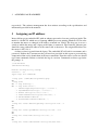
Figure 2: Setup to monitor the relative frequency error of both masers compared to the GPS.
4.1
Code in Linux: Daemon
The comparison between 1 PPS from the GPS and 1 PPS from the maser is done by the counter
after an initialization sequence which sets each counter. This initialization is governed by a
4
MEASURING THE DRIFT
6
program running as a daemon in a devoted Linux PC. The daemon starts during the PC boot
sequence. The daemon has been modified to control two different counters at the same time.
Each counter is managed by a different instance of a single C++ class which allows to control
HP 53131A/53132 counters. These two instances are created at the beginning of the Daemon.
Below we show how this is acomplished:
HPcounter * counter_im37;
HPcounter * counter_im66;
try {
counter_im37 = new HPcounter(0,4);
counter_im37->setModeComparator(1.3,1.3);
im37OK = true;
} catch (HPcounter::HPcounterException & s){
if (DEBUG)
printf("Excepcion: %s, Ibsta: %d, Iberr: %d\n", s.ShowMsg(), s.ShowStat(), s.ShowErr());
im37OK = false;
}
try {
counter_im66 = new HPcounter(0,3);
counter_im66->setModeComparator(1.3,1.3);
im66OK = true;
} catch (HPcounter::HPcounterException & s){
if (DEBUG)
printf("Excepcion: %s, Ibsta: %d, Iberr: %d\n", s.ShowMsg(), s.ShowStat(), s.ShowErr());
im66OK = false;
}
The constructor of the HPcounter class accepts the board address (always 0) and the
GPIB address of the device (4 for imaser37 counter and 3 for imaser66 counter). It resets the
counter by sending the following SCPI messages:
writeToHP("*RST");
writeToHP("*CLS");
writeToHP("*SRE 0");
writeToHP("*ESE 0");
writeToHP(":STAT:PRES");
Method setModeComparator() sets the counters to measure the time interval between
both 1 PPS signals:
writeToHP(":CONF:TINT");
writeToHP("FUNC ’TINT’");
// We switch off the levels
writeToHP(":EVEN:LEV:AUTO OFF");
// Signal in channel 1
// Manually set the levels of trigger.
sprintf(instr, ":EVEN:LEV %f V", lev1);
writeToHP(instr);
// Positive slope for the trigger
writeToHP(":EVEN:SLOP POS");
// Impedance of the signal: 50 Ohms
writeToHP(":INP:IMP 50");
writeToHP(":INP:COUP DC");
writeToHP(":INP:ATT 1");
writeToHP(":INP:FILT OFF");
writeToHP(":EVEN:HYST:REL 0");
// Signal in channel 1
// Manually set the levels of trigger.
writeToHP(":EVEN2:LEV:AUTO OFF");
sprintf(instr, ":EVEN2:LEV %f V", lev2);
4
MEASURING THE DRIFT
7
writeToHP(instr);
// Positive slope for the trigger
writeToHP(":EVEN2:SLOP POS");
// Impedance of the signal: 50 Ohms
writeToHP(":INP2:IMP 50");
writeToHP(":INP2:COUP DC");
writeToHP(":INP2:ATT 1");
writeToHP(":INP2:FILT OFF");
writeToHP(":EVEN2:HYST:REL 0");
The daemon then starts an infinite loop which reads both counters, and after each measuremnt processes the data. Each cycle of the loop takes 2 seconds to complete. The counter
reads the time interval with the following instructions:
writeToHP(":INIT:CONT ON");
writeToHP(":FETCH:TINT?");
readFromHP(data);
where writeToHP() and readFromHP() are high level calls to write and read in the GPIB
port.
The processing of the data is as follows:
• Each individual value is stored in a local variable and written on an intermediate file
data10m.log with two columns, one per counter.
• Each individual value is also stored in a shared memory variable, available to third part
applications.
• Every ten minutes the function reads file data10m.log, computes the mean value and
RMS of the time difference between the pulses and resets the file.
• The mean value and the RMS for both masers are stored in shared memory variables and
written on a database. The database contains two tables, one per maser and counter.
Shared memory variables are defined and reserved in a structure which is defined via a
program called get_countermem which is run during the PC startup. The structure is the
following:
struct maserdata {
double modifiedJulianDay;
double gps_im37_diff;
double gps_im37_diff_10m;
double gps_im37_rms_10m;
double modifiedJulianDay_im66;
double gps_im66_diff;
double gps_im66_diff_10m;
double gps_im66_rms_10m;
};
struct maserdata * shm_maserdata;
Variables modifiedJulianDay and modifiedJulianDay_im66 are duplicated and contain the same values.
In order to find out the current values of the comparison the user, can run program maserStatus
which produces the following output with instantaneous, mean and RMS values for both masers:
5
TUNING THE MASER. REMOTE CONTROL
8
./maserStatus
*** Shared memory content ***
Modified Julian Day: 55656.6231 55656.6231
Offset (each 1 sec)
im37: 915.40 ns
im66: -926.10 ns
Average and rms (10 min)
im37: 912.45 ns
0.00 ns
im66: -926.95 ns
0.00 ns
These values are available from any ACS client by using the gpsMaserComparator component but only one of the masers is available at a time. In order to get the values from the other
maser, file GPS_MASER_COMP_1 in the CDB database should be modified with the correct serial
number (either 37 or 66):
imaser="37"
5
Tuning the maser. Remote control
The maser control (and tuning) is done using a Python class with similar functionality to the
one written for imaser 37. The new class, named imaser66, uses UDP sockets on port 14000.
This version has some functionality not present in imaser37. It has some methods which allow
to:
• enableHTML(on) Start to display the monitoring of the Maser on the HTML page.
• recordData(interval) Record the monitoring in a file stored on the local SD memory card. The time period can be selected. Whenever the file reaches 2 MB size it is
copied to a second file with a name including the data and time. The first file is reset.
We have found that the commanded interval time does not match the one used and differs
several minutes from it.
• enableSerial(on) Stop the serial communication between the network module and
the maser.
• setDeltaFrequency(df) Correct the frequency by providing the relative error in frequency. Unlike imaser37 no intermediate calculations are required.
• getFrequency() Get the maser frequency (' 1420 MHz).
More methods are available but we have not mentioned them here since they provide less used
functionalities.
Class imaser66 is used by two python programs: correctiMaser66.py, which corrects
the frequency of the maser and imaser66Status2DB.py which writes the status information
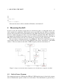
from the maser in a database. The status of the maser is composed of the list of parameters in
table 1.
The status of the maser can be obtained with a periodicity of 5 seconds by using a web
browser. Fig 3 is a snapshot of the web page.
correctiMaser66.py is a python script which corrects the frequency of the maser. It
uses a class which contains two methods for getting information from the maser status. One
retreives the data from the internal imaser FTP server. The data from this server is parsed and
5
TUNING THE MASER. REMOTE CONTROL
Channel
1
2
3
4
5
6
7
8
9
10
11
12
13
14
15
16
17
18
19
20
21
22
23
24
25
26
27
28
29
30
31
32
33
34
35
36
37
38
39
40
Description
Battery voltage A
Battery current A
Battery voltage B
Battery current B
Hydrogen pressure setting
Hydrogen pressure measurement
Purifier current
Dissociator current
Dissociator light
Internal top heater
Internal bottom heater
Internal side heater
Thermal control unit heater
External side heater
External bottom heater
Isolator heater
Tube heater
Boxes temperature
Boxes current
Ambient temperature
C-field voltage
Varactor voltage
external high voltage value
external high voltage current
internal high voltage value
internal high voltage current
Hydrogen storage pressure
Hydrogen storage heater
Pirani heater
Unused
405 kHz Amplitude
OCXO varicap voltage
+24 V supply voltage
+15 V supply voltage
-15 V supply voltage
+5 V supply voltage
-5 V supply voltage
+8 V supply voltage
+18 V supply voltage
Unused
Name
[physical unit/LSB]
U batt.A [V]
2.441E-02
I batt. A [A]
1.221E-03
U batt.B [V]
2.441E-02
I batt. B [A]
1.221E-03
Set. H [V]
3.662E-03
Meas. H [V]
1.221E-03
I purifier [A]
1.221E-03
I dissociator [A]
1.221E-03
H light [V]
1.221E-03
IT heater [V]
4.883E-03
IB heater [V]
4.883E-03
IS heater [V]
4.883E-03
UTC heater [V]
4.883E-03
ES heater [V]
4.883E-03
EB heater [V]
4.883E-03
I heater [V]
4.883E-03
T heater [V]
4.883E-03
Boxes temp. [C]
2.441E-02
I Boxes [A]
1.221E-03
Amb. Temp. [C]
1.221E-02
C field [V]
2.441E-03
U varactor [V]
2.441E-03
U HT ext. [Kv]
1.221E-03
I HT ext. [uA]
1.221E-01
U HT int. [kV]
1.221E-03
I HT int. [uA]
1.221E-01
Sto. press. [bar]
4.883E-03
Sto. heater [V]
6.104E-03
Pir. heater [V]
6.104E-03
Unused []
0.000E+00
U 405 kHz [V]
3.662E-03
U ocxo [V]
2.441E-03
+24Vdc [V]
9.766E-02
+15Vdc [V]
7.813E-02
-15Vdc [V]
-7.813E-02
+5Vdc [V]
3.906E-02
-5Vdc [V]
-3.906E-02
+8Vdc [V]
3.906E-02
+18Vdc [V]
7.813E-02
Unused []
0.000E+00
Table 1: List of iMaser monitor parameters. Taken from the imaser manual
9
5
TUNING THE MASER. REMOTE CONTROL
Figure 3: Web page with information from imaser66. The content is updated every 5 seconds.
10
6
COMPARISON BETWEEN BOTH MASERS
11
may be outdated as much as the time period of the FTP server. The second method obtains the
data from the web server and parses the data there. The information is 5 seconds old at most
since this web is refreshed with instantaneous values with a periodicity of 5 seconds. Below is
an example on how to use the script:
./correctiMaser66.py 9.5e-13
Connecting to the maser ...
Do you want to see all current parameters y/[n]) ? y
[27.611999999999998, 0.10100000000000001, 28.149000000000001,
....
1420405750.3
Current Maser frequency: 1420405750.297752 Hz
Do you want to apply this correction 9.5e-13 y/[n]) ? y
Applying the correction ...
Maser frequency after the correction: 1420405750.299098 Hz
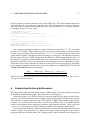
One tuning was enough to acquire a relative frequency error below 10−13 . The correction
was done on 17/3/2011. Table 2 summarizes the date and time of the tuning, the measured drift
and the correction applied. The measured drift (−9.5 10−13 ) was obtained from the slope of the
graph and the negative sign indicates that the function is decreasing. The function represents
the time elapsed between 1 PPS coming from the GPS and 1 PPS coming from the maser. If
the function is negative it means that the maser ticks slower than the GPS and both pulses get
more apart with time. In order to correct the maser frequency we had to command a positive
value, that is, the relative frequency by which we want to increase maser frequency. According
to the script the frequency of the maser before the tuning was 1420405750.297752 Hz and
1420405750.299098 Hz after the correction.
Date
17/03/2011
Time (UTC)
12:50
Meas. ∆f /f
−9.5 10−13
Appl. ∆f /f
9.5 10−13
Table 2: Date and time of the tuning. The measured drift is the drift up to the tuning date. The correction
was applied in that date and time.
6
Comparison between both masers
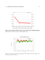
We compared the plots for both masers (maser - GPS) during 7 days after taking out the long
term drift for both individual graphs. The result can be seen in figure 5.
According to figure 5 we did not succeed in removing completely the long term drift. However it is very clear that the short term variations appear in both graphs with the same intensity.
Since the only common element was the GPS (and the 5 MHz synchronization signal in the
counters), we can conlude that these effects come from the GPS receiver. It is pobable that the
weather and conditions in the atmosphere affect the signal from the satellites. At the end of the
week we can see that there was jump downwards which is also common to both systems.
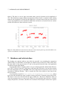
In order to check the difference between both masers we have substracted the data from both
of them, during 7 days and plotted it, taking out the slope, which corresponds to the relative
frequency difference between them. The resulting graph is rather awkward and is displayed in
6
COMPARISON BETWEEN BOTH MASERS
12
Figure 4: Maser drift since installation to April 1st 2011. The time units are Modified Julian Days.
Tuning was done on March 17th, 2011. The jump seen when tunning is due to an unknown origin and
affected both masers, therefore it may come from the GPS receiver.
Figure 5: Time ellapsed between the GPS 1 PPS and the maser 1 PPS for both masers during a week.
The long term drift was substracted.
7
DATABASE AND WEB INTERFACE
13
figure 6. The data is a sort of square waveform with a period of 48 hours and an amplitude of
2 ns. This behaviour requires further investigation to know if this is a numeric effect coming
from the data acquisition. To check if this behaviour is real and comes from one of the masers
a new setup should be used, in which the 1 PPS from each maser are injected into one counter
and the time difference between them recorded.
Figure 6: Time difference between masers 66 and 37 after removing the long term drift which corresponds to the difference in frequency between both masers
7
Database and web interface
The database was updated with two new tables for maser66: one containing the comparison
with the GPS every 10 minutes and another one with the status of the maser. These tables have
the same fields as the ones for maser 37 and can be queried from the same web application
described in report OAN-2010-1.
Currently the database contains 7 tables: two per each maser that has worked in the Observatory, CH1-75 (Kvarz), imaser37 (T4Science) amd imaser66 (T4Science) and one that contains
the room temperature up to 22-01-2009. The room temperature for the maser room is stored
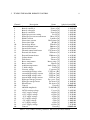
currently in a different database. Table 3 contains the dates since which we have data for the
masers in Yebes.
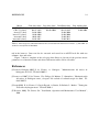
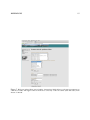
A web interface located in http://hera.oan.es/graficas_interactivas/ allows
to plot the drift and different status variables of imasers 66 and 37 from the private OAN LAN.
The maser to be used is chosen from the upper combo box. The lower combo box allows to
select the parameter that we want to plot. Below are the date/time interval from a calendar
widget, the plot title, axis labels, and the X axis resolution. The final plot is shown on a separate
REFERENCES
14
Maser
Start date (data) Stop date (data) Installation date Stop working date
CH1-75 (data)
01-10-1998 28-08-2009(*)
04-12-1995
15-06-2009
CH1-75 (status)
04-12-1995
02-02-2009
04-12-1995
15-06-2009
imaser37 (data)
28-08-2009
28-08-2009
imaser37 (status)
16-09-2009
28-08-2009
imaser66 (data)
10-03-2011
22-02-2011
imaser66 (status)
24-03-2011
22-02-2011
Table 3: Date ranges for which the database have stored data from the masers in Yebes. (*) The CH1-75
worked correctly until 15-06-2009.
tab in the browser. Data can also be extracted and stored in an ASCII local file with two
columns: date and value.
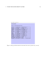
Figure 7 shows a snapshot of the web page that allows to plot any of the previous maser
parameters as a function of time and where both maser tables can be selectable.
References
[Vicente & Garrigues 2005] P. de Vicente, A. Garrigues. ”Monitorización del máser de
hidrógeno del CAY”, IT–OAN 2005-5
[Vicente et al. 2007] P. de Vicente, J.D. Gallego, R. Bolano, C. Almendros. ”Monitorización
del máser de hidrógeno antes y después del traslado al radiotelescopio de 40m”, IT–
OAN 2007-3
[Vicente2010] P. de Vicente, S. García-Espada, A. Barcia, R. Bolaño, L. Barbas. ”Tuning the
T4 Science hydrogen maser” IT-OAN 2010-1
[T4Science, 2008] T4 Science SA. ”Installation, Operation and Maintenance User Manual”,
2008
REFERENCES
15
Figure 7: Web page at http://hera.oan.es/graficas_interactivas/ which allows to plot maser parameters as
a function of time. The upper combo box allows to select any of the two tables (data and status) from
imaser 37 and 66.