Download ShipMo3D Tutorials - Dynamic Systems Analysis Ltd.

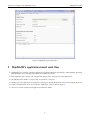
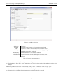
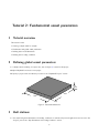
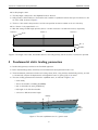
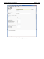
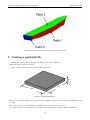
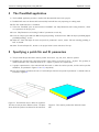
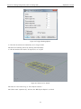
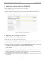
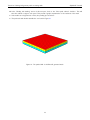
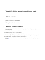
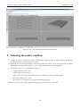
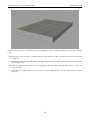
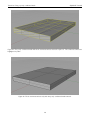
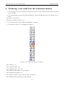
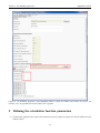
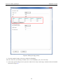
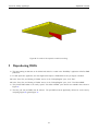
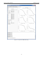
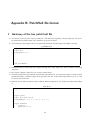
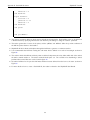
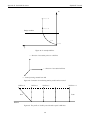
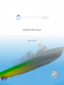
ShipMo3D 2014 Tutorials
January 22, 2015
Copyright 2015– Dynamic Systems Analysis Ltd.
Dynamic Systems Analysis Ltd.
101 - 19 Dallas Road
Victoria, BC, Canada
V8V5A6
phone: +1.250.483.7207
Dynamic Systems Analysis Ltd. (Halifax office)
201 - 3600 Kempt Road
Halifax, NS, Canada
B3K4X8
phone: +1.902.407.3722
ShipMo3D support: [email protected]
1
Contents
Introduction
3
Tutorial 1: Creating a new ShipMo3D project
4
Tutorial 2: Fundamental vessel parameters
8
Tutorial 3: Defining hull geometry using hull lines
12
Tutorial 4: Defining hull geometry with an existing mesh
18
Tutorial 5: Fixing a poorly conditioned mesh
24
Tutorial 6: Computing wave radiation and excitation
32
Tutorial 7: The BuildShip application
40
Tutorial 8: Computing RAOs
45
Tutorial 9: Adding appendages
49
A Appendix A: 20m×20m×2m box PatchHull input file
53
B Appendix B: PatchHull file format
54
2
Introduction
The tutorials presented in this document are intended to provide a basic understanding of how to set up, compute,
and simulate various hydrodynamics properties of floating vessels with ShipMo3D. ShipMo3D was originally designed for
computing wave radiation, diffraction, and resulting motions of ships, but it can also analyse a wide range of floating hull
shapes.
The tutorials are not intended to cover all possible model configurations or capabilities. Further information on features
and capabilities are detailed in the ShipMo3D User Manuals. DSA also offers training and support services to cover more
topics and assist with specific needs.
Each tutorial assumes that all prior tutorials have been completed and some tutorials build upon progress made in
previous ones. While each tutorial focuses on a different function, they are designed to be easily modified to explore the
influence of different parameters and functions available.
3
Tutorial 1: Creating a new ShipMo3D project
1
Tutorial overview
This tutorial covers:
• Creating a simulation project
• Overview of ShipMo3D application-based work flow
2
Creating a new project
+ To begin creating and editing a simulation, a project must be created.
J Open ShipMo3D by clicking on the ShipMo3D icon from the Windows Start Menu.
J In the newly opened ShipMo3D window, create a new project by clicking File→New Project.
+ A new project pane with title tab “Project*” appears. The ‘*’ signifies this pane has unsaved changes.
+ Only one project can be open at a time.
J Fill out the project information in the “ShipMo3D Project” section of the pan as shown in Figure 1:
– Set “Project directory” to the directory where project files will be stored,
– Specify a unique “Project name”
– Set “Default filename prefix”, which is used to provide unique file name prefix to the various project files created
– Set “Default label”, which is the title label used in output files.
J Do not change any other parameters in the “Project” pane.
4
Tutorial 1: Creating a new ShipMo3D project
ShipMo3D Tutorials
Figure 1: ShipMo3D project parameters.
3
ShipMo3D’s application-based work flow
+ ShipMo3D uses a collection of separate applications to perform tasks such as generating a vessel hull mesh, specifying
hull appendages, and computing wave radiation and diffraction effects.
+ Each application has a specific task and generates data for use in the project by other applications.
+ As applications are added to a project, they are opened in a new pane.
+ Usually, only a few applications are required for each project, though this depends on the specific analysis objectives.
+ A list of all applications can be seen under the “Application” menu as seen in Figure 3.
+ The role of several commonly used applications is listed in Table 1.
5
Tutorial 1: Creating a new ShipMo3D project
ShipMo3D Tutorials
Figure 2: Available applications
Application
PanelHull
RadDif
BuildShip
BuildSeaway
SeakeepRegular
FreeMo
Description
Creates the vessel geometry and computational panel mesh
Computes a database of wave radiation and excitation effects.
Defines additional manoeuvring models such as any appendages like
rudders, propellers, skegs, and keels.
Defines parameters for the sea state conditions.
Computes frequency domain vessel response in regular waves.
Computes time domain simulation response of the vessel in various
sea states.
Table 1: Commonly used applications.
J Scroll to the bottom of the “Project” pane as seen in Figure 3.
+ The “Application Data Files” section summarizes what data has been produced by applications as the project
develops.
J The project files created so far can be saved by clicking “Save” at the bottom of the “Project” pane.
+ Alternatively, individual project panes can be saved by clicking File→Save.
+ The entire project, including all open panes, can be saved by clicking File→Save All
6
Tutorial 1: Creating a new ShipMo3D project
ShipMo3D Tutorials
Figure 3: List of application data in the project
7
Tutorial 2: Fundamental vessel parameters
1
Tutorial overview
This tutorial covers:
• Creating a simple vessel for analysis
• Fundamental and global vessel parameters
• Defining basic model dimensions
• Defining static loading conditions
2
Defining global vessel parameters
+ A simple vessel consisting of a square box, seen in Figure 4, is used for this project.
J Open ShipMo3D and create a new project
J Specify a project name and directory location in the “ShipMo3D Project” section
2m
20m
20m
Figure 4: Vessel hull dimensions.
3
Hull stations
+ The vessel hull general dimensions and loading conditions are referenced by several applications and are set in the
“Project” pane in the “Ship Dimensions and Loading Condition” section.
8
Tutorial 2: Fundamental vessel parameters
ShipMo3D Tutorials
J Set Ship length to 20m
+ The ship length corresponds to the ShipMo3D frame x̂ direction.
+ Hull geometry is defined relative to the baseline and a number of equidistant stations that span from the bow to the
aft of the vessel as shown in Figure 5.
+ The bow of the vessel is always station 0 and the user specifies the station number at the aft of the ship.
J Set “Station of aft perpendicular” to 2.
+ With this setting and hull length specified, station 1 is 10m and station 2 is 20m from the bow, respectively.
Station 2
Stern
Station 1
Station 0
Ẑ = 0
Baseline
20m
Figure 5: The length of the vessel, the baseline relative to the hull geometry, and the location of each station specified.
4
Fundamental static loading parameters
+ Detailed hull geometry is defined in the PanelHull application.
+ Before detailed hull geometry is defined, several fundamental vessel parameters must be set.
+ These fundamental parameters include static loading values, which, along with the detailed hull geometry, are used
to automatically compute the displacement and longitudinal center of gravity (CG) of the vessel.
+ The static loading parameters that define the equilibrium state, as indicated in Figure 6, are:
– water density
– draft of the baseline at midship (draftBlMid)
– trim of the baseline by stern (trimBlStern)
– KG, height of the CG above baseline
– correction to GM, metacentric height
Midship
KG draftBlMid
trimBlStern
baseline
Figure 6: The static equilibrium state of a generic vessel.
9
Tutorial 2: Fundamental vessel parameters
5
ShipMo3D Tutorials
Setting specific static loading parameters
+ The specific static loading parameters for the simple vessel must be set.
J Set “Draft of baseline at midships” to 1.0.
J Set “KG, height of CG above baseline (m)” to 1.0.
J Leave all other parameters at their default values.
draftBlMid = 1m
KG = 1m
Figure 7: The vessel static condition.
6
Setting the number of rudders and propellers
J Set “Number of rudders” to 0
J Set “Number of propellers” to 0
+ The list of parameters should appear as in Figure 8.
J Save the project.
10
Tutorial 2: Fundamental vessel parameters
ShipMo3D Tutorials
Figure 8: The vessel global parameters.
11
Tutorial 3: Defining hull geometry using hull lines
1
Tutorial overview
This tutorial covers:
• Defining detailed hull geometry using surface patches and hull lines
• Defining hull panelling algorithm parameters
2
Patch hull files
+ ShipMo3D can read detailed hull geometry specified in a patch hull file.
+ The patch hull file is an ASCII text file that defines a set surface patches.
+ A surface patch represents a continuous surface. For example, an ellipsoid can be modelled using a single patch.
+ Surface discontinuities are handled by using multiple patches. For example, the hull of a ship may be formed by
many patches due to the discontinuities of the top, sides, and transom of the ship, as seen in Figure 9.
+ ShipMo3D requires geometric information for the port side only. It assumes symmetry about the x̂ − ẑ plane and
will mirror the geometry to generate the complete hull geometry.
+ Each patch is represented using a series of hull lines.
+ A patch requires at least 2 hull lines.
+ Each hull line requires at lease 1 point.
12
Tutorial 3: Defining hull geometry using hull lines
ShipMo3D Tutorials
Figure 9: Generic vessel patches defined for keel, top, and transom.
3
Creating a patch hull file
+ Detailed hull geometry will be specified for a simple box hull, seen in Figure 10.
J Open the project created in Tutorial
+ The box has 6 continuous surface patches to define each sides.
2m
20m
20m
Figure 10: Vessel hull dimensions.
J Create a new empty ASCII text file in any text editor program and save it as ‘box.inp’ in the ShipMo3D project
folder.
J Copy the contents of the patch hull file in Appendix A into the new text file and save it.
+ A detailed explanation of the format and contents of the patch hull file to be used is listed in Appendix B
13
Tutorial 3: Defining hull geometry using hull lines
4
ShipMo3D Tutorials
The PanelHull application
+ The PanelHull application provides a detailed and discretised hull form for the project
+ PanelHull will create the discrete hull automatically from hull lines or by importing an existing mesh.
J Click File→Add New Data→ PanelHull.
+ In the new “PanelHull” pane are sections titled “PanelHull” and “Ship Dimensions and Loading Condition”, which
are copied from the Project pane.
J Leave “Ship Dimension and Loading Condition” parameters as read only.
J Leave the “Import panel hull from OBJ and bypass panelling” unchecked in the ‘OBJ file import panelHull (bypass
patchHull panelling)” section
J Under the “Patch hull input file name and patch fit parameters” section, ensure “Full run including panelling of
hull” is checked.
J Under “Patch hull input file”, browse to the project folder location and select ‘Box.inp‘.
5
Specifying a patch file and fit parameters
+ The patch hull file specified has 5 surface patches: the bottom, top, side, front, and back patches.
+ PanelHull only uses the half of the hull geometry in the positive ŷ axis side of the x̂ − ẑ plane. The geometry is
assumed symmetric and is mirrored about the x̂ − ẑ plane to produce the complete hull.
+ A graphic representation of the mirrored hulls lines used to define the surface patches, and the surface patches
themselves, are presented in Figures 11 and 12, respectively.
J leave the remaining parameters in section “Patch hull input file name and patch fit parameters” at default values as
indicated in Figure 13.
Figure 11: The hull lines used to define the 5 patches.
The lines of each patch are different colours. The plane
about which the patches are mirrored is also indicated.
Figure 12: The 5 surface patches that define the vessel
hull.
14
Tutorial 3: Defining hull geometry using hull lines
6
ShipMo3D Tutorials
Adjusting the panelling parameters
J Check the “Panel dry hull” checkbox in the “Option for panelling dry hull” section.
+ Panelling the dry hull allows for complete visualisation of the hull as well as for the use of nonlinear buoyancy and
Froude-Krylov in FreeMo simulations
J Uncheck the “Compute draft and trim based on input displacement and LCG” from the “Option for Computing
Draft and Trim from Displacement and LCG” section.
+ If the displacement and LCG (longitudinal cg location) are provided, ShipMo3D will use an iterative procedure to
determine the static equilibrium state and determine the ship’s draft and trim.
J In the “Panelling parameters” section, set “Limit on area for panels” to 1.0 and the “Limit on aspect ratio for
panels” to 2.0.
J Leave remaining parameters in “Panelling parameters” at default values
+ Parameters should be set as indicated in Figure 13
15
Tutorial 3: Defining hull geometry using hull lines
ShipMo3D Tutorials
Figure 13: The PanelHull’s panelling parameters
J Save the project.
J Click “Run” in the “Save, Run, and viewing of Results” section of PanelHull.
+ After running the PanelHull application, check the summary of results by clicking “View Output”, which will open
a new pane titled “simpleVesselPanelHull3.out”.
J Scroll down to the section of the results titled “**** PATCH PROPERTIES FOR WET HULL ****” and check the
total number of panels used to model the hull. It should have about 556 panels in total. This is a coarse mesh and
more refined hydrodynamic effects will be obtained with more panels.
+ The patch hull lines and surfaces can be visualized by clicking “Plot PatchHullLine” and “Plot PatchHullSurface”,
respectively.
+ “Plot WetPatchHull” illustrates the portion of the hull that lies below the water line in static equilibrium.
16
Tutorial 3: Defining hull geometry using hull lines
ShipMo3D Tutorials
+ Similarly, “Plot DryPatchHull” illustrates the portion of the hull that lies above the water line in static equilibrium.
J Click “Plot PanelHull” in the “Save, Run, and Viewing of Results” section. This should open up a new pane titled
“Plot PanelHull”.
J In the “Shading and meshing” section of this new pane, add a check mark to the “Show panel outlines” checkbox.
This will show the outlines or edges of each panel. This provides a graphic representation of the resolution of the
mesh.
+ If the mesh is not corrupted, does not have any significant holes, anomalies, or inconsistencies, the panelling process
is completed.
+ The mesh on different faces or patches does not need to align
+ The produced mesh should resemble the one found in Figure 14.
Figure 14: The panelled hull of the vessel.
17
Tutorial 4: Defining hull geometry with an existing
mesh
1
Tutorial overview
This tutorial covers:
• Defining simple hull geometry using Rhino3D
• Importing a custom mesh
2
Generating a mesh in Rhino3D
+ A custom mesh can be used to represent the panels on a hull.
+ This can be done using the 3D modeling software, Rhino3D.
J Create a new object in Rhino3D using the “Large Objects - Meters.3dm” template.
J Save the object as “squarebox.3dm”.
+ Since ShipMo3D only requires half of a hull, split longitudinally, creating a 20x20x2m block in ShipMo3D requires
a 20x10x2m hull mesh created in Rhino3D.
+ It is good practice to model the hull split down the x-axis in Rhino3D so no frame rotations are necessary when
exporting it to an *.obj file.
+ ShipMo3D does not recognize mesh vertices in the negative (-) portion of each axis, so when creating the mesh,
keep all vertices in the positive (+) x̂, ŷ, and ẑ axes.
+ The baseline is at z=0.
+ The aft most vertices should be located at or near x=0.
J Select “Box: Corner to Corner, Height” on the left side tool bar.
18
Tutorial 4: Defining hull geometry with an existing mesh
ShipMo3D Tutorials
Figure 15: Box: Corner to Corner, Height button
J Place the first corner on the origin in the Top view window.
J Place the second corner 20m along the x-axis and 10m along the y-axis.
J In one of the other views that shows the z-axis, extend the box 2m in the positive z direction.
Figure 16: 20x10x2m Rhino3D surface
+ In order to control the meshing process, the single box surface must be “exploded” into separate surfaces.
J Select the box and click the “Explode” button.
19
Tutorial 4: Defining hull geometry with an existing mesh
ShipMo3D Tutorials
Figure 17: Explode button
+ Since ShipMo3D mirrors the panels supplied to it, the surface on the inside of the hull is not needed.
J Select the surface that is aligned with the x-axis and delete it by pressing the “Delete” button on the keyboard.
Figure 18: Inside surface
J Select all the surfaces by dragging a selection box over the whole object and click the “Mesh from surface/polysurface”.
+ The “Polygon Mesh Detailed Options” menu will pop up.
J Set meshing properties as shown in Figure 19.
20
Tutorial 4: Defining hull geometry with an existing mesh
ShipMo3D Tutorials
Figure 19: Polygon Meshing Options
+ Now that the surfaces are meshed they are no longer needed.
J Delete the remaining surfaces by selecting them individually.
+ All that remains is the mesh to be exported to an *.obj file.
Figure 20: Surfaces to be deleted
J Select all of the mesh and go to “File→Export Selected...”
J Call the mesh “squarebox.obj” and leave the “OBJ Export Options” as default.
21
Tutorial 4: Defining hull geometry with an existing mesh
3
ShipMo3D Tutorials
Importing a custom mesh into ShipMo3D
J Start a ShipMo3D project as done previously and create a new PanelHull.
J Call the Project “squarebox”.
J Instead of specifying a patch hull input file, select the “Import panel hull from OBJ and bypass panelling” box.
J Browse to the location of “squarebox.obj” for the OBJ input file.
Figure 21: Bypassing the patch hull paneling
4
Adjusting the paneling parameters
J Click “Save” in the “Save, Run, and viewing of Results” section.
J Click “Run” in the “Save, Run, and viewing of Results” section.
+ After running the PanelHull application, 5 greyed out and unclickable ‘plot’ buttons should now be available for
clicking. A summary of the results from the application run can be found by clicking “View Output”.
J Click “View Output” which will open a new pane titled “squareboxPanelHull3.out”.
J Scroll down to the section of the results titled “**** PATCH PROPERTIES FOR WET HULL ****” and check the
total number of panels used to model the box. It should have about 252 panels in total.
+ The PatchHullLine and PatchHullSurface can be visualized by clicking “Plot PatchHullLine” and “Plot PatchHullSurface” respectively.
+ The WetPatchHull can be visualized by clicking “Plot WetPatchHull”. The WetPatchHull is the portion of the
PatchHull that lies below the calm water line in static equilibrium.
+ Similarly, the DryPatchHull can be visualized by clicking “Plot DryPatchHull”. The DryPatchHull is the portion of
the PathHull that lies above the calm water line in a static equilibrium.
J Click “Plot PanelHull” in the “Save, Run, and Viewing of Results” section. This will open up a new pane titled
“Plot PanelHull”.
22
Tutorial 4: Defining hull geometry with an existing mesh
ShipMo3D Tutorials
J In the “Shading and meshing” section of this new pane, check to the “Show panel outlines” checkbox. This will
show the outlines or edges of each panel. This provides a graphic representation of the resolution of the mesh.
+ If the mesh has no degeneracies or holes, the paneling process is done.
+ The produced mesh should resemble the one found in Figure 22.
Figure 22: The paneled hull of the Rhino3D generated mesh.
23
Tutorial 5: Fixing a poorly conditioned mesh
1
Tutorial overview
This tutorial covers:
• Assessing the condition of an existing mesh file
• Regenerating geometry using continuous surfaces
• Producing new mesh from continuous surfaces
2
Importing a mesh in Rhino3D
+ This tutorial makes use of the Rhino3D software, which is primarily a surface modelling tool, though other programs
may be used instead
J Launch the Rhino3D software from the Windows start menu.
+ Rhino3D will ask for a choice of “Startup Template”.
J choose the “Large Objects - Meters” template and click “Open”.
+ Rhino3D can import NURBS geometry models, solid geometry models, and polygonal mesh geometry models.
J Click file→import... and navigate to a polygonal mesh geometry file.
+ In this case, a Wavefront OBJ file was imported that consists of a poorly conditioned box shaped geometry as shown
in Figure 23.
24
Tutorial 5: Fixing a poorly conditioned mesh
ShipMo3D Tutorials
Figure 23: The poorly conditioned mesh imported in Rhino3D.
3
Assessing the mesh’s condition
+ A polygonal mesh is a discretised geometry. Continuous and curved geometry are approximated by discretising it
into small linear surfaces called polygons or panels.
+ ShipMo3D uses the discretised surfaces to build the potential flow solution as well as for numerically integrating
fluid pressures over the geometry’s surface so a poor mesh will result in poor numerical results
+ The hallmark aspects of a poorly conditioned mesh are:
– polygons with large aspect ratios.
– polygons that are overly skewed.
– polygon sizes are not uniform; the mesh contains a combination of large and small polygons.
– The mesh resolution is too coarse.
– The mesh is not a closed surface or it has interpenetrating polygons.
J Figure 24 is poor as it includes polygons with high aspect ratio and a very coarse mesh.
25
Tutorial 5: Fixing a poorly conditioned mesh
ShipMo3D Tutorials
Figure 24: The poorly conditioned mesh imported in Rhino3D. A polygon with high aspect ratio is highlighted.
4
Reconstituting a new continuous geometric model
+ In order to produce a new well conditioned mesh of the geometry, new geometry is reconstituted using continuous
surfaces.
J Enable object snap (“Osnap”) “Mid” snap and “point” snap as shown in Figure 25
Figure 25: The “Osnap”, “Mid” and “Point” snap buttons.
+ This box has 6 sides, each side will be modelled using a continuous surface.
+ Because of the simplicity of the geometry, a surface will be constructed using two single segment polylines.
+ “Osnap” allows the mouse cursor to snap onto geometrical features.
+ The “Point” object snap setting allows the cursor to snap to mesh vertices (points).
J Select the “Surface from 3 or 4 corner points” tool.
+ The “Surface from 3 or 4 corner points” tool is highlighted in Figure 26
26
Tutorial 5: Fixing a poorly conditioned mesh
ShipMo3D Tutorials
Figure 26: The “Surface from 3 or 4 corner points” tool’s button
+ Each side of the box will be recreated as a continuous surface using the “Surface from 3 or 4 corner points” by
letting the cursor snap to the 4 corners that define each sides and click them.
J With the “Surface from 3 or 4 corner points” selected, snap to and click the 4 corners of the top side of the box.
+ This will create a surface representation of the top side of the box as shown in Figure 27.
27
Tutorial 5: Fixing a poorly conditioned mesh
ShipMo3D Tutorials
Figure 27: The creation of a continuous surface patch (highlighted yellow) created by snapping to 4 corners (red x) of the
mesh.
J Repeat the process of creating continuing surfaces for the remaining 5 sides. The results will look like that shown
in Figure 28.
+ Now that the geometry is perfectly represented using continuous surfaces, the poorly discretised mesh can be deleted
from the Rhino scene.
J Select the original mesh geometry so that it’s highlighted yellow and delete it by pressing the “Delete” or “Del” key
on the keyboard.
+ After deleted the original mesh, only the continuous surface representation of the box will remain as shown in
Figure 29.
28
Tutorial 5: Fixing a poorly conditioned mesh
ShipMo3D Tutorials
Figure 28: The poorly conditioned mesh with the 6 continuous surfaces created to replace it. The continuous surfaces are
highlighted in yellow.
Figure 29: The 6 continuous surfaces only with the poorly conditioned mesh removed.
29
Tutorial 5: Fixing a poorly conditioned mesh
5
ShipMo3D Tutorials
Producing a new mesh from the continuous surfaces
+ The continuous surfaces can be discretised and meshed as finely or coarsely as desired and the quality of the mesh
can be controlled.
+ It is recommended that each surface is meshed individually. This provides individual control over the mesh for each
surface.
J Select one of the surfaces.
J Select the “Mesh from Surface” tool.
+ A new dialogue titled “Polygon Mesh Detailed Options” will appear.
+ The “Mesh from Surface” tool is highlighted in Figure 30.
Figure 30: The “Mesh from Surface” tool’s button
J Set Density to 1.0.
J Set Maximum angle to 90.
J Set Maximum aspect ratio to 2.0.
J Set Minimum edge length to 0.0 (no minimum).
J Set Maximum edge length to 0.5.
J Set Maximum distance, edge to surface to 0.0 (no maximum).
J Set Minimum initial grid quads to 0.0 (no minimum).
30
Tutorial 5: Fixing a poorly conditioned mesh
ShipMo3D Tutorials
J Click “Preview” to see what the produced mesh will look like.
J If the mesh looks like it will be acceptable, click “OK” to accept the mesh.
J Repeat these steps for the remaining 5 surfaces, using the same meshing settings.
+ When completed, the mesh and continuous surfaces should both remain as shown in Figure 31.
Figure 31: The newly meshed continuous surfaces showing a well conditioned mesh.
6
Exporting the mesh geometry to OBJ file
+ The Rhino scene now contains the 6 continuous surfaces, and the 6 meshes.
+ The newly created meshes are now well conditioned for computation purposes.
+ The mesh is ready to be processed for importation in ShipMo3D.
+ To prepare the mesh for import into ShipMo3D, the reader is referred to Tutorial .
31
Tutorial 6: Computing wave radiation and excitation
1
Tutorial overview
This tutorial will guide the reader through the effects of wave radiation and determining the wave excitation loads on
the body using 3D potential flow panel method. The wave excitation loads include the computation of both incident wave
loads as well as wave diffraction loads. In order to compute the hydrodynamic forces acting on the body, the hull geometry
must be panelled as described in Tutorial . That is, it’s surface must be discretized into small panels which creates a
computational mesh. The panels are used to compute the potential flow solution as well as to integrate hydrodynamic
pressures over the surface of the hull.
This tutorial covers:
• Computing radiation effects database
• Understanding how frequency of oscillation affects added mass and damping
• Computing wave excitation loads
2
Pre-processing wave radiation effects
+ In order to compute wave radiation effects and wave excitation loads, the RadDif application requires the wetPanelHull
data that was produced by the PanelHull application.
J Click File→Add New Data→RadDif.
+ A new pane has opened with a tab titled “RadDif*”.
+ In Tutorial , when the “Run” button was pressed, a binary Wet Panel Hull file was produced as output called
“squareBoxWetPanelHull.bin” and stored in the project directory.
J In the “Wet Panel Hull File” section of the RadDif pane, select the Wet panel hull input file.
J Under the “Ship Radii of Gyration of Non-dimensional Hydrodynamic Coefficients” section, uncheck the “Use default
values” checkbox and enter the roll, pitch, and yaw radii of gyration properties of 5.8m, 5.8m and 8.2m respectively
as shown in Figure 32.
32
Tutorial 6: Computing wave radiation and excitation
ShipMo3D Tutorials
Figure 32: The RadDif application’s pane highlighting the roll, pitch, and yaw radii of gyration.
+ The “Options for Computing Hydrodynamic Coefficients” can be left default.
J Under the “Encounter frequencies for radiation computations (rad/s)” section of the RadDif pane, set the Min,
Max, and increment Encounter frequencies as 0.2rad/s, 8.2rad/s and 0.5rad/s. fill out the parameters as shown in
Figure 33.
+ The encounter frequency includes the effect a ship’s mean forward speed has on the perceived frequency of the waves
relative to the moving ship. If the ship is moving against the waves, the encounter frequency will be higher than
the wave’s frequency. If the ship is moving with the waves, the encounter frequency will be lower than the wave’s
frequency.
J Under the “Diffraction Computation Parameters” uncheck the ‘Include diffraction computations’ check box.
+ As a first run, it’s a good idea not to include diffraction computations. This is done in order to iterate quickly
through the radiation computations. It’s likely that the geometry will exhibit irregular frequencies which need to be
dealt with before completing a final run that includes wave excitation loads.
+ When an acceptable wave radiation effect solution is obtained, wave diffraction computations will be enabled which
33
Tutorial 6: Computing wave radiation and excitation
ShipMo3D Tutorials
will enable the computation of wave excitation loads for the vessel.
Figure 33: The RadDif application’s pane highlighting the radiation computation’s encounter frequency range.
J In the ‘Save, Run, and Viewing of Results’ section, click ‘Save’ and then click ‘Run’.
J After ShipMo3D is done processing the radiation computations, click ‘Plot RadCo’.
+ A new pane should have opened titled ‘Plot RadCo’ with non-dimensional added mass and damping plotted against
oscillation frequency. The plot should resemble the one shown in figure 34.
+ There are a few ‘irregular’ frequencies in the data. An irregular frequency is a frequency band where the system is
poorly conditioned for resolving the potential flow solution. Poor conditioning leads to inaccuracies in the potential
flow solution and generally produces discontinuities in the added mass and damping plots at those frequencies.
+ Poor condition numbers can be seen at frequencies around 3.2rad/s and 4.7rad/s in the longitudinal and lateral
condition number plots. These correspond to discontinuities in the surge, sway, roll, and pitch added mass plots.
+ To produce well conditioned added mass and damping plots, these irregular frequencies can be removed from the
computations.
34
Tutorial 6: Computing wave radiation and excitation
ShipMo3D Tutorials
J In the ‘Encounter frequencies for radiation computations (rad/s)’ section, is a table without any rows titled ‘Removed
enc freqs (rad/s)’. Add the frequency entries for 3.2rad/s and 4.7rad/s as shown in Figure 35.
35
Tutorial 6: Computing wave radiation and excitation
ShipMo3D Tutorials
Figure 34: A plot of non-dimensional added-mass and damping plotted against oscillation frequency for the 20m×20m×2m
box case.
36
Tutorial 6: Computing wave radiation and excitation
ShipMo3D Tutorials
Figure 35: The RadDif application’s pane highlighting how to removing irregular frequencies.
J In the ‘Save, Run, and Viewing of Results’ section, click ‘Save’ and then click ‘Run’.
J After ShipMo3D is done processing the radiation computations, click ‘Plot RadCo’.
+ The added mass and damping plots will resemble those shown in Figure 36.
+ Note how the added mass and damping plot are no longer exhibit sharp discontinuities.
37
Tutorial 6: Computing wave radiation and excitation
ShipMo3D Tutorials
Figure 36: A plot of non-dimensional added-mass and damping plotted against oscillation frequency for the 20m×20m×2m
box case. Irregular frequencies have been removed.
38
Tutorial 6: Computing wave radiation and excitation
ShipMo3D Tutorials
+ Now that the radiation effects solution is acceptable, the wave excitation loads can be included in the computations.
J In the ‘Diffraction Computation Parameters’ section, set the speed units to m/s, the ship speeds minimum and
maximum to 0.0m/s, the relative sea directions to span between 0.0degrees and 180degrees at 15degree increments,
and the wave frequencies to range between 0.2rad/s to 2.0rad/s at 0.2rad/s increments as shown in Figure 37.
J Enable the wave excitation computations by adding a check to ‘Include diffraction computations’
+ This option will compute the 6 DOF wave excitation force amplitudes and phase relative to the wave’s phase (both
incident wave forces and diffracted wave forces) for a set of ship speed, relative sea direction and wave frequency
combinations.
J In the ‘Save, Run, and Viewing of Results’ section, click ‘Save’ and then click ‘Run’.
Figure 37: The RadDif application’s pane highlighting the vessel’s speed, relative sea directions and wave frequencies to
use to compute the wave excitation load database.
39
Tutorial 7: The BuildShip application
1
Tutorial overview
This tutorial will guide the reader through the creation of the ship model. This step generally includes defining
manoeuvring models and appendages such as rudders and propellers. This simple square box example will not include any
appendages or manoeuvring models. These will be created in a future tutorial.
This tutorial covers:
• Evaluating the retardation functions for radiation effect modelling.
• Quick overview of building a complete ship model for time domain or frequency domain analysis.
• Exporting a radiation and diffraction database for use in ProteusDS
2
Including radiation/diffraction database and defining radii of
gyration
J Click File→Add New Data→BuildShip.
+ A new pane should have opened with a tab titled “BuildShip*”.
+ In Tutorial , when the “Run” button was pressed, a binary file was produced as output called “squareBoxRadDifDB.bin” and stored in the project directory. This file includes added mass and damping properties as a function
of frequency as well as wave excitation loads, amongst other things.
J In the “Input files for radiation and diffraction, and dry panelled hull” section of the BuildShip pane, select the
“squareBoxRadDifDB.bin” input file as shown in Figure 38.
+ The “include dry panelled hull” checkbox can be left unchecked.
J Under the “Ship Radii of Gyration of Non-dimensional Hydrodynamic Coefficients” section, uncheck the “Use default
values” checkbox and enter the roll, pitch and yaw radii of gyration of 5.8m, 5.8m and 8.2m respectively for the
vessel as shown in Figure 38
+ The radii of gyration defined in the RadDif application were only used to non-dimensionalise the added mass and
damping plots. The radii of gyration defined here will be used to compute the physical 6 DOF inertia matrix for the
body.
40
Tutorial 7: The BuildShip application
ShipMo3D Tutorials
Figure 38: The BuildShip application’s pane highlighting where to specify the RadDif output binary file location, the
inclusion of the dry panelled hull and the vessel’s radii of gyration.
3
Defining the retardation function parameters
+ The build ship application will compute the retardation functions required to perform time domain simulations with
radiation effects.
41
Tutorial 7: The BuildShip application
ShipMo3D Tutorials
J Under the “Terms for evaluation of hull retardation functions” section, set the time increment to 0.1s, the maximum
time to 10.0s, the encounter frequency increment to 0.2rad/s and the maximum encounter frequency of 8.0rad/s as
shown in Figure 39, including adding a check mark to “Use high frequency approximation”.
J In the ‘Save, Run, and Viewing of Results’ section, click ‘Save’ and then click ‘Run’.
J Click the newly available “Plot Retard” button.
+ A new pane titled “Plot Retard” should have appeared showing the Kernel functions plotted against delay time
(elapsed time). It should resemble the plots shown in Figure 40.
+ A sign that the retardation function are numerically well conditioned is that their oscillations decay to zero with
time.
+ The maximum time of the retardation functions should be chosen to be large enough to capture their decay to near
zero.
+ The time increment controls the time discretisation of the retardation functions.
+ The computation of the retardation function is completed by performing a frequency integral of added mass or
damping. The encounter frequency increment controls the that integration’s step size. The maximum encounter
frequency controls the bound of the frequency integral.
Figure 39: The BuildShip application’s pane highlighting the parameters required to compute the retardation functions.
42
Tutorial 7: The BuildShip application
ShipMo3D Tutorials
Figure 40: A plot of the square box’s retardation functions.
4
Defining manoeuvring model parameters
+ For this tutorial, manoeuvring models are ignore. The complete BuildShip model will not include any viscous loading
terms.
J Under the “Ship Resistance” section, set all parameters as shown in Figure 41.
J Under the “Hull Roll Eddy and Lateral Drag Coefficients” section, set all coefficients to 0.0 as shown in Figure 41.
+ The “Maneuvering Coefficients” and “Ship Appendages” section parameters can be left default.
J In the ‘Save, Run, and Viewing of Results’ section, click ‘Save’ and then click ‘Run’.
+ This produced a serialized binary containing the complete ship model parameters.
43
Tutorial 7: The BuildShip application
ShipMo3D Tutorials
Figure 41: The BuildShip application’s pane highlighting how to disable the ship’s resistance and lateral drag models.
5
Exporting a hydrodynamics database for use in ProteusDS
+ ShipMo3D can export a database to handle the modelling of radiation and wave excitation loading.
+ ShipMo3D will also export the ship resistance model and the lateral drag model. For this tutorial these were disabled
by zeroing their coefficients.
+ The database is exported in a ProteusDS compatible format in the form of an ASCII text file.
J In the ‘Save, Run, and Viewing of Results’ section, click “ProteusDS Export”.
J Choose an appropriate file name like “squareBoxSM3D.ini” and save it at some file path where it can later be
retrieved.
44
Tutorial 8: Computing RAOs
1
Tutorial overview
This tutorial will guide the reader through the computation of response amplitude operators (RAOs). This step requires
the reader to have completed Tutorial and have a “BuildShip” output binary database file ready for use.
This tutorial covers:
• Computing RAOs.
• Exporting RAOs for use in ProteusDS.
2
Producing RAOs
J Click File→Add New Data→SeakeepRegular.
+ A new pane should have opened with a tab titled “SeakeepRegular*”.
+ In Tutorial , when the “Run” button was pressed, a binary file was produced as output called “squareBoxShipForMotionDB.bin” and stored in the project directory. This file includes a database required for the computation of
ship motions.
J In the “Ship parameters” section of the SeakeepRegular pane, select the “squareBoxShipForMotionDB.bin” input
file as shown in Figure 42.
45
Tutorial 8: Computing RAOs
ShipMo3D Tutorials
Figure 42: The SeakeepRegular application’s pane highlighting where to specify the BuildShip output binary file location.
J Under the “Ship speeds, headings, and wave frequencies” section of the “SeakeepRegular” pane, enter the ship speed
range using units of m/s and supplying a minimum and maximum of 0.0m/s. Also set the relative sea direction
range as between 0.0degrees to 180degrees with 15degree increments and the wave frequency range as between
0.2rad/s to 2.0rad/s with 0.05rad/s increments as shown in Figure 43.
+ This instructs ShipMo3D to compute RAOs for every combination of these discrete ship speeds, sea direction and
wave frequencies.
J In the ‘Save, Run, and Viewing of Results’ section, click ‘Save’ and then click ‘Run’.
46
Tutorial 8: Computing RAOs
ShipMo3D Tutorials
Figure 43: The SeakeepRegular application’s pane highlighting how to specify the discrete ship speeds, relative sea
directions and wave frequencies for which RAOs will be computed.
+ ShipMo3D produces a report of the RAO amplitudes and phases for all 6 degrees of freedom.
J In the ‘Save, Run, and Viewing of Results’ section, click ‘View Output’ to see the report.
+ The RAO amplitudes and phases relative to the regular wave’s phase are found after the following line of text “****
Motions in Regular Waves ****”.
+ The resulting RAOs can also be represented graphically.
J In the ‘Save, Run, and Viewing of Results’ section of the “SeakeepRegular” pane, click ‘Plot MotionRAO’.
+ In the newly opened “Plot Motion RAOs” pane, the reader can select a ship speed and sea direction and view
corresponding plots of the RAOs of the square box in all 6 DOFs as shown in Figure 44
47
Tutorial 8: Computing RAOs
ShipMo3D Tutorials
Figure 44: A plot of the square box’ motion RAOs for a forward speed of 0.0 m/s and a relative sea direction of 45 degrees.
3
Exporting RAOs for use with ProteusDS
+ ShipMo3D can export an RAO database for use with ProteusDS.
+ The database is exported in a ProteusDS compatible format in the form of an ASCII text file.
J In the ‘Save, Run, and Viewing of Results’ section of the “SeakeepRegular” pane, click “ProteusDS Export”.
J Choose an appropriate file name like “squareBoxRAO.ini” and save it at some file path where it can later be retrieved.
48
Tutorial 9: Adding appendages
1
Tutorial overview
This tutorial will guide the reader through adding a skegs appendage in the BuildShip application and demonstrate the
skeg’s influence on frequency domain RAO predictions. This step requires the reader to have completed Tutorial .
This tutorial covers:
• Adding a skeg appendage.
• How manoeuvring models, which includes appendages, affect frequency domain RAO predictions.
2
Adding a skeg
J In the “Ship Appendages” section of the “BuildShip” pane, right-click the “Skegs” folder and select “Add skeg”.
J Right-click the newly added skeg and select “Edit skeg”.
J In the “Skegs member” window that opened, click “Add row” twice two add two rows.
J Fill in the skeg geometry information as shown in Figure 45.
J Click “OK”
49
Tutorial 9: Adding appendages
ShipMo3D Tutorials
Figure 45: Editing the skeg geometry.
+ The fully appended vessel model can be visualized in ShipMo3D.
J In the ‘Save, Run, and Viewing of Results’ section of the “BuildShip” pane, click “Plot Ship”.
+ In the newly open PlotShip pane, the square box vessel and it’s newly created skeg is rendered and should resemble
that shown in Figure 46
50
Tutorial 9: Adding appendages
ShipMo3D Tutorials
Figure 46: A render of the square box with its new skeg.
3
Reproducing RAOs
+ The manoeuvring models that can be defined and added to a vessel in the “BuildShip” application will affect RAO
predictions.
+ For this square box application, the most signification impact to RAO will be in the yaw degree of freedom.
J In the ‘Save, Run, and Viewing of Results’ section of the “SeakeepRegular” pane, click “Run”.
J In the ‘Save, Run, and Viewing of Results’ section of the “SeakeepRegular” pane, click “ Plot MotionRAO”.
+ The plotted RAO results in the newly opened “Plot Motion RAOs” pane should now resemble those shown in
Figure 47.
+ The sway, roll and yaw DOFs were all affected. The yaw DOF was most significantly affected as can be seen by
comparing Figure 44 against Figure 47.
51
Tutorial 9: Adding appendages
ShipMo3D Tutorials
Figure 47: The square box’ RAOs with the skeg.
52
Appendix A: 20m×20m×2m box PatchHull input
file
begin patchHull3
label box
lengthData 20 2
begin patch
label Box Bottom Patch
normalRanges -1.0 1.0 -1
begin hullLine
station 0
yOffsets 0 10
zOffsets 0 0
end hullLine
begin hullLine
station 2
yOffsets 0 10
zOffsets 0 0
end hullLine
end patch
begin patch
label Box Side Patch
normalRanges -1.0 1.0 -1
begin hullLine
station 0
yOffsets 10 10
zOffsets 0 2
end hullLine
begin hullLine
station 2
yOffsets 10 10
zOffsets 0 2
end hullLine
end patch
begin patch
label Box Top Patch
normalRanges -1.0 1.0 -1
begin hullLine
station 0
yOffsets 10 0
zOffsets 2 2
end hullLine
begin hullLine
station 2
yOffsets 10 0
zOffsets 2 2
end hullLine
end patch
begin patch
label back patch
normalRanges -1.0 1.0 -1
begin hullLine
station 2
yOffsets 10 10
zOffsets -0 2
end hullLine
begin hullLine
station 2
yOffsets 0 0
zOffsets 0 2
end hullLine
end patch
begin patch
label front patch
normalRanges -1.0 1.0 -1
begin hullLine
station 0.0
yOffsets 0 0
zOffsets 0 2
end hullLine
begin hullLine
station 0.0
yOffsets 10 10
zOffsets 0 2
end hullLine
end patch
end patchHull3
1.0 -1.0 1.0
1.0 -1.0 1.0
1.0 -1.0 1.0
1.0 -1.0 1.0
1.0 -1.0 1.0
53
Appendix B: PatchHull file format
1
Anatomy of the box patch hull file
+ The first line of the text file is begin patchHull3. This defines the beginning of the patch hull file. The end of
the patch hull file is defined using end patchHull3 at the end of the file.
+ The following two lines assign a label to the patch hull and define the hull’s length and number of stations:
patchHull3 block
begin patchHull3
label box
lengthData 20 2
...
...
...
end patchHull3
+ Individual patches are defined within the ‘begin patchHull3’ block using ‘begin patch’ which is similarly ended using
‘end patch’
+ Each patch is assigned a label and a set of surface normal ranges.
+ The normal ranges define the minimum and maximum surface normal x̂, ŷ, ẑ component ranges. If a surface normal
violates these limits, a warning message will be provided to the user. If the normal range limits are set to -1.0 and
1.0, they’ll never be violated.
+ Hull lines, used to define the surface patch are defined within the patch block. For example, the Side patch is defined
as:
Patch block
begin pathHull3
...
begin patch
label Box Side Patch
normalRanges -1.0 1.0 -1 1.0 -1.0 1.0
begin hullLine
station 0
yOffsets 10 10
54
Appendix B: PatchHull file format
ShipMo3D Tutorials
zOffsets 0 2
end hullLine
begin hullLine
stations 2 2
yOffsets 10 10
zOffsets 0 2
end hullLine
end patch
...
end patchHull3
+ The ‘station’ parameter defines at which station the hull line is being define. Each hull line point can be defined at
a different station by specifying which station each hull line point belongs to using the ‘stations’ parameter.
+ The station governs the x location of the points, and the ‘yOffsets’ and ‘zOffsets’ define the ŷ and ẑ coordinates of
the hull line points relative to the baseline.
+ ShipMo3D will fit bi-directional b-splines through the hull-lines to generate a continuous surface.
+ It is recommended that hull lines crossing the calm water line be defined in an order of increasing ẑ as shown in
Figure 48.
+ The order in which the hull-lines and their points are defined is important since they define which side of the surface
the surface normal resides on. The surface normals should point out. The convention for determining a surface
patches surface normal direction can be found in figure 49.
+ Successive hull lines for the port side hull must therefore because defined from the bow to the stern as shown in
Figure 50.
+ For more details on how to create a PatchHull file, the reader is referred to the ShipMo3D User Manual.
55
Appendix B: PatchHull file format
ShipMo3D Tutorials
ẑbl
i=n−1
i=n−2
Design waterline
i=1
i=0
ŷ
Figure 48: A example hull line.
t - direction of successive points on a hull line
s - direction of successive hull lines
n - normal pointing outward from hull
Figure 49: Convention for evaluating surface patch’s surface normal.
Hull line 0
Hull line 1
Hull line 2
Hull line n-1
Stern
Bow
Baseline
Figure 50: The profile of a hull’s port side surface patch’s hull lines.
56