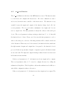
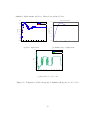
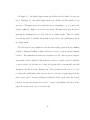
1
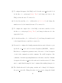
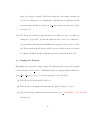
APPROVAL PAGE FOR GRADUATE THESIS OR PROJECT
GS-13
SUBMITTED IN PARTIAL FULFILLMENT OF REQUIREMENTS FOR
DEGREE OF MASTER OF SCIENCE AT CALIFORNIA STATE UNIVERSITY,
LOS ANGELES BY
Corey Baker
Candidate
Electrical and Computer Engineering
Department
TITLE:
DESIGN AND IMPLEMENTATION
OF A NON-LINEAR DYNAMICAL SYSTEM REPLICATING SPRING
BUCKLING BEHAVIOR
APPROVED:
Deborah Won
Faculty Member-CSULA
Signature
Kamran Karimlou
Faculty Member-CSULA
Signature
Fred Daneshgaran
Faculty Member-CSULA
Signature
Fred Daneshgaran
Department Chairperson
Signature
DATE: June 17, 2010
DESIGN AND IMPLEMENTATION OF A NON-LINEAR DYNAMICAL
SYSTEM REPLICATING SPRING BUCKLING BEHAVIOR
A Thesis
Presented to
The Faculty of the Department of Electrical and Computer Engineering
California State University, Los Angeles
In Partial Fulfillment
of the Requirements for the Degree
Master of Science
By
Corey Baker
June 2010
c 2010
Corey Baker
ALL RIGHTS RESERVED
ii
ACKNOWLEDGMENTS
I would like thank Francisco Valero-Cuevas and his Brain and Body Dynamics
Lab at the University of Southern California for allowing me to work in their lab,
providing me with the supplies needed, and guiding me in the project. Without the
help of all of you my work would have not been completed.
iii
ABSTRACT
Design and implementation of a non-linear dynamical system replicating spring
buckling behavior
By
Corey Baker
A device was designed and implemented to replicate spring buckling using a linear
motor. The device was designed using an off the shelf motor, microcontroller, DAQ,
and force transducer. Once the device was put together a program was written in
matlab to control the motor. Tests were done to replicate a spring damper system
and once this system was realized, tests were done to replicate the Duffing oscillater
that exhibits subcritical pitchfork bifurcation. The finished device can be used to
investigate how vision and tactile integration play a role in dynamic manipulation.
iv
TABLE OF CONTENTS
Acknowledgments
. . . . . . . . . . . . . . . . . . . . . . . . . . . . . . . . .
iii
. . . . . . . . . . . . . . . . . . . . . . . . . . . . . . . . . . . . . .
iv
List of Figures . . . . . . . . . . . . . . . . . . . . . . . . . . . . . . . . . . .
viii
Abstract
1 Introduction
. . . . . . . . . . . . . . . . . . . . . . . . . . . . . . . . . .
1
2 Methods and Design . . . . . . . . . . . . . . . . . . . . . . . . . . . . . .
5
2.1
Linear System . . . . . . . . . . . . . . . . . . . . . . . . . . . . . . .
6
2.1.1
Spring and Damper Equation . . . . . . . . . . . . . . . . . .
6
Non-Linear System . . . . . . . . . . . . . . . . . . . . . . . . . . . .
8
2.2.1
Duffing Oscillator . . . . . . . . . . . . . . . . . . . . . . . . .
8
2.3
Euler Integration . . . . . . . . . . . . . . . . . . . . . . . . . . . . .
12
2.4
Hardware . . . . . . . . . . . . . . . . . . . . . . . . . . . . . . . . .
14
2.4.1
National Instruments Data Acquisition Board . . . . . . . . .
14
2.4.2
Linear Motor and Microcontroller . . . . . . . . . . . . . . . .
15
2.4.3
Force Transducer . . . . . . . . . . . . . . . . . . . . . . . . .
17
2.4.4
Nano17 Transducer Holder . . . . . . . . . . . . . . . . . . . .
18
2.4.5
Linear Motor Holder . . . . . . . . . . . . . . . . . . . . . . .
18
2.2
v
2.5
Software . . . . . . . . . . . . . . . . . . . . . . . . . . . . . . . . . .
19
2.5.1
spring const Function . . . . . . . . . . . . . . . . . . . . . . .
20
2.5.2
spring Function . . . . . . . . . . . . . . . . . . . . . . . . . .
23
2.5.3
propagate Function . . . . . . . . . . . . . . . . . . . . . . . .
26
2.5.4
open serial Function . . . . . . . . . . . . . . . . . . . . . . .
27
2.5.5
wrc serial Function . . . . . . . . . . . . . . . . . . . . . . . .
29
. . . . . . . . . . . . . . . . . . . . . . . . . . . . . . . . . . . . .
32
3.1
Spring and Damper Equation . . . . . . . . . . . . . . . . . . . . . .
32
3.2
Duffing Oscilator . . . . . . . . . . . . . . . . . . . . . . . . . . . . .
35
3 Results
4 Instruction Manual
. . . . . . . . . . . . . . . . . . . . . . . . . . . . . .
39
4.1
Initial Setup . . . . . . . . . . . . . . . . . . . . . . . . . . . . . . . .
39
4.2
Code Modification . . . . . . . . . . . . . . . . . . . . . . . . . . . .
40
4.3
Running the Program . . . . . . . . . . . . . . . . . . . . . . . . . . .
42
References
. . . . . . . . . . . . . . . . . . . . . . . . . . . . . . . . . . . . .
vi
44
LIST OF FIGURES
1.1
Schematic of original experimental setup (1) . . . . . . . . . . . . . .
2
2.1
Designed System . . . . . . . . . . . . . . . . . . . . . . . . . . . . .
5
2.2
Simulated Spring Response . . . . . . . . . . . . . . . . . . . . . . . .
7
2.3
Potential Energy . . . . . . . . . . . . . . . . . . . . . . . . . . . . .
8
2.4
Potential Energy . . . . . . . . . . . . . . . . . . . . . . . . . . . . .
10
2.5
Subcritical Bifurcation, β > 0 and α < 0 . . . . . . . . . . . . . . . .
11
2.6
Subcritical Bifurcation Phase Portrait, β > 0 and α < 0 . . . . . . . .
12
2.7
Complete Hardware Block Diagram . . . . . . . . . . . . . . . . . . .
14
2.8
MCLM 3006 Circuit Design(2) . . . . . . . . . . . . . . . . . . . . . .
17
2.9
Nano17 Transducer Holder . . . . . . . . . . . . . . . . . . . . . . . .
18
2.10 Linear Motor Holder . . . . . . . . . . . . . . . . . . . . . . . . . . .
19
2.11 motor cntrl Function Block Diagram . . . . . . . . . . . . . . . . . .
20
2.12 spring const Function State Diagram . . . . . . . . . . . . . . . . . .
22
2.13 spring Function State Diagram . . . . . . . . . . . . . . . . . . . . .
25
2.14 propagate Function State Diagram . . . . . . . . . . . . . . . . . . . .
27
2.15 open serial Function State Diagram . . . . . . . . . . . . . . . . . . .
28
2.16 wrc serial Function State Diagram . . . . . . . . . . . . . . . . . . .
31
vii
3.1
Comparison of Motor Response to Simulated Response k = 95, δ = 10
3.2
Comparison of Motor Response to Simulated Response k = 295, δ = 10 34
3.3
Stable Motor Response β = 314, α = 3140000, δ = 10 . . . . . . . . .
36
3.4
Stable Motor Response β = 314, α = 3140000, δ = 10 . . . . . . . . .
36
3.5
Unstable Motor Response β = 314, α = 3140000, δ = 10 . . . . . . . .
37
3.6
Unstable Motor Response β = 314, α = 3140000, δ = 10 . . . . . . . .
37
viii
33
Chapter 1
INTRODUCTION
The nervous system is key to integrating and managing dynamic sensorimotor information. Understanding neural control can be complicated because the intricate
behavior is non-linear and highly dimensional (3). Grasping objects with the fingers
and thumb is a simple task that humans perform daily. Vision is often not needed to
grasp an object, but when sensory feedback such as feeling in fingers is absent, vision
is more relied upon (1). Force vectors applied by the fingers on an object must be of
sufficient magnitude to prevent slipping in the presence of gravity and other external
loads (4).
Identifying how vision assists in grasping objects along with identifying timedelays can aid in clinical efforts. To see how vision and time-delays play a role,
experiments where done and the results are in the paper, Manipulating the edge of
instability (1). Results from bifurcation theory suggests that many nonlinear dynamical systems exhibit low-dimensional dynamics at the edge of of instability (5). Based
on the center manifold theorem, a low dimensional form on a center manifold can
represent the dynamics of high-dimentional systems at the edge of instability (5).
In the paper, the thumbpad was used to compress a slender spring as far as possible
1
just before slipping. This brought the thumb+spring+nervous system to the edge of
instability (1). The experiments were done on 12 consenting young adults (9 male, 3
female), who were all right handed and had no recent hand impairments. All subjects
had no prior experience with the experimental setup. The experimental setup looks
like the figure below:
Figure 1.1: Schematic of original experimental setup (1)
Subjects wrapped their fingers around the vertical post and placed their thumbpad on top of the endcap in Figure 1.1. The bottom of the spring rests on a force
transducer that logged force at 1000Hz. The motion capture cameras captured the
3D location and orientation of the reflective markers at 200Hz using a 4-camera motion capture system. The palm of the hand never touched the spring or the vertical
2
post and the subject can view the setup from any angle of their choosing. Feedback
was provided using an audible 500Hz tone that linearly decreased in volume as the
vertical compressive spring force increased (1).
The subjects were instructed to slowly compress the spring using only their thumpad
to make the tone volume as faint as possible without letting the spring slip. Once this
point was reached, the subjects needed to maintain this load force (hear a constant
tone) for 10s without letting the spring slip and then slowly release the spring. It did
not matter if the spring oscillated or bent, but that the volume remained constant
and the spring did not slip (1).
Experiments were performed over two days. Day 1 was a training day, used for
acclimating the subjects to the system. During this day, the subjects performed
100 compressions and the performance was measured before and after the training.
On day 2, the performance of the subject was measured using normal thumbpad
sensibility, both with and without vision. Thumbpad sensibility was then reduced
when a hand surgeon administered 5 cc of 1% Lidocaine solution on the ulnar and
radial sides of the base of the thumb (just below the metacarpophalangeal (MCP)
joint of the thumb, but away from the thenar eminence) to obtain a digital nerve-block
without affecting any musculature (and associated sensors) (1).
In order to perform experiments like the one mentioned above, the spring will
be taken out of the system and replaced by a linear motor. If successful, the device
3
developed should provide us with a different set of testing abilities since we can
manipulate the edge of instability with a known low dimensional non-linear dynamical
system. The system of choice will be the Duffing oscillator which is known to model
chaotic behavior depending on the parameters chosen. If configured correctly, the
Duffing oscilator could resemble the subcritical pitchfork bifurcation(6) that models
spring buckling as seen in the paper Manipulating the edge of instability (1).
4
Chapter 2
METHODS AND DESIGN
In order to design the system, off the shelf components such as: a linear motor, data
acquisition board, and a force transducer will be needed to make the new device used
to manipulate the edge of stability. Also, parts designed in solid works such as: a
transducer holder, and linear motor holder are designed to help combine all of the
devices together. Before making the motor behave like a non-linear system, we first
attempt a linear case using the Spring and Damper Equation. After implementing
and testing the linear case, we move on to a non-linear system using the Duffing
oscillator. The designed system setup is pictured below:
(a) Complete View
(b) Top View
Figure 2.1: Designed System
5
2.1
Linear System
2.1.1
Spring and Damper Equation
Hooke’s Law of elasticity is known to approximate the extension of a spring. The
variables used in Hooke’s Law in terms of our application are below:
• Fmotor - restoring force of the motor
• x - displacement of the motor
• k - spring constant
The equation is below:
Fmotor = −kx
(2.1)
To approximate an oscillating spring whose oscillations reduce due to friction, we add
damping to the equation above. The following variables are added:
• c - damping coefficient
• ẋ - velocity
The equation turns into:
Fmotor = −kx − cẋ
6
(2.2)
Using Newton’s second law of motion, F = mẍ on the left side of the equation and
adding a forcing input, I on the right side, the equation becomes:
mẍ = −kx − cẋ + I
ẍ = = −
k
c
x − ẋ + I
m
m
(2.3)
The simulated response to an initial displacement of 0.03m, k = 1N/m, c = 0.5, I = 0
is below:
Response to Initial Conditions
0.03
0.025
0.02
Displacement (m)
0.015
0.01
0.005
0
−0.005
−0.01
−0.015
0
5
10
15
20
25
Time (sec)
Figure 2.2: Simulated Spring Response
The potential energy can be determined from equation 2.3 by putting all terms
on the left hand side and having no forcing input, I = 0 and integrating equation.
7
The potential energy equation is below:
1
1
E(t) = δ ẋ2 + kx2
2
2
(2.4)
The graph of the potential energy when δ = 0, k > 0 is pictured below:
Potential Energy
0.06
0.05
Energy
0.04
0.03
0.02
0.01
0
−0.04
−0.03
−0.02
−0.01
0
0.01
Displacement(m)
0.02
0.03
0.04
Figure 2.3: Potential Energy
2.2
2.2.1
Non-Linear System
Duffing Oscillator
The linear motor is meant to replace the spring in the experimental setup and bring
the system to the edge of instability by replicating spring buckling. The Duffing
oscillator is a dynamical non-linear system that is known to model chaotic behavior(7).
The system will model different behaviors depending on the variables below:
8
• δ - damping constant
• β - spring constant
• α - duffing constant
• γ - forcing constant
• ω - angle
• φ - phase angle
The Duffing equation is a non-linear second-order equation is seen below:
ẍ + δ ẋ + βx + αx3 = γ cos(ωt + φ)
(2.5)
The Duffing Oscillator can take on different behaviors, for instance changing β from
positive to negative gives a supercritical pitchfork bifurcation. If β > 0 the restoring
force is
Fmotor = −βx − αx3 − αẋ
(2.6)
When α > 0 and for small values of x, equation 2.7 is a hardening spring and when
α < 0 the equation is a softening spring (8). The case when β < 0 creates a double
well potential (6). The restoring force then becomes:
Fmotor = βx − αx3 − αẋ
9
(2.7)
The potential energy when there is no forcing (γ = 0) can be found for the oscillator
by integrating equation 2.5. The solution is below:
1
1
1
E(t) = δ ẋ2 + βx2 + αx4
2
2
4
(2.8)
The potential energy graph is pictured below:
Potential Energy
0.14
Potential Energy
0.02
0.12
0.015
0.1
Energy
Energy
0.01
0.08
0.06
0
0.04
−0.005
0.02
0
−0.04
0.005
−0.03
−0.02
−0.01
0
0.01
Displacement (m)
0.02
0.03
−0.01
−0.04
0.04
(a) β > 0, δ = 0, α < 0
−0.03
−0.02
−0.01
0
0.01
Displacement (m)
0.02
0.03
0.04
(b) β < 0, δ = 0, α < 0
Figure 2.4: Potential Energy
In order to manipulate the edge of instability, a subcritical pitchfork bifurcation
needs to be replicated. This done by changing β and α so that Figure 2.4(b) is
inverted. The graph of the subcritical bifurcation is pictured below:
10
Potential Energy
0.01
0.005
Energy
0
−0.005
−0.01
−0.015
−0.02
−0.04
−0.03
−0.02
−0.01
0
0.01
Displacement (m)
0.02
0.03
0.04
Figure 2.5: Subcritical Bifurcation, β > 0 and α < 0
There will always be an equilibrium point at (0, 0). To calculate the other two
equilibrium points, the equation below is used:
r
x=±
β
α
(2.9)
The phase portrait for the subcritical pitchfork bifurcation created using pplane8
which was designed by John C. Polking at Rice University. The phase portrait is
pictured below:
11
x’=y
y ’ = − (k x + c y + l x3)/m
−0.1
−0.08
k = 95
m=1
−0.06
−0.04
−0.02
0
x
0.02
0.04
0.06
c = 10
l = − 237500
0.08
0.1
Figure 2.6: Subcritical Bifurcation Phase Portrait, β > 0 and α < 0
The phase portrait shows the displacement versus the velocity. The middle point
is asymptotically stable and the points to the left and right are unstable which will
drive the system to positive or negative infinity. This phase portrait is used to see
how the system should behave.
2.3
Euler Integration
In order to handle linear and non-linear functions and calculate the the future displacement, velocity, and acceleration for the motor, the acceleration is integrated over
a small interval, τ = ∆t. The acceleration is calculated by using the linear or nonlinear function of choice and using the force along the rod as the input force. The
12
current displacement and velocity are also used. See variables below:
• xt - current displacement
• ẋt - current velocity
• Ft - current force applied along the rod of the motor
• xt+τ - future displacement
• ẋt+τ - future velocity
• ẍt+τ - future velocity
• f (xt , ẋt , Ft ) - the linear or nonlinear function
So the future acceleration is:
ẍt+τ = f (xt , ẋt , Ft )
(2.10)
The future velocity is:
Z
t+τ
xt+τ
˙
= ẋt +
ẍt dt
t
= ẋt + τ ẍt
(2.11)
The future displacement is:
Z
xt+τ = xt +
2τ
ẋt+τ dt
0
= xt + 2τ ẋt+τ + 2τ 2 ẍt+τ
13
(2.12)
2.4
Hardware
Multiple devices come together together to make the complete design. The block
diagram is below:
Nano 17
Signal
Conditioner
Nano17
Microcontroller
LM1247-080-01
NIDAQ
PC
RS232
Figure 2.7: Complete Hardware Block Diagram
2.4.1
National Instruments Data Acquisition Board
The data acquisition board used is the National Instruments NI-PCI-6025E. This
board has 16 analog inputs at up to 200kS/s at 12 or 16-bit resolution(9). It also
has up to 2 analog outputs at 10kS/s at 12 or 16 bit(9). The analog inputs of the
NI-PCI-6025E will be used to power and read the force values from the Nano17. One
analog output is used to control the position of the linear motor. For the application
14
in this thesis, matlab will be used to control all DAQ operations.
2.4.2
Linear Motor and Microcontroller
The linear dc motor used to for the S-D test is the Faulhaber Quickshaft LM 1247080-01 and is displayed below: The Quickshaft LM1247-080-01 provides us with no
residual static force and an excellent relationship between linear force and current.
The motor also has built-in Hall sensors which allow position control (10).
The MCLM 3006 S is provides precise positioning and very low speeds because it
contains a high performance digital signal processor (DSP). The microcontroller will
allow the following (10):
• Velocity control
• Velocity profiles
• Positioning mode
• Stepper motor mode
• Analog positioning mode
• Force control
Analog Position Control is utilized to control the linear motor. Initial settings as
well query commands for getting the current position of the motor are sent over
15
RS232 communication. The maximum baudrate the microcontroller can be set to is
115 kBaud, but 56 kbaud was the highest baudrate the motor was able to operate
properly at.
The maximum force the motor can exert is 9.36N and can deliver this force for
2 seconds or until the motor reaches a temperature cut-off. After this, the motor
drops down to a maximum continuous force of 3.13N and doesn’t go over this force
until the temperature drops below the cut-off temperature. The maximum speed
and acceleration the motor can provide are 2.71 m/s and 91.57 m/s2 respectively.
Variables that are used to calculate various equations for the motor are:
• Force constant - kF
• Continuous current - Ie
• Peak current - Ip
The equations used to calculate the force of the motor at any given time are:
• Constant force
Fe,max = kF Ie,max
(2.13)
Fp,max = kF Ip,max
(2.14)
• Peak force
The circuit design for the microcontroller is below:
16
Figure 2.8: MCLM 3006 Circuit Design(2)
2.4.3
Force Transducer
To interpret the force a patient is exerting on the linear motor, an ATI Nano17 force
transducer is used. Force is detected and fed back into a data acquisition board and
used as in input for the linear or non-linear equation. The Nano17 measures force
in the x,y, and z directions. This allows not only the vertical force of a patient to
be measured, but also the force along the rod of the linear motor. The maximum
force the Nano17 can endure in the x,y, and z directions are 25N, 25N, and 35N
17
respectively(11). The transducer can also measure torque in the x,y and z directions,
but this is not being used at the moment.
2.4.4
Nano17 Transducer Holder
A custom device was designed in Solid Works and printed to hold the Nano17 to
the linear motor. The device had to be made to both the specifications of the linear
motor and the force transducer. The printed device is pictured below:
Figure 2.9: Nano17 Transducer Holder
2.4.5
Linear Motor Holder
A custom holder needed to be designed in order to holster the linear motor. This
holder needed to fit the specifications of the linear motor and also needed to provide
stability since the user will be applying different forces to the linear motor. The holder
is made out of aluminum and is screwed into another aluminum device, which will
18
be strapped down to a table. The holder is versatile and allows various adjustments
of the linear motor to provide comfort for the user. The initial design of the linear
motor holder is pictured below:
Figure 2.10: Linear Motor Holder
2.5
Software
Code was written in Matlab, C, and C++ to control all tasks of the device will
perform. The matlab code controls the NIDAQ board which has inputs and outputs
to the Nano17 and microcontroller. The C and C++ code is only used for controlling
the serial communication. A state machine showing how the motor cntrl function
works is below:
19
Setup DAQ/Configure Motor
While
current_time <
stop_time
No
Yes
Get force from Load Cell
Set default values for the motor
Call spring constant function
Plot all saved values
Call spring function
Turn off motor and force
transducer
Set force of the motor
Set displacement of motor
Get displacement of motor
Save all values
Figure 2.11: motor cntrl Function Block Diagram
The motor cntrl functions makes calls to many other Matlab, C and C++ functions. These functions are described in the following sections.
2.5.1
spring const Function
This function sets the spring constant variable for the linear or non-linear function.
It has three inputs which are: spr const type, xy force, z force, and outputs the spring
20
constant to be used, k. The variable meanings are defined below:
• spr const type - string that will dictate how the spring constant is calculated
• xy force - horizontal force that is applied in the direction of the rod
• z force - vertical force applied
• k - the spring constant value that will be outputted
It works by first setting a default value to k const. The function checks spr const type
to see whether its’ value is “const” or “zforce”. If spr const type is “const”, then k
is set to k const. If spr const type is “zforce” then k becomes the product of k const
and z force. If spr const type is any other value, the function issues an error. The
block diagram for spring const is pictured below:
21
Initial State
k_const = const
spr_const_type
Constant State
k = k_const
Z Force State
k = k_const*z_force
Output
k
Figure 2.12: spring const Function State Diagram
The pseudo code for spring const is below:
[k] = spring_const(spr_const_type,xy_force,z_force)
k_const = const
switch(spr_const_type)
const: k = k_const
zforce: k = k_const*z_force
otherwise: error, unrecognized spring constant type
The xy force input variable is not used in the block diagram or the pseudo code.
This is because it currently has no affect on the spring constant, but this feature can
be added at a later date.
22
2.5.2
spring Function
This function determines what type of spring equation to use and makes calls to
calculate the future displacement, velocity, and acceleration. The function spring has
the following inputs: spr eq, m, k, x, v, f, t del. The outputs are: acc, x fut, and v fut.
These variables are defined below:
• spr eq - string that will dictate which equation will be used to calculate the
future acceleration, future displacement, and future velocity.
• m - mass of the system
• k - spring constant
• c - damping coefficient
• x - current displacement
• v - current velocity
• δ - damping constant
• α - duffing constant
• γ - current horizontal force applied to the system
• ω - angle
23
• φ - phase angle
• t del - current time delay
• acc - future acceleration
• x fut - future displacement
• v fut - future velocity
The function works by checking to see if spr eq equals “lin damp” or “non lin damp”.
If spr eq equals “lin damp”, it sets the damping coefficient c to a constant value,
calculates the future acceleration using k, m, c, v, and f, and plugging them into
the linear spring damper equation 2.3. If spr eq equals “non lin damp”, it sets the
damping coefficient c to a constant value, calculates the current acceleration using δ,
β, α, γ, ω, φ, c, v, and f and plugging them into equation (2.5). If spr eq is any other
value, the function issues an error. The block diagram for spring is pictured below:
24
spr_eq
Linear Damping State
acc = -(k/m)*x - (c/m}*v + (1/m)*f
Non-Linear Damping State
acc = -omega_not^2 -alpha*x^3 - delta*v + gamma*cos(ft+phi)
Propogat State
Call propagate function
Output
acc, x_future, v_future
Figure 2.13: spring Function State Diagram
The pseudo code for the spring function is below:
[acc,x_fut,v_fut] = spring(spr_eq,m,k,x,v,f,t_del)
switch(spr_eq)
lin_damp: c= 10
acc = -(k/m) - (c/m)*v + (1/m)*f
call propagate function
duffing: will be implemented later
otherwise: error, unrecognized spring constant type
25
2.5.3
propagate Function
The propagate Function calculates the future displacement and velocity based off of
the the current displacement, current velocity, future acceleration, and time delay of
the last time the loop was implemented. The inputs are: acc calc, x val, v val, delta t.
The outputs arex next and v next. The variables are defined below:
• acc calc - future acceleration
• x val - current displacement
• v val - current velocity
• delta t - current time delay
• x next - future displacement
• v next - future velocity
The function works by implementing the integration equations mentioned in section
2.3. First the equation multiplies delta t by acc calc and adds it to v val based off of
equation 2.11 to get v next. Then the function multiplies 2 by delta t and v val adds
it to 2 multiplied by delta t 2 and acc calc and adds that to x val to get x val based
off of equation 2.12. The state machine is pictured below:
26
V Next State
v_next = v_val + delta_t*acc_calc
X Next State
x_next = x_val + 2*delta_t*v_val + 2*dela_t^2)
Output
x_next,v_next
Figure 2.14: propagate Function State Diagram
The pseudo code for the spring function is below:
[x_next,v_next] = propagate(acc_calc,x_val,v_val, delta_t)
v_next = v_val + delta_t*acc_calc
x_next = x_val + 2*delta_t*v_val+ 2*(delta_t^2)*acc_calc
2.5.4
open serial Function
The open serial Function is one of the two MEX functions created. The function is
responsible for opening and configuring the serial port. The open serial Function has
no inputs and one output, output[0]. The MEX file for this function also has one
additional sub-function named SerialInit that has one input, BaudRate and returns
the serial object. The variables are defined below:
27
• output[0] - the address of the serial port.
• BaudRate - baudrate used to open the serial port.
The function works by calling the SerialInit function which opens the serial port with
the BaudRate passed to it by open serial. Once the serial port is opened properly,
the function exits outputing the address of the open serial port object. The state
machine is below:
Initial State
Declare all needed variables and
call SerialInit
Open Port State
Open Serial Port 5
Has the port
opened
properly?
No
Error State
Issue open port error
Yes
Set Port Parameters State
Set default parameters
Error State
Issue config port error
No
Able to set
parameters?
Yes
Output
Serial Port Address
Figure 2.15: open serial Function State Diagram
28
2.5.5
wrc serial Function
The wrc serial Function is the last of the MEX function created. The function writes
to, reads from, and configures the linear motor. All of the commands are sent to
and received from the microcontroller of the linear motor. The function is very
versatile because the inputs and outputs of the function change based off of its’
second parameter. The wrc serial takes a minimum of two inputs and does not
need to output data. The first parameter is always the address of the serial port
object. The second parameter is always an integer value from “1” to “4” that tells
the function how to behave. Every case below uses the first parameter to read or
write to the serial port, so the use of the first parameter will be omitted for the rest
of the discussion. When every case below is entered, the function checks to make sure
the right amount of inputs and outputs have been passed to the function before it
proceeds. If the wrong amounts of inputs or outputs are passed, the function issues
an error and exits. The input and output checking is omitted from below but is seen
in the function state machine.
If the second parameter is “1”, the function needs two inputs and no outputs.
The second parameter value of “1” is used to configure the motor by calling the
subfunction ConfigMotor. The ConfigMotor calls another subfunction SerialWrite to
write all the configuration values to the motor.
If the second parameter is “2”, the function needs two inputs and one output. The
29
second parameter value of “2” is used to set the position of the motor by using the
SerialWrite function to write the get position command, “POS” to the linear motor
and then using the SerialRead subfunction to receive the position value of the motor.
If the second parameter is “3”, the function has four inputs and no outputs. The
second parameter value of “3” sets the peak and continuous force of the motor using
the values of the third and fourth input parameters respectively. This is done by
calling the subfunction SerialWrite to write each value to the motor.
If the second parameter is “4”, the function has two inputs and no outputs. The
second parameter value of “4” is used to turn off the motor. The second parameter
value of “4” uses SerialWrite subfunction to send the disable command, “DI” to
the motor. After the motor has been disabled, the wrc serial Function calls the
subfunction CloseHandle to close the serial port.
The state machine for the wrc serial Function is pictured below:
30
Initial State
Declare all needed variables
Has the
minimum inputs
and outputs
been passed?
Error State
Issue open port error
No
Yes
Get Inputs State
Get the first and second input
1
Configure Motor State
Call ConfigMotor function
Get Motor Position State
No
Check
Second
Parameter
2
Has the correct
amount of inputs
and outputs been
passed?
3
4
Set Motor Force State
Has the correct
amount of inputs
and outputs been
passed?
Disable State
Call SerialWrite using "DI" is
second input
No
Error State
Issue open port error
Error State
Issue open port error
Yes
Yes
Want Position State
Call SerialWrite using "POS"
is second input
Write Peak Force State
Call SerialWrite using "LPC
parameter3" is second input
Read Position State
Write Continuos Force State
Call SerialWrite using "LCC
parameter4" is second input
Output
output position
Figure 2.16: wrc serial Function State Diagram
31
Chapter 3
RESULTS
Once the design of the system and program was completed, tests were done to obtain
behavior that mimicked the spring and damper system and the Duffing oscillator. All
of the results shown have the forcing input set to 0.
3.1
Spring and Damper Equation
To test whether the linear motor behaved like a spring that produced the correct
amount of restoring force for the appropriate displacement, the following calculation
was done to compute the spring constant when no velocity is present:
k=
Fe,motor
xmaxdisplacement
3.13N
k=
0.033m
k ∼ 95
(3.1)
Using the spring constant above, tests out the max force of the motor at the max
displacements. It also gives us a starting point to increase the spring constant if
a harder spring needs to be replicated. The results for the motor displacements,
32
simulated displacements, and force delivered are pictured below:
0.01
0.005
Response to Initial Conditions
0.005
Target Position
Actual Position
0
0
Displacement (m)
Distance m
−0.005
−0.005
−0.01
−0.01
−0.015
−0.015
−0.02
−0.02
−0.025
0
0.2
0.4
0.6
0.8
1
time s
1.2
1.4
1.6
1.8
−0.025
2
0
0.2
0.4
0.6
0.8
1
1.2
Time (sec)
(a) Motor displacement
(b) Simulated motor displacement
2.5
Peak Force
Continuous Force
2
1.5
Fmotor N
1
0.5
0
−0.5
−1
−1.5
−2
0
0.2
0.4
0.6
0.8
1
time
1.2
1.4
1.6
1.8
2
(c) Motor Force k = 95, δ = 10
Figure 3.1: Comparison of Motor Response to Simulated Response k = 95, δ = 10
33
0.025
0.005
0.015
0
Displacement (m)
0.01
Distance m
Response to Initial Conditions
0.01
Target Position
Actual Position
0.02
0.005
0
−0.005
−0.01
−0.005
−0.01
−0.015
−0.015
−0.02
−0.02
−0.025
0
−0.025
0.2
0.4
0.6
0.8
1
time s
1.2
1.4
1.6
1.8
2
0
0.2
0.4
0.6
0.8
1
1.2
Time (sec)
(a) Motor displacement
(b) Simulated motor displacement
8
Peak Force
Continuous Force
6
4
Fmotor N
2
0
−2
−4
−6
−8
−10
0
0.2
0.4
0.6
0.8
1
time
1.2
1.4
1.6
1.8
2
(c) Motor Force
Figure 3.2: Comparison of Motor Response to Simulated Response k = 295, δ = 10
In both of the figures, the initial displacement was −0.024m and the initial velocity
was 0m/s. The motor response and the simulated response were similar for the two
test trials above. A closer response to the simulated response can be realized by
adjusting the PID in the linear motor. For these test cases and the ones to follow,
the PID values were set to default values. When considering the motor force plots,
34
Figures 3.1(c) and 3.2(c), is the minimum value of the continuous force oscillates
from −1N to 1N . This is because 1N is the lowest force the motor would respond
correctly at when told to move to a given displacement. Also note that the motor
always applies the continuous force and applies the peak force only if the force in the
opposing direction is greater than the continuos force.
3.2
Duffing Oscilator
After the linear spring could be realized by the motor, the next step was to replicate
the Duffing oscillator that exhibits subcritical bifurcation. The details on the potential
energy graphs are found in section 2.2.1. The spring constant, β was calculated using
equation 3.1. The x value in the equation was changed to 0.01 because the desired
equilibrium points were set to (−0.01m, 0), (0m, 0).(0.01m, 0). The α value was then
calculated using equation 2.9. The results for the motor displacements and forces for
different initial displacements are pictured below:
35
−3
x 10
10
2
Target Position
Actual Position
Peak Force
Continuous Force
1.5
1
Fmotor N
Distance m
5
0.5
0
0
−0.5
−1
−5
0
0.2
0.4
0.6
0.8
1
time s
1.2
1.4
1.6
1.8
−1.5
0
2
0.2
0.4
(a) Motor displacement
0.6
0.8
1
time
1.2
1.4
1.6
1.8
2
(b) Motor Force
Figure 3.3: Stable Motor Response β = 314, α = 3140000, δ = 10
−3
5
x 10
1
Peak Force
Continuous Force
Target Position
Actual Position
0.5
0
Fmotor N
Distance m
0
−5
−0.5
−1
−1.5
−10
0
0.2
0.4
0.6
0.8
1
time s
1.2
1.4
1.6
1.8
−2
0
2
(a) Motor displacement
0.2
0.4
0.6
0.8
1
time
1.2
1.4
1.6
1.8
2
(b) Motor Force
Figure 3.4: Stable Motor Response β = 314, α = 3140000, δ = 10
In Figure 3.3, the initial displacement was 0.009m and the initial velocity of 0m/s.
In Figure 3.4 the initial displacement was 0.009m and the initial velocity of 0m/s. The
system stayed stable and decreased with an exponential oscillation to the equilibrium
36
point (0, 0). The behavior was similar to a spring since the motor was displaced in
between −0.01m and 0.01m. The behavior is different when the motor is displaced
beyond ±0.01m as pictured below:
0.035
10
Target Position
Actual Position
Peak Force
Continuous Force
9
0.03
8
6
Fmotor N
Distance m
7
0.025
0.02
5
4
3
0.015
2
1
0.01
0
0.2
0.4
0.6
0.8
1
time s
1.2
1.4
1.6
1.8
0
2
0
0.2
0.4
(a) Motor displacement
0.6
0.8
1
time
1.2
1.4
1.6
1.8
2
(b) Motor Force
Figure 3.5: Unstable Motor Response β = 314, α = 3140000, δ = 10
0
−0.01
Target Position
Actual Position
Peak Force
Continuous Force
−1
−2
−0.015
−4
Fmotor N
Distance m
−3
−0.02
−0.025
−5
−6
−7
−0.03
−8
−9
−0.035
0
0.2
0.4
0.6
0.8
1
time s
1.2
1.4
1.6
1.8
−10
0
2
(a) Motor displacement
0.2
0.4
0.6
0.8
1
time
1.2
1.4
1.6
(b) Motor Force
Figure 3.6: Unstable Motor Response β = 314, α = 3140000, δ = 10
37
1.8
2
In Figure 3.5. the initial displacement was 0.012m and the initial velocity was
0m/s. In Figure 3.6. the initial displacement was −0.012m and the initial velocity
was 0m/s. The figure shows the system the motor attempting to go to positive and
negative infinity for Figures 3.5 and 3.6 respectively. The figures also show the motor
applying the maximum force at each of the above displacements. This force makes
it nearly impossible to stabilize the system and get back to the equilibrium point at
0m displacement.
The linear motor successfully modeled the linear spring equation and the Duffing
oscillator. Using the Duffing oscillator, the motor is able to replicate spring buckling
behavior. The results show how the motor is attracted to its’ center region as long as it
says within certain boundaries. When the motor is moved outside of these boundaries
or moved with a velocity that is too high, the system will become unstable and will
attempt to hit the end rails. Further test of the parameters will need to be done
to adjust the equilibrium points, increase the force the motor applies applies in the
stable region, and to increase oscillations within the stable region. Once the desired
behavior is found, the system can be used to conduct tests similar to the those in the
paper Manipulating the edge of instability (1).
38
Chapter 4
INSTRUCTION MANUAL
I will go into details on how to setup the microcontroller and linear motor for usage.
There are some additional needed devices in order to get the system up and running
such as a data acquisition board and power supply.
4.1
Initial Setup
(1) Wire up the DAQ and the Nano17
(2) Connect one wire from the AO0 output channel of the DAQ to the analog input
of the microcontroller
(3) Connect one wire from the AO ground channel of the DAQ to the analog ground
of the microcontroller
(4) Hook up the RS232 cable to the microcontroller and the host computer
(5) Hook the power supply up to the microcontroller, the voltage range is 12V 30V, I typically operate the system at 24V
39
4.2
Code Modification
Once all connections are made, modifications to the matlab code need to be done in
order to get the correct functionality out of the system. The steps below will help
make these modifications:
(1) Set the path in matlab to the folder with all of the files
(2) Open up the open serial.c file and look in the function, SerialInit(int BaudRate)
and look for the line, hSerial = CreateFile( T(“COM5”) and change the value
in red to the communications port the microcontroller is hooked up to on the
host computer.
(3) If the baudrate needs to be changed, look in the open serial.c file, look in the
mexFunction(int nlhs...) and look for the line, *ptr =SerialInit(57600)) and
change the value in red to a baudrate of your choosing. To get further details
on how this function works look at section 2.5.4. Make sure to compile this file
if it is your first time using it or if you make changes to it. To compile, go to
the matlab window and type mex open serial.
(4) To configure the amount of time the program runs, look in the motor cntrl.m
file, and look for the line, stop time = 2 and change the value in red to the
amount of time in seconds you want the program to run.
40
(5) To configure the inputs of the DAQ board look in the motor cntrl.m file. Look
for the line, ai = analoginput(’nidaq’, ’Dev5’) and change the device to the
DAQ you have the nano 17 connected to.
(6) Look at the next line, ch = “addchannel(ai, [0 1 2 3 4 5]) and change the
numbers in red to the channels the nano 17 is connected to.
(7) To configure the output device of the DAQ to the microcontroller, look for
the line ao = analogoutput(’nidaq’, ’Dev5’) and change it values in red to the
appropriate device.
(8) Look at the next line, ch = “addchannel(ai, [0]) and change the number in red
to the channel the microcontroller is connected to.
(9) If you need to configure the default parameters that are sent to the motor, open
up the file, wrc serial.c and look in the ConfigMotor(HANDLE...) function.
Each line is a configuration parameter sent to the motor. A brief description
of each of the commands are in the comments. For a full description of the
commands, look in the Operating Instructions of the microcontroller. A further
description of how the wrc serial.c file works can be found in section 2.5.5. Make
sure to compile this file using the ”mex” command after making changes to it.
(10) The default value used for the spring constant can be changed by looking into
the spring const.m file. Change the value of std spr const to change the default
41
value of the spring constant. Additional variations of the spring constant can
be added by adding more case statements to this function or editing the current
case statements. Details on how the spring const.m function works can be found
in section 2.5.1
(11) The linear and non-linear equations the motor replicates can be modified by
editing the spring.m file. Additional equations can be added by adding more
case statements to the function and filling in the equation solved for the acceleration. Each equation should always call the propagate function after acceleration
is computed. Further details on this function can be found in section 2.5.2.
4.3
Running the Program
Everything is now properly setup for usage. The function that controls the program
for the system is ”motor cntrl.c”. This function has five input parameters which are
spring type, k type, por, vi, pp. To run the program, do the following:
(1) Place the motor in the middle of the rod
(2) Turn on the power supply and make sure the applied voltage is correct.
(3) Type the following command in the matlab window, motor cntrl(‘duffing’,‘const’,40,10,80)
and hit enter.
42
(4) The motor will collect baseline data from the Nano17. Do not touch the motor
while it is collecting this information
(5) The system will beep telling you the test is running and to put your hand on
the motor
(6) The system will beep again when the test is complete and tell you remove your
hand from the motor.
(7) To run the test again, go back to step 3.
(8) Turn off the power supply when you are finished
The first input to the function, spring type can be lin neg damp or duffing depending
which equation you want the spring to use. Further details of how this parameter is
used can be found in section 2.5.2. The second input k type can be const, rodforce,
zforce, or allforce. Further details of how this parameter is used can be found in
section 2.5.1. Further details on the motor cntrl function can be found in section 2.5.
Before running the program, make sure the motor is place in the middle of the rod.
This will serve is the 0 position of the motor. The program will tell you when to
place and remove your hand from the motor.
43
REFERENCES
[1] Venkadesan M, Guckenheimer J, Valero-Cuevas FJ. Manipulating the edge of
instability Journal of Biomechanics. 2007;40:1653-1661.
[2] Group Faulhaber. Operating Instructions2nd ed. 2008.
[3] Valero-Cuevas FJ. An integrative approach to the biomechanical function and
neuromuscular control of the fingers Journal of Biomechanics. 2005;38:673-684.
[4] Valero-Cuevas FJ, Smaby N, Vendkadesan M, T.Wright . The Strength-Dexterity
Test as a Measure of Dynamic Pinch Performance Journal of Biomechanics.
2003;36:265-270.
[5] Guckenheimer J, Holmes P. Nonlinear Oscillations, Dynamical Systems, and
Bifurcations of Vector Fields. Springer 1983.
[6] Moon Francis C.. Chaotic Vibrations An Introduction for Applied Scientists and
Engineers. John Wiley and Sons 2004.
[7] Hilton Robert C.. Chaos and nonlinear dynamics: an introduction for scientists
and engineers. Oxford University Press2nd ed. 2000.
[8] Thompson JMT, Stewart HB. Nonlinear Dynamics and Chaos. John Wiley and
Sons2nd ed. 2002.
44
[9] Instruments National. DAQ E Series E Series User Manual. National Instruments11500 North Mopac Expressway, Austin, Texas 787593504,USA 2007.
[10] Group Faulhaber. Quickshaft Linear DC-Servomotors, 3.13N15th ed. 2008.
[11] ATI . ATI F/T Controller Installation and Operation Manual. Pinnacle Park
and 1031 Goodworth Drive and Apex, NC 27539 USA9610-05-1017 daq ed. 2008.
45