Download BioXM™ Knowledge Management Environment

BioXM™ Knowledge
Management Environment
Quick Start
BioXM version 5.0 (252)
January 2014
Biomax Informatics AG
BioXM™ Knowledge Management Environment: Quick Start
Biomax Informatics AG
BioXM version 5.0 (252)
Publication date January 2014
Copyright © 2014 Biomax Informatics AG
Biomax Informatics AG; Sitz: Martinsried bei München, Amtsgericht München, HRB 134442; Ust-IdNr. DE 191 603 142; SteuerNr.: 143 / 100 / 10945; Vorstand: Dr. Klaus Heumann; Vorsitzender des Aufsichtsrates: Prof. Dr. Hans-Werner Mewes
Biomax and BioXM are registered trademarks of Biomax Informatics AG in Germany and other countries. Registered names,
trademarks, etc., used in this document, even when not specifically marked as such, are not to be considered unprotected by
law.
Table of Contents
Quick Start ................................................................................................................................... 1
1. Designing the data model .................................................................................................... 1
1.1. Starting the BioXM system ........................................................................................ 1
1.2. Displaying the data model ......................................................................................... 2
1.3. Adding element types ............................................................................................... 2
1.4. Adding a relation class ............................................................................................. 3
1.5. Adding an annotation form ........................................................................................ 4
1.6. Mapping BioRS entries ............................................................................................. 6
1.7. Associating an ontology ........................................................................................... 10
1.8. Defining object type scopes ..................................................................................... 11
1.9. Defining relation class scopes .................................................................................. 14
1.10. Saving the data model layout ................................................................................. 15
1.11. Displaying a saved data model layout ...................................................................... 15
2. Importing data .................................................................................................................. 17
2.1. Defining the import ................................................................................................. 17
2.2. Configuring the tab import script ............................................................................... 19
2.3. Simulating the import .............................................................................................. 24
2.4. Trouble-shooting the import ...................................................................................... 25
2.5. Completing the import ............................................................................................. 26
3. Preparing views and queries ............................................................................................... 28
3.1. Creating a view ..................................................................................................... 28
3.2. Displaying the view ................................................................................................ 35
3.3. Creating a query .................................................................................................... 36
3.4. Displaying the query results ..................................................................................... 37
3.5. Redefining the query .............................................................................................. 39
3.6. Saving the query and creating a smart folder .............................................................. 40
3.7. Editing the smart folder ........................................................................................... 40
4. Preparing a BioXM web portal ............................................................................................ 43
4.1. Logging into a BioXM web portal .............................................................................. 43
4.2. Setting up a query in the BioXM web portal ................................................................ 44
4.3. Displaying an object report in the web portal ............................................................... 49
5. Getting help ..................................................................................................................... 54
6. Logging out ..................................................................................................................... 54
6.1. Logging out of the BioXM client application ................................................................. 54
6.2. Logging out of the BioXM web portal ......................................................................... 54
iii
Quick Start
The BioXM™ Knowledge Management Environment is a project-centered, distributed platform that facilitates
communication and collaboration in a research environment. The BioXM system provides a central inventory of
information describing a particular area of research, making it easy for users to stay in touch with recent additions
or changes in knowledge that should be available to the entire organization. In addition, the BioXM system
provides a personalized work environment which supports user and project groups. This environment allows
researchers to focus specifically on generating knowledge in a particular scientific field.
This document describes the basic steps from getting started with an empty instance of the BioXM Knowledge
Management Environment to creating a productive "gene index" knowledge base:
1. Designing the data model
2. Importing data
3. Preparing views and queries
4. Preparing a BioXM web portal
These steps will allow a personalized work environment to be created using tailored views, smart folders and a
BioXM web portal.
Tip
For more information about the BioXM Knowledge Management Environment, see the BioXM User
Manual. Before using the BioXM system for the first time, you may want to read the overview of the
basic BioXM concepts and tools in the BioXM User Manual.
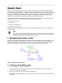
1. Designing the data model
The first step in building a knowledge base is to design the domain-specific data model in the BioXM Knowledge
Management Environment. In the example use case shown here, we will create a “gene index” knowledge
base using the following seed data: a table of gene names, synonyms, EntrezGene identifiers (IDs) and Gene
Ontology (GO) classification. A sketch of how we want to structure the data model is shown below.
Figure 1. Sketch of a data model
1.1. Starting the BioXM system
To start the BioXM client, complete the following steps.
1.
Start the BioXM client (e.g., by entering the uniform resource locator (URL) of your BioXM instance in a
browser). The login page will be displayed.
2.
Enter your user name and password and click the "Login" button.
The BioXM Knowledge Management Environment application will start and the main application window will
be displayed.
1
Quick Start
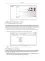
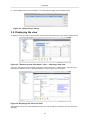
Figure 2. BioXM main application window
1.2. Displaying the data model
The BioXM system provides a graph viewer for visualization of semantic objects and the connections between
them as well as exploration of the resulting semantic network (or data model). The BioXM graph viewer renders
the data model as an interactive white board so semantic objects and associated objects in a data model can be
easily added, deleted, edited and visualized. The graph viewer allows this editing and extension while enforcing
consistency within the data model. To display the data model graph, complete the following steps.
1.
Select "Modeling → Visualize data model" in the main menu to display the "Visualize data model" dialog.
2.
Select "New visualization" and click the "OK" button to display the data model graph.
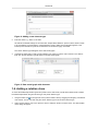
Figure 3. Data model graph with open context-sensitive menu
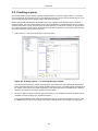
1.3. Adding element types
The data model will have two types of elements: genes and proteins. The properties of the elements are defined
by the element type. Before adding the data, relationships and annotation for the elements, we will add the
element types to the data model.
1.
Right-click anywhere in the empty field of the data model graph to display a context-sensitive menu. Select
"New → Element type". The "New element type" dialog will be displayed.
2
Quick Start
Figure 4. Adding a new element type
2.
Enter the name, e.g., "Gene" in the field.
We will use the default settings for the other tabs: "Object Name Definition" (used to set the element name
to be controlled by a certain pattern), "Representation" (used to define how the element appears in the
interface) and "Extensions" (used to set extensions for the element type). Click "OK".
The "Gene" element type will appear in the data model graph.
3.
Complete the steps again to add a protein element type. Instead of "Gene" enter "Protein" in the "Name"
field. The "Protein" element type will appear in the data model graph.
Figure 5. Data model graph with elements
1.4. Adding a relation class
To create the relationship between genes and proteins in the data model, we will add a relation class to define
the relationship between the gene element type and protein element type.
1.
Using the select tool (in the upper left corner) add a relation class by dragging-and-dropping one element
onto another. For our use case, drag the "Gene" element type to the "Protein" element type.
2.
Select "Create relation class: from 'Element: Gene' to 'Element: Protein'" from the menu. The "New relation
class" dialog will appear.
3
Quick Start
Figure 6. Adding a new relation class
3.
In the "General" tab, enter "encoding" in the name field. In the "Definition" tab, enter "encodes" in the
"Forward Name:" field and "is encoded by" in the "Backward Name:" field. We will use the default settings in
the "Representation" tab. Click the "OK" button.
The "Relation: encoding" will appear in the data model graph.
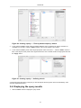
Figure 7. New relation class in the data model
1.5. Adding an annotation form
To add some basic information (including synonyms) to the genes and proteins, we will add a new annotation
form called "Basic information" to the data model and associate it with the gene and protein elements.
1.
Right click on the whitespace in the data model graph to display the context-sensitive menu. Select "New…
→ Annotation form…" from the drop-down menu. The "Create new annotation form" dialog will be displayed.
Figure 8. Adding a new annotation form to the data model
4
Quick Start
2.
Enter a name (e.g., "Basic information") for the new annotation form in the field and click "OK". The
"Annotation: Basic information" form will be displayed in the data model graph.
Figure 9. New annotation form in the data model
3.
Right click the "Annotation: Basic information" form and select "Edit" from the menu to display the "Edit
annotation form" dialog.
Figure 10. Editing an annotation form
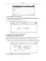
4.
In the "Attributes" section, click the "Add…" button to display the "Edit annotation form" dialog.
5
Quick Start
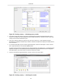
Figure 11. Adding an attribute to an annotation form
Enter a name for the attribute ("Synonyms") and a description (optional) in the text fields. Set the type to be
"Text". Click the "Next" button.
5.
Under "Attribute value properties" check the "Multiple values allowed" option. Click the "Finish" and the "OK"
buttons to return to the data model graph.
Tip
Under "Attribute type properties" you can also select the "Controlled by pattern" option and set
a pattern (i.e., a regular expression) to control the input data.
6.
Using the select tool assign the annotation form to the gene element by dragging and dropping it onto the
gene element type. Likewise, drag and drop the annotation form onto the protein element type.
The annotation form is now assigned to the gene element type and the protein element type.
Figure 12. Assigning an annotation form
1.6. Mapping BioRS entries
Next we will map the "Gene" and "Protein" elements to external database entries integrated using the BioRS
system (BioRS databanks). Genes will be mapped to the EntrezGene databank and proteins will be mapped to
the UniProt Swiss-Prot databank.
6
Quick Start
1.
Right click on the whitespace in the data model graph to display the context-sensitive menu. Select "New →
BioRS databank…". The "New BioRS Databank" dialog will be displayed.
Figure 13. Adding a new BioRS databank
2.
Click the "Choose" button to display the BioRS connection options, select a BioRS connection by clicking it
in the list and click "OK".
3.
Likewise, click the "Choose" button to display the available BioRS databanks, select a databank and click
"OK". For this use case, select the "EntrezGene" databank.
4.
Click the "OK" button in the "New BioRS Databank" dialog. The "EntrezGene" databank will appear in the
data model graph.
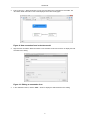
5.
Using the select tool assign the gene element type to the databank by dragging-and-dropping the "BioRS
entry: EntrezGene" to the "Element: Gene" and selecting the "Assign 'Element: Gene' to BioRS databank
'EntrezGene'" option from the context-sensitive menu.
7
Quick Start
Figure 14. Assigning an element to a BioRS databank
An assignment is created between the two. Assignments differ from relations as follows:
• Assignments are preferred if using a data set as the basis of an object definition; extra information cannot
be added. Assignments are indicated by italic text in the data model graph.
• Relations are semantic relationships; extra information can be added using annotation forms.
To add the UNIPROT_SPROT databank and assign the protein element type to it, complete the steps
again. In Step 3, select the "UNIPROT_SPROT" BioRS databank. In Step 5, drag the "BioRS entry:
UNIPROT_SPROT" to the "Element: Protein".
8
Quick Start
Figure 15. BioRS databanks in the data model
The BioRS databanks have been added to the data model. Additionally, the BioRS databanks are available in the
"BioRS entries" repository in the project tree of the BioXM client. In fact, all object types configured in the data
model graph are available under "Repositories" in the project tree. As the objects are configured and their scopes
are defined, the repositories corresponding to the object types become available automatically. Note that the
graphic below shows the project tree for the finished data model. In the current step only the "BioRS entries" and
"Ontologies" repositories are shown. Other repositories will be added after defining the scopes.
Figure 16. Object types of the data model in the project tree
9
Quick Start
1.7. Associating an ontology
Next we will add an ontology to the data model. Ontologies, a central concept in knowledge management, relate
the conceptualization of a domain to the data model. Ontologies are often developed by domain experts as a
set of “scientific nomenclature” and are widely used in the sciences. We will associate the GO ontology with the
"Gene" elements.
The GO ontology has already been imported into the BioXM system and is available in the project tree in the
"Ontologies" repository of the project tree (see Figure 16: “Object types of the data model in the project tree”).
We only need to associate the ontology with the "Gene" elements. (For more information about importing an
ontology, see the BioXM User Manual.)
1.
If the "Ontology entry: GO" is not already displayed in the data model graph, it needs to be displayed. From
the main menu, select "Modeling → Visualize Data Model" to display the "Visualize Data Model" dialog.
Figure 17. Setting what is displayed in the data model graph
2.
Click the "Select all" button or check the "Ontology entry: GO" check box. Click the "OK" button. The
"Ontology entry: GO" will be displayed in the data model graph.
10
Quick Start
Figure 18. Displaying the GO ontology in the data model graph
3.
Using the select tool drag the "Ontology entry: GO" to the "Element: Gene". Select "Create relation class:
from 'Ontology Entry:GO' to 'Element:Gene'" from the context-sensitive menu. The "New Relation Class"
dialog will be displayed.
Figure 19. Defining a new relation class
4.
In the "General" tab, enter a name for the relation class (e.g., "Functional Classification"). In the "Definition"
tab, enter a forward name (e.g., "classifies") and a backward name (e.g., "is classified by") in the fields. Click
"OK" to close the dialog.
The GO ontology will be related to the "Gene" element type.
1.8. Defining object type scopes
Next we will define the scopes for the object types. Scopes allow semantic objects of a specific class or type to
be restricted to a defined set of projects, i.e., the object type scope defines the project(s) in which the object type
can be used. The "Global Scope" setting allows the object type scope to be set to all projects. Objects based on
object types with the "Global Scope" setting can be created within any project, including any new projects that
may be created.
Special assignments (e.g., annotation assignments, BioRS databanks and ontologies) are not scope-capable,
but are considered to have the "Global Scope" setting. That is, they can be used in all projects. Elements (such
as Gene and Protein), relations and annotations, on the other hand, are scope-capable and can be restricted to
certain projects. In this use case, however, they will be given the "Global Scope" setting.
1.
In the data model graph, right click an element (e.g., "Element: Gene") and select "Scopes…" from the
context-sensitive menu.
11
Quick Start
Figure 20. Opening the "Object Type Scopes" dialog for an element type
Alternatively, select "Modeling → Element types…" in the main menu to display the "Element types" dialog.
Figure 21. Opening the "Object Type Scopes" dialog via the "Element types" dialog
2.
Select a element type and click the "Scopes…" button to display the "Object Type Scopes" dialog.
12
Quick Start
Figure 22. Setting an element type scope
3.
Click the "Enable Global Scope" button. After the scope is set, click "Close" to close the dialog window.
Alternatively, a new scope could be defined to restrict the element's use to certain projects by clicking the
"Add…" button in the "Object Type Scopes" dialog and selecting the desired projects in the "New Scopes"
dialog. In this use case, however, all scope-capable items should be given the "Global Scope" setting.
4.
Complete the steps again to set the rest of the scope-capable items (i.e., "Element:Protein" and "Annotation:
Basic information") to have the "Global Scope".
5.
The scope settings can be displayed in the data model graph by clicking the "Toggle scope display" button
(at the top of the window). The projects in the scope are displayed for each scope-capable item in the data
model (e.g., "Project: Public").
Figure 23. Displaying scopes in the data model graph
Upon defining the scopes, the elements and annotation become available in the "Repositories" folder of the
project tree (see Figure 16: “Object types of the data model in the project tree”). The "Gene" and "Protein"
element types are found in the "Elements" repository. The "Basic information" annotation form is found in the
"Annotation" repository.
13
Quick Start
1.9. Defining relation class scopes
Next we will define the scopes for the relation classes. Like scopes for objects, relation class scopes define the
project(s) in which a relation class can be used. Relation classes set to the "Global Scope" setting can be created
within any project, including any new projects that may be created.
1.
In the data model graph, right click a relation (e.g., "Relation: Functional Classification") and select
"Scopes…" from the context-sensitive menu.
Figure 24. Opening the "Object Type Scopes" dialog for a relation class
Alternatively, select "Modeling → Relation classes…" in the main menu to display the "Relation classes"
dialog.
Figure 25. Opening the "Object Type Scopes" dialog via the "Relation Classes"
dialog
2.
Select a relation class and click the "Scopes…" button to display the "Object Type Scopes" dialog.
14
Quick Start
Figure 26. Setting a relation class scope
3.
Click the "Enable Global Scope" button. After the scope is set, click "Close" to close the dialog window.
4.
Complete the steps again to set the rest of the scope-capable relations (i.e., "Relation: encoding") to have
the "Global Scope".
Upon defining the scopes, the relation classes become available in the "Relations" repository of the project tree
(see Figure 16: “Object types of the data model in the project tree”).
1.10. Saving the data model layout
Our data model is, in principle, complete. Before we import data into it, we will save the layout for future access.
1.
Click the "Save graph state" button
State" dialog.
(in the top right corner of the window) to display the "Save Graph
Figure 27. Naming the data model layout
2.
Enter a name for the model (e.g., "My Model") in the "Save as new:" field and click the "OK" button. The data
model layout is saved and can be subsequently selected for display in the data model graph.
1.11. Displaying a saved data model layout
The saved data model layout can be selected for display as follows.
1.
Select "Modeling → Visualize Data Model" in the main menu to display the "Visualize Data Model" window.
15
Quick Start
Figure 28. Selecting a saved layout for display
2.
Click the "Saved visualization" option and select the "My Model" layout from the drop-down menu. Click "OK"
to display the data model graph with the selected layout.
Figure 29. Displaying a saved layout in the data model graph
16
Quick Start
2. Importing data
Now that we have the basic data model established, we will populate the knowledge network with data and
information from external resources.
The BioXM system has a versatile importer for tables of data, which enables users to define the semantic of
the table columns and graphically build instruction sets (‘‘scripts’’) to guide the data import. During the import,
information contained in the input data file is transformed according to the semantics of the data model. This
mapping process between the defined data model and the input data ensures consistency in the knowledge
network.
This section describes importing a table of gene data, creating an import script and saving it for future use. An
import "wizard" guides the configuration of the import script. It includes specifying how the data is imported;
assigning annotation, external databank entries and ontology entries to the elements; and looking up and
creating relations.
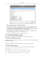
2.1. Defining the import
To import the table Genes.txt, we will use the "Tabular data import" function, which allows us to specify how data
will be uploaded according to the data model. In the following series of steps, only the specified options need to
be changed; other options can be left on the default settings.
1.
Select "File → Import Table…" in the main menu to display the first step of the "Import Table Data" wizard
(import wizard).
2.
Do the following to choose the data source.
1.
Enter the path to the file to be used for import. Alternatively, browse to the location of the file to upload.
2.
Select the type of file for import (e.g., the "Autodetect" option to detect the format automatically).
3.
Click the "Next" button to continue to the "Define Physical Layout" step of the import wizard.
Figure 30. Importing data — choosing the data source
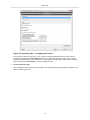
3.
Do the following to define the physical layout of the table. A preview of the data is displayed at the bottom of
the window.
1.
Under "Columns", click the "Separated columns" radio button. Specify the column separator under
"Separator" by selecting the "Preset:" option and "Tab" from the drop-down menu.
2.
Under "Columns" > "Text qualifier" select the "None" radio button.
3.
Under "Header" select "0" lines to skip and click the "Recognize table header" option.
4.
Under "Encoding" select "UTF-8" to accommodate special characters.
5.
Click the "Next" button to continue to the "Choose Script Kind" step of the import wizard.
17
Quick Start
Figure 31. Importing data — defining the physical layout
4.
Select the "New script" option and click the "Next" button to continue to the "Define Tab Import Script" step
of the import wizard.
Figure 32. Importing data — choosing the kind of script
After the script is defined and saved, it will be stored in the database. During subsequent data import, it can be
used by selecting the "Existing script" option.
18
Quick Start
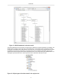
2.2. Configuring the tab import script
The next series of steps configures the tab import script used to import the Genes.txt data. A workflow of several
import operations is defined. Each import operation is selected from the "Available import operations" panel on
the left. The defined workflow is displayed in the "Tab import script" panel in the middle. Depending on the item
selected in the middle panel, a dialog for specifying the necessary information is displayed in the right panel.
Note, that this kind of three-panel layout is often used in the BioXM user interface. An option is selected in the left
panel, listed in the middle panel and defined in the right panel.
In the following series of steps, only the specified options need to be changed; other options can be left on the
default settings.
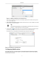
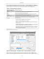
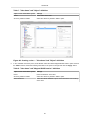
1.
Under "Available import operations" select "Lookup or create element" and click the "Add>>" button. Options
for the import operation will be displayed under "Tab import script". Click each option listed in the table below
to display the settings in the right panel. After selecting the listed settings, click the "Apply" button.
Table 1. "Look up or create element" operation
Option selected in the
Settings in right panel
"Tab import script" panel
Name
Select the "Take from column" option and "A:Gene Name" from the drop-down
menu.
Type
Select the "Use constant value" option and "Gene" from the drop-down menu.
Create in project
Select the "Default for Element Type" radio button. The project will be set to the
default for Gene elements, i.e., the "Public" project.
The defined operation is shown below.
Figure 33. Importing data — tab import script "Lookup or create element" operation
19
Quick Start
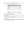
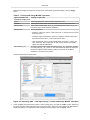
2.
Under "Available import operations" select "Create annotation" and click the "Add>>" button. Options for
the import operation will be displayed under "Tab import script". Click each option listed in the table below to
display the settings in the right panel. After selecting the listed settings, click the "Apply" button.
Table 2. "Create annotation" operation
Option selected in the
Settings in right panel
"Tab import script" panel
Object
Select the "$element1" option from the drop-down menu.
Name
Use the default settings. A name is optional.
Form
Select the "Basic information" annotation form from the drop-down menu.
Overwrite
Check the "Overwrite single anonymous" check box.
Create in project
Select the "Default for Annotation Form" radio button. The project will be set to
the default project for the annotation form, i.e., the "Public" project.
Synonyms
Set several options:
• Check the "Exclude duplicated values" check box.
• Check the "Add to existing values" check box.
• Select the "Take from column:" radio button and "B: Synonyms" from the
drop-down menu.
• Check the "Split with separator" check box, select the "Preset" radio button,
and select the semi-colon ";" from the drop-down menu.
• Click the "Edit" link next to "Empty/invalid values processing". A dialog will
open. Select the "Skip" radio button for both "Empty values" and "Invalid
values" and click the "OK" button.
The defined operation is shown below.
Figure 34. Importing data — tab import script "Create annotation" operation
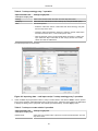
3.
Under "Available import operations" select "Lookup and assign BioRS" and click the "Add>>" button.
Options for the import operation will be displayed under "Tab import script". Click each option listed in the
20
Quick Start
table below to display the settings in the right panel. After selecting the listed settings, click the "Apply"
button.
Table 3. "Lookup and assign BioRS" operation
Option selected in the
Settings in right panel
"Tab import script" panel
Object
Select the "$element1" option from the drop-down menu.
Databank
Select "Use constant value" and "EntrezGene" from the drop-down menu.
Element name
Select "Use constant value" and "_ID_" from the drop-down menu. ("_ID_" is
the primary key in the EntrezGene databank.)
Element value
Set several options:
• Select the "Take from column:" radio button and "C: EntrezGene ID" from the
drop-down menu.
• Check the "Split with separator" check box, select the "Preset" radio button
and select the semi-colon ";" from the drop-down menu.
• Click the "Edit" link next to "Empty/invalid values processing". A dialog will
open. Select the "Skip" radio button for both "Empty values" and "Invalid
values" and click the "OK" button.
Skip lookup by _ID_
Check the "Assume entry exists when looking up by _ID_" check box. (Setting
the "Skip lookup by _ID_" option to "Yes" will increase the speed of the import
because the BioXM system will skip creating a connection to the BioRS
databank to check if the entry exists.)
The defined operation is shown below.
Figure 35. Importing data — tab import script "Lookup and assign BioRS" operation
4.
Under "Available import operations" select "Lookup ontology entry" and click the "Add>>" button. Options for
the import operation will be displayed under "Tab import script". Click each option listed in the table below to
display the settings in the right panel. After selecting the listed settings, click the "Apply" button.
21
Quick Start
Table 4. "Lookup ontology entry " operation
Option selected in the
Settings in right panel
"Tab import script" panel
Ontology
Select "Use constant value" and "GO" from the drop-down menu.
Lookup by
Select the "Uid" radio button to look entries up by a unique identifier (UID).
Value
Set several options:
• Select the "Take from column:" radio button and "D:GO.Ontology entry Uid"
from the drop-down menu.
• Check the "Split with separator" check box, select the "Preset" radio button
and select the semi-colon ";" from the drop-down menu.
• Click the "Edit" link next to "Empty/invalid values processing". A dialog will
open. Select the "Skip" radio button for both "Empty values" and "Invalid
values" and click the "OK" button.
The defined operation is shown below.
Figure 36. Importing data — tab import script "Lookup ontology entry" operation
5.
Under "Available import operations" select "Lookup or create relation" and click the "Add>>" button. Options
for the import operation will be displayed under "Tab import script". Click each option listed in the table below
to display the settings in the right panel. After selecting the listed settings, click the "Apply" button.
Table 5. "Lookup or create relation" operation
Option selected in the
Settings in right panel
"Tab import script" panel
Relation class
Select the "Use constant value" option and "Functional Classification" from the
drop-down menu.
22
Quick Start
Option selected in the
Settings in right panel
"Tab import script" panel
Source
Select the "Use result variable" option and "$ontology-entry1" from the dropdown menu.
Target
Select the "Use result variable" option and "$element1" from the drop-down
menu.
Create in project
Select the "Default for Relation Class" radio button. The project will be set to
the default project for the relation class, i.e., the "Public" project.
The defined operation is shown below.
Figure 37. Importing data — tab import script "Lookup or create relation" operation
6.
Before continuing, we will store the import script. Click the "Store as…" button at the top of the import
wizard. Enter a name for the tab-import script in the dialog and click the "OK" button to return to the wizard.
Figure 38. Importing data — storing the import script
Click the "Next>" button in the import wizard to continue to the "Choose Processing Policy" step.
23
Quick Start
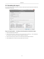
2.3. Simulating the import
First, we will simulate the import using the first 100 items to make sure the import script works as needed. Then
we will import the entire table.
Figure 39. Importing data — choosing a processing policy to simulate the import
1.
Click the "Simulate import" radio button.
2.
Click the "Process only lines:" check box and set a number of lines to process (e.g., "-100" to simulate the
first 100 lines) or leave the check box empty to simulate the entire import.
3.
Click the "Produce import log" check box to record all import operation activity for each line.
4.
Click the "Next" button to continue to the "Import Data" step of the wizard.
24
Quick Start
Figure 40. Importing data — simulating the import
The import simulation may take some time, but you can continue working with the BioXM system as the
import is processed by clicking the "Put to background" button. To display the task again, select "View
→ Show Background Task Manager" in the main menu. The "Background Task Manager" window will be
displayed. Click the task and the "Task Details…" button to display the task.
5.
If there are no problems upon completion of the simulation, we can proceed to the actual data import by
clicking the "Back" button. See Section 2.5: “Completing the import”.
If there are errors reported see Section 2.4: “Trouble-shooting the import”.
2.4. Trouble-shooting the import
The section lists some typical errors encountered when importing and how to overcome them.
2.4.1. Error: Insufficient privileges
If the following type of error is displayed, check that the correct scopes are set for all scope-capable objects and
relations in the data model.
ERROR: Insufficient privileges
See Section 1.8: “Defining object type scopes” and Section 1.9: “Defining relation class scopes”.
2.4.2. Error: Entry not found
If an entry is not found and a variable cannot be defined, the following type of error will be displayed.
Table parsing errors: No table parsing errors occurred.
Import errors:
Line 2: ERROR: Ontology entry with uid `GO:0017068' not found.
Line 2: ERROR: Ontology entry with uid `GO:0000004' not found.
Line 2: ERROR: Ontology entry with uid `GO:0005554' not found.
Line 2: ERROR: Ontology entry with uid `GO:0008372' not found.
Line 2: ERROR: Variable `$ontology-entry1' is not defined.
25
Quick Start
Line 4: ERROR: Ontology entry with uid `GO:0000004' not found.
Line 4: ERROR: Ontology entry with uid `GO:0005554' not found.
Line 4: ERROR: Variable `$ontology-entry1' is not defined.
Processed lines: The requested line ranges "-10" are rejected
and does not influence database modifications.
Database modifications summary: No database modifications were performed.
If the "Allow partial import" option is selected, such errors will be ignored during the import. See Section 2.5:
“Completing the import”.
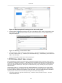
2.5. Completing the import
If there are no problems upon simulating the import, we can proceed to the actual data import.
1.
Open the "Choose processing policy" step of the import wizard.
In the import wizard, click the "Back" button. Alternatively, start a new import wizard by selecting "File →
Import Table…" in the main menu and using the existing "Import gene index table" script. Click the "Next"
button until the "Choose processing policy" step of the wizard is displayed.
2.
Choose a processing policy to perform the import.
Figure 41. Importing data — choosing a processing policy to perform the import
Do the following in this step of the import wizard:
1.
Click the "Allow partial import" radio button.
2.
Clear the "Process only lines:" check box.
3.
Click the "Produce import log" check box to record all import operation activity for each line (optional).
4.
Click the "Next" button to continue to the "Import Data" step of the wizard.
The "Allow partial import" option sets the BioXM system to process the import operations by small portions
(chunks). The system automatically optimizes the number of rows processed based on network capabilities
and import speed. Partial import allows multiple imports to run simultaneously — each allowing one chunk
at a time into the queue. If the "Cancel" button is clicked during the import, the import is not stopped
immediately, but after completing the current chunk. In addition, some import errors are ignored (e.g., "Entry
not found" errors).
The "Allow complete import only" option sets the BioXM system to import the entire table at once, not in
chunks. Other import scripts in the queue will wait until the entire upload has been processed.
26
Quick Start
Figure 42. Importing data — completing the import
The import may take some time, but you can continue working with the BioXM system as the import is
processed by clicking the "Put to background" button. To display the task again, select "View → Show
Background Task Manager" in the main menu. The "Background Task Manager" window will be displayed.
Click the task and the "Task Details…" button to display the task.
3.
Finishing the data import
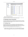
Click the "Finish" button to close the import wizard. The imported elements (genes) will be displayed in the
default "Element Type View".
27
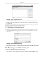
Quick Start
Figure 43. Displaying the gene list
The "Element general information" view is the built-in, default view for genes. In Section 3.1: “Creating a view”,
we will create a view for genes which is tailored for use in the "gene index" use case.
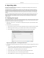
3. Preparing views and queries
In this section we will prepare the system for use by creating views, queries and smart folders. This will allow us
to tailor how the information in the gene index knowledge network is presented so we can query the knowledge
network, explore the network graph and report the query results as specifically needed. We will create a gene list
view and smart folders tailored to our use case.
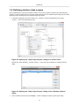
3.1. Creating a view
Views display a selection of information about selected objects. Information displayed in the view can be
taken from the object properties (such as name and description) or from other associated objects. For each
element, there is always one built-in view, e.g., "Element general information", which shows the default properties
available for the object (see Figure 43: “Displaying the gene list”). Initially, it is set as the default view; however,
additional views can be created to address specific needs and set as the default view.
We will create a new view so the gene list displays the information most relevant to this use case.
1.
To create a new view, select "Administration → Views…". (This item will be enabled only for users with the
appropriate privileges. For more information about privileges, see the BioXM User Manual.) Alternatively, in
any open view, click the "Manage…" button next to the name of the view. The "Views" dialog is displayed.
28
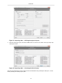
Quick Start
Figure 44. Creating a view — the "Views" dialog
2.
Click the "New…" button to display the "New View" dialog (see Figure 45, “Creating a view — "General"
tab”).
3.
Define the following information for the new view in the "General" tab.
Table 6. "General" tab options
Option in the "General" tab
Settings
Name
Enter "Gene list view" in the field.
Allowed types
Select the type of object for which the view will be available (e.g., kind
"Element" and element type "Gene") from the drop-down menus.
Description
Enter a short description of the view (optional).
Project
Select the "Public" project.
Allowed for table
Select the "Allowed for table" and "Use as default for table" options.
Allowed for report
Select the "Allowed for report" and "Use as default for report" options.
Figure 45. Creating a view — "General" tab
4.
Click the "View items" tab. The "View Items" interface (see Figure 46: “Creating a view — "View Items" tab
"Object" definition”) is similar to the import wizard with three panels. Each view item is selected from the
"Available view items" panel on the left. The added item is displayed in the "View items" panel in the middle.
Depending on the item selected in the middle panel, a dialog for specifying the necessary information
appears in the right panel. The view items will become the columns of the table in the order they are listed in
the middle panel.
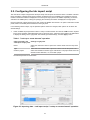
5.
In the "Available view items" panel, under "Object Properties" select the "Object" option and click the
"Add>>" button. Define the following information in the right panel and click the "Apply" button.
29
Quick Start
Table 7. "View Items" tab "Object" definition
Option in the "View Items" panel
Settings
Name
Enter "Gene" in the field.
Shown by default in tables
Select the "Shown by default in tables" option.
Figure 46. Creating a view — "View Items" tab "Object" definition
6.
In the "Available view items" panel, under "BioRS" select the "BioRS mapped BioRS entries" option and click
the "Add>>" button. Define the following information in the panel on the right and click the "Apply" button.
Table 8. "View Items" tab "Mapped BioRS entries" definition
Option in the "View Items" panel
Settings
Name
Enter "EntrezGene" in the field.
Shown by default in tables
Select the "Shown by default in tables" option.
BioRS databank
Select the "BioRS databank" option and "EntrezGene" from the dropdown menu.
30
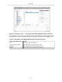
Quick Start
Figure 47. Creating a view — "View Items" tab "Mapped BioRS entries" definition
7.
In the "Available view items" panel, under "BioRS" select the "mapped BioRS entry attribute" option and click
the "Add>>" button. Define the following information in the panel on the right and click the "Apply" button.
Table 9. "View Items" tab "Mapped BioRS entry attribute" definition
Option in the "General" tab
Settings
Name
Enter "Chromosome" in the field.
Shown by default in tables
Select the "Shown by default in tables" option.
Databank
Select "EntrezGene" from the drop-down menu.
Attribute
Select "Chromosome" from the drop-down menu.
31
Quick Start
Figure 48. Creating a view — "View Items" tab "Mapped BioRS entry attribute"
definition
8.
In the "Available view items" panel, under "Annotation" select the "Assigned annotation attribute" option and
click the "Add>>" button. Define the following information in the panel on the right and click the "Apply"
button.
Table 10. "View Items" tab "Assigned annotation attribute" definition
Option in the "General" tab
Settings
Name
Enter "Synonym" in the field.
Shown by default in tables
Select the "Shown by default in tables" option.
Annotation form
Select "Basic information" from the drop-down menu.
Attribute
Select "Synonym" from the drop-down menu.
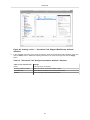
32
Quick Start
Figure 49. Creating a view — "View Items" tab "Assigned annotation attribute"
definition
9.
In the "Available view items" panel, under "Knowledge Network" select the "Related objects" option and click
the "Add>>" button. Define the following information in the panel on the right and click the "Apply" button.
Table 11. "View Items" tab "Related objects" definition
Option in the "General" tab
Settings
Name
Enter "GO" in the field
Shown by default in tables
Select the "Shown by default in tables" option.
Related object is
Select the "Source or target" option.
Relation class
Click the check box and select "Functional Classification" from the dropdown menu.
Related object type
Select the "Related object type" option. Under "Kind" select "Ontology
entry" from the drop-down menu. Under "Ontology" select "GO" from the
drop-down menu.
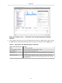
33
Quick Start
Figure 50. Creating a view — "View Items" tab "Related objects" definition
10. Before closing the dialog, we will reorder the view items so the "Synonyms" are shown in the second column
of the "Gene list view" table. Select the "Synonyms" item in the middle panel and click the arrow up button
to put it in the second position in the panel. The view items defined become the columns of the table in the
order they are listed in the middle panel.
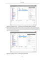
Figure 51. Creating a view — reordering the view items
34
Quick Start
11. Click the "OK" button to close the dialog. In the "Global Views" dialog, click the "Close" button.
Figure 52. "Global Views" dialog
3.2. Displaying the view
To display the new view, select "Gene list view" from the "View" drop-down menu in the "Gene" element window.
Figure 53. "Element general information" view — selecting a new view
In the view, the columns can be sorted by clicking any column header (e.g., "Chromosome"). Columns can be
selected to be displayed or not by clicking the table icon in the top right corner of the table.
Figure 54. Displaying the "Gene list view"
The appearance of the view is automatically saved for each user and will be the same the next time the view is
displayed.
35
Quick Start
3.3. Creating a query
Next we will create a query to answer a specific scientific question or perform a specific task in our use case.
In the first example we will create a query to find all signal transduction genes in the knowledge network. In the
second example we will create a general query to find genes by function.
Queries can be easily defined within the BioXM system using a graphical user interface which is similar to
the import wizard. The query builder features a query language similar to a natural language and can support
complex search tasks. A query can be stored in the query repository for later reuse. A query can also be saved
as a smart folder within a project folder. Each time the smart folder is opened the query is performed, ensuring
up-to-date information with no maintenance effort.
1.
Select "Search → Find by advanced query" in the main menu.
Figure 55. Creating a query — accessing the query wizard
The "Find by advanced query" wizard will be displayed. It is similar to the import wizard with three panels.
Query criteria are selected from the "Criteria available" panel on the left. The added criteria are displayed in
the "Object to find" panel in the middle. Depending on the criteria selected in the middle panel, a dialog for
specifying the necessary information appears in the right panel.
2.
We want to search for genes involved in signal transduction so we will perform a search for genes that are
classified by the GO ontology entry "signal transduction".
In the "Criteria available" panel under "Object Selection" open "is an element" and select "is a gene". Click
the "Add>>" button to list it in the "Object to find" panel. Nothing needs to be changed in the right panel.
36
Quick Start
Figure 56. Creating a query — "Find by advanced query" wizard
3.
In the "Criteria available" panel under "Knowledge Network" open "is related to an object" and select "is
classified by a GO entry". Click the "Add>>" button to list it in the "Object to find" panel.
4.
In the "Criteria available" panel under "Object properties" select "has name…". Click the "Add>>" button to
list it in the "Object to find" panel. Enter "signal transduction" in the "Pattern" field in the right panel and click
the "Apply" button.
Figure 57. Creating a query — defining criteria
A natural language description of the query is "Find all objects which are genes which are classified by a GO
entry like 'signal transduction'."
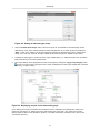
3.4. Displaying the query results
1.
Click the "Next>" button to display the query results.
37
Quick Start
Figure 58. Creating a query — displaying query results
2.
The results include 1505 objects: genes which are assigned the "GO:0007165 signal transduction" entry;
however, we actually want a list of all genes involved in signal transduction. We will look at the results more
closely to see if we have achieved this goal.
3.
One way to check the results is to open an entry in the "GO" column (e.g., click "GO:0007165 signal
transduction") to display the detailed report. Click the "Derived Concepts" tab to display all concepts derived
from the GO entry.
4.
To see other entries that may be involved in signal transduction, select the "Description" column, enter the
term "*signal transduction*" and click the "Search" button.
GO entries with a description including the term "signal transduction" are displayed (e.g., "GO:0000076 DNA
replication checkpoint" or "GO:0000750 pheromone-dependent signal transduction involved in conjugation
with cellular fusion"). We need to refine our search to include such entries.
5.
Close the "GO:0007165 signal transduction" window to return to the query wizard.
Figure 59. Creating a query — checking the results
38
Quick Start
3.5. Redefining the query
We will redefine the query to include all entries which are assigned the "GO:0007165 signal transduction"
classification or are inferred from such entries.
1.
Click the "Back" button to redefine the query.
2.
In the "Object to find" panel click the "has name" criteria to select it and click the "Delete" button. Click "Yes"
in the dialog to confirm the deletion.
3.
In the "Criteria available" panel under "Knowledge Network" select "is inferred by ontology entry which…"
and click the "Add>>" button to list it in the "Object to find" panel.
4.
In the "Criteria available" panel under "Object properties" select "has name…" and click the "Add>>" button
to list it in the "Object to find" panel. Enter "signal transduction" in the "Pattern" field in the right panel and
click the "Apply" button.
Figure 60. Creating a query — redefining criteria
A natural language description of the query is "Find all objects which are genes which are classified by a GO
entry that is inferred by an entry like 'signal transduction'."
5.
Click the "Next>" button to display the query results.
Figure 61. Creating a query — displaying refined query results
39
Quick Start
6.
The results include all genes which are assigned the "GO:0007165 signal transduction" entry and all genes
which are assigned entries derived from the signal transduction entry (1881 objects in total).
3.6. Saving the query and creating a smart folder
1.
Click the "Next>" button in the "Search results" window to save the query and create a smart folder. The
"Save query" window will be displayed.
Figure 62. Saving the a query and creating a smart folder
2.
Click the "Save query" check box and enter a name (e.g., "Find signal transduction genes") for the query.
3.
Click the "Create smart folder in" check box. Select the "Public" folder and click the "Add Folder…" button.
4.
Enter a name for the folder ("My queries") and click "OK" to close the dialog.
5.
Click the "Finish" button to close the query wizard.
The "My queries" folder containing the "Find signal transduction genes" smart folder will be created in the
"Public" project and is accessible using the project tree (see Figure 63: “Selecting a smart folder in the
project tree”).
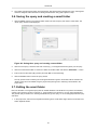
3.7. Editing the smart folder
Next, we will make a more general query that can handle variables. This will allow us to perform more flexible
queries to find genes by function in general, i.e., genes related to any GO terms, not only "signal transduction".
The general query is similar to the "Find signal transduction genes" query, so we can simply duplicate that query
and edit it.
1.
In the project tree, select the "Find signal transduction genes" smart folder. Right click the smart folder and
select "Duplicate folder".
40
Quick Start
Figure 63. Selecting a smart folder in the project tree
Enter "Find genes by function" to rename the smart folder.
Figure 64. Duplicating a smart folder
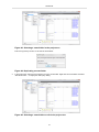
2.
In the project tree, select the "Find genes by function" smart folder. Right click the smart folder and select
"Edit smart folder…" to display the "Edit query" dialog.
Figure 65. Selecting a smart folder to edit in the project tree
41
Quick Start
3.
We will edit the query to create a more general query to find genes by functions specified by a GO term.
In the "Object to find" panel, select the criteria "like signal transduction" to display the "like…" panel on the
right. In the right panel, check the "Use variables" check box and click the "Introduce variable" button.
Figure 66. Editing a smart folder query
4.
In the "Variables" field, click the entry "Name" and click the "Edit" button to display the "Edit variable" dialog.
Figure 67. Adding variables to a query
Enter "GO term" as the variable name and any text in the "Value" field. We will enter "signal transduction"
to set it as the default variable value for the query. Click the "OK" button to define the variable and close the
dialog.
5.
In the right panel of the "Edit query" window, select "GO term" from the drop-down menu and click the
"Apply" button.
6.
In the "Description" field, we can enter a description for the query or click the "Generate" button to generate
a description from the query criteria. A natural language description of the query is "Find all genes which are
classified by a GO entry which is inferred by an entry which has a name like 'any GO term'."
7.
Click the "OK" button to close the "Edit query" window and display the "Find genes by function" results tab.
8.
Click the "Show Query Variables" button to display the "GO term" variable field. Use "signal transduction"
or enter another GO term in the field and click the "Apply" button. The query results will be displayed in the
table.
42
Quick Start
Figure 68. Using a variable query
The query results can be saved by clicking the "Save" button. See Section 3.6: “Saving the query and
creating a smart folder”.
4. Preparing a BioXM web portal
The first three sections have covered the basic steps to get started with the BioXM client software, create a data
model, populate the knowledge base and perform typical queries. We will now set up a BioXM web portal to allow
us to execute our query using a familiar Web interface rather than the BioXM client software. Instead of using the
BioXM query builder and displaying a query in the BioXM interface, we can click a hyperlink to run the query and
display the query results as a formatted table in a Web browser.
The BioXM Web Portal Builder has several functions for designing a BioXM Web interface for a specific project
(e.g., customizing reports and query forms, making reports editable, defining dynamic thesauri, and setting up
specific workflows and wizards), but we will focus on using the portal to run our queries and display the results.
Tip
We will cover the basic steps for using the BioXM web portal here. More information about the
BioXM Web Portal Builder can be found on the BioXM Support Web. https://ssl.biomax.de/
info/biomax/bin/view/BioXM/PortalBuilder. A working knowledge of HyperText Markup
Language (HTML) and Foswiki is helpful. http://foswiki.org/System/WebHome provides
numerous Foswiki materials.
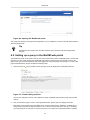
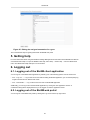
4.1. Logging into a BioXM web portal
To login into a BioXM web portal complete the following steps:
1.
Open a browser and enter the URL for the BioXM web portal login window. The login page will be displayed.
2.
Enter you user name and password. Click the "Login" button. The BioXM web portal entry page will be
displayed.
43
Quick Start
Figure 69. Opening the BioXM web portal
The content and design of this page will vary depending on your installation, but the functionality will be similar to
what is described here.
Tip
Administrators may need to click the "BioxmRefresh" link if the data model has had significant
changes.
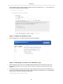
4.2. Setting up a query in the BioXM web portal
The BioXM web portal can be used to execute only queries that already exist in the BioXM system. The principle
approach is to first create queries using the BioXM query builder, which we have done already, create a wiki
page for the query and then implement calls of the appropriate web portal plugins into the page. To create a wiki
page and implement the plugins complete the following steps:
1.
Click the "Edit" tool
(in the toolbar near the top right corner) to display the Foswiki editing interface.
Figure 70. Foswiki editing interface
Here we can change the content of the "WebHome" page, the BioXM web portal entry page using Foswiki
markup.
2.
First we will create a page to run the "Find signal transduction genes" query and display the results.
New pages in the Foswiki system are called "topics" and are named using a "WikiWord". A WikiWord is a
string containing at least two uppercase letters, one of which is the first letter of the word (e.g., NewPage).
Any such string can be used, but we will use the names of our queries as in the BioXM client for simplicity.
44
Quick Start
Enter the following text to create a heading "Queries of interest" (indicated by the "---+") and a page for the
query called "FindSignalTransductionGenes".
---+ Queries of interest
* FindSignalTransductionGenes
Figure 71. Editing the "WebHome" page
3.
Click the "Save" button. The edited "WebHome" page will be displayed.
Figure 72. Displaying a new topic in the "WebHome" page
4.
Click the question mark (?) next to the "FindSignalTransductionGenes" text to edit the new page. The
Foswiki editing interface for the new page, which is similar to the "WebHome" editing interface, will be
displayed.
5.
We will edit the page to include a heading called "Find signal transduction genes" and a BioXM plugin to
list the content of the smart folder of that name. Listing the contents of smart folders (i.e., executing BioXM
queries) is done using the following general plugin call:
%BIOXM_QUERY{query="query_name"}%
45
Quick Start
More information about the plugin syntax used in the BioXM Web Portal Builder can be found
on the BioXM Support Web: https://ssl.biomax.de/info/biomax/bin/view/BioXM/
PortalBuilderReference.
To add the "Find signal transduction genes" query, enter the following text.
---+ Find signal transduction genes
%BIOXM_QUERY{query="Find signal transduction genes"}%
Figure 73. Adding the query plugin
Click the "Save" button. The edited "FindSignalTransductionGenes" page will be displayed.
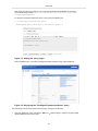
Figure 74. Displaying the "FindSignalTransductionGenes" query
The same steps can be used to add the second query "Find genes by function".
1.
Open the "WebHome" page and click the "Edit" tool
"FindGenesByFunction" for the query.
46
. Edit the page to create a new page called
Quick Start
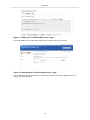
Figure 75. Editing the "WebHome" page
2.
Open the new page by clicking "FindGenesByFunction" in the "WebHome page".
Figure 76. Displaying the "WebHome" page
3.
Edit the page by clicking the "Edit" tool
include the plugin for the query.
to display the Foswiki editing interface. We will edit the page to
Executing a BioXM query that uses variables is done using the following general plugin call:
%BIOXM_QUERY{query="query_name" variables="var1=value;var2=value"}%
The variables parameter fixes the query variable values. Omitting this parameter will lead to a query form
in which values can be entered by the user; this is what we want to do. To edit the page to include the plugin
for the query without fixing the variable values, enter the following text and click "Save".
---+ Find genes by function
%BIOXM_QUERY{query="Find genes by function"}%
47
Quick Start
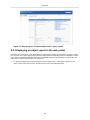
Figure 77. Editing the "FindGenesByFunction" page
The "FindGenesByFunction" page will be displayed with a field for entering any GO term.
Figure 78. Displaying the "FindGenesByFunction" page
4.
Use the default term "signal transduction" or enter any other GO term and click the "Search" button. The
query results will be displayed.
48
Quick Start
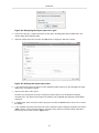
Figure 79. Displaying the "FindGenesByFunction" query results
4.3. Displaying an object report in the web portal
Information about each gene can be displayed in an object report by clicking the hyperlink in the "Gene" column.
Like any other view, object reports can be tailored to display particular information. Next we will display an object
report and use a predefined view tailored for use in the BioXM web portal. We will modify the view to allow the
object report to be annotated directly in the web portal
1.
To display information about a particular gene, click the hyperlink (e.g., "CDC6 [Homo sapiens]") in the
"Gene" column of the gene list view. The object report for the gene will be displayed.
49
Quick Start
Figure 80. Displaying the object report for a gene
The current object report for genes simply lists the information defined for the gene list view; however, we
can use a predefined view to display an object report layout designed specifically for the web portal. To do
this, we will first define a new object report view using the BioXM client software.
2.
Open the BioXM client software and select "Administration → Views..." to display the "Views" dialog.
Figure 81. Displaying the "Views" dialog in the BioXM client
3.
Select the "Gene list view" and click the "Duplicate..." button. The "Duplicate view" dialog will be displayed.
50
Quick Start
Figure 82. Displaying the object report for a gene
4.
Enter a new name (e.g., "Object report view") for the view in the dialog field. Click the "OK" button. The
"Views" dialog will be displayed again.
5.
Select the "Object report view" and click the "Edit" button to display the "Edit view" window.
Figure 83. Defining the object report view
6.
In the "General" tab remove the check from the "Allowed for table" check box so the view applies to single
objects only, not to tables of objects.
7.
Click the "View items" tab to open it.
Instead of only showing the "Synonyms" assigned annotation attribute, we will display the assigned
annotation form. This allows the annotation to be edited in both the BioXM client software and the BioXM
web portal.
8.
In middle panel, under "View items" select "Synonyms" and click the "Delete" button. Click "Yes" to confirm
the deletion.
9.
In the "Available view items" panel on the left, under "Annotation" select "Assigned annotation" and click the
"Add>>" button. In the right panel, select the "Annotation form" check box and select "Basic information"
from the drop-down menu. Click the "Apply" button.
51
Quick Start
Figure 84. Adding assigned annotation in the object report view
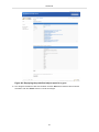
10. Click the "Report Layout" tab to open it. Select the "Predefined" radio button and select "Portal view" from
the drop-down menu.
Figure 85. Selecting the predefined layout for the object report view
11. Click the "OK" button to close the "Edit view" window. Click "Close" to close the "Views" window.
12. We can now return to the BioXM web portal. Reload the gene object report to show the new object report
layout.
52
Quick Start
Figure 86. Displaying the predefined object report for a gene
13. The "Assigned annotations" table can be edited. Click the "Edit" button below the table to edit the
annotation. Click the "Submit" button to commit the changes.
53
Quick Start
Figure 87. Editing the assigned annotation for a gene
This concludes the steps for getting started with the BioXM web portal.
5. Getting help
For more information about using the BioXM Knowledge Management Environment see the BioXM User Manual
or the BioXM online help. To open the BioXM online help, select "Help → Online Help…" from the BioXM main
menu. The BioXM online help will open in a new window.
6. Logging out
6.1. Logging out of the BioXM client application
You can log out of the BioXM client application by selecting one of the following options from the main menu:
• "File → Log Out…" — log out the current user without exiting the BioXM application; you can subsequently log
in again with the same or different user name
• "File → Exit BioXM…" — log out the current user and exit the BioXM application
Additionally, you can log out and exit the BioXM application by closing the main application window. A
confirmation dialog will be displayed before you are logged out and the application closes.
6.2. Logging out of the BioXM web portal
You can log out of the BioXM web portal by clicking the "Log Out" link in the top right corner.
54