Download Detecting Wormhole Attacks in Wireless Networks Using

Detecting Wormhole Attacks in Wireless Networks
Using Connectivity Information
Ritesh Maheshwari, Jie Gao and Samir R Das
Department of Computer Science, Stony Brook University
Stony Brook, NY 11794-4400, USA
{ritesh, jgao, samir}@cs.sunysb.edu
Abstract—We propose a novel algorithm for detecting wormhole attacks in wireless multi-hop networks. The algorithm uses
only connectivity information to look for forbidden substructures
in the connectivity graph. The proposed approach is completely
localized and, unlike many techniques proposed in literature, does
not use any special hardware artifact or location information,
making the technique universally applicable. The algorithm
is independent of wireless communication models. However,
knowledge of the model and node distribution helps estimate a
parameter used in the algorithm. We present simulation results
for three different communication models and two different
node distributions, and show that the algorithm is able to
detect wormhole attacks with a 100% detection and 0% false
alarm probabilities whenever the network is connected with high
probability. Even for very low density networks where chances
of disconnection is very high, the detection probability remains
very high.
I. I NTRODUCTION
Wireless ad hoc and sensor networks are typically used
out in an open, uncontrolled environment, often in hostile
territories. In particular, several important applications for
such networks come from military and defence arenas. Use
of wireless medium and inherent collaborative nature of the
network protocols make such network vulnerable to various
forms of attacks. In this paper our focus is on a particularly
devastating form of attack, called wormhole attack [1]–[3].
Here, the adversary connects two distant points in the network
using a direct low-latency link called the wormhole link. The
wormhole link can be established by a variety of means,
e.g., by using a network cable and any form of “wired”
link technology or a long-range wireless transmission in a
different band. The end-points of this link (wormhole nodes)
are equipped with radio transceivers compatible with the ad
hoc or sensor network to be attacked. Once the wormhole link
is established, the adversary captures wireless transmissions on
one end, sends them through the wormhole link and replays
them at the other end.
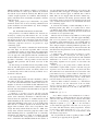
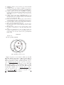
An example is shown in Figure 1. Here X and Y are the
two end-points of the wormhole link. As the signals received
on one end of the wormhole link are repeated at the other end,
any transmission generated by a node in the neighborhood of
X will also be heard by any node in the neighborhood of Y
and vice versa. The net effect is that all the nodes in region
A assume that nodes in region B are their neighbors and vice
versa. For example, traffic between nodes like a and e can now
take a one-hop path via the wormhole instead of a multi-hop
B
e
Y
d
a
X
c
Wormhole Link
b
A
Fig. 1. Demonstration of a wormhole attack. X and Y denote the wormhole
nodes connected through a long wormhole link. As a result of the attack,
nodes in Area A consider nodes in Area B their neighbors and vice versa.
path. If the wormhole is placed carefully by the attacker and
is long enough, it is easy to see that this link can attract a
lot of routes. Note that if the wormhole link is short, it may
not attract much traffic, and hence will not be of much use
to the adversary. Thus, throughout the paper we consider only
such attacks in which the wormhole link is long enough so
that regions A and B do not overlap.
A. Significance of Wormhole Attack
While wormhole could be a useful networking service as
this simply presents a long network link to the link layer and
up, the attacker may use this link to its advantage. After the
attacker attracts a lot of data traffic through the wormhole, it
can disrupt the data flow by selectively dropping or modifying
data packets, generating unnecessary routing activities by
turning off the wormhole link periodically, etc. The attacker
can also simply record the traffic for later analysis. Using
wormholes an attacker can also break any protocol that directly
or indirectly relies on geographic proximity. For example,
target tracking applications in sensor networks can be easily
confused in the presence of wormholes. Similarly, wormholes
will affect connectivity-based localization algorithms, as two
neighboring nodes are localized nearby and the wormhole
links essentially ‘fold’ the entire network. This can have a
major impact as location is a useful service in many protocols
and application, and often out-of-band location systems such
as GPS are considered expensive or unusable because of the
environment.
A wormhole attack is considered dangerous as it is independent of MAC layer protocols and immune to cryptographic
techniques. Strictly speaking, the attacker does not need to
understand the MAC protocol or be able to decode encrypted
packets to be able to replay them. In its most sophisticated
form, the wormhole can be launched at the bit level or at the
physical layer [4]. In the former, the replay is done bit-by-bit
even before the entire packet is received (similar to cut-through
routing [5]). In the latter, the actual physical layer signal is
replayed (similar to a physical layer relay [6]). These forms
of wormholes are even harder to detect. This is because such
replays can happen quite fast and thus they cannot be detected
easily by timing analysis. To distinguish these attacks from the
simpler form of attack, where the wormhole nodes copy the
entire packet before transmittal through the wormhole link, we
will refer to this simpler form of attack as store-and-forward
attack following the terminology used in [4].
B. Limitations of Prior Work and Our Contributions
The current solutions for wormhole are limited particularly
in connection with large sensor networks, where sensor nodes
carry low-cost, relatively unsophisticated hardware and scalability is an important design goal. This rules out use of
additional hardware artifact that several reported techniques
use – such as directional antennas [7], GPS [2], ultrasound
[8], guard nodes with correct location [9]. This also rules out
fine grain timing analysis used in several techniques [2], [4].
Also, physical-layer attacks may be immune to timing analysis
[4]. Finally, the scalability requirements rule out global clock
synchronization [2] or any form of global computations [10].
In the current work, we develop a localized algorithm for
detecting wormhole attacks that is purely based on local
connectivity information. Such information is often collected
any way by various upper layer protocols such as routing,
thus may not present any additional overhead. No additional
hardware artifact is needed making the approach universally
applicable. No timing analysis is done ensuring that we can
detect even physical layer attacks. Our technique does not
use location information and is able to detect attacks that are
launched even before the network is set up, that may influence
localization. We expect that our technique is particularly useful
for sensor networks as the existing techniques are quite limited
there. Also, connectivity is not expected to change frequently
in sensor networks, making our connectivity-based approach
quite practical.
The detection algorithm essentially looks for forbidden
substructures in the connectivity graphs that should not be
present in a legal connectivity graph. Understanding of the
wireless communication model (i.e., a model that describes
with some given confidence whether a link between two nodes
should exist) helps the detection algorithm substantially, but
is not strictly required. The models we require can be very
general and we will demonstrate the capability of the detection
using several realistic models such as quasi-unit disk graphs
[11] and link models for Berkeley motes as modeled in the
TOSSIM simulator [12].
II. R ELATED W ORK
Several papers in literature have developed countermeasures
for wormhole attacks. We discuss them in two categories.
A. Approaches that Bound Distance or Time
In [2] authors have considered packet leashes – geographic
and temporal. In geographic leashes, node location information
is used to bound the distance a packet can traverse. Since
wormhole attacks can affect localization, the location information must be obtained via an out-of-band mechanism such
as GPS. Further, the “legal” distance a packet can traverse is
not always easy to determine. In temporal leashes, extremely
accurate globally synchronized clocks are used to bound the
propagation time of packets that could be hard to obtain
particularly in low-cost sensor hardware. Even when available,
such timing analysis may not be able to detect cut-through or
physical layer wormhole attacks.
In [13], an authenticated distance bounding technique called
MAD is used. The approach is similar to packet leashes at
a high level, but does not require location information or
clock synchronization. But it still suffers from other limitations of the packet leashes technique. In the Echo protocol
[8], ultrasound is used to bound the distance for a secure
location verification. Use of ultrasound instead of RF signals as
before helps in relaxing the timing requirements; but needs an
additional hardware. In a recent work [4], authors have focused
on practical methods of detecting wormholes. This technique
uses timing constraints and authentication to verify whether a
node is a true neighbor. The authors develop a protocol that
can be implemented in 802.11 capable hardware with minor
modifications. Still it remains unclear how realistic such timing
analysis could be in low-cost sensor hardware.
B. Graph Theoretic and Geometric Approaches
LiteWorp [14] uses a combination of one-time authenticated
neighbor discovery and use of guard nodes that attest the
source of each transmission. The neighbor discovery process,
however, can be vulnerable to wormhole attacks, if the attack is launched prior to such discovery. A followup paper
from the same authors attempts to remove this inefficiency
[15], however assumes availability of location information. As
mentioned before, this itself could be suspect. In [9] a graphtheoretic framework is used to prevent wormhole attacks. The
protocol assumes the existence of special-purpose guard nodes
that know their “correct” locations, have higher transmit power
and have different antenna characteristics. Use of such specialpurpose guard nodes make this approach impractical.
In one approach, directional antennas are used to prevent
wormhole attacks [7]. The authors develop a cooperative
protocol where nodes share directional information to prevent
wormhole endpoints from masquerading as false neighbors.
that needs to be certified free from wormhole attack. However,
use of directional antennas limits use of such protocols.
In another approach [10] somewhat related, distance estimates between sensors that hear each other is used to
determine a “network layout” using multi-dimensional scaling
(MDS) technique. The technique is similar to localization of
the network nodes in a metric space. Without any wormhole
the network layout should be relatively flat. But the layout
could be warped in presence of wormholes. The technique is
purely centralized and is considerably susceptible to distance
estimation errors.
Finally, purely physical layer mechanisms can prevent
wormhole attacks such as those involving authentication in
packet modulation and demodulation [2]. Such techniques
require special RF hardware.
III. W ORMHOLE D ETECTION A LGORITHM
The placement of wormhole influences the network connectivity by creating long links between two sets of nodes
located potentially far away. The resulting connectivity graph
thus deviates from the true connectivity graph. Our detection
algorithm essentially looks for forbidden substructures in the
connectivity graph that should not be present in a legal
connectivity graph.
Knowledge of the wireless communication model between
the nodes helps our detection algorithm. This is because
a communication model can help define what substructures
observed in the connectivity graph could be forbidden. However, our approach is still applicable when the communication
model is unknown. In this case we need to run an extra search
procedure to determine a critical parameter for the detection
algorithm. This parameter will be made clear later in this
section.
We first develop our wormhole detection algorithm, starting
from the unit disk graph model and then general (known or
unknown) communication models, and finally discuss how
to automatically remove links created by wormhole once a
wormhole is detected.
A. Unit Disk Graph Model
In unit disk graphs (UDG) each node is modeled as a disk of
unit radius in the plane, modeling the communication range
of the node with omni-directional antenna. Each node is a
neighbor of all nodes located within its disk. UDGs have long
been used to create an idealized model of multi-hop wireless
networks. We start with this model and formulate our approach
of wormhole detection.
1) Hardness of wormhole detection: We first note that
under the UDG model, the problem of detecting wormhole
attacks with connectivity information is NP-hard. This is
observed from the equivalence of wormhole detection with
UDG embedding. If the observed connectivity graph has no
valid UDG embedding in the plane, it can be deduced that
there must be a wormhole present in the network. This can
happen when wormhole attack creates long-distance links
(longer than unity) which should not exist in a UDG. Conversely, if the observed connectivity graph does admit a valid
UDG embedding, then any algorithm based on connectivity
information only will have to output ‘no wormhole’. In such
a case, wormhole link, even present, is not distinguishable
from a valid link in the embedded UDG. In the absence of
any other information, this embedding has to be taken as the
ground truth. This can happen, for example, when wormhole
links are short and thus appear no different than a link in
UDG. This can also happen when the link is indeed long,
but lack of sufficient node density prevents detection. This
issue will be clearer as we move forward in the paper. In such
cases, wormhole detection has to use information other than
the connectivity graph.
It is known that finding a UDG embedding in 2D is a
NP-hard problem [16]. Thus, it is equally hard to detect
a wormhole attack using connectivity information alone. A
similar relationship between wormhole detection and network
localization is also exploited in [10].
The basic idea in our detection algorithm is to look for graph
substructures that do not allow a unit disk graph embedding,
thus can not be present in a legal connectivity graph. Due to
the hardness result mentioned above, our algorithm will not
guarantee the detection of wormhole in all cases. Rather, we
aim to design a simple localized algorithm that provides a sufficiently high detection probability in connected networks. We
will demonstrate the performance of the algorithm empirically
in the next section.
2) Disk packing: The key notion we exploit is a packing argument – inside a fixed region, one cannot pack too
many nodes without having edges in between. The forbidden
substructures we look for are actually those that violate
this packing argument. To be rigorous, we start with some
definitions.
Denote by p(S, r) the packing number, which is the maximum number of points inside a region S such that every pair
of points is strictly more than distance r away from each other.
We assume that no two network nodes are located at the same
point. Denote by DR (u) a disk of radius R centered at u. D
denotes just a unit disk to simplify notations. As a well-known
fact [17], in a unit disk there can be at most 5 nodes whose
pair-wise distances are strictly more than 1. Thus p(D, 1) = 5.
Given two disks of radius R centered at u, v with distance
r away, define by lune the intersection of the two disks,
L(r, R) = DR (u) ∩ DR (v). When R = r = 1, we sometimes
omit the radii and denote by L the lune of unit disks set at
unit distance apart.
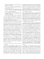
Lemma 3.1. p(L, 1) = 2.
Proof: Refer to Figure 2 for an illustration of a lune L.
The line segment uv divides the lune into two parts, the upper
and lower ones. The two intersections of the two unit circles
centered at u, v are denoted p, q respectively.
Denote by w the
√
midpoint of segment uv. |pw| = 3/2 < 1. It is not hard to
see that inside the upper half of the lune one can not place
two nodes with their distance strictly larger than 1. Indeed,
for any node x in the upper half of L, |xv| ≤ 1, |xu| ≤ 1,
|xp| ≤ 1. Thus there can only be two nodes inside L with
inter distance larger than 1.
We can generalize the result for packing of disks of radius
β, with the proof appearing in the appendix.
p
u
v
w
q
Fig. 2. One can only pack at most two nodes inside a lune with interdistance more than 1.
Lemma 3.2. p(L(r, R), β)
arccos(r/(2R + β)) −
r ≤ 2R.
≤
4r
πβ 2
π8 (R/β + 1/2)2 ·
(R + β/2)2 − r2 /4 for
Proof: See the appendix.
Remark. Lemma 3.2 only gives a loose bound for p(L, β).
When β = 1, Lemma 3.2 gives p(L, 1) ≤ 5, which is worse
than the bound in Lemma 3.1. This motivates us to find a
practical bound for p(L, β) by other techniques as will be
shown later.
3) Forbidden substructure for wormhole detection: The
packing results are used to define forbidden substructures for
unit disk graphs. The wormhole connects all nodes in region
A with all the nodes in region B (Figure 1). Thus we can
have two independent (i.e., non-neighbor) nodes in region A,
say, a, b, that share three common neighbors c, d, e in region
B that are independent. This constitutes a forbidden structure,
since in any valid UDG embedding of the connectivity graph
the three common neighbors must be within the intersection of
disks centering a, b. Since they are independent, their pairwise
distance must be more than 1. By Lemma 3.1 we know that
this can not happen. Thus the discovery of this forbidden
substructure reveals the existence of a wormhole.
However, this technique of finding forbidden substructure
cannot always guarantee detection of wormholes because the
existence of nodes like c, d, e in region B is dependent on
the density of nodes in the network. The technique will fail
when region B has only 2 nodes, for example. For such low
density cases, we need to go beyond 1-hop and look for
similar forbidden substructures among k-hop neighbors. Here,
we will look for fk common independent k-hop neighbors of
two non-neighboring nodes. fk is a parameter to be discussed
momentarily. To summarize, the forbidden substructures we
will use in our algorithm are the following.
•
•
3 independent common 1-hop neighbors: Two nonneighboring nodes having 3 independent common neighbors; In general, we have
fk independent common k-hop neighbors: Two nonneighboring nodes having fk independent common k-hop
neighbors.
We call fk the forbidden parameter of the wormhole detection algorithm. fk must be more than the packing number for
unit distance inside the lune of two disks of radii k (modeling
the k-hop neighborhood) placed at distance 1 (modeling the
lower bound for the distance between non-neighbors). Thus,
fk = p(L(1, k), 1)+1, with p(L(1, k), 1) as the corresponding
packing number to be determined by Lemma 3.2 or other
methods. Also, from Lemma 3.1, for k =1, f1 = 3. For
a communication model that is not unit disk graph, the
determination of fk will be discussed in subsection III-C.
If a network has one of these forbidden substructures,
we know for sure that there is a wormhole. For a given
node density, if there is wormhole present, the possibility of
finding it improves with increasing k. This is because larger
neighborhoods simply provide more nodes to work with, thus
increasing the possibility of finding forbidden substructures.
Our evaluations in the next section show that testing for 1hop is often sufficient to provide a very high detection rate
requiring 2-hops only for very sparse, disconnected or irregular
networks. This makes the approach quite practical.
B. Algorithm Description
Recall that the wormhole detection algorithm is to search
by each node a forbidden structure in its neighborhood. The
algorithm is localized and distributed. Each node searches
for forbidden structures in its k-hop neighborhood. We will
explain the algorithm for the general k-hop detection. In our
empirical studies k ≤ 2 was found sufficient for most of the
cases.
Each node u maintains the list of 2k-hop neighbors N2k (u).
Node u finds a non-neighboring node, v, from N2k (u) and
checks their k-hop neighbor lists to compute their common
k-hop neighbors Ck (u, v). Note that to find a non-empty
Ck (u, v) set, node u need not look for v beyond 2k hops.
We now need to look for the existence of the forbidden
substructure (i.e., fk independent nodes) in Ck (u, v). One way
to do this would be to compute the maximum independent
set among Ck (u, v) and comparing the size of this set with
fk . But computing the maximum independent set is a NPhard problem, even for unit disk graphs [18], [19]. Thus we
relax the detection rule by finding a maximal independent set
(a set of independent nodes such that no other node can be
included), which can be done by a simple greedy algorithm:
we start from an empty set, pick an arbitrary node and include
it in the independent set, remove its neighbors, and continue
until we run out of nodes in Ck (u, v). The resulting set is a
maximal independent set.
We compare the size of the maximal independent set thus
obtained with the forbidden parameter fk . If it is equal or
larger than fk , then we output ‘wormhole detected’. The
outline of the algorithm is as follows.
1) In a preprocessing stage, find the forbidden parameter
fk , based on the node distribution and communication
model. (For UDGs, the bound on fk can be derived from
Lemmas 3.1 and 3.2. We discuss other techniques of
finding fk in practice in the next subsection, which also
generalize to non-UDGs.)
2) Each node u determines its 2k-hop neighbor list,
N2k (u), and executes the following steps for each nonneighboring node v in N2k (u).
3) Node u determines the set of common k-hop neighbors with v from their k-hop neighbor lists. This is
Ck (u, v) = Nk (u) ∩ Nk (v). This can be determined
by simply exchanging neighbor lists.
4) Node u determines the maximal independent set of the
sub-graph on vertices Ck (u, v), by using the greedy
algorithm presented above.
5) If the maximal independent set size is equal or larger
than fk , node u declares the presence of a wormhole.
The way the algorithm is presented makes it appear as if
some work is duplicated (nodes u and v are doing the same
computation by symmetry). These can be easily resolved by
using some priority rules based on node ids.
The algorithm presented above depends only on the 2k and
k-hop neighbor lists of each node. If the wormhole attacks
are required to be detected as soon as they are in place,
ideally our algorithm can be run everytime there is a change in
topology. Since it is a local algorithm, only the nodes affected
by the change in topology need to re-run it. In practice, the
requirement to run it immediately after the attack is placed
is not so strict. In such cases, the algorithm can be run
periodically depending on the security requirements and the
network condition. For example, in mobile networks it is
probably more sensible to run it periodically, while in static
networks, it should be triggered by changes in topology.
The message and time complexity of the algorithm is
dependent on k. As we mentioned, for all cases we considered
in our simulations, including fairly low density cases, k ≤ 2
has been sufficient. In cases where the network in fact has
enough density to be connected and is fairly uniform (like in
most practical cases), k = 1 has been found to be sufficient.
The computational cost for k = 1 is roughly O(d3 ), where
d is the average degree of the nodes. Essentially a node
checks each of O(d2 ) non-neighboring nodes in its 2-hop
neighborhood, and pays a cost of O(d) for finding the maximal
independent set size in the intersection list. For any practical
network, d is typically a small constant. So the detection
algorithm is quite efficient.
C. Consideration of Node Distribution and General Communication Model
Consideration of node distribution is important in the performance of our algorithm. The packing number fk − 1 used
above, i.e., the maximum number of independent common khop neighbors of two independent nodes, is the theoretical
worst case bound for an arbitrary distribution. If the sensors
are deployed with a known distribution, then the forbidden
parameter fk we use in the forbidden substructure can be
much smaller than the theoretical worst case. For example,
for the 2-hop detection case, p(L(1, 2), 1) ≤ 18 by lemma
3.2, providing f2 = 19. Unless the node density is very high,
it is unlikely that we will be able to find that many common
independent 2-hop neighbors between two non-neighboring
nodes to be able to detect a wormhole attack. This observation
prompts us to tune this critical parameter fk according to
the specific node distribution and not relate it directly to the
packing number that models an absolute bound. In general, the
smaller fk is, the higher the detection rate. When fk is too
small, we may have false positives as some legal configuration
may be identified as wormhole.
The second important consideration is the communication
model. The unit disk graph model considered so far is an
overly simplified model for wireless communications. Experiments show that packet reception range is not a perfect
disk [20]. Our approach can be generalized to any communication model, and even to situations where communication
model is unknown. The algorithm indeed remains the same.
But the preprocessing step involving the determination of the
forbidden parameter fk in the first step of the algorithm differs.
In following we describe a number of techniques to obtain
the forbidden parameter fk in practice.
1) Known models: For any practical node deployment we
typically know the radio propagation characteristics for the
specific hardware used subject to the deployment environment,
as well as the spatial distribution of nodes. We could try to
find fk directly using mathematical or geometrical constructs.
For example, a quasi-unit disk graph model [11] assumes that
two nodes have a link if their distance is within α ≤ 1
and do not have a link if their distance is larger than 1.
If two non-neighboring nodes have f1 independent common
neighbors, these nodes must be within the lune L(α, 1) and are
pairwise distance α away. Thus the packing number is f1 =
p(L(α, 1), α) + 1. In general, we have fk = p(L(α, k), α) + 1.
For all communication models, it may not be always possible to evaluate such expressions, or even write such mathematical constructs. In such cases, we can run simulations with
the targeted distribution to obtain an estimated connectivity
graph, with which we can estimate the forbidden parameter
fk . For example, for any pair of non-neighboring nodes we
can find the maximal independent set among their common khop neighbors and take the maximum as fk −1. Our simulation
results in this paper actually use this method and obtain tight
bounds for fk . Notice that when the communication model is
probabilistic, the maximum number of independent neighbors
of two non-neighboring nodes, f1 − 1, is also probabilistic.
Thus false positives are possible in theory under our detection
algorithm.
2) Unknown models: When nothing is known about the
node distribution and/or communication model, it becomes
harder to estimate fk . In this case, we run the detection
algorithm with a standard parametric search for the unknown
parameter fk . We start with a large initial value for fk , and
run the algorithm as presented before. If no wormhole is
detected, we halve fk and rerun the algorithm. Notice that
when fk is small enough, false positives will show up. We
choose fk to be the value when only a very small fraction of
nodes report wormholes, or the minimum number of tolerable
B
e
Y
d
a
X
Wormhole Link
c
b
A
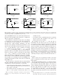
Fig. 3. Example of second possible placement of the forbidden substructure.
false positives. One good mechanism would be to run this
parametric search in a safe part of the network, guaranteed
to be free from wormhole, before deploying it in the entire
network. We can then estimate the parameter such that there
is no false positive detection in the safe part and apply the
parameter for the entire network
If no such safe part can be ascertained, the search must
run in the network that has potentially been inflicted with
wormholes already. In that case, a “threat level” must be
assumed. The threat level is to be used as a guidance for what
fraction of nodes must report wormholes before fk will not
be reduced any further.
D. Wormhole removal
Once a forbidden structure is discovered, it is usually
expected that user should manually intervene and remove the
wormhole links. Here, we devise a simple approach that can be
used to isolate all links possibly affected by wormhole without
manual intervention. We outline the approach for the 1-hop
detection case for UDGs. It can be easily extended for other
cases.
After a successful 1-hop detection in UDGs, we have
two non-neighboring nodes a, b with 3 common independent
neighbors c, d and e. Figure 1 shows one possible placement
of these nodes to form the forbidden substructure, such that a
and b are placed in one region (lets call it region A, without
loss of generality) and c, d and e are placed in another region,
B. Another possible placement is shown in Figure 3. Here, a,
b are located in region A; d, e are located in region B; but c is
located just outside A neighboring a and b. It can be verified
that these are the only two placements possible.
One can define two types of nodes neighboring the wormhole region – uncorrupted and corrupted nodes. An uncorrupted node is a node which is not in the transmission radius
of the wormhole nodes. Thus they are the nodes just outside A
and B. Corrupted nodes are the ones which do hear wormhole
nodes and are thus inside regions A and B. Corrupted nodes
have their neighbor lists corrupted due to the presence of
the wormhole link. Our wormhole removal algorithm tries to
identify, and blacklist, all nodes that are possibly corrupted
nodes (the rest are surely uncorrupted nodes). Once identified,
each corrupted node then purges its neighbor list by verifying
it with the neighbor lists of its neighboring uncorrupted nodes.
Note that even one link due to wormhole placement left out
un-removed will still make a huge damage to the network.
Thus our removal scheme allows error on the aggressive side
and removal of legals links, as long as all the illegal links are
definitely removed.
Inferring from the two placements discussed above, one can
say that nodes which satisfy any of these two conditions must
include all corrupted nodes:
•
•
The node is a neighbor of both a and b, or,
The node is a neighbor of at least 2 nodes out of c, d
and e.
This identification method finds a set of suspicious nodes
that will include all corrupted nodes and may also include
some uncorrupted nodes. While on the other hand, all nodes
not identified by this method, are definitely uncorrupted nodes
that do not have fake links created by wormhole.
To remove the fake links, each suspicious node, u, takes the
intersection of its neighbor set, N (u) with the neighbor sets
of its neighboring uncorrupted (non-suspicious) nodes. Any
node v ∈ N (u) which is not part of any such intersections,
is blacklisted by node u. All future transmissions from such
nodes will be ignored by node u making the wormhole attack
ineffective. When all suspicious nodes finish blacklisting nodes
from their neighbor list, this completes wormhole removal.
We note that the removal is a bit aggressive to guarantee that
all illegal links due to wormhole will be removed, however,
some legal links may be removed as well. This algorithm is
not evaluated here for brevity.
IV. S IMULATION R ESULTS
In this section, we present simulation results demonstrating
the effectiveness of our algorithm in detecting wormhole
attacks. In particular, we evaluate the probability of successful
detection for networks with various node distributions and
connectivity models. We consider three different connectivity
models in our simulations: a) unit disk graph, b) quasiunit disk graph and c) the model used in the TOSSIM
simulator [12], which is based on real empirical data from
a motes testbed. We evaluate the algorithm with two different
node distributions: i) grid distribution with some perturbations
(modeling a planned sensor deployment) and ii) random distribution.
A. Details of Models and Evaluation Approach
In the quasi-UDG model, if the transmission radius of the
nodes in the network is R and the quasi-UDG factor is α
(where, 0 ≤ α ≤ 1), then there exists a link between every
pair of nodes within distance αR. If the distance is greater than
R, then there is no link. If the distance d between a node pair is
within [αR, R], we assume presence of a link with probability
d
R−αR . For all our quasi-UDG simulations, we used α = 0.75.
In the TOSSIM model, the provided LossyBuilder tool
is used to generate bit error probabilities (say, Pb ) between
node pairs. In order to build the connectivity graph, it is
assumed that the link exists with probability (1 − Pb ). Note
0.6
Detection
Disconnected
False +ve
0.4
10
Detection
Disconnected
False +ves
f_1
f_2
0.6
0.4
8
6
4
0.2
0.2
2
0
0
0
0
2
4
6
8
10
12
14
16
0
3
Average Degree
6
9
16
1
14
0.8
Probability
0.8
Probability
Probability
0.8
12
Detection
Disconnected
False +ve
f_1
f_2
0.6
0.4
10
8
6
4
0.2
2
0
12
0
1
3
5
Average Degree
(a)
12
Forbidden Parameter
1
Forbidden Parameter
1
7
9
11
13
15
Average Degree
(b)
(c)
1
1
12
0.8
0.8
10
1
0.6
0.4
6
4
0.2
0.2
2
0
0
0
1
3
5
7
9
11
Average Degree
13
15
3
5
7
9
11
13
15
Average Degree
(d)
Probability
0.4
Probability
Detection
Disconnected
False +ves
13
Detection
Disconnected
False +ve
f_1
f_2
0.6
0.4
11
9
7
0.2
5
0
Forbidden Parameter
0.6
8
Detection
Disconnected
False +ves
f_1
f_2
Forbidden Parameter
Probability
15
0.8
3
2
4
6
8
10
12
14
16
18
Average Degree
(e)
(f)
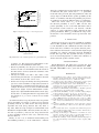
Fig. 4. Probability of wormhole detection, graph disconnection and false positives for various configurations. The first three graphs are for a Perturbed Grid
node distribution with p=0.2 for (a) UDG (b) Quasi-UDG and (c) TOSSIM connectivity models. The next three graphs are for Random node distribution with
(d) UDG (e) Quasi-UDG and (f) TOSSIM connectivity models.
that the TOSSIM model does not assume that the links are bidirectional. Our algorithm works irrespective of whether the
links are directional or bi-directional.
Each simulation is run with 144 nodes. Since our technique
is localized (we use only 1-hop and 2-hop detections in
our experiments) and the simulations so far concentrate on
detecting only a single wormhole, simulating a very large
networks is not required to determine the performance of our
approach. For the grid-like topologies the nodes are placed in
a 12 × 12 grid. Then their x and y coordinates are changed
to a randomly chosen value between [x − px, x + px] and
[y − py, y + py] respectively, where p is the perturbation
parameter. Values of p from 0.0 to 0.5 have been used, but for
brevity we only show results of p=0.2 here. For the random
case, x and y coordinates are chosen randomly. As noted
before node density is an important factor in our algorithm.
Node density is varied in different experiments by changing
the geographic area containing the nodes (for TOSSIM) or by
changing the transmission radius of the nodes (for UDG and
Quasi-UDG cases).
After the topology is created, the nodes are connected using
the given connectivity model. Once the connectivity graph is
established, the following experiments are performed:
•
•
Connectivity in the entire network is checked. The network is assumed disconnected if any two nodes do not
have a path to each other.1
The wormhole detection algorithm is run to see whether
there is a false positive. (At this time, there is no
1 While our technique is independent of whether the entire network is
connected or not, connected networks are more useful from a practical
standpoint.
wormhole attack)
A wormhole attack is established between two randomly
chosen locations. The algorithm is run again to see
whether it detects the wormhole.
The algorithm was run with k ≤ 2 only. We will see
momentarily that this already gives very good results for
most practical scenarios. We have repeated each experiment
for 10, 000 times with randomly generated topologies and
attacks, but with the same node distribution model and connectivity model, and then reported various probabilities for
different node densities. Three probabilities are computed: (i)
probability of detection, (ii) probability of false positive and,
(iii) probability of network disconnection. To avoid boundary
effects, we have not considered the boundary nodes when
calculating the degree, testing for disconnected networks, etc.
•
B. Results
Figure 4 shows all our performance results for the three
types of communication models and two types of node distribution models.
Recall that the forbidden parameter fk is an input parameter
to our algorithm and is evaluated separately in a pre-processing
step as shown in subsection III-C. Figure 4 also shows fk
values for different experiments. For UDG cases, it is observed
that only 1-hop detection is enough for all cases except at
very low densities (average degree ≤ 1), and f1 is constant
at 3. Thus, we do not show the fk curves for UDG graphs.
In general, the following observations can be made from the
results:
• Our algorithm provides very good results (no false alarms
and 100% detection) when the network disconnection
Probability
12
0.8
10
1 hop Detection
1+2 hop Detection
f_1
f_2
0.6
0.4
8
6
4
0.2
2
0
Forbidden Parameter
1
0
3
5
7
9
11
13
15
Average Degree
Fig. 5. Comparison of 1-hop vs 1 and 2-hop detection.
1
V. C ONCLUSION
0.8
Probability
where the communication model and/or the node distribution
are unknown. The given scenario uses k = 1, quasi-UDG
model and nodes placed in grid with perturbation of 0.2 and
average degree of 6. Both the false positive probability (in the
absence of wormhole) and detection probability (in presence
of wormhole) are shown for different values of f1 in Figure 6.
There exist critical values of f1 (4 in the plot) where
the detection probability is close to 100%, but the false
positive probability is close to 0%. This demonstrates that if
the parametric search is used in a safe network, a suitable
value for f1 can be estimated by simply observing the false
positive probabilities. When f1 is reduced from a large value,
the detection of real wormholes shows up first before false
positives.
0.6
Detection
False +ve
0.4
0.2
0
1
3
5
7
9
11
Forbidden Parameter
Fig. 6. Estimation of the forbidden parameter in a quasi-UDG model.
In this paper we propose a practical algorithm for wormhole
detection. The algorithm is simple, localized, and is universal
to node distributions and communication models. Our simulation results have confirmed a near perfect detection performance whenever the network is connected with a high enough
probability, for common connectivity and node distribution
models. We expect that this algorithm will have a practical
use in real-world deployments to enhance the robustness of
wireless networks against wormhole attacks.
ACKNOWLEDGMENT
•
•
•
probability is 0. This observation is independent of communication or node distribution model used.
Detection probability does drop for low density cases;
however, in such cases the likelihood that the network is
disconnected also increases (hence the usefulness of the
network also drops).
Amongst all results, even with a 50% chance of the
network being disconnected, our algorithm has detected
the wormhole attack in 90% or more cases.
For the same average node density, detection performance
gets worse as the randomness of deployment (in terms of
node distribution or communication model) increases. For
example, the detection rate is better in UDG Perturbed
Grid scenario (Figure 4a) than UDG Random scenario
(Figure 4d) or Quasi-UDG Perturbed Grid scenario (Figure 4b) and so on. This phenomenon is expected because
the estimation of fk is more accurate in less random
scenarios.
As mentioned earlier, 1-hop only detection does not perform
well in non-UDG cases. Figure 5 compares 1-hop detection
probability with the case when both 1 and 2-hop detection
algorithm were used (2-hop detection runs only when 1hop fails), under the setup of Figure 4e with Random node
distribution and Quasi-UDG connectivity model. Note that as
the value of parameter f1 increases, the 1-hop detection fails
to detect wormhole attacks in some cases, and hence 2-hop
detection kicks in.
Finally, we run a set of simulations demonstrating how
the forbidden parameter fk can be estimated for a situation
Ritesh Maheshwari and Samir Das’s research has been
partially supported by the NSF grants CNS-0519734, OISE0423460, CNS-0308631 and a grant from the SensorCAT
center.
R EFERENCES
[1] P. Papadimitratos and Z. J. Haas, “Secure routing for mobile ad hoc
networks,” in SCS Communication Networks and Distributed Systems
Modeling and Simulation Conference (CNDS 2002), 2002.
[2] Y. C. Hu, A. Perrig, and D. Johnson, “Packet leashes: a defense against
wormhole attacks in wireless networks,” in INFOCOM, 2003.
[3] K. Sanzgiri, B. Dahill, B. Levine, and E. Belding-Royer, “A secure
routing protocol for ad hoc networks,” in International Conference on
Network Protocols (ICNP), November 2002.
[4] J. Eriksson, S. Krishnamurthy, and M. Faloutsos, “Truelink: A practical
countermeasure to the wormhole attack,” in ICNP, 2006.
[5] L. M. Ni and P. K. McKinley, “A survey of wormhole routing techniques
in direct networks,” Computer, vol. 26, no. 2, pp. 62–76, 1993.
[6] A. Scaglione and Y. W. Hong, “Opportunistic large arrays: Cooperative
transmission in wireless multihop ad hoc networks to reach far distances,” IEEE Transactions on Signal Processing, vol. 51, no. 8, 2003.
[7] L. Hu and D. Evans, “Using directional antennas to prevent wormhole attacks,” in Network and Distributed System Security Symposium (NDSS),
2004.
[8] N. Sastry, U. Shankar, and D. Wagner, “Secure verification of location
claims,” in ACM Workshop on Wireless Security (WiSe 2003), September
2003.
[9] R. Poovendran and L. Lazos, “A graph theoretic framework for preventing the wormhole attack in wireless ad hoc networks,” ACM Journal of
Wireless Networks (WINET), 2005.
[10] W. Wang and B. Bhargava, “Visualization of wormholes in sensor
networks,” in WiSe ’04: Proceedings of the 2004 ACM workshop on
Wireless security, New York, NY, USA, 2004, pp. 51–60.
[11] F. Kuhn and A. Zollinger, “Ad-hoc networks beyond unit disk graphs,” in
Proc. 2003 Joint Workshop on Foundations of mobile computing, 2003,
pp. 69–78.
[12] “TOSSIM: A simulator for tinyos networks,” User’s manual in TinyOS
documentation.
[13] S. Capkun, L. Buttyn, and J. P. Hubaux, “SECTOR: Secure tracking of
node encounters in multi-hop wireless networks,” in 1st ACM Workshop
on Security of Ad Hoc and Sensor Networks (SASN), October 2003.
[14] I. Khalil, S. Bagchi, and N. B. Shroff, “LITEWORP: A Lightweight
Countermeasure for the Wormhole attack in multihop wireless network,”
in International Conference on Dependable Systems and Networks
(DSN), 2005.
[15] I. Khalil, S. Bagchi, and N. Shroff, “MOBIWORP: Mitigation of the
wormhole attack in mobile multihop wireless networks,” in Second
International Conference on Security and Privacy in Communication
Networks (SecureComm 2006), 2006.
[16] H. Breu and D. G. Kirkpatrick, “Unit disk graph recognition is NP-hard,”
Computational Geometry. Theory and Applications, vol. 9, no. 1-2, pp.
3–24, 1998. [Online]. Available: citeseer.ist.psu.edu/breu93unit.html
[17] J. H. Conway and N. J. A. Sloane, Sphere Packings, Lattices and Groups,
2nd ed. New York, NY: Springer-Verlag, 1993.
[18] M. R. Garey, R. L. Graham, and D. S. Johnson, “Some NP-complete
geometric problems,” in Proc. 8th Annu. ACM Sympos. Theory Comput.,
1976, pp. 10–22.
[19] M. R. Garey and D. S. Johnson, Computers and Intractability: A Guide
to the Theory of NP-Completeness. New York, NY: W. H. Freeman,
1979.
[20] D. Ganesan, B. Krishnamachari, A. Woo, D. Culler, D. Estrin, and
S. Wicker, “Complex behavior at scale: An experimental study of lowpower wireless sensor networks,” UCLA, Tech. Rep. UCLA/CSD-TR
02-0013, 2002.
A PPENDIX
Lemma 3.2:
We use a packing argument.
u
r
v
R + α/2
Fig. 7. Packing in a lune L(r, R).
Suppose we place a set of nodes P inside L(r, R) with
their inter distances more than β. Thus we place disks of
radius β/2 on each node in P . All the disks are disjoint.
Further, all the disks are inside a slightly larger lune L(r, R +
β/2), which
has an area of 2(R + β/2)2 arccos(r/(2R +
β)) − r (R + β/2)2 − r2 /4. Thus p(L, β) is no more than
the maximum number of non-overlapping disks of radius
β/2 packed inside the lune L(r, R + β/2). The total area
of the disks centered on P , π(β/2)2 · |P | ≤ 2(R +
β/2)2 arccos(r/(2R + β)) − r (R + β/2)2 − r2 /4. Thus
p(L,
β) ≤ |P | ≤ π8 (R/β + 1/2)2 arccos(r/(2R + β)) −
4r
(R + β/2)2 − r2 /4 as claimed.
πβ 2