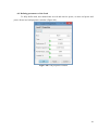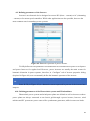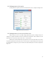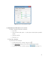
1
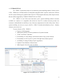
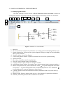
USER MANUAL Version 2.5.0.0724 Content 1. INTRODUCTION .......................................................................................................................................... 4 2. INSTALLING AND LAUNCHING “EA – PSM” SOFTWARE ............................................................................. 5 3. BASICS OF GRAPHICAL USER INTERFACE ................................................................................................... 6 3.1. Main program window ........................................................................................................................... 6 3.2. General setting window ......................................................................................................................... 7 4. CREATING THE POWER SYSTEM COMPONENTS ........................................................................................ 8 4.1. Principle of one line diagram drawing ................................................................................................... 8 4.2. Meanings of icons on the Grid Elements pane ...................................................................................... 9 4.3. Creating the Infinite Busbar ................................................................................................................. 10 4.4. Defining parameters of the regular Busbar ......................................................................................... 11 4.5. Defining parameters of the power Line ............................................................................................... 12 4.6. Defining parameters of the 2 – winding and 3 – winding transformers .............................................. 13 4.7. Defining parameters of the Generator ................................................................................................ 14 4.8. Defining parameters of the Load ......................................................................................................... 15 4.9. Defining parameters of the Inverter .................................................................................................... 16 4.10. Defining parameters of the Photovoltaic systems and Wind turbines ............................................ 16 4.11. Defining parameters of the capacitor .............................................................................................. 17 4.12. Defining parameters of series reactor and shunt reactor................................................................ 17 5. PERFORMING POWER GRID CALCULATIONS ........................................................................................... 18 5.1. Power flow calculations ....................................................................................................................... 18 5.2. Short circuit calculations ...................................................................................................................... 19 5.3. Harmonic analysis ................................................................................................................................ 21 5.4. Motor start - up analysis ...................................................................................................................... 22 6. PROTECTION COORDINATION .................................................................................................................. 23 6.1. Adding breaker unit to elements ......................................................................................................... 23 6.2. Breaker unit properties window overview .......................................................................................... 24 6.3. Configuring overcurrent protection ..................................................................................................... 27 6.4. Configuring non-direction overcurrent protection .............................................................................. 27 6.5. Configuring directional overcurrent protection ................................................................................... 28 6.6. Configuring undervoltage protection................................................................................................... 29 6.7. Configuring ground fault protection .................................................................................................... 30 6.8. Configuring non-directional ground fault protection .......................................................................... 31 6.9. Configuring directional ground fault protection .................................................................................. 31 6.10. Configuring fuse protection ............................................................................................................ 32 6.11. Configuring circuit breaker protection ............................................................................................. 33 2 6.12. Configuring user defined circuit breaker protection........................................................................ 35 6.13. Configuring mini circuit breaker protection ..................................................................................... 36 6.14. Configuring custom curve protection .............................................................................................. 36 7. DISTANCE PROTECTION............................................................................................................................ 38 7.1. Distance protection configuration window ......................................................................................... 40 7.2. Distance protection coordination chart ............................................................................................... 41 7.3. Line zero sequences parameters.......................................................................................................... 43 8. MODELING WIRES, CABLES AND TOWERS ............................................................................................... 43 9. DATA EXPORTING ..................................................................................................................................... 45 9.1. Calculation results exporting................................................................................................................ 45 9.2. One line diagram exporting.................................................................................................................. 45 10. HELP FUNCTIONS.................................................................................................................................. 46 10.1. Send feedback .................................................................................................................................. 46 10.2. System Log ....................................................................................................................................... 46 3 1. INTRODUCTION EA – PSM 2.5 is the latest release of our advanced system modeling software. In this version of EA – PSM users will find models of wind plants and photovoltaic systems, much more efficient one line system drawing tool, graphical data export to CAD programs and many other improvements that are mainly suggested by valuable feedback from our clients. EA – PSM 2.5 is one of the most innovative power system modeling software currently available on a market, it is compatible with all devices from PC to tablets and this provides our customers with unlimited accessibility to one of the most important tool in their daily works. Power system modeling was never as easy as with EA – PSM 2.5 which took definition of user – friendly software to the next level. Try new features of EA – PSM 2.5: Export to CAD programs Automated search for incorrect parameters of system elements “Undo” and “Redo” functions Functionality to easily change connection location of any system element Functionality to select a part of system with right mouse button pressed Availability to change loading of power appliances Updated Circuit Breakers characteristics Added support for touch events on tablets Figure 1.1 Screenshots of EA – PSM 2.5 4 2. INSTALLING AND LAUNCHING “EA – PSM” SOFTWARE Installing and launching “EA – PSM” software is simple and easy. User who purchased the software (all modules or part of it) gets a link to his specified e-mail address from where he/she can download execution file. After launching this file it takes 4 steps to complete installation. “EA – PSM” can be launched only using dongle as shown in Figure 1.1. Purchaser gets a dongle key at the moment he is buying the software or by post. Figure 2.1. Dongle for EA – PSM 5 3. BASICS OF GRAPHICAL USER INTERFACE 3.1. Main program window The main workspace window shown in Error! Reference source not found. contains the ost important functions to quickly model the grid and apply wanted study scenario or calculation. 5 6 7 9 8 1 2 3 10 00 00 25 00 20 00 11 1 12 13 14 4 Figure 3.1 Main EA – PSM window 1. Menu bar 2. The main tool bar. Contains a list of buttons for creating grid and calculating different cases 3. System elements bar for fast one line system diagram drawing (creating bus bars and adding other system elements) 4. Graphic window for one line diagram 5. Creates new graphic window. Opens new window for the one-line system drawing 6. Opens saved file 7. Save, Save As and Save As Picture functions 8. Zoom In, Zoom Out and Zoom to Fit functions 9. Creating a busbar. Opens window to configure a busbar 10. Add element. Opens window for creating a new system element (loads, generators and etc.) 11. Shows if all parameters of system elements are valid (“ ” in green background if no faults were found, “!” in yellow background if not recommended parameters were found and “ ” in red background if erroneous parameters where found ) 12. Calculate. Performs selected calculation (load flow, harmonics load flow, motor start-up, short circuit) 13. Display results. Select to depict results in a one – line diagram of a particular calculation 14. Summary. Results depicted in tables of different calculations 6 3.2. General setting window Settings window shown in Error! Reference source not found. is reached through the Main enu bar selecting “Tools” → “Settings”. Here in tab “General” user could change program language, frequency of AC, calculations standard and customize autosave options. Figure 3.2 Tab “General” in “Settings” window In tab “Display” it is possible to choose which of the calculated parameters should be displayed in a one – line diagram. Figure 3.3 Tab “Display” in “Settings” window 7 In a “Calculation” tab user can change load flow calculations accuracy and voltage factors Figure 3.4 Tab “Calculation” in “Settings” window for minimum and maximum short – circuit current calculations (determined by existing standards). 4. CREATING THE POWER SYSTEM COMPONENTS In EA – PSM 2.5 a new state – of – art one line diagram drawing tool was presented. This tool is developed for fast and really efficient diagram drawing either with PC or tablet, although, users can also draw system as in previous versions of EA – PSM (see User’s Manual Version 2.0r4). 4.1. Principle of one line diagram drawing To draw one line diagram in EA – PSM 2.5 user should choose one of the icons on Grid Elements pane (3 in Figure 3.1), each icon represents particular system element (See 4.2 paragraph). When icon is chosen it is shown in darker background, this means that it is possible to add element on graphic window (4 in Figure 3.1) by pushing at any point of it. In order to deselect icon just push Esc button on a keyboard. Elements like transformers and lines that need to be placed between two busbars are added in 3 simple steps: 1. Preferable element on Grid Elements pane is chosen. 2. The first busbar is selected. 3. The second busbar is selected. 8 Another way to do this is to simply push on a white space between two busbars and element will be added automatically. Hint 1: If by accident element was deleted or added not in the right place, user can always use “Undo” (Ctrl + Z) and “Redo” (Ctrl + Y) functions to correct a mistake. User can change location to which grid element is connected by double clicking on that element, pushing on a green dot at location where the element is connected to a busbar and simply dragging it to another bus. Hint 2: In order to select several elements user can push right mouse button and drag around those elements or can hold Ctrl button pushed and select several elements by clicking on them one by one. Parameters of a system element can be changed in its properties dialog which pops out after double clicking on that element or after pushing the right mouse key on it and selecting “Properties”. 4.2. Meanings of icons on the Grid Elements pane All icons on the Grid Elements pane (3 in Figure 3.1) have their own meaning: - Busbar. - Electric line. - 2-winding transformer. - 3-winding transformer. - Reactor. - Synchronous generator. - Wind turbine. - Photovoltaic system. - Inverter. - Load. - Induction motor. 9 - Capacitors bank. - Shunt reactor. 4.3. Creating the Infinite Busbar It is necessary to have one infinite bus in the system diagram before performing any of the calculations. Infinite bus represents the entire electrical network to which analyzed system is connected. Therefore, the first bus added to the graphic window will be infinite bus by default settings (infinite bus has different color compared to other busses) and user will be asked to enter its parameters right after it is added. First of all, the title and the voltage level of the infinite busbar should be entered in the “General” tab of the “Bus Properties” window. User can leave the title which is assigned by default, however, it is necessary to enter the voltage level manually. Other parameters that can be changed in this tab is minimum voltage level Umin and maximum voltage level Umax. When calculating if the voltage level exceeds boundary conditions Umin or Umax busbar voltage ratings will become red colored. Min and Max voltage levels for all busbars in the grid can be adjusted separately. Figure 4.1 Busbar properties window 10 After the first parameters are entered, user shall define short circuit current in the “System” tab depicted in Figure 4.2 (short circuit power or system impedances can be entered instead if known by choosing the appropriate description type from “Description type” menu). If the network is grounded, zero sequence impedances are also required. These parameters are needed for both minimum and maximum system modes. Hint 3: System parameters (short circuit power and etc.) are usually provided by local power grid operators. Figure 4.2 Infinite busbar properties window 4.4. Defining parameters of the regular Busbar By default regular busbar will have the voltage level of the last busbar added in the diagram. To change the voltage level of the busbar follow the suggestions from 4.1 paragraph. 11 4.5. Defining parameters of the power Line Power line parameters like resistance, reactance and capacitance can be entered manually in “Line properties” dialog depicted in Figure 4.3 or by selecting “Model line” feature user can enter overhead line/cable parameters like length and type as shown in Figure 4.4 and program will automatically create the power line model. Figure 4.3 Power line parameters window Figure 4.4 Overhead/cable line modelling window 12 4.6. Defining parameters of the 2 – winding and 3 – winding transformers As for other elements user needs to enter parameters of the transformer manually. For customizing transformer parameters “Configure” button is selected as shown in Figure 4.5 and all required fields are filled. If there is a possibility to regulate transformer’s tap then field next to inscription “Tap changer” is checked and tap changer parameters are entered (example is shown in Figure 4.6). In tab “Connection type” user can change phase difference between line – to – line voltage vectors and choose an appropriate connection type (star, delta or grounded star). Figure 4.5 “Configure” tab of transformer parameters Figure 4.6. “Configure” tab of transformer parameters 13 For 3 – winding transformer input parameters are the same, however, not two but three windings need to be considered. 4.7. Defining parameters of the Generator Parameters needed to be entered for a synchronous generator are depicted in generator parameters window in Figure 4.7. Generator transient reactance. Xd‘ is used for calculating minimum short-circuit currents Minimum and maximum reactive power. Not necessary Zero sequence impedance Generator subtransient reactance. Xd‘‘is used for calculating maximum short-circuit currents Armature resistance Figure 4.7 Generator parameters window Hint 4: It is possible to change loading of generators, motors, loads and inverters. This function is useful when these system elements are not working under full loading conditions and one needs to asses these conditions in the calculations. Loading can be changed in parameter window of these elements or in the load flow summary table (14 in Figure 3.1). 14 4.8. Defining parameters of the Load To fully define load, user should enter its real and reactive power, or enter real power and power factor in a load properties window (Figure 4.8). Figure 4.8 Load properties window 15 4.9. Defining parameters of the Inverter Inverter is an electronic device designed to convert DC (direct – current) to AC (alternating – current) or for motor speed controllers. While other applications are also possible, these are the most common ones in nowadays power systems. Figure 4.9 Harmonic spectrum of power inverter To fully define inverter parameters user should enter its real and reactive power or real power and power factor as for regular load. However, power inverters are usually the main reason for harmonic distortion in power systems, therefore, in “Configure” tab of inverter properties dialog (depicted in Figure 4.9) user can manually define the harmonic spectrum of the inverter. Hint 5: By default the harmonic spectrum of 6 pulse power inverter is defined in “Configure” tab. Ratio Ih/ IN (in Figure 4.9) is a harmonic current expressed in percent of the inverter base amperes. 4.10. Defining parameters of the Photovoltaic systems and Wind turbines Photovoltaic power systems and wind power plants are defined as well as inverters as these power plants are always connected to an electric grid through a power inverter, however, wind turbines and PV systems are power sources like synchronous generators, while inverters are loads. 16 4.11. Defining parameters of the capacitor To fully define the capacitor just enter its real and reactive power, example is in Figure 4.10. Figure 4.10 Capacitor parameters 4.12. Defining parameters of series reactor and shunt reactor Shunt reactors are used in very high voltage transmission systems to mitigate increase of voltage due to parallel capacitance between overhead lines and ground or other conductor. On the other hand, series reactors are used to reduce short – circuit currents. Shunt reactor is defined identically as the capacitor or load. On the other hand, series reactor is more like transformer but it has only one coil. Series reactor is connected between two busses and user shall define its voltage level, power of short circuit and nominal power of reactor as depicted in Figure 4.11. 17 Figure 4.11 Series reactor parameters dialog 5. PERFORMING POWER GRID CALCULATIONS EA-PSM 2.5 program performs these calculations: Power flow Short circuit (three phase, phase - to – phase, phase to neutral, phase to grounded neutral) Harmonics load flow Motor start – up 5.1. Power flow calculations To perform power flow in the grid: In main menu bar select “Calculate” and press icon Press “Power Flow” and power flows will be calculated almost instantly For opening results press “Load flow summary” (14 in Figure 3.1) 18 “Summary” window will open as depicted in Figure. 5.1 Figure 5.1 Power flow results in a summary table 5.2. Short circuit calculations To perform short circuit calculations: From icons list 13 in Figure 3.1 choose whether you want to display maximum or minimum short circuit results. Select a busbar at which short circuit appears by pushing on it with a left - key of the mouse. In main menu toolbar press “Calculate” button. Choose type of short circuit you want to perform (K 1; K 1,1; K 2; K 3). K3 – three–phase short circuit; K2 – phase – to – phase short circuit ; K1 – phase-to-earth short circuit; K1,1 – two-phase-to-earth short circuit; 19 Figure 5.2 Dialog for short circuit calculation results Results will instantly show – up on the one line diagram and can be also observed by pressing “Short circuit summary” (14 in Figure 3.1). Summary table of short circuit results is depicted in Figure 5.2. 20 5.3. Harmonic analysis To perform harmonic analysis: In main menu bar select “Calculate” and press icon Select “Harmonics” Results will instantly show up on the one line diagram and can be also observed by pressing “Harmonics load flow summary” (14 in Figure 3.1). Summary table of harmonics load flow results is depicted in Figure 5.3. Here user can observe voltage harmonics at each bus and current harmonics at each branch. By pressing icon results will be displayed graphically as depicted in Figure 5.4. Figure 5.3 Results of harmonics load flow analysis Figure 5.4 Graphical representation of harmonics 21 5.4. Motor start - up analysis To perform motor start – up analysis: First of all, user have to choose which motors should be assessed in the motor start – up calculation. This can be done by choosing an appropriate motor and pressing the right mouse key on it. A small list will shows up with inscription “Set Starting”. User need to push on this inscription and now motor will be assessed in the motor start – up calculation. Another way to do this is to choose “Calculate” (12 in Figure 3.1) → “Motor Start” →”Motor Selection” and select those motors that should be assessed in the calculation. After motors are selected user should press “Calculate” → “Motor Start” → Motor start simple” or push F7 button on keyboard to perform the motor start – up analysis. Results will instantly show up on a one line diagram or can be observed in “Motor Start – Up Summary” table (Figure 5.5) which is activated by pressing button (14 in Fig. 3.1). Figure 5.5 Results of motor start – up analysis 22 6. PROTECTION COORDINATION EA-PSM has a fast and easy to use protection modelling and coordination module. When grid is fully modelled and different grid modes are analyzed it is possible to model and coordinate grid relay protection. Users can add different kinds of protections: Overcurrent protection Undervoltage protection Ground fault protection Fuse Circuit breaker Mini circuit breaker User defined curve 6.1. Adding breaker unit to elements To add these elements double click on the system element to which protection need to be added. Table shown in Figure 6.1 will pop out and “in” and/or “out” can be selected. Figure 6.1 Adding protection for created element window By selecting “in” and “out” user adds ‘Breaker’ element at the beginning and at the end of the line, an example is shown in Figure 6.2. 23 Figure 6.2 Protection added for transformer 6.2. Breaker unit properties window overview By double clicking on each ‘Breaker’ element its properties window will open, shown in Figure 6.3. In “General” tab (Figure 6.3) user can edit breaker title and add current transformer to it. Figure 6.3 Breaker properties “General” tab 24 Figure 6.4 Breaker properties “Short Circuit” tab In a “Short Circuit” tab shown in Figure 6.4 filtered short circuit results can be seen. Only short circuits, which flow through selected breakers’ element are shown in the table. Pressing “Vectors” button in this table will open short circuit phasors diagram, shown in Figure 6.5. Figure 6.5 Short circuit current and voltage phasors at busbar 25 Also, selectivity and ground protection charts are plotted automatically (Figure 6.6). Select short circuit bus Enable value tracker Add more breakers to the chart Export chart as image Figure 6.6 Protection selectivity chart Figure 6.7 Breaker properties “Protection” tab 26 In a “Protection” tab shown in Figure 6.7 circuit breakers and relay protection can be selected and edited by clicking “Add protection” button user will be able to choose an appropriate type of protection. “Remove” button will delete selected protection. “Export” button will form a report with short circuit results and breaker protections parameters. 6.3. Configuring overcurrent protection When overcurrent protection is selected from the list (Figure 6.7) and added to Breaker unit, user can configure its parameters. There are three different stages of overcurrent protection – I>, I>> and I>>>. The configuration of all stages is the same, the only difference is the name to better distinguish different stages. User can choose to configure non-directional or directional overcurrent protection. 6.4. Configuring non-direction overcurrent protection By default, added overcurrent protections are non-directional, show in Figure 6.8. Figure 6.8 Non-directional overcurrent protection configuration 27 Selecting “Characteristic” drop-down menu, user can select one of IEC standard tripping curves: definite time, normal inverse time, very inverse time, extremely inverse time and long-time inverse time. “Direction” drop down menu defines direction of overcurrent protection. It can be nondirectional, directional forward and directional reverse. Check box “Connected curve” enables option to connect different overcurrent protection stages into one curve, shown in Figure 6.9. Figure 6.9 Connected overcurrent protection stages “Relay time setting” defines protection time setting. Minimum values is 20 ms. “Relay current setting” defines protection current setting in primary values. Table shown in Figure 6.8, depicts protection sensitivity values of each short circuit type based on current setting. If sensitivity is less than 2 table cell turns red. 6.5. Configuring directional overcurrent protection There are two types of directional overcurrent protection – forward and reverse. Direction overcurrent protection configuration window is shown in Figure 6.10. Basic parameters are the same as in non-directional protection – characteristic, direction, time settings and current setting. “Characteristic angle” defines angle in degrees in which the protection is facing. “Sector angle” is angle in degrees, which defines the tripping area of protection. “Polarization voltage” defines the voltage needed for protection to trip. 28 On the left in Figure 6.10 user can view the directional protection diagram. By clicking “Vectors” button in the table user can view different short circuit vectors and their direction. Figure 6.10 Directional overcurrent protection configuration 6.6. Configuring undervoltage protection When undervoltage protection is selected from the list (Figure 6.11) and added to Breaker unit, user can configure its parameters. Like in overcurrent protection, there are three different stages of undervoltage protection – U<, U<< and U<<<. Configuration of undervoltage protection is shown in Figure 6.11. “Phase selection type” defines the protection selection type. There are three types to choose from – Phase to Ground, Phase to Phase, Positive sequence. “Time setting” defines protection tripping time. “Voltage setting” defines minimum element voltage at which protection will trip. “Minimal current” defines minimum current at which protection can operate. Table shown in Figure 6.11, depicts protection sensitivity values of each short circuit type based on voltage setting. If sensitivity value is between 1 and 2, cell color is yellow, if sensitivity value is less that one or infinity, cell color is red. 29 Figure 6.11 Undervoltage protection configuration 6.7. Configuring ground fault protection When ground fault protection is selected from the list (Figure 6.7) and added to Breaker unit, user can configure its parameters. This protection is very similar to overcurrent protection, user also can choose non-directional or directional ground fault protection. 30 6.8. Configuring non-directional ground fault protection Configuration of non-directional ground fault protection is the same as non-directional overcurrent protection (see 6.4 paragraph). Configuration window is shown in Figure 6.12. Figure 6.11 Non-directional ground fault protection configuration Like in non-directional overcurrent protection, user have to define direction, time setting and current setting. Ground fault sensitivity table is similar to overcurrent protection sensitivity table, only ground fault table compares current setting with short circuit K1 and K1,1 zero sequence current multiplied by 3. If sensitivity value is less than 2, cell color is red. 6.9. Configuring directional ground fault protection Directional ground fault protection also has two directions – forward and reverse. Like in directional overcurrent protection user also have to define direction, time settings, current settings, characteristic angle and sector angle. Configuration window is shown in Figure 6.11. Differently than in overcurrent protection user can also define directional protection tripping zone characteristic. User can choose Sector (same like in directional overcurrent protection), Sin (no sector angle property) and Cos (no sector angle property). By selecting different short circuit from the table, user can view its vectors in diagram and see if protection will trip. If current vector is inside light blue area ground fault protection will trip. 31 Figure 6.11 Directional ground fault protection configuration 6.10. Configuring fuse protection When fuse protection is selected from the list (Figure 6.7) and added to Breaker unit, user can select different fuses from EA-PSM fuse library, shown in Figure 6.12. New fuses are added with every new EA-PSM release. Fuse configuration windows is shown in Figure 6.13. Figure 6.12 Fuse selection library 32 Figure 6.13 Fuse configuration window To select a fuse user has to click on “Select fuse” button. Then a fuse selection window, shown in Figure 6.11, will pop up. There user should expand one of the manufacturers (ABB, Siemens, Inter-Teknik..), then expand fuse models and select appropriate fuse current and press “OK”. Fuse will be added and its curve will be shown on the right in configuration window. User can modify fuse title to better distinguish it from other fuses. 6.11. Configuring circuit breaker protection When circuit breaker protection is selected from the list (Figure 6.7) and added to Breaker unit, user can select different circuit breakers from EA-PSM circuit breaker library, shown in Figure 6.14. New circuit breakers are added with every new EA-PSM release. To select a circuit breaker user has to click on “Select Breaker” button. Then a circuit breaker model selection window, shown in Figure 6.14, will pop up. There user should expand one of the manufacturers (ABB, Siemens, Schneider…), then expand one of breaker models and select appropriate tripping unit and press “OK”. Circuit breaker will be added and its curve will be shown on the right in configuration window, shown in Figure 6.15. 33 Figure 6.14 Circuit breaker model selection library Figure 6.15 Circuit breaker configuration window In configuration window (Figure 6.15) user can modify circuit breaker title, define nominal circuit breaker current, define overload protection values (IR value and tR time value), short circuit protection values (Isd value and tsd time value), instantaneous short circuit protection value (Ii value) and ground fault protection value (Ig current value tg time value). Protection number and number of 34 properties depend on manufacturer and circuit breaker tripping unit. Every property value arrays are taken from official public manufacturer documentation. On the right, in configuration window, user can instantly preview curve changes. To make configuration more easily there are several markers in the chart: I_N in red – this is the nominal current of element or current from power flows. I_Motor_start in green – current flowing through element during motor starting. I_max in yellow – current calculated based on I_N and coefficients “Ka” (reserve coefficient), “Kp” (transitional process coefficient), “Kg” (protection return coefficient). Coefficients are configure in main configuration window. I_max value is calculated based on (1). 𝐼_ max = 𝐼_𝑁 ∙ 𝐾𝑎∙𝐾𝑝 𝐾𝑔 (1) 6.12. Configuring user defined circuit breaker protection In circuit breaker model selection use can select “User Defined” option (Figure 6.14). This option is added if user did not find required circuit breaker in EA-PSM library. User can easily define his own circuit breaker characteristic. User defined circuit breaker configuration window is shown in Figure 6.15. Figure 6.15 User defined circuit breaker configuration window In configuration window user has to define nominal circuit breaker IN and three points (current on x axis and time on y axis) shown in right side of Figure 6.15. Each current point is defined as coefficient which is multiplied by nominal current and each time points is defined in seconds. 35 6.13. Configuring mini circuit breaker protection When mini circuit breaker protection is selected from the list (Figure 6.7) and added to Breaker unit, user can configure its parameters. Mini circuit breaker is a circuit breaker used to protect low voltage and low power appliances. Its configuration window is shown in Figure 6.16. Figure 6.16 Mini circuit breaker configuration window In configuration window user can modify mini circuit breaker title, its nominal current IN, ultimate current Iu (it should be larger than maximum short circuit current) and tripping characteristic (B, C, D, K or Z). Like in circuit breaker, there are markers in the chart to ease nominal current selection (see 6.11 paragraph). 6.14. Configuring custom curve protection When custom curve protection is selected from the list (Figure 6.7) and added to Breaker unit, user can configure its parameters. Custom curve is used when none of the protection fits user needs, or user has to add a dynamic protection curve, or user only has a protection curve on paper. Custom curve can be defined two ways – by defining a curve formula or by defining few points on the curve. To define a curve by formula user has to enter a correct formula containing variable “I” in it (Figure 6.17). User has to fully define the formula with all parentheses and correct mathematical operators. In Figure 6.17 normal inverse time formula is defined with 600 A and 1s settings. User 36 also must define a starting value from which the curve starts and end value at which the curve ends (or leave it at zero and let the curve extend to short circuit current). Figure 6.16 Custom curve defined by formula configuration window To define a curve by points, user has to enter few points from a known curve (Figure 6.17). To enter points user has to double-click on “Current, A” or “Time, s” column cell, enter a value and press “Enter”. There is an option to check “Interpolate” for each point. Use this option if you have a non-linear curve and you want it to be smoother. To get the best result change the polynomial power (best use 3-9 values). 37 Figure 6.16 Custom curve defined by points configuration window 7. DISTANCE PROTECTION EA-PSM has an extensive distance protection modelling and coordination module. User can add and coordinate different distance protections from manufacturers like “Siemens”, “Alstom”, “ABB” and also user can create user defined distance protection. To add distance protection to a breaker, in breaker unit properties (Figure 6.3), selected “Distance protection” tab and check the “Use distance protection” checkbox. Distance protection configuration is instant and does not require confirmation via OK or Apply. Note that distance protection can’t be added to end of line elements such as generators, loads, motors and similar. 38 Figure 7.1 Configuration tab of distance protection. In general distance protection toolbar user can enable or disable distance protection for selected breaker with “Use distance protection” checkbox, also by pressing “Export” button, user can export distance protection settings and short circuit results to a text editor compatible file, shown in Figure 7.1. Figure 7.2 Distance protection export settings 39 7.1. Distance protection configuration window In distance protection configuration window, shown in Figure 7.2, user can configure preview chart and its settings to ease the distance protection configuration. On the right side of the window user can configure: 1. “View settings” button: opens short circuit vectors selection window, shown in Figure 7.3. In view settings window user can configure configuration chart settings. Figure 7.3 View settings popup - System mode: select short circuit system mode for short circuit impedance vectors. - K2, K11, K1: selection checkboxes for which resistance measurement loops to show for each asymmetrical short circuit type. 1) A-B: Phase A to Phase B 2) B-C: Phase B to Phase C 3) C-A: Phase C to Phase A 4) A-G: Phase A to ground 5) B-G: Phase B to ground 6) C-G: Phase C to ground 2. “Max Z to show” field: short circuit vectors above specified value will not be shown, a notification will popup if a vector was hidden. 3. “Buses” list: list of all buses in the system. Each list cell is bordered and contains five checkboxes. The top-left checkbox shows impedance vectors from breaker unit bus to the selected 40 list bus. K3, K2, K1 and K1,1 checkboxes show appropriate short circuit impedance vectors from breaker unit bus to the selected list bus. Each short circuit vectors is colored as follows: K3 – red; K2 – green; K1 – blue; K1,1 – yellow; On the left side of the window, user can configure distance protection settings: 1) “IED” dropdown menu: select witch type of distance protection to use. 2) “Blinder” box: click to expand load blinder settings, a load blinder can be enabled or disabled, specific settings vary based on distance protection type. 3) “Zone” dropdown: select zone to edit, if zone has a ground current compensation factor it is set to the factor of the selected zone for drawing short circuit vectors. 4) “Direction” dropdown menu: select zone direction from Forward, Reverse and Nondirectional. 5) “Enable” checkbox: Enable or disable currently selected zone. 6) “Time delay” field: Set time delay for selected zone. 7) Other fields are distance protection type specific and are defined by manufacturer. 7.2. Distance protection coordination chart 1 2 3 Figure 7.4 Distance protection coordination tab 41 On the left side of configuration chart user can configure: 1) Select to show phase to phase or phase to ground zones. 2) Show or hide distance protection of current breaker. 3) List of all distance protections in the system. By double-clicking on a distance protection curve, user can open protection configuration popup, shown in Figure 7.5. Figure 7.5 Distance protection configuration popup Hint 6: Solid line in chart represent configured distance protection zones; Dashed colored lines represent distance protection tolerance; Dashed gray lines represent impedance from breaker unit bus to the marked bus. Hint 7: Basic chart controls: - Auto range chart by double-clicking; - Zoom in and out with mouse wheel; - Press and drag left mouse button to zoom to rectangle; - Press and drag mouse wheel button to pan chart; - Equalize axis scale by clicking on another axis (ex.: equalize y axis by clicking on x axis) 42 7.3. Line zero sequences parameters Each line positive sequence resistance, reactance are shown in Summary table. Relation of return path resistance and line resistance RE/RL, also relation of return path reactance and line reactance XE/XL are described for each line. Coefficient K0 for each line is calculated. The magnitude and angle is depicted for each line. Coefficient K0 and relations RE/RL and XE/XL are set to 0 for transformers. 8. MODELING WIRES, CABLES AND TOWERS In EA - PSM 2.5 user can create templates for cables and overhead lines that he/she usually use in electric schemes, although, it is not necessary as we offer a broad database of wire types by the well-known manufacturers (Draka, Nexans, TF, etc.), commonly used by system designers and operators. It is also possible to model towers for overhead lines. For creating templates for previously mentioned elements select “Modelling” from main menu bar (Figure 3.1) and choose “Wire types”, “Cable types” or “Tower types” from drop down menu. Table will pop out as shown in Error! Reference source not found., Figure 7.2 or Figure 7.3. ere user will have to enter the required parameters and press “Save new” to save model. If user wants to modify existing model, he should selected the model, update its parameters and press “Overwrite” button. 43 Figure 7.1 Wire type configuration window Figure 7.2 Cable type configuration window 44 Figure 7.3 Tower type configuration window 9. DATA EXPORTING 9.1. Calculation results exporting In order to export any of the calculation results user should open Summary window as was described in paragraph 5 and press button. He then will be asked to choose what data he wants to export and formatting type (export as numbers or as text). Diagrams shown in Figure 5.4 and Figure 6.5 can be exported as a picture in .png format or user can copy data as a text. By pressing right mouse button user will see a context menu with “Save Picture” (save .png format picture in selected location) and “Copy Data” (copy diagram data as text) option. 9.2. One line diagram exporting EA – PSM 2.5 allows to export a one – line diagram as picture in .png format or as drawing in .dxf format that can be later modified with CAD programs. To export one line diagram user should choose “File” → “Export” → “Drawing .dxf file” (or “Picture .png file”). He then will be asked to define location of exported file in his/ her computer. 45 Figure 8.1 One line diagram exporting 10. HELP FUNCTIONS In the main menu bar there is a button “Help”. By pressing it user can get important information about the program, send his feedback and observe system log information. 10.1. Send feedback Our goal is to create a power system modeling software with superior product experience to its end – user, therefore, we appreciate any feedback from our customers, as it helps us to accomplish our goals. Thus, if any idea or impression occurs while working with EA – PSM please don’t hesitate to send it by simply pressing “Help” → “Send feedback”. Any language is acceptable. 10.2. System Log Problems of the calculations are usually depicted in the “System Log” window that can be accessed by pressing “Help” → “System Log”. Therefore, if any problem occurs, please copy the text from this window by pressing “Save” button or send it directly to us by pressing “Report” button. We will solve the problem as fast as possible and contact you to inform about the possible solutions. 46