1
APPENDIX
by
John J. Nitao
Lawrence Livermore National laboratory
Livermore CA, 94551, USA
Many ow and transport problems of practical interest cannot be solved
analytically. They must be solved numerically, on a digital computer, using a
computer code, or program. Ideally, for the purpose of solving the forecasting
models discussed in this book, a computer code should be able to solve a
wide range of models in both the unsaturated zone and the saturated one,
including nonisothermal as well as isothermal cases. The obvious reason
for this statement is that, as emphasized throughout the book, we have
essentially only one partial dierential equation that appears in all models,
viz., the equation that describes the balance of an extensive quantity. Also,
the boundary conditions are essentially the same for all extensive quantities.
In most cases, a model would involve the transport of more than a single
extensive quantity, so that a code should be able to solve a number of p.d.e.'s
simultaneously. However, the actual numerical simultaneous solution of a
number of p.d.e.'s, and the transformation of such solution into a practical
and useful computer program may require many thousands of code lines.
NUFT (Nonisothermal Unsaturated-saturated Flow and Transport)
serves as an example of a code that can be applied to a large number of
ow and contaminant transport problems. We have included this code with
the book in order to facilitate the solution of the problems presented in
Chap. ?? (although other codes may also be used). As stated in the preamble to that chapter, the objectives of presenting these problems and using
the NUFT code to solve them are: (a) to gain some experience in the api
Dec. 17, 95
ii
???
APPENDIX
plication of numerical models and the use of computer codes, (b) to present
solutions to the models discussed in this book, and (c) to investigate how
these solutions vary as various input parameters are changed. Chap. ??
also contains exploratory problems that one may pursue on one's own.
The NUFT code is available from the International Groundwater
Modeling Center (IGWMC) Golden, Colorado, USA. The version described in this section and distributed with this book runs on IBMTM compatible personal computers under Microsoft WindowsTM . The NUFT code is
written in the computer language C. It also runs on UNIXTM workstations.
The code has been veried by comparison with analytical solutions of ow
and transport problems, and with numerical solutions by other computer
codes (Lee et al., 1993).
This appendix contains some information on the NUFT code, and guidelines on how to use it. It is written under the assumption that the potential
user of NUFT is familiar with the principles of numerical techniques, especially with those of the method of integrated nite dierences. It explains
how NUFT numerically solves the ow and contaminant transport models
that are described in the various sections of this book, focusing on the problems presented in Chap. ??. No prior experience with numerical methods or
the use of computer codes is required.
.1 General Description
.1.1 Objectives
NUFT was written in order to solve subsurface environmental problems,
especially problems that require the prediction of contaminant migration,
e.g., the analysis of remediation methods, and the study of nuclear waste
isolation problems. The original emphasis was on the transport of multiple
components in a multiphase ow system. It has recently been extended to
make it applicable to a wide variety of saturated and unsaturated ow and
contaminant transport problems. However, the more experienced user will
recognize how the general case is reduced to the particular cases of saturated
ow, single phase ow under saturated or unsaturated ow conditions, etc.
Essentially, NUFT solves the partial dierential equations that describe
the mass balances of multiple components transported within multiple phases
that together occupy the the void space of a porous medium domain. The
components and the phases are assumed to be in local thermodynamic equilibrium, as described in by Bear and Nitao (1995). The results of the calcu-
.2. MATHEMATICAL MODEL
iii
lations, using NUFT, are either time histories of concentrations, saturations,
and uid pressures at dierent locations within the problem domain, or spatial distribution of these state variables at specied times.
NUFT consists of four dierent models within a single code:
(a) ucsat|unconned aquifer, saturated ow model.
(b) us1p|unsaturated single phase ow model.
(c) us1c|unsaturated single component transport model.
(d) usnt|fully coupled unsaturated multiple phases, multiple components model with isothermal and nonisothermal options.
All models share a common set of internal utility routines, e.g., for inputoutput and numerical algorithms.
For a problem of ow in a saturated zone, or a problem of single phase
ow in the unsaturated zone, rather than using the usnt model, it is computationally more ecient to use the ucsat and us1p models, respectively, and
then to use the us1c model for solving the contaminant transport problem,
running alongside ucsat or us1p.
The usnt model has the option to solve the energy balance equation,
coupled to the mass balance equations, thus facilitating the solution of nonisothermal ow and transport problems. Of particular importance, especially for nonisothermal problems, is NUFT's ability to handle properly the
appearance or disappearance of any phase, due to condensation and evaporation.
.2 Mathematical Model
Actually, all the mathematical models, especially the p.d.e.'s, solved by
NUFT have already been presented in the appropriate chapters of the book.
To facilitate the use of NUFT, let us rewrite them in the forms that NUFT
solves them. In all cases, it will be assumed that the solid matrix is stationary and nondeformable @=@t = 0.
.2.1 Saturated Flow
The module ucsat is designed to solve both unconned and conned problems of saturated ow.
The mass balance and ux equations for the ow of water are:
@ = rq; q = k (rP + g rz) :
(.2.1)
@t
APPENDIX
iv
Note that in NUFT, p P .
For a compressible uid the constitutive relationship for the uid's density is, = (P ). The uid's coecient of compressibility, is given by
Assuming
equation (.2.1), reduces to
@ :
= 1 @P
(.2.2)
@ jqrj;
@t
(.2.3)
@P
@t = rq;
q = k (rP + grz) :
(.2.4)
Thus, in the general case of ow of a compressible uid in a nondeformable
porous medium, the variable is pressure, P = P (x; y; z; t).
For = constant, (.2.4) can be written in terms of the piezometric head,
h = h(x; y; z; t), which serves as the variable:
So @h
@t = rq;
So = g;
q = Krh;
(.2.5)
where So is the specic storativity.
Horizontal ow in conned and phreatic aquifers
For essentially horizontal ow in a conned aquifer, the variable is h =
h(x; y; t). The mass balance and ux equations are:
0
0
S @h
@t = rQ + Qw (x; y; t); S = So B; T = KB; Q = Trh; (.2.6)
where B represents the aquifer's thickness, and Qw represents, symbolically,
the source term, which, usually, takes the form of net recharge (negative
extraction) at specied points in the aquifer (pumping and recharging wells).
For essentially horizontal ow in a phreatic aquifer, the variable is the
water table elevation, h = h(x; y; t), and the ux and mass balance equations
are:
0
0
Sy @h
@t = rQ + Qw (x; y; t) + R(x; y; t); Q = (h )Krh; (.2.7)
.2. MATHEMATICAL MODEL
v
where = (x; y ) denotes the elevation of the aquifer's bottom, and R
represents a distributed source, e.g., due to natural replenishment from precipitation.
In both conned and phreatic aquifer balance equations, we may add on
the r.h.s. source terms that represent leakage through aquitards, into or out
of the aquifers. Such a term will take the form
qv = hextc h ;
r
where qv denotes leakage into the aquifer (as volume per unit area per unit
time), hext denotes the head in the underlying or overlying aquifer, and
cr = B0 =K 0 denotes the resistance of the aquitard, of thickness B 0 and
hydraulic conductivity, K 0.
Phreatic surface as a boundary
In Subs. ??, we have discussed the conditions along a phreatic surface which
serves as the upper boundary of a three-dimensional porous medium domain.
It was shown there that for the case of a phreatic surface with accretion, the
condition of equality of uxes normal to this boundary, takes the form of
(??)
w
eff @h
(.2.8)
@t = (Krh + N)r(h z);
where we have omitted the subscript w, N N rz denotes the rate of
accretion, and eff denotes the eective porosity (= r ).
If we make the assumption of small phreatic surface slopes (Bear, 1972,
p. 259), i.e.,
jrhj2 1; ;
the above condition can be approximated as
eff @h
@t = eff Vz + N:
(.2.9)
.2.2 Flow in the unsaturated zone
For the ow of a single uid phase in the unsaturated zone we employ the
module us1p of NUFT. It solves the mass balance equation for a single component in a single uid-phase. The mass balance equation for S < 0 is
@ = rKr ( + z);
@S
+
@t
@t
(.2.10)
APPENDIX
vi
where the primary variable used is saturation S . The pressure head pw =w g with atmospheric pressure as datum is given as a function of saturation by the moisture retention relationship = pc (S ). For S = 0 the
mass balance equation that is solved is
@@t = rKr ( + z);
(.2.11)
with has the primary variable. The actual implementation of the switching
between primary variables is described later.
For the relationships = pc (S ) and K = K (S ), the program employs
the Van Genuchten relationships (??) and (??), respectively, replacing Swr ,
A, and C , by Sr , , and m, respectively.
.2.3 Transport of a single component in a single uid phase
The module us1c of NUFT is used to solve this class of problems. The
ow eld can be solved by the module us1p or the module usnt which is
described later.
The mass balance equation for a component in a uid phase in multiphase
ow, with = (pw ), and c !w = =w , is (omitting subscripts and
superscripts):
@ (S!) = rS (!V Dr! D r!) f + S ; (.2.12)
f !s
@t
where , S , and V are transferred from the ow module. For the component
on the solid, we have
(1 )s @F
@t = ff !s + (1 )s s :
(.2.13)
A source due to decay is expressed by
= !;
s=
F:
NUFT employs the linear isotherm F = Kd ! .
.2.4 Transport of multiple components in multiple phases under isothermal and nonisothermal conditions
The module usnt is used for this class of problems. It considers the case of
NP uid phases and NC components.
.2. MATHEMATICAL MODEL
vii
Since by summing up mass balance equations for all components within
a phase, we obtain the mass balance equation for that phase, NUFT actually
solves the NC mass balance equations for the components.
The mass balance equation for an individual -component in all -phases
is:
@
@t
X
()
S! Rd =
X
r S ! V Dhr! X () + S + (1 )s s ;
(.2.14)
()
in which the sum is over all uid -phases, 's are sources due to rst order
growth (or negative sink for decay), Rd denotes the retardation factor for
the -component in the -phase, dened as
R = 1 + (1 )sKd ;
d
S
and the various Kd 's may be constant or functions of the temperature.
NUFT assumes that there is a unique wetting phase wet that can form a lm
on the solid surfaces which can lead to sorption on the surfaces. Therefore,
= 0 for all 6= .
Kd
wet
The phase velocities are given by darcy's law,
V = k (rp + grz) :
The phase pressures are given by the \capillary pressure" relationships.
For example, for a system with gas(g ) and liquid(`) phases,
p` = pg pc (S` ; T ):
(.2.15)
For a NAPL(n) and aqueous(`) phase system,
p` = pn pc(S`; T );
(.2.16)
assuming that the porous medium is \water-wet." For a gas, NAPL, aqueous
phase system,
p` = pn pc (Saq; T ); pn = pg pc (Sg ; T ):
(.2.17)
To determine all ! 's, we require partitioning coecients that relate
component concentrations between each pair of phases,
n :
n = K
(.2.18)
APPENDIX
viii
In using this relationship, note that the mole fractions n ; n must be converted to mass fractions ! ; ! .
NUFT has "hard-wired" partitioning coecients for the partitioning of
water between the gas and aqueous phases based on
Kg`w = (psat(T )=pg) exp ( M w =RTabs`)
(.2.19)
where is the matric suction potential for the aqueous phase, Tabs is absolute
temperature, and psat is the saturation pressure from the steam tables. The
exponential term is often called "vapor-pressure" lowering and is derived
from the porous media generalization of Kelvin's law (Nitao and Bear, 1996).
For TCE, NUFT also has "hard-wired" values of Henry's coecients for the
partitioning between the gas and aqueous phases. A general functional form
for partitioning coecients is
K = [(A + pg B + C )=pg] exp( D=Tabs)
(.2.20)
where constants A, B , and C are specied by the user.
In addition to the mass balance equations, under nonisothermal conditions, NUFT solves the energy balance equation:
2
3
@ 4X(S u ) + (1 ) c (T T )5
s ps
o
@t () 2
0
1
3
X
X
= r4 S @h V + h Dh r! A rT 5;
()
( )
(.2.21)
where u and h are the internal energy and the enthalpy, respectively, of
the -phase, cps is the heat capacity of the solid matrix, To is a reference
temperature, Dh is the coecient od hydrodynamic dispersion of the component in the -phase, h are partial enthalpies, and
X
= (T + DH )
()
is the combined thermal conductivity and coecient of thermal dispersion of
the porous medium as a whole. Since DH is a function of ow velocity, at this
time, NUFT does not have velocity dependent thermal dispersion coecient.
The coecient , e.g., for a liquid-gas system, is given by either
p
q
= s + S`(`+s s ) + Sg (g+s s )
.3. NUMERICAL MODEL
or
.
ix
= s + S`(`+s s ) + Sg (g+s s )
NUFT also has hard-wired correlations for aqueous phase viscosity and
densities and specic enthalpies of liquid water and air-water gas phases.
The mixing rule that used for the density of a liquid phase is
1 = X ! :
(.2.22)
( ) where are partial densities. The density for the gas phase is calculated
from the ideal gas law with a correction for water vapor based on the steam
tables. The enthalpy of a phase is approximated by the mixing rule
h =
X
( )
! h :
(.2.23)
.3 Numerical Model
.3.1 Finite dierence discretization of partial dierential equations
In both the ucsat and us1p modules, NUFT numerically solves a single
partial dierential equation|the mass balance equation for water. The us1c
module solves a single mass balance equation for the transport of a single
component. In the usnt module, NUFT solves a coupled set of balance
equations: one for the mass of each transported component. For the nonisothermal case, an energy balance equation is also included in the coupled
set. As we have seen above, each balance equation has more or less the
general form
@e = re(V + J) + ;
(.3.1)
@t
where ( S ) is the volumetric fraction of the uid, e is the density of the
considered extensive quantity. J is the non-advective ux of the considered
extensive quantity, and describes the strength of the source (as quantity
per unit volume of phase). For a uid's mass, e is replaced by the mass
density, . In order to discretize this partial dierential equation in time
and space, the time domain is subdivided into a sequence of time steps,
tn , n = 0; 1; : : :, and the space domain is partitioned into nite dierence
cells, or elements. Specifying an initial time step, the length of subsequent
APPENDIX
x
time steps is automatically controlled by the program, using user-specied
tolerances for the primary variables. The user also determines the size of
each FD cell, and the total number of cells within the domain. Henceforth,
we shall use the term `element', or `cell', interchangeably.
NUFT is based on the numerical technique called integrated nite dierences method (e.g., Bear and Verruijt, 1987, p. 244). It is also referred to
as the nite volume method. This method allows FD elements of arbitrary
polyhedral shapes, as long as the line segment connecting the centroids of
any pair of neighboring elements is orthogonal to their shared boundary.
The integrated nite dierence method reduces to the standard nite difference method when the elements constitute a standard rectangular mesh.
Here, we shall restrict the discussion to FD elements that are identical to
those assigned in the standard method of nite dierences for rectangular
or cylindrical coordinates. In cartesian coordinates, the elements are 2-d
rectangles or 3-d parallelepiped boxes, with sides parallel to the axes. In
cylindrical coordinates they are sectors of an annular cylinder.
The discretized form of the balance equation (??) at the mth element is
Um mn+1 nm+1 mn nm =tn+1 =
h
i
X
Am m (V )nm+1m + (J )nm+1m + Um mn+1 nm+1 ; (.3.2)
0
m 2Nm
0
0
0
where superscripts denote time levels and subscripts denote spatial locations,
with m0 2 Nm denoting the set of elements that are neighbors of the mth
one. Variables with single subscript are those dened at the centroid of
elements, and variables with double subscripts, such as m0 m, are dened at
the common boundary of elements m0 and m. The size of a time step is
dened as tn+1 ( tn+1 tn ). The component (density ) of the mass ux
vector perpendicular to the ow area, Am m , between elements m0 and m, is
expressed in the discretized form
0
(V )m m =
0
Kkr L
[pm
mm
(kr )m m , is
0
0
pm + m m g (zm
0
0
zm )] :
(.3.3)
The relative permeability,
evaluated at the upstream value, i.e.,
(
pm pm + m m g (zm zm ) 0
(kr )m m kkr ((SSm )) ifotherwise.
(.3.4)
r m
The non-advective ux (dispersive plus diusive) is expressed in the form
0
0
0
0
0
0
mm
(J )m m = ()m m D
L (!m
0
0
0
mm
0
0
!m) ;
(.3.5)
.3. NUMERICAL MODEL
xi
where Lm m is the distance between the centroids of the elements m0 and
m. For cylindrical coordinates, r; '; z along the angular '-direction, the
distance Lm m is the length of the arc of constant radius, r. The ow area
in the radial direction between two elements is given by
0
0
Am m = rm m z':
0
(.3.6)
0
Optionally, the logarithmic area
)z '
Am m = (rmln(rrm=r
)
(.3.7)
0
0
m
0
m
cal be used, which gives the exact steady-state solution for radial ow (but
not for transport).
The values of (Kkr =)m m correspond to the element that is located
upstream, relative to the sign of the ow velocity Vmm+1
m . The value of Dm m
is the harmonic average given by
0
0
Dm m = (L =DLm) ++ L(Lm =D ) :
m m
m m
0
0
0
0
0
(.3.8)
Note that the right-hand side of (.3.10) is evaluated at the (n + 1)-th time
step, which means that a set of equations, usually nonlinear, must be solved
at each time step. This method of time discretization is called implicit-intime. Evaluation at the n-th time step is called explicit-in-time. NUFT has
the option to use either method. The implicit-in-time method is more costly
to compute at each time step but often much larger time steps can be taken
because of its increased numerical stability. If the r.h.s. of (.3.2) dened
at time levels n and n + 1 is denoted by F n and F n+1 , respectively, NUFT
also allows a linear weighting for the r.h.s. in (.3.2) aF n+1 + (1 a)F n
where a, (0 a 1), is a weighting constant. Note that a = 1 is fully
implicit-in-time and a = 0 is explicit-in-time. The option a = 0:5 is the
so-called Crank-Nicholson method, which gives second order error in time
discretization whereas the other two methods are only rst order in time.
However, this method can lead to oscillations in time. The option a = 0:6
still gives good accuracy, but is more stable, and is recommended especially
for transport problems.
If we write (.3.2) in the residual form,
R(v) = 0;
(.3.9)
APPENDIX
xii
where v denotes the solution at time level n + 1, then the Newton-Raphson
method (Aziz and Settari, 1979) applied to this set of nonlinear equations is
J( ) (v( +1) v( )) = R(v( ) );
= 0; 1; : : :;
(.3.10)
where the superscript ( ) refers to -th iteration. The symbol J is the
Jacobian matrix of R. The initial iterate v(0) is taken from the solution at
the previous time step. Note that we must solve a system of linear equations
at each iteration. NUFT has two dierent options for determining when
convergence of the iterations has been suciently reached. One method
is to stop when changes in solution between two iterations are suciently
small. The other method is to stop when the current root-mean square of
the residual R is smaller than a specied tolerance.
.3.2 Switching of primary variables
The set of primary variables that is solved in a particular element depends
on the particular phases that are present (or absent) in that element.
For ucsat, the primary variable for a saturated element is the pressure
head of water, with atmospheric pressure used as zero datum. For an unsaturated element, the primary variable is the fractional portion of the void
space occupied by water within the element. We refer to this fraction as
element saturation.
An unsaturated element is switched to saturated in the course of a simulation, if the element's saturation becomes greater than or equal to unity.
A saturated element is switched to unsaturated if the pressure head in (i.e.,
at the centroid of) the element becomes less than the element's vertical
thickness.
For us1p, the primary variables are pressure head, with zero datum at atmospheric pressure, and saturation.
An unsaturated element is switched to saturated in the course of a simulation if the element's saturation becomes greater than or equal to unity.
A saturated element is switched to unsaturated if the pressure head in
that element becomes negative.
An important exception, in both ucsat and us1p modules is that an element is not switched to unsaturated conditions if there exists no neighboring
element that is unsaturated.
For the usnt module, let NC and NP denote the number of components
and number of phases, respectively. It can be shown (ref. Bear and Nitao,
.3. NUMERICAL MODEL
xiii
1995) that there are NC primary variables if the problem is isothermal, and
NC+1 primary variables if the problem is nonisothermal.
To determine the primary variables, let NZP denote the number of nonzero phase saturations ( the actual number of phases that exist in an
element), i.e., for the saturation S of an -phase, we have S > 0; =
1; : : :; NZP. Let NC denote the number of components, and let r denote
some phase such that Sr > 0. Then, the following are used:
pressure, P , of one selected phase,
NZP - 1 saturations, S; = 1; : : :; NZP 1,
NC - NZP mole fractions nr ; = 1; :::; NC-NZP, and
temperature T , if the case is nonisothermal.
At t = 0, we know the number NZP, and the primary variables are
selected. For t > 0, the code will determine the primary variables as the
number NZP varies, always using the last NC - NZP concentrations.
The disappearance of a phase is triggered by a saturation (as a variable)
becoming less than or equal to zero. Appearance of a phase is agged when
the sum of trial mole fractions of a phase is greater than or equal to unity
during a Newton-Raphson iteration.
Note that in order to generate the derivatives for the Jacobian matrix in
the Newton-Raphson method, the model must consider the appropriate set
of primary variables at each element.
Example of primary variables for an air-water system
Consider a system consisting of air (a) and water (w) as the only components.
(Of course, air is a mixture of many components but, here, we assume that
the problem being modeled allows treating the individual constituents as
indistinguishable so that air can be considered as a single component.) The
gaseous phase (g ) is a mixture of air and water vapor. The aqueous phase
(`) is a mixture of liquid water and dissolved air. The number of primary
variables is equal to NC+1=3. Examples of primary variables are:
If Sg = 0 and S` = 1 (NZP=1), then we use pg, !gw , and T .
If Sg = 1 and S` = 0 (NZP=1), then we use p`, !`w , and T .
If Sg ; S` > 0 (NZP=2), then we use pg , S`, and T .
Note that in the last case, the ! 's are dened by the thermodynamic equilibrium assumption and are functions of pg and T through the equilibrium
partitioning coecients.
APPENDIX
xiv
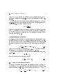
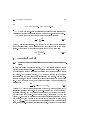
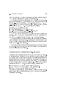
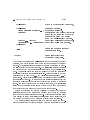
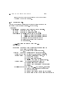
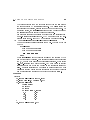
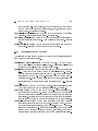
Figure .3.1: Denition sketch for numerical dispersion.
Example of primary variables for an air-water-contaminant system
Consider a system with air (a), water (w), and a single volatile contaminant
(c) as the components. Possible phases are the aqueous phase (`) which is
mixture of liquid water and dissolved contaminant and air; gaseous phase
(g ), which is a mixture of air, water vapor, and contaminant vapor, and
NAPL phase (n), which is a mixture of liquid contaminant with dissolved
air and water. The number of primary variables is NC+1=4. In the following examples of primary variables the , , denote distinct phases with
; ; = `; g; n.
If S = 1, S = 0, and S = 0 (NZP=1), then we use p, !w , !c , and T .
If S; S > 0 and S = 0, then we have p, S, !c , and T .
If S; S; S > 0, we have p, S, S , and T .
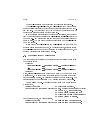
.3.3 Numerical representation of dispersive ux
Consider the dispersive ux between two elements 1 and 2 (Fig. .3.1), with
concentrations C1 and C2 at their centroids. Concentrations CA and CB are
calculated at the vertices A and B by interpolation, using centroid values of
adjacent elements.
By applying the nite dierence technique to the dispersive ux
qd = DrC;
(.3.11)
and taking the scalar product with respect to n, we obtain
d = nD n(C C )=(L + L ) nD t(C
q12
12
2
1
1
2
12
A CB )=LAB ; (.3.12)
.3. NUMERICAL MODEL
xv
d denotes the dispersive ux from element 1 to element 2, and D12
where q12
is the dispersion tensor, calculated from the ow velocity at the interface
between elements 1 and 2. The vectors t and n denote, respectively, the
tangential and normal unit vectors to the boundary between the two elements. This method has the disadvantage of excessive lateral dispersion
at the contact between materials of highly dissimilar permeabilities, with a
large contrast in ow velocities. The reason for this error comes from the assumption that the dispersion coecient varies smoothly between elements 1
and 2, whereas, in reality, it may have a discontinuous jump at their common
boundary.
The method used in NUFT avoids this diculty by using a treatment
that allows the dispersion tensor to be discontinuous at element boundaries.
Let C be the concentration at the boundary, AB, between elements 1 and 2.
The approximate dispersive ux through AB from element 1 to the boundary
is
q1d!AB = Kn1 (C C1) Kt1(CA CB):
(.3.13)
The ux from the boundary, AB, into element 2, is
d
qAB
C) Kt2(CA CB);
!2 = Kn2 (C2
where
(.3.14)
Kni nDin=Li; i = 1; 2;
Kti nDit=LAB; i = 1; 2:
(.3.15)
(.3.16)
We assume that, to a good approximation, these two uxes are equal, and
therefore,
d
d
q1d!AB = qAB
(.3.17)
!2 = q12 :
>From these equalities, we obtain an expression for C. Substituting this
d
expression into the expressions for q1d!AB and qAB
!2 , we obtain
d = [K K (C C ) (K K + K K )(C
q12
n1 n2 2
1
t1 n2
n1 t2 A CB)] =(Kn1 + Kn2 ):
(.3.18)
This ux may be viewed as a generalization of a `harmonically averaged'
ux.
.3.4 Treatment of a phreatic surface as a boundary
NUFT employs the following approximation to advance the position of the
phreatic surface from one time step to the next. If h is the average phreatic
APPENDIX
xvi
surface height in the mth element, the discretization of (.2.9) is
n+1 + A N n+1 ;
Az;m eff hnm+1 hnm =tn+1 = qz;m
z;m m
(.3.19)
where Az;m is the area of phreatic surface in the element, qz;m is the z component of the uid's ux just below the phreatic surface. Assuming
incompressibility we have
n+1 =
qz;m
X
m 2Nm
0
qmn+1m ;
0
(.3.20)
where qm m is dened to be the uxes out of the element into neighboring
elements m0 2 Nm .
0
.3.5 Specifying boundary conditions
Three types of boundary conditions may be applied at any given boundary,
or segment of a boundary:
Boundary condition of the rst type (Dirichlet condition), i.e., a boundary
along which the value of a variable is specied at all times.
Boundary condition of the second type (Neumann, or ux condition), i.e.,
a boundary along which the ux (normal to the boundary) is specied at
all times.
Boundary condition of the third type (Cauchy, or mixed condition), in
which a combination of the variable and its gradient are specied.
How does NUFT implement these boundary conditions? In NUFT, the
default boundary is one of no-ux, or impervious. All other types of boundary conditions are implemented through the addition by the user of a strip
of auxiliary elements next to the external side of the considered boundary.
As we shall see, the type and material of the auxiliary elements depends on
the boundary condition type.
The boundary condition of the rst type is implemented in NUFT by
specifying the, possibly time varying, primary variables of the auxiliary elements next to the considered boundary segment. (Although these primary
variables are not calculated during the simulation, they take part in the
calculation of the uxes through the boundary.) The values of the primary
variables can either be specied as a piecewise linear continuous function
of time or by the clamped command, the primary variables will be equal
to those specied in the input le as initial boundary values. The type of
porous medium material in an auxiliary boundary element is, usually, set
.3. NUMERICAL MODEL
xvii
to be the same as in the adjacent internal element. The range of elements
in the bc-1st-type command (described below) must include the auxiliary
elements in order to internally make the ow length from the center of these
elements to the boundary equal to zero. This action forces the primary variables to be set at the boundary edge by eectively moving the centroid of the
auxiliary element to the midpoint of the common boundary surface between
the auxiliary element and the adjacent interior element. The width of the
auxiliary elements as well as their volumes are immaterial.
NUFT has the option of turning on or o the ux of specied components
and/or phases across a rst type boundary. This option can be used for
turning on or o a contaminant source at a boundary.
A boundary condition of the second type is also implemented through
the use of auxiliary boundary elements (or a strip of such elements) on the
external side of the boundary. However, in this case, the primary variables of
the auxiliary elements do participate in the calculations. The specied ux
through the boundary is specied as a rate of discharge into each auxiliary
element. Again, the width of the auxiliary elements is immaterial, since the
user, by using the command `bc-2nd-type', causes NUFT, internally, to move
the centroid of the auxiliary element to the boundary, thereby, causing the
specied ux to along the common boundary surface between the auxiliary
and adjacent interior element. The pore space volume in these elements
should not be much larger than that in the neighboring element. Otherwise,
there may be a signicant storage eect which will result in a time lag in
the ux across the boundary. The porosity can be adjusted, if necessary to
change the volume of the pore space.
For the modules us1p and ucsat, the discharge rate through the boundary is specied in terms of m3/element/s. For usnt, the ux is specied in
kg/element/s. Both rates may be constant or time-dependent. An option to
specify uxes per unit ow area of boundary surface are also possible.
A ux can also be applied inside the considered domain by specifying a
ux into an element at its centroid. NUFT allows the user to specify either
the mass ow rate of a particular component or phase. In order to specify
a ux of a phase, the concentration of the phase must also be specied in
addition to the rate of ow of the phase. When withdrawing uid from an
element, the user can request that the concentration of the phase is that of
the producing element.
The boundary condition of the third type in a ow problem occurs whenever we have a semipervious thin domain between an external domain of
specied head or pressure, and the considered domain. In other words, a
APPENDIX
xviii
resistance exists to the ow from the external domain, in which the head or
pressure is specied into the considered domain. For saturated ow, referring to (.3.21), or (??), rewritten here for convenience in terms of h as the
variable:
qr n = h c ho ?(h ho );
(.3.21)
r
where ? is a transfer coecient, and cr is the hydraulic resistance of the
semipervious membrane. In NUFT, the resistance cr is made equal to B 0 =K 0,
where B 0 is half the width of the auxiliary element (=distance from centroid
of auxiliary element to the boundary), and K 0 is the hydraulic conductivity
of the material assigned to that element. By selecting the hydraulic conductivity, for a given element width, the desired value of cr can be achieved.
Using the bc-3rd-type command, NUFT optionally sets B 0 = 1, so that
any element width may be used. In this case cr = 1=K 0, i.e., the resistance
will be the reciprocal of the hydraulic conductivity. For multiphase problems
we have that the ux at the boundary of the -phase is
q;rn = ? kr [p po + g(z zo )] ;
(.3.22)
where we specify the transfer coecient by the value of permeability
K 0 = ?. The value of kr is based on upstream weighted values as dened
by (.3.4). Note that if the saturation of a phase in the auxiliary element
is zero, then there will be no ow coming into the boundary of that phase
because kr is zero.
A boundary condition of the third type occurs in a contaminant transport
problem when we assume the presence of a `well mixed zone' on the external
side of a boundary. This kind of boundary is discussed in Subs. ??. NUFT
uses condition (??) rewritten here for convenience, in the form:
(c00 c)(qr n + ? ) = Dh rcn;
(.3.23)
in which c00 denotes the concentration in the external domain, n denotes the
normal to the boundary, and plays the role of a transfer coecient. In
the numerical solution, NUFT approximates (.3.23) by the equation
(c00 c)(qr n + ?) = Dh (c00 c);
(.3.24)
where the value of Dh is the harmonic average between the values of the
auxiliary and adjacent interior elements are used. The value of Dh can be
adjusted by changing the the tortuosity factor of the material type of the
.3. NUMERICAL MODEL
xix
auxilliary element which multiplies the Fickian diusion coecient and the
dispersivities. If desired, setting the tortuosity factor and dispersivity of
the auxiliary element to zero will eliminate the dispersive ux in the above
boundary condition.
Some types of boundary conditions, especially for unsaturated problems,
require specialized techniques in their implementation and will be described
later in the section on the use of the computer model.
.3.6 Solving the system of linear equations
Equation (.3.10) requires the solution of a system of linear equations at each
iteration. NUFT can implement several dierent methods for solving the
system of linear equations. Which method is the most ecient in terms of
computational memory, and CPU time, depends on the number of elements
and on the dimensionality of the problem. The methods included in NUFT
are:
Gauss elimination, with various orderings of the components of the solution vector, including natural ordering, D4 ordering (Aziz and Settari,
1979), and ordering by the reverse Cuthill-McKee bandwidth minimization algorithm (Cuthill and McKee, 1969).
Preconditioned conjugate gradient method, using the ORTHOMIN algorithm (Behie and Forsyth, 1984), which is an iterative method. This
method requires that the matrix be preconditioned by multiplying it by
an approximate inverse matrix. The available preconditioning options are:
Block gauss-seidel, combinative (Behie and Forsyth, 1984).
Incomplete block LU decomposition, with the same ordering options as
for the Gauss elimination method.
For small two-dimensional problems, the standard Gauss elimination
method, with natural ordering is best in terms of memory and computational costs. For larger two-dimensional problems, the Gauss elimination
method, with D4 ordering, is, usually, the most ecient. For large threedimensional and very large two-dimensional problems, the preconditioned
conjugate gradient method is the most ecient. The block Gauss-Seidel
preconditioning method may be used for problems that are linear, such as
saturated zone problems. For nonlinear problems, e.g., multiphase ones, or
for problems with large contrasts in permeability, a good preconditioning
method is the incomplete block LU decomposition, with D4 ordering.
xx
APPENDIX
.3.7 Reduction of Numerical Dispersion
The ability of a numerical method to resolve sharp concentration fronts
is reduced by numerical dispersion (see Bear and Veruijt, 1987, p. 323),
whenever the grid Peclet number (= V L=D) is suciently large. Numerical
dispersion occurs because the discretized equations introduce an articial
`diusive' (or `dispersive') ux that is proportional to the grid Peclet number.
NUFT has two methods for reducing numerical dispersion appearing in the
numerical models of the transport equations:
Introduction of articial diusion, which uses midpoint weighting for the
concentration in the advective term, together with an articial diusion
term that is a function of the grid Peclet number (Alexander and Hughes,
1982).
Using the ux-correction method suggested by Smolarkiewicz (1984), which
uses upstream weighting, together with an `anti-diusive' term that cancels a portion of the rst-order numerical dispersion ux.
.4 Using the Computer Program
.4.1 Developing a Conceptual model of a problem
Before preparing the input parameters for the code, the conceptual model
(Subs. ??) of the considered problem must be developed.
We start by identifying the problem domain. The domain must contain
not only the region of direct interest, but also any possible larger domain
of inuence for the time span of the simulation. We identify subregions
in which we may need a more detailed solution, and others in which a less
accurate solution will suce. Sometimes, we have to take into account availability of information on boundary conditions, when selecting the domain's
boundaries.
Within the problem domain, we identify regions within each of which the
material (porous medium) is homogeneous with respect to relevant properties.
We then identify boundaries and and conditions on them. We divide
the boundaries into boundary segments on each of which conditions are
homogeneous, i.e., the same head, the same ux, etc., prevails along the
entire segment.
We identify internal sources distributed and point sources|their locations and strength. Here we include the locations and rates of pumping and
.4. USING THE COMPUTER PROGRAM
xxi
recharging wells.
We also identify the initial conditions, with respect to the relevant variables. Zones of common initial conditions may be specied. Sometimes,
we may wish to start from an initial steady state, the details of which are
a-priori unknown. We obtain this steady state regime by running an initialization problem, in which we x boundary conditions, and start from any
arbitrary initial conditions. After a suciently long time (depending on how
close are the suggested initial conditions to the ultimate steady state), the
system will reach steady state. This steady state regime is then used as input to the considered problem. NUFT has the option of dening the output
from the initialization problem as a <filename>.rst (standing for `restart'),
and inserting this <filename>.rst le as input for initial conditions in the
input le lename.inp.
We continue by identifying all the relevant physical processes (actually,
also the chemical and biological ones, but here we focus on the physical
processes only). Some important questions to be asked are:
Does the considered problem refer to a saturated domain? If not, which
uid phases, other than water (or an aqueous uid), are involved in the
problem?
Which, if any, of the components are volatile?
Is the problem isothermal or nonisothermal?
On the basis of the conceptual model, a A NUFT module is then selected
which can handle these processes eciently. The following criteria may be
used to select the most ecient module:
(a) Does the problem involve nonisothermal conditions? If yes, use the
usnt module.
(b) Is the problem saturated? If yes, use the ucsat module for ow and
the us1c module for contaminant transport.
(c) Is the problem unsaturated, but with transport occurring only in the
liquid phase? If yes, use the us1p module for ow and the us1c module
for transport.
(d) For all other problems, use the usnt module for both ow and transport.
Once we have identied the domain and its zones, associated with different materials, dierent initial conditions, dierent distributed sources,
etc., we establish the computational grid. The latter consists of elements in
rectangular or cylindrical coordinates, according to the selected coordinate
system. The elements are formed by subdividing the x, y , and z axes in
rectangular coordinates and r, , and z in cylindrical coordinates. The sub-
xxii
APPENDIX
divisions must be chosen such that element boundaries are on the boundaries
of zones of homogeneous material properties, boundary conditions, homogeneous distributed sources, and initial conditions. As a rule, consecutive
subdivisions should not increase by a factor larger than two. Boundaries
of the zones may have to be readjusted to accommodate this requirement.
Boundary elements are an exception to the above rule, unless the boundary
condition is of the second kind.
The default boundary condition in NUFT is a no-ow boundary. Boundary conditions of the rst and third kinds are implemented by adding a row
or column of auxiliary elements outside the domain next to boundaries. In
Subs. .3.5, we have described how these auxiliary elements are used to implement these two kinds of boundary conditions.
.4.2 Translating the conceptual model to an input le
The conceptual model must be converted to input parameters that can be
read by the NUFT program. These input parameters are specied in the
NUFT input le. The following steps describe how an input le may be
prepared:
Step 1. Prepare the input le which contains input parameters for the
NUFT program. These parameters include the geometry of the computational nite dierence mesh, material properties, boundary conditions, and
initial conditions. In each case, the particular set of input parameters to be
used depends on the model that is selected. Nevertheless, the key parameters
are similar for all models. Each problem has its own input le.
Given a problem, say P9xy (i.e., described in Subs. 9.x.y), there are three
options for creating the required input le:
Use the information in the NUFT Reference Manual to create the required
input le `lename.inp'.
Input les for the problems included in Chap. ?? are provided with the
NUFT software distributed with the book. Each such le can be modied
by using any text editor to create a new input le for any other set of
parameters, as long as the problem belongs to the same class of problems
(viz., has the same structure of input le). For example, if we have a
problem of saturated ow in a conned aquifer, we may modify the le
p911.inp provided with the software (to be used for solving the problem
described in Subs. ??) and name the newly created le `newname.inp'.
Use the NUFT preprocessor nprep by simply clicking on its icon which
.4. USING THE COMPUTER PROGRAM
xxiii
should have been created after its installation. The program will then
display a menu from which the user rst selects the desired problem, say
P9xy. He may then modify parameters on the screen and save the le, under the same name, `P9xy.inp', or under any desired name, `newname.inp'.
By using the command nprep, the user may later reopen the saved le
and make further modications, or create a new le.
While preparing the input le, the user is referred to the documentation
within the program for help or further information on how to prepare nprep.
NUFT is highly exible and has many more input options than described
here. More details may be found in the NUFT Reference Manual (Nitao,
1996) which is included with the distributed code.
Step 2. Once an input le, `lename.inp', has been prepared, the program is run by typing,
nuft filename.inp
in a DOS prompt window where filename.inp stands for the name of the
input le of the considered problem.
While running, the program will output to the window the following information at each time step,
(#)
# is time step number,
dt
length of previous time step,
In addition, the program has
ndt
length of current time step,
iter number of Newton-Raphson iterations.
the option to output the primary variable that is restricting the time step
size. For example, for the us1p module, the output line:
dt restricting Sl:
0.35 dSl:
0.15 -- H#1:1:2
indicates that the time step was restricted by a change in liquid saturation,
Sl, from the previous time step by 0.15 to the new value of 0.35 at element
R1#1:1:2. Note that NUFT refers to elements by their names, which take
the form:
<prefix>#<i>:<j>:<k>,
where <prefix> is usually the name of a region (here R1), and <i>,<j>,<k>
(here, 1,1,2) are the i,j,k indices of the element within the grid.
As requested in the input le, NUFT prepares an output le, using the
above time step information. The name of the output le has the form
<run>.out, where <run> is the the run name which is identical to the `lename' of the input le. For example, the run with the name p911.inp will
have an output le called p911.out.
NUFT will also create other output les upon request.
In particular, there are two types of graphics output les:
APPENDIX
xxiv
The le ending with .nvc (standing for `NUFT variables contours') contains
information for generating the data required for mapping contours (say of
H, S, P), while the le ending with .nvh (standing for NUFT variables histogram') contains the information required for plotting requested histograms
of variables, say, H(t), S(t), at specied locations.
Step 3. To obtain graphical output, whether contours or history plots
we use the program nview which is executed by clicking on its icon. In
the le menu we select the name of the input le for the run without the
le's extension. For example, selecting nview p911 will search the current
directory for the les p911.nvc and p911.nvh, and read them in accordance
with the user's specications concerning the les to be plotted.
.4.3 Input syntax and format
We shall now describe the key parameters in the NUFT input le for those
who wish to use a text editor in order to create or edit an input le.
The general syntax for an input item in the input le is either
or
(<key-word> <values>)
(\<key-word>
<values> \<key-word>)
where <key-word> is a key word for an input parameter, and <values> are
the values assigned to that parameter. For example,
(porosity 0.2)
would set an input parameter that is called `porosity' to a value of 0:2. An
input parameter may have values that are not just a single number, but a
list of numbers or a list of other associated input parameters. For example,
(\sand
(K 1.2e-12) (porosity 0.2) \sand)
assigns the properties hydraulic conductivity (K) and porosity for a material
type called sand.
Parenthesis, (...), must always come as a pair; they play an important role
in the input le. NUFT will check and issue a diagnostic message if either ) or
( are missing. The second form shown above is, therefore, recommended for
complicated statements that contained nested parentheses, because NUFT
will then indicate the exact location of any mismatched parentheses in the
issued diagnostic message. We shall use the second form in the examples
below wherever a statement contains a nested set of parentheses.
An input parameter may specify types of correlations. For example
(\kr krVanGen (m 0.2)(alpha 1e-4)(Sr 0.2)\kr)
species the set of parameters to be used for the relative permeability (kr)
.4. USING THE COMPUTER PROGRAM
xxv
as dened by the Van Genuchten correlation (??).
Following are some rules and conventions used in a NUFT input le:
(a) Spaces, tabs, and line breaks are ignored within an input le, except
to separate data or key words. Exponents in oating point numeric
values can be in `e' (e.g., 3.4e3) or `E' (e.g., 3.4E3) format, but `d' or
`D' FORTRAN-style format is forbidden. The ordering of input statements within another statement is irrelevant, unless otherwise noted
as part of the data input format.
(b) All characters after a semicolon to the end of a line are comments; they
are ignored by the program. The use of two consecutive semicolons is
recommended in order to make comments stand out.
(c) The MKS system is used throughout. Thus, for example, the following
units are used: meters for distances, Pascal for pressure, meter-squared
for permeability, meter per second for hydraulic conductivity, and kilogram per cubic meter for mass density.
(d) An exception to the above rule is the units for time. The units of
numeric values that designate time may be, optionally, represented by
appending one of the following characters to the end of the number
(with no intervening spaces): `s' for seconds, `m' for minutes, `h' for
hours, `d' for days, `M' for months, and `y' for years. For example,
4.2h represents 4.2 hours. The default unit (no appended character)
is seconds.
(e) Temperatures are in centigrade, unless otherwise noted.
(f) A pattern string is a special type of a string of characters which can
have unix type \wild" characters
* or ?
so that a pattern string can represent an entire class of strings that
matches the string pattern. The character * in a pattern matches any
sequence of characters. Hence, the pattern "*" matches all strings.
The character ? in a pattern matches any single character. Hence, the
pattern "?" matches all strings with exactly one character.
Other Examples:
(a) The pattern "ex*" matches all strings that begin with the characters "ex".
(b) The pattern "ex*b2*z" matches all strings that begin with the
characters ex, followed by any number (including zero) of strings
which are then followed by the string b2, and which end with the
character z.
APPENDIX
xxvi
(c) The pattern "r2?xay" matches all strings that begin with r2 followed by any single character, and then followed by the characters
xay.
(g) A set of elements in the input le can be specied by a statement of
the form
(range "<elem-range0>"
"<elem-range1>" ...)
where "<elem-range0>", "<elem-range1>", ... are pattern strings of
the element names. Element names are of the form <zone>#<i>:<j>:<k>,
where <i>, <j>, <k> are the indices i = 1; : : : nx, j = 1; : : :; ny,
k = 1; : : :; nz of the grid where nx,ny,nz are the number of elements in
the direction of the x,y, and z axes. Examples are that "e*" denotes
all elements which start with the letter e, and that "*#2:3:*" denotes
all elements that have indices i = 2 and j = 3.
Another way that a set of elements can be specied is through the
statement
(index-range
(<imin> <imax> <jmin> <jmax> <kmin> <kmax>)
...
...
...
...
...
...
(<imin> <imax> <jmin> <jmax> <kmin> <kmax>)
\index-range)
which denes a union of rectangular regions each of which is specied
their minimum and maximum i, j , k indices, i.e., i =<imin>; : : :;<imax>,
j =<jmin>; : : :;<jmax>, k =<kmin>; : : :;<kmax>.
In the documentation of the NUFT input that follows, the index-range
method can be used anywhere that it is stated that the range method
is used.
(h) The following statement
(include "<file-name>")
will paste the contents of a le in the current directory into the input
le. It can be placed anywhere in the input le where a complete
statement with matching parentheses is expected.
(i) The statement
(#define <symbol>)
will cause the stated symbol to be \dened." It is used in conjunction
with the #ifdef and #ifndef statements in order to conditionally
activate selected sections of the input le. That is, if the stated symbol
with name <symbol> is dened then the input statements within
(\#ifdef <symbol>)
...
.4. USING THE COMPUTER PROGRAM
xxvii
\#ifdef)
will be read as input data. If <symbol> is not dened by a #define
statement, then the statements will be ignored. Conversely, the statements inside of the following,
(\#ifndef <symbol>)
...
\#ifndef)
will be read if and only if the symbol with name <symbol> is not
dened. A special symbols is the one called INIT. It is considered
dened, if and only if the program nuftini is used to run the input
le. The program called nuft does not dene the symbol INIT. This
fact is the only dierence between nuftini and nuft. The program
nuftini is used to make an initialization run to obtain steady state
conditions. Thus, one can have a single input le with input used
only during initialization inside the #ifdef INIT statements and noninitialization input inside the #ifndef INIT statements.
.4.4 General Content of an Input File
Following is the general content of an input le:
(\<module-name>
(\init-eqts
...
\init-eqts)
(modelname <name>)
(time <t0>)
(dt <dt0>)
(stepmax <N>)
(\genmsh ... \genmsh)
(\rocktab ... \rocktab)
(\bctab
... \bctab)
(\srctab
... \srctab)
(\state
... \state)
;;
;;
;;
;;
;;
;;
;;
;;
;;
;;
;;
;;
;;
;;
;;
;;
;;
;;
;;
Set <module-name> to be name
of module: us1p, ucsat, etc.
Specify the names of components
and phases, isothermal or not;
not present for ucsat,us1p,us1c.
Name of this model, can be
any name; necessary because NUFT
has option to run multiple modules.
Initial time.
Initial time step.
Maximum number of time steps.
Specify grid and material zones.
Specify material properties.
Specify 1st and 3rd type
boundary conditions
Specify 2nd type boundary
conditions and sources.
Specify initial conditions;
not used if \read-restart
APPENDIX
xxviii
(\read-restart
...
\read-restart)
(\output ... \output)
(\compprop
...
\compprop)
(\phaseprop
...
\phaseprop)
(\generic
(T <temp>)
\generic)
;;
;;
;;
;;
;;
;;
;;
is employed.
Optionally, read in initial
conditions from another run;
not used if \state is employed.
Specify output variables and times.
Specify component properties; present
only for us1c and usnt modules.
;; Specify fluid phase properties;
;; present only for usnt module.
;; Present only for isothermal problem using
;; usnt module; used for setting
;; initial temperature to <temp>
;; in degrees centigrade.
(input-mass-fraction on) ;; If present, units of concentrations
;; in input file is in mass fractions.
;; If not present, concentrations
;; are in mole fractions.
(input-by-piezohead on) ;; Applies only to ucsat and us1p modules;
;; if present, the initial conditions for
;; the variable H are specified as
;; piezometric head instead of pressure
;; head.
(dispersion on)
;; If present, the model implements
;; hydrodynamic dispersion; use only
;; for us1c and usnt modules.
...numerical method options...
\<module-name>)
;; End module input parameters.
To use ow and transport modules together, such as ucsat for ow and
us1c for transport, two sets of statements of the kind presented above would
be required, each containing input parameters that are specic to one of the
models. In addition, there exists a common set of data which should also be
included. This is implemented by the command:
(\common
...
...
\common)
;; Place here common input parameters such as
;; genmsh data.
The following item is included in a ow model:
.4. USING THE COMPUTER PROGRAM
xxix
(\<flow-module-name> ;; Name of flow module, e.g. ucsat, us1p,
;; or usnt.
...
;; Flow module input parameters go here.
\<flow-module-name>)
The following item is included in a transport module:
(\<transport-module-name>
...
;; Name of transport model, e.g., us1c.
;; Transport module input parameters go here.
\<transport-module-name>)
.4.5 Specifying the names of phases and components.
In the ucsat and us1p modules, liquid is always the name of the phase and
water is the name of the component. For the us1c and usnt modules the
phase and component names must be specied by the following statements,
(\init-eqts
;;
;;
(components <comp0> <comp1>...) ;;
(phases <phase0> <phase1>...)
;;
(wetting-phase <phase>)
;;
;;
;;
;;
(primary-phase <phase>)
;;
;;
;;
;;
(thermal)
;;
;;
(isothermal)
;;
;;
\init-eqts)
Define components and
and component names.
Names of components.
Names of phases.
The wetting phase;
partitioning allowed
between this phase and
the solid.
The primary phase; other
phases are computed w.r.t.
this phase using capillary
pressure.
Present only if problem
is not isothermal.
Present only if problem
is isothermal.
Only the components and phases parameters are set for us1c module. The
following points apply to the usnt module:
(a) Either the isothermal or thermal must be set depending on whether
the problem is assumed to be isothermal or not. An isothermal the
temperature .e. uniform and constant temperature.
APPENDIX
xxx
(b) The order of components and phases are important. It aects which
primary variables will be used depending on which phases are present
in a given element. See the section on the setting of initial conditions
where the state command is described.
(c) The primary phase set by primary-phase is the phase in which the
pressure primary variable P is dened. The pressure of the other phases
is calculated with respect to this pressure using the capillary pressure
relationships. See the documentation of material types in rocktab for
how these relationships are dened.
(d) The wetting phase set by wetting-phase is the one which has partitioning of components between it and the solid phase.
(e) For three phase problems the names of phases must be gas, NAPL, and
aqueous with the primary phase set to gas. The name liquid can be
used instead of aqueous.
.4.6 Specifying the grid and material property zones
The input parameters for the grid and material property zones are:
(\genmsh
(coord <coord-type>)
(down <down_x> <down_y> <down_z>)
(dx <dx_1> <dx_2> ... <dx_nx>)
;; Begin mesh specification.
;; Coordinate type.
;; Vector pointing down.
;; Subdivisions in
;; x-direction.
(dy <dy_1> <dy_2> ... <dy_ny>)
;; Subdivisions in
;; y-direction.
(dz <dz_1> <dz_2> ... <dz_nz>)
;; Subdivisions in
;; z-direction.
(\mat
;; Begin assigning zones and materials.
;; Set <zone> to have material <mat>.
(<zone> <mat> <imin> <imax> <jmin> <jmax> <kmin> <kmax>)
;; Repeat for as many different materials are present.
...
...
...
...
...
...
...
...
(<zone> <mat> <imin> <imax> <jmin> <jmax> <kmin> <kmax>)
\mat)
;; End zones and materials.
(\null-blocks
;; Specify null, or inactive, elements
(<imin> <imax> <jmin> <jmax> <kmin> <kmax>)
...
...
...
...
...
...
(<imin> <imax> <jmin> <jmax> <kmin> <kmax>)
.4. USING THE COMPUTER PROGRAM
\null-blocks)
xxxi
;; End null blocks.
;; SPECIFY BOUNDARY ELEMENTS AND CONDITIONS.
;; In what follows, replace <range> by the name assigned to
;; a boundary segment.
(\bc-1st-type (range "<range>" "<range>" ...) \bc-1st-type)
(\bc-2nd-type (range "<range>" "<range>" ...) \bc-2nd-type)
(\bc-3rd-type (range "<range>" "<range>" ...) \bc-3rd-type)
;; Following is optional. If present, then the hydraulic
;; conductivities or permeabilities in the x,y,z directions
;; given in rocktab are used. If not present, the value
;; in the x direction is used for all three directions.
(anisotropic)
\genmsh)
;; End mesh specification.
Let us explain:
1. The user must rst select the type of coordinate system, by setting
(coord-type) to either rect, for rectangular coordinates, or cylind, for
cylindrical ones.
2. The user must specify the location of the main coordinate system
by choosing the coordinate origin and the direction of the coordinate axes
with respect to the problem domain. Typically, the origin will be at a
point of lowest elevation in the problem domain and the coordinate are
chosen parallel to domain, or subregion boundaries. The components of the
downward pointing vector, <down x>, <down y>, <down z>, must be dened
with respect to an auxiliary rectangular coordinate system. For rectangular
coordinates, this auxiliary system is the same as the main system. For
cylindrical coordinates, the x and y axes are dened as being perpendicular
to the z -axis and lying on the = 0 and = 90 deg planes, respectively.
The down pointing vector need not be a unit vector because the model will
internally normalize the vector. If all of the components are zero, then the
model will set the gravitational terms within the balance equations to zero.
For the usual case, the input item dening the direction of gravity is (0.0
0.0 -1.0).
3. The user must now dene the computational grid. The default shape
of an element in NUFT in rectangular coordinates is a rectangle in 2-d domains, and a parallelepiped `boxes' 3-d domains. In cylindrical coordinates,
it is an annular `box'. This means that in all cases, the edges of an element
are along lines of constant coordinate values.
xxxii
APPENDIX
The grid is dened by specifying the size of the elements in each coordinate direction through the parameters <dx 1> <dx 2> ... <dx nx>, <dy 1>
<dy 2> ... <dy ny>, <dz 1> <dz 2> ... <dz nz>, where nx, ny, nz are the
number of elements in each coordinate direction. The subdivisions start at
the origin of the coordinate system. For example,
(dx 1*100 10*50 5*30 1*50)
(dy 10*20 1*40)
(dz 1*100)
means that along the x-axis, we have 17 elements of the indicated sizes:
one of x = 100 m, then 10 times x = 50 m,..., nally, one of x = 50
m. Along the y -axis, we have 11 elements: 10 times y = 20 m, then
one y = 40 m. Along the z -axis, we have only one element, z = 100
m. The x-coordinate of the element centroids are x1 =<dx 1>=2, x2 =
x1+<dx 2>=2; :::.
For cylindrical coordinates the coordinates x and y corresponds to the r
and coordinates, respectively, with the angle in units of degrees.
The following steps describes how to dene a grid for a two-dimensional
problem in rectangular coordinates. However, this can be extended to threedimensional problems, or to cylindrical coordinates in the obvious way.
(a) Draw the problem domain and enclose it in the smallest possible rectangle, with sides that are parallel to the selected x and y axes.
(b) Subdivide the rectangle into elements by lines parallel to the x and
y directions that extend throughout the rectangle. The lines must be
drawn such that each homogeneous zone is dened as the set union of
subsets of element groups.
(c) To specify boundary conditions, the problem domain is extended by
adding a strip (or slab, in three dimensions) of boundary elements (of
constant width) immediately outside the domain, along every boundary on which conditions of the 1st and 3rd kinds prevail. No extension
is required along no-ow boundaries. The width of the strip or slab
can be taken to be the same as the size of the elements on the interior
side of the boundary, or any other size, depending on the boundary
condition to be implemented.
Zones of homogeneous material type are dened through the parameters
in the
(\mat .... \mat)
statement. The name of each zone is set by the <zone> parameter. Note that
names of elements within the zone will be of the form <zone>#<i>:<j>:<k>,
where <i>, <j>, <k> are the indices i = 1; : : : nx, j = 1; : : :; ny, k = 1; : : :; nz
.4. USING THE COMPUTER PROGRAM
xxxiii
of the subdivisions along the coordinate axes of the elements.
The name of the material within a zone is set by the <mat> parameter.
The following parameters
<imin> <imax>
<jmin> <jmax>
<kmin> <kmax>
indicate that the the zone contains elements with indices from i =<imin>
to <imax>, from j =<jmin> to <jmax>, and from k =<kmin> to <kmax>.
In rectangular coordinates, the elements so dened comprise a rectangular
zone; however, more complicated zones may also be dened.
Multiple zone denition statements with the same zone name and/or
material type are permitted, with the elements within any zone overriding
eect of any previous statement of zone denition. Thus, two options are
possible for the denition of zones:
Option 1: A zone is dened as a union of rectangular zones.
Option 2: A zone is dened by overlaying it (i.e., writing the statement
dening it later in the le) on top of another zone.
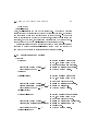
Note the equivalence of the following two examples. According to Option 1:
(\mat
(R1
(R1
(R1
(R1
(R1
(R1
(R2
(R3
\mat)
sand
sand
sand
sand
sand
sand
silt
clay
(\mat
(R1
(R2
(R3
(R3
\mat)
sand
silt
clay
clay
1
1
2
4
5
8
2
5
nx
1
3
4
nx
nx
3
7
1
4
7
4
4
7
4
7
3
ny
ny
ny
6
ny
6
ny
1
1
1
1
1
1
1
1
nz)
nz)
nz)
nz)
nz)
nz)
nz)
nz)
According to Option 2:
1
2
5
6
nx
3
7
7
1 ny
4 6
8 9
7 ny
1
1
1
1
nz)
nz)
nz)
nz)
;;
;;
;;
;;
First, set all elements as R1.
`Cut out' R2.
Define R3 as the union of
two rectangular regions.
Obviously, there is no uniqueness, and other subdivisions are possible. It
is obvious that in the above example, Option 2 is preferable. Note that
the model will accept the symbols nx, ny, and nz, instead of the maximum
element indices in the x, y , and z coordinate directions, respectively. Also,
simple arithmetic expressions, such as nx 1 and ny nz +1 are also allowed.
xxxiv
APPENDIX
The null-blocks command species which elements are inactive.
The bc-1st-type, bc-2nd-type, and bc-3rd-type commands are used
for the auxiliary elements (the added strip of elements just outside the problem domain). They indicate which type of boundary condition should be
implemented along a specied boundary segment.
In (numerical) implementation of the boundary conditions, the ow length
from the center of elements assigned in bc-1st-type or bc-2nd-type to the
boundary (i.e., any neighboring element that is not an auxiliary element)
is set to zero. The ow length in elements indicated in the bc-3rd-type
command is unity.
If elements in the bc-1st-type and bc-3rd-type commands are not
specied also in the bctab command, to be described later, or if elements in
the bc-2nd-type command are not specied in the srctab command, the
program will indicate `a fatal program error'.
.4.7 Material property parameters
The parameters that describe the properties of each material type are given
in the statements:
(\rocktab
(\<material-name> ...parameter values... \<material-name>)
...
...
... ...
(\<material-name> ...parameter values... \<material-name>)
\rocktab)
Here, <material-name> is the unique name given by the user to a given
material type. The input parameter values for each material type depend
on the particular module. We will briey describe the parameters here. The
user is referred to the appropriate NUFT user's manual for more details.
For the ucsat module. the following parameters must be set for each
material type,
(porosity <value>)
;; Fractional porosity.
(Kx <value>)(Ky <value)(Kz <value>) ;; Sat. hydraulic conductivity (m/s)
;; in the x, y, and directions.
;; The Kx value is used for all
;; directions unless the anisotropic
;; option is set in genmsh.
For the us1p module, the parameters are,
(porosity <value>)
;; Same as used in ucsat above.
(Kx <value>)(Ky <value)(Kz <value>) ;; Same as used in ucsat above.
.4. USING THE COMPUTER PROGRAM
(pc <function> <parameters>)
(kr <function> <parameters>)
The parameters for the us1c module
(porosity <value>)
(Kd <value>)
(\tort
<function> <parameters>
\tort)
(dispL <num>)
(dispT <num>)
are
xxxv
;; Capillary pressure head
;; function (m).
;; Relative permeability function.
;;
;;
;;
;;
;;
;;
;;
;;
;;
;;
;;
;;
;;
;;
;;
Same as used in ucsat above.
Normalized linear isotherm
adsorption coefficent (unitless)
equal to bulk soil density times
the usual Kd divided by
porosity; equal to one minus
the retardation factor.
Tortuosity factor (unitless)
equal to reciprocal of tortuosity;
multiplies binary diffusion
coefficient.
Longitudinal dispersivity (m);
the (dispersion on) statement
must also be present for dispersion.
Transverse dispersivity (m).
For an isothermal model using usnt module the parameters are
(porosity <value>)
;; Same as used in ucsat above.
(Kx <value>)(Ky <value)(Kz <value>) ;; Sat. permeability (m2)
;; in the x,y,z directions.
;; The Kx value is used for all
;; directions unless the anisotropic
;; option is set in genmsh.
(\Kd (<comp> <value>)... \Kd)
;; Normalized linear iosotherm;
;; same definition as for us1c above;
;; value needed for every mass
;; component.
(\pc
;; Capillary pressure (Pa) function;
(<phase> <function> <parameters>)... ;; function. See below for
\pc)
;; which phases are required.
(\kr
;; Relative permeability function;
(<phase> <function> <parameters> )... ;; function needed for all phases.
\kr)
(\tort
;; Tortuosity factor (unitless)
(<phase> <function> <parameters>)... ;; function; one needed for all
\tort)
;; phases; see definition for
APPENDIX
xxxvi
;; us1c module above.
;; Same as for us1c above.
;; Same as for us1c above.
(dispL <num>)
(dispT <num>)
If a model using the usnt module is nonisothermal, the following additional parameters are required in addition to those for the isothermal problem,
(\KdFactor
;;
(<comp> <function> <parameters>)... ;;
\KdFactor)
;;
(Cp <value>)
;;
(solid-density <value)
;;
(\tcond
;;
<function> <parameters>
;;
\tcond)
The following important notes are for the usnt
Temperature dependent factor
(unitless) multiplying the
normalized Kd factor.
Solid phase specific heat.
Grain density of solid (kg/m3).
Bulk thermal conductivity
(W/m-C).
module.
(a) In all of the above, a property can be set to a constant value by replacing the data elds <function> <parameters> by a single number.
(b) For a two phase system consisting of a gas (g ) phase and a liquid
(`) phase, the primary phase will be gas and the capillary pressure
parameter will be of the form
(\pc (liquid <function> <parameters>) \pc),
which will be used to calculate pc pg p` as a function of aqueous
phase saturation.
(c) For a two phase system consisting of a NAPL (n) phase and a aqueous (`) phase, the primary phase will be NAPL and capillary pressure
parameter will, again, be of the form
(\pc (liquid <function> <parameters>) \pc),
which will then be used to calculate pc pn p` as a function of
aqueous phase saturation.
(d) For a three phase system consising of gaseous (g ), NAPL (n), and
aqueous (`) phases, the capillary pressure parameter will be of the
form for
(\pc
(gas
<function> <parameters>)
(aqueous <function> <parameters>)
\pc)
The parameters for gas denes c;n
g
n as a
saturation. The parameters for aqueous denes c;`
p
function of aqueous phase saturation.
p
p
function of gas
p pn p` as a
.4. USING THE COMPUTER PROGRAM
xxxvii
.4.8 Specifying component and phase properties
The us1c and usnt modules requires that component property parameters
be set.
For us1c only the free binary diusion coecient (m2=s) is set by the
statement
(\compprop (<comp> (<phase> (freeDiffusivity <value>))) \compprops)
where <comp> and <phase> are the names of the component and phase,
respectively, set in the init-eqts statement.
For usnt the following parameters are set
(\compprop
(\<component>
(\intrinsic
(MoleWt <value>)
\intrinsic)
(\<phase>
;;
;;
;;
;;
;;
;;
;;
(Keq ...)
;;
(freeDiffusivity ...) ;;
(rhoC ...)
;;
(enthC ...)
;;
;;
\<phase>)
...
\<component>)
...
\compprop)
Name of component; set of parameters
is needed for each mass component.
Parameters that do not depend
on which phase go here.
Molecular mass (g/mole).
Properties of component that depend
on which phase it is in go here.
Equilibrium partitioning coefficient.
Free diffusion coefficient.
Partial mass density.
Partial specific enthalpy; not present
for isothermal problem.
We refer the reader to the NUFT user's manual for the usnt module for
details.
For usnt the following phase dependent parameters are set
(\phaseprop
(\<phase>
(rhoP ...)
(viscosity ...)
(enthP ...)
;;
;;
;;
;;
;;
;;
Name of phase; set of parameters
needed for each fluid phase.
Mass density of the phase.
Fluid viscosity of the phase.
Specific enthalpy of the phase; not
present for isothermal.
APPENDIX
xxxviii
(pcTemFac ...)
;; Temperature dependent factor multiplying
;; capillary pressure; not present for
;; isothermal.
\<phase>)
...
\phaseprop)
.4.9 Specifying boundary conditions of the rst and third
type
Boundary conditions of the rst and third types are implemented through
the bctab data record with form given by
(\bctab
;; Begin specification of
;; boundary conditions.
(\<bc-name>
;; Name of this particular boundary
;; condition; can be any name.
(range "<range>" "<range>"... ) ;; Range of elements.
(basephase <phase>)
;; Not present for ucsat
;; or us1p modules.
(\tables
;; Specify time history of
;; primary variables.
(<primary-var> <t0> <value0> <t1> <value1> ... )
...
... ...
... ...
...
(<primary-var> <t0> <value0> <t1> <value1> ... )
\tables)
;; End tables.
(\factor
;; Optional time table of factors
;; which multiplies all component fluxes
;; across this boundary condition.
(<comp. name> <t0> <v0> <t1> <v1> ...) ;; Factor table for component.
...
(<comp. name> <t0> <v0> <t1> <v1> ...)
\factor)
(\phasefactor
;; Optional time table of factors
;; which multiplies all phase fluxes
;; across this boundary condition.
(<phase name> <t0> <v0> <t1> <v1> ...) ;; Factor table for phase.
...
(<phase name> <t0> <v0> <t1> <v1> ...)
\phasefactor)
.4. USING THE COMPUTER PROGRAM
\<bc-name>)
xxxix
;; End of this boundary condition.
(\<bc-name>
;;
(range "<range>" "<range>"... ) ;;
(clamped)
;;
;;
;;
;;
(\factor ... \factor)
;;
(\phasefactor ... \phasefactor) ;;
\<bc-name>)
...
\bctab)
Name of boundary.
Range of elements.
Specifies that primary variables
are set to those set by initial
condition using {\tt state}
or {\tt read-restart} options.
Optional component flux factors.
Optional phase flux factors.
;; One can add more boundary
;; conditions here.
;; End specification of
;; boundary conditions.
The boundary condition name <bc-name> is unique and is used for output
purposes, such as for keeping track of the total ux across the boundary
segment. The range statement species the range of auxiliary or boundary elements for the boundary segment. The basephase statement species
the phase for which the concentrations will specied in the tables statement. The tables statement gives the values of the primary variables in
the auxiliary elements in the range statement. Values are given in the form
of tables at times <t0> <t1> ... and values <value0> <value1> ... at
these times. Linear interpolation is used to calculate values between the
time entries in the table. The times must be in strictly increasing order with
the last time greater than or equal to the ending time as given by the tstop
record. If a sharp change in primary variable is specied, the forcetimes
statement in the output record should be used so that the model will not
take too large of a time step and jump over the sharp change.
Instead of specifying the primary variables by tables one can use the
clamped statement which will tell the model to use the primary variables
set by one of the initial condition commands. This option is especially useful
when reading in steady state initial conditions read from a restart le, and
one wants the boundary to be maintained at steady state conditions.
The optional factor statement tells the model to multiply the component uxes calculated between the specied boundary elements and the rest
xl
APPENDIX
of the elements, not including other boundary elements, by time-dependent
factors calculated from the associated tables using linear interpolation in
time. Note that there has to be a table present for every component ux
corresponding to a separate factor for each component.
The phase-factor is similar to the factor statement except that it
multiplies the phase uxes between the boundary elements and the other
elements. There is a time-dependent factor and its associated table for each
phase. If both phase-factor and factor statements are present, the net
result will that a component ux in a particular phase will be multiplied by
the factor from phase-factor for that phase and by the factor from factor
for the component.
Note that the elements in the specied range can be, but do not have
to be, part of the bc-1st-type or bc-3rd-type commands set in genmsh in
order to set the ow lengths from the elements to the rest of model to zero
or unity, respectively. In this way, if one considers the elements as auxiliary
elements one can place the boundary condition right at the boundary of the
domain consisting of non-auxiliary elements.
The following boundary conditions require special treatment by using
auxilliary elements that have special material types. Most of them are
present in unsaturated problems.
(a) Atmosphere. In modeling the vadose zone with a volatile component
with the usnt model it is usually necessary to have elements which represents the atmosphere above the ground surface in order to model the
gas phase transport between the vadose zone and atmosphere. This
boundary condition is modeled by a row of auxiliary elements at the
top of the model implemented as a boundary condition of third type
with specied gas pressure, concentration of water vapor, and, if the
model is nonisothermal, temperature. The gas saturation of the elements is set to be one. Since the resistance to gas ow is negligible
compared to the soil, a permeability that is two orders of magnitude
greater than the maximum permeability of the soil surface can be used.
The half-thickness of the elements is set to the estimated thickness of
the mixing boundary layer over the ground surface. The tortuosity
factor of the elements is set in rocktab to be equal to the ratio of the
eective diusion coecient (\eddy diusivity") to the free diusion
coecient. The eddy diusivity across the boundary layer is a function
of wind velocity and vegetative cover; the reader is referred to any micrometerology text for details. The capillary pressure of the elements
must be set to identically zero. The relative permeability of the gas
.4. USING THE COMPUTER PROGRAM
xli
and liquid phases are set to one and zero, respectively. The porosity
of the material is taken to be unity.
(b) Ponded contaminant source of constant depth. To model a
ponded source of contaminated water with us1p/us1c or usnt one
uses a row of auxillary elements over the lateral extent of the desired
pond area. The permeability (or hydraulic conductivity) is set to be
two orders of magnitude larger than that of the maximum permeability
of the soil surface. The porosity of the material is taken to be unity.
The relative permeability of the liquid phase is set to one, and a linear
relative permeability krg = Sg is used for the gas phase.
Any normalized Kd values are set to zero. The aqueous phase saturation of the auxiliary elements is kept equal to one. For the usnt
module, the absolute pressure P for usnt is set to the equivalent pressure of a head of water plus the atmospheric pressure, say 1e5 Pa.
For the us1p module the pressure head H is set to the depth of the
pond. The concentration of the contaminant is kept at the desired
value which can vary in time. The concentration of dissolved air in the
aqueous phase must also be set.
The ow of aqueous phase from the pond can be turned on or o at
given times by using the phase-factor tables. The contaminant in
the pond can also be shut o using the factor tables or by changing
the specied concentration in the pond.
(c) Ponded contaminant source of varying depth. If no water is
added to the pond or if the amount of water that is added to the pond
changes in time, the level of the water in the pond will rise or fall at a
rate depending on the inltration ux which, in turn, depends on the
conditions in the soil. The ux of water into the pond is represented
using the srctab option in order to specify a time dependent ux into
the elements representing the pond. The material parameters of the
pond are chosen in the same manner as the ponded source of constant
depth except that a ctitious \capillary pressure" function is used to
maintain the correct pressure head in the pond as a function of water level. The aqueous saturation S` of the pond elements is used to
represent the fraction of each element lled with aqueous liquid, assuming vertical equilibrium within each element. The water elevation
level relative to the height of the centroid of the pond element is given
by Hc = (S` 0:5)(z )pond, where (z )pond is the thickness of the
ponding elements. Considering the usnt module, we desire that the
APPENDIX
xlii
aqueous phase pressure at the centroids of the pond elements be
p` = pg + `gHc
(.4.1)
where pg is atmospheric pressure. Therefore, the ctitious capillary
pressure function for the pond is
pc = pg p` = ` gHc = (S` 0:5)`g (z)pond:
(.4.2)
Similarly, for us1p we have
pc = (S` 0:5)(z)pond; for us1p:
(.4.3)
Note that unlike a true capillary pressure, it can be negative. In setting up the model, the linear interpolatory table option for specifying
capillary pressure is used to implement the above function.
For usnt a row of auxilliary elements above the row of ponding elements is needed to maintain atmospheric gas pressure, pg = patm , in
the elements through the use of bctab. For us1p a row of completely
unsaturated elements Sl = 0 is needed because an element, which in
this case is a pond element, can not become unsaturated unless there is
a neighboring element that is unsaturated. These added elements are
of the same type as those used for the atmospheric boundary elements.
(d) Surface precipitation with varying head. This type of boundary
condition is implemented in the same manner as the previous one. A
row of elements above the ground surface has ux implemented by the
srctab option. There is a another row above these to maintain a xed
gas pressure.
(e) Well inow. An element can be used represent a well screen for
injection or extraction of uids. These elements are similar to those
used for a ponded source except that in most cases the inow elements
should have the tortuosity factor set to zero so that there will be no
binary diusion ux coming out of them. Otherwise, suppose for example that the concentration of a contaminant is specied to be zero
and that there is an inow advective ux of contaminant coming into
the element. The very sharp gradient in contaminant concentration
that results between the soil element and the inow element will often
cause numerical instabilities and oscillations.
(f) Downstream boundary condition. A common problem that is
modeled is one-dimensional transport of a contaminant, say through
.4. USING THE COMPUTER PROGRAM
xliii
a soil column. An element at the inow side is kept at constant pressure and concentration. The width of the element can be made very
small or the bc-1st-type option can be used. At the outow side the
element is kept at constant pressure and zero concentration but with
zero tortuosity factor for the same reason as stated for the well inow
boundary condition.
(g) Water table. In building a vadose zone model one may or may not
wish to include the saturated zone depending on the domain of interest.
If the saturated zone is included, rows of elements at the lower part of
the domain is placed with initial aqueous saturation equal to one. An
initialization run may have to be made to equilibriate the pressures
in the saturated zone as well as for the vadose zone. If the water
table of the saturated zone has a gradient, a model with dimensions
greater than one will obviously have to be created with the lateral
boundary placed suciently far away where pressure heads which will
be maintained consistent with the gradient using auxiliary elements.
If transport in the saturated zone does not need to be modeled, such
as in a one dimensional vadose zone model, the bottom boundary at
the water table can be kept xed by an auxiliary element with aqueous
phase saturation set to unity and pressure (=aqueous phase pressure)
set to the hydrostatic pressure equal to the half-height of the element
so that the water table will be at the interface between the auxiliary
element and the vadose zone element immediately above it. Concentration can be set to some value, often zero. For a boundary condition
of the third type, the tortuosity factor can be adjusted so that the
eective diusion coecient is equal to that of lateral dispersion in the
saturated zone.
For a problem using the usnt module with a gas phase, one has to
be careful because an inconsistency may result from rst or third type
boundary conditions when there are multiple phases. In particular,
it is possible for the gas phase to anomalously ow from the vadose
zone into the saturated zone boundary element because the pressure in
the element is not allowed to equilibriate with the gravitational head
of gas in the vadose zone but is kept at a constant value. Even if
the pressure at the water is set correctly any changes in gas pressure
such as from vapor extraction or barometric pressure changes would
cause unphysical gas ow. One way to remedy this problem is to use
the factor option to turn advective gas ow o at the water table.
Another solution is to add at least one row of saturated elements above
APPENDIX
xliv
the auxiliary row of elements. In this case gas cannot ow into the
water table elements because any changes in gas pressure results in
slight changes in the vertical position of the water table equal to the
change in gas pressure.
.4.10 Specifying boundary condition of second type and source
terms
The following statements specify sources, both as 2nd kind boundary conditions (where a ux is specied along a boundary, as point sources and sinks
(actually, these sources and sinks are indicated for elements, rather than
points), and distributed sources over a range of elements (e.g., inltration in
a 2-d phreatic aquifer model).
(\srctab
(\phaseflux
;; Present if one wishes to specify a
;; a given flux of phase.
(name <source-name>)
;; Name of source term; used in
;; flux output option.
(phase <phase-name>)
;; Name of phase for which flux is
;; specified.
(range "<range>" "<range>"... ) ;; Range of elements.
(table <t0> <q0> <t1> <q1> ...) ;; Table of flux of the phase.
(\setcomp
(<comp> (table <t0><x0> <t1><x1> ...) ;; Specify concentration
...
;; of each component.
(<comp> (table <t0><x0> <t1><x1> ...)
(enthalpy <t0> <H1> <t1> <H1> ... )
;; Specify enthalpy of
\setcomp)
;; specified phase; not
;; present if isothermal.
...flux allocation options, see below...
\phaseflux)
;; End of the source term.
...
;; One can have any number of additional phase fluxes.
(\compflux
(name <source-name>)
(comp <comp-name>)
;;
;;
;;
;;
;;
Present if one wishes to specify a
given flux of a component.
Name of source term; used in
flux output option.
Name of component for which flux is
.4. USING THE COMPUTER PROGRAM
xlv
;; specified.
(range "<range>" "<range>" ...) ;; Range of elements.
(table <t0> <q0> <t1> <q1> ...) ;; Table of flux of the component.
(enthalpy <t0> <H1> <t1> <H1> ...) ;; Table of enthalpy of the component.
...flux allocation options, see below...
\compflux)
;; End of the source term.
...
;; One can have any number of component fluxes.
\srctab)
;; End of the all source terms.
Note that uxes can be specied either as a \phase ux," that is, a specied
ux of a phase, or as as \component ux," which is a specied ux of a given
component.
The elements in the specied range can be, but do not have to be, part
of the bc-2nd-type command set in genmsh in order to set the ow lengths
from the elements to the rest of model to zero. In this way, if one considers
the elements as auxiliary elements one can place the ux at the boundary of
the domain consisting of non-auxiliary elements.
The following items apply:
(a) Linear interpolation is time is used in all tables.
(b) Positive ux is ux into the elements, and negative ux is ux out of
the elements.
(c) Fluxes have units of kg/s except for us1p and ucsat which have units
of m3 /s.
(d) Specic enthalpy is in units of J/kg.
(e) Concentrations (variable name is C.<comp>) are in mole fractions unless the statement (input-mass-fraction on) is present; in which
case, the concentrations (variable name is X.<comp>) are in mass fractions.
(f) The entire setcomp statement in phaseflux can be replaced by
(setcomp-internal)
in which case concentrations and specic enthalpy will be those of each
corresponding element set in range. The setcomp-internal option is
the usual one if the uxes are going out of an element, i.e. are negative.
(g) Possible optional allocation methods are:
(a) Allocate the ux by volume:
(allocate-by-volume)
APPENDIX
xlvi
The ux at element
m equals the specied ux multiplied by
P
the factor Um = m Um where m0 runs over all elements specied
in the range of the particular source term and Um are element
volumes.
(b) Allocate ux by ow area:
0
0
0
(allocate-by-area <dir>)
The ux at P
element m equals the specied ux multiplied by the
factor Am = m Am where m0 runs over all elements specied in
the range of the particular source term and Am are element ow
areas. Since the ow area of element is dierent depending on
its sides, the direction of the ow area of an element is specied
by the <dir> parameter. Valid options for <dir> are x, y, or
z corresponding to the x, y , and z directions, respectively. In
cylindrical coordinates these directions correspond to the r, ,
and z -directions, and the ow area in r is set to the average of
the two ow areas in the r direction except for the elements with
i = 1 and i = nx in which case only a single ow area is used,
that of the ow area common to the neighboring element in the
r direction.
(c) Multiply ux by ow area of the particular element:
0
0
0
(mult-by-area <dir>)
The ux at element m equals the specied ux multiplied by the
ow area Am of the element in the <dir> direction where <dir>
is the same as the allocate-by-area option above and the same
conventions for determining ow area apply.
(d) Multiply ux by factor which depends on a group of elements:
(\allocate-by-element
("<range>" <fac>)
("<range>" <fac>)
...
\allocate-by-element)
If an element is not in the specied ranges, the ux value is that
computed from the table. Otherwise, if an element is within a
range, the ux at that element equals the value computed from
the table multiplied by the respective factor <fac>. Note that an
.4. USING THE COMPUTER PROGRAM
xlvii
element can be in more than one range in which the ux will be
multiplied by more than one factor.
.4.11 Specifying wells.
Although it is possible to use srctab to implement wells, it is often more
convenient to use the special well option. It is of the form,
(\setwells
(\<well-name> ;; Name of well; used for output purposes.
(rw <num>)
;; Radius of well bore (m).
(re <num>)
;; Radius of pressure support (m).
(\<well-type> ;; <well-type> is one of following:
;;
pres-inj = specified pressure injector
;;
pres-prod = specified pressure producer
;; producer can only have flow out of
;; formation; injector only flow into
;; the formation.
.... see below for rest of input data ...
\<well-type>)
(\intervals
;; Specifiy well intervals; intervals must be
;; in order of topmost first
;; (i.e. highest actual elevation first).
(\setint
;; Specify parameters for a single interval.
(index <i> <j> <k>) ;; Specify i,j,k index of element.
(zcoord <num>)
;; Optional, specifies z coord. of
;; midpoint of interval
;; w.r.t. mesh coord system;
;; default is z coord of element center.
(length <num>)
;; Optional, specifies length of
;; screened portion of interval;
;; default is z thickness of the completed
;; element.
(flow-factor <t0> <f0> <t1> <f1> ...) ;; Optional, specifies
;; table of time dependent flux factors
;; for this interval;
;; default flux factor is one for all times;
;; can be used to shut off or open an interval or
APPENDIX
xlviii
\setint)
(\setint
....
\setint)
...
;; modify its flow characteristics.
;; End of specifications for this interval.
;; Specify next interval.
;; Can add more intervals.
\intervals)
\<well-name>)
(\<well-name>
...
\<well-name>)
...
\setwells)
;; Specify next well.
;; Can add more wells
Note the wells uses the permeability (or hydraulic conductivity) Kx of the
completed element to compute its ow characteristics with the formation.
In particular, for usnt NUFT uses the formula for well ow at a particular
interval,
Kkr [p
q = 2h ln(
alpha;well p;elem + g (zwell zelem )] ; (.4.4)
re=rw )
where the subscript well and elem refer to the the center of the well interval
and the centroid of the completed element, respectively. Here, h is the
interval length. The permeability is set equal to Kx of the element.
A specied pressure production well (<well-type> is set to pres-prod)
has the following parameters
;; Table of time dependent pressure;
;; specified at the deepest interval of this well.
(ptab <t0> <p0> <t1> <p1> ... )
;; Optional friction loss factor; pressure drop in well bore
;; equals dp/dl = -rho*fac*v*v where v is flow velocity;
;; default value is 0.0.
(fricfac <fac>)
;; Optional table for computing time dependent factor
;; multiplying all phases; default is one at all times;
;; using this option an entire well can be shutin
.4. USING THE COMPUTER PROGRAM
xlix
;; by setting the factor to be zero at a particular point in time.
(well-factor <t0> <f0> <t1> <f1> ...)
The following are input parameters for a specied pressure production
well (<well-type> is set to pres-inj).
(pres-inj
;; name of injected phase
(phase <phase-name>)
;; Table of time dependent pressure of the
;; shallowest interval for this well.
(ptab <t0> <p0> <t1> <p1> ... )
;; Table for fluid mass density in well bore (kg/m3).
(density <t0> <rho0> <t1> <rho1> ...)
;; Following table of specific enthalpy is for thermal models
;; only (J/kg).
(enthalpy <t0> <H0> <t1> <H1> ...)
;; Optional friction factor for well bore flow; see above.
(fricfac <num>)
;; Optional well factor; see above.
(well-factor <t0> <f0> <t1> <f1> ...)]
;; Tables for time dependent concentrations of mass components
;; in injected stream; units are in mole fractions
;; unless (input-mass-fractions on) is present in which
;; concentrations are in mole fraction. <comp-name> is name of
;; the particular component.
(\conc
(<comp-name> <t0> <C0> <t1> <C1> ...)
...
(<comp-name> <t0> <C0> <t1> <C1> ...)
\conc)
)
.4.12 Specifying initial conditions
The initial conditions to the model can be specied by either of two methods:
(a) By specifying values using the state option.
(b) By reading in a restart le created from another simulation run. This
option is described later.
Only one of the above methods can be used.
We rst describe the state option. It is of the following form:
l
APPENDIX
(\state
(\<primary-variable> <method> <specification> \<primary-variable>)
...
...
...
...
(\<primary-variable> <method> <specification> \<primary-variable>)
\state)
Here, <primary-variable> is the name of each primary variable. The pri-
mary variables of each module has already been given. The name of the
primary variable for the ucsat and us1p modules are:
(a) H denotes the pressure head in meters of water relative to atmospheric
conditions. That is, setting H to zero is the same as atmospheric pressure head. Optionally, if the statement (input-by-piezohead on) is
present at the main input level, then the variable H is piezometric head.
(b) Sl denotes liquid saturation.
Since only one of the above variables can be the primary variable of a particular element, some rules for deciding which variable is being set is required.
In the us1p module the following rules apply in the following order of priority:
(a) If the pressure head H is set to a value greater than zero, then then the
model uses pressure head H as the primary variable. The value of Sl
is set to the maximum saturation Smax given in rocktab.
(b) If Sl is set to a value greater than or equal to Smax, then the model
sets pressure head H to be zero and uses pressure head H as the primary
variable. The variable Sl is set to be exactly equal to Smax.
(c) If pressure head H is set to a value less than zero, then the model sets
Sl to Smax and pressure head H to zero, and uses Sl as the primary
variable.
(d) If none of the above applies, that is, if Sl is less than Smax and pressure
head H is set to zero, then the model uses Sl as the primary variable.
Note that in the above, H is pressure head. If piezometric head is specied,
the model converts to pressure head before applying the above rules.
For the ucsat module the following rule applies. If Sl is less than unity,
then pressure head H is set to zero, and the primary variable is Sl. Otherwise,
Sl is set to unity, and the primary variable is pressure head H.
The primary variable for the us1c module is C.<comp> which denotes
the concentration in any units of the transported component called <comp>
whose name is set by init-eqts.
For the usnt module the following primary variables must be set.
(a) P denotes the pressure of the primary phase in Pascals. The denition of primary phase is given in the section on names of components
.4. USING THE COMPUTER PROGRAM
li
and phases where the init-eqts statement is dened. For two phase
problems, if if the primary phase is not present in an element, i.e.
saturation of the primary phase is zero, then P becomes the pressure
of the non-primary phase. For three phase problems (gas, aqueous,
NAPL phase), the primary phase has to be the gas phase. If only the
gas phase is not present, then P becomes the NAPL pressure. If both
gas and NAPL phases are not present, it becomes the aqueous phase
pressure.
(b) S.<phase> denotes the saturation where <phase> is the name of the
phase. The saturation of the rst phase that occurs in the list of phases
in init-eqt is not set by the user. It will be calculated as one minus
the sum of the saturation of the other phases set by the user.
(c) C.<comp> denotes the concentration where <comp> is the name of the
component. The default units for concentration are in mole fraction.
If the statement (input-mass-fraction on) is present than the units
are in mass fractions and the variable name is, instead, X.<comp>.
The concentration in a particular element refers to the component in
the rst phase with non-zero saturation in that element with respect
to the ordering of phases set in init-eqts.
If NC is dened as the total number of mass components and NZP is
the number phases with non-zero saturation in a given element. Only
the concentrations of the last NC-NZP components in the order appearing in init-eqts are actually used by the model for that element.
We call these concentrations the independent concentrations for the
element. The concentrations for the other components are internally
computed by the model using the partitioning coecients as a function of the NC-NZP independent concentrations, the temperature, and
pressure assuming thermodynamic equilibrium. These other concentrations are called the dependent concentrations. The user can set
dependent concentrations to a negative value. The model will give an
error message and stop if a negative value is set for an independent
concentration.
(d) T is the temperature in degrees centigrade. For isothermal problems the
initial temperature is not set by state but by the following generic
statement,
(\generic (T <temp>) \generic)
where <temp> is the value of temperature in degrees centigrade that
will be uniform over the entire model and constant in time.
APPENDIX
lii
All primary variables except those stated otherwise above must be set. The
order in which the primary variables are set in state is does not matter.
A primary variable can be specied more than once. A specication of an
initial condition that applies to a given element will override any previous
specication. That is, if the pressure of an element is set in more than one
specications, the last one is what the model takes as the initial condition.
Examples will be given below.
The various initialization methods are as follows.
(a) (<primary-variable> by-key ("<range>" <value>) ("<range>"
The primary variable is set to the <value> for all elements that are
specied by the associated element range string pattern "<range>". If
an element falls within more than one string pattern, the value associated with the last pattern that matches that element is used. For
example,
(P by-key ("*" 1e5) ("f*" 2e5))
(b)
rst species that all elements have pressure set to 1e5 and then overwrites the elements that start with the character f to the value 2e5.
(<primary-variable> by-xtable
(range "<elem-range>" ...)
<x0> <value0> <x1> <value1> ...)
(<primary-variable> by-ytable
(range "<elem-range>" ...)
<y0> <value0> <y1> <value1> ...)
(<primary-variable> by-ztable
(range "<elem-range>" ...)
<z0> <value0> <z1> <value1> ...)
Any one or more of the above methods can be used. The methods
<by-xtable>,<by-ytable>, and <by-ztable> sets the initial conditions from linear interpolation of a table with respect to the coordinates xi , yj , zk of the centroid of each element, respectively.
The
P
i
centroid
of an element with indices i, j , k is given by x = i =1 xi ,
y = Pij =1 yj , z = Pik =1 zk where xi , yj , zk are the grid
subdivisions of the elements as set in the genmsh statement described
earlier.
The coordinate values in the table must be strictly increasing order.
The minimum coordinate value in the table must be less than or equal
to the coordinates of the centroids of all elements that are specied by
range, and the maximum coordinate must be greater than or equal to
the coordinates of the centroids of all elements specied by the range.
0
0
0
0
0
0
0
0
0
<value>)...)
.4. USING THE COMPUTER PROGRAM
(c)
liii
The values obtained from the table are set only for the elements in
the range specied by the range statement. The range statement
is optional; if not present, all elements in the model will be set. As
mentioned before, the index-range statement can be used in place of
the range statement to specify the range of elements.
Sometimes it is useful to generate a table of primary variables from
a one-dimensional initialization run. NUFT can output primary variables in table format. See the NUFT Reference Manual for details.
(<primary-variable> by-ijk-file "<file-name>")
The model will read initial conditions from a le. The form of the le
must be
$<var-name>
<i0> <j0> <k0> <value0>
<i1> <j1> <k1> <value1>
... ... ... ...
$end
where $<var-name> is the character $
followed immediately by the
name of the primary variable. Each subsequent lines of the le contains
the i, j , k index of an element and its initial condition. Every active
(i.e., non-null) element must have a line. Any word with $ as its rst
character or the end of le can be used as the terminator instead of
$end. Multiple variables can be present in a single le; the model
will search through le for the rst occurrence of the primary variable
name before reading the element data that immediately follows.
Examples
(state
(C.contam by-ijk-file "initc.dat")
(C.water ("*" -1.0) ("atm*" 0.02))
(C.contam by-ztable
(range "WT*")
;; height
;; above
;; model base C.contam
0.0
0.001
18.0
0.01
20.0
0.01
21.0
0.0
)
(S.liquid by-key ("*" 1.0))
APPENDIX
liv
(S.liquid by-ztable
(range "VZ*")
;; height
;; above
;; WT
S.liquid
12.0
1.0
12.2
0.9
12.8
0.5
13.0
0.4
20.0
0.3
)
(P by-key ("*" 1.e5))
)
In this ctitious example, the concentrations C.contam of a contaminant are
rst read from a le "initc.dat". In the next specication, the concentration of the water component C.water is set to 0.02 for elements that start
with the characters atm and set to -1 for all other elements, denoting the fact
that the concentration is calculated internally. Then, the concentrations for
the contaminant at elements that begin with WT are overwritten by values
calculated from a table. Then, the liquid saturation S.liquid is set to 1.0
for all elements. The liquid saturation for those elements that start with
VZ are then overwritten by a table. Finally, the pressure is to 1e5 for all
elements.
.4.13 Using the restart option
It is often useful to be able to start a run from the results of another, dierent,
run. For instance, one may want to use steady state conditions created from
an initialization run as initial conditions for another run. Another example
is when modeling the eect of varying the duration of a remediation strategy. Restart les are written at various remediation times and subsequent
no-remediation runs are started at these dierent times to determine the
eectiveness of remediation and the transport of remaining contaminants.
Restart records are written out to a le using the restart option in the
output statement described below. Note that records at dierent times can
be written onto the same le. The following statement is used to read in
initial conditions from a restart le.
(\read-restart
(file "<file-name>")
.4. USING THE COMPUTER PROGRAM
lv
(time <t0>)
\read-restart)
Here, <file-name>
is the name of the restart le. The program will pass
restart records that corresponds to times that are less than <t0>. It will read
the rst record whose time is greater than or equal to <t0>. The run will
start at simulation time equal to the value <t0>, unless the time statement
is present, in which case, the initial time will start from the value set there.
It is an error to have both read-restart and state statements.
Initial conditions read from the restart le can be overwritten for selected
elements by using the overwrite-restart option which has exactly the
same syntax and options as the state option described earlier.
.4.14 Specifying output options
(\output
(\contour
;;
;;
;;
;;
;;
Output element variables
to .nvc NVIEW input file
for contouring and vectors.
Names of element variables.
List of output times.
(\elem-history
;;
;;
;;
(variables <var1> <var2>... )
;;
(range "<range>" "<range>" ...) ;;
(outtimes <t1> <t2> ... )
;;
\elem-history)
Output element variables
to .nvh NVIEW input file
for time history plots.
Names of element variables.
Range of elements.
List of output times.
(\connect-history
Output connection variables
to .nvh NVIEW input file
for time history plots.
Names of connection variables.
Names of elements of the
connection.
List of output times.
(variables <var1> <var2>... )
(outtimes <t1> <t2> ... )
\contour)
;;
;;
;;
(variables <var1> <var2>... )
;;
(connection "<elem0>" "<elem1>") ;;
;;
(outtimes <t1> <t2> ... )
;;
\connect-history)
APPENDIX
lvi
(\bcflux-history
(variables <var1> <var1> ...)
(name <bc-name>)
(outtimes <t1> <t2> ... )
\bcflux-history)
(\restart
(outtimes <t1> <t2> ... )
(file-ext ".res")
;;
;;
;;
;;
;;
;;
Output boundary condition
fluxes to .nvh file.
Names of fluxes.
Name of boundary condition
specified in bctab.
List of output times.
;;
;;
;;
;;
;;
Output primary variables
to a file for restart runs.
List of output times.
File name extension of
of restart output file.
;;
;;
;;
;;
Force the model to hit
the list of output times;
performs no output action.
List of output times.
\restart)
(\forcetimes
(outtimes <t1> <t2> ... )
\forcetimes)
\output)
The contour option will write its output to a le with le name extension
.nvc. The options elem-history, connect-history, and bc-history are
for writing the time history of an element variable, a connection variable,
and boundary ux variables, respectively, and will all write to a single le
with extension .nvh. Both the .nvc and nvh les are read by the nview
program.
(a) The list of output times must be strictly increasing order, and the
last output time must be less than or equal to the ending time of the
simulation.
(b) Using an astericks in the list of output times, i.e. (outtimes *),
denotes that output will be at every time step.
(c) The output le names are created by taking the part of the NUFT input
le name up to the character before the rst period and appending the
characters specied by the le extension. For example if the input le
was called run1.inp the NPREP input les would be run1.nvc and
run1.nvh, and the restart le would be run1.res.
(d) Instead of specifying the le extension for the restart, one can specify the full name. For example, one can use the statement (file
.4. USING THE COMPUTER PROGRAM
lvii
instead of (file-ext ".res").
(e) One can add the statement (dstep <num>) to any of the options (except for forcetimes) in order to request that the output will be at
every <num>-th time step. The outtimes statement is optional in this
case. If present, the counter that keeps track of the dstep option will
be reset to zero after every time that hits an output time given in the
outtimes statement.
(f) Placing the optional statement, (cumulative), in bcflux-history
will result in the cumulative ux being outputted instead of the instantaneous ux.
(g) One can use the statement (index-con <i0> <j0> <k0> <i1> <j1>
<k1>) to specify that the connection connects the elements with indices
<i0> <j0> <k0> and <i1> <j1> <k1>) instead of using the connection
statement.
The following is a partial list of output variables.
"run1ini.res")
Element Variables
H
P
PiezoH
Piezo
P.<phase>
Pc.<phase>
kr.<phase>
S.<phase>
X.<comp>.<phase>
C.<comp>.<phase>
porosity
Kx, Ky, or Kz
log10Kx, log10Ky,
or log10Kz
Vmag.<phase>
Pressure head (m), for ucsat
and us1p only; piezometric
head if (output-by-piezohead on
is present.
Primary phase pressure (Pa)
(pressure head (m) for
ucsat,us1p).
Piezometric head (m) for ucsat
Piezometric head (m) for us1p.
Absolute phase pressure (Pa).
Capillary pressure (Pa).
Relative permeability.
Saturation.
Mass fraction.
Mole fraction.
Porosity.
Saturated permeabilities (m2)
(m/s for us1p,ucsat).
Log base 10 of saturated permeabilities
(log 10 m2 for usnt and
log 10 m/s for us1p,ucsat).
Magnitude of ow velocity vector (m/s).
APPENDIX
lviii
Components of the ow velocity
vector in the x,y ,z directions
at each element centroid; valid
only for (field (format contour ....
or (contour... output options.
The following are connection variables are dened between every pair of
connected elements, usually those between neighboring elements. Specic
uxes are dened to be the total ux between elements divided by the ow
area between the elements. The units of ux are given below for the usnt
module. For ucsat and us1p the units of ux are volumetric, that is, m/s
for specic ux (synonymous with \specic discharge") and m3/s for total
ux.
Connection Variables
V.<phase>
Flow velocity (m/s).
q.<phase>
Specic ux of phase (kg/s-m2).
q.<comp>
Specic ux of component (kg/s-m2)
in all phases; if <comp> is `energy',
then specic energy ux (W/m2) in all
phases including solid phase is output.
q.<comp>.<phase>
Specic ux of component (kg/s-m2)
in a particular phase; if <comp> is
`energy', then specic energy ux
(W/m2) in the phase is output.
qcond
Specic conductive thermal ux (W/m2).
Q.<phase>
Total ux of phase (kg/s).
Q.<comp>
Total ux of a component (kg/s) in all phases;
if <comp> is `energy', then
total energy ux (W) in all
phases including solid phase is output.
Q.<comp>.<phase>
Total ux of a component (kg/s) in a phase;
if <comp> is `energy', then
total energy ux (W) in the phase is output.
Qcond
Total conductive thermal ux (W).
The following parameters control various output options.
Vel.<phase>
If present, all output les will consist of this
prex together with the sux of the dierence les. For example, setting (output-prefix "run1") will mean that the output les will be
"run1.out" for the main output le and "run1.nvc" and "run1.nvh"
(output-prefix "<prefix>")
.4. USING THE COMPUTER PROGRAM
lix
for the nview les. If not present, the model will use the rst part of
the name the input le until the rst period, if any, in its name as the
output prex. Default: not present.
(print-mat-bal <on-or-off>) Turns on or o the printing of material
balances. Valid options are on or off. Default: off.
(print-pcg <on-or-off>) Turns on or o the printing of preconditioned
conjugate gradient information. Valid options are on or off. Default:
off.
(tty-output-step <num>) Output time step information every this many
time steps. Default: 1 which means at every time step.
.4.15 Numerical Method Options
The following is a list of some options that aect the numerical solution of
the model and their default values.
(time-method "<method-name>") Time step method. Name of method
can be fully-explicit or fully-implicit. Default: fully-explicit
for us1c and fully-implicit for all other models.
(time-weighting <num>) Linear weighting factor dened in Subsection
.3.1. Valid only if time step method is fully-implicit. Recom-
a
mended value for transport problems is a = 0:6 which gives slightly
less accuracy than a = 0:5 (Crank-Nicholson method) but is more numerically stable. Recommended value for ow problems, especially for
simulations used to obtain steady state conditions is a = 1:0. Default:
1.0.
(itermax <num>) Maximum number of Newton-Raphson iterations before
a time step is reduced and the iterations restarted. Default: 8.
(iterbreak <num>) Maximum number of Newton-Raphson iterations before convergence is assumed. Should be set to one if the equations
that are being solved is linear because in that case only one iteration
is necessary. Default: set to a very large number so that convergence
is never assumed based on number of iterations but on other criteria.
(linear-solver <option>) Method used for solving the system of linear
equations during each step of the Newton-Raphson method. Some of
the valid options are lublkbnd, which is block-banded LU decomposition for a constant band-width matrix; d4vband, which is the direct
solver with D4 ordering (Behie and Forsyth, 1984); pcg, which is the
preconditioned conjugate gradient method with various precondition-
APPENDIX
lx
ing options. The option lublkbnd is best for small problems, d4vband
for intermediate problems, and pcg for large problems, especially in
three dimensions. Default: lublkbnd.
(pcg-parameters ... Parameters for preconditioned conjugate gradient
method. Following is the complete format:
(\pcg-parameters
(precond <option>) (north <num>)
(toler <num>) (itermax <num>)
\pcg-parameters)
Some valid values for precond are bgs, which
is preconditioning by
a single iteration of the symmetric block gauss seidel method; ilu,
which is the incomplete LU decomposition method; d4, which is the
incomplete LU decomposition method applied to a system that has
been reduced by D4 ordering; and comb, which is the combinative
method. The reader is referred to Behie and Forsyth (1984) for a
description of these methods and the ORTHOMIN algorithm which
is version of the conjugate gradient method for nonsymmetric matrices that used by the model. The bgs method is recommended for
relatively easy problems without severe nonlinearities such has saturated ow and transport problems. The d4 method is recommended
for most other problems. The ilu method uses less memory then d4
but usually requires more conjugate gradient iterations to converge.
The north parameter is the number of orthogonalizations used by the
ORTHOMIN algorithm. Recommended value is 25 for d4 and ilu and
30 for bgs. The tolerance for convergence is set by the toler parameter. Recommended value is 0.001 for most problems. In some cases
a smaller value 0.00001 is needed if frequent instances of NewtonRaphson nonconvergence is observed. The maximum number of allowed iterations is set by the itermax parameter. If this number of
iterations is reached, the model cuts back the time step and retries
the entire Newton-Raphson method. Recommended value is 200 for
d4 method and 500 for ilu and bgs methods. Default: none, because
pcg is not default for linear-solver.
(ilu-degree <num>) The degree of ll-in in the incomplete LU decomposition algorithm relevant to the ilu and d4 preconditioning options.
Recommended value is 0 for saturated ow and transport problems,
1 for nonlinear problems including when running the us1p module
and for most problems using the usnt module, and 2 or more for
severely nonlinear problems including many multiphase problems us-
.4. USING THE COMPUTER PROGRAM
lxi
ing the usnt module. Default: 1.
Turns on or o the articial diffusion method of Brooks and Hughes (1982) for reducing numerical
dispersion. Valid options are on or off. Default: off.
(artificial-diffusion-coef <num>) Sets articial diusion coecient.
Used for transport calcuations. Recommended that time-weighting
parameter be set to 0.6. In some cases value may have to be increased
slightly if oscillations in concentrations develop. Default: 10.
(tolerdt (<var> <num>) ...) Absolute tolerances for time step size control. The primary variable name is set by <var> and the tolerance by
<num>. For example,
(artificial-diffusion <off-or-on>)
(\tolerdt
(P 1e3)(C 0.01)(C.TCE 1e-6)(S 0.05)(S.NAPL 0.01)(T 0.5)
\tolerdt)
species that the pressure tolerance is 1e3, all mole fraction tolerances
are 0.01 except for the component called TCE which is 1e-6, all saturation tolerances are 0.05 except for the phase called NAPL which is
0.01, and temperature is 0.5. A time step is accepted if the absolute
magnitude of the change in primary variables between the previous
and current time step is less than the tolerance. This tolerance is the
larger of the absolute tolerances specied resulting from values given
by tolerdt and reltolerdt. The size of the time step of the next
time step is based on estimating which value will cause the changes in
primary variables a certain amount below the tolerance. If the time
step calculated at any Newton-Raphson iteration is too large because
the primary variables changed too much, the time step size is cut back
and the time step is redone. If the rms-time-step option is set to
on, then the tolerance apply only to determining if a primary variable
changes too much over the time step. Default: depends on the module.
(reltolerdt (<var> <num>) ...) Relative tolerances for time step size
control. See tolerdt. The tolerance for a particular variable is based
on multiplying the relative tolerance value by the maximum magnitude
of the variable over the entire problem domain. Default: depends on
the module.
(tolerconv (<var> <num>) ...) Absolute tolerances for Newton-Raphson
convergence. The Newton-Raphson iterations is assumed to converge
if the absolute magnitude of the change in primary variables between
the previous and current iterations is less than the tolerance. This
tolerance is based on the values set by tolerconv and reltolerconv.
lxii
APPENDIX
These parameters are ignored if the rms-NR-conv option is set to on.
Default: depends on the module.
(reltolerconv (<var> <num>) ...) Relative tolerances for Newton-Raphson
convergence. See tolerconv. The tolerance for a particular variable
is based on multiplying the relative tolerance value by the maximum
magnitude of the variable over the entire problem domain. Default:
depends on the module.
(cutbackmax <num>) Maximum times that a time step is cutback because
of lack of convergence of either Newton-Raphson or preconditioned
conjugate gradient iterations before the run is forced to terminate.
Default: 30.
(rms-time-step <on-or-off>) Turns on or o time step convergence based
on root-mean-square of the estimate of the relative time truncation error. If the error exceeds the tolerance set by rmstolderdt the time
step size is cutback and the time step is redone. The size of the time
step for the next step is based on how close the actual time step was
to the tolerance. Default: off.
(rmstolerdt <num>) Tolerance for the root-mean-square of the estimate of
the relative time truncation error. Default: 0.1.
(rms-NR-conv <on-or-off>) Turns on or o Newton-Raphson convergence
based on root-mean-square norm of the residual vector R. Default:
off.
(rmstolerconv <num>) Tolerance for Newton-Raphson convergence based
on root-mean-square norm of the residual vector R. Default: 0.001.
.5 Running the Exercises in the Book
.5.1 Problem 9.1.1
.5.2 Problem 9.2.1
Aziz, K., and A. Settari, Petroleum Reservoir Simulation, Applied Science
Publishers, London, 1979.
Bear, J., and J.J. Nitao, On equilibrium and the number of degrees of
freedom in modeling transport in porous media, Transport in Porous
Media, vol. 18, no. 2, 151-184, 1995.
Bear, J., and A. Verruijt, Modeling Groundwater Flow and Pollution, D.
Reidel Pub. Co., Dordrecht, The Netherlands, 1987.
.5. RUNNING THE EXERCISES IN THE BOOK
lxiii
Behie, G.A., and P.A. Forsyth, Jr., Incomplete factorization methods for
fully implicit simulation of enhanced oil recovery, SIAM J. Sci. Stat.
Computing, 5, 543-561, 1984.
Brooks, A., and T.J.R. Hughes, Streamline upwind/petrov-galerkin formulations for convection dominated ows with particular emphasis on the
incompressible navier-stokes equations, Comp. Meth. in App. Mech.
and Eng., 32, 199-259, 1982.
Cuthill, E. and J. McKee, Reducing the bandwidth of sparse symmetric
matrices, ACM Proc. of 24th National Conference, New York, 1969.
Lee, K.H., A. Kulshrestha, J.J. Nitao, Interim Report on Verication and
Benchmark Testing of the NUFT Computer Code, Lawrence Livermore
Laboratory Report UCRL-ID-113521, 1993.
Nitao, J.J., and J. Bear, Potentials and Their Role in Transport in Porous
Media, Water Resources Research, to be published, 1996.
Nitao, J.J., Reference Manual for the NUFT Flow and Transport Code,
Version 1.0 Lawrence Livermore National Laboratory, Rep. UCRLID-113520, 1996.
Smolarkiewicz, P.K., A fully multidimensional positive denite advection
transport algorithm with small implicit diusion, J. Comput. Phys.,
54, 325-362, 1984.