Download Icon - To Daim

Line-Of-Sight-based maneuvering
control design, implementation, and
experimental testing for the model ship
C/S Enterprise I.
Nam Dinh Tran
Marine Technology
Submission date: June 2014
Supervisor:
Roger Skjetne, IMT
Co-supervisor:
Øivind Kjerstad, IMT
Norwegian University of Science and Technology
Department of Marine Technology
NTNU Trondheim
Norwegian University of Science and Technology
Department of Marine Technology
PROJECT DESCRIPTION SHEET
Name of the candidate:
Dinh Nam Tran
Field of study:
Marine control engineering.
Thesis title (Norwegian):
Design av regulatoralgoritme for banefølging ved siktlinjemetoden,
implementering, og eksperimentell testing for modellfartøyet C/S
Enterprise I.
Thesis title (English):
Line-Of-Sight-based maneuvering control design, implementation, and
experimental testing for the model ship C/S Enterprise I.
Background
The maneuvering control problem was defined in 2002, providing a novel framework for solving pathfollowing problems for a wide variety of dynamical systems. By dividing the overall maneuvering
problem into a geometric and dynamic task, the methodology provides means to construct intelligent
control and guidance laws with natural behavior in terms of how a dynamical system solves a pathfollowing control objective. Within the field of marine technology, several applications have been
reported in the literature, including pipe-laying operations, transit operations, and cooperative formation
control for groups of surface vessels.
Recent developments have resulted in a generalization of the original maneuvering problem. Instead of
focusing solely on one-dimensional paths, the objective is to ensure that the output of the controlled
system converges to any desired manifold. This extension provides greater flexibility, effectively
extending the possible applications of the design methodology. Although several applications already
have been documented for marine vessels such as formation control, Line-Of-Sight (LOS)-based
guidance and control, and extensions of maneuvering-based path-following with positional constraints,
few experiments have yet been conducted. The aim of this thesis is therefore to design a LOS-based
maneuvering control law for the model ship C/S Enterprise I (CSE1), implement this on its real-time
control system architecture, and test it in the Marine Cybernetics Laboratory (MC Lab).
Work description
1. Allocate time in MC Lab for experimental testing.
2. Describe the new modularized HW/SW architecture for CSE1. This should show how different
control modes for CSE1 is implemented in separate modules and how one can switch between these
control modes. The description should explain the main function(s) of each control mode and what
resources that are required (e.g. what measurements must be available, communication, etc.)
3. Perform a (literature) study on applications of CSE1 in projects and papers, on the maneuvering
control design method, and on LOS-based control designs. Write a list with definitions and
descriptions of relevant terms and concepts.
4. Let
, be the position of a point mass, with a double integrator dynamics, i.e.
. Let a
desired path be a straight line, to be traversed with unit speed. Implement and simulate a
maneuvering control law for this system and explain its behavior in terms of how and why the
filtered/unfiltered gradient update laws work.
5. Propose how to implement a LOS-based maneuvering control mode within the control system
architecture for CSE1, with functionalities for setting the path, specifying the speed along the path,
and to get feedback on the actual motion of the ship relative to the desired path in the lab.
6. Design a guidance system and a LOS-based maneuvering control law based on full actuation of
CSE1. The path given by the guidance system should utilize the space in MC Lab as much as
possible without needing to terminate early the operation due to space constraints. To consider if
one can move the carriage during experiments to get more space available. Present simulation
results for the system.
NTNU
Norwegian University of Science and Technology
Faculty of Engineering Science and Technology
Department of Marine Technology
7. Implement and test the LOS-based maneuvering control system for CSE1 in MC Lab and present
the experimental results.
Tentative:
8. Design, implement, and test an underactuated LOS maneuvering control law for CSE1.
Guidelines
The scope of work may prove to be larger than initially anticipated. By the approval from the supervisor,
described topics may be deleted or reduced in extent without consequences with regard to grading.
The candidate shall present his personal contribution to the resolution of problems within the scope of work.
Theories and conclusions should be based on mathematical derivations and logic reasoning identifying the
various steps in the deduction.
The report shall be organized in a rational manner to give a clear exposition of results, assessments, and
conclusions. The text should be brief and to the point, with a clear language. The report shall be written in
English (preferably US) and contain the following elements: Abstract, acknowledgements, table of
contents, main body, conclusions with recommendations for further work, list of symbols and acronyms,
references, and (optionally) appendices. All figures, tables, and equations shall be numerated. The original
contribution of the candidate and material taken from other sources shall be clearly identified. Work from
other sources shall be properly acknowledged using quotations and a Harvard citation style (e.g. natbib
Latex package). The work is expected to be conducted in an honest and ethical manner, without any sort of
plagiarism and misconduct. Such practice is taken very seriously by the university and will have
consequences. NTNU can use the results freely in research and teaching by proper referencing, unless
otherwise agreed upon.
The thesis shall be submitted with two printed and electronic copies, to 1) the main supervisor and 2) the
external examiner, each copy signed by the candidate. The final revised version of this thesis description
must be included. The report must appear in a bound volume or a binder according to the NTNU standard
template. Computer code and a PDF version of the report shall be included electronically.
Start date:
August, 2013
Due date:
Supervisor:
Co-advisor(s):
Roger Skjetne
Øivind K. Kjerstad (PhD candidate)
As specified by the administration.
Trondheim,
_______________________________
Roger Skjetne
Supervisor
2
Summary
This report documents the progress, methods and engineering in building and testing the
framework for CyberShip Enterprise 1. The main focus have been to modularize, standardize and improve the infrastructure and the operative system with respect to performance.
With a secondary objective to create a user-manual to operate it.
The work is done for a surface vessel in 3 degrees of freedom, surge, sway and yaw, and
in calm waters and slow speed.
The reliability when conducting laboratory experiments with CyberShip Enterprise 1 have
greatly improved. This was achieved through repositioning and replacing the antenna
for wireless communication, and a restructuring of how signals were handled between
servers and softwares. The original setup with single frequency was replaced with a multifrequency producer-consumer structure.
The futherst away a vessel is visible for Qualinsys is around 17 meters from the cameras.
The shortest distance is roughly 4 meters infront of the cameras. This result in a lengthwise
workspace for a vessel to be in the range of 13 meters. This length length can be increased
to 27 meters, If the carriage start from the beach end, and moves toward the wavemaker
during the experiment. It is not possible to increase it futher due to the length of the
basin, the wavemaker, beach, in/outlet and carriage is occupying.
In the system identification, an addtitonal hydrodynamic damping coefficent for slow speed
have been determined for the hull (Nv = 0.18140). In addtion higher order coefficent have
also been estimated from the towing measurements. A pseudo library for lookup table
thruster mapping have been created. The bow thruster have been mapped for power limit
input = {0.15, 0.3, 0.4, 0.5}, and the voith schneider propellers for speed input = {0.3,
0.4}. Measurments for voith schneider propellers for speed = 0.2 have also been conducted,
but no lookup table have been created for it.
The starboard voith schneider propeller rotates slow than the port voith schneider propeller. It is also noted that the servos are significantly coupled and the force output drops
at the periphery value , 1 . Of the servos, servo 4 have the strongest coupling in surge-sway.
Two advance control design were implemeted, tuned and tested, a LgV backstepping and
a Nonlinear PID designed controller. In the ideal simulated word both of them were equal
in terms of maneuvering. Only ellipse path was used in the laboratory. This had to do
with space constraints, and a wish to have long run time on the experiments.
Originally only the LgV backstepping was tested in the laboratory. It converged and performed well. The only downside was it would constantly overshoot the heading, resulting
iii
iv
Preface
in a constant oscillation, while moving alone the path. The reason was due to the noisy
velocity estimation.
In the laboratory, their performance depended heavily on how they were implemented. If
both of them were fully implemented, LgV backstepping proved to handle the uncertainties
better. Although it would overshoot when exiting the sharper part of the ellipse path.
While the fully implemented Nonlinear PID would struggle to converge to the path and
behave erratic.The velocity dependent term distorted Nonlinear PID’s results the most.
The Nonlinear PID is the superior one if only the first term iss active. It would converge
naturally to the desired position. Once on, it would stay there indefinitely despite of the
broken servo arm.
With all the improvement in the reliability, one important problem still remains; the loss
of visibility. There are incidents when Qualinsys displays it sees all markes, but it is
unable to calculate the vessels position and orientation. The cause of this needs to be
further investigated. Spare part servo arms should be purchased, and padding for the hull
to dampen the impact to the basin walls. Several crack have been observed on the hull.
Simulation Interface Toolkit have been discontinued, modifying it for Modular Interface
Toolkit can be an option. The labeling and choice of variable name can be improved upon.
Preface
This thesis concludes my M.Sc studies, not what I expected, but more than what I could
hope for. The purpose of this report was to document the work carried out in the Marine
Cybernetics Laboratory at the Norwegian University of Science and Technology since Fall
2013. The original version of this report and content was lost durring transit as a result of
several unfortunate decisions. What is presented here is a shell of the original, recreated
during the last two weekends before the deadline. In hinsight, hubris was the reason, as
they say, pride come before the fall.
The work began with reviewing the previous work done on CyberShip Enterprise 1, before restructuring and improve it. This lead to a more modularized and generic control
architecture suitable for many types of control designs. In relation to this work, countless
days have been spent in the Marine Cybernetics Laboratory conducting measurements of
various parameters related to controlling CyberShip Enterprise 1.
This report tries to cover the main points of the original, an overview of the infrastructure
used by CyberShip Enterprise 1, the work related to it, and laboratory experiment carried
out with it.
I want to first and foremost thank my supervisor Roger Skjetne, for his advice, knowledge
and suggetions. Without those the final control architecture would be a real mess to work
with. And also for the opportunity to with CyberShip Enterprise 1.
I would like to thank my co-advisor Øivind K. Kjerstad for his inputs and support throughout this endeavor, expecially durring the the frustrating periods of debugging. I would
also like to express my graditude to Senior Engineer Torgeir Wahl for his assistance when
working in the laboratory, for teaching me how to utilize the various equipments, and for
developing the software need to improve the overall reliability. Lastly a thanks to my
familiy for nugging me in this direction.
Looking back, working on this (pre-report writing) have been the highlight of my life up
to this point. I have learned more the last year than any of the previous ones.
v
vi
Preface
Contents
Project description
i
Summary
iii
Preface
1 Introduction
1.1 Motivation . . . . . . .
1.2 Background . . . . . . .
1.3 Previous works . . . . .
1.4 Preliminaries . . . . . .
1.4.1 Notations . . . .
1.4.2 Reference frames
1.5 Model . . . . . . . . . .
1.6 Software . . . . . . . . .
1.7 Scope . . . . . . . . . .
1.8 Structure . . . . . . . .
v
.
.
.
.
.
.
.
.
.
.
.
.
.
.
.
.
.
.
.
.
.
.
.
.
.
.
.
.
.
.
.
.
.
.
.
.
.
.
.
.
.
.
.
.
.
.
.
.
.
.
.
.
.
.
.
.
.
.
.
.
.
.
.
.
.
.
.
.
.
.
.
.
.
.
.
.
.
.
.
.
.
.
.
.
.
.
.
.
.
.
.
.
.
.
.
.
.
.
.
.
.
.
.
.
.
.
.
.
.
.
.
.
.
.
.
.
.
.
.
.
.
.
.
.
.
.
.
.
.
.
.
.
.
.
.
.
.
.
.
.
.
.
.
.
.
.
.
.
.
.
.
.
.
.
.
.
.
.
.
.
.
.
.
.
.
.
.
.
.
.
.
.
.
.
.
.
.
.
.
.
.
.
.
.
.
.
.
.
.
.
.
.
.
.
.
.
.
.
.
.
.
.
.
.
.
.
.
.
.
.
1
1
1
2
2
2
3
3
4
4
5
2 The Infrastructure
2.1 Overview . . . . . . . . . . . . . . . . .
2.2 CyberShip Enterprise 1 . . . . . . . . .
2.2.1 Communication . . . . . . . . . .
2.2.2 Visibility . . . . . . . . . . . . .
2.2.3 Thrusters . . . . . . . . . . . . .
2.3 Marine Cybernetics Laboratory . . . . .
2.4 Qualisys . . . . . . . . . . . . . . . . . .
2.5 LabVIEW . . . . . . . . . . . . . . . . .
2.5.1 .vi files . . . . . . . . . . . . . . .
2.5.2 Front Panel . . . . . . . . . . . .
2.5.3 Block Diagram . . . . . . . . . .
2.5.4 Simulation interface toolkit . . .
2.5.5 Qualisys Track Manager Drivers
2.6 Simulink . . . . . . . . . . . . . . . . . .
2.6.1 Input from LabVIEW . . . . . .
2.6.2 Output to LabVIEW . . . . . . .
2.6.3 Guidance . . . . . . . . . . . . .
2.6.4 Control . . . . . . . . . . . . . .
.
.
.
.
.
.
.
.
.
.
.
.
.
.
.
.
.
.
.
.
.
.
.
.
.
.
.
.
.
.
.
.
.
.
.
.
.
.
.
.
.
.
.
.
.
.
.
.
.
.
.
.
.
.
.
.
.
.
.
.
.
.
.
.
.
.
.
.
.
.
.
.
.
.
.
.
.
.
.
.
.
.
.
.
.
.
.
.
.
.
.
.
.
.
.
.
.
.
.
.
.
.
.
.
.
.
.
.
.
.
.
.
.
.
.
.
.
.
.
.
.
.
.
.
.
.
.
.
.
.
.
.
.
.
.
.
.
.
.
.
.
.
.
.
.
.
.
.
.
.
.
.
.
.
.
.
.
.
.
.
.
.
.
.
.
.
.
.
.
.
.
.
.
.
.
.
.
.
.
.
.
.
.
.
.
.
.
.
.
.
.
.
.
.
.
.
.
.
.
.
.
.
.
.
.
.
.
.
.
.
.
.
.
.
.
.
.
.
.
.
.
.
.
.
.
.
.
.
.
.
.
.
.
.
.
.
.
.
.
.
.
.
.
.
.
.
.
.
.
.
.
.
.
.
.
.
.
.
.
.
.
.
.
.
.
.
.
.
.
.
.
.
.
.
.
.
.
.
.
.
.
.
.
.
.
.
.
.
.
.
.
.
.
.
.
.
.
.
.
.
.
.
.
.
.
.
.
.
.
.
.
.
.
.
.
.
.
.
.
.
.
.
.
.
.
.
.
.
.
.
.
.
.
.
.
.
.
.
.
.
.
.
.
.
.
.
.
.
.
.
.
.
.
.
.
.
.
.
.
.
7
7
8
8
9
9
10
10
10
11
12
13
13
14
15
16
16
16
20
.
.
.
.
.
.
.
.
.
.
.
.
.
.
.
.
.
.
.
.
.
.
.
.
.
.
.
.
.
.
.
.
.
.
.
.
.
.
.
.
.
.
.
.
.
.
.
.
.
.
.
.
.
.
.
.
.
.
.
.
.
.
.
.
.
.
.
.
.
.
vii
.
.
.
.
.
.
.
.
.
.
viii
CONTENTS
2.6.5
2.6.6
2.6.7
2.6.8
Plant . . . . . . . . . . .
Navigation . . . . . . . .
C/S Enterprise 1 Matrices
Data logging . . . . . . .
.
.
.
.
.
.
.
.
.
.
.
.
.
.
.
.
.
.
.
.
.
.
.
.
.
.
.
.
.
.
.
.
.
.
.
.
.
.
.
.
.
.
.
.
.
.
.
.
.
.
.
.
.
.
.
.
.
.
.
.
.
.
.
.
.
.
.
.
.
.
.
.
.
.
.
.
.
.
.
.
.
.
.
.
.
.
.
.
.
.
.
.
.
.
.
.
23
24
25
25
3 System identification
27
3.1 Hull . . . . . . . . . . . . . . . . . . . . . . . . . . . . . . . . . . . . . . . . 28
3.2 Thruster mapping . . . . . . . . . . . . . . . . . . . . . . . . . . . . . . . . 28
4 Line of Sight Experiments
33
4.1 Simulation runs . . . . . . . . . . . . . . . . . . . . . . . . . . . . . . . . . . 33
4.2 Laboratory runs . . . . . . . . . . . . . . . . . . . . . . . . . . . . . . . . . 33
5 Conclusion
35
5.1 Future works . . . . . . . . . . . . . . . . . . . . . . . . . . . . . . . . . . . 36
Bibliography
36
Glossary
39
Acronyms
41
Symbols
43
Appendix
44
A Thruster plots
45
B Draft for User Manual
73
Chapter 1
Introduction
This chapter provides the general background information to grasp a better understanding
of the following chapters. The thesis can be shortly described as a report focusing on the
maneuvering of a surface vessel in calm water and slow speed, and the infrastructure
surrounding CyberShip Enterprise 1 (CSE1).
1.1
Motivation
In the academic world of marine cybernetics, there are many great ideas. However they
remain there due to seveal factors, among others, the amount of resources need to process,
refine, simulate and verify them. Those that makes it past those initial stages, often stops
on the boarder between the academic and real world. The reasons can be many, one might
be limited possibility for real world verification.
Real world experiments are an important part of verifying designs and theories. The cost
of doing this in full scale and out in the field can be both a costly and time-consuming
investment of resources. A more reaonable, practical and effective way is to perform
laboratory experiments, since it is down scaled both in terms of size and cost. It can
provide a proof of concept beyond just simulations, and a stepping stone towards a full
scale experiment.
This thesis aims to advance one of these great ideas, Line-Of-Sight-based maneuvering
control design, and hopefully provide an easy framework for others to work on.
1.2
Background
The model based ship control began with the introduction of the gyrocompass in 1908, and
was further developed as other positioning systems became available. Another way to look
at is the dawn of autopilots. The purpose is to carry out operations or maneuvers without
constant human intervention. It can be applied surface and underwater vehicles. Examples
of this can be station-keeping, weather optimal positioning and tracking. There are various
ways to attain these objective, it can be through a simple Proportional-Integral-Derivative
1
2
CHAPTER 1. INTRODUCTION
(PID)- (linear or nonlinear, with feedback, feedforward, neither, both or just one of them),
Linear Quadratic Optimial-, Backstepping-, Sliding Mode-Control and several others. A
path can be parameterized discrete, continuous or a hybrid of those, for details on these
topics see Skjetne (2005), Fossen (2002) and Fossen (2011)
This thesis will use a continuous path and look at a backstepping- and a nonlinear control
with Line-Of-Sight-based maneuvering control design. Another way to describe it is, pathfollowing through forward speed and heading from two different approaches.
1.3
Previous works
The maneuvering design approach divides the problem statment into two: a Geometric
Task and a Dynamic Task. The geometric task is to force the output to converge to the
desired point or path. While the dynamic task is to foce the output to converge to a
desired time signal, speed and or acceleration. It was introduced in Skjetne (2005) and
more details can be found there and in Fossen (2011).
In Breivik and Fossen (2005), a general framework for path-following is presented, and in
Skjetne et al. (2011) the path-following is applied as a generic problem with Line-Of-Sight
(LOS) and the maneuvering approach. A step futher is taken in Thorvaldsen (2011), where
he explores the possibility of path-following in formation using different designs, among
those the generic maneuvering theory and LOS steering algorithm.
CSE1 have been used in Sundland (2013) for experiments related to towing of icebergs.
However several complications made it difficult to produce good results and they are addressed and improved upon in this thesis. CSE1 was originally developed for demonstrations and experiments at Marine Cybernetics Laboratory (MC Lab), and it is documented
in Skåtun (2011). His framework have been deconstructed and reconstructed in preperation for this thesis, see extract of Tran (2013). Instead of quoting half of Skåtun’s thesis,
it should be read before reading this thesis, as it is the foundation buildt upon. This thesis
is a continuation, where it will further develop and elaborate on the mechanics of CSE1’s
framework.
1.4
1.4.1
Preliminaries
Notations
The notations corresponds with Skjetne’s and Thorvaldsen’s work.
Time derivatives of x(t) are denoted as ẋ, ẍ, x(3) , . . . , x(n) , while partial differentiation:
∂2α
∂nα
x2
θn
αt (x, θ, t) := ∂α
∂t , α (x, θ, t) := ∂x2 and α (x, θ, t) := ∂θ n . The Euclidean vector norm
|x| := (xT x)1/2 and stacking vectors into one is denoted as col(x,y,z) := [xT , y T , z T ]T . The
subscript d stand for desired.
1.5. MODEL
1.4.2
3
Reference frames
Q-frame: is a inertial reference frame within MC Lab similar to a North-East-Down frame.
It is used by Qualisys to determine the position and orientation of the bodies observed.
The origin and orientation of the frame is set when calibrating Qualisys.
This is done using two sets of InfraRed (IR) markers, where in each set the markers have
fixed placement relative to eachother. One set of markers is placed on a fixed position,
specifying the origin and orientation of the frame, while the other is moved around to
calibrate the the the workspace. Normally the x-, y-, and z-axis are parallel the basins
walls, where x-axis points toward the wavemaker, y-axis points away from the walkway
and z-axis points down.
The orgin is roughly placed along the longitudinal centerline. If the basin is empty when
calibrating, the origin is set around approximately half a meter above the basins bottom.
If the basin is full when calibrating, then it is set a few centimeters abovethe water surface.
This has to do with the practical aspects of moving, placing and retrieving the markers.
B-frame: is a body frame for CSE1. The frame moves and rotates with the vessel. The
origin is in placed along the longitudinal centerline, approximately on the longitudinal
tipping point (determined by balancing CSE1 on a metal pipe) and on the waterline. The
x-axis pointing from stern to bow, y-axis from port to starboard and z-axis top to bottom.
1.5
Model
The general model used for CSE1 to describe the vessel dynamics
η̇ = R(ψ)ν
(1.1a)
M ν̇ = τ − Dν
(1.1b)
where η = col(p, ψ) is the position and heading in the Q-frame, p = col(x, y), ν =
col(u, v, r) is the velocitiy vector in the B-frame, τ = Bf act is the command force vector
in B-frame, R(ψ) is the corresponding 3 × 3 rotation matrix. M is the inertia matrix, and
D accounts for the hydrodynamic damping. See the section about system identification
or Fossen (2002) for more details.
It is a model suited for ship positioning (Fossen, 2002), and is suitable for slow speed
and calm water applications. Another reason is due to limited and inaccurate system
identification of the hull.
The coefficients in the matrices follows the notion of The Society of Navel Architects and
Marine Engineers,SNAME (1950), and are similar to those found in Skjetne (2005).


cos(ψ) − sin(ψ) 0
R(ψ) =  sin(ψ) cos(ψ) 0
0
0
1
(1.2)
The inertia matrix,

m − Xu̇
M = 0
0
0
m − Yv̇
mxg − Nv̇

0
mxg − Yṙ  , Yṙ = Nv̇
Iz − Nṙ
(1.3)
4
CHAPTER 1. INTRODUCTION
The hydrodynamic damping matrix,

−Xu
D= 0
0
0
−Yv
−Nv

0
−Yr 
−Nr
The thruster configuration matrix is the same as in Skåtun (2011),


1
0
1
0
0
1
0
1
1
B=0
ly1 lx1 ly2 lx2 lx3
(1.4)
(1.5)
However the coeffficent values have slightly change, f act = col(f1 , f2 , f3 , f4 , f5 ) is the
force actuator vector, that needs to be mapped to thruster inputs u. See the system
identification section for details.
1.6
Software
The softawares used in this thesis are LabVIEW 2010 service pack 1 with Field-Programmable
Gate Array (FPGA), Real-Time and Simulation Interface Toolkit (SIT) module, MATLAB 2009b with Simulink, Real-Time Workshop and Marine Systems Simulator (MSS)
Guidance, Navigation and Control (GNC) Toolbox, Qualisys Track Manager (QTM), BTSix, PPJoy, MCG Reg 4.0, and TeXworks
LabVIEW was used to create and is the Graphical User Interface (GUI) to operate CSE1.
The FPGA module is for signal handling within Compact Realtime Input and Output
(cRIO). The Real-Time module is for running the programs in realtime. The SIT module
is for connecting LabVIEW together with Simulink and Qualisys.
MATLAB was used for post-processing force ring measurement and generating graphs.
Simulink is used for creating and modifying the control architecture. Real-Time Workshop
is for convering the Simulink diagram for real-time experiments. Various blocks from MSS
GNC Toolbox are used in the diagram. Simulink version 8.2 have been used for creating
some of the pictures found in this report.
QTM is needed for measuring position and orientation in the MC Lab. BTSix and PPJoy
are used for signal processing of the PlayStation (PS) controller. MCG Reg 4.0 was used
for logging force ring data and TeXworks for creating this report.
For a simple introduction in how LabVIEW and Simulink are connected see Texas A&M
University (n.d.)
1.7
Scope
As previously mentioned the focus is on surface vessel in calm water and slow speed. This
means 3Degrees Of Freedom (DOF) surge, sway and yaw, and linear dynamics. This thesis
primarily centers around the infrastucture of CSE1, going into detail about the various
resources available. Two different approaches are implemeted for path-following within
1.8. STRUCTURE
5
the control architecture. They are the LgV backstepping 2 (LgV2) and the Nonlinear PID
(NLPID) design from Skjetne (2014). The behavior of the controls will be compared to
each other. However details of the control designs wont be covered here, just refered to
by the equation numbers. Description and comments of the infratructure components, as
well as the reason behind them will be documented as far as possible to give a clearer
understanding.
It is assumed that the reader have read or have access to Skjetne (2014) and Skåtun (2011).
Their contents are omitted, but referred or asssumed known to the reader.
1.8
Structure
The thesis is structured into five chapters, Introduction, Infrastructure, System identification, Control experiments and Conclusion. The introduction have already been covered.
In the Infrastructue chapter, a general overview is first presented, followed by a description
of each component with comments.
The System identification chapter documents the various procedures conducted in the MC
Lab for determining the coefficients of CSE1’s hull and the thrusters.
In Control experiments, the two controls are presented, analysed and simulated, and the
laboratory run results are disscused.
In the last chapter, the main points are summarized, and suggestions for future work are
presented based on those.
6
CHAPTER 1. INTRODUCTION
Chapter 2
The Infrastructure
This chapter presents the various components and equipments and how they interact
with each other. In the first section, an overview of the infrastructure is presented. The
following sections provides a more detailed view of each component of the infrastructure.
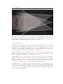
2.1
Overview
Figure 2.1: General overview of communication.
CSE1 was buildt with the intension for use in the MC Lab. According to Norwegian
University of Science and Technology (n.d.), the MC Lab was a storage tank for ship
models made of paraffin wax and operated by the Department of Marine Technology. It
contains a basin with wave-making, towing and real-time position measuring capability.
In addition it have equipments for measuring forces and wave heights.
At the time of use, the computers in MC Lab were running on Windows XP, limiting
the use of software versions toLabVIEW 2010 Service Pack 1 and MATLAB 2009b. As
a consequence, the programs developed in this thesis were created for compatability and
does not take advantage of certain simpler and more advance functions available in newer
versions. The support for Windows XP expired in April 2014, meaning the operating
systems needs to be upgraded to Windows 7, lifting the software version restriction.
7
8
CHAPTER 2. THE INFRASTRUCTURE
CSE1 is operated from a laptop using a LabVIEW Front Panel as the GUI, and the Block
Diagram and SIT for signal routing. The operator have the option of interacting directly
with CSE1 through the Front Panel or indirectly through a PS controller.
With the indirect apporach the PS controller communicates with LabVIEW via Bluetooth.
The signals are received by aDongle, and processed first by BTSix then by PPJoy before
LabVIEW aquires them. In the current setup, the indirect option have limited appliations
in terms of control modes. However, this approach can provde a faster, more intuitive and
direct control of CSE1 in terms of manual control. This is due to the mapping which each
Voith Schneider Propellers (VSPs)’s force direction is mapped to an analog stick, and the
lower shoulder button pair (L2 and R2) controls the bow thruster force direction.
The operator also have the option of choosing where the process programs should run,
internally (on the laptop) or externally (on the CSE1). The former utilize the .mdl file
while the latter make use of the nidll rtw files internally and uploads the nidll vxworks rtw
files to the CSE1. The nidll rtw and nidll vxworks rtw files are derived from the .mdl file
using Real-Time Workshop. This thesis focus on the latter option. How each signal and
controller is treated, is handled and structured in a Simulink diagram (.mdl).
The communication with CSE1 occurs wireless through HIL Lab. Qualisys tracks CSE1
using IR rays and sends the data back to LabVIEW.
2.2
CyberShip Enterprise 1
In principle CSE1 consist of a modified hull (1:50 model scale), a waterproof box, a
network adapter (D-Link), a cRIO, a bow thruster, two batteries, two VSPs, four servos
and several passive IR markers, in addition to wires and other electrical components, see
Skåtun (2011) for details.
2.2.1
Communication
Connection between cRIO and LabVIEW is of the utmost importance, without it, remote
control of CSE1 is impossible. An option to ensure a near 100 % connection is to have
a ethernet cable connecting the two together. However, this would severely cripple the
mobility, practiclly mooring it. The other option is wireless connection.
All communication with CSE1 takes place wirelessly through the D-Link. In the early
stagest, loss of connection with CSE1 was a common occurrence. This had to do with
where it was relative to where the HIL Lab router was and where on the hull the D-Link
was placed. Originally the standard antenna was used for the D-Link and placed within
the watertight box, bending the antenna almost parallel to the cRIO. The combination of
these naturally deteriorated strength of the wireless connection.
The loss of connection was lessen with the aid of Senior Engineer Torgeir Wahl. The first
action, adding an additional wireless (Asus), placed more centrally and closer to the space
CSE1 operated. However, this solution was short-lived since the Asus died after periode
of use. The cause of this is unknown. The next action gave a more permanent fix to the
problem. The antenna was moved outside the waterproof box, while the D-Link remained
2.3. MARINE CYBERNETICS LABORATORY
9
inside. This was achieved by attaching the D-Link to the inside of the waterproof box’s
lid with velcro tape, then drill a hole, connect the antenna and sealing it with caulk.
Involuntarily disconnection frequency lessen, but still a nuisance. The last improvement
was to to replace the standard antenna that followed the D-Link with an antenna roughly
three times the original’s length. Spontaneous disconnection became more or less extinct.
However, it is worth noting that, the probability of establishing connection is mostly determined by the sequence the various wires are connected to the batteries. From experience
(without any scientific documentation), connecting the red wire before the black requires
fewer attemps of establishing connection than vice versa.
2.2.2
Visibility
CSE1’s postion and orientation are aquired by Qualisys using the IR markers placed onboard. Therefore size and placement of the markers have an impact on CSE1’s visibility.
Orignally a fixed IR marker stand was used and placed on top of the waterproof box along
the longitudinal centerline. Qualisys had at times and certain orientation relative to the
cameras lost sight of CSE1, due to the relativ positions of the markers to each other, and
their proximity to the latest antenna. Sometimes the markes merge together, other times
they overshadows one another, in addition to the antenna overshadowing or dividing the
markers.
To increase the visibility, elevated passive IR markers were added, two on the longitudinal
centerline (bow and stern), three on the aft end (two port one starboard). The first setup
had the fixed stand and the five markers, a total of nine markers. With the marker at
bow bent forward and the marker at stern bent in the opposite direction. The stand was
removed since five markers gives a redundancy of two markers, and the stand could be
used for a seperate body. The marker at bow was later straighten to be as vertical as
possible due to constant shift of it’s position caused by CSE1 crashing bow first into the
basin walls.
2.2.3
Thrusters
The thrusters receives control signals from cRIO. The bow thruster is a simple tunnel
thruster, driven and controlled by a hobby motor. Each VSP have a motor for rotation
and two servos to position the stick. The distance between the stick and servos are fixed.
However, they move in an circular motion which needs to be accounted for.
2.3
Marine Cybernetics Laboratory
The basin’s dimensions imposes constraints on the maneuvering space of CSE1. As stated
in Norwegian University of Science and Technology (n.d.), the basin have a total length of
40 meters, a width of 6.45 meters and it can be filled up to a depth of 1.5 meters.However,
measuring it from end to end, it is closer to 39 meters and the length the real length where
a vessels position is measurable is limited by several factors.
10
CHAPTER 2. THE INFRASTRUCTURE
The basin’s water in- and outlet are located at the far end of the basin, aswell as it’s beach.
On the opposite is the wave maker. Between those are the measuring equipment, mounted
on the front side of the towing carriage. It’s motion is limited to the rails along the basins
length, that ends approximately at the edge of the beach. All of these machinery and
facility takes up space. The in- and outlet with the beach occupy roughly four meters of
the total basin length, around the furtherst position the towing carriage can be placed.
The towing carrage itself, fills up four meters of length. Lastly the wavemaker takes up
about one meter. Using 39 meters as the total length of the basin, a surface vessel should
have approximately 30 meters of basin length to maneuver in.
2.4
Qualisys
Qualisys is the real-time positioning system available in the MC Lab. It uses three IR
cameras (Oqus) to capture the motions. They are mounted on the towing carriage front,
one in the middle and one on each side, slightly tilted down.
Oqus sends out IR rays which is reflected by passive IR markers. If the reflected rays
are registred by two or more cameras, and they are able to clearly identify three or more
markes, then the position and orientation is captured. The visible field of each Oqus is
cone shaped. Due to height placement relative to water surface, the closes visible areas are
roughly three meters in front of the cameras. Taking the tilted orientation of the cameras
relative to the water surface, size and proximity of the markers the effective range is around
19 meters.
QTM is the software that process the data from Oqus and send it to a Qualisys server,
who in turn passes it on to the HIL Lab network
2.5
LabVIEW
As mentioned previously, LabVIEW routes and displays the data. The Front Panel provides the GUI, and the Block Diagram and SIT for signal routing. The programs have
been deconstructed and reconstructed several times.
The same .vi-file can be used for several .mdl-file, e.g. “Template HMI.vi” are used for
both “TemplateNIPID” files and “TemplateLgV2” files. SIT will generate separate project
files based on the .mdl-file name.
The drivers and FPGA files were orginally created by Senior Engineer Torgeir Wahl, some
of those have later been modified by the author. The programs are intended for single
vessel (body), with the possibility to expand for multiple bodies by modifications. The
focus will be on single body.
2.5.1
.vi files
Four .vi files have been created in connection with this thesis, “PS3 HMI.vi”, “Thruster
HMI.vi”, “StudentHMI.vi” and “Template HMI.vi”. Each of them shows different stages
2.5. LABVIEW
11
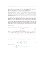
Figure 2.2: Qualisys Oqus area covered seen from above. The Oqus are placed on right
edge, white cones indicate visible area per cameera. The walkway is at the bottom edge,
and somewhere on the left edge is the wavemaker. Red arrow indicate x-axis and teal
arrow indicate y-axis. Each square in the grid is 0.5 × 0.5 meters.
of the development.
“PS3 HMI.vi” was the first one created, directly derived from Skåtun’s work. It contains
and require the bare minimum to manually control CSE1 through a PS controller. To run
it requires, LabVIEW with SIT package, BTSix and PPJoy installed and the .vi file, the
.mdl file or it’s derived files, a wirelss network, a PS controller with Bluetooth and Dongle.
In theory this enables CSE1 to not be confined to only the MC Lab.
“Thruster HMI.vi” was deveopled for the purpose of measuring the thruster forces produced. The input values needed to be fixed over a period. It is an expansion of “PS3
HMI.vi”, allowing direct thruster control from the Front Panel.
“StudentHMI.vi” is one of the last version of the GUI and the one who is most similar to
Skåtun’s program of the four. It can also be viewed as a simplified version of “Template
HMI.vi”. It was created for the avarage student to easily use and modifiy. It contains
a manual PS thruster control, a Dynamic Positioning (DP) control with setpoint, and a
Control Lyapunov Function (LgV) control with linear and ellipse path.
“Template HMI.vi” is the final product and will be the main focus. It is a mostly generic
GUI, with a setup for manual PS thruster control, two automated control systems with the
option of linear or ellipse path or setpoint. It is in essence the same as Skåtun’s program,
see Skåtun (2011) for a simple introduction. It requires data from qualisys to make use of
the automated control systems.
12
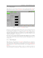
2.5.2
CHAPTER 2. THE INFRASTRUCTURE
Front Panel
This is where the operator interacts with the rest of the programs when using CSE1. The
panel is directly connected to the Block Diagram, and vertcally divided into two parts.
Figure 2.3: Overview of LabVIEW Front Panel.
The left part contains the dials, switches, indicators and controls for input and selections.
To switch between the different control mode, use the “radio button column” located on
top in the middel. It is mapped to a constant block in the .mdl file, sending an integer
from 0 and up. That value is then used in a switch-block to determine which input to use.
Similarly for which input to pass to the controller, the “radio button column” above the
“Enable Linear Simulator” boolean button.
The tabs are used for compact structuring. The right half are different types of visualization of the process taking place in the background, a 3D visualization, and plots of key
variables. The various controls, indicators and plots should be self-explanatory based on
the name label.
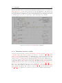
2.5.3
Block Diagram
This is where the each element in the Front Panel is defined with repect to interaction,
behavior and data to display among one another. In general it is here the mapping are
done. However, since the model structure and dynamics are created in Simulink the true
mapping happens in SIT, which in turn automatically create the mapping in the Block
Diagram
The diagram is basically the same as Skåtun’s. It have been organized and tweaked for
relative path definition, and with added comments and lables. It can be divided into four
2.5. LABVIEW
13
main groups. First is the loop stucture that handles the signals from the PS controller via
BTSix and PPJoy. Second is the blocks used for the 3D visualization. The third group
is the stuctures created by SIT. The last group is the miscellaneous group scattered all
across the diagram containing tab-, control-, and unmapped-blocks. Unless they are wired
to anything they can be more or less freely be placed anywhere in the diagram.
Figure 2.4: Overview of LabVIEW Block Diagram.
2.5.4
Simulation interface toolkit
SIT is the intersection that connects LabVIEW(Block Diagram and Base Rate Loop.vi)
, Simulink, CSE1 and Qualisys togehter. It connects to .mdl file or the derived files
(.dll/vxworks) in “Model and Host”. In “Mappings” the connection between the blocks
in Block Diagram and the blocks in .mdl file is established. The relationship of the SIT
output block in .mdl with (CSE1) the thrusters through cRIO are set in “Hardware’ I/O”
in connection with the FPGA bitfile. As well as the SIT input block in .mdl for the battery
voltages and any force ring connected to the cRIO. The link between Qualisys and the remaining SIT input block in .mdl is done indirectily through IO.llb and Base Rate Loop.vi.
The IO.llb is automatically created by SIT. It contains six .vi files, Base Rate Loop.vi,
Close-, Init-, Read-, Write.vi and Ref.ctl. It is in Base Rate Loop.vi the whole Qualisys
data acquisition is handled. The others are called, but it is not worth going into detail.
Base Rate Loop.vi makes use of a driver.vi created by Senior Engineer Torgeir Wahl.
14
2.5.5
CHAPTER 2. THE INFRASTRUCTURE
Qualisys Track Manager Drivers
The original driver used in Skåtun (2011), also created by Torgeir Wahl, aquired, processed
and sent the data all in the same timestep. The consequence of this forced the time step
of the.mdl to be the same as the sample rate of Qualisys.
If Qualisys had a higher sample rate than the rate the .mdl file was solved, the .mdl file
would would constantly be working with older and older data as the time progressed. If
the .mdl file had a higher frequency than Qualisys, the Base Rate Loop.vi would crash
ending the run. This is caused by the driver not having any data to pass on and nothing
is sent to the .mdl.
The orignal driver also contained an error where the size of the output array was smaller
then the actual size. This caused the shuffling of the data set. Even if both Qualisys
and .mdl were both set to the same frequency, it would have only been a matter of time
before .mdl in a time step began ahead of Qualisys. This is due to that each of them have
their own internal clock, that is not synchronized. When the difference between the two
becomes too large, Base Rate Loop.vi crashes.
Most runs could not last longer than a few minutes and this was the main problem. As
each crash meant a total reboot of LabVIEW, combined with the lost of connection, most
of the time was spent on establishing and deploying the software.
To fix this problem, a Producer/Consumer desgin pattern was implemented. The Producer (QTMTask.vi) and Consumer (QTMdriver ....vi) replaced the orignal QTMdriver.vi.
QTMTask.vi follows Qualisys freqency, and QTMdriver ....vi follows real-time target frequency (.mdl file).
This setup makes them frequency independent of each other. QTMdriver.vi) aquires the
data using other .vi files and add it to a shared memory block (data queue) it have with
QTMdriver ....vi. QTMdriver ....vi retrives the data set from the data queue, wipes the
queue clean, passes the data set on to the SIT server and stores the data in a memory
block. If there is no new data set, most of the data set in the memory block is passed
to the SIT server instead, analog to a zero order hold. This setup greatly improves the
reliability and robustness of the system.
For more information, National Instruments (n.d.b) and National Instruments (n.d.a).
2.6
Simulink
The control architecture is defined in the Simulink diagram. As previously mentioned
the mapping between Simulink and LabVIEW is handled by SIT. The blocks utilized
for the actual routing are “Constant”-blocks for signals from LabVIEW (Controls), and
“Gain”-blocks for signals to LabVIEW (Indicators).
The names given to the “Controls” in LabVIEW are set to be similar if not excatly the same
as their counterpart in Simulink (“Constant”-blocks). An example, The “Control” that
determines which controller to use is called “Mode Control” in LabVIEW. It’s counterpart,
meaning the “Constant”-block it shall be mapped to in the Simulink diagram, is given
the name “Mode Control Selector”. This simplifies the process when the mapping is done
2.6. SIMULINK
15
in SIT Connection Manager, making it easier to know which “Control”or “Indicator” to
mapped to which block.
The values set on the “Constant”-blocks are often set to the default value preferred.
However those values does not matter when running the it via LabVIEW, since the .vi
wiill send the signal which the Simulink diagram will update with before executing. The
values set in the “Gain”-blocks will be multiplied with the signal before sending it to
LabVIEW, if mapped. Therefore most often those values are set to one.
The latest versions utilize “GoTo”- and “From”-blocks, with global variables, to pass
values between subsustems. The previous versions used wires to send signals between the
subsystems. This created a lot of clutter and unnecessary work when adding, removing or
just moving blocks due to the path the wires would be automatically placed.
Figure 2.5: Blocks used for signal routing and mapping in Simulink diagram.
This enables most blocks to be placed anywhere in the Simulink diagram. However, for
structure and logical flow when looking at the it, the blocks are placed as if they were
using wires and parts placed in subsystems where it is logical. In general the diagram can
be read from top to bottom, and from left to right.
The top level contains four blocks, where three of them are subsystems. The “SignalProbe”block is the port for communication with the SIT server. All values mapped from LabVIEW are gathered in the subsystem “Input from LabVIEW”. Every signal mapped to
LabVIEW are located in the “Output to LabVIEW” subsystem. Each inputs from SIT
are in the subsystem “ Input from SIT” found under “Main Subsystems/Navigation”.
Outputs to SIT are within the subsystems located in “Main Subsystems/Plant/CSE1 actuator’. ’The block are color coded, where green means “Source”, red means “Sink”,
orange means “GoTo”, and magenta means “From”.
The solver used is ode5 (Dormand-Prince), with 0.1 as fixed-step size. Other solvers can
also be used, it depends on the complexity of the system, and if the solver is able to finish
within the time step. When compiling the fiile using Real-Time Workshop, the only way
to set the frequency of the model is by choosing fixed-step. If variable-step is chosen then
Real-Time Workshop will decide the frequency.
A small sidenote: Some comments and names of blocks in the .mdl-files may not be up to
date for what ithey are actually used for.
16
CHAPTER 2. THE INFRASTRUCTURE
Figure 2.6: Top level in Simulink diagram.
2.6.1
Input from LabVIEW
The function of this subsystem is to gather all input mappings from LabVIEW in one
place. It consists of “Constant”-blocks to map to, and “GoTo”-blocks to declare them
as global variables. The signals mapped here are structured into scalar, vector or matrix
depending on the application of the signal before being declared a global variable.
2.6.2
Output to LabVIEW
This subsystems functions is similar to the “Input from LabVIEW”, it gathers all mapping
in one place, just for outputs instead. It consists of “From”-blocks obtaining the signals
from the global variables, and divides most of them into scalars for mapping. The “Gain”blocks are the counterpart of the “Indicators” in LabVIEW.
2.6.3
Guidance
The “Guidance” module’s main function is to generate all the reference or desired variables
the controllers needs. It contains e a “Path”-, “Heading”-, “Speed assigment”- and “LineOf-Sight”-module.
2.6. SIMULINK
17
Figure 2.7: “Guidance” module in the Simulink diagram.
pathSelector
[-]
Guidance module input
Switch workaround parameter for path
s
[-]
Path parameter of desired path pd
x0
y0
rx
ry
k
[m]
[m]
[m]
[m]
[-]
x-coordinate of origin of ellipse path in Q-frame
y-coordinate of origin of ellipse path in Q-frame
Radius of ellipse path in x-direction in Q-frame
Radius of ellipse path in y-direction in Q-frame
Scaling parameter of path parameter s
x1
y1
x2
y2
[m]
[m]
[m]
[m]
x-coordinate
y-coordinate
x-coordinate
y-coordinate
ud
[m/s]
q
∆
µ
[m]
[m]
[-]
of linear path in Q-frame when s is zero
of linear path in Q-frame when s is zero
defining heading of linear path in Q-frame
defining heading of linear path in Q-frame
Desired surge speed in B-frame
Virtual point-mass coordiantes of vessel in Q-frame
Lookahead distance
Tuning parameter for s gradient algorithm
18
χ
χq
χs
q
ψlos
q2
ψlos
qs
ψlos
s
ψlos
s2
ψlos
CHAPTER 2. THE INFRASTRUCTURE
col([m],[m],[rad])
[rad/m]
[rad/m2 ]
[rad/m]
[rad]
[rad]
Guidance module output
3DOF reference vector in Q-frame, col(q,ψlos )
Partial differentiation of χ
Partial differentiation of χ
Partial
Partial
Partial
Partial
Partial
differentiation
differentiation
differentiation
differentiation
differentiation
of
of
of
of
of
ψlos
ψlos
ψlos
ψlos
ψlos
fq
fqq
fqs
fqt
Dynamic LOS assigment for q̇
Partial differentiation of f q
Partial differentiation of f q
Partial differentiation of f q
fs
f qs
fss
fst
Dynamic LOS assigment for ṡ
Partial differentiation of fs
Partial differentiation of fs
Partial differentiation of fs
Path
The “Path” module’s main function is to generate desired position pd . Continuous parameterization of the paths are implemented in this module. It have three modules, one
for linear path, one for ellipse path and a workaround switch. Both paths are created
simultaneously using the same path parameter s. However s will only be dependent on
the chosen path.uperscript
The linear path is created with:
x = (x2 − x1 )s + x1
xs = (x2 − x1 )
(2.1a)
(2.1b)
y = (y2 − y1 )s + y1
(2.1c)
s
(2.1d)
y = (y2 − y1 )
(2.1e)
where x1 and y1 are coordinates of linear path in Q-frame when s is zero, and x2 and y2
defines the heading of linear path in Q-frame. The higher order partial differentiations
are set to 0.
The ellipse path is created with:
2.6. SIMULINK
19
x = rx cos(ks) + x0
(2.2a)
s
(2.2b)
x = −rx k sin(ks)
2
xs = −rx k 2 cos(ks)
x
s3
3
= rx k sin(ks)
(2.2d)
y = ry sin(ks) + y0
(2.2e)
s
(2.2f)
y = ry k cos(ks)
y
y
(2.2c)
s2
2
= −ry k sin(ks)
(2.2g)
s3
3
(2.2h)
= −ry k cos(ks)
(2.2i)
where x0 and y0 are coordinates of origin of ellipse path in Q-frame, rx and ry are radius
of ellipse path and k is a scaling parameter of path parameter s, often much smaller than
1.
The values are merged together into p = col(x, y) for each of their respective partial
differentiations, and the module implements equation (36) in Skjetne (2014).
The workaround module is used due to unknown technical limitations that wont running
or compiling when a regular “Switch”-block for switching between paths. It uses a variable
dubbed “pathSelector” that can be either 1 or 0. The workaround make use of
pd = pd1 pathSelector + pd0 (1 − pathSelector)
(2.3)
For each partial differentiations, where pd is the chosen path, pd1 is the linear path and
pd0 is the ellipse path. If “pathSelector” is 0, then ellipse path is chosen. If it is 1, then
linear path is chosen.
Heading
The “Heading” module make use of the outputs from the “Path” module. It implements
equation (2) and (47) to (49) in Skjetne (2014), and outputs the desired heading ψd and
2
it’s partial differentiations, ψds and ψds .
Speed Assigment
The “Speed Assigment” module require the outputs from the “Path” module, in addtion
to the desired forward speed ud . It implements eappropriatequation (5), (38) and (39) in
Skjetne (2014), and passes on the speed assigment vs , it’s partial differentiations and the
time derivative of ud .
20
CHAPTER 2. THE INFRASTRUCTURE
Line-Of-Sight
The “Line-Of-Sight” module’s main function is to generate the 3DOF reference vector χ.
It takes in the outputs from the previous modules, in addtion to the lookahead distance
∆, tuning parameter for s gradient algorithm µ and the virtual point-mass coordiantes
in Q-frame q. Equation (6) to (8), (40) to (46) and (50) to (70) in Skjetne (2014) are
implemented here. It’s outputs are χ, dynamic LOS assigment for q̇, f q , and dynamic
LOS assigment for ṡ, fs .
2.6.4
Control
The “Control” module’s main function is to generate a 3DOF command output τ and a
set of thruster commands T c . It is currently made up of five modules, one switch, one
thruster allocation, and three control module. It is set up to handle three controllers, but
can be expanded by adding and increasing the number of ports in the switch.
Figure 2.8: “Control” module in the Simulink diagram.
2.6. SIMULINK
controlModeSelector
ctrlReset
s0
q0
21
Control module input
[-] Parameter for switching between controllers
[-] Parameter for reseting controllers
[-] Initial value of s
[m] Initial values of q
ηd
η
ν
Desired position and orientation in Q-frame
Position and orientation in Q-frame
Velocities in B-frame
χ
χq
χs
3DOF reference vector in Q-frame, col(q,ψlos )
Partial differentiation of χ
Partial differentiation of χ
q
ψlos
q2
ψlos
qs
ψlos
s
ψlos
s2
ψlos
Partial
Partial
Partial
Partial
Partial
fq
fqq
fqs
fqt
Dynamic LOS assigment for q̇
Partial differentiation of f q
Partial differentiation of f q
Partial differentiation of f q
fs
f qs
fss
fst
Dynamic LOS assigment for ṡ
Partial differentiation of fs
Partial differentiation of fs
Partial differentiation of fs
M
D
B
Inertia matrix
Hydrodynamic damping matrix
Thruster configuration matrix
differentiation
differentiation
differentiation
differentiation
differentiation
of
of
of
of
of
ψlos
ψlos
ψlos
ψlos
ψlos
KP
KI
KD
[-]
[-]
[-]
Diagonal tuning matrix
Diagonal tuning matrix
Diagonal tuning matrix
Γq
κ1
λ
[-]
[-]
[-]
Diagonal tuning matrix
Tuning parameter for virtual control α
Gradient update law tuning parameter
ASLY
ASLX
ASRY
ASRX
L2
R2
Bow Thruster (BT) power
VSP speed
[-]
[-]
[-]
[-]
[-]
[-]
[-]
[-]
Up/Down position of Left Analogstick
Left/Right position of Left Analogstick
Up/Down position of Right Analogstick
Left/Right position of Right Analogstick
Shoulder botton signal
Shoulder botton signal
BT power limit
VSP speed setpoint
22
τ
Tc
s
q
CHAPTER 2. THE INFRASTRUCTURE
[-]
[m]
Control module output
Force vector in B-frame
Thruster commands set
Path parameter of desired path pd
Virtual point-mass coordiantes of vessel in Q-frame
Control #n
Within each “Control #n” different kind of control design can be implemented, for modularity and structure one per subsystem. However, they can be placed anywhere as long
as it uses a “GoTo”-block to declare the τ produced as a global variable with a unique
variable name, and use a “From”-block in the “Control Switch” module to retrieve. For
automated controls; reference values, tuning parameters, η and ν.
“Control 0” is used for the direct thruster control through a PS controller. It need the
x- and y-coordinate of each analog stick, R2 and L2 signal, and BT power limit and VSP
speed setpoint to create T c .
For a DP PID controller; The desired position and orientation ηd , vessel dynamic matrices
M and D, tuning matrices K P , K I and K D , and η and ν are needed as inputs.
For the LgV2 and NLPID design from Skjetne (2014);, all the outputs from “Guidance” ,
a control reset variable called “ctrlReset”, intial values s0 and q0 , vessel dynamic matrices
M and D, tuning parameters and matrices κ1 , Γq , λ, K P , K I and K D , and η and ν
are needed as inputs. Their outputs are τ , virtual point q and path parameter s.
Control Switch
The “Control Switch” module is a straight forward subsystem with a “Switch”-block.
It takes in the τ ’s from the controller modules, and a variable named “controlModeSelector” to decide which controller to use. The “Switch”-block is zero-based, since the
“ControlMode” “radio button”’ in LabVIEW is zero-based.
Thruster allocation
The “Thruster allocation” module converts τ into T c , in two steps. First
f act = B + τ
(2.4)
where f act = col(f1 , f2 , f3 , f4 , f5 ) is the force actuator vector, τ is the force vector in
B-frame, and B + is the pseudoinverse of the thruster configuration matrix B.
Then f act is mapped to thruster inputs u through lookup tables, before merging with the
BT power limit and VSP speed setpoint to create the thruster commands set T c . If other
power limit or speed setpoint is desired by the user, then the lookup tables needs to be
replaced with the appropriate ones. This part is hardcoded into the control architecture.
For details on the lookup tables see system identification section.
2.6. SIMULINK
2.6.5
23
Plant
The “Plant” module’s main function is to make use of τ and T c , and directly or indirectly
produce η and ν. It is divided into two subsystems, “Real Target” and “Simulator”.
Figure 2.9: “Plant” module in the Simulink diagram.
controlModeSelector
enableCSE1
LS Enable
[-]
[-]
[-]
Plant module input
Parameter for switching between controllers
Parameter to enable the thruster subsystems
Parameter to enable the Linear simulator
τ
Tc
TC#n
Force vector in B-frame
Thruster commands set
Direct thuster command set from control
M
D
LS Reset’
η0
ν0
Inertia matrix
Hydrodynamic damping matrix
Parameter for reseting linear simulator
Initial values of ηLS
Initial values of νLS
ηLS
νLS
[-]
[-]
[m]
Plant module output
Position and heading form linear simulator
Velocities from linear simulator
Real Target
The “Real Target” uses the T c output from the “Control”-module, and convert them into
signals that each thruster is able to follow. It needs three input signals T c , “controlModeSelector” and an enabling variable “enableCSE1” to enable the thruster subsystems. The
creation and tuning of those subsystems are documented in Skåtun (2011). According to
24
CHAPTER 2. THE INFRASTRUCTURE
Skåtun, the 2D lookup tables should counteract the circular motion of each servo, and
create a linear movement of the VSP control sticks. The only thing different from the
original is the modularize structure.
There is a workaround for the T c , to account for controllers that are direct thruster controls
TC#n, if they are implemented in the “Control” module. However manual adjustment
and check is needed to make sure the workaround corresponds to the right controller.
This subsytem does not directly produce η and ν, since it just sends command signals to
a cRIO, who in turn routes the signal where they need to go. The η and ν are calculated
in the “Naviagtion” module.
Simulator
The “Simulator” does not make use of the thrusters, instead it runs on a linear vessel
dynamics model presented in the introduction, equation (1.1). It needs, τ , M D, an
enable parameter, “LS Enable, a reset parameter “LS Reset”, intial position and heading
η0 , intial velocities ν0 . The outputs are ηLS and νLS
2.6.6
Navigation
The “Navigation” module’s main function is to calculate and output η and ν. It consists
of “Input from SIT” and “Navigation Switch”.
Figure 2.10: “Navigation” module in the Simulink diagram.
Input from SIT
This subsystem have remained mostly the same since the orginal subsytem found in Skåtun
(2011) . The major difference is the passive low speed observer used to estimate the
velocities instead. Its function is to process the Qualisys values received through the SIT
server, and output ηQS and νQS . In addtion it needs T c M , D for the observer. It also
sends out other parameters given by Qualisys, seperatly battery voltages
The passive low speed observer was introduced into the stucture by Co-advisor Øivind
Kjerstad, due to the noisy velocities created when using a “Derivation”-block. It is a
modified version of an observer from MSS GNC Toolbox.
2.6. SIMULINK
25
Navigation Switch
The “Navigation Switch” is similar to “Control Switch”. it uses a varable called “controlInputSelector” to decide if it shall send the valuse from Qualisys or the simulator. The
addtional inputs are ηLS , ηQS , νLS and νQS . The outputs are η and ν.
2.6.7
C/S Enterprise 1 Matrices
The function of this subsystem is to define CSE1’s matrices. it is created to make it easy
and efficient to modify , without having to check if all the places the matrices are used are
up to date. It does not have any inputs, but it is possible to directly map controls from
LabVIEW here to provide an realtime way to change the matrices’ values. Its output are,
M , D and B.
Figure 2.11: “C/S Enterprise 1 Matrices” module in the Simulink diagram.
2.6.8
Data logging
The point of data log was chosen in Simulink since it is the performances of the control
system that are of interest. Each barrrier between the point of interest and point of
measuring is a potential source of error and delay. However, this approach requires the
operator to manually extract the log file if the .mdl file was running on the cRIO through
the “Measurment & Automation Explorer”. The data is stored in .mat formate using a
“ToFile”-block, which is generated and stored in the workspace wherever the model is
running (Execution Host). The name of the data file is set in the dialog window of the
“ToFile”-block.
Figure 2.12: Two “ToFile”-blocks used in Simulink diagram.
26
CHAPTER 2. THE INFRASTRUCTURE
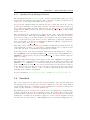
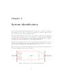
Chapter 3
System identification
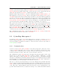
For the system identification arrangement twelve rotation free hook, three force ring and
three springs were used. Two force rings on portside and two springs on starboard side,
and one force ring in the aft and a spring at the bow.
In general each measurment series last 30 seconds, with 30 seconds in between measurment
to allow the surface distubance to die out and reset the zero settings. The first measurment
set did not have a zero measurment before the distubance is instroduced, e.g. towing or
activating CSE1, which was introduced in the latest measurment set.
The first set of measurments was done for towing the hull 0, 45 and 90 degrees, VSP force
generation with a VSP speed set to 0.4 with 0.1 step size, and for BT with power limit at
0.5 also 0.1. For the thrusters the input value ranged from -1 to 1.
The second set were done just for the thrusters for lower speed and power. VSP speed for
0.2 and 0.3 and BT power at 0.15, 0.3, 0.4 and 0.5.
Figure 3.1: The setup of CSE1 for system identification.
27
28
3.1
CHAPTER 3. SYSTEM IDENTIFICATION
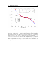
Hull
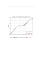
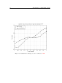
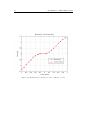
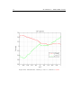
The measurements from 0 and 90 degrees towing yielded:
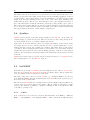
Figure 3.2: Measurments of dampning coefficient of CSE1
The values for Xu and Yv are similar to Skåtun’s values. And a new value can be added
for slow speed Nv = 0.18140.
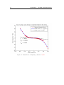
3.2
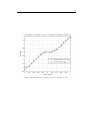
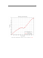
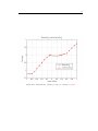
Thruster mapping
The VSP have been measured for 0.2, 0.3 and 0.4 in VSP speed, while the BT have been
measured for 0.15, 0.3, 0.4 and 0.5 in power limit.
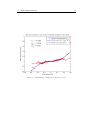
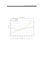
The starboard voith schneider propeller rotates slow than the port voith schneider propeller. The effect is notiable in the meaurment. However it does not come into effect unless
3.2. THRUSTER MAPPING
29
Figure 3.3: Measurments of dampning coefficient of CSE1
the maximum force are required, and it becomes less significant as higher rotation speed
are used. It is also noted that the servos are significantly coupled and the force output
drops at the periphery value , 1 . It can be seen from the thruster measurements that
the lookup tables for the voith schneider propellers does not truly cancel out the circular
motion of the servos. Some of it can be caused by the rotation when measureing, or due
to placement of thuster. However this can not fully explain the notable force meaured in
the other direction. Of the servos, servo 4 have the strongest coupling in surge-sway.
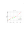
During the meaurment of the thrusters it is noted that the thuster commands have an
error of margin around 0.03. Meaning the 0.21, 0.22 and 0.23, can generate the same force.
See appendix for plots.
30
CHAPTER 3. SYSTEM IDENTIFICATION
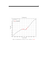
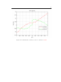
Figure 3.4: Measurments of dampning coefficient of CSE1
3.2. THRUSTER MAPPING
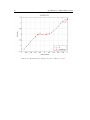
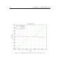
Figure 3.5: Measurments of dampning coefficient of CSE1
31
32
CHAPTER 3. SYSTEM IDENTIFICATION
Chapter 4
Line of Sight Experiments
As previously mentioned the two controllers implemented are from Skjetne (2014).
Two advance control design were implemeted, tuned and tested, a LgV backstepping and
a Nonlinear PID designed controller.Only ellipse path was used in the laboratory. This
had to do with space constraints, and a wish to have long run time on the experiments.
The gradient optimization finds the fastest or steppest change, this helps the controller
converge faster toward the desired setpoint. An unfiltered update law can be sensitive to
noise in the measurment, while a filtered update law woould smoothen out and therefore
be more stable with noisy measurments. However this will introduce a delay.
The controllers are designed with three points that chases each other, the path point η d ,
the virtual point χ and the vessels point η. η d stays on the path and moves to minimize
the distance between it and χ. χ tries first to minimize the distance between it and glseta
before η d . While η will only converge to χ. If the filltered update law is disabled controller
becomes a tracking case.
Attached electronically are the data from the runs, burt due to timeconstraint those are
not presented here.
4.1
Simulation runs
In the ideal simulated word both of them were equal in terms of maneuvering, both for
linear paths and for ellipse path. Depending on the tuning their inital transient behavior
can be erractic and unnatural.
4.2
Laboratory runs
Originally only the LgV backstepping was tested in the laboratory. It converged and performed well. The only downside was it would constantly overshoot the heading, resulting
in a constant oscillation, while moving alone the path. The reason was due to the noisy
velocity estimation.
33
34
CHAPTER 4. LINE OF SIGHT EXPERIMENTS
Other opportunity presented itself to run more experiments in the laboratory, However,
unknown at that time and discoved to late, one of the servo arms broke due to fatigue
from the constant oscillation of the previous runs, corruping the mapping and observer
estimates. In the laboratory, their performance depended heavily on how they were implemented. If both of them were fully implemented, LgV backstepping proved to handle the
uncertainties better. Although it would overshoot when exiting the sharper part of the
ellipse path. The vessel is able to follow the virtul point it is chasing, but the virtual point
is unable to stick to the desired path. While the fully implemented Nonlinear PID would
struggle to converge to the path and behave erratic.The velocity dependent term distorted
Nonlinear PID’s results the most . The reason is most likely due to the quality of the
estimations of the velocities from the observer. The feedfoward term also deteriorate the
control, and prevents it from converging.
If the Nonlinear PID was partially implemented, deactivating the feedforward and the
velocity dependent term, then it is the superior one. It would converge naturally to the
desired position. Once on, it would stay there indefinitely despite of the broken servo arm.
Chapter 5
Conclusion
The reliability when conducting laboratory experiments with CyberShip Enterprise 1 have
greatly improved. This was achieved through repositioning and replacing the antenna
for wireless communication, and a restructuring of how signals were handled between
servers and softwares. The original setup with single frequency was replaced with a multifrequency producer-consumer structure.
The futherst away a vessel is visible for Qualinsys is around 17 meters from the cameras.
The shortest distance is roughly 4 meters infront of the cameras. This result in a lengthwise
workspace for a vessel to be in the range of 13 meters. This length length can be increased
to 27 meters, If the carriage start from the beach end, and moves toward the wavemaker
during the experiment. It is not possible to increase it futher due to the length of the
basin, the wavemaker, beach, in/outlet and carriage is occupying.
In the system identification, an addtitonal hydrodynamic damping coefficent for slow speed
have been determined for the hull (Nv = 0.18140). In addtion higher order coefficent have
also been estimated from the towing measurements. A pseudo library for lookup table
thruster mapping have been created. The bow thruster have been mapped for power limit
input = {0.15, 0.3, 0.4, 0.5}, and the voith schneider propellers for speed input = {0.3,
0.4}. Measurments for voith schneider propellers for speed = 0.2 have also been conducted,
but no lookup table have been created for it.
The starboard voith schneider propeller rotates slow than the port voith schneider propeller. The effect is notiable in the meaurment. However it does not come into effect unless
the maximum force are required, and it becomes less significant as higher rotation speed
are used. It is also noted that the servos are significantly coupled and the force output
drops at the periphery value , 1 . It can be seen from the thruster measurements that
the lookup tables for the voith schneider propellers does not truly cancel out the circular
motion of the servos. Some of it can be caused by the rotation when measureing, or due
to placement of thuster. However this can not fully explain the notable force meaured in
the other direction. Of the servos, servo 4 have the strongest coupling in surge-sway.
Two advance control design were implemeted, tuned and tested, a LgV backstepping and
a Nonlinear PID designed controller. In the ideal simulated word both of them were equal
in terms of maneuvering. Only ellipse path was used in the laboratory. This had to do
with space constraints, and a wish to have long run time on the experiments.
35
36
CHAPTER 5. CONCLUSION
Originally only the LgV backstepping was tested in the laboratory. It converged and performed well. The only downside was it would constantly overshoot the heading, resulting
in a constant oscillation, while moving alone the path. The reason was due to the noisy
velocity estimation.
Other opportunity presented itself to run more experiments in the laboratory, However,
unknown at that time and discoved to late, one of the servo arms broke due to fatigue
from the constant oscillation of the previous runs, corruping the mapping and observer
estimates. In the laboratory, their performance depended heavily on how they were implemented. If both of them were fully implemented, LgV backstepping proved to handle the
uncertainties better. Although it would overshoot when exiting the sharper part of the
ellipse path. The vessel is able to follow the virtul point it is chasing, but the virtual point
is unable to stick to the desired path. While the fully implemented Nonlinear PID would
struggle to converge to the path and behave erratic.The velocity dependent term distorted
Nonlinear PID’s results the most . The reason is most likely due to the quality of the
estimations of the velocities from the observer. The feedfoward term also deteriorate the
control, and prevents it from converging.
If the Nonlinear PID was partially implemented, deactivating the feedforward and the
velocity dependent term, then it is the superior one. It would converge naturally to the
desired position. Once on, it would stay there indefinitely despite of the broken servo arm.
5.1
Future works
With all the improvement in the reliability, one important problem still remains; the loss
of visibility.
There are incidents when Qualinsys displays it sees all markes, but it is unable to calculate
the vessels position and orientation. The cause of this needs to be further investigated.
Spare part servo arms should be purchased, and padding for the hull to dampen the impact
to the basin walls.
Several crack have been observed on the hull. Simulation Interface Toolkit have been
discontinued, modifying it for Modular Interface Toolkit can be an option. The labeling
and choice of variable name can be improved upon.
There is a greate improvement potential of the contents of this report.
Graphical representation of the simulations and laboratory runs.
Adding comments and details on how the laboratory experiments were conducted.
Editing of the videos taken of the laboratory runs.
Analysis of the hundreds of data measurments taken.
Sorting and organizing the attached files.
Finishing the user manual for CSE1 and include the complementary screenshots.
Bibliography
Breivik, M. and Fossen, T. I. (2005), Principles of guidance-based path following in 2D
and 3D, in ‘Proceedings of the 44th IEEE Conference on Decision and Control and
European Control Conference’, Seville, Spain, pp. 627–634.
Fossen, T. I. (2002), Marine Control Systems: Guidance, Navigation, and Control of Ships,
Rigs and Underwater Vehicles, 1st edn, Marine Cybernetics, Trondheim, Norway.
Fossen, T. I. (2011), Handbook of Marine Craft Hydrodynamics and Motion Control, John
Wiley & Sons Ltd., United Kingdom.
National Instruments (n.d.a), ‘Components of a Simulation (Simulation Interface
Toolkit)’.
URL:
http://zone.ni.com/reference/en-XX/help/371504F01/lvsitconcepts/sit c components of a simulation/
National Instruments (n.d.b), ‘Understanding the Driver VI (Simulation Interface
Toolkit)’.
URL:
http://zone.ni.com/reference/en-XX/help/371504F01/lvsitconcepts/sit c understanding the driver vi/
Norwegian University of Science and Technology (n.d.), ‘Marine Cybernetics Laboratory’.
URL: http://www.ntnu.no/imt/lab/kybernetikk
Skåtun, H. N. (2011), Development of a DP system for CS Enterprise I with voith schneider
thrusters, Master’s thesis, Norwegian University of Science and Technology.
Skjetne, R. (2005), The Maneuvering Problem, PhD thesis, Norwegian University of Science and Technology.
Skjetne, R. (2014), Report: Maneuvering los control design: The fully actuated case. in
preparation Rev.E.
Skjetne, R., Jørgensen, U. and Teel, A. R. (2011), Line-of-sight path-following along regularly parametrized curves solved as a generic maneuvering problem, in ‘Proceedings of
the 50th IEEE Conference on Decision and Control and European Control Conference’,
Orlando, Florida, USA, pp. 2467–2474.
SNAME (1950), Nomenclature for treating the motion of a submerged body through a
fluid, in ‘Technical and Research Bulletin No. 1-5’.
37
Sundland, M. N. (2013), Guidance and control of iceberg towing operation in open water, with experimental testing, Master’s thesis, Norwegian University of Science and
Technology.
Texas A&M University (n.d.), ‘HOW TO CONNECT SIMULINK TO LABVIEW IN
ORDER TO COLLECT SYSTEM DATA ’.
URL: http://parlos.tamu.edu/MEEN364/Simulink2LabVIEW.pdf
Thorvaldsen, C. F. L. (2011), Formation control of marine vessels, Master’s thesis, Norwegian University of Science and Technology.
Tran, N. D. (2013), Development of a modularized control architecture for cs enterprise i
for path-following based on los and maneuvering theory, Technical report.
Glossary
.dll Dynamic-Link Library. 13
.mdl MoDeL, file extension. Models created with Simulink. 8, 10–14, 16, 25, 40
.vi Virtual Instrument, file extension. Basic building block for programs written in LabVIEW. 10–15, 39
B-frame CSE1’s body frame. 3, 17, 21–23, 43, 44
Q-frame Qualisys inertial reference frame in MC Lab. 3, 17–22, 43, 44
Base Rate Loop.vi Subprogram created by SIT for input/output of data. 13, 14
Block Diagram Part of a .vi-file containing Control Terminals, Wires, Structures and
various nodes. The main window used when constructing a LabVIEW program . 8,
10, 12–14
Bluetooth Wireless technology for exchanging data over short distances. 8, 11, 39
BTSix BlueToothSix, software that enables use of a Bluetooth PS controller on a computer. 4, 8, 11, 13
Dongle Small piece of hardware that attaches to electronic devices enabling additional
functions. 8, 11
Front Panel Part of a .vi-file containing Controls and Indicators. The main window used
when running a LabVIEW program . 8, 10, 11, 13
HIL Lab Hardware In Loop Laboratory, local ethernet in the MC Lab. 8, 10
IO.llb Program created by SIT for input/output of data. 14
LabVIEW Graphical programming language developed by National Instruments . 4, 8,
10–16, 22, 25, 39
MATLAB Matrix laboratory, high-leve technical computing language developed by MathWorks. 4, 8
MCG Reg Program used for logging data in the MC Lab. 4
39
40
Glossary
PPJoy Parallel Port Joystick, software designed to add virtual joysticks under windows
operating systems. 4, 8, 11, 13
Qualisys Motion capture system. 3, 4, 8–11, 13, 14, 24, 25, 39
Real-Time Workshop Generates C/C++ code from Simulink diagrams (.mdl-files), rebranded as Simulink Coder in later versions. 4, 8, 16, 40
servo device used to provide control of a desired operation through the use of feedback.
8, 9
Simulink Graphical programming language developed by MathWorks. 4, 8, 13, 15–17,
20, 23–25, 39, 40
Simulink Coder Rebranded name of Real-Time Workshop. 40
TeXworks Program used for writing in LaTeX. 4
vxworks Real-time operating system developed as proprietary software by Wind River
Systems, designed for use in embedded systems. 13
Acronyms
BT Bow Thruster. 21, 22, 27, 28, 44
cRIO Compact Realtime Input and Output. 4, 8, 9, 14, 24, 25
CSE1 CyberShip Enterprise 1. 1–5, 7–14, 25, 27–31, 39, 46–71
DOF Degrees Of Freedom. 4, 18, 20, 21, 43
DP Dynamic Positioning. 12, 22
FPGA Field-Programmable Gate Array. 4, 10, 14
GNC Guidance, Navigation and Control. 4, 24
GUI Graphical User Interface. 4, 8, 10–12
IR InfraRed. 3, 8–10
LgV Control Lyapunov Function. 12
LgV2 LgV backstepping 2. 5, 22
LOS Line-Of-Sight. 2, 18, 20, 21, 43
MC Lab Marine Cybernetics Laboratory. 2–5, 7, 8, 10, 11, 39, 40
MSS Marine Systems Simulator. 4, 24
NLPID Nonlinear PID. 5, 22
PID Proportional-Integral-Derivative. 1, 5, 22, 41
PS PlayStation. 4, 8, 11–13, 22, 39
QTM Qualisys Track Manager. 4, 10
SIT Simulation Interface Toolkit. 4, 8, 10, 11, 13–15, 24, 39
VSP Voith Schneider Propeller. 8, 9, 21, 22, 24, 27, 28, 44
41
42
Acronyms
Symbols
α Virtual controller. 21, 43
Γq Gradient update law tuning matrix. 21, 22
∆ Lookahead distance, [m]. 17, 20
η Position and heading in Q-frame, vector col(p,ψ). 3, 21–25, 33
η d Desired position and heading in Q-frame, vector col(pd ,ψd ). 33
κ1 Tuning parameter for virtual control α. 21, 22
λ Gradient update law tuning parameter. 21, 22
µ Tuning parameter for s gradient algorithm. 17, 20
ν Velocity in B-frame, vector col(u,v,r). 3, 21–25
τ Contol output, col(X,Y ,N ). 3, 20, 22–24
χ 3DOF reference vector in Q-frame. 18, 20, 21, 33
ψ Heading in Q-frame, in radians [rad]. 3, 43, 44
ψd Desired heading in Q-frame. 19
ψlos LOS heading in Q-frame. 18, 21
B Thruster configuration matrix. 3, 21, 22, 25
D hydrodynamic damping matrix. 3, 21–25
f act Thruster force vector, col(f1 , f2 , f3 , f4 , f5 ). 3, 4, 22
f q Dynamic LOS assigment for q̇. 18, 20, 21
fs Dynamic LOS assigment for ṡ. 18, 20, 21
k Scaling parameter of path parameter s, [-]. 17, 19
K D Diagonal tuning matrix. 21, 22
K I Diagonal tuning matrix. 21, 22
K P Diagonal tuning matrix. 21, 22
43
44
Symbols
M Inertial matrix. 3, 21–25
N Moment about z-axis, [Nm]. 43
p Vessels position as a point mass in Q-frame, vector col(x,y). 3, 19, 43
pd Desired position along desired path in Q-frame, vector col(xd ,yd ). 17, 18, 22, 44
q Virtual point-mass coordiantes of vessel in Q-frame. 17, 18, 20–22
r Yaw, angular velocity about z-axis in B-frame, radian per second rad/s]. 3, 43
R(ψ) 3 × 3 rotation matrix between Q-frame and B-frame. 3
rx Radius of ellipse path in x-direction in Q-frame, [m]. 17, 19
ry Radius of ellipse path in y-direction in Q-frame, [m]. 17, 19
s Path parameter of desired path pd , [-]. 17–22, 43
T c Thruster commands set, col(u, BT power limit, VSP speed). 20, 22–24
u Surge, linear velocity in x-direction in B-frame, meter per second [m/s]. 3, 43
ud Desired surge speed in B-frame, [m/s]. 17, 19, 44
u Thruster input signals, col(u1 , u2 , u3 , u4 , u5 ). 4, 22, 44
v Sway, linear velocity in y-direction in B-frame, meter per second [m/s]. 3, 43
vs Speed assigment corresponding to ud , [m/s]. 19
X Force in x-direction, [N]. 43
x Position in Q-frame, in meters [m]. 3, 44
x0 Origin position of ellipse path in Q-frame, in meters [m]. 17, 19
x1 Start position of linear path in Q-frame, in meters [m]. 17, 44
x2 Direction position relative to x1 of linear path in Q-frame, in meters [m]. 17
xd Desired position in Q-frame, in meters [m]. 44
Y Force in y-direction, [N]. 43
y Position in Q-frame, in meters [m]. 3, 44
y0 Origin position of ellipse path in Q-frame, in meters [m]. 17, 19
y1 Start position of linear path in Q-frame, in meters [m]. 17, 44
y2 Direction position relative to y1 of linear path in Q-frame in meters [m]. 17
yd Desired position in Q-frame, in meters [m]. 44
Appendix A
Thruster plots
45
46
APPENDIX A. THRUSTER PLOTS
Figure A.1: Measurments of VSP speed at 0.4 coefficient of CSE1
47
Figure A.2: Measurments of VSP speed at 0.4 coefficient of CSE1
48
APPENDIX A. THRUSTER PLOTS
Figure A.3: Measurments of VSP speed at 0.4 coefficient of CSE1
49
Figure A.4: Measurments of VSP speed at 0.4 coefficient of CSE1
50
APPENDIX A. THRUSTER PLOTS
Figure A.5: Measurments of VSP speed at 0.4 coefficient of CSE1
51
Figure A.6: Measurments of VSP speed at 0.4 coefficient of CSE1
52
APPENDIX A. THRUSTER PLOTS
Figure A.7: Measurments of VSP speed at 0.4 coefficient of CSE1
53
Figure A.8: Measurments of VSP speed at 0.4 coefficient of CSE1
54
APPENDIX A. THRUSTER PLOTS
Figure A.9: Measurments of VSP speed at 0.4 coefficient of CSE1
55
Figure A.10: Measurments of VSP speed at 0.4 coefficient of CSE1
56
APPENDIX A. THRUSTER PLOTS
Figure A.11: Measurments of VSP speed at 0.4 coefficient of CSE1
57
Figure A.12: Measurments of VSP speed at 0.4 coefficient of CSE1
58
APPENDIX A. THRUSTER PLOTS
Figure A.13: Measurments of VSP speed at 0.4 coefficient of CSE1
59
Figure A.14: Measurments of VSP speed at 0.4 coefficient of CSE1
60
APPENDIX A. THRUSTER PLOTS
Figure A.15: Measurments of VSP speed at 0.4 coefficient of CSE1
61
Figure A.16: Measurments of VSP speed at 0.3 coefficient of CSE1
62
APPENDIX A. THRUSTER PLOTS
Figure A.17: Measurments of VSP speed at 0.3 coefficient of CSE1
63
Figure A.18: Measurments of VSP speed at 0.3 coefficient of CSE1
64
APPENDIX A. THRUSTER PLOTS
Figure A.19: Measurments of VSP speed at 0.3 coefficient of CSE1
65
Figure A.20: Measurments of VSP speed at 0.2 coefficient of CSE1
66
APPENDIX A. THRUSTER PLOTS
Figure A.21: Measurments of VSP speed at 0.2 coefficient of CSE1
67
Figure A.22: Measurments of VSP speed at 0.2 coefficient of CSE1
68
APPENDIX A. THRUSTER PLOTS
Figure A.23: Measurments of VSP speed at 0.2 coefficient of CSE1
69
Figure A.24: Measurments of BT power at 0.15 coefficient of CSE1
70
APPENDIX A. THRUSTER PLOTS
Figure A.25: Measurments of BT power at 0.3 coefficient of CSE1
71
Figure A.26: Measurments of BT power at 0.4 coefficient of CSE1
72
APPENDIX A. THRUSTER PLOTS
Appendix B
Draft for User Manual
Connecting to Cybership Enterprise 1
(RT CompactRIO - NI-cRIO9024-CSE1 (192.168.0.77))
------------------------------------------------------------------Make sure:
- the ethernet cable is connected to "ACT/LiNK"
port 1 and to the "D-Link Wireless Bridge"
- the "Laptop" is connected to "HILlab"
- the "Main battery" (large fat one) is above 12 Volt
- the "Servo battery" (small slim one) is above 6 Volt
Place "Main battery" (large fat one) beneath wireless anntenna,
adjacent to waterproof box, between the wires, with battery
terminals furthest away from it.
Place "Servo battery" (small slim one) at bow between
tunnel thruster and waterproof box, with battery terminals
closes to the waterproof box.
Postive battery terminal ("RED-port") at portside and
negative battery terminal ("BLACK-port") at starboard side
Connect wire with red isolation ("RED-wire") to "RED-port"
and wire with black isolation ("BLACK-wire") to "BLACK-port"
Connect first the "RED-wire" before the "BLACK-wire" to
the batteries.
The "Main battery" (large fat one) should be connected
first then wait
a few sec (5s) before connecting the "Servo battery"
(small slim one).
Note: it should not matter in which order it is done,
but from experience connectiong "RED-wire" before
73
74
APPENDIX B. DRAFT FOR USER MANUAL
"BLACK-wire" gives a much higher probability for
communication with the CompactRIO on Cybership Enterprise 1
(99-100%’ish) than connecting the "BLACK-wire"
before the "RED-wire" (25%ish), and it is a habit to connect
main before the servo, since main powers "CompactRIO"
while servo powers "D-Link wireless bridge"
There should be 3 red lights lighting up,
one at bow in a purple box for indicatiing power
to tunnel thuster
two close to "Main battery", one on each side
for each Voith Schneider propeller
The indicators on "ACT/LiNK" port 1 should light up
(green) to indicate communication with "HILlab"
Test communication:
- opening "Command Promt"
- write: ping 192.168.0.77
Command promt should show something like:
C:\Documents and Settings\mcl>
when opened and
C:\Documents and Settings\mcl>ping 102.168.0.77
Pinging
Pinging
Pinging
Pinging
192.168.0.77:
192.168.0.77:
192.168.0.77:
192.168.0.77:
bytes=32
bytes=32
bytes=32
bytes=32
time
time
time
time
=
=
=
=
5ms
5ms
5ms
2ms
TTL=64
TTL=64
TTL=64
TTL=64
Ping statistics for 192.168.0.77:
Packets: Sent = 4, Received = 4, Lost = 0 <0% loss>,
Approximate round trip times in milli-seconds:
Minimum =2ms, Maximum = 5ms, Average = 4ms
after a successful ping
The most imprtant thing is that you receive packets in return,
the time might vary but the important thing is that it
responds to the ping.
If Lost = 100% meaning no repons means either "Laptop" or
"CompactRIO" is unable to communicate with "HILlab".
Check Laptop is connected to wireless network "HILlab",
if not connect to it "HILlab"
75
Check ACT/LiNK" port 1 are showing activity e.g. are lit, blinking,
if not check
ethernet cable is connected to "ACT/LiNK" port 1
and to the "D-Link Wireless Bridge"
if not connect to those
Battery gives power to "CompactRIO" and "D-Link",
lights/indicators are lit/blinking
if not check wiring
Check battery voltages,
"Main battery" should be 10 Volt or more, maximum around
13 Volt, regular 11 to 12 Volt, low 10 Volt
"Servo battery" should be in 5 Volt or more, max around
6.4 Volt, regular around 6 Volt
Note: Black wire should always be the last to be connected,
and "Main Battery" first
Using PS3 controller
-------------------BtSix.exe need to be running and can be found in the folder :
...\CS Enterprise I\PS3Control\BtSix.1.5c
BtSix must be active and connected to the PS3 controller prior
to "Deployment" of the of the vi-file
Tilting the PS3 controller should give some respons in the
BtSix window
Make sure the "Joystick info" have under "Device Name";
"PPJoy Virtual" else the signal might not get through
Scroll to channels untill you get it if it is no the right one
The boolean for the buttons and sticks should light up when
PS3 controller is used
Avoiding clutter in CS Enterprise I folder:
------------------------------------------Set "Project Directory" in "SIT Connection Manager" as it will
create five files,
"....sithwconfig", "..._Driver.aliases", "..._Driver.lvproj",
"..._Driver.vi and "..._IO.llb", for each mdl-file "connected"
with SIT Connection Manager"
Creating nidll.tlc and nidll_vxworks.tlc files
76
APPENDIX B. DRAFT FOR USER MANUAL
---------------------------------------------In "Matlab" > "Simulink" > "....mdl"
Set "Current Directory" to "...CS Enterprise I\models\simulink"
Simulation > Configuration Parameters... (Ctrl+E)
> Real-Time Workshop >Target selection
> Systen target file: > Browse...
Choose: nidll.tlc > OK >Apply > Build
Then: Brrowse... > nidll_vxowrks.tlc > OK >Apply > Build
And you have now "..._nidll_rtw" and "..._nidll_vxworks_rtw"
folder in "...CS Enterprise I\models\simulink" where "..."
is the name of the mdl-file. e.g.
StudentTemplate.mdl gives StudentTemplate_rtw and
StudentTemplate_nidll_vxworks_rtw
Connecting vi-file to mdl-file, Real-Time Target
------------------------------------------------------1. In "Matlab" "Simulink": create using RealTime Workshop,
nidll.tlc and nidll_vxworks.tlc files for the desired mdl-file
2. Make sure you are able to communicate with the
cRIO on C/S Enterprise 1
- Check by "Command Promt" > ping 192.168.0.77)
3. Open SIT Connection Manager
- "....vi" > "Front Panel" > "Tools" > "SIT Connection Manager ..."
4. In "Execution Host", have the "Real-Time Target" selected
- "Target" is "RT CompactRIO - NI-cRIO9024-CSE1 (192.168.0.77)"
5. "Add Targets and Devices on ...._Driver.lvproj"
> "Targets and Devices" > "Real-Time CompactRIO" folder
> " NI-cRIO9024-CSE1"
6. "Select Programming Mode" > "LabVIEW FPGA Interface"
7. "Current Model DLL", select the dll-file created in step 1 inside the folder
"..._nidll_rtw"
- the dll-file should have the same name as the mdl-file it was created from
8. Change "Project Directory" to "...\CS EnterpriseI\Project folder
You might have to redo step 5 again
========================================================
77
Starting from a clean slate hardware mapping in "SIT Connection Manager ...":
1. "Hardware I/O" > "Configure HW I/O..."
2. Easiest with "Import..." and select the hardwaremapping file or Right click on
"Device Tree" on the IP address: 192.168.0.77
3: Select Add Device > NI-FPGA
4: In "NI-FPGA Property Dialog"
- The "FPGA Target" should be:
- most often something ending with "... - cRIO-9113"
- The "FPGA Bitfile" should be the appropriate file:
if only input signals from battery voltages and Qualisys:
"sitfpga cRIO-9113 IO CSE.lvbitx" authored by
Senior Engineer Thorgeir Wahl
if with forcering: ""sitfpga cRIO-9113 IO CSE Strain.lvbitx"
authored by Senior Engineer Thorgeir Wahl
- In "Options" all "PWM out..." Frequency should be set to 50 Hz,
else strange behavior/ damage may happen
Sometimes when deploying, a "Conflict Resolution" window may pop up,
this means there is already a previous vi-file already deployed and
may also be running on the cRIO
press "Apply" will override the old stuff from a previous run
If unable to resolve the conflict, restart the cRIO by
1. Use "Measurement & Automation" (program found on desktop)
and remotly restart cRIO, if that fails
2. Disconnect and reconnect all power sources (batteries)
=======================================================
Qualisys:
Qualisys Oqus: The cameras used to register/see the IR markers
Qualisys Motion Capture Systems: is the system that process the data from Oqus
Qualisys Track Manager: The userinterface to interact with Motion Capture System
=======================================================
QTMdriver.vi
The QTMdriver is engineered by Senior Engineer Torgeir Wahl to aquire the data
from Qualisys.
It is:
- built in a producer-consumer pattern, this decouples the capture-rate of
Qualisys and the mdl solver-rate
- built to handle any number of bodies Qualisys needs to track
- 0-index based and passes the signals in the following order:
1. Frame number
2. Error signal
78
APPENDIX B. DRAFT FOR USER MANUAL
3. x-position in millimeter 1.body
4. y-position in millimeter 1.body
5. z-position in millimeter 1.body
6. yaw in degrees 1.body
7. pitch in degrees 1.body
8. roll in degrees 1.body
9. Residual, mean offset between all the IR markers compared to
the expected position-configuration 1.body
10. x-position in millimeter 2.body
11. y-position in millimeter 2.body
12. z-position in millimeter 2.body
13. yaw in degrees 2.body
14. pitch in degrees 2.body
15. roll in degrees 2.body
16. Residual, mean offset between all the IR markers compared
to the expected position-configuration 2.body
etc.
The driver will send only the lastet/newest data
- queues up all data given from Qualisys and send the newest dataset
when data is requested
- after sending the latest dataset it will purge the queue, but hold on
the the lastest dataset
- if capture rate is higher/faster than solver rate then, no all data
recieved from Qualisys will be used
- if capture rate is lower/slower than solver rate then, same data will
be sent one or several times untill new data is available
e.g will act as a zero order hold model
For one body tracking use: QTMDriver_OneBody.vi
For two body tracking use: QTMDriver_TwoBodies.vi
For three or more body tracking:
1. Make a copy of QTMDriver_OneBody.vi or QTMDriver_TwoBodies.vi in the
same folder
2. Rename it to an appropriate name e.g. for tracking three bodies
QTMDriver_ThreeBodies.vi
3. Open it and go to "Block diagram"
4. Inside "While Loop" go to "Case Structure"> Case "Read"
5. In there is another "Case Structure", To the right of it is a "Array Subset"
with 2 constant block attached to it.
One of those is "0" to indicate first index, the other one is
"2+(number of bodies)*7". input the correct number in the second one
79
that determines the length of the array. e.g. one body == 9,
two bodies == 16, 3 bodies == 23 etc.
6. exit and save.
7. NB the "SIT input block" in Simulink mdl-file should have the same port
size as the length of the array specified in the QTMdriver, else it may spill
over onto other sit input ports or become suffled in the order they are sent
=======================================================
Acquiring QTM data: Connect QTMdriver to .vi
The data from Qualisys is never explicitly mapped anywhere, but it is handled by
the FPGA file selected in the hardware mapping e.g.
"sitfpga cRIO-9113 IO CSE.lvbitx"
After Connecting the LabVIEW vi-file (TemplateLV_HMI.vi) to the mdl-file
(TemplateSL.mdl) via the dll-file (TemplateSL.dll) created
through Realtime Workshop in Simulink using SIT Connection Manager in
the vi-file (TemplateLV_HMI.vi),
see previous note on connecting .vi to .mdl.
The SIT Connection Manager should have created several files in the chosen
designated "Project Directory" with filenames begining with the mdlfilename.
e.g. "TemplateSL.mdl" will produce:
TemplateSL.sithwconfig
TemplateSL_Driver.aliases
TemplateSL_Driver.lvproj
TemplateSL_Driver.vi
TemplateSL_IO.llb
- Open the input-output-library e.g. "TemplateSL_IO.llb"
- Open baserate loop.vi e.g. "TemplateSL_Base Rate Loop.vi"
- From "Front Panel" go to "Blockdiagram, "Ctrl+E" or "Windows>Show Block Diagram"
- Add the QTM driver inside "Init Code"-, "Read Code"- and
"Close Code"-Flat Sequence Structure (Gray frames below the name tags)
- NB do not add the QTM driver to the "Write Code"-Flat Sequence Structure)
- Add QTM driver by (inside the Block Diagram):
1. "right click" to get "function curtain
2. Click on "Select a VI..."
3. Go to "QTMdrivers" folder, and select appropriate driver. e.g.
"QTMdriver_OneBody.vi
Tip. add one as decribed above and select the added block,
hold "Ctrl" and drag it to copy it
- Connect the vi’s together
80
APPENDIX B. DRAFT FOR USER MANUAL
Tip 1: Have "Context Help" window open
Tip 2: "right click" on the vi-block and uncheck "View as Icon
Tip 3: "Ctrl+U" or "Edit"> "Clean Up Diagram" will automatically
organize the wire and blocks for you,
if you dont like it press "Ctrl+z" or
"Edit">"Undo Window Move" to undo it
0. ONLY delete all wires inside "Init Code"-, "Read Code"- and
"Close Code"-Flat Sequence Structure (Gray frames below the name tags)
1. Hover above "Ring" port (blue top left) > "right click" > "Create" > "Constant"
2. Repeat 1. for all added vi-blocks
3. For each constant change it to appropriate "Value",
by "left click" "Constant" and select correct "value"
- For vi-block in "Init Code Flat Sequence Stucture": "Constant" == "Init"
- For vi-block in "Read Code Flat Sequence Stucture": "Constant" == "Read"
- For vi-block in "Close Code Flat Sequence Stucture": "Constant" == "Close"
4. For all Flat Sequence Structure with vi-blocks, connect
"Error wire"(alternating yellow/black wire) to it,
- left "Error" port to "error in" port
- "error out" port to right "Error" port
5. From "Init Code"Flat Sequence Structure vi-block port to
"Read Code" Flat Sequence Structure vi-block port
- "Connection ID out" to "Connection ID" (Turquoise wire )
- "QTMqueue Out" to "QTMqueue" (Orange with turquoise shell wire )
- "VI Refnumb QTMTask Out" to "VI Refnumb QTMTask" (light turquoise wire)
6. "Read Code" Flat Sequence Structure vi-block
- Hover above "DataOutIndex" port "right click"
> "Create" > "Constant" and set "Constant" == 0
- Connect Flat Sequence Structure
"presized input array" (Orange wire) port to vi-block
- left "presized input array" port to "DataIn" port
- "DataOut" port to right "presized input array" port
7. From "Read Code"Flat Sequence Structure vi-block port
to "Close Code" Flat Sequence Structure vi-block port
- "Connection ID out" to "Connection ID" (Turquoise wire )
- "QTMqueue Out" to "QTMqueue" (Orange with turquoise shell wire )
- "VI Refnumb QTMTask Out" to "VI Refnumb QTMTask" (light turquoise wire)
8. Save and exit