No category

Download Pedro Lima`s Master`s Thesis (pdf 2.6 MB)

100

101

102

103

104

105

106

107

108

109

110

111

112

113

114

115

116

Transcript

Implementation and Analysis of
Platoon Catch-Up Scenarios for
Heavy Duty Vehicles
PEDRO F. LIMA
Master’s Degree Project
Stockholm, Sweden 2013
XR-EE-RT 2013:008
Implementação e análise de cenários de estabelecimento
de pelotões de veículos pesados
Pedro Filipe Russo de Almeida Lima
Dissertação para a obtenção de Grau de Mestre em
Engenharia Eletrotécnica e de Computadores
Júri
Orientador:
Karl Henrik Johansson
Co-orientador:
Jonas Mårtensson
Junho 2013
ii
To my parents.
iii
iv
Acknowledgments
There are many people I would like to thank for supporting me during my academic career.
I would like to start acknowledging my examiner Karl Henrik Johansson who has given me the opportunity
to work in the Automatic Control department and in the Smart Mobility Lab with all the best conditions possible.
Your advices and detailed comments are irreplaceable.
Then, I would like to show my gratitude to the amazing support of my supervisor Jonas Mårtensson. Your
advices, availability, good mood, enthusiasm and dedication made everything a lot easier and rewarding for me.
Furthermore, this project would not be possible without the research made by Kuo-Yun Liang who has helped me
with all the technical and mathematical details.
I have to reserve a special thanks for José Araújo that introduced me to the lab and presented me to my examiner. Your constant compliments, advices, the inspiring discussions and the football afternoons were a fantastic
motivation to continue the good work!
Thanks to Matteo Vanin and Mani Amoozadeh for the inspiring days spent in the Smart Mobility Lab. We
finally got the good chairs and the window sills were not cleaned!
A sincere thanks to Lı́gia Fernandes, Inês do Ó, Inês Felix, João Feio, João Carriço, Tiago Rodrigues and Joana
Vieira for your support during my academic career. Even though you are not here with me right now, I owe you
my gratitude for what you have done.
Another sincere thanks to Elı́sio Quintino and Julius Adorf, the best corridor mates that one can have!
I have to acknowledge Instituto Superior Técnico in Portugal and The Royal Institute of Technology in Sweden
for giving me the possibility of studying in two of the best universities in the world and learn from the best.
A heartfelt thanks goes to João Pedro Alvito not only for the partnership in this thesis but for the last 5 years that
culminated with it. You have been my partner in almost all projects and our results have been fantastic. Thanks for
your unlimited friendship and all the patience for my countless idiosyncrasies! This project would not have been
possible without our FIFA matches, football watching marathons and long nights awaken doing brainstorming. No
thanks thank you enough for your support!
I would specially like to thank my girlfriend Madalena. Your love, care, dedication and patience were key to
overcome the great difficulty of being away from my beloved. Thanks to you, the few last years have been the best
years of my life.
Last but definitely not the least, there are no words to express my gratitude to my parents and my grandparents.
Mom and dad, thanks for encouraging me to study engineering. Thanks for everything that you gave me and that
enabled me to study abroad. Grandparents, thanks for all the love and care you have bestowed. Without you I
could never get to where I am. I hope to make you all proud.
v
vi
Resumo
O estabelecimento de pelotões de veı́culos pesados é, hoje em dia, um tema muito actual, tanto no mundo
académico como na indústria. A formação de pelotões é uma forma inteligente de resolver os problemas como
a segurança, o congestionamento do tráfego, consumo de combustı́vel e as emissões de gases nocivos, dado que
sua concepção permite que vários veı́culos conduzam perto uns dos outros, permitindo ainda assim a manutenção
de todos os requisitos de segurança. Dessa forma, cada veı́culo irá usar o chamado efeito de slipstream, uma
redução da resistência do ar que ocorre atrás de veı́culos, consumindo assim menos combustı́vel e reduzindo,
consequentemente, as emissões de combustı́vel. Além disso, aumenta o fluxo de tráfego visto que a distância entre
os veı́culos é significativamente reduzida. O conceito e a ideia de pelotões não é particularmente nova, mas só nas
últimas décadas é que tecnologia necessária emergiu e os tornou possı́veis.
Foram desenvolvidos cenários de formação de pelotões de camiões no completamente renovado Smart Mobility
Lab na KTH em Estocolmo. Um programa em LabVIEW foi desenvolvido permitindo um controlo robusto e
estável dos camiões, permitindo-lhes andar numa rede de estradas totalmente nova que foi projectada e construı́da
de raiz. Os camiões são capazes de andar sobre uma trajetória pré-definida, mudar de faixa e estrada, formar
pelotões uns com os outros com diferentes distâncias entre eles, ultrapassar quando outro mestre de pelotão é
definido a fim de assumir a sua liderança e mudar a velocidade para apanhar outro camião e assim formar pelotões,
entre outros.
A última parte desta tese é composta pela análise dos cenários desenvolvidos no laboratório. Estes cenários
representam diversas situações de formação de pelotões com camiões, focando o caso em que um camião é obrigado a acelerar para apanhar outro. Os objectos de estudo foram o combustı́vel poupado devido ao facto de ser
formado um pelotão e o momento em que se dá ponto de equilibro, ou seja, o rácio de distâncias em que nem continuando sozinho nem formando um pelotão é melhor. Usando modelos de camiões reais e modelos de consumo
de combustı́vel, foram realizadas simulações a fim de verificar os benefı́cios da formação de pelotões e os dados
adquiridos foram posteriormente analisados. Finalmente, foram também tiradas conclusões a partir de experiências
em que os parâmetros tais como o aumento da velocidade para que o camião que vai atrás apanhe o camião à frente
e a distância entre camiões quando o pelotão é formado eram diferentes em cada tentativa. Concluiu-se que um
único camião tem de viajar 8 a 15 vezes mais do que a distância que inicialmente o separa do camião à frente
para poder economizar 5 a 13% de combustı́vel, dependendo de se tratar de um camião ou um pelotão já existente.
Além disso, é menos benéfico para um pelotão já formado decidir capturar outro camião.
Palavras-chave: Estabelecimento de pelotões, veı́culos pesados, consumo de combustı́vel, redução da
resistência do ar.
vii
viii
Abstract
Heavy duty vehicle (HDV) platooning is currently a big topic both in the academic world and in industry.
Platooning is a smart way to solve problems such as safety, traffic congestion, fuel consumption and hazardous
exhaust emissions since its concept enables several vehicles to drive close to each other while maintaining all the
security requisites. This way, each vehicle will use the so called slipstream effect, an atmospheric drag reduction
that occurs behind a traveling vehicle, consuming less fuel and consequently reducing the exhausted gases. Furthermore, it increases the traffic flow since the distance between vehicles is significantly reduced. The concept and
idea of platooning is not particularly new, but only in the last few decades new technology made it possible.
HDV platooning scenarios for scale model trucks were developed in the completely renovated Smart Mobility
Lab, in KTH, Stockholm. A LabVIEW application was developed giving a robust and stable control of the trucks
while following and driving on a newly designed and built road network. The trucks are able to follow a predefined
trajectory, change lane and road, platoon with each other with different platooning distances, overtake when the
platoon master is changed in order to take the lead of the platoon and change speed to catch up, among other
features.
The last part of this thesis covers the analysis of the scenarios developed in the testbed. These scenarios
represent several situations of HDV platooning, particularly the platoon catch-up case. The main object of this
study was the saved fuel due to platooning, and the break-even point, i.e. the distance ratio when neither driving
alone nor catching up a platoon ahead would be more feasible. Using real HDV models and their fuel consumption
models, simulations were performed in order to check the benefits of platooning and the data got from the scenarios
was analyzed. Finally, conclusions were drawn from the experiments where the parameters such as HDV weight,
speed increment when catching up and intermediate distance when platooning were different in each trial. It was
concluded that a single HDV has to travel 8 to 15 times more than the initial distance that separates it from the
HDV(s) ahead and it can save 5 to 13% of fuel depending if catching up a single HDV or a platoon an already
existing platoon. Furthermore, it is less beneficial for a platoon already formed to decide to catch up another HDV.
Keywords: Heavy duty vehicle, platooning, fuel consumption, air drag reduction.
ix
x
Sammanfattning
Fordonståg är för närvarande ett stort ämne både i den akademiska världen och inom industrin. Platooning
är ett smart sätt att lösa problem såsom säkerhet, trafikstockningar, bränsleförbrukning och skadliga avgaser då
konceptet möjliggör att flera fordon kan köra nära varandra samtidigt som alla säkerhetsaspekter bibehålls. På
så sätt kommer varje fordon nyttja de så kallade fartvindseffekterna som är en reduktion av luftmotståndet som
inträffar bakom ett fordon i rörelse vilket då leder till mindre förbrukat bränsle och därmed reducerade avgaser.
Dessutom flödar trafiken bättre eftersom avståndet mellan fordonen minskas avsevärt. Konceptet och idén om
Fordonståg är inte särskilt nytt men det har inte varit implementerbart förrän de senaste decennierna då ny teknik
har gjort detta möjligt.
Fordonstågsscenarierna i detta projekt var framtagna i det nya Smart Mobility Lab på KTH i Stockholm. En
LabVIEW-applikation har utvecklats som ger en robust och stabil reglering av model lastbilar som kan följa och
köra på ett nydesignat vägnät. Lastbilarna har möjlighet att följa en fördefinierad bana, byta körfält och väg, köra
i fordonståg med varandra med olika relativa avstånd, byta ordning på fordonen i fordonståget samt många andra
funktioner.
Den sista delen av denna avhandling omfattar analys av de scenarier som utvecklats i testmiljön. Dessa scenarier representerar flera situationer som kan ske för fordonståg, särskilt fallet för ett fordon att köra ikapp en
fordonståg. Det huvudsakliga syftet med studien var att analysera bränslebesparingen, som fŒs genom att kšra
i fordonståg, samt den brytpunkt som definieras som det avstånd mellan fordonståget och det ensamma fordonet
då, mer bränsle sparas om fordonet kör ensam än om den skulle åka ikapp fordonståget. Genom att använda riktiga modeller för tunga fordon och deras bränsleförbrukning kunde simuleringar för att kontrollera fördelarna med
fordonståg utföras och de data som kom från dessa scenarier analyserades. Slutsatser drogs från experimenten där
parametrar såsom hastighetsökning när fordonet ska komma ikapp fordonståget samt det mellanliggande avståndet
mellan fordonen i fordonståget ändrades. Slutsatsen var att ett enda tungt fordon måste färdas 8 till 15 gånger
längre än det initiala avståndet till fordonståget men detta kan spara 5 till 13% av bränslet beroende på antalet
fordon i fordonståget. Dessutom är det mindre fördelaktigt för en fordonståg som redan bildats att åka ikapp ett
annat fordon eller en annan fordonståg.
Keywords: Tunga fordon, platooning, bränsleförbrukning, luftmotstånd minskning.
xi
xii
Contents
Acknowledgments . . . . . . . . . . . . . . . . . . . . . . . . . . . . . . . . . . . . . . . . . . . . . .
v
Resumo . . . . . . . . . . . . . . . . . . . . . . . . . . . . . . . . . . . . . . . . . . . . . . . . . . .
vii
Abstract . . . . . . . . . . . . . . . . . . . . . . . . . . . . . . . . . . . . . . . . . . . . . . . . . . .
ix
Sammanfattning . . . . . . . . . . . . . . . . . . . . . . . . . . . . . . . . . . . . . . . . . . . . . . .
xi
Nomenclature . . . . . . . . . . . . . . . . . . . . . . . . . . . . . . . . . . . . . . . . . . . . . . . . xvii
Acronyms and Abbreviations . . . . . . . . . . . . . . . . . . . . . . . . . . . . . . . . . . . . . . . . xix
1
2
Introduction
1
1.1
Motivation . . . . . . . . . . . . . . . . . . . . . . . . . . . . . . . . . . . . . . . . . . . . . . .
1
1.2
Background . . . . . . . . . . . . . . . . . . . . . . . . . . . . . . . . . . . . . . . . . . . . . .
3
1.2.1
Vehicle Platooning . . . . . . . . . . . . . . . . . . . . . . . . . . . . . . . . . . . . . .
3
1.2.2
Cruise Control and Adaptive Cruise Control . . . . . . . . . . . . . . . . . . . . . . . . .
3
1.2.3
V2X Communication . . . . . . . . . . . . . . . . . . . . . . . . . . . . . . . . . . . . .
4
1.2.4
Platoon Catch Up . . . . . . . . . . . . . . . . . . . . . . . . . . . . . . . . . . . . . . .
4
1.3
Problem Definition . . . . . . . . . . . . . . . . . . . . . . . . . . . . . . . . . . . . . . . . . .
5
1.4
Related Work . . . . . . . . . . . . . . . . . . . . . . . . . . . . . . . . . . . . . . . . . . . . .
5
1.4.1
Main Related Work . . . . . . . . . . . . . . . . . . . . . . . . . . . . . . . . . . . . . .
5
1.4.2
Other Related Work . . . . . . . . . . . . . . . . . . . . . . . . . . . . . . . . . . . . .
6
1.5
Thesis Objectives . . . . . . . . . . . . . . . . . . . . . . . . . . . . . . . . . . . . . . . . . . .
7
1.6
Thesis Contributions . . . . . . . . . . . . . . . . . . . . . . . . . . . . . . . . . . . . . . . . .
8
1.7
Thesis Outline . . . . . . . . . . . . . . . . . . . . . . . . . . . . . . . . . . . . . . . . . . . . .
9
Experimental Setup
11
2.1
Motion Capture System . . . . . . . . . . . . . . . . . . . . . . . . . . . . . . . . . . . . . . . .
13
2.1.1
Working Principle . . . . . . . . . . . . . . . . . . . . . . . . . . . . . . . . . . . . . .
13
2.1.2
Positioning of the Cameras . . . . . . . . . . . . . . . . . . . . . . . . . . . . . . . . . .
14
2.1.3
Markers Configuration and Placement . . . . . . . . . . . . . . . . . . . . . . . . . . . .
14
Communications . . . . . . . . . . . . . . . . . . . . . . . . . . . . . . . . . . . . . . . . . . .
15
2.2.1
Communication Between Mocap and PC . . . . . . . . . . . . . . . . . . . . . . . . . .
15
2.2.2
Communication Between PC and Trucks . . . . . . . . . . . . . . . . . . . . . . . . . .
15
2.2.3
Communication Between PC and Visualization Tool . . . . . . . . . . . . . . . . . . . .
16
2.2
xiii
CONTENTS
2.3
3
5
6
16
2.3.1
Concept and Ideia . . . . . . . . . . . . . . . . . . . . . . . . . . . . . . . . . . . . . .
16
2.3.2
States Division and Trajectories . . . . . . . . . . . . . . . . . . . . . . . . . . . . . . .
17
Control of the Trucks
19
3.1
Truck Kinematics Model . . . . . . . . . . . . . . . . . . . . . . . . . . . . . . . . . . . . . . .
19
3.2
Truck Controllers . . . . . . . . . . . . . . . . . . . . . . . . . . . . . . . . . . . . . . . . . . .
20
3.2.1
Speed Controller . . . . . . . . . . . . . . . . . . . . . . . . . . . . . . . . . . . . . . .
21
3.2.2
Steering Controller . . . . . . . . . . . . . . . . . . . . . . . . . . . . . . . . . . . . . .
21
3.2.3
Platoon Controller . . . . . . . . . . . . . . . . . . . . . . . . . . . . . . . . . . . . . .
22
Control Algorithms Details . . . . . . . . . . . . . . . . . . . . . . . . . . . . . . . . . . . . . .
24
3.3.1
Controlling the Speed . . . . . . . . . . . . . . . . . . . . . . . . . . . . . . . . . . . .
24
3.3.2
Controlling the Steering . . . . . . . . . . . . . . . . . . . . . . . . . . . . . . . . . . .
26
3.3.3
Driving on the road network . . . . . . . . . . . . . . . . . . . . . . . . . . . . . . . . .
27
3.3.4
Platooning . . . . . . . . . . . . . . . . . . . . . . . . . . . . . . . . . . . . . . . . . .
28
3.3.5
Overtaking . . . . . . . . . . . . . . . . . . . . . . . . . . . . . . . . . . . . . . . . . .
31
3.3
4
Road Network Design and Creation . . . . . . . . . . . . . . . . . . . . . . . . . . . . . . . . .
HDV Modeling
33
4.1
HDV Model . . . . . . . . . . . . . . . . . . . . . . . . . . . . . . . . . . . . . . . . . . . . . .
33
4.2
Fuel Consumption Model . . . . . . . . . . . . . . . . . . . . . . . . . . . . . . . . . . . . . . .
34
4.3
Fuel Ratio . . . . . . . . . . . . . . . . . . . . . . . . . . . . . . . . . . . . . . . . . . . . . . .
35
4.4
Break-Even Ratio . . . . . . . . . . . . . . . . . . . . . . . . . . . . . . . . . . . . . . . . . . .
36
4.5
Scaling from Trucks to HDVs . . . . . . . . . . . . . . . . . . . . . . . . . . . . . . . . . . . .
36
Experimental Scenarios and Results
37
5.1
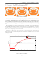
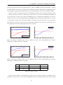
Scenario 1 - One HDV catching up one HDV . . . . . . . . . . . . . . . . . . . . . . . . . . . .
38
5.2
Scenario 2 - One HDV catching up two HDVs . . . . . . . . . . . . . . . . . . . . . . . . . . . .
41
5.3
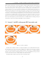
Scenario 3 - One HDV catching up two HDVs and the middle one has another destination . . . . .
44
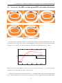
5.4
Scenario 4 - Two HDVs catching up one HDV . . . . . . . . . . . . . . . . . . . . . . . . . . . .
46
5.5
Scenario 5 - One HDV catching up one HDV from another road . . . . . . . . . . . . . . . . . .
48
5.6
Scenario 6 - One HDV catching up one HDV with another destination . . . . . . . . . . . . . . .
49
Conclusions and Future Work
51
References
56
A User’s Manual
57
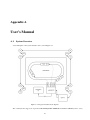
A.1 System Overview . . . . . . . . . . . . . . . . . . . . . . . . . . . . . . . . . . . . . . . . . . .
57
A.1.1 Key Features . . . . . . . . . . . . . . . . . . . . . . . . . . . . . . . . . . . . . . . . .
59
A.1.2 Who are we? . . . . . . . . . . . . . . . . . . . . . . . . . . . . . . . . . . . . . . . . .
60
A.2 Getting Started with the Tamiya Trucks . . . . . . . . . . . . . . . . . . . . . . . . . . . . . . .
61
A.2.1 T-Motes set up . . . . . . . . . . . . . . . . . . . . . . . . . . . . . . . . . . . . . . . .
62
xiv
CONTENTS
A.2.2 Trucks Set Up . . . . . . . . . . . . . . . . . . . . . . . . . . . . . . . . . . . . . . . . .
64
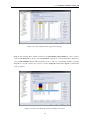
A.3 Getting Started with QTM . . . . . . . . . . . . . . . . . . . . . . . . . . . . . . . . . . . . . .
65
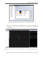
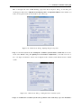
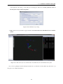
A.3.1 How to Define a truck as a 6DOF Body . . . . . . . . . . . . . . . . . . . . . . . . . . .
66
A.4 Trajectory Creation With Matlab . . . . . . . . . . . . . . . . . . . . . . . . . . . . . . . . . . .
71
A.4.1 Prerequisites . . . . . . . . . . . . . . . . . . . . . . . . . . . . . . . . . . . . . . . . .
71
A.4.2 Matlab Qualysis Client . . . . . . . . . . . . . . . . . . . . . . . . . . . . . . . . . . . .
71
A.4.3 Configuration File . . . . . . . . . . . . . . . . . . . . . . . . . . . . . . . . . . . . . .
72
A.4.4 Trajectory Creation . . . . . . . . . . . . . . . . . . . . . . . . . . . . . . . . . . . . . .
74
A.5 Getting Started with the LabVIEW Program . . . . . . . . . . . . . . . . . . . . . . . . . . . . .
77
A.5.1 Prerequisites . . . . . . . . . . . . . . . . . . . . . . . . . . . . . . . . . . . . . . . . .
78
A.5.2 Program Structure . . . . . . . . . . . . . . . . . . . . . . . . . . . . . . . . . . . . . .
79
A.5.3 Running the LabVIEW program . . . . . . . . . . . . . . . . . . . . . . . . . . . . . . .
82
A.6 Getting Started With The Visualization Tool . . . . . . . . . . . . . . . . . . . . . . . . . . . . .
85
A.6.1 Prerequisites . . . . . . . . . . . . . . . . . . . . . . . . . . . . . . . . . . . . . . . . .
85
A.6.2 Running The Visualization Tool . . . . . . . . . . . . . . . . . . . . . . . . . . . . . . .
87
A.6.3 Visualization Tool . . . . . . . . . . . . . . . . . . . . . . . . . . . . . . . . . . . . . .
89
A.7 Troubleshooting . . . . . . . . . . . . . . . . . . . . . . . . . . . . . . . . . . . . . . . . . . . .
93
A.7.1 Trucks . . . . . . . . . . . . . . . . . . . . . . . . . . . . . . . . . . . . . . . . . . . . .
93
A.7.2 Trajectory Creation . . . . . . . . . . . . . . . . . . . . . . . . . . . . . . . . . . . . . .
94
A.7.3 Visualization Tool . . . . . . . . . . . . . . . . . . . . . . . . . . . . . . . . . . . . . .
94
xv
CONTENTS
xvi
Nomenclature
↵
Slope of the road.
⌘¯eng
Mean combustion efficiency in the engine.
Indicates whether fuel is injected into the engine or not.

Platooning incentive factor.
Fuel consumed ratio.
Air drag parameter.
⇢a
Air density.
⇢d
Energy density of diesel fuel.
Aa
Frontal area of the vehicle.
cD
Air drag coefficient.
cr
Roll resistance coefficient.
Fb
Braking force.
fc
Instantaneous fuel consumption.
Fg
Gravity force.
Fr
Roll resistance force.
Fad
Air drag force.
Feng
Engine force.
g
Acceleration of gravity.
m
Accelerated vehicle mass.
T
Total time.
v
Vehicle speed.
xvii
CONTENTS
xviii
Acronyms and Abbreviations
ADR
Air Drag Reduction.
DOF
Degrees Of Freedom.
GPS
Global Positioning System.
HDV
Heavy Duty Vehicle.
IR
Infra-Red.
LUT
Look-Up Table.
MoCap
Motion Capture System.
PID
Proportional-Integral-Derivative.
QTM
Qualisys Track Manager.
RT
Real-Time.
SML
Smart Mobility Lab.
V2I
Vehicle-to-Infrastracture.
V2V
Vehicle-to-Vehicle.
xix
Acronyms and Abbreviations
xx
Chapter 1
Introduction
1.1
Motivation
T
he world financial crisis, especially the European financial crisis, triggered the emergence of the need
for more sustainable and efficient economies. The world population will exceed more than 8 billion
people in less than 15 years meaning that the need of goods will grow at least at the same rate [12]. In
rapid growing economies, like in some developing countries, the need of good growth rate could be even bigger.
Consequently, the traffic intensity will continue increasing making traffic congestions a major concern for decision
makers. Furthermore, predictions indicate that the classification of road traffic injuries will jump from the 9th place
in 1990 to the 3rd place in 2020 in the ranking of causes of the global burden of disease [24].
Studies done by the European Commission, described in [11], show that traffic congestions cost Europe about
1% of the European Union’s (EU) gross domestic product (GDP) every year. The transport industry is heavily
dependent on imported oil and this is another major problem since the oil price is expected to double its price in
less than 20 years. In the EU, the transport industry depends on oil for more than 96% of its energy needs. The
transport industry is responsible for about a quarter of the EU’s greenhouse gas emissions where 71.3% was the
share of road transport in 2008 and this industry is the main contributor of the increase in oil consumption in the
last decades. The transport industry is the backbone of today’s modern economy, directly employing more than
10 million people in the EU, accounting for 4.5% of total employment, and represents 4.6% of EU’s GDP. The
increasing emissions CO2 and the greenhouse effect problems are part of a very actual discussion and while most
sectors have been reducing CO2 emissions, transport’s quota continues increasing.
Naturally, a lot of research and work has been done during the last few decades to reduce these greenhouse
gas emissions. Consequently, the long haulage vehicles have been reducing the fuel consumption every year
which, naturally, yields to less pollution. The vast majority of the approaches taken in the last decades to the
above problems has been purely technical in the sense of optimizing the efficiency of engines or to produce lighter
vehicles, electric cars or hybrid cars. However, stricter requirements about the vehicle emissions in Europe mean
that other ways of reducing the fuel consumption must be found. Hence, in parallel with these approaches, research
about intelligent transport systems is being developed. In the 1960’s and 1970’s emerged the idea of driving in
1
1.1. MOTIVATION
formations, as platoons. In a platoon all vehicles drive close to each other taking advantage of the air drag reduction
due to the proximity to the vehicle ahead. Driving too close to a vehicle ahead at high speeds is not comfortable
for a human driver and sometimes not possible. However, it is feasible using automated navigation systems. It
was studied that in an ordinary life cycle of an European long haulage heavy duty vehicle (HDV), the fuel costs
represent almost one third of the total life cycle costs [4]. Since the air drag constitutes almost one fourth of the
total force that acts against an HDV it is very important to find ways to reduce it as much as possible. Aerodynamics
improvements were made on the HDVs but platooning is being in the last years studied as a major solution for
this problem. Research presented in [6] shows that it is possible to reduce the fuel consumption up to 7.7% when
platooning. Studies under the Safe Road Trains for the Environment (SARTRE) project [25] conclude that this
fuel reduction can potentially reach 20%, the road fatalities will be reduced by 10% and a smoother traffic flow
with potential increase in traffic flow. Well known researchers, such as Levine and Athans [17], Melzer and Kuo
[23] studied the problem control of vehicular platoons. However, it was only in the last decade that platooningenabling technology saw the light and made the implementation of such concepts feasible. Countless examples are
given in [6]: advanced driver assistance systems (ADAS), downhill speed control (DHSC), cruise control (CC),
adaptive cruise control (ACC) [15], information about the road grade [26] and communication technology such as
vehicle-to-vehicle (V2V) and vehicle-to-infrastructure (V2I).
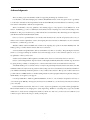
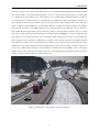
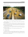
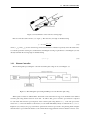
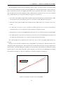
Figure 1.1: HDV platoon demonstration (courtesy of Scania).
2
1.2. BACKGROUND
1.2
Background
The idea of driving vehicles in formations, as platooning, is not new. However only a few decades ago the
technology that made it possible became available. The so called electronic control units (ECUs) are now faster,
cheaper and smaller because they are widely used, not necessarily only in the vehicle industry. Innumerable
examples can be given such as wireless networks, the Global Positioning System (GPS), temperature sensors, the
Anti-lock Braking System (ABS), the Electronic Stability Program (ESP), airbag, etc.
1.2.1
Vehicle Platooning
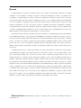
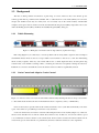
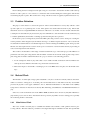
Figure 1.2: HDV platoon formation and air drag reduction (reprinted from [6]).
Platooning (Figure 1.2) is a smart way to solve the problems such as safety, traffic congestion, fuel consumption
and harmful exhaust emissions since its concept enables several vehicles to drive close to each other maintaining
all the security requisites. This way, each vehicle will use the so called slipstream effect, an atmospheric drag
reduction that occurs behind a traveling vehicle, consuming less fuel and consequently reducing the emissions.
Furthermore, it increases the traffic flow since the distance between vehicles is significantly reduced.
1.2.2
Cruise Control and Adaptive Cruise Control
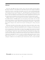
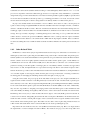
Figure 1.3: ACC is a cruise control system with enhanced functionality that helps the driver to keep a safe distance
to other traffic ahead and alerts the driver if manual intervention is required (courtesy of DAF trucks).
Cruise Control (CC) is present in almost all commercial vehicles. It is a system that automatically controls the
speed of the vehicle to a predefined speed reference set by the driver.
Some new vehicles have an extension of the CC called Adaptive Cruise Control (ACC) (Figure 1.3). ACC uses
the idea of CC but takes into account the vehicle ahead, if there is any. In that case, it lowers the vehicle’s speed
so it can maintain a reference distance to the vehicle ahead. In short, ACC is activated if an ahead vehicle in front
exists and its speed is lower than the one predefined by the driver. Otherwise it behaves as the original CC.
3
1.2. BACKGROUND
When platooning, the ACC is inherently present in the sense that the platooning HDVs maintain the same speed
as the HDV in front of them.
1.2.3
V2X Communication
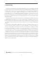
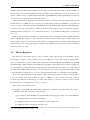
Figure 1.4: V2X Communication (courtesy of US Department of Transportation).
V2X is the combination of two types of vehicle communication: Vehicle-to-Vehicle (V2V) and Vehicle-toInfrastracture (V2I) (Figure 1.4).
V2V communication enables a vehicle to a 360 degree awareness of the position and speed of other vehicles. It
sends the driver warnings or advices in order to avoid crashes. This type of communication makes the platooning
possible, since every vehicle has the information of what is the status and intentions of the surrounding vehicles in
order to make driving adjustments accordingly.
V2I communication allows the vehicle to gather important information such as the traffic flow, traffic accidents,
road work ahead and information about the road grade. This can lead to fuel and time savings since the paths are
planned using more information.
As a result, V2X communication allows cooperative driving and automated platooning systems.
1.2.4
Platoon Catch Up
Today, HDVs are scattered on the road network and there are several ways to coordinate them in order to
platoon to reduce the fuel consumption. For example, rerouting the HDVs to align when the road merges ahead or
if the HDVs are on the same road then the leading HDV can slow down or the following HDV can catch up. In this
thesis, the catch up concept is studied in detail.
4
1.3. PROBLEM DEFINITION
Even reducing the fuel consumption when platooning, it is not trivial to decide when should a truck catch up
another in order to platoon or not. One has to consider the fuel consumed during the catch up phase and the fuel
saved during the platoon phase. This is where the concept of break-even ratio is applied (explained in Section 4.4).
1.3
Problem Definition
The purpose of this thesis is to answer the question ”when is it fuel efficient for a heavy duty vehicle to catch
up with a platoon?” in a practical point of view. This question was studied and answered in [19]. The models
that will be used are a longitudinal HDV model based on Newton’s second law of motion and the real-time fuel
consumption model studied in [21] and used in [19]. One will make use of the the break-even ratio defined in [19]
to evaluate quantitatively the benefits of catching up, thus answering the above question.
In this thesis project, an integrated system where HDV platooning scenarios can be developed, focusing the
catch up situation. This integrated system includes the usage of a Motion Capture System in order to track scale
model trucks in real time that are controlled throughout a road network using a LabVIEW program. Using a system
like this, the data acquired in the scenarios developed is converted into real-world values thereby representing in
scale, real world problems and situations.
The scenarios should address a wide range of situations within the scope of the catch up topic. The influence of
parameters such as the platooning distance and the number of trucks involved in the catch up phase and posterior
platooning phase should be studied. This thesis also proposes answers to the following questions:
1. Do the assumptions made in [19] such as flat road, no traffic and that accelerations will not influence the
catch up decision, influence the break-even point and the total fuel saved?
2. What is the impact on the benefits of catching up if one of the HDVs leaves the platoon in the middle of the
trip?
1.4
Related Work
The literature on vehicle platooning is quite substantial so only those works more directly related to this thesis
will be covered here. Among those one should point out a licentiate thesis on Automatic Control by Assad Alam
presented in [6] and a recent paper submitted to the 7th International Federation of Automatic Control (IFAC)
Symposium on Advances in Automotive Control by Kuo-Yun Liang, Jonas Mårtensson and Karl Henrik Johansson
[19].
Since most of the work will be done in the SML in KTH, Stockholm, the work done by Alejandro Marzinotto
[22] and the project course work for Automatic Control reported in [13] will be used as a starting point, especially
the work using Scania’s scale trucks.
1.4.1
Main Related Work
The focus of Alam’s research [6] is to establish and validate real constraints of fuel optimal control for platooning vehicles. The fuel reduction potential was investigated throughout simulation models and experimental
5
1.4. RELATED WORK
results that were derived from standard vehicles traveling on a Swedish highway. Fuel reduction of 4.7
7.7% was
proven to be dependent on the inter-vehicle time gap and does not compromise safety. Furthermore, a systematic
design methodology for inter-vehicle distance control based on linear quadratic regulators (LQRs) is presented and
it is shown that a decentralized controller provides a good tracking performance: it is robust, it lowers the control
effort downstream in the platoon and it is string stable for an arbitrary number of vehicles in the platoon.
In [19] it was studied whether it is beneficial or not for a HDV to drive faster in order to catch up and join
a platoon ahead. Using a longitudinal HDV model and a standard Scania fuel consumption model, a formula is
derived to calculate the break-even ratio. This ratio is defined as the distance ratio when neither driving alone nor
catching up a platoon ahead would be more feasible. Furthermore, simulations were made in order to forecast fuel
savings. It was proven that, comparing to continuing driving alone, a fuel saving of 7% is possible if the follower
vehicle decides to increase the speed from 80km/h to 90km/h in order to catch up and form a platoon with the
vehicle ahead when the distance to the vehicle ahead is 10km and the trip length is 350 km. These conclusions
are derived assuming flat road, no traffic and that accelerations will not influence the catch up decision break-even
ratio.
1.4.2
Other Related Work
In Marzinotto’s master thesis [22] an experimental testbed was developed to demonstrate several scenarios of
multi-agent systems such as platooning and surveillance using scale models of Scania trucks and quadrocopters.
Vehicle dynamics were studied and simulations and experiments were performed in the testbed. Both the hardware
and the software used is thoroughly explained. Besides the trucks and the quadrocopters, several T-Motes for
communication were used as well as infra-red (IR) sensors, Pololu boards to control the servos. In the thesis the
problem of creating a controller capable of forming a platoon of an arbitrary number of vehicles was approached
and, in order to do that, the implementation of a speed and a steering controller for each vehicle in a platoon and a
framework where it is possible to share information between them were described. Furthermore, an implementation
of a controller capable of removing any vehicle from the platoon except for the leader or inserting a vehicle into
an existing platoon rearranging the remaining vehicles in the same platoon was proposed.
Using the same testbed, the project group in the Automatic Control project course designed and built an integrated scenario which consisted in controlling wirelessly several scale models of Scania trucks, a quadrocopter
and a stationary tower crane. They designed and implemented Proportional-Integral-Derivative (PID) controllers
for the scale trucks and the quadrocopters and a Model Predictive Controller (MPC) for the crane. Additionally,
they were also responsible for designing a messaging scheme such that all the agents could communicate with
each other. Finally, the MoCap from Qualisys AB was used to retrieve the location information in each moment.
The MoCap offers an easy way to obtain accurate 3D and six degrees of freedom (DOF) position in real time. It
consisted of four cameras strategically placed in the lab and several passive IR markers. In the final scenario the
trucks were able to follow a certain path, navigate on the road network, arrive at a given destination and communicate with the crane and the quadrocopters. The trucks were also able to drive in platooning formation and avoid
collision with other trucks while on the road network that was also developed during the project.
Important work done in this area was also done by Macias in his master thesis [21]. Here, it is deeply studied
the requirements of a fuel consumption model for HDVs. Two methods were proposed: the look-up tables and
6
1.5. THESIS OBJECTIVES
real time calculations with a fuel consumption model. The goal of this study was to find eco-routes for HDVs, i.e
the route between two points that minimize the fuel consumption of the truck which is not necessarily the shortest
in time or distance. It was concluded that the Real-Time model (RT-Model) and the Oguchi Model were the best
ones. In fact, they are used in [19] as well as in this thesis.
Other research made by Alam [5] is worth mentioning since it is focused on the control methods that optimize
the fuel efficiency of a HDV due to the several road constraints like curvature speed limitations, road grade and
posted road speed. A non-linear model for the HDV was derived and Pontryagin’s Principle and LQR methods
were discussed. It was concluded that a switching controller based on optimal control and engineering experience
minimizes the fuel consumption 5 15%, and the brake wear by 5 15% while the traveling time is only increased
by 1
2%.
Liang in [18] considers the advantages of forming vehicle platoons, a LQR and a Linear Quadratic Tracking
(LQT) controller, with respect to a given information structure for a three-vehicle platoon. This resulted in an
energy reduction between 8.4% and 13.1% in the vehicles on a highway between Södertälje and Norrköping with
a time headway of 0.25 seconds. The energy consumption was assumed to be proportional to the fuel consumption
and it was used as cost value.
1.5
Thesis Objectives
The main goal of this master thesis is to show in practice, using scaled models of Scania HDVs1 , the implementation of solutions for the problem ”when is it fuel efficient for a heavy duty vehicle to catch up with a
platoon?” described in [19]. The scenario for the experiments is the Smart Mobility Lab (SML) located at KTH,
Stockholm. There, a Motion Capture System (MoCap) from Qualisys AB composed of 12 cameras is installed. A
lab environment is specially interesting for developing these experiments since one is able to try a huge range of
scenarios and possibilities without having to drive real trucks. It is a lot easier to experiment the feasibility of the
control algorithms and situations proposed on a controlled environment than on a real highway with real trucks.
Most of the available literature assumes that the vehicles are already in a platoon. However, that assumption
is not very realistic. Thus, when an HDV or a platoon of HDVs is on the road, the system must be able to
autonomously decide if it should catch up or not with other vehicle(s) or platoon(s), in known position, velocity
and trip destination, considering the pros and cons of doing so.
The work was divided in three phases:
1. designing, in partnership with another master student [9], a completely new testbed where it is possible to
simulate several different scenarios. This included:
(a) renovating the Smart Mobility Lab, which included increasing the working space and installing the
complete MoCap system with twelve cameras;
(b) designing a scaled road network on which the trucks are able to drive;
(c) building the entire road network on the lab’s floor;
1 For now one, the designation trucks will be used when referring to the scaled trucks and the designation HDV when referring to the real
trucks. The meaning should be obvious from the context.
7
1.6. THESIS CONTRIBUTIONS
(d) developing a program that creates the trajectories which the trucks are able to follow;
(e) developing a program that is able to control the trucks through the road network. The trucks should be
able to follow the trajectories created, do platooning with each other, overtake each other, change from
one road to another and stop due to virtual traffic lights;
(f) developing a visualization tool that can be used in demonstrations. It should be a real-time tool where
the position, speed and some other important informations appear in a form of plot, numbers or text
allowing the audience to understand what is happening in each moment.
2. developing and implementing demonstration scenarios where the HDV platoon catch up problem is clearly
stated and visualized. Different scenarios and theoretical improvements were proposed such as the catch up
of several trucks at the same time, the benefits of catching up for the entire platoon and possible fuel losses
due to the decision of leaving the platoon from one of the trucks. The data collected in the experiments using
the scale trucks is converted in real-time during the experiments in order to apply the real HDV and fuel
consumption models;
3. concluding about the testbed overall performance, the feasibility of all different scenarios and the possible
benefits of catching up.
The outcome of the thesis does not intend to be a new solution for the problem studied in [19] but to design,
implement and integrate such a simulation environment that complements the constraints of the Smart Mobility
Lab and make a realistic down-scaled demos of several different scenarios on this topic.
1.6
Thesis Contributions
• Development of HDV platooning scenarios, focusing the catch up situation, in the completely renovated
Smart Mobility Lab, in KTH, Stockholm;
• installation of the full complete MoCap system with twelve cameras strategically positioned;
• design and built a newly road network;
• development of a LabVIEW application giving a robust and stable control of the trucks while following and
driving on the road network. The trucks are able to:
– follow a predefined trajectory;
– change lane and road;
– platoon with each other with different platooning distances, i.e distance between two consecutive vehicles;
– overtake when the platoon master is changed in order to take the lead of the platoon;
– change speed to catch up;
– stop due to virtual traffic lights.
8
1.7. THESIS OUTLINE
• development of a visualization tool in MATLAB that allows audience-targeted demos. This visualization
tool includes all the relevant data of the running demo such as real speed, distance between trucks and fuel
consumption values;
• perform real-time demos with both the visualization tool and the trucks running simultaneously. Translation
of the scaled trucks data retrieved in the experiments to real trucks data in order to simulate fuel consumption.
The HDV platooning scenarios are used to demonstrate the feasibility and the phases involved in catching up
and platooning situation. Using real HDV models and their fuel consumption models, simulations were performed
in order to check the benefits of platooning and the data taken from the scenarios was analyzed. These simulations
were performed at the same time as the scale trucks drove on the road network. The real models were applied
scaling the trucks to real HDVs with all the assumptions that it implies.
Conclusions were drawn from the experiments where the parameters such as HDV, speed increment when
catching up and intermediate distance when platooning were different in each trial. It was concluded that:
• a single HDV has to travel to travel 8 to 15 times more than the initial distance that separates it from the
platoon, driving at constant speed of 80km/h, and it can save 5 to 13% of fuel depending if catching a single
HDV or a platoon already existent and if increasing the speed 12, 5% or 25%;
• it is less beneficial for a platoon already formed to decide to catch up another HDV;
• when one of the HDVs leaves the platoon the others either stay alone, if there was only one more HDV in the
platoon, or they continue platooning with the remaining HDVs of the previous platoon. The fuel benefits,
comparing to the situation when there is no HDV leaving the platoon, decrease for the HDVs that are behind
the HDV that leaves the platoon.
1.7
Thesis Outline
The outline of the thesis is as follows. In Chapter 1 the project developed in this thesis is clearly motivated.
The concept and the idea of platooning are explained together with the most important technologies that made it
possible. Furthermore, the problem dealt throughout this thesis is defined and the most important literature about
HDV platooning is reviewed in detail. The methods used and their conclusions are explained and an overview
about the influence of those works on this thesis is made. Finally, the objectives and contributions are enumerated.
In Chapter 2 the experimental setup in carefully presented and detailedly explained. The working principle of
the Motion Capture System, the camera positioning as well as the marker placement idea are explained. Then, the
communication between all the elements is overviewed. Finally, the design of the road network is then presented
as well as its usefulness.
In Chapter 3 the models used to control the trucks in the lab are introduced. The trucks’ kinematics are considered to be the same as car-like kinematics. The trucks’ PID controllers are then explained. In the end of the chapter,
the problem approached in this thesis is presented. Finally, the implementation of the speed, steering, platooning
and overtaking controllers is detailedly justified together with its performance and the calibration procedures.
9
1.7. THESIS OUTLINE
In Chapter 4 a longitudinal HDV model based on Newton’s second law of motion is considered and a simplified
fuel consumption model is introduced together with the model parameters typical values. Furthermore, from the
definition of fuel model, both fuel ratio and break-even ratio formulas are presented. Finally, the reasoning used
for scaling the results obtained with the scale trucks to the real HDVs is explained.
Chapter 5 addresses the development of six HDV platooning scenarios on the testbed. These scenarios are
supposed to represent HDV platooning situations, particularly the influence of the catching up decision. The
models previously described are applied in real time experiments and the parameters such as HDV and platooning
distance are changed and their influence evaluated. The scenarios cover a wide range of HDV platooning situations.
It is studied when it is good for a HDV to decide to catch up another and which are the more and less beneficial
cases. The results obtained are usually compared with theoretical results.
Finally, Chapter 6 provides the concluding remarks and future work ideas are provided.
10
11
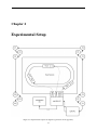
Chapter 2
Experimental Setup
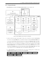
Figure 2.1: Experimental setup block diagram (reprinted from the appendix).
12
2.1. MOTION CAPTURE SYSTEM
A
s can be seen in Figure A.1 the developed testbed has several different elements. The system has up
to three PCs running at the same time, together with up to five trucks and the MoCap with twelve
cameras. This chapter is fully dedicated to all the technical details of the testbed development such as
how the communication between modules is accomplished and how are certain aspects implemented as well as
their performance.
For a less technical description and to learn how to use and start the system please refer to the User’s Manual
in appendix. Here, it is not intended to detail material specifications, to understand that refer to [22] and [10].
This experimental setup was developed in partnership with other master student and his thesis also makes use
of the testbed [9].
2.1
Motion Capture System
Figure 2.2: MoCap camera (courtesy of Qualisys AB).
The MoCap is constituted, in this testbed, by twelve cameras provided by Qualisys AB strategically positioned
in the SML. It is used as an indoor global positioning system (GPS) and it is used for 6DOF real-time tracking
of the trucks. The cameras are connected to a central computer running the Qualisys Track Manager (QTM) that
provides the cameras’ information to the other PCs.
2.1.1
Working Principle
The working principle of MoCap is similar, in fact, with GPS. It uses the principle of triangulation. In general,
only two cameras are sufficient to know a 3D position of a point in space if both see that point and if the cameras
position is known. Consequently, twelve cameras is more than enough to determine 3D coordinates of points
in space. The cameras are infrared sensitive and the objects to be tracked are equipped with markers placed in
strategic positions. These markers are small IR-reflective spheres.
13
2.1. MOTION CAPTURE SYSTEM
2.1.2
Positioning of the Cameras
The twelve cameras are divided in four groups of three cameras. Each group of cameras is placed on the corners
of the SML since it is cuboid-shaped. In all groups each camera is pointing to strategic locations as represented in
Figure 2.3.
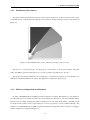
Figure 2.3: Smart Mobility Lab top-view. Cameras positioning setup on a corner.
The idea is to cover the whole space. In each group, two of the cameras cover the space using the orthogonal
walls of the SML as guidance and the third one covers the spot that is left empty by the other two.
The whole system must be calibrated once in a while since, even with twelve cameras, the noise inherent to the
utilization of the lab miscalibrates the system. The calibration is explained in detail onin [3].
2.1.3
Markers Configuration and Placement
To define a 6DOF Rigid Body in QTM at least three markers are required. The utilization of four markers is
recommended since if one marker is hidden, the system still has the other three to perform the 6DOF tracking.
This idea was used when designing the marker configurations for each truck. Each marker configuration must
be unique and the markers used for representing the X and Y axis must not form an equilateral triangle. The
definition of a 6DOF Rigid Body in QTM is explained detailedly in the appendix. The procedure for designing a
marker configuration is explained in Figure 2.4.
14
2.2. COMMUNICATIONS
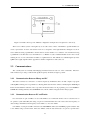
Figure 2.4: Truck’s cabin top-view. Markers configuration example and consequent axes of the body.
The local coordinate system of the rigid body is set at the center of mass of all markers. Specific markers are
used to represent the X and Y axis and the Z axis is a consequence of the right-hand rule. In Figure 2.4, the X
axis is defined as being a parallel line to the line that crosses the markers 1 to 2 and the Y axis is defined as being
a parallel line to the line that crosses the markers 1 to 3. Marker 4 is just a redundant marker used for more robust
tracking in case of some other marker is hidden, as explained before. The definition of a 6DOF rigid body in the
QTM is thoroughly explained in the appendix for marker configurations such as this one.
2.2
Communications
The overall system is constantly interchanging information between each one of the constituents. The information must be up-to-date possible and the update frequency should be as high as possible.
2.2.1
Communication Between Mocap and PC
The twelve cameras are connected to a central computer by an Ethernet cable. On that computer a program
called QTM is running. It is responsible for collecting all the data from the cameras, identifying the 6DOF Rigid
Bodies and track them in real-time. Also, it provides the measured data over an proprietary protocol via TCP/IP or
UDP/IP. For fetching that data, the LabVIEW PC runs a client, which is integrated in the main program.
2.2.2
Communication Between PC and Trucks
For each truck one pair of T-Motes is used. The T-Motes are commercial wireless sensor nodes that run on
an operative system called Tiny OS. Using one pair for each truck makes the control easier since the frequency of
data sending is maximized. The frequency used is 10Hz, i.e, once each 100ms.
One T-Mote of each pair is USB-connected to the LabVIEW PC. There, the LabVIEW program sends the data
to the T-Mote using a serial forward. Then, the T-Mote sends the data wirelessly to its pair in a specific radio
15
2.3. ROAD NETWORK DESIGN AND CREATION
channel and ID. The other T-Mote of the pair is connected into a serial adapter board in the truck. Hence, the serial
board converts the signals from the T-Mote to serial signals. Finally, the Pololu board receives the serial signal and
outputs two pulse-width modulated servo signals that are sent to control the servos. In this case, only two out of
eight outputs of the Pololu board are used since only the speed and the steering are controlled.
2.2.3
Communication Between PC and Visualization Tool
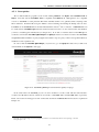
The visualization tool is a graphical user interface (GUI) application created in MATLAB in order to do demonstrations and to present real-time results and visualize the scenarios. In the LabVIEW PC a TCP/IP server is created
and initialized every time the program starts. Furthermore, a TCP/IP client was created in MATLAB. It can run
in every computer inside the KTH internet network. The message protocol is present on the User’s Manual in
appendix.
2.3
Road Network Design and Creation
Figure 2.5: Road network design.
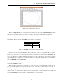
The road network that can be seen in Figure 2.5 was designed from scratch. It was designed in Google Sketch
Up and both real dimensions of the SML and the trucks were used in order to design a feasible road network.
2.3.1
Concept and Ideia
When picturing the road network the idea was to create something scalable into the real world. To do so, all
available space in the SML was used. The main and outer dual lane road are supposed to represent either a road
with two lanes used in opposite directions or a highway with two lanes both in the same direction. The inner road,
the smaller one and single laned, is used to simulate a merging of two highways, for example. It connects itself to
the outer road using two connection roads.
16
2.3. ROAD NETWORK DESIGN AND CREATION
2.3.2
States Division and Trajectories
Figure 2.6: Transitions programming idea.
The designed road network has three states. The outer lane and the inner lane of the main road, and the single
lane of the inner road are state 1, 2 and 3 correspondently. There are allowed transitions between states 2 and 3
and vice-versa. Those transitions are made through the connection segments between the states. Those segments
are not described as being additional states though which the truck must pass. A matrix
was created in order to
describe the transitions between states. The idea behind the construction of the matrix is sketched in Figure 2.6.
The matrix diagonal contains the exit waypoint number of each state if there exists one, otherwise it contains
1.
The index ij of the matrix contains the waypoint of the state j that the truck should head to if it actually is in state
i, otherwise contains
1. For example, if the truck is driving on the inner lane, i.e state 2 and wants to go to the
inner road, i.e state 3, the truck must be driving towards the waypoint 5 of the state 2 ( (2, 2)) and then the truck
drives towards the waypoint 1 of the state 3 ( (2, 3)).
The final form of
is
2
6
6
=6
4
1
1
1
5
1
50
17
1
3
7
7
1 7
5
25
(2.1)
2.3. ROAD NETWORK DESIGN AND CREATION
18
Chapter 3
Control of the Trucks
3.1
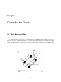
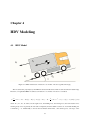
Truck Kinematics Model
The trucks used in the project are 1/14 scale models of the Scania V8 HDV. In order to be able to control those
trucks it is necessary to describe their kinematics. They can be approximated, without lost of generality, to car-like
vehicles. The back wheels are assumed to be used for traction and both front wheels behave as an equivalent single
steering wheel in between them. It is also assumed that there is no wheel slip. The control variables are the angular
speed of the back wheels and the steering wheel angle.
Figure 3.1: The notation used in the truck kinematics model.
19
3.2. TRUCK CONTROLLERS
Notation
Description
V
Linear velocity of the steering wheel in the robot coordinate system
Steering angle
✓
Orientation of the vehicle (yaw)
L
Length between the rear and front wheels axes
XW , YW and OW
World coordinate system
XT , YT and OT
Truck local coordinate system
Table 3.1: Truck kinematics model notation description.
From Figure 3.1 the differential truck kinematics are given by
2
ẋ
3
2
sin(✓)
6
7 6
6
7 6
6 ẏ 7 6 cos(✓)
6
7 6
6 ˙ 7=6
6 ✓ 7 6 tan( )/L
4
5 4
˙
0
3.2
0
3
72
3
7
0 7 V
74
5
7
0 7 !s
5
1
(3.1)
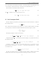
Truck Controllers
Since there are two control variables two different controllers were developed, one for the speed and other
for the steering of the truck. The system model, including the truck models, the transmission delays and possible
nonlinearities, was not deeply studied and a PID controller was used. Both the speed and the steering controller
are in the form
u(t) = KP e(t) + KI
Z
t
e(⌧ )d⌧ + KD
0
d
e(t)
dt
(3.2)
where u(t) is the control signal, KP , KD and KI are the proportional, differential and integral gains respectively
and e(t) is the error between the reference value and the actual value.
20
3.2. TRUCK CONTROLLERS
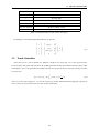
3.2.1
Speed Controller
The block diagram representing the PID speed controller can be seen in Figure 3.2.
Figure 3.2: Block diagram representing the PID speed controller.
The proportional control is adjusted so that the controller responds immediately to the error. The error is never
reduced to zero, i.e, there will be inherently present an offset error. This offset is removed using an integral term.
The integral term is essential since e(t) is zero when the truck speed reaches the reference speed meaning that
neither the proportional nor the derivative terms will influence the static error controller output. This way, the
integral part is responsible for maintaining the speed equal to the reference. In order to easily achieve stability,
the derivative control is introduced reducing the need of the proportional gain being large and to dampen out the
response oscillations.
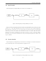
3.2.2
Steering Controller
The block diagram representing the PD speed controller can be seen in Figure 3.3. It is a PD controller since it
is only controlled the position of the steering wheel and consequently KI is zero.
Figure 3.3: Block diagram representing the PD steering controller.
21
3.2. TRUCK CONTROLLERS
Figure 3.4: Determination of the reference steering angle.
Here it is introduced the reference yaw angle, '. The reference yaw angle is calculated using
' = arctan(
yd
xd
yt
)
xt
(3.3)
where (xd ,yd ) and (xt ,yt ) are the desired waypoint and truck actual coordinates respectively. Since the trucks drive
at constant speed when steering it is assumed that controlling the steering is equivalent as controlling the yaw rate
directly itself then the steering angle is calculated using
=✓
3.2.3
'
(3.4)
Platoon Controller
The block diagram representing the controller used when platooning can be seen in Figure 3.3.
Figure 3.5: Block diagram representing the PID speed controller when platooning.
When a platoon master is defined all the other trucks on the same lane are supposed to maintain a user-defined
reference platooning distance between each other. To achieve that goal, a reference speed must be computed
for each truck. The reference speed depends on the reference platooning distance dref , on the real speed of the
master VM aster and on the distance to the master (or to the truck immediately ahead) of each truck DV ehicleAhead .
Equations (3.5) and (3.6) are proposed. In these equations the reference speed sent to the pursuing trucks is higher
than the master’s speed when the distance to the vehicle ahead is bigger than the reference distance and vice versa.
22
3.2. TRUCK CONTROLLERS
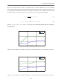
The reason for trying out these two functions is its different slope around the ”equilibrium point”. The ”equilibrium
point” corresponds to the reference platooning distance and master real speed used to compute the reference speed
for the pursuing trucks. In Figures 3.6 and 3.7 some examples of functions used to compute the reference speed of
the trucks in a platoon are represented. In Section 3.3.4 the choice of the equation used is justified.
Vref =
VM aster
DV ehicleAhead ;
dref
Vref = VM aster + (DV ehicleAhead
where Vref 2 [0.2; rv VM aster ]ms
1
(3.5)
dref )3 ;
(3.6)
where rv corresponds to how much faster the truck will drive comparing to
the master’s speed.
1.5
VMaster=0.4, Dref=0.8
VMaster=0.8, Dref=0.4
Equilibrium point
Vref
1
0.5
0
0
0.5
1
1.5
Distance to Master
Figure 3.6: Some examples of the function (3.5) used to compute the reference speed of the trucks in a platoon.
1.5
VMaster=0.4, Dref=0.8
VMaster=0.8, Dref=0.4
Equilibrium point
Vref
1
0.5
0
0
0.5
1
1.5
Distance to Master
Figure 3.7: Some examples of the function (3.6) used to compute the reference speed of the trucks in a platoon.
23
3.3. CONTROL ALGORITHMS DETAILS
3.3
Control Algorithms Details
The LabVIEW PC is responsible for controlling and for the decision making of the trucks on the road network.
The control of the trucks is, consequently, centralized in one single PC. It is assumed that the communications
V2V and V2I are instantaneous and that each truck knows all the time the exact position and speed of all other
trucks. The MoCap provides all the information needed for the trucks to be controlled. The implementation details
are explained in this section.
3.3.1
Controlling the Speed
Calibration
2
1.8
Empirical data
Linear function
1.6
speed (in m/s)
1.4
1.2
1
0.8
0.6
0.4
0.2
0
135
140
145
150
155
160
165
170
175
bits
Figure 3.8: Truck speed calibration function and empirical data.
The units used in the speed controller presented in Figure 3.2 are in m/s. However, the values sent to the truck
must be in the [0, 255] interval. With the purpose of converting the output of the controller from m/s to bits, a
calibration procedure was developed. Using a simple program, several values from 127 to 1751 were sent to the
truck and its real speed recorded in MATLAB. Then, using the curve fitting tool (cftool) of MATLAB, a linear
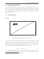
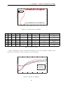
regression that better fitted the data was chosen (Figure 3.8). The function 3.7 was found.
Speedbits = 19Speedm/s + 135;
(3.7)
The assumption that the midrange value 127 was correctly set is made2 . One may ask why does the speed
0m/s does not correspond to the value 127. There is a deadzone in the interval [127, 135] that corresponds to
1 Below
2 How
127 the truck move backwards. Above 175 the speed saturates.
to set the midrange value is explained in the appendix.
24
3.3. CONTROL ALGORITHMS DETAILS
speed 0m/s. For that reason, when the controller output is within the interval [129, 135], the value sent is 135.
Bellow 129 it is sent 127. Only positive velocities, i.e. that make the truck move forward, are considered.
Controller Implementation
The MoCap only provides the coordinates of the position of the trucks. Therefore, to calculate the speed of
the truck one needs at least the current and the previous position of the truck as well as the time elapsed between
each measurement. So, the calculation of the actual speed of the truck is not directly given from the system but
computed simultaneously when computing the control values.
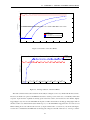
Performance
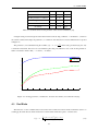
For the analysis of the speed controller (Figure 3.2) performance it is presented in Figure 3.9 the real speed of
a truck for two different reference speed values.
0.9
0.8
0.7
Speed (m/s)
0.6
0.5
0.4
0.3
Reference Speed
Real Speed
5% margin
0.2
0.1
0
0
5
10
15
20
25
30
Time (seconds)
Figure 3.9: Speed response of a truck.
In Table 3.2 some relevant performance indicators are summarized.
Overshoot
Settling time (5%)
Time constant, ⌧
10%
1.6s
0.6s
Table 3.2: Performance indicators for the speed controller.
The controller seems to behave very well. The real speed is maintained inside the limit ±5% every time except
the first one or two peaks. The overshoot is quite high but on the other hand the settling time is very fast.
25
3.3. CONTROL ALGORITHMS DETAILS
3.3.2
Controlling the Steering
Calibration
As for the speed, the units used in the steering controller presented in Figure 3.3 are in degrees, but the values
sent to the truck must be in the [0, 255] interval. With the purpose of converting the output of the controller from
degrees to bits, a calibration procedure was developed. Using a simple program, several values from 75 to 1753
were sent to the truck and the relative angle of the roads with the truck was recorded in MATLAB. Then, using the
curve fitting tool (cftool) of MATLAB, a linear regression that better fitted the data was chosen (Figure (3.10)).
The function 3.8 was found.
Steeringbits =
(3.8)
1.637Steeringdegrees + 127;
50
40
30
Empirical data
Linear function
steering angle (in degrees)
20
10
0
−10
−20
−30
−40
−50
50
100
150
200
bits
Figure 3.10: Truck steering calibration function and empirical data.
Once again, the assumption that the midrange value 127 was correctly set is made.
Controller Implementation
The MoCap automatically provides the yaw angle of the trucks. The reference yaw is directly calculated with
(3.3) and the steering controller model (Figure 3.3) is directly applied.
Performance
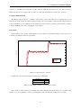
For the analysis of the steering controller (Figure 3.3) performance it is presented in Figure 3.11 the reference
yaw of a truck and its real yaw values when driving in one of the lanes of the road network.
3 Below
75 and above 175 the steering saturates.
26
3.3. CONTROL ALGORITHMS DETAILS
A small offset between the reference yaw angle and the real angles can be seen almost every time. This happens
in consequence of the controller design due to the absence of an integral part on the steering controller. This is not
a problem since the error is very small and has almost no influence in the road following.
200
150
Reference Yaw
Real Yaw
100
Yaw (Degrees)
50
0
−50
−100
−150
−200
120
122
124
126
128
130
132
134
136
138
140
Time (seconds)
Figure 3.11: Steering response of a truck.
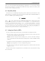
3.3.3
Driving on the road network
The trajectories on the road network are not fully described, i.e, the linear and angular speed are not defined in
each point. The trajectories are only described by waypoints. The waypoints are spaced approximately 30cm from
each other. The speed controller receives a reference constant speed. The steering controller receives the heading
of the next waypoint. Meanwhile, the waypoint for which the truck is heading to is computed. The truck should
head itself to the next waypoint when it is inside of a circle with 40cm of radius with the actual waypoint as center
(Figures 3.12 and Figures 3.13).
Figure 3.13: Heading to another waypoint.
Figure 3.12: Heading to a waypoint.
A simulation in MATLAB using the truck model and the control algorithms described in the Section 1.2 was
developed in order to find the approximate gains values for the controllers. After tuning the controllers in the real
trucks and road network, the gains values found are summarized in the Table 3.3.
27
3.3. CONTROL ALGORITHMS DETAILS
Gain
Steering Controller
Speed Controller
KP
1
1
KD
0.05
0.2
KI
0
3
Table 3.3: Reference controller gains values.
The values presented are reference values, since each truck is slightly different from each other and some
tuning around these values must be done.
3.3.4
Platooning
When a platoon master is chosen, all the trucks in the same state, i.e. lane, as well as the master are supposed
to maintain a user-defined reference distance to the truck ahead. One of the main aspects of this controller is the
distance between trucks calculation. The distance between trucks is measured along the trajectory of the lane. This
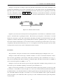
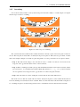
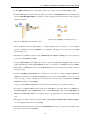
is achieved by measuring the Euclidean distance between waypoints in between each truck (Figure 3.14).
Figure 3.14: Method for calculating the distance between each truck.
The distance between trucks D is calculated according to (3.9).
D = d1 sign(cos('b )) +
N
X1
dn
dN sign(cos('a ))
(3.9)
n=2
where dn with n 2 [2, N
1] are the distances between waypoints in between each truck, d1 and dN are the
distance from the truck behind to its closest waypoint and the distance from the truck ahead to its closest waypoint
respectively. They are multiplied by sign(cos('b )) and sign(cos('a )) respectively in order to guarantee that it is
the total distance between trucks. 'b and 'a are the angle to the closest waypoint for the truck behind and the truck
ahead respectively. For instance, when the closest waypoint to the truck ahead is in front of it, the distance from
that waypoint to the truck must be subtracted from the total distance. The computation of the distance between
trucks is done very often, but the distances between waypoints are fixed from the moment the trajectories are
created. When the trajectories are created, a look-up table (LUT) with the distances between each waypoint is
created. This way computation time and effort is significantly reduced. So instead of calculating the second term
of (3.9), the LUT is accessed and only the first and the third are calculated.
When there are more than two trucks in a platoon the distances between the trucks are calculated as well. First
the distance to the platoon master is calculated, then if there are any trucks in between, the distance of the truck
ahead to the master is subtracted to its own distance to the master so the remaining is distance to the truck ahead.
28
3.3. CONTROL ALGORITHMS DETAILS
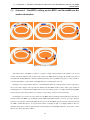
In Figure 3.15 represents an example of platooning with three trucks with the master truck. In that figure, each
truck has a fixed ID number just to be able to manipulate each one of the trucks in terms of programming language.
Each time a platoon is formed, an array is created with all the trucks’ ID in the platoon appearing in order. In this
case, the so called platoon array is 2
5
. Another array is created where the distance of each truck
3
to the truck ahead is placed in the index that corresponds to the truck’s ID. The distance to master array is in this
case:
D3
D5 .
Figure 3.15: Distances between trucks.
Equations (3.5) and (3.6) were already referred as being alternative control functions to calculate the reference
speed for the trucks that are pursuing the master. That reference speed depends on the distance to the truck
ahead and on the master’s speed. The control function with better performance was the linear function (3.5). The
explanation is that the cubic function is approximately linear around the ”equilibrium point”, i.e the point where
the reference distance and the master’s speed is achieved. However, this linear approximation has a very low slope
comparatively with the linear function proposed. As a consequence, the lower the slope the lower the control
reactivity and it is harder for the system to maintain the reference distance.
Performance
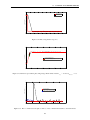
The performance of the platoon formation can be commented analyzing the plots in Figures 3.16 to 3.18.
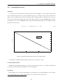
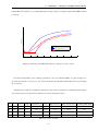
In Figure 3.16 the truck is first trying to maintain a distance of 3 meters to the master and then 0.3 meters.
One can see the approximation to the reference value with a constant slope due to the limitation of 1.25VM aster
imposed to the pursuing truck. Then, the distance is maintained quite well with a mean absolute error (MAE) of
0.02m and a mean squared error (MSE) of 5 · 10
4
m.
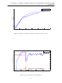
In Figure 3.17 shows how the reference speed for the platooning truck is calculated. Using a function as (3.5)
the reference speed is calculated depending on the master speed and distance to it.
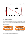
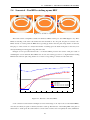
Figure 3.18 shows the performance of a case where three trucks are platooning (Scenario 3, Section 5.3). The
second truck, i.e. the middle one, leaves the platoon for some reason. The third and last truck must maintain the
predefined distance to the truck ahead and it has to fill the gap left empty by the truck that left the platoon. In this
case, the middle truck leaves the platoon around the 52nd second of the simulation and it is quite noticeable the
peak in the distance to the truck ahead. Then, it speeds up in order to maintain the reference platooning distance
to the first truck.
29
3.3. CONTROL ALGORITHMS DETAILS
3.5
Reference Distance
Real Distance
3
Distance (meters)
2.5
2
1.5
1
0.5
0
20
40
60
80
100
120
140
160
180
200
220
Time (seconds)
Figure 3.16: Platooning distance response.
1
0.9
0.8
0.7
Speed (m/s)
0.6
0.5
Real speed during platooning
Reference speed during platooning
Desired speed and distance to master when platooning
0.4
0.3
0.2
0.1
0
0
0.5
1
1.5
2
2.5
3
3.5
Distance to Master (meters)
Figure 3.17: Reference speed when platooning using a linear function with dref = 0.3 and VM aster = 0.6.
1.2
1.1
1
Distance (meters)
0.9
Reference Distance
Distance to truck ahead for the 3rd truck
Distance to truck ahead for the 2nd truck
0.8
0.7
0.6
0.5
0.4
0.3
0.2
40
50
60
70
80
90
100
Time (seconds)
Figure 3.18: The 2nd truck leaves the platoon. The 3rd has to maintain the distance to the truck ahead.
30
3.3. CONTROL ALGORITHMS DETAILS
3.3.5
Overtaking
One of the most fancy features of the system developed is the trucks’ ability to overtake. Figure 3.19 depicts
the three steps needed for overtaking.
Figure 3.19: The 3 steps for overtaking.
The system decides that a truck should overtake when there is already a platoon and a new platoon master is
chosen. The new platoon master had to be already in the previous platoon. Then, three steps are made. Assume
that, as the example of Figure 3.19, truck 2 is platooning truck 1. At some point, truck 2 is set as platoon master.
• Step 1. The truck 2 must change to the other lane in order to overtake. For that, it is chosen the closest
waypoint of the opposite lane that is in front of the new master;
• Step 2. While overtaking, the truck speeds up and the Euclidean distance between the new master and the
previous master do is constantly being evaluated. When that distance is do > dref + margin the new master
chooses again the closest waypoint of the opposite lane to re-enter as the platoon master.
• Step 3. The new master is now the actual platoon master and the other truck will follow it.
This works for more than two trucks. The new master, already in the platoon, will overtake all the trucks in
front of it until the previous master has been overtaken. Moreover, if the new master exits the middle of the platoon
for overtaking, the platoon would rearrange itself in order to maintain the reference distance between trucks.
31
3.3. CONTROL ALGORITHMS DETAILS
32
Chapter 4
HDV Modeling
4.1
HDV Model
Figure 4.1: HDV model based on Newton’s second law of motion (reprinted from [6]).
The model used in [19] and [21] is the HDV model used in this thesis. This model is described in detail in [6].
Therefore, a longitudinal HDV model based on Newton’s second law of motion is considered:
m
dv
= Feng
dt
Fb
Fad (v)
Fr (↵)
Fg (↵) = Feng
Fb
1
⇢ a Aa c D v 2
2
mgcr cos(↵)
mg sin(↵) (4.1)
where Feng , Fb , Fad , Fr and Fg are the engine force, the braking force, the air drag force, the roll resistance force
and the gravity force respectively. For the sake of simplicity and since all the scenarios do not include braking it is
considered Fb = 0. Additionally, m denotes the accelerated vehicle mass, v the vehicle speed, ↵ the slope of the
33
4.2. FUEL CONSUMPTION MODEL
road, ⇢a the air density, Aa the frontal area of the vehicle, cD the air drag coefficient, g the gravitational force and
cr the roll resistance coefficient. In all scenarios considered the road is assumed flat, therefore ↵ = 0.
The model can also be described as a distance based model
m
where
ds
dt
dv ds
= Feng
ds dt
Fad (v)
Fr (↵)
(4.2)
Fg (↵)
= v. Furthermore, we can derive the expression for Feng
Feng = m
4.2
Fb
dv
v + Fb + Fad (v) + Fr (↵) + Fg (↵)
ds
(4.3)
Fuel Consumption Model
The fuel consumption model studied in [21] and used in [19] is the model used in this thesis to evaluate the
fuel consumption behavior:
fc =
⌘¯eng ⇢d
(4.4)
vFeng
where fc [ml/s] denotes the instantaneous fuel consumption, ⌘¯eng the mean combustion efficiency of the engine,
⇢d the energy density of diesel fuel and indicates whether fuel is injected into the engine or not with
8
< 1
=
: 0
if Feng > 0
(4.5)
otherwise
The total fuel consumption over time T is also derived as:
fc =
Z
T
⌘¯eng ⇢d
0
Using the knowledge that
ds
dt
v(t)(m
dv
1
v + ⇢a Aa cD v 2 + mgcr cos(↵) + mg sin(↵)) dt.
ds
2
(4.6)
= v we can rewrite the total fuel consumption so it is distance based where D is
the total distance traveled.
fc =
Z
D
0
⌘¯eng ⇢d
(m
dv
1
v + ⇢a Aa cD v 2 + mgcr cos(↵) + mg sin(↵)) ds.
ds
2
(4.7)
Considering no acceleration or deceleration, that the initial and final velocities are equal, that the road is flat
and introducing the air drag parameter
2 [0, 1] where
no air reduction we get:
fc =
Z
D
0
= 0 means 100% air drag reduction and
= 1 means
1
( ⇢a Aa cD v 2 + mgcr ) ds.
⌘¯eng ⇢d 2
(4.8)
The values of the parameters used for a typical HDV are presented on Table 4.1. With these values, the fuel
consumption that is induced by the air drag is 42% while the remaining part is induce by roll resistance.
34
4.3. FUEL RATIO
Parameter
Symbol
Value
Unit
Vehicle Mass
m
40000
kg
Rolling resistance coefficient
cr
Air drag coefficient
7 · 10
cD
0.6
-
Front area
Aa
10.26
m2
Air density
⇢a
1.29
kg·m
3
-
3
Table 4.1: Nominal vehicle model parameter values used for simulations [26].
Using the study presented in [6] about the relation between the air drag coefficient cD and distance, d, between
the vehicles a function that maps the parameter
as a function of the distance was created. That function is plotted
in Figure 4.2.
The parameter
was calculated using the formula (d) = 1
(d)
0.8 cD100
. In the study presented in [6] it is only
considered frontal wind, therefore it is reasonable that platooning only influences 80% of the air drag reduction.
Other consideration made is that
= 1 when d > 60 meters.
1
Lead HDV
One HDV ahead
Two HDVs ahead
0.9
0.8
φ
0.7
0.6
0.5
0.4
0.3
0.2
0
5
10
15
20
25
30
35
40
45
50
Relative distance in convoy (meters)
Figure 4.2: Air drag parameter
4.3
and distance d between the vehicles (reconstructed from [6]).
Fuel Ratio
The fuel ratio
is the normalized ratio between the fuel consumed from the moment in which the decision of
catching up the truck ahead is made and the fuel consumed if the trucks had opted to continue alone.
(s) = 1
1
2
2 ⇢a Aa cD vcp (s) (dr ) + mgcr
1
2
2 ⇢a Aa cD va (s) + mgcr
35
(4.9)
4.4. BREAK-EVEN RATIO
where va (s) is the velocity that the truck would maintain if it continued alone, vcp (s) is the velocity it assumed
after the decision was taken and dr is the distance between HDVs. The subscript a stands for alone whilst cp stands
for the two moments: catching up + platooning.
4.4
Break-Even Ratio
The break-even ratio for the HDV platooning catch up problem is defined in [19] as the distance ratio when
neither driving alone nor catching up a platoon ahead would be more feasible. There, a mathematical definition of
this ratio for one HDV in a platoon catching up is derived.
dd
rv rv2
=
dp
rv 1 1
where rv =
vc
vp
(4.10)
> 1 and vc stands for the speed of the HDV when catching up and vp stand for the speed of the
HDV when platooning. The distance to the destination for the following HDV dd = Ta va and the distance between
both platoons at the moment the decision is made dp = Tc (vc
vp ) is also introduced. Basically, rv corresponds
to how much faster the driver or the system is willing to drive. The derivation of this break-even ratio assumes that
the speed is constant both in the catch up and in the platooning phase, that the leading and pursuing HDV(s) are
driving at the same speed when the decision to catch up is made and that va = vp .
4.5
Scaling from Trucks to HDVs
In order to convert the values used in the scenario to real-world values some assumptions are made.
• The platoon master is assumed to be always traveling at constant speed of 80km/h and the speed of the
other trucks is always calculated comparing to this value.
Example: In the lab, if the platoon master is traveling at 0.6m/s and some other truck is traveling at
0.75m/s it means that in real-world scale the master is traveling at 80km/h and the other HDV is traveling
at 100km/h.
• In simulation, the reference platooning distance is 30 times bigger than the one used in the lab.
Example: A platooning distance of 0.3 meters is simulated as being 9 meters.
• The ADR is assumed to be null for platooning distances bigger than 60m, otherwise the values of the model
in Figure 4.2 are used.
The fuel model (4.8) and the consequent fuel ratio (4.9) and break-even ratio (4.10) only make sense using
these converted values.
36
Chapter 5
Experimental Scenarios and Results
I
n this chapter HDV platooning scenarios focusing on the catch up problem are presented. Those scenarios
were implemented within the laboratory space constraints and the data is converted to real-world scale and
used in simulations related to the fuel models and the air drag reduction (ADR) to be made.
A scenario is a predefined set of actions using the experimental setup described in Chapter 2. The trucks
are autonomously controlled, the only things that are predefined are the reference speed, the reference platooning
distance and the lane where the truck should be.
The fuel consumption analysis can also be performed with only a simulation-based approach instead of converting the values from the trucks to real-world values. However, the focus in this thesis is to be able to use the
data retrieved from the experiments with the scale trucks as if they were real HDVs. So, the conclusions taken
about the fuel consumed and the comparisons with theoretical results give an insight of the system’s performance
and of the conversions made.
On the X axis of the plots represented for each scenario, is represented the ratio dd/dp in order to make the
plots comparable with the plots in [19]. This ratio represents the total distance traveled by the truck comparing to
the initial gap between the HDVs. For example, dd/dp = 25 means that the HDVs have traveled 25 times more
than the initial distance that separated them. The results related to the fuel ratio
ratio dd/dp.
37
are presented in terms of the
5.1. SCENARIO 1 - ONE HDV CATCHING UP ONE HDV
5.1
Scenario 1 - One HDV catching up one HDV
Figure 5.1: Scenario 1 explanation.
The first scenario exemplifies a situation of a single catch up (Figure 5.1). Two HDVs are traveling on the same
road and have the same destination. At some point, the HDV that is far away from its destination decides to catch
up with the HDV ahead speeding up until a reference platooning distance is achieved. The purpose of this scenario
is to analyze the benefit of catching up on an individual perspective, either for the leading HDV as for the catching
HDV.
The plots in Figures 5.2, 5.3 and 5.4 represent the fuel ratio
for both HDVs, the total fuel consumption for
the catching HDV and the ADR for both HDVs respectively. These plots result from simulating the case on which
both HDVs have 40 tons, the catch up speed is 12.5% higher than the leading HDV and the reference platooning
distance is 0.15m corresponding to 4.5m in real-world scale.
In Figure 5.2, two different types of lines are represented: a solid and dashed line. The solid lines represent
the data acquired and processed while running the scenario in real time. The dashed lines represent the theoretical
results proposed in [19].
15
Lead HDV
One HDV Ahead
Lead HDV − Kuo−Yun‘s Experiment
One HDV Ahead − Kuo−Yun‘s Experiment
10
Fuel Saved (%)
5
0
−5
−10
−15
0
5
10
15
20
25
30
dd/dp
Figure 5.2: Fuel ratio of both HDVs.
38
35
40
45
5.1. SCENARIO 1 - ONE HDV CATCHING UP ONE HDV
The main differences between the data acquired from the scenarios (solid lines) and the result obtained using
the model in [19] (dashed lines) are that for the leading HDV it is considered that it benefits as well for being in a
platoon; the break-even point occurs slightly earlier than in [19]’s experiment; if the scenario continued for longer
time and distance the saved fuel calculated would be smaller than the expected since the slope of the calculated
ratio is smaller than the one in [19]. These differences happen for several reasons:
1. the scenario starts with the truck speeding up until it reaches the catching up speed, which means that, unlike
the experience in [19], the catching up speed is not considered constant during the catch up phase;
2. during the catch up phase the HDV starts benefiting from the ADR, which is not considered in [19]’s experience;
3. for demo purposes and due to space constraints, the initial gap cannot be too big and consequently the
catching up phase is not very large when compared with the total distance traveled;
4. during the platoon, the speed of the HDV behind in the platoon is not constant and equal to the leading HDV;
5. the ADR assumed to represent the theoretical plot is the mean of the total ADR during the experiment and
the ADR of the following truck is not constant as assumed in the theoretical model.
The fourth and fifth reasons explain why the scenario ratio slope is, in the end, slightly smaller than the one
expected.
In Figure 5.3 the total fuel consumption of the pursuing HDV is represented. Two different moments can be
distinguished when analyzing the plot. First, the instant fuel consumed if it had decided to catch up is higher than if
it had decided to continue traveling alone, resulting in a faster increment of the total fuel consumed in the catching
up phase. However, after a while, the benefits of platooning start to be noticed due to the ADR (Figure 5.4) making
the instant fuel consumption to decrease resulting in less total fuel consumption if catching up.
7
2.5
x 10
Normalized Fuel Consumption
2
Fuel if traveling alone
Fuel if decides to catch up
1.5
1
0.5
0
0
5
10
15
20
25
30
35
dd/dp
Figure 5.3: Total fuel consumed for the catching HDV.
39
40
45
5.1. SCENARIO 1 - ONE HDV CATCHING UP ONE HDV
45
40
Lead HDV
One HDV Ahead
35
Air Drag Reduction (%)
30
25
20
15
10
5
0
0
5
10
15
20
25
30
35
40
45
dd/dp
Figure 5.4: Air drag reduction of both HDVs.
m
rv
dref
dd/dp
Expected dd/dp
(25)
Expected (25)
Platoon mean (25)
Catching HDV ADR
40t
1.125
0.15m
14.7
15.3
6.5%
6.2%
4.4%
38%
40t
1.125
0.3m
14.5
16.6
5.3%
4.4%
3%
31.5%
60t
1.125
0.3m
15.6
16.7
3.6%
3.3%
2.1%
31.1%
40t
1.25
0.15m
10.4
12.2
9.3%
8.2%
5.8%
39.3%
40t
1.25
0.3m
11.6
13.6
6.7%
6.2%
3.9%
32.7%
60t
1.25
0.3m
12.1
13.6
4.9%
4.8%
2.8%
32.8%
Table 5.1: Scenario 1 results.
Table 5.1 summarizes the results of six different combinations of the scenario parameters. In Figure 5.5 the
fuel ratio for the whole platoon can be compared for those 6 combinations.
10
Normalized Fuel Consumption
5
0
rv=1.25, mt=40t, dref=0.3m
rv=1.25, mt=40t, dref=0.15m
−5
rv=1.25, mt=60t, dref=0.3m
rv=1.125, mt=60t, dref=0.3m
rv=1.125, mt=40t, dref=0.3m
rv=1.125, mt=40t, dref=0.15m
−10
−15
0
5
10
15
20
dd/dp
Figure 5.5: Fuel ratio of both HDVs.
40
25
30
5.2. SCENARIO 2 - ONE HDV CATCHING UP TWO HDVS
The analysis of Figure 5.5 and Table 5.1 is quite similar. The experimental results are very close to the theoretical previsions. With the experiments one may be tempted to conclude that the benefits of catching up are higher
in practice than those expected theoretically. This is correct, but only partially. The results, obtained in practice,
are achieved using very small distances when compared with real situations where hundreds of kilometers are
involved. However, these experiments can be analyzed as being a zoom analysis of what happens around 1 or 2
kilometers where both HDVs meet. This means that for very large scale the differences in fuel saving during this
period result in almost insignificant savings, even if they exist.
General conclusions can be also taken. The ADR for smaller platooning distances is higher due to the proximity
between HDVs. The heavier the HDV the less benefits it has in catching up. The faster the driver is willing to drive
in order to catch up, the sooner the benefits of platooning start to be noticed.
5.2
Scenario 2 - One HDV catching up two HDVs
Figure 5.6: Scenario 2 explanation.
The second scenario exemplifies a situation of a platoon single catch up (Figure 5.6). Three HDVs are traveling
on the same road and have the same destination. At some point, the HDV that is far away from its destination
decides to catch up with the two HDVs ahead speeding up until a reference platooning distance is achieved. The
purpose of this scenario is to analyze the benefits of catching up, especially comparing to the first scenario where
there was no platoon already formed.
The plots in Figures 5.7 and 5.8 represent the fuel ratio
and the ADR for the three HDVs respectively. The
total fuel consumption is very similar with the one represented in Figure 5.3. These plots result from simulating
the case on which the three HDVs have 40 tons, the catch up speed is 12.5% higher than the leading HDV and the
reference platooning distance is 0.3 meters corresponding to 9 meters in real-world scale.
As in the previous scenario and for the same reason, in Figure 5.7 two different types of lines are represented:
a solid and dashed line. One more color is represented in the plot since this scenario includes one more truck.
41
5.2. SCENARIO 2 - ONE HDV CATCHING UP TWO HDVS
15
10
Fuel Saved (%)
5
0
−5
Lead HDV
One HDV Ahead
Two HDV Ahead
Two HDV Ahead − Kuo−Yun‘s Experiment
−10
−15
0
5
10
15
20
25
30
35
40
dd/dp
Figure 5.7: Fuel ratio of the three HDVs.
45
Lead HDV
One HDV Ahead
Two HDV Ahead
40
35
Air Drag Reduction (%)
30
25
20
15
10
5
0
0
5
10
15
20
25
30
35
40
dd/dp
Figure 5.8: Air drag reduction of the three HDVs.
The main conclusions that can be drawn from the analysis of Figure 5.7 are very similar with the first scenario.
However, the break-even point for the HDV that decided to catch up occurs, in this case, considerably earlier than
expected. Apart from the explanations already given in the first scenario, the fact that now the ADR is slightly
bigger (Figure 5.8) since it is the third HDV in the platoon makes the benefit of catching up being higher than in
the first scenario case. This means that, the initial slope of
for the third HDV is bigger that the one for the second
HDV resulting in an even earlier break-even ratio (compare with Scenario 1, Section 5.1). From the same figure,
it can be also concluded that the HDV that was already platooning has a benefit of almost 13% of doing so and the
42
5.2. SCENARIO 2 - ONE HDV CATCHING UP TWO HDVS
leading HDV has a benefit of 1% assuming that they were platooning for a long time when the third HDV decided
to catch up.
15
10
Fuel Saved (%)
5
0
−5
Scenario 2: Two HDV Ahead
Two HDV Ahead − Kuo−Yun‘s Experiment
Scenario 1: One HDV Ahead
One HDV Ahead − Kuo−Yun‘s Experiment
−10
−15
0
5
10
15
20
25
30
35
40
dd/dp
Figure 5.9: Fuel ratio of the HDV that decided to catch up in scenario 1 and 2.
For better understanding of the catching up benefits for the second and third HDV of a platoon, Figure 5.9
represents the fuel ratio for both cases. It is clear from the plots that the third truck benefits more from catching
up, as expected.
In Table 5.2 the results of four different combinations of the scenario parameters are summarized. The analysis
of the results expressed on the table are similar to those made in the first scenario.
m
rv
dref
dd/dp
Expected dd/dp
(25)
Expected (25)
Platoon mean (25)
Catching HDV ADR
40t
1.125
0.3m
10.0
15.4
9.5%
6.0%
7.8%
38%
40t
1.25
0.15m
7.7
11.4
12.6%
9.6%
10.5%
44%
40t
1.25
0.3m
8.7
12.4
10.4%
8.0%
8.1%
38%
60t
1.25
0.3m
8.1
12.3
8.3%
6.3%
6.4%
39%
Table 5.2: Scenario 2 results.
43
5.3. SCENARIO 3 - ONE HDV CATCHING UP TWO HDVS AND THE MIDDLE ONE HAS ANOTHER
DESTINATION
5.3
Scenario 3 - One HDV catching up two HDVs and the middle one has
another destination
Figure 5.10: Scenario 3 explanation.
The third scenario exemplifies a situation of a platoon single catch up (Figure 5.10) similar to the second
scenario. The main difference here is that, in this scenario, the HDV that is traveling in the middle of the platoon
just behind the leading HDV has a different destination than the other two HDVs. The purpose of this scenario is
to analyze the influence of this detail on the HDV that had to catch the platoon before.
In Figure 5.11 is represented the fuel ratio
of the HDV that decided to catch up in this scenario comparing to
the second scenario. Figure 5.12 represents the ADR for the three HDVs in this scenario. These plots result from
simulating the case on which the three HDVs have 40 tons, the catch up speed is 25% higher than the leading HDV
and the reference platooning distance is 0.3 meters corresponding to 9 meters in real-world scale.
From Figures 5.11 and 5.12 it is clear when does the HDV that was traveling in the middle leaves the platoon.
On that moment, that HDV stops benefiting from the ADR and the HDV behind is forced to speed up to keep the
reference to the distance of the leading HDV. For that reason, the third HDV spends extra fuel on that moment and
the ADR is smaller than before. As expected, the benefit of catching the platoon is slightly smaller in this case
than if the whole platoon had the same destination. The benefit for the third HDV will tend to be the same as if the
platoon was only formed by two HDVs.
44
5.3. SCENARIO 3 - ONE HDV CATCHING UP TWO HDVS AND THE MIDDLE ONE HAS ANOTHER
DESTINATION
15
Scenario 2: Two HDV Ahead
Scenario 3: Two HDV Ahead
10
5
Fuel Saved (%)
0
−5
−10
−15
−20
−25
0
5
10
15
20
25
30
dd/dp
Figure 5.11: Fuel ratio of the HDV that decided to catch up in scenarios 2 and 3.
45
Lead HDV
One HDV Ahead
Two HDV Ahead
40
35
Air Drag Reduction (%)
30
25
20
15
10
5
0
0
5
10
15
dd/dp
Figure 5.12: Air drag reduction of the three HDVs.
45
20
25
5.4. SCENARIO 4 - TWO HDVS CATCHING UP ONE HDV
5.4
Scenario 4 - Two HDVs catching up one HDV
Figure 5.13: Scenario 4 explanation.
The fourth scenario exemplifies a situation in which two HDVs catch up one other HDV (Figure 5.13). Three
HDVs are traveling on the same road and have the same destination. At some point, the platoon consisted of two
HDVs decides to catch up with the HDV ahead, speeding up until a reference platooning distance is achieved.
The purpose of this scenario is to analyze the benefits of catching up for the trucks in the platoon since they were
already benefiting from being platooning with each other.
In Figure 5.14 is represented the fuel ratio
of the three HDVs present in the scenario. This plot results of
simulating the case in which the three HDVs have 40 tons, the catch up speed is 12.5% higher than the leading
HDV and the reference platooning distance is 0.3 meters corresponding to 9 meters in real-world scale.
20
15
Fuel Saved (%)
10
5
0
Lead HDV
One HDV Ahead
Two HDV Ahead
One HDV Ahead − Kuo−Yun‘s Experiment
Two HDV Ahead − Kuo−Yun‘s Experiment
−5
−10
−15
0
5
10
15
20
25
30
35
40
45
50
dd/dp
Figure 5.14: Fuel ratio of the three HDVs.
Some conclusions can be drawn from Figure 5.14. It is interesting to look only for the second and third HDVs,
since they are already in a platoon and they decided to catch up. The fuel ratio of the leading HDV of the platoon
that decides to catch up has the same behavior as in the other scenarios and consequently the same justifications
46
5.4. SCENARIO 4 - TWO HDVS CATCHING UP ONE HDV
given before apply here. On the other had, the fuel ratio of the second HDV of the platoon that decides to catch up
has different behavior than if it was catching up alone, naturally. During the catch up phase, this HDV still benefits
from being platooning and the benefit increases even more when the platoon become formed with three HDVs.
Figures 5.15 and 5.16 compare the fuel ratio of the HDVs in the platoon in the situation where they decided
to catch up and if they would have continued alone. The fuel ratio is presented for each HDV individually and
for the whole platoon. These plots result from simulating the case on which the three HDVs have 40 tons, the
catch up speed is 12.5% and 25% higher than the leading HDV and the reference platooning distance is 0.3 meters
corresponding to 9 meters in real-world scale. In Table 5.3 the break-even points for these two cases are presented.
The break-even point here is the moment where individually each HDV or the whole platoon benefit more from
the catching up decision than continue platooning just two vehicles.
20
15
Scenario 2: Total Fuel Saved
Scenario 4: Total Fuel Saved
15
10
Fuel Saved (%)
Fuel Saved (%)
10
5
0
5
−5
0
Scenario 2: Lead HDV
Scenario 2: One HDV Ahead
Scenario 4: Lead HDV (catching platoon)
Scenario 4: One HDV Ahead (catching platoon)
−10
−15
0
5
10
15
20
25
30
−5
35
0
5
10
15
dd/dp
20
25
30
35
dd/dp
Figure 5.15: Fuel ratio of HDVs in platoon (of two vehicles) in scenario 2 and 4. Individual fuel ratio on the left.
Whole platoon (2 HDVs) fuel ratio on the right.
20
15
Scenario 2: Total Fuel Saved
Scenario 4: Total Fuel Saved
15
10
10
Fuel Saved (%)
Fuel Saved (%)
5
0
−5
5
0
−10
−15
−5
Scenario 2: Lead HDV
Scenario 2: One HDV Ahead
Scenario 4: Lead HDV (catching platoon)
Scenario 4: One HDV Ahead (catching platoon)
−20
−25
0
5
10
15
20
25
30
−10
35
0
5
dd/dp
10
15
20
25
30
dd/dp
Figure 5.16: Fuel ratio of HDVs in platoon (of two vehicles) in scenario 2 and 4. Individual fuel ratio on the left.
Whole platoon (2 HDVs) fuel ratio on the right.
rv
dd/dp leading HDV
dd/dp One HDV ahead
dd/dp Platoon
1.125
16
22
17.5
1.25
12.5
26.5
15.5
Table 5.3: Scenario 4 results.
From the values in Table 5.3 and in Figures 5.15 and 5.16 it is clear that catching up is beneficial in these
particular cases. However, two cases must be distinguished and some comments must be made. For the leading
47
5.5. SCENARIO 5 - ONE HDV CATCHING UP ONE HDV FROM ANOTHER ROAD
HDV of the platoon that decides to catch up, the benefits are similar if caught up being alone and the break-even
ratio occurs at the same distance traveled. Furthermore, the second HDV of the platoon does not benefit that
much from the catch up decision. The whole platoon must travel considerably longer so that this HDV becomes
rewarded, otherwise it does not get any benefit from catching up when comparing with platooning with just one
HDV ahead. If the perspective is the whole platoon that decides to catch up it can be seen that the break-even
occurs in between the break-evens of the two HDVs individually. When taking this decision, the decision maker
must take into account that benefitting the leading HDV may not mean that the whole platoon benefits and this may
not mean that the second HDV benefits as well. The catch up speed also influences the break-even points. The
higher the speed increment the earlier the leading HDV benefits from catching up as seen in the other scenarios.
The novelty is that the higher the speed increment the later the second HDV benefits from catching up. The speed
increment has to respect a trade-off between which HDV one want to benefit more.
5.5
Scenario 5 - One HDV catching up one HDV from another road
Figure 5.17: Scenario 5 explanation.
The fifth scenario exemplifies a situation of a single catch up (Figure 5.17) very similar with the first scenario.
The main difference here is that, in this scenario, the HDVs start on different roads and the platoon formation
occurs on the road where the platoon master is driving. The purpose of this scenario is to simulate the different
alternatives of platoon formation, showing that the platoons do not occur only when HDVs are driving on the same
roads. Also, this scenario shows the coordination ability of the trucks in the testbed.
The analysis and the conclusions are the same as the ones in the first scenario.
48
5.6. SCENARIO 6 - ONE HDV CATCHING UP ONE HDV WITH ANOTHER DESTINATION
5.6
Scenario 6 - One HDV catching up one HDV with another destination
Figure 5.18: Scenario 6 explanation.
The sixth scenario exemplifies a situation of a single catch up (Figure 5.18) similar with the first scenario. The
main difference here is that, in this scenario, the leading HDV has a different destination than the pursuing HDV.
The purpose of this scenario is to analyze the influence of this detail on the HDV that decides to catch up.
10
Fuel Saved (%)
5
0
Lead HDV
One HDV Ahead
Lead HDV − Kuo−Yun‘s Experiment
One HDV Ahead − Kuo−Yun‘s Experiment
−5
−10
−15
0
10
20
30
40
50
60
dd/dp
Figure 5.19: Fuel ratio of the HDV that decided to catch up in scenario 1 and 6 with rv = 1.125. The Kuo-Yun’s
experiment plot was made without the platoon master leaving.
In Figures 5.19 and 5.20 it is represented the fuel ratio
of the HDVs. These plots result from simulating the
cases on which the HDVs have 40 tons, the catch up speed is 12.5% and 25% higher than the leading HDV and the
49
5.6. SCENARIO 6 - ONE HDV CATCHING UP ONE HDV WITH ANOTHER DESTINATION
reference platooning distance is 0.3 meters corresponding to 9 meters in real-world scale. In these plots it is clear
the moment where the master leaves the platoon and consequently both trucks continue alone.
The fuel ratio of the HDV that has decided to catch up is similar to the one plotted for the first scenario (Figure
5.2). Naturally, when the master leaves the platoon the ADR is 0% for both HDVs since they carry on alone. For
that reason, the farther the HDVs continue driving the less they benefit from the catch up decision.
15
10
5
Fuel Saved (%)
0
−5
Lead HDV
One HDV Ahead
Lead HDV − Kuo−Yun‘s Experiment
One HDV Ahead − Kuo−Yun‘s Experiment
−10
−15
−20
−25
0
10
20
30
40
50
60
70
dd/dp
Figure 5.20: Fuel ratio of the HDV that decided to catch up in scenario 1 and 6 with rv = 1.25. The Kuo-Yun’s
experiment plot was made without the platoon master leaving.
50
Chapter 6
Conclusions and Future Work
W
ith the purpose of designing, evaluating and showing HDV platooning situations and a testbed was
developed. The complete implementation of the testbed was described as well as the experiments
and results obtained using it. The system includes up to three PCs running at the same time, together
with up to five scale trucks and an indoor GPS (MoCap) composed of twelve cameras. The scale trucks drive
themselves on a road network design and built from scratch composed of two roads and three lanes.
In this thesis, the particular case of platoon catch up is studied. To form an HDV platoon the HDVs scattered
on the road network should merge in order to save fuel. There are several merging options but the one used in this
thesis is to catch up the HDV ahead. This means that the following HDV(s) need to speed up in order to catch up
some other HDV or platoon. The problem is to decide in which situations the fuel is actually saved since the catch
up part imply an extra-spending of fuel from some of the HDVs.
In order to design HDV platooning situations, several theoretical models and mathematical definitions were
introduced and explained: the HDV model, the fuel consumption model, the fuel ratio and the break-even ratio.
These models were used when translating from the simulated environment to the real-world dimensions, velocities
and ADR values. In the implementation part, the truck kinematics model and controllers were explained and their
performance evaluated.
The last part of this thesis is composed by the analysis of the scenarios developed in the testbed. These scenarios
represent several situations of HDV platooning, particularly the platoon catch up case. In this part, everything is
integrated in one big system in order to apply the models earlier introduced. The object of study was the saved fuel
due to platooning and the break-even point, i.e. the moment when neither driving alone nor catching up a platoon
ahead would be more feasible.
Some conclusions were drawn from the experiments where the parameters such as HDV, speed increment when
catching up and intermediate distance when platooning were being changed for each trial. When a single HDV
catches up other HDV the break-even point occurs 10 to 15 times the initial distance that separates them. Then, the
HDV that decides to catch up, can save 5 to 10% of fuel comparing to continue driving alone with an ADR around
35%. If a single HDV decides to catch up a platoon with two HDVs ahead, it only needs to travel 8 to 10 times
more than the initial distance that separates them and it can save 8 to 13% of fuel.
Finally, another study about if a platoon with two HDVs should catch another HDV or not was performed.
51
Comparing to the previous cases it is less beneficial to catch up since the platoon that decided to catch up has to
travel more than 15 times more than the initial distance that separates it from the other HDV to start benefitting.
Additionally, the HDV that leads that platoon benefits a lot more than the HDV that was already platooning. For
the latter, it has to travel more than 20 times more than the initial distance that separates the platoon where it is
driving from the other HDV so that the catch up decision is beneficial.
It is inherent to every big project the feeling that a lot more can be done in the future. The evolution of the
SML was tremendous in the last few months. To continue this evolution some of these ideas can be followed:
1. The existing road network is static. An idea is to make the road network dynamic and dependent on the
scenario localization wanted. First, that road would be projected on the floor of the lab. That road network
would be different according to the scenario localization. For example, the road topology and form used in
a trip from Gothenburg to Stockholm is pretty different than one from Munich to Amsterdam.
2. The road network is assumed flat. Another idea could be simulate the road different grade during a travel.
The HDVs have different behaviors in different topologies. It could be also interesting to simulate platooning
strategies in extreme situations, like uphill or downhill.
3. No traffic is assumed during the scenarios developed. It would be good to integrate simulated traffic on the
road network. Either on the static road network or in the future dynamic one. A big challenge would be to
develop strategies to catch up and to overtake in situations were traffic is a problem.
4. The strategy of platooning used in this thesis is to select one HDV as the platoon master. From that moment
a platoon is formed behind the master. There is no possibility in manually reordering the trucks without
setting one as master, i.e, there is no way of switching the positions of the second and the third trucks, for
example. A nice implementation to developed would be a graphical way to, manually, sort the trucks in real
time while driving on the road network.
5. There is no remote control integrated in the system. Another idea is to add a remote control to the system in
order to control the trucks. The idea is, even if the user sent an acceleration command, the ACC would be
activated if another truck was dangerously close.
6. The speed and steering controllers are independent. It would be very interesting to develop a controller for
trajectory tracking instead of waypoint following. This may influence the trajectory generation procedure.
7. Integrate the system with other vehicles, such as quadcopters. The quadcopters could work as traffic announcers to the trucks so they could make decisions based on the existing traffic.
8. Develop a path planning algorithm such that the trucks could be able to drive autonomously between two
distinct points in the road network.
52
Figure 6.1: HDV platoon demonstration (courtesy of Scania).
53
54
References
[1] Qualysis AB. QTM Getting Started, 2011.
[2] Qualysis AB. QUALISYS MATLAB CLIENT v1.8, 2011.
[3] Qualysis AB. QTM User Manual, 2011.
[4] Scania CV AB. Annual report, 2001.
[5] A. Alam. Optimally fuel efficient speed adaptation. Master’s thesis, KTH Royal Institute of Technology,
March 2008.
[6] A. Alam. Fuel-efficient distributed control for heavy duty vehicle platooning, 2011. Licentiate Thesis in
Automatic Control, KTH Royal Institute of Technology.
[7] A. Alam, A. Gattami, and K. H. Johansson. An experimental study on the fuel reduction potential of heavy
duty vehicle platooning. In 13th International IEEE Conference on Intelligent Transportation Systems, 2011.
Madeira, Portugal.
[8] A. Alam, A. Gattami, K. H. Johansson, and C. J. Tomlin. Establishing safety for heavy duty vehicle platooning: A game theoretical approach. In 18th IFAC World Congress, September 2011. Milan, Italy.
[9] J. P. Alvito. Implementation of traffic control with heavy duty vehicle anti-platooning. Master’s thesis, KTH
The Royal Institute of Technology, 2013.
[10] M. Amoozadeh. Smart Mobility Lab Manual, 2013.
[11] European Commission. Roadmap to a single european transport area, 2011. URL http://ec.europa.eu/
transport/strategies/facts-and-figures/index_en.htm.
[12] United Nations Population Division. World population prospects: The 2010 revision, 2010. URL http:
//esa.un.org/unpd/wpp/Excel-Data/population.htm. Department of Economic and Social Affairs.
[13] A. Hauksson, B. Mengana, C. Westermark, F. Svensson, J. Lycke, J. Sundberg, K. Imhäuser, and S. van de
Hoef. Final report in automatic control project course. Technical report, KTH The Royal Institute of Technology, December 2012.
[14] A. Hernandéz and D. Huertas Péres. Communication between pc and motes is tiny os. Technical report, KTH
The Royal Institute of Technology, may 2012.
55
REFERENCES
[15] P. Ioannou and C. Chien. Autonomous intelligent cruise control. IEEE Transactions on Vehicular Technology,
42(4):657 – 672, 1993.
[16] Y. Kanayama and B. Hartman. Smooth local path planning for autonomous vehicles. In IEEE International
Conference on Robotics and Automation, 1989. Proceedings., 1989, may 1989.
[17] W. Levine and M. Athans. On the optimal error regulation of a string of moving vehicles. In IEEE Transactions on Automatic Control, July 1966. Volume AC-11, no. 3.
[18] K-Y. Liang. Linear quadratic control for heavy duty vehicle platooning. Master’s thesis, KTH Royal Institute
of Technology, April 2011.
[19] K.-Y. Liang, J. Mårtensson, and K. H. Johansson. When is it fuel efficient for a heavy duty vehicle to catch
up with a platoon? Submitted to the 7th International Federation of Automatic Control (IFAC) Symposium
on Advances in Automotive Control, 2013.
[20] P. Lima. Implementation and analysis of platoon catch up scenarios for heavy duty vehicles. Master’s thesis,
KTH The Royal Institute of Technology, 2013.
[21] D. Macias. Estimation of fuel consumption for real time implementation. Master’s thesis, KTH Royal
Institute of Technology, 2012.
[22] A. Marzinotto. Cooperative control of ground and aerial vehicles. Master’s thesis, KTH Royal Institute of
Technology, 2012.
[23] S. M. Melzer and B. C. Kuo. Optimal regulation of systems described by a countably infinite number of
objects. In Journal Automatica, volume 7, pages 359 – 366, May 1971.
[24] World Health Organization. Global status report on road safety: Time for action, 2009. URL www.who.int/
violence_injury_prevention/road_safety_status/2009. Geneva.
[25] T. Robinson, E. Chan, and E. Coelingh. Operating platoons on public motorways: An introduction to the
sartre platooning programme. In In 17th World Congress on Intelligent Transport Systems, 2010. Busan,
Korea.
[26] P. Sahlholm. Distributed Road Grade Estimation for Heavy Duty Vehicles. PhD thesis, KTH Royal Institute
of Technology, 2011.
56
Appendix A
User’s Manual
A.1
System Overview
A block diagram of the system structure can be seen in Figure A.1.
Figure A.1: Program structure block diagram.
The overall system is supposed to represent a real-world system in small scale in which the cameras (C1,C2,...,C12)
57
A.1. SYSTEM OVERVIEW
simulate the GPS system, the LabVIEW PC simulates an onboard computer responsible for the decision making of the truck and, naturally, the scale trucks represent the real trucks. The T-Motes exist in order to make
possible the communication between the PC and the trucks. Moreover, the QTM PC is the server that provides the
trucks’ localization retrieved by the cameras. Finally, the Visualization PC is used for demonstration purposes.
This system was developed in the first semester of 2013 in the Smart Mobility Lab of the Automatic Control
Department in KTH in Stockholm under the supervision of Jonas Mårtensson and Karl Henrik Johansson. It
is the kernel of two master’s thesis, since it is the test bed for the experiments reported on them (see [20] and [9]).
58
A.1. SYSTEM OVERVIEW
A.1.1
Key Features
With the set of programs developed the user is able to:
• Use the IR markers to create a set of waypoints that possibly represents a trajectory, then acquires those
points and the correspondent interpolated trajectory with more waypoints (see Chapter A.4);
• Define the trucks as being 6DOF bodies using the Qualysis’ QTM software. This way it is possible to track
them in real time with 6DOF (see Chapter A.3);
• Use the trucks and do a wide range of operations from platooning, platoon catch up and overtaking to
traffic control with traffic lights (see Chapter A.5);
• Run a visualization tool that allows the user and the target audience to easily understand what is happening
(see Chapter A.6).
59
A.1. SYSTEM OVERVIEW
A.1.2
Who are we?
Figure A.2: The authors: Pedro Lima on the left side and João Pedro Alvito on the right side.
We are two portuguese master students in Electrical and Computers Engineering from Instituto Superior
Técnico, Lisbon, Portugal. We both came to KTH under an agreement between IST an KTH to take the Master
Program in Systems, Control and Robotics (TSCRM) at KTH as part of a Dual Degree. This agreement includes
doing our master thesis in KTH.
If you want to know more about this project or if you have any doubts don’t hesitate to contact us (pfrdal@
kth.se and [email protected]).
60
A.2. GETTING STARTED WITH THE TAMIYA TRUCKS
A.2
Getting Started with the Tamiya Trucks
The Tamiya Scania trucks are 1/14 scale trucks of the real Scania V8. They are naturally one of the most
important parts of the overall system.
This chapter provides a basic tutorial of how to connect and start the trucks and some troubleshooting.
For a more detailed description of the material involved please refer to [10].
61
A.2. GETTING STARTED WITH THE TAMIYA TRUCKS
A.2.1
T-Motes set up
Figure A.3: Connection between a PC and a T-Mote
Figure A.4: Connection between a truck and a T-Mote
(courtesy of [10]).
(courtesy of [10]).
In order to communicate with the trucks from a PC you need to know how to use the T-Motes. In the project
we use the serial-forward tool to send data from LabVIEW to the mote attached to the PC, and the Tiny OS to
program them. In order to learn how to install the Tiny OS and serial-forward tool please refer to [14].
In Windows, after having the Cygwin and the serial-forward tool installed, you should be able to see the
T-Motes connected to the PC (like in Figure A.5) using the motelist command.
Figure A.5: motelist command result on a Cygwin terminal.
The T-Motes usually have its reference number (for example: MTF4LX0A) printed on it. If they don’t,
please connect one by one to know which COM port corresponds to each them. Then, it is possible to start a serial
forward of a specific T-Mote in a specific TCP/IP Port like in Figure A.6. The port chosen has to be a suitable
port that is not being used by any other device. The most common ports used when serial forwarding are 9002,
9003, 9004... When trying to communicate, if everything is okay, you should start seeing something similar with
Figure A.7.
Figure A.6: sf command result on a Cygwin terminal.
Figure A.7: sf normal execution on a Cygwin terminal.
It is very important that you pay a lot of attention when doing serial-forward of a T-Mote in order to be able
62
A.2. GETTING STARTED WITH THE TAMIYA TRUCKS
to communicate correctly with a truck. A T-Mote connected to the PC has a unique pair connected to a truck.
The T-Motes used so far for that purpose are all labeled with ”<COLOR> PC <ID>” and ”TRUCK <COLOR>
<ID>”, where <COLOR> is the color of the truck and the <ID> is the communication ID1 of the truck. The
communication ID has to be inputed in the LabVIEW program (see Chapter A.5).
If you receive messages like ”Note: write failed” (see Figure A.9) or ”unix error” (see Figure A.8), try to
kill the serial forward with CTRL+C inside of the Cygwin terminal and restart the serial forward again. If it still
doesn’t work, try to disconnect and connect the corresponding T-Mote and restart the serial forward. Restart the
PC if nothing else works. Always check if the IDs and COM ports you inserted in the LabVIEW program
correspond to the T-Motes you are using.
Figure A.8: sf ”unix error” example.
Figure A.9: sf ”Note: write failed” example.
If everything is okay you should see the T-Motes’ leds blinking stressfully when you try to transmit something
through them.
1 It
is not the same thing as the radio channel number!
63
A.2. GETTING STARTED WITH THE TAMIYA TRUCKS
A.2.2
Trucks Set Up
The truck connections are exemplified in figure A.10 and A.11.
Figure A.11: Detailed connections between a T-Mote and
a Polulu board (courtesy of [10]).
Figure A.10: Connections between each component in a
truck.
The following connections have to be made on the truck:
• Connect the 2-pin female jumper wire of the power cable to the serial board. Pay attention to the
polarity of the board;
• Connect the 2-pin female-female jumper between the serial board and the Polulu board. Pay attention
to the polarity of the board;
• Connect the 3 wire cable of the speed servo to the Polulu board. Pay attention to the cable order;
• Connect the 3 wire cable of the steering servo to the Polulu board. Pay attention to the cable order;
• Connect the T-Mote to the serial board so that the rightmost 10 pins of the T-Mote are connected;
• Set the motor switch to ”On”;
• Connect the battery female connection plug to the male connection plug of the power cable.
• Connect the power cable female connection plug to the speed servo male connection plug.
When everything is connected the yellow LED should turn on on the Polulu board. If you see a red LED this
can mean that the batteries are low, that you misconnected some of the cables or the T-Mote is misconnected
to the serial board.
When you try to communicate with the T-Mote that is on the truck you should see a blinking blue LED on
the T-Mote and a blinking green LED on the Polulu board. If you don’t see anything happening, check if the
IDs and COM ports you inserted in the LabVIEW program correspond to the T-Motes you are using.
To charge the batteries you should connect the battery to a battery charger.2 The charging rate must be 0.5A
and it takes about 10 hours for the battery to be fully charged. For safety reasons, it is important to never forget
a charging battery while no one is around.
2 The
one used in the Smart Mobility Lab is the Vector AC/DC NX85 Variable Output Charger.
64
A.3. GETTING STARTED WITH QTM
A.3
Getting Started with QTM
Qualisys Track Manager (QTM) is a Windows-based data acquisition software with an interface that allows
the user to perform 2D and 3D motion capture.
This chapter provides a basic tutorial of how to use QTM in order to define a truck as a 6DOF rigid body.
For a more detailed description of the software please refer to [1] and [3]3 .
3 Available
on the Qualysis website: http://www.qualisys.com. It requires log in credentials.
65
A.3. GETTING STARTED WITH QTM
A.3.1
How to Define a truck as a 6DOF Body
The trucks to be tracked are equipped with markers. These are small IR-reflective spheres placed on the top
of the truck. A minimum of 3 markers is required in order to define a 6DOF Rigid Body. We placed 4 markers
per truck so that the trucks are more robustly tracked. Each truck has its unique marker configuration in order to
be unequivocally recognized.
In order to define a 6DOF body you can follow the next steps.
• Step 1: Open the ”6DOF Tracking” page that can be found in the ”Project Options” dialog. There you
will see the already defined 6DOF Rigid Bodies, define new ones or load old ones. To acquire a new body,
right-click ”Acquire Body” on the right side of the dialog.
Figure A.12: ”6DOF Tracking” page in the ”Project Options” dialog.
• Step 2: Another dialog should appear. Then click ”Start”.
Figure A.13: ”Acquire Body” dialog.
• Step 3: All the markers that can be seen by the cameras will appear under the ”New Body” markers list.
You should delete from the list all the acquired markers that do not make part of the body you want
to define. The best way to do this is either by only putting the body you are defining on the visible are or
knowing more or less the coordinates of the markers which make part of the new body and you deleting all
the others.
66
A.3. GETTING STARTED WITH QTM
Figure A.14: The ”New Body #6” appeared on the page.
• Step 4: After deleting all the markers from the list, you should have just 4 markers in order to define a
truck as a 6DOF Rigid Body. Now, you should rename the ”New Body” to a logical name like ”Truck Grey”
and you must renumber all the markers acquired from 1 to N where N is the number of markers of the new
Rigid Body you want to define. If you want you can also change the color that the Rigid Body will assume
when recognized.
Figure A.15: The ”New Body #6” with just 4 markers associated.
67
A.3. GETTING STARTED WITH QTM
Figure A.16: The body was now renamed to ”Truck Grey”. Also the makers were renumbered.
• Step 5: You should now see the new body recognized with the color you have chosen. In Figure A.17, this
corresponds to the 4 grey points next to the X axis. The next step is to associate a local coordinate system
to the Rigid Body.
Figure A.17: 3D reconstruction to the space views by the cameras. The new body acquired appears with a new
color.
• Step 6: To associate the X and Y axis of local coordinate system to certain markers, right-click ”Trans68
A.3. GETTING STARTED WITH QTM
late” on the right side of the ”6DOF Tracking” page in the ”Project Options” dialog. A new dialog box
should appear. Then select ”Align the body using its points” and input the numbers of the markers you
want to be recognized as the X axis and the Y axis of the body.
Figure A.18: ”Rotate body” dialog - aligning using its own points.
• Step 7: Some final adjustments like rotating the coordinate system around a certain axis can be done.
On the same ”Rotate” dialog, if acquiring one of our marker configurations, you should rotate more or
less
20o degrees around the Y axis in order to align the local coordinate system with the world coordinate
system.
Figure A.19: ”Rotate body” dialog - rotating the local coordinate system.
• Step 8: To translate the coordinate system to the geometric center of the body, right-click ”Translate”
69
A.3. GETTING STARTED WITH QTM
on the right side of the dialog. A new dialog box should appear. Then select ”To the geometric center of
the body (the average of the body points)”.
Figure A.20: ”Translate body” dialog.
• Step 9: The new body should now appear with the correct label and color and with the local coordinate
system.
Figure A.21: The new body is now visible with correct label and color and with the local system.
If you are not getting the desired result please make sure you followed correctly all the steps and refer to [1]
and [3] for more detailed information.
70
A.4. TRAJECTORY CREATION WITH MATLAB
A.4
Trajectory Creation With Matlab
In order to move the trucks along the road network we have to create the trajectories. They are composed of
a sequence of points that will be followed by the trucks. There are several possible ways to create the trajectory.
Here we are going to present the method that we used and all the steps you should take if you want to replicate it
in some way.
A.4.1
Prerequisites
A.4.2
Matlab Qualysis Client
To communicate with the Qualysis system you need the MATLAB Client(which you can download in the
Qualysis website4 ). It will require login credentials, but if you use a computer in the Smart Mobility Lab you
will have the client already installed. Naturally, to use the MATLAB Client you need to have installed in your
computer a valid MATLAB license.
Figure A.22: Downloading the qualisys MATLAB Client.
Figure A.23: Qualisys MATLAB Client installation.
4 www.qualysis.com
71
A.4. TRAJECTORY CREATION WITH MATLAB
If you need to use it in a different computer just download the installation file and follow the normal procedures
to have the client installed. Note that a computer with Microsoft Windows installed is required.
A.4.3
Configuration File
When communicating with the Qualysis system, the MATLAB Client uses a configuration file where all the
settings are defined. With the purpose of creating a more dynamical experience, we created a MATLAB application
that generates the configuration file according to the settings chosen by the user.
Figure A.24: Configuration file generator software.
To know more about each parameter of the configuration file we recommend you to refer to [2]. In Figure
A.25, as an example, we present a sample of a generated configuration file with the settings shown in Figure A.24.
72
A.4. TRAJECTORY CREATION WITH MATLAB
Figure A.25: Example of a configuration file.
73
A.4. TRAJECTORY CREATION WITH MATLAB
A.4.4
Trajectory Creation
Now that you have everything needed to acquire a trajectory, start by running the file trajectory.m that will start
the acquisition process.
In case you already have a configuration file in the same folder you are running the trajectory.m file, the program
will use that file; otherwise, the configuration file generator will start and allow you to create a new one. This file
will be used as the configuration file to the acquisition process. If the communication is started successfully, it
should appear something similar to Figure A.26.
Figure A.26: Example of a MATLAB Client communication.
After that, something similar to Figure A.27 should appear.
Figure A.27: Example of points acquired for one lane.
Here you are asked to choose the first two points of the trajectory. This is done with the function ginput of
MATLAB, so to choose the points you just nee to click twice (once for each point) somewhere close to the desired
points. We need to choose two points because at this point we are stipulating the direction of the lane. Since the
LabVIEW program makes the truck follow the trajectory sequentially, it is important to choose beforehand the
direction of the trajectory.
74
A.4. TRAJECTORY CREATION WITH MATLAB
Figure A.28: Final trajectory generated.
We use an interpolation process to create more waypoints because this creates a smoother trajectory which
will create a more realistic trajectory following of the trucks. After that, the result is similar to Figure A.28.
In the end, two files are created. One is ”WPList.txt”, a file with a list of the coordinates in meters of all
the trajectory waypoints. Note that it is relevant to choose if you want numbers’ floating points to be ’.’ or ’,’.
Unfortunately, different versions of LabVIEW require different nomenclatures.
Version
Nomenclature
LabVIEW 2011
,
LabVIEW 2012
.
Table A.1: LabVIEW version floating point nomenclature.
It will also be created another file named ”TrajectoryLUT.txt”. This is a lookup table with the distances
between every waypoint to every other waypoints in meters. Once again, pay attention to the nomenclature that
you choose. We opted to calculate the distances between every point of the trajectory in the trajectory creation
stage, mainly because it only needs to be done once and since it is somewhat computational costly, it is beneficial
to do it in MATLAB and not in LabVIEW.
Now that you have the trajectory files, the last step is to copy them to the correct folders in the computer that is
running the LabVIEW program.
When creating a road network, you may need to create several roads or lanes. For that you need to do the
process previously explained for every road you want to create. After that you get two files for every road, one
containing the waypoints and the other one with the distances between the waypoints. If you need to create
connected roads, i.e. roads that have transition waypoints between them, you just create the roads normally and
then in the LabVIEW program you need to specify the number of those waypoints.
75
A.4. TRAJECTORY CREATION WITH MATLAB
76
A.5. GETTING STARTED WITH THE LABVIEW PROGRAM
A.5
Getting Started with the LabVIEW Program
LabVIEW is a powerful National Instruments software that allows the user to program using a graphical
interface like blocks and connecting wires. The developed LabVIEW program achieves the following objectives:
• Creates the connection between the PC and the trucks using the serial forwarded T-Motes;
• Creates the TCP connection between the PC and another PC running the Visualization Tool;
• Fetches the MoCap data;
• Controls the trucks behavior.
77
A.5. GETTING STARTED WITH THE LABVIEW PROGRAM
A.5.1
Prerequisites
We recommend that the program is used in a PC running Windows 7 or higher with LabVIEW 2011 or
higher. Note that only the LabVIEW 2012 is compatible with Windows 8. Although there are compatible
versions of LabVIEW for other platforms like Linux and Mac OSX it is not guaranteed that everything works
like in Windows. Problems like doing the T-Motes serial forwarding and fetching the MoCap data can arise.
LabVIEW can be downloaded from the National Instruments website5 and, for instance, a student license can
be downloaded from KTH Prodgist website6 and then activated. In order to do the serial forward of the T-Motes
you have to install Cygwin and TinyOS (see Chapter A.2). To be able to fetch the data from the MoCap it is
essential to download the LabVIEW QTM Plugin from Qualysis website7 -for that it is needed a client username
and password. The installation is pretty straightforward and the steps are pretty common among all the Windows
installations and is explained next.
In order to find the LabVIEW QTM Plugin you just need to go to the Qualysis website and you will see its
download link on the right side of the page.
Figure A.29: LabVIEW QTM Plugin download in the Qualisys webpage.
In the folder where the LabVIEW project is in, there should be as well a folder with the name RoadNetwork2011 and RoadNetwork2012, which are used inside of LabVIEW 2011 and LabVIEW 2012 respectively.
Inside of those there should appear several .txt files that describe the road network. Their creation is explained in
Chapter A.4.
5 www.ni.com
6 www.kth.se/student/support/itsc/progdist/software-for-windows/labview-2012-spring-1.337984
7 www.qualysis.com
78
A.5. GETTING STARTED WITH THE LABVIEW PROGRAM
A.5.2
Program Structure
A block diagram representing the LabVIEW program structure is shown on figure A.30.
Figure A.30: LabVIEW program structure block diagram.
• 1. This is where the program execution starts. At this point you should have created the serial forward
for each mote in the right COM ports. You should have checked as well if the Road Network files exist
or not. One of the main hidden aspects about this part is the setting of the midranges values of the trucks.
The midranges values are the values that are going to be considered as 0 in the truck. This means that if
we send the value 127 both for speed and for steering, the truck should be stopped and with its wheels
heading straightforward. If we sent below that value, the truck should go backward (in the case of the
speed value) and turn left (in the case of the steering value) and vice versa for upper values. The setting
of these midranges values is the first value sent to the truck after the connection is made;
• 2. A TCP connection is created and the PC where the program is running works as a server for the
Visualization Tool. The first message sent has the following format:
N Roads
Road1 Length
Scenario Name
N Trucks
Road1 WP
...
RoadN Length
Bridge Status
79
RoadN WP
Scenario Owner
A.5. GETTING STARTED WITH THE LABVIEW PROGRAM
• 3. The QTM connection is done in an infinite while loop in order to provide the latest value possible;
• 4.a The trucks poses are fetched using the method presented in a LabVIEW demo that is installed along
with the LabVIEW QTM Plugin. Nevertheless, we have changed the block Q6D Euler.vi. The following
changes were made:
Figure A.32: Q6D Euler.vi modification step 2.
Figure A.31: Q6D Euler.vi modification step 1.
These modifications allow the Q6D Euler.vi to output an array with the coordinates x and y in meters
(instead of millimeters) and the orientation yaw in degrees. The figure A.32 corresponds to the subvi
block in figure A.31;
• 4.b Whenever a scenario is selected to run, a MathScript will evaluate and change the control variables in
order to run a user-defined scenario;
• 4.c The decision maker is the brain of the trucks. It decides the trajectory waypoint to follow, the reference speed changes and the state transitions. In this case, each state is a road lane. We have an Outer
Lane (state 1), an Inner Lane (state 2) and an Inner Road (state 3). It is only allowed to transition between
the states 2 and 3;
• 4.d The overtaking decision maker does nothing more often than not. When the platoon master is
changed and that truck was already in a platoon, the new master will overtake in order to go to the
front of the platoon. The overtaking decision maker decides when the truck should start its overtaking
maneuver and when it should finish it.
At this point, the buttons’ values that the user can change in the Main.vi front panel are evaluated.
• 4.e If there is a platoon master, all the trucks in the same lane as the master will have its distance to
the master updated. Since the Outer Lane (state 1) and the Inner Lane (state 2) have traffic lights, the
distance of each truck to them is also updated. This is only applicable to the states where traffic lights
exist.
• 4.f Using the information given by the decision maker each truck is controlled using two PID controllers,
one for the speed and the other for the steering.
• 4.h All the updated information is sent to the Visualization Tool in order to be represented in real-time. The
message sent has the following format:
80
A.5. GETTING STARTED WITH THE LABVIEW PROGRAM
STOP
Traffic Lights State
Traffic Lights Position
Real Speed1
...
Real SpeedN
Current WP1
...
Current WPN
Distance to Master1
Platoon Array
...
Stop Array
Current State1
MasterID
...
Current StateN
Distance to Traffic Lights1
Distance to MasterN
Truck1 Pose
...
Platooning Reference Distance
...
Reference Speedi
TruckN Pose
Distance to Traffic LightsN
...
Reference SpeedN
Information String
• 5. When the button STOP is pressed (also called the panic button) everything stops. The trucks stop and
the connections to QTM, to the T-Motes and to the Visualization Tool are closed.
81
A.5. GETTING STARTED WITH THE LABVIEW PROGRAM
A.5.3
Running the LabVIEW program
In order to run the LabVIEW program you just need to know how to use the Main vi. The Main vi front panel
can be seen in Figure A.33 and is the control panel of the program. At first, one may think that it is too much
information at the same time, but everything is organized and has its own logic. Each part of the front panel will
be explained in detail.
Figure A.33: Main vi front panel.
• 1. This panel is mostly consisted of indicators. There we can see, for each truck, its Real Speed, Current
State, Current Pose (x, y and yaw), Distance to Master, Distance to Traffic Lights and the values of
Speed and Steering in bits sent to the truck. Each truck has an associated panel color which, naturally,
corresponds to its real color. In this panel, one can select if the truck has a trailer or not, which will
influence the program’s perception about the truck’s length. In order to easily tune the controllers for each
truck, the controller gains are available as well for each truck.
• 2. If the program is on the Manual Mode (see point 5.) you will do most of the modifications on this panel.
With a sliding bar you can change the Reference Speed of each truck and you can Change the State where
the truck is. Naturally, the truck will only change its state in the transition points, between the Inner Road
and the Inner Lane. If the program isn’t on the Manual Mode you don’t have to worry about this.
• 3. Once again, if the program is on the Manual Mode (see point 5.) you can modify several parameters of
the system. These parameters are: the Reference Gap Distance between trucks when they are on a platoon
formation, the Speed Increment (Vref = SpeedIncrement ⇥ VM aster when the truck starts catching up,
the Traffic Lights Position in Outer and Inner Lanes and each Traffic Light Status. The position of the
traffic lights can be hard to understand and to set. The values that are now set by default are waypoints
of the corresponding lane. In order to change these values you have to do trial and error until you find the
position wanted.
• 4. The missusage of the control boxes on this panel can lead to a strange behavior of the program. For
each truck you can set the corresponding ID used in the T-Motes communication, the Port used in the T82
A.5. GETTING STARTED WITH THE LABVIEW PROGRAM
Motes serial forwarding (see Chapter A.2) and QTM ID, which is the label of that truck on the MoCap (see
Chapter A.3). It’s also possible to see the Version of the LabVIEW where the program is running on and set
the Visualization Tool ”On” and ”Off”. If this button is set to ”On”, you must run the Visualization Tool
(see how to do it in Chapter A.6), otherwise the LabVIEW won’t run. The program will not run without
having the values from the MoCap, so if the connection is okay, you will see the Camera Timestamp
increasing. Always check the QTM computer IP address if you notice that the Camera Timestamp isn’t
changing.
• 5. In this panel you can choose two tabs. The ”Pedro Lima” tab and the ”Joao Pedro Alvito” tab. Those
are the names of the authors of the program. The tabs exist in order to run different scenarios created by
those using the program. In both tabs you have the option ”Manual” where you can control the trucks using
the panels explained above, otherwise you can choose a scenario from the list and the trucks will execute a
predefined set of actions.
• The STOP button on the left is the biggest button in the Main vi. This works as a panic button that stops all
trucks but also closes all the connections correctly. Try to use this button whenever you want to stop the
program and avoid the LabVIEW stop execution button.
Before you press the LabVIEW run execution button, you have to move the trucks by hand to strategic
positions . If the truck is set to start on the Outer Lane, you have to put the truck in the outer lane of the road
network on the opposite side of the bridge with anti-clockwise orientation. If the truck is set to start on the
Inner Lane you have to put the truck in the inner lane of the road network on the opposite side of the bridge with
clockwise orientation. Finally, if the truck is set to start on the Inner Road, you have to put the truck in the inner
road of the road network on the opposite side of the bridge with clockwise orientation. The truck is set to start
at the waypoint number 1. You can re-set this when fetching the trajectory waypoints (see Chapter A.4)
83
A.5. GETTING STARTED WITH THE LABVIEW PROGRAM
84
A.6. GETTING STARTED WITH THE VISUALIZATION TOOL
A.6
Getting Started With The Visualization Tool
To help with the visualization of the project we created a tool that shows all the important data that the user
might need to know in a more user friendly way. This is done by resorting to a communication TCP/IP between
the computer that is running the LabVIEW software and any computer with access to an internet connection. Note
that not all the data available is displayed here, but only the sufficient to aid the user understand what is happening
at the moment. Also, the data of every run is saved in a MATLAB data file type, which will be helpful to posterior
data analysis.
A.6.1
Prerequisites
• Once the [20] is already running you only need to run the [20]. Since this tool communicates with another
computer via TCP/IP, an internet connection is obviously needed.
• Next, you need to have a MATLAB version installed in the computer where the Visualization Tool is to be
run. In case that it is not possible there is an alternative that is to only install the MATLAB Compiler Runtime (MCR)8 . After downloading the version that suits your needs, you simply need to run the executable
file that we generated in case you use Microsoft Windows, or, if you use Mac OSX, you can run the app
that we also generated.
8 http://www.mathworks.se/products/compiler/mcr/
85
A.6. GETTING STARTED WITH THE VISUALIZATION TOOL
Figure A.34: MATLAB Compiler Runtime (MCR) download.
• The computer that runs the Visualization Tool doesn’t need any special graphical capabilities. Nonetheless,
we recommend that you use a computer with a considerable processing capability. This is a requirement
because the tool receives new data every 100ms. If the computer isn’t capable of processing the data and
display it in that time window, at some point it will start processing data that is not updated. This can be
seen by a delay between what you see in our tool and what is happening in real-time.
86
A.6. GETTING STARTED WITH THE VISUALIZATION TOOL
A.6.2
Running The Visualization Tool
To run the Visualization Tool, as mentioned in Section A.6.1, you can run the executable file (or the app file
in case of Mac OSX) or, if you prefer to run it within MATLAB, simply run the SML.m file. In both cases, the
first window to appear is the one in Figure A.35.
Figure A.35: Connection settings.
Here you have to define the settings for the TCP/IP connection between your computer and the computer
running the LabVIEW program. You have to set both the IP address and the port number of the remote computer.
If you don’t know the IP address of the remote computer just type ’ipconfig’ in the command line and the IP address
of that computer will be shown. The port number should preferably be a number between 49152
65535, but be
aware that it must be the same in both sides. So because the default value in the LabVIEW program is 55000, we
recommend to use it as port number. If by any chance you want to change it don’t forget to change in both places.
The values you see in Figure A.35 are the default values, only because it is the current configuration in the Smart
Mobility Labs’ computers.
Figure A.36: Start screen of the visualization tool.
After you push the run button your connection settings are defined and a start screen should appear. Preferably,
you should push the start button when you have done all the required steps in the LabVIEW program-this means
87
A.6. GETTING STARTED WITH THE VISUALIZATION TOOL
that at this point the LabVIEW program should be waiting for an order to proceed. If you press it before time, it
can cause some connection issues because there is a timeout in the connection. Summing-up: make sure to run the
LabVIEW program first with the Visualization Tool option turned on.
88
A.6. GETTING STARTED WITH THE VISUALIZATION TOOL
A.6.3
Visualization Tool
Next, we have two examples of our Visualization Tool, each one representing the layout that we decided that
better suited our scenarios. Of course you are free to improve it and adjust it to your needs. Both versions use the
same base but one is more concerned in fuel related data and the other more concerned with the traffic lights status.
We will briefly explain what each one of the panels represents.
Figure A.37: Visualization Tool (Pedro Lima).
Figure A.38: Visualization Tool (João Pedro Alvito).
89
A.6. GETTING STARTED WITH THE VISUALIZATION TOOL
• 1. This is, most likely, our most important block, mainly because it’s the one that contains more information.
This is basically a transcription of the reality to our display. In it, you can see the current position of each
truck that is visible in the Qualisys system, through the small rectangular shaped trucks colored accordingly
to the real trucks’ colors. It’s also possible to see how the road network looks. The Visualization Tool
simply receives the waypoints and processes it in order to display the several roads and its lanes in black,
and also the white dashed line that we usually see in real life. In the lanes, it is possible to display the
waypoints, representing them as yellow dots. Additionally, in the case of Figure A.38, there are extra
colored dots: the white dot represents a checkpoint that is used to measure the time distance between each
consecutive truck (it is possible to have several checkpoints); there are two dots that can be either red or
green, that at the same time give the position of the traffic lights of both lanes and its status (either if the
traffic light is green or red);
• 2. This block shows the real speeds of the trucks, i.e. in SI units (m/s). To make it easier to distinguish
between trucks, we used a color code that translates the user to the real color of the trucks that are being
used. There are two fields where it is possible to get information about the speeds: a horizontal bar that is
helpful to analyze the relative speed between trucks; a text field with the the absolute speed value; Note
that this block only displays the speed information of the trucks that are being used, so if for example a truck
is not being used or even if it is inside the visible zone but is out of the road, its speed information will be
suppressed from the display;
• 3. This block shows the most important information about the platooning that is the Platooning Distance.
This measurement represents the size of the gap between each consecutive truck that is part of the platoon.
For better understanding, we are using the measurement in cm and it is the real distance between the trucks
and not the real world distances. Note that the first truck of the platoon, the master, naturally doesn’t have
any distance to display so it just identifies itself as the master. To improve the visualization, the list of the
Platooning Distance’s order reorders itself according for the order in the platoon; this way the information
about the platoon order is embedded with the Platooning Distance. If a truck isn’t part of the platoon the
Platooning Distance is obviously suppressed from the display;
• 4. This field simply shows what is the Platooning Distance of the current scenario;
• 5. Here you can see what is the name of the current scenario. The names are pretty self-explanatory because
this way it is easily understood what the scenario is meant for;
• 6. This shows a simple explanation of what is happening at each moment. It is an one line sentence that
illustrates what might not be obvious; for example, it says what a truck is trying to accomplish or if some
event related to a traffic light is taking place;
• 7. This block contains the optional choices that the user can do. The ”waypoints” option is simply a radio
button that turns ”on” or ”off” the waypoints display in 1.. This option is defaulted to be ”on” because we
believe that the waypoints appearing are a great aid to observe the trucks’ trajectory. The other option that
we have available is ”ellipses”. We provide this option because the graphical roads in 1. are dynamically
generated, so sometimes, depending on the trajectory generated, the roads can be displayed in a rather
90
A.6. GETTING STARTED WITH THE VISUALIZATION TOOL
strange way. Since the roads that we created in the Smart Mobility Lab are shaped like ellipses we tried to
process the road data that we received from the trajectory generation and adjust it to ellipses. Sometimes,
this option improves the display of the roads but of course this is not a viable option if the road is not shaped
like an ellipse so feel free to try this option and see if it improves the display of the road network that you
are currently using;
• 8. Here you can see a relative indication of the instantaneous fuel consumption. It allows you to better
perceive how much fuel the trucks are consuming in relation to each other. In Figure A.37 there are two extra
pieces of information: the percentage of Air Drag Reduction (ARD) and, also surrounding the vertical bars
of the instantaneous fuel, you can see either red or green edges. If that edge is green, it means that for that
particular truck it is being beneficial in terms of fuel consumption to be part of the platoon, otherwise the
edge will appear red. For more technical information refer to [9] and [20];
• 9. Here you can see a fuel ratio for each truck involved in the scenario. This is the ratio between the
accumulated fuel consumption, when the truck decides to do catch up, and the accumulated fuel consumption
that the truck would have if it had continued alone. For more technical information refer to [20];
• 10. This close button, when pushed, closes the program. We do not recommend to use this button as a first
choice, it is preferable to use the stop button in the LabVIEW program which you can see in Figure A.33.
This way the LabVIEW program sends a closing order to the Visualization Tool which allows it to close by
itself and then closing all the TCP/IP connections from both sides;
• 11. This blocks provides a stop counter that shows the number of times each truck has stopped. This is
helpful to see if a truck stopped in a traffic light and how many times it did;
• 12. This block has two different sub-blocks that are basically the same but the information is divided in
inner and outer lane. So on the left side we have the traffic light information about the inner lane and on the
right side there appears the same information for the outer lane. These sub-blocks have all the information
about the traffic lights apart from its position: the status of the traffic light, either if it is red or green;
the estimated time of arrival (ETA) of each truck to the traffic light of the correspondent lane. The time
appears in a digital form (minutes:seconds:centiseconds). To improve the display we decided to order the
ETAs, such that the closest truck to the traffic light will always be on the top of the list;
• 13. Here you can check which are the time distances at a given checkpoint (time distance is given in
seconds). Note that this feature is only valuable if there is a platoon. If a truck is the master, the letter ’M’
will appear in the same place where it would show the time. Once the master passes through the checkpoint,
as showed in point 1., all the other fields of the trucks that are in the platoon are erased and updated with
the time distance as soon as the respective truck goes trough the same checkpoint. You can use several
checkpoints, but for bigger Platooning Distances we recommend to use only one checkpoint. Don’t forget
that the only values that are shown are the ones from trucks in the platoon.
91
A.6. GETTING STARTED WITH THE VISUALIZATION TOOL
92
A.7. TROUBLESHOOTING
A.7
Troubleshooting
A.7.1
Trucks
If you have read all the manual and you the trucks are behaving as they supposed to, please go through the following
checklist:
• Check if the batteries are charged;
• Check if all the Polulu boards have a yellow led on (see Chapter A.2);
• Check for any ”Note: write failed” or ”unix error” in the Cygwin terminal (see Chapter A.2);
• Check all the ID, Port and QTM ID in the panel 4. (see Section A.5.3);
• Check the IP address of the QTM computer;
• Check if the value sent for Speed and Steering in bits present in panel 1. are different from 127 (see Section
A.5.3);
• Check if the PC’s T-Motes are blinking, meaning that they are communicating (see Chapter A.2);
• Check if the trucks’ T-Motes are blincking as well (see Chapter A.2);
• Check if the truck motors are ”On” (see Chapter A.2);
• Check if the trucks are being recognized by the MoCap (see Chapter A.3);
• Check if the trucks are initially positioned as they should (see Section A.5.3);
• Check if there’s any commented block.
93
A.7. TROUBLESHOOTING
A.7.2
Trajectory Creation
One problem that might arise in the trajectory creation, is a message saying ”No Welcome Message Received”.
This happens when the program is trying to connect to the Qualysis system and it receives an error probably due
to a last connection that wasn’t closed. The most effective solution that we found was restating MATLAB.
A.7.3
Visualization Tool
When using the Visualization Tool sometimes you might get some error when receiving the data from the road
network in MATLAB. We are not completely sure about the source of the problem; nevertheless, this issue can be
solved with a simple restart of the Visualization Tool.
You still can’t get everything to work? Please, don’t hesitate to contact us ([email protected] and jpfa@kth.
se).
94

Top types

Top brands

Top types

Top brands

Top types

Top brands

Top types

Top brands

Top types

Top brands

Top types

Top brands

Top types

Top brands

Top types

Top brands

Top types

Top brands

Top types

Top brands

Top types

Top brands

Top types

Top brands

Top types

Top brands

Download Pedro Lima`s Master`s Thesis (pdf 2.6 MB)