Download "Structural Index" in Euler Deconvolution (T44)

INTREPID User Manual
Library | Help | Top
Euler Deconvolution (T44)
1
| Back |
Euler Deconvolution (T44)
Top
In this chapter:
•
Introduction to the extended Euler process
•
Stages in the extended Euler deconvolution process
•
Using the Euler Deconvolution tool—Steps
•
Specifying input and output files
•
Specifying the region for calculating solutions
•
Creating the complete set of Euler solutions—Steps
•
The standard and extended Euler equation options
•
Library | Help | Top
•
Method 1—Standard Euler
•
Method 2—Euler Werner
•
Method 3—Euler Werner 2 Equation SI solver
•
Method 4—Euler Werner basement solver
•
Method 5—Hybrid 2-pass Euler solver
•
Method 6—Euler Werner Full Solver
•
Method 7—Euler Werner property solver
Notes about tensor deconvolution
•
Method 8—Tensor Bouguer solver
•
Method 9—Tensor gravity estimator with fixed SI
•
Euler Deconvolution parameters and execution
•
Selecting and classifying Euler solutions—Steps
•
Selecting Euler solutions for output
•
Classifying Euler solutions
•
Displaying options and using task specification files
•
Bibliography
© 2012 Intrepid Geophysics
| Back |
INTREPID User Manual
Library | Help | Top
Euler Deconvolution (T44)
2
| Back |
Introduction to the extended Euler process
Parent topic:
Euler
Deconvolution
(T44)
This tool enables you to conveniently obtain Euler depth estimates using best
practice. This implementation of Euler deconvolution first appeared in 1993. It is
based on earlier implementations by De Beers and Stockdale.
Since then after work by Nabighian and Hansen (2001), we have extended the Euler
method to include equations from Hilbert transformations. Using this you can obtain
superior depth solutions and data about geological structure (that is, you can use the
process to calculate structural index). See Fitzgerald et al (2004) for details of this
method.
Also, full tensor gravity and magnetic gradient grids, derived directly from observed
survay data, are also supported in this tool. FTG data as it is known, gives a better
performance at estimating depths to structures and also in more sharply defining
boundaries, as there is more constraints in the signal and also more information
about the causitive bodies, comarped to the integrated response of a vertical gravity
or TMI survey. Often it is quite hard to get a good Euler solution from ground gravity
data, whilst gravity tensor data behaves much better.
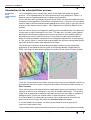
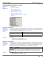
The following illustrations show a basement depth model and a corresponding
population of calculated structural index of the Bishop dataset (Fitzgerald et al,
2006). We used this test data to validate the ‘hybrid’ Euler solver for basin studies.
The Euler Deconvolution tool creates a solution set from your grid dataset containing
proposed sources which 'explain' the grid's anomalies. We refer to these sources as
Euler solutions.
Euler Deconvolution calculates location, depth below sensor and reliability for each
solution as well as error estimates in the form of standard deviations. The primary
signal that is measured in potential field data derives from the edges or contacts of
geological units. So this fact should reflect in what the solver is reporting.
In the standard Euler deconvolution process, each model contains solutions of a
particular structural type, defined by the structural index parameter.
In the extended Euler process, the solution calculates structural type as the
structural index output field.
The extended Euler method assumes that within a window, all gradients are caused
Library | Help | Top
© 2012 Intrepid Geophysics
| Back |
INTREPID User Manual
Library | Help | Top
Euler Deconvolution (T44)
3
| Back |
by just one causative body. This body has simple shape with an integer-power dropoff
for structural index. These assumptions may not hold true in many real geological
situations.
After INTREPID calculates the full set of solutions, you can output a dataset
containing classified and selected solutions:
•
Selected according to reliability (goodness), depth and depth error, structural
index, location and other calculated values.
•
Classified according to depth, geographic location or cluster.
There is also the batch option for restricting the Euler Deconvolution process to a
select set of XY pairs. We use this to continuously validate that for known models,
this technique is functioning as well as we can manage, and that the answers are
correct to within less than 1% error for the perfect cases, with no noise. Of course, this
scenario then also opens up the perfect opportunity to devise ways to find the outlier
solutions and why they occur in the first place. See the task specification section for
more details.
INTREPID has a range of available formats for the output dataset.
The Euler Decomposition tool uses components of the analytic signal of the data to
calculate the model. See "Analytic signal filter (reference)" in INTREPID spectral
domain operations reference (R14).
Stages in the extended Euler deconvolution process
;Parent topic:
Euler
Deconvolution
(T44);
The extended Euler deconvolution process has two stages:
1
Generating extended Euler solutions for the grid.
The left side of the Euler Deconvolution window has controls for the input of your
grid. It enables you to:
•
Select the Euler, Werner or Hilbert variation that you require
•
Immediately reject solutions with unrealistic depth
•
Perform reduction to pole for magnetic data
•
Save intermediate derivative and analytic signal grids for inspection.
At the end of this stage, you create an intermediate solutions file, a large ASCII
text file.
2
Selecting the solutions for output.
Using the selecting and sorting features, you can generate many different views of
the solutions.
You can also create 3D views in a two supported formats.
Continental Studies
In response to the availability of large scale contiental datasets ( Australia, Namibia
etc) that have a high fideleity, high frequency content, a new workflow is also being
released at V5.0, designed to make it practical to handle very large observational
geophysical grid datasets, in a repetative and sensible manner. Typically, the base
grid can be as large as 5 to 10 Gigabytes, and so beyond the capacity of most desktop
computers. The remaining optimization needed for a practical workflow here, is to
allow users to divided a continent or province into a series of “sheets”, and then
progressively work through each sheet. A new section is added to this manual to
explain all the thinking and the details.
Library | Help | Top
© 2012 Intrepid Geophysics
| Back |
INTREPID User Manual
Library | Help | Top
Euler Deconvolution (T44)
4
| Back |
Using the Euler Deconvolution tool—Steps
Parent topic:
Euler
Deconvolution
(T44)
Library | Help | Top
>> To use Euler Deconvolution with the INTREPID graphic user interface
Euler Deconvolution is memory and computer intensive. If you are using this tool you
require a relatively large amount of RAM and virtual memory.
1
Before using Euler Deconvolution, you could use Subsection (See Subsections of
datasets (T21) to limit your grid to a manageable size if required. Alternatively,
the tool itself allows you to create a simple rectangular subset.
2
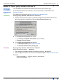
Choose Euler Deconvolution from the Interpretation menu in the Project
Manager, or use the command euler.exe. INTREPID displays the Euler
Deconvolution window. The left part of the window is different depending on
whether you are processing a scalar grid or a tensor grid.
3
If you have previously prepared file specifications and parameter settings for
Euler Deconvolution, load the corresponding task specification file using Load
Options from the File menu. (See Specifying input and output files for detailed
instructions.) If all of the specifications are correct in this file, go to step 5
(calculating complete set of Euler solutions) or step 8 (refining the Euler solutions
and creating an output dataset). If you wish to modify any settings, carry out the
following steps as required.
4
Specify the grid dataset to be processed. Use Open Input Grid from the File menu.
(See Specifying input and output files for detailed instructions.) INTREPID
displays the dataset in the Euler Deconvolution window.
5
If required, specify a rectangular subset of the grid for processing. See Specifying
the region for calculating solutions for detailed instructions.
© 2012 Intrepid Geophysics
| Back |
INTREPID User Manual
Library | Help | Top
Euler Deconvolution (T44)
5
| Back |
6
Specify the output point dataset to be created with the results of the process. Use
Specify Output Point Dataset from the File menu. (See Specifying input and
output files for detailed instructions.)
7
If the complete set of Euler solutions does not already exist for the current grid,
specify the Euler Deconvolution parameters and choose Apply Deconvolution.
See Creating the complete set of Euler solutions—Steps for details.
8
If you only wish to produce the complete set of Euler solutions without rejecting
any, go to step 11. In this case INTREPID produces only the complete set of
solutions (see Output—the complete set of Euler solutions). It does not produce
the output point dataset that you specified (see Output—Euler solutions point
dataset).
9
Specify the criteria for selecting classifying Euler solutions for output. See
Selecting and classifying Euler solutions—Steps for details.
10 When you have made specifications and settings according to your requirements,
choose Apply Sort. INTREPID selects the solutions and save the output data as
specified.
11 If you wish to record the specifications for this process in a .job file in order to
repeat a similar task later or for some other reason, use Save Options from the
File menu. (See Specifying input and output files for detailed instructions.)
12 If you wish to repeat the process, repeat steps 3–11, varying the parameters and
data files as required.
13 To exit from Euler Deconvolution, choose Quit from the File menu.
___
You can execute Euler Deconvolution as a batch task using a task specification (.job)
file that you have previously prepared. See Displaying options and using task
specification files for details.
Library | Help | Top
© 2012 Intrepid Geophysics
| Back |
INTREPID User Manual
Library | Help | Top
Euler Deconvolution (T44)
6
| Back |
Specifying input and output files
Parent topic:
Euler
Deconvolution
(T44)
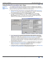
To use Euler Deconvolution, you will need to specify at least the grid dataset to be
examined and the point dataset for saving the results of the process. Choose the
options as required from the File menu or from the main Euler Deconvolution
window. You can preload the grid via the command line arguments, or via the
Intrepid Project manager.
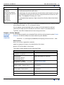
If you are browsing for a file. in each case INTREPID displays an Open or Save As
dialog box. Use the directory and file selector to locate the file you require. (See
"Specifying input and output files" in Introduction to INTREPID (R02) for
information about specifying files).
In this section:
•
•
Task files
Input
•
Input—input grid, band
•
Input—depth to basement grid
•
Input—vertical component
•
Input—solutions for re-sorting
•
Input—options
Output
•
Output—FFT and derivative products
•
Output—the complete set of Euler solutions
•
Output—Euler solutions point dataset
•
Output—cluster dataset
•
Output—vector dataset formats
•
Output visualisation formats
•
Output—report
•
Output—options
•
Output—Convention for displaying Euler solutions
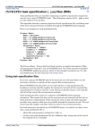
Example of input and output file specifications in a task specification (.job) file:
Input = C:/Intrepid/cookbook/eulerplay/tmi_ns.ers
Depth = C:/Intrepid/cookbook/eulerplay/dtm_ns.ers
Output = C:/Intrepid/cookbook/eulerplay/eulersols..DIR
ReportFile = euler.rpt
Cluster = C:/Intrepid/cookbook/eulerplay/eulercluster..DIR
At V5.0, the GOOGLE protobuf syntax is also supported. The above
translates easily, by quoting the strings, and changing the equals
to a colon.
Library | Help | Top
© 2012 Intrepid Geophysics
| Back |
INTREPID User Manual
Library | Help | Top
Euler Deconvolution (T44)
7
| Back |
Input—input grid, band
Parent topic:
Specifying
input and
output files
Specify the grid dataset for which you want to calculate solutions.
Interactive
To specify the input grid, choose main menu option File > Open Input Image.
Task files
(Task files only) You can also specify a list of individual data points in the grid. If you
do this, INTREPID only calculates solutions for the points specified.
INTREPID automatically detects tensor grids and processes them accordingly.
Note: If you are processing tensor data, ensure that you know its coordinate system.
See "Vector and tensor field data coordinate conventions" in INTREPID database, file
and data structures (R05).
INTREPID requires (x, y, z) triplets, where z is the known depth.
If you select Method 7—Euler Werner property solver as your calculation method, use
the third value of the triplet for the known depth.
If you select any other calculation method, put 0 as the value of the third number in
every triplet.
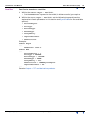
Example:
Input = C:/Intrepid/cookbook/eulerplay/tmi_ns.ers
Band = 0
Required_Points = { X, Y, Depth, ... }
Input—depth to basement grid
Parent topic:
Specifying
input and
output files
If you select Method 7—Euler Werner property solver as your calculation method,
INTREPID requires a depth to basement grid.
Interactive
You can enter its path or browse for it.
Task files
Example:
Depth = C:/Intrepid/cookbook/depth_ns.ers
Input—vertical component
Parent topic:
Specifying
input and
output files
If you use the Method 8—Tensor Bouguer solver method, INTREPID requires a
vertical component grid.
This could typically be a ground gravity dataset that must share the same grid
properties as the full tensor grid (the same number of rows and columns and the same
origin and cell size).
Interactive
Library | Help | Top
© 2012 Intrepid Geophysics
| Back |
INTREPID User Manual
Library | Help | Top
Task files
Euler Deconvolution (T44)
8
| Back |
Example:
VerticalComponent = C:/Intrepid/cookbook/grav_z.ers
Input—solutions for re-sorting
Parent topic:
Specifying
input and
output files
(Interactive only) If you already have a set of solutions (.rs file—see Output—Euler
solutions point dataset) and you want to classify and select from it to create an output
points dataset, use this option to spoecify the solutions file.
Interactive
Choose main menu option File > Open solutions for resorting.
Task files
In batch mode you must calculate the solutions in the same task. You cannot load an
existing set of solutions for sorting. There is no keyword in the task file language for
this input file.
Input—options
Parent topic:
Specifying
input and
output files
If you wish to use an existing task specification file to specify the Euler Deconvolution
process, choose File > Load Options to specify the task specification file required.
INTREPID will load the file and use its contents to set all of the parameters for the
Euler Deconvolution process. (See Displaying options and using task specification
files for more information).
Output—FFT and derivative products
Parent topic:
Specifying
input and
output files
For extended Euler deconvolution we need to prepare up to 15 grid products for use in
the process. INTREPID prepares and these automatically.
The products include:
•
FFT grid of original signal (1)
•
Original signal with Hilbert in X and Y (2)
•
Analytic signal, analytic signal with Hilbert in X and Y (3)
•
Derivatives of signal in X, Y and Z (3)
•
Derivatives of signal with added Hilbert in X (3)
•
Derivatives of signal with added Hilbert in Y (3)
Here is a complete list of intermediate grids. The filenames consist of:
•
The input grid name (inputgrid_)
•
A unique numeric code (tempcode_) to distinguish between different times that
you run the task and
•
The type of intermediate grid
•
The text _RESIZED if INTREPID expanded the grid beyond its boundaries to
prepare it for FFT. This does not normally happen if you use a subsection and
specify the border within the grid (see Specifying the region for calculating
solutions and Expanding the boundary of the input grid).
INTREPID saves these grids in the folder install_path/temp.
Since this is a routine process, INTREPID does not include options for you to
manually prepare these grids yourself and submit them to the tool.
You can specify whether to retain these files after the Euler Deconvolution process.
See Derivatives and analytic signal‘ for instructions.
You can examine any of the grids to make sure the FFT work does not contain
ringing. If there is ringing, work on the input grid to reduce noise.
Library | Help | Top
© 2012 Intrepid Geophysics
| Back |
INTREPID User Manual
Library | Help | Top
Euler Deconvolution (T44)
9
| Back |
The 3-dimensional analytic signal computes the non-directional derivative as the
square root of the square of the 2 horizontal and 1 vertical derivatives. The analytical
signal is used as input to a Single Value decomposition.
INTREPID deletes these unless you want to save them (see Derivatives and analytic
signal).
Transform products
inputgrid_tempcode_FFT
inputgrid_tempcode_HILBERT_0_real
inputgrid_tempcode_HILBERT_90_real
inputgrid_tempcode_Analytic
inputgrid_tempcode_Analytic_Hilbert_0
inputgrid_tempcode_Analytic_Hilbert_90
Derivatives
inputgrid_tempcode_XD_real
inputgrid_tempcode_YD_real
inputgrid_tempcode_ZD_real
inputgrid_tempcode_XD_HILBERT_0_real
inputgrid_tempcode_YD_HILBERT_0_real
inputgrid_tempcode_ZD_HILBERT_0_real
inputgrid_tempcode_XD_HILBERT_90_real
inputgrid_tempcode_YD_HILBERT_90_real
inputgrid_tempcode_ZD_HILBERT_90_real
Output—the complete set of Euler solutions
Parent topic:
Specifying
input and
output files
INTREPID stores the complete set of extended Euler solutions in an ASCII text file.
The name of this file is derived from the input grid's file name. The solutions file
name consists of the input grid name with _rs appended. For example, the Euler
solutions file for grid mag_342 will be mag_342_rs. INTREPID also produces a
history file with the _rsh appended.
The report file and this header file show what each column in the ASCII file
represents.
INTREPID uses this file when you select and classify solutions for output. These are
ASCII and contain all of the information necessary to preserve, sort, cull your
solutions.
INTREPID does not overwrite any existing _rs file when you recalculate the
extended Euler solutions using different parameters. It adds 1, 2, 3, ... to the name of
the input grid name as necessary. Thus, if you wish to resort to a previous output, you
just need to choose the appropriate intermediate solutions file.
Library | Help | Top
© 2012 Intrepid Geophysics
| Back |
INTREPID User Manual
Library | Help | Top
Euler Deconvolution (T44)
10
| Back |
Output—Euler solutions point dataset
Parent topic:
Specifying
input and
output files
When you select and classify the extended Euler solutions, INTREPID saves this
data to a point dataset.
Task files
Example:
Output= C:/Intrepid/cookbook/eulerplay/eulersols..DIR
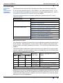
Dataset fields
The output point dataset for selected Euler solutions has the following fields:
Field
Description
CellSize
(Group by) Input grid cell size ('group by' field) previously CELLSIZE
Window
(Group by) Size of Euler window ('group by' field) previously WINDOW
Structural_Indx
Structural Index for solutions ('group by' field) previously STRUCTURE
BIN
Geographic bin number
LAYERDEPTH
Depth of mid point of layer (m). This acts as the layer number field.
X
East–West geographic location
Y
North–South geographic location
Elevation
Depth estimate for solution (m) previously DEPTH
Reliability
Reliability (0..1) of solution previously RELIABILITY
Background
Average field value in the region
Goodness
See Goodness for an explanation
Strike
The strike is the artan of the ratio of the two horizontal gradients, y/x
Obs_Dip
The vertical angle from observed grid point to the computed body location.
If these are low we reject them. See Minimum observed dip.
Grad_Amp
Gradient amplitude of the analytic signal
Trace
Sum of leading diagonal terms in the matrix solver
Grid_loc
Ordinal position of the cell in the grid, numbered columnwise then
rowwise.
Alpha
Beta
See Maximum absolute alpha for information.
Sratio
See Maximum singularity ratio for explanation
MaxDeterminant
(Group by) A constant output value for the whole dataset. INTREPID
looks through every solution, takes determinant of each solution matrix
and then places the maximum value in this field.
Library | Help | Top
© 2012 Intrepid Geophysics
| Back |
INTREPID User Manual
Library | Help | Top
Euler Deconvolution (T44)
11
| Back |
Field
Description
X_Error
Y_Error
Elevation_Error
Background_Error
SI_Error
XY_Error
YZ_Error
ZX_Error
ZSI_Error
The quantities XY_err, YZ_err, ZSI_err represent the cross correlation
of individual terms with each other.
Surprisingly, the cross correlations are extremely small except for the case
of a relatively small grid cell size and a large convolution kernel for a 2D
body. This appears in the XY_err term.
The weighted least squares single value solver directly determines these
values
The log file reports a full account of all solutions attempted and their reject or accept
status based on depth, XY, SI, or Numeric issues.
Also, the Norm_CovarianceXY field is a report of the estimated normalised
covariance for each solution window for all the XY terms in the observations.
Typically, over 80% of observations have strong covariance.
Output—cluster dataset
Parent topic:
Specifying
input and
output files
If you choose to classify your extended Euler solutions using clustering (see Cluster
analysis), INTREPID saves the cluster data to a point dataset.
Cluster= C:/Intrepid/cookbook/eulerplay/eulercluster..DIR
Dataset fields
Kurt is Kurtosis, a population statistic
Skew is a measure of skew in the distribution of a cluster
Error is SD of the data in the cluster
The output cluster dataset has the following fields:
Field
Description
X, Y,
X_Error, Y_Error
Library | Help | Top
Elevation,
Elevation_Error,
Elevation_Kurt
Depth estimates for solutions
Structural_Indx,
SI_Error, SI_Skew, SI_Kurt
See Structural Index
Alpha, Alpha_Error,
Alpha_Skew, Alpha_Kurt
See Maximum absolute alpha for
information.
Beta, Beta_Error,
Beta_Skew, Beta_Kurt
See Maximum absolute alpha for
information.
Radius
Radius of cluster area
Number
Number of points in the cluster
© 2012 Intrepid Geophysics
| Back |
INTREPID User Manual
Library | Help | Top
Euler Deconvolution (T44)
12
| Back |
Output—vector dataset formats
Parent topic:
Specifying
input and
output files
Task files
INTREPID can output the selected and classified extended Euler solution data in the
following formats. See INTREPID direct access, import and export formats (R11).
Option
Purpose
Database
Any supported binary database
XYZ
Geosoft XYZ format
GDB
Geosoft GDB format
Example:
ExportTypes= Database
Output visualisation formats
Parent topic:
Specifying
input and
output files
Task files
Two formats for 3D representation of your Euler Solutions are available.
Option
Purpose
VRML
Virtual Reality Markup Language (VRML) is a common file format for
internet browsers. The file produced here can be looked at in 3D using a
plug-in such as Blaxlan.
BREP
OpenCascade 3D object representation viewer. A free viewer for BREP
data is available from the OpenCascade WWW site.
Example:
Dump_VRML= No
Dump_BREP= No
Output—report
Parent topic:
Specifying
input and
output files
Euler Deconvolution produces a report file describing its actions. The default file
name of the report is euler.rpt in the current folder. In task files you can specify a
different name and path.
Task files
Example:
ReportFile= euler.rpt
Output—options
Parent topic:
Specifying
input and
output files
If you wish to save the current Euler Deconvolution file specifications and parameter
settings as an task specification file, choose File > Save Options to specify the
filename and save the file. (See Displaying options and using task specification files
for more information).
Output—Convention for displaying Euler solutions
Parent topic:
Specifying
input and
output files
Library | Help | Top
It is common practice to display Euler solutions point datasets using:
•
Symbol colour to represent Depth,
•
Symbol size to represent Reliability,
•
Symbol strike to represent Angle.
© 2012 Intrepid Geophysics
| Back |
INTREPID User Manual
Library | Help | Top
Euler Deconvolution (T44)
13
| Back |
Specifying the region for calculating solutions
Parent topic:
Euler
Deconvolution
(T44)
You can specify a rectangular subsection of the input grid. INTREPID only outputs
solutions located within the subsection. Specify the subset in distance units of the
grid dataset (usually metres).
If you specify extents of a region that completely contains the input grid, INTREPID
does use the subset feature.
INTREPID uses any actual grid data that is available outside the subset for FFT
filling and conditioning. You can specify the width of the grid expansion border for
FFT in relation to this subset. See Expanding the boundary of the input grid for more
details.
Library | Help | Top
Option
Purpose
LL Easting
Minimum value for eastern direction. This value allows the
interpreter to specify a minimum eastern value which forces
statistical calculations to be performed only for data points whose
eastern coordinate is greater than or equal to the eastern boundary
value.
UR Easting
Maximum value for eastern direction. This value allows the
interpreter to specify a maximum eastern value which forces
statistical calculations to be performed only for data points whose
eastern coordinate is less than or equal to the eastern boundary
value.
LL Northing
Minimum value for northern direction. This value allows the
interpreter to specify a minimum northern value which forces
statistical calculations to be performed only for data points whose
northern coordinate is greater than or equal to the northern
boundary value.
UR Northing
Maximum value for northern direction. This value allows the
interpreter to specify a maximum northern value which forces
statistical calculations to be performed only for data points whose
northern coordinate is less than or equal to the northern boundary
value.
© 2012 Intrepid Geophysics
| Back |
INTREPID User Manual
Library | Help | Top
Task files
Euler Deconvolution (T44)
14
| Back |
Example:
Subset Begin
XLower=
XUpper=
YLower=
YUpper=
...
Subset End
520129.158
595129.158
7236236.0
7311236.0
Creating the complete set of Euler solutions—Steps
Parent topic:
Euler
Deconvolution
(T44)
In the first stage of the Euler Deconvolution process INTREPID generates a complete
set of Euler solutions.
It saves these solutions to a file from which you can select solutions for the output
dataset. See Output—the complete set of Euler solutions for details.
>> To create the complete set of Euler solutions
1
Ensure that you have specified the input grid dataset. See Specifying input and
output files for instructions.
2
Specify
3
•
The extended Euler equation option (see The standard and extended Euler
equation options).
•
(Standard Euler and Euler Werner only) The required structural index (see
Method 1—Standard Euler, Method 2—Euler Werner and Structural Index).
•
(Euler Werner property solver only) The depth to basement grid (see Method
7—Euler Werner property solver and Input—depth to basement grid).
•
The FFT parameters (see Fast Fourier transform).
•
The survey height (see Survey observation height).
•
The size of the Euler window, determining the maximum depth of solutions
(see Determining the maximum depth for solutions (window size)).
•
Whether to convolve the derivatives before use (see Derivatives and analytic
signal).
•
Whether to save the derivatives and the analytic signal as grid datasets
during the process (see Derivatives and analytic signal).
Choose Apply Euler. INTREPID will calculate and save the solutions and
intermediate results datasets if specified.
See the following sections for details about this process.
Library | Help | Top
© 2012 Intrepid Geophysics
| Back |
INTREPID User Manual
Library | Help | Top
Euler Deconvolution (T44)
15
| Back |
The standard and extended Euler equation options
Parent topic:
Euler
Deconvolution
(T44)
In this section:
•
Method 1—Standard Euler
•
Method 2—Euler Werner
•
Method 3—Euler Werner 2 Equation SI solver
•
Method 4—Euler Werner basement solver
•
Method 5—Hybrid 2-pass Euler solver
•
Method 6—Euler Werner Full Solver
•
Method 7—Euler Werner property solver
•
Notes about tensor deconvolution
•
Method 8—Tensor Bouguer solver
•
Method 9—Tensor gravity estimator with fixed SI
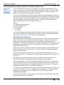
The Euler equation is solved using a singular value decomposition to determine the
unknowns of a system of linear equations.
The Traditional or Standard Euler technique uses the components of the analytic
signal—three orthogonal derivatives all in the spatial domain, usually determined by
Fourier methods.
∂M ∂M ∂M
------- ------Inputs are ------∂X , ∂Y , ∂Z and the structural index.
The calculated output is a vector distance to the source with estimates of x,y,z and
background and their errors.
For the extended Euler method, after Nabighian and Hansen (2001) and Fitzgerald
and Reid (2000), we use the Hilbert transform to formulate 2 or 3 equations. By4
applying the Hilbert transform, we have achieved a circular rotation of the coordinate
axes. This is an invariant for potential fields that allows us to create the new
differential equations.
The extended Euler options are a unification of the Euler and Werner deconvolution
in 3D using the generalized Hilbert transform.
The 2 Hilbert equations take the following parameters:
∂M ⎞
∂M
∂M
H ⎛ ------- ⎞ H ⎛ ------- ⎞
H (M )
Equation 1 H x ⎛⎝ ------∂X ⎠ , x ⎝ ∂Y ⎠ , x ⎝ ∂Z ⎠ and x
∂M ⎞
∂M
∂M
H ⎛ ------- ⎞ H ⎛ ------- ⎞
H (M )
Equation 2 H y ⎛⎝ ------∂X ⎠ , y ⎝ ∂Y ⎠ , y ⎝ ∂Z ⎠ and y
These extra equations use the Hilbert transform on standrad Euler equations. We
have shown that if the field satisfies both Euler and LaPlace rce then the Hilbert
transform of the fields also satisfies the Euler equation. Resulting independent
equations can solve for more unknowns and therefore we could achieve an improved
resulting set of estimates. You can test this by comparing the results of the Method
1—Standard Euler option with those of the Method 2—Euler Werner option.
The calculated output is a vector distance to the source with estimates of X, Y, Z,
structural index and corresponding errors and covariance.
Library | Help | Top
© 2012 Intrepid Geophysics
| Back |
INTREPID User Manual
Library | Help | Top
Euler Deconvolution (T44)
16
| Back |
For a particular model, such as a dipping contact, you can calculate other properties
including dip, strike and physical property contrast (density or susceptibility).
The Euler Deconvolution tool currently offers eight extended Euler equation options.
You can select the options in the user interface or using keywords in the task files.
The extended Euler calculations use combinations of three equations:
•
Classic Euler equation (Classic)
•
Hilbert transformation in North and East directions (Hilbert)
Depending on the options, you can solve for X, Y, Z, SI, B, α, β.
With some options you need to specify parameters or provide input data—SI, depth or
vertical component (Z).
α and β are body property indicators calculated in some options.
Background represents background magnetic field or gravity without local anomalies.
Method 1—Standard Euler
Parent topic:
The standard
and extended
Euler equation
options
This method uses only the Classic equation. This suffers from scatter and noise if the
gradient grids are not very good.
It assumes fixed structural index (SI), which you specify as a parameter (see
Structural Index).
It solves for X, Y, Z and B (Background).
Background represents background magnetic field or gravity without local anomalies.
Interactive
Standard Euler—interactive
In the Euler Deconvolution area:
Task files
1
Select Standard Euler.
2
Specify the Structural Index (see Structural Index).
Standard Euler—task files
Within the Solve Begin – End block:
•
Set the EquationCombo keyword to Classic.
•
Set the required value for the StructuralIndex keyword.
Example:
EquationCombo = Classic
Library | Help | Top
© 2012 Intrepid Geophysics
| Back |
INTREPID User Manual
Library | Help | Top
Euler Deconvolution (T44)
17
| Back |
StructuralIndex = 1
Method 2—Euler Werner
Parent topic:
The standard
and extended
Euler equation
options
This extended Euler method uses all three equations.
It assumes fixed structural index (SI), which you specify as a parameter (see
Structural Index).
It solves for X, Y, Z and B (Background).
If you already know the SI (perhaps because you have sythetic data from models), you
can compare the standard and extended Euler methods, and assess which one gives
the more acceptable error distribution.
In all cases this method should yield the lowest error range, as we are solving for the
least number of unknowns with the most equations.
Interactive
Euler Werner—interactive
In the Euler Deconvolution area:
Task files
1
Select Euler Werner.
2
Specify the Structural Index.
Euler Werner—task files
Within the Solve Begin – End block:
•
Set the EquationCombo keyword to All3_Fixed_SI.
•
Set the required value for the StructuralIndex keyword.
Example:
EquationCombo = All3_Fixed_SI
StructuralIndex = 1
Method 3—Euler Werner 2 Equation SI solver
Parent topic:
The standard
and extended
Euler equation
options
This extended Euler method uses only the two Hilbert equations. This is the default
and our preference for the new user.
It assumes fixed background.
It solves for X, Y, Z, SI, β.
We have found that this has a good focusing ability, with a tight error envelope
around discrete bodies. It is using phase inherent in the local stationary signal to
best advantage. In practice it does the best on deep basement contacts.
We suggest that, in the selecting and sorting stage, you apply an upper and lower clip
to calculated values of the SI. See Structural index clips.
Interactive
Euler Werner 2 Equation SI solver—interactive
In the Euler Deconvolution area:
1
Task files
Select Euler Werner 2 Equation SI solver.
Euler Werner 2 Equation SI solver—task files
Within the Solve Begin – End block:
•
Set the EquationCombo keyword to Hilbert_Only
Example:
EquationCombo = Hilbert_Only
Library | Help | Top
© 2012 Intrepid Geophysics
| Back |
INTREPID User Manual
Library | Help | Top
Euler Deconvolution (T44)
18
| Back |
Method 4—Euler Werner basement solver
Parent topic:
The standard
and extended
Euler equation
options
This extended Euler method uses all three equations. Not recommenede for the
novice user.
It solves for X, Y, Z, β.
We designed this option to solve for depth (Z), when you do not require the SI. It
eliminates the SI, producing a superior result for X, Y, Z.
Interactive
Euler Werner basement solver—interactive
In the Euler Deconvolution area:
1
Task files
Select Euler Werner basement solver.
Example:
EquationCombo = No_SI
Method 5—Hybrid 2-pass Euler solver
Parent topic:
The standard
and extended
Euler equation
options
Not recommeneded for the novice user. This extended Euler method is a combination
of:
•
Method 3—Euler Werner 2 Equation SI solver and
•
Method 4—Euler Werner basement solver
It solves for X, Y, Z, SI, α, β.
It produces all solutions using both of the methods. It then selects:
Interactive
•
X, Y and SI from Method 3—Euler Werner 2 Equation SI solver
•
The best Z results from the two methods. This is the deepest of the two depths
with a small scaling adjustment derived from the ‘Bishop’ study.
Hybrid 2 pass Euler solver—interactive
In the Euler Deconvolution area:
1
Task files
Select Hybrid 2 pass Euler solver.
Hybrid 2 pass Euler solver—task files
Within the Solve Begin – End block:
•
Set the EquationCombo keyword to Hilbert_then_no_SI
Example:
EquationCombo = Hilbert_then_no_SI
Method 6—Euler Werner Full Solver
Parent topic:
The standard
and extended
Euler equation
options
This extended Euler method uses all three equations.
Interactive
Euler Werner Full Solver—interactive
It solves for X, Y, Z, SI, α, β.
This method solves for all unknowns.
In the Euler Deconvolution area:
1
Task files
Select Euler Werner full solver.
Euler Werner Full Solver—task files
Within the Solve Begin – End block:
Library | Help | Top
© 2012 Intrepid Geophysics
| Back |
INTREPID User Manual
Library | Help | Top
•
Euler Deconvolution (T44)
19
| Back |
Set the EquationCombo keyword to All3_For_Contact_Case
Example:
EquationCombo = All3_For_Contact_Case
Method 7—Euler Werner property solver
Parent topic:
The standard
and extended
Euler equation
options
Not recommenede for the novice user. This extended Euler method uses all three
equations.
It solves for SI, α, β.
It assumes known depth (Z), which you specify as a grid dataset (possibly sourced
from other geophysical techniques such as seismic). Note that the values in the depth
grid must be negative.
Use this option to produce property (SI) values, where you know the depth.
Interactive
Euler Werner property solver—interactive
In the Euler Deconvolution area:
Task files
1
Select Euler Werner property solver.
2
Specify the Depth to basement grid (see Input—depth to basement grid)
Euler Werner property solver—task files
Within the Solve Begin – End block:
•
Set the EquationCombo keyword to Known_Depth
Within the Process Begin – End block:
•
Set the Depth keyword to the path of the depth to basement grid dataset.
Example:
Depth = C:/Intrepid/cookbook/tmi_ns_depth.ers
...
EquationCombo = Known_Depth
Notes about tensor deconvolution
Parent topic:
The standard
and extended
Euler equation
options
Notes:
•
If you are processing tensor data, ensure that you know its coordinate system.
See "Vector and tensor field data coordinate conventions" in INTREPID database,
file and data structures (R05).
Before processing your data, select the correct coordinate convention (ENU, NED,
END)
•
For information about test work on perfect model data, contact our technical
support service
Tensor methods:
Library | Help | Top
•
Method 8—Tensor Bouguer solver
•
Method 9—Tensor gravity estimator with fixed SI
© 2012 Intrepid Geophysics
| Back |
INTREPID User Manual
Library | Help | Top
Euler Deconvolution (T44)
20
| Back |
Method 8—Tensor Bouguer solver
Parent topic:
The standard
and extended
Euler equation
options
This extended Euler method calculates the solutions from a tensor grid. It requires
all three equations, and obtains the gradients from the tensor data in the input grid
(see Input—vertical component).
It solves for X, Y, Z, SI, B, Tx and Ty, where Tx and Ty are horizontal gravity
components
This method is similar to Method 6—Euler Werner Full Solver but uses the tensor
data to obtain the gradients.
For important information see Notes about tensor deconvolution.
Interactive
Tensor Bouguer solver—Interactive
1
Specify a tensor grid for input. INTREPID recognises and validates the tensor
grid automatically, displaying a different Euler Deconvolution panel in the
application window.
2
In the Euler Deconvolution area, select:
3
Task files
•
The Tensor Coordinate Convention of your dataset
•
Euler from Gravity Tensor and Tz.
In the Euler Deconvolution area, specify the Vertical component of gravity grid.
Tensor Bouguer solver—Task files
Within the Solve Begin – End block:
•
Set the EquationCombo keyword to Tensor_Tz
Within the Process Begin – End block:
•
Set the VerticalComponent keyword to the path of the vertical component grid
dataset.
Example:
VerticalComponent = C:/Intrepid/cookbook/grav_ns_z.ers
...
EquationCombo = Tensor_Tz
Library | Help | Top
© 2012 Intrepid Geophysics
| Back |
INTREPID User Manual
Library | Help | Top
Euler Deconvolution (T44)
21
| Back |
Method 9—Tensor gravity estimator with fixed SI
Parent topic:
The standard
and extended
Euler equation
options
This extended Euler method calculates the solutions from a tensor grid.
It assumes fixed structural index (SI), which you specify as a parameter (see
Structural Index).
For important information see Notes about tensor deconvolution.
Interactive
Tensor gravity estimator with fixed SI—Interactive
1
Specify a tensor grid for input. INTREPID recognises and validates the tensor
grid automatically, displaying a different Euler Deconvolution area.
2
In the Euler Deconvolution area, select:
3
Task files
•
The Tensor Coordinate Convention of your dataset
•
Estimate Tz from Tensor.
In the Euler Deconvolution area, specify:
•
The Structural Index (See Structural Index)
•
The Vertical component of gravity grid.
Tensor gravity estimator with fixed SI—Task files
Within the Solve Begin – End block:
•
Set the EquationCombo keyword to Tensor_Gravity_Estimator
•
Set the required value for the StructuralIndex keyword. See Structural Index.
Example:
EquationCombo = Tensor_Gravity_Estimator
StructuralIndex = 1
Library | Help | Top
© 2012 Intrepid Geophysics
| Back |
INTREPID User Manual
Library | Help | Top
Euler Deconvolution (T44)
22
| Back |
Euler Deconvolution parameters and execution
Parent topic:
Euler
Deconvolution
(T44)
In this section:
•
Fast Fourier transform
•
Structural Index
•
Determining the maximum depth for solutions (window size)
•
Survey observation height
•
Reduction to the pole
•
Derivatives and analytic signal
•
Apply Deconvolution
Fast Fourier transform
Parent topic:
Euler
Deconvolution
parameters
and execution
The Euler Deconvolution process requires partial derivatives and analytic signal of
the input grid. For a scalar input grid, INTREPID performs a Fast Fourier
Transform (FFT) as the first step in obtaining the derivatives. For a tensor input
grid, INTREPID obtains the derivatives directly from the tensor data and does not
need to perform FFT.
INTREPID always saves and retains some products of this process in a temporary
folder. You can specify that INTREPID retains all products for you to examine.
In this tool INTREPID always calculates the FFT (except for tensor input grid) and
derivatives. Since this is a routine process, we do not currently provide an option for
you to supply your own FFT or derivatives grids. See Output—FFT and derivative
products.
Expanding the boundary of the input grid
To prepare for the FFT, INTREPID extends the boundary of the input grid,
extrapolates values for this extended region and also interpolates any internal gaps
in the grid.
If you defined a subsection of the input grid dataset, INTREPID may use a margin
outside the subsection as the grid edge expansion (the FFTBorder text box or
FFTBorder keyword). See Specifying the region for calculating solutions for details.
If you did not define the subsection in this way, INTREPID expands the grid by
+10%.
If INTREPID expands the grid, it appends a notation to the temporary grid dataset
names that it produces from it. See Output—FFT and derivative products.
Detrending the grid
INTREPID always detrends the grid. See "Detrending data values" in INTREPID
spectral domain operations reference (R14) for information. The value you assign to
the keyword corresponds to the degrees in this reference topic.
Filling the gaps in the expanded grid
After expanding the grid, INTREPID assigns values to the new cells in the grid using
an extrapolation process. You can choose one of two available methods—Arthur fill
algorithm and maximum entropy. See "Estimating values for data gap cells" in
INTREPID spectral domain operations reference (R14) for details.
INTREPID notes the extrapolated and interpolated regions of the grid and does not
calculate solutions for them.
Library | Help | Top
© 2012 Intrepid Geophysics
| Back |
INTREPID User Manual
Library | Help | Top
Euler Deconvolution (T44)
23
| Back |
Grid edge rolloff
For best results from the FFT, the edges of the grid must be set to zero, but without
sudden changes from the data within the grid. The grid data needs to ‘roll off’ to zero
at the edge.
INTREPID has two sets of available edge roll off methods. See "Damping of dataset
edges before spectral transform" in INTREPID spectral domain operations reference
(R14) for details of this process.
Symmetry
With traditional FFT you can assume that the transformed dataset is symmetrical
and therefore we only process one half.
When you include the Hilbert transfom, the FFT grid is no longer symmetrical and
you need to process all of it. This parameter controls whether INTREPID processes
all of the dataset or only half.
For the options that include Hilbert (all except Method 1—Standard Euler—see The
standard and extended Euler equation options), the correct setting is No.
For Method 1—Standard Euler, the correct setting is Yes.
If you use interactive mode for the tool to run it or create a task file, INTREPID
automatically selects the correct setting.
FFT grid precision
You can specify the precision of the spectral domain grid. See "Data Types in
INTREPID datasets" in INTREPID database, file and data structures (R05) for the
available numeric data types.
You can choose between 4 byte and 8 byte precision.
Saving the derivative and analytic signal grids
See Output—FFT and derivative products for information and instructions.
Interactive
Fast Fourier transform—interactive
1
Choose main menu option Spatial > Rectangle.
2
Ensure that you have specified any subset rectangle that you require (see
Specifying the region for calculating solutions).
3
Enter the border width in metres in the FFT Border text box and then choose OK.
4
In the Euler Deconvolution area, check or clear the Use real*4 precision for
Fourier work check box.
See also Output—FFT and derivative products.
Library | Help | Top
© 2012 Intrepid Geophysics
| Back |
INTREPID User Manual
Library | Help | Top
Task files
Euler Deconvolution (T44)
24
| Back |
Fast Fourier transform—task files
1
Within the Subset Begin – End block:
•
2
Set the FFTborder keyword to the width (in distance units) you require.
Within the Solve Begin – End block, set the following keywords (see the
explanation of each parameter in this section and Syntax table for the available
options):
•
DetrendDegree
•
FillType
•
RolloffType
•
WindowType
•
UseSymmetry
•
ImproveEstimate
•
FFTPrecision
Example:
Subset Begin
...
FFTborder= 5000.0
Subset End
...
DetrendDegree = 1
FillType = ARTHUR
RolloffType = COSINE
WindowType = NONE
UseSymmetry = Yes
FFTPrecision = IEEE4ByteComplex
ImproveEstimate = No
...
See also Output—FFT and derivative products.
Library | Help | Top
© 2012 Intrepid Geophysics
| Back |
INTREPID User Manual
Library | Help | Top
Euler Deconvolution (T44)
25
| Back |
Structural Index
Parent topic:
Euler
Deconvolution
parameters
and execution
The extended Euler deconvolution processes calculates the Structural Index (SI).
If you are using standard Euler or Euler Werner, you need to specify the SI. If you
are using the other extended Euler options you no longer need to specify SI. See The
standard and extended Euler equation options for details.
The following table contains a summary showing the relevance of the SI to each
calculation option.
Structural Index
Option
Parameter that you specify
Method 1—Standard Euler
Method 2—Euler Werner
Method 9—Tensor gravity estimator with fixed SI
Calculated output field
Method 3—Euler Werner 2 Equation SI solver
Method 5—Hybrid 2-pass Euler solver
Method 6—Euler Werner Full Solver
Method 7—Euler Werner property solver
Method 8—Tensor Bouguer solver
Eliminated in the calculation
Method 4—Euler Werner basement solver
About structural index
This parameter indicates the shape of the inferred geological bodies that make up the
Euler solutions. Mathematically, the structural index is a power law operator that
we use to define the decay response of the source. The Structural Index must be nonnegative.
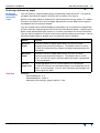
The following table shows some values of the Structural Index for four types of data
(gravity, magnetic, full tensor gradient gravity and magnetic) and the corresponding
shapes of inferred geological structures.
Structural Index
Structural
Index Type
Inferred geological structure
shape
Grav
Mag,
FTG Grav
FTG Mag
–0.5
.5
1.5
Step
Fault
0
1
2
Line of poles
Dyke
1
2
3
Point pole
Vertical pipe (e.g., Kimberlite)
2
3
4
Point dipole
Point source (nominally spherical)
Key: Grav = Gravity, Mag = Magnetic, FTG = Full Tensor Gradient
Whilst this is correct for homogenous bodies, for a basement step over which you have
a high quality gravity survey, the 2-equation Euler solver returns an SI > 0.0. This is
comforting from a basic physics viewpoint, but it also indicates that the Euler theory
has scope for further development.
Library | Help | Top
© 2012 Intrepid Geophysics
| Back |
INTREPID User Manual
Library | Help | Top
Euler Deconvolution (T44)
26
| Back |
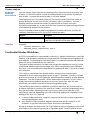
The following table shows typical structural index values for different structures and
potential fields. FTG = full tensor gradient data
Geological
Geophysical
Gravity
Magnetic,
FTG Gravity
FTG
Magnetic
basalt plug
point dipole
2
3
4
kimberlite
point pole
1
2
3
fault/dyke
line of dipoles
0
1
2
–0.5 (?)
0.5
1.5
–1.0 (?)
0
1
step
contact/edge
dipping contact
The negative values correspond generally to an inadmissable non-homogeneous
situation. There is no Euler solution in these cases. Recent studies show that SI for
gravity is, on average, not negative as shown above. The contact case appears to be
non-homogeneous for gravity and therefore further moving away from the
fundamental requirements of Euler's assumptions. Typical values of 0.2 for contact
and 0.5 for a step are shown for model studies.
You can specify other non-integer values, such as 0.5, depending on the type of
source.
Interactive
Structural index—interactive
(Standard Euler and Euler werner only) To set a fixed structural index value, in the
Euler Deconvolution area:
Task files
1
Ensure that you have selected the Standard Euler, Euler Werner or Tensor
gravity estimator with fixed SI equation option (see The standard and extended
Euler equation options).
2
Enter the value required in the Structural Index text box.
Structural index—task files
(Standard Euler and Euler werner only) Within the Solve Begin – End block:
•
Ensure that the value of EquationCombo is Classic or All3_Fixed_SI (see
The standard and extended Euler equation options).
•
Use the StructuralIndex keyword to specify the fixed structural index.
Example:
StructuralIndex = 1.0
...
EquationCombo = Classic
Library | Help | Top
© 2012 Intrepid Geophysics
| Back |
INTREPID User Manual
Library | Help | Top
Euler Deconvolution (T44)
27
| Back |
Determining the maximum depth for solutions (window size)
Parent topic:
Euler
Deconvolution
parameters
and execution
If you have come to this point in the manual, you maybe having problems. Do not
worry, as a new user, there are a few things it takes time to grasp. Firstly, the grid
extent dictates how deep you can see buried body edges. You cannot expect to see
deeper than 1/5 the horizontal extent of your grid.
If your grid is 2km square, you will be lucky to get many solutions deeper than 200 m.
Also, you can influence the maximum depth for Euler solutions found using the size of
the Euler window. The Euler window size is the number of cells INTREPID uses for
calculating derivatives and the analytic signal. The size of the Euler window is
directly related to the maximum depth of solutions.
Where:
D = Maximum solution depth
W = Euler window size
C = Grid cell size
k = a constant
D = kWC
In the second stage of the Euler process INTREPID stores the Euler window size as
the value of the 'group by' field Window in the output Euler solutions point dataset.
See Output—Euler solutions point dataset for more details.
Deciding the Euler window size
Size of the window is used for determining the number of observations to pass to the
solver (SVD) for the current point of interest in the grid. Choice of window size is
mainly determined by the resolution of the data and the spatial extent of the
anomalies. The larger the window size, the larger the matrices for the singular value
decomposition and thus the more CPU consumption is required (n*n equations are
formed for standard Euler).
While ensuring that you obtain solutions of sufficient depth, we recommend that you
minimise the size of the Euler window. The size of the Euler window also greatly
affects processing speed.
Time for Euler Deconvolution process increases as the cube of window size. The
default window size is 7 x 7 grid cells. We recommend window sizes in the range 5 x 5
to 15 x 15.
We suggest that you match window size with the grid and the resolution of its
features. ensure that it adequately spans the features being modelled.
With extended Euler, the number of equations passed to the solver is at least twice
that for standard Euler and so the window size does not need to be as large. This is
said from the perspective of an overdetermined set of input equations. The issue of
independence of observations in a window is separate.
For example, if an observed dyke in a grid is 300 m wide and the grid cell size is 100
m square, a window size of 5 x 5 is adequate (25 Eigen vectors). INTREPID would
process this 4 times faster than the default of 10 x 10 (100 Eigen vectors).
A simple rule of thumb
A rule of thumb for Euler Deconvolution is that maximum reliable depths are about
twice the window size. For example:
Library | Help | Top
© 2012 Intrepid Geophysics
| Back |
INTREPID User Manual
Library | Help | Top
Euler Deconvolution (T44)
28
| Back |
Max reliable depth = 2 x Grid Cell Size x Window Size – Survey Height
This simple rule should help you tune the parameter settings for a predicted range of
depth estimates.
Library | Help | Top
© 2012 Intrepid Geophysics
| Back |
INTREPID User Manual
Library | Help | Top
Interactive
Euler Deconvolution (T44)
29
| Back |
Width of window—interactive
In the Euler Deconvolution area, enter the number of data points in the Width of
window (points) text box.
Task files
Width of window—task files
Within the Solve Begin – End block, use the LateralSize keyword to specify the
number of data points in the window.
Example:
LateralSize = 7
Survey observation height
Parent topic:
Euler
Deconvolution
parameters
and execution
The height above the ground that the observations were taken, in the same units as
the grid cell size. The Euler depths are offset by this amount to convert them to
depths below the ground surface. This also significantly reduces the number of
spurious near-surface solutions by accepting only admissible depth solutions.
Interactive
Survey observation height—interactive
In the Euler Deconvolution area, enter the required height in metres in the Survey
observation height text box.
Task files
Survey observation height—task files
Within the Parameters Begin – End block, use the SurveyHeight keyword to
specify the survey observation height in metres—assign a numeric value.
Example:
SurveyHeight = 100.0
Reduction to the pole
Parent topic:
Euler
Deconvolution
parameters
and execution
For magnetic grids, optionally reduce the dataset to the pole (RTP). Enter the survey
date so that INTREPID can calculate the correct IGRF. As Euler is sensitive to the
instantaneous phase of the field, the RTP dataset is ‘new’ and independent of the
original TMI grid.
We have found that RTP is not necessary in Euler deconvolution and recommend that
you do not use it. This withdrawn from the User interface at V4.5.
Interactive
Reduction to the pole—interactive
In the Euler Deconvolution area:
Task files
•
Check or clear the Compute a reduction to the pole check box.
•
Enter the date of the survey in the Survey date text box.
Reduction to the pole—task files
Within the Solve Begin – End block:
•
Set the DoReductionToPole keyword to Yes or No.
•
Set the Date keyword to the date of the survey, in the format dd/mm/yyyy.
Example:
DoReductionToPole = Yes
Date = 31/12/1999
Library | Help | Top
© 2012 Intrepid Geophysics
| Back |
INTREPID User Manual
Library | Help | Top
Euler Deconvolution (T44)
30
| Back |
Derivatives and analytic signal
Parent topic:
Euler
Deconvolution
parameters
and execution
You can specify:
•
Whether to convolve the derivatives
•
Whether to save the derivatives
Convolve derivatives
The quality of Euler solutions critically depends on the coherence of your derivative
grids. Derivatives amplify noise, so will naturally strengthen any incoherence in your
data.
Of particular concern is aliasing, where there is more coherence in one direction than
the other. By nature, aerial survey data is aliased, and poor gridding can fail to
eliminate it.
The derivative covolution is a low pass filter, using local 3 x 3 Gaussian kernel.
Our ongoing testing shows that this filter distorts the perfect model tests and forces
the depths to be worse estimates than when we don’t apply this filter. This is
withdrawn from the User interface at V4.5
Save derivatives
You can save the derivatives used in the Euler deconvolution process. It may be
useful to display the Euler solutions point dataset with a derivatives grid as a
backdrop.
See Output—FFT and derivative products for information about the output files.
Interactive
Derivatives and analytic signal—interactive
In the Euler Deconvolution area:
Task files
•
Check or clear the Convolve Derivatives (Anti-aliasing) check box.
•
Check or clear the Save derivatives and analytic signal check box.
Derivatives and analytic signal—task files
Within the Solve Begin – End block:
•
Set the ConvolveDerivatives keyword to Yes or No.
•
Set the SaveDerivatives keyword to Yes or No.
Example:
SaveDerivatives = Yes
ConvolveDerivatives = Yes
Library | Help | Top
© 2012 Intrepid Geophysics
| Back |
INTREPID User Manual
Library | Help | Top
Euler Deconvolution (T44)
31
| Back |
Apply Deconvolution
Parent topic:
Euler
Deconvolution
parameters
and execution
After you have specified the input grid and parameters for calculating the complete
set of Euler solutions, choose Apply Deconvolution. INTREPID calculates the
solutions, saves them and also saves intermediate results datasets if you have
specified this.
You can specify how you want INTREPID to use the INTREPID_MEMORY system
parameter, RAM, virtual memory and temporary workfiles in the processing (task
files only) (see INTREPID system parameters and install.cfg (R07)). The options
are for INTREPID to:
Interactive
•
Use RAM according to the INTREPID_MEMORY system parameter value. If
more memory is required, use temporary workfiles. (AUTO).
•
Use temporary workfiles for all data (FORCE_DISK). All INTREPID data is
written to temporary workfiles as it is processed.
•
Use RAM and operating system virtual memory as required for data being
processed (FORCE_MEMORY). If you select this setting, INTREPID ignores its
INTREPID_MEMORY system parameter value.
Apply deconvolution—interactive
To execute the extended deconvolution process and produce the full solution set, in
the Euler Deconvolution area:
•
Task files
Choose Apply Deconvolution.
Apply deconvolution—task files
Within the Solve Begin – End block:
•
Set the DiskUsageRule keyword to AUTO or FORCE_MEMORY or FORCE_DISK.
Example:
DiskUsageRule = AUTO
Library | Help | Top
© 2012 Intrepid Geophysics
| Back |
INTREPID User Manual
Library | Help | Top
Euler Deconvolution (T44)
32
| Back |
Selecting and classifying Euler solutions—Steps
Parent topic:
Euler
Deconvolution
(T44)
After you have obtained the complete set of Euler solutions you can produce Euler
solutions point datasets containing selected and classified solutions.
See Output—Euler solutions point dataset for details about the output dataset.
In the following sections:
•
•
Selecting Euler solutions for output
•
Structural index clips
•
Minimum observed dip
•
Selecting solutions by depth
•
Maximum absolute alpha
•
Maximum singularity ratio
•
Restricting solutions to the grid boundary
•
Goodness
Classifying Euler solutions
•
Binning analysis—classifying Euler solutions by depth
•
Binning analysis—specifying geographic bins
•
Cluster analysis
>> To classify, select and output a collection of Euler solutions
1
Library | Help | Top
Ensure that the complete set of Euler solutions is available for you to process.
You can do this:
•
Immediately before starting the selecting and classifying process, without
exiting from Euler Deconvolution, so that INTREPID has just produced the
complete set of Euler solutions. See Creating the complete set of Euler
solutions—Steps for details.
•
By loading a previously created complete set of Euler solutions. From the
main menu choose File > Open solutions for resorting. See Output—the
complete set of Euler solutions.
2
Specify the criteria for selecting the solutions for output. See Selecting Euler
solutions for output for details.
3
(If required) Specify the method of classifying the Euler solutions—binning or
clustering. See Selecting and classifying Euler solutions—Steps for details.
4
Select the format for the output points datasets. See Output—vector dataset
formats.
5
(If required) Specify output to 3D visualisation formats. See Output visualisation
formats.
6
Choose Apply Sort. INTREPID selects, classifies and outputs the solutions
according to your specifications.
© 2012 Intrepid Geophysics
| Back |
INTREPID User Manual
Library | Help | Top
Euler Deconvolution (T44)
33
| Back |
Selecting Euler solutions for output
Parent topic:
Euler
Deconvolution
(T44)
In this section:
•
Structural index clips
•
Minimum observed dip
•
Selecting solutions by depth
•
Maximum absolute alpha
•
Maximum singularity ratio
•
Restricting solutions to the grid boundary
•
Goodness
Structural index clips
Parent topic:
Selecting Euler
solutions for
output
Task files
The structural index clip determines which of the solutions are to be selected based
on the characteristic power fall off of the signal. The structural index reflects the type
of causative body for the anomaly (see Structural Index).
Option
Purpose
Lower Structural clip
Should range between –2 and say +2.
Upper Structural clip
Should range between 0 and say +4.
Example:
LowerStructuralIndexClip= -0.5
UpperStructuralIndexClip= 4.5
Minimum observed dip
Parent topic:
Selecting Euler
solutions for
output
Task files
Library | Help | Top
The dip from the current point of observation of the field to the calculated source body
is a good filter for rejecting poorly conditioned solutions. The deconvolution process
ensures there are clusters of solutions around the causitive bodies and those solution
estimates that derive from further away for shallow bodies are suspect.
Option
Purpose
Minimum
observed or
source dip
The default angle should be lower for gravity as the field is less
varying and weaker - say 30, and higher for magnetics say 45.
Example:
MinimumObservationDip= 20.0
© 2012 Intrepid Geophysics
| Back |
INTREPID User Manual
Library | Help | Top
Euler Deconvolution (T44)
34
| Back |
Selecting solutions by depth
Parent topic:
Selecting Euler
solutions for
output
You can specify a range of depth values for selecting output solutions. If a solution
has depth outside this range INTREPID will not select it for output.
Before final output depth is measured in metres below the survey sensor. If it selects
a solution INTREPID will store its depth adjusted for Survey observation height in
the DEPTH field of the output dataset.
You will already have limited the depth range when you calculated the complete set
of Euler solutions, specifying the Size of the Euler Window parameter. Specifying the
depth range while selecting for output is a further refinement of the set of solutions.
You can use this selection criterion to eliminate solutions above ground level. Set the
Minimum Depth equal or greater than the nominal sensor clearance.
Task files
Library | Help | Top
Option
Purpose
Minimum
Depth
Minimum value for depth above which INTREPID omits
solutions from statistical analysis. The default value is 0 units.
INTREPID rejects solutions above the depth represented by this
parameter.
Maximum
Depth
Maximum value for depth below which INTREPID omits
solutions from statistical analysis. The default value is 1000
units. INTREPID rejects solutions below the depth represented
by this parameter.
Percent
depth error
Percentage depth error is the estimated error normalised.
INTREPID converts the estimated depth error divided by actual
depth to a percentage. You can set a maximum percentage, and
reject high-error data.
Example:
MinimumDepth= 0.0
MaximumDepth= 5000.0
Maximum_Percentage_Depth_Error= 900
© 2012 Intrepid Geophysics
| Back |
INTREPID User Manual
Library | Help | Top
Euler Deconvolution (T44)
35
| Back |
Maximum absolute alpha
Parent topic:
Selecting Euler
solutions for
output
The Extended Euler equations also solve for α & β.
α is associated with the Classic equation and is solved for instead of the
BACKGROUND term. It is meant to reflect dip and material properties for the case of
large scale geological structures such as a contact, where say, theoretically the SI is
0.0 for magnetics.
The generalized formulations in this tool allow for the calculation of α and β without
going into what this might mean for specifically solved for bodies. A solution
discrimination technique is based upon a requirment for this term to be zero or
disappear for bodies with an SI > 0. As it can be a primary output from the solver, it is
a better error indicator than values such as covariance and standard error estimates.
The population of α and β are well worth examining for patterns such as trends and
bi-modal peaks.
Option
Purpose
Maximum absolute alpha
Task files
Example:
MaximumAbsAlpha= 100.0
Maximum singularity ratio
Parent topic:
Selecting Euler
solutions for
output
The solution for a least squares best fit involves a Singular Value Decomposition,
where each term being solved for has a singular weight. The ratio of the maximum of
these weights to the minimum is known as the singularity ratio and reflects partly
the likelihood of the causitive body being 2-dimensional. It also has an element of illconditioning and signal strength. Tests indicate that solutions with high singularity
ratio (greater than 2000) are likely to be less plausible solutions.
The behaviour of this factor varies markedly for gravity and magnetics, with much
higher values reporting for gravity..
Option
Purpose
Max singularity ratio
Task files
Example:
MaximumSRatio= 20000
Restricting solutions to the grid boundary
Parent topic:
Selecting Euler
solutions for
output
See also Specifying the region for calculating solutions..
Option
Purpose
Cull solutions to Grid Extent
Task files
Library | Help | Top
Example:
Mask_Solutions= Yes
© 2012 Intrepid Geophysics
| Back |
INTREPID User Manual
Library | Help | Top
Euler Deconvolution (T44)
36
| Back |
Goodness
Parent topic:
Selecting Euler
solutions for
output
The Euler method generates many solutions and estimates of the errors associated
with each solution. There has been a lot of work reviewing and comparing the
available error estimate techniques. The depth error and depth percentage method
(see Selecting solutions by depth) has been popular, but our research indicates a
belief that it is less trustworthy than the ‘Reliability’ method.
Reliability is really just a normalisation of the signal strength for each solution. It is
a fractional number, ranging between 0 and 1. A value of 1 signifies perfect
reliability.
This strength of signal, from our experience, is one of the better measures that
indicate which Euler solutions to accept. The reliability field, output as part of a
solution set, is a scaled value of the local solution condition over the maximum
condition.
The maximum condition can be orders of magnitude bigger than those of perfectly
good solutions, so reliability as a discriminator may not have as much spread as one
would wish. Goodness is the reliability percentile of a solution. Since Goodness only
veires between 0 and 1, it is easier to use for selecting solutions.
You can specify a reliability distribution percentile (Goodness) range for selecting
output solutions. The Lower goodness clip and Upper goodness clip parameters
specify the percentiles of high and low reliability solutions to reject.
If you classify the Euler solutions using binning (see Binning analysis—classifying
Euler solutions by depth and Binning analysis—specifying geographic bins),
INTREPID performs separate goodness clipping within each layer or geographical
bin. If you do not use binning, INTREPID performs goodness clipping for the whole
set of Euler solutions.
Task files
Library | Help | Top
Option
Purpose
Lower goodness
clip
Lower goodness clip value should be greater than or equal
to zero. It determines the percentile at which you want
INTREPID to start selecting the poorer solutions. Specify a
value between 0 and 1, representing 0%–100%. For
example, if you set a a value of 0.1, INTREPID omits the
bottom 10% of results.
Upper goodness
clip
Upper goodness clip value should be less than or equal to 1.
It determines the percentile at which you want INTREPID
to reject the higher reliability solutions. Specify a value
between 0 and 1, representing 0%–100%. For example, if
you set a value of 0.9, INTREPID omits the top 10% of
results.
Example:
LowerGoodnessClip= 0.0
UpperGoodnessClip= 1.0
© 2012 Intrepid Geophysics
| Back |
INTREPID User Manual
Library | Help | Top
Euler Deconvolution (T44)
37
| Back |
Classifying Euler solutions
Parent topic:
Euler
Deconvolution
(T44)
You can classify Euler solutions by binning analysis or cluster analysis. Binning
analysis is the older of the two methods.
In this section:
•
Binning analysis—classifying Euler solutions by depth
•
Binning analysis—specifying geographic bins
•
Cluster analysis
Binning analysis—classifying Euler solutions by depth
Parent topic:
Classifying
Euler solutions
You can divide the range of solution depths into layers. The layers are numbered
from 1 (the shallowest). INTREPID will classify each solution according to the depth
layer to which it belongs. INTREPID computes statistics separately for the
individual layers.
Layers have equal thickness, divided equally between minimum and maximum
depths. If you have set minimum and maximum depths (see Selecting solutions by
depth), INTREPID divides up the distance between them for the layers. If you have
not specified depths, INTREPID uses the actual depth range of the full set of
solutions.
The default number of layers is 1.
Task files
Library | Help | Top
Option
Purpose
Do Binning Analysis
Check this box to perform vertical and horizontal binning
classification. See also Binning analysis—specifying
geographic bins. To disable vertical binning (layers),
specify 1 vertical layer
Number of Vertical
layers
Use this text box to specify the number of depth layers for
the Euler solutions.
Example:
Binning_Analysis= Yes
NumberVerticalLayers= 1
© 2012 Intrepid Geophysics
| Back |
INTREPID User Manual
Library | Help | Top
Euler Deconvolution (T44)
38
| Back |
Binning analysis—specifying geographic bins
Parent topic:
Classifying
Euler solutions
You may wish to obtain a collection of solutions which is well distributed
geographically. In order to achieve this, Euler Deconvolution has a system of
'geographic bins'—subregions of the output dataset area.
You define the size of the bins and INTREPID applies the Goodness selection (see
Goodness) to each bin separately. This means that, although solutions are selected
from each region of the dataset, solutions from sparsely populated 'geographic bins'
may have a lower average reliability than those from more densely populated bins.
Use Bin Size East, Bin Size North to specify the dimensions (in dataset distance
units) of a 'geographic bin'.
If you have specified a geographic region for selecting output (See Restricting
solutions to the grid boundary, a 'geographic bin' will be a subregion of this.
If you have not selected a geographic region, a 'geographic bin' will be a subregion of
the whole input dataset.
If you specify a bin size larger than the whole output dataset, INTREPID will not use
this selection method.
Task files
Library | Help | Top
Option
Purpose
Do Binning Analysis
Check this box to perform vertical and horizontal
binning classification. See also Binning analysis—
classifying Euler solutions by depth. To disable
horizontal binning, specify bin size larger than the
dataset or subsection (see Specifying the region for
calculating solutions) .
Bin size East
Use this parameter to specify the easting dimension (in
dataset distance units) of a geographic bin. If you
specify a bin size larger than the output dataset,
INTREPID will not use this selection method.
Bin size North
Use this parameter to specify the northing dimension
(in dataset distance units) of a geographic bin. If you
specify a bin size larger than the output dataset,
INTREPID will not use this selection method.
Example:
Binning_Analysis= Yes
XYBinEast= 10000000.0
XYBinNorth= 10000000.0
© 2012 Intrepid Geophysics
| Back |
INTREPID User Manual
Library | Help | Top
Euler Deconvolution (T44)
39
| Back |
Cluster analysis
Parent topic:
Classifying
Euler solutions
You can classify Euler solutions by grouping points that are close to each other into
clusters. INTREPID creates a fusion of clusters based on the centers of gravity of
each cluster. It stores the resulting data in a cluster dataset.
The algorithm puts in the same cluster all the clusters whose horizontal center of
gravity distances are less than 2*max_horizontal_radius_confidence. You can
perform iterations around the clusters is possible with a re-split and rejoin.
INTREPID eliminates any cluster with less than 5 points to improve the significance
of the statistical analysis of the clusters.
Since this process creates a good local populaion of similar solutions, INTREPID
computes skew and kurtosis for further comparison work.
Task files
Option
Purpose
Maximum point separation
For INTREPID to group points they must be
less than this distance from each other.
Example:
Cluster_Analysis= Yes
Maximum_Point_separation= 900.0
Continental Studies Workflows
At V5.0 a new wokflow is now available. Australia, Findland, Namibia etc. have high
fideleity, high frequency content very large potential field observational geophysical
grid datasets. The challenge is to be able to work in a repetative and sensible manner,
while still using this data at its full resolution.
The typical simple constraint for lower cost and quicker exploitation mining, is that
mineralised deposits should be no deeper than 500m, and perhaps more shallower
than that. You cannot afford to compromise the geophysical data, if you wish to apply
this constraint.
This requires a workflow that removes and/or minimizes the need to repeat
computation of the required gradient grids, using FFT methods. Typically, the base
grid can be as large as 5 to 10 Gigabytes, and so beyond the capacity of most desktop
computers. The use of penta-scale, LINUX based super computers, or the CLOUD,
allows one to do the gradient operations once, store them, then, with the new
workflows, just create a refernec to the existing gradient grids.
The remaining optimizations needed for a practical workflow, are to allow users to
divided a continent or province into a series of “sheets”, and then progressively work
through each sheet, adjusting the sorting, binning, quality and fractions of the
solutions as requried, depending upon the underlying geophysical responses to the
geology of the area. For instance,
1
in areas of deep sand cover, magnetic response can be quite muted, compared to
outcroping basement rocks.
2
your objective might be to find magnetic sources that are of a more 2D or 3D
character, so you sort looking for higher Structural Index bodies.
By way of example, the Australian TMI high resolution grid is 8 Gigabytes, with a cell
size of 80m. Euler requires typically 8 or 9 gradient grids, if the 2 Equation Euler/
Library | Help | Top
© 2012 Intrepid Geophysics
| Back |
INTREPID User Manual
Library | Help | Top
Euler Deconvolution (T44)
40
| Back |
Werner solver case is chosen, in order to not just get depths, but also estimates of the
Structural Index. On a desk top computer, the elapsed time to do the preconditional
work of gradient computation, can amout to more than a week of time. No-one wants
to have to carry this overhead, nor to be restricted to a limited number of “runs”.
The features of the new workflow are
•
You must create all the necessary gradient grids, however you like, and have
them sitting in a designated directory, that can then be referenced by each
invocation of the Euler tool.
•
This also applies to the primary spatial grid dataset. In this case, the prior work
involves a simple conversion to the spectral form of the same dataset ( Fourier
transfornmed grid), and then making sure the correct back refernce to the original
spatial form of the grid is carried in the metadata refeneced Intrepid “isi” file.
This is a block structred ASCII file, so easily examined and edited. The gfilt tool
will do this job for you.
•
The existing subsectioning capability within the tool has a modified behaviour,
when the above conditions are presented to the tool. Instead of cookie cutting a
small part of the spatial grid into a new, smaller grid, as is normally done, it
instead, just references back to the large scale gradient and original signal grids,
picking out the required readings by row and column.
•
As the solver section of the tool is likely to be exercised by geology sheet
boundaries, provision for storing the intermediate “raw solutions” in seperate
directories, is also made.
•
This then just leaves the task of sorting, clustering, sifting the solutions to reject
the many that fall outside your requirements. This aspect has not received any
attention so far with the new workflow.
•
This is only available through the batch interface at present, and not all the
Euler/Werner equations are tested or available. Choose the 2 equation Hilbert for
now.
An example of using the tool in this manner, via a batch task file follows. This task is
distributed with V5.0, and forms part of the internal testing suite.
# V5.0 Euler deconvolution Example job file # A workflow for
# a.very large scale,
# b. high resolution,
# c. subsection tiling
# involving precomputed grids that can be treated as READ_ONLY.
#
# this example uses FFT grid as input, previously computed
# this example also uses precomputed gradient grids for the
HILBERT 2 equation case
# the precompputed grids are refeneced via a new keyword
#
SaveDerivativeDirectoryName: “reuse_derivative_grids”;
#
# Euler consists of two stages:
# Stage 1: generates a solutions file from the grid (*.rs)
# Stage 2: accepts/rejects solutions according to user specified
criteria, and writes the
#
accepted solutions to an Intrepid point dataset.
#
Library | Help | Top
© 2012 Intrepid Geophysics
| Back |
INTREPID User Manual
Library | Help | Top
Euler Deconvolution (T44)
41
| Back |
# The example job file computes both stages and creates a report
file.
# Usage: fmanager -batch euler.task
#
IntrepidTask {
Euler {
#
InputGridName: “D:/test_data/FullTests/euler_test/
real_data/grids/mag_t.ers”
# start with an FFT grid as input
InputGridName: “D:/test_data/FullTests/euler_test/
real_data/fftGridName.ers”
Band: 0
Output: “D:/test_data/FullTests/euler_test/real_data/
output/mag_t..DIR”
ReportFile: “euler.rpt”
SurveyHeight: 100.0;
ExportTypes: Database;
# 3D visual formats of solutions
Dump_VRML: false
Dump_BREP: false
Sort {
# main rejection of false solutions criteria
LowerGoodnessClip: 0.0
UpperGoodnessClip: 1.0
LowerStructuralIndexClip: -0.5
UpperStructuralIndexClip: 4.5
NumberVerticalLayers: 1
MinimumDepth: 0.0
MaximumDepth: 5000.0
# if vector from observation point to solution
dips less than 20, discard
MinimumObservationDip: 20.0
# ratio of estimated Depth error to depth value
Maximum_Percentage_Depth_Error: 900
# extended Euler can calculate a property of teh
source - alpha
Maximum_Absolute_Alpha: 100.0
MaximumSingularityRatio: 1000000000.0
Binning_Analysis: false
# actual bin size
XYBinEast: 10000000.0
XYBinNorth: 10000000.0
Mask_Solutions: true # do not keep solutions
outside original spatial grid
Cluster_Analysis: false
# no cluster if values separated by more than this
distance
Maximum_Point_separation: 900.0;
}
Solver {
# method specifying which formulation you want
#### Classic Hilbert_Only All3_Fixed_SI
All3_For_Contact_Case No_SI
Library | Help | Top
© 2012 Intrepid Geophysics
| Back |
INTREPID User Manual
Library | Help | Top
Euler Deconvolution (T44)
42
| Back |
EquationCombo: Hilbert_Only
# default SI if one is needed, Most Solvers estimate
this quantity
StructuralIndex: 1.0
# window size for equations as you pass over the
grid
LateralSize: 7
# some conditioning for FFT work
RolloffType:
Cosine_RollOff;
WindowType:
NO_Window;
FillType: ARTHUR # MEM or maxiumum Entropy
FillStopAtEdge: false;
DetrendDegree: 1
OutputPrecision: IEEE4ByteReal
FFTPrecision: IEEE4ByteComplex
# Can exploit FFT symmetry for most operations..
Hilbert not always
UseSymmetry: false
DiskUsageRule: AUTO
# you can save computation time for repeated
runs, by saving the outputs
SaveDerivatives: true
SaveDerivativeDirectoryName:
“reuse_derivative_grids”;
# do an RTP on mag data... not necessary
DoReductionToPole: false
IGRF {Date: “31/12/1999” }
}
# it is possible to specify a smaller internal area
# in this special case, of starting from an FFT grid,
# 1. do not write out a subsection grid as the new source file
# 2. catch the subsection start row/col, end row/col
#
3. get the euler SVD solver to just use these limits
Subset {
XLower: 474550.0;
XUpper: 485250.0;
YLower: 5986850.0;
YUpper: 6000600.0;
# size of expanded grid as a percentage of
original grid size.
FFT_BorderPercentExpansion: 120.0;
}
}}
Displaying options and using task specification files
Parent topic:
Euler
Deconvolution
(T44)
Library | Help | Top
In this section:
•
Main block structure of a Euler Deconvolution task file
•
Displaying options
•
Syntax table
•
Using task specification files
© 2012 Intrepid Geophysics
| Back |
INTREPID User Manual
Library | Help | Top
Euler Deconvolution (T44)
43
| Back |
Main block structure of a Euler Deconvolution task file
Parent topic:
Displaying
options and
using task
specification
files
The following table shows the main block structure of a Euler Deconvolution task file.
See Syntax table for more details.
Block definition
Contents
Process Begin
Task file outer block
—Tool name and date stamp
—Input and output files specification
—Parameters block
——Survey height for calculating solutions
——Selecting and classifying solutions block
———
...
...
Parameters Begin
SurveyHeight =
Sort Begin
...
Sort End
Solve Begin
...
——Calculating solutions block
———
Solve End
Subset Begin
...
——Region for calculating solutions block
———
Subset End
Parameters End
Process End
—End
End
Displaying options
Parent topic:
Displaying
options and
using task
specification
files
Library | Help | Top
You can view the parameters selected for the Euler Deconvolution process:
•
In the controls of the Euler Deconvolution window OR
•
By saving the task specification (.job) file and viewing its contents
•
At V5.0, look at the protobuf language specification file “intrepid_tasks.proto”
that is available under the API directory, identify the syntax section for Euler,
and there it all is, with lots of comments. The beauty and power of this approach
is, that this is exactly the same file that is being used by INTREPID to build the
parsers that decode the *.task files.
© 2012 Intrepid Geophysics
| Back |
INTREPID User Manual
Library | Help | Top
Euler Deconvolution (T44)
44
| Back |
Syntax table
Parent topic:
Displaying
options and
using task
specification
files
This table has a complete task specification file outline with all possible statements
and blocks.
Statement
Description
Unit
Default
Process Begin
Name = Euler
Input = <path>
Depth = <path>
VerticalComponent = <path>
Output = <path>
ReportFile = <path>
Cluster = <path>
Parameters Begin
Specifies Euler Deconvolution as the
application for this task.
See Input—input grid, band
See Input—depth to basement grid
See Input—vertical component
See Output—Euler solutions point dataset
See Output—report
See Output—cluster dataset
Parameters block
oblig
oblig
oblig
oblig
euler.rpt
oblig
Subset Begin
XLower = <number>
XUpper = <number>
YLower = <number>
Extents of subsection.
See Specifying the region for calculating
solutions
YUpper = <number>
FFTborder = <number>
Width of FFT border. See Fast Fourier
transform
m or °
m or °
m or °
m or °
m or °
extent of
dataset
m
0
5000
Subset End
SurveyHeight = <number>
Solve Begin
Band = <ord>
StructuralIndex = <number>
LateralSize = <ord>
DetrendDegree = <0|1|2>
FillType = <ARTHUR|MEM>
See Survey observation height
Solve block
Band of input grid to process.
See Input—input grid, band
Structural Index setting when required
See Structural Index
Euler window size. See Determining the
maximum depth for solutions (window size)
Pre-FFT and FFT settings.
See Fast Fourier transform
<COSINE|LINEAR|NONE>
WindowType =
<COSINE_BELL|
HANNING|HAMMING|
BLACKMAN|TRIANGLE|NONE>
UseSymmetry = <Yes|No>
7
1
ARTHUR
COSINE
If Hilbert: No
If no Hilbert: Yes
FFTPrecision = <datatype>
EquationCombo = <Classic|
Processing option. See The standard and
Hilbert_Only|
extended Euler equation options
All3_Fixed_SI|
All3_For_Contact_Case|
No_SI|
Known_Depth|
TensorBouguer|
TensorEstimateGravity
DiskUsageRule = <AUTO|
See Apply Deconvolution
FORCE_MEMORY|
FORCE_DISK>
Required_Points =
See Input—input grid, band.
{x, y, depth, ...} The presence of this block changes the way
Date = <date>
1 or calc
NONE
RolloffType =
ConvolveDerivatives = <Yes|No>
SaveDerivatives = <Yes|No>
DoReductionToPole = <Yes|No>
0
the tool works. Just the required points are
used, instead of the whole grid.
See Derivatives and analytic signal
See Reduction to the pole
Survey date for calculated IGRF model
IEEE8ByteComplex
Classic
AUTO
all points in
dataset
Yes
No
No
31/12/1999
Solve End
Library | Help | Top
© 2012 Intrepid Geophysics
| Back |
INTREPID User Manual
Library | Help | Top
Statement
Sort Begin
LowerGoodnessClip = <number>
Euler Deconvolution (T44)
45
| Back |
Description
Unit
Sort block
See Goodness
0
1
UpperGoodnessClip = <number>
LowerStructuralIndexClip =
<number>
UpperStructuralIndexClip =
<number>
MinimumDepth = <number>
MaximumDepth = <number>
MinimumObservationDip = <number>
Maximum_Percentage_Depth_Error =
<number>
MaximumAbsAlpha = <number>
Mask_Solutions = <Yes|No>
Binning_Analysis = <Yes|No>
NumberVerticalLayers = <ord>
XYBinEast = <number>
See Selecting Euler solutions for output
–0.5
4.5
See Selecting solutions by depth
m
See Minimum observed dip
°
m
See Maximum absolute alpha
See Restricting solutions to the grid boundary
See Binning analysis—classifying Euler
solutions by depth and Binning analysis—
specifying geographic bins
XYBinNorth = <number>
Cluster_Analysis = <Yes|No>
Default
See Cluster analysis
See Cluster analysis
Maximum_Point_separation =
<number>
ExportTypes = <Database|XYZ|GDB> See Output—vector dataset formats
Dump_VRML = <Yes|No>
See Output visualisation formats
Dump_BREP = <Yes|No>
0
5000
20
900
100
Yes
No
1
m or °
m or °
10 000 000
10 000 000
No
m or °
900
Database
No
No
Sort End
Parameters End
Process End
Library | Help | Top
© 2012 Intrepid Geophysics
| Back |
INTREPID User Manual
Library | Help | Top
Euler Deconvolution (T44)
46
| Back |
Using task specification files
Parent topic:
Displaying
options and
using task
specification
files
You can store sets of file specifications and parameter settings for Euler
Deconvolution in task specification (.job) files.
>> To create or edit a task specification file with the Euler Deconvolution tool
1
Start Euler Deconvolution.
2
(If editing) Load the task specification (.job) file (File menu, Load Options).
3
Set parameters as required.
4
Save the task specification (.job) file (File menu, Save Options).
>> To use a task specification file in an interactive Euler Deconvolution
session
Load the task specification (.job) file (File menu, Load Options), modify any settings
as required, then choose Apply Deconvolution or Apply Sort or both as required.
>> To use a task specification file for a batch mode Euler Deconvolution task
Type the command euler.exe with the switch –batch followed by the name (and
path if necessary) of the task specification file.
For example, if you had a task specification file called surv329.job in the current
directory you would use the command euler.exe –batch surv329.job
Task specification file example
Here is an example of a Euler Deconvolution task specification file.
Process Begin
Name = Euler
Comments= "Intrepid Audit Stamp v4.0 Build 69-22/ 4/2006"
Input = C:/Intrepid/cookbook/eulerplay/tmi_ns.ers
Output= C:/Intrepid/cookbook/eulerplay/eulersols..DIR
ReportFile= euler.rpt
Cluster= C:/Intrepid/cookbook/eulerplay/eulercluster..DIR
Parameters Begin
SurveyHeight= 0.0
Sort Begin
ExportTypes= Database
LowerGoodnessClip= 0.0
UpperGoodnessClip= 1.0
LowerStructuralIndexClip= -0.5
UpperStructuralIndexClip= 4.5
NumberVerticalLayers= 1
MinimumDepth= 0.0
MaximumDepth= 5000.0
MinimumObservationDip= 20.0
Maximum_Percentage_Depth_Error= 900
MaximumAbsAlpha= 100.0
XYBinEast= 10000000.0
XYBinNorth= 10000000.0
Mask_Solutions= Yes
Dump_VRML= No
Dump_BREP= No
Cluster_Analysis= Yes
Library | Help | Top
© 2012 Intrepid Geophysics
| Back |
INTREPID User Manual
Library | Help | Top
Euler Deconvolution (T44)
47
| Back |
Binning_Analysis= No
Maximum_Point_separation= 900.0
Sort End
Solve Begin
StructuralIndex= 1.0
LateralSize= 7
RolloffType= COSINE
WindowType= NONE
FillType= ARTHUR
Band = 0
DetrendDegree= 1
FFTPrecision= IEEE4ByteComplex
UseSymmetry= Yes
EquationCombo= Classic
DiskUsageRule= AUTO
SaveDerivatives= Yes
ConvolveDerivatives= Yes
DoReductionToPole= Yes
Date = 31/12/1999
Solve End
Subset Begin
XLower= 520129.158
XUpper= 595129.158
YLower= 7236236.0
YUpper= 7311236.0
FFTborder= 5000.0
Subset End
Parameters End
Process End
Now for a model study example, where we already know the correct
answer, and we wish to verify that Euler can get the right answer.
The job repeats for each Euler equation type, and then checks the
answer at known HOT SPOT locations for each of the formulations.
This model data and the results are available for anyone wishing
to try this and devise something similar for themselves. This is
taken from our internal test system.
type = { Classic Hilbert_Only All3_Fixed_SI All3_For_Contact_Case
No_SI }
Repeat Begin
Process Begin
Name = Euler
Input = models/ModelCombo/ModelCombo_MagAtPole_160mCell.ers
# if you just want to do the sort in batch
#Input= ../models/ModelCombo/
ModelCombo_MagAtPole_160mCell.rs
Output= combo_$type
Parameters Begin
# will reject initial solutions if depth less than SurveyHeight
SurveyHeight= 0.0
Sort Begin
ExportTypes= XYZ
Library | Help | Top
© 2012 Intrepid Geophysics
| Back |
INTREPID User Manual
Library | Help | Top
Euler Deconvolution (T44)
48
| Back |
LowerGoodnessClip= 0.0
UpperGoodnessClip= 1.0
#NumberVerticalLayers= 5
MinimumDepth= 0.0
MaximumDepth= 4000.0
MinimumEast= -10000000.0
MaximumEast= 10000000.0
MinimumNorth= -10000000.0
MaximumNorth= 10000000.0
#XYBinEast= 3000.0
#XYBinNorth= 3000.0
Dump_VRML= Yes
Maximum_Percentage_Depth_Error = 10000
Sort End
Solve Begin
StructuralIndex= 2.0
LateralSize= 5
SaveDerivatives= No
RolloffType= COSINE
FillType= ARTHUR
#FftGridName
= models/ModelCombo/
ModelCombo_MagAtPole_160mCell_fft
Band = 0
DetrendDegree= 1
OutputPrecision= IEEE4ByteReal
FFTPrecision= IEEE4ByteComplex
#UseSymmetry= Yes
#EquationCombo= All3_For_Contact_Case
#EquationCombo= All3_Fixed_SI
EquationCombo= $type
#EquationCombo= Hilbert_Only
#EquationCombo= No_SI
#EquationCombo= Classic
DiskUsageRule= AUTO
Date
= “25/8/2000”
#DoReductionToPole = Yes
DoReductionToPole = No
Required_Points = { 540200, 6466500, -500,
546500, 6458400, -400,
554000, 6452500, -250 }
Solve End
Parameters End
Process End
Repeat End
And now an example in the new V5.0 syntax. We distribute this file
at V5.0 as part of the sample_data/examples/tasks area -#
# Example job file - Euler deconvolution
# Euler consists of two stages:
# Stage 1: generates a solutions file from the grid (*.rs)
# Stage 2: accepts/rejects solutions according to user specified
criteria, and writes the
#
accepted solutions to an Intrepid point dataset.
#
Library | Help | Top
© 2012 Intrepid Geophysics
| Back |
INTREPID User Manual
Library | Help | Top
Euler Deconvolution (T44)
49
| Back |
# The example job file computes both stages and creates a report
file.
# the fault/contact importer for Geomodeller is available from
V2012 onwards
# Usage: fmanager -batch euler.task
#
# when done, combine all the by worm contact, orientation and
limited fault extents solutions into a coherent “fault network”
for import into Geomodeller
IntrepidTask {
Euler {
InputGridName: “../datasets/mlevel_grid.ers”
Band: 0
Output: “../datasets/euler..DIR”
ReportFile: “../datasets/euler.rpt”
SurveyHeight: 60.0;
ExportTypes: Database;
# 3D visual formats of solutions
Dump_VRML: false
Dump_BREP: false
Sort {
# main rejection of false solutions criteria
LowerGoodnessClip: 0.0
UpperGoodnessClip: 1.0
LowerStructuralIndexClip: -0.5
UpperStructuralIndexClip: 4.5
NumberVerticalLayers: 1
MinimumDepth: 0.0
MaximumDepth: 5000.0
# if vector from observation point to solution
dips less than 20, discard
MinimumObservationDip: 20.0
# ratio of estimated Depth error to depth value
Maximum_Percentage_Depth_Error: 900
# extended Euler can calculate a property of teh
source - alpha
Maximum_Absolute_Alpha: 100.0
MaximumSingularityRatio: 1000000000.0
Binning_Analysis: false
# actual bin size
XYBinEast: 10000000.0
XYBinNorth: 10000000.0
Mask_Solutions: true # do not keep solutions
outside original spatial grid
Cluster_Analysis: false
# no cluster if values separated by more than this
distance
Maximum_Point_separation: 900.0;
}
Solver {
# method specifying which formulation you want
#### Classic Hilbert_Only All3_Fixed_SI
All3_For_Contact_Case No_SI
Library | Help | Top
© 2012 Intrepid Geophysics
| Back |
INTREPID User Manual
Library | Help | Top
Euler Deconvolution (T44)
50
| Back |
EquationCombo: Hilbert_Only
# default SI if one is needed, Most Solvers estimate
this quantity
StructuralIndex: 1.0
# window size for equations as you pass over the
grid
LateralSize: 7
# some conditioning for FFT work
RolloffType:
Cosine_RollOff;
WindowType:
NO_Window;
FillType: ARTHUR # MEM or maxiumum Entropy
FillStopAtEdge: false;
DetrendDegree: 1
OutputPrecision: IEEE4ByteReal
FFTPrecision: IEEE8ByteComplex
# Can exploit FFT symmetry for most operations..
Hilbert not always
UseSymmetry: false
DiskUsageRule: AUTO
# you can save computation time for repeated
runs, by saving the outputs
SaveDerivatives: false
# do an RTP on mag data... not necessary
DoReductionToPole: false
IGRF {Date: “31/12/1999” }
}
# it is possible to specify a smaller internal area
within a grid
Subset {
# size of expanded grid as a percentage of
original grid size.
FFT_BorderPercentExpansion: 120.0
}
}}
Bibliography
Parent topic:
Euler
Deconvolution
(T44)
Allsop, J.M., Evans, C.J. and McDonald, A.J.W., 1991. Visualizing and interpreting 3D Euler solutions using enhanced computer graphics: Surveys in Geophysics, v 12, p
553-564.
Barbosa, V.C.F., Silva, J.B.C and Medeiros, W.E., 1999. Stability analysis and
improvement of structural index estimation in Euler deconvolution. Geophysics v 64,
No 1, p 48-60
Barongo, J.O., 1984. Euler's differential equation and the identification of the
magnetic point-pole and point-dipole sources: Short Note, Geophysics, v 49, p 15491553.
Beasley, C.W. and Golden, H.C., 1993. Application of Euler Deconvolution to
Magnetics Data from the Ashanti Belt, Southern Ghana: Extended Abstract GM1.6,
p417-420, SEG Annual Meeting, Washington DC.
Corner, B., and Wilsher, W.A., 1989. Structure of the Witwatersrand Basin derived
Library | Help | Top
© 2012 Intrepid Geophysics
| Back |
INTREPID User Manual
Library | Help | Top
Euler Deconvolution (T44)
51
| Back |
from interpretation of the aeromagnetic and gravity data: in Garland, G.D. (ed),
Proceedings of Exploration '87: Third decennial international conference on
geophysical and geochemical exploration for minerals and groundwater. Ontario
Geological Survey, Special Volume 3, 960p.
Durrheim, R.J., 1983. Regional-residual separation and automatic interpretation of
aeromagnetic data: Unpublished M.Sc. thesis, University of Pretoria, 117 p.
Fairhead, J.D., Bennett, K.J., Gordon, D.R.H and Huang, D., 1994. Euler: beyond the
"Black Box": Extended Abstract GM1.1, p 422-424, SEG Annual Meeting, Los
Angeles.
Fitzgerald, D., Reid, A., Milligan, P., Reed, G., 2006. Hybrid Euler magnetic basement
depth estimation: Integration into 3D Geological Models, Australian Earth Sciences
Convention 2006, Melbourne.
FitzGerald, D., Reid, A., McInerney, P., 2004. New discrimination techniques for
Euler deconvolution, Computers & Geosciences 30 461–469.
Hansen, R. O., and Suciu, L., 2002. Multiple Source Euler Deconvolution.
Geophysics, .v 67, p. 525-535.
Hearst, R.B. and Morris, W.A., 1993. Interpretation of the Sudbury Structure
through Euler Deconvolution: Extended Abstract GM1.7, p 421-424, SEG Annual
Meeting, Washington DC.
Hood, P.J., 1963. Gradient measurements in aeromagnetic surveying: Geophysics, v
30, p 891-902.
Huang, D., Gubbins, D., Clark, R.A. and Whaler, K.A., 1995. Combined study of
Euler's homogeneity equation for gravity and magnetic field: (Abstract) Poster
presented at EAEG, Glasgow.
Kuttikul, P., 1995. Optimization of 3D Euler deconvolution for the interpretation of
potential field data: Unpublished M.Sc. Thesis, International Training Centre, Delft.
McDonald, A.J.W., Fletcher, C.J.N., Carruthers, R.M., Wilson, D. and Evans, R.B.,
1992. Interpretation of the regional gravity and magnetic surveys of Wales, using
shaded relief and Euler deconvolution techniques: Geol. Mag., v 129, p 523-531.
Marson, I., and Klinglele, E.E., 1993. Advantages of using the vertical gradient of
gravity for 3-D interpretation: Geophysics v 58, p 1588-1595.
M.F. Mushayandebvu, A.B. Reid, J.D. Fairhead, 2000, Grid Euler Deconvolution with
constraints for 2D structures. Extended Abstract GM XX, pxxx, SEG Annual Meeting,
Calgary.
Mushayandebvu, M F, van Driel, P, Reid, A B and Fairhead, J D, 2001. Magnetic
source parameters of two-dimensional structures using extended Euler
deconvolution. Geophysics, v 66, no 3, p 814-823.
Nabighian, M. N, and Hansen, R. O., 2001. Unification of Euler and Werner
deconvolution in three dimensions via the generalized Hilbert transform. Geophysics
v 66 no 6 p. 1805-1810.
Neil, C., 1990. A computer program to interpret automatically potential field data
using Euler's equation of homogeneity: Unpublished M.Sc. thesis, University of Leeds,
72p.
Library | Help | Top
© 2012 Intrepid Geophysics
| Back |
INTREPID User Manual
Library | Help | Top
Euler Deconvolution (T44)
52
| Back |
Neil, C., Whaler, K.A. and Reid, A.B., 1991. Extensions to Euler's method for threedimensional potential field interpretation: (Abstract) Presented at EAEG, Florence.
Library | Help | Top
© 2012 Intrepid Geophysics
| Back |
INTREPID User Manual
Library | Help | Top
Euler Deconvolution (T44)
53
| Back |
Paterson, N. R., Kwan, K.C.H. and Reford,, S.W., 1991. Use of Euler Deconvolution in
Recognizing Magnetic Anomalies of Pipelike Bodies: Extended Abstract G/M2.6, p
642-645, SEG Annual Meeting, Houston.
Ravat, D, 1994. Use of fractal dimension to determine the applicability of Euler's
homogeneity equation for finding source locations of gravity and magnetic anomalies:
in Proceedings of the Symposium on the Application of Geophysics to Engineering and
Environmental problems, Boston, March 1994, Environmental and Engineering
Geophysical Society, Englewood, CO, p 41-53.
Reid, A.B., Allsop, J.M., Granser, H., Millett, A.J. and Somerton, I.W., 1990. Magnetic
interpretation in three dimensions using Euler deconvolution: Geophysics, v 55, p 8091.
Reid, A B, 1998. Prospect scale interpretation: Euler depth estimates. Can Soc. Expl.
Geophys. Jour. v.34, nos 1&2, p23-29.
Ruddock, K.A., Slack, H.A. and Breiner, S, 1966. Method for determining depth and
falloff rate of subterranean magnetic disturbances utilising a plurality of
magnetometers: US Patent 3,263,161, filed Mar. 26, 1963, awarded July 26, 1966,
assigned to Varian Associates and Pure Oil Company.
Roy, L, Agarwal, B. N. P. & Shaw, R. K., 2000. A new concept in Euler deconvolution
of isolated gravity anomalies. Geophys. Prosp., v 48, No 3, p 559-575.
Sahil, A. and Ebinger, C., 1999. Interpretation of gravity data in the Murzuq Basin,
SW Libya. Petroleum Research Journal (Petroleum Research Centre, Tripoli), v 11 (1429/1999), p 13-17.
Silva, J.B.C, Barbosa, V.C.F, and Medeiros, W.E., 2001 Scattering, symmetry, and
bias analysis of source-position estimates in Euler deconvolution and its practical
implications. Geophysics v 66 no 4 p 1149-1156.
Slack, H.A., Lynch, V.M. and Langan, L., 1967. The geomagnetic gradiometer:
Geophysics, v 32, p 877-892.
Stavrev, P., 1994. Euler Deconvolution and similar transformations of gravity or
magnetic anomalies. Extended Abstract P004, EAEG Annual Meeting, Vienna.
Steenland, N.C., 1968. Discussion on "The geomagnetic gradiometer" by H.A Slack,
V.M. Lynch, and L. Langan (Geophysics, October 1967, p.877-892). Geophysics, v 323,
p681-684.
Thompson, D.T., 1982. EULDPH - a new technique for making computer-assisted
depth estimates from magnetic data: geophysics, v 47, p 31-37.
Wilsher, W. A.,, 1987. A structural interpretation of the Witwatersrand Basin through
the application of automated depth algorithms to both gravity and aeromagnetic data:
Unpublished M.Sc. dissertation, University of the Witwatersrand, Johannesburg, 70
p.
Yaghoobian, A., Boustead, G A. and Dobush, T.M., 1992. Object delineation using
Euler's Homogeneity Equation. Location and Depth Determination of Buried FerroMetallic Bodies: Proceedings of SAGEEP 92, San Diego, California.
Zhang, C, Mushayandebvu, M F, Reid, A B, Fairhead, J D, & Odegard, M E, 1999.
Euler deconvolution of gravity tensor gradient data. Geophysics, v 65, no 2, p 512-520,
March-April 2000.
Library | Help | Top
© 2012 Intrepid Geophysics
| Back |