1
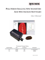
PIKA SERIES IMAGING SPECTROMETERS
AND SPECTRONON SOFTWARE
User Manual
Document Change History
Version Number
Date
Contributor
Description
V1.0
V1.1
V1.2
3/12/07
9/12/08
5/28/09
Cws
Cws
RCS
Document Creation
Updated
Updates
Updated 5/28/2009
i
Copyright and License
Spectronon - Resonon's hyperspectral image acquisition and analysis software.
(c) 2005-2007 Resonon
Below are thanks and credit to underlying libraries as well as links to their licenses. The Spectronon EULA follows.
Spectronon is built proudly and primarily with Python.
Python license: www.python.org/download/releases/2.4.2/license/
learn more: www.python.org
Spectronon was written by Resonon and employs the fine libraries listed below, each with links to the accompanying license.
numpy - BSD license:
http://en.wikipedia.org/wiki/BSD_license
learn more: http://www.numpy.org
wxPython - wxWidgets license:
http://wxwidgets.org/about/newlicen.htm
learn more: http://www.wxpython.org
matplotlib - matplotlib license:
http://matplotlib.sourceforge.net/license.html
learn more: http://matplotlib.sourceforge.net/
pywin32 - Python license:
http://www.python.org/download/releases/2.4.2/license/
learn more: http://sourceforge.net/projects/pywin32/
PIL - (c) Secret Labs AB and Fredrik Lundh:
http://www.pythonware.com/products/pil/license.htm
learn more: http://www.pythonware.com/products/pil/
The Full copyright is included at the bottom of this notice.
SPECTRONON END-USER SOFTWARE LICENSE AGREEMENT
Version 1.1 (April 2007)
The executable code version of Spectronon or SpectrononPro and all related media, printed material, electronic
documentation, and other documentation (collectively the "Software") is made available to you under the terms of this
RESONON END-USER SOFTWARE LICENSE AGREEMENT ("AGREEMENT"). BY INSTALLING, COPYING, OR OTHERWISE
USING THE SOFTWARE, YOU ARE CONSENTING TO BE BOUND BY THIS AGREEMENT. IF YOU DO NOT AGREE TO THE
TERMS AND CONDITIONS OF THIS AGREEMENT, DO NOT INSTALL OR USE ANY PART OF THE SOFTWARE.
DURING THE SOFTWARE INSTALLATION PROCESS, AND AT LATER TIMES, YOU MAY BE GIVEN THE OPTION OF
INSTALLING ADDITIONAL COMPONENTS FROM THIRD-PARTY SOFTWARE PROVIDERS. THE INSTALLATION AND USE OF
THOSE THIRD-PARTY COMPONENTS MAY BE GOVERNED BY ADDITIONAL LICENSE AGREEMENTS.
1. LICENSE GRANT. Resonon, Inc., a Montana business corporation ("Resonon"), grants you a non-exclusive license to
use the executable code version of the Software. This Agreement will also govern any software upgrades provided by
Resonon that replace and/or supplement the original Software, unless such upgrades are accompanied by a separate
license, in which case the terms of that license will govern.
2.
DESCRIPTION OF OTHER RIGHTS AND LIMITATIONS.
Maintenance of Proprietary Notices. You may not remove or alter any trademark, logo, copyright or other proprietary notice
in or on the Software. This license does not grant you any right to use the trademarks, service marks or logos of Resonon or
its licensors.
Distribution. You may not distribute copies of the Software to third parties.
Transfer. You may permanently transfer all of your rights under this Agreement, provided the recipient agrees to the terms
of this Agreement. You may not rent, lease, loan or sublicense the Software.
Prohibition on Modification, etc. Except as permitted by applicable law notwithstanding this Agreement, you may not modify,
translate or create derivative works from the Software.
Compliance with Law. You must comply with all applicable laws regarding use of the Software.
3. PROPRIETARY RIGHTS. Resonon, for itself and on behalf of its licensors, hereby reserves all intellectual property rights
(including but not limited to copyrights) in the Software except for the rights expressly granted in this Agreement.
4. TERMINATION. If you breach this Agreement your right to use the Software will terminate immediately and without
notice, but all provisions of this Agreement except the License Grant (Paragraph 1) will survive termination and continue in
effect. Upon termination, you must destroy all copies of the Software.
5. EXPORT CONTROLS. This license is subject to all applicable export restrictions. You must comply with all export and
import laws and restrictions and regulations of any United States or foreign agency or authority relating to the Software and
its use.
6. U.S. GOVERNMENT END-USERS. The Software is a "commercial item," as that term is defined in 48 CFR 2.101 (Oct.
2006), consisting of "commercial computer software" and "commercial computer software documentation," as such terms
are used in 48 CFR 12.212 (Oct. 2006) and 48 CFR 227.7202 (Oct. 2006). Consistent with 48 CFR 12.212, 48 CFR
27.405(b)(2), and 48 CFR 227.7202, all U.S. government end users acquire the Software with only those rights as set forth
in this Agreement.
7. DISCLAIMER OF WARRANTY. THE SOFTWARE IS PROVIDED "AS IS" WITH ALL FAULTS. TO THE EXTENT PERMITTED
BY LAW, RESONON AND RESONON'S DISTRIBUTORS and LICENSORS HEREBY DISCLAIM ALL WARRANTIES, WHETHER
EXPRESS OR IMPLIED, INCLUDING WITHOUT LIMITATION WARRANTIES THAT THE SOFTWARE IS FREE OF DEFECTS,
MERCHANTABLE, FIT FOR A PARTICULAR PURPOSE, AND NON-INFRINGING. YOU BEAR THE ENTIRE RISK AS TO
SELECTING THE SOFTWARE FOR YOUR PURPOSES AND AS TO THE QUALITY AND PERFORMANCE OF THE SOFTWARE.
THIS LIMITATION WILL APPLY NOTWITHSTANDING THE FAILURE OF ESSENTIAL PURPOSE OF ANY REMEDY. SOME
JURISDICTIONS DO NOT ALLOW THE EXCLUSION OR LIMITATION OF IMPLIED WARRANTIES, SO THIS DISCLAIMER MAY
NOT APPLY TO YOU.
8. LIMITATION OF LIABILITY. EXCEPT AS REQUIRED BY LAW, RESONON AND ITS DISTRIBUTORS, DIRECTORS,
LICENSORS, CONTRIBUTORS, AND AGENTS (COLLECTIVELY, THE "RESONON GROUP") WILL NOT BE LIABLE FOR ANY
INDIRECT, SPECIAL, INCIDENTAL, CONSEQUENTIAL OR EXEMPLARY DAMAGES ARISING OUT OF OR IN ANY WAY
RELATING TO THIS AGREEMENT OR THE USE OF OR INABILITY TO USE THE SOFTWARE, INCLUDING WITHOUT
LIMITATION DAMAGES FOR LOSS OF GOODWILL, WORK STOPPAGE, LOST PROFITS, LOSS OF DATA, AND COMPUTER
FAILURE OR MALFUNCTION, EVEN IF ADVISED OF THE POSSIBILITY OF SUCH DAMAGES AND REGARDLESS OF THE
THEORY (CONTRACT, TORT OR OTHERWISE) UPON WHICH SUCH CLAIM IS BASED. THE RESONON GROUP'S COLLECTIVE
LIABILITY UNDER THIS AGREEMENT WILL NOT EXCEED THE GREATER OF $500 (FIVE HUNDRED U.S. DOLLARS) AND THE
FEES PAID BY YOU UNDER THIS LICENSE (IF ANY). SOME JURISDICTIONS DO NOT ALLOW THE EXCLUSION OR
LIMITATION OF INCIDENTAL, CONSEQUENTIAL OR SPECIAL DAMAGES, SO THIS EXCLUSION AND LIMITATION MAY NOT
APPLY TO YOU.
9. MISCELLANEOUS. (a) This Agreement constitutes the entire agreement between Resonon and you concerning the
subject matter hereof, and it may only be modified by a written amendment signed by an authorized executive of Resonon.
(b) Except to the extent applicable law, if any, provides otherwise, this Agreement will be governed by the laws of the State
of Montana, U.S.A., excluding its conflict of law provisions, and, in respect of any dispute which may arise hereunder, you
consent to the jurisdiction of the federal and state courts sitting in the State of Montana (c) This Agreement will not be
governed by the United Nations Convention on Contracts for the International Sale of Goods. (d) If any part of this
Agreement is held invalid or unenforceable, that part will be construed to reflect the parties' original intent, and the
remaining portions will remain in full force and effect. (e) A waiver by either party of any term or condition of this
Agreement or any breach thereof, in any one instance, will not waive such term or condition or any subsequent breach
thereof. (f) Except as required by law, the controlling language of this Agreement is English. (g) You may assign your rights
under this Agreement to any party that consents to, and agrees to be bound by, its terms; Resonon may assign its rights
under this Agreement without condition. (h) This Agreement will be binding upon and will inure to the benefit of the parties,
their successors, and permitted assigns.
# End Spectronon EULA
The Python Imaging Library (PIL) is
Copyright © 1997-2006 by Secret Labs AB
Copyright © 1995-2006 by Fredrik Lundh
By obtaining, using, and/or copying this software and/or its associated documentation, you agree that you have read,
understood, and will comply with the following terms and conditions:
Permission to use, copy, modify, and distribute this software and its associated documentation for any purpose and without
fee is hereby granted, provided that the above copyright notice appears in all copies, and that both\ that copyright notice
and this permission notice appear in supporting documentation, and that the name of Secret Labs AB or the author not be
used in advertising or publicity pertaining to distribution of the software without specific, written prior permission.
SECRET LABS AB AND THE AUTHOR DISCLAIMS ALL WARRANTIES WITH REGARD TO THIS SOFTWARE, INCLUDING ALL
IMPLIED WARRANTIES OF MERCHANTABILITY AND FITNESS. IN NO EVENT SHALL SECRET LABS AB OR THE AUTHOR BE
LIABLE FOR ANY SPECIAL, INDIRECT OR CONSEQUENTIAL DAMAGES OR ANY DAMAGES WHATSOEVER RESULTING FROM
LOSS OF USE, DATA OR PROFITS, WHETHER IN AN ACTION OF CONTRACT, NEGLIGENCE OR OTHER TORTIOUS ACTION,
ARISING OUT OF OR IN CONNECTION WITH THE USE OR PERFORMANCE OF THIS SOFTWARE.
Contacts and Support
Customer support forum
www.spectronon.com/bb
Online Documentation
www.spectronon.com/
Table of Contents
Int roduction . . . . . . . . . . . . . . . . . . . . . . . . . . . . . . . . . . . . . . . . . . . . . . . . . . . . . . . . . . . . . . . . . . . . . . . . . . . . . . . . . . . . . . . . . . . . . . . . . . . 1
Brief Introduction to Hyperspectral Data................................................................................................... 1
Requirements ............................................................................................................................................. 2
I ns ta l lat io n . . . . . . . . . . . . . . . . . . . . . . . . . . . . . . . . . . . . . . . . . . . . . . . . . . . . . . . . . . . . . . . . . . . . . . . . . . . . . . . . . . . . . . . . . . . . . . . . . . . . . . 3
Installing the Hardware.............................................................................................................................. 3
Installing the Software ............................................................................................................................... 6
Co l l ect i ng Data . . . . . . . . . . . . . . . . . . . . . . . . . . . . . . . . . . . . . . . . . . . . . . . . . . . . . . . . . . . . . . . . . . . . . . . . . . . . . . . . . . . . . . . . . . . . . . 1 0
Lighting Fundamentals ............................................................................................................................ 10
Preparing for Data Collection .................................................................................................................. 11
Focusing.............................................................................................................................................. 11
Using AutoExposure .......................................................................................................................... 12
Adjusting the Aperture ....................................................................................................................... 13
Modes ...................................................................................................................................................... 13
Raw Data............................................................................................................................................. 13
Reflectance .......................................................................................................................................... 13
Radiance.............................................................................................................................................. 14
Collecting and Saving Data .................................................................................................................... 15
Collecting Data................................................................................................................................... 15
Saving Data ........................................................................................................................................ 15
Saturation Alarm................................................................................................................................ 16
Adjusting the Scanning Stage .................................................................................................................. 17
V i e w ing a nd M a n ip u la t ing t h e D a t a . . . . . . . . . . . . . . . . . . . . . . . . . . . . . . . . . . . . . . . . . . . . . . . . . . . . . . . . . . . . . . . . . 1 8
Opening a Datacube................................................................................................................................. 18
Zoom, Pan, Flip, and Rotate Tools .......................................................................................................... 18
Selecting Regions of Interest ................................................................................................................... 19
Spectral Plot and XY Plotter Windows ................................................................................................... 19
Plotting Data to the Spectral Plot and XY Plotter Windows ............................................................. 19
Zooming and Panning ....................................................................................................................... 20
Clearing the Spectral Plot Window.................................................................................................... 20
Renders and Filters .................................................................................................................................. 20
The Color Infrared (CIR) Render...................................................................................................... 20
Saving Spectra, Plots and Renders........................................................................................................... 21
A dv a nc ed D a t a M a n ipu lat io n a n d A na ly s i s . . . . . . . . . . . . . . . . . . . . . . . . . . . . . . . . . . . . . . . . . . . . . . . . . . . . . . 2 2
Cube Tools............................................................................................................................................... 22
Binning ............................................................................................................................................... 22
Spectral Correction ............................................................................................................................ 23
Radiance Correction .......................................................................................................................... 23
Cube Tools Example................................................................................................................................ 23
The Spectral Angle Map cube tool..................................................................................................... 23
Adv a nc ed Se tt ing s . . . . . . . . . . . . . . . . . . . . . . . . . . . . . . . . . . . . . . . . . . . . . . . . . . . . . . . . . . . . . . . . . . . . . . . . . . . . . . . . . . . . . . . . . . 2 6
5
Imager Settings ........................................................................................................................................ 26
Framerate ........................................................................................................................................... 26
Gain and Shutter ................................................................................................................................ 26
Binning ............................................................................................................................................... 26
Calibration Cube Sizes ....................................................................................................................... 26
Recording Modes................................................................................................................................ 26
Slope and Intercept (Calibration) ...................................................................................................... 27
Stage Settings .......................................................................................................................................... 27
Steps Per Frame ................................................................................................................................. 27
Seconds per Step................................................................................................................................. 27
Interface ................................................................................................................................................... 27
Video Update Speed............................................................................................................................ 27
P ro b l e m R es ol ut io n s . . . . . . . . . . . . . . . . . . . . . . . . . . . . . . . . . . . . . . . . . . . . . . . . . . . . . . . . . . . . . . . . . . . . . . . . . . . . . . . . . . . . . . . 2 8
6
Introduction
Resonon’s Pika imaging spectrometers are compact, high-fidelity, digital instruments for
industrial and scientific applications. Spectronon is a powerful hyperspectral data
collection and analysis software package. Spectronon’s data collection tools are highly
integrated with the Pika imaging spectrometers to streamline the collection of spectral
images. Spectronon’s data viewing and analysis functions can also be used without a
Pika imaging spectrometer. For data viewing and analysis, Spectronon is easy to learn,
offers efficient workflow, and is highly extensible by the user for custom applications.
This User Manual covers the installation and use of Pika series imaging spectrometers
and Spectronon software. Due to the tight integration between the Pika series imaging
spectrometers and Spectronon, both topics are covered together. Users of Spectronon
without a Pika can skip sections specific to the Pika II.
Topics covered in this manual:
x
x
x
x
x
x
x
Introduction to Hyperspectral Imaging
Setting up the Imaging Spectrometer and Additional hardware
Installing Spectronon Software
Collecting Hyperspectral Data
Viewing and manipulating Data
Advanced Features of Spectronon Software
Advanced Data Manipulation and Analysis
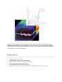
Brief Introduction to Hyperspectral Data
Hyperspectral Imaging, or imaging spectroscopy, refers to the creation of a digital image
containing very high spectral (color) resolution. Each spatial point (pixel) in a
hyperspectral image represents a continuous curve of incoming light intensity versus
wavelength. The data can also be interpreted as a stack of images, with each layer in
the stack representing the scene at a different wavelength.
1
Hyperspectral imaging has a long heritage as a remote sensing tool, operating from
satellites and airplanes. In this capacity, it has proven itself as a useful tool for scene
discrimination; the Pika series imaging spectrometers provide this powerful capability in
a cost-effective, compact package.
Requirements
x
x
x
x
x
x
Windows® XP Service Pack 2
512MB of RAM, 1 Gig or more recommended
Intel® Pentium 4 2.0GHZ or compatible processors
AGP video card with 64 MB video memory
32-bit standard PCI slot for IEEE-1394 card
Firewire 800 port with Texas Instruments OHCI Compliant IEEE 1394b Host Controller
2
Installation
This chapter covers:
x
x
Installing the Hardware
Installing the Software
Installing the Hardware
The Pika series spectrometers are linescanning instruments; meaning that they
collects one line of image data per frame. In order to collect a 2D image, a Pika
imaging spectrometer or the object to be imaged must be physically moved, or
scanned. Resonon sells two options for scanning: a Rotation Stage, which is a
tripod-based unit intended for outdoor use, and a Linear Stage which is intended
for scanning objects under controlled lighting.
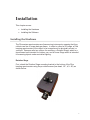
Rotation Stage
First, attach the Rotation Stage mounting bracket to the bottom of the Pika
imaging spectrometer using the provided screws (low-head, 1/8”, #¼ -20) as
shown below:
3
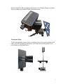
Second, attach the Pika imaging spectrometer to the Rotation Stage and tighten
the set screw in the Rotation Stage mounting bracket.
Translation Stage
To use the translation stage, attach mounting posts to the mounting holes in the
base of the Pika imaging spectrometer, then insert the mounting posts to the
post-holders on the stage frame.
4
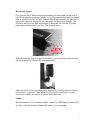
Microscope Option
First, screw in the C-Mount Microscope adapter into the threads on the front of
the Pika imaging spectrometer. (Note: If your Pika spectrometer was purchased
with an objective lens as well as a C-Mount Microscope adapter, you will have to
remove the objective lens before you can attach the Microscope adapter. This
should be done in a low-dust environment to decrease the chances of getting
particulate contamination in the slit.) This is shown below:
Second, mount the Pika II on the camera port of your microscope and lock down
the set screw in the C-Mount Microscope adapter.
Adjust the focus of the microscope while viewing the focusing object through the
microscope’s eyepieces. Then, adjust the focus on the camera port of your
microscope until the instrument is focused simultaneously.
Cables
Before installation of the software, please connect the USB Stage Controller and
the Pika II (via the provided Firewire 800 cable) to your computer.
5
Lighting
Proper lighting is very important to collecting high fidelity data. A brief
introduction to lighting techniques is covered in Chapter 3.
Installing the Software
Resonon’s hyperspectral data collection and analysis software, Spectronon,
provides the user interface for collecting data from Pika spectrometers. The
software also includes data viewing and manipulation functionality, which can be
used without a Pika spectrometer on any hyperspectral data of the proper format
(.bil, .bip, or .bsq, with an ENVI© formatted header file). To use the software for
data acquisition, the Pika imaging spectrometer and scanning stage controller
must be plugged in before the installation process begins. If Spectronon has
been installed previously without the Pika or scanning stage controller plugged
in, the software must be reinstalled with those units plugged in before they can
be used. Once installed, Spectronon can be run with or without the hardware
attached.
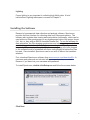
First, download Spectronon software from www.resonon.com/downloadPro. A
username and password are included with your spectrometer, or contact
Resonon if you have lost your username and password.
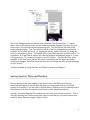
To install Spectronon, double-click Setup.exe and follow the screens below:
Click Next
6
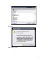
Click Install
Click Continue Anyway
7
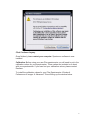
Click Continue Anyway
Once finished, please restart your computer. Spectronon software is now
installed.
Calibration: Before using your new Pika spectrometer you will need to put in the
calibration values for your spectrometer. These values are included on a sheet
with your spectrometer. If you have lost your calibration values, please contact
Resonon.
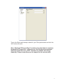
To install the calibration values for your Pika Spectrometer: WindowÆ
PreferencesÆ Imager Æ Advanced. This will bring up the window below.
8
Type in the Slope and Intercept values for your Pika spectrometer and click the
“set” buttons for each.
Note: Windows XP Service Pack 2 contains a bug that limits to maximum
bandwidth of Firewire 800. In Spectronon, this bug limits the maximum
framerate of the Pika II to 7.5 FPS. Patches are available, but change
frequently. Please contact Resonon for support for the current patch.
9
Collecting Data
This chapter covers:
x
x
x
x
x
x
Lighting Fundamentals
Using the Autoexposure feature
Focusing the Pika II
Dark Current and Response Correction
Collecting and Saving Data
Adjusting the Scanning Stage settings
Lighting Fundamentals
Proper lighting is essential in the process of collecting high fidelity hyperspectral data.
The three most important factors for lighting are:
1. Stable (spectral stability and intensity stability)
2. Diffuse
3. Spectrally Continuous (not fluorescent or discharge)
Halogen lights are good, inexpensive sources. Incandescent lamps are also
acceptable, but are not as bright as halogen. Fluorescent or discharge lamps, contain
sharp spectral features of high intensity at some wavelengths and low intensity at other
wavelengths. These lamps are not recommended, as they do not provide sufficient
illumination at many of the wavelengths of interest. If the blue and UV spectral
regions are of particular importance, a high color temperature (>4500ºK) or
‘Daylight’ halogen bulb should be used as most conventional halogen bulbs do
not emit much light in the low blue/UV region.
To improve the stability of halogen or incandescent lights, let the lights warm up for at
least 5 minutes prior to collecting data. Additionally, a regulated power supply for the
lights is highly recommended.
To diffuse the light sources, ground glass plates or plastic diffusers are recommended.
Integrating spheres are ideal but expensive and often impractical. Diffusers should be
positioned between the light sources in a manner to maximize the uniformity of the
illumination on the object.
10
Preparing for Data Collection
To begin the data collection process, ensure that the imager and scanning stage are
plugged in and that the lights are on and properly warmed-up. Launch Spectronon.
The imager and stage controls should be active (not grayed), as shown below.
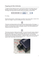
Focusing
Place the Spectralon© or Teflon© sheet in the field of view of the imager, in place of the
object to be imaged. Press the AutoExposure button, shown below.
This function will automatically set the exposure time and gain setting of the imager. It
is helpful to do this before focusing to make sure the camera settings are adjusted such
than you can see the object under your lighting conditions. Once the AutoExposure is
complete, press the Focuser button.
This function shows live data from the imager. It is used to focus the imager and also to
place the Spectralon© or Teflon© in the proper location for collecting correction data.
By waving your hand under the imager near the white reference, you should see
movement in the main Spectronon window. Place the object to scan in the field of view
of the instrument, using the data window for feedback. Unscrew the lock ring on the
objective lens of the imager, as shown below.
11
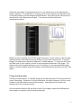
Screw the main body of the objective lens in or out until the lines in the data window
begin to sharpen. For assistance in focusing, click on the Inspector tool, and then click
on the data screen over the sharpest spatial features. Then click on the YPlotter tab on
the right side of the Spectronon window. Your screen should look like the
screencapture below.
When Focuser is running, the YPlotter graph shows the Y cross section of the live data.
Spatial features of the object show up as dips or rises in the cross section. Focus the
imager to maximize the contrast (steepness) of these features. You may use the Zoom
and Pan tools (on the toolbar) to zoom in and navigate the features in the graph. For
objects without fine spatial features to use for focusing, it is recommended that graph
paper or another suitable target with sharply contrasted features be placed on top of the
object.
Using AutoExposure
Position the Spectralon© or Teflon© (watching the data window) to fill the entire field of
view of the imager. Because of its high reflectance, the white reference will look much
brighter in the data window than its surroundings. Interpreting the live data is an
acquired skill, but is learned quickly.
Once the white reference fills the field of view of the imager, press the AutoExposure
button again to properly set the exposure and gain.
12
Adjusting the Aperture
The aperture of most objective lenses can be adjusted across a wide range. For the
Pika II, f/#s below f/3 are not recommended, and for the Pika NIR f/#s below f/2 are not
recommended because this will increase the amount of scattered light inside of the
instrument. Choosing an f/# is a trade; the higher the f/#, the less light the instrument
will collect but the depth of focus of the instrument will increase. A smaller f/# means
more light will be collected but the depth of focus will be shorter. For cases in which the
user wishes to post-correct the data from a reference object in the scene (for example,
when the user is using the Rotation Stage and the Teflon© reference does not fill the
entire field of view), it is required that the f/# be set no lower than f/4 for good results.
Again, after adjusting the aperture, you will need to run AutoExposure to set optimum
exposure and gain levels.
Modes
Pika imaging spectrometers can collect data in 3 modes: Raw Data, Reflectance, and
Irradiance. To select the mode of operation, navigate to the Mode menu item and
select the desired mode. Each mode is described below.
Raw Data
In Raw Data mode, data is recorded without any processing. The result is thus a
product of the reflectance of the object, the spatial and spectral distribution of the
lightning, and the response of the instrument.
Reflectance
For many applications, the absolute Reflectance of the scene is desired. Because all
light sources (including halogen lamps and the sun) have spectral structure, it is
necessary to remove the spectral component of the light source from the collected data.
Additionally, spectral imagers have non-uniform spectral and spatial response which
also must be removed from the data. In order to do this, data from a uniform reference
is collected. A flat sheet of Teflon© is an inexpensive reference with a nearly flat
spectral reflection near .95 (95%). However, for high fidelity applications it is
recommended to use a Spectralon© (www.labsphere.com) panel instead.
The first step in collecting Reflectance data is to set the exposure using Autoexposure
as described in the preceding section. Next, a Dark Current Correction Cube is
necessary.
Press the Dark Current button.
13
You will be instructed to cover the lens of the imager to block all incoming light. This is
best done with the included lens cap. Once the lens is covered, select OK. After
recording this data, the Dark Current button will show a red checkmark, indicating that
the dark current noise of the imager will be automatically removed from the data.
Next, a Response Correction Cube must be collected.
(Users of the Rotation stage for which the white reference does not fill the entire field of
view, skip this step. Correcting the data in this case is explained in Chapter 5)
Once the collection of the Dark current is complete, press the Response Correction
Cube button.
This will instruct you to place the white reference (e.g. Teflon©) in front of the imager.
Make sure the reference target fills the field of view of the imager. Press OK to
continue. Once complete, the Response Correction button will show a red checkmark.
The data will now be automatically corrected for the illumination spectrum and
instrument response. The resultant data is in units of 0-4095, representing Reflectance
from 0-100%. In Float Mode (covered in Chapter 6), the units are 0-1.0.
Anytime the aperture, gain, exposure time, or light source changes, the Dark
Current and Response Correction collection processes (as described above)
must be repeated.
Radiance
In Radiance Mode, data is recorded in relative units of Radiance. (To produce absolute
units of radiance, additional steps are required. This will be discussed later.) In order to
use Radiance Mode, a black body light source with a calibrated color temperature or a
radiance calibration standard is necessary.
First, set up the imager so the field of view is filled by the reference light source. The
intensity of the reference light should be adjusted to approximate the intensity of the
scene illumination. Set your exposure using the Autoexposure feature, as described
above. Cover the lens and collect a Dark Current correction cube. Then collect the
Radiance Correction cube by pressing the Response Correction Cube button. .
Then press the Set Black Body Temperature button:
14
When prompted, enter the Color Temperature of the reference light source.
In order to produce absolute units of radiance, keep the exposure settings of the system
at the same level they were at when the datacube of interest was collected. Position
the imager to ensure that the reference light is filling the field of view. Collect a data
cube in Radiance mode and find the peak intensity value. Scale this number by the
intensity reading of your reference light (in W/m²/sr). Using the Unit Conversion tool
within the Process to new Cube menu, produce a new datacube using this number as
the conversion factor.
Collecting and Saving Data
Collecting Data
To collect data, click the Start and Stop Recording button.
The stage will begin moving, and lines of image data will be displayed in the data
window. By default, the image data is represented by a True Color rendering of the
scene. More information on Renders and Filters is available in Chapter 4.
To stop, press the button again. The stage should move back to its starting location. To
adjust the starting location of the stage, press the Move Stage buttons, shown below.
Once the Start Recording button is pressed, data recording will continue until the button
is pressed again. If you would like to record a specific number of frames, enter in the
desired number of frames in the Frame Number window, show below.
If zero is entered, the software will record indefinitely. A non-zero number allows the
software to allocate the necessary resources for the data, which improves performance.
A scan can be stopped at anytime using the stop button.
Saving Data
Once data has been collected, it is temporarily stored and represented in the left side of
Spectronon, called the Resource Tree, as shown below.
15
To save the data, right-click on the Current Scan item (colored blue above). Select
Save Cube or Save Cube As to save to disk. You may also select the menu item Cube
Æ Save Cube instead of the right-clicking method.
If you would like to only save a portion of the cube, click the Select Areas tool on the
toolbar.
Select the portion of the image you would like to save by dragging a square over the
area. Right click inside of the square and select Crop Into New Cube. Alternatively,
you may select the menu item Selection Æ Crop Into New Cube. Once this is done,
right-click on the newly generated cube in the Resource Tree and save as described
above.
Saturation Alarm
The Saturation Alarm
warns the user of potentially erroneous data due to detector
saturation or bit overflow. This icon will turn yellow when saturation or bit overflow
occurs.
Detector saturation happens because too much light is incident on the detector for the
given gain and exposure settings. Saturated data is evident by flat-topped spectra. It is
recommended to run AutoExposure again to solve this problem.
Bit overflow occurs when a reflectivity greater than 100% is reported. Most likely, this is
caused by data noise while recording scenes of reflectivity near 100%, where the noise
pushes values over the 100% threshold. It can also occur when faceted sample
produces a glint from a non-diffuse light source directly into the scanner, or it may be
caused by light source fluctuations or a poorly recorded Response Correction file. It is
recommended to record a new Response Correction file when bit overflow occurs.
16
Adjusting the Scanning Stage
Once data has been collected, examine the image to determine if the aspect ratio (the
ratio of the X dimension scale to the Y dimension scale) is correct. If the image looks
compressed in the direction of the scan, the stage step size is too large. If the image
looks stretched in the direction of the scan, the stage step size is too small. To adjust
the step size, find Window in the Menu bar, and select Preferences. Find Stage in the
tree, and select it. Change the Steps Per Frame setting until the aspect ratio is correct.
Scanning an image of a circle is often useful for setting the aspect ratio correctly.
17
Viewing and Manipulating the
Data
This chapter includes the following topics
x
x
x
x
x
x
Opening a Datacube
Zoom, Pan, and Rotate Tools
Selecting Regions of Interest
Spectral Plot and XY Plotter Windows
Renders and Filters
Saving Spectra, Cubes, and Renders
Opening a Datacube
To open a datacube in Spectronon, select the File Æ Open menu item and select the
datacube to open. Spectronon can open any datacube with an ENVI© formatted
header.
Datacubes collected from a source other than a Resonon instrument need another
parameter to be added into the header file for certain functions to operate. If prompted
for the Reflectance Scale Factor (RSF), enter that value now. The RSF for an imaging
spectrometer is the data value that corresponds to 100% reflectivity.
By default, the data is opened with a True Color render of the data. This render
approximates the appearance of the object under normal lighting conditions by
combining red, green, and blue bands from the datacube. In general, a Render is a 2D
visualization of the datacube. Renders and Filters will be covered in detail later in this
chapter.
Zoom, Pan, Flip, and Rotate Tools
To Zoom into a specific area of the image, click the Zoom In tool from the toolbar.
18
By clicking in the Render, the view will zoom in. It is also possible to click and drag a
window within the render to zoom into the windowed area. To Zoom Out, use the Zoom
Out tool available on the toolbar.
The user may also Zoom In and Out using the mouse scroll wheel, if available.
To Pan the image while Zoomed In, select the Pan tool.
the Render to pan.
Click and Drag inside of
To Flip or Rotate the image, use these tools:
Selecting Regions of Interest
A Region of Interest is a selectable group of pixels within the datacube. The associated
spectra from these pixels can then be saved, averaged, or copied to the clipboard.
To select a Region of Interest, select either the
or
tools from the menu bar.
Click and drag a rectangle of interest with the first tool, or click and drag any shape with
the second.
Once selected, right-click within the selected areas for options.
Spectral Plot and XY Plotter Windows
Plotting Data to the Spectral Plot and XY Plotter Windows
The Spectral Plot window shows the spectrum of a selected pixel or the spectrum open
in the Resource Tree (far left side of the Spectronon window). To show the spectrum of
a pixel within the Render, select the Inspector tool.
Click a point inside of the Render to see the spectrum of that pixel. One can also click
and hold while dragging to update the Spectral Plot window continuously.
The X and Y Plotter Windows show cross-sections of the current Render (X and Y cross
sections respectively) at the point of the Inspector tool pointer. The black line in the X
or Y Plotter window represents the location of the Inspector tool pointer in the alternate
dimension (Y or X respectively).
19
Zooming and Panning
Zooming and Panning function in the plotting windows just as in the render window. To
zoom in, select the Zoom In tool from the toolbar. Click in the appropriate plot window,
or click and drag a rectangle in the plot window to zoom to that area. Select the Zoom
Out tool and click to zoom out. To Pan, select the Pan tool, then click and drag in the
plot window.
Clearing the Spectral Plot Window
To clear the Spectral Plot or XY Plotter Windows, select the Plot menu item, then Clear
Spectral Plot. This is useful to force a rescale of the Spectral Plot.
Renders and Filters
A Render is a 2D representation of a datacube. This representation can be
monochrome or full color, be one or more bands of a datacube, or contain the results of
analysis. A Filter is a set of rules that apply to a Render to alter its appearance. In this
section, two examples of using Renders and Filters will be presented.
The Color Infrared (CIR) Render
The Color Infrared Render maps an infrared band (~860 nm) of the datacube to the red
color channel of the display, a red band (~650 nm) to the green color channel, and a
green band (~550 nm) to the blue color channel. This Render may be useful in viewing
scenes containing vegetation, as chlorophyll is very reflective at 860 nm, making plant
life appear red in this Render.
To try the CIR Render, open the datacube leaf_small.bip located in the C:\Program
Files\Spectronon\examples folder. The datacube will show up in the left-side Resource
Tree and a True Color render of the datacube will appear. Right click on the leaf_small
object in the Resource Tree and select Make New Rendering Æ Tri Band Æ Color
Infrared. This can also be accessed by the menu item Cube Æ Make New Render Æ
Tri Band Æ Color Infrared.
20
The Color Infrared render will appear with the default Two Percent filter. To switch
filters, click on Rendering button on the toolbar and select Change Filter from the pulldown menu. Choose from rendering options given. You should see the view of the
render change slightly. The Two Percent filter is a contrast enhancement where the
brightest 2% of pixels are set to 1.0 brightness (white), and the darkest 2% pixels are
set to 0.0 brightness (black). The middle 96% of the pixels are then scaled from 0 to 1.0
brightness. A Linear filter is similar, but sets the brightest and darkest pixels to 1.0 and
0.0 respectively. This could be thought of as a 0% stretch. The Stretch Filter (also
available in the filter menu) allows the user to interactively set the upper and lower
stretch percentages. Note that these functions do not change the data, just its rendering
on your screen.
Another example of using Renders and Filters is covered in Chapter 5.
Saving Spectra, Plots and Renders
Once a spectrum has been added to the Spectra List in the Resource Tree (by
encircling the Region of Interest with the Lasso or Rectangular Area tool and rightclicking in its center), it can be save to disk as either a Spectrum file (for opening later in
Spectronon) or as text (for importing into Excel or other graphing program).
Similarly, the entire Spectral Plot window can be saved as an image or as text. This is
done by choosing the Plotters menu item, then choose the plot you wish to save, then
selecting either Save as Image or Save as Text.
21
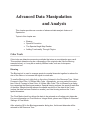
Advanced Data Manipulation
and Analysis
This chapter provides an overview of advanced data analysis features of
Spectronon.
Topics in this chapter are:
x
x
x
x
Binning
Spectral Correction
The Spectral Angle Map Render
Adding Functionality Through Plugins
Cube Tools
Cube tools are datacube processing methods that return a new datacube as a result.
This resultant datacube may be a resampling of the original cube (like the Binning
example below), or it may be an entirely different cube, such as a colorspace
conversion tool.
Binning
The Binning tool is used to average spectral or spatial channels together to reduce the
size of the cube or to increase the signal-to-noise ratio.
To use the Binning tool, right-click on the cube of interest in the Resource Tree. Select
Process to New Cube Æ UtilitiesÆBin Cube. Alternatively, you may select the menu
item CubeÆ Process to New Cube Æ UtilitiesÆBin Cube. This is followed by a dialog
box requesting the Binning parameters. Spectral binning reduces the spectral resolution
of the data, Sample binning reduces the spatial resolution of the data in the X axis
(unless the data has been rotated on screen), and Line binning reduces the Y axis
spatial dimension.
The Float Mode check box allows the data to be returned as a floating point datacube.
For more information on Float Mode vs. Integer Mode, please see Chapter 5 Advanced
Settings Æ Float Mode.
After selecting OK in the Binning parameter dialog box, the binned datacube will be
returned to the Resource Tree.
22
Spectral Correction
The Spectral Correction cube tool is used to correct a datacube for the response
function of the imager and the spectral component of the illumination source in
situations where the reflectance reference does not cover the entire field of view of the
imager. To use this tool, the datacube must contain a reflectance reference. It is also
required that the aperture of the imager be set at f/4 or higher.
First, create a Spectrum object in the Resource Tree from the reflectance reference in
the datacube. To do this, choose the appropriate ROI Tool, select the reflectance
reference in the image, and right-click to Make ROI and Mean. The mean spectra from
your selected ROI will be added to the Spectra list in the Resource Tree. Right click on
the datacube to correct in the Resource Tree, and select Process to New Cube Æ
Utilities ÆCorrect from Spectrum (or select menu item CubeÆ Process to New Cube Æ
Utilities ÆCorrect from Spectrum ). In the resulting dialog, select the Spectrum you
created before, and press OK. The entire cube will be corrected.
Radiance Correction
This procedure is used to correct a datacube for the response of the instrument and
leave the data in terms of relative radiance. To perform this procedure, select the
Correct from Cube tool from the CubeÆProcess to New CubeÆUtilities menu item.
Select the correction datacube and input the blackbody temperature of the correction
cube. A new, corrected cube will be generated. For more information on obtaining a
correction cube for use in this procedure, please contact Resonon.
Cube Tools Example
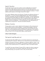
The Spectral Angle Map cube tool
The Spectral Angle Map (SAM) function is a powerful analysis tool for computing the
similarity between two spectra. SAM returns an n-dimensional angle that represents the
similarity of the spectra of a pixel in a datacube to a reference spectrum, where n = the
number of spectral bands in the datacube. This technique is relatively insensitive to the
intensity of the compared spectra; it is comparing the ‘shape’ of the spectra instead.
To use SAM, first create a Region Of Interest (ROI) to define the reference spectrum.
To do this, use the Lasso tool to encircle a small area of the red center vein of the
leaf_small.bip image (you may want to zoom in first), as shown below.
23
Right-click inside the selected area, and select Make ROI and Mean. Now, right-click
on the leaf_small.bip in the Resource Tree and select Process to new Cube Æ
Classification ÆSAM. In the Member count dialog, input the number of Member Spectra
you wish to classify. In this case, this number is one. Next, in the Member Spectrum 0
dropdown, select the leaf_small-spec-0 spectrum that you created, and click “OK.” The
controls for this Render will show up on the right side of Spectronon, as shown below:
Enter 0.1 for a Threshold. Now press update. The resulting render will appear. To see
the raw data from the SAM algorithm, use the Inspector tool and the X or Y Plotter
window (shown).
24
You may select a Live Update to interactively select a threshold. This option is
processor intensive and is only recommended on higher performance computers.
(Note: for scanned datacubes that have not yet been saved, the Live Update feature
may not be available under default settings. See Chapter 6 Advanced Settings Æ
Disk/Memory Mode for more information).
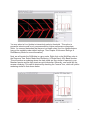
Next, we will render the SAM data in a grey scale. Right click on the MultiSam cube in
the Resource Tree. Select Make New Rendering Æ Single Band Æ By Band Number.
This will produce a rendering where the dark pixels are very similar in spectra to your
Member spectra and the light pixels are quite dissimilar. Generally, one would like the
reverse rendering. This can be obtained by checking the “Inverse” box, which will yield a
rendering similar to that shown below.
25
Advanced Settings
This chapter provides an explanation of the advanced settings of Spectronon.
x
x
Imager Settings
Stage Settings
Imager Settings
Framerate
By default, the framerate of the imager is set to 30 frames per second (FPS). The
framerate can be set as high as 60 FPS at normal detector settings, and as low as
1.875 FPS. (The imager can be set at higher frames rates for specialty applications,
please contact Resonon for more information). The lower the framerate, the more
integration time the imager has, increasing the signal-to-noise ratio (SNR), but also
increasing the amount of time necessary to collect data.
To adjust the Framerate of the imager, go to Window in the menu bar, then
PreferencesÆ Scanner.
Gain and Shutter
The gain and shutter settings of the imager are determined automatically during the
AutoExposure mode. To override or adjust these settings, go the Window Æ
PreferencesÆ Scanner. It is necessary to re-record Dark Correction and Response
Correct cubes after adjusting these settings.
Binning
Binning of the datacube increases the SNR of the data, decreases its size, but
decreases the spectral or spatial resolution of the data. To adjust the binning, select
Window Æ PreferencesÆ Scanner.
Calibration Cube Sizes
The size of the calibration cubes used in the data correction may be adjusted at Window
Æ PreferencesÆ Scanner. The size of the Dark Correction cube does normally not
need to be adjusted. It may be necessary to increase the size of the Response
Correction cube if the reflection standard shows obvious spatial variability.
Recording Modes
Four options for recording data are available. To change these options, see Window Æ
PreferencesÆ Imager. The options are reviewed below.
26
Buffer Mode: The Buffer Mode is the method of buffering data as it streams from the
imager. In Memory mode, the data is placed in the computers Random Access Memory
(RAM). This method is typically faster, allowing higher speed operation of the imager,
but is limited to the amount of available RAM on the computer. It is recommended for
smaller datacubes where speed is a priority. In Disk Mode, data is buffered to the hard
drive. It is recommended for most applications.
Float Mode: Data can be stored as Integers or Floats. Float mode has the advantage
of higher data fidelity in low signal applications (because the dark current is removed
more accurately) and has the convenience that reflectance is scaled from 0-1.
However, it requires twice the space on disk as the integer mode and requires more
time to load data.
Slope and Intercept (Calibration)
The calibration of the imager is stored in see WindowÆ PreferencesÆ ImagerÆ
Advanced. These settings should only be changed during the initial setup or under
consultation from Resonon.
Stage Settings
Steps Per Frame
The Steps Per Frame setting changes the distance that the stage moves between
frames. This setting should be adjusted to maintain proper aspect ratio. Go to
WindowÆ PreferencesÆ Stage to change this setting. If the image appears stretched
in the direction of scan, the Steps Per Frame setting is too low. Similarly, if the image is
compressed in the direction of scan, the setting is too high.
Seconds per Step
This setting is found in WindowÆ PreferencesÆ StageÆ Advanced and is used to
adjust the time delay in between steps while positioning the stage. It should normally
be set to 0.0, as a non-zero setting will limit the line rate of the system.
Interface
Video Update Speed
On lower performance computers, the responsiveness and line rate of Spectronon may
be increased by lowering the update rate of the data display. To adjust this setting, go
to WindowÆ PreferencesÆ Interface.
27
Problem Resolutions
If you have questions or are experiencing problems regarding your Pika imaging
spectrometer or Spectronon, please start your inquiry at http://www.spectronon.com.
The FAQ section may have the answer you or looking for.
Also, the solutions to many problems might also be found at the Forum section at
http://www.spectronon.com/bb/. If you do not see the answer to your question, post
your question and a Resonon support member will answer it as soon as possible.
28


![the file [< 1 MB]](http://vs1.manualzilla.com/store/data/005663565_1-91d1e4bcdfd7b45b626a6b88ab809728-150x150.png)