1
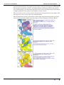
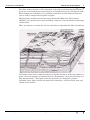
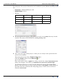
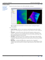
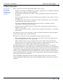
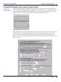
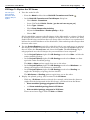
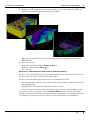
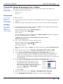
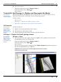
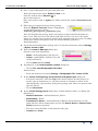
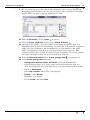
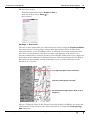
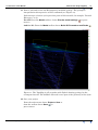
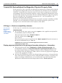
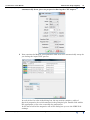
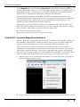
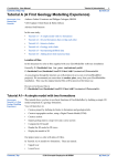
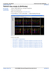
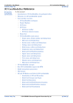
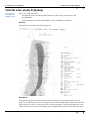
GeoModeller User Manual
Contents | Help | Top
Tutorial case study K (Dykes)
1
| Back |
Tutorial case study K (Dykes)
Parent topic:
User Manual
and Tutorials
This case study includes:
•
An introduction to building and updating a 3D geology model using 3D
GeoModeller.
•
A demonstration of 3D GeoModeller’s dyke modelling capability.
Authors
Desmond FitzGerald, Intrepid Geophysics
Disclaimer
Intrepid Geophysics provides this tutorial document and associated data for the
purpose of training in the use and application of 3D GeoModeller. The material and
data cannot be used or relied upon for any other purpose. Intrepid Geophysics is not
liable for any inaccuracies (including any incompleteness) in this material and data.
Contents Help | Top
© 2013 BRGM & Desmond Fitzgerald & Associates Pty Ltd
| Back |
GeoModeller User Manual
Contents | Help | Top
Tutorial case study K (Dykes)
2
| Back |
In this case study:
•
Case Study K Introduction
•
Course Structure
•
Tutorial K1: Create the PlatDykes 3D GeoModeller Project
•
Tutorial K2: Examine then Import Project Dykes
•
Tutorial K3: Update Stratigraphy Order of Dykes
•
Tutorial K4: Add Geology 2—Digitise and Recompute the Model
•
Tutorial K5: Import Drillhole Data and Recompute the Model
Case Study K Introduction
Parent topic:
Tutorial case
study K (Dykes)
In this case study we demonstrate the main methods available in 3D GeoModeller
v2012 to rapidly create complex 3D geology involving many dykes. Dykes are
assumed to mostly be observed but geologists on the topographic surface and in
borehole logs. Also, a means is shown of taking an airborne magnetics survey that
appears to be dominated by dyke-like bodies, and have a means of rapidly setting up a
3D geology model directly from the “automated” interpretation of “dykes” below each
individual magnetics profile. For this case, the Intrepid “NAUDYD” tool is shown in a
workflow. When there are more than 50 discrete dykes in a study area, it becomes
quite complex to track the order in which the dykes formed, and also to date the
geological events. Magnetics can help, if there is any sign of either remanent
magnetizm. The prevailing magnetic azimuth and inclination at the time of
emplacement of the dyke, if different from the current magnetic field vector, can be
used to assist dating.
Importance of Dykes for aiding Geology Interpretation
We can do no better than quoting Henry Halls from the University of Toronto. “My
general field of research is the application of geophysical methods (gravity, magnetics
and paleomagnetism) to the solution of geological problems, mainly involving major
tectonic units of the Canadian shield. More recently, I have concentrated on the
integrated paleomagnetic, geochronological and geochemical study of Precambrian
dyke swarms worldwide in an effort to understand their origins and their use as links
between dispersed Precambrian terranes.”
The last 10 years has seen a burgeoning of papers on dykes and particularly on the
recognition of “giant radiating dyke swarms”. Heat plums can be a factor here.
Dykes as barriers to subsurface groundwater flow
The recognition of dykes acting as fluid barriers has importance in relation to water
supply, mineral deposition, induced seismicity and to failure planes related to major
volcanic landslides.
Dykes project scenario
An interpretation of the dykes is required to assist forward planning for mining in the
context of a Platinum reef operation. In this case, dykes disrupt the mining process. A
magnetics geophysical survey shows the presence of many granite and dolerite dykes,
some or which appear to have reverse magnetization. The dolerite dykes are quite
extensive while the earlier Archean granite dykes are shorter and have more
variability in their shape. The mine is located somewhere near Pretoria, in the
Bushveld complex, with terrain relief of over 300 meters in the project area. This is
close to a real setting, but all the dyke data is fabricated for this study. There are
Contents Help | Top
© 2013 BRGM & Desmond Fitzgerald & Associates Pty Ltd
| Back |
GeoModeller User Manual
Contents | Help | Top
Tutorial case study K (Dykes)
3
| Back |
around 7 dolerite dykes all mapped on the surface and one also logged in a borehole.
The geology map shown is from a 1978 hand drawn exploration map of the general
area. Subsequently, several producing mines have been established and each of them
is highly profitable. The project box is 20km x 30 km x 5 km.
The aim of the exercise is to reconcile a 3D geological interpretation of the dykes with
the magnetic survey as an aid for the mine planners.
The interpretation below is illustrative of how dyke magnetization studies can help
sort out major tectonic shifts in your geology and their timings.(ref.Henry Halls)
Contents Help | Top
© 2013 BRGM & Desmond Fitzgerald & Associates Pty Ltd
| Back |
GeoModeller User Manual
Contents | Help | Top
Tutorial case study K (Dykes)
4
| Back |
Course Structure
Parent topic:
Tutorial case
study K (Dykes)
This case study has two main sections:
•
Build and Revise a 3D Geology Model
•
Perform Geophysical Modelling
Build and Revise a 3D Geology Model
Parent topic:
Course
Structure
Tutorial K1: Create the PlatDykes 3D GeoModeller Project
We create a new project, define a 3D project box and import the DTM (digital terrain
model).
Tutorial K2: Examine then Import the Project Mapped dykes
We first examine the surface mapped dykes for the project, and create the project’s
stratigraphic pile. Compute the dyke network. Plot the dyke model in map and
section views in the 2D Viewer. Build the 3D shapes of the dyke model and examine in
the 3D Viewer.
Tutorial K3: Adjust the dyke Stratigraphy
We want to change the stratigraphic order of the dyke intrusives. We update the
stratigraphic pile.
Tutorial K4: Add interpretive dyke points —Digitise and Recompute the Model
We can now digitise on the topography section, points that allow dykes to vary their
thickness, and build a revised 3D geology model. And again examine the 3D geology
model in 2D and 3D views. There are some conventions that need to be followed.
Tutorial K5: Import Drillhole Data and Recompute the Model
We import data for a drillhole. We create a vertical section, and project the drillhole
geology onto this vertical cross-section. Note the inconsistency between the new data
and the existing 3D model. We then recompute the dyke model and note the
adjustment to the dyke geometry. Again examine the 3D geology model in 2D and 3D
views.
Perform Geophysical Modelling
Parent topic:
Course
Structure
Tutorial K6: Review/Adjust the Magnetics Physical Property Data
We now add/adjust Magnetics physical property data for each dyke unit—the
susceptibility, the magnetic declination and inclination.
Tutorial K7: Compute Magnetics Solutions
There are 3 strategies for computing the magnetic solutions:
The original ‘hot spot’ bodies that may come from airborne profile data, can have local
approximations of the dyke geometry computed as prisms. In this case, the strike,
length, depth, thickness are constant at each ‘hot spot’. Within Geomodeller, the
option to use the Dykes specified as linked lists of “Hot-spot” bodies, is provided as a
quick means of assessing the forward geophysical response. The “task” file to spawn
the process is created automatically and a grid that contains the result, is available
after completion, to be inspected in the topography section.
In a similar manner, the second option involves using an Intrepid Database
conatining the Naudy body solutions, but not sorted into a form that you have
reviewed.
Contents Help | Top
© 2013 BRGM & Desmond Fitzgerald & Associates Pty Ltd
| Back |
GeoModeller User Manual
Contents | Help | Top
Tutorial case study K (Dykes)
5
| Back |
The third method involves a 3D realization of the dyke network being skeletonized,
by means of each dyke being represented as a triangulated curved, semi-planar mesh.
Each triangle has a thickness, susceptibility attributes and the infintely thin facet
code is used to compute the magnetic response.
This function is handled outside the main 3D GeoModeller tool. The Intrepid
“MTDyke” tool perfoms the actual modelling, using any of the methods for specifying
a dyke model.
There are options to control the cell size and choice of algorithm for dyke calculations.
To illustate some of the complexity where we should attempt to model the influnce of
dykes, the above diagram is reproduced from “Weijwemars - Structural Geology and
Map Interpretation”. The figure shows the geometry of a magmatic complex,
including: stock, dyke, sill and laccolith in the subsurface, and lava flows, neck and
caldera at the surface.
Contents Help | Top
© 2013 BRGM & Desmond Fitzgerald & Associates Pty Ltd
| Back |
GeoModeller User Manual
Contents | Help | Top
Tutorial case study K (Dykes)
6
| Back |
Tutorial K1: Create the PlatDykes 3D GeoModeller Project
Parent topic:
Tutorial case
study K (Dykes)
In this tutorial we load a 3D GeoModeller project and examine the components of
the 3D GeoModeller workshops.
In the tutorial:
•
K1 Steps
•
K1 Discussion
•
K1 More information
1
Launch 3D GeoModeller from the desktop icon
K1 Steps
Parent topic:
Tutorial K1:
Create the
PlatDykes 3D
GeoModeller
Project
The 3D GeoModeller welcome screen appears with a main menu and toolbars
arranged across the top, left and right sides. Only 3D GeoModeller V2.0 and
greater supports dykes.
Figure 1. 3D GeoModeller V2.0 welcome screen.
2
Create the start-point 3D GeoModeller project.
From the main menu choose Project > New or
from the Project toolbar choose New
or
press CTRL+N
In the Create a project dialog box browse to choose the parent directory of the new
project and set the project name to something like TutorialDyke1.
Contents Help | Top
© 2013 BRGM & Desmond Fitzgerald & Associates Pty Ltd
| Back |
GeoModeller User Manual
Contents | Help | Top
Tutorial case study K (Dykes)
7
| Back |
For this project the project dimensions and coordinate system (Datum and Projection)
are:
•
Projection—WGS84/UTM zone 35S
•
Height Datum—Local
•
Extents
Minimum
Maximum
Range
683,000
703,000
20,000 m
North
7,330,000
7,360,000
30,000 m
Z-axis
–3,000
2,000
5,000 m
East
3
Set the DTM for this project. The grid to be used is in the Data directory for this
tutorial. The name of the SRTM file is srtm_survey.ers
.
4
Save your own copy of this project, so that you can always start again from this
point in the workflow.
From the main menu choose Project > Save as or
from the Project toolbar choose Save As
or
press CTRL+SHIFT+S.
Save your project work as dyke1 in a folder outside the original StartTutorial
folder. For example, one folder up: GeoModeller\tutorial\CaseStudyK
Use Windows Explorer to review the files that make up the 3D GeoModeller
project. You can see that you have created a folder called dyke1, within which are
all of the files that constitute this 3D geology project. These also use the base
filename TutorialK.
Contents Help | Top
© 2013 BRGM & Desmond Fitzgerald & Associates Pty Ltd
| Back |
GeoModeller User Manual
Contents | Help | Top
Tutorial case study K (Dykes)
8
| Back |
K1 Discussion
Parent topic:
Tutorial K1:
Create the
PlatDykes 3D
GeoModeller
Project
Examine the main elements of the 3D GeoModeller workspace.
Figure 2. 3D GeoModeller End of section K1 tutorial, showing the Digital
Terrain Model.
Note in particular:
Contents Help | Top
•
Project Explorer—this has a tree structure containing the many objects that
make up our 3D geology project: Formations, Faults, Models, Sections, Drillholes,
etc.
•
2D Viewer—contains 2D sections. This Tutorial K1 project contains several
sections—a special one—the ‘geological map view’ (labelled as TopoMap in this
project), and four vertical cross-sections. We use the sections for data input, and
for examining 2D plots of our 3D model.
•
3D Viewer—contains the 3D view of our project. At this stage it shows only the
bounding extents of the project. The yellow lines are the outlines of the TopoMap
section (the topography of the project area) in the 3D Viewer, and the four vertical
sections.
•
MeshGrids —contains the DTM grid as a separate item to be queried,
manipulated, visualized. Both the 2D and 3D view have the DTM displayed using
a default colour look up table. the shortcut (right click) menu shows all the query
options.
© 2013 BRGM & Desmond Fitzgerald & Associates Pty Ltd
| Back |
GeoModeller User Manual
Contents | Help | Top
Tutorial case study K (Dykes)
9
| Back |
K1 More information
Parent topic:
Tutorial K1:
Create the
PlatDykes 3D
GeoModeller
Project
Some comments about the 3D GeoModeller project space:
•
X (East), Y (North) and Z (Elevation, positive upwards) are a standard coordinate
framework according to a right-hand rule
•
X, Y and Z are all in the same units—metres (Cannot be degrees of latitude or
longitude)
•
X and Y would typically be real world projected coordinates, but could be a local
mine grid, etc.
•
Z is Elevation, and is positive upwards. It also would typically use a real world
vertical datum such as mean sea level
•
You can (and should) define the Projection (actually a Coordinate System,
consisting of a Datum and Projection)
•
All data must be within the project limits; data outside those limits cannot be
imported or created
•
Likewise all modelled results—geology lines, polygons and surfaces—are within
those limits
So, when you create your own project, make the project dimensions large enough to
include all geology data used in the project.
Remember to allow for the full topographic height of the project area:
•
We recommend that you leave, say, 5–10% extra space at the top of the project,
above the highest point of the topography
•
Allow sufficient project space at the bottom for the entire range of modelled
geology that you are interested in. Don’t, however, make it too large or you will
take extra time to compute model shapes that are of no interest
The topography map view (TopoMap) in a 3D GeoModeller project is a special
(pseudo-non-planar) section, and it is an essential part of the project. You cannot do
any practical work in a 3D GeoModeller project until the map view section has been
created. Since topography defines the natural upper limit of a typical 3D geology
model, we use a digital terrain model (DTM) file to correctly define the shape of this
special TopoMap section. Using the correct topographic shape has geology mapping
advantages, and we recommend it.
Once the DTM (topography) has been loaded, and the map view section created
(called TopoMap in this project), the 3D GeoModeller project dimensions cannot be
changed.
Contents Help | Top
© 2013 BRGM & Desmond Fitzgerald & Associates Pty Ltd
| Back |
GeoModeller User Manual
Contents | Help | Top
Tutorial case study K (Dykes)
10
| Back |
Tutorial K2: Examine then Import Project Dykes
Parent topic:
Tutorial case
study K (Dykes)
The Tutorial K1 3D GeoModeller Project that we have just loaded already has an
automatic interpretation of ‘hot spot’dyke locations available as a .csv file. This file
is the output of the INTREPID NaudyD tool. A seperate cookbook tutorial exists to
explain how to get a good result from any airborne magnetic survey.
There are options to choose the character of the dykes you wish to see selected by the
clustering and sorting algorithm. These are shown below. The options have been
tuned to assist you in having the best chance of getting some observations of the
dykes in your project that will remain coherent and controlable as you attempt a 3D
interpretation.
Contents Help | Top
© 2013 BRGM & Desmond Fitzgerald & Associates Pty Ltd
| Back |
GeoModeller User Manual
Contents | Help | Top
Tutorial case study K (Dykes)
11
| Back |
In this section:
•
K2 Overview
•
K2 Stage 1—Examine the HOT-SPOT dyke data
•
K2 Stage 2—Explore model plotting options
•
K2 Stage 3—Explore the 3D Viewer
K2 Overview
Parent topic:
Tutorial K2:
Examine then
Import Project
Dykes
Contents Help | Top
In this tutorial we:
1
Examine the ‘hot spot’ dyke mapping data.
2
Import the Dyke Mapping data via as data located on the topography.
3
Review the Project’s stratigraphic pile
4
Compute the geology model, and plot modelled geology in map and section views
(2D Viewer)
5
Build 3D shapes of the geology model and examine (3D Viewer)
© 2013 BRGM & Desmond Fitzgerald & Associates Pty Ltd
| Back |
GeoModeller User Manual
Contents | Help | Top
Tutorial case study K (Dykes)
12
| Back |
K2 Stage 1—Examine the HOT-SPOT dyke data
Parent topic:
Tutorial K2:
Examine then
Import Project
Dykes
1
If it is not already open, open your project, or the supplied start-point 3D
GeoModeller project for Tutorial K1.
From the main menu choose Project > Open or
from the toolbar choose Open
or
press CTRL+O
(For the start-point project supplied) In the Open a project dialog box navigate to
the 3D GeoModeller Project .xml file
GeoModeller\tutorial\CaseStudyK\StartTutorialK2\
dyke2.xml . The dyke data is in the Data directory and is called
“project_dykes.csv”.
// 3D Dykes Data
// Map Projectio
Dyke
X
Mag_inclination
Dyke5,690337.77,
Dyke5,689418.10,
Dyke5,700122.57,
Dyke5,699046.24,
Dyke5,697880.21,
Dyke5,697368.95,
Dyke5,696176.01,
from naudyd. kluge from digitized stuff as well
n SUTM53/WGS84
Y
Depth Thickness Height Strike Plunge Susceptibility Similarity RMS Mag_Azimuth
7334537.86,
7333562.44,
7348562.02,
7346283.78,
7344104.20,
7343261.07,
7341673.48,
188.8,
310.9,
308.8,
44.8,
390.7,
7.2,
305.9,
173.7,
393.1,
393.1,
131.6,
471.7,
91.4,
393.1,
5868,
1965,
1965,
658,
2358,
457,
1965,
60.0, 60, 0.00190, 2.42, -1.0,
6.2, -62.8
50.0, 48.0, 0.00020, 2.48, -1.0,
6.2, -62.8
35.0, 73.2, 0.00020, 2.24, -1.0,
6.2, -62.8
40.0, 65, 0.00009, 1.62, -1.0,
6.2, -62.8
45.0, 56, 0.00036, 2.49, -1.0,
6.2, -62.8
50.0, 50, 0.00003, 2.84, -1.0,
6.2, -62.8
52.0, 67.7, 0.00421, 1.46, -1.0,
6.2, -62.8
Figure 2a. Plan view of Naudy tool, showing aeromagnetic profile lines, ‘hot spot’
solutions, then sorted’
Contents Help | Top
© 2013 BRGM & Desmond Fitzgerald & Associates Pty Ltd
| Back |
GeoModeller User Manual
Contents | Help | Top
Tutorial case study K (Dykes)
13
| Back |
Notes on HOT-SPOT format.
This format must contain standard fields that capture the essential features of an
observation of a dyke. Required fields are :
•
Location X & Y
•
Depth to top of dyke, below surface
•
Length - can be set to a constant, say 200m
•
Strike
•
Plunge
•
Thickness
•
Susceptibility - can be set to 0.0
•
Magnetic Azmiuth - can be set to 0.0
•
Magnetic Declination - can be set to 0.0
2
Import the dykes. With V2.0, many new options are supported. This includes
direct support for most geohysical database formats, as well as the usual ASCII
styles. In this case, we show the ASCII “csv” importer at work. Choose from Main
menu Import>Import>.3D Data>Dykes
Now Browse to this required file with the CSV import Wizard, panel1
Contents Help | Top
© 2013 BRGM & Desmond Fitzgerald & Associates Pty Ltd
| Back |
GeoModeller User Manual
Contents | Help | Top
Tutorial case study K (Dykes)
14
| Back |
With the Next Wizard panel, the most important lessons to be learnt are:
•
Set data to start at row 3
•
Treat consecutive delimiters as one
•
Choose both Comma ans Space delimiters.
The next Wizard pane requires you to match the fields from the CSV file to the
required fields with the Dyke Importer protocols. Most of the default selected
fields are exactly what is required. The exceptions are :
Z -> Depth ( This is the depth below surface to top of Dyke)
Length should be changed away from “FILE” to “USER” and then set to 200
FieldDeclination set to Mag Azimuth
FieldDeclination set to Mag inclination
Contents Help | Top
© 2013 BRGM & Desmond Fitzgerald & Associates Pty Ltd
| Back |
GeoModeller User Manual
Contents | Help | Top
Tutorial case study K (Dykes)
15
| Back |
The final Wizard pane assigns default colours to the incoming dyke intrusives,
once you choose to “Create dyke” in the Import all drop down list.
When the data is processed, a small report is popped up for you to examine, that
records the status of the import job.
The import process has created 5 new Dykes in the strategraphic pile, that are
initially defined using 20 field observations of an interface with an associated
foliation and thickness. This particular combination only applies to the first data
that is assigned to a Dyke formation. In effect, we use the exact same interface
and foliation primative data points as elsewhere, but impose the special condition
that the foliation must be associated with a pre-decalred Dyke formation. Then
the final piece of the puzzle is to allow a thickness of the Dyke to be specified at
the same observation point. This same approach can be used to input an
observation into 3D GeoModeller of a manually digitized dyke. Note that the
limitaion introduced here is that the observation is constained to the Topography
surface and the interface must also be defined by 2 near by points ( not the normal
one). Once an initial observation point is established, the usual rules for extra
interface and foliation points anywhere in 3D space can still be applied, to further
guide where the dyke model should appear in your model.
Contents Help | Top
© 2013 BRGM & Desmond Fitzgerald & Associates Pty Ltd
| Back |
GeoModeller User Manual
Contents | Help | Top
Tutorial case study K (Dykes)
16
| Back |
3
From the main menu choose Geology > Stratigraphic Pile: Visualise to open the
Stratigraphic Pile Viewer. The Dykes have been added to the Strategraphic pile,
each with their own series and each with an Erosional or Intrusive character. It
should be noted that the default time order of the dykes in the pile follows the
same order as in the imput file, ie the yougest are at the top of the file. It is a
simple manner to change the order in the strategraphic pile editor.
4
Compute the 3D geology model for the Project that we have loaded (to be
constrained by the geological data existing within the current Project).
From the Model toolbar, choose Compute
or press CTRL+M
In the Compute the Model dialog box:
•
Series to interpolate—Select All
•
Faults to interpolate—Select All
•
Sections to take into account—Select All
•
Faults only—Clear (therefore DO compute faults)
•
Choose OK
3D GeoModeller computes the model. (Nothing to see yet.) The model is a
mathematical model—a set of interpolator equations that are computed from the
geology contacts and orientation data. There is an interpolator equation for each
series, including each dyke, in the stratigraphic pile, and also an equation for each
fault.
Figure 3. Dyke map of the PlatDykes Project - note the cross-cutting and the
variable thickness.
Contents Help | Top
© 2013 BRGM & Desmond Fitzgerald & Associates Pty Ltd
| Back |
GeoModeller User Manual
Contents | Help | Top
Tutorial case study K (Dykes)
17
| Back |
Figure 4. Stratigraphic Pile for the PlatDykes (Tutorial K2) Project.
View the modelled geology
To see the modelled geology, we need to interrogate the model equations. We can:
•
Plot the modelled geology on the TopoMap 2D section (the Project’s geological
map)
•
Plot the modelled geology on any other 2D cross-section
•
Build the 3D shapes of the modelled geology, and view in the 3D Viewer
5
Select TopoMap in the 2D Viewer (click it)
6
From the Model toolbar, choose Plot the model settings
or press CTRL+D
In the Plot the model settings dialog box:
•
Check Show lines
•
Choose OK
The lines of the modelled geology are plotted on the TopoMap 2D Section (map).
7
Save your project
From the main menu choose Project > Save or
from the toolbar choose Save
or
press CTRL+S.
Contents Help | Top
© 2013 BRGM & Desmond Fitzgerald & Associates Pty Ltd
| Back |
GeoModeller User Manual
Contents | Help | Top
Tutorial case study K (Dykes)
18
| Back |
K2 Stage 2—Explore model plotting options
Parent topic:
Tutorial K2:
Examine then
Import Project
Dykes
1
2
Experiment with other options in the Plot the model settings dialog box:
•
Check Show fill to plot ‘solid’ geology
•
Choose Apply to All (sections) to plot all (open) 2D sections
•
For Show lines or Show fill, select or de-select various combinations of
formations
•
Choose Show trend lines in combination with Show lines or Show fill
•
Modify the Plotting resolution from the default u=50, v=50 to, say, 100 x 100
Experiment with the three plot buttons in the Model toolbar:
•
Plot the model settings
or press CTRL+D
•
Plot the model on the current section
•
Plot the model on all sections
Figure 5. Various plots options displaying the 3D geology model on Sections
TopoMap.
3
Save your project
From the main menu choose Project > Save or
from the toolbar choose Save
or
press CTRL+S.
Contents Help | Top
© 2013 BRGM & Desmond Fitzgerald & Associates Pty Ltd
| Back |
GeoModeller User Manual
Contents | Help | Top
Tutorial case study K (Dykes)
19
| Back |
K2 Stage 3—Explore the 3D Viewer
Parent topic:
Tutorial K2:
Examine then
Import Project
Dykes
1
View the model in 3D:
•
From the Model toolbar choose Build 3D Formations and Faults
•
In the Build 3D Formation and Fault Shapes dialog box:
•
Check Build—Formations
•
Leave UnChecked Build—Faults ( you do not have any as yet)
•
Select Type—Volume
•
Check Draw Shapes after building
•
Adjust the Resolution—Render quality to High
•
Choose OK
3D GeoModeller computes the 3D shapes of the dyke model as ‘volumes’ defined
by triangle mesh surfaces, which it displays in the 3D Viewer. As there are many
implicit fields being used when there are many dykes and there is a requirment to
honour the variable thickness of the thin bodies, this rendering takes longer than
for most other cases.
2
Use the Project Explorer (typically on the left-side of your work space) to manage
the display of modelled objects in the 3D Viewer. Note that the Dykes appear in
the tree below the Formations and above the Faults. The 3D Geology tag is
only populated once the 3D shapes for your model have been computed.
•
In the Project Explorer right-click 3D Geology > and select Hide—to hide the
entire modelled geology
•
In the Project Explorer right-click 3D Geology > and select Show—to show
again the entire modelled geology
The Hide or Show options toggle from one to the other.
•
In the Project Explorer right-click 3D Geology > and select Wireframe—to
change the displayed 3D volumes to wireframes
•
In the Project Explorer right-click 3D Geology > and select Shading—to
toggle the 3D display of geology back to shaded
The Wireframe or Shading options toggle from one to the other.
3
Display the plotted geology (2D) sections in the 3D Viewer
•
With any 2D Viewer window selected (for example, sAA) from the shortcut
(right-click the background of the 2D viewer), and choose from the Menu:
•
Show modelled geology polygons in 3D Viewer
•
or, Show modelled geology lines in 3D Viewer
•
Hide modelled geology polygons in 3D Viewer
These menu items toggle between Hide and Show.
Contents Help | Top
© 2013 BRGM & Desmond Fitzgerald & Associates Pty Ltd
| Back |
GeoModeller User Manual
Contents | Help | Top
4
Tutorial case study K (Dykes)
20
| Back |
Display the 3D mapping points by using right mouse button and choosing both
Interfaces and Foliations for any/all of your dykes
Figure 6. Various 3D plots of the 3D geology model, including one showing the
HOT-SPOTs.
5
Save your project
From the main menu choose Project > Save or
from the toolbar choose Save
or
press CTRL+S.
Discussion—What data have been used to make this model?
We have now examined this project in traditional 2D views, and also in a 3D Viewer,
but what data have been used to make this model?
We have used the following geological facts and interpretive data:
•
The stratigraphic order of events and the rock relationships—both recorded in the
stratigraphic pile
•
Mapped dyke contacts on the TopoMap surface section
•
Some co-incident field-measured orientation data, also on the TopoMap section
To examine these actual data, use the Project Explorer to investigate the geology
interface and orientation data catalogued within, and find the corresponding data for
each lithology stored in structures linked to either: 2D Sections, or Drillholes.
Contents Help | Top
© 2013 BRGM & Desmond Fitzgerald & Associates Pty Ltd
| Back |
GeoModeller User Manual
Contents | Help | Top
Tutorial case study K (Dykes)
21
| Back |
Tutorial K3: Update Stratigraphy Order of Dykes
Parent topic:
Tutorial case
study K (Dykes)
We want to change the Dyke5 intrusive to our geology model. We update the
stratigraphic pile. In this section:
•
K3 Overview
•
K3 Steps
K3 Overview
Parent topic:
Tutorial K3:
Update
Stratigraphy
Order of Dykes
In this tutorial we:
1
Place Dyke5 in the correct chrono-stratigraphic order in stratigraphic pile for the
Project
2
Declare the rock relationship. In this case it cuts across the older stratigraphy
1
If it is not already open, open your project dyke3 or the supplied start-point 3D
GeoModeller project for Tutorial K3.
K3 Steps
Parent topic:
Tutorial K3:
Update
Stratigraphy
Order of Dykes
From the main menu choose Project > Open or
from the toolbar choose Open
or
press CTRL+O
(For the start-point project supplied) In the Open a project dialog box navigate to
the 3D GeoModeller Project .xml file
GeoModeller\tutorial\CaseStudyK\StartTutorialK3\
StartTutorialK3.xml
2
Save a copy of this project in your own data area.
From the main menu choose Project > Save as or
from the toolbar choose Save As
or
press CTRL+SHIFT+S.
Save your project work as dyke4 in a folder outside the original StartTutorial
folder.
3
From the main menu choose Geology > Stratigraphic Pile: Create or Edit
4
In the Create or Edit geology series and the stratigraphic pile dialog box:
•
5
Contents Help | Top
For future reference, note that Top is the chosen option; for this project we
model ‘top’ of formations (i.e., all data entered is assumed to relate to the
chronologically, top-boundary of the given geology unit, where it contacts with
the unit below).
In the Create or Edit geology series and the stratigraphic pile dialog box:
•
Check that the series are in the correct
stratigraphic order, with this late-stage
Dyke5 placed towards the top of the list,
above the other Dykes (select the new series,
and use the Move up and Move down
buttons as required).
•
Then Close
6
From the main menu choose Geology > Stratigraphic Pile: Visualise
7
In the Stratigraphic Pile Viewer dialog box, review and then Close
© 2013 BRGM & Desmond Fitzgerald & Associates Pty Ltd
| Back |
GeoModeller User Manual
Contents | Help | Top
8
Tutorial case study K (Dykes)
22
| Back |
Save your project
From the main menu choose Project > Save or
from the toolbar choose Save
or
press CTRL+S.
Tutorial K4: Add Geology 2—Digitise and Recompute the Model
Parent topic:
Tutorial case
study K (Dykes)
Having updated the stratigraphic pile in Tutorial K3, we can now digitise the an
Archean Granite dyke, and build a revised 3D geology model.
In this section:
•
K4 Overview
•
K4 Stage 1—Digitise the Dyke5 geology contact
•
K4 Stage 2—Recompute and visualise in 2D and 3D
K4 Overview
Parent topic:
Tutorial K4:
Add Geology 2—
Digitise and
Recompute the
Model
In this tutorial we:
1
Digitise the ArcheanGranite1 dyke contact
2
Recompute the 3D geology model
3
Again examine the 3D geology model in 2D and 3D views
K4 Stage 1—Digitise the Dyke5 geology contact
Parent topic:
Tutorial K4:
Add Geology 2—
Digitise and
Recompute the
Model
K4 Stage 1—Steps
1
If it is not already open, open your project dyke or the supplied start-point 3D
GeoModeller project for Tutorial K4.
From the main menu choose Project > Open or
from the toolbar choose Open
or
press CTRL+O
(For the start-point project supplied) In the Open a project dialog box navigate to
the 3D GeoModeller Project .xml file
GeoModeller\tutorial\CaseStudyK\StartTutorialK4\
StartTutorialK4.xml
Contents Help | Top
© 2013 BRGM & Desmond Fitzgerald & Associates Pty Ltd
| Back |
GeoModeller User Manual
Contents | Help | Top
2
Tutorial case study K (Dykes)
23
| Back |
Save a copy of this project in your own data area.
From the main menu choose Project > Save as or
from the toolbar choose Save As
or
press CTRL+SHIFT+S.
Save your project work as dyke5 in a folder outside the original StartTutorial
folder.
3
Show the geo-registered image of the geology.
From the Explore Tree view, Surface Topography
section shortcut menu, choose
Platreef_geologyscal_wgs84z35s.png
Note the hand drawn geology map is not strictly registered with the dykes we
have so far. This was never the intent with this exercise, but now is the point
where we can add a non-magnetic granite body mapped in the top centre, trending
mostly due south of the project area. We will model this granite as
ArcheanGranite1.
4
Create the ArcheanGranite1 geology object. From the main menu choose Geology
> Dykes: Create or Edit
5
From the Create or Edit dyke dialog box
(Create a new dyke formation):
6
•
Name—ArcheanGranite1 (No spaces!)
•
Colour—(pink (RGB = 255,20,147) used
in this document)
•
Choose Add and then Close
If prompted, in the New formation creation dialog box:
•
Choose Yes, start Stratigraphic Pile editor
Alternatively:
•
7
8
Contents Help | Top
From the main menu choose Geology > Stratigraphic Pile: Create or Edit
In the Create or Edit geology series and the stratigraphic pile dialog box:
•
For future reference, note that Top is the chosen option; for this project we
model ‘tops’ of formations (i.e., all data entered is assumed to relate to the
chronologically, top-boundary of the given geology unit, where it contacts with
the unit above).
•
Choose New series
In the Create Geology Series dialog box, confirm default entries, or change the
following to:
•
Name of the series—ArcheanGranite1_Series
•
Relationship—Erode
•
Formations in Series—ArcheanGranite1 (Ensure this formation is in the
right-side list. Select formation(s) and use the Add to Series or Remove from
Series buttons as required)
•
The new series should be at the bottom of the pile.
•
Commit then Close
© 2013 BRGM & Desmond Fitzgerald & Associates Pty Ltd
| Back |
GeoModeller User Manual
Contents | Help | Top
9
Tutorial case study K (Dykes)
24
| Back |
We are now ready to use that object when digitising a few contact data points
along the granite boundary. We also need to create some associated orientation
data to define the dyke as steeply dipping to the west.
10 From the 2D toolbar, choose Create
or press C
11 From the Points List Editor toolbar, choose Delete all Points
12 Starting at the top end, click two or three points along the granite dyke. For
digitizing dykes, at least two points must e specified for each segment, so that the
strike is locally established, and the thickness is a right angles to this “HOTSPOT” interpretation, and then an associated dip can also be entered. This
condition must be met, if you have chosen a Dyke formation. You cannot commit
your input until this is done, for an associated Dyke foliation.
13 From the Structural toolbar choose Create geology data
or press CTRL+G
14 In the Create geology data dialog box:
Contents Help | Top
•
Geological Formations, Dykes and Faults—select ArcheanGranite1
•
This dialog box allows us to create some associated orientation data, too—
these are orientation data created between each pair of digitised data points.
•
Check on Associated
•
Select Dip constant, and set Dip = 80 (degrees)
•
Polarity—select Normal
•
Thickness = 30 meters
•
Choose Create, and then Close
© 2013 BRGM & Desmond Fitzgerald & Associates Pty Ltd
| Back |
GeoModeller User Manual
Contents | Help | Top
Tutorial case study K (Dykes)
25
| Back |
15 Save your project
From the main menu choose Project > Save or
from the toolbar choose Save
or
press CTRL+S.
K4 Stage 1—Discussion
The two or three points that we clicked along the contact using the Points List Editor
have been used to create geology contact data which define the local dyke of the
ArcheanGranite1 at the TopoMap surface. In addition, associated orientation data
have been created between each pair of points, each dipping at 90 degrees, in a
direction orthogonal to each line segment. Note that the Points List is now empty; the
points have been committed to ArcheanGranite1, and removed from the list. Repeat
this again for the thinning section of the dyke as you go south. this time set the
thickness to 15 meters.
First digitised dyke at 30 m thickness
Note the pink digitised ‘hot spot’
Second digitised dyke observation at 15 m
thickness
Figure 8. Digitised points in the Points List (of the Points List Editor) are made into
‘observations’ of the position of the ArcheanGranite1 by using the Create geology
data dialog box.
Contents Help | Top
© 2013 BRGM & Desmond Fitzgerald & Associates Pty Ltd
| Back |
GeoModeller User Manual
Contents | Help | Top
Tutorial case study K (Dykes)
26
| Back |
In order to build the 3D model of any surface—fault, dyke or geology formation—3D
GeoModeller requires at least one point of contact (or fault position) data, and at
least one point of orientation data, describing the attitude of that geology surface.
Note that orientation data (of a surface) are entered by ‘dip, and dip-direction’
protocol in 3D GeoModeller.
Because we used the ‘associated orientation data’ case above, we have met the
criteria, above, for building surfaces (need at least one point of contact [or fault
position] data, and at least one point of orientation data).
K4 Stage 2—Recompute and visualise in 2D and 3D
Parent topic:
Tutorial K4:
Add Geology 2—
Digitise and
Recompute the
Model
K4 Stage 2—Steps
1
From the Model toolbar, choose Compute
2
In the Compute the Model dialog box:
3
or press CTRL+M
•
Note that a new series—the ArcheanGranite1—is now available to be
computed:
•
Clear the ‘Faults only’ box
•
Series to interpolate—Select All
•
Faults to interpolate—Leave unselected
•
Sections to take into account—Select All
•
Choose OK
From the Model toolbar, choose from the available plotting options
•
Plot the model settings
or press CTRL+D
•
Plot the model on the current section
•
Plot the model on all sections
Repeat these steps, choosing different options to plot the geology model in
different ways on one or more of the sections.
4
From the Model toolbar, choose Build 3D Formations and Faults
Visualise the revised geology model in the 3D Viewer. Use the Project Explorer to
Show or Hide different formations or units of the 3D geology model.
5
Save your project
From the main menu choose Project > Save or
from the toolbar choose Save
or
press CTRL+S.
Contents Help | Top
© 2013 BRGM & Desmond Fitzgerald & Associates Pty Ltd
| Back |
GeoModeller User Manual
Contents | Help | Top
Tutorial case study K (Dykes)
27
| Back |
K4 Stages 1 and 2—Discussion
Did your revision produce the expected granite dyke in the top, going south of the
project area? To check this you need to plot ‘solid geology’ rather than ‘lines’, and
compare your result with Figure 9, below.
If your solid geology map looks like Figure 9, your 3D geology model is correct; the
ArcheanGranite1 body is a 3D body in the top/middle of the project.
Figure 9. The geology map of the revised 3D geology model is correct in (a), with the
ArcheanGranite1 appearing in the south-east corner. In (b) the ‘associated’
orientation data are dipping in the wrong direction, and the modelled
ArcheanGranite1 plots on the incorrect side of the digitised contact.
Contents Help | Top
© 2013 BRGM & Desmond Fitzgerald & Associates Pty Ltd
| Back |
GeoModeller User Manual
Contents | Help | Top
Tutorial case study K (Dykes)
28
| Back |
Tutorial K5: Import Drillhole Data and Recompute the Model
Parent topic:
Tutorial case
study K (Dykes)
The geology model at this point has been developed using geology observations
derived mainly from surface geological mapping mostly derived from a geophysical
interpretation. But things are about to change.
•
One drillhole is now available, confirming the Dyke5 position at depth, and
consequently the model requires major revision.
Change is easily implemented in 3D GeoModeller. Let’s now make the changes.
K5 Overview
Parent topic:
Tutorial K5:
Import
Drillhole Data
and Recompute
the Model
In this tutorial we:
1
Import data for a drillhole, and project the drillhole geology onto vertical crosssections
2
Examine the Dyke5 interval in the 3D viewer
3
Examine the Dyke logging in the pop-up drill log viewer.
4
Note and respond to discrepancy between the new drillhole data and the existing
3D model
In this section:
•
K5 Overview
•
K5 Stage 1—Add drillhole data
•
From the main menu choose Project > Save or from the toolbar choose Save or
press CTRL+S.
K5 Stage 1—Add drillhole data
Parent topic:
Tutorial K5:
Import
Drillhole Data
and Recompute
the Model
In this stage we add and examine the drillhole data
Load the project
1
If it is not already open, open your project dyke4 or the supplied start-point 3D
GeoModeller project for Tutorial K5.
From the main menu choose Project > Open or
from the toolbar choose Open
or
press CTRL+O
(For the start-point project supplied) In the Open a project dialog box navigate to
the 3D GeoModeller Project .xml file
GeoModeller\tutorial\CaseStudyK\StartTutorialK5\
StartTutorialK5.xml
2
Save a copy of this project in your own data area.
From the main menu choose Project > Save as or
from the toolbar choose Save As
or
press CTRL+SHIFT+S.
Save your project work as dyke6 in a folder outside the original StartTutorial
folder.
Contents Help | Top
© 2013 BRGM & Desmond Fitzgerald & Associates Pty Ltd
| Back |
GeoModeller User Manual
Contents | Help | Top
Tutorial case study K (Dykes)
29
| Back |
Load the drillhole data
3
From the main menu choose Import > Import Drillhole Data > Import Collars,
Surveys, Geology (3 files)
4
In the Load Drillhole CSV dataset dialog box:
5
•
Browse to the ‘Collar Table’ file (Collars.csv in the CaseStudyK\Data\
folder) and then use the drop-down lists of labelled ‘columns’ to assign the
correct file columns to the fields required by 3D GeoModeller—the drillhole’s
Hole ID, its (X, Y, Z) collar coordinate and the Hole Depth.
•
Similarly, browse to the ‘Survey Table’ file and assign the correct file columns
to the required fields.
•
Similarly, browse to the ‘Geology Table’ file and assign the correct file columns
to the required fields.
Choose OK
The drillhole (DDH1) is now loaded, and a brief load
report is presented.
6
From the explorer tree, click on the DrillHole>DDH1
The drillhole can also be displayed in the 3D Viewer (see
Figure 10).
Show or Hide drillholes in the 3D Viewer
7
In the Project Explorer, choose Drillholes > Show—
shows all drillholes in the 3D Viewer
8
In the Project Explorer, choose Drillholes > Hide—hides
them from the view
Or, for a chosen drillhole either Show or Hide it
9
Next, let’s examine the drillhole data relative to the
original 3D geology model.
Examine these by plotting and visualising the new
drillhole in 2D (Section) and 3D (Viewer). Consider the interpretive changes that
you need to make to best accommodate the new drillhole data (Figure 10).
Use the same plotting options that we have used previously.
Contents Help | Top
•
Project the drillholes onto Sections
•
Plot the geology on Sections
•
Show the drillholes in the 3D Viewer
•
Display the section plots in the 3D Viewer
•
Build 3D shapes
and manage the 3D Viewer display using Project Explorer
© 2013 BRGM & Desmond Fitzgerald & Associates Pty Ltd
| Back |
GeoModeller User Manual
Contents | Help | Top
Tutorial case study K (Dykes)
30
| Back |
Note dyke in drillhole inter
Figure 10. The 3D view shows the drillhole relative to the 3D modelled geology.
Now let’s recompute the model so that the drill hole is taken into account.
10 From the Model toolbar, choose Compute
or press CTRL+M
In the Compute the Model dialog box:
•
Series to interpolate—Select All
•
DrillHoles to interpolate—Select All
•
Sections to take into account—Select All
•
Faults only—Clear (therefore DO compute faults)
Choose OK
Contents Help | Top
© 2013 BRGM & Desmond Fitzgerald & Associates Pty Ltd
| Back |
GeoModeller User Manual
Contents | Help | Top
Tutorial case study K (Dykes)
31
| Back |
11 Now re-plot and review the Recomputed, modelled geology. The geological
interpretation-discrepancies will be confirmed (see Figure 10).
Perform steps as before (as in previous parts of this tutorial, for example, Tutorial
K2 stages 1 to 3):
For 2D: From the Model toolbar, choose Plot the model settings
CTRL+D
or press
And for 3D: From the Model toolbar choose Build 3D Formations and Faults
Figure 11. The TopoMap in 3D, together with Dyke5 showing geology for the
recomputed model. The drillhole interval is now part of the geometry of the dyke.
12 Save your project
From the main menu choose Project > Save or
from the toolbar choose Save
or
press CTRL+S.
Contents Help | Top
© 2013 BRGM & Desmond Fitzgerald & Associates Pty Ltd
| Back |
GeoModeller User Manual
Contents | Help | Top
Tutorial case study K (Dykes)
32
| Back |
Tutorial K6: Review/Adjust the Magnetics Physical Property Data
In the exercise to date, each dyke has had physical properties automatically assigned
to it during the Import CSV process. The properties are estimated in the companion
“NAUDY” and profile data inversion steps. As each body is imported, its estimated
susceptibility, has been stastically analysed, so that a Log Normal distribution can be
automatically assigned to each dyke. We now add/adjust Magnetics physical property
data for each dyke unit. The important properties are —the susceptibility, the
magnetic declination and inclination.
If you are not using dyke data imported from an outside automatic modelling tool like
NAUDY, you are responsible for setting up each dykes properties, prior to any
attempt to run a forward model of the response of the dykes.
K6 Stage 1—Review susceptibility estimates
Parent topic:
Tutorial K5:
Import
Drillhole Data
and Recompute
the Model
In this stage we examine the rock magnetic property data
Load the project
1
If it is not already open, open your project dyke4 or the supplied start-point 3D
GeoModeller project for Tutorial K6.
From the main menu choose Project > Open or
from the toolbar choose Open
or
press CTRL+O
(For the start-point project supplied) In the Open a project dialog box navigate to
the 3D GeoModeller Project .xml file
GeoModeller\tutorial\CaseStudyK\StartTutorialK6\
StartTutorialK6.xml
Display physical properties in the geological formation dialog box - Information
Contents Help | Top
1
From the main menu choose Geophysics > Define physical properties. 3D
GeoModeller displays the Physical properties of geological formation dialog
box. Some default values are shown as we have not set ‘considered’ values yet.
You should choose the Magnetics TAB, as these are the only properties supported
so far for the geophysics of dykes.
2
Activate the IGRF button and set the flying height to 80 meters. Just provide the
date of the observed geophysics survey using the IGRF calculator, and these will
adjust accordingly. Alternatively, you can manually enter the Total field (nT),
Declination and Inclination from independent sources. Each dyke has
© 2013 BRGM & Desmond Fitzgerald & Associates Pty Ltd
| Back |
GeoModeller User Manual
Contents | Help | Top
Tutorial case study K (Dykes)
33
| Back |
automatically been given its properties during the CSV import..
3
Now examine the Magetic susceptibilities that have been automatically setup for
you during the import CSV process.
In each of the five tabs of the dialog box, the top section contains a table of
physical properties for each formation in the geological pile. Double click within
the appropriate cell to view or modify the parameters.
In the lower half of the magnetics tab of the dialog box you see the IGRF field
settings.
Contents Help | Top
© 2013 BRGM & Desmond Fitzgerald & Associates Pty Ltd
| Back |
GeoModeller User Manual
Contents | Help | Top
Tutorial case study K (Dykes)
34
| Back |
In the Magnetic tab, note that the Total field (nT), Declination and Inclination are
default values. This is due to a “local” co-ordinate system being set in this project (see
Main Menu: Project > Properties). A real world co-ordinate system for the model
would result in appropriate fields being automatically filled here.
As part of work in progress, each HOT-SPOT has an individual estimate of its
susceptibility, height, length, thickness etc. The persistence model for Geomodeller is
being extended to also capture not just a statistical law for the properties, but
individual spatial distributions of dyke properties.
During the same session that an import was undertaken, the current V2012 also
keeps the spatial distribution data and can use that to predict the forward response
for each dyke, rather than use the mean for the whole dyke.
4
Close the Pop-up property panel.
Keep the session open for the next tutorial exercise.
Tutorial K7: Compute Magnetics Solutions
A Beta capability exists in Geomodeller V2012, to estimate the magentic response of
the individual “HOT-SPOT” solutions with the press of just one extra button. The
option is currently hidden away under the Research Menu, Geophysics, 3D.
The reason for this is that it is relatively new and untested, as well as being a
compromise on what will be provided in the near future. The aim is to do a full 3D
skeletonized mesh of the dyke , using a new algorithm that assumes an infinetely
thin sheet for the planar geometry, and a thickness/susceptibility for the bulk. Tests
show this approximation remains very acceptable for even quite thick dykes.
Contents Help | Top
1
The first step is to reveal the Research Menu. Go to the Help item, and click on
the Show Reeasech Menu item.
2
In the research menu, go to the Geophysics item, pull right to 3D and then choose
© 2013 BRGM & Desmond Fitzgerald & Associates Pty Ltd
| Back |
GeoModeller User Manual
Contents | Help | Top
Tutorial case study K (Dykes)
35
| Back |
Forward Dyke.
3
Contents Help | Top
At this point, a process that parallels other forward modelling workflows is
started. Behind the scenes, Geomodeller makes up a task file and dispatches that
to a seperate tool to do the actual work. Examples of the task file and a sample
grid are attached. As this task file is assembled and before spawning a subprocess, an automatic “dykecase” subdirectory is created to capture all the inputs
and proceeds of this transaction. The magnetic vector is always taken from the
currently set IGRF. There is no busy clock or progress bar, so wait a minute or so
for the calculation to finish. The screen will repair itself at this point.
© 2013 BRGM & Desmond Fitzgerald & Associates Pty Ltd
| Back |
GeoModeller User Manual
Contents | Help | Top
Contents Help | Top
Tutorial case study K (Dykes)
36
| Back |
4
To view the result, go to Grids and Meshes in the data explorer tree.
5
Navigate to the current tutorial starting model and then look inside the directory
there till you find one that has the title “dykecase” You should choose the
© 2013 BRGM & Desmond Fitzgerald & Associates Pty Ltd
| Back |
GeoModeller User Manual
Contents | Help | Top
Tutorial case study K (Dykes)
37
| Back |
“calculated _magnetism_1.ers” grid.
Contents Help | Top
6
The data needs a colour stretch to show the response to its best effect. Choose a
right mouse button > Colour table option. The Log transformation works well.
7
Now examine the effect on the geophysical forward model response grid in the
© 2013 BRGM & Desmond Fitzgerald & Associates Pty Ltd
| Back |
GeoModeller User Manual
Contents | Help | Top
Tutorial case study K (Dykes)
38
| Back |
topographic section, by choosing the viewing manager.
Contents Help | Top
8
And now finally, the image itself can be seen in the topography window.
9
All data can be examined outside the Geomodeller environment in the following
© 2013 BRGM & Desmond Fitzgerald & Associates Pty Ltd
| Back |
GeoModeller User Manual
Contents | Help | Top
Tutorial case study K (Dykes)
39
| Back |
directory “...tutorial\CaseStudyK\StartTutorialK7\dykecase”
Contents Help | Top
© 2013 BRGM & Desmond Fitzgerald & Associates Pty Ltd
| Back |
GeoModeller User Manual
Contents | Help | Top
Tutorial case study K (Dykes)
40
| Back |
10 This is the end point in the tutorial. Note the dykes are not being modelled in this
example as continuous bodies, as the HOT-SPOT representations have been
thinned extensively. When a skeleton thin sheet is calculated from the underlying
potentials, this will not matter.
11 To get a better result in the meantime, you need to use most of the HOT-SDPOT
solutions from profile to profile, so they form continuous detail traces over the
extent of the dyke, without leaving big breaks. To do this, you need to start again,
perhaps with your own aero-magnetic dataset and the NAUDY tool. Ask Intrepid
if you wish to try this more expansive proceedure.
Contents Help | Top
© 2013 BRGM & Desmond Fitzgerald & Associates Pty Ltd
| Back |