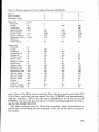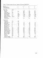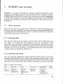
1
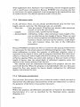
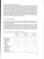
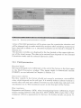
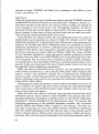
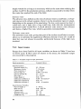
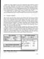
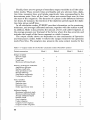
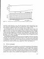
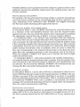
~
7
FURDEV user manual
FURDEV is a modular, menu-driven computer program developed to solve
problems in the design, operation and evaluation of furrow irrigation systems.
FURDEV deals with the flow in one furrow and does not provide suggestions
for field layout design. You start the program by selecting it in the SURDEV
package. The installation procedure of this package was discussed in Chapter
4,Section 1.
7.1
Menu structure
There are six main menu items, five of which have sub-menus that you can
select by moving the highlight with the arrow keys and pressing [ENTER], or
by typing the red (bold) character. Table 7.1 shows the structure of the main
menu and its first layer of sub-menus.
7.1.1 Sub-menu files
The sub-menu Files has two options: Load and ViewlPrint. With Load, you
can select an existing file and continue with the calculations. With
ViewlPrint, you can select an existing file, the contents of which will subsequently be displayed on the screen. Pressing [F51 gives you the option to print
this file or to save it as a text file, or a spreadsheet file. For more information
on these topics, see Chapter 4,Section 4.3.
7.1.2 Sub-menu operation
You can select the appropriate system operation mode from the sub-menu
Operation. Selecting Fixed pow means that a constant inlet flow rate is used
to irrigate the furrows during the entire application time. Cutback pow means
that at the end of advance the initial inflow is reduced once for the remainder
Table 7.1 Furdev menu structure
Files
Operation
Load
Fixed flow
ViewPrint Cutback flow
Tailwater reuse
Units
Parameters
Calculation
Flow rate
Length
Amount/depth
Time
Infiltration
Geometry
2. Length
Quit
1. Flow rate
3.Cutoff time
4. Min. Amount
85
of the application time. Tailwater reuse represents a furrow irrigation system
with a runoff reuse arrangement. Because FURDEV only simulates the flow
in one furrow, the reuse component is not integrated in the required flow rate
of another furrow. The default operation mode is Fixed flow.
7.1.3 Sub-menu units
In the sub-menu Units, you can choose pre-determined units for flow rate,
length, amount, and time. The following units are available:
- Flow rate:
litres per second, US gallons per minute, cubic metres per
minute, or cubic feet per minute.
- Length:
metres or feet, used for furrow length.
- Amountldepth: millimetres, inches, cubic metres per metre length of furrow, or cubic feet per foot length of furrow. These are used
for the various supplied and infiltrated amounts or depths.
minutes or hours, used not only for advance, cutoff, deple- Time:
tion, and recession times, but also in the infiltration
parameters.
Because FURDEV simulates the flow in one furrow, the spacing of the furrows
is a parameter for the actual amount of infiltrated irrigation water. When you
select millimetres or inches, the quantity of infiltrated irrigation water is
expressed as the depth of water, and the program transforms this value internally to a volume per metre length of furrow by taking into account the selected furrow spacing. When you select cubic metres (or feet) per metre (or foot)
length of furrow, then the actual depth of infiltrated irrigation water will
depend on the chosen spacing of the furrows.
The selected units are maintained throughout the program and are also
saved with the file. When the program is started default units are: litres per
second for flow rate; metres for furrow length; millimetres for infiltrated
depths; and minutes for time.
7.1.4 Sub-menu parameters
The sub-menu Parameters allows you to select the mode in which you want to
characterise the infiltration characteristics of the soil (Infiltration)as well as
the geometry of the furrow cross-section (Geometry).
Infiltration
Within the program, all infiltration calculations are based on the infiltration
characteristics of a soil as described by the Kostiakov-Lewis equation
(Equation 3.4)
86
Di = kTA + foT
where Di is the cumulative infiltration depth after an infiltration opportunity
time T, k is the infiltration constant, A is the infiltration exponent, and fa is
the basic infiltration rate. The menu offers three options for entering the soil
infiltration characteristics. These are:
- Indirectly by using Intake family;
- Directly by specifying values for A, k and fa in the Kostiakov-Lewis equation;
- Determining a kind of average furrow infiltration parameter from Field
data on advance times.
For more background information on this subject, see Chapter 3, Section 1.1.
The default infiltration input mode is Intake family.
Geometry
All surface flow calculations in the program are based on the furrow geomet r y expressed in terms of the furrow geometry parameters al,a2, 71, and 72.
For more information on these parameters, see Section 7.2.1 and Appendix B.
In the sub-sub-menu Geometry, these parameters can be specified under
the Sigma & tau option. Because of the complexity of these parameters, however, FURDEV also offers you the option Cross-section type where you can
simply indicate one of three cross-sectional shapes that is the closest match to
the real cross-section of the furrow. Here,.you can choose between 7kiangular,
Parabolic, or Trapezoidal (Figure 7.1). Later on, in the input windows, you
will be required to specify the characteristic data for the selected cross-section
Figure 7.1
Selecting a furrow cross-section in Furdev
87
(eg, flow depth, side slope, top width, etc). Using these data, the program will
calculate the corresponding furrow geometry parameters (TI, a2,71, and 72.
The default geometry input mode is Cross-section type and the default
furrow cross-section shape is niangular.
7.1.5 Sub-menu calculation
The sub-menu Calculation is the only place in FURDEV where input data can
be entered. Before entering data, however, you have to select one of four different calculation modes (Table 7.1). What the first three modes have in common
is that the calculated minimum infiltrated depth at the downstream end of the
furrow always equals the required depth. In other words, no under-irrigation
will occur in the downstream end, whereas over-irrigation will always occur in
the upstream part. When to use the various modes is summarised below:
Calculation Mode 1: Flow Rate
Calculation Mode 1 is primarily for design purposes, when you know the
length of the furrow and want to know the approximate flow rate that is needed to achieve a reasonable performance. The program will also give you the
required cutoff time and the primary performance indicators as well as various depth and time parameters.
For Fixed flow and Tailwater reuse operation modes, FURDEV calculates
the flow rate in such a way that the application efficiency is maximised. For
the Cutback flow operation mode, FURDEV calculates the flow rate so that
the user-specified advance ratio is achieved. Although the result obtained in
Mode 1is close to these targets, it is advisable to continue running in Modes
3 and or 4, because in most cases refinements will still be necessary.
'
Calculation Mode 2: Furrow Length
Calculation Mode 2 is the reverse of Calculation Mode 1:the flow rate is now
known and you want to know the approximate furrow length that is needed
to achieve a reasonable performance. The program will also give you the
required cutoff time and the primary performance indicators as well as various depth and time parameters. Here too it is necessary to continue in Modes
3 and/or 4 to get the final result.
Calculation Mode 3: Cutoff Time
Here, both the flow rate and furrow length are input. The required cutoff time
is the resulting design variable, while also the application efficiency and secondary output parameters are given. Note, in this mode the advance ratio is
an output. This is because it is impossible to fix advance ratio, length, and
flow rate and at the same time satisfy the requirement that the minimum
infiltrated depth equals the required depth.
88
i
~
Calculation Mode 4: Minimum Depth
Here, the cutoff time is also specified as input, in addition to the furrow length
and the flow rate. Thus, all design variables are now input, which means that
the required depth at the end of the field will usually not be achieved (ie, that
under and/or over-irrigation can occur). The minimum infiltrated depth that
occurs at the far end of the field is the determining factor of whether there is
under or over-irrigation. It is therefore given as first output, followed by the
primary performance indicators: application efficiency, storage efficiency and
distribution uniformity. This mode is most suitable for a performance evaluation of an existing furrow irrigation system and for testing the performance
sensitivity to a change in the field parameters.
7.2
Input windows
When you have selected a calculation mode, FURDEV will display the input
screen for data entry. The input data to be provided in these windows are
summarised in Table 7.2.
The box located in the upper left corner of the screen (Figure 7.2) contains
all the field parameters, except infiltration. Directly below is the box containing infiltration data. The contents of these two boxes, particularly those items
pertaining to Geometry and Infiltration, vary depending on the option selected under the sub-menu Parameters. With normal usage of the program, the
Table 7.2 Input variables for the Furdev calculation modes
~
Item
Field Parameters
Required depth
Max.velocity
Flow resistance
Slope
Spacing
Geometry
Infiltration
Input Decision Variables
Inlet flow rate
Furrow length
Cutoff time
Advance ratio
Cutback ratio
Tailwater recovery ratio
~~
Fixed flow
Cutback flow
Tailwater reuse
Mode
Mode
Mode
1
2
3
4
1
2
3
4
1
2
3
4
O
0
0
0
O
0
0
o
o
O
0
O
0
0
0
O
0
0
o
O
0
o
o
O
0
0
0
O
0
0
o
o
o
O
0
o
O
0
0
0
O
0
0
o
O
0
0
0
O
0
0
0
O
0
0
0
0
0
0
0
0
O
0
0
o
o
O
O
O
0
0
0
O
0
0
0
O
0
0
o
O
0
0
0
O
0
0
O
0
O
O
0
O
O
O
0
0
O
0
0
O
0
O
O
O
0
O
0
0
O
o
O
0
0
0
contrast to basin and border irrigation, there are no crops in the furrow, consequently, the range of n-values is smaller. Walker (1989) uses this n = 0.04 in
all calculation examples. See also Section 3.1.2.
Field slope
The field slope of graded furrows should neither be too high, to avoid erosion,
nor too low, which would result in a slow advance. For furrows, suitable slopes
normally vary between 0.05 and 1per cent. Small furrows and corrugations,
however, can be used on steeper slopes up to 2 per cent.
I
I
I
Furrow spacing
The furrow spacing is a dual-purpose parameter. In the first place, it is a field
dimension, which is primarily used to convert volumes to depths. But, it is
also used for modelling the infiltration process, where the furrow spacing is
used to convert the A, k and f,, values corresponding to the modified SCS
intake families.
The input value should not conflict with the given furrow geometry. Just
suppose that you have specified a trapezoidal section with 151side slope and
0.1 m bed width. Suppose also that in your field the depth of the furrows is 20
cm and the top width of the ridges is 25 cm. The actual spacing should then
be equal to 12.5+30+10+30+12.5=95cm.
Furrow geometry
Under this menu there are two sub-options: Cross-sectional type and Sigma &
tau. The second option refers to the parameters UI, q,71 and 72 that are used
in the program to specify the furrow cross-section. For details, see Appendix
B. Because most users would not know which value to give here, and calculating the parameters could be a tiresome job, the program offers the easier
option of just specifying the furrow shape by selecting Cross-sectional type.
If you select lFianguZczr as the cross-sectional shape, the input window will
ask you to specify only the side slope of the furrow cross-section. If you select
Parabolic, you need to specify the maximum depth and the corresponding
water top width, either estimated or obtained from field measurements. If you
select fiapezoidal, you need to enter the side slope and the bed width.
For all three cross-sectional shapes, the program will transform the given
input values into the corresponding geometry parameters (TI,a 2 , q and 72. You
can check this by selecting a particular cross-sectional shape, entering the
required input data, making a run, going back to the sub-menu Parameters,
selecting Geometry and Sigma & tau mode, and returning to the input window again.
When selecting the geometry shape and geometry parameters, care should
be taken that the geometry and spacing are not conflicting. For instance, the
combination of small spacing with a wide and deep trapezoidal section may be
geometrically impossible. In such cases, if impossible combinations are
91
entered as input, FURDEV will flash you a message to that effect on your
screen, see Section 7.4.
Infiltration
When the Intake family type of infiltration data is selected, FURDEV uses the
modified SCS families for furrows, as was discussed in Chapter 3, Section 1.1.
Seventeen families can be chosen. If a wrong number is typed, you will get an
error message on your screen with a list of acceptable numbers. To select a
particular family, you can get Help by pressing [Fll while the cursor is on the
family number. A help screen will pop up from which you can make your selection, using the upward and downward arrow keys.
Upon selection of a family number, the corresponding values A, k, and f, of
the Kostiakov-Lewis equation (as shown in Table 3.3) will give you the “soil
infiltration parameters”, as determined from infiltrometer measurements, for
instance. To simulate the furrow infiltration, these are converted to “furrow
infiltration parameters”. In furrows, infiltration takes place along the wetted
perimeter of the furrow and is assumed to spread in the soil over the width of
the furrow spacing (see Jensen 1980, and Walker 1989). The values of Table
3.3 are therefore adjusted by using the ratio of wetted perimeter to furrow
spacing. Once you make a run with FURDEV, this is automatically done within the program. You can check this by selecting a family number, making a
run, going back to the sub-module Infiltration, selecting the Kostiakou-Lewis
equation mode, and returning to the input window again, where you then see
the adjusted “furrow infiltration parameters”.
When you select the Kostiakou-Lewis equation, you can specify the values
of the intake parameters A, k, and f, directly. Note, these values represent the
“furrow values” and therefore include the two-dimensional infiltration
process. In other words, these parameter here should have been obtained from
furrow infiltration trials and do not represent the infiltration characteristics
of the soil for a flat surface.
Converting the intake parameters to values other than default units can be
done as follows: Go back to the Units menu, change time and amountddepth
units, and return to the Field Parameters input window, where the new values and their units will appear.
When the Field data option is selected, enter the data obtained from field
infiltration tests as input, based on which FURDEV will calculate the corresponding infiltration parameters. Logically, these are the “furrow infiltration
parameters”, already including the two-dimensional aspect. To estimate the
infiltration parameters of the modified Kostiakov equation, the “two-point
method (Elliott and Walker 1982) is applied in the program. The data you
now need to prescribe are: flow rate, stable tailwater runoff (the runoff rate
after the runoff hydrograph levels o@, advance time to downstream end of
furrow, advance time to halfway down the furrow, furrow length and furrow
bed slope. Note, only the spacing belonging to the field measurements must be
92
1
I
I
~
entered under parameters Field. For more information on this option, see
Appendix B.
The above difference between “soil” parameters and “furrow” parameters
implies that one has to be careful when changing from one infiltration mode
to another, because the infiltration parameters for the Intake family option
are not the same as those used for the other two options.
7.2.2 Decision variables
The decision variables in surface irrigation are normally the field dimensions
(furrow length and spacing), the flow rate, and the cutoff time. It depends on
the calculation mode that you have selected which of these parameters appear
under the heading “Decision variables’’ (see Table 7.2).
Furrow length
For open-ended furrows, there is an optimum length, giving a maximum possible application efficiency. Too long a field will result in poor performance
because of a long advance time, with uneven infiltration and excessive deep
percolation losses in the upstream part of the field. On the other hand, too
short a field would result in excessive surface runoff. Consequently, there is
one length (with all other variables given) for open-end furrows, for which the
sum of deep percolation and surface runoff losses is at its minimum and the
application efficiency is at its maximum.
Flow rate
For furrows, the flow rate is the inflow into one furrow, representing the unit
flow rate per width of one furrow spacing. It should not be too low, otherwise
the flow would not reach the end of the furrow, and it should not be too high
to avoid scouring. In the case of open-end furrows there is also an optimum
flow rate (similar to the furrow length), where the sum of deep percolation
losses and surface runoff losses is at its minimum.
Cutoff time
For all three irrigation methods, cutoff is usually done some time after the end
of advance to achieve infiltration of the required depth at the downstream
end. If the cutoff time is much later than the advance time, it will have a clear
effect on the deep percolation and surface runoff losses. If cutoff is too early,
this will often result in not achieving the required depth at the end of the
field.
Cutback ratio
The cutback ratio, defined as the ratio of reduced flow rate to the initial flow
rate, must be such that the reduced flow is sufficient to keep the entire field
93
length wetted for as long as is necessary, while at the same time reducing the
surface runoff. In the simulation process, cutback is assumed to be done when
the water has reached the end of the field.
Advance ratio
The advance ratio, defined as the ratio of advance time to cutoff time, is of special interest with cutback systems where it can be simulation input or output,
depending on the purpose of the simulation. Too low a ratio means too short a
cutoff time, and a high ratio a long cutoff time, both with the consequences
mentioned under Cutoff Tzme. A small advance ratio means a fast advance
and hence a higher flow rate, which is generally recommendable.
Tailwater reuse ratio
The tailwater reuse ratio, giving that part of the surface runoff that is reused,
allows us to calculate the application efficiency directly. A ratio of 1 would be
ideal but may not always be possible, particularly because of the high costs
involved.
7.2.3 Input ranges
Ranges have been fixed for all input variables, as shown in Table 7.3 and are
in metric units. If other units are chosen in the menu, the indicated ranges
are converted in the program.
Table 7.3 Accepted ranges of input parameters
Input parameters
Accepted values
Field Parameters
Required depth, Dreq
Maximum velocity
Flow resistance, n
Furrow slope, So
Furrow spacing, W,
Side slope, z
Intake family #
Infiltration coefficient k
Infiltration exponent A
Infiltration constant fo
25 - 250 mm
7 - 15 mlmin
0.01 - 0.08
0.0003 - 0.03 d m
0.5 - 1.5 m
0.5 - 3.0 m/m
0.05 - 2.0
0.050 - 30 “/minA
0.01 - 0.7
0.005 - 10 “/min
Input Decision Variables
Furrow length, L
Flow rate, Q
Cutback ratio
Advance ratio
Tailwater reuse ratio
Cutoff time, T,,
5 - 700 m
0.02 - 16.67 V S
0.65 - 1.00
0.1 - 0.9
0.1 - 1.0
10 - 2000 min
94
.
Based on a large number of runs, the ranges have been fixed in a bid to
avoid too many impossible combinations and corresponding error messages.
For all practical purposes, the ranges of the individual parameters will be
more than sufficient. If you combine extreme values of the individual parameters, you may not get a result. FURDEV will then flash you a message on the
screen indicating how to change these values in order to get a result.
For output results, the above ranges are ignored. So, if such an out-of-range
value is subsequently used as input in another mode, no warning will be given.
7.3
Output windows
After all the input has been entered, press [F21 for the calculations and the
output. The screen again shows the three input windows, but a fourth window
has now been added showing the results (Figure 7.3). These results are presented in various groups, separated by a blank line. The first group contains
the desired decision variable or variables, according to the calculation mode
you have selected: in Mode 1 they are the flow rate and the cutoff time; in
Mode 2 the furrow length and cutoff time; in Mode 3 the cutoff time; and in
Mode 4 the minimum infiltrated depth.
The second group contains the primary performance indicators as discussed
in Chapter 3, Section 3. All the calculation modes allow the performance of an
irrigation scenario to be evaluated with the application efficiency, the surface
runoff ratio, the deep percolation ratio, the distribution uniformity, and the
uniformity coefficient; Mode 4 adds the storage efficiency. Note, the first three
indicators also represent the overall water balance of the furrow.
Figure 7.3
Applic. e f f i c i e n c y =
surf. run-off r a t i o =
Deep perc. r a t i o
=
71 %
12 %
17 %
Distr. uniformity
unif. c o e f f i c i e n t
80 %
93 %
=
=
Results screen in Furdev
95
Finally, there are two groups of secondary output variables in all the calculation modes. These concern times and depths and are: advance time, depletion time, recession time, and intake opportunity time corresponding to the
downstream point. Note, all the “time” values are counted from zero (ie, from
the start of the irrigation). The duration of a phase is the difference between
two times, for instance, the duration of the depletion period equals the depletion time minus cutoff time.
In all calculation modes, FURDEV provides information on the maximum,
minimum, and average infiltrated amounts, together with the surface runoff.
In addition, Mode 4 also presents the amount of over and under-irrigation as
the average amount over that part of the furrow where this has occurred, and
includes the length of the furrow segment on which it occurs.
The output results shown are dependent on the combination of Operation
and Calculation modes. Table 7.4 shows the output results for the operation
mode Fixed flow. The program also presents the same output results for the
Table 7.4 Output results for the Furdev calculation modes (Fixed flow system)
Output parameters
Design variables
Furrow length
Flow rate
Cutoff time
Minimum infiltrated depth
Primary performance indicators
Application efficiency
Surface runoff ratio
Deep percolation ratio
Storage efficiency
Distribution uniformity
Uniformity coefficient
Time variables
Advance time
Depletion time
Recession time
Intake opportunity time
Infiltrated depths
Maximum infiltrated depth
Minimum infiltrated depth
Average infiltrated depth
Surface runoff
Over-irrigation
Under-irrigation
Length of over-irrigation
Length of under-irrigation
96
Mode 1
Mode 2
Mode 3
Mode 4
O
O
O
O
O
O
O
O
O
O
O
O
O
O
O
O
O
O
O
O
O
O
O
O
O
O
O
O
O
O
O
O
O
O
O
O
O
O
O
O
O
O
O
O
O
O
O
O
O
O
O
O
O
O
O
O
O
O
O
O
O
O
A
530 -
c
._
E
397 -
Tr
TCO
uE 265 ._
c
Ta
132 -
'-O
I
1
Figure 7.4
L over-irrigation
I
I *
under-irrigation
Advance curves, recession curves, and infiltration profiles in Furdev
operation mode Tailwater reuse. For the operation mode Cutback @ow, however, and for all calculation modes, the cutback flow rate is added to the output variables; in Modes 3 and 4, the advance ratio is added as well.
By pressing [F31, you will see two graphs showing the main results: the
upper one shows advance and recession times in relation to furrow distance,
while the lower one shows the infiltrated depths along the furrow length.
Under and over-irrigation are indicated where applicable. This graph can be
saved with [F81 or [F91. Figure 7.4 shows a graph of the results of Run 3 from
Example 1 (see Table 7.5). Note, here the recession time is depicted and not
the cutoff time as with BASDEV.
The tabulated simulation results can be saved, together with the input data
with [F41. In a small window, the path (directory + file name) can be confirmed
or changed, as described in Section 4.3.3. You can overwrite the previous file
or append the current results to it. Further processing of the saved results file
must be done under the Files menu using View /Print. See Section 4.4.
7.4
Error messages
FURDEV usually gives an output as a result of the calculations. Nevertheless,
some combinations of variables and parameters - mostly physically unrealistic combinations - could cause mathematical problems. When such problems
are encountered, the program terminates the calculation process and flashes
a message on the screen. The message typically contains two layers of information: the nature of the problem and suggestions on how to remedy it.
97
Possible problems can be grouped into three categories: general advance time
problems, advance time problems related only to the cutback system, and cutoff time problems.
General advance time problem
The problem with the advancing front being unable to reach the downstream
end of the furrow problem can be encountered with all three operation systems. Depending on the calculation mode, FURDEV will suggest increasing
the flow rate and/or decreasing the length of the furrow.
Advance time problem with cutback system
In Calculation Modes 1and 2, FURDEV calculates the required advance time
as a function of the user-specified advance ratio and the required intake
opportunity time. You can satisfy the advance time requirement by selecting
the appropriate value of flow rate in Mode 1or furrow length in Mode 2.
In Calculation Mode 1, the advance time associated with the maximum
non-erosive flow rate can be longer than that of the required advance time. In
such a situation, the required advance time cannot be achieved without using
a flow rate that is greater than the maximum non-erosive one. This is clearly
unacceptable. The only way out of this problem is to reduce the furrow length
and/or increase the advance ratio. In addition, there are cases in which the
flow rate corresponding to the required advance time is less than the minimum flow rate required to advance to the downstream end of the furrow.
When this happens, FURDEV.wil1 advise you to increase the furrow length
and/or the advance ratio.
In Calculation Mode 2 - with some parameter and variable combinations it is possible that the required advance time is greater than the advance time
that corresponds to the maximum length to which the user-specified flow rate
can advance. To overcome this difficulty, FURDEV will recommend that you
increase the flow rate and/or decreasing the advance ratio.
Cutofftime problem
In Calculation Modes 1,2 and 3, the cutoff time is calculated so that the minimum infiltrated amount is equal to the required amount. In Mode 4, the cutoff time is an input. If the user-specified cutoff time is too short, it is possible
that the calculated advance time will exceed it. This is a situation that cannot
be handled by FURDEV. When such a problem is encountered, the screen
message will recommend decreasing the furrow length and/or increasing the
flow rate, and/or increasing the cutoff time.
Check furrow cross-section
The message is generated based on an assumed furrow depth of 20 cm and a
ridge width of 20 cm. For the given side slope of a triangular furrow of 1.5:1,
the furrow spacing should then be 2x1.5~20+20=80cm. If your spacing input
98
value is less than this 80 cm, this message appears on the monitor, together
with the results of the simulation.
Spacing and section are incompatible
This message deals with the same geometrical check as explained above, but
instead of the assumed furrow depth, the actual flow depth calculated in the
simulations is used, considering no freeboard. The width of the ridge is still
assumed to be 20 cm. If the input furrow spacing is less than the calculated
required minimum one, the message that will appear on the monitor is: spacing and section are incompatible, meaning physically impossible. Therefore,
you will get no results and will have to change one of the input values.
Calculated flow velocity is more than maximum permissible
The meaning of this message is obvious. The flow velocity calculated by the
program is more than the permissible value of the input field parameters.
Nevertheless, the calculation results will show up on the screen. The idea is
that you will have to decide whether you find the high velocity acceptable or
not.
I
7.5
Assumptions and limitations
The FURDEV program is based on the volume balance method, which is
explained in detail in Appendix B. The main difference between furrows and
basins or borders is that the geometry of their cross-sections is different and
that therefore the infiltration process and the flow process.also differ. In
basins and borders, it is generally assumed that the infiltration is one-dimensional in the vertical downward direction, whereas in furrows water infiltrates over the entire wetted perimeter in the furrow and should therefore be
characterised as a two-dimensional process.
The volume balance method calculates the propagation of the wetting front
along the furrow during the advance phase. Algebraic equations are used to
simulate the pounding, depletion and recession phases. Implicit assumptions
for the modelling of the advance phase are as follows:
- The furrow slope is greater than zero. The field can have a minor cross slope
as long as the slope in the furrow is constant.
- The cutoff time is always greater than the advance time. This limitation is
introduced to make sure that advance and recession do not occur simultaneously; a situation that the volume balance model cannot handle. During
the advance time, the inflow is constant.
- The furrow is free-draining at the end. FURDEV is not able to calculate the
advance and recession curve for closed-end conditions. To reduce losses and
in particular runoff losses, the program can be.run in the operation modes
Cutback flow and Tailwater reuse. FURDEV does not compute how the
99
runoff water re-enters the system. That will be determined by local conditions. In the Tailwater reuse mode, it is assumed that a certain fraction of
the runoff water, to be specified by the user, is reused within the same furrow, or in a downstream furrow. In the Cutback mode, it is assumed that,
when water reaches the end of the furrow, the inflow is reduced to a value
less than the inflow rate during the advance phase. Before and after cutback, the flow rate is constant.
Additional assumptions involved in the simulation of depletion and recession
phases are discussed in detail in Appendix B. Other general theoretical
assumptions are that the infiltration can be described by the modified
Kostiakov-Lewis infiltration function, and that the infiltration parameters
have to be derived from a furrow used as infiltrometer. Further, the water
depth at the upper boundary of the furrow can be described with Manning’s
equation. The geometry of the cross-section of the furrow (triangular, parabolic or, trapezoidal) is simulated in the program by a power law for the wetted cross-section and the wetted perimeter: the upper boundary of the inflow
is the maximum non-erosive flow rate, which can be calculated with the
method developed by Hart et al. (1980); and the minimum flow rate is determined by advance considerations (Hart et al. 1980).
Apart from these more theoretical assumptions related to the algorithm
and its solutions (ie, accepting the model as it is), the following practical conditions are assumed for the use of FURDEV
- The inflow rate is constant during the entire application time, apart of
course from a possible reduction in case of a cutback operation.
- The soil is homogeneous throughout the length of the furrow.
- The roughness coefficient is constant in space and time.
- The cross-section is constant over the furrow length.
- The cutoff time is always greater than advance time.
- The furrow slope is uniform along the length.
The simulation results obtained with FURDEV will be much in line with field
observations, provided that the field conditions match the assumptions made
in the program and that the consequent limitations are respected. As stated
in the other programs, FURDEV only deals with the technical and hydraulic
aspects of furrow irrigation. The program should therefore be regarded as an
aid in the design, operation, and evaluation. In addition to the findings of the
program, final decisions in the field will be affected by agricultural, economic
and social considerations.
100
7.6
Program usage
The following 10 steps are important in the usage of the FURDEV program.
1. Start the SURDEV package. Select FURDEV from the main menu of
SURDEV.
If you want to use an existing file, retrieve it with the Load command
under the Files menu. If you want to make a new file, go straight to the
Calculation menu bypassing the Files menu, and you will get a set of
default data.
3. If you want to simulate Cutback flow or Reuse, go to the Operation menu
and select the operation mode to work with. The program default operation mode is Fixed inflow.
4. Select the Units menu only when you want to work with units other than
the default units.
5. The default infiltration mode is the “Modified SCS families”. If you want
to work with another infiltration mode, go to the Parameters menu and
select the Infiltration menu.
6. The program default geometry is the triangular cross-section under the
heading cross-sectional shapes. Changes can be made under Parameters
and Geometry.
7. Select a mode to work in from the Calculation menu. Most work will be
done in Modes 3 andlor 4. Less experienced users can start in Mode 1or
2 to get a first estimate of the flow rate or field dimensions, respectively,
and then continue in Mode 3 andlor 4.Mode 4 can be used to evaluate an
existing situation or to do sensitivity analyses.
8. You can specify field parameters and decision variables in the input window, after which the program can be run by pressing the key [F21.
9. You can view the results of each run in tabular form in the output window, or in graphical form by pressing [F31.You can save the results of one
simulation run (output and input in one file) in a separate file or append
them to earlier runs in an existing file by pressing [F41.
10. Select Files and ViewlPrint from the main menu to see what has been
done andlor to print a file directly, or convert it to a print file for a wordprocessor program, or convert it to a file to be imported into a spreadsheet program where you can make your own graphs.
2.
7.7
Sample problems
In most cases, users will not be satisfied with a solution obtained after one
run, and will usually do a number of runs to get an acceptable solution. Two
simple examples are given to illustrate this procedure. More elaborate problems can be found in Chapter 8, Section 3.
101
7.7.1 Determine furrow length
A design combination is to be developed for a fixed-flow furrow irrigation system in which the available inflow rate into the furrow is fixed at 1Vs. The soil
is silty-loam and can be classified by the Intake Family # 0.6. The value of the
flow resistance is fixed at 0.04. The net irrigation requirement is 100 mm. The
furrows have a triangular cross-section with a side slope of 1:1, a slope of
0.008, and a spacing of 75 cm. Determine the furrow length in such a way that
the application efficiency is at least 70 per cent and the cutoff time has a practical value. The maximum feasible furrow length is 600 m in the direction of
the main field slope.
1. We want to make a new file, and therefore do not need to use the Files submenu. Note, the default operation, units, and parameter modes must be
used in this problem, so you can go directly to the Calculation menu and
select Mode 2: Furrow length. Enter the above values in the two input windows and make a run ([F21).
2. The results of this run (Table 7.5, Run 1)show that, with an available flow
rate of 1 Us, a furrow 338 m long can be irrigated with an application efficiency of 71 per cent. This requires a cutoff time of 596 minutes. The corresponding uniformity coefficient is 93 per cent and the distribution uniformity is 82 per cent. From these values, it will be clear that a furrow
length of 600 m is too long for an application efficiency of 70 per cent.
Suppose the field can be divided into two parts, each 300 m long. Run
FURDEV in Mode 3 to see the effect when the furrow length is reduced to
300 m.
3. The results of this run (Table 7.5, Run 2) show that a slightly shorter furrow reduces the application efficiency from 7 1 to 70 per cent, which is
acceptable. The cutoff time, however, has an impractical value (536 min).
Run FURDEV in Mode 4 to see the effect when the cutoff time is reduced
from 536 to 480 minutes.
4. The results of this run (Table 7.5, Run 3) show that this reduction in cutoff time results in a slight under-irrigation: the minimum infiltrated depth
is now 90 mm instead of 100 mm, while the uniformity coefficient is 95 per
cent. The application efficiency has increased to 77 per cent and the distribution uniformity is 86 per cent. Over the lower 75 m of the furrow, the
average depth infiltrated would be 4 mm less than that required. The
upper 225 m of the furrow would receive an average over-irrigation depth
of 8 mm. These results are acceptable.
Table 7.5 can be made with FURDEV. The procedure is as follows. Save Run
1with [F41 and prescribe a particular file name (EXAMPLE1).FURDEV automatically adds the extension .FDR to this file name. Save Runs 2 and 3 with
[F4] under the same file name using the Append option. Go back to the main
102
Table 7.5 Furdev program for furrow irrigation (Filename: EXAMPLEl)
1
1
2
2
1
3
3
1
4
VS
1
m
min
min
mJm
m
dmin
-
-
1
300
-
100
0.04
0.008
0.75
13.8
1
0.6
100
0.04
0.008
0.75
13.8
1
0.6
1
300
480
100
0.04
0.008
0.75
13.8
1
0.6
VS
-
m
min
338
596
71
100
93
82
16
14
226
602
647
42 1
122
131
100
19
22
O
338
O
-
Run no.
Type of system
Calculation mode
Input data
Flow rate
Length
Cutoff time
Required depth
Flow resistance
Furrow slope
Furrow spacing
Maximum velocity
Side slope
Intake family
Output data
Flow rate
Length
Cutoff time
Application eff.
Storage eff.
Uniform. coeff.
Distrib. unif.
Deep perc. ratio
Runoff ratio
Advance time
Depletion time
Recession time
Opportunity time
Avg. inf. depth
Max. inf. depth
Min. inf. depth
Surface runoff
Over-irr.
Under-irr.
Over-irr. Length
Under-irr. Length
Units
%
%
%
%
%
%
min
min
min
min
mm
mm
mm
mm
mm
mm
m
m
536
70
100
95
87
10
20
163
541
584
42 1
115
121
100
28
15
O
300
O
77
99
95
86
5
18
163
485
528
365
105
111
90
23
8
4
225
75
menu, then to the Files menu and select View. See the results and select [F51
(PrintlSaue) and then use the option Text file. FURDEV now automatically
adds the extension .TXT to the file name EXAMPLE1. If you now go out of
FURDÉV, you can load the results in a word processing program by retrieving the file EXAMPLELTXT.
The above problem uses the Fixed flow operation mode. Nevertheless, a
similar line of reasoning can be employed in the use of the other two operation modes.
103
7.7.2 Determine flow rate
A design is to be made for an existing field with 400 m long furrows. The soil
is silty-loam and can be classified by the Intake Family # 0.6. The net irrigation requirement is 100 mm. The furrows have a triangular side slope of 1:1,
a slope of 0.008, and a spacing of 75 cm. Determine the flow rate in such a way
that the application efficiency is at least 70 per cent and the cutoff time is not
more than 420 minutes.
1. Go to the Calculation menu and select Mode 1:Flow rate. Enter the above
values in the two input windows and make a run. Save the results as
EXAMPLE2.
2. This run (Table 7.6, Run 1)shows that at a flow rate of 1.21 l/s this furrow
can be irrigated with an application efficiency of 71 per cent. A cutoff time
of 587 min will then be required, so, the cutoff time needs to be reduced.
Run FURDEV in Mode 4 to see the effect when the cutoff time is reduced
from 602 to 480 minutes.
3. The results of this run (Table 7.6, Run 2) show that, although the application efficiency has increased to 84 per cent, there is under-irrigation: the
minimum infiltrated depth is 80 mm. Run FURDEV again in Mode 4 to see
the effect when the flow rate is increased from 1.21 to 1.5 Vs.
4. From this run (Table 7.6, Run 3) you will see that there is now slight overirrigation (the minimum infiltrated depth is 101 mm) and the application
efficiency is reduced to 69. So, there is now scope to reduce the cutoff even
further. Run FURDEV again in Mode 4 to see the effect when the cutoff
time is reduced from 480 to 420 minutes;
5. Once again this run (Table 7.6, Run 4) will show that there is under-irrigation (the minimum infiltrated depth is 89 mm), while the uniformity
coefficient is 95 per cent. The application efficiency is 78 per cent and the
distribution uniformity is 86 per cent. Over the lower 117 m of the furrow,
the average depth infiltrated would be 5 mm less than that required. The
upper 283 m of the furrow would receive an average depth of 107 mm.
These results are acceptable.
Table 7.6 was also made with FURDEV. Once you are familiar with the foregoing basic elements of working with the program, you can tackle more elaborate problems. Examples are presented in Chapter 8 and concern several
sets of runs with which various relationships can be established. They not
only illustrate the potential of FURDEV, but also provide you with a deeper
insight into the complex nature of the furrow irrigation process.
104
Table 7.6 Furdev program for furrow irrigation (File name: EXAMPLE21
1
1
Run no.
Type of system
Calculation mode
Input data
Flow rate
Length
Cutoff time
Required depth
Flow resistance
Furrow slope
Furrow spacing
Maximum velocity
Side slope
Intake family
Output data
Flow rate
Cutoff time
Application eff.
Storage eff.
Uniform. Coeff.
Distrib. Unif.
Deep perc. ratio
Runoff ratio
Advance time
Depletion time
Recession time
Opportunity time
Avg. inf. Depth
Max. inf. Depth
Min. inf. Depth
Surface runoff
Over-irr.
Under-irr.
Over-irr. Length
Under-irr. Length
2
1
4
3
1
4
4
1
4
400
100
0.04
0.008
0.75
13.8
1
0.6
1.21
400
480
100
0.04
0.008
0.75
13.8
1
0.6
1.5
400
480
100
0.04
0.008
0.75
13.8
1
0.6
1.5
400
420
100
0.04
0.008
0.75
13.8
1
0.6
1.21
587
71
100
93
80
17
12
243
594
644
401
125
134
100
17
25
O
400
O
84
97
91
75
7
9
243
486
534
291
106
116
80
10
12
9
283
117
69
100
95
88
11
20
157
486
538
381
115
121
101
29
15
O
400
O
-
1
Units
ws
m
min
mm
m/m
m
&min
-
-
l/S
min
%
%
%
%
%
%
min
min
min
min
mm
mm
mm
mm
mm
mm
m
m
-
-
78
99
95
86
4
17
157
426
477
320
104
110
89
22
7
5
283
117
105