Download FFT — fRISCy fourier transforms?

______________ Tutorial
FFT - fRISey Fourier
transforms?
M R Smith
This is an applications tutorial oriented towards the practical use
of the discrete Fourier transform (Off) implemented via the fast
Fourier transform (FFf) algorithm. The Off plays an important
role in many areas of digital signal processing, including linear
filtering, convolution and spectral analysis. The first part of the
article is a practical industrial example and takes the reader
through the thought process an engineer might take as Off
familiarity is gained. If standard software packages did not
provide the necessary performance, the engineer would need to
port the application to specialized hardware. The second part of
the tutorial discusses the theoretical concepts behind the FFf
algorithm and a processor architecture suitable for high speed
FFf handling. Rather than examining the standard digital signal
processors (OSP) in this situation, the final section looks at how
the reduced instruction set (RISC) processors perform. The
Advanced Micro Devices scalar Am290S0 and the super-scalar
Intel i860 processors are detailed. Comparison of the OSP and
RISCprocessors is given showing that the more generalized RISC
chips do well, although changes in certain aspects of the RISC
architecture would provide for considerable improvements in
performance.
Keywords: FFT, digital signal processing, RiSe, Am29050
processor
Many digital signal processing (DSP) algorithms are now
available in application packages.The 'standard' engineer
(such as myself) would approach any new DSP problem
by starting with a quick glance in the user manual to get a
flavour of how to solve the problem and usethe package.
Next would come testing with a few simple examples to
ensure that the concepts were understood. This would be
followed by more complex examples where the expected
'results' were known and then the algorithm would be
Department of Electrical and Computer Engineering, University of Calgary,
Calgary, Alberta, Canada. Email: smlthe-enel.ucalgarv.ca
Paper received: 22 June 1992. Revised: 11 February 1993
tried on the 'real' data. The success of this approach
depends on the expertise and judgement of the engineer.
These factors must be tempered by the following descriptions of 'judgement' and 'experts'.
Good judgement is gained from experience.
Experience is gained from bad judgement.
An expert is made of two parts: 'X' - a has-been, and
'spurt' - a drip* under pressure.
This tutorial examines the implementation of a major
digital signal processing technique, the discrete Fourier
transform (OFT). It is intended to provide a person
unfamiliar with using the OFT with the experience to
avoid any unnecessary pitfalls. The OFT playsan important
role in many areas of digital signal processing, including
linear filtering, correlation analysis and spectrum analysis.
A major reason for its importance is the existence of
efficient algorithms for computing the OFT and a thorough
understanding of the problems in its application.
The first part of the article is a practical industrial
example involving digital filtering to remove an unwanted
signal. This section discusses the importance of data
windowing and the trick of deliberate synchronous
sampling to avoid problems when usingthe efficient fast
Fourier transform (FFT) algorithm to calculate the OFT.
This section would be useful for the engineer intending to
use the FFT algorithm from a standard package. (An
excellent source of algorithms and their theoretical
background can be found in the book by Press et al. 1 A
diskette with (debugged) source code is available.)
If using a standard package did not provide the
required performance, the engineer would need a more
thorough understanding of the FFT algorithm and how
current processors match the required resources for this
algorithm. The second part of this tutorial provides a brief
analysis of the fast Fouriertransform. The characteristics
needed for the efficient implementation of the FFT are
discussed in terms of chip architecture in general. The
architecture of specialized OSP chips (Texas Instrument
'Drip is a colloquialism for idiot.
0141-9331/93/090507-15 «J 1993 Butterworth-Heinemann Ltd
Microprocessors and Microsystems Volume 17 Number 9 November 1993
507
FFT-fRISCy Fourier transforms?: M R Smith
TMS32020, 32025 and 32030 t , Motorola DSP56001 and
DSP56002* and Analog Devices ADSP-2100 family§) and
a number of RiSechips (the superscalar Intel i860 and the
scalar Advanced Micro Devices Am29050 RISe1J ) are
compared.
Since the FFT performance of DSP processors is well
documented in application notes, the final part of the
tutorial provides a detailed analysis of the ease (and
problems) of implementing DSP algorithms on RISC
chips. The RISC performances are compared to those of
the DSP processors.
The reason for examining the RiSe chip in DSP
applications is that many systems already have a high
performance RISe as the main engine or a coprocessor.
What hasto be taken into account to get maximum (DSP)
performance from these processors? In addition, there are
a number of low-end RISC processors appearing on the
market- the Intel RISC processor i960SAand the Advanced
Micro Devices RISC Am29240 controller. Although not
yet up to the top-end DSP chips in terms of performance,
future variants of these chips, based around the same
RISC core, may be.
INDUSTRIAL APPLICATION OF THE OFT
In this section, we discuss a simple practical application
through the eyes of an engineer gaining greater familiarity
with usingthe DFT.The first part sets the scene of how the
data were gathered. The unwanted signal or 'noise' on the
data hasa particuladrequency characteristic. This suggests
that if the data were transformed into the frequency
domain using a DFT, this 'noise' would appear at one
particular location in the frequency spectrum. It could
then be 'cut out' (filtered) and the spectrum transformed
back into the original data domain. The resulting 'noiseless'
data could then be analysed.
The problem
Beta Monitors and Controls Ltd. is a typical small
company servicing the oil and gas industry in Alberta,
Canada. One particular problem they handle on a daily
basis is monitoring the performance of the heavy
reciprocating compressors used in the natural gas industry.
This analysis requires the determination of the compressor's effective input and exhaust strokes. This is
obtained by measuring the 'pressure' as a function of
'crankshaft angle' for a complete stroke. This crankshaft
angle is then converted by a non-linear transform to a
'stroke volume'. The compressor's efficiency is determined
from the area under the pressure versus volume curve.
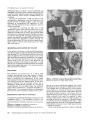
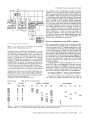
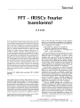
Experimental measurement technique
The pressure is obtained by attaching a transducer to the
compressor (Figure 1). The transducer's output is fed
tTMS32020, TMS32025, TMS32030 are trademarks of Texas Instruments
ltd.
*DSP56001 and DSP96002 are trademarks of Motorola Ltd.
§ADSP"2100 is a trademark of Analog Devices.
'Am29050 and Am29240 are trademarks of Advanced Micro Devices Ltd.
508
Figure 1
Measurement of the pressure is obtained by attaching a
transducer to the heavy compressor cylinder (Figure courtesy of Beta
Monitors and Controls Ltd., Calgary, Alberta, Canada)
through a low-pass anti-aliasing analogue filter before
being digitized by an analogue-to-digital (A/D) converter.
The analogue filter is an important part of the measurement system as it removes all frequency components
(such as high frequency random noise) greater than half
the digital sampling frequency. This ensures that the
digitized signal accurately represents the analogue signal
being converted/ and avoids the problems of signal
'aliasing'. Signal aliasing is when one signal appears, on
sampling, as another. For example a 7 kHz signal sampled
at an 8 kHz rate will be indistinguishable from a 1 kHz
signal sampledat the samerate. An unnecessary degradation
of the signal-to-noise ratio occurs if high frequency noise
is aliased on sampling.
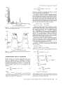
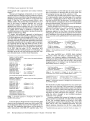
Actual measurements are shown in Figure 2. Although
Microprocessors and Microsystems Volume 17 Number 9 November 1993
FFT-fRISCy Fourier transforms?: M R Smith
290
25 00
270
20 00
250
{l
1500
.a
.15,
,
e
Channel resonance
~1000
190
500
170
150:t-O---.--....-:-:r::--+--~-~~---+-----+---+
100
200
300
40 0
Crankshaft angle
I cycle of actua I data
0.05
0 .1
0.15
0.2
0 25
Normal ized frequ ency
Spectru m of I cycle padded 10 512pts
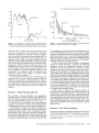
Figure 2
The pressure as a fun ction of the crankshaft angle is
measured for a Natural Gas reciprocating compressor. There are data,
compressor-related pulsations and unwanted channel noise components
Figure 3
The transform of the data from Figure2. The noi se orchannel
reson ance frequency com p onents are ind icated
the basic curve is simple and has a high signal-to-noise
ratio, the measurements are distorted by important
(wanted) low frequen cy 'compressor related pulsation s'
and (unwanted) high frequency noise components. The
unwanted noise arises from the transducer which is
attached to the cylinder via a small channel or pipe (see
Figure 1). Justas a bottle will whistle if you blow across th e
top, this channel will resonate during the cylinder stroke,
appearing as rapid vibrations du ring one part of the
measured cycle. Even a 2% error in the measurement of
the comp ressor performance can mean under-production
(loss of profits) or over-l oad (premature failure of the
compressor). The problem is made more difficult by the
non-linear transform from 'angle' to 'volume' which
distorts the noise oscillations.
The way to remove this noise is to transform the data
using the OFT into the frequency domain where its
frequency components can be identified and removed.
By inverse transforming the modified spectrum, it should
be possible to get the data without the noise component.
This data can be converted to 'vo lume' and analysed as
requi red.
noise frequency components can be zeroed (filt ered out)
for normalized frequen cies 0.12 to 0.16/ and the modified
spectrum transformed back into the data domain for the
compressoranalysis. It can be seen from the resulting data
(Figure 4) that the majority of the noise oscillations have
been removed by the filtering, but there are now different
distortions that were not there be fore.
There are many books that will explain the problems
during this simple fil tering2, 3; however, the following
argument outlines th e underlying principles. The new
distortions can be understood at a number of levels.
Because of the finite am ount of data, there are discontinuities at its boundaries on padding with zeros". These
'sharp edges' have frequency components all across the
spectrum (the background signal of Figure 3). This means
that the data is no longer confined to the low frequencies .
When the noise frequ ency components are removed , so
is a significant part of the 'spread-out ' data components.
On inverse transforming, the removed data components
mean that the filtered signal w ill be incorrect, particularly
near the discontinu it ies. In addi tion, since the noise
components were also spread out, they are more difficult
to identify and (correctly) rem ove.
There is also a second, less obv ious problem. If
discontinuities in the data lead to a range of frequencies in
the spectrum, then di scontinuities in the spectrum will
lead to a range of original data values. When we removed
the noise frequency components by setting them to zero,
this created discontinuities in the spectrum which can
lead to additional dist ortions in the filtered data. Proper
application of the OFT can remove or reduce many of
the se artifacts.
Attempt 1 - Bull-at-the-gate approach
The scientific computer libraries and applications
packages typically include an efficient implementation of
the OFT, the fast Fourier transform (FFT) algorithm, based
on a data length M that is a power of 2 (M ::: 16, 32, . .. ,
512, 1024 etc.). Since the pressureversus angle data have
a length of 360 points (1 cycle), it seems appropriate to
pad the data with zeros to size 512 and then apply the FIT.
Transforming the o riginal data (Figure 2) produces a
spectrum (Figure 3) with the channel resonancefrequency
com ponents fairly evident above a background signal.
The frequency scale has been normalized (frequency!
DFT-points) so that spectra from different sized DFTs can
be compared. Large frequency com ponentsaredisplayed
so that the smaller componentsare more easily seen.The
Attempt 2 - OFT with windowing
The previo us section described t he problems associated
with blindly applying the Off. The difficulties are deeper
'To make the problem more obvious, the data's DC offset was
dellb eratolv increased.
Microprocessors and Mic rosyslems Volume 17 Number 9 November 1993
509
FFT-fRISCy Fourier transforms?: M R Smith
300
100+--_ _I--I-->_--+-+_ _+_--...-.-..,__+
o
100
200
300
400
Crankshaft angle
Filtered signal of I cycle padded to 512
~
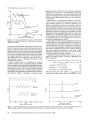
Figure 4 The original data isshown as the upper trace. When thedata
ispadded with zeros before filtering, the resulting filtered signal has new
distortions at its edges
and more complicated than what appears on the surface.
We 'think' we are trying to transform the signal shown in
Figure 2. However, when we use the OFf what we are
actually tryin gto do is to transform an infinitely long signal
of which we only know a small part. This subtle effect is
known as 'windowing' and has a very pronounced effect
on a signal's spectrum. If we had an 'infinite' amount of
data taken from the compressor, there would be no
discontinuities and no distortions introduced when
calculating its spectrum.
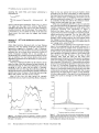
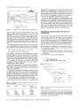
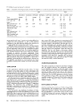
Figure 5 . (top) shows an 'infinitely-long' complex
sinusoid and its spectrum, a single spike. Figure 5 (middle)
shows a 'windowed' sinusoid and its (magnitude) spectrum.
It can be seen that the single spike has spread into a wide
centre lobe and there are a number of high side-lobes.
Everyfrequency component in the data shown in Figure 2
undergoes a similar spreading. The discontinuities associated with the effective 'rectangular' sampling window
applied to get the 'finite' data record lead to a wide range
of frequency components - 'spectral-leakage'. When we
filter the noise components, we will remove some of the
spread-out data frequency components. This will produce
distortion in the filtered signal when an inverse transform
is performed.
Windowing is a fundamental limitation to the OFf.
There is no way around it; the best that you can do is to
apply different windows to minimize distortion. The
secret is to modify the window on your data so that the
spectral leakage (side-lobes) of the window is reduced.
This means that you will be able to better discern small
signals (the channel resonance) in the presence of larger
signals (the frequency components associated with the
data edges). However, applying the window to reduce the
sidelobes must be balanced against the fact that each
spectral peak is Widened, resulting in a loss of resolution.
An excellent paper on the properties of the OFf and
windows has been given by Harris",
Applying the window to reduce distortions introduces
different distortions. By gathering additional data (say 2.5
cycles padded to 1024 points, Figure 6) it is possible to
minimize the effect of these new distortions. A window
with smoothly changing edges is applied to this extended
data before calculating the OFf. This window will allow
the noise frequency components to be more clearly
identified and filtered. The spectrum can then be inverse
transformed and the window removed.
Suppose that you have M data points, xtrn): 0 <; n <; M,
which you intend to filter. The steps in generating the
filtered signal are:
Xwindowed(m) = x(m) X Wwindow(m);
X(f) = FT[xwindowed(m)];
0
<M
f<M
0 <: m
(1)
<: m,
(2)
Xfiltered(f) = X(t) X Ffilter(f)
(3)
1
Xfiltered (rn) = Fr- [Xfiltered (f)]
(4)
xcorrected(m) = Xfiltered(m)/Wwindow(m)
(5)
First the windowed data points (Xwindowed (m)) are
generated from the original data points using one of the
Infinite
!--
_Infinite
--1.
Windowed
OJ
-0
.;
a.
E
Windowed
«
Synchronously
windowed
o
200
400
600
800
1000
Synchronously
Windowed
1200
o
Time
Effect of windows on sinusoid
200
400
600
Normalized frequency
Effect of windowing on spectrum
Figure 5 (Top) An 'infinitely-long' sinusoid and itsspectrum; (middle) a 'windowed' sinusoid and itsspectrum. Note how the windowing produces
'spectral leakage'; (bottom) a 'synchronously sampled' sinusoid. Note how this spectrum appears not to have any 'spectral leakage'
510
Microprocessors and Microsystems Volume 17 Number 9 November 1993
FFT-fRISCy Fourier transforms?: M R Sm ith
300
F(f) =
1- ao -
al cos
- a2cos
250
(~ 2«( -
P - 8/2 <.f
F(f) = 1;
200
400
600
800
Crankshaft angle
Filtered signal of 2.5 cycles podded to 1024
Figure (,
Byapplying windowing techniques to a number of cycles of
data (top) before using the DFTIt is poss ible to generate the filtered signal
(bottom). By throwing away the distorted ends , the analysis can be
performed on the undistorted centre cycle
filter window shapes (W window(m» suggested by Harris.
The windowed data is then transformed (FT
into the
frequency domain (X(f)), where the unwanted noise
components are removed using a band -stop filter (Ffilter(f)).
The filtered frequency domain signal (Xfiltered (f)) is inverse
transformed (FT-' D) back to th e data domain (Xfiltered(m))
where the original window is removed to produce the
required signal (xcorrected (m)).
There are a number of popular windows, chosen
because they are simple to remember and because
applying any window is often better than none. A simple
w indow is given by:
m
F(m)=:ao+a1cos(~m}
I
(B + P)!2));
< P + 8/2
L
xtv) (bandstop(m - v)
(5)
v
where (bandstop (m) is the (inverse)discrete Fouriertransfonn
of the frequency domain notch filter. Windowing,
ao = 0 .54;
al
= -0.46
(2)
2500
I prefer to use a slightly more complex window known
as the 'Blackmann-Harris 3 term window':
=:
ao + al cos
(~ m ) + a2cos (~ 2m );
0 <' m
<M
2000
(3)
'" 150 0
Channel resonance
!
'CJ
.g
where
ao
+ P)/2))
Note that for most data the noise will have components
at two locations (P and at N - P), because of the way the
DFf generates the data spectrum , so that two bandstop
filters must be applied. There is also some reasonable
argument to recommend (smoothly) removing all the
frequency components P - 8/2 <: n < N - P + 8/2 as
these will mainly contain unwanted random noise.
However, if there are some valid high-frequency components present in the data, then removing them will
degrade any sharp edges actually present in the data.
Figure 7 shows the un-windowed spectrum for 2.5
cycles of data padded with zero out to 1024 points. The
spreading of the DC components is very evident. By
com parison, in the widowed data spectrum, the channel
resonance and pulsations become very clear asthe sidelobes are removed. When the noise ;s removed, the
modified spectrum inverse transformed and the w ind ow
removed, the filtered signal shown in Figure 6 is obtained.
It might be assumed that multiplying by a window
Wwindow(m) and later div iding by the same window,
cancels out the effect of the window. This is not the case
because the frequency domain filtering changes the
window so that the division and multipl ication effects no
longer cancel. Filtering in the frequency domain is
equivalent to perform ing a convolution on the data. The
simple ' non-w idow ed' filtering can be expressed as:
(1)
where
F(m)
(8
P+ 8/2 <' f < M
XSimple(m) =
O<.m<M
(2Tr
(f 8
= 0.44959;
a,
= -0.49364;
a
en
a2 = 0.05677
(4)
~
1000
which was designed to have a reasonable main lobe width
and minimum side -lobe height.
It should also be remembered that it is often important
to filter out the noise frequ ency components rather than
zeroing them out, again to avo id discontinuities. Suppose
that the spectrum X(f) has been evaluated using M points
and that the noise frequency components are centred
around location P with a bandwidth of B, then a suitable
bandstop filter with which to multiply the spectrum
would be:
F(f)=1;
O<.f<P-B/2
500
0 .2
0.1
0 .15
Normalized frequency
Spectrum of 2.5 cyclespodded to1024
0 .25
Figure 7
The upper spectrum is from 2.5 cycles of data padded to
1024 points .. Note the large background because of 'spectral leakage'
from the main data components. The lower spectrum is obtained by
windowing the data before filtering
Micropr ocessors and Microsystems Volume 17 Number 9 Novembe r 1993
511
FFT-fRISCy Four ier transforms?: M R Smith
applying the notch filter, and inverse windowing is
equivalent to:
xcorrected (rn)
L
=
x(v) wwindow (v) {bandstop (m - V)/Wwindow (rn)
(6)
v
which is not the same expression. Since 1/Wwindow (rn) is
very large near the edge of the window, the division
operation will amplify any noise on the data, leading to
possible distortion near the data edges.This means that it
is necessary to use a number of cycles of the data and
'throwaway' the parts (near the edges) that remain
distorted.
Attempt 3 - OFT with deliberate synchronous
sampling
When Beta Monitors discussed with me their filtering
problems, they had already empirically attempted the
approaches suggested in Attempts 1 and 2. However,
they wanted more. They wanted to remove the windowing
problems but, at the same time, reduce the number of
points measured. Normally, this is not possible as a
fundamental OFT limitation is the window effects of some
form or another. You must simp ly decide wh ich of the
distortions (resolution lossor side-lobes) you can best live
with in practice.
One way of reducing the effect of the window can be
taken for data of the form obtained by Beta Monitors. By
removing the large DC offset and shifting the start of the
sampling, it can be seen that the signal is 'nat urally'
windowed with very few edge discontinuities (Figure 8).
Rlteringthe spectrum produced by the naturally windowed
signal is also shown in Figure 8. Note that there are edge
effects still present, but they are less evident.
Most of the time, the data cannot be naturally
windowed and you must live with the effects. However,
there is one very special and unusual situation where
something can be done. Fortunately for Beta Monitors,
their data could be manipulated into t he required format.
Figure 5 (lower) shows a 'windowed ' sine wave and its
spectrum obtained by using a DFT.This spectrum appears
to contradict all that was said in the previous section.
Where are the side-lobes from the w indow?
When you are applying the OFT you do not calculate
the continuous spectrum assuggested in Figure5 (top and
middle). Instead you determine only certain parts of that
continuous spectrum. The 'window ing' in Figure 5
(bottom) has been chosen so that a whole number of
cycles of the sinusoid are included in the sampling period,
called synchronous sampling. This has the effect that
when you apply the OFT you only sample the 'spectral
leakage' at the central maximum and at all places where
the 'leakage' is zero (Figure 9). This means that if you can
achieve synchronous sampling, then it as if there was not
any leakage when using the OFT.
True synchronous sampling of all components of your
data is not something that can be readily achieved. It is
normally only done by mistake when students choose a
poor example for use with thei r spectral analysis programs
in OS? courses. By accidentally synchronously sampling,
their algorithms will appear to perform much better than
they would in real life. However, in the case of Beta
Monitor's data, both the data and the noise were
repeatable every 360 po ints asthe fixed speed compressor
made one rotation. By performing a 720 point OFT rather
than a standard 1024 point OFT, it was possible to achieve
synchronous sampling and generate the spectrum shown
in Figure 10. The spectral components just jump out at
you . It is now very easy to identify and remove the noise
frequency components without disturbing the main data
components and achieve 'perfect fi ltering'. After inverse
transforming, the signal shown in Figure 11 was obtained.
A further improvement in the signal could be obtained by
adding two cycles to average out the effect of random
noise.
0 .06
200
0 .05
0 .04
150
! 0 .03
e
~IOO
£
1 0 .0 2
5
200
100
200
300
400
600
Normalized frequency
400
Crankshaft angle
Synchronou s sampling- evaluatedat peak andat zeros
Filtered signalof I cycle naturallywindowed
Figure 8
Less distortion arises from filtering a 'naturally widowed'
signal obtained byremoving the zero offset and adjusting the position of
the signal in the window
512
Figure 9 When windowing asynchronously sampled signal, the wide
main lo?~ and .the side-lobes are in fact present. However the 'spectral
leakage signal IS sampled only atthe centre of the main lobeand atthe
zero-crossing points between the side-lobes
Microprocessors and Microsystems Volume 17 Numbe r 9 November 1993
FFT-fRISCy Fourier transforms?: M R Smith
2.500
x(m) =
~
L X(f)WM
mf
,
0 <m < M
(9)
f= 0
2000
<ll
M -1
Since these equations are basically equivalent, we shall
discuss only the OFT implementation.
A number of steps can be taken to speed the direct
implementation of the OFT. Firstthe coefficients Wtp can
be pre-calculated and stored for reuse (in ROM or RAM).
The calculation time for all the sine and cosine values can
take almost as long as the OFT calculation itself. If the
inputvaluesx(m) are real,a furthertimesavingof2 can be
made usingthe OFTsince halfthe spectrumcan be derived
from the other half rather than being calculated.
1500
]
<=
go
:;; 1000
500
0.05
0.1
0.\5
0.2
0.25
Normalized frequency
Spectrumof 2 cyclessynchronously sampled
= af -
X(M - f)
The spectrum from a 720 point 'synchronously sampled'
Figure 10
data set. Note the sharp spectral spikes
300
250
e
~ 2.00
0..
godd(m)
750
500
Crankshaftangle
Filtered signal of 2 cycles synchronously sampled
0
jbf
Despite all these 'special' fixes, basically the direct
implementation of the OFTis a real number-cruncher. For
each value off, we require M complex multiplications (4M
real multiplications) and M - 1 complex additions
(4M - 2 real additions). This meansthat to compute all M
values of the DFT requires M 2 complex multiplications
and M 2 - M complex additions. Take M = 1024 as a
realistic data size and you have over 4 million multiplications and 4 million additions, which is alot of CPU time,
even with the current high-speed processors.
There are a number of ways around this problem,
based on a divide and conquer concept wh lch leads to a
group of FFT algorithms. One such algorithm is the M
point decimation-in-frequency* radix 2 FFT.
Consider computing the OFT of the data sequence
xtm) with M = 2 r points. These data can be split into odd
and even series:
= x(2m)
geven(m)
250
<f < M/2
0 <f < M/2
= af + jb f
XU)
= x(2m
+ 1);
0 <; m MI2
These series can be used in calculating the DFT of xlrn).
M-l
Figure 11
This filtered data set was achieved by using a 720 point DFT
on two data cycles
XU) '"
I
x(m)W~, ocr < M
m=O
=
THEORY BEHIND THE FFT ALGORITHM
Before moving on to detail a suitable processor upon
which to implement the OFT efficiently, we need to
determine what the processor must handle. The basic
computational problem for the OFT is to compute the
(complex number) spectrum XU); 0 < f < M, given the
input sequence x(m); 0 < m < M according to the
formula:
L
x(m)WIT
L x(m)W~,
L
x(m)WIT
m odd
(M/2) - 1
(MI2) - 1
L
x(2n)W~f+
n=O
L
X(2n+1)W~2n+1)
n=O
(MI2) -1
I
geven(n)Wtp/2
n=O
(M/2) -1
M-1
XU) =
+
m even
0
«t < M
(7)
+ W~
L
gOdd(n)W~/2
n=O
m= 0
where
WIT = e-j2ITfmIM = cos (2lTfm/M) -
jsin (2lTfm/M) (8)
In general the data sequence x(m) may also be complex
valued. The inverse OFT is given by:
*DSP and gratuitous violence - the word 'decimate' comes from the
ancient Roman method of punishing mutinous legions of soldiers by
lining them up and killing every 10th soldier.
Microprocessors and Microsystems Volume 17 Number 9 November 1993
513
FFT-fRISCy Fourier transforms?: M R Smith
h
~
<,
/-" X[I]
I-------FFT-----·
INPUT
x [0]
x [I]
BIT
REVERSE
AODFfESSING
OUTPUT
____________• X [oj
--':::_--".L--- x [21
.... ....,.'";,...,..:::........ ".. X[3]
...»<
. .~~::: .... x [4]
X[2]
X[3]
X[4]
......... .....-. ....
---"..::"_':. ---. X [5J
X[5]
",. .....,...
X[6J
<[71
-,........... X(6)
X [7J
_ _ _ _ _ _ _ _ _ _ _ -0
o
A>::::A+B
e
(A-B) "p (-j211"p/N)
BUTTERFlY
Figure 12
The flow chart for an eight point Radix 2 FFT algorithm
where we have used the property that w~ "" WM/2' This
analysis means that the M-point OFT X (f) can be
calculated from the Ml2-point OFTs G even (f) and Godd (f).
This does not seem much until you realize that geven (rn)
and godd(m) can also be broken up into their odd and
even components, and these components into theirs.
This breaking up and calculating a higher OFTfrom a set of
other DFTsis demonstrated in Figure 12 for an eight-point
OFT.
The advantage of this approach can be seen by the fact
that calculating an M-point OFT from known M/2-point
OFTs requires only M/2 additional complex computations.
X(f) =
X(f
approach is more general. For example, the 720 point FFT
needed for the Beta Monitor data discussed in the last
section might be obtained by decimating the data into
four groups of two, two groups of three and one group of
five". Forfurther information on Radix 2, 4, 8, split radix or
720 point FFT algorithms see References 2 and 3.
As can be seen from Figure 2, a disadvantage to this
approach to the FFT algorithm isthat the results are stored
at a location whose address is 'bit-reversed' to the correct
address. Thus the data value X(%011) is stored at location
%110. This requires a final pass through the data to sort
them into the correct order. As will be shown in the final
part of this tutorial, this plays an important role in the
efficient implementation of the FFT on RISC chips.
Ceven(f)
+ wl,
+ M/2) = GevenW
Godd(f);
-
0
<J < MI2
wl, Godd(f)
This operation is known asan FFT butterfly and, as can be
seen from Figure 12, forms the basisof the FFT calculation.
Calculating the M/2-point G even (f) and Codd (f) from their
M/4-point components takes asimilar numberof multiplications. Thus by using this divide and conquer approach,
it is possible to calculate an M-point OFT usin§
(M/2)log2M complex multiplications rather than the M
required for the direct method.
The time saving that this new approach provides is
enormous as can be seen from Table 1, which compares
the number of complex multiplications forthe direct and
Radix 2 OFT algorithms.
The speed improvements rapidly increase as the
number of points in creases. The C-code for implementing
this Radix 2 algorithm is given in Figure 13 (modified from
Reference 2). Breaking up the data into four components
(Radix 4) also provides some speed improvement, which
for 1024 poi nts gives an additional 30% advantage.
The divide-and-conquer approach is most often used
for data numbers that are a power of 2. However, the
PROCESSOR ARCHITECTURE FOR THE FFT
ALGORITHM
A recent article'' discusses in detail how DSP and RISC
chips handle various OSP algorithms. This article points
out that although the FFT is a specialized algorithm, it
makes a fairly good test-bed for investigating the architecture required in OSP applications. Examiningthe Radix 2
'C-code' shown in Figure 13 provides a good indication of
what the processor should handle in an efficient way:
• The algorithm is multiplication and addition intensive.
• The precision should be high to avoid round-off errors
as values are reused.
• There are many accesses to memory. These accesses
should not compete with instruction access to avoid
bottlenecks.
• The algorithm uses complex arithmetic.
/*************.****"
xr -- array of real part of
xi -- array af imag part of
wr - array of precalculated
wi - array of precalculated
m
= log'
(n)
2
4
32
128
1024
514
Direct
16
1024
16384
1048576
Radix 2
4
80
448
5120
Speed
improvement
400%
1280%
2130%
20488%
*"' .. *"'1'''''''''''''**
*
DOFPr(xr, xi, wr, wi, n, m)
float xr I l . xi[], wr[], wifJ;
int n , mt
I
int i, i, k, m, inc, Ie , La, nl, n2;
float xrt, xit, c , S;
n2 = 0;
for (k
= 0; k
n1
~
ia
'=
< rnl
n2 = n2 I 2;
j < n2;
j ++)
ie = n I n1;
{
I * sine and cosine values ""I
wr l LeI i
ia := ia + Le r
s = wd l Lel r
C '"
for (i
I
/* outer-loop" I
k1-+) {
n2;
1;
for (j .. 0 i
=j1
m
;- next address offset *1
i c:
=i
nr
i
+= nl)
(
+ n2,
1* offset */
*I
xrt; :;:: xr[ij - xr(m];
xit = xHiJ -xd Iml i
1* common
xr l 1) += xr Iml ;
xi[i] += xi [m] i
1* upper */
xr Iml = c * xrt + s - xit;
;- lower */
xi [m] = c * xit - s * xrt i
Table 1
Comparison of complex operations required for direct and
radix 2 OFTalgorithms
Points
data
data
cosine vafuas for n points
sine ve iuee for n points
Figure 13
The 'C-code' for a simple three-loop non-custom N point
Radix 2 FFT algorithm
'On the basis of 'if it ain't broke, don't fix it', if I had a very fast processor
and only had to do a 720 point DFTa veryfew times, I would be tempted
to simply code a straightOFT.That was the approach I took for this paper.
I also forgot to turn on the maths coprocessor and was really reminded
just how slow a 'slow OFT' algorithm is,
Microprocessors and Microsystems Volume 17 Number 9 November 1993
FFT-fRISCy Fourier transforms?: M R Srnith
• The algorithm hasa number of loops, which should not
cause 'dead-time' in the calculations.
• There are many address calculations, which should not
compete with the data calculations for the use of the
arithmetic processor unit (APU) or the floating point
unit (FPU).
• There are a number of values that are reused. Rather
than storing these out to a slower external memory, it
should be possible to store these values in fast onboard registers (or data cache).
• There are fixed coefficients associated with the
algorithm.
• Speed, speed and more speed.
The DSP processor is designed with this sort of problem
in mind - all the resources needed are provided on the
chip. Typically, DSP processors run at one instruction
every two clock cycles. In that time, they might perform
an arithmetic operation, read and store values to memory
and calculate various memory addresses. By comparison,
RiSe chips are more highly pipelined and can complete
one instruction every clock cycle. When there is an
equivalent instruction (for example the highly pipelined
multiply and accumulate instruction or a basic add) this
gives the RiSe processor the edge. It loses the edge when
many RiSe instructions are needed to imitate a complex
DSP instruction. Depending on the algorithm and the
architecture of the particular chips, the DSP and Rise
processors come out fairly even in DSP appllcatlons".
None of the processors on the market has true
'complex arithmetic' capability with data paths and ALUs
duplicated to simultaneously handle the real and imaginary
data values. Since complex arithmetic is notthat common,
adding the additional resources to a single chip is not
worthwhile. This is the realm of expensive custom chip
fabrication, microprogram mabie DSP parts" or multiprocessor systems.
Many DSP applications have extensive looping. This
can be handled by hardware zero overhead loop(s) (Texas
Instruments TMS320 DS?family and Motorola DSP96002).
On RiSe processors, the faster instruction cycle, the
delayed branch and unfolding loops (straight line coding)
remove the majority of the delay problems with using
branches. This is particularly true for algorithms, such as
the FFT, where the loops are long.
Nor is there significant difference in the available
precision on the DSP and the RiSe processors. For
example, the DSP56001 has a 24 bit wide on-chip
memory but uses 56 bits forsum-of-products' operations
to avoid loss of precision. The i860 and Am29050
processors have 32 bit wide data buses and can use 64
bits for single cycle sum-of-products operations. Many of
the RiSe and DSP chips now come with floating point
capability at no time penalty. Although not strictly
necessary, the availability of floating point makes DSP
algorithms easier to develop and can provide improved
accuracy in many applications.
There is one area in which the DSP chips appear to
have a significant advantage, and that is in the area of
address calculation. The FFT algorithm requires 'bit
reversal' addressing to correct the positions of the data in
memory, a standard DSP processor mode. This mode
must be implemented in software on the RiSe chips.
However, as was pointed out to me at a recent DSP
seminar", it is possible to avoid the overhead for bitreverseaddressingby modifying the FFT algorithm sothat
it does not do the calculation in place.
Auto-incrementing addressing modes are also standard
as part of the longer DSP processor instruction cycle. On
the Am29050 processor this must be done in software (at
the faster instruction cycle) or by taking advantage of this
processor's ability to bring in bursts of data from memory
(see the section on 'Efficient handling of the RISC's
pipelined FPU'). The super-scalar i860 RiSe is almost a
else chip in some of its available addressing modes.
When comparing the capabilities of RiSe and DSP
processors it is important to consider the possibility that
the processor is about to run out of resources. For
example the TMS32025 has sufficient data resources on
board to perform a 256 point complex FFT on-chip in
1.8 ms with a 50 MHz clock. The available resources are
insufficient for 1024 complex points, which takes 15 ms
rather than the 9 ms if the 256 point timing is simply
scaled? The various processors have different break
points depending on the algorithm chosen". The evaluation
is, however, difficult because of the different parallel
operations that are possible on the variouschips, some of
the time.
Thereareas manysolutionsto the problem of instruction/
data fetch bus clashes as there are processors. The DSP
chips have on-chip memory while the RiSe chips have
caches (i860), Harvard architecture and large registerfiles
(Am29050). However, it is often possible to find a
(practical) number of points that will cause any particular
processor to run out of resources and reintroduce bus
clashes.
Many DSP chips conveniently havethe FFT coefficients
(up to size M = 256 or 1024) stored 'on-chip'. Bycontrast,
the RiSe chips must fetch these coefficients from main
memory (ROM or RAM). Provided the fetching of these
coefficients can be done efficiently, there is no speed
penalty. Again there are problems of 'running out of
resources' if the appropriate number of points being
processed is sufficiently large on either type of processor.
Changes in the architecture of RiSeand DSP chips can
be expected in the next couple of years asthe fabricators
respond to the market and what they perceive as
advantages present in other chips. For example the
TMS32030 can perform a 1024 complex FFT in 3.23 ms
with a 33 MHz clock" compared to 1.58 ms with a
40 MHz clock for a DSP96002 9 • The advantage of the
DSP96002 is not just in clock speed. It has the capability
of simultaneously performing a floating point add and a
subtract on two registers. This is particularly appropriate
for the FFT algorithm, which is made up of many such
operations. The advantagethat it gives the DSP96002 can
be seen from the fact that it performs an FFT butterfly in
four instructions compared to 7-30 instructions on the
other RiSe and DSP processors. With this sort of
advantage, can it be long before the samefeature is seen
on other chips?
The FFT implementation on the DSP processors iswell
documented in the data books and will not be further
discussed here. In the next section, we shall examine in
'Analog Devices mini-DSP seminar, Calgary, [anuarv 1993.
Microprocessors and Microsystems Volume 17 Number 9 November 1993
515
FFT-fRISCy Fourier transforms?: M R Smith
some detail the less familiar problems associated with
efficiently implementing the FFT on RISC chips.
EFFICIENT FFT IMPLEMENTATION ON THE
RISC PROCESSORS
One of the reasons that DSPprocessors perform so well in
OSP applications is that full use is made of their resources.
To get maximum performance out of a RiSe processor a
similar programming technique must be taken. Although
in due time, good 'DSP-intelligent' C compilers will
become available for RISC processors, best DSP performance is currently obtained in Assembler by a programmer
familiar with the chip's architecture.
In terms of available instructions there is little major
difference between the scalar and super-scalar chip. Both
the scalar Am29050 and super-scalar i860 RISCs have an
integer and a floating point pipeline that can operate in
parallel. The major advantage of super-scalar chips is that
they can initiate (get started) both a floating point and an
integer operation at the same time. However, other
architectural features, such as the large floating point
register window on the Am29050 processor, can sometimes be used to avoid the necessity of issuing dual
instructions. The relative advantages depends on the DSP
algorithm. For example, in a real-time FIRapplication, the
scalarAm290S0 processor outperformed the super-scalar
i860, and both RISCs outperformed the DSP chips 11.
The practical considerations of using RiSe chips forthe
OFT algorithm could equally be explained using the i860
and the Am29050 processors. However, for a person
unfamiliar with FPU pipelining and RISe assembler
language code, the Am29050 processor has the more
user-friendly assembly language"? and is the easier to
understand. The information on the i860 performance is
based on References 13 and 14. The Am29050 processor
FFT results are based on my own research in modelling
and spectral analysis in medical imaging6, 1 S-17 and the
use of the Am290S0 processor in a fourth year computer
engineering course on comparative architecture which
discusses ClSC, DSP and RISC architectures.
Efficient handling of the RiSe's pipe lined FPU
The basic reasonsthat DSP and RISC chips perform so well
are associated with the pipelining of all the important
resources. However, there is an old saying 'you don't get
something for nothing'. This FPU speed is available if and
only if the pipeline can be kept full. If you cannot tailor
your algorithm to keep the pipelines full, then you do not
get the speed. A 95 tap finite impulse filter (FI R) DSP
application 11 is basically 95 multiply-and-accumulate
instructions one afterthe other and is fairly easyto custom
program formaximum performance. The FFT algorithm on
the other hand is a miscellaneous miss-modge of floating
point add (FAOD), multiplication (FMUL), LOAD and
STORE instructions, which is far more difficult to code
efficiently.
The problems can be demonstrated by considering a
butterfly from a decimation-ln-tlrne FFT algorithm. Similar
problems will arise from the decimation-in-frequency FFT
discussed earlier.
516
The butterfly is given by:
C =A
+ WB
D =A - WB
which must be split into the real and imaginary components
before being processed:
Cre
==
+ WreB re -
WimB im
(10)
+ WreB im + WimB re
Are + WreB re + WimB im
(11)
Are
C im = Aim
D re =
Dim
= Aim -
WreB im - WimB re
The values A and B are the complex input values to the
butterfly and W the complex Fourier multiplier. The
output values C and 0 must be calculated and then stored
at the same memory address from which A and B were
obtained.
Forthe sake of initial simplicity we shall assumethat all
the components of A, Band Ware present in the RISC
registers. The Am29050 processor has192 general-purpose
registers available and, more importantly, directly wired to
the pipelined FPU. The problems of efficiently getting the
information into those registers will be discussed later.
At first glance, calculation of the butterfly requi res
a total of eight multiplications and eight additions!
subtractions. Since the Am290S0 processor is capable of
initiating and completing a floating point operation every
cycle, it appearsthat the FFT butterfly would take 16 FPU
operations and therefore 16 cyclesto complete. However
by rearrangingthe butterfly terms the number of instructions can be reduced to 10 instructions.
* B im)
Tmpim == (W re * Bim) + (Wim * Bre)
TmPre == (W re * Bre)
ere == Are
- (Wim
+ Tmo.;
Ore == Are -
TmPre
eim == Aim + Tmpim
Dim
== Aim - Tmpim
which can be implemented in Am29050 RISC code as:
FMUL TR, WR, BR
FMUL T1, WI, BI
FMUL TI, WR, BI
FMUL T2, WI, BI
FSUB TR, TR, T1
FADD TI, TI, T2
FADO CR, AR, TR
FSUB OR, AR, TR
FAOO CI, AI, TI
FSUB 01, AI, TI
;
;
;
;
;
;
;
;
;
== Wre *B re
T1 == Wim *Bim
Tmpim = Wre *B im
T2 = Wim »e.;
Tmp.; - == T1
Tmpim + == T2
TmPre
= Are + Tmpre
= Are - Ttnp.,
eim = Aim + Tmpim
ere
Ore
; Dim = Aim - Tmpim
Figure 14 shows the floating point unit architecture of
the Am29050 processor.The multiplier unit is made up of
a three-stage pipeline (MT, PS and RU). The adder unit is
also a three-stage pipeline (ON, AD and RU). Figure 15
shows the passage through the Am29050 FPU of the
register values used in the butterfly (based on staging
information provided in Reference 12). The fact that the
two pipelines overlap andthat the steps are interdependent
means the butterfly is a mixture of very efficient pipeline
usageintermingled with stalls. These stalls arecompletely
Microprocessors and Mlcrosyslems Volume 17 Number 9 November 1993
FFT-fRISCy Fourier transforms?: M R Smith
A Bu.
B Bus
7
I
I
61
D
-B2
7
c'(&f", r
D .:::.
,~,~
RenormaJizel
(RN)
I>
"
t
D
I
I
~~
-
I
I
~u,
DeiBNillzer
:>- " ~~,
-1
...~
~
Adder
(AD)
I
32-by.:l2
lAullip/ior (l.ln
r ~:'o~~ - I
D . '
> ;,.;~,;~.
1
,;.
~=~sr
> q
>
1
y
•
RND Bus
l
AoundUnh
(RU)
!{>-
~
To register U.
ACCO
ACC1
ACC2
ACC3
and
torwardlng logic
Noto : AI &\ai
p4th s aN
Efficient management of the RiSe's registers
64 bilS wide unlG .., ulhet'Ni se nolttd.
Figure 14
The floating point unit architecture of the Am290S0
processor. © 1991 Advanced Micro Devices, lnc"
transparent to the programmer, but that does not make
the algorithm execute any faster. The' 0 FPU instructions
take' 5 cycles to complete. However, it is possible to fill
the stall positions with address calculations, memory
fetches or additional FPU instructions from another
butterfly. Although this example was for the Am29050
processor, a similar analysis holds for the Motorola scalar
MC88100 RISC processor t. The problem is slightly more
complicated forthe MC88' 00 asthe pipelines are deeper
(four and five steps) and there are only 32 registers.
By comparison with the' 92 registers on the Am29050
processor, the i8bO has only a few floating point registers
"Advanced Micro Devices reserves the right to make changes in its
products without notice in order to improve design or performance
characteristics.This publication neither states nor implies any warranty of
any kind, including but not limited to implied warranties of merchantability or fitness for a particular application.
t Me88l 00 is a registered trademark of Motorola Ltd.
fpuflow. fig
wed Jan 27 09:39z09 1993
no BOSBS
INSTll.
BusB
)IT
Wr
wi
Wr
Wi
Tr
Br
Bi
Bi
Br
'1'1
WrBr
WiBi
Wrai
lriBr
------- --.. -_.-
FMUL
FMUL
FMUL
FMUL
FSUB
-s-s-
LOAD RegValue, RegAddress ; RegValue = Memory[RegAddressJ
STORE RegValue, RegAddress; MemorylRegAddressJ = RegValue
The actual Am29050 syntax is a little more complex as
the LOAD and STORE instructions are also used to
nu RlQIS'1':UIB
PS
DII
WrBr
WiBi
"rBi
"iBr
'l'rT1
-sFADD
-sFADD
FSOB
FADD
FSUB
-s-
The previous section showed how to efficiently handle
the Am29050 RiSe FPU based on the assumption that the
necessary values forthe FFT butterflies were stored in the
on-board registers. While the super-scalar i860 can bring
in four 32-bit registers at a time from the (limited) data
cache in parallel with floating point operations, this is not
the situation for the Am29050 and MC88100 processors.
The i960SA and Am29240 processor variants suggested in
the introduction for low end embedded DSPapplications
are also scalar rather than super-scalar. The following
discussion explains how to handle the situation on the
Am29050 processor.
Consider again the butterfly equations (10) and (1').
Scalar RISC chips have essentially very simple memory
access instructions. The Am29050 processor has the
capability of a LOAD or a STORE of a register value using
the address stored in another register. For simplicity, we
shall assume that these instructions can be written as:
1
IIJl'RIIHAL
BusA
(32). However, for the FFT algorithm, the dual instruction
capability of this processor allows integer operations
(such as memory fetches) to be peformed in parallel with
FPUoperations. Does this give the super-scalar processor
an advantage over the scalar RISC processor?The general
answer is a definite 'maybe' for many algorithms as it is not
always possible to find suitable parallel operations.
However, the FFT can be performed with great advantage
since the super-scalar dual instruction capability allows
floating point calculations to be moved into the stalls with
the integer operations (memory moves) occurring for
'free'. In addition, although the Am29050 processor has
some capability of simultaneously performing FADD and
FMULT instructions, it does not have the depth of
instructions available on the super-scalar i8bO. Using all
the i860 resources to overlap integer/floating point and
FADD/FMULT operations, a custom (overlapped) FFT
butterfly effectively takes seven cycles13.
Ti
'1'2
'1'iT2
Ar
Tr
'1'r
Ti
'1'i
Ar'l'r
Ar'1'r
AiTi
Ai'l'i
LOCAL RlQ:I8'1'UlS
AD
au
Tr'1'l
"rBr
"18i
WrBi
"18r
'1'2
"rBr
"1B1
lIrai
'l'rT1
"iBr
'I'iT.2
Ar
Ai
Ai
'1'1
DBS'1'
TrT1
'1'iT2
Ar'l'r
Ar'l'r
Ai'l'i
Ai'1'!
:1'1'1'2
ArTr
Ar'l'r
UTi
AiTi
Cr
Dr
Ci
Di
Figure 15
Passage of the register values through the Am290S0 processor FPU during the execution of a single decimation-in-time FH butterfly. The
transparent stalls (-s-) must be filled with other instructions to get maximum performance from the RiSe
Microprocessors and Microsystems Volume 17 Number 9 November 1993
517
FFT-fRISCy Fourier transforms?: M R Smith
communicate with coprocessors and various memory
spacesl",
The real and imaginary components of A, 8 and W
would be stored in adjacent memory locations (complex
array) since this is more efficientthan the separatereal and
imaginary components given earlier. It can be seen from
Figure 12 that the FFT memory accesses follow a very
definite pattern. We assume that the addresses for A, 8
and Ware stored in registers Aaddress etc., and the
increments needed to move onto the next butterfly
addresses are stored in registers Ainc etc.. It can be seen
that a basic requirement for efficient FFT implementation
on a RiSe chip is either a multitude of registers (e.g.
Am29050 processor) orthe ability to be able to reload the
registers on the fly (e.g. i860).
A simple 'bull-at-the-gate' approach to fetching and
storing the values for the butterfly of Equations (10) and
(11) would generate code something like Listing 1. How
does this match up againstthe OSP processor with all the
necessary resources to handle OSP algorithms (particularly
the address calculations)?We can get a rough comparison
by supposing that the OSP chip takes the same 10 FPU
instructions as does the RiSe chip operation and assume
it requires no additional cycles to handle the addressing.
On a RiSe chip the same 10 FPU instructions plus
associated memory handling require 33 instructions. At
first sight, things do not look promising for the RISC chip
as it executes nearly 3.3 times more instructions.
Prepare to load the registers
ADD Atmp, Aaddress, 0
; make a copy of the starting addresses
ADD Btmp, Baddress, 0
ADD Wt, Wad dress, 0
LOAD Are, Atmp
ADD Atrnp, Atmp, 4
LOAD Aim, Atmp
LOAD Bre, Btmp
ADD Btmp, Btmp, 4
LOAD Bim, Btmp
LOAD Wre, Wtmp
ADD Wtmp, Wtmp, 4
LOAD Wim, Wtmp
; Aim
= MIAtmp++]
= M [Atmp]
; Br•
= M[Btmp++]
; Ar•
; Bim = M[Btmp]
; Wr•
; W1m
= M [Wtmp++]
= M [Wtmp]
the 10 instructions on the OSP take 20 clock cycles and
the 33 instructions on the RiSetake 33 clock cycles. The
time required is now only off by a factor of 1.65.
The reasonwhy the OSP chips perform well is that their
FIT implementation takes full advantage of the available
resources. A similar thing must be done to get the best
from the Am29050 RiSe architecture. The major problem
with the address calculations is all the time manipulating
pointers usingsoftware. This hasto be moved to hardware
to achieve any speed improvement.
The first problem to fix is the fact that it is necessary to
calculate the address for Aim and Cim despite the fact that
they are the same address. Let us use additional
temporary registers to store these calculated addresses
(see Listing2). Since the same thing can be done for the 8
and 0 addresses, this reduces the addressing calculations
by six out of 23 cycles: performance is now down only by
1.35X.
LOAD Are, Aaddress
ADD Aimaddress, Aaddress, 4
LOAD Aim, Aimaddress
; Are = M [Aaddress]
; Aimaddress = Aaddress+4
; Aim = M [Aimaddress]
STORE Cre, Aaddress
STORE Clrn, Aimaddress
; M [Aaddressl = Cre
; M [Aimaddress] = im
e
Listing 2 Reusing addresses stored in the large Am29050 register cuts
calculation time
The scalar Am29050 has a LOAOM (load multiple)
instruction which will bring in adjacent locations of
memory into adjacent registers automatically. This is
nothing more than another name for an auto-incrementing
addressing mode. Thus the code to bring in the real and
imaginary parts of A (Listing 3) can be replaced by the
instructions shown in Listing 4*.
LOAD Are, Aaddress
ADD Aimaddress, Aaddress, 4
LOAD Aim, Aimaddress
; Are = M [Aaddress]
; Aimaddress = Aaddress+4 II
; Aim = M [Aim address]
Listing 3 One approach to bringing in real and imaginary data
components from memory to the Am29050 register window
Now handle the butterfly calculations using the FPU
Prepare to store the resuIts
ADD Atmp, Aaddress, 0
; make a copy of the starting addresses
ADD Btmp, Baddress, 0
STORE Cre, Atmp
ADD Atmp, Atmp, 4
STORE Cirn, Atmp
STORE Ore, Btmp
ADD Btmp, Btmp, 4
STORE Dim, Btmp
; M[Atmp++]
; M[Atmp++]
'=
'=
Cr.
Clm
; M[Btmp++] '= Ore
; M[Btmp++] '" Dim
Prepare for next butterfly
ADD Aaddress, Aaddress, Ainc
ADD Baddress, Baddress, Binc
ADD Waddress, Wad dress, Winc
Listing 1
Am290S0
Bull-at-gate approach to developing FFT algorithm for
msc processor
At second glance,things become more promising. OSP
chips run at one instruction every two clock cycles, RiSe
at one instruction every clock cycle if the pipeline can be
kept full. The addressing instructions can be placed as
useful instructions in the Rise FPU pipeline stalls. Thus
518
LoadMemoryCounter 2
LOADM Are, Aaddress
; prepare to fetch 2 memory values
; Are = M[Aaddress]; Aim = M[Aaddress+4]
Listing 4 An alternative approach to bringing in data components into
the Am290S0 registers
This iooks like a further improvement to two cycles from
three, but is not. With the LOAD instruction it is possible
to bring in one registerwhile anotheris used. The LOAOM
instruction, however, makes more extensive use of all the
Am29050 processor resources and therefore stalls the
execution of other instructions for (COUNT - 1) cycles
while the data is brought in (an Am29050 processor
weakness in my opinion).
However, suppose that instead of bringing in enough
data to perform one butterfly, we take further advantage
of the 192 Am29050 registers and bring in and store
enough data to perform four butterflies. This means that
there will be only one LoadMemoryCounter and one
Adjust Aaddress calculation for all the A value fetches
• 'LoadMemoryCounter value' is a macro for 'mtsrim cnt, (value - 1)'.
Microprocessors and Microsystems Volume 17 Number 9 November 1993
FFT-fRISCY Fourier transtormsv: M R Smith
during those butterflies, a considerable saving. The code
then becomes" as shown in Listing 5 t.
LoadMemoryCounter 8
LOADM Are, Aaddress
LoadMemoryCounter 8
LOADM 8re, Baddress
; Bring in 4 complex A numbers
; Bring in 4 complex B numbers
.setn=O
.rep 4
ADD Wreaddress, Wreaddress. Winc
LOAD offset (Wre + n), Wreaddress
ADD Wimaddress, Wimaddress, Winc
; Bringin the four complex W numbers
LOADoffset (Wim + n), Wimaddress
.set n = n + 1
.endrep
"FPU usage***
LoadMemoryCounter 8
STOREM Cre, Aaddress
LoadMemoryCounter 8
STOREM Ore, Baddress
ADD Aaddress, Aaddress, Ainc
AOO Baddress, Baddress, Blnc
listing 5
memory
; Do 4 intermingled FFT butterflies
; Output 4 complex C numbers
; Output 4 complex D numbers
; Get ready for next butterfly set
An efficient approach to loading the Am29050 registers from
This reduces the total time for four butterflies from 132
clock cycles to 94, or approximately 24 per butterfly. With
the faster instruction cycle of the Am29050, it is performing
within 1.2X of a DSP chip for the FFf algorithm: not bad
for a general purpose scalar RISC processor. It has been
shown'' that for equivalent clock rates, the Am29050
handled DSP algorithms with between 50% and 200% of
the efficiency of a specialized DSP chip depending on the
algorithm chosen.
Taking the same FFf programming approach with the
i860 RISC processorwouldjust make it curl up and die. Its
registers are just not designed to be used the same way as
those of the Am29050 chip. The Am29050 processor has
192 registers attached to the FPU, the i860 only 32. A
different approach that makes use of the dual instruction
capability of the super-scalari860 must betaken. The i860
has the capability of overlapping the fetching of four
registers from a data cache over a 128 bit wide bus (an
integer operation) with the use of a different bank of
registers in conjunction with the FPU (a floating point
operation). By combining two butterflies, and making
good use of its ability to fetch four registers at a time and
its really convoluted (flexible) FPU architecture, this gives
an extremely efficient seven cycles per butterfly. This and
the faster instruction cycle givesthe i860 a 2X performance
edge over most DSP chips for the FFT algorithm.
Full details on implementing the FFf algorithm on the
Am29050 processor are beyond the scope of this article.
Further information can be found in Reference 18.
How can you improve the DSP performance of
RISe chips?
In the previous section, we indicated that the RiSe chips
can already give equivalent or better performance than
t 'LOADoffset
REG2'.
REG1, REC2' is a macro equivalent to 'LOAD %%(&REC, +n),
DSP chips in providing an efficient platform for implementing the FFf algorithm. Table 2 provides details of the
FFf performance of a number of integer and floating point
DSP and RISC processors.
The FFT algorithm is not just 'butterflies' in the FPU.
There are loop and bit-reverse addressing overheads to
be considered. The performance figuresare gleaned from
the various processor data books with the timings scaled
up to the latest announced clock rates. The Am29050
timings are based on my own research using a 25 MHz
YARC card and an 8 MHz STEB board scaled up to a
40 MHz clock. The standalone STEB board is an inexpensive evaluation board configured for single cycle memory
but, to keep costs down, with overlapped instruction and
data buses so that Am29050 performance will be
degraded by bus conflicts. The PC processor YARC card
avoids the bus conflicts but uses multi-cycle data memory.
Comparison of the timings for the FFT on the DSPand
RISC .processors is rather like comparing apples and
oranges. Some of the code is more custom than others
and the full details on the limitations or set up conditions
are not always obvious - so take the timings with a heavy
pinch of salt. If the timings differ by 10%, then there is
probably nothing much to choose between the chips in
terms of DSP performance. If the difference is more than
50% then perhaps the processor has something that will
very shortly be stolen and added to the other chips (or the
conditions were non-obviously different).
In Reference 5 the (fictitious) DSP-oriented comprehensive reduced instruction set processor (the Smith's
CRISP) was introduced. This is ascalarRISC because of the
cost associated with using the current super-scalar RISCs
in embedded DSP applications. It was essentially an
Am29050 processor, with its large registerfile, combined
with some elements from the i860. The major improvement recognized was the need to have sufficient
resources to allow the memory and FPU pipelines to be
operated in parallel for more of the Am29050 processor
instructions. Improvements were alsosuggested in allowing
more instructions where the FADDand FMULToperations
were combined (cl la i860). The FFf performance for the
CRISP was simulated and is given in Table 2.
If you read the literature on RISC and DSP chips, you
will notice that the inverse DFf takes longer than the
straight DFf. This is becausethe inverse DFf requires that
each data point be normalized by dividing by M, the
number of data points. Division takes a long time when
doing floating point numbers. What is needed is a fast
floating point divide by 2.0 equivalent to the integer shift
operations. This is available as an FSCAlE instruction on
the DSP96002 and as a one or two cyclesoftwareoperation
on the Am29050 and i860 processors". However, in
many applications the scalefactor is just ignored as being
irrevelant to the analysis.
Reference 5 suggested that there was one major flaw
with both the Am29050 and the i860 chips as DSP
processors made evident by the implementation of the
FFT algorithm. Neither of the architectures will support
bit-reversed memory addressing which is required in the
last pass of the FFT to correctly reorder the output values.
Done in software, this requires an additional 20% overhead. It was suggested that the overhead be reduced by
adding an external address (bit reverse) generator. If you
Microprocessors and Microsystems Volume 17 Number 9 November 1993
519
FFT-fRISCy Fourier transforms?: M R Smith
Table 2
Comparison of the timings for Radix 2 and Radix 4 FFT algorithms on a number of current DSPand RiSe processors. Based on Reference 5
DSP
RISC
TMS32025 TMS32030 DSP56001 DSP96002 ADSP2100 AOSP21000
Integer
Type
Clock speed (MHz) 50
lnstr, cycle (ns)
80
Radix 2
256 Complex (rns) 1.8
256 Bit rev. (rns)
1024 Complex (ms) 15.6
1024 Bit rev. (rns)
Radix 4
256 Complex (ms) 1.2
256 Bit rev. (ms)
1024 Complex (rns)
1024 Bit rev, (ms)
FP
Integer
FP
Integer
FP
FP
FP
FP
40
50
33
60
40
50
16.7
60
33.3
30
40
25
40
25
50
20
0.68
0.94
0.32
0.85
0.135
1.04
0.69
0.79
3.74
3.74
0.36
1.97
0.18
0.22
1.11
1.11
0.45
0.121
0.44
0.26
2.13
2.52
1.2
0.53
0.54
2.53
are in need for a fix 'now', it would not be that difficult for
a fixed size FIT application to add a little external
hardware to 'flip' the effective address line positions at
the appropriate time during the final FFT pass.
However, it was recently pointed out to me that the
flaw was not in the processors but in the algorithm. There
are FFT algorithms other than the decimation-in-time/
frequency ones discussed here. This includes algorithms
that use extra memory (not-in-place FFT) and avoid the
necessity to petform bit-reverse addressing. These
algorithms seemto have dropped out of sight over the last
20 years. My next task will be to investigate both OSP and
RiSe processors using these algorithms to determine if
anything is to be gained by revisiting them. After all, the
FFT algorithm was known to many authors over many
hundreds of years before Cooley and Tukey 'discovered'
it!
CONCLUSION
In this applications oriented tutorial article, we have
covered a very wide range of topics associated with
implementing the discrete Fourier transform (DFT) using
the efficient fast Fourier transform (FFT) algorithm. (Make
sure you can explain the difference between the OFT and
the FFT, if you want to make a DSP expert happy.)
We first examined an industrial application of the OFT
and explained the importance of correctly handling the
data if the results were to mean anything. The theoretical
aspects of generating an efficient algorithm to implement
the OFTwere then discussed and a class of FFT algorithms
detailed. We examined the architectural features
required in a processor to handle the FFT algorithm and
discussed how the current crop of processors meet these
requirements.
This final section was dedicated to details of implementing the FFT on a scalar (Am290S0) and a super-scalar
(i860) RISC chip. It was shown that by taking into account
the architecture of the RISe chips, it was possible to get
FFT performance out of these chips approaching or better
520
i860 Am290S0 CRISP
1.81
2.23
0.577
than current DSP chips. Methods for improving the OSP
petformance of current RISC processorswere indicated. It
has been stated in the literature'' that the lack of a bitreversed addressing mode penalized the RISC chips as
this was a standard DSP processor capability. However,
this is not a problem with the RISC processors but rather
with the choice of FFT algorithm. There are many FFT
algorithms that do not require a bit-reverse address
correction pass, although these have been ignored in the
literature formanyyears. Bymaking proper use ofthe RISC
processor's deep pipelined FPU, large register bank or
equivalent dual instruction capability and specialized
MMU functionality, it was quite obvious that FFT really
did stand for fRISey Fourier transforms!
ACKNOWLEDGEM ENTS
The author would like to thank the University of Calgary
and the Natural Sciences and Engineering Research
Council (NSERC) of Canada for financial support. Bryan
Long of Beta Monitors and Control Ltd, Calgary, Canada
was kind enough to provide the data for the 'Industrial
Application' section and to make constructive comments
on this note. The Am29050 processor evaluation timings
were generated using a YARC card and a STEB board
supplied courtesy of 0 Mann and R McCarthy under the
auspices of the Advanced Micro Devices University
Support Program.
NOTE ADDED IN PROOF
AMD has recently announced (lune 1993) an integer RISC
microcontroller, the Am29240, which has an on-board
single cycle hardware multiplier. This processor performs
the FFT algorithm in cycle times close to that of the
Am29050 floating point processor (preliminary results).
Integer RISC processors will be the subject of a future
article.
Microprocessors and Mlcrosystems Volume 17 Number 9 November 1993
FFT-fRISCy Fourier transforms?: M R Smith
14
REFERENCES
2
3
4
6
7
8
9
10
11
12
13
Pre", W H, Flannery, B P, Teukolsky, S A and Vettrling, W T,
Numerical Recipes in C - The Art of Scientific Computing Cambridge
University Press, Cambridge (1988)
Burrus, C 5 and Parks, T W DFT/FFT and Convolution Algorithms Theory and Implementation John Wiley, Toronto (1985)
Proakis, JG and Manolakis, 0 G Digital Signal Processing- Principles,
Algorithms and Applications Maxwell Macmillan, Canada, Toronto
(1992)
Harris, F J 'On the use of windows for harmonic analysis with the
discrete Fourier Transform' Proc. IEEE, Vol 66 (1978) pp 51-83
Smith, M R 'How RISCy is DSP?' IEEE Micro Mag. (December 1992)
pp 10-23
Smith, M R, Srnit, T J, Nichols,S W, Nichols, S T, Orbay, Hand
Campbell, K 'A hardware implementation of an autoregressive
algorithm' Meas. Sci. Techno!. Vol 1 (1991) pp 1000-1006
Papamichalis, P and So, J 'Implementation of fast fourier transform
on the TMS32020' in Digital Signal Processing Applications with
TMS320 Family Vol 1, Texas Instruments (1986) pp 69-92
Papamichalis, P 'An implementation of FFT, DCT and other
transforms on the TMS320C30' in Algorithms and Implementations
Vol 3, Texas Instruments (1990)
Sohie, G Implementation of Fast Fourier Transforms on Motorola's
DSP56000lDSPS6001 and DSP96002 Digital Signal Processors
Motorola Inc. (1989)
'Analog devices' in Digital Signal Processing Applications using the
ADSP-2100 family Vol 1, Prentice-Hall, Englewood Cliffs, NJ
(1992)
Smith, M R'To DSPor not to OSP' Comput Appl. J. No 28 (August/
September 1992) pp 14-25
Am29050 32-8it Streamlined Instruction Processor, User's Manual
(1991)
Atkins, M FAST Fourier Transforms in the i860 Microprocessor Intel
Application Note Ap-435, Intel Corporation (1990)
15
16
17
18
19
Margulis, N 1860 Microprocessor Architecture Osbourne McGrawHill (1990}
Smith, M R, Nichols, S T, Henkelman, R M and Wood, M L
'Application of autoregressive moving averageparametric modeling
in magnetic resonance image reconstruction IEEE Med. Imag. Vol
MI5 No 3 (1986) pp 132-139
Mitchel, 0 K, Nichols, S T, Smith, M R and Scott, K 'The use of band
selectable digital filtering in magnetic resonance Image enhancement' Magn. Reson. Med. Vol 19 (1989) pp 353-368
Smith, M R, Nichols, S T, Constable, R T and Henkelman, R M 'A
quantitative comparison of the TERA modeling and OFT magnetic
resonance image reconstruction technique,' Magn. Reson. Med.
Vol 21 (1991) pp 1-19
Smith, M R The FFT On the Am29050 Processor AMD Application
note PIO 17245 (to be published)
Smith, M Rand tau, C 'Fast floating point scaling operations on RISC
and DSP processors' Comput. App!. J. (to be published)
Dr Michael Smith emigrated from the UK to
Canada in 1966 to undertake a PhD ;n physics,
during which he was introduced to computer
programming. After spending several years in
digital signal processing applications in the
pathology area, he left research to teach junior
and high school science and mathematics. He
joined the Electrical and Computer Engineering
Department at the University of Calgary,Canada
in 1981. His current interests are ;n the software and hardware
implementation of ARMA modelling algorithms ior use in resDlution
enhancement and artifact reduction of magnetic resonance (MRI)
images.
Microprocessors and Microsystems Volume 17 Number 9 November 1993
521