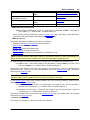
1
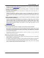
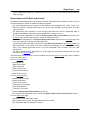
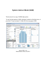
System Advisor Model (SAM)
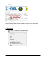
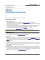
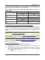
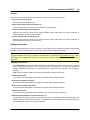
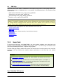
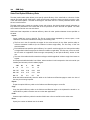
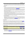
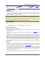
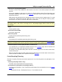
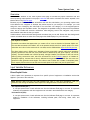
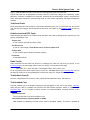
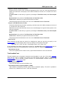
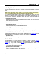
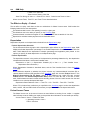
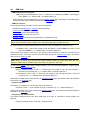
This document is a copy of SAM's Help system.
To see the Help system in SAM, click Help Contents on the Help menu, or
press the F1 key (command-? in Mac OS) from any page in SAM.
Version 2014.1.14
Manual Release Date 1/14/2014
2
© 2014 National Renewable Energy Laboratory
The System Advisor Model ("Model") is provided by the National Renewable Energy Laboratory ("NREL"), which is
operated by the Alliance for Sustainable Energy, LLC ("Alliance") for the U.S. Department Of Energy ("DOE") and
may be used for any purpose whatsoever.
The names DOE/NREL/ALLIANCE shall not be used in any representation, advertising, publicity or other manner
whatsoever to endorse or promote any entity that adopts or uses the Model. DOE/NREL/ALLIANCE shall not
provide any support, consulting, training or assistance of any kind with regard to the use of the Model or any
updates, revisions or new versions of the Model.
YOU AGREE TO INDEMNIFY DOE/NREL/ALLIANCE, AND ITS AFFILIATES, OFFICERS, AGENTS, AND
EMPLOYEES AGAINST ANY CLAIM OR DEMAND, INCLUDING REASONABLE ATTORNEYS' FEES, RELATED TO
YOUR USE, RELIANCE, OR ADOPTION OF THE MODEL FOR ANY PURPOSE WHATSOEVER. THE MODEL IS
PROVIDED BY DOE/NREL/ALLIANCE "AS IS" AND ANY EXPRESS OR IMPLIED WARRANTIES, INCLUDING BUT
NOT LIMITED TO THE IMPLIED WARRANTIES OF MERCHANTABILITY AND FITNESS FOR A PARTICULAR
PURPOSE ARE EXPRESSLY DISCLAIMED. IN NO EVENT SHALL DOE/NREL/ALLIANCE BE LIABLE FOR ANY
SPECIAL, INDIRECT OR CONSEQUENTIAL DAMAGES OR ANY DAMAGES WHATSOEVER, INCLUDING BUT NOT
LIMITED TO CLAIMS ASSOCIATED WITH THE LOSS OF DATA OR PROFITS, WHICH MAY RESULT FROM ANY
ACTION IN CONTRACT, NEGLIGENCE OR OTHER TORTIOUS CLAIM THAT ARISES OUT OF OR IN
CONNECTION WITH THE USE OR PERFORMANCE OF THE MODEL.
Microsoft and Excel are registered trademarks of the Microsoft Corporation.
While every precaution has been taken in the preparation of this document, the publisher and the author assume
no responsibility for errors or omissions, or for damages resulting from the use of information contained in this
document or from the use of programs and source code that may accompany it. In no event shall the publisher and
the author be liable for any loss of profit or any other commercial damage caused or alleged to have been caused
directly or indirectly by this document.
Produced: January 2014
System Advisor Model 2014.1.14
January 2014
Contents
3
Table of Contents
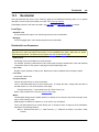
1 Introduction
11
1.1
About SAM
...........................................................................................................................11
1.2
Component
...........................................................................................................................20
Models and Databases
1.3
User Support
...........................................................................................................................22
1.4
Keep SAM
...........................................................................................................................23
Up to Date
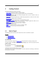
2 Getting Started
25
2.1
Start a Project
...........................................................................................................................25
2.2
Welcome
...........................................................................................................................29
Page
2.3
Main Window
...........................................................................................................................31
2.4
Input Pages
...........................................................................................................................32
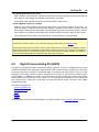
2.5
Run Simulations
...........................................................................................................................34
2.6
Results Page
...........................................................................................................................35
2.7
Export Data
...........................................................................................................................37
and Graphs
2.8
Manage ...........................................................................................................................41
Cases
2.9
Menus ...........................................................................................................................43
2.10
Notes
2.11
File Formats
...........................................................................................................................48
...........................................................................................................................47
3 YouTube Channel
49
4 Weather Data
50
4.1
Weather...........................................................................................................................50
Data Overview
4.2
Weather...........................................................................................................................54
Data Viewer
4.3
Weather...........................................................................................................................55
File Folders
4.4
Create TMY3
...........................................................................................................................56
File
4.5
Embed a...........................................................................................................................59
Weather File
4.6
Download
...........................................................................................................................60
Weather File
4.7
Weather...........................................................................................................................63
Data Online
4.8
Weather...........................................................................................................................66
File Formats
4.9
Location...........................................................................................................................71
and Resource
4.10
Wind Resource
...........................................................................................................................76
4.11
Location...........................................................................................................................80
and Ambient Conditions
4.12
Ambient...........................................................................................................................84
Conditions
System Advisor Model 2014.1.14
January 2014
4
SAM Help
5 Performance Models
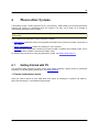
88
6 Photovoltaic Systems
91
6.1
Getting Started
...........................................................................................................................91
with PV
6.2
Shading...........................................................................................................................96
6.3
Microinverters
...........................................................................................................................104
6.4
Flat Plate
...........................................................................................................................105
PV
Sizing
............................................................................................................................105
the Flat Plate PV System
Module
............................................................................................................................112
Inverter
............................................................................................................................130
Array............................................................................................................................140
PV Subarrays
............................................................................................................................152
6.5
High-X ...........................................................................................................................159
Concentrating PV (HCPV)
Array............................................................................................................................160
Module
............................................................................................................................163
Inverter
............................................................................................................................165
6.6
PVWatts
...........................................................................................................................167
PVWatts
............................................................................................................................168
Solar Array
7 Concentrating Solar Power
7.1
171
Parabolic
...........................................................................................................................171
Trough Physical
Trough
............................................................................................................................172
Physical Overview
Solar............................................................................................................................174
Field
Collectors
............................................................................................................................194
(SCAs)
Receivers
............................................................................................................................196
(HCEs)
Power
............................................................................................................................200
Cycle
Thermal
............................................................................................................................205
Storage
Parasitics
............................................................................................................................213
7.2
Parabolic
...........................................................................................................................215
Trough Empirical
Trough
............................................................................................................................215
Empirical Overview
Solar............................................................................................................................216
Field
SCA ............................................................................................................................231
/ HCE
Power
............................................................................................................................237
Block
Thermal
............................................................................................................................241
Storage
Parasitics
............................................................................................................................249
7.3
Power ...........................................................................................................................251
Tower Molten Salt
System Advisor Model 2014.1.14
January 2014
Contents
5
Tower
............................................................................................................................252
Molten Salt Overview
Heliostat
............................................................................................................................253
Field
Tower
............................................................................................................................258
and Receiver
Power
............................................................................................................................262
Cycle
Thermal
............................................................................................................................267
Storage
Parasitics
............................................................................................................................274
7.4
Power ...........................................................................................................................275
Tower Direct Steam
Tower
............................................................................................................................276
Direct Steam Overview
Heliostat
............................................................................................................................277
Field
Tower
............................................................................................................................282
and Receiver
Power
............................................................................................................................286
Cycle
Parasitics
............................................................................................................................292
7.5
Linear ...........................................................................................................................293
Fresnel
Linear
............................................................................................................................294
Fresnel Overview
Solar............................................................................................................................295
Field
Collector
............................................................................................................................309
and Receiver
Power
............................................................................................................................316
Cycle
Parasitics
............................................................................................................................322
7.6
Dish Stirling
...........................................................................................................................323
Dish ............................................................................................................................323
Stirling Overview
System
............................................................................................................................324
Library
Solar............................................................................................................................325
Field
Collector
............................................................................................................................327
Receiver
............................................................................................................................329
Stirling
............................................................................................................................331
Engine
Parasitics
............................................................................................................................334
Reference
............................................................................................................................335
Inputs
7.7
Generic...........................................................................................................................336
Solar System
Generic
............................................................................................................................337
Solar Overview
Solar............................................................................................................................337
Field
Power
............................................................................................................................348
Block
Thermal
............................................................................................................................351
Storage
8 Generic System
355
8.1
Generic...........................................................................................................................355
System Overview
8.2
Power ...........................................................................................................................356
Plant
System Advisor Model 2014.1.14
January 2014
6
SAM Help
9 Solar Water Heating
358
9.1
Solar Water
...........................................................................................................................358
Heating Overview
9.2
Solar Water
...........................................................................................................................363
Heating
10 Wind Power
368
10.1
Wind Power
...........................................................................................................................368
Overview
10.2
Siting Considerations
...........................................................................................................................372
10.3
Turbine...........................................................................................................................373
10.4
Wind Farm
...........................................................................................................................374
11 Geothermal
11.1
377
Geothermal
...........................................................................................................................378
Power
Geothermal
............................................................................................................................378
Power Overview
Geothermal
............................................................................................................................379
Resource
Plant............................................................................................................................380
and Equipment
Power
............................................................................................................................381
Block
11.2
Geothermal
...........................................................................................................................384
Co-production
Resource
............................................................................................................................384
and Power Generation
12 Biomass Power
387
12.1
Biopower
...........................................................................................................................388
Overview
12.2
Feedstock
...........................................................................................................................389
12.3
Plant Specs
...........................................................................................................................393
12.4
Life-Cycle
...........................................................................................................................397
Emissions
13 Financial Models
400
13.1
Financing
...........................................................................................................................400
Overview
13.2
Performance
...........................................................................................................................406
Adjustment
13.3
Residential
...........................................................................................................................409
13.4
Commercial
...........................................................................................................................412
13.5
Utility IPP
...........................................................................................................................416
and Commercial PPA
13.6
Utility Single
...........................................................................................................................423
Owner
13.7
Utility All
...........................................................................................................................431
Equity Partnership Flip
13.8
Utility Leveraged
...........................................................................................................................440
Partnership Flip
13.9
Utility Sale
...........................................................................................................................449
Leaseback
13.10 Time of...........................................................................................................................458
Delivery Factors
13.11 Incentives
...........................................................................................................................460
System Advisor Model 2014.1.14
January 2014
Contents
7
13.12 Depreciation
...........................................................................................................................466
14 Retail Electricity Rates
469
14.1
Rates Overview
...........................................................................................................................469
14.2
Utility Rate
...........................................................................................................................470
14.3
Electric...........................................................................................................................480
Load
15 System Costs
487
15.1
System...........................................................................................................................487
Costs Overview
15.2
PV System
...........................................................................................................................488
Costs
15.3
HCPV Costs
...........................................................................................................................493
15.4
Trough...........................................................................................................................498
System Costs
15.5
Tower System
...........................................................................................................................504
Costs
15.6
Linear ...........................................................................................................................511
Fresnel System Costs
15.7
Dish System
...........................................................................................................................517
Costs
15.8
Generic...........................................................................................................................523
Solar System Costs
15.9
Generic...........................................................................................................................526
System Costs
15.10 SWH System
...........................................................................................................................531
Costs
15.11 Wind System
...........................................................................................................................536
Costs
15.12 Geothermal
...........................................................................................................................538
System Costs
15.13 Co-Production
...........................................................................................................................541
Costs
15.14 Biopower
...........................................................................................................................541
System Costs
15.15 Biopower
...........................................................................................................................544
Feedstock Costs
16 Results
545
16.1
Metrics...........................................................................................................................545
Table
16.2
Graphs...........................................................................................................................548
16.3
Tables ...........................................................................................................................551
16.4
Cash Flows
...........................................................................................................................554
16.5
Time Series
...........................................................................................................................555
16.6
Loss Diagram
...........................................................................................................................557
17 Reports
17.1
558
Generate
...........................................................................................................................559
Reports
18 Financial Metrics
559
18.1
Financial
...........................................................................................................................560
Metrics Overview
18.2
Project...........................................................................................................................562
Costs
System Advisor Model 2014.1.14
January 2014
8
SAM Help
18.3
Debt and
...........................................................................................................................562
Equity
18.4
Debt Fraction
...........................................................................................................................563
18.5
Financing
...........................................................................................................................563
Cost
18.6
Electricity
...........................................................................................................................564
Cost and Savings
18.7
Internal...........................................................................................................................565
Rate of Return (IRR)
18.8
Land Area
...........................................................................................................................567
18.9
Levelized
...........................................................................................................................568
Cost of Energy (LCOE)
18.10 Minimum
...........................................................................................................................575
DSCR
18.11 Net Present
...........................................................................................................................576
Value (NPV)
18.12 Payback
...........................................................................................................................577
Period
18.13 PPA Price
...........................................................................................................................579
18.14 PPA Price
...........................................................................................................................580
Escalation
18.15 Real Estate
...........................................................................................................................580
Value Added
19 Performance Metrics
581
19.1
Performance
...........................................................................................................................581
Metrics Overview
19.2
Annual...........................................................................................................................583
Biomass Usage
19.3
Annual...........................................................................................................................584
Energy
19.4
Annual...........................................................................................................................584
Water Usage
19.5
Aux with
...........................................................................................................................585
and without Solar (kWh)
19.6
Capacity
...........................................................................................................................585
Factor
19.7
First year
...........................................................................................................................586
kWhac/kWdc
19.8
Gross to
...........................................................................................................................586
Net Conv Factor
19.9
Heat Rate
...........................................................................................................................587
and Thermal Efficiency
19.10 Plant Capacity
...........................................................................................................................587
19.11 Pump Power
...........................................................................................................................587
19.12 Resource
...........................................................................................................................588
Capability
19.13 Solar Fraction
...........................................................................................................................588
19.14 System...........................................................................................................................588
Performance Factor
20 Cash Flow Variables
589
20.1
Residential
...........................................................................................................................589
and Commercial
20.2
IPP and...........................................................................................................................605
Commercial PPA
20.3
Single ...........................................................................................................................618
Owner
20.4
All Equity
...........................................................................................................................637
Partnership Flip
20.5
Leveraged
...........................................................................................................................662
Partnership Flip
System Advisor Model 2014.1.14
January 2014
Contents
20.6
9
Sale Leaseback
...........................................................................................................................687
21 Performance Model Results
706
21.1
Performance
...........................................................................................................................707
Results Overview
21.2
Flat Plate
...........................................................................................................................708
PV
21.3
PVWatts
...........................................................................................................................712
21.4
High-X ...........................................................................................................................713
Concentrating PV
21.5
Parabolic
...........................................................................................................................714
Trough (Physical)
21.6
Parabolic
...........................................................................................................................716
Trough (Empirical)
21.7
Power ...........................................................................................................................719
Tower (Molten Salt)
21.8
Power ...........................................................................................................................722
Tower (Direct Steam)
21.9
Generic...........................................................................................................................725
Solar System
21.10 Linear ...........................................................................................................................727
Fresnel
21.11 Dish Stirling
...........................................................................................................................729
21.12 Solar Water
...........................................................................................................................731
Heating
21.13 Geothermal
...........................................................................................................................733
22 Savings and Revenue
734
22.1
Time Dependent
...........................................................................................................................734
Pricing Overview
22.2
PPA Revenue
...........................................................................................................................736
with TOD Factors
22.3
Retail Electricity
...........................................................................................................................737
Savings
23 Software Development Kit (SDK)
740
24 SamUL Scripting Language
741
24.1
Writing...........................................................................................................................742
and Running SamUL Scripts
24.2
Why use
...........................................................................................................................744
SamUL?
24.3
Data Variables
...........................................................................................................................745
24.4
Flow Control
...........................................................................................................................748
24.5
Arrays of
...........................................................................................................................752
Data
24.6
Function
...........................................................................................................................755
Calls
24.7
Input, Output,
...........................................................................................................................758
and System Access
24.8
Interfacing
...........................................................................................................................761
with SAM Analyses
24.9
Code Sample:
...........................................................................................................................763
Latin Hypercube Sampling
24.10 Library...........................................................................................................................766
Reference
25 Analysis Options
25.1
779
Parametric
...........................................................................................................................780
Analysis
System Advisor Model 2014.1.14
January 2014
10
SAM Help
25.2
Sensitivity
...........................................................................................................................787
Analysis
25.3
Statistical
...........................................................................................................................791
25.4
Multiple...........................................................................................................................795
Subsystems
25.5
Excel Exchange
...........................................................................................................................797
25.6
P50/P90...........................................................................................................................799
Analysis
26 Advanced Modeling Topics
802
26.1
Libraries
...........................................................................................................................802
26.2
Simulator
...........................................................................................................................809
Options
26.3
Exchange
...........................................................................................................................810
Variables
27 References
System Advisor Model 2014.1.14
811
January 2014
11
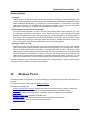
1
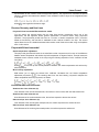
Introduction
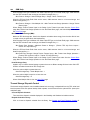
The System Advisor Model (SAM) is a performance and financial model for renewable energy power
systems and projects.
For a general description of SAM, see About SAM.
For information about getting help using SAM, see User Support.
For instructions on getting the latest version or updating your version of SAM, see Keep SAM Up to
Date.
1.1
About SAM
The System Advisor Model (SAM) is a performance and financial model designed to facilitate decision
making for people involved in the renewable energy industry:
Project managers and engineers
Policy analysts
Technology developers
Researchers
SAM makes performance predictions and cost of energy estimates for grid-connected power projects based
on installation and operating costs and system design parameters that you specify as inputs to the model.
Projects can be either on the customer side of the utility meter, buying and selling electricity at retail rates,
or on the utility side of the meter, selling electricity at a price negotiated through a power purchase
agreement (PPA).
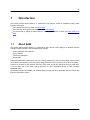
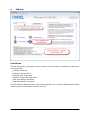
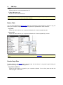
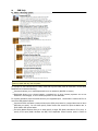
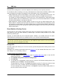
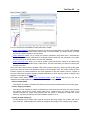
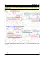
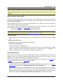
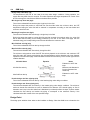
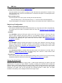
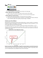
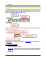
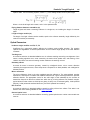
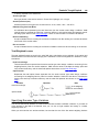
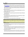
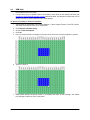
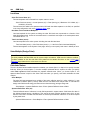
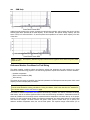
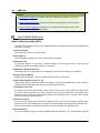
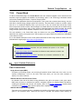
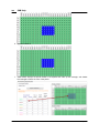
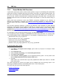
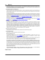
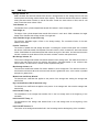
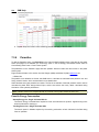
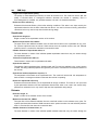
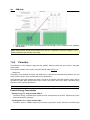
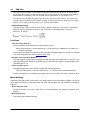
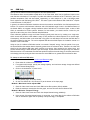
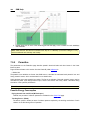
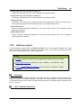
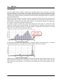
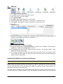
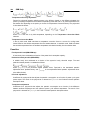
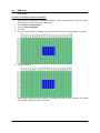
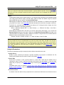
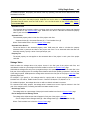
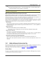
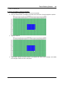
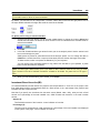
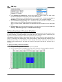
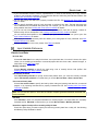
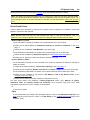
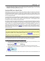
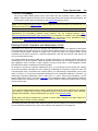
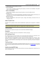
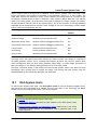
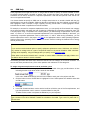
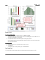
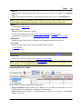
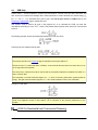
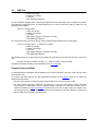
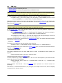
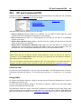
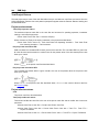
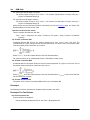
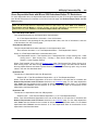
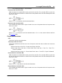
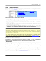
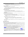
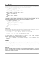
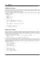
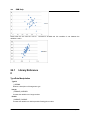
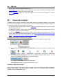
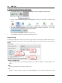
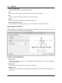
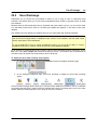
The following image shows SAM's main window showing monthly electricity generation and the annual cash
flow for a photovoltaic system.
System Advisor Model 2014.1.14
12
SAM Help
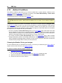
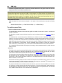
The first step in creating a SAM file is to choose a technology and financing option for your project. SAM
automatically populates input variables with a set of default values for the type of project. It is your
responsibility as an analyst to review and modify all of the input data as appropriate for each analysis.
Next, you provide information about a project's location, the type of equipment in the system, the cost of
installing and operating the system, and financial and incentives assumptions.
SAM Models and Databases
SAM represents the cost and performance of renewable energy projects using computer models developed
at NREL, Sandia National Laboratories, the University of Wisconsin, and other organizations. Each
performance model represents a part of the system, and each financial model represents a project's
financial structure. The models require input data to describe the performance characteristics of physical
equipment in the system and project costs. SAM's user interface makes it possible for people with no
experience developing computer models to build a model of a renewable energy project, and to make cost
and performance projections based on model results.
SAM requires a resource data file describing the renewable energy resource and weather conditions a the
project location. Depending on the kind of system you are modeling, you either choose a resource data file
from a list, download one from the internet, or create the file using your own data.
SAM can automatically download data from the following online databases:
DSIRE for U.S. incentives.
OpenEI Utilities Gateway for retail electricity rate structures for U.S. utilities
NREL Solar Prospector for solar resource data and ambient weather conditions.
NREL Wind Integration Datasets for wind resource data.
NREL Biofuels Atlas and DOE Billion Ton Update for biomass resource data.
NREL Geothermal Resource database for temperature and depth data.
SAM includes several databases of performance data and coefficients for system components such as
photovoltaic modules and inverters, parabolic trough receivers and collectors, wind turbines, or biopower
combustion systems. For those components, you simply choose an option from a list. For U.S. locations,
SAM can also automatically download data describing incentives and retail electricity rate structures from
online databases.
January 2014
About SAM
13
For the remaining input variables, you either use the default value or change its value. Some examples of
input variables are:
Installation costs including equipment purchases, labor, engineering and other project costs, land costs,
and operation and maintenance costs.
Numbers of modules and inverters, tracking type, derating factors for photovoltaic systems.
Collector and receiver type, solar multiple, storage capacity, power block capacity for parabolic trough
systems.
Analysis period, real discount rate, inflation rate, tax rates, internal rate of return target or power
purchase price for utility financing models.
Building load and time-of-use retail rates for commercial and residential financing models.
Tax and cash incentive amounts and rates.
Once you are satisfied with the input variable values, you run simulations, and then examine results. A
typical analysis involves running simulations, examining results, revising inputs, and repeating that process
until you understand and have confidence in the results.
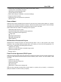
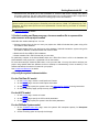
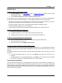
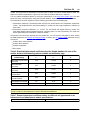
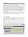
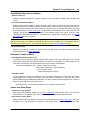
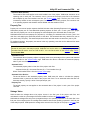
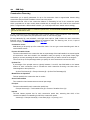
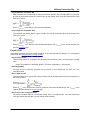
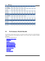
Results: Tables, Graphs, and Reports
SAM displays modeling results in tables and graphs, ranging from the metrics table displaying levelized
cost of energy, first year annual production, and other single-value metrics, to the detailed annual cash flow
and hourly performance data that can be viewed in tabular or graphical form.
A built-in graphing tool displays a set of default graphs and allows for creation of custom graphs. All graphs
and tables can be exported in various formats for inclusion in reports and presentations, and also for further
analysis with spreadsheet or other software.
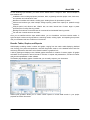
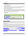
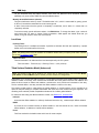
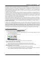
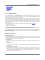
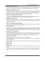
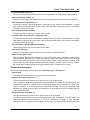
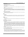
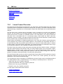
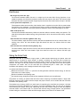
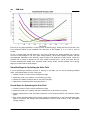
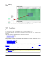
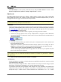
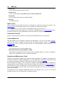
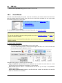
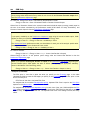
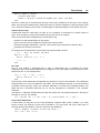
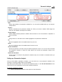
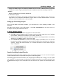
The Results page displays graphs of results that you can easily export to your documents:
SAM's report generator allows you to create custom reports to include SAM results in your project
proposals and other documents:
System Advisor Model 2014.1.14
14
SAM Help
Performance Model
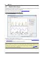
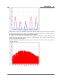
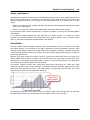
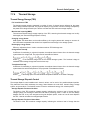
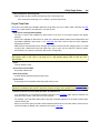
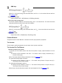
SAM's performance model makes hour-by-hour calculations of a power system's electric output, generating
a set of 8,760 hourly values that represent the system's electricity production over a single year. You can
explore the system's performance characteristics in detail by viewing tables and graphs of the hourly and
monthly performance data, or use performance metrics such as the system's total annual output and
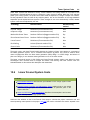
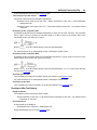
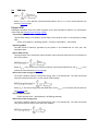
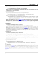
capacity factor for more general performance evaluations.
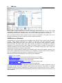
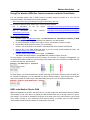
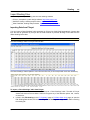
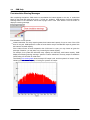
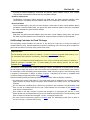
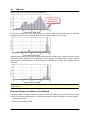
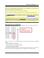
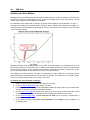
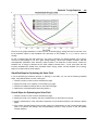
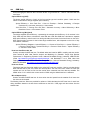
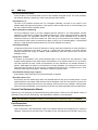
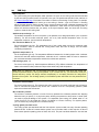
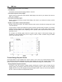
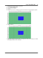
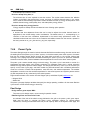
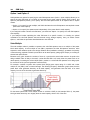
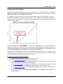
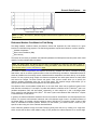
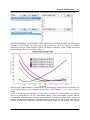
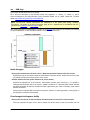
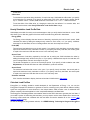
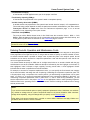
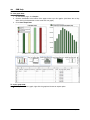
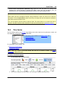
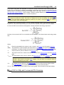
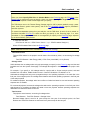
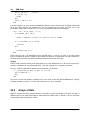
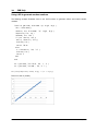
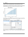
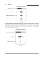
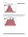
The Time Series graph on the Results page showing hourly electricity generation for a 100 MW parabolic
trough system with 6 hours of storage in Blythe, California:
The current version of the SAM includes performance models for the following technologies:
Photovoltaic systems (flat-plate and concentrating)
Parabolic trough concentrating solar power
January 2014
About SAM
15
Power tower concentrating solar power (molten salt and direct steam)
Linear Fresnel concentrating solar power
Dish-Stirling concentrating solar power
Conventional fossil-fuel thermal
Solar water heating for residential or commercial buildings
Large and small wind power
Geothermal power and geothermal co-production
Biomass power
Financial Model
SAM's financial model calculates financial metrics for various kinds of power projects based on a project's
cash flows over an analysis period that you specify. The financial model uses the system's electrical output
calculated by the performance model to calculate the series of annual cash flows.
SAM includes financial models for the following kinds of projects:
Residential (retail electricity rates)
Commercial (retail rates or power purchase agreement)
Utility-scale (power purchase agreement):
Single owner
Leveraged partnership flip
All equity partnership flip
Sale leaseback
Residential and Commercial Projects
Residential and commercial projects are financed through either a loan or cash payment, and recover
investment costs by selling electricity through either a net metering or time-of-use pricing agreement. For
these projects, SAM reports the following financial metrics:
Levelized cost of energy
Electricity cost with and without renewable energy system
After-tax net present value
Payback Period
Power Purchase Agreement (PPA) Projects
Utility and commercial PPA projects are assumed to sell electricity through a power purchase agreement at
a fixed price with optional annual escalation and time-of-delivery (TOD) factors. For these projects, SAM
calculates:
Levelized cost of energy
PPA price (electricity sales price)
Internal rate of return
Net present value
Debt fraction or debt service coverage ratio
SAM can either calculate the internal rate of return based on a power price you specify, or calculate the
power price based on the rate of return you specify.
System Advisor Model 2014.1.14
16
SAM Help
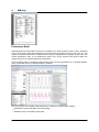
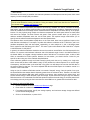
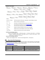
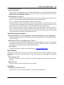
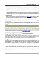
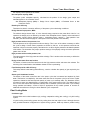
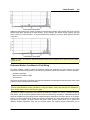
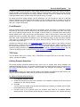
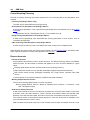
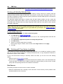
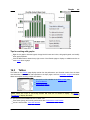
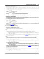
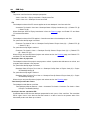
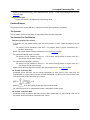
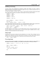
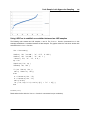
Levelized Cost of Energy and Cash Flow
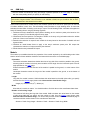
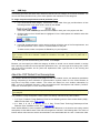
SAM calculates the levelized cost of energy (LCOE) after-tax cash flows for projects using retail electricity
rates, and from the revenue cash flow for projects selling electricity under a power purchase agreement.
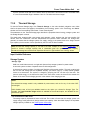
The following image shows several rows of the cash flow table for a utility-scale project:
The project annual cash flows include:
Value of electricity sales (or savings) and incentive payments
Installation costs
Operating, maintenance, and replacement costs
Loan principal and interest payments
Tax benefits and liabilities (accounting for any tax credits for which the project is eligible)
Incentive payments
Project and partner's internal rate of return requirements (for PPA projects)
Incentives
The financial model can account for a wide range of incentive payments and tax credits:
Investment based incentives (IBI)
Capacity-based incentives (CBI)
Production-based incentives (PBI)
Investment tax credits (ITC)
Production tax credits (PTC)
Depreciation (MACRS, Straight-line, custom, bonus, etc.)
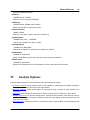
Analysis Options
In addition to simulating a system's performance over a single year and calculating a project cash flow over
January 2014
About SAM
17
a multi-year period, SAM's analysis options make it possible to conduct studies involving multiple
simulations, linking SAM inputs to a Microsoft Excel workbook, and working with custom simulation
modules.
The following options are for analyses that investigate impacts of variations and uncertainty in assumptions
about weather, performance, cost, and financial parameters on model results:
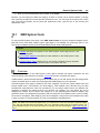
Parametric Analysis: Assign multiple values to input variables to create graphs and tables showing the
value of output metrics for each value of the input variable. Useful for optimization and exploring
relationships between input variables and results.
Sensitivity Analysis: Create tornado graphs by specifying a range of values for input variables as a
percentage.
Statistical: Create histograms showing the sensitivity of output metrics to variations in input values.
P50/P90: For locations with weather data available for many years, calculate the probability that the
system's total annual output will exceed a certain value.
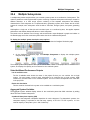
For files with multiple cases, the Multiple Subsystems option allows you to model a project that combines
systems from the cases, assuming that the system's total electrical output is the sum of the output of the
subsystems modeled in each case, and applies the financing model from one case to this total output.
SAM also makes it possible to work with external models developed in Excel or the TRNSYS simulation
platform:
Excel Exchange: Use Excel to calculate the value of input variables, and automatically pass values of
input variables between SAM and Excel.
Exchange Variables: Create your own input variables for use with Excel Exchange or a custom
TRNSYS deck.
Simulator Options: Change the simulation time step, or run SAM with your own simulation modules
developed in the TRNSYS modeling platform.
Finally, SAM's scripting language SamUL allows you to write your own programs within the SAM user
interface to control simulations, change values of input variables, and write data to text files.
Software Development History and Users
SAM, originally called the "Solar Advisor Model" was developed by the National Renewable Energy
Laboratory in collaboration with Sandia National Laboratories in 2005, and at first used internally by the U.S.
Department of Energy's Solar Energy Technologies Program for systems-based analysis of solar technology
improvement opportunities within the program. The first public version was released in August 2007 as
Version 1, making it possible for solar energy professionals to analyze photovoltaic systems and
concentrating solar power parabolic trough systems in the same modeling platform using consistent
financial assumptions. Since 2007, two new versions have been released each year, adding new
technologies and financing options. In 2010, the name changed to "System Advisor Model" to reflect the
addition of non-solar technologies.
The DOE, NREL, and Sandia continue to use the model for program planning and grant programs. Since the
first public release, over 35,000 people representing manufacturers, project developers, academic
researchers, and policy makers have downloaded the software. Manufacturers are using the model to
evaluate the impact of efficiency improvements or cost reductions in their products on the cost of energy
from installed systems. Project developers use SAM to evaluate different system configurations to maximize
earnings from electricity sales. Policy makers and designers use the model to experiment with different
incentive structures.
System Advisor Model 2014.1.14
18
SAM Help
Downloading SAM and User Support
SAM runs on both Windows and OS X. It requires about 500 MB of storage space on your computer.
SAM is available for free download at http://sam.nrel.gov. To download the software, you must register for an
account on the website. After registering, you will receive an email with your account information.
SAM's website includes software descriptions, links to publications about SAM and other resources:
The following resources are available for learning to use SAM and for getting help with your analyses:
The built-in Help system (also available on the website)
User support forum: https://sam.nrel.gov/forums/support-forum
Demonstration videos on the SAM website: https://sam.nrel.gov/content/resources-learning-sam
Periodic webinars: https://sam.nrel.gov/content/resources-learning-sam
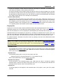
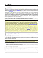
You can contact the SAM support team by emailing [email protected].
SAM's help system includes detailed descriptions of the user interface, modeling options, and results:
January 2014
About SAM
19
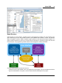
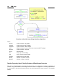
Model Structure
SAM consists of a user interface, calculation engine, and programming interface. The user interface is the
part of SAM that you see, and provides access to input variables and simulation controls, and displays
tables and graphs of results. SAM's calculation engine performs a time-step-by-time-step simulation of a
power system's performance, and a set of annual financial calculations to generate a project cash flow and
financial metrics. The programming interface allows external programs to interact with SAM.
The user interface performs three basic functions:
Provide access to input variables, which are organized into input pages. The input variables describe the
physical characteristics of a system, and the cost and financial assumptions for a project.
System Advisor Model 2014.1.14
SAM Help
20
Allow you to control how SAM runs simulations. You can run a basic simulation, or more advanced
simulations for optimization and sensitivity studies.
Provide access to output variables in tables and graphs on the Results page, and in files that you can
access in a spreadsheet program or graphical data viewer.
SAM's scripting language SamUL allows you to automate certain tasks. If you have some experience writing
computer programs, you can easily learn to write SamUL scripts to set the values of input variables by
reading them from a text file or based on calculations in the script, run simulations, and write values of
results to a text file. You can also use SamUL to automatically run a series of simulations using different
weather files.
Excel Exchange allows you to use Microsoft Excel to calculate values of input variables. With Excel
Exchange, each time you run simulations, SAM opens a spreadsheet and, depending on how you've
configured Excel Exchange, writes values from SAM input pages to the spreadsheet, and reads values from
the spreadsheet to use in simulations. This makes it possible to use spreadsheet formulas to calculate
values of SAM input variables.
Calculation Engine
Each renewable energy technology in SAM has a corresponding performance model that performs
calculations specific to the technology. Similarly, each financing option in SAM is also associated with a
particular financial model with its own set of inputs and outputs. The financial models are as independent as
possible from the performance models to allow for consistency in financial calculations across the different
technologies.
A performance simulation consists of a series of many calculations to emulate the performance of the
system over a one year period in time steps of one hour for most simulations, and shorter time steps for
some technologies.
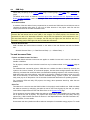
A typical simulation run consists of the following steps:
1.
2.
3.
4.
5.
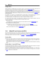
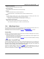
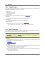
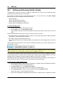
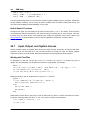
1.2
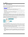
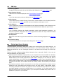
After starting SAM, you select a combination of technology and financing options for a case in the
user interface.
Behind the scenes, SAM chooses the proper set of simulation and financial models.
You specify values of input variables in the user interface. Each variable has a default value, so it is
not necessary to specify a value for every variable.
When you click the Run button, SAM runs the simulation and financial models. For advanced
analyses, you can configure simulations for optimization or sensitivity analyses before running
simulations.
SAM displays graphs and tables of results in the user interface's Results page.
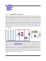
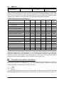
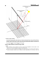
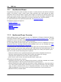
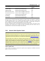
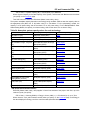
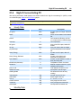
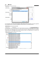
Component Models and Databases
This topic lists all of SAM's performance models and describes the component-level models and databases
SAM uses.
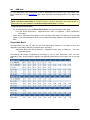
System Performance Models
The system models represent a complete renewable energy system and were developed by NREL using
algorithms from partners listed below.
January 2014
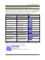
Component Models and Databases
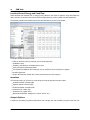
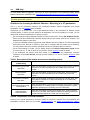
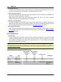
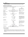
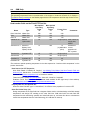
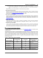
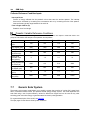
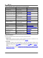
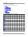
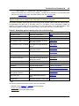
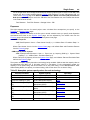
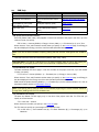
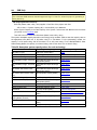
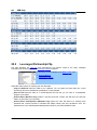
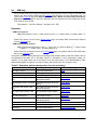
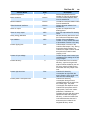
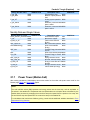
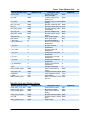
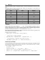
Model Name
21
Partner (if any)
Flat Plate PV
Component models from Sandia National
Laboratories and the University of Wisconsin
High-X Concentrating PV
PVWatts System Model
Parabolic Trough Physical Model
Parabolic Trough Empirical Model
Molten Salt Power Tower
Direct Steam Power Tower
Linear Fresnel
Dish Stirling
Generic Solar System
Generic System
Solar Water Heating
Wind Power
Geothermal Power
Geothermal Co-production
Biomass Power
University
University
University
University
University
University
of Wisconsin
of Wisconsin
of Wisconsin
of Wisconsin
of Wisconsin
of Wisconsin
University of Wisconsin
Princeton Energy Resources International
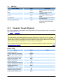
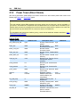
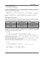
Component Performance Models
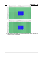
The Flat Plate PV and Wind Power model include options for choosing a component performance model to
represent part of the system.
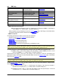
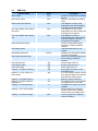
Model Name
Component
Developer
Simple Efficiency Module Model
Photovoltaic module
NREL
CEC Performance Model with
Module Data base
Photovoltaic module
University of Wisconsin
CEC Performance Model with User Photovoltaic module
Entered Specifications
Adapted by NREL
Sandia PV Array Performance
Model with Module Database
Photovoltaic module
Sandia National Laboratories
Single Point Efficiency Inverter
Inverter
NREL
Sandia Performance Model for Grid Inverter
Connected PV Inverters
Sandia National Laboratories
Wind Turbine Design Model
Wind Turbine
NREL
Wind Power Curve Model
Wind Turbine
NREL
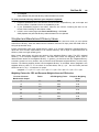
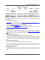
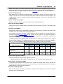
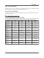
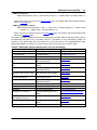
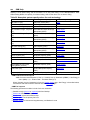
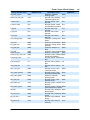
Component Parameter Databases
Some of the component models use a library of input parameters to represent the performance
characteristics of the component. The libraries listed below are owned by organizations other than NREL.
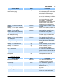
Library Name
CEC Modules
Sandia Inverters
System Advisor Model 2014.1.14
Component
PV module
Inverter
Owner
California Energy Commission
Sandia National Laboratories
22
SAM Help
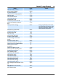
Library Name
Component
Sandia Modules
PV module
Owner
Sandia National Laboratories
Online Financial Model Data
SAM can automatically download data from the following online databases to populate values on its financial
model input pages.
Database Name
Type of Data
Database Manager
OpenEI Utilities Gateway
Retail electricity prices and rate
structures
NREL and Illinois State University
DSIRE
Incentives
North Carolina Solar Center and
Interstate Renewable Energy
Council
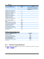
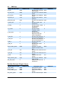
Online Renewable Resource and Weather Data Sources
SAM can automatically download renewable energy resource and weather data from the following online
databases.
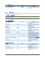
Database Name
Type of Resource Data
Database Manager
Solar Prospector
Solar and Meteorological
NREL
Wind Integration Datasets
Wind and Meteorological
NREL with 3Tier and AWS
Truepower
Geothermal Resource
Ground temperature and depth
Southern Methodist University
NREL Biofuels Atlas
Agricultural Residues
NREL
Billion Ton Update
Dedicated energy crops
Department of Energy
SAM also comes with a complete set of TMY2 files (1961-1990) from the National Solar Radiation Database
(NSRDB). It can read NSRDB TMY3 files, and EPW files developed for the Department of Energy's
EnergyPlus building simulation model.
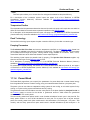
1.3
User Support
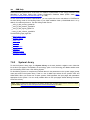
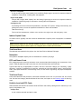
For information about any page in the software, do one of the following:
Press the F1 key in Windows or Command-? in Mac OS.
Click the help button at the top right corner of each input page.
Click Help Contents from the Help menu.
January 2014
User Support
23
In secondary windows, click the Help button for information about the
window.
For additional help, try:
For general information about the model, including a discussion of project costs, references to
related publications and a list of frequently asked questions, and other information visit the SAM
website: http://sam.nrel.gov/.
For user support, post a question on the SAM forum at https://sam.nrel.gov/forums/supportforum.
To send an email to the SAM team, contact us at [email protected].
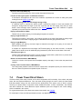
1.4
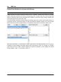
Keep SAM Up to Date
SAM Versions
The SAM team releases new versions of SAM periodically. To find out if your version of SAM is the latest
version, check the SAM website at http://sam.nrel.gov/.
SAM's Welcome page also displays news from the SAM team, including announcements of new versions.
SAM displays the version number in the title bar of the Main window:
You can also find the SAM version number along with version numbers of other components of the software
by clicking About on the Help menu:
System Advisor Model 2014.1.14
24
SAM Help
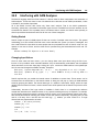
Checking for Updates
Updates may be available before a new release is available to address minor issues with the software.
By default, SAM checks the SAM website for updates each time you start the software. You can disable
this feature by clearing the checkmark on the Help menu next to Allow SAM to check for updates at
startup.
To check for updates:
On the Help menu, click Check for updates to this version.
January 2014
25
2
Getting Started
The Getting Started topics introduce you to SAM:
Start a Project describes the steps for creating a SAM file.
Welcome Page describes the Welcome page that appears when you first start SAM.
Main Window describes SAM's main window that appears when you open a SAM file, where you
access input pages and results.
Input Pages describes the general layout of SAM's input pages where you specify the value of input
variables.
Run Simulations explains how to run simulations.
Results Page describes the general layout of the page displaying results.
Export Data and Graphs explains how to export data and images of graphs from SAM for use in
spreadsheets, reports, presentations, and other documents.
Manage Cases explains how to work with cases in a SAM file.
Menus describes SAM's menus.
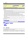
Notes explains how to use notes to store text messages in SAM.
File Formats describes the types of files used with SAM.
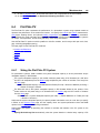
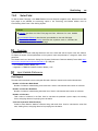
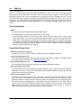
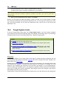
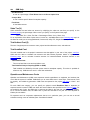
2.1
Start a Project
The following procedure describes the basic steps to set up and run a simulation of a project.
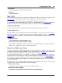
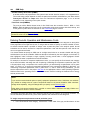
See also:
Financing Overview
Technology Options
Getting Started with PV
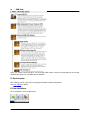
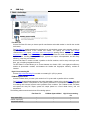
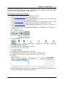
A. Create a file
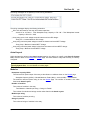
When you start SAM, it displays the Welcome page with several options for creating or opening a file.
To create a new file, under Enter a new project name to begin, type a name for your project and click
Create a new file.
SAM displays the technology and financing options. You must choose both a technology to model and a
financing option for the project.
System Advisor Model 2014.1.14
26
SAM Help
B. Choose a technology
The technology option you choose determines the performance model that SAM uses for simulations. SAM
offers performance models for photovoltaic, concentrating solar power, solar water heating, wind,
geothermal, and biomass power systems. The generic system model allows you to represent a system
using only a nameplate capacity and capacity factor, or an hourly or subhourly generation profile from
another performance model or data source.
For photovoltaic systems, click Photovoltaics to expand the list of options. If you want to choose a specific
module and inverter from a list, choose Flat Plate PV. If you want to model the entire system using a single
derate factor, choose PVWatts System Model.
For parabolic trough systems, click Concentrating Solar Power to expand the list of options and then
choose Parabolic Trough (Physical Model). If you are modeling a system with a configuration similar to
the SEGS plants choose Parabolic Trough (Empirical Model).
For other technologies, choose the appropriate option. See Technology Options for descriptions.
January 2014
Start a Project
27
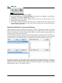
C. Choose a financing option
When you choose a technology option, SAM displays financing options available for the technology under
the Select a financing option heading. For a description of the financing options, see Financing Overview.
For projects on the customer side of the electric power meter that buy and sell electricity at retail rates,
choose either Residential or Commercial.
For power generation projects that sell power at a price negotiated through a power purchase agreement,
choose either Commercial PPA, Utility Independent Power Producer (IPP), or one of the Advanced
Utility IPP options.
System Advisor Model 2014.1.14
28
SAM Help
When you choose a financing option, and click OK, SAM creates a new file and populates all of the input
variables with values from the default values database.
D. Review inputs
After creating your file, open each input page and review the default assumptions.
See Input Pages for details.
E. Run simulations
To run simulations, click the Run button.
January 2014
Start a Project
29
See Run Simulations for details.
F. Review results
When simulations are complete, SAM displays a summary of results in the Metric table.
You can display graphs and tables of detailed results data on the Results page.
2.2
Welcome Page
When you start SAM, it displays a Welcome window with several options for starting a project:
Create a new file to start a project. Type the project name and click Create a new file to display the
Technology and Market window where you choose a technology and financing option.
Open a sample file. The sample files illustrate how to model some common types of projects and how to
use some of SAM's more advanced modeling techniques.
Open a recent file. The Recent Files list contains project files that were saved during previous SAM
sessions.
Note. To return to the Welcome page after creating a case, click Close on the File menu.
System Advisor Model 2014.1.14
30
SAM Help
Solar Wizard
The solar wizard walks you through the steps to create a file for the following combinations of performance
and financial model:
PVWatts, Residential
PVWatts, Commercial PPA
PVWatts, Utility Single Owner
Empirical Trough, Utility Single Owner
Solar Water Heating, Residential
Solar Water Heating, Commercial
The Solar Wizard is designed to help you get started using SAM. You can open the SAM file that the wizard
creates to explore all of the inputs and results in the file.
January 2014
Main Window
2.3
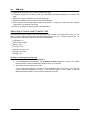
31
Main Window
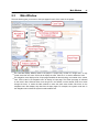
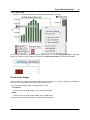
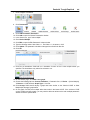
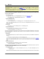
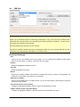
The main window gives you access to the input pages for each of the cases in the project:
The case tabs display different cases in the project. A project may consist of a single case, or may
contain more than one case. Click a tab to display the case. Click the 'x' on a tab to delete the case.
The navigation menu displays a list of input pages available for the technology and market of the current
case. Click an item in the navigation menu to display an input page. The active input page is indicated
on the menu in blue. When the menu is too long to fit in the window, use the vertical scroll bar to move
through the menu, or resize the Main window to make the entire menu visible. Each item on the
navigation menu also displays key data from the input pages. For example, the system costs item in
the navigation menu shows the system's total installed cost.
System Advisor Model 2014.1.14
SAM Help
32
2.4
Input Pages
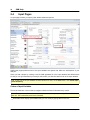
An input page is where you specify input variable values and options.
SAM's input pages provide access to the input variables and options that define the assumptions of your
analysis.
When you start a project by creating a new file SAM populates all of the input variables with default values
so that you can get started with your analysis even before you have final values for all of the input variables.
Tip. To see a list of all input variables and their values for a case, on the Case menu, click Show Input
Value Summary.
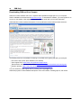
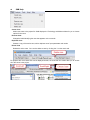
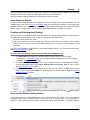
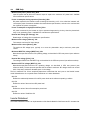
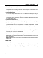
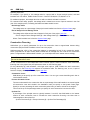
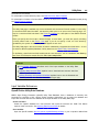
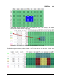
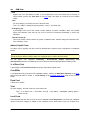
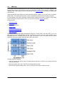
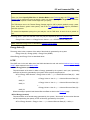
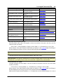
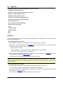
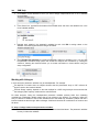
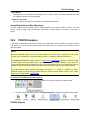
Colors of Input Variables
The text and data box colors on the input pages indicate the kind of information they contain:
Note. The appearance of text and text boxes depends on whether you are running SAM on Windows or
Mac OS. The screenshots below are for Windows.
White data boxes display input variables that you can modify by typing values in the box:
January 2014
Input Pages
33
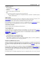
Blue data boxes are for reference values that SAM either displays from other input pages, or calculates
from other input variables. Data in blue cannot be modified. Press the F1 key on your keyboard
(Command-? on a Mac) to see the Help topic with descriptions of the equations SAM uses to calculate
these values:
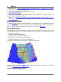
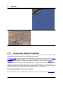
Gray data boxes show values for your reference. For example, these input variables on the Location and
Resource page show annual averages calculated from data stored in the weather file. You cannot modify
data in gray:
Blue underlined text indicates links to websites with useful information related to the input page:
Informational text describing the input variables appears in orange font:
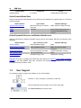
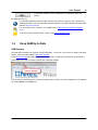
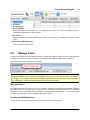
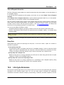
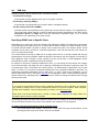
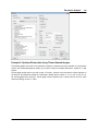
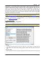
Library buttons populate input variables with values from a library of stored parameters. Modifying a value
on an input page does not change the value stored in the library. See Working with Libraries to learn
more about libraries:
System Advisor Model 2014.1.14
SAM Help
34
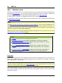
2.5
Run Simulations
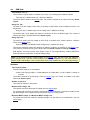
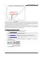
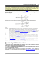
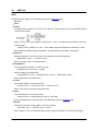
After reviewing and modifying inputs on the input pages, click the Run all Simulations button to run
simulations:
SAM runs simulations based on the values of input variables that appear on the input pages and reports
those values as "base case" results.
In addition to the base case, SAM runs simulations for any additional simulations you may have set up on
the Configure Simulations pages, such as parametric or sensitivity analyses.
You can also run simulations from the Case menu (See Menus for a description of menu commands):
Run All Simulations
Runs all of the simulations configured in the current case. Equivalent to clicking the Run button.
Run Base Case Only
Runs a single simulation based on the input values shown on the input pages, ignoring any parametric,
sensitivity, or other configurations requiring multiple simulation runs.
January 2014
Results Page
2.6
35
Results Page
The Results page displays data from both the performance model and financial model. You can export data
from any graph or table displayed on the Results page to Excel or text files.
To display the Results page:
Click Run to run simulations and display the Results page.
Or, click Switch to Results to show the Results page without running simulations.
Note. If you try to display the Results page before running simulations, and there are no results from an
earlier simulation run, SAM displays variable names like sv.annual_output or cf.energy because there
are no results to display. If you see these variable names, click Run to generate results.
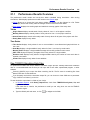
Performance Model Results
When you run simulations based on inputs you specify on the Systems pages in SAM, the performance
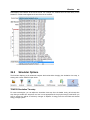
model creates a file of hourly data called the simulation results file. There are several options in SAM for
viewing data from this file:
Note. For some advanced simulations, the simulation file may contain data with a different time step.
The Metrics table displays key metrics that summarize the performance model results, such as total
annual electrical output, capacity factor, etc.
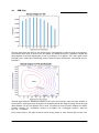
Graphs displays monthly electrical output and an annual energy flow graph, and allows you to create
your own graphs.
Tables allows you to build custom tables of hourly, monthly, and annual results on the Results page.
Time Series displays time series and statistical graphs of hourly data.
Financial Model Results
SAM's financial model uses the sum of the performance model's 8,760 hourly output values in kWh as an
input representing the system's total annual electrical output in kWh. The financial model then calculates
the project's cash flow based on the inputs you specify on the Costs and Financing pages. SAM displays
financial model results in the following places:
The Metrics table displays key metrics such as the LCOE, PPA price, IRR, and payback period.
The Cash Flows table shows details of the project's cash flow.
Tables allows you to build custom tables of cost and cash flow data along with metrics.
Simulation Warning Messages
System Advisor Model 2014.1.14
36
SAM Help
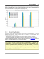
Under some conditions, SAM displays simulation warnings. When there are simulation warnings, the
simulation warning button appears at the top right corner of the Results page. Click the Show Simulation
Warnings button to view warning messages:
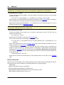
Screenshots
The Display Results button shows results for the last simulation without running a new set of simulations. If
you show the Results page using this button after changing values on the input pages, the data on the
results page will not match the inputs.
January 2014
Results Page
2.7
37
Export Data and Graphs
SAM provides several options for exporting data and graph images to other applications for further analysis
or inclusion in reports and other documents.
Input Data
The input value summary is a list of all the input variables in a case with their values.
To view the input value summary:
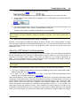
On the Tools menu, click Export input variable list, or press the F8 key.
The table lists input variables with the convention [Input page name]/[Variable Name], where {CALC}
indicates that the variable is for a calculated value rather than one that you can enter.
To export the list of input variables:
Choose one of the options for exporting the variable lists.
Copy
Copies the table to your computer's clipboard so you can paste the data into another program.
System Advisor Model 2014.1.14
SAM Help
38
Save
Saves the data to a comma-separated text file.
To Excel (Windows only)
Exports the data to Microsoft Excel.
Note. For files that contain more than one case, you can also display and export input variables along
with results for one or more case using Case Compare.
Metrics Table
You can export data from the Metrics table either by right-clicking it and choosing an option to copy the
data to your computer's clipboard, which you can paste into a spreadsheet or other document:
Copy table
Copies the metrics table to your computer's clipboard with columns separated by tabs.
Copy as CSV
Copies the metrics table to your computer's clipboard with columns separated by commas.
Note. You can choose Metrics table variables to display in the data table, and export the values from
there.
Results Graph Data
For most graphs on the Results page, you can export the data shown in the graph by right-clicking the
graph and choosing one of the following options:
Copy data to clipboard
Copies the data visible in the graph to your computer's clipboard. You can then paste the data into
another program or document.
January 2014
Export Data and Graphs
39
Save data to CSV
Creates a comma-separated text file containing the data visible in the graph.
For the graphs you see on the Results page in Graphs mode, you can click Copy Graph Data to copy data
visible in the graphs to your computer's clipboard. Click Show Graph Data to see a table of the data.
Results Graph Images
To export images of graphs, right-click the graph and choose options to copy the image to the clipboard or
save it to a file, and to determine the size of the exported image.
You can export the graph image to the clipboard or to a file:
To clipboard
Place a copy of the graph image in your computer's clipboard.
Export
Creates a file of the graph image in BMP, JPG, or PNG format.
You can export the graph image with one of the following dimensions:
System Advisor Model 2014.1.14
40
SAM Help
as shown
Export the graph image with the same dimensions you see on the screen.
400x300
Scale the graph image to a 400 by 300 pixel rectangle before exporting it.
800x600
Scale the graph image to a 800 by 600 pixel rectangle before exporting it.
Note. For graphs that appear with a legend, if the legend is partially or completely hidden in the exported
image, use your cursor to move the legend to a different position on the Results page and export the
image again. Legends do not appear in the same position in the exported image as they do on the
Results page.
Results Page Cash Flow and Tables
The Cash Flows table and Tables provide three options for exporting data shown in the tables:
January 2014
Export Data and Graphs
41
Copy to clipboard
Copies the table to your clipboard. You can paste the entire table into a word processing document,
spreadsheet, presentation or other software.
Save as CSV
Saves the table in a comma-delimited text file that you can open in a spreadsheet program or text
editor.
Send to Excel (Windows only)
Saves the table in an Excel file.
2.8
Manage Cases
A case is a complete set of input data and results. A project file contains at least one case. SAM uses tabs
to display each case in the project, analogous to the way Excel displays worksheets in a workbook.
SAM indicates the active case name in bold type:
Note. The number of cases that a project file can contain depends on the storage and computing
resources available on your computer. SAM displays a warning if you try to add more than six cases to
your project. Your computer may be able to handle projects with more than six cases, but for the model
to run efficiently, it is best to keep the number of cases to less than seven.
Why Use Cases?
By creating more than one case in a file, you can easily compare the assumptions and results of different
analysis scenarios. For example, you could use cases to compare the cost and performance of a residential
photovoltaic system in several locations by defining a separate case for each location, or you could compare
a utility-scale photovoltaic and concentrating solar power systems.
Creating and Deleting Cases
To add, remove, and rename cases, used the four commands on the Case menu:
System Advisor Model 2014.1.14
42
SAM Help
Create Case
Adds a new case to the project file. SAM displays the Technology and Market window for you to choose
options for the case.
Rename Case
Change the label identifying the case that appears on the case tab.
Duplicate Case
Creates a copy of the active case, with a duplicate set of input parameters and results.
Delete Case
Deletes the active case. You can also delete a case by clicking the 'x' on the case's tab.
For projects with more cases than can be displayed on tabs, the scroll and list controls allow you to access
all of the cases in the project.
January 2014
Menus
2.9
43
Menus
SAM's menus provide access to commands for managing projects, running simulations, exporting results,
and getting more information about the model.
New
Create a new file using default input values. SAM
creates a zsam file with a single case and no results.
Open
Open an existing zsam file.
Open sample file
Open a sample file that contains a complete set of
inputs and results. The submenu lists the available
sample files. SAM creates a zsam file with inputs
and results for one or more cases.
Save
Save the project as a zsam file in its current
location.
This option saves annual and monthly results, but
does not save hourly results to minimize the size of
the file. When you open the file after closing it you
will need to run simulations to view hourly data on
the Results page.
Save with hourly results
Save the project as a zsam file in its current location,
and include hourly results.
Use this option if you want hourly data to be available
on the Results page when you next open the file after
closing it.
Save As
Save the project as a zsam file in a different location
or with a new name.
Close
Close the zsam file without exiting SAM.
Clear Cached Simulations
Clears stored results and other data from computer
memory. Use this command if the program becomes
sluggish after running a very large number of
simulations, or if you are setting up very complex
simulations and want to clear the cache before
running them.
System Advisor Model 2014.1.14
44
SAM Help
Recent Files
Open a zsam file from the recent files list.
Quit
Close the zsam file and exit SAM.
Create Case
Create a new case in the project. SAM
opens the Technology and Market window
where you choose options for the case. The
new case will open with default input values
and no results.
Import Case
Import one or more cases from another
zsam file.
Rename Case
Change the name of the current case.
Duplicate Case
Create a copy of the current case.
Delete Case
Delete the current case. You can also
delete a case by clicking the 'x' in the
case's tab.
Run All Simulations
Runs all of the simulations configured in the
current case. Equivalent to clicking the Run
button.
Run Base Case Only
Runs a single simulation based on the input
values shown on the input pages, ignoring
any parametric, sensitivity, or other
configurations requiring multiple simulation
runs, and does not save hourly results.
Reset to Tech/Market Default Inputs
Replaces all values on input pages with
default values.
Clear Case Results
Clears results from the current case. SAM
removes any graphs you may have created
for the case.
January 2014
Menus
45
Parametrics
Displays the parametric analysis page allowing you to assign
multiple values to input variables for parametric studies and
optimization. See Parametric Analysis for details.
Sensitivity
Displays the sensitivity analysis page allowing you to specify
a range of values to input variables for sensitivity analyses.
See Sensitivity Analysis for details.
Statistical
Displays the statistical analysis page allowing you to explore
uncertainty in input variables. See Statistical Analysis for
details.
Multiple Subsystems
Displays the multiple systems page where you can build a
system as a set of subsystems. See Multiple Subsystems for
details.
P50/P90 Analysis
Displays a list of weather files for locations with data available
for multiple year analyses. See P50/P90 Analysis for details.
Excel Exchange
Displays the excel exchange page where you can set up a
data exchange between SAM and Excel when you want to
use Excel to calculate values of SAM input variables. Excel
Exchange works only with the Windows version of SAM. See
Excel Exchange for details.
Simulator Options
Displays the simulator options page where you can specify
the simulation time step and configure SAM to run custom
TRNSYS decks. See Simulator Optionsfor details.
Create report
Generate a PDF report of inputs and results for the current
case.
Export input variable list
Displays a list of input variables with their values that you
can copy and paste into documents and spreadsheets. In
Windows, you can also export the table as an Excel
workbook.
Compare cases
Open the Case Compare window to compare inputs and
results for all cases in the file.
System Advisor Model 2014.1.14
46
SAM Help
Start SAM solar wizard
Opens the solar wizard, which walks you through the
steps to create a case using a small number of input
variables.
Library Editor
Open the library editor to view or modify component
libraries.
The Developer menu displays
development environment.
commands
for
the
SamUL
New SamUL Script
Create a new script, which appears as a tab in the SAM file.
Rename Script
Change the script name that appears on the tab.
Remove Script
Delete the current script.
Run Script
Execute the code in the SamUL script.
Undo
Erase the last change in the script.
Redo
Revert last Undo action.
Cut
Delete selected text and store it in the clipboard.
Copy
Copy the selected text and store it in the clipboard.
Paste
Paste the contents of the clipboard.
Select All
Select all of the text in the script.
Find Text
Search the script.
January 2014
Menus
47
Help Contents
Opens SAM's help system.
Support forum
Opens your computer's web browser to the
SAM support forum page. (Requires an
internet connection.)
Website
Opens the SAM website in your computer's
default browser. (Requires an internet
connection.)
Email
Opens your computer's default email client
with an email addressed to the SAM support
team at [email protected]. (Requires an
internet connection.)
Release Notes
Displays SAM's version history.
Download New Versions of SAM
Opens the SAM website's download page.
See Keep SAM Up to Date for details.
Check for updates to this version
Checks for updates to the version of SAM
installed on your computer, and allows you
install available updates. (Requires an internet
connection.)
Allow SAM to check for updates at startup
When the checkmark is visible, each time you
start SAM, it will check the SAM website to
see if updates are available.
Clear the checkmark to disable this feature.
About
Displays the legal disclaimer and information
about the version of your copy of the software.
2.10
Notes
The Notes feature allows you to store text associated with each input page and with the Results page.
To create notes:
1.
From any input page or the Results page, click the Show Notes button at the top right of the
System Advisor Model 2014.1.14
SAM Help
48
window.
2.
3.
Type your text in the notes window.
Click the Notes window's close button to hide the window and save your notes.
For input page notes, SAM displays a Notes icon in the navigation menu indicating that there are
notes associated with the input page.
For Results page notes, SAM opens the notes whenever you navigate to the page and after running
simulations.
To delete notes:
1.
2.
3.
Open the Notes window containing the notes you want to delete.
Select all text in the Notes window and press the Delete key.
Close the Notes window. SAM will remove the appropriate Notes icon from the navigation menu.
2.11
File Formats
SAM uses the following types of files to store and transfer data. The file formats are listed below by file
extension in alphabetical order.
BMP
Graphics file format used to export graph images.
CSV
Text file containing a table of comma-delimited columns that the model uses to export results data from
graphs and tables. Weather files in TMY3 format also use the CSV extension.
CBWFDB
File format used for P50/P90 analysis.
EPW
Weather file format.
OUT
Text file format generated by SAM performance models that use the TRNSYS simulation engine to
store hourly simulation results.
January 2014
File Formats
49
SAMLIB
Text file used to store data for a SAM library.
SAMREPORT
File format used to store reports.
SCIF
An obsolete compressed file format used in SAM versions 2.5 through 3.0.
SMW
Special weather file format designed to work with the physical trough model and is designed to allow for
sub-hourly simulations. The flat plate PV, PVWatts, and high-X concentrating PV models also read this
weather format.
SUL
Text file containing SamUL script for automating SAM analyses.
SRW
Text file containing wind resource data for the wind power model.
TM2
Weather file format.
XLS
Excel files used to export data from SAM and to exchange data between the model and Excel. Note
that Excel files must be in Excel 2003-2007 XLS format, and not in the newer XLSX format.
ZSAM
Files store project data, which includes inputs and results for one or more cases.
3
YouTube Channel
For video demonstrations of SAM, please visit the SAM Demo Video YouTube Channel at: http://
www.youtube.com/user/SAMDemoVideos
Demonstration videos on the SAM YouTube Channel include:
Use TMY3 Weather Files in SAM (Created September 2011)
SAM Overview (Created April 2010)
Please feel free to leave comments on the site with suggestions for improving the videos, or for videos you
would like us to add to the channel.
System Advisor Model 2014.1.14
SAM Help
50
4
Weather Data
Each of the performance models in SAM requires data describing the renewable resource and ambient
weather conditions at the project location.
For a general description of weather data in SAM, see Weather Data Overview.
For a description of the weather data inputs, see:
Weather Data Viewer describes options for viewing graphs and tables of data in your weather files.
Weather File Folders explains how to store weather files on your computer where SAM can find them.
Create a TMY3 File explains how to use SAM's TMY3 Creator to use your own weather data in SAM.
Embed a Weather File explains how to include a weather file in your SAM file to share with other
people.
Download Weather File explains how to use SAM to download weather files from NREL's Solar
Prospector web service.
Download Weather Files describes online sources of weather files and how to use them.
Weather File Formats describes the file formats SAM's weather data processor can read.
Location and Resource describes the Location and Resource page for solar technologies, including
photovoltaic, concentrating solar power, and solar water heating systems.
Wind Resource describes the Wind Resource page for the Wind Power model.
Location and Ambient Conditions describes the Location and Ambient Conditions page for the biopower
model's power block.
Ambient Conditions describes the Ambient Conditions page for the geothermal model's power block.
4.1
Weather Data Overview
SAM's performance models use data from a weather file to simulate a system's hourly performance for a
single year. Each performance model requires weather data that describes the energy resource and ambient
conditions at the project location.
The weather data required by the performance model depends on the technology. You choose the weather
data on the following input page, depending on the performance model:
All solar technologies: Location and Resource
Wind power: Wind Resource
Biopower: Location and Ambient Conditions
Geothermal power: Ambient Conditions
Because SAM's financial models use multi-year cash flow calculations, SAM is designed to work with
typical year weather data that describe weather conditions over a long time period. This makes it possible to
use a single year of data to represent a system's annual electricity output over many years. When you run
simulations, the performance model uses hourly data from the weather file to calculate the quantity of
electricity generated by the system in one year by summing the 8,760 hourly generation values. The
January 2014
Weather Data Overview
51
financial model assumes that this value is the amount of electricity the system generates in each year of
the analysis period on the Financing page. If you specify a non-zero Year-to-year decline in output value
on the Performance Adjustment page, then the financial model assumes that the system's electricity output
decreases from year to year throughout the analysis period.
For some analyses, it may be appropriate to use single year data instead of typical year data. For example:
To model a system's performance (ignoring the financial model inputs and results).
To explore savings and revenue when electricity prices are weather dependent, for example, in a location
with hot summers and electricity prices that increase with demand to meet summer cooling loads.
For statistical studies involving single year data for many years, such as for P50/P90 analysis.
Note. For a good discussion of weather data for renewable energy modeling, see Stoffel T et al, 2010.
Concentrating Solar Power Best Practices Handbook for the Collection and Use of Solar Resource Data.
National
Renewable
Energy
Laboratory
NREL/TP-550-47465.
http://www.nrel.gov/docs/
fy10osti/47465.pdf. Although the handbook was written with CSP technologies in mind, the information is
useful for other technologies.
Weather Data Elements Used by Each Performance Model
Each performance model uses different data elements from the weather file.
The following abbreviations represent the different performance models in the table below:
PVFP: Flat Plate PV
PVW: PVWatts
HCPV: High-X concentrating PV
CSP: Concentrating solar power, includes Parabolic Trough - Physical, Parabolic Trough - Empirical,
Power Tower - Molten Salt, Power Tower - Direct Steam, Linear Fresnel, Dish Stirling, and Generic
Solar System
SWH: Solar Water Heating
GP: Geothermal Power
BP: Biomass Power
WP: Wind Power
Note. The generic system and geothermal co-production models do not use weather data.
Weather Data
Element
Latitude
(decimal degrees)
Longitude
(decimal degrees)
Elevation above
sea level (m)
Hour of the day
Diffuse horizontal
radiation (W/m²)
Direct normal
radiation (W/m²)
PVFP
PVW
HCPV
CSP
SWH
•
•
•
•
•
•
•
•
•
•
•
•
•
•
•
•
•
•
•
•
•
•
•
•
•
•
•
System Advisor Model 2014.1.14
2
GP
BP
WP4
•
•
52
SAM Help
Weather Data
Element
Global horizontal
radiation (W/m²)
Albedo
Atmospheric
pressure (mbar)(1)
Dry bulb
temperature (°C)
Dew point
temperature (°C)
Wet bulb
temperature (°C)
Relative humidity
(%)
Wind velocity
(m/s)
Wind direction
(degrees)
Snow depth
PVFP
•
2
•
3
PVW
HCPV
GP
BP
WP4
•
•
•
•
•
•
•
•
•
•
•
•
CSP
SWH
•
•
3
•
•
•
•
•
•
•
•
•
•
•
•
•
•
•3
1
Weather files in EPW format store pressure data in Pa. SAM converts those values into mbar.
2
For the flat plate PV model, the Radiation Components settings on the Array page determine whether
SAM uses the diffuse or global horizontal radiation value. By default, SAM uses the beam and diffuse
components and ignores the total horizontal radiation from the weather file.
3
The PVWatts model uses the albedo and snow depth values only if it is available in the weather file. The flat
plate PV model provides an option on the Array page where you can choose whether to use the albedo value
from the weather file or the value you specify on the Array page.
4
The wind power model requires wind speed, velocity, and temperature data at three different heights above
the ground. See Weather File Formats for details.
Typical Year and Single Year Weather Data
SAM can simulate systems using either typical year data representing the resource and weather at a given
location over a multi-year period, or single-year data.
Note. A file in the TMY2 (.tm2) or TMY3 (.csv) weather file format may contain either typical year data or
single year data. The file format defines how the data is stored in the file, not the time span that the data
represents.
Typical Year Data
A typical year file uses a single year of hourly data to represent the renewable resource and weather
conditions over a multi-year period. The typical year methodology involves analyzing a multi-year data set
and choosing a set of 12 months from the multi-year period that best represent typical conditions over the
long term period. For example, a typical year file developed from a set of data for the years 1998-2005,
might use data from 2000 for January, 2003 for February, 1999 for March etc. Annual simulation results from
January 2014
Weather Data Overview
53
typical year weather data are suitable for long-term economic analysis.
The following are examples of weather data files that contain typical year data:
TMY2 files from the National Solar Radiation Database included with SAM.
The representative wind data files (SRW) included with SAM.
TMY3 files from the National Solar Radiation Database website.
EPW files from the EnergyPlus website.
TMY, TDY, or TGY files in TMY2 format from the Solar Prospector database.
Single Year Data
Single year data represents the weather at a location for a specific year. Single year data is appropriate for
analysis of a system's performance in a particular year, and may be appropriate for analyses involving timedependent electricity pricing or electric loads for a given year.
The following are examples of weather files that contain single-year data:
Wind data files (SRW) from the NREL Wind Integration Dataset.
Single-year data in TMY2 format from the Solar Prospector database.
Time Convention and Sun Position
The time convention of the weather data file determines the time convention of SAM's simulations. You
should refer to the weather file documentation for a description of the time convention in the file you are
using.
For example, for the TMY2 and TMY3 weather file formats from the NREL National Solar Radiation Database
store hourly data with the time stamps that refer to local standard time. In those files, the solar radiation
values represent the total energy received during the 60 minutes preceding the indicated hour. The global
horizontal radiation shown for hour 1 represents the total radiation incident on a horizontal surface between
midnight and 1:00 am of the first hour of the year. Both data sets assume that there are 8,760 hours in one
year and do not account for leap years. SAM assumes that the solar angle at the middle of the hour (at 30
minutes past the hour) applies to the entire hour. The wind speed, ambient temperature, and humidity values
are instantaneous values at the end of the hour
During simulations, SAM's solar performance models use the sun position at the midpoint of each time step
for sun angle and incident angle calculations. For the sunrise hour, the sun position is at the midpoint
between sunrise time and the end of the time step. Similarly, for the sunset hour, the sun position is the
midpoint between the beginning of the time step and sunset time. The air mass calculation uses the site
elevation value from the weather file header and the solar zenith angle calculated for each time step.
Because SAM's performance models calculate values at the midpoint of the time step, the weather
processing algorithm converts values so that the calculations correctly represent the values during
simulations.
For time-dependent pricing calculations, SAM assumes that first hour of the year is the hour ending at 1 am
on Monday, January 1.
System Advisor Model 2014.1.14
SAM Help
54
4.2
Weather Data Viewer
SAM displays summary data from a weather file. If you want to see the weather data itself, you can use the
weather data viewer to display data from the weather file.
To learn about the weather data viewer controls, see Time Series Data Viewer.
To open the current weather file in the data viewer:
Click View Hourly Data.
Alternatively, to view the data in a weather file, you can:
Use the DView software to open the weather file. You can download DView at http://www.mistaya.ca/
software/dview.htm.
Use a spreadsheet program or a text editor to open the file.
Important Note! If you use Microsoft Excel to open a weather file in one of the comma-delimited formats
(TMY3 and EPW), do not save the file! Excel reformats CSV files by adding commas to header rows and
changing date and number formats in a way that renders the weather file unreadable by SAM. If you want
to use Excel to modify values in a weather file, after modifying the data, use SAM's TMY3 Creator to
create a new weather file with the modified data.
January 2014
Weather File Folders
4.3
55
Weather File Folders
When you install SAM, it creates a default weather file folder in the SAM installation folder (C:\SAM\SAM
2014.1.14\weather by default in Windows). The default folder contains the complete set of TMY2 files from
the NSRDB database, a set of typical wind resource files, and a few sample weather files in other formats.
Those files appear in the weather file list on the Location and Resource, Ambient Conditions, or Wind
Resource page:
SAM can read weather files stored in any folder on your computer. Because the default folder can be difficult
to find, we recommend that you create an easy-to-find folder to store weather files that you download from
the web, create with the TMY3 Creator, or from another source.
In order for your weather files to appear in the list, you must add one or more folders containing weather files
to the list weather file search paths as described below.
Note. If you store your weather files in the installation folder, you may lose them when you uninstall old
versions of SAM.
SAM weather files must meet the following requirements:
Be stored in a folder on your computer that you have specified as containing weather files, or in the
default folder.
Be correctly formatted in the TMY2, TMY3, EPW, SMW or SRW format.
To specify a folder as containing weather files:
1.
2.
3.
4.
On the weather file input page, click Folder Settings.
In the Weather Data Settings window, click Add.
Navigate to the folder on your computer that contains the weather file(s).
You can add as many file search paths as you wish.
Click OK to return to the input page.
SAM displays the search paths you added at the end of the list of weather files.
To remove a search path from the list, click Folder Settings to open the Library Settings window,
select the search path and then click Remove. Note that removing a search path does not delete
any weather files.
To specify the folder for weather files you download with the Download Weather File feature:
1.
On the weather file input page, click Folder Settings.
System Advisor Model 2014.1.14
SAM Help
56
2.
3.
In the Weather Data Settings Window, under Folder for Downloaded Weather Files, navigate to
the folder where you want to store downloaded weather files. You can specify a folder that is the
same as one under Weather File Folders, or a different folder.
Click OK to return to the input page.
4.4
Create TMY3 File
SAM's TMY3 creator is a tool for converting your own weather data into the TMY3 format.
Although it is possible to create your own TMY3 weather file outside of SAM, or to use your data in one of
the other weather file formats, using the TMY3 Creator will help you avoid data formatting issues that can
render a weather file unreadable by SAM's weather data processor. For example, the following problems will
cause SAM's weather file reader to fail:
Incorrectly formatted dates or decimal values.
Data with the wrong units.
Empty columns or cells, even for a data element that the performance model does not use.
Note. The TMY3 Creator is not available for the wind power or geothermal co-production models because
those models use resource data in different formats.
To open the TMY3 Creator:
Click Create TMY3 File.
The TMY3 Creator allows you to use your own weather data in SAM, and helps to ensure that the data is
correctly formatted. Although SAM only uses some of the columns of data in a TMY3 file, the weather file
reader will fail if any of the columns in the file contain incorrectly formatted data because it reads the
weather file before the performance model simulations begin.
Using the TMY3 Creator involves three overall steps:
1. Open an existing, correctly formatted TMY3 file to use as a base file.
2. Type and paste data in the the tables in the TMY3 Creator window to replace data in the base file with
your data.
3. Save the data to a new TMY3 file.
Notes.
Unless you have a complete set of weather data for your location that you can use with confidence,
using your own data introduces uncertainty into your analysis, and may result in inaccurate results or
simulation errors.
As an alternative to the TMY3 Creator, if you plan to use your weather data with the physical trough
model or one of the photovoltaic models, you may want to create a weather file in the SMW format.
To use the TMY3 Creator, you must have the following:
A "base" TMY3 file, which is an existing file in TMY3 format that SAM modifies by replacing only the
January 2014
Create TMY3 File
57
columns that SAM needs for simulations with your data. If you have a complete data set that includes
all of the columns shown in the table below, then you can use any valid TMY3 file as a base file. If you
do not have data for all of the categories listed in the table below, you may want to use a base file with
data for the same or a nearby location with similar weather characteristics.
Hourly data (8,760 rows) for each of the data columns shown in the table below with no gaps. If you do
not have data for one or more of the columns, you can choose to not replace data for those columns,
and instead use data from the base file. This will result in a data set that SAM can read but with
mismatched elements that may cause inaccurate results or errors in the simulation. In some cases,
you maybe able to use a null value indicator such as 999 or -999 for columns or cells for which you have
no data.
A Note about Excel and TMY3 Files.
Opening TMY3 files in Excel and saving them can cause the data in the files to become unreadable in
SAM:
1. Excel adds commas to the header rows to match the number of columns in the data rows because it
assumes that all rows in the file have the same number of columns.
2. Excel automatically changes date and number formats so that SAM's weather data processor can no
longer recognize the data, for example changing 01/01/1987 to 1/1/1987.
To avoid these problems, do not open and save your TMY3 format files in Excel. To examine the data,
use a program like DView (http://www.mistaya.ca/software/dview.htm) or a text editor. If you do use
Excel to make changes to data in a TMY3 file, you can avoid the inadvertently changing the data format
by using the TMY3 Creator to create a new file containing your modified data.
To prepare your data:
1.
2.
Identify a file in TMY3 format to use as the base file (see description above). This can be any of the
following:
One of the TMY3 files included with SAM in the \weather folder of you SAM installation folder (c:
\SAM\SAM 2014.1.14 in Windows). The TMY3 files have the .csv extension, for example,
723815TY.csv.
A TMY3 file for a location near your weather file location from the NSRDB database http://
rredc.nrel.gov/solar/old_data/nsrdb/1991-2005/tmy3/.
A valid TMY3 file that you created for a different location, and tested in SAM.
To facilitate copying and pasting data, create a spreadsheet with tables of data that match the two
TMY3 Creator tables: One containing a row of header information (Site Identifier Code, Station
Name, etc.), and the other containing columns of weather data. Organize the columns in your
spreadsheet so that they are in the same order as those in the TMY3 Creator tables.
To create a TMY3 weather file:
1.
2.
3.
4.
Open the file or files containing your weather data in a spreadsheet program or any software that
allows you to copy columns of 8,760 rows to your computer's clipboard.
Start SAM, and create a new case for the technology you want to use with your weather data.
On the Location and Resource page, click Create TMY3 file.
In the TMY3 Creator window, click Open base TMY3 file, and navigate to the folder containing the
System Advisor Model 2014.1.14
SAM Help
58
5.
6.
7.
8.
9.
10.
11.
12.
13.
14.
base file.
Type values in the header fields as appropriate. See below descriptions of the fields.
If you have organized the data in your spreadsheet as a table with columns in the same order as
they are in the TMY3 Creator: Select and copy the entire table in the spreadsheet (without column
headings), click the first column in the TMY3 Creator table, and click Paste to populate the entire
table.
In your weather data file, copy the column of global horizontal radiation data. Be sure to copy all
8,760 rows of data, but do not include the row header. The column should contain 8,760 rows of
numbers.
In the TMY3 Creator window, click the GHI (W/m2) column heading. SAM should highlight the
entire column in dark gray.
Click Paste.
Repeat the copy and paste procedure for each column until you have pasted all of your data into the
table.
Alternatively, you can copy and paste the entire 9 x 8760 table as described under Step 6 above.
Click Save as TMY3 file (at the bottom of the window).
Save the file in a folder that you have included in the weather file search list, or to a folder that you
plan to add to the list. See Weather File Folders for details.
Click the close button at the top right of the window, or click Cancel and Discard Data to close
the TMY3 Creator.
Click Refresh list. SAM may take a moment or two to refresh the location list.
In the Location list, select the new TMY3 file. You should find it toward the end of the list.
Click View Hourly Data to open the time series data viewer and visually inspect the data.
After creating and loading your weather file, run some test simulations and examine the time series results
to see if there are any problems with the data. You can view graphs of the data with the weather data viewer.
Header Data
Site Identifier Code
A six-digit number identifying the location. If you do not have a station code, use a dummy value like
999999.
Station Name
A text description identifying the location. The station name must contain at least one character.
Station State
A two-letter text abbreviation for the location's state. If you do not have a state abbreviation, use a
dummy value like NA.
Site Time Zone (GMT)
The location's time zone offset from Greenwich Mean Time (GMT) with no daylight savings adjustment.
A positive value indicates a time zone east of the Prime Meridian. Decimals indicate fractions of hours.
A negative value indicates a time zone west of the prime meridian. For example, Chicago is -6; India is
5.5.
Site Latitude (DD)
Location's latitude in decimal degrees. A positive value between zero and 90 indicates a latitude north of
the equator. A negative value between 0 and -90 indicates a latitude south of the equator. For example,
January 2014
Create TMY3 File
59
Durban (South Africa) is -29.97; New York City is 40.71.
Site Longitude (DD)
Location's longitude in decimal degrees. A positive value between zero and 180 indicates a longitude
east of the Prime Meridian. A negative value between zero and -180 indicates a longitude west of the
Prime Meridian. For example, Durban (South Africa) is 30.95; New York City is -74.01.
Site Elevation (m)
Location's height above sea level in meters.
Hourly Data
GHI (W/m2)
Global horizontal irradiance: Total amount of direct and diffuse solar radiation received on a horizontal
surface Watts per square meter.
DNI (W/m2)
Direct normal irradiance: Amount of solar radiation received within a limited field of view centered on the
sun in Watts per square meter.
DHI (W/m2)
Diffuse horizontal irradiance: Amount of solar radiation received from the sky, excluding the solar disk
on a horizontal surface in Watts per square meter.
Dry-bulb (C)
Average dry bulb temperature for the hour in degrees Celsius..
Dew-point (C)
Average dew point temperature for the hour in degrees Celsius.
RHum (%)
Average relative humidity for the hour.
Pressure (mbar)
Station pressure or measured atmospheric pressure in millibars corrected for temperature and humidity
for the hour.
Wspd (m/s)
Average speed of the wind for the hour in meters per second.
Albedo (unitless)
Ratio of reflected solar radiation to global horizontal radiation. Use -99 for null.
4.5
Embed a Weather File
When you want to share a SAM project with another person, and the project uses one or more weather files
that the other person does not have, you can include a copy of the data from the weather files in the SAM
file. Embedding a weather file increases the size of the SAM file, but also makes it more portable.
System Advisor Model 2014.1.14
SAM Help
60
To copy data from a weather file to the project file:
1.
2.
Choose the weather file from the Location list.
Click Copy to project.
SAM adds the file to the location list with the "USER/" prefix, indicating that the data is included in
the SAM project file.
To remove an embedded file, select it from the list, and click Remove from project.
4.6
Download Weather File
SAM's Download Weather File feature allows you to type an address, zip code, or latitude and longitude to
download a weather file data for locations in the United States. The weather file that SAM downloads
depends on the technology:
For solar technologies, SAM downloads a file from NREL Solar Power Prospector database.
For wind, the weather file comes from the NREL Wind Integration Datasets.
For geothermal and biopower, SAM downloads a file from the NREL Solar Power Prospector database.
SAM uses data from the weather file to represent ambient conditions for the power cycle. For these
models, the weather file data does not represent the system's primary energy resource.
Notes.
SAM's Download Weather File feature uses the Google Maps API Geocoding Service service to identify
the geographic coordinates of a location. To use the feature, your computer must be connected to the
Internet.
For information about downloading weather files and data from other sources, or for locations outside the
United States, see Weather Data Online.
Download Weather File is available on the following input pages:
Location and Resource for the photovoltaic, concentrating solar power, and solar water heating models.
Wind Resource for the wind power model.
Location and Ambient Conditions for the biomass power model.
Ambient Conditions for the geothermal power model.
To use the Download Weather File feature:
1.
2.
Click Download weather file.
If you have a street address or zip code for the site, click Enter street address or zip code and
type a street address zip code, or latitude and longitude in the search box. For example, any of the
following three lines will return results for a location in Golden, Colorado:
golden colorado
15013 Denver West Parkway, Golden CO
80401
If you have a latitude and longitude for the site, click Enter location coordinates (deg), and type
the site's coordinates in the Latitude and Longitude boxes. For example:
January 2014
Download Weather File
3.
4.
61
39 44 N, 105 09 W
39.75, -105.15
For Select data year, choose a year to download a file for a specific year. You can only download
a single file at a time.
For some data sets, you can choose to download a typical year file.
Click OK to download the file.
SAM stores the file in the weather file folder that you specify in the Weather Data Settings window.
To change the location of the folder, click Folder Settings.
Solar Power Prospector
The Download Weather File feature for the following performance models downloads weather data from
NREL's Solar Power Prospector database:
Photovoltaic
Concentrating solar power
Solar water heating
Biopower
Geothermal
The NREL Solar Prospector database contains satellite-derived data in weather files with the TMY2 format
for single years between 1998 and 2009.
It also contains three kinds of typical year data files:
TMY is typical meteorological year data, and uses the National Solar Radiation Database's TMY
weighting methodology described in the TMY3 User's Manual (PDF 1.7 MB). These files were originally
designed for use with building simulation models. The typical months in these files are based on both
the global horizontal and direct radiation in the long term data, and to a lesser degree on the
temperature and wind speed data. These files may be most suitable for modeling non-solar technologies
that use the weather data in the file (biopower, geothermal) to estimate thermal losses from the steam
power cycle, or for modeling solar technologies.
TDY is typical direct-radiation-year data. For these files, only the direct normal radiation in the long-term
radiation data set is analyzed to choose the months to include in the typical data file. These files may
be suitable for modeling solar technologies that use only the direct component of solar radiation incident
on the collector such as the CSP technologies and concentrating solar power.
TGY is typical global-radiation-year data with typical months chosen based only on the global horizontal
radiation data in the long term data set. These files may be suitable for modeling solar technologies that
use a flat collector such as photovoltaic and solar water heating.
Notes.
Although the files you download from the Solar Power Prospector website are in TMY2 format, they may
contain TMY, TDY, TGY or single-year data depending on the option you choose when you download the
files.
When you download weather data from the Solar Power Prospector website, SAM displays
"satellitedata" for the city and "??" for the state because the Solar Prospector database does not include
city and state names.
For a description of the data used for the Solar Prospector website, see:
System Advisor Model 2014.1.14
62
SAM Help
Perez, R et. al. A New Operational Satellite-to-irradiance Model -- Description and Validation,
Manuscript Submitted to Solar Energy 4/2002.
For information about the Solar Power Prospector website, see:
The Solar Power Prospector
For a discussion of the application of the Solar Prospector data for modeling of solar power systems in the
context of other available weather data, see:
Stoeffel T et al. Concentrating Solar Power: Best Practices Handbook for the Collection and Use of
Solar Resource Data. 2010. NREL Technical Report. NREL/TP-550-47465.
Wind Integration Datasets
For SAM's wind power model, the Download Weather File feature allows you to download wind resource
data from one of two databases, the Western Wind Dataset or the Eastern Wind Dataset, depending on the
location you specify. SAM downloads the data and saves it in a file with the SRW format.
Western Wind Dataset
The NREL Western Wind Data set contains modeled wind resource data for about 32,000 locations roughly
west of longitude 100° west in the western United States. For each location, the data set includes the
following wind resource data:
Atmospheric pressure at ground level
Wind speed at 10, 20, 50, 100, and 200 meters
Wind direction at 10, 20, 50, 100, and 200 meters
Ambient temperature at 10, 20, 50, 100, and 200 meters
The following map shows the region covered by the Western Wind Dataset:
The data was produced for NREL by 3Tier using the WRF mesoscale model. For information about the data
set, see the NREL Western Wind Dataset website.
The Eastern Wind Integration Set
January 2014
Download Weather File
63
The NREL Eastern Wind Dataset contains modeled wind resource data for about 1,300 locations roughly
east of longitude 100° west in the United States, including some offshore locations off of the Eastern
seaboard. For each location, the data set includes the following wind resource data:
Wind speed at 80 and 100 meters
When you use download data from the Eastern Wind Dataset, SAM displays a notice showing the distance
between your location and the nearest available wind data location.
Because this data is insufficient for SAM's wind power performance model, when you download data from
the Eastern Wind Dataset, SAM prompts you to provide additional data. See Specify Missing Wind Data
Window for details.
Note. If there is no data available within a reasonable distance of your location, or if you do not have wind
direction, temperature, and atmospheric pressure data to supplement the data set, you may want to use
one of the representative typical wind resource files instead of the Eastern Wind Data file.
The following maps shows the locations included in the Eastern Wind Dataset:
The data was produced for NREL by AWS Truepower using the MASS mesoscale model. See NREL
Eastern Wind Dataset website for more information.
4.7
Weather Data Online
SAM allows you to use correctly formatted weather files that you download from the web. Weather files
must meet the following requirements:
Be stored in a folder on your computer that you have specified in SAM as containing weather files. See
Weather File Folders for details.
Be in TMY2, TMY3, EPW, SMW, or SRW file format. See Weather File Formats for details.
This section describes how to download and use weather files from the NREL National Solar Radiation
Database, EnergyPlus website, and from SAM weather file collections for India prepared by NREL, and for
Australia prepared for the Australian Solar Thermal Energy Association (AUSTELA).
System Advisor Model 2014.1.14
SAM Help
64
Note. If you cannot find weather data for your location on one of those websites, you may want to
purchase data from one of the following companies (all links last accessed July 2013):
•
•
•
•
Meteonorm
SolarAnywhere
SolarGIS
Weather Analytics
NREL cannot guarantee that files from sources outside of NREL will work correctly in SAM.
NSRDB Typical Meteorological Year (TMY) data
NREL's National Solar Radiation Database (NSRDB) typical meteorological year (TMY) data represents
average weather data over a range of years for locations in the United States. Each TMY file contains data
from different years within the range. For example, a TMY file for a given location might contain 1995 data for
the month of February, 2001 data for March, 1998 data for April, etc. The NREL typical year data is based
on and analysis of solar radiation and meteorological data measured or modeled at each location. The
NSRDB TMY files are appropriate for economic and performance predictions of a project over a long analysis
period. For details about the methodology for developing the TMY data, see the user manuals on the
NSRDB website.
There are two versions of the NSRDB TMY database, TMY2 and TMY3. The TMY2 files are available for 239
locations and represent the years 1961-1990. The TMY3 files are available for 1,020 locations and represent
the years 1991-2005. The TMY3 database is an update of the TMY2 database and includes the 239 TMY2
locations. For those 239 locations, the time span in the TMY3 database is 1976-2005. The TMY3 data were
developed from more recent data and better modeling techniques than the TMY2 data. However, the TMY3
data was developed using data from a shorter time period than the TMY2 data, so may be less
representative of the resource over the long term. On the other hand, the TMY2 data includes effects from
two major volcanic eruptions in 1981 and 1991 that reduced the solar resource during the TMY2 time period.
If both TMY2 and TMY3 files are available for your project site, you may want to run SAM with both sets of
data to compare results.
When you install SAM, it copies a the complete NSRDB TMY2 data set to the SAM installation folder on
your computer. To use TMY2 data, you choose a location from the list on the Location and Resource page.
To use an NSRDB TMY3 file, you must first download it from the web.
To download a TMY3 file from the web:
1.
2.
3.
4.
5.
6.
On the Location and Resource page, click the Best weather data for the U.S. (1200 + locations
in TMY3 format) link to open the NSRDB TMY3 database page in your web browser.
On the NSRDB website, click the In alphabetical order by state and city link.
Scroll to the state and city at or nearest your location.
Click the identification code link for the location to download the TMY3 file.
Save the file in your SAM weather file folder. If you do not have a SAM weather file folder, see
Manage Weather File Folders for instructions.
In SAM, on the weather file input page, click Refresh.
The weather file should appear in the Location list, toward the bottom of the list.
January 2014
Weather Data Online
65
EnergyPlus Weather (EPW) files: Data for locations outside the United States
You can download weather data in EPW format for locations around the world at no cost from the
EnergyPlus weather data website at the following website:
http://www.eere.energy.gov/buildings/energyplus/cfm/weather_data.cfm.
For information about the EPW weather files, see the following websites:
For a description
of the
file
format:
weatherdata_format.cfm
For
a
description
of
data
sources:
weatherdata_sources.cfm
http://apps1.eere.energy.gov/buildings/energyplus/
http://apps1.eere.energy.gov/buildings/energyplus/
To download an EPW file:
1.
On the Location and Resource page, click Best weather for international locations (in EPW
format) to open the EnergyPlus Weather Files website in your web browser.
2. On the EPW website, navigate to the region, country, and location you want to model.
3. Download the EPW file for the location you are modeling.
If there is not an EPW file for the location, download the ZIP file and extract the EPW file.
4. Save the file in your SAM weather file folder. If you do not have a SAM weather file folder, see
Manage Weather File Folders for instructions.
5. In SAM, on the Location and Resource page, click Refresh.
The weather file should appear in the Location list, toward the bottom of the list.
For some regions, you can download an EPW file directly for a location. For example, for Bangladesh, you
can download the data for Dhaka by right-clicking the blue square next to the word EPW for Dhaka. Be sure
to save the file with the .epw extension.
For other regions, you must first download a zip file containing the EPW file and then extract the EPW file.
For example, for Malaysia, you can download the data for Kuala Lumpur by right-clicking the red square
next to the word ZIP for Kuala Lumpur. After downloading the zip file, you can extract the EPW file.
NREL India Weather Files for SAM
NREL has prepared a set of files in the TMY3 format (.csv) with single-year data between 2002 and 2008 for
nine locations in India. This data is not typical-year data because there are not enough years for a typicalyear analysis. You should run simulations using each of the seven years for a given location to get a sense
of the range of values of your performance and financial metrics of interest. See the India SAM file
documentation available from the website for a description of the data.
System Advisor Model 2014.1.14
SAM Help
66
To download the NREL India Weather Files for SAM:
1.
2.
3.
4.
In your web browser, go to http://www.nrel.gov/international/ra_india.html.
On the website, under India Weather Files Designed to be Used in System Advisor Model
(SAM), download the .zip file for the location you want to model.
Each ZIP file contains a set of weather files for a location in the TMY3 format (.csv) for a range of
years.
Extract the CSV files and save them in your SAM weather file folder. If you do not have a SAM
weather file folder, see Manage Weather File Folders for instructions to create one.
The weather files should appear in SAM on the Location and Resource page in the Location list,
toward the bottom of the list. If you do not see the files, try clicking Refresh.
AUSTELA Australia Solar Data Files for SAM
IT Power Australia and NREL collaborated on a project supported by the Australian Renewable Energy
Agency for the Australian Solar Thermal Energy Association to develop a set of SAM sample files and
weather files. See the Australian Companion Guide to SAM for Concentrating Solar Power from the website
for a description of the weather files.
To download the AUSTELA Australia Solar Data Files for SAM:
1.
2.
3.
4.
4.8
In your web browser, go to http://www.austela.org.au/projects.
On the website, click the A selection of solar data files for input to SAM for selected
representative Australian sites and years link to download the .zip file.
The ZIP file contains a set of weather files several locations in the TMY3 format (.csv) for a range of
years, and the set of Australia weather files available on the EnergyPlus website in EPW format
(.epw).
Extract the CSV and EPW files that you want to use and save them in your SAM weather file folder.
If you do not have a SAM weather file folder, see Manage Weather File Folders for instructions to
create one.
The weather files should appear in SAM on the Location and Resource page in the Location list,
toward the bottom of the list. If you do not see the files, try clicking Refresh.
Weather File Formats
A SAM weather file is a text file that contains hourly data describing the solar resource, wind speed,
temperature, and other weather characteristics at a particular location. For a description of how the different
performance models use weather data, see Weather Data Overview.
SAM can read weather files in any of the five formats described below:
TMY3, comma-delimited (.csv)
TMY2, non-delimited (.tm2)
EPW, comma-delimited (.epw)
SRW, comma-delimited (.srw), a special SAM weather file format for the wind power model
January 2014
Weather File Formats
67
SMW, comma-delimited (.smw), a special SAM weather file format for sub-hourly simulations with the
physical trough model
SAM can read a weather file in one of these formats that contains data from any source, as long as it is
correctly formatted. You can create your own weather file with data from a resource measurement program
or meteorological stations.
TMY3
The TMY3 file format is a comma-delimited text format with the extension .csv. The first row of a TMY3 file
stores data describing the location's name, and the geographic coordinates, time zone, and elevation above
sea level data required for sun angle calculations. The second row stores the column headings showing
units for each data element. Rows 3-8762 store weather data elements used by SAM's performance
models. Many of the data elements are not used by the SAM performance models.
Note. Opening and saving a TMY3 file in Excel can cause formatting changes that renders the file
unreadable by SAM's weather file reader. See the note in Create TMY3 File for details.
For a complete description of the TMY3 file format, see the TMY3 user's manual (PDF 1.7 MB) Tables 1-1
and 1-2 (p 3) describe the header data, and Table 1-3 (p 4-7) describes the weather data elements.
The TMY3 format is the most suitable for using your own weather data in SAM. You can use SAM's TMY3
Creator to convert your own weather data into the TMY3 format.
The TMY3 format is described in the TMY3 user manual available at http://rredc.nrel.gov/solar/old_data/
nsrdb/1991-2005/tmy3/.
TMY2
The TMY2 file format is a text format with the extension .tm2. The TMY2 format is not delimited, which
makes the data in the text file difficult to read. You can use SAM's weather data viewer to examine the data
in a TMY2 file, or use another program like DView.
For a description of the data elements in the TMY2 format, see the TMY2 user's manual. The header
elements are described in Table 3-1, and the weather data elements are described in Table 3-2.
The TMY2 user manual is available at http://rredc.nrel.gov/solar/old_data/nsrdb/1961-1990/tmy2/.
EPW
The EPW file format was developed for the U.S. Department of Energy's EnergyPlus building simulation
model. EPW files store comma-delimited data, and use the extension .epw.
The first eight lines of a file in EPW format stores header data. SAM's performance models use only the
latitude, longitude, elevation, and time zone data from the header to calculate solar angles. The remaining
8760 lines store weather data used by the SAM performance models and other data describing the quality of
the data that SAM ignores.
For more details about the EPW format see the Weather Data Format Definition page of the EnergyPlus
Simulation Software website.
The EPW weather file format
weatherdata_format.cfm.
System Advisor Model 2014.1.14
is
described
at
http://apps1.eere.energy.gov/buildings/energyplus/
SAM Help
68
SMW
The SMW format is a comma-delimited format with the extension .smw. The SMW format allows you to use
weather data in different time steps.
Note. In the current version of SAM, only the physical trough fully supports the SMW file format. The flat
plate PV, PVWatts, and high-X concentrating PV models can read data from an SMW weather file, but
only with hourly (3600 second) time steps.
The SMW weather file format differs from the standard TMY2 and TMY3 weather file formats in the following
ways:
It contains only the weather data elements used by SAM's solar models.
It can contain weather data in time steps of one second or greater.
All weather data values represent an instantaneous value at the mid-point of the time step. (For the
standard TMY formats, the solar radiation values are totals over the hour, and temperature, wind speed,
and other values are instantaneous at the end of the hour.)
Weather data columns can be separated by commas, tabs, or spaces.
Here's what the first four rows of an SMW file with hourly data might look like:
723860,"Clark /El Dorado",NV,-8.0,35.796245,-114.974334,548.64,3600.,2010,0:30:00
5.15,-4.7,-999.,46.4225,0.65,295.0,941.97,0.0,0.016517,0.0,0.23,-999.
3.85,-4.1,-999.,54.1635,0.35,245.0,944.99,0.0,0.008,0.0,0.23,-999.
2.95,-3.85,-999.,58.752,0.3,225.0,945.785,0.0,0.08555,0.0,0.23,-999.
Header
The first row of an SMW file contains the header with the ten elements described in the table below
separated by commas, and ending with a comma. The header columns cannot be separated by spaces or
tabs.
The data in columns 1, 2, 3, 7, and 9 are not used by the current version of the physical trough model.
Table 1. Header line items by column number.
Column
Entry
1
2
3
4
5
6
7
8
Station/ID#
Location name
State
Time zone
Latitude
Longitude
Elevation
Time step
9
10
Start year*
Start time (time at mid-point
of first time step)
Units
Example
n/a
n/a
n/a
hours
deg
deg
m
sec
23161
“Daggett”
CA
-8
34.867
-116.783
588
3600 for time steps of one
hour
1970
0:30:00
years
hr:min:sec
January 2014
Weather File Formats
69
*The start year has been included to make it possible to model calendar irregularities or holiday schedules,
but is not used by the current version of SAM's SMW file reader.
Weather Data
The second row of an SMW file contains weather data for the first time step, indicated by column 8 of the
header row. The number of weather data rows depends on the time step. For example, for a 3600 second
time step, the file would contain 8,760 weather data rows.
Unlike the header information which must be comma-separated, the weather data columns can be
separated by commas, tabs, or spaces. Each row may end with a separator character or not.
SAM's SMW weather file reader determines the time stamp for each row based on the start time and time
step from the header and the row number.
You can indicate unused weather data elements with the value -999. For example, in the data shown above
for the physical trough model, the global horizontal radiation, diffuse horizontal radiation, albedo, and snow
depth columns contain the value -999 because the model does not use those elements.
Table 2: Weather data record format by column number.
Column
Entry
Units
1
Dry-bulb temperature
°C
2
Dew-point temperature
°C
3
Wet-bulb temperature
°C
4
Relative humidity
%
5
Wind speed
m/s
6
Wind direction
deg
7
Atmospheric pressure
mbar
8
Global horizontal radiation
W/m²
9
Direct normal radiation
W/m²
10
Diffuse horizontal radiation
W/m²
11
Albedo
none
12
Snow depth
m
SRW
The SRW format is a comma-delimited text format with the extension .srw for the wind power performance
model. The format allows you to use wind resource data at one or more heights above the ground, and is
designed to be flexible enough to handle a range of data:
The file stores four data types: wind speed, wind direction, air temperature, and atmospheric pressure.
The data can be for one measurement height or multiple heights. The measurement heights can be
different for the different types of data. The file can contain air temperature, atmospheric pressure, and
wind direction data at one height, and wind speed data at multiple heights.
The file stores 8,760 values for a single year of hourly data.
The file must contain a least one complete set of the four data types with 8,760 values.
The direction measurement height must be within 10 meters of the nearest wind speed measurement
height.
The file must contain a wind speed measurement height within 35 meters of the turbine hub height.
System Advisor Model 2014.1.14
70
SAM Help
Note. Although the weather file format allows for wind resource data at time steps smaller than one hour,
the current version of SAM's wind power model is designed for hourly simulations, so the wind resource
data must use a time step of one hour with 8,760 values.
After running simulations, SAM reports the hourly wind speed and wind direction on the Results page tables
and time series graphs so you can see what values it used in simulations. For a general description of how
the wind power model uses the data in the file, see Wind Power Overview:
For a description of how SAM determines wind speed at hub height, see Hub Height and Wind Shear.
For a description of how SAM uses temperature and pressure data from the weather file, see Elevation
above Sea Level.
The following eight rows of sample data are for a correctly formatted SRW file containing wind resource data
at four heights above the ground for Golden, Colorado. You can find examples of SRW files in the \weather
folder in your SAM installation folder (c:\SAM\SAM 2014.1.14 by default in Windows).
Header Rows 1 and 2
The first two rows of the file store information about the location, and descriptive text that you can use for
any purpose. SAM displays some of this information in the fields on the Wind Resource page. You can use
the weather data viewer to examine the data in the file before running simulations.
Row 1
<location id>,<city>,<state>,<country>,<year>,<latitude>,<longitude>,<elevation>,<time
hours>,<number of rows>
step
in
SAM displays the eight location-related values on the Wind Resource page, but does not use these
values in calculations.
SAM uses the <timestep in hours> and <number of rows> to determine the data's temporal resolution,
but does not use any of the other values in calculations. SAM requires hourly data, so the time step
must be 1, and the number of rows must be 8760.
You must provide a value for each column: If you do not have a value for a column, you can use an
indicator like n/a or ?? for the missing value.
SAM ignores the extra commas at the end of the row that your spreadsheet software may insert.
Note. SAM uses the air temperature and atmospheric pressure data for each time step to adjust the
turbine power curve. It does not use the elevation above sea level for this purpose.
Row 2
<data source>
One line of descriptive text that SAM displays on the Wind Resource page. You may leave this line
blank.
SAM ignores the extra commas at the end of the row that your spreadsheet software may insert.
January 2014
Weather File Formats
71
Header Rows 3 - 5
Rows 3 and 4 tell SAM what data each column contains. SAM determines the type of data for each column
based on the information in Rows 3 and 4. Rows 3 and 4 must have the same number of columns as the
resource data rows 6 - 8765.
Row 3
The resource data type definition for each column of Rows 6 - 8765. Each column in Row 3 must
contain one of the following text values (not case-sensitive) that corresponds to the resource data type
in that column: temperature, pressure, speed, or direction. The resource data types do not have to be in
any particular order, and can be in a different order for each hub height.
Row 3 must contain at least one column for each of the four data types. For a weather file with data at
more than one height above the ground, Row 3 must contain a set of column definitions for each height.
Row 4
Measurement units for the resource data in each column corresponding to the resource data type in
Row 3. Each column in Row 4 must contain a text value describing the measurement units. SAM
displays this text in graphs and tables. For example: atm, m/s, degrees, Celsius, etc.
Note. SAM assumes that the resource data are in the units described below regardless of the values
you specify in Row 4.
Row 5
Measurement height above the ground in meters for the resource data for each column defined in Row 3.
Each column in Row 5 must contain an integer or decimal value.
Resource Data Rows 6 - 8765
The resource data rows store the wind speed, wind direction, air temperature, and atmospheric pressure
values.
Row 6 should contain data for the hour ending at 1 am on January 1. (For time-dependent pricing
calculations, SAM's financial models assume that January 1 is a Monday.)
The 8,760 resource data rows store integers or decimal values with the following units:
Wind speed in meters per second (m/s).
Wind direction in degrees east of north (degrees), with zero degrees indicating wind from the north, and
90 degrees indicating wind from the east.
Atmospheric pressure in in atmospheres.
Ambient temperature in degrees Celsius.
4.9
Location and Resource
The Location and Resource page allows you to choose a weather file describing the solar resource at the
project location.
System Advisor Model 2014.1.14
72
SAM Help
Notes.
You may want to model your system using weather data from several different sources
and locations around your project site to understand both how sensitive your analysis
results are to the weather assumptions, and how much variation there is in the data from
the different weather files.
You can compare results for a system using more than one weather file in a single case by using
SAM's parametric simulation option.
For a helpful discussion of weather data and power system simulation, see Stoffel T et al, 2010.
Concentrating Solar Power Best Practices Handbook for the Collection and Use of Solar Resource Data.
National
Renewable
Energy
Laboratory
NREL/TP-550-47465.
http://www.nrel.gov/docs/
fy10osti/47465.pdf.
Use the following guidelines to help you choose a weather file for your analysis.
For locations in the United States:
Use the Best weather data for the U.S. web link at the bottom of the Location and Resource page to
download a TMY3 file. If the TMY3 database does not include a file for a location at or very near your
project site, try to find TMY3 files for locations near the site. You can run simulations for the different
locations and compare them to get a sense of what the resource might be at the project site. See
Download Weather Files for instructions.
SAM comes with the complete set of the 239 TMY2 weather files. To use a TMY2 file, type a few letters
of the file name (city or state), and choose the file from the Location list on the Location and Resource
page. These files are in the \weather folder in your SAM installation folder (c:\SAM\SAM 2014.1.14 by
default in Windows).
If no TMY3 or TMY2 data is available for your project site, and it is in the continental United States, you
can use the Download Weather File feature to download files from NREL's Solar Power Prospector
website.
For locations outside of the United States:
Use the Best weather data for international locations web link on the Location and Resource page
to download an EPW file, or purchase data from a commercial data provider. See Download Weather
Files for instructions and more details.
To use your own weather data from a resource measurement program or from
meteorological weather station:
Use SAM's TMY3 creator to create a TMY3 formatted file with the data.
If you have sub-hourly weather data and are using the physical trough performance model, use the SMW
weather file format.
Choosing the Weather File for your Analysis
To use a weather file that you download from the web, or a file that you created using the TMY3 creator or
from another source, the file must be in your weather file folder.
January 2014
Location and Resource
73
To choose a weather data file from the Location list:
1.
2.
3.
4.
Download a weather file from the Internet.
Place the file in your weather file folder.
Or, you can skip steps 1 and 2, and use one of the TMY2 files included with SAM.
Type a few characters of the weather file name in Filter Locations by Name.
Click the file name in the list to select it.
Choose Weather Data File
Filter locations by name
Type a few characters to search the contents of your weather file folders for a weather file.
The weather file list displays the current file with a blue highlight, and a list of other files in your weather
file folders that match the search filter:
File names preceded by "SAM/" are standard weather data files included with SAM and stored in the
\weather folder of your SAM installation folder (c:\SAM\SAM 2014.1.14 by default in Windows).
File names preceded by "USER/" are weather files embedded in your SAM file.
Weather files in your other weather file folder locations appear at the end of the list.
Note. The current weather file appears in the list regardless of whether it matches the search filter.
Download weather file
Type an address or coordinates for a U.S. location to download specific-year satellite-derived data from
the Solar Prospector website. See Download Weather File for details.
Folder Settings
Manage the list of folders on your computer that SAM searches for weather data files, and set the
default folder for weather data files that you download using the Download Weather File fature. SAM
lists all weather files in folders that you add to the search list in the location list. See Weather File
Folders for details.
Refresh List
Refreshes the list of files in the location list. SAM automatically refreshes the list each time you visit the
weather data page. If you add a weather file to one of the folders in the search list, you may need to
System Advisor Model 2014.1.14
SAM Help
74
refresh the list for the file to be visible in the location list.
Copy to project
Embeds the data from a weather file to the project (.zsam) file. This useful when you share your project
file with another person and do not want to send the weather file separately. Embedding weather data in
a project increases the size of the project file. When you copy data to a project, SAM indicates the data
with "USER/" in the location list. See Embed a Weather File for details.
Remove from project
Remove embedded weather data. The button is only active when the active location in the location list is
preceded by "USER/."
Create TMY3 file
Use the TMY3 Creator to convert your own weather data into the TMY3 format. See Create TMY3 File
for details.
Location Information
The location information variables display data from the weather file header that describes the location. An
empty variable indicates that the information does not exist in the weather file's header. The location
information variables cannot be edited.
Note. If the location information displays question marks ('??') instead of values, you must reload the
weather file. This can happen when you open a SAM file that someone else created using a weather file
that is either not on your computer, or not in one of the folders that you specified as a weather file folder.
To resolve this problem, you should either add a copy of the original weather file to your weather file
folder, or choose a different weather file. See Manage Weather File Folders for details.
To avoid this problem in SAM files that you plan to share with other people, you can embed the weather
file in your SAM. See Embed a Weather File.
City
The name of the city.
When you use Location Look up to download weather data, SAM displays "satellitedata" in the City
field because the database does not provide a city name with the weather data.
State
The state abbreviation.
When you use Location Look up to download weather data, SAM displays "??" in the State field
because the database does not provide a state name with the weather data.
Timezone
The location's time zone, relative to Greenwich Mean Time (GMT). A negative number indicates the
number of time zones west of GMT. A positive number indicates the number of time zones east of GMT.
Elevation (m)
The location's elevation above sea level in meters.
Latitude (degrees)
The location's latitude in degrees. A positive number indicates a location north of the equator.
January 2014
Location and Resource
75
Longitude (degrees)
The location's longitude in degrees. A negative number indicates the number of degrees west of the
Prime Meridian.
Weather Data Information (Annual)
SAM calculates and displays the annual totals and averages of four of the hourly data columns from the
weather file in the weather data information variables. Weather data information variables cannot be edited.
Direct Normal (kWh/m2)
The sum of the 8,760 hourly values of the direct normal radiation data in the weather file, expressed in
kWh per square meter. Direct normal radiation is solar energy that reaches the ground in a straight line
from the sun.
To convert this number to kWh per square meter per day, divide it by 365 days/yr.
Global Horizontal (kWh/m2)
The sum of the 8,760 hourly values of the global horizontal radiation data in the weather file, expressed
in kWh per square meter. The global horizontal radiation is the total amount of direct and diffuse solar
radiation incident on a horizontal surface over the period of one year.
To convert this number to kWh per square meter per day, divide it by 365 days/yr.
Dry-bulb Temp (°C)
The annual average of the ambient temperature data in the weather file in degrees Celsius.
Wind Speed (m/s)
The annual average wind speed in meters per second.
For NREL TMY2 and TMY3 data, and EPW from the EnergyPlus website, wind speed data is at 10
meters above the ground.
View hourly data
Displays graphs of data from the weather file in SAM's built-in data viewer, DView. See Weather Data
Viewer for details.
Web Links
Links to websites with weather files on the internet. Each link opens one of three website in your computer's
default web browser. See Download Weather Files for details.
Best weather data for the U.S. (1200 + locations in TMY3 format) takes you to NREL's National
Solar Radiation Data Base (NSRDB) page for the Typical Meteorological Year 3 data.
Best weather data for international locations (in EPW format) takes you to the EnergyPlus
weather file page.
U.S. satellite-derived weather data (10 km grid cells in TMY2 format) takes you to NREL's Solar
Power Prospector website.
System Advisor Model 2014.1.14
SAM Help
76
4.10
Wind Resource
The Wind Resource page allows you to choose weather data to use for your simulation with the Wind Power
model.
Wind Resource by Location
The Wind Resource by Location option uses a wind resource file to describe the wind resource. The file
contains hourly wind speed, direction, and temperature data at one or more heights above the ground,
and an atmospheric pressure data value at a single height.
You can use this option to model a single wind turbine or a wind farm.
Note. If the turbine hub height on the Turbine page is not within 35 meters of either the lowest or highest
wind data height in the wind data file, SAM displays an error message when you try to run simulations.
Wind Resource Characteristics
The Wind Resource Characteristics option uses an annual wind speed and Weibull K factor to describe
the wind resource for a single turbine. SAM disables the inputs on the Wind Farm page with this option,
so you can only model a single turbine.
Use this option for performance studies of different wind regimes, for example for a parametric analysis
on annual average wind speed.
Wind Resource by Location
You can either choose a wind resource file from the list, or download a file from the internet:
The wind resource files are stored in the file folder that you specify in the Folder Settings window.
SAM's wind power model uses wind resource files in the SRW format. To use your own wind resource
data, you can use the SRW format description to create a .srw file with your data.
SAM comes with a set of typical data files for representative locations in the United States, which were
developed for NREL by AWS Truepower. These files are appropriate for preliminary studies to explore
the feasibility of potential projects, or for policy studies.
For specific locations in the United States, you can download files from one of the NREL Wind
Integration data sets using the Download Weather File feature.
Filter locations by name: Choose a wind resource file:
1.
2.
In the list of files, choose the name of the file. You can type a few letters of a location name to filter
the list.
The file may be one of the typical wind data files included with SAM, a wind data file you
downloaded, or a file that you created with your own data.
Click View Hourly Data to examine the data and decide whether it is suitable for your analysis.
The diurnal and seasonal distribution wind speeds and direction should be reasonably similar to the
actual resource at the site under investigation. You can use the Time Series, Monthly Profile, and
PDF/CDF graphs in the Weather Data Viewer to explore the data.
Download weather file: Download wind resource data for a location in the United States:
1.
2.
Click Download Weather File.
Type a latitude and longitude, street address, or zip code.
January 2014
Wind Resource
3.
77
Click OK.
SAM displays information that describes the location represented by the data from the file for your
information. This information is stored in the file header. SAM does not use any of this information or data in
simulations.
Data Source
A text description of where the data in the file came from.
Latitude / Longitude
If you use the Download Weather File feature to download a file, this is the latitude and longitude of the
location represented by the data. (It may differ from the latitude of the location you requested.)
If the wind data file does not have a value for the latitude and longitude, SAM displays "N/A."
Elevation
The location's height above sea level.
SAM does not use this value in calculations. It uses the temperature and atmospheric pressure data
from the file to calculate the air density.
City / State
The city and state names stored in the file.
You can manage your wind data files using the following buttons:
Folder Settings
Add or remove a folder on your computer from the list of folders SAM searches for wind resource files.
SAM lists all files in folders that you add to the search list in the location list. See Weather File Folders
for details.
Refresh List
Refreshes the list of files in the location list. SAM automatically refreshes the list each time you visit the
Wind Resource page. If you add a file to one of the folders in the search list, you may need to refresh
the list for the file to be visible in the location list.
Copy to project
Embeds the data from a wind resource file to the project (.zsam) file. This is useful when you share your
project file with another person and do not want to send the wind resource file separately. Embedding
wind resource data in a project increases the size of the project file. When you copy data to a project,
SAM indicates the data with "USER/" in the location list. See Embed a Weather File for details.
Remove from project
Remove embedded weather data. The button is only active when the active location in the location list is
preceded by "USER/."
Wind Resource Characteristics
Define the wind resource using an annual wind speed and Weibull K factor. Use this option for wind turbine
design studies when you want to examine the performance of a wind turbine under different wind resource
regimes.
System Advisor Model 2014.1.14
78
SAM Help
Note. When you choose the Wind Resource Characteristics option, you can only model a project with
a single wind turbine. SAM disables the inputs on the Wind Farm page because there is no data
describing wind direction that SAM requires to model systems with more than one turbine.
Average Annual Wind Speed (@ 50 meters)
The average annual wind speed at the turbine location at 50 meters above the ground.
Weibull K Factor
The wind resource's Weibull K factor, describing the annual distribution of wind speeds at the turbine
site.
Elevation Above Mean Sea Level
The height of the ground at the turbine site above mean sea level. This variable is active only when you
choose the Define turbine characteristics below option on the Turbine page.
SAM displays a graph of probability distribution functions for of the wind resource that you specify. The
graph shows the Weibull and Rayleigh probability distribution of the wind speed data, and the Weibull Betz
probability distribution of energy over a range of wind speeds.
After running simulations, you can display tables of the 160 data bins on the Results page for the annual
energy, hub efficiency, and turbine power curve values.
Representative Typical Wind Data Files
SAM comes with a set of representative typical wind resource files that are appropriate for very preliminary
studies to explore the feasibility of potential projects, or for policy studies. The files were developed for
NREL by AWS Truepower. Each file contains simulated hourly resource data and includes wind speed, wind
direction, ambient temperature, and atmospheric pressure data at 50, 80, and 110 meters above the ground.
The files are for 39 representative locations, and use the following naming convention: [State] [Region][Terrain Description].srw to help you choose an appropriate file. For example, the file AZ Eastern-Rolling
Hills.srw contains data appropriate for a location in eastern Arizona with rolling hills.
State indicates where the data in the file was measured.
Region is the part of the state where the data was measured.
Terrain Description describes the type of terrain at the measurement site. See the table below for
Google Earth images of the different terrain types.
Each file contains typical month data for a single year selected from the 14 years between 1997 and 2010.
See Typical Year and Single Year Weather Data for a brief description of typical year data.
When you use one of these files, you should examine the data with SAM's Weather Data Viewer to make
sure it is appropriate for your analysis. You may want to compare the data in the file to data from nearby
meteorological stations or other data. Some things to look for are:
The annual average wind speed is close to what you expect.
The prevailing wind direction is similar to what you would expect at the site you are investigating. (This
only matters if you are modeling a wind farm with more than one turbine.)
The annual diurnal wind speed pattern is similar to what you would expect at the site.
Using data with similar terrain type as the site under investigation may help ensure that the wind shear
profile (variation of the wind with height above the ground) of the data is reasonable for the site.
If you want to use one of the representative typical wind data files for a location that is not among the 39
January 2014
Wind Resource
79
representative locations, you can try to find a file with characteristics similar to those of your site.
You can use the images below to help choose a typical file with terrain characteristics similar to your site.
Agriculture
Barren/Prairie
Flat Lands
Forest
Mountainous
Offshore
System Advisor Model 2014.1.14
80
SAM Help
Rolling Hills
4.11
Location and Ambient Conditions
The Location and Ambient Conditions page allows you to choose a weather file to specify ambient
conditions for the Steam Rankine Cycle for a biomass power system.
The biomass power model uses data from a weather file to describe ambient conditions for the Rankine
steam cycle, and for modeling feedstock drying. It uses separate data set to describe the biomass resource
(feedstock). The geographical coordinates in the weather file determines the location for the feedstock.
Ambient conditions also affect biomass composition, but on a monthly rather than hourly timescale. SAM
calculates average monthly temperature, pressure, and humidity values from the hourly values in the
weather file, and uses those values to represent the average ambient conditions for each month of the year.
SAM uses the same set of twelve monthly average values for each year of the plant's life.
Choosing the Weather File for your Analysis
To use a weather file that you download from the web, or a file that you created using the TMY3 creator or
January 2014
Location and Ambient Conditions
81
from another source, the file must be in your weather file folder.
To choose a weather data file from the Location list:
1. Download a weather file from the Internet.
2. Place the file in your weather file folder.
Or, you can skip steps 1 and 2, and use one of the TMY2 files included with SAM.
3. Type a few characters of the weather file name in Filter Locations by Name.
4. Click the file name in the list to select it.
Choose Weather Data File
Filter locations by name
Type a few characters to search the contents of your weather file folders for a weather file.
The weather file list displays the current file with a blue highlight, and a list of other files in your weather
file folders that match the search filter:
File names preceded by "SAM/" are standard weather data files included with SAM and stored in the
\weather folder of your SAM installation folder (c:\SAM\SAM 2014.1.14 by default in Windows).
File names preceded by "USER/" are weather files embedded in your SAM file.
Weather files in your other weather file folder locations appear at the end of the list.
Note. The current weather file appears in the list regardless of whether it matches the search filter.
Download weather file
Type an address or coordinates for a U.S. location to download specific-year satellite-derived data from
the Solar Prospector website. See Download Weather File for details.
Folder Settings
Manage the list of folders on your computer that SAM searches for weather data files, and set the
default folder for weather data files that you download using the Download Weather File fature. SAM
lists all weather files in folders that you add to the search list in the location list. See Weather File
Folders for details.
System Advisor Model 2014.1.14
SAM Help
82
Refresh List
Refreshes the list of files in the location list. SAM automatically refreshes the list each time you visit the
weather data page. If you add a weather file to one of the folders in the search list, you may need to
refresh the list for the file to be visible in the location list.
Copy to project
Embeds the data from a weather file to the project (.zsam) file. This useful when you share your project
file with another person and do not want to send the weather file separately. Embedding weather data in
a project increases the size of the project file. When you copy data to a project, SAM indicates the data
with "USER/" in the location list. See Embed a Weather File for details.
Remove from project
Remove embedded weather data. The button is only active when the active location in the location list is
preceded by "USER/."
Create TMY3 file
Use the TMY3 Creator to convert your own weather data into the TMY3 format. See Create TMY3 File
for details.
Location Information
The location information variables display data from the weather file header that describes the location. An
empty variable indicates that the information does not exist in the weather file's header. The location
information variables cannot be edited.
Note. If the location information displays question marks ('??') instead of values, you must reload the
weather file. This can happen when you open a SAM file that someone else created using a weather file
that is either not on your computer, or not in one of the folders that you specified as a weather file folder.
To resolve this problem, you should either add a copy of the original weather file to your weather file
folder, or choose a different weather file. See Manage Weather File Folders for details.
To avoid this problem in SAM files that you plan to share with other people, you can embed the weather
file in your SAM. See Embed a Weather File.
City
The name of the city.
When you use Location Look up to download weather data, SAM displays "satellitedata" in the City
field because the database does not provide a city name with the weather data.
State
The state abbreviation.
When you use Location Look up to download weather data, SAM displays "??" in the State field
because the database does not provide a state name with the weather data.
Timezone
The location's time zone, relative to Greenwich Mean Time (GMT). A negative number indicates the
number of time zones west of GMT. A positive number indicates the number of time zones east of GMT.
January 2014
Location and Ambient Conditions
83
Elevation (m)
The location's elevation above sea level in meters.
Latitude (degrees)
The location's latitude in degrees. A positive number indicates a location north of the equator.
Longitude (degrees)
The location's longitude in degrees. A negative number indicates the number of degrees west of the
Prime Meridian.
Weather Data Information (Annual)
SAM calculates and displays the annual totals and averages of four of the hourly data columns from the
weather file in the weather data information variables. Weather data information variables cannot be edited.
Direct Normal (kWh/m2)
The sum of the 8,760 hourly values of the direct normal radiation data in the weather file, expressed in
kWh per square meter. Direct normal radiation is solar energy that reaches the ground in a straight line
from the sun.
To convert this number to kWh per square meter per day, divide it by 365 days/yr.
Global Horizontal (kWh/m2)
The sum of the 8,760 hourly values of the global horizontal radiation data in the weather file, expressed
in kWh per square meter. The global horizontal radiation is the total amount of direct and diffuse solar
radiation incident on a horizontal surface over the period of one year.
To convert this number to kWh per square meter per day, divide it by 365 days/yr.
Dry-bulb Temp (°C)
The annual average of the ambient temperature data in the weather file in degrees Celsius.
Wind Speed (m/s)
The annual average wind speed in meters per second.
For NREL TMY2 and TMY3 data, and EPW from the EnergyPlus website, wind speed data is at 10
meters above the ground.
View hourly data
Displays graphs of data from the weather file in SAM's built-in data viewer, DView. See Weather Data
Viewer for details.
Web Links
Links to websites with weather files on the internet. Each link opens one of three website in your computer's
default web browser. See Download Weather Files for details.
Best weather data for the U.S. (1200 + locations in TMY3 format) takes you to NREL's National
Solar Radiation Data Base (NSRDB) page for the Typical Meteorological Year 3 data.
Best weather data for international locations (in EPW format) takes you to the EnergyPlus
weather file page.
U.S. satellite-derived weather data (10 km grid cells in TMY2 format) takes you to NREL's Solar
Power Prospector website.
System Advisor Model 2014.1.14
SAM Help
84
4.12
Ambient Conditions
The Ambient Conditions page allows you to choose a weather file to specify ambient conditions for the
geothermal system's power block model when you specify either Power Block Monthly or Power Block
Hourly as the Model option on the Power Block page.
The geothermal resource is specified on the Resource page.
Important Note! You do not need to specify a weather file with the GETEM power block option. With
the GETEM power block option, SAM ignores the weather file you choose on the Ambient Conditions
page.
The geothermal performance model runs simulations over the life of the plant (defined by Analysis Period
on the Financing page) in order to account for the annual decline in resource temperature. SAM assumes
that the data in the weather file represents typical ambient conditions at the power block over the entire
analysis period. Because the weather file contains data for a single year, SAM reads data from the weather
file multiple times to complete the multi-year simulation:
For hourly simulations (Power Block Hourly option on the Power Block page), SAM reads hourly data
from the weather file, and uses it to represent ambient conditions in each hour for each year of the
analysis period. For example, for an analysis period of 30 years, SAM would use the same temperature,
pressure, and humidity values for each July 2nd at 2 pm for each of the 30 years.
For monthly simulations (Power Block Monthly option on the Power Block page), SAM calculates
average temperature, pressure, and humidity values from the hourly values in the weather file, and uses
them to represent the average ambient conditions for each month of the year. SAM uses the same set
of twelve monthly average values for each year of the plant's life.
Choosing the Weather File for your Analysis
To use a weather file that you download from the web, or a file that you created using the TMY3 creator or
another source, the file must be in your weather file folder.
To choose a weather data file from the Location list:
1. Download a weather file from the Internet.
2. Place the file in your weather file folder.
Or, you can skip steps 1 and 2, and use one of the TMY2 files included with SAM.
3. Type a few characters of the weather file name in Filter Locations by Name.
4. Click the file name in the list to select it.
January 2014
Ambient Conditions
85
Choose Weather Data File
Filter locations by name
Type a few characters to search the contents of your weather file folders for a weather file.
The weather file list displays the current file with a blue highlight, and a list of other files in your weather
file folders that match the search filter:
File names preceded by "SAM/" are standard weather data files included with SAM and stored in the
\weather folder of your SAM installation folder (c:\SAM\SAM 2014.1.14 by default in Windows).
File names preceded by "USER/" are weather files embedded in your SAM file.
Weather files in your other weather file folder locations appear at the end of the list.
Note. The current weather file appears in the list regardless of whether it matches the search filter.
Download weather file
Type an address or coordinates for a U.S. location to download specific-year satellite-derived data from
the Solar Prospector website. See Download Weather File for details.
Folder Settings
Manage the list of folders on your computer that SAM searches for weather data files, and set the
default folder for weather data files that you download using the Download Weather File fature. SAM
lists all weather files in folders that you add to the search list in the location list. See Weather File
Folders for details.
Refresh List
Refreshes the list of files in the location list. SAM automatically refreshes the list each time you visit the
weather data page. If you add a weather file to one of the folders in the search list, you may need to
refresh the list for the file to be visible in the location list.
Copy to project
Embeds the data from a weather file to the project (.zsam) file. This useful when you share your project
file with another person and do not want to send the weather file separately. Embedding weather data in
a project increases the size of the project file. When you copy data to a project, SAM indicates the data
with "USER/" in the location list. See Embed a Weather File for details.
System Advisor Model 2014.1.14
SAM Help
86
Remove from project
Remove embedded weather data. The button is only active when the active location in the location list is
preceded by "USER/."
Create TMY3 file
Use the TMY3 Creator to convert your own weather data into the TMY3 format. See Create TMY3 File
for details.
Location Information
The location information variables display data from the weather file header that describes the location. An
empty variable indicates that the information does not exist in the weather file's header. The location
information variables cannot be edited.
Note. If the location information displays question marks ('??') instead of values, you must reload the
weather file. This can happen when you open a SAM file that someone else created using a weather file
that is either not on your computer, or not in one of the folders that you specified as a weather file folder.
To resolve this problem, you should either add a copy of the original weather file to your weather file
folder, or choose a different weather file. See Manage Weather File Folders for details.
To avoid this problem in SAM files that you plan to share with other people, you can embed the weather
file in your SAM. See Embed a Weather File.
City
The name of the city.
When you use Location Look up to download weather data, SAM displays "satellitedata" in the City
field because the database does not provide a city name with the weather data.
State
The state abbreviation.
When you use Location Look up to download weather data, SAM displays "??" in the State field
because the database does not provide a state name with the weather data.
Timezone
The location's time zone, relative to Greenwich Mean Time (GMT). A negative number indicates the
number of time zones west of GMT. A positive number indicates the number of time zones east of GMT.
Elevation (m)
The location's elevation above sea level in meters.
Latitude (degrees)
The location's latitude in degrees. A positive number indicates a location north of the equator.
Longitude (degrees)
The location's longitude in degrees. A negative number indicates the number of degrees west of the
Prime Meridian.
January 2014
Ambient Conditions
87
Weather Data Information (Annual)
SAM calculates and displays the annual totals and averages of four of the hourly data columns from the
weather file in the weather data information variables. Weather data information variables cannot be edited.
Direct Normal (kWh/m2)
The sum of the 8,760 hourly values of the direct normal radiation data in the weather file, expressed in
kWh per square meter. Direct normal radiation is solar energy that reaches the ground in a straight line
from the sun.
To convert this number to kWh per square meter per day, divide it by 365 days/yr.
Global Horizontal (kWh/m2)
The sum of the 8,760 hourly values of the global horizontal radiation data in the weather file, expressed
in kWh per square meter. The global horizontal radiation is the total amount of direct and diffuse solar
radiation incident on a horizontal surface over the period of one year.
To convert this number to kWh per square meter per day, divide it by 365 days/yr.
Dry-bulb Temp (°C)
The annual average of the ambient temperature data in the weather file in degrees Celsius.
Wind Speed (m/s)
The annual average wind speed in meters per second.
For NREL TMY2 and TMY3 data, and EPW from the EnergyPlus website, wind speed data is at 10
meters above the ground.
View hourly data
Displays graphs of data from the weather file in SAM's built-in data viewer, DView. See Weather Data
Viewer for details.
Web Links
Links to websites with weather files on the internet. Each link opens one of three website in your computer's
default web browser. See Download Weather Files for details.
Best weather data for the U.S. (1200 + locations in TMY3 format) takes you to NREL's National
Solar Radiation Data Base (NSRDB) page for the Typical Meteorological Year 3 data.
Best weather data for international locations (in EPW format) takes you to the EnergyPlus
weather file page.
U.S. satellite-derived weather data (10 km grid cells in TMY2 format) takes you to NREL's Solar
Power Prospector website.
System Advisor Model 2014.1.14
88
SAM Help
5
Performance Models
Each energy technology in SAM has a corresponding performance model that performs calculations specific
to the technology. Most of the performance models are hourly simulation models that calculate the total
annual electric output of the system, which is then used by the financial model to calculate the project cash
flow and financial metrics.
Notes.
The solar water heating models calculate the thermal output of the system, assuming that it displaces
electricity that would normally heat water in a conventional water heating system.
Because of the nature of the technology, the geothermal model calculates system performance over a
period of years rather than hours.
SAM can perform sub-hourly simulations for advanced analyses, but relies on interpolation to determine
the solar resource based on hourly weather data.
Photovoltaic Systems
SAM models grid-connected photovoltaic systems that consist of a photovoltaic array and inverter. The array
can be made up of flat-plate or concentrating photovoltaic (CPV) modules with one-axis, two-axis, or no
tracking.
Flat Plate PV
The Flat Plate PV option represents the performance of a photovoltaic system using separate models to
represent the performance of the module and inverter. This is in contrast with the PVWatts System Model,
which represents the entire system using a single model.
This option allows you to choose between the Sandia, CEC, and simple efficiency models for photovoltaic
modules, and between the Sandia and single-point efficiency models for inverters.
High-X Concentrating PV
The High-X Concentrating PV option (HCPV) is appropriate for concentrating photovoltaic systems. Like the
flat plate model, the HCPV model uses separate models to represent the module and inverter.
PVWatts System Model
The PVWatts System Model represents the entire photovoltaic system using a single model. This is in
contrast with the Flat Plate PV option, which uses separate models to represent the performance of the
module and inverter.
Concentrating Solar Power
Parabolic Trough (Physical Model)
January 2014
89
The physical trough model calculates the electricity delivered to the grid by a parabolic trough solar field that
delivers thermal energy to a power block for electricity generation, with an optional thermal energy storage
system. The physical trough model characterizes many of the system components from first principles of
heat transfer and thermodynamics, rather than from empirical measurements as in the empirical trough
system model. While the physical model is more flexible than the empirical model (see below), it adds more
uncertainty to performance predictions than the empirical model.
Parabolic Trough (Empirical Model)
The empirical trough model models the same type of parabolic trough system as the physical trough model,
but uses a set of curve-fit equations derived from regression analysis of data measured from the SEGS
projects in the southwestern United States, so you are limited to modeling systems composed of
components for which there is measured data. The model is based on Excelergy, originally developed for
internal use at at the National Renewable Energy Laboratory.
Molten Salt Power Tower
A molten salt power tower system (also called central receiver system) consists of a heliostat field, tower
and receiver, power block, and optional storage system. The field of flat, sun-tracking mirrors called
heliostats focus direct normal solar radiation onto a receiver at the top of the tower, where a molten salt is
heated and pumped to the power block. The power block generates steam that drives a conventional steam
turbine and generator to convert the thermal energy to electricity.
Direct Steam Power Tower
The direct steam power tower model is for a system that uses steam in the receiver instead of a salt heat
transfer fluid.
Linear Fresnel
A linear Fresnel system consists of a field of slightly curved or flat Fresnel reflectors that focus light on an
absorber in the focal plane above the reflector. The absorber circulates a heat transfer fluid that transfers
heat to a power block. The system may include thermal storage.
Dish Stirling
A dish-Stirling system consists of a parabolic dish-shaped collector, receiver and Stirling engine. The
collector focuses direct normal solar radiation on the receiver, which transfers heat to the engine's working
fluid. The engine in turn drives an electric generator. A dish-Stirling power plant can consist of a single dish
or a field of dishes.
Generic Solar System
The generic solar system model allows you to model a system that consists of a solar field, power block
with a conventional steam turbine, and optional thermal energy storage system. The model represents the
solar field using a set of optical efficiency values for different sun angles and can be used for any solar
technology that uses solar energy to generate steam for electric power generation.
Generic System
The generic system model is a basic representation of a conventional power plant. The Generic technology
option makes it possible to compare analyses of renewable energy project to a base case conventional
plant using consistent financial assumptions.
The generic system model allows you to characterize the plant's performance either using one of two
System Advisor Model 2014.1.14
SAM Help
90
options:
Specify a nameplate capacity and capacity factor value: Assumes that the plant generates power at a
constant rate over the year.
Specify an hourly our sub-hourly generation profile: Assumes that the plant generates power according
to the generation profile you specify.
Solar Water Heating
SAM's Solar Water Heating model represents a two-tank glycol system with an auxiliary electric heater and
storage tank for residential or commercial applications. The model allows you to vary the location, hot water
load profiles, and characteristics of the collector, heat exchanger, and solar tanks.
Wind Power
Wind Power
The wind power model can model a single small or large wind turbine, or a project with two or more large or
small wind turbines that sells power to the grid.
Note. The Wind Power model combines the small-scale and utility-scale wind turbine models in previous
versions.
Geothermal
Note. SAM's geothermal models are for electricity generation systems, not ground source heat pumps
or geoexchange systems.
Geothermal Power
A geothermal power plant uses heat from below the surface of the ground to drive a steam electric power
generation plant. SAM analyzes the plant's performance over its lifetime, assuming that changes in the
resource and electrical output occur monthly over a period of years, rather than over hours over a period of
one year as in the solar and other technologies modeled by SAM.
Geothermal Co-Production
The co-production model is for relatively small commercial-scale projects that generate electricity from a
geothermal resource available at the site of an oil or gas well.
Biomass Power
A biomass power system burns a biomass feedstock (with or without supplementary coal) in a combustion
system to generate electricity.
January 2014
91
6
Photovoltaic Systems
A photovoltaic system converts light from the sun into electricity. SAM models grid-connected photovoltaic
systems that consist of a photovoltaic array and inverters. The array can be made up of flat-plate or
concentrating photovoltaic (CPV) modules.
Note. The current version of SAM does not model off-grid photovoltaic systems, or photovoltaic systems
with storage.
SAM includes three photovoltaic system performance models:
Flat Plate PV models the system using separate sub-models for the module and inverter components of
the system.
High-X Concentrating PV models concentrating PV (CPV) systems.
PVWatts System Model uses a simple set of inputs to model a crystalline silicon based system, and is
an implementation of NREL's web-based PVWatts model.
For step-by-step instructions on using the photovoltaic models, see Getting Started with PV.
6.1
Getting Started with PV
The procedure below describes the basic steps to get started modeling a project based on photovoltaic
technology. For general getting started topics, see Getting Started.
1. Choose a performance model
When you create a new file or case, SAM offers three options for modeling PV systems: Flat Plate PV,
High-X Concentrating PV, and PVWatts System Model.
System Advisor Model 2014.1.14
92
SAM Help
Flat Plate PV
Choose Flat Plate PV when you have a specific manufacturer and model number in mind for the module
and inverter.
The Flat Plate PV model represents the performance of a photovoltaic system using separate models to
represent the performance of the module and inverter. You specify the module and inverter
characteristics, array layout, pre-inverter and interconnection derating factors, and optional shading,
temperature correction, and backtracking parameters. The Flat Plate PV model calculates and reports
detailed results, including the array's DC output, system's AC output, cell temperature, and the hourly
efficiency of the array and inverters.
Use the Flat Plate PV model to model crystalline or thin-film modules, and for arrays with open rack,
flush, gap, or building-integrated mounting.
The Flat Plate PV model allows you to choose between the Sandia, CEC, and single-point efficiency
models for photovoltaic modules, and between the Sandia and single-point efficiency models for
inverters.
High-X Concentrating PV
Choose High-X Concentrating PV to model concentrating PV (CPV) systems.
PVWatts System Model
Choose PVWatts when you want quick results for a PV system with crystalline silicon modules.
The PVWatts System Model represents the entire photovoltaic system using a single derate factor and
accounts for the effects of temperature on the system's performance. The PVWatts model is appropriate
for modeling rack-mounted systems with crystalline silicon modules. The PVWatts model calculates
and reports the array DC output, system AC output (based on a fixed derate factor), and cell
temperature.
The following table summarizes the three PV modeling options:
Array output (DC)
Inverter output (AC)
Temperature effects
Flat Plate PV
PVWatts System Model
•
•
•
•
•
•
High-X Concentrating
PV
•
•
•
January 2014
Getting Started with PV
Array shading
Tracking options
Row-to-row shading
Backtracking
Mounting options
Multiple subarrays
•
•
•
•
•
•
•
•
93
•
2. Choose a financing option
For projects that buy and sell power at retail rates and displace a building or facility electric load, choose
Residential or Commercial:
For projects that sell all of the power the system generates at a price determined in a power purchase
agreement (PPA), choose Commercial PPA, Utility Independent Power Producer (IPP), or one of the
Advanced Utility IPP options (click Advanced Utility IPP Options to expand or collapse the list):
System Advisor Model 2014.1.14
94
SAM Help
Note. SAM does not impose a size limit based on the financing option you choose. You can use any
financing option with any size of system.
For a project on the customer side of a utility meter that buys and sells power at retail rates, choose either
Residential or Commercial financing:
Commercial allows you to model depreciation as a tax deduction (MACRS or custom).
Residential allows you to choose between a standard loan in which interest payments are not tax
deductible, and mortgage, in which interest payments are tax deductible.
For a power generation project that sells electricity at a negotiated price, choose either Commercial PPA or
one of the Utility Market options:
Commercial PPA calculates a power purchase price (PPA price) based on a target internal rate of return
(IRR) that you specify. You can either specify a debt fraction and annual PPA price escalation rate, or
allow SAM to find optimal values.
The Utility Market Options allow you to either specify a target IRR (SAM calculates a PPA price), or
specify a PPA price (SAM calculates the IRR). The Independent Power Producer option is similar to
January 2014
Getting Started with PV
95
Commercial PPA, but allows you to add constraints for minimum debt-service coverage ratio (DSCR)
and positive cash flow. The other Utility Market options allow you to model projects with a single owner,
or with two parties with different structures for sharing project costs and revenues.
Note. The Commercial PPA and Utility Independent Power Producer financing options are legacy
options to allow you to model projects consistently with older versions of SAM. The partnership flip, sale
leaseback, and single owner options are more representative of actual financing structures for renewable
energy projects.
See Financing Overview for details.
3. On the Location and Resource page, choose a weather file to represent the
solar resource at the project location
SAM offers four weather data options. You can:
Choose a location from the list at or near your project site. SAM will simulate the system using a file
from NREL's TMY2 database.
Download a weather file for your site from an online database. SAM will simulate the system using a file
from NREL's database of satellite-derived solar resource data.
Download a file from NREL's TMY3 database.
Create a weather file in TMY3 format with your own data
For preliminary analyses in the United States either use a TMY2 file if there is a file in the database with
similar weather to the project site, or download a file for the location.
For more robust analysis, download TMY3 data, or use your own data. You may also want to analyze your
project using weather data from different sources to develop an understanding of how uncertainty in the
weather data affects the metrics of interest for your project.
See Location and Resource for details.
4. Specify the system's characteristics
For the Flat Plate PV model
1.
2.
3.
4.
On the Inverter page, choose a model option and inverter.
On the Module page, choose a model option and module.
On the Array page, specify the system's size. See Sizing the PV System for sizing instructions.
On the PV Subarrays page, specify the array orientation.
For the HCPV model
1.
2.
3.
On the Inverter page, choose an inverter.
On the Module page, specify the CPV module parameters.
On the Array page, specify the system's size and other parameters.
For the PVWatts System model
1.
2.
On the PVWatts Solar Array page, enter the system's DC nameplate capacity for Nameplate
Capacity.
Choose a tracking option and specify the tilt angle.
System Advisor Model 2014.1.14
SAM Help
96
5. On the PV System Costs page, specify the project costs
The capital costs (direct and indirect) are construction and installation costs that SAM applies to year zero
of the cash flow.
The operation and maintenance costs apply in years one and later of the cash flow.
See PV System Costs for details.
6. Run a simulation and review results
See Results Page for details.
6.2
Shading
SAM models two types of shading for photovoltaic systems:
Array shading affects the entire subarray (Flat Plate PV) or array (PVWatts) uniformly. SAM models
array shading as a set of hourly shading factors that reduce the solar radiation incident on the array. The
Flat Plate PV, PVWatts, and HCPV models each include a version of the array shading model.
Self shading where neighboring modules within the array shade each other. SAM models self shading
as a set of DC derate factors that reduce the array's DC output. Self shading only works with the Flat
Plate PV model for systems with one PV subarray and fixed tracking.
For the Flat Plate PV and PVWatts models, you can also import shading files created by PVSyst,
Solmetric Suneye, or Solar Pathfinder software. When you import these files, SAM converts the data they
contain to shading factors for the array shading model.
Notes.
For the Flat Plate PV and HCPV models, the monthly soiling derate factors also reduce the radiation
incident on the array.
For the Flat Plate PV model, the self-shading model only works when the model option on the Module
page is either CEC Performance Model or Sandia PV Array Performance Model. If the Simple
Efficiency Module option is active, the self-shading parameters on the Array page have no effect on
simulation results.
If you use the PVWatts array shading model, be sure to choose a DC to AC derate factor on the
PVWatts Solar Array page that does not include the effect of shading.
Array Shading
January 2014
Shading
97
The array shading model calculates the effect of a reduction of the solar radiation incident on the array due
to shadows on the array created by nearby objects such as trees and buildings.
The array shading model assumes that the entire array is uniformly shaded.
Array Shading in Results
To see the effect of shading factors on the radiation incident on the array, after running simulations, you can
compare values in the hourly Tables on the Results page for nominal beam and diffuse, and incident beam
and diffuse radiation. The "nominal" values are radiation values before SAM applies the shading and soiling
factors, and the "incident" values are net radiation values SAM assumes is incident on the array.
Enabling and Disabling Array Shading
The Flat Plate PV and PVWatts models provide five options for importing shading data files, three options for
specifying beam shading factors, and one option for specifying a sky diffuse factor.
You must choose at least one option.
SAM does not prevent you from enabling more than one option even if that results in an unrealistic
shading model. Be sure to verify that you have enabled the set of options you intend before running
simulations.
The HCPV model provides a single option to specify beam shading factors in an Azimuth by Altitude table.
See Azimuth by Altitude for details.
To enable the array shading model for the Flat Plate PV or PVWatts model:
1.
2.
3.
Click Edit Shading. The location of the Edit Shading button depends on the PV model:
Flat Plate PV: PV Subarrays page. You can specify different shading factors for each subarray.
PVWatts: PVWatts Solar Array page.
If you are working with a shading file from PVsyst, Solmetric Suneye, or Solar Pathfinder software,
click the appropriate button under Import shading data from external tools to import the file.
See Import Shading Files for details.
If you are using a table to specify shading factors (you can type, import, or paste values into the
table), check the appropriate Enable box. Checking each box causes a table to expand. See Beam
Radiation Factors for details.
Beam and Sky Diffuse Shading Factors
Each shading factor is a value between zero and one that represents the fraction of the solar radiation
component (either beam or diffuse) allowed to reach the array. A shading factor of one represents no
shading. A shading factor of zero represents complete blockage of either the beam or sky diffuse radiation
System Advisor Model 2014.1.14
SAM Help
98
from the array.
The value of the shading factor in each hour depends on the method you use to specify the values.
To calculate the effect of shading on the array, SAM adjusts the incident beam and diffuse radiation value
that it calculates from the data in the weather file and solar angles in each hour as appropriate:
SAM multiplies the incident normal radiation in each hour by the beam shading factor for that hour. The
incident normal radiation is the solar radiation that reaches the array in a straight line from the sun.
For example, for a beam shading factor of 0.90 for the 8 a.m. hour of December 20, SAM would multiply
the beam radiation value in the weather file by 0.90 for that hour, and use that derated value to calculate
the total incident radiation on the array for that hour.
SAM multiplies the incident sky diffuse radiation for each hour by the sky diffuse shading factor. Sky
diffuse radiation is radiation that reaches the array from the sun indirectly after being reflected by clouds
and particles in the atmosphere. Sky diffuse radiation does not include diffuse radiation reflected from
the ground. Note that you can only specify a single value that applies to all hours of the year for the sky
diffuse shading factor.
Beam Radiation Shading Factors
The Flat Plate PV and PVWatts models provide three options for specifying beam shading factors: Hourly
8760, Month by Hour, and Solar Azimuth by Altitude angle. The HCPV model provides only the Solar
Azimuth by Altitude option.
Typically, you would enable only one of the three options. However, if you enable more than one option,
SAM multiplies the shading factors you enabled for each hour to calculate a total shading factor.
Tip. If you plan to import hourly, month-by-hour, or azimuth-by-altitude shading data from text files, you
can see the correct file format by exporting dummy data. SAM will create a text file in the correct format
that you can use as an example for your data.
Hourly 8760
The Hourly 8760 option allows you to use a set of hourly (8,760 hours/year) beam shading factors for the
project location.
The data's time convention should follow that of the weather file. For the standard TMY files, Hour 1 is the
hour ending at 1 a.m. on Monday, January 1.
To specify hourly beam shading factors:
1.
2.
3.
4.
Click Edit shading on the PV Subarrays page or PVWatts Solar Array page to open the Edit
Shading Data window.
Check Enable hourly beam irradiance shading factors.
Click Edit Data.
To copy data from a spreadsheet, select and copy a column of 8,760 beam shading factors in the
spreadsheet and click Paste in the Edit Data window.
To import data from a text file, click Import and navigate to the file. The file must contain a single
column of 8,761 rows: A header in the first row followed by 8,760 beam radiation values.
To see an example of the correct file format, click Export to export the default shading table to a
text file and open it with a text editor.
January 2014
Shading
99
Month by Hour
To specify month by hour shading factors:
1.
2.
Click Edit shading on the PV Subarrays page or PVWatts Solar Array page to open the Edit
Shading Data window.
Check Enable month by hour beam irradiance shading factors.
To the month-by-hour shading factor matrix is a 24-by-12 table containing a set of 24 hourly shading factors
for each month of the year. The shading factor in a cell applies to a given hour for an entire month.
The data's time convention should follow that of the weather file. For the standard TMY files, the value in
the first row and column is for the hour ending at 1 a.m. for all days in January.
A red cell indicates a value of zero, or full shading (beam radiation completely blocked).
A white cell indicates a value of one, or no shading.
A dark shade of red indicates more shading (more beam radiation) than a light shade of red.
To define a shading factor for a single cell:
Click the cell and type the shading factor.
To replace the value in a cell, click the cell and type a replacement value.
To delete the value from a cell, double-click the cell and press the Delete key.
To define a single shading factor for multiple cells:
Use your mouse to select the cells to which you want to apply the shading factor.
Type a value between zero and one.
Press the Enter key or click Apply to selected cells.
To import or export month-by-hour beam shading factors:
Solar Advisor allows you to import and export the shading factor matrix as a comma-delimited text file that
contains 12 rows of 24 hourly shading factors separated by commas. The file should not have row or column
headings.
To see an example of the correct file format, export the default shading table to a text file and open it with a
text editor.
To export the shading matrix as a text file, click Export. SAM saves the file with the .csv
extension.
To import a data from a comma-delimited text file, click Import. You can open a correctly formatted
text file with any extension, although SAM expects a .csv file by default.
Solar Azimuth by Altitude
The solar azimuth-by-altitude table is a two-dimensional look-up table of beam irradiance shading factors.
For each hour in the simulation, SAM calculates the position of the sun as a set of solar azimuth and
altitude angles and looks up the shading factor to use for that hour based on the solar position. SAM uses
linear interpolation to estimate the value of the shading factor for solar angles that fall between values in the
table row and column headings.
System Advisor Model 2014.1.14
SAM Help
100
Important Note: Azimuth values use the following convention: 0 = north, 90 = east, 180 = south, 270 =
west.
This differs from the convention in older versions of SAM. If you use the current version of SAM to open a
file you saved with an older version, SAM should correctly convert the column heading values, but you
should check the values before running simulations.
To define the azimuth-altitude shading factor table by hand:
1.
2.
3.
4.
5.
6.
Click Edit shading on the PV Subarrays page or PVWatts Solar Array page to open the Edit
Shading Data window.
Click Enable solar azimuth by altitude beam irradiance shading factor table.
In Rows and Cols, type the number of rows and columns in the table.
Specify a number of rows that is one greater than the number of azimuth values: For example for a
table with ten rows of solar azimuth values, specify a Rows value of 11. Similarly, specify a Cols
value that is one greater than the number of altitude values.
In the top row (highlighted in blue), type a set of solar azimuth values between zero and 360 and
increasing monotonically from left to right.
In the leftmost column (highlighted in blue), type a set of solar altitude between zero and 90 and
increasing monotonically from top to bottom.
Type a beam shading factor value (between zero and one) in each cell of the table. A value of zero
indicates that beam irradiance is fully blocked by a shading object. A value of one indicates that
beam irradiance is not blocked.
To import or export azimuth-by-altitude beam shading factors:
SAM allows you to import and export the azimuth-altitude lookup table as a comma-delimited text file that
contains shading factors separated by commas. The file should include the row and column headings.
To see an example of the correct file format, export the default shading table to a text file and open it with a
text editor.
To export the shading matrix as a text file, click Export. You can save the file with any file
extension, including .txt or .csv.
To import data from a comma-delimited text file, click Import.
Sky Diffuse Shading Factor
A shading factor for sky diffuse radiation may be used. This factor is applied to every hour in the year. This
value is considered to be the fraction of the sky that is obstructed, and is therefore constant.
To define a sky diffuse shading factor:
1.
2.
3.
Click Edit shading on the PV Subarrays page or PVWatts Solar Array page to open the Edit
Shading Data window.
Click Enable sky diffuse shading factor (constant).
Type a value for the shading factor.
January 2014
Shading
101
Import Shading Files
SAM allows you to import shading data from the following software:
PVsyst, photovoltaic system design software, http://www.pvsyst.com
Solmetric SunEye, shading analysis device, http://www.solmetric.com
Solar Pathfinder, shading analysis device, http://www.solarpathfinder.com
Importing Data from PVsyst
You can import a "Near Shadings" table generated by PVsyst into SAM. SAM automatically imports data
from the text file generated by PVsyst into the Solar Azimuth by Altitude Shading Factor table and the
diffuse shading factor value.
Notes. We have tested the following procedure with Version 5 of PVsyst.
The "Near Shadings" table in PVsyst looks like this:
The "Near Shadings" data exported to a text file looks like this (in this example with semicolon delimiters):
To import a "Near Shadings" table from PVsyst:
1.
2.
In PVsyst, follow the procedure to create and export a "Near Shadings" table. The table in PVsyst
should look similar to the one below. SAM will recognize any of the delimiter options: tab, comma,
or semicolon.
In SAM, click Edit shading (on the PV Subarrays page or PVWatts Solar Array page) to open the
Edit Shading Data window, and click the PVsyst near shading and navigate to the folder containing
the shading file.
System Advisor Model 2014.1.14
SAM Help
102
3.
When SAM imports data from the file, it displays the message "Azimuth-Altitude Table and Diffuse
Factor update" and populates the azimuth-altitude shading table, the sky diffuse shading factor, and
enables both options.
Disable any shading options that do not apply to your analysis.
Importing from Solmetric SunEye
The Solmetric SunEye software generates shading data in two formats: The obstruction table, which
characterizes shading using an altitude-azimuth angle table to indicate solar positions that are blocked by
nearby obstructions, and the hourly shading file, which lists hourly beam radiation shading factors. SAM can
read data from both tables.
Use the obstruction table if you plan to model the system for different locations (assuming the same
shading obstructions). Use the hourly shading factor table if you plan to model the system for a single
location.
Note. If you use the hourly shading factor table, be sure that the weather data specified on the Location
and Resource page is for the same location as the one where the SunEye measurements were made.
To import a SunEye obstruction table:
1.
2.
3.
4.
In the Solmetric SunEye software (not the PV Designer software), on the File menu, click Export
Session Report and Data.
The SunEye software creates a set of files, and assigns a default name like
Sk y01ObstructionElevations.csv to the obstruction data file. By default, the files are in a folder
named ExportedFiles in the exported report folder.
In SAM, click Edit shading (on the PV Subarrays page or PVWatts Solar Array page) to open the
Edit Shading Data window, and click Suneye obstructions table, and navigate to the folder
containing the file you want to import.
Open the obstruction data file for any of the available skies (Sk y01ObstructionElevations,
Sk y02ObstructionElevations, etc.).
If the average or worst case obstruction data from multiple skylines will be used, then an extra step
is required. In a spreadsheet program, open the ObstructionElevation file containing the average and
maximum values as well as all skylines in the SunEye session. Make sure that the desired data
(average or maximum) is in the third column, delete the other columns, and save the file as .csv
with a name like ObstructionElevationsAVG.csv. Use this file as the obstruction data file in SAM.
SAM displays the message "Azimuth-Altitude Table updated," populates the azimuth-altitude
shading factor table, and enables the Enable solar azimuth by altitude beam irradiance
shading factor option.
Be sure to enable and disable the other shading options as appropriate.
To import a SunEye hourly shading file:
1.
2.
In the Solmetric SunEye software (not the PV Designer software), on the File menu, click Export
Session Report and Data.
The SunEye software creates a set of files, and assigns a default name like Sk y01Shading.csv to
the hourly shading file. By default, the files are in a folder named ExportedFiles in the exported
report folder.
In SAM, click Edit shading (on the PV Subarrays page or PVWatts Solar Array page) to open the
January 2014
Shading
3.
4.
5.
6.
103
Edit Shading Data window, and click Suneye hourly shading, and navigate to the folder containing
the shading file.
Open the shading file for any of the available skies (Sk y01Shading, Sk y02Shading, etc.). To use
average shading for multiple skylines, open AverageShading.csv.
SAM displays the message "Hourly Shading Factors for Beam Radiation updated," populates the
hourly shading factor table, and enables the Enable Hourly Beam Shading Factors option.
To see the hourly data, click Edit Data under Hourly Shading Factors for Beam Radiation.
Be sure to enable and disable the other shading options as appropriate.
On the Location and Resource page, choose a weather file for the same location represented by the
SunEye shading data.
Importing from SolarPathfinder Assistant
The SolarPathfinder Assistant software generates shading data in two formats: The obstruction table, which
characterizes shading using an altitude-azimuth angle table to indicate solar positions that are blocked by
nearby obstructions, and the hourly shading file, which lists hourly beam radiation shading factors. SAM can
read data from both tables.
Use the obstruction table if you plan to model the system for different locations (assuming the same
shading obstructions). Use the hourly shading factor table if you plan to model the system for a single
location.
Note. If you use the month-by-hour shading factor table, be sure that the weather data specified on the
Location and Resource page is for the same location as the one where the Solar Pathfinder
measurements were made.
To import a Solar Pathfinder obstruction table:
1.
2.
3.
4.
5.
In SolarPathfinder Assistant, on the File menu, click Export, Horizon Angles.
In the Save window, specify the location and name of the data file.
In SAM, click Edit shading (on the PV Subarrays page or PVWatts Solar Array page) to open the
Edit Shading Data window, and click Solar Pathfinder obstructions, and navigate to the folder
containing the file you want to import.
Open the obstruction data file you saved in Step 2.
SAM displays the message "Azimuth-Altitude Table updated," populates the azimuth-altitude
shading factor table, and enables the Enable Azimuth-Altitude Shading Factors for Beam Radiation
option.
Be sure to enable and disable the other shading options as appropriate.
To import a Solar Pathfinder Month by Hour shading file:
1.
2.
3.
4.
In SolarPathfinder Assistant, on the File menu, click Export, Shading Data.
In the Save window, specify the location and name of the data file.
In SAM, click Edit shading (on the PV Subarrays page or PVWatts Solar Array page) to open the
Edit Shading Data window, and click Solar Pathfinder month by hour shading, and navigate to
the folder containing the shading file.
Open the shading file you saved in Step 2.
SAM displays the message "Hourly Shading Factors for Beam Radiation updated," populates the
System Advisor Model 2014.1.14
SAM Help
104
5.
6.
7.
hourly shading factor table, and enables the Enable Hourly Beam Irradiance Shading Factors
option.
To see the hourly data, click Edit Data under Enable hourly beam irradiance shading factors.
Be sure to enable and disable the other shading options as appropriate.
On the Location and Resource page, choose a weather file for the same location represented by the
Solar Pathfinder shading data.
6.3
Microinverters
For an example of how to model a PV system with microinverters, see the sample file PV
Microinverters.zsam (on the File menu, click Open sample file).
A microinverter is an inverter designed to be connected to a single module. A PV system with microinverters
has a single inverter for each module, rather than the more traditional single inverter connected to the array
or to individual strings of modules. Microinverters track each module’s maximum power point independently,
and minimize shading and module mismatch losses associated with string inverters.
Notes.
SAM assumes that all modules in the array operate at their maximum power point. The derate factor
associated with module mismatch losses is an input on the Array page. When you model a system with
microinverters, you should change the mismatch derate factor to 100% as described in the procedure
below.
SAM's self shading model does not account for MPPT tracking of individual modules and is not suitable
for use with microinverters.
To model a system with using microinverters in SAM:
1.
2.
3.
4.
5.
6.
On the Inverter page, choose the CEC Database inverter model.
Choose an Enphase inverter from the inverter list.
On the Module page, choose a module matched with the microinverter.
For the Enphase microinverters, choose a module with rated maximum DC power ratings (Pmp) in
the range of 200-240 Wdc, and a nominal maximum power DC voltage (Vmp) in the 30-60 Vdc
range.
Consult the Enphase datasheet for more specific details.
On the Array page, choose the Specify number of modules and inverters mode.
For Modules per String, enter 1.
To calculate the number of Strings in Parallel, divide the system's nameplate capacity by the
module maximum power rating (Pmp) from the Module page:
Strings in Parallel = System Nameplate Capacity (Wdc) / Module Maximum Power (Wdc)
7.
For Number of Inverters, enter the value you calculated for the number of strings in parallel:
Number of Inverters = Strings in Parallel
8.
Under System Derates, for Mismatch, enter 100.
Microinverters avoid system losses due to module-to-module mismatch.
January 2014
Microinverters
105
9. On the PV System Costs, be sure that the inverter cost is appropriate for the microinverter.
10. On the Shading page, clear the Enable Self-Shading Calculator check box.
6.4
Flat Plate PV
The Flat Plate PV option represents the performance of a photovoltaic system using separate models to
represent the performance of the module and inverter. You specify the module and inverter characteristics,
array layout, derating factors, and optional shading, temperature correction, and backtracking parameters.
The Flat Plate PV model calculates and reports detailed results, including the array's DC output, system's
AC output, cell temperature, and the hourly efficiency of the array and inverters.
Use the Flat Plate PV option to model crystalline or thin-film modules, and for arrays with open rack, flush,
gap, or building-integrated mounting.
The input pages for the Flat Plate PV model are:
Location and Resource
Module
Inverter
Array
PV Subarrays
6.4.1
Sizing the Flat Plate PV System
For photovoltaic systems, SAM considers the system nameplate capacity to be the photovoltaic array's
nameplate capacity in DC kilowatts:
The system nameplate capacity is the module maximum power rating in DC kilowatts (at 1,000 W/m2
and 25°C cell temperature) from the Module page multiplied by the number of modules in the array from
the Array page:
System Nameplate Capacity = Module Maximum Power (DC k W) × Number of Modules per String ×
Number of Strings in Parallel
The DC-to-AC ratio is the system nameplate capacity in DC kilowatts divided by the product of the
inverter maximum AC power rating in AC kilowatts from the Inverter page and the number of inverters
from the Array page:
DC-to-AC Ratio = System Nameplate Capacity (DC k W) ÷ ( Inverter Maximum AC Power (AC k W)
× Number of Inverters )
SAM uses the system nameplate capacity for capacity-related calculations such as costs that you specify
in $/Wdc on the System Costs page, and the capacity factor and system performance factor that SAM
reports in the Metrics table after running simulations.
SAM provides two options for specifying the numbers of modules and inverters in the PV system on the
Array page:
Specify Desired Array Size automatically sizes the system based on a desired array capacity in DC
System Advisor Model 2014.1.14
SAM Help
106
kilowatts and a DC-to-AC ratio..
Specify Numbers of Modules and Inverters allows you to specify the number of modules per string,
strings and inverters explicitly.
You might want to start your analysis using the Specify Desired Array Size mode for an initial array
configuration, and then refine your design using the Specify Numbers of Modules and Inverters mode.
Use the Sizing Calculator: Specify Desired Array Size
This option is appropriate for very preliminary analyses to get a rough idea of a system's annual output, or
as a first step in determining the number of modules per string, strings in parallel, and number of inverters for
your system.
The array sizing calculator estimates the number of modules and inverters required for the array size and
DC-to-AC ratio that you specify. It uses the manufacturer data sheet specifications of the modules and
inverters from the Module and Inverter pages to calculate values for the numbers of modules per string,
strings in parallel, and inverters. Because SAM makes the calculation before running simulations, it has no
information about the expected output of the array for these calculations. However, SAM does display postsimulation messages based on the expected output of the photovoltaic array and inverter that you can use
to refine the array size.
A better sizing approach is to optimize the inverter capacity to match the array's DC output rather than its
nameplate capacity, because in an actual system the array rarely operates at its nameplate capacity. See
the instructions for this approach under Size the System by Hand.
To size the photovoltaic array with the array sizing calculator:
1.
2.
3.
4.
5.
6.
7.
8.
9.
Choose an inverter or specify its parameters on the Inverter page.
Choose a module or specify its parameters on the Module page.
On the Array page, choose Specify desired array size.
Type the array DC capacity value in kilowatts for Desired Array Size.
Type the ratio of DC array capacity to AC inverter capacity for DC / AC Ratio.
SAM calculates values for Modules per String, Strings in Parallel, and Number of Inverters,
and displays them in the Actual Layout column.
Verify that Nameplate Capacity under Modules is acceptably close to the desired capacity value
you specified. If it is not, try choosing a slightly smaller or larger module or inverter to see if you can
get closer to the desired capacity.
If the values for the inverter maximum DC voltage, or inverter minimum MPPT voltage and maximum
MPPT voltage are zero, see the note below.
Also on the Array page, specify the AC derate factors, and if your analysis involves land costs,
specify a land area packing factor.
On the PV Subarrays page, specify the tracking and orientation and system derate factors as
appropriate.
January 2014
Flat Plate PV
107
Note for inverters in the CEC database with missing voltage limit data.
For some of the inverters in the CEC inverter database, the maximum DC voltage, minimum MPPT
voltage, and maximum MPPT voltage are missing from the database, and SAM displays zeros for those
variables on the Inverter and Array pages. For those inverters, there is insufficient information for SAM to
determine whether the array rated voltages are within the acceptable ranges for the inverter. To properly
size the array, you must refer to the inverter manufacturer specifications outside of SAM, and manually
size the array by choosing the Specify numbers of modules and inverters mode.
PV Array Sizing Calculator Algorithm
The array sizing calculator uses the following algorithm to determine the number of modules and inverters in
the array:
1. Choose an initial number of modules per string that results in a string maximum power voltage close to
the midpoint between the inverter minimum MPPT voltage and maximum MPPT voltage.
2. If the resulting string open circuit voltage exceeds the inverter maximum DC input voltage, reduce the
number of modules per string by one until the string voltage is less than the inverter limit.
3. Calculate the number of strings in parallel required to meet the desired array capacity.
4. Calculate the number of inverters required to meet the DC-to-AC ratio you specify.
The algorithm uses the following rules to size the array:
The string open circuit voltage (Voc) is less than the inverter's maximum DC voltage.
The ratio of the array's nameplate capacity in DC kW to the inverter total capacity in AC kW is close
to the DC-to-AC ratio that you specify.
For the inverters in the CEC database with missing voltage limits:
If the inverter minimum MPPT voltage and maximum MPPT voltage values are not available, then the
number of modules per string is one.
If the inverter maximum DC voltage is not available, but the minimum and maximum MPPT voltage
values are, then the number of modules in series is determined from the MPPT voltage limits and the
module maximum power voltage (see flowchart for details).
System Advisor Model 2014.1.14
SAM Help
108
Flowchart of the PV Array Sizing Calculator Algorithm
Where:
Vdcmax
Inverter maximum DC voltage
Vmppmin
Inverter minimum MPPT voltage
Vmppmax
Inverter maximum MPPT voltage
Vmid
Midpoint between inverter minimum and maximum MPPT voltages
Pinverter
Inverter maximum AC power
Fdc-ac
DC-to-AC ratio
Voc
String open circuit voltage
Vmp
String maximum power voltage
Pmodule
Module maximum DC power
Nseries
Number of modules in series
Nparallel
Number of strings in parallel
Size the System by Hand: Specify Numbers of Modules and Inverters
This option is appropriate when you know the array layout, or to determine the optimal combination of
modules, strings, and inverters. The following instructions explain one approach for choosing optimal values
for the numbers of modules and inverters based on the array's expected DC output instead of its nameplate
capacity.
January 2014
Flat Plate PV
109
To specify numbers of modules and inverters by hand:
1.
2.
3.
4.
5.
6.
7.
8.
Choose an inverter for the system or specify its parameters on the Inverter page.
If you are using the Inverter CEC Database model, note that some inverters in the database do not
have the values for the voltage limits that you will need to size the system. If you are using such an
inverter, download the inverter's data sheet from the manufacturer's website and note the inverter
maximum DC voltage, and minimum and maximum MPPT voltages.
Choose a module or specify its parameters on the Module page.
On the Array page, choose Specify numbers of modules and inverters.
For Modules per String, type a value that results in a string open circuit voltage less than but as
close as possible to the inverter's maximum DC input voltage, and greater than the inverter's
minimum MPPT voltage. For an initial estimate, you can try an integer value less than:
Modules per String = [ ( Minimum MPPT Voltage + Maximum MPPT Voltage ) ÷ 2 ] ÷ Module
Maximum Power Voltage
If the resulting string open circuit DC voltage on the Array page is greater than the inverter's
maximum DC voltage, reduce the number of modules per string. You may also want to try a similar
module or inverter with slightly lower or higher maximum power.
For Strings in Parallel, type a value that results in an array nameplate capacity that is close to
your desired system DC capacity. You can choose an integer value close to the value:
Strings in Parallel = Array Nameplate Capacity (k Wdc) × 1000 (W/k W) ÷ Module Maximum Power
(Wdc) ÷ Modules Per String.
For Number of Inverters, type a value that results in a DC-to-AC ratio (shown in the message box)
close to your desired value. To calculate the value, use the smallest integer greater than:
Number of Inverters = ( Modules per String × Strings in Parallel × Module Maximum Power (Wdc) )
÷ ( DC-to-AC Ratio × Inverter Maximum AC Power (Wac) )
You may need to experiment with different sizes of modules and inverter within the same family to
find a combination that works for your system.
On the Array page, specify the AC derate factors, and if your analysis involves land costs, specify a
land area packing factor.
On the PV Subarrays page, specify the tracking and orientation and system derate factors as
appropriate.
9. Run simulations.
10. On the Results page, check the capacity factor in the Metrics table to make sure it is a reasonable
value. (For example, the capacity factor for the default system based on mono-crystalline modules
in Phoenix, Arizona is about 17.5%.) If it seems too low, check that the total inverter capacity is not
too low and limiting the system's AC output. If it is, you may want to try using a larger inverter,
fewer modules, or a module from the same family with slightly lower capacity.
11. Also on the Results page, click Time Series, and display the Hourly Energy variable. This is the
system's derated AC output in kWh/h. You can use this information to decide whether to reduce the
inverter capacity. For example if you specified a 400 kW inverter capacity, but the time series data
indicates the system rarely operates at that level, you could try reducing the number of inverters to
model a system with 315 kW of inverter capacity to reduce the system's installation cost.
12. Be sure to check the post-simulation warning messages (see below) for information about the
relative size of the inverter and array.
13. Adjust the numbers of inverters, modules per string, and strings in parallel, and run more
simulations until you are satisfied with the cost and performance of the system.
System Advisor Model 2014.1.14
110
SAM Help
Post-simulation Warning Messages
After completing simulations, SAM checks to see whether the inverter appears to be over- or under-sized
based on the actual DC output of the array. If it finds any problems, SAM displays the Show Simulation
Warnings button in the notification area at the top right corner of the main window. Click the button to
display the warning message.
Post-simulation checks include:
Inverter undersized: The array output is greater than inverter rated capacity for one or more of the 8,760
hours in one year. SAM reports the number of hours that the array's simulated DC output is greater than
the inverter's AC rated capacity.
If the number of hours is small compared to the 8,760 hours in a year, you may choose to ignore the
message. Otherwise, you may want to try increasing the inverter capacity.
For example, for a system with 400 kWdc array capacity and 150 kWac total inverter capacity, SAM
displays the following warning message: "pvsamv1: Inverter undersized: The array output exceeded the
inverter rating 157.62 kWdc for 2128 hours."
The following time series graphs show the array's DC output in red, and the system's AC output in blue,
indicating that the inverter capacity is limiting the system's AC output:
January 2014
Flat Plate PV
111
Inverter output less than 75 percent of inverter rated capacity: SAM compares the inverter's maximum
AC output to the total inverter AC capacity and displays a simulation warning if the inverter's maximum
AC output is less than 75% of the total inverter rated AC capacity.
For example, for a system with 400 kWdc array capacity and 750 kWac inverter capacity, SAM
displays the following warning message: "pvsamv1: Inverter oversized: The maximum inverter output was
43.13% of the rated value 750 kWac."
In this case, the time series graph of gross AC output shows that the inverter output never reaches the
750 kWac capacity.
System Advisor Model 2014.1.14
SAM Help
112
6.4.2
Module
The Module page allows you to choose a photovoltaic module performance model and either choose a
module from a list, specify module parameters from a module manufacturer's data sheet, or specify basic
module efficiency parameters. SAM can only model a photovoltaic system with a single type of module.
Specify the number of modules in the system on the Array page, and orientation, tracking, shading, and
other parameters on the PV Subarrays page.
SAM displays the name of the active module model at the top of the Module page. Click Change to choose
a different model.
You can choose from four different module performance models:
Sandia PV Array Performance Model with Module Database calculates hourly efficiency values based
on data measured from modules and arrays in realistic outdoor operating conditions. The database
includes modules with different cell types, including crystalline silicon, and various thin film
technologies.
California Energy Commission (CEC) Performance Model with Module Database predicts module
performance based on a database of module characteristics determined from module ratings. Like the
Sandia model, the CEC model calculates hourly efficiency values, and allows you to choose from a list
of a commercially-available modules. The CEC module database tends to be more up-to-date than the
Sandia database.
CEC Performance Model with User Entered Specifications uses the same algorithms as the CEC model
with Module Database, but allows you to enter your own module specifications from a manufacturer's
data sheet instead of relying on parameters provided by the California Energy Commission.
Simple Efficiency Module Model is a simple representation of module performance that requires you to
provide the module area, a set of conversion efficiency values, and temperature correction parameters.
The simple efficiency model is the least accurate of the three models for predicting the performance of
specific modules. It is useful for preliminary performance predictions before you have selected a specific
module, and allows you to specify a module efficiency and temperature performance parameters, which
is useful for analyses involving sensitivity or parametric analysis.
January 2014
Flat Plate PV
113
Note. You can also model a photovoltaic system using the simpler PVWatts model, or concentrating
photovoltaic system using the High-X Concentrating PV (HCPV) model. To use these options you must
choose the appropriate option in the Technology and Market window when you create a new file or case.
Contents
Guidelines for Choosing a Module Performance Model describes the Module page
options and general guidelines for choosing a photovoltaic module model.
Modeling Thin-film Modules provides suggestions for modeling thin-film modules in
SAM.
Sandia PV Array Performance Model with Module Database describes the Sandia
model in more detail, explains the model parameters, and suggests resources for
learning more about the model.
CEC Performance Model with Module Database describes the CEC model, and
suggests resources for learning more about the model.
CEC Performance Model with User Entered Specifications describes the CEC
model option that allows you to enter parameters from a manufacturer's data sheet.
Simple Efficiency Module Model describes the input variables and algorithms for the
simple efficiency model for flat-plate modules.
Guidelines for Choosing a Module Performance Model
The module performance model calculates the hourly DC electrical output of a single module based on the
module's specifications on the Module page, and the hourly incident solar radiation (plane-of-array
irradiance) calculated from data in the weather file specified on the Location and Resource page. SAM
assumes that the system consists of an array of identical modules, and uses the array orientation and
tracking information from the Array page to determine the module's orientation with respect to the sun.
The photovoltaic array's electric output depends on the number and configuration of modules in the array,
and the soiling and pre-inverter derate factors that you specify on the Array page. The array's electrical
output is fed to one or more inverters, whose characteristics appear on the Inverter page.
Note. SAM assumes that the array operates at its maximum power point. During simulations, SAM
does not track changes in voltage and current levels in the system.
Each of the module performance models uses a different algorithm to predict module performance. In
general, if you are modeling a system that uses a particular brand and type of flat-plate PV module, you
should first look for the module in the Sandia database, and then in the CEC database. If you do not find the
module in either database, you can either choose a similar module from one of the databases, or use the
CEC Performance Model with User Entered Specifications.
The Flat Plate Simple Efficiency Model is ideal for analyses involving explorations of the relationship
between module efficiency and the system's performance and cost of energy because it allows you to
specify the module efficiency as an input. The Sandia and CEC models with module databases do not allow
you to modify module parameters such as efficiency.
The Sandia PV Array Performance Model with Module Database calculates hourly efficiency values
System Advisor Model 2014.1.14
114
SAM Help
based on data measured from modules and arrays in realistic outdoor operating conditions. The
database includes modules with different cell types, including crystalline silicon, and various thin film
technologies.
The California Energy Commission (CEC) Performance Model with Module Database predicts module
performance based on a database of module characteristics determined from module ratings. Like the
Sandia model, the CEC model calculates hourly efficiency values, and allows you to choose from a list
of a commercially-available modules. The CEC module database tends to be more up-to-date than the
Sandia database.
The CEC Performance Model with User Entered Specifications uses the same algorithms as the CEC
model with Module Database, but allows you to enter your own module specifications from a
manufacturer's data sheet instead of relying on parameters provided by the California Energy
Commission.
The Simple Efficiency Module Model is a simple representation of module performance that requires you
to provide the module area, a set of conversion efficiency values, and temperature correction
parameters. The simple efficiency model is the least accurate of the three models for predicting the
performance of specific modules. It is useful for preliminary performance predictions before you have
selected a specific module, and allows you to specify a module efficiency and temperature performance
parameters, which is useful for analyses involving sensitivity or parametric analysis.
Table 3. Guidelines for choosing a photovoltaic module performance model.
Use this model...
...if your analysis
involves...
Comments
Sandia with Module Database
Model based on field test data.
estimates of module performance If your module is in both the
for crystalline or thin-film
Sandia and CEC lists, use the
modules.
Sandia model.
CEC with Module Database
Model based on module ratings.
estimates of module performance The CEC model may not
for crystalline-silicon modules or accurately model thin film
for new modules recently available modules.
on the market.
CEC with User Entered
Specifications
Model based on module ratings.
estimates of module performance You can find module parameters
for crystalline-silicon modules not on the module manufacturer's
available in the Sandia or CEC
data sheet.
database.
Simple Efficiency Module Model
Simple efficiency curve with
temperature correction.
sensitivity or parametric studies
on module efficiency or
temperature coefficients, or for
preliminary analyses before you
have chosen a specific module.
Modeling Thin-film Modules
For modules based on thin-film cell technology, including amorphous silicon, copper indium diselenide
(CIS), cadmium telluride (CdTe), and heterojunction with intrinsic thin layer (HIT), the Sandia model may
provide more accurate results than the CEC and simple efficiency models, which do not adequately
represent module performance at low-light levels. For best results, if you are modeling a thin-film module,
January 2014
Flat Plate PV
115
look for the module in the Sandia database. If the module is not available in the Sandia database, you may
want to use a module from the database with similar characteristics to the one you are modeling. Use the
table below to help identify the thin-film modules in the Sandia database.
Table 4. Thin-film module manufacturers and model numbers available in the Sandia
module database.
Cell Type
amorphous tandem junction (2-aSi)
Manufacturer
Model Series or Number
Solarex
MST
EPV Solar
EPV-40
amorphous silicon triple junction
(3-a-Si)
Uni-Solar
PVL, SHR, US, USF
cadmium telluride (CdTe)
BP Solar
BP980, BP990
First Solar
FS
copper indium diselenide (CIS)
amorphous silicon heterojunction
(HIT-Si)
Shell Solar
ST
Siemens Solar
ST
Sanyo
HIP
Sandia PV Array Performance Model with Module Database
The Sandia PV Array Performance model consists of a set of equations that provide values for five points on
a module's I-V curve and a database of coefficients for the equations whose values are stored in the Sandia
Modules library. The coefficients have been empirically determined based on a set of manufacturer
specifications and measurements taken from modules installed outdoors in real, operating photovoltaic
systems.
Note. SAM's Sandia module library contains parameters for modules involved in Sandia's Test and
Evaluation program, http://energy.sandia.gov/?page_id=279.
If you are a module manufacturer and would like to add your module to the Sandia database, you should
contact Sandia National Laboratories directly. See http://energy.sandia.gov/?page_id=2772 for the PV
Testing and Evaluation contact.
The Sandia model is described in King et al, 2004. Photovoltaic Array Performance Model. Sandia National
Laboratories. SAND2004-3535. http://prod.sandia.gov/techlib/access-control.cgi/2004/043535.pdf. Also see
the Sandia PV Modeling and Analysis website at http://energy.sandia.gov/?page_id=2493 for more on PV
system performance modeling.
To use the Sandia photovoltaic model:
1.
2.
On the Module page, choose Sandia PV Array Performance Model.
Choose a module from the list of available modules. SAM displays the module's characteristics and
model coefficients.
When you choose a module from the list, SAM displays the module characteristics at reference
conditions on the Module page. Internally, the model applies a set of coefficients from the Sandia
Modules library to the simulation equations.
System Advisor Model 2014.1.14
SAM Help
116
3.
Choose a module structure from the three available options (displayed as front material / cell / back
material). See Temperature Correction for details. Module manufacturers typically include a
description of the front material, and frame or back material in a mechanical characteristics section
of module specification sheets.
Notes.
The current version of the Sandia database contains a single concentrating PV module, listed as Entech
22X Concentrator [1994].
The first several items in the module list are arrays instead of single modules. The arrays are indicated
by the word "Array" in the name. The array coefficients account for some losses not accounted for in the
single module parameters, including module mismatch, diodes and connections, and DC wiring losses.
When you use an array from the database, you should be sure that the Pre-Inverter derate factor on the
Array page does not include these losses.
Module Characteristics at Reference Conditions
SAM displays the module characteristics so that you can compare modules in the database to
manufacturer specifications or to different modules in the database.
Reference Conditions
The reference conditions describe the incident solar radiation, air mass, ambient temperature, and wind
speed that apply to the module characteristics. The module efficiency, power, current, voltage, and
temperature coefficients values are those for the module operating at the reference conditions.
Efficiency (%)
The module's rated efficiency at reference conditions. SAM displays this value for reference only. During
simulations, the model calculates an efficiency value for each hour, which you can see in the time
series output data in the Tables on the Results page.
Maximum Power (Pmp), Wdc
The module rated power in DC Watts. Equal to the product of the maximum power voltage and
maximum power current.
Maximum Power Voltage (Vmp), Vdc
Maximum power voltage in DC Volts under reference conditions.
Maximum Power Current (Imp), Adc
Maximum power current in DC Amps under reference conditions. Defines the maximum power point on
the module's I-V curve.
Open Circuit Voltage (Voc), Vdc
Open circuit voltage under reference conditions. Defines the open circuit point on the module's I-V curve.
Short Circuit Current (Isc), Adc
Short circuit current under reference conditions. Defines the short circuit point on the module's I-V curve.
Temperature Coefficients
SAM displays the temperature coefficients in %/°C and W/°C at the different points on the power curve.
January 2014
Flat Plate PV
117
Module Structure and Mounting
This option determines the coefficients that SAM uses to calculate the cell temperature in each hour of
the simulation. The default option is User Database Values, which displays the coefficients from the
measured data at reference conditions. See Temperature Correction for details.
Physical Characteristics
Material
A description of the semiconductor technology used in the photovoltaic cells.
2-a-Si: dual-junction amorphous silicon
3-a-Si: triple-junction amorphous silicon
CdTe: cadmium telluride
CIS: copper indium diselenide
HIT-Si: amorphous silicon heterojunction
c-Si: single-crystal silicon
mc-Si: multi-crystalline silicon
Vintage
The year that module coefficients were added to the database.
The letter "E" indicates that the coefficients were estimated from a combination of published
manufacturer specifications and data from the outdoor testing of a similar module. Entries without an
"E" are for modules whose coefficients were derived entirely from outdoor tests involving one more or
more modules of that type.
Because the tested modules (listed without an "E") may have had different average power ratings than
production versions of the same module, the database typically also includes an "E" entry for each of
the tested modules that represents the average power rating specified by the manufacturer.
Module Area, m2
The total area of the module, including spaces between cells and the frame.
Number of Cells
Total number of cells in the module, equal to the product of the number of cells in series and number of
cell strings in parallel.
Number of Cells in Series
Number of cells connected in series per cell string.
Number of Cell Strings in Parallel
Number of cell strings connected in parallel per module.
Sandia Temperature Correction
The Sandia temperature correction algorithm calculates a temperature correction factor that accounts for
efficiency losses due to heating of the module during the day when the sun is shining. The algorithm
calculates an hourly module temperature as a function of the solar radiation, ambient temperature, and wind
speed in a given hour, and a set of properties describing the thermal characteristics of the cell and module.
System Advisor Model 2014.1.14
118
SAM Help
For more details about the algorithm, see King et al, 2004. Photovoltaic Array Performance Model. Sandia
National Laboratories. SAND2004-3535. http://prod.sandia.gov/techlib/access-control.cgi/2004/043535.pdf
Note. The SAM temperature correction algorithms do not account for cooling strategies used in some
innovative photovoltaic systems.
Guidelines for choosing the Module Structure - Mounting (a, b, dT) parameters
The a, b, and dT parameters determine the relationship between ambient temperature and module
temperature. See the equations below for details.
SAM allows you to choose from a set of pre-determined values of the parameters for different module
mounting options, or specify your own values for the parameters. For the Concentrating PV model, you can
assign a set values to the parameters, or specify your own.
For most analyses involving flat-plate modules mounted on open racks, choose Use Database Values.
These are the values determined empirically during testing of the module. Most of the modules in the
database were tested on open racks.
To see how a flat-plate module might perform under different mounting conditions, choose an appropriate
option from the list. Be sure to choose an option that is consistent with the module you are modeling.
You may need to refer to the module's specification sheet for information about its structure.
For the Concentrating PV model, use the default values (click Default Temperature Inputs) unless
you have a set of a, b, and dT values for your module. See the equations below for details.
If you understand the Sandia model well enough to generate your own temperature correction
coefficients, choose User Defined, and type your own values for a, b, and dT. See the equations below
for details.
Table 5. Description of the module structure and mounting options.
Module Structure
and Mounting
Glass/Cell/Polymer Sheet
Open Rack
Description
Solar cells are between a glass front and polymer back, and the module is
mounted on an open rack allowing air to circulate freely around the
module.
Glass/Cell/Glass
Open Rack
Solar cells are between a glass front and glass back, and the module is
mounted on an open rack allowing air to circulate freely around the
module.
Polymer/Thin Film/Steel
Open Rack
Solar cells are between a transparent polymer front and steel back, and
the module is mounted on an open rack allowing air to circulate freely
around the module.
Glass/Cell/Polymer Sheet
Insulated Back
Glass/Cell/Glass
Close Roof Mount
Solar cells are between a glass front and polymer back, and the module is
mounted directly to a building surface in a building-integrated PV (BIPV)
application preventing air from flowing over the module back.
Solar cells are between a glass front and glass back, and the module is
mounted on a rack with little clearance between the building surface and
module back allowing little air to flow over the module back.
Sandia Temperature Correction Method
SAM uses the Sandia temperature correction method to calculate a module and cell temperature and
temperature correction factor for the Sandia, Simple Efficiency and High-X Concentrating PV (HCPV)
January 2014
Flat Plate PV
119
models. The model uses the temperature correction factor to adjust each hour's module efficiency value: The
higher the module's temperature in a given hour, the lower the module's efficiency in that hour.
You can explore temperature effects on the array's performance in the time series output data. The data
shows the hourly cell temperature, along with the solar radiation, wind speed, and ambient temperature.
The temperature correction equations use the following input values from the Module page:
Temperature coefficients. The Sandia model uses the four values listed in the Temperature Coefficients
column. The Simple Efficiency and Concentrating PV models use the single temperature coefficient of
power value.
Temperature correction coefficients: a , b , and dT. For the Sandia and Simple Efficiency models, the
three values appear under the Module Structure - Mounting option. For the Concentrating PV model, the
values appear below the temperature coefficient variable.
The equations use four hourly data sets from the weather file. You can see the hourly data by either viewing
the weather data from the Location and Resource page, or viewing the time series results data after running
simulations:
Incident direct normal radiation
Incident diffuse radiation
Ambient temperature
Wind speed
Table 6. Empirically-determined coefficients from the Sandia database for each of the
module structure and mounting options available on the Module page.
Module Structure
and Mounting
a
b
dT
ºC
Glass/Cell/Polymer Sheet
Open Rack
-3.56
-0.0750
3
Glass/Cell/Glass
Open Rack
-3.47
-0.0594
3
Polymer/Thin Film/Steel
Open Rack
-3.58
-0.113
3
Glass/Cell/Polymer Sheet
Insulated Back
-2.81
-0.0455
0
Glass/Cell/Glass
Close Roof Mount
-2.98
-0.0471
1
Concentrating PV Module
-3.2
-0.09
17
User Defined
-99
0
0
Note. The default values for the User Defined option effectively remove temperature correction from the
model so that the cell temperature is equal to the ambient temperature.
Table 7. Sample temperature coefficient values for different cell types based on an
informal survey of manufacturer module specifications.
Cell Type
System Advisor Model 2014.1.14
Maximum Power Temperature Coefficient (%/°C)
120
SAM Help
Monocrystalline Silicon
-0.49
Polycrystalline Silicon
-0.49
Amorphous Silicon
-0.24
Amorphous Silicon Triple Junction
-0.21
Copper Indium Gallium DiSelenide (CIGS)
-0.45
Cadmium Telluride (CdTe)
-0.25
Sandia Temperature Correction Equations
The temperature correction algorithm first calculates the module back temperature based on the incident
solar radiation, a and b coefficients, and the ambient temperature and wind speed:
Note. SAM assumes that the ambient temperature and wind speed data in the weather file are mid-hour
values and that the radiation values are end-of-hour values. SAM interpolates temperature and wind
speed values by averaging the current hour value with the previous hour value.
Next, the cell temperature is calculated based on the module back temperature, incident radiation, and dT:
The temperature correction factor FTempCorr is:
In general, the temperature corrected module power is the product of the power calculated by the module
model and the temperature correction factor. Each module model (Sandia, Simple Efficiency, Concentrating
PV) uses a different algorithm to calculate the module power before temperature correction:
Where,
EIncident (W/m2)
The sum of the direct normal and diffuse radiation for the current hour in the weather
data. SAM determines this value based on the data in the weather file.
E0 (W/m2)
The reference total incident radiation, equal to 1000 W/m2.
Tref (°C)
The reference temperature in degrees Celsius, equal to 25°C.
gamma (%/°C)
a, b
The maximum power temperature coefficient from Module page.
Values from the Module page. They are empirically-determined coefficients
accounting for the effect of wind on the module temperature: a defines the module
temperature upper limit (at low wind speed and high solar radiation levels), and b
defines the rate at which module temperature decreases as wind speed increases.
The values depend on the module's construction, which determines its ability to
absorb and shed heat. See the table above for typical values.
January 2014
Flat Plate PV
dT
121
vWind (m/s)
Value from the Module page. The temperature difference between the cell and
module back surface at the reference incident radiation of 1000 W/m2. The value
depends on how the module is mounted in the system, which determines how
much air comes into contact with the module back surface. See the table above for
typical values.
Wind speed from the weather file in meters per second.
TAmbient (°C)
Ambient temperature from weather file.
FTempCorr
Temperature correction factor
PBeforeTempCorr
Module power before temperature correction
PTempCorr
Temperature-corrected module power
CEC Performance Model with Module Database
The California Energy Commission (CEC) Performance Model uses the University of Wisconsin-Madison
Solar Energy Laboratory's five-parameter model with a database of module parameters for modules from the
database of eligible photovoltaic modules maintained by the California Energy Commission (CEC) for the
California Solar Initiative.
The five-parameter model calculates a module's current and voltage under a range of solar resource
conditions (represented by an I-V curve) using an equivalent electrical circuit whose electrical properties can
be determined from a set of five reference parameters. These five parameters, in turn, are determined from
standard reference condition data provided by either the module manufacturer or an independent testing
laboratory, such as the Arizona State University Photovoltaic Testing Laboratory.
Note. SAM's CEC module library contains parameters for the modules in the List of Eligible SB1
Guidelines
Compliant
Photovoltaic
Modules
at
http://www.gosolarcalifornia.org/equipment/
pv_modules.php. We try to keep the library as current as possible, but there may be periods when
SAM's library is out of date. If the library appears to be out of date, you can check for updates by
clicking the link on the Help menu to see if we have prepared a new module library.
If you are a module manufacturer and would like to add your module to the CEC database, you should
contact the CEC directly. See http://www.gosolarcalifornia.ca.gov/equipment/add.php.
The five-parameter model is described in De Soto 2004, Improvement and Validation of a Model for
Photovoltaic Array Performance, Master of Science Thesis, University of Wisconsin-Madison. http://
minds.wisconsin.edu/handle/1793/7602.
To use the CEC photovoltaic model:
1.
2.
On the Module page, choose CEC Performance Model.
Choose a module from the list of available modules. SAM displays the model's characteristics and
model coefficients.
When you select a module from the CEC database on the Module page, SAM displays module's
parameters. You can see the complete set of parameters in the Module library by using SAM's
library editor.
System Advisor Model 2014.1.14
122
SAM Help
Module Characteristics at Reference Conditions
Efficiency, %
The module's rated efficiency at reference conditions. SAM displays this value for reference only. During
simulations, the model calculates an efficiency value for each hour, which you can see in the time
series output data.
Maximum Power (Pmp), Wdc
The module rated power. Equal to the product of the maximum power voltage and maximum power
current.
Maximum Power Voltage (Vmp), Vdc
Reference maximum power voltage at the reference conditions.
Maximum Power Current (Imp), Adc
Reference maximum power current at the reference conditions.
Open Circuit Voltage (Voc), Vdc
Reference open circuit voltage at the reference conditions.
Short Circuit Current (Isc), Adc
Reference short circuit current at the reference conditions.
Temperature Coefficients
SAM displays the temperature coefficients in %/°C and W/°C at maximum power, open circuit, and
short circuit.
The temperature coefficients are based on data collected from laboratory test results and may not
match coefficients provided by the manufacturer on the module's data sheet.
CEC Temperature Correction
The CEC model provides two modes for modeling the effect of cell temperature on module performance:
The NOCT method determines the cell temperature based on the nominal operating cell temperature
(NOCT) specified in the module parameters. In SAM 2010.11.9 and earlier versions, this was the only
available temperature correction option for the CEC mode. For a description, see De Soto 2004,
Improvement and Validation of a Model for Photovoltaic Array Performance, Master of Science Thesis,
University of Wisconsin-Madison. http://minds.wisconsin.edu/handle/1793/7602.
The mounting-specific method uses a steady state heat transfer model to calculate cell temperatures,
and is described in Neises T, 2011. Development and Validation of a Model to Predict the Temperature
of a Photovoltaic Cell. Master of Science Thesis. University of Wisconsin-Madison. http://
sel.me.wisc.edu/publications/theses/neises11.zip.
January 2014
Flat Plate PV
123
Notes.
The temperature correction algorithms use wind speed and ambient temperature data from the weather
file. SAM assumes that the ambient temperature and wind speed data in the weather file are mid-hour
values and that the radiation values are end-of-hour values. SAM interpolates temperature and wind
speed values by averaging the current hour value with the previous hour value.
When you specify a vertical or horizontal mounting structure option, SAM also uses wind direction data
in the cell temperature calculation. Note that for the NREL TMY weather data files, the degree of
uncertainty in the wind direction data is high.
Temperature Correction Mode
NOCT cell temp model. Choose this option to use the nominal operating cell temperature (NOCT)
method from the original five-parameter model.
Mounting specific cell temp model. Choose this option to use the steady state heat transfer model
for calculating the cell temperature, and when you want to model different module mounting options.
Nominal operating cell temperature (NOCT) parameters
The NOCT parameters are active in NOCT Cell Temp Model mode.
Mounting standoff Choose the option that best describes how the module is mounted: Ground or
rack mounted when there is a when there is a lot of space between the module back and the ground
or roof surface; For roof-mounted modules, choose a distance between the module back and roof in
inches; or choose building-integrated for a module that is part of the building structure.
For standoff heights less than 0.5 inches, and between 0.5 inches and 3.5 inches, SAM increases
the NOCT value by several degrees as the standoff height decreases to account for reduced airflow
between the module and roof surface. This is the same approach as is used in the CECPV Calculator
Spreadsheet, available at http://gosolarcalifornia.ca.gov/tools/nshpcalculator/index.php.
Array height Choose the option that best describes the height of the array from the ground.
Mounting configuration heat transfer cell temperature model
These parameters are active in Mounting Specific Cell Temp Model mode.
The mounting configuration affects the movement of air around the module and the transfer of heat
between the module and the building surface or ground. SAM assumes that all modules in the array use
the same mounting configuration.
Mounting Configuration Choose the option that best describes how the modules are mounted:
Rack when modules are mounted on open racks that allow ambient air to flow freely over the front and
back of the modules; Flush when modules are in direct contact with a roof or wall, preventing air from
flowing over the back of the module; Integrated when modules form part of the roof or wall so that the
back of the module is in contact with the indoor air (when you specify integrated mounting, you must
also specify the temperature behind the module); Gap for modules that are mounted with a space
between the module and building surface that allows limited air flow over the back of each module
(when you specify gap mounting, you must also specify the mounting structure orientation and gap
spacing).
Heat Transfer Dimensions Choose whether you want SAM to calculate the cell temperature based
on the module or array dimensions. The Array Dimensions option assumes that modules in the array
are in direct contact with each other and results in a higher calculated cell temperatures than the
System Advisor Model 2014.1.14
124
SAM Help
Module Dimensions option. Use the Array Dimensions option for more conservative array output
estimates.
Mounting Structure Orientation (gap mounting configuration only) Choose how the mounting
structure interferes with airflow under the modules for the gap mounting configuration: None if the
mounting structure does not impede air flow over the back of the modules; vertical supporting
structures if the mounting structures on module back are perpendicular to the roof ridge and impede
air flow parallel to the ridge; or horizontal supporting structures if the mounting structures are parallel
to the roof ridge and impede air flow perpendicular to the ridge.
Module Width
Length of side of module parallel to the ground.
Module Height
SAM calculates this value by dividing the module area from the parameter library by the module width
that you specify.
Module Height (m) = Module Area (m²) ÷ Module Width
When you choose array dimensions for the heat transfer dimensions, you must also specify how modules
are physically configured in the array.
Rows of modules in array (array heat transfer dimensions only)
Assuming a rectangular array, the number of rows of modules, where a row is parallel to the line defined
by the Module Width variable.
Columns of modules in array (array heat transfer dimensions only)
Assuming a rectangular array, the number of modules along the side perpendicular to the line defined by
the module width variable.
Note. The rows and columns of modules variables are independent of the similar variables on the Array
page and Shading page. Before running simulations, verify that the values on the different pages are
consistent.
Temperature behind the module (integrated mounting configuration only)
The indoor air temperature for the integrated mounting configuration option. SAM assumes a constant
indoor air temperature.
Gap spacing (gap mounting configuration only)
The distance between the back of the modules and the roof or wall surface for the gap mounting
configuration option.
Physical Characteristics
Material
A description of the semiconductor technology used in the photovoltaic cells.
1-a-Si: single-junction amorphous silicon
2-a-Si: dual-junction amorphous silicon
3-a-Si: triple-junction amorphous silicon
a-Si/nc: amorphous silicon - microcrystalline silicon tandem module
January 2014
Flat Plate PV
125
CdTe: cadmium telluride
CIGS: copper indium gallium sulfide
CIS: copper indium diselenide
HIT-Si: amorphous silicon heterojunction
Mono-c-Si: single-crystal silicon
Multi-c-Si: multi-crystalline silicon
Module Area
The total area of the module, including spaces between cells and the frame.
Number of Cells
Number of cells per module.
Additional Parameters
T_noct
Nominal operating cell temperature
A_ref
Modified ideality factor at reference conditions
I_L_ref
Photocurrent at reference conditions
I_o_ref
Reverse saturation current at reference conditions
R_s
Series resistance (constant)
R_sh_ref
Shunt resistance at reference conditions
Simple Efficiency Module Model
The flat-plate photovoltaic simple efficiency module model calculates the module's hourly DC output
assuming that the module efficiency varies with radiation incident on the module as defined by the radiation
level and efficiency table. The model makes an adjustment for cell temperature using the Sandia
temperature correction algorithm.
To use the simple efficiency module model:
1.
2.
3.
4.
On the Module page, choose Simple Efficiency Module Model.
Enter a temperature coefficient. This is the number typically reported on manufacturer specification
sheets as the maximum power coefficient. See Sandia Temperature Correction for suggested
values.
Enter the module's total cell area in square meters, equivalent to the product of the cell area and
number of cells.
Type values for the module's maximum power and open circuit voltages. SAM uses these values for
System Advisor Model 2014.1.14
SAM Help
126
5.
6.
7.
array sizing on the Array page.
Choose a module structure from the three available options (displayed as front material / cell / back
material). See Sandia Temperature Correction for details.
Module manufacturers typically include a description of the front material, and frame or back
material in a mechanical characteristics section of module specification sheets.
In the Radiation Level and Efficiency Table, enter an efficiency value for each of the five incident
global radiation reference values in increasing order. If you are defining the efficiency curve with
fewer than five efficiency values, you must include five radiation values, but you can assign the
same efficiency value to more than one radiation value. For example, to represent a module with
13.5% constant efficiency, you would assign the value 13.5 to each of the five radiation values 200,
400, 600, 850, 1000.
Choose the radiation level that represents the reference value, often 1000 W/m2 for flat-plate
modules.
SAM uses the reference value to calculate the module's rated power, displayed as the Power
variable on the Module page.
Characteristics
The module characteristics define the module's capacity, efficiency, and thermal characteristics.
Maximum Power (Pmp), Wdc
The module's rated maximum DC power at the reference radiation indicated in the radiation level and
efficiency table. SAM uses this value to calculate the array cost on the PV System Costs page, but not
in simulation calculations. The module power is the product of the reference radiation, reference
efficiency, and area.
Temperature Coefficient (Pmp), %/C
The rated maximum-power temperature coefficient as specified in the module's technical specifications.
See Sandia Temperature Correction for details.
Area, m2
The module collector area in square meters. To calculate the area for a given module power rating at a
given reference radiation level, divide the power rating by the module efficiency and radiation level. For
example, a module with a 100 W rating and 13.5% efficiency at 1000 W/m2 would requires an area of
100 W / (0.135 × 1000 W/m2) = 0.74074 m2.
Maximum Power Voltage (Vmp)
The voltage at the module's maximum power point. SAM uses this value for Array sizing.
Open Circuit Voltage (Voc)
The module's open circuit voltage. SAM uses this value for Array sizing.
Module Structure and Mounting
The module's front and back materials (front material/cell/back material) used in the Sandia temperature
correction algorithm.
Radiation Level and Efficiency Table
Radiation (W/m2)
The incident global (beam and diffuse) radiation level at which the given efficiency value applies.
January 2014
Flat Plate PV
127
Efficiency (%)
The module conversion efficiency at a given incident global radiation level. SAM calculates an efficiency
value for each hour in the simulation using linear extrapolation to determine the value based on radiation
data from the weather file. The efficiency values represent the efficiency of conversion from incident
global radiation to DC electrical output.
Reference
Indicates the value to use for the reference calculations. SAM uses the reference values to calculate the
module's rated power on which module costs are based.
Diffuse utilization factor
This advanced input allows you to adjust the diffuse component of the radiation incident on the module.
For most applications, you should use the default value of 1. For modules that do not use all of the
diffuse radiation, such as low-x concentrator, you can use a value less than one.
For each hour of the year, the flat-plate single-point efficiency model calculates the module DC output as the
product of the total incident global radiation, module area, and temperature correction factor:
Where,
ETotalIncident (W/m2)
Total incident radiation from the weather data processor.
AModule (m2)
The module area in square meters.
n Module
Module efficiency at a given incident global radiation level, calculated by
extrapolating values from the Radiation Level and Efficiency Table.
Temperature correction factor. See Sandia Temperature Correction for details.
FTempCorr
CEC Performance Model with User Entered Specifications
The CEC Performance Model with User Entered Specifications allows you to run the CEC module model
with module specifications from test data supplied by the module manufacturer or an independent testing
laboratory, or data from a manufacturer's module data sheet.
When you use the model, you first enter a set of specifications to generate a set of coefficients for the
module on the Module page, and then run simulations of the PV system after specifying the rest of the
system on the Array, Inverter, and other input pages.
SAM uses the module specifications you provide to calculate a set of parameters at reference conditions for
the equivalent electrical circuit in the CEC module model. During simulations, the model adjusts
temperature and incident irradiance coefficients to calculate the module efficiency at operating conditions
other than STC. Note that the model does not account for all non-linear effects in the relationship of module
power and irradiance.
The calculations involve a combination of empirical regressions and heuristic methods to automatically solve
a multidimensional set of non-linear equations. An error checking algorithm ensures that the model can find
solutions for most modules.
System Advisor Model 2014.1.14
SAM Help
128
Note. SAM stores the calculated parameters with the case in your zsam file. It does not store them in a
library that you can use in other files or cases. To use a module in a different file or case, either save a
copy of the file, or duplicate the case. If you plan to enter parameters for many modules for use with
different SAM files, you can create your own library of modules, see Libraries for details.
If you use specifications from a manufacturer's data sheet for a module that exists in the CEC Performance
Model with Module Database, SAM may calculate a different set of parameters than those in the CEC
library. That is because the specifications used to generate parameters in the CEC library are based on
specifications provided by third party testing facilities, which may differ from data on the manufacturer data
sheet.
To use the CEC Performance Model with User Entered Specifications:
1.
2.
3.
On the Module page, choose CEC Performance Model with User Entered Specifications.
Enter the required module specifications.
Module description is an optional field you can use for the module name or other description.
Click Calculate and plot.
After solving the module model equations, SAM displays a current-voltage (I-V) curve at STC.
Note. In some rare cases, SAM may not be able to find a solution for the set of specifications you
provide. (It performs a series of internal checks that should ensure that it finds a solution in most cases.)
If SAM displays an error message, first verify that the specifications you entered are correct. If the
specifications are correct, you may be able to generate an I-V curve by making small adjustments to the
specifications, such as slightly increasing the Isc value.
4.
Under Mounting Configuration, choose the standoff height and array's height above ground.
Note. SAM's scripting language, SamUL, includes a function called Coeffgen6par() that you can use to
automate the process of generating model coefficients from module specifications. For example,
r es ul t = c oef f gen6par ( " monoSi " , 30, 6, 36, 7, - 0. 43, 0. 001, - 0. 1, 60)
Out Ln( r es ul t )
Would display an array containing the six parameters a, Il, Io, Rs, Rsh, and Adjust, or the string "false" if
the solution failed.
General Information
Module description
An optional string describing the module.
Cell type
A description of the semiconductor technology used in the photovoltaic cells. This parameter is used to
guide the solution of normalized module coefficients, but is not directly used for power calculations once
the coefficients are determined.
monoSi: Single-crystal silicon
multiSi: Multi-crystalline silicon
CdTe: Cadmium telluride
January 2014
Flat Plate PV
129
CIS: Copper indium diselenide
CIGS: Copper indium gallium sulfide
amorphous: Amorphous silicon
Module area, m²
The surface area of the entire module.
Nominal operating cell temperature, °C
The nominal operating cell temperature (NOCT) of the module is the measured cell temperature of the
module at NOCT test conditions: 800 W/m² incident irradiance, 20 degrees Celsius ambient
temperature, and 1 m/s wind speed. The mounting configuration under test conditions is typically open
rack, except building-integrated (BIPV) modules which are tested in a building-integrated configuration.
Electrical Specifications
Maximum power point voltage (Vmp), V
The reference maximum power point voltage at STC.
Maximum power point current (Imp), A
The reference maximum power point current at STC.
Open circuit voltage (Voc), V
The open circuit voltage at STC.
Short circuit current (Isc), A
The short circuit current at STC.
Temperature dependence of Voc, V/°C or %/°C
The absolute change in Voc per degree change in temperature, also called alpha.
Temperature dependence of Isc, A/°C or %/°C
The absolute change in Isc per degree change in temperature, also called beta.
Temperature dependence of Pmp, %/°C
The percentage change in the maximum power point Pmp per degree change in temperature, also
called gamma. To convert units from W/ºC to %/ºC, divide the %/ºC value by Pmp.
Number of cells in series
The number of cells wired together in series inside the module.
Mounting Configuration
SAM's CEC Performance Model with User Entered Specifications uses the NOCT Cell Temperature model
from the CEC Performance Model with Module Database model.
Standoff height
The standoff height is the distance between the back of the module and surface of the roof for roofmounted modules. For modules integrated with the building (BIPV), or for ground mounted modules,
choose the appropriate option.
System Advisor Model 2014.1.14
SAM Help
130
Note. SAM does not make NOCT adjustments for the Building integrated, Greater than 3.5 in, or
Ground or rack mounted options. For these options, the Nominal operating cell temperature value
you provide should be at conditions appropriate for those types of installations.
Approximate installation height
SAM uses the installation height option to make an adjustment to the effect of wind speed on the cell
temperature calculation. SAM assumes that an array with an installation height of one story or lower
experiences lower wind speeds than those in the weather file because of the effect of nearby trees and
structures. For the two story building or higher option, the wind is less impeded.
Nominal Maximum Power Ratings at STC
Power, Wdc
The module’s rated maximum power point power at STC. This is equal to the product of the maximum
power point voltage and maximum power point current.
Efficiency, %
The module’s rated efficiency at STC 1000 W/m² irradiance. SAM displays this value for reference only.
During simulations, the model calculates an efficiency value for each hour, which you can see in the
Tables on the Results page.
6.4.3
Inverter
The Inverter page allows you to choose an inverter performance model and either choose an inverter from a
list, or enter inverter parameters from a manufacturer's data sheet using either a weighted efficiency or a
table of part-load efficiency values.
SAM can only model a photovoltaic system with a single type of inverter. Specify the number of inverters in
the system on the Array page.
SAM displays the name of the active inverter model at the top of the Inverter page. Click Change to choose
a different model.
January 2014
Flat Plate PV
131
You can choose from three different inverter performance models:
Inverter CEC Database calculates the system's AC output using parameters from SAM's CEC database
of inverter parameters with the Sandia inverter model. To use this model, you simply choose an inverter
from the list. Use this model for most analyses.
Inverter Datasheet allows you to specify the inverter's parameters using values from a manufacturer's
data sheet, and calculates coefficients for the Sandia inverter model from the parameters you provide.
Use this model for an inverter that is not in the CEC database.
Inverter Part Load Curve allows you to specify a table of part-load efficiency values for an inverter using
data from a manufacturer's data sheet or other source. Use this model when you have the inverter's partload efficiency data.
Each of the three inverter models calculates a DC to AC conversion efficiency, assuming that the DC power
input to the inverter is equal to the derated DC output of the photovoltaic array. The inverter models limit the
inverter's output to the inverter's Maximum AC Power parameter so that the inverter's output is "clipped" to
this value. SAM uses the inverter Operating Ranges parameters to either size the system or display sizing
suggestion messages on the Array page.
The inverter model reports several hourly simulation results on the Results page that you can use to
understand how SAM models the inverter or to troubleshoot your analyses:
Gross ac output (kWh)
The inverter's AC output in kilowatt-hours before the interconnection derate factors from the Array page.
Inverter clipping loss (Wac)
The portion of the inverter's AC output not delivered to the grid during hours when the AC output exceeds
the inverter's maximum AC output. During these hours, inverter's gross AC output is equal to the
inverter's maximum AC output. SAM assumes that the system is designed to handle this excess
electricity, but does not explicitly model the hardware required to do so.
Inverter dc input voltage (V)
The DC voltage at the inverter's input, equal to the array's DC string voltage. For systems with two or
more subarrays, SAM estimates the inverter DC voltage as the average of the subarray string voltages.
System Advisor Model 2014.1.14
132
SAM Help
Inverter efficiency (%)
The inverter's DC to AC conversion efficiency. The inverter efficiency is equal to the gross AC output
divided by the net DC array output.
Inverter night time loss (Wac)
The amount of electricity consumed by the inverter at night when the array does not generate electricity.
The night-time loss is equal to the value you specify for hours when the gross DC array output is zero.
The night-time loss is zero for hours when the gross DC array output is greater than zero.
Inverter power consumption loss (Wdc)
The amount of electricity consumed by the inverter, not including the night-time loss. SAM estimates
the hourly power consumption loss by adjusting the value you specify for Power consumption during
operation based on the inverter's DC input voltage. The Inverter Part Load model assumes that the
inverter's power consumption is accounted for in the part-load efficiency table that you specify, so it
reports an inverter power consumption loss value of zero for all hours.
Net ac output (kWh)
The inverter's AC output, before the interconnection derate factors.
Contents
Inverter CEC Database describes the Sandia inverter model parameters and
describes how to use it.
Inverter Datasheet explains how to enter data from a manufacturer's datasheet to
model an inverter with the Sandia inverter mode.
Inverter Part Load Curve explains how to specify a part-load curve for an inverter.
Inverter CEC Database
The Inverter CEC Database model is an implementation of the Sandia Model for Grid-Connected PV Inverters
(Sandia inverter model). It is an empirically-based performance model of inverter performance that uses
parameters from a database of commercially available inverters maintained by the California Energy
Commission (CEC).
The Inverter CEC Database model consists of a set of equations that SAM uses to calculate the inverter's
hourly AC output based on the DC input (equivalent to the derated output of the photovoltaic array) and a set
of empirically-determined coefficients that describe the inverter's performance characteristics. The
coefficients for each inverter are empirically determined from data provided by the inverter's manufacturer and
either field measurements from an inverter of the same type installed in an operating photovoltaic system, or
laboratory measurements. Measured values are taken using the CEC inverter test protocol.
The Sandia inverter model is described in King D et al (2007) Performance Model for Grid-Connected
Photovoltaic Inverters, Sandia National Laboratories, SAND2007-5036, and on the PV Performance
Modeling Collaborative website.
The CEC inverter test protocol is described in Bower W et al (Draft 2004) Performance Test Protocol for
Evaluating Inverters Used in Grid-Connected Photovoltaic Systems, and on the PV Performance Modeling
Collaborative website.
January 2014
Flat Plate PV
133
Note. SAM stores the list of inverters for the Inverter CEC Database model in the Sandia Inverter library.
The library contains parameters for inverters in the List of Eligible Inverters per SB1 Guidelines at http://
www.gosolarcalifornia.org/equipment/inverters.php. We try to keep the library as current as possible, but
there may be periods when SAM's library is out of date. If the library appears to be out of date, you can
check for updates by clicking Check for updates to this version on the Help menu.
You can export the entire Sandia inverter library as a comma-separated values (CSV) text file from
SAM's library editor. To open the library editor, on the Tools menu, click Library Editor.
If you are an inverter manufacturer and would like to add your inverter to the list, you should contact the
California Energy Commission (CEC) or Sandia National Laboratories directly. For information about the
Sandia Test and Evaluation program, see http://energy.sandia.gov/?page_id=279. For a list of Sandia
contacts,
see
http://energy.sandia.gov/?page_id=2772.
For
CEC
contacts,
see
http://
www.gosolarcalifornia.ca.gov/equipment/add.php.
To use the Inverter CEC Database model:
1.
2.
On the Inverter page, click Change and choose Inverter CEC Database.
Choose an inverter from the list of available inverters. You can type a few letters of the manufacturer
or inverter name in the Search box to filter the list.
If you are modeling an inverter not included in the database and want to use the Sandia inverter
model, you can use the Inverter Datasheet model with values from a manufacturer's data sheet.
Each inverter listing shows the manufacturer name, model number and AC voltage rating, and information in
brackets about the organization responsible for generating the test data and the year the data was
generated. "CEC" indicates that test data was generated by the California Energy Commission.
Efficiency Curve and Characteristics
When you select an inverter from the list, SAM displays an efficiency curve and the inverter's parameters for
your reference. The parameter values are from the Sandia inverter library, and are values that the Sandia
inverter model uses as inputs.
Note. SAM displays a few of the parameters from the CEC database on the Inverter page. If you want to
see the complete set of parameters, you can do so in the library editor.
Weighted Efficiency, %
SAM calculates and displays both the CEC weighted efficiency and European weighted efficiency for
your reference. It does not use these efficiency values during simulations. To calculate the efficiencies,
SAM calculates the inverter's nominal efficiency at seven different power levels, and applies the set of
weighting factors for the CEC and European methods of calculating the weighted efficiency.
The following list briefly describes the each parameter that SAM displays on the Inverter page. You can read
more about these and all of the other Sandia inverter model input parameters in the King 2004 reference
cited above. The names in brackets are the names used in the King reference.
Maximum AC power [Power ACo], Wac
Maximum output AC power at reference or nominal operating conditions. Available from manufacturer
specifications.
System Advisor Model 2014.1.14
134
SAM Help
Maximum DC power [Power DCo], Wdc
Input DC power level at which the inverter's output is equal to the maximum AC power level. Available
from manufacturer specifications.
Power consumption during operation [PowerSo], Wdc
DC power required for the inverter to start converting DC electricity to AC. Also called the inverter's selfconsumption power. Sometimes available from manufacturer specifications, and not to be confused with
the nighttime AC power consumption.
Power consumption at night [PowerNTare], Wac
AC power consumed by the inverter at night to operate voltage sensing circuitry when the photovoltaic
array is not generating power. Available from manufacturer specifications.
Nominal AC voltage [AC Voltage], Vac
Rated output AC voltage from manufacturer specifications.
Maximum DC voltage [Vdcmax], Vdc
The inverter's maximum DC input voltage.
Maximum DC current [Idcmax], Adc
The maximum DC voltage input, typically at or near the photovoltaic array's maximum power point
current.
Minimum MPPT DC voltage [MPPT-low], Vdc
Manufacturer-specified minimum DC operating voltage, as described in CEC test protocol (see reference
above).
Nominal DC voltage [Vdco], Vdc
The average of MPPT-low and MPPT-high, as described in the CEC test protocol (see reference above).
Maximum PPT DC voltage [MPPT-hi], Vdc
Manufacturer-specified maximum DC operating voltage, as described in CEC test protocol (see
reference above). The test protocol specifies that the inverter's maximum DC voltage should not exceed
80% of the array's maximum allowable open circuit voltage.
The four coefficients C0..C3 are empirically-determined coefficients that are inputs to the Sandia inverter
model. Manufacturers do not provide these coefficients on inverter datasheets.
C0, 1/V
Defines the relationship between AC and DC power levels at the reference operating condition.
C1, 1/V
Defines the value of the maximum DC power level.
C2, 1/V
Defines the value of the self-consumption power level.
C3, 1/V
Defines the value of Coefficient C0.
Inverter Datasheet
The Inverter Datasheet model is an implementation of the Sandia Model for Grid-Connected PV Inverters that
January 2014
Flat Plate PV
135
allows you to model an inverter by entering data from a manufacturer's data sheet.
The Inverter Datasheet model consists of a set of equations that SAM uses to calculate the inverter's hourly
AC output based on the DC input (equivalent to the derated output of the photovoltaic array) and a set of
coefficients that describe the inverter's performance characteristics. SAM calculates the coefficients from
the manufacturer data you provide.
Note. If you have a table of part-load efficiency values for the inverter, you may want to use the Inverter
Part Load Curve model instead of the Inverter Datasheet model.
To use the Inverter Datasheet model:
On the Inverter page, click Change, and choose Inverter Datasheet.
Enter input values from the manufacturer's data sheet. See below for descriptions of the inputs.
Power Ratings
Maximum AC output power
The inverter's rated maximum AC output in Watts. Manufacturers may use different names for this value,
such as continuous output power, rated active power, peak output, etc.
Weighted efficiency and Manufacturer efficiency
Inverter manufacturers provide different efficiency ratings on their product data sheets. SAM can model
the inverter using either a weighted efficiency or a nominal efficiency. If the manufacturer provides a
weighted efficiency, you should use it rather than the nominal efficiency. The weighted efficiency more
accurately reflects the inverter's performance under different operating conditions.
If you choose Weighted efficiency, you can use the weighted efficiency calculated with either the
European or CEC method. The European method is best for locations with lower solar resource where
the inverter operates more often at lower load levels. The CEC method is best for sunnier locations
where the inverter operates at higher load levels. See Inverter Efficiency Values for more details.
If you choose Nominal efficiency, you can use either a peak efficiency or another efficiency value from
the data sheet that represents the inverter's efficiency at a single load level. You should also specify a
value for Power consumption during operation to improve the accuracy of the model at low power
levels.
Maximum DC input power
SAM calculates and displays the equivalent rated DC input capacity based on the maximum AC output
power and efficiency value that you specify (either weighted or nominal):
Maximum DC Input Power (Wdc) = Maximum AC Output Power (Wac) ÷ Efficiency (%) × 100%
SAM uses the maximum DC input power value to size the array when you choose Specify desired
array size on the Array page, and to display sizing messages when you choose Specify modules
and inverters.
Operating Ranges
SAM uses the operating range variables to help you size the system on the Array page.
Nominal AC operating voltage
The inverter's nominal AC output voltage.
System Advisor Model 2014.1.14
136
SAM Help
Maximum DC voltage
The inverter's maximum input DC voltage.
Maximum DC current
The inverter's maximum input DC current.
Minimum MPPT DC voltage
The inverter's minimum DC operating voltage.
Nominal DC voltage
The inverter's nominal DC operating voltage.
Maximum MPPT DC voltage
The inverter's maximum DC operating voltage.
Losses
The two loss variables account for electricity consumed by inverter components during operation and to
keep the inverter in standby mode at night when the array is not generating electricity.
When you specify the inverter's efficiency using a weighted efficiency, you only need to specify a value for
the night-time power consumption because the weighting factors account for the power consumption during
operation.
SAM displays a suggested value for each loss variable, which is based on an analysis of the loss
parameters for the inverters in the SAM 2013.1.5 CEC library, and should be a reasonable approximation for
inverters currently available on the market. If the manufacturer does not provide values for the inverter's power
consumption, you can use the suggested value. (You must type the value in the input box, SAM does not
automatically assign the suggested value to the variable.)
Power consumption during operation
Electricity consumed by the inverter during the day when the photovoltaic array is generating power.
SAM disables this variable when you specify a weighted efficiency.
SAM calculates the suggested value using the following equation:
Suggested Value for Consumption during Operation (Wdc) = 0.8% × Maximum AC Output Power
(Wac)
Power consumption at night
Electricity consumed by the inverter during the night when the photovoltaic array is not generating
power. This value is sometimes also called tare loss or standby loss.
SAM calculates the suggested value using the following equation:
Suggested Value for Consumption at Night (Wac) = 0.25% × Maximum AC Output Power (Wac)
Inverter Part Load Curve
The Inverter Part Load Curve model allows you to model an inverter by entering part-load efficiency and other
data from a manufacturer's data sheet. Unlike the CEC Database and Inverter Datasheet inverter models,
this model is not based on the Sandia inverter model. Instead, it determines the inverter's hourly conversion
efficiency based on the part-load efficiency data points and night-time loss values you provide.
January 2014
Flat Plate PV
137
Note. If you do not have a table of part-load efficiency values for the inverter, you may want to use the
Inverter Datasheet model instead of the Part Load Curve model.
To use the Inverter Part Load Curve model:
1.
2.
3.
4.
On the Inverter page, click Change, and choose Inverter Part Load Curve.
Type a value for the Maximum AC output power, and choose CEC efficiency or European
efficiency.
Type values for the Operating Ranges input variables and for Power consumption at night loss.
Type values in the part-load efficiency table and for the operating range input variables.
See below for descriptions of the variables, and more detailed instructions for working with the partload efficency table.
Power Ratings
Maximum AC output power
The inverter's rated maximum AC output in Watts. Manufacturers may use different names for this value,
such as continuous output power, rated active power, peak output, etc.
CEC efficiency and European efficiency
Specify the inverter's weighted efficiency calculated with either the European or CEC method. The
European method is best for locations with lower solar resource where the inverter operates more often
at lower load levels. The CEC method is best for sunnier locations where the inverter operates at higher
load levels. See Inverter Efficiency Values for more details.
Maximum DC input power
SAM calculates and displays the equivalent rated DC input capacity based on the maximum AC output
power and efficiency value that you specify (either weighted or nominal):
Maximum DC Input Power (Wdc) = Maximum AC Output Power (Wac) ÷ Efficiency (%) × 100%
SAM uses the maximum DC input power value to size the array when you choose Specify desired
array size on the Array page, and to display sizing messages when you choose Specify modules
and inverters.
Operating Ranges
SAM uses the operating range variables to help you size the system on the Array page.
Nominal AC operating voltage
The inverter's nominal AC output voltage.
Maximum DC voltage
The inverter's maximum input DC voltage.
Maximum DC current
The inverter's maximum input DC current.
Minimum MPPT DC voltage
The inverter's minimum DC operating voltage.
Nominal DC voltage
The inverter's nominal DC operating voltage.
System Advisor Model 2014.1.14
SAM Help
138
Maximum MPPT DC voltage
The inverter's maximum DC operating voltage.
Losses
The two loss variables account for electricity consumed by inverter components to keep the inverter in
standby mode at night when the array is not generating electricity.
Power consumption at night
Electricity consumed by the inverter during the night when the photovoltaic array is not generating
power. This value is sometimes also called tare loss or standby loss.
Part Load Efficiency
SAM uses the part-load efficiency table you specify to determine the inverter's efficiency during simulations.
You can either type values in the table by hand, import values to the table from a properly formatted text file,
or paste data to the table from your computer's clipboard.
SAM uses linear interpolation to calculate efficiency values for output power levels between the points in the
table. If you specify only a single row, SAM assumes that the inverter's efficiency is constant over its full
output power range.
Tips for working with the part-load efficiency table:
To clear the table, change Rows to 1, and then change it to the number of rows in your data set.
Double click a cell to select it.
Use the Tab and Shift-Tab keys to move between columns.
Use the Enter key to move down a column.
If you type a non-numeric character, SAM replaces the character with a zero.
To specify the part-load efficiency curve using the table:
1.
2.
Under Rows, type the number of data points you want to include in the table. You must specify at
least one row of values in the table.
For each row in the table, type a value for output power as a percentage of the inverter's rated
capacity, and a DC to AC conversion efficiency value as a percentage.
SAM displays the part-load efficiency curve in the plot area as you type values in the table.
To import part-load efficiency data from a text file:
1.
Prepare a text file of comma-separated values. The file should have one line for each outputefficiency value pair separated by a comma with no header rows. For example:
0,0
10,96.1
20,97.55
30,97.87
...
The output percentages should increase from the first row to the last, but not necessarily in equal
increments.
You can also export the efficiency data from the default flat plate photovoltaic case to see an
example of what the file should look like.
January 2014
Flat Plate PV
2.
139
Click Import.
SAM populates the part-load efficiency table with data from the file.
To paste part-load efficiency data from your computer's clipboard:
1.
2.
3.
Prepare a spreadsheet file or text file with one row for each output-efficiency pair, and output and
efficiency values in separate columns or separated by a tab.
In your spreadsheet program or text editor, select the two columns containing the data. Do not
include column headings or other labels or data.
In SAM, on the Inverter page under Part Load Efficiency, click Paste.
SAM populates the part-load efficiency table with data from the clipboard.
Weighted and Manufacturer Efficiency Values
When you use either the Inverter Datasheet model or the Inverter Part Load Curve model, you must provide
SAM with an efficiency value that determines the invereter's maximum DC input power that SAM uses for
sizing the photovoltaic array.
Inverter manufacturers often show several efficiency values on an inverter's datasheet. Weighted efficiency
values are more accurate representations of an inverter's efficiency over a range of output levels than an
efficiency value at a single operating point.
Many inverter data sheets will show two versions of the weighted efficiency value: The CEC weighted
efficiency, or the European weighted efficiency. The table below shows the weighting factors used to
determine both versions of the weighted efficiency. In general, you should use the CEC weighted efficiency
to model a system in a sunny location, and you should use the European weighted efficiency for less sunny
locations. The following equation shows how the weighted efficiency is calculated, where ηweighted is the
weighted efficiency value, F1..F7 are shown in the table below, and η5, η10... are the inverter part-load
efficiencies at 5%, 10%... of maximum AC output:
ηweighted = F1 × η5 + F2 × η10 + F3 × η20 + F4 × η30 + F5 × η50 + F6 × η75 + F7 × η100
Weighting Factors for CEC and European Weighted Inverter Efficiencies
Percent of Inverter
Maximum AC Output
Factor
CEC Weighting Factor
European Weighting
Factor
5
F1
0.00
0.03
10
F2
0.04
0.06
20
F3
0.05
0.13
30
F4
0.12
0.10
50
F5
0.21
0.48
75
F6
0.53
0.00
100
F7
0.05
2.00
System Advisor Model 2014.1.14
SAM Help
140
6.4.4
Array
The Flat Plate PV model's Array page displays variables and options that specify the number of modules
and inverters in the system, AC derate factors, and land area. You can also use the Array page to choose
options for how SAM handles weather data, and to model array self-shading. SAM uses the array properties
to calculate the array's DC output and the system's AC output.
Notes.
See Sizing Messages for a description of the messages that appear under Specify System Size.
Before specifying parameters on the Array page, you should specify the module characteristics on the
Module page, and the inverter characteristics on the Inverter page.
After specifying Array parameters, specify the array tracking and orientation, shading and soiling factors,
and DC derate factors on the PV Subarrays page.
Layout
The Layout variables determine the number of modules in the system, string configuration, and number of
inverters in the system.
SAM considers the system's nameplate capacity to be the photovoltaic array's size in DC kW.
See Sizing the PV System for step-by-step instructions.
Note. Choosing an appropriate module and inverter for your system depends on many factors, some of
which are outside of the scope of SAM. Finding the right combination of inverter and module to model for
your system in SAM will probably require some trial and error and iteration.
Specify System Size
SAM provides two options for specifying the system size:
Specify desired array size allows you to type a desired value for the system nameplate capacity and
a DC-to-AC ratio, and SAM calculates the number of modules and inverters to get as close as possible
to the desired size. Use this option for a rough estimate of an array layout.
Specify numbers of modules and inverters allows you to specify the number of modules per string,
strings in parallel, and number of inverters in the system. Use this option to model a specific array
layout.
Option 1: Specify desired array size
For Desired Array Size, type the DC capacity, and for DC to AC Ratio, type the ratio of nameplate
capacity (DC kW) to total inverter capacity (AC kW) you want for your system. SAM determines the
number of modules and inverters required to get as close as possible to the desired size using the
module and inverter properties from the Inverter and Module pages.
If the resulting nameplate capacity under Actual Layout is not suitable for your analysis, you may need
to choose a different module or inverter.
See Sizing the PV System for step-by-step instructions.
January 2014
Flat Plate PV
141
Note. The desired array size and DC to AC ratio is likely to be different from the actual Nameplate
capacity and DC to AC ratio because the desired array size is typically not an even multiple of the
module capacity.
Option 2: Specify numbers of modules and inverters
Type values for Modules per String, Strings in Parallel, and Number of Inverters. Verify that the
nameplate capacity and other parameters under Actual Layout are reasonable for the system you are
simulating.
See Sizing the PV System for step-by-step instructions.
About Numbers of Modules and Inverters
The Modules per string, Strings in parallel, and Number of inverters input variables determine the
number of modules and inverters in the system. As described above, you can either specify the values
yourself, or specify a desired size so that SAM calculates the values for you.
For example, the line diagram for a system with 7 modules per string, 2 strings in parallel, and 1 inverter
would look like this:
System Advisor Model 2014.1.14
142
SAM Help
Modules per string
The number of modules connected in series in a single string. SAM assumes that all strings in the array
have the same number of modules connected in series, even when the array consists of multiple
subarrays.
The number of modules per string determines the array's open circuit voltage (String Voc) and
maximum power rated voltage (String Vmp).
For most analyses, you should ensure that String Voc is less than the inverter Maximum DC voltage.
If the inverter does not have a value for the maximum DC voltage, you can find the value on inverter
manufacturer's data sheet, which you may be able to find on the manufacturer or equipment supplier
website.
Similarly, you should ensure that String Vmp is between the inverter Minimum MPPT voltage and
Maximum MPPT voltage.
Note. If you are using a module from the Sandia database on the Module page with the word "array" in
its name, the module represents an array, so the Modules per String variable represents the number of
arrays in the system rather than number of modules.
Strings in parallel
The number of strings of modules connected in parallel to form the array. Once you specify the number
of modules per string to determine the array's string voltage, the number of strings in parallel determines
the array's nameplate DC capacity in kilowatts.
Number of inverters
The total number of inverters in the system, which determines the total inverter capacity. SAM assumes
that all inverters in the system are connected in parallel so that the inverter bank's rated voltage limits
are the same as those of a single inverter. The current version of SAM does not model string inverters
with different voltages.
Note. If you are modeling a system with microinverters, see Modeling Microinverters for instructions.
Sizing Messages
As you type values to determine the array layout, SAM displays messages to help you ensure that the DCto-AC ratio is close to your target value, and that the nominal string voltages are within the inverter rated
voltage limits. These messages are based on the module and inverter rated voltages from the manufacturer
data sheets, not on operating voltages. After running simulations, you can check the operating voltages to
refine your system design. See Size the PV Array by Hand for instructions.
January 2014
Flat Plate PV
143
The sizing messages do not prevent you from running simulations.
The sizing messages display the following information:
DC to AC ratio based on the array and inverter capacities:
Actual DC to AC Ratio = Total Nameplate Array Capacity in DC k W ÷ Total Nameplate Inverter
Capacity in DC k W × 100%
Array string open circuit voltage exceeds inverter maximum DC voltage:
String Voc > Inverter Maximum DC Voltage
Array string maximum power voltage exceeds the inverter maximum MPPT voltage:
String Vmp > Maximum Inverter MPPT Voltage
Array string maximum power voltage is less than the inverter minimum MPPT voltage:
String Vmp < Minimum Inverter MPPT Voltage
Actual Layout
SAM calculates the values under Actual Layout based on the values you specify under Specify System
Size, and from values on the Module and Inverter page. Use these values to verify that the array is correctly
configured.
Note. You cannot edit the Actual Layout values. To change the values, you must edit values under
Specify System Size, or on the Module or Inverter pages.
Modules
Nameplate capacity, kWdc
The maximum DC power output of the array at the reference conditions shown on the Module page:
Nameplate Capacity (k Wdc) = Module Maximum Power (Wdc) × 0.001 (k W/W) × Total Modules
The module's maximum power rating is from the Module page. The number of modules is the value
listed under Actual Layout.
Number of modules
The number of modules in the array:
Total Modules = Modules per String × Strings in Parallel
The numbers of modules and strings are the values listed under Actual Layout.
Modules per string
The number of modules per string.
Strings in parallel
The number of strings of modules in the array.
System Advisor Model 2014.1.14
144
SAM Help
Total module area, m²
The total area in square meters of modules in the array, not including space between modules:
Total Area (m²) = Module Area (m²) × Number of Modules
The module area is shown on the Module page. The number of modules is the value listed under Actual
Layout.
String Voc, Vdc
The open circuit DC voltage of each string of modules at 1000 W/m2 incident radiation and 25°C cell
temperature:
String Voc (Vdc) = Module Open Circuit Voltage (Vdc) × Modules per String
The module open circuit voltage and reference conditions are from the Module page. The number of
modules per string is the value listed under Actual Layout.
String Vmp, Vdc
The maximum power point DC voltage of each string of modules at the module reference conditions
shown on the Module page:
String Vmp (Vdc) = Module Max Power Voltage (Vdc) × Modules per String
The module's maximum power point voltage is at reference conditions as specified on the Module page.
The number of modules per string is the value listed under Actual Layout under Array sizing.
SAM displays a maximum power point voltage of zero for the simple efficiency module performance
model because the model does not include voltage ratings.
Note. For the Sandia and CEC module models on the Module page, the open circuit and maximum
power voltages are at 1,000 W/m² incident radiation and 25ºC cell temperature. For the simple efficiency
module model, SAM displays a zero for both values because the model does not include voltage ratings.
Inverters
Total capacity, kWac
The total inverter capacity in AC kilowatts:
Inverter Total Capacity (k Wac) = Inverter Maximum AC Power (Wac) × 0.001 (k W/W) × Number of
Inverters
The inverter's nominal AC power rating is from the Inverter page. The number of inverters is the value
listed under Actual Layout.
Number of inverters
The number of inverters in the system.
Maximum DC voltage, Vdc
The inverter's maximum rated input DC voltage from the Inverter page.
For systems with more than one inverter, SAM assumes that inverters are connected in parallel so that
the rated voltages of the inverter bank are the same as those of a single inverter.
Minimum MPPT voltage and Maximum MPPT voltage, Vdc
The inverter minimum and maximum operating voltages, as specified by the manufacturer, from the
Inverter page.
January 2014
Flat Plate PV
145
Note. When SAM displays zero for the inverter voltage limits, you should refer to the inverter data sheet
for those values and make sure that array string Voc does not exceed the inverter's maximum DC
voltage. SAM displays a value of zero for inverters in the CEC library for which there is not a value in the
database.
Interconnection Derates (AC)
The interconnection derate factors account for losses in the system that the inverter model does not
account for, such as electrical losses in AC wiring that connects the inverter to the grid and any external
power conditioning equipment.
During simulations, SAM uses the interconnection derate factors you specify to reduce the inverter AC
electric output calculated by the inverter model.
You can see the effect of the interconnection derate factors in the hourly results (and in the monthly and
annual averages) in the Tables on the Results page. In the hourly results:
Net AC Output = Gross AC Output × Total Interconnection Derate
Note. SAM applies additional factors to the net AC output to calculate the system's delivered net AC
output based on the values you specify on the Performance Adjustment page.
AC wiring losses
Derate factor to account for electrical losses in AC wiring between the inverter and the grid connection
point.
Step-up transformer losses
Derate factor to account for transformer electrical losses.
Total interconnection derate
The product of the two AC derate factors.
In the hourly simulation, SAM calculates the net AC power for each hour by multiplying the inverter's
gross AC output by the total interconnection derate factor. A derate factor of 1 is equivalent to no
derating. A derate factor of 0.75 would reduce the gross AC output by 25%.
Ground Reflectance
SAM uses the ground reflectance value (also called albedo) to make a small adjustment to the amount of
radiation incident on the array to represent radiation reflected onto the array from the ground. For most
analyses, you can use the default value of 0.2 assigned to each month.
After running simulations, you can see the albedo value that SAM uses for simulations on the Results page
in Tables under Hourly Data or in the Time Series data viewer.
Use albedo in weather file if it exists
Check this option if you want SAM to use albedo data from the weather file you specify on the Location
and Resource page instead of the Monthly Ground Reflectance (albedo) values.
For each time step in the simulation, SAM checks the value in the albedo column of the weather
file to see if it is between zero and one. If it is within that range, SAM uses that value for the
albedo in that hour. If the value in the weather file is outside of that range for a given hour, then
SAM uses the appropriate Monthly Ground Reflectance (albedo) input value for that hour.
System Advisor Model 2014.1.14
146
SAM Help
For the standard TMY2 and TMY3 weather files from the National Solar Radiation Database
(NSRDB), only some of the TMY3 files contain albedo values.
Monthly Ground Reflectance (albedo)
The ground reflectance value by month. The default value is 0.2, which is reasonable for grassy ground.
A value of 0.6 would be reasonable for snow-covered ground.
A value of zero means that the ground is completely non-reflective, and a value of 1 means that it is
completely reflective.
To see the monthly ground reflectance values, click Edit Values. To change the values, type a value for
each month that you want to change. During simulations, SAM applies the albedo value that you
specify for a given month to each hour of that month.
Land Area
Packing Factor
The packing factor is a multiplier that makes it possible to estimate the land area required by a project
based on the total module area of the array.
Note. The packing factor only has an effect on simulation results when you specify land costs in $/acre
on the the PV System Costs page.
Total Land Area
The total land area is an estimate of the land area required by the PV system:
Total Land Area = Total Area (m²) × Pack ing Factor ÷ 4,047 (m²/acre)
Tilted Surface Radiation Model (Advanced)
Note. The radiation model and tilt radiation type options are for advanced users. Use the default Beam
and Diffuse and Perez Model options unless you have a reason to change them.
SAM allows you to choose the method it uses to convert global horizontal solar radiation data to global solar
radiation incident on the array. Each method uses information about the global horizontal solar radiation and
either the direct normal or diffuse solar radiation, and about the sun's position and orientation of the array.
The four methods differ in how they estimate the diffuse radiation incident on the array.
The isotropic model tends to under-predict the global radiation on a tilted surface, and is included as an
option for analysis wanting to compare SAM results with those from other models using this approach. The
remaining three methods provide comparable estimates of the incident global radiation.
For references describing the different radiation models, see References, Weather Data.
Isotropic
Assumes that diffuse radiation is uniformly distributed across the sky, called isotropic diffuse radiation.
HDKR
Accounts for the increased intensity of diffuse radiation in the area around the sun, called circumsolar
diffuse radiation, in addition to isotropic diffuse radiation.
Perez
The Perez method is the default value and is best for most analysis.
January 2014
Flat Plate PV
147
Accounts for horizon brightening, circumsolar and isotropic diffuse radiation using a more complex
computational method than the Reindl and Hay and Davies methods.
Radiation Components
The Radiation Components options determine how SAM uses the global horizontal radiation, direct
normal radiation, and diffuse horizontal radiation data from the weather file in radiation calculations.
Beam and Diffuse
This is the default option, and is best for most analyses. SAM reads the direct normal radiation (beam)
and diffuse horizontal radiation data, and ignores the global horizontal radiation data from the weather
file. SAM calculates the global incident radiation.
Total and Beam
SAM reads the global horizontal radiation (total) and direct normal radiation (beam) data, and ignores
the diffuse horizontal radiation from the weather file. SAM calculates the diffuse incident radiation.
Self Shading Calculator for Fixed Tilt Arrays
The self-shading model estimates the reduction in the array's DC output due to row-to-row shading of
modules within the array, where shadows from modules in neighboring rows of the array block sunlight from
parts of other modules in the array during certain times of day.
Important Note!
The self shading model only works for Subarray 1 on the PV Subarrays page with fixed tracking. If you
run simulations with more than one subarray, self-shading applies only to Subarray 1.
If you try to run simulations with self-shading and 1 Axis, 2 Axis or Azimuth Axis tracking for Subarray 1,
SAM will generate a simulation error. To model shading for those tracking options, use the input
variables on the PV Subarrays page.
The response of a real photovoltaic module to shading is complex, and depends on several factors including
the cell material, shape and layout of cells in the module, and configuration of bypass diodes in the module.
For a description of the self-shading model implemented in SAM, see the pre-print of the forthcoming article
in Progress in Photovoltaics: C. Deline, A. Dobos, S Janzou, J. Meydbrey, M. Donovan. A simplified model
of uniform shading in large photovoltaic arrays (PDF 1.3 MB).
SAM's self-shading model has several limitations, and only works under the following conditions:
The performance model is Flat Plate PV. The self-shading model is disabled for the PVWatts modeling
option because the model requires information about modules and inverters that is not available with
PVWatts.
The cell material is crystalline silicon, either mono-crystalline or poly-crystalline. The self-shading model
does not work for modules with thin film cells. SAM indicates the cell material on the Module page
under Physical Characteristics.
Each module in the array consists of square cells arranged in a rectangular grid with one or more
bypass diodes and can be described using the input variables described below. The self-shading model
does not work for modules with rectangular, circular, or triangular shaped cells.
The array uses the fixed tracking option on the Array page. The self-shading model does not work for
one-axis, two-axis, or azimuth-axis tracking.
System Advisor Model 2014.1.14
148
SAM Help
The the number of modules per string and strings in parallel specified on the Array page is consistent
with the corresponding values you specify for self shading.
Note. To use the self-shading model, you need information about the module's dimensions, cell layout,
and number of bypass diodes. This information is not available in SAM, but you should be able to find it
on the manufacturer's data sheet for the module.
SAM's module performance models assume that modules operate at the maximum power point for the level
of incident radiation in each hour. The self-shading model calculates a single derating factor for each that
estimates the total effect of shading on the array's output. The self-shading model calculates and applies the
hourly DC derating factors using the following algorithm:
1. Calculate the array's derated DC output (without shading) at the maximum power point based on the
inputs you specify on the Module page and Array page.
2. Calculate the size and position of rectangles of shade on the array using information about the relative
positions of the sun and modules in the array.
3. Determine the reduction in output of each module in the array based on the number of shaded cells and
bypass diodes.
4. Calculate an overall derate factor to apply to the array's maximum power point DC output that
represents the reduction of output caused by the shadows.
5. Recalculate the array's derated DC output.
Module
The module input variables describe the properties of the module required by the self-shading model. Note
that the values of these variables should be consistent with those shown on the Module page.
Orientation
The module orientation determines whether the short or long side of the module is parallel to the ground,
assuming that all modules in the array are mounted at a fixed angle from the horizontal equal to the tilt
angle specified on the Array page.
Portrait orientation means the short end of the module is parallel to the ground, or at the bottom of the
module.
Landscape orientation means the long end of the module is parallel to the ground, or at the bottom of
the module.
Length
Long side of a module in meters. SAM calculates this value based on the width (short side) you specify
and area from the Module page (shown under Characteristics from Module Page).
Length (m) = Module Area (m2) ÷ Width (m)
Width
Short side of a module in meters. You should be able to find this value on the manufacturer data sheet.
Number of cells along length
The number of cells along the long side of the module. SAM calculates this value based on the number
of cells along width that you specify and the number of cells from the Module page (shown under
Characteristics from Module Page). You should verify that the number of cells on the Module page is
consistent with the number shown on the manufacturer data sheet.
Number of Cells Along Length = Number of Cells ÷ Number of Cells Along Width
January 2014
Flat Plate PV
149
Note. If you use the Simple Efficiency Model option on the Module page, SAM assumes a number of
cells of 60.
Number of cells along width
The number of cells along the short side of the module. You should be able to find this value on the
manufacturer's data sheet.
Number of bypass diodes
The number of bypass diodes in each module. Here are some typical bypass diode configurations:
All crystalline silicon modules include bypass diodes at a minimum in the junction box to prevent hotspot damage from partial shading, typically one diode per 20-24 cells (3-4 diodes per module).
Amorphous silicon module, such as Unisolar, typically include one bypass diode per cell.
Thin-film modules with thin cells that provides built-in shade tolerance, such as First Solar, have no
bypass diodes. This requires an array layout that results in little or no shading of modules.
The images below show examples of a module with four cells along its width and in portrait orientation.
Because the module is in portrait orientation, SAM would consider it to have four cells along the bottom
of the module, and would assume the diode connections shown in the diagrams for the module with two,
four, and eight diodes.
Note. SAM only uses the diode connections to estimate the DC power output reduction of the array due
to shading. The model does not consider diode polarity or current flow through the modules.
System Advisor Model 2014.1.14
150
SAM Help
The number of diodes determines what portion of the module output is reduced. In the following images,
the grey square indicates the shaded cell for each of the combinations of numbers of diodes, and
rectangle with broken lines indicates the portion of the module affected by the shaded cell. For example,
for a module with four cells along the bottom and two diodes, when any single cell is shaded, SAM
reduces the module's power output by 50%.
Characteristics from Module Page
SAM displays the module area and number of cells for your reference.
January 2014
Flat Plate PV
151
Note. If you use the Simple Efficiency Model option on the Module page, SAM assumes a number of
cells of 60.
Array
The array input variables describe how modules are oriented in the array, and should be consistent with the
values specified on the Array page.
String Wiring
Describes the orientation of strings of modules in the array.
Horizontal Strings are parallel to the ground (the diagram shows modules in portrait orientation):
Vertical: Strings are inclined at the array's tilt angle (the diagram shows modules in portrait orientation):
Number of strings along bottom
The number of strings (as defined on the Array page) along the bottom of a row.
This option is only available for horizontal string wiring.
Number of modules along bottom
The number of modules along the bottom of a row.
This is a calculated value that you cannot edit. The value depends on the string wiring option and the
number of modules per string or strings in parallel from the Array page.
For horizontal string wiring:
Number of Modules Along Bottom = Modules per String * Number of Strings Along Bottom
For vertical string wiring:
Number of Modules Along Bottom = Strings in Parallel
Number of modules along side
The number of modules along the edge of the array perpendicular to the bottom of the array as defined
above.
System Advisor Model 2014.1.14
SAM Help
152
SAM uses the number of modules along side to calculate the number of rows. Be sure to specify a
value that makes sense given the division shown below.
Side Length
The length of a row in meters of modules in the plane inclined at the array tilt angle. The equation
depends on module orientation.
For portrait:
Side Length = Length × Number of Modules along Side
For landscape:
Side Length = Width × Number of Modules along Side
Row spacing
The distance in meters between the bottoms of two adjacent rows.
Number of rows
One row consists of one or more strings and is inclined from the horizontal at the tilt angle specified on
the Array page.
For horizontal string wiring:
Number of Rows = Strings in Parallel ÷ Modules along Side
For vertical string wiring:
Number of Rows = Modules per String ÷ Modules along Side
Note. The number of rows must be an integer greater than zero. If you specify an unrealistic value for
modules along side that results in a fractional number of rows, SAM discards the fractional part of the
division. Similarly, if you specify a number of modules along the side that is greater than the number of
rows, SAM assigns a zero to the number of rows.
Layout from Array Page
The Modules per String and Strings in Parallel values from the Array page are shown for your
reference to facilitate calculating the correct shading layout values described above.
6.4.5
PV Subarrays
The Flat Plate PV Subarrays page allows you to specify the number of strings, tracking and orientation,
shading and soiling, and DC derate factors for up to four subarrays of modules.
Note. Before specifying parameters on the PV Subarray page, you should specify the number of
modules and inverters and AC derate factors on the Array page.
To model a typical system with a single array, enable a single subarray (Subarray 1) and disable Subarrays
2, 3, and 4.
Modeling multiple subarrays may be useful for the following applications:
A residential or commercial rooftop system with modules installed on different roof surfaces with different
orientations.
January 2014
Flat Plate PV
153
A ground-mounted system with groups of modules installed at different orientations, with different
lengths of DC wiring, or exposed to different shading scenes or soiling conditions.
A system that combines different tracking systems.
Note. You cannot use subarrays to model a system that combines different types of modules or
inverters. You can use the Multiple Subsystems analysis option to model a system as a combination of
subsystems, which may consist of different types of modules and inverters.
To model a system with a single subarray of modules (typical):
1.
2.
3.
On the Array page, either specify the desired array size, or specify the number of modules per
string, number of strings in parallel, and number of inverters.
On the PV Subarrays page, disable Subarrays 2, 3, and 4.
On the PV Subarrays page, for Subarray 1, specify the array tracking and orientation parameters,
DC derate factors and optional shading and soiling factors.
To model a system with a multiple subarrays of modules:
1.
2.
3.
On the Array page, either specify the desired array size, or specify the number of modules per
string, number of strings in parallel, and number of inverters.
On the PV Subarrays page, enable Subarrays 2, 3, and 4 as appropriate. Subarray 1 is always
enabled.
On the PV Subarrays page, specify the array tracking and orientation parameters, DC derate
factors and optional shading and soiling factors for each subarray.
String Configuration
By default, when you create a Flat Plate PV case, SAM assigns the Number of Strings in Parallel value
from the Array page to the number of strings for Subarray 1, and enables only Subarray 1. If you are
modeling a system as a single array, you do not need to enable any other subarrays.
To model a system that consists of multiple subarrays, check Enable for each additional Subarray 2, 3, or
4 that you want to include in the system, and type a number of strings to allocate to each subarray. SAM
allocates remaining strings to Subarray 1.
For example, to configure strings for a 10 MW system consisting of SunPower SPR-305 modules, and
Advanced Energy Solaron 333 inverters with two subarrays of 5 MW each:
1.
2.
3.
On the Module and Inverter pages, choose the SunPower module and Solaron inverter.
On the Array page, choose Specify numbers of modules and inverters, and specify 8 modules
per string, 440 strings in parallel, and 3 inverters.
On the PV Subarrays page, enable Subarray 2, and type 220 for the number of strings allocated
Subarray 2.
Note. You can enable any combination of subarrays. For example, you can model a system with two
subarrays by enabling Subarrays 1 and 3, and disabling Subarrays 2 and 4.
Tracking & Orientation
The four tracking options allow you specify whether and how modules in each subarray follow the movement
of the sun across the sky.
System Advisor Model 2014.1.14
SAM Help
154
Note. SAM does not adjust installation or operating costs on the System Costs page based on the
tracking options you specify. Be sure to use appropriate costs for the type of tracking system you
specify.
To specify subarray tracking and orientation:
1.
2.
3.
For each enabled subarray, choose a tracking option: Fixed, 1 axis, 2 axis, or azimuth tracking.
If you use an option other than fixed, be sure that the Balance of System cost category on the PV
System Costs page includes the cost of installing the tracking system, and that the Operation
and Maintenance costs include the cost of maintaining the system.
Type a value for the subarray tilt angle in degrees from horizontal. Zero degrees is horizontal, 90
degrees is vertical.
If you are unsure of a value, you can use the location's latitude (displayed in the navigation menu
under Location and Resource and on the Location and Resource page), or check Tilt = Latitude
if you want SAM to automatically assign the value of the latitude from the weather file to the array
tilt angle. Note that SAM does not display the tilt angle when you choose this option, but it does
use the correct value in simulations.
If the subarray is oriented away from due south in the northern hemisphere, change the default
azimuth angle to the desired value. For southern hemisphere locations, change the azimuth value to
zero degrees for an array facing due north.
An azimuth angle of 180 degrees in the northern hemisphere, or zero in the southern hemisphere
(facing the equator) usually maximizes energy production over the year.
Fixed
The subarray is fixed at the tilt and azimuth
angles defined by the values of Tilt and
Azimuth and does not follow the sun's
movement.
2 Axis
The subarray rotates from east in the morning
to west in the evening to track the daily
movement of the sun across the sky, and
north-south to track the sun's seasonal
movement throughout the year. For two-axis
tracking, SAM ignores the values of Tilt and
Azimuth.
1 Axis
The subarray is fixed at the angle from the
horizontal defined by the value of Tilt and
rotates about the tilted axis from east in the
January 2014
Flat Plate PV
morning to west in the evening to track the
daily movement of the sun across the sky.
Azimuth determines the array's orientation
with respect to a line perpendicular to the
equator. For a horizontal subarray with oneaxis tracking, use a Tilt value of zero.
155
Azimuth Axis
The subarray rotates in a horizontal plane to
track the daily movement of the sun. SAM
ignores the value of Azimuth.
Note. For an example of how to use parametric analysis to optimize the tilt and azimuth angles, see
Optimize Photovoltaic Array Tilt and Azimuth Angles.
Tilt = Latitude
Assigns the array tilt value with the latitude value stored in the weather file and displayed on the
Location and Resource page. Note that SAM does not display the tilt value on the Array page, but does
use the correct value during simulations.
Tilt, degrees
Applies only to fixed arrays and arrays with one-axis tracking. The array's tilt angle in degrees from
horizontal, where zero degrees is horizontal, and 90 degrees is vertical and facing the equator (in both
the southern and northern hemispheres.
As a rule of thumb, system designers sometimes use the location's latitude (shown on the Location and
Resource page) as the optimal array tilt angle. The actual tilt angle will vary based on project
requirements.
For a horizontal subarray, use a tilt angle of zero.
Azimuth, degrees
Applies only to fixed arrays with no tracking. The array's east-west orientation in degrees. An azimuth
value of zero is facing north, 90 degrees = east, 180 degrees = south, and 270 degrees = west,
regardless of whether the array is in the northern or southern hemisphere.
For systems north of the equator, a typical azimuth value would be 180 degrees. For systems south of
the equator, a typical value would be 0 degrees.
System Advisor Model 2014.1.14
156
SAM Help
Note. This convention is different than that used in older versions of SAM. Please be sure to use the
correct array azimuth angle convention.
Tracker Rotation Limit, degrees
The maximum and minimum allowable rotation angle for one-axis tracking. The default value of 360
degrees allows the tracker to follow the full movement of the sun from horizon to horizon.
Shading mode for 1 axis tracking
Backtracking is a PV tracking strategy that attempts to avoid row-to-row shading of modules in an array
with one-axis tracking.
Without backtracking, a tracking array typically points the modules directly at the sun. However, for an
array with closely spaced rows, modules in adjacent rows may shade each other at certain sun angles,
which can dramatically reduce the array's power output. With backtracking, under these conditions, the
tracker will orient the modules away from the sun to avoid shading.
When you run a simulation with backtracking, SAM adjusts the tracking angle of different rows to
minimize row-to-row shading. The following diagram illustrates how backtracking reduces row-to-row
shading:
These options are available only when you choose 1 Axis tracking:
Self-shaded models the array with no backtracking, but does estimate losses from self-shading
caused by shading of modules in one row by modules in neighboring rows based on the GCR value
you specify. This is an improvement over previous versions of SAM that assumed that rows in arrays
with one-axis tracking were ideally spaced to have no self shading.
Backtracking adds backtracking to the self-shaded option, and adjusts the tracking angle to
minimize shading.
None uses the approach of the previous versions of SAM. Because this option does not account for
any self-shading, it tends to overestimate the array's production. We included this option to allow for
comparison between the different options to see the effect of the self-shaded and backtracking
options, and for comparison between results from this version and older versions of SAM.
Ground coverage ratio (GCR)
The ratio of the photovoltaic array area to the total ground area. An array with a low ground coverage
ratio (closer to zero) has rows spaced further apart than an array with a high ground coverage ratio
January 2014
Flat Plate PV
157
(closer to 1).
The ground coverage ratio must be a value greater than 0.01 and less than 0.99.
To see the effect of the ground coverage ratio, you can compare the hourly simulation results Subarray
n Nominal POA total irradiance (kW/m2) and Subarray n POA total irradiance after shading
only (kW/m2). You can also run a parametric analysis on the ground coverage ratio value to find its
optimal value.
Note. The ground coverage ratio is completely independent from the Packing Factor variable on the
Array page and has no effect on the Total Land Area value on the System Costs page. If your analysis
uses costs in $/acre, you should choose a packing factor value that is consistent with the ground
coverage ratio.
Shading & Soiling
The shading and soiling factors reduce the solar radiation incident on the subarray.
SAM calculates the nominal incident radiation value for each simulation time step using solar radiation
values from the weather file, and sun and subarray angles. When you specify soiling or shading factors,
SAM multiplies the nominal incident radiation value by each soiling and shading factor that applies to the
time step.
You can see the effect of the derate factors in the hourly results (and in the monthly and annual averages) in
the Tables on the Results page. In the hourly results:
Incident Beam = Nominal Incident Beam × Soiling Factor (the Soiling factor may be different for
different months)
Incident Diffuse = Nominal Incident Diffuse × Soiling Factor (the Soiling factor may be different for
different months)
Configure shading scene
The shading scene defines the effect of shadows from nearby objects on the subarray.
Click Edit shading to specify a set of shading factors for each subarray. See Shading for details.
Monthly soiling factors
You can use the soiling factors to represent incident radiation losses due to dust, snow or other
seasonal soiling of the module surface that reduce the radiation incident on the subarray.
Soiling reduces the hourly total radiation incident on the array (plane-of-array irradiance) that SAM
calculates from radiation data in the weather file, and array and sun angles.
Click Edit values to specify a set of monthly soiling factors.
Annual Average Soiling
The product of the twelve soiling derate factors.
Pre-inverter Derates (DC)
The pre-inverter DC derate factors account for DC electrical losses in the system that the module model
does not calculate, such as electrical losses in the DC wiring that connects modules in the array.
The five DC derate factor categories (mismatch, diodes and connections, etc) are to help you keep track of
factors influencing the total DC derate factor. The total DC derate factor is the product of the five factors.
SAM uses the total DC derate factor in calculations.
System Advisor Model 2014.1.14
158
SAM Help
You can see the effect of the DC derate factor in the hourly results (and in the monthly and annual averages)
in the Tables on the Results page. In the hourly results:
Net DC Array Output = Gross DC Array Output × Estimated DC Power Derate 1
× Estimated DC Power Derate 2 × Estimated DC Power Derate 3 ×
Estimated DC Power Derate 4
Note. For a discussion of derate factors in the context of the NREL PVWatts model that includes
suggested values, see the Help system for the web version of PVWatts at http://pvwatts.nrel.gov/. Note
that SAM only includes derate factors for losses that the module, inverter, and shading models do not
calculate.
The five DC derate categories represent the following sources of DC electrical loss:
Mismatch
Slight differences in performance of individual modules in the array.
Diodes and connections
Voltage drops across blocking diodes and electrical connections.
DC wiring loss
Resistive losses in wiring on the DC side of the system.
Tracking error
Inaccuracies in the tracking mechanisms ability to keep the array oriented toward the sun. The default
value of 100% assumes a fixed array with no tracking. Applies only to systems with one- or two-axis
tracking arrays.
Nameplate
Accounts for accuracy of the manufacturer's nameplate rating, often for the performance degradation
modules may experience after being exposed to light.
The total DC derate factor for each subarray represents the subarray's total DC electrical loss:
Estimated DC power derate
The total pre-inverter derate factor is the product of the five DC derate factor categories.
In the hourly simulation, SAM calculates the net DC array output at the inverter's input for each hour by
multiplying the gross DC array output by the total estimated DC power derate. A derate factor of 1 is
equivalent to no derating. A derate factor of 0.75 would reduce the calculated array DC output by 25%.
Subarray Mismatch
The subarray mismatch option is an advanced option that calculates the effect of voltage mismatch between
subarrays for systems with two or more subarrays.
Because the number of modules per string is the same for all subarrays in the system, the subarrays have
the same nominal string voltage. However, during operation each subarray is exposed to different radiation
levels and wind speeds, which causes the cell temperatures in each subarray to differ. Because cell voltage
depends on cell temperature, each subarray will have slightly different voltages. This voltage mismatch
causes electrical losses so that the inverter input voltage is less than the array's maximum power voltage.
SAM uses two methods to estimate the inverter input voltage.
January 2014
Flat Plate PV
159
Averaging Method (check box clear)
SAM calculates each subarray's output at its maximum power point voltage (Vmp), and assumes that
the inverter DC input voltage is the average of the subarray Vmp values.
This method is fast and works with both the Sandia and CEC module option.
Iterative Method (check box checked)
SAM tries many string voltages to find the value that results in the maximum power from the array. For
each test voltage, it finds the current from each subarray, and adds up the currents. Then the power is
the summed current times the test voltage. The test voltage that yields the maximum power is used for
each subarray to calculate the total output power, and this voltage is also the inverter DC input voltage.
This method takes on the order of 10-30 seconds for a system with two or more subarrays.
Notes.
The subarray mismatch option is only active with the CEC model option on the Module page.
The iterative method typically results in lower system output over the year than the averaging method.
The averaging method is a reasonable approximation of mismatch losses, and is suitable for simulations
where the main metric of interest is the system's total annual output for financial analysis. The difference
in annual output between the two methods is often less than one percent.
6.5
High-X Concentrating PV (HCPV)
The High-X Concentrating PV (HCPV) represents a HCPV system as an array of modules with one or more
inverters as specified on the Array page. SAM models the HCPV module using a cell efficiency curve and a
set of loss factors that you specify on the Module page. The multi-junction cell's efficiency curve is a linear
interpolation of the table of power conversion efficiencies as a function of incident beam irradiance (direct
normal irradiance, or DNI) that you specify. The model uses an air mass modifier polynomial to approximate
spectral effects on the performance of the module. You can also specify loss factors to account for optical
lens, alignment error, tracker error, wind flutter, and other CPV-specific losses. The HCPV uses SAM's
Sandia inverter model.
The HCPV input pages are:
Location and Resource
PV System Costs
Array
Module
Inverter
The input pages for the financial model depend on the financing option. See Financing Overview for details.
System Advisor Model 2014.1.14
SAM Help
160
6.5.1
Array
The Concentrating Array page displays inputs for the High-X Concentrating PV performance model.
SAM assumes that HCPV modules are mounted on 2-axis trackers, and calculates tracking power
consumption based on the tracking power that you specify. SAM allows you to set tracker limits and to set
a maximum wind speed to move modules into stow position during periods of high wind.
Array Configuration
The array configuration variables determine the number of modules and inverters in the system.
Number of trackers
The total number of trackers in the array.
Modules on each tracker
The number of modules on each tracker.
Single tracker nameplate capacity, kWdc
The capacity in DC kilowatts of a single tracker at the reference radiation value specified on the Module
page.
Single Track er Nameplate Capacity (k Wdc) = Modules on Each Track er × Module Maximum Power
(Wdc) / 1000 (Wdc/k Wdc)
The module maximum power is Pmp from the Module page.
System nameplate capacity, kWdc
The array's nameplate capacity in DC kilowatts at the reference radiation value specified on the Module
page.
System Nameplate Capacity (k Wdc) = Single Track er Nameplate Capacity (k Wdc) × Number of
Track ers
Number of inverters
The number of inverters specified on the Inverter page required to match the array's capacity.
Number of Inverters = System Nameplate Capacity (k Wdc) / Inverter DC Rated Power (Wdc) / 1000
(Wdc/k Wdc)
The number of inverters is the nearest integer greater than the nameplate capacity divided by a single
inverter's rated DC capacity.
The inverter's rated DC capacity is Power DCo from the Inverter page.
Note. The HCPV model works only in conjunction with the Sandia inverter model option on the Inverter
page. The inverter single-point efficiency model is only available for the flat-plate/low-x PV model.
Inverter AC capacity, kWac
The total AC capacity of inverters in the system.
Inverter AC Capacity (k Wac) = Number of Inverters × Inverter AC Rated Power (Wac) / 1000 (Wac/
k Wac)
The inverter's rated AC capacity is Power ACo from the Inverter page.
January 2014
High-X Concentrating PV (HCPV)
161
Tracker
The tracker options determine the type of two-axis active tracking used by the system.
General tracking error factor
Defines losses due to tracker error.
Single tracker power during operation, W
The total rated power of the tracking mechanism for a single tracker.
Tracker elevation angle limits (degrees)
Minimum and maximum values for the tracker elevation angle. SAM limits the tracker movement to
values between the minimum and maximum.
Tracker azimuth angle limits (degrees)
Minimum and maximum values for the tracker azimuth angle. SAM limits the tracker movement to
values between the minimum and maximum.
Soiling and derates
The soiling and derate factors account for losses in the system that the module and inverter models do not
calculate, such as electrical losses in the DC wiring that connects modules in the array.
Note. For a discussion of derate factors in the context of the NREL PVWatts model that includes
suggested values, see the Help system for the web version of PVWatts at http://pvwatts.nrel.gov/. Note
that SAM only includes derate factors for losses that the module, inverter, and shading models do not
calculate.
Monthly soiling factors
Click Edit Values to specify the soiling derate factor that applies for each month of the year. A derate
factor of 100 represents an array with no soiling, a value of 0 would be for an array that receives no
sunlight. SAM assumes that Hour 1 of the 8,760 hours in a year is the hour ending at 1 am on Monday,
January 1.
SAM applies the soiling derate factor to the direct radiation incident on the array.
DC wiring loss factor
A loss factor that SAM applies to the array's hourly DC output during simulations.
DC module mismatch loss factor
A loss factor that SAM applies to the array's hourly DC output during simulations.
Diodes and connections loss factor
A loss factor that SAM applies to the array's hourly DC output during simulations.
AC wiring loss factor
A loss factor that SAM applies to the system's hourly AC output during simulations.
Estimated overall system conversion efficiency, %
An estimate of the system's DC-to-AC conversion efficiency at nameplate conditions. SAM displays this
value for reference only. During simulations, it calculates the system's efficiency for each hour based on
the available solar resource and system properties.
System Advisor Model 2014.1.14
SAM Help
162
Estimated Efficiency = Estimated Module Efficiency × General Track ing Error × DC Wiring Loss ×
Average Annual Soiling Loss × DC Module Mismatch × Diode and Connections × AC wiring ×
Inverter AC Capacity ÷ Inverter DC Capacity
Average Annual Soiling loss is the average of the 12 monthly soiling factors in the Edit Values window.
Stowing
Max allowed wind speed before stowing, m/s
Determines the wind speed that causes the trackers to move to stow position.
Land Area
Packing Factor
The packing factor is a multiplier that makes it possible to estimate the land area required by a project
based on the total module area of the array.
Note. The packing factor only has an effect on simulation results when you specify land costs in $/acre
on the PV System Costs page.
Total Land Area
The total land area is an estimate of the land area required by the PV system:
Total Land Area = Overall Module Area (m²) × Number of Track ers × Modules on Each Track er ×
Pack ing Factor ÷ 4,047 (m²/acre)
Where Overall Module Area is from the Module page.
Shading Derate
The azimuth-by-altitude table is a two-dimensional look-up table of beam shading factors. Each column in
the table contains a set of shading factors for the solar azimuth value shown in the column heading. Each
row in the table contains a set of shading factors for the solar altitude value in the row heading.
Solar azimuth values in the column headings must increase monotonically from left to right. Solar altitude
values must increase monotonically from bottom to top.
For each hour in the simulation, SAM calculates the position of the sun as a set of solar azimuth and
altitude angles. SAM uses a linear interpolation method to estimate the value of the beam shading factor for
the hour based on the nearest values in the look-up table.
Important Note: Azimuth values use the following convention: 0 = north, 90 = east, 180 = south, 270 =
west.
To define the azimuth-altitude shading factor table by hand:
1.
2.
3.
In Rows and Cols, type the number of rows and columns in the table.
Specify a number of rows that is one greater than the number of azimuth values: For example for a
table with ten rows of solar azimuth values, specify a Rows value of 11. Similarly, specify a Cols
value that is one greater than the number of altitude values.
Type a set of column headings, solar azimuth values increasing from left to right.
Type a set of row headings with solar altitude values decreasing from top to bottom.
January 2014
High-X Concentrating PV (HCPV)
4.
163
Type a beam shading factor value (between zero and one) in each cell of the table.
To import or export azimuth-by-altitude beam shading factors:
SAM allows you to import and export the azimuth-altitude lookup table as a comma-delimited text file that
contains shading factors separated by commas. The file should have row or column headings.
To export the shading matrix as a text file, click Export.
To import a data from a comma-delimited text file, click Import.
6.5.2
Module
The HCPV Module page inputs are for the High-X Concentrating PV performance model.
High Concentration Photovoltaic (HCPV) Module
Single cell area, cm²
The area in square centimeters of one cell in the module.
Number of cells
The number of cells in a single module.
Concentration ratio
The ratio of lens area to cell area. SAM uses this value to calculate the Overall Module Area based on
the Single Cell Area and Number of Cells that you specify.
Optical error factor
SAM applies this factor to the plane-of-array beam irradiance to adjust the value to account for losses
due to lens optical error.
Alignment loss factor
SAM applies this factor to the plane-of-array beam irradiance to adjust the value to account for losses
due to alignment error.
Wind flutter loss factor (per m/s)
SAM uses this factor to reduce the cell power value based on the wind speed to account for losses due
to motion of the module caused by the wind. For each time step in the simulation, SAM reduces the
calculated cell output power by 1 - Flutter Loss Factor × Wind Speed.
Maximum Power (Pmp), Wdc
The module's maximum power point rating in DC Watts.
Maximum Power (Wdc) = Reference Cell Efficiency (%) ÷ 100
× Reference POA Irradiance (W/m²)
× Overall Module Area (m²)
× Optical Error Factor
× (1 - Wind Flutter Loss Factor × 4 m/s)
× Alignment Loss Factor
× Modifier at AM 1.5
System Advisor Model 2014.1.14
164
SAM Help
Overall module area, m²
The module's reflective area in square meters.
Overall Module Area (m²) = Concentration Ratio × Single Cell Area (cm²) × 0.0001 (m²/cm²) ×
Number of Cells
Estimated reference module efficiency, %
The module's nominal efficiency.
Estimated Module Efficiency (%) = Reference Cell Efficiency (%)
× Optical Error Factor
× (1 - Wind Flutter Loss Factor × 4 m/s)
× Alignment Loss Factor
× Modifier at AM 1.5
Spectral Effects
As you enter air mass modifier coefficients, SAM displays the air mass modifier values as a function of solar
zenith angle in the graph that SAM will use during simulations.
Air mass modifier coefficients (a0 - a4)
Air mass coefficients.
Modifier at AM 1.5
Reference air mass coefficient at 1.5 Air Mass.
Modifier at AM 1.5 = a0 + a1 × 1.5 + a2 × 2.25 + a3 × 5.0625 + a4 × 7.59375
Reset to AM Defaults
Replaces the a0 - a4 coefficient values with default value.
Multi-Junction Cell Efficiency
The cell efficiency table defines the cell's efficiency curve. Specify the cell efficiency at each of up to five
plane-of-array (POA) beam irradiance values, and specify the reference value for capacity calculations.
SAM uses the reference value to determine the module capacity used in capacity-related cost calculations
and to calculate the system's capacity factor.
During simulations, SAM uses linear interpolation to estimate efficiency values between the points that you
specify. For example, given POA Irradiance and cell efficiency values of 34% at 400 W/m2 and 36% 600 W/
m2, for an hour when the plane-of-array incident radiation value is 432 W/m2, SAM would estimate the cell
efficiency at 34.32%.
Note. Be sure that the POA irradiance values increase monotonically from top to bottom.
POA Irradiance (W/m2, Beam Normal)
The beam (direct normal) radiation in the plane of the array (POA).
Concentrated (Suns)
The POA Irradiance value expressed in Suns, given the concentration ratio you specify.
Concentrated (Suns) = Concentration Ratio × POA Irradiance (W/m²) ÷ 1000 (W/m² / Sun)
January 2014
High-X Concentrating PV (HCPV)
165
MJ cell efficiency (%)
The multi-junction (MJ) cell efficiency at the given POA irradiance value.
Reference
The reference POA irradiance and cell efficiency values for nameplate capacity calculations.
6.5.3
Inverter
The Sandia Performance Model for Grid-Connected PV Inverters is an empirically-based performance model
that uses parameters from a database of commercially available inverters maintained by Sandia National
Laboratory. The parameters are based on manufacturer specifications and laboratory measurements for a
range of inverter types.
The Sandia model consists of a set of equations that SAM uses to calculate the inverter's hourly AC output
based on the DC input (equivalent to the derated output of the photovoltaic array) and a set of empiricallydetermined coefficients that describe the inverter's performance characteristics. The equations involve a set
of coefficients that have been empirically determined based on data from manufacturer specification sheets
and either field measurements from inverters installed in operating systems, or laboratory measurements
using the California Energy Commission (CEC) test protocol.
Because SAM does not track voltage levels in the system, it assumes that for each hour of the simulation,
the inverter operates at the photovoltaic array's maximum power point voltage, given the solar resource data
in the weather file for that hour.
The inverter single-point efficiency model calculates the inverter's AC output by multiplying the DC input
(equivalent to the array's derated DC output) by a fixed DC-to-AC conversion efficiency that you specify on
the Inverter page. Unlike the Sandia inverter model, the single-point efficiency model assumes that the
inverter's efficiency does not vary under different operating conditions.
Note. SAM's Sandia inverter library contains parameters for inverters in the List of Eligible Inverters per
SB1 Guidelines at http://www.gosolarcalifornia.org/equipment/inverters.php. We try to keep the library as
current as possible, but there may be periods when SAM's library is out of date. If the library appears to
be out of date, you can check for updates by clicking the link on the Help menu to see if we have
prepared a new module library.
If you are an inverter manufacturer and would like to add your inverter to the list, you should contact the
California Energy Commission (CEC) or Sandia National Laboratories directly. For information about the
Sandia Test and Evaluation program, see http://energy.sandia.gov/?page_id=279. For a list of Sandia
contacts,
see
http://energy.sandia.gov/?page_id=2772.
For
CEC
contacts,
see
http://
www.gosolarcalifornia.ca.gov/equipment/add.php.
The Sandia inverter model is described in King D et al, 2007. Performance Model for Grid-Connected
Photovoltaic Inverters. Sandia National Laboratories. SAND2007-5036. http://infoserve.sandia.gov/
sand_doc/2007/075036.pdf. Also see the Sandia PV Modeling and Analysis website at http://
energy.sandia.gov/?page_id=2493 for more on PV system performance modeling.
The CEC inverter test protocol is described in Bower W et al, 2004. Performance Test Protocol for
Evaluating Inverters Used in Grid-Connected Photovoltaic Systems. http://bewengineering.com/docs/
index.htm
System Advisor Model 2014.1.14
SAM Help
166
To use the Sandia inverter model:
1.
Choose an inverter from the list of available inverters. SAM displays the inverter's characteristics
and model coefficients for your reference.
If you are modeling an inverter not included in the database and want to use the Sandia model, you
can try to find an inverter with similar characteristics to your inverter's specifications.
Each inverter listing shows the manufacturer name, model number and AC voltage rating, and information in
brackets about the organization responsible for generating the test data and the year the data was
generated. "CEC" indicates that test data was generated by the California Energy Commission.
Inverter Characteristics
When you select an inverter from the Sandia database on the Inverter page, SAM displays the inverter's
parameters for your reference.
Note. SAM displays a few of the parameters from the library on the Inverter page. If you want to see the
complete set of parameters in the Inverter library, you can do so in the library editor.
The following table describes the parameters in the Sandia inverter library, which are explained in more
detail in the King 2004 reference cited above.
AC Voltage (Vac)
Rated output AC voltage from manufacturer specifications.
Power ACo (Wac)
Maximum output AC power at reference or nominal operating conditions. Available from manufacturer
specifications.
Power DCo (Wdc)
Input DC power level at which the inverter's output is equal to the maximum AC power level. Available
from manufacturer specifications.
PowerSo (Wdc)
DC power required for the inverter to start converting DC electricity to AC. Also called the inverter's selfconsumption power. Sometimes available from manufacturer specifications, and not to be confused with
the nighttime AC power consumption.
PowerNTare (Wac)
AC power consumed by the inverter at night to operate voltage sensing circuitry when the photovoltaic
array is not generating power. Available from manufacturer specifications.
Vdcmax (Vdc)
The inverter's maximum DC input voltage.
Idcmax (Adc)
The maximum DC voltage input, typically at or near the photovoltaic array's maximum power point
current.
Coefficient 0 (1/V)
Empirically-determined coefficient that defines the relationship between AC and DC power levels at the
reference operating condition.
January 2014
High-X Concentrating PV (HCPV)
167
Coefficient 1 (1/V)
Empirically-determined coefficient that defines the value of the maximum DC power level.
Coefficient 2 (1/V)
Empirically-determined coefficient that defines the value of the self-consumption power level.
Coefficient 3 (1/V)
Empirically-determined coefficient that defines the value of Coefficient 0.
MPPT-low (Vdc)
Manufacturer-specified minimum DC operating voltage, as described in CEC test protocol (see reference
above).
Vdco (Vdc)
The average of MPPT-low and MPPT-high, as described in the CEC test protocol (see reference above).
MPPT-hi (Vdc)
Manufacturer-specified maximum DC operating voltage, as described in CEC test protocol (see
reference above). The test protocol specifies that the inverter's maximum DC voltage should not exceed
80% of the array's maximum allowable open circuit voltage.
6.6
PVWatts
The PVWatts Solar Array page displays variables for SAM's implementation of NREL's PVWatts model.
SAM includes an implementation of NREL's PVWatts model to facilitate comparing results calculated by
SAM's three other photovoltaic module performance models with PVWatts results, and to generate results
based on the PVWatts performance model but using SAM's cost and financial model and assumptions.
Note. NREL's PVWatts model is a web-based simulation model for grid-connected photovoltaic
systems. To use the model or find out more about it, visit the PVWatts website at http://pvwatts.nrel.gov/
.
The model is also described in the following documents:
Marion B. (2010), Overview of the PV Module Model in PVWatts, http://www.nrel.gov/docs/
fy10osti/49607.pdf
Marion B et al. (2004), Recent and Planned Enhancements for PVWatts, http://www.nrel.gov/docs/
fy05osti/37016.pdf
Marion B et al. (2001), PVWatts Version 2: Enhanced Spatial Resolution for Calculated Grid-Connected
PV Performance. http://www.nrel.gov/docs/fy02osti/30941.pdf.
The input pages for the PVWatts performance model are:
PV System Costs
Location and Resource
PVWatts Solar Array
The input pages for the financial model depend on the financing option. See Financing Overview for details.
System Advisor Model 2014.1.14
SAM Help
168
6.6.1
PVWatts Solar Array
The PVWatts Solar Array page displays variables for SAM's implementation of NREL's PVWatts model. For
links to references describing the PVWatts model, see PVWatts.
PVWatts System Inputs
The system inputs define the size of the system, derate factor, and the array orientation.
Nameplate Capacity (kWdc)
The array's nameplate DC power rating in kilowatts under standard test conditions (STC). The DC rating
is equal to a single module's DC power rating in watts at 25°C and 1,000 W/m2 multiplied by the number
of modules in the array divided by 1,000.
DC to AC Derate Factor
A factor accounting for conversion of the array's DC nameplate capacity to the system's AC power
rating at STC. The default value is 0.77.
Note. SAM's implementation includes a separate shading model to estimate the effect of array shading.
If you use the shading model, be sure not to include shading losses in the DC to AC Derate factor. (The
default value of 0.77 does not include shading effects, assuming that the array is never shaded.)
Array Tracking Mode
The three array tracking modes are fixed, 1 axis, and 2 axis described below.
Fixed
The array is fixed at the tilt and azimuth angles defined by the values of Tilt and Azimuth and does not
follow the sun's movement.
1 Axis
The array is fixed at the angle from the horizontal defined by the value of Tilt and rotates about the tilted
axis from east in the morning to west in the evening to track the daily movement of the sun across the
sky. Azimuth determines the array's orientation with respect to a line perpendicular to the equator.
January 2014
PVWatts
169
2 Axis
The array rotates from east in the morning to west in the evening to track the daily movement of the sun
across the sky, and north-south to track the sun's seasonal movement throughout the year. For twoaxis tracking, SAM ignores the values of Tilt and Azimuth.
Tilt (degrees)
Applies only to fixed arrays and arrays with one-axis tracking.
The array's tilt angle in degrees from horizontal, where zero degrees is horizontal, and 90 degrees is
vertical and facing the equator (in both the southern and northern hemispheres.
As a rule of thumb, system designers sometimes use the location's latitude (shown on the Location and
Resource page) as the optimal array tilt angle. The actual tilt angle will vary based on project
requirements.
Force Tilt = Latitude
Assigns the array tilt value with the latitude value stored in the weather file and displayed on the
Location and Resource page. Note that SAM does not display the tilt value on the PVWatts Solar Array
System Advisor Model 2014.1.14
SAM Help
170
page, but does use the correct value during simulations.
Azimuth (degrees)
Applies only to fixed arrays with no tracking. The array's east-west orientation in degrees. An azimuth
value of zero is facing north, 90 degrees = east, 180 degrees = south, and 270 degrees = west,
regardless of whether the array is in the northern or southern hemisphere.
For systems north of the equator, a typical azimuth value would be 180 degrees. For systems south of
the equator, a typical value would be 0 degrees.
Shading
The shading scene defines the effect of shadows from nearby objects on the subarray.
Click Edit shading to specify a set of shading factors for each subarray. See Shading for details.
Advanced: Module thermal behavior
The module thermal behavior inputs allow you to adjust the parameters of PVWatts' temperature correction
algorithm. You should not change these values unless you are familiar with the algorithm.
Installed nominal operating cell temp (INOCT)
The photovoltaic cell's nominal operating temperature.
Temperature coefficent
The cell's temperature coefficient of power.
The temperature correction algorithm is described in Fuentes, M. K. (1987). "A simplified thermal model for
flat-plate photovoltaic arrays." Sandia National Laboratories. SAND85-0330. (PDF 3.6 MB).
Advanced: POA Irradiance Input
The POA Irradiance Input option allows you to model a system using your own measured hourly plane-ofarray irradiance data as input. SAM calculates the system's AC electrical output using the POA irradiance
data as input to the PVWatts model.
The option requires that you have an 8,760 data set of hourly POA irradiance values in Wh/m2.
Use measured plane-of-array irradiance as model input
Check this option to use your own measured plane-of-array irradiance data instead of the solar resource
data from the weather file.
SAM uses meteorological data (ambient dry-bulb temperature and wind speed) from the weather file that
you specify on the Location and Resource page. If you have your own meteorological data that matches
the POA irradiance data, you can use the TMY3 Creator to cut and paste your data into a TMY3
formatted weather file.
Enter hourly POA irradiance Data
1.
Click Edit Data to open the Edit Data window.
If your POA irradiance data is in a single column of 8,760 rows in a text file, spreadsheet file, or
other file that allows you to copy it to your computer's clipboard as a single column: In your text
editor, spreadsheet program, or other software, copy the column of data. In SAM's Edit Data
window, click Paste.
If your POA irradiance data is in a text file with one row at the top containing header text followed by
January 2014
PVWatts
2.
3.
4.
171
8,760 rows of POA data, click Import,and navigate to the folder containing the text file to import it.
Scroll through the table to verify that all of the data was imported or pasted into the table.
Click OK to return to the PVWatts Array page.
On the Location and Resource page, either choose a weather file for the location where you
measured the data, or use the TMY3 Creator to paste your own wind speed and ambient
temperature data into a TMY3-formatted weather file.
Tip. If you are importing your POA irradiance data from a text file, before importing the data, you can
export the sample data from the Edit Data window to a text file to see what the correct file format looks
like.
7
Concentrating Solar Power
The Concentrating Solar Power (CSP) technologies that SAM can model are:
Parabolic Trough (Physical)
Parabolic Trough (Empirical)
Power Tower Molten Salt
Power Tower Direct Steam
Linear Fresnel
Dish Stirling
Generic Solar System
For an overview of all technologies, see Technology Options.
7.1
Parabolic Trough Physical
The physical trough model calculates the electricity delivered to the grid by a parabolic trough solar field that
delivers thermal energy to a power block for electricity generation, with an optional thermal energy storage
system. The physical trough model characterizes many of the system components from first principles of
heat transfer and thermodynamics, rather than from empirical measurements as in the empirical trough
system model. While the physical trough model is more flexible than the empirical trough model, it adds
more uncertainty to performance predictions than the empirical model.
For a general description of the model, see Overview.
The parabolic trough input pages for this option described in this section are:
Trough System Costs
Solar Field
Collectors (SCAs)
System Advisor Model 2014.1.14
SAM Help
172
Receivers (HCEs)
Power Cycle
Thermal Storage
Parasitics
7.1.1
Trough Physical Overview
A parabolic trough system is a type of concentrating solar power (CSP) system that collects direct normal
solar radiation and converts it to thermal energy that runs a power block to generate electricity. The
components of a parabolic trough system are the solar field, power block, and in some cases, thermal
energy storage and fossil backup systems. The solar field collects heat from the sun and consists of
parabolic, trough-shaped solar collectors that focus direct normal solar radiation onto tubular receivers. Each
collector assembly consists of mirrors and a structure that supports the mirrors and receivers, allows it to
track the sun on one axis, and can withstand wind-induced forces. Each receiver consists of a metal tube
with a solar radiation absorbing surface in a vacuum inside a coated glass tube. A heat transfer fluid (HTF)
transports heat from the solar field to the power block (also called power cycle) and other components of the
system. The power block is based on conventional power cycle technology, using a turbine to convert
thermal energy from the solar field to electric energy. The optional fossil-fuel backup system delivers
supplemental heat to the HTF during times when there is insufficient solar energy to drive the power block at
its rated capacity.
The physical trough system model approaches the task of characterizing the performance of the many of
the system components from first principles of heat transfer and thermodynamics, rather than from empirical
measurements as in the empirical trough model. The physical model uses mathematical models that
represent component geometry and energy transfer properties, which gives you the flexibility to specify
characteristics of system components such as the absorber emissivity or envelope glass thickness. The
empirical model, on the other hand, uses a set of curve-fit equations derived from regression analysis of data
measured from real systems, so you are limited to modeling systems composed of components for which
there is measured data. While the physical model is more flexible than the empirical model, it adds more
uncertainty to performance predictions than the empirical model. In a physical model, uncertainty in the
geometry and property assumptions for each system component results in an aggregated uncertainty at the
system level that tends to be higher than the uncertainty in an empirical model. We've included both models
in SAM so that you can use both in your analyses.
January 2014
Parabolic Trough Physical
173
The following are some key features of the physical model:
Includes transient effects related to the thermal capacity of the heat transfer fluid in the solar field piping,
headers, and balance of plant.
Allows for flexible specification of solar field components, including multiple receiver and collector types
within a single loop.
Relatively short simulation times to allow for parametric and statistical analyses that require multiple
simulation runs.
As with the other SAM models for other technologies, the physical trough model makes use of
existing models when possible:
Collector model adapted from NREL's Excelergy model.
Receiver heat loss model by Forristall (2003).
Field piping pressure drop model by Kelley and Kearney (2006).
Power cycle performance model by Wagner (2008) for the power tower (also known as a central
receiver) CSP system model in SAM.
For publications describing the subcomponent models, see References, Parabolic Trough Technology and
Modeling.
For a detailed description of SAM's physical trough model, see Wagner M, 2011. Technical Manual for the
SAM Physical Trough Model. NREL/TP-550-51825. http://www.nrel.gov/docs/fy11osti/51825.pdf. You can
also explore the source code written in FORTRAN for the physical trough model in the following folder of
your SAM installation folder (c:\SAM\SAM 2014.1.14 by default): C:\exelib\trnsys\source. The physical
trough model files are:
Solar Field: sam_mw_trough_Type250.f90
Collectors (SCAs): sam_mw_trough_Type250.f91
Receivers (HCEs): sam_mw_trough_Type250.f91
Power cycle: sam_mw_pt_TYPE224.f90
Thermal Storage: sam_mw_trough_Type251.f90
Parasitics: sam_mw_trough_Type251.f91 / sam_mw_pt_Type228.f90
System control: sam_mw_trough_Type251.f90
The parabolic trough input pages for this option described in this section are:
Trough System Costs
Solar Field
Collectors (SCAs)
Receivers (HCEs)
Power Cycle
Thermal Storage
Parasitics
System Advisor Model 2014.1.14
SAM Help
174
7.1.2
Solar Field
To view the Solar Field page, click Solar Field on the main window's navigation menu. Note that for the
physical trough input pages to be available, the technology option in the Technology and Market window
must be Concentrating Solar Power - Physical Trough System.
The Solar Field page displays variables and options that describe the size and properties of the solar field,
properties of the heat transfer fluid. It also displays reference design specifications of the solar field. See
Input Variable Reference for a description of the solar field input variables.
SAM provides two options for specifying the size of the solar field: Option 1 specifies the field area as a
multiple of the area required to drive the power cycle at its rated capacity under design conditions, and
Option 2 specifies the field area as an explicit value in square meters. See Sizing the Solar Field for details.
You can specify the heat transfer fluid by choosing from a list of pre-defined fluids, or by creating your own
fluid. See Specifying a Custom Heat Transfer Fluid for details.
SAM assumes that all collectors in the field use single-axis tracking with the collector tilt and azimuth
defined by the collector orientation input variables. See the variable descriptions in Input Variable Reference
for details.
The mirror washing variables determine the quantity of water required for mirror washing. See the variable
descriptions in Input Variable Reference for details.
Note. For a detailed explanation of the physical trough model, see Wagner, M. J.; Gilman, P. (2011).
Technical Manual for the SAM Physical Trough Model. 124 pp.; NREL Report No. TP-5500-51825. http://
www.nrel.gov/docs/fy11osti/51825.pdf (3.7 MB)
Contents
Input Variable Reference describes the input variables and options on the Solar
Field page.
Sizing the Solar Field describes how to choose between Option 1 and Option 2,
choose a field layout, choose an irradiation at design value, and optimize the solar
multiple for systems with and without storage.
Specifying a Custom Heat Transfer Fluid describes the steps for creating your own
heat transfer fluid
Specifying the Loop Configuration describes the single loop configuration diagram
and how to specify collector-receiver assemblies in the loop.
Defining Collector Defocusing describes the collector defocusing options
Input Variable Reference
Solar Field Parameters
Option 1 and Option 2
For Option 1 (solar multiple mode), SAM calculates the total required aperture and number of loops
January 2014
Parabolic Trough Physical
175
based on the value you enter for the solar multiple. For option 2 (field aperture mode), SAM calculates
the solar multiple based on the field aperture value you enter. Note that SAM does not use the value
that appears dimmed for the inactive option. See Sizing the Solar Field for details.
Solar Multiple
The field aperture area expressed as a multiple of the aperture area required to operate the power cycle
at its design capacity. See Sizing the Solar Field for details.
Field Aperture (m²)
The total solar energy collection area of the solar field in square meters. Note that this is less than the
total mirror surface area.
Note. SAM uses the Actual Solar Multiple and Total Aperture Reflective Area values shown under
Design Point for simulations. The calculated value of the inactive option may differ from the value you
see under Solar Field Parameters.
Row spacing (m)
The centerline-to-centerline distance in meters between rows of collectors, assuming that rows are laid
out uniformly throughout the solar field. Default is 15 meters.
Stow angle (degrees)
The collector angle during the hour of stow. A stow angle of zero for a northern latitude is vertical facing
east, and 180 degrees is vertical facing west. Default is 170 degrees.
Deploy angle (degrees)
The collector angle during the hour of deployment. A deploy angle of zero for a northern latitude is
vertical facing due east. Default is 10 degrees.
Number of field subsections
SAM assumes that the solar field is divided into between two and 12 subsections. Examples of solar
field with 2, 4, and 6 subsections are shown below:
The number of field subsections determine the location and shape of header piping that delivers heat
transfer fluid to the power block, which affects the heat loss calculation.
Header pipe roughness (m)
The header pipe roughness is a measure of the internal surface roughness of the header and runner
piping. SAM uses this value in calculation of the shear force and piping pressure drop in the headers.
Surface roughness is important in determining the scale of the pressure drop throughout the system. As
a general rule, the rougher the surface, the higher the pressure drop (and parasitic pumping power load).
The surface roughness is a function of the material and manufacturing method used for the piping.
System Advisor Model 2014.1.14
176
SAM Help
HTF pump efficiency
The electrical-to-mechanical energy conversion efficiency of the field heat transfer fluid pump. This value
accounts for all mechanical, thermodynamic, and electrical efficiency losses.
Freeze protection temp (ºC)
The minimum temperature that the heat transfer fluid is allowed to reach in the field. The temperature at
which freeze protection equipment is activated.
SAM assumes that electric heat trace equipment maintains the fluid at the freeze protection
temperature during hours that freeze protection is operating.
Irradiation at design (W/m²)
The design point direct normal radiation value, used in solar multiple mode to calculate the aperture area
required to drive the power cycle at its design capacity. Also used to calculate the design mass flow
rate of the heat transfer fluid for header pipe sizing. See Sizing the Solar Field for details.
Allow partial defocusing
Partial defocusing assumes that the tracking control system can adjust the collector angle in response
to the capacity of the power cycle (and thermal storage system, if applicable). See Defining Collector
Defocusing for details.
Heat Transfer Fluid
Field HTF fluid
The heat transfer fluid (HTF) used in the heat collection elements and headers of the solar field. SAM
includes the following options in the HTF library: Solar salt, Caloria, Hitec XL, Therminol VP-1, Hitec
salt, Dowtherm Q, Dowtherm RP, Therminol 59, and Therminol 66. You can also define your own HTF
using the user-defined HTF fluid option.
Note. During simulations, SAM counts the number of instances that the HTF temperature falls outside of
the operating temperature limits in the table below. If the number of instances exceeds 50, it displays a
simulation warning message on the Results page with the HTF temperature and time step number for the
50th instance.
Heat transfer fluids on the Field HTF Fluid list.
Name
Hitec Solar Salt
Hitec
Hitec XL
Caloria HT 43
Type
Nitrate Salt
Nitrate Salt
Nitrate Salt
Mineral
Hydrocarbon
Min Optimal
Operating
Temp
ºC
Max Optimal
Operating
Temp*
ºC
238
142
120
-12
593
538
500
315
Freeze Point
ºC
Comments
238
142
120
-12 (pour point) used in first Luz
trough plant,
SEGS I
January 2014
Parabolic Trough Physical
Name
Type
Min Optimal
Operating
Temp
ºC
Max Optimal
Operating
Temp*
ºC
Therminol VP-1
Mixture of
Biphenyl and
Diphenyl Oxide
12
400
Therminol 59
Therminol 66
Dowtherm Q
Dowtherm RP
Synthetic HTF
?
Synthetic Oil
Synthetic Oil
-45
0
-35
n/a
315
345
330
330
Freeze Point
ºC
177
Comments
12
Standard for
(crystallization current
point)
generation oil
HTF systems
-68 (pour point)
-25 (pour point)
n/a
n/a
*The maximum optimal operating temperature is the value reported as "maximum bulk temperature" on the
product data sheets.
Data Sources for HTF Properties
Hitec fluids: Raade J, Padowitz D, Vaughn J. Low Melting Point Molten Salt Heat Transfer Fluid with
Reduced Cost. Halotechnics. Presented at SolarPaces 2011 in Granada, Spain.
Caloria HT 43: Product comparison tool on Duratherm website.
Therminol Fluids: Solutia Technical Bulletins 7239115C, 7239271A, 7239146D.
Dowtherm Fluids: Dow Data Sheet for Q, no data sheet available for RP (high temp is from website):
http://www.dow.com/heattrans/products/synthetic/dowtherm.htm).
User-defined HTF fluid
To define your own HTF, choose User-defined for the Field HTF fluid and specify a table of material
properties for use in the solar field. You must specify at least two data points for each property:
temperature, specific heat, density, viscosity, and conductivity. See Specifying a Custom Heat Transfer
Fluid for details.
Field HTF min operating temp (ºC)
The minimum HTF operating temperature recommended by the HTF manufacturer.
In some cases the minimum operating temperature may be the same as the fluid's freeze point.
However, at the freeze point the fluid is typically significantly more viscous than at design operation
temperatures, so it is likely that the "optimal" minimum operating temperature is higher than the freeze
point.
Field HTF max operating temp (ºC)
The minimum HTF operating temperature recommended by the HTF manufacturer.
Operation at temperatures above this value may result in degradation of the HTF and be unsafe. To avoid
this, you may want to include a safety margin and use a maximum operating temperature value slightly
lower than the recommended value.
Design loop inlet temp (ºC)
The temperature of HTF at the loop inlet under design conditions. The actual temperature during
operation may differ from this value. SAM sets the power cycle's design outlet temperature equal to this
value.
System Advisor Model 2014.1.14
178
SAM Help
Design loop outlet temp (ºC)
The temperature of the HTF at the outlet of the loop under design conditions. During operation, the
actual value may differ from this set point. This value represents the target temperature for control of the
HTF flow through the solar field and will be maintained when possible.
Min single loop flow rate (kg/s)
The minimum allowable flow rate through a single loop in the field.
During time steps that produce a solar field flow rate that falls below the minimum value, the HTF
temperature leaving the solar field will be reduced in temperature according to the heat added and
minimum mass flow rate.
Max single loop flow rate (kg/s)
The maximum allowable flow rate through a single loop in the field.
During time steps that produce a solar field flow rate that exceeds the maximum value, the solar field
will be defocused according to the strategy selected by the user on the Solar Field page until the
absorbed energy and corresponding mass flow rate fall below the maximum value.
Min field flow velocity (m/s)
The minimum allowable HTF flow velocity through the field.
Max field flow velocity (m/s)
The maximum allowable HTF flow velocity through the field.
The minimum and maximum solar field HTF flow velocity depend on the minimum and maximum HTF
mass flow rates, HTF density at the design loop inlet temperature, and the absorber tube inner diameter
specified on the Receivers page. SAM calculates the field HTF flow velocity for the receiver type with the
smallest diameter.
Variable Name
Equation
Notes
Min field flow velocity
Evaluate rho at SF inlet
temp
Minimum tube diameter is
for tube diameters from
whole loop
Max field flow velocity
Evaluate rho at SF outlet
temp
Header design min flow velocity (m/s)
The minimum allowable HTF flow velocity in the header piping under design conditions.
Header design max flow velocity (m/s)
The maximum allowable HTF flow velocity in the header piping under design conditions. The minimum/
maximum header flow velocities are used to determine the diameter of the header piping as flow is
diverted to each loop in the field. After flow is distributed (or collected) to/from the loops, System Advisor
calculates the flow velocity and resizes the piping to correspond to the maximum velocity if the
calculated value falls outside of the user-specified range.
Design Point
The design point variables show values at the Irradiation at Design Value that SAM uses to determine the
January 2014
Parabolic Trough Physical
179
system capacity in sizing calculations, and for area-based costs on the System Costs page.
For a description of the equations for the design point variables, see See Equations for Calculated Values.
Single loop aperture (m²)
The aperture area of a single loop of collectors, equal to the product of aperture width, reflective area,
times the structure length times the number of collector assemblies per loop according to the
distribution of the up to four collector types in the field. This area does not include non-reflective surface
on the collector or non-reflective space between collectors.
Single Loop Aperture (m²) = Sum of the SCA Reflective Aperture Area (m²) values for each SCA in
the loop
The SCA reflective aperture area for each SCA type is specified on the Collectors (SCAs) page. The
number of each type of SCA in a single loop is specified under Single Loop Configuration as
described in Specifying the Loop Configuration.
Loop optical efficiency
The optical efficiency when incident radiation is normal to the aperture plane, not including end losses or
cosine losses. This value does not include thermal losses from piping and the receivers.
Loop Optical Efficiency = SCA Optical Efficiency at Design × HCE Optical Derate
The SCA and HCE optical efficiency values are from the Collectors (SCA) page and Receivers (HCEs)
page, respectively.
Total loop conversion efficiency
The total conversion efficiency of the loop, including optical losses and estimated thermal losses. Used
to calculate the required aperture area of the solar field.
Total required aperture, SM=1 (m²)
The exact mirror aperture area required to meet the design thermal output for a solar multiple of 1.0.
SAM uses the required aperture to calculate the total aperture reflective area. The total aperture
reflective area may be slightly more or less than the required aperture, depending on the collector
dimensions you specify on the Collectors page.
Required number of loops, SM=1
The exact number of loops required to produce the total required aperture at a solar multiple of 1.0. This
number may be a non-integer value, SAM rounds this value to the nearest integer to calculate the value
of the actual number of loops variable.
Actual number of loops
The actual number of loops in the field, equal to the solar multiple times the required number of loops at
a solar multiple of 1.0. The required number of loops is rounded to the nearest integer to represent a
realistic field layout.
Total aperture reflective area (m²)
The actual aperture area based on the actual number of loops in the field, equal to the single loop
aperture times the actual number of loops.
Actual solar multiple
For Option 1 (solar multiple mode), the calculated solar multiple based on the actual (rounded) number
of loops in the field. For Option 2 (field aperture mode), the solar multiple value corresponding to the
thermal output of the field based at design point: The total aperture reflective area divided by the field
thermal output.
System Advisor Model 2014.1.14
180
SAM Help
Field thermal output (MWt)
The thermal energy delivered by the solar field under design conditions at the actual solar multiple.
Equations for Calculated Values
The following table shows the equations SAM uses to calculate the values for the variables above that you
cannot edit. (In Windows, the calculated values appear in blue.)
Variable Name
Equation
Sum of aperture area of
each individual SCA in the
loop
Single loop aperture
Loop optical
efficiency
Notes
= Aggregate SCA Efficiency * Aggregate Receiver
Optical Efficiency
Efficiencies are calculated
elsewhere
= Loop Optical Efficiency * Receiver Heat Loss
Efficiency
used in Total
Required Aperture equation
Total loop conversion
efficiency
Total required
aperture, SM=1
used in Required
Number of Loops equation
Required number of
loops, SM=1
Equation depends on solar
field option: Option 1 uses
the solar multiple value that
you specify, Option 2 uses
the field aperture area that
you specify.
Actual number of
loops
Total aperture
reflective area
Actual solar multiple
Equation depends on solar
field option: Option 1 is the
solar multiple value that you
specify, Option 2 is the
ratio.
Field thermal output
pb = power block
Solar field area
is the aperture width
of each SCA i in the loop
Total land area
= Solar field area * Non-Solar field land area multiplier
Collector Orientation
Collector tilt (degrees)
The angle of all collectors in the field in degrees from horizontal, where zero degrees is horizontal. A
positive value tilts up the end of the array closest to the equator (the array's south end in the northern
hemisphere), a negative value tilts down the southern end. SAM assumes that the collectors are fixed at
the tilt angle.
January 2014
Parabolic Trough Physical
181
Collector azimuth (degrees)
The azimuth angle of all collectors in the field, where zero degrees is pointing toward the equator,
equivalent to a north-south axis. West is 90 degrees, and east is -90 degrees. SAM assumes that the
collectors are oriented 90 degrees east of the azimuth angle in the morning and track the daily
movement of the sun from east to west.
Mirror Washing
SAM reports the water usage of the system in the results based on the mirror washing variables. The annual
water usage is the product of the water usage per wash and 365 (days per year) divided by the washing
frequency.
Water usage per wash (L/m²,aper)
The volume of water in liters per square meter of solar field aperture area required for periodic mirror
washing.
Washes per year
The number of washes in a single year.
Plant Heat Capacity
The plant heat capacity values determine the thermal inertia due to the mass of hot and cold headers, and of
SCA piping, joints, insulation, and other components whose temperatures rise and fall with the HTF
temperature. SAM uses the thermal inertia values in the solar field energy balance calculations.
You can use the hot and cold piping thermal inertia inputs as empirical adjustment factors to help match
SAM results with observed plant performance.
Hot piping thermal inertia (kWht/K-MWt)
The thermal inertia of the hot header to account for any thermal inertia not accounted for in the HTF
volume calculations: Thermal energy in kilowatt-hours per gross electricity capacity in megawatts
needed to raise the hot side temperature one degree Celsius. The default value is 0.2 kWht/K-MWt.
Cold piping thermal inertia (kWht/K-MWt)
The thermal inertia of the cold header to account for any thermal inertia not accounted for in the HTF
volume calculations: Thermal energy in kilowatt-hours per gross electricity capacity in megawatts
needed to raise the hot side temperature one degree Celsius. The default value is 0.2 kWht/K-MWt.
Field loop thermal inertia (Wht/K-m)
The thermal inertia of piping, joints, insulation, and other SCA components: The amount of thermal
energy per meter of SCA length required to raise the temperature of piping, joints, insulation, and other
SCA components one degree K. The default value is 4.5 Wht/K-m.
Land Area
Solar Field Land Area (m²)
The actual aperture area converted from square meters to acres:
Solar Field Area (acres) = Actual Aperture (m²) × Row Spacing (m) / Maximum SCA Width (m) ×
0.0002471 (acres/m²)
The maximum SCA width is the aperture width of SCA with the widest aperture in the field, as specified
System Advisor Model 2014.1.14
182
SAM Help
in the loop configuration and on the Collectors (SCA) page.
Non-Solar Field Land Area Multiplier
Land area required for the system excluding the solar field land area, expressed as a fraction of the
solar field aperture area. A value of one would result in a total land area equal to the total aperture area.
The default value is 1.4.
Total Land Area (acres)
Land area required for the entire system including the solar field land area
Total Land Area (acres) = Solar Field Area (acres) × (1 + Non-Solar Field Land Area Multiplier)
The land area appears on the System Costs page, where you can specify land costs in dollars per acre.
Single Loop Configuration
Number of SCA/HCE assemblies per loop
The number of individual solar collector assemblies (SCAs) in a single loop of the field. Computationally,
this corresponds to the number of simulation nodes in the loop. See Specifying the Loop Configuration
for details.
Edit SCAs
Click Edit SCAs to assign an SCA type number (1-4) to each of the collectors in the loop. Use your
mouse to select collectors, and type a number on your keyboard to assign a type number to the
selected collectors. SAM indicates the SCA type by coloring the rectangle representing the collector in
the diagram, and displaying the type number after the word "SCA." See Specifying the Loop
Configuration for details.
Edit HCEs
Click Edit HCEs to assign a receiver type number (1-4) to each of the collectors in the loop. Use your
mouse to select collectors, and type a number on your keyboard to assign a type number. SAM
indicates the HCE type by coloring the line representing the receiver, and displaying the type number
after the word "HCE." See Specifying the Loop Configuration for details.
Edit Defocus Order
Click Edit Defocus Order to manually define the defocus order of the collectors in the field. Click an
assembly to assign the defocus order. You should assign each collector a unique defocus order
number. See Defining Collector Defocusing for details.
Reset Defocus
Click to reset the defocus order to the default values, starting at the hot end of the loop and proceeding
sequentially toward the cold end of the loop. See Defining Collector Defocusing for details .
Sizing the Solar Field
Sizing the solar field of a parabolic trough system in SAM involves determining the optimal solar field
aperture area for a system at a given location. In general, increasing the solar field area increases the
system's electric output, thereby reducing the project's LCOE. However, during times there is enough solar
resource, too large of a field will produce more thermal energy than the power block and other system
components can handle. Also, as the solar field size increases beyond a certain point, the higher
installation and operating costs outweigh the benefit of the higher output.
January 2014
Parabolic Trough Physical
183
An optimal solar field area should:
Maximize the amount of time in a year that the field generates sufficient thermal energy to drive the
power block at its rated capacity.
Minimize installation and operating costs.
Use thermal energy storage and fossil backup equipment efficiently and cost effectively.
The problem of choosing an optimal solar field area involves analyzing the tradeoff between a larger solar
field that maximizes the system's electrical output and electricity revenue, and a smaller field that
minimizes installation and operating costs.
The levelized cost of energy (LCOE) is a useful metric for optimizing the solar field size because it includes
the amount of electricity generated by the system, the project installation costs, and the cost of operating
and maintaining the system over its life. Optimizing the solar field involves finding the solar field aperture
area that results in the lowest LCOE. For systems with thermal energy storage systems, the optimization
involves finding the combination of field area and storage capacity that results in the lowest LCOE.
For an example showing how to use parametric analysis to optmize the solar field for a trough system with
storage, see the Parabolic Trough Field and Storage Optimization sample file: On the File menu, click
Open Sample File, and choose the file from the list.
Option 1 and Option 2
SAM provides two options for specifying the solar field aperture area: Option 1 (solar multiple) allows you to
specify the solar field area as a multiple of the power block's rated capacity (design gross output), and
Option 2 (field aperture) allows you to specify the solar field aperture area as an explicit value in square
meters.
Option 1: You specify a solar multiple, and SAM calculates the solar field aperture area required to meet
power block rated capacity.
Option 2: You specify the aperture area independently of the power block's rated capacity.
If your analysis involves a known solar field area, you should use Option 2 to specify the solar field aperture
area explicitly.
If your analysis involves optimizing the solar field area for a specific location, or choosing an optimal
combination of solar field aperture area and thermal energy storage capacity, then you should choose
Option 1, and follow the procedure described below to size the field.
Solar Multiple
The solar multiple makes it possible to represent the solar field aperture area as a multiple of the power
block rated capacity. A solar multiple of one (SM=1) represents the solar field aperture area that, when
exposed to solar radiation equal to the design radiation value (irradiation at design), generates the quantity
of thermal energy required to drive the power block at its rated capacity (design gross output), accounting for
thermal and optical losses.
Because at any given location the number of hours in a year that the actual solar resource is equal to the
design radiation value is likely to be small, a solar field with SM=1 will rarely drive the power block at its
rated capacity. Increasing the solar multiple (SM>1) results in a solar field that operates at its design point
for more hours of the year and generates more electricity.
For example, consider a system with a power block design gross output rating of 111 MW and a solar
multiple of one (SM=1) and no thermal storage. The following frequency distribution graph shows that the
power block never generates electricity at its rated capacity, and generates less than 80% of its rated
System Advisor Model 2014.1.14
184
SAM Help
capacity for most of the time that it generates electricity:
For the same system with a solar multiple chosen to minimize LCOE (in this example SM=1.5), the power
block generates electricity at or slightly above its rated capacity almost 15% of the time:
Adding thermal storage to the system changes the optimal solar multiple, and increases the amount of time
that the power block operates at its rated capacity. In this example, the optimal storage capacity (full load
hours of TES) is 3 hours with SM=1.75, and the power block operates at or over its rated capacity over 20%
of the time:
Note. For clarity, the frequency distribution graphs above exclude nighttime hours when the gross power
output is zero.
Reference Weather Conditions for Field Sizing
The design weather conditions values are reference values that represent the solar resource at a given
location for solar field sizing purposes. The field sizing equations require three reference condition variables:
Ambient temperature
Direct normal irradiance (DNI)
January 2014
Parabolic Trough Physical
185
Wind velocity
The values are necessary to establish the relationship between the field aperture area and power block rated
capacity for solar multiple (SM) calculations.
Note. The design values are different from the data in the weather file. SAM uses the design values to
size the solar field before running simulations. During simulations, SAM uses data from the weather file
you choose on the Location and Resource page.
The reference ambient temperature and reference wind velocity variables are used to calculate the design
heat losses, and do not have a significant effect on the solar field sizing calculations. Reasonable values for
those two variables are the average annual measured ambient temperature and wind velocity at the project
location. For the physical trough model, the reference temperature and wind speed values are hard-coded
and cannot be changed. The linear Fresnel and generic solar system models allow you to specify the
reference ambient temperature value, but not the wind speed. The empirical trough model allows you to
specify both the reference ambient temperature and wind speed values.
The reference direct normal irradiance (DNI) value, on the other hand, does have a significant impact on the
solar field size calculations. For example, a system with reference conditions of 25°C, 950 W/m2, and 5 m/s
(ambient temperature, DNI, and wind speed, respectively), a solar multiple of 2, and a 100 MWe power
block, requires a solar field area of 871,940 m2. The same system with reference DNI of 800 W/m2 requires
a solar field area of 1,055,350 m2.
In general, the reference DNI value should be close to the maximum actual DNI on the field expected for the
location. For systems with horizontal collectors and a field azimuth angle of zero in the Mohave Desert of
the United States, we suggest a design irradiance value of 950 W/m2. For southern Spain, a value of 800
W/m2 is reasonable for similar systems. However, for best results, you should choose a value for your
specific location using one of the methods described below.
Linear collectors (parabolic trough and linear Fresnel) typically track the sun by rotating on a single axis,
which means that the direct solar radiation rarely (if ever) strikes the collector aperture at a normal angle.
Consequently, the DNI incident on the solar field in any given hour will always be less than the DNI value in
the resource data for that hour. The cosine-adjusted DNI value that SAM reports in simulation results is a
measure of the incident DNI.
Using too low of a reference DNI value results in excessive "dumped" energy: Over the period of one year,
the actual DNI from the weather data is frequently greater than the reference value. Therefore, the solar field
sized for the low reference DNI value often produces more energy than required by the power block, and
excess thermal energy is either dumped or put into storage. On the other hand, using too high of a reference
DNI value results in an undersized solar field that produces sufficient thermal energy to drive the power block
at its design point only during the few hours when the actual DNI is at or greater than the reference value.
To choose a reference DNI value:
1.
2.
3.
4.
Choose a weather file on the Location and Resource page.
Enter values for collector tilt and azimuth.
For systems with storage, specify the storage capacity and maximum storage charge rate defined
on the Thermal Storage page.
Click run all simulations, or press Ctrl-G.
System Advisor Model 2014.1.14
SAM Help
186
5. On the Results page, click Time Series.
6. On the Time Series tab, click Zoom to Fit (at the bottom of the input page).
Method 1: Maximum Cosine-adjusted DNI
7. Clear all of the check boxes and check DNI-cosine effect product (W/m2) variable.
8. Read the maximum annual value from the graph, and use this value for the reference DNI.
Method 2: Minimize "Dumped" Energy
7.
8.
Clear all of the check boxes and check the dumped thermal energy variable(s).
If the amount of dumped thermal energy is excessive, try a lower value for the reference DNI value
and run simulations again until the quantity of dumped energy is acceptable.
Optimizing the Solar Multiple
Representing the solar field aperture area as a solar multiple (Option 1) makes it possible to run parametric
simulations in SAM and create graphs of LCOE versus solar multiple like the ones shown below. You can
use this type of graph to find the optimal solar multiple.
For a parabolic trough system with no storage, the optimal solar multiple is typically between 1.4 and 1.5.
The graph shown below is for a system with no storage in Blythe, California, the optimal solar multiple is 2,
meaning that the solar field aperture area should be chosen to be twice the area required to drive the power
cycle at its rated capacity:
Because the optimal solar multiple depends on the LCOE, for accurate results, you should specify all of the
project costs, financing, and incentive inputs in addition to the inputs specifying the physical characteristics
of the solar field, power cycle and storage system before the optimization. However, for preliminary results,
you can use default values for any variables for which you do not have values.
January 2014
Parabolic Trough Physical
187
The following instructions describe the steps for optimizing the solar multiple for a preliminary system
design that mostly uses default values except for a few key variables. This example is for a 50 MW system,
but you can use the same procedure for a system of any size.
To optimize the solar field with no storage:
1.
2.
3.
7.
Create a new physical trough project with Utility IPP financing.
On the Location and Resource page, choose a location.
Follow the instructions above to find an appropriate irradiation at design value for your weather data.
Use zero for both the collector tilt and azimuth variables.
On the Power Cycle page, for Design gross output, type 55 to specify a power block with a rated
net electric output capacity of 50 MW (based on the default net conversion factor of 0.9).
On the Thermal Storage page, for Full load hours of TES, type 0 to specify a system with no
storage.
On the Solar Field page, under Solar Field Parameters, choose Option 1 (solar multiple) if it is
not already active.
Click Configure simulations.
8.
Click Parametrics.
9.
10.
11.
12.
13.
14.
15.
16.
Click Add Parametric Simulation.
Click Add to open the Choose Parametrics window.
In the Search box, type "solar multiple."
Check Solar Multiple.
Click Edit to open the Edit Parametric Values window.
Type the following values: Start Value = 1, End Value = 2, Increment = 0.25.
Click Update. The parametric simulation setup options should look like this:
Click OK.
4.
5.
6.
17. Click Run all simulations. SAM will run a simulation for each of the 5 solar multiple values you
specified. The simulations may take a few minutes to run.
System Advisor Model 2014.1.14
188
SAM Help
18. On the Results page, click Add a new graph.
19. Choose the following options: Choose Simulation = Parametric Set 1, X Value = {Solar Multiple},
Y1 Values = LCOE Nominal, Graph Type = Line Plot
20. Click Accept. SAM should display a graph that looks similar to the "Nominal LCOE vs Solar
Multiple (No Storage)" graph above.
21. On the graph, find the solar multiple value that results in the lowest LCOE. If the minimum LCOE
occurs at either end of the graph, you may need to add more values to the solar multiple parametric
variable to find the optimal value.
Optimal Solar Multiple for a System with Storage
Adding storage to the system introduces another level of complexity: Systems with storage can increase
system output (and decrease the LCOE) by storing energy from an larger solar field for use during times
when the solar field output is below the design point. However, the thermal energy storage system's cost
and thermal losses also increase the LCOE.
To find the optimal combination of solar multiple and storage capacity for systems with thermal storage, run
a parametric analysis as described above, but with two parametric variables instead of one: Solar multiple
and Full load hours of TES (storage capacity). The parametric setup options should look similar to this:
After running simulations, you will be able to create a graph like the one below that allows you to choose the
combination of solar multiple and storage capacity that minimizes the LCOE. For example, the following
graph shows that for a system in Blythe, California, the optimal combination of solar multiple and thermal
storage capacity is SM = 1.75 and Hours of TES = 3.
January 2014
Parabolic Trough Physical
189
Each line in the graph represents a number of hours of thermal energy storage from the list we saw in the
list of parametric values for the Equivalent Full Load Hours of TES variable: 0, 3, 6, 9, and 12 hours of
storage.
For the no storage case (the dark green line, zero hours of storage), the lowest levelized cost of energy
occurs at a solar multiple of 1.25. For a given storage capacity, as the solar multiple increases, both the
area-dependent installation costs electricity output increase. The interaction of these factors causes the
levelized cost of energy to decrease as the solar multiple increases from 1, but at some point the cost
increase overwhelms the benefit of the increased electric energy output, and the levelized cost of energy
begins to increase with the solar multiple.
Simplified Steps for Optimizing the Solar Field
If you are performing a preliminary analysis or learning to use SAM, you can use the following simplified
steps, using default values for most of the inputs:
1.
2.
3.
4.
Choose a location on the Location and Resource page.
Specify the power cycle capacity on the Power Cycle page.
Choose an irradiation at design value on the Solar Field page.
Optimize the solar field aperture area using Option 1.
Overall Steps for Optimizing the Solar Field
1. Choose a location on the Location and Resource page.
2. Specify the power cycle capacity and other characteristics on the Power Cycle page.
3. Specify characteristics of the solar field components on the Receivers (HCEs) and Collectors (SCAs)
pages.
4. If the system includes thermal energy storage, specify its characteristics on the Thermal Storage page.
(Note. For systems with storage, use the optimization process in Step 8 below to find the optimal
storage capacity.)
System Advisor Model 2014.1.14
SAM Help
190
5. Define the project costs on the Trough System Costs page.
6. Configure a single loop and specify solar field heat transfer fluid (HTF) properties on the Solar Field
page.
7. Specify the collector orientation on the Solar Field page.
8. Choose an irradiation at design value on the Solar Field page.
9. Either optimize the solar field aperture area using Option 1, or specify the solar field area explicitly
using Option 2 on the Solar Field page.
10.Refine your analysis by adjusting other model parameters.
Specifying a Custom Heat Transfer Fluid
If the heat transfer fluid you want to use in the solar field is not included in the Field HTF Fluid list, you can
define a custom heat transfer fluid using the User-defined option in the list. To define a custom fluid, you
need to know the following properties for at least two temperatures:
Temperature, ºC
Specific heat, kJ/kg-K
Density, kg/m³
Viscosity, Pa-s
Kinematic viscosity, m²-s
Conductivity, W/m-K
Enthalpy, J/kg
To define a custom heat transfer fluid:
1.
2.
3.
In the Field HTF fluid list, click User-defined.
In the Edit Material Properties table, change Number of data points to 2 or higher. The number
should equal the number of temperature values for which you have data.
Type values for each property in the table.
You can also import data from a text file of comma-separated values. Each row in the file should
contain properties separated by commas, in the same the order that they appear in the Edit
Material Properties window. Do not include a header row in the file.
January 2014
Parabolic Trough Physical
191
Notes
Each row in the materials property fluid table must be for a set of properties at a specific temperature.
No two rows should have the same temperature value.
SAM calculates property values from the table using linear interpolation.
The rows in the table must sorted by the temperature value, in either ascending or descending order.
The physical trough model uses the temperature, specific heat, density, viscosity, and conductivity
values. It ignores the enthalpy and kinematic viscosity values (the empirical trough model does use
those values).
For the physical trough model, if you specify user-defined HTF fluids with the same properties for the
solar field and thermal storage system, on the Thermal Storage page, you should set both the Hot side
HX approach temp and Cold side HX approach temp to zero to represent a system with no heat
exchanger. (When the hot and cold side approach temperatures are zero, Heat exchanger derate is
one.)
Specifying the Loop Configuration
The solar field consists of loops of collector-receiver assemblies. On the Solar Field page, you specify the
characteristics of a single loop in the field.
When you configure a loop, you specify the following characteristics using the single loop configuration
diagram:
Number of assemblies in a single loop.
Collector (SCA) type of each assembly in the loop.
Receiver (HCE) type of each assembly in the loop.
Collector defocusing order, if applicable.
Each rectangle in the diagram represents a collector-receiver assembly. SAM allows you to specify a single
loop of up to 35 collector-receiver assemblies, and up to four different receiver and collector types.
System Advisor Model 2014.1.14
SAM Help
192
Note. In the current version of SAM, it is not possible to specify more than one loop. If your field
consists of different types of collectors and receivers, you must represent the proportion of different types
in a single loop.
Assembly #1, at the cold end of the loop, appears at the top left corner of the diagram. Depending on the
collector defocusing option you use, you may need to know each assembly's number to assign a collector
defocusing order. See Defining Collector Defocusing for details.
The color of the rectangle and SCA number indicates the collector type of each assembly. Similarly, the
color of the line representing the receiver and the HCE number indicates the receiver type. The "DF" number
indicates the collector defocusing order:
The characteristics of each collector type are defined on the Collectors page, and of each receiver type on
the Receivers page.
To specify the loop configuration:
1.
2.
3.
In Number of SCA/HCE assemblies per loop, type a number between 1 and 32. SAM displays a
rectangle for each assembly in the loop.
If the loop has more than one type of collector, define each of up to four collector types on the
Collectors page. At this stage in your analysis, you can simply make note of the type number for
each collector type you plan to include in the loop and define its characteristics on the Collectors
page later.
Click Edit SCAs.
January 2014
Parabolic Trough Physical
4.
5.
6.
7.
193
Use your mouse to select all of the collectors to which you want to assign a type number. You can
use the Ctrl key to select individual collectors.
Use your keyboard to type the number corresponding to the collector's type number as defined on
the Collectors page. SAM displays the collector (SCA) type number and color in the rectangle
representing the collector type.
Repeat Steps 4-5 for each collector type in the loop.
If the loop includes more than one receiver type, click Edit HCEs, and follow Steps 4-6 for each
receiver (HCE) type. You can define up to four receiver types on the Receivers page.
Defining Collector Defocusing
During hours when the solar field delivers more thermal energy than the power cycle (and thermal storage
system, if available) can accept, or when the mass flow rate is higher than the maximum single loop flow
rate defined on the Solar Field page, SAM defocuses collectors in the solar field to reduce the solar field
thermal output. Mathematically, the model multiplies the radiation incident on the collector by a defocusing
factor. In a physical system, the collector tracker would adjust the collector angle to reduce the amount of
absorbed energy.
SAM provides three defocusing options:
Option 1. No partial defocusing allowed: Collectors are either oriented toward the sun or in stow position.
Collectors defocus in the order you specify. You should define a defocusing order as described below for
this option.
Option 2. Partial defocusing allowed with sequenced defocusing: Collectors can partially defocus by
making slight adjustments in the tracking angle. Collectors defocus in the order you specify. You should
define a defocusing order as described below for this option.
Option 3. Partial defocusing allowed with simultaneous defocusing: Collectors can partially defocus by
making slight adjustments in the tracking angle. All of the collectors in the field defocus by the same
amount at the same time. You do not need to define a defocusing order for this option.
To define collector defocusing option:
In the Solar Field Parameters options, choose a defocusing option (see descriptions above):
Option 1: Clear Allow partial defocusing.
Option 2: Check Allow partial defocusing, and choose Sequenced.
Option 3: Check Allow partial defocusing, and choose Simultaneous.
If you choose Option 1 or Option 2, you should define the defocus order as described in the next procedure.
If you choose Option 3, SAM ignores the defocusing order displayed in the single loop diagram.
To define the defocus order:
1.
2.
If you choose Option 1 or 2 for the defocusing option, under Single Loop Configuration, click Edit
Defocus Order.
Click each collector-receiver assembly in the loop, and type a number in the Defocus Order window.
Assemblies are numbered starting at the top right corner of the diagram, at the cold end of the loop.
Be sure to assign a unique defocus order number to each assembly.
Click Reset Defocus if you want the defocus order to start at the hot end of the loop and proceed
sequentially to the cold end of the loop.
System Advisor Model 2014.1.14
SAM Help
194
7.1.3
Collectors (SCAs)
To view the Collectors page, click Collectors (SCAs) on the main window's navigation menu. Note that for
the physical trough input pages to be available, the technology option in the Technology and Market window
must be Concentrating Solar Power - Physical Trough System.
A collector (SCA, solar collector assembly) is an individually tracking component of the solar field that
includes mirrors, a supporting structure, and receivers.
Note. See the Troughnet website at http://www.nrel.gov/csp/troughnet/solar_field.html for more
information about collectors.
On the Collectors page, you can define the characteristics of up to four collector types. On the Solar Field
page, you specify how the different collector types are distributed in each loop of the field, assuming that the
field consists of identical loops. SAM only uses data for collector types that you have included in the single
loop specification on the Solar Field page
Note. For a detailed explanation of the physical trough model, see Wagner, M. J.; Gilman, P. (2011).
Technical Manual for the SAM Physical Trough Model. 124 pp.; NREL Report No. TP-5500-51825. http://
www.nrel.gov/docs/fy11osti/51825.pdf (3.7 MB)
Collector Type and Configuration Name
Collector Type
Choose the active SCA type (1-4). SAM displays the properties of the active SCA type on the Collectors
page. You can assign different properties to each of the up to four collector types. See Specifying the
Loop Configuration for details on including different SCA types in the solar field.
Configuration Name
The name of library entry for the receiver type.
Collector Geometry
Reflective aperture area (m 2)
The total reflective area of a single collector, used to calculate the loop aperture area of a loop, and
number of loops required for a solar field with the aperture area defined on the Solar Field page.
Aperture width, total structure (m)
The structural width of the collector, including reflective and non-reflective area. SAM uses this value to
calculate row-to-row shadowing and blocking effects.
Length of collector assembly (m)
The length of a single collector assembly.
Number of modules per assembly
The number of individual collector-receiver sections in a single collector.
Average surface-to-focus path length (m)
The average distance between the collector surface and the focus of the parabola. This value is not
equal to the focal length of the collector. To calculate the value when you know the focal length and
January 2014
Parabolic Trough Physical
195
aperture width, use the following equation, where Favg is the average surface-to-focus path length:
Where a is the focal length at the vertex, and w is the aperture width
Piping distance between assemblies (m)
Length of pipes and hoses connecting collectors in a single row, not including the length of crossover
pipes.
Length of single module (m)
The length of a single collector-receiver module, equal to the collector assembly length divided by the
number of modules per assembly.
Optical Parameters
Incidence angle modifier coef F0, F1, F2
Coefficients for a polynomial equation defining the incidence angle modifier equation. The equation
captures the degradation of collector performance as the incidence angle (theta) of the solar radiation
increases.
Tracking error
Accounts for reduction in absorbed radiation error in collectors tracking caused by poor alignment of sun
sensor, tracking algorithm error, errors caused by the tracker drive update rate, and twisting of the
collector end at the sun sensor mounting location relative to the tracking unit end.
Geometry effects
Accounts for errors in structure geometry caused by misaligned mirrors, mirror contour distortion
caused by the support structure, mirror shape errors compared to an ideal parabola, and misaligned or
distorted receiver.
Mirror reflectance
The mirror reflectance input is the solar weighted specular reflectance. The solar-weighted specular
reflectance is the fraction of incident solar radiation reflected into a given solid angle about the specular
reflection direction. The appropriate choice for the solid angle is that subtended by the receiver as
viewed from the point on the mirror surface from which the ray is being reflected. For parabolic troughs,
typical values for solar mirrors are 0.923 (4-mm glass), 0.945 (1-mm or laminated glass), 0.906 (silvered
polymer), 0.836 (enhanced anodized aluminum), and 0.957 (silvered front surface).
Dirt on mirror
Accounts for reduction in absorbed radiation caused by soiling of the mirror surface. This value is not
linked to the mirror washing variables on the Solar Field page.
General optical error
Accounts for reduction in absorbed radiation caused by general optical errors or other unaccounted error
sources.
System Advisor Model 2014.1.14
196
SAM Help
Optical Calculations
The optical calculations are values that SAM calculates using the equations described below. You cannot
directly edit these values.
Variable Name
Length of single
module
Equation
= Length of Collector Assembly ÷ Number of Modules per
Assembly
Note
used in End Loss
at Design described
below.
Incidence angle
Not used in actual
modifier at summer
efficiency calculation.
solstice
Provided as reference
only. Theta is in
radians.
End loss at
Optical end loss at
summer solstice
noon on the summer
solstice due to
where:
reflected radiation
spilling off of the end
of the collector
assembly. This value
is provided as a
reference and is not
used in determining
the design of the
solar field.
Optical efficiency = Track ing Error × Geometry Effects × Mirror Reflectance × Dirt The collector's optical
at design
on Mirror
efficiency under
× General Optical Error
design conditions.
7.1.4
Receivers (HCEs)
To view the Receivers page, click Receivers (HCEs) on the main window's navigation menu. Note that for
the physical trough input pages to be available, the technology option in the Technology and Market window
must be Concentrating Solar Power - Physical Trough System.
A receiver (HCE, heat collection element) is a metal pipe contained in a vacuum within glass tube that runs
through the focal line of the trough-shaped parabolic collector. Seals and bellows ensure that a vacuum is
maintained in each tube. Anti-reflective coatings on the glass tube maximize the amount of solar radiation
that enters the tube. Solar-selective radiation absorbing coatings on the metal tube maximize the transfer of
energy from the solar radiation to the pipe.
Note. See the Troughnet website at http://www.nrel.gov/csp/troughnet/solar_field.html for more
information about receivers.
On the Receivers page, you define the characteristics of up to four receiver types. On the Solar Field page,
January 2014
Parabolic Trough Physical
197
you specify how the different receiver types are distributed in each loop of the field, assuming that the field
consists of identical loops. SAM only uses data for receiver types that you have included in the single loop
specification on the Solar Field page.
For each receiver type, you also specify up to four variations. You can use the variations to describe different
conditions of the receiver type. For example, you may use one variation to describe the receiver type in good
condition, and another to describe the receiver type with a damaged glass envelope.
Note. For a detailed explanation of the physical trough model, see Wagner, M. J.; Gilman, P. (2011).
Technical Manual for the SAM Physical Trough Model. 124 pp.; NREL Report No. TP-5500-51825. http://
www.nrel.gov/docs/fy11osti/51825.pdf (3.7 MB)
Contents
Input Variable Reference describes the input variables and options on the Receivers
page.
Specifying Receiver Type Variations describes an example of using variant
weighting fraction values and different receiver types.
Input Variable Reference
Receiver Type and Configuration Name
Receiver Type
Choose the active receiver type (1-4). SAM displays the properties of the active receiver.
Configuration Name
The name of library entry for the receiver type.
Choose receiver from library
Allows you to choose a receiver from the library of available receivers.
Receiver Geometry
Absorber tube inner diameter (m)
Inner diameter of the receiver absorber tube, this surface in direct contact with the heat transfer fluid.
Absorber tube outer diameter (m)
Outer diameter of the receiver absorber tube, the surface exposed to the annular vacuum.
Glass envelope inner diameter (m)
Inner diameter of the receiver glass envelope tube, the surface exposed to the annular vacuum.
Glass envelope outer diameter (m)
Outer diameter of the receiver glass envelope tube, the surface exposed to ambient air.
System Advisor Model 2014.1.14
198
SAM Help
Absorber flow plug diameter (m)
A non-zero value represents the diameter of an optional plug running axially and concentrically within
the receiver absorber tube. A zero value represents a receiver with no plug. The plug allows for an
increase in the receiver absorber diameter while maintaining the optimal heat transfer within the tube
heat transfer fluid. For a non-zero value, be sure to use annular flow for the absorber flow pattern option.
Internal surface roughness
The surface roughness of the inner receiver pipe surface exposed to the heat transfer fluid, used to
determine flow shear force and the corresponding pressure drop across the receiver.
Surface roughness is important in determining the scale of the pressure drop throughout the system. As
a general rule, the rougher the surface, the higher the pressure drop (and parasitic pumping power load).
The surface roughness is a function of the material and manufacturing method used for the piping. A
conservative roughness value for extruded steel pipe (the type often used for the absorber pipe) is about
3e-6 meters. The default value of 4.5e-5 m is based on this value and the absorber tube inner diameter
value of 0.066 m: 3e-6 m / 6.6e-2 m = 4.5e-5.
Absorber flow pattern (m)
Use standard tube flow when the absorber flow plug diameter is zero. Use annual flow with a non-zero
absorber flow plug diameter.
Absorber material type
The material used for the absorber tube. Choose from stainless steel or copper.
Parameters and Variations
Variant weighting fraction
The fraction of the solar field that consists of the active receiver variation. For each receiver type, the
sum of the four variations should equal one. See Specifying Receiver Type Variations for details.
Absorber absorptance
The ratio of radiation absorbed by the absorber to the radiation incident on the absorber.
Absorber emittance
The energy radiated by the absorber surface as a function of the absorber's temperature. You can either
specify a table of emittance and temperature values, or specify a single value that applies at all
temperatures.
Envelope absorptance
The ratio of radiation absorbed by the envelope to the radiation incident on the envelope, or radiation that
is neither transmitted through nor reflected from the envelope. Used to calculate the glass temperature.
(Does not affect the amount of radiation that reaches the absorber tube.)
Envelope emittance
The energy radiated by the envelope surface.
Envelope transmittance
The ratio of the radiation transmitted through the glass envelope to the radiation incident on the
envelope, or radiation that is neither reflected nor refracted away from the absorber tube.
Broken glass
Option to specify that the envelope glass has been broken or removed, indicating that the absorber tube
January 2014
Parabolic Trough Physical
199
is directly exposed to the ambient air.
Annulus gas type
Gas type present in the annulus vacuum. Choose from Hydrogen, air, or Argon.
Annulus pressure (torr)
Absolute pressure of the gas in the annulus vacuum, in torr, where 1 torr = 133.32 Pa
Estimated avg heat loss (W/m)
An estimated value representing the total heat loss from the receiver under design conditions. SAM
uses the value to calculate the total loop conversion efficiency and required solar field aperture area for
the design point values on the Solar Field page. It does not use the value in simulation calculations.
Bellows shadowing
An optical derate factor accounting for the fraction of radiation lost after striking the mechanical bellows
at the ends of the receiver tubes.
Dirt on receiver
An optical derate factor accounting for the fraction of radiation lost due to dirt and soiling on the receiver.
Total Weighted Losses
The total weighted losses are used in the solar field sizing calculations as an estimate of the optical and
thermal losses in the solar field at the design point. SAM does not use the weighted loss variables in hourly
simulations.
Heat loss at design
The total thermal loss expected from the active receiver type under design conditions accounting for the
weighting fraction of the four receiver variations. SAM uses the value to calculate the design point total
loop conversion efficiency and the solar field aperture area shown on the Solar Field page.
Optical derate
Represents the total optical losses expected from the active receiver type under design conditions
accounting for the weighting fraction of the four receiver variations. SAM uses the value to calculate the
design point total loop conversion efficiency and the solar field aperture area shown on the Solar Field
page.
Variable
Heat loss at design
Equation
Optical derate
Note
is the weighting
fraction for each variation
is the envelope
transmittance
Specifying Receiver Type Variations
You can use the receiver variations to model a solar field with receivers in different conditions. If you want all
of the receivers in the field to be identical, then you can use a single variation and assign it a variant
weighting fraction of 1.
When you use more than one receiver variation, be sure that the sum of the four variant weighting fractions
System Advisor Model 2014.1.14
SAM Help
200
is 1.
Here's an example of an application of the receiver variations for a field that consists of a two receiver types.
The first type, Type 1, represents receivers originally installed in the field. Type 2 represents replacement
receivers installed as a fraction of the original receivers are damaged over time.
Over the life of the project, on average, 5 percent of the Type 1 receivers have broken glass envelopes, and
another 5 percent have lost vacuum in the annulus. We'll also assume that degraded receivers are randomly
distributed throughout the field -- SAM does not have a mechanism for specifying specific locations of
different variations of a given receiver type. To specify this situation, we would start with Type 1, and use
Variation 1 to represent the 90 percent of intact receivers, assigning it a variant weighting fraction of 0.90.
We'll use Variation 2 for the 5 percent of receivers with broken glass envelopes, giving it a weighting fraction
of 0.05, and Variation 3 for the other 5 percent of lost-vacuum receivers with a weighting fraction of 0.05.
We'll assign appropriate values to the parameters for each of the two damaged receiver variations.
Next, we'll specify Type 2 to represent intact replacement receivers. We will us a single variation for the
intact Type 2 receivers.
On the Solar Field page, we'll specify the single loop configuration (assuming a loop with eight assemblies),
using Type 2 for the first and second assembly in the loop, and Type 1 receivers (with the variant weighting
we assigned on the Receivers page) for the remaining six assemblies in the loop.
7.1.5
Power Cycle
To view the Power Cycle page, click Power Cycle on the main window's navigation menu. Note that for the
physical trough input pages to be available, the technology option in the Technology and Market window
must be Concentrating Solar Power - Physical Trough System.
The power cycle model represents a power block that converts thermal energy delivered by the solar field
and optional thermal energy system to electric energy using a conventional steam Rankine cycle power
plant.
The power cycle can use either an evaporative cooling system for wet cooling, or an air-cooled system for
dry cooling.
The power cycle may include a fossil-fired backup boiler that heats the heat transfer fluid before it enters the
power cycle during times when there is insufficient solar energy to drive the power cycle at its design load.
The power cycle model for the SAM physical trough model is the same as that used for the power tower
model. For a detailed description of the power cycle model, see Chapter 4 of Wagner M, 2008. Simulation
and Predictive Performance Modeling of Utility-Scale Central Receiver System Power Plants. Master of
Science Thesis. University of Wisconsin-Madison. http://sel.me.wisc.edu/publications/theses/wagner08.zip.
Note. For a detailed explanation of the physical trough model, see Wagner, M. J.; Gilman, P. (2011).
Technical Manual for the SAM Physical Trough Model. 124 pp.; NREL Report No. TP-5500-51825. http://
www.nrel.gov/docs/fy11osti/51825.pdf (3.7 MB)
Contents
Input Variable Reference describes the input variables and options on the Power
Cycle page.
January 2014
Parabolic Trough Physical
201
Modeling a Fossil-fired Backup Boiler describes the steps for including a backup
boiler in the system.
Input Variable Reference
Plant Capacity
Design gross output (MWe)
The power cycle's design output, not accounting for parasitic losses. SAM uses this value to size
system components, such as the solar field area when you use the solar multiple to
specify the solar field size.
Estimated gross to net conversion factor
An estimate of the ratio of the electric energy delivered to the grid to the power cycle's gross output.
SAM uses the factor to calculate the power cycle's nameplate capacity for capacity-related
calculations, including the estimated total cost per net capacity value on the Trough System Costs
page, capacity-based incentives on the Incentives page, and the capacity factor reported in the results.
Estimated net output design (nameplate) (MWe)
The power cycle's nameplate capacity, calculated as the product of the design gross output and
estimated gross to net conversion factor.
Estimated Net Output at Design (MWe) = Design Gross Output (MWe) × Estimated Gross to Net
Conversion Factor
Power Block Design Point
Rated cycle conversion efficiency
The thermal to electric conversion efficiency of the power cycle under design conditions.
Design inlet temperature (ºC)
The heat transfer fluid temperature at the power cycle inlet under design conditions. This value is the
design loop outlet temperature from the Solar Field page.
Design outlet temperature (ºC)
The heat transfer fluid temperature at the power cycle outlet under design conditions. This value is the
design loop inlet temperature from the Solar Field page.
Boiler operating pressure (bar)
The steam pressure in the main Rankine cycle boiler at design, used to calculate the steam saturation
temperature in the boiler, and thus the driving heat transfer temperature difference between the inlet heat
transfer fluid and the steam in the boiler.
Steam cycle blowdown fraction
The fraction of the steam mass flow rate in the power cycle that is extracted and replaced by fresh
water. This fraction is multiplied by the steam mass flow rate in the power cycle for each hour of plant
operation to determine the total required quantity of power cycle makeup water. The blowdown fraction
accounts for water use related directly to replacement of the steam working fluid. The default value of
0.013 for the wet-cooled case represents makeup due to blowdown quench and steam cycle makeup
System Advisor Model 2014.1.14
202
SAM Help
during operation and startup. A value of 0.016 is appropriate for dry-cooled systems to account for
additional wet-surface air cooling for critical Rankine cycle components.
Fossil backup boiler LHV efficiency
The back-up boiler's lower heating value efficiency, used to calculate the quantity of gas required by the
back-up boiler for hours that the fossil backup system supplements solar energy from the solar field or
thermal storage system.
The boiler LHV efficiency value determines the quantity of fuel used by the backup boiler. A value of
0.9 is reasonable for a natural gas-fired backup boiler. SAM includes the cost of fuel for the backup
system in the levelized cost of energy and other metrics reported in the results, and reports the energy
equivalent of the hourly fuel consumption in the time series simulation results. The cost of fuel for the
backup boiler is defined on the Trough System Costs page.
The timing of the backup boiler's operation depends on the fossil fill fraction values from the Thermal
Storage page. See Storage and Fossil Backup Dispatch Controls for details.
Aux heater outlet set temp (ºC)
The temperature set point for the auxiliary heaters for the fossil backup system.
Fossil Dispatch Mode
Determines how SAM operates the fossil backup system:
Minimum Backup Level:
In the Minimum Backup Level mode, whenever the fossil fill fraction is greater than zero for any
dispatch period defined on the Thermal Storage page, the system is considered to include a fossil
burner that heats the HTF before it is delivered to the power cycle.
In this mode, the fossil fill fraction defines the fossil backup as a function of the thermal energy from the
solar field (and storage, if applicable) in a given hour and the design turbine gross output.
For example, for an hour with a fossil fill fraction of 1.0 when solar energy delivered to the power cycle is
less than that needed to run at the power cycle design gross output, the backup heater would supply
enough energy to "fill" the missing heat, and the power cycle would operate at the design gross output.
If, in that scenario, solar energy (from either the field or storage system) is driving the power cycle at full
load, the fossil backup would not operate. For a fossil fill fraction of 0.75, the heater would only be fired
when solar output drops below 75% of the power cycle's design gross output.
Supplemental Operation:
In the Supplemental Operation mode, SAM assumes a fossil backup system of a fixed maximum
capacity, for example, capable of supplying 10 MW of thermal energy to the HTF.
Heat capacity of balance of plant (kWht/ºC-MWhe)
A term to introduce additional thermal capacity into the solar field to account for thermal inertia effects
not directly linked to the mass of heat transfer fluid in the solar field. The units for this value are thermal
kilowatt-hours per megawatt of gross electric output capacity needed to raise the balance of plant
temperature one degree Celsius.
Plant Control
Low resource standby period (hr)
During periods of insufficient flow from the heat source due to low thermal resource, the power block
may enter standby mode. In standby mode, the cycle can restart quickly without the startup period
January 2014
Parabolic Trough Physical
203
required by a cold start. The standby period is the maximum number of hours allowed for standby mode.
This option is only available for systems with thermal storage. Default is 2 hours.
Fraction of thermal power needed for standby
The fraction of the power cycle's design thermal input required from storage to keep the power cycle in
standby mode. This thermal energy is not converted into electric power. SAM does not calculate
standby energy for systems with no storage.
Power block startup time (hr)
The time in hours that the system consumes energy at the startup fraction before it begins producing
electricity. If the startup fraction is zero, the system will operate at the design capacity during the
startup time.
Fraction of thermal power needed for startup
The fraction of the turbine's design thermal input energy required during startup. This thermal energy is
not converted to electric power.
Minimum required startup temp (ºC)
The temperature at which heat transfer fluid circulation through the power cycle heat exchangers begins,
typically near the power block design heat transfer fluid outlet temperature.
Max turbine over design operation
The maximum allowable power cycle output as a fraction of the electric nameplate capacity. Whenever
storage is not available and the solar resource exceeds the irradiation at design value from the Solar
Field page, some collectors in the solar field are defocused to limit the power block output to the
maximum load.
Min turbine operation
The fraction of the nameplate electric capacity below which the power cycle does not generate
electricity. Whenever the power block output is below the minimum load and thermal energy is available
from the solar field, the field is defocused. For systems with storage, solar field energy is delivered to
storage until storage is full before the field is defocused.
Turbine Inlet Pressure Control
Determines the power cycle working fluid pressure during off-design loading.
Fixed Pressure: The power block maintains the design high pressure of the power cycle working fluid
during off-design loading.
Sliding Pressure: The power block decreases the high pressure of the power cycle working fluid during
off-design loading.
Cooling System
Condenser type
Choose either an air-cooled condenser (dry cooling), evaporative cooling (wet cooling), or hybrid cooling
system.
In hybrid cooling a wet-cooling system and dry-cooling share the heat rejection load. Although there are
many possible theoretical configurations of hybrid cooling systems, SAM only allows a parallel cooling
option.
System Advisor Model 2014.1.14
204
SAM Help
Hybrid Dispatch
For hybrid cooling, the hybrid dispatch table specifies how much of the cooling load should be handled
by the wet-cooling system for each of 6 periods in the year. The periods are specified in the matrices on
the Thermal Storage page. Each value in the table is a fraction of the design cooling load. For example,
if you want 60% of heat rejection load to go to wet cooling in Period 1, type 0.6 for Period 1. Directing
part of the heat rejection load to the wet cooling system reduces the total condenser temperature and
improves performance, but increases the water requirement. SAM sizes the wet-cooling system to
match the maximum fraction that you specify in the hybrid dispatch table, and sizes the air-cooling
system to meet the full cooling load.
Ambient temp at design (ºC)
The ambient temperature at which the power cycle operates at its design-point-rated cycle conversion
efficiency. For the air-cooled condenser option, use a dry bulb ambient temperature value. For the
evaporative condenser, use the wet bulb temperature.
Ref Condenser Water dT (ºC)
For the evaporative type only. The temperature rise of the cooling water across the condenser under
design conditions, used to calculate the cooling water mass flow rate at design, and the steam
condensing temperature.
Approach temperature (ºC)
For the evaporative type only. The temperature difference between the circulating water at the condenser
inlet and the wet bulb ambient temperature, used with the ref. condenser water dT value to determine
the condenser saturation temperature and thus the turbine back pressure.
ITD at design point (ºC)
For the air-cooled type only. Initial temperature difference (ITD), difference between the temperature of
steam at the turbine outlet (condenser inlet) and the ambient dry-bulb temperature.
Note. When you adjust the ITD, you are telling the model the conditions under which the system will
achieve the thermal efficiency that you've specified. If you increase the ITD, you should also modify the
thermal efficiency (and/or the design ambient temperature) to accurately describe the design-point
behavior of the system. The off-design penalty in the modified system will follow once the parameters are
corrected.
Condenser pressure ratio
For the air-cooled type only. The pressure-drop ratio across the air-cooled condenser heat exchanger,
used to calculate the pressure drop across the condenser and the corresponding parasitic power
required to maintain the air flow rate.
Min condenser pressure
The minimum condenser pressure in inches if mercury prevents the condenser pressure from dropping
below the level you specify. In a physical system, allowing the pressure to drop below a certain point
can result in physical damage to the system. For evaporative (wet cooling), the default value is 1.25
inches of mercury. For air-cooled (dry cooling), the default is 2 inches of mercury. For hybrid systems,
you can use the dry-cooling value of 2 inches of mercury.
Cooling system part load levels
The cooling system part load levels tells the heat rejection system model how many discrete operating
points there are. A value of 2 means that the system can run at either 100% or 50% rejection. A value of
three means rejection operating points of 100% 66% 33%. The part load levels determine how the heat
January 2014
Parabolic Trough Physical
205
rejection operates under part load conditions when the heat load is less than full load. The default value
is 2, and recommended range is between 2 and 10. The value must be an integer.
7.1.6
Thermal Storage
To view the Thermal Storage page, click Thermal Storage on the main window's navigation menu. Note
that for the physical trough input pages to be available, the technology option in the Technology and Market
window must be Concentrating Solar Power - Physical Trough System.
A thermal energy storage system (TES) stores heat from the solar field in a liquid medium. Heat from the
storage system can drive the power block turbine during periods of low or no sunlight. A thermal storage
system is beneficial in many locations where the peak demand for power occurs after the sun has set.
Adding thermal storage to a parabolic trough system allows the collection of solar energy to be separated
from the operation of the power block. For example, a system might be able to collect energy in the morning
and use it to generate electricity late into the evening.
In direct storage systems, the solar field's heat transfer fluid itself serves as the storage medium. In indirect
systems, a separate fluid is the storage fluid, and heat is transferred from the solar field's heat transfer fluid
to the storage fluid through heat exchangers. The thermal storage system consists of one or more tank
pairs, pumps to circulate the liquids, and depending on the design, heat exchangers. Each tank pair
consists of a hot tank to store heat from the solar field, and a cold tank to store the cooled storage medium
after the power block has extracted its energy.
Note. For more information on thermal energy storage systems for parabolic trough systems, see http://
www.nrel.gov/csp/troughnet/thermal_energy_storage.html.
The storage system variables describe the thermal energy storage system. The thermal storage dispatch
control variables determine when the system dispatches energy from the storage system, and from a fossilfired backup system if the system includes one.
Note. For a detailed explanation of the physical trough model, see Wagner, M. J.; Gilman, P. (2011).
Technical Manual for the SAM Physical Trough Model. 124 pp.; NREL Report No. TP-5500-51825. http://
www.nrel.gov/docs/fy11osti/51825.pdf (3.7 MB)
Contents
Input Variable Reference describes the input variables and options on the Thermal
Storage page.
Storage and Fossil Backup Dispatch Controls describes the storage dispatch
options, and the control parameters for a fossil-fired backup boiler.
Defining Dispatch Schedules explains how to assign times to the six dispatch
periods using the weekday and weekend schedules.
Input Variable Reference
System Advisor Model 2014.1.14
206
SAM Help
Storage System
Full Load Hours of TES (hours)
The thermal storage capacity expressed in number of hours of thermal energy delivered at the power
block's design thermal input level. The physical capacity is the number of hours of storage multiplied by
the power cycle design thermal input. Used to calculate the system's maximum storage capacity.
Storage volume (m 3)
SAM calculates the total heat transfer fluid volume in storage based on the storage hours at full load
and the power block design turbine thermal input capacity. The total heat transfer fluid volume is divided
among the total number of tanks so that all hot tanks contain the same volume of fluid, and all cold
tanks contain the same volume of fluid. See Equations for Calcualated Values.
TES Thermal capacity (MWht)
The equivalent thermal capacity of the storage tanks, assuming the thermal storage system is fully
charged. This value does not account for losses incurred through the heat exchanger for indirect storage
systems. See Equations for Calcualated Values.
Parallel tank pairs
The number of parallel hot-cold storage tank pairs. Increasing the number of tank-pairs also increases
the volume of the heat transfer fluid exposed to the tank surface, which increases the total tank thermal
losses. SAM divides the total heat transfer fluid volume among all of the tanks, and assumes that each
hot tank contains an equal volume of fluid, and each cold tank contains and equal volume.
Tank height (m)
The height of the cylindrical volume of heat transfer fluid in each tank.
Tank fluid min height (m)
The minimum allowable height of fluid in the storage tank(s). The mechanical limits of the tank
determine this value.
Tank diameter (m)
The diameter of a storage tank, assuming that all tanks have the same dimensions. SAM calculates
this value based on the specified height and storage volume of a single tank, assuming that all tanks
have the same dimensions. See Equations for Calcualated Values.
Min fluid volume (m 3)
The volume of fluid in a tank that corresponds to the tank's minimum fluid height specified above. See
Equations for Calcualated Values.
Tank loss coeff (W/m 2-K)
The thermal loss coefficient for the storage tanks. This value specifies the number of thermal watts lost
from the tanks per square meter of tank surface area and temperature difference between the storage
fluid bulk temperature and the ambient dry bulb temperature.
Estimated heat loss (MWt)
The estimated value of heat loss from all storage tanks. The estimate assumes that the tanks are 50%
charged, so that the storage fluid is evenly distributed among the cold and hot tanks, and that the hot
tank temperature is equal to the solar field hot (outlet) temperature, and the cold tank temperature is
equal to the solar field cold (inlet) temperature. See Equations for Calcualated Values.
January 2014
Parabolic Trough Physical
207
Cold and Hot tank heater set point (ºC)
The minimum allowable storage fluid temperature in the storage tanks. If the fluid temperature falls
below the set point, the electric tank heaters deliver energy to the tanks, attempting to increase the
temperature to the set point. SAM reports this energy in the performance model results as "Tank freeze
protection energy."
Tank heater capacity (MWt)
The maximum rate at which heat can be added by the electric tank heaters to the storage fluid in the
tanks.
Tank heater efficiency
The electrical to thermal conversion efficiency of the electric tank heaters.
Hot side HX approach temp (ºC)
Applies to systems with a heat exchanger only (indicated by a heat exchanger derate value of less than
one). The temperature difference on the hot side of the solar-field-to-thermal-storage heat exchanger.
During charge cycles, the temperature is the solar field hot outlet temperature minus the storage hot
tank inlet temperature. During discharge cycles, it is defined as the storage hot tank temperature minus
the power cycle hot inlet temperature.
Cold side HX approach temp (ºC)
Applies to systems with a heat exchanger only (indicated by a heat exchanger derate value less than
one). The temperature difference on the cold side of the solar field-to-thermal-storage heat exchanger.
During charge cycles, the temperature is the storage cold temperature (storage outlet) minus the heat
exchanger cold temperature. During discharge cycles, it is the heat exchanger cold temperature minus
the storage cold temperature (storage inlet).
Heat exchanger derate
A calculated value indicating the temperature derate caused by the heat exchanger approach
temperatures. The derate factor is for reference only and not used in performance calculations. The
derate is defined as the temperature difference between the hot and the cold field design temperatures
minus the heat exchanger approach temperatures all divided by the difference between the hot and cold
field design temperatures. A derate of one indicates a system that uses the same fluid for the solar field
heat transfer fluid and for the storage fluid and therefore does not require a heat exchanger between the
solar field and storage system. See Equations for Calcualated Values.
Initial TES Fluid temp (ºC)
The temperature of the storage fluid in the thermal energy storage system in the first time step of the
simulation.
Storage HTF fluid
The storage fluid used in the thermal energy storage system.
When the storage fluid and solar field heat transfer fluid (HTF) are different, the system is an indirect
system with a heat exchanger (heat exchanger derate is less than one).
When the storage fluid and solar field HTF are the same, the system is a direct system that uses the
solar field HTF as the storage medium. For a direct system, SAM disables the Hot side HX approach
temp and Cold side HX approach temp variables, and sets the Heat exchanger derate value to
one. See the Solar Field page for table of fluid properties.
User-defined HTF fluid
When you choose user-defined from the Storage HTF fluid list, you can specify a table of material
System Advisor Model 2014.1.14
208
SAM Help
properties of a storage fluid. You must provide values for two temperatures (two rows of data) of specific
heat, density, viscosity, and conductivity values. See Specifying a Custom Heat Transfer Fluid for
details.
Storage HTF min operating temp (ºC)
The minimum HTF operating temperature recommended by the HTF manufacturer.
In some cases the minimum operating temperature may be the same as the fluid's freeze point.
However, at the freeze point the fluid is typically significantly more viscous than at design operation
temperatures, so it is likely that the "optimal" minimum operating temperature is higher than the freeze
point.
Storage HTF max operating temp (ºC)
The minimum HTF operating temperature recommended by the HTF manufacturer.
Operation at temperatures above this value may result in degradation of the HTF and be unsafe. To avoid
this, you may want to include a safety margin and use a maximum operating temperature value slightly
lower than the recommended value.
Fluid Temperature (ºC)
A reference value indicating the temperature at which the substance properties are evaluated for thermal
storage. See Equations for Calcualated Values.
TES fluid density (kg/m 3)
The density of the storage fluid at the fluid temperature, used to calculate the total mass of thermal fluid
required in the storage system. See Equations for Calcualated Values.
TES specific heat (kJ/kg-K)
The specific heat of the storage fluid at the fluid temperature, used to calculate the total energy content
of the fluid in the storage system. See Equations for Calcualated Values.
Equations for Calculated Values
The following table shows the equations SAM uses to calculate the values for the variables above that you
cannot edit. (In Windows, the calculated values appear in blue.)
Variable
Storage
volume
TES
thermal
capacity
Tank
diameter
Equation
Note
is the
number of fullload hours of
thermal storage
is the tank
height;
is
the number of
tank pairs;
is the Storage
Volume
January 2014
Parabolic Trough Physical
209
Min fluid
volume
Estimate
d heat
loss
Heat
exchange
r derate
Fluid
temperat
ure
TES fluid
density
TES
specific
heat
Equivalent to the
product of the
total interacting
tank area,
number of tank
pairs,
temperature
difference with
ambient, and
heat loss
coefficient
Average fluid
temperature for
evaluating TES
properties
Lookup function
for density,
evaluated at
Fluid
temperature
Lookup function
for specific heat,
evaluated at
Fluid
temperature
Thermal Storage Dispatch Control
The storage dispatch control variables each have six values, one for each of six possible dispatch periods.
They determine how SAM calculates the energy flows between the solar field, thermal energy storage
system, and power block. The fossil-fill fraction is used to calculate the energy from a backup boiler.
Storage Dispatch Fraction with Solar
The fraction of the TES maximum storage capacity indicating the minimum level of charge that the
storage system can discharge to while the solar field is producing power. A value of zero will always
dispatch the TES in any hour assigned to the given dispatch period; a value of one will never dispatch
the TES. Used to calculate the storage dispatch levels.
Storage Dispatch Fraction without Solar
The fraction of the TES maximum storage capacity indicating the minimum level of charge that the
storage system can discharge to while no solar resource is available. A value of zero will always
dispatch the TES in any hour assigned to the given dispatch period; a value of one will never dispatch
the TES. Used to calculate the storage dispatch levels.
System Advisor Model 2014.1.14
210
SAM Help
Turbine Output Fraction
The fraction of design-point thermal load to the power block before part-load and temperature efficiency
corrections. These values allow the user to dispatch the power cycle at a desired level according to the
time-of-dispatch period. See Storage and Fossil Backup Dispatch Controls for details.
Fossil Fill Fraction
A fraction of the power block design turbine gross output from the Power Block page that can be met by
the backup boiler. Used by the power block module to calculate the energy from the backup boiler. See
Storage and Fossil Backup Dispatch Controls for details.
TOD Factor
The time-of-delivery (TOD) factors allow you to specify a set of TOD power price factors to model timedependent pricing for projects with one of the Utility Financing options.
The TOD factors are a set of multipliers that SAM uses to adjust the PPA price based on time of day and
month of year for utility projects. The TOD factors work in conjunction with the assumptions on the
Financing page.
Note. For utility projects with no TOD factors, set the value for all periods to one.
For the CSP models, although the TOD power price factors are financial model inputs, they are on the
Storage page because it includes other time-dependent variables, and there may be a relationship between
the dispatch factors and the TOD power price factors. For PV and other technology models, the TOD power
price factors are on a separate Time of Delivery Factors input page. For a description of how to specify the
TOD power price factors for all technology models, see Time of Delivery Factors.
For a description of TOD-related simulation results, see PPA Revenue with TOD Factors.
Storage and Fossil Dispatch Controls
The thermal storage dispatch controls determine the timing of releases of energy from the thermal energy
storage and fossil backup systems to the power block. When the system includes thermal energy storage
or fossil backup, SAM can use a different dispatch strategy for up to six different dispatch periods.
Timing for Storage and Fossil Backup
SAM decides whether or not to operate the power cycle in each hour of the simulation based on how much
energy is available in storage, how much energy is delivered by the solar field, and the values of the thermal
storage dispatch control parameters. You can define a different dispatch strategy for each of six dispatch
periods for weekdays and weekends. See Defining Dispatch Schedules for details. For each hour, SAM also
decides whether to supplement solar energy with energy from the fossil backup system.
Storage Dispatch
For each hour in the simulation, SAM looks at the amount of energy in storage at the beginning of the hour
and decides whether or not to operate the power cycle in that hour. For each dispatch period, there are two
dispatch targets for starting or continuing to run the power cycle: one for periods of sunshine (storage
dispatch fraction w/solar), and one for periods of no sunshine (storage dispatch fraction w/o solar). The
dispatch target for each dispatch period is the product of the storage dispatch fraction for that period and the
thermal storage capacity defined by the TES thermal capacity input variable.
During periods of sunshine when there is insufficient energy from the solar field to drive the power cycle
at its load requirement, the system dispatches energy from storage only when energy in storage is
January 2014
Parabolic Trough Physical
211
greater than or equal to the dispatch target.
During periods of no sunshine, the power cycle will not run unless energy in storage is greater than or
equal to the dispatch target.
The turbine output fraction for each dispatch period determines the power cycle output requirement for
hours that fall within the dispatch period. A turbine output fraction of one defines an output requirement
equivalent to the power cycle's design gross output defined on the Power Cycle page. For hours when the
solar field energy is insufficient to drive the power cycle at the output requirement, the power cycle runs on
energy from both the solar field and storage system. For hours when the solar field energy exceeds the
output requirement, the power block runs at the required output level, and any excess energy goes to
storage. If the storage system is at capacity, the collectors in the field defocus as specified on the Solar
Field page to reduce the field's thermal output.
By setting the thermal storage dispatch control parameters, you can simulate a dispatch strategy for clear
days when storage is at capacity that allows the operator to start the plant earlier in the day to avoid
defocusing collectors in the field, for cloudy days that allows the operator to store energy for later use in a
time period when the value of power is higher.
Fossil Fill
The fossil fill fraction defines the size of the fossil backup as a fraction of the power cycle design gross
output. The quantity of fossil backup energy also depends on the fossil backup boiler LHV efficiency,
aux heater outlet set temp, and fossil dispatch mode parameters on the Power Cycle page. is added
to the input from the solar field and storage system.
Operation of the power block in a given hour with fossil backup is constrained by the Turb out fraction you
specify for each period, and the Max turbine over design operation and Min turbine operation from
the Power Cycle page. For hours that the added fossil energy is insufficient to meet the Min turbine
operation requirement, fossil backup is not dispatched. For hours when the combined fossil and solar
contribution exceeds the Turb out fraction for the hour, the amount of fossil energy dispatched is reduced
until the required turbine output is met.
Defining Dispatch Schedules
The weekday and weekend dispatch schedules determine when each of the six dispatch periods apply
during throughout the year. You can either choose an existing schedule from one of the schedules in the
dispatch schedule library or define a custom schedule. For information about libraries, see Working with
Libraries.
The dispatch schedule library only assigns period numbers to the weekday and weekend schedule
matrices. The dispatch fractions that you specify are not stored in the library.
Note. SAM also uses the dispatch schedules when you choose Hybrid Cooling on the Power Cycle
page to assign hybrid dispatch fractions to the periods specified in the dispatch schedules..
To choose a schedule from the library:
1.
2.
3.
Click Dispatch schedule library.
Choose a schedule from the list of four schedules. The schedules are based on time-of-use pricing
schedules from four California utilities.
Click OK.
You can modify a schedule using the steps described below. Modifying a schedule does not affect
System Advisor Model 2014.1.14
SAM Help
212
4.
the schedule stored in the library.
For each of the up to six periods used in the schedule, enter values for the dispatch fractions (see
Storage and Fossil Backup Dispatch Controls) described above. Use the period number and color to
identify the times in the schedule that each period applies.
To specify a weekday or weekend schedule:
1.
2.
3.
4.
5.
Assign values as appropriate to the Storage Dispatch, Turbine Output Fraction, Fossil Fill Fraction,
and TOD Factor for each of the up to nine periods.
Click Dispatch schedule library.
Choose a Uniform Dispatch.
Click OK.
Use your mouse to draw a rectangle in the matrix for the first block of time that applies to period 2.
6.
Type the number 2.
7.
SAM shades displays the period number in the squares that make up the rectangle, and shades
the rectangle to match the color of the period.
January 2014
Parabolic Trough Physical
8.
7.1.7
213
Repeat Steps 2-4 for each of the remaining periods that apply to the schedule.
Parasitics
To view the Parasitics page, click Parasitics on the main window's navigation menu. Note that for the
physical trough input pages to be available, the technology option in the Technology and Market window
must be Concentrating Solar Power - Physical Trough System.
The variables on the Parasitics page define electrical loads in the system. For each hour of the simulation,
SAM calculates the parasitic load and subtracts it from the power cycle's gross electrical output to
calculate the net electrical output.
Note. For a detailed explanation of the physical trough model, see Wagner, M. J.; Gilman, P. (2011).
Technical Manual for the SAM Physical Trough Model. 124 pp.; NREL Report No. TP-5500-51825. http://
www.nrel.gov/docs/fy11osti/51825.pdf (3.7 MB)
Parasitics
Piping thermal loss coefficient (W/m 2-K)
The thermal loss coefficient that is used to calculate thermal losses from piping between receivers,
crossover piping, header piping, and runner piping. The coefficient specifies the number of thermal watts
lost from the system as a function of the piping surface area, and the temperature difference between
the fluid in the piping and the ambient air (dry bulb temperature). The length of crossover piping depends
on the row spacing variable on the Solar Field page, and the piping distance between assemblies on
the Collectors page.
Tracking power (W per collector)
The amount of electrical power consumed by a single collector tracking mechanism. SAM only
calculates tracking losses during hours when collectors are actively tracking the sun. The total field
tracking power is calculated by multiplying this value by the number of loops in the field and number of
System Advisor Model 2014.1.14
SAM Help
214
assemblies per loop specified on the Solar Field page.
Required pumping power for HTF through power block (kJ/kg)
A coefficient used to calculate the electric power required to pump heat transfer fluid through the power
cycle. SAM applies the coefficient to all heat transfer fluid flowing through the power cycle. The
coefficient can alternatively be defined as the pumping power divided by the mass flow rate kW/kg-s,
which is equivalent to the units kJ/kg.
Required pumping power for HTF through storage (kJ/kg)
A coefficient used to calculate the electric power consumed by pumps to move heat transfer fluid
through the storage heat exchanger on both the solar field side and the storage tank side (for cases
where a heat exchanger exists, specified on the Thermal Storage page). This coefficient is applied
separately to the solar field flow and the tank flow.
Fraction of rated gross power consumed at all times
A fixed electric load applied to all hours of the simulation, expressed as a fraction of rated gross power
at design from the Power Cycle page.
Balance of plant parasitic (MWe/MWcap)
A parasitic load that is applied as a function of the thermal input to the power cycle.
Aux heater, boiler parasitic (MWe/MWcap)
A parasitic load that is applied as a function of the thermal output of the auxiliary fossil-fired heaters.
Applies only when the system includes fossil backup. See the fossil backup inputs on the Power Cycle
page.
Design Point Total Tracking (W)
A value displayed for reference indicating what the total tracking parasitic load would be if all collectors
in the field were actively tracking simultaneously.
Design Point Total Fixed (MWe)
The value of the fixed parasitic load applied at all times.
Fixed (MWe) = Fraction of Gross Power Consumed at All Times × Design Gross Output (MWe)
Design Point Total BOP (MWe)
The value of the balance-of-plant parasitic load assuming design-point operation.
Design Point Total Aux (MWe)
The value of the auxiliary heater (for the backup gas boiler) parasitic load assuming the auxiliary heater
is providing 100% of the thermal load required for the power cycle.
Design Point Totals
The design point total values represent the maximum limit of parasitic losses. SAM calculates actual
parasitic losses during simulations.
Variable
Tracking
Equation
Note
Fixed
BOP
Only multiply gross power by
the first coefficient
January 2014
Parabolic Trough Physical
Aux
7.2
215
Only multiply gross power by
the first coefficient
Parabolic Trough Empirical
The empirical trough model models the same type of parabolic trough system as the physical trough model,
but uses a set of curve-fit equations derived from regression analysis of data measured from the SEGS
projects in the southwestern United States, so you are limited to modeling systems composed of
components for which there is measured data. The model is based on Excelergy, originally developed for
internal use at at the National Renewable Energy Laboratory.
For a general description of the model, see Overview.
The parabolic trough input pages for this option described in this section are:
Trough System Costs
Solar Field
SCA / HCE (solar collector assembly / heat collection element)
Power Block
Thermal Storage
Parasitics
7.2.1
Trough Empirical Overview
A parabolic trough system is a type of concentrating solar power (CSP) system that collects direct normal
solar radiation and converts it to thermal energy that runs a power block to generate electricity. The
components of a parabolic trough system are the solar field, power block, and in some cases, thermal
energy storage and fossil backup systems. The solar field collects heat from the sun and consists of
parabolic, trough-shaped solar collectors that focus direct normal solar radiation onto tubular receivers. Each
collector assembly consists of mirrors and a structure that supports the mirrors and receivers, allows it to
track the sun on one axis, and can withstand wind-induced forces. Each receiver consists of a metal tube
with a solar radiation absorbing surface in a vacuum inside a coated glass tube. A heat transfer fluid (HTF)
transports heat from the solar field to the power block (also called power cycle) and other components of the
system. The power block is based on conventional power cycle technology, using a turbine to convert
thermal energy from the solar field to electric energy. The optional fossil-fuel backup system delivers
supplemental heat to the HTF during times when there is insufficient solar energy to drive the power block at
its rated capacity.
The empirical parabolic trough model uses a set of equations based on empirical analysis of data collected
from installed systems (the SEGS projects in the southwestern United States) to represent the performance
of parabolic trough components. The model is based on Excelergy, a model initially developed for internal
use at at the National Renewable Energy Laboratory. For information about the physical parabolic trough
model, see Parabolic Trough Physical.
For a more detailed description of the empirical trough model, please download the draft empirical trough
reference manual from the SAM website's support page: https://sam.nrel.gov/reference. You can also
System Advisor Model 2014.1.14
SAM Help
216
explore the source code written in FORTRAN for the empirical trough model in the following folder of your
SAM installation folder (c:\SAM\SAM 2014.1.14 by default): C:\exelib\trnsys\source. The empirical trough
model files are:
Solar Field and SCA/HCE: sam_trough_model_type805.f90
Power Block: sam_trough_plant_type807.f90
Thermal Storage: sam_trough_storage_type806.f90
Parasitics: sam_trough_plant_type807.f90
Note. Many of the input variables in the parabolic trough model are interrelated and should be changed
together. For example, the storage capacity, which is expressed in hours of thermal storage, should not
be changed without changing the tank heat loss value, which depends on the size of the storage
system. Some of these relationships are described in this documentation, but not all.
The parabolic trough input pages for this option described in this section are:
Trough System Costs
Solar Field
SCA / HCE (solar collector assembly / heat collection element)
Power Block
Thermal Storage
Parasitics
7.2.2
Solar Field
To view the Solar Field page, click Solar Field on the main window's navigation menu. Note that for the
empirical trough input pages to be available, the technology option in the Technology and Market window
must be Concentrating Solar Power - Empirical Trough System.
The Solar Field page displays variables and options that describe the size and properties of the solar field,
properties of the heat transfer fluid, reference design specifications of the solar field, and collector
orientation.
Contents
Input Variable Reference describes the input variables and options on the Solar
Field page.
Sizing the Solar Field describes how to choose between Option 1 and Option 2,
choose a field layout, choose an irradiation at design value, and optimize the solar
multiple for systems with and without storage.
About the Heat Transfer Fluid Properties explains the role of the heat transfer fluid in
the system and describes the properties of the HTFs available in the default library.
Input Variable Reference
January 2014
Parabolic Trough Empirical
217
Field Layout
Options 1 and 2
For Option 1, (solar multiple mode), you specify a value for Solar Multiple, and SAM calculates the
solar field area and displays it under Calculated Values as Aperture Reflective Area. In this mode,
SAM ignores the solar field area value under Field Layout.
For Option 2 (solar field area mode), you specify a value for Solar Field Area, and SAM calculates the
solar multiple and displays it under Calculated Values. In this mode, SAM ignores the Solar Multiple
value under Field Layout.
See Sizing the Solar Field for details.
Distance Between SCAs in Row (m)
The end-to-end distance in meters between SCAs (solar collection elements, or collectors) in a single
row, assuming that SCAs are laid out uniformly in all rows of the solar field. SAM uses this value to
calculate the end loss. This value is not part of the SCA library on the SCA / HCE page, and should be
verified manually to ensure that it is appropriate for the SCA type that appears on the SCA / HCE page.
Row spacing, center-to-center (m)
The centerline-to-centerline distance in meters between rows of SCAs, assuming that rows are laid out
uniformly throughout the solar field. SAM uses this value to calculate the row-to-row shadowing loss
factor. This value is not part of the SCA library, and should be verified manually to ensure that it is
appropriate for the SCA type that appears on the SCA / HCE page.
Number of SCAs per Row
The number of SCAs in each row, assuming that each row in the solar field has the same number of
SCAs. SAM uses this value in the SCA end loss calculation.
Deploy Angle (degrees)
The SCA angle during the hour of deployment. A deploy angle of zero for a northern latitude is vertical
facing due east. SAM uses this value along with sun angle values to determine whether the current hour
of simulation is the hour of deployment, which is the hour before the first hour of operation in the
morning. SAM assumes that this angle applies to all SCAs in the solar field.
Stow Angle (degrees)
The SCA angle during the hour of stow. A stow angle of zero for a northern latitude is vertical facing
east, and 180 degrees is vertical facing west. SAM uses this value along with the sun angle values to
determine whether the current hour of simulation is the hour of stow, which is the hour after the final
hour of operation in the evening.
Heat Transfer Fluid
Solar Field HTF Type
The heat transfer fluid (HTF) used in the heat collection elements and headers of the solar field. SAM
includes the following options in the HTF library: Solar salt, Caloria, Hitec XL, Therminol VP-1, Hitec
salt, Dowtherm Q, Dowtherm RP, Therminol 59, and Therminol 66. You can also define your own HTF
using the user-defined HTF fluid option.
System Advisor Model 2014.1.14
SAM Help
218
Note. During simulations, SAM counts the number of instances that the HTF temperature falls outside of
the operating temperature limits in the table below. If the number of instances exceeds 50, it displays a
simulation warning message on the Results page with the HTF temperature and time step number for the
50th instance.
Heat transfer fluids on the Field HTF Fluid list.
Name
Type
Min Optimal
Operating
Temp
ºC
Max Optimal
Operating
Temp*
ºC
Freeze Point
ºC
Comments
Hitec Solar Salt
Nitrate Salt
238
593
238
Hitec
Nitrate Salt
142
538
142
Hitec XL
Nitrate Salt
120
500
120
Caloria HT 43
Mineral
Hydrocarbon
-12
315
-12 (pour point) used in first Luz
trough plant,
SEGS I
Therminol VP-1
Mixture of
Biphenyl and
Diphenyl Oxide
12
400
12
Standard for
(crystallization current
point)
generation oil
HTF systems
Therminol 59
Synthetic HTF
-45
315
-68 (pour point)
Therminol 66
?
0
345
-25 (pour point)
Dowtherm Q
Synthetic Oil
-35
330
n/a
Dowtherm RP
Synthetic Oil
n/a
330
n/a
*The maximum optimal operating temperature is the value reported as "maximum bulk temperature" on the
product data sheets.
Data Sources for HTF Properties
Hitec fluids: Raade J, Padowitz D, Vaughn J. Low Melting Point Molten Salt Heat Transfer Fluid with
Reduced Cost. Halotechnics. Presented at SolarPaces 2011 in Granada, Spain.
Caloria HT 43: Product comparison tool on Duratherm website.
Therminol Fluids: Solutia Technical Bulletins 7239115C, 7239271A, 7239146D.
Dowtherm Fluids: Dow Data Sheet for Q, no data sheet available for RP (high temp is from website):
http://www.dow.com/heattrans/products/synthetic/dowtherm.htm).
Property table for user-defined HTF
When the Solar Field HTF type is "User-defined," click Edit to enter properties of a custom HTF.
Solar Field Inlet Temp (ºC)
Design temperature of the solar field inlet in degrees Celsius used to calculate design solar field average
temperature, and design HTF enthalpy at the solar field inlet. SAM also limits the solar field inlet
temperature to this value during operation and solar field warm up, and uses this value to calculate the
actual inlet temperature when the solar field energy is insufficient for warm-up.
January 2014
Parabolic Trough Empirical
219
Solar Field Outlet Temp (ºC)
Design temperature of the solar field outlet in degrees Celsius, used to calculate design solar field
average temperature. It is also used to calculate the design HTF enthalpy at the solar field outlet, which
SAM uses to determine whether solar field is operating or warming up. SAM also uses this value to
calculate the actual inlet temperature when the solar field energy is insufficient for warm-up.
Solar Field Initial Temp (ºC)
Initial solar field inlet temperature. The solar field inlet temperature is set to this value for hour one of the
simulation.
Piping Heat Losses @ Design Temp (W/m 2)
Solar field piping heat loss in Watts per square meter of solar field area when the difference between the
average solar field temperature and ambient temperature is 316.5ºC. Used in solar field heat loss
calculation.
Piping Heat Loss Coeff (1-3)
These three values are used with the solar field piping heat loss at design temperature to calculate solar
field piping heat loss.
Solar Field Piping Heat Losses (W/m 2)
Design solar field piping heat losses. This value is used only in the solar field size equations. This
design value different from the hourly solar field pipe heat losses calculated during simulation.
Solar Field Piping Heat Losses = ( PHLTC3 × ∆T³ + PHLTC2 × ∆T² + PHLTC1 × ∆T ) × Solar Field
Piping Heat Losses @ Design T
∆T = Average Solar Field Temperature - Ambient Temp
Average Solar Field Temperature = ( Solar Field Inlet Temp + Solar Field Outlet Temp ) ÷ 2
Where PHLTC1-3 are the Piping Heat Loss Coefficients you specify, and the temperature value are
design point values that you specify as inputs. During simulations, SAM calculates the actual piping
heat losses using simulated field temperatures and the ambient temperature from the weather file you
specify on the Location and Resource page.
Minimum HTF Temp (ºC)
Minimum heat transfer fluid temperature in degrees Celsius. SAM automatically populates the value
based on the properties of the solar field HTF type, i.e., changing the HTF type changes the minimum
HTF temperature. The value determines when freeze protection energy is required, is used to calculate
HTF enthalpies for the freeze protection energy calculation, and is the lower limit of the average solar
field temperature. SAM assumes that heat protection energy is supplied by electric heat trace
equipment.
HTF Gallons Per Area (gal/m 2)
Volume at 25°C of HTF per square meter of solar field area, used to calculate the total mass of HTF in
the solar field, which is used to calculate solar field temperatures and energies during hourly
simulations. The volume includes fluid in the entire system including the power block and storage
system if applicable. Example values are: SEGS VI: 115,000 gal VP-1 for a 188,000 m2 solar field is
0.612 gal/m2, SEGS VIII 340,500 gal VP-1 and 464,340 m2 solar field is 0.733 ga/m2.
System Advisor Model 2014.1.14
220
SAM Help
Land Area
Solar Field Land Area (m²)
The actual aperture area converted from square meters to acres:
Solar Field Area (acres) = Actual Aperture (m²) × Row Spacing (m) / Maximum SCA Width (m) ×
0.0002471 (acres/m²)
The maximum SCA width is the aperture width of SCA with the widest aperture in the field, as specified
in the loop configuration and on the Collectors (SCA) page.
Non-Solar Field Land Area Multiplier
Land area required for the system excluding the solar field land area, expressed as a fraction of the
solar field aperture area. A value of one would result in a total land area equal to the total aperture area.
The default value is 1.4.
Total Land Area (acres)
Land area required for the entire system including the solar field land area
Total Land Area (acres) = Solar Field Area (acres) × (1 + Non-Solar Field Land Area Multiplier)
The land area appears on the System Costs page, where you can specify land costs in dollars per acre.
Solar Multiple (Design Point)
Note. The ambient temperature, direct normal radiation, and wind velocity reference variables differ from
the hourly weather data that SAM uses for system output calculations. SAM uses the reference ambient
condition variables to size the solar field. Hourly data from the weather file shown on the Location and
Resource page determine the solar resource at the site.
Calculated Values
The two calculated values variables depend on whether you choose Option 1 or Option 2 to specify the solar
field size. When you choose Option 1, the solar multiple calculated value is equal to the value you specify
under Field Layout and SAM calculates the aperture reflective area. When you choose Option 2, the
aperture reflective area is equal to the Solar Field Area value you specify, and SAM calculates the solar
multiple.
Solar Multiple
The solar field area expressed as a multiple of the exact reflective area for a solar multiple of 1 (see
"Reference Conditions (SM=1)" below). SAM uses the calculated solar multiple value to calculate the
design solar field thermal energy and the maximum thermal energy storage charge rate.
Solar Multiple = Aperture Reflective Area ÷ Exact Aperture Reflective Area at SM=1
Aperture Reflective Area (m 2)
The total reflective area of collectors in solar field expressed in square meters. SAM uses this value in
the delivered thermal energy calculations. This area is the total collection aperture area, which is less
than the mirror area. The solar field area does not include space between collectors or the land required
by the power block.
Aperture Reflective Area = Solar Multiple × Exact Aperture Reflective Area at SM=1
January 2014
Parabolic Trough Empirical
221
Solar Multiple Reference Conditions
Ambient Temp (ºC)
Reference ambient temperature in degrees Celsius. Used to calculate the design solar field pipe heat
losses.
Direct Normal Radiation (W/m 2)
Reference direct normal radiation in Watts per square meter. Used to calculate the solar field area that
would be required at this insolation level to generate enough thermal energy to drive the power block at
the design turbine thermal input level. SAM also uses this value to calculate the design HCE heat
losses displayed on the SCA / HCE page. The appropriate value depends on the system location. For
example, 950 W/m2 is an appropriate value for the Mohave Desert and typical locations under
consideration for development in the U.S., and 800 W/m2 is appropriate for southern Spain. See Sizing
the Solar Field for more information.
Note. Direct Normal Radiation does not represent weather conditions at the site, but is the reference
radiation value used to calculate the solar field area when the solar multiple is one. The radiation values
used during simulation are from the weather file specified on the Location and Resource page.
Wind Velocity (m/s)
Reference wind velocity in meters per second. SAM uses this value to calculate the design HCE heat
losses displayed on the SCA / HCE page.
Reference Condition (SM=1)
Exact Aperture Reflective Area (m 2)
The solar field area required to deliver sufficient solar energy to drive the power block at the design
turbine gross output level under reference weather conditions. It is equivalent to a solar multiple of one,
and used to calculate the solar field area when the Layout mode is Solar Multiple.
Exact Aperture Reflective Area = Design Turbine Thermal Input
÷ ( Direct Normal Radiation × Optical Efficiency
- HCE Thermal Losses
- Solar Field Piping Heat Losses )
Exact Num. SCAs
The exact aperture reflective area divided by the SCA aperture reflective area. SAM uses the nearest
integer greater than or equal to this value in the solar field size equations to calculate value of the
Aperture Reflective Area variable described above. The exact number of SCAs represents the number of
SCAs in a solar field for a solar multiple of one.
Exact Num SCAs = Exact Aperture Reflective Area ÷ Aperture Area per SCA
Values from Other Pages
Aperture Area per SCA (m 2)
SCA aperture reflective area variable from the SCA / HCE page. SAM uses this value in the solar field
size equations to calculate the value of the Aperture Reflective Area variable described above.
HCE Thermal Losses (W/m 2)
Design HCE thermal losses based on the heat loss parameters from the SCA / HCE page. SAM uses
this value only in the solar field size equations. This design value is different from the hourly HCE
System Advisor Model 2014.1.14
222
SAM Help
thermal losses calculated during simulation.
Optical Efficiency
Weighted optical efficiency variable from the SCA / HCE page. SAM uses this design value only in the
solar field size equations. This design value is different from SCA efficiency factor calculated during
simulations.
Design Turbine Thermal Input (MWt)
Design turbine thermal input variable from the Power Block page. Used to calculate the exact aperture
reflective area described above.
Orientation
Collector Tilt (degrees)
The collector angle from horizontal, where zero degrees is horizontal. A positive value tilts up the end of
the array closest to the equator (the array's south end in the northern hemisphere), a negative value tilts
down the southern end. Used to calculate the solar incidence angle and SCA tracking angle. SAM
assumes that the SCAs are fixed at the tilt angle.
Collector Azimuth (degrees)
The azimuth angle of the collector, where zero degrees is pointing toward the equator, equivalent to a
north-south axis. Used to calculate the solar incidence angle and the SCA tracking angle. SAM
calculates the SCAs' tracking angle for each hour, assuming that the SCAs are oriented 90 degrees
east of the azimuth angle in the morning and track the daily movement of the sun from east to west.
Sizing the Solar Field
Sizing the solar field of a parabolic trough system in SAM involves determining the optimal solar field
aperture area for a system at a given location. In general, increasing the solar field area increases the
system's electric output, thereby reducing the project's LCOE. However, during times there is enough solar
resource, too large of a field will produce more thermal energy than the power block and other system
components can handle. Also, as the solar field size increases beyond a certain point, the higher
installation and operating costs outweigh the benefit of the higher output.
An optimal solar field area should:
Maximize the amount of time in a year that the field generates sufficient thermal energy to drive the
power block at its rated capacity.
Minimize installation and operating costs.
Use thermal energy storage and fossil backup equipment efficiently and cost effectively.
The problem of choosing an optimal solar field area involves analyzing the tradeoff between a larger solar
field that maximizes the system's electrical output and project revenue, and a smaller field that minimizes
installation and operating costs.
The levelized cost of energy (LCOE) is a useful metric for optimizing the solar field size because it includes
the amount of electricity generated by the system, the project installation costs, and the cost of operating
and maintaining the system over its life. Optimizing the solar field involves finding the solar field aperture
area that results in the lowest LCOE. For systems with thermal energy storage systems, the optimization
involves finding the combination of field area and storage capacity that results in the lowest LCOE.
January 2014
Parabolic Trough Empirical
223
Option 1 and Option 2
SAM provides two options for specifying the solar field aperture area: Option 1 (solar multiple) allows you to
specify the solar field area as a multiple of the power block's rated capacity (design gross output), and
Option 2 (field aperture) allows you to specify the solar field aperture area as an explicit value in square
meters.
Option 1: You specify a solar multiple, and SAM calculates the solar field aperture area required to meet
power block rated capacity.
Option 2: You specify the aperture area independently of the power block's rated capacity.
If your analysis involves a known solar field area, you should use Option 2 to specify the solar field aperture
area explicitly.
If your analysis involves optimizing the solar field area for a specific location, or choosing an optimal
combination of solar field aperture area and thermal energy storage capacity, then you should choose
Option 1, and follow the procedure described below to size the field.
Solar Multiple
The solar multiple makes it possible to represent the solar field aperture area as a multiple of the power
block rated capacity. A solar multiple of one (SM=1) represents the solar field aperture area that, when
exposed to solar radiation equal to the design radiation value (irradiation at design), generates the quantity
of thermal energy required to drive the power block at its rated capacity (design gross output), accounting for
thermal and optical losses.
Because at any given location the number of hours in a year that the actual solar resource is equal to the
design radiation value is likely to be small, a solar field with SM=1 will rarely drive the power block at its
rated capacity. Increasing the solar multiple (SM>1) results in a solar field that operates at its design point
for more hours of the year and generates more electricity.
For example, consider a system with a power block design gross output rating of 111 MW and a solar
multiple of one (SM=1) and no thermal storage. The following frequency distribution graph shows that the
power block never generates electricity at its rated capacity, and generates less than 80% of its rated
capacity for most of the time that it generates electricity:
For the same system with a solar multiple chosen to minimize LCOE (in this example SM=1.5), the power
block generates electricity at or slightly above its rated capacity almost 15% of the time:
System Advisor Model 2014.1.14
224
SAM Help
Adding thermal storage to the system changes the optimal solar multiple, and increases the amount of time
that the power block operates at its rated capacity. In this example, the optimal storage capacity (full load
hours of TES) is 3 hours with SM=1.75, and the power block operates at or over its rated capacity over 20%
of the time:
Note. For clarity, the frequency distribution graphs above exclude nighttime hours when the gross power
output is zero.
Reference Weather Conditions for Field Sizing
The design weather conditions values are reference values that represent the solar resource at a given
location for solar field sizing purposes. The field sizing equations require three reference condition variables:
Ambient temperature
Direct normal irradiance (DNI)
Wind velocity
The values are necessary to establish the relationship between the field aperture area and power block rated
capacity for solar multiple (SM) calculations.
Note. The design values are different from the data in the weather file. SAM uses the design values to
size the solar field before running simulations. During simulations, SAM uses data from the weather file
you choose on the Location and Resource page.
The reference ambient temperature and reference wind velocity variables are used to calculate the design
heat losses, and do not have a significant effect on the solar field sizing calculations. Reasonable values for
those two variables are the average annual measured ambient temperature and wind velocity at the project
location. For the physical trough model, the reference temperature and wind speed values are hard-coded
and cannot be changed. The linear Fresnel and generic solar system models allow you to specify the
reference ambient temperature value, but not the wind speed. The empirical trough model allows you to
January 2014
Parabolic Trough Empirical
225
specify both the reference ambient temperature and wind speed values.
The reference direct normal irradiance (DNI) value, on the other hand, does have a significant impact on the
solar field size calculations. For example, a system with reference conditions of 25°C, 950 W/m2, and 5 m/s
(ambient temperature, DNI, and wind speed, respectively), a solar multiple of 2, and a 100 MWe power
block, requires a solar field area of 871,940 m2. The same system with reference DNI of 800 W/m2 requires
a solar field area of 1,055,350 m2.
In general, the reference DNI value should be close to the maximum actual DNI on the field expected for the
location. For systems with horizontal collectors and a field azimuth angle of zero in the Mohave Desert of
the United States, we suggest a design irradiance value of 950 W/m2. For southern Spain, a value of 800
W/m2 is reasonable for similar systems. However, for best results, you should choose a value for your
specific location using one of the methods described below.
Linear collectors (parabolic trough and linear Fresnel) typically track the sun by rotating on a single axis,
which means that the direct solar radiation rarely (if ever) strikes the collector aperture at a normal angle.
Consequently, the DNI incident on the solar field in any given hour will always be less than the DNI value in
the resource data for that hour. The cosine-adjusted DNI value that SAM reports in simulation results is a
measure of the incident DNI.
Using too low of a reference DNI value results in excessive "dumped" energy: Over the period of one year,
the actual DNI from the weather data is frequently greater than the reference value. Therefore, the solar field
sized for the low reference DNI value often produces more energy than required by the power block, and
excess thermal energy is either dumped or put into storage. On the other hand, using too high of a reference
DNI value results in an undersized solar field that produces sufficient thermal energy to drive the power block
at its design point only during the few hours when the actual DNI is at or greater than the reference value.
To choose a reference DNI value:
1.
2.
3.
4.
Choose a weather file on the Location and Resource page.
Enter values for collector tilt and azimuth.
For systems with storage, specify the storage capacity and maximum storage charge rate defined
on the Thermal Storage page.
Click run all simulations, or press Ctrl-G.
5. On the Results page, click Time Series.
6. On the Time Series tab, click Zoom to Fit (at the bottom of the input page).
Method 1: Maximum Cosine-adjusted DNI
7. Clear all of the check boxes and check DNI-cosine effect product (W/m2) variable.
8. Read the maximum annual value from the graph, and use this value for the reference DNI.
Method 2: Minimize "Dumped" Energy
7.
8.
Clear all of the check boxes and check the dumped thermal energy variable(s).
If the amount of dumped thermal energy is excessive, try a lower value for the reference DNI value
and run simulations again until the quantity of dumped energy is acceptable.
System Advisor Model 2014.1.14
SAM Help
226
Optimizing the Solar Multiple
Representing the solar field aperture area as a solar multiple (Option 1) makes it possible to run parametric
simulations in SAM and create graphs of LCOE versus solar multiple like the ones shown below. You can
use this type of graph to find the optimal solar multiple.
For a parabolic trough system with no storage, the optimal solar multiple is typically between 1.4 and 1.5.
The graph shown below is for a system with no storage in Blythe, California, the optimal solar multiple is 2,
meaning that the solar field aperture area should be chosen to be twice the area required to drive the power
cycle at its rated capacity:
Because the optimal solar multiple depends on the LCOE, for accurate results, you should specify all of the
project costs, financing, and incentive inputs in addition to the inputs specifying the physical characteristics
of the solar field, power cycle and storage system before the optimization. However, for preliminary results,
you can use default values for any variables for which you do not have values.
The following instructions describe the steps for optimizing the solar multiple for a preliminary system
design that mostly uses default values except for a few key variables. This example is for a 50 MW system,
but you can use the same procedure for a system of any size.
To optimize the solar field with no storage:
1.
2.
3.
4.
5.
6.
Create a new physical trough project with Utility IPP financing.
On the Location and Resource page, choose a location.
Follow the instructions above to find an appropriate irradiation at design value for your weather data.
Use zero for both the collector tilt and azimuth variables.
On the Power Cycle page, for Design gross output, type 55 to specify a power block with a rated
net electric output capacity of 50 MW (based on the default net conversion factor of 0.9).
On the Thermal Storage page, for Full load hours of TES, type 0 to specify a system with no
storage.
On the Solar Field page, under Solar Field Parameters, choose Option 1 (solar multiple) if it is
not already active.
January 2014
Parabolic Trough Empirical
7.
Click Configure simulations.
8.
Click Parametrics.
9.
10.
11.
12.
13.
14.
15.
16.
Click Add Parametric Simulation.
Click Add to open the Choose Parametrics window.
In the Search box, type "solar multiple."
Check Solar Multiple.
Click Edit to open the Edit Parametric Values window.
Type the following values: Start Value = 1, End Value = 2, Increment = 0.25.
Click Update. The parametric simulation setup options should look like this:
Click OK.
227
17. Click Run all simulations. SAM will run a simulation for each of the 5 solar multiple values you
specified. The simulations may take a few minutes to run.
18. On the Results page, click Add a new graph.
19. Choose the following options: Choose Simulation = Parametric Set 1, X Value = {Solar Multiple},
Y1 Values = LCOE Nominal, Graph Type = Line Plot
20. Click Accept. SAM should display a graph that looks similar to the "Nominal LCOE vs Solar
Multiple (No Storage)" graph above.
21. On the graph, find the solar multiple value that results in the lowest LCOE. If the minimum LCOE
occurs at either end of the graph, you may need to add more values to the solar multiple parametric
variable to find the optimal value.
System Advisor Model 2014.1.14
228
SAM Help
Optimal Solar Multiple for a System with Storage
Note. The linear Fresnel model in the current version of SAM does not include a storage option.
Adding storage to the system introduces another level of complexity: Systems with storage can increase
system output (and decrease the LCOE) by storing energy from an larger solar field for use during times
when the solar field output is below the design point. However, the thermal energy storage system's cost
and thermal losses also increase the LCOE.
To find the optimal combination of solar multiple and storage capacity for systems with thermal storage, run
a parametric analysis as described above, but with two parametric variables instead of one: Solar multiple
and Full load hours of TES (storage capacity). The parametric setup options should look similar to this:
After running simulations, you will be able to create a graph like the one below that allows you to choose the
combination of solar multiple and storage capacity that minimizes the LCOE. For example, the following
graph shows that for a system in Blythe, California, the optimal combination of solar multiple and thermal
storage capacity is SM = 1.75 and Hours of TES = 3.
January 2014
Parabolic Trough Empirical
229
Each line in the graph represents a number of hours of thermal energy storage from the list we saw in the
list of parametric values for the Equivalent Full Load Hours of TES variable: 0, 3, 6, 9, and 12 hours of
storage.
For the no storage case (the dark green line, zero hours of storage), the lowest levelized cost of energy
occurs at a solar multiple of 1.25. For a given storage capacity, as the solar multiple increases, both the
area-dependent installation costs electricity output increase. The interaction of these factors causes the
levelized cost of energy to decrease as the solar multiple increases from 1, but at some point the cost
increase overwhelms the benefit of the increased electric energy output, and the levelized cost of energy
begins to increase with the solar multiple.
Simplified Steps for Optimizing the Solar Field
If you are performing a preliminary analysis or learning to use SAM, you can use the following simplified
steps, using default values for most of the inputs:
1.
2.
3.
4.
Choose a location on the Location and Resource page.
Specify the power cycle capacity on the Power Cycle page.
Choose an irradiation at design value on the Solar Field page.
Optimize the solar field aperture area using Option 1.
Overall Steps for Optimizing the Solar Field
1. Choose a location on the Location and Resource page.
2. Specify the power cycle capacity and other characteristics on the Power Cycle page.
3. Specify characteristics of the solar field components on the Receivers (HCEs) and Collectors (SCAs)
pages.
4. If the system includes thermal energy storage, specify its characteristics on the Thermal Storage page.
(Note. For systems with storage, use the optimization process in Step 8 below to find the optimal
storage capacity.)
System Advisor Model 2014.1.14
SAM Help
230
5. Define the project costs on the Trough System Costs page.
6. Configure a single loop and specify solar field heat transfer fluid (HTF) properties on the Solar Field
page.
7. Specify the collector orientation on the Solar Field page.
8. Choose an irradiation at design value on the Solar Field page.
9. Either optimize the solar field aperture area using Option 1, or specify the solar field area explicitly
using Option 2 on the Solar Field page.
10.Refine your analysis by adjusting other model parameters.
About the Heat Transfer Fluid Properties
The solar field heat transfer fluid (HTF) absorbs heat as it circulates through the heat collection elements in
the solar field and transports the heat to the power block where it is used to run a turbine. Several types of
heat transfer fluid are used for trough systems, including hydrocarbon (mineral) oils, synthetic oils, silicone
oils and nitrate salts.
When you choose a heat transfer fluid, SAM populates the minimum HTF temperature variable with that oil's
minimum operating temperature value. SAM will not allow the system to operate at a temperature below the
minimum HTF temperature. Electric heaters in the system maintain the fluid temperature. SAM accounts for
the electric power requirement for heating on the Parasitics page.
The remaining heat transfer fluid parameters describe characteristics of the solar field that affect the
performance of the heat transfer fluid. The two area-related parameters refer to square meters of solar field
area. If you are unsure of what values to use for these parameters, refer to the Solar Field page for the case
in Sample Parabolic Trough Systems.zsam.
Note. Solar field outlet temperature and solar field area data for U.S. parabolic trough power plants are
available on the Troughnet website at http://www.nrel.gov/csp/troughnet/power_plant_data.html.
If the heat transfer fluid you want to use in the solar field is not included in the Field HTF Fluid list, you can
define a custom heat transfer fluid using the User-defined option in the list. To define a custom fluid, you
need to know the following properties for at least two temperatures:
Temperature, ºC
Specific heat, kJ/kg-K
Density, kg/m³
Viscosity, Pa-s
Kinematic viscosity, m²-s
Conductivity, W/m-K
Enthalpy, J/kg
To define a custom heat transfer fluid:
1.
2.
3.
In the Field HTF fluid list, click User-defined.
In the Edit Material Properties table, change Number of data points to 2 or higher. The number
should equal the number of temperature values for which you have data.
Type values for each property in the table.
You can also import data from a text file of comma-separated values. Each row in the file should
contain properties separated by commas, in the same the order that they appear in the Edit
Material Properties window. Do not include a header row in the file.
January 2014
Parabolic Trough Empirical
231
Notes
Each row in the materials property fluid table must be for a set of properties at a specific temperature.
No two rows should have the same temperature value.
SAM calculates property values from the table using linear interpolation.
The rows in the table must sorted by the temperature value, in either ascending or descending order.
The physical trough model uses the temperature, specific heat, density, viscosity, and conductivity
values. It ignores the enthalpy and kinematic viscosity values (the empirical trough model does use
those values).
For the physical trough model, if you specify user-defined HTF fluids with the same properties for the
solar field and thermal storage system, on the Thermal Storage page, you should set both the Hot side
HX approach temp and Cold side HX approach temp to zero to represent a system with no heat
exchanger. (When the hot and cold side approach temperatures are zero, Heat exchanger derate is
one.)
7.2.3
SCA / HCE
To view the SCA / HCE page, click Solar Field on the main window's navigation menu. Note that for the
empirical trough input pages to be available, the technology option in the Technology and Market window
must be Concentrating Solar Power - Empirical Trough System.
The SCA / HCE page displays the characteristics of the solar collector assembly (SCA) and heat collection
elements (HCE) in the solar field. Note that the SCA is often referred to as the collector. The HCE is often
referred to as the receiver.
A solar collector assembly (SCA) is an individually tracking component of the solar field that includes
mirrors, a supporting structure, and heat collection elements or receivers.
A heat collection element (HCE) is a metal pipe contained in a vacuum within glass tube that runs through
the focal line of the trough-shaped parabolic collector. Seals and bellows ensure that a vacuum is
maintained in each tube. Anti-reflective coatings on the glass tube maximize the amount of solar radiation
that enters the tube. Solar-selective radiation absorbing coatings on the metal tube maximize the transfer of
energy from the solar radiation to the pipe.
Note. See http://www.nrel.gov/csp/troughnet/solar_field.html for more information on solar collector
assemblies and heat collection elements. Also see relevant articles in the list of publications on the
Troughnet website.
For a more detailed description of the model, please download the CSP trough reference manual from the
SAM website's support page: https://sam.nrel.gov/reference.
System Advisor Model 2014.1.14
232
SAM Help
Contents
Input Variable Reference describes the input variables and options on the SCA /
HCE page.
About the SCA Parameters describes the physical characteristics of the four SCAs
included in the default library.
About the HCE Parameters describes the four HCE (receiver) types and five HCE
conditions included in the default library.
Input Variable Reference
Solar Collector Assembly (SCA)
The solar collector assembly (SCA) input variables describe the dimensions and optical characteristics
of the SCA or collector.
Current SCA inputs
The name of the collector in the SCA library
SCA Length (m)
The total length of a single SCA. Used in SCA end loss calculation.
SCA Aperture (m)
The structural width of a single SCA, including reflective area and gaps. Used in the row-to-row
shadowing loss factor and HCE thermal loss calculations.
SCA Aperture Reflective Area (m 2)
The reflective area of a single SCA, not including gaps. Used in the solar field size calculations.
Average Focal Length (m)
Average trough focal length. Used in end gain and end loss factor calculations.
Incident Angle Modifier Coef F0, F1, F2
Incident angle modifier coefficients. Used to calculate the incident angle modifier factor, which is used to
calculate the HCE absorbed energy and the solar field optical efficiency.
Tracking Error and Twist
Accounts for errors in the SCA's ability to track the sun. Sources of error may include poor alignment of
sun sensor, tracking algorithm error, errors caused by the tracker drive update rate, and twisting of the
SCA end at the sun sensor mounting location relative to the tracking unit end. A typical value is 0.985.
Used to calculate SCA field error factor.
Geometric Accuracy
Accounts for SCA optical errors caused by misaligned mirrors, mirror contour distortion caused by the
support structure, mirror shape errors compared to an ideal parabola, and misaligned or distorted HCE.
A typical range of values is between 0.97 and 0.98. Used to calculate SCA field error factor.
Mirror Reflectance
The mirror reflectance input is the solar weighted specular reflectance. The solar-weighted specular
January 2014
Parabolic Trough Empirical
233
reflectance is the fraction of incident solar radiation reflected into a given solid angle about the specular
reflection direction. The appropriate choice for the solid angle is that subtended by the receiver as
viewed from the point on the mirror surface from which the ray is being reflected. For parabolic troughs,
typical values for solar mirrors are 0.923 (4-mm glass), 0.945 (1-mm or laminated glass), 0..906 (silvered
polymer), 0.836 (enhanced anodized aluminum), and 0.957 (silvered front surface).
Mirror Cleanliness Factor (avg)
Accounts for dirt and dust on the mirrors that reduce their effective reflectivity. Typically, mirrors are
continuously cleaned, but a single mirror may be cleaned once each one or two weeks. The expected
overall effect on the total solar field would be an average loss of between one and two percent. A typical
value would be 0.985. Used to calculate SCA field error factor.
Dust on Envelope (avg)
Accounts for dust on the HCE envelope that affects light transmission. A typical value would be 0.99.
Used to calculate HCE heat loss.
Concentrator Factor
A additional error factor to make it possible to adjust the SCE performance without modifying the other
error factors. Useful for modeling an improved or degraded SCE. The default value is 1. Used to
calculate SCA field error factor.
Solar Field Availability
Accounts for solar field down time for maintenance and repairs. Used to calculate absorbed energy.
Heat Collection Element (HCE)
The HCE variables describe the properties of up to four HCE types that can make up the solar field. This
makes it possible to model a solar field with HCEs in different states. Each set of properties applies to one
of the HCE types. The Fraction of Field variable determines what portion of the solar field is made up of a
given HCE type.
Current HCE inputs
The name of the receiver and its condition. Vacuum refers to an HCE in good condition, lost vacuum,
broken glass, and hydrogen refer to different problem conditions. You can define up to four HCE
(receiver) conditions.
Fraction of Field
Fraction of solar field using this HCE type and condition. Used to calculate HCE field error factor and
HCE heat loss.
Bellows Shadowing
The portion of the HCE tube that does not absorb solar thermal radiation. Used to calculate HCE field
error factor.
Envelope Transmissivity
Used to calculate HCE field error factor.
Absorber Absorption
Accounts for inefficiencies in the HCE black coating. Used to calculate HCE field error factor.
Unaccounted
Allows for adjustment of the HCE performance to explore effect of changes in performance of the HCE
System Advisor Model 2014.1.14
234
SAM Help
without changing the values of other correction factors. A typical value is 1. Used to calculate HCE field
error factor.
Optical Efficiency (HCE)
The design optical efficiency of each of the four receiver type and condition options. SAM uses the
values to calculate the design weighted optical efficiency.
Optical Efficiency = SCA Field Error × Dust on Envelope × Bellows Shadowing × Envelope
Transmissivity × Absorber Absorption × Unaccounted
SCA Field Error = Track ing Error and Twist × Geometric Accuracy × Mirror Reflectivity × Mirror
Cleanliness Factor × Concentrator Factor
Optical Efficiency (Weighted)
The design weighted optical efficiency, representing the average optical efficiency of all receivers in the
field. SAM uses the value to calculate the solar field area. Note that SAM also calculates a separate
HCE optical efficiency value for each hour during simulation that counts for the loss factors on the SCA /
HCE page that also accounts for the incident angle modifier factor, which depends on the time of day
and collector orientation.
Optical Efficiency Weighted = Optical Efficiency 1 × Percent of Solar Field 1 + Optical Efficiency 2
× Percent of Solar Field 2 + Optical Efficiency 3 × Percent of Solar Field 3 + Optical Efficiency
4 × Percent of Solar Field 4
Heat Loss Coefficient A0...A6
Used to calculate the HCE heat loss. The default values are based on NREL modeling and test results.
(See Forristall R, 2003. Heat Transfer Analysis and Modeling of a Parabolic Trough Solar Receiver
Implemented in Engineering Equation Solver. National Renewable Energy Laboratory NREL/TP-55034169. http://www.nrel.gov/csp/troughnet/pdfs/34169.pdf., and Burkholder F et al, 2009, Heat Loss
Testing of Schott's 2008 PTR70 Parabolic Trough Receiver. National Renewable Energy Laboratory
NREL/TP-550-45633. http://www.nrel.gov/csp/troughnet/pdfs/45633.pdf)
Heat Loss Factor
The design heat loss factor that applies to the active HCE type and condition. Used to calculate design
HCE heat loss that is part of the solar field area equation. The heat loss factor scales the heat loss
equation and can be used to fine tune the results when measured heat loss data are available. The
default value of 1.0 is valid for the current version of SAM using the default heat loss coefficients.
Min windspeed (m/s)
Used to calculate the HCE heat loss for hours when the wind speed from the weather file is lower than
the minimum wind speed.
The following heat loss values are provided for reference. SAM calculates the HCE heat loss for each hour
during simulation based on the loss factor coefficients on the SCA / HCE page and other values from the
weather data.
January 2014
Parabolic Trough Empirical
235
HCE Heat Losses (W/m)
Where,
QHCEHLD,n (W/m)
HCE heat losses for HCE type n expressed in thermal Watts per meter
FHeatLoss,n
Heat Loss Factor for HCE type n
FA0 ... FA6
A0 Heat Loss Coefficient through A6 Heat Loss Coefficient
TSFin (°C)
Solar Field Inlet Temperature from the Solar Field page
TSFout (°C)
Solar Field Outlet Temperature from the Solar Field page
TAmb (°C)
Reference ambient temperature from the Solar Field page
QDNIRef
Reference direct normal radiation from the Solar Field page
nWind (m/s)
Reference wind velocity from the Solar Field page
Thermal Losses (Weighted W/m)
Thermal Losses Weighted W/m = HCE Heat Losses 1 × Percent of Solar Field 1 + HCE Heat
Losses 2 × Percent of Solar Field 2 + HCE Heat Losses 3 × Percent of Solar Field 3 + HCE
Heat Losses 4 × Percent of Solar Field 4
Thermal Losses (Weighted W/m2)
Thermal Losses Weighted W/m2 = Thermal Losses Weighted W/m ÷ SCA Aperture
About the SCA Parameters
The default SCA library includes a set of parameters for four types of SCAs described in the table below.
These SCA types are either installed in currently operating systems, or were used in past system designs.
See Working with Libraries for information about managing libraries.
Table 8. Default collector types.
Name
Description
Location
Euro Trough ET150
Torque box, galvanized steel
SEGS V, Kramer Junction, California
Luz LS-2
Torque-tube, galvanized steel
SEGS I - VII, Kramer Junction, California
Luz LS-3
Bridge truss, galvanized steel
SEGS VII - IX, Kramer Junction, California
System Advisor Model 2014.1.14
236
SAM Help
Solargenix SGX-1
Organic hubbing structure,
extruded aluminum
Nevada Solar One, Boulder City, Nevada
The values of input variables on the SCA / HCE page are stored in libraries. See Working with Libraries for
information about managing libraries.
About the HCE Parameters
The HCE library includes four HCE types, and for each HCE type, five HCE conditions. See Working with
Libraries for information about managing libraries.
For each HCE type and condition, you can assign a Percent of Field value. For example, in the figure below,
the receiver type is Schott PTR70, and 98.5% percent of the HCEs are in normal condition, 1.0% have lost
vacuum, 0.5% have glass damage, and 0% have allowed hydrogen to enter the tube.
When you select a name from the Receiver Type and Condition list, SAM populates the optical and heat
loss parameters using values stored in the library. When you change one or more of these values, SAM
creates a copy of the parameter set and adds it to the library under the name "CUSTOM CUSTOM."
The four HCE types are described in the table below.
Table 9. Default HCE types.
HCE Type
Description
Luz Cermet
Original HCE design. Low reliability of seals.
Schott PTR70 Vacuum
Newer design with improved reliability. Two versions are available.
Solel UVAC2
Newer design with improved reliability.
Solel UVAC3
The newest HCE available as of May 2008.
The performance of the HCE is highly dependent on the quality of the vacuum in the glass tube. SAM
models the HCE under the five conditions described in the following table.
Table 10. HCE conditions.
HCE Condition
Description
Broken glass
Glass tube is damaged, increasing heat transfer between tube and atmosphere.
Fluorescent
Selective coating on metal tube is compromised, reducing absorption of solar
radiation
Hydrogen
Hydrogen from hydrocarbon-based heat transfer fluid (e.g., mineral oil) has
permeated through metal tube into the vacuum, increasing heat transfer between
metal tube and glass.
Lost vacuum
Glass-to-metal seal is compromised
Vacuum
HCE is not damaged and is operating as designed.
January 2014
Parabolic Trough Empirical
7.2.4
237
Power Block
To view the Power Block page, click Power Block on the main window's navigation menu. Note that for the
empirical trough input pages to be available, the technology option in the Technology and Market window
must be Concentrating Solar Power - Empirical Trough System.
The Power Block parameters describe the equipment in the system that converts thermal energy from the
solar field or thermal energy storage system into electricity. The power block is based on a steam turbine
that runs on a conventional Rankine power cycle and may or may not include fossil fuel backup. Power
block components include a turbine, heat exchangers to transfer heat from the solar field or thermal energy
storage system to the turbine, and a cooling system to dissipate waste heat. SAM considers the thermal
energy storage system to be a separate component, which is described on the Thermal Storage page.
The input variables on the Power Block page are divided into two groups. The turbine ratings group
determines the capacity of the power block, and the power cycle group defines the performance parameters
of the reference turbine.
For a more detailed description of the model, please download the CSP trough reference manual from the
SAM website's support page: https://sam.nrel.gov/reference.
Contents
Input Variable Reference describes the input variables and options on the Power
Block page.
Power Cycle Library Options describes the reference steam turbines included in the
default power block library.
Power Block Simulation Calculations describes the simulation calculations for the
power block model.
Input Variable Reference
Plant Characteristics
Design Gross Output (MWe)
The power cycle's design output, not accounting for parasitic losses. SAM uses this value to size
system components, such as the solar field area when you use the solar multiple to
specify the solar field size.
Estimated Gross to Net Conversion Factor
An estimate of the ratio of the electric energy delivered to the grid to the power cycle's gross output.
SAM uses the factor to calculate the system's nameplate capacity for capacity-related calculations,
including the estimated total cost per net capacity value on the System Costs page, capacity-based
incentives on the Incentives page, and the capacity factor reported in the results.
Estimated Net Output at Design (MWe)
The power cycle's nominal capacity, calculated as the product of the design gross output and estimated
gross to net conversion factor. SAM uses this value to calculate the system's rated capacity for
System Advisor Model 2014.1.14
238
SAM Help
capacity-related calculations, including the estimated total cost per net capacity value on the System
Costs page, capacity-based incentives on the Incentives page, and the capacity factor reported in the
results.
Power Cycle
The variables in the power cycle group describe a reference steam turbine. SAM uses the reference turbine
specifications to calculate the turbine output, and then scales the actual output based on the turbine rating
variables. Each set of reference turbine specifications is stored in the reference turbine library.
Current Power Block
Name of the reference turbine. Selecting a reference system determines the values of the other power
cycle variables.
Design Cycle Thermal Input (MWt)
The thermal energy required as input to the power block to generate the design turbine gross (electric)
output. SAM uses the design turbine thermal input to calculate several power block capacity-related
values, including the solar field size, power block design point gross output, and parasitic losses.
Design Cycle Thermal Input = Design Turbine Gross Output ÷ Rated Cycle Conversion Efficiency
Rated Cycle Conversion Efficiency
Total thermal to electric efficiency of the reference turbine. Used to calculate the design turbine thermal
input.
Max Turbine Over Design Operation
The turbine's maximum output expressed as a fraction of the design turbine thermal input. Used by the
dispatch module to set the power block thermal input limits.
Min Turbine Operation
The turbine's minimum load expressed as a fraction of the design turbine thermal input. Used by the
dispatch module to set the power block thermal input limits.
Frac of Thermal Power for Startup
Fraction of the design turbine thermal input required to bring the system to operating temperature after a
period of non-operation. Used by the dispatch module to calculate the required start-up energy.
Boiler LHV Efficiency
The back-up boiler's lower heating value efficiency. Used by the power block module to calculate the
quantity of gas required by the back-up boiler.
Max Thermal Input (MWt)
The maximum thermal energy that can be delivered to the power block by the solar field, thermal energy
storage system or both.
Max Thermal Input = Design Cycle Thermal Input × (F4 × Max Turbine Over Design Operation4 + F3
× Max Turbine Over Design Operation³ + F2 × Max Turbine Over Design Operation² + F1 × Max
Turbine Over Design Operation + F0)
Where F0-4 are the Cycle Part-load Elec to Therm factors that you specify.
Min Thermal Input (MWt)
The minimum thermal energy that can be delivered to the power block by the solar field, thermal energy
storage system or both.
January 2014
Parabolic Trough Empirical
239
Max Thermal Input = Design Cycle Thermal Input × (F4 × Min Turbine Operation4 + F3 × Max
Turbine Over Design Operation³ + F2 × Min Turbine Operation² + F1 × Min Turbine Operation +
F0)
Where F0-4 are the Cycle Part-load Elec to Therm factors that you specify.
Cycle Part-load Therm to Elec
Factors for the turbine thermal-to-electric efficiency polynomial equation. Used to calculate the design
point gross output, which is the portion of the power block's electric output converted from solar energy
before losses. See Power Block Simulation Calculations for details.
Cycle Part-load Elec to Therm
Factors for turbine's part load electric-to-thermal efficiency polynomial equation. Used to calculate the
energy in kilowatt-hours of natural gas equivalent required by the backup boiler. SAM dispatches the
backup boiler based on the fossil-fill fraction table in the thermal storage dispatch parameters on the
Thermal Storage page.
Cooling Tower Correction
Cooling tower correction factor. Used to calculate the temperature correction factor that represents
cooling tower losses. To model a system with no cooling tower, set F0 to 1, and F1 = F2 = F3 = F4 =0.
Temperature Correction Mode
In the dry bulb mode, SAM calculates a temperature correction factor to account for cooling tower
losses based on the ambient temperature from the weather data set. In wet bulb mode, SAM calculates
the wet bulb temperature from the ambient temperature and relative humidity from the weather data.
Power Cycle Library Options
The power cycle library includes six reference turbines. See Working with Libraries for information about
managing libraries.
The reference turbines include five conventional Rankine-cycle steam turbines in a range of sizes, and one
organic Rankine-cycle turbine. Conventional Rankine-cycle turbines are similar to those used in coal,
nuclear, or natural gas power plants. A heat exchanger transfers energy from the solar field's heat transfer
fluid to generate steam that drives the turbine. The organic Rankine-cycle turbine operates on the same
principle as the conventional turbine, but uses an organic fluid, typically butane or pentane, to run the
turbine instead of water.
Table 11. Power cycle reference systems.
Reference System
Approximate Solar
Field Size Range
m2
Approximate Operating
Temperature
ºC
APS Ormat 1 MWe 300C
10,000
300
Organic Rankine-cycle
power block
Nexant 450C HTF
-
450
High-temperature heat
transfer fluid (molten salt)
Nexant 500C HTF
-
500
High-temperature heat
transfer fluid (molten salt)
SEGS 30 MWe Turbine
180,000 - 230,000
300 - 400
Typical applications
SEGS 80 MWe Turbine
460,000 - 480,000
400
Typical applications
System Advisor Model 2014.1.14
Suggested Modeling
Application
240
SAM Help
Siemens 400C HTF
High-temperature heat
transfer fluid
400
When you choose a turbine from the reference system library, SAM changes the values of the Power Cycle
variables. The following table shows the power cycle parameters for the standard reference systems. Note
that you can use any value for the Rated Turbine Net Capacity and Design Turbine Gross Output variables,
SAM will use the reference system parameters with the rated and design turbine parameters.
Table 12. Reference system parameters.
Parameter Name
SEGS 30
SEGS 80
APS ORC
Nexant
450
Nexant
500
Siemens
400
Estimated Net Output at Design
30
80
1
100
100
50
Design Gross Output
35
89
1.160
110
110
55
93.3
235.8
5.600
278.0
269.9
147.2
0.3749
0.3774
0.2071
0.3957
0.4076
0.3736
Max Turbine Over Design Operation
1.15
1.15
1.15
1.15
1.15
1.15
Min Turbine Operation
0.15
0.15
0.15
0.15
0.15
0.15
Cycle Part-load Therm to Elec F0
-0.0571910
-0.0377260
-0.1593790
-0.0240590
-0.0252994
-0.0298
Cycle Part-load Therm to Elec F1
1.0041000
1.0062000
0.9261810
1.0254800
1.0261900
0.7219
Cycle Part-load Therm to Elec F2
0.1255000
0.0763160
1.1349230
0.0000000
0.0000000
0.7158
Cycle Part-load Therm to Elec F3
-0.0724470
-0.0447750
-1.3605660
0.0000000
0.0000000
-0.5518
Cycle Part-load Therm to Elec F4
0.0000000
0.0000000
0.4588420
0.0000000
0.0000000
0.1430
Cycle Part-load Elec to Therm F0
0.0565200
0.0373700
0.1492050
0.0234837
0.0246620
0.044964
Cycle Part-load Elec to Therm F1
0.9822000
0.9882300
0.8521820
0.9751230
0.9744650
1.182900
Cycle Part-load Elec to Therm F2
-0.0982950
-0.0649910
-0.3247150
0.0000000
0.0000000
-0.563880
Cycle Part-load Elec to Therm F3
0.0595730
0.0393880
0.4486300
0.0000000
0.0000000
0.467190
Cycle Part-load Elec to Therm F4
0.0000000
0.0000000
-0.1256020
0.0000000
0.0000000
-0.130090
Design Cycle Thermal Input
Rated Cycle Conversion Efficiency
You can use any of the built-in power cycle options to model most systems expected to run at or near the
power block's design point for most operating hours. You can specify your own power cycle if you have a set
of part load coefficients from the manufacturer, or if you have calculated coefficients using power plant
simulation or equation solving software. The part load equation is a fourth-order or lower polynomial equation
that describes the relationship between power cycle efficiency and operating load.
Power Block Simulation Calculations
The equations below show how SAM uses the Power Cycle parameters during simulations to calculate the
thermal energy delivered to the power block, Qpb . You can use this information to develop your own set of
coefficients instead of coefficients from the power cycle library.
This is the non-dimensional thermal energy into the power block. This fractional value is input into the Cycle
Part-load Therm to Elec polynomial equation that describes non-dimensional net electric output as a
January 2014
Parabolic Trough Empirical
241
function of load:
This non-dimensional gross cycle output is multiplied by the design-point gross cycle output to get the
preliminary dimensional gross power output:
The gross power output is also adjusted by the ambient temperature using the Cooling Tower Correction
polynomial. It generally follows the same form as the polynomial for load shown above, except the nondimensional load term (Qpb ) is replaced by the actual wet or dry-bulb temperature in units of °C. The
temperature adjustment factor is calculated as follows:
The gross power cycle output is then multiplied by the temperature correction factor to increase or decrease
the total power cycle productivity.
The Cycle Part-load Elec to Therm polynomial equation is used to determine the performance and fuel
consumption of the fossil backup system. Note that this relationship is only used when the fossil backup
system is running and is not part of the normal solar-to-electric conversion process. The formula for
obtaining heat input from a fossil backup using the polynomial coefficients depends on whether the fossil
backup in combination with thermal storage and energy from the solar field can meet the design-point
thermal input of the power cycle. If the total thermal input including fossil backup meets the thermal load
requirement for the power cycle, the fuel usage is calculated at the design-point as follows:
The fraction of the thermal load that is supplied by fossil energy is indicated as Xfossil in this equation, and
the lower-heating-value efficiency of the fossil source is ηLHV. In cases where the total thermal input to the
power cycle falls short of the amount required to power the cycle at full load, a polynomial equation with
user-defined coefficients is used to calculate the conversion efficiency.
In this case, the total non-dimensional energy to the power cycle Qpb is equal to the sum of the
contributions from thermal storage, the solar field, and the fossil backup. Consequently, the non-fossil
contributions are subtracted after the polynomial result has been applied. The total fuel consumption is
calculated by converting from thermal energy to fuel usage with the lower-heating-value efficiency.
7.2.5
Thermal Storage
To view the Thermal Storage page, click Thermal Storage on the main window's navigation menu. Note
that for the empirical trough input pages to be available, the technology option in the Technology and Market
window must be Concentrating Solar Power - Empirical Trough System.
System Advisor Model 2014.1.14
242
SAM Help
A thermal energy storage system (TES) stores heat from the solar field in a liquid medium. Heat from the
storage system can drive the power block turbine during periods of low or no sunlight. A TES is beneficial in
many places where the peak demand for power occurs after the sun has set. Adding TES to a parabolic
trough system allows the collection of solar energy to be separated from the operation of the power block.
For example, a system might be able to collect energy in the morning and use it to generate electricity late
into the evening.
In direct systems, the heat transfer fluid itself serves as the storage medium. In indirect systems, a
separate fluid is the storage medium, and heat is transferred from the HTF to the storage medium through
heat exchangers. The TES system two tanks, pumps to circulate the liquids, and depending on the design,
heat exchangers. The two-tank system consists of a hot tank to store heat from the solar field, and a cold
tank to store the cooled storage medium after the power block has extracted its energy.
Note. For more information on thermal energy storage systems for parabolic trough systems, see http://
www.nrel.gov/csp/troughnet/thermal_energy_storage.html.
The user inputs on the Thermal Storage page are divided into two groups. The thermal energy storage (TES)
group defines the thermal energy storage capacity and type along with some efficiency parameters. The
thermal storage dispatch controls group variables determine the operation of the storage and fossil back up
systems.
For a more detailed description of the model, please download the CSP trough reference manual from the
SAM website's support page: https://sam.nrel.gov/reference.
Contents
Input Variable Reference describes the input variables and options on the Thermal
Storage page.
Storage and Fossil Backup Dispatch Controls describes the dispatch controls that
determine the timing of energy releases from the storage and fossil back up
systems, and explains how to assign dispatch periods to weekday and weekend
schedules.
Input Variable Reference
Thermal Energy Storage (TES)
Equiv Full Load Hours of TES hours (hours)
The thermal storage capacity expressed in number of hours of thermal energy delivered at the power
block's design thermal input level. The physical capacity is the number of hours of storage multiplied by
the power block design thermal input. Used to calculate the TES maximum storage capacity.
Storage System Configuration
The current version of SAM models a two-tank TES consisting of a cold storage tank and hot storage
tank.
Storage Fluid Type
The Storage fluid used in the TES. When the storage fluid and solar field heat transfer fluid (HTF) are
January 2014
Parabolic Trough Empirical
243
different, the system is an indirect system with a heat exchanger. When the storage fluid and solar field
HTF are the same, the system is a direct system that uses the solar field HTF as the storage medium.
Used to calculate the heat exchanger duty. See the Solar Field page for a table of fluid properties.
Turbine TES Adj Efficiency
SAM applies the TES efficiency adjustment factor to the turbine efficiency for trough systems with
storage to account for the lower steam temperature that results from imperfect heat exchange in the
storage system. Used to calculate maximum TES discharge rate. Also used to calculate a TES
correction factor.
Turbine TES Adj Gross Output
Efficiency adjustment factor. Used to calculate maximum TES discharge rate.
Initial Thermal Storage (MWht)
The amount of energy in storage when the simulation starts, at midnight on January 1. The default value
is zero.
Tank Heat Losses (MWht)
Storage tank thermal losses. SAM subtracts value from the total energy in storage at the end of each
simulation hour. See the table below for suggested values.
An increase in the hours of thermal storage requires a both an increase in the solar field size to
minimize the levelized cost of energy for the system, and an increase in the tank heat losses to
account for the larger tank. See Sizing the Solar Field for a discussion of an approach to optimize the
solar field for system with storage.
The following table shows suggested tank heat loss values for three sample systems over a range of
thermal storage capacities. The relationship between tank heat losses and hours of thermal storage is
linear, so you can extrapolate to estimate values for storage capacity values not on the table.
Hours of Thermal Storage
System Description
0
3
6
9
12
15
100 MW Two Tank Indirect VP1/Nitrate Salt
0
0.62
0.96
1.23
1.56
1.87
200 MW Two Tank Indirect VP1/Nitrate Salt
0
1.0
1.61
2.21
2.81
3.56
200 MW Two Tank Direct Hitec
Salt
0
0.34
0.64
0.93
1.24
1.52
Maximum Energy Storage (MWht)
The maximum thermal energy storage capacity of the TES.
Maximum Energy Storage = Equiv. Full Load Hours of TES × Design Turbine Thermal Input
Design Turbine Thermal Input (MWt)
The thermal input requirement of the power block to operate at its design point. Used to calculate the
following dispatch parameters: power block input limits, power block load requirement, TES maximum
storage capacity, and the start-up requirement
Max Power to Storage (MWt)
Maximum TES charge rate. Used in the dispatch calculation when energy from the solar field exceeds
the power block load requirement.
System Advisor Model 2014.1.14
244
SAM Help
When Storage Fluid Type is different from Solar Field HTF Type on the Solar Field page, SAM assumes
that the TES includes a heat exchanger, and Heat Exchanger Duty > 1:
Max Power to Storage = Heat Exchanger Duty × Design Turbine Thermal Input
When the TES and Solar Field fluids are the same, SAM assumes there is no heat exchanger, and
Heat Exchanger Duty = 1:
Max Power to Storage = Solar Multiple Calc × Max Turbine Over Design Operation × Design Turbine
Thermal Input
Where Design Turbine Thermal Input is the Design Cycle Thermal Input value from the Power Block
page, Max Turbine Over Design Operation is from the Power Block page, and Solar Multiple Calc is from
the Solar Field page.
Max Power From Storage (MWt)
Maximum TES discharge rate. Used in the dispatch calculation when energy from the solar field is less
or equal to than the power block load requirement.
When Storage Fluid Type is different from Solar Field HTF Type on the Solar Field page, SAM assumes
that the TES includes a heat exchanger, and Heat Exchanger Duty > 1:
Max Power From Storage = Maximum Power to Storage × (Turbine TES Adj Gross Output ÷
Turbine TES Adj Efficiency)
When the TES and Solar Field fluids are the same, SAM assumes there is no heat exchanger, and
Heat Exchanger Duty = 1:
Max Power From Storage = Design Turbine Thermal Input × Max Turbine Over Design Operation ×
(Turbine TES Adj Gross Output ÷ Turbine TES Adj Efficiency)
Where Design Turbine Thermal Input is the Design Cycle Thermal Input value from the Power Block
page, Max Turbine Over Design Operation is from the Power Block page.
Heat Exchanger Duty
Applies only to indirect thermal storage systems that use a different storage fluid and solar field HTF.
Used to calculate the maximum TES charge rate.
When the solar multiple is greater than one:
Heat Exchanger Duty = Solar Multiple Calc - 1
When the solar multiple is equal to or less than one:
Heat Exchanger Duty = 0
Where Solar Multiple Calc is from the Solar Field page.
Thermal Storage Dispatch Control
The thermal storage dispatch control variables determine how energy is dispatched from the TES, what load
level the power block and optional backup boiler operate, and the times that the optional PPA power price
multipliers apply.
Current Dispatch Schedule
The name of the dispatch schedule displayed in the Weekday and Weekend schedule matrices.
Dispatch Schedule Library
Click to choose a dispatch schedule from the library. See Storage and Fossil Dispatch Controls for
January 2014
Parabolic Trough Empirical
245
details.
The storage dispatch control variables each have six values, one for each of six possible dispatch periods.
They determine how SAM calculates the energy flows between the solar field, thermal energy storage
system, and power block. The fossil-fill fraction is used to calculate the energy from a backup boiler.
Storage Dispatch Fraction with Solar
The fraction of the TES maximum storage capacity indicating the minimum level of charge that the
storage system can discharge to while the solar field is producing power. A value of zero will always
dispatch the TES in any hour assigned to the given dispatch period; a value of one will never dispatch
the TES. Used to calculate the storage dispatch levels.
Storage Dispatch Fraction without Solar
The fraction of the TES maximum storage capacity indicating the minimum level of charge that the
storage system can discharge to while no solar resource is available. A value of zero will always
dispatch the TES in any hour assigned to the given dispatch period; a value of one will never dispatch
the TES. Used to calculate the storage dispatch levels.
Turbine Output Fraction
The fraction of design-point thermal load to the power block before part-load and temperature efficiency
corrections. These values allow the user to dispatch the power cycle at a desired level according to the
time-of-dispatch period.
Fossil Fill Fraction
A fraction of the power block design turbine gross output from the Power Block page that can be met by
the backup boiler. Used by the power block module to calculate the energy from the backup boiler.
TOD Factor
The time-of-delivery (TOD) factors allow you to specify a set of TOD power price factors to model timedependent pricing for projects with one of the Utility Financing options.
The TOD factors are a set of multipliers that SAM uses to adjust the PPA price based on time of day and
month of year for utility projects. The TOD factors work in conjunction with the assumptions on the
Financing page.
Note. For utility projects with no TOD factors, set the value for all periods to one.
For the CSP models, although the TOD power price factors are financial model inputs, they are on the
Storage page because it includes other time-dependent variables, and there may be a relationship between
the dispatch factors and the TOD power price factors. For PV and other technology models, the TOD power
price factors are on a separate Time of Delivery Factors input page. For a description of how to specify the
TOD power price factors for all technology models, see Time of Delivery Factors.
For a description of TOD-related simulation results, see PPA Revenue with TOD Factors.
Storage and Fossil Dispatch Controls
The thermal storage dispatch controls determine the timing of releases of energy from the thermal energy
storage and fossil backup systems to the power block. When the system includes thermal energy storage
or fossil backup, SAM can use a different dispatch strategy for up to six different dispatch periods.
System Advisor Model 2014.1.14
246
SAM Help
Storage Dispatch
SAM decides whether or not to operate the power block in each hour of the simulation based on how much
energy is stored in the TES, how much energy is provided by the solar field, and the values of the thermal
storage dispatch controls parameters. You can define when the power block operates for each of the six
dispatch periods. For each hour in the simulation, if the power block is not already operating, SAM looks at
the amount of energy that is in thermal energy storage at the beginning of the hour and decides whether it
should operate the power block. For each period, there are two targets for starting the power block: one for
periods of sunshine (w/solar), and one for period of no sunshine (w/o solar).
The turbine output fraction for each dispatch period determines at what load level the power block runs using
energy from storage during that period. The load level is a function of the turbine output fraction, design
turbine thermal input, and the five turbine part load electric to thermal factors on the Power Block page.
For each dispatch period during periods of sunshine, thermal storage is dispatched to meet the power block
load level for that period only when the thermal power from the solar field is insufficient and available storage
is equal to or greater than the product of the storage dispatch fraction (with solar) and maximum energy in
storage. Similarly, during periods of no sunshine when no thermal power is produced by the solar field, the
power block will not run except when the energy available in storage is equal to or greater than the product
of storage dispatch fraction (without solar) and maximum energy in storage.
By setting the thermal storage dispatch controls parameters, you can simulate the effect of a clear day
when the operator may need to start the plant earlier in the day to make sure that the storage is not filled to
capacity and solar energy is dumped, or of a cloudy day when the operator may want to store energy for
later use in a higher value period.
Fossil Dispatch
When the fossil fill fraction is greater than zero for any dispatch period, the system is considered to include
fossil backup. The fossil fill fraction defines the solar output level at which the backup system runs during
each hour of a specific dispatch period. For example, a fossil fill fraction of 1.0 would require that the fossil
backup operate to fill in every hour during a specified period to 100% of design output. In that case, during
periods when solar is providing 100% output, no fossil energy would be used. When solar is providing less
than 100% output, the fossil backup operates to fill in the remaining energy so that the system achieves
100% output. For a fossil fill fraction of 0.5, the system would use energy from the fossil backup only when
solar output drops below 50%.
The boiler LHV efficiency value on the Power Block page determines the quantity of fuel used by the fossil
backup system. A value of 0.9 is reasonable for a natural gas-fired backup boiler. SAM includes the cost of
fuel for the backup system in the levelized cost of energy and other metrics reported in the results, and
reports the energy equivalent of the hourly fuel consumption in the time series simulation results. The cost
of fuel for the backup system is defined on the Trough System Costs page.
TOD Factor
The time-of-delivery (TOD) factors allow you to specify a set of TOD power price factors to model timedependent pricing for projects with one of the Utility Financing options.
The TOD factors are a set of multipliers that SAM uses to adjust the PPA price based on time of day and
month of year for utility projects. The TOD factors work in conjunction with the assumptions on the
Financing page.
January 2014
Parabolic Trough Empirical
247
Note. For utility projects with no TOD factors, set the value for all periods to one.
For the CSP models, although the TOD power price factors are financial model inputs, they are on the
Storage page because it includes other time-dependent variables, and there may be a relationship between
the dispatch factors and the TOD power price factors. For PV and other technology models, the TOD power
price factors are on a separate Time of Delivery Factors input page. For a description of how to specify the
TOD power price factors for all technology models, see Time of Delivery Factors.
For a description of TOD-related simulation results, see PPA Revenue with TOD Factors.
Defining Dispatch Schedules
The storage dispatch schedules determine when each of the six periods apply during weekdays and
weekends throughout the year. You can either choose an existing schedule from one of the schedules in the
CSP trough TES dispatch library or define a custom schedule. For information about libraries, see Working
with Libraries.
The TES dispatch library only assigns period numbers to the weekday and weekend schedule matrices. The
dispatch fractions assigned to each of the six periods are not stored in the library.
To choose a schedule from the library:
1.
2.
3.
4.
Click Dispatch schedule library.
Choose a schedule from the list of four schedules. The schedules are based on time-of-use pricing
schedules from four California utilities.
Click OK.
You can modify a schedule using the steps described below. Modifying a schedule does not affect
the schedule stored in the library.
For each of the up to six periods used in the schedule, enter values for the dispatch fractions
described above. Use the period number and color to identify the times in the schedule that each
period applies.
To specify a weekday or weekend schedule:
1.
2.
3.
4.
5.
Assign values as appropriate to the Storage Dispatch, Turbine Output Fraction, Fossil Fill Fraction,
and TOD Factor for each of the up to nine periods.
Click Dispatch schedule library.
Choose a Uniform Dispatch.
Click OK.
Use your mouse to draw a rectangle in the matrix for the first block of time that applies to period 2.
System Advisor Model 2014.1.14
SAM Help
248
6.
Type the number 2.
7.
SAM shades displays the period number in the squares that make up the rectangle, and shades
the rectangle to match the color of the period.
January 2014
Parabolic Trough Empirical
8.
7.2.6
249
Repeat Steps 2-4 for each of the remaining periods that apply to the schedule.
Parasitics
To view the Parasitics page, click Parasitics on the main window's navigation menu. Note that for the
empirical trough input pages to be available, the technology option in the Technology and Market window
must be Concentrating Solar Power - Empirical Trough System.
The Parasitics page displays parameters describing losses due to parasitic electrical loads, such as drive
motors, electronic circuits, and pump motors. SAM includes a set of default parasitic parameters for a range
of solar trough power systems. Choose a reference parasitic system option that is the same or similar to
the system you are modeling. SAM will automatically adjust the total parasitic load to match the size of the
solar field and power block in the system you are modeling.
The design point parasitic values are the maximum possible values for each parasitic loss category. SAM
calculates the hourly parasitic loss value for each category during simulation based on the design point, the
PF and F0-F2 coefficients, and the solar field thermal output and power block load in each hour, and reports
them in the time series simulation results. The calculated parasitic loss values are never as high as the total
design point parasitic losses.
For a more detailed description of the model, please download the CSP trough reference manual from the
SAM website's support page: https://sam.nrel.gov/reference.
The values of input variables on the Parasitics page are stored in a library of reference solar fields. You can
change the parameter values without changing the values stored in the library. For information about
libraries, See Working with Libraries.
Parasitic Electric Energy Use
Current reference parasitic system
The reference system from the CSP trough parasticis library. SAM stores a set of parasitic parameters
for reference systems.
Solar Field Area (m 2)
The calculated solar field area from the Solar Field page. Used to calculate parasitic losses that are
based on the solar field size with units of MWe/m2.
Gross Turbine Output (MWe)
The design turbine gross output value from the Power Block page. Used to calculate parasitic losses
that are based on the power block capacity with units of MWe/Mwe.
SCA Drives and Electronics (MWe)
Electrical losses from electric or hydraulic SCA drives that position the collector to track the sun and
from electronic SCA tracking controllers and alarm monitoring devices. For hours when the solar field is
operating, SAM calculates the loss as the product of the value you specify and the solar field area. For
hours when the solar field is not operating, the value of the loss is zero.
Note. SAM does not use the "PF" value for the SCA Drives and Electronics loss calculation.
System Advisor Model 2014.1.14
250
SAM Help
Solar Field HTF Pumps
Electrical losses from cold HTF pumping in the solar field. Calculated as a function of the solar field
area. These losses are calculated only in hours when the solar field is operating, which is defined as
when the solar field load is greater than zero.
TES Pumps
Electrical losses from pumps in the TES system. Calculated as a function of the design turbine gross
output.
Antifreeze Pumping (MWe)
Electrical losses from HTF pumps in the solar field. Calculated as a function of the solar field area,
calculated as a fraction of the solar field HTF pumps design point parasitic loss. These losses are used
only in hours when the solar field is not operating, which is defined as when the solar field load is zero.
Power Block Fixed (MWe)
These fixed losses apply 24 hours per day, for all of the 8,760 hours of the year.
Balance of Plant (MWe)
Electrical losses that apply in hours when the power block operates at part or full load.
Heater and Boiler (MWe)
Losses that apply only when the back-up boiler is in operation.
Cooling Towers (MWe)
The cooling tower parasitic losses are electrical losses that occur when the power block operates at
part or full load. Calculated either as a function of power block load or at a fixed 50% or 100% of the
design cooling tower parasitic losses.
Cooling Tower Operation Mode
Determines how cooling tower parasitic losses are calculated. For "Cooling Tower at 50% or 100%,"
parasitic losses are calculated as 50% of the design cooling tower parasitic losses when the power
block load is 0.5 or less, and as or 100% of the design parasitic losses when the power block load is
greater than 0.5. For "Cooling Tower parasitics a function of load," cooling tower parasitic losses are
calculated as a function of power block load.
Total Design Parasitics (MWe)
The sum of collector drives and electronics, solar field HTF pump, night circulation pumping, power
block fixed, balance of plant, heater/boiler, and cooling towers design loss values. This value represents
the maximum possible value if all parasitic losses were to occur simultaneously in a given hour, and is
typically greater than the actual parasitic losses. SAM displays the value for reference only, and does
not use it in simulation calculations.
Each parasitic loss type has a set of parameters that includes a factor, PF and F0, F1, and F2 coefficient.
The design point values are maximum values and are calculated using the factor and PF coefficient. SAM
uses the F0-F2 coefficients in calculations for the hourly simulations, which are described in the reference
manual.
January 2014
Parabolic Trough Empirical
251
Table . Design point parasitic loss equations for each parasitic loss category.
Source of Parasitic Loss
Equation
SCA Drives and Electronics
Factor x PF x Solar Field Area
Solar Field HTF Pumps
Factor x PF x Solar Field Area
TES Pumps
Factor x PF x Gross Turbine Output
Antifreeze Pumping
Factor x Solar Field HTF Pump losses
Power Block Fixed
Factor x Gross Turbine Output
Balance of Plant
Factor x PF x Gross Turbine Output
Heater and Boiler
Factor x PF x Gross Turbine Output
Cooling Towers
Factor x PF x Gross Turbine Output
The Total Design Point Parasitics is the sum of the design point parasitic loss categories:
SCA Drives and Electronics
Solar Field HTF Pumps
TES Pumps
Power Block Fixed
Balance of Plant
Heater and Boiler
Cooling Towers
7.3
Power Tower Molten Salt
A power tower system (also called a central receiver system) is a type of concentrating solar power (CSP)
system that consists of a heliostat field, tower and receiver, power block, and optional storage system. The
field of flat, sun-tracking mirrors called heliostats focus direct normal solar radiation onto a receiver at the
top of the tower, where a heat-transfer fluid is heated and pumped to the power block. The power block
generates steam that drives a conventional steam turbine and generator to convert the thermal energy to
electricity.
For a general description of the model, see Overview.
For a description of the solar field optimization process, see Optimization Wizard.
The molten salt power tower model input pages are:
Location and Resource
Tower System Costs
Heliostat Field
Tower and Receiver
Power Cycle
Thermal Storage
Parasitics
System Advisor Model 2014.1.14
SAM Help
252
7.3.1
Tower Molten Salt Overview
A power tower system (also called a central receiver system) is a type of concentrating solar power (CSP)
system that consists of a heliostat field, tower and receiver, power block, and optional storage system. The
field of flat, sun-tracking mirrors called heliostats focus direct normal solar radiation onto a receiver at the
top of the tower, where a heat-transfer fluid is heated and pumped to the power block. The power block
generates steam that drives a conventional steam turbine and generator to convert the thermal energy to
electricity.
SAM's power tower performance model uses TRNSYS components developed at the University of
Wisconsin and described in Simulation and Predictive Performance Modeling of Utility-Scale Central
Receiver System Power Plants, Wagner (2008) http://sel.me.wisc.edu/publications/theses/wagner08.zip (32
MB).
The solar field optimization algorithm is based on the DELSOL3 model developed at Sandia National
Laboratories, and described in A User's Manual for DELSOL3: A Computer Code for Calculating the Optical
Performance and Optimal System Design for Solar Thermal Central Receiver Plants, Kistler (1986),
(SAND86-8018) http://www.prod.sandia.gov/cgi-bin/techlib/access-control.pl/1986/868018.pdf (10 MB). The
DELSOL software and user's manual is available from Sandia here: http://energy.sandia.gov/?page_id=6530.
For a description of the solar field optimization process, see Optimization Wizard.
You can explore the source code written in FORTRAN for the tower molten salt model in the following folder
of your SAM installation folder (c:\SAM\SAM 2014.1.14 by default): C:\exelib\trnsys\source. The files are:
Heliostat Field: sam_mw_pt_Type221.for
Tower and Receiver: sam_mw_pt_Type222.f90
Power Cycle: sam_mw_pt_TYPE224.f90
Thermal Storage: sam_mw_trough_Type251.f90
Parasitics: sam_mw_trough_Type251.f91 / sam_mw_pt_Type228.f90
To use the power tower model:
1.
2.
Start SAM.
Under Enter a new project name to begin, type a name for your project. For example, "Power
Tower System."
3. Click Create New File.
4. Under 1. Select a technology, click Concentrating Solar Power.
5. Click Power Tower System.
6. Under 2. Select a financing option, click an appropriate financing option. You may want to start
with the Utility Independent Power Producer (IPP) option.
7. Click OK.
SAM creates a new .zsam file with a single case populated with default input values for a 100 MW
power tower system.
This section describes the system input pages that are available when the technology option in the
Technology and Market window is Concentrating Solar Power - Power Tower System.
The molten salt power tower model input pages are:
Location and Resource
Tower System Costs
Heliostat Field
January 2014
Power Tower Molten Salt
253
Tower and Receiver
Power Cycle
Thermal Storage
Parasitics
7.3.2
Heliostat Field
To view the Heliostat page, click Heliostat Field on the main window's navigation menu. Note that for the
power tower input pages to be available, the technology option in the Technology and Market window must
be Concentrating Solar Power - Power Tower System.
The Heliostat Field page displays the variables that specify the position of the heliostats in the solar field
along with the heliostat geometry and optical properties. Unlike parabolic trough and dish system designs,
which can be based on modular designs of individual components, power tower system designs typically
require optimization of the tower height, receiver geometry, and distribution of heliostats around the receiver
as a complete system.
Page numbers relevant to this section from the Wagner (2008) and Kistler B (1986) references are:
Wagner p 10, 23-42, 49
Kistler p 25-37, 39-47, 74-75
You can define the heliostat field layout in two ways: If you have a field layout in mind, you can enter values
by hand. Or, you can use SAM's optimization wizard to determine the optimal layout for you.
For an example of a SamUL script that optimizes the solar field and storage capacity, see the sample file
Power Tower Field and Storage Optimization with SamUL: On the File menu, click Open Sample File and
choose the file from the list.
Input Variable Reference
Heliostat Properties
The heliostat properties define the area of a single heliostat mirrored surface, shape of the heliostat, and the
boundaries of the solar field area. Note that SAM assumes that each heliostat employs a two-axis drive
system with a pivot at the center of the mirrored surface.
Heliostat Width, m
The width of the heliostat surface in meters, including the mirrored surface, edge supports and any
cutouts.
Heliostat Height, m
The height of the heliostat surface in meters, including the mirrored surface, edge supports and any
cutouts or slots.
Ratio of Reflective Area to Profile
The fraction of the area defined by the heliostat width and height that actually reflects sunlight. This
value determines the ratio of reflective area on each heliostat to the total projected area of the heliostat
on a plane normal to the heliostat surface. The ratio accounts for non-reflective area on the heliostat that
may cause shading of neighboring heliostats.
System Advisor Model 2014.1.14
254
SAM Help
Use Round Heliostats (D=W)
Check the box to use round heliostats in place of the standard rectangular shape. For round heliostats,
the heliostat diameter is equal to the value of the Heliostat Width variable.
Heliostat Area, m²
The area of the heliostat mirrored area. For rectangular heliostats, the area is the product of the
heliostat width and height (or the product of the square of half the width and pi for round heliostats) and
the ratio of reflective area to heliostat profile.
Mirror Reflectance and Soiling
The mirror reflectance input is the solar weighted specular reflectance. The solar-weighted specular
reflectance is the fraction of incident solar radiation reflected into a given solid angle about the specular
reflection direction. The appropriate choice for the solid angle is that subtended by the receiver as
viewed from the point on the mirror surface from which the ray is being reflected. For parabolic troughs,
typical values for solar mirrors are 0.923 (4-mm glass), 0.945 (1-mm or laminated glass), 0..906 (silvered
polymer), 0.836 (enhanced anodized aluminum), and 0.957 (silvered front surface).
Heliostat Availability
An adjustment factor that accounts for reduction in energy output due to downtime of some heliostats in
the field for maintenance and repair. A value of 1 means that each heliostat in the field operates
whenever sufficient solar energy is available. SAM multiplies the solar field output for each hour by the
availability factor.
Image Error, radians
A measure of the deviation of the actual heliostat image on the receiver from the expected or ideal
image that helps determine the overall shape and distribution of the reflected solar flux on the receiver.
This value specifies the total conical error distribution for each heliostat at one standard deviation in
radians. SAM applies the value to each heliostat in the field regardless of its distance from the tower.
The image error accounts for all error sources, including tracking imprecision, foundation motion, mirror
waviness, panel alignment problems, atmospheric refraction and tower sway.
Heliostat Stow Deploy Angle, degrees
Solar elevation angle below which the heliostat field will not operate.
Wind Stow Speed, m/s
Wind velocity from the weather file at which the heliostats defocus and go into stowed position. At wind
speeds above the stow speed, SAM assumes that the heliostats move into stow position to protect the
mirror surface and support structure from wind damage. SAM accounts for the parasitic tracking power
required to stow the heliostats, and to reposition them when the wind speed falls below the stow speed.
Circular Field Optimization Wizard
When the you are specifying the heliostat field using radial sections, SAM can find the optimal number of
heliostats for each section automatically. See Optimization Wizard for more information.
Note. The optimization wizard will not work if you are specifying the solar field using x-y coordinates.
Field Parameters
Total Reflective Area, m²
Total mirrored area of the heliostat field, equal to the heliostat reflective area multiplied by the number of
heliostats. SAM uses the total field area to calculate the site improvements and heliostat costs on the
January 2014
Power Tower Molten Salt
255
Tower System Costs page.
Number of Heliostats
The total number of individual heliostats in the field. SAM displays the number of heliostats based either
on the results of the optimization wizard, or based on the data in the heliostat layout file when the
heliostat locations are loaded from a text file.
Radial Step Size for Layout, m
The radial distance between centers of heliostat field zones. The zone centers are indicated by the
symbol + in the zone layout sample diagram shown on the Heliostat Field page.
In the x-y coordinate mode, SAM disables the radial step size variable.
When you define the number of heliostats per zone by entering values in the field layout table by hand
or by loading a file, the radial step size is the difference between the initial maximum distance from the
tower and initial minimum distance from the tower divided by the number of radial zones.
When you use the optimization wizard to specify the field, SAM calculates the radial step size as a
function of the initial minimum and maximum distances from the tower, which it in turn calculates as a
function of the ratio of the optimized tower height to the minimum and maximum tower height specified
on the Receiver/Tower Sizing tab of the optimization wizard.
Solar Field Layout Constraints
Max Heliostat Distance to Tower Height Ratio and Min Heliostat Distance to Tower Height Ratio
The maximum and minimum ratio of the distance from the heliostat furthest and closest from the tower
to the tower height.
Max Distance to Tower and Min Distance from Tower, m
The maximum and minimum allowable radial distances in meters between the center of the tower base
and heliostats furthest from the tower. Under certain conditions, SAM uses this value to calculate the
radial step size. (See radial step size variable description below.)
Tower Height, m
The height of the tower in meters. Specify this value on the Tower and Receiver page.
Mirror Washing
SAM reports the water usage of the system in the results based on the mirror washing variables. The annual
water usage is the product of the water usage per wash and 365 (days per year) divided by the washing
frequency.
Water usage per wash
The volume of water in liters per square meter of solar field aperture area required for periodic mirror
washing.
Washes Per Year
Number of times per year that heliostats mirrors are washed.
Land Area
Non-Solar Field Land Area, acres
The land area in acres occupied by the project, not including the heliostat field.
System Advisor Model 2014.1.14
256
SAM Help
Solar Field Land Area Multiplier
The total solar field land area, including the area occupied by heliostats and space between heliostats,
expressed as a multiple of the area occupied by heliostats. The default value is 1.3, which represents a
total solar field land area that is 1.3 times the area occupied by heliostats.
Calculated Total Land Area, acres
Land area required for the entire system including the solar field land area.
Total Land Area (acres) = Non-Solar Field Area (acres) + Area of Zones Occupied by Heliostats
(m²) × Solar Field Land Area Multiplier × 0.0002471 (acres/m)
The area of zones occupied by heliostats depends on the field geometry, which is either calculated by
the field optimization wizard, or for a rectangular field, depends on the geometry you specify.
The land area appears on the System Costs page, where you can specify land costs in dollars per acre.
Specifying the Field
SAM allows the heliostat locations in the field to be specified either by a set of rectangular coordinates (x-y)
or as a number of heliostats per radial section of the field (number of radial and azimuthal zones).
Span Angle
For external receivers the span angle should be 360 degrees. For a cavity receiver, specify a span angle
less than 180 degrees. The default value for cavity receivers is 120 degrees. Specify the receiver type on
the Tower and Receiver page.
Radial and Azimuthal Zones
To specify the field as a number of heliostats per radial zone enter the number of radial zones and azimuthal
zones to divide the heliostat field into radial zones shown in the field diagram. You can then specify the field
manually or automatically. To specify the field manually, either type values in the Number of Heliostats Per
Zone table or import the data as a text file. To specify the field automatically, use the optimization wizard to
specify a set of optimization parameters and allow SAM to optimize the heliostat field design and calculate
the optimal number of heliostats per zone, receiver tower height, receiver height and diameter, and other
variables.
January 2014
Power Tower Molten Salt
257
The diagram shows that solar field is divided into evenly distributed sections of a circle called zones. The
rows of the Zones table specify the radial position if each zone relative to the tower located at the center of
the field. The zone closest to the tower is assigned the number one, with each successively farther zone
incrementing by one. The columns specify the position of the zone's center in degrees east of due north,
where zero is north, 90 degrees is east, 180 degrees is south, and 270 degrees is west. The number of
heliostats per zone can be a non-integer value because SAM converts the value to a mirror surface area for
each zone that is equivalent to the total mirrored surface of all heliostats in the zone.
Rectangular (x-y) Coordinates
To specify the field as a set of rectangular coordinates, change the value of Azimuthal Zones to 2, and enter
the number of heliostats for # of Heliostats. You can then either type the x-y coordinates of each heliostat in
the field, or import a text file of x-y coordinates. SAM displays the location of each heliostat on the field
diagram. It models the system based on the heliostat locations specified by the set of x-y locations, and
based on the values you specify for the tower height, receiver height, receiver diameter, and other input
values. This approach is appropriate for predicting the output of a system with a known design. The
optimization wizard does not work in the x-y coordinate mode.
Each row specifies the position of an individual heliostat relative to the tower. The first column in the table
specifies the x-coordinate along the east-west axis of the field, with negative values indicating positions west
of the tower, and positive values indicating positions east of the tower. The second column specifies the ycoordinate along the north-south axis, with positive values indicating positions north of the tower, and
negative values indicating positions south of the tower. The tower is assumed to be at 0,0. Note that this
convention also applies to systems in the southern hemisphere. In the x-y coordinate mode, SAM requires
that the field be symmetric about the north-south axis.
Working with Heliostat Field Files
SAM allows you to use text files to save and load field layout data when you specify the field layout by hand
instead of relying on the optimization wizard to calculate the optimal layout.
For radial zone data, each row in the file represents a radial step (distance away from the center of the
circle), and each column represents an azimuthal division (distance clockwise around the circle from the
zero degree line pointing north), as shown on the sample layout diagram. The first row must contain data for
the radial step closest to the center of the field, and subsequent rows should be in consecutive order away
from the center. The first column of each row must contain data for the azimuthal division containing the
north line at zero degrees, and the second column the next division moving counterclockwise from the first
column, and so on. Zones with no heliostats should be indicated by a zero. Each column in the file should
be separated by a space, and each row by a new line. For example, a text file with the following contents
would describe a field with three radial steps and four azimuthal divisions:
9.0 10.0 9.0 10.0
15.5 15.5 15.5 15.5
22.5 18.0 18.5 22.5
For rectangular coordinate data, each row represents an individual heliostat position in the field, with the x
coordinate in the first column and the y coordinate in the second column. A positive x value is east, and a
positive y value is north of the tower. Use negative values for positions west and south of the tower. The
heliostat coordinates do not have to be in a particular order in the file. Each column in the file should be
separated by a space, and each row by a new line. A file with the following contents would describe a solar
field with three heliostats at (x = 0.0, y = 75.0), (x = 7.5, y = 70.0), and (x = 15.0, y = 65.0):
0.0 75.0
7.5 70.0
System Advisor Model 2014.1.14
SAM Help
258
15.0 65.0
7.3.3
Tower and Receiver
To view the Tower and Receiver page, click Tower and Receiver on the main window's navigation menu.
Note that for the power tower input pages to be available, the technology option in the Technology and
Market window must be Concentrating Solar Power - Power Tower System.
Overview
The Tower and Receiver page displays variables that specify the geometry of the heat collection system.
The receiver model uses semi-empirical heat transfer and thermodynamic relationships to determine the
thermal performance of the receiver. This allows the model to represent a wide array of geometries without
deviating from a hypothetical reference system.
Page numbers relevant to this section from the Wagner (2008) and Kistler B (1986) references are:
Wagner p 43-47, 68-71
The model makes several assumptions about the system geometry for external receivers:
The receiver consists of a discrete number of panels.
Each panel in the receiver consists of a set of parallel tubes in thermal contact that share a common
heat transfer fluid (HTF) header.
The panel tubing is vertical and the heat transfer fluid flows through each sequential panel in a
serpentine pattern (up one panel and down the adjacent panel).
The number of tubes per panel is a function of the Number of Panels, Receiver Diameter, and Tube
Outer Diameter variables.
The model varies the heat transfer fluid mass flow rate through the receiver to maintain the required outlet
heat transfer fluid temperature. The model includes several practical safeguards to ensure realistic behavior
in the receiver. For example, the mass flow rate through the receiver is limited to the value of the Max Flow
Rate to Receiver variable, and the maximum receiver heat transfer fluid inlet temperature is kept at a value
below the value of the Max Temp to Receiver variable.
SAM allows several options for the heat transfer fluid flow patterns through the receiver as indicated by the
diagrams on the Receiver / Tower page. The Flow Pattern variable specifies the path taken by the fluid as it
passes through the receiver. Options include a full circle around the receiver, a split path around the
receiver, and a split pass with a single cross-over.
Input Variable Reference
SAM models power tower systems with either an external receiver or cavity receiver. When you change the
receiver option, you should run the optimization wizard to optimize the field for the new receiver type.
External Receiver
Note. The external receiver parameters are only active when you select External Receiver.
For analyses involving the optimization wizard to optimize the heliostat field layout, SAM populates these
variables with optimal values. You can change the values after running the optimization wizard, but results
January 2014
Power Tower Molten Salt
259
will no longer be for the optimal system.
Receiver Height, m
Height in meters of the receiver panels.
Receiver Diameter, m
Total diameter in meters of the receiver. The distance from center of the receiver to center of a receiver
panel. The width of a single panel is the circumference of receiver divided by number of panels.
Number of Panels
Number of vertical panels in the receiver.
Note. For Flow Pattern options 1-4, Number of Panels must be a multiple of 2. If you specify an
invalid number, the simulation will fail, and SAM will generate an error message.
Coating Emittance
The emissivity of the receiver coating, assumed to be black-body emissivity constant over the range of
wavelengths.
Enable Night Recirculation through Receiver
With night circulation enabled, whenever the radiation incident on the receiver is zero, hot heat transfer
fluid circulates through the receiver to prevent fluid in the receiver from freezing. For systems with
storage, the system pumps heat transfer fluid from hot storage. For systems with no storage, or when
there is insufficient energy in storage, the circulating fluid is heated with an electric heater. The heat
transfer fluid is assumed to enter the receiver at the temperature required for it to exit the receiver at the
required outlet temperature, accounting for thermal losses. SAM adjusts the heat transfer fluid mass
flow rate accordingly.
Recirculation Heater Efficiency
With night circulation enabled, the electric-to-thermal conversion efficiency of the heater used to supply
thermal energy for preventing the receiver heat transfer fluid from freezing. SAM calculates the heater
electricity based on the required thermal recirculation energy and the heater efficiency, and reports the
hourly electricity required by the heater as Par_recirc_htr in the hourly results.
Cavity Receiver
SAM assumes that the cavity receiver consists of four panels arranged at the circumference of a semicircle:
System Advisor Model 2014.1.14
SAM Help
260
Where:
HL: Lip height
HA: Aperture height
HP: Internal panel height
WA: Aperture width
SAM also assumes that the aperture of the cavity faces north when the location specified on the Location
and Resource page the northern hemisphere, and south when the location is in the southern hemisphere.
Notes.
The cavity receiver parameters are only active when you select Cavity Receiver.
If you run the optimization wizard, SAM automatically populates the cavity receiver values. If you modify
these values, they will be inconsistent with other values calculated by the wizard.
Aperture Width
The width of the rectangle in the plane of the cavity opening.
Aperture Height To Width Ratio
The ratio of aperture height to aperture width.
Aperture Height
The height of the rectangle in the plane of the cavity opening: Aperture Height = Aperture Width ×
Aperture Height to Width Ratio. Note that the receiver height may be greater than the aperture height.
Lip to Height Ratio
The "lip" is the difference between the aperture height and receiver height.
Internal Panel Height
The internal height of the panel: Internal Height = Aperture Height × (1 + Lip to Height Ratio).
January 2014
Power Tower Molten Salt
261
Aperture Lip Height
The height of the aperture lip: Aperture Lip Height = Internal Panel Height × Lip to Height Ratio
Receiver Thermodynamic Characteristics
Tube Outer Diameter, mm
The outer diameter in millimeters of the tubing that carries the heat transfer fluid through the receiver
panels. Typical values range from 25 mm to 50 mm.
Tube Wall Thickness, mm
The thickness in millimeters of the individual receiver panel tube walls.
Required Outlet HTF Temp, °C
The temperature set point in degrees Celsius for the heat transfer fluid at the receiver outlet.
Max Temp to Receiver, °C
The maximum allowable temperature of the heat transfer fluid at the receiver inlet.
Coating Absorptance
Absorptance fraction of receiver tube coating. Typical values are 0.91 to 0.95.
Heat Loss Factor
A receiver heat loss adjustment factor that can be used when the calculated heat loss value deviates
from an expected value. The default value is 1, corresponding to no heat loss correction. The calculated
receiver heat loss is the sum of convection and radiation losses from the receiver, reported in the hourly
results as Rec_conv_loss and Rec_rad_loss, respectively.
Max Flow Rate to Receiver, kg/s
The maximum heat transfer fluid flow rate at the receiver inlet. SAM calculates this value as a function of
the maximum heat transfer fluid velocity in the receiver.
Max Receiver Flux, kWt/m 2
The upper limit of solar radiation incident on the receiver allowed to be reflected from the heliostat field.
SAM ensures that the optimal receiver size and heliostat positions do not result in a receiver flux that
exceeds this value.
Materials and Flow
HTF Type
One of two types of solar salt used for the heat transfer fluid, also called the working fluid. You can also
add a user defined HTF by choosing the user defined option and clicking the Edit button to open the
HTF properties editor.
Property table for user-defined HTF
When the HTF type is "user defined," the Edit button provides access to the HTF properties editor.
Material Type
The material of the receiver panel tubes, typically a stainless-steel alloy. The current version of SAM
allows only one material type.
Flow Pattern
One of eight available heat transfer fluid flow configurations shown in the diagram.
For an external receiver, the views are from the top of the receiver, assuming that panels are arranged in
System Advisor Model 2014.1.14
SAM Help
262
a circle around the center of the receiver. Arrows show the direction of heat transfer fluid flow into,
through, and out of the receiver.
Note. For Flow Pattern options 1-4, Number of Panels must be a multiple of 2. If you specify an
invalid number, the simulation will fail, and SAM will generate an error message.
Design Operation
Solar Multiple
This value is populated by the optimization wizard, but you can modify it to use a different value than the
one calculated by the wizard. If you modify the solar multiple without running the optimization wizard,
the receiver design thermal power will change, but the solar field will not. The solar multiple is the ratio
of the receiver's design thermal output to the power block's design thermal input. For systems with no
storage, the solar multiple should be close to or equal to one.
Min receiver turndown fraction
The minimum allowable fraction of the maximum flow rate to receiver.
Max receiver operation fraction
The maximum allowable fraction of the maximum flow rate to receiver. SAM removes heliostats from
operation if the HTF mass flow rate exceeds the maximum allowable value.
Receiver design thermal power
Product of solar multiple and power cycle design thermal power on the Power Cycle page.
Receiver startup delay time
The time in hours required to start the receiver. The receiver starts whenever the radiation incident on the
field in the previous hour is zero, and there is sufficient thermal energy in the current hour to meet the
thermal design requirement. SAM calculates the start up energy as the product of the available thermal
energy, startup delay time, and startup delay energy fraction.
Receiver startup delay energy fraction
Fraction of receiver design thermal power required by the receiver during the startup period.
Tower Dimension
Tower Height, m
Height in meters of the tower structure from the ground, equal to the vertical distance between the
heliostat pivot points and the vertical center of receiver.
7.3.4
Power Cycle
To view the Power Cycle page, click Power Cycle on the main window's navigation menu. Note that for the
power tower input pages to be available, the technology option in the Technology and Market window must
be Concentrating Solar Power - Power Tower System.
The power cycle converts thermal energy to electric energy. The power cycle is assumed to consist of a
Rankine-cycle steam engine, two open feed-water heaters, and a pre-heater, boiler and super-heater.
The parameters on the Power cycle page describe the steam turbine size and other properties.
January 2014
Power Tower Molten Salt
263
Page numbers relevant to this section from the Wagner (2008) and Kistler B (1986) references are:
Wagner 83, 86, 114, 164
Kistler 224
The power cycle page displays variables that specify the design operating conditions for the steam Rankine
cycle used to convert thermal energy to electricity.
Input Variable Reference
Plant Capacity
Design Turbine Gross Output, MWe
The power cycle's design output, not accounting for parasitic losses.
Estimated Gross to Net Conversion Factor
An estimate of the ratio of the electric energy delivered to the grid to the power cycle's gross output.
SAM uses the factor to calculate the power cycle's nameplate capacity for capacity-related
calculations, including the estimated total cost per net capacity value on the System Costs page, and
the capacity factor reported in the results.
Estimated Net Output at Design (Nameplate), MWe
The power cycle's nameplate capacity, calculated as the product of the design gross output and
estimated gross to net conversion factor.
Estimated Net Output at Design (MWe) = Design Gross Output (MWe) × Estimated Gross to Net
Conversion Factor
Power Block Design Point
Rated Cycle Conversion Efficiency
The thermal to electric conversion efficiency of the power cycle under design conditions.
Design Thermal Power, MWt
The turbine's design thermal input. It is the thermal energy required at the power block inlet for it to
operate at its design point, as defined by the value of the nameplate electric capacity and an estimate of
the parasitic losses: Design thermal power = nameplate electric capacity + total parasitic loss
estimate. (See the Parasitics page for a description of the total parasitic loss estimate.)
Design HTF Inlet Temp, °C
The design temperature in degrees Celsius of the hot heat transfer fluid at the power block inlet.p 114.
design htf inlet temperature can be different from receiver outlet temperature when power block design
specifications require a different inlet temperature for maximum efficiency. The design values are the
operating conditions at which the power block operates at its nameplate capacity.
Design HTF Outlet Temp, °C
The design temperature in degrees Celsius of the cold heat transfer fluid at the power block outlet.p 114
The design values are the operating conditions at which the power block operates at its nameplate
capacity.
Boiler Operating Pressure, Bar
The saturation pressure of the steam as it is converted from liquid to vapor in the boiler or steam
generator. SAM uses this value to determine the steam's saturation temperature and thus the
System Advisor Model 2014.1.14
264
SAM Help
superheating capability of the heat exchangers. The temperature difference that drives the steam mass
flow rate in the Rankine cycle is the difference between the hot heat transfer fluid inlet temperature and
the saturation temperature of the steam boiler pressure.
Fossil Backup Boiler LHV Efficiency
The back-up boiler's lower heating value efficiency, used to calculate the quantity of gas required by the
back-up boiler for hours that the fossil backup system supplements solar energy from the solar field or
thermal storage system.
The boiler LHV efficiency value determines the quantity of fuel used by the backup boiler. A value of
0.9 is reasonable for a natural gas-fired backup boiler. SAM includes the cost of fuel for the backup
system in the levelized cost of energy and other metrics reported in the results, and reports the energy
equivalent of the hourly fuel consumption in the time series simulation results. The cost of fuel for the
backup boiler is defined on the Tower System Costs page.
The timing of the backup boiler's operation depends on the fossil fill fraction values from the Thermal
Storage page. See Storage and Fossil Backup Dispatch Controls for details.
Steam cycle blowdown fraction
The fraction of the steam mass flow rate in the power cycle that is extracted and replaced by fresh
water. This fraction is multiplied by the steam mass flow rate in the power cycle for each hour of plant
operation to determine the total required quantity of power cycle makeup water. The blowdown fraction
accounts for water use related directly to replacement of the steam working fluid. The default value of
0.013 for the wet-cooled case represents makeup due to blowdown quench and steam cycle makeup
during operation and startup. A value of 0.016 is appropriate for dry-cooled systems to account for
additional wet-surface air cooling for critical Rankine cycle components.
Aux heater outlet set temp (ºC)
The temperature set point for the auxiliary heaters for the fossil backup system.
Fossil Dispatch Mode
Determines how SAM operates the fossil backup system:
Minimum Backup Level
In the Minimum Backup Level mode, whenever the fossil fill fraction is greater than zero for any
dispatch period defined on the Thermal Storage page, the system is considered to include a fossil
burner that heats the HTF before it is delivered to the power cycle.
In this mode, the fossil fill fraction defines the fossil backup as a function of the thermal energy from the
solar field (and storage, if applicable) in a given hour and the design turbine gross output.
For example, for an hour with a fossil fill fraction of 1.0 when solar energy delivered to the power cycle is
less than that needed to run at the power cycle design gross output, the backup heater would supply
enough energy to "fill" the missing heat, and the power cycle would operate at the design gross output.
If, in that scenario, solar energy (from either the field or storage system) is driving the power cycle at full
load, the fossil backup would not operate. For a fossil fill fraction of 0.75, the heater would only be fired
when solar output drops below 75% of the power cycle's design gross output.
Supplemental Operation
In the Supplemental Operation mode, SAM assumes a fossil backup system of a fixed maximum
capacity, for example, capable of supplying 10 MW of thermal energy to the HTF.
Plant Control
January 2014
Power Tower Molten Salt
265
Min Required Temp for Startup, °C
The temperature at which heat transfer fluid circulation through the power cycle heat exchangers begins,
typically near the power block design heat transfer fluid outlet temperature. Default is 500 degrees.
Low-Resource Standby Period, hours
During periods of insufficient flow from the heat source due to low thermal resource, the power block
may enter standby mode. In standby mode, the cycle can restart quickly without the startup period
required by a cold start. The standby period is the maximum number of hours allowed for standby mode.
This option is only available for systems with thermal storage. Default is 2 hours.
Fraction of Thermal Power Needed for Standby
The fraction of the turbine's design thermal input required from storage to keep the power cycle in
standby mode. This thermal energy is not converted into electric power. Default is 0.2.
Power Block Startup Time, hours
The time in hours that the system consumes energy at the startup fraction before it begins producing
electricity. If the startup fraction is zero, the system will operate at the design capacity over the startup
time. Default is 0.5 hours.
Fraction of Thermal Power Needed for Startup
The fraction of the turbine's design thermal input required by the system during startup. This thermal
energy is not converted to electric power. Default is 0.75.
Min Turbine Operation
The fraction of the nameplate electric capacity below which the power block does not generate
electricity. Whenever the power block output is below the minimum load and thermal energy is available
from the solar field, the field is defocused. For systems with storage, solar field energy is delivered to
storage until storage is full. Default is 0.25.
Max Turbine Over Design Operation
The maximum allowable power block output as a fraction of the electric nameplate capacity. Whenever
storage is not available and the solar resource exceeds the design value of 950 W/m2, some heliostats
in the solar field are defocused to limit the power block output to the maximum load. Default is 1.05
Turbine Inlet Pressure Control
Determines the power cycle working fluid pressure during off-design loading.
Fixed Pressure: The power block maintains the design high pressure of the power cycle working fluid
during off-design loading.
Sliding Pressure: The power block decreases the high pressure of the power cycle working fluid during
off-design loading.
Cooling System
Condenser type
Choose either an air-cooled condenser (dry cooling), evaporative cooling (wet cooling), or hybrid cooling
system.
In hybrid cooling a wet-cooling system and dry-cooling share the heat rejection load. Although there are
many possible theoretical configurations of hybrid cooling systems, SAM only allows a parallel cooling
option.
System Advisor Model 2014.1.14
266
SAM Help
Hybrid Dispatch
For hybrid cooling, the hybrid dispatch table specifies how much of the cooling load should be handled
by the wet-cooling system for each of 6 periods in the year. The periods are specified in the matrices on
the Thermal Storage page. Each value in the table is a fraction of the design cooling load. For example,
if you want 60% of heat rejection load to go to wet cooling in Period 1, type 0.6 for Period 1. Directing
part of the heat rejection load to the wet cooling system reduces the total condenser temperature and
improves performance, but increases the water requirement. SAM sizes the wet-cooling system to
match the maximum fraction that you specify in the hybrid dispatch table, and sizes the air-cooling
system to meet the full cooling load.
Ambient temp at design , ºC
The ambient temperature at which the power cycle operates at its design-point-rated cycle conversion
efficiency. For the air-cooled condenser option, use a dry bulb ambient temperature value. For the
evaporative condenser, use the wet bulb temperature.
Ref. Condenser Water dT, ºC
For the evaporative type only. The temperature rise of the cooling water across the condenser under
design conditions, used to calculate the cooling water mass flow rate at design, and the steam
condensing temperature.
Approach temperature, ºC
For the evaporative type only. The temperature difference between the circulating water at the condenser
inlet and the wet bulb ambient temperature, used with the ref. condenser water dT value to determine
the condenser saturation temperature and thus the turbine back pressure.
ITD at design point , ºC
For the air-cooled type only. Initial temperature difference (ITD), difference between the temperature of
steam at the turbine outlet (condenser inlet) and the ambient dry-bulb temperature.
Note. When you adjust the ITD, you are telling the model the conditions under which the system will
achieve the thermal efficiency that you've specified. If you increase the ITD, you should also modify the
thermal efficiency (and/or the design ambient temperature) to accurately describe the design-point
behavior of the system. The off-design penalty in the modified system will follow once the parameters are
corrected.
Condenser Pressure Ratio
For the air-cooled type only. The pressure-drop ratio across the air-cooled condenser heat exchanger,
used to calculate the pressure drop across the condenser and the corresponding parasitic power
required to maintain the air flow rate.
Min condenser pressure
The minimum condenser pressure in inches if mercury prevents the condenser pressure from dropping
below the level you specify. In a physical system, allowing the pressure to drop below a certain point
can result in physical damage to the system. For evaporative (wet cooling), the default value is 1.25
inches of mercury. For air-cooled (dry cooling), the default is 2 inches of mercury. For hybrid systems,
you can use the dry-cooling value of 2 inches of mercury.
Cooling system part load levels
The cooling system part load levels tells the heat rejection system model how many discrete operating
points there are. A value of 2 means that the system can run at either 100% or 50% rejection. A value of
three means rejection operating points of 100% 66% 33%. The part load levels determine how the heat
January 2014
Power Tower Molten Salt
267
rejection operates under part load conditions when the heat load is less than full load. The default value
is 2, and recommended range is between 2 and 10. The value must be an integer.
7.3.5
Thermal Storage
To view the Thermal Storage page, click Thermal Storage on the main window's navigation menu. Note
that for the power tower input pages to be available, the technology option in the Technology and Market
window must be Concentrating Solar Power - Power Tower System.
The parameters on the Thermal Storage page describe the properties thermal energy storage system and
the storage dispatch controls.
The power tower storage model uses storage tank geometry, which requires that the heat transfer fluid
volume, tank loss coefficients, and tank temperatures be specified. SAM calculates the storage tank
geometry to ensure that the storage system can supply energy to the power block at its design thermal
input capacity for the number of hours specified by the Full Load TS Hours variable.
Note. Because the storage capacity is not tied to the solar multiple on the Heliostat Field page, be
careful to choose a storage capacity that is reasonable given the system's thermal capacity.
Mismatched storage and solar thermal capacities will result in high levelized cost of energy values.
Input Variable Reference
Storage System
Storage Type
SAM can model either two-tank or single tank (thermocline) storage systems for power towers.
A two-tank system consists of separate hot and cold storage tanks.
A thermocline system consists of a single tank filled with solid storage medium. The tank contains both
the hot and cold storage that are separated vertically (hot above cold) by a sharp thermal gradient
known as a thermocline. The system is charged by pumping hot HTF into the top of the tank. This
process adds energy to the thermocline area of the tank which moves the thermocline towards the
bottom of the tank. The discharging process is the reverse of the charging pocess.
Notes.
The thermocline storage model is only available for power towers, and not for any of the other CSP
technologies.
SAM disables some of the input variables based on the option you choose for Storage Type. For
example, the Tank Fluid Min Height variable is available for the two-tank option, and disabled for the
thermocline option.
Full Load Hours of TES, hours
The storage capacity expressed in hours at full load: The number of hours that the storage system can
supply energy at the power block design turbine input capacity. Note that SAM displays the equivalent
storage capacity in MWht on the Tower System Costs page.
System Advisor Model 2014.1.14
268
SAM Help
Storage Volume, m³
SAM calculates the total heat transfer fluid volume in storage based on the storage hours at full load
and the power block design turbine thermal input capacity. The total heat transfer fluid volume is divided
among the total number of tanks so that all hot tanks contain the same volume of fluid, and all cold
tanks contain the same volume of fluid.
Tank Diameter, m
The diameter of the cylinder-shaped heat transfer fluid volume in each storage tank.
Tank Height, m
The height of the cylinder-shaped heat transfer fluid volume in each tank. SAM calculates the height
based on the diameter and storage volume of a single tank.
Tank Fluid Min Height, m (two-tank only)
The minimum allowable height of fluid in the storage tank(s). The mechanical limits of the tank
determine this value.
Parallel Tank Pairs
The number of parallel hot-cold storage tank pairs. Increasing the number of tank-pairs also increases
the volume of the heat transfer fluid exposed to the tank surface, which increases the total tank thermal
losses. SAM divides the total heat transfer fluid volume among all of the tanks, and assumes that each
hot tank contains an equal volume of fluid, and each cold tank contains and equal volume.
Min Storage Volume, m³
The minimum storage heat transfer fluid volume allowed in each storage tank. The usable fluid volume is
equal to the total volume minus the minimum fluid volume. Calculated based on the minimum tank
volume fraction, the total volume, and the number of parallel tank pairs.
Max Storage Volume, m³
The maximum usable heat transfer fluid volume allowed in each storage tank. The maximum volume is
less than the total volume when the minimum tank volume is greater than zero, or the number of parallel
tank pairs is greater than 1.
Wetted Loss Coefficient, W/m²/K
The thermal loss coefficient that applies to the portion of the storage tank holding the storage heat
transfer fluid.
Dry Loss Coefficient, W/m²/K (two-tank only)
The thermal loss coefficient that applies to the portion of the storage tank that contains storage heat
transfer fluid.
Initial Hot HTF Temp, °C
The temperature of the storage heat transfer fluid in the hot storage tank at the beginning of the
simulation.
Initial Cold HTF Temp, °C
The temperature of the storage heat transfer fluid in the cold storage tank at the beginning of the
simulation.
Initial Hot HTF Percent, %
The fraction of the storage heat transfer fluid in the hot storage tank at the beginning of the simulation.
January 2014
Power Tower Molten Salt
269
Initial Hot Storage Volume, m³
The volume of the storage heat transfer fluid in the hot storage tank at the beginning of the simulation.
Initial Cold Storage Volume, m³
The volume of the storage heat transfer fluid in the cold storage tank at the beginning of the simulation.
Cold Tank Heater Temp Set-Point, °C
The minimum allowed cold tank temperature. Whenever the heat transfer fluid temperature in storage
drops below the set-point value, the system adds sufficient thermal energy from an electric tank heater
to storage to reach the set-point.
Cold Tank Heater Capacity, MWe
The maximum electric load of the cold tank electric heater.
Hot Tank Heater Temp Set-Point, °C (two-tank only)
The minimum allowed hot tank temperature. Whenever the heat transfer fluid temperature in storage
drops below the set-point value, the system adds sufficient thermal energy from an electric tank heater
to storage to reach the set-point.
Hot Tank Heater Capacity, MWe (two-tank only)
The maximum electric load of the hot tank electric heater.
Tank Heater Efficiency
The electric-to-thermal conversion efficiency of the hot tank and cold tank heaters.
Enable storage bypass valve
When the storage bypass valve is disabled, all of the HTF from the tower is delivered to storage before
being delivered to the power block. Enabling the storage bypass valve allows the HTF to be delivered
from the tower either to the power block or storage system. When the bypass valve is enabled, SAM
only calculates hot HTF storage pumping power losses when the storage system is running. Without
the bypass valve, storage pumping losses apply whenever HTF is circulating in the system.
Thermocline Parameters
The following input variables are active only when the Storage Type is Thermocline.
Void Fraction
The fraction of total tank volume occupied by the heat transfer fluid.
Minimum discharge outlet temp, °C
This value determines the extent to which the thermocline can be discharged.
From a theoretical standpoint, full discharge is desirable because it increases the storage capacity and
negates thermal spreading. However, when considering the storage as a component of a larger CSP
system, the effects of full discharge must be considered. Primarily, the minimum discharge outlet
temperature is limited by the minimum inlet temperature to the power block, which is greater than the
cold storage temperature
Maximum charge outlet temp, °C
This value determines the extent to which the thermocline can be charged.
This value is limited by the receiver and the maximum flow rate achievable by the HTF pumps. The
relationship between these parameters is not easily determined. Generally, a high discharge
temperature will force a high flow rate through the receiver, which increases parasitic and thermal losses
System Advisor Model 2014.1.14
270
SAM Help
while increasing the capacity of the storage.
Filler Material
The material used as the solid storage medium in the tank.
Filler material specific heat, kJ/kgK
Specific heat of the thermocline filler material. SAM displays this value for your reference but does not
allow you to change it.
Filler material density, kg/m3
Density of the thermocline filler material. SAM displays this value for your reference but does not allow
you to change it.
Number of calculation nodes for thermocline
Number of thermocline nodes: The number of discrete nodes used to discretize the storage tank model
in the flow direction.
A large number of nodes (about 2000) are typically required to provide enough resolution to accurately
model the abrupt changes in the thermocline region. However, such a high value results in long
simulation run times (about 2 hours, depending on the computer). Fewer nodes will reduce accuracy but
decrease run time.
For example, the following graph shows the system annual output in kWh (annual energy) and
simulation run time (computing time) over a range of number of nodes calculated using the default
molten salt power tower system.
Thermal Storage Dispatch Control
The storage dispatch control variables each have six values, one for each of six possible dispatch periods.
They determine how SAM calculates the energy flows between the solar field, thermal energy storage
system, and power block. The fossil-fill fraction is used to calculate the energy from a backup boiler.
Storage Dispatch Fraction with Solar
The fraction of the TES maximum storage capacity indicating the minimum level of charge that the
storage system can discharge to while the solar field is producing power. A value of zero will always
dispatch the TES in any hour assigned to the given dispatch period; a value of one will never dispatch
the TES. Used to calculate the storage dispatch levels.
January 2014
Power Tower Molten Salt
271
Storage Dispatch Fraction without Solar
The fraction of the TES maximum storage capacity indicating the minimum level of charge that the
storage system can discharge to while no solar resource is available. A value of zero will always
dispatch the TES in any hour assigned to the given dispatch period; a value of one will never dispatch
the TES. Used to calculate the storage dispatch levels.
Turbine Output Fraction
The fraction of design-point thermal load to the power block before part-load and temperature efficiency
corrections. These values allow the user to dispatch the power cycle at a desired level according to the
time-of-dispatch period.
Fossil Fill Fraction
A fraction of the power block design turbine gross output from the Power Cycle page that can be met by
the backup boiler. Used by the power block module to calculate the energy from the backup boiler.
TOD Factor
The time-of-delivery (TOD) factors allow you to specify a set of TOD power price factors to model timedependent pricing for projects with one of the Utility Financing options.
The TOD factors are a set of multipliers that SAM uses to adjust the PPA price based on time of day and
month of year for utility projects. The TOD factors work in conjunction with the assumptions on the
Financing page.
Note. For utility projects with no TOD factors, set the value for all periods to one.
For the CSP models, although the TOD power price factors are financial model inputs, they are on the
Storage page because it includes other time-dependent variables, and there may be a relationship between
the dispatch factors and the TOD power price factors. For PV and other technology models, the TOD power
price factors are on a separate Time of Delivery Factors input page. For a description of how to specify the
TOD power price factors for all technology models, see Time of Delivery Factors.
For a description of TOD-related simulation results, see PPA Revenue with TOD Factors.
Storage and Fossil Dispatch Controls
The thermal storage dispatch controls determine the timing of releases of energy from the thermal energy
storage and fossil backup systems to the power block. When the system includes thermal energy storage
or fossil backup, SAM can use a different dispatch strategy for up to six different dispatch periods.
Storage Dispatch
For each hour in the simulation, SAM looks at the amount of energy in storage at the beginning of the hour
and decides whether or not to operate the power cycle in that hour. For each dispatch period, there are two
dispatch targets for starting or continuing to run the power cycle: one for periods of sunshine (storage
dispatch fraction w/solar), and one for periods of no sunshine (storage dispatch fraction w/o solar). The
dispatch target for each dispatch period is the product of the storage dispatch fraction for that period and the
thermal storage capacity defined by the TES thermal capacity input variable.
During periods of sunshine when there is insufficient energy from the solar field to drive the power cycle
at its load requirement, the system dispatches energy from storage only when energy in storage is
greater than or equal to the dispatch target.
During periods of no sunshine, the power cycle will not run unless energy in storage is greater than or
equal to the dispatch target.
System Advisor Model 2014.1.14
SAM Help
272
The turbine output fraction for each dispatch period determines the power cycle output requirement for
hours that fall within the dispatch period. A turbine output fraction of one defines an output requirement
equivalent to the power cycle's design gross output defined on the Power Cycle page. For hours when the
solar field energy is insufficient to drive the power cycle at the output requirement, the power cycle runs on
energy from both the solar field and storage system. For hours when the solar field energy exceeds the
output requirement, the power block runs at the required output level, and any excess energy goes to
storage. If the storage system is at capacity, the collectors in the field defocus as specified on the Heliostat
Field page to reduce the field's thermal output.
By setting the thermal storage dispatch control parameters, you can simulate a dispatch strategy for clear
days when storage is at capacity that allows the operator to start the plant earlier in the day to avoid
defocusing collectors in the field, for cloudy days that allows the operator to store energy for later use in a
time period when the value of power is higher.
Fossil Fill
The fossil fill fraction defines the size of the fossil backup as a fraction of the power cycle design gross
output. The quantity of fossil backup energy also depends on the fossil backup boiler LHV efficiency,
aux heater outlet set temp, and fossil dispatch mode parameters on the Power Cycle page. is added
to the input from the solar field and storage system.
Operation of the power block in a given hour with fossil backup is constrained by the Turb out fraction you
specify for each period, and the Max turbine over design operation and Min turbine operation from the
Power Cycle page. For hours that the added fossil energy is insufficient to meet the Min turbine operation
requirement, fossil backup is not dispatched. For hours when the combined fossil and solar contribution
exceeds the Turb out fraction for the hour, the amount of fossil energy dispatched is reduced until the
required turbine output is met.
Defining Dispatch Schedules
The storage dispatch schedules determine when each of the six periods apply during weekdays and
weekends throughout the year. You can either choose an existing schedule from one of the schedules in the
CSP Tower TES dispatch library or define a custom schedule. For information about libraries, see Working
with Libraries.
The TES dispatch library only assigns period numbers to the weekday and weekend schedule matrices. The
dispatch fractions assigned to each of the six periods are not stored in the library.
To choose a schedule from the library:
1.
2.
3.
4.
Click Dispatch schedule library.
Choose a schedule from the list of four schedules. The schedules are based on time-of-use pricing
schedules from four California utilities.
Click OK.
You can modify a schedule using the steps described below. Modifying a schedule does not affect
the schedule stored in the library.
For each of the up to six periods used in the schedule, enter values for the dispatch fractions
described above. Use the period number and color to identify the times in the schedule that each
period applies.
To specify a weekday or weekend schedule:
1.
Assign values as appropriate to the Storage Dispatch, Turbine Output Fraction, Fossil Fill Fraction,
January 2014
Power Tower Molten Salt
273
2.
3.
4.
5.
and TOD Factor for each of the up to nine periods.
Click Dispatch schedule library.
Choose a Uniform Dispatch.
Click OK.
Use your mouse to draw a rectangle in the matrix for the first block of time that applies to period 2.
6.
Type the number 2.
7.
SAM shades displays the period number in the squares that make up the rectangle, and shades
the rectangle to match the color of the period.
System Advisor Model 2014.1.14
SAM Help
274
8.
7.3.6
Repeat Steps 2-4 for each of the remaining periods that apply to the schedule.
Parasitics
To view the Parasitics page, click Parasitics on the main window's navigation menu. Note that for the power
tower input pages to be available, the technology option in the Technology and Market window must be
Concentrating Solar Power - Power Tower System.
The parameters on the Parasitics page describe parasitic electrical loads and other losses in the power
tower system.
Page numbers relevant to this section from the Wagner (2008) and Kistler B (1986) references are:
Kistler 224
The parasitic loss variables are factors that SAM uses to calculate the estimated total parasitic loss and
hourly parasitic losses, which are described in more detail below.
SAM calculates two types parasitic loss values. The first is an estimate of the total parasitic losses used to
calculate the power block design thermal input, and the second are the hourly values calculated during
simulation of the system's performance.
Note. Parasitic losses from components that do not exist in the system should be set to zero.
Parasitic Energy Consumption
Startup Energy of a Single Heliostat, kWe-hr
The electric energy in kilowatt-hours required to move each heliostat into position. Applies during hours
when the heliostat is starting up.
Tracking Power for a Single Heliostat, kWe
The electric power in kilowatts required by the tracking mechanism of each heliostat in the field during
hours of operation.
January 2014
Power Tower Molten Salt
275
Receiver HTF Pump Efficiency
The electro-mechanical efficiency of the receiver heat transfer fluid pump.
Fraction of rated gross power consumed at all times
A fixed electric load applied to all hours of the simulation, expressed as a fraction of rated gross power
at design from the Power Cycle page.
Required pumping power for HTF through storage, kJ/kg
A coefficient used to calculate the electric power consumed by pumps to move heat transfer fluid
through the storage heat exchanger on both the solar field side and the storage tank side (for cases
where a heat exchanger exists, specified on the Thermal Storage page). This coefficient is applied
separately to the solar field flow and the tank flow.
Piping Loss Coefficient, Wt/m
Thermal loss per meter of piping. Includes piping throughout the system.
Piping Length Constant, m
The length of hot piping in the system, not including hot piping in the tower. SAM adds the piping length
constant value to the tower hot piping length to calculate the total hot piping thermal losses.
Piping Length Multiplier
SAM multiplies this value by the tower height to determine the length of hot piping in the tower for
thermal loss calculations.
A multiplier of 2 represents the total length of HTF header piping up and down the tower. A multiplier
greater than 2 would account for additional piping between the power block and the base of the tower.
Total Piping Length, m
Length of piping throughout the system: From the receiver to power block, power block to process heat,
etc. The piping loss varies with output produced by turbine.
Balance of Plant Parasitic, MWe/MWcap
Losses as a fraction of the power block nameplate capacity that apply in hours when the power block
operates.
Cooling Tower Parasitic Power, MWe/MWcap
The cooling tower parasitic losses as a fraction of power block nameplate capacity are electrical losses
that occur when the power block operates at part or full load.
7.4
Power Tower Direct Steam
The direct steam power tower consists of the same components and functionality of the molten salt power
tower, with two important differences. First, the steam flowing through the tower is both the heat transfer
fluid that transfers energy from the receiver and the working fluid of the power cycle (a "direct" system).
Secondly, the steam tower is composed of three individual receivers: a boiler, superheater, and reheater;
each with a defined role. These differences require additional inputs and changes to the control strategy,
which are detailed in this section.
For a general description of the direct steam power tower model, see Overview.
For a description of the solar field optimization process, see Optimization Wizard.
System Advisor Model 2014.1.14
SAM Help
276
The input pages for the direct steam power tower model are:
Location and Resource
Tower System Costs
Heliostat Field
Tower and Receiver
Power Cycle
Parasitics
7.4.1
Tower Direct Steam Overview
The direct steam power tower is based upon the same concepts as the molten salt power tower: a firstprinciples energy balance model of the receiver, regression methodology to determine Rankine cycle
performance while maintaining flexibility to account for various cycle configurations, and field layout/receiver
optimization options. However, the direct steam power tower is characterized by two important differences
that result in significant modifications to the molten salt tower model.
1. The steam flowing through the tower is both the heat transfer fluid that transfers energy from the receiver
and the working fluid of the power cycle (a "direct" system). In other words, the flow from receiver travels
directly through the power block and back to the receiver. This coupling requires that information
describing the power cycle such as pressures, feedwater extraction mass flow rates, and the feedwater
outlet temperature be known for the direct steam system. Therefore, you have control over additional
information detailing the Rankine cycle for the direct steam power tower.
2. The steam tower receiver is composed of three individual receivers: a boiler, superheater and reheater,
each with a uniquely defined role. The recirculating boiler accepts feedwater from the power cycle and
generates a two-phase (boiling) flow at a user-specified quality. The dry steam from the boiler then
passes through a superheater where flux heats the steam to a temperature and pressure that you
specify. SAM also models a reheat loop, where steam from the high pressure turbine is redirected
through a dedication portion of the receiver and reaches a user-specified target temperature before
passing through the remainder of the power cycle.
The configuration of multiple receiver sections on the tower requires a strategy to allocate flux from the field
to each of the receivers. The strategy developed for the direct steam power tower assumes that all of the flux
from the field can be allocated to any one of the receivers at any time. SAM uses an iterative procedure to
solve for the flux distribution on the receiver for each simulation time step. The iterative procedure
progresses as follows:
First, a portion of the total flux is assigned to the boiler and superheater. A fraction of this portion is then
assigned to the boiler and the mass flow rate of steam that results in the target outlet quality is
calculated.
The outlet temperature of the superheater is calculated based on the guessed incident flux and the
steam conditions. If the calculated temperature does not meet the target, the fraction assigned to the
boiler is adjusted.
Once the superheater outlet temperature is resolved, SAM determines the reheater performance. If the
calculated outlet temperature does not match the target, then the portion of total flux assigned to the
boiler and superheater is adjusted once again, and the process is repeated until the target reheater
outlet temperature is met.
January 2014
Power Tower Direct Steam
277
The solar field optimization algorithm is based on the DELSOL3 model developed at Sandia National
Laboratories, and described in A User's Manual for DELSOL3: A Computer Code for Calculating the Optical
Performance and Optimal System Design for Solar Thermal Central Receiver Plants, Kistler (1986),
(SAND86-8018) http://www.prod.sandia.gov/cgi-bin/techlib/access-control.pl/1986/868018.pdf (10 MB). The
DELSOL software and user's manual is available from Sandia here: http://energy.sandia.gov/?page_id=6530.
For a description of the solar field optimization process, see Optimization Wizard.
You can explore the source code written in FORTRAN for the tower direct steam model in the following
folder of your SAM installation folder (c:\SAM\SAM 2014.1.14 by default): C:\exelib\trnsys\source. The files
are:
Heliostat Field: sam_mw_pt_Type221.for
Tower and Receiver Controller: sam_dsg_controller_Type265.f90
Tower and Receiver Boiler: sam_dsg_boiler.f90
Tower and Receiver Superheater: sam_dsg_superheater.f90
Tower and Receiver Reheater: sam_dsg_reheater.f90
Power Cycle: sam_mw_pt_TYPE234.f90
Parasitics: sam_dsg_controller_Type265.f90 / sam_mw_pt_Type228.f90
The input pages for the direct steam power tower model are:
Location and Resource
Tower System Costs
Heliostat Field
Tower and Receiver
Power Cycle
Parasitics
7.4.2
Heliostat Field
The Heliostat Field page displays the variables that specify the position of the heliostats in the solar field
along with the heliostat geometry and optical properties. Unlike parabolic trough and dish system designs,
which can be based on modular designs of individual components, power tower system designs typically
require optimization of the tower height, receiver geometry, and distribution of heliostats around the receiver
as a complete system.
Page numbers relevant to this section from the Wagner (2008) and Kistler B (1986) references are:
Wagner p 10, 23-42, 49
Kistler p 25-37, 39-47, 74-75
You can define the heliostat field layout in two ways: If you have a field layout in mind, you can enter values
by hand. Or, you can use SAM's optimization wizard to determine the optimal layout for you.
Input Variable Reference
Heliostat Parameters
The heliostat properties define the area of a single heliostat mirrored surface, shape of the heliostat, and the
System Advisor Model 2014.1.14
278
SAM Help
boundaries of the solar field area. Note that SAM assumes that each heliostat employs a two-axis drive
system with a pivot at the center of the mirrored surface.
Heliostat width, m
The width of the heliostat surface in meters, including the mirrored surface, edge supports and any
cutouts or slots.
Heliostat height, m
The height of the heliostat surface in meters, including the mirrored surface, edge supports and any
cutouts or slots.
Ratio of reflective area to profile
The fraction of the area defined by the heliostat width and height that actually reflects sunlight. This
value determines the ratio of reflective area on each heliostat to the total projected area of the heliostat
on a plane normal to the heliostat surface. The ratio accounts for non-reflective area on the heliostat that
may cause shading of neighboring heliostats.
Use round heliostats (Dia=W)
Check the box to use round heliostats in place of the standard rectangular shape. For round heliostats,
the heliostat diameter is equal to the value of the Heliostat Width variable.
Heliostat area, m²
The area of the heliostat mirrored area. For rectangular heliostats, the area is the product of the
heliostat width and height (or the product of the square of half the width and pi for round heliostats) and
the ratio of reflective area to heliostat profile.
Total reflective area, m²
Total mirrored area of the heliostat field, equal to the heliostat reflective area multiplied by the number of
heliostats. SAM uses the total field area to calculate the site improvements and heliostat costs on the
Tower System Costs page.
Solar field land area
The total land area required for the solar field.
Number of heliostats
The total number of individual heliostats in the field. SAM displays the number of heliostats based either
on the results of the optimization wizard, or based on the data in the heliostat layout file when the
heliostat locations are loaded from a text file.
Derates
Reflectance and soiling
The mirror reflectance input is the solar weighted specular reflectance. The solar-weighted specular
reflectance is the fraction of incident solar radiation reflected into a given solid angle about the specular
reflection direction. The appropriate choice for the solid angle is that subtended by the receiver as
viewed from the point on the mirror surface from which the ray is being reflected. For parabolic troughs,
typical values for solar mirrors are 0.923 (4-mm glass), 0.945 (1-mm or laminated glass), 0..906 (silvered
polymer), 0.836 (enhanced anodized aluminum), and 0.957 (silvered front surface).
Heliostat availability
An adjustment factor that accounts for reduction in energy output due to downtime of some heliostats in
the field for maintenance and repair. A value of 1 means that each heliostat in the field operates
whenever sufficient solar energy is available. SAM multiplies the solar field output for each hour by the
January 2014
Power Tower Direct Steam
279
availability factor.
Image error, radians
A measure of the deviation of the actual heliostat image on the receiver from the expected or ideal
image that helps determine the overall shape and distribution of the reflected solar flux on the receiver.
This value specifies the total conical error distribution for each heliostat at one standard deviation in
radians. SAM applies the value to each heliostat in the field regardless of its distance from the tower.
The image error accounts for all error sources, including tracking imprecision, foundation motion, mirror
waviness, panel alignment problems, atmospheric refraction and tower sway.
Operation
Stow deploy angle, degrees
Solar elevation angle below which the heliostat field will not operate.
Stow wind speed, m/s
Wind velocity from the weather file at which the heliostats defocus and go into stowed position. At wind
speeds above the stow speed, SAM assumes that the heliostats move into stow position to protect the
mirror surface and support structure from wind damage. SAM accounts for the parasitic tracking power
required to stow the heliostats, and to reposition them when the wind speed falls below the stow speed.
Mirror Washing
SAM reports the water usage of the system in the results based on the mirror washing variables and the
power cycle water use determined in the annual performance calculation. The annual water usage is the
product of the water usage per wash and 365 (days per year) divided by the washing frequency plus the
calculated power cycle usage.
Water usage per wash, L/m²
The volume of water in liters per square meter of solar field aperture area required for periodic mirror
washing.
Washes per year
Number of times per year that heliostats mirrors are washed.
Distance to Tower
Min and Max heliostat dist to tower height ratio
The minimum and maximum allowable radial distances expressed as the ratio of minimum and
maximum distances between tower and nearest and furthest heliostat to the center of the tower base.
Under certain conditions, SAM uses this value to calculate the radial step size. (See radial step size
variable description below.)
Land Area
Non-Solar Field Land Area, acres
The land area in acres occupied by the project, not including the heliostat field.
Solar Field Land Area Multiplier
The total solar field land area, including the area occupied by heliostats and space between heliostats,
expressed as a multiple of the area occupied by heliostats. The default value is 1.3, which represents a
total solar field land area that is 1.3 times the area occupied by heliostats.
System Advisor Model 2014.1.14
280
SAM Help
Calculated Total Land Area, acres
Land area required for the entire system including the solar field land area.
Total Land Area (acres) = Non-Solar Field Area (acres) + Area of Zones Occupied by Heliostats
(m²) × Solar Field Land Area Multiplier × 0.0002471 (acres/m)
The area of zones occupied by heliostats depends on the field geometry, which is either calculated by
the field optimization wizard, or for a rectangular field, depends on the geometry you specify.
The land area appears on the System Costs page, where you can specify land costs in dollars per acre.
Heliostat Field Layout Optimization
When the you are specifying the heliostat field using radial sections, SAM can find the optimal number of
heliostats for each section automatically. See Optimization Wizard for more information.
Note. The optimization wizard will not work if you are specifying the solar field using x-y coordinates.
Specifying the Field
SAM allows the heliostat locations in the field to be specified either by a set of rectangular coordinates (x-y)
or as a number of heliostats per radial section of the field (number of radial and azimuthal zones).
Radial and Azimuthal Zones
To specify the field as a number of heliostats per radial zone enter the number of radial zones and azimuthal
zones to divide the heliostat field into radial zones shown in the field diagram. You can then specify the field
manually or automatically. To specify the field manually, either type values in the Number of Heliostats Per
Zone table or import the data as a text file. To specify the field automatically, use the optimization wizard to
specify a set of optimization parameters and allow SAM to optimize the heliostat field design and calculate
the optimal number of heliostats per zone, receiver tower height, receiver height and diameter, and other
variables.
The diagram shows that solar field is divided into evenly distributed sections of a circle called zones. The
rows of the Zones table specify the radial position if each zone relative to the tower located at the center of
the field. The zone closest to the tower is assigned the number one, with each successively farther zone
January 2014
Power Tower Direct Steam
281
incrementing by one. The columns specify the position of the zone's center in degrees east of due north,
where zero is north, 90 degrees is east, 180 degrees is south, and 270 degrees is west. The number of
heliostats per zone can be a non-integer value because SAM converts the value to a mirror surface area for
each zone that is equivalent to the total mirrored surface of all heliostats in the zone.
Rectangular (x-y) Coordinates
To specify the field as a set of rectangular coordinates, change the value of Azimuthal Zones to 2, and enter
the number of heliostats for # of Heliostats. You can then either type the x-y coordinates of each heliostat in
the field, or import a text file of x-y coordinates. SAM displays the location of each heliostat on the field
diagram. It models the system based on the heliostat locations specified by the set of x-y locations, and
based on the values you specify for the tower height, receiver height, receiver diameter, and other input
values. This approach is appropriate for predicting the output of a system with a known design. The
optimization wizard does not work in the x-y coordinate mode.
Each row specifies the position of an individual heliostat relative to the tower. The first column in the table
specifies the x-coordinate along the east-west axis of the field, with negative values indicating positions west
of the tower, and positive values indicating positions east of the tower. The second column specifies the ycoordinate along the north-south axis, with positive values indicating positions north of the tower, and
negative values indicating positions south of the tower. The tower is assumed to be at 0,0. Note that this
convention also applies to systems in the southern hemisphere. In the x-y coordinate mode, SAM requires
that the field be symmetric about the north-south axis.
Working with Heliostat Field Files
SAM allows you to use text files to save and load field layout data when you specify the field layout by hand
instead of relying on the optimization wizard to calculate the optimal layout.
For radial zone data, each row in the file represents a radial step (distance away from the center of the
circle), and each column represents an azimuthal division (distance clockwise around the circle from the
zero degree line pointing north), as shown on the sample layout diagram. The first row must contain data for
the radial step closest to the center of the field, and subsequent rows should be in consecutive order away
from the center. The first column of each row must contain data for the azimuthal division containing the
north line at zero degrees, and the second column the next division moving counterclockwise from the first
column, and so on. Zones with no heliostats should be indicated by a zero. Each column in the file should
be separated by a space, and each row by a new line. For example, a text file with the following contents
would describe a field with three radial steps and four azimuthal divisions:
9.0 10.0 9.0 10.0
15.5 15.5 15.5 15.5
22.5 18.0 18.5 22.5
For rectangular coordinate data, each row represents an individual heliostat position in the field, with the x
coordinate in the first column and the y coordinate in the second column. A positive x value is east, and a
positive y value is north of the tower. Use negative values for positions west and south of the tower. The
heliostat coordinates do not have to be in a particular order in the file. Each column in the file should be
separated by a space, and each row by a new line. A file with the following contents would describe a solar
field with three heliostats at (x = 0.0, y = 75.0), (x = 7.5, y = 70.0), and (x = 15.0, y = 65.0):
0.0 75.0
7.5 70.0
15.0 65.0
System Advisor Model 2014.1.14
SAM Help
282
7.4.3
Tower and Receiver
The Tower and Receiver page displays variables that specify the geometry of the heat collection system.
The receiver model uses semi-empirical heat transfer and thermodynamic relationships to determine the
thermal performance of the receiver. This allows the model to represent a wide array of geometries without
deviating from a hypothetical reference system.
Wagner (2008) p 43-47, 68-71
The model makes several assumptions about the system geometry for external receivers:
The receiver consists of a discrete number of panels, in multiples of two.
Each panel in the receiver consists of a set of parallel tubes in thermal contact that share a common
steam header.
The panel tubing is vertical and the heat transfer fluid flows through each sequential panel in a
serpentine pattern (up one panel and down the adjacent panel).
The number of tubes per panel is a function of the Number of Panels, Receiver Diameter, and Tube
Outer Diameter variables.
The steam tower receiver is composed of three receiver sections: a boiler, superheater and reheater. The
recirculating boiler accepts feedwater from the power cycle and generates a two-phase (boiling) flow at a
user-specified quality. The dry steam from the boiler then passes through a superheater where flux heats the
steam to a temperature that you specify. SAM also models a reheat loop, where steam from the high
pressure turbine is redirected through a dedicated portion of the receiver and reaches a user-specified target
temperature before passing through the remainder of the power cycle.
SAM allows you to choose from two steam flow patterns through the receiver. The following diagram shows
Option 1, where steam flows through the receiver from north to south:
The configuration of multiple receiver sections on the tower requires a strategy to allocate flux from the field
to each of the receiver sections. The strategy developed for the direct steam power tower employs a
simplifying assumption that the flux from the field can be allocated to any one of the receiver sections at any
time. SAM uses an iterative procedure to solve for the flux distribution on the receiver for each simulation
time step that maintains the boiler outlet quality and steam temperature requirements in the superheater
and reheater sections. The iterative procedure progresses as follows:
First, a portion of the total flux is assigned to the boiler and superheater. A fraction of this portion is then
assigned to the boiler and the steam mass flow rate that results in the target outlet quality is
calculated.
The outlet temperature of the superheater is calculated based on the guessed incident flux and the
steam conditions exiting the boiler. If the calculated temperature does not meet the target, flux is
redistributed between the boiler and superheater until the required steam outlet temperature is
achieved.
January 2014
Power Tower Direct Steam
283
Once the superheater outlet temperature is resolved, SAM determines the reheater performance using
the remaining un-apportioned flux. If the calculated outlet temperature does not match the target, then
the portion of total flux assigned to the boiler and superheater is readjusted, and the process is repeated
until the target reheater outlet temperature is met.
Direct Steam Receiver
For analyses involving the optimization wizard to optimize the heliostat field layout, SAM populates several
of these variables with optimal values. You can change the values after running the optimization wizard, but
results will no longer be for the optimal system.
Receiver diameter, m
Total diameter in meters of the receiver. The distance from center of the receiver to center of a receiver
panel. The width of a single panel is the circumference of receiver divided by number of panels.
Receiver height, m
Height in meters of the receiver panels.
Number of groups of two panels
The number of pairs of receiver panels.
Number of panels
Number of vertical panels in the receiver. The number of panels must be divisible by two to
accommodate the available flow patterns.
Coating emittance
Average receiver-temperature weighted thermal emittance of coatings on boiler, superheater and
reheater tubes. This value is used in the calculation of radiation losses to the surroundings.
Coating Absorptance
Solar-weighted absorptance of coatings on boiler, superheater, and reheater tubes: The fraction of
incident radiation absorbed by the receiver in the solar spectrum.
Boiler
Boiler height, m
Height in meters of the boiler section of the receiver.
Maximum boiler flux, kWt/m²
The upper limit of the reflected irradiation from the solar field incident on the boiler at any point. For
systems optimized with the wizard, SAM ensures that the optimal receiver size and heliostat positions
result in a receiver flux that does not exceed this value.
Outside diameter of boiler tubes, m
The outer diameter in meters of the individual parallel boiler tubes that carry the water/steam through the
boiler panels.
Thickness of boiler tubes, m
The thickness in meters of the boiler tube walls.
Boiler tube material
The material of the boiler tubes. Stainless-steel and T-91 steel are available in the current version of
SAM. The tubing material properties and geometry are used to calculate the heat transfer behavior of
the receiver.
System Advisor Model 2014.1.14
284
SAM Help
Target boiler output steam quality
The quality (or mass-based vapor fraction) of steam at the boiler exit. The model will ensure that this
quality is reached within a convergence tolerance whenever the receiver is operating. Since a
recirculating boiler is modeled, only qualities between 0.25 and 0.75 should be evaluated.
Reference boiler efficiency
Estimate of the thermal efficiency of the boiler at design conditions. This value is one input used by the
optimization wizard to size the boiler. Note that this value is not used in the annual hourly performance
calculation but is only used to help size the boiler during design.
Superheater
Superheater height, m
Height in meters of the superheater section of the receiver.
Maximum superheater flux, kWt/m²
The upper limit of the reflected irradiation from the solar field incident on the superheater at any point.
For systems optimized with the wizard, SAM ensures that the optimal receiver size and heliostat
positions result in a receiver flux that does not exceed this value.
Outside diameter of superheater tubes, m
The outer diameter in meters of the individual parallel superheater tubes that carry the steam through
the superheater panels.
Thickness of superheater tubes, m
The thickness in meters of the superheater tube walls.
Superheater material
The material of the superheater tubes. Stainless-steel and T-91 steel are available in the current version
of SAM. The tubing material properties and geometry are used to calculate the heat transfer behavior of
the receiver.
Superheater outlet temperature set point, °C
The temperature of the steam at the superheater exit. The model will ensure that this temperature is
reached within a convergence tolerance whenever the receiver is operating.
Reference superheater efficiency
Estimate of the thermal efficiency of the superheater at design conditions. This value is one input used
by the optimization wizard to size the superheater. Note that this value is not used in the annual hourly
performance calculation but is only used to help size the superheater during design.
Reheater
Reheater height, m
Height in meters of the reheater section of the receiver.
Maximum reheater flux, kWt/m²
The upper limit of the reflected irradiation from the solar field incident on the reheater at any point. For
systems optimized with the wizard, SAM ensures that the optimal receiver size and heliostat positions
result in a receiver flux that does not exceed this value.
Outside diameter of reheater tubes, m
The outer diameter in meters of the individual parallel reheater tubes that carry the steam through the
January 2014
Power Tower Direct Steam
285
reheater panels.
Thickness of reheater tubes, m
The thickness in meters of the reheater tube walls.
Reheater material
The material of the boiler tubes. Stainless-steel and T-91 steel are available in the current version of
SAM.
Reheater outlet temperature set point, °C
The temperature of the steam at the reheater exit. The model will ensure that this temperature is
reached within a convergence tolerance whenever the receiver is operating. Note that this value is not
used in the annual hourly performance calculation but is only used to help size the reheater during
design.
Reference reheater efficiency
Estimate of the thermal efficiency of the reheater at design conditions. This value is one input used by
the optimization wizard to size the reheater.
Flow
Flow Pattern
The direction of flow of steam through the receiver. Choose Option 1 if steam flows through the receiver
from south to north. Choose Option 2 if the steam flows in the opposite direction, from south to north.
Tower
Tower height, m
The optical height in meters of the tower structure from the heliostat pivot point to the vertical center of
the receiver.
Thermal Design and Operation
Solar multiple
The solar multiple represents the ratio of the thermal power produced by the solar field at design
conditions to the thermal power required by the power cycle at design. The solar multiple is used by
the optimization wizard to determine the heliostat field and receiver geometry that produce the required
thermal output. If you modify the solar multiple without running the optimization wizard, the receiver
design thermal power will change, but the solar field will not. Consequently, you should modify the solar
multiple only during optimization runs or to match a manually entered heliostat field/receiver system
design. The optimal solar multiple will typically be higher for molten salt tower systems with thermal
storage, though direct steam systems without storage may also have an optimal solar multiple greater
than one.
Min fraction of design thermal power
The minimum allowable fraction of the design thermal power transferred to the steam by the receiver.
Receiver design thermal power, MWt
Product of solar multiple and power cycle design thermal power on the Power Cycle page.
Note that this value may not correspond with the realized thermal power output from the receiver during
the performance simulation if the user-specified solar multiple deviates from the ratio of power produced
by the heliostat field/receiver to the power cycle input requirement. For more information, refer to the
System Advisor Model 2014.1.14
SAM Help
286
Solar Multiple input reference notes.
Receiver startup delay time, hr
The minimum time in hours required to start the receiver. The receiver starts whenever the radiation
incident on the field in the previous hour is zero, and there is sufficient thermal energy in the current
hour to meet the thermal design requirement. SAM calculates the start up energy as the product of the
available thermal energy, startup delay time, and startup delay energy fraction.
Receiver startup delay energy fraction
Energy required to startup receiver calculated as hours of design point operation.
Heat loss factor
A receiver heat loss adjustment factor that can be used to adjust the receiver thermal losses as
appropriate for the receiver design under consideration. The default value is 1, corresponding to no
correction of the heat loss correlations implemented in the annual hourly performance model. The
calculated receiver heat loss is the sum of convection and radiation losses from the receiver, reported in
the hourly results as rec_conv_loss and rec_rad_loss, respectively.
7.4.4
Power Cycle
The steam flowing through the tower is both the heat transfer fluid that transfers energy from the receiver and
the working fluid of the power cycle (a "direct" system). In the direct-steam power tower system, the steam
flow from the receiver passes directly through the power block and back to the receiver without heat
exchange. This coupling requires that information describing the power cycle such as pressures, feedwater
extraction mass flow rates, and the feedwater outlet temperature be known for the direct steam system.
The power cycle converts thermal energy to electric energy. The power cycle is assumed to consist of a
superheated two-stage turbine with multiple extractions for feedwater heating and a reheat extraction
between the high and low pressure turbine stages. The design-point efficiency of this cycle is the value you
specify on the Power Cycle page, and SAM models the part-load behavior with normalized performance
curves as a function of steam inlet temperature, mass flow rate, and ambient temperature. The ambient
temperature correction uses the wet-bulb temperature for wet-cooled systems and hybrid systems and the
dry-bulb temperature for dry cooled and hybrid cooled systems.
Page numbers relevant to this section from the Wagner (2011) and Kistler B (1986) references are:
Wagner 55-63
Kistler 224
The power cycle page displays variables that specify the design operating conditions for the steam Rankine
cycle used to convert thermal energy to electricity.
Plant Design
Design turbine gross output, MWe
The power cycle's design output, not accounting for parasitic losses.
Estimated gross to net conversion Factor
An estimate of the ratio of the electric energy delivered to the grid to the power cycle's gross output.
SAM uses the factor to calculate the power cycle's nameplate capacity for capacity-related
calculations, including the estimated total cost per net capacity value on the System Costs page, and
January 2014
Power Tower Direct Steam
287
the capacity factor reported in the results.
Net nameplate capacity, MWe
The power cycle's nameplate capacity, calculated as the product of the design gross output and
estimated gross to net conversion factor.
Net Nameplate Capacity (MWe) = Design Gross Output (MWe) × Estimated Gross to Net
Conversion Factor
Rated cycle efficiency
The thermal to electric conversion efficiency of the power cycle under design conditions.
Design thermal input power, MWt
The turbine's design thermal input. It is the thermal energy required at the power block inlet for it to
operate at its design point, as defined by the value of the nameplate electric capacity and an estimate of
the parasitic losses: Design thermal power = nameplate electric capacity + total parasitic loss
estimate. (See the Parasitics page for a description of the total parasitic loss estimate.)
High pressure turbine inlet pressure, bar
The inlet pressure of the high pressure turbine at design. This is one of the values necessary to define
the cycle at design. Current steam properties are limited to 190 bar, so this pressure should be set
lower than 190 bar so that the property calculations do not fail at higher pressures calculated upstream
of the turbine. The simulation may stop or produce warnings if the property routing encounters pressures
greater than 190 bar.
High pressure turbine outlet pressure, bar
The outlet pressure of the high pressure turbine at design. This is another value necessary to define the
cycle at design.
Design reheat mass flow rate fraction
The fraction of steam mass flow rate that exits the high pressure turbine and enters the reheater. The
remaining flow is transferred to the feedwater heaters for use in preheating.
Fossil backup boiler LHV efficiency
The backup boiler's lower heating value efficiency, used to calculate the quantity of gas required by the
boiler.
Steam cycle blowdown fraction
The fraction of the steam mass flow rate in the power cycle that is extracted and replaced by fresh
water. This fraction is multiplied by the steam mass flow rate in the power cycle for each hour of plant
operation to determine the total required quantity of power cycle makeup water. The blowdown fraction
accounts for water use related directly to replacement of the steam working fluid. The default value of
0.013 for the wet-cooled case represents makeup due to blowdown quench and steam cycle makeup
during operation and startup. A value of 0.016 is appropriate for dry-cooled systems to account for
additional wet-surface air cooling for critical Rankine cycle components.
Plant Cooling Mode
Condenser type
Choose either an air-cooled condenser (dry cooling), evaporative cooling (wet cooling), or hybrid cooling
system.
In hybrid cooling a wet-cooling system and dry-cooling share the heat rejection load. Although there are
many possible theoretical configurations of hybrid cooling systems, SAM only allows a parallel cooling
System Advisor Model 2014.1.14
288
SAM Help
option.
Ambient temp at design, ºC
The ambient temperature at which the power cycle operates at its design-point-rated cycle conversion
efficiency. For the air-cooled condenser option, use a dry bulb ambient temperature value. For the
evaporative condenser, use the wet bulb temperature.
Reference condenser water dT, ºC
For the evaporative type only. The temperature rise of the cooling water across the condenser under
design conditions, used to calculate the cooling water mass flow rate at design, and the steam
condensing temperature.
Approach temperature, ºC
For the evaporative type only. The temperature difference between the circulating water at the condenser
inlet and the wet bulb ambient temperature, used with the ref. condenser water dT value to determine
the condenser saturation temperature and thus the turbine back pressure.
ITD at design point , ºC
For the air-cooled type only. Initial temperature difference (ITD), difference between the temperature of
steam at the turbine outlet (condenser inlet) and the ambient dry-bulb temperature.
Note. When you adjust the ITD, you are telling the model the conditions under which the system will
achieve the thermal efficiency that you've specified. If you increase the ITD, you should also modify the
thermal efficiency (and/or the design ambient temperature) to accurately describe the design-point
behavior of the system. The off-design penalty in the modified system will follow once the parameters are
corrected.
Condenser pressure ratio
For the air-cooled type only. The pressure-drop ratio across the air-cooled condenser heat exchanger,
used to calculate the pressure drop across the condenser and the corresponding parasitic power
required to maintain the air flow rate.
Minimum condenser pressure
The minimum condenser pressure in inches if mercury prevents the condenser pressure from dropping
below the level you specify. In a physical system, allowing the pressure to drop below a certain point
can result in physical damage to the system. For evaporative (wet cooling), the default value is 1.25
inches of mercury. For air-cooled (dry cooling), the default is 2 inches of mercury. For hybrid systems,
you can use the dry-cooling value of 2 inches of mercury.
Cooling system part load levels
The cooling system part load levels tells the heat rejection system model how many discrete operating
points there are. A value of 2 means that the system can run at either 100% or 50% rejection. A value of
three means rejection operating points of 100% 66% 33%. The part load levels determine how the heat
rejection operates under part load conditions when the heat load is less than full load. The default value
is 2, and recommended range is between 2 and 10. The value must be an integer.
Operation
Low resource standby period, hours
During periods of insufficient flow from the heat source due to low thermal resource, the power block
may enter standby mode. In standby mode, the cycle can restart quickly without the startup period
required by a cold start. The standby period is the maximum number of hours allowed for standby mode.
January 2014
Power Tower Direct Steam
289
This option is only available for systems with thermal storage. Default is 2 hours.
Fraction of thermal power needed for standby
The fraction of the turbine's design thermal input required from storage to keep the power cycle in
standby mode. This thermal energy is not converted into electric power. Default is 0.2.
Startup time, hours
The time in hours that the system consumes energy at the startup fraction before it begins producing
electricity. If the startup fraction is zero, the system will operate at the design capacity over the startup
time. Default is 0.5 hours.
Fraction of thermal power needed for startup
The fraction of the turbine's design thermal input required by the system during startup. This thermal
energy is not converted to electric power. Default is 0.75.
Minimum operation fraction
The fraction of the nameplate electric capacity below which the power block does not generate
electricity. Whenever the power block output is below the minimum load and thermal energy is available
from the solar field, the field is defocused. For systems with storage, solar field energy is delivered to
storage until storage is full. Default is 0.25.
Max over design operation fraction
The maximum allowable power block output as a fraction of the electric nameplate capacity. Whenever
storage is not available and the solar resource exceeds the design value of 950 W/m², some heliostats
in the solar field are defocused to limit the power block output to the maximum load. Default is 1.05.
Fossil dispatch mode
SAM operates the fossil backup system based on the option you choose for Fossil dispatch mode:
Minimum backup level
In the Minimum Backup Level mode, whenever the fossil fill fraction is greater than zero for any dispatch
period, the system is considered to include a fossil burner that heats the HTF before it is delivered to
the power cycle.
In this mode, the fossil fill fraction defines the fossil backup as a function of the thermal energy from the
solar field in a given hour and the design turbine gross output.
For example, for an hour with a fossil fill fraction of 1.0 when solar energy delivered to the power cycle is
less than that needed to run at the power cycle design gross output, the backup heater would supply
enough energy to "fill" the missing heat, and the power cycle would operate at the design gross output.
If, in that scenario, solar energy (from either the field or storage system) is driving the power cycle at full
load, the fossil backup would not operate. For a fossil fill fraction of 0.75, the heater would only be fired
when solar output drops below 75% of the power cycle's design gross output.
Supplemental operation
In the Supplemental Operation mode, SAM assumes a fossil backup system of a fixed maximum
capacity, for example, capable of supplying 10 MW of thermal energy to the HTF.
The fossil fill fraction defines the size of the fossil backup as a fraction of the power cycle design gross
output and this energy is added to the input from the solar field and storage system.
Operation of the power cycle in a given hour is constrained by the Max turbine over design operation
fraction and Minimum operation fraction. For hours that the added fossil energy is insufficient to
meet the minimum requirement, fossil backup is not dispatched.
System Advisor Model 2014.1.14
SAM Help
290
SAM includes the cost of fuel for the backup system in the levelized cost of energy and other metrics
reported in the results, and reports the energy equivalent of the hourly fuel consumption in the time
series simulation results. The cost of fuel for the backup system is defined on the Tower System Costs
page.
Dispatch Control
The dispatch control variables each have six values, one for each of six possible dispatch periods.
Hybrid Cooling Dispatch
When you choose Hybrid as the condenser type, the hybrid dispatch table specifies how much of the
cooling load should be handled by the wet-cooling system for each of 6 periods in the year. The periods
are specified in the matrices at the bottom of the Power Cycle page. Each value in the table is a fraction
of the design cooling load. For example, if you want 60% of heat rejection load to go to wet cooling in
Period 1, type 0.6 for Period 1. Directing part of the heat rejection load to the wet cooling system
reduces the total condenser temperature and improves performance, but increases the water
requirement. SAM sizes the wet-cooling system to match the maximum fraction that you specify in the
hybrid dispatch table, and sizes the air-cooling system to meet the full cooling load.
Fossil Fill Fraction
Determines how much energy the backup boiler delivers during hours when there is insufficient energy
from the solar field to drive the power cycle at its design output capacity. A value of one for a given
dispatch period ensures that the power cycle operates at its design output for all hours in the period:
The boiler "fills in" the energy not delivered by the solar field or storage system. For a fossil fill fraction
less than one, the boiler supplies enough energy to drive the power cycle at a fraction of its design
point. To define a system with no fossil backup, use a value of zero for all six dispatch periods. See
Storage and Fossil Backup Dispatch Controls for details.
TOD Factor
The time-of-delivery (TOD) factors allow you to specify a set of TOD power price factors to model timedependent pricing for projects with one of the Utility Financing options.
The TOD factors are a set of multipliers that SAM uses to adjust the PPA price based on time of day and
month of year for utility projects. The TOD factors work in conjunction with the assumptions on the
Financing page.
Note. For utility projects with no TOD factors, set the value for all periods to one.
For the CSP models, although the TOD power price factors are financial model inputs, they are on the
Storage page because it includes other time-dependent variables, and there may be a relationship between
the dispatch factors and the TOD power price factors. For PV and other technology models, the TOD power
price factors are on a separate Time of Delivery Factors input page. For a description of how to specify the
TOD power price factors for all technology models, see Time of Delivery Factors.
For a description of TOD-related simulation results, see PPA Revenue with TOD Factors.
Dispatch Schedules
The dispatch schedules determine when each of the six periods apply during weekdays and weekends
throughout the year.
To specify a weekday or weekend schedule:
1.
Assign values as appropriate to the Storage Dispatch, Turbine Output Fraction, Fossil Fill Fraction,
January 2014
Power Tower Direct Steam
291
2.
and TOD Factor for each of the up to nine periods.
Use your mouse to draw a rectangle in the matrix for the first block of time that applies to period 2.
3.
Type the number 2.
4.
SAM displays the period number in the squares that make up the rectangle, and shades the
rectangle to match the color of the period.
System Advisor Model 2014.1.14
SAM Help
292
5.
Repeat Steps 2-4 for each of the remaining periods that apply to the schedule for both weekdays
and weekends.
Note. SAM assumes that the first simulation time step is on a Monday (in the hour ending at 1 a.m.),
and that weekends are Saturday and Sunday.
7.4.5
Parasitics
The parameters on the Parasitics page describe parasitic electrical loads and other losses in the power
tower system.
Page numbers relevant to this section from the Kistler B (1986) reference is:
Kistler 224
The parasitic loss variables are factors that SAM uses to calculate the estimated total parasitic loss and
hourly parasitic losses, which are described in more detail below.
SAM calculates two types parasitic loss values. The first is an estimate of the total parasitic losses used to
calculate the power block design thermal input, and the second are the hourly values calculated during
simulation of the system's performance.
Note. Parasitic losses from components that do not exist in the system should be set to zero.
Parasitic Energy Consumption
Startup energy of a single heliostat, kWe-hr
The electric energy in kilowatt-hours required to move each heliostat into position. Applies during hours
when the heliostat is starting up.
Tracking power for a single heliostat, kWe
The electric power in kilowatts required by the tracking mechanism of each heliostat in the field during
January 2014
Power Tower Direct Steam
293
hours of operation.
Feedwater to boiler pump efficiency
The electro-mechanical efficiency of the pump.
Fraction of rated gross power consumed at all times
The fraction of design-point gross power output from the power cycle that is used for parasitic losses
associated with facility operation, HVAC, control, lighting, etc.
Piping loss coefficient, Wt/m
Thermal loss per meter of piping as calculated on the Parasitics page. The Total piping length is
multiplied by the Piping loss coefficient to determine the thermal losses from piping that are incurred
during solar field operation.
Piping length constant, m
A constant piping length independent of the tower height that contributes to the Total piping length
value.
Piping length multiplier
A value that multiplies the tower height from the Tower and Receiver page to help determine the Total
piping length for thermal losses. The multiplier only applies to the tower height and does not multiply the
Piping length constant on the Parasitics page.
Total piping length, m
Length of piping throughout the system: From the receiver to power block, power block to process heat,
etc. The piping loss varies with output produced by turbine. The Total piping length is calculated as
follows:
where HTower is the tower height, Fp,mult is the piping length multiplier, and Lp,const is the piping length
constant.
Balance of plant parasitic, MWe/MWcap
Losses as a fraction of the power cycle electrical power output that apply in hours when the power block
operates.
Aux heater, boiler parasitic, MWe/MWcap
Parasitic power consumption incurred during operation of the backup fossil boiler, as a function of
thermal power production of the fossil system. This parasitic is only applicable for systems with active
fossil backup, and applies during hours in which the fossil system produces thermal power.
7.5
Linear Fresnel
The Linear Fresnel model predicts the performance of a direct-steam generation (DSG) plant that produces
superheated steam at temperature and pressure settings that you specify. The model is designed to allow
several technology configurations and characterization options that allow flexible and accurate performance
analysis.
For an overview of the model see Overview.
System Advisor Model 2014.1.14
SAM Help
294
The input pages for the linear Fresnel model are:
Location and Resource
Linear Fresnel System Costs
Solar Field
Collector and Receiver
Power Cycle
Parasitics
7.5.1
Linear Fresnel Overview
The Linear Fresnel model predicts the performance of a direct-steam generation (DSG) plant that produces
superheated steam at temperature and pressure settings that you specify. The model is designed to allow
several technology configurations and characterization options that allow flexible and accurate performance
analysis.
The solar field can be configured with an adjustable number of modules for the boiler and superheater
sections, and the modules can use different geometry and optical performance input data depending on
whether they are part of the boiler or superheater sections. The model allows you to specify whether the
solar field uses a recirculated boiler or a once-through design. SAM models the steam mass flow,
temperature, pressure, enthalpy, and quality throughout the field and uses this information to predict thermal
losses, pressure drops, and transient effects for each hour of the year.
Several options are available for modeling the performance of the solar field. Collector optical performance
can be specified using incidence angle modifier equations in the transversal and longitudinal directions, or
an optical efficiency table can provide the optical efficiency as a function of either solar position or collector
incidence angles. The Linear Fresnel model allows you to specify thermal loss relationships either using a
set of polynomial equations or with a detailed evacuated tube receiver model.
The Linear Fresnel tool models all major subsystems associated with direct steam systems, including the
solar field, optional auxiliary fossil backup system, the steam Rankine power cycle, heat rejection system,
feedwater pumps, and plant control system. Output from the model includes financial metrics as well as
detailed performance data covering temperature, pressure, mass flow, thermal energy flow, water use,
parasitic consumption, turbine power output, and many other relevant values.
The linear Fresnel model can also be used for compact linear Fresnel reflector (CLFR) systems by using the
appropriate coefficients with the polynomial heat loss model for the receiver geometry and heat loss
parameters on the Collector and Receiver page.
You can explore the source code written in FORTRAN for the linear Fresnel model in the following folder of
your SAM installation folder (c:\SAM\SAM 2014.1.14 by default): C:\exelib\trnsys\source. The files are:
Solar Field: sam_mw_lf_Type261_steam.f90
Collector and Receiver: sam_mw_lf_Type261_steam.f90
Power Cycle: sam_mw_pt_TYPE234.f90
Parasitics: sam_mw_lf_Type261_steam.f90
The input pages for the linear Fresnel model are:
Location and Resource
Linear Fresnel System Costs
January 2014
Linear Fresnel
295
Solar Field
Collector and Receiver
Power Cycle
Parasitics
7.5.2
Solar Field
Contents
Input Variable Reference describes the input variables and options on the Solar
Field page.
Sizing the Solar Field describes how to choose between Option 1 and Option 2,
choose a field layout, choose an irradiation at design value, and optimize the solar
multiple for systems with and without storage.
Input Variable Reference
Solar Field Parameters
Option 1 and Option 2
For Option 1 (solar multiple mode), SAM calculates the total required aperture and number of loops
based on the value you enter for the solar multiple. For option 2 (field aperture mode), SAM calculates
the solar multiple based on the field aperture value you enter. Note that SAM does not use the value
that appears dimmed for the inactive option. See Sizing the Solar Field for details.
Solar Multiple
The field aperture area expressed as a multiple of the aperture area required to operate the power cycle
at its design capacity. See Sizing the Solar Field for details.
Design point irradiation, W/m²
The design point direct normal radiation value, used in solar multiple mode to calculate the aperture area
required to drive the power cycle at its design capacity. Also used to calculate the design mass flow
rate of the heat transfer fluid for header pipe sizing. See Sizing the Solar Field for details.
Design point ambient temperature, °C
The reference ambient temperature for the solar field, used as a basis for calculating thermal losses
from the receivers and piping. Note that this value is not used as a reference for receiver thermal losses
if the evacuated tube receiver option is selected on the Collector and Receiver page.
Loop flow configuration
The loop flow configuration determines whether the boiler is configured as once-through or recirculated.
In the once-through design, subcooled feedwater from the power cycle outlet enters the solar field
collector loop, is boiled to steam as it passes through the loop, and exits to the hot header as
System Advisor Model 2014.1.14
296
SAM Help
superheated steam.
In the recirculated boiler design, a portion of the collectors in the loop are dedicated to boiling the
subcooled feedwater, but the boiler mass flow rate is controlled such that the boiling mixture exits the
boiler section with a vapor fraction (quality) equal to the value that you specify in the Boiler outlet steam
quality input on the Solar Field page. The liquid fraction is extracted and recirculated to the inlet of the
solar field loop where it mixes with the subcooled liquid from the power cycle outlet. The saturated
steam at the outlet of the boiler section does not recirculate, but instead passes into the dedicated
superheater section where it continues to increase in temperature before entering the power cycle.
The most common configuration for existing Linear Fresnel plants is the recirculated boiler design,
though developments in the technology show the once-through design to be promising. Both options are
included in this model for comparative purposes.
Superheater has unique geometry
SAM allows you to select unique geometry for the superheater and boiler sections. If this option is
selected, the boiler modules will inherit the geometry defined on the Collector and Receiver page under
the Linear Fresnel Boiler Geometry option in the dropdown menu near the top of the page. Likewise, the
superheater section modules will inherit geometry from the inputs corresponding to the Linear Fresnel
Superheater Geometry in the dropdown menu. Note that the inputs and options for the boiler and
superheater are identical by default, and changes that you wish to apply must be applied to both sets
separately.
If the boiler and superheater sections have consistent geometry, then the inputs corresponding to the
Linear Fresnel Boiler Geometry option are applied to both the boiler and superheater sections.
Number of modules in boiler section
The number of boiler units in series in a single loop, each with geometry as defined on the Collector and
Receiver page under the Linear Fresnel Boiler Geometry dropdown option.
Number of modules in superheater section
The number of superheater units in series in a single loop, each with geometry as defined on the
Collector and Receiver page. If the superheater has unique geometry (as indicated by the checkbox on
the Solar Field page, see above), each unit will have geometry corresponding to the Linear Fresnel
Superheater Geometry option in the dropdown on the Collector and Receiver page, otherwise the
superheater units will have geometry as defined under the Linear Fresnel Boiler Geometry dropdown
option.
Note. Take special care in selecting the number of boiler and superheater sections. The steam
conditions at the outlet of the solar field depend on the ratio between the heat absorbed by the boiler and
the superheater. As the heat absorbed in the superheater sections increases relative to the boiler
sections, the outlet steam temperature will also increase beyond the design point. Consequently, the
number of superheater modules should correspond to the desired thermal input in addition to the
saturated steam produced by the boiler.
Field pump efficiency
The isentropic efficiency of the feedwater and recirculation pump (if applicable) in the solar field. The
total work required to propel the feedwater is divided by this efficiency value to give the electrical
parasitic pumping requirement.
Collector azimuth angle (degrees)
The azimuth angle of all collectors in the field, where zero degrees is pointing toward the equator,
January 2014
Linear Fresnel
297
equivalent to a north-south axis. West is 90 degrees, and east is -90 degrees. SAM assumes that the
collectors are oriented 90 degrees east of the azimuth angle in the morning and track the daily
movement of the sun from east to west.
The collector azimuth angle variable is not active with the Solar position table option on the Collector
and Receiver page. The variable is only active with either the two incidence angle options for specifying
the solar field.
Thermal inertia per unit of solar field
The amount of energy required to increase the working temperature of the solar field, per unit aperture
area of the solar field. The thermal inertia term is used to model the startup and shutdown transient
behavior of the solar field. During startup, the thermal energy produced by the solar field is reduced
according to the energy that goes into heating the working fluid, receiver components, piping, fittings,
and insulation. This input captures all of those aspects of transient startup in the solar field.
Steam Conditions at Design
This set of inputs defines the design-point operating conditions of the steam in the solar field. The field inlet
and outlet temperatures, the pressure constraints, and the boiler outlet quality (if applicable) are used to
calculate the enthalpy of steam during the annual performance calculation at each collector module in the
loop.
Field inlet temperature, °C
The estimated temperature of feedwater from the power cycle at the inlet of the solar field. This value is
used to calculate estimated thermal losses from the solar field at design, and is not directly used in
calculating the hourly performance for the annual simulation. The field inlet temperature is calculated
during performance runs based on the power cycle conversion efficiency and the steam temperature at
the inlet of the power cycle.
Field outlet temperature, °C
The estimated design-point steam outlet temperature from the solar field. The actual field outlet
temperature is calculated in the performance runs based on the Loop flow configuration (once-through or
recirculated boiler), the boiler outlet quality (for recirculated designs), collector performance, and flow
rate constraints. The actual field outlet temperature during performance calculations is highly sensitive
to the ratio of superheater to boiler aperture area, and consequently, the Field outlet temperature that
you specify may differ substantially from the actual outlet temperature if care is not taken in selecting
the correct number of superheater modules in the recirculated boiler design. Refer to the documentation
on the number of boiler/superheater modules for more information.
Boiler outlet steam quality
For the recirculated boiler configuration, the boiler outlet steam quality is used to calculate the mass
flow rate of steam in the boiler section. This value represents the fraction of fluid exiting the boiler
section that is in vapor phase. The balance of the unevaporated fluid recirculates to the inlet of the solar
field and is mixed with the subcooled feedwater from the power cycle outlet.
This value is not used for the once-through Loop flow configuration.
Turbine inlet pressure
The steam pressure at the inlet of the turbine at design conditions. The actual steam pressure during
the performance calculations will vary as a function of the steam mass flow rate into the power cycle.
The minimum steam pressure is limited to 50% of the design-point rating. Note that the steam mass
flow rate into the power cycle may differ from the steam mass flow rate in the solar field if auxiliary fossil
System Advisor Model 2014.1.14
298
SAM Help
backup is used.
Cold header pressure drop fraction
The fractional pressure drop across the cold header section of the solar field at design. The absolute
pressure drop at design is equal to the fractional drop times the rated turbine inlet pressure.
Boiler pressure drop fraction
The fractional pressure drop across the boiler section of the solar field at design. The absolute pressure
drop at design is equal to the fractional drop times the rated turbine inlet pressure.
Pressure drop fraction between boiler and superheater
The fractional pressure drop across any piping or steam separation equipment between the boiler and
superheater sections at design. The absolute pressure drop at design is equal to the fractional drop
times the rated turbine inlet pressure.
Design point pressure drop across the superheater fraction
The fractional pressure drop across the superheater section of the solar field at design. The absolute
pressure drop at design is equal to the fractional drop times the rated turbine inlet pressure.
Average design point hot header pressure drop fraction
The fractional pressure drop across the hot header section of the solar field at design. The absolute
pressure drop at design is equal to the fractional drop times the rated turbine inlet pressure.
Total solar field pressure drop
The total calculated solar field pressure drop at design. The calculated value is based on a sum of the
fractional pressure drops from individual solar field subsystems and is multiplied by the rated turbine
pressure at design.
Note that the pressure at the inlet of the solar field is equal to the pressure at the inlet of the turbine
plus the total pressure drop across the solar field. You should choose a turbine design-point pressure to
maintain operable steam pressures at the solar field inlet.
The steam property algorithms currently used in the SAM performance runs limit the maximum steam
pressure to 190 bar, and values exceeding this limit will be reset during the simulation. This limit has
been known to cause convergence issues in cases where design-point pressures are too high or where
the solar field is designed to frequently operate with mass flow rates significantly higher than the designpoint flow rate on which the pressure drop relationship is based.
Design Point
Single loop aperture, m²
This calculated value indicates the total reflective aperture area of the collectors in a
single loop. The value is calculated by multiplying the number of nodes in the boiler and
superheater sections by their corresponding reflective aperture area on the Collector and
Receiver page. The total aperture area calculation is as follows:
Loop optical efficiency
The total loop optical efficiency at design, where the solar position is normal to the
collector aperture. The efficiency is the weighted product of the boiler and superheater
January 2014
Linear Fresnel
299
sections, if applicable.
Loop thermal efficiency
The estimated thermal efficiency at design conditions corresponding to the input
selections on the Collector and Receiver page. If the Polynomial fit heat loss model is
used, the polynomial equation for temperature-based heat loss is evaluated at the
average design-point solar field temperature, where that temperature is equal to the
average of the outlet and inlet solar field temperatures on the Solar Field page.
If the Evacuated tube heat loss model is used, Solar Advisor estimates thermal efficiency
based on the user-specified Estimated avg. heat loss and Variant weighting fraction
values on the Collector and Receiver page.
Note that the design-point thermal efficiency value is used only to size the solar field
aperture area and is not part of the annual performance calculation.
Piping thermal efficiency
The estimated non-collector piping thermal efficiency at design. This value is calculated
based on the Piping thermal loss coefficient on the Parasitics page. The estimated
efficiency is equal to the compliment of the product of the average solar field operating
temperature at design and the heat loss coefficient divided by the design-point solar
irradiation.
Total loop conversion efficiency
The total estimated loop conversion efficiency at design, including collector optical
performance, receiver thermal losses, and piping thermal losses. This value is used to size
the solar field aperture area given a solar multiple and required power cycle thermal input.
Total required aperture, SM=1
The calculated aperture area that provides a thermal output from the solar field that
exactly matches the power cycle design-point thermal input (i.e. a solar multiple of 1).
This value is used to calculate the corresponding number of loops at a solar multiple of 1.
Required number of loops, SM=1
The number of loops that fulfills the thermal output requirement of the solar field at a
solar multiple of 1.
Actual number of loops
The number of loops in the solar field that produces a thermal output at design equal to
the power cycle thermal input rating times the solar multiple.
Actual aperture
The actual aperture area is a calculated value equal to the product of the actual number
of loops and the reflective aperture area of a single loop, as calculated above.
Actual solar multiple
System Advisor Model 2014.1.14
300
SAM Help
The actual solar multiple is calculated using the thermal power produced at design with
an aperture area equal to the Actual aperture calculated value, the design-point ambient
and irradiation conditions, and the thermal power requirement of the power cycle.
The actual solar multiple may differ from the user-specified input value if the sum of the
thermal output provided by the integer number of loops matches the product of the solar
multiple (user input) and the power cycle thermal requirement.
Field thermal output
Thermal energy output from the solar field at design conditions. This value is calculated
based on the actual aperture area of the field and the estimated loop conversion
efficiency at design.
Land Area
Solar Field Land Area (m²)
The actual aperture area converted from square meters to acres:
Solar Field Area (acres) = Actual Aperture (m²) × Row Spacing (m) / Maximum SCA Width (m) ×
0.0002471 (acres/m²)
The maximum SCA width is the aperture width of SCA with the widest aperture in the field, as specified
in the loop configuration and on the Collectors (SCA) page.
Non-Solar Field Land Area Multiplier
Land area required for the system excluding the solar field land area, expressed as a fraction of the
solar field aperture area. A value of one would result in a total land area equal to the total aperture area.
The default value is 1.4.
Total Land Area (acres)
Land area required for the entire system including the solar field land area
Total Land Area (acres) = Solar Field Area (acres) × (1 + Non-Solar Field Land Area Multiplier)
The land area appears on the System Costs page, where you can specify land costs in dollars per acre.
Mirror Washing
SAM reports the water usage of the system in the results based on the mirror washing variables. The annual
water usage is the product of the water usage per wash and 365 (days per year) divided by the washing
frequency.
Water usage per wash
The volume of water in liters per square meter of solar field aperture area required for periodic mirror
washing.
Washing frequency
The number of days between washing.
January 2014
Linear Fresnel
301
Field Control
Min single loop flow rate, kg/s
The minimum allowable steam flow rate in a single loop of the solar field. During night-time or lowinsolation operation, the field will recirculate at a mass flow rate equal to this value. The minimum solar
field mass flow rate is equal to the Min single loop flow rate times the actual number of loops in the field.
Freeze protection temperature, °C
The temperature below which auxiliary fossil backup heat is supplied to the solar field to prevent water
from freezing in the equipment. You should set this value such that a reasonable margin exists between
activation of the electric heat trace freeze protection equipment and the actual freezing point of water.
Stow wind speed, m/s
The maximum allowable wind velocity before the collectors defocus and enter safety stow position. The
solar field cannot produce thermal energy during time steps in which the ambient wind velocity exceeds
this limit.
Solar elevation for collector nighttime stow, deg
The solar elevation angle (above the horizon) that sets the operational limit of the collector field in the
evening hours. When the solar elevation angle falls below this value, the collector field will cease
operation.
Solar elevation for collector morning deploy, deg
The solar elevation angel (above the horizon) that sets the operational limit of the collector field in the
morning hours. When the solar elevation angle rises above this value, the collector field will begin
operation.
Sizing the Solar Field
Sizing the solar field of a parabolic trough system in SAM involves determining the optimal solar field
aperture area for a system at a given location. In general, increasing the solar field area increases the
system's electric output, thereby reducing the project's LCOE. However, during times there is enough solar
resource, too large of a field will produce more thermal energy than the power block and other system
components can handle. Also, as the solar field size increases beyond a certain point, the higher
installation and operating costs outweigh the benefit of the higher output.
An optimal solar field area should:
Maximize the amount of time in a year that the field generates sufficient thermal energy to drive the
power block at its rated capacity.
Minimize installation and operating costs.
Use thermal energy storage and fossil backup equipment efficiently and cost effectively.
The problem of choosing an optimal solar field area involves analyzing the tradeoff between a larger solar
field that maximizes the system's electrical output and project revenue, and a smaller field that minimizes
installation and operating costs.
The levelized cost of energy (LCOE) is a useful metric for optimizing the solar field size because it includes
the amount of electricity generated by the system, the project installation costs, and the cost of operating
and maintaining the system over its life. Optimizing the solar field involves finding the solar field aperture
area that results in the lowest LCOE. For systems with thermal energy storage systems, the optimization
involves finding the combination of field area and storage capacity that results in the lowest LCOE.
System Advisor Model 2014.1.14
302
SAM Help
Option 1 and Option 2
SAM provides two options for specifying the solar field aperture area: Option 1 (solar multiple) allows you to
specify the solar field area as a multiple of the power block's rated capacity (design gross output), and
Option 2 (field aperture) allows you to specify the solar field aperture area as an explicit value in square
meters.
Option 1: You specify a solar multiple, and SAM calculates the solar field aperture area required to meet
power block rated capacity.
Option 2: You specify the aperture area independently of the power block's rated capacity.
If your analysis involves a known solar field area, you should use Option 2 to specify the solar field aperture
area explicitly.
If your analysis involves optimizing the solar field area for a specific location, or choosing an optimal
combination of solar field aperture area and thermal energy storage capacity, then you should choose
Option 1, and follow the procedure described below to size the field.
Solar Multiple
The solar multiple makes it possible to represent the solar field aperture area as a multiple of the power
block rated capacity. A solar multiple of one (SM=1) represents the solar field aperture area that, when
exposed to solar radiation equal to the design radiation value (irradiation at design), generates the quantity
of thermal energy required to drive the power block at its rated capacity (design gross output), accounting for
thermal and optical losses.
Because at any given location the number of hours in a year that the actual solar resource is equal to the
design radiation value is likely to be small, a solar field with SM=1 will rarely drive the power block at its
rated capacity. Increasing the solar multiple (SM>1) results in a solar field that operates at its design point
for more hours of the year and generates more electricity.
For example, consider a system with a power block design gross output rating of 111 MW and a solar
multiple of one (SM=1) and no thermal storage. The following frequency distribution graph shows that the
power block never generates electricity at its rated capacity, and generates less than 80% of its rated
capacity for most of the time that it generates electricity:
For the same system with a solar multiple chosen to minimize LCOE (in this example SM=1.5), the power
block generates electricity at or slightly above its rated capacity almost 15% of the time:
January 2014
Linear Fresnel
303
Adding thermal storage to the system changes the optimal solar multiple, and increases the amount of time
that the power block operates at its rated capacity. In this example, the optimal storage capacity (full load
hours of TES) is 3 hours with SM=1.75, and the power block operates at or over its rated capacity over 20%
of the time:
Note. For clarity, the frequency distribution graphs above exclude nighttime hours when the gross power
output is zero.
Reference Weather Conditions for Field Sizing
The design weather conditions values are reference values that represent the solar resource at a given
location for solar field sizing purposes. The field sizing equations require three reference condition variables:
Ambient temperature
Direct normal irradiance (DNI)
Wind velocity
The values are necessary to establish the relationship between the field aperture area and power block rated
capacity for solar multiple (SM) calculations.
Note. The design values are different from the data in the weather file. SAM uses the design values to
size the solar field before running simulations. During simulations, SAM uses data from the weather file
you choose on the Location and Resource page.
The reference ambient temperature and reference wind velocity variables are used to calculate the design
heat losses, and do not have a significant effect on the solar field sizing calculations. Reasonable values for
those two variables are the average annual measured ambient temperature and wind velocity at the project
location. For the physical trough model, the reference temperature and wind speed values are hard-coded
and cannot be changed. The linear Fresnel and generic solar system models allow you to specify the
reference ambient temperature value, but not the wind speed. The empirical trough model allows you to
System Advisor Model 2014.1.14
SAM Help
304
specify both the reference ambient temperature and wind speed values.
The reference direct normal irradiance (DNI) value, on the other hand, does have a significant impact on the
solar field size calculations. For example, a system with reference conditions of 25°C, 950 W/m2, and 5 m/s
(ambient temperature, DNI, and wind speed, respectively), a solar multiple of 2, and a 100 MWe power
block, requires a solar field area of 871,940 m2. The same system with reference DNI of 800 W/m2 requires
a solar field area of 1,055,350 m2.
In general, the reference DNI value should be close to the maximum actual DNI on the field expected for the
location. For systems with horizontal collectors and a field azimuth angle of zero in the Mohave Desert of
the United States, we suggest a design irradiance value of 950 W/m2. For southern Spain, a value of 800
W/m2 is reasonable for similar systems. However, for best results, you should choose a value for your
specific location using one of the methods described below.
Linear collectors (parabolic trough and linear Fresnel) typically track the sun by rotating on a single axis,
which means that the direct solar radiation rarely (if ever) strikes the collector aperture at a normal angle.
Consequently, the DNI incident on the solar field in any given hour will always be less than the DNI value in
the resource data for that hour. The cosine-adjusted DNI value that SAM reports in simulation results is a
measure of the incident DNI.
Using too low of a reference DNI value results in excessive "dumped" energy: Over the period of one year,
the actual DNI from the weather data is frequently greater than the reference value. Therefore, the solar field
sized for the low reference DNI value often produces more energy than required by the power block, and
excess thermal energy is either dumped or put into storage. On the other hand, using too high of a reference
DNI value results in an undersized solar field that produces sufficient thermal energy to drive the power block
at its design point only during the few hours when the actual DNI is at or greater than the reference value.
To choose a reference DNI value:
1.
2.
3.
4.
Choose a weather file on the Location and Resource page.
Enter values for collector tilt and azimuth.
For systems with storage, specify the storage capacity and maximum storage charge rate defined
on the Thermal Storage page.
Click run all simulations, or press Ctrl-G.
5. On the Results page, click Time Series.
6. On the Time Series tab, click Zoom to Fit (at the bottom of the input page).
Method 1: Maximum Cosine-adjusted DNI
7. Clear all of the check boxes and check DNI-cosine effect product (W/m2) variable.
8. Read the maximum annual value from the graph, and use this value for the reference DNI.
Method 2: Minimize "Dumped" Energy
7.
8.
Clear all of the check boxes and check the dumped thermal energy variable(s).
If the amount of dumped thermal energy is excessive, try a lower value for the reference DNI value
and run simulations again until the quantity of dumped energy is acceptable.
January 2014
Linear Fresnel
305
Optimizing the Solar Multiple
Representing the solar field aperture area as a solar multiple (Option 1) makes it possible to run parametric
simulations in SAM and create graphs of LCOE versus solar multiple like the ones shown below. You can
use this type of graph to find the optimal solar multiple.
For a parabolic trough system with no storage, the optimal solar multiple is typically between 1.4 and 1.5.
The graph shown below is for a system with no storage in Blythe, California, the optimal solar multiple is 2,
meaning that the solar field aperture area should be chosen to be twice the area required to drive the power
cycle at its rated capacity:
Because the optimal solar multiple depends on the LCOE, for accurate results, you should specify all of the
project costs, financing, and incentive inputs in addition to the inputs specifying the physical characteristics
of the solar field, power cycle and storage system before the optimization. However, for preliminary results,
you can use default values for any variables for which you do not have values.
The following instructions describe the steps for optimizing the solar multiple for a preliminary system
design that mostly uses default values except for a few key variables. This example is for a 50 MW system,
but you can use the same procedure for a system of any size.
To optimize the solar field with no storage:
1.
2.
3.
4.
5.
6.
Create a new physical trough project with Utility IPP financing.
On the Location and Resource page, choose a location.
Follow the instructions above to find an appropriate irradiation at design value for your weather data.
Use zero for both the collector tilt and azimuth variables.
On the Power Cycle page, for Design gross output, type 55 to specify a power block with a rated
net electric output capacity of 50 MW (based on the default net conversion factor of 0.9).
On the Thermal Storage page, for Full load hours of TES, type 0 to specify a system with no
storage.
On the Solar Field page, under Solar Field Parameters, choose Option 1 (solar multiple) if it is
not already active.
System Advisor Model 2014.1.14
SAM Help
306
7.
Click Configure simulations.
8.
Click Parametrics.
9.
10.
11.
12.
13.
14.
15.
16.
Click Add Parametric Simulation.
Click Add to open the Choose Parametrics window.
In the Search box, type "solar multiple."
Check Solar Multiple.
Click Edit to open the Edit Parametric Values window.
Type the following values: Start Value = 1, End Value = 2, Increment = 0.25.
Click Update. The parametric simulation setup options should look like this:
Click OK.
17. Click Run all simulations. SAM will run a simulation for each of the 5 solar multiple values you
specified. The simulations may take a few minutes to run.
18. On the Results page, click Add a new graph.
19. Choose the following options: Choose Simulation = Parametric Set 1, X Value = {Solar Multiple},
Y1 Values = LCOE Nominal, Graph Type = Line Plot
20. Click Accept. SAM should display a graph that looks similar to the "Nominal LCOE vs Solar
Multiple (No Storage)" graph above.
21. On the graph, find the solar multiple value that results in the lowest LCOE. If the minimum LCOE
occurs at either end of the graph, you may need to add more values to the solar multiple parametric
variable to find the optimal value.
January 2014
Linear Fresnel
307
Optimal Solar Multiple for a System with Storage
Note. The linear Fresnel model in the current version of SAM does not include a storage option.
Adding storage to the system introduces another level of complexity: Systems with storage can increase
system output (and decrease the LCOE) by storing energy from an larger solar field for use during times
when the solar field output is below the design point. However, the thermal energy storage system's cost
and thermal losses also increase the LCOE.
To find the optimal combination of solar multiple and storage capacity for systems with thermal storage, run
a parametric analysis as described above, but with two parametric variables instead of one: Solar multiple
and Full load hours of TES (storage capacity). The parametric setup options should look similar to this:
After running simulations, you will be able to create a graph like the one below that allows you to choose the
combination of solar multiple and storage capacity that minimizes the LCOE. For example, the following
graph shows that for a system in Blythe, California, the optimal combination of solar multiple and thermal
storage capacity is SM = 1.75 and Hours of TES = 3.
System Advisor Model 2014.1.14
308
SAM Help
Each line in the graph represents a number of hours of thermal energy storage from the list we saw in the
list of parametric values for the Equivalent Full Load Hours of TES variable: 0, 3, 6, 9, and 12 hours of
storage.
For the no storage case (the dark green line, zero hours of storage), the lowest levelized cost of energy
occurs at a solar multiple of 1.25. For a given storage capacity, as the solar multiple increases, both the
area-dependent installation costs electricity output increase. The interaction of these factors causes the
levelized cost of energy to decrease as the solar multiple increases from 1, but at some point the cost
increase overwhelms the benefit of the increased electric energy output, and the levelized cost of energy
begins to increase with the solar multiple.
Simplified Steps for Optimizing the Solar Field
If you are performing a preliminary analysis or learning to use SAM, you can use the following simplified
steps, using default values for most of the inputs:
1.
2.
3.
4.
Choose a location on the Location and Resource page.
Specify the power cycle capacity on the Power Cycle page.
Choose an irradiation at design value on the Solar Field page.
Optimize the solar field aperture area using Option 1.
Overall Steps for Optimizing the Solar Field
1. Choose a location on the Location and Resource page.
2. Specify the power cycle capacity and other characteristics on the Power Cycle page.
3. Specify characteristics of the solar field components on the Receivers (HCEs) and Collectors (SCAs)
pages.
4. If the system includes thermal energy storage, specify its characteristics on the Thermal Storage page.
(Note. For systems with storage, use the optimization process in Step 8 below to find the optimal
storage capacity.)
January 2014
Linear Fresnel
309
5. Define the project costs on the Trough System Costs page.
6. Configure a single loop and specify solar field heat transfer fluid (HTF) properties on the Solar Field
page.
7. Specify the collector orientation on the Solar Field page.
8. Choose an irradiation at design value on the Solar Field page.
9. Either optimize the solar field aperture area using Option 1, or specify the solar field area explicitly
using Option 2 on the Solar Field page.
10.Refine your analysis by adjusting other model parameters.
7.5.3
Collector and Receiver
Linear Fresnel Boiler Geometry / Superheater Geometry
This dropdown specifies whether the collector and receiver geometry displayed on the Collector and
Receiver page corresponds to the boiler or superheater section. If the Superheater has unique geometry
checkbox on the Solar Field page is not selected, the boiler geometry will apply to all modules in the
collector loop. If the checkbox is selected, the boiler geometry applies only to the first Number of
modules in boiler section modules, and the remaining superheater modules inherit geometry from the
inputs that appear when the Linear Fresnel Superheater Geometry option is selected from the dropdown
menu.
Collector Geometry and Optical Performance
Reflective aperture area, m²
The total reflective aperture area for the module. This value is multiplied by the collector optical
efficiency and the solar irradiance value to determine the total thermal energy incident on the module’s
receiver.
Length of collector module, m
The length of a collector module along the receiver axis. This value is used to calculate thermal losses
that are expressed in units of W/m.
Tracking error
A fixed optical loss representing collector tracking error. This value multiplies the other fixed optical
losses and the time-varying collector optical efficiency to determine the total optical efficiency.
Geometry effects
A fixed optical loss representing collector geometry effects. This value multiplies the other fixed optical
losses and the time-varying collector optical efficiency to determine the total optical efficiency.
Mirror reflectivity
The optical loss fraction associated with mirror reflectivity, excluding soiling. This value multiplies the
other fixed optical losses and the time-varying collector optical efficiency to determine the total optical
efficiency.
Mirror soiling
The optical loss fraction associated with soiling on the mirrors. This value multiplies the other fixed
System Advisor Model 2014.1.14
310
SAM Help
optical losses and the time-varying collector optical efficiency to determine the total optical efficiency.
General optical error
Other optical loss not captured in the time-varying collector optical efficiency table/polynomials and
fixed derates. This value multiplies the other fixed optical losses and the time-varying collector optical
efficiency to determine the total optical efficiency.
Optical characterization method
You can select one of three options for characterizing the optical performance of the solar
field in addition to the fixed optical losses specified in the Collector Geometry and Optical
Performance section. The three methods determine how the optical efficiency varies with sun
position.
The optical efficiency is defined as follows:
Optical Efficiency = Total Thermal Energy Absorbed by Receiver ÷ ( Direct Normal Irradiance ×
Actual Aperture Area )
Solar position table
The solar position table option allows you to specify optical efficiency of the solar field as a function of
solar azimuth and zenith angles. SAM uses a solar azimuth angle convention where true North is equal
to -180/+180° and South equals 0°. The solar zenith angle is zero when the sun is directly overhead and
90° when the sun is at the horizon.
The solar position may contain any number of rows and columns, but should contain enough information
to fully define the performance of the solar field at all sun positions for which the field will operate. The
table must contain more than one row and column.
Collector incidence angle table
The collector incidence angle table option allows you to specify solar field optical efficiency as a
function of the longitudinal and transversal solar incidence angles. The collector incidence angles are
defined as shown in the following figure, where the transversal incidence angle is given as
and the
longitudinal incidence angle is . The solar zenith angle is .
January 2014
Linear Fresnel
311
Incidence angle modifiers
The incidence angle modifier option allows you to specify optical performance of the solar field collectors
using polynomial equations (up to fourth order) in both the transversal and longitudinal incidence angle
directions. Refer to the Collector incidence angle table input documentation (above) for descriptions of
the transversal ( ) and longitudinal ( ) collector angles.
Solar Position/Collector Incidence Angle Table
Import
Import a table from a text or data file. The file can contain values separated by comma, space, or tab
characters, but must be formatted according to the following rules:
The first row in the file specifies the angles for the solar azimuth (for the Solar position table) or
collector transversal incidence (for the Collector incidence angle table). The first entry of this row
System Advisor Model 2014.1.14
SAM Help
312
should be blank.
Each additional row specifies optical efficiency for a specific zenith angle (for the Solar position table)
or longitudinal incidence angle (for the Collector incidence angle table). The first entry of the row must
be the zenith or longitudinal incidence angle corresponding to the optical efficiency entries in that
row.
The rows of the table should be sorted according to zenith/longitudinal incidence angle from lowest to
highest.
An example tab-delimited table is as follows, where numbers in bold correspond to the solar zenith (row
headers) and azimuth (column headers) angles:
-180
90
0
90
180
1.0
1.0
1.0
1.0
1.0
30 0.95
0.98
0.99
0.98
0.95
60 0.60
0.70
0.75
0.70
0.60
90 0.0
0.0
0.0
0.0
0.0
0
Note that SAM automatically sizes the table on the Collector and Receiver page to match the size of
the array that is being imported.
Export
Export the optical efficiency table on the Collector and Receiver page to a text file.
Copy
Copy the optical efficiency table on the Collector and Receiver page to the clipboard for transfer to an
optical efficiency table in another case or to other text applications.
Paste
Paste an optical efficiency table from another SAM case or from a text file into the active case.
Rows
Specify the number of desired rows in the table.
Cols
Specify the number of desired columns in the table.
Incidence Angle Modifier Coefficients
This option allows you to specify the optical performance of the collector field as functions of the transversal
and longitudinal incidence angles where the performance is expressed in polynomial form.
Transverse incidence angle modifier
The incidence angle modifier polynomial for the transversal incidence angle, as defined in the
documentation for the collector incidence angle table (above). The polynomial to calculate the optical
efficiency reduction associated with deviation of the irradiation incidence angle in the transversal plane is
as follows:
where
is the transversal incidence angle.
Longitudinal incidence angle modifier
The incidence angle modifier polynomial for the longitudinal incidence angle, as defined in the
January 2014
Linear Fresnel
313
documentation for the collector incidence angle table (above). The polynomial to calculate the optical
efficiency reduction associated with deviation of the irradiation incidence angle in the longitudinal plane
is as follows:
where
is the longitudinal incidence angle.
Receiver Geometry and Heat Loss
Polynomial heat loss model/Evacuated tube model
You can specify the thermal losses from the solar field receiver components using one of two
approaches: the first approach allows general specification of thermal losses using polynomial
equations. The polynomials provide heat loss as a function of steam temperature with a correction
based on wind velocity, and heat loss is evaluated at each collector module in the loop. The second
option allows the use of a detailed evacuated tube receiver model. Select the model using the dropdown
menu in this section.
Polynomial fit heat loss model
Steam temperature adjustment
This polynomial gives thermal losses in the solar field receiver component as a function of the difference
between steam temperature and ambient dry-bulb temperature in degrees Celsius. Thermal losses are
evaluated at each collector module in the loop using the following expression for the coefficient of heat
loss [W/m]:
where
is the local (to the module) difference between the steam temperature and ambient dry
bulb temperature.
Wind velocity adjustment
SAM allows you to adjust the thermal loss coefficient calculated from the Steam temperature
adjustment polynomial (
). The resulting value from the wind velocity polynomial multiplies the
steam temperature heat loss polynomial, as follows:
Evacuated tube heat loss model
Absorber tube inner diameter (m)
Inner diameter of the receiver absorber tube, this surface in direct contact with the heat transfer fluid.
Absorber tube outer diameter (m)
Outer diameter of the receiver absorber tube, the surface exposed to the annular vacuum.
Glass envelope inner diameter (m)
Inner diameter of the receiver glass envelope tube, the surface exposed to the annular vacuum.
Glass envelope outer diameter (m)
Outer diameter of the receiver glass envelope tube, the surface exposed to ambient air.
System Advisor Model 2014.1.14
314
SAM Help
Absorber flow plug diameter (m)
A non-zero value represents the diameter of an optional plug running axially and concentrically within
the receiver absorber tube. A zero value represents a receiver with no plug. The plug allows for an
increase in the receiver absorber diameter while maintaining the optimal heat transfer within the tube
heat transfer fluid. For a non-zero value, be sure to use annular flow for the absorber flow pattern option.
Internal surface roughness
The surface roughness of the inner receiver pipe surface exposed to the heat transfer fluid, used to
determine flow shear force and the corresponding pressure drop across the receiver.
Surface roughness is important in determining the scale of the pressure drop throughout the system. As
a general rule, the rougher the surface, the higher the pressure drop (and parasitic pumping power load).
The surface roughness is a function of the material and manufacturing method used for the piping. A
conservative roughness value for extruded steel pipe (the type often used for the absorber pipe) is about
3e-6 meters. The default value of 4.5e-5 m is based on this value and the absorber tube inner diameter
value of 0.066 m: 3e-6 m / 6.6e-2 m = 4.5e-5.
Absorber flow pattern (m)
Use standard tube flow when the absorber flow plug diameter is zero. Use annual flow with a non-zero
absorber flow plug diameter.
Absorber material type
The material used for the absorber tube. Choose from stainless steel or copper.
Variant weighting fraction
The fraction of the solar field that consists of the active receiver variation. For each receiver type, the
sum of the four variations should equal one. You can use the receiver variations to model a solar field
with receivers in different conditions. If you want all of the receivers in the field to be identical, then you
can use a single variation and assign it a variant weighting fraction of 1.
When you use more than one receiver variation, be sure that the sum of the four variant weighting
fractions is 1.
Here's an example of an application of the receiver variations for a field that consists of a two receiver
types. The first type, Type 1, represents receivers originally installed in the field. Type 2 represents
replacement receivers installed as a fraction of the original receivers are damaged over time.
Over the life of the project, on average, 5 percent of the Type 1 receivers have broken glass envelopes,
and another 5 percent have lost vacuum in the annulus. We'll also assume that degraded receivers are
randomly distributed throughout the field -- SAM does not have a mechanism for specifying specific
locations of different variations of a given receiver type. To specify this situation, we would start with
Type 1, and use Variation 1 to represent the 90 percent of intact receivers, assigning it a variant
weighting fraction of 0.90. We'll use Variation 2 for the 5 percent of receivers with broken glass
envelopes, giving it a weighting fraction of 0.05, and Variation 3 for the other 5 percent of lost-vacuum
receivers with a weighting fraction of 0.05. We'll assign appropriate values to the parameters for each of
the two damaged receiver variations.
Next, we'll specify Type 2 to represent intact replacement receivers. We will us a single variation for the
intact Type 2 receivers.
On the Solar Field page, we'll specify the single loop configuration (assuming a loop with eight
assemblies), using Type 2 for the first and second assembly in the loop, and Type 1 receivers (with the
variant weighting we assigned on the Receivers page) for the remaining six assemblies in the loop
January 2014
Linear Fresnel
315
Absorber absorptance
The ratio of radiation absorbed by the absorber to the radiation incident on the absorber.
Absorber emittance
The energy radiated by the absorber surface as a function of the absorber's temperature. You can either
specify a table of emittance and temperature values, or specify a single value that applies at all
temperatures.
Envelope absorptance
The ratio of radiation absorbed by the envelope to the radiation incident on the envelope, or radiation that
is neither transmitted through nor reflected from the envelope. Used to calculate the glass temperature.
(Does not affect the amount of radiation that reaches the absorber tube.)
Envelope emittance
The energy radiated by the envelope surface.
Envelope transmittance
The ratio of the radiation transmitted through the glass envelope to the radiation incident on the
envelope, or radiation that is neither reflected nor refracted away from the absorber tube.
Broken glass
Option to specify that the envelope glass has been broken or removed, indicating that the absorber tube
is directly exposed to the ambient air.
Annulus gas type
Gas type present in the annulus vacuum. Choose from Hydrogen, air, or Argon.
Annulus pressure (torr)
Absolute pressure of the gas in the annulus vacuum, in torr, where 1 torr = 133.32 Pa
Estimated avg. heat loss (W/m)
An estimated value representing the total heat loss from the receiver under design conditions. SAM
uses the value to calculate the total loop conversion efficiency and required solar field aperture area for
the design point values on the Solar Field page. It does not use the value in simulation calculations.
Bellows shadowing
An optical derate factor accounting for the fraction of radiation lost after striking the mechanical bellows
at the ends of the receiver tubes.
Dirt on receiver
An optical derate factor accounting for the fraction of radiation lost due to dirt and soiling on the receiver.
Aggregate Weighted Losses
Average field temp difference at design
The effective temperature for thermal loss estimates, equal to the average solar field temperature. This
temperature is used to evaluate thermal losses from the solar field receivers (polynomial heat loss
model only) and from piping as specified on the Parasitics page. This value is calculated as the average
of the Field inlet temperature and Field outlet temperature on the Solar Field page.
Heat loss at design
Calculated estimate of thermal losses at the Average field temp difference at design. In the case of the
System Advisor Model 2014.1.14
SAM Help
316
polynomial heat loss model, the estimate is calculated based on the difference between the average
temperature and the design-point ambient temperature from the Solar Field page. In the case of the
evacuated tube receiver model, the estimate is based on the user-specified Estimated avg. heat loss
values on the Collector and Receiver page.
Receiver thermal derate
Calculated value indicating the estimated thermal efficiency of the solar field receivers. This value is
calculated based on the Heat loss at design calculated value, and is used only to size the solar field
aperture area. Note that this value is not used in annual hourly performance calculations.
Receiver optical derate
The reduction in optical efficiency associated with envelope transmittance and receiver soiling. This
derate is calculated as a weighted sum for the four receiver variants and only applies to the evacuated
receiver model option.
Collector optical loss at normal incidence
The optical efficiency from the optical table or incident angle modifier polynomials at normal solar
incidence.
7.5.4
Power Cycle
The power cycle converts thermal energy to electric energy. The power cycle is assumed to consist of a
superheated two-stage turbine with multiple extractions for feedwater heating and a reheat extraction
between the high and low pressure turbine stages. You specify the design-point efficiency of this cycle on
the Power Cycle page, and SAM models the part-load behavior with normalized performance curves as a
function of steam inlet temperature, mass flow rate, and ambient temperature. The ambient temperature
correction uses the wet-bulb temperature for wet-cooled systems and hybrid systems and the dry-bulb
temperature for dry cooled and hybrid cooled systems.
Page numbers relevant to this section from the Wagner (2011) and Kistler B (1986) references are:
Wagner 55-63
Kistler 224
The power cycle page displays variables that specify the design operating conditions for the steam Rankine
cycle used to convert thermal energy to electricity.
Plant Design
Design Turbine Gross Output (MWe)
The power cycle's design output, not accounting for parasitic losses.
Estimated Gross to Net Conversion Factor
An estimate of the ratio of the electric energy delivered to the grid to the power cycle's gross output.
SAM uses the factor to calculate the power cycle's nameplate capacity for capacity-related
calculations, including the estimated total cost per net capacity value on the System Costs page, and
the capacity factor reported in the results.
Net Nameplate Capacity (MWe)
The power cycle's nameplate capacity, calculated as the product of the design gross output and
estimated gross to net conversion factor.
January 2014
Linear Fresnel
317
Net Nameplate Capacity (MWe) = Design Gross Output (MWe) × Estimated Gross to Net
Conversion Factor
Rated Cycle Efficiency
The thermal to electric conversion efficiency of the power cycle under design conditions.
Design Thermal Input Power (MWt)
The turbine's design thermal input. It is the thermal energy required at the power block inlet for it to
operate at its design point, as defined by the value of the nameplate electric capacity and an estimate of
the parasitic losses: Design thermal power = nameplate electric capacity + total parasitic loss
estimate. (See the Parasitics page for a description of the total parasitic loss estimate.)
High Pressure turbine inlet pressure (bar)
The inlet pressure of the high pressure turbine at design. This is one of the values necessary to define
the cycle at design. Current steam properties are limited to 190 bar, so this pressure should be set
lower than 190 bar so that the property calculations do not fail at higher pressures calculated upstream
of the turbine. The simulation may stop or produce warnings if the property routing encounters pressures
greater than 190 bar.
High Pressure Turbine Outlet Pressure (bar)
The outlet pressure of the high pressure turbine at design. This is another value necessary to define the
cycle at design.
Design Reheat Mass Flow Rate Fraction
The fraction of steam mass flow rate that exits the high pressure turbine and enters the reheater. The
remaining flow is transferred to the feedwater heaters for use in preheating.
Fossil Backup Boiler LHV Efficiency
The backup boiler's lower heating value efficiency, used to calculate the quantity of gas required by the
boiler.
Steam cycle blowdown fraction
The fraction of the steam mass flow rate in the power cycle that is extracted and replaced by fresh
water. This fraction is multiplied by the steam mass flow rate in the power cycle for each hour of plant
operation to determine the total required quantity of power cycle makeup water. The blowdown fraction
accounts for water use related directly to replacement of the steam working fluid. The default value of
0.013 for the wet-cooled case represents makeup due to blowdown quench and steam cycle makeup
during operation and startup. A value of 0.016 is appropriate for dry-cooled systems to account for
additional wet-surface air cooling for critical Rankine cycle components.
Plant Cooling Mode
Condenser type
Choose either an air-cooled condenser (dry cooling), evaporative cooling (wet cooling), or hybrid cooling
system.
In hybrid cooling a wet-cooling system and dry-cooling share the heat rejection load. Although there are
many possible theoretical configurations of hybrid cooling systems, SAM only allows a parallel cooling
option.
Ambient temp at design (ºC)
The ambient temperature at which the power cycle operates at its design-point-rated cycle conversion
efficiency. For the air-cooled condenser option, use a dry bulb ambient temperature value. For the
System Advisor Model 2014.1.14
318
SAM Help
evaporative condenser, use the wet bulb temperature.
Reference Condenser Water dT (ºC)
For the evaporative type only. The temperature rise of the cooling water across the condenser under
design conditions, used to calculate the cooling water mass flow rate at design, and the steam
condensing temperature.
Approach temperature (ºC)
For the evaporative type only. The temperature difference between the circulating water at the condenser
inlet and the wet bulb ambient temperature, used with the ref. condenser water dT value to determine
the condenser saturation temperature and thus the turbine back pressure.
ITD at design point (ºC)
For the air-cooled type only. Initial temperature difference (ITD), difference between the temperature of
steam at the turbine outlet (condenser inlet) and the ambient dry-bulb temperature.
Note. When you adjust the ITD, you are telling the model the conditions under which the system will
achieve the thermal efficiency that you've specified. If you increase the ITD, you should also modify the
thermal efficiency (and/or the design ambient temperature) to accurately describe the design-point
behavior of the system. The off-design penalty in the modified system will follow once the parameters are
corrected.
Condenser pressure ratio
For the air-cooled type only. The pressure-drop ratio across the air-cooled condenser heat exchanger,
used to calculate the pressure drop across the condenser and the corresponding parasitic power
required to maintain the air flow rate.
Minimum condenser pressure
The minimum condenser pressure in inches if mercury prevents the condenser pressure from dropping
below the level you specify. In a physical system, allowing the pressure to drop below a certain point
can result in physical damage to the system. For evaporative (wet cooling), the default value is 1.25
inches of mercury. For air-cooled (dry cooling), the default is 2 inches of mercury. For hybrid systems,
you can use the dry-cooling value of 2 inches of mercury.
Cooling system part load levels
The cooling system part load levels tells the heat rejection system model how many discrete operating
points there are. A value of 2 means that the system can run at either 100% or 50% rejection. A value of
three means rejection operating points of 100% 66% 33%. The part load levels determine how the heat
rejection operates under part load conditions when the heat load is less than full load. The default value
is 2, and recommended range is between 2 and 10. The value must be an integer.
Operation
Low-Resource Standby Period (hours)
During periods of insufficient flow from the heat source due to low thermal resource, the power block
may enter standby mode. In standby mode, the cycle can restart quickly without the startup period
required by a cold start. The standby period is the maximum number of hours allowed for standby mode.
This option is only available for systems with thermal storage. Default is 2 hours.
Fraction of Thermal Power Needed for Standby
The fraction of the turbine's design thermal input required from storage to keep the power cycle in
standby mode. This thermal energy is not converted into electric power. Default is 0.2.
January 2014
Linear Fresnel
319
Startup Time (hours)
The time in hours that the system consumes energy at the startup fraction before it begins producing
electricity. If the startup fraction is zero, the system will operate at the design capacity over the startup
time. Default is 0.5 hours.
Fraction of Thermal Power Needed for Startup
The fraction of the turbine's design thermal input required by the system during startup. This thermal
energy is not converted to electric power. Default is 0.75.
Minimum Operation Fraction
The fraction of the nameplate electric capacity below which the power block does not generate
electricity. Whenever the power block output is below the minimum load and thermal energy is available
from the solar field, the field is defocused. For systems with storage, solar field energy is delivered to
storage until storage is full. Default is 0.25.
Max Turbine Over Design Operation Fraction
The maximum allowable power block output as a fraction of the electric nameplate capacity. Whenever
storage is not available and the solar resource exceeds the design value of 950 W/m2, some heliostats
in the solar field are defocused to limit the power block output to the maximum load. Default is 1.05.
Fossil Dispatch Mode
SAM operates the fossil backup system based on the option you choose for Fossil dispatch mode.
Minimum Backup Level
In the Minimum Backup Level mode, whenever the fossil fill fraction is greater than zero for any dispatch
period, the system is considered to include a fossil burner that heats the HTF before it is delivered to
the power cycle.
In this mode, the fossil fill fraction defines the fossil backup as a function of the thermal energy from the
solar field in a given hour and the design turbine gross output.
For example, for an hour with a fossil fill fraction of 1.0 when solar energy delivered to the power cycle is
less than that needed to run at the power cycle design gross output, the backup heater would supply
enough energy to "fill" the missing heat, and the power cycle would operate at the design gross output.
If, in that scenario, solar energy (from either the field or storage system) is driving the power cycle at full
load, the fossil backup would not operate. For a fossil fill fraction of 0.75, the heater would only be fired
when solar output drops below 75% of the power cycle's design gross output.
Supplemental Operation
In the Supplemental Operation mode, SAM assumes a fossil backup system of a fixed maximum
capacity, for example, capable of supplying 10 MW of thermal energy to the HTF.
The fossil fill fraction defines the size of the fossil backup as a fraction of the power cycle design gross
output and this energy is added to the input from the solar field and storage system.
Operation of the power cycle in a given hour is constrained by the Max turbine over design operation
fraction and Minimum operation fraction. For hours that the added fossil energy is insufficient to
meet the minimum requirement, fossil backup is not dispatched.
SAM includes the cost of fuel for the backup system in the levelized cost of energy and other metrics
reported in the results, and reports the energy equivalent of the hourly fuel consumption in the time
series simulation results. The cost of fuel for the backup system is defined on the Tower System Costs
page.
System Advisor Model 2014.1.14
SAM Help
320
Dispatch Control
The dispatch control variables each have six values, one for each of six possible dispatch periods.
Hybrid Cooling Dispatch
When you choose Hybrid as the condenser type, the hybrid dispatch table specifies how much of the
cooling load should be handled by the wet-cooling system for each of 6 periods in the year. The periods
are specified in the matrices at the bottom of the Power Cycle page. Each value in the table is a fraction
of the design cooling load. For example, if you want 60% of heat rejection load to go to wet cooling in
Period 1, type 0.6 for Period 1. Directing part of the heat rejection load to the wet cooling system
reduces the total condenser temperature and improves performance, but increases the water
requirement. SAM sizes the wet-cooling system to match the maximum fraction that you specify in the
hybrid dispatch table, and sizes the air-cooling system to meet the full cooling load.
Fossil Fill Fraction
Determines how much energy the backup boiler delivers during hours when there is insufficient energy
from the solar field to drive the power cycle at its design output capacity. A value of one for a given
dispatch period ensures that the power cycle operates at its design output for all hours in the period:
The boiler "fills in" the energy not delivered by the solar field or storage system. For a fossil fill fraction
less than one, the boiler supplies enough energy to drive the power cycle at a fraction of its design
point. To define a system with no fossil backup, use a value of zero for all six dispatch periods. See
Storage and Fossil Backup Dispatch Controls for details.
TOD Factor
The time-of-delivery (TOD) factors allow you to specify a set of TOD power price factors to model timedependent pricing for projects with one of the Utility Financing options.
The TOD factors are a set of multipliers that SAM uses to adjust the PPA price based on time of day and
month of year for utility projects. The TOD factors work in conjunction with the assumptions on the
Financing page.
Note. For utility projects with no TOD factors, set the value for all periods to one.
For the CSP models, although the TOD power price factors are financial model inputs, they are on the
Storage page because it includes other time-dependent variables, and there may be a relationship between
the dispatch factors and the TOD power price factors. For PV and other technology models, the TOD power
price factors are on a separate Time of Delivery Factors input page. For a description of how to specify the
TOD power price factors for all technology models, see Time of Delivery Factors.
For a description of TOD-related simulation results, see PPA Revenue with TOD Factors.
Dispatch Schedules
The dispatch schedules determine when each of the six periods apply during weekdays and weekends
throughout the year.
To specify a weekday or weekend schedule:
1.
2.
Assign values as appropriate to the Storage Dispatch, Turbine Output Fraction, Fossil Fill Fraction,
and TOD Factor for each of the up to nine periods.
Use your mouse to draw a rectangle in the matrix for the first block of time that applies to period 2.
January 2014
Linear Fresnel
321
3.
Type the number 2.
4.
SAM displays the period number in the squares that make up the rectangle, and shades the
rectangle to match the color of the period.
System Advisor Model 2014.1.14
SAM Help
322
5.
Repeat Steps 2-4 for each of the remaining periods that apply to the schedule for both weekdays
and weekends.
Note. SAM assumes that the first simulation time step is on a Monday (in the hour ending at 1 a.m.),
and that weekends are Saturday and Sunday.
7.5.5
Parasitics
The parameters on the Parasitics page describe parasitic electrical loads and other losses in the linear
fresnel system.
Page numbers relevant to this section from the Kistler B (1986) reference is:
Kistler 224
The parasitic loss variables are factors that SAM uses to calculate the estimated total parasitic loss and
hourly parasitic losses, which are described in more detail below.
SAM calculates two types parasitic loss values. The first is an estimate of the total parasitic losses used to
calculate the power cycle design thermal input, and the second are the hourly values calculated during
simulation of the system's performance.
Note. Parasitic losses from components that do not exist in the system should be set to zero.
Parasitic Energy Consumption
Piping thermal loss coefficient (W/K-m2-aper)
Thermal loss per area of collector aperture as calculated on the Solar Field page.
Tracking Power (W/m2)
The electric power in Watts per area of collector aperture required by the tracking mechanism of each
collector in the field during hours of operation.
January 2014
Linear Fresnel
323
Tracking Power Loss (W)
SAM calculates the power loss in Watts based on the W/m2 value you specify above.
Fraction of rated gross power consumed at all times
The fraction of design-point gross power output from the power cycle that is used for parasitics
associated with facility operation, HVAC, control, lighting, etc.
Fixed parasitic loss (MWe)
SAM calculates the fixed loss based on the fraction you specify above.
Balance of Plant Parasitic (MWe/MWcap)
Losses as a fraction of the power cycle electrical power output that apply in hours when the power block
operates.
Aux heater, boiler parasitic (MWe/MWcap)
Parasitic power consumption incurred during operation of the backup fossil boiler, as a function of
thermal power production of the fossil system. This parasitic is only applicable for systems with active
fossil backup, and applies during hours in which the fossil system produces thermal power.
7.6
Dish Stirling
A dish-Stirling system consists of a parabolic dish-shaped collector, receiver and Stirling engine. The
collector focuses direct normal solar radiation on the receiver, which transfers heat to the engine's working
fluid. The engine in turn drives an electric generator. A dish-Stirling power plant can consist of a single dish
or a field of dishes.
For a general description of the model, see Overview.
The dish-Stirling input pages are:
Dish System Costs
System Library
Solar Field
Collector
Receiver
Stirling Engine
Parasitics
Reference Inputs
7.6.1
Dish Stirling Overview
A dish-Stirling system is a type of concentrating solar power (CSP) system that consists of a parabolic
dish-shaped collector, receiver and Stirling engine. The collector focuses direct normal solar radiation on the
receiver, which transfers heat to the engine's working fluid. The engine in turn drives an electric generator. A
dish-Stirling power plant can consist of a single dish or a field of dishes.
System Advisor Model 2014.1.14
SAM Help
324
SAM's dish-Stirling performance model uses the TRNSYS implementation of the energy prediction model
described in the thesis Stirling Dish System Performance Prediction Model (Fraser 2008) http://
sel.me.wisc.edu/publications/theses/fraser08.zip (4.1 MB).
To learn more about the model's implementation, you can explore the source code written in FORTRAN for
the dish Stirling model in the following folder of your SAM installation folder (c:\SAM\SAM 2014.1.14 by
default): C:\exelib\trnsys\source. The dish Stirling model files are:
sam_pf_dish_receiver_type296.for
sam_pf_dish_parasitic_type298.for
sam_pf_dish_engine_type297.for
sam_pf_dish_collector_type295.for
The dish-Stirling input pages are:
Dish System Costs
System Library
Solar Field
Collector
Receiver
Stirling Engine
Parasitics
Reference Inputs
Exchange Variables
7.6.2
System Library
To view the System Library page, click System Library on the main window's navigation menu. Note that
for the dish input pages to be available, the technology option in the Technology and Market window must
be Concentrating Solar Power - Dish Stirling System.
For dish-Stirling systems, a complete set of default values for the parameters on the system pages (except
costs) are stored in the system library. There is a set of default input values for two systems: SES and
WGA-ADDS. When you choose one of these systems, SAM populates the input pages with parameters
appropriate for the system. You can modify variable values on the input pages without affecting the values
stored in the library.
Note: These systems are discussed in the thesis Stirling Dish System Performance Prediction Model
(Fraser 2008) http://sel.me.wisc.edu/publications/theses/fraser08.zip (4.1 MB).
January 2014
Dish Stirling
7.6.3
325
Solar Field
To view the Solar Field page, click Solar Field on the main window's navigation menu. Note that for the dish
input pages to be available, the technology option in the Technology and Market window must be
Concentrating Solar Power - Dish Stirling System.
Contents
Overview describes the Solar Field page and lists references for more detailed
information.
Input Variable Reference describes the input variables on the solar field page.
Equations for Calculated Values describes the equations used to calculated the
calculated values on the Solar Field page.
Overview
The parameters on the Solar Field page define the size of the solar field and the layout of the dish network.
To explore the impact of these parameters on the system's costs and performance, change the value of the
parameter.
The relevant sections of the thesis Stirling Dish System Performance Prediction Model (Fraser 2008) http://
sel.me.wisc.edu/publications/theses/fraser08.zip (4.1 MB) are:
3.1 Parabolic Collector Model, p 63
Appendix A: TRNSYS Parabolic Collector Model, p 152
Input Variable Reference
Field Layout
The solar field is assumed to be a rectangular field with collectors oriented north-south and east-west.
Number of Collectors North-South
Number of collectors oriented along north-south lines. Used to calculate the total number of collectors.
Number of Collectors East-West
Number of collectors oriented along east-west lines. Used to calculate the total number of collectors.
Number of Collectors
Total number of collectors in the field. Used to calculate the predicted system output, the shading
factor, and piping distance for pumping loss calculation.
Collector Separation North-South (m)
Center-to-center distance between collectors along north-south lines. Used to calculate the solar field
area, shading factor, and piping distance for pumping loss calculation.
System Advisor Model 2014.1.14
SAM Help
326
Collector Separation East-West (m)
Center-to-center distance between collectors along east-west lines. Used to calculate the solar field
area, shading factor, and piping distance for pumping loss calculation.
Total Solar Field Area (m 2)
The total ground area occupied by the collectors. Used in area-related cost calculations.
System Properties
Wind Stow Speed (m/s)
When the wind velocity from the weather file for the current hour is greater than or equal to this value,
the concentrator moves into stow position to prevent wind damage. The solar power intercepted by the
receiver is zero during this hour.
Total Solar Field Capacity (kWe)
Nominal electric output capacity of the solar field. Used in capacity-related cost calculations.
Array Shading Parameters
SAM uses the shading parameters to calculate the shading of the concentrator mirror by the dish
components and by neighboring dish systems. SAM's approach to modeling shading is different from the
Osborn approach described in the Fraser thesis.
Ground Slope, North-South (%)
Slope of the ground in percent (rise over run) along a north-south line. A positive slope indicates that for
two dishes aligned north-south, the dish to the south is lower than the dish to the north. Used to
calculate shading factor.
Ground Slope,East-West (%)
Slope of the ground in percent (rise over run) along a east-west line. A positive slope indicates that for
two dishes aligned east-west, the dish to the east is lower than the dish to the west. Used to calculate
shading factor.
Slot Gap Width (m)
Average width of the slot in the mirror perpendicular to the vertical support post. Used to calculate
shading factor.
Slot Gap Height (m)
Average height of the slot in the mirror parallel to the vertical support post. Used to calculate shading
factor.
Equations for Calculated Values
Number of Collectors
The total number of collectors is calculated based on the numbers of north-south and east-west oriented
collectors.
Where,
January 2014
Dish Stirling
NColl
Number of Collectors
NColl,N-S
Number of Collectors North-South
NColl,E-W
Number of Collectors East-West
327
Total Solar Field Area
The total solar field area is the product of the north-south and east west dish collector separation distances
and the number of collectors.
Where,
ASF (m2)
Total Solar Field Area
d CollSep,N-S
Collector Separation North-South
(m)
d CollSep,E-W
(m)
NColl
Collector Separation East-West
Number of Collectors
Total Capacity
The total solar field capacity is the product of the number of collectors and the engine nameplate capacity
on the Stirling Engine page.
Where,
PSF (W)
Total Capacity
PEngine (W)
Singe Unit Nameplate Capacity from the Stirling Engine page.
NColl
Number of Collectors
7.6.4
Collector
To view the Collector page, click Collector on the main window's navigation menu. Note that for the dish
input pages to be available, the technology option in the Technology and Market window must be
Concentrating Solar Power - Dish Stirling System
Contents
Overview describes the Collector page and lists references for more detailed
information.
System Advisor Model 2014.1.14
328
SAM Help
Input Variable Reference describes the input variables on the Collector page.
Default Parameter Values shows a table of default values for different systems.
Overview
The collector consists of parabolic mirrors, a support structure, and two-axis tracking system. The mirrors
focus direct normal solar radiation on the aperture of the receiver. The receiver aperture size is typically
optimized to maximize the quantity of reflected solar radiation that enters the receiver and minimize
convection and radiation losses out of the aperture.
The relevant sections of the thesis Stirling Dish System Performance Prediction Model (Fraser 2008) http://
sel.me.wisc.edu/publications/theses/fraser08.zip (4.1 MB) are:
2.1 Parabolic Concentrator, p 7
3.1 Parabolic Collector Model, p 63
Appendix A: TRNSYS Parabolic Collector Model, p 150
Appendix A: TRNSYS Parasitic Power Model, p 158
Input Variable Reference
The parameters on the Collector page are used to calculate the power output of the collector. The
parameters are for a single dish collector, and are assumed to apply to each dish in the solar field.
Mirror Parameters
Projected Mirror Area (m 2)
Area of one concentrator's mirror projected on the aperture plane. Used to calculated the solar power
intercepted by the receiver, and the shading factor.
Total Mirror Area (m 2)
Area of mirrored parabolic surface. Used to calculate collector diameter, which is used in the rim angle
calculation and in the shading factor calculation.
Mirror Reflectance
The mirror reflectance input is the solar weighted specular reflectance. The solar-weighted specular
reflectance is the fraction of incident solar radiation reflected into a given solid angle about the specular
reflection direction. The appropriate choice for the solid angle is that subtended by the receiver as
viewed from the point on the mirror surface from which the ray is being reflected. For parabolic troughs,
typical values for solar mirrors are 0.923 (4-mm glass), 0.945 (1-mm or laminated glass), 0..906 (silvered
polymer), 0.836 (enhanced anodized aluminum), and 0.957 (silvered front surface).
Performance
Insolation Cut In (W/m 2)
Direct normal radiation value above which the cooling system fan operates. Used to calculated parasitic
losses.
January 2014
Dish Stirling
329
Default Parameter Values
Table 13. Collector default parameter values.
Variable
SES
WGA
SBP
SAIC
Projected Mirror Area
87.7
41.2
56.7
113.5
Total Mirror Area
91.0
42.9
60
117.2
Insolation Cut In
200
275
250
375
16
16
16
16
Receiver Aperture Diameter for Reference Intercept Factor
0.184
0.14
0.15
0.38
Reference Intercept Factor
0.995
0.998
0.93
0.90
Reference Focal Length of Mirror
7.45
5.45
4.5
12.0
Wind Stow Speed
7.6.5
Receiver
To view the Receiver page, click Receiver on the main window's navigation menu. Note that for the dish
input pages to be available, the technology option in the Technology and Market window must be
Concentrating Solar Power - Dish Stirling System.
Contents
Overview describes the Receiver page and lists references for more detailed
information.
Input Variable Reference describes the input variables on the Receiver page.
Default Parameter Values shows a table of default values for different systems.
Overview
The receiver absorbs thermal energy from the parabolic concentrator and transfers the energy to the working
fluid of the Stirling engine. The receiver consists of an aperture and absorber. The receiver aperture is
located at the parabolic concentrator's focal point. The current version of SAM models one receiver type,
direct illumination receivers, in which solar radiation is directly absorbed by absorber tubes containing the
working fluid. Direct illumination receivers are the receiver type most commonly used for dish-Stirling
systems.
The relevant sections of the thesis Stirling Dish System Performance Prediction Model (Fraser 2008) http://
sel.me.wisc.edu/publications/theses/fraser08.zip (4.1 MB) are:
2.2 Receiver, p 14
6.1 Modifying the Receiver Aperture Diameter, p 133
6.2 Receiver Cover versus no Cover, p 134
System Advisor Model 2014.1.14
SAM Help
330
Appendix A: TRNSYS Receiver Model, p 153
SAM uses the receiver parameters to calculate thermal losses from the receiver, which typically account for
over 50% of the system's total losses. Other system losses include collector losses due to mirror
reflectivity, receiver intercept losses, and Stirling engine losses. Receiver thermal losses are due to
conduction, convection, and radiation:
Conductive losses through the receiver housing.
Natural convection from the cavity in the absence of wind.
Forced convection in the presence of wind.
Emission losses due to thermal radiation emitted from the receiver aperture.
Radiation losses reflected off of the receiver cavity surfaces and out of the receiver through the aperture.
Input Variable Reference
Aperture
Receiver Aperture Diameter (m)
Diameter of the opening in the receiver that allows solar radiation to reach the absorber, and radiation
and convection losses to escape the receiver cavity. Typical values range from 0.14 m to 0.20 m.
Insulation
Thickness (m)
Thickness of the receiver housing insulation. Typically about 75 mm. Used to calculate conduction
losses.
Thermal Conductivity (W/m-K)
Thermal conductivity of the receiver cavity wall at 550 degrees Celsius. For high-temperature ceramic
fiber, the value is 0.061 W/m-K. Used to calculate conduction losses.
Absorber
The absorber is a component of the receiver that absorbs solar radiation and transfers thermal energy to the
Stirling engine.
Absorber Absorptance
The ratio of energy absorbed by the receiver absorber to the solar radiation reaching the absorber. Used
to calculate radiation losses.
Absorber Surface Area (m 2)
Area of the absorber surface. Used to calculate the internal cavity area.
Cavity
The cavity parameters determine the cavity's geometry. The internal cavity area is the sum of the cavity wall
surface area and absorber area and is used to calculate radiation, conduction and convection losses.
January 2014
Dish Stirling
331
Cavity Absorptance
The ratio of energy absorbed by the cavity wall to radiation reaching it. Used to calculated reflected
radiation losses.
Cavity Surface Area (m 2)
Area of the cavity wall surface. Used to calculate the internal cavity area.
Internal diameter of the Cavity Perp. to Aperture (m)
Average diameter of the cavity perpendicular to the receiver aperture. Used to calculate the internal
cavity area.
Internal Cavity Pressure with Aperture covered (kPa)
Applies only to receivers with a cover. Used to calculate convection losses.
Internal Depth of the Cavity Perpendicular to the Aperture (m)
Equivalent to the cavity's characteristic length, which is used to calculate convection losses.
Default Parameter Values
Table 14. Receiver default parameter values.
Variable
SES
WGA
SBP
SAIC
Absorber Absorptance
0.90
0.90
0.90
0.90
Absorber Surface Area
0.6
0.15
0.15
0.8
Cavity Wall Absorptance
0.6
0.6
0.6
0.6
Cavity Wall Surface Area
0.6
0.15
0.15
0.8
Internal Diameter of the Cavity Perpendicular to the Receiver
Aperture
0.46
0.35
0.37
0.5
Internal Depth of the Cavity Perpendicular to the Aperture
0.46
0.35
0.37
0.5
Receiver Insulation Thickness
0.075
0.075
0.075
0.075
Insulation Thermal Conductivity
0.06
0.06
0.06
0.06
90
70
70
90
Delta Temp. for DIR Receiver
7.6.6
Stirling Engine
To view the Stirling Engine page, click Stirling Engine on the main window's navigation menu. Note that for
the trough input pages to be available, the technology option in the Technology and Market window must be
Concentrating Solar Power - Dish Stirling System.
Contents
Overview describes the Stirling Engine page and lists references for more detailed
information.
Input Variable Reference describes the input variables on the Stirling Engine page.
System Advisor Model 2014.1.14
332
SAM Help
Default Parameter Values shows a table of default values for different systems.
Overview
The Stirling engine converts heat from the receiver's absorber to mechanical power that drives an electric
generator.
The relevant sections of the thesis Stirling Dish System Performance Prediction Model (Fraser 2008) http://
sel.me.wisc.edu/publications/theses/fraser08.zip (4.1 MB) are:
2.3 Stirling Engine Design, p 29
2.4 Stirling Engine Analysis Methods, p 40
3.3 Stirling Engine/System Models, p 82
6 TRNSYS Model Performance Predictions, p 132
Appendix A: TRNSYS Stirling Engine and Generator Model, p 156
The Stirling engine model is based on the Beale curve-fit equation with temperature correction described in
Fraser (2008). The model calculates the average hourly engine power output in Watts as a function of the
Beale curve-fit equation, pressure curve-fit equation, the engine displacement and operating speed, and
expansion space (heater head) temperatures. The Beale curve-fit equation calculates the engine's gross
output power as a function of the input power calculated by the collector and receiver models. SAM
determines the compression space temperature from the ambient temperatures in the weather data file.
Input Variable Reference
Estimated Generation
Single Unit Nameplate Capacity (kW)
The nominal electrical power output of the engine-generator set for a single dish-Stirling unit. Used for
capacity-related cost calculations.
Engine Parameters
Heater Head Set Temperature (K)
Expansion space temperature set point.
Heater Head Lowest Temperature
The expansion space temperature in an engine with multiple cylinders of the heater head with the lowest
temperature. The heater head temperature is equivalent to the expansion space temperature.
Engine Operating Speed (rpm)
The rotational speed of the engine drive shaft. Used to calculate the engine output power.
Displaced Engine Volume (m 3)
The volume displaced by the pistons. Used to calculate the engine output power.
January 2014
Dish Stirling
333
Beale Curve Fit Coefficients
The Beale numbers are a set of coefficients for the Beale curve-fit equation that describes the engine's
power output as a function of its input power and the engine pressure.
Pressure Curve Fit Coefficients
The pressure curve-fit equation expresses the engine pressure as a function of engine input power for a
constant volume system.
Default Parameter Values
Table 15. Stirling engine default parameter values.
The following parameter values are based on values developed for the model. The SBP and SAIC engines
are not included in the SAM standard library and require a different set of equations (see Fraser 35).
Variable
SES
WGA
SBP
SAIC
Heater Head Set
Temperature
993
903
903
993
Heater Head Lowest
Temperature
973
903
903
973
Engine Operating
Speed
1800
1800
1800
2200
Displaced Engine
Volume
-4
3.80 × 10
-4
1.60 × 10
-4
1.60 × 10
-4
4.80 × 10
Beale Constant
Coefficient
-2
4.247 × 10
-2
8.50686 × 10
-3
-1,82451 × 10
-2
-1.6 × 10
Beale First-order
Coefficient
-5
1.682 × 10
-5
1.94116 × 10
-5
2.60289 × 10
-5
1.5 × 10
-10
-5.105 × 10
-10
-3.18449 × 10
-10
-4.68164 × 10
-10
-3.50 × 10
-15
7.07260 × 10
0
0
-15
3.85 × 10
Beale Fourth-order
Coefficient
-20
-3.586 × 10
0
0
-20
-1.6 × 10
Pressure Constant
Coefficient
-1
6.58769 × 10
-1
-7.36342 × 10
-2
-2.00284 × 10
-5
3.47944 × 10
Pressure First-order
Coefficient
-4
2.34963 × 10
-4
3.6416 × 10
-4
3.52522 × 10
-9
5.26329 × 10
Beale Second-order
Coefficient
Beale Third-order
Coefficient
System Advisor Model 2014.1.14
SAM Help
334
7.6.7
Parasitics
To view the Parasitics Costs page, click Parasitics on the main window's navigation menu. Note that for the
dish input pages to be available, the technology option in the Technology and Market window must be
Concentrating Solar Power - Dish Stirling System.
Contents
Overview describes the Parasitics page and lists references for more detailed
information.
Input Variable Reference describes the input variables on the Parasitics page.
Overview
The input variables on the Parasitics page are used to calculate the compression space temperature and
the electrical power consumption of pumps, cooling fans, and tracking controls.
The relevant sections of the thesis Stirling Dish System Performance Prediction Model (Fraser 2008) http://
sel.me.wisc.edu/publications/theses/fraser08.zip (4.1 MB) are:
2.5 Cooling System, p 55
3.4 Cooling System Analysis for Total System Optimization, p 92
Appendix A: TRNSYS Parasitic Power Model, p 158
Input Variable Reference
Parasitic Parameters
Control System Parasitic Power, Avg. (W)
Average power required by the tracking control system.
Cooling System Pump Speed (rpm)
Cooling fluid pump operating speed. Used to calculated parasitic losses due to cooling fluid pumping.
Cooling System Fan Speed 1 (rpm)
Fan operating speed when the cooling fluid temperature is less than the fan speed 2 cut-in temperature
below.
Cooling System Fan Speed 2 (rpm)
Fan operating speed when the cooling fluid temperature is greater than the fan speed 2 cut-in and less
than fan speed 3 cut-in temperature below.
Cooling System Fan Speed 3 (rpm)
Fan operating speed when the cooling fluid temperature is greater than fan speed 3 cut-in temperature
below.
January 2014
Dish Stirling
335
Cooling Fluid Temp. for Fan Speed 2 Cut-In (°C)
Cooling fluid temperature set point. Used to determine fan operating speeds.
Cooling Fluid Temp. for Fan Speed 3 Cut-In (°C)
Cooling fluid temperature set point. Used to determine fan operating speeds.
Cooling Fluid Type
Fluid used in the cooling system. Options are water, 50% ethylene glycol (EG), 25% ethylene glycol,
40% propylene glycol (PG), and 40% propylene glycol. Percentages are by volume.
Cooler Effectiveness
Used to calculate working fluid temperatures in the cooling system as part of the compression space
temperature calculation.
Radiator Effectiveness
Used to calculate cooling fluid temperature at the cooling system outlet as part of the compression
space temperature calculation.
7.6.8
Reference Inputs
To view the Reference Inputs page, click Reference Inputs on the main window's navigation menu. Note
that for the dish input pages to be available, the technology option in the Technology and Market window
must be Concentrating Solar Power - Dish Stirling System.
Contents
Overview describes the Reference Inputs page and lists references for more detailed
information.
Input Variable Reference describes the input variables on the Reference Inputs
page.
Parasitic Variable Reference Conditions lists the reference conditions for different
systems.
Overview
SAM uses the reference condition parameters in an iterative process to calculate the total collector error for
a given set of values for the aperture diameter, focal length, and collector diameter. Once the collector error
is calculated, that value can be used to calculate a new intercept factor for different aperture diameters (See
Fraser, p 150-151).
Input Variable Reference
System Advisor Model 2014.1.14
SAM Help
336
Collector Reference Condition Inputs
Intercept Factor
Fraction of energy reflected from the parabolic mirror that enters the receiver aperture. The intercept
factor can be increased by increasing the concentration ratio or by increasing the size of the aperture.
Intercept factors typically range between 0.94 and 0.99.
Focal Length of Mirror (m)
Parabolic mirror focal length.
Parasitic Variable Reference Conditions
The reference condition parameters given in the table below and as user inputs in SAM are used in the
pump law calculations that are part of the parasitic loss equations.
Variable
SES
WGA
SBP
SAIC
Pump Parasitic
Power
150
100
175
300
Pump Speed (rpm)
1800
1800
1800
1800
Cooling Fluid Type
50% EG
50% EG
water
50% EG
Cooling Fluid
Temperature (K)
288
288
288
288
Cooling Fluid
Volumetric Flow
Rate (gal/min)
9
7.5
7.5
12
Cooling System Fan
Test Power (W)
1000
410
510
2500
Cooling System Fan
Test Speed (rpm)
890
890
890
850
Fan Air Density
(kg/m3)
1.2
1.2
1.2
1.2
6000
4000
4500
10000
Fan Volumetric Flow
Rate (CFM)
7.7
Generic Solar System
The generic solar system model allows you to model a system that consists of a solar field, power block
with a conventional steam turbine, and optional thermal energy storage system. The model represents the
solar field using a set of optical efficiency values for different sun angles and can be used for any solar
technology that uses solar energy to generate steam for electric power generation.
For a general description of the model, see Overview.
The input pages for the Generic Solar System model are:
January 2014
Generic Solar System
337
Location and Resource
Generic Solar System Costs
Solar Field
Power Block
Thermal Storage
7.7.1
Generic Solar Overview
The generic solar system model allows you to model a system that consists of a solar field, power block
with a conventional steam turbine, and optional thermal energy storage system. The model represents the
solar field using a set of optical efficiency values for different sun angles and can be used for any solar
technology that uses solar energy to generate steam for electric power generation.
To learn more about the model's implementation, you can explore the source code written in FORTRAN for
the generic solar system model in the following folder of your SAM installation folder (c:\SAM\SAM
2014.1.14 by default): C:\exelib\trnsys\source. The generic solar system model files are:
sam_mw_gen_type260.f90
sam_mw_gen_module.f90
The input pages for the Generic Solar System model are:
Location and Resource
Generic Solar System Costs
Solar Field
Power Block
Thermal Storage
7.7.2
Solar Field
Contents
Input Variable Reference describes the input variables and options on the Solar
Field page.
Sizing the Solar Field describes how to choose between Option 1 and Option 2,
choose a field layout, choose an irradiation at design value, and optimize the solar
multiple for systems with and without storage.
Input Variable Reference
System Advisor Model 2014.1.14
SAM Help
338
Solar Field Optical Efficiency Data
The solar position table option allows you to specify optical efficiency of the solar field as a function of solar
azimuth and zenith angles. SAM uses a solar azimuth angle convention where true North is equal to -180/
+180° and South equals 0°. The solar zenith angle is zero when the sun is directly overhead and 90° when
the sun is at the horizon.
The solar position may contain any number of rows and columns, but should contain enough information to
fully define the performance of the solar field at all sun positions for which the field will operate. The table
must contain more than one row and column.
SAM uses linear interpolation to estimate efficiency values for solar positions between those specified on
the table.
Import
Import a table from a text or data file. The file can contain values separated by comma, space, or tab
characters, but must be formatted according to the following rules:
The first row in the file specifies the angles for the solar azimuth (for the Solar position table) or
collector transversal incidence (for the Collector incidence angle table). The first entry of this row
should be blank.
Each additional row specifies optical efficiency for a specific zenith angle (for the Solar position table)
or longitudinal incidence angle (for the Collector incidence angle table). The first entry of the row must
be the zenith or longitudinal incidence angle corresponding to the optical efficiency entries in that
row.
The rows of the table should be sorted according to zenith/longitudinal incidence angle from lowest to
highest.
An example tab-delimited table is as follows, where numbers in bold correspond to the solar zenith (row
headers) and azimuth (column headers) angles:
-180
90
0
90
180
1.0
1.0
1.0
1.0
1.0
30 0.95
0.98
0.99
0.98
0.95
60 0.60
0.70
0.75
0.70
0.60
90 0.0
0.0
0.0
0.0
0.0
0
Note that SAM automatically sizes the table on the Collector and Receiver page to match the size of
the array that is being imported.
Export
Export the optical efficiency table on the Collector and Receiver page to a text file.
Copy
Copy the optical efficiency table on the Collector and Receiver page to the clipboard for transfer to an
optical efficiency table in another case or to other text applications.
Paste
Paste an optical efficiency table from another SAM case or from a text file into the active case.
Rows
Specify the number of desired rows in the table.
January 2014
Generic Solar System
339
Cols
Specify the number of desired columns in the table.
Interpolate table
Choose this option if you want SAM to use interpolation to calculate radiation values for points between
those included in the table.
Irradiation basis
Determines the column of data that SAM reads from the weather file.
Design Point Parameters
Solar Multiple
The field aperture area expressed as a multiple of the aperture area required to operate the power cycle
at its design capacity. See Sizing the Solar Field for details.
Solar field design output (MWt)
The thermal energy delivered by the solar field under design conditions at the given solar multiple. This
value is calculated in the interface as the function of the solar multiple, the Reference conversion
efficiency on the Power Block page, and the Design gross output on the Power Block page, as follows:
Ambient temp at design (°C)
The design point ambient temperature (dry-bulb), used to calculate solar field thermal
efficiency and the aperture area required to drive the power cycle at its design capacity.
Solar resource at design (W/m²)
The design point direct normal radiation value, used in solar multiple mode to calculate the aperture area
required to drive the power cycle at its design capacity.
Stow angle (degrees)
The collector angle during the hour of stow. A stow angle of zero for a northern latitude is vertical facing
east, and 180 degrees is vertical facing west. Default is 170 degrees.
Deploy angle (degrees)
The collector angle during the hour of deployment. A deploy angle of zero for a northern latitude is
vertical facing due east. Default is 10 degrees.
Estimated Solar Field Area (m²)
The total solar energy collection area of the solar field in square meters.
Estimated Solar Field Area = ( Solar Field Design Output + Thermal Loss at Design )
/ Total Optical Efficiency × 1,000,000
/ Solar Resource at Design
Efficiency Derates
Peak optical efficiency
The maximum value of the optical efficiency values in the Solar Field Optical Efficiency Data table.
System Advisor Model 2014.1.14
340
SAM Help
Cleanliness factor
A derating factor to account for optical losses by soiling on the mirror surface or other losses.
General optical derate
Accounts for reduction in absorbed radiation caused by general optical errors or other unaccounted error
sources.
Total optical efficiency
The product of the three optical efficiency factors.
Generalized Thermal Losses
Reference thermal loss fraction
The fraction of thermal power generated by the solar field that is lost to thermal losses at design. The
heat loss calculation during the annual hourly performance run multiplies this value by the resulting
values of the heat loss correction polynomials to obtain the total solar field thermal efficiency. The
thermal losses from the solar field are evaluated according to the following relationship, where the
various Fhl coefficients are evaluated according to the descriptions provided below.
where Qhl,ref is the reference thermal loss from the solar field at design.
Irradiation thermal loss adjustment
This polynomial adjust the thermal loss fraction in the solar field as a function of the solar irradiation
available during the current time step of the performance simulation. The polynomial is evaluated to
determine the sensitivity of thermal losses to irradiation as follows:
where Ibn is the solar irradiation during the current time step and Ibn,des is the design-point solar
irradiation from the Solar resource at design input on the Solar Field page.
Ambient temp thermal loss adjustment
This polynomial adjusts the thermal loss fraction in the solar field as a function of the ambient dry-bulb
temperature in degrees Celsius. The Reference thermal loss fraction is multiplied by the result of the
following polynomial:
where
or the ambient temperature for the current time step of the simulation minus the ambient dry-bulb
temperature at design.
Wind speed thermal loss adjustment
This polynomial adjusts the thermal loss fraction in the solar field as a function of the wind speed during
the current time step of the performance simulation. The result of the evaluated wind speed adjustment
polynomial multiplies the Reference thermal loss fraction and other correction polynomials to determine
the total solar field efficiency. The polynomial is evaluated as follows:
January 2014
Generic Solar System
341
Thermal loss at design
The calculated thermal losses at design conditions, equal to the product of the Reference thermal
loss fraction and the Solar field design output. SAM calculates actual thermal losses during
simulation runs using on the design-point thermal losses and the results of the thermal loss correction
polynomials described above. The design thermal losses are used to size the aperture area of the solar
field that is required to drive the power cycle.
Sizing the Solar Field
Sizing the solar field of a parabolic trough system in SAM involves determining the optimal solar field
aperture area for a system at a given location. In general, increasing the solar field area increases the
system's electric output, thereby reducing the project's LCOE. However, during times there is enough solar
resource, too large of a field will produce more thermal energy than the power block and other system
components can handle. Also, as the solar field size increases beyond a certain point, the higher
installation and operating costs outweigh the benefit of the higher output.
An optimal solar field area should:
Maximize the amount of time in a year that the field generates sufficient thermal energy to drive the
power block at its rated capacity.
Minimize installation and operating costs.
Use thermal energy storage and fossil backup equipment efficiently and cost effectively.
The problem of choosing an optimal solar field area involves analyzing the tradeoff between a larger solar
field that maximizes the system's electrical output and project revenue, and a smaller field that minimizes
installation and operating costs.
The levelized cost of energy (LCOE) is a useful metric for optimizing the solar field size because it includes
the amount of electricity generated by the system, the project installation costs, and the cost of operating
and maintaining the system over its life. Optimizing the solar field involves finding the solar field aperture
area that results in the lowest LCOE. For systems with thermal energy storage systems, the optimization
involves finding the combination of field area and storage capacity that results in the lowest LCOE.
Option 1 and Option 2
SAM provides two options for specifying the solar field aperture area: Option 1 (solar multiple) allows you to
specify the solar field area as a multiple of the power block's rated capacity (design gross output), and
Option 2 (field aperture) allows you to specify the solar field aperture area as an explicit value in square
meters.
Option 1: You specify a solar multiple, and SAM calculates the solar field aperture area required to meet
power block rated capacity.
Option 2: You specify the aperture area independently of the power block's rated capacity.
If your analysis involves a known solar field area, you should use Option 2 to specify the solar field aperture
area explicitly.
If your analysis involves optimizing the solar field area for a specific location, or choosing an optimal
combination of solar field aperture area and thermal energy storage capacity, then you should choose
Option 1, and follow the procedure described below to size the field.
System Advisor Model 2014.1.14
342
SAM Help
Solar Multiple
The solar multiple makes it possible to represent the solar field aperture area as a multiple of the power
block rated capacity. A solar multiple of one (SM=1) represents the solar field aperture area that, when
exposed to solar radiation equal to the design radiation value (irradiation at design), generates the quantity
of thermal energy required to drive the power block at its rated capacity (design gross output), accounting for
thermal and optical losses.
Because at any given location the number of hours in a year that the actual solar resource is equal to the
design radiation value is likely to be small, a solar field with SM=1 will rarely drive the power block at its
rated capacity. Increasing the solar multiple (SM>1) results in a solar field that operates at its design point
for more hours of the year and generates more electricity.
For example, consider a system with a power block design gross output rating of 111 MW and a solar
multiple of one (SM=1) and no thermal storage. The following frequency distribution graph shows that the
power block never generates electricity at its rated capacity, and generates less than 80% of its rated
capacity for most of the time that it generates electricity:
For the same system with a solar multiple chosen to minimize LCOE (in this example SM=1.5), the power
block generates electricity at or slightly above its rated capacity almost 15% of the time:
Adding thermal storage to the system changes the optimal solar multiple, and increases the amount of time
that the power block operates at its rated capacity. In this example, the optimal storage capacity (full load
hours of TES) is 3 hours with SM=1.75, and the power block operates at or over its rated capacity over 20%
of the time:
January 2014
Generic Solar System
343
Note. For clarity, the frequency distribution graphs above exclude nighttime hours when the gross power
output is zero.
Reference Weather Conditions for Field Sizing
The design weather conditions values are reference values that represent the solar resource at a given
location for solar field sizing purposes. The field sizing equations require three reference condition variables:
Ambient temperature
Direct normal irradiance (DNI)
Wind velocity
The values are necessary to establish the relationship between the field aperture area and power block rated
capacity for solar multiple (SM) calculations.
Note. The design values are different from the data in the weather file. SAM uses the design values to
size the solar field before running simulations. During simulations, SAM uses data from the weather file
you choose on the Location and Resource page.
The reference ambient temperature and reference wind velocity variables are used to calculate the design
heat losses, and do not have a significant effect on the solar field sizing calculations. Reasonable values for
those two variables are the average annual measured ambient temperature and wind velocity at the project
location. For the physical trough model, the reference temperature and wind speed values are hard-coded
and cannot be changed. The linear Fresnel and generic solar system models allow you to specify the
reference ambient temperature value, but not the wind speed. The empirical trough model allows you to
specify both the reference ambient temperature and wind speed values.
The reference direct normal irradiance (DNI) value, on the other hand, does have a significant impact on the
solar field size calculations. For example, a system with reference conditions of 25°C, 950 W/m2, and 5 m/s
(ambient temperature, DNI, and wind speed, respectively), a solar multiple of 2, and a 100 MWe power
block, requires a solar field area of 871,940 m2. The same system with reference DNI of 800 W/m2 requires
a solar field area of 1,055,350 m2.
In general, the reference DNI value should be close to the maximum actual DNI on the field expected for the
location. For systems with horizontal collectors and a field azimuth angle of zero in the Mohave Desert of
the United States, we suggest a design irradiance value of 950 W/m2. For southern Spain, a value of 800
W/m2 is reasonable for similar systems. However, for best results, you should choose a value for your
specific location using one of the methods described below.
Linear collectors (parabolic trough and linear Fresnel) typically track the sun by rotating on a single axis,
which means that the direct solar radiation rarely (if ever) strikes the collector aperture at a normal angle.
System Advisor Model 2014.1.14
SAM Help
344
Consequently, the DNI incident on the solar field in any given hour will always be less than the DNI value in
the resource data for that hour. The cosine-adjusted DNI value that SAM reports in simulation results is a
measure of the incident DNI.
Using too low of a reference DNI value results in excessive "dumped" energy: Over the period of one year,
the actual DNI from the weather data is frequently greater than the reference value. Therefore, the solar field
sized for the low reference DNI value often produces more energy than required by the power block, and
excess thermal energy is either dumped or put into storage. On the other hand, using too high of a reference
DNI value results in an undersized solar field that produces sufficient thermal energy to drive the power block
at its design point only during the few hours when the actual DNI is at or greater than the reference value.
To choose a reference DNI value:
1.
2.
3.
4.
Choose a weather file on the Location and Resource page.
Enter values for collector tilt and azimuth.
For systems with storage, specify the storage capacity and maximum storage charge rate defined
on the Thermal Storage page.
Click run all simulations, or press Ctrl-G.
5. On the Results page, click Time Series.
6. On the Time Series tab, click Zoom to Fit (at the bottom of the input page).
Method 1: Maximum Cosine-adjusted DNI
7. Clear all of the check boxes and check DNI-cosine effect product (W/m2) variable.
8. Read the maximum annual value from the graph, and use this value for the reference DNI.
Method 2: Minimize "Dumped" Energy
7.
8.
Clear all of the check boxes and check the dumped thermal energy variable(s).
If the amount of dumped thermal energy is excessive, try a lower value for the reference DNI value
and run simulations again until the quantity of dumped energy is acceptable.
Optimizing the Solar Multiple
Representing the solar field aperture area as a solar multiple (Option 1) makes it possible to run parametric
simulations in SAM and create graphs of LCOE versus solar multiple like the ones shown below. You can
use this type of graph to find the optimal solar multiple.
For a parabolic trough system with no storage, the optimal solar multiple is typically between 1.4 and 1.5.
The graph shown below is for a system with no storage in Blythe, California, the optimal solar multiple is 2,
meaning that the solar field aperture area should be chosen to be twice the area required to drive the power
cycle at its rated capacity:
January 2014
Generic Solar System
345
Because the optimal solar multiple depends on the LCOE, for accurate results, you should specify all of the
project costs, financing, and incentive inputs in addition to the inputs specifying the physical characteristics
of the solar field, power cycle and storage system before the optimization. However, for preliminary results,
you can use default values for any variables for which you do not have values.
The following instructions describe the steps for optimizing the solar multiple for a preliminary system
design that mostly uses default values except for a few key variables. This example is for a 50 MW system,
but you can use the same procedure for a system of any size.
To optimize the solar field with no storage:
1.
2.
3.
7.
Create a new physical trough project with Utility IPP financing.
On the Location and Resource page, choose a location.
Follow the instructions above to find an appropriate irradiation at design value for your weather data.
Use zero for both the collector tilt and azimuth variables.
On the Power Cycle page, for Design gross output, type 55 to specify a power block with a rated
net electric output capacity of 50 MW (based on the default net conversion factor of 0.9).
On the Thermal Storage page, for Full load hours of TES, type 0 to specify a system with no
storage.
On the Solar Field page, under Solar Field Parameters, choose Option 1 (solar multiple) if it is
not already active.
Click Configure simulations.
8.
Click Parametrics.
4.
5.
6.
System Advisor Model 2014.1.14
SAM Help
346
9.
10.
11.
12.
13.
14.
15.
16.
Click Add Parametric Simulation.
Click Add to open the Choose Parametrics window.
In the Search box, type "solar multiple."
Check Solar Multiple.
Click Edit to open the Edit Parametric Values window.
Type the following values: Start Value = 1, End Value = 2, Increment = 0.25.
Click Update. The parametric simulation setup options should look like this:
Click OK.
17. Click Run all simulations. SAM will run a simulation for each of the 5 solar multiple values you
specified. The simulations may take a few minutes to run.
18. On the Results page, click Add a new graph.
19. Choose the following options: Choose Simulation = Parametric Set 1, X Value = {Solar Multiple},
Y1 Values = LCOE Nominal, Graph Type = Line Plot
20. Click Accept. SAM should display a graph that looks similar to the "Nominal LCOE vs Solar
Multiple (No Storage)" graph above.
21. On the graph, find the solar multiple value that results in the lowest LCOE. If the minimum LCOE
occurs at either end of the graph, you may need to add more values to the solar multiple parametric
variable to find the optimal value.
Optimal Solar Multiple for a System with Storage
Note. The linear Fresnel model in the current version of SAM does not include a storage option.
Adding storage to the system introduces another level of complexity: Systems with storage can increase
system output (and decrease the LCOE) by storing energy from an larger solar field for use during times
when the solar field output is below the design point. However, the thermal energy storage system's cost
and thermal losses also increase the LCOE.
To find the optimal combination of solar multiple and storage capacity for systems with thermal storage, run
a parametric analysis as described above, but with two parametric variables instead of one: Solar multiple
January 2014
Generic Solar System
347
and Full load hours of TES (storage capacity). The parametric setup options should look similar to this:
After running simulations, you will be able to create a graph like the one below that allows you to choose the
combination of solar multiple and storage capacity that minimizes the LCOE. For example, the following
graph shows that for a system in Blythe, California, the optimal combination of solar multiple and thermal
storage capacity is SM = 1.75 and Hours of TES = 3.
Each line in the graph represents a number of hours of thermal energy storage from the list we saw in the
list of parametric values for the Equivalent Full Load Hours of TES variable: 0, 3, 6, 9, and 12 hours of
storage.
For the no storage case (the dark green line, zero hours of storage), the lowest levelized cost of energy
occurs at a solar multiple of 1.25. For a given storage capacity, as the solar multiple increases, both the
area-dependent installation costs electricity output increase. The interaction of these factors causes the
levelized cost of energy to decrease as the solar multiple increases from 1, but at some point the cost
increase overwhelms the benefit of the increased electric energy output, and the levelized cost of energy
System Advisor Model 2014.1.14
SAM Help
348
begins to increase with the solar multiple.
Simplified Steps for Optimizing the Solar Field
If you are performing a preliminary analysis or learning to use SAM, you can use the following simplified
steps, using default values for most of the inputs:
1.
2.
3.
4.
Choose a location on the Location and Resource page.
Specify the power cycle capacity on the Power Cycle page.
Choose an irradiation at design value on the Solar Field page.
Optimize the solar field aperture area using Option 1.
Overall Steps for Optimizing the Solar Field
1. Choose a location on the Location and Resource page.
2. Specify the power cycle capacity and other characteristics on the Power Cycle page.
3. Specify characteristics of the solar field components on the Receivers (HCEs) and Collectors (SCAs)
pages.
4. If the system includes thermal energy storage, specify its characteristics on the Thermal Storage page.
(Note. For systems with storage, use the optimization process in Step 8 below to find the optimal
storage capacity.)
5. Define the project costs on the Trough System Costs page.
6. Configure a single loop and specify solar field heat transfer fluid (HTF) properties on the Solar Field
page.
7. Specify the collector orientation on the Solar Field page.
8. Choose an irradiation at design value on the Solar Field page.
9. Either optimize the solar field aperture area using Option 1, or specify the solar field area explicitly
using Option 2 on the Solar Field page.
10.Refine your analysis by adjusting other model parameters.
7.7.3
Power Block
Capacity
Design gross output (MWe)
The power cycle's design output, not accounting for parasitic losses. SAM uses this value to size
system components, such as the solar field area when you use the solar multiple to specify the solar
field size.
Estimated gross to net conversion factor
An estimate of the ratio of the electric energy delivered to the grid to the power cycle's gross output.
SAM uses the factor to calculate the system's nameplate capacity for capacity-related calculations.
Estimated net output at design (MWe)
The power cycle's nominal capacity, calculated as the product of the design gross output and estimated
January 2014
Generic Solar System
349
gross to net conversion factor. SAM uses this value for capacity-related calculations, including the
estimated total cost per net capacity value on the System Costs page, capacity-based incentives on
the Cash Incentives page, and the capacity factor reported in the results.
Estimated Net Output at Design (MWe) = Design Gross Output (MWe) × Estimated Gross to Net
Conversion Factor
Conversion
Note. The generic solar system model's steam turbine model is based on the empirical parabolic trough
model's power block model. For a description of how SAM uses the part-load and temperature
adjustment coefficients, see Power Block Simulation Calculations.
Reference conversion efficiency
Total thermal to electric efficiency of the reference turbine at design. Used to calculate the design
turbine thermal input and required solar field aperture area.
Max over design operation
The turbine's maximum output expressed as a fraction of the design turbine thermal input. Used by the
dispatch module to set the power block thermal input limits. In cases where the normalized thermal
power delivered to the power block by the solar field exceeds this fraction, the field will dump excess
energy.
Minimum load
The turbine's minimum load expressed as a fraction of the design turbine thermal input. Used by the
dispatch module to set the power block thermal input limits. In cases where the solar field, thermal
storage, and/or fossil backup system are unable to produce enough energy to meet this fractional
requirement, the power cycle will not produce electricity.
Power cycle startup energy
Hours of equivalent full-load operation of the power cycle required to bring the system to operating
temperature after a period of non-operation. Used by the dispatch module to calculate the required startup energy.
Boiler LHV Efficiency
The back-up boiler's lower heating value efficiency. Used by the power block module to calculate the
quantity of gas required by the back-up boiler.
Power cycle design ambient temperature
The ambient temperature at which the power cycle conversion efficiency is equal to the reference
conversion efficiency. The temperature corresponds to either the wet-bulb or dry-bulb temperature,
depending on the value selected by the user in the Temperature correction mode list. The temperature is
used in the Temperature adjustment polynomial in the Parasitics group on the Power Block page to
determine cycle conversion efficiency.
Part load efficiency adjustment
Coefficients for the turbine thermal-to-electric efficiency polynomial equation. This polynomial is used to
adjust the cycle conversion efficiency as the thermal load into the power cycle varies from its designpoint value. The resulting value from the evaluated polynomial multiplies the reference conversion
efficiency, where the polynomial is formulated as follows:
System Advisor Model 2014.1.14
350
SAM Help
Temperature efficiency adjustment
Factors for polynomial equation adjusting power cycle efficiency based on the difference between the
power cycle design temperature and ambient temperature (either wet bulb or dry bulb temperature from
the weather file, depending on the option you choose for Temperature Correction Mode.) The polynomial
is formulated as follows:
where Tamb is the wet or dry bulb temperature, depending on the Temperature Correction Mode
selection.
Temperature Correction Mode
In the dry bulb mode, SAM calculates a temperature correction factor to account for cooling tower
losses based on the ambient temperature from the weather data set. In wet bulb mode, SAM calculates
the wet bulb temperature from the ambient temperature and relative humidity from the weather data.
Parasitics
Fixed parasitic load (MWe/MWcap)
A fixed hourly loss calculated as a fraction of the power block nameplate capacity.
Production based parasitic (MWe/MWe)
A variable hourly loss calculated as a fraction of the system's hourly electrical output. The total
production-based parasitic is evaluated as follows:
where Fpar,prod,ref is the production based parasitic factor, Fpar,load is the load-based parasitic
adjustment factor (defined below), and Fpar,temp is the temperature-based parasitic adjustment factor
(also defined below).
Part load adjustment
Coefficients for a polynomial that adjusts the parasitic consumption as a function of power cycle gross
power output. The result of the polynomial is denoted as Fpar,load in the Production based parasitic
description above.
Temperature adjustment
Coefficients for a polynomial that adjusts the parasitic consumption as a function of the difference
between ambient temperature and the reference power cycle ambient temperature. The result of the
polynomial is denoted as Fpar,temp in the Production based parasitic description above.
January 2014
Generic Solar System
7.7.4
351
Thermal Storage
Thermal Energy Storage (TES)
Full Load Hours of TES
The thermal storage capacity expressed in number of hours of thermal energy delivered at the power
block's design thermal input level. The physical capacity is the number of hours of storage multiplied by
the power block design thermal input. Used to calculate the TES maximum storage capacity.
Max thermal capacity (MWh)
The maximum thermal energy storage capacity of the TES, assuming that thermal storage can be fully
discharged (see Thermal Storage Dispatch Control).
Charging energy derate
SAM applies the derate factor to the turbine efficiency for trough systems with storage to account for
the lower steam temperature that results from imperfect heat exchange in the storage system.
Discharging energy derate
Efficiency adjustment factor. Used to calculate maximum TES discharge rate.
Charge based loss adj
Coefficients for evaluating a polynomial equation that adjust thermal losses from the thermal storage
system based on charge level. The polynomial is formulated as follows:
where Xcharge is the fractional charge level of the thermal storage system. The fractional charge is
evaluated at the average charge level over the time step.
Temp based loss adj
Coefficients for evaluating a polynomial equation that adjust thermal losses from the thermal storage
system based on ambient temperature. The polynomial is formulated as follows:
where Tsf,des is the design-point solar field ambient temperature defined on the Solar Field page.
Thermal Storage Dispatch Control
The storage dispatch control variables each have six values, one for each of six possible dispatch periods.
They determine how SAM calculates the energy flows between the solar field, thermal energy storage
system, and power block. The fossil-fill fraction is used to calculate the energy from a backup boiler.
Storage Dispatch Fraction with Solar
The fraction of the TES maximum storage capacity indicating the minimum level of charge that the
storage system can discharge to while the solar field is producing power. A value of zero will always
dispatch the TES in any hour assigned to the given dispatch period; a value of one will never dispatch
the TES. Used to calculate the storage dispatch levels.
Storage Dispatch Fraction without Solar
The fraction of the TES maximum storage capacity indicating the minimum level of charge that the
System Advisor Model 2014.1.14
352
SAM Help
storage system can discharge to while no solar resource is available. A value of zero will always
dispatch the TES in any hour assigned to the given dispatch period; a value of one will never dispatch
the TES. Used to calculate the storage dispatch levels.
Turbine Output Fraction
The fraction of design-point thermal load to the power block before part-load and temperature efficiency
corrections. These values allow the user to dispatch the power cycle at a desired level according to the
time-of-dispatch period.
Fossil Fill Fraction
A fraction of the power block design turbine gross output from the Power Block page that can be met by
the backup boiler. Used by the power block module to calculate the energy from the backup boiler.
TOD Factor
The time-of-delivery (TOD) factors allow you to specify a set of TOD power price factors to model timedependent pricing for projects with one of the Utility Financing options.
The TOD factors are a set of multipliers that SAM uses to adjust the PPA price based on time of day and
month of year for utility projects. The TOD factors work in conjunction with the assumptions on the
Financing page.
Note. For utility projects with no TOD factors, set the value for all periods to one.
For the CSP models, although the TOD power price factors are financial model inputs, they are on the
Storage page because it includes other time-dependent variables, and there may be a relationship between
the dispatch factors and the TOD power price factors. For PV and other technology models, the TOD power
price factors are on a separate Time of Delivery Factors input page. For a description of how to specify the
TOD power price factors for all technology models, see Time of Delivery Factors.
For a description of TOD-related simulation results, see PPA Revenue with TOD Factors.
Storage and Fossil Dispatch Controls
The thermal storage dispatch controls determine the timing of releases of energy from the thermal energy
storage and fossil backup systems to the power block. When the system includes thermal energy storage
or fossil backup, SAM can use a different dispatch strategy for up to six different dispatch periods.
Storage Dispatch
SAM decides whether or not to operate the power block in each hour of the simulation based on how much
energy is stored in the TES, how much energy is provided by the solar field, and the values of the thermal
storage dispatch controls parameters. You can define when the power block operates for each of the six
dispatch periods. For each hour in the simulation, if the power block is not already operating, SAM looks at
the amount of energy that is in thermal energy storage at the beginning of the hour and decides whether it
should operate the power block. For each period, there are two targets for starting the power block: one for
periods of sunshine (w/solar), and one for period of no sunshine (w/o solar).
The turbine output fraction for each dispatch period determines at what load level the power block runs using
energy from storage during that period. The load level is a function of the turbine output fraction, design
turbine thermal input, and the five turbine part load electric to thermal factors on the Power Block page.
For each dispatch period during periods of sunshine, thermal storage is dispatched to meet the power block
load level for that period only when the thermal power from the solar field is insufficient and available storage
January 2014
Generic Solar System
353
is equal to or greater than the product of the storage dispatch fraction (with solar) and maximum energy in
storage. Similarly, during periods of no sunshine when no thermal power is produced by the solar field, the
power block will not run except when the energy available in storage is equal to or greater than the product
of storage dispatch fraction (without solar) and maximum energy in storage.
By setting the thermal storage dispatch controls parameters, you can simulate the effect of a clear day
when the operator may need to start the plant earlier in the day to make sure that the storage is not filled to
capacity and solar energy is dumped, or of a cloudy day when the operator may want to store energy for
later use in a higher value period.
Fossil Dispatch
When the fossil fill fraction is greater than zero for any dispatch period, the system is considered to include
fossil backup. The fossil fill fraction defines the solar output level at which the backup system runs during
each hour of a specific dispatch period. For example, a fossil fill fraction of 1.0 would require that the fossil
backup operate to fill in every hour during a specified period to 100% of design output. In that case, during
periods when solar is providing 100% output, no fossil energy would be used. When solar is providing less
than 100% output, the fossil backup operates to fill in the remaining energy so that the system achieves
100% output. For a fossil fill fraction of 0.5, the system would use energy from the fossil backup only when
solar output drops below 50%.
The boiler LHV efficiency value on the Power Block page determines the quantity of fuel used by the fossil
backup system. A value of 0.9 is reasonable for a natural gas-fired backup boiler. SAM includes the cost of
fuel for the backup system in the levelized cost of energy and other metrics reported in the results, and
reports the energy equivalent of the hourly fuel consumption in the time series simulation results. The cost
of fuel for the backup system is defined on the Trough System Costs page.
TOD Factor
The TOD factors allow you to specify a set of TOD factors for projects with one of the Utility Financing
options. See above for details.
Defining Dispatch Schedules
The storage dispatch schedules determine when each of the six periods apply during weekdays and
weekends throughout the year. You can either choose an existing schedule from one of the schedules in the
CSP trough TES dispatch library or define a custom schedule. For information about libraries, see Working
with Libraries.
The TES dispatch library only assigns period numbers to the weekday and weekend schedule matrices. The
dispatch fractions assigned to each of the six periods are not stored in the library.
To choose a schedule from the library:
1.
2.
3.
4.
Click Dispatch schedule library.
Choose a schedule from the list of four schedules. The schedules are based on time-of-use pricing
schedules from four California utilities.
Click OK.
You can modify a schedule using the steps described below. Modifying a schedule does not affect
the schedule stored in the library.
For each of the up to six periods used in the schedule, enter values for the dispatch fractions
described above. Use the period number and color to identify the times in the schedule that each
System Advisor Model 2014.1.14
SAM Help
354
period applies.
To specify a weekday or weekend schedule:
1.
2.
3.
4.
5.
Assign values as appropriate to the Storage Dispatch, Turbine Output Fraction, Fossil Fill Fraction,
and TOD Factor for each of the up to nine periods.
Click Dispatch schedule library.
Choose a Uniform Dispatch.
Click OK.
Use your mouse to draw a rectangle in the matrix for the first block of time that applies to period 2.
6.
Type the number 2.
7.
SAM shades displays the period number in the squares that make up the rectangle, and shades
the rectangle to match the color of the period.
January 2014
Generic Solar System
8.
8
355
Repeat Steps 2-4 for each of the remaining periods that apply to the schedule.
Generic System
The generic system model allows you to represent a power plant using a simple model based on capacity
factor and nameplate capacity, or to import hourly or sub-hourly electric generation data from another
simulation model or measured from an operating system.
For a description of the model, see Overview.
The generic system input pages are:
Generic System Costs
Power Plant
8.1
Generic System Overview
The generic system model allows you to represent a power plant using a simple model based on capacity
factor and nameplate capacity, or to import hourly or sub-hourly electric generation data from another
simulation model or measured from an operating system.
You can use the generic system model for the following applications:
Model a thermal power plant as a baseline case for comparison with renewable alternatives.
Use energy generation profiles for any type of power system from other software with SAM's financial
models.
System Advisor Model 2014.1.14
SAM Help
356
Use measured data from an installed plant with SAM's financial models.
The generic system model input pages are:
Generic System Costs
Power Plant
8.2
Power Plant
The Power Plant page allows you to specify the electricity output of the generic power system either as a
nameplate capacity and capacity factor, or using time series data from other simulation software or
measurements from an installed system.
After running simulations, you can see the hourly energy values in the Tables or time series graphs on the
Results page.
Nameplate Capacity
The system's nameplate electrical capacity in electric kilowatts.
SAM uses the nameplate capacity to calculate capacity-based costs that you specify in $/kW on the
Generic System Costs page, and also to calculate the capacity factor when you run the generic system
model in user-specified generation profile mode.
Constant generation profile (via capacity factor)
In constant generation profile mode, SAM calculates the total energy generated by the system over a single
year from the nameplate capacity, capacity factor, and performance adjustment factor values that you
specify. SAM assumes that the system's hourly output is constant over the entire year so that:
Hourly Energy (k Wh/hour) = Annual Energy (k Wh/year) ÷ 8760 (hour/year)
Note. Because of the way SAM's internal calculations work, the hourly energy values displayed on the
Results page data tables and graphs are not adjusted by the percent of annual output factor on the
Performance Adjustment page.
Capacity factor
The power plant's capacity factor. SAM uses the value to calculate the first year annual generation
value. The capacity factor input is disabled in user-specified generation profile mode.
User specified generation profile (hourly or subhourly)
SAM represents the system's electricity output using hourly or subhourly electricity generation data that
you provide.
Hourly (or sub-hourly) Energy Production Profile
Click Edit data to import electric generation data from a text file, or to paste the data from your
computer's clipboard.
In user-specified generation profile mode, SAM uses the time series data you provide to represent the
system's electricity production.
If you are working with data in a time step other than hourly (60-minute time steps), click Change time
January 2014
Power Plant
357
step and type the time step in minutes.
The data must be in a single column with one row for each time step. Each row should contain a value
in kWh of electricity generated over the time step. For example, an hourly data set should consist of
8,760 rows of kWh/h values. A 15-minute data set would consist of 35,040 rows of values of kWh
generated over each 15-minute time step.
To paste the data from a text editor, spreadsheet, or other software, copy the data to your clipboard,
and then click Paste.
To import the data from a text file, click Import, navigate to the file, and open it.
If you import the data from a text file, the first row is reserved for a header, so do not include any
electricity generation data in the first row. SAM checks the number of data rows in the file to ensure it is
consistent with the time step you specify. For example, for a 60-minute time step, the text file should
contain 8761 rows: One row at the top of the file for the header followed by 8760 data rows.
Derate and Heat Rate
Derate
A loss factor to account for output reductions caused by inefficiencies in the system, such as from
wiring losses or other factors. For example, a value of 5% would reduce the system output in each time
step by 5%.
Note. To calculate annual energy values for the financial models, SAM also applies the factors from the
Performance Adjustment page.
Heat Rate
SAM uses the heat rate value to calculate the cost of fuel consumed by the system using a simple
conversion of the kWh values you specify for the energy output to equivalent MMBtu of fuel.
If you are using the generic plant to represent a system that does not consume fuel, you should change
the heat rate value to zero.
SAM uses the heat rate to calculate the annual year fuel cost:
Fuel Cost ($/yr) = Fossil Fuel Cost ($) × Heat Rate (MMBtu/MWhe) × Energy (k Wh/yr) ÷ 1000
(k Wh/MWh)
Where Fossil Fuel Cost is an annual cost in $/MMBtu that you specify on the Generic System Costs
page, under Operation and Maintenance Costs, and Fuel Cost and Energy are reported on the Results
page.
Calculated Values
SAM calculates the system's conversion efficiency and annual electrical output for the first year in the
project cash flow based on the inputs you specify.
Thermal to Electric Conversion Eff.
SAM calculates and displays the system's thermal to electric conversion efficiency for reference to help
you verify that the heat rate you specified is reasonable. SAM does not use this value during
simulations.
Thermal to Electric Conversion Eff = 100% ÷ Heat Rate (MMBtu/MWhe) ÷ 0.2931 (Wh/Btu)
System Advisor Model 2014.1.14
SAM Help
358
First Year Annual Generation
The system's output in the first year of operation.
This value is either the sum of hourly or subhourly generation values you specify with the user-specified
generation profile option, or calculated as described below for the constant generation profile option.
First Year Annual Generation (k Wh) = Nameplate Capacity (k W) × Capacity Factor (%) ÷ 100 % ×
Percent of Annual Output (%) ÷ 100 %
Where Percent of Annual Output is from the Performance Adjustment page.
9
Solar Water Heating
The Solar Hot Water model represents a two-tank glycol system with an auxiliary electric heater and
storage tank for residential and commercial applications. The model allows you to vary the location, hot
water load profiles, and characteristics of the collector, heat exchanger, and solar tanks.
The solar water heating input pages are:
Location and Resource
SWH System Costs
SWH System
9.1
Solar Water Heating Overview
The solar water heating (SWH) model represents a one-tank water or glycol system with an auxiliary electric
heater. The solar water heating performance model works with either the residential or commercial financial
model, and assumes that the solar water heating system displaces purchases of electricity for an electric
water heater. Installation and operating costs, financial assumptions, and retail electricity prices determine
the value of the energy delivered by the solar water heating system.
Notes.
The solar water heating model in SAM 2013.1.15 and earlier has been replaced with a new model that
has similar but not identical input variables. If you use the current version of SAM to open file or case
created with the previous model, SAM converts the input variables from the previous model to the new
model as closely as possible. You should expect slightly different results between the old and new
models. See below for details.
As of September 2013, we are writing reference manual describing the SAM solar water heating model.
When the manual is published, it will be available for download on the SAM website.
The SWH model allows you to vary the location, hot water load profiles, mains and set temperature profiles,
January 2014
Solar Water Heating Overview
359
and characteristics of the collector, heat exchanger, and solar tanks. The model was developed at the
National Renewable Energy Laboratory for SAM.
To model a solar water heating system in SAM:
1. On the Location and Resource page, choose a weather file that represents the solar resource and
ambient weather conditions at the project location.
2. On the SWH System page, specify the properties of the solar hot water system, including the hot water
draw, collector parameters, storage tank and auxiliary heater parameters, and pump and heat
exchanger parameters.
3. On the Performance Adjustment page, specify any adjustments you would like to make to the
calculated hourly outputs to account for system down times or degradation.
4. On the SWH System Costs page, specify the cost of installing and operating the solar water heating
system.
5. On the Incentives page, enter values for any incentives for which the project qualifies. For a commercial
project, also review the inputs on the Depreciation page.
6. On the Utility Rate page, specify the electricity rate structure that applies to the system.
7. Run simulations and review results.
Solar Water Heating Model Notes
SAM calculates the water mains inlet temperature based on the correlation to local air temperature used
in the Building America Benchmark. The algorithm is described in Burch and Christensen (2007)
Towards Development of an Algorithm for Mains Water Temperature. SAM reports the hourly water
mains temperatures on Tables on the Results page as T mains (C). If you have your own mains
temperature data, you can override the mains inlet temperature calculation import an 8,760 hourly mains
profile on the SWH System page.
SAM assumes that the flow rate is constant over each hour, using values from the hourly hot water draw
profile that you specify. SAM calculates the flow rate in kg/hr as the draw volume converted to kg for a
given hour divided by one hour.
Collectors are assumed to be flat plate collectors plumbed in parallel, with uniform flow through each
collector at the tested flow rate.
Collectors are characterized by the linear form of the collector efficiency and IAM (incident angle
modifier) equations with parameters available from test data such as those available at www.solarrating.org.
The collector loop is assumed to be charged with water having Cp = 4.18 k J/k G-ºC or glycol having Cp
= 3.4 k J/k G-ºC. You can specify which fluid to use.
Collector parameters are corrected for the flow rate, heat exchanger, and pipe losses using relations in
Duffie and Beckman, Solar Engineering of Thermal Processes, 3rd. Edition. Specifically, see p. 307 for
the flow rate corrections, p. 430 for pipe-loss adjustment, and p. 427 for heat exchanger adjustment.
The heat exchanger is external to the solar tank, has no thermal losses, and is assumed to have the
constant effectiveness that you specify on the SWH System page.
A standard differential controller controls the collector loop pump. Pump power is input and assumed
totally lost.
The energy balance differential equations are approximated with the implicit-Euler method.
Solar Water Heating Model Results
After running simulations, SAM displays graphs and tables of results on the Results page. You can display
hourly performance model results to explore details of how SAM models the system's performance.
System Advisor Model 2014.1.14
360
SAM Help
SAM does not explicitly model the auxiliary tank. Instead, it calculates the amount of energy required
from the auxiliary heater to raise the water temperature from the solar storage tank to the set
temperature and reports
it
as
Q
auxiliary
(kWh)
in
the
simulation
results:
, where
is the temperature of the water delivered from the solar tank.
Because solar heat has been added to the water,
, and less energy is needed to bring the
water to the desired set temperature than would be required without the solar water heating system.
SAM also calculates the energy that would be required without the solar water heating system and
reports it as Q auxiliary only (kWh):
The energy saved by the solar
.
water
heating
system
is
Q
saved
(kWh):
. This value is equivalent to the energy delivered by the solar water
heating system.
The solar fraction reported in the Metrics table is the ratio of the quantity of energy from the solar water
heating system to the total energy required to heat the water:
.
The hourly results Q useful (kWh) is the energy delivered by the collector to the solar water storage
tank.
The hourly outputs Hourly Energy Delivered (kWh), Q delivered (kWh), and Q saved (kWh)
represent the same quantity. The Energy Delivered value will be less than the other two values when you
specify system loss factors on the Performance Adjustment page (a Percent of annual output less
than 100% or Hourly Factors values less than one).
Important Notes about the New Solar Water Heating Model
The solar-water heating model has undergone a complete replacement since version 2013.1.15. The
previous model was based on a two-tank glycol TRNSYS model. The TRNSYS model has been replaced
with a faster, more customizable model based on a pending publication. Specific features that were hardcoded or unavailable in the previous model were:
Certain properties within the previous model were hard-coded or difficult to determine. For instance, the
Diffuse Sky Model was based on the model by Hayes and Davies, but not specified as such except in
the source code. Users can now choose between an isotropic sky model, or anisotropic models based
on HDKR (Hay-Davies-Klucher-Reindl) or Perez.
The irradiance inputs were also not clearly stated, and were based on Total and Beam irradiance. Now
users can specify whether to use Beam and Diffuse irradiance, or Total and Beam irradiance to compute
the incident irradiance quantity.
The previous model used a hard-coded value of 0.2 for the ground reflectance (albedo). Now users can
input a value.
The collector mass flow rate was hard-coded as 55 kg/(hr m2), now the user can specify the value for
both the anticipated use and the test condition mass flow rate.
The previous model assumed a room-temperature of 20°C, now the user can input this value.
The previous model did not appear to have any pipe properties or pumping efficiency factor. These
features have been added.
The previous model had an auxiliary tank required as part of the inputs. This has been removed. The
calculation instead proceeds by performing energy balances on the solar storage tank and estimating
the auxiliary energy that would be required in addition to the solar collector to bring the water delivered
up to the desired user set-point.
January 2014
Solar Water Heating Overview
361
Solar Water Heating Model Description
SAM models a closed-loop flat plate collector which transfers solar energy from the working fluid to the
water in an external heat exchanger. This setup is often used in climates where freezing temperatures
occur, because the collector working fluid can be different than water. Water from the solar tank is typically
used to preheat water in an auxiliary water tank and reduce the amount of heat needed to bring the delivered
water to the set point desired by the user. In the model used here, the solar tank is filled with water from the
mains, pumped through the heat exchanger, and returned to the top of the tank.
The specific equations solved depend on whether useful solar energy is being collected or not. Below is a
system diagram for when energy is being collected.
System Advisor Model 2014.1.14
362
SAM Help
During solar collection, the tank is assumed to be fully mixed. This assumption is made because hot water
continually is entering the top of the tank and mixing with cooler water underneath. A simple energy balance
is performed on the tank to solve for the mean tank temperature each hour. Note that energy is added from
the solar collector loop, energy is lost to the environment, mass enters the tank at the mains temperature
and exits the tank at the mean tank temperature. Making an assumption that the mass in the tank is
constant results in the differential equation:
Where the value for the useful energy delivered is derived using relations from the third edition of Solar
Engineering of Thermal Processes by John Duffie and William Beckman.
When useful solar energy is not being collected, the tank is assumed to be stratified into one hot node and
one cold node.
This stratification occurs because user draws reduce the volume of hot water in the tank, and cold water
from the mains is input to replace that water. Gradually, the cold volume will increase until solar collection
begins again. In the stratified discharging mode, variable volume energy balances are performed on both the
January 2014
Solar Water Heating Overview
363
hot and cold nodes. The only heat transfer modeled is transfer to the environment which is drawn in a
positive sense above. The heat transfer direction is usually reversed for the hot node. The mass coming into
the cold node is at the mains temperature, and no mass is assumed to leave. The variable volume nature of
each node means that mass cannot be assumed constant, resulting in the following differential equation for
the cold node:
The mass leaving the hot node at the hot-node temperature, and no mass is assumed to enter.
These three differential equations are approximated for each hour, with the express interest of determining
how much energy is saved by using solar water heating.
9.2
Solar Water Heating
The SWH System page is where you specify the design parameters for the solar water heating system. For
a general description of the model, see Solar Water Heating Overview.
Notes.
The solar water heating model in SAM 2013.1.15 and earlier has been replaced with a new model that
has similar but not identical input variables. If you use the current version of SAM to open file or case
created with the previous model, SAM converts the input variables from the previous model to the new
model as closely as possible. You should expect slightly different results between the old and new
models. See here for details.
You can explore the details of the SWH model by reviewing the hourly performance model results.
Hot Water Draw
You must specify a set of 8,760 hourly values representing the hot water system's heating load. You can
either import values from a text file, paste values from a spreadsheet or other file using your computer's
clipboard, or type a set of 24-hour load profiles for each of the twelve months of the year, with the option of
specifying separate profiles for weekdays and weekends.
See Specifying the Hot Water Draw for details.
Hourly Hot Water Draw Profile (kg/hr)
The mass of hot water drawn over an hour. Click Edit Data to specify the hot water draw.
Scale draw profile to average daily usage
Check this box to scale the 8,760 hourly data to the average value you specify in Average Daily Hot
Water Usage.
Average Daily Hot Water Usage (kg/day)
The daily average hot water usage. SAM scales the 8,760 hourly data you specify in the Edit Data
System Advisor Model 2014.1.14
364
SAM Help
window to this annual average value.
Total Annual Hot Water Draw (kg/year)
SAM calculates the total annual hot water draw in kilograms per year by adding the 8,760 values you
specify in the Edit data window, and scaling it to the average daily hot water usage value you specify.
System
Tilt (degrees)
The array's tilt angle in degrees from horizontal, where zero degrees is horizontal, and 90 degrees is
vertical. As a rule of thumb, system designers often use the location's latitude (shown on the Location
and Resource page) as the optimal array tilt angle. The actual tilt angle will vary based on project
requirements.
Azimuth (degrees)
The array's east-west orientation in degrees. An azimuth value of 180° is facing south in the northern
hemisphere. As a rule of thumb, system designers often use an array azimuth of 180°, or facing the
equator.
Total system flow rate (kg/s)
The flow rate in the collector loop when it is operating.
Working fluid
The fluid in the solar collector loop, which one may choose either glycol or water.
Number of Collectors
The number of collectors in the system
Diffuse Sky Model
Allows three different sky models to be chosen: Isotropic, HDKR (Hay-Davies-Klucher-Reindl), or Perez.
Irradiance Inputs
Allows either Beam & Diffuse irradiation or Total & Beam irradiation.
Albedo
The ground reflectance.
Total Collector Area (m2)
Total area of all collectors. :
Total Collector Area = Single Collector Area × Number of Collectors
Rated System Size (kWt)
The system's nominal capacity in thermal kilowatts, used to in capacity based cost and financing
calculations, and to calculate the system capacity factor reported in results:
Nameplate Capacity = Total Collector Area × FRta - FRUL × 30/1000
Collector
Enter user defined parameters
Choose this option to specify your own collector parameters.
January 2014
Solar Water Heating
365
Select from library
Use this option to choose a collector from the collector library. SAM applies parameters from the library
to model the collector.
The collector library contains parameters for collectors certified by the Solar Rating and Certification
Corporation (SRCC): http://www.solar-rating.org.
Search by collector name
Type a few characters of the collector manufacturer or model name to filter the list of available
collectors.
Click the collector name in the list to select it.
SRCC#
The collector's SRCC number.
Type
The collector's optic type.
Fluid
The solar system's heat transfer fluid.
Test flow
Fluid flow rate used to generate test data.
The User-defined Collector variables are active for the User Specified option. (SAM ignores the userspecified values when you use the Choose From Library option.)
Collector Area
Area of a single collector. Choose a value consistent with the area convention used in the collector
efficiency equation. For example, use gross area for all SRCC data.
FRta
Optical gain a in Hottel-Whillier-Bliss (HWB) equation, hcoll = a – b × dT.
FRUL (W/m2-°C)
Thermal loss coefficient b in the Hottel-Whillier-Bliss (HWB) equation, hcoll = a – b × dT.
IAM
The incident angle modifier coefficient: The constant b0 in the equation, IAM = 1 – b0 × (1/cos(q) – 1).
Solar Tank and Heat Exchanger
Solar Tank Storage Volume (m³)
The actual volume of the solar storage tank. Note that the actual volume may be different from the rated
volume.
Solar Tank Height/Diameter Ratio
Defines the solar storage tank geometry, and by extension its geometry.
Solar Tank U Value (W/m²-ºC)
The solar storage tank loss coefficient. Note that 1 kJ/h-m²-ºC = 3.6 W/m²-ºC.
System Advisor Model 2014.1.14
366
SAM Help
Heat Exchanger Efficiency
Heat exchanger effectiveness, where the effectiveness e, is defined as e = (Tcold-out – Tcold-in) / (Thotin - Tcold-in).
Outlet Set Temperature
The desired set temperature delivered to the user. The value in this box is used only if Use custom set
temperatures is not checked.
Ambient Temperature in Mechanical Room
The temperature where the solar tank is stored. This temperature is used to compute heat transfer to
and from the storage tank as:
Piping and Pumping
Total piping in system (m)
Estimate of piping in system to compute pipe losses. For studies where piping loss is not of interest,
reduce this length to small value, such as 0.001 m.
Pipe diameter (m)
Average diameter of system piping
Pipe Insulation Conductivity (W/m2 - °C)
Thermal conductivity of pipe insulation
Pipe insulation thickness (m)
Average thickness of insulation
Pump Power (W)
The pump's peak power rating in Watts.
Pump Efficiency (0 to 1)
An estimate of the pump efficiency.
Custom Water Input
Use custom mains profile
If checked, the model will use the hourly data that you specify instead of calculating the mains
temperature from the ambient temperature. Check this box if you have detailed experimental
measurements of the mains temperature.
Hourly custom mains profile (°C)
A set of 8760 values specifying the incoming mains temperature, used only if Use custom mains
profile is checked.
Use custom set temperatures
Check this box if you want to specify custom hourly or monthly values for the outlet set temperature.
If the box is not checked, SAM uses the Outlet set temperature value for every hour of the year.
Hourly custom set temperatures
A set of 8760 values specifying hourly desired set temperatures. SAM only uses these values if Use
January 2014
Solar Water Heating
367
custom set temperatures is checked.
Specifying the Hot Water Draw
The hot water draw represents the solar water heating system's hourly thermal load over the period of one
year.
A load data file is a text file with 8,761 rows: The first row is a text header that SAM ignores, and the
remaining 8,760 rows must contain average hourly hot water demand data in kg/hr. The first data element
represents the hour beginning at midnight and ending at 1 a.m. on January 1 when you run the model with a
weather file in one of SAM's standard formats, TMY2, TMY3, or EPW.
To import load data from a properly formatted text file:
1.
2.
3.
4.
On the SWH System page, click Edit data.
In the Edit Hourly Data window, click Import.
Navigate to the folder containing the load data file and open the file.
SAM displays the data in the data table. Use the scroll bars to see all of the data.
Click OK to return to the SWH System page.
To import load data from a spreadsheet or other file:
1.
2.
3.
4.
5.
On the SWH System page, click Edit.
Open the spreadsheet containing the load data. The data must be in a single column of 8,760 rows,
and expressed in kg.
In the spreadsheet, select the load data and copy it.
In the Edit Hourly Data window, click Paste.
You can also copy data from the Edit Hourly Data window by clicking Copy, or export the data to a
text file by clicking Save.
If you do not have a complete 8,760 set of load data, you can use a set of daily load profiles for each month,
and use SAM to create a set of 8,760 values.
To create a load data set using daily load profiles:
1.
2.
3.
4.
On the SWH System page, click Edit data.
In the Edit Hourly Data window, check Use monthly grid to generate 8760 data.
For each month of the year, define a daily load profile by typing a kg hot water draw value for each
of the 24 hours of the day. The first column represents the first hour of the day, beginning at
midnight and ending at 1:00 a.m.
If you want to specify separate load profiles for weekdays and weekends, click Weekend Values to
define profiles that apply to two days each week. SAM arbitrarily assumes that the first day in the
data set is a Monday, and that weekends fall on Saturday and Sunday.
If you do not specify separate weekend profiles, SAM applies the weekday profile to all days of the
week.
When you have specified all of the daily load profiles, click To 8760 to transfer the data to the User
Specified data table. You must complete this step for SAM to use the profile data in simulations.
When you define a load with daily load profiles, SAM assumes that all days in a given month have
identical load profiles.
System Advisor Model 2014.1.14
SAM Help
368
5.
10
If you want to export the 8,760 data to a text file, click Save. You can also copy the data to a
spreadsheet or other file by clicking Copy, and then pasting the data in to the file.
Wind Power
The Wind Power model is for projects involving one or more large or small turbines with any of the financing
options.
The wind power model uses weather data from a database for United States locations.
The wind power model input pages are:
Wind Resource
Turbine
Wind Farm
Wind Farm Costs
10.1
Wind Power Overview
The Wind Power model is for projects involving one or more large or small turbines with any of the financial
models for residential, commercial, or utility projects.
The Wind Power input pages are:
Wind Resource
Turbine
Wind Farm
Wind Farm Costs
Wind Power Model Algorithm
Note. As of October 2013, NREL is writing a reference manual describing SAM's wind power model
algorithm. When the manual is finished, it will be available on the SAM website at https://sam.nrel.gov/
reference.
SAM's wind power model uses wind resource data that you specify on the Wind Resource page to calculate
the electricity delivered to the grid by a wind farm that consists of one or more wind turbines.
SAM can either read wind resource data from a time series data file in the SRW format, or make
calculations based on an estimate of the wind resource specified using a Weibull distribution.
SAM calculates the wind farm's output over a single year in hourly time steps. It uses the following algorithm
to calculate the wind farm output for each time step of the simulation:
January 2014
Wind Power Overview
1.
2.
3.
4.
5.
369
Determine the wind data height, and adjusts the wind resource data to account for differences
between the turbine hub height and the wind resource data height. See Hub Height and Wind Shear
below for details.
Calculate output of a single turbine, accounting for the turbine's height above the ground.
On the Turbine page, you choose to represent the turbine's performance characteristics either as a
turbine power curve from the turbine library, or by specifying values for a set of turbine design
parameters. For both options, you also specify a turbine hub height and shear coefficient.
Calculate output of wind farm, accounting for wake effects.
On the Wind Farm page, you specify the number of turbines and wind farm layout geometry for a
simple representation of a wind farm on a flat surface, and a value for the ambient turbulence
intensity. See Wake Effect Model below for details.
Adjust wind farm output.
You can account for additional losses by specifying a value for a wind farm loss factor on the Wind
Farm page.
Calculate electricity delivered to the grid.
SAM adjusts the wind farm's output using the adjustment factors you specify on the Performance
Adjustment page to represent curtailment, system availability, or other operating losses.
Hub Height and Wind Shear
SAM makes wind shear adjustments to account for variation in wind speed with height above the ground.
When you choose the Wind Resource by Location option (time series data from a wind data file) on the
Wind Resource page, SAM ignores the value of the Shear Coefficient on the Turbine page when the data
file contains wind speed data columns for more than one height and the turbine hub height is between the
minimum and maximum wind data heights in the file. SAM looks for the data column with the measurement
height closest to the hub height. If it finds an exact match, it uses that data column. If it does not find an
exact match, SAM finds the two measured heights on either side of the hub height and uses linear
interpolation to estimate the wind speed at the hub height.
For wind direction data, SAM interpolates to estimate wind direction at different hub heights when the wind
direction for two neighboring measurement heights differ by less than 90 degrees. Otherwise it uses the
direction measured closest to the hub height.
Note: SAM stops simulations and reports a simulation error if either of the following is true:
The hub height is more than 35 meters above the highest measurement height or more than 35 meters
below the lowest measurement height.
The measurement height used for the wind speed is more than 10 meters from the measurement height
used for direction.
Wind Power Law
SAM uses the value of the Shear Coefficient on the Turbine page to estimate the wind speed at the hub
height instead of the method described above under the following conditions:
The wind speed data in the wind data file is measured at more than one height, and the turbine hub
height is above the maximum height or below the minimum height in the file.
The wind data file with contains wind speed data measured at a single height.
System Advisor Model 2014.1.14
370
SAM Help
You choose the Wind Resource Characteristics option on the Wind Resource page to specify a
Weibull distribution instead of a wind data file.
The wind power law equation to estimate the wind speed at the turbine height vhub , using the wind speed
vdata and wind measurement height h data from the data file, and the turbine hub height h hub and shear
coefficient α is:
For data from a wind file with more than one column of wind speed data, h data is either the lowest or highest
wind speed data height, whichever is closest to the hub height. For a wind data file with wind speed data
measured at one height, h data is the that height. For wind resource that you specify using a Weibull
distribution, h data = 50 meters.
Elevation above Sea Level
SAM assumes that the wind turbine power curve on the Turbine page represents the turbine's performance
at sea level. How SAM adjusts the turbine power curve to represent its performance at the project elevation
above sea level depends on the options you choose to model the wind resource and turbine.
When you choose the Wind Resource by Location option (time series data from a wind data file) on the
Wind Resource page, SAM uses the ideal gas law with values from the file to calculate the air density ρ,
and adjusts the turbine output by the ratio of air density to the air density at sea level: ρ ÷ 1.225 kg/m3. The
air density is a function of the air temperature T (converted to Kelvin), atmospheric pressure P, and the gas
constant Rspecific = 287.058 J/kg?·K:
When you choose the Wind Resource Characteristics option (Weibull distribution) with:
The Select a turbine from the list option on the Turbine page, SAM does not adjust the power curve,
effectively modeling the turbine as if it were installed at sea level.
The Define the turbine characteristics below option, SAM uses the Elevation above Mean Sea
Level value from the Wind Resource page to calculate the air density for the turbine power output
calculations.
Wake Effect Model
As wind passes through a wind turbine rotor, its speed and turbulence characteristics change. For wind
farms with more than one turbine, the spacing of turbines affects the wind farm output because upwind
turbines can reduce the energy in the wind available for downwind turbines.
SAM allows you to choose from three different wake effect models to estimate the effect of upwind turbines
on downwind turbine performance:
Simple Wake Model is described below, and in more detail in Chapter 3 of Quinlan P (M.S., 1996),
Time Series Modeling of Hybrid Wind Photovoltaic Diesel Power Systems, University of WisconsinMadison. (ZIP 2.1 MB).
Park (WAsP) is described in Open Wind Theoretical Basis and Validation (Version 1.3, April 2010), 2.1
Park Model, p. 6.
January 2014
Wind Power Overview
371
Eddy-Viscosity is described in Open Wind Theoretical Basis and Validation (Version 1.3, April 2010),
2.3 Eddy-Viscocity Wake Model, p. 7.
Simple Wake Model
The model makes the following simplifying assumptions:
All turbines in the wind farm have the same hub height and height above sea level.
The wind farm terrain is uniform with a single ambient turbulence coefficient
The wake model uses wind direction data from the wind data and information about the relative position of
turbines from the inputs you specify on the Wind Farm page to calculate the distance between neighboring
downwind turbines and neighboring crosswind turbines. It then calculates a set of coefficients representing
the effects of the turbine on the wind speed:
Power coefficient, Cp
Thrust coefficient, Ct
Turbulence coefficient, σ
The power and thrust coefficients are related by the axial induction factor, a :
The resulting relationship between Cp and Ct for 0 < Cp < 0.6 is:
Where A = -0.01453989, B = 1.473506, C = -2.330823, and D = 3.885123.
The power coefficient is a function of the turbine power Pturbine that SAM calculates from the power curve
and the theoretical power in the wind Pwind :
The theoretical power in the wind Pwind depends on the air density σair, wind speed vwind , and rotor radius,
rrotor:
The difference in wind speed ∆U between an upwind and downwind turbine is then:
Where σ is the local turbulence coefficient at the turbine, and x and r are, respectively, the downwind and
crosswind distance between turbines expressed as a number of rotor radii.
The local turbulence coefficient calculation is beyond the scope of this description. For the first turbine, the
value is equal to the turbulence coefficient on the Wind Farm page. For downwind turbines, see Quinlan
(1996) p 55-57.
System Advisor Model 2014.1.14
SAM Help
372
10.2
Siting Considerations
The Siting Considerations page allows you to download a list of public agencies and land ownership and
environmental information for locations in the United States from NREL's Wind Prospector database. The list
is informational only, and does not affect simulation results.
Download Siting Considerations from Wind Prospector
You can download siting considerations data for the latitude and longitude specified in the weather file, or for
a location that you specify.
Use location from weather file
Choose this option to download data for the latitude and longitude in the wind resource data file.
Note. Many of the default wind resource data files do not have latitude and longitude data. For those
files, you should enter location data to download the siting considerations data.
Enter location
Choose this option to type a street address or latitude and longitude instead of using location data from
the wind resource file.
Site Radius
Defines a circle around the location to include in the search.
Download Siting Considerations
Click the button to download the siting considerations data. If you chose Enter location, you will be
prompted to type either a street address or latitude and longitude.
Go to Wind Prospector website
Click the link to open the Wind Prospector website (http://maps.nrel.gov/wind_prospector) in your web
browser.
Results
After you click Download Siting Considerations, SAM displays a list of the considerations from the Wind
Prospector website. The percentages show the portion of the circle of land defined by the location and
radius you specified (the location's latitude and longitude are the center of the circle) occupied by each land
category.
These results do not affect SAM's simulations, and are intended to give you an idea of the issues and
organizations likely to be involved in the project's permitting process. SAM does not automatically adjust the
costs on the System Costs page to account for these considerations.
Confirmation
The latitude, longitude, and radius sent to the Wind Prospector website for the data query.
January 2014
Turbine
10.3
373
Turbine
The wind turbine parameters specify the turbine power curve and hub height of a single turbine.
For a project with multiple turbines, SAM assumes that the wind farm consists of identical turbines.
SAM offers two options to specify the turbine parameters:
Select a Turbine from the list
Choose a turbine from SAM's wind turbine library. SAM automatically populates the power curve, Rated
Output and Rotor Diameter values from the library. You cannot change these values.
Use this option when you want to model a project that uses commercially available wind turbines.
Note. You can use the Library Editor to add turbines to the Wind Turbine library. The turbine parameters
are stored in SAM/Wind Turbine Library.
Define the turbine characteristics below
Use this option when you are investigating different turbine design parameters.
For either option, you specify the turbine hub height and shear coefficient:
Hub Height
The height of the center of the rotor above the ground.
Note. If you specify a wind resource file on the Wind Resource page, and the difference between the hub
height and the nearest wind speed data height in the file is greater than 35 meters, SAM stops
simulations and generates an error message.
Shear Coefficient
The shear coefficient is a measure of the variation in wind speed with height above the ground at the
turbine installation site. The default value of 0.14 (1/7) is a common assumption for the value in wind
resource studies on land, and 0.11 may be appropriate over water for offshore wind farms.
How and whether SAM uses the shear coefficient to estimate the wind speed at the turbine's hub height
depends on the option you choose on the Wind Resource page:
For the Wind Resource by Location option (wind data file with time series data), SAM ignores the
shear coefficient unless the file contains wind speed data at only a single height, or when the turbine
hub height is either below the lowest height or above the highest height in the file.
For the Wind Resource Characteristics option (specify a Weibull distribution), SAM uses the shear
coefficient with the power law, assuming that the measured wind speed height is 50 meters above the
ground.
See Wind Shear and Power Curve Adjustments for an explanation of how SAM uses this value.
Wind Turbine Design Parameters
The wind turbine design parameters are the input variables that are active when you choose the Define the
turbine characteristics option.
System Advisor Model 2014.1.14
SAM Help
374
Note. When you use the Select a turbine from the list option, you can ignore the turbine design
parameters. SAM only uses these values when with the Define the turbine characteristics below
option.
User Defined Rated Output
The turbine's nameplate capacity in kW.
User Defined Rotor Diameter
The turbine's rotor diameter in meters.
Max Cp
The rotor's power efficiency.
The fraction of the rotor's total available power that the blades can convert to mechanical power. The
theoretical maximum is the Betz limit of 0.59.
Max Tip Speed
The maximum velocity of the blade tip.
Max Tip Speed Ratio
The maximum ratio of the blade tip speed to wind speed.
Cut-in Wind Speed
The minimum wind speed at which the turbine generates electricity.
Cut-out Wind Speed
The maximum wind speed at which the turbine generates electricity.
Drive Train Design
Choose an option from the four available designs.
Blade Design
Choose an option from the two available designs.
Tower Design
Choose an option from the two available designs.
10.4
Wind Farm
The Wind Farm page allows you to specify the number of turbines in the project and includes a simple
representation of the wind farm layout to estimate wake effect losses that result when upwind turbines
interfere with wind flow to downwind turbines.
Use more than one wind turbine
Check this option if you want to model a project with two or more turbines. SAM assumes that all of the
turbines in the wind farm are the same.
To model a project with one turbine, clear the check box. SAM disables the Turbine Layout options
when the check box is cleared.
January 2014
Wind Farm
375
Note. The Use more than one wind turbine option is disabled when you choose the Wind Resource
Characteristics option on the Wind Resource page because that method of specifying the wind
resource does not include information about wind direction that SAM requires to model wake effects for
systems with more than one turbine.
Number of Turbines
Number of turbines in the project specified under Turbine Layout.
System Nameplate Capacity
Total capacity of the project in AC kilowatts, equal to the product of the number of turbines in the wind
farm and the nameplate capacity of a single turbine (Rated Output from the Turbine page).
Turbine Layout
The Turbine Layout options allow you to specify the parameters of a project with two or more turbines. You
must check Use more than one wind turbine to make the parameters active.
You can either specify the turbine layout using the turbine and row spacing inputs, or by importing a text file
of turbine locations.
Enter wind turbine locations using a file
Use this option to import a text file of turbine locations. When you import the file, SAM displays the
turbine locations in the turbine layout map.
When you chose the Enter wind turbine locations using a file, click Import turbine layout file to
open the file. SAM looks for a file with the .csv extension with the following format:
A text file.
The first row is a header that SAM ignores.
Rows 2 to up to 502 each contain comma-separated values of x,y coordinates in meters indicating a
single turbine's position as it would appear on the turbine layout map.
For an example of a turbine location file, see the sample_turbine_layout.csv file in the /samples folder in
the SAM installation folder (c:\SAM\2013.9.20\samples).
Enter wind turbine locations using controls below
Use this option to specify the turbine locations using turbine and row spacing inputs.
Turbine Layout Map
A diagram showing the locations of turbines in the field. Each blue dot in the map represents a turbine.
Shape
Choose the shape defined by a set of lines connecting outermost turbines in the project.
Turbines per Row / Turbines in First Row
For the Square / Rectangle / Parallelogram shape, Turbines per Row is the number of turbines in
each row.
For the Triangle / Trapezoid shape, Turbines in the First Row determines the number of turbines at
the base of a triangle or trapezoid. SAM assumes that the number of turbines in each successive row is
one less than in the previous row.
System Advisor Model 2014.1.14
376
SAM Help
Number of Rows
Number of rows of turbines in the wind farm.
Notes.
To specify a triangle shape, Number of Rows should be equal to Turbines in First Row. For a
trapezoid, Number of Rows should be less than Turbines in First Row.
If you specify more rows than there are turbines in the first row, SAM assumes a triangle shape, and
sets the number of rows equal to the number of turbines in the first row.
Turbines in Layout
The total number of turbines in the wind farm. For a square, rectangle, or parallelogram shape:
Turbines in Layout = Turbines per Row × Number of Rows
For a triangle or trapezoid shape, SAM assumes that each row has one less turbine than the previous
row:
Turbines in Layout = Turbines in First Row + Turbines in Second Row + Turbines in Third Row
+ ... + Turbines in Last Row
Turbine Spacing
Distance in meters between turbines in each row.
Row Spacing
Distance in meters between rows.
Offset for Rows
The distance in meters between a line drawn through a turbine perpendicular to its row, and a similar
line drawn through a turbine in the nearest neighboring row.
Offset Type
Every Other Row applies the offset distance to alternating rows. Each Row applies the distance to
every row.
Row Orientation
The angle west of north of a line perpendicular to the rows of turbines. A value of either zero or 180
degrees means the rows are parallel to the equator.
You can set the value by either typing a number or dragging the slider with your mouse.
The compass rose indicates the cardinal directions.
Wind Farm Losses
Expected losses in the wind farms electrical output as a percentage of the wind farm's total output. Use
this factor to account for wiring, transformer, or other losses.
January 2014
Wind Farm
377
Notes.
SAM calculates wake effect losses based on the turbine layout that you specify, so you should not
include these losses in the Wind Farm Losses value. See Wake Effect model for details.
SAM also applies the performance adjustment factors from the Performance Adjustment page to the
system's electrical output. You can use the performance adjustment factors to represent system
availability, curtailment, and annual decline in output.
Turbulence Coefficient
The ambient turbulence intensity representing variation in wind speed caused by terrain or local thermal
effects as air moves across the wind farm. SAM uses this value in the wake effect model. Wake effects
are more significant for a wind farm with a lower turbulence coefficient than for one with a higher
coefficient.
The turbulence intensity is the standard deviation of the wind speed at a short time step divided by the
mean wind speed. For smooth terrain such as a flat plain with little vegetation and a low turbulence
coefficient, a typical value might be 0.1 (or less over water for offshore wind farms). For a forest or area
with air mixing caused by thermal effects with a high turbulence coefficient, a typical value might be 0.5.
Wake Model
SAM allows you to choose from three different wake effect models to estimate the effect of upwind
turbines on downwind turbine performance. For details see wake effect model.
Simple Wake Model uses a thrust coefficient to calculate the wind speed deficit at each turbine due
to wake effects of the upwind turbines. This is the original wake effect model used in SAM versions
2013.1.15 and earlier.
Park (WAsP) calculates the wind speed deficit behind each turbine using a decay constant, and
calculates the overlap of that wake profile with the downwind turbine to calculate the wind speed at
the downwind turbine. This model was originally developed for the Risø DTU WAsP wind farm model.
Eddy-Viscosity is similar to the Park model, except that the wind speed deficit behind each turbine is
assumed to have a Gaussian shape (there is no decay constant).
11
Geothermal
SAM's geothermal models include:
Geothermal Power
Geothermal Co-production
For an overview of all technologies, see Technology Options.
System Advisor Model 2014.1.14
SAM Help
378
11.1
Geothermal Power
The geothermal power plant model calculates the output of a power plant that uses heat from below the
surface of the ground to drive a steam electric power generation plant. SAM analyzes the plant's
performance over its multi-year lifetime, assuming that changes in the resource and electrical output occur
monthly over a period of years. (This is different from the solar and other technologies modeled by SAM,
where SAM models the system's performance on an hour-by-hour basis over a single-year period.)
For a general description of the geothermal power model, see Geothermal Overview.
The Geothermal Power input pages are:
Ambient Conditions
Geothermal System Costs
Resource
Plant and Equipment
Power Block
11.1.1 Geothermal Power Overview
SAM's geothermal power model is based on the U.S. Department of Energy's Geothermal Electricity
Technology Evaluation Model (GETEM), http://www1.eere.energy.gov/geothermal/getem.html. The model
calculates the annual and lifetime electrical output of a utility-scale geothermal power plant, and the
levelized cost of energy and other economic metrics for the plant.
For more details about the model, please refer to the documentation for the U.S. Department of Energy's
Geothermal Electricity Technology Evaluation Model (GETEM), which you can download from http://
www1.eere.energy.gov/geothermal/getem_manuals.html
The geothermal power model calculates the output of a power plant that uses heat from below the surface of
the ground to drive a steam electric power generation plant. SAM analyzes the plant's performance over its
lifetime, assuming that changes in the resource and electrical output occur monthly over a period of years.
SAM can be used to answer the following kinds of questions:
What is the levelized cost of a geothermal power plant, given a known configuration and resource?
How does changing the design of the plant affect its output and levelized cost of energy?
What plant size is required to meet an electric capacity requirement?
Given a known number of wells, what would the plant's electric capacity be?
SAM models the following types of systems:
Hydrothermal resources, where the underground heat reservoir is sufficiently permeable and contains
sufficient groundwater to make the resource useful without any enhancements.
Enhanced geothermal systems (EGS) that pump water or steam underground to collect heat stored in
rock. These systems involve drilling or fracturing the rock to improve heat transfer. Over time (typically
years), as heat is collected from the rock, its temperature decreases, and more drilling is required.
SAM's recapitalization cost accounts for the cost of these improvements to reach new resources.
Both flash and binary conversion plants.
January 2014
Geothermal Power
379
The geothermal input pages are:
Ambient Conditions
Geothermal System Costs
Resource
Plant and Equipment
Power Block
11.1.2 Geothermal Resource
Resource Characterization
The resource characterization inputs describe the energy available in the underground geology at the project
site.
Resource Type
For Hydrothermal resources, the rocks have enough permeability, heat, and water to be useful
immediately.
For Enhanced Geothermal System (EGS) resources, there is heat, but either water, or permeability,
or both are missing and must be added during the project development and operation.
Total Resource Potential
The total resource potential is an estimate of the total size of the energy available in the underground
thermal reservoir. SAM uses the value to calculate the number of times over the project life that new
drilling would be required to renew the resource based on the reduction of the reservoir's temperature
over time. As the system operates and draws heat from the reservoir, the reservoir temperature drops.
After a number of years, there may be insufficient heat to maintain the steam temperature required to
drive the plant, and new wells may need to be drilled to renew the resource by reaching another section
of the reservoir where there is sufficient heat. Eventually, the reservoir may cool to the point that it is
impossible to find more heat by drilling from the plant location. Total resource potential is meant to be a
measure of how many times the reservoir can be renewed. For example, a 210 MW reservoir divided by
30 MW plant capacity could support up to seven renewals (210 ÷ 30 = 7).
Resource Temperature
The temperature of the reservoir at the depth given by the resource depth.
Resource Depth
The depth below ground at which the temperature specified by the resource temperature exists.
Note. In general, the higher the temperature of the resource, the lower the cost of energy generated by
the plant. However, SAM does not handle systems that operate at extremely high steam temperatures
that require special equipment.
For a description of the resource characterization inputs, see page 2 of the "Revisions to GETEM
Spreadsheet (Version 2009-A15)" document available at http://www1.eere.energy.gov/geothermal/
getem_manuals.html.
System Advisor Model 2014.1.14
380
SAM Help
Reservoir Parameters
The reservoir parameters describe the geologic formation. SAM provides three options for calculating the
change in reservoir pressure. The option you choose affects the plant's overall efficiency, which depends on
the design parameters that SAM displays under Calculated Design. The design value determines the
pumping power or parasitic load required by the plant.
For a description of the reservoir parameters, see page 6 of the "Revisions to GETEM Spreadsheet (Version
2009-A15)" document available at http://www1.eere.energy.gov/geothermal/getem_manuals.html.
11.1.3 Plant and Equipment
Note. This topic is still under development.
For more details about SAM's geothermal model, please refer to the documentation for the U.S.
Department of Energy's Geothermal Electricity Technology Evaluation Model (GETEM), which you can
download from http://www1.eere.energy.gov/geothermal/getem_manuals.html
If you have questions about SAM's geothermal model, please contact [email protected].
Plant Configuration
The plant configuration describes the plant's conversion technology and how SAM models it.
Specify plant output
The Specify Plant Output option allows you to specify the plant's electrical capacity in kilowatts. SAM
calculates the plant size required to ensure that the plant's net output meets this output requirement,
with enough extra power to supply parasitic load defined by the Calculated Design values on the
Resource page.
Use exact number of wells
When you choose Use Exact Number of Wells, you specify the number of wells, and SAM calculates
the plant's gross capacity based on the energy available from the wells, and the plant net output by
subtracting the parasitic load from the gross output. The parasitic load is defined by the Calculated
Design values on the Resource page.
Conversion Plant Type
The Conversion Plant Type determines the plant's steam-to-electricity conversion efficiency, also called
"brine effectiveness.” The plant efficiency is different from the system efficiency, which also accounts for
pumping losses from the parasitic load.
Binary
When you choose the Binary option, you can specify the plant efficiency.
Plant Efficiency
The steam-to-electricity conversion efficiency, expressed as a percentage of the theoretical maximum
conversion efficiency.
January 2014
Geothermal Power
381
Flash
The Flash option allows you to choose from four subtypes that determine the plant efficiency.
For a description of the conversion system inputs see pages 12-16 of the "Revisions to GETEM
Spreadsheet (Version 2009-A15)" document available at http://www1.eere.energy.gov/geothermal/
getem_manuals.html.
Temperature Decline
The temperature decline parameters determine when and how often the project will require that new wells be
drilled, and are related to the total resource potential specified on the Resource page.
For a description of the temperature decline inputs, see page 9 of the "Revisions to GETEM Spreadsheet
(Version 2009-A15)" document available at http://www1.eere.energy.gov/geothermal/getem_manuals.html.
Flash Technology
The two flash technology inputs impact the plant conversion efficiency for the flash conversion type.
Pumping Parameters
The Production Well Flow Rate and resource temperature specified on the Resource page dictate how
much energy is available to the plant for conversion into electricity. The higher the flow rate, the more steam
(or hot water) moves through the system, making thermal energy available for conversion, which, in turn,
means fewer wells have to be drilled and therefore a lower capital expense.
The remaining inputs impact the parasitic load for pumping. The Injection Well Diameter applies only
when the resource type on the Resource page is EGS.
For a description of pumping, see Section 5.7 of the GETEM Technical Reference Manual (Volume I)
available at http://www1.eere.energy.gov/geothermal/getem_manuals.html.
For a description of EGS pumping, see Section 6.1.a of the GETEM User's Manual (Volume II), and page 4
of "Revisions to GETEM Spreadsheet (Version 2009-A15)" both available at http://www1.eere.energy.gov/
geothermal/getem_manuals.html.
11.1.4 Power Block
The Power Block page allows you to specify the parameters of a power block that converts thermal energy
from the geothermal resource to electric energy using a conventional steam Rankine cycle power plant.
The power cycle can use either an evaporative cooling system for wet cooling, an air-cooled system for dry
cooling, or a hybrid cooling system with both wet and dry cooling.
The geothermal model runs simulations over the multi-year life of the plant (defined by Analysis Period on
the Financing page) to account for the decline in geothermal resource. SAM models the geothermal
resource decline on a monthly basis.
The two monthly power block options result in a set of twelve calculations for each year in the plant life. The
hourly option results in a set of 8,760 calculations for each year. For a project with a 30-year analysis
period, the monthly power block option would result in 360 simulations (12 months/year × 30 years = 360
months), and the hourly power block option would result in 262,800 simulations (8,760 hours/year × 30
System Advisor Model 2014.1.14
382
SAM Help
years = 262,800 hours).
Because it is unlikely that you will have weather data available for each of the years in the analysis period,
SAM uses the same weather file for each year. The only value that might change from year to year in the
performance model is the resource temperature as the geothermal resource degrades over time. For the
hourly simulation option, SAM only calculates the monthly geothermal temperature decline. This is done for
two reasons: 1) it helps maintain comparability between the monthly and hourly options; and 2) the resource
temperature does not typically change measurably on an hourly basis, but might change from month to
month.
Power Block Model
Model
You can choose from two different power block model options:
The GETEM option calculates the power block's monthly output.
The Power Block Monthly and Power Block Hourly options calculate either monthly or hourly power
block output values, and use a more sophisticated algorithm based on physical principles using the
power block model developed for SAM's physical parabolic trough model. For a detailed description,
see Chapter 4 of Wagner M, 2008. Simulation and Predictive Performance Modeling of Utility-Scale
Central Receiver System Power Plants. Master of Science Thesis. University of Wisconsin-Madison.
http://sel.me.wisc.edu/theses/wagner08.zip.
Power Block Design Point
Rated cycle conversion efficiency
The thermal to electric conversion efficiency of the power cycle under design conditions.
Design inlet temperature (ºC)
The heat transfer fluid temperature at the power cycle inlet under design conditions. SAM sets this value
to the plant design temperature on the Plant and Equipment page.
Design outlet temperature (ºC)
The heat transfer fluid temperature at the power cycle outlet under design conditions.
Boiler operating pressure (bar)
The steam pressure in the main Rankine cycle boiler at design, used to calculate the steam saturation
temperature in the boiler, and thus the driving heat transfer temperature difference between the inlet heat
transfer fluid and the steam in the boiler.
Steam cycle blowdown fraction
The fraction of the steam mass flow rate in the power cycle that is extracted and replaced by fresh
water. This fraction is multiplied by the steam mass flow rate in the power cycle for each hour of plant
operation to determine the total required quantity of power cycle makeup water. The blowdown fraction
accounts for water use related directly to replacement of the steam working fluid. The default value of
0.013 for the wet-cooled case represents makeup due to blowdown quench and steam cycle makeup
during operation and startup. A value of 0.016 is appropriate for dry-cooled systems to account for
additional wet-surface air cooling for critical Rankine cycle components.
January 2014
Geothermal Power
383
Cooling System
Condenser type
Choose either an air-cooled condenser (dry cooling), evaporative cooling (wet cooling), or
hybrid cooling system.
In hybrid cooling a wet-cooling system and dry-cooling share the heat rejection load.
Although there are many possible theoretical configurations of hybrid cooling systems,
SAM only allows a parallel cooling option.
Hybrid Dispatch
For hybrid cooling, the hybrid dispatch table specifies how much of the cooling load should be handled
by the wet-cooling system for each of 6 periods in the year. The periods are specified in the matrices.
Each value in the table is a fraction of the design cooling load. For example, if you want 60% of heat
rejection load to go to wet cooling in Period 1, type 0.6 for Period 1, and then user your mouse to select
the hours and months in the schedule that Period 1 applies, and type the number 1. See Time of
Delivery Factors for step-by-step instructions for using assigning periods to a schedule matrix.
Directing part of the heat rejection load to the wet cooling system reduces the total
condenser temperature and improves performance, but increases the water requirement.
SAM sizes the wet-cooling system to match the maximum fraction that you specify in the
hybrid dispatch table, and sizes the air-cooling system to meet the full cooling load.
Note. The hybrid dispatch option only works with the hourly power block model. The option
does not work with the monthly or GETEM power block model.
Ambient temperature at design (ºC)
The ambient temperature at which the power cycle operates at its design-point-rated cycle conversion
efficiency. For the air-cooled condenser option, use a dry bulb ambient temperature value. For the
evaporative condenser, use the wet bulb temperature.
Ref. Condenser Water dT (ºC)
For the evaporative type only. The temperature rise of the cooling water across the condenser under
design conditions, used to calculate the cooling water mass flow rate at design, and the steam
condensing temperature.
Approach temperature (ºC)
For the evaporative type only. The temperature difference between the circulating water at the condenser
inlet and the wet bulb ambient temperature, used with the ref. condenser water dT value to determine
the condenser saturation temperature and thus the turbine back pressure.
ITD at design point (ºC)
For the air-cooled type only. Initial temperature difference (ITD), difference between the temperature of
steam at the turbine outlet (condenser inlet) and the ambient dry-bulb temperature.
Condenser pressure ratio
For the air-cooled type only. The pressure-drop ratio across the air-cooled condenser heat exchanger,
used to calculate the pressure drop across the condenser and the corresponding parasitic power
required to maintain the air flow rate.
Min condenser pressure
The minimum condenser pressure in inches if mercury prevents the condenser pressure from dropping
System Advisor Model 2014.1.14
SAM Help
384
below the level you specify. In a physical system, allowing the pressure to drop below a certain point
can result in physical damage to the system. For evaporative (wet cooling), the default value is 1.25
inches of mercury. For air-cooled (dry cooling), the default is 2 inches of mercury. For hybrid systems,
you can use the dry-cooling value of 2 inches of mercury.
Cooling system part load levels
The cooling system part load levels tells the heat rejection system model how many discrete operating
points there are. A value of 2 means that the system can run at either 100% or 50% rejection. A value of
three means rejection operating points of 100% 66% 33%. The part load levels determine how the heat
rejection operates under part load conditions when the heat load is less than full load. The default value
is 2, and recommended range is between 2 and 10. The value must be an integer.
11.2
Geothermal Co-production
The Geothermal Co-Production model estimates power output from co-production resources based on the
resource temperature and flow rate and the power plant model chosen. The power plant model calculates
the plant net power output based on either the thermal efficiency or utilization efficiency assumed for the
power plant.
The input page for the geothermal co-production model is:
Resource and Power Generation
11.2.1 Resource and Power Generation
The Geothermal Co-Production model estimates power output from co-production resources based on the
resource temperature and flow rate and the power plant model chosen. The power plant model calculates
the plant net power output based on either the thermal efficiency or utilization efficiency assumed for the
power plant.
Thermal Efficiency
The thermal or “First Law” efficiency is defined as the ratio of the net rate of work output of the power plant to
the net rate of heat input into the power plant:
Where,
ηth = thermal efficiency
W dot = rate of net work/power output from power plant, kJ/s
Q dot = rate of net heat input to power plant, kJ/s
The thermal efficiency represents the amount of thermal energy input into the power plant that is converted
to useful work. The rate of heat input to the power plant is calculated from the change in enthalpy of the
resource fluid between the inlet and outlet of the power plant:
January 2014
Geothermal Co-production
385
Where,
Q dot= mass flow rate of co-production resource (water from well), kg/s
H(T) = specific enthalpy of fluid at temperature T, kJ/kg
Tin = temperature of resource fluid into power plant in degrees Celsius. SAM assumes that the
temperature into the power plant is the same as the resource temperature entered under the “specify
resource” section
Tout = plant outlet temperature in degrees Celsius.
When calculating enthalpy, SAM assumes that the co-production resource is pure water and pressure
effects are ignored so that enthalpy is a function of temperature only. The correlation for enthalpy is the
same as that used in the Geothermal Energy Technology Evaluation Model (GETEM) (http://
www1.eere.energy.gov/geothermal/getem.html). The correlation used is a 6th order polynomial of form:
Where,
c6 = 1.0122595469E-14
c5 = -1.8805783302E-11
c4 = 1.4924845946E-08
c3 = -5.9760546933E-06
c2 = 0.0013462856545
c1 = 0.83827719984
c0 = -24.113934502
Utilization Efficiency
The utilization or “Second Law” efficiency is defined as the ratio of the work output of the power plant to the
theoretical maximum power that could be extracted from the resource relative to the ambient or dead state,
defined by its exergy:
Where,
S(T) = specific entropy of fluid at temperature T, kJ/(kg-ºC)
Tambient = ambient temperature, degrees Celsius
The utilization efficiency is then defined as:
Where:
ηu = utilization efficiency
Like with the enthalpy of the fluid, when calculating entropy, SAM assumes that the co-production resource
is pure water and pressure effects are ignored so that entropy is a function of temperature only. The
correlation for enthalpy is the same as that used in the Geothermal Energy Technology Evaluation Model
(GETEM) (http://www1.eere.energy.gov/geothermal/getem.html). The correlation used is a 6th order
System Advisor Model 2014.1.14
SAM Help
386
polynomial of form:
Where,
c6 = 7.39915E-18
c5 = -1.29452E-14
c4 = 8.84301E-12
c3 = -0.00000000184191
c2 = -0.00000120262
c1 = 0.002032431
c0 = -0.060089552
Choose how to model geothermal production
You can model your system using either a theoretical model or a model based on the performance curves of
existing commercial power plants to calculate the plant power output.
Theoretical Model
Thermal Efficiency - MIT Report
Power output is based on the specified resource temperature (assumed to be plant input temperature),
specified plant output temperature, and the thermal efficiency defined in Equation 7.1 of the “Future of
Geothermal Energy” report published in 2006 by MIT:
ηth = 0.0935*T(oC) - 2.3266
This correlation is based on existing binary hydrothermal power plants with operating temperatures
between roughly 100-200 degrees Celsius.
Thermal Efficiency – User Defined
Power output is based on a user defined thermal efficiency curve for the power plant, the specified
resource temperature (assumed to be plant input temperature), and specified plant output temperature.
You create the thermal efficiency curve using the “Enter curve efficiency” button to input temperature/
thermal efficiency data. The thermal efficiency curve is created from the data points entered by using
linear interpolation to estimate the curve between points. Performance beyond the maximum and
minimum temperatures is determined by linear extrapolation.
Entering a single temperature/efficiency data point results in a power plant with constant thermal
efficiency at all temperatures. Entering two data points gives a linear thermal efficiency curve similar in
shape to the MIT correlation described above. More complex curves can be created by entering a large
number of data points that approximate the shape of the user-defined curve. In this way, you can define
a curve of any shape desired. Data can be input by cutting and pasting values into the “Efficiency Curve”
columns.
Utilization Efficiency – User Defined
Power output is based on a user defined utilization efficiency curve for the power plant, the specified
resource temperature (assumed to be plant input temperature), and specified ambient temperature. You
create the utilization efficiency curve in the same manner as for the thermal efficiency curve described
above.
January 2014
Geothermal Co-production
387
Existing Systems
PureCycle
Thermal efficiency curves for the PureCycle system are based on performance curves published by UTC
at (http://www.pratt-whitney.com/StaticFiles/Pratt%20&%20Whitney%20New/Media%20Center/Press%
20Kit/1%20Static%20Files/pwps_orc_brochure.pdf). The thermal efficiency curves assume a net power
plant output of 260 kW. It is assumed that cooling water is available. You can specify cooling water
temperatures from 50-80 oF, consistent with the published performance curves.
Size plant based on resource power potential
You can also specify whether you want to use the system design power output of 260 kW, or to size
the power plant specifically to the resource. This is identical to having a power plant that has similar
performance characteristics of the PureCycle system but is sized specifically to the defined resource.
Such systems are hypothetical and are not actually available commercially, but are included to allow
you to determine how having a system with performance similar to available commercial systems but
more-closely sized to their resource would affect the economics of their projects.
Specify the number of units
Plant output for each unit is assumed to be the same as that advertised for the commercially available
system. If the resource power potential is greater than the design output of the specified units, then the
resource is under-utilized and the power output is limited by the number of units. If the resource power
potential is less than the design output of the specified units, then the power plant is under-utilized and
the power output from the plant will not reach its maximum, but will be limited by the resource. The
capital costs for the project will still be based on the plant’s design power output. In this way, you can
explore how a power plant vs. resource power potential mismatch affects the economics of the system.
A similar comparison can be done with theoretical plants by choosing whether to specify the plant design
net output or size it to match the resource power potential.
12
Biomass Power
The biopower model is a performance- and cost-modeling tool for assessing the biomass power resource of
a location.
For a basic description of the model, see Biopower Overview.
The biopower input pages are:
Location and Ambient Conditions: Weather data used by the model and how to specify a weather file.
Feedstock: Biomass feedstock resource and optional supplemental coal feedstock inputs.
Plant Specs: Feedstock handling options, combustion system and Rankine cycle parameters.
Biopower System Cost: Installation and O&M costs.
Feedstock Costs: Cost of the biomass and optional supplemental coal feedstock.
Life-Cycle Impacts: Inputs for life cycle emissions analysis.
System Advisor Model 2014.1.14
SAM Help
388
12.1
Biopower Overview
The biopower model is a performance- and cost-modeling tool for assessing the biomass power resource of
a location. SAM can model biopower plants that use crop and wood residues as a feedstock. It can also
model a supplementary coal feedstock for a co-fired plant, or completely coal-fed power plant for comparison
with a biopower option. You can also specify custom feedstocks.
SAM can access and download data from NREL’s Biofuels Atlas (http://maps.nrel.gov/biomass) to quantify
the type and amount of biomass available at the location you specify on the Location and Ambient
Conditions page.
You specify the basic mass and energy balances for the plant's combustor and steam turbine.
SAM generates performance metrics such as heat rate, thermal efficiency, and capacity factor. It also
generates financial metrics such as the levelized cost of energy (LCOE), net present value (NPV), and
payback period.
Dedicated biomass power facilities are generally on the order of 1 – 60 MW, but SAM can evaluate plants of
any size.
For a technical description of the biopower model, see Jorgenson, J.; Gilman, P.; Dobos, A. (2011).
Technical Manual for the SAM Biomass Power Generation Model. 40 pp.; NREL Report No. TP-6A2052688. http://www.nrel.gov/docs/fy11osti/52688.pdf
To create a case based on the biopower model and run a simulation:
1.
2.
3.
4.
5.
6.
7.
8.
9.
10.
11.
12.
13.
Start SAM.
Under Enter a new project name to begin, type a name for your project. For example, “Biopower
System.”
Click Create New File.
Under 1. Select a technology, click Biomass Power.
Under 2. Select a financing option, click an appropriate financing option.
Choose Commercial for a project that serves an electric load and buys and sells electricity at retail
rates. Choose one of the utility rates for projects that sell power at a price negotiated through a
power purchase agreement.
Click OK.
On the Location and Ambient Conditions page, choose a weather file.
Specify options for the financial model as appropriate on the Financing, Incentives, and Depreciation
pages.
On the Feedstock page, click Obtain Resource Data to download data from the NREL Biofuels
Atlas database for the location you specified on the Location and Ambient Conditions page. You
can also specify other resource properties.
Specify parameters for the performance model as appropriate on the Plant Specs page.
Specify installation, operation and maintenance, and feedstock costs on the Biopower System Cost
and Feedstocks Costs pages.
If your analysis involves avoided emissions studies, review and revise the emissions factors on the
Life-Cycle Impacts page.
Click Run, and review results.
The biopower input pages are:
January 2014
Biopower Overview
389
Location and Ambient Conditions: Weather data used by the model and how to specify a weather file.
Feedstock: Biomass feedstock resource and optional supplemental coal feedstock inputs.
Plant Specs: Feedstock handling options, combustion system and Rankine cycle parameters.
Biopower System Cost: Installation and O&M costs.
Feedstock Costs: Cost of the biomass and optional supplemental coal feedstock.
Life-Cycle Impacts: Inputs for life cycle emissions analysis.
12.2
Feedstock
The Feedstock page inputs define the biomass resource of the location you specify on the Location and
Ambient Conditions page, and the physical content of the resource.
For a technical description of the biopower model, see Jorgenson, J.; Gilman, P.; Dobos, A. (2011).
Technical Manual for the SAM Biomass Power Generation Model. 40 pp.; NREL Report No. TP-6A2052688. http://www.nrel.gov/docs/fy11osti/52688.pdf
You can use any combination of the following options to specify the feedstock:
Download feedstock data from the NREL Biofuels Atlas (http://maps.nrel.gov/biomass) to determine the
feedstock available for common agricultural and wood residues at the location you specify on the
Location and Ambient Conditions page.
Specify feedstock availability, obtainability, and moisture content by hand.
Specify elemental composition and heating values for up to two user-specified feedstocks.
Specify properties of a supplemental coal feedstock.
Biomass Feedstock Resource
Describes the amount of biomass available as an energy resource within a certain radius of a the location
specified on the Location and Ambient Conditions page.
Collection radius, miles
The collection radius defines a circle with the location specified on the Location and Ambient Conditions
page at its center.
Increasing the collection radius increases the amount of available biomass, but also causes the
distance-dependent feedstock delivery costs (specified on the Feedstock Costs page) to increase.
Generally, a collection radius of greater than 50 miles is unrealistic.
Obtain resource data
Downloads data from the NREL Biofuels Atlas. SAM uses location data from the Location and Ambient
Conditions page when it queries the biofuels resource database.
For descriptions of the NREL Biofuels Atlas data sources, see the Data Sources tab of the web atlas at
http://maps.nrel.gov/biomass.
Resource Available
Quantity of each resource available in bone dry tons/year. When you click Obtain Resource Data,
SAM automatically populates these values with data from the NREL Biofuels Atlas. You can also
specify or edit the values by hand.
System Advisor Model 2014.1.14
390
SAM Help
Resource Obtainability
The obtainability percentages apply to the quantities under Resource Available to define the
obtainable resource.
Note. The available resource data from the NREL Biofuels Atlas assume that a certain amount of harvest
residue remains on the field to prevent soil erosion and maintain nutrients. The resource obtainability
percentages apply to the portion of the residue that does not remain on the field.
Moisture (wet %)
The average annual wet moisture content of the crop or wood residue as collected.
SAM uses the wet basis moisture (Mwb), which is the ratio of the weight of water to the weight of the
wet biomass weight.
Biomass moisture can also be quantified using the dry basis moisture (Mdb), which is the ratio of the
weight of water to the dry biomass weight. The following equations show the relationship between the
two moisture content quantities:
Mwb = Mdb ÷ (1 + Mdb)
Mdb = Mwb ÷ (1 - Mwb)
Traditional Residues
Traditional residues generally fall into two categories: field residue and process residue.
Bagasse is a residue that is product of sugarcane and sorghum processing.
Barley straw, corn stover, rice straw, and wheat straw are all field residues that remain after harvest.
Forest residues usually refer to lumber that is unfit for sawmill processing, such as smaller-diameter
branches or stumps, misshapen trees, and undergrowth that may fuel forest fires.
Primary mill residues are wastes generated by mill processes.
Urban wood waste includes prunings from residential areas, as well as woody construction materials
and used pallets.
Dedicated Energy Crops
Dedicated energy crops are grown specifically for use as a fuel. These crops typically have high yields and
densities per acre.
Woody crops are trees such as willow and poplar.
Herbaceous crops are grasses such as miscanthus and switchgrass.
Energy Crop Resource Data for Year
Data from the Billion Ton Update study is available for years between 2012 and 2030.
Obtain energy crop data
Download energy crop data from the Billion Ton Update online database.
User-Specified Biomass Feedstocks
You can specify up to two custom feedstocks for biomass resource for locations with biomass resources
not listed under Traditional Residues and Dedicated Energy Crops.
January 2014
Feedstock
391
Specify Additional Feedstocks
Check the box to specify custom feedstocks.
Feedstock Resource
The annual total obtainable resource quantity in dry tons per year.
Moisture Content (% wet basis)
The average annual wet moisture content of the crop or wood residue as collected.
SAM uses the wet basis moisture (Mwb), which is the ratio of the weight of water to the weight of the
wet biomass weight. See above for equations relating the wet and dry moisture content.
Input dry higher heating value (HHV)
Choose this option to specify the feedstock's higher heating value in Btu per dry pound.
Calculate HHV based on elemental composition
Choose this option to have SAM calculate a higher heating value based on the elemental composition
values you specify.
Carbon content (wt %)
The mass percent carbon content of the feedstock.
This value is used for defining the combustion reaction and determining the higher heating value.
For biomass, typical carbon content is around 45%-50%. For coal, the carbon content may be as high
as 75%-80%.
Hydrogen content (wt %)
The mass percent hydrogen content of the feedstock.
SAM uses the hydrogen content in combustion calculations, and to determine the latent heat loss when
hydrogen in the sample is combusted.
Hydrogen content for most solid fuels is 5%-6%.
Nitrogen content (wt %)
The mass percent nitrogen content of the feedstock.
The typical nitrogen content for some biomass and coal can be up to 2%. Many biomass types can be
as low as 0.1% nitrogen.
Supplemental Coal Feedstock
In some cases, you may be interested in comparing the performance of biomass feedstocks to traditional
fossil fuels. Alternatively, for regions of scarce or costly biomass feedstocks, coal may be used to augment
plant capacity.
SAM determines whether a plant is co-fired based on the resource availability quantities you specify. If you
specify zero for all of the biomass feedstocks, SAM will model the plant as a coal-fired plant with no
biomass.
For co-fired plants, SAM assumes direct co-firing, where coal and biomass are fed to the same boiler.
Use a coal feedstock to augment plant capacity
Check this box to model a plant with coal.
To model a coal-only plant, change all of the biomass feedstock availability values to zero.
System Advisor Model 2014.1.14
392
SAM Help
Bituminous Coal Resource
Bituminous coal is the most prevalent rank of coal in the United States. It has a high heat content and
is found mostly in the eastern US.
Sub-bituminous Coal Resource
Sub-bituminous coal has a slightly lower heat content than bituminous coal and is most commonly
mined in Wyoming.
Lignite Coal
Lignite coal is the cheapest and lowest quality rank of coal. Lignite coal mining occurs primarily in
Texas and North Dakota.
Resource Available
The annual availability of the coal feedstock in dry tons/year.
Higher Heating Value (HHV)
The coal resource higher heating value in Btu/dry pound. The default values are Bituminous = 13272,
Sub-bituminous = 10958, and Lignite = 7875.
Moisture (wet %)
The wet-basis moisture content of the coal feedstock in percent. The default values are Bituminous =
10, Sub-bituminous = 25, and Lignite = 39.
Overall Feedstock Characteristics
Total estimated plant capacity with selected feedstock
The estimated nameplate capacity calculated based on type of biomass, amount of biomass, and
performance parameters specified on the Feedstock and Plant Specs pages. In order to increase the
capacity, the biomass supplied on the Feedstock page must be directly increased.
SAM does not use the estimated max gross nameplate capacity value in simulations. It is shown purely
for reference. The simulation engine computes the actual efficiency, whereas the estimated nameplate
capacity is based on an estimated efficiency. The simulation engine takes into account variations like
ambient conditions or the dispatch schedule. To capture this temporality, the simulation engine
averages the hourly efficiencies.
Average HHV and LHV
SAM calculates and displays the weighted average of the HHV and LHV for each feedstock based the
obtainable biomass that you specify. Changing the resource availability or obtainability for one or more
feedstock changes the average HHV and LHV values.
Typical heating values for biomass are generally between 7000-8000 Btu/lb (or about 16,000 – 19,000
kJ/kg).
Wt frac of total feedstock
The weight of the biomass and coal feedstock as a fraction of the total feedstock weight.
January 2014
Plant Specs
12.3
393
Plant Specs
The Plant Specs page inputs define the major unit operations that make up a biomass power plant: biomass
processing, combustion system and boiler, and steam turbine.
For a technical description of the biopower model, see Jorgenson, J.; Gilman, P.; Dobos, A. (2011).
Technical Manual for the SAM Biomass Power Generation Model. 40 pp.; NREL Report No. TP-6A2052688. http://www.nrel.gov/docs/fy11osti/52688.pdf
Biomass Feedstock Handling
The biopower model has three options for specifying biomass moisture content.
Fed as received
The biomass feedstock does not undergo any substantial drying before being fed to the combustor. This
option avoids drying costs but penalizes the boiler efficiency since evaporation of biomass moisture
requires energy input.
Allow feedstock to air-dry to atmospheric Equilibrium Moisture Content (EMC)
The biomass is exposed to the ambient atmospheric conditions for a sufficient amount of time to reach
EMC. However, moisture composition doesn’t change instantly, and thus the equilibrium moisture levels
are calculated on a monthly basis.
Dry to specified moisture content
The feedstock handling system includes a dryer as an additional capital expenditure that you specify on
the Biopower System Cost page. Adding a dryer also increases the parasitic load of the plant and may
add an incremental operation and maintenance cost. Although adding a dryer can increase the boiler
efficiency by several percent, dryers are not widely used in practice because of the additional costs and
parasitic loads.
Combustion System
SAM can model three common combustion systems encountered in biomass power plants. For a more
detailed description of the combustion systems with suggestions for choosing input values, see Section
3.1.2 of the SAM biomass power technical manual referenced at the top of this page.
Grate Stoker Furnace
A grate stoker furnace is designed to feed solid fuel onto a grate where burning occurs, with combustion
air passing through the grate. Stokers are generally the least expensive of the three boiler types and are
best suited for large fuel feed rates, typically between 75,000 lb/hr and 700,000 lb/hr.
Fluidized Bed Combustor (FBC)
Fluidized bed combustion features a bed of fuel and sand or other inert substance that becomes
suspended by the combustion air flowing upward. This technology reduces the fluctuations in steam
production associated with changeable feedstocks, and features a lower combustion temperature and
reduced formation of pollutants. However, capital costs and O&M costs are typically higher for the FBC
than the other combustion systems.
Cyclone Furnace
Cyclone furnaces allow for flexibility in fuel types and increase combustion efficiency over stoker boilers
by feeding the fuel in a spiral manner. Additionally, cyclone furnaces are smaller and have a lower
System Advisor Model 2014.1.14
394
SAM Help
capital cost than FBCs.
Note. SAM does not automatically change the cost assumptions on the Biopower System Cost page
when you change the combustion system option. Be sure to use costs appropriate for the type of plant
you specify.
Boiler Parameters
You can specify the main parameters that determine boiler and furnace efficiency.
Note. The values of the parameters depend on the type of combustor. The default values are for a boiler
for a steam grade of 900 F, 900 psig. If you choose a different steam grade, be sure to change the value
of the other parameters accordingly.
Steam Grade
The severity of the steam grade is often determined by the type of boiler. For example, lower
combustion temperatures in fluidized bed combustors often result in lower steam grades. The steam
grade directly determines the enthalpy of the steam produced in the boiler.
Percent excess fed air, %
By convention, the percent excess air is specified on a volumetric/molar basis. Combustion air from the
atmosphere is only 21% oxygen by volume (and the balance nitrogen). Therefore, most of the enthalpy
losses result from heating the nitrogen that accompanies the combustion oxygen. Increasing the
excess fed air percentage decreases the boiler efficiency because more energy is required to heat the
combustion air. If the excess air fed air percentage is too low, the fuel will not combust fully and the
boiler can emit carbon monoxide and smoke.
Number of boilers
Using fewer boilers reduces installation costs. Using more boilers may also reduce costs by offering the
benefit of economies of scale. Typically, small utility scale-sized biopower plants use between one and
three boilers.
Flue gas temperature, °F
The flue gas is the mixture of gases exiting the plant through the stack. All useable heat has been
collected when the combustion gases reach the specified flue gas temperature. Flue gas heat is often
used to preheat other process streams, such as the boiler feedwater. The most efficient boilers utilize
as much of the flue gas heat as possible before it exits the plant.
Estimated steam produced, lb/hr steam
This metric is calculated based on the estimated efficiency of the boiler and the enthalpy of the steam
produced. The steam produced in the boiler directly powers the steam turbine.
Boiler overdesign factor, %
Boilers are generally oversized to prevent operating above capacity and for the ability to accommodate
more biomass throughput. A higher value increases the boiler capital cost. Too low of a value results in
lower overall efficiency.
Design capacity of each boiler, lb/hr steam
Boilers are generally oversized to accommodate fluctuations in steam production and to allow for
additional capacity. However, highly oversized boilers can result in increased efficiency loss and capital
cost. The boiler overdesign factor input will directly adjust the design capacity of each boiler metric.
January 2014
Plant Specs
395
Estimated Efficiency Losses (HHV)
Dry flue gas losses, %
Combustion air enters the furnace at ambient temperature, where it is immediately subject to preheating
by waste process heat. Regardless of how the air is preheated, a significant loss of enthalpy occurs
when the combustion gas exits the plant at a much higher temperature than the temperature at which it
was fed. The Dry Flue Gas Loss is largely determined by the input percent excess fed air. Combustion
air from the atmosphere is only 21% oxygen by volume (and the balance nitrogen). Thus, much of the
enthalpy losses result from heating up the nitrogen that accompanies the combustion oxygen.
Moisture in flue, %
Moisture in fuel adversely affects plant efficiency in two primary ways. First, water in biomass imposes
extra mass that must be consequently hauled and processed with the biomass itself. Additionally, the
water absorbs heat from the combustion reaction that is unlikely to be recovered. Some power plants
employ pre-combustion biomass drying to reduce moisture content and efficiency loss in this category.
SAM allows the user to add a dryer under the dry to specified moisture content input on the Plant
Specs page.
Latent heat, %
Loss of latent heat results when elemental hydrogen in biomass combusts to form water. The water
produced will leave the stack at the flue gas temperature as water vapor, thus requiring the latent heat of
vaporization of water as well as the sensible heat of the vapor at the flue gas temperature.
Unburned fuel, %
Unburned fuel losses simply result from incomplete combustion in the boiler. In practice, the unburned
fuel percentage depends on the type of boiler and excess fed air. This efficiency loss is one of the most
difficult to predict, but for well-maintained boilers at proper levels of excess air, the degree of incomplete
combustion should be similar among various technologies. Therefore, the boiler type input will determine
this value.
Radiation and miscellaneous, %
This category encompasses radiation losses and various other losses that are difficult to quantify or
predict, such as moisture in air, sensible heat in ash, and radiation in ash pit. The other derates are
lumped together under a “manufacturer’s margin” derate, which is taken to be 2.03%. For more
information about this category, consult the Technical Manual.
Total Boiler Efficiency (HHV Basis), %
Total Boiler Efficiency =100 - Dry Flue Gas Losses - Moisture in Fuel - Latent Heat - Unburned Fuel
- Radiation and Miscellaneous
Steam Rankine Cycle
Steam produced in the boiler at the specified grade drives a steam turbine and electric generator to convert
the thermal energy of the steam to electricity.
Note. The biomass power's steam turbine model is based on the empirical parabolic trough model's
power block model. For a description of how SAM uses the part-load and temperature adjustment
coefficients, see Power Block Simulation Calculations.
Estimated max gross nameplate capacity, kW
The estimated nameplate capacity calculated based on type of biomass, amount of biomass, and
System Advisor Model 2014.1.14
396
SAM Help
performance parameters specified on the Feedstock and Plant Specs pages. In order to increase the
capacity, the biomass supplied on the Feedstock page must be directly increased.
SAM does not use the estimated max gross nameplate capacity value in simulations. It is shown purely
for reference. The simulation engine computes the actual efficiency, whereas the estimated nameplate
capacity is based on an estimated efficiency. The simulation engine takes into account variations like
ambient conditions or the dispatch schedule. To capture this temporality, the simulation engine
averages the hourly efficiencies.
Rated cycle conversion efficiency
The rated efficiency of the turbine, equivalent to average conversion efficiency of the steam's thermal
energy to electricity.
Minimum load
Most turbines do not operate below a certain fraction of full load, when the turbine performance is
difficult to predict and the economics may become unfavorable. The fractional value for minimum load
represents the threshold below which the turbine will not operate.
Max overdesign operation
Prevents the turbine from operating above a certain fraction of the design load.
Power cycle design temperature, °F
The design temperature of the turbine. The actual efficiency of the turbine is temperature dependent.
Fluctuations of the temperature cause changes in the efficiency.
Part Load and Temperature Efficiency Adjustments
The effect of temperature and part load on efficiency can be adjusted with the coefficients F0 – F4.
These coefficients define a polynomial equation for adjusting the amount of heat supplied to the power
block based on deviations from full load and design temperature.
Temperature Correction Mode
Choose either an air-cooled condenser (dry bulb) or evaporative cooling (wet bulb).
Dry-bulb temperature refers to the thermodynamic temperature of the air that can be found with a
standard thermometer. The wet-bulb temperature also captures the moisture content of the air, and is
always less than the dry-bulb temperature (except at 100% relative humidity, when the two are equal).
Evaporative cooling uses the evaporation of water to cool the process condensate to near the wet-bulb
temperature. Dry cooling uses air and thus the minimum heat rejection is the dry-bulb temperature.
Typically, air-cooled systems require more capital, are less thermodynamically efficient, and use more
energy. However, evaporative cooling demands more water and might not be suitable in some regions.
Parasitics
Parasitic load (% of nameplate), %
The electric load requirement as a percentage of the nameplate capacity for plant loads such as pumps,
compressors, fans, lighting, etc.
Total plant parasitic load, kWe
Total Plant Parasitic Load (k W) = Parasitic Load (% of Nameplate) ÷ 100 × Estimated Max Gross
Nameplate Capacity (k W)
January 2014
Plant Specs
397
Time of Dispatch Schedule
The Time of Dispatch controls allow you to specify at what times the plant operates, and at what fraction of
its nameplate capacity.
If you want the plant to operate at its full capacity at all times, do not check Enable Time of Dispatch
Schedule.
Check Enable Time of Dispatch Schedule to specify fractional generation levels for up to nine periods.
For each period, you can specify a fraction of the nameplate capacity.
Use your mouse to select blocks of hours in the schedule matrix and type a period number to specify the
hours of each month that the period applies. For example, to specify the hours for Period 2, use your mouse
to select a block of hours, and then type the number 2. See Time of Delivery Factors for step-by-step
instructions for using assigning periods to a schedule matrix.
You can use the dispatch schedule to model:
Scheduled seasonal outages by specifying a fraction of zero for times when the plant will be down.
Periods of high demand when the plant can operate above its nameplate capacity, for example during
summer months.
Note. If you specify a Fractional Generation value greater than the Max Over Design Operation value, the
simulation will fail.
Periods of feedstock shortages and surpluses when the plant is forced to operate below or above
capacity.
Ramp Rate
SAM provides three options for specifying the ramp rate, or the rate at which a plant can increase or
decrease its generation.
Do not specify ramp rate
Assumes that the plant can operate at the fraction of nameplate capacity in each hour that the fraction
applies. This option is appropriate when the ramp rate is less than SAM's hourly simulation time step,
or when you model the ramp rate explicitly using a series of ramp rates over a period of hours.
Specify ramp rate in kW per hour
Model the ramp rate as an energy requirement as a kW per hour value during periods when the plant
operates at a fraction of the nameplate capacity.
Specify ramp rate in percent of capacity per hour
Model the ramp rate as an energy requirement as a percentage of the nameplate capacity during
periods when the plant operates at a fraction of the nameplate capacity.
12.4
Life-Cycle Emissions
The Life-Cycle Impacts page allows you to specify inputs for a set of life-cycle greenhouse gas emissions
calculations for the biomass supply chain. You can use these inputs to estimate the independent
contributions of biomass collection, transport, pre-processing, combustion, and CO2 re-uptake on the life-
System Advisor Model 2014.1.14
398
SAM Help
cycle carbon dioxide emissions of the project.
For a technical description of the biopower model, see Jorgenson, J.; Gilman, P.; Dobos, A. (2011).
Technical Manual for the SAM Biomass Power Generation Model. 40 pp.; NREL Report No. TP-6A2052688. http://www.nrel.gov/docs/fy11osti/52688.pdf
Note. The life-cycle impacts calculations are independent of the power plant energy modeling
calculations. The inputs on the life-cycle impacts page are for a separate set of calculations than the
inputs on the Feedstock and Plant Specs pages.
After running simulations, SAM displays a graph on the Results page similar to the following one showing
the percent difference in CO2 equivalent emissions from the different sources.
Inside farmgate
Diesel-powered biomass collection vehicle / Biodiesel-powered biomass collection vehicle
Specifies the type of fuel used to power the field biomass collection vehicle. Please note that this input
only affects the life-cycle analysis portion of the model.
Assume biomass was not grown dedicated to power (waste)
Specifies the intended use of the biomass. When waste biomass goes unused (e.g., in a landfill), it
undergoes decomposition which can result in methane emissions. If a biopower plant utilizes biomass
that would otherwise decompose, the plant receives a greenhouse gas "credit" for avoiding more harmful
methane emissions.
Clearing this box signifies that the biomass was grown explicitly for power generation, meaning that no
decomposition emissions were avoided.
From farmgate to biopower facility
Diesel-powered vehicle for truck transport / Biodiesel-powered vehicle for truck transport
This input specifies the type of fuel used to power the vehicle used to haul the biomass from the
January 2014
Life-Cycle Emissions
399
farmgate to the biopower facility. Please note that this input only affects the life-cycle analysis portion of
the model. For instance, if using biodiesel increases the delivery cost of biomass, you must reflect the
increased cost on the Feedstock Costs page.
One-stage truck transport (no separate pre-processing facility) / Two-stage truck transport
(separate pre-processing facility)
Occasionally, regional biomass will be pre-processed at a separate facility before being used in a
biopower plant. This input
considers the vehicle-miles traveled for biomass to arrive at the biopower plant. For instance, the
vehicle-miles traveled may increase if the biomass must travel to a pre-processing facility that is not on
the way to the plant. Again, please note that this input only affects the life-cycle analysis portion of the
model.
Enable long-distance transport after xx miles: Freight rail transport for long distances / Freight
barge transport for long distances
Currently, most biomass is transported via truck for short distances. However, after a certain amount of
miles, rail or barge transport may become more economical. This option allows you to see the
emissions benefits of using a more efficient transport option for a specified "longer" distance. Again,
please note that this input only affects the life-cycle analysis portion of the model. For instance, if using
railroad transport decreases the delivery cost of biomass, you must reflect the changed cost on the
Feedstock Costs page.
Preprocessing Options
Pre-processing includes grinding or chipping / Pre-processing includes pelletization
Most biomass typically undergoes some pre-processing before being fed into a biopower plant. The preprocessing may include light grinding or chipping, heavy grinding, and/or pelletization. In most cases
each pre-processing step would be subsequent to the previous step. For example, biomass pelletization
only occurs after heavy grinding.
Pre-processing increases the resources required to prepare the biomass and thus increase the
emissions impact of biomass power
Electricity grid carbon intensity, g CO2 eq/kWh
This input allows you to specify the carbon intensity of the electricity being used for pre-processing,
fertilizer production, and biomass storage.
For example, if a carbon-efficient technology is used to generate the power required for pre-processing,
the overall greenhouse burden of the biopower facility would be less than a less efficient technology.
You can choose from several US regional values with sample values for 100% coal and 100% renewable
energy. The default value is the 2010 United States average.
System Advisor Model 2014.1.14
SAM Help
400
13
Financial Models
SAM's financial models calculate project cash flows and financial metrics for the financing option you
choose in the Technology and Market window.
For a description of the different financing options, see Financing Overview.
SAM displays different variables on the Financing page, depending on the financing option you choose:
Residential
Commercial
Commercial PPA
Utility IPP
For projects with more complex financial structures, SAM displays the Financing page with inputs for the
advanced utility IPP financing options:
Single Owner
All Equity Partnership Flip
Leveraged Partnership Flip
Sale Leaseback
The financial models use inputs from the Financing pages listed above, and from the following input pages:
System costs
Incentives
Depreciation
For residential and commercial models include additional use inputs for retail electricity rates.
The utility and commercial PPA models may use inputs from the Time of Delivery Factors page.
13.1
Financing Overview
SAM's financial models calculate a project's cash flow over an analysis period that you specify. The cash
flow captures the value of electricity generated by the system and incentives, and the cost of installation,
operation and maintenance, taxes, and debt.
Note. SAM is designed to calculate the value of electricity generated by a system. The economic
metrics it reports are based on units of electrical energy rather than thermal energy. The solar water
heating model calculates the value of electricity saved by the system, assuming that heat from the
system displaces heat that would be generated by a conventional electric water heater without the solar
system.
The financial models can represent two main types of projects:
Residential and commercial projects that buy and sell electricity at retail rates and displace purchases
of power from the grid.
January 2014
Financing Overview
401
Utility and commercial PPA projects that sell electricity at a wholesale rate to meet internal rate of
return requirements.
Background
SAM's residential, commercial, and utility IPP financial models are based on principles described in Short
W et al, 1995. Manual for the Economic Evaluation of Energy Efficiency and Renewable Energy
Technologies. National Renewable Energy Laboratory. NREL/TP-462-5173. http://www.nrel.gov/docs/legosti/
old/5173.pdf
The advanced utility models (single owner, leveraged partnership flip, and sale leaseback) models are based
on work done by a team of analysts to adapt recent developments in renewable energy finance to SAM.
Annual Electrical Output
The cash flow models for the different financing options require a single value representing the system's total
electrical output in a single year to determine the project's annual income (utility and commercial PPA) or
savings (residential and commercial). The performance model calculates this value by adding up the results
of an hourly simulation of the system's performance over the year. The weather data and system's technical
specifications from the performance model's input pages determine the annual output of the system.
When you specify a Year-to-year decline in output value on the Performance Adjustment page, SAM
reduces the annual output from year to year in Years Two and later. When the value rate is zero, SAM
assumes that the annual output is the same for all years in the analysis period.
Note. For geothermal systems, SAM uses a different method for calculating annual output that depends
on the long-term resource data rather than the Year-to-year decline in output value.
Financial Model Inputs
SAM's input pages are organized so that groups of related input variables appear together. Variables on the
following input pages are inputs to the financial models. The input pages that are available depend on the
financing option:
System Costs (all options): Installation and operation and maintenance (O&M) costs for the project.
Performance Adjustment (all options)
Financing (all options): Financial structure, debt parameters, tax and insurance rates, partner shares,
etc.
Residential
Commercial
Utility IPP and Commercial PPA
Utility Single Owner
Utility All Equity Partnership Flip
Utility Leveraged Partnership Flip
Utiltiy Sale Leaseback
Time of Delivery Factors (utility and commercial PPA, except for CSP systems): Time-dependent PPA
price adjustment factors.
Incentives (all options): Tax credits and cash incentives.
Depreciation (utility and commercial PPA): Accelerated depreciation tax benefit.
Utility Rate (residential and commercial options): Retail electricity pricing.
Electric Load (residential and commercial options): Building electric load.
System Advisor Model 2014.1.14
402
SAM Help
Financial Model Results
The Results page displays the cash flow and economic metrics that summarize the cash flow, such as the
levelized cost of energy, net present value, and others depending on the financial model.
Incentives
For all of the financing options in SAM, you can include different combinations of incentives, which may be
either tax credits or cash payments. SAM allows for modeling of separate federal and state income tax
credits, and for cash incentives from up to four different entities.
Note. Although the incentive options are based on those available in the United States, and use U.S.
nomenclature, it may be possible to use the options to model incentives available in other countries.
Tax credits reduce a project's annual tax payment, and are specified on the Incentives page. Tax credits can
apply to federal income tax, state income tax, or both. The options are:
Investment tax credits (ITC) based on the cost of installing equipment.
Production tax credits (PTC) based on the amount of electricity generated by the project.
Cash incentives are payments to the project specified on the Incentives page. The options are:
Investment-based incentives (IBI) based on the cost of installing equipment.
Capacity-based incentives (CBI) based on the size of the system.
Production-based incentives (PBI) based on the amount of electricity generated by the project.
For commercial and utility projects, SAM also models accelerated depreciation (including MACRS),
specified on the Depreciation page.
Residential and Commercial Projects
In SAM, residential and commercial projects (excluding Commercial PPA) buy and sell power at retail rates.
They may be financed through either a loan or cash payment (0% debt fraction). These projects recover
investment costs by selling electricity at rates established by the electricity service provider. SAM
calculates metrics for these projects at the project level, assuming that a single entity develops, owns, and
operates the project.
For residential and commercial projects, SAM calculates the project's levelized cost of energy, which
represents the cost of installing and operating the system, including debt and tax costs, and accounting for
incentives. The model also calculates the net present value of the after tax cash flow, and a payback period
representing the number of years required for the cumulative after tax cash flow to cover the initial equity
investment in the project.
Commercial projects may qualify for tax deductions under the Modified Accelerated Depreciation Schedule
(MACRS) described in the United States tax code. SAM provides options for specifying custom depreciation
schedules in addition to the MACRS mid-quarter and half-year schedules on the Depreciation page.
Residential and commercial projects are typically smaller than 500 kW, although SAM does not restrict
system sizes, so it is possible to model any size system using either the residential or commercial
financing option.
SAM's Utility Rate page provides a range of options for specifying the utility rate structure for a project. The
rate structure may include any of the following:
Flat buy and sell rates (with or without net metering)
January 2014
Financing Overview
403
Time-of-use energy charges
Monthly demand charges (either fixed or time-of-use)
Tiered rates
Fixed monthly charges
For projects with demand charges and tiered rates, SAM requires electric load data, which is specified on
the Electric Load page.
Commercial PPA Projects
Commercial PPA projects sell electricity at a price negotiated through a power purchase agreement (PPA).
SAM either calculates a power purchase price (PPA price) given a target minimum IRR, or calculates the
IRR for a given PPA price with options for optimizing the debt fraction and PPA escalation rate to minimize
the PPA price.
For commercial PPA projects, SAM calculates the PPA price, IRR, NPV, and other metrics for the project
as a whole, assuming that a single entity participates in the project and has sufficient tax liability to absorb
tax credits and depreciation benefits.
Commercial PPA projects are typically larger than 500 kW, although SAM does not restrict system sizes,
so it is possible to model any size system using either the residential or commercial financing option.
Note. The Commercial PPA and Utility IPP financing options in SAM are mathematically identical. The
only difference between the two models is that the Utility IPP option offers two financial optimization
settings on the Financing page that are not available for the Commercial PPA option.
Utility Projects
Utility projects sell electricity at a price negotiated through a power purchase agreement (PPA) to meet a
set of equity returns requirements, and may involve one or two parties.
SAM provides options for calculating a power purchase price given a target internal rate of return, or for
calculating the rate of return given a power purchase price. An optional annual escalation rate allows for
pricing that varies annually, and optional time-of-delivery (TOD) factors allow for pricing that varies with time
of day.
For utility projects, depending on the options you choose, SAM either calculates an electricity sales price
(PPA price) or IRR. For the advanced utility options, SAM reports IRRs and NPVs for the project as a whole,
and as appropriate, for each project partner.
The utility market options are typically appropriate for large-scale projects because of the costs associated
with financial customization. However, developers of smaller commercial projects are experimenting with
lower cost approaches, such as using standardized versions of some of the advanced financing structures,
financing projects on an aggregated basis, seeking corporate financing rather than project-level financing,
and partnering with community-based lending institutions and investors. Because SAM does not restrict the
size of the system, it is possible to use these financing structures with any size of system.
The five options available in SAM for utility projects are described below.
All Equity Partnership Flip, Leveraged Partnership Flip
The All Equity Partnership Flip and Leveraged Partnership Flip options are two-party projects that involve
equity investments by a project developer and a third party tax investor. The tax investor has sufficient
tax liability from its other business operations to utilize any tax benefits (tax credits and depreciation
deductions) fully in the years in which the project generates the benefits. The project sets up a limited
System Advisor Model 2014.1.14
404
SAM Help
liability entity, and once the project begins generating and selling electricity, all of the project’s net cash
flows and tax benefits are passed through this entity to its owners. The project allocates a majority of
the cash and tax benefits to the tax investor when the project begins operation and until the tax investor
receives a pre-negotiated after-tax IRR, also known as the flip target. Once the flip target is reached, a
majority of the cash and any remaining tax benefits are allocated to the developer.
Sale Leaseback
The Sale Leaseback option is another two-party structure that involves a tax investor purchasing 100%
of the project from the developer and then leasing it back to the developer. This structure differs from the
partnership flip structures in that the tax investor and the developer do not share the project cash and
tax benefits (or liability). Instead, each party has its own separate cash flow and taxable income. The
purchase price paid by the tax investor is equal to the total project cost, less a lease payment and the
value of working capital reserve accounts. The developer typically funds the reserve accounts to ensure
it has some financial exposure. The tax investor receives lease payments from the developer and any
ownership-related incentives such as the tax credits, incentive payments, and the depreciation tax
deductions. The developer operates the project and keeps any excess cash flow from operations, after
payment of all operating expenses and the lease payments. This provides the developer with an
incentive to operate the project as efficiently as possible.
Note. SAM assumes that the tax investor receives the ITC in the sale leaseback structure. SAM does
not model alternative lease structures that treat the ITC differently.
Single Owner, Independent Power Producer
In the Single Owner and Independent Power Producer options, one entity owns the project and has
sufficient tax liability to utilize the tax benefits. This structure is less complicated than the Partnership
Flip and Sale Leaseback structures because there is no need to allocate cash and tax benefits to
different partners. The owner may be either the original developer or a third-party tax investor that
purchases the project from the developer. (See above for a discussion of the differences between the
Single Owner and Independent Power Producer options.)
Below is a table summarizing the five structures.
All Equity
Partnership Flip
Leveraged
Partnership Flip
Sale Leaseback
Single Owner,
Utility IPP
Equity Owners
Tax investor
Developer
Tax investor
Developer
Tax investor
(Lessor)
Developer
(third party if sold)
Project Debt
No
Yes
No
Optional (owner
choice)
Return Target
Tax investor aftertax IRR
(Flip Target)
Tax investor after-tax Lessor after-tax IRR Owner after-tax IRR
IRR
(Flip Target)
Cash Sharing
Pre-Flip: Bifurcated Pre-Flip: Pro rata
Post-Flip: Primarily Post-Flip: Primarily
developer
developer
Lessor: Lease
payment
Lessee: Project
margin
Owner receives
100% of project
cash
January 2014
Financing Overview
Tax Benefit
Sharing
Pre-Flip: Primarily
tax investor
Post-Flip: Primarily
developer
Pre-Flip: Primarily
tax investor
Post-Flip: Primarily
developer
405
Tax investor and
Owner receives
developer have
100% of project tax
different taxable
benefits
incomes
ITC and Depreciation
goes to tax investor
Advanced Utility and Utility IPP/Commercial PPA Options
The old financing options, commercial PPA and utility IPP, available in the current version of SAM, are
based on the financing options available in SAM 2010.11.9 and older versions. They are included in the
current version to allow for comparison of results with older versions of SAM:
Commercial PPA in the current version is equivalent to Commercial Third Party in previous versions.
Utility IPP in the current version combines the Independent Power Producer, Time of Dispatch, and First
Year Bid Price financing options from previous versions into a single model.
The new advanced utility financing options (All Equity Partnership Flip, Leveraged Partnership Flip, Sale
Leaseback, and Single Owner) are options added since SAM 2011.5.4 may better represent actual project
financing structures for renewable energy projects than the older Utility IPP option.
All of the utility financial options assume that a project sells electricity at a price negotiated determined by a
power purchase agreement (PPA).
The following list summarizes some of the differences between the old and new financing options:
Debt fraction is an input for the commercial PPA and utility IPP options. For the single owner and
leveraged partnership flip options that involve debt, the debt fraction is a result that SAM calculates
based on the debt service coverage requirements you specify as an input on the Financing page, and
the available cash in the project cash flow.
The advanced utility options include structures with two partners, and report IRRs, NPVs, and cash
flows for each partner. The commercial PPA and utility IPP financing options report only the total project
IRR, NPV, and cash flow.
The single owner and utility IPP options model the same financing structure: A project financed with
debt and involving a single entity that develops and operates the project and receives all project income
and benefits. The single owner option is more representative of actual projects. The utility IPP option
may be suitable for basic preliminary analysis before some of the details required by the single owner
option are known.
The advanced utility options allow you to specify a reserve account for major equipment replacement
that is not available in the commercial PPA and utility IPP options.
The advanced utility options include inputs for bonus depreciation and more sophisticated handling of
depreciation with tax credits and cash incentives than the commercial PPA and utility IPP options.
The commercial PPA and utility IPP models have been updated since SAM 2010.11.9. Improvements
include:
You can specify whether the PPA price is an input and IRR a result, or IRR is an input and PPA price a
result using the Solution Mode option on the Financing page.
The utility IPP model allows you to model a PPA price with time-of-delivery factors, where the negotiated
power price varies based on a pre-determined time-of-day schedule. (TOD factors were available for the
Time of Dispatch and Bid Price options in previous versions.) For the concentrating solar power
technologies, you specify the TOD factors on the Thermal Energy Storage page. For other technologies,
see the Time of Delivery Factors page.
System Advisor Model 2014.1.14
SAM Help
406
The construction period financing cost includes the option to specify an up-front fee based on the
approach used in the new financing models.
The property tax calculation allows you to specify the property's assessed value as a percentage of the
total installed cost, and to specify an annual rate of decline in the assessed value. Previous versions
assumed that the assessed value was equal to the total installed cost throughout the analysis period.
13.2
Performance Adjustment
To view the Performance Adjustment page, click Performance Adjustment in the main windows navigation
menu. The Performance Adjustment page displays input variables that impact the system's total annual
electric output.
The performance adjustment variables allow you to model reductions in the system's output due to
maintenance down times (availability), system shutdowns required by the grid operator (curtailment), annual
reduction in system output due to aging of equipment (degradation), or any other factor that may cause the
energy delivered to the grid to be less than the energy value that SAM's performance model calculates.
SAM's performance model calculates the system's net hourly electrical output over a single year. The sum
of these hourly values is the system's net annual electrical output. The financial model applies the
adjustment factors to the net values to determine the amount of electricity delivered by the system to the
grid, and uses this value to determine the monetary value of the electricity used in the financial metric
calculations.
The following list shows some examples of how to use the Performance Adjustment variables for different
applications:
Unscheduled maintenance results in a 96% availability for the system: Specify a value of 96 for Percent
of annual output.
The system is scheduled for maintenance between 8 am and noon for one week in October: Use the
Hourly Factors table to specify a value of 0.20 for the October hours of 8 am, 9 am, 10 am, 11 am, and
12 pm to approximate the reduction in output during that time frame, assuming that there are 5 weeks in
October.
The grid operator curtails the system for one week during the month of April: In the Hourly Factors
table, specify values of 0.25 for the April hours of 12 am through 11 pm, assuming that April has 4
weeks.
A wind project is in a region with transmission constraints that the project expects will cause
curtailment of 5% of the system's electrical output starting in Year 6 of the project life: Use the Percent
of total annual output annual schedule to specify values of 100 for Years 1 through 5, and 95 for Years
6 and later.
The inverter in a photovoltaic system is replaced in Year 15 with a 5% more efficient model than was
originally installed in Year 0: Use the Percent of annual output annual schedule to specify values of
100% for Years 1 through 14, and 105% for Years 15 and later.
The module output in a photovoltaic system degrades at an annual rate of 0.5%: For Annual decline in
output, specify a value of 0.5. This is only an approximation of the module degradation rate because
SAM applies it to the system's AC output. You may want to adjust the degradation rate by the inverter's
nominal efficiency for a more accurate representation of the module degradation rate.
January 2014
Performance Adjustment
407
Notes.
For the solar water heating model, the performance model calculates the electrical energy saved by the
system rather than electricity generated by the system.
For the geothermal power model, the performance model calculates the electricity generated by the
system in each month over its lifetime rather than hourly over a single year. The Annual decline in
output variable is not available for geothermal systems because the model calculates the system's
electrical output from year to year.
System Output Adjustments
Percent of annual output (%)
SAM multiplies the net annual electrical output by the percentage that you specify. For example, a
value of 95% for a system with a net annual output of 100,000 kWh results in a delivered electrical
output of 95,000 kWh for each year.
If you assign percentages to specific years using an annual schedule (see below), SAM applies the
percentage the year 1 net annual output value to calculate each year's delivered annual output value. For
example, if you specify 100% for years 1 through 5, and 95% for years 6 and later for the system with a
net annual output of 100,000 kWh, the delivered annual output is 100,000 kWh in years 1 through 5, and
95,000 kWh in years 6 and later.
Annual decline in output (%)
SAM applies the percentage to the system's total annual net electrical output value in years 2 and later.
For example, a value of 1% for a system with a net annual output of 100,000 kWh results in delivered
annual output values of 100,000 kWh in year 1, 99,000 kWh in year 2, 98,010 kWh in year 3, 97,029.9
kWh in year 4, etc.
If you assign values to specific years using an annual schedule, SAM applies the decline in output rate
to the year 1 annual output value, not to the previous year's value.
Hourly Factors (24-hour profile for each month)
SAM uses the table to determine what factor to apply to each hour's net electrical output value. For
example, a value in the table of 0.75 for 10 am in October for a system with net output of 1,000 kWh at
10 am on October 5, and 1,500 kWh at 10 am on October 6 would result in a delivered electrical output
of 1,000 kWh × 0.75 = 750 kWh at 10 am on October 5, and 1,500 kWh × 0.75 = 1,125 kWh at 10 am
on October 6.
Note. If you use combinations of performance adjustment values, SAM multiplies the resulting
percentages and factors. For example, if you specify a Percent of annual output of 95%, and an
Hourly Factor of 0.75 for 10 am in February, SAM reduces the net electrical output for that hour by 0.95
× 0.75 = 0.7125.
Performance Adjustments in Results
The annual energy value that SAM reports in the Metrics table and for Year 1 in the cash flow table Energy
row is the product of Percent of annual output and the sum of hourly delivered energy values reported in
the tables and time series graphs of performance model results. This annual energy value accounts for the
Percent of annual output and Hourly Factors adjustments, but not the Annual decline in output factor,
which only applies to Years 2 and later of the cash flow.
System Advisor Model 2014.1.14
SAM Help
408
The "delivered energy" values that SAM reports in monthly and hourly tables and time series graphs of
performance model results account for the Hourly Factors adjustments, but not Percent of annual output
or Annual decline in output factors.
The Energy values that SAM reports in the cash flow table for Years 2 and later accounts for all of the
performance adjustment factors, including the Annual decline in output factor.
Annual Schedules
Variables with an annual schedule option have a small Value / Sched button next to the variable label. The
variable's current mode is indicated in blue.
When the word "Value" is highlighted in blue, you define the variable's value as a single number.
You can use an annual schedule to enter annual values either by hand, typing values or pasting values from
a spreadsheet or text file. You can also exchange data from an annual schedule with an Excel worksheet,
see Excel Exchange for details.
Note. When you specify rates using an annual schedule, SAM applies the rate to the year 1 value. For
example, an Annual decline in output value of 0.5% for year 5 would when the year 1 net annual
output is 10,000 kWh would result in a delivered annual output value of (1 - 0.005) × 10,000 kWh = 9,950
kWh in year 5.
To enter year-by-year values by hand:
1.
Click Sched to change the variable's mode from a single value to annual schedule mode. SAM
displays the Edit button.
2.
3.
Click Edit to open the Edit Schedule window.
In # Values, type the number of years for which you want to assign values. Typically, this number
should be equal to or less than the number of years in the Analysis Period defined on the Financing
page.
Important Note. If you specify a number greater than the number of years in the analysis period, SAM
ignores any values in the table for years after the end of the analysis period, which does not affect
analysis results. However, if you specify a number less than the analysis period, SAM assigns a zero to
each year after the number of years you specify, which may cause unexpected results.
4.
5.
For each year in the schedule, type a value. For Percent of annual output, the value should be a
percentage of the system's net annual electrical output. For Annual decline in output, the value
should be a percent reduction in the net output.
You can also copy a row of values from Excel, or a line of comma separated values from a text file
to your computer's clipboard, and click Paste to paste them into the table.
Click Accept to return to the Performance Adjustment page.
January 2014
Residential
13.3
409
Residential
This topic describes the inputs on the Financing page for the Residential financing option. For a general
description of financial structures SAM can model, see Financing Overview.
SAM displays results of the financial model in the cash flow. See Cash Flow Variables for details.
Loan Type
Standard Loan
For the standard loan option, loan interest payments are not tax deductible.
Mortgage
For the mortgage option, loan interest payments are tax deductible.
Residential Loan Parameters
Note. For the residential mortgage and commercial financing options, SAM deducts loan interest
payments from state and federal income taxes. For the residential loan option, SAM does not deduct
loan interest payments. For details see, the project cash flow on the Results page.
Debt Fraction
Percentage of the total installed cost to be borrowed.
For example, specifying a debt fraction of 25% means that the project borrows 25% of the total installed
cost amount shown on the system costs page for a 25/75 debt-equity ratio.
Loan Term
Number of years required to repay a loan. Note that this value is different than the analysis period.
Loan Rate
Annual loan interest rate.
Principal Amount
The loan principal amount, or amount borrowed.
This is a calculated value that you cannot directly edit. To change the value, change either the value of
the debt fraction or a cost on the System Costs page.
Principal Amount ($) = Total Installed Cost ($) × Debt Fraction (%)
Where Total Installed Cost is from the System Costs page.
WACC
The Weighted Average Cost of Capital (WACC) is defined as the minimum return that the project must
earn to cover financing costs.
SAM displays the WACC for reference. It is not used in any calculations.
This is calculated value that you cannot directly edit. To change its value, change one of the parameters
described in the following equation:
WACC = Real Discount Rate × (1 - Debt Fraction) + (1 - Effective Tax Rate) × Loan Rate × Debt
Fraction
System Advisor Model 2014.1.14
410
SAM Help
The effective tax rate is a single number that includes both the federal income tax rate and state income
tax rate. SAM uses the effective tax rate for several calculations requiring a total income tax value:
Effective Tax Rate = Federal Tax Rate × ( 1 - State Tax Rate ) + State Tax Rate
Analysis Parameters
The analysis parameters specify the analysis period, inflation rate and discount rate.
Analysis Period
Number of years covered by the analysis. Typically equivalent to the project or investment life. The
analysis period determines the number of years in the project cash flow.
Inflation Rate
Annual rate of change of costs, typically based on a price index. SAM uses the inflation rate to
calculate the value of costs in years two and later of the project cash flow based on Year One dollar
values that you specify on the System Costs page, Financing page, Utility Rate page, Incentives, or
pages.
The default value of 2.5% is based on consumer price index data from the U.S. Department of Labor
Bureau of Labor Statistics, and is the average of the annual average consumer price index between
1991 and 2012.
Real Discount Rate
A measure of the time value of money expressed as an annual rate. SAM uses the real discount rate to
calculate the present value (value in year one) of dollar amounts in the project cash flow over the
analysis period and to calculate annualized costs.
Note. For projects with one of the Utility or Commercial PPA financing options, SAM includes both a
discount rate and internal rate of return (IRR) in the analysis. For these projects, the discount rate
represents the value of an alternative investment, and the IRR can represent a profit requirement or the
risk associated with the project. For example, the IRR may be higher than the discount rate for a
renewable energy project with higher risk than an alternative investment.
Nominal Discount Rate
SAM calculates the nominal discount based on the values of the real discount rate and the inflation
rate:
Nominal Discount Rate = (1 + Real Discount Rate) × (1 + Inflation Rate) - 1
Tax and Insurance Rates
Federal and State Income Tax Rates
The annual federal and state income tax rate applies to taxable income and is used to calculate tax
benefits or liabilities.
For all projects, taxable income includes income from any incentives marked on the Incentives page as
taxable.
For residential and commercial projects, SAM does not consider the value of electricity saved by the
system to be income. However, for commercial projects, because those savings represent the value of
electricity purchases that would have been a tax-deductible operating expense to the commercial entity,
SAM does reduce the project after-tax cash flow by the amount of federal and state income tax on the
January 2014
Residential
411
value of the electricity. In other words, with the renewable energy system in place, the commercial
entity must pay tax on that portion of its income that it would have deducted as an operating expense.
For commercial PPA and utility IPP projects, the energy value represents electricity sales that are
taxable income.
Sales Tax
The sales tax is a one-time tax that SAM includes in the project's total installed cost. SAM calculates
the sales tax amount by multiplying the sales tax rate on the Financing page by the rate you specify
under Indirect Capital Costs and the Total Direct Cost on the System Costs page.
For tax purposes, because SAM includes the sales tax amount in the total installed cost, it treats sales
tax as part of the cost of property. For projects with depreciation (Commercial and Utility financing
options only), SAM includes the sales tax amount in the depreciable basis. See IRS Publication 551,
Basis of Assets, for more details.
Some states and other jurisdictions offer a sales tax exemption for renewable energy projects. To model
a sales tax exemption in SAM, reduce the sales tax percentage as appropriate. For example, for a
100% sales tax exemption, enter a sales tax rate of zero.
For projects with debt, because SAM includes the sales tax amount in the total installed cost, the sales
tax influences the debt amount and debt interest payment. For projects where debt interest payments
are deductible from federal and state income tax (all financing options except Residential with standard
loan), SAM includes sales tax in the calculation of the deductions.
Insurance Rate (Annual)
The annual insurance rate applies to the total installed cost of the project. SAM treats insurance as an
operating cost for each year. The insurance cost in year one of the project cash flow is the insurance
rate multiplied by the total installed cost from the System Costs page. The first year cost is then
increased by inflation in each subsequent year. For commercial and utility projects, the insurance cost
is an operating expense and therefore reduces federal and state taxable income.
Property Tax
Property tax is an annual project expense that SAM includes under Operating Expenses in the cash flow.
SAM treats property tax as a tax-deductible operating expense for each year. In each year of the project
cash flow, the property tax cost is the property tax rate multiplied by the assessed value for that year.
SAM determines the annual property tax payment by calculating an assessed value for each year in the
cash flow, and applying the assessed percent to that value. The assessed value may decline from year to
year at the rate you specify. The assessed percent and tax rate both remain constant from year to year.
For residential projects, the property tax amount is the only operating cost that can be deducted from state
and federal income tax.
Note. For the residential and commercial financing option, SAM calculates a real estate value added
amount for each year in the analysis period. SAM does not use the value to calculate property tax, or to
calculate financial metrics such as LCOE or NPV. You can find the value on the Results page Tables
under Annual Data.
Assessed Percent
The assessed value of property subject to property taxes as a percentage of the system total installed
cost specified on the System Costs page. SAM uses this value to calculate the assessed property
value in year one of the project cash flow.
System Advisor Model 2014.1.14
SAM Help
412
Assessed Value
The assessed property value in Year One of the project cash flow:
Assessed Value ($) = Assessed Percent (%) × Total Installed Cost ($)
Where Total Installed Cost is from the System Costs page.
Assessed Value Decline
The annual decline in the assessed property value. SAM uses this value to calculate the property
assessed value in years two and later of the project cash flow. For an assessed value that does not
decrease annually, specify a value of zero percent per year.
Property Tax
The annual property tax rate applies to the assessed value of the project in each year of the project
cash flow.
Salvage Value
SAM considers the salvage value to be project income in the final year of the project cash flow, and
calculates the value as a percentage of the total installed cost from the System Costs page.
SAM adds the salvage value as income (a negative value) to the operating expenses in the cash flow in the
final year of the analysis period. The salvage value therefore reduces the operating expenses in the final year
of the analysis period. SAM reports the salvage value amount in the final year of the project cash flow under
Operating Expenses.
For example, if you specify a 10% salvage value for a project with a 30-year analysis period, and total
installed cost of $1 million, SAM includes income in Year 30 of $100,000 = $1,000,000 × 0.10.
For residential projects, the salvage value has no effect on federal and state income tax.
For commercial and utility projects, the salvage value is treated as a source of pre-tax revenue in the final
year of the analysis period, increasing the federal and state taxable income.
Net Salvage Value
The salvage value as a percentage of the project's total installed cost from the System Costs page.
End of Analysis Period Salvage Value
The salvage value dollar amount that will appear in final year of the project cash flow.
End of Analysis Period Salvage Value ($) = Net Salvage Value (%) × Total Installed Cost ($)
Where Total Installed Cost is from the System Costs page.
13.4
Commercial
This topic describes the inputs on the Financing page for the Commercial financing option. For a general
description of financial structures SAM can model, see Financing Overview.
SAM displays results of the financial model in the cash flow. See Cash Flow Variables for details.
January 2014
Commercial
413
Commercial Loan Parameters
Note. For the residential mortgage and commercial financing options, SAM deducts loan interest
payments from state and federal income taxes. For the residential loan option, SAM does not deduct
loan interest payments. For details see, the project cash flow on the Results page.
Debt Fraction
Percentage of the total installed cost to be borrowed.
For example, specifying a debt fraction of 25% means that the project borrows 25% of the total installed
cost amount shown on the system costs page for a 25/75 debt-equity ratio.
Loan Term
Number of years required to repay a loan. Note that this value is different than the analysis period.
Loan Rate
Annual loan interest rate.
Principal Amount
The loan principal amount, or amount borrowed.
This is a calculated value that you cannot directly edit. To change the value, change either the value of
the debt fraction or a cost on the System Costs page.
Principal Amount ($) = Total Installed Cost ($) × Debt Fraction (%)
Where Total Installed Cost is from the System Costs page.
WACC
The Weighted Average Cost of Capital (WACC) is defined as the minimum return that the project must
earn to cover financing costs.
SAM displays the WACC for reference. It is not used in any calculations.
This is calculated value that you cannot directly edit. To change its value, change one of the parameters
described in the following equation:
WACC = Real Discount Rate × (1 - Debt Fraction) + (1 - Effective Tax Rate) × Loan Rate × Debt
Fraction
The effective tax rate is a single number that includes both the federal income tax rate and state income
tax rate. SAM uses the effective tax rate for several calculations requiring a total income tax value:
Effective Tax Rate = Federal Tax Rate × ( 1 - State Tax Rate ) + State Tax Rate
Analysis Parameters
The analysis parameters specify the analysis period, inflation rate and discount rate.
Analysis Period
Number of years covered by the analysis. Typically equivalent to the project or investment life. The
analysis period determines the number of years in the project cash flow.
Inflation Rate
Annual rate of change of costs, typically based on a price index. SAM uses the inflation rate to
calculate the value of costs in years two and later of the project cash flow based on Year One dollar
System Advisor Model 2014.1.14
414
SAM Help
values that you specify on the System Costs page, Financing page, Utility Rate page, Incentives, or
pages.
The default value of 2.5% is based on consumer price index data from the U.S. Department of Labor
Bureau of Labor Statistics, and is the average of the annual average consumer price index between
1991 and 2012.
Real Discount Rate
A measure of the time value of money expressed as an annual rate. SAM uses the real discount rate to
calculate the present value (value in year one) of dollar amounts in the project cash flow over the
analysis period and to calculate annualized costs.
Note. For projects with one of the Utility or Commercial PPA financing options, SAM includes both a
discount rate and internal rate of return (IRR) in the analysis. For these projects, the discount rate
represents the value of an alternative investment, and the IRR can represent a profit requirement or the
risk associated with the project. For example, the IRR may be higher than the discount rate for a
renewable energy project with higher risk than an alternative investment.
Nominal Discount Rate
SAM calculates the nominal discount based on the values of the real discount rate and the inflation
rate:
Nominal Discount Rate = (1 + Real Discount Rate) × (1 + Inflation Rate) - 1
Tax and Insurance Rates
Federal and State Income Tax Rates
The annual federal and state income tax rate applies to taxable income and is used to calculate tax
benefits or liabilities.
For all projects, taxable income includes income from any incentives marked on the Incentives page as
taxable.
For residential and commercial projects, SAM does not consider the value of electricity saved by the
system to be income. However, for commercial projects, because those savings represent the value of
electricity purchases that would have been a tax-deductible operating expense to the commercial entity,
SAM does reduce the project after-tax cash flow by the amount of federal and state income tax on the
value of the electricity. In other words, with the renewable energy system in place, the commercial
entity must pay tax on that portion of its income that it would have deducted as an operating expense.
For commercial PPA and utility IPP projects, the energy value represents electricity sales that are
taxable income.
Sales Tax
The sales tax is a one-time tax that SAM includes in the project's total installed cost. SAM calculates
the sales tax amount by multiplying the sales tax rate on the Financing page by the rate you specify
under Indirect Capital Costs and the Total Direct Cost on the System Costs page.
For tax purposes, because SAM includes the sales tax amount in the total installed cost, it treats sales
tax as part of the cost of property. For projects with depreciation (Commercial and Utility financing
options only), SAM includes the sales tax amount in the depreciable basis. See IRS Publication 551,
Basis of Assets, for more details.
Some states and other jurisdictions offer a sales tax exemption for renewable energy projects. To model
January 2014
Commercial
415
a sales tax exemption in SAM, reduce the sales tax percentage as appropriate. For example, for a
100% sales tax exemption, enter a sales tax rate of zero.
For projects with debt, because SAM includes the sales tax amount in the total installed cost, the sales
tax influences the debt amount and debt interest payment. For projects where debt interest payments
are deductible from federal and state income tax (all financing options except Residential with standard
loan), SAM includes sales tax in the calculation of the deductions.
Insurance Rate (Annual)
The annual insurance rate applies to the total installed cost of the project. SAM treats insurance as an
operating cost for each year. The insurance cost in year one of the project cash flow is the insurance
rate multiplied by the total installed cost from the System Costs page. The first year cost is then
increased by inflation in each subsequent year. For commercial and utility projects, the insurance cost
is an operating expense and therefore reduces federal and state taxable income.
Property Tax
Property tax is an annual project expense that SAM includes under Operating Expenses in the cash flow.
SAM treats property tax as a tax-deductible operating expense for each year. In each year of the project
cash flow, the property tax cost is the property tax rate multiplied by the assessed value for that year.
SAM determines the annual property tax payment by calculating an assessed value for each year in the
cash flow, and applying the assessed percent to that value. The assessed value may decline from year to
year at the rate you specify. The assessed percent and tax rate both remain constant from year to year.
For residential projects, the property tax amount is the only operating cost that can be deducted from state
and federal income tax.
Note. For the residential and commercial financing option, SAM calculates a real estate value added
amount for each year in the analysis period. SAM does not use the value to calculate property tax, or to
calculate financial metrics such as LCOE or NPV. You can find the value on the Results page Tables
under Annual Data.
Assessed Percent
The assessed value of property subject to property taxes as a percentage of the system total installed
cost specified on the System Costs page. SAM uses this value to calculate the assessed property
value in year one of the project cash flow.
Assessed Value
The assessed property value in Year One of the project cash flow:
Assessed Value ($) = Assessed Percent (%) × Total Installed Cost ($)
Where Total Installed Cost is from the System Costs page.
Assessed Value Decline
The annual decline in the assessed property value. SAM uses this value to calculate the property
assessed value in years two and later of the project cash flow. For an assessed value that does not
decrease annually, specify a value of zero percent per year.
Property Tax
The annual property tax rate applies to the assessed value of the project in each year of the project
cash flow.
System Advisor Model 2014.1.14
SAM Help
416
Salvage Value
SAM considers the salvage value to be project income in the final year of the project cash flow, and
calculates the value as a percentage of the total installed cost from the System Costs page.
SAM adds the salvage value as income (a negative value) to the operating expenses in the cash flow in the
final year of the analysis period. The salvage value therefore reduces the operating expenses in the final year
of the analysis period. SAM reports the salvage value amount in the final year of the project cash flow under
Operating Expenses.
For example, if you specify a 10% salvage value for a project with a 30-year analysis period, and total
installed cost of $1 million, SAM includes income in Year 30 of $100,000 = $1,000,000 × 0.10.
For residential projects, the salvage value has no effect on federal and state income tax.
For commercial and utility projects, the salvage value is treated as a source of pre-tax revenue in the final
year of the analysis period, increasing the federal and state taxable income.
Net Salvage Value
The salvage value as a percentage of the project's total installed cost from the System Costs page.
End of Analysis Period Salvage Value
The salvage value dollar amount that will appear in final year of the project cash flow.
End of Analysis Period Salvage Value ($) = Net Salvage Value (%) × Total Installed Cost ($)
Where Total Installed Cost is from the System Costs page.
13.5
Utility IPP and Commercial PPA
This topic describes the inputs on the Financing page for the Utility IPP and Commercial PPA financing
options. For a general description of financial structures SAM can model, see Financing Overview.
SAM displays results of the financial model in the cash flow. See Cash Flow Variables for details.
Solution Mode
SAM offers two solution modes for the Commercial PPA and Independent Power Producer financing options:
Specify IRR Target allows you to specify the internal rate of return (IRR) as an input, and SAM uses a
search algorithm to find the PPA price required to meet the target IRR.
Specify PPA Price allows you to specify the PPA price as an input, and SAM calculates the resulting
IRR.
Solution Mode 1: Specify IRR Target
The Specify IRR Target option allows you to specify a desired target IRR. SAM finds the PPA price required
to meet the target given the financing assumptions and system costs you specify.
SAM uses an iterative algorithm to search for the PPA price that meets the target IRR. If it cannot find a
solution, it finds the PPA price that results in an IRR as close as possible to the target value, and reports
the IRR in results as an "actual" value.
January 2014
Utility IPP and Commercial PPA
417
Notes.
In some cases, the actual IRR may differ significantly from the target IRR. If you are not satisfied with the
actual values, you can adjust your assumptions and rerun simulations until the actual and target values
match.
If your analysis involves time-of-delivery (TOD) factors, see the Notes under the PPA Price description
below (Under the Solution Mode 2 description).
After running simulations, SAM shows both the target values and the actual values in the Metrics table.
Minimum Required IRR
The project's minimum internal rate of return target.
PPA Escalation Rate
An escalation rate applied to the PPA price in Year One of the cash flow to calculate the electricity
sales price in Years two and later. When the financial optimization option is checked, the PPA
escalation rate is a result instead of an input variable.
Note. SAM does not apply the inflation rate to the PPA price.
Constraint: Require a Minimum DSCR
A requirement that the debt-service coverage ratio not be allowed to fall below the specified level.
Minimum Required DSCR
The lowest value of the DSCR required for the project to be financially feasible. The DSCR is the ratio of
operating income to costs in a given year.
Constraint: Require a positive cash flow
A requirement that the annual project cash flow be positive throughout the project life.
The financial optimization options allow you to automatically optimize the debt fraction and PPA escalation
rate to minimize the levelized cost of energy. When you optimize the value of these variables, SAM finds the
debt fraction and PPA escalation rates that result in the lowest levelized cost of energy. This optimization is
often necessary to minimize project costs when you specify constraints on the internal rate of return (IRR),
debt-service coverage ratio (DSCR), and positive cash flow (See Wiser 1996 in References).
Allow SAM to pick a debt fraction to minimize the LCOE
Check this option instead of entering a value for Debt Fraction to allow SAM to find the debt fraction
value that results in the lowest levelized cost of energy. When you check this option, SAM disables the
debt fraction input variable and reports it as a result in the Metrics table on the Results page.
Allow SAM to pick a PPA escalation rate to minimize the LCOE
Check this option instead of entering a value PPA Escalation Rate to allow SAM to find the PPA
escalation rate value that results in the lowest levelized cost of energy. When you check this option,
SAM disables the PPA escalation rate input variable and reports it as a result in the Metrics table on
the Results page.
Solution Mode 2: Specify PPA Price
Choose this option when you want SAM to calculate the IRR based on a power purchase bid price that you
specify.
System Advisor Model 2014.1.14
418
SAM Help
After simulations, SAM shows the project IRR that it calculated in the Metrics table, along with the PPA
price you specify.
PPA Price
The power purchase bid price in dollars per kilowatt-hour.
Notes.
For most analyses, the PPA price is equal to the price in Year One of the cash flow. The price in Years
two and later is the PPA price adjusted by the optional escalation rate.
If your analysis involves TOD factors, the Year One price is the PPA price that you specify on the
Financing page adjusted by the time-of-delivery (TOD) factors and schedule that you specify either on
the Time of Delivery Factors page, or for CSP systems, on the Thermal Energy Storage page.
PPA Escalation Rate
An optional annual power price escalation rate.
Note. SAM does not apply the inflation rate to the PPA price.
Loan Parameters
Debt Fraction
Percentage of the total installed cost to be borrowed.
For example, specifying a debt fraction of 25% means that the project borrows 25% of the Total
Installed Cost amount shown on the system costs page for a 25/75 debt-equity ratio.
Note. For projects with Independent Power Producer or Commercial PPA financing, if you check Allow
SAM to pick a debt fraction to minimize the LCOE under Specify IRR Target, SAM disables the
Debt Fraction input variable.
Loan Term
Number of years required to repay a loan. Note that this value is different than the analysis period.
Loan Rate
Annual loan interest rate.
Installed Cost
The Total Installed Cost from the System Costs page.
Construction Financing Cost
The Total Construction Financing Cost that you specify under Construction Period.
Principal Amount
The loan principal amount.
This is a calculated value and cannot be edited. To change the value, either change the value of the debt
fraction, or change the value of cost variables on the System Costs page.
Principal Amount ($) = ( Total Installed Cost ($) + Construction Financing Cost ($) ) × Debt Fraction
(%)
January 2014
Utility IPP and Commercial PPA
419
Note. The Principal Amount is different from the Debt Balance in Year One reported in the Cash Flow
when your analysis includes either investment-based or capacity-based incentives: The principal amount
does not account for incentives because the total incentive amounts are not available until after you run
simulations.
WACC
The Weighted Average Cost of Capital (WACC) is an estimated value representing the weighted average
cost of the project's after-tax equity and debt capital. SAM calculates the WACC using the minimum
required IRR value that you specify under Specify IRR Target.
SAM displays the WACC for reference and does not use it for calculations. It is based on the target IRR
you specify as an input, not the actual IRR that SAM calculates as a result from the project cash flows.
The WACC is a calculated value that you cannot directly edit. To change its value, change one of the
parameters described in the following equations:
WACC = Minimum Required IRR × (1 - Debt Fraction) + (1 - Effective Tax Rate) × Loan Rate ×
Debt Fraction
Where Minimum Required IRR is the value you choose under Specify IRR Target. (If you choose the
Specify PPA Price solution mode option, SAM uses the Minimum Required IRR value visible in the
inactive variable for the WACC calculation.) Effective Tax Rate is a single number that includes both the
federal income tax rate and state income tax rate:
Effective Tax Rate = Federal Tax Rate × (1 - State Tax Rate) + State Tax Rate
A Note about WACC and IRR. The WACC is a value that represents the project's after-tax cost of
equity and debt, and can be calculated before you know the project cash flows. The IRR is the discount
rate that results a net present value of zero for after-tax project cash flows. SAM shows you the WACC
on the Financing page for reference, as a value that assumes that the IRR target you specify can be
met. SAM calculates the actual IRR during simulations, and displays it in the Metrics table on the
Results page.
Analysis Parameters
The analysis parameters specify the analysis period, inflation rate and discount rate.
Analysis Period
Number of years covered by the analysis. Typically equivalent to the project or investment life. The
analysis period determines the number of years in the project cash flow.
Inflation Rate
Annual rate of change of costs, typically based on a price index. SAM uses the inflation rate to
calculate the value of costs in years two and later of the project cash flow based on Year One dollar
values that you specify on the System Costs page, Financing page, Utility Rate page, Incentives, or
pages.
The default value of 2.5% is based on consumer price index data from the U.S. Department of Labor
Bureau of Labor Statistics, and is the average of the annual average consumer price index between
1991 and 2012.
Real Discount Rate
A measure of the time value of money expressed as an annual rate. SAM uses the real discount rate to
System Advisor Model 2014.1.14
420
SAM Help
calculate the present value (value in year one) of dollar amounts in the project cash flow over the
analysis period and to calculate annualized costs.
Note. For projects with one of the Utility or Commercial PPA financing options, SAM includes both a
discount rate and internal rate of return (IRR) in the analysis. For these projects, the discount rate
represents the value of an alternative investment, and the IRR can represent a profit requirement or the
risk associated with the project. For example, the IRR may be higher than the discount rate for a
renewable energy project with higher risk than an alternative investment.
Nominal Discount Rate
SAM calculates the nominal discount based on the values of the real discount rate and the inflation
rate:
Nominal Discount Rate = (1 + Real Discount Rate) × (1 + Inflation Rate) - 1
Tax and Insurance Rates
Federal and State Income Tax Rates
The annual federal and state income tax rate applies to taxable income and is used to calculate tax
benefits or liabilities.
For all projects, taxable income includes income from any incentives marked on the Incentives page as
taxable.
For residential and commercial projects, SAM does not consider the value of electricity saved by the
system to be income. However, for commercial projects, because those savings represent the value of
electricity purchases that would have been a tax-deductible operating expense to the commercial entity,
SAM does reduce the project after-tax cash flow by the amount of federal and state income tax on the
value of the electricity. In other words, with the renewable energy system in place, the commercial
entity must pay tax on that portion of its income that it would have deducted as an operating expense.
For commercial PPA and utility IPP projects, the energy value represents electricity sales that are
taxable income.
Sales Tax
The sales tax is a one-time tax that SAM includes in the project's total installed cost. SAM calculates
the sales tax amount by multiplying the sales tax rate on the Financing page by the rate you specify
under Indirect Capital Costs and the Total Direct Cost on the System Costs page.
For tax purposes, because SAM includes the sales tax amount in the total installed cost, it treats sales
tax as part of the cost of property. For projects with depreciation (Commercial and Utility financing
options only), SAM includes the sales tax amount in the depreciable basis. See IRS Publication 551,
Basis of Assets, for more details.
Some states and other jurisdictions offer a sales tax exemption for renewable energy projects. To model
a sales tax exemption in SAM, reduce the sales tax percentage as appropriate. For example, for a
100% sales tax exemption, enter a sales tax rate of zero.
For projects with debt, because SAM includes the sales tax amount in the total installed cost, the sales
tax influences the debt amount and debt interest payment. For projects where debt interest payments
are deductible from federal and state income tax (all financing options except Residential with standard
loan), SAM includes sales tax in the calculation of the deductions.
January 2014
Utility IPP and Commercial PPA
421
Insurance Rate (Annual)
The annual insurance rate applies to the total installed cost of the project. SAM treats insurance as an
operating cost for each year. The insurance cost in year one of the project cash flow is the insurance
rate multiplied by the total installed cost from the System Costs page. The first year cost is then
increased by inflation in each subsequent year. For commercial and utility projects, the insurance cost
is an operating expense and therefore reduces federal and state taxable income.
Property Tax
Property tax is an annual project expense that SAM includes under Operating Expenses in the cash flow.
SAM treats property tax as a tax-deductible operating expense for each year. In each year of the project
cash flow, the property tax cost is the property tax rate multiplied by the assessed value for that year.
SAM determines the annual property tax payment by calculating an assessed value for each year in the
cash flow, and applying the assessed percent to that value. The assessed value may decline from year to
year at the rate you specify. The assessed percent and tax rate both remain constant from year to year.
For residential projects, the property tax amount is the only operating cost that can be deducted from state
and federal income tax.
Note. For the residential and commercial financing option, SAM calculates a real estate value added
amount for each year in the analysis period. SAM does not use the value to calculate property tax, or to
calculate financial metrics such as LCOE or NPV. You can find the value on the Results page Tables
under Annual Data.
Assessed Percent
The assessed value of property subject to property taxes as a percentage of the system total installed
cost specified on the System Costs page. SAM uses this value to calculate the assessed property
value in year one of the project cash flow.
Assessed Value
The assessed property value in Year One of the project cash flow:
Assessed Value ($) = Assessed Percent (%) × Total Installed Cost ($)
Where Total Installed Cost is from the System Costs page.
Assessed Value Decline
The annual decline in the assessed property value. SAM uses this value to calculate the property
assessed value in years two and later of the project cash flow. For an assessed value that does not
decrease annually, specify a value of zero percent per year.
Property Tax
The annual property tax rate applies to the assessed value of the project in each year of the project
cash flow.
Salvage Value
SAM considers the salvage value to be project income in the final year of the project cash flow, and
calculates the value as a percentage of the total installed cost from the System Costs page.
SAM adds the salvage value as income (a negative value) to the operating expenses in the cash flow in the
final year of the analysis period. The salvage value therefore reduces the operating expenses in the final year
of the analysis period. SAM reports the salvage value amount in the final year of the project cash flow under
System Advisor Model 2014.1.14
422
SAM Help
Operating Expenses.
For example, if you specify a 10% salvage value for a project with a 30-year analysis period, and total
installed cost of $1 million, SAM includes income in Year 30 of $100,000 = $1,000,000 × 0.10.
For residential projects, the salvage value has no effect on federal and state income tax.
For commercial and utility projects, the salvage value is treated as a source of pre-tax revenue in the final
year of the analysis period, increasing the federal and state taxable income.
Net Salvage Value
The salvage value as a percentage of the project's total installed cost from the System Costs page.
End of Analysis Period Salvage Value
The salvage value dollar amount that will appear in final year of the project cash flow.
End of Analysis Period Salvage Value ($) = Net Salvage Value (%) × Total Installed Cost ($)
Where Total Installed Cost is from the System Costs page.
Construction Financing
SAM allows you to specify parameters for up to five construction loans to approximate interest during
construction (IDC) that SAM considers to be a cost to the project.
SAM assumes that 100% of the construction balance is outstanding for half of the construction period,
which is equivalent to an even monthly draw schedule with an average loan life of half of the construction
period. To approximate a different draw schedule, you could adjust the loan's interest rate accordingly.
Note. To model a project with no construction period loans, set the Percent of Installed Costs value for
each of the five loans to zero.
For the Commercial PPA and Independent Power Producer options, SAM includes the total construction
financing cost in the project loan principal amount shown on the Financing page.
For the partnership flip, sale leaseback, and single owner options, SAM includes the total construction
financing cost in the Financing Cost reported in the Metrics table. The financing cost, in turn, is part of
issuance of equity value reported in the project cash flow.
Construction Loans
SAM allows you to specify up to five construction loans. You can type a name describing each loan or
use the default names.
Percent of Installed Costs
The amount borrowed for the construction loan as a percentage of the total installed cost, assuming that
all construction costs are included in the installation costs you specify on the System Costs page.
Specify a non-zero percentage for each construction period loan you want to include in the analysis.
The sum of the up to five percentage values you specify for each construction loan must be 100%.
Up-front Fee
A percentage of the principal amount, typically between 1% and 3% that SAM adds to the interest
amount for each construction loan to calculate the total construction financing cost. Note that no
interest applies to the up-front fee.
Up-front Fee Amount ($) = Principal Amount ($) × Up-front Fee Percentage (%)
January 2014
Utility IPP and Commercial PPA
423
Months Prior to Operation
The loan period for the construction loan in months.
Annual Interest Rate
The construction loan interest rate as an annual percentage.
Principal
The amount borrowed for each construction period loan:
Principal Amount ($) = Total Installed Cost ($) × Percent of Installed Costs (%)
Interest
The total interest payment due for each construction period loan, assuming that 100% of the
construction balance is outstanding for half of the construction period.
Interest ($) = Principal Amount ($) × Loan Rate (%/yr) / 12 (mos/yr) × 0.5
Total Construction Financing Cost
SAM includes the total construction financing cost in the project cost.
Total Construction Financing Cost = Interest + Up-front Fee Amount
13.6
Utility Single Owner
This topic describes the inputs on the Financing page for the Utility Single Owner financing option. For a
general description of financial structures SAM can model, see Financing Overview.
SAM displays results of the financial model in the cash flow. See Cash Flow Variables for details.
Solution Mode
The solution mode determines whether SAM calculates a PPA price based on IRR targets that you specify,
or an IRR based on a PPA price that you specify.
Specify IRR Target allows you to specify the IRR as an input, and SAM uses a search algorithm to find
the PPA price required to meet the target IRR.
Specify PPA Price allows you to specify the PPA price as an input, and SAM calculates the resulting
IRR.
Solution Mode 1: Specify IRR Target
The Specify IRR Target option allows you to specify a desired IRR target and the year you would like the
IRR to be achieved. SAM finds the PPA price required to meet the target given the financing assumptions
and system costs you specify. For the partnership financing options that involve a tax investor and
developer, you specify the target IRR from the tax investor's perspective.
SAM uses an iterative algorithm to search for the PPA price that meets the IRR target in the year you
specify. If it cannot find a solution, it finds the PPA price that results in an IRR and year as close as
possible to the target values, and reports the IRR and year in results as "actual" values.
System Advisor Model 2014.1.14
424
SAM Help
Notes.
In some cases, the actual values may differ significantly from the target values. If you are not satisfied
with the actual values, you can adjust your assumptions and rerun simulations until the actual and target
values match.
If your analysis involves time-of-delivery (TOD) factors, see the notes under the Solution Mode 2
description below.
After running simulations, SAM shows both the target values and the actual values in the Metrics table. For
the partnership financing options that involve a tax investor and developer, SAM shows the IRR for both
partners.
IRR Target
The desired IRR target as a percentage:
For the Single Owner option the required IRR is the project IRR.
For the All Equity and Leveraged Partnership Flip options and Sale Leaseback option, the target IRR
is the tax investor IRR. SAM calculates the developer IRR as a function of the value in excess of the
tax investor IRR.
Tip. SAM assumes a default tax equity return rate of 8.5% for the All Equity Partnership
Flip option and a default rate of 10.5% for the Leveraged Partnership Flip option. In
practice, tax investors may accept lower or require higher returns for specific projects
than these rates, depending on project size, market conditions, and perceived project
risks.The solution mode determines whether SAM calculates a PPA price based on an IRR that you
specify or whether SAM calculates IRR values based on a PPA price that you specify.
Target Year
The year in which the target IRR will be achieved. For the partnership flip options, this is the flip year
when project returns switch from the tax investor (pre-flip) to the developer (post-flip).
Solution Mode 2: Specify PPA Price
The Specify PPA Price option allows you to specify a power purchase bid price:
For the Single Owner option, SAM calculates the project IRR.
For All Equity and Leveraged Partnership Flip options, and Sale Leaseback option that involve two
parties, SAM calculates two IRR values: One from the tax investor perspective, and one from the
developer perspective. For the partnership flip options, SAM also calculates the flip year when project
returns switch from the tax investor to the developer.
After running simulations, SAM shows the IRR values in the Metrics table and cash flow.
Note. For the Specify PPA Price option, the IRR target year, IRR target, IRR actual year, and IRR in
target years shown in the Metrics table are not valid results because these values do not apply to the
option.
PPA Price
The power price in cents per kWh. This is the price that would be negotiated as part of a power
purchase agreement.
January 2014
Utility Single Owner
425
Escalation Rate
An escalation rate applied to the PPA price in Year One to calculate the electricity sales price in years two
and later in the project cash flow.
SAM does not apply the inflation rate to the PPA price. If you do not specify a PPA price escalation rate,
SAM assumes that the same price applies in all years of the analysis period.
Notes.
For most analyses, the PPA price is equal to the PPA price in Year One of the cash flow. The price in
Years two and later is the PPA price adjusted by the optional escalation rate.
If your analysis involves TOD factors, the Year One PPA price is the PPA price that you specify on the
Financing page adjusted by the time-of-delivery (TOD) factors and schedule that you specify either on
the Time of Delivery Factors page, or for concentrating solar power (CSP) systems, on the Thermal
Energy Storage page.
Analysis Parameters
The analysis parameters specify the analysis period, inflation rate and discount rate.
Analysis Period
Number of years covered by the analysis. Typically equivalent to the project or investment life. The
analysis period determines the number of years in the project cash flow.
Inflation Rate
Annual rate of change of costs, typically based on a price index. SAM uses the inflation rate to
calculate the value of costs in years two and later of the project cash flow based on Year One dollar
values that you specify on the System Costs page, Financing page, Utility Rate page, Incentives, or
pages.
The default value of 2.5% is based on consumer price index data from the U.S. Department of Labor
Bureau of Labor Statistics, and is the average of the annual average consumer price index between
1991 and 2012.
Real Discount Rate
A measure of the time value of money expressed as an annual rate. SAM uses the real discount rate to
calculate the present value (value in year one) of dollar amounts in the project cash flow over the
analysis period and to calculate annualized costs.
Note. For projects with one of the Utility or Commercial PPA financing options, SAM includes both a
discount rate and internal rate of return (IRR) in the analysis. For these projects, the discount rate
represents the value of an alternative investment, and the IRR can represent a profit requirement or the
risk associated with the project. For example, the IRR may be higher than the discount rate for a
renewable energy project with higher risk than an alternative investment.
Nominal Discount Rate
SAM calculates the nominal discount based on the values of the real discount rate and the inflation
rate:
Nominal Discount Rate = (1 + Real Discount Rate) × (1 + Inflation Rate) - 1
System Advisor Model 2014.1.14
426
SAM Help
Taxes and Insurance Rates
Federal and State Income Tax Rates
The annual federal and state income tax rate applies to taxable income and is used to calculate tax
benefits or liabilities.
For all projects, taxable income includes income from any incentives marked on the Incentives page as
taxable.
For residential and commercial projects, SAM does not consider the value of electricity saved by the
system to be income. However, for commercial projects, because those savings represent the value of
electricity purchases that would have been a tax-deductible operating expense to the commercial entity,
SAM does reduce the project after-tax cash flow by the amount of federal and state income tax on the
value of the electricity. In other words, with the renewable energy system in place, the commercial
entity must pay tax on that portion of its income that it would have deducted as an operating expense.
For commercial PPA and utility IPP projects, the energy value represents electricity sales that are
taxable income.
Sales Tax
The sales tax is a one-time tax that SAM includes in the project's total installed cost. SAM calculates
the sales tax amount by multiplying the sales tax rate on the Financing page by the rate you specify
under Indirect Capital Costs and the Total Direct Cost on the System Costs page.
For tax purposes, because SAM includes the sales tax amount in the total installed cost, it treats sales
tax as part of the cost of property. For projects with depreciation (Commercial and Utility financing
options only), SAM includes the sales tax amount in the depreciable basis. See IRS Publication 551,
Basis of Assets, for more details.
Some states and other jurisdictions offer a sales tax exemption for renewable energy projects. To model
a sales tax exemption in SAM, reduce the sales tax percentage as appropriate. For example, for a
100% sales tax exemption, enter a sales tax rate of zero.
For projects with debt, because SAM includes the sales tax amount in the total installed cost, the sales
tax influences the debt amount and debt interest payment. For projects where debt interest payments
are deductible from federal and state income tax (all financing options except Residential with standard
loan), SAM includes sales tax in the calculation of the deductions.
Insurance Rate (Annual)
The annual insurance rate applies to the total installed cost of the project. SAM treats insurance as an
operating cost for each year. The insurance cost in year one of the project cash flow is the insurance
rate multiplied by the total installed cost from the System Costs page. The first year cost is then
increased by inflation in each subsequent year. For commercial and utility projects, the insurance cost
is an operating expense and therefore reduces federal and state taxable income.
Property Tax
Property tax is an annual project expense that SAM includes under Operating Expenses in the cash flow.
SAM treats property tax as a tax-deductible operating expense for each year. In each year of the project
cash flow, the property tax cost is the property tax rate multiplied by the assessed value for that year.
SAM determines the annual property tax payment by calculating an assessed value for each year in the
cash flow, and applying the assessed percent to that value. The assessed value may decline from year to
year at the rate you specify. The assessed percent and tax rate both remain constant from year to year.
January 2014
Utility Single Owner
427
For residential projects, the property tax amount is the only operating cost that can be deducted from state
and federal income tax.
Note. For the residential and commercial financing option, SAM calculates a real estate value added
amount for each year in the analysis period. SAM does not use the value to calculate property tax, or to
calculate financial metrics such as LCOE or NPV. You can find the value on the Results page Tables
under Annual Data.
Assessed Percent
The assessed value of property subject to property taxes as a percentage of the system total installed
cost specified on the System Costs page. SAM uses this value to calculate the assessed property
value in year one of the project cash flow.
Assessed Value
The assessed property value in Year One of the project cash flow:
Assessed Value ($) = Assessed Percent (%) × Total Installed Cost ($)
Where Total Installed Cost is from the System Costs page.
Assessed Value Decline
The annual decline in the assessed property value. SAM uses this value to calculate the property
assessed value in years two and later of the project cash flow. For an assessed value that does not
decrease annually, specify a value of zero percent per year.
Property Tax
The annual property tax rate applies to the assessed value of the project in each year of the project
cash flow.
Salvage Value
SAM considers the salvage value to be project income in the final year of the project cash flow, and
calculates the value as a percentage of the total installed cost from the System Costs page.
SAM adds the salvage value as income (a negative value) to the operating expenses in the cash flow in the
final year of the analysis period. The salvage value therefore reduces the operating expenses in the final year
of the analysis period. SAM reports the salvage value amount in the final year of the project cash flow under
Operating Expenses.
For example, if you specify a 10% salvage value for a project with a 30-year analysis period, and total
installed cost of $1 million, SAM includes income in Year 30 of $100,000 = $1,000,000 × 0.10.
For residential projects, the salvage value has no effect on federal and state income tax.
For commercial and utility projects, the salvage value is treated as a source of pre-tax revenue in the final
year of the analysis period, increasing the federal and state taxable income.
Net Salvage Value
The salvage value as a percentage of the project's total installed cost from the System Costs page.
End of Analysis Period Salvage Value
The salvage value dollar amount that will appear in final year of the project cash flow.
End of Analysis Period Salvage Value ($) = Net Salvage Value (%) × Total Installed Cost ($)
Where Total Installed Cost is from the System Costs page.
System Advisor Model 2014.1.14
428
SAM Help
Construction Financing
SAM allows you to specify parameters for up to five construction loans to approximate interest during
construction (IDC) that SAM considers to be a cost to the project.
SAM assumes that 100% of the construction balance is outstanding for half of the construction period,
which is equivalent to an even monthly draw schedule with an average loan life of half of the construction
period. To approximate a different draw schedule, you could adjust the loan's interest rate accordingly.
Note. To model a project with no construction period loans, set the Percent of Installed Costs value for
each of the five loans to zero.
For the Commercial PPA and Independent Power Producer options, SAM includes the total construction
financing cost in the project loan principal amount shown on the Financing page.
For the partnership flip, sale leaseback, and single owner options, SAM includes the total construction
financing cost in the Financing Cost reported in the Metrics table. The financing cost, in turn, is part of
issuance of equity value reported in the project cash flow.
Construction Loans
SAM allows you to specify up to five construction loans. You can type a name describing each loan or
use the default names.
Percent of Installed Costs
The amount borrowed for the construction loan as a percentage of the total installed cost, assuming that
all construction costs are included in the installation costs you specify on the System Costs page.
Specify a non-zero percentage for each construction period loan you want to include in the analysis.
The sum of the up to five percentage values you specify for each construction loan must be 100%.
Up-front Fee
A percentage of the principal amount, typically between 1% and 3% that SAM adds to the interest
amount for each construction loan to calculate the total construction financing cost. Note that no
interest applies to the up-front fee.
Up-front Fee Amount ($) = Principal Amount ($) × Up-front Fee Percentage (%)
Months Prior to Operation
The loan period for the construction loan in months.
Annual Interest Rate
The construction loan interest rate as an annual percentage.
Principal
The amount borrowed for each construction period loan:
Principal Amount ($) = Total Installed Cost ($) × Percent of Installed Costs (%)
Interest
The total interest payment due for each construction period loan, assuming that 100% of the
construction balance is outstanding for half of the construction period.
Interest ($) = Principal Amount ($) × Loan Rate (%/yr) / 12 (mos/yr) × 0.5
January 2014
Utility Single Owner
429
Total Construction Financing Cost
SAM includes the total construction financing cost in the project cost.
Total Construction Financing Cost = Interest + Up-front Fee Amount
Project Term Debt
The Project Term Debt input variables determine the quantity and cost of debt. SAM calculates the debt
fraction as a result based on the debt terms you specify here.
Debt Service Coverage Ratio (DSCR)
The ratio of annual cash available for debt service to the sum of the annual principal and interest
payment.
Annual cash available for debt service is equal to the Earnings Before Interest Taxes Depreciation and
Amortization (EBITDA) value shown in the cash flow less cash used to fund the major equipment
replacement reserves.
SAM assumes that the debt service coverage ratio remains constant over the analysis period. To model
a project with a debt-service ratio that varies from year to year, use the utility IPP financing option,
which allows you to specify a minimum debt-service coverage ratio.
Tip. The DSCR generally ranges between 1.40 and 1.50 for proven wind technology. For solar, the ratios
are slightly lower: In the 1.30 to 1.40 range for PV, and perhaps slightly lower for CSP and CPV
technologies.
Tenor
The loan period in years.
Annual All-In Interest Rate
Annual loan interest rate.
Debt Closing Costs
A dollar amount representing debt closing costs.
Up-Front Fee
A percentage of the total debt representing debt closing costs.
Note. SAM considers debt closing costs and up-front fee to be part of the project's Financing Cost
reported in the Metrics table, which is part of the issuance of equity value reported in the cash flow.
Production Based Incentives (PBI) Available for Debt Service
If you specified one or more production-based incentives on the Incentives page, and the incentives can
be used to service debt, check the box for the incentive.
For example, if you specified a Utility PBI on the Cash Incentives page that can be used to service debt,
check the Utility box.
When you check the option for a PBI, SAM includes the PBI amount in the total revenue amount that is
used to calculate the DSCR, and is reported in the project cash flow.
System Advisor Model 2014.1.14
430
SAM Help
Cost of Acquiring Financing
The Cost of Acquiring Financing input values represent the cost of securing debt or the participation of tax
investors.
Financing Cost (Single Owner only)
The dollar amount associated with acquiring financing.
Development Fee (All options except Single Owner)
A fee paid to the developer in Year 0, specified as a percentage of the total installed cost on the System
Costs page.
Development Fee ($) = Development Fee (%) × Total Installed Cost ($)
Equity Closing Cost (All options except Single Owner)
A dollar amount representing costs associated with securing participation of a tax investor, such as
consultants and legal fees.
Other Financing Costs (All options except Single Owner)
A dollar amount for financing costs not included in the equity closing cost or development fee.
SAM calculates the project's total cost of financing and reports it as the Financing Cost in the Metrics table,
which is part of the issuance of equity value reported in the cash flow.
Reserve Accounts
Interest on Reserves
Annual interest rate earned on funds in reserve accounts. The different financing options have different
reserve accounts, and the interest on reserves rate applies to all of the accounts available for a given
option:
Working capital reserve account, specified under Cost of Acquiring Financing.
Major equipment reserve account, specified under Major Equipment Replacement Reserves.
Debt service reserve account (Leveraged Partnership Flip, Single Owner), specified under Debt
Service.
Lessee reserve account (Sale Leaseback), specified under Sale Leaseback.
Working Capital Reserve Account
The size of the working capital reserve in months of operation.
Work ing Capital Reserve Amount = Months of Operating Costs (months) / 12 months/yr × Year
One Total Expenses ($/yr)
Debt Service Reserve Account
A debt service reserve account is a fund that may be required by the project debt provider. The account
is funded in Year 0 and earns interest in Years 1 and later at the reserve interest rate specified under
Reserves. Once debt has been repaid, the funds in the account are released to the project cash flow.
The number of months of principal and interest payments in Year One whose value is equivalent to the
size of the debt reserve account in Year 0.
SAM calculates the reserve account size in Year 0 based on the principal and interest amounts in Year
January 2014
Utility Single Owner
431
One:
Year 0 Debt Service Reserve Amount = ( Year One Principal ($/yr) + Year One Interest ($/yr) ) ×
Debt Service Reserve Account (months) / 12 (months/yr)
Tip. Debt Service Reserve Accounts for utility-scale projects are typically sized to cover 6 to 12 months
of principal and interest payments.
Major Equipment Replacement Reserve Accounts
Major equipment replacement reserves are funds that the project sets aside to cover the cost of replacing
equipment during the analysis period. You can specify up to three replacement reserve accounts.
SAM assumes that the cost of each major equipment replacement is capitalized rather than expensed. You
can specify a depreciation schedule for each the major equipment replacement cost.
SAM calculates the inflation-adjusted cost of each major equipment replacement and funds a reserve
account in each of the replacement cycle. At the time of the major equipment replacement, funds are
released from the reserve account in an amount sufficient to cover the expense.
Account Name
The name of the reserve account for your reference. SAM reports value associated with each account in
the cash flow and other graphs and tables using the name Reserve Account 1, 2, and 3, regardless of
the name you enter.
Replacement Cost
The cost in Year One dollars per kW of nameplate capacity.
Replacement Cost ($) = Replacement Cost (Year One $/k W) × Nameplate Capacity (k W)
Replacement Frequency
The frequency in years that the replacement cost occurs.
For example, a replacement cost of $10,000 and frequency of 5 years results in an inflation-adjusted
major equipment capital spending amount of $10,000 occurring in Years 5, 10, 15, 20, etc.
Depreciation Treatment For All Capital Expenditure
Specify a federal and state depreciation method for the major equipment replacement cost.
SAM includes major equipment replacement reserves in the annual total depreciation amount in the
cash flow.
13.7
Utility All Equity Partnership Flip
This topic describes the inputs on the Financing page for the Utility All Equity Partnership Flip financing
option. For a general description of financial structures SAM can model, see Financing Overview.
SAM displays results of the financial model in the cash flow. See Cash Flow Variables for details.
Solution Mode
The solution mode determines whether SAM calculates a PPA price based on IRR targets that you specify,
or an IRR based on a PPA price that you specify.
System Advisor Model 2014.1.14
432
SAM Help
Specify IRR Target allows you to specify the IRR as an input, and SAM uses a search algorithm to find
the PPA price required to meet the target IRR.
Specify PPA Price allows you to specify the PPA price as an input, and SAM calculates the resulting
IRR.
Solution Mode 1: Specify IRR Target
The Specify IRR Target option allows you to specify a desired IRR target and the year you would like the
IRR to be achieved. SAM finds the PPA price required to meet the target given the financing assumptions
and system costs you specify. For the partnership financing options that involve a tax investor and
developer, you specify the target IRR from the tax investor's perspective.
SAM uses an iterative algorithm to search for the PPA price that meets the IRR target in the year you
specify. If it cannot find a solution, it finds the PPA price that results in an IRR and year as close as
possible to the target values, and reports the IRR and year in results as "actual" values.
Notes.
In some cases, the actual values may differ significantly from the target values. If you are not satisfied
with the actual values, you can adjust your assumptions and rerun simulations until the actual and target
values match.
If your analysis involves time-of-delivery (TOD) factors, see the notes under the Solution Mode 2
description below.
After running simulations, SAM shows both the target values and the actual values in the Metrics table. For
the partnership financing options that involve a tax investor and developer, SAM shows the IRR for both
partners.
IRR Target
The desired IRR target as a percentage:
For the Single Owner option the required IRR is the project IRR.
For the All Equity and Leveraged Partnership Flip options and Sale Leaseback option, the target IRR
is the tax investor IRR. SAM calculates the developer IRR as a function of the value in excess of the
tax investor IRR.
Tip. SAM assumes a default tax equity return rate of 8.5% for the All Equity Partnership
Flip option and a default rate of 10.5% for the Leveraged Partnership Flip option. In
practice, tax investors may accept lower or require higher returns for specific projects
than these rates, depending on project size, market conditions, and perceived project
risks.The solution mode determines whether SAM calculates a PPA price based on an IRR that you
specify or whether SAM calculates IRR values based on a PPA price that you specify.
Target Year
The year in which the target IRR will be achieved. For the partnership flip options, this is the flip year
when project returns switch from the tax investor (pre-flip) to the developer (post-flip).
Solution Mode 2: Specify PPA Price
The Specify PPA Price option allows you to specify a power purchase bid price:
For the Single Owner option, SAM calculates the project IRR.
January 2014
Utility All Equity Partnership Flip
433
For All Equity and Leveraged Partnership Flip options, and Sale Leaseback option that involve two
parties, SAM calculates two IRR values: One from the tax investor perspective, and one from the
developer perspective. For the partnership flip options, SAM also calculates the flip year when project
returns switch from the tax investor to the developer.
After running simulations, SAM shows the IRR values in the Metrics table and cash flow.
Note. For the Specify PPA Price option, the IRR target year, IRR target, IRR actual year, and IRR in
target years shown in the Metrics table are not valid results because these values do not apply to the
option.
PPA Price
The power price in cents per kWh. This is the price that would be negotiated as part of a power
purchase agreement.
Escalation Rate
An escalation rate applied to the PPA price in Year One to calculate the electricity sales price in years two
and later in the project cash flow.
SAM does not apply the inflation rate to the PPA price. If you do not specify a PPA price escalation rate,
SAM assumes that the same price applies in all years of the analysis period.
Notes.
For most analyses, the PPA price is equal to the PPA price in Year One of the cash flow. The price in
Years two and later is the PPA price adjusted by the optional escalation rate.
If your analysis involves TOD factors, the Year One PPA price is the PPA price that you specify on the
Financing page adjusted by the time-of-delivery (TOD) factors and schedule that you specify either on
the Time of Delivery Factors page, or for concentrating solar power (CSP) systems, on the Thermal
Energy Storage page.
Equity Structure
The Equity Structure variables determine how project income is divided between the tax investor and
developer before and after the flip year.
The flip year is the year in the project cash flow that the tax investor IRR target is met. Typically, the
majority of project cash and tax benefits is allocated to the tax investor before the flip year, and to the
developer after the flip year. For example, the pre-flip tax investor share might be 98% (2% developer share),
and the post-flip tax investor share might be 10% (90% developer share).
Tax Investor
The tax investor's share of the project investment, revenue, and tax benefits before and after the flip year.
Equity Investment
The tax investor's share of the project equity requirement as a percentage of:
For Leveraged Partnership Flip, the total installed cost less the debt amount.
For All Equity Partnership Flip, the total installed cost.
System Advisor Model 2014.1.14
SAM Help
434
Share of Project Cash, Pre-flip
The percentage of annual project cash returns allocated to the tax investor in years before the flip target
is reached.
Share of Project Cash, Post-flip
The percentage of annual project cash returns allocated to the tax investor in years after the flip target is
reached.
Share of Tax Benefits, Pre-flip
The percentage of taxable income and any tax benefits, including depreciation-related tax losses and
ITC-related tax credits, allocated to the tax investor before the flip target is reached.
Share of Tax Benefits, Post-flip
The percentage of taxable income and any tax benefits, including depreciation-related tax losses and
ITC-related tax credits, allocated to the tax investor after the flip target is reached.
Developer
The developer's initial capital contribution and share of cash and tax flows are based on the tax investor
quantities.
SAM calculates these values by subtracting the tax investor quantities from 100%. You cannot directly edit
these values. To change the values, edit values under Tax Investor.
Developer Capital Recovery
The Developer Capital Recovery options determine the timing of cash flows to the developer.
During the capital recovery period, the developer cannot receive an amount of cash greater than its initial
investment.
Time
Choose this option to specify the duration of the developer's capital recovery period.
Full Capital Recovery
Choose this option to allocate 100% of the project cash flow to the developer until the developer
recovers its investment. Note that there is no return on investment, just a return of investment.
Duration
The number of years during which the developer receives 100% of the project cash flow. If the number of
years exceeds the time required for full capital recovery the developer only receives 100% of the project
cash for years up to the year the developer recovers its investment.
Analysis Parameters
The analysis parameters specify the analysis period, inflation rate and discount rate.
Analysis Period
Number of years covered by the analysis. Typically equivalent to the project or investment life. The
analysis period determines the number of years in the project cash flow.
Inflation Rate
Annual rate of change of costs, typically based on a price index. SAM uses the inflation rate to
calculate the value of costs in years two and later of the project cash flow based on Year One dollar
January 2014
Utility All Equity Partnership Flip
435
values that you specify on the System Costs page, Financing page, Utility Rate page, Incentives, or
pages.
The default value of 2.5% is based on consumer price index data from the U.S. Department of Labor
Bureau of Labor Statistics, and is the average of the annual average consumer price index between
1991 and 2012.
Real Discount Rate
A measure of the time value of money expressed as an annual rate. SAM uses the real discount rate to
calculate the present value (value in year one) of dollar amounts in the project cash flow over the
analysis period and to calculate annualized costs.
Note. For projects with one of the Utility or Commercial PPA financing options, SAM includes both a
discount rate and internal rate of return (IRR) in the analysis. For these projects, the discount rate
represents the value of an alternative investment, and the IRR can represent a profit requirement or the
risk associated with the project. For example, the IRR may be higher than the discount rate for a
renewable energy project with higher risk than an alternative investment.
Nominal Discount Rate
SAM calculates the nominal discount based on the values of the real discount rate and the inflation
rate:
Nominal Discount Rate = (1 + Real Discount Rate) × (1 + Inflation Rate) - 1
Tax and Insurance Rates
Federal and State Income Tax Rates
The annual federal and state income tax rate applies to taxable income and is used to calculate tax
benefits or liabilities.
For all projects, taxable income includes income from any incentives marked on the Incentives page as
taxable.
For residential and commercial projects, SAM does not consider the value of electricity saved by the
system to be income. However, for commercial projects, because those savings represent the value of
electricity purchases that would have been a tax-deductible operating expense to the commercial entity,
SAM does reduce the project after-tax cash flow by the amount of federal and state income tax on the
value of the electricity. In other words, with the renewable energy system in place, the commercial
entity must pay tax on that portion of its income that it would have deducted as an operating expense.
For commercial PPA and utility IPP projects, the energy value represents electricity sales that are
taxable income.
Sales Tax
The sales tax is a one-time tax that SAM includes in the project's total installed cost. SAM calculates
the sales tax amount by multiplying the sales tax rate on the Financing page by the rate you specify
under Indirect Capital Costs and the Total Direct Cost on the System Costs page.
For tax purposes, because SAM includes the sales tax amount in the total installed cost, it treats sales
tax as part of the cost of property. For projects with depreciation (Commercial and Utility financing
options only), SAM includes the sales tax amount in the depreciable basis. See IRS Publication 551,
Basis of Assets, for more details.
Some states and other jurisdictions offer a sales tax exemption for renewable energy projects. To model
System Advisor Model 2014.1.14
436
SAM Help
a sales tax exemption in SAM, reduce the sales tax percentage as appropriate. For example, for a
100% sales tax exemption, enter a sales tax rate of zero.
For projects with debt, because SAM includes the sales tax amount in the total installed cost, the sales
tax influences the debt amount and debt interest payment. For projects where debt interest payments
are deductible from federal and state income tax (all financing options except Residential with standard
loan), SAM includes sales tax in the calculation of the deductions.
Insurance Rate (Annual)
The annual insurance rate applies to the total installed cost of the project. SAM treats insurance as an
operating cost for each year. The insurance cost in year one of the project cash flow is the insurance
rate multiplied by the total installed cost from the System Costs page. The first year cost is then
increased by inflation in each subsequent year. For commercial and utility projects, the insurance cost
is an operating expense and therefore reduces federal and state taxable income.
Property Tax
Property tax is an annual project expense that SAM includes under Operating Expenses in the cash flow.
SAM treats property tax as a tax-deductible operating expense for each year. In each year of the project
cash flow, the property tax cost is the property tax rate multiplied by the assessed value for that year.
SAM determines the annual property tax payment by calculating an assessed value for each year in the
cash flow, and applying the assessed percent to that value. The assessed value may decline from year to
year at the rate you specify. The assessed percent and tax rate both remain constant from year to year.
For residential projects, the property tax amount is the only operating cost that can be deducted from state
and federal income tax.
Note. For the residential and commercial financing option, SAM calculates a real estate value added
amount for each year in the analysis period. SAM does not use the value to calculate property tax, or to
calculate financial metrics such as LCOE or NPV. You can find the value on the Results page Tables
under Annual Data.
Assessed Percent
The assessed value of property subject to property taxes as a percentage of the system total installed
cost specified on the System Costs page. SAM uses this value to calculate the assessed property
value in year one of the project cash flow.
Assessed Value
The assessed property value in Year One of the project cash flow:
Assessed Value ($) = Assessed Percent (%) × Total Installed Cost ($)
Where Total Installed Cost is from the System Costs page.
Assessed Value Decline
The annual decline in the assessed property value. SAM uses this value to calculate the property
assessed value in years two and later of the project cash flow. For an assessed value that does not
decrease annually, specify a value of zero percent per year.
Property Tax
The annual property tax rate applies to the assessed value of the project in each year of the project
cash flow.
January 2014
Utility All Equity Partnership Flip
437
Salvage Value
SAM considers the salvage value to be project income in the final year of the project cash flow, and
calculates the value as a percentage of the total installed cost from the System Costs page.
SAM adds the salvage value as income (a negative value) to the operating expenses in the cash flow in the
final year of the analysis period. The salvage value therefore reduces the operating expenses in the final year
of the analysis period. SAM reports the salvage value amount in the final year of the project cash flow under
Operating Expenses.
For example, if you specify a 10% salvage value for a project with a 30-year analysis period, and total
installed cost of $1 million, SAM includes income in Year 30 of $100,000 = $1,000,000 × 0.10.
For residential projects, the salvage value has no effect on federal and state income tax.
For commercial and utility projects, the salvage value is treated as a source of pre-tax revenue in the final
year of the analysis period, increasing the federal and state taxable income.
Net Salvage Value
The salvage value as a percentage of the project's total installed cost from the System Costs page.
End of Analysis Period Salvage Value
The salvage value dollar amount that will appear in final year of the project cash flow.
End of Analysis Period Salvage Value ($) = Net Salvage Value (%) × Total Installed Cost ($)
Where Total Installed Cost is from the System Costs page.
Construction Financing
SAM allows you to specify parameters for up to five construction loans to approximate interest during
construction (IDC) that SAM considers to be a cost to the project.
SAM assumes that 100% of the construction balance is outstanding for half of the construction period,
which is equivalent to an even monthly draw schedule with an average loan life of half of the construction
period. To approximate a different draw schedule, you could adjust the loan's interest rate accordingly.
Note. To model a project with no construction period loans, set the Percent of Installed Costs value for
each of the five loans to zero.
For the Commercial PPA and Independent Power Producer options, SAM includes the total construction
financing cost in the project loan principal amount shown on the Financing page.
For the partnership flip, sale leaseback, and single owner options, SAM includes the total construction
financing cost in the Financing Cost reported in the Metrics table. The financing cost, in turn, is part of
issuance of equity value reported in the project cash flow.
Construction Loans
SAM allows you to specify up to five construction loans. You can type a name describing each loan or
use the default names.
Percent of Installed Costs
The amount borrowed for the construction loan as a percentage of the total installed cost, assuming that
all construction costs are included in the installation costs you specify on the System Costs page.
Specify a non-zero percentage for each construction period loan you want to include in the analysis.
System Advisor Model 2014.1.14
438
SAM Help
The sum of the up to five percentage values you specify for each construction loan must be 100%.
Up-front Fee
A percentage of the principal amount, typically between 1% and 3% that SAM adds to the interest
amount for each construction loan to calculate the total construction financing cost. Note that no
interest applies to the up-front fee.
Up-front Fee Amount ($) = Principal Amount ($) × Up-front Fee Percentage (%)
Months Prior to Operation
The loan period for the construction loan in months.
Annual Interest Rate
The construction loan interest rate as an annual percentage.
Principal
The amount borrowed for each construction period loan:
Principal Amount ($) = Total Installed Cost ($) × Percent of Installed Costs (%)
Interest
The total interest payment due for each construction period loan, assuming that 100% of the
construction balance is outstanding for half of the construction period.
Interest ($) = Principal Amount ($) × Loan Rate (%/yr) / 12 (mos/yr) × 0.5
Total Construction Financing Cost
SAM includes the total construction financing cost in the project cost.
Total Construction Financing Cost = Interest + Up-front Fee Amount
Cost of Acquiring Financing
The Cost of Acquiring Financing input values represent the cost of securing debt or the participation of tax
investors.
Financing Cost (Single Owner only)
The dollar amount associated with acquiring financing.
Development Fee (All options except Single Owner)
A fee paid to the developer in Year 0, specified as a percentage of the total installed cost on the System
Costs page.
Development Fee ($) = Development Fee (%) × Total Installed Cost ($)
Equity Closing Cost (All options except Single Owner)
A dollar amount representing costs associated with securing participation of a tax investor, such as
consultants and legal fees.
Other Financing Costs (All options except Single Owner)
A dollar amount for financing costs not included in the equity closing cost or development fee.
SAM calculates the project's total cost of financing and reports it as the Financing Cost in the Metrics table,
which is part of the issuance of equity value reported in the cash flow.
January 2014
Utility All Equity Partnership Flip
439
Reserve Accounts
Interest on Reserves
Annual interest rate earned on funds in reserve accounts. The different financing options have different
reserve accounts, and the interest on reserves rate applies to all of the accounts available for a given
option:
Working capital reserve account, specified under Cost of Acquiring Financing.
Major equipment reserve account, specified under Major Equipment Replacement Reserves.
Debt service reserve account (Leveraged Partnership Flip, Single Owner), specified under Debt
Service.
Lessee reserve account (Sale Leaseback), specified under Sale Leaseback.
Working Capital Reserve Account
The size of the working capital reserve in months of operation.
Work ing Capital Reserve Amount = Months of Operating Costs (months) / 12 months/yr × Year
One Total Expenses ($/yr)
Debt Service Reserve Account
A debt service reserve account is a fund that may be required by the project debt provider. The account
is funded in Year 0 and earns interest in Years 1 and later at the reserve interest rate specified under
Reserves. Once debt has been repaid, the funds in the account are released to the project cash flow.
The number of months of principal and interest payments in Year One whose value is equivalent to the
size of the debt reserve account in Year 0.
SAM calculates the reserve account size in Year 0 based on the principal and interest amounts in Year
One:
Year 0 Debt Service Reserve Amount = ( Year One Principal ($/yr) + Year One Interest ($/yr) ) ×
Debt Service Reserve Account (months) / 12 (months/yr)
Tip. Debt Service Reserve Accounts for utility-scale projects are typically sized to cover 6 to 12 months
of principal and interest payments.
Major Equipment Replacement Reserve Accounts
Major equipment replacement reserves are funds that the project sets aside to cover the cost of replacing
equipment during the analysis period. You can specify up to three replacement reserve accounts.
SAM assumes that the cost of each major equipment replacement is capitalized rather than expensed. You
can specify a depreciation schedule for each the major equipment replacement cost.
SAM calculates the inflation-adjusted cost of each major equipment replacement and funds a reserve
account in each of the replacement cycle. At the time of the major equipment replacement, funds are
released from the reserve account in an amount sufficient to cover the expense.
Account Name
The name of the reserve account for your reference. SAM reports value associated with each account in
the cash flow and other graphs and tables using the name Reserve Account 1, 2, and 3, regardless of
the name you enter.
System Advisor Model 2014.1.14
SAM Help
440
Replacement Cost
The cost in Year One dollars per kW of nameplate capacity.
Replacement Cost ($) = Replacement Cost (Year One $/k W) × Nameplate Capacity (k W)
Replacement Frequency
The frequency in years that the replacement cost occurs.
For example, a replacement cost of $10,000 and frequency of 5 years results in an inflation-adjusted
major equipment capital spending amount of $10,000 occurring in Years 5, 10, 15, 20, etc.
Depreciation Treatment For All Capital Expenditure
Specify a federal and state depreciation method for the major equipment replacement cost.
SAM includes major equipment replacement reserves in the annual total depreciation amount in the
cash flow.
13.8
Utility Leveraged Partnership Flip
This topic describes the inputs on the Financing page for the Utility Leveraged Partnership Flip financing
option. For a general description of financial structures SAM can model, see Financing Overview.
SAM displays results of the financial model in the cash flow. See Cash Flow Variables for details.
Solution Mode
The solution mode determines whether SAM calculates a PPA price based on IRR targets that you specify,
or an IRR based on a PPA price that you specify.
Specify IRR Target allows you to specify the IRR as an input, and SAM uses a search algorithm to find
the PPA price required to meet the target IRR.
Specify PPA Price allows you to specify the PPA price as an input, and SAM calculates the resulting
IRR.
Solution Mode 1: Specify IRR Target
The Specify IRR Target option allows you to specify a desired IRR target and the year you would like the
IRR to be achieved. SAM finds the PPA price required to meet the target given the financing assumptions
and system costs you specify. For the partnership financing options that involve a tax investor and
developer, you specify the target IRR from the tax investor's perspective.
SAM uses an iterative algorithm to search for the PPA price that meets the IRR target in the year you
specify. If it cannot find a solution, it finds the PPA price that results in an IRR and year as close as
possible to the target values, and reports the IRR and year in results as "actual" values.
January 2014
Utility Leveraged Partnership Flip
441
Notes.
In some cases, the actual values may differ significantly from the target values. If you are not satisfied
with the actual values, you can adjust your assumptions and rerun simulations until the actual and target
values match.
If your analysis involves time-of-delivery (TOD) factors, see the notes under the Solution Mode 2
description below.
After running simulations, SAM shows both the target values and the actual values in the Metrics table. For
the partnership financing options that involve a tax investor and developer, SAM shows the IRR for both
partners.
IRR Target
The desired IRR target as a percentage:
For the Single Owner option the required IRR is the project IRR.
For the All Equity and Leveraged Partnership Flip options and Sale Leaseback option, the target IRR
is the tax investor IRR. SAM calculates the developer IRR as a function of the value in excess of the
tax investor IRR.
Tip. SAM assumes a default tax equity return rate of 8.5% for the All Equity Partnership
Flip option and a default rate of 10.5% for the Leveraged Partnership Flip option. In
practice, tax investors may accept lower or require higher returns for specific projects
than these rates, depending on project size, market conditions, and perceived project
risks.The solution mode determines whether SAM calculates a PPA price based on an IRR that you
specify or whether SAM calculates IRR values based on a PPA price that you specify.
Target Year
The year in which the target IRR will be achieved. For the partnership flip options, this is the flip year
when project returns switch from the tax investor (pre-flip) to the developer (post-flip).
Solution Mode 2: Specify PPA Price
The Specify PPA Price option allows you to specify a power purchase bid price:
For the Single Owner option, SAM calculates the project IRR.
For All Equity and Leveraged Partnership Flip options, and Sale Leaseback option that involve two
parties, SAM calculates two IRR values: One from the tax investor perspective, and one from the
developer perspective. For the partnership flip options, SAM also calculates the flip year when project
returns switch from the tax investor to the developer.
After running simulations, SAM shows the IRR values in the Metrics table and cash flow.
Note. For the Specify PPA Price option, the IRR target year, IRR target, IRR actual year, and IRR in
target years shown in the Metrics table are not valid results because these values do not apply to the
option.
PPA Price
The power price in cents per kWh. This is the price that would be negotiated as part of a power
purchase agreement.
System Advisor Model 2014.1.14
442
SAM Help
Escalation Rate
An escalation rate applied to the PPA price in Year One to calculate the electricity sales price in years two
and later in the project cash flow.
SAM does not apply the inflation rate to the PPA price. If you do not specify a PPA price escalation rate,
SAM assumes that the same price applies in all years of the analysis period.
Notes.
For most analyses, the PPA price is equal to the PPA price in Year One of the cash flow. The price in
Years two and later is the PPA price adjusted by the optional escalation rate.
If your analysis involves TOD factors, the Year One PPA price is the PPA price that you specify on the
Financing page adjusted by the time-of-delivery (TOD) factors and schedule that you specify either on
the Time of Delivery Factors page, or for concentrating solar power (CSP) systems, on the Thermal
Energy Storage page.
Equity Structure
The Equity Structure variables determine how project income is divided between the tax investor and
developer before and after the flip year.
The flip year is the year in the project cash flow that the tax investor IRR target is met. Typically, the
majority of project cash and tax benefits is allocated to the tax investor before the flip year, and to the
developer after the flip year. For example, the pre-flip tax investor share might be 98% (2% developer share),
and the post-flip tax investor share might be 10% (90% developer share).
Tax Investor
The tax investor's share of the project investment, revenue, and tax benefits before and after the flip year.
Equity Investment
The tax investor's share of the project equity requirement as a percentage of:
For Leveraged Partnership Flip, the total installed cost less the debt amount.
For All Equity Partnership Flip, the total installed cost.
Share of Project Cash, Pre-flip
The percentage of annual project cash returns allocated to the tax investor in years before the flip target
is reached.
Share of Project Cash, Post-flip
The percentage of annual project cash returns allocated to the tax investor in years after the flip target is
reached.
Share of Tax Benefits, Pre-flip
The percentage of taxable income and any tax benefits, including depreciation-related tax losses and
ITC-related tax credits, allocated to the tax investor before the flip target is reached.
Share of Tax Benefits, Post-flip
The percentage of taxable income and any tax benefits, including depreciation-related tax losses and
ITC-related tax credits, allocated to the tax investor after the flip target is reached.
January 2014
Utility Leveraged Partnership Flip
443
Developer
The developer's initial capital contribution and share of cash and tax flows are based on the tax investor
quantities.
SAM calculates these values by subtracting the tax investor quantities from 100%. You cannot directly edit
these values. To change the values, edit values under Tax Investor.
Analysis Parameters
The analysis parameters specify the analysis period, inflation rate and discount rate.
Analysis Period
Number of years covered by the analysis. Typically equivalent to the project or investment life. The
analysis period determines the number of years in the project cash flow.
Inflation Rate
Annual rate of change of costs, typically based on a price index. SAM uses the inflation rate to
calculate the value of costs in years two and later of the project cash flow based on Year One dollar
values that you specify on the System Costs page, Financing page, Utility Rate page, Incentives, or
pages.
The default value of 2.5% is based on consumer price index data from the U.S. Department of Labor
Bureau of Labor Statistics, and is the average of the annual average consumer price index between
1991 and 2012.
Real Discount Rate
A measure of the time value of money expressed as an annual rate. SAM uses the real discount rate to
calculate the present value (value in year one) of dollar amounts in the project cash flow over the
analysis period and to calculate annualized costs.
Note. For projects with one of the Utility or Commercial PPA financing options, SAM includes both a
discount rate and internal rate of return (IRR) in the analysis. For these projects, the discount rate
represents the value of an alternative investment, and the IRR can represent a profit requirement or the
risk associated with the project. For example, the IRR may be higher than the discount rate for a
renewable energy project with higher risk than an alternative investment.
Nominal Discount Rate
SAM calculates the nominal discount based on the values of the real discount rate and the inflation
rate:
Nominal Discount Rate = (1 + Real Discount Rate) × (1 + Inflation Rate) - 1
Tax and Insurance Rates
Federal and State Income Tax Rates
The annual federal and state income tax rate applies to taxable income and is used to calculate tax
benefits or liabilities.
For all projects, taxable income includes income from any incentives marked on the Incentives page as
taxable.
For residential and commercial projects, SAM does not consider the value of electricity saved by the
System Advisor Model 2014.1.14
444
SAM Help
system to be income. However, for commercial projects, because those savings represent the value of
electricity purchases that would have been a tax-deductible operating expense to the commercial entity,
SAM does reduce the project after-tax cash flow by the amount of federal and state income tax on the
value of the electricity. In other words, with the renewable energy system in place, the commercial
entity must pay tax on that portion of its income that it would have deducted as an operating expense.
For commercial PPA and utility IPP projects, the energy value represents electricity sales that are
taxable income.
Sales Tax
The sales tax is a one-time tax that SAM includes in the project's total installed cost. SAM calculates
the sales tax amount by multiplying the sales tax rate on the Financing page by the rate you specify
under Indirect Capital Costs and the Total Direct Cost on the System Costs page.
For tax purposes, because SAM includes the sales tax amount in the total installed cost, it treats sales
tax as part of the cost of property. For projects with depreciation (Commercial and Utility financing
options only), SAM includes the sales tax amount in the depreciable basis. See IRS Publication 551,
Basis of Assets, for more details.
Some states and other jurisdictions offer a sales tax exemption for renewable energy projects. To model
a sales tax exemption in SAM, reduce the sales tax percentage as appropriate. For example, for a
100% sales tax exemption, enter a sales tax rate of zero.
For projects with debt, because SAM includes the sales tax amount in the total installed cost, the sales
tax influences the debt amount and debt interest payment. For projects where debt interest payments
are deductible from federal and state income tax (all financing options except Residential with standard
loan), SAM includes sales tax in the calculation of the deductions.
Insurance Rate (Annual)
The annual insurance rate applies to the total installed cost of the project. SAM treats insurance as an
operating cost for each year. The insurance cost in year one of the project cash flow is the insurance
rate multiplied by the total installed cost from the System Costs page. The first year cost is then
increased by inflation in each subsequent year. For commercial and utility projects, the insurance cost
is an operating expense and therefore reduces federal and state taxable income.
Property Tax
Property tax is an annual project expense that SAM includes under Operating Expenses in the cash flow.
SAM treats property tax as a tax-deductible operating expense for each year. In each year of the project
cash flow, the property tax cost is the property tax rate multiplied by the assessed value for that year.
SAM determines the annual property tax payment by calculating an assessed value for each year in the
cash flow, and applying the assessed percent to that value. The assessed value may decline from year to
year at the rate you specify. The assessed percent and tax rate both remain constant from year to year.
For residential projects, the property tax amount is the only operating cost that can be deducted from state
and federal income tax.
Note. For the residential and commercial financing option, SAM calculates a real estate value added
amount for each year in the analysis period. SAM does not use the value to calculate property tax, or to
calculate financial metrics such as LCOE or NPV. You can find the value on the Results page Tables
under Annual Data.
January 2014
Utility Leveraged Partnership Flip
445
Assessed Percent
The assessed value of property subject to property taxes as a percentage of the system total installed
cost specified on the System Costs page. SAM uses this value to calculate the assessed property
value in year one of the project cash flow.
Assessed Value
The assessed property value in Year One of the project cash flow:
Assessed Value ($) = Assessed Percent (%) × Total Installed Cost ($)
Where Total Installed Cost is from the System Costs page.
Assessed Value Decline
The annual decline in the assessed property value. SAM uses this value to calculate the property
assessed value in years two and later of the project cash flow. For an assessed value that does not
decrease annually, specify a value of zero percent per year.
Property Tax
The annual property tax rate applies to the assessed value of the project in each year of the project
cash flow.
Salvage Value
SAM considers the salvage value to be project income in the final year of the project cash flow, and
calculates the value as a percentage of the total installed cost from the System Costs page.
SAM adds the salvage value as income (a negative value) to the operating expenses in the cash flow in the
final year of the analysis period. The salvage value therefore reduces the operating expenses in the final year
of the analysis period. SAM reports the salvage value amount in the final year of the project cash flow under
Operating Expenses.
For example, if you specify a 10% salvage value for a project with a 30-year analysis period, and total
installed cost of $1 million, SAM includes income in Year 30 of $100,000 = $1,000,000 × 0.10.
For residential projects, the salvage value has no effect on federal and state income tax.
For commercial and utility projects, the salvage value is treated as a source of pre-tax revenue in the final
year of the analysis period, increasing the federal and state taxable income.
Net Salvage Value
The salvage value as a percentage of the project's total installed cost from the System Costs page.
End of Analysis Period Salvage Value
The salvage value dollar amount that will appear in final year of the project cash flow.
End of Analysis Period Salvage Value ($) = Net Salvage Value (%) × Total Installed Cost ($)
Where Total Installed Cost is from the System Costs page.
Construction Financing
SAM allows you to specify parameters for up to five construction loans to approximate interest during
construction (IDC) that SAM considers to be a cost to the project.
SAM assumes that 100% of the construction balance is outstanding for half of the construction period,
which is equivalent to an even monthly draw schedule with an average loan life of half of the construction
period. To approximate a different draw schedule, you could adjust the loan's interest rate accordingly.
System Advisor Model 2014.1.14
446
SAM Help
Note. To model a project with no construction period loans, set the Percent of Installed Costs value for
each of the five loans to zero.
For the Commercial PPA and Independent Power Producer options, SAM includes the total construction
financing cost in the project loan principal amount shown on the Financing page.
For the partnership flip, sale leaseback, and single owner options, SAM includes the total construction
financing cost in the Financing Cost reported in the Metrics table. The financing cost, in turn, is part of
issuance of equity value reported in the project cash flow.
Construction Loans
SAM allows you to specify up to five construction loans. You can type a name describing each loan or
use the default names.
Percent of Installed Costs
The amount borrowed for the construction loan as a percentage of the total installed cost, assuming that
all construction costs are included in the installation costs you specify on the System Costs page.
Specify a non-zero percentage for each construction period loan you want to include in the analysis.
The sum of the up to five percentage values you specify for each construction loan must be 100%.
Up-front Fee
A percentage of the principal amount, typically between 1% and 3% that SAM adds to the interest
amount for each construction loan to calculate the total construction financing cost. Note that no
interest applies to the up-front fee.
Up-front Fee Amount ($) = Principal Amount ($) × Up-front Fee Percentage (%)
Months Prior to Operation
The loan period for the construction loan in months.
Annual Interest Rate
The construction loan interest rate as an annual percentage.
Principal
The amount borrowed for each construction period loan:
Principal Amount ($) = Total Installed Cost ($) × Percent of Installed Costs (%)
Interest
The total interest payment due for each construction period loan, assuming that 100% of the
construction balance is outstanding for half of the construction period.
Interest ($) = Principal Amount ($) × Loan Rate (%/yr) / 12 (mos/yr) × 0.5
Total Construction Financing Cost
SAM includes the total construction financing cost in the project cost.
Total Construction Financing Cost = Interest + Up-front Fee Amount
Project Term Debt
The Project Term Debt input variables determine the quantity and cost of debt. SAM calculates the debt
fraction as a result based on the debt terms you specify here.
January 2014
Utility Leveraged Partnership Flip
447
Debt Service Coverage Ratio (DSCR)
The ratio of annual cash available for debt service to the sum of the annual principal and interest
payment.
Annual cash available for debt service is equal to the Earnings Before Interest Taxes Depreciation and
Amortization (EBITDA) value shown in the cash flow less cash used to fund the major equipment
replacement reserves.
SAM assumes that the debt service coverage ratio remains constant over the analysis period. To model
a project with a debt-service ratio that varies from year to year, use the utility IPP financing option,
which allows you to specify a minimum debt-service coverage ratio.
Tip. The DSCR generally ranges between 1.40 and 1.50 for proven wind technology. For solar, the ratios
are slightly lower: In the 1.30 to 1.40 range for PV, and perhaps slightly lower for CSP and CPV
technologies.
Tenor
The loan period in years.
Annual All-In Interest Rate
Annual loan interest rate.
Debt Closing Costs
A dollar amount representing debt closing costs.
Up-Front Fee
A percentage of the total debt representing debt closing costs.
Note. SAM considers debt closing costs and up-front fee to be part of the project's Financing Cost
reported in the Metrics table, which is part of the issuance of equity value reported in the cash flow.
Production Based Incentives (PBI) Available for Debt Service
If you specified one or more production-based incentives on the Incentives page, and the incentives can
be used to service debt, check the box for the incentive.
For example, if you specified a Utility PBI on the Cash Incentives page that can be used to service debt,
check the Utility box.
When you check the option for a PBI, SAM includes the PBI amount in the total revenue amount that is
used to calculate the DSCR, and is reported in the project cash flow.
Cost of Acquiring Financing
The Cost of Acquiring Financing input values represent the cost of securing debt or the participation of tax
investors.
Financing Cost (Single Owner only)
The dollar amount associated with acquiring financing.
Development Fee (All options except Single Owner)
A fee paid to the developer in Year 0, specified as a percentage of the total installed cost on the System
Costs page.
Development Fee ($) = Development Fee (%) × Total Installed Cost ($)
System Advisor Model 2014.1.14
448
SAM Help
Equity Closing Cost (All options except Single Owner)
A dollar amount representing costs associated with securing participation of a tax investor, such as
consultants and legal fees.
Other Financing Costs (All options except Single Owner)
A dollar amount for financing costs not included in the equity closing cost or development fee.
SAM calculates the project's total cost of financing and reports it as the Financing Cost in the Metrics table,
which is part of the issuance of equity value reported in the cash flow.
Reserve Accounts
Interest on Reserves
Annual interest rate earned on funds in reserve accounts. The different financing options have different
reserve accounts, and the interest on reserves rate applies to all of the accounts available for a given
option:
Working capital reserve account, specified under Cost of Acquiring Financing.
Major equipment reserve account, specified under Major Equipment Replacement Reserves.
Debt service reserve account (Leveraged Partnership Flip, Single Owner), specified under Debt
Service.
Lessee reserve account (Sale Leaseback), specified under Sale Leaseback.
Working Capital Reserve Account
The size of the working capital reserve in months of operation.
Work ing Capital Reserve Amount = Months of Operating Costs (months) / 12 months/yr × Year
One Total Expenses ($/yr)
Debt Service Reserve Account
A debt service reserve account is a fund that may be required by the project debt provider. The account
is funded in Year 0 and earns interest in Years 1 and later at the reserve interest rate specified under
Reserves. Once debt has been repaid, the funds in the account are released to the project cash flow.
The number of months of principal and interest payments in Year One whose value is equivalent to the
size of the debt reserve account in Year 0.
SAM calculates the reserve account size in Year 0 based on the principal and interest amounts in Year
One:
Year 0 Debt Service Reserve Amount = ( Year One Principal ($/yr) + Year One Interest ($/yr) ) ×
Debt Service Reserve Account (months) / 12 (months/yr)
Tip. Debt Service Reserve Accounts for utility-scale projects are typically sized to cover 6 to 12 months
of principal and interest payments.
Major Equipment Replacement Reserve Accounts
Major equipment replacement reserves are funds that the project sets aside to cover the cost of replacing
equipment during the analysis period. You can specify up to three replacement reserve accounts.
SAM assumes that the cost of each major equipment replacement is capitalized rather than expensed. You
January 2014
Utility Leveraged Partnership Flip
449
can specify a depreciation schedule for each the major equipment replacement cost.
SAM calculates the inflation-adjusted cost of each major equipment replacement and funds a reserve
account in each of the replacement cycle. At the time of the major equipment replacement, funds are
released from the reserve account in an amount sufficient to cover the expense.
Account Name
The name of the reserve account for your reference. SAM reports value associated with each account in
the cash flow and other graphs and tables using the name Reserve Account 1, 2, and 3, regardless of
the name you enter.
Replacement Cost
The cost in Year One dollars per kW of nameplate capacity.
Replacement Cost ($) = Replacement Cost (Year One $/k W) × Nameplate Capacity (k W)
Replacement Frequency
The frequency in years that the replacement cost occurs.
For example, a replacement cost of $10,000 and frequency of 5 years results in an inflation-adjusted
major equipment capital spending amount of $10,000 occurring in Years 5, 10, 15, 20, etc.
Depreciation Treatment For All Capital Expenditure
Specify a federal and state depreciation method for the major equipment replacement cost.
SAM includes major equipment replacement reserves in the annual total depreciation amount in the
cash flow.
13.9
Utility Sale Leaseback
This topic describes the inputs on the Financing page for the Utility Sale Leaseback financing option. For a
general description of financial structures SAM can model, see Financing Overview.
SAM displays results of the financial model in the cash flow. See Cash Flow Variables for details.
Solution Mode
The solution mode determines whether SAM calculates a PPA price based on IRR targets that you specify,
or an IRR based on a PPA price that you specify.
Specify IRR Target allows you to specify the IRR as an input, and SAM uses a search algorithm to find
the PPA price required to meet the target IRR.
Specify PPA Price allows you to specify the PPA price as an input, and SAM calculates the resulting
IRR.
Solution Mode 1: Specify IRR Target
The Specify IRR Target option allows you to specify a desired IRR target and the year you would like the
IRR to be achieved. SAM finds the PPA price required to meet the target given the financing assumptions
and system costs you specify. For the partnership financing options that involve a tax investor and
developer, you specify the target IRR from the tax investor's perspective.
SAM uses an iterative algorithm to search for the PPA price that meets the IRR target in the year you
System Advisor