Download ANAELU USER`S MANUAL

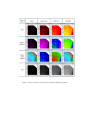
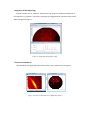
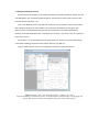
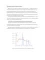
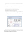
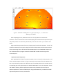
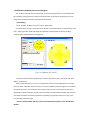
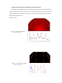
ANAELU USER’S MANUAL L. Fuentes‐Montero1,2*, M. E. Montero‐Cabrera2, L. Fuentes‐Cobas2 1
2
Diffraction Group, Institute Laue‐Langevin (ILL), Grenoble, France Centro de Investigación en Materiales Avanzados (CIMAV), Chihuahua, Mexico *
fuentes‐[email protected] Anaelu is Software for analysing diffraction patterns obtained with area detectors. This Users’s Guide complements the article devoted to the presentation of the program. The software represents crystalline structures (including their stereographic projections) and textures with axial symmetry. It represents the texture by means of the Inverse Pole Figure of the sample symmetry axis. The information that the user must give is: a) Crystal: Space group, lattice parameters and asymmetric unit. b) Texture: Miller indexes of the preferred orientation(s), widths and relative intensities of maxima in the distribution of orientations. To characterise the diffraction pattern, the software comprises different tools, namely: displaying radial and azimuthal profiles, azimuthal integration, zooming on the image and providing information related to the position of the pointer in the pattern. Anaelu models diffraction patterns from single crystals and from textured polycrystals. For single crystals, the user virtually explores orientations and the software generates in real time the positions of the diffraction peaks (Laue or monochromatic beam). For polycrystals there are two possible paths: a) The user programs and Anaelu runs a scan of orientations. The program calculates the positions and intensities of all the generated reflections. The modelled diffraction spots are superposed to the experimental diagram. b) By using statistical descriptors of a proposed texture (Inverse Pole Figure and corresponding Pole Figures) Anaelu calculates the theoretical 2D pattern. Next, different methods for using the software are described. The functions of all the windows in Anaelu are presented. STEPS TO FOLLOW: * Unzip the installation file. The following files must be located in the same folder: P_Anaelu10.exe f_d_atm.dat TABCTL32.ocx atomic_radi.dat mass_atm.dat 230 “.sym” files Platinum_2D_XRD.asc Å (an example of experimental data file, for training) * Run the program by double clicking on the executable file. When the program starts up, it normally takes some seconds activating and minimising all the interior windows. It is strongly recommended to work with the operational windows activated (opened) and all the other windows minimised but not closed. (The program constantly transfers information among internal windows and, if one of them is closed, it will pop up and disorient the user). * Check or edit the correct configuration. The first window that must be checked is the “Configuration” one. In this window, different constants that describe the experiment are editable. These are: resolution, detector diameter, sample‐detector distance, position where the direct beam hits the 2D detector (Beam Center”) and path to the file with the experimental pattern. For training with the default demo, it is recommended to preserve the preloaded configuration. The files with configuration parameters generally have the extension “.cfn” and may be saved or loaded from the “Config” pull‐down menu in the Main window of the program. * Load the experimental pattern. To show the dialog box that helps finding the experimental pattern, use the command “Browse 2D XRD Pattern”. There are two equivalent ways to call this command: from the “Experiment” menu in the upper part of the Main window or in the “Configuration” child window. To run the demo it is recommended to load the file “Platinum_2D_XRD.asc”. To load this file, click the “Apply ‐ Load ASC” command (in the same windows where “Browse 2D XRD Pattern” may be found). The program Anaelu is capable of loading XRD Patterns in binary unsigned integer two bytes per pixel or ASCII format. To convert among different formats, pertinent programs (for example “fit2d”) may be used. 2D patterns are displayed with different scales and color conventions, see Figure 1. Figure 1: Scales and color conventions for plotting 2D diffraction patterns
* Determination of the diffraction pattern center. Several alternatives are possible. ‐ Mouse pointer selection “Hybrid” window. Click on “Beam Centr”. Click on “Click Manual”. Click on the beam center location. The coordinates of the checked point are entered into the “Configuration” Window and applied to Anaelu. ‐ Selection of Debye ring points (Figure 2) “Hybrid” window. Click on “Beam Centr”. Click on “Debye Ring Point” and then in a Debye ring representative point. Do this several (3 to 30) times. Finish the process by clicking “Calc. Beam Center”. The coordinates of the calculated beam center are entered into the “Configuration” Window and applied to Anaelu. ‐ Keyboard Center coordinates can also be keyed‐in directly into the “Configuration” Window. After entering the center coordinates, click on “Apply Config”. To check the correctness of the “Beam Center” location, displaying “Arc Cuts” is highly demonstrative. Once confirmed that the “Beam Center” selection is correct, saving the Configuration is strongly recommended. To save, enter the “Config” menu in the Main window. Figure 2: Determination of the incident beam position by selection of points belonging to a Debye
ring.
* Integration of the Debye rings. “Hybrid” window, click on “Integrate”. Anaelu opens the “Show Cut” window and displays on it the integrated I=I(2θ) pattern. The result is analogous to a Bragg‐Brentano experiment, with texture effect averaged‐out. Figure 3. Figure 3: Integration along Debye rings
* Zoom of a selected area Hybrid window. Clicking the left button of the mouse, select a pattern area. See Figure 4. Figure 4: Zoom of selected area in a diffraction pattern.
* Pattern analysis with the “ArcCut” and “RadCut” tools. Figure 5 ‐ RadCut If the“RadCut” button in the window “Hybrid” is clicked and the mouse pointer over the pattern is moved, then Anaelu will display (in the “ShowCut” window) the intensity distribution along a straight line that goes from the direct beam position to the mouse pointer location. ‐ ArcCut In the “Hybrid” window, click the “ArcCut” button and move the mouse pointer over the pattern image. Anaelu will activate the “ShowCut” window. In this new window, the intensity distribution along the arc that contains the mouse pointer will be shown. If the user puts the mouse pointer over a Debye ring, then Anaelu will show the intensity distribution along the ring. Figure 5: Radial and arc cuts.
* Movement of the mouse over the “Hybrid” window When the mouse pointer is in the “Hybrid” window, Anaelu shows information about the pixel behind the pointer in one of the fields of the “Hybrid” window. This information is: azimuthal angle, 2θ dispersion angle, inter‐planar distance, colour palette, scale and intensity at the considered point. * Loading and editing the unit cell Crystal structure information may be loaded and edited via the Main window of Anaelu. Click the pull‐down Menu “File” and select the desired option. The files that contain crystal structures’ data normally have the extension “.cel” In the “Cell” Window, the first tab “Edit Cell” allows the user to introduce crystal structure data. After typing the space group, the asymmetric unit and lattice parameters, by clicking the “Ok” button, the user commands Anaelu to generate the complete unit cell. Anaelu automatically activates a third tab “View‐Rotate Cell” and displays all the atoms in the unit cell. The so‐created cell represents a crystal. For the demo it is recommended to preserve the default “Pt” structure. This will lead to fitting results when modelling the experimental pattern “Platinum_2D_XRD.asc” Figure 6 shows a Pt unit cell and its stereographic projection, as plotted by Anaelu. Figure 6: Anaelu “Cell” and “Reciprocal Lattice” windows. Pt crystal.
Crystal rotations are controlled by the user via keyboard-given rotation angles or by dragging the
mouse. The crystal cell and its stereographic projection rotate synchronically.
* Modelling a powder 1D diffraction pattern With the unit cell in memory, the program can now calculate the I = I(2θ) diffraction pattern of a non‐textured powder. In the “Reciprocal Lattice” window, near to the upper border, there is the “Calculate XRD Powder Pattern” button. By clicking this button, the user asks the program to calculate and display (in the “ShowCut” window) a pattern that may be used for comparing model and experiment. Peak broadening is calculated as a function of crystal size, which can be entered at the low left corner of the “Reciprocal Lattice” window. The program first calculates the pattern as obtained with a conventional diffractometer. Then it asks the user if a 2D pattern is needed. For the demo, to favour time economy, it is recommended to answer “no” to the “2D Detector Model” option. ‐ Check peaks’ coincidence between experimental and calculated 1D patterns. The “Hybrid” window (with the experimental 2D pattern) and the “ShowCut” one (with the calculated 1D powder pattern) should be activated. The rest of the windows may be minimised (it is not recommended to close child windows). By using the “RadCut” or the “Integrate” command from the “Hybrid” window, experimental 1D (red) diffraction patterns will appear superposed to the calculated (blue) one. See Figure 7. Figure 7: Observed (red) and calculated (blue) 1D diffraction patterns
* Manual rotation of the unit cell and modelling single‐crystal 2D diffraction spots. Crystal orientation is controlled under the “View‐Rotate Cell” tab of the “Cell” window. The user may chose to rotate the unit cell in one of the following ways: a) By dragging the unit cell. Dragging with the left button will rotate the crystal in the direction of the mouse movement around an axis perpendicular to the said movement but parallel to the screen. Dragging with the right button will rotate the crystal around an axis normal to the computer display. b) By dragging the mouse pointer over the stereographic projection. c) By typing the orientation angles that are shown in the “Cell” window. d) By clicking the rotation buttons that surround the unit cell. No matter how the user rotates the cell, the program calculates the corresponding positions of diffracted spots in an area detector, in real time. The user should imagine that the X‐rays hit the computer display perpendicularly (the user itself is the X‐ray source) and the crystal is oriented just like the shown unit cell in the “cell” window. The positions of diffraction maxima are shown (red points) in the upper left corner of the “Reciprocal Lattice” window, see Figure 8. Figure 8: A Pt crystal stereographic projection and its calculated Laue pattern.
Diffraction maxima also appear, as blue spots over the experimental pattern in the “Hybrid” window. See Figure 9, below. To visualize the diffraction spots, it is necessary to have activated the tree involved windows: “Cell”, “Reciprocal Lattice” and “Hybrid”. * Programmed rotation of a crystal and simulation of diffraction by a sharp axial texture. ‐ Crystal initial orientation Simulation of the 2D diffraction pattern from a highly textured sample can now be prepared. As a first step, the analysed crystal must be put on the appropriate initial orientation. For example, put the Pt crystal with its [111] direction perpendicular to the sample surface. This means that the (111) pole must be located in the upper border of the stereographic projection. This exercise may be performed by dragging the mouse pointer over the unit cell or over the stereographic projection (“View‐Rotate Cell” tab, left and right mouse buttons). The angular step for crystal orientation control (step = 1° by default) is also applied on the “Rotate Cell Cycle” tab. ‐ Edit cycles and sub‐cycles for simulating a sharp axial texture. Consider that the adequate initial orientation has being established. In the considered example, the crystal direction [111] is parallel to the virtual experiment vertical (“Y”) axis. For programming the simulation of a sharp axial texture, the tab “Rotate Cell Cycle” must be activated. This tab is the second one from left to right on the “Cell” window. As can be seen in the “Rotate Cell Cycle” window, the default rotation axis is “Y”. For cubic crystals, the [111] direction represents a 3‐fold symmetry axis, so a rotation interval of 120° (= 120 cycles x 1°/cycle ) will be representative. Insert the mouse pointer into the box below the “Num of Cycles” label (the default value of “120” is suggested). Re‐type “120”. Insert the mouse pointer into the box below the “Num of Sub Cycles” label (the default value of “3” is suggested). Re‐
type “3”. As the angular step is 1°, the boxes “Total Angle” and “Total Sub Angle” will show respectively “120” and “3”. ‐ Click on “Run” and wait while Anaelu works. For the simulation to work, the windows “Hybrid”, “Cell” and “Reciprocal Lattice” must be activated. Anaelu will generate the 2D pattern of a textured sample. This modelling has two stages. (The user should be patient for both of them). Explanation of Stage 1 ‐ Rotating the crystal according to user instructions: The user has chosen the primary rotation axis, step and rotation interval. He (She) has also chosen how much will the crystal depart (by secondary rotations or sub‐cycles) from the orientations determined by the primary rotations. The program now will rotate around the primary axis and on every step it will execute secondary rotations. In every rotation (no matter if primary or secondary) the program will calculate the positions and intensities of every generated diffraction peak corresponding to the considered crystal orientation. Anaelu displays the positions of all the generated diffraction spots in the “Hybrid” window, see Figure 9. Figure 9: Simulated 2D-XRD pattern. Pt polycrystal, sharp (1, 1, 1) axial texture.
Rotating crystal model.
After completing the scan, Anaelu will ask the user if he (she) wants to continue with calculations. The user should check if the calculated (blue) spots coincide with the experimental (red and yellow) maxima. In this demo they will coincide, so the user can choose “yes” to ask for more results. Stage 2: With the permission of the user, the program will calculate the 2D pattern. “Anaelu” will calculate the intensity of every pixel, taking into account all the positions and intensities calculated in the previous stage. Then it will show the calculated 2D pattern in the “Model XRD” window. The user should wait until the program activates the “Model XRD” window with the image of the calculated pattern. ‐ Experiment‐model comparison With “Model XRD” and “Hybrid” windows activated, the user can move the mouse pointer in one of them and the program will show a (+) sign in exactly the same position of the other window. The user can put the mouse pointer over a diffraction spot of a window and check if it coincides with the corresponding spot in the other window. The window “Model XRD” also has the commands “ArcCut” and “RadCut”. Naturally, different preferred orientations may be tested in the search for the optimum qualitative fit. Patterns modelled by the “Programmed Rotations” procedure fit well with experimental patterns from sharp axial textures. * 2D diffraction modelling via Inverse Pole Figure The “PF & IPF” window contains a generator of inverse pole figures (IPF). The user defines the IPF resolution and proposes the number and characteristics of the texture components. For each component, its width and relative intensity must be entered. ‐ IPF modelling In the “PF & IPF” window, the user first clicks “Restart IPF”. To run the demo, the user may preserve the default 111 orientation with 3° width and click “Pref Pole”. The program will model and display two different representations of the IPF, including symmetry‐generated multiplicity. See Figure 10. Figure 10: Modelling IPF and PFs
To become familiar with the IPF generator, restart the IPF and try other “Pref Pole” and “Peak Width” combinations. With a chosen IPF the user can click in “Selected PF” and see the pole figure (PF) of a selected family of planes. Otherwise the user can click on “All PF and XRD” to ask the program to calculate all PF and the 2D pattern. The calculation of the pattern may last from a few seconds to a few hours, depending on the IPF resolution, the 2D pattern resolution and the number of Debye rings. For each pixel Anaelu calculates how much contributes each Debye ring and how intense is the ring in the corresponding azimuthal angle. ‐ Click on “All Pf and XRD” and wait until the calculated pattern appears in the “Model XRD” window ‐ Analysis of calculated pattern and comparison with the experiment The 2D pattern calculated from IPF can be studied and compared just like it was done with the pattern obtained from a cycle of rotations. The user can move the mouse and compare the positions and intensity distributions of peaks, can observe cuts and can also ask the program to recalculate with different parameters. See Figures 11 and 12. Figure 11: Pt observed 2D-XRD
pattern and ArcCut
Figure 12: Pt calculated 2D-XRD
pattern and ArcCut
‐ Sample rotation Consideration of samples where the symmetry axis is inclined with respect to the vertical (“Y”) axis is possible. In the “PF & IPF” window, entering a certain angle in degrees will rotate the modelled 2D XRD pattern by that amount in clockwise direction. ‐‐‐ The authors of Anaelu are active on expanding and optimizing the program. We appreciate possible suggestions and bugs detection from the users. Enjoy modelling!