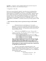
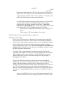
Download Collecting Powder Data on a Mo SMART1000 CCD

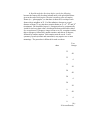
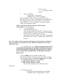
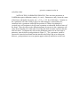
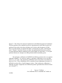
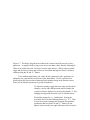
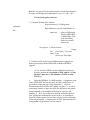
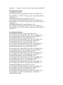
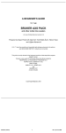
Tech note 2008-04-09
Joseph H. Reibenspies, Department of Chemistry, Texas A & M University, Copyright
2008
Collecting Powder Data on a Mo SMART1000 CCD, APEX and APEXII.
Move the beam stop as close to the sample as possible, without blocking the very low
angle diffraction peaks. Move the detector to about 6 cm and set size to 1024. Use the
calibration single crystal to obtain crystal-to-detector distance, x distance, and y distance
values.
Mount your sample on a loop or pin by first wetting the sample with a minimum of
mineral oil and rolling the sample into a sphere. If possible produce a sample that is
larger than the X-ray beam (this will reduce air scatter, but will increase non-Bragg
scattering from the oil and the mount). Place your sample on the diffractometer and cool
to at least -60C. Center the sample as you would for a single-crystal.
SMART/APEX I
Drive the goniometer to 30 deg two-theta, 0.0 deg theta and 0.0 deg phi (chi fixed). Take
a rotation photo, be sure to uncheck the DRIVE to ZERO box. For the Smart 1000
unwarp the frame (not necessary for the APEXI) and save the file.
APEXII
Start the APEX2server program. Center your sample and then choose simple scans.
Drive the goniometer to 30 deg two-theta, 0.0 deg theta and 0.0 deg phi. Select the 360
deg phi scan. Use the frmutility (in Bruker AXS folder) to convert the frames to the older
SMART frame.
FIT2D
Use FIT2D (http://www.esrf.eu/computing/scientific/FIT2D/) to generated the 1D trace.
Save in the chi format. Use ConVX to convert the file to a Bruker EVA RAW file.
Use PowderX to read the file and locate peaks.
Appendix 1. A Beginner’s Guide to SMART/Gadds: Brief procedures for powder
diffraction data collection on the APEX SMART System
S. Guggenheim, 3 May 2004
The first two parts of this guide (Appendix 1) provides recipes for obtaining DebyeScherrer type and Gandolfi type data, respectively. It is assumed that the user has
minimal experience with SMART and no experience with GADDS. Appendix 2 shows
how to calibrate the instrument, a necessary requirement before data collection. This
needs to be done once after a tube installation and perhaps every 6 months thereafter.
Appendix 3 lists the *.slm files for (batch) data collection for part 1 and part 2. It is
required that the user has a program for peak locate, JCPDF/PDF searches, etc. such as
either DIFFRAC (or DIFFRACplus), the Bruker software for processing a pattern, or MDI
JADE.
1. Data Collection for Debye-Scherrer type Patterns Using the APEX/SMART
System
a.
Change the detector to crystal distance to 12 cm. (on the
goniometer). It is best to use an “extended” beam stop and the 0.2 mm
Monocap (if you have these available, otherwise use the normal beam stop
and the standard collimator). The Administrator should mount the beam
stop and collimator for you.
b.
Double click on the SMART icon to open. Then go to Edit 
Config  User Settings. The values here are given as examples; they will
change depending on the latest calibration.
Change resolution (frame size) setting from 512 to 1024.
Change sample-to-detector setting from 5.972 cm to 11.891 cm
Change x distance from 257.884 to 517.488
Change y distance from 255.864 to 512.428
When exiting the Configuration file, the system will ask if it should
modify the collision-limit settings. Answer “yes” to do this. WHEN
FINISHED WITH YOUR EXPERIMENTS, BE CERTAIN TO
RESET THE DETECTOR TO 60 mm ON THE DETECTOR ARM,
CHANGE BACK TO THE 0.5 MM COLLIMATOR, AND RETURN
TO THE REGULAR BEAM STOP.
c
Place the 0.2-mm capillary containing the powder on the
goniometer and optically align in the Bruker APEX System as you would
a single crystal. See Data Collection section (p. 4-7 to 4-11, stopping at
item 14) of the User’s Manual for the SMART APEX. Now establish the
appropriate dark current:
Go to Detector  Dark Current
Set seconds per exposure to 1200
# of exposures to average
2
Output file
3125H
120._DK
Label the new dark current as 3125H120._DK (where 3120 is the serial
number of the UIC APEX (Use your serial number instead, of course), H
= high resolution of 1024 x 1024, and 120 = 1200 sec.). The dark current
needs to be collected just once prior to data collection.
The APEX detector does not require a spatial correction. The flood field
correction will not differ for the APEX running at different framecollection times, in contrast with dark current times. Use (at UIC)
D:\Frames\ccd_1K\3125H150._FL. The file name is based on the APEX
serial number at UIC (3125) and high resolution of 1024 (H).
Go to Detector  flood field  D:\Frames\ccd_1K\3125H150._FL
(OK)
Go to Detector  Dk, Flood enabled (Yes, check)
The following corrections and related items are of interest:
Description of Corrections
Dark Current: This correction is a function of accumulation time and thermal
noise related to the CCD detector. Thus, the dark current and bias depends on
collection time and temperature, and because there are no useful data in the dark
current relating to the crystal under study, dark current is subtracted from the
frames during data processing. Note: Never leave the light for orientation on in
the hutch either during dark current collection or during data collection, because
the light will produce thermal noise.
Flood field: This correction relates to the response across the detector face
depending on the orientation of the Be window, the phosphor, and fiber-bonding
agent uniting the CCD to the optical fibers. The flood field file never needs
updating unless there has been a mechanical change to the Be, phosphor, or
binding agent of the fibers.
Spatial: The APEX detector does not require this correction, although the
GADDS software often is used with detectors that do. This correction involves a
change to the spot imaging or distortion that is a function of the angle of
incidence of the X-ray on the Be window and the optical fiber twist as viewed by
the CCD chip. The spatial-correction file builds a correction table based on
observed vs actual hole and spot position. The APEX CCD chip is 4K x 4K and
does not use a “magnifying glass” fiber lens system, so no spatial correction is
needed.
Unwarp: In GADDS, this is the term used for applying the spatial, flood
field, and dark current to the raw image of the frame. This creates a new
image without distortion (i.e., “unwarping the distortion”). Because data
from the APEX is already corrected for the dark current and the flood field
in the SMART software, and the spatial correction is unnecessary, do not
apply an unwarp in GADDS.
Goal of taking frames for powder data:
d.
The aim is to take a series of rotation frames (i.e., “photographs”)
so that there is about 20% overlap of each frame with its neighbor in 22.
For Mo radiation, detector-to-crystal distance of about 12 cm, take three
rotation frames at 22 = 00, 200 and 350 (maximum). Omega and phi
should both be 00. Read through the directions before you do this,
because the frames may be taken in batch mode, which is explained at the
end of this discussion, thereby making data collection automatic:
1
Goniom  Drive
set the angles for first
rotation
Acquire  Rotation
Exposure time: 1200 seconds
Do not click zero 2-theta, omega box
After each frame is taken, you must save the frame to your
directory (file  save). Thus, you should have three frames after
completing the series as “samp_0.rot”, “samp_20.rot”, and
“samp_35.rot” (where “samp” is the sample/user name).
NOTE: A batch routine has been developed to collect this data
automatically. To use this routine:
1
Go to Level  Command line
2
at the SMART cursor, type:
“@E:\Geology\Powd\Powd1200.slm” (without the quotes,
followed with an enter)
3
After data collection is complete and to leave the command
line dialogue, type: “menu” (without quotes, followed by
an enter)
2
e.
Exit SMART (File  exit) WHEN FINISHED WITH YOUR
EXPERIMENTS, BE CERTAIN TO RESET THE DETECTOR TO
60 mm ON THE DETECTOR ARM, CHANGE BACK TO THE 0.5
mm COLLIMATOR, AND RETURN TO THE REGULAR-SIZE
BEAM STOP.
f.
Enter GADDS [click on GADDS (off line) icon]:
First determine that the correct calibration values in GADDS, by
Edit  Config  User Settings and change resolution (Frame size)
setting 1024.
Change crystal-to-detector setting to 11.906 cm: At UIC, the
present
GADDS software does not allow changes from 11.99, but
this has been changed in future releases. The values are
usually pre-set in the calibration section, and in most cases
they do not require changing.
Change Direct beam x distance to 514.50
Change Direct beam y distance to 516.93
1. File  Display  Open
Bring in the first photograph (Frame filename)
Set High Counts to a large number, e.g. 4095
If Mag is left
as 1.0 (recommended), then Region X, Y,
can
be left at the default setting and they
have no effect on the data.
2. The Lp (Lorentz-polarization) correction may be applied to the
powder
data, but this correction is rarely used (and depends on how
you plan to use the data). If you choose to apply these
corrections:
Process  Corrections
Choose LPA only. Set Mono 2T = 12.0
degrees
3. Integrate the Debye rings to one (linear) integrated value:
Peaks  integrate chi (to set
conic peak integration)
Two theta and chi start and end points will be set
graphically, so leave values as is (In future
releases of GADDS, the “chi” integration
angle is renamed to “gamma”. At omega of
zero, chi equals gamma, but at any other
omega value, chi is not equal to gamma.)
Bin Normalize intensity = 5 (Future releases of
GADDS
will drop other intensity algorithms).
step size = 0.02 (always keep the same for
all rotation frames, usually 0.02)
A white outline will be superimposed over the
frame.
Sequentially type 1, 2, 3 and 4 to see
how each can
be adjusted:
1 adjusts center point
2 adjusts 2theta region
3 adjusts the lower chi region
4 adjusts the upper chi region
Adjust to the extremes of the frame (but not beyond,
where there are no data). Keep adjustments to
within 180o and maintain for all frames.
After each adjustment (1, 2, 3 or 4) click the left
mouse
button to accept adjustment.
After the 4th adjustment is entered, click the left
mouse
button to see integrate options display:
Formats: Use
DiffracPlus format for
Siemens
DiffracPlus software
and for MDI JADE software
(“name.raw”)
Use Plotso to get format that
will
graph the Intensity vs. Theta
(name.pH). Not usually
done.
Append: Choose
Y (check) to set the output up
to allow the merging of
several
sets of data (i.e., at 00, 200,
350
rotation frames)
Note: After making a diffraction profile, check to make certain that the
profile produced makes sense for the frame undergoing the conic peak
integration (chi or gamma). Occasionally, a “hot pixel” will be present in
the frame that causes a high peak in the diffraction profile that should not
exist. If you notice an apparently anomalous peak, File > Display > Open,
set High Counts to 50,000. A white pixel should be evident at the two
theta position where there is an anomalous peak. It is possible to work
around the hot pixel, but it is not necessary at this point. In JADE, for
example, it is very easy to remove a “peak” that formed from an exited
pixel. Peaks formed from hot pixels appear as spikes, and they have a
different shape from peaks obtained from the sample.
Repeat chi integration sequence for each rotation
frame (i.e., at 00, 200 and 350)
4. Minimize the GADDS window
g. Enter Merge program (click on Bruker AXS Programs  Merge). The Merge
program places all three frames on to one scale.
Default option: Makes a scale factor based on the overlap of range A
and range B. Thus, range A may vary from 100% to 0%, and the reverse
for range B, i.e., [x*A + (1-x)*B]. The background of range B is not
compensated to match the background of A.
Scale option: Same as the default option, but the background of range B is
compensated to match the background of A by the addition of a constant
so that the B background is either raised or lowered to match A.
Average option: Range A and range B are averaged, such that (A + B)/2.
Both the Average and Scale Options may be checked (to obtain an
Average with background compensation, as in: [A + (B + s)]/2
We will use the Scale option only here
1. Complete the data in the window:
Project directory: E:\Geology\Sam
(example)
Input filenames: provide each filename in
list
name.raw
refers to Diffracplus
files for MDI JADE
or DiffracPlus. This
is the most likely
format you would
want to use.
name.plt
refers to
Plotso file
name.uxd
refers to ascii
file type
Set range to -1 (all) in first box
Output
file: set to name_T to create
name_T.out
file for raw file output
set to name_TP to create name_TP.out
file for Plotso file output
2. Transfer the file to the Powder Diffractometer computer for
further processing with the MDI JADE or Bruker DIFFRAC
program. For reasons of your own, you may want to continue to
PLOTSO.
h. Enter Plotso program (Bruker AXS  Plotso)
Input filename *.dat
Use the output file from Merge
(name_TP.out)
This produces a plot (I vs Theta) of file.
i. Other utility programs by Bruker
1. To convert an image file use “Frm2Frm” Program to Tiff, JPeg,
Bruker ASCII, or Bruker Frame File.
For example, a rotation frame (“photograph”) is already in the
Bruker
Frame File format, but it can be converted to a Tiff file for another
program (e.g., to display in PhotoShop,)
2. To convert one raw file to another, use “Raw2Raw”.
Output file examples include Diffracplus, Plotso, DBW, GSAS,
UXD
(Bruker Ascii)
3. “GADDSmap” is for sample mapping and cannot be used in our lab.
2. Data Collection for Gandolfi-type Patterns Using SMART Software
a. Change the detector-to-sample distance to 12 cm. (on the goniometer).
If available, use the “extended” beam stop and the 0.2 mm Monocap (have
the administrator change these for you do this for you). If not available,
use the standard beam stop and 0.3 collimator instead.
b Double click on the SMART icon to open. Then go to Edit  Config 
User Settings. The following values will be different for your instrument,
depending on its current calibration.
Change resolution (frame size) setting from 512 to 1024.
Change sample-to-detector setting from 5.972 cm to 11.891 cm
Change Direct beam x distance from 257.884 to 517.488
Change Direct beam y distance from 255.864 to 512.428
When exiting the Configuration file, the system will ask if it should
modify the collision-limit settings. Answer “yes” to do this.
c Place the single crystal on the goniometer and optically align in the
Bruker APEX System as you would any other single crystal. See Data
Collection section (p. 4-7 to 4-11, stopping at item 14) of the User’s
Manual for the SMART APEX. Now establish the appropriate dark
current:
Go to Detector  Dark Current
Set seconds per exposure to 1200
# of exposures to average
2
Output file
3125H
120._DK
Label the new dark current as 3125H120._DK (where 3120 is the serial
number of the UIC APEX and you should use the appropriate serial
number for your lab, H = high resolution of 1024 x 1024, and 120 = 1200
sec.). The dark current needs to be collected just once before the data
collection.
For a discussion of the different types of corrections for the APEX
detector, see the section previous to this one (Debye-Scherrer).
The APEX detector does not require a spatial correction. The flood field
correction will not differ for the APEX running at different framecollection times, in contrast with dark current times. Thus, use the highresolution flood field. Use (at UIC) D:\Frames\ccd_1K\3125H150._FL.
The file name is based on the APEX serial number at UIC (3125) and high
resolution of 1024 (H).
Go to Detector  flood field  D:\Frames\ccd_1K\3125H150._FL
(OK)
Go to Detector  Dk, Flood enabled (Yes, check)
d. Read through the directions before you do the following,
because the frames may be taken in batch mode, with special directions
given at the end of this section. The aim is to take a series of rotation
frames (i.e., “photographs”) so that there is about 20% overlap of each
frame with its neighbor in 22. For Mo radiation, detector-to-crystal
distance of about 12 cm, take three rotation frames at 22 = 00, 200 and 350
(maximum). Phi should be kept at 0. Omega needs to be systematically
varied for each two-theta value, which must be done at allowable values.
So, at two theta of 35 degrees, omega is first set to -20, a rotation is taken,
then at 0 degrees, followed by another rotation, and then at 20 degrees,
followed by another rotation. Each rotation must be saved. Lower
symmetry crystals (triclinic and monoclinic) may require two or more
mountings. The procedure is followed for each two theta:
Two
Omega
theta
35
-20
35
0
35
20
20
-20
20
0
20
20
0
-20
0
0
0
10 (20 is not allowed)
1
Goniom  Drive
set the angles for first
rotation
Acquire  Rotation
Exposure time: 1200 seconds
Do not click zero 2-theta, omega box
After each frame is taken, you must save the frame to your
directory (file  save). Thus, you should have at least nine frames
after completing the series as “samp_010.rot”, “samp_00.rot”,
“samp_0m20.rot”, etc. for 0 two theta, 10 omega, etc. (where
“samp” is the sample/user name).
NOTE: A routine has been developed to collect this data
automatically. To use this routine:
1
Level  Command line
2
at the SMART cursor, type:
“@E:\Geology\Gand\Gan_1200.slm” (without the quotes,
followed with an enter, Gan_1200.slm is the file containing
the directions, see Appendix 3 for a listing)
3
After data collection is complete and to leave the command
line dialogue, type: “menu” (without quotes, followed by
an enter)
2
Note: For samples with low symmetry and if precise intensity data are required, it
may be necessary to remount the crystal in a different orientation and to collect
additional frames.
e. Exit SMART (File  exit) WHEN FINISHED WITH YOUR
EXPERIMENTS, BE CERTAIN TO RESET THE DETECTOR TO
60 mm ON THE DETECTOR ARM, CHANGE BACK TO THE 0.5
mm COLLIMATOR, AND RETURN TO THE REGULAR-SIZE
BEAM STOP.
f. Enter GADDS [click on GADDS (off line) icon]
First determine that the settings are correct: go to Edit  Config 
User Settings should be at a resolution (frame size) setting 1024.
The crystal-to-detector setting is at 11.906 cm
The Direct beam x distance is 514.50
The Direct beam y distance is 516.93
The actual values depend on the calibration of the
instrument!
1. File  Display  Open
Bring in the first photograph (Frame filename)
Set High Counts to a large number, e.g. 4095
If Mag is left as 1.0 (recommended), then Region X,
Y, is
left at the default setting and it has no effect
on the data.
2. The Lp (Lorentz-polarization) correction may be applied to the
powder
data, but this correction is rarely used (and depends on how
you plan to use the data). If you choose to apply these
corrections:
Process  Corrections
Choose LPA only. Set Mono 2T = 12.0
degrees
3. Integrate the Debye rings to one (linear) integrated value. This
is done by treating each of the nine (or more) files.
Peaks  integrate chi (to set
conic peak integration)
Two theta and chi start and end points will be set
graphically, so leave values as is (In future
releases of GADDS, the “chi” integration
angle is renamed to “gamma”. At omega of
zero, chi equals gamma, but at any other
omega value, chi is not equal to gamma.)
Bin Normalize intensity = 5 (Future releases of
GADDS
will drop other intensity algorithms).
step size = 0.02 (always keep the same for
all rotation frames, usually 0.02)
A white outline will be superimposed over the
frame.
Sequentially type 1, 2, 3 and 4 to see
how each can
be adjusted (integrate only areas of
intensity):
1 adjusts center point
2 adjusts 2theta region
3 adjusts the lower chi region
4 adjusts the upper chi region
Adjust to the extremes of the frame, but do not go
beyond where there are no data. Do not adjust
beyond 180o and keep each region the same for a set
of 2 theta.
After each adjustment (1, 2, 3 or 4) click the left
mouse
button to accept adjustment
At UIC, always keep the same settings for each set
of
2theta frames
After the 4th adjustment is entered, click the left
mouse
button to see integrate options display:
Formats: Use
DiffracPlus format for
Siemens
DiffracPlus software
and for MDI JADE software
(name.raw)
Use Plotso to get format that
will
graph the Intensity vs. Theta
(name.pH)
Append: Choose
Y (check) to set the output up
to allow the merging of
several
sets of data (i.e., at 00, 200,
350
rotation frames)
Note: After making a diffraction profile, check to
make certain that the profile produced makes sense
for the frame undergoing the conic peak integration
(chi or gamma). Occasionally, a “hot pixel” will be
present in the frame that causes a high peak in the
diffraction profile that should not exist. If you
notice an apparently anomalous peak, File >
Display > Open, set High Counts to 50,000. A
white pixel should be evident at the two theta
position where there is an anomalous peak.
Corrections to eliminate the effects of the hot pixel
are most easily made in, for example, JADE.
Repeat chi integration
sequence for each rotation frame
4. Minimize the GADDS window
g. Enter Merge program (click on Bruker AXS Programs  Merge). The
Merge program places all nine (or more) frames on to one scale. To do
this, those frames of equal two theta are merged by average overlap (not
scaling). Then the three two theta output files are merged without
averaging, but by scaling that is a function of the overlap percentage,
along with the background adjusted.
Default option: Makes a scale factor based on the overlap of
range A and range B. Thus, range A may vary from 100% to 0%,
and the reverse for range B, i.e., [x*A + (1-x)*B]. The background
of range B is not compensated to match the background of A.
Scale option: Same as the default option, but the background of
range B is compensated to match the background of A by the
addition of a constant so that the B background is either raised or
lowered to match A.
Average option: Range A and range B are averaged, such that (A
+ B)/2.
Note: Both the Average and Scale Options may be checked (to
obtain an Average with background compensation, as in: [A + (B +
s)]/2
1. Complete the data in the window:
Project
directory: E:\Geology\Sam (example)
Input
filenames: provide each filename in
list. First take all the files of one two-theta
value and merge by the Average option.
name.raw
refers to Diffracplus
files for MDI JADE
or DiffracPlus. This
is the most likely
foramt you would
want to use.
name.plt
refers to
Plotso file
name.uxd
refers to ascii
file type
Set range to -1 (all) in first box
Output
file: set to name_T to create
name_T.out
file for raw file output
2. You should now have three output files containing the merged
(via average) data for each of the two-theta ranges. Now take the
output files and make them input for the next merge (this time via
the Scale Option).
Complete the data in the window:
Project directory: E:\Geology\Sam (example)
Input filenames: provide each filename in list. This
time take the files containing the three two-theta
ranges and merge by the Scale option.
name.raw
refers to Diffracplus
files for MDI JADE
or DiffracPlus. This
is the most likely
foramt you would
want to use.
name.plt
refers to
Plotso file
name.uxd
refers to ascii
file type
Set range to -1 (all) in first box
Output
file: set to name_TT to create
name_TT.out
file for raw file output
3. Transfer the file to the Powder Diffractometer computer for
further processing with the MDI JADE program.
Appendix 2. Calibration of the GADDS software
1. Calibration
This section may be skipped if the system has already been calibrated. Only the
Laboratory Administrator calibrates the instrument. Calibration is for detector distance
and x, y coordinates for detector center and symmetry of shape of powder rings. A more
detailed description of the parameters are given below. GADDS supports the following
standards (Corundum, PDF #10-0173; Aluminum, PDF#04-0787; Silicon, PDF#27-1402;
and Quartz, PDF#33-1161) . We use Corundum NBS (NIST) 674a in 0.2 mm capillary.
STEP 1. Calibration of SMART using the YLID crystal for 120 mm.
a Change the detector to crystal distance to 12 cm. (on the goniometer).
Use the calibration single crystal YLID to obtain crystal-to-detector
distance, x distance, and y distance values (if this has not been done
previously for this detector position). These values, using YLID, should
be done with the resolution in the config file set at 1024. Using YLID at
UIC, determined values at d = 11.891, x-distance = 517.488, y-distance =
512.428 were determined.. You will use the same technique as is done for
the 60-mm calibration.
b. Double click on the SMART icon to open. Then go to Edit  Config  User
Settings. Change resolution (Frame size) setting from 512 to 1024.
Change crystal-to-detector setting from 5.972 cm to 11.891 cm
Change Direct beam x distance from 257.884 to 517.488
Change Direct beam y distance from 255.185 to 512.428
Your values for the crystal-to-detector distance, x distance and y distance
may be slightly different depending on the results from the last tube
optimization or realignment. When exiting the Configuration file, the
system will ask if it should modify the collision-limit settings. Answer
“yes” to do this. WHEN FINISHED WITH YOUR EXPERIMENTS,
BE CERTAIN TO RESET THE DETECTOR TO 60 mm ON THE
DETECTOR ARM.
c. Place the capillary on the goniometer and optically align in the Bruker APEX
System
as you would a single crystal. See Data Collection section (p. 4-7 to 4-11,
stopping at item 14) of the User’s Manual for the SMART APEX. Now
establish the appropriate dark current:
Go to Detector  Dark Current
Set seconds per exposure to 1200
# of exposures to average
2
Output file
3125H
120._DK
Label the new dark current as 3125H120._DK (where 3120 is the serial
number of the UIC APEX, H = high resolution of 1024 x 1024, and 120 =
1200 sec.)
The APEX detector does not require a spatial correction. The floodfield
correction will not differ for the APEX running at different framecollection times, in contrast with dark current times. Use (at UIC)
D:\Frames\ccd_1K\3125H150._FL. The file name is based on the APEX
serial number at UIC (3125) and high resolution of 1024 (H).
Go to Detector  flood field  D:\Frames\ccd_1K\3125H150._FL
(OK)
Go to Detector  Dk, Flood enabled (Yes, check)
d. The aim is to take a series of rotation frames (i.e., “photographs”) so that there
is about
20% overlap of each frame with its neighbor in 22. For Mo radiation and
for the detector-to-crystal distance of 12 cm, take three rotation frames at
22 = 00, 200 and 350 (maximum). Omega and phi should both be 00.
Note: A batch program is available to collect this data, see Appendix 3 for
the file listing and instructions in Appendix 2, page 2.
Goniom  Drive
set the angles for first
rotation
1
Acquire  Rotation
Exposure time: 1200 seconds
Do not click zero 2-theta, omega box
After each frame is taken, you must save the frame to your
directory. Thus, you should have three frames after completing the
series as “cor_0.rot”, “cor_20.rot”, and “cor_35.rot” (or a similar
name for each).
2
e. Close the SMART software.
Open the GADDS (off-line) software by:
1.
2.
Bruker AXS Programs  GADDS off-line
File  Display  Open
Use file frame of first rotation frame collected at 0o
two
theta (i.e., cor_0.rot).
In “high counts”, use a fairly high value (i.e., 4095)
because
the frame was collected at 1200 seconds.
This will
give nice contrast in color in
red/yellow/white.
NOTE ON THE CALIBRATION PROCESS: There are three parameters in
GADDS that require calibration, namely, d, x and y. Parameters x and y locate the center
of the frame, and ideally, but rarely, are x = 512, y = 512 for a 1024 frame. Variation in
the x parameter will cause a Debye ring to be offset along the x (horizontal) axis,
variations in the y parameter with affect the position of a Debye ring along the y
(vertical) axis, and variations in d will cause expansion or contraction from the center of
the frame. Thus, the effect on the diffraction pattern for an error in the x-parameter will
cause observed peaks to be either all at lower than the ideal two theta or greater than the
ideal two theta. To illustrate the effect on the diffraction pattern for an error in the d
parameter, note the shift in peak positions in Figure 2.1. The y-parameter would be
expected to locate the horizontal line that intersects the Debye ring at its widest part,
however, peak positions in an x-ray pattern appear relatively insensitive to this error.
Figure 2.1 The effect of an incorrect d-parameter in the diffraction pattern of corundum.
The line positions of the standard are given as superimposed vertical lines in green, the
position of the peaks in the observed pattern are in brown, and the pattern is in blue.
Errors in peak position are symmetrical about a central point (or peak), with that peak
near 17 degrees. Note that at lower two theta, the peak positions (brown) are at lower
two theta positions than the standard (green), and at higher two theta above 17, the peak
positions (brown) are at higher two theta positions than the standard (green).
We will make a calibration in GADDS from different portions of an x-ray pattern
obtained in SMART. It is easiest to make a y-parameter calibration at a low two-theta
frame (e.g., 0o), and x- and d-parameter calibration from a frame taken at a medium twotheta (e.g., 20o). These calibrations will be considered coarse adjustments, because it is
difficult to see the effect of small changes in values. Final, and precise calibration, is
obtained only after comparison to the diffraction patterns generated from all three frames
(at 0, 20 and 35o).
3.
Process  Calibrate
Set Calibration file to “corundum.std” which is a
resident
file with JCPDF-PDF data in the GADDS software
minimum relative intensity = 5
sample-to-detector distance should be set to
approximately what the APEX was
set at (near 12.0, or 11.895)
detector angle set to 22 value (0, and later 20
or 35)
delta distance 0.005 (this is the amount of
movement/sensitivity in d)
delta angle must be set to 0.000 for factory
calibration
Detector x-center of near 512 (assuming that
you
are using a frame resolution.of
1024)
Detector y-center of near 512 (assuming that
you
are using a frame resolution.of
1024)
Delta xy movement: 0.2 (movement
sensitivity in x,
y)
Values for sample-to-detector distance, detector
x and detector y values will change based on the
calibration.
Blue rings will be overlaid on the Debye rings. The rings
indicate the calculated positions of the resident corundum
file. You need to adjust the d parameter, detector x, and
detector y to have the resident pattern superpose over the
rings of your experimental pattern.
NOTE: For a low-angle (i.e., 0o) two-theta frame, there will be at least one Debye-ring
forming a full circle. This will allow an initial determination (a very rough estimate
when compared to other frames) for the y-parameter. Figure 2.2 shows the effect of an
error in the y-parameter.
Figure 2.2. The Debye ring shows an offset in the vertical caused by an error in the yparameter. A complete Debye-ring occurs at low two-theta values, thereby allowing the
effect to be readily observed. However, because most data (i.e., Debye rings or partial
rings) and the more accurate data will occur at medium and high two theta, it is best to
calibrate using the 20 and 35 o frames.
For a medium-angle frame, the values for the d parameter and x parameter (in
addition to the y-parameter) can be more easily determined. Use the x parameter to
locally adjust the ring sections of measured and calculated rings in the detector center.
Then, use the distance parameter to get full coincidence.
To adjust the settings, toggle between center mode (which
changes x and y) and calibrate mode (which changes the
crystal-to-detector distance) by pressing (keyboard) “c” and
nudging the rings with the arrow keys or with the mouse.
Record the settings for x, y, and distance. Repeat the
procedure above for the remaining frame (e.g., 35o). Then
review the recorded settings and determine the optimum
parameters that best fit the 20 and 35 o frames (if your
phases involve mostly low-angle reflections, then it may be
advisable to consider the 0 and 20 o frames).
NOTE: Now treat the frames of the calibration sample (e.g., 0, 20, 35o) as an unknown
and determine an Intensity vs Two-theta plot (a “scan”). You should compare the scan to
the JCPDS pattern in DIFFRAC or JADE, and then determine the cell parameters.
Because the same frames were used to derive the scan that was also used in calibration,
the observed unit cell parameters should be in close agreement with those given in
JCPDF.
f. First generate a scan:
1. File  Display  Open
Bring in the first Frame
Set High Counts to a large number, e.g. 4095
If Mag is left
as 1.0 (recommended), then Region X, Y,
can
be left at the default setting and they
have no effect on the data.
2. Integrate the Debye rings to one (linear) integrated value:
Peaks  integrate chi (to set
conic peak integration)
Two theta and chi start and end points will be set
graphically, so leave values as is (In future
releases of GADDS, the “chi” integration
angle is renamed to “gamma”. At omega of
zero, chi equals gamma, but at any other
omega value, chi is not equal to gamma.)
Bin Normalize intensity = 5 (Future releases of
GADDS
will drop other intensity algorithms).
step size = 0.02 (always keep the same for
all rotation frames, usually 0.02)
A white outline will be superimposed over the
frame.
Sequentially type 1, 2, 3 and 4 to see
how each can
be adjusted:
1 adjusts center point
2 adjusts 2theta region
3 adjusts the lower chi region
4 adjusts the upper chi region
Adjust to the extremes of the frame (but not beyond,
where there are no data). Keep adjustments to
within 180o and maintain for all frames.
After each adjustment (1, 2, 3 or 4) click the left
mouse
button to accept adjustment.
After the 4th adjustment is entered, click the left
mouse
button to see integrate options display:
Formats: Use
DiffracPlus format for
Siemens
DiffracPlus software
and for MDI JADE software
(“name.raw”)
Append: Choose
Y (check) to set the output up
to allow the merging of
several
sets of data (i.e., at 00, 200,
350
rotation frames)
Repeat chi integration sequence for each rotation
frame (i.e., at 00, 200 and 350)
3. Minimize the GADDS window
g. Enter Merge program (click on Bruker AXS Programs  Merge). The
Merge program places all three frames on to one scale.
Default option: Makes a scale factor based on the overlap of
range A and range B. Thus, range A may vary from 100% to 0%,
and the reverse for range B, i.e., [x*A + (1-x)*B]. The background
of range B is not compensated to match the background of A.
Scale option: Same as the default option, but the background of
range B is compensated to match the background of A by the
addition of a constant so that the B background is either raised or
lowered to match A.
Average option: Range A and range B are averaged, such that (A
+ B)/2.
Both the Average and Scale Options may be checked (to obtain an
Average with background compensation, as in: [A + (B + s)]/2
Use the Scale option only here
1. Complete the data in the window:
Project directory: E:\Geology\Sam
(example)
Input filenames: provide each filename in
list
name.raw
refers to Diffracplus
files for MDI JADE
or DiffracPlus. This
is the most likely
format you would
want to use.
Set range to -1 (all) in first box
Output
file: set to name_T to create
name_T.out
file for raw file output
2. Transfer the file to the Powder Diffractometer computer for
further processing with the MDI JADE or Bruker DIFFRAC
program.
At UIC and for GADDS, the best calibration values of a
detector position at a resolution of 1024, and for ~12 cm,
the best values are 11.906 (distance), 514.50 (x), and
516.93 (y)
h.
Enter the DIFFRAC or JADE program. Compare the scan
to the JCPDS PDF file (use the same one that GADDS uses, as
given above in the frist page of the Appendix 1). Check to
determine that the scan does NOT appear as Figure 2.1. or with a
consistently smaller or larger two theta for all peaks in the pattern
when compared to the standard (indicating an error in x and,
possibly, y). If so, you will need to start the calibration process
over, paying special attention to errors in the x- or d-parameter.
Once the patterns appear correct, make a least-squares refinement
of the cell parameters. Compare to the JCPDS, and determine the
best possible cell parameters you can achieve.
_______________________________________________________end of
calibration________
Appendix 3.
Listing of *.slm files used for data collection in SMART
Powd1200.slm file listing:
GONIOMETER /ZERO
SCAN /ROTATION 1200.00 /PHI=0.00 /CHI=54.74 /DISPLAY=-1
SAVE POWD_0.rot /TITLE="Powder, generic data collection file" &
/DISPLAY=-1
GONIOMETER /DRIVE 20.00 0.000 0.000 54.736
SCAN /ROTATION 1200.00 /PHI=0.00 /CHI=54.74 /DISPLAY=-1
SAVE POWD_20.rot /TITLE="Powder, generic data collection file" &
/DISPLAY=-1
GONIOMETER /DRIVE 35.000 0.000 0.000 54.736
SCAN /ROTATION 1200.00 /PHI=0.00 /CHI=54.74 /DISPLAY=-1
SAVE POWD_35.rot /TITLE="Powder, generic data collection file" &
/DISPLAY=-1
Gan_1200.slm file listing:
GONIOMETER /DRIVE 35.000 -20.000 0.000 54.736
SCAN /ROTATION 1200.00 /PHI=0.00 /CHI=54.74 /DISPLAY=-1
SAVE GAN35m20.rot /TITLE="Gandolfi pattern" /DISPLAY=-1
GONIOMETER /DRIVE 35.000 0.000 0.000 54.736
SCAN /ROTATION 1200.00 /PHI=0.00 /CHI=54.74 /DISPLAY=-1
SAVE GAN350.rot /TITLE="Gandolfi pattern" /DISPLAY=-1
GONIOMETER /DRIVE 35.000 20.000 0.000 54.736
SCAN /ROTATION 1200.00 /PHI=0.00 /CHI=54.74 /DISPLAY=-1
SAVE GAN3520.rot /TITLE="Gandolfi pattern" /DISPLAY=-1
GONIOMETER /DRIVE 20.000 -20.000 0.000 54.736
SCAN /ROTATION 1200.00 /PHI=0.00 /CHI=54.74 /DISPLAY=-1
SAVE GAN20m20.rot /TITLE="Gandolfi pattern" /DISPLAY=-1
GONIOMETER /DRIVE 20.000 0.000 0.000 54.736
SCAN /ROTATION 1200.00 /PHI=0.00 /CHI=54.74 /DISPLAY=-1
SAVE GAN200.rot /TITLE="Gandolfi pattern" /DISPLAY=-1
GONIOMETER /DRIVE 20.000 20.000 0.000 54.736
SCAN /ROTATION 1200.00 /PHI=0.00 /CHI=54.74 /DISPLAY=-1
SAVE GAN2020.rot /TITLE="Gandolfi pattern" /DISPLAY=-1
GONIOMETER /DRIVE 0.000 -20.000 0.000 54.736
SCAN /ROTATION 1200.00 /PHI=0.00 /CHI=54.74 /DISPLAY=-1
SAVE GAN0m20.rot /TITLE="Gandolfi pattern" /DISPLAY=-1
GONIOMETER /DRIVE 0.000 0.000 0.000 54.736
SCAN /ROTATION 1200.00 /PHI=0.00 /CHI=54.74 /DISPLAY=-1
SAVE GAN00.rot /TITLE="Gandolfi pattern" /DISPLAY=-1
GONIOMETER /DRIVE 0.000 10.000 0.000 54.736
SCAN /ROTATION 1200.00 /PHI=0.00 /CHI=54.74 /DISPLAY=-1
SAVE GAN010.rot /TITLE="Gandolfi pattern" /DISPLAY=-1
GONIOMETER /ZERO