Download Network II.5 User`s Manual

Network II.5
User’s Manual
Release 12, November 1997
CACI Products Company
3333 N Torrey Pines Ct
La Jolla, CA 92037
619-824-5200
Fax 619-457-1184
www.caciasl.com
CACI Products Division
1600 Wilson Blvd
Arlington, VA 22209
703-875-2900
Fax 703-875-2904
CACI Products Company
Coliseum Business Centre
Riverside Way, Camberley
Surrey GU15 3YL UK
+44 (0) 1276-671-671
Fax +44 (0) 1276-670-677
Copyright © 1997 CACI Products Company • Release 12, November 1997
All rights reserved. No part of this publication may be reproduced by any means without written permission
from CACI Products Company.
For product information, contact:
CACI Products Company
3333 North Torrey Pines Court
La Jolla, CA 92037
619-824-5200
Fax: 619-457-1184
CACI Products Company
Coliseum Business Centre, Riverside Way
Camberley, Surrey, GU15 3YL, UK
Telephone: +44 (0) 1276-671-671
Fax: +44 (0) 1276-670-677
The information in this publication is believed to be accurate in all respects. However, CACI Products
Company cannot assume the responsibility for any consequences resulting from the use thereof. The information contained herein is subject to change. Revisions to this publication or new editions of it may be issued
to incorporate such change.
COMNET III, COMNET Baseliner, COMNET Predictor, and Network II.5, are trademarks of CACI
Products Company.
1. INTRODUCTION TO NETWORK II.5
1.1 NETWORK II.5 OBJECTIVES
NETWORK II.5 is a design tool which takes a computer system description you specify
and provides measures of hardware utilization, software execution, message delivery
times, response times and contention. It is intended for the person who designs or
specifies computer systems and computer networks. NETWORK II.5 is used both to
evaluate the ability of a proposed system configuration to meet the required workload and
to evaluate competing designs. NETWORK II.5 is designed to model a wide variety of
computer architectures, from a single processor to a complex system of processors and
storage devices connected in a network. It is extremely flexible, allowing the portions of
a computer system of special interest to be modeled at a detailed level while the rest of
the system is modeled at a coarser level. Most importantly, NETWORK II.5 is a tool and
not a computer language. It has an interactive graphical interface and can be used after a
short period of training.
1
NETWORK II.5 User’s Manual
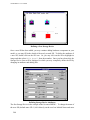
Building a Model
One of the main considerations in the design of a computer system is the effect of
contention between devices on total system operation. This effect is not readily
determined by the use of analytical models. Because NETWORK II.5 actually models
the interactions between all devices in the system, the effects of contention are identified
in NETWORK’s report of total system performance.
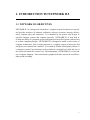
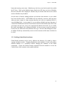
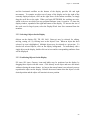
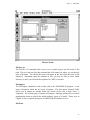
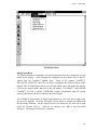
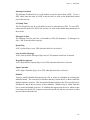
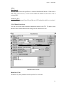
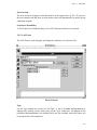
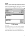
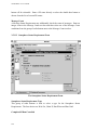
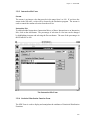
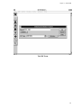
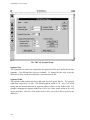
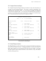
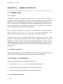
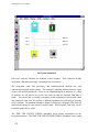
1.2 OVERVIEW OF THE NETWORK II.5 SYSTEM
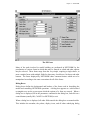
The NETWORK II.5 package provides three main functions; system description, system
simulation and simulation analysis. System description is handled by graphical layout of
the hardware elements and the use of graphics based forms to describe the component
attributes. System simulation is simply a matter of invoking the simulation program for
the system description that you have built. NETWORK II.5 does not require any
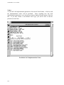
programming, so there are never any programming delays. You can look at any of the
reports as the simulation runs and/or follow an event trace that tells you exactly what is
going on inside the simulation. NETWORK II.5 contains a rich repertoire of simulation
2
Chapter 1: Introduction
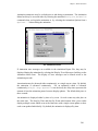
analysis tools. First and foremost is animation. You can actually see your system in
operation, making many problems obvious by inspection. You can plot device status and
utilization as a function of time. The plots are based on a database constructed during the
simulation run. You may access that database directly for custom reports. Finally, there
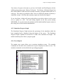
is a comprehensive set of tabular reports written at the end of the simulation. You can
view this file with our built in browser, or print it out as documentation.
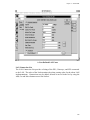
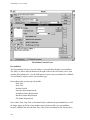
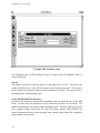
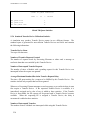
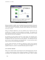
Running a Simulation
The computer system to be simulated is described in a data structure consisting of
Processing Elements, Gateways, Transfer Devices, LANs, Storage Devices, Modules, and
Files. Each of these building blocks has a series of attributes whose values are supplied
by the user. For example, each Processing Element has a Basic Cycle Time attribute to
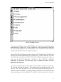
represent its clock speed. The powerful NETWORK II.5 icon-oriented graphic user
interface allows a user to build and maintain the requisite data structure by means of
simple but powerful graphical operations. For example, a new Processing Element can
be brought into existence by clicking on the Processing Element icon on the palette and
dragging the icon to the display.
3
NETWORK II.5 User’s Manual
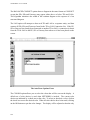
NETWORK II.5 stores the system description created graphically in a text network
description data file which describes the hardware and software of the system to be
simulated. This network description file is a concise English description of the system to
be simulated that can serve as the definitive documentation of the system simulated. The
format of this file is documented under separate cover and may be used as an interface to
other databases and programs. After acquiring the runtime control parameters (such as
simulation length, devices to graph) from you, NETWORK II.5 builds and executes the
simulation. You can optionally monitor the simulation as it progresses through the use of
trace and snapshot reports. Running NETWORK II.5 produces periodic and end-ofsimulation reports. An event trace data file may also be requested. The event trace data
file contains hardware and Semaphore status information that can be post processed by
NETWORK II.5 and by custom report routines written by you.
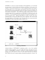
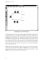
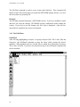
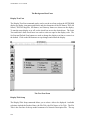
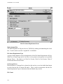
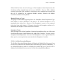
Animating a Simulation
Animated displays of NETWORK II.5 simulations provide a view of the modeled
computer system in operation. It is easy to define the location, color and icon of every
device in a NETWORK II.5 simulation. Interfaces to network management software
packages, such as HP OpenView, Netview for AIX, Digital PolyCenter and Cabletron
SPECTRUM, allow users to import topology information automatically, if desired. The
4
Chapter 1: Introduction
animation may be advanced in single steps or continuously. Animation and event trace
messages describing simulation activity can be displayed concurrently.
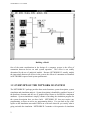
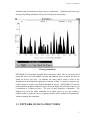
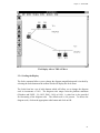
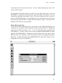
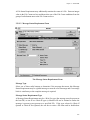
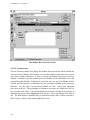
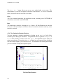
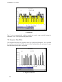
Plotting a Simulation
NETWORK II.5 can produce a graphical time line status report. This is a post-processed
report that shows, for each Module, message and hardware device selected, the times at
which the device was busy. In addition, the status and/or count of each of the
Semaphores in the simulation is plotted as a function of time. It can show whenever any
of these items exceeded a user defined threshold of activity. NETWORK II.5 can also
produce detailed graphical utilization reports that will display the utilization of devices in
a simulation as a function of time. The scale of these diagrams is adjustable. The
diagram may cover the entire simulation (on a single screen) or you can examine a
smaller period of particular interest in greater detail to study conflicts or dependencies,
without rerunning the simulation.
1.3 NETWORK II.5 DATA STRUCTURES
5
NETWORK II.5 User’s Manual
NETWORK II.5 data structures fall into two primary groups: hardware and software.
There are other data structures (Global Flags and Variables, Statistical Distribution
Functions, etc.) that are used by these two groups.
Hardware devices are specified in NETWORK II.5 as one of three basic types:
Processing Elements, Transfer Devices, or Storage Devices. Gateways are a special case
of a Processing Element and LANs are a special case of a Transfer Device. Complicated
real world devices may be simulated by a combination of these NETWORK II.5 building
blocks.
Processing Elements are characterized by their Instruction set and cycle time. Transfer
Devices are characterized by their data transfer rate, data transfer protocol, and
connections. Storage Devices are characterized by capacity, access time, and access
method. By using generalized building blocks, the user is not restricted to predefined
hardware types. For example, a Transfer Device building block is used to model
anything that transfers data from one device to another. This could represent a bus, a
satellite communications link, a LAN, a WAN, etc.
There is no arbitrary limit to the number of hardware device building blocks that may be
used in a NETWORK II.5 simulation. There is also no arbitrary limit to the number of
Processing Elements and Storage Devices that can be connected to a single Transfer
Device.
The software of the simulated system is presented to NETWORK II.5 in the form of
software Modules. Each Module contains a list of the Processing Elements on which it
may execute, a description of when it may run, what it is to do when running, and which
other Modules (if any) to start upon completion. A Module may be assigned to a specific
Processing Element, it may be allowed to run on any Processing Element on a list,
required to run on every Processing Element in a list or it may be allowed to run on any
Processing Element in the system. You can specify a limit to the number of copies of the
same Module that may execute concurrently.
NETWORK II.5 provides you with the ability to specify many different kinds of
conditions that must be met before a Module can start executing. These Module
preconditions include time-, hardware-, message-, and Semaphore-based conditions.
Time-based preconditions include starting a Module at a specific time during the
simulation and/or automatically iterating at a rate specified by the user. Hardware-based
preconditions include waiting until a particular set of Processing Element(s), Transfer
Device(s), and/or Storage Device(s) are available at the same time. Message- and
Semaphore-based preconditions include waiting until a given message or set of messages
6
Chapter 1: Introduction
are received or a given Semaphore is set. Semaphores can also be used to interrupt or
cancel the execution of Modules. Messages and Semaphores have count values which
can also be used in specifying preconditions.
7
NETWORK II.5 User’s Manual
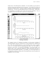
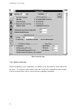
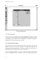
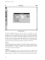
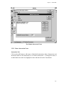
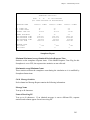
1.4 NETWORK II.5 REPORTS
NETWORK II.5 offers a variety of different reports on system activity. These reports
are:
· Graphical Reports
Automatic Hardware Layout
Software Module Diagram
Status Plot
Utilization Plot
Verify Report
· Tabular Reports
Processing Element Statistics
Instruction Execution
Transfer Device Statistics
Storage Device Statistics
Module Summary
Semaphore Report
Message Statistics
Received Message
Message Delivery
Snapshot Report
· Interactive Simulation Runtime
Narrative Trace
Snapshot Report
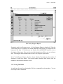
The Automatic Hardware Layout feature shows each device in the system and how it is
connected to other devices. There are three layout algorithms to choose from. The
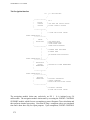
Software Module diagram shows, for each Module, its preconditions, host Processing
Element, instructions, message, Semaphore and File outputs, and successor Modules.
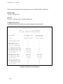
The tabular reports show statistics on the operation of each hardware device, Module or
Semaphore in the simulation. Average, maximum, minimum and standard deviation
values are reported for execution, delay and queue sizes, as appropriate. The Narrative
Trace produces an (optional) step-by-step trace of the execution of the simulation,
showing, for example, when an Instruction begins execution, completes execution, is
interrupted, and so on.
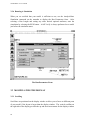
The interactive reports may be printed at your terminal while the simulation is
progressing. The Snapshot Report shows the current status of all elements (both
8
Chapter 1: Introduction
hardware and software) in the simulation. The Snapshot Report may be printed
periodically or interspersed with the Narrative Trace.
1.5 USER’S MANUAL ORGANIZATION
The organization of this manual is based on the parts of the NETWORK II.5 package.
The parts are presented in the order in which they would be first encountered during a
typical NETWORK II.5 session.
Chapter 1 - An overview and brief introduction to the NETWORK II.5 system.
Chapter 2 - How NETWORK II.5 interprets the world to be modeled.
Chapter 3 - Using the graphic user interface to develop and verify a system description.
Chapter 4 - How to run a simulation.
Chapter 5 - The reports produced by a simulation.
Chapter 6 - Using animation.
Chapter 7 - Plotting simulation results.
Chapter 8 - A complete example of a NETWORK II.5 simulation, from problem
statement to analysis of simulation results.
Chapter 9 - Several methods and guidelines to debug a system description.
Chapter 10 - Using TRAFLINK to import topology and /or to drive a simulation with a
LAN analyzer trace file.
Chapter 11 - How to convert a Simulation Plot File between binary and text format.
Appendices describing implementation-specific procedures on available hardware
platforms are included. These currently include:
MS Windows (Windows 3.1, Windows 95 and Windows NT)
OS/2 Warp 3.0
Unix (HP 9000/700, SUN SPARC, IBM RISC/6000, Silicon Graphics)
NETWORK II.5 is written in a higher level language (SIMSCRIPT II.5), and is very
portable. Implementations for other platforms will be added as required.
9
NETWORK II.5 User’s Manual
The final appendix in this manual describes using the SimGraphics II editor for the
creation and modification of icons which can be added to your system description.
10
Chapter 2: Modeling with NETWORK II.5
2. MODELING WITH NETWORK II.5
2.1 INTRODUCTION
In this chapter, all of the elements which can be used to describe the hardware and
software of a computer system in NETWORK II.5 are defined. We are not concerned
with the exact form of input preparation, which is described in Chapter 3.
2.1.1 Overview
Hardware devices are specified in NETWORK II.5 by using building blocks based on the
functions of the device being modelled. There are three functions performed by the
hardware elements in a computer system. These are:
· Process data — performed by a Processing Element building block
· Transfer data — performed by a Transfer Device building block
· Store data — performed by a Storage Device building block.
These building blocks are powerful enough to model any device that performs the given
function. NETWORK II.5 uses an event driven simulation. In an event driven
simulation, you only need to know the timing aspects of an operation, not its
implementation. For example, to model a communications link, NETWORK II.5 only
needs to know when to send the data and how long it takes to move the data from source
to destination. Whether the technology involved is a satellite channel or a fiber optics
link is immaterial.
Actual devices are modelled by defining one or more building blocks to perform the
function of the device being modelled. Most devices can be modelled by a single
building block. As an example, when modeling a personal computer connected to a local
area network, the personal computer can usually be adequately modelled by a single
Processing Element building block. However, if the internal operation of the personal
computer were of interest, it could be modelled as a collection of one Processing Element
(representing the microprocessor), one Transfer Device (modeling the internal bus), and
one Storage Device (modeling the disk drive).
11
NETWORK II.5 User’s Manual
The software components of a system are characterized in NETWORK II.5 as modules,
instruction mixes, macro instructions and files. Modules direct a NETWORK II.5
simulation by using hardware components as required to process, read, write, and send
information through a network. Instruction mixes and macro instructions support
modules by making random and/or repetitive simulation tasks easier to control and
maintain.
2.1.2 Processing Element Overview
A Processing Element (abbreviated PE) is used to model anything in your simulation that
executes instructions or makes decisions. A PE might be used to simulate a bus
controller, a display, a sensor, or an entire arithmetic logic unit. A Processing Element is
characterized by its Basic Cycle Time, Instruction Repertoire, Message List Size, I/O
Setup Time, Time Slice, Interrupt Overhead and Input Controller. The Instructions listed
in the PE’s Instruction Repertoire define what a Processing Element can do.
Each instruction in the Instruction Repertoire is defined by using a generalized instruction
building block. The defined instruction may be as detailed as desired. There are four
kinds of generalized instruction building blocks; they are:
1.
2.
3.
4.
Processing Instructions
Read/Write Instructions
Message Instructions
Semaphore Instructions
The Instruction Repertoire of a Processing Element in NETWORK II.5 is not meant to be
the literal instruction set of the machine being simulated (although it may be). Instead, it
is more likely to consist of very high level pseudo-instructions. A database query might
thus be listed as a single instruction, even though it consists of hundreds of machine-level
instructions. This level of description may be used because the actual code of the
algorithm is undecided, or because timing considerations for an entire system are being
studied, and simulation at the machine instruction level would be unnecessarily detailed.
NETWORK II.5 is designed to simulate the effect of an instruction on the system being
simulated, as opposed to computing a numerical result. Therefore, macro instructions
(such as database query) can be mixed with assembler instructions in a Processing
Element’s Instruction Repertoire. This allows a simulation with items of special interest
12
Chapter 2: Modeling with NETWORK II.5
modelled down to the machine instruction level, while the remainder of the system is
modelled at a coarser level.
Gateways are a special case of the PE building block. A Gateway is a modeling
convenience which allows you to easily model a device whose function is to transfer data
from one Transfer Device to another. The name Gateway is used in a generic sense. The
devices a NETWORK II.5 Gateway connects may be of the same protocol or different
protocols.
Additional information about the operation of the PE building block will be covered in
the Processing Element Details section, which appears later in this chapter.
2.1.3 Transfer Device Overview
Transfer Devices (TDs) are the links connecting Processing Elements and Storage
Devices. They are used to move data between two or more Processing Elements or
between a Processing Element and a Storage Device. They can connect as many of these
devices as desired. Each Transfer Device has a user-defined specification giving the
transfer speed, transfer overhead and protocol definition.
Data is moved between Processing Elements over a Transfer Device as the result of a
Message Instruction, and between a Processing Element and a Storage Device as the
result of a Read/Write Instruction.
Transfer Devices automatically organize every file or message transmitted into words and
blocks. You specify word and block transfer and overhead times for the TD. Then, at
run time, NETWORK II.5 computes the amount of time to send the actual amount of data
a PE is sending or requesting. The TD protocol you select defines the method to resolve
contention between Processing Elements for a Transfer Device. The TD protocol
attribute may be set to model FIFO (First Come, First Served), Collision, Token Ring,
Token Bus, FDDI, Priority, Aloha and others.
A LAN (Local Area Network) is a special case of a TD. A LAN is a standard TD
building block with its parameters predefined to match industry standards. The
advantage of the LAN building block is that the parameters for industry standard LANs
are built in. The built in LANs types include Ethernet, 10BASE2, 10BASET, 4 Mb
Token Ring, 16 Mb Token Ring, FDDI and others.
13
NETWORK II.5 User’s Manual
Additional information about the operation of the TD building block will be covered in
the Transfer Device Details section, which appears later in this chapter.
2.1.4 Storage Device Overview
Storage Devices contain both user-named files and unstructured storage, called General
Storage. Every Storage Device has a capacity measured in bits.
When a Read Instruction references a Storage Device, it checks to see if the requested file
is available. If it is not, a warning message is printed and the simulation continues as if
the file were available. If it is available, the file is read into the PE. You have the option
of reading in the entire file or a specified portion. You may also specify if the Read
Instruction will destroy the entire user-named file just read, or decrease the file size by
the amount read, or leave the file size unchanged.
When a Write Instruction attempts to put a file in a Storage Device, it checks to see if
there is enough space available. If there is, it accepts the file. If adequate space is not
available, a warning message is issued to the user and the simulation continues as if there
is enough room to transfer the entire file. Write Instruction options you may choose from
are replacing an entire user-named file (if one by the same name existed before the write),
or increasing the file size by the number of bits written, or leaving the file size
unchanged.
For simulations where the file structure has yet to be determined or is not significant to
the simulation, files can be read from or written to a Storage Device’s General Storage.
General Storage keeps track of the number of bits stored, but not individual file names.
Commonly, for simplicity, some files are written to a Storage Device’s General Storage
while more significant ones are explicitly named and stored.
A Storage Device may be defined to serve more than one PE simultaneously. The user
specifies that a Storage Device has n ports where n is the number of simultaneous
accesses that can be handled by the Storage Device.
Additional information about the operation of the SD building block will be covered in
the Storage Device Details section, which appears later in this chapter.
14
Chapter 2: Modeling with NETWORK II.5
2.1.5 Module Overview
A Module is the specification of a task to be performed by a Processing Element. The
Module description consists of four parts:
1.
2.
3.
4.
Scheduling conditions
Host Processing Element options
A list of instructions to execute
A list of Module(s) to execute when this Module completes
Each of these parts maps into a stage that every Module goes through in its “life.” The
stages in a Module's life are:
1.
2.
3.
4.
Checking preconditions
Requesting a host PE
Executing instructions
Choosing successors
When a Module checks its preconditions, it is really checking to see if the user-defined
scheduling criteria are met. When they are, the Module then queues up for a host PE (i.e.,
the processor on which it will run). After obtaining a host PE, a Module begins executing
by issuing instruction names from its Instruction List to its host Processing Element, one
at a time. The PE executes the instruction it was given and then asks its host Module for
another. After a Module has issued the last instruction in its Instruction List, it frees its
host PE. The Module then chooses its successor Modules (if any were specified).
Additional information about the operation of the Module building block will be covered
in the Module Details section, which appears later in this chapter.
2.1.6 Overview Summary
This overview section covered the major NETWORK II.5 building blocks at a fairly high
level. It is now time to present the details. A description of a computer system may be
developed beginning with either the hardware or the software. We will start with the
hardware because it is, perhaps, the easier task. The software description will then
follow.
15
NETWORK II.5 User’s Manual
2.2 NETWORK HARDWARE COMPONENTS
Hardware components consist of Processing Elements, Transfer Devices, Storage
Devices, Routes, Echo PE Lists, LANs, Gateways, and Destination Mixes. Each is
described in turn below.
2.2.1 Processing Element Details
As mentioned in the Processing Element Overview section, a Processing Element
(abbreviated PE) is used to model a hardware device which is not merely a data source or
sink. A PE might be used to simulate a bus controller, a display, a sensor, or an entire
arithmetic logic unit. A Processing Element is characterized by its Quantity, Instruction
Repertoire, Message List Size, I/O Setup Time, Basic Cycle Time, Time Slice, Interrupt
Overhead and Input Controller. This section will cover the details of these
characterizations.
The Quantity of a PE will determine if a single PE is defined (Quantity = 1) or if a
number of identical PEs are defined (Quantity is greater than 1). If you select a number
greater than 1 for a PE Quantity, NETWORK II.5 will recognize that number of separate,
but identical PEs. NETWORK will allow you to clone a PE, but once clones are created,
they are unrelated to the parent PE. If you edit a PE in NETWORK with a Quantity
greater than 1, you are essentially editing the entire group at one time. This cannot be
done if a group of cloned PEs is created. Each PE must be edited individually if all are to
have the same changes.
The Basic Cycle Time of a PE is the basic time unit on which all of the processing
instructions of a PE are built; its purpose is to give the user one “knob” which can be
turned to speed up or slow down a PE for sensitivity studies (for example). Although the
Basic Cycle Time may be the actual clock cycle time of the simulated PE, it need not be.
As an example, if the minimum time to execute an instruction is 50 microseconds (mic)
and all other instruction execution times are multiples of 50 mic, 50 mic would be an
obvious choice for the Basic Cycle Time.
Every PE has an Interrupt Overhead specification. Switching from one Module to
another due to an interrupt will always invoke the delay given by this specification. If
you do not want to add any interrupt overhead, disable this feature by leaving Interrupt
Overhead in the NR (No Response) state. An Interrupt Overhead of zero is not allowed
because it adds to simulation execution time without an improvement in simulation
accuracy.
16
Chapter 2: Modeling with NETWORK II.5
Every PE has a Time Slice attribute. The Time Slice attribute specifies automatic
swapping between equal priority Modules during their execution. Setting it to NR will
disable this feature. Time Slice only applies to Modules whose Interruptibility Flag is set
to YES. This means you can exclude certain Modules from being affected by Time
Slicing.
The Time Slice feature works as follows. When a Module starts executing its first
instruction, a timer is started which will expire in the amount of time specified by Time
Slice. If the Module completes before the timer expires, the timer is canceled. If the
timer expires before the Module completes, the Module is interrupted and put at the back
of the queue for its priority class. Then the PE selects the next Module to execute
according to standard rules. Normally, it will select another Module of equal priority. If
there are no other Modules of equal or higher priority to execute, the PE will restart the
interrupted Module. Interrupt Overhead applies to Modules interrupted by a Time Slice.
Whenever an interrupted Module is restarted, a new timer is started to expire in one full
Time Slice.
Every PE may have a Message List Size. This attribute defines the number of bits
available for storing received messages. If Lose Overflow Messages is set to YES, this
will cause any messages which overflow the PE’s Received Message List to be lost. If set
to NO, a warning flag is set, but the message is stored regardless.
Every PE has an I/O Setup Time, which applies to all Read, Write, and Message
instructions. This attribute is used to add an additional amount of processing time before
every Transfer Device access. This delay might represent various operations including
checking Transfer Device status and breaking a message into packets.
Instructions form the link between hardware and software. The correspondence is
established through a user-defined name. Each Module includes an Instruction List
containing a sequence of instruction names. When the Module is “executed” on a
particular PE, it issues the instructions it has in its Instruction List by name to the PE, in
the order in which they appear. The PE is then responsible for examining its Instruction
Repertoire to find an instruction definition by that name. The PE's instruction definition
contains all of the information describing the instruction's type and characteristics. Thus,
a Module executing an instruction on one PE (for example, a general-purpose processor)
might require a long execution time whereas another (special-purpose) PE may execute
the same instruction very quickly.
17
NETWORK II.5 User’s Manual
NETWORK II.5 supports a priority interrupt scheme. Modules have a priority associated
with them. If a Module having a higher priority than a PE’s current Module becomes
available to execute, a PE will interrupt its current Module to work on the higher priority
Module. You may disable priority-based interrupts of a Module by setting its
Interruptibility Flag to NO.
When a Module executing a Processing Instruction is interrupted, the remaining
execution time of the instruction is recorded. When the instruction execution is resumed,
it will occupy the PE for that remaining length of time (unless interrupted again!).
Message and Read/Write Instructions, if interrupted, are either resumed or restarted from
their beginning based on a user-defined attribute of the instruction, called the Resume
Flag. If a Module is interrupted during a Semaphore Instruction, the instruction will be
completed and the Module will resume with the next instruction in its Instruction List.
2.2.1.1 Input Controller
Every PE may have an Input Controller. If a PE has an Input Controller, then it may
accept messages and execute instructions simultaneously. Otherwise the PE must be in a
non-busy state to accept messages. Messages may be received in parallel if more than
one Transfer Device is sending a message to this PE. After a message has been received,
it is put on the PE’s Received Message List, where it may trigger the execution of a
Module. A PE with an Input Controller which is receiving a message and is not
executing a Module will be listed as idle.
A PE without an Input Controller must work the entire amount of time it takes to receive
the message from the Transfer Device. The PE cannot execute a Module in parallel with
the receipt of a message. A PE without an Input Controller that is executing a Module
when another PE attempts to send a message to it over a Transfer Device will block the
incoming message, thereby blocking the sending PE and the connecting Transfer Device.
The sending PE and Transfer Device will remain blocked until the receiving PE becomes
idle, having finished executing its scheduled Modules. A PE without an Input Controller
will be listed as busy while receiving a message.
2.2.1.2 Keep Blocks Separate
The Keep Blocks Separate flag of a Processing Element is used to control the way in
which messages are received and assembled by a PE. When a PE with Keep Blocks
Separate = NO receives a message that arrives in blocks, the blocks will be combined as
they are received to form a single message. If Keep Blocks Separate = YES, the blocks
18
Chapter 2: Modeling with NETWORK II.5
will not be combined, but remain available as distinct blocks in the received message list
of the PE. Keep Blocks Separate = YES will guarantee that a Module with a Wait For
Block Message Status Requirement will respond to each individual block that is received
for a message.
2.2.1.3 Queue Flag
The Queue Flag of a Processing Element is used to control the saving of messages in the
Received Message List. If Queue Flag = NO, whenever a message arrives at the PE, if a
message of the same name already is stored in the Received Message List, the new
message is discarded. If Queue Flag = Yes, duplicate messages will be stored in the
Received Message List if room is available. Message Instructions also have a Queue
Flag to control saving messages in a destination PE, but the Queue Flag of the receiving
PE takes precedence over the Queue Flag of the Message Instruction that originates the
message. Thus, if a Message Instruction with Queue Flag = YES sends a copy of a
message currently queued in a PE with Queue Flag = NO, the incoming message will not
be stored in the Received Message List.
2.2.1.4 Processing Instructions
Processing Instructions are used to model instructions which execute on a Processing
Element without any external references (such as reading or writing). They are
commonly used to model arithmetic and logic instructions.
Every Processing Instruction has a name and a Number of Cycles. Names in
NETWORK II.5 can be (almost) any combination of characters up to 40 characters in
length. Embedded spaces are allowed; however, certain special characters are not
allowed on some systems. The following characters are not permitted in names entered
in NETWORK: “/”, “\”, “;”. If you attempt to enter a name using any of these characters,
or, if for any reason a name you entered is considered invalid, you will be prompted to
enter a new name.
The execution time for Processing Instructions is expressed in terms of a multiplier of the
Basic Cycle Time. Therefore, a change in a PE's Basic Cycle Time automatically
changes the execution time of all Processing Instructions in the Instruction Repertoire of
that PE. The amount of PE time it takes to execute a Processing Instruction is simply the
Number of Cycles of the instruction multiplied by the Basic Cycle Time of this PE.
19
NETWORK II.5 User’s Manual
The Number of Cycles for a Processing Instruction is always an integer. When a
statistical distribution is used for a Number of Cycles calculation, the result is always
rounded to an integer. Processing Instructions may use one of the Linear Distributions to
compute a Number of Cycles based on the size of a received message, the size of a file
that has been read, or a Semaphore count. See the section on Statistical Distributions
later in this chapter for further details on Linear Distributions.
2.2.1.5 Read/Write Instructions
Read/Write Instructions move a file between a Storage Device and a Processing Element.
Files have a name and a size, and reside on one or more Storage Device(s). Trying to
read a file from a Storage Device where it does not reside, or trying to write a file to a
Storage Device that does not have sufficient space available, produces a warning in
NETWORK II.5.
A Processing Element will execute a Read/Write Instruction according to the following
sequence of events:
1.
2.
3.
4.
5.
6.
7.
Request a Transfer Device.
Request the Storage Device To Access.
Request the File Accessed.
Work the amount of time it takes to read/write the Number Of Bits To
Transmit taking into account the Storage Device time and the Transfer
Device time.
Relinquish the File.
Relinquish the Storage Device.
Relinquish the Transfer Device.
The time it takes to read or write a file depends on the speed of the Transfer Device and
Storage Device used. Specifically, it will take the greater of either the time to transfer the
file over the Transfer Device or to read/write the file from/to the Storage Device. Read
Instructions which use a Transfer Device that is slower than the Storage Device used will
add the time for the Storage Device to access the first word of the requested file to the
Transfer Device time. A Read/Write Instruction may be delayed by contention for a
Transfer Device, contention for a Storage Device, or contention for a file. It is these
delays, plus the potential for interruption, that make the exact execution time of a
Read/Write Instruction impossible to predict in advance (although a lower bound based
on the transfer time/storage time does exist).
20
Chapter 2: Modeling with NETWORK II.5
During file transfer, the PE will be listed as busy executing the Read or Write Instruction,
even though it is not officially executing any “cycles.” To simulate a PE which concurrently executes other instructions during a file transfer, a separate PE building block must
be added to the system to handle the I/O operations for this PE. Because NETWORK II.5
uses one building block per function, it is quite reasonable to model one “real” device as
a number of these building blocks when the “real” device performs more than one
function simultaneously.
The TD and SD used by a Read/Write instruction will be listed as utilized for as long as
the PE executing this instruction holds them. So, if a PE acquires a TD and then holds it
while queueing for a SD, the TD will be listed as utilized during that time. Also, if a TD
is much faster than a SD, the TD will still be listed as utilized for the entire time of the
file transfer. The TD is counted as utilized because it is held by the PE for the duration of
the entire transfer. The TD's ability to transfer bits faster than they are presented does not
override the fact that the TD was held by the PE for the full length of the file transfer.
Sometimes it is not necessary to deal with specific files when describing input/output
operations. In this case, the default “file” of General Storage may be specified for
both read and write operations. General Storage is the name given to that part of memory
with no specific file structure. General Storage is unique in that more than one user may
simultaneously use this file. General Storage must be created like any other file, and will
be removed from a Storage Device should its size ever fall to zero bits. The size of
General Storage is monitored and reported separately.
Every Read/Write Instruction has:
·
·
·
·
·
·
·
·
A name
A Storage Device To Access
A File Accessed
A File Count
A Number Of Bits To Read/Write
File Modification Options
A Resume Flag
An Allowed Transfer Device List
The number of bits an instruction is to read or write may be an integer or a reference to a
statistical distribution. The value given will be used to compute the length of time
needed to access the file. For a Read Instruction, a NR (“No Response”) to this attribute
tells NETWORK II.5 to read all the bits the File Accessed contains. If an instruction tries
to read more bits than a file contains or write more bits than the Storage Device To
21
NETWORK II.5 User’s Manual
Access has available, a runtime warning message will be issued. Execution continues as
if the file was available or the Storage Device had sufficient space. This approach is
taken because canceling the transfer would produce artificially low utilization reports.
The Linear Distributions can be used to specify the Number Of Bits To Read/Write based
on the size of a received message, another file or the count of a Semaphore, message, or
file.
Read Instructions have three file modification options: Erase File, Decrement File, and
Do Not Modify File. The Erase File option will release all of the storage occupied by a
file upon completion of the instruction. Decrement File will only destroy the number of
bits read from a file upon completion of the instruction. When Do Not Modify File is
selected, the file size will remain unchanged at the end of the execution of the instruction.
Write Instructions have three file modification options: Append to file, Replace File, and
Update File. Append to File adds the number of bits to write to the size of the file. If an
instruction writes to a file that does not exist, a file will be dynamically created on the
Storage Device To Access and will contain the number of bits to write at the completion
of the instruction. The Replace File option replaces an existing file with the new data and
the file will have a size equal to the number of bits written when this instruction
completes. Update File does not affect a file it is greater than or equal to the number of
bits written. In case you write more bits as an "update" than the file contains, it will grow
in size to be the number of bits written by the "update" instruction.
The Resume Flag applies to both Read and Write instructions in instances where an
interruption of the instruction occurs. If the Resume Flag = NO, this instruction will
restart from the beginning if interrupted. If the Resume Flag = YES, this instruction will
only read or write the number of bits not yet transmitted when resumed.
The Storage Device To Access is the name of the Storage Device that contains the File
Accessed. Wild cards are allowed for the Storage Device To Access (see Section Wild
Cards for a description of wild cards). For a Read Instruction, a wild card in the Storage
Device To Access specification will cause a search for a Storage Device whose name
matches the wild card and contains the File Accessed. The order of search is the order of
appearance in the Connection List of the Transfer Device chosen. Failure to find a
matching Storage Device name results in a runtime error and the instruction is aborted.
For a Write Instruction, a wild card in the Storage Device To Access specification will
cause the file to be written to a Storage Device whose name matches the wild card and
has enough room to store the entire file written. The order of search is the order of
appearance in the Connection List of the Transfer Device chosen. If none of the Storage
22
Chapter 2: Modeling with NETWORK II.5
Devices has sufficient room, the transfer is blocked until sufficient room becomes
available.
The File Accessed is the name of the file this instruction will manipulate. Reading a file
that does not exist produces a runtime error. The Read Instruction will then continue to
execute as if the file is present. Writing to a file that does not exist will cause a file by
this name to be automatically created. Files may be predefined in the SD (Storage
Device) form when using NETWORK, so that they exist at the start of a simulation.
Files are distinguished not only by there names, but also by an optional File Count. A
File Count can either be an integer value or a statistical distribution. When a Read/Write
Instruction attempts to access a file, it will search for a file with the appropriate name. If
the Read/Write Instruction also has a specified File Count, then the instruction will search
for a file with a matching count, in addition to a matching name. If a Write Instruction
dynamically creates a file during a simulation, and if a File Count is specified, the new
file will then be given this value as its count. Writing to an existing may change its size,
but its count will not be altered. The File Count can be used to create new “versions” of
the same file and can also be a part of a Module’s File Status Requirement
A Read/Write Instruction may optionally contain a list of Allowed Transfer Device(s). A
file is transferred to/from a Processing Element via a Transfer Device. The default
response of ANY presumes that any Transfer Device that connects the source and
destination will be acceptable. Although NETWORK II.5 would never pick a Transfer
Device that does not connect the source and destination, this feature allows the user to
restrict the transfer of a large file to a high speed local data link, even though a low speed
global bus also connects the two devices.
The first file read by a Module becomes its “original file.” Original files are inherited, so
that the original file for a successor Module becomes the first file read in by the
predecessor Module. For example, assume Module K read in FILE 1, then FILE 2, and
then chained to Module J. Module J would inherit FILE 1 as its original file. . If you do
not want a Module to pass inherited files to successor Modules, you may set the Inhibit
File Inheritance flag of the successor Module to NO. The “original file” concept is only
used by the File Linear Distribution and the File Count Distribution. The File Linear
Distribution performs an Ax + B calculation where A and B are user-defined coefficients
and x is the number of bits read in the original file. The File Count Distribution performs
a similar Ax + B calculation in which the count of the original file is substituted for x.
23
NETWORK II.5 User’s Manual
2.2.1.6 Message Instructions
Message Instructions are used to provide communication between two PEs. The effect of
a Message Instruction is to deliver the Message Text of this instruction to the Destination
Processor’s Received Message List. The entries on the Received Message List can best
be thought of as “tokens” which will remain in this list until “used” by a software Module
which has this Message Text as a Message Status Requirement. Every PE has its own
Received Message List. The same Message Text may appear more than once in the same
list, and may appear simultaneously in more than one PE's list.
A PE executes one instruction at a time. The time it takes to execute a Message
Instruction will be the time required to transfer the number of bits that make up this
message across the chosen Transfer Device, plus any delays encountered. Every Message
Instruction “executes” by the following sequence of events:
1. Request a Transfer Device.
2. Request the Destination Processor (only if the Destination Processor does not
have an Input Controller).
3. Work the amount of time it takes to transfer the
number of bits to send across the chosen Transfer Device.
4. Relinquish the Destination Processor (if one was requested).
5. Relinquish the Transfer Device.
If a Message Instruction is delayed for a Destination Processor, it will continue to hold its
assigned Transfer Device. The Transfer Device will be listed as busy even though the
transfer has not yet begun. These delays, plus the potential for interruption, make the
exact execution time of a Message Instruction impossible to predict in advance (although
a lower bound based on the data transfer time does exist).
During a message transfer, a PE is listed as busy executing this Message Instruction, even
though it is not officially executing any “cycles.” To model a PE that executes other
instructions while sending a message, a new PE may be added to the system to handle the
output operations.
A message may be sent by a Processing Element to itself. This operation does not require
the use of a Transfer Device; therefore, it takes zero time for a PE to send a message to
itself. This feature is useful in cases where Module coordination is handled by messages
and Module-to-PE assignments are either dynamic or determined after the Modules are
defined.
24
Chapter 2: Modeling with NETWORK II.5
Every Message Instruction has:
· A name
· A Message Text
· A Message Count
· A Destination
· A Queue Flag
· A Resume Flag
· A Continue Message Flag
· An Inhibit Message to Self Flag
· An Inhibit Message Delivery Flag
· An Allowed Transfer Device List
The Message Text is the name that this instruction will put in the Received Message List
of the Destination(s). It defaults to the name of the instruction that sends this message if
no Message Text has been entered for the instruction. A Message Text can be a text
string or a wild card. If the Message Text is not a wild card, this text string will be sent to
the Destination(s). If the Message Text is a wild card, the message text is determined by
the following two cases.
In the first case, a Message Text of * (i.e., an unqualified wild card) will retransmit the
text of the “original message”. The “original message” is the message that satisfied the
initial Message Requirement of the Module executing this Message Instruction, or the
predecessor to this Module. For example, consider a Module with this Message Status
Requirement list:
PACKET ONE
PACKET TWO
PACKET THREE
The “original message” is PACKET ONE since it is first in the list. If a Module with the
above Message Status Requirements list does not execute the Message Instruction, but
chains to that Module which does, the “original message” remains the same because it is
inherited by successor Modules. A Module will also inherit all of the messages that
match the Message Status Requirements list of its predecessors. If you do not want a
Module to pass inherited messages to successor Modules, you may set the Inhibit
Message Inheritance flag of the successor Module to NO.
In the second case of a wild card used for the Message Text, the wild card will contain
some text along with one or two asterisks. The Message Text will be selected by
matching the wild card to the inherited message set of the Module that is executing the
25
NETWORK II.5 User’s Manual
Message Instruction. The first name in this list to match the wild card will be used.
Messages satisfying Message Status Requirements will be added to the inherited message
set of a Module chain.
In both cases of a wild card Message Text, if the Module has no inherited messages, then
the Message Status Requirements list of the Module will be used to determine the
Message Text. A search is made, starting at the top of the list, until a match with the wild
card is found. When a match occurs, the name of the Message Requirement becomes the
Message Text.
A Message Count can be specified in a Message Instruction as an integer value or a
reference to a statistical distribution. A Message Count has various uses. A Message
Count may be included to distinguish messages that have the same Message Text. A
Module can be given a Message Status Requirement that keys on a message’s count, as
well as its text. The Message Count Distribution relies on the Message Count to generate
Ax + B values in which the Message Count of the “original message” is substituted for x.
The length of a Message Instruction is the number of bits to send. It may be an integer, a
reference to a statistical distribution, or NR (“No Response”). The length of a message is
used to compute the amount of time to transfer the message over a Transfer Device. A
length of NR will set the length of the message sent to the same number of bits as the
“original message” received by the Module. A Message Linear Distribution will perform
an Ax + B calculation for message length, where x is the length of the original message
and A and B are user-defined coefficients. A File Linear Distribution will also perform
an Ax + B calculation, where x is the length of the original file. Thus, to turn a file into a
message, use a File Linear Distribution for message length.
The Queue Flag describes the course of action should another Received Message with the
same Message Text appear in the Received Message List of a Destination. If the Queue
Flag = NO and a copy of this Message Text already appears in the Destination's Received
Message List, the new copy of the Message Text is not added to the list. The check of the
list is made after the message has been completely transmitted. This means all devices
will be utilized as if there were a message transfer, but no new copy of the message token
will appear in the Received Message List. The message will be considered “lost” and
recorded as such in the Received Message Report. This feature can be used to prevent
multiple schedulings of a Module when the system loading causes a PE to fall behind. It
also prevents cluttering the Received Message List if you send a PE messages which are
not “used” by a Module.
26
Chapter 2: Modeling with NETWORK II.5
If the Queue Flag = NO and no copy of this Message Text appears in the Received
Message List, the newly transmitted message will be added to the Destination’s Received
Message List. If the Queue Flag = YES, the new copy of the message will always be
added to the Destination’s Received Message List.
If the Resume Flag = NO, an interrupted instruction will restart transmission of the
message from the beginning when resumed. If the Resume Flag = YES, an interrupted
instruction will only transmit the number of bits not yet sent when resumed.
The Continue Message Flag can be used if the Message Instruction has inherited an
original message. If Continue Message = YES, the message is passed to its destination
and the PE executing the instruction is considered to be an intermediary to the message,
rather than the originator of the message. If this message is then echoed back from the
destination, it will be returned to the origin of the original message. If Continue Message
= NO, the PE executing the instruction is considered the originator of the message, even
though an original message has been inherited.
If the Inhibit Message to Self Flag = YES, the message sent by this instruction is
prevented from being received by the host PE executing this instruction. This allows the
broadcast of a message to be received by every PE on a TD or LAN except the host PE.
If a message is sent to a destination selected from a Destination Mix, when the
destination selected is the Host PE for this instruction, a new selection will be made from
the mix until a PE other than the host is selected. There is an upper limit of 100 attempts
to find another PE to prevent an infinite loop.
If the Inhibit Message Delivery Flag = YES, the Processing Element will execute the
Message Instruction, but no message will actually be delivered to the Destination(s) upon
completion of the instruction. When this flag = NO, a message is delivered to the
Destination(s) as controlled by the Queue Flag. The time required to execute a Message
Instruction is not affected by the Inhibit Message Delivery Flag.
A Destination indicates where to send the Message Text. A Destination may be:
· the name of a PE
· the name of a Route
· the name of a Destination Mix
· the reserved phrase “GLOBAL MESSAGE LIST”
· the reserved word “ECHO”
· the reserved word “NEXT”
· a name using a wild card
27
NETWORK II.5 User’s Manual
Most Message Instructions will send a message to a Destination using a Transfer Device.
This device must connect the sender and receiver, either directly or indirectly. To
transfer a message over more than one Transfer Device from source to destination
requires use of a Route. A Route defines a path from source to destination. The path
consists of a list of PE names with an optional allowed TD list for each PE. Routes are
covered as a separate topic in Section Routes.
Sending a message to the Destination GLOBAL MESSAGE LIST does not send it to any
PE at all! Instead, it sends the message to a phantom list that all PEs have access to.
Since it is not sending a message to an actual PE, this instruction does not use a Transfer
Device and therefore executes in zero simulated time. This feature is very valuable when
you would like to schedule a fixed number of tasks (perhaps a number randomly chosen)
which have a choice of host processors. As an example, to model a parallel processor
that spawns n copies of a task that run on the first available of y PEs, just send n
messages to the Global Message List and define one Module that waits for that message
and runs on any of the y PEs.
If the Destination is the reserved word ECHO, this instruction will send its Message Text
to the Processing Element that sent the “original message” (as previously defined) via the
same Transfer Device(s) on which it was received. If a message that arrives via the
Global Message List is to be ECHOed, a Transfer Device will be dynamically selected
from those TDs that link the source PE to the Destination. If no such TD exists, a
runtime warning message will be issued and the message will not be delivered.
If the Destination is the reserved word NEXT, this instruction will send its Message Text
to the Processing Element that appears next in the Route of the original message. If the
original message is not traveling along a route, a runtime warning message is produced.
If the Destination is a , this instruction will send the Message Text to every PE on the
selected Transfer Device whose name matches the given wild card name. The
Destination may also be the host PE executing this instruction. In this case, the PE is just
sending the message to itself. This takes zero time, and does not require a Transfer
Device.
Finally, if the Destination is a Destination Mix, the ultimate destination for the message is
selected randomly according to the percentages specified in the mix.
If the Allowed Transfer Device List is set to ANY (the default), it will be presumed that
any Transfer Device that connects the source and destination will be an acceptable path.
28
Chapter 2: Modeling with NETWORK II.5
2.2.1.7 Semaphore Instructions
Semaphore Instructions are used to set or reset global flags called Semaphores and/or to
modify the count of a Semaphore. These Semaphores are named by the user and may
have a status of either SET or RESET and a count represented as an integer. The status
(SET/RESET) and/or the count of a Semaphore can be examined or changed by any
Processing Element or Module. Semaphores are commonly used to indicate device
availability, to synchronize parallel activities, to record the duration of certain events, or
to indicate the current phase of the simulation.
Executing a Semaphore Instruction takes zero simulated time. Therefore, Semaphore
Instructions will never be interrupted in the midst of execution by another Module
because they never can be “caught” executing. However, a Module might execute a
Semaphore Instruction that changes a Semaphore to a state where the Module's own run
conditions are no longer met. In this case of Module suicide, the Module will be
interrupted (or cancelled) and listed as having this Semaphore Instruction as its current
instruction. However, if the Module resumes, it will start with the next instruction in the
Module's Instruction List.
Every Semaphore Instruction has:
· A name
· A Semaphore
· A Set/Reset Flag
· An assignment type
· A count
The Semaphore represents the name of the Semaphore this instruction is to modify. The
Set/Reset Flag determines the effect the Semaphore Instruction will have on the status of
the Semaphore. If the Set/Reset Flag = SET, then the status of the Semaphore will be
SET upon completion of the Semaphore Instruction. If the Set/Reset Flag = RESET, then
the status of the Semaphore will be RESET upon completion of the Semaphore
Instruction. If the Set/Reset Flag = TOGGLE, then the status of the Semaphore will be
reversed (from SET to RESET or from RESET to SET) when the instruction is finished.
If the Set/Reset Flag does not equal SET, RESET or TOGGLE, then the Semaphore
Instruction will have no effect on the status of the Semaphore.
The assignment type will determine if a Semaphore Instruction will modify the count of a
Semaphore upon execution. Three different assignment types may be specified;
“Increment By”, “Decrement By”, and “Equal To”. The assignment type is used in
29
NETWORK II.5 User’s Manual
conjunction with the count of a Semaphore Instruction to modify a Semaphore’s count.
The effects of the assignment types are:
· Increment By —
add the Semaphore Instruction count
to the count of the Semaphore
· Decrement By —
subtract the Semaphore Instruction
count from the count of the Semaphore
· Equal To —
set the count of the Semaphore equal to the
count of the Semaphore Instruction
A Semaphore count can be used by a Module's Wait For and Chain If preconditions and
Run When and Run Until conditions. See Section 2.3.1.1 Module Preconditions for more
information on the use of Counter Semaphore preconditions. See Section 2.3.1.3 for
information on Module run conditions. The count of a Semaphore can never be less than
zero, so subtracting from the count of a Semaphore whose count is zero has no effect on
the count and decrementing by a value greater than the Semaphore count will merely set
the count to zero. Semaphores also can be used to create responses to time operations.
See the Semaphore Report section in chapter 5, entitled Network Output Reports for an
explanation of how to time operations using Semaphores to define a response.
2.2.2 Transfer Device Details
As mentioned in the Transfer Device Overview section, Transfer Devices (TDs) are the
links connecting Processing Elements and Storage Devices. They are used to move data
between two Processing Elements or between a Processing Element and a Storage
Device. Data is moved between Processing Elements over a Transfer Device as the result
of a Message Instruction and between a Processing Element and a Storage Device as the
result of a Read/Write Instruction.
30
Chapter 2: Modeling with NETWORK II.5
2.2.2.1 Words and Blocks
Transfer Devices organize all transmissions of data into groups called words and blocks.
This allows the user to model up to two levels of a data packet structure by means of a
user-specified word overhead time and block overhead time.
Words are the lowest level of a user-defined packet structure. Each is made up of a group
of bits. The user-defined word overhead time can then be used for adding parity bits,
start/stop bits, and so on. Fractions of a full word incur the full word overhead time. The
term word is fairly standard across most implementations, so a NETWORK II.5 word
generally represents a "word" in the modeled systems.
Blocks are the highest level of a user-defined packet structure. Each is made up of a
group of words. The user-defined block overhead time can be used for adding source
and/or destination headers to message packets, adding message checksums, and so on.
Fractions of a block incur the full block overhead time. Blocks generally represent
packets on an Ethernet and frames on a token ring. However, the term Block is
intentionally generic. A Block can represent any structure that is a collection of words.
A Transfer Device will transmit data in one of two ways, depending on an attribute called
Separate Blocks. If Separate Blocks = YES, the TD will transmit data one block at a
time. The PE using the TD will have to contend for the TD once for every block sent. To
send a message that required 10 blocks over an Ethernet, a PE would have to contend for
the TD 10 times. If Separate Blocks = NO, the time to transfer the total number of words
and blocks will be computed. However, the actual transmission will be made as one
transfer. So, in the previous example, the PE would contend for the TD only once.
Setting Separate Blocks to NO may reduce the execution time of your model by
decreasing the number of TD requests. If the system that you are modeling actually
transfers data one block at a time, this speedup will result in some loss of modeling
accuracy.
2.2.2.2 Transfer Device Attributes
Every Transfer Device has:
· A protocol
· A Cycle Time
· A Bits Per Cycle
· A Cycles Per Word
· A Words Per Block
31
NETWORK II.5 User’s Manual
·
·
·
·
·
·
·
·
·
A Word Overhead Time
A Block Overhead Time
A Minimum Bits to Send
A Block Error Probability
A Block Error Stream
A Scale Error Probability flag
A Block Retry Time
A Separate Blocks flag
A Connection List
The Protocol defines the method of resolving contention between Processing Elements
for a Transfer Device. Your choices of Protocol are FCFS (First Come, First Served),
Collision, Priority, Token Ring, Slotted Token Ring, Priority Token Ring, Aloha and
Crossbar. Based on your selection, you may be required to specify additional attributes
that are specific to the protocol chosen. As the protocols are all quite different from each
other, each protocol will be covered in a separate section. Protocols not predefined in
NETWORK II.5 may be modelled by the user by using Semaphores and messages to
control the Modules that access a Transfer Device.
Cycle Time is a real number that specifies the “clock speed” of a Transfer Device. It is
usually given as the time for one clock tick. If a Transfer Device is to send one bit at a
time (i.e. serial), the Cycle Time is the inverse of the data rate. Bits Per Cycle is an
integer, and specifies the number of bits transmitted in one cycle. Cycles Per Word is
also an integer. The number of bits per word is obtained by multiplying Bits Per Cycle
by Cycles Per Word.
For example, a serial bus with a transfer rate of 10 Mb (Megabits) per second translates to
a Cycle Time of .1 microsecond per bit (the inverse of 10,000,000 bits per second). For
parallel transfer devices, the Cycle Time is the inverse of the clock speed multiplied by
the number of bits sent in parallel. As an example, take a 16 bit parallel transfer device
running at clock speed of 64,000,000 cycles per second The Cycle Time is
(1/(64,000,000)) × 16 = .25 microseconds per cycle.
Words Per Block may be either an integer or NR (“No Response”). An integer value
represents the number of words required to make one full block. A value of NR means
that transfers are not to be broken up into blocks.
Word Overhead Time is a real number specifying the amount of time to add to each word
transferred to account for parity bits, start/stop bits, and so on. This attribute should be
set to zero if no overhead is desired. Block Overhead Time is a real number specifying
32
Chapter 2: Modeling with NETWORK II.5
the amount of time to add to each block transferred to account for destination addresses,
checksums, and so on. It should also be set to zero if no overhead is desired.
A Minimum Bits to Send may be specified to “pad” the data to a minimum size. This is
especially useful for various LAN protocols that require a minimum frame size. This
padding will apply only to the transfer. The number of bits received will always equal
the number of bits sent.
The Separate Blocks Flag will determine if the transmission of a message or file will be
handled as one transmission or as several transmissions of the component blocks of the
message or file. If the flag is set to YES, messages or files will be transmitted one block
at a time, with the controlling Processing Element releasing the Transfer Device and
destination Processing Element/Storage Device between frame transmissions. If the flag
is set to NO, the Transfer Device will be held by the Processing Element for the entire
message or file. NOTE: setting the flag to YES may significantly increase the model
simulation time due to the increased number of TD requests/relinquishes required to send
every message or file.
The Connection List is a list of the names of the Processing Elements, Storage Devices
and Gateways which connect to this Transfer Device. Using the reserved word in this list
will connect this Transfer Device to every Processing Element, Storage Device, and
Gateway in the simulation. Some of the TD protocols also require a key value, to be
associated with some or all of the Connections. Generally, this list will be created
graphically in NETWORK by drawing the connections from a TD to PEs and SDs.
2.2.2.2.1 Transfer Device Error Attributes
A Block Error Probability may be specified to model data transfers lost due to noise on a
TD. The probability is a percentage, between 0 and 100 percent. The default is zero
percent, which means no blocks are lost. A probability of 100 percent is allowed,
meaning that no blocks are ever delivered.
The Scale Error flag is used if you set a non-zero Block Error Probability. Blocks have a
maximum size. If you send less than a full block and set the Scale Error flag = YES, the
probability of error will be scaled down since fewer bits are being sent. In effect, setting
the Block Error Probability to YES turns it from a block error probability to a bit error
probability. As an example, take the case of sending 512 bits over a TD with an Error
Probability of .02 percent and a 1024 bit block size. If Scale Error = YES, the Error
Probability used will be multiplied a factor of 1/2, resulting in a probability of .01
33
NETWORK II.5 User’s Manual
percent, since only 1/2 of a block is being sent. If Scale Error = NO, the probability of
error would be fixed at .02 per cent per block.
The Block Retry Time specifies how long a PE is to wait before retransmitting a block
lost due to a transmission error or message buffer overflow. It is only used if this TD’s
Separate Blocks flag is set to YES. By default, this attribute is zero and the PE will
retransmit the lost block immediately.
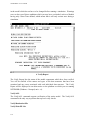
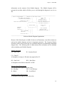
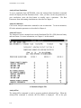
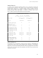
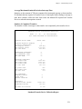
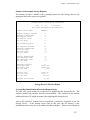
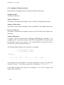
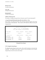
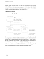
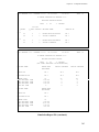
2.2.2.3 Transfer Time Example
An example computation of the time needed to transfer bits over a Transfer Device
follows.
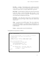
To transfer 56 bits over a Transfer Device with:
9600 baud transfer rate
Basic Cycle Time = 104 mic
serial bus
Bits Per Cycle = 1
7 bits/word
Cycles Per Word = 7
5 words/block
Words Per Block = 5
1 bit per word overhead
Word Overhead Time = 104 mic
1 word per block overhead
Block Overhead Time = 8 × 104 = 832 mic
Number of cycles = bits to transmit / bits per cycle
= 56 / 1
= 56 cycles
Number of words = number of cycles / cycles per word
= 56 / 7
= 8 words
Number of blocks = number of words / words per block
= 8/5
= 1.6 (which rounds up to 2 blocks)
Transmission time = (number of blocks × block overhead time) +
(number of words × word overhead time) +
(number of cycles × bus cycle time)
= (2 × (8 × 104)) +
34
Chapter 2: Modeling with NETWORK II.5
(8 × 104) +
(56 × 104)
= 1,664 + 832 + 5,824
= 8,320 microseconds
2.2.2.4 FCFS (First Come, First Served) Protocol
This is the simplest protocol and is therefore the default. In this protocol, requests are
served in the order in which they are made. Once a PE is allocated a Transfer Device, it
may use it once, regardless of how long that takes. No other PE may interrupt the current
user of a Transfer Device. However, if the Module executing on the PE which is using
Transfer Device is interrupted, the Transfer Device is released and the TD updates its
statistics reporting an interrupted transfer.
2.2.2.5 Collision Protocol
The Collision Protocol does not use a central controller to arbitrate among contending
Transfer Device users. Instead, each PE is responsible for checking the Transfer Device
to see if it is busy before using it. If the Transfer Device is busy, each PE will wait until
the requested device is idle and then wait an additional amount of time (the Contention
Interval) before attempting to access the TD. A collision occurs if two or more PE’s
“see” a TD as idle and both try to use it. A TD is vulnerable to a collision for a period of
time (the Collision Window) after a new user takes the TD. This value accounts for
propagation delays, and delays between checking a TD status and actually beginning to
transmit. In the event of a collision, all users must abort their current transmission and
retry later (the Retry Interval).
In addition to all of the standard TD attributes listed in Section 2.2.2.2 Transfer Device
Attributes, a collision TD has the following attributes:
· A Collision Window
· An Interframe Gap
· A Contention Interval
· A Retry Interval
· A Jam Time
A collision protocol Transfer Device has three states: idle , unsettled and busy. If the
Transfer Device is idle, any PE on the Transfer Device may use it immediately. The
35
NETWORK II.5 User’s Manual
Transfer Device will then be considered unsettled from the time the PE starts using the
Transfer Device until the user-specified time (the Collision Window) has elapsed.
If any PE attempts to access a Transfer Device while it is unsettled, a collision will be
declared and the current user of the Transfer Device will be interrupted. Both the former
user and the requesting PE will send a jamming signal for the length of time given in the
Jam Time attribute. They will then each wait their randomly selected Retry Interval and
then try to access the TD again. The number of collisions which occurred during a
simulation will be reported in the Transfer Device report.
If any PE attempts to access a Transfer Device while it is busy (i.e., in use, but after its
Collision Window is over), it will queue up for the Transfer Device. When the Transfer
Device becomes available, the Interframe Gap (if specified) is imposed on all PEs waiting
to use the TD. The Interframe Gap and the Contention Interval timers run concurrently.
This means that a deferring PE waits the greater of the Contention Interval or the
Interframe Gap before requesting the Transfer Device.
The Retry Interval must be a statistical distribution function (to avoid infinite loops). The
Contention Interval, Jam Time and the Collision Window may be either statistical
distributions or real numbers. Care must be taken in selecting the Retry Interval and
Contention Interval to be used. If the Retry Interval or the Contention Interval return
delay times for the two contending PEs that are within the Collision Window of a
Transfer Device, another collision will occur. “Infinite loops” of collisions are possible!
If a Key Linear type statistical distribution function is used for the Retry Interval, Jam
Time, and/or the Contention Interval of a collision Transfer Device, the additional entry
of key values is required for every PE in the Transfer Device Connection List. These key
values will be used as the x value in the Key Linear distribution's calculation. This value
is a real number, greater than or equal to zero and unique within the Transfer Device
Connection List in which it appears. Key values are only required for Transfer Device
connections that are Processing Elements and are superfluous for other Transfer Device
connections.
NETWORK II.5 supports the IEEE 802.3 standard Truncated Binary Exponential
Backoff algorithm. It may be used for the Retry Interval only by selecting the Standard
Retry Interval option. In brief, this algorithm uses the number of collisions to determine
the length of time to wait before again requesting a Transfer Device after a collision. The
algorithm is called in NETWORK and has the following parameters:
TYPE = IEEE BACKOFF
36
Chapter 2: Modeling with NETWORK II.5
Slot Time — a multiplier. The distribution picks a random integer based
on the number of collisions, then multiplies that integer by this value to
compute the amount of time to wait before RETRYING to get the TD.
Retry Limit — After this number of collisions, the processor stops retrying
for the TD. Instead, it waits the Limit Delay, then tries again. If you
reach the Retry Limit, you are in real trouble! The number of times that
you reach this limit is included in the TD report.
Limit Delay — After a PE reaches its Retry Limit, it waits this amount of
time before trying for the TD again. When it retries, the collision count
restarts at zero.
Offset — a parameter not in the IEEE standard. This value is added to the
result of the IEEE algorithm. It is included merely to add flexibility. Set
to zero if you do not want to modify what would be the standard result of
the IEEE formula.
Stream — a random number stream for this distribution.
The algorithm uses the parameters as follows:
IF TYPE = "IEEE.BACKOFF"
’’
’’uses PE.COLLISION.COUNT to store the number of collisions
’’COMPUTED.DELAY is the value to be used as the
’’backoff delay
’’RANDI.F(A, B, C) returns a random integer value
’’between A and B. C is the random number stream.
’’
ADD 1 TO PE.COLLISION.COUNT..
IF PE.COLLISION.COUNT.. GT RETRY.LIMIT
’’the maximum number of retries
LET PE.COLLISION.COUNT.. = 0
LET COMPUTED.DELAY = LIMIT.DELAY
ELSE
LET COMPUTED.DELAY = SLOT.TIME * RANDI.F(0,
2**(MIN.F(10., PE.COLLISION.COUNT..)),
ST.STREAM..) + OFFSET
ENDIF
ENDIF
37
NETWORK II.5 User’s Manual
2.2.2.6 Priority Protocol
A Priority Transfer Device is allocated in the same way as in the FCFS protocol, with the
exception that the request queue is ordered by PE priority, not by time of request. The PE
priority is assigned by the Key associated with its the PE name in the Transfer Device
Connection List. Because the priority definition is local to a particular Transfer Device, a
PE can have a different priority on each Transfer Device. The Priority Protocol uses
priority to resolve contention, not to provide for interruption. Therefore, if a higher
priority request is received while a lower priority PE was using the Transfer Device, that
new request would be served as soon as the lower priority PE completed its transfer. As
with the FCFS protocol, if the Module executing on the PE which has the Transfer
Device is interrupted, the Transfer Device is released and updates its statistics reporting
an interrupted transfer.
Interestingly, the 802.6 MAN (Metropolitan Area Network) standard can be easily
modeled with the Priority Protocol. The control bus in the 802.6 is used by all stations on
the ring to compute a prioritized request queue for the ring. To model this in NETWORK
II.5, you only need to model the data bus and let the Priority Protocol mechanism handle
the ordering of TD requests.
2.2.2.7 Token Ring Protocol
A Token Ring Protocol views the Transfer Device Connection List as a ring with the last
member of the list followed (at least in a logical sense) by the first member of the list.
After a PE has used the Transfer Device an allowed number of times (given by the
connection’s Key), the Transfer Device is allocated to the next PE on this ring. PEs
without pending requests will be skipped. It is possible that no other PE has a request
and control will immediately return to the PE that was using the Transfer Device. Once a
PE has control of a Transfer Device, it may not be interrupted by any other PE. It will
release control of the Transfer Device when one of the following occurs:
1. It has finished the Key number of accesses of this TD. The Key is specified for a
given PE in the Connection List. The default value for Key is one time. If the
Key value is greater than 1, the PE must execute a continuous series of
instructions that all access this TD to retain control. When a PE executes an
instruction that does not access this TD, the TD is allocated to the next PE on the
ring with a request. An exception to this rule is the Semaphore type instruction,
which does not force the PE to give up the TD because it always takes zero time
to execute.
38
Chapter 2: Modeling with NETWORK II.5
2. It has no further requests.
3. The current Module is interrupted (the Transfer Device updates its statistics
reporting an interrupted transfer) and the interrupting Module does not
immediately use the TD.
A Token Ring TD also has a Token Passing Time attribute. It may either be, “NR” (No
Response), a real number or a statistical distribution. The Token Passing Time specifies
how long it takes to pass the token from one station to the next. The default Token
Passing Time is NR (“No Response”) which disables adding a delay to pass the token.
NOTE: If you specify a Token Passing Time, your TD will always be 100% busy. When
not serving a PE it will be actually passing the token from station to station. This looks
very good in the animation but can easily double (or worse!) the execution time of a
model and cloud the actual data utilization of the TD.
2.2.2.8 Slotted Token Ring Protocol
A Slotted Token Ring Protocol also views the Transfer Device Connection List as a ring
with the last member of the list followed (at least in a logical sense) by the first member
of the list. It differs from a Token Ring Protocol by using a Slot Time to control Transfer
Device access.
Every time a new PE is granted a TD, a timer is started. As long as the PE continually
uses (except for Semaphore instructions) the allotted TD with an unbroken sequence of
instructions, it maintains exclusive use of the TD (so long as it is still within its allowed
slot). If a PE's Slot Time expires and it is still using the TD, it will finish its current
instruction before control passes to the next PE along the ring.
Slot Time may be either a real number or a statistical distribution. If a Key Linear type
statistical distribution is used, the key value associated with each PE in the Connection
list will be used as x in the Ax + B computation. This allows giving a different Slot Time
to each PE on a Transfer Device.
The Token Passing Time may be NR (“No Response”), a real number, or a reference to a
statistical distribution. If set to NR, when a PE relinquishes a TD it is immediately
allocated to the next PE on the ring with a request. If there are no pending requests, the
TD will be idle. If a PE has many items to send but its Slot Time expires, it will
39
NETWORK II.5 User’s Manual
immediately continue with a new Slot Time if there are no other PEs with a pending
request.
If a Token Passing Time is specified, it will give the delay in passing the token from PE
to PE. If there are no pending requests, the token will still circulate around the ring at the
stated rate. When a PE requests a TD, it must wait until the token arrives. While Token
Passing Time adds realism to a model, it can dramatically increase model execution time.
Even a TD which is never requested will be 100% busy passing the token! Use the Key
Linear distribution to get a different Token Passing Time from each PE on the ring.
2.2.2.9 Priority Token Ring Protocol
The Priority Token Ring Protocol offers a generic capability that can be used to model
both the 802.4 Token Bus and the Fiber Distributed Data Interface (FDDI) Token Ring.
It is defined by a token rotation sequence, allocations for synchronous traffic and target
token rotation times for asynchronous traffic. An unlimited number of priority classes
may be specified for asynchronous traffic.
When a simulation starts, the first PE in the TD Connection List is given the token.
When the token is released, it is passed to the next PE in the Connection List. After the
token has been passed to each PE in the Connection List, it is once again passed to the
first PE in the Connection List and this cycle will continue for the duration of the run.
Both synchronous and asynchronous timers may be specified which will determine how
long an individual PE will retain the token.
When a PE receives the token, it will first transmit using its synchronous allocation. A
PE’s synchronous allocation is a guaranteed amount of time that the PE may use the TD
every time that PE receives the token. Each Connection within the TD Connection List
that represents a PE will have its own synchronous allocation defined. Synchronous
allocation may be a value greater than or equal to zero. Each of these Connections may
also have a minimum synchronous priority defined; used to prevent low priority transfers
from using the synchronous allocation of a PE. The priority of a transfer request is based
on the priority of the Module executing the instruction invoking the transfer. The
synchronous allocation is tested before the start of every transmission and is not used to
interrupt a transmission. Therefore, a PE will continue to transmit after the expiration of
the synchronous allocation for any transmission begun before the allocation expires.
After a synchronous allocation ends, a PE will begin its asynchronous traffic, which is
traffic that is controlled by Target Token Rotation Times (TTRT). For each PE
40
Chapter 2: Modeling with NETWORK II.5
Connection of the TD, a list of Target Token Rotation Times may be defined for any
number of priority classes. The list of Target Token Rotation Times is used to provide a
dynamic allocation for the PE based on the priorities of its transmission requests. Each
TTRT will have a priority and a time value associated with that priority. The TD priority
of a transfer request is based on the priority of the executing Module that is invoking the
transfer. Multiple levels of priority are available to a PE to restrict the use of a Transfer
Device when it is highly utilized.
Asynchronous traffic is regulated by the Target Token Rotation Times of a Connection
and the Token Holding Time (THT). Whenever a token is received, the time between the
current time and when the token was last received is recorded as the current Token
Holding Time. When asynchronous traffic begins, the THT clock is started beginning
with this assigned value. The time spent on synchronous traffic does not affect the THT
clock. The priority of an asynchronous transmission will be used to select the TTRT
whose priority is equal to or most nearly equals without exceeding the priority of the
asynchronous transmission. If the lowest priority TTRT has a priority greater than the
priority of the asynchronous transmission request, the token is passed to the next PE.
Before each asynchronous transmission, The PE compares the Token Holding Time to
the time of the selected TTRT. If the Token Holding Time is equal to or greater than the
TTRT, the token is passed to the next PE in the Connection List. A Target Token
Rotation Time will not interrupt a transmission, but is used to determine if a transmission
should begin.
2.2.2.10 Aloha Protocol
The Aloha protocol can be described as a Collision protocol in which the status of the
Transfer Device is unknown. Transmitting PEs are not aware of when the TD is busy
nor do they recognize when a collision occurs. When a PE wants to use an Aloha TD, it
immediately begins transmitting and continues even if a collision occurs. An instruction
that calls an Aloha TD should not list any other Allowed Transfer Devices because
succeeding Allowed TDs will never be selected due to the fact that there is never a delay
for an Aloha TD.
An Aloha protocol TD has three attributes in addition to the normal TD attributes;
Automatic Retry, Retry Interval, and Slot Width. Automatic Retry can be set to YES or
NO. If Automatic Retry is set to NO and a collision occurs, the colliding instructions will
continue until completed and then its host Module will move on to its next instruction.
However, the message or file being transmitted will not have been sent or received. If
Automatic Retry is set to YES and a collision occurs, the colliding instruction will
41
NETWORK II.5 User’s Manual
complete and then be rescheduled for another transmission attempt at the end of the
collided transmission. The time the instruction will wait before retrying is derived from
the Retry Interval which must be a statistical distribution function if it is specified. The
IEEE BACKOFF statistical distribution function may be used for Retry Interval. Retry
Interval is provided as a modeling convenience because the actual Aloha protocol uses
acknowledge messages to detect undelivered transmissions. This feature permits
modeling this mechanism without adding additional Modules and messages.
The Slot Width can be used to convert a pure Aloha TD (Slot Width = NR) into a slotted
Aloha TD. When you provide a value for the Slot Width, a timer equal to the Slot Width
is used to control the Transfer Device. PEs will only be allowed to transmit on the TD at
the beginning of each time cycle defined by the Slot Width.
The Resume Flag of Message and Read/Write Instructions acts normally on an Aloha TD.
This flag determines whether an interrupted instruction restarts completely or will resume
and complete the remaining transmission. A collision on an Aloha TD does not interrupt
a Module so the Resume Flag will not cause the retransmission of bits lost due to a
collision because the sender is not interrupted. To automatically retransmit all lost
transfers on an Aloha TD, set Automatic Retry to YES.
2.2.2.11 Crossbar Protocol
The Crossbar protocol permits simultaneous transmissions on the same Transfer Device
at any time without any complications resulting from multiple transmissions. A Crossbar
Transfer Device can be refined by using the Source Blocking Flag, the Destination
Blocking Flag and the Number of Circuits attribute. If the Source Blocking Flag = YES,
a PE will be blocked from transmitting to any other PE that is currently sending a
message or a file. The blocked PE will delay until its intended destination has finished
sending its transmission. If the Destination Blocking Flag = YES, a PE will be blocked
from transmitting to any other PE that is currently receiving a message or a file. The
blocked PE will delay until its intended destination has finished receiving the current
transmission.
The Number of Circuits attribute can be used to limit the number of transmissions
occurring on the TD at any given time. If Number of Circuits is NR (the default), the
number of transmissions is limited only by the number of devices that are connected to
the Transfer Device. If Number of Circuits is set to a number, then that number
represents the maximum number of transmissions that can occur on the TD at any given
time. A PE attempting to send a message or a file when the number of transmissions
42
Chapter 2: Modeling with NETWORK II.5
equals the Number of Circuits will delay until the number of transmissions is less than
the Number of Circuits.
2.2.3 Storage Devices
As mentioned in the Storage Device Overview section, Storage Devices contain both
user-named files and unstructured storage (called General Storage). They have a capacity
measured in bits. They are used to model anything that stores data either temporarily or
permanently. This includes buffers, disk drives, tape drives and random access memory.
Files are read or written analogous to the way real storage devices work.
2.2.3.1 Words and Blocks
Storage Devices automatically decompose all file reads and writes into words and blocks.
Words are the smallest segment and usually correspond directly to the actual word size of
the Storage Device being modelled (but they need not be). A word overhead time may
also be specified.
Blocks are the largest segment of data storage and are made up of groups of words.
Blocks are commonly used to model features of real Storage Devices. For example, one
feature easily modelled by a block is the sector of a disk. Once a sector is located (Block
Overhead Time models the disk seek time), the words in the sector are transmitted
without delay.
When a read or write involves a block that is not completely “full,” the partial block will
incur the full Block Overhead Time, but is not filled with blank words to pad out the
transfer. The amount of time it takes a Storage Device to read or write a file depends not
only on the speed of this device but may also depend on the speed of the requesting
Transfer Device. If the Storage Device is faster than the Transfer Device, the read/write
proceeds at the speed of the Transfer Device. The Storage Device is marked as busy for
the entire length of the transfer. If, on the other hand, the speed of the Storage Device is
the limiting speed, the read/write will take the amount of time it takes to move the data in
or out of the Storage Device.
43
NETWORK II.5 User’s Manual
2.2.3.2 Storage Device Attributes
Every Storage Device has:
· A name
· A Capacity
· A Bits Per Word
· A Words Per Block
· A Number of Ports
· A Read Word Access Time
· A Write Word Access Time
· A Read Word Overhead Time
· A Write Word Overhead Time
· A Read Block Overhead Time
· A Write Block Overhead Time
· A Read Access Delay
· A Write Access Delay
Capacity is a real number specifying the total number of bits a Storage Device can hold.
It should not include any overhead bits. Even though bits are usually integers, capacity is
a real number to allow capacities greater than an integer’s upper bound of slightly more
than two billion. The upper bound of a real number depends on the word size of the host
computer, but is generally at least 1.7 E+32.
The Number of Ports is the number of simultaneous accesses that can be made to the
Storage Device. The value is independent of the actual number of Transfer Devices that
connect to this Storage Device. If, for example, four TDs are connected to a Storage
Device which had the Number of Ports = 2, the Storage Device would serve up to 2
Transfer Devices simultaneously. All other requests would be queued on a first-come,
first-served basis. In addition, no more than one PE can access a given user named file at
any given time. However, multiple users may access General Storage simultaneously.
Read Word Access Time and Write Word Access Time are real numbers, or references to
a statistical distribution. They reflect the amount of time to read/write one word of data.
Read Word Overhead Time and Write Word Overhead Time are real numbers or
references to statistical distributions specifying an additional amount of time to add per
word accessed. Bits Per Word is an integer specifying the number of bits in a word (not
including overhead bits). Words Per Block is an integer specifying the number of words
in one block. Read Block Overhead Time and Write Block Overhead Time are real
numbers, or references to statistical distributions, specifying the amount of time to add to
each block read or written to account for Storage Device overhead.
44
Chapter 2: Modeling with NETWORK II.5
Read/Write Access Delay represents the initial amount of time before a read/write
transfer can begin on the Storage Device, regardless of the length of the read/write. An
example when this attribute is helpful is modeling the hard disk drive on a laptop
computer. A hard disk request might be delayed waiting for a powered down hard disk to
come up to speed. Once the hard disk is up to speed, the entire read/write transfer may
proceed. The time for the transfer will then be based on the other SD speed and overhead
attributes and the Transfer Device rate connecting the SD to the PE requesting the
read/write.
2.2.3.3 Example — MODELING A DISK DRIVE
A sample calculation of the amount of time needed to move data from a Storage Device
follows.
Disk Read Time Example:
To read 133 words from a Storage Device with a:
- 64 word sector
- Read Word Access Time = 500 mic
- average seek time = 10 mic (Read Block Overhead Time)
Word Time: 133 words × 500 mic/word = 66500 mic
Block Overhead Time: 133 words / 64 words per block = 2.08 blocks
3 blocks x 10000 mic = 30000 mic
Total Transfer Time: Word Time + Block Overhead Time =
66500 + 30000 = 96500 mic
2.2.4 Routes
Message instructions let you specify a Route as a destination. A Route is defined at the
top level by giving it a name and a list of PE, Gateway, and Destination Mix names, each
of which may have an allowed TD/LAN list. If a message instruction uses a Route, the
message sent will visit each PE or Gateway along the Route in the order they appear until
it reaches the end of the Route. The last entry in a Route must be a PE or a Destination
Mix that will produce a PE name. A Gateway is not a valid final destination for a
message.
45
NETWORK II.5 User’s Manual
Gateways automatically include the ability to forward messages along a route. However,
each PE found in a Route must have a user defined Module to pass along the message.
This user defined Module must use the message as a Wait For type Message Status
Requirement (or a wild card Message Status Requirement that matches the message) and
then call a Message Instruction whose Message Text is * and whose destination is the
reserved word NEXT. The message instruction will then use the destinations and allowed
TD lists found in the Route. If no forwarding Module exists at the destination, no error is
generated and the message is not forwarded.
For example, consider the case of a system of 3 TDs connecting 4 PEs as shown in the
following diagram.
A Sample Simulation Using a Route
The easiest way to send a message from PE 1 to PE 4 is to define a route that consists of
PE 2, PE 3 and PE 4. The destination of the message instruction in PE 1 would then be
the name of this Route. PE 2 and PE 3 require a Module with a Message Requirement
matching the name of the message to forward. This Module will execute a message
instruction whose destination is NEXT. So when PE 1 sends its message, it is then
46
Chapter 2: Modeling with NETWORK II.5
forwarded by PE 2 and then PE 3 until it reaches PE 4. If you use wild cards for the
Message Requirement of the forwarding Modules, one Module is able to forward many
different messages. Also note that the forwarding Module can work in any direction. It
forwards messages regardless of source and destination. Therefore, you probably will not
need more than 1 forwarding Module per PE.
47
NETWORK II.5 User’s Manual
***** ROUTES
HARDWARE TYPE
NAME = PE 1
NEXT PE =
NEXT PE =
NEXT PE =
= ROUTE
TO 4
PE 2
PE 3
PE 4
A Sample Route
2.2.5 Echo Processor Lists
Message Instructions allow you to reference an Echo Processor List. Echo Processor
Lists are defined at the top level. The EPL (Echo Processor List) is given a name. It
consists of a list of TD names, each of which has a PE name associated with it. This
feature allows a PE to mark a message so that it ECHOs via a different PE than itself. By
default, whenever a PE retransmits a message, it tags the message with its own name. If
the message sent was returned using the ECHO feature, it would then return via this PE.
If you specify an EPL for a message instruction, a PE can tag a message with a different
PE’s name. When an EPL is specified, the selection of which PE’s name to use is based
on the incoming TD’s name.
48
Chapter 2: Modeling with NETWORK II.5
A Sample Model of a Gateway
49
NETWORK II.5 User’s Manual
HARDWARE TYPE = ECHO PE LIST
NAME = GATEWAY CLUSTER LIST
TD = ETHERNET
ECHO PE = G1/GATEWAY
TD = TOKEN RING
ECHO PE = G2/GATEWAY
TD = TOKEN BUS
ECHO PE = G3/GATEWAY
*
HARDWARE TYPE = PROCESSING
NAME = G1/GATEWAY
INSTRUCTION REPERTOIRE =
INSTRUCTION TYPE = MESSAGE
NAME ; RETRANSMIT ANYTHING
MESSAGE ; *
DESTINATION PROCESSOR ; NEXT
ECHO PE LIST = GATEWAY CLUSTER LIST
NAME = G2/GATEWAY
INSTRUCTION REPERTOIRE =
INSTRUCTION TYPE = MESSAGE
NAME ; RETRANSMIT ANYTHING
MESSAGE ; *
DESTINATION PROCESSOR ; NEXT
ECHO PE LIST = GATEWAY CLUSTER LIST
NAME = G3/GATEWAY
INSTRUCTION REPERTOIRE =
INSTRUCTION TYPE = MESSAGE
NAME ; RETRANSMIT ANYTHING
MESSAGE ; *
DESTINATION PROCESSOR ; NEXT
ECHO PE LIST = GATEWAY CLUSTER LIST
SOFTWARE TYPE = MODULE
NAME = GATEWAY/RETRANSMIT
PRIORITY = 0
INTERRUPTIBILITY FLAG = NO
CONCURRENT LIMIT = 32000
ALLOWED PROCESSORS =
G1/GATEWAY
G2/GATEWAY
G3/GATEWAY
REQUIRED MESSAGES =
*
INSTRUCTION LIST =
EXECUTE A TOTAL OF ; 1 RETRANSMIT ANYTHING
A Partial Listing of an Echo PE List and Gateway Model
The Echo Processor List feature is useful when modeling devices like gateways. Presume
that you model a gateway between 3 TDs by using 3 PEs. Each PE is dedicated to serve
50
Chapter 2: Modeling with NETWORK II.5
as the output buffer for a single TD. If a PE serving as an output buffer forwards a
message, it obviously wants that message (if ECHOed) to return back through the correct
output buffer. Since that output buffer is a different PE than the forwarding PE, an EPL
is required. A sample gateway model using the EPL follows.
In the above example, any message arriving from the Ethernet which is forwarded by any
message instruction which references GATEWAY CLUSTER LIST will be returned via
G1/GATEWAY (if returned through the use of the ECHO feature). Otherwise, the
message would be returned via the forwarding PE, which would make dedicating a PE as
an output buffer impossible.
2.2.6 LANs
The LAN building block is used to quickly specify common LAN implementations in
NETWORK II.5. A LAN is really just a standard Transfer Device with its parameters
automatically filled in to match industry standard LAN implementations. A LAN
connects as many Processing Elements, Storage Devices, or Gateways as desired. Traffic
on the LAN is in the form of messages or files. A LAN operates identically to a TD
when the TD is specified with the same parameters as the LAN. Therefore, refer to the
relevant TD section for the details on how a LAN operates.
Every LAN has a:
· Name
· Implementation
· Connection List
To specify a LAN, all you need to do is give it a name, select an implementation from the
list of implementations presented and draw the connections.
The following
implementations are included in this release.
Collision LAN Implementations
Ethernet
IEEE 802.3 CSMA/CD 10BASE5
IEEE 802.3 CSMA/CD 10BASE2
IEEE 802.3 CSMA/CD 10BASET
IEEE 802.3 CSMA/CD 1BASE5 STAR
IEEE 802.3 TOP
51
NETWORK II.5 User’s Manual
Token Ring LAN Implementations
IEEE 802.5 4Mb
IEEE 802.5 16Mb
FDDI
Token Bus LAN Implementations
IEEE 802.4 1Mb
IEEE 802.4 5Mb
IEEE 802.4 MAP 10Mb
In addition to the above LAN implementations, three other LAN implementations are
available; User Defined Collision, User Defined Token Bus and User Defined Token
Ring. Although these three LAN implementations have predefined parameters, they can
also be customized by changing any of the basic LAN parameters. The other LAN
implementations have fixed parameters which can be viewed, but not altered.
2.2.7 Gateways
A Gateway is a device for multidirectional interconnection between two or more TDs
and/or LANs. A NETWORK II.5 Gateway is the generic term for a repeater, router,
bridge, gateway, or any type of hardware connecting two or more TDs and/or LANs.
Gateways cannot generate traffic, they only forward messages sent to them by Processing
Elements or other Gateways. A Gateway is made up of a number of output units equal to
the number of TDs/LANs that the Gateway connects. These output units are modeled by
standard NETWORK II.5 PEs and Modules automatically written for you when you save
your model. Each output unit is dedicated to serve a single TD/LAN. It is responsible
for properly requesting the TD/LAN and queueing the messages for that LAN. You may
specify a Buffer Capacity for each of the output units of a Gateway.
When a Gateway receives a message, the output unit performs any required reformatting
of the message. If the processing component of the output buffer is busy with another
message, a message queue builds. If the size of the message queue exceeds the Buffer
Capacity of the output unit, a runtime warning will be issued. However, the message will
not be lost, but will always be forwarded. If the message arrives over a TD or LAN
which has Separate Blocks = NO, the message will not be considered for processing
and/or retransmission until the entire message is received at the Gateway. If the message
arrives over a TD or LAN which has Separate Blocks = YES, the message will be
considered for processing and/or retransmission block by block, as it arrives.
52
Chapter 2: Modeling with NETWORK II.5
There is a set of reformatting parameters for processing time and message length for each
TD/LAN connected to the Gateway. The processing time is calculated using the equation
of the form Ax + B where A, referred to as the Message Multiplier, is any real number; x
is the incoming message length (in bits), and B, referred to as the Message Additive, is
any real number. The processing time is the time for any required translation and
message length adjustment between the two TDs/LANs. The retransmitted message
length is calculated using a different equation, also of the form Ax + B, where A, the
Processing Multiplier, is any real number; x is the incoming message length (in bits); and
B, the Processing Additive, is any real number. By default, the processing time is zero
(A = 0, B = 0) and the outgoing message length is equal to the incoming message length
(A = 1, B = 0).
The set of reformatting parameters for processing time and message length can be either
identical for all output units or set individually. You set these parameters by clicking on
the name of the TD/LAN that the output unit serves in the connection list of the Gateway
form. There is no reason that the formatting time must be the same no matter what
direction a message is going.
2.2.8 Destination Mixes
A Destination Mix is a list of names of Processing Elements, Routes, and Destination
Mixes with a percentage associated with each. The percentages must sum to 100%. Each
time a Destination Mix is referenced as a destination for a message instruction, a new
probability is randomly selected from a uniform distribution. The corresponding
destination from the mix is the selected and executed. You use a Destination Mix by
giving its name as the destination for a Message Instruction. Because the names of
Destination Mixes, PEs and routes must be unique, there will be no confusion.
***** DESTINATION MIXES
HARDWARE TYPE = DESTINATION
NAME = WORKSTATION MIX
DESTINATIONS ARE ; 40 %
DESTINATIONS ARE ; 17 %
DESTINATIONS ARE ; 10 %
DESTINATIONS ARE ; 33 %
MIX
ADMIN
FINANCE
GATEWAY TO WAN
PRINT SERVER
A Sample Destination Mix
53
NETWORK II.5 User’s Manual
Destination Mixes are recursive. Therefore, the name of a Destination Mix can be
included as a “destination” in a Destination Mix, exactly as it could be inserted for a
destination of a Message Instruction. To catch infinite loops, a limit of 100 levels of
recursion for Destination Mixes has been built into NETWORK II.5. A message
instruction attempting to find a destination from a Destination Mix that reaches the 100
level limit will be cancelled and a runtime warning will be issued.
2.3 NETWORK SOFTWARE COMPONENTS
The software components of a system are characterized in NETWORK II.5 as Modules,
Instruction Mixes, Macro Instructions and Files. The role and use of each is described
below.
2.3.1 Modules
A Module is the specification of a task to be performed by a Processing Element. The
Module description consists of four parts:
1.
2.
3.
4.
Scheduling conditions
Host Processing Element options
A list of instructions to execute
A list of Module(s) to execute when this Module completes
Each of these parts maps into a stage that every Module goes through in its “life.” The
stages in a Module's life are:
1.
2.
3.
4.
Checking preconditions
Requesting a host PE
Executing instructions
Choosing successors
When a Module checks its preconditions, it is really checking to see if the user-defined
scheduling criteria are met. When they are, the Module then queues up for a host PE (i.e.,
the Processing Element on which it will run). After obtaining a host PE, a Module begins
executing by issuing instruction names from its Instruction List to its host Processing
Element for execution. After a Module has issued the last instruction in its Instruction
54
Chapter 2: Modeling with NETWORK II.5
List, it then chooses its successor Modules (if any were specified). Each of these four
stages will be described in turn below.
2.3.1.1 Module Preconditions
There are a variety different conditions which may be used to schedule a Module. Every
Module must have at least one of these conditions so that NETWORK II.5 knows when
to “run” the Module. Sophisticated combinations of these preconditions for the same
Module permit modeling real world scheduling criteria.
The different Module preconditions fall into four basic categories:
1.
2.
3.
4.
Time-based
Awaited
Checked once
System state
Each category will be described separately.
Time-based preconditions are the Module's Start Time, Stop Time and Iteration Period.
Start Time, Stop Time and Iteration Period may be either real numbers or the name of a
statistical distribution. If the specified Iteration Period is a Statistical distribution, a new
pick from the distribution will be made each time the Module is scheduled to activate.
The action that occurs at the start and iteration times is called a scheduling, because the
Module may not immediately begin execution due to host PE availability or to other
preconditions which must still be satisfied.
Start Time and Iteration Period may be specified either alone or in combination for the
same Module. Because they interact, three cases are possible.
1. Only the Start Time is specified -- the Module will be scheduled to execute only
once, at the given time.
2. Both the Start Time is specified and the Iteration Period is also specified -- the
Module will be first scheduled for the given Start Time. Thereafter, the Module
will schedule the next copy of this Module after a delay equal to the Iteration
Period from the time when the last scheduling occurred.
3. Only the Iteration Period is specified -- a Start Time will be chosen randomly (using
a uniform distribution) between 0 (zero) and one Iteration Period. If the Iteration
Period is a statistical distribution, the uniform distribution used for Start Time will
55
NETWORK II.5 User’s Manual
use one selection from the Iteration Period statistical distribution as an upper
bound. After that, the time between schedulings will be the specified Iteration
Period.
If the Stop Time is specified for a module, the Module will continue to schedule
executions until the Stop Time is reached. If there are Modules scheduled and queued
when the Stop Time occurs, those queued Modules will execute. Once a Module Stop
Time is reached, no new copies of the Module will be scheduled for the remainder of the
simulation.
Awaited preconditions are the Module’s Anded Predecessors and Ored Predecessors. If
one Module lists another Module as a successor, it implies that the successor Module has
a predecessor precondition. A given Module may have a number of other Module(s)
which list it as a . When a Module completes and then notifies its successor(s) that it has
completed, that notification is called chaining;. When any Module chains to another
Module, the successor Module must determine whether its predecessor preconditions
have been met. If a Module is defined as having Ored Predecessors, any Module
chaining to it is sufficient to meet the predecessor precondition. If a Module is defined as
having Anded Predecessors, then every Module which lists this Module as a successor
must chain to this Module before its predecessor precondition is met.
Every new copy of this Module will have its own predecessor conditions which must be
met. Therefore, if a Module has three Anded Predecessors, all three must chain to this
Module once before this Module can be scheduled. Once the Module is scheduled, it
creates a new copy of this Module, which starts by checking its preconditions. All three
predecessor Modules must then chain to this new copy before it may be scheduled. Any
“extra” chainings predecessor Modules made to the old copy will not be used to satisfy
this new copy's Anded Predecessor preconditions.
It is often useful to specify a Module as its own successor, thus allowing a Module to be
always ready to perform an action. When specifying a Module as its own successor, do
not specify that it has a predecessor, thus avoiding a logical impossibility (Start only after
you have completed). A scheduling precondition must still be provided for the Module.
Commonly, the Module is given a Start Time of zero to bring it into existence at the start
of a simulation. It will then chain to itself to remain active throughout the simulation.
Checked once preconditions are Chain If Semaphore, Chain If File, and Chain If
Message Requirements. Chain If conditions are used to select a successor Module based
on user defined conditions. Chain If conditions determine whether a Module can be
Chained to at the time they are checked. The same Module may Chain If due to file,
56
Chapter 2: Modeling with NETWORK II.5
Semaphore and message conditions. Chain If conditions are specified for a successor
module and apply to all predecessor Modules which call this Module. Modules without
predecessors cannot have Chain If preconditions, because this test is made only by a
Module attempting to chain to a successor.
If a Module fails its Chain If test, it remains waiting for its predecessor precondition as if
the predecessor never completed execution. The Chain If precondition is tested once by
the predecessor when it is about to chain to a successor. If all Chain If requirements are
met, the chaining occurs and the successor’s predecessor condition for the Module that
chained will be met. The successor Module will then check its remaining preconditions
to see if they are satisfied. If any of the successor’s Chain If requirements are not met, the
successor Module remains inactive.
A Chain If file precondition allows you to select a Module based on the availability (or
nonavailability) of a file either on a particular device or on any device. A Chain If
Semaphore precondition; allows you to select a successor based on whether the
Semaphore is set or reset or the Semaphore’s count is greater than, less than, or equal to, a
particular integer value. See Section 2.2.1.6 Semaphore Instructions. for an explanation of
Semaphore counts. A Chain If message precondition allows you to select a Module
successor based on the presence or absence of a particular message in the received
message list of a specific Processing Element.
System state preconditions are Wait For Semaphore Status Requirement, Wait For File
Status Requirement, Wait For Message Status Requirement, and Hardware Status
Requirement.
After a Module has passed all of its time-based, awaited and checked preconditions, it
then begins to check its system state conditions. When checking the system state
conditions, a Module behaves as an impartial observer. The Module will remain in an
observer state until every system state precondition is simultaneously true. When this
happens, the Module then removes any messages it requires from the Received Message
List of the host PE and moves to the next state where it waits its Delay (if any) and then
queues for its host Processing Element.
Wait For Semaphore Status Requirement preconditions; allow a Module to require that
one or more Semaphores have a specific setting (SET or RESET, or a count greater than,
less than, or equal to, an integer. Wait For File Status Requirement preconditions allow a
Module to require that a given file exist (or not exist) on a given Storage Device (or any
Storage Device). A Wait For File Status may also be based on the count of a file. A Wait
For precondition is a delaying precondition, not a scheduling precondition. Therefore, a
57
NETWORK II.5 User’s Manual
Module must have another precondition in addition to the Wait For precondition(s) to be
considered for execution. For example, to start a Module every time a particular file was
written, the Module could be given a Start Time of zero, and be listed as its own
successor. This will meet the NETWORK requirement that a Module have a scheduling
precondition (the zero Start Time) and cause a new copy of this Module to be made after
the old one completes (because it is a successor to itself). BEWARE: This method
requires that the Module, during its lifetime, do something to inhibit its next execution
(such as to Read and Destroy the file). Otherwise, an infinite loop will result.
Wait For Message Status Requirements allow a Module to require that one or more
messages be received at the Module’s host Processing Element. When the Module leaves
the checking preconditions state, each of the messages which satisfied the Module’s Wait
For Message Status Requirements is taken from its host PE’s Received Message List.
This effectively “uses up” the message. Another message must be received before the
requirement would be satisfied again. If two or more Modules had the same message as a
precondition, the first Module to execute would “use up” the message and the other
Modules would have to wait until this message was received again.
Messages are only allocated to Modules which have all of their preconditions met. If two
or more Modules with all other preconditions met were waiting for the same message, the
message would be allocated to the highest priority Module. Within equal priority, it
would go to the Module that waited the longest for this message. All else being equal, a
random choice will be made.
Wild cards are permitted in a Module's Message Status Requirement. Therefore, a
Module could wait for one of many different messages with only one wild card Message
Status Requirement. See Section 2.3.7 for a complete description of wild cards.
The Wait For Message Status Requirement List is presumed to be an Anded List. This
means that every message in the list must be received to satisfy this Module's Message
Requirements. Wild cards are commonly used to effectively provide an Ored List, where
any one of a group of messages would be sufficient to start this Module.
An additional Module attribute that relates to Wait For Message Status Requirements is
the One Message At A Time flag. This flag is used in cases in which you may want only
one copy of a Module that has a Wait For Message Status Requirement to exist at a host
PE at any given time. When One Message At A Time = NO (the default), every time a
new copy of the message which will satisfy the Module’s Message Status Requirement
arrives, a new copy of the Module is created and will contend for the host PE. This may
lead to many Modules queueing for the host PE if many copies of the message are
58
Chapter 2: Modeling with NETWORK II.5
received. If One Message At A Time = YES, a new copy of the Module will not be
created in response to a message arrival until the currently executing copy of the Module
is completed.
A Module may require any number of hardware devices to have a given status as a
precondition to Module execution. These requirements specify that a PE, Storage
Device, or Transfer Device be busy or idle before starting this Module. In addition, you
may require Collision for Transfer Devices with a collision protocol and Overflow for a
Storage Device or PE (if the PE has a Message List Size specified). If any device
specified in the Hardware Status Requirements List does not have the required status, the
Module execution will be deferred and retried when the monitored device’s status
changes. Appearance in this list does not allocate the device to this Module. Instead, it
merely inhibits Module execution until the named device attains the requested status.
A Message Status Requirement must be defined in the Message Status Requirement form
as one of four types; Global Message, Global Block, Local Message and Local Block.
NETWORK II.5 allows you to specify if a message is to be sent across a Transfer Device
entirely in one transmission, or in several transmissions with the message divided into
blocks. If you want a Module to respond to the receipt of a part of a message, select
either the Global Block or Local Block options for the Message Status Requirement of
the Module. A Message Status Requirement with either of these options selected may be
satisfied when a message block is received. If a message is sent from one PE to another
in the form of five blocks, Modules with a Wait For Message Status Requirement of type
Global Message or Local Message cannot begin execution until all five blocks of the
complete message have arrived. However, a Module with a Wait For Message Status
Requirement of type Global Block or Local Block could begin execution immediately
after the first block is received.
During a simulation, messages may be sent to the Global Message List. Messages
received in the Global Message List may satisfy Message Status Requirements for all
Modules on any host PE. If a Message Status Requirement is designated either Local
Message or Local Block, messages/blocks received in the Global Message List will
cannot be used to satisfy the Message Status Requirement. In this case, only
messages/blocks sent directly from one PE to another (or itself) or messages/blocks
passed by means of a Route (i.e. - messages in a host PE’s Received Message List) can be
used to fulfill the Message Status Requirement.
59
NETWORK II.5 User’s Manual
2.3.1.2 Host Processing Element
Once all of the preconditions for a Module have been satisfied, it then waits its specified
Delay. A Module will take its required messages (if any) before entering the Delay state
and will not re-check its preconditions. When a Module’s Delay has expired, it then
requests a host PE. When a Module does not have a Delay specified, it requests a host PE
immediately after its preconditions are met. To execute, a Module must acquire a host
PE.
For Modules with a predecessor, the host PE will always be the host PE used by the
predecessor Module. This is why Modules with predecessors may not have an Allowed
Processor List or Resident Processor List.
For Modules without a predecessor, the host PE will be selected from the PEs available
from among those in the Module’s Allowed/Resident Processor List. Every Module
which does not have a predecessor must have an Allowed/Resident Processor List
defined. In the most common case, the “list” contains a single name. If an Allowed
Processor List is specified, the first available PE in the list is used. If a Resident
Processor List is specified, one copy of the Module will automatically be created for each
PE in the list at the start of simulation. This allows you to define one Module and
populate multiple PEs with independently running copies of that Module.
A Module queues up for a host PE only after all of its preconditions are met. Every
Module has a priority and an Interruptibility Flag. The priority determines when it will
execute relative to other Modules contending for the same Processing Element. A
Module will be placed ahead of any other Modules with a lower priority in the queue of
Modules waiting for a host Processing Element. A Module of higher priority will
interrupt a Module of lower priority already executing in a PE only if the Interruptibility
Flag of the executing Module is set to YES.
2.3.1.3 Module Execution
After a Module has acquired a host PE, it begins its execution stage. A Module executes
by sequentially issuing all of the instructions in its Instruction List by name to its host PE.
Each instruction name in the Instruction List contains a Number of Executions
specification. The Number of Executions is the number of times to execute an instruction
before going on to the next instruction in the Instruction List. Note that the name of an
60
Chapter 2: Modeling with NETWORK II.5
instruction is the link to the Processing Element. An instruction with the name MULT on
one PE may require a different number of basic cycles than on another PE. An
instruction by the same name on a different PE may even have an entirely different
instruction type. This is transparent to the Module.
Instructions can be of any degree of complexity. A user may specify Fast Fourier
Transform as an instruction with an execution time of 200 cycles just as easily as a 2
cycle ADD instruction. The timing is, of course, specified in the Processing Element
description. Only the names of instructions are given in the Module descriptions. During
execution, an attempt to execute an instruction on a Processing Element which does not
have that instruction in its Instruction Repertoire will cause a runtime warning message to
be generated. The instruction execution will be abandoned and the next instruction will
be attempted. The Verify feature of NETWORK will warn you about any Modules that
may call an instruction which is not defined on any of its possible host PEs.
An instruction name in a Module’s Instruction List may also refer to an Instruction Mix or
a Macro Instruction, rather than to an instruction in a PE’s Instruction Repertoire. Each of
these features will be described in its own section. No special specification is required to
indicate that a name represents one of these features. If a host PE has an instruction in its
Instruction Repertoire with the same name as an Instruction Mix or Macro Instruction, the
Instruction Mix or Macro Instruction will be executed in preference to the host PE’s
instruction.
A Module may be interrupted in three ways. If a Module with a higher priority requests a
PE, and this Module’s Interruptibility Flag is set to YES, this Module will be interrupted.
In addition, for a Module with a Required Semaphore Status, if the required Semaphore
status changes after a Module has its preconditions met, the Module will be interrupted.
Also, if you specify a Time Slice for a PE, the PE will interrupt the Module if the Time
Slice expires and this Module’s Interruptibility Flag is set to YES. The Interruptibility
flag takes precedence over Time Slicing. Statistics on the interruption will be reported in
both the Module and the Processing Element reports (see Section 2.2.1 for a full
description of what happens during an interrupt).
A Module may monitor the value of a Semaphore during its operation by using a
Semaphore Status Requirement based on a Semaphore’s state (SET or RESET), a
Semaphore’s count, or both. The Module will interrupt itself whenever the Semaphore
does not have the required setting. When the Semaphore regains the required setting, the
Module will resume according to standard interrupt/resume rules. The Run Until
condition is similar to the Run When condition, except that if a Module fails any of its
Run Until conditions, the Module is first interrupted (to give up its resources) and then
61
NETWORK II.5 User’s Manual
this copy of the Module is deleted from the simulation. Statistics on this action will be
found in the reports.
Run When and Run Until Semaphore conditions differ from Wait For and Chain If
Semaphore conditions, in that they are checked after a Module has its preconditions met.
Wait For and Chain If conditions are only checked before a Module’s preconditions are
met. A Module may have any desired combination of these run, wait and chain
conditions (including none). A Run Until Semaphore condition has an additional
attribute, Completed If Run Cancelled. This attribute, if set to YES, means that a
cancelled Module is “complete,” and therefore chains to its successors (if any) and
updates the completed Module statistics. If Completed If Run Cancelled = NO, this
Module will not chain to successors if cancelled and will not update the completed
Module statistics.
A Module may be defined such that more than one copy of it exists in the simulation at
the same time. For example, more than one copy of the Module might be queued up for
the same PE, or different copies of the same Module might be simultaneously running on
different PEs. The “number of copies” specification is called the Concurrent Limit. The
default Concurrent Limit is one. This limit includes all copies of this Module, whether
executing, queued, or interrupted.
When a Module is scheduled, the Concurrent Limit is compared to the current number of
copies of a particular Module, to see whether the limit is exceeded. If the limit is
exceeded, the new copy of the Module fails the concurrent limit test. The failed copy of
the Module is removed from the simulation, a warning message is issued, and failure
statistics are updated. The preconditions of a Module determine when this test is made.
For a Module with an Iteration Period, the test is made at the scheduled iteration time,
regardless of any other preconditions. For a Module with Message Requirements but
without an Iteration Period, the test is performed when all of its Message Requirements
are met (regardless of any other preconditions). The failed Module still takes the
messages that met its Message Requirements from its potential host PE's Received
Message List. For a Module with predecessor Modules, the test is made when any
predecessor chains to this Module.
The Concurrent Limit value can be helpful in debugging when Module executions should
not overlap: If the system simulated cannot keep up with the workload, warning
messages regarding too many copies of the same Module will be produced.
62
Chapter 2: Modeling with NETWORK II.5
2.3.1.4 Module Completion
After all of the instructions in a Module have executed, the Module is marked as
completed and any successor Modules are automatically considered for activation.
Successor Modules will queue for the same PE as their predecessor.
A Module may be defined to select one of a list of Modules as a successor upon
completion. The potential successor Modules are referred to as Statistical Successors or
Anded Successors. The Module that has successors defined in its successor list is called a
predecessor Module. Each statistical successor Module has an associated probability of
selection. For example:
CHOOSE AS SUCCESSOR ;
CHOOSE AS SUCCESSOR ;
30.00 % TRANSMIT
70.00 % RECEIVE
At each completion of the predecessor Module, one of the successors is selected
according to the specified probabilities, using a uniform distribution. You may specify a
random number stream for use by this mechanism.
As an alternative to statistical selection, a Module may have Anded Successors. The
Anded Successor list is a list of Modules, all of which are to be selected for activation
when this Module completes. Each selection may be subject to a further condition. This
condition is a “chain count” of two possible types: Iterate Then Skip Count and Iterate
Then Chain Count.
If the Iterate Then Skip Count for a Module is n, a successor Module will be scheduled
after the execution of the current Module (on the same PE) n times. At the n + 1th
execution, the chaining attempt to the successor Module will be skipped. This sequence
repeats indefinitely. Separate counts are kept for each of a Module's host PEs, to
maintain the independence of the individual PE's.
If the Iterate Then Chain Count for a Module is n, a chaining attempt to a successor
Module will be skipped n times and then activated after the n + 1th execution of the
current Module (on the same PE). This sequence will then repeat indefinitely. Separate
counts are kept for each of the Module's host PEs.
Skip and chain counts are used to control looping through a Module chain: they can cut
iteration rates in half (for example). To have a Module always chain to its Anded
Successors, select the Always Chain option.
63
NETWORK II.5 User’s Manual
2.3.2 Instruction Mixes
Instruction Mixes are “pseudo-instructions” included in the Instruction List of a Module.
An Instruction Mix is a list of names of instructions, Instruction Mixes and Macro
Instructions with a percentage associated with each. The percentages must sum to 100%.
Each time an Instruction Mix is referenced, a new probability is randomly selected from a
uniform distribution. The corresponding instruction from the mix is then selected and
executed. The name of the Instruction Mix appears in a Module's Instruction List,
exactly like the name of an instruction. NETWORK determines whether a name in an
Instruction List specifies an actual instruction or an Instruction Mix at run time. Should a
PE have an instruction of the same name as an Instruction Mix, the Instruction Mix will
be executed.
An example of an Instruction Mix is:
NAME = MIX 1
INSTRUCTIONS ARE ;
INSTRUCTIONS ARE ;
INSTRUCTIONS ARE ;
STREAM ; 22
10.000 % PROCESSING INSTRUCTION
10.000 % MESSAGE INSTRUCTION
80.000 % MIX 2
The stream parameter is the number (1 through 999) of the random number stream to be
used by the uniform distribution to pick the successor probability. In the absence of any
user specification, unique streams will be automatically assigned to each Instruction Mix,
assuring statistical independence. Further details on the use of random number streams
are given in Section 2.3.8 Statistical Distributions.
Instruction Mixes are recursive. Therefore, the name of an Instruction Mix can be
included as an “instruction” in an Instruction Mix, exactly as it could be inserted in a
Module's Instruction List. To limit infinite loops, a limit of 10 levels of recursion for
Instruction Mixes has been built into NETWORK II.5. A Module attempting to run an
Instruction Mix that reaches the 10 level limit will stop executing and is considered
completed. A runtime warning will be issued when this occurs.
2.3.3 Macro Instructions
Macro Instructions are collections of instructions which are referenced by a single name.
A Macro Instruction can be thought of as an Instruction List that is not tied to any
specific Module. Macro Instructions allow recursion; they can be made up of actual PE
instructions, Instruction Mixes, or other Macro Instructions. To prevent infinite loops (if,
64
Chapter 2: Modeling with NETWORK II.5
for example, a Macro Instruction directly or indirectly referenced itself), a limit of 10
levels of recursion for Macro Instructions has been built into NETWORK II.5. A Module
attempting to run a Macro Instruction after 10 levels will stop execution and then is
marked as complete, at which point a runtime warning will be issued.
The user is cautioned that the use of Macro Instructions can be very deceptive. It is quite
possible to have a Module with only a “single instruction” that is a Macro Instruction that
expands into literally hundreds of instructions to execute. Take, for example, a Module
that has a Macro Instruction which is made up of 10 instructions which are really Macro
Instructions, which are themselves made up of 10 PE instructions. This Module would
execute 10 x 10 = 100 instructions before it is done!
Macro Instructions are useful in reducing the amount of work required to produce a
simulation where many Modules have sections of their instruction lists in common. They
are also valuable in top-down refinement of a simulation. For example, a Write
Instruction
in
a
preliminary
simulation
could
be
defined
as
WRITE 600 BITS TO MEM 1, but later refined into a series of 3 instructions that
SET STATUS FLAG, WRITE 600 BITS TO MEM 1 and RESET STATUS FLAG
with one simple change. Macro Instructions are also used to create loops within a
Module. If you have a series of instructions that you would like to loop through n times,
put the instructions in a Macro Instruction and call it with a number of executions of n.
An example of a Macro Instruction is:
SOFTWARE TYPE = MACRO INSTRUCTION
NAME = MACRO 1
NUMBER OF INSTRUCTIONS ; UNIFORM BETWEEN 1 AND 10
INSTRUCTION NAME ; PROCESSING INSTRUCTION
NUMBER OF INSTRUCTIONS ; 1
INSTRUCTION NAME ; SET SEMAPHORE 1
Notice the use of the name of a Statistical distribution instead of a number for the number
of times to execute the first instruction.
2.3.4 Files
A File represents the organized storage of information in a Storage Device. It may be
created by NETWORK when a model is being constructed, or a file may be dynamically
created during a simulation by a PE executing a Write Instruction. A File may be the
object of Read Instructions as well. Files defined by NETWORK (within the SD form)
65
NETWORK II.5 User’s Manual
are specified by name, count, size, where they initially reside, and whether they are Read
Only Files.
A Read Instruction or a Write Instruction will search for a File on a given Storage Device
by name, and also by count, if a count has been specified in the instruction. If a File has a
matching name, but not a matching count, then the File cannot be used by the instruction.
When a Write Instruction attempts to access a File which is not currently resident in the
referenced Storage Device, the file is created with a size equal to the number of bits
written to it. It remains resident until destroyed by a Read Instruction with the Erase File
option selected or until the number of bits in the file is reduced to zero by one or more
Read Instructions with Decrement File selected. If you write to an existing file, there are
three options. If the Replace File option is selected, on completion of the instruction the
file will contain the exact number of bits that the instruction writes. If the Append to File
option is selected, the number of bits written to the file is added to the number of bits the
file already contains. If the Do Not Modify File option is selected, the file size remains
unchanged. You might use the Do Not Modify File selection to model updating records
in a database. If you write more bits to a File than it currently contains and you selected
Do Not Modify File, the File size is set to the actual number of bits written.
If a Read Instruction attempts to access a file which is not currently resident in the
Storage Device, a runtime warning message is generated and the instruction continues as
if the file exists.
General Storage is a special type of file. It has special characteristics and was intended to
be used for modeling a Storage Device where explicitly defined files are not used.
General Storage can best be considered a “bit bucket” from which anyone may pour or
draw bits (up to the number of bits the bucket contains). The special characteristic of
General Storage is that more than one user may access it at one time. Other than this
special characteristic, General Storage is treated like any other file. It may be created by
NETWORK or a Write Instruction and will be deleted from a Storage Device whenever
its size becomes zero. General Storage may coexist with other named files within the
same Storage Device.
2.3.5 Messages
Messages are commonly used to schedule and coordinate tasks. A message is sent from
one Processing Element to another over a Transfer Device as the result of a Message
Instruction. When a message is received, it is always filed in the receiving PE's Received
Message List. Once in that list, Modules with that message name as a Wait For Message
66
Chapter 2: Modeling with NETWORK II.5
Status Requirement will contend for that message. The highest priority Module that has
all of its preconditions met will be assigned the message. In the event of a tie, the
Module that waited the longest will get the message; if there is a time tie, a random
assignment will be made.
There are two exceptions to the above message scenario. When a PE sends a message to
itself, it does not use a Transfer Device and the “transfer” is completed in zero simulated
time. The message sent still goes into the PE's Received Message List, just like any other
message. The other exception occurs when a message is sent to the Global Message List.
The Global Message List is essentially a system wide Received Message List from which
any PE can take a message. Because it is a modeling convenience, not a real PE, no
Transfer Device is required and the transfer takes zero simulated time.
A message can be viewed as a token. One message token can satisfy no more than one
Module's Wait For Message Status Requirement precondition. Multiple copies of the
same message token may reside in the same Received Message List (or different ones)
until taken by a Module.
A message is defined implicitly through the definition of Message Instructions. In the
instruction, a message is described by the Message Text (which defaults to the name of
the issuing instruction), and a length in bits. The length is used in determining message
transmission times over the various Transfer Devices. A Message Instruction has a
Message Text separate from the Message Instruction name to allow more than one
instruction to send the same message, and to allow the same instruction name to send
different messages on different PE's.
For example, a Module issuing the message THIS PE FAILING might want to send a
message that indicates who is failing. However, the Module that issues this instruction
might be dynamically assigned to different PE's. Having an instruction of the same name
on different Pes send a different message text from each PE (PE1 IS FAILING from PE1,
PE2 IS FAILING from PE2, etc.) solves this problem. The Message Instruction's
Message Text is the name that appears in the receiving PE's Received Message List and is
the name that will be compared to a Module's Message Status Requirements.
2.3.6 Semaphores
Semaphores are also used to schedule and coordinate tasks. Semaphores are global flags
with both a binary value (SET or RESET) and an integer count. They may be modified
67
NETWORK II.5 User’s Manual
by any PE in the simulation and examined by any Module in the simulation. Modifying a
Semaphore does not take any simulation time.
Every Semaphore has a count associated with it. You may increment, decrement or
assign a Semaphore’s count by using a Semaphore Instruction. This count can be used by
a Module’s Wait For and Chain If preconditions. See Section 2.3.1.1 Module Preconditions
for further details on the use of Semaphore counters.
Scheduling a task by a Semaphore differs from scheduling by message in that:
1.
2.
3.
4.
Scheduling is instantaneous (no transfer time).
All Modules monitoring the Semaphore will immediately take action
(messages start only one Module).
Run When and Run Until Semaphore conditions may stop an executing
Module (messages are strictly preconditions).
Semaphore actions may be timed.
Simulations which require message and Semaphore capabilities can easily use both.
Sending a message (to properly load a Transfer Device) and then setting a Semaphore (to
schedule many Modules) is very reasonable. Also, setting a Semaphore when a message
is sent and resetting it when it is received is a common way to gather statistics on
message traffic (see Section 6.4.6 for an explanation of how Semaphores are used to
measure response time).
From the top level of NETWORK, you can select a semaphore using the
Define/Semaphore command to edit its parameters in the Semaphore form. On this form
you can give the semaphore a comment and set the initial status, initial count, Maximum
Pending Responses and the Inhibit Response Time flag.
Every semaphore has an initial status and an initial count. The default is an initial status
of RESET and an initial count of zero. Setting Inhibit Response Time to YES for
Semaphores which are not used to measure response times will speed the execution of
your model and reduce the clutter in the Semaphore Report. The Maximum Pending
Responses value allows you to define boundaries for a Semaphore response computation.
Every time you start a response by SETing a Semaphore, a few words of storage are
allocated to store the attributes of this pending response. Every time you complete a
response by RESETing the Semaphore, that storage is released. If you start thousands of
responses without completing them, you will lose valuable memory.
68
Chapter 2: Modeling with NETWORK II.5
A default of 999 maximum pending responses is presumed to warn users of potentially
memory wasting Semaphores. If the specified maximum count is exceeded, a run time
warning is issued and the new response is not started. All other features of a Semaphore
instruction (SET/RESET/TOGGLE and INCREMENT/DECREMENT/ASSIGN COUNT)
will work normally even in the event of a maximum pending response error.
Semaphore counts can be assigned from a statistical distribution. This will permit you to
assign a value to a Semaphore count from a random distribution. Then you can use that
selected value multiple times through the use of the Semaphore linear distribution.
2.3.7 Wild Cards
Wild cards are used to allow one text string to match more than one name. Wild cards
can be used in Message Status Requirements and as Destinations for Message
Instructions. For example, using a Wait For Message Status Requirement of NEW
DATA* would allow a Module to be started by any message which starts with the text
string “NEW DATA”.
Wild cards in NETWORK II.5 are position dependent. Wild cards are indicated by the *
character. The * may appear at the beginning, the end, or both sides of a text string. If
the * is at the beginning of the text, the wild card will match anything that ends in the
given text. If the * is at the end of the text, the wild card will match any text that begins
with the given text. If the * is at both the beginning and the end, the wild card text will
match any text string that contains, in whole or in part, the wild card text. Spaces
between the * and the adjoining text will be ignored. For example,
*NEW DATA
Matches
NEW DATA
MORE NEW DATA
SOMENEW DATA
Does not match
NEWDATA
OLD DATA
NEW DATA COLLECTED
Matches
NEW DATA
NEW DATA FOUND
NEW DATAHERE
Does not match
NEWDATA
OLD DATA
COLLECTED NEW DATA
NEW DATA*
69
NETWORK II.5 User’s Manual
*NEW DATA*
Matches
NEW DATA
MORE NEW DATA
SOMENEW DATAHERE
Does not match
NEWDATA
OLD DATA
NEW COLLECTED DATA
2.3.8 Statistical Distributions
Many applications require choosing a value at run time from a user specified statistical
distribution. Most NETWORK II.5 specifications will accept either a number or the
name of a Statistical Distribution Function (SDF). NETWORK will indicate this option
by offering in a dialog box all known SDF names and a prompt that allows you to enter a
number or a new distribution name. Statistical Distributions are referenced by their userdefined name. The parameters of the distribution are defined separately at the top level of
NETWORK.
Each Statistical Distribution Function has a name, an optional comment, and a
distribution type (normal, beta, etc.). After you have selected a type, you will be able to
access the parameter list containing a maximum of five attributes and possibly a stream to
be used by the SDF.
NETWORK II.5 supports the following different types of distributions with the following
attributes:
DISTRIBUTION
Beta
ATTRIBUTES
K1
K2
Lower Bound
Upper Bound
------------------------------------------------------------------------------------------------------------------------------Constant
Value
------------------------------------------------------------------------------------------------------------------------------Erlang
Mean
Variance
------------------------------------------------------------------------------------------------------------------------------Exponential
Mean
Lower Bound
Upper Bound
------------------------------------------------------------------------------------------------------------------------------File Count
A
B
Lower Bound
Upper Bound
------------------------------------------------------------------------------------------------------------------------------File Linear
A
B
Lower Bound
Upper Bound
------------------------------------------------------------------------------------------------------------------------------Gamma
Mean
K
Lower Bound
Upper Bound
------------------------------------------------------------------------------------------------------------------------------IEEE BACKOFF
Slot Time
Offset
70
Chapter 2: Modeling with NETWORK II.5
Retry Limit
Limit Delay
Stream
-------------------------------------------------------------------------------------------------------------------------------Key Linear
A
B
Upper Bound
Lower Bound
-------------------------------------------------------------------------------------------------------------------------------Log Normal
Standard Deviation
Mean
Lower Bound
Upper Bound
-------------------------------------------------------------------------------------------------------------------------------Message Linear
A
B
Lower Bound
Upper Bound
-------------------------------------------------------------------------------------------------------------------------------Message Count
A
B
Lower Bound
Upper Bound
-------------------------------------------------------------------------------------------------------------------------------Normal
Standard Deviation
Mean
Lower Bound
Upper Bound
-------------------------------------------------------------------------------------------------------------------------------Pattern
Table
-------------------------------------------------------------------------------------------------------------------------------Pattern From File
File Name
-------------------------------------------------------------------------------------------------------------------------------Random Linear
Table
-------------------------------------------------------------------------------------------------------------------------------Random Step
Table
-------------------------------------------------------------------------------------------------------------------------------Semaphore Linear
A
B
Lower Bound
Upper Bound
Semaphore
-------------------------------------------------------------------------------------------------------------------------------Triangle
Mean
Lower Bound
Upper Bound
-------------------------------------------------------------------------------------------------------------------------------Uniform
Lower Bound
Upper Bound
--------------------------------------------------------------------------------------------------------------------------------
Table of Statistical Distributions
The parameters for these distributions are in accordance with standard mathematical
usage. The optional upper and lower bounds are extensions which allow bounding many
of the distributions by truncation.
The Random Linear and Random Step Distributions allow defining a table of values
selected based on a percentage from a Distribution. In the case of a Random Step
Distribution, only those values given in the table will be returned. A Random Linear
Distribution will perform a linear interpolation between the two nearest data points to
determine a value.
A Pattern Distribution is a table of values. Every time a reference is made to this
distribution, the next element in the table is returned. When the end of the table is
71
NETWORK II.5 User’s Manual
reached, the pattern is restarted at the first table element. Pattern Distributions may
consist of one to 32000 elements.
A Pattern From File Distribution is a table of values with the table contained in a file
external to the system description. This SDF behaves much like the Pattern SDF. Values
are taken sequentially from the table of values contained in a file.
The Constant Distribution is obviously not a random distribution. This distribution type
allows you to define named constants through the standard statistical distribution syntax.
The Key Linear, Message Linear, Semaphore Linear, File Linear Distribution, File Count
and Message Count distributions perform a computation of the form Ax + B where x is
chosen based on the type of distribution. For Message Linear Distributions, x is the
number of bits in the “original” message that started the Module. (See Section 2.2.1.6
Message Instructions for how to determine which is the “original” message.) For Key Linear
Distributions, x is the key value of the PE which is currently using this device. For File
Linear Distributions, x is the number of bits in the “original” file (see Section 2.2.1.5
Read/Write Instructions for an explanation of which is the “original” file). For Semaphore
Linear distributions, x is the count of the named Semaphore. For Message Count
Distributions, x is the count of the “original” message. For File Count Distributions, x is
the count of the “original” file.
The Message Linear Distribution may be used to base the Number of Cycles of a
Processing Instruction on the size of the incoming message, to change the length of a
message being retransmitted, and so on. The File Linear Distribution can be used to send
a message of the same size as a file just read.
The IEEE Backoff Distribution is only acceptable as the Retry Interval for a Transfer
Device with a Collision Protocol. As such, it is described in Section 2.2.2.5 Collision
Protocol.
All random distributions in NETWORK II.5 have a random number stream attribute. The
stream is an integer value between 1 and 999. If omitted, NETWORK automatically
assigns a unique random number stream to each distribution. The stream is actually an
index into an array of random number seeds, which are integers. An index is used instead
of an actual seed value to preserve the machine independence of a NETWORK II.5
simulation. Using unique random number streams preserves the statistical independence
of the distributions in a model. For instance, independence allows changing the iteration
distribution of one Module without affecting the iteration periods statistically chosen for
any other Module.
72
Chapter 2: Modeling with NETWORK II.5
The user is given control over the starting random number seeds to be used so that the
effect of different random number streams on the simulation can be studied. If a
simulation contained 100 different random distributions, manually editing the simulation
data file to alter them would be tedious.
At the top level of NETWORK, use the Define/Controls command to get to the form that
allows you to define parameters which apply to all statistical distributions. On this form,
you can set the values of Antithetic Variate, Randomizer and Minimize Random Seed
Array.
The Randomizer and Antithetic Variate features are offered to make it easy to change
every distribution’s starting condition. The Randomizer is an integer between 0 and 9. It
merely specifies which of 10 random number seed arrays is to be used by the simulation.
The Antithetic Variate is either YES or NO. The Antithetic Variate takes advantage of the
principle that all distributions can be derived by one or more selections from the uniform
distribution on the interval 0 to 1. All of the distributions in NETWORK II.5 which are
really statistical (i.e., not Pattern, Linear, etc.) are derived in this way. If the
Antithetic Variate is YES, it subtracts the value returned by the uniform distribution from
1 and uses that value to compute a pick from a distribution. This may convert “lucky” to
“unlucky,” or vice versa; however, note that 1 - .5 = .5, so “middle of the road” choices
remain unchanged.
Both the Randomizer and the Antithetic Variate are useful in studying the effect of the
randomness on a particular simulation run. If changing one or both of these attributes
produces a dramatic change in the final results, a longer simulation time is probably
desirable. Long simulations will smooth out the perturbations caused by “luck” when
drawing from a Statistical Distribution.
An additional global control, Minimize Random Seed Array, is offered. Minimize
Random Seed Array is YES or NO. If NO, automatically assigned seeds are assigned
starting at one greater than the largest seed value specified by the user. In addition, the
last seed value is used for random start time generation for Modules with an iteration
period but no start time. If YES, seed 1 is reserved for the distribution used by Modules
with an iteration period but no start time. The remaining automatically defined seeds try
to use the seeds not specified by the user, starting with seed 2. The most significant
difference you will notice occurs when you add a SDF. If Minimize Random Seed Array
is NO, the seed used to generate random start time changes, so the start times change. If
YES, seed 1 is still used, and all start times remain the same. The default for Minimize
73
NETWORK II.5 User’s Manual
Random Seed Array is YES. This option is provided for compatibility with older
releases, where Minimize Random Seed Array was always NO.
2.3.9 Global Controls
There are three categories of Global Controls: Run Logic Options, Statistical Options,
and Miscellaneous Options. All global flags are defined at the top level of NETWORK
with the Define/Controls command.
Run Logic Options
Iterate By Priority
Maximum Message Delivery Combinations
Maximum Module Messages
The Iterate By Priority Flag is used to control the situation in which copies of one or
more Modules scheduled by an Iteration Period are scheduled to execute at the same
time. If Iterate By Priority = NO, the Module with the longest Iteration Period will run
next. No consideration of the priority of the Modules is made. Sometimes a lower
priority Module will run in preference one with a higher priority, because it was
scheduled first. If Iterate By Priority = YES, all copies of Modules scheduled by an
iteration period for execution at the same time will execute in priority order. This results
in a slightly longer run time, but is useful in modeling a smart scheduler. The default for
Iterate By Priority is NO.
Maximum Message Delivery Combinations can be set to limit the size of the Message
Delivery Report. By default, the Message Delivery report includes statistics on every
combination of message, source and destination that occurred during the simulation.
However, this can sometimes result in a very large report. Presume that you have a 100
node network where any station might send a message to any other station. If there is
only one message type, that could lead to 1 * 100 * 99 = 9,900 combinations. Printing a
maximum of 12 combinations per page, the report would require 9,900 / 12 = 825 pages.
You can limit this by either turning reports off for specific messages or by setting
Maximum Message Delivery Combinations to some reasonable value. Any combinations
that occur after the maximum is reached will not be reported. This also saves
computation time and memory space. The default Maximum Message Delivery
Combinations is 999.
Maximum Module Messages is provided mostly as a debugging tool. By default, a
module gives its messages to its successor unless the Inhibit Message Inheritance Flag of
74
Chapter 2: Modeling with NETWORK II.5
the successor = YES. If you have a Module in a chain of Modules that loops back, it is
possible that this inherited list will continue to grow without bounds. By default,
Maximum Module Messages is set to 999. This means that if a Module is given more
than 999 messages by its predecessor, a warning message will be issued and only the first
999 will be taken. If you would like to catch this condition sooner, you could set the
Maximum Module Messages to a lower value.
Statistical Options
Antithetic Variate
Randomizer
Minimize Random Seed Array
These options are described in detail in Section 2.3.8 Statistical Distributions.
Miscellaneous Options
Autosave
Full Verify
Batch Run Simulation
NETWORK has the ability to automatically save your work at fixed time intervals. If
Autosave is set to N (a positive, non zero integer), your work will be automatically saved
every N minutes. The default Autosave is zero, which turns off the Autosave feature.
The Full Verify flag can provide more information when running a NETWORK Verify.
The standard Verify only reports errors or warnings with a high likelihood of being an
error. If Full Verify = YES, less significant warnings and notes will be included in the
Verify report. The additional messages may help you track down a problem, but are
generally not presented because they are often warnings and notes about situations that
will not preclude running the simulation. The default is Full Verify = NO.
The Batch Run Simulation flag is useful for those systems on which you can build a
script to execute a NETWORK II.5 simulation as a batch job. If Batch Run Simulation =
YES, interactive prompts for a simulation are not provided. TEXTWORK, the text-based
simulation provided on certain platforms, will use the run parameters saved within a
model when Batch Run Simulation = YES. If Batch Run Simulation = NO, the default,
TEXTWORK will ask for run parameters before starting a simulation. SIMWORK, the
graphics-based NETWORK II.5 simulation engine, is never run as a batch job. Complete
descriptions of SIMWORK, TEXTWORK and all run parameters are given in Chapter 4.
75
NETWORK II.5 User’s Manual
2.4 SIMULATION PARAMETERS
The preceding simulation building blocks have been described qualitatively in order to
give an overview of all of the elements of a NETWORK II.5 simulation. The interactive
input processor, NETWORK, provides a graphic screen-based input environment for
describing the system to simulate. The method of entering building block descriptions is
covered in Chapter 3.
After this step is complete, the only additional inputs are the simulation control
parameters relating to the run length (simulated time) and reporting options. A
description of how to run a NETWORK II.5 simulation and a complete discussion of
these options are given in Chapter 4.
Some consideration should be given to the selection of run length versus the smallest
time increments. For example, if the Basic Cycle Time is one microsecond, there may be
excessive activity in a one second simulation period (and a correspondingly excessive
expense in computer use). However, it may be reasonable to “upgrade” the basic
instructions to larger units. For example, if Module descriptions include executions of
100 ADDs, followed by 100 MULTs, it might be more reasonable (and equally accurate)
to define a LARGE ADD instruction which represents the time of 100 ADD instructions
but executes as a single instruction. Since the only effect of a processing instruction is to
keep the processor busy for a period of time, the effect is the same but the simulator will
complete the simulation an order of magnitude faster. Further information on how long
to run a NETWORK II.5 simulation and efficiency considerations are included in Chapter
4. A sample problem is presented in Chapter 8.
76
Chapter 3: NETWORK
3. THE NETWORK II.5 GRAPHICAL USER INTERFACE
3.1 INTRODUCTION
NETWORK is the graphical user interface to NETWORK II.5 that is used to create,
modify, and analyze a model. The Network Description File (.NET) that NETWORK
produces serves as an input to the simulation program.
The NETWORK II.5 User Interface
3.1.1 OVERVIEW
The primary focus of this chapter is to describe how to create, edit, and manipulate a
model. A detailed description is given on how to use the menubar, toolbar and associated
forms to create model components and edit their attributes. This chapter does not focus
77
NETWORK II.5 User’s Manual
on the underlying modeling purposes of these attributes, these topics are covered in
Chapter 2. The major data and graphics editing functions found in NETWORK will be
discussed in this chapter. The other major capabilities provided by NETWORK II.5 are
described in the following chapters: running a simulation - Chapter 4, animation of a
model - Chapter 6, plotting simulation results - Chapter 7, using external traffic files in a
simulation - Chapter 10, and file conversion - Chapter 11.
NETWORK is started by double-clicking on the NETWORK program icon, or by typing
NETWORK at the command prompt, depending on the computer and windowing system
in use. Please refer to the appropriate appendix for further information.
3.1.2 The NETWORK Display
When NETWORK is started, an introductory form is displayed followed by the
presentation of the main display. The display is the window in which a graphic layout of
a model is developed and the various forms of NETWORK are displayed. At the top of
the display is a menubar. Selecting an option on the menubar will present a menu from
which related commands may be selected. A complete description of all the menubar
menus and commands is found in section 3.4.
On the left side of the NETWORK display is a vertical toolbar from which other
commands may be invoked by selecting a toolbar button. The NETWORK toolbar is
described in section 3.2.1. Scrollbars are positioned at the bottom and right edges of the
NETWORK display to enable you to move the display to a different area of the current
graphical layout. The use of these scrollbars is described in section 3.3.1.
3.1.3 Working With NETWORK’s Forms
78
Chapter 3: NETWORK
The PE Form
Many of the tasks involved in model building are performed in NETWORK by the
presentation of various forms in which data may be entered or edited and other options
may be selected. These forms range from the very simple, requiring a single choice, to
more complex forms with multiple fields for data entry, check boxes, list boxes and radio
buttons. The forms displayed by NETWORK share common features which are to be
manipulated according to the same conventions for all of the forms.
Dialog Boxes
Dialog boxes define the background and borders of the forms used in describing the
model and controlling NETWORK operations. A dialog box appears as a solid-colored
rectangular area on the screen upon which the options of a form are arrayed. When a
dialog box is displayed, fill in the parameters contained in the dialog box, and click on a
control button (usually OK, CANCEL or RETURN) to exit.
When a dialog box is displayed, all other fields outside the dialog box are nonselectable.
This includes the menubar, the palette, display icons, and all other underlying dialog
79
NETWORK II.5 User’s Manual
boxes. Dialog boxes may be displayed on top of other dialog boxes, in which case, the
most recently displayed dialog box is active.
Scrolling List Boxes
List Boxes display a list of text items (usually names) or numeric values. Moving
through the list box is accomplished by using the scrollbar on the right hand side of the
list box. The list boxes provide the means for selecting an item from a list, and in some
cases, performing additional operations on the item selected.
There are several ways to add an item to a list box, depending upon the form containing
the list box. An ADD button may appear next to the list box for this purpose. Click on
the ADD button, enter the new name in the resulting dialog box, and click on OK. The
new entry will then be added to the list box. A text box by which a new list entry may be
added may also appear above a list box. Click on the text box, add a new list item, and
press the Enter/Return key. The new item will then be added to the list.
Entries in the list box may be selected by clicking on the appropriate line of the list,
which will highlight the line. In most cases, selecting a list item will activate buttons
associated with the list, such as the EDIT, CUT, and MOVE buttons. These buttons will
allow you to edit a list item (EDIT - display an attributes form for a list item), or edit the
list itself (MOVE - change an items position in the list), or do both (CUT - remove an
item from the list and from the model). To deselect a list item that has been highlighted,
simply click on it again and it is no longer selected/highlighted. To retrieve an entry
which had been previously cut, click on the UNCUT button that appears next to the list
box. If no items appropriate to the list had been deleted, the UNCUT button will remain
deactivated, it cannot be selected and appears “grayed-out.”
80
Chapter 3: NETWORK
Buttons
Buttons are primarily used to transfer control from one form to another, or to initiate an
operation. Examples of buttons include the OK, CANCEL and RETURN buttons, or the
Set Button (double-dots). Selecting OK means that all of the values appearing on the
form have been accepted. If CANCEL is selected, any changes made to values on the
form will be rejected. The primary function of the Set Button is to enter the name of a
Statistical Distribution Function (SDF) in an attribute field, e.g. to enter a distribution for
the Iteration Period of a Module. The Set Button may also be used to display an
additional form in which values may be presented and edited.
Text Boxes, Value Boxes
Text and value boxes display current text and numeric attributes and allow the entry of
new text or values. In many cases, the initial text or value displayed is NR ("No
Response") to indicate that the default value is to be used and no user selected text or
value has been entered. A new value can be entered directly by clicking within the box
and changing the text/number displayed there.
Combo Boxes
A combo box is used to make a selection from a fixed list of choices, such as setting time
units. Selecting the down arrow on the right side of the combo box displays the list of
choices and selecting a list item will remove the list and put the selected list item in the
combo box.
Check Boxes
Check boxes represent a YES/NO value. A check mark in the box is equivalent to a YES
value, while no check mark is equivalent to a NO value.
Radio Buttons
Radio buttons are used in situations where only one option from a series of options is
valid at a given time. Selecting a radio button from a radio button group will deselect all
of the other radio buttons in the group. The selected radio button is represented as a filled
circle while deselected radio buttons are shown as empty circles
3.1.4 Chapter Organization
Section 3.2 explains the basics of creating a model using NETWORK’s menubar, toolbar,
and forms. Section 3.3 describes how to manipulate the graphical display. Section 3.4
provides a reference for the menubar pulldown items.
Section 3.5 describes
81
NETWORK II.5 User’s Manual
NETWORK’s attribute forms. Section 3.6 describes the Library function of NETWORK
that is available for several NETWORK II.5 data types.
3.2 BASICS OF CREATING A MODEL
The basics in building a model (system description) are as follows:
1.
Establish the network topology by creating PEs, SDs, Gateways, TDs, and LANs.
Connect the PEs, SDs, and Gateways to the TDs and LANs as desired.
2.
Define the network operation by creating Modules, instructions, statistical
distribution functions, Semaphores, Routes, Echo PE Lists, Destination Mixes,
Instruction Mixes, and Macro Instructions and by setting the attributes of the PEs,
SDs, Gateways, TDs, and LANs.
3.
Set global model attributes via the Define/Controls commands.
4.
Verify the model by selecting Verify from the menubar.
5.
Set up the run parameters with the Analysis/Start Simulation command.
6.
Save the model by clicking on the File/Save command.
3.2.1 Defining the Network Topology
The NETWORK toolbar on the left side of the display contains buttons for creating and
manipulating the network topology and display. The toolbar buttons used in creating the
network topology include the Connect Button, Processing Element Button, Transfer
Device Button, LAN Button, Storage Device Button, and the Gateway Button. The
Select Button is used to select building blocks for editing and by default is the active
button. The Label Button allows you to position text labels throughout the display. The
Scale Button is used to change the magnification of the display.
82
Chapter 3: NETWORK
The NETWORK Toolbar
To create a new hardware structure (PE, TD, SD, LAN, Gateway), select the appropriate
toolbar button by clicking on it. A new building block icon is automatically created and
the cursor will be displayed as the building block’s icon. Position the icon at the desired
location, and click on the mouse once again to anchor it.
Now the PEs, SDs, and Gateways can be connected to the TDs and LANs. PEs, SDs, and
Gateways may not be connected directly to each other (i.e., no direct PE to PE, PE to SD,
PE to Gateway connections are allowed). PEs, SDs, and gateways may only connect to
each other through TDs and LANs. Similarly, no direct TD/LAN to TD/LAN
connections are permitted. TDs/LANs may only be connected to other TDs/LANs
through PEs and Gateways.
To create a connection, click on the toolbar’s Connect Button. Position the cursor on a
TD or LAN, and click the mouse. This anchors the first connection point to the
TD/LAN. Next, move the mouse to a PE, SD or Gateway and click the mouse again. A
connection has been established. Continue making connections in this manner until the
network topology has been established. The order in which a connection is created is
83
NETWORK II.5 User’s Manual
important. The first connection point must be on a TD or LAN, with the second point on
a PE, SD, or Gateway.
When the toolbar’s Connect Button has been selected, you may create as many
connections as you desire. After you have finished creating connections, deselect the
Connect Button by clicking on the display background. If you wish to redraw a
connection between to devices, make a new connection between them and the old
connection between the two devices will be removed.
3.2.2 Defining Network Operations
In order to define the network operations, you must specify the characteristics of each PE,
SD, Gateway, TD, LAN, and Module in your model. For a more complex model, you
may need to create Semaphores, SDFs, Instruction Mixes, Destination Mixes, Routes, or
Macro Instructions.
When a new hardware data structure is created, it is given a default set of attributes
(name, icon, model parameters). To add meaning to these structures, you must edit the
structure’s attributes so that they reflect the system under consideration.
To edit a hardware structure’s attributes, double click on the hardware structure’s icon.
The hardware structure’s attribute form will then be displayed. Make the desired changes
and click on OK to save the changes to the structure and remove the form. Alternatively,
you may access the hardware structure’s attribute form by selecting Define from the
menubar, selecting the appropriate hardware type from the menu that appears, selecting
the name of the specific hardware structure from the list of names, and then selecting the
EDIT button.
To create a non-graphical building block, the software data structures, select Define from
the menubar and then the appropriate entity type. When the name list for the entity type
selected appears, enter a new name for the building block by selecting the ADD button.
The name will be added to the list and a new building block has been created. To edit
the building block’s attributes, select the name in the list and then select the EDIT button
which will be enabled as a result of highlighting a list item. You may create and edit
Modules, statistical distribution functions, Semaphores, Routes, Echo PE Lists,
Destination Mixes, Instruction Mixes, Macro Instructions, and messages in this manner.
Modules may be defined by using on the Define/Module menubar command which will
display a list of existing modules. You may add a new Module by selecting the ADD
84
Chapter 3: NETWORK
button and entering a new name. Modules may also be accessed and created when within
the PE form. Click on the Modules button found in the PE form and a list of Modules
that run on this PE will be displayed. Modules may be selected from the list to be edited
and new Modules may be added.
Several means of directly adding hardware and software data structures to your model
have been described above. NETWORK will also indirectly create new data structures
when you enter a name of a data structure that does not exist in an attribute field of a
current building block. As an example, if you are editing a Module and enter the name of
a Statistical Distribution Function for the Iteration Period of the Module and a SDF of the
given name does not exist, a new one is automatically added to the model. If you verified
the model immediately after editing the Module, an error message would be generated
because the new SDF has not been defined with a type. Be aware that adding new names
in attribute fields may automatically create new data structures which must be defined to
be valid.
3.2.3 Defining Global Model Attributes
Global Model Attributes can be used to influence the behavior of a model to achieve
varying simulation results. Changing Randomizer and Antithetic Variate will produce
different numbers in a simulation without changing the attributes of the model
components. Choose the Define/Controls command from the menubar to access the
Controls form which contains various global attributes.
85
NETWORK II.5 User’s Manual
The Controls Form
3.2.4 Model Verification
Before attempting to run a simulation, you should verify the model to ensure that it has
no errors. To verify the entire model, select the Verify/ALL command on the menubar.
If errors are found, they can be corrected prior to running a simulation.
86
Chapter 3: NETWORK
The Verify Progress Report
During the model verification process, a Verify Progress Report is displayed. When the
verification process is complete, two buttons: REPORT and DONE, are displayed at the
bottom of the form. If verify errors are found, click the REPORT button to view a
description of the errors. You can then save this description to a file to use as a reference
later. Selecting the DONE button removes the Verify Progress Report form.
In the Verify Progress Report, the first column, Number Checked, notes the number of
structures of each type found. The second column, Number With Errors, notes the
number of data structures that have errors.
3.2.5 Saving The Model
A model may be saved by selecting the File/Save command from the menubar. You are
now ready to run a simulation.
87
NETWORK II.5 User’s Manual
3.2.6 Running A Simulation
When you are satisfied that your model is sufficient to test, use the Analysis/Start
Simulation command on the menubar to display the Run Parameters form. After
selecting a Run Length and setting any other desired optional attributes, start the
simulation by selecting the RUN button. A full Verify is always performed on a model
just before the simulation starts.
The Run Parameters Form
3.3 MANIPULATING THE DISPLAY
3.3.1 Scrolling
Scroll bars are positioned on the display window to allow you to focus on different parts
of your model, if the layout is larger than the display window. The vertical scrollbar on
the right side of the display provides the up and down movements for the display window
88
Chapter 3: NETWORK
and the horizontal scrollbar on the bottom of the display provides left and right
movements. To examine an object out of range of the display and to the right of the
currently displayed objects, click on the right arrow of the bottom scrollbar, or simply
drag the scroll box to the right. When you begin NETWORK, the working area size,
which is the area on which you may position hardware icons, is equal to 1.5 times the
display window, expanded to the right and bottom of the display. To increase the size of
the work area for large layouts, select the Display/Work Area Size command from the
menubar.
3.3.2 Selecting Objects On the Display
Objects on the display (PE, TD, SD, LAN, Gateway) may be selected for editing,
moving, cutting, etc., by clicking once on the object’s icon. When an object has been
selected, its icon is highlighted. Multiple objects may be selected at a given time. To
deselect all selected objects, click on the display background. To immediately edit a
single object on the display, double click on its icon and its corresponding attributes form
will be displayed.
3.3.3 Positioning Objects On the Display
PE icons, SD icons, Gateway icons and labels may be positioned on the display by
dragging these objects with the cursor. Click directly on an object and move the mouse
without releasing the mouse button. As long as the mouse button is not released you may
reposition the object on the display. Release the mouse button when the object is in the
desired position and the object will remain in its new position.
89
NETWORK II.5 User’s Manual
The Display Prior to a TD/LAN Move
If you position a TD or LAN icon, the manner in which the TD/LAN icon and the icons
of connected PEs/SDs move depends on NETWORK’s TD/LAN Move Mode (four are
available in the Controls Form). If the mode is TD/LAN only, the TD/LAN icon moves
independent of all connected devices. If the mode is TD/LAN and Local PEs, SDs, all
Pes and SDs that are connected solely to this TD/LAN will move relative to the TD/LAN
icon. If the mode is TD/LAN and All Connected PEs, SDs, all Pes and SDs connected to
this TD/LAN will move relative to the TD/LAN icon. The fourth move mode, TD/LAN
and All Connected PEs, SDs and Gateways, will also move any connected Gateways
relative to the TD/LAN icon.
Multiple objects may be positioned as a group. To do so, click once on several icons (PE,
TD, SD, LAN, Gateway, label) on the display to highlight them. Then, click and drag a
single icon (PE, SD, Gateway, or label but not a TD or LAN) and reposition it. Each
highlighted icon will move relative to the repositioned icon.
90
Chapter 3: NETWORK
The Display After a TD/LAN Move
3.3.4 Scaling the Display
The Scale command allows you to change the diagram magnification and is invoked by
selecting the Scale button on the toolbar which will display the Scale Form.
The Scale form has a set of radio buttons which will allow you to change the diagram
scale in increments of 10%. The diagram scale ranges from the platform minimum
(Windows and UNIX - 1%, OS/2, DOS - 10%) to 100%. A value box is also provided
for fine-tuning of the diagram scale. The default scale is 40 percent. To choose the
diagram scale, click on the appropriate radio button and click on OK.
91
NETWORK II.5 User’s Manual
The Scale Selection Form
3.3.5 User-Created Icons
You may create your own hardware icons using the SIMGRAPHICS II editor. After you
create an icon, it must be included in the proper NETWORK II.5 graphics library file to
be available for your models. Refer to Appendix G for details on running the
SIMGRAPHICS II editor and saving your new icons.
3.3.6 Managing Complex Displays
Large models may become quite cluttered and confusing on the display, especially if the
diagram is scaled to view all model components. For highly meshed networks, the
topology may also become quite messy. To produce a more coherent network layout, it
is often helpful to hide individual hardware icons on the display.
Icons may be hidden individually or as a group. Single click on one or more hardware
icons to select/highlight the items to be hidden. Then use the Edit/Hide command on the
92
Chapter 3: NETWORK
menubar to remove the selected icons from the display. Although a hidden item is not
found on the display, the data structure still exists in the model and it can still de accessed
with the Define command on the menubar.
The PE List
Individual icons may also be hidden by selecting the GRAPHICS button from within the
attributes form of the hardware entity. The Hide check box on the form is used to control
the hiding of icons. Marking this box with a check mark will hide the item if the OK
button is selected in the Graphics form. To redisplay a hardware icon, it is necessary to
enter the Graphics form of the hidden hardware element. The Define command will be
required because there is no display icon to highlight. Once in the Graphics form, click
on the Hide check box to remove the check mark and OK the form. The hardware icon
will then be restored to its previous position. Thus, to redisplay a PE that is hidden, you
must select Define/PE from the menubar, select the PE name from the list, select the
EDIT button to get to the PE attributes form, select the GRAPHICS button, and finally
remove the check mark from the Hide check box and OK the from.
93
NETWORK II.5 User’s Manual
3.4 NETWORK MENUBAR COMMANDS
This section describes the commands available through the NETWORK menubar. The
items on each of the pulldown menus are listed from top to bottom.
3.4.1 The File Menu
The File Menu
File/New
The File/New command clears the current model from NETWORK. By using this
command, you do not need to leave and restart NETWORK to begin building a new
model.
File/Open
The File/Open command retrieves a previously saved Network Description File (.NET).
If an existing model has already been loaded in NETWORK or data structures have
already been created, you have the option to either merge the data from the file to be
94
Chapter 3: NETWORK
opened with the current description or to replace the current data with the file to be
opened.
The Open Form
After the File/Open command has been entered, a form is presented to permit you to enter
the name of a Network Description File (.NET). A file name may be entered directly into
the File Name box, or selected from the list of names below this box. The list of file
names displayed is based on the current directory selected and contains all Network
Description Files found in that directory. Depending upon the platform you are using,
options should be available to select a different directory or drive.
A form is displayed during the process of loading the model, in which NETWORK
displays the number of individual model components read in from the Network
Description File. When the model is completely loaded, this form is erased and all model
components with drawing information are displayed.
95
NETWORK II.5 User’s Manual
The Load Progress Form
File/Save
The File/Save command stores the current model in a Network Description File (.NET)
using the current file name. If you wish to save a model using a different name, use the
File/Save As command (see below).
96
Chapter 3: NETWORK
The Save Form
File/Save As
The File/Save As command allows you to save a model using a new file name or file
path. The save form used by this command has a file name box where you can directly
enter a file name. The current file name will appear in this box when the form is first
displayed. Depending upon the platform in use, you may be able to select which
directory or drive your Network Description File (.NET) is saved to.
File/Import
The File/Import command is used to make calls to the TRAFLINK III program. A side
menu is displayed which has two types of options. The first option External Traffic
allows you to import an external traffic file which can be used to help “drive” a
simulation. The second group of options will import a topology produced by a network
management system to provide the initial hardware layout of a model. Please refer to
Chapter 10 for a complete description of TRAFLINK III and how to use it.
File/Print
97
NETWORK II.5 User’s Manual
The File/Print command is used to access system print functions. This command will
display a form which will permit you to print the NETWORK display directly, or to save
the screen shot to a postscript file.
File/Quit
The File/Quit command terminates a NETWORK session. If you have modified a model
and have not saved the changes, NETWORK requests confirmation before ending the
session. If you elect to save the changes, the Save Form is displayed. After the save
operation has completed, the session is terminated.
3.4.2 The Edit Menu
Edit/Detail
After selecting (highlighting) an object, or a group of objects (PEs, TDs, LANs, SDs, and
Gateways), the Edit/Detail command accesses the forms which contain the object’s
attributes. When multiple items are selected, PEs are edited first, followed by Gateways,
TDs, LANs, and SDs. If you have not selected an object, the Edit/Detail command will
not be selectable.
98
Chapter 3: NETWORK
The Edit Menu
Edit/Clone
After selecting an object, or a group of objects, use the Edit/Clone command to produce
another object with identical attributes. Multiple copies of an object can be created,
connections may be duplicated, Modules specific to a cloned PE may be copied and
Semaphores specific to a cloned PE may be cloned. If you have not selected an object on
the display, the Edit/Clone command will not be available.
Clones are positioned next to each other in a line. The X Offset (default = 20) and Y
Offset (default = 0) values determine the position of the newly created objects relative to
the original cloned object. Clones are automatically named by adding a copy number to
the name of the parent object. For example, if two clones are created from the PE named
WORKSTATION, the resulting clone names are WORKSTATION.1 and
WORKSTATION.2.
PE, SD, and Gateway connections to TDs and LANs may be replicated by selecting the
Clone Connections check box. An example application of Clone is to produce multiple
identical PEs connected to the same TD or LAN. For this application, it is helpful to set
the attributes and draw options of the PE, and to connect the PE to the TD or LAN before
performing the Clone.
The Clone Modules check box is only used when PEs are cloned. Setting this check box
to yes may have two effects on the cloning process. Any Modules that run exclusively on
a PE that is cloned (i.e. those Modules with a single Resident or Allowed PE name
identical to the cloned PE) will be duplicated and renamed for each clone. For example,
the Module called SEND MESSAGE runs on the PE WORKSTATION. When
WORKSTATION is cloned, the new Module WORKSTATION.1 - SEND MESSAGE
will be created if Clone Modules was selected. Also, those Modules that may run on
several PEs including the PE being cloned will be will have their Resident/Allowed PE
lists altered by the addition of clone names in these lists. In this case, no new Modules
are created, but current Modules may now run on the clones. If you do not select Clone
Modules, new Modules will not be created, and the existing Modules will not be altered.
99
NETWORK II.5 User’s Manual
The Clone Form
The Clone Semaphores check box is only used if PEs are to be cloned. If Clone
Semaphores = YES, for any cloned PE, a check is made to see if this PE has Semaphore
Instructions that access Semaphores that are not accessed by any other Pes in the model.
If such a PE is to be cloned, a newly named Semaphore is created for each of the
Semaphores specific to the PE and the Semaphore Instructions of the cloned copies of the
PE will have the new Semaphore names. This will allow you to retain PE/Semaphore
groupings so that statistics gathered for Semaphores will relate to one PE only.
Edit/Cut
The Edit/Cut command removes objects (TD, LAN, PE, SD, Gateway) which have been
selected (highlighted) from the model. Cutting a PE, SD, or Gateway will also delete any
TD/LAN connections. The Edit/Cut command is only available when one or more
objects have been selected on the display.
Edit/Hide
After selecting (highlighting) an object, or a group of objects (PEs, TDs, LANs, SDs, and
Gateways), use the Edit/Hide command to hide these objects from the display. Once
hidden, an object is not visible, but it is still present in the model and will be included in
100
Chapter 3: NETWORK
your .NET file if a save is requested. To redisplay a hidden object, you must use the
Edit/Select command to access the hidden object by its name and set the Hide check box
of the object to NO in the appropriate Draw Options Form. The Edit/Hide command is
only available if at least one object on the display has been highlighted.
The Uncut Form
Edit/Uncut
The Edit/Uncut command allows you to restore objects which have been previously cut
from the model. After selecting this command, a list of cut data structures will be
displayed. Selecting names from the list of cut data structures and then clicking on the
OK button will restore the Cut data structures. TD/LAN connections to PEs, SDs, and
Gateways will not be restored when you return a PE, SD, or Gateway to the model. The
Edit/Uncut command is selectable only when a hardware data structure has been cut from
the model.
3.4.3 The Define Menu
101
NETWORK II.5 User’s Manual
The Define Menu
The Define Menu allows you to create, edit, cut, restore and clone the data-structures of
your model in a list-oriented fashion. You may also edit program and simulation control
parameters by selecting Controls from the Define Menu. The Define Menu is an
alternate means for working with the hardware data structures of NETWORK II.5 which
can be created and selected directly on the display. For most of the software data
structures, the Define Menu is the only way to access them within NETWORK.
When the Define command is selected, a menu with the names of all the types of building
blocks of NETWORK II.5 is displayed with the additional choice of Controls. Selecting
Define/Controls will present the Controls Form which is described in section 3.5.17.
Selection of any of the Define Menu options other than Controls (Destination Mix, Echo
PE List, Gateway, Instruction Mix, LAN, Macro Instruction, Message, Module,
Processing Element, Route, Storage Device, Statistical Distribution Function, Semaphore
and Transfer Device) will display the Define Form which has a name list containing the
names of the current data structures for the type selected. To the right of the name list is
a group of buttons that will let you edit data structures and perform other tasks.
102
Chapter 3: NETWORK
The Add button is always selectable from the Define Form and is used to introduce new
data structures to your models. When the Add button is selected, you will be prompted
for a new name. If a valid name is entered, a new data structure is created and its name is
then placed at the bottom of the name list in the Define Form.
The Cut button is used to remove data structures from a model. The Cut button is only
selectable when one or more names have been highlighted in the name list. When entities
are removed with the Cut button, their names are removed from the name list. If a PE,
Gateway, SD, TD or LAN is cut in this way, its icon will also be removed from the
display.
The Uncut button will restore cut data structures. If any data structures of the type
selected in the Define menu have been cut during your current NETWORK session
(unless you select File/New), the Uncut button will be selectable. The Cut button will
display a list of the cut data structures from which names may be selected to restore the
cut data structures to the model.
The Move button will reposition a name within the name list and is selectable only when
1 name has been selected/highlighted in the list. This is useful not only to position those
items in the list that are frequently edited in a more convenient location, but in some
cases, the list position of a data structure can influence the model. The order of PEs is
important, as an example, when a Module with an Allowed PE List of “any” is searching
for a host PE. The name to be moved will be removed from the list, and list position
numbers will be inserted between the remaining list names to assist you in repositioning
names. Once a Move is started, it must be finished before any other actions can be
performed.
The Clone button is selectable when a list name is highlighted and will create new copies
of the selected data structure. If a hardware data structure is being cloned, the standard
Clone Form will be displayed to allow multiple clones. If the Clone button is used for a
software data structure, you will be asked merely to supply a new name and only one
copy is made. The names of the clones will then be displayed in the name list.
The Edit button will display the standard attributes form for each of the selected list
names so that you can examine/modify your data structures.
103
NETWORK II.5 User’s Manual
Adding a New Data Structure
3.4.4 The Display Menu
104
Chapter 3: NETWORK
The Display Menu
Display/AutoDraw
The Display/AutoDraw command is used to automatically draw the components of your
model on the display. After selecting this command you may choose one of the five
options from the AutoDraw Options form. Three of the options, CONNECT,
BALANCED CONNECT, and LAN, are used to reconfigure the layout of objects on the
display. The COLORS option allows you to decide which colors will used in the display.
Click on the desired option and click on the OK button. If CONNECT, BALANCED
CONNECT or LAN is chosen, NETWORK requests confirmation since all current
drawing information will be lost when the auto draw begins.
The CONNECT option draws all Processing Elements in a row from left to right across
the top of the diagram. All of the TDs and LANs are drawn as straight lines underneath
the Processing Elements. All the Storage Devices are drawn in a row from left to right
below the Transfer Devices. Gateways are drawn to the right of any Processing
Elements. This results in a hardware “sandwich”.
105
NETWORK II.5 User’s Manual
The BALANCED CONNECT option draws a diagram in the same format as CONNECT
except that PEs, SDs and Gateways may appear either above or below TDs and LANs.
This algorithm minimizes the width of the resultant diagram at the expense of a less
structured diagram.
The LAN option will attempt to draw each TD and LAN as a separate entity, and then
connect all PEs, SDs and Gateways found in the TD or LAN Connection List. If the PE,
SD or Gateway has already been connected to another TD or LAN, a connection is drawn
from the TD or LAN to the PE, SD or Gateway from wherever it has been placed on the
screen.
The Auto Draw Options Form
The COLORS option allows you to select the colors that will be seen on the display. A
default set of color choices is used when NETWORK is invoked. The current color
choices are indicated by a check next to the color. To select (or deselect) a color, click on
the check box next to the desired color. When all color choices have been made, clicking
on the OK button accepts the color changes. The display will be adjusted so that the only
106
Chapter 3: NETWORK
colors shown are the current color choices. To leave without adjusting any colors, click
on the CANCEL button.
The Reposition R10 Model option is useful if you an older model that is read into
NETWORK is displayed with connections from TDs/LANS to hardware icons not
completely connecting to the hardware icons. This offset of hardware icons is a result of
the newer NETWORK graphics system defining an icon’s origin in the center of the icon
rather than the upper left corner. Simply select this option to “adjust” your layout if the
hardware icons seem to be out of position.
Display/Background Icon
If you wish to add a background icon to your model, use the Display/Background Icon
command. An icon may be selected from the list of icons in the combo box. Background
icons can be scaled and rotated as well. A set of background icons is provided with
NETWORK II.5. You may create your own icons by using the SIMGRAPHICS II editor
supplied with NETWORK II.5. Background icon file names must start with the letters
BK, end with a file extension of .ICN and must be stored in the appropriate graphics
library file. A further description of the SIMGRAPHICS II editor and creating your own
background icons is given in Appendix G.
107
NETWORK II.5 User’s Manual
The Background Icon Form
Display/Text Font
The Display/Text Font command can be used to set the text font used on the NETWORK
display (to display icon names and labels) and also determines if the PE Names, TD/LAN
Names, TD/LAN Msg/File, SD Names, and Gateway Names are shown on the display.
To turn the name display on or off, set the check box next to the desired item. The Scale
Text and Scale Labels check boxes are used to scale text equal to the display scale. The
Set Font and Default Font buttons are used to change the display text font or restore it to
the default. Click on the OK button to accept changes and redraw the display.
The Text Font Form
Display/Title Setup
The Display/Title Setup command allows you to select a title to be displayed. Available
selections include the Product Name, the File Title, the File Name, or No Title. The File
Title is the first line of the top model comment of a Network Description File. The top
108
Chapter 3: NETWORK
model comment may be entered by clicking on the File Title button. The Position button
will let you change the position of a title on the display. Use the Set Font and Default
Font buttons to change the title’s text font or restore it to the original default font.
The Title Setup Form
Display/Refresh Screen
The Display/Refresh Screen command redraws the entire display with the current model
drawing information. This command may be useful in cleaning up the display.
Display/Scale Diagram
The Display/Scale Diagram command allows you to change the magnification of objects
on the display. Selecting the Display/Scale Diagram command has the same affect as
clicking on the toolbar's Scale Button. After selecting this command, the Scale Selection
form is presented. The diagram scale ranges from the platform minimum (Windows,
UNIX- 1%, OS/2, DOS - 10%) to 100%. A value box is also provided for fine-tuning of
the diagram scale. The default scale is 40 percent. To choose the diagram scale, click on
the appropriate radio button and click on OK.
109
NETWORK II.5 User’s Manual
The Work Area Size Form
Display/Work Area Size
The Display/Work Area Size will let you expand the size of the canvas on which you can
position a hardware layout. When you start NETWORK, the default size of the work
area is 1.5 times the size of the display window, with the extra space defined to the right
and below the display. Initially, the scroll box of the vertical scrollbar is at the extreme
top and the scroll box of the horizontal scrollbar is at the extreme left. This means that if
you scroll all the way to the right, you have shifted the display one half screen to the
right, and if you scroll all the way to the bottom, you have shifted the display down one
half screen. To increase the available work space, enter a larger number in the Percent Of
Work Area Space box. You have two options of increasing the size of the work area,
extra space may be added to the right and bottom of the display, or extra space may be
added to the top and left of the display.
110
Chapter 3: NETWORK
3.4.5 The Verify Menu
The Verify Menu
Before executing a simulation, you should verify your model to ensure that the model
does not contain logic errors. During the process of verifying the model, NETWORK
displays the Verify Progress Report. The first column in the report, Number Checked,
notes how many data structures of the given type have been verified. The second column
in the report, Errors, notes how many data structures of the given type contained errors.
The third column in the report, Warnings, notes how many data structures of the given
type contained warnings. The last row of the report presents the cumulative totals for
number of data structures checked, number of data structures with errors, and number of
data structures with warnings. The counts for SDFs and Echo PE Lists are included in
the Top Level counts.
If errors or warnings were found in the model, select the Report button to view the
verification report. If no verify errors were found, you may select the Done button to
remove the Verify Progress Report. Errors should always be removed from a model
before running a simulation. Warnings are produced in a verify report to note conditions
111
NETWORK II.5 User’s Manual
in the model which do not have to be changed before running a simulation. Warnings
serve to alert you of these conditions which you may have overlooked, such as a Module
having only a Start Time defined, which means that it will only execute once during a
simulation.
A Verify Report
The Verify Report lists the status of the model components which have been verified.
You will be notified of the names and types of the data structures that have been
examined and any errors associated with each individual data structure. The Verify
Report will be displayed in an editor native to the platform on which you are running
NETWORK (Windows - Notepad, unix - vi).
Verify/ALL
The Verify/ALL command requests verification of the entire model. The Verify/ALL
command is the only way to perform the top-level verify checks.
Verify/Destination Mix
Verify/Echo PE List
112
Chapter 3: NETWORK
Verify/Gateway
Verify/Instruction Mix
Verify/LAN
Verify/Macro Instruction
Verify/Module
Verify/Processing Element
Verify/Route
Verify/Storage Device
Verify/Statistical Distribution Function
Verify/Transfer Device
To verify only those data structures of the same type, select that type from the Verify
Menu. Verification will then proceed for all data structures of the given type. Thus,
selecting the Verify/Module command will perform a verification on all Modules in your
model. If three are no data structures of any of the given types, that type will not be
selectable on the Verify Menu.
Verify/Recall
The Verify/Recall command redisplays the most recent verification report and is not
available if verify has not been previously called.
3.4.6 The Analysis Menu
113
NETWORK II.5 User’s Manual
The Analysis Menu
Analysis/Display Modules
The Analysis/Display Modules command will create text diagrams of the Modules in
your model. Four diagram options are available: Display All, Display by Message,
Display by Semaphore, and Display by Name. Display All will generate a diagram of all
Modules currently in your model. Display by Message will present a list of all current
messages from which you may select a name. The Module diagram created will show all
Modules that may transmit the selected message and all Modules that have this message
as a Message Status Requirement, as well as all successors to the second group of
Modules. Display by Semaphore will present a list of all Semaphores in the model from
which you may select a name. The module diagram created will show all Modules that
affect the status or count of the selected Semaphore and all Modules that have a
Semaphore Status Requirement using this Semaphore, as well as all successors to the
second group of Modules. Display by Name presents a list of all Module names from
which you may pick a name to create a diagram of that Module only.
Each of the four choices will provide a diagram of one or more Modules. The diagram
includes the Module’s attributes and a chaining schematic. See the chart below for more
114
Chapter 3: NETWORK
information on the contents of the Module diagram. The Module diagram will be
presented in an editor which will allow you to scroll through the diagram or save it to a
file.
______________________________________________________________________
[
CHAIN IF REQUIREMENTS ] | [PERCENT OR SKIP/CHAIN COUNT]
[ RUN WHEN AND RUN UNTIL ] |
[
START TIME
]
[ SEMAPHORE REQUIREMENTS ] |
[
DELAY
]
|
[
ITERATION PERIOD
]
PREDECESSOR LINE ->
|
[
REQUIRED MESSAGES
]
ANDED/ORED PRED INDICATOR]
v
/[ WAIT FOR PRECONDITIONS]
*************** /
*
* [ RESIDENT/ALLOWED PE ]
*
*
* [MODULE NAME] * [
INSTRUCTION
]
*
* [
LIST
]
*
* [
]
REPEATED
^
*************** \
MODULE
|
|
| |
\[
FILES WRITTEN
]
INDICATOR ->
|
|
| |
[
MESSAGES SENT
]
--------- ^ | |
[ SEMAPHORES MODIFIED ]
SELF-SUCCEEDING
| | |
INDICATOR
-> | | |
--- |
SUCCESSOR LINE ->
|
______________________________________________________________________
Software Module Diagram Organization
Because of the limited space available for these text illustrations, some abbreviations are
used in the module diagrams and text is frequently truncated. The Compress Display
check box can be used to reduce the size of Module diagrams by eliminating unimportant
diagram lines. The following table of abbreviations and conventions can be consulted
when examining your Module diagrams.
Module Activation
ST: - Start Time
IP: - Iteration Period
CI: - Chain If
A Semaphore, message or file name may appear after CI:.
RU: - Run Until
RW: - Run When
A Semaphore name follows either RU: or RW:.
Message Status Requirements
The message name appears after the colon.
M: - Message
LM: - Local Message
B: - Block
LB: - Local Block
Semaphore Status Requirements
A Semaphore name appears before the colon.
115
NETWORK II.5 User’s Manual
:S - Set
:INT or :I - Integer
:R - Reset
:(a number) - Semaphore Count
File Status Requirements
A file name appears before the colon.
:O - On
:N - Not On
Hardware Status Requirements
Hardware data structure name appears before the colon.
:IDL - Idle
:BSY - Busy
:COL or :COLLIS - Collision
:OVR or OVRFLW - Overflow
Module Outputs
M: - Message, the name of the message sent by the Module.
F: - File, the name of the file written to by the Module.
A Module may affect the status and count of a Semaphore. Thus a letter or symbol or
both may appear before a Semaphore name. (e.g. S+:)
S: - Set
+: - increment Semaphore count
R: - Reset
-: - decrement Semaphore count
T: - Toggle
=: - set Semaphore count
116
Chapter 3: NETWORK
A Sample Module Diagram
117
NETWORK II.5 User’s Manual
Analysis/Start Simulation
To run a simulation from NETWORK, select the Analysis/Start Simulation command
which will display the Run Parameters form. Once you have set the run parameters to
your satisfaction, select the Run button to actually start a simulation. The Run
Parameters form and running simulations are described in Chapter 5.
Analysis/Animation
Click on the Analysis/Animation command to start an animation. To run an animation,
fill in the animation parameters as described in Chapter 6.
Analysis/Convert
The Analysis/Convert command converts the Simulation Plot File (.PIN) between binary
and text format. For more information, see Chapter 11 in this manual.
A Simulation Report File
Analysis/Plot
The Analysis/Plot command is used to generate graphical utilization Plots. When the
Analysis/Plot command is selected, the Plot Menu is displayed. Fill in the plot
118
Chapter 3: NETWORK
parameters as described in Chapter 7. Analysis/Plot is only selectable after a simulation
has been run if a Simulation Plot File had been requested for the simulation.
Analysis/Browse Report
The Analysis/Browse Report command displays the Simulation Report File (.LIS) which
was generated by the simulation engine for the current model.
To use the
Analysis/Browse Report command, you must have previously run a simulation for the
current model. For example, if the model EXAMPLE.NET is the current model read in
by NETWORK, the Analysis/Browse Report command will allow you to examine the
contents of the file EXAMPLE.LIS. If a Simulation Report File (.LIS) does not exist for
the current model, the Analysis/Browse Report command will not be selectable.
3.5 ATTRIBUTE FORMS
To completely define the data structures that comprise your NETWORK II.5 model, it
will be necessary to provide values for the various attributes of the data structures. These
attributes describe the behavior of an object during a simulation. Each data structure type
has its corresponding attributes form which presents these attributes for examination and
editing. Many of the attributes, such as a name, are common to all or most of the data
structures. These comment attributes will be described in the first part of this section
along with the most common forms control buttons. The remainder of this section will
detail the attribute forms for each of the NETWORK II.5 data structures and how to edit
these attributes.
The hardware data structures also have a set of graphics attributes which defines the
appearance of an object on the display. The attributes and controls of these forms will be
described after the section detailing all of the attributes forms of the various data
structures.
3.5.1 Common Attributes and Controls
Name
A name identifies a data structure within a model. To change a name, enter a new name
in the name text box. The name may be up to 40 characters long, and must be unique
within the model. If a name is changed, any occurrences of the name will automatically
be changed. For example, if you change the name of a PE, any Message Instructions
which had the old PE name as a Destination will be changed so that they use the new
name.
119
NETWORK II.5 User’s Manual
Comment
Each data structure may have a comment that describes it in further detail or holds any
type of note you may wish to include. To enter or change a comment, select the
Comment button and then make your changes in the Comment form. A comment may be
as many lines long as you wish. If a data structure is given a comment, the first line of
the comment will be displayed on the attributes form as a label to the left of the Comment
button.
Time Units
Many of the attributes of data structures are related to time. You may change the time
units used in a form by selecting new time units from the Time Units combo box. Time
units may be set to seconds, milliseconds, microseconds, or nanoseconds. Any time
values displayed on a form will be scaled to the new units. If you have specific time
values to enter into a form given in a certain time unit, it is easier to convert the time
units on the form than it is to convert the numbers to a time unit.
Include In Plot File
This check box is provided so that you can determine if an individual item is to be
included in or excluded from the plot file. To include a data structure in the plot file,
make sure the check box is marked. The Controls Form also has similar check boxes
which can be used to mark whether or not an entire group of data structures will be
included in the plot file. These check boxes are useful if you wish to ignore plot data on
less important modeling objects and to restrict the size of the plot file.
OK
To accept changes that have been entered in a form, click on the OK button. When you
OK the form, NETWORK may check the validity of your entries, such as checking a new
name to make sure that it conforms to NETWORK II.5 naming rules. If an invalid entry
is found, NETWORK will display a form to explain what new entries must be changed.
In this case, your OK will be cancelled and you will be returned to the attributes form to
make any corrections.
Cancel
To reject changes that have been entered in a form, click on the CANCEL button. If you
cancel from the PE Form, changes made to the PE’s drawing information and to Modules
that may run on the PE will be retained.
Verify
A data structure may be verified individually by clicking on the Verify button.
120
Chapter 3: NETWORK
The Library button will display the Library Form which has a variety of functions related
to the creation, use and maintenance of data structure library files. The Library command
is available for Modules, Processing Elements, Storage Devices and Transfer Devices
only. The last section of this chapter describes how to use the Library command.
To make changes to the drawing information of a hardware data structure (PE, Gateway,
SD, TD, or LAN) select the Graphics button from within the initial attributes form. The
Graphics form will then be displayed from which you can change the graphics
characteristics of an object, such as changing color or selecting a new display
icon.Processing Element Form
The Processing Element form lists a PE’s current attributes. To modify the attributes,
enter new parameters and select OK.
The Processing Element Form
Quantity
The PE quantity determines if there is a single PE (PE quantity is 1) or a group of
identical PEs (PE quantity is greater than 1). The PE quantity can be any integer value
from 1 to 999.
121
NETWORK II.5 User’s Manual
Cycle Time
The Cycle Time must be a real number greater than or equal to zero.
Time Slice
The Time Slice may be a real number or may be chosen from a SDF. To use a SDF,
either enter the name of a SDF in the text box, or click on the double-dots button next to
the text box.
122
Chapter 3: NETWORK
Interrupt Overhead
The Interrupt Overhead may be a real number or may be chosen from a SDF. To use a
SDF, either enter the name of a SDF in the text box, or click on the double-dots button
next to the text box.
I/O Setup Time
The I/O Setup Time may be a real number or may be chosen from a SDF. To use a SDF,
either enter the name of a SDF in the text box, or click on the double-dots button next to
the text box.
Message List Size
The Message List Size must be a real number or NR (No Response). If Message List
Size = NR, it has an infinite capacity.
Queue Flag
A PE’s Queue Flag is set to YES when the check box is selected.
Lose Overflow Messages
A PE's Lose Overflow Messages flag is set to YES when the check box is selected.
Keep Blocks Separate
A PE's Keep Blocks Separate flag is set to YES when the check box is selected.
Input Controller
A PE's Input Controller flag is set to YES when the check box is selected.
Modules
You may modify Modules that operate on a PE, or create new Modules by selecting the
Modules button. The current list of Modules that may run on the PE is shown when the
Modules button is selected. This list includes Modules that have the PE as an Allowed or
Resident PE, and all the successors of these Modules. Modules may be edited from this
list or created and added to the list. If a Module that appeared in the list is edited so that
it no longer runs on the PE, its name is removed from the list and any successors it called
may be removed from the list.
123
NETWORK II.5 User’s Manual
The Modules List Form
Instruction List
The Instruction List contains the names of instructions used by a PE. You may use the
Instruction List to create, modify and delete PE instructions. Four control buttons are
provided for the Instruction List; Add, Cut, Uncut, Move and Edit.
To add a new instruction to a PE, click on the Add button. You will be asked to enter a
new name or select from a list of instruction names. This name list includes Module
instruction names taken from Modules that may run on the PE and for which a
corresponding instruction name does not yet exist in the PE Instruction List. After you
have chosen a name, you will be asked to select the instruction type for the new
instruction (either read, write, message, semaphore or processing) from the Instruction
Types Form. If you cancel from the Instruction Types Form, the new instruction is
discarded. When a new instruction is given a type, it will be entered in the Instruction
List of the PE.
124
Chapter 3: NETWORK
To complete the definition of a new instruction, or to examine or change the attributes of
any PE instruction, highlight the name in the Instruction List and then select the Edit
button. The attributes form for the selected instruction will then be displayed.
The Instruction Types Form
To delete an instruction from the PE Instruction List, highlight the name in the list and
select the Cut button. Cut instructions can be restored to a PE Instruction List by
selecting the Uncut button and then selecting names from the list of cut instructions. The
Cut button will be selectable if instructions have been cut from the PE in the current
NETWORK session.
3.5.2.1 Instructions
Processing Elements may use five types of instructions: processing, message, read, write,
and semaphore. The attribute forms for each type are described next.
3.5.2.1.1 Message Instruction Form
125
NETWORK II.5 User’s Manual
Length
The message length may be an integer number or may be chosen from a SDF. To use a
SDF, either enter the name of a SDF in the text box, or click on the double-dots button
next to the text box.
126
Chapter 3: NETWORK
The Message Instruction Form
Message Text
The message text may be up to 40 characters long. If the value NR is selected, the
message text will default to the message name in the simulation. To choose from a list of
current messages in the model, click on the Message Text double-dots button.
Message Count
The Message Count can be an integer value or the name of a Statistical Distribution
Function. Select the Message Count double-dots button to choose a current SDF name.
Destination
You may enter the message destination directly, or choose from the list of available
destinations by clicking on the Destination double-dots button.
If the destination does not exist in the model, a new destination will be created. You will
be asked to select the destination type (PE, Route, or Destination Mix) when you click on
the OK button.
127
NETWORK II.5 User’s Manual
Echo PE List
You may enter the name of an echo PE list directly, or choose from the list of available
destinations by clicking on the Echo PE List double-dots button.
Resume Flag
A Message Instruction’s Resume Flag will be set to YES when this check box is selected.
Queue Flag
A Message Instruction’s Queue Flag will be set to YES when this check box is selected.
Continue Message Flag
A Message Instruction’s Continue Message Flag will be set to YES when this check box
is selected.
Inhibit Msg to Self
A Message Instruction’s Inhibit Message to Self Flag will be set to YES when this check
box is selected.
Inhibit Msg Delivery
A Message Instruction’s Inhibit Message Delivery Flag will be set to YES when this
check box is selected.
Allowed TD/LAN
You may use the Allowed TD/LAN List to add and delete allowed TDs/LANs for the
Message Instruction. The creation, deletion and positioning of entries in the Allowed
TD/LAN List is controlled by the Add, Cut and Move buttons to the right of the list.
3.5.2.1.2 Processing Instruction Form
128
Chapter 3: NETWORK
The Processing Instruction Form
Time
The processing time may be a real number or chosen from a Statistical Distribution
Function. To use a SDF, either enter the name of a SDF in the text box, or click on the
double-dots button next to the text box for a list of SDFs.
3.5.2.1.3 Read Instruction Form
129
NETWORK II.5 User’s Manual
The Read Instruction Form
SD to Access
The Storage Device name may be up to 40 characters long. To change the SD name,
either enter a name in the text box, or click on the double-dots button next to the text box
to choose from the list of current SD names. If the name of a nonexistent SD is entered, a
new one will be created when you OK the form.
File to Access
The file name may be up to 40 characters long. To change the file name, either enter a
name in the text box, or click on the File to Access double-dots button to choose a name
from the list of current files. If you enter the name of a nonexistent file, a new one will
be created when you OK the form.
File Count
The File Count can be an integer value or the name of a Statistical Distribution Function.
Select the File Count double-dots button to choose a current SDF name.
Bits to Read
130
Chapter 3: NETWORK
The number of bits read may be an integer number or may be chosen from a SDF. To use
a SDF, either enter the name of a SDF in the text box, or click on the double-dots button
next to the text box.
131
NETWORK II.5 User’s Manual
File Modification Method
One of three file modification methods may be chosen from the group of radio buttons.
These are Erase File, Decrement File, and Do Not Modify File.
Resume Flag
A Read Instruction’s Resume Flag will be set to YES when this check box is selected.
Allowed TD/LAN
You may use the Allowed TD/LAN List to add and delete allowed TDs/LANs for the
Read Instruction. The creation, deletion and positioning of entries in the Allowed
TD/LAN List is controlled by the Add, Cut and Move buttons to the right of the list.
3.5.2.1.4 Write Instruction Form
The Write Instruction Form
132
Chapter 3: NETWORK
The attributes on the Write Instruction form are nearly identical to the attributes of the
Read Instruction (see directly above) with one exception, the options for modifying files
are different. All other attributes are the same.
File Modification Method
One of three file modification methods may be chosen. These are Replace File, Update
File, and Append to File.
133
NETWORK II.5 User’s Manual
3.5.2.1.5 Semaphore Instruction Form
The Semaphore Instruction Form
Semaphore
The name of the Semaphore to be accessed by this instruction may be up to 40 characters
long. To change the Semaphore name, either enter a name in the text box, or click on the
double-dots button next to the text box. If the name of a nonexistent Semaphore is
entered, a new one will be created when OK the form.
Semaphore Status
One of four Semaphore status modification methods may be chosen. These are Set,
Reset, Toggle, and Do Not Modify.
Semaphore Count
To modify the Semaphore count, you need to specify the modification value in the
Semaphore Count text box, and the Semaphore modification value. Four modification
methods are available. These are Increment By, Decrement By, Equal To, and Do Not
Modify. The Semaphore modification value is used to alter the semaphore count,
134
Chapter 3: NETWORK
depending on the modification method. The Semaphore modification value may be a real
number or may be derived from a SDF. To use a SDF, either enter the name of a SDF in
the text box, or click on the double-dots button next to the text box.
135
NETWORK II.5 User’s Manual
3.5.3 Gateway Form
The Gateway Form lists a Gateway’s current attributes. To modify the attributes, enter
new parameters and select OK.
The Gateway Form
TD/LAN Connection List
The TD/LAN connection list identifies the TDs and LANs that the Gateway is connected
to. Names may only be added to this list by creating LAN connections, either graphically
on the display, or else by adding the name of this Gateway to the Connection List of a
TD/LAN. To edit the Gateway speed parameters, select a name in the list.
Gateway Speed
The Gateway speed determines how the processing overhead, message reformatting
overhead, and buffer capacity are applied to each TD/LAN connection. If the Gateway is
single speed, the overhead and buffer parameters are the same for all TD/LAN
connections If the Gateway is multiple speed, the overhead and buffer parameters may
be specified individually for each LAN connection. To edit the Gateway speed
136
Chapter 3: NETWORK
parameters, click on a name in the TD/LAN Connection List. Alternatively, for a single
speed Gateway, you may edit the Gateway speed parameters by clicking on the doubledots button next to the Single Speed radio button.
137
NETWORK II.5 User’s Manual
3.5.3.1 Gateway Speed Parameters Form
The Gateway Speed Parameters Form
Buffer Capacity
The Buffer Capacity must be a real number. The unit of the Buffer Capacity is bits.
Processing Multiplier
The Processing Multiplier must be a real number. The unit of the Processing Multiplier
is microseconds per bit.
Processing Additive
The Processing Additive must be a real number. The unit of the Processing Additive is
microseconds.
Message Multiplier
The Message Multiplier is a unitless quantity that must be a real number.
Message Additive
138
Chapter 3: NETWORK
The Message Additive must be a real number. It is measured in bits.
3.5.4 Transfer Device Form
The Transfer Device form is used to display and change the attributes of a selected
Transfer Device. Protocol independent TD attributes are displayed on the TD form and
protocol specific attributes are displayed in subforms for the various protocols.
The Transfer Device Form
Protocol
To establish a protocol for the Transfer Device, click on the down-arrow of the Protocol
combo box and select one of the protocol choices from the list.
Cycle Time
The cycle time must be a real number.
Bits per Cycle
The bits per cycle must be an integer value.
139
NETWORK II.5 User’s Manual
Cycles per Word
The cycles per word must be an integer value.
Words per Block
The words per block must be an integer value.
Word Overhead
The word overhead parameter must be specified as a real value.
Block Overhead
The block overhead parameter must be specified as a real value.
Min Bits to Send
The minimum bits per transfer (min bits to send) parameter must be specified as an
integer value.
Separate Blocks
A TD’s Separate Blocks flag is set to YES when this check box is selected.
Connection List
The Connection List displays all of the hardware data structures (Pes, Gateways and
Storage Devices) that are connected to the TD. Use the Add, Cut and Move buttons to
add connections, cut names from the Connection List and to position names in the
Connection List. The Edit button is only selectable if the TD protocol is Priority Token
Ring because connections of a TD having this protocol are given additional attributes.
The Key button will let you change the Key values of the connections.
3.5.4.1 Protocol Specific Attributes
Select the Protocol Attributes button to edit protocol specific attributes. A protocol must
have been selected for the TD before attempting to edit the attributes.
140
Chapter 3: NETWORK
A Protocol Specific Attributes Form
141
NETWORK II.5 User’s Manual
First Come First Served
The First Come First Served protocol has no protocol specific attributes.
Collision
Retry Interval
The Retry Interval must be specified as a Statistical Distribution Function. Either enter a
SDF name in the text box, or click on the double-dots button to select from a list of
current SDFs.
Collision Window, Contention Interval, Jam Time
These parameters may be a real number or may be chosen from a SDF. To use a SDF,
either enter the name of a SDF in the text box, or click on the double-dots button next to
the text box.
Interframe Gap
The interframe gap must be specified as a real number.
Token Ring
Token Passing Time
This parameter may be a real number or may be chosen from a SDF. To use a SDF,
either enter the name of a SDF in the text box, or click on the double-dots button next to
the text box.
Slotted Token Ring
Slot Time, Token Passing Time
These parameters may be a real number or may be chosen from a SDF. To use a SDF,
either enter the name of a SDF in the text box, or click on the double-dots button next to
the text box.
TD Connection Key Values
If a key linear distribution is used for the slot time parameter, the TD connection key
values are used as x in an Ax + B calculation. To enter a key value, click on the key
number next to the appropriate connection and enter a new value.
Priority
TD Connection Key Values
In a priority TD, the key values are used to assign the PE priority. To enter a key value,
click on the key number next to the appropriate connection and enter a new value.
142
Chapter 3: NETWORK
Priority Token Ring
Token Passing Time
These parameters may be a real number or may be chosen from a SDF. To use a SDF,
either enter the name of a SDF in the text box, or click on the double-dots button next to
the text box.
The following attributes of a Priority Token Ring TD are found in the TD Connection
Menu, which is accessed by selecting a name from the TD Connection List and then
selecting the Edit button.
Synchronous Allocation, Target Token Rotation Times
These parameters must be specified as real numbers.
Minimum Synchronous Priority, Priority
These parameters must be specified as integer numbers.
Set All Connections
If this flag is selected, the synchronous allocation, minimum synchronous priority,
priority, and target rotation time parameters will be used for all TD connections.
143
NETWORK II.5 User’s Manual
Priority Token Ring TD Connection Form
144
Chapter 3: NETWORK
Aloha
Retry Interval
The retry interval must be specified as a statistical distribution function. Either enter a
SDF name in the text box, or click on the double-dots button to select from a list of
existing SDFs.
Automatic Retry
An Aloha TD’s Automatic Retry Flag will be set to YES when this check box is selected.
3.5.4.2 Block Error Form
You may set several values related to transmission errors for the TD. To do this, select
the Block Error button and then make changes on the Block Error Form.
The Block Error Form
Block Retry Time
The block retry time parameter must be specified as a real value.
145
NETWORK II.5 User’s Manual
Block Error Probability
The block error probability parameter must be specified as a real value.
146
Chapter 3: NETWORK
Error Stream
The error stream is an integer value that must be in the range from 1 to 999. If you leave
the error stream in the NR state, an error stream value will automatically be chosen by the
simulation program.
Scale Error Probability
A TD’s Scale Error Probability flag is set to YES when this check box is selected.
3.5.5 LAN Form
The LAN Form is used to display and change the attributes of a selected LAN.
The LAN Form
Type
Use the Type combo box to select a LAN Type. A list of available implementations is
displayed by clicking on the down arrow of the Type combo box. In addition to the
predefined implementations, user defined LANs are also available which will allow you
to customize the LAN parameters.
147
NETWORK II.5 User’s Manual
Values
To view the LAN implementation parameters, click on the Values button. A list box with
the implementation values will be presented.
Notes regarding how the LAN
implementation parameters were derived may also be displayed at the bottom of the list
box. If you have chosen a user-defined LAN Type, you will be able to edit the
parameters in the form.
Predefined LAN Implementation Values
148
Chapter 3: NETWORK
A User-Defined LAN Form
LAN Connection List
The LAN Connection List provides a listing of the PE’s, Gateways, and SD’s connected
to the LAN. The order of the list determines the token passing order for the token LAN
implementations. Connections may be added, deleted or moved in the list by using the
Add, Cut and Move buttons next to the list box.
149
NETWORK II.5 User’s Manual
3.5.6 Storage Device Form
The Storage Device Form
Capacity
A Storage Device’s capacity must be entered as a real value.
Number of Ports, Bits per Word, Words per Block
These parameters must be entered as integer values.
150
Chapter 3: NETWORK
The File List Form
Access Time per Word, Overhead per Word, Overhead per Block, Access Delay
These parameters may be a real number or may be chosen from a SDF. To use a SDF,
either enter the name of a SDF in the text box, select the double-dots button next to the
text box and choose a name from the list of current SDFs.
File List
To edit the Storage Device’s File List, click on the Edit Files button. The File List Form
will then be displayed with a list of all Files currently resident on the SD. Use the Add,
Cut and Move buttons to add Files, cut them from the list or change their list positions.
To edit a File’s parameters, highlight its name in the list and select the Edit button to
display the File Form. A count is displayed on the SD Form of the current number of
Files in the File List.
3.5.7 File Form
Number of Bits
The number of bits must be specified as a real number.
151
NETWORK II.5 User’s Manual
File Count
An integer only (or NR) may be entered for the File Count.
Read Only Flag
A file will be marked as read-only when this check box is selected.
The File Form
152
Chapter 3: NETWORK
3.5.8 Route Form
Routes define the order in which a message will be passed through a network. The Route
Form is used to construct a path for messages.
The Route Form
Route List
The Route List describes the order of hardware elements along which a message using
this route will be passed. To add items to the list, use the Add PE, Add Gateway, and
Add DMIX (Destination Mix) buttons. The final item in the list must be a PE or
Destination Mix.
You may cut, move, or edit individual items in the Route List by using the Cut, Move and
Edit buttons. Each intermediate hop in the route may have an Allowed TD/LAN list. If a
processing element or Gateway is connected to multiple TDs and/or LANs, the Allowed
TD/LAN list determines which Transfer Device or LAN may be used to pass a message.
If the Allowed TD/LAN list is empty, any valid TD or LAN (connected to origin and
153
NETWORK II.5 User’s Manual
destination) may be used at runtime. The Edit button will allow you to set up the
Allowed TD/LAN list for an entry in the Route List.
The Allowed TD/LAN Form
3.5.9 Echo PE List Form
154
Chapter 3: NETWORK
The Echo PE List Form
Echo PE List
The Echo PE List Form consists of a single list box with control buttons to its right. An
Echo PE List is essentially a list of linked PE and TD/LAN names. The Add button will
let you enter a new PE name in the Echo PE List. The TD Name button will permit you
to attach a TD/LAN name to a PE name in the list. Use the Cut and Move buttons to
remove list entries or change their positions.
155
NETWORK II.5 User’s Manual
3.5.10 Destination Mix Form
Stream
The stream is an integer value that must be in the range from 1 to 999. If you leave the
stream in the NR state, it will be selected by the simulation program. The stream is used
to control the random sequence in which destinations are chosen.
The Destination Mix Form
Destination List
The Add button is used to add destinations to a Destination Mix. Valid destinations
include Processing Elements, other Destination Mixes, Routes , Global Message List,
Next, and Self. The Cut and Move buttons may be used to cut or move entries in the list.
The destination’s percentage of selection can be set by highlighting the destination name
in the list and selecting the Percent button. The Destination List list box will display a
destination name followed by its percentage of selection. The sum of the percentages in
the list must be 100.
156
Chapter 3: NETWORK
3.5.11 Module Form
Owing to the large number of attributes a Module possesses, the Module Form is one of
the more complex NETWORK forms. All of the attributes of a Module are accessed
from within this form or from subforms emanating from the Module Form.
The Module Form
Instruction List
The Instruction List of a Module is displayed in the large list box on the bottom of the
Module Form. This list holds the names of Module instructions and the number of times
each is to be executed. If more than one instruction is listed, the instructions will be
executed in the order they appear in the list. The Add, Cut, and Move buttons are used to
create, remove and reposition instructions in this list. The Count button is used to change
the number of executions attribute of a Module instruction. To change the execution
count of a Module instruction, select its name in the list and then click on the Count
button. A form will appear which will allow you to set the instruction count to an integer
or to the name of a Statistical Distribution Function.
157
NETWORK II.5 User’s Manual
Predecessors
The Predecessors combo box is used to select a predecessor type for this Module. Click
on the down arrow to select either No Predecessors, Anded Predecessors, or Ored
Predecessors. If either of the latter two choices are made, the Allowed/Resident
Processors list will be emptied.
158
Chapter 3: NETWORK
View Outputs
Clicking on the View Outputs button at the bottom of the Module Form will display the
names of any Files that will be written, Messages sent, or Semaphores modified as a
result of the Module’s execution. An example is shown below. In the example, a
semaphore named “TIME THE FLIGHT STRING” is SET and its count is incremented.
This is indicated by the text “S+:” which appears before the Semaphore name.
The Module Outputs Form
Module Controls
Select the Module Controls button to access the Module Controls Form. The Module
Controls form contains seven control parameters for a Module. Priority and Concurrent
Limit can be set to an integer value. The Delay attribute may be set to a real value or
given the name of a SDF. Use the Delay double-dots button to select the name of a
current SDF. The remaining four attributes; Interruptibility Flag, Inhibit Message
Inheritance, Inhibit File Inheritance and One Message at a Time, are check boxes which
can be set to YES or NO.
159
NETWORK II.5 User’s Manual
The Module Controls Form
Preconditions
The Preconditions list box is used to display, create and edit a Module’s preconditions.
The Add, Cut, Move and Edit buttons to the right of the list box will allow you to work
with the Preconditions list. Use the Add button to enter a new precondition for a Module.
You will then be asked to select a precondition type.
Preconditions that you may specify include:
Start Time
Stop Time
Iteration Period
Message Status Requirement
Semaphore Status Requirement
Hardware Status Requirement
File Status Requirement
Once a Start Time, Stop Time or Iteration Period is added to the precondition list, it will
no longer appear in the list of precondition types when you add a new precondition,
because a Module has only one Start Time, Stop Time or Iteration Period, but may have
160
Chapter 3: NETWORK
several of the other precondition types. Preconditions may be removed from the list (Cut
button) or repositioned in the list (Move button).
The Preconditions list is actually several lists combined into a single list. Preconditions
selected for a Module will be displayed in the Preconditions list in the following order:
Start Time, Stop Time, Iteration Period, Message Status Requirements, Semaphore Status
Requirements, Hardware Status Requirements and File Status Requirements. The first
three preconditions cannot be moved in the list, but will always appear at the top. The
remaining preconditions (Message, Semaphore, Hardware and File Status Requirements)
can only be moved if two or more of a particular type exist. The movement will be
confined to that portion of the Preconditions list that held the selected type of
precondition to be moved. For example, if you wish to move a File Status Requirement
in the Preconditions list, it may only be moved to the top, bottom or another part of the
sublist that contains only File Status Requirements.
To change a current precondition, highlight it in the list box and then select the Edit
button. For Start Time, Stop Time and Iteration Period, you will be asked merely to enter
a new value or SDF name. The other preconditions will have their attributes displayed in
a separate form in which you may make changes. The Hardware Status Requirement
Form is simply a group of four radio buttons to determine the required status of the
selected hardware data structure (busy, idle, collision and overflow). The remaining
Module precondition forms are described below.
3.5.11.1 File Status Requirement Form
161
NETWORK II.5 User’s Manual
The File Status Requirement Form
Make Original File
The Make Original File flag can be set to YES/NO by marking and unmarking the check
box. It can be used to reset the “original file” of a Module.
File Status Requirement Type
A group of radio buttons is used to determine the if the File Status Requirement will be a
Wait For or Chain If type and if the File is to be present or not present on a specified
Storage Device. The choices are Wait For Present, Wait For Not Present, Chain If
Present and Chain If Not Present.
On Storage Device
Enter the name of a Storage Device directly in this text box, or use the double-dots button
to select from the list of current SD names. This is used in conjunction with the File
Status Requirement Type to determine when the Module may execute.
File Count
162
Chapter 3: NETWORK
A File Status Requirement may additionally monitor the count of a File. Enter an integer
value in the File Count text box and then select one of the File Count conditions from the
group of radio buttons next to the File Count text box.
3.5.11.2 Message Status Requirement Form
The Message Status Requirement Form
Message Type
Select one of these radio buttons to determine if the message that meets this Message
Status Requirement may be a global message or must be a local message and if a message
block is satisfactory or the complete message is required.
Message Status Requirement Type
A Message Status Requirement may be a Wait For type (the message must be present at
the host PE) or one of two Chain If types (a Module will not be chained to unless the
message is present or not present at a specified PE). If the type selected is Chain If
Queued or Chain If Not Queued, the text box to enter a PE name and its double-dots
163
NETWORK II.5 User’s Manual
button will be selectable. Enter a PE name directly or select the double-dots button to
choose from the list of current PE names.
Message Count
A Message Status Requirement may additionally check the count of messages. Enter an
integer value in the Message Count text box and then select one of the Message Count
conditions from the group of radio buttons next to the Message Count text box.
3.5.11.3 Semaphore Status Requirement Form
The Semaphore Status Requirement Form
Semaphore Status Requirement Type
This group of radio buttons is used to select a type for the Semaphore Status
Requirement. The four choices are Wait For, Chain If, Run When and Run Until.
Completed If Run Cancelled
164
Chapter 3: NETWORK
If Run Until has been selected as the type of the Semaphore Status Requirement, this
check box will be selectable and can be set to YES/NO. If set to YES, a Module
cancelled by the Run Until condition is considered to have completed its execution and
this will be included in the completed Module statistics, otherwise the Module
cancellation statistics will be updated.
Required Status or Count
The group of radio buttons appearing below the Semaphore Status Requirement Type
radio buttons is used to determine if the status of the selected Semaphore is to be
monitored (select either Set or Reset) or if the Semaphore’s count is to be monitored
(select the Count radio button). If Count is selected as the Semaphore attribute to be
monitored, the Semaphore Count fields will be selectable.
Semaphore Count
Enter an integer value in the Semaphore Count text box and then select one of the count
checks from the group of radio buttons to the right of the Count box. You may set up a
Semaphore Status Requirement to be true if the Semaphore’s count is greater than, less
than, equal to, or not equal to the count entered in the Semaphore Count box.
3.5.11.4 Set Host Processing Elements
The Set Host Processing Elements button will display the Module Host Processors Form
to select a list of host Pes for a Module and to select their type (Allowed or Resident). If
any Allowed/Resident are added to a Module, the number and type of host Pes will be
displayed on the Module form next to the Set Host Processing Elements Button.
165
NETWORK II.5 User’s Manual
The Module Host Processors Form
3.5.11.5 Set Successors
The Set Successors button will display the Module Successors Form which controls the
successor list of a Module. This form has a set of radio buttons to determine the successor
type, None, Anded or Statistical. If None is selected, the Module Successors list will be
emptied. If Anded is selected, all listed successor Modules will be scheduled to run at the
completion of this Module. If Statistical is selected, only one successor Module will be
selected and the selection is determined by the percentage attribute of the successor
Modules. Use the Add, Cut and Move buttons to create, remove and reposition
successors in the list. The percentages of Statistical Successors are displayed in the list
box, just after their names. The Percent button can be used to change the percentage of
Statistical Successor names highlighted in the list box. These percentages must sum to
100. The Edit button is selectable only for Anded Successors and is used to associate a
Skip Count or a Chain Count with an Anded Successor.
166
Chapter 3: NETWORK
The Module Successors Form
3.5.12 Macro Instruction Form
Instruction List
Click on the Add button to add names of individual instructions, Macro Instructions and
Instruction Mixes to the Instruction List of a Macro Instruction. To change the count of
an individual item in the list, highlight its name and then select the Count button.
167
NETWORK II.5 User’s Manual
The Macro Instruction Form
168
Chapter 3: NETWORK
3.5.13 Instruction Mix Form
Stream
The stream is an integer value that must be in the range from 1 to 999. If you leave the
stream in the NR state, a value will be chosen by the simulation program. The stream is
used to control the random selection from the mix list.
Instruction List
To add individual instructions, Instruction Mixes or Macro Instructions to an Instruction
Mix, click on the Add button. The percentage of selection of a list item can be changed
by highlighting its name and selecting the Percent button. The sum of the percentages in
the list must be to 100.
The Instruction Mix Form
3.5.14 Statistical Distribution Function Form
The SDF Form is used to display and manipulate the attributes of Statistical Distribution
Functions.
169
NETWORK II.5 User’s Manual
Type
To select a SDF type, click on the down arrow of the Type combo box and then select a
type from the list.
Attributes
The attributes of a SDF are determined by the SDF type that has been selected. After a
choice of SDF type is made, clicking on the Attributes button will display the SDF
attributes form. SDF parameters are displayed and edited within this form.
170
Chapter 3: NETWORK
The SDF Form
171
NETWORK II.5 User’s Manual
Example SDF Attributes Form
The following types of SDF parameters may be found on the Set Attributes forms of
various SDF types.
Stream
The stream is an integer value that must be in the range from 1 to 999. If you leave the
stream in the NR state, a value will be chosen by the simulation program. The stream is
used to control the random sequence in which numbers are chosen. The stream value is
not displayed for all distribution types.
Non-Table Distribution Parameters
In general, the parameters for non-table distributions may be edited directly on the SDF
Form. In most cases, the parameters will be entered in the form of real values. The
number of parameters varies based on the distribution type. Non-table SDF types include
beta, constant, erlang, exponential, file count, file linear, gamma, IEEE backoff, key
linear, log normal, message count, message linear, normal, pattern from file, semaphore
linear, triangle, and uniform.
172
Chapter 3: NETWORK
Table Distribution Parameters
The table distribution types include pattern, random linear, and random step. The pattern
distribution has a simple table of values which is controlled by Add Cut and Move
buttons.
The random linear and random step distributions also have a percent probability
associated with each value entry, so their tables consist of rows of value and percent
boxes. To enter a new value/probability percent row to the bottom of the table, enter a
value and percent in the Value and Percent boxes to the right of the table, and then click
on the Add to Table button. To change either the value or percent of a row in the table,
click directly on the value or percent box of the row in the table. The Value and Percent
boxes to the right of the table will then display the current values for the row. Enter a
new value for either or both of these boxes and select the Update Table button. To
remove a table row, highlight the value or percent box of the row to be deleted and then
select the Remove button. The probabilities may be displayed either cumulatively or
discretely by selecting the appropriately named radio button. A table of cumulative
probabilities will show the probability of a particular table value with the probabilities of
all previous values added to it. The first probability in this table should be 0 and the last
should be 100. A table of discrete probabilities displays a table value’s probability
independent of all other table values. The probabilities in such a table should sum to 100.
173
NETWORK II.5 User’s Manual
3.5.15 Semaphore Form
The Semaphore Form
Maximum Pending Responses
The semaphore’s maximum pending responses must be input as an integer value.
Initial Semaphore Count
The semaphore’s initial count must be input as an integer value.
Initial Semaphore Status
Either Set or Reset at simulation startup.
Measure Response Time
Response times will be computed for this semaphore when this check box is selected.
Include Count in Plot File, Include Response in Plot File
These check boxes determine if data on the Semaphore’s count and response will be
added to the plot file during a simulation.
174
Chapter 3: NETWORK
3.5.16 Message Form
The Message Form
Delivery Report
The Delivery Report flag will be set to YES when this check box is selected and
determines if the message will appear in the Delivery Report.
3.5.17 Controls Form
The Controls Form allows you to manage NETWORK (Full Verify, Autosave, TD/LAN
Move Options) and change certain simulation parameters (Iterate by Priority, Minimize
Random Seed Array, Antithetic Variate, Max Message Delivery Combinations,
Maximum Module Messages, and Randomizer).
Full Verify
The Full Verify check box determines the type of verification report produced when
Verify is invoked either at the top level or from a data structure form. If the Full Verify
175
NETWORK II.5 User’s Manual
check box is not selected, a brief description of verification errors is given. If the Full
Verify check box is selected, additional notes on default parameters and model
characteristics are given in the verification report.
The Controls Form
Antithetic Variate, Randomizer
The Randomizer and Antithetic Variate parameters provide short cuts in defining the
random number seeds. For example, if a model contained 100 different SDFs, manually
editing each SDF would be tedious.
The Randomizer is an integer between 0 and 9. It specifies the ordering of the random
number seeds in the array generated when the simulation is being initialized.
The Antithetic Variate is a YES/NO value. It takes advantage of the principle that all
distributions can be derived from a uniform distribution whose values range from 0 to 1.
All distributions are derived in this manner.
176
Chapter 3: NETWORK
If the Antithetic Variate flag is set to YES, the value picked from the uniform distribution
is subtracted from 1. That value is used to calculate the value of the SDF in question.
Iterate by Priority
If the Iterate by Priority check box is selected, Modules scheduled by iteration period at
the same time will be scheduled in the order of highest priority. If the Iterate by Priority
check box is not selected, a Module with a lower priority than another Module scheduled
at the same time may be activated first.
177
NETWORK II.5 User’s Manual
Run Batch Simulation
This check box is intended for those platforms in which a non-interactive simulation can
be launched. If the box is marked YES, SIMWORK will use the run parameters saved in
the model description to control the simulation.
Minimize Random Seed Array
If the Minimize Random Seed Array check box is selected, random seed array
assignments will use as few seeds as possible, as close to each other as possible. If the
Minimize Random Seed Array check box is not selected, random seed array assignments
are made as they were prior to NETWORK II.5 R6.0.
Maximum Message Delivery Combinations
The Maximum Message Delivery Combinations control allows you to specify the number
of delivery combinations a message will traverse before the simulation program generates
a runtime warning. The runtime warning notifies you of potential memory wasting
conditions. A message delivery combination is uniquely identified by the source PE,
message text, and destination PE (either interim or final). The default value is 999.
Maximum Module Messages
The Maximum Module Messages control allows you to specify the number of messages a
Module may inherit from a predecessor before the simulation program generates a
runtime warning. The runtime warning notifies you of potential memory wasting
conditions. The default is 999.
TD/LAN Move Options
The manner in which a TD or LAN is moved on the display when you double click on its
icon is dependent on the setting of the TD/LAN Move Option. The TD/LAN may be
moved independent of all connected devices, with all local PEs/SDs (i.e. PE/SD only has
connection to one TD/LAN), with all connected PEs/SDs, or with all connected
PEs/SDs/Gateways.
Autosave
The Autosave value box indicates the number of minutes that will elapse in a
NETWORK session before an autosave is invoked. When an Autosave occurs,
NETWORK saves the current model to the file AUTOSAVE.NET in the current
directory. When NETWORK begins execution, the default Autosave value is 0 minutes.
Autosave can be set from 0 (no autosave will occur) to 9999 minutes.
178
Chapter 3: NETWORK
Plot File Selections
Check boxes exist which allow you to include (box is marked YES) or exclude a type of
data structure from the Simulation Plot File. The choices are PE and Gateway, TD, SD
and Semaphore.
Global Message List
This section of the Controls Form permits you to set the characteristics of the Global
Message List. The List Size box will accept real or integer values. Real values are
permitted to allow values greater than the maximum integer, and will be truncated
because this field is measured in bits. The Global Message List is the global equivalent
of a PE’s Received Message List and it has similar check boxes to define it; Queue Flag,
Keep Blocks Separate and Lose Overflow Messages can be set to YES or NO.
Name Offset
Three attributes are grouped under the Name Offset label to control how names of new
data structures are shown on the display. The attributes can be set for an individual data
structure in its graphics form. The X (horizontal) value controls how far the starting
position of a name is offset from the center of an icon. A negative value positions names
to the left, a value of zero will start a name at the icon’s center, and a positive value
moves names to the right. The Y (vertical) value controls the vertical offset of names in
relation to the center of an icon. Positive values will move the name above the icon’s
center, while negative values move the name downward. The Line Spacing value is used
to control the spacing of lines for names that are broken into more than one line.
179
NETWORK II.5 User’s Manual
3.6 Graphics Forms
Each of the hardware data structures of NETWORK II.5 has graphical attributes to
describe its appearance on the display. The graphics form of a data structure is accessed
from within the attributes form of the data structure. The attributes and controls common
to all or most of the graphics forms will be described next, followed by illustrations and
descriptions of each of the specific graphics forms found in NETWORK.
3.6.1 Common Graphics Forms Attributes and Controls
Name
The name is included for informational purposes and is not selectable. If you want to
change the name of a data structure, you must enter a new name in the appropriate
Attributes Form.
Position
Select the Position button to change the placement of an icon on the display. The icon
will move with the cursor until you press the mouse button to anchor the icon in a new
location.
View
You may view how changes made in a graphics form will affect the a data structure’s
appearance on the display by selecting the View button. After you are finished viewing
the changes, click on the Continue button to return control to the current graphics form.
If the graphical changes made to an icon are unsatisfactory, merely cancel from the
graphics form and the old graphics attributes will be retained.
Hide
If the Hide flag is set to YES (the check box contains a mark), the data structure will not
be shown on the display. The hidden item will still be available for editing through the
Define/(data structure type) command. To display a hidden icon, click again on the Hide
check box to set the Hide flag to NO (mark is removed from the check box).
Icon
The Icon combo box is used to select the icon used to represent a hardware data structure
on the display. The list includes a variety of icon names, as well as the default icon a
hardware data structure has when created with the toolbar (shown as <default icon> in
the name list) and a group of basic shape icons. The basic shape icons are listed as
<rectangle icon> (available only for PEs), <hexagon icon> (available only for SDs), and
180
Chapter 3: NETWORK
<octagon icon> (available only for Gateways). The special basic shape icons cannot be
scaled or rotated.
Color
The Color combo box is available on the PE and Gateway graphics forms only. To
change the color of an icon, select the down arrow of the Color combo box and choose a
new color from the list.
Scale
The icon scale controls the size of a hardware data structure’s icon on the display. The
scale value ranges from 0.01 to 10. The default scale of 1 presents a file icon at the size it
was created. Increasing the scale above 1 increases the size of the icon. Decreasing the
scale below 1 decreases the file icon size. The special basic shape icons rectangle (PE),
octagon (Gateway) and hexagon (SD) cannot be scaled. Because a TD/LAN is drawn
using line segments, it has Horizontal and Vertical Scale parameters.
Rotate
The icon rotation controls the angle at which a hardware data structure’s icon is
displayed. The rotation value may range from -359.9 degrees to 359.9 degrees. The
default rotation is 0 degrees. Only a file icon may be rotated. Attempting to rotate an
internal icon will have no effect on the icon.
Name Offset
The PE, Gateway and SD graphics forms have the three Name Offset fields that were
described above in the Controls Form. Setting the X, Y, and Name Space attributes will
allow you to reposition an icon’s name in relation to the center of the icon.
Style
You may change the fill style of any of the basic shape icons (rectangle, hexagon,
octagon) by selecting the down arrow of the Style combo box and choosing a style from
the available choices (solid, diagonal, small diagonal, dash diagonal, cross hatch, large
hatch and dash hatch).
3.6.2 Processing Element Graphics Form
In addition to the graphics forms attributes mentioned above, you will find attributes
related to the Quantity field of a PE.
181
NETWORK II.5 User’s Manual
The PE Graphics Form
Drawing Mode
There are three PE Drawing Mode options you may select in the PE Draw Options Form.
Individual mode will create a PE icon for each copy of the PE group. Each of these
copies can be positioned independently. Grouped mode will also create a PE icon for
each copy of a PE group, but each PE icon will be positioned relative to the group.
Single Icon mode will create a single PE icon to represent an entire PE group, regardless
of the quantity of the PE group.
Max Group Members Displayed
Max Group Members Displayed will limit the number of copies of a PE group that can be
shown on the display. If the quantity of a PE group exceeds this number, it will be shown
in Single Icon mode on the display.
PE Group Offset
The X (horizontal) and Y (vertical) values of PE Group Offset are used to position copies
of a PE group displayed in Individual or Group mode. You may change either of these
values by clicking in the box and entering a real value. When a PE group is displayed,
182
Chapter 3: NETWORK
the first icon is presented and then succeeding group icons are displayed by adding the
offset values to the coordinates of the previously displayed icon.
3.6.3 Gateway Graphics Form
The Gateway Graphics Form is nearly the same as the PE Graphics Form. There is no
Drawing Mode or Group Offset controls on the Gateway’s form because Gateways do
not have a Quantity attribute.
3.6.4 Storage Device Graphics Form
The Storage Device Graphics Form has all of the fields found on the Gateway Graphics
Form with one exception. There is no Color combo box on the SD Graphics Form
because Storage Devices do not have a color attribute.
3.6.5 Transfer Device/LAN Graphics Form
Because Transfer Devices and LANs are drawn as line segments in NETWORK II.5, the
TD Graphics Form is unlike the other graphics forms described above.
183
NETWORK II.5 User’s Manual
The TD/LAN Graphics Form
Segment Style
The Segment Style combo box controls the line pattern used for the Transfer Device line
segments. Five different line styles are available. To change the line style, select the
down arrow of the combo box and make a selection from the list.
Segment Width
The segment width controls the line width used for the Transfer Device. The segment
width may range from 0 to 999. The default segment width is 120. Also, it is worth
noting that the increase/decrease in segment width is relative to the model scale. For
example, changing the segment width from 120 to 190 with a model scaled at 30% will
not be noticeable. However, if the model scale is 80%, you will be able to perceive the
difference.
184
Chapter 3: NETWORK
Connection Style
The Segment Style combo box controls the line pattern used for the Transfer Device
connections to PEs, SD and Gateways. Five different line styles are available. To
change the line style, select the down arrow of the combo box and make a selection from
the list.
Connection Width
The connection width controls the line width used for the Transfer Device connections.
The segment width may range from 0 to 999. The default segment width is 120.
Automatic Draw Type
You may change the drawing type of the Transfer Device by selecting the down arrow of
the Automatic Draw Type combo box. The available selections include Bus, Ring, Star,
and User.
Position Options
Three buttons are available for positioning Transfer Devices and LANs. Select the Entire
TD/LAN button to move the Transfer Device or LAN on the display. The TD/LAN icon
will move with the cursor until you click on the mouse again to anchor the TD/LAN icon
in a new position. The Name and MSG/File buttons will move only the TD/LAN name
and TD/LAN Msg/File locations respectively.
Horizontal Scale
The Horizontal Scale controls the horizontal size of the TD icon on the display. The
horizontal scale value ranges from 0.01 to 10. The default scale of 1 presents the TD
icon at its original size. Increasing the scale above 1 increases the horizontal size of the
TD icon. Decreasing the scale below 1 decreases the horizontal TD icon size.
Vertical Scale
The Vertical Scale controls the vertical size of the TD icon on the display. The vertical
scale value ranges from 0.01 to 10. The default scale of 1 presents the TD icon at its
original size. Increasing the scale above 1 increases the vertical size of the TD icon.
Decreasing the scale below 1 decreases the vertical TD icon size.
Rotate
The rotation controls the angle at which a TD icon is displayed. The rotation value may
range from -359.9 degrees to 359.9 degrees. The default rotation is 0 degrees.
185
NETWORK II.5 User’s Manual
Add Segments
By selecting the Add Segments button, you may add line segments to the TD icon. After
selecting this command, a ribbon cursor that is attached to the last TD segment point
appears. Move the cursor to a new position and click once to anchor a new segment.
You may create as many segments as you need. To return control to the TD/LAN Draw
Options Form, double click the mouse at the same location. The Automatic Draw Type
of the Transfer Device/LAN will be changed to user when you add a segment.
Delete Options
To remove all or part of the graphical description of a TD/LAN, select the Delete Options
button. Options are available using this command to delete the Entire TD/LAN, the Name
label, the MSG/File label, connections, and the last segment of the TD/LAN icon.
3.7 LIBRARY
NETWORK provides a library command for PEs, TDs, SDs, and Modules. Each of the
attribute forms of these data types will permit access to the library command by selecting
the Library button. You may save data elements to a library file, examine and edit the
attributes of items saved in library files, and load the attributes of library items into your
current model. When the library command is called, NETWORK displays the Library
Form from which all of the library operations proceed.
186
Chapter 3: NETWORK
The Library Form
The Library Form has a list box in its center which is used to display the names of all
current library items, and a group of control buttons to the right of the list box. You may
load a library file by selecting the Load button. When a library file is loaded, the names
of all items in the file are then displayed in the list box.
The four different types of library files will have a specific file suffix attached to the
names you give them. PE library files are designated by a .PEL suffix. TD library files
are designated by a .TDL suffix. SD library files are designated by a .SDL suffix.
Module library files are designated by a .MDL suffix. You are not limited to only one
library file for each data type. You may create as many library files for each data type as
you desire by specifying a different name for each file.
You may save a library file by selecting the Save button. NETWORK will save all items
found in the list box to the library file. A new file may be created by entering a new
name or an old library file can be updated by selecting its name.
187
NETWORK II.5 User’s Manual
The Add button is used to add the current data structure being edited to the list of library
items. If the item added is a PE, you may also save all Modules associated with the PE to
the PE library. If the item added to the library name list is to be saved in a library file,
you must use the library Save command before leaving the library form.
You can remove items from the list by highlighting a name and then selecting the Cut
button. However, if the file is not saved after this is done, the item will still reside in the
library file because Cut merely removes the name from the list, but the Save button saves
the current library list.
You may position items in the library name list by highlighting a name and then selecting
the Move button. A new list position is then given by selecting one of the numbers
inserted between the names.
If you wish to examine or edit a library item, use the Edit button after you have
highlighted the name of the item. The attribute form for the data structure type of the
library item selected will be shown with the current attributes of the library item. Most of
the attributes of the library item may be changed, including the name. Again, these
changes are not retained unless you use the Save button to save the new attributes in a
file.
You may copy the attributes of a library element into the data structure of your current
model that is being edited by using the Insert button. To do this, highlight a name in the
name list of library items and then select Insert. The attributes of the data structure will
then be the same as those of the library item when you return from the library form.
The Copy button allows you to copy a library element from the current list of library
elements directly to a different library file. After the name of an item is highlighted and
the Copy button is selected, NETWORK will request a library file name in which the
selected item will be saved.
188
Chapter 4: Running a Simulation
4. RUNNING A SIMULATION
4.1 INTRODUCTION
A NETWORK II.5 simulation is normally launched directly from the menubar in
NETWORK by selecting Analysis, Start Simulation. It also can be started by
invoking the SIMWORK or TEXTWORK programs directly. SIMWORK is the graphics
based simulation program which is activated by NETWORK. TEXTWORK (not
available for Windows 3.1) is the same simulation program with a text based user
interface. The purpose of providing a text based interface to the modeling engine is to
allow batch simulation runs. TEXTWORK also allows running a simulation from a
remote computer which only has command line access to a host computer. An example
of using remote command line access would be to run a simulation over the internet using
a telnet session.
During the simulation, reports and trace messages are available. In addition, you will be
notified of simulation warning and error conditions as they occur throughout the
simulation run. Output produced by the simulation program includes the simulation
Report File (file type .LIS) and the simulation Plot File (file type .PIN). The simulation
Report File is a text file which contains summary statistics from the simulation run. This
is the file presented when you Browse, Reports from within NETWORK. The file
consists of plain text and can be printed and viewed with an editor. The simulation Plot
File is a binary file which is used by NETWORK to generate plots and animation. The
Plot File is not normally examined by the user.
4.2 SIMWORK
SIMWORK is the simulation program with a graphics based user interface. SIMWORK
is started from within NETWORK by selecting Analysis, Start Simulation
from the menubar. Prior to starting SIMWORK, you should have opened or created a
model containing at least one Module to be executed by a Processing Element.
When you invoke SIMWORK, it begins execution by displaying the Run Parameters
form where you may set the values that control your simulation. The Run Length is
the only run parameter that must be supplied. If no other parameters are entered, the
simulation will produce a progress graph, a simulation Plot File (file type .PIN) for the
entire simulation and a simulation Report File (file type .LIS) which contains every
189
NETWORK II.5 User’s Manual
applicable report. Fill in the run parameters as appropriate, and then click the Run button
to begin the simulation. Additional run parameters can be accessed on the Advanced
Options Form when you click the Advanced... button from the Run Parameters form.
The Run Parameters Form
4.2.1 Run Parameters Form
Run Length
The Run Length represents the amount of simulated time to run the simulation. Run
Length is a real number greater than zero. Use the combo box to change the simulation
time units to seconds, milliseconds, microseconds or nanoseconds. If the Run Length
time unit is changed, all other time values will be scaled to the new unit. In addition, the
trace and warning messages will be produced using the Run Length time units.
Trace to Screen, Trace to File
You can generate a narrative trace report of simulation by selecting either Trace to
Screen or Trace to File (or both). When you select either (or both) of these, the
Traced Items List must also be specified. The Trace Start Time will default to 0 and the
Trace Stop time will default to the current Run Length. Click on Trace Times... to
select a different interval.
Trace Times
To display the Time Menu in order to set new trace start and stop times, click on the
Trace Times... button. The Trace Start Time must be greater than or equal to zero
and less than the simulation Run Length. The default Trace Start Time is zero. The
190
Chapter 4: Running a Simulation
Trace Stop Time must be greater than the Trace Start Time and less than or equal to the
simulation Run Length. The default Trace Stop Time is the simulation Run Length.
Traced Items
The Traced Items List may be displayed and modified by clicking on the Traced
Items... button. Use the Add and Cut buttons to enter and remove names of items
that are to be traced during the simulation. Everything in your model can be traced by
selecting ALL and entire classes may be selected by clicking on ALL PES, ALL TDS,
ALL SDS, ALL INSTRUCTIONS, and ALL MODULES. External traffic which was
captured with a LAN Analyzer may be traced by selecting <External Traffic>.
Set Graph 1..., Set Graph 2..., Set Graph 3...
Three separate utilization graphs may be displayed during the simulation. To select the
name of a Processing Element, Storage Device, or Transfer Device, click the Set Graph
buttons and then select a device name.
The Advanced Options Form
4.2.2 Advanced Options Form
Default Listing
By selecting the Default Listing option, a copy of the internal model database
used in the simulation will be saved in the simulation Report File. Any required
191
NETWORK II.5 User’s Manual
parameters omitted in the Network Description File will have their default values
displayed in this listing.
Periodic Reports
If the number of Periodic Reports is greater than zero, the simulation program will
generate the specified number of summary reports evenly spaced over the course of the
simulation. The number of reports does not include the final report at the end of the
simulation. The Periodic Reports generated cover from start of simulation (or time of
statistics reset, if applicable) until the time of the report. The same reports offered at the
end of simulation are offered as Periodic Reports. The Periodic Reports List may be
edited by clicking on the Select Periodic... button located on the Advanced
Options Form. For example, if the simulation run length is one second and you would
like reports every quarter second, request three periodic reports. Periodic Reports will be
produced at 0.25 seconds, 0.50 seconds, and 0.75 seconds. The final report will be
produced at 1.0 second.
Reset Time
Simulation statistics can be reset by specifying a Reset Time greater than zero. If a
reset time is specified, all simulation activity that occurred prior to the reset time is not
included in the summary reports. This feature is valuable to warm up a simulation whose
start-up activities are different from its steady-state activities. If a Periodic Report is
generated before the reset time is reached, it will include statistics from the start of
simulation to the time of the report.
Runtime Warnings
The Warnings to Screen and Warnings to File check boxes determine how
runtime warnings are handled. Runtime warnings notify you of illogical and/or
impossible conditions encountered during the simulation. Not all problems can be
identified by the static test performed by Verify. Some problems only turn up during the
dynamics of a simulation. The runtime messages may be sent to the simulation Report
File and/or your display. If runtime warnings are directed to your display, the simulation
will halt after each message to await user interaction. By default, runtime warnings go to
both the display and the simulation Report File. You might want to ignore runtime
messages either to let the simulation continue regardless of warnings and/or to reduce the
size of the simulation Report File.
If Warnings to File is checked and Warnings to Screen is not, the
simulation will not halt when a runtime warning is encountered. Any warnings that occur
during the simulation will be written in the simulation Report File.
192
Chapter 4: Running a Simulation
If neither the Warnings to Screen option nor the Warnings to File option is
selected, the simulation will only count the number of runtime warnings encountered
during the simulation. The count will then be displayed in the Simulation Completed
message box when the simulation concludes.
A complete description of the runtime warnings that may be encountered during a
simulation is given in Chapter 9, Debugging a NETWORK II.5 Model.
Plot Data to File
If Plot Data to File is checked, the simulation program will generate a
simulation Plot File (file type .PIN). The simulation Plot File is a binary file which is
used by NETWORK’s plotting and animation features.
The Plot Start Time and Plot Stop Time may be entered in the dialog box that appears
after clicking on Set Plot Times.... The Plot Start Time must be greater than or
equal to zero and less than the simulation Run Length. The Plot Stop Time must be
greater than the Plot Start Time and less than or equal to the simulation Run Length.
Final Reports
The reports included in the final report at the end of the simulation may be selected by
editing the Final Reports List. To access this list, click on the Select Final...
button in the on the Advanced form. By default, all of the available reports will be printed
(Processing, Instruction, Transfer Device, Storage Device, Module, Semaphore, Message
Statistics, Received Message, Message Delivery, and Snapshot). The order that reports
appear in this list is the order that they will be put in the simulation Report File. This
allows you to both choose which reports are presented and the order in which they are
presented.
4.2.3 Run Parameters Buttons
Save
The Save command saves the simulation run parameters in the Network Description File
(file type .NET). The next time you load the saved file into NETWORK, these
parameters will be used to initialize the NETWORK Run Parameters Form. Because
NETWORK performs a Save every time that you Run a simulation, it is generally not
necessary to perform a Save unless you want to set up the run parameters without
actually running a simulation.
Save As...
193
NETWORK II.5 User’s Manual
The Save As... button allows you to save your model under a new name. The
current name of your file will appear in this box as the default. To save to a different
name, click in the text box and enter a new name.
Close
The Close command terminates this simulation session, returning you to NETWORK if
simulation was invoked from NETWORK.
Run
The simulation is started by selecting the Run button. All Run Parameters are checked
for errors at this time and you will not be allowed to start the simulation until any errors
noted are corrected.
4.2.4 The Simulation Runtime Menubar
You may interrupt a running simulation by clicking on the Options field of the
menubar present during the simulation. The pulldown offers to generate a Report, to
Print what currently is on the screen or to Quit. The simulation pauses while you
make your selection. If you select Report, a dialog box will open up from which you
can select which report(s) you would like to see. The simulation will remain paused until
you have finished viewing the requested reports.
The Run Time Menubar
194
Chapter 4: Running a Simulation
Your choice of reports is the same as you have for Periodic and Final Reports with the
addition of one other report, Memory Utilization. The Memory Utilization Report lists
those NETWORK II.5 data structures currently in memory, giving the number and size of
each type. This report is provided to allow a user to estimate the amount of memory a
simulation is using. All of the other summary reports are described in chapter 5.
If you select Print, a dialog will open up that allows you to direct what is on the screen
out to a printer or a file. The exact dialog depends on the host system running
NETWORK. If you select Quit, the simulation will be halted and final reports written to
the Listing file as of the current simulation time.
4.2.5 Simulation Progress Graph
The Simulation Progress Graph measures the percentage of the simulation which has
been completed and is displayed along the bottom of the screen. The Simulation
Progress Graph is updated at an interval of 1/50th of the simulation run length. The
runtime menubar picture shows a progress graph.
4.2.6 Trace Reports
The runtime trace report allows you to monitor simulation events. The menubar
commands are the same when a runtime trace report is displayed as when it is not. The
menubar commands were described in the preceding paragraphs.
195
NETWORK II.5 User’s Manual
A Sample Runtime Trace
Trace Report Button: Halt
The Halt command discontinues the simulation trace to both the display and the
simulation Report File (if specified). Halt merely stops the generation of trace messages.
The simulation will continue until the specified stop time. A confirmation is requested
before the Halt command is accepted.
Trace Report Button: Resume
The Resume command temporarily discontinues the simulation trace from the current
time to a user specified time in the future. You will be asked to enter a Resume Time
which must be a value greater than the current simulation time and less than the
simulation Run Length. When the simulation time reaches the Resume Time, the
simulation trace will be continued.
Trace Report Button: Continue
The Continue command advances the simulation to the next listing of traced events. The
list of events is updated only when there is enough to fill the list box. This is normally
about 20 lines which represents about 5 events.
4.2.7 .i.Runtime Warnings
Runtime warnings notify you that a potential problem has occurred in the simulation. If a
runtime warning occurs and the Warnings to Screen option has been selected, the
Runtime Warning Form will be displayed.
The Runtime Warning Form provides several reporting and course-of-action options
including Close, Quit, Report, Message to File, and Future Messages to Screen. In
addition, the Print option from the menubar remains active. These options allow you to
determine the state of the simulation at the time of the runtime warning, and to prescribe
how to handle future runtime warnings. Each of these options is described below.
196
Chapter 4: Running a Simulation
A Sample Runtime Error
Runtime Warning Button: Report
Summary reports containing simulation statistics may be generated by clicking on the
Report button of the Runtime Warnings Form. Select the name of a desired report from
the list that is presented or use the Cancel command to return immediately to the
simulation. Your choice of reports is the same as you have from the menubar.
Runtime Warning Button: Quit
The Quit button terminates the simulation run. A confirmation will be requested prior to
exiting. The Final Reports are produced as of the time the simulation was canceled.
Runtime Warning Button: Continue
Selecting the Continue command will resume the simulation from the point at which it
was interrupted. The action that the simulation will take in response to the runtime
warning will be included in the runtime warning message.
Runtime Warning Check Boxes:
Message to File
Future Messages to Screen
The Message to File and Future Messages to Screen options allow you to enable/disable
the notification of future runtime warning messages. If the same type of runtime
197
NETWORK II.5 User’s Manual
warnings are being generated frequently, these options allow you to speed up the
simulation execution and reduce the size of the simulation Report File.
4.2.8 The Simulation Completed Message
At the end of the simulation, the simulation completed message form is displayed. This
message includes the actual time to run the simulation and the number of runtime
warnings encountered. Click on the View button to observe the runtime utilization
graphs (if they have been created). Final summary reports can also be viewed at this time
by selecting the Report button.
The End of Simulation Message
4.3 .i.TEXTWORK
TEXTWORK is the text-based user interface simulation program. The program is started
by typing TEXTWORK at the command prompt (textwork on UNIX platforms).
TEXTWORK is available on all platforms with the exception of Windows 3.1.
After starting TEXTWORK, you will be asked to enter the model name, and the
simulation run parameters. When all of the prompts from TEXTWORK have been
answered, the simulation begins. During the run, you may monitor the simulation
progress by interactively generating summary reports, snapshot reports, and trace reports.
198
Chapter 4: Running a Simulation
The main advantage of TEXTWORK over SIMWORK is that you do not need graphics
to run a simulation. Running TEXTWORK over the internet via a telnet session is one
example where you will not have graphics capabilities. Also, it is easier to run
TEXTWORK as a batch or background job because it does not try to open a graphics
window. Because TEXTWORK does not incur the overhead of SIMWORK’s graphical
interface, a TEXTWORK simulation may run faster than a SIMWORK simulation,
depending on your model.
4.3.1 Simulation Setup
The following paragraphs describe the steps necessary to load a file into TEXTWORK
and run a simulation. The prompts you will encounter during a TEXTWORK run appear
in the bordered sections of the text. Sample replies to the prompts are presented below
these prompts and are indicated by ">".
4.3.2 Loading a File
Entering a File Name
TEXTWORK will prompt you for the name of the input file. The file name may include
a path (e.g., d:\net\user\case1.net). If you do not specify a path in the file name,
TEXTWORK assumes that the file is located in the default directory. The default
directory is established by the N25DEV.CFG file.
Welcome to CACI NETWORK II.5, Release 11.00.
Please enter the name of the NETWORK II.5 input data file. (or ABORT)
> \case1
Input File = \CASE1.NET; Listing File = \CASE1.LIS
Title = CASE 1A - A 2 COMPUTER, 1 BUS ARCHITECTURE
TEXTWORK Setup Parameters: Input Listing
If the Input Listing option is selected, a copy of the Network Description File (.NET)
used in the simulation will be inserted in the Simulation Report File (.LIS). This allows
you to preserve the model that produced the simulation results.
Do you want a copy of your input file in the listing file?
> y
(Y/N/ABORT)
TEXTWORK loads the Model and conducts Pass One Error Check
199
NETWORK II.5 User’s Manual
As your input file is read in by TEXTWORK, the load progress report is displayed on
your screen indicating the number of entities that have been loaded.
8
2
1
2
Global Flags initialized.
Processing Elements initialized.
Transfer Devices initialized.
Modules initialized.
If there are any pass one errors in the model, the resulting error messages will be written
to the display and to the Simulation Report File (.LIS). Pass One checks the model for
syntax and completeness. TEXTWORK terminates execution when a pass one error is
encountered. If a pass one error occurs, load the model into NETWORK, verify the
model, and correct the identified errors.
If an input listing was requested, the pass one error messages will be written below the
line that caused the error. If the error resulted from an incomplete description, the error
messages will be written at the end listing of the offending Module, PE, Transfer Device
or Storage Device.
PASS ONE found FATAL ERRORS in the input file.
Refer to the listing file for error messages.
Simulation stopped.
If no pass one errors are found in the model, TEXTWORK continues the simulation setup
dialog.
NETWORK II.5 took 1 seconds to read the 93 line data file
TEXTWORK Setup Parameters: Default Listing
After TEXTWORK has read in the input file, you are given the opportunity to send the
default listing to the simulation Report File. The default listing provides a copy of the
internal model database to be used in the simulation with all default and omitted values
filled in. See Chapter 5 for further information.
Do you want a report in the listing file showing the input file complete
with all assumed default values? (Y/N/ABORT)
> y
TEXTWORK conducts Pass Two Error Check
200
Chapter 4: Running a Simulation
After building the internal model database, TEXTWORK conducts the pass two error
check. Pass Two identifies model logic errors (e.g., a module with an allowed PE that
does not exist). If an error is encountered, the resulting error message will be written to
the simulation Report File. TEXTWORK terminates execution when a pass two error is
encountered. If a pass two error occurs, load the model into NETWORK, verify the
model, and correct the identified errors.
FATAL ERRORS found by PASS TWO in the input file.
Refer to the listing file for error messages. Simulation stopped.
When the model has been successfully loaded by TEXTWORK, the following message is
displayed.
NO FATAL INPUT ERRORS HAVE BEEN DETECTED.
4.3.3 Entering TEXTWORK Run Parameters
TEXTWORK Run Parameters: Time Units
You will be requested for the time units to be used for all the time-based simulation run
parameters (Run Length, Reset Time, Plot Start Time, Plot Stop Time, Trace Start Time,
Trace Stop Time). Your choices for time units are seconds, milliseconds, microseconds,
and nanoseconds.
Enter the time unit which you wish to use for input.
It must be SECONDS, MILLISECONDS OR MICROSECONDS. (SEC/MIL/MIC/NAN)
> s
TEXTWORK Run Parameters: Run Length
The Run Length tells TEXTWORK how long to run the simulation. The Run Length
parameter is specified in simulated time, not actual time. Large numbers may be entered
in scientific notation (e.g., 56,000 could be entered 5.6E4).
Enter length of simulation (IN SECONDS).
> 1000
Default Run Parameters
201
NETWORK II.5 User’s Manual
If you do not wish to specify additional run parameters (Reset Time, Periodic Reports,
Final Reports, Plot Data File, LAN Analyzer File, and Runtime Warnings) before starting
the simulation, answer NO to the question below. The default run parameters will then
be used in the simulation (Reset Time = none, Periodic Reports = none, Final Reports =
ALL, Plot Data File = yes, Plot Interval = entire simulation, LAN Analyzer File = none,
Runtime Warnings = send to both Listing file and Terminal).
Do you want to define any additional run parameters? (Y/N/ABORT)
> n
Do you wish to trace the event flow? (Y/N/ABORT)
> n
Simulation begins.
TEXTWORK Run Parameters: Reset Time
The statistics collected by TEXTWORK may be reset at some point during the simulation
by specifying a Reset Time. If a Reset Time is entered, the simulation activity which
occurs before the Reset Time will be ignored in the simulation Report File’s summary
reports. This feature allows you to warm up a simulation whose start-up activities may
be different from its steady-state activities.
Do you want the statistics reset during the run? (Y/N/ABORT)
> y
Enter the time to reset statistics
> 10
(IN SECONDS)
TEXTWORK Run Parameters: Periodic Reports
The periodic summary reports provide simulation statistics for the selected items in the
Periodic Report List (PE, instruction, TD, SD, module, semaphore, message, snapshot).
The reports are written to the Simulation Report File.
Do you wish to have periodic reporting? (Y/N/ABORT)
> y
202
Chapter 4: Running a Simulation
Report Scheduling
If evenly-spaced reports are requested, TEXTWORK asks for the number of reports to be
produced during the simulation. For example, if the simulation run length is one second
and reports are desired every quarter second, three periodic reports should be requested.
Do you want evenly spaced periodic reports? (Y/N/ABORT)
> y
How many periodic reports do you want?
> 4
Otherwise, TEXTWORK asks when the reports should first be printed, the time interval
for succeeding sets of reports, and the time for the last set of reports to be printed.
Do you want evenly spaced periodic reports? (Y/N/ABORT)
> n
When do you want the first report? (IN SECONDS)
> 100
What interval do you want between reports? (IN SECONDS)
> 100
When do you want the last report? (IN SECONDS)
> 900
Report List
After the scheduling method for Periodic Reports has been determined, TEXTWORK
will prompt you for the specific list of Periodic Reports to print.
Which report do you want?
> ?
(? for choices, LIST for current selections)
Choices:
Processing Element
Transfer Device
Snapshot
Message Delivery
("P")
("TD")
("S")
("MD")
Storage Device
Instruction Execution
Message Statistics
Received Message
("SD")
("IE")
("MS")
("RM")
Module ("M")
Semaphore ("SE")
All
203
NETWORK II.5 User’s Manual
Which report do you want? (? for choices, LIST for current selections)
> p
Do you want to add another report? (Y/N/ABORT)
> n
TEXTWORK Run Parameters: Final Reports
You have the opportunity to choose those reports to be included in the Final Reports at
the end of the simulation by specifying the Final Reports List. If you do not specify the
Final Reports List, all of the available reports will be printed (PE, instruction, TD, SD,
module, semaphore, message, and snapshot).
Do you want to specify the list of final reports? (Y/N/ABORT)
>y
Which report do you want?
> LIST
> No reports are selected
(? for choices, LIST for current selections)
Which report do you want?
> ?
(? for choices, LIST for current selections)
Choices:
Processing Element
Transfer Device
Snapshot
Message Delivery
("P")
("TD")
("S")
("MD")
Storage Device
Instruction Execution
Message Statistics
Received Message
("SD")
("IE")
("MS")
("RM")
Module ("M")
Semaphore ("SE")
All
Which report do you want? (? for choices, LIST for current selections)
> p
Do you want to add another report? (Y/N/ABORT)
> n
TEXTWORK Run Parameters: Plot Data File
The simulation Plot File (file type .PIN) is a binary file which is used by the
NETWORK’s post-simulation processing functions. It records simulation events as they
occur. For long simulations, this file may grow quite large. Therefore, you may specify
a plot file for only a portion of the simulation or you may choose to have no Plot File
created during the simulation.
204
Chapter 4: Running a Simulation
Should the plot data file cover All, Part, or None of the simulation?
(A/P/N)
> p
When do you want the plot file to start? (IN SECONDS)
> 100
When do you want the plot file to stop? (IN SECONDS)
> 900
If All or None is entered in reply to the first question, the Plot Start Time and Plot Stop
Time are not requested because the plot interval will be the entire simulation (All) or no
plot is being generated (None).
The Plot Start Time and Plot Stop Time determine the plot interval. The Plot Start Time
must be greater than or equal to zero and less than or equal to the simulation Run Length.
The Plot Stop Time must be greater than the Plot Start Time and less than or equal to the
simulation Run Length.
TEXTWORK Run Parameters: LAN Analyzer File
The LAN Analyzer File parameter specifies the name of an External Traffic File (file
type .EXT) that you wish to use in the simulation. The External Traffic File is generated
by the TRAFLINK program.
If you choose to enter a LAN Analyzer file name, TEXTWORK attempts to locate the
file. If the file cannot be found, TEXTWORK will inform you that it is unable to find the
file and then again ask if you wish to specify a LAN Analyzer File.
Do you want to specify a LAN Analyzer Name? (Y/N/ABORT)
> y
Please enter the LAN Analyzer file name
> case1.ext
TEXTWORK Run Parameters: Runtime Warnings
Runtime Warnings notify you of potential error conditions in the simulation. Runtime
Warnings may be sent to the simulation Report File and/or to your display.
Do you want to specify how to handle runtime errors now? (Y/N/ABORT)
> y
205
NETWORK II.5 User’s Manual
Would you like runtime messages directed to your Terminal, the Listing
file, Both places or Neither place? (T/L/B/N).
> b
By default, Runtime Warnings will be sent to both your terminal and the simulation
Report File. The simulation will halt when a Runtime Warning is encountered and you
will then be prompted to take a course of action. If you wish to run a simulation
unattended, send Runtime Warnings only to the simulation Report File or to neither the
listing file nor your display.
A complete description of the Runtime Warnings which may be encountered during a
simulation is given in Chapter 9 of this manual.
TEXTWORK Run Parameters: Trace
If a narrative trace is requested, TEXTWORK writes a brief description of simulation
events to your display and/or to the simulation Report File.
Do you wish to trace the event flow? (Y/N/ABORT)
> y
If you choose to trace simulation events, you must specify the names of model
components to be traced, the Trace Start Time, and the Trace Stop Time. Everything in
your model can be traced by selecting ALL and entire entity classes may be selected by
clicking on ALL PES, ALL TDS, ALL SDS, ALL INSTRUCTIONS, and ALL
MODULES. External traffic which was captured with a LAN Analyzer may be traced by
selecting <External Traffic>.
Enter the name of a PE, Instruction, Transfer Device, Storage Device or
Module to trace. Type LIST to display all traceable names. (ALL, ALL
PES, ALL INSTRUCTIONS, ALL MODULES, ALL TDS, ALL SDS and <EXTERNAL
TRAFFIC> may be specified)
> all
Do you want the trace to be printed on your SCREEN, on the LISTING FILE,
or BOTH? (T/L/B)
> t
The Trace Start Time and Trace Stop Time determine the trace interval which is the
period during the simulation that trace messages will be generated. The Trace Start Time
must be greater than or equal to zero and less than or equal to the simulation Run Length.
206
Chapter 4: Running a Simulation
The Trace Stop Time must be greater than the Trace Start Time and less than or equal to
the simulation Run Length.
Enter time to start trace (IN SECONDS) or All to trace
entire simulation.
> 0
Do you want the trace to stop at the end of every page? (Y/N/ABORT)
> y
Simulation begins.
4.3.4 Runtime Reports
Trace Report
The trace report provides a brief description of simulation events. An example of a trace
report is given below.
After a page of trace messages is printed on your display, TEXTWORK offers you the
option to continue the trace (C), resume the trace at a later time (R), halt the trace (H),
print a Snapshot Report (S), print a summary report (O), or stop the simulation (A). The
number of lines displayed may be adjusted by editing the terminal height field in the
N25DEV.CFG File.
At
233.142163 SEC module REQUEST "DATA" FILE (8) can now proceed to
execute as pe COMPUTER A is now available.
>
233.142163 SEC pe COMPUTER A will attempt to execute instruction
ASK FOR "DATA" FILE from module REQUEST "DATA" FILE (8).
>
233.142163 SEC message instruction ASK FOR "DATA" FILE from module
REQUEST "DATA" FILE (8) sending message ASK FOR "DATA" FILE (8) 256 bits
to pe COMPUTER B is beginning to execute on pe COMPUTER A.
>
233.142163 SEC td BUS 1 has been allocated to pe COMPUTER A.
Continue/Resume/Halt trace, Snapshot/Other report, Abort?
> s
(C/R/H/S/O/A)
207
NETWORK II.5 User’s Manual
Continue (C)
The simulation will proceed and a new page of simulation events are displayed when the
Continue command is selected.
Resume (R)
The Resume command puts the simulation trace into sleep mode. TEXTWORK will ask
you for the wake up time when the trace shall be resumed. The simulation proceeds
without producing any trace messages until the simulation clock reaches the wake up
time. The trace is then resumed at this time.
Enter time to resume trace.
> 50
(IN SECONDS)
Do you want the trace to stop at the end of every page?
(Y/N/ABORT)
> n
Enter the time to stop trace. (IN SECONDS)
> 60
Halt (H)
The Halt command discontinues the simulation trace to both the display and the
simulation Report File. Once the Halt command has been executed, it will not be
possible to start a trace again during the current simulation.
Snapshot Report (S)
Selecting the Snapshot command will generate a Snapshot Report. An example of a
snapshot report is given below.
S N A P S H O T
R E P O R T
AT
23.142163 SECONDS
pe COMPUTER A is BUSY executing instruction ASK FOR "DATA" FILE
resident module is REQUEST "DATA" FILE (1)
pe COMPUTER B is idle
td BUS is IDLE
module REQUEST "DATA" FILE (1)
instruction ASK FOR "DATA" FILE iteration 1 of 1
start time =
23.142163 SEC host pe = COMPUTER A
208
Chapter 4: Running a Simulation
Summary Report (O)
A summary report containing simulation statistics may be generated by entering the
Summary Report command. The available reports include Processing, Instruction,
Transfer Device, Storage Device, Module, Semaphore, Message Statistics, Received
Message, Message Delivery and Snapshot. A sample of a summary report is given
below. Chapter 5 provides a full description of the report contents.
COMPLETED MODULE STATISTICS
FROM
10. TO
500. SECONDS
(ALL TIMES REPORTED IN MICROSECONDS)
MODULE NAME
HOST PE
COMPLETED EXECUTIONS
CANCELLATIONS DUE TO
CONCURRENT LIMIT
RUN UNTIL SEMAPHORES
NUM PRECONDITION TIME
AVG PRECONDITION TIME
MAX PRECONDITION TIME
MIN PRECONDITION TIME
STD DEV TIME
AVG EXECUTION TIME
MAX EXECUTION TIME
MIN EXECUTION TIME
STD DEV TIME
RESTARTED INTERRUPTS
AVG INTERRUPTED TIME
MAX INTERRUPTED TIME
STD DEV TIME
REQUEST "DATA"
FILE
COMPUTER A
TRANSMIT "DATA"
FILE
COMPUTER B
16
16
0
0
0
0
16
0.
0.
0.
0.
16
0.
0.
0.
0.
244069.000
244069.000
244069.000
0.
0
0.
0.
0.
3900106.000
3900106.000
3900106.000
0.
0
0.
0.
0.
Stop the Simulation (A)
The simulation may be terminated by issuing the Abort command. TEXTWORK will
confirm that you really wish to end the program before terminating. The Simulation
Report File (.LIS) and the Simulation Plot File (.PIN) are produced and will contains
statistics and events from the start of the simulation or the Reset Time up to the time the
simulation was canceled.
209
NETWORK II.5 User’s Manual
Continue/Resume/Halt trace, Snapshot/Other report, Abort?
> a
(C/R/H/S/O/A)
Do you really want to Abort now? (Y/N)
> y
4.3.5 Runtime Warnings
Runtime Warnings notify you that a potential error has occurred in the simulation. If a
runtime warning occurs and you have elected to send runtime warnings to your screen,
the warning message will be displayed immediately. You will then have the opportunity
to generate reports and to direct the destination of future runtime warnings. A complete
list of runtime warnings is included in Chapter 9.
---WARNING--- At 0.00308989 SEC module TEST has failed the iteration
concurrent limit test.
A runtime warning has been encountered. Would you like to stop at every
runtime message for a chance to interact with NETWORK II.5? (Y/N/ABORT)
> y
Future Messages
TEXTWORK will allow you to direct Runtime Warnings and future messages to the
display, listing file, both or neither to enable/disable the notification of future runtime
warning messages. If the same type of runtime warnings are being generated frequently,
these options allow you to speed up the simulation execution and reduce the size of the
Simulation Report File (.LIS) by having runtime warning messages directed to neither
destination.
Would you like runtime messages directed to your Terminal, the Listing
file, Both places or Neither place? (T/L/B/N)
> t
Simulation Control
When a runtime warning is generated, you are given the option to stop the simulation
(A), print a snapshot report (S), print a summary report (O), or continue the simulation
(C).
Do you want to Abort, print Snapshot/Other report or Continue?
(A/S/O/C).
210
Chapter 4: Running a Simulation
> o
Which Report do you want?
> ?
Choices:
Processing Element ("P")
Transfer Device
("TD")
Snapshot
("S")
(? for choices, LIST for current selections)
Module
("M")
Semaphore ("SE")
Message
("ME")
Which Report do you want?
Storage Device
("SD")
Instruction Execution ("IE")
All
(? for choices, LIST for current selections)
4.3.6 The Simulation Completed Message
Current Time is 1000.000000 SECONDS
Simulation complete. No runtime warning or error messages were issued.
This simulation took 2 seconds to execute.
At the end of a TEXTWORK simulation, the simulation completed message is displayed.
This message includes the actual amount of real time elapsed during the simulation and
the number of runtime warnings encountered.
4.4 HOW LONG TO RUN A NETWORK II.5 SIMULATION
One of the more difficult decisions to make when conducting a simulation is the length of
time to simulate. The longer the simulation is run, the greater the confidence you may
have in the answers, and the higher the cost in computer time. Therefore the length of the
simulation run can be a tradeoff between confidence and cost. Choosing simulation
lengths is an art, and this section simply presents qualitative concepts that you may find
useful.
In many simulations, there is an underlying time basis for scheduling most of the
workload. Modules may be iterating in terms of seconds, microseconds, etc. If the
longest iteration period for any module is T, then running the simulation for 10 times T
might be a good starting point. As a minimum, a simulation length that will allow all
modules to run at least once should probably be chosen.
An important reason for using NETWORK II.5 is that it simulates the interaction
between various hardware and software elements. An ideal simulation would run until
every possible combination of interactions has occurred. Unfortunately, in a complex
211
NETWORK II.5 User’s Manual
system this could take days, weeks, or years. One approach is to use the periodic reports
to help determine the run length. By running the simulation with periodic reports, you
may determine if the simulation statistics approach either a constant value or follow a
pattern. When the difference between the reports is insignificant or when there appears
to be a pattern to the results, it probably is time to stop the simulation.
Another technique is to explore a worst case scenario. Sometimes, the main concern
driving the simulation is how well the simulated system will perform under stress. The
scenario for a failure or some other worst case condition may be fairly well defined, with
a definite beginning and end. This would make choosing a simulation length
considerably easier.
The choice of simulation run length should influence the simulation design. If a module
executes at a very low rate (e.g., once a year), you should either restrict the time
period for that event so that it occurs within the projected simulation run length, or ignore
the module if it has an insignificant impact on the simulation. This will eliminate the
need to run a simulation for an excessive length of time just to see what happens when
this module executes.
4.5 .i.EFFICIENCY CONSIDERATIONS
NETWORK II.5 is a very efficient program. However, some users have limited
computer resources, while others have enormous problems to solve. This section should
help these users minimize execution costs and decrease run times.
Because NETWORK II.5 is a commercial product, a number of runtime optimization
features are already incorporated into the package. They are, however, invisible to you
and are automatically invoked. The main way that you can reduce the CPU time needed
to execute a NETWORK II.5 simulation is to limit the amount of work to be done.
Reducing the amount of work performed does not necessarily diminish the quality of the
simulation.
Run Length
One major efficiency consideration is the simulation run length. Running a simulation
twice as long as necessary will cost nearly twice as much and will not improve the
results.
212
Chapter 4: Running a Simulation
Number of Instructions
Another major efficiency consideration is the number of instructions executed. The
amount of work required to set up an instruction and execute it is approximately fixed
(within an instruction type). Having a message instruction send 600 bits takes
NETWORK II.5 approximately the same amount of CPU time as sending 6 bits. Thus, it
pays to combine instructions when there is no (significant) impact on the simulation
results. Make one 400 cycle processing instruction instead of 100 4 cycle processing
instructions. The NETWORK II.5 CPU time to execute this workload will go down by a
factor of 100!
Extreme care also must be employed in the use of Macro Instructions. Used properly,
they contribute to an easy-to-read module definition, and they save time when specifying
a module. However, they can also be deceptive, in that each Macro Instruction is mapped
into two or more real instructions. In addition, Macro Instructions can be made up of
Macro Instructions. Therefore, what looks like a single instruction in a module definition
may turn out, in reality, to expand to 100 or 1000 actual instructions to execute.
Instruction Type
Different types of instructions take different amounts of NETWORK II.5 CPU time to
execute. The hierarchy of instruction CPU execution times is:
Highest
>
Lowest
>
Read/Write Instruction
Message Instruction
Semaphore Instruction
Processing Instruction
Unfortunately, instruction type choices are generally dictated by the job that needs to be
done. However, when designing a simulation, execution time considerations may help a
you decide the instruction type to choose when there is a choice. In general terms, a
Processing Instruction takes half the CPU time of a Semaphore Instruction , and a
Semaphore Instruction takes half the time of either a Message or a Read/Write
Instruction. Therefore, using a semaphore instead of a message to synchronize two
modules could result in a modest saving at runtime.
213
NETWORK II.5 User’s Manual
Preconditions
Combining modules will cut down on the simulation execution time because it will
reduce the amount of precondition checking NETWORK II.5 will be required to perform.
It takes approximately the same amount of CPU time to set up a module with 6
instructions in its instruction list as it takes to set up a module with a single instruction
(exclusive of the actual instruction execution times). This is because NETWORK II.5
spends a considerable portion of the CPU time required to set up a module checking the
module’s preconditions.
Level of Detail
Make sure that your model provides the proper level of detail. If a function is of no real
importance to a simulation, leave it out! Don’t model every PE at the micro instruction
level if you only need that much detail on one PE. Don’t add more preconditions than are
absolutely necessary. Sometimes, once a function is modeled in very fine detail,
conclusions can be drawn based on simulation results that allow remodeling that function
at a much higher level in future simulation runs, at a significant saving in CPU time.
4.6 Summary
The techniques most likely to produce a payoff in reduced execution time are reducing
the simulation run length and aggregating instructions and modules. Cutting the
NETWORK II.5 simulation time in half by going through an existing simulation and
combining instructions and modules is sometimes possible.
214
Chapter 5: Simulation Report File
CHAPTER 5. THE SIMULATION REPORT FILE
______________________________________________________
5.1 INTRODUCTION
The simulation Report File (file type .LIS) is a text file which contains the results
generated by either SIMWORK or TEXTWORK during a simulation. Three categories
of reports are available in the simulation Report File. These are the Playback Reports, the
Runtime Trace Reports, and the Summary Reports.
The Playback Reports describe the components of the simulated network. It is produced
before the simulation starts based on the Network Description File that was loaded. The
Runtime Trace Reports allow you to trace specific simulation events, determine the status
of a system, and record simulation run time warnings. The Summary Reports lists
statistics for each component of your model during the simulation. Each of these reports
is described in further detail in the following sections.
You may examine the report files using a text editing program or via NETWORK’s
Analysis, Browse Listing command. The report file is an ASCII text file which
is located in the same directory as its corresponding Network Description File (file type
.NET).
5.2 PLAYBACK REPORTS
Two types of playback reports are available. These are the Input Playback Report and the
Default Playback Report. Both playback reports result from an analysis of the input
Network Description File. They are optional and are generated before the start of the
simulation. You may request either of these reports at the beginning of a simulation by
setting the proper flags in the Advanced Form of NETWORK.
5.2.1 The Input Playback Report
The Input Playback report is a line-by-line copy of the Network Description File used in
the simulation, with line numbers added. Any errors in the Network Description file are
detected and reported directly below the line containing the error.
215
NETWORK II.5 User’s Manual
CACI NETWORK II.5
RELEASE 11.00
03/23/1996
10:29:16
Instructor’s solution to Part 2 of Case 4
1
2
3
4
5
6
7
8
9
10
11
12
13
14
15
16
17
18
19
20
21
22
23
24
25
26
27
28
29
30
31
32
33
34
35
36
37
38
39
40
41
42
43
44
45
46
47
48
49
50
51
* Instructor’s solution to Part 2 of Case 4
* Run for 50 milliseconds.
***** NETGEN RELEASE 11.00 FILE SAVED 03/22/1996 15:11:29
***** GLOBAL FLAGS
GLOBAL FLAGS =
GRAPH1 = CENTRAL OFFICE
GRAPH2 = OFFICE LINK
ANTITHETIC VARIATE = NO
RANDOMIZER = 0
CLOCK = YES
BATCH = NO
INPUT LISTING = NO
DEFAULT LISTING = NO
LENGTH =
50.000000 MIL
FINAL REPORTS =
PROCESSOR
INSTRUCTION
TRANSFER DEVICE
STORAGE DEVICE
MODULE
SEMAPHORE
MESSAGE
SNAPSHOT
PLOT DATA FILE = YES
RUNTIME WARNINGS = BOTH
TEXT SCALE FACTOR = 10 24
DIAGRAM BOUNDARIES =
0.
103.325
30.970
0.
***** STATISTICAL DISTRIBUTION FUNCTIONS
STATISTICAL DISTRIBUTIONS =
NAME = INTERARRIVAL TIME
TYPE = UNIFORM
LOWER.BOUND =
350.000
UPPER.BOUND =
3500.000
NAME = STANDARD BACKOFF
TYPE = IEEE.BACKOFF
SLOT.TIME =
51.200
RETRY.LIMIT =
16.000
LIMIT.DELAY = +1.00E+006
***** PROCESSING ELEMENTS
HARDWARE TYPE = PROCESSING
NAME = OFFICE 1
LOCATION =
5.981
2.265
STYLE/COLOR = 14
6
ICON = PC.ICN
BASIC CYCLE TIME = 1.0 MIC
INPUT CONTROLLER = YES
INSTRUCTION REPERTOIRE =
INSTRUCTION TYPE = PROCESSING
NAME ; NO OP
Sample Input Playback Report
216
PAGE
1
Chapter 5: Simulation Report File
The Input Playback Report is not normally needed, but it does give you the opportunity to
view your model exactly as it has been saved. Also, when SIMWORK or TEXTWORK
find any Pass One errors, error messages will be placed in the Input Playback Report
beneath the lines containing the errors.
5.2.2 The Default Playback Report
The Default Playback Report displays the information contained in the internal model
database after the model has been loaded. Any parameters added or default terms (such
as ALL and ANY) replaced will have their new values displayed in this listing. This
listing is also not normally needed. It is useful if you want to inspect the defaults inserted
by the simulation program into the model.
Default values are in some cases inserted at input time and in others signified by the
omission of a field in the Network Description File. For example, in NETWORK, if you
leave a stream parameter in the NR (No Response) state, the Network Description file
will not contain an entry and the simulation program will automatically assign a default
value. As another example, in older versions of NETWORK II.5, storage device files did
not have a read-only flag. Now, when a file specification does not mention the read-only
flag, a default value of NO is assumed and reported in the Default Playback Report.
5.3 RUNTIME TRACING REPORTS
The Runtime Trace Reports will grant you insight into specific events which have taken
place during a simulation. They are beneficial in monitoring simulation progress and
simulation troubleshooting. Runtime Tracing Reports include the Narrative Trace
Reports, the Periodic Snapshot Report, and the simulation Runtime Warning Reports.
The Runtime Trace Reports are requested when setting up a simulation run in
NETWORK before the simulation starts. All module and message names that appear in
the reports are followed by a sequence number, which is included in parentheses. A
separate sequence of identification numbers is maintained for every module and message,
starting with the number 1.
217
NETWORK II.5 User’s Manual
CACI NETWORK II.5
RELEASE 11.00
06/24/1996
09:20:37
Instructor’s solution to Part 2 of Case 4
I N P U T
D A T A
P L A Y B A C K
GLOBAL FLAGS =
GRAPH1 = CENTRAL OFFICE
GRAPH2 = OFFICE LINK
ANTITHETIC VARIATE = NO
RANDOMIZER = 0
CLOCK = YES
UNIFORM DISTRIBUTIONS
INTERARRIVAL TIME
LOWER.BOUND =
350.000
UPPER.BOUND =
3500.000
STREAM =
10
IEEE.BACKOFF DISTRIBUTIONS
STANDARD BACKOFF
SLOT.TIME =
51.200
RETRY.LIMIT =
16.000
LIMIT.DELAY = +1.00E+006
OFFSET =
0.
STREAM =
11
SOFTWARE TYPE = SEMAPHORE
NAME = OFFICE 1 TIMER
INHIBIT RESPONSE = NO
MAXIMUM PENDING RESPONSES =
999
SET/RESET FLAG = RESET
COUNT =
0
NAME = OFFICE 2 TIMER
INHIBIT RESPONSE = NO
MAXIMUM PENDING RESPONSES =
999
SET/RESET FLAG = RESET
COUNT =
0
NAME = OFFICE 3 TIMER
INHIBIT RESPONSE = NO
MAXIMUM PENDING RESPONSES =
999
SET/RESET FLAG = RESET
COUNT =
0
HARDWARE TYPE = PROCESSING
NAME = OFFICE 1
BASIC CYCLE TIME =
1.000
INPUT CONTROLLER = YES
INTERRUPT OVERHEAD = NR
TIME SLICE = NR
I/O SETUP TIME = NR
INSTRUCTION REPERTOIRE =
INSTRUCTION TYPE = PROCESSING
NAME ; NO OP
TIME ;
0.
INSTRUCTION TYPE = MESSAGE
NAME ; SEND REQUEST
LENGTH ;
2400.
RESUME FLAG ; NO
MESSAGE ; OFFICE 1 REQUEST
DESTINATION PROCESSOR ; CENTRAL OFFICE
QUEUE FLAG ; YES
ALLOWABLE BUSSES ;
OFFICE LINK
INSTRUCTION TYPE = SEMAPHORE
NAME = SET TIMER SEMAPHORE
SEMAPHORE = OFFICE 1 TIMER
SET/RESET FLAG ; SET
INCREMENT BY ;
1.
NAME = RESET TIMER SEMAPHORE
Sample Default Listing
218
PAGE
8
Chapter 5: Simulation Report File
5.3.1 Narrative Trace Reports
The Narrative Trace Reports allow you to trace the flow of events for the Processing
Elements, Instructions, Transfer Devices, Storage Devices, Modules, and external traffic
in your simulation. Model components may be selected for tracing individually, by entity
class, or you may trace every event (Select ALL).
The narrative trace is a description of the events that occur during the simulation. These
messages will first list the time at which the event occurred during the simulation. The
first trace message written at a given time during the simulation will begin with "At" and
then the time of the event. Subsequent messages listed for the same time begin with ">"
followed by the time of the event. Because these messages are self-explanatory, a
complete list is not presented. In fact, because these messages are dynamically generated,
based on the current simulation state, a complete list is probably impossible! A narrative
trace message will be generated under the following conditions:
Processing Element
· PE starts a module
· PE starts an instruction
· PE considers a module for execution
· PE is interrupted
· PE finishes a module
· PE finishes an instruction
Instruction
· Instruction begins execution
· Instruction is interrupted/resumed
· Instruction finishes execution
Transfer Device/LAN
· TD/LAN is allocated
· TD/LAN is deallocated
· TD/LAN passes a token
· TD/LAN starts a new slot
Storage Device
· SD is allocated
· SD is deallocated
Module
· Module preconditions are met
· Module is called as a successor
219
NETWORK II.5 User’s Manual
·
·
·
·
Module is interrupted/resumed
Module is canceled
Module finishes execution
Module reaches its Stop Time
External Traffic
· external traffic is assigned to a PE
· PE is available to send external traffic
· PE starts to send external traffic
· PE finishes transmission of external traffic
A Narrative Trace Report may be requested before starting a simulation from
NETWORK and TEXTWORK. When requesting the report, you will need to identify the
Trace Start Time, Trace Stop Time, and the model components to be traced. To send the
narrative trace report to the Simulation Report File, select the Trace to File option.
You need to exercise caution in defining the Trace Start Time and Trace Stop Time.
Each simulation event generates approximately two to four lines of text in the trace. As a
result, the Simulation Report File can grow quite large due to the Narrative Trace Report.
At
.244800000 MIL message instruction SEND REQUEST from module REQUESTING
USER 1 (1) sending message OFFICE 1 REQUEST (1) 2400 bits to pe
CENTRAL OFFICE is completing execution on pe OFFICE 1.
>
.244800000 MIL module CENTRAL REQUEST PROCESSING (1) is being activated
for execution.
>
.244800000 MIL pe CENTRAL OFFICE has received an execution request from
module CENTRAL REQUEST PROCESSING (1).
>
.244800000 MIL module CENTRAL REQUEST PROCESSING (1) can now proceed to
execute as pe CENTRAL OFFICE is now available.
>
.244800000 MIL pe CENTRAL OFFICE will attempt to execute instruction
PROCESS USER REQUEST from module CENTRAL REQUEST PROCESSING (1).
>
.244800000 MIL processing instruction PROCESS USER REQUEST from module
CENTRAL REQUEST PROCESSING (1) is beginning to execute on pe
CENTRAL OFFICE.
At
.245050000 MIL processing instruction PROCESS USER REQUEST from module
CENTRAL REQUEST PROCESSING (1) is completing execution on pe
CENTRAL OFFICE.
>
.245050000 MIL pe CENTRAL OFFICE is completing execution of instruction
PROCESS USER REQUEST from module CENTRAL REQUEST PROCESSING (1).
A Sample Narrative Trace
220
Chapter 5: Simulation Report File
The sequence of events that occur when a module has its preconditions is represented in
the above trace, starting with the second trace message. One of those messages may
require some additional explanation. Modules continuously check their preconditions.
When the preconditions have been satisfied, a module will request its host PE to begin
execution. Processing Elements choose which modules they run. If the host PE is busy,
the module will be queued. The trace message shown below means that the module
CENTRAL REQUEST PROCESSING has put in a request to a PE named CENTRAL
OFFICE for service. It does not mean that the module has begun execution.
At
.244800000 MIL pe CENTRAL OFFICE has received an execution request from
module CENTRAL REQUEST PROCESSING (1).
5.3.2 Snapshot Reports
The Snapshot Report describes the status of each Processing Element, Transfer Device,
LAN, Storage Device, Semaphore, and Module (if active) in the simulation at a specific
time.
A snapshot report may be produced while tracing a simulation. If you request an
interactive narrative trace (i.e. the report is sent to the display), you may request a
snapshot report every time the simulation pauses for user interaction. When used while
tracing, the snapshot report is an excellent summary of all the changes that have occurred
during the trace execution. It also is useful in determining changes in those devices and
modules which are not currently being traced.
You may request the simulation program to produce snapshot reports periodically during
the simulation run. In this manner, you may monitor the progress of a simulation less
verbosely than with a full narrative trace. Periodic reports may be requested at the start of
a simulation in NETWORK and TEXTWORK.
Finally, a snapshot report may be included in the set of summary reports produced at the
end of a simulation. This snapshot report identifies model elements (incomplete
Modules, incomplete instructions, undelivered messages) that have not finished execution
at the end of the simulation. These elements will not be included in the model’s summary
reports.
Snapshot Reports vary in length based on the model size, the amount of activity in the
model, and the Module and message queue sizes. For example, if a module’s iteration
period = 100 microseconds, the module’s concurrent execution flag = YES, and the
221
NETWORK II.5 User’s Manual
simulation run length = 1 second, up to 1000 copies of the module may exist at the end of
the simulation. The snapshot report in this situation is likely to be very large.
Modules are listed in a snapshot report only when they are active. A module is classified
as active if it is executing on a PE, if its preconditions have been met, or if it is waiting
for message, semaphore or hardware preconditions.
Modules that are waiting for time based preconditions are excluded from the snapshot. A
module waiting for predecessor preconditions will be listed as active only if it has
multiple Anded Predecessors and at least one of these predecessors has chained to this
module. Otherwise, a module waiting for predecessor preconditions is not active and is
omitted from the Snapshot Report.
A module may have multiple preconditions and be unable to execute because it fails two
or more preconditions. The snapshot report lists only one of the failed preconditions
because the module stopped checking when it found a precondition that had not been
satisfied.
The Snapshot Report includes the following information:
Processing Elements:
1. PE name
2. PE status - idle, busy, or listening
A PE is listening if a message is being received and the PE does not have an input
controller.
3. The name of the current Instruction being executed
4. The name and identification number of the Module running on the PE
5. The name of the TD/LAN being used by the PE
6. The name of the current Storage Device
7. The name of the current file being used by the PE
8. A list of Modules queued for PE services (in order of priority)
9. A list of messages received by the PE that have not been used
10. If a message list size was specified, the number of bits available
11. The source of delay at the PE, if any (i.e., waiting for a File, Storage Device,
Transfer Device, or destination PE)
Transfer Devices/LANs:
1. TD/LAN name
2. TD/LAN status - idle or busy
3. The name of the current TD/LAN User
222
Chapter 5: Simulation Report File
Semaphores:
1. semaphore name
2. semaphore status - SET or RESET
3. semaphore count
Storage Devices:
1. SD name
2. SD status - idle or busy
3. The number of bits available for use
This is the number of bits not committed to either files or general storage.
4. The list of PE(s) currently being served.
5. The list of PE instructions waiting to access the SD that have been blocked out due to
an insufficient number of ports.
6. The list of files stored in the SD and their current size
Modules (when active):
1. Module name followed by a sequence number
2. The Instruction which the Module is executing
3. The number of times the current Instruction has been started for the Module along
with the total number of times it will be scheduled.
4. The Module’s start time
5. The host PE.
6. The reason an active Module is not currently executing on a PE (if applicable).
Potential reasons include:
a) Module waiting for a host PE. A Module will be in the PE Local Queue if it will
run on a specific PE (one allowed PE or successor to another Module). The
Module will be in the System PE Queue if it is waiting for one of a group of host
PEs.
b) Module waiting for a hardware precondition.
c) Module waiting for a Semaphore precondition.
d) Module waiting for a message precondition.
e) Module waiting for a File precondition.
f) Module waiting for more Anded Predecessors. If a Module has more than one
Anded Predecessor, when the first predecessor to chains to a Module, the
Module’s status is changed to active This report will list those predecessors to
an active Module that have yet to chain to this Module.
7. Module interrupt status
If no interrupt status is shown, the Module is not currently interrupted. An
interrupted Module will also be listed as being in the host PE’s Interrupt Queue.
223
NETWORK II.5 User’s Manual
Global Message List:
1. A list of messages in the Global Message List (if any.)
S N A P S H O T
AT
R E P O R T
50. MILLISECONDS
pe
pe
pe
pe
OFFICE 1 is IDLE
OFFICE 2 is IDLE
OFFICE 3 is IDLE
CENTRAL OFFICE is BUSY executing instruction PASS MESSAGE ON
resident module is PASS REQUEST ON (3)
it holds transfer device STATE LINK
CENTRAL REQUEST PROCESSING (81) is in the pe local queue
message ACK (1) 48 bits queued
pe STATE OFFICE is IDLE
message ACK (3) 48 bits queued
td OFFICE LINK is IDLE
td STATE LINK is BUSY, assigned to pe CENTRAL OFFICE
semaphore OFFICE 1 TIMER is SET, count is
semaphore OFFICE 2 TIMER is SET, count is
semaphore OFFICE 3 TIMER is RESET, count is
1
1
0
module PASS REQUEST ON (3)
instruction PASS MESSAGE ON iteration
1 of
1
start time =
48.464347 MIL host pe = CENTRAL OFFICE
module CENTRAL REQUEST PROCESSING (81)
start time =
49.047053 MIL host pe = CENTRAL OFFICE
and is in the host pe’s pe.local.queue
A Snapshot Report
5.4 Runtime Warning Reports
Runtime warnings notify you of error conditions and potential error conditions which
occur in the course of the simulation. A complete listing of runtime warnings is provided
in Chapter 9 of this manual.
Runtime warnings may be sent to the simulation Report File by selecting the Warnings to
File option at the start of a simulation in NETWORK and TEXTWORK.
5.5 SUMMARY REPORTS
224
Chapter 5: Simulation Report File
The Summary Reports contains the simulation statistics for the Processing Elements,
Transfer Devices, Storage Devices, Modules, Instructions, messages, and Semaphores in
your model. The summary reports are automatically generated at the end of the
simulation, and may be generated periodically, in conjunction with a narrative trace, or
interactively during the simulation.
The summary reports include the following information:
· Processing Element Utilization Statistics
· Completed Instruction Statistics
· Global TD Queue Statistics
· Transfer Device Utilization Statistics
· Storage Device Utilization Statistics
· Global Module Queue Statistics
· Completed Module Statistics
· Semaphore Statistics
· Message Statistics
· Received Message Report
· Message Delivery Report
5.5.1 Processing Element Utilization Statistics
The following information is provided for each column in the Processing Element report:
Processing Element Name
Text up to 40 characters.
Number of Storage Requests Granted
This is the number of times PE requests to use Storage Devices were granted. It does not
include requests still pending.
Number of Interrupted Storage Requests
This is the number of times a Module operating on this PE was interrupted while it had a
pending Storage Device request.
Average/Maximum/Standard Deviation Wait Time
Statistics on the time a PE waited to use a Storage Device. They do not include pending
requests or time waiting for a file once a Storage Device request is granted.
Number of General Storage Requests
This is the number of times the PE accessed General Storage of a Storage Device. There
is never any delay in accessing General Storage, so no delay statistics are kept.
225
NETWORK II.5 User’s Manual
Number of File Requests Granted
The number of times the PE was granted access to a file in a Storage Device, not
including pending requests.
Number of Interrupted File Requests
The number of times a Module operating on this PE was interrupted while it had a
pending file request.
Average/Maximum/Standard Deviation File Request Wait Time
Statistics on the time Modules operating on this PE spent waiting for a file request to be
fulfilled. The statistics do not include pending requests or time waiting for the Storage
Device.
Number of Transfer Requests Granted
This is the number of times that the PE was granted access to a TD/LAN. It does not
include pending TD/LAN requests. When a PE is connected to a collision TD/LAN, this
statistic includes the number of successful transfers plus the number of collided attempts.
Number of Interrupted Transfer Requests
The number of times a Module operating on this PE was interrupted while it had a
pending Transfer Device request.
Average/Maximum/Standard Deviation TD Wait Time
Statistics on the time a PE spent waiting to access a TD/LAN, not including pending
requests.
Input Controller Requests
The number of times this PE sent a message to a PE with an Input Controller. Separate
statistics are kept for the no Input Controller case, because there is no chance for a delay
waiting for a PE that has an Input Controller (although there is the possibility for delay
when requesting a TD to contact a destination PE.)
Destination PE Requests Granted
The number of times a message was sent from this PE to a PE that does not have an Input
Controller. It does not include pending requests.
Average/Maximum/Standard Deviation Destination PE Wait Time
The time the PE spent waiting for another PE to become available to receive a message.
This statistic applies only to cases where the destination PE does not have an Input
226
Chapter 5: Simulation Report File
Controller. Neither pending requests nor delays in acquiring a TD/LAN to access the
destination PE are included.
Number of PE Restarted Interrupts
This is the number of times interrupted Modules were restarted on this PE. It does not
include Modules that were interrupted and not yet resumed. See the snapshot report to
identify those Modules that have not been restarted.
Average/Maximum/Standard Deviation Interrupt Time
Statistics on the time spent by interrupted Modules waiting for the PE to complete a
higher priority Module. The statistics do not include Modules which were interrupted
and have not been restarted.
Maximum/Average/Standard Deviation Interrupt Queue Size
Each PE has its own Interrupt Queue. The Interrupt Queue contains Modules that are
interrupted. These time-weighted queue statistics refer to the number of interrupted
Modules in the queue from the start of simulation (or reset time) to the current time,
including those times the queue was empty.
Maximum/Average/Standard Deviation Message Bits
Time weighted statistics on the size of a PE’s received message list. When a PE receives
a message, it is stored in the PE’s received message list until it is removed by a Module.
If every message that is placed in the PE’s received message list is removed
instantaneously by a Module, then the Maximum will have a value greater than zero,
while the Average and Standard Deviation remain zero.
Maximum/Average/Standard Deviation Module Queue Size
Statistics on the size of the PE Module Queue. Modules enter the PE Module Queue
when:
1. A Module with no predecessors has met all of its preconditions and this PE is an
Allowed or Resident PE of the Module.
2. A predecessor Module on this PE chains to the Module
3. A Module with multiple Allowed or Resident PEs takes a message from the
Received Message List of this PE and then queues for this PE.
Modules leave the queue when they are scheduled to execute by the PE.
Percent Utilization
The percentage of time from the start of the simulation (or reset time) to the time of the
report that the PE was not idle. This includes the time a PE spent waiting for a resource
(Storage Device, Transfer Device, etc.), as well as the time it spent executing Modules.
227
NETWORK II.5 User’s Manual
PROCESSING ELEMENT UTILIZATION STATISTICS
FROM
0. TO
50. MILLISECONDS
(ALL TIMES REPORTED IN MICROSECONDS)
PROCESSING ELEMENT NAME
OFFICE 1
OFFICE 2
OFFICE 3
STORAGE REQUESTS GRANTED
REQUESTS INTERRUPTED
AVG WAIT TIME
MAX WAIT TIME
STD DEV TIME
0
0
0.
0.
0.
0
0
0.
0.
0.
0
0
0.
0.
0.
GEN STORAGE REQUESTS
FILE REQUESTS GRANTED
REQUESTS INTERRUPTED
AVG WAIT TIME
MAX WAIT TIME
STD DEV TIME
0
0
0
0.
0.
0.
0
0
0
0.
0.
0.
0
0
0
0.
0.
0.
TRANSFER REQUESTS GRANTED
REQUESTS INTERRUPTED
AVG WAIT TIME
MAX WAIT TIME
STD DEV TIME
INPUT CONTROLLER REQUEST
DEST PE REQUESTS GRANTED
AVG WAIT TIME
MAX WAIT TIME
STD DEV TIME
33
0
72.162
314.505
105.637
26
0
48.819
316.450
89.794
33
0
78.794
563.200
144.906
32
0
0.
0.
0.
23
0
0.
0.
0.
31
0
0.
0.
0.
0
0.
0.
0.
0
0.
0.
0
0.
0.
0.
0
0.
0.
0
0.
0.
0.
0
0.
0.
MAX MESSAGE BITS
AVG MESSAGE BITS
STD DEV BITS
600.
0.
0.
600.
0.
0.
600.
0.
0.
MAX MODULE QUEUE
AVG MODULE QUEUE
STD DEV QUEUE
1
0.
0.
1
0.
0.
RESTARTED INTERRUPTS
AVG INTERRUPT TIME
MAX INTERRUPT TIME
STD DEV TIME
MAX INTERRUPT QUEUE
AVG INTERRUPT QUEUE
STD DEV QUEUE
PER CENT UTILIZATION
20.430
13.799
Processing Element Utilization Statistics
228
1
.023
.150
17.930
Chapter 5: Simulation Report File
5.5.2 Completed Instruction Report
The Completed Instruction Report displays the number of times each instruction was
executed by each Processing Element. This report is useful in determining if the
simulation fully exercised the model. It is also useful in checking the instructions
selected from an Instruction Mix. If an exact log of the Instruction Mix selections is
required, trace the Module under study and send the trace output to the simulation Report
File. To log the instructions executed by a PE, simply trace the PE.
COMPLETED INSTRUCTION REPORT
FROM
INSTRUCTION NAME
0.
TO
COUNT
50. MILLISECONDS
INSTRUCTION NAME
COUNT
OFFICE 1
NO OP
SET TIMER SEMAPHORE
0
32
SEND REQUEST
RESET TIMER SEMAPHORE
32
31
OFFICE 2
NO OP
SET TIMER SEMAPHORE
0
23
SEND REQUEST
RESET TIMER SEMAPHORE
23
22
OFFICE 3
NO OP
SET TIMER SEMAPHORE
0
26
SEND REQUEST
RESET TIMER SEMAPHORE
26
26
CENTRAL OFFICE
PROCESS USER REQUEST
REPLY
ACK
80
79
2
PROCESS STATE REPLY
PASS MESSAGE ON
2
2
STATE REPLY
2
STATE OFFICE
STATE REQUEST
ACK
2
2
Instruction Execution Report
5.5.3 Global TD Queue Statistics
The Global TD Queue is used in situations when a message instruction has more than one
allowed TD/LAN and all are busy. A Message Instruction is stored in the Global TD
Queue while waiting for one of its allowed TD/LANs to become available. The Global
TD Queue Statistics report contains information on the maximum, average, and standard
deviation of this queue’s size.
229
NETWORK II.5 User’s Manual
GLOBAL TD QUEUE STATISTICS
FROM
MAX QUEUE SIZE
AVG QUEUE SIZE
STD DEV QUEUE SIZE
0.
TO
1. SECONDS
1
0.
0.
Global TD Queue Statistics
5.5.4 Standard Transfer Device Utilization Statistics
A simulation may produce Transfer Device reports in two different formats. The
standard report is generated for non-collision Transfer Devices and LANs and contains
the following information:
Transfer Device Name
Text up to 40 characters
Number of Transfer Requests Granted
The number of requests made by Processing Elements to either send a message or
read/write data that were satisfied by this Transfer Device.
Number of Interrupted Transfer Requests
The number of times a Module with a pending request for this Transfer Device was
interrupted before the request was granted.
Average/Maximum/Standard Deviation Transfer Request Delay
The time a PE spent waiting for a request to be fulfilled by this Transfer Device. The
statistics include only requests that have been granted.
Whenever a Processing Element attempts to send a message or to read/write data, it must
first acquire a Transfer Device. If the requested Transfer Device is available, it is
immediately assigned and a value of zero is added to these statistics. If the Transfer
Device is unavailable, the PE request will be queued until a Transfer Device becomes
available. When the requesting PE is assigned a Transfer Device, the delay it
encountered is added to these statistics.
Number of Interrupted Transfers
The number of times a Module was interrupted while using this Transfer Device.
230
Chapter 5: Simulation Report File
Average/Maximum/Standard Deviation Interrupt Time
Statistics on the amount of TD time consumed by interrupted message or data transfers.
If a Module that has acquired a Transfer Device is interrupted while sending a message or
data, these statistics reflect the time from when the Module/PE acquired the Transfer
Device to when the interruption occurred.
Number of Completed Transfers
The number of times a message or data transfer was completed by this transfer device.
TRANSFER DEVICE UTILIZATION STATISTICS
FROM
0. TO
50. MILLISECONDS
(ALL TIMES REPORTED IN MICROSECONDS)
TRANSFER DEVICE NAME
TRANSFER REQUESTS GRANTED
REQUESTS INTERRUPTED
AVG REQUEST DELAY
MAX REQUEST DELAY
STD DEV DELAY
INTERRUPTED TRANSFERS
AVG INTERRUPT TIME
MAX INTERRUPT TIME
STD DEV TIME
COMPLETED TRANSFERS
AVG USAGE TIME
MAX USAGE TIME
MIN USAGE TIME
STD DEV TIME
AVG QUEUE SIZE
MAX QUEUE SIZE
STD DEV SIZE
STATE LINK
9
0
454.464
1718.000
658.864
0
0.
0.
0.
8
2004.800
2649.200
1718.400
382.239
.082
1.000
.274
LOST TRANSFERS
TRANSMIT ERRORS
QUEUE FLAG
BUFFER OVERFLOW
0
2
0
THROUGHPUT
DATA/BITS/PER SECOND
TRANSFERS/SECOND
PER CENT UTILIZATION
10890.000
160.000
35.148
Standard Transfer Device Utilization Report
231
NETWORK II.5 User’s Manual
Average/Minimum/Maximum/Standard Deviation Usage Time
These statistics show how long a PE used a TD from its acquisition until its release.
Usage time does not include any delay time encountered waiting for this TD.
Average/Maximum/Standard Deviation Queue Size
Statistics on the queue size of PE requests for this TD. These time-weighted statistics
cover the period from the start of the simulation (or reset time) to the current time
including any periods when the queue was empty.
Token Passes
The number of token passes on the TD. This statistic is only collected if the TD has one
of the token type protocols with an explicit token passing time defined. If token passing
time is left in the NR (No Response) state, token passes will not be displayed in the TD
utilization report
Transmission Error/Queue Flag/Buffer Overflow Lost Transfers
These statistics show the number of times that a transferred message or block was lost by
the Transfer Device. Transmission error lost transfers can occur on a Transfer Device
with a non-zero block error probability. Queue Flag lost transfers result if the Queue Flag
= NO in a Message Instruction and a copy of the message being sent is already present at
the destination PE. Buffer overflow lost transfers can result when messages are sent to a
PE with a full received message list and Lose Overflow Messages = YES. There is no
distinction made between messages and blocks by this statistic. Each time a message or
block is lost, the count is incremented.
Throughput
Two statistics related to throughput are provided in the Transfer Device report. Data Bits
Per Second is the number of bits transmitted on this Transfer Device per second in the
course of the simulation. Although this value is related to the speed of a Transfer Device,
a slower TD may have a higher throughput than a faster TD if more bits are sent on the
slower TD. Transfers Per Second is the number of transmissions per second conducted
by this Transfer Device in the course of the simulation.
Per Cent Utilization
The percentage of time from the start of simulation (or reset time) until the time of this
report that the transfer device was either allocated to a PE or passing a token.
For a TD with a token passing protocol, the percent utilization is dependent on the token
passing time. If the token passing time is left in the NR (No Response) state, token
passes occur in zero time and do not affect the percent utilization. However, if an explicit
232
Chapter 5: Simulation Report File
token passing time is used, the percent utilization will be 100 percent because the TD will
always be in use, either allocated to a PE or else passing a token.
5.5.5 Collision Transfer Device Utilization Statistics
The collision Transfer Device utilization report is generated for TDs/LANs which utilize
a collision protocol (CSMA/CD LANs, Aloha, Collision) and contains the following
information:
Transfer Device Name
Text up to 40 characters.
Collision Episodes
The total number of collision episodes that occurred during the simulation. A collision
episode occurs when two or more potential users attempt to use the TD/LAN when the
TD/LAN is in an unsettled state. The collision episode count is incremented at the start
of the episode and thus includes any episode that was in progress at the time of the report.
Collided Transfers
The total number of times that a PE request resulted in a collision. Each PE involved in a
collision counts as one collided transfer. For example, if two PEs are involved in a
collision, the collided transfers count is incremented by two. If there are five PEs in the
collision, the collided transfers count is increased by five.
Average/Maximum To Resolve
These statistics are derived from the number of retries required to resolve collisions.
Number which reached Retry Limit
This is the number of times that a PE attempting the same collided transfer reached the
TD/LAN’s Retry Limit while attempting to gain access to the TD/LAN.
Transfer Device Deferrals
The total number of times a PE was ready to use the TD but did not because the TD was
busy.
The deferral period starts when the PE detects the TD is busy and ends when the current
user stops transmitting. There may be many deferrals for every successful transfer.
When the TD becomes available, every PE that was waiting stops deferring and waits its
contention interval. If the TD is busy when a PE’s contention interval ends, the PE begins
233
NETWORK II.5 User’s Manual
a new deferral. This value will always be zero for an Aloha protocol TD because PEs
using an Aloha TD do not check the TD status and never defer.
Average/Maximum/Standard Deviation Deferral Delay
Statistics on the time spent by a PE deferring for a TD. The statistics do not include
delays from the Contention Interval.
Average/Maximum/Standard Deviation Deferral Queue
Statistics on the number of Processing Elements in the deferral queue of this Transfer
Device.
Multiple Collisions
The total number of times that a collision episode included more than two PEs.
Average/Maximum Multiple Collisions
Statistics on the number of PEs involved in multiple collisions.
Number of Interrupted Transfers
The number of times a Module was interrupted while using this Transfer Device.
Average/Maximum/Standard Deviation Interrupt Time
Statistics on the amount of TD time consumed by interrupted message or data transfers.
If a Module that has acquired a Transfer Device is interrupted while sending a message or
data, these statistics reflect the time from when the Module/PE acquired the Transfer
Device to when the interruption occurred.
234
Chapter 5: Simulation Report File
TRANSFER DEVICE UTILIZATION STATISTICS
FROM
0. TO
50. MILLISECONDS
(ALL TIMES REPORTED IN MICROSECONDS)
TRANSFER DEVICE NAME
COLLISION EPISODES
COLLIDED TRANSFERS
AVG TO RESOLVE
MAX TO RESOLVE
NUM RETRY LIMIT
TRANSFER DEVICE DEFERRALS
AVG DEFERRAL DELAY
MAX DEFERRAL DELAY
STD DEV DEFERRAL DELAY
OFFICE LINK
6
14
2.000
5
0
49
102.754
242.800
74.848
AVG DEFERRAL QUEUE
MAX QUEUE SIZE
STD DEV QUEUE SIZE
.101
2.000
.336
MULTIPLE COLLISIONS
AVG MULT COLLISIONS
MAX MULT COLLISIONS
2
3.000
3
INTERRUPTED TRANSFERS
AVG INTERRUPT TIME
MAX INTERRUPT TIME
STD DEV INTERRUPT TIME
0
0.
0.
0.
SUCCESSFUL TRANSFERS
AVG USAGE TIME
MAX USAGE TIME
MIN USAGE TIME
STD DEV USAGE TIME
LOST TRANSFERS
TRANSMIT ERRORS
QUEUE FLAG
BUFFER OVERFLOW
160
155.925
244.800
64.800
89.993
0
0
0
THROUGHPUT
DATA/BITS/PER SECOND
TRANSFERS/SECOND
PER CENT UTILIZATION
48360000.000
3200.000
49.903
Collision Transfer Device Utilization Report
235
NETWORK II.5 User’s Manual
Number of Successful Transfers
The number of completed data transfer requests on this Transfer Device. An interrupted
transfer is not considered successful.
Average/Minimum/Maximum/Standard Deviation Usage Time
Statistics on the amount of time PEs used this TD from acquisition to release. Usage
time does not include the delay time encountered waiting for this TD.
Transmission Error/Queue Flag/Buffer Overflow Lost Transfers
These statistics show the number of times that a transferred message or block was lost by
the Transfer Device. Transmission error lost transfers can occur on a Transfer Device
with a non-zero block error probability. Queue Flag lost transfers result if the Queue Flag
= NO in a Message Instruction and a copy of the message being sent is already present at
the destination PE. Buffer overflow lost transfers can result when messages are sent to a
PE with a full received message list and Lose Overflow Messages = YES. There is no
distinction made between messages and blocks by this statistic. Each time a message or
block is lost, the count is incremented.
Throughput
Two statistics related to throughput are provided in the Transfer Device report. Data Bits
Per Second is the number of bits transmitted on this Transfer Device per second in the
course of the simulation. Although this value is related to the speed of a Transfer Device,
a slower TD may have a higher throughput than a faster TD if more bits are sent on the
slower TD. Transfers Per Second is the number of transmissions per second conducted
by this Transfer Device in the course of the simulation.
Percent Utilization
The percentage of time that the TD’s status was either unsettled or busy.
5.5.6 Storage Device Utilization Statistics
The Storage Device Utilization Statistics Report contains the following information:
Storage Device Name
Text up to 40 characters.
Number of Storage Requests Granted
The number of read/write requests granted by this Storage Device to Processing
Elements.
236
Chapter 5: Simulation Report File
Number of Interrupted Storage Requests
The number of times a Module with a pending request for this Storage Device was
interrupted before the request was granted.
STORAGE DEVICE UTILIZATION STATISTICS
FROM
0. TO
1. SECONDS
(ALL TIMES REPORTED IN MICROSECONDS)
STORAGE DEVICE NAME
MEMORY 1
STORAGE REQUESTS GRANTED
REQUESTS INTERRUPTED
AVG REQUEST DELAY
MAX REQUEST DELAY
STD DEV DELAY
GEN STORAGE REQUESTS
FILE REQUESTS GRANTED
REQUESTS INTERRUPTED
AVG FILE DELAY
MAX FILE DELAY
STD DEV DELAY
ACCESSES INTERRUPTED
AVG INTERRUPT TIME
MAX INTERRUPT TIME
STD DEV TIME
12
0
0.
0.
0.
0
12
0
0.
0.
0.
0
0.
0.
0.
COMPLETED ACCESSES
AVG USAGE TIME
MAX USAGE TIME
STD DEV TIME
12
56663.040
56663.040
.000
AVG BITS USED
MAX BITS USED
STD DEV USED
24883.817
25552.
487.597
PER CENT UTILIZATION
67.996
Storage Device Utilization Report
Average/Maximum/Standard Deviation Request Delay
The time a PE spent waiting for a request to be fulfilled by this Storage Device. The
statistics include only requests that have been fulfilled. The statistics do not include
additional delays a PE might encounter after acquiring this storage device.
After a PE acquires a Transfer Device to perform a read/write, it requests to use the
Storage Device. If the Storage Device has an idle port, the PE acquires a port
immediately and a value of zero is added to the delay statistics. If there are no idle ports,
237
NETWORK II.5 User’s Manual
the PE request is queued until a port becomes available. SD ports are allocated on a first
come first served basis. When the requesting PE is assigned a SD port, the delay the PE
encountered is added to these statistics.
Number of General Storage Requests
Statistics on the number of requests to access General Storage. Because multiple users
can access General Storage simultaneously, a PE can never be delayed when requesting
it. Therefore, General Storage Request statistics are kept separately from File Request
statistics. This avoids averaging in a zero delay to the File Request delay statistics every
time an access is made to General Storage.
Number of File Requests Granted
The total number of requests granted for files other than General Storage.
Number of Interrupted File Requests
The number of times a Module with a pending request for a file in this Storage Device
was interrupted before the request was granted.
Average/Maximum/Standard Deviation File Delay
The time a PE spent waiting to access a file on a Storage Device. The statistics include
only file requests that have been fulfilled.
Only one PE may access a particular file at a time. After a PE acquires a Storage Device,
it requests a file. If the file request is granted immediately, a value of zero is added to the
statistics. If another PE is using the file, the PE request is queued. When the requested
file becomes available, it is assigned on a first come first served basis to a requesting PE
and the delay the PE encountered is added to these statistics. If a Storage Device has only
one port, only one PE at a time may access the SD, and there will be no file delay.
Number of Interrupted Accesses
The number of times a Module was interrupted while using this Storage Device after
being granted access to both the Storage Device and a file.
Average/Maximum/Standard Deviation Interrupt Time
Statistics on the amount of Storage Device time consumed by interrupted file accesses.
Number of Completed Accesses
The number of file accesses completed on the Storage Device.
238
Chapter 5: Simulation Report File
Average/Maximum/Standard Deviation Usage Time
Statistics on the amount of time a PE used a SD port before releasing it. The usage time
does not include delays encountered while waiting for a port to become available, but
does include delays encountered while waiting for a file.
Average/Maximum/Standard Deviation Bits Used
Cumulative statistics on size in bits of both files and General Storage, compiled from the
start of simulation (or reset time) to the time of the report.
Per Cent Utilization
The percentage of time from the start of simulation (or reset time) until the time of this
report that one or more ports of this device were allocated to a PE.
5.5.7 Global Module Queue Statistics
The Global Module Queue is used when a module which may run on more than one PE is
ready to become active, and all potential host PE’s are busy. The module will be stored in
the Global Module Queue until a host PE becomes available. The Global Module Queue
Statistics report contains information on the maximum, average, and standard deviation
of the queue size.
GLOBAL MODULE QUEUE STATISTICS
FROM
0.
MAX MODULE QUEUE SIZE
AVG MODULE QUEUE SIZE
STD DEV MODULE QUEUE
TO
1. SECONDS
1
0.
0.
Global Module Queue Statistics
5.5.8 Completed Module Statistics
The Completed Module Statistics Report contains statistics for each Module/PE
combination in the simulation. Reports are only printed for Modules which have
completed an execution. See the snapshot report for more information on Modules in
progress at the time of the report.
Module statistics are reported separately for each Module/PE combination, because each
PE has its own instruction repertoire. Instructions having the same name may take a
different amount of time (or do something entirely different!) on different PEs. To
combine Module execution time statistics could therefore be misleading.
239
NETWORK II.5 User’s Manual
Each column contains the following information for each Module/PE combination:
Module Name
Text up to 40 characters.
Host PE
The name of the host PE on which the Module ran.
Completed Executions
The number of times the Module successfully completed on the host PE.
COMPLETED MODULE STATISTICS
FROM
0. TO
50. MILLISECONDS
(ALL TIMES REPORTED IN MICROSECONDS)
MODULE NAME
WAIT FOR STATE
REPLY
START REQUEST
PROCESSING
HOST PE
CENTRAL OFFICE
STATE OFFICE
COMPLETED EXECUTIONS
2
2
CANCELLATIONS DUE TO
CONCURRENT LIMIT
RUN UNTIL SEMAPHORES
0
0
0
0
NUM PRECONDITION TIME
AVG PRECONDITION TIME
MAX PRECONDITION TIME
MIN PRECONDITION TIME
STD DEV TIME
2
6110.596
6851.192
5370.000
740.596
2
0.
0.
0.
0.
AVG EXECUTION TIME
MAX EXECUTION TIME
MIN EXECUTION TIME
STD DEV TIME
2367.504
2951.708
1783.300
584.204
4511.000
5370.000
3652.000
859.000
0
0.
0.
0.
0
0.
0.
0.
RESTARTED INTERRUPTS
AVG INTERRUPTED TIME
MAX INTERRUPTED TIME
STD DEV TIME
Completed Module Execution Report
240
Chapter 5: Simulation Report File
Cancellations Due To Concurrent Limit
The total number of Module cancellations that occurred when the Module Concurrent
Limit was exceeded due to Iteration Period, Wait For Required Messages, or successor
activation.
Cancellations Due To Run Until Semaphores
The total number of Module cancellations due to the failure of a semaphore Run Until
condition.
Number of Precondition Times
The number of times a Module’s precondition requirements were met, or the number of
times a Module having no preconditions executes.
Average/Maximum/Minimum/Standard Deviation Precondition Time
This statistic measures the interval between the first attempt to activate a Module copy
and the time that Module copy starts its first instruction. Only Modules which have
completed execution are included in this report. All delays recorded in these statistics
will be due to hardware, Wait For, message, additional predecessor (delay for the second
and subsequent Module predecessors), and host PE requirements.
A Module with a Start Time and/or an Iteration Period will have a copy activated at the
Start Time and/or each Iteration Period. A Module with predecessor conditions will be
activated the first time a predecessor chains to it. A Module which has a Wait For
Required Message as its only precondition will have a copy activated whenever its
message preconditions are satisfied. This assures that there is always a copy of this
Module to wait for the message.
Average/Maximum/Minimum/Standard Deviation Execution Time
This statistic measures the time from the start of this Module’s first instruction to the last
instruction’s completion. It includes time spent during interrupts, instruction execution,
and contention delays.
Number of Restarted Interrupts
The number of times the Module was restarted after it had been interrupted.
Average/Maximum/Standard Deviation Interrupt Time
A measurement of the interval between the time an active Module was interrupted and the
time it was restarted. Only Modules which have been restarted are included.
241
NETWORK II.5 User’s Manual
5.5.9 Semaphore Utilization Statistics
Each column in a Semaphore Report contains the following information:
Semaphore Name
Text up to 40 characters.
Number of Times Set.
The number of times that the semaphore’s status was SET by a Semaphore Instruction.
Number of Times Reset.
The number of times that the semaphore’s status was RESET by a Semaphore Instruction.
Per Cent of Time Set.
The amount of time that the semaphore’s status was SET divided by the length of the
simulation.
Number of Responses
A response is the time interval between SETting and RESETting a semaphore. If a
semaphore is SET a second time before it is RESET, the first RESET will be paired with
the first SET to make up one response. The second RESET will be paired with the
second SET to make up the second response.
The following display illustrates how responses are calculated:
S = time semaphore is SET
R = time semaphore is RESET
Semaphore 1
|
S
S
R
R
|-------*-------*-------*---------------*---->
0
1
2
3
4
5
TIME
Two responses occur for Semaphore 1. The first is from time 1 to time 3. The second is
from time 2 to time 5. The average response time of Semaphore 1 is (2+3)/2 = 2.5
If the Inhibit Response Time Flag for this Semaphore is set to YES, response time
statistics are not collected.
242
Chapter 5: Simulation Report File
SEMAPHORE STATISTICS
FROM
0. TO
50. MILLISECONDS
(ALL TIMES REPORTED IN MICROSECONDS)
SEMAPHORE NAME
OFFICE 1 TIMER
NO. TIMES SET
NO. TIMES RESET
PERCENT TIME SET
NUMBER RESPONSES
AVG RESPONSE TIME
MAX RESPONSE TIME
MIN RESPONSE TIME
STD DEV TIME
MAXIMUM COUNT
AVG COUNT
MIN COUNT
OFFICE 2 TIMER
OFFICE 3 TIMER
32
31
39.634
23
22
38.214
26
26
34.597
31
1228.607
6213.435
309.850
1684.114
22
1911.001
9319.518
309.850
2682.645
26
1085.736
6164.683
309.850
1492.061
5
5
.798
0
4
.865
0
.565
0
Semaphore Report
Minimum/Maximum/Average/Standard Deviation Response Time
Statistics on the semaphore response times. If the Inhibit Response Time Flag for this
Semaphore is set to YES, the response time statistics are not collected.
Maximum/Average/Minimum Count
These statistics monitor the semaphore count during the simulation as it is modified by
Semaphore Instructions.
5.6.10 Message Statistics
Each column in a Message Report contains the following information:
Message Name
Text up to 40 characters.
Name of Receiving PE
Text up to 40 characters. If an identical message is sent to different PEs, separate
statistics and columns appear for each receiving PE.
243
NETWORK II.5 User’s Manual
Number Queued
The total of all messages with this name that have entered the received message list of the
receiving PE.
MESSAGE STATISTICS
FROM
0. TO
50. MILLISECONDS
(ALL TIMES REPORTED IN MICROSECONDS)
MESSAGE NAME
OFFICE 1 REQUEST
OFFICE 2 REQUEST
OFFICE 2 REQUEST
RECEIVING PE
CENTRAL OFFICE
CENTRAL OFFICE
STATE OFFICE
NUMBER QUEUED
32
23
2
NUMBER USED
AVG QUEUE TIME
MAX QUEUE TIME
MIN QUEUE TIME
STD DEV TIME
32
0.
0.
0.
0.
23
0.
0.
0.
0.
2
0.
0.
0.
0.
Message Report
Number Used
The number of messages that have entered the received message list of the receiving PE
and subsequently satisfied a Wait For Message Requirement of a Module executing on
the receiving PE.
Average/Maximum/Minimum/Standard Deviation Queue Time
The statistics on the time spent by messages in the received message list of a receiving
PE.
5.5.12 Received Message Report
The Received Message Report displays the number of times a specific message was
received by a PE. Each PE that receives messages during the simulation will appear in
this report. The statistics are grouped for each receiving PE with a separate line for every
message name and sending PE combination. Thus, if a receiving PE receives the same
message from two different PEs, separate statistics are displayed for both combinations of
message and sending PE on two lines. The Received Message report contains the
following information:
244
Chapter 5: Simulation Report File
Name of Receiving PE
Text up to 40 characters.
Number Queued
The total number of messages entering the receiving PE’s received message list for the
given combination of message name and sending PE.
Number Lost
The total number of messages lost for the given combination of message name and
sending PE. Two separate values for lost messages are displayed. Messages are lost by
Queue Flag when a Message Instruction’s Queue Flag = NO and a copy of the message
being sent is already present in the received message list of the receiving PE. Messages
are lost by overflow when the received message list of the receiving PE is full and the
receiving PE’s Lose Overflow Messages Flag = YES.
Message Name
Text up to 40 characters.
Sending PE
The name of the PE sending the specific message.
RECEIVED MESSAGE REPORT
FROM
QUEUED
LOST BY
Q_FLAG OVRFLOW
0.
TO
10. SECONDS
MESSAGE NAME
SENDING PE
PE 1
200
283
0
0
0
0
RADAR DATA PROCESSED
STRING COMPLETE
PE 2
PE 1
200
200
0
0
0
0
RADAR DATA AVAILABLE
STRING COMPLETE
PE 1
PE 2
PE 2
Received Message Report
5.5.13 Message Delivery Report
The Message Delivery Report displays the delivery times of each message from a source
PE to a destination PE.
245
NETWORK II.5 User’s Manual
Message Name
Text up to 40 characters.
Source PE
Text up to 40 characters.
Destination PE
Text up to 40 characters.
Number of Messages Sent
The number of complete message deliveries from the source PE to the destination PE.
Average/Maximum/Minimum/Standard Deviation Delivery Time
These statistics are gathered on the time that a Message Instruction begins to the arrival
of the message at the destination. These statistics will include any delays involving the
Transfer Device.
MESSAGE DELIVERY REPORT
FROM
0. TO
50. MILLISECONDS
(ALL TIMES REPORTED IN MICROSECONDS)
MESSAGE NAME
OFFICE 1 REQUEST
OFFICE 2 REQUEST
OFFICE 1
OFFICE 2
CENTRAL OFFICE
CENTRAL OFFICE
SOURCE PE
DESTINATION PE
NUMBER SENT
AVG DELIVERY TIME
MAX DELIVERY TIME
MIN DELIVERY TIME
STD DEV TIME
32
319.217
559.305
244.800
109.384
23
299.986
766.050
244.800
124.502
Message Delivery Report
5.5.14 Snapshot Status Report
The Snapshot Status Report lists the status of the model’s elements at the end of the
simulation. The Snapshot Status Report contains the same information as the Periodic
Snapshot Report described earlier in this chapter.
246
Chapter 5: Simulation Report File
5.6 SIMULATION REPORT FILE FORMAT
The simulation Report File format may be changed by editing the printer width value in
the N25DEV.CFG file. The parameters in the N25DEV.CFG file are read by
NETWORK II.5 at the start of execution. If the N25DEV.CFG file is not present or is
incomplete, default values are assumed. The printer width may be set to either 80 (the
default) or 130 columns. The default printer width is 80.
247
NETWORK II.5 User’s Manual
CHAPTER 6. MODEL ANIMATION
______________________________________________________
6.1 INTRODUCTION
6.1.1 Overview
NETWORK’s animation capability enables you to see your modeled network in
operation. During an animation, your model's hardware elements (Processing Element,
Transfer Device, LAN, Storage Device, Gateway) are highlighted as they become active.
Icons are displayed at the beginning and end of data transmissions, moving first from
source to Transfer Device and then from Transfer Device to destination. The hardware
element's descriptive text tells you what is happening.
Prior to running an animation, you must have successfully run a simulation of your
model. Select Analysis, Start Simulation to run the simulation. The
simulation produces a plot file (file type .PIN) which is used by the animation.
An animation may be advanced either continuously or a single step at a time. Trace
messages, which describe simulation activity, may be displayed concurrent with the
animation. In order to display trace messages during an animation, you must create a
simulation Report File (file type .LIS) which contains simulation trace messages. You do
this by turning tracing on before you start a simulation and directing the trace messages to
the Report File.
6.1.2 Chapter Organization
Section 6.2 describes how to run an animation. Section 6.3 provides a reference for the
Animation Menu Form and the options provided by the animation menubar.
6.2 RUNNING AN ANIMATION
The basic steps needed to run an animation are as follows:
1.
Select the Analysis, Animation command from the menubar.
2.
Set the desired animation options on the Animation Menu form.
3.
Select OK on the Animation Menu form to start the animation.
6.2.1 Set Animation Parameters
248
Chapter 6: Model Animation
Animation parameters may be set both prior to and during an animation. The Animation
Menu form may be accessed either by selecting the menubar’s Analysis, Animation
command when you begin the animation or by selecting the Animation Options form‘s
Options... button during the animation.
The Animation Menu
If Animation trace messages are available in the simulation Report File, they may be
displayed during the animation by selecting the Display Trace Messages checkbox on the
Animation Menu form. The display of trace messages can be turned on/off as the
animation proceeds.
An animation may be advanced either continuously, or a single step at a time. By default,
the animation is advanced continuously. For an animation which is advanced
continuously (Single Step Operation not checked), the delay time represents the
amount of time the animation pauses between display updates. The default delay time is
three seconds.
An animation is displayed either by time or by event. Several events may take place at
the same time. The Step By Time and Step By Event radio buttons allow you to either
display multiple events which occur at the same time with a single screen update or show
each event updated individually. By default, the animation is displayed by time.
249
NETWORK II.5 User’s Manual
Animation with Trace Messages
During an animation in which events are displayed by time, the animation clock moves
forward to the next recorded event time. All events which took place at that specific time
will be updated together. The animation will pause and the animation clock will advance
to the next event time.
During an animation displayed by event, the animation moves forward to the next
recorded event. The single event is then updated on your display. The animation will
pause momentarily and advance to the next recorded event which may also have occurred
at the same time as the last event displayed.
The Animation start time parameter shows the current setting of the animation clock.
Initially, the animation clock is set to zero. If you only want to see a specific portion of
an animation, enter a new value for the start time parameter. The animation clock may
never be set to a value less than the current animation time. You may reset this value as
often as you like to fast forward during an animation.
You may change the diagram scale during an animation by clicking on the Animation
Menu Form’s Change Diagram Scale button. The Scale menu works the same way,
regardless of where it is selected. For further information, please see Chapter 3.
6.2.3 Start The Animation
When you are satisfied with the values displayed on the Animation Menu form, select the
OK button to start the animation. Before running the animation, NETWORK first checks
to determine if the information in the simulation Plot File agrees with the currently
250
Chapter 6: Model Animation
loaded network description. If there are no errors, the animation proceeds. There might
be errors if you modified the simulated system without rerunning the simulation.
NETWORK will then remove the Animation Menu form and then display all of the
hardware elements in the idle color (gray, in the default color set) at the start of the
animation.
6.2.4 Observing The Animation
As the model’s hardware elements become active, they are displayed using a color. PEs
use the color either assigned to them by default or assigned by a user in the PE’s Graphics
Menu. Every new PE is assigned a randomly selected default color. Other devices will
turn the color of the PE that is using them. When a Module runs on a PE, the name of the
Module will be displayed in place of the PE name. Descriptive text may also be added to
indicate simulation events. For example, if a PE transmits a message over a TD, the PE
is highlighted with its characteristic color, the TD color changes to the source PE color,
the message text is displayed by the TD, and the TD connection to the destination PE
changes to the source PE's color.
The animation display of a PE with a Quantity greater than 1 and with a Drawing Mode
of Single Icon is handled in a special way. Whenever a member of the PE group becomes
busy, a count of active PEs in the group is incremented. The name of the displayed PE
icon will be replaced by the count, followed by the name of the most recently started
Module on any of the group members. When a member of the PE group becomes idle,
the name of the most recently started Module and the adjusted count will be displayed.
Hardware elements will undergo the following display changes in the course of an
animation:
PE
An active PE is displayed with its normal color. The name of a Module executing on a
PE is displayed in place of the PE name.
TD
A TD carrying a message or file data is displayed in the color of the PE sending the
message or reading/writing the file. The connection from the PE to the TD is also
displayed in the color of the PE. The name of the message or file being transferred is
displayed in the Msg/File location (if one is defined) for the TD.
251
NETWORK II.5 User’s Manual
SD
When a PE is reading from/writing to a Storage Device, the SD is displayed with the
color of the PE. The file name is displayed in place of the SD name during a read or
write.
During an animation, an icon may also be displayed to indicate data being carried over a
Transfer Device. When a PE begins a Message Instruction or a Read/Write Instruction, a
solid sphere in the highlight color travels along the connection from the PE to the TD. A
similar icon is next displayed traveling from the TD along the connection to the
destination PE or to a Storage Device. When the Message or Read/Write Instruction
completes, a hollow sphere is then displayed along the same paths as the solid icon. You
may select if one, both or neither of these icons are to be displayed during the animation.
The Animation Menu form also has a speed control to allow you to adjust the speed of
these icons.
NETWORK adds a display box at the bottom of your screen during an animation. If you
choose to display trace messages, the trace messages are shown in this box. If no trace
messages are available or you choose not to display any, NETWORK updates the current
animation time in this box.
Animation parameters may be changed during the animation by selecting the Animation
Options menu Options... button. When this is done, the Animation Menu form will
be displayed. After you are satisfied with the values on the form, select OK to resume the
animation. Selecting the CANCEL button will resume the animation without changing
any of the parameters.
A snapshot status of the model’s elements may be obtained by clicking on the Animation
Options Snapshot button. You may select a status for PE, SD, Semaphore, TD or
ALL. The PE Status Report gives the name, status (busy or idle) and active Module (if
any) for each PE. The SD Status Report gives the name, status (busy or idle) and active
files for each SD in your model. The TD Status Report lists the name, status (busy, idle,
unsettled or collision) and messages or files currently carried by each TD. The
Semaphore Status Report lists the name, status (SET or RESET) and count of each
Semaphore in your model.
252
Chapter 6: Model Animation
A Sample Animation Snapshot Report
If the animation is being run in single step mode, you may advance the animation by
selecting the Animation Option’s Step button.
6.2.5 Stopping an Animation
To stop an animation in progress and return to the top level of NETWORK, click on the
Animation Option’s Stop button. NETWORK will request a confirmation that you wish
to end the animation.
If you allow an animation to run to completion (all the events in the simulation have been
displayed), the Animation Completed dialog box will be displayed
6.3 ANIMATION PARAMETERS AND CONTROLS
The menubar is the entry point to start an animation. To access the Animation Menu
form, select Analysis, Animation. To start an animation, click on the Animation
Menu form’s OK button.
253
NETWORK II.5 User’s Manual
Selecting Animation from the Menubar
6.3.1 The Animation Menu Form
The Animation Menu Form is used to control your animation display. All of the fields
found on this form are described in this section in the order that they appear on the form
from top to bottom.
The Animation Menu form
254
Chapter 6: Model Animation
Display Trace Messages
If Display Trace Messages is checked, any Trace Messages found in the simulation
Report File will be displayed during the animation at the time that the corresponding
event is displayed. These Trace Messages will be displayed in the box added to the
bottom of your screen for the animation. If Display Trace Messages is not checked or no
Trace Messages are available, NETWORK will update the animation time in a the box at
the bottom of your screen.
Single Step Operation
If Single Step Operation is checked, the animation will pause until you click on the Step
option of the Animation Options dialog box. If Single Step Operation is not checked, the
Delay Time is the time interval used between updates of the animation display.
Step By Time
If Step By Time (the default) is selected, the animation will proceed from one recorded
time to the next as listed in the simulation. If several events occurred during the same
time in the simulation, each of those events will be updated together on the display.
Step By Event
If Step By Event is selected, the animation will proceed from one recorded event to the
next as it occurred in the simulation. If several events occurred during the same time in
the simulation, each of the events will be updated separately on the display.
Delay Time
Delay Time will only be used if Single Step Operation is not checked. Delay Time is
used to control the pause between updates of the animation. You may select a value from
0 to 999 seconds.
Start Time
Start Time defaults to the current time of the animation. When you begin an animation,
Start Time will be set to zero and is given in the time units recorded for the simulation
used to generate the animation. Start Time can be used to "jump ahead" in an animation.
To do this, select the Options command from the Animation Options dialog box to
display the Animation Menu form. Then select a new time value for Start Time and click
on the OK button to resume the animation. You will see a message that the animation is
being advanced to the new Start Time.
Move Icon at Start of Transmission
If Move Icon at Start of Animation is checked, an icon will be displayed
whenever a Message Instruction or Read/Write Instruction begins. The icon will appear
255
NETWORK II.5 User’s Manual
as a filled circle displayed in the highlight color (red, by default). The icon will first
travel from the PE to the TD/LAN carrying the message/file and then travel from the
TD/LAN to the destination PE or Storage Device. Do not check the Move Icon at Start of
Transmission if you do not want the icon displayed during the animation.
Move Icon at End of Transmission
If Move Icon at End of Animation is checked, an icon will be displayed
whenever a Message Instruction or Read/Write Instruction finishes. The icon will appear
as an empty circle displayed in the highlight color (red, by default). The icon will first
travel from the PE to the TD/LAN carrying the message/file and then travel from the
TD/LAN to the destination PE or Storage Device.
Icon Speed Scale
The Icon Speed Scale is used to control the speed of the icons shown at the start and end
of transmissions. The rate at which these icons travel may vary on various platforms, so
this is added as a means for you to regulate the speed of these icons. You may set the
Icon Speed Scale to any integer value in the range from 1 (slowest) to 1000 (fastest). The
default is 750.
Change Drawing Scale
The Scale button can be selected to change scale of your model on the display either prior
to or during an animation. See Chapter 3 for a complete explanation of the Scale dialog.
OK
Select the OK button to begin the animation or to resume an animation.
CANCEL
If you select the CANCEL button when the Animation Menu form is first displayed, the
animation will be terminated and control is returned to the top level. If, during an
animation, you select the Options command from the animation menubar, CANCEL
will resume the animation and ignore any changes you may have made to the animation
parameters on the Animation Menu form.
256
Chapter 6: Model Animation
6.3.2 The Animation Options dialog box
Animation Options Dialog Box with Single Step
Stop
Selecting the animation menubar’s Stop command ends the animation and returns
control to the Top Menubar.
Step
The Step command advances the animation to the next event or time when single step
mode is being used. The Step command is only available if Single Step Operation was
selected. If the animation is advanced continuously, the Step command is not shown on
the dialog box.
Options
The Options... button allows you to change animation run parameters during the
animation. After the Options button is selected, the animation pauses and the Animation
Menu form is displayed. To restart the animation, click on either the OK (new
parameters are accepted) or the CANCEL button (new parameters are ignored).
Snapshot
The Snapshot command allows you to monitor your model elements during an
animation. When the Snapshot command is executed, the Status Menu appears and you
will be prompted for the type of elements to be reported. You may select either a PE, SD,
Semaphore or TD status report. If you wish to view all of the reports, select ALL from
the Status Menu. After the reports you selected have been displayed, the animation
proceeds.
257
NETWORK II.5 User’s Manual
The PE Status Report lists the name, status (idle, busy), and current active Module for
each Processing Element. The SD Status Report lists the name, status (idle, busy), and
current file in use for each of the Storage Devices. The TD Status report lists the name,
status (busy, idle), and messages/files being carried for each TD. The Semaphore Status
Report lists the name, status (set, reset) and count of each Semaphore.
258
Chapter 7: Plotting Simulation Results
CHAPTER 7. PLOTTING SIMULATION RESULTS
______________________________________________________
7.0 INTRODUCTION
NETWORK II.5’s plotting capability allows you to generate graphical displays of
utilization, status, count and response times for the Processing Elements, Transfer
Devices, Storage Devices, Semaphores, Modules, and messages in your model. It creates
these plots by processing the simulation events listed in the simulation Plot File (file type
.PIN). The simulation Plot File is produced by the NETWORK during a simulation.
7.1 DEVELOPING A PLOT
To start plotting, select Analysis, Plot from the top menubar. The Plot Menu form
will then be displayed. Prior to selecting Plot, you must select a plot type, a list of plot
items and the plotting time span as defined by the Plot Start and Plot End times.
The Plot Menu form
259
NETWORK II.5 User’s Manual
Four types of plots are available; Status, Utilization Count and Response Time. In
addition, the Utilization plot is available in two varieties. Each type of plot will be
described in its own section. Selecting the items to plot is the same for all plot types.
The start and end times define the time span over which plots will be created. By default,
the plot start is set to 0 and the plot end is set to the run length of the most recent
simulation run.
The time units may be changed by clicking on the Plot Menu’s Plot Time Units.
The time units which may be selected are seconds, milliseconds, microseconds, and
nanoseconds.
7.1.1 Defining a Plot List
The plot list is used to select which items to plot. The Plot List form may be accessed by
clicking on the Plot List... button on the Plot Menu form. Three methods of
specifying the plot list are available. You may plot all items, plot a list of items that you
select or plot by item class. The default value is Plot All.
Define a Plot List
Plot All
A plot will be developed for every Processing Element, Transfer Device, Storage Device,
Semaphore, Module and message found in the simulation.
260
Chapter 7: Plotting Simulation Results
Specific Names
You may pick specific items to be plotted by clicking the Plot Specific Names
radio button. To add a name to the list, click on one of the Add buttons beside the name
list. After selecting an Add button, a list of all items of that particular class will be
displayed. Click on the name of an item and click on OK to add the name to the Plot
Names list.
Names in the plot list may be cut or moved. Moving the name in the plot list will alter
the order in which the graphs are displayed. To edit the plot list, select a name in the list
and select the desired option from the buttons on the side of the list.
When the Plot Specific Names option is chosen, the contents of the plot list may be
loaded and saved in the Plot Names File (file type .PRO). To load a Plot Names File,
click on the Plot List Form’s LOAD NAMES... button, select a filename from the Load
Form, and click on OK. Only files with a .PRO extension may be loaded. The names
contained in the Plot Names File will be displayed in the plot list.
To save the contents of the plot list in a Plot Names File, click on the Plot List form’s
SAVE NAMES... button. Enter the filename in the Save Form, and click on OK.
Plot by Class
All members of a specific class may be plotted by clicking the Plot by Class radio
button. Classes may be selected by clicking on the check box next to the class name.
More than one class may be selected for plotting.
7.2 Timeline Status Plots
The Timeline Status Plot displays each device’s pattern of activity during the most
recently completed simulation. Several individual plots are displayed at one time to
allow for comparison between model elements.
261
NETWORK II.5 User’s Manual
A Status Plot
In order to create a Timeline Status Plot, the plotted time span is divided into a series of
50 equal frames or time bins. For all devices, the percent utilization during each time bin
is calculated and displayed. For a semaphore, being SET is considered utilized, being
RESET is considered idle. For a message, being transmitted over a TD or LAN is
considered utilized, not being sent is considered idle.
For example, if the plot start is 0 and the plot end is 100 seconds, then the plotting time
span is 100 seconds. Time bin 1 represents the utilization from 0 to 2 seconds, time bin 2
represents the utilization from 2 to 4 seconds, and so on, for the remainder of the 50 time
bins.
Only a Status plot has a Threshold. The threshold value serves as a graphical aid to
identify when a device’s utilization passes above a certain value. You specify the
threshold in the Plot Menu form. A horizontal line will be drawn through each graph at
the specified threshold value. The default value for the threshold is 100%. The threshold
must be greater than zero percent and less than or equal to 100 percent.
7.3 Utilization Plots
The Utilization Plot is a histogram which measures a device’s percentage utilization
during a completed simulation. There are two kinds of Utilization plots, differing by how
you specify the size of the bin that the plot uses. The Select Plot Interval type
of plot is specified by giving a Start Time and a Stop Time. NETWORK then computes
262
Chapter 7: Plotting Simulation Results
the size of the bin by dividing the time between Stop and Start by 100. The Select
Plot Increment type of plot is specified by giving a Start Time and an increment
size. The stop time will then be the Start Time plus 100 of the specified increments.
Each plot type be discussed in its own section.
7.3.1 Select Plot Interval Utilization
A Select Plot Interval Utilization plot is defined by 3 parameters; a start time, an
averaging window size (called the interval) and an end time. The interval is used to
adjust the time bins so that they may cover more than just the distance between two
marks on the graph. So, one plotted point could represent the average of the previous 10
time bins, not just the current one. This creates a “moving window” averaging capability.
The interval can be no less than the size of one time bin, and no greater than the
simulation end time. Intervals less than one time bin are not allowed so that no gaps of
unmonitored activity exist in the utilization plot. The default value for the plot interval is
the difference of the plot end time and the plot start time divided by ten. So, by default,
each plotted point would represent the average of the previous 10 time bins.
The end time for the bin plotted by a point is the time of the point. The start time for the
bin plotted by a point is computed by subtracting the user specifed interval from the time
of the point. If the resulting value for a start time is less than zero, then the start time of
the time bin will be set to zero. So, if you specify an interval of 10 seconds for a plot
from 0 to 100 seconds, the point plotted at time 50 represents from time 40 to time 50.
However, the point at 5 seconds represents from time 0 to time 5 seconds, because there
is no plot data for the time before time zero!
263
NETWORK II.5 User’s Manual
A Select Plot Interval Utilization Plot
The value assigned to each plotted point represents the percentage of time the device was
busy during the time span defined by the time bin. For example, if the plot start = 0
milliseconds and the plot end = 50 milliseconds, then the plot time span = 50
milliseconds. If the plot interval = 5 milliseconds, the percentage utilization of a device
at time = 25 milliseconds (time bin 50) is the percent of time the device was in use from
20 to 25 milliseconds. Correspondingly, if the interval were 10 milliseconds, the percent
of time busy would be measured from 15 seconds to 25 milliseconds.
If the interval specified is equal to one time bin, the utilization plot approaches the
device’s instantaneous utilization. If the maximum interval is employed, the final point of
the utilization plot represents the device’s average utilization during the simulation.
7.3.2 Select Plot Increment Utilization
A Select Plot Increment Utilization plot is defined by 2 parameters; a start time and an
interval. The end time is then computed as 100 intervals from the start time. The end
time must be within the run length of the simulation plotted. The Select Plot Increment
Utilization plot does not offer “moving window” averaging capability. Each plotted point
represents only the activity that occurred during that time bin.
The Select Plot Increment Utilization plot is offered so systems with unusual intervals
can be easily plotted using intervals that make sense in the simulated domain.
264
Chapter 7: Plotting Simulation Results
A Select Plot Increment Utilization Plot
The scale at the bottom of the plot represents the percent of the plotted range. So, point
50 represents 50 percent of the plotted range, not an absolute time.
7.4 Count Plots
The Count Plots show the maximum, average and minimum Count for a Semaphore and
the current number of users for a Crossbar or Aloha TD over a user defined period of
time. The user specified interval from start time and end time is divided into 100 bins.
Then, for each of the 100 plotted bins, the maximum, average and minimum count or
users (labeled Circuits) are plotted. The colors used to distinguish the different levels
may be set from the Plot Menu form by selecting the Display... button
265
NETWORK II.5 User’s Manual
A Count Plot
The Y axis is automatically scaled to match the actual count reached during the
simulation. The X axis represents the plotted time.
7.5 Response Time Plots
The Response Plots show the response times for each plotted Semaphore. It is specified
by a start time and end time. Then, for each of the 50 plotted bins, the maximum, average
and minimum response times are plotted.
A Response Time Plot
266
Chapter 7: Plotting Simulation Results
The Y axis is automatically scaled to match the actual maximum response time reached
during plotted range of the simulation. The X axis represents the plotted time.
7.6 PLOT SCAN OPTIONS
First
The First button jumps you to the first plot requested. This button is deactivated if you
are already viewing the first plot.
Last
The Last command jumps you to the last utilization plot or group of timeline status plots.
This button is deactivated if you are already viewing the last plot.
Previous
The Previous button redisplays the previous plot display. This button is deactivated if
you are viewing the first plot.
Next
The Next command erases the current plot display and displays the next utilization, count
or response time plot or group of timeline status plots. This button is deactivated if you
are viewing the last plot.
Data
The Data button invokes the routine that saves the data used to generate plots in a Graph
Data File (file type .PDT). You will be prompted for a file name before the save begins.
The data for each plot in the plot list will be saved. The data is saved in a fixed column
format. A sample data file follows.
267
NETWORK II.5 User’s Manual
PLOT ITEM : WORKSTATION
PLOT TYPE : PE
PLOT UNITS: SECONDS
START TIME
END TIME
0.
.1000000
0.
.2000000
0.
.3000000
0.
.4000000
0.
.5000000
0.
.6000000
0.
.7000000
0.
.8000000
0.
.9000000
0.
1.0000000
.10000
1.1000000
.20000
1.2000000
.30000
1.3000000
.40000
1.4000000
.50000
1.5000000
.60000
1.6000000
VALUE
0.
0.
0.
.005300
.004240
.007067
.006057
.007950
.007067
.006360
.013320
.013320
.015440
.015440
.015440
.013320
A Graph Data File
Done
The Done button removes the plot display and returns control to the Plot Menu form.
268
Chapter 8: A Complete Simulation
CHAPTER 8. A COMPLETE SIMULATION
______________________________________________________
8.1 INTRODUCTION
This chapter provides a complete example of building a model and running a simulation
using NETWORK II.5. From a description of an example system, you are shown how to
create a Network Description using and then how to run a simulation. The Network
Description file for this problem is included with the standard distribution package as
CHAPTER8.NET.
8.1.1 Overview
Section 8.2 describes the system to be modeled and describes how the NETWORK II.5
data entities were selected for the system components. Section 8.3 gives step-by-step
instructions on how to construct some of the major components of the model. Section 8.4
explains how to run a simulation using the newly constructed model. Section 8.5 lists the
resulting output reports.
8.2 PROBLEM STATEMENT
This example measures the time allocated to each function (navigation, radar data
processing, communications, and self-test) in a simple flight control system. The system
consists of two processors, three busses, one memory device and a radar dish sensor. The
two processors are called PE 1 and PE 2, the three busses are called BUS 1, BUS 2, and
BUS 3, the memory is called MEM 1 and the radar dish is called RADAR DISH.
·
·
·
·
·
·
·
·
PE 1 is a general purpose processor which executes navigation, communication, and
self test functions.
PE 2 is a special purpose radar processor.
Self test functions are called every time a major function is completed by a
processor.
BUS 1 is a low speed bus.
BUS 2 is a high speed bus.
BUS 3 is a high speed bus.
MEM 1 models a hard disk. Each sector on the disk is modeled as a block. The
random seek time for the disk sectors is input as a statistical block overhead time.
MEM 1 will contain 2 files, RADAR DATA and COMM DATA, in addition to
GENERAL STORAGE.
The RADAR DISH sensor is modeled as a memory device because its function is to
provide data to a PE upon command. The preprocessing and buffering of data within
the sensor is not under study and will not be modeled.
269
NETWORK II.5 User’s Manual
The System Simulated
Four basic software functions are modeled in this example. These functions include
navigation, radar data processing, communications and self-test.
The navigation, radar data processing, and communications functions are each
implemented through module chains. The standard Completed Module Statistics report
covers each module individually. Since we are implementing these functions as a chain
of modules, we will need to set up our own timers to time the function from start to
finish. You can do this by setting a semaphore at the beginning of each module chain
and resetting it at the end. We will use a different semaphore for each string to keep the
reports separate. The standard Semaphore Report will then list a Response Time that will
represent the timing for each chain of module chain. This Response Time may also be
presented graphically as a plot.
The TIME THE FLIGHT STRING semaphore keeps timing information for the
navigation function. The TIME THE MSG BUFFER STRING semaphore keeps timing
270
Chapter 8: A Complete Simulation
information for the communications function. The TIME THE DATA STRING
semaphore keeps the timing information for the radar data processing function.
Because the self test function consists of only 1 module, no semaphores were required to
time its duration. The timing information is available in the Completed Module Statistics
report.
271
NETWORK II.5 User’s Manual
The Navigation function
IP:
50. MILLISECONDS
/
/
/
***************
*
*
*
*
*
*
FLIGHT
CONTROL
SUPPORT
PE 1
*
* SET TIME THE FLIGHT STRING
* FLIGHT CONTROL SUPPORT
*
*
*
***************
|
\
|
\ S:TIME THE FLIGHT STRING
|
ANDED PREDECESSOR v
***************
*
*
*
RADAR
*
*
PROCESSING
* GET RADAR DATA
*
* RADAR PROCESSING
*
* STORE RADAR DATA
*
* RADAR DATA AVAILABLE
***************
|
\
|
\ M:RADAR DATA AVAILABLE
|
\F:RADAR DATA
|
|
WF:M:RADAR DATA PROCESSED
|
/
|
/
ANDED PREDECESSOR v
/
***************
*
*
*
NAVIGATION
*
*
SYSTEM
* NAVIGATION SYSTEM MANAGEMENT
*
MANAGEMENT
*
*
*
*
*
***************
|
ANDED PREDECESSOR v
***************
*
*
*
TACTICAL
*
*
OPERATIONS
* TACTICAL OPERATIONS
*
* STRING COMPLETE
*
* RESET TIME THE FLIGHT STRING
*
*
***************
\
\ M:STRING COMPLETE
\R:TIME THE FLIGHT STRING
The navigation module chain runs exclusively on PE 1. It is initiated every 50
milliseconds. The navigation module chain starts by executing the FLIGHT CONTROL
SUPPORT module, which first sets a semaphore to start a Response Time calculation and
then performs internal processing. Note that SETing a semaphore takes zero simulated
time and is done here only for report purposes. Upon completion, FLIGHT CONTROL
272
Chapter 8: A Complete Simulation
SUPPORT chains to the RADAR PROCESSING module. The RADAR PROCESSING
module retrieves radar data from the radar disk, preprocesses the data, and stores the data
in MEM 1. RADAR PROCESSING then sends a message to PE 2 to tell it that radar
data is available. The RADAR PROCESSING module then sets up the NAVIGATION
SYSTEM MANAGEMENT module to wait for the RADAR DATA PROCESSED
message from PE 2. Upon receiving this message, the NAVIGATION SYSTEM
MANAGEMENT module performs internal processing and then chains to the
TACTICAL OPERATIONS module. TACTICAL OPERATIONS then performs
additional internal processing, sends a STRING COMPLETE message to PE 1 and resets
a semaphore to end a Response Time calculation. The STRING COMPLETE message
initiates the SELF TEST module on PE 1.
Radar Data Processing function
WF:M:RADAR DATA AVAILABLE
/
/
/
***************
*
*
*
*
*
*
GET DATA
PE 2
*
* SET TIME THE DATA STRING
* GET DATA
*
*
*
***************
|
\
|
\
|
ANDED PREDECESSOR v
***************
*
*
*
*
*
FFT
*
*
*
*
*
*
*
***************
|
ANDED PREDECESSOR v
***************
*
*
*
*
* REPLACE DATA
*
*
*
*
*
*
*
***************
\
\
S:TIME THE DATA STRING
FFT
REPLACE DATA
RADAR DATA PROCESSED
STRING COMPLETE
RESET TIME THE DATA STRING
M:RADAR DATA PROCESSED
\M:STRING COMPLETE
R:TIME THE DATA STRING
The radar data processing module chain operates exclusively on PE 2. The receipt of the
RADAR DATA AVAILABLE message by PE 2 initiates the GET DATA module. GET
DATA reads the file RADAR DATA from MEM 1 and chains to the FFT module. FFT
273
NETWORK II.5 User’s Manual
performs internal processing within PE 2 and starts the REPLACE DATA module.
REPLACE DATA performs internal processing, sends a RADAR DATA PROCESSED
message to PE 1, and a STRING COMPLETE message to PE 2. The STRING
COMPLETE message initiates the SELF TEST module on PE 2.
Communications function
IP:
120. MIL
/
/
/
***************
*
*
*
*
*
*
CHECK MESSAGE
BUFFER
PE 1
*
* SET TIME THE MSG STRING
* GET MESSAGE BUFFER
* CHECK MESSAGE BUFFER
*
*
***************
|
\
|
\ S:TIME THE MSG
|
-------------------------------------|90. %
|10. %
|
|
ANDED PRED v
ANDED PRED v
***************
***************
*
*
*
*
*
MSG NOT
*
*
DISPLAY
*
*
AVAILABLE
* STRING COMPLETE
*
MESSAGE
* DISPLAY MESSAGE
*
* RESET TIME THE
*
* STRING COMPLETE
*
*
*
* RESET TIME THE MS
*
*
*
*
***************
***************
\
\
\ M:STRING COMPLETE
\ M:STRING COMPLETE
\R:TIME THE MSG
\R:TIME THE MSG
The communications module chain begins a new execution every 120 milliseconds on PE
1, starting with the CHECK MESSAGE BUFFER module. CHECK MESSAGE
BUFFER reads in the message buffer from MEM 1 and processes it. Ninety percent of
the time, the message buffer is empty, so the module chains to a MESSAGE NOT
AVAILABLE module which sends a STRING COMPLETE message to its host
processor and then terminates. Ten percent of the time, data is found in the message
buffer. As a result the module DISPLAY MESSAGE is activated to display the data.
DISPLAY MESSAGE calls a processing instruction to perform the display.
274
Chapter 8: A Complete Simulation
Self Test function
WF:M:STRING COMPLETE
/
/
/
***************
*
*
*
*
*
*
PE 1
* PE 2
*
* SELF TEST
*
SELF TEST
*
*
***************
The self-test function is initiated by the receipt of a STRING COMPLETE message at
either PE 1 or PE 2. Both PE 1 and PE 2 each have an independent SELF TEST
instruction which models the length of the self test operation on each processor. The
SELF TEST instruction is called by the SELF TEST module which executes on both PE
1 and PE 2. Because a module references instructions by name, only one SELF TEST
module, that runs on either PE 1 or PE 2, needs to be defined.
8.3 BUILDING THE MODEL
When building a NETWORK II.5 model, it may be easiest to proceed by laying out the
hardware structures on the display and then adding their attributes. After this is
accomplished, the software elements and other refinements can be added to the model. In
the following paragraphs of this section, the steps required to add a Processing Element
(PE), Transfer Device (TD), Storage Device (SD), Module and Statistical Distribution
Function (SDF) will be described.
When building your model, the simplest way to create any of the NETWORK II.5
hardware data structures is to select the appropriate hardware icon from the palette on the
left side of the display. See Chapter 3 for a complete explanation of the palette icons.
When you click on a hardware palette icon, your cursor will become the image of the data
type you have selected. You may then position this image anywhere on the display and
then click once again to anchor the hardware element on the display.
8.3.1 Adding Processing Elements
To add a PE to your model, click once on the PE palette icon (third from the top) and
then position the PE image in the desired location and click again. A new PE has now
been created with the default PE icon and with a default name (PE 1, PE 2, etc.). Perform
this operation twice to create the two Processing Elements that are used in the example
model.
275
NETWORK II.5 User’s Manual
Adding a PE
Once the new PE has been added, you may continue adding hardware components to
your model, or you may fill in the details of the newly created PE. To define the details
of a new PE (add instructions, define attributes) double click on the PE icon you have just
positioned. Or, click once on the PE to highlight its image and then select the Edit,
Detail from the menubar. Once you have done this, the PE Form will be displayed in
which you make changes to the PE.
Defining Processing Element Attributes
The Processing Element named "PE 1" in the example file will have 17 instructions in its
instruction list. This list represents the available instructions that a Module executing on
276
Chapter 8: A Complete Simulation
this particular PE may perform. To add an instruction to a PE, click on the Add.. button
beside the Instruction List on the PE Form. Select a name for the instruction and then
select the instruction type in the next form that appears. After this is done, the new
instruction will be displayed in the Instruction List of the PE Form. You may then add
attributes to the new instruction by clicking directly on the instruction name and then
clicking on the Edit.. button.
You may change any of the attributes found in the PE Form. Because PE 1 will execute
several Processing Instructions, a value is required for the Basic Cycle. To set the Basic
Cycle Time of PE 1, click directly in the value box labeled Cycle Time and then enter 1.
PE 1 now has a Basic Cycle Time of 1.0 microsecond. This will be multiplied by the
number of cycles defined for each Processing Instruction executing on this PE to
determine the processing time for the instruction. Enter 2 as the Basic Cycle Time of PE
2.
If you wish to change the appearance of a PE, select the button labeled Graphics..
from the PE Form. The PE Draw Options form will then be displayed. In this model, a
new icon was selected for PE 1 by clicking on the Icon button and then selecting the
mac.icn from the available icon list. PE 2 was displayed using the pc.icn.
Defining Processing Element Graphics
8.3.2 Adding Transfer Devices
To add a TD to your model, click on the TD palette icon (fourth from the top) and then
position the TD image in the desired location and click again. A new TD has now been
277
NETWORK II.5 User’s Manual
created with the default TD icon (a single line segment of minimum width and style
continuous) and with a default name (TD 1, TD 2, etc.).
Defining a New Transfer Device
Once the new TD has been added, you may continue adding hardware components to
your model, or you may fill in the details of the newly created TD. You should create
three separate TDs for the example model. To define the attributes of a new TD, double
click on the TD icon you have just positioned. Or, you could click on the TD to highlight
its image, then select the Edit, Detail from the menubar. Once you have done this,
the TD Form will be displayed in which you may make changes to the TD attributes.
Defining Transfer Device Attributes
278
Chapter 8: A Complete Simulation
The first Transfer Device in the example model is named BUS 1. To change the name of
the new TD (default name TD 1) click directly on the text box labeled Name and enter
"BUS 1". Once you OK the form, the TD will have its name changed and any other
references to the name TD 1 in the model will also be changed. Change the names of the
two other TDs to the names used in the example model in the same way.
The default protocol for a TD is First Come First Served, but you may change a TD’s
protocol by selecting the Protocol button on the TD Form. The Three TDs in the example
model are First Come First Served. If the protocol of a TD is changed, additional
protocol attributes (for some protocols) can be accessed by selecting the Protocol Specific
Attributes button of the Transfer Device Form.
When a TD is created from the palette, it will be given several default values for its
attributes including Cycle Time of 0, Bits Per Cycle of 1, Cycles Per Word of 1, Words
Per Block of 1, and Block and Word Overhead Times of 0. These values are used to
calculate the amount of time required to transfer bits on a particular TD. A Cycle Time
of zero will produce a verify warning because no time is spent in sending bits on the TD.
To set the Cycle Time, click on the value box labeled Cycle Time and enter a value. BUS
1 in the example model has a Cycle Time of 13.0 microseconds. Change Cycles Per
Word of BUS 1 to 8 by clicking on the value box labeled Cycles Per Word and entering
8. The attributes of BUS 2 and BUS 3 should also be changed. BUS 2 has a Cycle Time
of .1 mic, 8 Bits Per Cycle, 256 Words Per Block and a Block Overhead Time of 15
microseconds. BUS 3 has a Cycle Time of .2 mic., 8 Bits Per Cycle, 256 Words Per
Block and a Block Overhead Time of 25 microseconds.
You also have the option of changing the appearance of a TD by selecting the
Graphics.. button and then making changes in the TD Draw Options form. Segments
may be added to or removed from the TD, it may be scaled and rotated and other display
options can be selected from within this form.
8.3.3 Adding Storage Devices
To add a Storage Device to your model, click once on the SD palette icon (fifth from the
top) and then position the SD image in the desired location and click again. A new SD
has now been created with the default SD icon and with a default name (SD 1, SD 2,
etc.). Perform this operation twice to add the two Storage Devices to be used in the
example model.
279
NETWORK II.5 User’s Manual
Defining a New Storage Device
Once a new SD has been added, you may continue adding hardware components to your
model, or you may fill in the details of the newly created SD. To define the attributes of
a new SD, double click on the SD icon. Or, you may click on the SD to highlight its
image and then select Edit, Detail from the menubar. Once you have done this, the
Storage Device form will be displayed in which you may completely define the SD by
changing its attributes and adding files.
Defining Storage Device Attributes
The first Storage Device in the example model is named MEM 1. To change the name of
the new SD (default name SD 1) click directly on the text box labeled Name and enter
280
Chapter 8: A Complete Simulation
"MEM 1". Once you OK the form, the SD will have its name changed and any other
references to the name SD 1 in the model will also be changed. Change the name of the
second SD to RADAR DISH in the same way.
MEM 1 will have a sector size of 1024 bytes. This is modeled by setting the Bits per
Word to 8 bits and the Words per Block to 1024. The access time is added by setting the
Read and Write Access Time per Word to .2 microseconds. The seek time will be
modeled with a Statistical Distribution Function by selecting the Read Overhead per
Block double dots button and entering the name of a new SDF, "SEEK TIME". The
capacity of MEM 1 is also defined in the SD Form by clicking on the value box labeled
Capacity and entering a value (1000000).
RADAR DISH will have a sector size of 256 bytes. This is modeled by setting the Bits
per Word to 8 bits and the Words per Block to 256. The access time is added by setting
the Read and Write Access Time per Word to .4 microseconds. No additional attributes
are changed for RADAR DISH.
8.3.4 Connecting a TD to a PE or SD
After you have added PEs, SDs and TDs to the display, you need to connect the hardware
devices. The Connect Icon on the palette (second from the top) provides this function.
Click once on the Connect icon and then position your cursor on a TD. Click on the TD
to start the connection and then click on the PE or SD to be connected and click again.
The devices connected should now be joined by a line and the name of the device
connected will appear in the connection list of the TD. You can continue adding
connections at this point, or click anywhere on the background to end the creation of
connections. If you redraw a connection between two connected items, the previously
displayed connection is removed.
To create the connections found in the example, click on the Connect Icon from the
palette. Next previously described steps to connect Bus 1 to PE 1, MEM 1 and PE 2.
Connect BUS 2 to MEM 1, PE 2, and RADAR DISH. Connect BUS 3 to PE 1, MEM 1,
and RADAR DISH.
8.3.5 Adding Files to Storage Devices
A File named GENERAL STORAGE needs to be present on the Storage Devices MEM 1
and RADAR DISH at the start of the simulation. To add these Files to your model, click
on the Edit Files.. button on the SD form of both MEM 1 and RADAR DISH. The
File List Form will then be displayed and this form contains the list of those Files resident
on this particular SD. Initially, the File List of MEM 1 and RADAR DISH will be
empty. To add the File GENERAL STORAGE to this list, select the Add.. button at
281
NETWORK II.5 User’s Manual
the right of the File List form. When the File Menu form is displayed, select the name
GENERAL STORAGE from the list box and then OK the form. The File GENERAL
STORAGE should now be displayed in the list box of the File List Form.
Defining a File
Click directly on the name GENERAL STORAGE and then choose Edit.. to set the
initial size of the File in the File Attribute form. Click on the value box labeled Number
of Bits and enter the value 60000. This should be done for both MEM 1 and RADAR
DISH so that both Storage Devices have a resident file named GENERAL STORAGE
with a size of 60000 bits.
Defining File Size
282
Chapter 8: A Complete Simulation
8.3.6 Adding Modules
Modules may be added to a model by selecting Define, Module command from the
menubar or by selecting the button labeled Modules.. from the PE Form. The
difference between approaches is that if you access a module from a PE form, that
module is presumed to run on that PE. If you access a module from the menubar, you
must specify where the module is to run.
Defining a Module
In the example model, four separate software functions are to be included: navigation,
radar data processing, communications and self-test. The self-test function will be
modeled as a single Module and the other three functions will be modeled using Module
chains.
The navigation function will be entered into the model by double clicking on the PE 1
icon to get to the PE form. Click on the Modules.. button and the Module Menu form
will be presented for PE 1. This form has a list box showing those Modules that may run
on PE 1 during the simulation. Select the Add.. button at the right of the form and the
New Name form will appear. Enter the text FLIGHT CONTROL SUPPORT in this form
and then select OK to create a new Module by this name. FLIGHT CONTROL
SUPPORT should now appear in the Module list of PE 1. Select the name FLIGHT
CONTROL SUPPORT and then select Edit.. to display the Module Form in which
the Module can be defined.
283
NETWORK II.5 User’s Manual
Picking a Module
FLIGHT CONTROL SUPPORT will have PE 1 as a Resident Processor because it was
created from within the PE Form. This Module is to iterate every 50 milliseconds, so an
Iteration Period should be defined for the Module. Select the Preconditions Add..
button in the Module Form and then select Iteration Period from the Module
Preconditions list presented. In the next form that appears, enter the value 50000 in the
value box at the top of the form. This represents the Iteration Period for the Module
FLIGHT CONTROL SUPPORT. The empty list below the value box contains every
Statistical Distribution Function defined in the Simulation.
284
Chapter 8: A Complete Simulation
Defining a Module
Although the Iteration Period was entered as microseconds (the default time units), you
can change the time units by selecting the Time Units button appears on many forms.
Thus, the time units could have been changed to milliseconds from within the Module
Form and then the Iteration Period could have been entered as 50 milliseconds rather than
50,000 microseconds. When the time units are changed, any time values displayed will
be scaled as well.
The Module FLIGHT CONTROL SUPPORT will execute two instructions each time it
runs and then chain to a successor Module. The first instruction is a Semaphore
Instruction which will be used to time the execution of the navigation function. The
second instruction is a Processing Instruction which will emulate the processing to be
performed by FLIGHT CONTROL SUPPORT. To add these instructions to the Module,
click on the Add... button next to the Instruction List. A form will then be presented
where you may enter a new instruction name or select from the list of those instructions
already found in the instruction lists of the PEs on which this particular Module will run.
Enter the new name SET TIME FLIGHT STRING and then repeat the process to enter
the instruction name FLIGHT CONTROL SUPPORT.
It is important to note that whenever a Module is to execute an instruction, the instruction
name must appear in the instruction list of the Module, as well as the instruction list of
the PE on which the Module will run. This is because the details of how to perform an
instruction are defined with the Processing Element. When to call an instruction is
defined in a Module. This structure allows the same Module to execute an instruction of
the same name that behaves differently on different PEs. Thus, a Module named
MODULE 1 which runs on the PEs PE A and PE B and executes the instruction INS 1
can execute a Message Instruction on PE A and a Semaphore Instruction on PE B, if INS
1 is defined as a Message Instruction on PE A and as a Semaphore Instruction on PE B.
The two instructions just added to the Module FLIGHT CONTROL SUPPORT will be
defined from within PE 1 as described later.
After the two new instructions have been added to the Module FLIGHT CONTROL
SUPPORT, they will appear in the Instruction List box of the Module Form. The number
to the right of each instruction name represents the number of times the instruction is to
be executed when the Module runs. The default value for number of executions is 1, so
no changes are required.
285
NETWORK II.5 User’s Manual
Defining a Successor Module
After FLIGHT CONTROL SUPPORT completes execution, it will chain to a successor
Module named RADAR PROCESSING on PE 1. This Module name can be added to the
successor list of FLIGHT CONTROL SUPPORT by clicking on the Set
Successors.. button that appears at the bottom of the Module form. This button
activates the Module Successors Form in which a successor type may be selected and the
names of successors may be added. RADAR PROCESSING is to be an Anded successor
to FLIGHT CONTROL SUPPORT, so click on the radio button labeled Anded in the
Module Successors Form. Next, click on the Add.. button and add the name RADAR
PROCESSING. A new Module named RADAR PROCESSING has now been added to
the model and it can be defined by completing its attributes as was just done for FLIGHT
CONTROL SUPPORT. When you OK the Module Successors Form and then OK the
Module Form, you will be returned to the Module Menu form for PE 1. This form will
now contain two Module names, FLIGHT CONTROL SUPPORT and RADAR
PROCESSING.
Select the name RADAR PROCESSING and then select Edit.. to enter the Module
Form and complete the definition of RADAR PROCESSING. Because RADAR
PROCESSING is a successor to a Module, a Predecessor type must be declared. To do
this, click on the button located just to the right of a text box containing the words "NO
PREDECESSORS". A form will appear in which you should select the radio button
labeled ANDED. You can now fill in the instruction list for this Module by adding the
names, GET RADAR DATA, RADAR PROCESSING, STORE RADAR, and RADAR
DATA AVAILABLE. Once you have done this, from within the Module Successors
286
Chapter 8: A Complete Simulation
Form, selected the radio button labeled Anded and add the name NAVIGATION
SYSTEM MANAGEMENT to the successor list.
When you return to the Modules Menu, the name NAVIGATION SYSTEM
MANAGEMENT should now be included. Select this name and then Edit.. to enter
the Module Form so that this new Module can be defined. Although this Module has a
predecessor Module, it also has a Message Requirement of RADAR DATA
PROCESSED as an additional precondition. This Message Requirement forces the
Module NAVIGATION SYSTEM MANAGEMENT to wait until the message RADAR
DATA PROCESSED is received by PE 1 before it will execute. To add the Message
Requirement, click on the Add.. Button next to the Preconditions list on the Module
form and then select Message Requirement from the Preconditions list. Then enter the
message name RADAR DATA PROCESSED in the form that is displayed. To complete
the Module, add the instruction NAVIGATION SYSTEM MANAGEMENT to its list
and declare the Module TACTICAL OPERATIONS as an Anded successor. Return to
the Modules Menu, select TACTICAL OPERATIONS and then add the instructions
TACTICAL OPERATIONS, STRING COMPLETE, and RESET TIME THE FLIGHT
STRING to its instruction list. This completes the Modules used for the navigation
function. Click on OK to get back to the top level.
The radar data processing function will consist of three Modules. Select PE 2 and then
Modules.. and then create a module called GET DATA. Click on the name GET DATA
and then Edit.. to complete the definition of the new Module. This Module begins the
processing of radar data and starts execution whenever the message RADAR DATA
AVAILABLE is received on PE 2. Add the Message Requirement RADAR DATA
AVAILABLE to this Module, enter the instruction names SET TIME THE DATA
STRING and GET DATA in its instruction list, and declare the Module FFT as an Anded
Predecessor. Module GET DATA is now complete.
When you return to the Module List Form, add the Module names FFT and REPLACE
DATA to the list and then select Edit.. to complete their definitions. FFT will have
Anded Predecessors, one instruction named FFT, and will have an Anded Successor,
REPLACE DATA. REPLACE DATA will have Anded Predecessors and four
instructions to execute: REPLACE DATA, RADAR DATA PROCESSED, STRING
COMPLETE, and RESET TIME THE DATA STRING.
The communications function will consist of three Modules. Because the first Module of
this chain executes only on PE 1, you may wish to return to the PE Form for PE 1 to add
these Modules. Start by adding the Module CHECK MESSAGE BUFFER. Select the
new name and then Edit.. to complete the definition of this Module. This Module will
287
NETWORK II.5 User’s Manual
iterate every 120 milliseconds, so an Iteration Period must be defined. Three instructions
will be performed by this Module, SET TIME THE MSG BUFFER STRING, GET
MESSAGE BUFFER, and CHECK MESSAGE BUFFER. This Module will also have
two Statistical Successors which can be added in the Module Successors Form. Select
the radio button Statistical and then add the names MSG NOT AVAILABLE and
DISPLAY MESSAGE. Because these are Statistical Successors, their chaining is based
on percentages. When new Statistical Successors are added to the list, they are given a
default percentage of zero. The Percent... button to the right of the successor list is
used to edit these percentages. Select MSG NOT AVAILABLE, click on Percent...
and enter the value 90, and then change the percent for DISPLAY MESSAGE to 10.
Defining Statistical Successors
The last function to be added to the model is the self-test function. Because this is to be
modeled as a single Module that may run on several Processing Elements, it should be
created from the menubar using the Define, Module command. When the list of
Modules is displayed, select the Add.. button, and then enter the name of the new
Module, SELF TEST. Click on the name SELF TEST and then select Edit.. to
complete the description for the Module. This module will have one Message
Requirement, STRING COMPLETE, which will start the Module on the PE that has just
completed a software function.
Add this Message Requirement.
Select the
Allowed/Resident Processors button to add PE 1 and PE 2 as Allowed Processing
Elements for this Module.
288
Chapter 8: A Complete Simulation
Defining an Allowed Processor List
This Module will execute only one instruction, SELF TEST, which should be added by
selecting the Add.. Instruction List button on the Module Form. When this is finished,
the software functions to be included in the example model will be complete.
8.3.7 Adding Statistical Distribution Functions
To include Statistical Distribution Functions in a model, use the Define,
Statistical Distribution Function command from the menubar. You may
then enter new names of SDFs with the Add.. button. If you add an SDF name as an
attribute of a hardware or software entity, the SDF will be automatically created and
presented in the list of names following Define, SDF.
Click directly on the name of an SDF and select Edit.. to define the attributes of the
SDFs in the SDF form. In the example model, only one SDF is present, SEEK TIME.
Each SDF must be given a type within the SDF Form by clicking on the SDF TYPE
button and selecting from the available SDF types. SEEK TIME is defined as a uniform
distribution. After selecting the SDF type, click on the Attributes.. button to
display the SDF Attributes form to provide values for the SDF attributes. In the case of
SEEK TIME, two attributes will be supplied, the Lower Bound will be set to 200 and the
Upper Bound will be set to 1200.
289
NETWORK II.5 User’s Manual
Defining a Statistical Distribution Function
8.3.8 Adding PE Instructions
After instruction names have been included in the instruction lists of Modules, they must
then be defined within Processing Elements on which the Modules will execute. You can
either fill out the Module instruction list first, as was done above, or define an instruction
on a PE and add it to the Module list later.
To complete the definition of the instructions in the example, double click on a PE to get
to its form. Start with the PE named PE 1. From within the PE form, select the Add..
button beside the Instruction List to add instruction names to this PE. The next form
displayed will have a list of those instructions found in the Modules which will execute
on this PE and which have not yet been added to the PE. The first time this list appears
for PE 1, you should see a list of 17 names. Select one of these names from the list and
OK the form to add the instruction to PE 1. You will then be asked to select an
instruction type for the instruction.
Use the complete listing of the model found in the Network Description File found later
in this chapter to select the type and attributes for the instructions in this model. Once the
instruction has been added to the PE instruction list, select the name and then Edit.. to
complete the instruction definition. For example, when you add the instruction GET
RADAR DATA to PE 1, select READ as the instruction type. When you then Edit..
this instruction, the Read Instruction Form will be displayed in which the instruction
attributes can be added by using the model listing as a guide.
290
Chapter 8: A Complete Simulation
Defining a Read Instruction
8.4 RUNNING THE SIMULATION
To start the simulation, click on Analysis, Simulation from the menubar. The
results presented here are from a simulation that was run for 1 second of simulated time.
An example of NETWORK’s Run Parameters Form is shown with the desired run
parameters. The simulation Report File (file type .LIS) produced by this run, which
contains all of the output reports, is shown at the end of this chapter. The Network
Description file (file type .NET) used to generate this simulation follows the Report File.
Defining the Simulation Run Parameters
291
NETWORK II.5 User’s Manual
Select Analysis, Browse Reports to look at the results of a simulation. Also try
Analysis, Animation and Analysis, Plot to see animation and plots of this
simulation.
The simulation reports show that every module in the system executed the expected
number of times. No serious conflicts were reported. This is the expected result because
the system is very lightly loaded. PE 2 is the busiest device, but none of the devices
experienced utilization greater than 35%.
A Status Plot
The status plot shows when different devices were busy and how busy they were. The
status plot for a semaphore shows the semaphore state SET as busy and RESET as idle.
The semaphore count is plotted as a separate type of plot.
292
Chapter 8: A Complete Simulation
A Utilization Plot
The utilization plot for MEM 1 shows a fairly stable average usage of just under 40%.
A Response Time Plot
The response time plot shows response times for the semaphore TIME THE FLIGHT
STRING between 17,000 and 21,000 microseconds (approximately). You could select
the Data button to save the exact data points into a file.
293
NETWORK II.5 User’s Manual
The following pages contain a copy of the report file created by running this (file type
.LIS) and the Network Description (file type .NET) that NETWORK II.5 created. The
Network Description file is provided for reference. Normally, you would only work with
the model graphically.
294
Chapter 8: A Complete Simulation
CACI NETWORK II.5
RELEASE 11.09
04/01/1996
14:35:41
PAGE
1
A SAMPLE PROBLEM FOR NETWORK II.5
PROCESSING ELEMENT UTILIZATION STATISTICS
FROM
0. TO
1. SECONDS
(ALL TIMES REPORTED IN MICROSECONDS)
PROCESSING ELEMENT NAME
PE 1
PE 2
STORAGE REQUESTS GRANTED
REQUESTS INTERRUPTED
AVG WAIT TIME
MAX WAIT TIME
STD DEV TIME
49
0
0.
0.
0.
GEN STORAGE REQUESTS
FILE REQUESTS GRANTED
REQUESTS INTERRUPTED
AVG WAIT TIME
MAX WAIT TIME
STD DEV TIME
29
20
0
0.
0.
0.
0
40
0
0.
0.
0.
69
0
292.744
10342.552
1472.667
60
0
34.935
1269.700
192.434
20
0
0.
0.
0.
20
0
0.
0.
0.
RESTARTED INTERRUPTS
AVG INTERRUPT TIME
MAX INTERRUPT TIME
STD DEV TIME
MAX INTERRUPT QUEUE
AVG INTERRUPT QUEUE
STD DEV QUEUE
0
0.
0.
0.
0
0.
0.
0
0.
0.
0.
0
0.
0.
MAX MESSAGE BITS
AVG MESSAGE BITS
STD DEV BITS
8.
0.
0.
41.
0.
0.
MAX MODULE QUEUE
AVG MODULE QUEUE
STD DEV QUEUE
1
0.
0.
1
0.
0.
PER CENT UTILIZATION
9.556
TRANSFER REQUESTS GRANTED
REQUESTS INTERRUPTED
AVG WAIT TIME
MAX WAIT TIME
STD DEV TIME
INPUT CONTROLLER REQUEST
DEST PE REQUESTS GRANTED
AVG WAIT TIME
MAX WAIT TIME
STD DEV TIME
40
0
13.234
529.368
82.648
33.906
Simulation Report File (file type .LIS)
295
NETWORK II.5 User’s Manual
CACI NETWORK II.5
RELEASE 11.09
04/01/1996
14:35:41
PAGE
2
A SAMPLE PROBLEM FOR NETWORK II.5
COMPLETED INSTRUCTION REPORT
FROM
INSTRUCTION NAME
0.
TO
COUNT
1. SECONDS
INSTRUCTION NAME
COUNT
PE 1
GET RADAR DATA
STORE RADAR DATA
STRING COMPLETE
CHECK MESSAGE BUFFER
NAVIGATION SYSTEM MANAGEMENT
TEST MESSAGE BUFFER
SELF TEST
RESET TIME THE FLIGHT STRING
RESET TIME THE MSG BUFFER STRING
20
20
28
8
20
0
28
20
8
GET MESSAGE BUFFER
RADAR DATA AVAILABLE
FLIGHT CONTROL SUPPORT
RADAR PROCESSING
TACTICAL OPERATIONS
DISPLAY MESSAGE
SET TIME THE FLIGHT STRING
SET TIME THE MSG BUFFER STRING
8
20
20
20
20
1
20
9
PE 2
GET DATA
STRING COMPLETE
FFT
SET TIME THE DATA STRING
20
20
20
20
REPLACE DATA
RADAR DATA PROCESSED
SELF TEST
RESET TIME THE DATA STRING
20
20
20
20
CACI NETWORK II.5
04/01/1996
RELEASE 11.09
14:35:41
A SAMPLE PROBLEM FOR NETWORK II.5
GLOBAL TD QUEUE STATISTICS
FROM
MAX QUEUE SIZE
AVG QUEUE SIZE
STD DEV QUEUE SIZE
0.
TO
1. SECONDS
1
0.
0.
Simulation Report File (continued)
296
PAGE
3
Chapter 8: A Complete Simulation
CACI NETWORK II.5
RELEASE 11.09
04/01/1996
14:35:41
PAGE
4
A SAMPLE PROBLEM FOR NETWORK II.5
TRANSFER DEVICE UTILIZATION STATISTICS
FROM
0. TO
1. SECONDS
(ALL TIMES REPORTED IN MICROSECONDS)
TRANSFER DEVICE NAME
BUS 1
TRANSFER REQUESTS GRANTED
REQUESTS INTERRUPTED
AVG REQUEST DELAY
MAX REQUEST DELAY
STD DEV DELAY
INTERRUPTED TRANSFERS
AVG INTERRUPT TIME
MAX INTERRUPT TIME
STD DEV TIME
COMPLETED TRANSFERS
AVG USAGE TIME
MAX USAGE TIME
MIN USAGE TIME
STD DEV TIME
BUS 2
BUS 3
88
0
253.357
10342.552
1315.136
1
0
0.
0.
0.
40
0
0.
0.
0.
0
0.
0.
0.
0
0.
0.
0.
0
0.
0.
0.
87
3896.793
11528.468
104.000
4322.384
1
895.573
895.573
895.573
0.
40
1132.864
1500.000
263.977
437.538
AVG QUEUE SIZE
MAX QUEUE SIZE
STD DEV SIZE
.022
1.000
.148
0.
0.
0.
0.
1.000
0.
LOST TRANSFERS
TRANSMIT ERROR
QUEUE FLAG
BUFFER OVERFLOW
0
0
0
0
0
0
0
0
0
THROUGHPUT
DATA BITS/SECOND
TRANSFERS/SECOND
PER CENT UTILIZATION
24644.000
87.000
400.000
1.000
616000.000
40.000
33.939
.090
4.531
Simulation Report File (continued)
297
NETWORK II.5 User’s Manual
CACI NETWORK II.5
RELEASE 11.09
04/01/1996
14:35:41
A SAMPLE PROBLEM FOR NETWORK II.5
STORAGE DEVICE UTILIZATION STATISTICS
FROM
0. TO
1. SECONDS
(ALL TIMES REPORTED IN MICROSECONDS)
STORAGE DEVICE NAME
RADAR DISH
STORAGE REQUESTS GRANTED
REQUESTS INTERRUPTED
AVG REQUEST DELAY
MAX REQUEST DELAY
STD DEV DELAY
20
0
0.
0.
0.
GEN STORAGE REQUESTS
20
MEM 1
69
0
7.672
529.368
63.265
9
FILE REQUESTS GRANTED
REQUESTS INTERRUPTED
AVG FILE DELAY
MAX FILE DELAY
STD DEV DELAY
0
0
0.
0.
0.
60
0
0.
0.
0.
ACCESSES INTERRUPTED
AVG INTERRUPT TIME
MAX INTERRUPT TIME
STD DEV TIME
0
0.
0.
0.
0
0.
0.
0.
20
1500.000
1500.000
0.
68
5028.850
11528.468
4261.783
60000.000
60000.
0.
72041.194
84000.
6938.917
3.000
34.233
COMPLETED ACCESSES
AVG USAGE TIME
MAX USAGE TIME
STD DEV TIME
AVG BITS USED
MAX BITS USED
STD DEV USED
PER CENT UTILIZATION
Simulation Report File (continued)
298
PAGE
5
Chapter 8: A Complete Simulation
CACI NETWORK II.5
RELEASE 11.09
04/01/1996
14:35:41
PAGE
6
A SAMPLE PROBLEM FOR NETWORK II.5
COMPLETED MODULE STATISTICS
FROM
0. TO
1. SECONDS
(ALL TIMES REPORTED IN MICROSECONDS)
MODULE NAME
CHECK MESSAGE
BUFFER
MSG NOT
AVAILABLE
DISPLAY MESSAGE
PE 1
PE 1
PE 1
COMPLETED EXECUTIONS
8
7
1
CANCELLATIONS DUE TO
CONCURRENT LIMIT
RUN UNTIL SEMAPHORES
0
0
0
0
0
0
NUM PRECONDITION TIME
AVG PRECONDITION TIME
MAX PRECONDITION TIME
MIN PRECONDITION TIME
STD DEV TIME
9
0.
0.
0.
0.
7
0.
0.
0.
0.
1
0.
0.
0.
0.
3493.327
11623.920
625.250
3768.855
0.
0.
0.
0.
0
0.
0.
0.
0
0.
0.
0.
HOST PE
AVG EXECUTION TIME
MAX EXECUTION TIME
MIN EXECUTION TIME
STD DEV TIME
RESTARTED INTERRUPTS
AVG INTERRUPTED TIME
MAX INTERRUPTED TIME
STD DEV TIME
87.000
87.000
87.000
0.
0
0.
0.
0.
Simulation Report File (continued)
299
NETWORK II.5 User’s Manual
CACI NETWORK II.5
RELEASE 11.09
04/01/1996
14:35:41
PAGE
7
A SAMPLE PROBLEM FOR NETWORK II.5
COMPLETED MODULE STATISTICS
FROM
0. TO
1. SECONDS
(ALL TIMES REPORTED IN MICROSECONDS)
MODULE NAME
FFT
GET DATA
REPLACE DATA
HOST PE
PE 2
PE 2
PE 2
COMPLETED EXECUTIONS
20
20
20
CANCELLATIONS DUE TO
CONCURRENT LIMIT
RUN UNTIL SEMAPHORES
0
0
0
0
0
0
NUM PRECONDITION TIME
AVG PRECONDITION TIME
MAX PRECONDITION TIME
MIN PRECONDITION TIME
STD DEV TIME
20
0.
0.
0.
0.
20
0.
0.
0.
0.
20
0.
0.
0.
0.
730.000
730.000
730.000
0.
10995.487
11528.468
10666.133
238.780
5193.583
6573.700
999.573
1014.380
0
0.
0.
0.
0
0.
0.
0.
0
0.
0.
0.
AVG EXECUTION TIME
MAX EXECUTION TIME
MIN EXECUTION TIME
STD DEV TIME
RESTARTED INTERRUPTS
AVG INTERRUPTED TIME
MAX INTERRUPTED TIME
STD DEV TIME
Simulation Report File (continued)
300
Chapter 8: A Complete Simulation
CACI NETWORK II.5
RELEASE 11.09
04/01/1996
14:35:41
PAGE
8
A SAMPLE PROBLEM FOR NETWORK II.5
COMPLETED MODULE STATISTICS
FROM
0. TO
1. SECONDS
(ALL TIMES REPORTED IN MICROSECONDS)
MODULE NAME
FLIGHT CONTROL
SUPPORT
RADAR PROCESSING
NAVIGATION
SYSTEM
MANAGEMENT
HOST PE
PE 1
PE 1
PE 1
COMPLETED EXECUTIONS
20
20
20
CANCELLATIONS DUE TO
CONCURRENT LIMIT
RUN UNTIL SEMAPHORES
0
0
0
0
0
0
NUM PRECONDITION TIME
AVG PRECONDITION TIME
MAX PRECONDITION TIME
MIN PRECONDITION TIME
STD DEV TIME
20
0.
0.
0.
0.
20
0.
0.
0.
0.
20
16919.070
17969.833
13258.040
889.337
AVG EXECUTION TIME
MAX EXECUTION TIME
MIN EXECUTION TIME
STD DEV TIME
RESTARTED INTERRUPTS
AVG INTERRUPTED TIME
MAX INTERRUPTED TIME
STD DEV TIME
132.000
132.000
132.000
0.
3078.729
3476.118
2576.977
336.604
0
0.
0.
0.
0
0.
0.
0.
43.000
43.000
43.000
0.
0
0.
0.
0.
Simulation Report File (continued)
301
NETWORK II.5 User’s Manual
CACI NETWORK II.5
RELEASE 11.09
04/01/1996
14:35:41
PAGE
A SAMPLE PROBLEM FOR NETWORK II.5
COMPLETED MODULE STATISTICS
FROM
0. TO
1. SECONDS
(ALL TIMES REPORTED IN MICROSECONDS)
MODULE NAME
TACTICAL
OPERATIONS
SELF TEST
SELF TEST
HOST PE
PE 1
PE 1
PE 2
COMPLETED EXECUTIONS
20
28
20
CANCELLATIONS DUE TO
CONCURRENT LIMIT
RUN UNTIL SEMAPHORES
0
0
0
0
0
0
NUM PRECONDITION TIME
AVG PRECONDITION TIME
MAX PRECONDITION TIME
MIN PRECONDITION TIME
STD DEV TIME
20
0.
0.
0.
0.
28
0.
0.
0.
0.
20
0.
0.
0.
0.
AVG EXECUTION TIME
MAX EXECUTION TIME
MIN EXECUTION TIME
STD DEV TIME
51.000
51.000
51.000
0.
38.000
38.000
38.000
0.
34.000
34.000
34.000
0.
RESTARTED INTERRUPTS
AVG INTERRUPTED TIME
MAX INTERRUPTED TIME
STD DEV TIME
0
0.
0.
0.
0
0.
0.
0.
Simulation Report File (continued)
302
0
0.
0.
0.
9
Chapter 8: A Complete Simulation
CACI NETWORK II.5
RELEASE 11.09
04/01/1996
14:35:41
PAGE
10
A SAMPLE PROBLEM FOR NETWORK II.5
SEMAPHORE STATISTICS
FROM
0. TO
1. SECONDS
(ALL TIMES REPORTED IN MICROSECONDS)
SEMAPHORE NAME
NO. TIMES SET
NO. TIMES RESET
PERCENT TIME SET
NUMBER RESPONSES
AVG RESPONSE TIME
MAX RESPONSE TIME
MIN RESPONSE TIME
STD DEV TIME
MAXIMUM COUNT
AVG COUNT
MIN COUNT
TIME THE FLIGHT
STRING
TIME THE MSG
BUFFER STRING
TIME THE DATA
STRING
20
20
40.448
9
8
2.840
20
20
33.838
20
20223.799
21245.338
16942.748
896.583
8
3504.202
11623.920
625.250
3761.010
20
16919.070
17969.833
13258.040
889.337
0
0.
0
0
0.
0
0
0.
0
Simulation Report File (continued)
303
NETWORK II.5 User’s Manual
CACI NETWORK II.5
RELEASE 11.09
04/01/1996
14:35:41
PAGE
11
A SAMPLE PROBLEM FOR NETWORK II.5
MESSAGE STATISTICS
FROM
0. TO
1. SECONDS
(ALL TIMES REPORTED IN MICROSECONDS)
MESSAGE NAME
RADAR DATA
AVAILABLE
STRING COMPLETE
STRING COMPLETE
RECEIVING PE
PE 2
PE 2
PE 1
NUMBER QUEUED
20
20
28
NUMBER USED
AVG QUEUE TIME
MAX QUEUE TIME
MIN QUEUE TIME
STD DEV TIME
20
0.
0.
0.
0.
20
0.
0.
0.
0.
28
0.
0.
0.
0.
MESSAGE NAME
RADAR DATA
PROCESSED
RECEIVING PE
PE 1
NUMBER QUEUED
20
NUMBER USED
AVG QUEUE TIME
MAX QUEUE TIME
MIN QUEUE TIME
STD DEV TIME
20
0.
0.
0.
0.
Simulation Report File (continued)
304
Chapter 8: A Complete Simulation
CACI NETWORK II.5
RELEASE 11.09
04/01/1996
14:35:41
PAGE
12
PAGE
13
A SAMPLE PROBLEM FOR NETWORK II.5
RECEIVED MESSAGE REPORT
FROM
QUEUED
LOST BY
Q_FLAG OVRFLOW
0.
TO
1. SECONDS
MESSAGE NAME
SENDING PE
PE 1
20
28
0
0
0
0
RADAR DATA PROCESSED
STRING COMPLETE
PE 2
PE 1
20
20
0
0
0
0
RADAR DATA AVAILABLE
STRING COMPLETE
PE 1
PE 2
PE 2
CACI NETWORK II.5
RELEASE 11.09
04/01/1996
14:35:41
A SAMPLE PROBLEM FOR NETWORK II.5
MESSAGE DELIVERY REPORT
FROM
0. TO
1. SECONDS
(ALL TIMES REPORTED IN MICROSECONDS)
MESSAGE NAME
RADAR DATA
AVAILABLE
STRING COMPLETE
STRING COMPLETE
SOURCE PE
PE 1
PE 2
PE 1
DESTINATION PE
PE 2
PE 2
PE 1
20
533.000
533.000
533.000
0.
20
0.
0.
0.
0.
28
0.
0.
0.
0.
NUMBER SENT
AVG DELIVERY TIME
MAX DELIVERY TIME
MIN DELIVERY TIME
STD DEV TIME
MESSAGE NAME
RADAR DATA
PROCESSED
SOURCE PE
PE 2
DESTINATION PE
PE 1
NUMBER SENT
AVG DELIVERY TIME
MAX DELIVERY TIME
MIN DELIVERY TIME
STD DEV TIME
20
208.805
1373.700
104.000
322.132
Simulation Report File (continued)
305
NETWORK II.5 User’s Manual
CACI NETWORK II.5
RELEASE 11.09
04/01/1996
14:35:41
A SAMPLE PROBLEM FOR NETWORK II.5
S N A P S H O T
AT
R E P O R T
1. SECONDS
pe PE 1 is BUSY executing instruction GET MESSAGE BUFFER
resident module is CHECK MESSAGE BUFFER (9)
it holds transfer device BUS 1 and storage device MEM 1
and file GENERAL STORAGE
pe PE 2 is IDLE
td BUS 1 is BUSY, assigned to pe PE 1
td BUS 2 is IDLE
td BUS 3 is IDLE
semaphore TIME THE FLIGHT STRING is RESET, count is
0
semaphore TIME THE MSG BUFFER STRING is SET, count is
0
semaphore TIME THE DATA STRING is RESET, count is
0
sd RADAR DISH is IDLE and has +1.000000E+032 bits available
file GENERAL STORAGE is IDLE and contains 60000. bits
sd MEM 1 is BUSY and has
916000. bits available
and is now serving pe PE 1
file GENERAL STORAGE is BUSY and contains 60000. bits
file RADAR DATA is IDLE and contains 16000. bits
file COMM DATA is IDLE and contains 8000. bits
module CHECK MESSAGE BUFFER (9)
instruction GET MESSAGE BUFFER iteration
1 of
start time = .999634714 SEC host pe = PE 1
A SAMPLE PROBLEM FOR NETWORK II.5
Simulation Report File (continued)
306
1
PAGE
14
Chapter 8: A Complete Simulation
* A SAMPLE PROBLEM FOR NETWORK II.5
* Run for 1 second, reset statistics at .1 second.
***** NETWORK II.5 RELEASE 11.10 FILE SAVED 04/01/1996 14:23:45
***** GLOBAL FLAGS
GLOBAL FLAGS =
TEXT SCALE FACTOR = 10 24
01111111 1.00
0.
-2.50 -2.50
0.
DIAGRAM BOUNDARIES =
-11.429
95.238
28.250
-3.750
WINDOW =
-11.429
397.835
119.029
-3.750 0.
0.
ANTITHETIC VARIATE = NO
RANDOMIZER = 0
BATCH = NO
INPUT LISTING = NO
DEFAULT LISTING = YES
LENGTH =
1.000000 SEC
FINAL REPORTS =
ALL
PLOT DATA FILE = YES 1 1 1 1 15 9 1
GRAPH1 = BUS 1
GRAPH2 = PE 1
GRAPH3 = PE 2
RUNTIME WARNINGS = BOTH
ANIMATION = 3.0 1 1
500 0 0 1
***** STATISTICAL DISTRIBUTION FUNCTIONS
STATISTICAL DISTRIBUTIONS =
NAME = SEEK TIME
TYPE = UNIFORM
LOWER.BOUND = 200.
UPPER.BOUND = 1200.
***** SEMAPHORES
SOFTWARE TYPE = SEMAPHORE
NAME = TIME THE FLIGHT STRING
INCLUDE IN PLOT FILE = YES
INCLUDE COUNT IN PLOT FILE = YES
INCLUDE RESPONSE IN PLOT FILE = YES
MEASURE RESPONSE = YES
MAXIMUM PENDING RESPONSES = 999
NAME = TIME THE MSG BUFFER STRING
INCLUDE IN PLOT FILE = YES
INCLUDE COUNT IN PLOT FILE = YES
INCLUDE RESPONSE IN PLOT FILE = YES
MEASURE RESPONSE = YES
MAXIMUM PENDING RESPONSES = 999
NAME = TIME THE DATA STRING
INCLUDE IN PLOT FILE = YES
INCLUDE COUNT IN PLOT FILE = YES
INCLUDE RESPONSE IN PLOT FILE = YES
MEASURE RESPONSE = YES
MAXIMUM PENDING RESPONSES = 999
***** PROCESSING ELEMENTS
HARDWARE TYPE = PROCESSING
NAME = PE 1
LOCATION =
15.254
STYLE/COLOR =
1
3 1.00
ICON = mac.icn
BASIC CYCLE TIME = 1. MIC
INPUT CONTROLLER = YES
QUEUE FLAG = YES
1.699
0.
1
-2.50
2.00
2.00
The Network Description File
307
NETWORK II.5 User’s Manual
INSTRUCTION REPERTOIRE =
INSTRUCTION TYPE = READ
NAME ; GET RADAR DATA
STORAGE DEVICE TO ACCESS ; RADAR DISH
FILE ACCESSED ; GENERAL STORAGE
NUMBER OF BITS TO TRANSMIT ; 30000 BITS
DESTROY FLAG ; NO
RESUME FLAG ; NO
ALLOWABLE BUSSES ;
BUS 3
NAME ; GET MESSAGE BUFFER
STORAGE DEVICE TO ACCESS ; MEM 1
FILE ACCESSED ; GENERAL STORAGE
NUMBER OF BITS TO TRANSMIT ; 8 BITS
DESTROY FLAG ; NO
RESUME FLAG ; NO
ALLOWABLE BUSSES ;
BUS 1
INSTRUCTION TYPE = WRITE
NAME ; STORE RADAR DATA
STORAGE DEVICE TO ACCESS ; MEM 1
FILE ACCESSED ; RADAR DATA
NUMBER OF BITS TO TRANSMIT ; 800 BITS
REPLACE FLAG ; NO
RESUME FLAG ; NO
ALLOWABLE BUSSES ;
BUS 3
INSTRUCTION TYPE = MESSAGE
NAME ; RADAR DATA AVAILABLE
MESSAGE ; RADAR DATA AVAILABLE
LENGTH ; 41 BITS
DESTINATION PROCESSOR ; PE 2
QUEUE FLAG ; NO
RESUME FLAG ; NO
CONTINUE MESSAGE ; NO
INHIBIT MESSAGE TO SELF ; NO
ALLOWABLE BUSSES ;
BUS 1
NAME ; STRING COMPLETE
LENGTH ; 0 BITS
DESTINATION PROCESSOR ; PE 1
QUEUE FLAG ; NO
RESUME FLAG ; NO
CONTINUE MESSAGE ; NO
INHIBIT MESSAGE TO SELF ; NO
INSTRUCTION TYPE = PROCESSING
NAME ; FLIGHT CONTROL SUPPORT
TIME ; 132. CYCLES
NAME ; CHECK MESSAGE BUFFER
TIME ; 22. CYCLES
NAME ; RADAR PROCESSING
TIME ; 280. CYCLES
NAME ; NAVIGATION SYSTEM MANAGEMENT
TIME ; 43. CYCLES
NAME ; TACTICAL OPERATIONS
TIME ; 51. CYCLES
NAME ; TEST MESSAGE BUFFER
TIME ; 6. CYCLES
NAME ; DISPLAY MESSAGE
TIME ; 87. CYCLES
The Network Description File (continued)
308
Chapter 8: A Complete Simulation
NAME ; SELF TEST
TIME ; 38. CYCLES
INSTRUCTION TYPE = SEMAPHORE
NAME ; SET TIME THE FLIGHT STRING
SEMAPHORE ; TIME THE FLIGHT STRING
SET/RESET FLAG ; SET
MODIFY COUNT ; NO
NAME ; RESET TIME THE FLIGHT STRING
SEMAPHORE ; TIME THE FLIGHT STRING
SET/RESET FLAG ; RESET
MODIFY COUNT ; NO
NAME ; SET TIME THE MSG BUFFER STRING
SEMAPHORE ; TIME THE MSG BUFFER STRING
SET/RESET FLAG ; SET
MODIFY COUNT ; NO
NAME ; RESET TIME THE MSG BUFFER STRING
SEMAPHORE ; TIME THE MSG BUFFER STRING
SET/RESET FLAG ; RESET
MODIFY COUNT ; NO
NAME = PE 2
LOCATION =
14.945
19.177
STYLE/COLOR =
1
4 1.00
0.
1 -4.00
ICON = pc.icn
BASIC CYCLE TIME = 2. MIC
INPUT CONTROLLER = YES
QUEUE FLAG = YES
INSTRUCTION REPERTOIRE =
INSTRUCTION TYPE = READ
NAME ; GET DATA
STORAGE DEVICE TO ACCESS ; MEM 1
FILE ACCESSED ; RADAR DATA
NUMBER OF BITS TO TRANSMIT ; 800 BITS
DESTROY FLAG ; NO
RESUME FLAG ; NO
INSTRUCTION TYPE = WRITE
NAME ; REPLACE DATA
STORAGE DEVICE TO ACCESS ; MEM 1
FILE ACCESSED ; COMM DATA
NUMBER OF BITS TO TRANSMIT ; 400 BITS
REPLACE FLAG ; NO
RESUME FLAG ; NO
INSTRUCTION TYPE = MESSAGE
NAME ; STRING COMPLETE
LENGTH ; 0 BITS
DESTINATION PROCESSOR ; PE 2
QUEUE FLAG ; NO
RESUME FLAG ; NO
CONTINUE MESSAGE ; NO
INHIBIT MESSAGE TO SELF ; NO
NAME ; RADAR DATA PROCESSED
LENGTH ; 8 BITS
DESTINATION PROCESSOR ; PE 1
QUEUE FLAG ; NO
RESUME FLAG ; NO
CONTINUE MESSAGE ; NO
INHIBIT MESSAGE TO SELF ; NO
ALLOWABLE BUSSES ;
BUS 1
INSTRUCTION TYPE = PROCESSING
-2.30
2.00
The Network Description File (continued)
309
NETWORK II.5 User’s Manual
NAME ; FFT
TIME ; 365. CYCLES
NAME ; SELF TEST
TIME ; 17. CYCLES
INSTRUCTION TYPE = SEMAPHORE
NAME ; SET TIME THE DATA STRING
SEMAPHORE ; TIME THE DATA STRING
SET/RESET FLAG ; SET
MODIFY COUNT ; NO
NAME ; RESET TIME THE DATA STRING
SEMAPHORE ; TIME THE DATA STRING
SET/RESET FLAG ; RESET
MODIFY COUNT ; NO
***** TRANSFER DEVICES
HARDWARE TYPE = DATA TRANSFER
NAME = BUS 1
DRAW TYPE = BUS
NAME/MSG LOCATION =
1.000
9.500
STYLE/WIDTH =
0
60
1
60
SEGMENTS =
2
10.000
10.000
58.000
10.000
PROTOCOL = FIRST COME FIRST SERVED
CYCLE TIME = 13. MIC
BITS PER CYCLE = 1
CYCLES PER WORD = 8
WORDS PER BLOCK = 1
SEPARATE BLOCKS = NO
WORD OVERHEAD TIME = 0. MIC
BLOCK OVERHEAD TIME = 0. MIC
BLOCK RETRY TIME = 0. MIC
SCALE ERROR PROBABILITY = NO
BUS CONNECTIONS =
PE 2
SEGMENTS =
16.252
10.000
MEM 1
SEGMENTS =
46.650
10.000
PE 1
SEGMENTS =
12.147
10.000
NAME = BUS 2
DRAW TYPE = BUS
NAME/MSG LOCATION =
1.000
11.500
STYLE/WIDTH =
4
60
4
60
SEGMENTS =
2
10.000
12.000
58.000
12.000
PROTOCOL = FIRST COME FIRST SERVED
CYCLE TIME = .1 MIC
BITS PER CYCLE = 8
CYCLES PER WORD = 1
WORDS PER BLOCK = 256
SEPARATE BLOCKS = NO
WORD OVERHEAD TIME = 0. MIC
BLOCK OVERHEAD TIME = 15. MIC
BLOCK RETRY TIME = 0. MIC
SCALE ERROR PROBABILITY = NO
62.000
16.252
17.495
0
46.650
5.164
0
12.147
5.209
0
62.000
The Network Description File (continued)
310
9.500
11.500
Chapter 8: A Complete Simulation
BUS CONNECTIONS =
PE 2
SEGMENTS =
18.804
MEM 1
SEGMENTS =
44.098
NAME = BUS 3
DRAW TYPE = BUS
NAME/MSG LOCATION =
1.000
STYLE/WIDTH =
2
60
2
60
SEGMENTS =
2
10.000
14.000
58.000
14.000
PROTOCOL = FIRST COME FIRST SERVED
CYCLE TIME = .2 MIC
BITS PER CYCLE = 8
CYCLES PER WORD = 1
WORDS PER BLOCK = 256
SEPARATE BLOCKS = NO
WORD OVERHEAD TIME = 0. MIC
BLOCK OVERHEAD TIME = 25. MIC
BLOCK RETRY TIME = 0. MIC
SCALE ERROR PROBABILITY = NO
BUS CONNECTIONS =
MEM 1
SEGMENTS =
41.658
RADAR DISH
SEGMENTS =
45.763
PE 1
SEGMENTS =
14.033
12.000
18.804
17.180
0
12.000
44.098
5.164
0
13.500
62.000
13.500
14.000
41.658
4.984
0
14.000
45.763
17.000
0
14.000
14.033
5.164
0
***** STORAGE DEVICES
HARDWARE TYPE = STORAGE
NAME = RADAR DISH
LOCATION =
45.541
18.710
STYLE/COLOR =
1
8 1.00
0.
1 -5.00 -2.50
ICON = earthsta.icn
READ WORD ACCESS TIME = .4 MIC
WRITE WORD ACCESS TIME = .4 MIC
READ OVERHEAD TIME PER WORD ACCESS = 0. MIC
WRITE OVERHEAD TIME PER WORD ACCESS = 0. MIC
BITS PER WORD =
8 BITS
WORDS PER BLOCK =
256
OVERHEAD TIME PER BLOCK ACCESS = 0. MIC
READ ACCESS DELAY = 0. MIC
WRITE ACCESS DELAY = 0. MIC
CAPACITY = 1.0000000000E032
NUMBER OF PORTS =
1
NAME = MEM 1
LOCATION =
44.053
2.978
STYLE/COLOR =
1
8 1.00
0.
1 -2.50
2.20
ICON = tapeunit.icn
READ WORD ACCESS TIME = .2 MIC
WRITE WORD ACCESS TIME = .2 MIC
READ OVERHEAD TIME PER WORD ACCESS = 0. MIC
WRITE OVERHEAD TIME PER WORD ACCESS = 0. MIC
BITS PER WORD =
8 BITS
WORDS PER BLOCK =
1024
OVERHEAD TIME PER BLOCK ACCESS = SEEK TIME
READ ACCESS DELAY = 0. MIC
WRITE ACCESS DELAY = 0. MIC
1.00
1.00
The Network Description File (continued)
311
NETWORK II.5 User’s Manual
CAPACITY = 1000000
NUMBER OF PORTS =
1
***** MODULES
SOFTWARE TYPE = MODULE
NAME = CHECK MESSAGE BUFFER
PRIORITY =
0
INTERRUPTIBILITY FLAG = NO
CONCURRENT LIMIT =
1
ITERATION PERIOD = 120000. MIC
ALLOWED PROCESSORS =
PE 1
INSTRUCTION LIST =
EXECUTE A TOTAL OF ; 1 SET TIME THE MSG BUFFER STRING
EXECUTE A TOTAL OF ; 1 GET MESSAGE BUFFER
EXECUTE A TOTAL OF ; 1 CHECK MESSAGE BUFFER
STATISTICAL SUCCESSORS =
CHOOSE AS SUCCESSOR ; 90.00 % MSG NOT AVAILABLE
CHOOSE AS SUCCESSOR ; 10.00 % DISPLAY MESSAGE
NAME = DISPLAY MESSAGE
PRIORITY =
0
INTERRUPTIBILITY FLAG = NO
CONCURRENT LIMIT =
1
INSTRUCTION LIST =
EXECUTE A TOTAL OF ; 1 DISPLAY MESSAGE
EXECUTE A TOTAL OF ; 1 STRING COMPLETE
EXECUTE A TOTAL OF ; 1 RESET TIME THE MSG BUFFER STRING
ANDED PREDECESSOR LIST =
CHECK MESSAGE BUFFER
NAME = FFT
PRIORITY =
0
INTERRUPTIBILITY FLAG = NO
CONCURRENT LIMIT =
1
INSTRUCTION LIST =
EXECUTE A TOTAL OF ; 1 FFT
ANDED PREDECESSOR LIST =
GET DATA
ANDED SUCCESSORS =
CHAIN TO ; REPLACE DATA
NAME = FLIGHT CONTROL SUPPORT
PRIORITY =
0
INTERRUPTIBILITY FLAG = NO
CONCURRENT LIMIT =
1
ITERATION PERIOD = 50000. MIC
ALLOWED PROCESSORS =
PE 1
INSTRUCTION LIST =
EXECUTE A TOTAL OF ; 1 SET TIME THE FLIGHT STRING
EXECUTE A TOTAL OF ; 1 FLIGHT CONTROL SUPPORT
ANDED SUCCESSORS =
CHAIN TO ; RADAR PROCESSING
NAME = GET DATA
PRIORITY =
0
INTERRUPTIBILITY FLAG = NO
CONCURRENT LIMIT =
1
ALLOWED PROCESSORS =
PE 2
REQUIRED MESSAGE STATUS =
WAIT FOR ; RADAR DATA AVAILABLE
The Network Description File (continued)
312
Chapter 8: A Complete Simulation
INSTRUCTION LIST =
EXECUTE A TOTAL OF ; 1 SET TIME THE DATA STRING
EXECUTE A TOTAL OF ; 1 GET DATA
ANDED SUCCESSORS =
CHAIN TO ; FFT
NAME = MSG NOT AVAILABLE
PRIORITY =
0
INTERRUPTIBILITY FLAG = NO
CONCURRENT LIMIT =
1
INSTRUCTION LIST =
EXECUTE A TOTAL OF ; 1 STRING COMPLETE
EXECUTE A TOTAL OF ; 1 RESET TIME THE MSG BUFFER STRING
ANDED PREDECESSOR LIST =
CHECK MESSAGE BUFFER
NAME = NAVIGATION SYSTEM MANAGEMENT
PRIORITY =
0
INTERRUPTIBILITY FLAG = NO
CONCURRENT LIMIT =
1
REQUIRED MESSAGE STATUS =
WAIT FOR ; RADAR DATA PROCESSED
INSTRUCTION LIST =
EXECUTE A TOTAL OF ; 1 NAVIGATION SYSTEM MANAGEMENT
ANDED PREDECESSOR LIST =
RADAR PROCESSING
ANDED SUCCESSORS =
CHAIN TO ; TACTICAL OPERATIONS
NAME = RADAR PROCESSING
PRIORITY =
0
INTERRUPTIBILITY FLAG = NO
CONCURRENT LIMIT =
1
INSTRUCTION LIST =
EXECUTE A TOTAL OF ; 1 GET RADAR DATA
EXECUTE A TOTAL OF ; 1 RADAR PROCESSING
EXECUTE A TOTAL OF ; 1 STORE RADAR DATA
EXECUTE A TOTAL OF ; 1 RADAR DATA AVAILABLE
ANDED PREDECESSOR LIST =
FLIGHT CONTROL SUPPORT
ANDED SUCCESSORS =
CHAIN TO ; NAVIGATION SYSTEM MANAGEMENT
NAME = REPLACE DATA
PRIORITY =
0
INTERRUPTIBILITY FLAG = NO
CONCURRENT LIMIT =
1
INSTRUCTION LIST =
EXECUTE A TOTAL OF ; 1 REPLACE DATA
EXECUTE A TOTAL OF ; 1 RADAR DATA PROCESSED
EXECUTE A TOTAL OF ; 1 STRING COMPLETE
EXECUTE A TOTAL OF ; 1 RESET TIME THE DATA STRING
ANDED PREDECESSOR LIST =
FFT
NAME = SELF TEST
PRIORITY =
0
INTERRUPTIBILITY FLAG = NO
CONCURRENT LIMIT =
32000
ALLOWED PROCESSORS =
PE 1
PE 2
REQUIRED MESSAGE STATUS =
WAIT FOR ; STRING COMPLETE
The Network Description File (continued)
313
NETWORK II.5 User’s Manual
INSTRUCTION LIST =
EXECUTE A TOTAL OF ; 1 SELF TEST
NAME = TACTICAL OPERATIONS
PRIORITY =
0
INTERRUPTIBILITY FLAG = NO
CONCURRENT LIMIT =
1
INSTRUCTION LIST =
EXECUTE A TOTAL OF ; 1 TACTICAL OPERATIONS
EXECUTE A TOTAL OF ; 1 STRING COMPLETE
EXECUTE A TOTAL OF ; 1 RESET TIME THE FLIGHT STRING
ANDED PREDECESSOR LIST =
NAVIGATION SYSTEM MANAGEMENT
***** FILES
SOFTWARE TYPE = FILE
NAME = GENERAL STORAGE
NUMBER OF BITS = 60000 BITS
READ ONLY FLAG = NO
INITIAL RESIDENCY =
RADAR DISH
NAME = GENERAL STORAGE
NUMBER OF BITS = 60000 BITS
READ ONLY FLAG = NO
INITIAL RESIDENCY =
MEM 1
The Network Description File (continued)
314
Chapter 9: Debugging
CHAPTER 9. DEBUGGING A NETWORK II.5 MODEL
______________________________________________________
9.0 INTRODUCTION
NETWORK II.5 contains several mechanisms which aid the process of debugging a
model. These include:
· Interactive Input Check
· Verify
· Pass One
· Pass Two
· Runtime Warnings
9.1 INTERACTIVE INPUT CHECK
The first line of defense against errors is a syntax check performed on every entered
value. For example, if the value MEM1 is entered for a Processing Element’s Basic
Cycle Time, you will be required to enter a new value. This will be signified by a “ding”
(if you have sound) and a “<“ pointing to the offending field when you OK the form.
This is because a non-numeric entry is invalid for the Basic Cycle Time.
When you OK a form, in addition to type checking, boundary checks are performed on all
numeric responses. With few exceptions, numeric responses must be greater than or
equal to zero. Any attempt to respond with a negative number will be flagged as an error.
There may also be some logical upper boundary. For example, a percentage would have
to be 100 or less. For all numeric responses, there is an absolute maximum value that the
host computer can represent. For an integer value, the maximum is generally slightly
more than 2 billion. For a double precision value, the maximum is approximately
1.3e+38. Any value above the absolute maximum will be rejected.
9.2 VERIFY
The second line of defense against model errors is the verify command. The Verify
command checks the model for completeness, consistency, and logic errors. Before
attempting to simulate a model, the model should be verified to ensure that it does not
contain errors. If you do not run verify, it will be run automatically when you select
Analysis, Start Simulation.
315
NETWORK II.5 User’s Manual
The output of the Verify command is a listing which describes the types of errors
encountered in your model. Also, verification of individual classes of model components
is available.
The Verify command’s error messages are self-explanatory. They are built phrase by
phrase based on the error found, not selected from a table. Therefore, a discussion of
them will not be presented here. A discussion of the Verify command’s options is
presented in Chapter 3.
Verify Messages
9.3 PASS ONE
The when you start a simulation, the Network Description file is saved and the simulation
program then scans it twice in the process of loading a model. Pass one checks the model
for syntax and completeness errors. For example, a pass one error will be generated if a
model’s Plot Start Time is greater than the Plot Stop Time.
When a error occurs, a warning message is displayed at the terminal, a description of the
error is written in the simulation Report File (file type .LIS), and the simulation is
stopped. If an input listing is requested in the simulation setup, the error message(s) will
be written above the line which caused them.
The pass one error messages are intentionally brief. If a pass one error message is
insufficient to determine the source of a problem, run Verify on the model and correct all
noted errors. A model which has been successfully verified should not encounter any
316
Chapter 9: Debugging
pass one errors. Pass one error generally come from editing a Network Description file
and trying to directly load it into Simwork or Textwork. They also can occur due to
corrupted Network Description file, perhaps caused by moving the file over a modem or
moving from a UNIX file system to a PC file system without proper file conversion.
9.4 PASS TWO
The simulation pass two checks a model for logic and consistency errors. Two examples
of common errors are giving a Module an allowed PE that does not exist and defining a
Read Instruction that uses an allowed Transfer Device that does connect to the desired
Storage Device.
When a pass two error occurs, a warning message is displayed at the terminal, a
description of the error is written in the simulation Report File and the simulation is
stopped. In order to correct a pass two error, verify the model. A model which has been
successfully verified should not encounter pass two errors. Pass two errors generally
come from editing a Network Description file and trying to directly load it into Simwork
or Textwork.
9.5 RUNTIME WARNINGS
It is not possible for verify, pass one and pass two to isolate all of the potential problems
in a model. Error conditions may result from the timing or the frequency of events.
Therefore, NETWORK continually checks for runtime error conditions which may arise
during a simulation.
For example, a runtime error will be generated by attempting to read data from a file that
does not yet exist but will be created later. This type of error would not be identified by
pass one, pass two or model verification. Only by running the simulation could
NETWORK determine if the file in question was created before it was requested.
The general philosophy in dealing with runtime errors is to keep the simulation going
rather than to kill the model run when a runtime error is encountered. You may have a
substantial investment in computer time and useful information may still be available,
despite the error. Also, multiple runtime errors may be detected in a single simulation.
Runtime warnings may be sent to the simulation Report File, to the display or to both
places. If a simulation is submitted as a batch run, runtime errors and warnings will be
sent to the Simulation Report File. Runtime warnings may be viewed after the simulation
by selection Analysis, Browse Reports.
317
NETWORK II.5 User’s Manual
When a runtime warning is sent to your display, a description of the error condition and
several options are presented to you. These options are described in further detail in
Chapter 5.
A Runtime Warning
TEXTWORK is the text-based simulation program. It produces the same Runtime
Warnings, but displayed as plain text.
are presented in a different manner for TEXTWORK in comparison with the graphical
version SIMWORK. An example of a TEXTWORK runtime warning is given below.
TEXTWORK runtime warning options are also described in Chapter 5.
The following is a complete list of the NETWORK II.5 runtime warnings, along with an
explanation of their possible causes.
Transfer Device/LAN Runtime Warnings
1.
Token Passing Time equal Zero
----WARNING--- At 34.555500 SEC Token Passing Time (TPT) for
td RING BUS returned a zero. TPT must be either NR or a
number or a distribution that never returns a zero. TPT set
to NR.
318
Chapter 9: Debugging
The Token Passing Time for a Transfer Device which uses a Token Passing protocol
must be greater than zero. If a zero value is returned, the Token Passing Time will not be
modelled for the remainder of the simulation. Make sure that any distribution used for
the Token Passing Time cannot return a zero value.
Processing Element Runtime Warnings
2.
PE Message List Overflow - Message Transfer
----WARNING--- At .456455500 SEC there was insufficient room
in the message list of pe PE A to add message EMAIL.
An attempt to add a message to a Processing Element’s message list failed because of
insufficient space in the PE’s message list. If the PE’s Lose Overflow Messages Flag is
set to YES, the message will be lost. If the PE’s Lose Overflow Messages Flag is set to
NO, the message will be stored. Setting the Lose Overflow Messages Flag to NO is a
way of ensuring that messages will not be lost due to a low message list size.
If Lose Overflow Messages = NO for the PE, an additional message is included.
Despite this, the message will be
OVERFLOW MESSAGES = NO for this pe.
stored
because
LOSE
If Lose Overflow Messages = YES for the PE, an additional message is included.
It won’t be stored because LOSE OVERFLOW MESSAGES = YES for
this pe.
3.
PE Message List Overflow - Message Block Transfer
----WARNING--- At .456455500 SEC there was insufficient room
in the message list of pe PE A to add block 2 of 20 for
message E-MAIL.
An attempt to add a message block to a processing element’s message list failed because
of insufficient space in the PE’s message list.
If Lose Overflow Messages = NO for the PE, an additional message is included.
Despite this, the message will be stored because LOSE
OVERFLOW MESSAGES = NO for this pe.
319
NETWORK II.5 User’s Manual
If Lose Overflow Messages = YES for the PE, an additional message is included.
It won’t be stored because LOSE OVERFLOW MESSAGES = YES for
this pe.
If the destination PE’s Lose Overflow Messages flag is set to YES, the message block
will be lost. The source PE will retransmit the message block until it is successfully
added to the destination PE’s message list.
If the destination PE’s Lose Overflow Messages flag is set to NO, the message block will
be added to the message list. Setting the Lose Overflow Messages Flag to NO is a way of
ensuring that message blocks will not be lost due to a low message list size.
4.
Wild Card Error - No PE Input Controller
---WARNING--- At 100.004500 SEC module SEND MESSAGES called
instruction BROADCAST on pe HOST which sends, by using a
wild card, to pe CLIENT 1. This pe does not have an input
controller. Message not delivered.
To ensure delivery of a message broadcast, NETWORK requires that Input Controller =
YES for all potential destination PEs.
Module Runtime Warnings
5.
Instruction not defined on Host PE
---WARNING--- At .002500000 SEC pe PE 2 was asked to execute
an instruction, INS 3, which is not in its instruction list
by module MOD 1 (1). No execution possible.
If a Module tries to execute an instruction which is not defined on its host PE, this
message will be produced and the instruction will be skipped. NETWORK checks for
this condition dynamically as the simulation runs. This error may also be trapped by
verifying the model.
6.
Module Iteration Period set to Zero
---WARNING--- At .000750060 SEC module MOD 2 (10) has tried
to iterate every zero time units. Iteration for this module
aborted.
320
Chapter 9: Debugging
NETWORK will not run a simulation that contains a Module with an Iteration Period
equal to 0. This message will also be produced during a simulation if a SDF returns a
value of 0 for a Module’s Iteration Period. To avoid infinite loops, the Module will not
attempt to iterate again for the duration of the simulation.
7.
Module Concurrent Limit exceeded
---WARNING--- At .000150000 SEC Module MOD 1 (19) has failed
the iteration concurrent execution test.
This is probably the most common runtime warning. Prior to scheduling a new copy of a
Module, the NETWORK checks the number of active Module copies currently in the
simulation (total = # executing + # queued). If the number exceeds the Concurrent Limit,
a runtime warning is generated and the proposed iteration is cancelled. The concurrent
limit can be set in the Module’s Control form. The default concurrent limit is 1. The
Module's iteration mechanism will continue and another check will be made at the next
Module iteration. This runtime warning only applies to Modules with an Iteration Period
defined.
8.
Module Message Concurrent Limit exceeded
---WARNING--- At .014578025 SEC module MOD 1 (4) has failed
the message concurrent limit test.
Prior to scheduling a Module with Message Requirements and no Iteration Period, the
NETWORK checks the number of active Module copies currently in the simulation (total
= # executing + # queued). If the number exceeds the Concurrent Limit of the Module, a
runtime warning is generated and the proposed Module is cancelled. The messages
which triggered the Module will be consumed by the cancelled Module.
9.
Successor Module Concurrent Limit exceeded
---WARNING--- At .240550000 SEC module MOD 3 (3) has failed
the successor concurrent execution test.
Prior to scheduling a Module with predecessors, NETWORK checks the number of active
Module copies currently in the simulation (total = # executing + # queued). If the number
exceeds the Module's Concurrent Limit, a runtime warning is generated and the proposed
Module is cancelled.
10.
Instruction Mix or Macro Instruction exceeded Maximum Recursion Level
321
NETWORK II.5 User’s Manual
---WARNING--- At .050750090 SEC Module MOD 2 (1) instruction
INS 1 did not resolve to a PE instruction in 10 levels.
Module execution aborted.
If a Module searches through Instruction Mixes and/or Macro Instructions 10 times
before acquiring an actual instruction to execute, an error will be generated. It is likely
that an infinite loop has been encountered. NETWORK will skip the instruction and
terminate the Module’s execution.
11.
Module Priority too low to use Priority Token Ring
----WARNING--- At 12.367650 SEC pe CONTROLLER executing
instruction REQUEST DATA called from module PROCESS DATA
requested td BUS with priority
2 which is lower than
the lowest this td can serve. Request not honored.
In order to use a Priority Token Ring protocol Transfer Device, a Module’s Priority must
be greater than or equal to the Minimum Synchronous Priority of the PE connection
defined for the TD. The Module’s instruction will be cancelled.
Message Instruction Runtime Warnings
12.
Message Instruction Message Length set to NR
----WARNING--- At 24.000787 SEC module DO SOMETHING called
instruction DATA which uses a message length of NR on pe
CONTROLLER. No message started this module. Instruction
cancelled.
This error is caused by leaving a Message Instruction’s length attribute in the NR (No
Response) state and calling it from a module that did not have a message requirement or
decend from a module that had a message requirement. The message length must be
greater than or equal to zero when executed by a Module that does not have message
preconditions.
13.
Invalid use of ECHO for Message Destination
----WARNING--- At 14.004500 SEC module INFO REQUEST called
instruction RESPONSE which tries to echo a message from pe
SERVER. No message started this module, so ECHO is
impossible! Instruction cancelled.
322
Chapter 9: Debugging
A Message Instruction with the reserved word ECHO as it’s destination must be executed
from a Module that has at least one Required Message to provide the destination for
echoing the message.
14.
Wild Card Error - Invalid Broadcast Message Destination
---WARNING--- At 545.867765 SEC module DO SOMETHING called
instruction SEND MSGS on pe SERVER which sends to the wild
card destination USER* via td OFFICE LAN. No pe connected
to this td matched this wild card.
This runtime warning was caused by a broadcast message which did not have a valid
destination. As a result the Message Instruction was cancelled. Check that at least one
PE connected to the TD has a name that is matched by the wild card destination.
15.
Destination Mix exceeds Maximum Recursion Level
----WARNING--- At 12.4564500 SEC module MOD A called
instruction SEND MSG on pe PE A which called a destination
mix that did not resolve to a pe name in 100 levels.
Instruction execution aborted.
If a Message Instruction searches through a Destination Mix 100 times before finding a
destination PE, a runtime warning is generated. It is likely that an infinite loop has been
encountered. The Message Instruction is then skipped.
16.
Invalid Message ECHO
----WARNING--- At 65.093303 SEC TRANSMIT MESSAGE tried to
echo a message from pe MY PE to pe YOUR PE but no td
connects these devices. Instruction aborted.
A Message Instruction attempted to echo a received message. However, no Transfer
Device provided a connection between the source PE and the destination PE. This error
only occurs if the original message arrived via the Global Message List.
17.
Echoing a previously echoed Message
----WARNING--- At .240550000 SEC module REPLY called
instruction SEND REPLY which echoes the message PROCESSED
DATA on pe SERVER. This message has already been echoed!
Echoing an echoed message is not allowed. Instruction
cancelled.
323
NETWORK II.5 User’s Manual
In order to prevent endlessly circulating messages, a message may only be echoed once.
This warning can be prevented by sending a new message with an explicit destination
instead of using the reserved word ECHO to return a reply.
18.
Invalid use of Wild Card in Message Instruction Text
----WARNING--- At .240550000 SEC module RETRANSMIT called
instruction RETRANSMIT ANYTHING which uses a message wild
card of MESSAGE* on pe GATEWAY. No message matching this
wild card started this module! Instruction cancelled.
The use of a wild card in a Message Instruction’s message text field allows a Message
Instruction to retransmit an incoming message. When a Module is executing a Message
Instruction with a wild card message text, a match must exist between the host PE’s
received message list and the Message Instruction’s message text. If there is no match, a
runtime warning is generated. The Message Instruction will be cancelled.
19.
Message Block Retry - Zero Microseconds
----WARNING--- At 7.623180 SEC module TRANSFER DATA called
instruction SEND MESSAGE BLOCKS which sent a block in 0 mic
and selected a block retry time of 0 mic. Instruction in an
infinite loop, so instruction cancelled.
This error occurs after an attempt to add a message block to a PE’s message list has failed
and the TD’s Block Retry Time is equal to zero. If the instruction was not cancelled, the
simulation would enter an infinite loop by resending the message block. If you use an
SDF for the Block Retry Time, make sure it cannot return a zero value.
20.
No Connection between Message Source and Destination
----WARNING--- At 24.734563 SEC SEND INFO tried to send a
message from pe SOURCE PE to pe DESTINATION PE but no td
connects these devices. Instruction aborted.
In order for a Message Instruction to execute, a Transfer Device must provide a
connection between the source PE and the destination PE.
21.
No TD connection to Message source PE
----WARNING--- At 29.060464 SEC TRANSMIT DATA tried to send
a message from pe STATION1 to pe STATION2 using td ETHERNET
324
Chapter 9: Debugging
but it does not connect to the source pe.
aborted.
Instruction
In order for a message to be transmitted, a Transfer Device must provide a connection
between the source PE and the destination PE. If there is no Transfer Device connection
to the source PE, the Message Instruction will be cancelled.
22.
No TD connection to Message destination PE
----WARNING--- At 30.112962 SEC SEND FILE tried to send a
message from pe PC1 to pe WORKSTATION using td TOKEN BUS but
it does not connect to the destination pe. Instruction
aborted.
In order for a message to be transmitted, a Transfer Device must provide a connection
between the source PE and the destination PE. If there is no Transfer Device connection
to the destination PE, the Message Instruction will be cancelled.
Message and Read/Write Instruction Runtime Warnings
23.
Crossbar TD listed with other TDs
----WARNING--- At 12.003420 pe WS 1 called instruction SEND
MSG 4 which has multiple allowed tds, one of which uses the
CROSSBAR protocol. Multiple allowed tds not permitted for
CROSSBAR. Allowed td CENTRAL SWITCH ignored.
If a Message Instruction or a Read/Write Instruction has more than 1 TD in the Allowed
TD list, none of the Allowed TDs should have the Crossbar protocol.
Read/Write Instruction Runtime Warnings
24.
Non-Existent File Referenced
---WARNING--- At .000500000 SEC instruction INS 1 on pe PE 1
tried to access file FILE 1 from MEMORY 1 but the file is
not there.
A Read Instruction has attempted to access a file that does not exist on the referenced
Storage Device. Possibly, the file has not been created by a Write Instruction, the file
was not created in the model, or a destructive Read Instruction has been performed
unexpectedly.
325
NETWORK II.5 User’s Manual
In response to this error condition, the NETWORK will create the referenced file with
size equal to zero bits and proceed as if the file were available.
25.
Storage Device Full
---WARNING--- At .000723056 SEC No room in MEMORY1 to
enlarge file FILE1.
NETWORK continuously monitors the available space in a Storage Device. If a Write
Instruction attempts to add bits to a file when the Storage Device is full, this runtime
warning is generated.
When the error occurs, the Write Instruction will continue as if the storage capacity is
available. The number of bits used in the Storage Device will exceed the stated capacity
until another instruction removes the overflow. As a result, the number of bits available
listed in the Snapshot Report may be greater than the capacity of the Storage Device.
26.
Number of Bits Read exceeds File Size
---WARNING--- At .001500000 SEC instruction INS 1 on pe PE 1
tried to read
250. bits from file F1 on storage device
MEMORY 1 but the file contains only 0. bits.
All files in a model have a size. Trying to read more bits from a file than it contains will
produce this error message. However, the instruction will proceed as if the file had all the
bits requested. The file size will remain unchanged.
Route Runtime Warnings
27.
No NEXT Destination in Route
----WARNING--- At .240550000 SEC Module PASS MESSAGE ON
called instruction CONTINUE MESSAGE ON ROUTE to send message
USER REQUEST using a destination of NEXT on pe GATEWAY.
There is no NEXT destination in the route! Instruction
cancelled.
A Message Instruction attempted to send a message to the NEXT PE in a route.
However, no NEXT destination existed in the route. This error may indicate either an
incomplete Route or a message being claimed by the wrong Module.
28.
Invalid Route List Entry
326
Chapter 9: Debugging
a.) ---WARNING--- At 70.786520 SEC pe PE ONE called
instruction RETRANSMIT which called ROUTE ONE which itself
called route ROUTE TWO. Routes may not call other routes.
Instruction execution aborted.
b.) ---WARNING--- At 45.123312 SEC pe PE A called
instruction RETRANSMIT which called ROUTE A which used NEXT
to forward message MESSAGE A along a route which itself
called route ROUTE B. Routes may not call other routes.
Instruction execution aborted.
To limit a message circulating forever, NETWORK does not allow Routes to be
referenced by other routes.
Semaphore Runtime Warnings
29.
Semaphore’s Maximum Pending Responses exceeded
----WARNING--- At .240550000 SEC pe TIMER executing
instruction SET SEMAPHORE 1 tried to start a new response
for semaphore MEASURE DELIVERY TIME when it already was at
its limit of 999 pending responses.
When this runtime warning occurs, the Semaphore will be set. However, the response
time statistics will not be kept for instances when the maximum number of pending
responses has been exceeded.
A default value of 999 is provided for the maximum number of pending responses. This
default was chosen to catch models which öloseì memory during simulation runtime.
Statistical Distribution Function Runtime Warnings
30.
Invalid use of Message Linear SDF
---WARNING--- At .000985098 SEC Message Linear distribution
LIN DIST 2 is not used in a module (or by an instruction
called by a module) which received a message!
An instruction which used a type SDF was called by a Module that did not have either a
Required Message, or a predecessor with Required Messages. A value of zero will be
returned by the SDF and this runtime warning will be generated.
31.
Invalid use of Key Linear SDF
327
NETWORK II.5 User’s Manual
---WARNING--- At .087500000 SEC Key Linear distribution LAN
DIST 3 used by a TD without a proper connection.
A Key Linear type SDF was referenced by a parameter other than a Transfer Device
attribute. The Key Linear SDF uses the key values associated with a TD’s connection list
for the x parameter in an Ax + B calculation. A value of zero will be returned by the
SDF.
32.
Invalid use of File Linear SDF
---WARNING--- At .000356877 SEC File Linear Distribution SDF
B1 not used by a module (or an instruction called by a
module) after it read a file!
An instruction which used a File Linear SDF was called by a Module that neither
executed a Read Instruction previously nor was chained to by a predecessor which
executed a Read Instruction. As a result, a runtime warning was generated. A File Linear
distribution uses a file length for the x parameter in an Ax + B calculation. A value of
zero will be returned by the SDF.
33.
Invalid use of Key Linear, IEEE Backoff SDF
---WARNING--- At .89786450 SEC Key.Linear, IEEE Backoff
distribution DIST 5 used by something other than a td.
Both the Key Linear and IEEE Backoff SDFs may only be used in conjunction with a
Transfer Device. Any other use will result in a runtime warning. A value of zero will be
returned by the SDF.
34.
IEEE Backoff SDF Error
----WARNING--- At 3.154680 SEC Distribution MY.IEEE.BACKOFF
used by a TD without a proper connection.
An IEEE Backoff SDF was used by a Transfer Device that does not have a connection.
As a result of this error, the simulation will stop.
35.
Pattern From File SDF Not Found
---WARNING--- At .125004500 SEC file RECORDS.PFF used by
PATTERN.FROM.FILE distribution MESSAGE LENGTHS not found.
Simulation halted.
328
Chapter 9: Debugging
NETWORK was unable to locate the specified file to be used for this Pattern From File
SDF. As a result, the simulation was terminated. Check the spelling of the file name and
the location of the file. If necessary, specify the explicit path from the root directory in
the SDF Form.
36.
Non-Numeric Entry in Pattern From File SDF
---WARNING--- At .2304500 SEC file RECORDS.PFF used by the
distribution MESSAGE LENGTHS contains the non numeric entry
’ONE’ Entry skipped.
Only numeric entries are allowed in a Pattern from File SDF data file. When a nonnumeric entry is encountered, a runtime warning is generated, the non-numeric entry is
skipped, the next entry in the file is read, and the simulation proceeds.
Echo PE List Runtime Warnings
37.
Incomplete or Incorrect Echo PE List
----WARNING--- At .240550000 SEC Instruction NEW DATA
AVAILABLE on pe DATA CRUNCHER tried to use echo pe list
RETURN PES to change the return pe for a message that
arrived via td DATA HIGHWAY but this td is not in this list.
When a Message Instruction utilizes an Echo PE List, the selection of the new echo PE is
based on the TD which transmitted the original source message. If the TD is not listed in
the Echo PE List, this runtime warning will be generated. The message’s current echo PE
will be maintained. NETWORK assumes no defaults for Echo PE Lists.
External Traffic Runtime Warnings
38.
External Traffic File Format Corrupt
----WARNING--- At 0.0
SEC First non comment line in file
CLASS4.EXT is not an integer. File format corrupted.
Simulation cannot be started.
The first non-comment line in an External Traffic File (.EXT) must be an integer value.
Otherwise, the simulation will not run. If you encounter this error, run TRAFLINK again
to recreate the External Traffic File.
329
NETWORK II.5 User’s Manual
39.
External Traffic PE does not match Simulation PE
----WARNING--- At 0.0
SEC pe SERVER is listed in the
external LAN Traffic data file but not in the simulation.
Simulation cannot be started.
The entities in an External Traffic File (.EXT) must match those in the Network
Description File (.NET). Otherwise the simulation will not run. If you encounter this
error, Check the entities in the Network Description File and rerun TRAFLINK.
40.
External Traffic - No TD connection to source PE
----WARNING--- At 0.0
SEC the external traffic file tried
to send a message from pe PE2 over td ETHERNET. This pe is
not connected to this td! Traffic ignored.
This error is generated if, in the course of sending a message by external traffic, the
source PE is not connected to the TD to be used as the carrier. When this error occurs,
the external traffic message is skipped and the external traffic file advances to the next
event.
41.
External Traffic - No TD connection to destination PE
----WARNING--- At
49.224880 SEC the external traffic file
tried to send a message to pe PE1 over td TOKEN RING. This
pe is not connected to this td! Traffic ignored.
This error is generated if the destination PE of an external traffic message is not
connected to the TD used as the carrier. When this error occurs, the external traffic
message is skipped and the external traffic file advances to the next event.
Global Flag Runtime Warnings
42.
Max Message Delivery Combinations Global Flag exceeded
----WARNING--- At 4.992211 SEC the number of Message
Delivery Report combinations of message, source and
destination are greater than the maximum of 999. Maximum is
a Global Flag, which can be set to a higher number.
Additional combinations ignored.
To limit the length of output reports and minimize statistics that might not be of value,
the NETWORK limits the number of unique Message Text, Source PE, and Destination
330
Chapter 9: Debugging
PE combinations used in the Message Delivery Report. A Destination PE can be an
intermediate PE or the final destination PE.
43.
Max Module Messages Global Flag exceeded
----WARNING--- At 3.021290 SEC Module PROCESS DATA REQUESTS
has inherited more than 100 messages. It is probably is in
a loop of modules. Increase the global flag MAX MODULE
MESSAGES or set the predecessor module’s INHIBIT MESSAGE
INHERITANCE to YES to avoid this condition.
The number of messages which a module may inherit from a predecessor is established
by the Max Module Messages Flag. Messages in excess of the limit will be lost. In other
words, the ones most recently received will be lost. The maximum number of messages
that a module may inherit is set by selecting Define, Controls from the menubar
System Runtime Warnings
44.
Traceback
Under rare circumstances, bad input may cause an execution problem too severe for
NETWORK to handle. As a result, the simulation will abort and produce a standard
SIMSCRIPT II.5 error report, called a traceback. If this happens, load the input
description into NETWORK, verify the model, and correct any noted problems. If the
execution attempt still produces a traceback, please contact CACI Products Company
customer support.
331
NETWORK II.5 User’s Manual
CHAPTER 10. TRAFLINK III
10.1 INTRODUCTION
10.1.1 Overview
TRAFLINK III provides the link between NETWORK II.5 and other software packages.
It allows you to import network topology information and traffic traces into NETWORK
II.5 and use the developed model as a foundation for “what-if” scenarios. TRAFLINK
formats and filters the data gathered from network management tools and network
analyzers into information which can reduce the development time of your NETWORK
II.5 model.
TRAFLINK III enables you to represent your existing network topology as a NETWORK
II.5 model. Existing Network topology can be captured by network management tools
such as SPECTRUM, NetView/6000, OpenView and PolyCenter. TRAFLINK extracts
Processing Element (PE) and Transmission Device (TD) information from this and
generates a NETWORK II.5 model automatically. The PE and TD parameters can be
modified once they are in the NETWORK II.5 environment.
To represent your network further, you can also use TRAFLINK to add “real” traffic to
your network model. This is achieved by converting traffic captured by network analyzers
and/or network analysis software into a format which can be directly used by
NETWORK.
External network traffic can is represented by messages. External Traffic can include
traffic from multiple sources being sent over multiple segments. Within the simulation,
external traffic is similar to the internal traffic. External traffic queues for PE in the same
manner as internal traffic. External traffic packets will also be transferred over the TD or
LAN as specified in the External Traffic File. External traffic may be mixed with internal
traffic within the model. This is useful for both baseline and “what-if” scenarios.
10.1.2 Starting TRAFLINK
The TRAFLINK program is invoked in NETWORK II.5 using the File/Import menu
option. There are four further choices, under the import option,
(i) External Traffic
(ii) Cabletron Spectrum Topology
(iii) HP OpenView Topology
(iv) IBM NetView/6000 Topology
332
Chapter 10: TRAFLINK III
Importing Network Topology
TRAFLINK starts with a network topology file (file type .top) which is captured using
your Network Management System (refer to section 10.4). TRAFLINK is invoked by
selecting the appropriate import option based on the NMS software you have. When
TRAFLINK begins execution, the topology file is scanned for PE names and TDs in the
network. The Import Form is displayed showing the TDs found in the network topology
file. This form allows you to filter the number of PEs and TDs which are imported into
the NETWORK II.5 model. TRAFLINK will automatically generate a NETWORK II.5
model and place the PEs and TDs found in your topology file on the NETWORK II.5
canvas. The configuration of the PEs and TDs are set to default and may be customized in
NETWORK II.5 environment. The next step in model building would be to add “real”
traffic to the model.
Importing External Traffic
TRAFLINK generates an external messages file which will be used to model “real”
traffic in NETWORK II.5. When TRAFLINK begins execution, an External Traffic Form
is displayed. This Form allows you to map external traffic patterns to your NETWORK
II.5 model. The main purpose of this mapping is to match names in your NETWORK II.5
model with the names in the Traffic file (file type .prn) captured using Network
Analyzers. With the Traffic file coming from various sources, you must define the layout
of the file. Configuration for HP NetMetrix and Network General SNIFFER are built in.
Other configurations may be user defined and saved for later use. TRAFLINK formats
the “real” traffic captured into an external Traffic File (file type .ext) which
NETWORK II.5 can use. To create the external traffic file, TRAFLINK will display
various forms which are required to build over this initial External Traffic Form.
10.1.3 Chapter Organization
Section 10.2 explains how to use TRAFLINK with a reference for it’s forms. Section
10.3 describes files used with TRAFLINK. Section 10.4 provides guidelines on how to
use network analyzer, network management tools with TRAFLINK.
333
NETWORK II.5 User’s Manual
10.2 RUNNING TRAFLINK
10.2.1 Importing Network Topology into NETWORK II.5
The basic steps in creating a NETWORK II.5 model file (.net) are as follows:
1.
2.
3.
4.
Capture a Network Topology (.top) file.
Import file using NETWORK II.5.
Filter TDs/LAN Segment to be imported.
Import PEs and TDs to build a NETWORK II.5 model file (.net).
10.2.1.1 Capturing a Network Topology File
The Network Topology File (.top) is a text file representing your network. It is
generated by putting the data stored in network management software into a file. The
exact procedure to export the .top file depends on the Network Management Software
you are using. Please refer to section 10.4 for further details on how to capture and save
network topologies from your particular NMS system.
10.2.1.2 Importing .TOP into NETWORK II.5
Invoke NETWORK II.5, and select File/Import menu option. Select the appropriate
network management software used for capturing the topology information.
Figure 10.1 : Importing Network Topology
334
Chapter 10: TRAFLINK III
Once TRAFLINK has scanned the file for PEs and TDs, it will display the Import Form.
The Import Form listbox labeled Links Selected, displays the TDs/LAN Segments
found in the data file. At this stage you can filter out any TDs which you might not be
interested in.
10.2.1.3 Filtering LAN Traffic
TRAFLINK provides various filtering options to aid you in selecting the links you are
interested in importing into NETWORK. Hint: select only the segments of your network
which are relevant for your study. With large networks, the number of events generated
would effect the speed performance of the simulation. While TRAFLINK can import a
network of 1,000 links and 20,000 nodes, it would be too large to study. Study of a model
for a Backbone might be a more practicable solution.
Figure 10.2 : Import Topology Form
The links selected can be filtered in three different ways :
(a) Explicit Selection
The TDs can be added to the list by using the Add Link option. This will display all the
available TDs in the data file from which you select the appropriate TD(s). The listbox
allows multiple links to be selected using the mouse. To remove TDs from the list,
highlight those TDs and select the Remove Link option.
335
NETWORK II.5 User’s Manual
(b) Using Filters
You can create an entire new list of TDs in the Links Selected listbox by selecting
the New Using Filter option. The filter allows you to use wild-card options for
adding/removing TDs to/from the list. The wild-card filtering may also be used on
existing list by using the Add Using Filter and Remove Using Filter
option.
Figure 10.3 : Remove [link(s)] Using Filter Form
(c) Global Filtering
Select the Set Globals option at the bottom of the Import Form. This acts as a global
filter, it allows you to set the number of PE connections a particular TD/LAN Segment
should have before it is selected for import. You can also specify to import all the PEs
and/or import all the unmanaged links. Please consult your network management tool’s
user manual for further information on managed and unmanaged links. By default, only
PEs connected to a link are included in the topology import. Set Min Connect/Link
to zero to import all nodes.
336
Chapter 10: TRAFLINK III
Figure 10.4 : Global Filter Form
10.2.1.4 Importing LAN Traffic
Traflink imports only those PEs which are connected to the TDs/LAN Segments selected.
TRAFLINK allows you to examine this using the Preview option. This shows you
what you would get if you were to Import, displaying all the TDs and PEs which have
been selected/filtered for import. You can repeat this process until you are satisfied with
the TDs you want to import.
Figure 10.5 : Import Topology Preview Form
On selection of the Import option, TRAFLINK will automatically generate a
NETWORK II.5 model file based on the TDs and LANs you have chosen. TRAFLINK
will place your network topology on the NETWORK canvas. Now, you are back into the
NETWORK environment and you can edit, modify and perform “what-if” scenarios by
extending the model, without the need of any programming. The PEs and TDs
represented in the network have default values and may be modified to your
requirements. The next step might be to import LAN Traffic into the model topology just
developed.
337
NETWORK II.5 User’s Manual
10.2.2 Importing LAN Traffic into NETWORK II.5
The basic steps in creating an External Traffic File (.ext) are as follows:
1. Capture a LAN traffic file.
2 Build a model using NETWORK II.5 (possibly by using Topology import).
3. Invoke TRAFLINK using the Menu option Import/External Traffic
4. Select Traffic File (.prn) captured using network analyzer tools such as
Network General SNIFFER, HP NetMetrix etc.
5. Match names in the LAN traffic file with NETWORK II.5 model names.
6. Create the External Traffic File (.ext).
Steps 4 and 5 may be repeated to create an External Traffic File that includes several
LAN traffic files.
10.2.2.1 Capturing a LAN Traffic File
The LAN Traffic File (.prn) is a text listing of captured LAN data. It may be generated
from packets captured with a network analyzer, network management software, or some
other means of monitoring LAN traffic. If the captured traffic is in binary format, you
must generate a report of the captured traffic in text format. Save the LAN Traffic File
with a .prn file extension (refer to section 10.3). Please consult your user’s manual for
further information on how to capture and save LAN traffic.
Figure 10.6 : Importing LAN Traffic
338
Chapter 10: TRAFLINK III
10.2.2.2 Building a Model with NETWORK II.5
TRAFLINK matches Network PE names in a captured Network Traffic File (.prn)
with NETWORK II.5 model. You must first create, possibly by TRAFLINK topology
import, and save a NETWORK II.5 model file before running TRAFLINK for Traffic
import.
Make sure that each node in the Network has a corresponding NETWORK II.5 PE in
your model. Otherwise, TRAFLINK will not be able to generate an external traffic file.
A single PE in the model may be linked with multiple nodes in the LAN traffic file.
10.2.2.3 Initializing TRAFLINK
From the menu, select Import/External Traffic option. TRAFLINK will scan
your network model to search for device names. TRAFLINK will then display the Setup
Form.
Figure 10.8 : TRAFLINK Setup Form
The TRAFLINK Setup Form has three main functions: the entry of file names, defining
the format of the captured traffic file and the process of name matching. Three file names
may be entered on each line of the Setup Form;
(i) the name of the LAN Traffic File (.prn) to be linked with your model
(ii) the name of the LAN Traffic Profile (.pro)
339
NETWORK II.5 User’s Manual
(iii) the name of an existing Name Match linking process File (.lnk)
You must enter the name of a LAN Traffic File in order to proceed with TRAFLINK. To
enter the name of a LAN Traffic File, click on the Add option button. The LAN Traffic
File can be selected from the from a list of .prn files found in the default directory.
Selecting a file from this list and choosing the OK button would take you back to the
initial Setup dialog form. The LAN Traffic File selected would be added to the textbox
and by default, it adds Sniffer Profile (.pro) as the Traffic format file, and
<default> Name Matching file. The <default> name matching assumes that the
names in the traffic file maps directly to the names in the model.
The other function of the Setup Form is to describe to TRAFLINK the format of the
captured traffic file (Starting Positions, Text Lengths, Ignore Lines Containing, Overhead
per Message, and Time Units). The format to be used by TRAFLINK can be defined by
directly setting the format field Start and Length values and the Ignore Lines
Containing text boxes, or by reading in a file (.pro) that contains these values.
Refer to section 10.3 for the format of profile file and various Traffic Form parameters.
A listing of the format definition fields can be edited from default Sniffer Traffic Format
File (.pro) by selecting the Edit Layout button at the top of the Setup Form (refer
to section 10.3). The modified profile may be saved using Save As button. You can
load the values saved in a Traffic Format File into the Traffic Form by selecting the
Open button and then selecting a file from the TRAFLINK Load Form. If you want to
use a previously saved profile, you can select that directly from the Setup dialog box by
selecting the Set Layout button.
10.2.2.5 Matching Names
After the Setup Form parameters have been entered, you may start the linking process by
clicking on the Match Names button located on the bottom of the form. TRAFLINK
will then scan the LAN Traffic File (.prn) in Pass 1, searching the file for PE names
and message names. The TRAFLINK File Progress Form displays a running count of
lines read, number of PE names found, and number of messages found during Pass 1.
When TRAFLINK completes Pass 1, the Name Match Form is displayed. The function
of the Name Match Form is to establish the name map between PE names found in the
LAN Traffic File with the PE names found in your model.
340
Chapter 10: TRAFLINK III
Figure 10.9 : The TRAFLINK Name Match Form
At this point, a Name Match Form would be displaying all the names found in your LAN
Traffic File. TRAFLINK will not generate the External File until all the names in the
traffic file have been mapped with the names in the model. PE names in the model may
be mapped to multiple PE names in the traffic file. In order to create a name match, click
on a PE name in the scrolling list box beneath the column labeled External Name,
Model Name. TRAFLINK will present the PE Name Menu (see figure 10.10) which
lists all the PEs connected to the LAN Link segment that you have selected. Choose a PE
name from this list to be matched with the selected network node Name. Repeat this
process until all of the PE names have a match.
341
NETWORK II.5 User’s Manual
Figure 10.10 : The Node Name Matching Option
By default, all PE names in the model will appear when you click on an external name. If
you select the name of a particular link using Set Link, then, only the names of PEs in
that link segment will be shown. TRAFLINK will not generate an External Traffic File
(.ext) if the Name Match List is incomplete. The names can be mapped as a one-toone function, using the Default Name Match button, if the names in the LAN
Traffic File matches the names in the model. The Automatic Match could be useful
when dealing with large models, where the PE names in the model are matched randomly
to the external PE names. The list (range) of PE names selected for automatic match is
governed by the links in Set Link option. By default, all links in the model are
selected, hence resulting in all PEs in the model to be used for random pairing of
unpaired names in the node list.
342
Chapter 10: TRAFLINK III
Figure 10.11 : The Set Link Form
The Name Match List may be stored in a Name Map File (.lnk) (refer to section 10.3).
After creating the name map, use the Save As button at the top of the Name Match
Form to save a Name Map File with the name that you select. Use the Load button to
retrieve this file.
Other Name Match Form Options
TRAFLINK Name Match Form Option - Replace Selected Names
If Replace Selected Names = YES (a mark is in the check box), PE names will not be
removed from the PE Name Menu after they have been matched with a external PE name.
This allows the same Processing Element to be matched to more than one external PE.
This feature would be useful when a single PE supports multiple protocol stack. If
Replace Selected Names = NO, a PE name can only be matched to one external PE name
and it will be removed from the PE Name Menu if it is selected.
TRAFLINK Name Match Form Option - Display Matched Names
If Display Matched Names = YES (a mark in the check box), PE names which have been
matched will be removed from the PE Name List-box. By default, Display Matched
Names = NO.
10.2.2.6 Creating the External Traffic File
343
NETWORK II.5 User’s Manual
After you have finished matching names, on the Name Match Form, generate the
External Traffic File (.ext) by selecting the Create Ext File button at the top of
the Setup Form. With Pass 1 consisting of scanning the traffic file (.prn) for PE and
TD/LAN Segment names, TRAFLINK will proceed with Pass 2 in which, information is
written to a temporary file based on the linking process options. During Pass 3, your
External Traffic File (.ext) is generated and saved. The TRAFLINK File Progress
Form will be displayed during Pass 2 and Pass 3. TRAFLINK will also display messages
if any errors are found during this process.
At the conclusion of Pass 3, TRAFLINK returns to NETWORK II.5. The newly created
External Traffic File will be stored with name same as the type of traffic it represents, i.e.
Message with extension (.ext).
For large models, multiple LAN Traffic Files may be selected at the Setup dialog box.
The LAN Traffic Files may have been gathered using different Network traffic capturing
tools or may be representing different LAN segments. This will allow you to build/merge
traffic from different segments into a single External Traffic File.
By checking ON the Use External File option, all the external files generated by
TRAFLINK will be used by NETWORK during simulation.
10.3 TRAFLINK FILES
10.3.1 LAN Traffic File (.PRN)
This file contains captured traffic data. TRAFLINK scans this file to determine LAN
node names and messages used to create the External Traffic File (.ext). TRAFLINK
requires that the LAN Traffic File contain the following information in plain text:
Delta time : in seconds, milliseconds or microseconds OR
Hours Minutes Seconds : time stamp of each event
Size : in bytes
Destination : any combination of letters and numbers
Source : any combination of letters and numbers
Message/Summary : text which gives an indication of message purpose
344
Chapter 10: TRAFLINK III
Each field must be separated from adjacent fields by a blank. Fields may be in any order
and the length of the fields may vary. File width is limited to 132 characters. Generally,
you will need to define a configuration file for your network analyzer to get a file in this
format.
The sequence of fields in the LAN Traffic File (.prn) must be reflected in the column
positions and character lengths listed in the TRAFLINK Traffic Form. In the following
example, the Destination field starts in column 25 and is 12 characters long. The Message
field starts in column 52 and is 18 characters long. The Source field starts in column 38
and is 12 characters long. The Time field starts in column 11 and is 6 characters long.
The Size field starts in column 18.
Sniffer Network Analyzer data from 29-Jun-95 at 09:06:16, file C:\CAPTURE\TEST2.ENC,Page 1
SUMMARY
M
1
2
3
4
5
6
7
8
9
10
11
12
13
14
15
16
17
18
Delta T
Size
0.0000
0.0009
0.0320
0.0009
0.0321
0.0009
0.0321
0.0009
5.0846
0.0009
0.0320
0.0009
0.0320
0.0009
0.0321
0.0009
0.3857
0.0012
60
106
60
106
60
106
60
106
60
106
60
106
60
106
60
106
64
630
Destination
WstDig8A1707
0000442DCF7D
WstDig8A1707
0000442DCF7D
WstDig8A1707
0000442DCF7D
WstDig8A1707
0000442DCF7D
WstDig8A1707
0000442DCF7D
WstDig8A1707
0000442DCF7D
WstDig8A1707
0000442DCF7D
WstDig8A1707
0000442DCF7D
WstDig8A1707
WstDigCECD1B
Source
0000442DCF7D
WstDig8A1707
0000442DCF7D
WstDig8A1707
0000442DCF7D
WstDig8A1707
0000442DCF7D
WstDig8A1707
0000442DCF7D
WstDig8A1707
0000442DCF7D
WstDig8A1707
0000442DCF7D
WstDig8A1707
0000442DCF7D
WstDig8A1707
WstDigCECD1B
WstDig8A1707
Summary
NCP
NCP
NCP
NCP
NCP
NCP
NCP
NCP
NCP
NCP
NCP
NCP
NCP
NCP
NCP
NCP
NCP
NCP
C
R
C
R
C
R
C
R
C
R
C
R
C
R
C
R
C
R
Service queue 000200A7 job
Bindery error
Service queue 000000CF job
Bindery error
Service queue 000400E5 job
Bindery error
Service queue 00010015 job
Bindery error
Service queue 000200A7 job
Bindery error
Service queue 000000CF job
Bindery error
Service queue 000400E5 job
Bindery error
Service queue 00010015 job
Bindery error
F=D21A Read 576 at 371136
OK 576 bytes read
Figure 10.12 : Example LAN Traffic File (.PRN)
10.3.2 Traffic Format File (.PRO) and TRAFLINK Layout Form
This file contains the position/length of all name and time fields in a capture Traffic File.
It may be loaded and saved from TRAFLINK’s Traffic Form.
345
NETWORK II.5 User’s Manual
Figure 10.13 : TRAFLINK Traffic Form
10.3.2.1 TRAFLINK Traffic Form Parameters
TRAFLINK Traffic Parameter - Start
The label Start appears above seven value boxes on the Traffic Form which constitute
the Starting Position parameters. The Starting Position parameters tell TRAFLINK where
to expect the starting column for the Destination, Source, Message, Time, Size, Class and
Holding Time per Message fields in the LAN Traffic File (.prn).
TRAFLINK Traffic Parameter - Length
The label Length appears above four value boxes on the Setup Form which constitute
the Text Length parameters. The Text Length parameters notify TRAFLINK of the
number of characters in the Destination, Source, Message, and Time fields. For example,
if the starting position for the Destination is column 25 and the text length is 12
characters, TRAFLINK expects the message destinations to be located in columns 25 to
36 in the LAN Traffic File (.prn). This would be reflected in the Setup Form with the
number 25 in the Destination Start value box and the number 12 in the Destination
Length value box.
TRAFLINK Traffic Parameter - Ignore Lines Containing
These fields alert TRAFLINK that it should skip over lines containing the listed text
strings in the LAN Traffic File (.prn). This is useful in bypassing header and footer
346
Chapter 10: TRAFLINK III
text inserted by a network analyzer in the Traffic File (.prn). Up to six separate text
strings may be entered directly in these text boxes.
TRAFLINK Traffic Parameter - Overhead Per Message
The Overhead Per Message field allows you to add an additional overhead (in bits) to
each packet in the captured traffic file. This is useful for restoring data which has been
stripped from the captured packets by a LAN interface card.
For an IEEE 802.3 LAN, an overhead of 96 bits should be specified to account for the
Preamble and Frame Checksum fields which have been stripped from the packet. Please
review your network analyzer documentation for further information on your LAN
implementation.
The application of message overhead is another area in which external captured traffic
and internal message traffic are treated differently in a simulation. Prior to transmission,
an internal message is formatted with the specified LAN overhead and packetization
parameters. However, no formatting is applied to external traffic. External traffic is
transferred as specified in the External Traffic File (.EXT).
TRAFLINK Traffic Parameter - First Traffic Arrives At
This parameter allows you to synchronize the incoming traffic with the model traffic. By
default, the incoming Traffic is set to start at 0.00 seconds. This can be modified, such
that it can start after some delay in simulated time, which allows for the boot-up delay of
the nodes such as hubs, routers, print servers etc.
TRAFLINK Traffic Parameter - Time Units
The Time Units parameter specifies the what units of time is used for the delta time
field in the captured LAN traffic file. The time units may be specified in seconds,
milliseconds, or microseconds. Different Time Units may be selected from the drop
down combo box at the bottom right hand corner.
TRAFLINK Traffic Parameter - Time in Hours Minutes Seconds
The Time in Hours Minutes Seconds check box, representing absolute time, should be
selected (a check mark in the box) if the LAN Traffic File to be linked does not have a
delta time (relative time) between events but time stamps each event with the elapsed
time from the start of the capture (time 0:0:0). The seconds column may have arbitrary
digits of precision. In the LAN Traffic file, “:”, “,” or a blank may be used as a separator
between fields.
347
NETWORK II.5 User’s Manual
The following is a sample Layout Profile File (.pro), this file is not directly modified
by you.
***** TRAFLINK III RELEASE 2.00 FILE SAVED 06/28/1995 15:20:25
TIME FIELD START =
11
CLASS OF SERVICE START =
0
HOLDING TIME START =
0
SIZE FIELD START =
18
DESTINATION FIELD START =
25
SOURCE FIELD START =
38
MESSAGE TEXT START =
52
MESSAGE TEXT LENGTH =
18
SOURCE TEXT LENGTH =
12
DESTINATION TEXT LENGTH =
12
TIME TEXT LENGTH =
6
OVERHEAD PER MESSAGE =
96
TIME IN HOURS MINUTES SECONDS = NO
TIME UNITS = SECONDS
IGNORE 1 = SNIFFER NETWORK ANALYZER
IGNORE 2 = SUMMARY DELTA T
Figure 10.14 : Example Layout Profile File (.PRO)
10.3.3 Name Map File (.LNK)
This file contains the name map of external PE names with NETWORK PE names. It
may be loaded and saved from TRAFLINK’s Name Match Form. This file is not directly
modified by you.
***** TRAFLINK III RELEASE 2.00 FILE SAVED 06/30/1995 11:02:54
OFFICE TOKEN RING
WstDig8A1707
S1/OFFICE PC
0000442DCF7D
S2/OFFICE PC
WstDigCECD1B
S3/OFFICE PC
Broadcast
<Local Broadcast>
WstDig343A19
S4/OFFICE PC
Novell032CA8
S5/OFFICE PC
WstDigF1DB1B
S6/OFFICE PC
0C00C0D69E1C
S7/OFFICE PC
Figure 10.15 : Example Linking Process File (.LNK)
10.3.4 External Traffic File (.EXT)
348
Chapter 10: TRAFLINK III
The External Traffic File is the trace file which NETWORK will read to add captured
LAN traffic to a simulation. It is the output of TRAFLINK, and is the input traffic file to
NETWORK II.5. This file is not modified by the user.
10.4 TRAFLINK III Interface with Networking Tools
The steps described in this section in utilizing existing network management
tools/analyzers with TRAFLINK are to be used as guidelines only. Different versions of
software might behave differently.
10.4.1 The Network General SNIFFER
The following steps of collecting historical traffic files with Network General SNIFFER
was tested using release 4.49w of the Expert SNIFFER software. Other releases should
work similarly. Traflink III can also be used with any other LAN analyzer or traffic
monitoring tool that produces a historical traffic file in a similar format. The main
requirement is that the historical traffic file have one line per packet. That line must
include time, size, source, destination and some description of the packet.
Sniffer Instructions
1.
Start the appropriate analyzer (such as the Ethernet II Analyzer)
2.
Select Capture, then Expert Mode
3.
Let Capture proceed until you have enough data
4.
Press F9 (pause)
5.
Press F5 (menu)
6.
Select Display, then Summary. Turn off all fields except Delta
Time, Bytes and DLC.
7.
At menu, select Display,Print,File,Plain Text Format.
8.
Then go back to Print and press Enter.
9.
Give a file name but no type (.prn is the default type)
10.
Your file now contains the trace in the format expected by Traflink III.
10.4.2 NETWORK II.5 Cabletron SPECTRUM Interface
The Topology export command has to be installed within SPECTRUM. The format of the
file which will be installed is a tar file. This file can be expanded using the Extensions
Tool-kit provided as part of the core SPECTRUM installation. If the core SPECTRUM
is not present, the product will not be installed.
Move the tar file (i.e. TopExport.tar) to the top level SPECTRUM area. In order to
invoke SpectroINSTALL perform the following steps:
349
NETWORK II.5 User’s Manual
1.
2.
Become root.
Type the following line at command prompt:
INSDK/Install.quick
3.
This will invoke SpectroINSTALL.
4.
From here the SPECTRUM 3.0 Installation Procedures can be
followed, with one exception.
NOTE: The only component that should be selected for installation
is topex1.0 (i.e. Topology Export).
5.
Exit root.
This procedure will add menu options within SPECTRUM. Select command Export
Topology, to capture the topological information of your network.
10.4.3 NETWORK II.5 HP OpenView Interface
NETWORK II.5 can be installed such that it can be started from within HP OpenView
(refer to appendix for instructions). To export the network topology, click on the Tools
menu option from the Root Window, and then NETWORK II.5, Topology Export. The
exported file will be stored in /tmp/n25.top which is set by default in n25.reg.
To manually export the file without installing within HP OpenView, type at the command
line :
ovtopodump -l -r
>
<filename>
This command can be used even when HP OpenView is not running.
10.4.4 NETWORK II.5 IBM NetView/6000 - NetView for AIX Interface
The topological commands for IBM NetView/6000 are same as HP OpenView
instructions above, except NETWORK II.5 commands may also be invoked directly
using the icons provided on the tools palette. The command line for topological dump is
same.
10.4.5 NETWORK II.5 Digital PolyCenter Interface
The topological capture commands for Digital PolyCenter are same as IBM
NetView/6000 instructions above.
10.5: Tips and Troubleshooting - Error Messages
10.5.1 File Related Errors
•
“---ERROR--- File FORM_NAME not found. Please reinstall this software.”
350
Chapter 10: TRAFLINK III
TRAFLINK looks for its forms in a file called traflink.sg2. This file must be
located in the same directory as TRAFLINK. Check to see that this file is present.
If it is present, possibly it is an older version of the file. If the problem persists,
delete the current program directory, and re-install the software.
•
“---ERROR--- File not found. Tried to find FILE_NAME”
The input file (FILE_NAME) you are trying to load does not exist. Check to see
that the spelling, extension and path of the file you are trying to load is correct.
•
“---ERROR--- Do not save a file using a name longer than 8 characters!”
Number of characters in DOS and Windows 3.x operating systems is limited to 8.
This is should not be a problem in any other operating systems.
•
“---ERROR--- You cannot save a file using a name that contains blanks!”
Blanks within a file name is not permitted in TRAFLINK.
•
“---ERROR--- FILE_NAME is reserved for use by PROGRAM_NAME and cannot
be used by the user file.”
The following file names are invalid since they are used internally by the
program: AUTOSAVE.NET, SIMUDUMP.NET.
10.5.2 Traffic File Related Error Messages
•
•
“ERROR: NODE = not defined for ARC LV_ARC in file FILE_NAME”
“ERROR: LINK = not defined for ARC LV_ARC in file FILE_NAME”
These two errors are related to your NETWORK II.5 model file. The model file is
either corrupt or did not save properly. Try saving your model again, preferably in
a different file and restart TRAFLINK.
•
“---ERROR--- TEXT_VALUE cannot be used as a name in ", PROGRAM_NAME.
This word is reserved for system use.”
Text name used (TEXT_VALUE) within you model is a reserved word. Change
the offending text variable. Reserved words within TRAFLINK include: ECHO,
NEXT, GLOBAL MESSAGE LIST, ANY, ALL, GENERAL STORAGE.
•
“Your input file (.PRN) does not have an integer in the size field on line LINE_NUM.
Unable to finish traffic file.”
A non-integer size value on line LINE_NUM was found in the data file where an
integer size value was expected. A blank field, a real number or a text field will
351
NETWORK II.5 User’s Manual
also fail this test. Check the Traffic Layout profile (.PRO), and make sure the
columns are defined correctly.
•
“Your input file (.PRN) has a negative size value on line LINE_NUM. Size must be
positive! Unable to finish traffic file.”
A negative size value in on line LINE_NUM was found in the data file. Negative
values are not allowed within TRAFLINK. You should never get this error
message!
•
“Your input file (.EXT) has a size value that, with overhead, exceeds 1E+38 bits on
line LINE_NUM. Size will be reduced to 1E+38.”
This is just a warning message stating that the message size in the external file has
been capped to 1E+38 bits, this is the maximum limit of message size within
NETWORK II.5.
•
“Input file (.PRN) does not have a number in the Holding/Msgs field on line
LINE_NUM. Set Holding/Msgs Start to 0 to disable reading this field. Unable to
finish traffic file.”
The Traffic file has incomplete data column (Holding/Msgs) based on the profile
settings you have set. Check the profile settings again and if you need to disable
this particular field, set Holding/Msgs Start value to 0.
•
“Input file (.PRN) has a negative Holding/Msgs value on line LINE_NUM. Value
must be positive. Set Holding/Msgs Start to 0 to disable reading this field. Unable to
finish traffic file.”
A negative value was found on line LINE_NUM in the Holding/Msgs column.
Negative values are not allowed within TRAFLINK.
•
“Your traffic file (.PRN) has a blank source/destination/message field on line
LINE_NUM. Unable to finish traffic file.”
The source/destination/message field in the Traffic file on line LINE_NUM was
undefined. TRAFLINK requires a name for all the source, destination and
message fields.
•
“Your input file (.PRN) has an external name not matched to a simulation name.
Unmatched name is SOURCE_NAME/DEST_NAME/MSG_NAME. Unable to
finish traffic file.”
During the name matching process all the names in the external file have to be
matched with the names in the simulation model. This message will be displayed
when either SOURCE_NAME, DEST_NAME or MSG_NAME in the external
352
Chapter 10: TRAFLINK III
file was not matched with a model name. Match the names either explicitly or use
automatic name matching option. To match the names use Name Match option
in the Setup Form.
•
“---ERROR--- found TEXT data where a INTEGER was expected on line
LINE_NUM. Column COL_NUM of file FILE_NAME.”
Check the Traffic Layout Profile and make sure the columns are properly matched
with the file format.
•
“Line LINE_NUM of file FILE_NAME does not begin with a time value.
PROGRAM_NAME cannot process this file.”
All Traffic files begin with the time value as the first column of data. Due to
traffic file formatting, some of these values might be out of place. Make sure all
the values in the file are properly lined up.
•
“---ERROR--- found TEXT data where a NUMBER was expected on line
LINE_NUM. Column COL_NUM of file FILE_NAME.”
Check the Layout Profile Settings and make sure the columns match with the file
layout.
•
“You must have at least one link and two nodes in your model to run the traffic
portion of PROGRAM_NAME.”
This is the minimum size of model which is necessary to import external traffic.
This is required so a message/call/session can have a source, link and a
destination.
•
“LINK_FILE does not match #NUM_LINKS External Names found in PRN_FILE to
Model Names. Select <filename> in the Traffic File list and then choose 'Match
Names...' to define the match for these names.”
External file will not be created until all the names in the external traffic file have
been matched with the model names. This message shows how many names
(#NUM_LINKS) have not yet been matched. Use the “Match Names..” button in
the Setup Form to match the names either explicitly or use automatic name
matching option. Hint: the Match Names.. button is active only when the
traffic file in the External Traffic file list box is selected. Use the mouse to select
the external traffic file and then select the Match Names... button to get the
Name Match Form.
10.5.3 Topology File Related Error Messages
353
NETWORK II.5 User’s Manual
•
“---ERROR--- Non hex character found in HEX_VALUE”
During topology import, applies to Cabletron SPECTRUM topology exports only,
non-hex characters were found for devices names within the file. Make sure the
topology file was saved correctly.
•
“---ERROR--- No devices found in file TOP_FILE. File may be corrupted, empty or
from a different NMS than the one selected NMS_TYPE.”
Error while reading the input topology file (TOP_FILE). Check whether the file is
corrupted or empty. The most common cause of this error is selecting a NMS type
(SPECTRUM, OpenView, NetView etc.) that does not match the source of the
topology file. Currently supported NMS software and exporting of network
topology from them is covered in the next section.
354
Chapter 11: File Conversion
CHAPTER 11. FILE CONVERSION
______________________________________________________
11.1 INTRODUCTION
Overview
NETWORK’s file conversion capability allows you to convert the simulation Plot File
between binary format (file type .PIN) and text format (file type .ASC) and back again.
Converting the simulation Plot File between binary format and text format allows you to
move the file between different hardware platforms (e.g., PC and UNIX), and to access to
the simulation Plot File if custom simulation results analysis is desired. The Simulation
Plot File must be in binary format to be used by the plotting and animation capabilities.
11.2 CONVERTING A FILE
Assuming that you have a plot file to convert, select Analysis, Convert from the
menubar. Prior to starting the file conversion, you must set the translation method to
either binary-to-text, or text-to-binary.
The File Conversion binary to text translation method converts a simulation Plot File
currently in binary format to an ASCII text format. When the space compression option
is selected, excess blank spaces are removed from the resulting text file Simulation Plot
File (.ASC). If the translation progress option is selected, the translation status is
displayed and updated during the file conversion.
The File Conversion text to binary translation method converts a simulation Plot File
currently in text format to binary format.
355
NETWORK II.5 User’s Manual
Plot File Conversion Options
To start the file conversion, click on the File Conversion Form’s OK button. When the
file conversion is complete, the File Conversion Form is erased and control is returned to
the top level.
11.3 The Simulation Plot File
The simulation Plot File (file type .PIN) is a binary file which lists simulation events. It
is generated as the events occur during a simulation. You must run a simulation to create
this file. Do not try to view this file with an editor. It is in a compressed binary format
that may break a standard text editor.
The ASCII simulation Plot File (file type .ASC) is a text file which lists simulation
events. This file contains the same information as the binary Simulation Plot File (file
type .PIN). It can be easily viewed with any standard text editor or used as input to a user
written program.
The Module INTERRUPT OVERHEAD and the Messages COLLISION!, JAMMED!,
UNSETTLED!, and TOKEN PASSING! are not actual names appearing in a simulation.
They are names created to trace special events when running an animation.
The simulation Plot File contains the following information:
a) the title of the model used in the simulation
b) the NETWORK version number
356
Chapter 11: File Conversion
c) the simulation time span (Plot Start and Plot End Times)
d) the date and time of the simulation run
e) an index of all Processing Elements, Transfer Devices, Storage Devices, Modules,
Files, Semaphores, Messages, and Special Flags in the simulation.
Each entry includes the index number, entity type, and entity name.
f) a listing of simulation events including the event time and the entities involved
*PLOT DATA FILE EXAMPLE - 4 PES, 1 TD, 1 SD
*RUN UNDER RELEASE 11.09 OF NETWORK II.5
*DATA GENERATED FROM 0 TO 4000.000000 MICROSECONDS
*ON 03/09/1996 AT 09:56:28
20
1FLAG
LISTENING
2FLAG
TRACE MESSAGE
3FLAG
END OF SIMULATION
4PE
COMPUTER A1
5PE
COMPUTER A2
6PE
COMPUTER B1
7PE
COMPUTER B2
8STORAGE DEVICEMAIN STORAGE
9SEMAPHORE
SEMAPHORE
10BUS
BUS 1
11MODULE
INTERRUPT OVERHEAD
12MODULE
DATA RETRIEVAL
13MODULE
DATA TRANSMIT
14MESSAGE
COLLISION!
15MESSAGE
JAMMED!
16MESSAGE
UNSETTLED!
17MESSAGE
TOKEN PASSING!
18MESSAGE
DATA PACKET
19FILE
GENERAL STORAGE
20FILE
DATA FILE
0.
1348.363 4 12 9 1 10 4 20 8
1398.363 8 4 20 0 10 4 2 0
1448.363 10 4 2 0 10 0 5 13
1498.363 10 5 2 0 10 0 9 0
2848.363 4 12 9 1 10 4 20 8
2898.363 8 4 20 0 10 4 2 0
2948.363 10 4 2 0 10 0 5 13
2998.363 10 5 2 0 10 0 9 0
4000.000 3 0
8
10
10
5
8
10
10
5
4
0
5
0
4
0
5
0
20
10
18
1
4 18
1 6
5
7
1
0
4
0
20
10
18
1
4 18
1 6
5
7
1
0
4
0
In the portion of the simulation Plot File that lists simulation events, each line lists the
simulation time followed by a series of numbers that describe the simulation events. At
least one event will be listed on a line, but several events may also appear on the same
line. The same simulation time may appear in multiple lines if the listing of events that
occurred for that time does not fit on a single line.
Each simulation event is described by the index numbers of simulation entities. Also, the
number of simulation entities involved in an event varies. For example, if the item
identified is a PE, only the next number will be part of the event, but if the item is a TD
(identified as a Bus in the index), two or more numbers may be part of the same event. A
new event starts with the next number following the listing of the previous event.
357
NETWORK II.5 User’s Manual
Events in the simulation Plot File may be interpreted as follows. The entities and events
in the examples correspond to the Example simulation Plot File shown above.
Processing Element
2 numbers (x, y)
x index number of the Processing Element
y index number of the Module beginning execution on this PE or will be 0 if the PE
becomes idle or 1 if this PE does not have an input controller and is receiving a
message
Example listing of a PE becoming active:
1348.363 4 12 9 1 10 4 20 8 8 4 20 1
At 1348.363 microseconds the Processing Element COMPUTER A1 (index number 4)
begins executing module DATA RETRIEVAL (index number 12).
Example listing of a PE going idle:
1448.363 10 4 2 0 10 0 5 13 10 5 18 1 6 7 1 0 4 0
At 1448.363 microseconds the PE COMPUTER A1 (index number 4) is idle (as noted by
the zero).
Semaphore
2 or more numbers (x, y)
x index number of the semaphore
y status of the semaphore; 1 if SET, 0 if RESET
Example listing of a Semaphore being SET:
1348.363 4 12 9 1 10 4 20 8 8 4 20 1
If the semaphore count was assigned, 10 is added to the status to indicate that another
value, an double precision number representing the count, follows.
If the semaphore response time was assigned, 100 is added to the status to indicate that a
double precision number representing the just completed response time follows.
If both count and response time are assigned, the count appears first.
Transfer Device
4 or more numbers if active (w, x, y, z)
358
Chapter 11: File Conversion
w
x
y
z
index number of the Transfer Device
index number of the Processing Element using this Transfer Device
index number of the File or Message being sent
index number of the destination (either a Storage Device or Processing Element). If
z is 1, then a list of the index numbers of all destination Processing Elements is
shown. The beginning and end of the list is denoted by the number 1. The number 0
then immediately follows the list.
4 or numbers if PE relinquishes TD (w, x, 2, 0)
w index number of the Transfer Device
x index number of the Processing Element relinquishing this Transfer Device
When the TD is relinquished by a PE, the last two numbers of the four number sequence
are 2 and 0. These numbers are for internal coding only and do not identify any
simulation entities.
2 numbers if idle (x, y)
x index number of the Transfer Device
y set to 0 to indicate the Transfer Device is not in use
Example listing of a Transfer Device allocated for accessing a file in a Storage Device:
1348.363 4 12 9 1 10 4 20 8 8 4 20 1
At 1348.363 microseconds Transfer Device BUS 1 (index number 10) is allocated to PE
COMPUTER A1 (index number 4) to access File DATA FILE (index number 20) in
Storage Device MAIN STORAGE (index number 8).
Example listing of a TD broadcasting to several PEs:
1448.363 10 4 2 0 10 0 5 13 10 5 18 1 6 7 1 0 4 0
At 1448.363 microseconds TD BUS 1 (index number 10) is allocated to PE COMPUTER
A2 (index number 5) to transmit the message DATA PACKET (index number 18) to PEs
COMPUTER B1 and COMPUTER B2 (index numbers 6 and 7, with a 1 in front and at
the end of the list of destination PEs).
Storage Device
4 numbers (w, x, y, z)
w index number of the Storage. Device
x index number of the Processing Element using the Storage device
y index number of the File being accessed within the Storage Device
z status of the Storage Device; 1 when busy, 0 when idle
359
NETWORK II.5 User’s Manual
Example listing of a Storage Device in use:
1348.363 4 12 9 1 10 4 20 8 8 4 20 1
At 1348.363 microseconds Storage Device MAIN STORAGE (index number 8) is being
used by PE COMPUTER A1 (index number 4). The File accessed is DATA FILE (index
number 20).
In addition, each time a trace message is produced by NETWORK, the entry 2 0 is
written to the plot file to inform the animation of the trace message time. The entry 3 0
in the plot file denotes the end of the simulation.
A common trick to add more information on Modules to the plot file is to set a
Semaphore when a Module starts and reset it as soon as the Module completes.
360
Appendix A: Unix Implementation Notes
APPENDIX A: SPECIAL NOTES ON UNIX
______________________________________________________
INTRODUCTION
NETWORK II.5 is available on the Sun/4, Sun SPARCstation, HP 9000/700, IBM
RISC/6000 and Silicon Graphics UNIX workstations. Requirements vary among the
platforms. However, to run UNIX NETWORK II.5, your workstation should have 16MB
(or more) of primary memory and 20MB hard disk space available.
NETWORK II.5’s graphical programs run under OpenWindows on Sun platforms, Motif
on the HP 9000/700 and RISC/6000, and Xwindows on all others. Do not try to invoke
the graphics programs unless you are in a OpenWindows/Motif/Xwindows session. If
you do not have the necessary hardware and software, you can still run a simulation using
TEXTWORK, the text-based simulation program.
OPERATION
There are two primary differences between what is described in this manual and the
UNIX environment. First, under UNIX, all file names and types are in lower case. Also,
to start a program, switch to the directory where your model is located and type the
program name. You may also specify a file name on the command line. For example, to
work on a model called case1.net, type: network case1.net at the command
prompt. Refer to the appropriate chapter in this manual for further details on each
program.
At program startup, the NETWORK II.5 programs reference the n25dev.cfg file to obtain
program operating environment information (default user directory, icon directory, date
format, etc.). This file is located in the same directory as the executables for
NETWORK II.5’s. Please read the N25DEV.CFG appendix for further information.
A simulation may be submitted as a batch run. To do this, set the simulation run
parameters for your model using network. Make sure you set the Batch Flag to YES in
the Define/Controls menu. Then, at your command line prompt, type:
network input.file > dialog.file &
Your simulation will then run as a batch job. The Input.file does not require a file
suffix. The dialog.file will contain the standard output and progress dialog from a
network simulation run. Omit the "> dialog.file" if you would like to see a
simulation progress report in the window from which the program was invoked.
361
NETWORK II.5 User’s Manual
APPENDIX B: N25DEV.CFG
______________________________________________________
The file N25DEV.CFG is a text file which establishes the operating environment for each
NETWORK II.5 program.
The N25DEV.CFG file may be modified using a text editor. When a NETWORK II.5
program begins execution, it attempts to read this file from the same directory where the
executable was found. If N25DEV.CFG is not found, the default values are assumed. An
example file is listed below.
* File Name
: N25DEV.CFG
Platform
: Windows
* Date Created: 1/12/1996
*
* This file is defines NETWORK II.5’s operating environment
*
* An asterisk in column 1 defines a comment.
*
* If this file is not present or an item is not mentioned,
* the following defaults apply:
* date format
= us
(us = mm/dd/yyyy uk = dd/mm/yyyy)
* form path
= <same directory as executable>
* user directory
= <working directory>\USER\
* editor command
= NOTEPAD
* palette start
= 22000 (super vga), 21250 (win3.11 vga), 19500 (Win95)
*
palette start value must be between 12000 and 25000
*
*To make changes, uncomment and update any of the following lines
*
*DATE FORMAT
= US
*FORM PATH
=
*USER DIRECTORY = USER\
*EDITOR COMMAND = NOTEPAD
*PALETTE START = 19000
*
* end of file*
The parameters in the N25DEV.CFG file may include:
TERM WIDTH
The TERM WIDTH field determines the number of text columns per line for interactive
output from TEXTWORK. The default value for the TERM WIDTH is 80 columns per
line.
TERM HEIGHT
The TERM HEIGHT parameter is the number of rows of per page for interactive output
from TEXTWORK. The default value for the TERM HEIGHT is 24.
PRINTER WIDTH
362
Appendix B: N25DEV.CFG
The PRINTER WIDTH is the number of text columns per line to use for reports. The
default value is 80.
DATE FORMAT
When set to US, dates are printed in the Month/Day/Year format. When set to a value
other than US, such as UK, dates are given in the Day/Month/Year format. The default
date format is US.
ALPHA ORDER
The ALPHA ORDER parameter determines if most of the lists presented in NETWORK
and NETWORK will be displayed in alphabetical order (ALPHA ORDER = YES) or if
items in a list appear in the order that they are found (ALPHA ORDER = NO).
FORM PATH
The FORM PATH parameter tells NETWORK II.5 programs where to look for internal
form and graph files. By default, NETWORK II.5 forms and graphs are stored in the
same directory as the executables.
ICON PATH
The ICON PATH parameter tells NETWORK II.5 programs where to look for internal
icon files. Normally, NETWORK II.5 icons are stored in the directory which contains
the NETWORK II.5 executables.
USER DIRECTORY
The USER DIRECTORY parameter tells NETWORK II.5 programs where to look for
Network Description Files (.NET) and where to write simulation output (Simulation Plot
Files (.PIN), Simulation Report Files (.LIS)).
For the OS/2, and Windows platforms, the default value for the USER DIRECTORY is
"USER\". The default value for the UNIX platform is the null string.
LIBRARY DIRECTORY
The LIBRARY DIRECTORY parameter tells NETWORK where to look for the library
files PE.LIB, TD.LIB, SD.LIB, and MODULE.LIB. These files store libraries of userdefined components.
The default value for the LIBRARY DIRECTORY is the path established for the USER
DIRECTORY for all platforms.
EDITOR COMMAND
363
NETWORK II.5 User’s Manual
NETWORK II.5 allows you to view files, such as the simulation report file, by invoking
a text editor. The exact command to start the editor varies from system to system. For
example, under Microsoft Windows, the editor Notepad is invoked with the command
NOTEPAD. If you wished to change the editor to WordPad under Windows 95, just
remove the “*” that makes EDITOR COMMAND a comment and replace NOTEPAD
with C:\WINDOWS\WORDPAD.EXE. A special note about Windows 95. You must put
the full path to WordPad in this command. If you do not, the editor will not be found.
PALETTE START
NETWORK tried to query the system to learn how large the window opened is and
whether certain locations are visible or not. However, in some cases the reports from the
system are inaccurate and NETWORK will put the palette in the wrong place. This value
is the Y coordinate for the Palette start position. Try different values if your palette does
not appear at the correct location.
364
Appendix C: Creating Icons
Appendix C: Creating Icons
______________________________________________________
C.1 INTRODUCTION
The SIMGRAPHICS II graphics editor is provided for creating hardware icons and
background icons. SIMGRAPHICS II has other graphics capabilities in addition to the
icon editor. However, NETWORK II.5 users only need to be concerned with the icon
editor. The mechanics of using the icon editor is covered in a separate manual. This
section addresses the unique aspects of creating an icon for NETWORK II.5.
C.2 Creating custom icons for NETWORK II.5
Start Simdraw.
If this is the first time that you want to create an icon, you should copy the file
NEWICON.SG2 to the file name USERICON.SG2. User defined icons are kept separate
from system defined ones so that user defined icons are not lost when a new release is
installed and the system icon file, NGUSER.SG2, is updated. However, you may want to
cut and paste from NGUSER.SG2 into USERICON.SG2 to create an icon just like a
system icon but with special characteristics.
Click on File, Load, Browse. Then use browse to find the file USERICON.SG2.
Click on OK, then on Load Library.
Select an icon from the list that most closely matches your intended icon. Note that icons
whose names begin with “bk” are used for backgrounds, all others are available for
devices. . It is far better to modify an existing icon than to create a new one. This is true
even if the only part you keep is the square background. The file NEWICON.SG2 (which
you copied over to USERICON.SG2 contained a few simple icons to help you get started.
Click on Load Object, then Close.
Now, save this under a new name by clicking on File, Save. Then type in a new name
(in all lower case). Use a name that does not begin with "bk" (this name prefix denotes a
background icon). Also, all names must end with ".icn". The next time NETWORK is
run, this icon should be available in the icon list. Now click on Save to Library.
Then click on Return From Save. You now have a new icon.
365
NETWORK II.5 User’s Manual
Now, click on an icon piece that you do not want to be in your final icon. That piece
should now turn a highlight color and be surrounded by a box. Now select Edit, Cut to
remove the piece. Repeat until you have removed all unneeded pieces.
Now create and position a new piece on the icon. Select Group, Add to... to make
this a part of the icon. Repeat until you have the desired result.
Select that part of the icon that you would like to be color-changeable.
Select Edit and Detail from the menu bar.
The Icon Detail form will appear with a checkbox labeled Color definable with
DCOLOR.A. Make sure the box is checked. Now that part of the icon can then have
its color changed in NETWORK II.5.
Now, save your icon. Perform this step very carefully because it is quite common to
accidentally not save an icon by skipping one step. First, click on the icon in the Tags
window that represents the icon that you want to save. That icon should now be
highlighted. Then select File, Save. Make sure the name of your icon appears in the
Name box. If it does not, it is because you did not select the icon in the Tags window.
You may change the icon name in the Name box, if you wish. Now click on Save to
Library and then on Return From Save.
Exit Simdraw. The icon you just created should be available from the standard menus
when you restart Network II.5. The portions of the icon that you have just created which
are marked “Color definable with 'DCOLOR.A” will be assigned the color of device
during layout and when busy during animation.
Potential Problems
1. A new piece does not appear above an existing piece.
Every piece of the icon has a priority. Pieces are drawn and overlap based on their
priority. Click on the piece, then on Edit, Detail to get to the form where you can set
priority. Higher numbers are higher priority. Simply make sure the priority of your piece
is higher than the priority of the piece that was obscuring it.
366